Advances in Applied Mathematics and Mechanics June 2009Adv. Appl. Math. Mech., Vol. 1, No. 3, pp. 415-437 (2009)

Lattice Boltzmann Simulation of Free-SurfaceTemperature Dispersion in Shallow Water Flows

Mohammed Seaıd1,∗and Guido Thommes2

1School of Engineering, University of Durham, South Road, Durham DH1 3LE, UK2Fraunhofer-Institut fur Techno-und Wirtschaftsmathematik, 67663 Kaiserslautern,Germany

Received 01 March 2009; Accepted (in revised version) 12 March 2009Available online 22 April 2009

Abstract. We develop a lattice Boltzmann method for modeling free-surface tem-perature dispersion in the shallow water flows. The governing equations are de-rived from the incompressible Navier-Stokes equations with assumptions of shal-low water flows including bed frictions, eddy viscosity, wind shear stresses andCoriolis forces. The thermal effects are incorporated in the momentum equation byusing a Boussinesq approximation. The dispersion of free-surface temperature ismodelled by an advection-diffusion equation. Two distribution functions are usedin the lattice Boltzmann method to recover the flow and temperature variables us-ing the same lattice structure. Neither upwind discretization procedures nor Rie-mann problem solvers are needed in discretizing the shallow water equations. Inaddition, the source terms are straightforwardly included in the model without re-lying on well-balanced techniques to treat flux gradients and source terms. Wevalidate the model for a class of problems with known analytical solutions and wealso present numerical results for sea-surface temperature distribution in the Straitof Gibraltar.

AMS subject classifications: 65M10, 78A48Key words: Shallow water flows, free-surface temperature, lattice Boltzmann method, adve-ction-diffusion equation, strait of Gibraltar.

1 Introduction

During the last years the increase of sea-surface temperature has attracted much inter-est in numerical methods for the prediction of its transport and dispersion. In manysituations, this sea-surface temperature has detriment impact on the ecology and en-vironment and may cause potential risk on the human health and local economy.

∗Corresponding author.URL: http://www.dur.ac.uk/m.seaidEmail: m.seaid@durham.ac.uk (M. Seaıd), thoemmes@mathematik.uni-kl.de (G. Thommes)

http://www.global-sci.org/aamm 415 c©2009 Global Science Press

416 M. Seaıd, G. Thommes / Adv. Appl. Math. Mech., 3 (2009), pp. 415-437

Efficient and reliable estimates of impacts on the water quality due to free-surfacetemperature could play essential role in establishing control strategy for environmen-tal protection. Introduction and utilization of such measures are impossible withoutknowledge of various processes such as formation of water flows and dispersion ofsea-surface temperature. The mathematical models and computer softwares could bevery helpful to understand the dynamics of both, water flow and sea-surface temper-ature dispersion. In this respect mathematical modeling of water flows and the pro-cesses of transport-dispersion of sea-surface temperature could play a major role inestablishing scientifically justified and practically reasonable programs for long-termmeasures for a rational use of water resources, reduction of thermal discharge fromparticular sources, estimation of the impact in the environment of possible technolog-ical improvements, development of methods and monitoring facilities, prediction andquality management of the environment, etc. The success of the computational meth-ods in solving practical problems depends on the convenience of the models and thequality of the software used for the simulation of real processes.

Clearly, the process of free-surface temperature dispersion is determined by thecharacteristics of the hydraulic flow and the temperature properties of the water. Thus,dynamics of the water and dynamics of the temperature must be studied using a math-ematical model made of two different but dependent model variables: (i) a hydrody-namic variable defining the dynamics of the water flow, and (ii) a thermal variabledefining the transport and dispersion of the temperature. In the current work, the hy-drodynamic model is based on a two-dimensional shallow water equations while, aconvection-diffusion equation is used for the free-surface temperature. For environ-mental flows, the shallow water system is a suitable model for adequately describingsignificant hydraulic processes. The different characteristics of thermal problems re-quire an appropriate model to describe their dynamics, nevertheless for a wide class ofthermal predictions the standard convection-diffusion equation can be used. The in-teraction between the two processes gives rise to a hyperbolic system of conservationlaws with source terms.

Various numerical methods developed for general systems of hyperbolic conserva-tion laws have been applied to the shallow water equations. For instance, most shock-capturing finite volume schemes for shallow water equations are based on approx-imate Riemann solvers which have been originally designed for hyperbolic systemswithout accounting for source terms such as bed frictions, eddy viscosity, wind shearstresses and Coriolis forces. Therefore, most of these schemes suffer from numericalinstability and may produce nonphysical oscillations mainly because dicretizationsof the flux and source terms are not well-balanced in their reconstruction. The well-established Roe’s scheme [26] has been modified by Bermudez and Vazquez [7] totreat source terms. This method has been improved by Vazquez [38] for general one-dimensional channel flows. However, for practical applications, this method may be-come computationally demanding due to its treatment of the source terms. Alcrudoand Garcia-Navarro [2] have presented a Godunov-type scheme for numerical solu-tion of shallow water equations. Alcrudo and Benkhaldoun [1] have developed exact

M. Seaıd, G. Thommes / Adv. Appl. Math. Mech., 3 (2009), pp. 415-437 417

solutions for the Riemann problem at the interface with a sudden variation in the to-pography. The main idea in their approach was to define the bottom level such that asudden variation in the topography occurs at the interface of two cells. LeVeque [18]proposed a Riemann solver inside a cell for balancing the source terms and the fluxgradients. However, the extension of this scheme for complex geometries is not trivial.Numerical methods based on surface gradient techniques have also been applied toshallow water equations by Zhou et al. [44]. The TVD-MacCormak scheme has beenused by Ming-Heng [22] to solve water flows in variable bed topography. A differentapproach based on local hydrostatic reconstructions have been studied by Audusseel al. [4] for open channel flows with topography. The performance of discontinuousGalerkin methods has been examined by Xing and Shu [40] for some test examples onshallow water flows. A central-upwind scheme using the surface elevation instead ofthe water depth has been used by Kurganov and Levy [19]. Vukovic and Sopta [39]extended the ENO and WENO schemes to one-dimensional shallow water equations.Unfortunately, most ENO and WENO schemes that solves real flows correctly are stillvery computationally expensive.

In recent years, the Lattice Boltzmann (LB) method has been considered as an ef-ficient numerical tool for simulating fluid flows and transport phenomena based onkinetic equations and statistical physics. Because of its distinctive advantages overconventional numerical methods, the LB method has become an attractive algorithmfor free-surface flows. Some numerical methods based on the gas kinetic theory havebeen proposed in [23,30,41] to study shallow water flows. Zhou [43] has studied an LBmethod for simulating shallow water flows. The LB method has also been successfullyapplied to shallow water equations which describe wind-driven ocean circulation bySalmon [27] and Zhong et al. [42]. Application of LB method to three-dimensionalplanetary geostrophic equations was performed by Salmon [28]. Feng et al. [13] stud-ied an LB method for atmospheric circulation of the northern hemisphere. It wasconcluded that the LB method is an efficient approach for simulation of shallow waterflows. Implementation of the LB method for two-dimensional shallow equations inirregular domains and complex bathymetry was investigated by Thommes et al. [34].Recently, Banda et al. [5] has extended this method to pollutant transport by the shal-low water flows. It is noticed that all above LB methods have been mainly appliedto the isothermal shallow water flows and no thermal sources have been accountedfor. However, temperature can strongly interact with hydraulic in many situationsof engineering interest and neglecting its effects may have significant consequencesin the overall predictions. For a discussion on the thermal effects on hydraulic flowswe refer to [10, 21, 24, 29, 37] and further references can be found therein. Therefore,our main objective in the present work is to extend the LB techniques to free-surfacetemperature dispersion in shallow water flows.

The purpose of this study is to develop an LB method for modelling free-surfacetemperature dispersion in the shallow water flows. The governing equations are de-rived from the incompressible Navier-Stokes equations with assumptions of shallowwater flows including bed frictions, eddy viscosity, wind shear stresses and Corio-

418 M. Seaıd, G. Thommes / Adv. Appl. Math. Mech., 3 (2009), pp. 415-437

lis forces. Assuming a low temperature differences, a Boussinesq approximation isused to incorporate the thermal effects in the momentum equation. The dispersion offree-surface temperature in shallow water flows is modelled by a convection-diffusionequation. In order to reconstruct macroscopic flow and temperature variables we con-sider two distribution functions in the LB method using the same lattice structure.The proposed method avoids upwind discretization procedures and Riemann prob-lem solvers which are indisponsible in most conventional methods for the shallowwater flows. Moreover, the bed frictions, wind shear stresses and Coriolis forces arestraightforwardly included in the LB model without relying on well-balanced tech-niques to treat flux gradients and source terms. Several test examples including prob-lems with analytical solutions are used to validate the LB method. As a final exam-ple we simulate a test example of sea-surface temperature dispersion in the Strait ofGibraltar. To the best of our knowledge, this is the first time that the LB method isused to simulate the free-surface temperature dispersion in the shallow water flows.

This paper is organized as follows: in section 2 we introduce the governing equa-tions for depth-averaged models for sea-surface dispersion in shallow water flows.The lattice Boltzmann method is formulated in section 3. This section includes theLB method for shallow water equations and for the convection-diffusion equation.Section 4 is devoted for numerical results and applications. Concluding remarks aresummarized in section 5.

2 Equations for free-surface flow and temperaturedistribution

Modelling free-surface temperature dispersion requires two sets of coupled partialdifferential equations. The first set of equations describes the water motion on thefree-surface flow while, the second set of equations models the distribution of tem-perature on the water free-surface. In the present study, the flow is governed bythe depth-averaged Navier-Stokes equations involving several assumptions includ-ing: (i) the domain is shallow enough to ignore the vertical effects, (ii) the pressureis hydrostatic, (iii) all the water properties are assumed to be constant with the ex-pection of the temperature dependence of the density, which is accounted for usingthe Boussinesq approximation, and (iv) viscous dissipation of energy is ignored andany radiative heat losses are assumed to have occurred over a time scale small com-pared with that which characterizes the flow motion. Thus, the starting point forthe derivation of the free-surface flow model is the three-dimensional incompressibleNavier-Stokes/Boussinesq equations,

∂u∂x

+∂v∂y

+∂w∂z

= 0, (2.1a)

∂u∂t

+ u∂u∂x

+ v∂u∂y

+ w∂u∂z

+1ρ

∂p∂x

= ν∆u +∂

∂z(νV

∂u∂z

)−Ωv, (2.1b)

M. Seaıd, G. Thommes / Adv. Appl. Math. Mech., 3 (2009), pp. 415-437 419

∂v∂t

+ u∂v∂x

+ v∂v∂y

+ w∂v∂z

+1ρ

∂p∂y

= ν∆v +∂

∂z(νV

∂v∂z

) + Ωu, (2.1c)

∂w∂t

+ u∂w∂x

+ v∂w∂y

+ w∂w∂z

+1ρ

∂p∂z

= ν∆w +∂

∂z(νV

∂w∂z

)− g + F, (2.1d)

where t is the time variable, (x, y, z)T the space coordinates, ρ the water density, (u, v, w)T

the velocity field, p the pressure, Ω the Coriolis parameter, g the acceleration due togravity, ν and νV are the coefficients of horizontal and vertical eddy viscosity, respec-tively. In (2.1),

∆ =∂2

∂x2 +∂2

∂y2 ,

denotes the two-dimensional Laplace operator and the force term F is given accordingto the Boussinesq approximation as

F = gα(T − T∞), (2.2)

with α is the thermal expansion coefficient and T∞ is the reference temperature. In thepresent work, we are interested in flows which occur on the water free-surface whereassumptions of shallow water flows applied. In most shallow water modelling, theratio of vertical length scale to horizontal length scale is very small. As a consequence,the horizontal eddy viscosity terms are typically orders of magnitude smaller than thevertical viscosity terms and their effect is normally small and obscured by numericaldiffusion. Therefore most models either neglect these terms or simply use a constanthorizontal eddy viscosity coefficient. In addition, assuming that the pressure is hydro-static, the momentum equation in the vertical direction (2.1d) reduces to the followingform

1ρ

∂p∂z

= −g + gα (T − T∞) . (2.3)

Integrating vertically the continuity equation (2.1a) from the sea bed z=−B to the seasurface z=η and using the kinematic condition at the free surface leads to the free-surface equation

∂η

∂t+

∂

∂x

(∫ η

−Bu dz

)+

∂

∂y

(∫ η

−Bv dz

)= 0, (2.4)

where η(x, y, t) is the water surface elevation and B(x, y) is the water depth measuredfrom the undisturbed water surface. We also denote the total water depth by

h(x, y, t) = η(x, y, t) + B(x, y).

The boundary conditions at the water free-surface are specified by the prescribed windstresses T ω

x and T ωy

νV∂u∂z

= T ωx , νV

∂v∂z

= T ωy , (2.5)

420 M. Seaıd, G. Thommes / Adv. Appl. Math. Mech., 3 (2009), pp. 415-437

with the wind stresses T ωx and T ω

y are given by a quadratic function of the windvelocity (ωx, ωy)T as

T ωx = Cωωx

√ω2

x + ω2y, T ω

y = Cωωy

√ω2

x + ω2y, (2.6)

where Cω is the coefficient of wind friction. The boundary conditions at the bottom aregiven by expressing the bottom stress in terms of the velocity components taken fromvalues of the layer adjacent to the sediment-water interface. The bottom stress can berelated to the turbulent law of the wall, a drag coefficient associated with quadraticvelocity or using a Manning-Chezy formula such as

−νV∂u∂z

= T bx , −νV

∂v∂z

= T by , (2.7)

with T bx and T b

y are the bed shear stresses defined by the depth-averaged velocities as

T bx = ρg

u√

u2 + v2

C2z

, T by = ρg

v√

u2 + v2

C2z

, (2.8)

where Cz is the Chezy friction coefficient. Thus, using the free surface equation (2.4)and the boundary conditions (2.6) and (2.7), and after standard approximations onconvective terms, we obtain the two-dimensional vertically averaged shallow waterequations rewritten in conservative form as

∂h∂t

+∂(hU)

∂x+

∂(hV)∂y

= 0, (2.9a)

∂(hU)∂t

+∂

∂x(hU2 +

12

g′h2) +∂

∂y(hUV)

= −g′h∂B∂x− gαh

∂(hΘ)∂x

+ ν∆(hU) +T ω

xρ− T b

xρ−ΩhV, (2.9b)

∂(hV)∂t

+∂

∂x(hUV) +

∂

∂y(hV2 +

12

g′h2)

= −g′h∂B∂y− gαh

∂(hΘ)∂y

+ ν∆(hV) +T ω

y

ρ− T b

y

ρ+ ΩhU, (2.9c)

where g′ = g (1 + αT∞), Θ is the depth-averaged temperature, U and V are the depth-averaged horizontal velocities in x- and y-direction given by

Θ =1h

∫ η

−BT dz, U =

1h

∫ η

−Bu dz, V =

1h

∫ η

−Bv dz.

The temperature distribution on the sea-surface can be correctly traced by a depth-averaged convection-diffusion equation of the form

∂Θ∂t

+∂

∂x(hUΘ) +

∂

∂y(hVΘ) = λ∆ (hΘ) + hQ, (2.10)

M. Seaıd, G. Thommes / Adv. Appl. Math. Mech., 3 (2009), pp. 415-437 421

where Q is the depth-averaged source term and λ is the depth-averaged diffusioncoefficient. In practical situations the eddy viscosity ν and the eddy thermal diffusivitycoefficients depend on water temperature, water salinity, water depth, flow velocity,bottom roughness and wind, compare [6,16] for more discussions. For the purpose ofthe present work, the problem of the evaluation of eddy diffusion coefficients is notconsidered.

3 Lattice Boltzmann methods

The starting point for the LB method is the discrete Boltzmann equation formulatedfor a two-dimensional geometry as

∂ fi

∂t+ ei · ∇ fi = Ji + ei · Fi, i = 1, 2, . . . , N, (3.1)

where fi is the particle distribution function which denotes the number of particles atthe lattice node x=(x, y)T and time t moving in direction i with velocity ei along thelattice ∆x=∆y=ei∆t connecting the nearest neighbors and N is the total number ofdirections in a lattice. In (3.1), Ji represents the collision term and Fi includes the effectof external forces. Using the single time relaxation of the Bhatanagar-Gross-Krook(BGK) approach [8], the discrete collision term is given by

Ji = − 1τ

(fi − f eq

i

), (3.2)

where τ is the relaxation time and f eqi is the equilibrium distribution function.

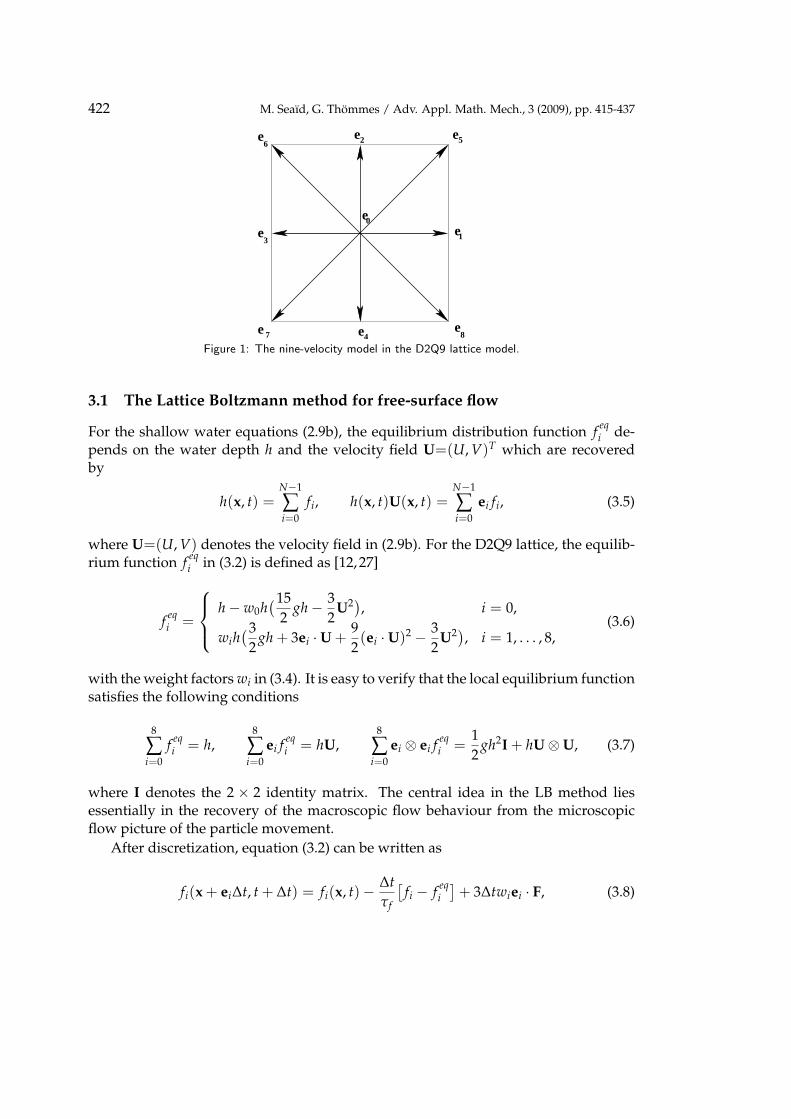
In the current work we consider the D2Q9 square lattice model [25], as depicted inFig. 1. The nine velocities ei in the D2Q9 lattice are defined by

ei =

(0, 0)T, i = 0,(cos

((i− 1)π

4

), sin

((i− 1)π

2

))Tc, i = 1, 2, 3, 4,

(cos

((i− 5)π

2 + π4

), sin

((i− 5)π

2 + π4

))T√2c, i = 5, 6, 7, 8,

(3.3)

where c=∆x/∆t=∆y/∆t. Here, ∆t is chosen such that the particles travel one latticespacing during the time step. The corresponding weights wi to the above velocitiesare

wi =

4/9, i = 0,1/9, i = 1, 2, 3, 4,1/36, i = 5, 6, 7, 8.

(3.4)

The selection of the relaxation time τ and the equilibrium distribution function f eqi

in (3.2) depend on the macroscopic equations under study. Next, we describe theformulation of these parameters for the shallow water equations (2.9b) and the depth-averaged convection-diffusion equation (2.10).

422 M. Seaıd, G. Thommes / Adv. Appl. Math. Mech., 3 (2009), pp. 415-437

e

e

e

e e

e

ee7

3

6 2 5

1

84

e0

Figure 1: The nine-velocity model in the D2Q9 lattice model.

3.1 The Lattice Boltzmann method for free-surface flow

For the shallow water equations (2.9b), the equilibrium distribution function f eqi de-

pends on the water depth h and the velocity field U=(U, V)T which are recoveredby

h(x, t) =N−1

∑i=0

fi, h(x, t)U(x, t) =N−1

∑i=0

ei fi, (3.5)

where U=(U, V) denotes the velocity field in (2.9b). For the D2Q9 lattice, the equilib-rium function f eq

i in (3.2) is defined as [12, 27]

f eqi =

h− w0h(15

2gh− 3

2U2), i = 0,

wih(3

2gh + 3ei ·U +

92(ei ·U)2 − 3

2U2), i = 1, . . . , 8,

(3.6)

with the weight factors wi in (3.4). It is easy to verify that the local equilibrium functionsatisfies the following conditions

8

∑i=0

f eqi = h,

8

∑i=0

ei f eqi = hU,

8

∑i=0

ei ⊗ ei f eqi =

12

gh2I + hU⊗U, (3.7)

where I denotes the 2 × 2 identity matrix. The central idea in the LB method liesessentially in the recovery of the macroscopic flow behaviour from the microscopicflow picture of the particle movement.

After discretization, equation (3.2) can be written as

fi(x + ei∆t, t + ∆t) = fi(x, t)− ∆tτf

[fi − f eq

i

]+ 3∆twiei · F, (3.8)

M. Seaıd, G. Thommes / Adv. Appl. Math. Mech., 3 (2009), pp. 415-437 423

where F represents the force term in the shallow water equations (2.9b)

F =

−g′h∂B∂x− gαh

∂ (hΘ)∂x

+T ω

xρ− T b

xρ−ΩhV

−g′h∂B∂y− gαh

∂ (hΘ)∂y

T ωy

ρ− T b

y

ρ+ ΩhU

. (3.9)

By applying a Taylor expansion and the Chapman-Enskog procedure to equation (3.8),it can be shown that the solution of the discrete lattice Boltzmann equation (3.8) withthe equilibrium function (3.6) results in the solution of the shallow water equations(2.9b). The external force terms such as wind stress, Coriolis force, and bottom frictionare easily included in the model by introducing them into the force term F. For detailson this multi-scale expansion, we refer to [12, 27, 42].

To complete the formulation of LB method for equations (2.9b), the relaxation timeτf has to be defined. In our LB implementation, the relaxation time is determined bythe physical viscosity in (2.9b) and the time step through the formula

τf =3νH

c2 +∆t2

. (3.10)

In the lattice Boltzmann method, equation (3.8) is solved in two steps: collision andstreaming. In the collision step, the equations for each direction are relaxed towardequilibrium distributions. Then, at the streaming step, the distributions move to theneighboring nodes.

3.2 The lattice Boltzmann method for free-surface temperature

The LBM for transport equation (2.10) is derived using a similar approach as the oneused for the shallow water equations (2.9b). Hence, starting from equation (3.2) andusing the D2Q9 lattice form Fig. 1, a lattice Boltzmann discretization of the transportequation is

gi(x + ei∆t, t + ∆t)− gi(x, t) = −∆tτg

[gi − geq

i

]+ ∆tQi, (3.11)

where gi is the distribution function, τg is the relaxation time andQi is the source termassociated with the convection-diffusion equation (2.10). In (3.11), geq

i is an equilib-rium distribution function satisfying the following conditions

8

∑i=0

gi =8

∑i=0

geqi = hΘ,

8

∑i=0

eigi =8

∑i=0

eigeqi = UhΘ. (3.12)

To process equation (3.11), a relaxation time and equilibrium function are required.For the convection-diffusion equation, the equilibrium function is given by

geqi = wihΘ

[1 + 3ei ·U

], (3.13)

424 M. Seaıd, G. Thommes / Adv. Appl. Math. Mech., 3 (2009), pp. 415-437

where the lattice weights wi are defined in (3.4). For this selection, the source term in(3.11) is set to

Qi = wihQ. (3.14)

It should be noted that the convection-diffusion equation (2.10) can be obtained fromequation (3.11) using the Chapman-Enskog expansion. Details on these derivationswere given in [5]. It should be stressed that a similar approach was applied in [11] forreaction-diffusion equations.

As in the LB method for shallow water equations, the relaxation time is defined bythe thermal diffusion coefficient in (2.10) and the time step as

τg =3λ

c2 +∆t2

. (3.15)

Notice that conditions (3.10) and (3.15) give the relation between the lattice diffusionand the time step to be used in the LB simulations.

3.3 Boundary conditions

It well established that implementation of boundary conditions in the LB method hasa crucial impact on the accuracy and stability of the method, see [14, 46] for morediscussions. When no-slip boundary conditions for the flow velocities are imposed atwalls, the bounce-back rule is usually used in the LB algorithm. At a boundary pointxb, populations fi of links ei which intersect the boundary and point out of the fluiddomain are simply reflected (bounce-back) since they cannot participate in the normalpropagation step

fi∗(xb, t + ∆t) = fi(xb, t), index i∗ s.t. ei∗ = −ei.

For the numerical examples considered in the present study, flow boundary conditionsfor the height, H, and/or the velocities, (U, V), are needed at the inlet and the outletof computational domains. When the height Hl is prescribed at the left boundary,the three distributions f1, f5 and f8 are unknown. We use the techniques describedin [43,46] for flat interfaces to implement these boundary conditions in the frameworkof LB method. Assuming that V = 0, the velocity in x-direction can be recovered fromthe relation

HlU = Hl −(

f0 + f2 + f4 + 2( f3 + f6 + f7))

,

and we define the unknown distributions as

f1 = f3 +23

HlU, (3.16a)

f5 = f7 − 12( f2 − f4) +

16

HlU, (3.16b)

f8 = f6 +12( f2 − f4) +

16

HlU. (3.16c)

M. Seaıd, G. Thommes / Adv. Appl. Math. Mech., 3 (2009), pp. 415-437 425

Neumann boundary conditions are implemented by imposing the equilibrium dis-tribution corresponding to the prescribed height, Hl , and the velocity of the nearestneighbor in direction of the normal, (Un, Vn)

fi = f eqi (Hl , Un, Vn) , i = 0, 1 . . . , 8.

Dirichlet boundary conditions for the prescribed temperature Θ0 can be imposed bythe equilibrium for the unknown populations

gi = geqi (Θ0, U, V) , i = 0, 1 . . . , 8.

Neumann boundary conditions are also frequently used in convection-diffusion prob-lems. They are implemented in the LB framework in a similar way by prescribing theconcentration of the neighbour node Θn at the boundary

gi = geqi (Θn, U, V) , i = 0, 1 . . . , 8.

For the simulation of sea-temperature dispersion in the Strait of Gibraltar, we haveflow boundary conditions for the water height and a Neumann boundary conditionfor the velocity. These boundary conditions are implemented by imposing the equilib-rium distribution corresponding to the prescribed height, H0, and the velocity of thenearest neighbor in the direction of the normal (Un, Vn)

fi = f eqi (H0, Un, Vn) , i = 0, 1 . . . , 8.

Moreover, for the convection-diffusion LB equation in the test example of the Strait ofGibraltar, boundary conditions at the coastlines and the open sea boundaries are re-quired. We impose fixed temperature (Dirichlet) boundary conditions at the coastlinesand Neumann boundary conditions for the temperature at the western and easternends of the Strait of Gibraltar.

Other types of boundary conditions can also be incorporated. For further detailson the implementation of general boundary conditions for lattice Boltzmann shallowwater models we refer the reader to [5, 14, 34, 46]. General details on the implementa-tion of an LB method for irregular domains can also be found in [20,36] among others.

4 Numerical examples

In this section the accuracy and performance of the LB scheme is tested. Three testexamples are used: a tidal flow problem, an advection-diffusion of a Gaussian pulsein a uniform rotating flow field, and simulation of free-surface temperature in theStrait of Gibraltar. The former first tests have analytical solutions that can be usedto quantify error in the LB method while the latter is used to qualify LB results formore complicated free-surface flows. In all the examples, the gravitation constant g istaken as 9.81 m/s2, the time step is chosen according to the latice sizes as well as withstability conditions given in (3.10) and (3.15).

426 M. Seaıd, G. Thommes / Adv. Appl. Math. Mech., 3 (2009), pp. 415-437

4.1 Tidal wave problem

This example was used in [7], in which an asymptotic analytical solution was obtained.Here, a channel with length L = 14 Km is considered with a bed elevation defined by

Z(x) = 10 +40x

L+ 10 sin

(π(

4xL− 1

2))

.

The bottom frictions, wind stresses and Coriolis effect were neglected in this test. Ifwe take the initial and boundary conditions as

H(x, 0) = 60.5− Z(x), U(x, 0) = 0,

H(0, t) = 64.5− 4 sin(

π(4t

86400+

12))

, U(L, t) = 0,

an analytical solution, based on the asymptotic analysis, can be given by [7]

H(x, t) = 64.5− Z(x)− 4 sin(

π(4t

86400+

12))

,

U(x, t) =(x− L) π

5400h(x, t)cos

(π(

4t86400

+12))

.

This asymptotic analytical solution is used to quantify the results obtained by the LBmethod. We compute the L∞-, L1- and L2-error norms as

L1 =N

∑i=1|En

i |∆x, L2 =( N

∑i=1|En

i |2 ∆x) f rac12

, L∞ = max1≤i≤N

|Eni | , (4.1)

where Eni =Un

i − U(xi, tn) is the error between the numerical solution, Uni , and the an-

alytical solution, U(xi, tn), at time tn and lattice point xi. We used τH=0.6, c=200 m/s

1.5 2 2.5 3 3.5 4 4.5−4.5

−4

−3.5

−3

−2.5

−2

log ∆x

log

| u−

u 0 |

L∞ normL1 norm

L2 norm

Figure 2: Error plots for the tidal wave flow at time t = 9117.5s.

M. Seaıd, G. Thommes / Adv. Appl. Math. Mech., 3 (2009), pp. 415-437 427

0 2000 4000 6000 8000 10000 12000 140000

10

20

30

40

50

60

70

distance x

free

sur

face

h+

z

exactnumerical

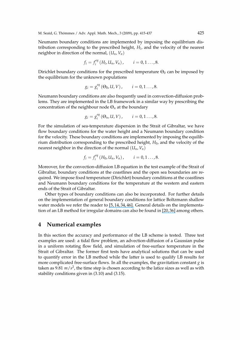
Figure 3: Numerical and analytical free-surface for the tidal wave flow at time t=9117.5s.

and the results are displayed at time t=9117.5s. For this test example the ratio U/c=0.0009. Note that we used a two-dimensional code to reproduce numerical solutionsfor the one-dimensional problem. Therefore, boundary conditions in the y-directionhave to be supplied for the two-dimensional code. For this test example, the dimen-sion in y-direction is fixed to 50 lattice points. Periodic boundary conditions are as-sumed on the upper and lower walls.

In Fig. 2, we display the error norms for the velocity solution using four uniformlattices with sizes ∆x=∆y=56 m, 28 m, 14 m and 7 m at the considered time. Alogarithmic scale is used on the x- and y-axis. It is clear that decreasing the lattice sizeresults in a decrease of all error norms. Similar results, not reported here, are obtainedfocusing the attention on the water depth. As expected the LB method shows a first-order accuracy for this nonlinear example.

Fig. 3 presents the numerical and analytical solutions for the water free-surfaceat the simulation time t=9117.5 s using a lattice size of ∆x=∆y=7 m. It is clear thegood agreement between the asymptotic analytical solution and the numerical resultsobtained by the LB method using the coarse lattice. The LB method performs wellfor this unsteady shallow water problem and produces accurate solutions withoutrequiring special treatment of the source terms or complicated upwind discretizationof the gradient fluxes as in [7] among others.

4.2 Advection-dispersion problem

In this example we will test the accuracy of LB method for an advection-dispersionequation with a prescribed velocity field and known analytical solution. Hence, wesolve the equation (2.10) with constant water depth

∂Θ∂t

+∂

∂x(UΘ) +

∂

∂y(VΘ)− λ∆Θ = 0. (4.2)

428 M. Seaıd, G. Thommes / Adv. Appl. Math. Mech., 3 (2009), pp. 415-437

We consider the test problem of the advection-dispersion of a Gaussian pulse in auniform rotating flow field proposed in [31]. Thus, the computational domain is a3200 km long square equipped with the initial condition

Θ(x, y, 0) = 100 exp(− (x− x0)2 + (y− y0)2

2σ2

), (4.3)

where (x0, y0)=(−800 km, 0) is the centre of the initial Gaussian and σ=2× 104 km2.As in [31] we take U=−ωy and V=ωx, with ω=10−5/s being the angular velocity. Itis easy to verify that the problem (4.2)-(4.3) has an exact solution given by

Θ(x, y, t) =100

1 + 2λtσ2

exp(− x2 + y2

2(σ2 + 2λt)

), (4.4)

withx = x− x0 cos ωt + y0 sin ωt, y = y− x0 sin ωt− y0 cos ωt.

Two diffusivity coefficients namely, λ=104 m2/s and 2× 104 m2/s are considered. Tocheck the accuracy of the LB method for this test problem, a simulation is carried outuntil a full rotation of the Gaussian is completed using different lattice sizes, L1, L2 andL∞ norms of the errors are computed using (4.1). We used homogeneous Neumannboundary conditions on all domain boundaries, and we set D=0.01.

In Table 1, the accuracy analysis results, obtained considering four different latticesteps, are summarized. For the selected diffusivity coefficients, a decay behaviour isobserved for each increase of the number of lattice points. A slower decay is seen forcomputations with λ=2× 103 m2/s than those computed with λ=103 m2/s. This factcan be attributed to the large physical diffusion in the advection-dispersion problemsuch that the Gaussian spreads strongly and the solution is significantly different fromzero at the boundaries and outside of the domain. It is evident, however, that our LBmethod converges to the correct solution also for this advection-dispersion problem.

Surface plots of the solution at times t=T/4, T/2, 3T/4 and T are presented in Fig.4. Those corresponding to contour plots are displayed in Fig. 5. Here, we used

λ = 103 m2/s, ∆x = ∆y = 100 Km, T = 628318 s,

which corresponds to the time necessary for a complete rotation. In the figures, we canclearly see that there are no spurious numerical oscillations in vicinity of the Gaussianpulse, verifying the of the LB method.

Table 1: L1, L2 and L∞ errors for the advection-dispersion problem after a complete rotation.

λ=103 m2/s λ=2× 103 m2/sN L∞-error L1-error L2-error L∞-error L1-error L2-error40 3.733E-02 2.338E-02 2.416E-02 2.435E-03 2.293E-02 1.856E-0280 9.650E-03 5.811E-03 6.093E-03 2.435E-03 7.170E-03 5.944E-03

160 2.935E-03 1.456E-03 1.527E-03 4.940E-03 3.218E-03 3.658E-03320 6.098E-04 3.679E-04 3.821E-04 3.907E-03 2.067E-03 2.277E-03

M. Seaıd, G. Thommes / Adv. Appl. Math. Mech., 3 (2009), pp. 415-437 429

Figure 4: Surface plots for the advection-dispersion problem at four different times.

0 800 1600 2400 32000

800

1600

2400

3200

x [km]

y [k

m]

Figure 5: Contour plots for the advection-dispersion problem at four different times.

4.3 Free-surface temperature in the Strait of Gibraltar

The purpose of this test problem is to examine the performance of our LB model forsimulating sea-surface temperature in the Strait of Gibraltar. The basic circulation inthe Strait of Gibraltar consists in an upper layer of cold, fresh surface Atlantic wa-ter and an opposite deep current of warmer, salty Mediterranean outflowing water,compare [3, 15]. The sea-surface temperatures in the Strait of Gibraltar are maxima in

430 M. Seaıd, G. Thommes / Adv. Appl. Math. Mech., 3 (2009), pp. 415-437

Morocco•Tangier

•Ceuta

Spain

•Tarifa

• Algeciras

•Barbate

•Gibraltar

•Sidi Kankouch

6ο05‘ 5ο55‘ 5ο45‘ 5ο35‘ 5ο25‘ 5ο15‘35ο45‘

35ο55‘

36ο05‘

36ο15‘

0 10Km5

Figure 6: Computational domain for the Strait of Gibraltar.

summer (August-September) with average values of 23-24C and minima in winter(January-February) with averages of 11-12C. The north Atlantic water is about 5-6Ccolder than the Mediterranean water, elaborate details are available in [21, 24].

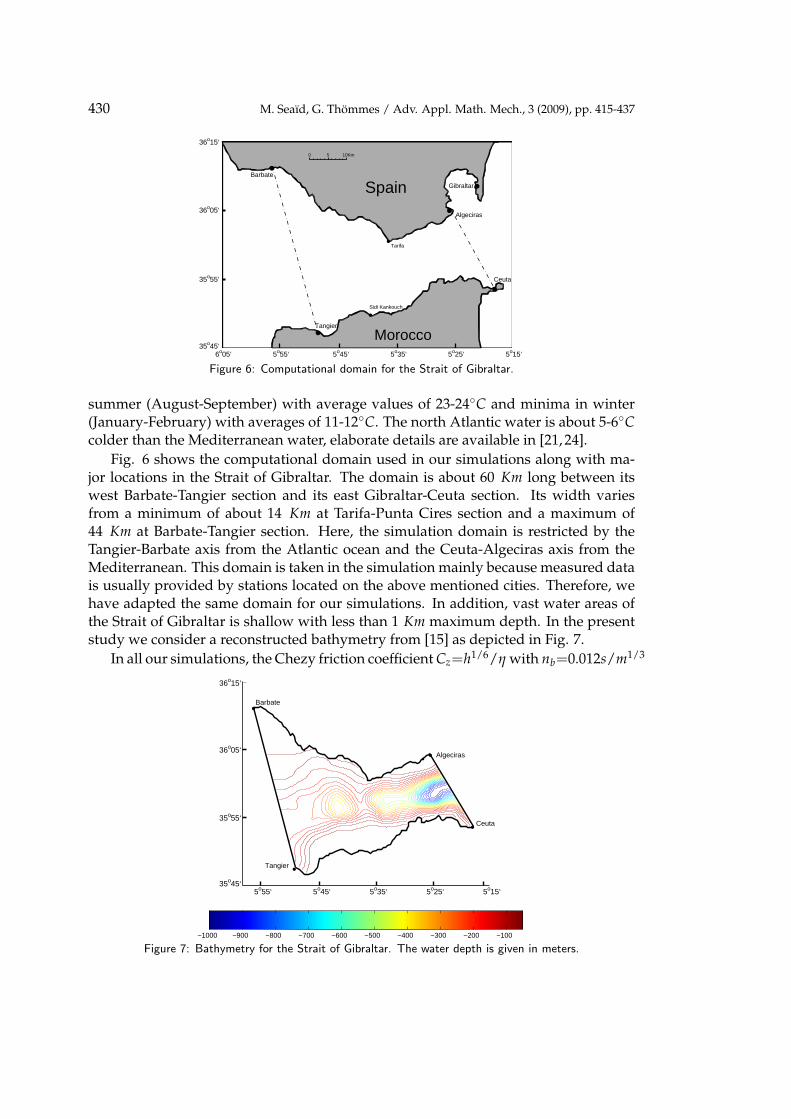
Fig. 6 shows the computational domain used in our simulations along with ma-jor locations in the Strait of Gibraltar. The domain is about 60 Km long between itswest Barbate-Tangier section and its east Gibraltar-Ceuta section. Its width variesfrom a minimum of about 14 Km at Tarifa-Punta Cires section and a maximum of44 Km at Barbate-Tangier section. Here, the simulation domain is restricted by theTangier-Barbate axis from the Atlantic ocean and the Ceuta-Algeciras axis from theMediterranean. This domain is taken in the simulation mainly because measured datais usually provided by stations located on the above mentioned cities. Therefore, wehave adapted the same domain for our simulations. In addition, vast water areas ofthe Strait of Gibraltar is shallow with less than 1 Km maximum depth. In the presentstudy we consider a reconstructed bathymetry from [15] as depicted in Fig. 7.

In all our simulations, the Chezy friction coefficient Cz=h1/6/η with nb=0.012s/m1/3

•Tangier

• Ceuta

•Barbate

• Algeciras

5ο55‘ 5ο45‘ 5ο35‘ 5ο25‘ 5ο15‘35ο45‘

35ο55‘

36ο05‘

36ο15‘

−1000 −900 −800 −700 −600 −500 −400 −300 −200 −100

Figure 7: Bathymetry for the Strait of Gibraltar. The water depth is given in meters.

M. Seaıd, G. Thommes / Adv. Appl. Math. Mech., 3 (2009), pp. 415-437 431

is the Manning constant, the coefficient of wind friction Cω=10−5, the Coriolis param-eter Ω=8.55× 10−5 1/s, and the horizontal eddy viscosity of νH=100 m2/s, see forexample [15,33]. A mesh with lattice size ∆x=∆y=250 m is used for all the results pre-sented in this section. This mesh structure has been selected after a grid independencestudy assessed by comparing numerical results obtained using different meshes, com-pare [34] for more details. Depending on the wind conditions, three situations aresimulated namely:

1. Calm situation corresponding to (ωx=0 m/s, ωy=0 m/s);2. Wind blowing from the east corresponding to (ωx=−1 m/s, ωy=0 m/s);3. Wind blowing from the west corresponding to (ωx=1 m/s, ωy=0 m/s).

A no-slip boundary condition for velocity variables has been applied at the coastalboundaries. At the open boundaries, Neumann boundary conditions are imposed forthe velocity, and the water elevation is prescribed as a periodic function of time usingthe main semidiurnal and diurnal tides. The tidal constants at the open boundary lat-tice nodes were calculated by interpolation from those measured at the coastal stationsTangier and Barbate on the western end and the coastal stations Ceuta and Algecirason the eastern end of the Strait. We considered the main semidiurnal M2, S2 and N2tidal waves, and the diurnal K1 tidal wave in the Strait of Gibraltar. Thus,

H = H0 + AM2 cos (ωM2 t + ϕM2) + AS2 cos (ωS2 t + ϕS2)+AN2 cos (ωN2 t + ϕN2) + AK1 cos (ωK1 t + ϕK1) , (4.5)

where Ak is the wave amplitude, ωk the angular frequency and ϕk the tide phase forthe considered tide k, with k=M2, S2, N2 or K1. The measured data for these pa-rameters are provided for the cities defining the computational domain and are givenin [5, 15]. In (4.5), H0 is the averaged water elevation set to 3m in our simulations.Initially, the simulated flow has been at warm rest, i.e.,

U = V = 0, H = H0 and Θ = Θh, (4.6)

where Θh=23C is the Mediterranean temperature and the western temperature bound-ary of the Strait is fixed to the Ocean temperature Θc=17C. Note that, in order toensure that the initial conditions of the water flow and sea-surface temperature areconsistent we proceed as follows. The shallow water equations (2.9b) are solved with-out temperature dispersion for two weeks of real time to obtain a well-developed flow.The obtained results are taken as the real initial conditions and the sea-surface tem-perature is included at this stage of the simulation. At the end of the simulation timethe velocity fields and temperature contours are displayed after 12, 18 and 24 hoursfrom the inclusion of sea-surface temperature.

In Fig. 8, we present numerical results obtained using calm wind conditions. Thoseobtained for the wind blowing from the east and the wind blowing from the west aredisplayed in Figs. 9 and 10, respectively. In these figures, we show the velocity fieldand 10 equi-distributed contours between Θc and Θh of the temperature at the instants

432 M. Seaıd, G. Thommes / Adv. Appl. Math. Mech., 3 (2009), pp. 415-437

6ο05‘ 5ο55‘ 5ο45‘ 5ο35‘ 5ο25‘ 5ο15‘35ο45‘

35ο55‘

36ο05‘

36ο15‘

6ο05‘ 5ο55‘ 5ο45‘ 5ο35‘ 5ο25‘ 5ο15‘35ο45‘

35ο55‘

36ο05‘

36ο15‘

6ο05‘ 5ο55‘ 5ο45‘ 5ο35‘ 5ο25‘ 5ο15‘35ο45‘

35ο55‘

36ο05‘

36ο15‘

6ο05‘ 5ο55‘ 5ο45‘ 5ο35‘ 5ο25‘ 5ο15‘35ο45‘

35ο55‘

36ο05‘

36ο15‘

6ο05‘ 5ο55‘ 5ο45‘ 5ο35‘ 5ο25‘ 5ο15‘35ο45‘

35ο55‘

36ο05‘

36ο15‘

6ο05‘ 5ο55‘ 5ο45‘ 5ο35‘ 5ο25‘ 5ο15‘35ο45‘

35ο55‘

36ο05‘

36ο15‘

Figure 8: Flow field (first row) and temperature contours (second row) for calm situation at three differenttimes. From left to right t=12, 18 and 24 hours.

t=12, 18 and 24 hours. It is clear that using the conditions for the tidal waves and theconsidered wind situations, the flow exhibits a recirculating zone with different orderof magnitudes near the Caraminal Sill (i.e. the interface separating the water bodiesbetwen the Mediterranean sea and the Atlantic Ocean). At the beginning of simulationtime, the water flow enters the Strait from the eastern boundary and flows towardsthe eastern exit of the Strait. At later time, due to tidal waves, the water flow changesthe direction pointing towards the Atlantic Ocean. A recirculating flow region is also

6ο05‘ 5ο55‘ 5ο45‘ 5ο35‘ 5ο25‘ 5ο15‘35ο45‘

35ο55‘

36ο05‘

36ο15‘

6ο05‘ 5ο55‘ 5ο45‘ 5ο35‘ 5ο25‘ 5ο15‘35ο45‘

35ο55‘

36ο05‘

36ο15‘

6ο05‘ 5ο55‘ 5ο45‘ 5ο35‘ 5ο25‘ 5ο15‘35ο45‘

35ο55‘

36ο05‘

36ο15‘

6ο05‘ 5ο55‘ 5ο45‘ 5ο35‘ 5ο25‘ 5ο15‘35ο45‘

35ο55‘

36ο05‘

36ο15‘

6ο05‘ 5ο55‘ 5ο45‘ 5ο35‘ 5ο25‘ 5ο15‘35ο45‘

35ο55‘

36ο05‘

36ο15‘

6ο05‘ 5ο55‘ 5ο45‘ 5ο35‘ 5ο25‘ 5ο15‘35ο45‘

35ο55‘

36ο05‘

36ο15‘

Figure 9: The same as in Fig. 8 but for a wind blowing from the east.

M. Seaıd, G. Thommes / Adv. Appl. Math. Mech., 3 (2009), pp. 415-437 433

6ο05‘ 5ο55‘ 5ο45‘ 5ο35‘ 5ο25‘ 5ο15‘35ο45‘

35ο55‘

36ο05‘

36ο15‘

6ο05‘ 5ο55‘ 5ο45‘ 5ο35‘ 5ο25‘ 5ο15‘35ο45‘

35ο55‘

36ο05‘

36ο15‘

6ο05‘ 5ο55‘ 5ο45‘ 5ο35‘ 5ο25‘ 5ο15‘35ο45‘

35ο55‘

36ο05‘

36ο15‘

6ο05‘ 5ο55‘ 5ο45‘ 5ο35‘ 5ο25‘ 5ο15‘35ο45‘

35ο55‘

36ο05‘

36ο15‘

6ο05‘ 5ο55‘ 5ο45‘ 5ο35‘ 5ο25‘ 5ο15‘35ο45‘

35ο55‘

36ο05‘

36ο15‘

6ο05‘ 5ο55‘ 5ο45‘ 5ο35‘ 5ο25‘ 5ο15‘35ο45‘

35ο55‘

36ο05‘

36ο15‘

Figure 10: The same as in Fig. 8 but for a wind blowing from the west.

detected on the top eastern exits of the strait near Algeciras. Similar flow behaviourshave been also reported in [3, 15, 34].

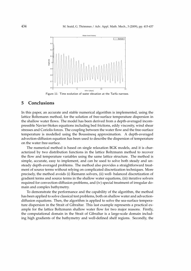
The effects of wind conditions are observed in the temperature distributions pre-sented in Figs. 8, 9 and 10. A boundary layer of high sea-surface temperatures hasbeen detected on the Spanish coastal lines. For the considered tides and wind condi-tions, the buoyancy force has been seen to play a weak role for driven the sea-surfacetamperature in the Strait of Gibraltar which results in thiner mixing layers. In Fig-ure 11 we display the time evolution of the water free-surface elevation at the Tarifanarrows for a time period of two weeks. As expected, the time series show two tidalperiods with different amplitude and frequencies. They are in good agreement withthose previously computed in [9, 33]. Similar results not presented here, have beenobtained at other locations in the Strait of Gibraltar.

Note that the proposed lattice Boltzmann shallow water model performs well forthis test problem since it does not diffuse the moving fronts and no spurious oscilla-tions have been observed near steep gradients of the flow field in the computationaldomain. It can be clearly seen that the complicated flow structures on the CaraminalSill and near Tarifa narrows and Tangier basin are being captured by the LB method. Inaddition, the presented results clearly indicate that the method is suited for predictionof sea-surface temperature dispersion in the Strait of Gibraltar. It should be stressedthat ideally, results from the temperature dispersion model should be compared withobservations of real sea-surface temperatures in the Strait of Gibraltar. However, thereare no available data until now to carry out this work. Thus, we could only simulatesome hypothetical simulations simply to show that LB results are logical and consis-tent.

434 M. Seaıd, G. Thommes / Adv. Appl. Math. Mech., 3 (2009), pp. 415-437

0 5 10 152.6

2.7

2.8

2.9

3

3.1

3.2

3.3

3.4Water level history

time t [days]

heig

ht [m

]

Barbate

Figure 11: Time evolution of water elevation at the Tarifa narrows.

5 Conclusions

In this paper, an accurate and stable numerical algorithm is implemented, using thelattice Boltzmann method, for the solution of free-surface temperature dispersion inthe shallow water flows. The model has been derived from a depth-averaged incom-pressible Navier-Stokes equations including bed frictions, eddy viscosity, wind shearstresses and Coriolis forces. The coupling between the water flow and the free-surfacetemperature is modelled using the Boussinesq approximation. A depth-averagedadvection-diffusion equation has been used to describe the dispersion of temperatureon the water free-surface.

The numerical method is based on single relaxation BGK models, and it is char-acterized by two distribution functions in the lattice Boltzmann method to recoverthe flow and temperature variables using the same lattice structure. The method issimple, accurate, easy to implement, and can be used to solve both steady and un-steady depth-averaged problems. The method also provides a straightforward treat-ment of source terms without relying on complicated discretization techniques. Moreprecisely, the method avoids (i) Riemann solvers, (ii) well- balanced discretization ofgradient terms and source terms in the shallow water equations, (iii) iterative solversrequired for convection-diffusion problems, and (iv) special treatment of irregular do-main and complex bathymetry.

To demonstrate the performance and the capability of the algorithm, the methodhas been applied to solve classical test problems, both on shallow water and advection-diffusion equations. Then, the algorithm is applied to solve the sea-surface tempera-ture dispersion in the Strait of Gibraltar. This last example represents a practical ex-ample for the lattice Boltzmann shallow water flow for two major reasons. Firstly,the computational domain in the Strait of Gibraltar is a large-scale domain includ-ing high gradients of the bathymetry and well-defined shelf regions. Secondly, the

M. Seaıd, G. Thommes / Adv. Appl. Math. Mech., 3 (2009), pp. 415-437 435

Strait contains complex fully two-dimensional tidal flow structures, eddy viscosity,Coriolis forces and wind shear stresses, which present a challenge for most numericalmethods used for the shallow water modelling. The presented results demonstratethe accuracy of the lattice Boltzmann method and its capability to simulate tidal flowsand sea-surface temperature transport in the hydrodynamic regimes considered.

Acknowledgments

The authors acknowledged the financial support by the DeutscheForschungsGemein-schaft (DFG) under grant No. KL 1105/9.

References

[1] F. ALCRUDO AND F. BENKHALDOUN, Exact solutions to the Riemann problem of the shallowwater equations with a bottom step, Comput. Fluids., 30 (2001), pp. 643-671.

[2] F. ALCRUDO AND P. GARCIA-NAVARRO, A high resolution Godunov-type scheme in finitevolumes for the 2D shallow water equation, Int. J. Numer. Methods in Fluids., 16 (1993), pp.489-505.

[3] J.I. ALMAZAN, H. BRYDEN, T. KINDER AND G. PARRILLA, Seminario Sobre laOceanografıa Fısica del Estrecho de Gibraltar, SECEG, Madrid, (1988).

[4] E. AUDUSSE, F. BOUCHUT, M.O. BRISTEAU, R. KLEIN AND B. PERTHAME, A fast andstable well-balanced scheme with hydrostatic reconstruction for shallow water flows, SIAM J.Sci. Comp., 25 (2004), pp. 2050–2065.

[5] M.K. BANDA, M. SEAID AND G. THOMMES, Lattice Boltzmann simulation of dispersion intwo-dimensional tidal flows, International Journal for Numerical Methods in Engineering,77 (2009), pp. 878–900.

[6] A. BARTZOKAS, Estimation of the eddy thermal diffusivity coefficient in water, J. Meteorologyand Atmospheric Physics, 33 (1985), pp. 401–405.

[7] A. BERMUDEZ AND M.E. VAZQUEZ, Upwind methods for hyperbolic conservation laws withsource terms, Computers & Fluids, 23 (1994), pp. 1049–1071.

[8] P. BHATNAGAR, E. GROSS AND M. KROOK, A model for collision process in gases, Phys.Rev. Lett., 94 (1954), pp. 511–525.

[9] M.J. CASTRO, J.A. GARCIA-RODRIGUEZ, J.M. GONZALEZ-VIDA, J. MACIAS, C. PARESAND M.E. VAZQUEZ-CENDON, Numerical simulation of two-layer shallow water flowsthrough channels with irregular geometry, J. Comp. Physics., 195 (2004), pp. 202–235.

[10] DUDLEY B. CHELTON, STEVEN K. ESBENSEN, MICHAEL G. SCHLAX, NICOLAI THUM,MICHAEL H. FREILICH, FRANK J. WENTZ, CHELLE L. GENTEMANN, MICHAEL J.MCPHADEN AND PAUL S. SCHOPF, Observations of coupling between surface wind stressand sea surface temperature in the Eastern Tropical Pacific, Journal of Climate, 14 (2001), pp.1479–1498.

[11] S.P. DAWSON, S. CHEN AND G.D. DOOLEN, Lattice Boltzmann computations for reaction-diffusion equations, J. Chem. Phys., 98 (1993), pp. 1514–1523.

[12] P.J. DELLAR, Non-hydrodynamic modes and a priori construction of shallow water lattice Boltz-mann equations, Phys. Rev. E (Stat. Nonlin. Soft Matter Phys., 65 (2002), 036309 (12 Pages).

[13] S. FENG, Y. ZHAO, M. TSUTAHARA AND Z. JI, Lattice Boltzmann model in rotational flowfield, Chinese J. of Geophys., 45 (2002), pp. 170–175.

436 M. Seaıd, G. Thommes / Adv. Appl. Math. Mech., 3 (2009), pp. 415-437

[14] M.A. GALLIVAN, D.R. NOBLE, J.G. GEORGIADS AND R.O. BUCKIUS, An evaluation of thebounce-back boundary condition for lattice Boltzmann simulations, Int. J. Num. Meth. Fluids.,25 (1997), pp. 249–263.

[15] M. GONZALEZ AND A. SANCHEZ-ARCILLA, Un Modelo Numerico en Elementos Finitospara la Corriente Inducida por la Marea. Aplicaciones al Estrecho de Gibraltar, Revista Inter-nacional de Metodos Numericos para Calculo y Diseno en Ingenierıa., 11 (1995), pp.383–400.

[16] J.H. LACASCE AND A. MAHADEVAN, Estimating sub-surface horizontal and vertical veloci-ties from sea surface temperature, J. Mar. Res., 64 (2006), pp. 695–721.

[17] J.G. LAFUENTE, J.L. ALMAZAN, F. CATILLEJO, A. KHRIBECHE AND A. HAKIMI, Sea levelin the strait of Gibraltar: Tides, Int. Hydrogr. Rev. LXVII., 1 (1990), pp. 111–130.

[18] R.J. LEVEQUE, Balancing source terms and the flux gradients in high-resolution Godunov meth-ods: the quasi-steady wave-propagation algorithm, J. Comput. Phys., 146 (1998), pp. 346–365.

[19] A. KURGANOV AND D. LEVY, Central-upwind schemes for the Saint-Venant system, Math.Model. Numer. Anal., 36 (2002), pp. 397–425.

[20] R. MEI, L.S. LUO AND W. SHYY, An accurate curved boundary treatment in the Lattice Boltz-mann method, J. Comput. Phys., 1999; 155 (1999), pp. 307–330.

[21] M. MILLAN, M.J. ESTRELA AND V. CASELLES, Torrential Precipitations on the SpanishEast Coast: The role of the mediterranean sea surface temperature, Atmospheric Re-search, 36 (1995), pp. 1–16.

[22] T. MING-HEN, The improved surface gradient method for flows simulation in variable bed topog-raphy channel using TVD-MacCormack scheme, Int. J. Numer. Methods in Fluids., 43 (2003),pp. 71–91.

[23] B. PERTHAME AND C. SIMEONI, A kinetic scheme for the Saint-Venant system with a sourceterm, CALCOLO., 38 (2001), pp. 201–231.

[24] B.G. POLYAK, M. FERNANDEZ, M.D. KHUTORSKOY, J.I. SOTO, I.A. BASOV, M.C. CO-MAS, V.YE. KHAIN, B. ALONSO, G.V. AGAPOVA, I.S. MAZUROVA, A. NEGREDO, V.O.TOCHITSKY, J. DE LA LINDE, N.A. BOGDANOV AND E. BANDA, Heat flow in the AlboranSea, Western Mediterranean. Tectonophysics, 263 (1996), pp. 191–218.

[25] Y.H. QIAN, D. D’HUMIERES AND P. LALLEMAND, Lattice BGK models for the Navier-Stokesequation, Europhys. Letters., 17 (1992), pp. 479–484.

[26] P.L. ROE, Approximate Riemann solvers, parameter vectors and difference schemes, J. Comp.Phys., 43 (1981), pp. 357-372.

[27] R. SALMON, The Lattice Boltzmann method as a basis for ocean circulation modeling, J. Mar.Res., 57 (1999), pp. 503–535.

[28] R. SALMON, The Lattice Boltzmann solutions of the three-dimensional planetary geostrophicequations, J. Mar. Res., 57 (1999), pp. 847–884.

[29] J. CLIM, R.M. SAMELSON, E.D. SKYLLINGSTAD, D.B. CHELTON, S.K. ESBENSEN ANDL.W. O’NEILL, Thum N, On the coupling of wind stress and sea surface temperature, Journalof Climate., 19 (2006), pp. 1557–1566.

[30] M. SEAID, Non-oscillatory relaxation methods for the shallow water equations in one and twospace dimensions, Int. J. Numer. Methods in Fluids., 46 (2004), pp. 457–484.

[31] A. STANIFORTH AND J. CoTE, Semi-Lagrangian integration schemes for the atmospheric mod-els: A review, We. Rev., 119 (1991), pp. 2206–2223.

[32] P.K. STANSBY AND J.G. ZHOU, Shallow water flow solver with non-hydrostatic pressure: 2Dvertical plane problems, Int. J. Numer. Meth. Fluids, 28 (1998), pp. 541–563.

[33] L. TEJEDOR, A. IZQUIERDO, B.A. KAGAN AND D.V. SEIN, Simulation of the semidiurnaltides in the Strait of Gibraltar, J. Geophysical Research., 104 (1999), pp. 13541–13557.

M. Seaıd, G. Thommes / Adv. Appl. Math. Mech., 3 (2009), pp. 415-437 437

[34] G. THOMMES, M. SEAID, M. K. BANDA, Lattice Boltzmann methods for shallow water flowapplications, Int. J. Num. Meth. Fluids., 55 (2007), pp. 673–692.

[35] E.F. TORO, Riemann problems and the WAF method for solving two-dimensional shallow waterequations, Phil. Trans. Roy. Soc. Lond. A, 338 (1992), pp. 43–68.

[36] R.G.M. VAN DER SMAN AND M. H. ERNST, Convection-Diffusion Lattice Boltzmann Schemefor Irregular Lattices, J. Comput. Phys., 160 (2000), pp. 766–782.

[37] M. VARGAS, T. SARHAN, J. GARCIA LAFUENTE AND N. CANO, An advection-diffusionmodel to explain thermal surface anomalies off Cape Trafalgar, Bol. Inst. Esp. Oceanogr., 15(1999), pp. 91–99.

[38] M. E. VAZQUEZ-CENDON, Improved treatment of source terms in upwind schemes for shallowwater equations in channels with irregular geometry, J. Comput. Phys., 148 (1999), pp. 497–526.

[39] S. VUKOVIC AND L. SOPTA, ENO and WENO schemes with the exact conservation propertyfor one-dimensional shallow-water equations, J. Comput. Phys., 179 (2002), pp. 593–621.

[40] Y. XING AND C. SHU, High order well-balanced finite volume WENO schemes and discontin-uous Galerkin methods for a class of hyperbolic systems with source terms, J. Comp. Physics.,214 (2006), pp. 567–598.

[41] K. XU, Well-balanced gas-kinteic scheme for the shallow water equations with source terms, J.Comp. Phys., 178 (2002), pp. 533–562.

[42] L. ZHONG, S. FENG AND S. GAO, Wind-driven ocean circulation in shallow water LatticeBoltzmann Model, Adv. in Atmospheric Sci., 22 (2005), pp. 349–358.

[43] J.G. ZHOU, A lattice Boltzmann model for the shallow water equations, Comput. MethodAppl. M., 191 (2002), pp. 3527–3539.

[44] J.G. ZHOU, D.M. CAUSON, C.G. MINGHAM AND D.M. INGRAM, The surface gradientmethod for the treatment of source terms in the shallow water equations, J. Comp. Phys., 20(2001), pp. 1–25.

[45] J.G. ZHOU, Velocity-depth coupling in shallow water flows., J. Hydr. Engrg., ASCE, 10 (1995),pp. 717–724.

[46] Q. ZOU AND X. HE, On pressure and velocity boundary condition for the lattice BoltzmannBGK model, Phys. Fluids., 9 (6) (2002), pp. 1591–1598.