Quasiequilibrium lattice Boltzmann models with tunable Prandtl number for incompressible...

QUASIEQUILIBRIUM LATTICE BOLTZMANN MODELS

WITH TUNABLE PRANDTL NUMBER FOR

INCOMPRESSIBLE HYDRODYNAMICS

CHAKRADHAR THANTANAPALLY*, SHIWANI SINGH†

and DHIRAJ V. PATIL‡

EMU, JNCASR, Jakkur

Bangalore 560064, India*[email protected]

†[email protected]‡[email protected]

SAURO SUCCI

Istituto Applicazioni Calcolo \Mauro Picone"

C.N.R., Via dei Taurini, 19, 00185

Rome, Italy

[email protected]

SANTOSH ANSUMALI

EMU, JNCASR, Jakkur, Bangalore 560064, [email protected]

Received 9 November 2012Accepted 27 July 2013

Published 9 September 2013

Recently, it was shown that energy conserving (EC) lattice Boltzmann (LB) model is moreaccurate than athermal LB model for high-resolution simulations of athermal °ows. However, in

the sub-grid (SG) domain, the behavior is found to be opposite. In this work, we show that via

multi-relaxation model, it is possible to preserve the accuracy of the EC LB for both SG and

direct numerical simulation (DNS) models. We show that by introducing a nonunit Prandtlnumber, under-resolved simulations can also be performed quite e±ciently, a property which we

attribute to the enhanced sound-relaxation.

Keywords: Turbulence; lattice Boltzmann; direct numerical simulation; multi-relaxation.

PACS Nos.: 47.27.ek, 47.11.+j, 05.20.Dd

1. Introduction

The Lattice Boltzmann (LB) method is an attractive option for the direct numerical

simulation (DNS) of turbulent °ows, due to its high parallel scalability and ease of

International Journal of Modern Physics C

Vol. 24, No. 12 (2013) 1340004 (12 pages)

#.c World Scienti¯c Publishing CompanyDOI: 10.1142/S0129183113400044

1340004-1

Int.

J. M

od. P

hys.

C D

ownl

oade

d fr

om w

ww

.wor

ldsc

ient

ific

.com

by D

r. D

hira

j Pat

il on

10/

02/1

3. F

or p

erso

nal u

se o

nly.

http://dx.doi.org/10.1142/S0129183113400044

application to complex geometries.1–6 However, unlike conventional methods, such

as pseudo-spectral (PS) for Navier–Stokes,7 grid-resolution requirements and accu-

racy of the LB method for DNS, have been thoroughly tested for a few setups only.8

Furthermore, it is empirically known that compressibility-related errors may lead to

poor comparison between PS and LB methods at moderate grid-sizes.9 At this point,

we would also like to remind that in sub-grid (SG) domain, multiple relaxation

models with high bulk viscosity often perform better than single relaxation models,

which exhibit no bulk viscosity. The typical interpretation for such a behavior is

that, in the SG domain, acoustic oscillations can be e®ectively suppressed by high

bulk viscosity.10

However, it was recently shown that for high resolution DNS, the energy con-

serving (EC) LB models deliver an order of magnitude increase in accuracy, as

compared to their athermal counterpart.11 This was attributed to the absence of

unphysical bulk viscosity in the thermal model. However, it was also found that in

the under-resolved regime, very often, the athermal model behaves better than the

EC model. It can be argued that in the under-resolved domain, high bulk viscosity

present in athermal model, helps damping down the acoustic oscillations. Thus, it is

natural to wonder whether it would be possible to keep the best of both approaches.

The aim of this work is to show that it is indeed possible to design an EC LB model

which is e±cient in damping acoustic oscillations and thus delivering better per-

formance in both resolved and under-resolved regimes.

Sections 2 and 3 give the details of the LB formulations. In Sec. 4, we show the

empirical observation that models with a higher bulk viscosity are better at

reducing acoustic perturbations, is consistent with the linearized hydrodynamics.

Furthermore, we argue that high energy dissipation introduced via low-Prandtl

number, is also an e®ective mechanism to damp down the acoustic perturbations

and that low-Prandtl number simulations are preferable to high bulk viscosity

simulations in the nonlinear °ow regime. Finally, we discuss the results of the

numerical simulations.

2. Isothermal and Thermal LB Formulation

In the LB formulation (for review, see Refs.1–3, 12) the °uid is represented by a set

of discrete populations f ¼ ffiðx; tÞg, describing the probability of ¯nding a particle

at position x in the lattice, at time t and with discrete velocity ci ði ¼ 1; . . . ;NÞ.Since the particles are grid-bound, the number of discrete velocities, N , also de¯nes

the connectivity of the lattice. Therefore, the basic variables in LB are the discrete

populations fi de¯ned for a set of discrete velocities ci (i ¼ 1; . . . ;N). The evolution

equations for these discrete populations are in the form

@tfi þ ci�fi ¼ �iðfÞ; ð1Þwhere �i is the collision term and it ensures that the dynamics goes to the chosen

equilibrium. In the entropic formulation of LB, in order to de¯ne equilibrium one

C. Thantanapally et al.

1340004-2

Int.

J. M

od. P

hys.

C D

ownl

oade

d fr

om w

ww

.wor

ldsc

ient

ific

.com

by D

r. D

hira

j Pat

il on

10/

02/1

3. F

or p

erso

nal u

se o

nly.

begins by assuming the existence of a discrete H functional13 in the form

H ¼XNi¼1

fi lnfiwi

� �� 1

� �� ; wi > 0; ð2Þ

where wi are the normalization weights. Once the lattice H-function is known, the

equilibrium feq can be evaluated as a minimum of the H-function under constraints

of local conservation of macroscopic variables such as the mass density, �, the mo-

mentum density J� � �u� and the energy (trace of the pressure tensor

P � 12 �u

2 þ D2 ��), where � is temperature (in Boltzmann units), are de¯ned as linear

combinations of the discrete populations

� ¼XNi¼1

fi; �u� ¼XNi¼1

fici� P ¼ 1

2

XNi¼1

fic2i : ð3Þ

The only di®erence between isothermal and thermalmodels is that, in an isothermal

model, the constraint on energy conservation is relaxed by taking � ¼ 1=3. This for-

mulation of LB, which lacks energy conservation implies a ¯nite bulk viscosity.

In this work, we refer to the so-called D3Q27 model, for which mass, momentum

and energy conservation is taken into account. The explicit form of the equilibrium,

correct up to Oðu3Þ, reads as follows14:

f eqi ¼ �Wið�Þ 1þ u�ci�

�þ u�u�

2 �2ðci�ci� �Kið�Þ��Þ

h i; ð4Þ

where the temperature-dependent weights and factor Ki are

Wið�Þ ¼ ð1� �ÞD �

2ð1� �Þ� �ðci=cÞ2

; Kið�Þ ¼2D�2 þ ci

c

� �2ð1� 3�Þ

Dð1� �Þ : ð5Þ

The latter term reduces to the standard lattice sound speed squared, c2s ¼ 1=3, in the

limit � ! 1=3. Also, in the case of � ¼ 1=3, f eqi is given by

f eqi ¼ �Wið1=3Þ 1þ 3u�ci� þ 9

2u�u�ci�ci� �

3

2u�u�

� �: ð6Þ

The set of discrete populations obeys a discrete evolution equation based on two

basic steps: free-streaming and local collisions. This reads as follows

f �i ðx; tþ�tÞ ¼ fiðx; tÞ þ �iðfðx; tÞÞ;fiðx; tþ�tÞ ¼ f �

i ðx� ci�t; tÞ; ð7Þ

where the collision term �i, describes the collisions taking the system toward local

equilibrium. For most hydrodynamic purposes, this collision term can be modeled as

single-relaxation time with �i ¼ 1� ðf eq

i � fiÞ, known as a Bhatnagar–Gross–Krook

(BGK) model. In Sec. 3, we describe the entropic quasi-equilibrium procedure to

construct collision model with multiple-relaxation times, which o®ers a signi¯cant

improvement of the numerical stability of the method.

Quasiequilibrium LB Models with Tunable Prandtl Number

1340004-3

Int.

J. M

od. P

hys.

C D

ownl

oade

d fr

om w

ww

.wor

ldsc

ient

ific

.com

by D

r. D

hira

j Pat

il on

10/

02/1

3. F

or p

erso

nal u

se o

nly.

3. Generalized Quasi-equilibrium LB Formulation

In this section, following the procedure outlined in Ref. 15, we brie°y remind how

Prandtl number as an independent parameter can be introduced in the LB frame-

work via quasi-equilibrium models. In this framework, multi-relaxation time can be

introduced, via the method of the so-called quasi-equilibrium distribution. As shown

in Fig. 1, BGK is a one-step relaxation to equilibrium, while the actual multi-re-

laxation formulation makes use of an intermediate quasi-equilibrium f� (found as a

minimum of H-function, under constraints on the additional quasi-conserved vari-

ables, such as the energy °ux). The two-step relaxation proceeds as follows. First

comes a fast relaxation to the quasi-equilibrium state f�, which is then followed by a

slow relaxation to the equilibrium state feq. Both relaxation mechanisms are taken in

the BGK form, with � � �1 (where � corresponds to the fast relaxation of f to f� and�1 corresponds to slow relaxation of f� to feq).16,15

As mentioned above, besides the usual conserved quantities, mass–momentum-

energy, a quasi-conserved one, namely the energy °ux (nonequilibrium part),

�q� ¼PNi¼1ðfi � f eq

i Þc2i ci�, is included in the relaxation process, which de¯nes quasi-

equilibrium.15 The resulting quasi-equilibrium distribution with accuracy OðMa2Þreads

f �i ¼ �Wið�Þ 1þ ci�

�u� � u 0

�

� �þ u�u�

2 �2ci�ci� �Kið�Þ��

þ q�ðD� 1Þ�2ð1� �Þ ci�c

2i

�; ð8Þ

where we have set

u 0� ¼ q�

1þ ðD� 1Þ�ðD� 1Þ�ð1� �Þ : ð9Þ

Fig. 1. Approach to equilibrium in two stages. The curved path denotes the relaxation trajectory under

the e®ect of the actual Boltzmann collision integral.


1340004-4

Int.

J. M

od. P

hys.

C D

ownl

oade

d fr

om w

ww

.wor

ldsc

ient

ific

.com

by D

r. D

hira

j Pat

il on

10/

02/1

3. F

or p

erso

nal u

se o

nly.

The two-time relaxation operator in equation Eq. (1) is given by

�i ¼1

�f �i �;u; �;qð Þ � fið Þ þ 1

�1f eqi �;u; �ð Þ � f �

i �;u; �;qð Þð Þ: ð10Þ

The relaxation time � ¯xes the dynamic viscosity � via usual relation, � ¼ � p,

while the second relaxation time controls thermal di®usion via the Prandtl number

Pr ¼ ð5=4Þð�=�1Þ. The kinetic equation (Eq. (1)) is integrated along the character-

istics, using the trapezoidal scheme to obtain the following evolution equation:

giðxþ c�t; tþ�tÞ ¼ giðx; tÞ 1� 2�ð Þ

þ 2� 1� �

�1

� �f �i �;u; �;qð Þ þ �

�1f eqi �;u; �ð Þ

� �; ð11Þ

where g is the auxiliary population de¯ned as,

gðx; tÞ ¼ fðx; tÞ � �t

2� fðx; tÞð Þ; � ¼ �t

2� þ�t: ð12Þ

The moments in terms of the auxiliary population g are given by:

�ðgÞ ¼ �ðfÞ; u�ðgÞ ¼ u�ðfÞ; T ðgÞ ¼ T ðfÞ and q�ðgÞ ¼ q�ðfÞ 1þ �t

2�1

� �:

ð13Þ

4. Analysis of Compressible Navier–Stokes

In LB simulations with initial conditions which are not consistent with incompres-

sibility, huge spurious acoustic disturbances may arise. These spurious waves also

arise whenever resolution is poor and there are sharp changes in space-time distri-

bution of the hydrodynamic ¯elds. Typically, one avoids such scenarios by enhancing

the resolution and carefully tuned initial conditions17. In this section, we propose an

alternate solution based on compressible Navier–Stokes–Fourier equations, with

delta perturbations in density as initial condition, as a model problem to describe

such behavior.

To this aim, we follow the usual prescription of decomposing the momentum j

into longitudinal and transverse components as

j ¼ jl þ jt; r� jl ¼ 0; r � jt ¼ 0: ð14ÞIn case of linear hydrodynamics, it is readily shown that the dynamics of the

transverse component is fully decoupled from the longitudinal component and obeys

the di®usion equation with � ¼ =� as di®usion coe±cient where is the shear

viscosity, � is density. Similarly, the longitudinal part of the dynamics can be written

as18

�@t2 þ 1

�

4

3 þ

� �@tr2

� ��ðx; tÞ þ @p

@�

��S

r2��þ 1

T�

@p

@~s

��

r2~q ¼ 0; ð15Þ


1340004-5

Int.

J. M

od. P

hys.

C D

ownl

oade

d fr

om w

ww

.wor

ldsc

ient

ific

.com

by D

r. D

hira

j Pat

il on

10/

02/1

3. F

or p

erso

nal u

se o

nly.

where is bulk viscosity, p is pressure, S is the entropy, ~s is entropy per unit mass, T

is the temperature, ~q is the heat per unit mass and @t~q ¼ �r2T ðx; tÞ where � is

thermal conductivity. In this case, it is known that any density perturbation decays

at a distance r from the disturbance source as,14,19

��ðr; tÞ ¼ ðLaLrÞ� 12 exp � ðr� cstÞ2

2LaL r

� �; ð16Þ

where, L is the characteristic length and La is the Landau number, de¯ned as

La ¼ Kn 2� 2

Dþ �

� �þ Knð � 1Þ

Pr; ð17Þ

with Knudsen number Kn as the ratio of Mach number Ma and Reynolds number Re,

Prandtl number Pr, spatial dimension D, � is the ratio of bulk to shear viscosity and

is the ratio of speci¯c heat at constant pressure and volume.19 From this solution,

we see that the density pro¯le becomes increasingly sharper as La is decreased and

thus a possible solution for low-Mach number simulations is to allow for large La,

which leads to smoother pro¯les (see Eq. (16)). Thus, it is not surprising that in LB

simulations, often a higher value of bulk viscosity is introduced via multi-relaxation

type collision models, to smoothen the solution.10,15 However, Eq. (17) suggests that,

an alternative way of increasing La is to perform simulations at very low-Prandtl

number. Here, we remind that the Prandtl number is largely irrelevant to low-Mach

number isothermal dynamics, and consequently, customizing it to e®ectively dampen

acoustic waves, appears to o®er a viable strategy. However, we must stress that

linear hydrodynamics cannot predict which one, whether low-Prandtl number or

high bulk viscosity, is to be preferred for numerical simulations. Only, the nonlinear

analysis can suggest which approach is to be favored. The nonlinear term in

momentum balance equation is given by

@�

j�j��

� �¼ @�

j l�jl� þ j t�j

t�

�

!þ j t�@�

j l��

� �þ j t�

�

� �@�j

l� þ j l�@�

j t��

� �

¼ @�

j l�jl� þ j t�j

t�

�

!|fflfflfflfflfflfflfflfflfflfflfflfflfflfflffl{zfflfflfflfflfflfflfflfflfflfflfflfflfflfflffl}

A

þ �� @� j l�j t��

� �|fflfflfflfflfflfflfflfflfflfflfflfflfflfflffl{zfflfflfflfflfflfflfflfflfflfflfflfflfflfflffl}

B

þ j t�@�

j l��

� �þ j t�

�

!@�j

l� þ j l�@�

j t��

!|fflfflfflfflfflfflfflfflfflfflfflfflfflfflfflfflfflfflfflfflfflfflfflfflfflfflfflfflfflfflfflfflfflfflfflffl{zfflfflfflfflfflfflfflfflfflfflfflfflfflfflfflfflfflfflfflfflfflfflfflfflfflfflfflfflfflfflfflfflfflfflfflffl}

C

; ð18Þ

where the term fBg does not contribute to the longitudinal dynamics and provides a

source for the transverse component evolution equation. Similarly, the term fCg,which is also linear in jl, shows that there is a contribution from the longitudinal to

the transverse part evolution. The choice between low-Prandtl number or high bulk

viscosity can be made by observing that the longitudinal and transverse components

are coupled in the nonlinear hydrodynamics. In the nonlinear regime, the arti¯cial


1340004-6

Int.

J. M

od. P

hys.

C D

ownl

oade

d fr

om w

ww

.wor

ldsc

ient

ific

.com

by D

r. D

hira

j Pat

il on

10/

02/1

3. F

or p

erso

nal u

se o

nly.

(due to unphysical values of bulk viscosity) dynamics of longitudinal part also a®ects

the transverse part. Therefore, it may be argued that introducing a very high bulk

viscosity in the model may corrupt the numerical simulation. This was indeed

reported in the recent work, where it was observed that, when resolution is su±-

ciently high, models with bulk viscosity do not converge to the right solution.11

Based on the above, we believe that acoustic °uctuations are best controlled by

introducing an arti¯cially high thermal conductivity (low-Prandtl number). Here, we

remind that the error introduced because of temperature dynamics (driven solely by

viscous heating) is at least of second-order in momentum.

In the sequel, we shall present a series of simulations aimed at illustrating the

points discussed above. Since a detailed and thorough investigation of each of these

points would warrant a paper on its own, our analysis will often be con¯ned to a

semi-quantitative level.

5. Numerical Simulation of Acoustic Perturbations

In order to support this conjecture, we have carried out numerical simulations of

decay of acoustic perturbations with di®erent LB schemes. The initial condition is

that of °uid at rest with uniform density (� ¼ 1:0) throughout the domain except at

the center where the density is perturbed (�� ¼ 0:01). This initial condition is sim-

ulated with isothermal, thermal and quasi-equilibrium (with variable Pr) LB

methods with a grid size of 200� 200 and Re ¼ 100. To show the acoustic damping

behavior of various methods we show the L2 norm of the density perturbation in the

domain after 100 iterations with varying La (by varying Kn and Pr). Figure 2(a)

qualitatively shows the density °uctuations in the domain with initial condition

given above after 100 iterations. The La number (see Eq. (17)) for isothermal,

thermal and Prandtl models considering � ¼ f2=3; 0; 0g; ¼ 5=3 and Pr ¼ f4; 4; 0:1gare f11/6Kn, 7/6Kn, 46/6Kng respectively where Kn ¼ 1:73� 10�4. The ¯gure

0

0.2

0.4

-0.4 -0.2 0 0.2 0.4

δρ

x

x10-3

IsothermalThermalPrandtl

(a)

5

6

7

8

9

10

11

12

13

2 3 4 5 6 7 8

L2

norm

of

δρ

Kn x10-4

x10-6

IsothermalThermal

x10-4

x10-6

(b)

2.5

3

3.5

4

4.5

5

5.5

6

6.5

7

5 10 15 20 25 30 35 40

L2

norm

of

δρ

Pr x10-2

x10-6

Prandtl-model

(c)

Fig. 2. (Color online) (a) Variation of density °uctuation in x-direction, through the centre of the

domain, with same Kn for the three LB methods discussed. (b) Variation of L2 norm of density °uctuationwith Kn at a ¯xed Pr. (c) Variation of L2 norm of density °uctuation with Pr at a ¯xed Kn.


1340004-7

Int.

J. M

od. P

hys.

C D

ownl

oade

d fr

om w

ww

.wor

ldsc

ient

ific

.com

by D

r. D

hira

j Pat

il on

10/

02/1

3. F

or p

erso

nal u

se o

nly.

shows that the density °uctuations indeed decrease with increasing La number. To

quantify the results obtained, these simulations are performed with varying Kn,

shown in Fig. 2 (b), to quantify the e®ect of La in damping the acoustic °uctuations.

As expected the acoustic °uctuations in the domain decrease with increasing Kn.

Further, the quasi-equilibrium (or Prandtl model) LB simulation is run with the least

of the Kn (1:73� 10�4) used in other two methods (i.e. with lowest damping of

oscillations), but with varying Pr e®ectively changing the La. The results of the

simulation are shown in Fig. 2 (c) which are supportive of the fact that density

perturbations decay faster with decreasing Pr number.

6. Two-dimensional Benchmark Simulations

6.1. Taylor–Green vortex

To further validate our method, we have chosen the Taylor–Green vortex simulation

as a model problem, in order to analyze the behavior of an isothermal (with a ¯nite

bulk viscosity), thermal (EC) and quasi-equilibrium model with tunable Prandtl

number. This setup was analyzed earlier, to compare isothermal and EC LB.11 In

order to compare the performance of the current model with that of Ref. 11, we

performed a grid resolution study for the velocity pro¯le, analytically given by

u ¼ sinx cos y e�2�t;

v ¼ �cosx sin y e�2�t;ð19Þ

along the x direction at a ¯xed Mach (Ma) and Reynolds (Re) numbers. Here, Mach

number is de¯ned as Ma ¼ U0=cs and Re is based on the characteristic length of the

°ow-¯eld, taken as 1 in a periodic-box of length 2�, thus Re ¼ U0=�. As the Prandtl

number is just a tunable parameter in the current study, all our simulations have

used Prandtl number Pr / ffiffiffiffiffiffiffiKn

pand Kn and La is completely dictated by behavior

of Pr. In the current simulations of Taylor–Green °ow, we have chosenffiffiffiffiffiffiffiKn

p ¼ 0:0014. As shown in Fig. 3, even at low grid resolution, the model with a

change in Pr, with di®erent �=�1 (here, Pr ¼ 4�=�1), provides a more accurate

simulation of the Taylor–Green vortex, in comparison to isothermal model (except at

a very poorly resolved regime). This result reinforces the fact varying Pr is a better

choice than changing the bulk viscosity for damping the acoustic °uctuations.

6.2. Double periodic shear layer

To demonstrate the method at least on semi-quantitative basis, we consider

the setup of doubly periodic shear layer in two dimensions, which is sensitive to the

computational method used because of the presence of large velocity gradients in the

domain. Thus, this initial condition permits a sensible comparison between various

methods, both in terms of stability and accuracy. The parameters used in simulation

are Re ¼ 30000, U0 ¼ 0:04 for isothermal as well as for simulations with Prandtl

correction. The ratio between two time scales in the latter, i.e. �=�1, is taken to be

0:005 and in this caseffiffiffiffiffiffiffiKn

p ¼ 0:00152. Figure 4 (top) shows that the Prandtl model


1340004-8

Int.

J. M

od. P

hys.

C D

ownl

oade

d fr

om w

ww

.wor

ldsc

ient

ific

.com

by D

r. D

hira

j Pat

il on

10/

02/1

3. F

or p

erso

nal u

se o

nly.

0 500 1000 15000

0.002

0.004

0.006

0.008

0.01

N

L 1 nor

m

IsothermalECPr=0.4(τ/τ

1=0.1)

Pr=0.04(τ/τ1=0.01)

Pr=0.02(τ/τ1=0.005)

0 500 1000 15000

0.002

0.004

0.006

0.008

0.01

N L 2 n

orm

IsothermalECPr=0.4(τ/τ

1=0.1)

Pr=0.04(τ/τ1=0.01)

Pr=0.02(τ/τ1=0.005)

Fig. 3. (Color online) L1 and L2 norm for velocity in x direction at Re ¼ 4000 andMa ¼ 0:05 for Taylor–

Green vortex with di®erent grid size.

X

Y

0 0.2 0.4 0.6 0.8 10

0.2

0.4

0.6

0.8

1

−80

−60

−40

−20

0

20

40

60

80

X

Y

0 0.2 0.4 0.6 0.8 10

0.2

0.4

0.6

0.8

1

−60

−40

−20

0

20

40

60

X

Y

0 0.2 0.4 0.6 0.8 10

0.2

0.4

0.6

0.8

1

−60

−40

−20

0

20

40

60

X

Y

0 0.2 0.4 0.6 0.8 10

0.2

0.4

0.6

0.8

1

−60

−40

−20

0

20

40

60

Fig. 4. (Color online) Vorticity ¯eld at time t ¼ 1 on 200� 200 (top) and 312� 312 (bottom) grid for

athermal (left) and Prandtl (right) models at Re = 30000, Ma = 0.04.


1340004-9

Int.

J. M

od. P

hys.

C D

ownl

oade

d fr

om w

ww

.wor

ldsc

ient

ific

.com

by D

r. D

hira

j Pat

il on

10/

02/1

3. F

or p

erso

nal u

se o

nly.

is stable, while the athermal model blows up at a given lower resolution setup. This

simple qualitative comparison shows that the range of applicability of Pr model is

broader than that of isothermal model, in the SG domain, in terms of stability. It can

be seen that at su±ciently high resolution, both collision models converge to the

same solution, as shown in Fig. 4 (bottom). However, at lower resolution the Prandtl

model leads to higher quality results, as shown in Fig. 4 (top).

7. Three-dimensional Benchmark Simulation

As a more stringent test for the current formulation, we simulate three-dimensional

decaying turbulence with a highly symmetric initial condition, proposed by Kida.20

These simulations are compared with the results obtained with a PS code,21,22. Kida–

Pelz initial conditions are a simple benchmark initial °ow conditions, that evolve to

turbulent °ows in time. Kida °ow has been used in Refs. 23 and 24 to study the

problem of Euler blowup and DNS of viscous turbulence was analyzed using this

initial °ow condition.25

In order to show the accuracy of the present formulation, we compare various

physical quantities, like enstrophy and maximum vorticity. As LB is a primitive

formulation of hydrodynamics, vorticity is not directly accessible to LB simulations.

However, the energy and enstrophy can be calculated on the °y, without taking any

spatial derivative. We remind that enstrophy can be computed from the symmetric

velocity gradient tensor,26 which is locally available in LB simulations locally via

S�� ¼ 2

�T ð2� þ�tÞXi

f eqi � fið Þci�ci�; � ¼ �

c2s: ð20Þ

Note that this does not imply the calculation of any explicit spatial derivative.

Enstrophy shown in Fig. 5, which is more sensitive to the numerical resolution

than the kinetic energy, is compared in both PS and LB. The ¯gure shows the

2 3 4 524

26

28

30

32

34

36

Time

Ens

trop

hy

2 3 4 524

26

28

30

32

34

36

Time

Ens

trop

hy

LB 5133 Pr

LB 5123 Thm

LB 5133 Iso

PS 5123

LB 7683 Pr

LB 7683 Thm

LB 7683 Iso

PS 5123

PS 7683

Fig. 5. (Color online) Comparison of Enstrophy for Kida °ow at Re = 1000 using D3Q27.


1340004-10

Int.

J. M

od. P

hys.

C D

ownl

oade

d fr

om w

ww

.wor

ldsc

ient

ific

.com

by D

r. D

hira

j Pat

il on

10/

02/1

3. F

or p

erso

nal u

se o

nly.

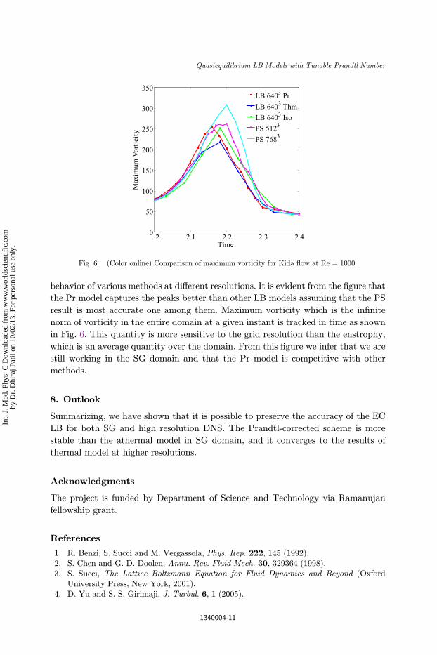
behavior of various methods at di®erent resolutions. It is evident from the ¯gure that

the Pr model captures the peaks better than other LB models assuming that the PS

result is most accurate one among them. Maximum vorticity which is the in¯nite

norm of vorticity in the entire domain at a given instant is tracked in time as shown

in Fig. 6. This quantity is more sensitive to the grid resolution than the enstrophy,

which is an average quantity over the domain. From this ¯gure we infer that we are

still working in the SG domain and that the Pr model is competitive with other

methods.

8. Outlook

Summarizing, we have shown that it is possible to preserve the accuracy of the EC

LB for both SG and high resolution DNS. The Prandtl-corrected scheme is more

stable than the athermal model in SG domain, and it converges to the results of

thermal model at higher resolutions.

Acknowledgments

The project is funded by Department of Science and Technology via Ramanujan

fellowship grant.

References

1. R. Benzi, S. Succi and M. Vergassola, Phys. Rep. 222, 145 (1992).2. S. Chen and G. D. Doolen, Annu. Rev. Fluid Mech. 30, 329364 (1998).3. S. Succi, The Lattice Boltzmann Equation for Fluid Dynamics and Beyond (Oxford

University Press, New York, 2001).4. D. Yu and S. S. Girimaji, J. Turbul. 6, 1 (2005).

2 2.1 2.2 2.3 2.40

50

100

150

200

250

300

350

Time

Max

imum

Vor

tici

ty

LB 6403 PrLB 6403 ThmLB 6403 IsoPS 5123

PS 7683

Fig. 6. (Color online) Comparison of maximum vorticity for Kida °ow at Re = 1000.


1340004-11

Int.

J. M

od. P

hys.

C D

ownl

oade

d fr

om w

ww

.wor

ldsc

ient

ific

.com

by D

r. D

hira

j Pat

il on

10/

02/1

3. F

or p

erso

nal u

se o

nly.

5. D. Yu and S. S. Girimaji, Physica A: Stat. Mech. Appl. 362, 118 (2006).6. R. Benzi and S. Succi, J. Phys A: Math. Gen., 23, L1 (1990).7. C. Canuto, M. Y. Hussaini, A. Quarteroni and T. A. Zang, Spectral Methods in Fluid

Dynamics (Springer-Verlag, 1988).8. D. J. Bespalko, Validation of the lattice Boltzmann method for direct numerical simu-

lation of wall-bounded turbulent °ows, Canadian theses, (2011).9. Y. Peng, W. Liao, L. S. Luo and L. P. Wang, Comput. Fluids 39, 568 (2010).10. P. Asinari and I. V. Karlin, Phys. Rev. E 81, 016702 (2010).11. S. Singh, S. Krithivasan, I. V. Karlin, S. Succi and S. Ansumali, Commun. Comput. Phys.

13, 603 (2011).12. C. K. Aidun and J. R. Clausen, Annu. Rev. Fluid Mech. 42, 439 (2010).13. S. Ansumali, I. V. Karlin and H. C. Öttinger, Europhys. Lett. 63, 798 (2003).14. S. Ansumali and I. V. Karlin, Phys. Rev. Lett. 95, 260605 (2005).15. S. Ansumali, S. Arcidiacono, S. S. Chikatamarla, N. I. Prasianakis, A. N. Gorban and

I. V. Karlin, Eur. Phys J. B Condens. Matter Complex Syst. 56, 135 (2007).16. C. D. Levermore, J. Stat. Phys. 83, 1021 (1996).17. R. Mei, L. S. Luo, P. Lallemand and D. dHumi�eres, Comput. Fluids 35, 855 (2006).18. P. M. Chaikin and T. C. Lubensky, Principles of Condensed Matter Physics (Cambridge

University Press, 1998).19. L. D. Landau and E. M. Lifshitz, Course of Theoretical Physics, Vol. 6, Fluid Mechanics

(Pergamon Press, Oxford, 1987).20. S. Kida, J. Phys. Soc. Japan 54, 2132 (1985).21. S. Kida and Y. Murakami, Phys. Fluids 30, 2030 (1987).22. O. N. Boratav and R. B. Pelz, Phys. Fluids 9, 1400 (1997).23. R. B. Pelz, Fluid Dyn. Res. 33, 207 (2003).24. C. Cichowlas and M. E. Brachet, Fluid Dyn. Res. 36, 239 (2005).25. O. N. Boratav and R. B. Pelz, Phys. Fluids 6, 2757 (1994).26. U. Frisch, Turbulence: The Legacy of AN Kolmogorov (Cambridge University Press,

Cambridge, UK, 1995).


1340004-12

Int.

J. M

od. P

hys.

C D

ownl

oade

d fr

om w

ww

.wor

ldsc

ient

ific

.com

by D

r. D

hira

j Pat

il on

10/

02/1

3. F

or p

erso

nal u

se o

nly.

Quasiequilibrium lattice Boltzmann models with tunable Prandtl number for incompressible...

Documents

Transcript of Quasiequilibrium lattice Boltzmann models with tunable Prandtl number for incompressible...