Unsteady flow simulation of the Ahmed reference body using a lattice Boltzmann approach

www.elsevier.com/locate/compfluid

Computers & Fluids 35 (2006) 940–950

Unsteady flow simulation of the Ahmed reference body usinga lattice Boltzmann approach

Ehab Fares

EXA GmbH, Curiestrasse 4, D-70563 Stuttgart, Germany

Received 29 July 2004; accepted 6 April 2005Available online 10 January 2006

Abstract

The Ahmed reference body represents a simplified car geometry that can be used to investigate the main flow features in the wake ofvehicles. The present work presents unsteady flow simulations at the rear slant angles 25� and 35� using the PowerFLOW 4.0 D3Q19lattice Boltzmann model. The flow of the wake is discussed and distributions of averaged pressure and velocities are compared with avail-able experimental findings. The resolution requirement is investigated in terms of computational requirement and accuracy achieved. Thepredictive capability and the feasibility of the very large eddy simulation (VLES) approach within the lattice Boltzmann framework isdemonstrated.� 2005 Elsevier Ltd. All rights reserved.

1. Introduction

The external aerodynamics of a car determines many rel-evant aspects of an automobile such as stability, comfortand fuel consumption at high cruising speeds. Several sim-ple generic reference models have been proposed in the pastto experimentally investigate the automotive aerodynamicsand isolate relevant flow phenomena [26,33]. One of the firstsimple bluff bodies proposed for such investigations is theMorel model [41] or the slightly modified Ahmed referencehatch-back model [2] pointing out the significance of thebacklight geometry angle on the flow characteristics andhence the drag. A critical angle of the slanted rear of�30� was found to lead to an abrupt decrease in drag asso-ciated with the merging of separation regions and vortexbreakdown [2,33]. Several recent experimental studies inves-tigating the same geometry at different yaw angles [8] andfocusing on the transient flow effects [21,25,48,49,51] wereconducted. Moreover, the flow over the geometrically sim-ple Ahmed reference body is being used as a validation casefor numerical simulations and still constitutes a challenge tonumerical algorithms and turbulence modeling due to its

0045-7930/$ - see front matter � 2005 Elsevier Ltd. All rights reserved.

doi:10.1016/j.compfluid.2005.04.011

E-mail address: [email protected]

complex three dimensional wake vortex interaction. It waschosen during the 9th ERCOFTAC Workshop [34] onrefined turbulence modeling as a three dimensional complextest case. Although many participants applied different con-cepts ranging from steady Reynolds averaged Navier–Stokes (RANS) to large eddy simulations (LES) this caseis still not considered to be satisfactory predicted. It wasconcluded that unsteady calculations such as unsteady Rey-nolds averaged Navier–Stokes (URANS) or LES have astronger potential to adequately capture the details of theflow. Several other numerical simulations [7,8,24,39] usingsteady state approaches also address the necessity of a tran-sient calculation. One of the pioneer unsteady simulationsthat correctly predicted the drag crisis and the vortex break-down phenomena was performed using the lattice gasapproach [5], which was also used in the analysis of thecoherent structures and aeroacoustic sources of the flow[22,49]. Other recent unsteady simulations such as LES[32,36] and detached eddy simulations (DES) [35] basedon the Navier–Stokes equations shown qualitative andquantitative promising results emphasizing the impact ofsuch methodologies. However, the growing demand onaccuracy in the computation compared to wind tunnel mea-surements require predictions within 5% of sensitive values

mailto:[email protected]

E. Fares / Computers & Fluids 35 (2006) 940–950 941

such as the drag coefficient using approaches that are feasi-ble in industrial research and production contexts.

In this paper the well documented velocity and pressuremeasurements of Leinhart et al. [37,27] are taken as a refer-ence for the calculations. First, an overview of the appliedlattice Boltzmann approach is presented giving detailsabout the turbulence model used and the wall treatment.The second part concentrates on the grid resolution require-ment. In the third part the results of the simulations arecompared to experiments and are discussed with emphasison the resolution requirements. Finally, the applicabilityof the presented methodology to similar exterior flows overrealistic road vehicles is outlined.

2. Numerical method

The numerical simulations are carried out using thePowerFLOW 4.0a software based on the floating point19 state (D3Q19) lattice Boltzmann model. Previous ver-sions based on the integer based 34 state thermal latticegas automata were validated in many publications for awide variety of applications [5,22,28,29,47,42]. Many ofthe approaches described below such as turbulence model-ing, wall treatment and grid refinement strategies werealready implemented in older versions. Results using thenew version are documented e.g. in [38].

2.1. Basic lattice Boltzmann approach

The discrete velocity model of the Boltzmann equations[1,17,18,30,31,44]

ofi

otþ ni �

ofi

ox¼ Ci with Ci � xðF i � fiÞ ¼

F i � fi

sð1Þ

represent the time evolution of the particle velocity distri-bution fi of the ith direction in the phase space spannedby the particle velocity vector ni and the space coordinatevector x according to the collision operator Ci, which isapproximated using the Bhatnagar–Gross–Krook (BGK)simple collision form [9] as a relaxation to the equilibriumdistribution Fi with the collision frequency x or collisiontime s, respectively. Macroscopic hydrodynamic quantitiessuch as density q or momentum density qu can be obtainedeasily using moments of the distribution functions

qðx; tÞ ¼X

i

fiðx; tÞ and quðx; tÞ ¼X

i

nifiðx; tÞ. ð2Þ

The appropriate symmetric discretization of the velocityspace according to the 19 state model [17,18,44] on anequidistant cartesian lattice leads to the well known simplelattice Bhatnagar–Gross–Krook (LBGK) equation

fiðxþ niDt; t þ DtÞ ¼ fiðx; tÞ þDts� ðF iðx; tÞ � fiðx; tÞÞ ð3Þ

with the equilibrium distributions approximated up tothird order [4,14,46] as

F i ¼ qwi 1þ ni � uTþ ðni � uÞ

2

2T 2� u2

2Tþ ðni � uÞ

3

6T 3� ni � u

2T 2u2

" #

ð4Þusing the weighting factors wi equal to 1/3, 1/18 and 1/36for the rest particles, the 12 bi-diagonal directions andthe 6 coordinate directions, respectively. The particlesvelocities ni are chosen in such a way, that the niDt corre-sponds to a simultaneous propagation of the particle distri-butions fi to the neighboring lattice sites in direction i. Thelattice temperature T is set to 1/3 for isothermal flows [15]leading to a linear relation p = qT for the pressure p, whichgives a constant lattice sound speed Cs ¼ 1=

ffiffiffi3p

. Using theChapman–Enskog expansion [11] the compressible Navier–Stokes equations can be derived for small Mach numbersup to �0.3. However, in contrast to the Navier–Stokesequations the LBGK defined through equation (3) is linearand relies on simple computational operations for advec-tion and collision allowing for both an efficient and accu-rate implementation, which is one of the main advantagesover classical computational fluid dynamics (CFD) solvers.Furthermore, the local computational nature of the LBGKmakes its solution algorithm an excellent candidate forparallelization.

The relaxation time s is related directly to the kinematicviscosity s = m/T + Dt/2. In order to ensure positivity of thedistributions fi and hence enhance stability especially at lowviscosities [38] the relaxation time is bounded locally to aminimum value

s ¼ max m=T þ Dt2;Dt

fiðx; tÞ � F iðx; tÞfiðx; tÞ

� �i ¼ 0; . . . ; 18. ð5Þ

Note, that such a measure is only active for insufficientlycoarse meshes. In practice it is active at regions where theeddy viscosity, which is usually orders of magnitudes high-er than the kinematic molecular viscosity, is not the deter-mining value. These regions usually indicate flow regionswith low shear stress and thus do not interfere with the glo-bal adequate prediction of the flow behavior.

Furthermore, it is known that multiple-relaxation-time(MRT) models [19,20] is more stable than the abovemen-tioned LBGK formulation. However, for high Reynoldsnumbers and turbulent flows the LBGK including turbu-lence modeling has a different stability behavior since theeddy viscosity and hence the effective viscosity can beorders of magnitudes higher than the laminar viscosityand acts therefore as a stabilizing mechanism.

2.2. Turbulence modeling

Almost all flows in engineering applications are turbu-lent and consist of a wide spectrum of scales of vortices,over which the turbulence energy is distributed. Resolvingall these scales, i.e. performing a direct numerical simula-tion (DNS), is not feasible today for the Reynolds (Re)

942 E. Fares / Computers & Fluids 35 (2006) 940–950

number ranges of practical interest. Resolving only thelarge structures like in LES is sufficient [45] to capture mostof the turbulent energy contained in the large eddies whilethe influence of the small structures is usually modeledusing subgrid scale models. However, the LES approachstill has considerable requirements on resolution and com-putational resources that forbids its regular use in indus-trial applications. Recent developments such as thedetached eddy simulation (DES) [50], the scale-adaptivesimulation (SAS) [40] or one of the several hybridURANS/LES models [6,10] indicate the need for feasibleadvanced approaches that in fact try best to resolve eitherdirectly or via a turbulence model the structures on a givengrid spacing. This is still an interesting ongoing researchtopic and improvements over current approaches are tobe expected.

In the underlying approach a k–e turbulence model isincorporated into the LBE [52]. The original two equationrenormalization group (RNG) k–e [55] is modified [43,53]

qDkDt¼ 1

ro

oxjlþ ltð Þ ok

oxj

� �þ sijSij � qe ð6Þ

qDeDt¼ 1

ro

oxjlþ ltð Þ oe

oxj

� �þ Ce1

eksijSij

� Ce2þ Cl

g3ð1� g=g0Þ1þ bg3

� �q

e2

kð7Þ

with k representing the turbulence kinetic energy, e theturbulent dissipation, sij the stress tensor, Sij the strain ratetensor defined as

sij ¼ 2ltSij �2

3qkdij Sij ¼

1

2

oui

oxjþ ouj

oxi

� �

with lt ¼ qClk2

eð8Þ

the closure coefficients

Cl ¼ 0:085 Ce1¼ 1:42 Ce2

¼ 1:68

r ¼ 0:719 g0 ¼ 4:38 b ¼ 0:012 ð9Þ

and the closure function g modified to be a function of thedimensionless shear rate jSjk/e and the dimensionless vor-ticity jXjk/e using Xij = 1/2 (oui/oxj � ouj/oxi) [43,53]. Thisswirl correction together with the inherently unsteady nat-ure of the lattice Boltzmann equation adequately repro-duces the large vortices. This represents, from a pragmaticpoint of view [40] the key factor in predicting LES similarsolutions on coarse grids using an unsteady turbulencemodel, a methodology referred to as very large eddy simu-lation (VLES). Note also that the LBGK approach pos-sesses from a conceptual point of view an advantageousrepresentation of fluid turbulence over the solution of theNavier–Stokes equations due to it’s computationally effi-cient formulation [13]. The turbulence model is solved onthe same grid used for the lattice Boltzmann simulationusing an explicit Lax-Wendroff second-order finite differ-ence scheme [43]. The equations are linked to the lattice

Boltzmann simulation through the turbulent viscositymt = lt/q which now is added to the molecular viscosity min Eq. (5) according to the Boussinesq hypothesis. To en-sure positivity of k and e as well as to enhance the robust-ness of the numerical scheme, unphysical negative or veryhigh values are limited [43,53].

2.3. Grid refinement strategy

Local variable refinement regions VRs can be defined tolocally allow for refinement or coarsening the grid perregion by a factor of 2. The cells at every VR level are uni-form in size in all directions. The transfer of the velocitydistributions fi across the VRs is done similar to [23,56]but ensuring mass and momentum conservation via avolumetric formulation [12].

The aforementioned discretization of the k–e equationsuses a non-uniform mesh formulation [43] that takes intoaccount the VR transition spatially and temporally. Thephysical timestep Dt used on each VR is accordinglyproportional to the local grid size Dx for both the latticeBoltzmann and the turbulence model solution.

3. Boundary conditions

3.1. Inflow/outflow

Inflow or outflow boundary conditions based on simpleextrapolations or simplified characteristics can be easilydefined using the assumption of local equilibrium fi � Fi

on the boundary. More complex non-reflecting unsteadyboundary conditions [54] are also implemented but notused here. Usually velocity and turbulence kinetic energyis imposed at the inflow boundaries, whereas the staticpressure is kept constant at the outflow. Other values areextrapolated from the simulation domain. The boundaryconditions is implemented in an underrelaxation mannerto avoid large local gradients especially during the startupprocess. Therefore, the prescribed values are not fixed butmay change slightly according to the local flow behavior.

3.2. Wall treatment

3.2.1. Lattice Boltzmann wall BC

The standard bounce back boundary condition for noslip or the specular reflection for free slip condition doesnot produce accurate results on non-lattice aligned curvedsurfaces. Higher order interpolation modifications havebeen proposed [23] but still do not give satisfactory smoothresults. The boundary condition applied here is based on avolumetric formulation near the wall [16]. The surface isfacetized within each volume element Voxel intersectingthe wall geometry using planar surface elements Surfels.A particle bounce back or specular reflection is performedon each of them and further linear interpolation andweighted averaging ensures the conservation of mass andmomentum [16,38], which is shown to achieve vanishingly


small numerical friction along an arbitrarily oriented flatsurface and across VRs. This is essential for realizing thewall turbulent momentum flux requirements.

3.2.2. Wall model

Boundary layers at high Re numbers possess muchhigher gradients in the normal directions than the stream-wise direction. Usually stretched grids with aspect ratiosup to 1000 are used to adequately resolve such layers with-out enlarging the number of grid cells considerably. In theunderlying lattice Boltzmann approach such stretched gridsare still not present. In many cases the details within thewall bounded boundary layer are not relevant and alge-braic relations such as the logarithmic law of the wall canbe used to derive a wall model [43,53] to implicitly calculatethe friction velocity us and turbulent quantities at the firstcell center near the wall at a normalized wall distancey+ > 30. The formulation is an extension to the standardwall model formulation below

ut

us¼ f ðyus=m; ks; nðrpÞÞ k ¼ u2

sffiffiffiffiffiffiCl

p e ¼ u4s

mjyþð10Þ

using the local tangential component of velocity ut, the nor-mal wall distance y and a surface roughness length ks. Thefunction n($p) includes the influence of adverse and favor-able pressure gradients. The wall model has been validatedfor a number of applications such as [3,47] and was formu-lated primarily to account for pressure induced separa-tions, and hence constitutes a compromise in the range ofapplications.

4. Geometry and grid

4.1. Description of the case

The measurements conducted by Leinhart et al. [37,27]of the Ahmed reference body are used for comparison withthe underlying simulations. They included LDA and HWvelocity measurements as well as pressure measurementsconcentrating on the slanted back of the geometry andthe wake region. The measurements are conducted in a1.87 · 1.40 m2 3/4 open test section with a blockage ratioof about 4%, a turbulence intensity less than 0.25% and abulk air velocity of 40 m/s. The geometry of the Ahmedbody is shown in Fig. 1. The simulation domain is based

Fig. 1. Geometry of the Ahmed referen

on the wind tunnel geometry as shown in Fig. 2. The roofand the side walls are treated as slip wall, whereas theAhmed body geometry and the floor is simulated as a noslip wall. The constant static pressure outflow boundaryis located five car lengths l away, while the inflow is located�0.4l upstream of the body, where experimentally mea-sured velocities and turbulence kinetic energy wereimposed on the inflow boundary using linear interpolationon the computational grid. The Mach number used forsimulation was chosen to Ma = 0.27 instead of the realMareal = 0.11 to allow a larger timestep. Since no com-pressibility effects are expected this change does not influ-ence the solution, which is observed for several similarcases. The Reynolds number is kept the same as in experi-ment through an appropriate transformation. Further-more, no symmetry plane was used to allow asymmetricinteractions in the wake flow.

4.2. Relevant length and time scales

There are several geometrical and turbulent length scalesassociated with the flow over a vehicle. In our case there aremainly two geometrical length scales, the length l and theheight h of the Ahmed model as shown in Fig. 1. The Rey-nolds number Rel = u1l/m based on l can be crudely con-sidered the determining parameter for the boundary layeraround the vehicle whereas Reh = u1h/m describes theunsteady separation at the rear of the vehicle, which is con-sidered to be the relevant flow feature here. Further flowdependent length scales are the turbulent boundary layerthickness at the end of the vehicle estimated using the 1/7th wall law d=l � 0:37Re�0:2

l , the wall unit y+ = 1 as ameasure for the viscous boundary sublayer at the end ofthe vehicle yyþ

l=l � 5:9Re�0:9

l , the Taylor microscale associ-ated with the integral motions in the wake estimated simi-lar to [32] kh=h � 5:5Re�0:5

h and the Kolmogorov lengthscale describing the smallest turbulent scales of the wakegh=h � 1:2Re�0:75

h . Similarly, the flow in the underbodyregion can be treated as a channel flow with the determin-ing characteristic integral length as the ground clearance g.The flow over the cylinder type stilts are characterizedaccordingly by the diameter d. Table 1 summarizes thelength scales present in the simulation.

The smallest timescale associated with turbulence canbe approximated based on the Kolmogorov timescale

ce model (dimensions given in mm).

Fig. 2. Simulation domain and VR setup.

Table 1Approximate length scales of the simulation compared to the body height h

l/h g/h d/h d/h kh/h kg/h kd/h gh/h yyþl=h

3.6 0.17 0.10 7.0 · 10�2 6.3 · 10�3 2.3 · 10�3 2.0 · 10�3 4.6 · 10�5 3.4 · 10�5


Dtk � L=u � Re�0:5L , where ReL represents the Reynolds num-

ber based on the characteristic velocity u and the character-istic length L whereas the lattice timescale used for theconstant time stepping in the lattice Boltzmann frameworkon a lattice size of Dx and using a sound speed a is

Fig. 3. Computational la

Table 2Number of lattices and computational effort associated with the resolution

khDxmin

hDxmin

Voxels Surfe

Mtotal MFeV Mtot

0.5 80 1.8 1.6 0.231.0 160 12.2 10.9 0.771.5 240 18.4 13.5 1.39

Dt � Dx/a. For a Re � O(106) and Ma � O(0.1) we requirea resolution of Dx/L � 0.01, a condition to temporallyresolve all scales which is typically satisfied in the latticeBoltzmann concept.

ttice at the centerline.

ls Dtmin · 10�6 BeVots1s

al MFeS

0.21 14.2 1100.72 7.1 15311.27 4.7 2870

Timesteps [-]

CD,C

L[-

]

10000 20000 30000 400000

0.2

0.4

0.6

0.8

1

CD - coarse gridCD - middle gridCD - fine gridCL - coarse gridCL - middle gridCL - fine grid

Timesteps [-]

CD,C

L[-

]

20000 40000 600000

0.2

0.4

0.6

0.8

1

CD - coarse gridCD - middle gridCD - fine gridCL - coarse gridCL - middle gridCL - fine grid

Fig. 4. Development of the drag and lift coefficients during the simulation for the 25� (left) and the 35� (right) case.

Fig. 5. Simulated streak lines at the slant for the 25� (left) and the 35� (right) case using the fine grid.

Fig. 6. Back light pressure distribution for the 25� case. Experiment, simulation on coarse, medium and fine grid (left to right). Only half the geometry isshown.

Fig. 7. Back light pressure distribution for the 35� case. Experiment, simulation on coarse, medium and fine grid (left to right). Only half the geometry isshown.



4.3. Grid generation

It is clear from the above estimation that a DNS typesolution resolving up to the Kolmogorov length scale gh

or resolving the boundary layer up to the viscous regiony+= 1 is not feasible today even with the use of refinementregions VRs. Following the resolution requirements dis-cussed previously three grids like the one presented inFig. 3 are constructed with a minimum lattice size resolvingthe Taylor microscale kh by factors of 0.5, 1.0, 1.5. SevenVR levels are used to reduce the size of the problem as seenin Fig. 2, where the finest resolution region is located at theoffset of the body, the underbody and the wake regionadjacent to the slant and tail. The grid is generated auto-matically within �1 h on a dual 900 MHz Itanium proces-sor workstation for this simple geometry. Table 2 gives thenumber of million (M) total voxels and surfels as well as anequivalent the number of updates on the finest region(FeV,FeS), that takes into account the different time stepDt of each VR. Using the physical timestep Dt a computa-tional effort (BeVots1s) can be expressed in terms of billiontimesteps on the fine equivalent voxels to reach a physicaltime of e.g. 1 s.

5. Results and discussion

The simulations were run on a 16 and 32 2.8 GHz XeonCPU cluster under Linux. The simulation on the finest gridtakes about 50 h for 50,000 timesteps corresponding to aphysical time of 0.23 s, 0.36 s and 0.71 s on the fine, med-ium and coarse grid. Drag coefficient CD and lift coefficientCL were monitored during the calculation and the simula-tion was stopped after a convergent behavior of these val-ues in an averaged manner was achieved. The time historiesare given in Fig. 4 for the two slant angles and each at threedifferent resolutions. The 35� case shows a more complexflow behavior and hence needs more timesteps to achievea settled flow. The values of the total drag and lift coeffi-cients were not measured experimentally [37,27] for thisRe number. However, measurements of the pressure distri-

x [m]

z [m

]

0 0.5

0

0.1

0.2

0.3

0.4

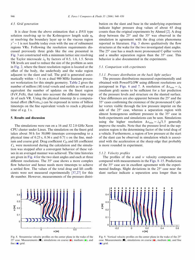
Fig. 8. Streamwise velocity profiles on the center plane in the wake of the25� case. Measurements (j), simulations on coarse (●), medium (●), andfine (●) grid.

bution on the slant and base in the underlying experimentindicate higher pressure drag values of about 65 dragcounts than the original experiments by Ahmed [2]. A dragdrop between the 25� and the 35� was observed in thesimulation in agreement with the drag crisis phenomenareported in literature. Fig. 5 shows qualitatively the flowstructures at the wake for the two investigated slant angles.The 25� case has a much more pronounced C-pillar vortexand a smaller separation region than the 35� case. Thisbehavior is also documented in the experiments.

5.1. Comparison with experiments

5.1.1. Pressure distribution on the back light surfaceThe pressure distributions measured experimentally and

obtained with PowerFLOW using different resolutions arejuxtaposed in Figs. 6 and 7. A resolution of Dxmin = kh

(medium grid) seems to be sufficient for a fair predictionof the pressure levels and structure on the slanted surface.Clear differences are also apparent between the 25� and the35� cases confirming the existence of the pronounced C-pil-lar vortex visible through the low pressure imprint on theside of the 25� case, whereas a separation region withalmost homogenous ambient pressure in the 35� case inboth experiments and simulations can be seen. Simulationsusing the higher resolution Dxmin = kh/1.5 generallyimprove the results. Note that the pressure level in the sep-aration region is the determining factor of the total drag ofa vehicle. Furthermore, a region of low pressure at the startof the slant can be observed in simulation which is associ-ated with the acceleration at the sharp edge that probablyis more rounded in experiment.

5.1.2. Velocity profiles

The profiles of the u and w velocity components arecompared with measurements in the Figs. 8–15. Predictionsof the 35� case are in excellent agreement with the experi-mental findings. Slight deviations in the 25� case near theslant surface indicate a separation area longer than in

x [m]

z [m

]

-0.2 0 0.2 0.4 0.6

0

0.1

0.2

0.3

0.4

Fig. 9. Vertical velocity profiles on the center plane in the wake of the 25�case. Measurements (j), simulations on coarse (●), medium (●), and fine(●) grid.

x [m]

z [m

]

-0.2 -0.15 -0.1 -0.05 00.25

0.3

0.35


x [m]

z [m

]

-0.2 -0.1 0

0.25

0.3

0.35

Fig. 11. Vertical velocity profiles on the center plane in the wake of the25� case. Measurements (j), simulations on coarse (●), medium (●), andfine (●) grid.

x [m]

z [m

]

-0.2 -0.1 0 0.1 0.2 0.3 0.4 0.5 0.6

0

0.1

0.2

0.3

0.4


x [m]

z [m

]

-0.2 -0.1 0 0.1 0.2 0.3 0.4 0.5 0.6

0

0.1

0.2

0.3

0.4


x [m]

z [m

]

-0.2 -0.1 0

0.25

0.3

0.35

0.4


x [m]

z [m

]

-0.25 -0.2 -0.15 -0.1 -0.05 0

0.22

0.24

0.26

0.28

0.3

0.32

0.34

0.36

0.38



experiment, i.e. a delayed reattachment. This can also bededuced from the pressure distribution in Fig. 6. The com-parison confirms that the coarse grid Dxmin = kh/0.5 isinsufficient for accurate predictions and that accuracy canbe increased using both the highest resolutions that indi-cate grid convergence.

5.1.3. Wake flow

The analysis of the flow structures in the wake of theAhmed body for the two slant angles shows the differentwake behavior as depicted in Fig. 16. The figure showsthe streamwise velocity component at different planesbehind the body. The vortical structures are apparent for

Fig. 16. Streamwise velocity distribution at x/L = 0.077, x/L = 0.19, x/L = 0.48 (top to bottom). Experiment, simulation on coarse, medium and fine grid(left to right). View in streamwise direction. Outline of the Ahmed body geometry is shown.


the 25� case whereas the 35� case exhibits a separationregion. Simulations on medium and fine grid agree wellwith measurements for both the flow structures and thequantitative levels. Slight asymmetry and small flow struc-tures are present in the calculation, which may be a con-sequence of a too short averaging interval.

6. Conclusions and application to further vehicles

The simulation of the Ahmed reference model using thelattice Boltzmann solver PowerFLOW has been conductedfor two slant angles 25� and 35� bracketing the critical angleof�30�. Analysis of the flow documents the different vortical


and separation behavior in the wake of the two configura-tions. Qualitative and quantitative comparisons with experi-ments show excellent agreement with experimental findingsand evidence the accuracy of the underlying unsteady numer-ical method in capturing the averaged flow phenomena.

The resolution requirement represents a key issue in thesimulation process. Different resolutions based on the Tay-lor microscale kh were conducted. The separation region iscaptured well using Dxmin = kh/1.5 and a fair prediction isalso achieved using Dxmin = kh. The approximation of kh

for different flow regions based on the relevant local Re

number can be used to determine the requirements in othersimulations. However, the computational requirements forrealistic vehicle geometries may be higher due to the reso-lution of the complex curved surfaces and details attachedto it such as side mirrors or wheels.

A general estimate of the timesteps required to achieveconvergence cannot be given, since it is highly dependenton the unsteadiness of the flow structures.

Acknowledgements

The author would like to thank B. Crouse and H. Chenfor their reviews and valuable comments.

References

[1] Abe T. Derivation of the lattice Boltzmann method by means of thediscrete ordinate method for the Boltzmann equation. J Comput Phys1997;131:241–6.

[2] Ahmed SR, Ramm G, Faltin G. Some salient features of the time-averaged ground vehicle wake. SAE Paper 1984;840:300.

[3] Alexander CG, Kandasamy S, Chen H, Shock RA, Govindappa SR.Simulations of engineering thermal turbulent flows using a latticeBoltzmann based algorithm. In: ASME PVP, proc of the 3rd int sympon comput technol for fluid/thermal/chemical/stress systems withindustrial applications; 2001.

[4] Alexander FJ, Chen S, Sterling JD. Lattice Boltzmann thermo-hydrodynamics. Phys Rev E 1992;47:2249–52.

[5] Anagnost A, Alajbegovic A, Chen H, Hill D, Teixeira C, Molving K.Digital physics analysis of the Morel body in ground proximity. SAEPaper 970139; 1997.

[6] Arunajatesan S, Sinha N. Hybrid RANS-LES modeling for cavityaeroacoustic predictions. Int J Aeroacoustics 2003;2(1):65–93.

[7] Basara B, Alajbegovic A, Steady state calculations of turbulent flowaround Morel body. In: Proceedings of the 7th int. symp. on flowmodelling and turbulence measurements. Taiwan; 1998.

[8] Bayraktar I, Landman D, Baysal O. Experimental and computationalinvestigation of Ahmed body for ground vehicle aerodynamics. SAEPaper 2001-01-2742; 2001.

[9] Bhatnagar P, Gross E, Krook M. A model for collision processes ingases. I. Small amplitude processes in charged and neutral one-component system. Phys Rev 1954;94:511–25.

[10] Bush RH, Mani M. A two-equation large eddy stress model for highsub-grid shear. AIAA Paper 2001-2561; 2001.

[11] Chapman S, Cowling T. The mathematical theory of non-uniformgases. Cambridge University Press; 1990.

[12] Chen H. Volumetric formulation of the lattice Boltzmann method forfluid dynamics: basic concept. Phys Rev E 1998;58:3955–63.

[13] Chen H, Kandasamy S, Orszag S, Shock R, Succi S, Yakhot V.Extended Boltzmann kinetic equation for turbulent flows. Science2003;301:633–6.

[14] Chen H, Molving K, Teixeira C. Digital physics approach tocomputational fluid dynamics: some basic theoretical features. Int JMod Phys C 1997;8:675–84.

[15] Chen H, Teixeira C. H-theorem and origins of instability in thermallattice Boltzmann models. Comput Phys Commun 2000;129:21–31.

[16] Chen H, Teixeira C, Molving K. Realization of fluid boundarycondition via discrete Boltzmann dynamics. Int J Mod Phys C 1998;9:1281–92.

[17] Chen S, Chen H, Martinez D, Matthaeus W. Lattice Boltzmannmodel for simulation of magnetohydrodynamics. Phys Rev Lett 1991;67:3776–9.

[18] Chen S, Doolen G. Lattice Boltzmann method for fluid flows. AnnRev Fluid Mech 1998;30:329–64.

[19] D. d’Humieres. Generalized lattice-Boltzmann equations. In: ShizgalBD, Weave DP, editors. Rarefied gas dynamics: theory and simula-tions, prog astronaut aeronaut, vol. 159. p. 450–58, 1992.

[20] d’Humieres D, Ginzburg I, Krafczyk M, Lallemand P, Luo L.Multiple-relaxation-time lattice Boltzmann models in three dimen-sions. Phil Trans R Soc Lond A 2002;360:437–51.

[21] Duell EG, George AR. Experimental study of a ground vehicle bodyunsteady near wake. SAE Paper 1999-01-0812; 1999.

[22] Duncan BD, Sengupta R, Mallick S, Sims-Williams DB. Numericalsimulation and spectral analysis of pressure fluctuations in vehicleaerodynamic noise generation. SAE Paper 2002-01-0597; 2002.

[23] Fillipova O, Hanel D. Grid refinement for Lattice-BGK models.J Comput Phys 1998;147:219–28.

[24] Gillieron P, Chometon F. Modelling of stationary three-dimensionalseparated air flows around an Ahmed reference model. ESAIM Proc1999;7:173–82.

[25] Gillieron P, Noger C. Contribution to the analysis of transientaerodynamic effects acting on vehicles. SAE Paper 2004-01-1311;2004.

[26] Le Good GM, Garry KP. On the use of reference models inautomotive aerodynamics. SAE Paper 2004-01-1308; 2004.

[27] Becker S, Leinhart H. Flow and turbulence structures in the wake of asimplified carmodel. SAE Paper 2003-01-0656; 2003.

[28] Halliday J, Teixeira C. Validating lattice-based CFD for automotiveHVAC ducting systems. In: Proc of ISATA conference, Dusseldorf;1998.

[29] Halliday J, Teixeira C, Alexander C. Simulation of engine internalflows using digital physics. Oil Gas Sci Technol—Rev IFP 1999;54(2):187–91.

[30] He X, Luo L-S. A priori derivation of the lattice Boltzmann equation.Phys Rev E 1997;55:6333–6.

[31] He X, Luo L-S. Theory of the lattice Boltzmann method: from theBoltzmann equation to the lattice Boltzmann equation. Phys Rev E1997;56:6811–7.

[32] Howard RJA, Pourquie M. Large eddy simulation of an Ahmedreference model. J Turbulence 2002;3.

[33] Hucho W-H. Aerodynamik des automobils. 3rd ed. Springer-Verlag;1999.

[34] Jakirlic S, Jester-Zurker R, Tropea C. Proc 9th ERCOFTAC/IAHR/COST workshop on refined turbulence modelling, Darmstadt; 2001.

[35] Kapadia S, Roy S. Detached eddy simulation over a reference Ahmedcar model. AIAA Paper 2003-0857; 2003.

[36] Krajnovic S, Davidson L. Large-Eddy simulation of the flow aroundsimplified car model. SAE Paper 2004-01-0227; 2004.

[37] Leinhart H, Stoots C, Becker S. Flow and turbulence structures in thewake of a simplified car model. In: Proc DGLR Fach Symp, AGSTAB, Stuttgart University; 2002.

[38] Li Y, Shock R, Zhang R, Chen H. Numerical study of flow past animpulsively started cylinder by lattice Boltzmann method. J FluidMech 2004;519:273–300.

[39] Makowski FT, Kim S. Advances in external-aero simulation ofground vehicles using the steady RANS equations. SAE Paper 2000-01-0484; 2000.

[40] Menter FR, Kuntz M, Bender R. A scale-adaptive simulation modelfor turbulent flow predictions. AIAA Paper 2003-0767; 2003.


[41] Morel T, Aerodynamic drag of bluff body shapes characteristic ofhatch-back cars, SAE Paper 780267; 1978.

[42] Vaillant O, Maillard V. Numerical simulation of wall pressurefluctuation on a simplified vehicle shape. AIAA Paper 2003-3271; 2003.

[43] Pervaiz MM, Teixeira CM. Two equation turbulence modeling withthe lattice-Boltzmann method. In: Proc of ASME PVP DivisionConference, Boston; 1999.

[44] Qian Y, d’Humieres D, Lallemand P. Lattice BGK models for theNavier–Stokes equations. Europhys Lett 1992;17:479–84.

[45] Sagaut P. Large Eddy simulation for incompressible flows. 2nded. Berlin: Springer-Verlag; 2004.

[46] Shan X, He X. Discretization of the velocity space in the solution ofthe Boltzmann equation. Phys Rev Lett 1998;80(1):65–8.

[47] Shock RA, Mallick S, Chen H, Yakhot V, Zhang R. Recent results ontwo-dimensional airfoils using a lattice Boltzmann-based algorithm.J Aircraft 2002;39(3):434–9.

[48] Sims-Williams DB, Dominy RG, Howell JP. An investigation intolarge scale unsteady structures in the wake of real and idealizedhatchback car models. SAE Paper 2001-01-1041; 2001.

[49] Sims-Williams DB, Duncan BD. The Ahmed model unsteady wake:Experimental and computational analyses. SAE Paper 2002-01-1315;2002.

[50] Spalart PR. Strategies for turbulence modeling and simulations. Int JHeat Fluid Flow 2000;21:252–63.

[51] Spohn A, Gillieron P, Flow separations generated by a simplifiedgeometry of an automotive vehicle. In: Proc of IUATM symb onunsteady separated flows, Toulouse; 2002.

[52] Succi S, Amati G, Benzi R. Challenges in lattice Boltzmanncomputing. J Stat Phys 1995;81(1/2):5–16.

[53] Teixeira CM. Incorporating turbulence models into the lattice-Boltzmann method. Int J Mod Phys C 1998;9(8):1159–75.

[54] Thompson KW. Time dependent boundary conditions for hyperbolicsystems II. J Comput Phys 1990;89:439–61.

[55] Yakhot V, Orszag SA, Thangam S, Gatski TB, Speziale CG.Development of turbulence models for shear flows by a doubleexpansion technique. Phys Fluids A 1992;4(7):1510–20.

[56] Yu D, Mei R, Shyy W. A multi-block lattice Boltzmann method forviscous fluid flow. Int J Numer Meth Fluids 2002;39:99–120.

Unsteady flow simulation of the Ahmed reference body using a lattice Boltzmann approach

Documents

Transcript of Unsteady flow simulation of the Ahmed reference body using a lattice Boltzmann approach