Fast Aerodynamic Calculations based on a Generalised1

Unsteady Coupling Algorithm2

Daniel Kharlamov ∗, Andrea Da Ronch †, Jernej Drofelnik ‡, and Scott Walker §3

Faculty of Engineering and Physical Sciences4

University of Southampton, Southampton, SO17 1BJ, U.K.5

An aerodynamic model for applications to external flows is formulated that provides a6

great trade–off between computational cost and prediction accuracy. The novelty of the work7

is the ability to deal with any unsteady flow problem, irrespective of the frequency of motion8

and motion kinematics. The aerodynamic model, baptised FALCon, combines an in–house9

unsteady vortex lattice method with an infinite–swept wing Navier–Stokes solver. The two10

specialised methods are orchestrated by an unsteady coupling algorithm that represents our11

main research contribution. The paper gives the formulation and algorithmic implementation.12

FALCon is demonstrated on three test cases of increasing complexity in flow physics, up to flow13

conditions well outside its validity range. On average, FALCon achieves a computational speed14

up of a factor of about 50, compared to a full Navier–Stokes run, while capturing relevant flow15

physics: three–dimensional, viscous, compressible and unsteady phenomena.16

Nomenclature17

: Reduced frequency [-], : = l2A4 5 /+A4 5

l Frequency [Hz]

�' Aspect ratio of a wing [-], �' = 12/(

W Taper ratio of a wing [-]

Λ Sweep of the wing [◦]

1 Span of the wing [<]

2 Chord length [<]

+ Freestream velocity [-]

V∞,= Local freestream angle of attack at =-th panel corrected by ΔU= [</B]

Δ+F,= Local VLM panel velocity contribution from unsteady wake in UVLM [</B]

Vn Local velocity on the =-th VLM panel [</B]

∗PhD student. Currently, Junior Researcher at ISL (French–German Research Institute of Saint–Louis, France). Email: D.Kharlamov@soton.ac.uk†Associate Professor, AIAA Senior Member. Email: A.Da-Ronch@soton.ac.uk‡Research Fellow. Currently, Aerodynamics Design Engineer at Pipistrel Vertical Solutions, Slovenia.§Associate Professor.

U Angle of attack [A03]

ΔU Angle of attack correction increment [A03]

UBC0;; Stall angle of attack [A03]

U4 Effective angle of attack [A03]

U8=3 Induced angle of attack [A03]

# Total number of wing bounded vortex ring elements [-], # = #G × #H

#G Amount of vortex–ring elements along the chord of a lifting surface [-]

#H Amount of vortex–ring elements along the span of a lifting surface [-]

A Global aerodynamic influence matrix

Γ Vortex intensity of a vortex–ring element [<2/B]

� Global vortex intensity vector

R Global non–circulatory vector

n= Local normal vector of the =-th vortex ring element [<]

d Density of the fluid [:6/<3]

XFB Local steady–state aerodynamic force [#]

XFD Local unsteady aerodynamic force contribution [#]

�! Lift force coefficient [-]

�!, <0G Maximal lift force coefficient [-]

�!,8=E Inviscid, linear lift force coefficient [-]

�!,E8B2 Viscous lift force coefficient [-]

�!,E,0 Viscous lift at U = 0◦ [-]

�U!

Lift slope [1/◦]

( Surface area [<2]

(= Local surface area of =-th vortex–ring element [<2]

a Relaxation factor [-]

Y Convergence tolerance [-]

H/1 Non–dimensional span coordinate [-]

#H/1 Number of predefined CFD airfoil solvers along the span [-]

#U Number of predefined angle of attacks of CFD airfoil solvers [-]

ΔC Physical time step [B]

Δg Reduced time step [-], Δg = ΔC+/2

ΔU0 Pitching amplitude [◦]

2

Δℎ2,0 Non–dimensional heaving plunge amplitude [-]

ℎ2 Non–dimensional vertical displacement [-]

" Mach number [-]

'4 Reynolds number [-]

H+ Dimensionless wall distance [-]

I. Introduction18

Aerodynamic models based on linear aerodynamic assumptions have been used in the aerospace industry since19

the 1960s [1] due to: a) straightforward set–up of the problem, using simplified descriptions of the lifting surfaces;20

b) low computational effort enabling efficient trade–off studies for envelop searches; and c) its applicability, as the21

method has been calibrated on a number of existing aircraft configurations to account for unmodelled nonlinear flow22

phenomena. These models are deployed to support the development of unconventional configurations at the conceptual23

stage, expediting the exploration and down–selection of a large number of configurations. Higher–fidelity aerodynamic24

models based on full three–dimensional (3D) Reynolds–averaged Navier–Stokes (RANS) solvers may provide a feasible25

alternative to existing practice. However, these models are too expensive for routine use to industrial applications26

owing to the high computational costs involved in solving the RANS equations. Today, they find deployment in the27

late preliminary to detailed stages, mostly for steady–state problems. A third level of fidelity in aerodynamic analysis28

tools exists in an attempt to bridge knowledge–based and linear models with higher–fidelity models. A brief historical29

overview of this mixed–fidelity level follows in the subsequent paragraphs.30

The steady–state analysis for a subsonic flow is traditionally performed using the lifting–line model, or models31

based on linear panel theory. As an extension, the first nonlinear coupling between the lifting–line model and viscous32

lift curves of airfoils was proposed in 1934 by Tani [2] and in 1938 by Multhopp [3]. In their approach, the circulation33

intensity of the vortex–ring elements is corrected within the lifting–line model by using sectional viscous data extracted34

from aerofoil lift curves. This approach ensures a better match of the nonlinear lift slope of a finite wing at higher angles35

of attack. In 1947, an improved nonlinear lifting–line model, but based on the same approach of [2, 3], was proposed36

in [4] which iteratively corrects the numerical results obtained by the lifting–line model using nonlinear sectional lift37

curve data. In 1951, Sivells et al. [5] extended the coupling algorithm to unswept wings including flaps and ailerons into38

the model. The underlying idea is to correct iteratively the vortex intensity of the wing bounded vortex lattice method39

(VLM) panels using available two–dimensional (2D), nonlinear aerodynamic data. This method is commonly denoted40

Γ–based coupling algorithm. The 3D numerical results of the aerodynamic loads on wings obtained by this approach41

3

were in good agreement with 3D reference data before the stall angle of attack, UBC0;; . However, the applicability of the42

Γ–based coupling algorithm is limited to the maximum wing lift coefficient, �!, <0G . Beyond stall, the lift curve slope,43

�U!, becomes negative and the solution not unique.44

To overcome the non–uniqueness of the Γ–based coupling algorithm near stall, Tseng and Lan [6] proposed45

the U–based correction method in 1988. Their method couples the lifting–line model or the VLM with sectional46

aerodynamic data by correcting, at each aerodynamic panel along the wing span, the local freestream angle of attack.47

The algorithm, however, suffered from poor convergence in post–stall conditions. In the 2000s, Van Dam et al. [7, 8]48

introduced a revised formulation to improve the convergence properties of the Γ–based coupling algorithm. More49

recently, Gallay and Laurendeau [9] [10] extended the formulation to general wing planforms in low– and high–speed of50

flight, and at high angles of attack.51

A formulation for unsteady flows was presented in 2017 [11]. Two approaches, with a precomputed viscous52

database, were discussed. In cases where the quasi–steady assumption holds valid, the database is computed from53

RANS calculations. This approach is limited to low reduced frequencies, i.e. heuristically : < 0.1, and low angles54

of attack. In the second approach, the database is enriched with information extracted from a set of forced motion55

calculations at several values of mean angles of attack and frequencies. Limitations of this approach are related to the56

neglect of flow unsteadiness, which becomes a dominant feature in modern aircraft manoeuvres [12], and to the wing57

kinematics being restricted to a pure sinusoidal motion. It is also worth noting that time marching the unsteady RANS58

(URANS) equations for periodic flows, as those developing when a forced motion is imposed, is inefficient [13] given59

the availability of dedicated frequency–domain methods [14]. The second approach carries a resemblance with the60

concept of aerodynamic tables used for flight simulation, and the incidental drawbacks preventing the full representation61

of unsteady flows [15].62

The quest for a reliable methodology offering affordable prediction and accurate reconstruction of scalar and63

vector fields has intensified in the last few years. A reason for this ascending trend is the emergence of open–source,64

off–the–shelf, machine–learning resources. Beyond studies on applied aerodynamics above–mentioned, fluid mechanics65

has seen a surge of applications leveraging on data assimilation techniques [16–19]. Common to all approaches, which66

range from Gradient–enhanced Kriging [19] to deep learning [17] models, is the need to improve the prediction accuracy67

of a lower fidelity model, which may span the entire spectrum of the fluid equations, by assimilating some, distilled68

information from a higher fidelity model or available measurements. The enhanced, lower fidelity model is then used69

to reconstruct the scalar or vector field across the whole spatial domain. In Europe, in particular, data assimilation70

and machine learning techniques are core to the European Commission funded project "Holistic Optical Metrology for71

Aero–Elastic Research". ∗72

At the core of our work is the need to develop a general framework for unsteady flow problems. Rather than73

∗HOMER project website: https://cordis.europa.eu/project/id/769237. Grant agreement ID: 769237.

4

restricting the admissible kinematics of motion due to underlying simplifications, we have chosen to solve certain74

implementation challenges to retain generality, in such a way to analyse any arbitrary motion. The paper continues in75

Section II outlining the overall approach and providing implementation details. Then, Section III contains a validation76

of the specialised aerodynamic models that constitute the computational framework. A demonstration on test cases of77

increasing complexity is presented in Section IV. Finally, concluding remarks are drawn in Section V.78

II. Formulation79

Analysing the external aerodynamics of a wing configuration to a suitable physical resolution is computationally80

expensive. To address this challenge, we have developed a methodology that computes rapidly aerodynamic loads81

for steady and unsteady flows. The methodology is compatible with generally available aerodynamic models, using82

information and data shared during the aircraft conceptual design, and favouring a seamless integration within an83

existing environment.84

The approach we have followed partitions the complex flow problem into two simpler problems. The first problem85

provides a quick but global overview of the impact that wing planform design variables have on aerodynamic loads.86

Design variables common to the aircraft designer are aspect ratio, taper ratio, and sweep/dihedral angles, among others.87

The second problem solves the relevant flow physics to a desired accuracy around a 2D wing section. This local88

representation shall account for viscous and compressible flow effects, as well as thickness effects, otherwise neglected89

in the general problem. The two separate problems are united by the wing sweep angle, which is a common design90

parameter to both problems. In our implementation, the global problem is solved using the unsteady VLM (UVLM)91

that is computationally cheap, described in Section II.A, and the local problem is solved using the infinite–swept wing92

Navier–Stokes solver, overviewed in Section II.B.93

The resulting computational tool, referred to as FALCon, builds on two independent, specialised aerodynamic94

solvers of different fidelity and computational cost which are brought together by one dedicated coupling algorithm that95

orchestrates the timely execution of the two solvers in the time domain. The novel coupling algorithm is thoroughly96

discussed in Section II.C.97

A. Vortex Lattice Method98

The VLM follows the classic implementation of Katz and Plotkin [20] and Murray [21]. However, there are certain99

necessary expedients to transform the classic implementation into one suitable to exchange information with an external,100

viscous solver. These expedients are highlighted hereafter.101

A typical unsteady VLM lattice is shown in Figure 1. The lattice consists of wing bounded and free wake panels102

which are shed at each time step, C: = C0 + : ΔC, into the farfield. The body–fixed frame of reference has the G–axis in103

line with the in–coming flow and the H–axis directed towards the wing tip. Each wing bounded panel is identified by the104

5

chordwise index, 8, and the spanwise index, 9 . The vortex ring elements are placed at the quarter–chord line of every105

panel.106

Fig. 1 Unsteady Vortex–Lattice method (Katz and Plotkin [20])

The necessary expedients relate to the calculation of the spanwise distribution of the local angle of attack, U 9 , at the107

collocation point of a wing bounded panel and the corresponding sectional inviscid lift coefficient, �!,8=E, 9 . These108

parameters shall be calculated and manipulated independently from the values assigned to freestrem and to neighbouring109

panels. The local angle of attack at the 9–th wing bounded vortex panel is computed:110

U 9 = U∞ + ΔU 9 9 = 1, 2, . . . , # 9 − 1 (1)

where # 9 is the number of spanwise wing bounded vortex ring panels. The correction of the local angle of attack, ΔU 9 ,111

is only relevant when the VLM is coupled with a viscous solver. The parameter ΔU 9 interfaces the coupling algorithm112

and the VLM model.113

Using Eq. (1), the local non–circulatory freestream velocity vector at the 9–th spanwise position of the lattice is:114

V∞, 9 = +∞[

cos(U 9

), 0, sin

(U 9

) ]) (2)

Here, +∞ is the freestream speed. Further, Biot–Savart law is employed for the calculation of the circulatory velocity115

contribution, V=<, of the <–th vortex ring element on the =–th collocation point [21] :116

V=< = Γ<

∮3s< × r=<4c |r=< |3

= Γ< q=< (3)

The vortex ring intensity is Γ< and s< is the geometrical contour line of the vortex ring of the <–th VLM panel.117

Further, r=< is the distance vector between the current position on the vortex ring contour of the <–th panel and the118

6

collocation point of the =–th panel. The integral is calculated clockwise.119

The total local flow velocity at the =–th collocation point of a vortex–ring element is:120

V= = V=,00 + V=,10 + V∞,= + Δ¤x2,= (4)

where V=,00 is the circulatory velocity contribution induced by all wing bounded VLM panels onto the collocation point121

of the =–th wing bounded panel. The term V=,10 is the circulatory velocity contribution of all wake panels onto the122

collocation point of the =–th wing bounded panel and V∞,= is the non–circulatory local freestream velocity contribution123

(refer to Eq. (2)). Finally, Δ¤x2,= is the time derivative of the position of the collocation point in space.124

Kinematic boundary conditions are enforced at all collocation points of the wing bounded VLM panels:125

V= · n= = 0 (5)

where n= is the normal vector of a panel placed at the collocation point (see Figure 1). This ensures that the potential126

flow is tangential to the surface of the panel at the collocation point. Combining Eq. (3) with Eq. (4) allows rewriting127

Eq. (5) for the =–th VLM panel as:128

n= ·#∑<=1

Γ(8)< q=< = −n=

(V∞,= (ΔU=) +

#F∑<F=1

Γ(8−1)F0:4,<

q=<F+ ¤x2,=

)(6)

Here, # = #8 · # 9 is the total number of wing bounded vortex–ring elements and #F is the total number of all wake129

panels at a particular time, C8 . The circulatory wing bounded vortex ring intensity, Γ(8)< , at the actual time step, C8 , may130

be calculated as the vortex ring intensity of the wake panels, Γ(8−1)F0:4,<

, is known. New panels are shed into the wake131

during the unsteady process. These panels, departing from the wing trailing edge, have the same vortex intensity as132

the wing bounded trailing edge vortex elements at a generic time step, Γ(8)#8+1 , 9

= Γ(8−1)#8 , 9

. Then, the new wake panels133

travel into the farfield with a constant vortex intensity, ΓF0:4,<. This guarantees the Kutta–Joukowski flow tangency134

condition at each time step.135

Equation (6) is conveniently rewritten in a compact, matrix–vector form:136

A · � = R(ΔU) (7)

where A represents the aerodynamic influence coefficient matrix and R is the residual vector of non–circulatory velocity137

and current wake contributions, updated at each time step. It is worth noting that, for integration to the coupling138

algorithm, the non–circulatory velocity shall include the increment of the current angle of attack correction, ΔU, from139

Eq. (6).140

7

1. Calculation of Aerodynamic Loads141

The calculation of aerodynamic loads is a prerequisite for the execution of the coupling algorithm. The reason for142

this is that the algorithm matches, to a user–defined tolerance, the lift coefficient from the inviscid solver, i.e. the VLM,143

and that from the viscous solver (refer to Eq. (21)).144

Aerodynamic loads generated from wing panels are calculated once � is known. A non–planar formulation based145

on the Kutta–Joukowski theorem in vectorised form is used [22]:146

XFB= = d∞ V∞,= × Δ�= = d∞ ΔΓ= V= × Δl= = = 1, 2, 3, . . . , # (8)

where d∞ is the fluid density, V∞,= is the local non–circulatory freestream velocity at the collocation point (Eq. 2) and147

Δ�= is the total vortex strength placed at the quarter–chord line of the =–th panel. This total vortex strength can be148

expressed as Δ�= = ΔΓ= Δl=, where Δl= is the vector representing the quarter–chord line of the particular VLM panel.149

The local vortex strength intensity, ΔΓ8, 9 , of the quarter–chord line of the panel is obtained from the global vector �150

as follows:151

ΔΓ8, 9 =

Γ8, 9 − Γ8−1, 9 if 8 > 1

Γ8, 9 if 8 = 1(9)

For all panels, which are not directly located at the leading edge of the lattice, i.e. 8 > 1, ΔΓ is obtained as difference152

between the vortex ring intensity of the current panel, (8, 9), and the intensity of the corresponding upstream VLM153

panel, (8 − 1, 9).154

In an unsteady analysis, Eq. (8) is augmented with a contribution from unsteady, transient loads [22]:155

XFD= = d∞Δ ¤Γ=(=n= (10)

where Δ ¤Γ= is the time derivative of ΔΓ= and (= the reference panel area. The time derivative, Δ ¤Γ=, is approximated156

with first order, forward Euler method:157

Δ ¤Γ= ≈ΔΓ(:)= − ΔΓ(:−1)

=

ΔC(11)

As a final step, the lift coefficient at the 9–th panel is calculated as:158

�!,8=E, 9 =1

@∞ ( 9

#8∑8=1

(X�BI,8, 9 + X�DI,8, 9

)(12)

where @∞ = 0.5 d∞+2∞ is the freestream dynamic pressure, ( 9 is the reference area of the 9–th panel, and X�BI,8, 9 and159

X�DI,8, 9

are, respectively, the steady and unsteady lift contributions.160

8

2. Calculation of Induced Angle of Attack161

The induced angle of attack, U8 , plays an important role as part of the coupling algorithm. Practically, the induced162

angle of attack allows including 3D aerodynamic effects, which are predicted by the VLM, within the sectional viscous163

data. The calculation of U8 is needed at each time step, as represented in Eq. (19).164

Following Katz and Plotkin [20], denote 1=< the aerodynamic influence coefficient of the <–th vortex ring on the165

collocation point of the =–th panel. Then:166

1=< = n= · q=< (13)

where q=< is the normalised velocity contribution by the vortex ring intensity, Γ<, of the <–th vortex wing, when only167

two streamwise vortices of the panel are taken into account. The induced downwash coefficient, F8=3 , at the collocation168

point of the =–th wing bounded vortex ring element is calculated as:169

F8=3,= = 1=< Γ< (14)

This post–processing step is carried out for all wing bounded vortex–ring elements at each time step. Finally, U8 is170

calculated at the collocation point of every wing bounded vortex–ring panel:171

tan(U8=3,=

)= −

F8=3,=

+∞(15)

As a final consideration, a careful implementation of the above–mentioned expedients ensures accessing the spanwise172

distribution of the induced angle of attack, U8=3, 9 , and that of the inviscid lift coefficient, �!,8=E, 9 , at each VLM panel.173

These quantities will be feed in to the coupling algorithm.174

B. Infinite–swept Wing Navier–Stokes Solver175

In the interest of conciseness, a high–level presentation of the infinite–swept wing Navier–Stokes solver is here176

given. The reader shall consult Ref. [23] for further details here irrelevant.177

In a 2D analysis, the flow solution does not depend on the third direction. Practically, this approach is restrictive178

when the wing cross–section is swept from the in–flight direction (or the direction of the in–coming flow). Cross–flow179

effects become dominant, and greatly affect the flow development around the wing cross–section. The infinite–swept180

wing Navier–Stokes solver is developed for these cases in mind. It relaxes the assumptions of a 2D solver, only enforcing181

the flow to be uniform along the third direction. The flow component along the third direction is calculated as part of182

the solution process, rather than being prescribed as in a 2D analysis.183

Advantages of the infinite–swept wing Navier–Stokes solver are two–fold. The solver allows investigating a greater184

9

generality of flow conditions around unswept and swept wings, employing the same 2D grid traditionally used in a185

classical, 2D analysis. The implementation of this specialised solver is easily done starting from a 2D or 3D flow solver.186

Geometric sweep effects are included through a thickening of the wing cross–section.187

All results here reported were generated using the DLR�tau flow solver. Our group at Southampton implemented and188

integrated the infinite–swept wing Navier–Stokes solver into DLR�tau. Due to its computational efficiency compared189

to existing state–of–the–art options, the implementation is denoted as 2.5D+. The steady and unsteady 2.5D+ flow190

solver was demonstrated [23] around single and multi–element wing sections in low– and high–speed of flight, using191

laminar and various turbulence models. The flow solver was applied to study transonic buffet for a family of wing192

configurations [24] and in aerodynamic shape optimisation using solvers of different fidelity [25]. Since its deployment193

within an industrial environment, the 2.5D+ flow solver has been used in excess of hundreds of thousands of times for194

production.195

C. Unsteady Coupling Algorithm196

Having described two specialised aerodynamic models of different fidelity, we now turn our attention to the197

coupling algorithm that represents the novelty of this paper. The formulation of the coupling algorithm builds upon198

the steady–state, U–based coupling algorithm. A schematic of the unsteady coupling algorithm is shown in Figure 2.199

Confronted with the steady–state version, the unsteady counterpart features an outer time loop to advance the two200

aerodynamic models in time. The algorithm, designed to spawn new processes, connect to their input/output/error pipes,201

and obtain their results, is structured in two main parts. These are discussed thoroughly in the following sections. At the202

core of the unsteady coupling algorithm is the ability to deal with any arbitrary, a–priori unknown motion in order to203

overcome limitations of current state–of–the–art alternatives.204

1. Part I: Synchronous Management of Aerodynamic Models205

The overarching goal of Part I is to manage data generation from two specialised and separate aerodynamic models.206

The different aspects of coordinating the time integration of the models are seen as elements of an interdependent207

process, managing them in a manner to optimise the performance of data generation for any arbitrary motion.208

Part I supervises critical aspects, such as, advancing the UVLM and URANS solutions in the time domain, adopting209

the same time step size. For cases with geometry motion, the position and rotation of the planar VLM lattice is210

trivially updated. Moving the 2D grid of the URANS solver is done by a rigid translation and rotation. This method is211

preferred over alternatives because, in all cases, it avoids warping the mesh or re–meshing the grid, operations that212

would otherwise become necessary and add computational cost when performing an aeroelastic analysis with a 3D grid.213

It is worth noting that a translation, i.e. in–plane or out–of–plane bending, and a rotation, i.e. torsion, are fundamental214

components to reconstruct any general type of motion. Motion rates have an impact on flow unsteadiness and shall be215

10

PART I

Start

Advance time in URANS solvers and UVLM

Move VLM/CFD grids

Compute visc. CL

Run linear UVLM solver

Interpolate visc. CL

Correct angle of attack

Convergence?

tk = t

END?

Finish

i+1tk+Δt

no

noyes

yes

2D CFD solver Nr. 1

2D CFD solver Nr. 2

2D CFD solver Nr. 3

...

Δ α , qΔh ,h

Δ t

2D URANS CFD solver container

CL,visc,01

CL,visc,02

CL,visc,03

PA

RT

IP

AR

T I

I

Fig. 2 Schematic of the unsteady coupling algorithm: Part I performs synchronous management of aerody-namic models, and Part II executes data fusion

11

included. In the UVLM, the velocity of the collocation point of every wing bounded panel, Δ¤x2,=, contributes to Eq. (4)216

and is calculated with first order, forward Euler method:217

¤x2,= ≈x(:)2,= − x(:−1)

2,=

ΔC(16)

In the URANS solver, motion rates are imposed through additional unsteady whirl–flux velocities calculated once218

the motion at the current time step is known. As a result, FALCon offers the capability to analyse any arbitrary motion,219

whether prescribed or unknown a–priori.220

Managing data generation is the most challenging aspect of the coupling algorithm. The view is to have a database,221

or container, of unsteady, viscous aerodynamic data which is interrogated on–demand during the iterative process222

coordinated by Part II (further details follow in Section II.C.2). Confronted with existing alternatives already discussed in223

the Introduction, our implementation follows the most general approach which comes with a number of implementation224

challenges. With support of Figure 3, consider a wing with a cross section that varies along the span. As an example,225

three sections (20, 50 and 80% of the span) are considered where sectional aerodynamic characteristics are sought226

after. At the core of Part I is the ability to compute the dependence of the unsteady, sectional lift coefficient on the227

instantaneous angle of attack and on relevant motion rates, at each particular wing section. The dependence on the angle228

of attack is not unexpected because our approach builds upon the steady–state, U–based coupling algorithm. From229

Figure 3, Part I spawns 15 URANS analyses, grouped into three spanwise sections. Initially, the viscous database stores230

data from 15 RANS analyses which are initialised from different freestream values of the angle of attack. Figure 3231

shows an exemplary range chosen between −8 and 8◦. The initial database is steady–state and does not include unsteady232

effects. To overcome this limitation, at each time step iteration, C: , the instantaneous motion and rates become known.233

Then, Part I spoons this information to all URANS analyses (which are marched in time using dual–time stepping [26])234

and a new database valid at C: is generated. Data are stored in a tabular form that visually takes the form of a carpet plot235

(see insert in Figure 2) representing the sectional, viscous �! (C: ) versus U (C: ) and H/1. The dependence on motion236

rates is omitted for brevity. As explained in the next Section, Part II will access this database to extract, at each wing237

section H/1, the viscous lift coefficient at the current time step, C: , interpolated at a specified value of the effective angle238

of attack:239

�!,E8B2 (C: ) = 5 (U4 (C: ) , H/1) (17)

Particular attention shall be devoted to two considerations. The first is for the initial angle of attack range, see240

Figure 3. Part II accesses the viscous aerodynamic database with a value of U4 (C: ) calculated from Eq. (19). The241

iterative nature of data fusion, exemplified by Eq. (21), proceeds through variations or corrections of the angle of242

attack. It is therefore critical to have a sufficiently wide range to avoid hampering the convergence of the algorithm (i.e.243

12

interpolation is preferred over extrapolation). The second consideration relates to the motion. There are cases where the244

motion is unknown a–priori, such as in flight dynamics or aeroelasticity. An external, dedicated model will then be245

responsible to calculate the motion and rates for a set of aerodynamic loads calculated at C: . The motion information is246

then spooned to Part I that continues the above–mentioned process.247

α

α=0o

α=4o

α=8o

α=−4o

α=−8o

y /b=0.5 y /b=0.8y /b=0.2

y /b

Fig. 3 Schematic of the tabular format of the viscous aerodynamic container, showing dependence on angle ofattack and spanwise location. Dependence on motion rates is not represented for simplicity

2. Part II: Data Fusion248

At the core of Part II is the process of integrating aerodynamic data from two aerodynamic sources to produce more249

consistent and accurate information than that provided by any individual data source. For steady–state problems, one250

turns to Van Dam’s U–based coupling algorithm [7]. The literature is scarce when unsteady problems are considered.251

A possible approach is to resort to the calculation of the sectional, effective angle of attack, U4, 9 , using the252

formulation [27]:253

U4, 9 =�=

2c(18)

where �= is the unsteady, sectional normal force coefficient from the inviscid solver. The caveat of this simple254

relationship is that �= shall relate to the circulatory contribution only, but the UVLM does not separate the circulatory255

contribution from the non–circulatory one [28]. As a result, we have observed an overestimation of U4, 9 which leads to256

a significant overprediction of the unsteady, sectional, viscous lift coefficient, �!,E8B2 . Our suggestion is to consider the257

13

alternative:258

U4, 9 = U∞ − U8=3, 9 | (2/4) (19)

where U∞ is the nominal freestream angle of attack. The second term on the right hand side is the induced angle of259

attack at the quarter chord of the wing section calculated using the inviscid solver. Generally, the VLM formulation260

calculates the induced angle of attack at the collocation point of wing bounded panels. To obviate this conflict, the261

interpolated value at the wing sectional quarter chord is based on interpolation of the values at the collocation points of262

two or more chordwise panels, #8 > 1.263

At the 9–th wing section, the instantaneous, viscous lift coefficient �!,E8B2 is extracted from the viscous database264

created at the actual time step, C: . The database is interrogated with the value of U4, 9 obtained from Eq. (19). Then, the265

angle of attack correction at the 9–th wing section is estimated for the next time step, C:+1:266

ΔU(:+1)9

= ΔU(:)9+ a

�(:)!,E8B2

− � (:)!,8=E

2 c(20)

where a is the relaxation factor used to control the update of the variable at each inner iteration. As depicted in Figure 2,267

Part II supervises the convergence behaviour of the pseudo–iterations. Convergence at each time step is achieved when268

the lift coefficient from the two aerodynamic sources, at all spanwise wing stations, meets the following condition269

‖�!,E8B2, 9 − �!,8=E, 9 ‖ < Y (21)

The parameter Y is a user–defined tolerance regulating solution accuracy.270

III. Validation271

This section concerns the validation of the UVLM for a set of canonical problems: a suddenly accelerated flat plate272

of different aspect ratios, and a thin aerofoil undergoing forced motion in two degrees of freedom. The validation of the273

infinite–swept wing Navier–Stokes solver is here omitted for brevity. The reader eager to learn more details about this is274

encouraged to examine Ref. [23].275

A. Suddenly accelerated flat plate276

The lift coefficient build–up for a suddenly accelerated flat plate is reported in Figure 4 for values of the aspect ratio277

(�') from 4 to infinity. The VLM lattice consists of 4 chordwise panels and 26 spanwise panels, equally distributed278

between root and tip. When �' = ∞, the flow is fully 2D. Practically, the UVLM uses a sufficiently large aspect279

ratio (�' = 100) combined with one spanwise panel to neglect modelling 3D effects. A nondimensional time step280

Δg = 1/16 is used for all unsteady analyses, and the freestream angle of attack is 5◦. The initial impulsive part and the281

14

trend to steady state for increasing times are well captured, for all values of �'. Reference data are from Ref. [20].282

τ [­]

CL [

­]

0 2 4 6 8 100.1

0.2

0.3

0.4

0.5

0.6

Reference

FALCon, linear UVLM

AR 4

AR 12

AR 8

AR 20

AR ∝

dτ = U∝dt/c = 1/16

α∝ = 5.0°

Fig. 4 UVLM validation: suddenly accelerated flat plate. Reference data from [20]

B. Forced motion of a thin aerofoil in pitch and plunge283

The second validation test case is for a thin aerofoil undergoing a prescribed motion. The test case introduces the284

dependence on two degrees of freedom that are independently excited and on the reduced frequency of oscillations,285

: = l 2/+∞.286

For an harmonic motion, the time history of the pitch degree of freedom is defined by:287

U (g) = U0 + U� sin (2 : g) (22)

where U0 is the mean value and U� the amplitude of oscillations. Similarly, for plunge:288

b (g) = b0 + b� sin (2, : g) (23)

where b = ℎ/2 represents the nondimensional plunge or heave. Two types of motion are here considered: 1) a pure289

pitch around the quarter–chord point, defined by parameters U0 = 0◦ and U� = 2.5◦; and 2) a pure plunge, b0 = 0 and290

b� = 0.1. For both types of motion, three values of the reduced frequency are used: : = 0.5, 1.0 and 1.5. In the291

UVLM, the 2D aerodynamics around the thin aerofoil is obtained using one panel in the spanwise direction, as in the292

previous Section for �' = ∞. The number of chordwise panels was determined by a convergence study, similarly to293

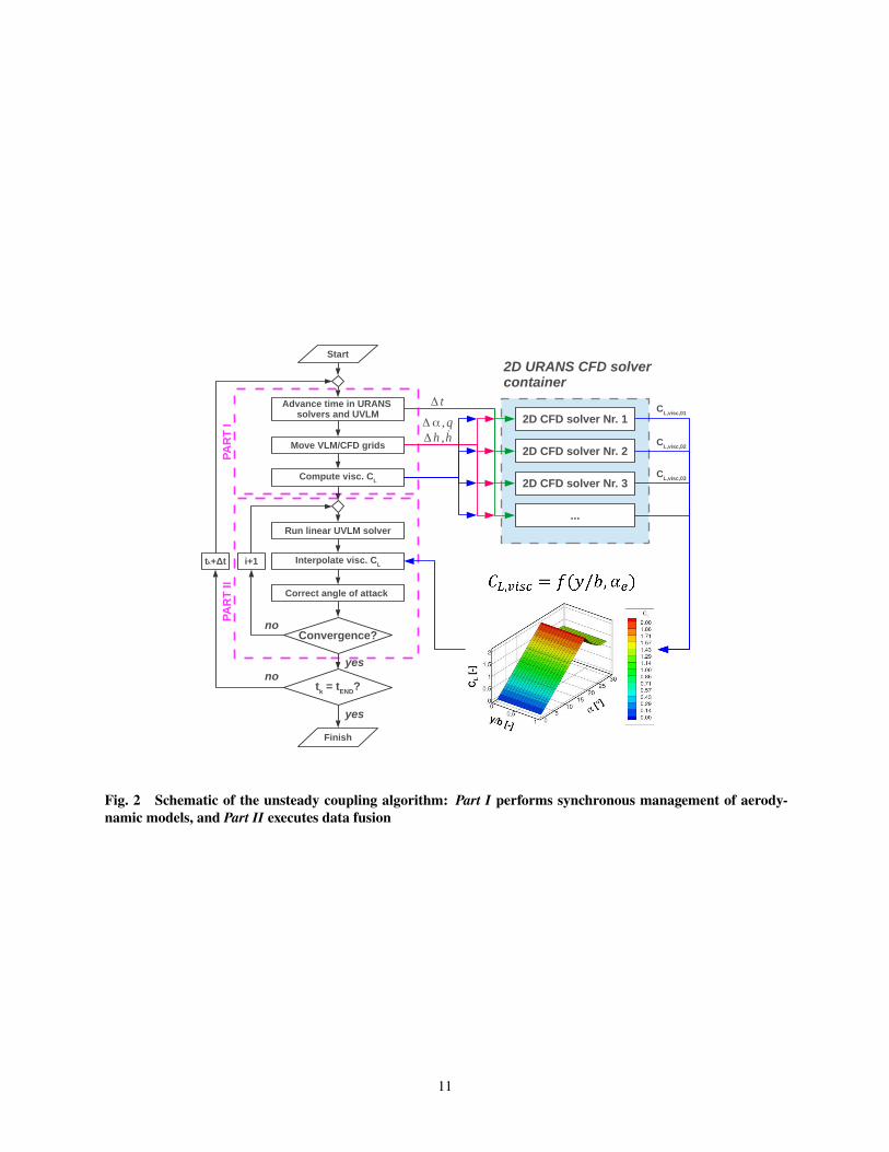
Ref. [29], summarised in Table 1. It is worth noting that the nondimensional time step satisfies the relation Δg = 1/#8 .294

This ensures that the chord length of new panels shed into the wake is equal to the chord length of wing bounded panels.295

15

: #8 # 9 Δg [ ]0.5 25 1 0.04001.0 28 1 0.03571.5 42 1 0.0238

Table 1 UVLM validation: space and time discretisation parameters

Hysteresis loops are shown in Figure 5. Initial transients were removed to highlight the periodic nature of the lift296

coefficient. Reference data are obtained using Theodorsen’s analytical model [30]. One observes a good match between297

the analytical curves and the UVLM for all cases considered, ranging from low to high values of the reduced frequency.298

Pitching angle α [°]

CL [

­]

­3 ­2 ­1 0 1 2 3­0.3

­0.2

­0.1

0

0.1

0.2

0.3

Linear UVLM, thin airfoil

Theodorsen

k 1.5

k 1.0

k 0.5

(a) Pitch motion

Vertical plunging displacement (h/c) [­]

CL [

­]

­0.1 ­0.05 0 0.05 0.1­0.9

­0.6

­0.3

0

0.3

0.6

0.9

k 1.5

k 1.0

k 0.5

(b) Plunge motion

Fig. 5 UVLM validation: forced motion of a thin airfoil. Reference data reproduced from [30]

IV. Results299

This Section demonstrates the applicability of the complete computational tool FALCon to a number of test cases of300

increasing complexity. The physics ranges from incompressible to compressible flows in a 2D and 3D setting, driven301

by unsteady motions at different reduced frequencies. Reference data are obtained from DLR-Tau code solving the302

URANS equations. The turbulence model is based on Spalart–Allmaras model [31].303

A. Forced harmonic motion in pitch and plunge: infinite–span wing304

The first demonstration test case is for a pitching and plunging NACA 2412 aerofoil (infinite–span wing). The305

compressible flow, which features a weak shock wave, is for " = 0.7 and '4 = 5.5 · 106. The harmonic motions are306

prescribed at low and high values of the reduced frequency, respectively, : = 0.025 and 0.750. In pitch, U0 = 0◦ and307

U� = 2.51◦, and in plunge, b0 = 0 and b� = 0.1. The pitch axis is at the quarter–chord point.308

Reference data are obtained from time marching the 2D URANS equations. The O–type, structured grid in Figure 6a309

16

used in all calculations was chosen to guarantee grid independent results. Three levels of grids were generated, from310

about 25 thousand to 70 thousand grid points. The coarser grid was found adequate to model the unsteady lift coefficient,311

as reported in Figure 6b. The convective RANS flux is discretised using the second–order central scheme. For time312

integration, the dual time–stepping scheme is used. The 2w–cycle multigrid scheme with 50 quasi–steady subiterations313

per physical time step is chosen at a Courant–Friedrichs–Lewy number of 2.5.314

(a)

α [°]

CL [

­]

­2 ­1 0 1 2

0

0.2

0.4

0.6

0.8

Coarse, 25704 grid point

Middle, 42120grid points

Fine, 69472 grid points

M 0.7

k 0.025

(b)

Fig. 6 Test case A: in (a), coarse 2D grid used in all calculations; and in (b), grid convergence study (" = 0.7and : = 0.025)

The analysis setup for FALCon is as follows. The UVLM lattice consists of one single panel (# 9 = 1 and #8 = 1)315

of high aspect ratio (�' = 100) motivated by the 2D aerodynamics of this test case. For the viscous solver, numerical316

parameters are identical to those above–mentioned for the reference data. For this 2D case, the coupling algorithm317

initially spawns one URANS analysis at the static freestream angle of attack of U0 = 0◦. As for the 2D nature of the318

flow, Eq. (19) of the unsteady, U–based coupling algorithm simplifies to:319

U4, 9 = U∞ = U0 (24)

after eliminating the induced angle of attack from the original formulation. For the coupling algorithm, the relaxation320

factor is set to a = 0.1, and the convergence criterion at each time step is defined by the parameter Y = 10−5.321

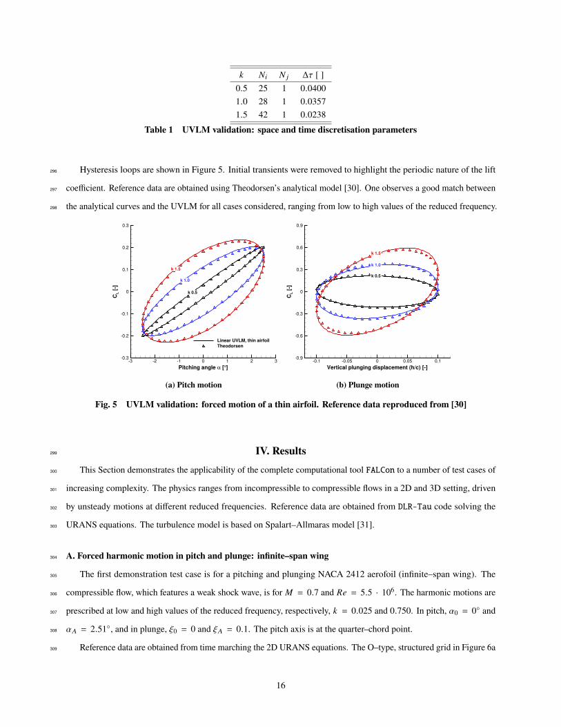
Figure 7 reports the lift coefficient hysteresis loops. Initial transients were removed and arrows indicate the direction322

of the loops. One finds an excellent agreement between FALCon results and reference data, for all reduced frequencies323

and motions. This indicates a correct conception and implementation of the unsteady coupling algorithm.324

17

α [°]

CL [

­]

­2 0 2

0

0.2

0.4

0.6

FALCon, 2D

DLR­tau, 2D

k 0.75

k 0.025

(a) Pitch motion

(h/c) [­]

CL [

­]

­0.1 ­0.05 0 0.05 0.1­0.2

0

0.2

0.4

0.6

FALCon, 2D

DLR­tau, 2D

k 0.75

k 0.025

(b) Plunge motion

Fig. 7 Test case A: lift coefficient hysteresis loops for forced harmonic motion at " = 0.7. In the legend,"DLR–tau, 2D" denotes reference data

B. Forced harmonic motion in pitch and plunge: finite–span wing325

The second test case is for a finite–span, unswept and untapered wing. The aspect ratio is 10. The wing cross–section326

is the NACA 2412 aerofoil. The forced harmonic motion in pitch and plunge has the same parameters described in327

Section IV.A. The pitch axis is at the wing quarter–chord. The test case is run at three values of Mach number (" = 0.3,328

0.5 and 0.7) keeping the Reynolds number fixed at 5.5 · 106. This allows investigating the effect of compressibility329

and the impact that mild shock waves appearing and disappearing during the forced motion have on the predictive330

performance of the hybrid aerodynamic solver.331

Reference data were obtained solving the 3D URANS equations. Results were calculated for three cycles, using332

100 time steps per cycle, to achieve a periodic flow state after the decay of initial transients. The maximum number of333

pseudo–iterations per time step was set to 600, and the single grid method was used. Other relevant numerical settings334

are the same as those described in Section IV.A. Figure 8 shows the 3D grid. The grid point distribution at the symmetry335

plane reuses the coarse 2D grid from Figure 6a. This grid was then extruded in the spanwise direction. It was found336

that a discretisation with 63 layers of 2D planes, along the wing span, was adequate for grid independent results, as337

documented in Figure 10a. The final 3D grid consists of about two million grid points.338

For the hybrid aerodynamic solver FALCon, the VLM lattice consists of #8 = 2 and # 9 = 100 panels, refer to339

Figure 9. Coarser grids revealed a tendency to overestimate the lift coefficient at the lowest and highest values of the340

angle of attack, as shown in Figure 10b. The coupling algorithm spawns nine URANS analyses uniformly distributed341

between -6 and 2 degrees angle of attack. The angle of attack range considers the asymmetric nature of the aerofoil and342

the expected variation of the effective angle of attack which decreases moving from the symmetry plane to the wing tip.343

The relaxation factor is a = 5 · 10−2, and the convergence criterion at each time step is based on the tolerance Y = 10−6.344

We now focus on the reproducibility of the flow physics using the hybrid aerodynamic solver. Reference data345

18

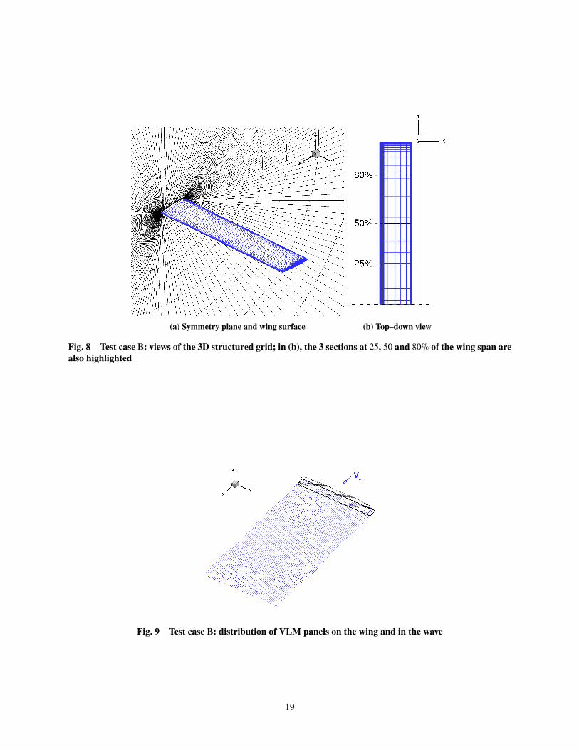
(a) Symmetry plane and wing surface (b) Top–down view

Fig. 8 Test case B: views of the 3D structured grid; in (b), the 3 sections at 25, 50 and 80% of the wing span arealso highlighted

Fig. 9 Test case B: distribution of VLM panels on the wing and in the wave

19

3rd

cycle [rad]

CL [

­]

0π 0.5π 1π 1.5π 2π

0

0.2

0.4

Coarse

Middle

Fine

(a) 3D structured grid

3rd

cycle [rad.]

CL [

­]

0π 0.5π 1π 1.5π 2π

0

0.2

0.4

Coarse

Middle

Fine

DLR­tau, 3D

(b) VLM lattice

Fig. 10 Test case B: grid convergence results for pitch motion (" = 0.7 and : = 0.025). In (a), the coarse 3Dgrid contains about 2 million points, the medium grid 4.2 million points and the fine grid 9 million points; in (b),the coarse VLM lattice consists of 2 × 25 panels, the medium lattice 2 × 50 panels and the fine lattice 2 × 100panels

are from time marching the 3D URANS equations. Figure 11 reports time domain results for the forced motion in346

pitch. Qualitatively, the fundamental characteristics associated with flow unsteadiness, i.e. reduced frequency, and347

compressibility, i.e. Mach number, are well captured in FALCon. In particular, the hybrid aerodynamic solver correctly348

captures the following elements: 1) the increase of the hysteresis loops for increasing reduced frequency, and the decrease349

of this trend for increasing Mach number; 2) although flow unsteadiness is marginal at the lowest reduced frequency,350

: = 0.025, aerodynamic damping [13] switches sign between " = 0.5 and 0.7; 3) for increasing reduced frequency,351

loops tilt anticlockwise and the aerodynamic stiffness, related to the loop mean slope, increases. Reproducing these352

features, in particular point 2 above, guarantees the suitability of the hybrid aerodynamic solver for future aeroelastic353

analysis. In Figure 12, results for the forced motion in plunge are compared. Qualitatively, the impact of reduced354

frequency and Mach number on aerodynamic loops are reproduced. Quantitatively, we define the percent reconstruction355

error n as:356

n =1#

#∑:=1

�URANS!,:

− �FALCon!,:

�URANS!

· 100 (25)

where the percent reconstruction error over one cycle is normalised by the time averaged value of the lift coefficient357

from the 3D URANS analysis, �URANS!

. The largest values of n are found at the highest Mach number, and these are358

summarised in Table 2. For all cases tested, n is well below 10%, apart from the single occurrence at " = 0.7 and359

: = 0.750 for the plunging motion.360

The hybrid aerodynamic solver offers the appealing feature to reconstruct distributed flow features at any spanwise361

location which does not coincide with the sections (refer to Figure 8) used to generate the viscous database. This is done362

at no extra cost because the existing database, at any generic time instant, is simply interrogated with the effective angle363

20

α [°]

CL [

­]

­2 0 2

­0.2

­0.1

0

0.1

0.2

0.3

0.4

0.5

0.6

FALCon

DLR­tau, 3D

k 0.025

k 0.750

(a) " = 0.3

3rd cycle [rad]

CL

[-]

0π 0.5π 1π 1.5π 2π

-0.2

0

0.2

0.4

0.6

k 0.025k 0.750

(b) " = 0.3

α [°]

CL [

­]

­2 0 2

­0.2

­0.1

0

0.1

0.2

0.3

0.4

0.5

0.6

k 0.025

k 0.750

(c) " = 0.5

3rd cycle [rad]

CL

[-]

0π 0.5π 1π 1.5π 2π

-0.2

0

0.2

0.4

0.6

k 0.025k 0.750

(d) " = 0.5

α [°]

CL [

­]

­2 0 2

­0.2

­0.1

0

0.1

0.2

0.3

0.4

0.5

0.6

k 0.025

k 0.750

(e) " = 0.7

3rd cycle [rad]

CL

[-]

0π 0.5π 1π 1.5π 2π

-0.2

0

0.2

0.4

0.6

k 0.025k 0.750

(f) " = 0.7

Fig. 11 Test case B: lift coefficient hysteresis loops for forced pitch motion. In the legend, "DLR–tau, 3D"denotes reference data

21

h/c [­]

CL [

­]

­0.1 0 0.1

­0.2

0

0.2

0.4

0.6

FALCon

DLR­tau, 3D

k 0.025

k 0.750

(a) " = 0.3

3rd cycle [rad]

CL

[-]

0π 0.5π 1π 1.5π 2π

-0.2

0

0.2

0.4

0.6

k 0.025

k 0.750

(b) " = 0.3

h/c [­]

CL [

­]

­0.1 0 0.1

­0.2

0

0.2

0.4

0.6

k 0.025

k 0.750

(c) " = 0.5

3rd cycle [rad]

CL

[-]

0π 0.5π 1π 1.5π 2π

-0.2

0

0.2

0.4

0.6

k 0.025

k 0.750

(d) " = 0.5

h/c [­]

CL [

­]

­0.1 0 0.1

­0.2

0

0.2

0.4

0.6

k 0.025

k 0.750

(e) " = 0.7

3rd cycle [rad]

CL

[-]

0π 0.5π 1π 1.5π 2π

-0.2

0

0.2

0.4

0.6

k 0.025

k 0.750

(f) " = 0.7

Fig. 12 Test case B: lift coefficient hysteresis loops for forced plunge motion. In the legend, "DLR–tau, 3D"denotes reference data

22

Pitch Plunge: 0.025 0.750 0.025 0.750n 1.8 8.0 1.1 11.5

Table 2 Test case B: percent reconstruction error for forced motion in pitch and plunge at " = 0.7

of attack provided by the unsteady coupling algorithm.364

For further discussion, Figures 13 and 14 depict the instantaneous pressure coefficient for the pitch and plunge cases,365

respectively, at " = 0.7. Figures 15 and 16 are the counterpart for the skin friction coefficient. To comprehend these366

articulated figures, rows correspond to time instants of a cycle and columns to three locations (25, 50 and 80%) along367

the wing span. The time snapshots capture the motion variable (either U or b) at four instants uniformly distributed368

within an oscillatory cycle: at the maximum value, the mean value during downstroke, the minimum value, and the369

mean value during upstroke. As an example, the fourth row of Figure 13 illustrates the instantaneous �? at stations370

located at 25, 50 and 80% of the wing span during the upstroke, for U = 0◦. The reconstruction of the instantaneous371

flow features is done well generally. It is not unexpected that the larger discrepancies in prediction are at the wing tip for372

" = 0.7. These are due to the presence of a strong wing tip vortex forming around a straight wing, which is not a373

common design feature for application to high speed flows. A better agreement is therefore expected for an airliner wing374

which has a moderate sweep angle, reducing the strength of the tip vortex at high speed. Comparing pitch and plunge,375

differences seen in �! are attributed to deviations in the high speed region of the flow interacting with the wing tip376

vortex. As the reduced frequency of motion increases, FALCon predictions deviate on the suction peak of the pressure377

coefficient. We believe this to be attributed to the estimation of the induced angle of attack. A possible confirmation is378

found analysing the excellent aerofoil results in Section IV.A, where the induced angle of attack vanishes due to the 2D379

nature of that problem.380

Notes on Convergence381

The L2 norm of the residual of the hybrid aerodynamic solver FALCon is shown in Figure 17. An exemplary382

behaviour is for the forced motion in pitch at " = 0.7 and : = 0.025. The convergence behaviour is shown for the first383

six time steps of the motion, when the flow has yet to achieve periodicity. Convergence to the prescribed tolerance,384

Y = 10−6, occurs in just over 50 pseudo iterations, and the convergence rate seems unaffected as time progresses. A385

preliminary study was carried out and it was found that an optimal relaxation factor is a = 5 · 10−2, in order to provide386

a good balance between convergence rate and number of iterations to convergence.387

Notes on Computational Cost388

The 3D URANS analysis required about 1,500 CPU hours. For FALCon, Part I of the unsteady coupling algorithm389

spawned nine 2D URANS analyses for angles of attack between −6 and 2◦ in order to update the viscous database at390

23

x/c [­]

cp [

­]

0 0.5 1

­1.5

­1

­0.5

0

0.5

1Hybrid VLM

DLR­tau, 3D

k 0.025

k 0.750

(a) U = 2.51◦ at 25% wing span

x/c [­]

cp [

­]

0 0.5 1

­1.5

­1

­0.5

0

0.5

1

k 0.025

k 0.750

(b) U = 2.51◦ at 50% wing span

x/c [­]

cp [

­]

0 0.5 1

­1.5

­1

­0.5

0

0.5

1

k 0.025

k 0.750

(c) U = 2.51◦ at 80% wing span

x/c [­]

cp [

­]

0 0.5 1

­1.5

­1

­0.5

0

0.5

1

k 0.025

k 0.750

(d) U = 0◦ (down) at 25% wingspan

x/c [­]

cp [

­]

0 0.5 1

­1.5

­1

­0.5

0

0.5

1

k 0.025

k 0.750

(e) U = 0◦ (down) at 50% wingspan

x/c [­]

cp [

­]

0 0.5 1

­1.5

­1

­0.5

0

0.5

1

k 0.025

k 0.750

(f) U = 0◦ (down) at 80% wingspan

x/c [­]

cp [

­]

0 0.5 1

­1.5

­1

­0.5

0

0.5

1

k 0.025

k 0.750

(g) U = −2.51◦ at 25% wing span

x/c [­]

cp [

­]

0 0.5 1

­1.5

­1

­0.5

0

0.5

1

k 0.025

k 0.750

(h) U = −2.51◦ at 50% wing span

x/c [­]

cp [

­]

0 0.5 1

­1.5

­1

­0.5

0

0.5

1

k 0.025

k 0.750

(i) U = −2.51◦ at 80% wing span

x/c [­]

cp [

­]

0 0.5 1

­1.5

­1

­0.5

0

0.5

1

k 0.025

k 0.750

(j) U = 0◦ (up) at 25% wing span

x/c [­]

cp [

­]

0 0.5 1

­1.5

­1

­0.5

0

0.5

1

k 0.025

k 0.750

(k) U = 0◦ (up) at 50% wing span

x/c [­]

cp [

­]

0 0.5 1

­1.5

­1

­0.5

0

0.5

1

k 0.025

k 0.750

(l) U = 0◦ (up) at 80% wing span

Fig. 13 Test case B: instantaneous pressure coefficient for forced pitch motion at " = 0.7. Rows depict timeinstants ("up" for upstroke and "down" for downstroke) and columns represent spanwise stations. In the legend,"DLR–tau, 3D" denotes reference data

24

x/c [­]

cp [

­]

0 0.5 1

­1.5

­1

­0.5

0

0.5

1Hybrid VLM

DLR­tau, 3D

k 0.025

k 0.750

(a) b = 0.1 at 25% wing span

x/c [­]

cp [

­]

0 0.5 1

­1.5

­1

­0.5

0

0.5

1

k 0.025

k 0.750

(b) b = 0.1 at 50% wing span

x/c [­]

cp [

­]

0 0.5 1

­1.5

­1

­0.5

0

0.5

1

k 0.025

k 0.750

(c) b = 0.1 at 80% wing span

x/c [­]

cp [

­]

0 0.5 1

­1.5

­1

­0.5

0

0.5

1

k 0.025

k 0.750

(d) b = 0 (down) at 25% wingspan

x/c [­]

cp [

­]

0 0.5 1

­1.5

­1

­0.5

0

0.5

1

k 0.025

k 0.750

(e) b = 0 at 50% wing span

x/c [­]

cp [

­]

0 0.5 1

­1.5

­1

­0.5

0

0.5

1

k 0.025

k 0.750

(f) b = 0 (down) at 80%wing span

x/c [­]

cp [

­]

0 0.5 1

­1.5

­1

­0.5

0

0.5

1

k 0.025

k 0.750

(g) b = −0.1 at 25% wing span

x/c [­]

cp [

­]

0 0.5 1

­1.5

­1

­0.5

0

0.5

1

k 0.025

k 0.750

(h) b = −0.1 at 50% wing span

x/c [­]

cp [

­]

0 0.5 1

­1.5

­1

­0.5

0

0.5

1

k 0.025

k 0.750

(i) b = −0.1 at 80% wing span

x/c [­]

cp [

­]

0 0.5 1

­1.5

­1

­0.5

0

0.5

1

k 0.025

k 0.750

(j) b = 0 (up) at 25% wing span

x/c [­]

cp [

­]

0 0.5 1

­1.5

­1

­0.5

0

0.5

1

k 0.025

k 0.750

(k) b = 0 (up) at 50% wing span

x/c [­]

cp [

­]

0 0.5 1

­1.5

­1

­0.5

0

0.5

1

k 0.025

k 0.750

(l) b = 0 (up) at 80% wing span

Fig. 14 Test case B: instantaneous pressure coefficient for forced plunge motion at " = 0.7. Rows depicttime instants ("up" for upstroke and "down" for downstroke) and columns represent spanwise stations. In thelegend, "DLR–tau, 3D" denotes reference data

25

x/c [­]

cf [

­]

0 0.5 1­0.005

0

0.005

0.01

Hybrid VLM

DLR­tau, 3D

k 0.025

k 0.750

(a) U = 2.51◦ at 25% wing span

x/c [­]

cf [­

]

0 0.5 1­0.005

0

0.005

0.01

k 0.025

k 0.750

(b) U = 2.51◦ at 50% wing span

x/c [­]

cf [­

]

0 0.5 1­0.005

0

0.005

0.01

k 0.025

k 0.750

(c) U = 2.51◦ at 80% wing span

x/c [­]

cf [­

]

0 0.5 1­0.005

0

0.005

0.01

k 0.025

k 0.750

(d) U = 0◦ (down) at 25% wingspan

x/c [­]

cf [­

]

0 0.5 1­0.005

0

0.005

0.01

k 0.025

k 0.750

(e) U = 0◦ (down) at 50% wingspan

x/c [­]

cf [­

]

0 0.5 1­0.005

0

0.005

0.01

k 0.025

k 0.750

(f) U = 0◦ (down) at 80% wingspan

x/c [­]

cf [­

]

0 0.5 1­0.005

0

0.005

0.01

k 0.025

k 0.750

(g) U = −2.51◦ at 25% wing span

x/c [­]

cf [­

]

0 0.5 1­0.005

0

0.005

0.01

k 0.025

k 0.750

(h) U = −2.51◦ at 50% wing span

x/c [­]

cf [­

]

0 0.5 1­0.005

0

0.005

0.01

k 0.025

k 0.750

(i) U = −2.51◦ at 80% wing span

x/c [­]

cf [­

]

0 0.5 1­0.005

0

0.005

0.01

k 0.025

k 0.750

(j) U = 0◦ (up) at 25% wing span

x/c [­]

cf [­

]

0 0.5 1­0.005

0

0.005

0.01

k 0.025

k 0.750

(k) U = 0◦ (up) at 50% wing span

x/c [­]

cf [­

]

0 0.5 1­0.005

0

0.005

0.01

k 0.025

k 0.750

(l) U = 0◦ (up) at 80% wing span

Fig. 15 Test case B: instantaneous skin friction coefficient for forced pitch motion at " = 0.7. Rows depicttime instants ("up" for upstroke and "down" for downstroke) and columns represent spanwise stations. In thelegend, "DLR–tau, 3D" denotes reference data

26

x/c [­]

cf [

­]

0 0.5 1­0.005

0

0.005

0.01

Hybrid VLM

DLR­tau, 3D

k 0.025

k 0.750

(a) b = 0.1 at 25% wing span

x/c [­]

cf [­

]

0 0.5 1­0.005

0

0.005

0.01

k 0.025

k 0.750

(b) b = 0.1 at 50% wing span

x/c [­]

cf [­

]

0 0.5 1­0.005

0

0.005

0.01

k 0.025

k 0.750

(c) b = 0.1 at 80% wing span

x/c [­]

cf [­

]

0 0.5 1­0.005

0

0.005

0.01

k 0.025

k 0.750

(d) b = 0 (down) at 25% wingspan

x/c [­]

cf [­

]

0 0.5 1­0.005

0

0.005

0.01

k 0.025

k 0.750

(e) b = 0 (down) at 50% wingspan

x/c [­]

cf [­

]

0 0.5 1­0.005

0

0.005

0.01

k 0.025

k 0.750

(f) b = 0 (down) at 80%wing span

x/c [­]

cf [­

]

0 0.5 1­0.005

0

0.005

0.01

k 0.025

k 0.750

(g) b = −0.1 at 25% wing span

x/c [­]

cf [­

]

0 0.5 1­0.005

0

0.005

0.01

k 0.025

k 0.750

(h) b = −0.1 at 50% wing span

x/c [­]

cf [­

]

0 0.5 1­0.005

0

0.005

0.01

k 0.025

k 0.750

(i) b = −0.1 at 80% wing span

x/c [­]

cf [­

]

0 0.5 1­0.005

0

0.005

0.01

k 0.025

k 0.750

(j) b = 0 (up) at 25% wing span

x/c [­]

cf [­

]

0 0.5 1­0.005

0

0.005

0.01

k 0.025

k 0.750

(k) b = 0 (up) at 50% wing span

x/c [­]

cf [­

]

0 0.5 1­0.005

0

0.005

0.01

k 0.025

k 0.750

(l) b = 0 (up) at 80% wing span

Fig. 16 Test case B: instantaneous skin friction coefficient for forced plunge motion at " = 0.7. Rows depicttime instants ("up" for upstroke and "down" for downstroke) and columns represent spanwise stations. In thelegend, "DLR–tau, 3D" denotes reference data

27

Iteration

Co

up

lin

g r

es

idu

al

CL [

­]

0 100 200 30010

­7

10­6

10­5

10­4

10­3

10­2

10­1

100

­0.1

0

0.1

0.2

0.3

0.4

0.5

0.6

Coupling residual

Total lift, CL

t1=1.08e­2 sec. t

2t3

t4

t5

Fig. 17 Test case B: convergence of the hybrid aerodynamic solver during the first 6 time steps for forced pitchmotion at " = 0.7 and : = 0.025

each time step. The 2D URANS analyses were run in parallel and required a total of 28 CPU hours. As both the UVLM391

and Part II of the unsteady coupling algorithm are inexpensive, it is conservative to indicate that FALCon required less392

than 30 CPU hours. Therefore, predictions obtained using the hybrid aerodynamic solver are, on average, a factor of 50393

times faster than the results from time marching the 3D URANS equations. This significant speedup becomes a tangible394

asset of the proposed aerodynamic model when balanced against the accuracy of predictions for a number of valuable395

test cases.396

C. Forced harmonic motion in pitch: finite–span wing in transonic flow397

The final demonstration test case features a pitching wing exposed to a " = 0.8 air flow. The wing geometry and398

the pitch motion kinematics are the same as those described in Section IV.B. The complex nature of the resulting flow399

provides the opportunity to assess the predictive performance of the hybrid aerodynamic solver on a problem well400

beyond its underlying assumptions. In this regard, consider Figure 18 that depicts the temporal evolution of areas with401

flow separation.402

The flow physics is characterised by the appearance and disappearance of a shock wave which locks–in with the403

periodic motion and causes the flow to separate. The shock moves periodically and extends uniformly in the spanwise404

direction until it interacts with the vortex emanating at the wing tip. These interactions and the complex dynamics405

resulting from the forced motion go beyond the assumptions (most notably, of uniform flow) of the hybrid aerodynamic406

model. Therefore, limitations of the proposed aerodynamic model will start to appear.407

For completeness, FALCon predictions are summarised in Figures 19 and 20 for the pressure coefficient and skin408

friction coefficient, respectively. One observes that the flow reconstruction at lower frequency outperforms the one at409

higher frequency. This is in line with Figure 18 conveying a stronger flow three–dimensionality for : = 0.750. For410

28

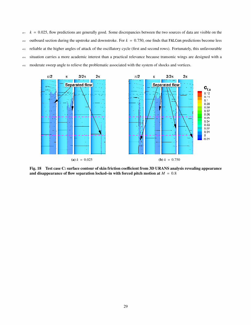
: = 0.025, flow predictions are generally good. Some discrepancies between the two sources of data are visible on the411

outboard section during the upstroke and downstroke. For : = 0.750, one finds that FALCon predictions become less412

reliable at the higher angles of attack of the oscillatory cycle (first and second rows). Fortunately, this unfavourable413

situation carries a more academic interest than a practical relevance because transonic wings are designed with a414

moderate sweep angle to relieve the problematic associated with the system of shocks and vortices.415

(a) : = 0.025 (b) : = 0.750

Fig. 18 Test case C: surface contour of skin friction coefficient from 3D URANS analysis revealing appearanceand disappearance of flow separation locked–in with forced pitch motion at " = 0.8

29

x/c [­]

cp [

­]

0 0.5 1

­1.5

­1

­0.5

0

0.5

1Hybrid VLM

DLR­tau, 3D

k 0.025

k 0.750

(a) U = 2.51◦ at 25% wing span

x/c [­]

cp [

­]

0 0.5 1

­1.5

­1

­0.5

0

0.5

1

k 0.025

k 0.750

(b) U = 2.51◦ at 50% wing span

x/c [­]

cp [

­]

0 0.5 1

­1.5

­1

­0.5

0

0.5

1

k 0.025

k 0.750

(c) U = 2.51◦ at 80% wing span

x/c [­]

cp [

­]

0 0.5 1

­1.5

­1

­0.5

0

0.5

1

k 0.025

k 0.750

(d) U = 0◦ (down) at 25% wingspan

x/c [­]

cp [

­]

0 0.5 1

­1.5

­1

­0.5

0

0.5

1

k 0.025

k 0.750

(e) U = 0◦ (down) at 50% wingspan

x/c [­]

cp [

­]

0 0.5 1

­1.5

­1

­0.5

0

0.5

1

k 0.025

k 0.750

(f) U = 0◦ (down) at 80% wingspan

x/c [­]

cp [

­]

0 0.5 1

­1.5

­1

­0.5

0

0.5

1

k 0.025

k 0.750

(g) U = −2.51◦ at 25% wing span

x/c [­]

cp [

­]

0 0.5 1

­1.5

­1

­0.5

0

0.5

1

k 0.025

k 0.750

(h) U = −2.51◦ at 50% wing span

x/c [­]

cp [

­]

0 0.5 1

­1.5

­1

­0.5

0

0.5

1

k 0.025

k 0.750

(i) U = −2.51◦ at 80% wing span

x/c [­]

cp [

­]

0 0.5 1

­1.5

­1

­0.5

0

0.5

1

k 0.025

k 0.750

(j) U = 0◦ (up) at 25% wing span

x/c [­]

cp [

­]

0 0.5 1

­1.5

­1

­0.5

0

0.5

1

k 0.025

k 0.750

(k) U = 0◦ (up) at 50% wing span

x/c [­]

cp [

­]

0 0.5 1

­1.5

­1

­0.5

0

0.5

1

k 0.025

k 0.750

(l) U = 0◦ (up) at 80% wing span

Fig. 19 Test case C: instantaneous pressure coefficient for forced pitch motion at " = 0.8. Rows depict timeinstants ("up" for upstroke and "down" for downstroke) and columns represent spanwise stations. In the legend,"DLR–tau, 3D" denotes reference data

30

x/c [­]

cf [

­]

0 0.5 1­0.005

0

0.005

0.01

Hybrid VLM

DLR­tau, 3D

k 0.025

k 0.750

(a) U = 2.51◦ at 25% wing span

x/c [­]

cf [­

]

0 0.5 1­0.005

0

0.005

0.01

k 0.025

k 0.750

(b) U = 2.51◦ at 50% wing span

x/c [­]

cf [­

]

0 0.5 1­0.005

0

0.005

0.01

k 0.025

k 0.750

(c) U = 2.51◦ at 80% wing span

x/c [­]

cf [­

]

0 0.5 1­0.005

0

0.005

0.01

k 0.025

k 0.750

(d) U = 0◦ (down) at 25% wingspan

x/c [­]

cf [­

]

0 0.5 1­0.005

0

0.005

0.01

k 0.025

k 0.750

(e) U = 0◦ (down) at 50% wingspan

x/c [­]

cf [­

]

0 0.5 1­0.005

0

0.005

0.01

k 0.025

k 0.750

(f) U = 0◦ (down) at 80% wingspan

x/c [­]

cf [­

]

0 0.5 1­0.005

0

0.005

0.01

k 0.025

k 0.750

(g) U = −2.51◦ at 25% wing span

x/c [­]

cf [­

]

0 0.5 1­0.005

0

0.005

0.01

k 0.025

k 0.750

(h) U = −2.51◦ at 50% wing span

x/c [­]

cf [­

]

0 0.5 1­0.005

0

0.005

0.01

k 0.025

k 0.750

(i) U = −2.51◦ at 80% wing span

x/c [­]

cf [­

]

0 0.5 1­0.005

0

0.005

0.01

k 0.025

k 0.750

(j) U = 0◦ (up) at 25% wing span

x/c [­]

cf [­

]

0 0.5 1­0.005

0

0.005

0.01

k 0.025

k 0.750

(k) U = 0◦ (up) at 50% wing span

x/c [­]

cf [­

]

0 0.5 1­0.005

0

0.005

0.01

k 0.025

k 0.750

(l) U = 0◦ (up) at 80% wing span

Fig. 20 Test case C: instantaneous skin friction coefficient for forced pitch motion at " = 0.8. Rows depicttime instants ("up" for upstroke and "down" for downstroke) and columns represent spanwise stations. In thelegend, "DLR–tau, 3D" denotes reference data

31

V. Conclusion416

The paper addressed the problem of enhancing the predictive capability of a potential flow–based aerodynamic model417

with viscous sectional information. Whereas the existing knowledge and practice is well–established for steady–state418

problems, the same cannot be stated for unsteady flows. The contribution of this research work is the extension of the419

U–based coupling algorithm to unsteady problems. The unsteady coupling algorithm is formulated in such a way to420

permit any type of wing motion, outperforming prior attempts limited by the motion kinematics and restricted to low421

frequencies of motion. The algorithm consists of two main operation blocks: Part I which concerns data generation422

from two specialised and separate aerodynamic models that are synchronously marched forward in time, and Part II423

which executes data fusion to produce more consistent and accurate information than that provided by any individual424

aerodynamic source. The aerodynamic models used herein are an in–house unsteady vortex lattice method and an425

infinite–swept wing Navier–Stokes solver. We have named the resulting computational tool FALCon, as an acronym for426

Fast Aircraft Load Calculations. A preliminary study was carried out to validate the two aerodynamic models and the427

unsteady coupling algorithm. Then, the predictive performance capability of FALCon was demonstrated on three test428

cases of increasing complexity. Test case A featured an unsteady, two–dimensional flow problem which was superseded429

by a family of three–dimensional flow problems in Test case B. Predictions matched well reference data for all Mach430

numbers tested and for both low and high reduced frequencies of motion (up to : = 0.75). Test case C superseded431

previous cases and featured flows with a strong three–dimensional character caused by a shock wave interacting with432

areas of flow separation and with the wing tip vortex, driven by the prescribed motion of the wing. Test case C was433

chosen to exercise FALCon on problems where the underlying assumption (i.e. uniform or slowly changing flow along434

the span) is not met. An acceptable agreement was found, balanced by a speed–up of a factor of about 50 compared to435

solving in time the three–dimensional Reynolds–averaged Navier–Stokes equations. FALCon reproduced important436

physical features, such as the influence of compressibility and flow unsteadiness on the aerodynamic stiffness and437

damping, prerequisites in any aeroelastic analysis. Finally, it is worth noting that alternative aerodynamic models may438

be considered as a replacement for the specific inviscid and viscous models here discussed.439

Acknowledgements440

Da Ronch acknowledges the financial support from the Engineering and Physical Sciences Research Council441

(grant number: EP/P006795/1), the Royal Academy of Engineering (grant number: ISS1415/7/44) and Airbus Oper-442

ations SAS. The authors acknowledge the use of the IRIDIS High–Performance Computing Facility, and associated443

support services at the University of Southampton, in the completion of this work.444

Data supporting this study will be openly available from the University of Southampton repository after publication.445

32

References446

[1] Badcock, K. J., Timme, S., Marques, S., Khodaparast, H., Prandina, M., Mottershead, J. E., Swift, A., Da Ronch, A., and447

Woodgate, M. A., “Transonic aeroelastic simulation for instability searches and uncertainty analysis,” Progress in Aerospace448

Sciences, Vol. 47, No. 5, 2011, pp. 392–423. doi:10.1016/j.paerosci.2011.05.002.449

[2] Tani, I., A simple method of calculating the induced velocity of a monoplane wing, Aeronautical Research Institute, Tokyo450

Imperial University, 1934.451

[3] Multhopp, H., and Schwabe, M., Die Berechnung der Auftriebsverteilung von Tragflügeln, 1938.452

[4] Sivells, J. C., and Neely, R. H., “Method for calculating wing characteristics by lifting-line theory using nonlinear section lift453

data,” Tech. rep., DTIC Document, 1947.454

[5] Sivells, J. C., and Westrick, G. C., “Method for Caluculating Lift Distributions for Unswept Wings with Flaps or Ailerons by455

use of Nonlinear Section Lift Data,” 1951.456

[6] Tseng, J.-B., and Lan, C. E., “Calculation of aerodynamic characteristics of airplane configurations at high angles of attack,”457

1988.458

[7] Dam, C. V., “The aerodynamic design of multi-element high-lift systems for transport airplanes,” Progress in Aerospace459

Sciences, Vol. 38, No. 2, 2002, pp. 101 – 144. doi:10.1016/S0376-0421(02)00002-7.460

[8] Van Dam, C., Vander Kam, J., and Paris, J., “Design-oriented high-lift methodology for general aviation and civil transport461

aircraft,” Journal of aircraft, Vol. 38, No. 6, 2001, pp. 1076–1084.462

[9] Gallay, S., and Laurendeau, E., “Nonlinear Generalized Lifting-Line Coupling Algorithms for Pre/Poststall Flows,” AIAA463

Journal, Vol. 53, No. 7, 2015, pp. 1784–1792. doi:10.2514/1.J053530.464

[10] Gallay, S., and Laurendeau, E., “Preliminary-Design Aerodynamic Model for Complex Configurations Using Lifting-Line465

Coupling Algorithm,” Journal of Aircraft, Vol. 53, No. 4, 2016, pp. 1145–1159.466

[11] Parenteau, M., Plante, F., Laurendeau, E., and Costes, M., “Unsteady Coupling Algorithm for Lifting-Line Methods,” 55th467

AIAA Aerospace Sciences Meeting, 2017, p. 0951.468

[12] Da Ronch, A., Ghoreyshi, M., and Badcock, K., “On the generation of flight dynamics aerodynamic tables by computational469

fluid dynamics,” Progress in Aerospace Sciences, Vol. 47, No. 8, 2011, pp. 597–620. doi:10.1016/j.paerosci.2011.09.001.470

[13] Da Ronch, A., Vallespin, D., Ghoreyshi, M., and Badcock, K., “Evaluation of dynamic derivatives using computational fluid471

dynamics,” AIAA Journal, Vol. 50, No. 2, 2012, pp. 470–484. doi:10.2514/1.J051304.472

[14] Da Ronch, A., Ghoreyshi, M., Badcock, K. J., Görtz, S., Widhalm, M., Dwight, R. P., and Campobasso, M. S., “Linear473

frequency domain and harmonic balance predictions of dynamic derivatives,” Journal of Aircraft, Vol. 50, No. 3, 2013, pp.474

694–707. doi:10.2514/1.C031674.475

33

[15] Ghoreyshi, M., Badcock, K. J., Da Ronch, A., Marques, S., Swift, A., and Ames, N., “Framework for establishing limits of tabular476

aerodynamic models for flight dynamics analysis,” Journal of Aircraft, Vol. 48, No. 1, 2011, pp. 42–55. doi:10.2514/1.C001003.477

[16] Eldredge, J. D., Colonius, T., and Williams, D., “EnKF–based Dynamic Estimation of Separated Flows with a Low–Order478

Vortex Model,” AIAA SciTech Forum, 2018. AIAA Paper 2018–0811.479

[17] Le Provost, M., Hou, W., and Eldredge, J. D., “Deep learning and data assimilation approaches to sensor reduction in estimation480

of disturbed separated flows,” AIAA SciTech Forum, 2020. AIAA Paper 2020–0799.481

[18] Clark Di Leoni, P., Mazzino, A., and Biferale, L., “Synchronization to Big Data: Nudging the Navier-Stokes Equations for Data482

Assimilation of Turbulent Flows,” Physical Review X, Vol. 10, No. 1, 2020. doi:10.1103/physrevx.10.011023.483

[19] Bagheri, A. K., and Da Ronch, A., “Adjoint–Based Surrogate Modelling of Spalart–Allmaras Turbulence Model Using Gradient484

Enhanced Kriging,” AIAA Aviation Forum, 2020. AIAA Paper 2020–2991.485

[20] Katz, J., and Plotkin, A., Low-speed aerodynamics, Vol. 13, Cambridge University Press, 2001.486

[21] Murua, J., Palacios, R., and Graham, J. M. R., “Applications of the unsteady vortex-lattice method in aircraft aeroelasticity and487

flight dynamics,” Progress in Aerospace Sciences, Vol. 55, No. Supplement C, 2012, pp. 46 – 72. doi:10.1016/j.paerosci.2012.488

06.001.489

[22] Simpson, R. J. S., Palacios, R., and Murua, J., “Induced-Drag Calculations in the Unsteady Vortex Lattice Method,” AIAA490

Journal, Vol. 51, No. 7, 2013, pp. 1775–1779. doi:10.2514/1.J052136.491

[23] Franciolini, M., Da Ronch, A., Drofelnik, J., Raveh, D., and Crivellini, A., “Efficient infinite-swept wing solver for steady and492

unsteady compressible flows,” Aerospace Science and Technology, Vol. 72, 2018, pp. 217 – 229. doi:10.1016/j.ast.2017.10.034.493

[24] Drofelnik, J., Da Ronch, A., Franciolini, M., and Crivellini, A., “Fast identification of transonic buffet envelope using494

computational fluid dynamics,” Aircraft Engineering and Aerospace Technology, Vol. 91, No. 2, 2019, pp. 309–316. doi:495

10.1108/AEAT-01-2018-0057.496

[25] Yang, G., Da Ronch, A., Kharlamov, D., and Drofelnik, J., “Wing twist optimisation using aerodynamic solvers of497

different fidelity,” 31st Congress of the International Council of the Aeronautical Sciences (ICAS 2018), 2018. URL498

https://eprints.soton.ac.uk/423722/.499

[26] Jameson, A., Schmidt, W., and Turkel, E., “Numerical solutions of the Euler equations by finite volume methods using Runge–500

Kutta time–stepping schemes,” 14th Fluid and Plasma Dynamics Conference, Fluid Dynamics and Co–located Conferences,501

Palo Alto, CA, 1981. doi:10.2514/6.1981-1259.502

[27] Leishman, J., and Crouse, G., “State-space model for unsteady airfoil behavior and dynamic stall,” Structures, Structural503

Dynamics, and Materials and Co-located Conferences, 1989. doi:10.2514/6.1989-1319, 0.504

[28] Lambert, T., Abdul Razak, N., and Dimitriadis, G., “Vortex Lattice Simulations of Attached and Separated Flows around Flapping505

Wings,” Aerospace, Vol. 4, No. 2, 2017. doi:10.3390/aerospace4020022, URL http://www.mdpi.com/2226-4310/4/2/22.506

34

[29] Murua, J., “Flexible Aircraft Dynamics with a Geometrically-Nonlinear Description of the Unsteady Aerodynamics,” Ph.D.507

thesis, Imperial College London, United Kingdom, 2012.508

[30] Theodorsen, T., and Mutchler, W., “General theory of aerodynamic instability and the mechanism of flutter,” 1935.509

[31] Spalart, P., and Allmaras, S., “A One-Equation Turbulence Model for Aerodynamic Flows,” AIAA, Vol. 439, 1992. doi:510

10.2514/6.1992-439.511

35