A mia madre Liana ed a Rosanna - ePrints Soton
369
A mia madre Liana ed a Rosanna The moving power of mathematical invention is not reasoning but imagination. Augustus De Morgan
-
Upload
khangminh22 -
Category
Documents
-
view
0 -
download
0
Transcript of A mia madre Liana ed a Rosanna - ePrints Soton
A mia madre Lianaed a Rosanna
The moving power of mathematical inventionis not reasoning but imagination.
Augustus De Morgan

Foreword
I still wonder whether the title of this thesis is the right one or whether it shouldhave been somehow different. I admit I like it. However, the first idea that came tomy mind and that, in my opinion, described properly the thesis has been somethingvery similar to the following:
“On the semantics and on the structure of place/transition Petri netsin their status of nicely intuitive formalization of the notion of causalityand influential instance of the concurrency paradigm, and on the rela-tionships which they bear to other models for concurrency, investigatedby means of processes, unfoldings, infinite computations, some algebra,some category theory, . . . ”
The reader will probably agree that a similar title would not fit nicely in what-ever page layout. Since this was certainly my opinion, I followed the aestheticmotivation and I decided to shorten it drastically, arriving gradually to the actualtitle. However, I must admit that probably my choice has not been nice to the“other models for concurrency” which disappeared completely from the title. (Notfrom the thesis, though!) Well, I shall make justice here by saying that, despite thetitle, I consider the part of the thesis dealing with “other models” as relevant asthe others.
A similar remark applies indeed to categories: although category theory is notexplicitly mentioned in the title, it plays a considerable role in the formal devel-opment to follow. This is because it provides a formal framework in which certaininteresting questions can be asked naturally and (sometimes) answered.
In order for the reader to get in tune with the author’s choice of dedicating(large part of) his doctoral thesis to the issue of categorical semantics for Petrinets, I indicate below the two “postulates” upon which such a choice is based.
i) Petri net are interesting from the point of view of noninterleaving concurrency,since, informally speaking, they are flexible enough to model all the sensibilecause/effect interactions which may occur between a set of computing agents;
i
Foreword
ii) Category Theory is useful both “in the small” to look for appropriate axiomaticdescriptions of algebraic structures, e.g., such as the processes of net, and “inthe large” to establish formal relationships between different structures, e.g.,how to translate uniformly from Petri nets to transition systems.
In other words, the first point above means that a convincing causal semanticsfor Petri nets is likely to yield convincing causal semantics for a large class of othermodels. The second point, instead, implies that the categorical paradigm possessesa good ability of abstracting away from undesired details, while keeping consistencyof the desired ones. I would consider it an excellent outcome if this thesis couldconvince a skeptic reader at least of the second postulate.
Acknowledgements
It is customary to start the acknowledgment list of a thesis by saying sometime like“without my supervisor this thesis could not have been written”. Well, I certainlywill not escape this tradition. Actually, I dare say that never ever as in my casethis is indeed true. In fact, the topics treated and the tools exploited here wereat the beginning so hostile to me, that I had to be pushed rather strongly andrepeatedly in order to get through with them. I heartily give full credit for this tomy supervisor Ugo Montanari. But of course there is more than that. I met himwhen I was a third year undergraduate student: since then he supported almost allmy professional activities and he taught me, directly or indirectly, almost everythingI know about computer science.
In the autumn 91, I spent three months in California working in strict contactwith Jose Meseguer at the SRI International. First of all, I like to remember thenice time I had there and to thank Narciso Martı-Oliet and Jose Meseguer fortheir friendship. But clearly, that stay also represented a very good professionalopportunity for me. In particular, I learnt from Jose what it means to write apaper and to put it in a good shape. (I hope that the reader will not raise strongobjections!)
From March to August 92 I was at DAIMI in Aarhus. The relevance of thatstay for my education is witnessed by the fact that the works I produced therejointly with Mogens Nielsen and Glynn Winskel have their place in this thesis asChapter 2. I really like to mention that, thanks to the favorable environmentthat DAIMI provides and thanks to the friendship that Mogens and Glynn showedto me, being in particular always lavish with helpful suggestions, I think I reallymade the best out of my stay in Denmark. Probably above all the rest, thatperiod raised my confidence in my working skills, so marking an improvement in myapproach to the research activity. In Aarhus I also happened to meet more than onceMadhavan Mukund, with whom I shared a flat for five months, P.S. Thiagarajan
ii
Foreword
and Jeremy Gunawardena. I have benefited a lot from several discussions withthem.
During the entire PhD programme I have of course taken advantage by the highstandard of the Computer Science Department in Pisa, which provided several goodcourses and seminars. In particular, I had good advices from PierPaolo Deganoand Roberto Gorrieri. Moreover, I have enjoyed many interesting discussions withAndrea Corradini, Roberto Di Meglio, Gianluigi Ferrari, Simone Martini and LucaRoversi. I would also like to thank my room-mates Fabio Gadducci, Corrado Priami,Gioia Ristori and Laura Semini for the company. (Paola Quaglia is intentionallynot thanked.) In particular, I cannot forget that Corrado and Fabio heroicallytolerated the smoke of my cigarettes.
During the years 90–92 I have taken part in the project “Modelling DistributedConcurrency” at Hewlett-Packard Laboratories, Pisa Science Centre. I thank theproject managers Wulf Rehder, Monica Frontini and Lorenzo Coslovi. I mostlyregret that my colleagues and good friends Luca Aceto, Cosimo Laneve, Mar-tina Marre and Daniel Yankelevich working at that project have all left at thebeginning of 93. Doubtless, had I had their suggestions, this thesis would havebeen better.
During the last months several people have spent some time with me chatting aboutwork and other issues. In particular, I warmly thank Gerard Boudol, Ilaria Castel-lani, Matthew Hennessy, Furio Honsell, David Murphy, Nino Salibra and Colin Stir-ling. In connection with Chapter 3, I had helpful long discussions with Andrea Cor-radini and Pino Rosolini. Also Bart Jacobs, Anders Kock and Eugenio Moggi gaveme good advices on this topic.
I am pleased to thank Narciso Martı-Oliet and Axel Poigne, the reviewers of thisthesis, for their nice reports and for the helpful suggestions they gave. Unofficially,also Andrea Corradini and Fabio Gadducci have acted as reviewers spotting manytypos in the text. Of course, all the remaining mistakes are mine.
Switching to the most personal side of the story, I want to thank Rosanna, whoshared with me the last ten years. And now, it comes the turn of my parents,grandparents and friends. Well, I’d better switch to Italian now. . . Ringrazio imiei genitori Liana e Antonio per il loro continuo supporto morale. Non dimenticoi miei nonni Maria Cristina e Aldo. Constatare la loro soddisfazione nel vedermiprogredire negli studi, dopo una partenza ben poco promettente, e stato un ulteriorestimolo per me. Voglio anche ricordare i miei amici Sara Tesini e Pietro Falaschi chenegli ultimi tempi mi hanno dimostrato un insospettato affetto. Infine, nonostantela sua pazzia galoppante che ha causato qualche problema, non posso fare a meno diriconoscere che il mio vecchio maestro Giorgio Rugieri ha giocato un ruolo rilevantenella mia formazione.
This thesis has been written using TEX, LaTEX and XY-pic.
iii

Foreword
iv
Contents
Overview of the Results ix
1 Processes and Unfoldings 1
Introduction . . . . . . . . . . . . . . . . . . . . . . . . . . . . . . . . . . . 3
1.1 Petri Nets and their Computations . . . . . . . . . . . . . . . . . . . 11
1.2 Axiomatizing Concatenable Processes . . . . . . . . . . . . . . . . . 30
1.3 A Functorial Construction for Processes . . . . . . . . . . . . . . . . 40
A Negative Result about Functoriality . . . . . . . . . . . . . . . . . 42
The Category Q[N ] . . . . . . . . . . . . . . . . . . . . . . . . . . . 44
1.4 Strong Concatenable Processes . . . . . . . . . . . . . . . . . . . . . 56
1.5 Place/Transition Nets . . . . . . . . . . . . . . . . . . . . . . . . . . 65
The Categories PTNets, Safe and Occ . . . . . . . . . . . . . . . . . 65
Composition of PT Nets . . . . . . . . . . . . . . . . . . . . . . . . . 70
1.6 Decorated Occurrence Nets . . . . . . . . . . . . . . . . . . . . . . . 79
1.7 PT Net Unfoldings . . . . . . . . . . . . . . . . . . . . . . . . . . . . 85
Composition of Decorated Occurrence Nets . . . . . . . . . . . . . . 90
1.8 PT Nets, Event Structures and Domains . . . . . . . . . . . . . . . . 93
Occurrence Nets, Event Structures and Domains . . . . . . . . . . . 100
1.9 Process versus Unfolding Semantics of Nets . . . . . . . . . . . . . . 105
Conclusions and Further Work . . . . . . . . . . . . . . . . . . . . . . . . 123
2 Models for Concurrency 125
Introduction . . . . . . . . . . . . . . . . . . . . . . . . . . . . . . . . . . . 127
2.1 Preliminaries . . . . . . . . . . . . . . . . . . . . . . . . . . . . . . . 131
v
Contents
2.2 Deterministic Transition Systems . . . . . . . . . . . . . . . . . . . . 134
2.3 Noninterleaving vs. Interleaving Models . . . . . . . . . . . . . . . . 137
Synchronization Trees and Labelled Event Structures . . . . . . . . . 139
Transition Systems with Independence . . . . . . . . . . . . . . . . . 141
2.4 Behavioural, Linear Time, Noninterleaving Models . . . . . . . . . . 143
Semilanguages and Event Structures . . . . . . . . . . . . . . . . . . 145
Trace Languages and Event Structures . . . . . . . . . . . . . . . . . 148
2.5 Transition Systems with Independence and Labelled Event Structures151
Unfolding Transition Systems with Independence . . . . . . . . . . . 156
Occurrence TSI’s and Labelled Event Structures . . . . . . . . . . . 159
2.6 Deterministic Transition Systems with Independence . . . . . . . . . 173
2.7 Deterministic Labelled Event Structures . . . . . . . . . . . . . . . . 188
Labelled Event Structures without Autoconcurrency . . . . . . . . . 189
Deterministic Labelled Event Structures . . . . . . . . . . . . . . . . 190
Conclusions . . . . . . . . . . . . . . . . . . . . . . . . . . . . . . . . . . . 206
3 Infinite Computations 207
Introduction . . . . . . . . . . . . . . . . . . . . . . . . . . . . . . . . . . . 209
3.1 Motivations from Net Theory . . . . . . . . . . . . . . . . . . . . . . 212
3.2 Presheaf Categories as Free Cocompletions . . . . . . . . . . . . . . 214
3.3 ℵ-Filtered Cocompletion . . . . . . . . . . . . . . . . . . . . . . . . . 219
Chains versus Directed Partial Orders . . . . . . . . . . . . . . . . . 220
Filtered Categories and Cofinal Functors . . . . . . . . . . . . . . . . 223
ℵ-Ind-Representable Functors . . . . . . . . . . . . . . . . . . . . . . 231
3.4 KZ-Doctrines and Pseudo-Monads . . . . . . . . . . . . . . . . . . . 235
3.5 A KZ-Doctrine for the Ind Completion . . . . . . . . . . . . . . . . . 245
Ind Objects . . . . . . . . . . . . . . . . . . . . . . . . . . . . . . . . 246
Ind( ) as a 2-endofunctor on CAT . . . . . . . . . . . . . . . . . . . 258
Constant Ind-objects: the 2-natural unit y . . . . . . . . . . . . . . . 260
Filtered Colimits in Ind(C) : the 2-natural multiplication . . . . . . 262
Some Remarks on Ind(C) . . . . . . . . . . . . . . . . . . . . . . . . 272
The Ind KZ-Doctrine . . . . . . . . . . . . . . . . . . . . . . . . . . . 273
3.6 Ind Completion of Monoidal Categories . . . . . . . . . . . . . . . . 278
Cocompletion of Monoidal Categories: First Solution . . . . . . . . . 280
vi
Contents
Cocompletion of Monoidal Categories: Second Solution . . . . . . . 286
3.7 Applications to Petri Nets . . . . . . . . . . . . . . . . . . . . . . . . 289
Conclusions and Further Work . . . . . . . . . . . . . . . . . . . . . . . . 294
Bibliography 297
Appendices 311
A.1 Categories . . . . . . . . . . . . . . . . . . . . . . . . . . . . . . . . . 313
Functor Categories . . . . . . . . . . . . . . . . . . . . . . . . . . . . 325
Monads . . . . . . . . . . . . . . . . . . . . . . . . . . . . . . . . . . 326
A.2 Monoidal Categories . . . . . . . . . . . . . . . . . . . . . . . . . . . 330
A.3 2-Categories . . . . . . . . . . . . . . . . . . . . . . . . . . . . . . . . 333
A.4 Categories of Fractions . . . . . . . . . . . . . . . . . . . . . . . . . . 338
Glossary 343
Index 347
vii

Contents
viii
On the Semantics of Petri Nets: Processes,Unfoldings and Infinite Computations.
An Overview
This thesis is concerned with Petri nets [109] and related models of concurrency.Petri nets are unanimously considered among the most representative models forconcurrency, since they are a fairly simple and natural model of concurrent anddistributed computation. Notwithstanding their “naturality”—perhaps because ofthat—Petri nets are, in our opinion, still far from being completely understood.
The focus here is on the semantics and on the structure of Petri nets. Toaddress the issue, we exploit standard categorical tools which on the one handhelp in axiomatizing the structure of net computations as monoidal categories, vialeft adjoint functors corresponding to free constructions, and, on the other hand,provide a nice framework to formalize the intuitive connections between nets andother models of concurrency, via adjunctions which express translations betweenmodels.
Process Semantics for Petri Nets
In recent works, Degano, Meseguer and Montanari [97, 16] have shown thatthe semantics of Petri nets can be understood in terms of symmetric monoidalcategories—where objects are states, arrows processes, and the tensor product andthe arrow composition model respectively the operations of parallel and sequentialcomposition of processes. This yields an axiomatization of the causal behaviour ofnets as an essentially algebraic theory whose models are monoidal categories.
More precisely, [16] introduces the concatenable processes of a Petri net N ,a slight refinement of Goltz and Resig’s non-sequential processes of N [36]on which an operation of sequential composition can be defined, and shows thatthey can be characterized abstractly as the arrows of a symmetric strict monoidalcategory P [N ]. However, [16] provides only a partial axiomatization of the non-sequential behaviour of N , since the construction of the category P [N ] is basedon a concrete, seemingly ad hoc chosen, underlying category of symmetries. We
ix
Overview of the results
present here a completely abstract , purely algebraic description of the category ofconcatenable processes of N .
The construction of the concatenable processes of N is unsatisfactory in anotherrespect: it is not functorial. In other words, given a morphism between two nets,which can be safely thought of as a simulation, it may not be possible to identify acorresponding monoidal functor between the respective categories of computations.This situation, besides showing that perhaps our undestanding of the structure ofPetri nets is still incomplete, prevents us to identify the category (of the categories)of net behaviours, i.e., to axiomatize the behaviour of Petri nets “in the large”.
We present an analysis of the functoriality issue and a possible solution basedon the new notion of strong concatenable processes of N , a refinement of concaten-able processes still rather close to the standard notion of non-sequential process.We show that, similarly to the concatenable processes, the strong concatenableprocesses of N can be axiomatized as the arrows of a symmetric strict monoidalcategory Q[N ], and that, differently from P [ ], Q[ ] is a functor. The key featureof Q[ ] is that it associates to a net N a monoidal category whose objects form afree, non-commutative monoid. The reason for renouncing to the commutativityof such monoids is a strong negative new result which shows that Q[ ] is a reason-able proposal: under very mild assumptions, no mapping from nets to symmetricstrict monoidal categories with commutative monoids of objects can be extendedto a functor. Clearly, the functoriality of Q[ ] provides a category of symmetricmonoidal categories which is our attempt to identify the category of net computa-tions.
Unfolding Semantics for Petri Nets
A seminal approach to net semantics is the Nielsen, Plotkin and Winskel’sunfolding [106]. This approach explains the behaviour of nets through a chain ofcoreflections
Safe ← Occ ← PES ← Dom,
where Safe, Occ, PES and Dom are, respectively, the categories of 1-safe nets,occurrence nets, prime event structures and dI-domains. Roughly speaking, theunfolding semantics consists, as the name indicates, in “unfolding” a net to simpledenotational structures in which the identity of every event in its computations isunambiguous. The relevance of these constructions resides in the fact that theyprovide 1-safe Petri nets with an abstract semantics where causality is taken in fullaccount. In addition, the unfolding a 1-safe net N to an occurrence net has thegreat merit of collecting together all the processes of N as a whole, so accountingat the same time for concurrency and nondeterminism.
We show how the unfolding semantics of 1-safe nets can be extended to the fullcategory of Petri nets, by presenting a chain of adjunctions
PTNets← DecOcc← Occ,
x
Overview of the results
PTNets and DecOcc being, respectively, the category of Petri nets and a categoryof appropriately decorated occurrence nets.
This work has already appeared in [98, 99].
Process versus Unfolding Semantics for Petri Nets
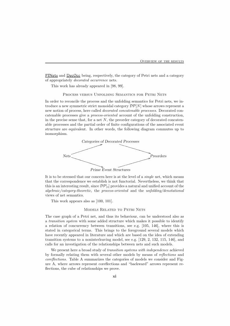
In order to reconcile the process and the unfolding semantics for Petri nets, we in-troduce a new symmetric strict monoidal category DP [N ] whose arrows represent anew notion of process, here called decorated concatenable processes. Decorated con-catenable processes give a process-oriented account of the unfolding construction,in the precise sense that, for a net N , the preorder category of decorated concaten-able processes and the partial order of finite configurations of the associated eventstructure are equivalent. In other words, the following diagram commutes up toisomorphism.
Categories of Decorated Processes
Nets Preorders
Prime Event Structures
VVVVVVVVVVVVVVVVV **iiiiiiiiiiiiiiiii 44UUUUUUUUUUUUUUUUU** hhhhhhhhhhhhhhhhh44It is to be stressed that our concern here is at the level of a single net, which meansthat the correspondence we establish is not functorial. Nevertheless, we think thatthis is an interesting result, sinceDP [ ] provides a natural and unified account of thealgebraic/category-theoretic, the process-oriented and the unfolding/denotationalviews of net semantics.
This work appears also as [100, 101].
Models Related to Petri Nets
The case graph of a Petri net, and thus its behaviour, can be understood also asa transition system with some added structure which makes it possible to identifya relation of concurrency between transitions, see e.g. [105, 146], where this isstated in categorical terms. This brings to the foreground several models whichhave recently appeared in literature and which are based on the idea of extendingtransition systems to a noninterleaving model, see e.g. [129, 2, 132, 115, 146], andcalls for an investigation of the relationships between nets and such models.
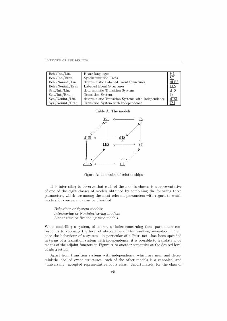
We present here a broad study of transition systems with independence achievedby formally relating them with several other models by means of reflections andcoreflections. Table A summarizes the categories of models we consider and Fig-ure A, where arrows represent coreflections and “backward” arrows represent re-flections, the cube of relationships we prove.
xi
Overview of the results
Beh./Int./Lin. Hoare languages HLBeh./Int./Bran. Synchronization Trees STBeh./Nonint./Lin. deterministic Labelled Event Structures dLESBeh./Nonint./Bran. Labelled Event Structures LESSys./Int./Lin. deterministic Transition Systems dTSSys./Int./Bran. Transition Systems TSSys./Nonint./Lin. deterministic Transition Systems with Independence dTSISys./Nonint./Bran. Transition System with Independence TSI
Table A: The models
dTSI
���
....................................................
..........�⊳−−−−−−−−− dTS
���
....................................................
..........�△
||||||||||∪
△
||||||||||∪
dLES���
....................................................
..........�⊳−−−−−−−−− HL
���
....................................................
..........�
TSI ⊳−−−−−−−−− TS△
||||||||||∪
△
||||||||||∪
LES ⊳−−−−−−−−− ST
Figure A: The cube of relationships
It is interesting to observe that each of the models chosen is a representativeof one of the eight classes of models obtained by combining the following threeparameters, which are among the most relevant parameters with regard to whichmodels for concurrency can be classified:
Behaviour or System models;Interleaving or Noninterleaving models;Linear time or Branching time models.
When modelling a system, of course, a choice concerning these parameters cor-responds to choosing the level of abstraction of the resulting semantics. Then,once the behaviour of a system—in particular of a Petri net—has been specifiedin terms of a transition system with independence, it is possible to translate it bymeans of the adjoint functors in Figure A to another semantics at the desired levelof abstraction.
Apart from transition systems with independence, which are new, and deter-ministic labelled event structures, each of the other models is a canonical and“universally” accepted representative of its class. Unfortunately, for the class of
xii
Overview of the results
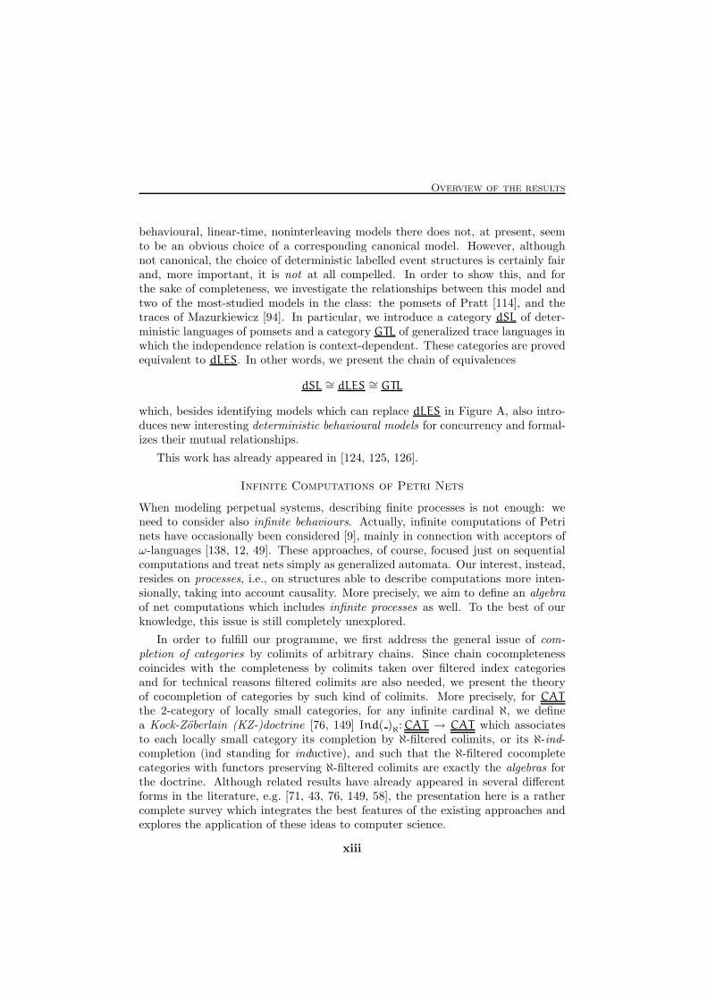
behavioural, linear-time, noninterleaving models there does not, at present, seemto be an obvious choice of a corresponding canonical model. However, althoughnot canonical, the choice of deterministic labelled event structures is certainly fairand, more important, it is not at all compelled. In order to show this, and forthe sake of completeness, we investigate the relationships between this model andtwo of the most-studied models in the class: the pomsets of Pratt [114], and thetraces of Mazurkiewicz [94]. In particular, we introduce a category dSL of deter-ministic languages of pomsets and a category GTL of generalized trace languages inwhich the independence relation is context-dependent. These categories are provedequivalent to dLES. In other words, we present the chain of equivalences
dSL ∼= dLES ∼= GTL
which, besides identifying models which can replace dLES in Figure A, also intro-duces new interesting deterministic behavioural models for concurrency and formal-izes their mutual relationships.
This work has already appeared in [124, 125, 126].
Infinite Computations of Petri Nets
When modeling perpetual systems, describing finite processes is not enough: weneed to consider also infinite behaviours. Actually, infinite computations of Petrinets have occasionally been considered [9], mainly in connection with acceptors ofω-languages [138, 12, 49]. These approaches, of course, focused just on sequentialcomputations and treat nets simply as generalized automata. Our interest, instead,resides on processes, i.e., on structures able to describe computations more inten-sionally, taking into account causality. More precisely, we aim to define an algebraof net computations which includes infinite processes as well. To the best of ourknowledge, this issue is still completely unexplored.
In order to fulfill our programme, we first address the general issue of com-pletion of categories by colimits of arbitrary chains. Since chain cocompletenesscoincides with the completeness by colimits taken over filtered index categoriesand for technical reasons filtered colimits are also needed, we present the theoryof cocompletion of categories by such kind of colimits. More precisely, for CAT
the 2-category of locally small categories, for any infinite cardinal ℵ, we definea Kock-Zoberlain (KZ-)doctrine [76, 149] Ind( )ℵ: CAT → CAT which associatesto each locally small category its completion by ℵ-filtered colimits, or its ℵ-ind-completion (ind standing for inductive), and such that the ℵ-filtered cocompletecategories with functors preserving ℵ-filtered colimits are exactly the algebras forthe doctrine. Although related results have already appeared in several differentforms in the literature, e.g. [71, 43, 76, 149, 58], the presentation here is a rathercomplete survey which integrates the best features of the existing approaches andexplores the application of these ideas to computer science.
xiii
Overview of the results
small locally smallmonoidal strict monoidal monoidal strict monoidal
STRICT
nonsymmetric
MonCat sMonCat MonCAT sMonCAT
symmetricSMonCat SsMonCat SMonCAT SsMonCAT
strictlysymmetric
sSMonCat sSsMonCat sSMonCAT sSsMonCAT
STRONG
nonsymmetric
MonCat⋆ sMonCat⋆ MonCAT⋆ sMonCAT⋆
symmetricSMonCat⋆ SsMonCat⋆ SMonCAT⋆ SsMonCAT⋆
strictlysymmetric
sSMonCat⋆ sSsMonCat⋆ sSMonCAT⋆ sSsMonCAT ⋆
MONOIDAL
nonsymmetric
MonCat⋆⋆ sMonCat⋆⋆ MonCAT⋆⋆ sMonCAT⋆⋆
symmetricSMonCat⋆⋆ SsMonCat⋆⋆ SMonCAT⋆⋆ SsMonCAT ⋆⋆
strictlysymmetric
sSMonCat⋆⋆ sSsMonCat⋆⋆ sSMonCAT⋆⋆ sSsMonCAT⋆⋆
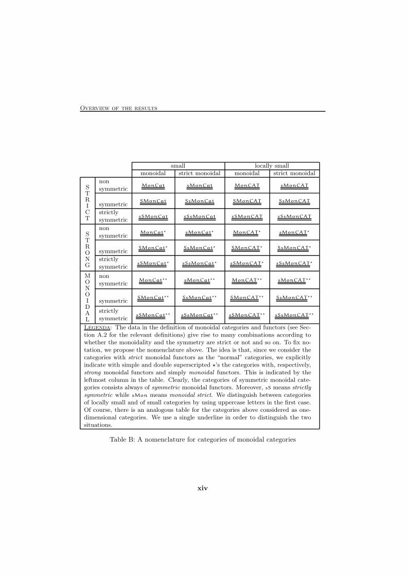
Legenda: The data in the definition of monoidal categories and functors (see Sec-tion A.2 for the relevant definitions) give rise to many combinations according towhether the monoidality and the symmetry are strict or not and so on. To fix no-tation, we propose the nomenclature above. The idea is that, since we consider thecategories with strict monoidal functors as the “normal” categories, we explicitlyindicate with simple and double superscripted ⋆’s the categories with, respectively,strong monoidal functors and simply monoidal functors. This is indicated by theleftmost column in the table. Clearly, the categories of symmetric monoidal cate-gories consists always of symmetric monoidal functors. Moreover, sS means strictlysymmetric while sMon means monoidal strict. We distinguish between categoriesof locally small and of small categories by using uppercase letters in the first case.Of course, there is an analogous table for the categories above considered as one-dimensional categories. We use a single underline in order to distinguish the twosituations.
Table B: A nomenclature for categories of monoidal categories
xiv
Overview of the results
Then, we show that the cocompletion doctrine, when applied to a symmetricmonoidal category, yields a symmetric monoidal category. More precisely, we showthat the KZ-doctrine Ind( )ℵ lifts to a KZ-doctrine on any of the 2-categories ofmonoidal categories appearing in Table B, which, from the technical point of view,is main result of Chapter 3.
We discuss how this result generalizes the algebraic approach to the processsemantics of Petri nets to the case in which infinite processes and compositionoperations on them are considered. In particular, the infinite processes of a Petrinet can in this way be given an algebraic presentation which combines the essentiallyalgebraic presentation of monoidal categories with the monadic presentation of theircompletion in terms of KZ-doctrines.
We should like to remark mention that, since in the last years many computingsystems have been given a semantics through the medium of category theory, thegeneral pattern being to look at objects as representing states and at arrows asrepresenting computations, the theory of cocompletion of categories yields a generalmethod to construct and manipulate infinite computations of those systems. Themain purpose of Chapter 3 is to substantiate this claim by studying in detail thecase of Petri nets.
This work appears also as [123].
Put up in a placewhere it’s easy to see,
the cryptic admonishment T. T. T.
When you feel how depressinglyslowly you climb,
it’s well to remember thatThings Take Time.
Piet Hein, Grooks
“Fermi!” disse il Grande Bastardo.“Stiamo inventando troppe cose in una volta.”
Stefano Benni, La compagnia dei Celestini
xv

Overview of the results
xvi
Chapter 1
Processes and Unfoldings
Abstract. The sematics of Petri nets has been investigated in several different ways.Apart from the classical “token game”, we can model the behaviour of Petri nets vianon-sequential processes, via algebraic approaches, which view Petri nets as essentiallyalgebraic theories whose models are monoidal categories, and, in the case of safe nets, viaunfolding constructions, which provide formal relationships between nets and domains.
In this chapter we extend Winskel’s result to PT nets and we show that the unfoldingsemantics can be reconciled with the process-oriented and the algebraic points of view.In our formal development a relevant role is played by a category of occurrence netsappropriately decorated to take into account the history of tokens. The structure ofdecorated occurrence nets at the same time provides natural unfoldings for PT nets andsuggests a new notion of processes, the decorated processes, which induce on Petri nets thesame semantics as that of the unfolding. In addition, the decorated processes of a net forma symmetric monoidal category which yield an algebraic explanation of net behaviours.
In addition, we propose solutions to some open problems in the algebraic/categoricaltheory of net processes.
I would rather discover one causethat gain the kingdom of Persia.
Democritus
I problemi sono universali.Le soluzioni sono individuali.
Just do it.
Nike’s commercial
This chapter is based on joint work with Jose Meseguer and Ugo Montanari [98, 99, 100,
101] and on [121, 122].
1

Chapter 1. Processes and Unfoldings
2
Introduction
Petri nets, introduced by C.A. Petri in [109] (see also [110, 119, 120, 30]), area widely used model of concurrency. This model is attractive from a theoreticalpoint of view because of its simplicity and because of its intrinsically concurrentnature, and has often been used as a semantic basis on which to interpret concurrentlanguages (see for example [140, 108, 139, 15]).
For Place/Transition (PT) nets, having a satisfactory semantics—one that doesjustice to their truly concurrent nature, yet is abstract enough—remains in our viewan unresolved problem. Certainly, several different semantics have been proposed inthe literature. Most of them can be coarsely classified as process-oriented semantics,unfolding semantics or algebraic semantics, though the latter class is not as clearlydelimited and not as widely diffused as the former two. Of course, such classesare not at all disjoint, as this chapter aims to support. We further discuss theseapproaches below.
At the most basic operational level we have of course the “token game”, the com-putational mechanisms semantics of Petri nets. The development of theory Petrinets, focusing on the noninterleaving aspects of concurrency, brought to the fore-ground various notions of process, e.g. [111, 36, 9, 97, 16]. Generally speaking, Petrinet processes—whose standard version is given by the Goltz-Reisig non-sequentialprocesses [36]—are structures needed to account for the causal relationships whichrule the occurrences of events in computations. Thus, ideally, processes are simplycomputations in which the explicit information about such causal connections isadded. More precisely, since it is a well-established idea that, as far as the theoryof computation is concerned, causality can be faithfully described by means of par-tial orderings—though “heretic” ideas appear sometimes—abstractly, the processesof a net N are ordered sets whose elements are labelled by transitions of N . Inconcrete, in order to describe exactly what multisets of transitions are processesof and what are not, one defines a process of N to be a map π: Θ → N whichmaps transitions to transitions and places to places respecting the “bipartite graphstructure” of nets, where Θ is a finite deterministic occurrence net, i.e., roughlyspeaking, a finite deterministic 1-safe acyclic net whose “flow relation” induces apartial ordering of its elements, the minimal and maximal elements of which areplaces. Of course, the role of π is to “label” the places and the transitions of Θwith places and transitions of N in a way compatible with the structure of N .
The main criticism raised against process models is that they do not providea semantics for a net as a whole, but specify only the meaning of single, deter-ministic computations, while the accurate description of the fine interplay betweenconcurrency and nondeterminism is one of the most valuable features of nets.
Other semantic investigations have capitalized on the algebraic structure of PTnets, first noticed by Reisig [119] and later exploited by Winskel to identify a sen-
3
Chapter 1. Processes and Unfoldings
sible notion of morphism between nets [141, 144]. The clear advantage of theseapproaches resides in the fact that they tend to clarify both the structure of thesingle PT net, so giving insights about their essential properties, and the globalstructure of the class of all nets. Providing, for example, useful net combinatorsassociated to standard categorical constructions such as product and coproduct,which can be used to give a simple account of corresponding compositional opera-tions at the level of a concurrent programming language, such as various forms ofparallel and non-deterministic composition [143, 144, 97].
An original interpretation of the algebraic structure of PT nets has been pro-posed in [97], where the theory of monoidal categories is exploited to the purpose.Unlike the preceding approaches, [97] yields an algebraic theory of Petri nets inwhich notions such as firing sequence, case graph, relationships between net de-scriptions at different abstraction levels, duality and invariants find adequate al-gebraic/categorical formulations. However, generally speaking, the algebraic ap-proaches are often too concrete, and a more abstract semantics—one allowinggreater semantic identifications between nets—would be sometimes preferable.
Roughly speaking the unfolding semantics consists, as the name indicates, in“unfolding” a net to simple denotational structures in which the identity of everyevent in its computations is unambiguous. More precisely, very attractive for-mulation for such a semantics would be an adjoint functor assigning an abstractdenotation to each PT net and preserving certain compositional properties in theassignment. This is exactly what Winskel has done for the subcategory of safenets [143]. In that work—which builds on the previous work [106]—the denotationof a safe net is a Scott domain [128, 133], and Winskel shows that there exists acoreflection—a particularly nice form of adjunction—between the category Dom
of (coherent) finitary prime algebraic domains and the category Safe of safe Petrinets. This construction is completely satisfactory: from the intuitive point of view itgives the “truly concurrent” semantics of safe nets in the most universally acceptedtype of model, while from the formal point of view the existence of an adjunctionguarantees its “naturality”. Winskel’s coreflection factorizes through the chain ofcoreflections
Safe Occ PES DomU [ ] ///Ooo
E[ ] //
N [ ]oo
L[ ] //
Pr[ ]oo
where PES is the category of prime event structures (with binary conflict relation),which is equivalent to Dom, Occ is the category of occurrence nets [143] and ← isthe inclusion functor.
Recently, various attempts have been made to extend this chain or, more gen-erally, to identify a suitable semantic domain for PT nets. Among them, we re-call [115], where, in order to obtain a model “mathematically more attractive thanPetri nets”, a geometric model of concurrency based on n-categories as models of
4
higher dimensional automata is introduced, but it is not clear whether the mod-elling power obtained is greater than that of ordinary PT nets; [50], in which theauthors give semantics to PT nets in terms of generalized trace languages anddiscuss how using their work it could perhaps be possible to obtain a concept ofunfolding for PT nets; and [23], where the unfolding of Petri nets is given in termof a branching process. However, the nets considered in [23] are not really PT netsbecause their transitions are restricted to have pre and post-sets where all placeshave no multiplicities. A yet more recent approach is [51], where the unfolding isexplained in terms of a notion of local event structure. Finally, we would like tocite [105, 46, 107].
A large part of this chapter is devoted to present an extension of Winskel’s ap-proach from safe nets to the category of PT nets. We define the unfoldings of PTnets and relate them by an adjunction to occurrence nets and therefore—exploitingthe already existing adjunctions—to prime event structures and finitary prime al-gebraic domains. The adjunctions so obtained are extensions of the correspondingWinskel’s coreflections.
The category PTNets which we consider for the unfolding functor is quite gen-eral. Objects are PT nets in which markings may be infinite and transitions areallowed to have infinite pre- and post-sets, but, as usual, with finite multiplicities.The only technical restriction we impose, with respect to the natural extensionto nets with infinite markings of the general formulation in [97], is the usual con-dition that transitions must have non-empty pre-sets. Actually, the objects ofPTNets strictly include those of the categories considered in [143, 144]. Althougha technical restriction applies to the morphisms—they are required to map placesbelonging to the initial marking or to the post-set of the same transition to disjointmultisets—they are still quite general. In particular, the category PTNets has ini-tial and terminal objects, and has products and coproducts which faithfully model,respectively, the operations of parallel and non-deterministic composition of netsas in [144] and in [97]. It is worth remarking that, while coproducts do not existin the categories of generally marked, non-safe PT nets considered in the abovecited works, they do in PTNets. This quite interesting fact is due to the aforesaidrestriction we impose on the arrows of PTNets.
Concerning the presentation of these results, in Section 1.5 we start the formaldevelopment regarding the unfolding semantics by defining the category PTNets.In the same section it is shown that it has products and coproducts. In Section 1.6we introduce a new kind of nets, the decorated occurrence nets, which naturallyrepresent the unfoldings of PT nets and can account for the multiplicities of placesin transitions. They are occurrence nets in which places belonging to the post-setof the same transition are partitioned into families. Families are used to relateplaces corresponding in the unfolding to multiple instances of the same place in theoriginal net. When all the families of a decorated occurrence net have cardinalityone, we have (a net isomorphic to) an ordinary occurrence net. Therefore, Occ is
5
Chapter 1. Processes and Unfoldings
(isomorphic to) a full subcategory of DecOcc, the category of decorated occurrencenets. Products and coproducts of decorated occurrence nets are studied in thesecond part of Section 1.7.
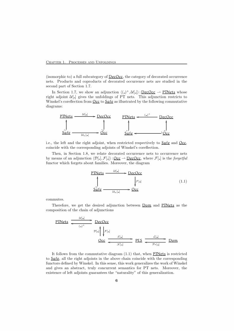
In Section 1.7, we show an adjunction 〈( )+,U [ ]〉 : DecOcc ⇀ PTNets whoseright adjoint U [ ] gives the unfoldings of PT nets. This adjunction restricts toWinskel’s coreflection from Occ to Safe as illustrated by the following commutativediagrams:
PTNets DecOcc
Safe Occ
U [ ] ///� OOUw[ ]
///� OO PTNets DecOcc
Safe Occ
( )+oo/� OO /Ooo/� OO
i.e., the left and the right adjoint, when restricted respectively to Safe and Occ,coincide with the corresponding adjoints of Winskel’s coreflection.
Then, in Section 1.8, we relate decorated occurrence nets to occurrence netsby means of an adjunction 〈D[ ],F [ ]〉 : Occ ⇀ DecOcc, where F [ ] is the forgetfulfunctor which forgets about families. Moreover, the diagram
PTNets DecOcc
Safe Occ
U [ ] //
F [ ]
��/� OOUw[ ]
//
(1.1)
commutes.
Therefore, we get the desired adjunction between Dom and PTNets as thecomposition of the chain of adjunctions
PTNets DecOcc
Occ PES Dom
U [ ] //
( )+oo
F [ ]
��D[ ]
OO
E[ ] //
N [ ]oo
L[ ] //
Pr[ ]oo
It follows from the commutative diagram (1.1) that, when PTNets is restrictedto Safe, all the right adjoints in the above chain coincide with the correspondingfunctors defined by Winskel. In this sense, this work generalizes the work of Winskeland gives an abstract, truly concurrent semantics for PT nets. Moreover, theexistence of left adjoints guarantees the “naturality” of this generalization.
6
We have already mentioned that the three views of net semantics we are dis-cussing are not mutually exclusive. In fact, a unification of the process-orientedand algebraic views has recently been proposed in [16] (see also [17]), by showingthat the commutative processes [9] of a net N are isomorphic to the arrows of astrictly symmetric monoidal category T [N ]. Moreover, [16] introduced the con-catenable processes of N to account, as the name indicates, for the issue of processconcatenation. Let us briefly reconsider the ideas which led to their definition.
Given the definition of process discussed above, one can assign the natural sourceand target states to a process π: Θ → N by considering the multisets of places ofN which are the image via π of, respectively, the minimal and maximal (wrt. tothe ordering identified by Θ) places of Θ. Now, the simple minded attempt toconcatenate a process π1: Θ1 → N with source u to a process π0: Θ0 → N withtarget u by merging the maximal places of Θ0 with the minimal places of Θ1 in away which preserves the labellings breaks down immediately. In fact, if more thanone place of u is labelled by a single place of N , there are many ways to put inone-to-one correspondence the maximal places of Θ0 and the minimal places of Θ1
respecting the labels, i.e., there are many possible concatenations of π0 and π1,each of which gives a possibly different process of N . In other words, processconcatenations has to do with merging tokens rather than merging places, as theabove argument shows clearly.
Therefore, any attempt to deal with process concatenation must disambiguatethe identity of each token in a process. This is exactly the idea of concatenableprocesses, which are simply Goltz-Reisig processes in which the minimal and maxi-mal places carrying the same label are linearly ordered. This yields immediately anoperation of concatenation, since the ambiguity about token indentities is brokenusing the additional information given by the orderings. Moreover, the existence ofconcatenation brings us easily to the definition of a category of concatenable pro-cesses. It turns out that such category is a symmetric monoidal category in whichthe tensor product represents faithfully the parallel composition of processes [16].The relevance of this result resides in the fact that it describes processes of Petri netsas essentially algebraic theories (whose models are given by symmetric monoidalcategories), which indeed is a remarkable property.
Naturally linked to the fact that they are algebraic structures, concatenableprocesses can also be described in abstract terms. In [16] the authors give suchan abstract description by providing for each net N a symmetric monoidal cate-gory P [N ] whose arrows are in one-to-one correspondence with the concatenableprocesses of N . Since this category is obtained as a “free” (in a weak sense toexplained later) construction, this yields an explanation of Petri net processes as aterm algebra by means of which one can easily “compute” with them. In particular,the distributivity of tensor product and arrow composition in monoidal categoriesis shown to capture the basic facts about net computations, so providing a modelof computation for Petri nets.
7
Chapter 1. Processes and Unfoldings
However, strictly speaking, the category P [N ] is only partially axiomatizedin [16], since it is built on a concrete category of symmetries SymN which is con-structed in an ad hoc way. After recalling in Section 1.1 the basic facts about thealgebraic approach to Petri nets as given in [97, 16, 17], in Section 1.2 we showthat also SymN can be characterized abstractly, thus yielding a purely algebraicand completely abstract characterization of the category of concatenable processesof N . Namely, we shall see that P [N ] is the free symmetric strict monoidal cate-gory on the net N modulo two simple additional axioms. We remark that a similarconjecture has been proposed in [37].
In spite of accounting for algebraic and process-oriented aspects in a simpleand unified way, the approach of [16] is still somehow unsatisfactory, since it is notfunctorial, a property which would be greatly recommendable indeed, since it wouldguarantee (to a certain extent) a “good” quality to the semantics induced by P [ ].More strongly, given a morphism between two nets, which can be safely thoughtof as a simulation, it may be not possible to identify a corresponding monoidalfunctor between the respective categories of computations. This situation, besidesshowing that perhaps our understanding of the algebraic structure of Petri nets isstill incomplete, has also other drawbacks, the most relevant of which is probablythat it prevents us to identify the category (of the categories) of net behaviours,i.e., to axiomatize the behaviour of Petri nets “in the large”.
In Section 1.3, we present an analysis of the issue of functoriality of the pro-cess semantics of nets founded on symmetric monoidal categories, and a possiblesolution based on the new notion of strong concatenable processes of N , introducedin Section 1.4. These are a slight refinement of concatenable processes which arestill rather close to the standard notion of process: namely, they are Goltz-Reisigprocesses whose minimal and maximal places are linearly ordered. In the paperwe show that, similarly to the concatenable processes, the strong concatenable pro-cesses of N can be axiomatized as a free construction on N , by building on Nan abstract symmetric monoidal category Q[N ] and by proving that the arrowsof Q[N ] are isomorphic to the strong concatenable processes of N .
The key feature of Q[ ] is that, differently from P [ ], it associates to net N asymmetric monoidal category whose objects form a free, non-commutative monoid.The reason for renouncing to commutativity, a choice that at a first glance mayseem odd, is explained in Section 1.3, where the following negative result is proved:
under very reasonable assumptions, no mapping from nets to symmetricmonoidal categories whose monoids of objects are commutative can beextended to a functor, since there exists a morphism of nets whichdoes not have a corresponding symmetric monoidal functor betweenthe appropriate categories.
Thus, abandoning the commutativity of the monoids of objects seems to be a price
8
which is necessary to pay in order to obtain a functorial semantics of nets. Then,bringing such condition to the net level, instead of taking multisets of places assources and targets of computations, we consider strings of places, a choice whichleads us directly to strong concatenable processes. Correspondingly, a transitionof N will be represented by many arrows in Q[N ], one for each different “lineariza-tion” of its pre-set and its post-set. However, such arrows will be “linked” to eachother by a “naturality” condition, in the precise sense that, when collected together,they form a natural transformation between appropriate functors. Such naturalityaxiom is the second relevant feature of Q[ ] and it is actually the key to keep thecomputational interpretation of the new category Q[N ] surprisingly close to thecategory P [N ] of concatenable processes.
Clearly, the functoriality of Q[ ] allows us to identify a category SSMC⊗, to-gether with a “forgetful” functor from it to the category of Petri nets, which rep-resents our proposed axiomatization of net computations in categorical terms. Al-though we are aware that this contribution constitutes simply a first attempt to-wards the aim, we honestly think that the results illustrated here help to deepenthe understanding of the subject. We remark that the refinement of concatenableprocesses represented by strong concatenable processes is similar and comparableto the one which brought from Goltz-Reisig processes to them. Of course, thepassage here is more “hazardous” on the intuitive ground, since it brings us tomodel Petri nets, which after all are just multiset rewriting systems, using strings.However, it is important to remind the negative result in Section 1.3, which makesstrong concatenable processes interesting, showing that, in a sense, they are theleast refinement of Goltz-Reisig processes which yield an operation of sequentialcomposition and a functorial treatment.
Getting back to the relationships between the various kind of semantics for Petrinets, concerning process and unfolding semantics, in the case of safe nets the ques-tion is easily answered by exploiting the existence of a coreflection of Occ into Safe,which directly implies the existence of an isomorphism between the processes of Nand the deterministic finite subnets of U [N ], i.e., the finite configurations of EU [N ].(More details about such correspondence will be given in Section 1.9.) Thus, in thiscase, the process and unfolding semantics coincide, although it should not be forgot-ten that the latter has the great merit of collecting together all the processes of Nas a whole, so accounting at the same time for concurrency and nondeterminism.
In Section 1.9, we study the relationships between the algebraic paradigm, theprocess semantics described above and the unfolding semantics for PT nets givenin Sections 1.5–1.8. We find that, in the context of general PT nets, the latter twonotions do not coincide. In particular, the unfolding of a netN contains informationstrictly more concrete than the collection of the processes of N . However, we showthat the difference between the two semantics can be axiomatized quite simply. Inparticular, we introduce a new notion of process, whose definition is suggested bythe idea of families in decorated occurrence nets, and which are therefore called
9
Chapter 1. Processes and Unfoldings
decorated processes, and we show that they capture the unfolding semantics, in theprecise sense that there is a one-to-one translation between decorated processesof N and finite configurations of EFU [N ]. Then, following the approach of [16],we axiomatize the notion of decorated (concatenable) process in terms of monoidalcategories. More precisely, we define an abstract symmetric monoidal categoryDP [N ] and we show that its arrows represent decorated concatenable processes.
The natural environment for the development of a theory of net processes basedon monoidal categories is, as illustrated in [16], a category Petri of unmarked nets,i.e., nets without initial markings, whose transitions have finite pre- and post-sets.Although there seem to be no formal reasons preventing one from extending thetheory to nets with infinite markings, such an extension would be at least technicallyrather involved. Therefore, our choice here is to follow [16] and define DP [ ] on thecategory Petri of unmarked nets with finite markings introduced in [97].
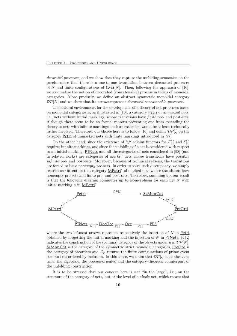
On the other hand, since the existence of left adjoint functors for F [ ] and E [ ]requires infinite markings, and since the unfolding of a net is considered with respectto an initial marking, PTNets and all the categories of nets considered in [98] (andin related works) are categories of marked nets whose transitions have possiblyinfinite pre- and post-sets. Moreover, because of technical reasons, the transitionsare forced to have nonempty pre-sets. In order to solve such discrepancy, we simplyrestrict our attention to a category MPetri∗ of marked nets whose transitions havenonempty pre-sets and finite pre- and post-sets. Therefore, summing up, our resultis that the following diagram commutes up to isomorphism for each net N withinitial marking u in MPetri∗
Petri SsMonCat
MPetri∗ PreOrd
PTNets DecOcc Occ PES
DP[ ] //
〈u↓ 〉NNNNNNNNNN&&rrrrrrrrr 99LLLLLLLLL &&
U [ ]//
F [ ]//
E[ ]//
LF [ ]pppppppppp88where the two leftmost arrows represent respectively the insertion of N in Petri
obtained by forgetting the initial marking and the injection of N in PTNets, 〈u↓ 〉indicates the construction of the (comma) category of the objects under u in DP[N ],SsMonCat is the category of the symmetric strict monoidal categories, PreOrd isthe category of preorders and LF returns the finite configurations of prime eventstructu+res ordered by inclusion. In this sense, we claim that DP [ ] is, at the sametime, the algebraic, the process-oriented and the category-theoretic counterpart ofthe unfolding construction.
It is to be stressed that our concern here is not “in the large”, i.e., on thestructure of the category of nets, but at the level of a single net, which means that
10
1.1. Petri Nets and their Computations
the diagram above is defined only at the object level, i.e., the correspondence weestablish is not functorial. Of course, this is due to the fact that DP [ ], exactlyas P [ ], is not a functor. Nevertheless, we think that this is an interesting result,since it provides a natural and unified account of the algebraic, the process-orientedand the denotational views of net semantics. We remark that a similar approachhas been followed in [107] in the case of elementary net systems—a particularclass of safe nets without self-looping transitions—for unfoldings and non-sequentialprocesses.
Finally, we conclude this chapter by briefly discussing some natural variationson the unfolding theme in order to justify further the construction.
Notation. Given a category C, we denote the composition of arrows in C by the usual◦ in the usual right to left order. The identity of c ∈ C is written as idc. However,
we make the following exception. When dealing with a category in which arrows aremeant to represent computations, in order to stress this computational meaning, we writearrow composition from left to right, i.e., in the diagramatic order, and we denote it by; . Moreover, when no ambiguity arises, idc is simply written as c. We assume thattensor product binds more strictly than arrow composition, i.e., f ⊗ g;h ⊗ k stands for(f ⊗ g); (h⊗ k). The reader is referred to the Appendix for the categorical concepts used.A thorough introduction to category theory can be acquired from any of the textbooks [90,1, 103, 127, 26, 92].
Remark. Concerning foundational issues, following [89], we assume as usual the existenceof a fixed universe U [55, 136, 43] of small sets upon which categories are built (seealso Appendix A.1). However, since the explicit distinction between “small” and “large”objects plays a significant role only in Chapter 3, in this and in the following chapter weshall avoid any further reference to small sets. Of course, in order to make the categorieswe shall define in Chapter 1 and Chapter 2 agree with the definition given in Appendix A.1,it is enough to read “set” as “small set” where appropriate.
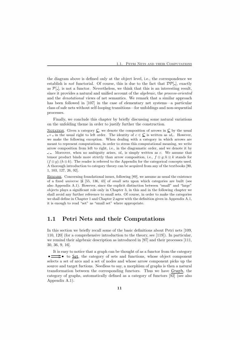
1.1 Petri Nets and their Computations
In this section we briefly recall some of the basic definitions about Petri nets [109,110, 120] (for a comprehensive introduction to the theory, see [119]). In particular,we remind their algebraic description as introduced in [97] and their processes [111,30, 36, 9, 16].
It is easy to notice that a graph can be thought of as a functor from the category• •//// to Set, the category of sets and functions, whose object componentselects a set of arcs and a set of nodes and whose arrow component picks up thesource and target fuctions. Needless to say, a morphism of graphs is then a naturaltransformation between the corresponding functors. Thus we have Graph, thecategory of graphs, automatically defined as a category of functors [92] (see alsoAppendix A.1).
11
Chapter 1. Processes and Unfoldings
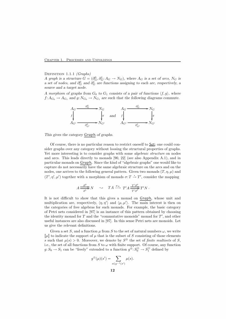
Definition 1.1.1 (Graphs)A graph is a structure G = (∂0
G, ∂1G:AG → NG), where AG is a set of arcs, NG is
a set of nodes, and ∂0G and ∂1
G are functions assigning to each arc, respectively, asource and a target node.
A morphism of graphs from G0 to G1 consists of a pair of functions 〈f, g〉, wheref :AG0 → AG1 and g:NG0 → NG1 are such that the following diagrams commute.
AG NG
AG′ NG′
∂0G //
f
��g
��
∂0G′
//
and
AG NG
AG′ NG′
∂1G //
f
��g
��
∂1G′
//
This gives the category Graph of graphs.
Of course, there is no particular reason to restrict oneself to Set; one could con-sider graphs over any category without loosing the structural properties of graphs.Yet more interesting is to consider graphs with some algebraic structure on nodesand arcs. This leads directly to monads [90, 22] (see also Appendix A.1), and inparticular monads on Graph. Since the kind of “algebraic graphs” one would like tocapture do not necessarily have the same algebraic structure on the arcs and on thenodes, one arrives to the following general pattern. Given two monads (T, η, µ) and
(T ′, η′, µ′) together with a morphism of monads σ:T�
→ T ′, consider the mapping
A N∂0 //∂1
// ; TAσA−→ T ′A T ′N
T ′∂0 //T ′∂1
// .
It is not difficult to show that this gives a monad on Graph, whose unit andmultiplication are, respectively, 〈η, η′〉 and 〈µ, µ′〉. The main interest is then onthe categories of free algebras for such monads. For example, the basic categoryof Petri nets considered in [97] is an instance of this pattern obtained by choosingthe identity monad for T and the “commutative monoids” monad for T ′, and otheruseful instances are also discussed in [97]. In this sense Petri nets are monoids. Letus give the relevant definitions.
Given a set S, and a function µ from S to the set of natural numbers ω, we write[[µ]] to indicate the support of µ that is the subset of S consisting of those elementss such that µ(s) > 0. Moreover, we denote by S⊕ the set of finite multisets of S,i.e., the set of all functions from S to ω with finite support. Of course, any functiong:S0 → S1 can be “freely” extended to a function g⊕:S⊕0 → S⊕1 defined by
g⊕(µ)(s′) =∑
s∈g−1(s′)
µ(s).
12
1.1. Petri Nets and their Computations
This definition makes ( )⊕ an endofunctor on Set. Consider now a finite multisetof finite multisets φ:S⊕ → ω. It can be considered a formal “linear combination”of multisets, and thus identified with the multiset µ such that
µ(s) =∑
ν∈S⊕
φ(ν)ν(s).
It is then easy to see that ( )⊕ is a commutative monad [72, 73, 74, 75] on Set whosemultiplication is the operation of linear combination of multisets above and whoseunit maps s ∈ S to the function which yields 1 on s and zero elsewhere. Clearly,the ( )⊕-algebras are the commutative monoids and the ( )⊕-homomorphisms aremonoid homomorphisms.
We shall represent a finite multiset µ ∈ S⊕ as a formal sum⊕
s∈S µ(s) · s.Moreover, we shall often denote µ ∈ S⊕ by
⊕i∈I nisi where {si | i ∈ I} = [[µ]]
and ni = µ(si), i.e., as a sum whose summands are all nonzero. For instance, themultiset which contains the unique element s with multiplicity one is written as1 · s, or simply s. In this setting, the multiplication of finite multisets is written as
⊕
µ∈S⊕
nµ · µ =⊕
µ∈S⊕
nµ ·
(⊕
s∈S
µ(s) · s
)=⊕
s∈S
( ∑
µ∈S⊕
nµµ(s))· s,
while the monoid homomorphism condition for a function g:S⊕0 → S⊕1 is
g(µ) =⊕
s∈S0
µ(s) · g(1 · s).
Finally, given S′ ⊆ S, we will write⊕S′ for
⊕s∈S′ 1 · s =
⊕s∈S′ s.
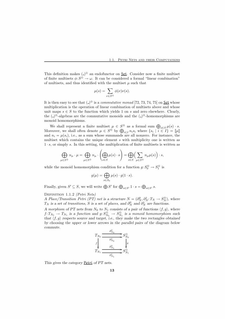
Definition 1.1.2 (Petri Nets)A Place/Transition Petri (PT) net is a structure N = (∂0
N , ∂1N :TN → S⊕N ), where
TN is a set of transitions, S is a set of places, and ∂0N and ∂1
N are functions.
A morphism of PT nets from N0 to N1 consists of a pair of functions 〈f, g〉, wheref :TN0 → TN1 is a function and g:S⊕N0
→ S⊕N1is a monoid homomorphism such
that 〈f, g〉 respects source and target, i.e., they make the two rectangles obtainedby choosing the upper or lower arrows in the parallel pairs of the diagram belowcommute.
TN0 S⊕N0
TN1 S⊕N1
∂0N0 //
∂1N0
//
f
��g
��∂0N1 //
∂1N1
//
This gives the category Petri of PT nets.
13
Chapter 1. Processes and Unfoldings
This describes a Petri net precisely as a graph whose set of nodes is a freecommutative monoid, i.e., the set of finite multisets on a given set of places. Sourceand target of an arc, here called transition, are meant to represent, respectively,the marking which enables the transition, i.e., the states which allow the transitionto fire, and the marking produced by the firing of the transition.
Observe that we are only considering finite markings. Although this is clearlya restriction, it does not have serious drawbacks on the pratical ground of systemmodelization and verification. Moreover, it usually does not have strong conse-quences also from the theoretical point of view, since, to the best of our knowledge,not many notions in the theory require the existence of infinite markings. However,we shall encounter two of those notions in which infinite markings are needed, onein Section 1.5 and one in Chapter 3, since the existence of a left adjoint for theunfolding functor requires infinite markings and, of course, so do infinite computa-tions.
Notation. To simplify notation, we assume the standard constraint that TN ∩SN = ∅—which of course can always be achieved by an appropriate renaming. Moreover, we shallsometimes use a single letter to denote a morphism 〈f, g〉. In these cases, the type of theargument will identify which component we are referring to. Observe further that by thevery definition of free algebras, an ( )⊕-homomorphism g:S⊕N0
→ S⊕N1, which constitutes
the place component of a morphism 〈f, g〉, is completely defined by its behaviour onSN0 , the generators of the free algebra S⊕N0
. Therefore, we will often define morphisms
between nets by giving their transition components and a map g:SN0 → S⊕N1for their place
components: it is implicit that they have to be thought of as lifted to the corresponding( )⊕-homomorphisms.
Another point which is worth raising concerns the observation that the mor-phisms in Petri are total, while in the literature nets (and many other models)are often provided with partial morphisms (see e.g. [144, 146]). Since the intuitionabout morphisms in categories of models of computation is that they represent“simulations,” partial morphisms model situations in which some computationalstep may be simulated vacuosly. Partial morphisms may be recovered in this ap-proach simply by considering a sligthly refined monad for the algebra of transitions,namely the lifting monad.
A pointed set is a pair (S, s) where S is a set and s ∈ S is a chosen elementof S: the pointed element. Morphisms of pointed sets are functions that preservethe pointed elements. Therefore, pointed set morphisms provide a convenient wayto treat partial functions between sets as total functions. Of course, this yieldsa monad ( )0 on Set whose functor part adds a pointed element to a set, whosemultiplication forgets it and whose unit is the inclusion of S in S + {∗}.
We will regard S⊕ also as a pointed set whose pointed element is the emptymultiset, i.e., the function which always yields zero, that, in the following, we denote
by 0. Of course, this is nothing but defining a morphism of monads σ: ( )0�
→ ( )⊕
14
1.1. Petri Nets and their Computations
where σS : (S, ∗) → S⊕ sends ∗ to 0 and s to 1 · s. Thus, following the generalpattern above we have the following definition.
Definition 1.1.3 (Pointed Petri Nets)A pointed (PT) net is a structure N = (∂0
N , ∂1N : (TN , 0) → S⊕N ), where (TN , 0) is
a pointed set of transitions, S is a set of places, and ∂0N and ∂1
N are morphisms ofpointed sets.
A morphism of pointed nets from N0 to N1 consists of a pair of functions 〈f, g〉,where f :TN0 → TN1 is a morphism of pointed sets and g:S⊕N0
→ S⊕N1is a monoid
homomorphism such that 〈f, g〉 respects source and target, i.e., g ◦ ∂0N0
= ∂0N1◦ f
and g ◦ ∂1N0
= ∂1N1◦ f . In other words, a pointed net morphism is a morphism of
the underlying PT nets which, in addition, preserves the pointed element.
This gives the category Petri0 of pointed nets.
The next issue we need to treat concerns the initial marking, i.e., the initialstate, of a net. It is rather common to consider the kind of nets we defined abovecloser to system schemes than to systems, since they lack an initial state from whichto start computing and, of course, different initial markings can give rise to verydifferent behaviours for the same net. Although this distinction is clearly agreeable,we shall not put much emphasis on it, since in the categorical framework this isnot always necessary. We shall for instance define processes and computations ofunmarked nets, so obtaining the collection of the computations for any possibleinital marking, the point being that it is always possible to recover all the relevantinformation about the behaviour for a given marking via canonical constructionssuch as comma categories [90] (see also Appendix A.1).
Definition 1.1.4 (Marked Petri Nets)A marked (pointed) PT net is a pair (N, uN ), where N is a (pointed) PT net anduN ∈ S
⊕N is the initial marking.
A morphism of marked (pointed) PT nets from N0 to N1 consists of a (pointed)PT net morphism 〈f, g〉:N0 → N1 which preserves the initial marking, i.e., suchthat g(uN0) = uN1 .
This gives the category MPetri of marked PT nets and the category MPetri0 ofmarked pointed nets.
Transitions are the basic units of computation in a PT net. A transition twith ∂0
N (t) = u and ∂1N (t) = v—usually written t:u→ v—performs a computation
consuming the tokens in u and producing the tokens in v. A finite number oftransitions can be composed in parallel to form a step, which, therefore, is a finitemultiset of transitions. We write u[α〉v to denote a step α with source u and
15
Chapter 1. Processes and Unfoldings
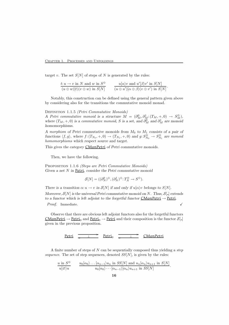
target v. The set S [N ] of steps of N is generated by the rules:
t:u→ v in N and w in S⊕
(u⊕ w)[t〉(v ⊕ w) in S [N ]
u[α〉v and u′[β〉v′ in S [N ]
(u⊕ u′)[α⊕ β〉(v ⊕ v′) in S [N ].
Notably, this construction can be defined using the general pattern given aboveby considering also for the transitions the commutative monoid monad.
Definition 1.1.5 (Petri Commutative Monoids)A Petri commutative monoid is a structure M = (∂0
M , ∂1M : (TM ,+, 0) → S⊕M ),
where (TM ,+, 0) is a commutative monoid, S is a set, and ∂0M and ∂1
M are monoidhomomorphisms.
A morphism of Petri commutative monoids from M0 to M1 consists of a pair offunctions 〈f, g〉, where f : (TN0 ,+, 0) → (TN1 ,+, 0) and g:S⊕N0
→ S⊕N1are monoid
homomorphisms which respect source and target.
This gives the category CMonPetri of Petri commutative monoids.
Then, we have the following.
Proposition 1.1.6 (Steps are Petri Commutative Monoids)Given a net N in Petri, consider the Petri commutative monoid
S[N ] = ((∂0N )⊕, (∂1
N )⊕:T⊕N → S⊕).
There is a transition α:u→ v in S[N ] if and only if u[α〉v belongs to S [N ].
Moreover, S[N ] is the universal Petri commutative monoid onN . Thus, S[ ] extendsto a functor which is left adjoint to the forgetful functor CMonPetri→ Petri.
Proof. Immediate. X
Observe that there are obvious left adjoint functors also for the forgetful functorsCMonPetri→ Petri0 and Petri0 → Petri and their composition is the functor S[ ]given in the previous proposition.
Petri Petri0 CMonPetri⊥//
oo ⊥//
oo
A finite number of steps of N can be sequentially composed thus yielding a stepsequence. The set of step sequences, denoted SS [N ], is given by the rules:
u in S⊕
u[∅〉uu0[α0〉 . . . [αn−1〉un in SS [N ] and un[αn〉un+1 in S [N ]
u0[α0〉 · · · [αn−1〉[αn〉un+1 in SS [N ].
16
1.1. Petri Nets and their Computations
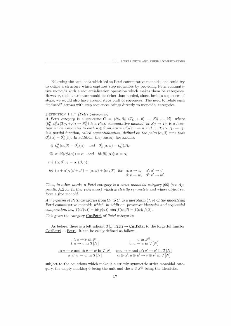
Following the same idea which led to Petri commutative monoids, one could tryto define a structure which captures step sequences by providing Petri commuta-tive monoids with a sequentialization operation which makes them be categories.However, such a structure would be richer than needed, since, besides sequences ofsteps, we would also have around steps built of sequences. The need to relate such“induced” arrows with step sequences brings directly to monoidal categories.
Definition 1.1.7 (Petri Categories)A Petri category is a structure C = (∂0
C , ∂1C : (TC ,+, 0) → S⊕C , ; , id), where
(∂0C , ∂
1C : (TC ,+, 0) → S⊕C ) is a Petri commutative monoid, id :SC → TC is a func-
tion which associates to each u ∈ S an arrow id(u):u→ u and ; :TC × TC → TCis a partial function, called sequentialization, defined on the pairs (α, β) such that∂1C(α) = ∂0
C(β). In addition, they satisfy the axioms:
i) ∂0C(α;β) = ∂0
C(α) and ∂1C(α;β) = ∂1
C(β);
ii) α; id(∂1C(α)) = α and id(∂0
C(α));α = α;
iii) (α;β); γ = α; (β; γ);
iv) (α+ α′); (β + β′) = (α;β) + (α′;β′), for α:u→ v, α′:u′ → v′
β: v → w, β′: v′ → w′.
Thus, in other words, a Petri category is a strict monoidal category [90] (see Ap-pendix A.2 for further references) which is strictly symmetric and whose object setform a free monoid.
A morphism of Petri categories from C0 to C1 is a morphism 〈f, g〉 of the underlyingPetri commutative monoids which, in addition, preserves identities and sequentialcomposition, i.e., f(id(u)) = id(g(u)) and f(α;β) = f(α); f(β).
This gives the category CatPetri of Petri categories.
As before, there is a left adjoint T [ ]: Petri→ CatPetri to the forgetful functorCatPetri→ Petri. It can be easily defined as follows.
t:u→ v in Nt:u→ v in T [N ]
u in S⊕
u:u→ u in T [N ]
α:u→ v and β: v → w in T [N ]α;β:u→ w in T [N ]
α:u→ v and α′:u′ → v′ in T [N ]α⊕ α′:u⊕ u′ → v ⊕ v′ in T [N ]
subject to the equations which make it a strictly symmetric strict monoidal cate-gory, the empty marking 0 being the unit and the u ∈ S⊕ being the identities.
17
Chapter 1. Processes and Unfoldings
It is easy to realize that T [ ] factors through S[ ], and therefore we have thefollowing chain of adjunctions.
Petri Petri0 CMonPetri CatPetri⊥//
oo ⊥//
oo ⊥//
oo
The interesting fact about Petri categories is that the axioms of monoidal cate-gories induce identifications also on step sequences, thus yielding a representationof net behaviour which is more abstract than step sequences. More precisely, thearrows of T [N ], called commutative processes in [16], have been found in [9], eventhough following different motivations and through quite a different formalization,and characterized as the least quotient of step sequences which is more abstractthan processes [36]. In order to be more precise on this we first need to introducethe classical notion of process of a Petri net.
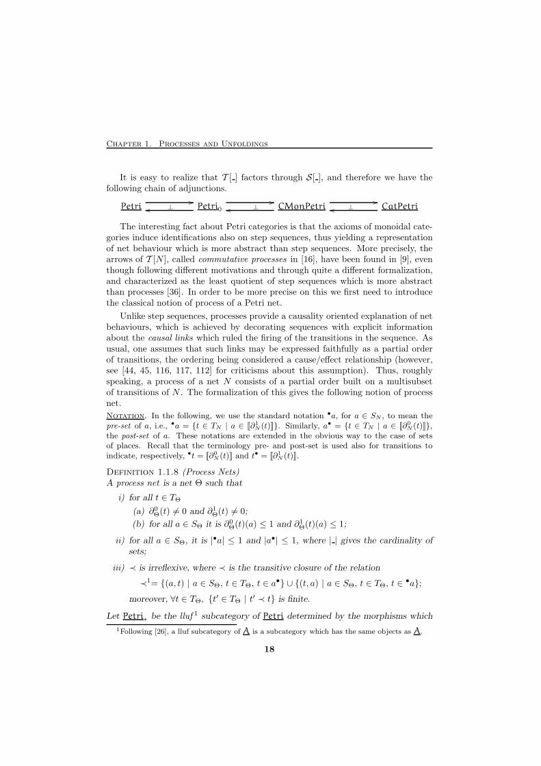
Unlike step sequences, processes provide a causality oriented explanation of netbehaviours, which is achieved by decorating sequences with explicit informationabout the causal links which ruled the firing of the transitions in the sequence. Asusual, one assumes that such links may be expressed faithfully as a partial orderof transitions, the ordering being considered a cause/effect relationship (however,see [44, 45, 116, 117, 112] for criticisms about this assumption). Thus, roughlyspeaking, a process of a net N consists of a partial order built on a multisubsetof transitions of N . The formalization of this gives the following notion of processnet.
Notation. In the following, we use the standard notation •a, for a ∈ SN , to mean thepre-set of a, i.e., •a = {t ∈ TN | a ∈ [[∂1
N (t)]]}. Similarly, a• = {t ∈ TN | a ∈ [[∂0N (t)]]},
the post-set of a. These notations are extended in the obvious way to the case of setsof places. Recall that the terminology pre- and post-set is used also for transitions toindicate, respectively, •t = [[∂0
N (t)]] and t• = [[∂1N (t)]].
Definition 1.1.8 (Process Nets)A process net is a net Θ such that
i) for all t ∈ TΘ
(a) ∂0Θ(t) 6= 0 and ∂1
Θ(t) 6= 0;
(b) for all a ∈ SΘ it is ∂0Θ(t)(a) ≤ 1 and ∂1
Θ(t)(a) ≤ 1;
ii) for all a ∈ SΘ, it is |•a| ≤ 1 and |a•| ≤ 1, where | | gives the cardinality ofsets;
iii) ≺ is irreflexive, where ≺ is the transitive closure of the relation
≺1= {(a, t) | a ∈ SΘ, t ∈ TΘ, t ∈ a•} ∪ {(t, a) | a ∈ SΘ, t ∈ TΘ, t ∈
•a};
moreover, ∀t ∈ TΘ, {t′ ∈ TΘ | t′ ≺ t} is finite.
Let Petri∗ be the lluf 1 subcategory of Petri determined by the morphisms which
1Following [26], a lluf subcategory of A is a subcategory which has the same objects as A.
18
1.1. Petri Nets and their Computations
map places to places (as opposed to morphisms which map places to markings).Then, we define ProcNets to be the full subcategory of Petri∗ determined byprocess nets.
Thus, in process nets every transition has non-empty pre- and post-set. More-over, each place belongs at most to one pre-set and at most to one post-set. Thismakes of the “flow” relation ≺ be a pre-order. Thus, requiring it to be irreflexive,which is equivalent to requiring that the net be acyclic, identifies a partial order onthe transitions. The constraint about the cardinality of the set of predecessors ofa transition is then the fairly intuitive requirement that each transition be finitelycaused. (See [143] for a discussion in terms of event structures of this issue.) Theexpert reader will have already noticed that the process nets above are the usual(deterministic) occurrence nets. However, we prefer to reserve this terminology forthe kind of nets used in the context of the unfolding semantics in Section 1.7.
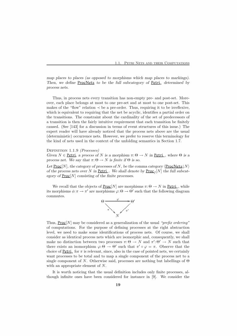
Definition 1.1.9 (Processes)Given N ∈ Petri, a process of N is a morphism π: Θ → N in Petri∗, where Θ is aprocess net. We say that π: Θ→ N is finite if Θ is so.
Let Proc[N ], the category of processes of N , be the comma category 〈ProcNets↓N〉of the process nets over N in Petri∗. We shall denote by Procf [N ] the full subcat-egory of Proc[N ] consisting of the finite processes.
We recall that the objects of Proc[N ] are morphisms π: Θ→ N in Petri∗, whileits morphisms φ:π → π′ are morphisms ϕ: Θ→ Θ′ such that the following diagramcommutes.
Θ Θ′
N
ϕ //
π
������ π′
~~}}}}}}Thus, Proc[N ] may be considered as a generalization of the usual “prefix ordering”of computations. For the purpose of defining processes at the right abstractionlevel, we need to make some identifications of process nets. Of course, we shallconsider as identical process nets which are isomorphic and, consequently, we shallmake no distinction between two processes π: Θ → N and π′: Θ′ → N such thatthere exists an isomorphism ϕ: Θ → Θ′ such that π′ ◦ ϕ = π. Observe that thechoice of Petri∗ for π is relevant, since, also in the case of pointed nets, we certainlywant processes to be total and to map a single component of the process net to asingle component of N . Otherwise said, processes are nothing but labellings of Θwith an appropriate element of N .
It is worth noticing that the usual definition includes only finite processes, al-though infinite ones have been considered for instance in [9]. We consider the
19
Chapter 1. Processes and Unfoldings
broader definition above, since in Section 3.7 we shall be talking about infinite pro-cesses. However, in this section we only consider finite processes. Moreover, thedefinition of processes for nets is usually given with respect to some initial marking.In the following, we shall briefly see that, in this setting, this does not make anydifference.
Definition 1.1.10 (Marked Process Nets and Processes )A marked process net is a pair (Θ, u) where Θ is a process net and u is the set ofthe minimal (wrt. ≺) elements of Θ, which are necessarily places. Let MProcNets
denote the full subcategory of MPetri∗ consisting of marked process nets ad mor-phisms, MPetri∗ being the lluf subcategory of MPetri consisting of the morphismswhich map places to places.
The category MProc[(N, u)] of processes of a marked net (N, u) is the commacategory 〈MProcNets↓(N, u)〉 of the marked process nets over (N, u) in MPetri∗,i.e., a process of marked nets is obtained by considering processes which map theminimal elements of process nets to u, the initial marking of N . Similarly to theprevious case, MProcf [(N, u)] will denote the category of finite processes of N .
There is the following obvious link between Proc[N ] and MProc[(N, u)].
Proposition 1.1.11MProc[(N, u)] (respectively MProcf [(N, u)]) is the full subcategory of Proc[N ](respectively Procf [(N, u)]) consisting of those processes π: Θ → N such thatπ(min(Θ)) = u, where min(Θ) denotes the set of minimal elements of Θ.
We can now get quickly back to the characterization of T [N ] we referred to ear-lier. Observe that, by definition, processes are more concrete than step sequences,i.e., different processes may give rise to common step sequences, corresponding tothe fact that different partial orders may have common linearizations. On the otherhand, different step sequences may be sequentializations of the same process
Proposition 1.1.12 (Step Sequences and Petri Categories)For N in Petri, the arrows of T [N ], i.e., the commutative processes of N , areobtained by quotienting the processes of N by the least equivalence such that if astep sequence is a linearization of two different processes, then they are equivalent.
Proof. See [9, 16]. X
The categories of processes Proc[N ] are not completely satisfactory, at leastfor two relevant reasons. Firstly, when “categorizing” computational formalismsthe focus is on representing states—respectively types, formulas—as objects andcomputations—respectively terms, proofs—as arrows, and this is because the focus
20
1.1. Petri Nets and their Computations
is actually on computations and, after all, categories consist mainly of arrows.Therefore, to consider Proc[N ] as a satisfactory solution would be, at the very least,out of the current mainstream of research. Secondly, both the monoidal structureof Petri nets and the monoidal structure which intuitively should be enjoyed by thecomputations of a concurrent system under the operation of parallel compositionare not reflected in Proc[N ]. Clearly, T [N ] does not suffer of these problems.However, the very observation that T [N ] provides a description of the behaviourof N even more abstract than step sequences of course put it out of the game, sincewe are looking for a causal semantics for nets. It is easy to realize that the problemwith T [N ] concerning causality is due to the strict symmetry which confuses the“causal streams” of computations. Therefore, a possible way out of this problem isto look for a non strictly symmetric version of T [N ], where the flow of causality istaken into account by the symmetry isomorphism.
Of course, another possible solution consists of looking for a version of Proc[N ]in which the processes are represented by arrows, sequential composition being theconcatenation of processes. More strongly, inspired by the current trends in thedevelopment of the theory of computation, one would certainly like to describethe processes of a net N as an algebra whose operations model a minimal set ofcombinators on processes which capture the essence of concurrency. Clearly, in thepresent case, the core of such algebra must consist of the operations of sequentialand parallel composition of processes. The problem which arises immediately is thatnon-sequential processes cannot be concatenated when multiplicities are present: inorder to support such an operation one must disambiguate the identity of all thetokens in the multisets source and target of processes. In other words, one mustrecognize that process concatenation has to do with tokens rather than with places.This is the approach followed in [16] where the above sketched variation of theprocesses of N is modelled by means of a symmetric strict monoidal category P [N ].Next, we briefly recall such a construction, which represents the meeting point ofthe two development lines indicated above.
A symmetric strict monoidal category (SSMC in the following) is a structure(C,⊗, e, γ), where C is a category, e is an object of C, called the unit object,⊗: C × C → C is a functor, called the tensor product, subject to the followingequations
⊗ ◦ 〈⊗ × 1C〉 = ⊗ ◦ 〈1C ×⊗〉; (1.2)
⊗ ◦ 〈e, 1C〉 = 1C; (1.3)
⊗ ◦ 〈1C, e〉 = 1C; (1.4)
where e: C → C is the constant functor which associate e and id e respectively toeach object and each morphism of C, 〈 , 〉 is the pairing of functor induced by
the cartesian product, and γ is a natural transformation ⊗�
→ ⊗ ◦ ∆, where ∆ isthe endofunctor on C × C which “swaps” its arguments, subject to the following
21
Chapter 1. Processes and Unfoldings
Kelly-MacLane coherence axioms [87, 62, 67]:
(γx,z ⊗ idy) ◦ (idx ⊗ γy,z) = γx⊗y,z; (1.5)
γy,x ◦ γx,y = idx⊗y. (1.6)
Of course, equation (1.2) states that the tensor is associative on both objects andarrows, while (1.3) and (1.4) state that e and ide are, respectively, the unit objectand the unit arrow for ⊗. Concerning the coherence axioms, axiom (1.6) says thatγy,x is the inverse of γx,y, while (1.5), the real key of symmetric monoidal categories,links the symmetry at composed objects to the symmetry at the components.2
Remark. Adapting the general definition of monoidal category to the special case ofSSMC’s, one finds that there is a further axiom to state, namely γe,x = idx. Observehowever that it follows from the others. In fact, by (1.3) we have that e ⊗ e = e andthus γe,x = γe⊗e,x, which by (1.5) is equal to (γe,x ⊗ ide) ◦ (ide ⊗ γe,x). Now, by (1.3)and (1.4) we have that γe,x = γe,x ◦ γe,x and thus, multiplying both terms by γx,e andexploiting (1.6), we have γe,x = ide⊗x = idx.
A symmetry in a symmetric monoidal category is any arrow obtained as com-position and tensor of components of γ and identities. We shall write SymC todenote the lluf subcategory of a symmetric monoidal category C whose arrows arethe symmetries of C. It is important to stress that, in our context, i.e., from thepoint of view of the semantics of concurrency, symmetries provide a precise andelegant way to account for causality streams in computations. This will be clearshortly.
A symmetric strict monoidal functor from (C,⊗, e, γ) to (D,⊗′, e′, γ′), is a func-tor F: C→ D such that
F(e) = e′, (1.7)
F(x ⊗ y) = F(x) ⊗′ F(y), (1.8)
F(γx,y) = γ′Fx,Fy. (1.9)
Let SsMonCat be the category of SSMC’s and symmetric strict monoidal func-tors (see also Appendix A.2 and Table A.3). In the following, we shall be concernedwith a particular kind of SSMC’s, namely those whose objects form a free commu-tative monoid. Let SSMC⊕ be the full subcategory of SsMonCat consisting ofsuch categories. Remarkably, a very similar kind of categories have appeared asdistinguished algebraic structures also in [88], where thery are called PROP’s (forProduct and Permutation categories) , and in [85]. The difference between thecategories we use and PROP’s is that the monoid of objects of the latter have asingle generator, i.e., it is the monoid of natural numbers with addition.
2Strictly speaking the coherence axioms of SSMC’s consists of both (1.5) and (1.6). However,by abuse of language, we shall often say “the coherence axiom” to refer to (1.5).
22
1.1. Petri Nets and their Computations
Let N be a PT net in Petri. In order to define P [N ], we start by introducing thevectors of permutations (vperms) of N ,3 which will play the role of the symmetryisomorphism of the symmetric strict monoidal category P [N ].
Remark. A permutation of n elements is an automorphism of the segment of the firstn positive natural numbers, i.e., an isomorphism of {1, . . . , n} with itself. Permutationscan be represented by a matrix-like notation: the permutation σ such that σ(i) = σi iswritten as (
1
σ1
2
σ2
· · ·
· · ·
n
σn
).
Sometimes we use a graphical variation of the notation above, according to which thepermutation σ is depicted by drawing a line from i to σ(i) (see for example Figure 1.5 inpage 34).
The set Π(n) of the n! permutations of n elements is a group under the operation ofcomposition of functions. The unit element of Π(n) is the identity function on {1, . . . , n}and the inverse of σ is its inverse function σ−1. The group Π(n) is called the symmetricgroup on n elements, or the symmetric group of order n!. As a notation, when σ ∈ Π(n),we write |σ| = n. Due to its triviality, the notion of permutation of zero elements isnever considered. However, to simplify notation, we shall assume that the empty function∅:∅→ ∅ is the (unique) permutation of zero elements. Observe that Π(0) and Π(1) areisomorphic, consisting each of a single permutation; in other words, they are (abstractly)the same group.
We say that σ ∈ Π(n) is a transposition if there exists i < n such that σ(i) = i+1, σ(i+1) =i and σ(k) = k elsewhere. We shall denote such a σ simply as {i→ i+1, i+1→ i}. Thus,transpositions are just “swappings” of adjacent elements. They are a relevant kind ofpermutations, since any permutation can be written as the composition of transpositions.
Definition 1.1.13 (Vectors of Permutations )For u ∈ S⊕N , a vperm s:u → u is a function which assigns to each a ∈ SN apermutation s(a) ∈ Π(u(a)). Given u = n1a1⊕ . . .⊕nkak in S⊕N , we shall representa vperm s on u as a vector of permutations, 〈σa1 , . . . , σak
〉, where s(aj) = σaj,
whence their name.
Thus, the vperms on a given u ∈ S⊗N are a product of permutation groups.Moreover, they form a symmetric monoidal category under the operations definedbelow (see also Figure 1.1).
Definition 1.1.14 (Operations on vperms)Given the vperms s = 〈σa1 , . . . , σak
〉:u → u and s′ = 〈σ′a1, . . . , σ′ak
〉:u → u theirsequential composition s; s′:u→ u is the vperm 〈σa1 ;σ
′a1, . . . , σak
;σ′ak〉, where σ;σ′
is the composition of permutations, which we write in diagrammatic order.
3Vperms are called symmetries in [16]. Here, in order to avoid confusion with the generalnotion of symmetry in a symmetric monoidal category, we prefer to use another term.
23
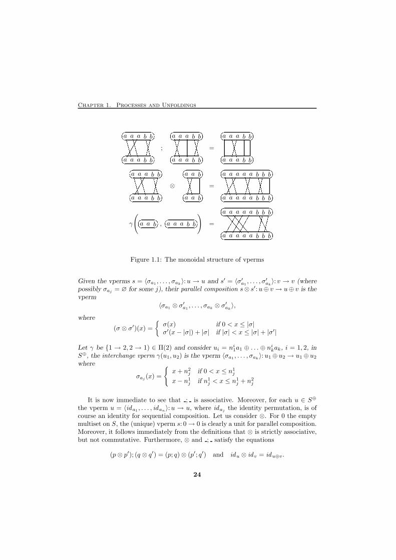
Chapter 1. Processes and Unfoldings
a a a b b
a a a b b
((((((� �� �(((((( '''''������ �� � ;
a a a b b
a a a b b
((((((� �� ������� '''''������ �� � =
a a a b b
a a a b b
� �� �((((((������� �� �a a a b b
a a a b b
((((((� �� �(((((( '''''������ �� � ⊗
a a b
a a b
((((((� �� �������� �� � =
a a a a a b b b
a a a a a b b b
((((((� �� �(((((( ((((((������ '''''������ �� �γ
(a a b� �� �, a a a b b
� �� �) =
a a a a a b b b
a a a a a b b b
::::::� �� �:::::: /////����� ������ �� �Figure 1.1: The monoidal structure of vperms
Given the vperms s = 〈σa1 , . . . , σak〉:u → u and s′ = 〈σ′a1
, . . . , σ′ak〉: v → v (where
possibly σaj= ∅ for some j), their parallel composition s⊗ s′:u⊕ v → u⊕ v is the
vperm
〈σa1 ⊗ σ′a1, . . . , σak
⊗ σ′ak〉,
where
(σ ⊗ σ′)(x) =
{σ(x) if 0 < x ≤ |σ|σ′(x− |σ|) + |σ| if |σ| < x ≤ |σ|+ |σ′|
Let γ be {1 → 2, 2 → 1) ∈ Π(2) and consider ui = ni1a1 ⊕ . . . ⊕ nikak, i = 1, 2, inS⊕, the interchange vperm γ(u1, u2) is the vperm 〈σa1 , . . . , σak
〉:u1⊕ u2 → u1⊕ u2
where
σaj(x) =
{x+ n2
j if 0 < x ≤ n1j
x− n1j if n1
j < x ≤ n1j + n2
j
It is now immediate to see that ; is associative. Moreover, for each u ∈ S⊕
the vperm u = 〈ida1 , . . . , idan〉:u → u, where idaj
the identity permutation, is ofcourse an identity for sequential composition. Let us consider ⊗. For 0 the emptymultiset on S, the (unique) vperm s: 0→ 0 is clearly a unit for parallel composition.Moreover, it follows immediately from the definitions that ⊗ is strictly associative,but not commutative. Furthermore, ⊗ and ; satisfy the equations
(p⊗ p′); (q ⊗ q′) = (p; q)⊗ (p′; q′) and idu ⊗ idv = idu⊕v.
24
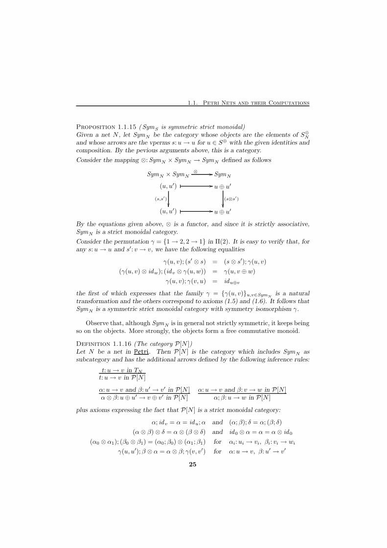
1.1. Petri Nets and their Computations
Proposition 1.1.15 ( SymS is symmetric strict monoidal)Given a net N , let SymN be the category whose objects are the elements of S⊕Nand whose arrows are the vperms s:u→ u for u ∈ S⊕ with the given identities andcomposition. By the pevious arguments above, this is a category.
Consider the mapping ⊗:SymN × SymN → SymN defined as follows
(u, u′) u⊕ u′
(u, u′) u⊕ u′
� //
(s,s′)
��(s⊗s′)
��� //
SymNSymN × SymN⊗ //
By the equations given above, ⊗ is a functor, and since it is strictly associative,SymN is a strict monoidal category.
Consider the permutation γ = {1→ 2, 2→ 1} in Π(2). It is easy to verify that, forany s:u→ u and s′: v → v, we have the following equalities
γ(u, v); (s′ ⊗ s) = (s⊗ s′); γ(u, v)
(γ(u, v)⊗ idw); (idv ⊗ γ(u,w)) = γ(u, v ⊕ w)
γ(u, v); γ(v, u) = idu⊕v
the first of which expresses that the family γ = {γ(u, v)}u,v∈SymNis a natural
transformation and the others correspond to axioms (1.5) and (1.6). It follows thatSymN is a symmetric strict monoidal category with symmetry isomorphism γ.
Observe that, although SymN is in general not strictly symmetric, it keeps beingso on the objects. More strongly, the objects form a free commutative monoid.
Definition 1.1.16 (The category P [N ])Let N be a net in Petri. Then P [N ] is the category which includes SymN assubcategory and has the additional arrows defined by the following inference rules:
t:u→ v in TNt:u→ v in P [N ]
α:u→ v and β:u′ → v′ in P [N ]α⊗ β:u⊕ u′ → v ⊕ v′ in P [N ]
α:u→ v and β: v → w in P [N ]α;β:u→ w in P [N ]
plus axioms expressing the fact that P [N ] is a strict monoidal category:
α; idv = α = idu;α and (α;β); δ = α; (β; δ)
(α⊗ β)⊗ δ = α⊗ (β ⊗ δ) and id0 ⊗ α = α = α⊗ id0
(α0 ⊗ α1); (β0 ⊗ β1) = (α0;β0)⊗ (α1;β1) for αi:ui → vi, βi: vi → wi
γ(u, u′);β ⊗ α = α⊗ β; γ(v, v′) for α:u→ v, β:u′ → v′
25
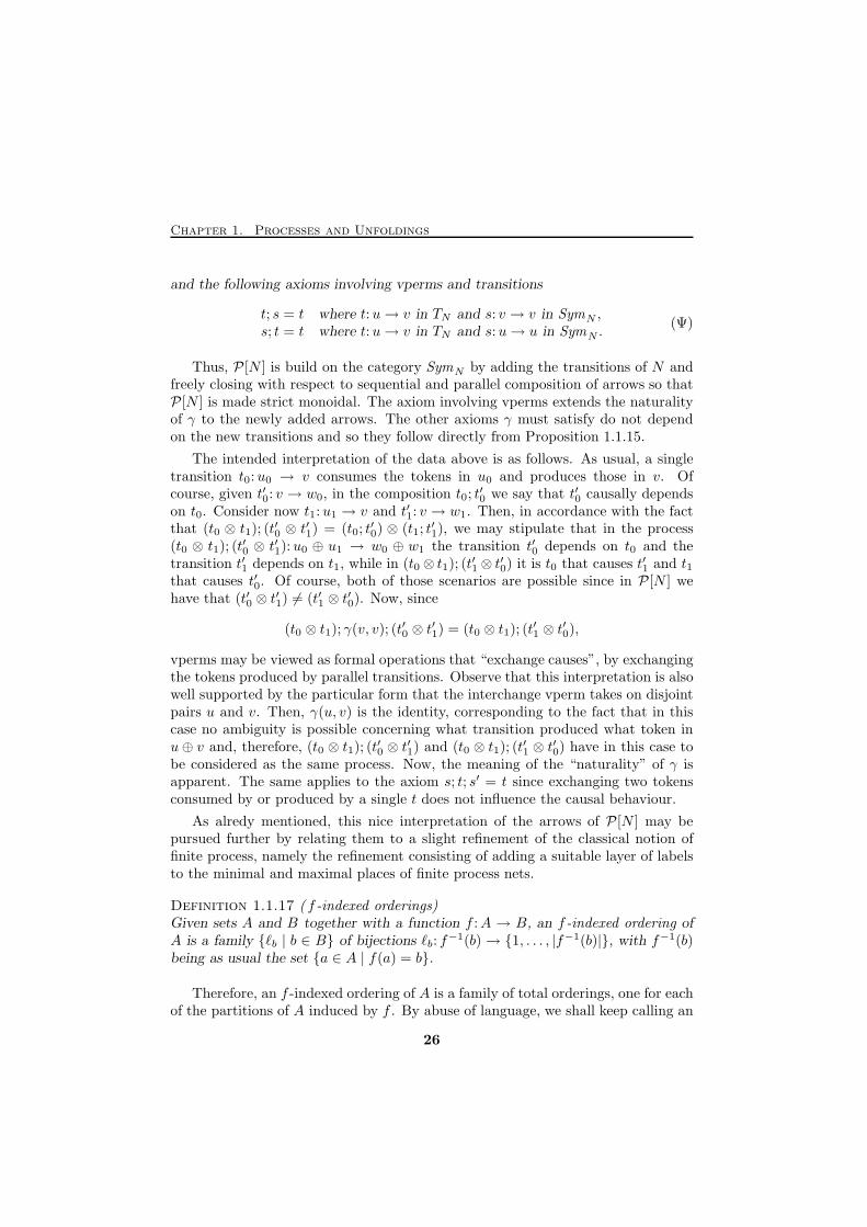
Chapter 1. Processes and Unfoldings
and the following axioms involving vperms and transitions
t; s = t where t:u→ v in TN and s: v → v in SymN ,s; t = t where t:u→ v in TN and s:u→ u in SymN .
(Ψ)
Thus, P [N ] is build on the category SymN by adding the transitions of N andfreely closing with respect to sequential and parallel composition of arrows so thatP [N ] is made strict monoidal. The axiom involving vperms extends the naturalityof γ to the newly added arrows. The other axioms γ must satisfy do not dependon the new transitions and so they follow directly from Proposition 1.1.15.
The intended interpretation of the data above is as follows. As usual, a singletransition t0:u0 → v consumes the tokens in u0 and produces those in v. Ofcourse, given t′0: v → w0, in the composition t0; t
′0 we say that t′0 causally depends
on t0. Consider now t1:u1 → v and t′1: v → w1. Then, in accordance with the factthat (t0 ⊗ t1); (t′0 ⊗ t
′1) = (t0; t
′0) ⊗ (t1; t
′1), we may stipulate that in the process
(t0 ⊗ t1); (t′0 ⊗ t′1):u0 ⊕ u1 → w0 ⊕ w1 the transition t′0 depends on t0 and the
transition t′1 depends on t1, while in (t0 ⊗ t1); (t′1⊗ t′0) it is t0 that causes t′1 and t1
that causes t′0. Of course, both of those scenarios are possible since in P [N ] wehave that (t′0 ⊗ t
′1) 6= (t′1 ⊗ t
′0). Now, since
(t0 ⊗ t1); γ(v, v); (t′0 ⊗ t
′1) = (t0 ⊗ t1); (t
′1 ⊗ t
′0),
vperms may be viewed as formal operations that “exchange causes”, by exchangingthe tokens produced by parallel transitions. Observe that this interpretation is alsowell supported by the particular form that the interchange vperm takes on disjointpairs u and v. Then, γ(u, v) is the identity, corresponding to the fact that in thiscase no ambiguity is possible concerning what transition produced what token inu⊕ v and, therefore, (t0 ⊗ t1); (t′0 ⊗ t
′1) and (t0 ⊗ t1); (t′1 ⊗ t
′0) have in this case to
be considered as the same process. Now, the meaning of the “naturality” of γ isapparent. The same applies to the axiom s; t; s′ = t since exchanging two tokensconsumed by or produced by a single t does not influence the causal behaviour.
As alredy mentioned, this nice interpretation of the arrows of P [N ] may bepursued further by relating them to a slight refinement of the classical notion offinite process, namely the refinement consisting of adding a suitable layer of labelsto the minimal and maximal places of finite process nets.
Definition 1.1.17 ( f -indexed orderings)Given sets A and B together with a function f :A → B, an f -indexed ordering ofA is a family {ℓb | b ∈ B} of bijections ℓb: f
−1(b) → {1, . . . , |f−1(b)|}, with f−1(b)being as usual the set {a ∈ A | f(a) = b}.
Therefore, an f -indexed ordering of A is a family of total orderings, one for eachof the partitions of A induced by f . By abuse of language, we shall keep calling an
26
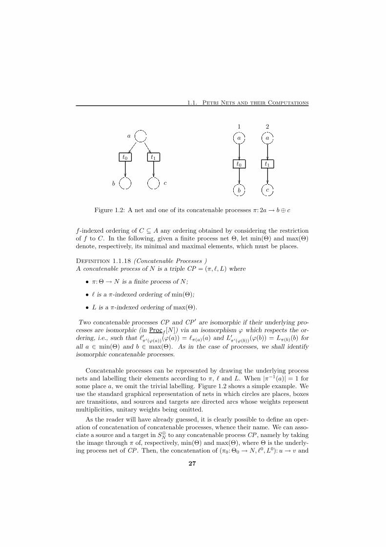
1.1. Petri Nets and their Computations
t0 t1
'&$%������ 3333��a� �� ���
� �� ���
b
'&$% c'&$%
a a
t0 t1
b c
1'&$%��
2'&$%��� �� �
��
� �� ���'&$% '&$%
Figure 1.2: A net and one of its concatenable processes π: 2a→ b⊕ c
f -indexed ordering of C ⊆ A any ordering obtained by considering the restrictionof f to C. In the following, given a finite process net Θ, let min(Θ) and max(Θ)denote, respectively, its minimal and maximal elements, which must be places.
Definition 1.1.18 (Concatenable Processes )A concatenable process of N is a triple CP = (π, ℓ, L) where
• π: Θ→ N is a finite process of N ;
• ℓ is a π-indexed ordering of min(Θ);
• L is a π-indexed ordering of max(Θ).
Two concatenable processes CP and CP ′ are isomorphic if their underlying pro-cesses are isomorphic (in Procf [N ]) via an isomorphism ϕ which respects the or-dering, i.e., such that ℓ′π′(ϕ(a))(ϕ(a)) = ℓπ(a)(a) and L′π′(ϕ(b))(ϕ(b)) = Lπ(b)(b) for
all a ∈ min(Θ) and b ∈ max(Θ). As in the case of processes, we shall identifyisomorphic concatenable processes.
Concatenable processes can be represented by drawing the underlying processnets and labelling their elements according to π, ℓ and L. When |π−1(a)| = 1 forsome place a, we omit the trivial labelling. Figure 1.2 shows a simple example. Weuse the standard graphical representation of nets in which circles are places, boxesare transitions, and sources and targets are directed arcs whose weights representmultiplicities, unitary weights being omitted.
As the reader will have already guessed, it is clearly possible to define an oper-ation of concatenation of concatenable processes, whence their name. We can asso-ciate a source and a target in S⊕N to any concatenable process CP , namely by takingthe image through π of, respectively, min(Θ) and max(Θ), where Θ is the underly-ing process net of CP . Then, the concatenation of (π0: Θ0 → N, ℓ0, L0):u→ v and
27
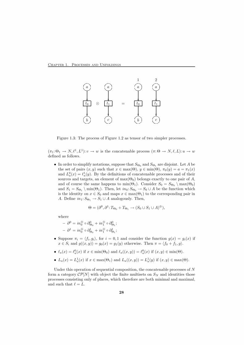
Chapter 1. Processes and Unfoldings
a
t0
b
'&$%��� �� ���'&$% ⊗
a
t1
c
'&$%��� �� ���'&$% =
a a
t0 t1
b c
1'&$%��
2'&$%��� �� �
��
� �� ���'&$% '&$%
Figure 1.3: The process of Figure 1.2 as tensor of two simpler processes.
(π1: Θ1 → N, ℓ1, L1): v → w is the concatenable process (π: Θ → N, ℓ, L):u → wdefined as follows.
• In order to simplify notations, suppose that SΘ0 and SΘ1 are disjoint. LetA bethe set of pairs (x, y) such that x ∈ max(Θ), y ∈ min(Θ), π0(y) = a = π1(x)and L0
a(x) = ℓ1a(y). By the definitions of concatenable processes and of theirsources and targets, an element of max(Θ0) belongs exactly to one pair of A,and of course the same happens to min(Θ1). Consider S0 = SΘ0 \max(Θ0)and S1 = SΘ1 \min(Θ1). Then, let in0:SΘ0 → S0 ∪A be the function whichis the identity on x ∈ S0 and maps x ∈ max(Θ1) to the corresponding pair inA. Define in1:SΘ1 → S1 ∪A analogously. Then,
Θ = (∂0, ∂1:TΘ0 + TΘ1 → (S0 ∪ S1 ∪A)⊕),
where
– ∂0 = in⊕0 ◦ ∂0Θ0
+ in⊕1 ◦ ∂0Θ1
;
– ∂1 = in⊕0 ◦ ∂1Θ0
+ in⊕1 ◦ ∂1Θ1
;
• Suppose πi = 〈fi, gi〉, for i = 0, 1 and consider the function g(x) = gi(x) ifx ∈ Si and g((x, y)) = g0(x) = g1(y) otherwise. Then π = 〈f0 + f1, g〉.
• ℓa(x) = ℓ0a(x) if x ∈ min(Θ0) and ℓa((x, y)) = ℓ0a(x) if (x, y) ∈ min(Θ).
• La(x) = L1a(x) if x ∈ max(Θ1) and La((x, y)) = L1
a(y) if (x, y) ∈ max(Θ).
Under this operation of sequential composition, the concatenable processes of Nform a category CP[N ] with object the finite multisets on SN and identities thoseprocesses consisting only of places, which therefore are both minimal and maximal,and such that ℓ = L.
28
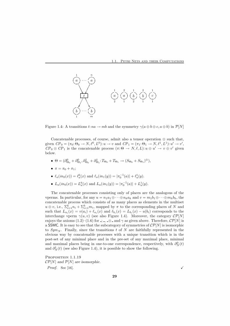
1.1. Petri Nets and their Computations
a · · · a
t
b · · · b
1'&$%/////�� n'&$%�������� �� �������� ///// ��1
'&$%m
'&$% a a b b c
1
2
'&$% 2
1
'&$% 1
2
'&$% 2
1
'&$% 1
1
'&$%Figure 1.4: A transitions t:na→ mb and the symmetry γ(a⊕ b⊕ c, a⊕ b) in P [N ]
Concatenable processes, of course, admit also a tensor operation ⊗ such that,given CP0 = (π0: Θ0 → N, ℓ0, L0):u→ v and CP1 = (π1: Θ1 → N, ℓ1, L1):u′ → v′,CP0 ⊗ CP1 is the concatenable process (π: Θ → N, ℓ, L):u ⊕ u′ → v ⊕ v′ givenbelow.
• Θ = (∂0Θ0
+ ∂0Θ1, ∂1
Θ0+ ∂1
Θ1:TΘ0 + TΘ1 → (SΘ0 + SΘ1)
⊕),
• π = π0 + π1;
• ℓa(in0(x)) = ℓ0a(x) and ℓa(in1(y)) = |π−10 (a)|+ ℓ1a(y).
• La(in0(x)) = L0a(x) and La(in1(y)) = |π−1
0 (a)|+ L1a(y).
The concatenable processes consisting only of places are the analogous of thevperms. In particular, for any u = n1a1⊕· · ·⊕nkak and v = m1b1⊕· · ·⊕mhbh, theconcatenable process which consists of as many places as elements in the multisetu ⊕ v, i.e., Σki=1ni + Σhi=1mi, mapped by π to the corresponding places of N andsuch that Lai
(x) = v(ai) + ℓai(x) and ℓbi
(x) = Lbi(x) − u(bi) corresponds to the
interchange vperm γ(u, v) (see also Figure 1.4). Moreover, the category CP [N ]enjoys the axioms (1.2)–(1.6) for ; , ⊗ and γ as given above. Therefore, CP[N ] isa SSMC. It is easy to see that the subcategory of symmetries of CP[N ] is isomorphicto SymN . Finally, since the transitions t of N are faithfully represented in theobvious way by concatenable processes with a unique transition which is in thepost-set of any minimal place and in the pre-set of any maximal place, minimaland maximal places being in one-to-one correspondence, respectively, with ∂0
N (t)and ∂1
N (t) (see also Figure 1.4), it is possible to show the following.
Proposition 1.1.19CP[N ] and P [N ] are isomorphic.
Proof. See [16]. X
29
Chapter 1. Processes and Unfoldings
Furthermore, it can be shown—and it is indeed easy to get convinced—thatconcatenable processes are the least refinement of processes on which such a se-quentialization may be given. In other words, they are the finest concretion ofclassical processes which may act as arrows in a category. Observe that this con-sideration, together with the fact that concatenable processes correspond with thearrows of P [N ], links the two approaches we discussed earlier: making T [N ] notstrictly symmetric and making the objects of Proc[N ] be the arrows of some cate-gory.
As already remarked in the introduction, P [N ] provides an axiomatization ofthe causal behaviour of N which, however, builds on the concrete choice of thecategory of vperms on SN as the subcategory of symmetries of P [N ]. Clearly, itwould be nice to be able to give an abstract characterization also of SymN . Thisis what we shall do in the next section.
1.2 Axiomatizing Concatenable Processes
In this section we show that the category of vperms SymN can be described inabstract terms, thus yielding a fully axiomatic characterization of concatenableprocesses. We start by showing that we can associate a free SSMC to each net N .Although this fact is not very surprising, our proof of it will give a “minimal”description of the free category on N which will be useful later on.
Proposition 1.2.1The forgetful functor U: SSMC⊕ → Petri has a left adjoint F: Petri→ SSMC⊕.
Proof. Consider the category F(N) whose objects are the elements of S⊕N and whosearrows are generated by the inference rules
u ∈ S⊕Nidu:u→ u in F(N)
a and b in SNca,b: a⊕ b→ a⊕ b in F(N)
t:u→ v in TNt:u→ v in F(N)
α:u→ v and β: u′ → v′ in F(N)α⊗ β:u⊕ u′ → v ⊕ v′ in F(N)
α: u→ v and β: v → w in F(N)α;β:u→ w in F(N)
modulo the axioms expressing that F(N) is a strict monoidal category, namely,
α; idv = α = idu;α and (α;β); γ = α; (β; γ),
(α⊗ β) ⊗ γ = α⊗ (β ⊗ γ) and id0 ⊗ α = α = α⊗ id0, (1.10)
idu ⊗ idv = idu⊕v and (α⊗ α′); (β ⊗ β′) = (α;β)⊗ (α′;β′),
the latter whenever the righthand term is defined, and the following axioms
ca,b; cb,a = ida⊕b (1.11)
cu,u′ ; (β ⊗ α) = (α⊗ β); cv,v′ for α:u→ v, β: u′ → v′ (1.12)
30
1.2. Axiomatizing Concatenable Processes
where cu,v for u, v ∈ S⊕N denote any term obtained from ca,b for a, b ∈ SN by applyingrecursively the following rules (compare with axiom (1.5)):
c0,u = idu = cu,0
ca⊕u,v = (ida ⊗ cu,v); (ca,v ⊗ idu) (1.13)
cu,v⊕a = (cu,v ⊗ ida); (idv ⊗ cu,a)
Observe that equation (1.12), in particular, equalizes all the terms obtained from (1.13)for fixed u and v. In fact, let cu,v and c′u,v be two such terms and take α and β tobe, respectively, the identities of u and v. Now, since idu ⊗ idv = idu⊕v = idv ⊗ idu,from (1.12) we have that cu,v = c′u,v in F(N). Then, we claim that the collection{cu,v}u,v∈S⊕
N
is a symmetry natural isomorphism which makes F(N) into a SSMC and
that, in addition, F(N) is the free SSMC on N .
In order to show the first claim, observe that the naturality of c is expressed directlyfrom axiom (1.12). Then, we need to check that for any u and v we have cu,v; cv,u =idu⊕v, which follows easily from (1.11) by induction on the least of the sizes of u and v.
base cases. If u = 0 or v = 0 then the thesis follows from the first of (1.13). If instead|u| = |v| = 1, then required equation is (1.11).
inductive step. Without loss of generality, assume that u = a⊕ u′. Then, by (1.13),
cu,v; cv,u = (ida ⊗ cu′,v); (ca,v ⊗ idu′); (cv,a ⊗ idu′); (ida ⊗ cv,u′)
= (ida ⊗ cu′,v); ((ca,v; cv,a))⊗ idu′); (ida ⊗ cv,u′)
= (ida ⊗ cu′,v); (ida ⊗ cv,u′)
= ida ⊗ (cu′,v; cv,u′) = ida ⊗ idu′⊕v = idu⊕v.
Consider now the net UF(N) obtained from F(N) by forgetting about its categoricalstructure. More precisely, the markings of UF(N) are the markings of N and itstransitions are the arrows F(N) with the given sources and targets. Consider thenthe Petri net morphism η:N → UF(N) where ηp is the identity homomorphism and ηtis the obvious injection of TN in TUF(N). We show that η is universal, i.e., that for any
SSMC C in SSMC⊕ and for any Petri net morphism f :N → U(C), there is a uniquesymmetric strict monoidal functor F: F(N) → C which makes the following diagramcommute.
N UF(N)
U(C)
η //
f
OOOOOOOOOOOO'' U(F)
��
Let C = (C,⊗, 0, γ) and f :N → U(C) be as in the hypothesis above. Then, in orderfor the diagram to commute and in order for F to be a symmetric strict monoidalfunctor, its definition on the generators of F(N) is compelled to be:
F(u) = fp(u), F(t) = ft(t), F(idu) = idF(u), F(ca,b) = γfp(a),fp(b).
31
Chapter 1. Processes and Unfoldings
Of course, also the extension of F to composition and tensor is uniquely determined,namely, it must be F(α;β) = F(β) ◦F(α) and F(α⊗β) = F(α)⊗F(β). To conclude theproof we only need to show that F is a well-defined symmetric strict monoidal functor,since, in this case, it is necessarily the unique which makes the diagram commute.
In order to show that F is well-defined, it is enough to see that it preserves the axiomswhich generates F(N). Since C is a strict monoidal category and since F(idu) = idF(u),axioms (1.10) are clearly preserved. Moreover, since C is symmetric with symmetryisomorphism γ, we have that
F(ca,b; cb,a) = γF(b),F(a) ◦ γF(a),F(b) = idF(a)⊕F(b) = idF(a⊕b),
i.e., F respects axiom (1.11). Thus, the last missing steps are to show that F preservesaxiom (1.12) and that it is a symmetric strict monoidal functor, which actually reducesto show that for each u and v we have F(cu,v) = γF(u),F(v). We start by showing, byinduction on the structure of the c’s, that for any term cu,v generated from (1.13), wehave F(cu,v) = γF(u),F(v).
base cases. If u = 0 then cu,v = idv and thus F(cu,v) = idF(v). However, we havealready shown in the remark in page 22 that γe,x = idx holds in any symmetricmonoidal category. Thus, since F(u) = 0, we have F(cu,v) = γF(u),F(v) as required. Asymmetric argument applies if v = 0. If instead |u| = |v| = 1, the claim is proved byappealing directly to the definition of F.
inductive step. Suppose that u = a ⊕ u′. Then, exploting the induction hypothesis,F(cu,v) = (γF(a),F(v) ⊗ idF(u′)) ◦ (idF(a) ⊗ γF(u′),F(v)) and thus, by the coherence ax-iom (1.5) of symmetric monoidal categories, we have F(cu,v) = γF(a)⊕F(u′),F(v) which isγF(a⊕u′),F(v), i.e., γF(u),F(v). If instead we have that v = v′⊕a and cu,v is generated bythe last of (1.13), then the claim is proved similarly by using the inverse of (1.5), i.e.,γx,y⊗z = (idy⊗ γx,z) ◦ (γx,y⊗ idz), which, of course, holds in any symmetric monoidalcategory.
Now, since F(cu,v) = γF(u),F(v) and since γ is a natural transformation, it followsimmediately that F preserves axiom (1.12).
This shows that F is left adjoint to U, in symbols F ⊣ U. X
Thus, establishing the adjunction Petri ⇀ SSMC⊕, we have identified the freeSSMC onN as a category generated, modulo some equations, from the netN viewedas a graph enriched with formal arrows idu, which play the role of the identities,and ca,b for a, b ∈ SN , which generate all the needed symmetries. In the following,we speak of the free SSMC on N to mean F(N) as constructed above.
Remark. Observe that the above choice is the only sensible one for the notion of freeSSMC on N . In fact, the notion of free algebra, or free construction, makes sense onlywhen one has a functor F which is left adjoint to a forgetful functor. or, in other words,when you have a monadic functor. Then, the free algebra on an object a is F(a). Now, itis not possible to have a forgetful functor from a category of SSMC’s to Petri unless onerestricts oneself to SSMC⊕. Ergo the term “free” makes sense only in this case.
32
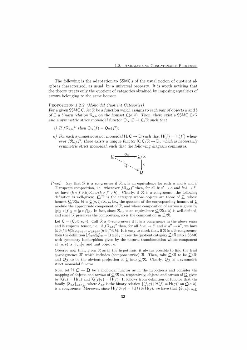
1.2. Axiomatizing Concatenable Processes
The following is the adaptation to SSMC’s of the usual notion of quotient al-gebras characterized, as usual, by a universal property. It is worth noticing thatthe theory treats only the quotient of categories obtained by imposing equalities ofarrows belonging to the same homset.
Proposition 1.2.2 (Monoidal Quotient Categories)For a given SSMC C, let R be a function which assigns to each pair of objects a and bof C a binary relation Ra,b on the homset C(a, b). Then, there exist a SSMC C/Rand a symmetric strict monoidal functor QR: C→ C/R such that
i) If fRa,bf′ then QR(f) = QR(f ′);
ii) For each symmetric strict monoidal H: C→ D such that H(f) = H(f ′) when-ever fRa,bf
′, there exists a unique functor K: C/R→ D, which is necessarilysymmetric strict monoidal, such that the following diagram commutes.
C C/R
D
QR //
H
NNNNNNNNNNNN&& K
��
Proof. Say that R is a congruence if Ra,b is an equivalence for each a and b and ifR respects composition, i.e., whenever fRa,bf
′ then, for all h: a′ → a and k: b → b′,we have (k ◦ f ◦ h)Ra′,b′(k ◦ f
′ ◦ h). Clearly, if R is a congruence, the followingdefinition is well-given: C/R is the category whose objects are those of C, whosehomset C/R(a, b) is C(a, b)/Ra,b, i.e., the quotient of the corresponding homset of Cmodulo the appropriate component of R, and whose composition of arrows is given by[g]R ◦ [f ]R = [g ◦ f ]R. In fact, since Ra,b is an equivalence C/R(a, b) is well-defined,and since R preserves the composition, so is the composition in C/R.
Let C = (C,⊗, e, γ). Call R a ⊗-congruence if it is a congruence in the above senseand it respects tensor, i.e., if fRa,bf
′ then, for all h: a′ → b′ and k: a′′ → b′′, we have(h⊗f⊗k)Ra′⊗a⊗a′′,b′⊗b⊗b′′ (h⊗f
′⊗k). It is easy to check that, if R is a ⊗-congruence,then the definition [f ]R⊗[g]R = [f⊗g]R makes the quotient category C/R into a SSMCwith symmetry isomorphism given by the natural transformation whose componentat (u, v) is [γu,v]R and unit object e.
Observe now that, given R as in the hypothesis, it always possible to find the least⊗-congruence R
′ which includes (componentwise) R. Then, take C/R to be C/R′
and QR to be the obvious projection of C into C/R. Clearly, QR is a symmetricstrict monoidal functor.
Now, let H:C → D be a monoidal functor as in the hypothesis and consider themapping of objects and arrows of C/R to, respectively, objects and arrows of D givenby K(a) = H(a) and K([f ]R) = H(f). It follows from definition of functor that thefamily {Sa,b}a,b∈C, where Sa,b is the binary relation {(f, g) | H(f) = H(g)} on C(a, b),is a congruence. Moreover, since H(f ⊗ g) = H(f) ⊗H(g), we have that {Sa,b}a,b∈C
33
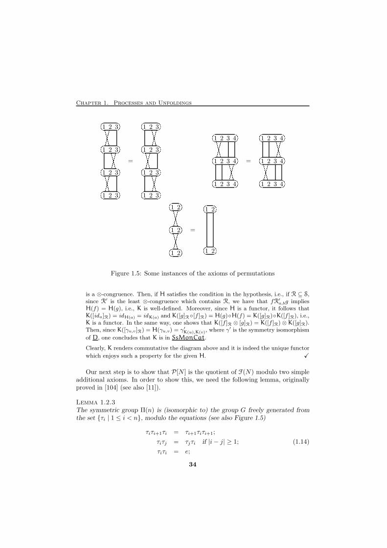
Chapter 1. Processes and Unfoldings
1 2 3
1 2 3
1 2 3
1 2 3
(((((� �� ������� �� �(((((�����(((((� �� ������� �� � =
1 2 3
1 2 3
1 2 3
1 2 3
� �� �(((((�����(((((� �� ������� �� �(((((������ �� �1 2 3 4
1 2 3 4
1 2 3 4
(((((� �� ������� �� �(((((������ �� � =
1 2 3 4
1 2 3 4
1 2 3 4
� �� �(((((�����(((((� �� ������� �� �1 2
1 2
1 2
(((((� �� ������(((((� �� ������� �� � =
1 2
1 2
� �� �� �� �Figure 1.5: Some instances of the axioms of permutations
is a ⊗-congruence. Then, if H satisfies the condition in the hypothesis, i.e., if R ⊆ S,since R
′ is the least ⊗-congruence which contains R, we have that fR′a,bg impliesH(f) = H(g), i.e., K is well-defined. Moreover, since H is a functor, it follows thatK([ida]R) = idH(a) = idK(a) and K([g]R◦[f ]R) = H(g)◦H(f) = K([g]R)◦K([f ]R), i.e.,K is a functor. In the same way, one shows that K([f ]R ⊗ [g]R) = K([f ]R) ⊗ K([g]R).Then, since K([γu,v]R) = H(γu,v) = γ′K(u),K(v), where γ′ is the symmetry isomorphism
of D, one concludes that K is in SsMonCat.
Clearly, K renders commutative the diagram above and it is indeed the unique functor
which enjoys such a property for the given H. X
Our next step is to show that P [N ] is the quotient of F(N) modulo two simpleadditional axioms. In order to show this, we need the following lemma, originallyproved in [104] (see also [11]).
Lemma 1.2.3The symmetric group Π(n) is (isomorphic to) the group G freely generated fromthe set {τi | 1 ≤ i < n}, modulo the equations (see also Figure 1.5)
τiτi+1τi = τi+1τiτi+1;
τiτj = τjτi if |i− j| ≥ 1; (1.14)
τiτi = e;
34
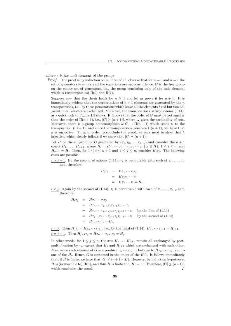
1.2. Axiomatizing Concatenable Processes
where e is the unit element of the group.Proof. The proof is by induction on n. First of all, observe that for n = 0 and n = 1 the
set of generators is empty and the equations are vacuous. Hence, G is the free groupon the empty set of generators, i.e., the group consisting only of the unit element,which is (isomorphic to) Π(0) and Π(1).
Suppose now that the thesis holds for n ≥ 1 and let us prove it for n + 1. It isimmediately evident that the permutations of n + 1 elements are generated by the ntranspositions, i.e., by those pemutations which leave all the elements fixed but two ad-jacent ones, which are exchanged. Moreover, the transpositions satisfy axioms (1.14),as a quick look to Figure 1.5 shows. It follows that the order of G must be not smallerthan the order of Π(n+ 1), i.e., |G| ≥ (n+ 1)!, where | | gives the cardinality of sets.Moreover, there is a group homomorphism h:G → Π(n + 1) which sends τi to thetransposition (i i + 1), and since the transpositions generate Π(n+ 1), we have thath is surjective. Thus, in order to conclude the proof, we only need to show that hinjective, which clearly follows if we show that |G| = (n+ 1)!.
Let H be the subgroup of G generated by {τ1, τ2, . . . , τn−1} and consider the n + 1cosets H1, . . . , Hn+1, where Hi = Hτn · · · τi = {xτn · · · τi | x ∈ H}, 1 ≤ i ≤ n, andHn+1 = H . Then, for 1 ≤ i ≤ n + 1 and 1 ≤ j ≤ n, consider Hiτj . The followingcases are possible.
i > j + 1. By the second of axioms (1.14), τj is permutable with each of τi, . . . , τnand, therefore,
Hiτj = Hτn · · · τiτj
= Hτjτn · · · τi
= Hτn · · · τi = Hi.
i < j. Again by the second of (1.14), τj is permutable with each of τi, . . . , τj−2 and,therefore,
Hiτj = Hτn · · · τiτj
= Hτn · · · τj+1τjτj−1τj · · · τi
= Hτn · · · τj+1τj−1τjτj−1 · · · τi by the first of (1.14)
= Hτj−1τn · · · τj+1τjτj−1 · · · τi by the second of (1.14)
= Hτn · · · τi = Hi.
i = j. Then Hjτj = Hτn · · · τjτj . i.e., by the third of (1.14), Hτn · · · τj+1 = Hj+1.
i = j + 1. Then Hj+1τj = Hτn · · · τj+1τj = Hj .
In other words, for 1 ≤ j ≤ n, the sets H1 . . . Hn+1 remain all unchanged by post-
multiplication by τj , except that Hj and Hj+1 which are exchanged with each other.
Now, since each element of G is a product τi1 · · · τik , it belongs to Hτi1 · · · τik , i.e., to
one of the Hi. Hence, G is contained in the union of the Hi’s. It follows immediately
that, if H is finite, we have that |G| ≤ (n+1) · |H |. However, by induction hypothesis,
H is (isomorphic to) Π(n), and thusH is finite and |H | = n!. Therefore, |G| ≤ (n+1)!,
which concludes the proof. X
35
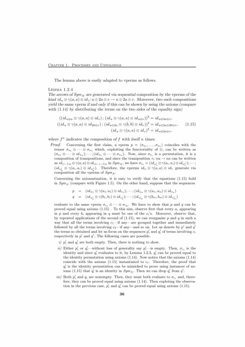
Chapter 1. Processes and Unfoldings
The lemma above is easily adapted to vperms as follows.
Lemma 1.2.4The arrows of SymN are generated via sequential composition by the vperms of thekind idu⊗ γ(a, a)⊗ idv:u⊕ 2a⊕ v → u⊕ 2a⊕ v. Moreover, two such compositionsyield the same vperm if and only if this can be shown by using the axioms (comparewith (1.14) by distributing the terms on the two sides of the equality sign)
((idu⊕a ⊗ γ(a, a)⊗ idv) ; (idu ⊗ γ(a, a)⊗ ida⊕v))3 = idu⊕3a⊕v,
((idu ⊗ γ(a, a)⊗ id2b⊕v) ; (idu⊕2a ⊗ γ(b, b)⊗ idv))2 = idu⊕2a⊕2b⊕v, (1.15)
(idu ⊗ γ(a, a)⊗ idv)2 = idu⊕2a⊕v.
where fn indicates the composition of f with itself n times.
Proof. Concerning the first claim, a vperm p = 〈σa1 , . . . , σan〉 coincides with thetensor σa1 ⊗ · · · ⊗ σan which, exploiting the functoriality of ⊗, can be written as(σa1 ⊗ · · · ⊗ idun); · · · ; (idu1 ⊗ · · · ⊗ σan). Now, since σai is a permutation, it is acomposition of transpositions, and since the transposition τi:na→ na can be writtenas id(i−1)a⊗γ(a, a)⊗ id(n−i−1)a in SymN , we have σai = (idu′
1⊗γ(ai, ai)⊗ idu′′
1); · · · ;
(idu′k⊗ γ(ai, ai) ⊗ idu′′
k). Therefore, the vperms idu ⊗ γ(a, a) ⊗ idv generate via
composition all the vperms of SymN .
Concerning the axiomatization, it is easy to verify that the equations (1.15) holdin SymN (compare with Figure 1.5). On the other hand, suppose that the sequences
p = (idu1 ⊗ γ(a1, a1)⊗ idv1); · · · ; (idun ⊗ γ(an, an)⊗ idvn)
q = (idu′1⊗ γ(b1, b1)⊗ idv′
1); · · · ; (idu′
m⊗ γ(bm, bm)⊗ idv′m )
evaluate to the same vperm σc1 ⊗ · · · ⊗ σck. We have to show that p and q can be
proved equal using axioms (1.15) . To this aim, observe first that every ai appearingin p and every bi appearing in q must be one of the ci’s. Moreover, observe that,by repeated applications of the second of (1.15), we can reorganize p and q in such away that all the terms involving c1—if any—are grouped together and immediatelyfollowed by all the terms involving c2—if any—and so on. Let us denote by p′ and q′
the terms so obtained and let us focus on the sequences p′i and q′i of terms involving cirespectively in p′ and q′. The following cases are possible.
i) p′i and q′i are both empty. Then, there is nothing to show.
ii) Either p′i or q′i—without loss of generality say p′i—is empty. Then, σci is theidentity and since q′i evaluates to it, by Lemma 1.2.3, q′i can be proved equal tothe identity permutation using axioms (1.14). Now notice that the axioms (1.14)coincide with the axioms (1.15) instantiated to ci. Therefore, the proof thatq′i is the identity permutation can be mimicked to prove using instances of ax-ioms (1.15) that q′i is an identity in SymN . Then we can drop q′i from q′.
iii) Both p′i and qi are nonempty. Then, they must both evaluate to σci and, there-fore, they can be proved equal using axioms (1.14). Then exploting the observa-tion in the previous case, p′i and q′i can be proved equal using axioms (1.15).
36
1.2. Axiomatizing Concatenable Processes
Thus, p and q are proved equal using axioms (1.15), which concludes the proof. X
We are now ready to show the promised characterization of P [N ].
Proposition 1.2.5P [N ] is the monoidal quotient of the free SSMC on N modulo the axioms
ca,b = ida⊕b if a, b ∈ SN and a 6= b, (1.16)
s; t; s′ = t if t ∈ TN and s, s′ are symmetries. (1.17)
Proof. We show that P [N ] enjoys the universal property of F(N)/R stated in Propo-sition 1.2.2, where R is the congruence generated from equations (1.16) and (1.17). Itfollows then from general facts about universal constructions that P [N ] is isomorphicto F(N)/R.
First of all observe that P [N ] belongs to SSMC⊕. Therefore, corresponding to thePetri net inclusion morphism N → UP [N ], there is a symmetric strict monoidalfunctor Q:F(N)→ P [N ] which is the identity on the places and on the transitions ofN , i.e., such that
Q(a) = a if a ∈ SN ,
Q(t) = t if t ∈ TN ,
Q(ca,b) = γ(a, b) if a, b ∈ SN .
Thus, since γ(a, b) = ida⊕b if a 6= b ∈ SN , we have that Q(ca,b) = Q(ida⊕b) fora 6= b ∈ SN . Moreover, since Q is a symmetric monoidal functor, it sends symmetriesto symmetries. Therefore, since (1.17) holds in P [N ], if s and s′ are symmetries andt ∈ TN , we have that Q(s; t; s′) = s; t; s′ = t = Q(t). We shall show that Q isuniversal among the functors which equalize the pairs (ca,b, ida⊕b) with a 6= b and thepairs (s; t; s′, t) with s and s′ symmetries and t ∈ TN .
We start by showing that SymN can be embedded in SymF(N), though not via asymmetric strict monoidal functor. Consider the mapping G of objects and arrowsof SymN to, respectively, objects and arrows of SymF(N) which is the identity on theobjects and such that
G(idu ⊗ γ(a, a)⊗ idv) = idu ⊗ ca,a ⊗ idv ,
G(p; q) = G(p);G(q)
G(idu) = idu.
It follows from Lemma 1.2.4 that the above definition defines G on all vperms. Thus,in order to see that G is a functor we only need to see that it is well-defined which,by exploiting Lemma 1.2.4, can be seen by showing that it respects axioms (1.15).
i) From (1.13) we have that (ida⊗ ca,a); (ca,a⊗ ida) = ca⊕a,a and then from (1.12)we have ca⊕a,a; (ida ⊗ ca,a) = (ca,a ⊗ ida); ca⊕a,a, which, again by (1.13), yields
37
Chapter 1. Processes and Unfoldings
(ida ⊗ ca,a); (ca,a ⊗ ida); (ida ⊗ ca,a) = (ca,a ⊗ ida); (ida ⊗ ca,a); (ca,a ⊗ ida),which is ((ida ⊗ ca,a); (ca,a ⊗ ida))
3 = id3a. Then, tensoring both terms by iduon the left and idv on the right and using (1.10), we have the required equality((idu⊕a ⊗ ca,a ⊗ idv); (idu ⊗ ca,a ⊗ ida⊕v))
3 = idu⊕3a⊕v
ii) By two applications of the last of (1.10), we have
(ca,a ⊗ id2b); (id2a ⊗ cb,b) = (ca,a ⊗ cb,b) = (id2a ⊗ cb,b); (ca,a ⊗ id2b).
Then, applying the tensor of idu and idv as before, the required equality follows.
iii) (idu⊗ ca,a⊗ idv); (idu⊗ ca,a⊗ idv) = idu⊕2a⊕v follows immediately from (1.11).
Therefore, G is a functor. Of course, G is not symmetric strict monoidal, sinceG(γ(a, b)) = ida⊕b 6= ca,b, i.e., axiom (1.9) does not hold. However, G is monoidal inthe sense that conditions (1.7) and (1.8) hold. The claim is immediate for (1.7), whileG(s⊗ s′) = G((s⊗ idv); (idu ⊗ s
′)) = (G(s)⊗ idv); (idu ⊗G(s′)) = G(s)⊗G(s′).
Let C = (C,⊗, e, γ) be a SSMC and suppose that there exists a symmetric strictmonoidal functor H:F(N) → C such that, for any pair a 6= b ∈ SN and for anysymmetries s and s′, H(ca,b) = H(ida⊕b) and H(s; t; s′) = H(t). We have to showthat there exists a unique K:P [N ]→ C such that H = KQ. We consider the followingdefinition of K on objects and generators
K(u) = H(u) if u ∈ S⊕N ,
K(s) = H(G(s)) if s is a symmetry
K(t) = H(t) if t ∈ TN ,
extendend to P [N ] by K(α;β) = K(α);K(β) and K(α⊗β) = K(α)⊗K(β). First of all,we have to show that K is well-defined, i.e., that the equations which hold in P [N ] arepreserved by K. To this aim, recall that P [N ], by definition, is the category generatedon top of SymN from the transitions of N modulo the axioms of monoidality, i.e., (1.2)–(1.6) plus the functoriality of ⊗ and the naturality of the symmetry isomorphism, andaxioms (Ψ). Now, since H is symmetric strict monoidal and since G is monoidal, it isimmediate to see that the functoriality of ⊗ and the axioms (1.2)–(1.4) are preserved.The key to show that the same happens for the naturality of the symmetry, (1.5)and (1.6) is to show that K(γ(u, v)) = γK(u),K(v). In fact, once this fact is established,the aforesaid points follow from the fact that C is a SSMC. Thus, we proceed to proveour claim by induction on the least of the sizes of u and v.
base cases. If u = 0 then γ(u, v) = idv and since K(0) = e, we have that K(γ(u, v)) =idK(v) = γe,K(v). Otherwise, if v = 0, a symmetric argument applies. If instead|u| = |v| = 1, we have the following two cases.
u = v = a. Then K(γ(a, a)) = H(ca,a) = γK(a),K(a), since H is symmetric.
u 6= v Then K(γ(u, v)) = H(idu⊕v) which, by hypothesis on H, is γK(u),K(v).
inductive step. Suppose that u = a ⊕ u′. Then, by the coherence axiom (1.5),K(γ(u, v)) = (K(γ(a, v)) ⊗ idK(u′)) ◦ (idK(a) ⊗ K(γ(u′, v))) and thus, exploting theinduction hypothesis, K(γ(u, v)) = (γK(a),K(v)⊗ idK(u′))◦(idK(a)⊗γK(u′),K(v)), which,
38
1.2. Axiomatizing Concatenable Processes
again by (1.5), is γK(a)⊗K(u′),K(v), i.e., γK(a⊕u′),K(v). If instead we have that v = v′⊕athe induction is mantained similarly by using the inverse of (1.5).
Thus, the last step we have left is to prove that axioms (Ψ) are mantained. This is clear,since if s is a symmetry, then G(s) is also a symmetry. Therefore K(s; t) = H(G(s); t) =H(G(s); t; id) = H(t) = K(t) and, reasoning in the same way, K(t; s) = K(t). Now,the fact that K is a functor follows from its own definition and from the fact that Gis so. Observe that, by showing that the symmetry isomorphism of P [N ] is preserved,we have actually shown that K is a symmetric strict monoidal functor.
Our next task is to show that H = KQ. This is of course the case for objects andtransitions. Observe further that, since Q is symmetric strict monoidal, we have thatQ(cu,v) = γ(u, v), whence it follows that KQ(cu,v) = γH(u),H(v) = H(cu,v). Now,since the symmetries of F(n) are by definition generated via tensor and compositionfrom c and from identities, we conclude that H and KQ coincide on SymF(N). Then,one proves that H = KQ by proving, by easy induction on the structure of the terms,that each arrow of F(N) can be written as the composition of symmetries and arrowsof the kind idu ⊗ t⊗ idv, for t ∈ TN .
Finally, concerning the uniqueness condition on K, observe that it must necessarily
be K(idu ⊗ γ(a, a) ⊗ idv) = idH(u) ⊗ γH(a),H(a) ⊗ idH(v), which, by Lemma 1.2.4,
defines K uniquely on SymN . Moreover, the behaviour of K on the arrows formed as
composition and tensor of transitions is uniquely determined by H. Therefore, the
proof is concluded. X
The next corollary gives an alternative form for axiom (1.17).
Corollary 1.2.6Axiom (1.17) in Proposition 1.2.5 can be replaced by the axioms
t; (idu ⊗ ca,a ⊗ idv) = t if t ∈ T and a ∈ S,
(idu ⊗ ca,a ⊗ idv); t = t if t ∈ T and a ∈ S. (1.18)
Proof. Since (idu⊗γa,a⊗ idv) and all the identities are symmetries, axiom (1.17) impliesthe present ones. It is easy to see that, on the contrary, the axioms above, togetherwith axiom (1.16) implies (1.17).
Let s:u→ u by a symmetry of F(N) and suppose s 6= idu. By repeated applicationsof (1.13), together the functoriality of ⊗ , we obtain the following equality:
s = (idu1 ⊗ ca1,b1 ⊗ idv1); . . . ; (iduh⊗ cah,bh ⊗ idvh
)
for some h ∈ ω. Moreover, by exploiting axiom (1.16), we can drop every term inwhich ai 6= bi. Thus we have
s = (idu1 ⊗ ca1,a1 ⊗ idv1); . . . ; (iduk⊗ cak,ak
⊗ idvk) (1.19)
for some k ≤ h. Then, by (1.19) and repeated applications of the axioms (1.18), one
can prove s; t; s′ = t. X
39
Chapter 1. Processes and Unfoldings
The next corollary sums up the purely algebraic characterization of the categoryof concatenable processes that we have proved in this note.
Corollary 1.2.7The category P [N ] of concatenable processes of N is the category whose objectsare the elements of S⊕N and whose arrows are generated by the inference rules
u ∈ S⊕Nidu:u→ u in P [N ]
a in SNca,a: a⊕ a→ a⊕ a in P [N ]
t:u→ v in TNt:u→ v in P [N ]
α:u→ v and β:u′ → v′ in P [N ]α⊗ β:u⊕ u′ → v ⊕ v′ in P [N ]
α:u→ v and β: v → w in P [N ]α;β:u→ w in P [N ]
modulo the axioms expressing that P [N ] is a strict monoidal category, namely,
α; idv = α = idu;α and (α;β); γ = α; (β; γ),
(α⊗ β)⊗ γ = α⊗ (β ⊗ γ) and id0 ⊗ α = α = α⊗ id0,
idu ⊗ idv = idu⊕v and (α ⊗ α′); (β ⊗ β′) = (α;β) ⊗ (α′;β′),
the latter whenever the righthand term is defined, and the following axioms
ca,a; ca,a = ida⊕b
t; (idu ⊗ ca,a ⊗ idv) = t if t ∈ T,
(idu ⊗ ca,a ⊗ idv); t = t if t ∈ T,
cu,u′ ; (β ⊗ α) = (α⊗ β); cv,v′ for α:u→ v, β:u′ → v′
where cu,v for u, v ∈ S⊕N is obtained from ca,a by applying recursively the followingrules:
ca,b = ida⊕b if a = 0 or b = 0 or (a, b ∈ SN and a 6= b)
ca⊕u,v = (ida ⊗ cu,v); (ca,v ⊗ idu)
cu,v⊕a = (cu,v ⊗ ida); (idv ⊗ cu,a)
Proof. Easy from Proposition 1.2.1, Proposition 1.2.5 and Corollary 1.2.6. X
1.3 A Functorial Construction for Processes
Among the primary requirements usually imposed on constructions like P [ ] there isthe functoriality. One of the main reasons which support the choice of a categoricaltreatment of semantics is the need of specifying further the structure of the systems
40
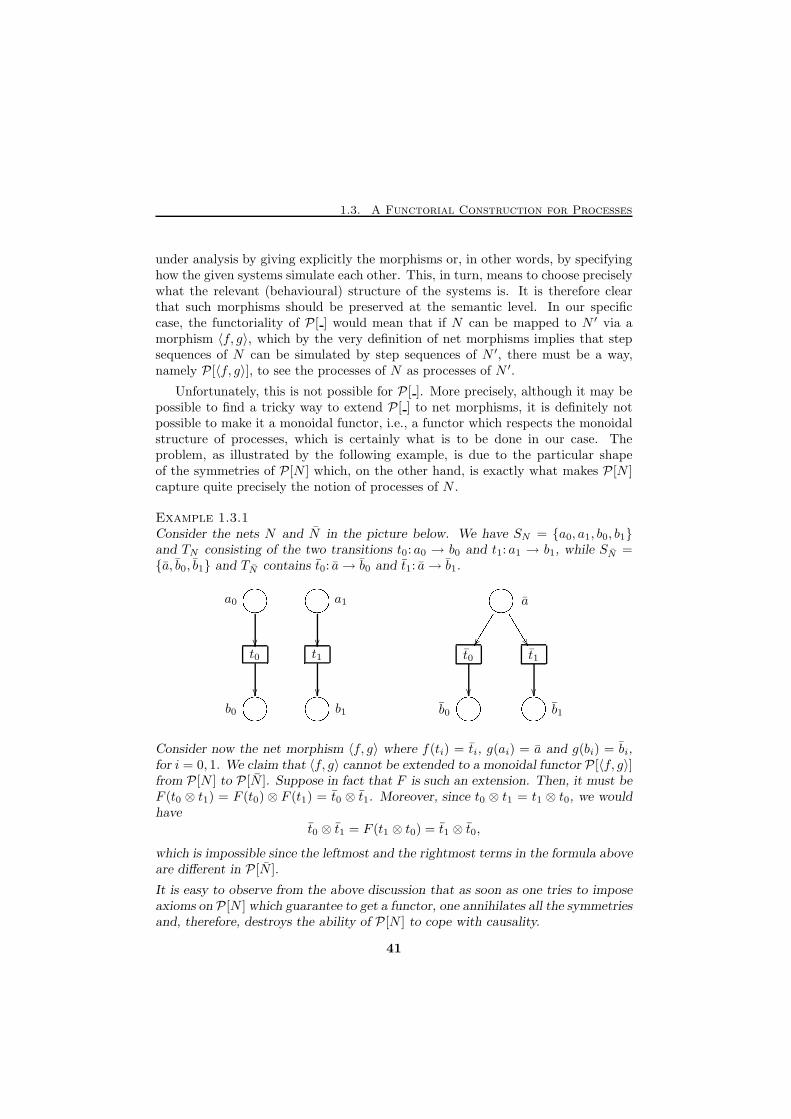
1.3. A Functorial Construction for Processes
under analysis by giving explicitly the morphisms or, in other words, by specifyinghow the given systems simulate each other. This, in turn, means to choose preciselywhat the relevant (behavioural) structure of the systems is. It is therefore clearthat such morphisms should be preserved at the semantic level. In our specificcase, the functoriality of P [ ] would mean that if N can be mapped to N ′ via amorphism 〈f, g〉, which by the very definition of net morphisms implies that stepsequences of N can be simulated by step sequences of N ′, there must be a way,namely P [〈f, g〉], to see the processes of N as processes of N ′.
Unfortunately, this is not possible for P [ ]. More precisely, although it may bepossible to find a tricky way to extend P [ ] to net morphisms, it is definitely notpossible to make it a monoidal functor, i.e., a functor which respects the monoidalstructure of processes, which is certainly what is to be done in our case. Theproblem, as illustrated by the following example, is due to the particular shapeof the symmetries of P [N ] which, on the other hand, is exactly what makes P [N ]capture quite precisely the notion of processes of N .
Example 1.3.1Consider the nets N and N in the picture below. We have SN = {a0, a1, b0, b1}and TN consisting of the two transitions t0: a0 → b0 and t1: a1 → b1, while SN ={a, b0, b1} and TN contains t0: a→ b0 and t1: a→ b1.
t0 t1 t0 t1
a0
'&$%��
a1
'&$%��
a'&$%22222 ���������� �� �
��
� �� ���
� �� ���
� �� ���
b0
'&$% b1
'&$% b0
'&$% b1
'&$%Consider now the net morphism 〈f, g〉 where f(ti) = ti, g(ai) = a and g(bi) = bi,for i = 0, 1. We claim that 〈f, g〉 cannot be extended to a monoidal functor P [〈f, g〉]from P [N ] to P [N ]. Suppose in fact that F is such an extension. Then, it must beF (t0 ⊗ t1) = F (t0) ⊗ F (t1) = t0 ⊗ t1. Moreover, since t0 ⊗ t1 = t1 ⊗ t0, we wouldhave
t0 ⊗ t1 = F (t1 ⊗ t0) = t1 ⊗ t0,
which is impossible since the leftmost and the rightmost terms in the formula aboveare different in P [N ].
It is easy to observe from the above discussion that as soon as one tries to imposeaxioms on P [N ] which guarantee to get a functor, one annihilates all the symmetriesand, therefore, destroys the ability of P [N ] to cope with causality.
41
Chapter 1. Processes and Unfoldings
The problem can be explained formally by saying that the category SymN ,sitting inside P [N ], is not free, and that is why we cannot find an extension toP [N ] of the morphism 〈f, g〉:N → N → P [N ]. In fact, Proposition 1.2.5 showsthat SymN is the free category of symmetries on S⊕N modulo axiom (1.16), i.e., theSSMC which has S⊕N as objects and whose arrows are freely generated from a familyof formal arrows cu,v, for u, v ∈ S⊕N modulo the axioms which express that c is anatural transformation, the axioms (1.2)–(1.6) of SSMC’s, and the axiom
ca,b = ida⊕b if a 6= b in SN .
Clearly, it is exactly this conditional axiom with a negative premise which preventsSymN from being the free model of the axioms (and us from getting any free modelsof them). To make things worse, the theory illustrated so far makes it clear that,in order for P [N ] to have the interesting computational meaning it has, such anaxiom is strictly needed.
There does not seem to be an easy and satisfactory solution to the functorialityproblem for P [ ]. A possible solution which comes naturally to the mind wouldconsist of looking for a non strict monoidal functor, i.e., a functor F together with
a natural transformation ϕ:F (x1) ⊗ F (x2)�
→ F (x1 ⊗ x2) which substitutes theequality required by strict functors. However, simple examples show that this ideadoes not bring anywhere, at least unless P [ ] is heavily modified also on the objects,since it is not possible to choose the components of ϕ “naturally”.
However, we present here a solution to the problem based on a rather radicalchange of models for net behaviours. Namely, instead of considering SSMC’s withcommutative monoids of objects, we choose as semantic domain a category SSMC⊗
of SSMC’s whose objects form free, non-commutative monoids. The reason forrenouncing to commutativity is explained in the following subsection. The mostinteresting thing is, in our view, that the objects of SSMC⊗ still admit a very nicecomputational interpretation. We are aware that our approach is to be consideredonly a first step towards a satisfactory solution. With the same strenght, however,we believe that our results contribute to deepen the understanding of the subject.
A Negative Result about Functoriality
In this subsection we show that the problem illustrated in Example 1.3.1 is serious,actually deep enough to prevent any naive modification of P [ ] to be functorial.
Proposition 1.3.2Let X [ ] be a function which assigns to each net N a symmetric strict monoidalcategory whose monoid of objects is commutative and contains SN , the places of N .Suppose further the group of symmetries at any object of X [N ] is finite. Finally,suppose that there exists a net N with a place a ∈ N such that, for each n > 1, wehave that the symmetry of X [N ] at (na, na) is not an identity.
42
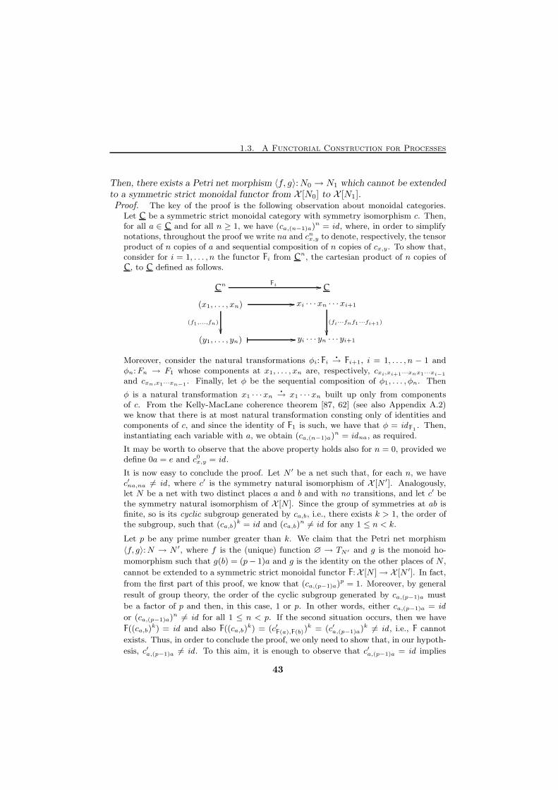
1.3. A Functorial Construction for Processes
Then, there exists a Petri net morphism 〈f, g〉:N0 → N1 which cannot be extendedto a symmetric strict monoidal functor from X [N0] to X [N1].Proof. The key of the proof is the following observation about monoidal categories.
Let C be a symmetric strict monoidal category with symmetry isomorphism c. Then,for all a ∈ C and for all n ≥ 1, we have (ca,(n−1)a)
n = id , where, in order to simplifynotations, throughout the proof we write na and cnx,y to denote, respectively, the tensorproduct of n copies of a and sequential composition of n copies of cx,y. To show that,consider for i = 1, . . . , n the functor Fi from Cn, the cartesian product of n copies ofC, to C defined as follows.
(x1, . . . , xn) xi · · ·xn · · ·xi+1
(y1, . . . , yn) yi · · · yn · · · yi+1
� //
(f1,...,fn)
��(fi···fnf1···fi+1)
��� //
CCn Fi //
Moreover, consider the natural transformations φi: Fi�
→ Fi+1, i = 1, . . . , n − 1 andφn:Fn → F1 whose components at x1, . . . , xn are, respectively, cxi,xi+1···xnx1···xi−1
and cxn,x1···xn−1 . Finally, let φ be the sequential composition of φ1, . . . , φn. Then
φ is a natural transformation x1 · · ·xn�
→ x1 · · ·xn built up only from componentsof c. From the Kelly-MacLane coherence theorem [87, 62] (see also Appendix A.2)we know that there is at most natural transformation consting only of identities andcomponents of c, and since the identity of F1 is such, we have that φ = idF1
. Then,instantiating each variable with a, we obtain (ca,(n−1)a)
n = idna, as required.
It may be worth to observe that the above property holds also for n = 0, provided wedefine 0a = e and c0x,y = id .
It is now easy to conclude the proof. Let N ′ be a net such that, for each n, we havec′na,na 6= id , where c′ is the symmetry natural isomorphism of X [N ′]. Analogously,let N be a net with two distinct places a and b and with no transitions, and let c′ bethe symmetry natural isomorphism of X [N ]. Since the group of symmetries at ab isfinite, so is its cyclic subgroup generated by ca,b, i.e., there exists k > 1, the order ofthe subgroup, such that (ca,b)
k = id and (ca,b)n 6= id for any 1 ≤ n < k.
Let p be any prime number greater than k. We claim that the Petri net morphism
〈f, g〉:N → N ′, where f is the (unique) function ∅ → TN′ and g is the monoid ho-
momorphism such that g(b) = (p− 1)a and g is the identity on the other places of N ,
cannot be extended to a symmetric strict monoidal functor F:X [N ]→ X [N ′]. In fact,
from the first part of this proof, we know that (ca,(p−1)a)p = 1. Moreover, by general
result of group theory, the order of the cyclic subgroup generated by ca,(p−1)a must
be a factor of p and then, in this case, 1 or p. In other words, either ca,(p−1)a = id
or (ca,(p−1)a)n 6= id for all 1 ≤ n < p. If the second situation occurs, then we have
F((ca,b)k) = id and also F((ca,b)
k) = (c′F(a),F(b))k = (c′a,(p−1)a)
k 6= id , i.e., F cannot
exists. Thus, in order to conclude the proof, we only need to show that, in our hypoth-
esis, c′a,(p−1)a 6= id . To this aim, it is enough to observe that c′a,(p−1)a = id implies
43
Chapter 1. Processes and Unfoldings
c′na,na = id for n = p− 1, which is against our hypothesis on N ′. In fact, c′ka,(p−1)a =
ac′(k−1)a,(p−1)a; c′a,(p−1)ana, whence it follows directly that c′(p−1)a,(p−1)a = id . X
The contents of the previous proposition may be restated in different termsby saying that in the free category of symmetries on a commutative monoid Mthere are infinite homsets. This means that dropping axiom (1.16) in the definitionof P [N ] causes an “explosion” of the structure of the symmetries. More precisely, ifwe omit axiom (1.16), we can find some object u such that the group of symmetrieson u has infinite order. Of course, since symmetries represent causality, this makesthe category so obtained completely useless for the kind of application we have inmind.
The hypothesis of Proposition 1.3.2 can be certainly weakened in several ways,clearly to the price of complicating the proof. However, we avoided such compli-cations, since the conditions stated above are already weak enough if one wantsto regard X [N ] as a category of processes of N . In fact, since places representthe atomic bricks on which states are built, one needs to consider them in X [N ],since symmetries regulate the “flow of causality”, there will be cna,na different fromthe identity, and since in a computation we can have only finitely many “causalitystreams”, there will not be categories with infinite groups of symmetries. Therefore,the given result means that there is no chance to have a functorial construction ofthe processes of N on the line of P [N ] whose objects form a commutative monoid.
The Category Q[N ]
This subsection introduces the symmetric strict monoidal category Q[N ] which ismeant to represent the processes of a Petri net N and which supports a functorialconstruction. This allows us to characterize the category of the categories of netbehaviours, or, in other words, to axiomatize the behaviour of nets “in the large”. Infact, although [97] and [16] clarify how the behaviour of a single net may be capturedby a symmetric strict monoidal category, because of the missing functoriality of P [ ],nothing is said about what the semantic domain for Petri nets is.
Necessarily, there is a price to be payed. Here, the idea is to abandon thecommutativity of the monoids of the objects. More precisely, we build the arrowsof Q[N ] starting from Sym∗N , the free category of symmetries over the set SN .This makes transitions to have many corresponding arrows in Q[N ]; however, allthe arrows of Q[N ] which differ only for instances of transitions will be equated by a“naturality” condition which, therefore, guarantees that Q[N ] remains close to thecategory P [N ] of concatenable processes. Namely, the arrows of Q[N ] correspondto Goltz-Reisig processes in which the minimal and the maximal places are totallyordered.
Similarly to SymN , Sym∗N serves a double purpose. From the categorical pointof view it provides the symmetry isomorphism of a symmetric monoidal category,
44
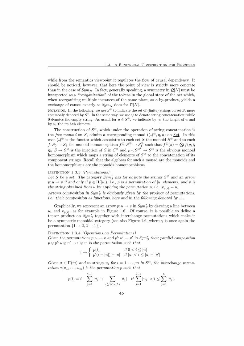
1.3. A Functorial Construction for Processes
while from the semantics viewpoint it regulates the flow of causal dependency. Itshould be noticed, however, that here the point of view is strictly more concretethan in the case of SymN . In fact, generally speaking, a symmetry in Q[N ] must beinterpreted as a “reorganization” of the tokens in the global state of the net which,when reorganizing multiple instances of the same place, as a by-product, yields aexchange of causes exactly as SymN does for P [N ].
Notation. In the following, we use S⊗ to indicate the set of (finite) strings on set S, morecommonly denoted by S∗. In the same way, we use ⊗ to denote string concatenation, while0 denotes the empty string. As usual, for u ∈ S⊗, we indicate by |u| the lenght of u andby ui the its i-th element.
The construction of S⊗, which under the operation of string concatenation isthe free monoid on S, admits a corresponding monad (( )⊗, η, µ) on Set. In thiscase ( )⊗ is the functor which associates to each set S the monoid S⊗ and to eachf :S0 → S1 the monoid homomorphism f⊗:S⊗0 → S⊗1 such that f⊗(u) =
⊗f(ui),
ηS :S → S⊗ is the injection of S in S⊗ and µS :S⊗2
→ S⊗ is the obvious monoidhomomorphism which maps a string of elements of S⊗ to the concatenation of itscomponent strings. Recall that the algebras for such a monad are the monoids andthe homomorphisms are the monoids homomorphisms.
Definition 1.3.3 (Permutations)Let S be a set. The category Sym∗S has for objects the strings S⊗ and an arrowp:u→ v if and only if p ∈ Π(|u|), i.e., p is a permutation of |u| elements, and v isthe string obtained from u by applying the permutation p, i.e., vp(i) = ui.
Arrows composition in Sym∗S is obviously given by the product of permutations,i.e., their composition as functions, here and in the following denoted by ; .
Graphically, we represent an arrow p:u→ v in Sym∗S by drawing a line betweenui and vp(i), as for example in Figure 1.6. Of course, it is possible to define atensor product on Sym∗S together with interchange permutations which make itbe a symmetric monoidal category (see also Figure 1.6, where γ is once again thepermutation {1→ 2, 2→ 1}).
Definition 1.3.4 (Operations on Permutations)Given the permutations p:u→ v and p′:u′ → v′ in Sym∗S their parallel compositionp⊗ p′:u⊗ u′ → v ⊗ v′ is the permutation such that
i 7→
{p(i) if 0 < i ≤ |u|p′(i− |u|) + |u| if |u| < i ≤ |u|+ |u′|
Given σ ∈ Π(m) and m strings ui for i = 1, . . . ,m in S⊗, the interchange permu-tation σ(u1, . . . , um) is the permutation p such that
p(i) = i−h−1∑
j=1
|uj |+∑
π(j)<π(h)
|uj| if
h−1∑
j=1
|uj| < i ≤h∑
j=1
|uj |.
45
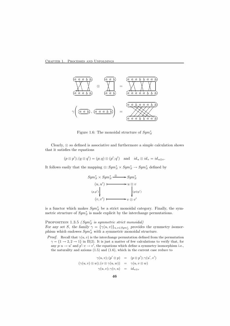
Chapter 1. Processes and Unfoldings
a a a b b
a a a b b
((((((� �� �(((((( '''''������ �� � ⊗
a a b
a a b
((((((� �� �������� �� � =
a a a b b a a b
a a a a a b b b
((((((� �� �(((((( ((((((������ ((((((������� �� �γ
(a a b� �� �, a a a b b
� �� �) =
a a b a a a b b
a a a b b a a b
HHHHHHHHH� �� �HHHHHHHHHHHHHHHHHH������ ������ ������ ������ ������ �� �Figure 1.6: The monoidal structure of Sym∗S
Clearly, ⊗ so defined is associative and furthermore a simple calculation showsthat it satisfies the equations
(p⊗ p′); (q ⊗ q′) = (p; q)⊗ (p′; q′) and idu ⊗ idv = idu⊗v.
It follows easily that the mapping ⊗:Sym∗S × Sym∗S → Sym∗S defined by
(u, u′) u⊗ v
(v, v′) v ⊗ v′
� //
(p,p′)
��(p⊗p′)
��� //
Sym∗SSym∗S × Sym∗S⊗ //
is a functor which makes Sym∗S be a strict monoidal category. Finally, the sym-metric structure of Sym∗S is made explicit by the interchange permutations.
Proposition 1.3.5 ( Sym∗S is symmetric strict monoidal)For any set S, the family γ = {γ(u, v)}u,v∈Sym∗
Sprovides the symmetry isomor-
phism which endowes Sym∗S with a symmetric monoidal structure.
Proof. Recall that γ(u, v) is the interchange permutation defined from the permutationγ = {1 → 2, 2 → 1} in Π(2). It is just a matter of few calculations to verify that, forany p:u→ u′ and p′: v → v′, the equations which define a symmetry isomorphism i.e.,the naturality and axioms (1.5) and (1.6), which in the current case reduce to
γ(u, v); (p′ ⊗ p) = (p⊗ p′); γ(u′, v′)
(γ(u, v)⊗w); (v ⊗ γ(u,w)) = γ(u, v ⊗ w)
γ(u, v); γ(v, u) = idu⊗v
46
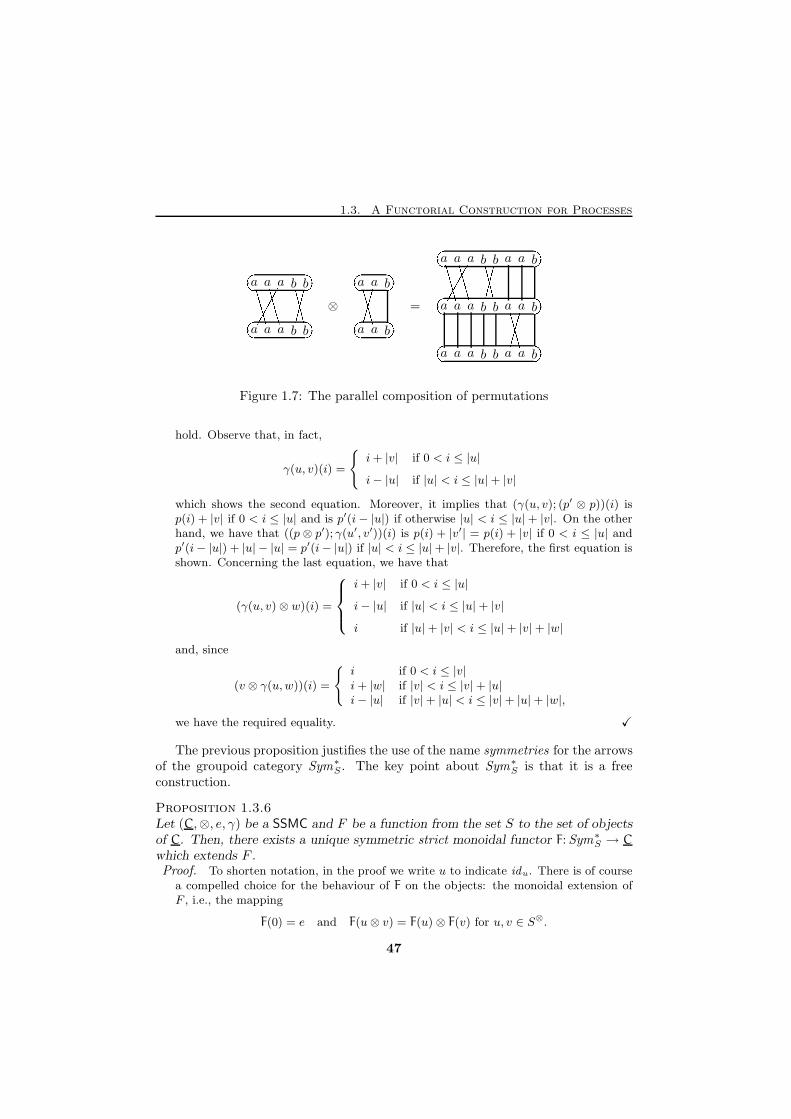
1.3. A Functorial Construction for Processes
a a a b b
a a a b b
((((((� �� �(((((( '''''������ �� � ⊗
a a b
a a b
((((((� �� �������� �� � =
a a a b b a a b
a a a b b a a b
a a a b b a a b
((((((� �� �(((((( '''''������ �� �((((((������� �� �Figure 1.7: The parallel composition of permutations
hold. Observe that, in fact,
γ(u, v)(i) =
{i+ |v| if 0 < i ≤ |u|
i− |u| if |u| < i ≤ |u|+ |v|
which shows the second equation. Moreover, it implies that (γ(u, v); (p′ ⊗ p))(i) isp(i) + |v| if 0 < i ≤ |u| and is p′(i− |u|) if otherwise |u| < i ≤ |u|+ |v|. On the otherhand, we have that ((p ⊗ p′); γ(u′, v′))(i) is p(i) + |v′| = p(i) + |v| if 0 < i ≤ |u| andp′(i− |u|) + |u| − |u| = p′(i− |u|) if |u| < i ≤ |u|+ |v|. Therefore, the first equation isshown. Concerning the last equation, we have that
(γ(u, v)⊗ w)(i) =
i+ |v| if 0 < i ≤ |u|
i− |u| if |u| < i ≤ |u|+ |v|
i if |u|+ |v| < i ≤ |u|+ |v|+ |w|
and, since
(v ⊗ γ(u,w))(i) =
{i if 0 < i ≤ |v|i+ |w| if |v| < i ≤ |v|+ |u|i− |u| if |v|+ |u| < i ≤ |v|+ |u|+ |w|,
we have the required equality. X
The previous proposition justifies the use of the name symmetries for the arrowsof the groupoid category Sym∗S . The key point about Sym∗S is that it is a freeconstruction.
Proposition 1.3.6Let (C,⊗, e, γ) be a SSMC and F be a function from the set S to the set of objectsof C. Then, there exists a unique symmetric strict monoidal functor F:Sym∗S → C
which extends F .Proof. To shorten notation, in the proof we write u to indicate idu. There is of course
a compelled choice for the behaviour of F on the objects: the monoidal extension ofF , i.e., the mapping
F(0) = e and F(u⊗ v) = F(u) ⊗ F(v) for u, v ∈ S⊗.
47
Chapter 1. Processes and Unfoldings
Concerning the morphisms, we know by Lemma 1.2.3 that each arrow in Sym∗S canbe written as composition of transpositions. Moreover, observe that the transposition{i→ i+1, i+ 1→ i}: u⊗ a⊗ b⊗ v → u⊗ b⊗ a⊗ v, where u is a string of length i− 1,coincides in Sym∗S with the tensor of γ(a, b): a⊗ b→ b⊗ a with appropriate identities,namely (u⊗ γ(a, b) ⊗ v). Thus, recalling also that 0 ⊗ γ(a, b) = γ(a, b) = γ(a, b) ⊗ 0,the following definition defines F on all the arrows of Sym∗S .
F(u⊗ γ(a, b)⊗ v) = F(u)⊗ γF(a),F(b) ⊗ F(v) a, b ∈ S, u, v ∈ S⊗;
F(p; p′) = F(p′) ◦ F(p). (1.20)
Observe that both the equations (1.20) are forced by the definition of symmetric strictmonoidal functor, i.e., axioms (1.7)–(1.9) in page 22. It follows that the extension of Fto a strict monoidal functor, if it exists, is unique and must be given by (1.20). Then,in order to conclude the proof, we only need to show that F is well-defined and that itis a symmetric monoidal functor.
We first show that F is well-defined. To this aim, it is enough to show that theaxioms (1.14) of Lemma 1.2.3 are preserved by F. In fact, this implies that applyingthe definition of F to two different factorizations of p actually yield the same result,i.e., it implies that F is well-defined. Concering axioms (1.14), the third one matchesdirectly with the fact that the inverse of γF(a),F(b) is γF(b),F(a), while the second onefollows easily from the fact that ⊗ is a functor. In fact, in the hypothesis, we haveτi = (u⊗ γ(a, b)⊗ v⊗ c⊗ d⊗w) and τj = (u⊗ b⊗ a⊗ v⊗ γ(c, d)⊗w). Thus, we have
F(τi; τj) = (F(u)⊗ F(b)⊗ F(a)⊗ F(v) ⊗ γF(c),F(d) ⊗ F(w)) ◦
(F(u)⊗ γF(a),F(b) ⊗ F(v) ⊗ F(c) ⊗ F(d)⊗ F(w))
= (F(u)⊗ γF(a),F(b) ⊗ F(v)⊗ γF(c),F(d) ⊗ F(w))
= (F(u)⊗ γF(a),F(b) ⊗ F(v)⊗ F(d)⊗ F(c)⊗ F(w)) ◦
(F(u)⊗ F(a)⊗ F(b)⊗ F(v)⊗ γF(c),F(d) ⊗ F(w))
= F(τj ; τi)
Finally, concerning the third axiom, we have
F(τi; τi+1; τi) = (F(u) ⊗ γF(b),F(c) ⊗ F(a)⊗ F(v)) ◦
(F(u)⊗ F(b)⊗ γF(a),F(c) ⊗ F(v)) ◦
(F(u)⊗ γF(a),F(b) ⊗ F(c)⊗ F(v))
= (F(u) ⊗ F(b) ⊗ γF(a),F(c) ⊗ F(v)) ◦
(F(u)⊗ γF(a),F(b)⊗F(c) ⊗ F(v))
= (F(u) ⊗ γF(a),F(c)⊗F(b) ⊗ F(v)) ◦
(F(u)⊗ F(a)⊗ γF(b),F(c) ⊗ F(v))
= (F(u) ⊗ F(c) ⊗ γF(a),F(b) ⊗ F(v)) ◦
(F(u)⊗ γF(a),F(c) ⊗ F(b)⊗ F(v)) ◦
(F(u)⊗ F(a)⊗ γF(b),F(c) ⊗ F(v))
= F(τi+1; τi; τi+1)
48
1.3. A Functorial Construction for Processes
where the third equation is by naturality of γ and the others follow from the coherenceaxiom for γ.
Let us prove now that F is a symmetric monoidal functor. Since C is a symmetricstrict monoidal category, we have that γe,x = γe⊗e,x = γe,x ⊗ e ◦ e⊗ γe,x = γe,x ◦ γe,x,and since γe,x is invertible, it follows that γe,x = idx. Of course, the same holds forevery symmetric strict monoidal category. Therefore, since F(idu) = F(γ(0, u)) andγe,F(u) = idF(u), we have that the F(idu) = idF(u). This, together with the second ofthe equations (1.20), means that F is a functor.
Observe that for p:u→ v and p′:u′ → v′ in Sym∗S we have p ⊗ p′ = (p ⊗ u′); (v ⊗ p′)(see also Figure 1.7). Then, we have that
F(p⊗ p′) = F(v ⊗ p′) ◦ F(p⊗ u′) = (F(v)⊗ F(p′)) ◦ (F(p)⊗ F(u′)) = F(p)⊗ F(p′),
i.e., F is a strict monoidal functor.
Finally, thanks to the coherence axiom for symmetries, i.e., axiom (1.5), we have thatγ(a, b ⊗ c) = (γ(a, b) ⊗ c); (b ⊗ γ(a, c)) and thus, by the aforesaid axiom and by thecoherence of γ,
F(γ(a, b⊗ c)) = F((γ(a, b)⊗ c); (b⊗ γ(a, c)))
= (F (b)⊗ γF (a),F (c)) ◦ (γF (a),F (b) ⊗ F (c))
= γF (a),F (b)⊗F (c) = γF(a),F(b⊗c).
Now, by considering the inverse of (1.5), we have γ(a⊗b, c) = (a⊗γ(b, c)); (γ(a, c)⊗b)
and γF(a⊗b),F(c) = (γF(a),F(c) ⊗ F(b)) ◦ (F(a) ⊗ γF(b),F(c)). Therefore, it follows easily
by induction that F(γ(u, v)) = γF(u),F(v). Then, F maps each component of the sym-
metry natural isomorphism of Sym∗S to the corresponding component of γ, i.e., F is a
symmetric monoidal functor. X
In other words, the previous proposition proves that the mapping S 7→ Sym∗Sextends to a left adjoint functor Set ⇀ SsMonCat. Equivalently, we can say thatSym∗S is the free symmetric strict monoidal category on the set S.
Remark. It may be worth remarking that this adjunction does not exist if SsMonCatis replaced by SsMonCat⋆ (see Appendix A.2) or, a fortiori, by SsMonCat⋆⋆, sincethe last category does not admit a free category of symmetries on a set S. In fact, amapping F from S to the objects of a symmetric monoidal category (C,⊗, e, α, λ, ρ, γ)can be extended to a (non-strict) monoidal functor F from Sym∗S to C in two differentway, namely,
F(0) = e;F(γ(u, v)) = γF (u),F (v);
F(u⊗ v) = F(u) ⊗ F(v);F(p⊗ p′) = F(p)⊗ F(p′),
with ϕ0 = id and ϕ = idF(x1)⊗F(x2) and
F(0) = e;F(γ(u, v)) = γF (v),F (u);
F(u⊗ v) = F(v)⊗ F(u);F(p⊗ p′) = F(p′)⊗ F(p),
with ϕ0 = id and ϕ = γF(x1),F(x2).
49
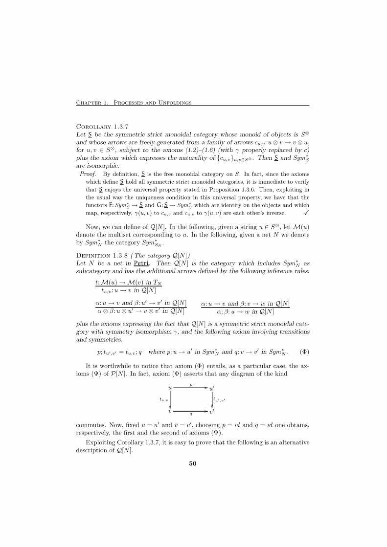
Chapter 1. Processes and Unfoldings
Corollary 1.3.7Let S be the symmetric strict monoidal category whose monoid of objects is S⊗
and whose arrows are freely generated from a family of arrows cu,v:u⊗ v → v ⊗ u,for u, v ∈ S⊗, subject to the axioms (1.2)–(1.6) (with γ properly replaced by c)plus the axiom which expresses the naturality of {cu,v}u,v∈S⊗ . Then S and Sym∗Sare isomorphic.
Proof. By definition, S is the free monoidal category on S. In fact, since the axioms
which define S hold all symmetric strict monoidal categories, it is immediate to verify
that S enjoys the universal property stated in Proposition 1.3.6. Then, exploiting in
the usual way the uniqueness condition in this universal property, we have that the
functors F: Sym∗S → S and G:S→ Sym∗S which are identity on the objects and which
map, respectively, γ(u, v) to cu,v and cu,v to γ(u, v) are each other’s inverse. X
Now, we can define of Q[N ]. In the following, given a string u ∈ S⊗, let M(u)denote the multiset corresponding to u. In the following, given a net N we denoteby Sym∗N the category Sym∗SN
.
Definition 1.3.8 (The category Q[N ])Let N be a net in Petri. Then Q[N ] is the category which includes Sym∗N assubcategory and has the additional arrows defined by the following inference rules:
t:M(u)→M(v) in TNtu,v:u→ v in Q[N ]
α:u→ v and β:u′ → v′ in Q[N ]α⊗ β:u⊗ u′ → v ⊗ v′ in Q[N ]
α:u→ v and β: v → w in Q[N ]α;β:u→ w in Q[N ]
plus the axioms expressing the fact that Q[N ] is a symmetric strict monoidal cate-gory with symmetry isomorphism γ, and the following axiom involving transitionsand symmetries.
p; tu′,v′ = tu,v; q where p:u→ u′ in Sym∗N and q: v → v′ in Sym∗N . (Φ)
It is worthwhile to notice that axiom (Φ) entails, as a particular case, the ax-ioms (Ψ) of P [N ]. In fact, axiom (Φ) asserts that any diagram of the kind
u u′
v v′
p //
tu,v
��tu′,v′
��q
//
commutes. Now, fixed u = u′ and v = v′, choosing p = id and q = id one obtains,respectively, the first and the second of axioms (Ψ).
Exploiting Corollary 1.3.7, it is easy to prove that the following is an alternativedescription of Q[N ].
50
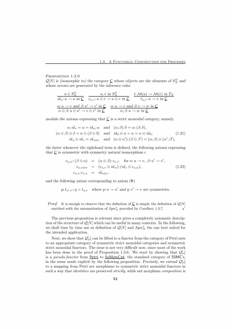
1.3. A Functorial Construction for Processes
Proposition 1.3.9Q[N ] is (isomorphic to) the category C whose objects are the elements of S⊗N andwhose arrows are generated by the inference rules
u ∈ S⊗Nidu:u→ u in C
u, v in S⊗Ncu,v:u⊗ v → u⊗ v in C
t:M(u)→M(v) in TNtu,v:u→ v in C
α:u→ v and β:u′ → v′ in C
α⊗ β:u⊗ u′ → v ⊗ v′ in C
α:u→ v and β: v → w in C
α;β:u→ w in C
modulo the axioms expressing that C is a strict monoidal category, namely,
α; idv = α = idu;α and (α;β); δ = α; (β; δ),
(α⊗ β)⊗ δ = α⊗ (β ⊗ δ) and id0 ⊗ α = α = α⊗ id0, (1.21)
idu ⊗ idv = idu⊗v and (α⊗ α′); (β ⊗ β′) = (α;β)⊗ (α′;β′),
the latter whenever the righthand term is defined, the following axioms expressingthat C is symmetric with symmetry natural isomorphism c
cu,u′ ; (β ⊗ α) = (α⊗ β); cv,v′ for α:u→ v, β:u′ → v′,
cu,v⊗w = (cu,v ⊗ idw); (idv ⊗ cu,w), (1.22)
cu,v; cv,u = idu⊗v,
and the following axiom corresponding to axiom (Φ)
p; tu′,v′ ; q = tu,v where p:u→ u′ and q: v′ → v are symmetries.
Proof. It is enough to observe that the definition of C is simply the definition of Q[N ]
enriched with the axiomatization of Sym∗N provided by Corollary 1.3.7. X
The previous proposition is relevant since gives a completely axiomatic descrip-tion of the structure ofQ[N ] which can be useful in many contexts. In the following,we shall time by time use as definition of Q[N ] and Sym∗N the one best suited forthe intended application.
Next, we show that Q[ ] can be lifted to a functor from the category of Petri netsto an appropriate category of symmetric strict monoidal categories and symmetricstrict monoidal functors. The issue is not very difficult now, since most of the workhas been done in the proof of Proposition 1.3.6. We start by showing that Q[ ]is a pseudo-functor from Petri to SsMonCat, the standard category of SSMC’s,in the sense made explicit by the following proposition. Precisely, we extend Q[ ]to a mapping from Petri net morphisms to symmetric strict monoidal functors insuch a way that identities are preserved strictly, while net morphism composition is
51
Chapter 1. Processes and Unfoldings
preserved only up to a monoidal natural isomorphism. In order to do that, the keypoint which is still missing is to be able to embed N into Q[N ]. To this purpose,we assume for each set S a function inS :S⊕ → S⊗ such thatM(inS(u)) = u, i.e.,a function which chooses a “linearization” of each u ∈ S⊕. Clearly, correspondingto different choices of the functions inS we shall have a different—yet equivalent—extension of Q[ ] to a pseudo-functor. We would like to remark that this apparentarbitrariness of Q[ ] is not at all a concern, since the relevant fact we want to shownow is that such an extension exists. Moreover, we shall see shortly that introducingthe category SSMC⊗ one can completely dispense with the inS . In the following,given a net N , we shall use inN to denote inSN
.
Remark. An elegant way to express the idea of “linearization” of a multiset, would be to
look for a morphism of monads in: ( )⊕�
→ ( )⊗. This would indeed simplify the followingformal development and would actually make Q[ ] be a functor Petri → SsMonCat.However, such a morphism does not exist. It is worth noticing that this is because it isnot possibile to choose the inS “naturally”.
Proposition 1.3.10 (Q[ ]: Petri→ SsMonCat)Let 〈f, g〉:N0 → N1 be a morphism in Petri. Then, there exists a symmetricstrict monoidal functor Q[〈f, g〉]:Q[N0] → Q[N1] which extends 〈f, g〉. Moreover,Q[idN ] = idQ[N ] and Q[〈f1, g1〉 ◦ 〈f0, g0〉] ∼= Q[〈f1, g1〉] ◦ Q[〈f0, g0〉].
Proof. Let 〈f, g〉:N0 → N1 be a morphism of Petri nets. Since g is a monoid homomor-phism from the free monoid S⊕N0
to S⊕N1, it corresponds to a unique function g ◦ ηSN0
from SN0 to S⊕N1, where η is the unit of the “commutative monoids” monad, whence we
obtain g = inN1 ◦g◦ηSN0:SN0 → S⊗N1
, i.e., a function from SN0 to the set of objects ofQ[N1]. Then, from Proposition 1.3.6, we have the symmetric strict monoidal functorF′:SymSN0
→ Q[N1]. Clearly, the objects component of F′ is µSN1◦ g⊗, where µ is
the multiplication of the “monoids” monad. Finally, we extend F′ to a functor F fromQ[N0] to Q[N1] by considering the symmetric strict monoidal functor which coincideswith F′ on SymN0
and maps tu,v:u→ v to f(t)F(u),F(v): F(u)→ F(v). Since monoidalfunctors map symmetries to symmetries, and since f(t) is transition of N1, it followsimmediately that F preserves axiom (Φ), i.e., that F is well defined.
Next, we have to show that the above definition makesQ[ ] into a pseudo-functor. First
of all, observe that whatever inN , the function SN → S⊕NinN−→ S⊗N is the inclusion of SN
in S⊗N . It follows easily from the uniqueness part of the universal property stated inProposition 1.3.6 that Q[idN ]:Q[N ] → Q[N ] is the identity functor. Now consider〈f0, g0〉:N0 → N1 and 〈f1, g1〉:N1 → N2 and, for i = 0, 1, let Fi be Q[〈fi, gi〉]:Q[Ni]→Q[Ni+1] and F be Q[〈f1 ◦ f0, g1 ◦ g0〉]. We have to show that F ∼= F1F0. Let u ∈ S⊗N0
.By definition, we have that F(ui) = inN2 ◦ g1 ◦ g0(ui) is a permutation of F1F0(ui) =µSN2
◦ g⊗1 ◦ g0(ui) and, therefore, there exists a symmetry si: F(ui) → F1F0(ui) inQ[N2]. Then, we take su to be s1 ⊗ · · · ⊗ sn: F(u) → F1F0(u), where n is the lenghtof the string u. We shall prove that the family of the su, for u ∈ S⊗N0
is a natural
transformation F�
→ F1F0. Since s is clearly a monoidal transformation and each su isan isomorphism, this concludes the proof.
52
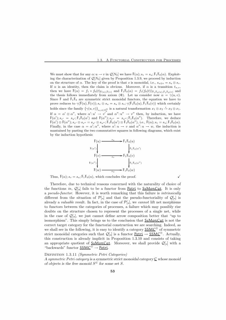
1.3. A Functorial Construction for Processes
We must show that for any α: u→ v in Q[N0] we have F(α); sv = su; F1F0(α). Exploit-ing the characterization of Q[N0] given by Proposition 1.3.9, we proceed by inductionon the structure of α. The key of the proof is that s is monoidal, i.e., su⊗v = su ⊗ sv.If α is an identity, then the claim is obvious. Moreover, if α is a transition tu,v,then we have F(α) = f1 ◦ f0(t)F(u),F(v) and F1F0(α) = f1(f0(t))F1F0(u),F1F0(v) andthe thesis follows immediately from axiom (Φ). Let us consider now α = γ(u, v).Since F and F1F0 are symmetric strict monoidal functors, the equation we have toprove reduces to γ(F(u), F(v)); sv ⊗ su = su ⊗ sv; γ(F1F0(u), F1F0(v)) which certainly
holds since the family {γ(u, v)}u,v∈S⊗
0is a natural transformation x1 ⊗ x2
�
→ x2 ⊗ x1.
If α = α′ ⊗ α′′, where α′:u′ → v′ and α′′:u′′ → v′′ then, by induction, we haveF(α′); sv′ = su′ ; F1F0(α
′) and F(α′′); sv′′ = su′′ ; F1F0(α′′). Therefore, we deduce
F(α′)⊗ F(α′′); sv′ ⊗ sv′′ = su′ ⊗ su′′ ; F1F0(α′)⊗ F1F0(α
′′), i.e., F(α); sv = su; F1F0(α).Finally, in the case α = α′;α′′, where α′:u → v and α′′:u → w, the induction ismantained by pasting the two commutative squares in following diagrams, which existby the induction hypothesis
F(u) F1F0(u)
F(v) F1F0(v)
F(w) F1F0(w)
F(α′)
��
su //
F1F0(α′)
��
F(α′′)
��
sv//
F1F0(α′′)
��sw
//
Thus, F(α); sv = su; F1F0(α), which concludes the proof. X
Therefore, due to technical reasons concerned with the naturality of choice ofthe functions in, Q[ ] fails to be a functor from Petri to SsMonCat. It is onlya pseudo-functor. However, it is worth remarking that this failure is intrinsicallydifferent from the situation of P [ ] and that the pseudo-functoriality of Q[ ] isalready a valuable result. In fact, in the case of P [ ], we cannot lift net morphismsto functors between the categories of processes, a failure which may possibly risedoubts on the structure chosen to represent the processes of a single net, whilein the case of Q[ ], we just cannot define arrow composition better that “up toisomorphism”. This simply brings us to the conclusion that SsMonCat is not thecorrect target category for the functorial construction we are searching. Indeed, aswe shall see in the following, it is easy to identify a category SSMC⊗ of symmetricstrict monoidal categories such that Q[ ] is a functor Petri → SSMC⊗. Actually,this construction is already implicit in Proposition 1.3.10 and consists of takingan appropriate quotient of SsMonCat. Moreover, we shall provide Q[ ] with a“backwards” functor SSMC⊗ → Petri.
Definition 1.3.11 (Symmetric Petri Categories)A symmetric Petri category is a symmetric strict monoidal category C whose monoidof objects is the free monoid S⊗ for some set S.
53
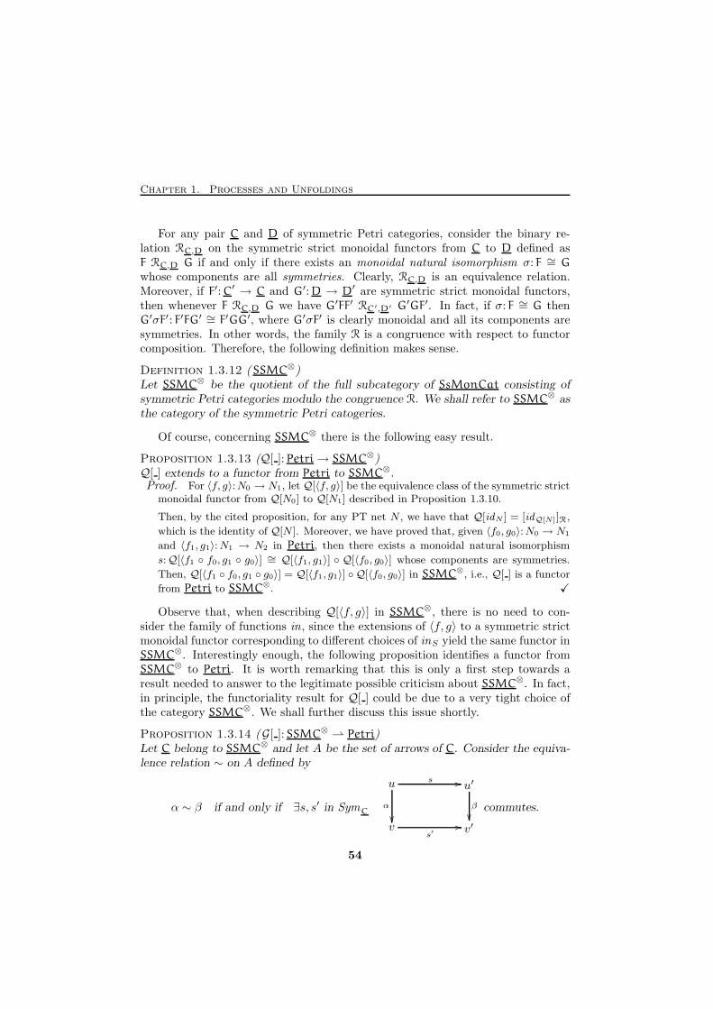
Chapter 1. Processes and Unfoldings
For any pair C and D of symmetric Petri categories, consider the binary re-lation RC,D on the symmetric strict monoidal functors from C to D defined asF RC,D G if and only if there exists an monoidal natural isomorphism σ: F ∼= G
whose components are all symmetries. Clearly, RC,D is an equivalence relation.Moreover, if F′: C′ → C and G′: D → D′ are symmetric strict monoidal functors,then whenever F RC,D G we have G′FF′ RC′,D′ G′GF′. In fact, if σ: F ∼= G thenG′σF′: F′FG′ ∼= F′GG′, where G′σF′ is clearly monoidal and all its components aresymmetries. In other words, the family R is a congruence with respect to functorcomposition. Therefore, the following definition makes sense.
Definition 1.3.12 (SSMC⊗)Let SSMC⊗ be the quotient of the full subcategory of SsMonCat consisting ofsymmetric Petri categories modulo the congruence R. We shall refer to SSMC⊗ asthe category of the symmetric Petri catogeries.
Of course, concerning SSMC⊗ there is the following easy result.
Proposition 1.3.13 (Q[ ]: Petri→ SSMC⊗)Q[ ] extends to a functor from Petri to SSMC⊗.Proof. For 〈f, g〉:N0 → N1, let Q[〈f, g〉] be the equivalence class of the symmetric strict
monoidal functor from Q[N0] to Q[N1] described in Proposition 1.3.10.
Then, by the cited proposition, for any PT net N , we have that Q[idN ] = [idQ[N]]R,
which is the identity of Q[N ]. Moreover, we have proved that, given 〈f0, g0〉:N0 → N1
and 〈f1, g1〉:N1 → N2 in Petri, then there exists a monoidal natural isomorphism
s:Q[〈f1 ◦ f0, g1 ◦ g0〉] ∼= Q[〈f1, g1〉] ◦ Q[〈f0, g0〉] whose components are symmetries.
Then, Q[〈f1 ◦ f0, g1 ◦ g0〉] = Q[〈f1, g1〉] ◦ Q[〈f0, g0〉] in SSMC⊗, i.e., Q[ ] is a functor
from Petri to SSMC⊗. X
Observe that, when describing Q[〈f, g〉] in SSMC⊗, there is no need to con-sider the family of functions in, since the extensions of 〈f, g〉 to a symmetric strictmonoidal functor corresponding to different choices of inS yield the same functor inSSMC⊗. Interestingly enough, the following proposition identifies a functor fromSSMC⊗ to Petri. It is worth remarking that this is only a first step towards aresult needed to answer to the legitimate possible criticism about SSMC⊗. In fact,in principle, the functoriality result for Q[ ] could be due to a very tight choice ofthe category SSMC⊗. We shall further discuss this issue shortly.
Proposition 1.3.14 (G[ ]: SSMC⊗ ⇀ Petri)Let C belong to SSMC⊗ and let A be the set of arrows of C. Consider the equiva-lence relation ∼ on A defined by
α ∼ β if and only if ∃s, s′ in SymC
u u′
v v′
s //
α
��β
��
s′//
commutes.
54
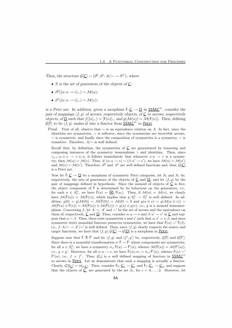
1.3. A Functorial Construction for Processes
Then, the structure G[C] = (∂0, ∂1:A/∼ → S⊕), where
• S is the set of generators of the objects of C;
• ∂0([α:u→ v]∼) =M(u);
• ∂1([α:u→ v]∼) =M(v);
is a Petri net. In addition, given a morphism F: C → D in SSMC⊗, consider thepair of mappings 〈f, g〉 of arrows, respectively objects, of C to arrows, respectivelyobjects, of D such that f([α]∼) = [F(α)]∼ and g(M(u)) =M(F(u)). Then, definingG[F] to be 〈f, g〉 makes G into a functor from SSMC⊗ to Petri.
Proof. First of all, observe that ∼ is an equivalence relation on A. In fact, since theidentities are symmetries, ∼ is reflexive, since the symmetries are invertible arrows,∼ is symmetric, and finally since the composition of symmetries is a symmetry, ∼ istransitive. Therefore, A/∼ is well defined.
Recall that, by definition, the symmetries of C are generatared by tensoring andcomposing instances of the symmetry isomorphism γ and identities. Then, sinceγu,v:u ⊗ v → v ⊗ u, it follows immediately that whenever s:u → v is a symme-try, then M(u) =M(v). Then, if (α:u→ v) ∼ (β:u′ → v′), we have M(u) =M(u′)and M(v) =M(v′). Therefore, ∂0 and ∂1 are well defined functions and, thus, G[C]is a Petri net.
Now let F: C → D be a morphism of symmetric Petri categories, let S0 and S1 be,respectively, the sets of generators of the objects of C and D, and let 〈f, g〉 be thepair of mappings defined in hypothesis. Since the monoid of objects of C is free,the object component of F is determined by its behaviour on the generators, i.e.,for each u ∈ S⊗0 , we have F(u) =
⊗iF(ui). Then, if M(u) = M(v), we clearly
have M(F(u)) = M(F(v)), which implies that g:S⊕0 → S⊕1 is well defined. In ad-dition, g(0) = g(M(0)) = M(F(0)) = M(0) = 0 and g(u ⊕ v) = g(M(u ⊗ v)) =M(F(u) ⊗ F(v)) = M(F(u)) ⊕M(F(v)) = g(u) ⊕ g(v), i.e., g is a monoid homomor-phism. Concerning f , let A, ∼, A′ and ∼′ be the set of arrows and the equivalence onthem of, respectively, C and D. Then, consider α: u→ v and β:u′ → v′ in C and sup-pose that α ∼ β. Then, there exist symmetries s and s′ such that α; s′ = s;β, and sincesymmetric strict monoidal functors preserves symmetries, we have that F(α) ∼′ F(β),i.e., f :A/∼ → A′/∼′ is well defined. Then, since 〈f, g〉 clearly respects the source andtarget functions, we have that 〈f, g〉:G[C]→ G[D] is a morphism in Petri.
Suppose now that F R F′ and let 〈f, g〉 and 〈f ′, g′〉 be, respectively, G[F] and G[F′].
Since there is a monoidal transformation σ: F→ F′ whose components are symmetries,
for all u ∈ S⊗0 , we have a symmetry σu: F(u) → F′(u), whence M(F(u)) =M(F′(u)),
i.e., g = g′. Moreover, for all α: u→ v, we have F(α); σv = σu; F′(α), whence F(α) ∼′
F′(α), i.e., f = f ′. Thus, G[ ] is a well defined mapping of functors in SSMC⊗
to arrows in Petri. Let us demonstrate that such a mapping is actually a functor.
Clearly, G[1C] = idG[C]. Then, consider F0:C0 → C1 and F1:C1 → C2, and suppose
that the objects of Ci are generated by the set Si, for i = 0, . . . , 2. Moreover, let
55
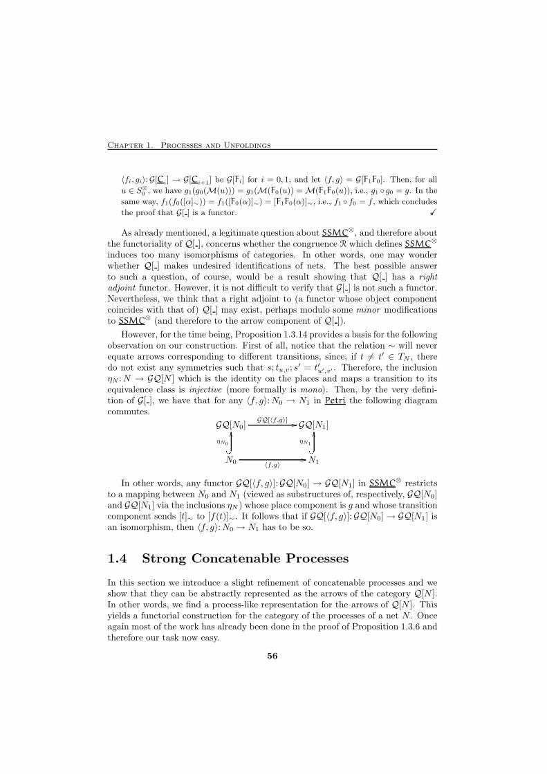
Chapter 1. Processes and Unfoldings
〈fi, gi〉:G[Ci] → G[Ci+1] be G[Fi] for i = 0, 1, and let 〈f, g〉 = G[F1F0]. Then, for all
u ∈ S⊗0 , we have g1(g0(M(u))) = g1(M(F0(u)) =M(F1F0(u)), i.e., g1 ◦ g0 = g. In the
same way, f1(f0([α]∼)) = f1([F0(α)]∼) = [F1F0(α)]∼, i.e., f1 ◦ f0 = f , which concludes
the proof that G[ ] is a functor. X
As already mentioned, a legitimate question about SSMC⊗, and therefore aboutthe functoriality of Q[ ], concerns whether the congruence R which defines SSMC⊗
induces too many isomorphisms of categories. In other words, one may wonderwhether Q[ ] makes undesired identifications of nets. The best possible answerto such a question, of course, would be a result showing that Q[ ] has a rightadjoint functor. However, it is not difficult to verify that G[ ] is not such a functor.Nevertheless, we think that a right adjoint to (a functor whose object componentcoincides with that of) Q[ ] may exist, perhaps modulo some minor modificationsto SSMC⊗ (and therefore to the arrow component of Q[ ]).
However, for the time being, Proposition 1.3.14 provides a basis for the followingobservation on our construction. First of all, notice that the relation ∼ will neverequate arrows corresponding to different transitions, since, if t 6= t′ ∈ TN , theredo not exist any symmetries such that s; tu,v; s
′ = t′u′,v′ . Therefore, the inclusionηN :N → GQ[N ] which is the identity on the places and maps a transition to itsequivalence class is injective (more formally is mono). Then, by the very defini-tion of G[ ], we have that for any 〈f, g〉:N0 → N1 in Petri the following diagramcommutes.
GQ[N0] GQ[N1]
N0 N1
GQ[〈f,g〉] //
〈f,g〉//
ηN0/� OO ηN1/� OOIn other words, any functor GQ[〈f, g〉]:GQ[N0] → GQ[N1] in SSMC⊗ restricts
to a mapping between N0 and N1 (viewed as substructures of, respectively, GQ[N0]and GQ[N1] via the inclusions ηN ) whose place component is g and whose transitioncomponent sends [t]∼ to [f(t)]∼. It follows that if GQ[〈f, g〉]:GQ[N0]→ GQ[N1] isan isomorphism, then 〈f, g〉:N0 → N1 has to be so.
1.4 Strong Concatenable Processes
In this section we introduce a slight refinement of concatenable processes and weshow that they can be abstractly represented as the arrows of the category Q[N ].In other words, we find a process-like representation for the arrows of Q[N ]. Thisyields a functorial construction for the category of the processes of a net N . Onceagain most of the work has already been done in the proof of Proposition 1.3.6 andtherefore our task now easy.
56
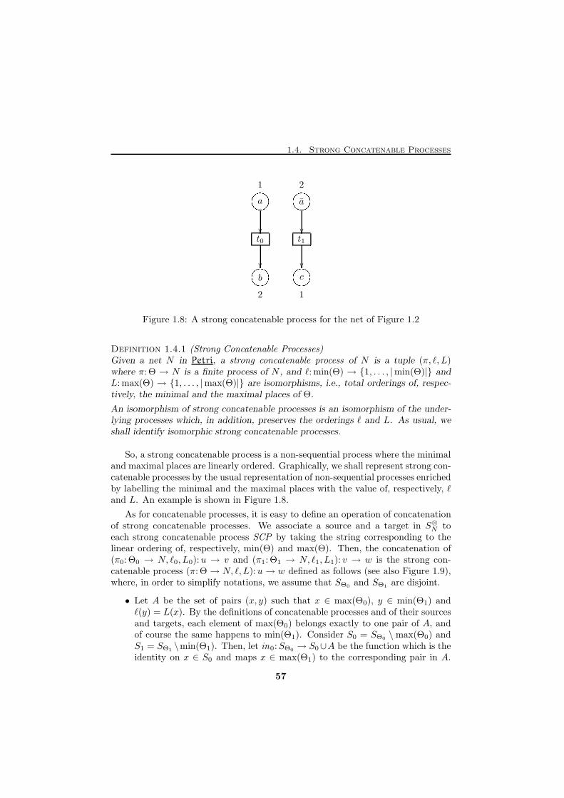
1.4. Strong Concatenable Processes
a a
t0 t1
b c
1'&$%��
2'&$%��� �� �
��
� �� ���
2
'&$%1
'&$%Figure 1.8: A strong concatenable process for the net of Figure 1.2
Definition 1.4.1 (Strong Concatenable Processes)Given a net N in Petri, a strong concatenable process of N is a tuple (π, ℓ, L)where π: Θ → N is a finite process of N , and ℓ: min(Θ) → {1, . . . , |min(Θ)|} andL: max(Θ) → {1, . . . , |max(Θ)|} are isomorphisms, i.e., total orderings of, respec-tively, the minimal and the maximal places of Θ.
An isomorphism of strong concatenable processes is an isomorphism of the under-lying processes which, in addition, preserves the orderings ℓ and L. As usual, weshall identify isomorphic strong concatenable processes.
So, a strong concatenable process is a non-sequential process where the minimaland maximal places are linearly ordered. Graphically, we shall represent strong con-catenable processes by the usual representation of non-sequential processes enrichedby labelling the minimal and the maximal places with the value of, respectively, ℓand L. An example is shown in Figure 1.8.
As for concatenable processes, it is easy to define an operation of concatenationof strong concatenable processes. We associate a source and a target in S⊗N toeach strong concatenable process SCP by taking the string corresponding to thelinear ordering of, respectively, min(Θ) and max(Θ). Then, the concatenation of(π0: Θ0 → N, ℓ0, L0):u → v and (π1: Θ1 → N, ℓ1, L1): v → w is the strong con-catenable process (π: Θ → N, ℓ, L):u → w defined as follows (see also Figure 1.9),where, in order to simplify notations, we assume that SΘ0 and SΘ1 are disjoint.
• Let A be the set of pairs (x, y) such that x ∈ max(Θ0), y ∈ min(Θ1) andℓ(y) = L(x). By the definitions of concatenable processes and of their sourcesand targets, each element of max(Θ0) belongs exactly to one pair of A, andof course the same happens to min(Θ1). Consider S0 = SΘ0 \max(Θ0) andS1 = SΘ1 \min(Θ1). Then, let in0:SΘ0 → S0∪A be the function which is theidentity on x ∈ S0 and maps x ∈ max(Θ1) to the corresponding pair in A.
57
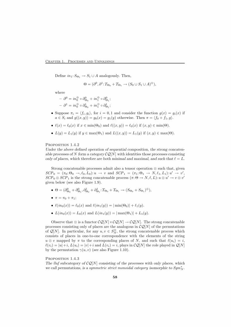
Chapter 1. Processes and Unfoldings
Define in1:SΘ1 → S1 ∪A analogously. Then,
Θ = (∂0, ∂1:TΘ0 + TΘ1 → (S0 ∪ S1 ∪A)⊕),
where
– ∂0 = in⊕0 ◦ ∂0Θ0
+ in⊕1 ◦ ∂0Θ1
;
– ∂1 = in⊕0 ◦ ∂1Θ0
+ in⊕1 ◦ ∂1Θ1
;
• Suppose πi = 〈fi, gi〉, for i = 0, 1 and consider the function g(x) = gi(x) ifa ∈ Si and g((x, y)) = g0(x) = g1(y) otherwise. Then π = 〈f0 + f1, g〉.
• ℓ(x) = ℓ0(x) if x ∈ min(Θ0) and ℓ((x, y)) = ℓ0(x) if (x, y) ∈ min(Θ).
• L(y) = L1(y) if y ∈ max(Θ1) and L((x, y)) = L1(y) if (x, y) ∈ max(Θ).
Proposition 1.4.2Under the above defined operation of sequential composition, the strong concaten-able processes ofN form a category CQ[N ] with identities those processes consistingonly of places, which therefore are both minimal and maximal, and such that ℓ = L.
Strong concatenable processes admit also a tensor operation ⊗ such that, givenSCP0 = (π0: Θ0 →, ℓ0, L0):u → v and SCP1 = (π1: Θ1 → N, ℓ1, L1):u
′ → v′,SCP0 ⊗ SCP1 is the strong concatenable process (π: Θ→ N, ℓ, L):u⊗ u′ → v ⊗ v′
given below (see also Figure 1.9).
• Θ = (∂0Θ0
+ ∂0Θ1, ∂1
Θ0+ ∂1
Θ1:TΘ0 + TΘ1 → (SΘ0 + SΘ1)
⊕),
• π = π0 + π1;
• ℓ(in0(x)) = ℓ0(x) and ℓ(in1(y)) = |min(Θ0)|+ ℓ1(y).
• L(in0(x)) = L0(x) and L(in1(y)) = |max(Θ1)|+ L1(y).
Observe that ⊗ is a functor CQ[N ]×CQ[N ]→ CQ[N ]. The strong concatenableprocesses consisting only of places are the analogous in CQ[N ] of the permutationsof Q[N ]. In particular, for any u, v ∈ S⊗N , the strong concatenable process whichconsists of places in one-to-one correspondence with the elements of the stringu ⊗ v mapped by π to the corresponding places of N , and such that ℓ(ui) = i,ℓ(vi) = |u|+ i, L(ui) = |v|+ i and L(vi) = i, plays in CQ[N ] the role played in Q[N ]by the permutation γ(u, v) (see also Figure 1.10).
Proposition 1.4.3The lluf subcategory of CQ[N ] consisting of the processes with only places, whichwe call permutations, is a symmetric strict monoidal category isomorphic to Sym∗N .
58
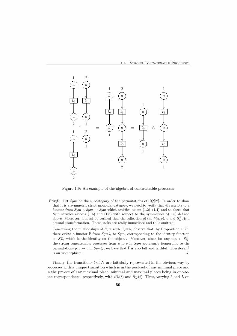
1.4. Strong Concatenable Processes
a a
t0 t1
a a
1'&$%��
2'&$%��� �� �
��
� �� ���
2
'&$%1
'&$%;
a a
t0
a
1'&$%��
2
1
'&$%� �� ���
2
'&$%=
a a
t0 t1
a a
t0
a
1'&$%��
2'&$%��� �� �
��
� �� ���
1
'&$%'&$%��� �� ���
2
'&$%=
a
t0
a
1'&$%��� �� ���
1
'&$% ⊗
a
t1
a
t0
a
1'&$%��� �� ���'&$%��� �� ���
1
'&$%Figure 1.9: An example of the algebra of concatenable processes
Proof. Let Sym be the subcategory of the permutations of CQ[N ]. In order to showthat it is a symmetric strict monoidal category, we need to verify that ⊗ restricts to afunctor from Sym × Sym → Sym which satisfies axiom (1.2)–(1.4) and to check thatSym satisfies axioms (1.5) and (1.6) with respect to the symmetries γ(u, v) definedabove. Moreover, it must be verified that the collection of the γ(u, v), u, v ∈ S⊗N , is anatural transformation. These tasks are really immediate and thus omitted.
Concerning the relationships of Sym with Sym∗N , observe that, by Proposition 1.3.6,
there exists a functor F from Sym∗N to Sym, corresponding to the identity function
on S⊗N , which is the identity on the objects. Moreover, since for any u, v ∈ S⊗N ,
the strong concatenable processes from u to v in Sym are clearly isomorphic to the
permutations p:u→ v in Sym∗N , we have that F is also full and faithful. Therefore, F
is an isomorphism. X
Finally, the transitions t of N are faithfully represented in the obvious way byprocesses with a unique transition which is in the post-set of any minimal place andin the pre-set of any maximal place, minimal and maximal places being in one-to-one correspondence, respectively, with ∂0
N (t) and ∂1N (t). Thus, varying ℓ and L on
59
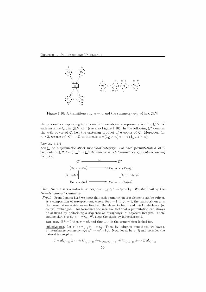
Chapter 1. Processes and Unfoldings
u1 · · · un
t
v1 · · · vm
1'&$%/////�� n'&$%�������� �� �������� ///// ��1
'&$%m
'&$% u1 · · · un v1 · · · vm
1
m+1
'&$% n
m+n
'&$%n+1
1
'&$% n+m
n
'&$%Figure 1.10: A transitions tu,v:u→ v and the symmetry γ(u, v) in CQ[N ]
the process corresponding to a transition we obtain a representative in CQ[N ] ofeach instance tu,v in Q[N ] of t (see also Figure 1.10). In the following Cn denotesthe n-th power of C, i.e., the cartesian product of n copies of C. Moreover, forn ≥ 2, we use ⊗n: Cn → C to indicate ⊗ ◦ (1C ×⊗) ◦ · · · ◦ (1Cn−2 ×⊗).
Lemma 1.4.4Let C be a symmetric strict monoidal category. For each permutation σ of nelements, n ≥ 2, let Fσ: C
n → Cn the functor which “swaps” is arguments accordingto σ, i.e.,
(x1, . . . , xn) (xσ(1), . . . , xσ(n))
(y1, . . . , yn) (yσ(1), . . . , yσ(n))
� //
(f1,...,fn)
��(fσ(1),...,fσ(n))
��� //
CnCnFσ //
Then, there exists a natural isomorphism γσ:⊗n�
→ ⊗n ◦ Fσ. We shall call γσ the“σ-interchange” symmetry.Proof. From Lemma 1.2.3 we know that each permutation of n elements can be written
as a composition of transpositions, where, for i = 1, . . . , n− 1, the transposition τi isthe permutation which leaves fixed all the elements but i and i + 1, which are (ofcourse) exchanged. This formalizes the intuitive fact that a permutation can alwaysbe achieved by performing a sequence of “swappings” of adjacent integers. Then,assume that σ is τik ◦ · · · ◦ τi1 . We show the thesis by induction on k.
base case. If k = 0 then σ = id , and thus 1⊗n is the isomorphism looked for.
inductive step. Let σ′ be τik−1 ◦ · · · ◦ τi1 . Then, by inductive hypothesis, we have aσ′-interchange symmetry γσ′ :⊗n → ⊗n ◦ Fσ′ . Now, let ik be σ′(i) and consider thenatural isomorphism
τ = idxσ′(1)⊗ · · · ⊗ idxσ′(i−1)
⊗ γxσ′(i),xσ′(i+1)⊗ idxσ′(i+2)
⊗ · · · ⊗ idxσ′(n)
60
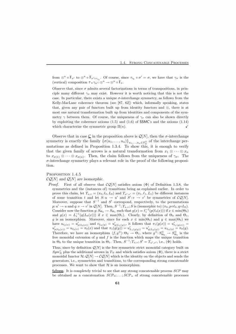
1.4. Strong Concatenable Processes
from ⊗n ◦ Fσ′ to ⊗n ◦ Fσ′◦τi1. Of course, since τik ◦ σ
′ = σ, we have that γσ is the
(vertical) composition τ � γσ′ :⊗n → ⊗n ◦ Fσ.
Observe that, since σ admits several factorizations in terms of transpositions, in prin-
ciple many different γσ may exist. However it is worth noticing that this is not the
case. In particular, there exists a unique σ-interchange symmetry, as follows from the
Kelly-MacLane coherence theorem (see [87, 62]) which, informally speaking, states
that, given any pair of functors built up from identity functors and ⊗, there is at
most one natural transformation built up from identities and components of the sym-
metry γ between them. Of course, the uniqueness of γσ can also be shown directly
by exploiting the coherence axioms (1.5) and (1.6) of SSMC’s and the axioms (1.14)
which characterize the symmetric group Π(n). X
Observe that in case C in the proposition above is Q[N ], then the σ-interchangesymmetry is exactly the family {σ(u1, . . . , un)}u1,...,un∈S
⊗
Nof the interchange per-
mutations as defined in Proposition 1.3.4. To show this, it is enough to verifythat the given family of arrows is a natural transformation from x1 ⊗ · · · ⊗ xnto xσ(1) ⊗ · · · ⊗ xσ(n). Then, the claim follows from the uniqueness of γσ. Theσ-interchange symmetry plays a relevant role in the proof of the following proposi-tion.
Proposition 1.4.5CQ[N ] and Q[N ] are isomorphic.
Proof. First of all observe that CQ[N ] satisfies axiom (Φ) of Definition 1.3.8, thesymmetries and the (instances of) transitions being as explained earlier. In order toprove this claim, let Tu,v = (π0, ℓ0, L0) and Tu′,v′ = (π1, ℓ1, L1) be different instancesof some transition t and let S: u → u′ and S′: v → v′ be symmetries of CQ[N ].Moreover, suppose that S−1 and S′ correspond, respectively, to the permutationsp:u′ → u and q: v → v′ in Q[N ]. Then, S−1;Tu,v;S is (isomorphic to) (π0, p◦ℓ0, q◦L0).Consider now the function g:SΘ0 → SΘ1 such that g(x) = ℓ−1
1 (p(ℓ0(x))) if x ∈ min(Θ0)and g(x) = L−1
1 (q(L0(x))) if x ∈ max(Θ1). Clearly, by definition of Θ0 and Θ1,g is an isomorphism. Moreover, since for each x ∈ min(Θ0) and y ∈ max(Θ0) wehave uℓ0(x) = u′p(ℓ0(x)) and vL0(y) = u′q(L1(y)), it follows that π1(g(x)) = u′ℓ1(g(x)) =u′p(ℓ0(x)) = uℓ0(x) = π0(x) and that π1(g(y)) = u′L1(g(y)) = u′q(L0(y)) = uL0(y) = π0(y).
Therefore, we have an isomorphism 〈f, g⊗〉: Θ0 → Θ1, where g⊗:S⊗Θ0→ S⊗Θ1
is thefree monoidal extension of g and f is the function which maps the unique transitionin Θ0 to the unique transition in Θ1. Then, S−1;Tu,v;S
′ = Tu′,v′ , i.e., (Φ) holds.
Thus, since by definition Q[N ] is the free symmetric strict monoidal category built onSym∗N plus the additional arrows in TN and which satisfies axiom (Φ), there is a strictmonoidal functor H:Q[N ]→ CQ[N ] which is the identity on the objects and sends thegenerators, i.e., symmetries and transitions, to the corresponding strong concatenableprocesses. We want to show that H is an isomorphism.
fullness. It is completely trivial to see that any strong concatenable process SCP maybe obtained as a concatenation SCP0; . . . ;SCPn of strong concatenable processes
61
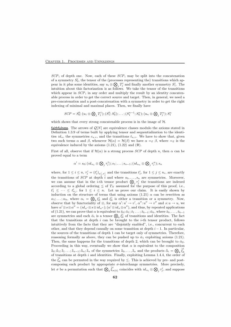
Chapter 1. Processes and Unfoldings
SCP i of depth one. Now, each of these SCP i may be split into the concatenationof a symmetry Si0, the tensor of the (processes representing the) transitions which ap-pear in it plus some identities, say ui ⊗
⊗jT ij and finally another symmetry Si1. The
intuition about this factorization is as follows. We take the tensor of the transitionswhich appear in SCP i in any order and multiply the result by an identity concaten-able process in order to get the correct source and target. Then, in general, we need apre-concatenation and a post-concatenation with a symmetry in order to get the rightindexing of minimal and maximal places. Then, we finally have
SCP = S00 ; (u1 ⊗
⊗jT 1j ); (S0
1 ;S10); . . . ; (Sn−1
1 ;Sn0 ); (un ⊗⊗
jTnj );Sn1
which shows that every strong concatenable process is in the image of H.
faithfulness. The arrows of Q[N ] are equivalence classes modulo the axioms stated inDefinition 1.3.9 of terms built by applying tensor and sequentialization to the identi-ties idu, the symmetries cu,v, and the transitions tu,v. We have to show that, giventwo such terms α and β, whenever H(α) = H(β) we have α =E β, where =E is theequivalence induced by the axioms (1.21), (1.22) and (Φ).
First of all, observe that if H(α) is a strong process SCP of depth n, then α can beproved equal to a term
α′ = s0; (idu1 ⊗⊗
jτ 1j ); s1; . . . ; sn−1; (idun ⊗
⊗jτnj ); sn
where, for 1 ≤ i ≤ n, τ ij = (tij)uij,vi
jand the transitions tij , for 1 ≤ j ≤ ni, are exactly
the transitions of SCP at depth i and where s0, . . . , sn are symmetries. Moreover,we can assume that in the i-th tensor product
⊗jτ ij the transitions are indexed
according to a global ordering ≤ of TN assumed for the purpose of this proof, i.e.,ti1 ≤ · · · ≤ tini
, for 1 ≤ i ≤ n. Let us prove our claim. It is easily shown byinduction on the structure of terms that using axioms (1.21) α can be rewritten asα1; . . . ;αh, where αi =
⊗kξik and ξik is either a transition or a symmetry. Now,
observe that by functoriality of ⊗, for any α′:u′ → v′, α′′:u′′ → v′′ and s:u→ u, wehave α′⊗s⊗α′′ = (idu′⊗s⊗ idu′′); (α′⊗ idu⊗α
′′), and thus, by repeated applicationsof (1.21), we can prove that α is equivalent to s0; α1; s1 . . . ; sh−1; αh, where s0, . . . , sh−1
are symmetries and each αi is a tensor⊗
kξik of transitions and identities. The fact
that the transitions at depth i can be brought to the i-th tensor product, followsintuitively from the facts that they are “disjointly enabled”, i.e., concurrent to eachother, and that they depend causally on some transition at depth i− 1. In particular,the sources of the transitions of depth 1 can be target only of symmetries. Therefore,reasoning formally as above, they can be pushed up to α1 exploiting axioms (1.21).Then, the same happens for the transitions of depth 2, which can be brought to α2.Proceeding in this way, eventually we show that α is equivalent to the composition
¯s0; ¯α1; ¯s1 . . . ; ¯sn−1; ¯αn; ¯sn of the symmetries ¯s0, . . . , ¯sn and the products ¯αi =⊗
k¯ξi
k
of transitions at depth i and identities. Finally, exploiting Lemma 1.4.4, the order of
the ¯ξi
k can be permuted in the way required by ≤. This is achieved by pre- and post-composing each product by appropriate σ-interchange symmetries. More precisely,
let σ be a permutation such that⊗
k¯ξi
σ(k) coincides with idui ⊗⊗
jτ ij , and suppose
62
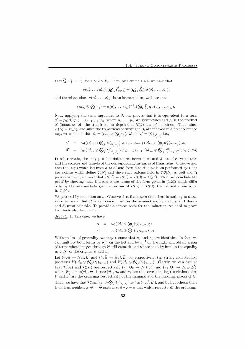
1.4. Strong Concatenable Processes
that ¯ξi
k:uik → vik, for 1 ≤ k ≤ ki. Then, by Lemma 1.4.4, we have that
σ(ui1, . . . , uiki
); (⊗
k¯ξi
σ(k)) = (⊗
k¯ξi
k);σ(vi1, . . . , viki
),
and therefore, since σ(ui1, . . . , uiki
) is an isomorphism, we have that
(idui ⊗⊗
jτ ij) = σ(ui1, . . . , u
iki
)−1; (⊗
k¯ξi
k);σ(vi1, . . . , viki
).
Now, applying the same argument to β, one proves that it is equivalent to a termβ′ = p0;β0; p1; . . . pn−1;βn; pn, where p0, . . . , pn are symmetries and βi is the productof (instances of) the transitions at depth i in H(β) and of identities. Then, sinceH(α) = H(β), and since the transitions occurring in βi are indexed in a predeterminedway, we conclude that βi = (idui ⊗
⊗jτ ij ), where τ ij = (tij)ui
j,vi
ji.e.,
α′ = s0; (idu1 ⊗⊗
j(t1j)u1
j,v1
j); s1; . . . ; sn−1; (idun ⊗
⊗j(tnj )un
j,vn
j); sn
β′ = p0; (idu1 ⊗⊗
j(t1j )u1
j,v1
j); p1; . . . ; pn−1; (idun ⊗
⊗j(tnj )un
j,vn
j); pn (1.23)
In other words, the only possible differences between α′ and β′ are the symmetriesand the sources and targets of the corresponding instances of transitions. Observe nowthat the steps which led from α to α′ and from β to β′ have been performed by usingthe axioms which define Q[N ] and since such axioms hold in CQ[N ] as well and Hpreserves them, we have that H(α′) = H(α) = H(β) = H(β′). Thus, we conclude theproof by showing that, if α and β are terms of the form given in (1.23) which differonly by the intermediate symmetries and if H(α) = H(β), then α and β are equalin Q[N ].
We proceed by induction on n. Observe that if n is zero then there is nothing to show:since we know that H is an isomorphism on the symmetries, s0 and p0, and thus αand β, must coincide. To provide a correct basis for the induction, we need to provethe thesis also for n = 1.
depth 1. In this case, we have
α = s0; (idu ⊗⊗
j(tj)uj ,vj ); s1
β = p0; (idu ⊗⊗
j(tj)uj,vj ); p1.
Without loss of generality, we may assume that p0 and p1 are identities. In fact, wecan multiply both terms by p−1
0 on the left and by p−11 on the right and obtain a pair
of terms whose images through H still coincide and whose equality implies the equalityin Q[N ] of the original α and β.
Let (π: Θ → N, ℓ, L) and (π: Θ → N, ℓ, L) be, respectively, the strong concatenableprocesses H(idu ⊗
⊗j(tj)uj ,vj ) and H(idu ⊗
⊗j(tj)uj ,vj ). Clearly, we can assume
that H(s0) and H(s1) are respectively (π0: Θ0 → N, ℓ′, ℓ) and (π1: Θ1 → N,L, L′),where Θ0 is min(Θ), Θ1 is max(Θ), π0 and π1 are the corresponding restrictions of π,ℓ′ and L′ are the orderings respectively of the minimal and the maximal places of Θ.
Then, we have that H(s0; (idu⊗⊗
j(tj)uj,vj ); s1) is (π, ℓ′, L′), and by hypothesis there
is an isomorphism ϕ: Θ→ Θ such that π ◦ϕ = π and which respects all the orderings,
63
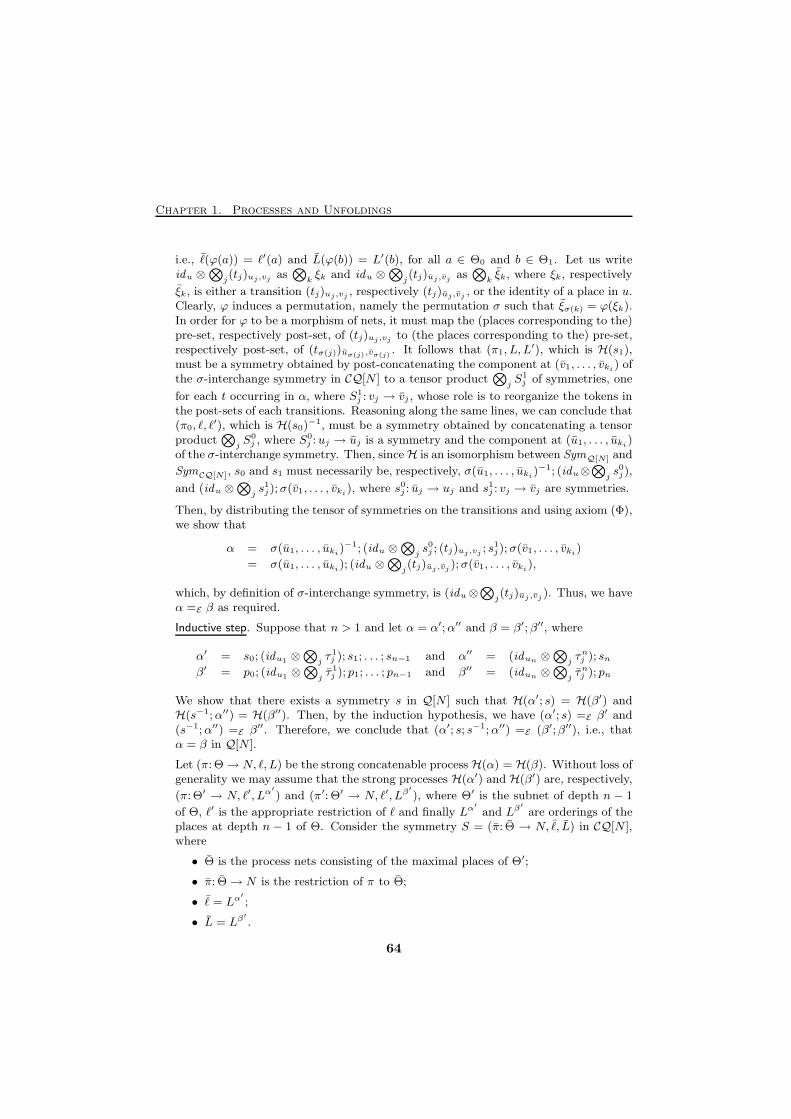
Chapter 1. Processes and Unfoldings
i.e., ℓ(ϕ(a)) = ℓ′(a) and L(ϕ(b)) = L′(b), for all a ∈ Θ0 and b ∈ Θ1. Let us writeidu ⊗
⊗j(tj)uj,vj as
⊗kξk and idu ⊗
⊗j(tj)uj,vj as
⊗kξk, where ξk, respectively
ξk, is either a transition (tj)uj,vj , respectively (tj)uj,vj , or the identity of a place in u.Clearly, ϕ induces a permutation, namely the permutation σ such that ξσ(k) = ϕ(ξk).In order for ϕ to be a morphism of nets, it must map the (places corresponding to the)pre-set, respectively post-set, of (tj)uj,vj to (the places corresponding to the) pre-set,respectively post-set, of (tσ(j))uσ(j),vσ(j)
. It follows that (π1, L, L′), which is H(s1),
must be a symmetry obtained by post-concatenating the component at (v1, . . . , vki) of
the σ-interchange symmetry in CQ[N ] to a tensor product⊗
jS1j of symmetries, one
for each t occurring in α, where S1j : vj → vj , whose role is to reorganize the tokens in
the post-sets of each transitions. Reasoning along the same lines, we can conclude that(π0, ℓ, ℓ
′), which is H(s0)−1, must be a symmetry obtained by concatenating a tensor
product⊗
jS0j , where S0
j :uj → uj is a symmetry and the component at (u1, . . . , uki)
of the σ-interchange symmetry. Then, sinceH is an isomorphism between SymQ[N] and
SymCQ[N], s0 and s1 must necessarily be, respectively, σ(u1, . . . , uki)−1; (idu⊗
⊗js0j),
and (idu ⊗⊗
js1j);σ(v1, . . . , vki
), where s0j : uj → uj and s1j : vj → vj are symmetries.
Then, by distributing the tensor of symmetries on the transitions and using axiom (Φ),we show that
α = σ(u1, . . . , uki)−1; (idu ⊗
⊗js0j ; (tj)uj ,vj ; s
1j);σ(v1, . . . , vki
)
= σ(u1, . . . , uki); (idu ⊗
⊗j(tj)uj ,vj );σ(v1, . . . , vki
),
which, by definition of σ-interchange symmetry, is (idu⊗⊗
j(tj)uj ,vj ). Thus, we have
α =E β as required.
Inductive step. Suppose that n > 1 and let α = α′;α′′ and β = β′;β′′, where
α′ = s0; (idu1 ⊗⊗
jτ 1j ); s1; . . . ; sn−1 and α′′ = (idun ⊗
⊗jτnj ); sn
β′ = p0; (idu1 ⊗⊗
jτ 1j ); p1; . . . ; pn−1 and β′′ = (idun ⊗
⊗jτnj ); pn
We show that there exists a symmetry s in Q[N ] such that H(α′; s) = H(β′) andH(s−1;α′′) = H(β′′). Then, by the induction hypothesis, we have (α′; s) =E β
′ and(s−1;α′′) =E β
′′. Therefore, we conclude that (α′; s; s−1;α′′) =E (β′;β′′), i.e., thatα = β in Q[N ].
Let (π: Θ→ N, ℓ, L) be the strong concatenable process H(α) = H(β). Without loss ofgenerality we may assume that the strong processes H(α′) and H(β′) are, respectively,
(π: Θ′ → N, ℓ′, Lα′
) and (π′: Θ′ → N, ℓ′, Lβ′
), where Θ′ is the subnet of depth n − 1
of Θ, ℓ′ is the appropriate restriction of ℓ and finally Lα′
and Lβ′
are orderings of theplaces at depth n − 1 of Θ. Consider the symmetry S = (π: Θ → N, ℓ, L) in CQ[N ],where
• Θ is the process nets consisting of the maximal places of Θ′;
• π: Θ→ N is the restriction of π to Θ;
• ℓ = Lα′
;
• L = Lβ′
.
64
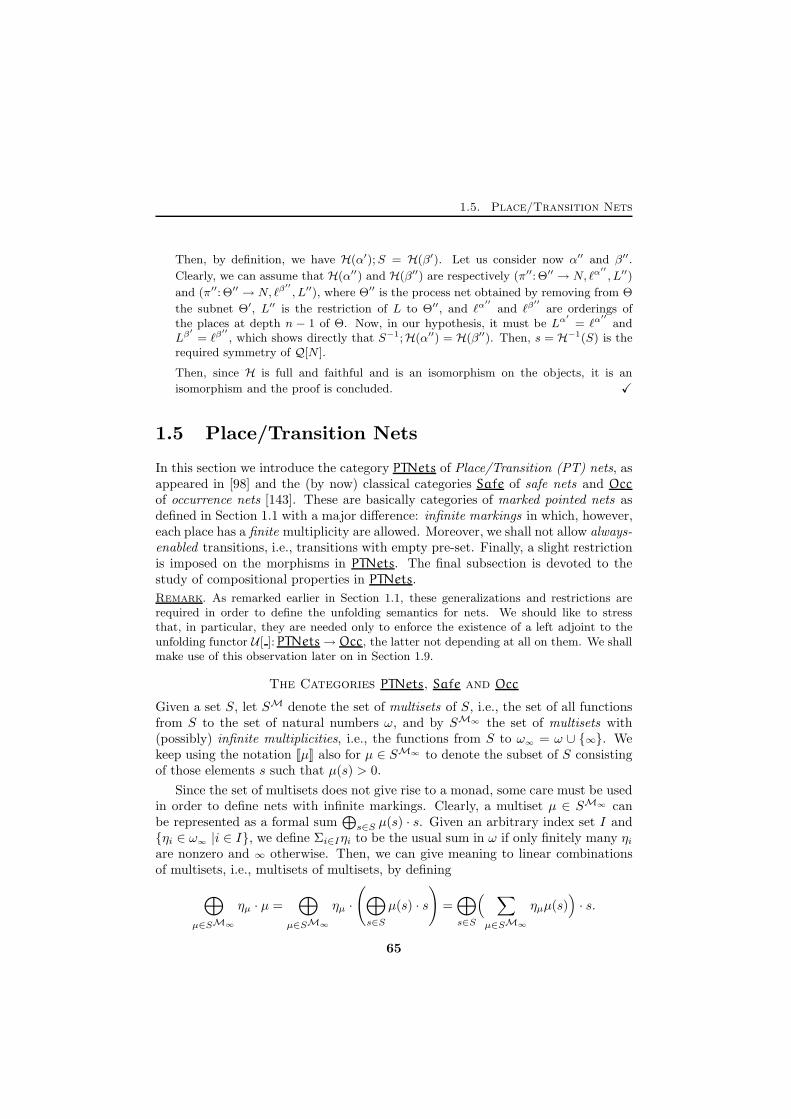
1.5. Place/Transition Nets
Then, by definition, we have H(α′);S = H(β′). Let us consider now α′′ and β′′.
Clearly, we can assume that H(α′′) and H(β′′) are respectively (π′′: Θ′′ → N, ℓα′′
, L′′)
and (π′′: Θ′′ → N, ℓβ′′
, L′′), where Θ′′ is the process net obtained by removing from Θ
the subnet Θ′, L′′ is the restriction of L to Θ′′, and ℓα′′
and ℓβ′′
are orderings ofthe places at depth n − 1 of Θ. Now, in our hypothesis, it must be Lα
′
= ℓα′′
andLβ
′
= ℓβ′′
, which shows directly that S−1;H(α′′) = H(β′′). Then, s = H−1(S) is therequired symmetry of Q[N ].
Then, since H is full and faithful and is an isomorphism on the objects, it is an
isomorphism and the proof is concluded. X
1.5 Place/Transition Nets
In this section we introduce the category PTNets of Place/Transition (PT) nets, asappeared in [98] and the (by now) classical categories Safe of safe nets and Occ
of occurrence nets [143]. These are basically categories of marked pointed nets asdefined in Section 1.1 with a major difference: infinite markings in which, however,each place has a finite multiplicity are allowed. Moreover, we shall not allow always-enabled transitions, i.e., transitions with empty pre-set. Finally, a slight restrictionis imposed on the morphisms in PTNets. The final subsection is devoted to thestudy of compositional properties in PTNets.
Remark. As remarked earlier in Section 1.1, these generalizations and restrictions arerequired in order to define the unfolding semantics for nets. We should like to stressthat, in particular, they are needed only to enforce the existence of a left adjoint to theunfolding functor U [ ]:PTNets→ Occ, the latter not depending at all on them. We shallmake use of this observation later on in Section 1.9.
The Categories PTNets, Safe and Occ
Given a set S, let SM denote the set of multisets of S, i.e., the set of all functionsfrom S to the set of natural numbers ω, and by SM∞ the set of multisets with(possibly) infinite multiplicities, i.e., the functions from S to ω∞ = ω ∪ {∞}. Wekeep using the notation [[µ]] also for µ ∈ SM∞ to denote the subset of S consistingof those elements s such that µ(s) > 0.
Since the set of multisets does not give rise to a monad, some care must be usedin order to define nets with infinite markings. Clearly, a multiset µ ∈ SM∞ canbe represented as a formal sum
⊕s∈S µ(s) · s. Given an arbitrary index set I and
{ηi ∈ ω∞ |i ∈ I}, we define Σi∈Iηi to be the usual sum in ω if only finitely many ηiare nonzero and ∞ otherwise. Then, we can give meaning to linear combinationsof multisets, i.e., multisets of multisets, by defining
⊕
µ∈SM∞
ηµ · µ =⊕
µ∈SM∞
ηµ ·
(⊕
s∈S
µ(s) · s
)=⊕
s∈S
( ∑
µ∈SM∞
ηµµ(s))· s.
65
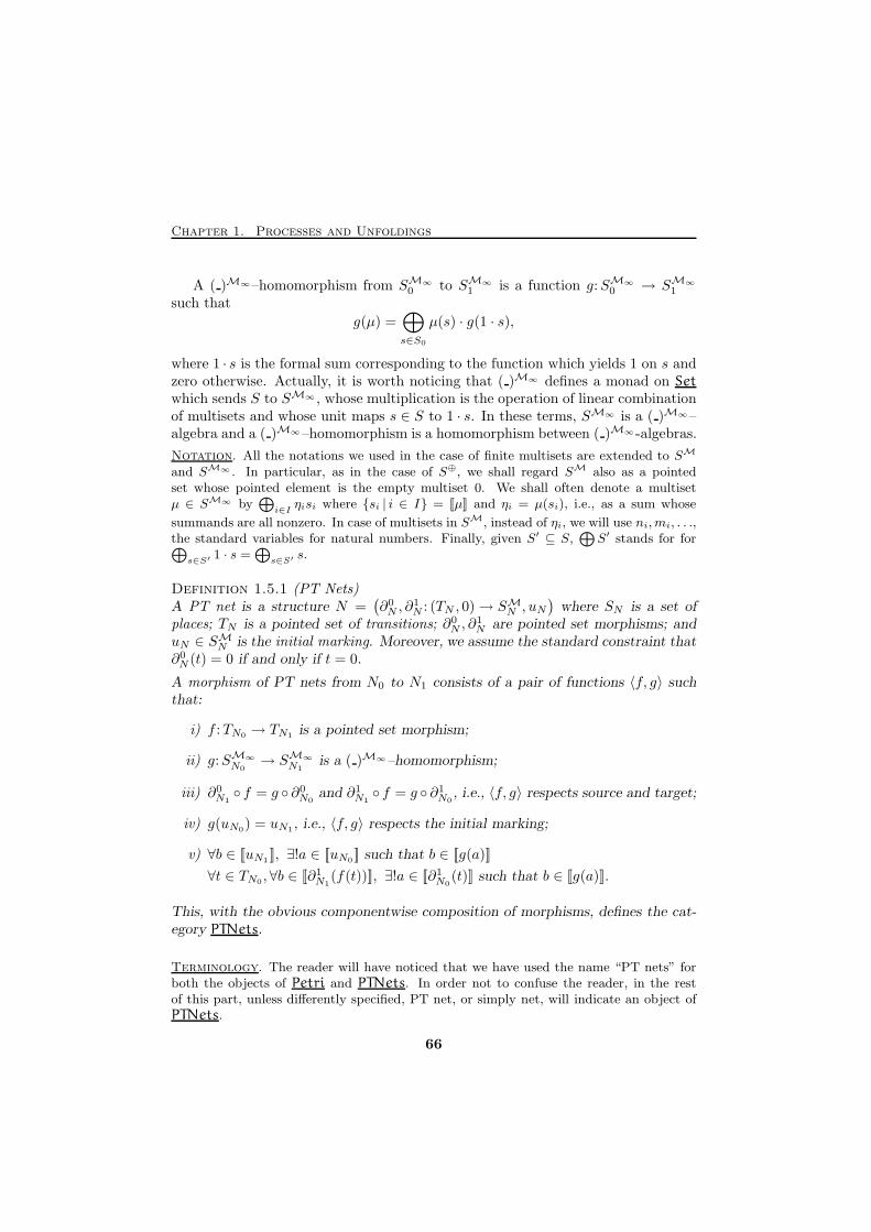
Chapter 1. Processes and Unfoldings
A ( )M∞–homomorphism from SM∞
0 to SM∞
1 is a function g:SM∞
0 → SM∞
1
such that
g(µ) =⊕
s∈S0
µ(s) · g(1 · s),
where 1 · s is the formal sum corresponding to the function which yields 1 on s andzero otherwise. Actually, it is worth noticing that ( )M∞ defines a monad on Set
which sends S to SM∞ , whose multiplication is the operation of linear combinationof multisets and whose unit maps s ∈ S to 1 · s. In these terms, SM∞ is a ( )M∞–algebra and a ( )M∞–homomorphism is a homomorphism between ( )M∞ -algebras.
Notation. All the notations we used in the case of finite multisets are extended to SM
and SM∞ . In particular, as in the case of S⊕, we shall regard SM also as a pointedset whose pointed element is the empty multiset 0. We shall often denote a multisetµ ∈ SM∞ by
⊕i∈I
ηisi where {si | i ∈ I} = [[µ]] and ηi = µ(si), i.e., as a sum whose
summands are all nonzero. In case of multisets in SM, instead of ηi, we will use ni,mi, . . .,the standard variables for natural numbers. Finally, given S′ ⊆ S,
⊕S′ stands for for⊕
s∈S′ 1 · s =⊕
s∈S′ s.
Definition 1.5.1 (PT Nets)A PT net is a structure N =
(∂0N , ∂
1N : (TN , 0)→ SMN , uN
)where SN is a set of
places; TN is a pointed set of transitions; ∂0N , ∂
1N are pointed set morphisms; and
uN ∈ SMN is the initial marking. Moreover, we assume the standard constraint that∂0N (t) = 0 if and only if t = 0.
A morphism of PT nets from N0 to N1 consists of a pair of functions 〈f, g〉 suchthat:
i) f :TN0 → TN1 is a pointed set morphism;
ii) g:SM∞
N0→ SM∞
N1is a ( )M∞–homomorphism;
iii) ∂0N1◦ f = g ◦ ∂0
N0and ∂1
N1◦ f = g ◦ ∂1
N0, i.e., 〈f, g〉 respects source and target;
iv) g(uN0) = uN1, i.e., 〈f, g〉 respects the initial marking;
v) ∀b ∈ [[uN1 ]], ∃!a ∈ [[uN0 ]] such that b ∈ [[g(a)]]
∀t ∈ TN0, ∀b ∈ [[∂1N1
(f(t))]], ∃!a ∈ [[∂1N0
(t)]] such that b ∈ [[g(a)]].
This, with the obvious componentwise composition of morphisms, defines the cat-egory PTNets.
Terminology. The reader will have noticed that we have used the name “PT nets” forboth the objects of Petri and PTNets. In order not to confuse the reader, in the restof this part, unless differently specified, PT net, or simply net, will indicate an object ofPTNets.
66
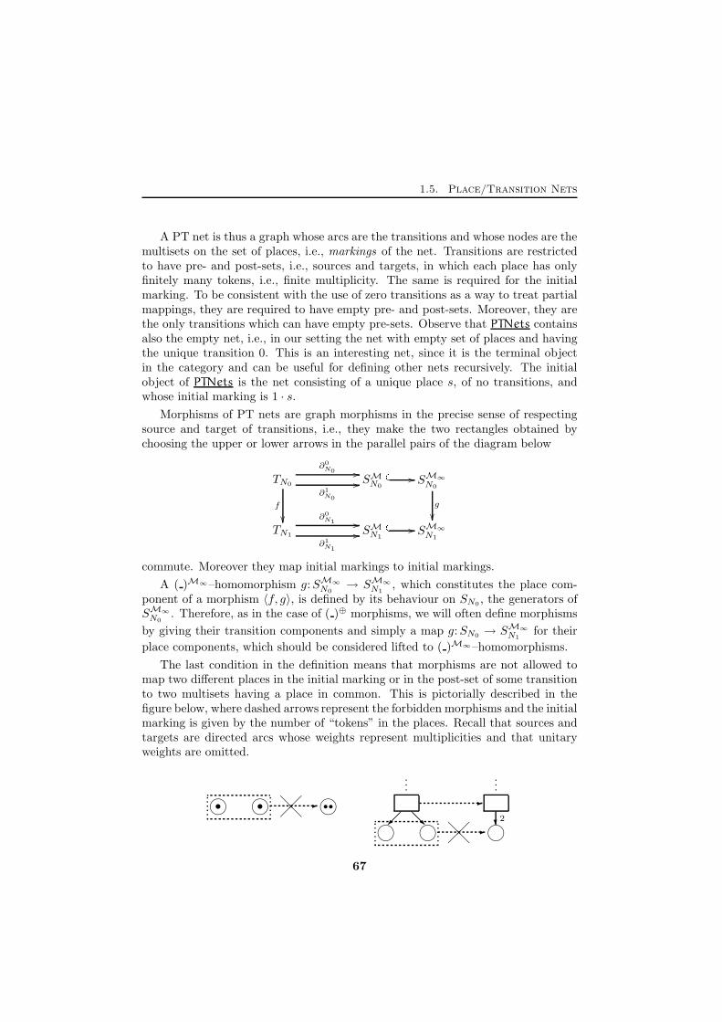
1.5. Place/Transition Nets
A PT net is thus a graph whose arcs are the transitions and whose nodes are themultisets on the set of places, i.e., markings of the net. Transitions are restrictedto have pre- and post-sets, i.e., sources and targets, in which each place has onlyfinitely many tokens, i.e., finite multiplicity. The same is required for the initialmarking. To be consistent with the use of zero transitions as a way to treat partialmappings, they are required to have empty pre- and post-sets. Moreover, they arethe only transitions which can have empty pre-sets. Observe that PTNets containsalso the empty net, i.e., in our setting the net with empty set of places and havingthe unique transition 0. This is an interesting net, since it is the terminal objectin the category and can be useful for defining other nets recursively. The initialobject of PTNets is the net consisting of a unique place s, of no transitions, andwhose initial marking is 1 · s.
Morphisms of PT nets are graph morphisms in the precise sense of respectingsource and target of transitions, i.e., they make the two rectangles obtained bychoosing the upper or lower arrows in the parallel pairs of the diagram below
TN0 SMN0SM∞
N0
TN1 SMN1SM∞
N1
f
��
∂0N0 //
∂1N0
//�o //
g
��∂0N1 //
∂1N1
//�o //
commute. Moreover they map initial markings to initial markings.
A ( )M∞–homomorphism g:SM∞
N0→ SM∞
N1, which constitutes the place com-
ponent of a morphism 〈f, g〉, is defined by its behaviour on SN0 , the generators ofSM∞
N0. Therefore, as in the case of ( )⊕ morphisms, we will often define morphisms
by giving their transition components and simply a map g:SN0 → SM∞
N1for their
place components, which should be considered lifted to ( )M∞–homomorphisms.
The last condition in the definition means that morphisms are not allowed tomap two different places in the initial marking or in the post-set of some transitionto two multisets having a place in common. This is pictorially described in thefigure below, where dashed arrows represent the forbidden morphisms and the initialmarking is given by the number of “tokens” in the places. Recall that sources andtargets are directed arcs whose weights represent multiplicities and that unitaryweights are omitted.
l l-@@�� l l l
l��
-
@@R ?-@
@��
......
2
• • ••
67
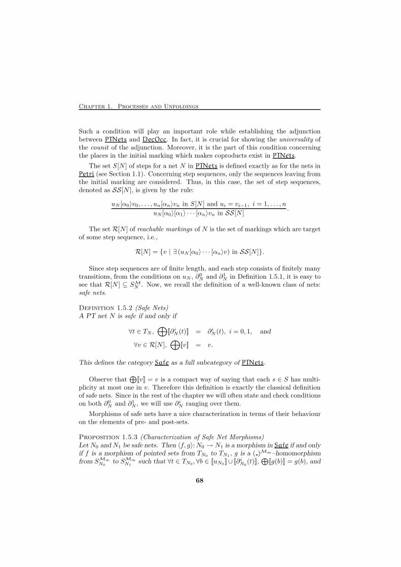
Chapter 1. Processes and Unfoldings
Such a condition will play an important role while establishing the adjunctionbetween PTNets and DecOcc. In fact, it is crucial for showing the universality ofthe counit of the adjunction. Moreover, it is the part of this condition concerningthe places in the initial marking which makes coproducts exist in PTNets.
The set S [N ] of steps for a net N in PTNets is defined exactly as for the nets inPetri (see Section 1.1). Concerning step sequences, only the sequences leaving fromthe initial marking are considered. Thus, in this case, the set of step sequences,denoted as SS[N ], is given by the rule:
uN [α0〉v0, . . . , un[αn〉vn in S [N ] and ui = vi−1, i = 1, . . . , n
uN [α0〉[α1〉 · · · [αn〉vn in SS[N ].
The set R[N ] of reachable markings of N is the set of markings which are targetof some step sequence, i.e.,
R[N ] = {v | ∃ (uN [α0〉 · · · [αn〉v) in SS[N ]}.
Since step sequences are of finite length, and each step consists of finitely manytransitions, from the conditions on uN , ∂0
N and ∂1N in Definition 1.5.1, it is easy to
see that R[N ] ⊆ SMN . Now, we recall the definition of a well-known class of nets:safe nets.
Definition 1.5.2 (Safe Nets)A PT net N is safe if and only if
∀t ∈ TN ,⊕
[[∂iN (t)]] = ∂iN (t), i = 0, 1, and
∀v ∈ R[N ],⊕
[[v]] = v.
This defines the category Safe as a full subcategory of PTNets.
Observe that⊕
[[v]] = v is a compact way of saying that each s ∈ S has multi-plicity at most one in v. Therefore this definition is exactly the classical definitionof safe nets. Since in the rest of the chapter we will often state and check conditionson both ∂0
N and ∂1N , we will use ∂iN ranging over them.
Morphisms of safe nets have a nice characterization in terms of their behaviouron the elements of pre- and post-sets.
Proposition 1.5.3 (Characterization of Safe Net Morphisms)LetN0 andN1 be safe nets. Then 〈f, g〉:N0 → N1 is a morphism in Safe if and onlyif f is a morphism of pointed sets from TN0 to TN1 , g is a ( )M∞–homomorphismfrom SM∞
N0to SM∞
N1such that ∀t ∈ TN0, ∀b ∈ [[uN0 ]]∪ [[∂iN0
(t)]],⊕
[[g(b)]] = g(b), and
68
1.5. Place/Transition Nets
i) [[g(uN0)]] ⊆ [[uN1 ]] and ∀b1 ∈ [[uN1 ]], ∃!b0 ∈ [[uN0 ]] such that b1 ∈ [[g(b0)]];
ii) ∀t ∈ TN0, [[g(∂iN0(t))]] ⊆ [[∂iN1
(f(t))]] and
∀b1 ∈ [[∂iN1(f(t))]], ∃!b0 ∈ [[∂iN0
(t)]] such that b1 ∈ [[g(b0)]].
Proof. (⇒) The proof is completely trivial, but observe that there is no need to usecondition (v) in the definition of PT net morphisms: in fact if there were b1 in [[uN1 ]]or [[∂iN1
(f(t))]] and b, b′ respectively in [[uN0 ]] or [[∂iN0(t)]] such that b1 ∈ [[g(b)]]∩ [[g(b′)]],
by definition of morphism, it would be g(uN0)(b1) = uN1(b1) ≥ 2 or g(∂iN0(t))(b1) =
∂iN1(f(t))(b1) ≥ 2. But this is impossible, since N1 is a safe net.
(⇐) Conditions (i), (ii) and (v) in the definition of PT net morphisms are alreadypresent. Points (i) and (ii) above imply that
[[uN1 ]] =⋃{ [[g(a)]] | a ∈ [[uN0 ]]} and [[∂iN1
(f(t))]] =⋃{
[[g(a)]] | a ∈ [[∂iN0(t)]]}.
Now, since⊕
[[g(a)]] = g(a) and all the [[g(a)]] in the unions are disjoint, we obtain
g(uN0) = uN1 and g(∂iN0(t)) = ∂iN1
(f(t)). X
Corollary 1.5.4 (Correspondence with Winskel’s Safe Nets)Winskel’s category of safe nets [143], called Net, is a full subcategory of Safe.
Proof. The conditions given in the above proposition are a characterization of mor-
phisms in Net [143, Proposition 3.1.9], while the objects in Safe strictly contain
the objects in Net. In fact, the objects of Net are the objects of Safe with sets
of places, initial markings and post-sets which are non-empty, and without isolated
places—places belonging neither to the initial marking nor to the pre- or post-set of
any transition. X
Since in the proof of Proposition 1.5.3 the demonstration of the ⇒ implicationnever used the fifth axiom of PT net morphisms, we have shown an easier charac-terization of morphisms between safe nets: 〈f, g〉:N0 → N1 is a morphism in Safe
between the safe nets N0 and N1 if and only if conditions (i), (ii), (iii) and (iv) ofDefinition 1.5.1 hold, i.e., condition (v) is already implied by the structure of safenets.
Another important class of nets is that of occurrence nets. They are safe netswith a nice stratified structure whose minimal element constitute the initial mark-ing. The definition is very close to that of process nets, the difference being thathere we allow “forward branching”, i.e., non-determinism.
Definition 1.5.5 (Occurrence Nets)A occurrence net is a safe net Θ such that
i) a ∈ [[uΘ]] if and only if •a = ∅;
69
Chapter 1. Processes and Unfoldings
ii) for all a ∈ SΘ, |•a| ≤ 1, where | | gives the cardinality of sets;
iii) ≺ is irreflexive, where ≺ is the transitive closure of the relation
≺1= {(a, t) | a ∈ SΘ, t ∈ TΘ, t ∈ a•} ∪ {(t, a) | a ∈ SΘ, t ∈ TΘ, t ∈
•a};
moreover, for all t ∈ TΘ, {t′ ∈ TΘ | t′ ≺ t} is finite;
iv) the binary “conflict” relation # on TΘ ∪ SΘ is irreflexive, where
∀t1, t2 ∈ TΘ, t1 #m t2 ⇔ [[∂0Θ(t1)]] ∩ [[∂0
Θ(t2)]] 6= ∅ and t1 6= t2,
∀x, y ∈ TΘ ∪ SΘ, x # y ⇔ ∃t1, t2 ∈ TΘ : t1 #m t2 and t1 4 x and t2 4 y,
where 4 is the reflexive closure of ≺.
This defines the category Occ as a full subcategory of Safe.
From Definition 1.5.5 and Corollary 1.5.4, it is immediate to see that Winskel’scategory of occurrence nets [143], here called OccW , is a full subcategory of Occ.However, since all the results in [143] easily extend to Safe and Occ, in the followingwe will ignore any difference between Safe and Net and between Occ and OccW .
Composition of PT Nets
Products and coproducts are importante constructions for nets, and generally incategories of models for concurrency, due to their natural role, respectively, in theoperations of parallel and non-deterministic composition [144]. In this section, weshow that the category PTNets has both products and coproducts and, studyingthe relationships between the computations of the composed nets and those of theoriginal nets, we clarify in what sense products and coproducts are related to theoperations of parallel and non-deterministic composition.
While in the categories of safe nets and of occurrence nets products and coprod-ucts exist [144], the category of PT nets with initial markings introduced in [144]has products but does not have coproducts. In [97], it is shown that coproductsexist in the full subcategory of PT nets whose initial markings are sets rather thanmultisets. However, due to the additional condition (v) in Definition 1.5.1, we canprove the existence of coproducts of any pair of objects in PTNets.
Given the PT nets N0 and N1, we define
N0 ×N1 =(∂0N0× ∂0
N1, ∂1N0× ∂1
N1: (TN0 × TN1 , (0, 0))→ SMN0
× SMN1, (uN0 , uN1)
).
Since SMN0×SMN1
∼= (SN0 +SN1)M, and SM∞
N0×SM∞
N1
∼= (SN0 +SN1)M∞ ∼= SM∞
N0⊕
SM∞
N1, where + is the disjoint union of sets and ⊕ the coproduct in the category
of multisets (with possibly infinite multiplicities) and ( )M∞–homomorphisms, wehave that N0 ×N1 is indeed a net with places SN0 + SN1 .
70
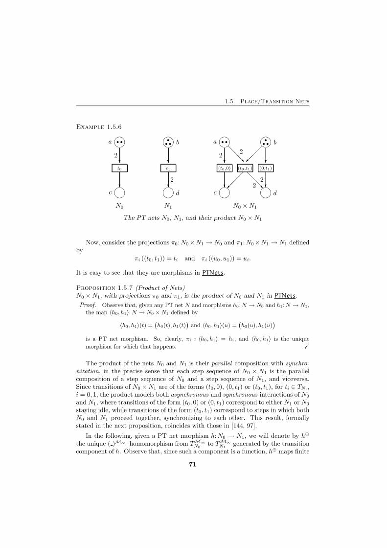
1.5. Place/Transition Nets
Example 1.5.6
� ��
� ��
� ��
� ��
� ��
� ��
� ��
� ��?
?
?
?
?
?
?
?
@@@R
���
���
@@@R
N0 N1 N0 ×N1
2
2
2
22
2
t0 (t0,0)t1 (0,t1)(t0,t1)
• • •• • • • •
• •a b a b
c d c d
The PT nets N0, N1, and their product N0 ×N1
Now, consider the projections π0:N0×N1 → N0 and π1:N0×N1 → N1 definedby
πi ((t0, t1)) = ti and πi ((u0, u1)) = ui.
It is easy to see that they are morphisms in PTNets.
Proposition 1.5.7 (Product of Nets)N0 ×N1, with projections π0 and π1, is the product of N0 and N1 in PTNets.
Proof. Observe that, given any PT net N and morphisms h0:N → N0 and h1:N → N1,the map 〈h0, h1〉:N → N0 ×N1 defined by
〈h0, h1〉(t) =(h0(t), h1(t)
)and 〈h0, h1〉(u) =
(h0(u), h1(u)
)
is a PT net morphism. So, clearly, πi ◦ 〈h0, h1〉 = hi, and 〈h0, h1〉 is the unique
morphism for which that happens. X
The product of the nets N0 and N1 is their parallel composition with synchro-nization, in the precise sense that each step sequence of N0 × N1 is the parallelcomposition of a step sequence of N0 and a step sequence of N1, and viceversa.Since transitions of N0 ×N1 are of the forms (t0, 0), (0, t1) or (t0, t1), for ti ∈ TNi
,i = 0, 1, the product models both asynchronous and synchronous interactions of N0
and N1, where transitions of the form (t0, 0) or (0, t1) correspond to either N1 or N0
staying idle, while transitions of the form (t0, t1) correspond to steps in which bothN0 and N1 proceed together, synchronizing to each other. This result, formallystated in the next proposition, coincides with those in [144, 97].
In the following, given a PT net morphism h:N0 → N1, we will denote by h⊕
the unique ( )M∞–homomorphism from TM∞
N0to TM∞
N1generated by the transition
component of h. Observe that, since such a component is a function, h⊕ maps finite
71
Chapter 1. Processes and Unfoldings
multisets to finite multisets. In particular, h⊕ can be defined on such multisetssimply by:
h⊕(t) = h(t) and h⊕(α ⊕ β) = h⊕(α)⊕ h⊕(β).
Proposition 1.5.8 (Product and Parallel Composition)The sequence uN0×N1 [α0〉 · · · [αn〉v belongs to SS[N0×N1] if and only if, for i = 0, 1,the sequence πi(uN0×N1)[π
⊕i (α0)〉 · · · [π
⊕i (αn)〉πi(v) belongs to SS[Ni].
Therefore, v ∈ R[N0 ×N1] if and only if πi(v) ∈ R[Ni] for i = 0, 1.
Proof. It suffices to show that u[α〉v is in S [N0 ×N1] if and only if πi(u)[π⊕i (α)〉πi(v)
is in S [Ni], i = 0, 1.
Suppose α =⊕
j∈J(tj0, t
j1). The ‘only if’ implication follows directly from the fact that
π0 and π1 are PT net morphisms. In fact, by definition of S [N ], u[α〉v in S [N0×N1] ifand only if u = w⊕
⊕j∈J
uj , v = w⊕⊕
j∈Jvj , and the (tj0, t
j1):uj → vj are transitions
of N0 ×N1. Thus, we have that πi(tj0, t
j1):πi(uj)→ πi(vj) is a transition (possibly 0)
of Ni, i = 0, 1, j ∈ J . Therefore, for i = 0, 1,(πi(w)⊕
⊕
j∈J
πi(uj))[⊕
j∈J
πi(tj0, t
j1)⟩(πi(w)⊕
⊕
j∈J
πi(vj))
is in S [Ni],
i.e., πi(u)[π⊕i (α)〉πi(v) belongs to S [Ni], i = 0, 1.
In order to show the ‘if’ implication, observe that t0:π0(u) → π0(v) in N0 andt1: π1(u) → π1(v) in N1 implies (t0, t1):u → v in N0 × N1. In fact, by definition(t0, t1): (π0(u), π1(u))→ (π0(v), π1(v)), and since SM∞
N0×N1is the product of SM∞
N0and
SM∞N1
with projections the place components of π0 and π1, we have (π0(u), π1(u)) = uand (π0(v), π1(v)) = v.
Assume πi(u)[π⊕i (α)〉πi(v) in S [Ni], i = 0, 1, and u = (u0, u1), v = (v0, v1). Then,
by definition of S [Ni], we have that ui = wi ⊕⊕
j∈Juij , v
i = wi ⊕⊕
j∈Jvij and
πi(tj0, t
j1):u
ij → vij in Ni, i = 0, 1, j ∈ J . Now consider uj = (u0
j , u1j), vj = (v0
j , v1j )
and w = (w0, w1). Clearly, we have u = w ⊕⊕
j∈Juj , v = w ⊕
⊕j∈J
vj and
πi(tj0, t
j1):πi(uj)→ πi(vj) in Ni. Therefore, (tj0, t
j1):uj → vj in Ni, i = 0, 1, j ∈ J and
we have (w ⊕
⊕
j∈J
uj
)[⊕
j∈J
(tj0, tj1)⟩(w ⊕
⊕
j∈J
vj
)in S [N0 ×N1],
i.e., u[α〉v in S [N0 ×N1]. X
Example 1.5.9 (Parallel Computations)Consider again the nets of Example 1.5.6.
The step (2a, 3b)[(t0, t1)〉(c, 2b⊕ 2d) of N0 ×N1 corresponds to the steps
2a[t0〉c of N0 and 3b[t1〉2b⊕ 2d of N1,
(2a, 3b)[(t0, 0)〉[(0, t1)〉(c, 2b⊕ 2d) corresponds to 2a[t0〉[0〉c and 3b[0〉[t1〉2b⊕ 2d.
72
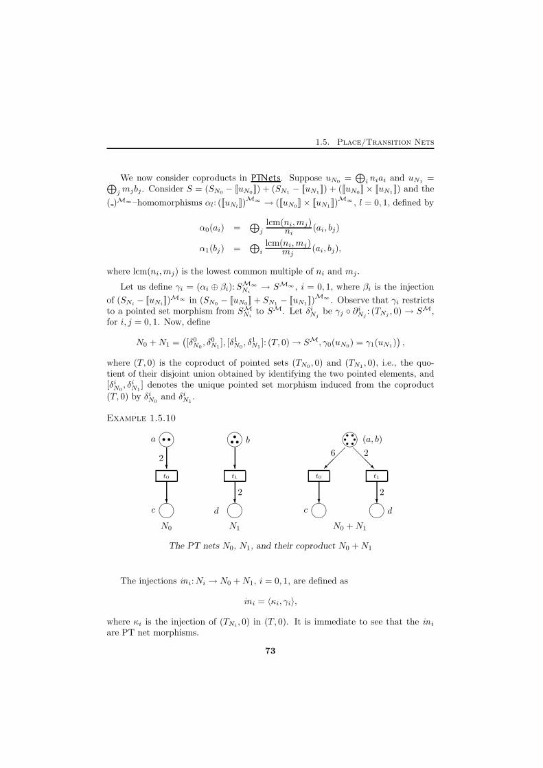
1.5. Place/Transition Nets
We now consider coproducts in PTNets. Suppose uN0 =⊕
i niai and uN1 =⊕jmjbj. Consider S = (SN0 − [[uN0 ]]) + (SN1 − [[uN1 ]]) + ([[uN0 ]]× [[uN1 ]]) and the
( )M∞–homomorphisms αl: ([[uNl]])M∞ → ([[uN0 ]]× [[uN1 ]])
M∞ , l = 0, 1, defined by
α0(ai) =⊕
j
lcm(ni,mj)ni (ai, bj)
α1(bj) =⊕
i
lcm(ni,mj)mj
(ai, bj),
where lcm(ni,mj) is the lowest common multiple of ni and mj .
Let us define γi = (αi ⊕ βi):SM∞
Ni→ SM∞ , i = 0, 1, where βi is the injection
of (SNi− [[uNi
]])M∞ in (SN0 − [[uN0]] + SN1 − [[uN1 ]])M∞ . Observe that γi restricts
to a pointed set morphism from SMNito SM. Let δiNj
be γj ◦ ∂iNj: (TNj
, 0) → SM,for i, j = 0, 1. Now, define
N0 +N1 =([δ0N0
, δ0N1], [δ1N0
, δ1N1]: (T, 0)→ SM, γ0(uN0) = γ1(uN1)
),
where (T, 0) is the coproduct of pointed sets (TN0 , 0) and (TN1 , 0), i.e., the quo-tient of their disjoint union obtained by identifying the two pointed elements, and[δiN0
, δiN1] denotes the unique pointed set morphism induced from the coproduct
(T, 0) by δiN0and δiN1
.
Example 1.5.10
� ��
� ��
� ��
� �� � �� � ��
� ��?
?
?
? ? ?
���
@@@R
N0 N1 N0 +N1
2
2
6 2
2
t0 t0t1 t1
• • •• • • •
• •••a b (a, b)
c d c d
The PT nets N0, N1, and their coproduct N0 +N1
The injections ini:Ni → N0 +N1, i = 0, 1, are defined as
in i = 〈κi, γi〉,
where κi is the injection of (TNi, 0) in (T, 0). It is immediate to see that the in i
are PT net morphisms.
73
Chapter 1. Processes and Unfoldings
Given any PT net N and a pair of morphisms h0:N0 → N and h1:N1 → N , let[h0, h1]:N0 +N1 → N be the map such that
[h0, h1](t) = hi(t′) if t = in i(t
′) for t′ ∈ TNi
[h0, h1](c) = hi(c′) if c = in i(c
′) for c′ ∈ SNi− [[uNi
]]
[h0, h1](ai, bj) =⊕{
nklcm(ni,mj)
ck
∣∣∣∣ ck ∈ [[h0(ai)]] ∩ [[h1(bj)]]
}
where nk is the coefficient of ck in uN . To simplify the notation, in the proof of thefollowing proposition we will denote [[h0(ai)]] ∩ [[h1(bj)]] by [[ℑ(ai, bj)]].Remember that u ∈ SM is a function from S to ω. Therefore, u(a), for a ∈ S, isthe multiplicity of a in u.
Proposition 1.5.11 (Coproducts of Nets)N0 +N1, with injections in0 and in1, is the coproduct of N0 and N1 in PTNets.
Proof. We show that for any PT net N and for any pair of morphisms h0:N0 → N ,h1:N1 → N , [h0, h1] is the unique morphism in PTNets such that [h0, h1] ◦ ini = hi.First we have to show that [h0, h1] is well-defined, i.e., that nk
lcm(ni, mj)is actually a
natural number. If ck ∈ [[h0(ai)]] then h0(ai) = rkck⊕u and so h0(niai) = nirkck⊕niu.Thus, by definition of PT net morphisms, we know that uN (ck) = nirk and so it mustbe nirk = nk. In the same way, there exists qk such that mjqk = nk. Therefore nk isdivisible by lcm(ni,mj).
Now, observe that [h0, h1] ◦ ini = hi. This is clear for transitions and for places inSNi − [[uNi ]]. So, consider ai ∈ [[uN0 ]]. We have
[h0, h1](in0(ai)) = [h0, h1](⊕
j
lcm(ni,mj)ni (ai, bj)
)
=⊕
j
lcm(ni,mj)ni [h0, h1]((ai, bj))
=⊕
j
lcm(ni,mj)ni
⊕{nk
lcm(ni, mj)ck
∣∣∣ ck ∈ [[ℑ(ai, bj)]]}
=⊕
j
{ nkni ck
∣∣ ck ∈ [[ℑ(ai, bj)]]}.
Since for each ck ∈ [[h0(ai)]] there exists a unique bj such that ck ∈ [[h1(bj)]], the lastterm is equal to
⊕{nknick
∣∣∣ ck ∈ [[h0(ai)]]}
=⊕{
rkck | h0(ai) = rkck ⊕ u′}
= h0(ai).
The same argument goes through for bj ∈ [[uN1 ]].
To prove uniqueness, suppose that there exists h such that h ◦ ini = hi. Clearly,h = [h0, h1] on the transitions and on places in SN0 − [[uN0 ]] and in SN1 − [[uN1 ]].Therefore, in order to show that h coincides with [h0, h1] we need to show that it does
74
1.5. Place/Transition Nets
so for (ai, bj) ∈ [[uN0 ]] × [[uN1 ]]. Since h(in0(ai)) = h0(ai) and h is a morphism, wehave
⊕j
lcm(ni, mj)ni h(ai, bj) =
⊕{ nkni ck
∣∣ ck ∈ [[h0(ai)]]}
=⊕
j
{ nkni ck
∣∣ ck ∈ [[ℑ(ai, bj)]]}
=⊕
j
lcm(ni, mj)ni
·(⊕{
nklcm(ni,mj)
ck
∣∣∣ ck ∈ [[ℑ(ai, bj)]]})
.
In the same way, we obtain that
⊕i
lcm(ni,mj)mj
h(ai, bj) =⊕
i
lcm(ni,mj)mj
⊕{nk
lcm(ni,mj)ck
∣∣∣ ck ∈ [[ℑ(ai, bj)]]}.
Now fix i and j. Since ck ∈ [[ℑ(ai, bj)]] for a unique pair (ai, bj), the summands in theabove equalities are all distinct except for
⊕{ nklcm(ni,mj)
ck | ck ∈ [[ℑ(ai, bj)]]}, which
appears in both. Therefore it must be
h(ai, bj) =⊕{
nklcm(ni,mj)
ck
∣∣∣∣ ck ∈ [[ℑ(ai, bj)]]
}which is [h0, h1](ai, bj).
The last thing we have left to show is that [h0, h1] is a morphism in PTNets. But now
this task is trivial and is therefore omitted. X
The coproduct of N0 and N1 is their non-deterministic composition in the sensethat the two nets are put side by side to compete for common resources (tokens).
Differently from the CCS non-deterministic operator [102], the result of such acomposition cannot be thought of simply as the system which performs an initialchoice between passing the control to N0 or to N1 and discards the net whichhas not been chosen. Nevertheless, we think that it gives the right notion of non-deterministic composition of PT nets. In fact, since a resource can be consumed andproduced several times during a single computation, it is possible that the composednet returns several times to a state in which common resources are present and thetwo nets compete for them. Clearly, there is no reason why the outcome of suchcompetitions should always favor the same net. This is illustrated by the followingexample.
Example 1.5.12Consider the simple PT nets N0 and N1 given in the picture below together with
75
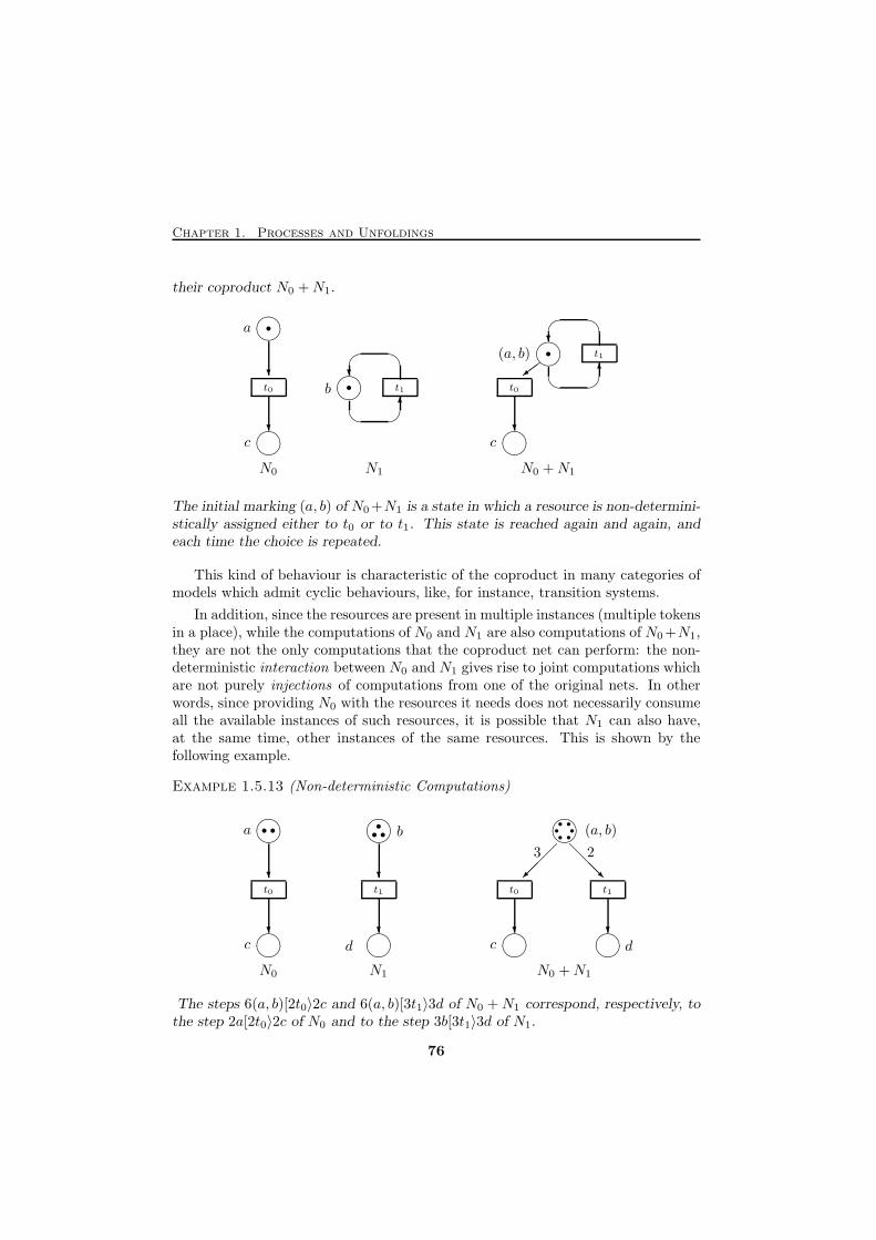
Chapter 1. Processes and Unfoldings
their coproduct N0 +N1.
� ��
� ��?
?
N0
a
t0
c
•
� ��� �
� ?
6
N1
• t1b
� ��� ��
?
��=t0
•(a, b)
c
� �
� ?
6t1
N0 +N1
The initial marking (a, b) of N0+N1 is a state in which a resource is non-determini-stically assigned either to t0 or to t1. This state is reached again and again, andeach time the choice is repeated.
This kind of behaviour is characteristic of the coproduct in many categories ofmodels which admit cyclic behaviours, like, for instance, transition systems.
In addition, since the resources are present in multiple instances (multiple tokensin a place), while the computations of N0 and N1 are also computations of N0+N1,they are not the only computations that the coproduct net can perform: the non-deterministic interaction between N0 and N1 gives rise to joint computations whichare not purely injections of computations from one of the original nets. In otherwords, since providing N0 with the resources it needs does not necessarily consumeall the available instances of such resources, it is possible that N1 can also have,at the same time, other instances of the same resources. This is shown by thefollowing example.
Example 1.5.13 (Non-deterministic Computations)
� ��
� ��
� ��
� �� � �� � ��
� ��?
?
?
? ? ?
���
@@@R
N0 N1 N0 +N1
3 2
t0 t0t1 t1
• • •• • • •
• •••a b (a, b)
c d c d
The steps 6(a, b)[2t0〉2c and 6(a, b)[3t1〉3d of N0 +N1 correspond, respectively, tothe step 2a[2t0〉2c of N0 and to the step 3b[3t1〉3d of N1.
76
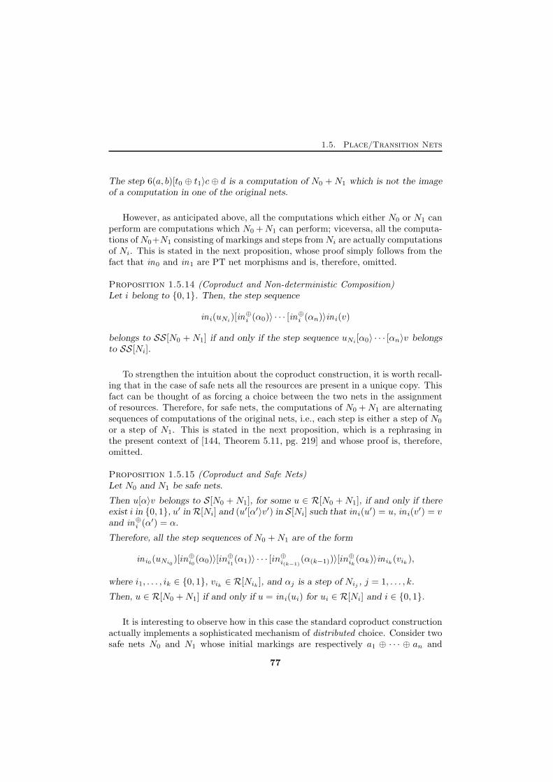
1.5. Place/Transition Nets
The step 6(a, b)[t0 ⊕ t1〉c ⊕ d is a computation of N0 +N1 which is not the imageof a computation in one of the original nets.
However, as anticipated above, all the computations which either N0 or N1 canperform are computations which N0 +N1 can perform; viceversa, all the computa-tions ofN0+N1 consisting of markings and steps fromNi are actually computationsof Ni. This is stated in the next proposition, whose proof simply follows from thefact that in0 and in1 are PT net morphisms and is, therefore, omitted.
Proposition 1.5.14 (Coproduct and Non-deterministic Composition)Let i belong to {0, 1}. Then, the step sequence
in i(uNi)[in⊕i (α0)〉 · · · [in
⊕i (αn)〉in i(v)
belongs to SS[N0 + N1] if and only if the step sequence uNi[α0〉 · · · [αn〉v belongs
to SS[Ni].
To strengthen the intuition about the coproduct construction, it is worth recall-ing that in the case of safe nets all the resources are present in a unique copy. Thisfact can be thought of as forcing a choice between the two nets in the assignmentof resources. Therefore, for safe nets, the computations of N0 +N1 are alternatingsequences of computations of the original nets, i.e., each step is either a step of N0
or a step of N1. This is stated in the next proposition, which is a rephrasing inthe present context of [144, Theorem 5.11, pg. 219] and whose proof is, therefore,omitted.
Proposition 1.5.15 (Coproduct and Safe Nets)Let N0 and N1 be safe nets.
Then u[α〉v belongs to S[N0 + N1], for some u ∈ R[N0 +N1], if and only if thereexist i in {0, 1}, u′ inR[Ni] and (u′[α′〉v′) in S[Ni] such that ini(u
′) = u, in i(v′) = v
and in⊕i (α′) = α.
Therefore, all the step sequences of N0 +N1 are of the form
in i0(uNi0)[in⊕i0(α0)〉[in
⊕i1
(α1)〉 · · · [in⊕i(k−1)
(α(k−1))〉[in⊕ik
(αk)〉in ik(vik ),
where i1, . . . , ik ∈ {0, 1}, vik ∈ R[Nik ], and αj is a step of Nij , j = 1, . . . , k.
Then, u ∈ R[N0 +N1] if and only if u = in i(ui) for ui ∈ R[Ni] and i ∈ {0, 1}.
It is interesting to observe how in this case the standard coproduct constructionactually implements a sophisticated mechanism of distributed choice. Consider twosafe nets N0 and N1 whose initial markings are respectively a1 ⊕ · · · ⊕ an and
77
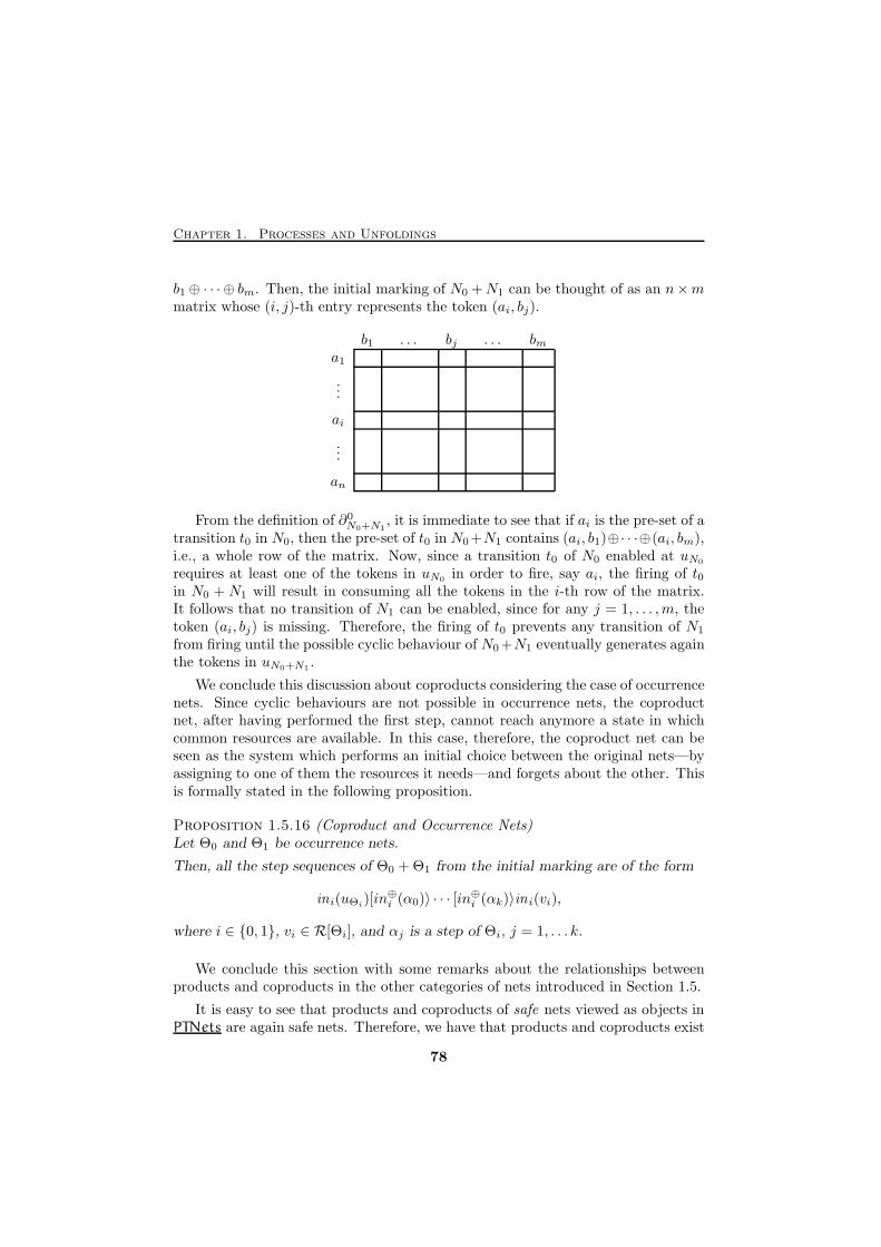
Chapter 1. Processes and Unfoldings
b1⊕ · · · ⊕ bm. Then, the initial marking of N0 +N1 can be thought of as an n×mmatrix whose (i, j)-th entry represents the token (ai, bj).
b1 . . . bj . . . bma1
...
ai
...
an
From the definition of ∂0N0+N1
, it is immediate to see that if ai is the pre-set of atransition t0 in N0, then the pre-set of t0 in N0+N1 contains (ai, b1)⊕· · ·⊕(ai, bm),i.e., a whole row of the matrix. Now, since a transition t0 of N0 enabled at uN0
requires at least one of the tokens in uN0 in order to fire, say ai, the firing of t0in N0 + N1 will result in consuming all the tokens in the i-th row of the matrix.It follows that no transition of N1 can be enabled, since for any j = 1, . . . ,m, thetoken (ai, bj) is missing. Therefore, the firing of t0 prevents any transition of N1
from firing until the possible cyclic behaviour of N0+N1 eventually generates againthe tokens in uN0+N1 .
We conclude this discussion about coproducts considering the case of occurrencenets. Since cyclic behaviours are not possible in occurrence nets, the coproductnet, after having performed the first step, cannot reach anymore a state in whichcommon resources are available. In this case, therefore, the coproduct net can beseen as the system which performs an initial choice between the original nets—byassigning to one of them the resources it needs—and forgets about the other. Thisis formally stated in the following proposition.
Proposition 1.5.16 (Coproduct and Occurrence Nets)Let Θ0 and Θ1 be occurrence nets.
Then, all the step sequences of Θ0 + Θ1 from the initial marking are of the form
ini(uΘi)[in⊕i (α0)〉 · · · [in
⊕i (αk)〉in i(vi),
where i ∈ {0, 1}, vi ∈ R[Θi], and αj is a step of Θi, j = 1, . . . k.
We conclude this section with some remarks about the relationships betweenproducts and coproducts in the other categories of nets introduced in Section 1.5.
It is easy to see that products and coproducts of safe nets viewed as objects inPTNets are again safe nets. Therefore, we have that products and coproducts exist
78
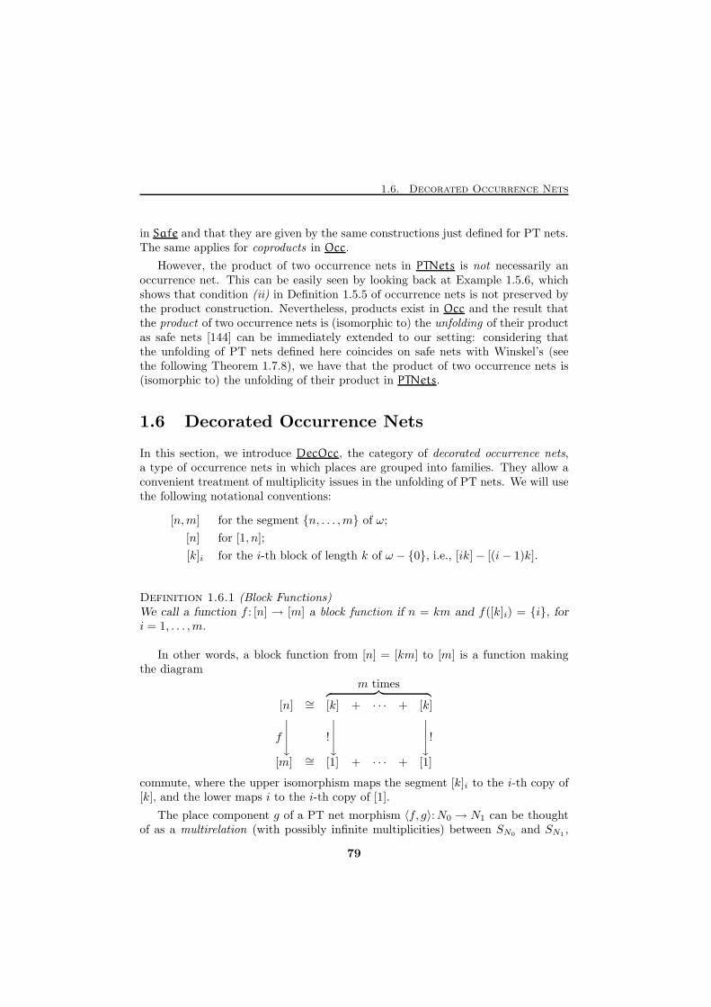
1.6. Decorated Occurrence Nets
in Safe and that they are given by the same constructions just defined for PT nets.The same applies for coproducts in Occ.
However, the product of two occurrence nets in PTNets is not necessarily anoccurrence net. This can be easily seen by looking back at Example 1.5.6, whichshows that condition (ii) in Definition 1.5.5 of occurrence nets is not preserved bythe product construction. Nevertheless, products exist in Occ and the result thatthe product of two occurrence nets is (isomorphic to) the unfolding of their productas safe nets [144] can be immediately extended to our setting: considering thatthe unfolding of PT nets defined here coincides on safe nets with Winskel’s (seethe following Theorem 1.7.8), we have that the product of two occurrence nets is(isomorphic to) the unfolding of their product in PTNets.
1.6 Decorated Occurrence Nets
In this section, we introduce DecOcc, the category of decorated occurrence nets,a type of occurrence nets in which places are grouped into families. They allow aconvenient treatment of multiplicity issues in the unfolding of PT nets. We will usethe following notational conventions:
[n,m] for the segment {n, . . . ,m} of ω;
[n] for [1, n];
[k]i for the i-th block of length k of ω − {0}, i.e., [ik]− [(i− 1)k].
Definition 1.6.1 (Block Functions)We call a function f : [n] → [m] a block function if n = km and f([k]i) = {i}, fori = 1, . . . ,m.
In other words, a block function from [n] = [km] to [m] is a function makingthe diagram
m times︷ ︸︸ ︷[n] ∼= [k] + · · · + [k]
f
y !
y
y!
[m] ∼= [1] + · · · + [1]
commute, where the upper isomorphism maps the segment [k]i to the i-th copy of[k], and the lower maps i to the i-th copy of [1].
The place component g of a PT net morphism 〈f, g〉:N0 → N1 can be thoughtof as a multirelation (with possibly infinite multiplicities) between SN0 and SN1 ,
79
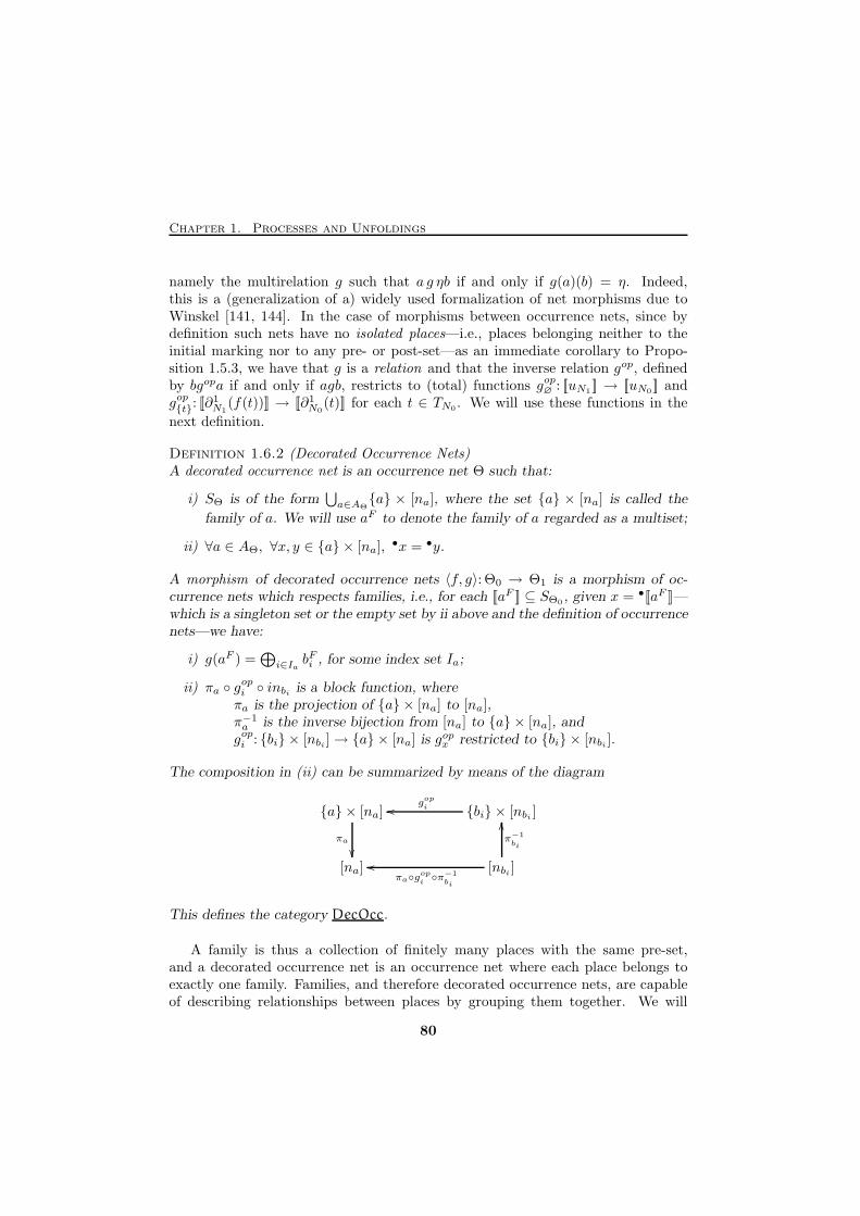
Chapter 1. Processes and Unfoldings
namely the multirelation g such that a g ηb if and only if g(a)(b) = η. Indeed,this is a (generalization of a) widely used formalization of net morphisms due toWinskel [141, 144]. In the case of morphisms between occurrence nets, since bydefinition such nets have no isolated places—i.e., places belonging neither to theinitial marking nor to any pre- or post-set—as an immediate corollary to Propo-sition 1.5.3, we have that g is a relation and that the inverse relation gop, definedby bgopa if and only if agb, restricts to (total) functions gop
∅: [[uN1 ]] → [[uN0 ]] and
gop{t}: [[∂1N1
(f(t))]] → [[∂1N0
(t)]] for each t ∈ TN0 . We will use these functions in the
next definition.
Definition 1.6.2 (Decorated Occurrence Nets)A decorated occurrence net is an occurrence net Θ such that:
i) SΘ is of the form⋃a∈AΘ
{a} × [na], where the set {a} × [na] is called the
family of a. We will use aF to denote the family of a regarded as a multiset;
ii) ∀a ∈ AΘ, ∀x, y ∈ {a} × [na],•x = •y.
A morphism of decorated occurrence nets 〈f, g〉: Θ0 → Θ1 is a morphism of oc-currence nets which respects families, i.e., for each [[aF ]] ⊆ SΘ0 , given x = •[[aF ]]—which is a singleton set or the empty set by ii above and the definition of occurrencenets—we have:
i) g(aF ) =⊕
i∈IabFi , for some index set Ia;
ii) πa ◦ gopi ◦ inbi
is a block function, whereπa is the projection of {a} × [na] to [na],π−1a is the inverse bijection from [na] to {a} × [na], andgopi : {bi} × [nbi
]→ {a} × [na] is gopx restricted to {bi} × [nbi].
The composition in (ii) can be summarized by means of the diagram
{a} × [na] {bi} × [nbi]
[na] [nbi]
πa
��
gop
ioo
π−1bi
OO
πa◦gop
i◦π−1
bi
oo
This defines the category DecOcc.
A family is thus a collection of finitely many places with the same pre-set,and a decorated occurrence net is an occurrence net where each place belongs toexactly one family. Families, and therefore decorated occurrence nets, are capableof describing relationships between places by grouping them together. We will
80

1.6. Decorated Occurrence Nets
use families to relate places which are instances of the same place obtained in aprocess of unfolding. Therefore, morphisms treat families in a special way: theymap families to families (condition (i)) and they do that in a unique pre-determinedway (condition (ii)). This is because what we want to describe is that aF is mappedto bF . Hence, since the way to map a family to another family is fixed by definition,in the following we will often define morphisms by just saying what families are sentto what families.
Observe that the full subcategory of DecOcc consisting of all nets Θ such thatSΘ =
⋃a∈AΘ
{a} × [1] is (isomorphic to) Occ. Observe also that, since the initialmarking consists exactly of the elements with empty pre-set and, by point (ii)in Definition 1.6.2, elements of a family have the same pre-set, for a decoratedoccurrence net uΘ is of the form
⊕i∈I a
Fi .
The following is a useful property of decorated occurrence net morphisms whichdirectly follows from their definition.
Proposition 1.6.3 (Decorated Occurrence Net Morphisms)Let Θ0 and Θ1 be decorated occurrence nets and 〈f, g〉: Θ0 → Θ1 a morphism inDecOcc. Then
∀[[bF ]] ⊆ [[uN1 ]], ∃![[aF ]] ⊆ [[uN0 ]] such that [[bF ]] ⊆ [[g(aF )]] and
∀[[bF ]] ⊆ [[∂1N1
(f(t))]], ∃![[aF ]] ⊆ [[∂1N0
(t)]] such that [[bF ]] ⊆ [[g(aF )]].
We have seen that for occurrence nets and decorated occurrence nets simpleconcepts of causal dependence (≺) and conflict (#) can be defined. The orthogonalconcept is that of concurrency.
Definition 1.6.4 (Concurrent Elements)Given a (decorated) occurrence net Θ (which defines ≺, 4 and #), we can define
• For x, y ∈ TΘ ∪ SΘ, x co y iff ¬(x ≺ y or y ≺ x or x # y);
• For X ⊆ TΘ ∪ SΘ, Co(X) iff(∀x, y ∈ X, x co y) and |{t ∈ TΘ | ∃x ∈ X, t 4 x}| ∈ ω.
As a first step in relating the categories DecOcc and PTNets, we define a functorfrom decorated occurrence nets to PT nets.
Definition 1.6.5 ( ( )+: from DecOcc to PTNets)For Θ =
(∂0Θ, ∂
1Θ: (TΘ, 0)→ (
⋃a∈AΘ
{a} × [na])M, uΘ
), let ( )+ denote the ( )M∞–
homomorphism from SM∞
Θ to AM∞
Θ such that (a, j)+ = a.Then, we define Θ+ to be the net
(( )+ ◦ ∂0
Θ, ( )+ ◦ ∂1Θ: (TΘ, 0)→ AMΘ , (uΘ)+
).
Given a morphism 〈f, g〉: Θ0 → Θ1, let 〈f, g〉+: Θ+0 → Θ+
1 be 〈f, ( )+ ◦ g ◦ ρ〉 whereρ:AM∞
Θ0→ SM∞
Θ0is the ( )M∞–homomorphism such that ρ(a) = (a, 1).
81
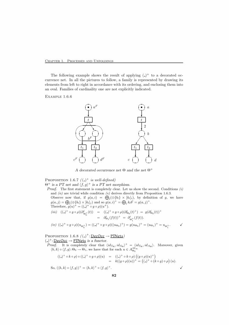
Chapter 1. Processes and Unfoldings
The following example shows the result of applying ( )+ to a decorated oc-currence net. In all the pictures to follow, a family is represented by drawing itselements from left to right in accordance with its ordering, and enclosing them intoan oval. Families of cardinality one are not explicitly indicated.
Example 1.6.6
����
� �
� ���
�� ��
�� ��
#" !
?
JJ
�
?
??? ?
JJ
?
�
??
2
•• aF a
b
bF
cF cdF d
t t
t1 t1t2 t2
A decorated occurrence net Θ and the net Θ+
Proposition 1.6.7 ( ( )+ is well-defined)Θ+ is a PT net and 〈f, g〉+ is a PT net morphism.Proof. The first statement is completely clear. Let us show the second. Conditions (i)
and (ii) are trivial while condition (v) derives directly from Proposition 1.6.3.Observe now that, if g(a, i) =
⊕l(⊕{bl} × [kl]i), by definition of g, we have
g(a, j) =⊕
l(⊕{bl} × [kl]j) and so g(a, i)+ =
⊕lklb
l = g(a, j)+.Therefore, g(u)+ = (( )+ ◦ g ◦ ρ)(u+).
(iii) (( )+ ◦ g ◦ ρ)(∂iΘ+
0
(t)) = (( )+ ◦ g ◦ ρ)(∂iΘ0(t)+) = g(∂iΘ0
(t))+
= ∂iΘ1(f(t))+ = ∂i
Θ+1
(f(t)).
(iv) (( )+ ◦ g ◦ ρ)(uΘ+
0) = (( )+ ◦ g ◦ ρ)((uΘ0)
+) = g(uΘ0)+ = (uΘ1)
+ = uΘ+
1. X
Proposition 1.6.8 ( ( )+: DecOcc→ PTNets)
( )+: DecOcc→ PTNets is a functor.Proof. It is completely clear that 〈idTΘ , idSΘ〉
+ = 〈idTΘ , idAΘ〉. Moreover, given〈h, k〉 ◦ 〈f, g〉:Θ0 → Θ1, we have that for each u ∈ AM∞
Θ0
(( )+ ◦ k ◦ ρ) ◦ (( )+ ◦ g ◦ ρ)(u) = (( )+ ◦ k ◦ ρ)((g ◦ ρ)(u)+
)
= k((g ◦ ρ)(u))+ =(( )+ ◦ (k ◦ g) ◦ ρ
)(u).
So, (〈h, k〉 ◦ 〈f, g〉)+ = 〈h, k〉+ ◦ 〈f, g〉+. X
82
1.6. Decorated Occurrence Nets
Nets obtained via ( )+ from decorated occurrence nets have a structure verysimilar to that of occurrence nets. We will denote by DecOcc+ the full subcategoryof PTNets consisting of (nets isomorphic to) nets of the form Θ+.
Proposition 1.6.9 (Structure of Decorated Occurrence Nets)If Θ is a decorated occurrence net, then Θ+ is a PT net such that:
i) a ∈ [[uΘ+ ]] if and only if •a = ∅;
ii) ∀a ∈ SΘ+ , |•a| ≤ 1;
iii) the relation ≺ is irreflexive and ∀t ∈ TΘ+ , {t′ ∈ TΘ+ | t′ ≺ t} is finite.
Moreover, if Θ is (isomorphic to) an occurrence net, then Θ+ is an occurrence netisomorphic to Θ.
Proof. Obvious from the definition of ( )+. X
Let B range over Occ, DecOcc and DecOcc+. For any net in B, we can definethe concept of depth of an element of the net, thanks to their nicely stratifiedstructure.
Definition 1.6.10 (Depth)Let Θ be a net in B. The depth of an element in TΘ ∪SΘ is inductively defined by
• depth(x) = 0 if b ∈ SΘ and •b = ∅;
• depth(x) = max{depth(b) | b ≺ x}+ 1 if x ∈ TΘ;
• depth(x) = depth(t) if x ∈ SΘ and •x = {t}.
Definition 1.6.11 (Subnets of a Net)Given a net Θ in B define its subnet of depth n, Θ(n), as
• TΘ(n) = {t ∈ TΘ | depth(t) ≤ n};
• SΘ(n) = {b ∈ SΘ | depth(b) ≤ n};
• ∂0Θ(n) and ∂1
Θ(n) are the restrictions of ∂0Θ and ∂1
Θ to TΘ(n) ;
• uΘ(n) = uΘ.
It is easy to see that Θ(n) is a net in B.
83
Chapter 1. Processes and Unfoldings
Clearly, for each n ≤ m there is a morphism inn,m: Θ(n) → Θ(m) whose com-ponents are both set inclusions. In the following we will call such net morphismssimply inclusions. Obviously, if 〈f, g〉: Θ0 → Θ1 is an inclusion, then we haveuΘ0 = uΘ1 and, for each t ∈ TΘ0 , ∂
iΘ0
(t) = ∂iΘ1(t), i = 0, 1.
Now, consider the category ω = {0→ 1→ 2→ 3 · · ·} and the class of diagramsD:ω → B such that D(n → n + 1) = inn:D(n) → D(n + 1) is an inclusion. Forsuch a class we have the following results. The reader is referred to [90, III.3] (andto Appendix A.1) for the definition of the categorical concepts involved.
Proposition 1.6.12 (Colim(D) exists)For any D ∈ D, the colimit of D in B exists.
Proof. Consider the net Θ =(∂0Θ, ∂
1Θ: (TΘ, 0)→ SMΘ , uΘ
)where
TΘ =⋃nTD(n)
SΘ =⋃nSD(n)
uΘ = uD(0)
∂iΘ(t) = ∂iD(n)(t) for n such that t ∈ TD(n).
Clearly, Θ is well-defined, is a net, and belongs to B.
Now, for any n, let µn:D(n) → Θ be the obvious inclusion. By definition we haveµn = µn+1 ◦ inn. Now consider a family of morphisms τn:D(n) → Θ′, n ∈ ω, suchthat τn = τn+1 ◦ inn. Define σ:Θ→ Θ′ by:
σ(t) = τn(t) for n such that t ∈ TD(n);
σ(a) = τn(a) for n such that a ∈ SD(n).
σ is clearly a morphism in B. Now consider σ ◦µn:D(n)→ Θ′. We have that, for anyt ∈ TD(n), σ(t) = τn(t) and for any a ∈ SD(n), σ(a) = τn(a). Therefore, since µn is aninclusion, we have σ ◦ µn = τn for each n ∈ ω.
Given any σ′: Θ → Θ′, suppose that σ′ ◦ µn = τn for each n ∈ ω. Since t ∈ TΘ
(a ∈ SΘ) belongs to TD(n) (to SD(n)) for some n, we have that σ′(t) = τn(t) = σ(t)
(σ′(a) = τn(a) = σ(a)). Therefore, σ′ = σ. X
Proposition 1.6.13 (Θ is the colimit of its subnets)Given a net Θ in B, let DΘ:ω → B be the functor such that DΘ(n) = Θ(n) andDΘ(n→ n+ 1) = inn,n+1: Θ
(n) → Θ(n+1). Then Θ = Colim(DΘ).
Proof. Since DΘ ∈ D, we are in the conditions of the previous proposition. So, it is
enough to observe that the colimit construction for diagrams in D in the proof of that
proposition gives a family µn:D(n) → Θ, n ∈ ω, where µn: Θ(n) → Θ is the inclusion
of Θ(n) in Θ. X
Proposition 1.6.14 ( ( )+
preserves the colimit of DΘ)If B = DecOcc, then Colim(DΘ)+ = Colim(D+
Θ).
84
1.7. PT Net Unfoldings
Proof. Since the previous proposition states that each Θ is completely identified by the
diagram DΘ, it is enough to observe that D+Θ is exactly DΘ+ .
So, Colim(D+Θ) = Colim(DΘ+) = Θ+ = Colim(DΘ)+. X
1.7 PT Net Unfoldings
In this section, we define the unfolding of PT nets in term of decorated occurrencenets and show that it is a functor from PTNets to DecOcc which is right adjointto ( )+.
We start by giving the object component of such a functor. To this aim, givena net N , we define a family of decorated occurrence nets, one for each n ∈ ω, wherethe n-th net approximates the unfolding of N up to depth n, i.e., it reflects thebehaviour of the original net up to step sequences of length at most n. Clearly,the unfolding of N will be defined to be the colimit of an appropriate ω-shapeddiagram built on the approximant nets. We will use the following notation: givens ∈ X1 × · · · ×Xn, we denote by s ↓ Xi the projection of s on the Xi component.
Moreover, given S = {sj | j ∈ J}, S ↓ Xi will be {sj ↓ Xi | j ∈ J} and S⊕↓ Xi will
denote⊕
j∈J (sj ↓ Xi).
Definition 1.7.1 (PT Nets Unfoldings: U [ ](k)
)Let N =
(∂0N , ∂
1N : (TN , 0)→ SMN , uN
)be a net in PTNets.
We define the nets U [N ](k) =(∂0k, ∂
1k: (Tk, 0)→ SMk , uk
), for k ∈ ω, where:
• S0 =⋃{{(∅, b)} × [n] | uN(b) = n};
• T0 = {0}, and the ∂i0 with the obvious definitions;
• u0 =⊕S0;
and for k > 0,
• Tk = Tk−1 ∪
{(B, t)
∣∣∣ B ⊆ Sk−1, Co(B), t ∈ TN , B⊕
↓ SN = ∂0N (t)
};
• Sk = Sk−1 ∪
(⋃t0∈Tk, b∈SN
∂1N
(t0↓T)(b)=n
{{({t0}, b
)}× [n]
});
• ∂0k(B, t) =
⊕B, and ∂1
k(B, t) =⊕{(
({(B, t)}, b), i)∈ Sk
};
• uk =⊕{(
(∅, b), i)∈ Sk
}=⊕S0 = u0.
85
Chapter 1. Processes and Unfoldings
Therefore, informally speaking, the net U [N ](0) is obtained by exploding in fam-ilies the initial marking of N , and U [N ](n+1) is obtained, inductively, by generatinga new transition for each possible subset of concurrent places of U [N ](n) whose cor-responding multiset of places of N constitutes the source of some transition t of N ;the target of t is also exploded in families which are added to U [N ](n+1). As a con-sequence, the transitions of the n-th approximant net are instances of transitionsof N , in the precise sense that each of them corresponds to a unique occurrence ofa transition of N in one of its step sequences of length at most n.
Lemma 1.7.2 (U [N ](n)
is a decorated occurrence net)For all n ∈ ω, U [N ](n) is a decorated occurrence net of depth n. Moreover, for eachn ∈ ω there is an inclusion inn:U [N ](n) → U [N ](n+1).
Proof. That U [N ](n) has depth n and that there exists an inclusion from U [N ](n) toU [N ](n+1) is obvious from the definition. We have to show that U [N ](n) is a decoratedoccurrence net. For each t ∈ Tn, ∂
in(t) is a multiset where all the elements have
multiplicity one, i.e., a set. The same happens for un.
i) Observe that for each ((x, b), i) ∈ Sn,•((x, b), i) = x which is the empty set or a
singleton. So |•((x, b), i)| ≤ 1.
ii) Moreover, ((x, b), i) ∈ [[un]] iff x = ∅ iff •((x, b), i) = ∅.
iii) By definition of U [N ](n), whenever x ≺1 y ≺1 z we have that depth(z) =depth(x) + 1. Since x, z ∈ Tn or x, z ∈ Sn implies that there exists at leastone y such that x ≺ y ≺1 z we have that depth(x) < depth(z) and so x 6= z.Therefore, ≺ is irreflexive. This, together with (i) and (ii), implies that, in anyreachable marking, each place has multiplicity at most one. In fact, that beingtrue in un, each place having only one pre-event and each transition occurringat most once in any computation, there is no way to generate more than onetoken in a place. Moreover, ∀t ∈ Tn, {t
′ ∈ Tn | t′ ≺ t} is finite, because of the
definition of Co.
iv) # is irreflexive. Recall that x # x iff ∃t, t′ ∈ Tn, t 6= t′ and t #m t′ such thatt 4n x and t′ 4n x. So, by point (i), x cannot be a place, otherwise we wouldhave backward branching. This means that there exist b, b′ ∈ [[∂0
n(x)]], b 6= b′
such that b co b′, i.e., x = (B, t) and ¬Co(B). This is impossible.
The other conditions of decorated occurrence nets are obviously true. X
Definition 1.7.3 (PT Net Unfoldings: U [ ])We define U [N ] to be the colimit of the diagram D:ω → DecOcc such that D(n) =U [N ](n) and D(n → n + 1) = inn. By Lemma 1.7.2 D belongs to D and so, byProposition 1.6.12, the colimit exists and is a decorated occurrence net.
86
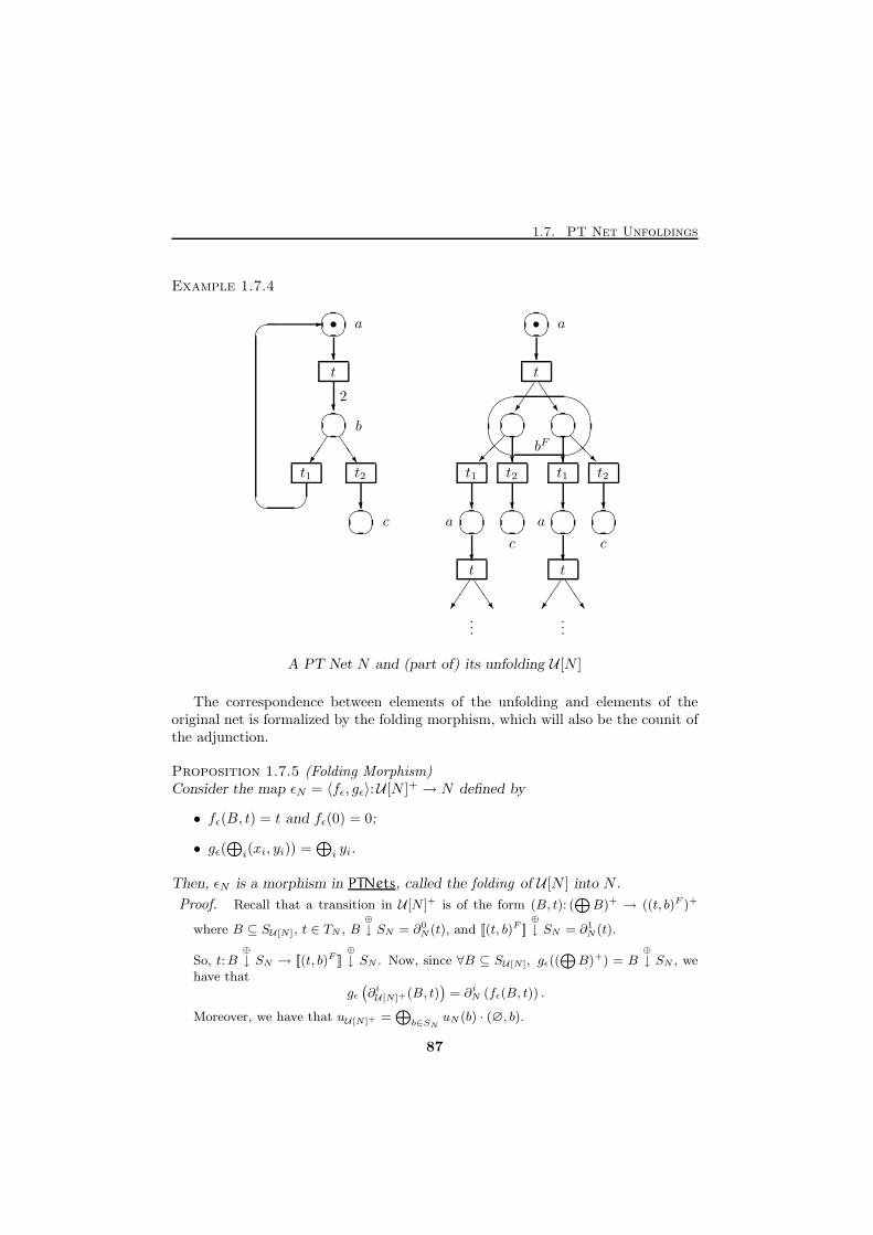
1.7. PT Net Unfoldings
Example 1.7.4
#" !����
� �
� ��� � �����
��
��
@@R??
��
�
?
JJ
? ? ? ?
?
JJ
�
?
?�
� -
? ?
�JJ
�JJ
......
2
• •
t t
t1 t2 t1 t2 t1 t2
t t
a a
b
bF
c a
c
a
c
A PT Net N and (part of) its unfolding U [N ]
The correspondence between elements of the unfolding and elements of theoriginal net is formalized by the folding morphism, which will also be the counit ofthe adjunction.
Proposition 1.7.5 (Folding Morphism)Consider the map ǫN = 〈fǫ, gǫ〉:U [N ]+ → N defined by
• fǫ(B, t) = t and fǫ(0) = 0;
• gǫ(⊕
i(xi, yi)) =⊕
i yi.
Then, ǫN is a morphism in PTNets, called the folding of U [N ] into N .
Proof. Recall that a transition in U [N ]+ is of the form (B, t): (⊕
B)+ → ((t, b)F )+
where B ⊆ SU [N], t ∈ TN , B⊕
↓ SN = ∂0N(t), and [[(t, b)F ]]
⊕
↓ SN = ∂1N(t).
So, t:B⊕
↓ SN → [[(t, b)F ]]⊕
↓ SN . Now, since ∀B ⊆ SU [N], gǫ((⊕
B)+) = B⊕
↓ SN , wehave that
gǫ(∂iU [N]+(B, t)
)= ∂iN (fǫ(B, t)) .
Moreover, we have that uU [N]+ =⊕
b∈SNuN (b) · (∅, b).
87
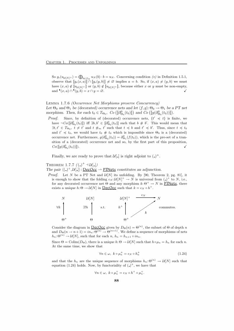
Chapter 1. Processes and Unfoldings
So gǫ(uU [N]+) =⊕
b∈SNuN (b) · b = uN . Concerning condition (v) in Definition 1.5.1,
observe that [[gǫ(x, a)]] ∩ [[gǫ(y, b)]] 6= ∅ implies a = b. So, if (x, a) 6= (y, b) we must
have (x, a) 6∈ [[uU [N]+ ]] or (y, b) 6∈ [[uU [N]+ ]], because either x or y must be non-empty,
and •(x, a) ∩ •(y, b) = x ∩ y = ∅. X
Lemma 1.7.6 (Occurrence Net Morphisms preserve Concurrency)Let Θ0 and Θ1 be (decorated) occurrence nets and let 〈f, g〉: Θ0 → Θ1 be a PT netmorphism. Then, for each t0 ∈ TΘ0 , Co
([[∂0
Θ0(t0)]]
)and Co
([[g(∂0
Θ0(t0))]]
).
Proof. Since, by definition of (decorated) occurrence nets, {t′ 4 t} is finite, we
have ¬Co([[∂0Θ0
(t0)]]) iff ∃b, b′ ∈ [[∂0Θ0
(t0)]] such that b # b′. This would mean that
∃t, t′ ∈ TΘ0 , t 6= t′ and t #m t′ such that t 4 b and t′ 4 b′. Thus, since t 4 t0and t′ 4 t0, we would have t0 # t0 which is impossible since Θ0 is a (decorated)
occurrence net. Furthermore, g(∂0Θ0
(t0)) = ∂0Θ1
(f(t0)), which is the pre-set of a tran-
sition of a (decorated) occurrence net and so, by the first part of this proposition,
Co([[g(∂0Θ0
(t0))]]). X
Finally, we are ready to prove that U [ ] is right adjoint to ( )+.
Theorem 1.7.7 ( ( )+ ⊣ U [ ])
The pair 〈( )+,U [ ]〉 : DecOcc ⇀ PTNets constitutes an adjunction.
Proof. Let N be a PT Net and U [N ] its unfolding. By [90, Theorem 2, pg. 81], itis enough to show that the folding ǫN :U [N ]+ → N is universal from ( )+ to N , i.e.,for any decorated occurrence net Θ and any morphism k: Θ+ → N in PTNets, thereexists a unique h: Θ→ U [N ] in DecOcc such that k = ǫN ◦ h
+.
6 6
-
�������36
Θ+
∃!h s.t. commutes.∀k
N U [N ]+
Θ+
NǫN
h+
k
U [N ]
Θ
Consider the diagram in DecOcc given by DΘ(n) = Θ(n), the subnet of Θ of depth nand DΘ(n→ n+1) = inn: Θ(n) → Θ(n+1). We define a sequence of morphisms of netshn: Θ(n) → U [N ], such that for each n, hn = hn+1 ◦ inn.
Since Θ = Colim(DΘ), there is a unique h: Θ→ U [N ] such that h◦µn = hn for each n.At the same time, we show that
∀n ∈ ω, k ◦ µ+n = ǫN ◦ h
+n (1.24)
and that the hn are the unique sequence of morphisms hn: Θ(n) → U [N ] such that
equation (1.24) holds. Now, by functoriality of ( )+, we have that
∀n ∈ ω, k ◦ µ+n = ǫN ◦ h
+ ◦ µ+n .
88
1.7. PT Net Unfoldings
Therefore, since by Proposition 1.6.14 ( )+ ◦DΘ = DΘ+ , and, by Proposition 1.6.13,Θ+ = Colim(D+
Θ) = Colim(( )+ ◦ DΘ), by the universal property of the colimit wemust have k = ǫN ◦ h
+.
To show the uniqueness of h, let h′ be such that k = ǫN ◦ h′+. Then we have k ◦µ+
n =ǫN ◦ h
′+ ◦ µ+n . But hn is the unique morphism for which this happens. Therefore, for
each n, hn = h′ ◦ µn and so, by the universal property of the colimit, h = h′.
Let us now define hn and therefore h: Θ→ U [N ], and show that the hn, n ∈ ω are theunique sequence of morphisms such that (1.24) holds.
depth 0. Suppose uΘ+ =⊕
iniai. So uΘ =
⊕i(⊕{ai} × [ni]). Suppose k(aj) =⊕
lmjl bjl . By definition of k, since k does not merge different places in the initial
marking and k(uΘ+) = uN , we have uN = v ⊕⊕
lnjm
jl bjl , with bjl 6∈ [[v]]. Thus, in
U [N ] we have the places⋃l{(∅, bjl )} × [njm
jl ]. So, we define
h0(aj , i) =⊕
l
(⊕{(∅, bjl )} × [mj
l ]i
).
We have h+0 (aj) = (h0(aj , i))
+ =⊕
jmjl (∅, b
jl ) and
ǫN ◦ h+0 (aj) =
⊕lmjl bjl = k(aj) = k ◦ µ+
0 (aj).
Observe that h0 so defined, lifting its place component to a ( )M∞–homomorphism, isa morphism Θ(0) → U [N ] and that it is completely determined by k and the conditionsof decorated occurrence net morphisms.
depth n+1. Let us suppose that we have defined hn: Θ(n) → U [N ] and that it is amorphism. Suppose that for each m ≤ n, hm is the unique morphism such thatǫN ◦ h
+m = k ◦ µm. Let hn+1 be hn on the elements of depth less or equal to n. Now,
we define hn+1 on the elements of depth n+ 1.
Let t1 ∈ TΘ such that depth(t1) = n+ 1 and k(t1) = t.
Since [[∂0Θ(t1)]] is a set of elements of depth less or equal to n, hn(∂0
Θ(t1)) is defined.Since hn is a morphism, by Lemma 1.7.6, we have Co([[hn(∂0
Θ(t1))]]).
Moreover, since ǫN ◦ h+n = k ◦ µ+
n ,
∂0N(t) = k(∂0
Θ(t)) = ǫN ◦ (hn)+(∂0Θ+(t1)
)= ǫN ◦ (hn)+
((∂0
Θ(t1))+)
= ǫN ◦ hn(∂0Θ(t1))
+ = [[hn(∂0Θ(t1))]]
⊕
↓ SN
Therefore t0 =([[hn(∂0
Θ(t1))]], t)
=([[hn+1(∂
0Θ(t1))]], t
)∈ TU [N].
Now, since hn+1 has to make the diagram commute, hn+1(t1) must be of the form (B, t)and, since it has to be a morphism, it must be ∂0
U [N]((B, t)) =⊕
B = hn+1(∂0Θ(t1)).
Therefore hn+1(t1) = t0. Observe that there is only one choice for hn+1(t1), given kand hn by inductive hypothesis.
Obviously, ǫN ◦ h+n+1(t1) = t = k(t1) = k ◦ µ+
n+1(t1).
Now, let ∂1Θ+(t1) =
⊕iniai. So ∂1
Θ(t1) =⊕
i(⊕{ai} × [ni]) in Θ. Suppose k(aj) =⊕
lmjl bjl . By definition of k, since it does not merge different places in the post-set of
89
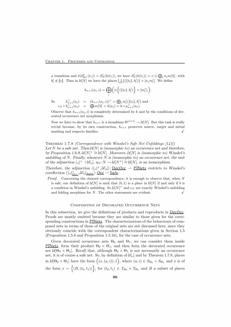
Chapter 1. Processes and Unfoldings
a transition and k(∂1Θ+(t1)) = ∂1
N(k(t1)), we have ∂1N(k(t1)) = v ⊕
⊕lnjm
jl bjl , with
bjl 6∈ [[v]]. Thus in U [N ] we have the places⋃l{({t0}, b
jl )} × [njm
jl ]. We define
hn+1(aj , i) =⊕
l
(⊕{
({t0}, bjl )}× [mj
l ]i
).
So h+n+1(aj) = (hn+1(aj , i))
+ =⊕
lmjl ({t0}, b
jl ) and
ǫN ◦ h+n+1(aj) =
⊕mjl bjl = k(aj) = k ◦ µ+
n+1(aj).
Observe that hn+1(aj , i) is completely determined by k and by the conditions of dec-orated occurrence net morphisms.
Now we have to show that hn+1 is a morphism Θ(n+1) → U [N ]. But this task is really
trivial because, by its own construction, hn+1 preserves source, target and initial
marking and respects families. X
Theorem 1.7.8 (Correspondence with Winskel’s Safe Net Unfoldings [143])Let N be a safe net. Then U [N ] is (isomorphic to) an occurrence net and therefore,by Proposition 1.6.9, U [N ]+ ∼= U [N ]. Moreover, U [N ] is (isomorphic to) Winskel’sunfolding of N . Finally, whenever N is (isomorphic to) an occurrence net, the unitof the adjunction ( )+ ⊣ U [ ], ηN :N → U [N+] ∼= U [N ], is an isomorphism.
Therefore, the adjunction 〈( )+,U [ ]〉 : DecOcc ⇀ PTNets restricts to Winskel’scoreflection
⟨( )+Occ,U [ ]Safe
⟩: Occ ⇀ Safe.
Proof. Concerning the claimed correspondence, it is enough to observe that, when N
is safe, our definition of U [N ] is such that (b, 1) is a place in U [N ] if and only if b is
a condition in Winskel’s unfolding. So U [N ]+ and ǫN are exactly Winskel’s unfolding
and folding morphism for N . The other statements are evident. X
Composition of Decorated Occurrence Nets
In this subsection, we give the definitions of products and coproducts in DecOcc.Proofs are mostly omitted because they are similar to those given for the corre-sponding constructions in PTNets. The characterizations of the behaviours of com-posed nets in terms of those of the original nets are not discussed here, since theyobviously coincide with the correspondent characterizations given in Section 1.5(Proposition 1.5.8 and Proposition 1.5.16), for the case of occurrence nets.
Given decorated occurrence nets Θ0 and Θ1, we can consider them insidePTNets, form their product Θ0 × Θ1, and then form the decorated occurrencenet U [Θ0 × Θ1]. Recall that, although Θ0 × Θ1 is not necessarily an occurrencenet, it is of course a safe net. So, by definition of U [ ] and by Theorem 1.7.8, places
in U [Θ0 × Θ1] have the form((x, (a, i)), 1
), where (a, i) ∈ SΘ0 + SΘ1 and x is of
the form x ={(B, (t0, t1))
}, for (t0, t1) ∈ TΘ0 × TΘ1 and B a subset of places
90
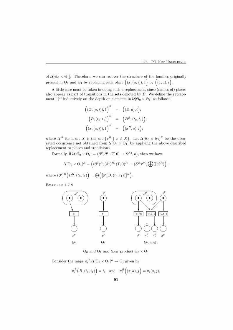
1.7. PT Net Unfoldings
of U [Θ0 × Θ1]. Therefore, we can recover the structure of the families originally
present in Θ0 and Θ1 by replacing each place((x, (a, i)), 1
)by((x, a), i
).
A little care must be taken in doing such a replacement, since (names of) placesalso appear as part of transitions in the sets denoted by B. We define the replace-ment [ ]R inductively on the depth on elements in U [Θ0 ×Θ1] as follows:
((∅, (a, i)), 1
)R=
((∅, a), i
);
(B, (t0, t1)
)R=
(BR, (t0, t1)
);
((x, (a, i)), 1
)R=
((xR, a), i
);
where XR for a set X is the set {xR | x ∈ X}. Let U [Θ0 × Θ1]R be the deco-
rated occurrence net obtained from U [Θ0 × Θ1] by applying the above describedreplacement to places and transitions.
Formally, if U [Θ0 ×Θ1] =(∂0, ∂1: (T, 0)→ SM, u
), then we have
U [Θ0 ×Θ1]R =
((∂0)R, (∂1)R: (T, 0)R → (SR)M,
⊕([[u]]R)
),
where (∂i)R(BR, (t0, t1)
)=⊕(
[[∂i(B, (t0, t1))]]R).
Example 1.7.9
� ��
� ��
����B
BBN
?
� �� � ��?
?� ��
� ��� ������� ��
?
?
?
?
@@@R
���
? ?� �� � ��� ��� ��
Θ0 Θ1 Θ0 ×Θ1
• • • • • •
t0 t1 (t0,0) (t0,t1) (0,t1)
aF bF
aF bF
cF dF cF dFcFu dF
u
Θ0 and Θ1 and their product Θ0 ×Θ1
Consider the maps πRi :U [Θ0 ×Θ1]R → Θi given by
πRi
(B, (t0, t1)
)= ti and πRi
((x, a), j
)= πi(a, j),
91
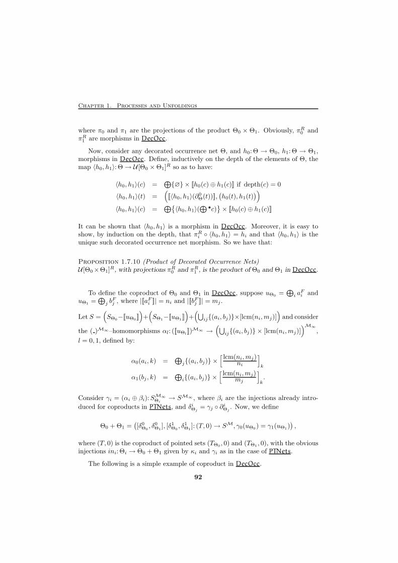
Chapter 1. Processes and Unfoldings
where π0 and π1 are the projections of the product Θ0 × Θ1. Obviously, πR0 andπR1 are morphisms in DecOcc.
Now, consider any decorated occurrence net Θ, and h0: Θ → Θ0, h1: Θ → Θ1,morphisms in DecOcc. Define, inductively on the depth of the elements of Θ, themap 〈h0, h1〉: Θ→ U [Θ0 ×Θ1]
R so as to have:
〈h0, h1〉(c) =⊕{∅} × [[h0(c)⊕ h1(c)]] if depth(c) = 0
〈h0, h1〉(t) =([[〈h0, h1〉(∂
0Θ(t))]],
(h0(t), h1(t)
))
〈h0, h1〉(c) =⊕{〈h0, h1〉(
⊕•c)}× [[h0(c)⊕ h1(c)]]
It can be shown that 〈h0, h1〉 is a morphism in DecOcc. Moreover, it is easy toshow, by induction on the depth, that πRi ◦ 〈h0, h1〉 = hi and that 〈h0, h1〉 is theunique such decorated occurrence net morphism. So we have that:
Proposition 1.7.10 (Product of Decorated Occurrence Nets)U [Θ0×Θ1]
R, with projections πR0 and πR1 , is the product of Θ0 and Θ1 in DecOcc.
To define the coproduct of Θ0 and Θ1 in DecOcc, suppose uΘ0 =⊕
i aFi and
uΘ1 =⊕
j bFj , where |[[aFi ]]| = ni and |[[bFj ]]| = mj .
Let S =(SΘ0−[[uΘ0 ]]
)+(SΘ1−[[uΘ1 ]]
)+(⋃
ij{(ai, bj)}×[lcm(ni,mj)])
and consider
the ( )M∞–homomorphisms αl: ([[uΘl]])M∞ →
(⋃ij{(ai, bj)} × [lcm(ni,mj)]
)M∞
,
l = 0, 1, defined by:
α0(ai, k) =⊕
j{(ai, bj)} ×[lcm(ni,mj)
ni
]
k
α1(bj , k) =⊕
i{(ai, bj)} ×[lcm(ni,mj)
mj
]
k.
Consider γi = (αi ⊕ βi):SM∞
Θi→ SM∞ , where βi are the injections already intro-
duced for coproducts in PTNets, and δiΘj= γj ◦ ∂
iΘj
. Now, we define
Θ0 + Θ1 =([δ0Θ0
, δ0Θ1], [δ1Θ0
, δ1Θ1]: (T, 0)→ SM, γ0(uΘ0) = γ1(uΘ1)
),
where (T, 0) is the coproduct of pointed sets (TΘ0 , 0) and (TΘ1 , 0), with the obviousinjections ini: Θi → Θ0 + Θ1 given by κi and γi as in the case of PTNets.
The following is a simple example of coproduct in DecOcc.
92
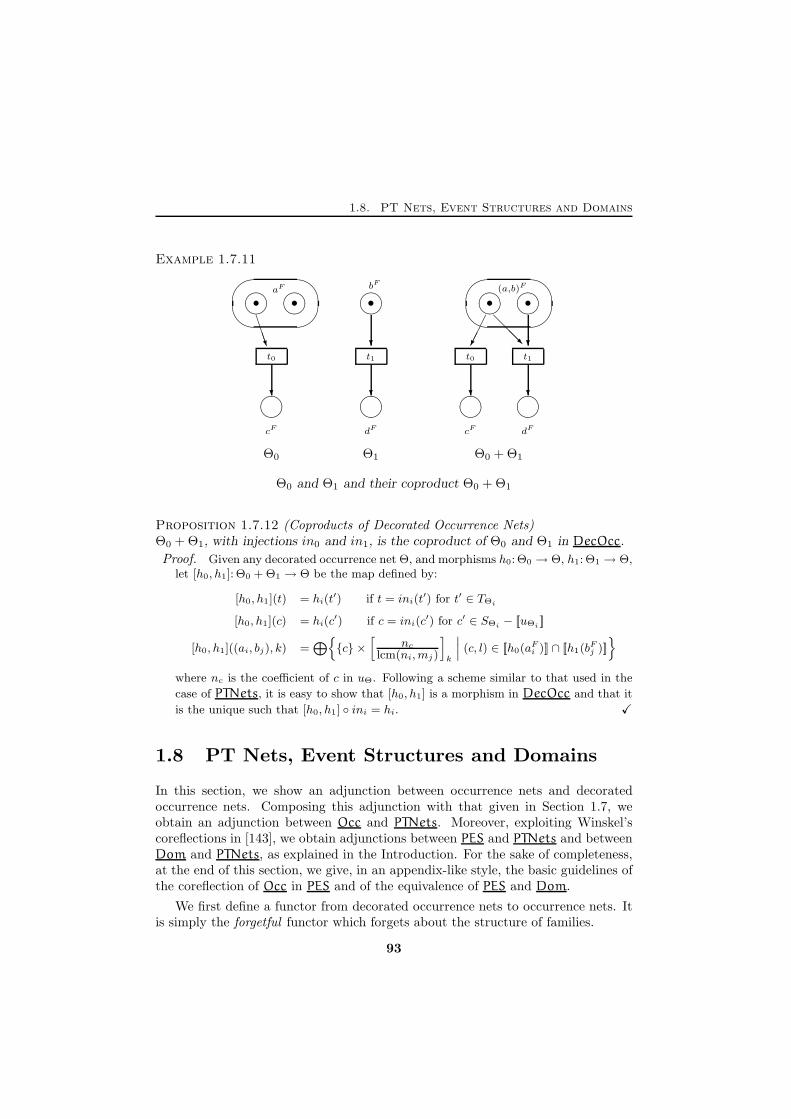
1.8. PT Nets, Event Structures and Domains
Example 1.7.11
� ��
� ��
����B
BBN
?
� �� � ��?
?� ��
� ��� ������
?
����@@@R
?
?
� �� � ��
Θ0 Θ1 Θ0 + Θ1
• • • • •
t0 t1 t0 t1
aF bF(a,b)F
cF dF cF dF
Θ0 and Θ1 and their coproduct Θ0 + Θ1
Proposition 1.7.12 (Coproducts of Decorated Occurrence Nets)Θ0 + Θ1, with injections in0 and in1, is the coproduct of Θ0 and Θ1 in DecOcc.
Proof. Given any decorated occurrence net Θ, and morphisms h0: Θ0 → Θ, h1: Θ1 → Θ,let [h0, h1]: Θ0 + Θ1 → Θ be the map defined by:
[h0, h1](t) = hi(t′) if t = ini(t
′) for t′ ∈ TΘi
[h0, h1](c) = hi(c′) if c = ini(c
′) for c′ ∈ SΘi − [[uΘi ]]
[h0, h1]((ai, bj), k) =⊕{{c} ×
[nc
lcm(ni,mj)
]
k
∣∣∣ (c, l) ∈ [[h0(aFi )]] ∩ [[h1(b
Fj )]]}
where nc is the coefficient of c in uΘ. Following a scheme similar to that used in the
case of PTNets, it is easy to show that [h0, h1] is a morphism in DecOcc and that it
is the unique such that [h0, h1] ◦ ini = hi. X
1.8 PT Nets, Event Structures and Domains
In this section, we show an adjunction between occurrence nets and decoratedoccurrence nets. Composing this adjunction with that given in Section 1.7, weobtain an adjunction between Occ and PTNets. Moreover, exploiting Winskel’scoreflections in [143], we obtain adjunctions between PES and PTNets and betweenDom and PTNets, as explained in the Introduction. For the sake of completeness,at the end of this section, we give, in an appendix-like style, the basic guidelines ofthe coreflection of Occ in PES and of the equivalence of PES and Dom.
We first define a functor from decorated occurrence nets to occurrence nets. Itis simply the forgetful functor which forgets about the structure of families.
93
Chapter 1. Processes and Unfoldings
Definition 1.8.1 (F [ ]: from DecOcc to Occ)Given a decorated occurrence net Θ define F [Θ] to be the occurrence net Θ. Fur-thermore, given 〈f, g〉: Θ0 → Θ1, define F [〈f, g〉] to be 〈f, g〉.
In order to define a left adjoint for F [ ], we need to identify, for any occurrencenet Θ, a decorated occurrence net D[Θ] which is, informally speaking, a “saturated”version of Θ, in the sense that it can match in a unique way the structure of anydecorated occurrence net whose transitions are “similar” to those of Θ. Moreprecisely, the existence of an adjunction requires D[Θ] to be such that, for anyoccurrence net Θ′,
Occ[Θ,F [Θ′]] ∼= DecOcc[D[Θ],Θ′]
i.e., the set of morphisms from Θ to F [Θ′] in Occ and the set of morphisms fromD[Θ] to Θ′ in DecOcc are isomorphic. It follows from this condition that eachtransition of D[Θ] must have enough families in its post-set to “cover” those in thepost-set of any transition of Θ′ to which it could be mapped by an occurrence netmorphism and, at the same time, it must not have too many of them so that sucha covering is realized by a unique decorated occurrence net morphism from D[Θ]to Θ′.
Because of the uniqueness requirement, saturating occurrence nets is a delicatematter: we need to identify a suitable set of families which can “represent” uniquelyall the possible others. To this aim are devoted the following definition and lemma,where the relation 7→ is introduced to capture the behaviour of decorated occurrencenet morphisms on families—which will be represented as strings on appropriatealphabets—and prime strings are meant to represent—in a sense that will be clearlater—exactly the families which we must add to Θ in order to saturate it.
In the following, given a string s on an alphabet Σ, as usual we denote the i-thelement of s by si and its length by |s|. Moreover, σn, for σ ∈ Σ and n ∈ ω, willdenote the string consisting of the symbol σ repeated n times.
Definition 1.8.2 (Prime Strings)Let Σ be an alphabet, i.e., a set of symbols. Define the binary relation 7→ on Σ+,the language of non-empty strings on Σ, by
σn11 · · ·σ
nk
k 7→σm11 · · ·σmk
k ⇔ σi 6= σi+1 and ∃q ∈ ω s.t. qni = mi, i = 1, . . . , k.
Define the language of prime strings on Σ to be
ΣP = Σ+ − {σn11 σn2
2 · · ·σnk
k | σi ∈ Σ, σi 6= σi+1, gcd(n1, . . . , nk) > 1} ,
where gcd is the greatest common divisor.
Lemma 1.8.3 (Prime Strings are primes)Given s′ ∈ Σ+ there exists a unique s ∈ ΣP such that s 7→s′.
94
1.8. PT Nets, Event Structures and Domains
Proof. Let s′ = σm11 · · ·σmk
k , where σi 6= σi+1. Consider h = gcd(m1, . . . ,mk). Since h
is the unique integer such thatmi is divisible by h for 1 ≤ i ≤ k and gcd(m1h, . . . , mk
h) =
1, and since h always exists (possibly h = 1) we have that s = σm1/h1 · · ·σmk/h
k is the
unique prime string such that s 7→s′. X
We start relating strings and nets by looking at sets of places as alphabets andat families as strings on such alphabets. Given a (decorated) occurrence net Θ anda transition t ∈ TΘ, we denote by Σ{t} the alphabet [[∂1
Θ(t)]]. By analogy, since theplaces in the initial marking are in the post-set of no transition, Σ∅ will consistof the places [[uΘ]]; following the analogy, in the rest of the section uΘ will also bedenoted by ∂1
Θ(∅).
Since a family bF of a decorated occurrence net Θ is nothing but an orderedsubset of the initial marking or of the post-set of a transition, it corresponds natu-rally to a string in Σ+
x where x = •[[bF ]], namely, the string of length |[[bF ]]| whose
i-th element is (b, i). We will write bF to indicate such a string.
Now, we can define the saturated net corresponding to an occurrence net Θ. Itis the net D[Θ] whose transitions are the transitions of Θ, and whose families inthe post-set of a transition t are the prime strings on the alphabet defined by t inΘ. It is immediate to see that this construction is well-defined, i.e., that D[Θ] is adecorated occurrence net.
Definition 1.8.4 (D[ ]: from Occ to DecOcc)Let Θ be a net in Occ. We define the decorated occurrence net
D[Θ] =(∂0D[Θ], ∂
1D[Θ]: (TΘ, 0)→ SMD[Θ], uD[Θ]
),
where
• SD[Θ] =⋃{{s} ×
[| s |] ∣∣ s ∈ ΣPx and (x = {t} ⊆ TΘ or x = ∅)
};
• ∂0D[Θ](t) =
⊕{(s, i) ∈ SD[Θ] | si ∈ [[∂0
Θ(t)]]}
;
• ∂1D[Θ](t) =
⊕{(s, i) ∈ SD[Θ] | si ∈ [[∂1
Θ(t)]]}
=⊕{
sF | s ∈ ΣP{t}
};
• uD[Θ] =⊕{
sF | s ∈ ΣP∅
}.
The following example shows the decorated occurrence net corresponding to avery simple occurrence net Θ. The place σ2 is filled to the purpose of making thedifference between the family (σ1σ2)
F and the family (σ2σ1)F of D[Θ] graphically
suggestive. Of course, only part of D[Θ] is shown.
95
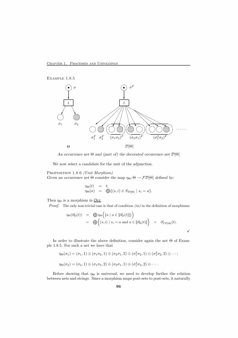
Chapter 1. Processes and Unfoldings
Example 1.8.5
?
n n
n n.............................................
n n............................................. n n.....................
.......
.................����n.....................
.......
................. n����nnn.....................
.......
.................
����
?
����
AAAU
HHHHHHHHHHHj
QQQQQQQs
@@@@@R
CCCCCCW
AAAAAAU
�������
�������
������
�������=σ1 σ2
σF1 σF2 (σ1σ2)F (σ2σ1)
F (σ21σ2)
F
. . . . . .
tt
• •σ σF
Θ D[Θ]
An occurrence net Θ and (part of) the decorated occurrence net D[Θ]
We now select a candidate for the unit of the adjunction.
Proposition 1.8.6 (Unit Morphism)Given an occurrence net Θ consider the map ηΘ: Θ→ FD[Θ] defined by:
ηΘ(t) = t;ηΘ(a) =
⊕{(s, i) ∈ SD[Θ] | si = a}.
Then ηΘ is a morphism in Occ.
Proof. The only non-trivial case is that of condition (iii) in the definition of morphisms:
ηΘ(∂iΘ(t)) =⊕
ηΘ
({a | a ∈ [[∂iΘ(t)]]}
)
=⊕{
(s, i) | si = a and a ∈ [[∂iΘ(t)]]}
= ∂iFD[Θ](t).
X
In order to illustrate the above definition, consider again the net Θ of Exam-ple 1.8.5. For such a net we have that
ηΘ(σ1) = (σ1, 1)⊕ (σ1σ2, 1)⊕ (σ2σ1, 2)⊕ (σ21σ2, 1)⊕ (σ2
1σ2, 2)⊕ · · · ;
ηΘ(σ2) = (σ2, 1)⊕ (σ1σ2, 2)⊕ (σ2σ1, 1)⊕ (σ21σ2, 2)⊕ · · · .
Before showing that ηΘ is universal, we need to develop further the relationbetween nets and strings. Since a morphism maps post-sets to post-sets, it naturally
96
1.8. PT Nets, Event Structures and Domains
induces a (contravariant) mapping between the languages associated to transitionsrelated by the morphism. To simplify the exposition, in the rest of this section,for k a morphism of nets, k({t}) and k(∅), denote, respectively, {k(t)} and ∅;moreover, ∂1
Θ({t}) denotes ∂1Θ(t).
Definition 1.8.7 (Sxk : from Σ+k(x) to Σ+
x )
Let Θ0 and Θ1 be (decorated) occurrence nets, let k = 〈f, g〉: Θ0 → Θ1 be amorphism and let x = {t} ⊆ TΘ0 or x = ∅ and y be such that f(x) = y. Thenk induces a unique semigroup homomorphism Sxk from Σ+
y to Σ+x defined on the
generators b ∈ [[∂1Θ1
(y)]] by
Sxk (b) = a ∈ [[∂1Θ0
(x)]] such that g(a) = b.
From the properties of safe net morphisms in Proposition 1.5.3, it is easy to seethat Sxk is well-defined, i.e., there exists one and only one a ∈ [[∂1
Θ0(x)]] such that
g(a) = b.
To clarify the relation between 7→ and decorated occurrence net morphisms, ob-serve that, in the condition of the previous definition, if Θ is a decorated occurrencenet and k is a decorated occurrence net morphism, then aF 7→Sxk (bF ) if and only ifk(aF ) = bF .
Example 1.8.8Consider the following figure, where the morphism 〈f, g〉 is such that g(σ1) = s2⊕s3and g(σ2) = s1.
n
n n n nn
?
����
AAAU
����
@@@R
CCCW
n?
-................................
-............................
-................................................................. �...
...σ1 σ2 s1 s2 s3g
g
g
f
• •
t t′
Then, for instance, we have that S{t}〈f,g〉(s1s2s3s2s1) = σ2σ
31σ2.
Finally, we show that D[ ] extends to a functor which is left adjoint to F [ ].
Theorem 1.8.9 (D ⊣ F)The pair 〈D,F〉 : Occ ⇀ DecOcc constitutes an adjunction.
97
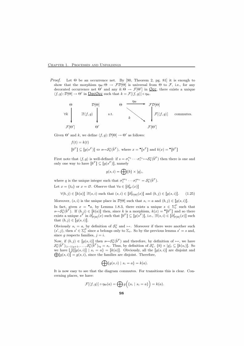
Chapter 1. Processes and Unfoldings
Proof. Let Θ be an occurrence net. By [90, Theorem 2, pg. 81] it is enough toshow that the morphism ηΘ: Θ → FD[Θ] is universal from Θ to F , i.e., for anydecorated occurrence net Θ′ and any k: Θ → F [Θ′] in Occ, there exists a unique〈f, g〉:D[Θ]→ Θ′ in DecOcc such that k = F [〈f, g〉] ◦ ηΘ.
? ?
ZZZZZ~
-
?
∀k
Θ
F [Θ′]
∃!〈f, g〉
D[Θ]
Θ′
s.t.
Θ
k
ηΘ
F [Θ′]
FD[Θ]
F [〈f, g〉] commutes.
Given Θ′ and k, we define 〈f, g〉:D[Θ]→ Θ′ as follows:
f(t) = k(t)
[[bF ]] ⊆ [[g(sF )]]⇔ s 7→Sxk (bF ), where x = •[[sF ]] and k(x) = •[[bF ]]
First note that 〈f, g〉 is well-defined: if s = σn11 · · ·σ
nrr 7→S
xk (bF ) then there is one and
only one way to have [[bF ]] ⊆ [[g(sF )]], namely
g(s, i) =⊕{b} × [q]i,
where q is the unique integer such that σqn11 · · · σqnr
r = Sxk (bF ).
Let x = {t0} or x = ∅. Observe that ∀a ∈ [[∂1Θ′(x)]]
∀(b, j) ∈ [[k(a)]] ∃!(s, i) such that (s, i) ∈ [[∂1D[Θ](x)]] and (b, j) ∈ [[g(s, i)]]. (1.25)
Moreover, (s, i) is the unique place in D[Θ] such that si = a and (b, j) ∈ [[g(s, i)]].
In fact, given x = •a, by Lemma 1.8.3, there exists a unique s ∈ ΣPx such thats 7→Sxk (bF ). If (b, j) ∈ [[k(a)]] then, since k is a morphism, k(x) = •[[bF ]] and so thereexists a unique sF in ∂1
D[Θ](x) such that [[bF ]] ⊆ [[g(sF )]], i.e., ∃!(s, i) ∈ [[∂1D[Θ](x)]] such
that (b, j) ∈ [[g(s, i)]].
Obviously si = a, by definition of Sxk and 7→. Moreover if there were another such(s′, j), then s′ ∈ ΣPx since a belongs only to Σx. So by the previous lemma s′ = s and,since g respects families, j = i.
Now, if (b, j) ∈ [[g(s, i)]] then s 7→Sxk (bF ) and therefore, by definition of 7→, we haveSxk (bF )(i−1)q+1, . . . ,S
xk (bF )iq = si. Thus, by definition of Sxk , {b} × [q]i ⊆ [[k(si)]]. So
we have⋃{[[g(s, i)]] | si = a} = [[k(a)]]. Obviously, all the [[g(s, i)]] are disjoint and⊕
[[g(s, i)]] = g(s, i), since the families are disjoint. Therefore,⊕{g(s, i) | si = a} = k(a).
It is now easy to see that the diagram commutes. For transitions this is clear. Con-cerning places, we have:
F [〈f, g〉] ◦ ηΘ(a) =⊕
g({si | si = a}
)= k(a).
98
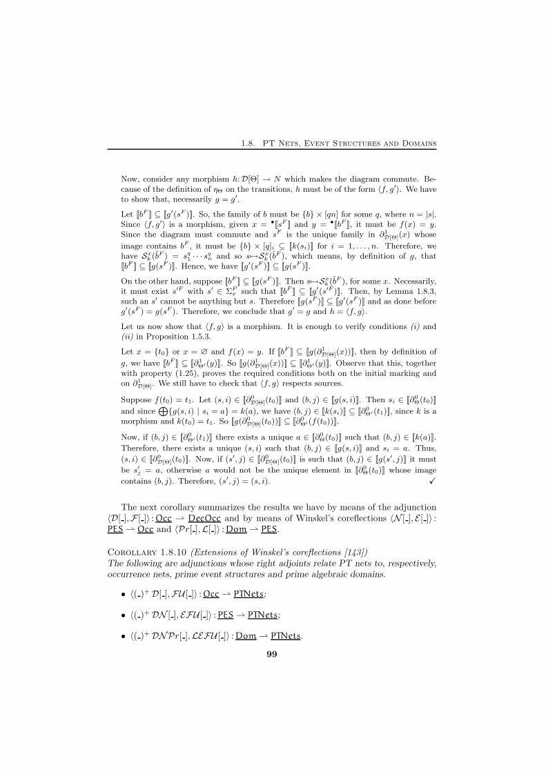
1.8. PT Nets, Event Structures and Domains
Now, consider any morphism h:D[Θ] → N which makes the diagram commute. Be-cause of the definition of ηΘ on the transitions, h must be of the form 〈f, g′〉. We haveto show that, necessarily g = g′.
Let [[bF ]] ⊆ [[g′(sF )]]. So, the family of b must be {b} × [qn] for some q, where n = |s|.Since 〈f, g′〉 is a morphism, given x = •[[sF ]] and y = •[[bF ]], it must be f(x) = y.Since the diagram must commute and sF is the unique family in ∂1
D[Θ](x) whose
image contains bF , it must be {b} × [q]i ⊆ [[k(si)]] for i = 1, . . . , n. Therefore, wehave Sxk (bF ) = sq1 · · · s
qn and so s 7→Sxk (bF ), which means, by definition of g, that
[[bF ]] ⊆ [[g(sF )]]. Hence, we have [[g′(sF )]] ⊆ [[g(sF )]].
On the other hand, suppose [[bF ]] ⊆ [[g(sF )]]. Then s 7→Sxk (bF ), for some x. Necessarily,it must exist s′F with s′ ∈ ΣPx such that [[bF ]] ⊆ [[g′(s′F )]]. Then, by Lemma 1.8.3,such an s′ cannot be anything but s. Therefore [[g(sF )]] ⊆ [[g′(sF )]] and as done beforeg′(sF ) = g(sF ). Therefore, we conclude that g′ = g and h = 〈f, g〉.
Let us now show that 〈f, g〉 is a morphism. It is enough to verify conditions (i) and(ii) in Proposition 1.5.3.
Let x = {t0} or x = ∅ and f(x) = y. If [[bF ]] ⊆ [[g(∂1D[Θ](x))]], then by definition of
g, we have [[bF ]] ⊆ [[∂1Θ′(y)]]. So [[g(∂1
D[Θ](x))]] ⊆ [[∂1Θ′(y)]]. Observe that this, together
with property (1.25), proves the required conditions both on the initial marking andon ∂1
D[Θ]. We still have to check that 〈f, g〉 respects sources.
Suppose f(t0) = t1. Let (s, i) ∈ [[∂0D[Θ](t0)]] and (b, j) ∈ [[g(s, i)]]. Then si ∈ [[∂0
Θ(t0)]]
and since⊕{g(s, i) | si = a} = k(a), we have (b, j) ∈ [[k(si)]] ⊆ [[∂0
Θ′(t1)]], since k is amorphism and k(t0) = t1. So [[g(∂0
D[Θ](t0))]] ⊆ [[∂0Θ′(f(t0))]].
Now, if (b, j) ∈ [[∂0Θ′(t1)]] there exists a unique a ∈ [[∂0
Θ(t0)]] such that (b, j) ∈ [[k(a)]].
Therefore, there exists a unique (s, i) such that (b, j) ∈ [[g(s, i)]] and si = a. Thus,
(s, i) ∈ [[∂0D[Θ](t0)]]. Now, if (s′, j) ∈ [[∂0
D[Θ](t0)]] is such that (b, j) ∈ [[g(s′, j)]] it must
be s′j = a, otherwise a would not be the unique element in [[∂0Θ(t0)]] whose image
contains (b, j). Therefore, (s′, j) = (s, i). X
The next corollary summarizes the results we have by means of the adjunction〈D[ ],F [ ]〉 : Occ ⇀ DecOcc and by means of Winskel’s coreflections 〈N [ ], E [ ]〉 :PES ⇀ Occ and 〈Pr[ ],L[ ]〉 : Dom ⇀ PES.
Corollary 1.8.10 (Extensions of Winskel’s coreflections [143])The following are adjunctions whose right adjoints relate PT nets to, respectively,occurrence nets, prime event structures and prime algebraic domains.
• 〈( )+D[ ],FU [ ]〉 : Occ ⇀ PTNets;
• 〈( )+DN [ ], EFU [ ]〉 : PES ⇀ PTNets;
• 〈( )+DNPr[ ],LEFU [ ]〉 : Dom ⇀ PTNets.
99

Chapter 1. Processes and Unfoldings
In addition, FU [ ]Safe = Uw[ ] and, therefore, EFU [ ]Safe = EUw[ ] andLEFU [ ]Safe = LEUw[ ], i.e., the semantics given to safe nets by the chain ofadjunctions presented in this work coincides with the semantics given by Winskel’schain of coreflections. X
Occurrence Nets, Event Structures and Domains
This subsection contains a brief summary of Winskel’s work on the coreflectionof PES in Occ and on the equivalence of the category of prime event structures(with binary conflict) and the category of finitary, (coherent), prime algebraic do-mains [143] (see also [20, 148]).
Prime event structures [143] are the simplest event based model of computation.They consist of a set of events, intended as indivisible quanta of computation, whichare related to each other by two binary relation: causality, modelled by a partialorder relation ≤, and conflict, modelled by an irreflexive, symmetric and hereditaryrelation #.
Definition 1.8.11 (Prime Event Structures and PES)A prime event structure is a structure ES = (E,#,≤) consisting of a set of eventsE partially ordered by ≤, and a symmetric, irreflexive relation # ⊆ E × E, theconflict relation, such that
{e′ ∈ E | e′ ≤ e} is finite for each e ∈ E
e # e′ ≤ e′′ implies e # e′′ for each e, e′, e′′ ∈ E.
For an event e ∈ E, define ⌊e⌋ = {e′ ∈ E | e′ ≤ e}.
A prime event structure morphism θ: (E0,≤0,#0)→ (E1,≤1,#1) is a partial func-tion θ:E0 ⇀ E1 such that
θ(e) is defined implies ⌊θ(e)⌋ ⊆ θ(⌊e⌋)
(θ(e) #1 θ(e′) or θ(e) = θ(e′)) implies (e #0 e
′ or e = e′)
This defines the category PES of prime event structures.
The computational intuition behind event structures is really simple: an event ecan occur when all its causes, i.e. ⌊e⌋, have occurred and no event which it is inconflict with has already occurred. This is formalized by the following notion ofconfiguration, which gives the computations of event structures.
Definition 1.8.12 (Configurations)Given a prime event structure (E,#,≤), define its configurations to be those subsets
100
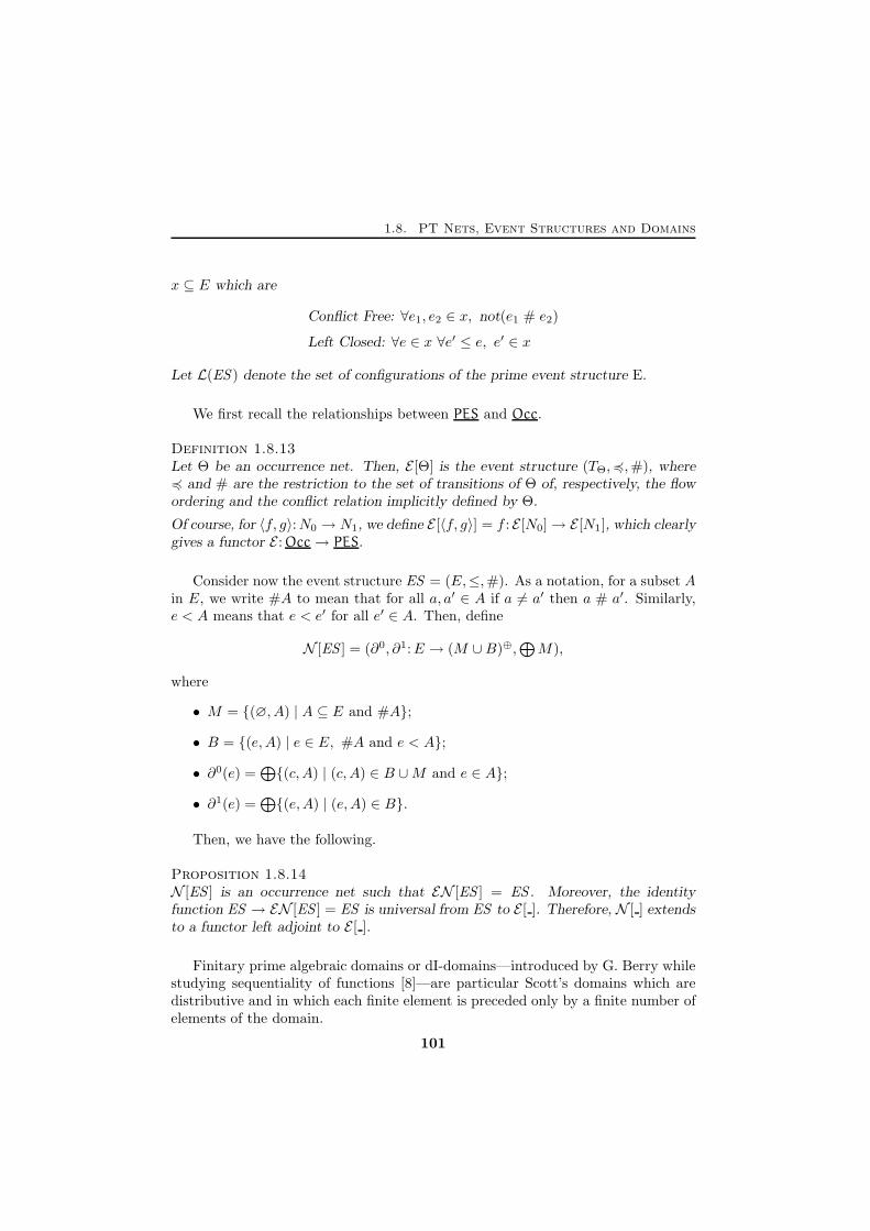
1.8. PT Nets, Event Structures and Domains
x ⊆ E which are
Conflict Free: ∀e1, e2 ∈ x, not(e1 # e2)
Left Closed: ∀e ∈ x ∀e′ ≤ e, e′ ∈ x
Let L(ES ) denote the set of configurations of the prime event structure E.
We first recall the relationships between PES and Occ.
Definition 1.8.13Let Θ be an occurrence net. Then, E [Θ] is the event structure (TΘ,4,#), where4 and # are the restriction to the set of transitions of Θ of, respectively, the flowordering and the conflict relation implicitly defined by Θ.
Of course, for 〈f, g〉:N0 → N1, we define E [〈f, g〉] = f : E [N0]→ E [N1], which clearlygives a functor E : Occ→ PES.
Consider now the event structure ES = (E,≤,#). As a notation, for a subset Ain E, we write #A to mean that for all a, a′ ∈ A if a 6= a′ then a # a′. Similarly,e < A means that e < e′ for all e′ ∈ A. Then, define
N [ES ] = (∂0, ∂1:E → (M ∪B)⊕,⊕M),
where
• M = {(∅, A) | A ⊆ E and #A};
• B = {(e,A) | e ∈ E, #A and e < A};
• ∂0(e) =⊕{(c, A) | (c, A) ∈ B ∪M and e ∈ A};
• ∂1(e) =⊕{(e,A) | (e,A) ∈ B}.
Then, we have the following.
Proposition 1.8.14N [ES ] is an occurrence net such that EN [ES ] = ES . Moreover, the identityfunction ES → EN [ES ] = ES is universal from ES to E [ ]. Therefore, N [ ] extendsto a functor left adjoint to E [ ].
Finitary prime algebraic domains or dI-domains—introduced by G. Berry whilestudying sequentiality of functions [8]—are particular Scott’s domains which aredistributive and in which each finite element is preceded only by a finite number ofelements of the domain.
101
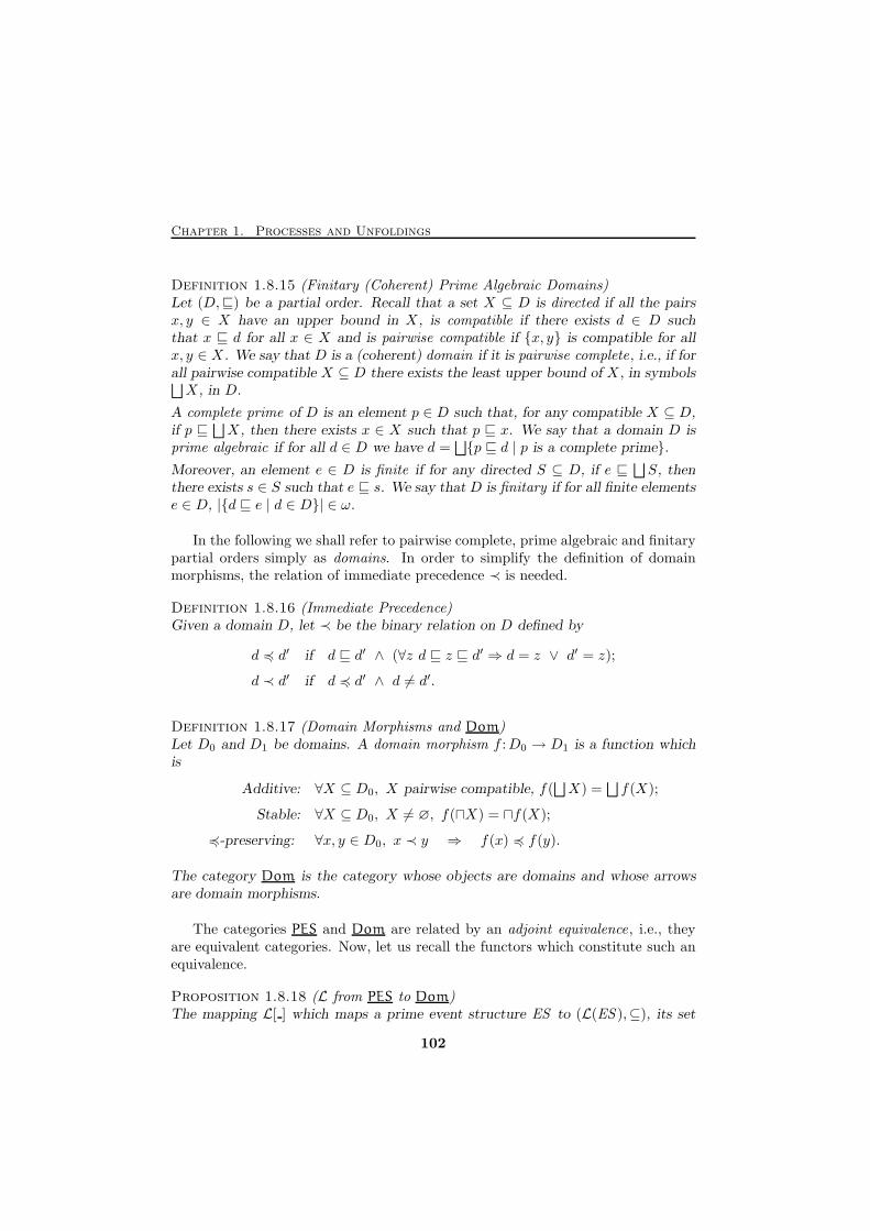
Chapter 1. Processes and Unfoldings
Definition 1.8.15 (Finitary (Coherent) Prime Algebraic Domains)Let (D,⊑) be a partial order. Recall that a set X ⊆ D is directed if all the pairsx, y ∈ X have an upper bound in X , is compatible if there exists d ∈ D suchthat x ⊑ d for all x ∈ X and is pairwise compatible if {x, y} is compatible for allx, y ∈ X . We say that D is a (coherent) domain if it is pairwise complete, i.e., if forall pairwise compatible X ⊆ D there exists the least upper bound of X , in symbols⊔X , in D.
A complete prime of D is an element p ∈ D such that, for any compatible X ⊆ D,if p ⊑
⊔X , then there exists x ∈ X such that p ⊑ x. We say that a domain D is
prime algebraic if for all d ∈ D we have d =⊔{p ⊑ d | p is a complete prime}.
Moreover, an element e ∈ D is finite if for any directed S ⊆ D, if e ⊑⊔S, then
there exists s ∈ S such that e ⊑ s. We say that D is finitary if for all finite elementse ∈ D, |{d ⊑ e | d ∈ D}| ∈ ω.
In the following we shall refer to pairwise complete, prime algebraic and finitarypartial orders simply as domains. In order to simplify the definition of domainmorphisms, the relation of immediate precedence ≺ is needed.
Definition 1.8.16 (Immediate Precedence)Given a domain D, let ≺ be the binary relation on D defined by
d 4 d′ if d ⊑ d′ ∧ (∀z d ⊑ z ⊑ d′ ⇒ d = z ∨ d′ = z);
d ≺ d′ if d 4 d′ ∧ d 6= d′.
Definition 1.8.17 (Domain Morphisms and Dom)Let D0 and D1 be domains. A domain morphism f :D0 → D1 is a function whichis
Additive: ∀X ⊆ D0, X pairwise compatible, f(⊔X) =
⊔f(X);
Stable: ∀X ⊆ D0, X 6= ∅, f(⊓X) = ⊓f(X);
4-preserving: ∀x, y ∈ D0, x ≺ y ⇒ f(x) 4 f(y).
The category Dom is the category whose objects are domains and whose arrowsare domain morphisms.
The categories PES and Dom are related by an adjoint equivalence, i.e., theyare equivalent categories. Now, let us recall the functors which constitute such anequivalence.
Proposition 1.8.18 (L from PES to Dom)The mapping L[ ] which maps a prime event structure ES to (L(ES ),⊆), its set
102
1.8. PT Nets, Event Structures and Domains
of configurations ordered by inclusion, and which maps a prime event structuremorphism θ:ES 0 ⇀ ES 1 to the function L[θ]: (L(ES 0),⊆)→ (L(ES 1),⊆), definedby
L(θ)(x) = θ(x),
is a functor from PES to Dom.
Moreover, the complete primes of L[ES ] are the elements ⌊e⌋ for e ∈ E.
The definition on the objects of the “quasi-inverse” functor from Dom to PES
is as easy as that of L.
Proposition 1.8.19 (Pr: from Dom to PES, part I)Given a domain D, let PD denote its set of complete primes. Then Pr(D) is theprime event structure (PD,#,≤), where
p ≤ p′ if p ⊑ p′ and p # p′ if not ∃ p ⊔ p′
is a prime event structure.
However, as far a morphisms is concerned, the behaviour of Pr is a bit morecomplex. In order to be able to define it, we are required to look more closely todomain morphisms.
Definition 1.8.20 (Prime Intervals)A prime interval of a domain D is a pair [d, d′] such that d ≺ d′. Define
[c, c′] ≤ [d, d′] if (c = c′ ⊓ d) and (c′ ⊔ d = d′),
and let ∼ be the equivalence relation obtained as the transitive and symmetricclosure of (the preorder) ≤.
Then, the following result can be shown.
Proposition 1.8.21 (∼-classes are complete primes and viceversa)Given a domain D, the map
[d, d′]∼ 7→ p,
where {p} = φ(d′) \ φ(d), is an isomorphism of the ∼–classes of prime intervals ofD and the complete primes PD of D, whose inverse is the function
p 7→[⊔{c ⊑ p ∧ c 6= p}, p
]
∼.
103
Chapter 1. Processes and Unfoldings
Lemma 1.8.22Let f :D0 → D1 be a morphism in Dom. Then
[c, c′] ∼ [d, d′] and f(c) ≺ f(c′) ⇒
f(d) ≺ f(d′) and [f(c), f(c′)] ∼ [f(d), f(d′)]
It is now easy to define Pr on domain morphisms.
Proposition 1.8.23 (Pr: from Dom to PES, part II)For f :D0 → D1 in Dom define Pr(f):Pr(D0)→ Pr(D1) by
Pr(f)(p) = p′ if p 7→ [d, d′]∼ and f(d) ≺ f(d′) and [f(d), f(d′)]∼ 7→ p′.
The lemma above guarantees that this definition is well given. Moreover, it makesPr: Dom→ PES into a functor.
The functors L and Pr are adjoints via the unit and counit of such adjunctionand established by the following.
Theorem 1.8.24 (ψ, θ, ψ, η are isomorphisms)Given a domain D, the function φ:D → LPr(D), defined by
φ(d) = {p ⊑ d | p ∈ PD},
is a domain morphism which is an isomorphism with inverse θ:LPr(D)→ D, givenby θ(x) =
⊔x. Given a prime event structure E the map ψ:PrL(E)→ E, defined
byψ(⌊e⌋) = e,
is a morphism of prime event structures which is an isomorphism whose inverseη:E → PrL(E) is given by η(e) = ⌊e⌋.
Theorem 1.8.25 (ψ, θ, ψ, η are natural)φ is a natural isomorphism 1 ∼= LPr with inverse θ.ψ is a natural isomorphism PrL ∼= 1 with inverse η.
Therefore, we can conclude that
L: PES→ Dom and Pr: Dom→ PES
are equivalences of categories and, equivalently, that
〈Pr,L, φ, ψ〉: Dom ⇀ PES and 〈L,Pr, η, θ〉: PES ⇀ Dom
are adjoint equivalences.
104
1.9. Process versus Unfolding Semantics of Nets
1.9 Process versus Unfolding Semantics of Nets
The semantics obtained via the unfolding yields an explanation of the behaviourof nets in terms of event structures, that is, in terms of domains. Domains can beunambiguously thought as partial orderings of computations, where a computationis represented by a configuration, which, in our context, is a “downward” closed,conflict free set of occurrences of transitions. On the other hand, processes areby definition left closed and conflict free (multi)sets of transition. Moreover, theprocesses from a given initial marking are naturally organized in a preorder-likefashion via a comma category construction. The question which therefore arisesspontaneously concerns the relationships between these two notions, and this is thequestion addressed in this section.
It is worth noticing that in the case of safe nets the question is readily answeredexploiting Winskel’s coreflection 〈→,U [ ]〉: Occ ⇀ Safe. In fact, by definition anadjunction 〈F,G〉: C ⇀ D determines an isomorphism between arrows of the kindF(c)→ d in D and the arrows of the kind c→ G(d) in C. Then, in the case of safenets, we have a one-to-one correspondence
π: Θ→ N ⇐⇒ π′: Θ→ U [N ]
for each safe netN and each occurrence net Θ. Therefore, since such correspondenceis easily seen to map processes to processes, in this special case, the correspondencebetween process and unfolding semantics ofN is very tidy: they are the same notionin the precise sense that there is an isomorphism between the processes of N andthe processes of U [N ], i.e., the deterministic finite subnets of the unfolding of N ,i.e., the finite configurations of EU [N ].
In our context, however, we have that the unfolding of N is strictly more con-crete than the processes of N . For example, consider the simple net N and itsunfolding FU [N ] shown in Figure 1.11. Clearly, there is a unique process of N inwhich a single instance of t has occurred. Nevertheless, there are two determinis-tic subnets of FU [N ] which correspond to such process, namely those obtained bychoosing respectively the left and the right instance of t. It is worth noticing thatsuch subnets are isomorphic and that this is not a fortunate case, since it is easy toshow that two finite deterministic subnets of FU [N ] correspond to the same processof N if and only if they are isomorphic via an isomorphism which sends instancesof an element of N to instances of the same element. More interestingly, the re-sults in this paper will prove that this is the exact relationship between the twosemantics of N : the unfolding contains several copies of the same process which,as illustrated in the preceding Sections 1.7 and 1.8 , are needed to provide a fullycausal explanation of the behaviour of N , i.e., to obtain an occurrence net whosetransitions represent exactly the instances of the transitions of N in all the possiblecausal contexts and which can therefore account for concurrent multiple instances
105
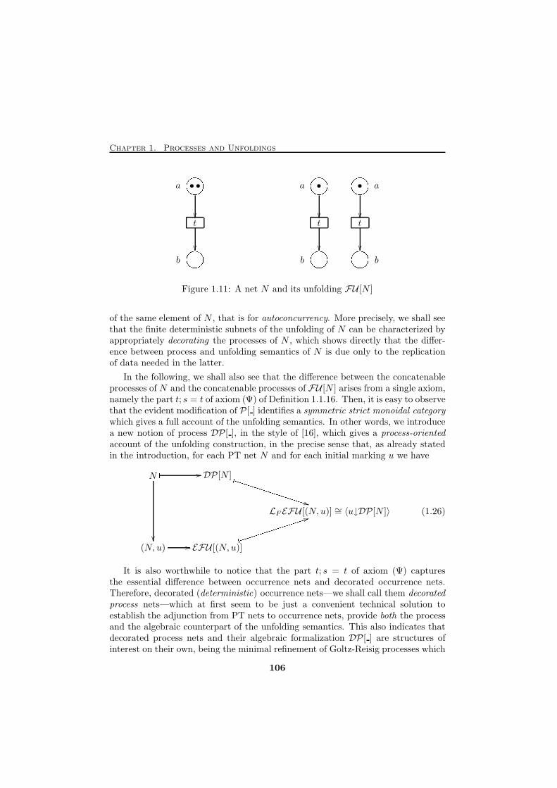
Chapter 1. Processes and Unfoldings
• •
t
a'&$%
��� �� ���
b'&$%
• •
t t
a'&$%
��
a'&$%
��� �� ���
� �� ���
b'&$% b
'&$%Figure 1.11: A net N and its unfolding FU [N ]
of the same element of N , that is for autoconcurrency. More precisely, we shall seethat the finite deterministic subnets of the unfolding of N can be characterized byappropriately decorating the processes of N , which shows directly that the differ-ence between process and unfolding semantics of N is due only to the replicationof data needed in the latter.
In the following, we shall also see that the difference between the concatenableprocesses of N and the concatenable processes of FU [N ] arises from a single axiom,namely the part t; s = t of axiom (Ψ) of Definition 1.1.16. Then, it is easy to observethat the evident modification of P [ ] identifies a symmetric strict monoidal categorywhich gives a full account of the unfolding semantics. In other words, we introducea new notion of process DP[ ], in the style of [16], which gives a process-orientedaccount of the unfolding construction, in the precise sense that, as already statedin the introduction, for each PT net N and for each initial marking u we have
N DP [N ]
LF EFU [(N, u)] ∼= 〈u↓DP[N ]〉
(N, u) EFU [(N, u)]
� //_��
�UUUUUUUUUUUUUUUUU **� //)iiiiiiiiiiiiiii44 (1.26)
It is also worthwhile to notice that the part t; s = t of axiom (Ψ) capturesthe essential difference between occurrence nets and decorated occurrence nets.Therefore, decorated (deterministic) occurrence nets—we shall call them decoratedprocess nets—which at first seem to be just a convenient technical solution toestablish the adjunction from PT nets to occurrence nets, provide both the processand the algebraic counterpart of the unfolding semantics. This also indicates thatdecorated process nets and their algebraic formalization DP [ ] are structures ofinterest on their own, being the minimal refinement of Goltz-Reisig processes which
106
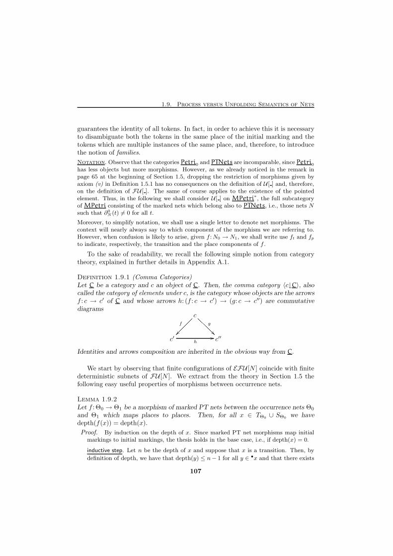
1.9. Process versus Unfolding Semantics of Nets
guarantees the identity of all tokens. In fact, in order to achieve this it is necessaryto disambiguate both the tokens in the same place of the initial marking and thetokens which are multiple instances of the same place, and, therefore, to introducethe notion of families.
Notation. Observe that the categories Petri0 and PTNets are incomparable, since Petri0has less objects but more morphisms. However, as we already noticed in the remark inpage 65 at the beginning of Section 1.5, dropping the restriction of morphisms given byaxiom (v) in Definition 1.5.1 has no consequences on the definition of U [ ] and, therefore,on the definition of FU [ ]. The same of course applies to the existence of the pointedelement. Thus, in the following we shall consider U [ ] on MPetri∗, the full subcategoryof MPetri consisting of the marked nets which belong also to PTNets, i.e., those nets Nsuch that ∂0
N (t) 6= 0 for all t.
Moreover, to simplify notation, we shall use a single letter to denote net morphisms. Thecontext will nearly always say to which component of the morphism we are referring to.However, when confusion is likely to arise, given f :N0 → N1, we shall write use ft and fpto indicate, respectively, the transition and the place components of f .
To the sake of readability, we recall the following simple notion from categorytheory, explained in further details in Appendix A.1.
Definition 1.9.1 (Comma Categories)Let C be a category and c an object of C. Then, the comma category 〈c↓C〉, alsocalled the category of elements under c, is the category whose objects are the arrowsf : c → c′ of C and whose arrows h: (f : c → c′) → (g: c → c′′) are commutativediagrams
c
c′ c′′
f������� g
����� ��h
//
Identities and arrows composition are inherited in the obvious way from C.
We start by observing that finite configurations of EFU [N ] coincide with finitedeterministic subnets of FU [N ]. We extract from the theory in Section 1.5 thefollowing easy useful properties of morphisms between occurrence nets.
Lemma 1.9.2Let f : Θ0 → Θ1 be a morphism of marked PT nets between the occurrence nets Θ0
and Θ1 which maps places to places. Then, for all x ∈ TΘ0 ∪ SΘ0 we havedepth(f(x)) = depth(x).
Proof. By induction on the depth of x. Since marked PT net morphisms map initialmarkings to initial markings, the thesis holds in the base case, i.e., if depth(x) = 0.
inductive step. Let n be the depth of x and suppose that x is a transition. Then, by
definition of depth, we have that depth(y) ≤ n− 1 for all y ∈ •x and that there exists
107
Chapter 1. Processes and Unfoldings
z ∈ •x such that depth(z) = n − 1. Then, since f(•x) = •f(x), the thesis follows
immediately by induction. If instead x is a place we have that depth(t) = n, where t
is the unique element in •x. Then, as we just proved, depth(f(t)) = n and since
f(x) ∈ f(t)• the proof is concluded. X
Lemma 1.9.3Let f : Θ0 → Θ1 be a morphism of marked PT nets between the occurrence nets Θ0
and Θ1 which maps places to places. Consider x ∈ TΘ0 ∪ SΘ0 and suppose thaty 4 f(x) for some y ∈ TΘ1 ∪ SΘ1 . Then, there exists y 4 x such that f(y) = y.Proof. In order to show the thesis, it is enough to consider the following two cases.
i) Suppose that a ∈ t• and f(a) = a. Since a does not belong to the initial markingof Θ1, then a cannot belong to the initial marking of Θ0. Therefore, there existsa unique t ∈ •a and, necessarily, f(t ) = t.
ii) Suppose that a ∈ •t and that f(t ) = t. Then, since f(• t ) = •t and since f mapsplaces to places, it must exists a ∈ SΘ0 such that f(a) = a. X
Lemma 1.9.4Let f : Θ0 → Θ1 be a morphism of marked PT nets between the occurrence nets Θ0
and Θ1 which maps places to places, and consider elements x and y in TΘ0 ∪ SΘ0 .Then, if f(x) = f(y) or f(x) # f(y), we have x = y or x # y.Proof. We proceed by induction on the least of the depths of x and y.
base case. If depth(x) = depth(y) = 0, then f(x) = f(y). In fact, in this case x and ybelong to the initial marking of Θ0 and thus, by definition of marked morphism, f(x)and f(y) are in the initial marking of Θ1. It follows that they cannot be in conflict,since # ∩ [[uΘ]] × [[uΘ]] = ∅. Now, if x 6= y, we have f(uΘ0) = f(x ⊕ y ⊕ u) =f(x) ⊕ f(y) ⊕ f(u) = 2f(x) ⊕ f(u). But this is impossible, since f(uΘ0) = uΘ1 andeach token in uΘ1 has multiplicity one.
inductive step. Let n ≥ 1 be the least of the depths of x and y. Without loss ofgenerality, assume depth(x) = n. First suppose that f(x) = f(y). Then, there existz ∈ •x and z′ ∈ •y such that f(z) = f(z′). Then, if x is a transition, depth(z) < nand therefore, by induction, f(z) = f(z′) or f(z) # f(z′), whence it follows thatf(x) = f(y) or f(x) # f(y). If instead x is a place, then z is a transition at depth nand the induction is maintained exploiting the proof given above for such a case.
Suppose instead that f(x) # f(y). By definition, this means that there exist t0 and t1in TΘ1 such that t0 #m t1, t0 4 f(x) and t1 4 f(y). Then, by Lemma 1.9.3, there
exist t0 4 x and t1 4 y in TΘ0 such that f(t0) = t0 and f(t1) = t1. This concludes
the proof since, by induction, we have t0 # t1 which implies x # y. X
Observe that the restriction to morphisms which map places to places in theprevious lemmas is not necessary to show that morphisms of occurrence nets pre-serve the depth of elements and reflect 4-chains and the conflict relation. However,the formulations above suffices for application in the following propositions.
108
1.9. Process versus Unfolding Semantics of Nets
Proposition 1.9.5Let N be a marked net in MPetri∗. There is an isomorphism between the set offinite configurations of EFU [N ] and the set of (marked) processes π of FU [N ].
Proof. Let φ be the function which maps a process π: Θ → FU [N ] to the set oftransitions π(TΘ). Recall that π is a marked net morphism between occurrence netswhich maps places to places. Then, by Lemma 1.9.4, we have that π maps concurrenttransitions to concurrent transitions. Since Θ is a process net, and thus deterministic,π(TΘ) is conflict free. Consider now t ∈ π(TΘ) and let t′ ∈ TFU [N] be such thatt′ 4 t. Then, by Lemma 1.9.3, there exists x ∈ TΘ such that π(x) = t′, i.e., π(TΘ) isdownwards closed and, thus, a finite configuration of EFU [N ].
On the contrary, let X be a finite configuration of EFU [N ]. By depth of an element xof X we mean the length of the shortest chain in X whose maximal element is x; thedepth of X is the greatest of the depths of its elements. We show by induction onthe depth of X that there exists a unique (up to isomorphism) process π: Θ→ FU [N ]such that π(TΘ) = X.
base case. IfX = ∅, let Θ be the subnet of depth zero of FU [N ], i.e., the net consistingof the minimal places of FU [N ], and let π be the inclusion FU [N ](0) → FU [N ].Clearly, π is the unique (marked) process of FU [N ] such that φ(π) = ∅.
inductive step. Suppose that the depth of X is n + 1. Let Z be the set of elementsof X at depth n + 1. Since the elements of Z are necessarily maximal in X, theset Y = X \Z is a configuration of EFU [N ]. Moreover, the depth of Z is n. Then, byinduction, there exists a unique π: Θ → FU [N ] such that π(TΘ) = Y . Let t ∈ Z andconsider a ∈ ∂0
FU [N](t). We show that there exists a unique place xa ∈ SΘ, which inaddition is maximal, such that π(xa) = a. The following two cases are possible.
i) •a = ∅. Then, a belongs to the initial marking of FU [N ] and thus, by definitionof marked net morphism, there exists a unique xa ∈ uΘ such that π(xa) = a.Moreover, since by Lemma 1.9.2 π preserves the depth of elements, there is noother x ∈ SΘ such that π(x) = a.
ii) •a = {t′}. Then, t′ ≺ t and thus, since X is downwards closed, there existsx ∈ TΘ such that π(x) = t′. It follows that we can find a unique xa ∈ x
• suchthat π(xa) = a. Now, since by Lemma 1.9.4 π maps concurrent transitions toconcurrent transitions, x is the unique transition of Θ mapped to t′. Therefore,xa is the unique place of Θ mapped to a.
Observe that xa must be maximal in Θ. In fact, is there were x ∈ x•a, there would beπ(x) ∈ X with π(x) # t, which is impossible since X is a configuration.
Now, it is easy to see that π can be extended to a process π′ such that φ(π′) = Xin essentially a unique way. To this purpose, consider the net Θ′ obtained by addingto Θ, for each t ∈ Z, a new transition xt and a new place a for each a ∈ ∂1
FU [N](t)with
∂0Θ′(xt) =
⊕{xa | a ∈ ∂
0FU [N](t)} and ∂1
Θ′(xt) =⊕{a | a ∈ ∂1
FU [N](t)}.
Since FU [N ] is an occurrence net, we have that ∂1FU [N](t0) ∩ ∂
1FU [N](t1) = ∅, for
t0 6= t1 in Z, and therefore, by definition, Θ′ is an occurrence net. Moreover, since Z
109
Chapter 1. Processes and Unfoldings
is a set of concurrent transitions, we also have ∂0FU [N](t0) ∩ ∂
0FU [N](t1) = ∅. Then,
considering also that each xa is maximal in Θ, we conclude that Θ′ is deterministic.Therefore, π′ defined as
π′(x) =
π(x) if x ∈ TΘ ∪ SΘ
t if x = xt for t ∈ Z
a if x = a for a ∈ ∂1FU [N](t) and t ∈ Z
is a process of FU [N ] such that φ(π′) = π′(TΘ′) = X. Observe that, given theuniqueness of xa, the only possible variation in the construction of π′ is in the choice of“names” for the transitions and the places added to Θ. Then, since π is by inductivehypothesis the unique process such that π(TΘ) = Y , we conclude that π′ is (up toisomorphism) the unique process such that π′(TΘ′) = X.
Therefore, φ is an isomorphism. X
Our next task is to characterize the processes of FU [N ] in terms of processesof N . We shall do it by means of the following notion of decorated process.
Definition 1.9.6 (Decorated Processes)Let N ∈MPetri∗. A decorated process of N is a triple DP = (π, ℓ, τ) where
• π: Θ→ N is a finite (marked) process of N ;
• ℓ is a π-indexed ordering of min(Θ);
• τ is a family {τ(t)} indexed by the non maximal transitions t of Θ, whereeach τ(t) is a π-indexed ordering of the post-set of t in Θ.
The decorated processes (π: Θ → N, ℓ, τ) and (π′: Θ′ → N, ℓ′, τ ′) are isomorphic,and then identified, if their underlying processes are isomorphic via an isomor-phism ϕ which respects all the orderings, i.e., ℓ′π′(ϕ(a))(ϕ(a)) = ℓπ(a)(a) for all
a ∈ min(Θ), and τ ′(ϕ(t))π′(ϕ(a))(ϕ(a)) = τ(t)π(a)(a) for all non maximal t ∈ TΘ
and for all a ∈ t•.
We say that (π: Θ → N, ℓ, τ) ≤ (π′: Θ′ → N, ℓ′, τ ′) if there exists ϕ: Θ → Θ′
which preserves all the orderings and such that π = π′ ◦ ϕ. Clearly, the set ofdecorated processes of N is preordered by ≤. We shall write DP [N ] to indicatesuch preordering.
Proposition 1.9.7DP [N ] is a partial order.
Proof. Consider DP = (π: Θ → N, ℓ, τ ) and DP ′ = (π′: Θ′ → N, ℓ′, τ ′), and supposethat DP ≤ DP ′ and DP ′ ≤ DP . Then, by definition, there exist ϕ: Θ → Θ′ andϕ′: Θ′ → Θ which respect all the orderings and such that π = π′ ◦ ϕ and π′ = π ◦ ϕ′.
110
1.9. Process versus Unfolding Semantics of Nets
Since we identify isomorphic decorated processes, to conclude the proof it is enough toshow that ϕ is an isomorphism. Observe however that, since π and π′ map places toplaces and since π = π′ ◦ϕ, it follows that ϕ has to map places to places. The same ofcourse holds for ϕ′. Then, we show the thesis by showing the following more generalfact: whenever the process nets Θ and Θ′ are linked by marked PT net morphismsϕ: Θ→ Θ′ and ϕ′: Θ′ → Θ which map places to places, then ϕ (ϕ′) is an isomorphism.Observe that, because of the aforesaid property of its place component, in order toshow that ϕ (ϕ′) is an isomorphism it is enough to show that it is injective andsurjective on both places and transitions.
injectivity. Since Θ is deterministic, it follows immediately in virtue of Lemma 1.9.2and Lemma 1.9.4 that ϕ is injective. Of course, for the same reason, also ϕ′ is injective.
surjectivity. By Lemma 1.9.2, we know that, for each n ≥ 1 (n ≥ 0), ϕ and ϕ′ restrict tofunctions between the sets of transitions (places) at depth n of Θ and Θ′. Moreover, bydefinition of process nets, we have that such sets are finite. Then, the surjectivity of ϕfollows immediately from the injectivity of ϕ and ϕ′ and from the following generalfact: if f :A → B is an injective function between the finite sets A and B, and ifthere is injective function g:B → A, then f (g) is surjective. We prove this claim byinduction on the cardinality of A.
base case. If A = ∅, then necessarily B = ∅ and the thesis holds.
inductive step. Let |A| = n+ 1 and consider x ∈ B. We have to show that there exists
y ∈ A such that f(x) = y. Consider y = g(x) in A and x′ = f(y) in B. If x = x′
we are done. Otherwise, since f and g are injective, they restrict, respectively, to
injective functions f :A\{y} → B \{x′} and g:B \{x′} → A\{y}. Then, by induction
hypothesis, there exists y′ ∈ A \ {y}, i.e., y′ ∈ A, such that f(y′) = x. X
Consider now the marked net morphism ǫN :FU [N ]→ N given by
((x, a), i) 7→ a and (B, t) 7→ t.
By construction of FU [N ], this is clearly a morphism in MPetri∗ (though not inPTNets). Given its similarity with the folding morphism of U [N ] into N defined inProposition 1.7.5, i.e., the counit of the adjunction DecOcc ⇀ PTNets, we use thesame notation for both the morphisms. Moreover, we shall refer to ǫN :FU [N ]→ Nas the folding of FU [N ] into N . However, the reader is warned not to confuse thetwo notions. The folding ǫN provides an obvious way to map a process π: Θ →FU [N ] to a process of N , namely ǫN ◦ π: Θ → N . Moreover, we also have thefollowing natural way of finding ℓ and τ which decorate this process and make itbe a decorated process P (π) = (ǫ ◦ π, ℓ, τ) of N .
• Let b be in min(Θ) and suppose that π(b) = ((∅, a), i). Then, taking ℓa(b) = iclearly gives a ǫπ-indexed ordering of min(Θ).
• Let t be a transition of Θ, and consider b ∈ t•. Since π is a process morphism,its image through π must be a place in the post-set of π(t), i.e., a component
111
Chapter 1. Processes and Unfoldings
of some family in π(t)•, say π(b) = ((π(t), a), j). Then, taking τ(t)a(b) = jclearly gives a ǫπ-indexed ordering of t•.
In the opposite direction, we define a mapping F as follows. Let (π, ℓ, τ) be adecorated process of N with π: Θ→ N . Then, F (π, ℓ, τ) is f : Θ→ FU [N ] definedinductively as follows.
depth 0. For b ∈ min(Θ), consider fp(b) = ((∅, a), i) with a = π(b) and i = ℓa(b),while, of course, for t ∈ TΘ, ft(t) is ([[fp(
•t)]], π(t)).
depth n+1. Let t be an element of depth n+1 in TΘ. Again, ft(t) is ([[fp(•t)]], π(t)).
Consider now b ∈ t•. If t is not maximal, then fp(b) = (({ft(t)}, π(b)), i) for i =τ(t)a(b). If instead t is maximal, take g(b) to be any place of FU [N ] (correspondingin U [N ] to an element) in the family (π(t), π(b))F in such a way that the restrictionof fp to π−1(b)∩ t• is an isomorphism. It follows immediately from the definition ofU [N ] and from the fact that, by definition of process, π maps places to places, thatthis is always possible. Moreover, observe that all the different possible choices forfp(b) give rise to isomorphic decorated processes. For this, it is enough to considerthe isomorphism of process nets ϕ: Θ→ Θ which permutes appropriately the placesin π−1(b) ∩ t• and is the identity elsewhere.
Informally, the behaviour of P and F may be explained by saying that P and Fjust move the information about families, respectively, in ℓ and τ from π and backin π from ℓ and τ . Of course, we have that FP (π) = π and it shows clearly in theconstruction of F (π, ℓ, τ) that PF (π, ℓ, τ) is (up to isomorphism) again (π, ℓ, τ).Therefore, we have shown the announced correspondence.
Proposition 1.9.8The set of decorated processes of N is isomorphic to the set of (marked) processesof FU [N ] via the maps F and P given above.
The correspondence above can be easily lifted to the partial orders of decoratedprocesses and finite configurations of EFU [N ].
Proposition 1.9.9For any N ∈ Petri∗, DP [N ] is isomorphic to LFEFU [N ].
Proof. We only need to show that, given the decorated processes DP = (π: Θ→ N, ℓ, τ )and DP ′ = (π′: Θ′ → N, ℓ′, τ ′), we have DP ≤ DP ′ if and only if φF (DP) ⊆ φF (DP ′),where φF gives the configuration corresponding to a marked decorated process asdescribed by Proposition 1.9.5 and Proposition 1.9.8.
If DP ≤ DP ′, then there exists ϕ: Θ → Θ′ which preserves the labellings and such
that π = π′ ◦ϕ. It follows immediately that ϕ is a morphism between the process nets
underlying F (DP) and F (DP ′), and therefore φF (DP) ⊆ φF (DP ′). The other impli-
cation comes along the same lines: if φF (DP) ⊆ φF (DP ′), then there is a morphism ϕ
from the process net underlying F (DP), i.e., Θ, to the process net underlying F (DP ′),
112
1.9. Process versus Unfolding Semantics of Nets
i.e., Θ′, such that F (DP) = F (DP ′)◦ϕ. Clearly, ϕ is the marked net morphisms which
maps the element x of Θ to the unique element of Θ′ in F(DP ′)−1(F (DP)(x)). Then,
ϕ is a morphism from Θ to Θ′ which preserves the labellings ℓ and τ and such that
π = π′ ◦ ϕ. Therefore, ϕ shows that DP ≤ DP ′. X
Exploiting further the idea of decorated processes, the same conceptual stepwhich led from non-sequential processes to concatenable processes suggests thefollowing definition.
Definition 1.9.10 (Decorated Concatenable Processes)A decorated concatenable process of the (unmarked) net N in Petri, is a quadruple(π, ℓ, τ, L) where (π, ℓ, L) is a concatenable process of N and τ is a family {τ(t)}indexed by all transitions t of Θ, where each τ(t) is a π-indexed ordering of thepost-set of t in Θ.
An isomorphism of decorated concatenable processes is an isomorphism of the un-derlying concatenable processes which, in addition, preserves all the orderings givenby τ , i.e., τ ′(ϕ(t))π′(ϕ(a))(ϕ(a)) = τ(t)π(a)(a) for all t ∈ TΘ and a ∈ t•.
So, a decorated concatenable process is a concatenable process where the post-sets of all transitions are π-indexed ordered. Observe that in the definition above(π, ℓ, τ) is different from a decorated process in two respects: first of all, π isunmarked and secondly, and more importantly, there is a component of τ also forthe maximal transitions. It follows that a place in max(Θ) has in every case adouble ordering: derived from L and ℓ if it is also minimal, and derived from Land τ otherwise.
Since decorated concatenable processes are concatenable processes, they can begiven a source and a target, namely those of the underlying concatenable process.Moreover, the concatenation of concatenable processes can be lifted to an operationon decorated concatenable processes. The concatenation of (π0, ℓ0, τ0, L0):u → vand (π1, ℓ1, τ1, L1): v → w is the decorated concatenable process (π, ℓ, τ, L):u→ wdefined as follows (see also Figure 1.12, where τ(t) is depicted by decorating thearcs outgoing from t). In order to simplify notation, we assume that the processnets corresponding to π0 and π1, say Θ0 and Θ1, are disjoint.
• Let A be the set of pairs (y, x) such that x ∈ max(Θ0), y ∈ min(Θ1),π0(x) = π1(y) and (ℓ1)π1(y)(y) = (L0)π0(x)(x). By the definitions of deco-rated concatenable processes and of their sources and targets, A determinesan isomorphism A: min(Θ1)→ max(Θ0). Consider S1 = SΘ1 \min(Θ1), andlet in:SΘ1 → SΘ0 ∪ S1 be the function which is the identity on S1 and mapsy ∈ min(Θ1) to A(y). Then,
Θ = (∂0Θ, ∂
1Θ:TΘ0 ∪ TΘ1 → (SΘ0 ∪ S1)
⊕),
where
113
Chapter 1. Processes and Unfoldings
– ∂0Θ(t) = ∂0
Θ0(t) if t ∈ TΘ0 and ∂0
Θ(t) = in⊕(∂0Θ1
(t)) if t ∈ TΘ1 ;
– ∂1Θ(t) = ∂1
Θi(t) if t ∈ TΘi
.
Then, π: Θ→ N coincides with π0 on SΘ0 ∪ TΘ0 and with π1 on S1 ∪ TΘ1 .
• ℓ = ℓ0.
• τ(t) = τi(t) if t ∈ TΘi.
• La(y) = (L1)a(y) if y ∈ S1, La(x) = (L1)a(A−1(x)) if x ∈ max(Θ0).
Therefore, we can consider the category DCP [N ] whose objects are the finitemultisets on SN and whose arrows are the decorated concatenable processes.
Proposition 1.9.11Under the above defined operation of sequential composition, DCP [N ] is a categorywith identities those decorated concatenable processes consisting only of places,which therefore are both minimal and maximal, and such that ℓ = L.
Decorated concatenable processes admit also a tensor operation ⊗ such that,given DCP0 = (π0, ℓ0, τ0, L0):u→ v and DCP1 = (π1, ℓ1, τ1, L1):u
′ → v′, its tensorDCP0 ⊗ DCP1 is the decorated concatenable process (π, ℓ, τ, L):u ⊕ u′ → v ⊕ v′
given below (see also Figure 1.12), where again we suppose that Θ0 and Θ1, theunderlying process nets, are disjoint.
• Θ = (∂0Θ, ∂
1Θ:TΘ0 ∪ TΘ1 → (SΘ0 ∪ SΘ1)
⊕), where
– ∂0Θ(t) = ∂0
Θi(t) if t ∈ TΘi
;
– ∂1Θ(t) = ∂1
Θi(t) if t ∈ TΘi
.
Then, π: Θ→ N is obviously given by π(x) = πi(x) for x ∈ TΘi∪ SΘi
.
• ℓa(x) = (ℓ0)a(x) if x ∈ SΘ0 , and ℓa(x) = |π−10 (a) ∩ min(Θ0)| + (ℓ1)a(x)
otherwise.
• τ(t) = τi(t) if t ∈ TΘi.
• La(x) = (L0)a(x) if x ∈ SΘ0 , and La(x) = |π−11 (a) ∩ max(Θ1)| + (L1)a(x)
otherwise.
It is easy to see that ⊗ is a functor from DCP[N ] × DCP[N ] → DCP[N ].Moreover, as in the case of concatenable and strong concatenable processes, we havethat the decorated concatenable processes consisting only of places play the role ofthe symmetries of monoidal categories. In particular, for any u = n1a1⊕· · ·⊕nkakand v = m1b1 ⊕ · · · ⊕ mhbh, the concatenable process having as many places aselements in the multiset u⊕ v mapped by π to the corresponding places of N and
114
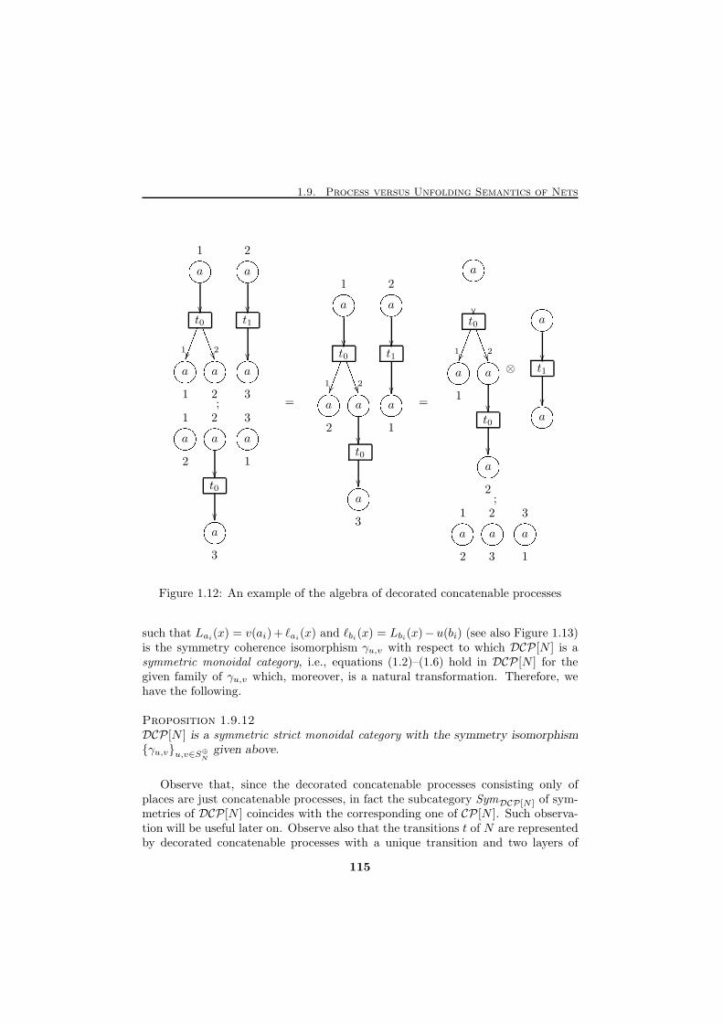
1.9. Process versus Unfolding Semantics of Nets
a a
t0 t1
a a'&$%'&$% a
1'&$%��
2'&$%��� �� �
1
������ 2
++++++�� � �� ���1 2 3
'&$%;
a a'&$%'&$% a
a'&$%
1 2
2��
3
1
'&$%t0� �� ���
3
=
a a
t0 t1
a a'&$%'&$% a
a'&$%
1'&$%��
2'&$%��� �� �
1
������ 2
++++++�� � �� ���2
��1
'&$%t0� �� ���
3
=
a'&$%
t0
a a'&$%'&$%
a'&$%
������ ��� �� �1
������ 2
++++++��1
��t0� �� ���
2
⊗
a
t1
a
'&$%��� �� ���'&$%
;
a a'&$%'&$% a
1 2
2 3
3
1
'&$%Figure 1.12: An example of the algebra of decorated concatenable processes
such that Lai(x) = v(ai)+ ℓai
(x) and ℓbi(x) = Lbi
(x)− u(bi) (see also Figure 1.13)is the symmetry coherence isomorphism γu,v with respect to which DCP[N ] is asymmetric monoidal category, i.e., equations (1.2)–(1.6) hold in DCP [N ] for thegiven family of γu,v which, moreover, is a natural transformation. Therefore, wehave the following.
Proposition 1.9.12DCP[N ] is a symmetric strict monoidal category with the symmetry isomorphism{γu,v}u,v∈S⊕
Ngiven above.
Observe that, since the decorated concatenable processes consisting only ofplaces are just concatenable processes, in fact the subcategory SymDCP[N ] of sym-metries of DCP[N ] coincides with the corresponding one of CP [N ]. Such observa-tion will be useful later on. Observe also that the transitions t of N are representedby decorated concatenable processes with a unique transition and two layers of
115
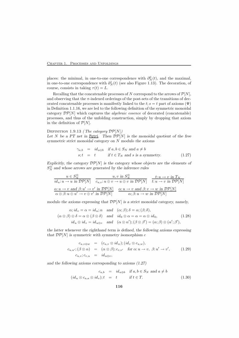
Chapter 1. Processes and Unfoldings
places: the minimal, in one-to-one correspondence with ∂0N (t), and the maximal,
in one-to-one correspondence with ∂1N (t) (see also Figure 1.13). The decoration, of
course, consists in taking τ(t) = L.
Recalling that the concatenable processes ofN correspond to the arrows of P [N ],and observing that the π-indexed orderings of the post-sets of the transitions of dec-orated concatenable processes is manifestly linked to the t; s = t part of axioms (Ψ)in Definition 1.1.16, we are led to the following definition of the symmetric monoidalcategory DP [N ] which captures the algebraic essence of decorated (concatenable)processes, and thus of the unfolding construction, simply by dropping that axiomin the definition of P [N ].
Definition 1.9.13 (The category DP [N ])Let N be a PT net in Petri. Then DP [N ] is the monoidal quotient of the freesymmetric strict monoidal category on N modulo the axioms
γa,b = ida⊕b if a, b ∈ SN and a 6= b
s; t = t if t ∈ TN and s is a symmetry. (1.27)
Explicitly, the category DP [N ] is the category whose objects are the elements ofS⊕N and whose arrows are generated by the inference rules
u ∈ S⊕Nidu:u→ u in DP [N ]
u, v in S⊕Ncu,v:u⊕ v → u⊕ v in DP [N ]
t:u→ v in TNt:u→ v in DP [N ]
α:u→ v and β:u′ → v′ in DP [N ]α⊗ β:u⊕ u′ → v ⊕ v′ in DP [N ]
α:u→ v and β: v → w in DP [N ]α;β:u→ w in DP [N ]
modulo the axioms expressing that DP [N ] is a strict monoidal category, namely,
α; idv = α = idu;α and (α;β); δ = α; (β; δ),
(α⊗ β)⊗ δ = α⊗ (β ⊗ δ) and id0 ⊗ α = α = α⊗ id0, (1.28)
idu ⊗ idv = idu⊕v and (α⊗ α′); (β ⊗ β′) = (α;β)⊗ (α′;β′),
the latter whenever the righthand term is defined, the following axioms expressingthat DP [N ] is symmetric with symmetry isomorphism c
cu,v⊕w = (cu,v ⊗ idw); (idv ⊗ cu,w),
cu,u′ ; (β ⊗ α) = (α⊗ β); cv,v′ for α:u→ v, β:u′ → v′, (1.29)
cu,v; cv,u = idu⊕v,
and the following axioms corresponding to axioms (1.27)
ca,b = ida⊕b if a, b ∈ SN and a 6= b
(idu ⊗ ca,a ⊗ idv); t = t if t ∈ T. (1.30)
116
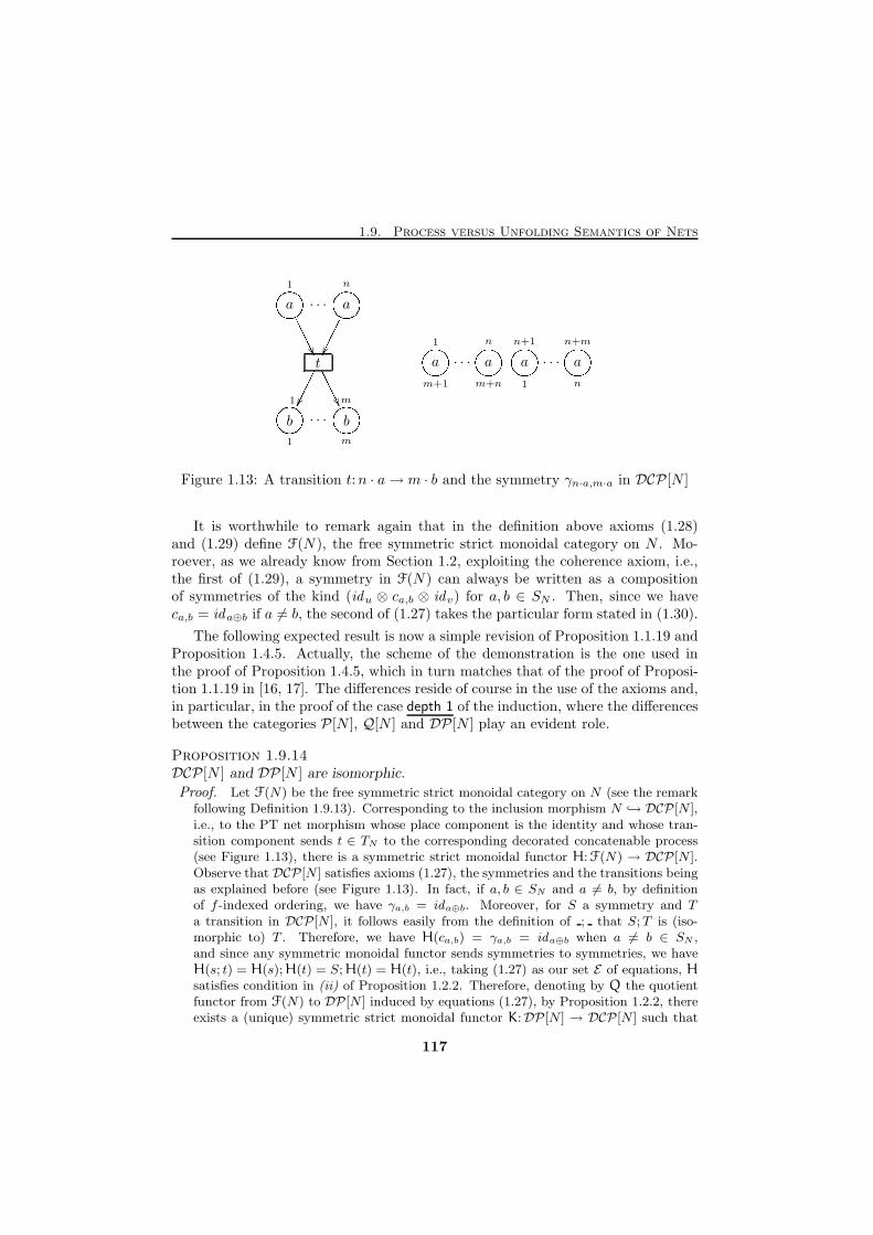
1.9. Process versus Unfolding Semantics of Nets
a · · · a
t
b · · · b
1'&$%/////�� n'&$%�������� �� �1
������� m
///// ��1
'&$%m
'&$% a · · · a a · · · a
1
m+1
'&$% n
m+n
'&$%n+1
1
'&$% n+m
n
'&$%Figure 1.13: A transition t:n · a→ m · b and the symmetry γn·a,m·a in DCP [N ]
It is worthwhile to remark again that in the definition above axioms (1.28)and (1.29) define F(N), the free symmetric strict monoidal category on N . Mo-roever, as we already know from Section 1.2, exploiting the coherence axiom, i.e.,the first of (1.29), a symmetry in F(N) can always be written as a compositionof symmetries of the kind (idu ⊗ ca,b ⊗ idv) for a, b ∈ SN . Then, since we haveca,b = ida⊕b if a 6= b, the second of (1.27) takes the particular form stated in (1.30).
The following expected result is now a simple revision of Proposition 1.1.19 andProposition 1.4.5. Actually, the scheme of the demonstration is the one used inthe proof of Proposition 1.4.5, which in turn matches that of the proof of Proposi-tion 1.1.19 in [16, 17]. The differences reside of course in the use of the axioms and,in particular, in the proof of the case depth 1 of the induction, where the differencesbetween the categories P [N ], Q[N ] and DP [N ] play an evident role.
Proposition 1.9.14DCP[N ] and DP [N ] are isomorphic.
Proof. Let F(N) be the free symmetric strict monoidal category on N (see the remarkfollowing Definition 1.9.13). Corresponding to the inclusion morphism N → DCP[N ],i.e., to the PT net morphism whose place component is the identity and whose tran-sition component sends t ∈ TN to the corresponding decorated concatenable process(see Figure 1.13), there is a symmetric strict monoidal functor H:F(N) → DCP[N ].Observe that DCP[N ] satisfies axioms (1.27), the symmetries and the transitions beingas explained before (see Figure 1.13). In fact, if a, b ∈ SN and a 6= b, by definitionof f -indexed ordering, we have γa,b = ida⊕b. Moreover, for S a symmetry and Ta transition in DCP[N ], it follows easily from the definition of ; that S;T is (iso-morphic to) T . Therefore, we have H(ca,b) = γa,b = ida⊕b when a 6= b ∈ SN ,and since any symmetric monoidal functor sends symmetries to symmetries, we haveH(s; t) = H(s);H(t) = S;H(t) = H(t), i.e., taking (1.27) as our set E of equations, Hsatisfies condition in (ii) of Proposition 1.2.2. Therefore, denoting by Q the quotientfunctor from F(N) to DP [N ] induced by equations (1.27), by Proposition 1.2.2, thereexists a (unique) symmetric strict monoidal functor K:DP [N ] → DCP[N ] such that
117
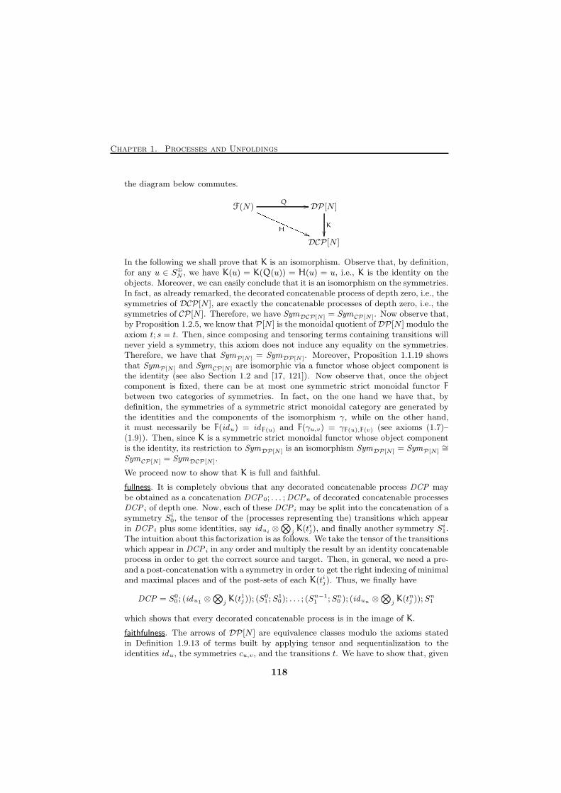
Chapter 1. Processes and Unfoldings
the diagram below commutes.
F(N) DP [N ]
DCP[N ]
H
QQQQQQQQQQQQ((Q //
K
��
In the following we shall prove that K is an isomorphism. Observe that, by definition,for any u ∈ S⊕N , we have K(u) = K(Q(u)) = H(u) = u, i.e., K is the identity on theobjects. Moreover, we can easily conclude that it is an isomorphism on the symmetries.In fact, as already remarked, the decorated concatenable process of depth zero, i.e., thesymmetries of DCP[N ], are exactly the concatenable processes of depth zero, i.e., thesymmetries of CP [N ]. Therefore, we have SymDCP[N] = SymCP[N]. Now observe that,by Proposition 1.2.5, we know that P [N ] is the monoidal quotient of DP [N ] modulo theaxiom t; s = t. Then, since composing and tensoring terms containing transitions willnever yield a symmetry, this axiom does not induce any equality on the symmetries.Therefore, we have that SymP[N] = SymDP[N]. Moreover, Proposition 1.1.19 showsthat SymP[N] and SymCP[N] are isomorphic via a functor whose object component isthe identity (see also Section 1.2 and [17, 121]). Now observe that, once the objectcomponent is fixed, there can be at most one symmetric strict monoidal functor Fbetween two categories of symmetries. In fact, on the one hand we have that, bydefinition, the symmetries of a symmetric strict monoidal category are generated bythe identities and the components of the isomorphism γ, while on the other hand,it must necessarily be F(idu) = idF(u) and F(γu,v) = γF(u),F(v) (see axioms (1.7)–(1.9)). Then, since K is a symmetric strict monoidal functor whose object componentis the identity, its restriction to SymDP[N] is an isomorphism SymDP[N] = SymP[N]
∼=SymCP[N] = SymDCP[N].
We proceed now to show that K is full and faithful.
fullness. It is completely obvious that any decorated concatenable process DCP maybe obtained as a concatenation DCP0; . . . ;DCPn of decorated concatenable processesDCP i of depth one. Now, each of these DCP i may be split into the concatenation of asymmetry Si0, the tensor of the (processes representing the) transitions which appearin DCP i plus some identities, say idui ⊗
⊗jK(tij), and finally another symmetry Si1.
The intuition about this factorization is as follows. We take the tensor of the transitionswhich appear in DCP i in any order and multiply the result by an identity concatenableprocess in order to get the correct source and target. Then, in general, we need a pre-and a post-concatenation with a symmetry in order to get the right indexing of minimaland maximal places and of the post-sets of each K(tij). Thus, we finally have
DCP = S00 ; (idu1 ⊗
⊗jK(t1j)); (S
01 ;S1
0); . . . ; (Sn−11 ;Sn0 ); (idun ⊗
⊗jK(tnj ));S
n1
which shows that every decorated concatenable process is in the image of K.
faithfulness. The arrows of DP [N ] are equivalence classes modulo the axioms statedin Definition 1.9.13 of terms built by applying tensor and sequentialization to theidentities idu, the symmetries cu,v, and the transitions t. We have to show that, given
118
1.9. Process versus Unfolding Semantics of Nets
two such terms α and β, whenever K(α) = K(β) we have α =E β, where =E is theequivalence induced by (1.28), (1.29) and (1.30).
First of all, observe that if K(α) is a decorated process DCP of depth n, then α canbe proved equal to a term
α′ = s0; (idu1 ⊗⊗
jt1j); s1; . . . ; sn−1; (idun ⊗
⊗jtnj ); sn
where, for 1 ≤ i ≤ n, the transitions tij , for 1 ≤ j ≤ ni, are exactly the transi-tions of DCP at depth i and where s0, . . . , sn are symmetries. Moreover, we canassume that in the i-th tensor product
⊗jtij the transitions are indexed according
to a global ordering ≤ of TN assumed for the purpose of this proof, i.e., ti1 ≤ · · · ≤tini
, for 1 ≤ i ≤ n. Let us prove our claim. It is easily shown by induction onthe structure of terms that using axioms (1.28) α can be rewritten as α1; . . . ;αh,where αi =
⊗kξik and ξik is either a transition or a symmetry. Now, observe that
by functoriality of ⊗, for any α′:u′ → v′, α′′:u′′ → v′′ and s:u → u, we haveα′ ⊗ s ⊗ α′′ = (idu′ ⊗ s ⊗ idu′′); (α′ ⊗ idu ⊗ α
′′), and thus, by repeated applicationsof (1.28), we can prove that α is equivalent to s0; α1; s1 . . . ; sh−1; αh, where s0, . . . , sh−1
are symmetries and each αi is a tensor⊗
kξik of transitions and identities. The fact
that the transitions at depth i can be brought to the i-th tensor product, followsintuitively from the facts that they are “disjointly enabled”, i.e., concurrent to eachother, and that they depend causally on some transition at depth i− 1. In particular,the sources of the transitions of depth 1 can be target only of symmetries. Therefore,reasoning formally as above, they can be pushed up to α1 exploiting axioms (1.28).Then, the same happens for the transitions of depth 2, which can be brought to α2.Proceeding in this way, eventually we show that α is equivalent to the composition
¯s0; ¯α1; ¯s1 . . . ; ¯sn−1; ¯αn; ¯sn of the symmetries ¯s0, . . . , ¯sn and the products ¯αi =⊗
k¯ξi
k
of transitions at depth i and identities. Finally, exploiting Lemma 1.4.4, the order of
the ¯ξi
k can be permuted in the way required by ≤. This is achieved by pre- and post-composing each product by appropriate σ-interchange symmetries. More precisely,
let σ be a permutation such that⊗
k¯ξi
σ(k) coincides with idui ⊗⊗
jtij , suppose that
¯ξi
k:uik → vik, for 1 ≤ k ≤ ki and let γσ be the σ-interchange symmetry guaranteed by
Lemma 1.4.4 in DP [N ]. Then, since γσ is a natural transformation, we have that
γσ ui1,...,ui
ki
; (⊗
k¯ξi
σ(k)) = (⊗
k¯ξi
k); γσ vi1,...,vi
ki
,
and then, since γσ is an isomorphism, we have that
(idui ⊗⊗
jtij) = γ−1
σ ui1,...,ui
ki
; (⊗
k¯ξi
k); γσ vi1,...,vi
ki
.
Now, applying the same argument to β, one proves that it is equivalent to a termβ′ = p0;β0; p1; . . . pn−1;βn; pn, where p0, . . . , pn are symmetries and βi is the productof the transitions at depth i in K(β) and of identities. Then, since K(α) = K(β), andsince the transitions occurring in βi are indexed in a predetermined way, we conclude
119
Chapter 1. Processes and Unfoldings
that βi = (idui ⊗⊗
jtij), i.e.,
α′ = s0; (idu1 ⊗⊗
jt1j); s1; . . . ; sn−1; (idun ⊗
⊗jtnj ); sn
β′ = p0; (idu1 ⊗⊗
jt1j ); p1; . . . ; pn−1; (idun ⊗
⊗jtnj ); pn. (1.31)
In other words, the only possible differences between α′ and β′ are the symmetries.Observe now that the steps which led from α to α′ and from β to β′ have been per-formed by using the axioms which defineDP [N ] and since such axioms hold in DCP[N ]as well and K preserves them, we have that K(α′) = K(α) = K(β) = K(β′). Thus, weconclude the proof by showing that, if α and β are terms of the form given in (1.31)which differ only by the intermediate symmetries and if K(α) = K(β), then α and βare equal in DP [N ].
We proceed by induction on n. Observe that if n is zero then there is nothing to show:since we know that K is an isomorphism on the symmetries, s0 and p0, and thus αand β, must coincide. To provide a correct basis for the induction, we need to provethe thesis also for n = 1.
depth 1. In this case, we have
α = s0; (idu ⊗⊗
jtj); s1
β = p0; (idu ⊗⊗
jtj); p1.
Without loss of generality, we may assume that p0 and p1 are identities. In fact, wecan multiply both terms by p−1
0 on the left and by p−11 on the right and obtain a pair
of terms whose images through K still coincide and whose equality implies the equalityin DP [N ] of the original α and β.
Let (π: Θ → N, ℓ, τ, L) be the decorated concatenable process K(idu ⊗⊗
jtj). Of
course, we can assume that K(s0) and K(s1) are respectively (π0: Θ0 → N, ℓ′,∅, ℓ)and (π1: Θ1 → N,L,∅, L′), where Θ0 is min(Θ), Θ1 is max(Θ), π0 and π1 are thecorresponding restrictions of π, and ℓ′ and L′ are π-indexed orderings respectively ofthe minimal and the maximal places of Θ.
Then, we have that K(s0; (idu ⊗⊗
jtj); s1) is (π:Θ→ N, ℓ′, τ, L′), and by hypothesis
there is an isomorphism ϕ: Θ → Θ such that π ◦ ϕ = π and which respects all theorderings, i.e., ℓ′π(ϕ(a))(ϕ(a)) = ℓπ(a)(a) and L′π(ϕ(b))(ϕ(b)) = Lπ(b)(b), for all a ∈ Θ0
and b ∈ Θ1, and τ (ϕ(t))πϕ(a)(ϕ(a)) = τ (t)π(a)(a) for all t ∈ Θ and a ∈ t•. Let uswrite idu⊗
⊗jtj as
⊗kξk, where ξk is either a transition tj or the identity of a place
in u. Moreover, let ξk:uk → vk, for 1 ≤ k ≤ ki. Clearly, ϕ induces a permutation ofthe symbols ξk, namely the permutation σ such that ξσ(k) = ϕ(ξk). Then, in orderto be a morphism of nets, ϕ must map the (places corresponding to the) pre-set,respectively post-set, of tj to (the places corresponding to the) pre-set, respectivelypost-set, of tσ(j). Observe now that this identifies ϕ uniquely on the maximal placesof Θ, which implies that K(s1) is completely determined. In fact, if a maximal place xis also minimal, then the corresponding ξk is the identity iduk
and thus x must bemapped to the object for which ξσ(k) is the identity. If instead x is in the post-setof tj then x must be mapped to the post-set of tσ(j) in the unique way compatiblewith the family of π-indexed orderings τ . In other words, K(s1) is the component at
120
1.9. Process versus Unfolding Semantics of Nets
(v1, . . . , vki) of the σ-interchange symmetry. Then, since K is an isomorphism between
SymDP[N] and SymDCP[N], s1 must necessarily be the corresponding component of theσ-interchange symmetry in DP [N ].
Concerning K(s0), we cannot be so precise. However, since we know that the pre-setsof transitions are mapped by ϕ according to σ, reasoning as above we can conclude that(π0, ℓ,∅, ℓ′), which is K(s0)
−1, must be a symmetry obtained by post-concatenatingthe component at (u1, . . . , uki
) of the σ-interchange symmetry to some product⊗
jSj
of symmetries, one for each t occurring in α, whose role is to reorganize the tokens inthe pre-sets of each transitions. It follows that s0 is γ−1
σ u1,...,uki; (idu⊗
⊗jsj), where sj
is a symmetry on the source of tj .
Then, by distributing the tensor of symmetries on the transitions and using the secondof (1.30), we show that α = γ−1
σ u1,...,uki; (idu⊗
⊗jtj); γσ v1,...,vki
, which, by definition
of σ-interchange symmetry, is (idu ⊗⊗
jtj). Thus, we have α =E β as required.
Inductive step. Suppose that n > 1 and let α = α′;α′′ and β = β′;β′′, where
α′ = s0; (idu1 ⊗⊗
jt1j); s1; . . . ; sn−1 and α′′ = (idun ⊗
⊗jtnj ); sn
β′ = p0; (idu1 ⊗⊗
jt1j ); p1; . . . ; pn−1 and β′′ = (idun ⊗
⊗jtnj ); pn
We show that there exists a symmetry s in DP [N ] such that K(α′; s) = K(β′) andK(s−1;α′′) = K(β′′). Then, by the induction hypothesis, we have (α′; s) =E β
′ and(s−1;α′′) =E β
′′. Therefore, we conclude that (α′; s; s−1;α′′) =E (β′;β′′), i.e., thatα = β in DP [N ].
Let (π: Θ→ N, ℓ, τ, L) be the decorated concatenable process K(α) = K(β). Withoutloss of generality we may assume that the decorated occurrence nets K(α′) and K(β′)
are, respectively, (π′: Θ′ → N, ℓ′, τ ′, Lα′
) and (π′: Θ′ → N, ℓ′, τ ′, Lβ′
), where Θ′ is thesubnet of depth n− 1 of Θ, ℓ′ and τ ′ are the appropriate restrictions of ℓ and τ andfinally Lα
′
and Lβ′
are π-indexed orderings of the places at depth n−1 of Θ. Considerthe symmetry S = (π, ℓ,∅, L) in DCP[N ], where
• Θ is the process nets consisting of the maximal places of Θ′;
• π: Θ→ N is the restriction of π to Θ;
• ℓ = Lα′
;
• L = Lβ′
.
Then, by definition, we have K(α′);S = K(β′). Let us consider now α′′ and β′′.
Clearly, we can assume that K(α′′) and K(β′′) are (π′′: Θ′′ → N, ℓα′′
, τ ′′, L′′) and
(π′′: Θ′′ → N, ℓβ′′
, τ ′′, L′′), where Θ′′ is the process net obtained by removing from Θ
the subnet Θ′, τ ′′ and L′′ are respectively the restrictions of τ and L to Θ′′, and ℓα′′
andℓβ
′′
are π-indexed orderings of the places at depth n−1 of Θ. Now, in our hypothesis,it must be Lα
′
= ℓα′′
and Lβ′
= ℓβ′′
, which shows directly that S−1;K(α′′) = K(β′′).Then, s = K−1(S) is the required symmetry of DP [N ].
Then, since K is full and faithful and is an isomorphism on the objects, it is an
isomorphism and the proof is concluded. X
121
Chapter 1. Processes and Unfoldings
We conclude the section by getting back to diagram (1.26). We first make thefollowing observation on the structure of the comma category 〈uN↓DP[N ]〉.
Proposition 1.9.15The category 〈uN↓DP[N ]〉 is a preorder.
Proof. We have to show that in 〈uN↓DP [N ]〉 there is at most one arrow between anypair of objects α:uN → v and α′: uN → w. Exploiting the characterization of arrows ofDP [N ] in terms of decorated concatenable processes established by Proposition 1.9.14,the thesis can be reformulated as follows: for each pair of concatenable decoratedprocesses DCP0:uN → v and DCP1:uN → w there exists at most one decoratedconcatenable process DCP : v → w such that DCP0;DCP = DCP1.
In order to show the claim, suppose that there exist DCP and DCP ′ from v to w such
that DCP0;DCP = DCP1 = DCP0;DCP′. Let π: Θ → N and π′: Θ′ → N be the
(plain) processes underlying, respectively, DCP0;DCP and DCP1;DCP ′. Without
loss of generality, we can assume that Θ, respectively Θ′, is formed by joining Θ0,
the process net underlying DCP0, with Θ, the process net underlying DCP , respec-
tively Θ′, the process net underlying DCP ′. Then, since DCP0;DCP = DCP0;DCP′,
there exists an isomorphism ϕ: Θ→ Θ′ which respects all the orderings and such that
π = π′ ◦ ϕ. Since, we can assume that ϕ restricts to the identity of Θ0 (as a subnet
of Θ and Θ′), it follows that it restricts to an isomorphism ϕ′: Θ → Θ′ which shows
DCP = DCP ′. X
The next proposition essentially shows that, for any (N, uN ) ∈ MPetri∗, thecanonical partial order associated to 〈uN↓DP [N ]〉 is DP [(N, uN )].
Proposition 1.9.16For any marked PT net (N, uN ) in MPetri∗,
〈uN↓DP[N ]〉 ∼= DP [(N, uN )] ∼= LFEFU [(N, uN )].
Proof. Consider the mapping from the objects of 〈uN↓DP [N ]〉 to DP [(N, uN )] given by(π, ℓ, τ, L) 7→ (π, ℓ, τ), where τ is the restriction of τ to the non maximal transitionsof process net underlying π. Now, observe that there is a morphism from DCP =(π: Θ → N, ℓ, τ, L) to DCP ′ = (π′: Θ′ → N, ℓ′, τ ′, L′) in 〈uN↓DP [N ]〉 if and only ifthere exists a decorated concatenable process DCP ′′ such that DCP ;DCP ′′ = DCP ′
if and only if there exists ϕ: Θ → Θ′ such that π = π′ ◦ ϕ and which preserves allorderings, i.e., if and only if (π, ℓ, τ ) ≤ (π′, ℓ′, τ ′) in DP [(N,uN )]. Thus, since fromProposition 1.9.15 we know that 〈uN↓DP [N ]〉 is a preorder, the mapping above isclearly a full and faithful functor. Moreover, since such a mapping is surjective on theobjects, it is an equivalence of categories.
Observe that the second equivalence is actually an isomorphism, as shown by Propo-
sition 1.9.9. X
122
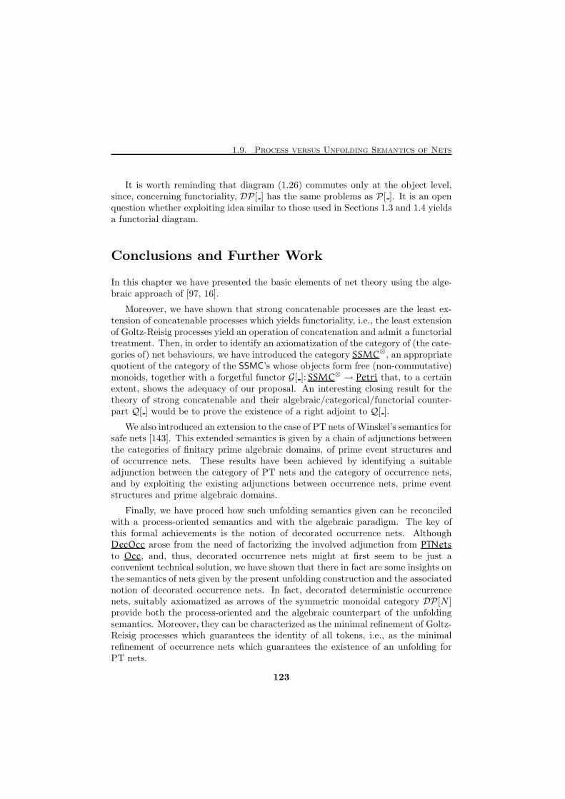
1.9. Process versus Unfolding Semantics of Nets
It is worth reminding that diagram (1.26) commutes only at the object level,since, concerning functoriality, DP [ ] has the same problems as P [ ]. It is an openquestion whether exploiting idea similar to those used in Sections 1.3 and 1.4 yieldsa functorial diagram.
Conclusions and Further Work
In this chapter we have presented the basic elements of net theory using the alge-braic approach of [97, 16].
Moreover, we have shown that strong concatenable processes are the least ex-tension of concatenable processes which yields functoriality, i.e., the least extensionof Goltz-Reisig processes yield an operation of concatenation and admit a functorialtreatment. Then, in order to identify an axiomatization of the category of (the cate-gories of) net behaviours, we have introduced the category SSMC⊗, an appropriatequotient of the category of the SSMC’s whose objects form free (non-commutative)monoids, together with a forgetful functor G[ ]: SSMC⊗ → Petri that, to a certainextent, shows the adequacy of our proposal. An interesting closing result for thetheory of strong concatenable and their algebraic/categorical/functorial counter-part Q[ ] would be to prove the existence of a right adjoint to Q[ ].
We also introduced an extension to the case of PT nets of Winskel’s semantics forsafe nets [143]. This extended semantics is given by a chain of adjunctions betweenthe categories of finitary prime algebraic domains, of prime event structures andof occurrence nets. These results have been achieved by identifying a suitableadjunction between the category of PT nets and the category of occurrence nets,and by exploiting the existing adjunctions between occurrence nets, prime eventstructures and prime algebraic domains.
Finally, we have proced how such unfolding semantics given can be reconciledwith a process-oriented semantics and with the algebraic paradigm. The key ofthis formal achievements is the notion of decorated occurrence nets. AlthoughDecOcc arose from the need of factorizing the involved adjunction from PTNets
to Occ, and, thus, decorated occurrence nets might at first seem to be just aconvenient technical solution, we have shown that there in fact are some insights onthe semantics of nets given by the present unfolding construction and the associatednotion of decorated occurrence nets. In fact, decorated deterministic occurrencenets, suitably axiomatized as arrows of the symmetric monoidal category DP [N ]provide both the process-oriented and the algebraic counterpart of the unfoldingsemantics. Moreover, they can be characterized as the minimal refinement of Goltz-Reisig processes which guarantees the identity of all tokens, i.e., as the minimalrefinement of occurrence nets which guarantees the existence of an unfolding forPT nets.
123
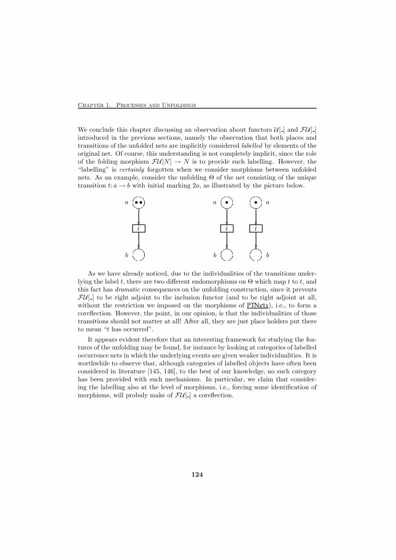
Chapter 1. Processes and Unfoldings
We conclude this chapter discussing an observation about functors U [ ] and FU [ ]introduced in the previous sections, namely the observation that both places andtransitions of the unfolded nets are implicitly considered labelled by elements of theoriginal net. Of course, this understanding is not completely implicit, since the roleof the folding morphism FU [N ] → N is to provide such labelling. However, the“labelling” is certainly forgotten when we consider morphisms between unfoldednets. As an example, consider the unfolding Θ of the net consisting of the uniquetransition t: a→ b with initial marking 2a, as illustrated by the picture below.
• •
t
a'&$%
��� �� ���
b'&$%
• •
t t
a'&$%
��
a'&$%
��� �� ���
� �� ���
b'&$% b
'&$%As we have already noticed, due to the individualities of the transitions under-
lying the label t, there are two different endomorphisms on Θ which map t to t, andthis fact has dramatic consequences on the unfolding construction, since it preventsFU [ ] to be right adjoint to the inclusion functor (and to be right adjoint at all,without the restriction we imposed on the morphisms of PTNets), i.e., to form acoreflection. However, the point, in our opinion, is that the individualities of thosetransitions should not matter at all! After all, they are just place holders put thereto mean “t has occurred”.
It appears evident therefore that an interesting framework for studying the fea-tures of the unfolding may be found, for instance by looking at categories of labelledoccurrence nets in which the underlying events are given weaker individualities. It isworthwhile to observe that, although categories of labelled objects have often beenconsidered in literature [145, 146], to the best of our knowledge, no such categoryhas been provided with such mechanisms. In particular, we claim that consider-ing the labelling also at the level of morphisms, i.e., forcing some identification ofmorphisms, will probaly make of FU [ ] a coreflection.
124
Chapter 2
Models for Concurrency
Abstract. Models for concurrency can be classified with respect to three rele-vant parameters: behaviour/system, interleaving/noninterleaving, linear/branching time.When modelling a process, a choice concerning such parameters corresponds to choos-ing the level of abstraction of the resulting semantics. The classifications are formalizedthrough the medium of category theory.
To Thales . . . the primary question is not“What do we know”, but
“How do we know it”.
Aristotle
Our three dimensional spaceis the only true reality we know.
Maurits Cornelis Escher
The tools we use havea profound (and devious!)
influence on our thinking abits,and, therefore, on our thinking ability.
Edsges W. Dijkstra
This chapter is based on joint work with Mogens Nielsen and Glynn Winskel [124, 125,
126].
125

Chapter 2. Models for Concurrency
126
Introduction
Since its beginning, many efforts in the development of the theory of concurrencyhave been devoted to the study of suitable models for concurrent and distributedprocesses, and to the formal understanding of their semantics.
As a result, in addition to standard models like languages, automata and tran-sition systems [60, 113], models like Petri nets [109], process algebras [102, 47],Hoare traces [48], Mazurkiewicz traces [94], synchronization trees [142] and eventstructures [106, 143] have been introduced.
The idea common to the models above is that they are based on atomic units ofchange—be they called transitions, actions, events or symbols from an alphabet—which are indivisible and constitute the steps out of which computations are built.
The difference between the models may be expressed in terms of the parametersaccording to which models are often classified. For instance, a distinction madeexplicitly in the theory of Petri nets, but sensible in a wider context, is that be-tween so-called “system” models allowing an explicit representation of the (possiblyrepeating) states in a system, and “behaviour” models abstracting away from suchinformation, which focus instead on the behaviour in terms of patterns of occur-rences of actions over time. Prime examples of the first type are transition systemsand Petri nets, and of the second type, trees, event structures and traces. Thus,we can distinguish among models according to whether they are system models orbehaviour models, in this sense; whether they can faithfully take into account thedifference between concurrency and nondeterminism; and, finally, whether they canrepresent the branching structure of processes, i.e., the points in which choices aretaken, or not. Therefore, relevant parameters when looking at models for concur-rency are
Behaviour or System model;Interleaving or Noninterleaving model;Linear or Branching Time model.
These parameters correspond to choices of the level of abstraction at which weexamine processes and which are not necessarily fixed for a process once and for all.It is the actual application one has in mind for the formal semantics which time bytime guides the choice of the abstraction level. It can therefore be of value to beable to move back and forth between the representation of a process in one modeland its representation in another, if possible in a way which respects its structure.In other words, it is relevant to study translations between models, and particularlywith respect to the three parameters above.
This chapter presents a classification of models for concurrency based on thethree parameters, which represent a further step towards the identification of sys-tematic connections between transition based models. In particular, we study a
127
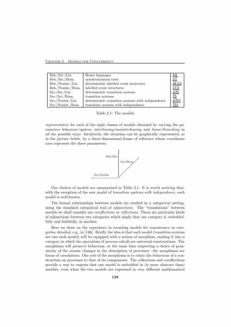
Chapter 2. Models for Concurrency
Beh./Int./Lin. Hoare languages HLBeh./Int./Bran. synchronization trees STBeh./Nonint./Lin. deterministic labelled event structures dLESBeh./Nonint./Bran. labelled event structures LESSys./Int./Lin. deterministic transition systems dTSSys./Int./Bran. transition systems TSSys./Nonint./Lin. deterministic transition systems with independence dTSISys./Nonint./Bran. transition systems with independence TSI
Table 2.1: The models
representative for each of the eight classes of models obtained by varying the pa-rameters behaviour/system, interleaving/noninterleaving and linear/branching inall the possible ways. Intuitively, the situation can be graphically represented, asin the picture below, by a three-dimensional frame of reference whose coordinateaxes represent the three parameters.
Int/NonInt←−−−−−−−−−−−
Beh/Sys
↑|||||||||||||||||
Lin/Bran
�����ր
Our choices of models are summarized in Table 2.1. It is worth noticing that,with the exception of the new model of transition systems with independence, eachmodel is well-known.
The formal relationships between models are studied in a categorical setting,using the standard categorical tool of adjunctions. The “translations” betweenmodels we shall consider are coreflections or reflections. These are particular kindsof adjunctions between two categories which imply that one category is embedded ,fully and faithfully, in another.
Here we draw on the experience in recasting models for concurrency as cate-gories, detailed, e.g., in [146]. Briefly the idea is that each model (transition systemsare one such model) will be equipped with a notion of morphism, making it into acategory in which the operations of process calculi are universal constructions. Themorphisms will preserve behaviour, at the same time respecting a choice of gran-ularity of the atomic changes in the description of processes—the morphisms areforms of simulations. One role of the morphisms is to relate the behaviour of a con-struction on processes to that of its components. The reflections and coreflectionsprovide a way to express that one model is embedded in (is more abstract than)another, even when the two models are expressed in very different mathematical
128
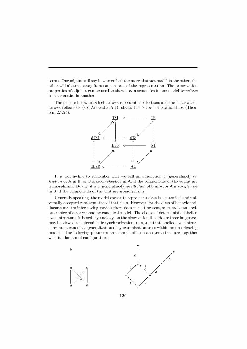
terms. One adjoint will say how to embed the more abstract model in the other, theother will abstract away from some aspect of the representation. The preservationproperties of adjoints can be used to show how a semantics in one model translatesto a semantics in another.
The picture below, in which arrows represent coreflections and the “backward”arrows reflections (see Appendix A.1), shows the “cube” of relationships (Theo-rem 2.7.24).
dTSI
���
....................................................
..........�⊳−−−−−−−−− dTS
���
....................................................
..........�△
||||||||||∪
△
||||||||||∪
dLES���
....................................................
..........�⊳−−−−−−−−− HL
���
....................................................
..........�
TSI ⊳−−−−−−−−− TS△
||||||||||∪
△
||||||||||∪
LES ⊳−−−−−−−−− ST
It is worthwhile to remember that we call an adjunction a (generalized) re-flection of A in B, or B is said reflective in A, if the components of the counit areisomorphisms. Dually, it is a (generalized) coreflection of B in A, or A is coreflectivein B, if the components of the unit are isomorphisms.
Generally speaking, the model chosen to represent a class is a canonical and uni-versally accepted representative of that class. However, for the class of behavioural,linear-time, noninterleaving models there does not, at present, seem to be an obvi-ous choice of a corresponding canonical model. The choice of deterministic labelledevent structures is based, by analogy, on the observation that Hoare trace languagesmay be viewed as deterministic synchronization trees, and that labelled event struc-tures are a canonical generalization of synchronization trees within noninterleavingmodels. The following picture is an example of such an event structure, togetherwith its domain of configurations
@@@I
����
@@@I
����
����
6
����
����
......
......
..
•
•
• •
•
•
•
a
a
b
b a
ba
b
#
a
a
b
a
129
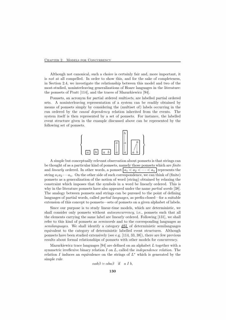
Chapter 2. Models for Concurrency
Although not canonical, such a choice is certainly fair and, more important, itis not at all compelled. In order to show this, and for the sake of completeness,in Section 2.4, we investigate the relationship between this model and two of themost-studied, noninterleaving generalizations of Hoare languages in the literature:the pomsets of Pratt [114], and the traces of Mazurkiewicz [94].
Pomsets, an acronym for partial ordered multisets, are labelled partial orderedsets. A noninterleaving representation of a system can be readily obtained bymeans of pomsets simply by considering the (multiset of) labels occurring in therun ordered by the causal dependency relation inherited from the events. Thesystem itself is then represented by a set of pomsets. For instance, the labelledevent structure given in the example discussed above can be represented by thefollowing set of pomsets.
a b a b
a∣∣∣a
b∣∣∣a∣∣∣a
/
a
a∣∣∣b
A simple but conceptually relevant observation about pomsets is that strings canbe thought of as a particular kind of pomsets, namely those pomsets which are finiteand linearly ordered. In other words, a pomset a1 < a2 < · · · < an represents the
string a1a2 · · · an. On the other side of such correspondence, we can think of (finite)pomsets as a generalization of the notion of word (string) obtained by relaxing theconstraint which imposes that the symbols in a word be linearly ordered. This iswhy in the literature pomsets have also appeared under the name partial words [38].The analogy between pomsets and strings can be pursued to the point of defininglanguages of partial words, called partial languages, as prefix-closed—for a suitableextension of this concept to pomsets—sets of pomsets on a given alphabet of labels.
Since our purpose is to study linear-time models, which are deterministic, weshall consider only pomsets without autoconcurrency, i.e., pomsets such that allthe elements carrying the same label are linearly ordered. Following [131], we shallrefer to this kind of pomsets as semiwords and to the corresponding languages assemilanguages. We shall identify a category dSL of deterministic semilanguagesequivalent to the category of deterministic labelled event structures. Althoughpomsets have been studied extensively (see e.g. [114, 33, 38]), there are few previousresults about formal relationships of pomsets with other models for concurrency.
Mazurkiewicz trace languages [94] are defined on an alphabet L together with asymmetric irreflexive binary relation I on L, called the independence relation. Therelation I induces an equivalence on the strings of L∗ which is generated by thesimple rule
αabβ ≃ αbaβ if a I b,
130
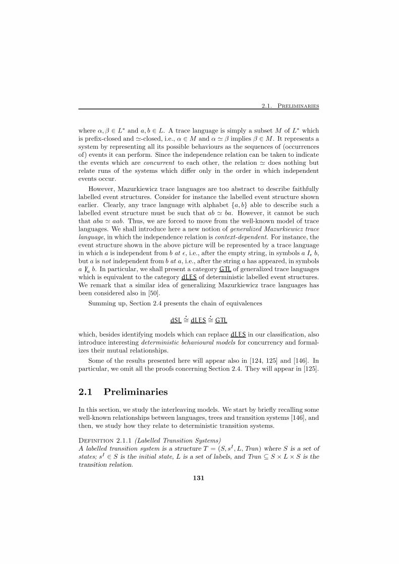
2.1. Preliminaries
where α, β ∈ L∗ and a, b ∈ L. A trace language is simply a subset M of L∗ whichis prefix-closed and ≃-closed, i.e., α ∈M and α ≃ β implies β ∈M . It represents asystem by representing all its possible behaviours as the sequences of (occurrencesof) events it can perform. Since the independence relation can be taken to indicatethe events which are concurrent to each other, the relation ≃ does nothing butrelate runs of the systems which differ only in the order in which independentevents occur.
However, Mazurkiewicz trace languages are too abstract to describe faithfullylabelled event structures. Consider for instance the labelled event structure shownearlier. Clearly, any trace language with alphabet {a, b} able to describe such alabelled event structure must be such that ab ≃ ba. However, it cannot be suchthat aba ≃ aab. Thus, we are forced to move from the well-known model of tracelanguages. We shall introduce here a new notion of generalized Mazurkiewicz tracelanguage, in which the independence relation is context-dependent. For instance, theevent structure shown in the above picture will be represented by a trace languagein which a is independent from b at ǫ, i.e., after the empty string, in symbols a Iǫ b,but a is not independent from b at a, i.e., after the string a has appeared, in symbolsa 6 Ia b. In particular, we shall present a category GTL of generalized trace languageswhich is equivalent to the category dLES of deterministic labelled event structures.We remark that a similar idea of generalizing Mazurkiewicz trace languages hasbeen considered also in [50].
Summing up, Section 2.4 presents the chain of equivalences
dSL�
∼= dLES�
∼= GTL
which, besides identifying models which can replace dLES in our classification, alsointroduce interesting deterministic behavioural models for concurrency and formal-izes their mutual relationships.
Some of the results presented here will appear also in [124, 125] and [146]. Inparticular, we omit all the proofs concerning Section 2.4. They will appear in [125].
2.1 Preliminaries
In this section, we study the interleaving models. We start by briefly recalling somewell-known relationships between languages, trees and transition systems [146], andthen, we study how they relate to deterministic transition systems.
Definition 2.1.1 (Labelled Transition Systems)A labelled transition system is a structure T = (S, sI , L,Tran) where S is a set ofstates; sI ∈ S is the initial state, L is a set of labels, and Tran ⊆ S × L × S is thetransition relation.
131
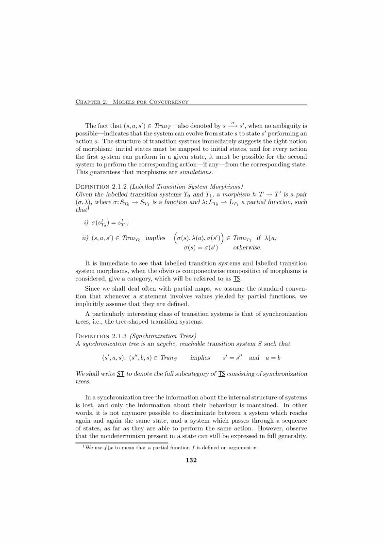
Chapter 2. Models for Concurrency
The fact that (s, a, s′) ∈ TranT—also denoted by sa−→ s′, when no ambiguity is
possible—indicates that the system can evolve from state s to state s′ performing anaction a. The structure of transition systems immediately suggests the right notionof morphism: initial states must be mapped to initial states, and for every actionthe first system can perform in a given state, it must be possible for the secondsystem to perform the corresponding action—if any—from the corresponding state.This guarantees that morphisms are simulations.
Definition 2.1.2 (Labelled Transition System Morphisms)Given the labelled transition systems T0 and T1, a morphism h:T → T ′ is a pair(σ, λ), where σ:ST0 → ST1 is a function and λ:LT0 ⇀ LT1 a partial function, suchthat1
i) σ(sIT0) = sIT1
;
ii) (s, a, s′) ∈ TranT0 implies(σ(s), λ(a), σ(s′)
)∈ TranT1 if λ↓a;
σ(s) = σ(s′) otherwise.
It is immediate to see that labelled transition systems and labelled transitionsystem morphisms, when the obvious componentwise composition of morphisms isconsidered, give a category, which will be referred to as TS.
Since we shall deal often with partial maps, we assume the standard conven-tion that whenever a statement involves values yielded by partial functions, weimplicitily assume that they are defined.
A particularly interesting class of transition systems is that of synchronizationtrees, i.e., the tree-shaped transition systems.
Definition 2.1.3 (Synchronization Trees)A synchronization tree is an acyclic, reachable transition system S such that
(s′, a, s), (s′′, b, s) ∈ TranS implies s′ = s′′ and a = b
We shall write ST to denote the full subcategory of TS consisting of synchronizationtrees.
In a synchronization tree the information about the internal structure of systemsis lost, and only the information about their behaviour is mantained. In otherwords, it is not anymore possible to discriminate between a system which reachsagain and again the same state, and a system which passes through a sequenceof states, as far as they are able to perform the same action. However, observethat the nondeterminism present in a state can still be expressed in full generality.
1We use f↓x to mean that a partial function f is defined on argument x.
132
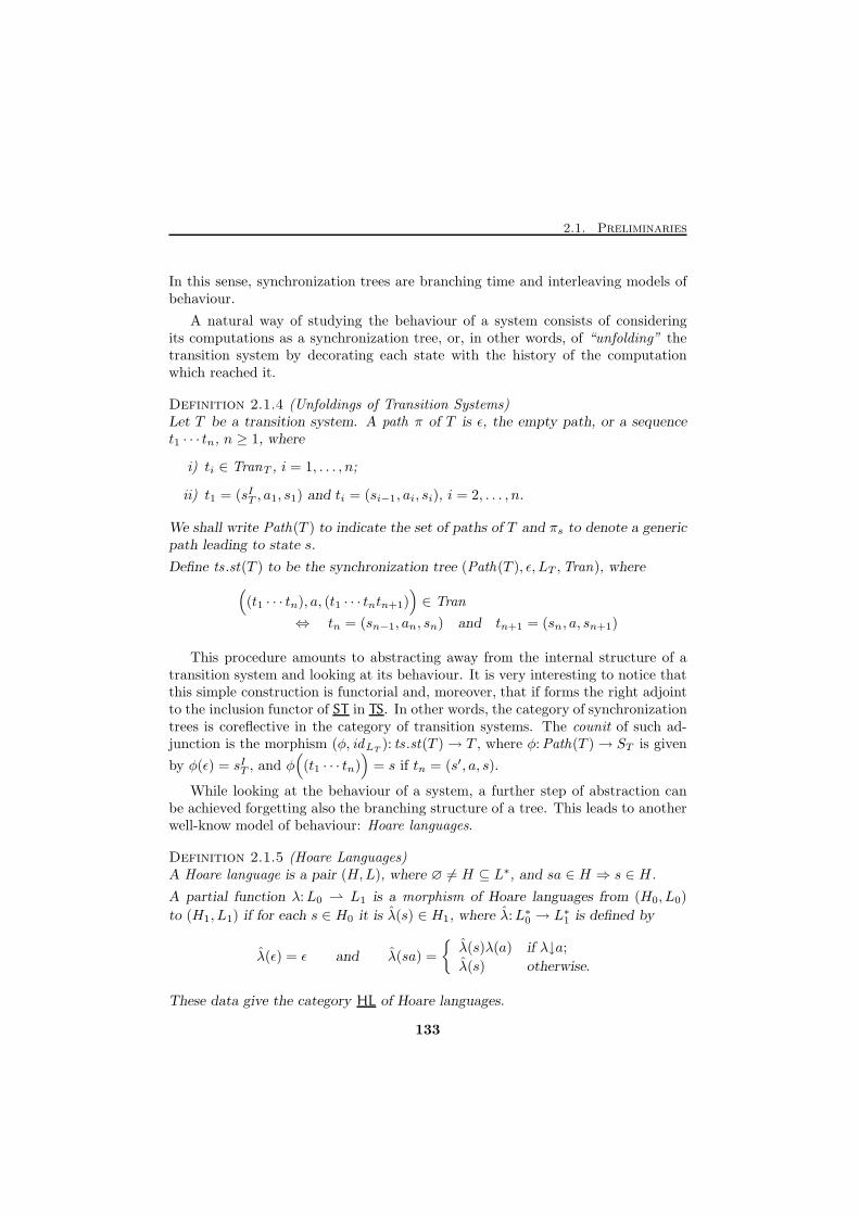
2.1. Preliminaries
In this sense, synchronization trees are branching time and interleaving models ofbehaviour.
A natural way of studying the behaviour of a system consists of consideringits computations as a synchronization tree, or, in other words, of “unfolding” thetransition system by decorating each state with the history of the computationwhich reached it.
Definition 2.1.4 (Unfoldings of Transition Systems)Let T be a transition system. A path π of T is ǫ, the empty path, or a sequencet1 · · · tn, n ≥ 1, where
i) ti ∈ TranT , i = 1, . . . , n;
ii) t1 = (sIT , a1, s1) and ti = (si−1, ai, si), i = 2, . . . , n.
We shall write Path(T ) to indicate the set of paths of T and πs to denote a genericpath leading to state s.
Define ts .st(T ) to be the synchronization tree (Path(T ), ǫ, LT ,Tran), where
((t1 · · · tn), a, (t1 · · · tntn+1)
)∈ Tran
⇔ tn = (sn−1, an, sn) and tn+1 = (sn, a, sn+1)
This procedure amounts to abstracting away from the internal structure of atransition system and looking at its behaviour. It is very interesting to notice thatthis simple construction is functorial and, moreover, that if forms the right adjointto the inclusion functor of ST in TS. In other words, the category of synchronizationtrees is coreflective in the category of transition systems. The counit of such ad-junction is the morphism (φ, idLT
): ts .st(T )→ T , where φ:Path(T )→ ST is given
by φ(ǫ) = sIT , and φ((t1 · · · tn)
)= s if tn = (s′, a, s).
While looking at the behaviour of a system, a further step of abstraction canbe achieved forgetting also the branching structure of a tree. This leads to anotherwell-know model of behaviour: Hoare languages.
Definition 2.1.5 (Hoare Languages)A Hoare language is a pair (H,L), where ∅ 6= H ⊆ L∗, and sa ∈ H ⇒ s ∈ H .
A partial function λ:L0 ⇀ L1 is a morphism of Hoare languages from (H0, L0)
to (H1, L1) if for each s ∈ H0 it is λ(s) ∈ H1, where λ:L∗0 → L∗1 is defined by
λ(ǫ) = ǫ and λ(sa) =
{λ(s)λ(a) if λ↓a;
λ(s) otherwise.
These data give the category HL of Hoare languages.
133
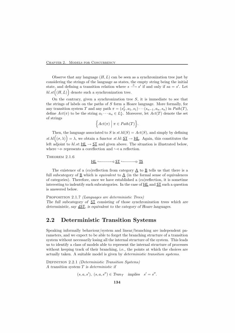
Chapter 2. Models for Concurrency
Observe that any language (H,L) can be seen as a synchronization tree just byconsidering the strings of the language as states, the empty string being the initialstate, and defining a transition relation where s
a−→ s′ if and only if sa = s′. Let
hl .st((H,L)
)denote such a synchronization tree.
On the contrary, given a synchronization tree S, it is immediate to see thatthe strings of labels on the paths of S form a Hoare language. More formally, forany transition system T and any path π = (sIT , a1, s1) · · · (sn−1, an, sn) in Path(T ),define Act(π) to be the string a1 · · · an ∈ L∗T . Moreover, let Act(T ) denote the setof strings {
Act(π)∣∣∣ π ∈ Path(T )
}.
Then, the language associated to S is st .hl(S) = Act(S), and simply by defining
st .hl((σ, λ)
)= λ, we obtain a functor st .hl : ST → HL. Again, this constitutes the
left adjoint to hl .st : HL → ST and given above. The situation is illustrated below,where −⊲ represents a coreflection and −⊳ a reflection.
Theorem 2.1.6HL −−−−−−−⊳ ST −−−−−−−⊲ TS
The existence of a (co)reflection from category A to B tells us that there is afull subcategory of B which is equivalent to A (in the formal sense of equivalencesof categories). Therefore, once we have established a (co)reflection, it is sometimeinteresting to indentify such subcategories. In the case of HL and ST such a questionis answered below.
Proposition 2.1.7 (Languages are deterministic Trees)The full subcategory of ST consisting of those synchronization trees which aredeterministic, say dST , is equivalent to the category of Hoare languages.
2.2 Deterministic Transition Systems
Speaking informally behaviour/system and linear/branching are independent pa-rameters, and we expect to be able to forget the branching structure of a transitionsystem without necessarily losing all the internal structure of the system. This leadsus to identify a class of models able to represent the internal structure of processeswithout keeping track of their branching, i.e., the points at which the choices areactually taken. A suitable model is given by deterministic transition systems.
Definition 2.2.1 (Deterministic Transition Systems)A transition system T is deterministic if
(s, a, s′), (s, a, s′′) ∈ TranT implies s′ = s′′.
134
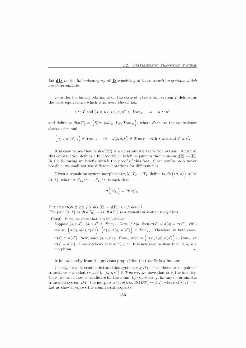
2.2. Deterministic Transition Systems
Let dTS be the full subcategory of TS consisting of those transition systems whichare deterministic.
Consider the binary relation ≃ on the state of a transition system T defined asthe least equivalence which is forward closed, i.e.,
s ≃ s′ and (s, a, u), (s′, a, u′) ∈ TranT ⇒ u ≃ u′;
and define ts .dts(T ) =(S/≃, [sIT ]≃, LT ,Tran≃
), where S/≃ are the equivalence
classes of ≃ and([s]≃, a, [s
′]≃
)∈ Tran≃ ⇔ ∃(s, a, s′) ∈ TranT with s ≃ s and s′ ≃ s′.
It is easy to see that ts .dts(TS) is a deterministic transition system. Actually,this construction defines a functor which is left adjoint to the inclusion dTS → TS.In the following we briefly sketch the proof of this fact. Since confusion is neverpossible, we shall not use different notations for different ≃’s.
Given a transition system morphism (σ, λ):T0 → T1, define ts .dts((σ, λ)
)to be
(σ, λ), where σ:ST0/≃ → ST1/≃ is such that
σ([s]≃
)= [σ(s)]≃.
Proposition 2.2.2 ( ts .dts: TS→ dTS is a functor)The pair (σ, λ): ts .dts(T0)→ ts .dts(T1) is a transition system morphism.
Proof. First, we show that σ is well-defined.
Suppose (s, a, s′), (s, a, s′′) ∈ TranT0 . Now, if λ↑a, then σ(s′) = σ(s) = σ(s′′). Oth-
erwise,(σ(s), λ(a), σ(s′)
),(σ(s), λ(a), σ(s′′)
)∈ TranT1 . Therefore, in both cases,
σ(s′) ≃ σ(s′′). Now, since (s, a, s′) ∈ TranT0 implies(σ(s), λ(a), σ(s′)
)∈ TranT1 or
σ(s) = σ(s′), it easily follows that σ(≃) ⊆ ≃. It is now easy to show that (σ, λ) is a
morphism. X
It follows easily from the previous proposition that ts .dts is a functor.
Clearly, for a deterministic transition system, say DT , since there are no pairs oftransitions such that (s, a, s′), (s, a, s′′) ∈ TranDT , we have that ≃ is the identity.Thus, we can choose a candidate for the counit by considering, for any deterministictransition system DT , the morphism (ε, id): ts .dts(DT )→ DT , where ε([s]≃) = s.Let us show it enjoys the couniversal property.
135
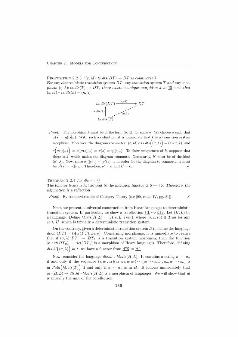
Chapter 2. Models for Concurrency
Proposition 2.2.3 ( (ε, id): ts .dts(DT )→ DT is couniversal)For any deterministic transition system DT , any transition system T and any mor-phism (η, λ): ts .dts(T ) → DT , there exists a unique morphism k in TS such that(ε, id) ◦ ts .dts(k) = (η, λ).
ts .dts(DT ) DT
ts .dts(T )
(ε,id) //
ts.dts(k)
OO
(η,λ)mmmmmmmmmmmmm 66Proof. The morphism k must be of the form (σ, λ), for some σ. We choose σ such that
σ(s) = η([s]≃). With such a definition, it is immediate that k is a transition system
morphism. Moreover, the diagram commutes: (ε, id) ◦ ts.dts((σ, λ)
)= (ε ◦ σ, λ), and
ε(σ([s]≃)
)= ε([σ(s)]≃) = σ(s) = η([s]≃). To show uniqueness of k, suppose that
there is k′ which makes the diagram commute. Necessarily, k′ must be of the kind
(σ′, λ). Now, since σ′([s]≃) = [σ′(s)]≃, in order for the diagram to commute, it must
be σ′(s) = η([s]≃). Therefore, σ′ = σ and k′ = k. X
Theorem 2.2.4 ( ts .dts ⊣ ←)The functor ts .dts is left adjoint to the inclusion functor dTS → TS. Therefore, theadjunction is a reflection.
Proof. By standard results of Category Theory (see [90, chap. IV, pg. 81]). X
Next, we present a universal construction from Hoare languages to deterministictransition system. In particular, we show a coreflection HL −⊲ dTS. Let (H,L) bea language. Define hl .dts(H,L) = (H, ǫ, L,Tran), where (s, a, sa) ∈ Tran for anysa ∈ H , which is trivially a deterministic transition system.
On the contrary, given a deterministic transition system DT , define the languagedts .hl(DT ) = (Act(DT ), LDT ). Concerning morphisms, it is immediate to realizethat if (σ, λ):DT 0 → DT 1 is a transition system morphism, then the functionλ:Act(DT 0) → Act(DT 1) is a morphism of Hoare languages. Therefore, defining
dts .hl((σ, λ)
)= λ, we have a functor from dTS to HL.
Now, consider the language dts .hl ◦ hl .dts(H,L). It contains a string a1 · · ·anif and only if the sequence (ǫ, a1, a1)(a1, a2, a1a2) · · · (a1 · · · an−1, an, a1 · · ·an) is
in Path(hl .dts(T )
)if and only if a1 · · · an is in H . It follows immediately that
id : (H,L)→ dts .hl ◦ hl .dts(H,L) is a morphism of languages. We will show that idis actually the unit of the coreflection.
136
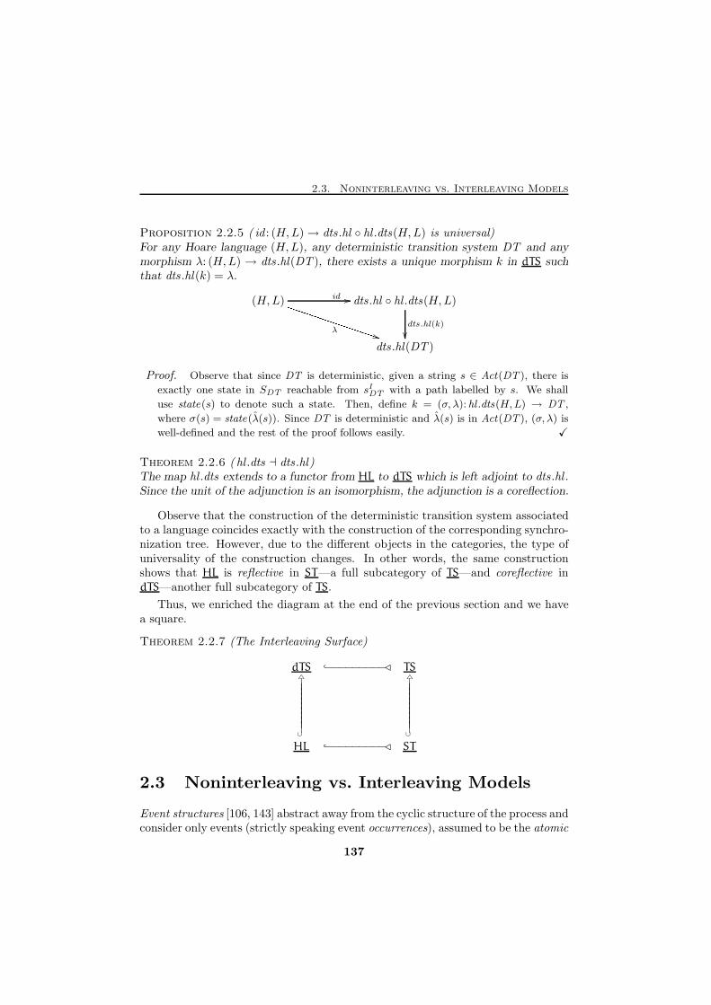
2.3. Noninterleaving vs. Interleaving Models
Proposition 2.2.5 ( id : (H,L)→ dts .hl ◦ hl .dts(H,L) is universal)For any Hoare language (H,L), any deterministic transition system DT and anymorphism λ: (H,L) → dts .hl(DT ), there exists a unique morphism k in dTS suchthat dts .hl (k) = λ.
(H,L) dts .hl ◦ hl .dts(H,L)
dts .hl(DT )
id //
λ
TTTTTTTTTTTTTTTT** dts.hl(k)
��
Proof. Observe that since DT is deterministic, given a string s ∈ Act(DT ), there is
exactly one state in SDT reachable from sIDT with a path labelled by s. We shall
use state(s) to denote such a state. Then, define k = (σ, λ): hl .dts(H,L) → DT ,
where σ(s) = state(λ(s)). Since DT is deterministic and λ(s) is in Act(DT ), (σ, λ) is
well-defined and the rest of the proof follows easily. X
Theorem 2.2.6 ( hl .dts ⊣ dts .hl)The map hl .dts extends to a functor from HL to dTS which is left adjoint to dts .hl .Since the unit of the adjunction is an isomorphism, the adjunction is a coreflection.
Observe that the construction of the deterministic transition system associatedto a language coincides exactly with the construction of the corresponding synchro-nization tree. However, due to the different objects in the categories, the type ofuniversality of the construction changes. In other words, the same constructionshows that HL is reflective in ST—a full subcategory of TS—and coreflective indTS—another full subcategory of TS.
Thus, we enriched the diagram at the end of the previous section and we havea square.
Theorem 2.2.7 (The Interleaving Surface)
dTS −−−−−−−−−⊳ TS△
||||||||||∪
△
||||||||||∪
HL −−−−−−−−−⊳ ST
2.3 Noninterleaving vs. Interleaving Models
Event structures [106, 143] abstract away from the cyclic structure of the process andconsider only events (strictly speaking event occurrences), assumed to be the atomic
137
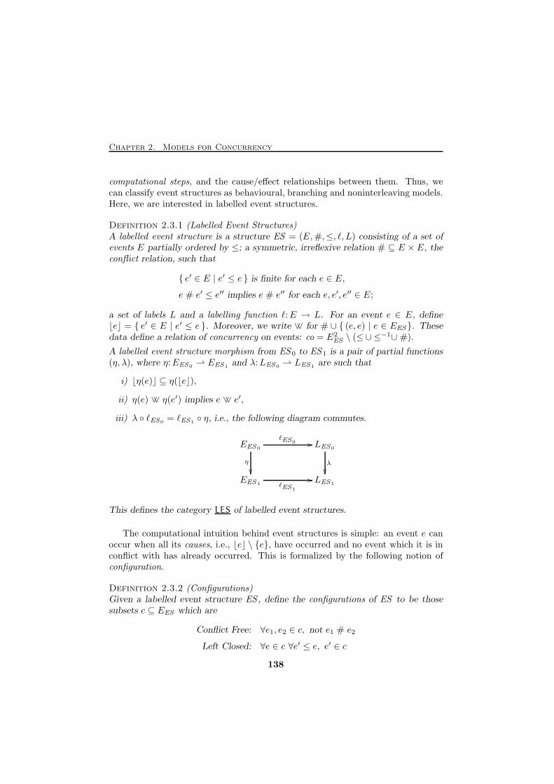
Chapter 2. Models for Concurrency
computational steps, and the cause/effect relationships between them. Thus, wecan classify event structures as behavioural, branching and noninterleaving models.Here, we are interested in labelled event structures.
Definition 2.3.1 (Labelled Event Structures)A labelled event structure is a structure ES = (E,#,≤, ℓ, L) consisting of a set ofevents E partially ordered by ≤; a symmetric, irreflexive relation # ⊆ E × E, theconflict relation, such that
{ e′ ∈ E | e′ ≤ e } is finite for each e ∈ E,
e # e′ ≤ e′′ implies e # e′′ for each e, e′, e′′ ∈ E;
a set of labels L and a labelling function ℓ:E → L. For an event e ∈ E, define⌊e⌋ = { e′ ∈ E | e′ ≤ e }. Moreover, we write ∨∨ for # ∪ { (e, e) | e ∈ EES}. Thesedata define a relation of concurrency on events: co = E2
ES \ (≤ ∪≤−1∪ #).
A labelled event structure morphism from ES 0 to ES 1 is a pair of partial functions(η, λ), where η:EES0
⇀ EES1and λ:LES0
⇀ LES1are such that
i) ⌊η(e)⌋ ⊆ η(⌊e⌋),
ii) η(e) ∨∨ η(e′) implies e ∨∨ e′,
iii) λ ◦ ℓES0= ℓES1
◦ η, i.e., the following diagram commutes.
EES0LES0
EES1 LES1
η
��
ℓES0 //
λ
��
ℓES1
//
This defines the category LES of labelled event structures.
The computational intuition behind event structures is simple: an event e canoccur when all its causes, i.e., ⌊e⌋ \ {e}, have occurred and no event which it is inconflict with has already occurred. This is formalized by the following notion ofconfiguration.
Definition 2.3.2 (Configurations)Given a labelled event structure ES , define the configurations of ES to be thosesubsets c ⊆ EES which are
Conflict Free: ∀e1, e2 ∈ c, not e1 # e2
Left Closed: ∀e ∈ c ∀e′ ≤ e, e′ ∈ c
138
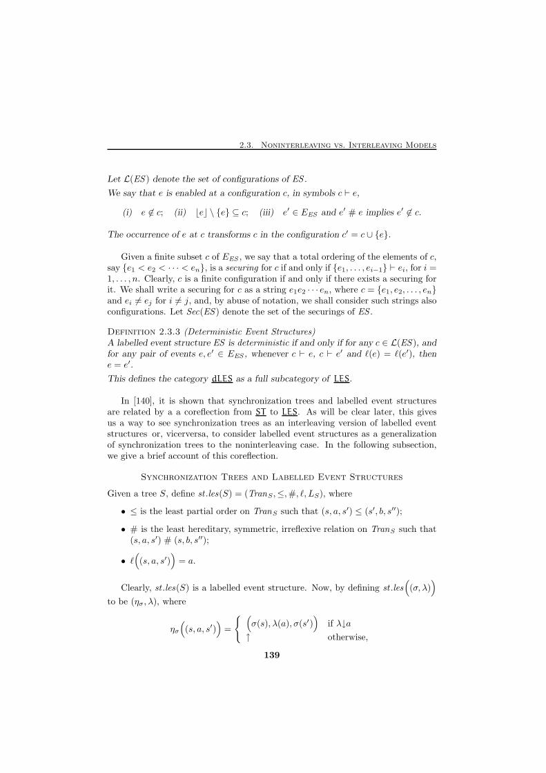
2.3. Noninterleaving vs. Interleaving Models
Let L(ES ) denote the set of configurations of ES .
We say that e is enabled at a configuration c, in symbols c ⊢ e,
(i) e 6∈ c; (ii) ⌊e⌋ \ {e} ⊆ c; (iii) e′ ∈ EES and e′ # e implies e′ 6∈ c.
The occurrence of e at c transforms c in the configuration c′ = c ∪ {e}.
Given a finite subset c of EES , we say that a total ordering of the elements of c,say {e1 < e2 < · · · < en}, is a securing for c if and only if {e1, . . . , ei−1} ⊢ ei, for i =1, . . . , n. Clearly, c is a finite configuration if and only if there exists a securing forit. We shall write a securing for c as a string e1e2 · · · en, where c = {e1, e2, . . . , en}and ei 6= ej for i 6= j, and, by abuse of notation, we shall consider such strings alsoconfigurations. Let Sec(ES ) denote the set of the securings of ES .
Definition 2.3.3 (Deterministic Event Structures)A labelled event structure ES is deterministic if and only if for any c ∈ L(ES ), andfor any pair of events e, e′ ∈ EES , whenever c ⊢ e, c ⊢ e′ and ℓ(e) = ℓ(e′), thene = e′.
This defines the category dLES as a full subcategory of LES.
In [140], it is shown that synchronization trees and labelled event structuresare related by a a coreflection from ST to LES. As will be clear later, this givesus a way to see synchronization trees as an interleaving version of labelled eventstructures or, vicerversa, to consider labelled event structures as a generalizationof synchronization trees to the noninterleaving case. In the following subsection,we give a brief account of this coreflection.
Synchronization Trees and Labelled Event Structures
Given a tree S, define st .les(S) = (TranS ,≤,#, ℓ, LS), where
• ≤ is the least partial order on TranS such that (s, a, s′) ≤ (s′, b, s′′);
• # is the least hereditary, symmetric, irreflexive relation on TranS such that(s, a, s′) # (s, b, s′′);
• ℓ((s, a, s′)
)= a.
Clearly, st .les(S) is a labelled event structure. Now, by defining st .les((σ, λ)
)
to be (ησ, λ), where
ησ
((s, a, s′)
)=
{ (σ(s), λ(a), σ(s′)
)if λ↓a
↑ otherwise,
139
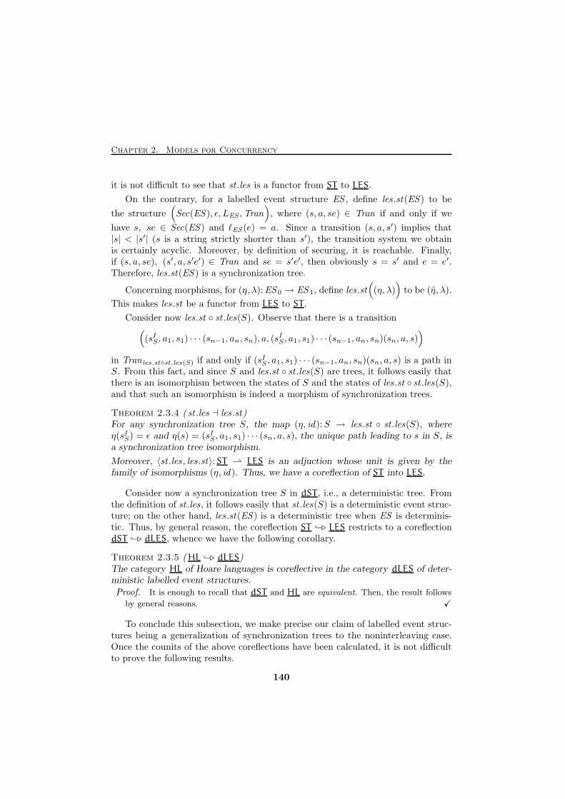
Chapter 2. Models for Concurrency
it is not difficult to see that st .les is a functor from ST to LES.
On the contrary, for a labelled event structure ES , define les .st(ES ) to be
the structure(Sec(ES ), ǫ, LES ,Tran
), where (s, a, se) ∈ Tran if and only if we
have s, se ∈ Sec(ES ) and ℓES (e) = a. Since a transition (s, a, s′) implies that|s| < |s′| (s is a string strictly shorter than s′), the transition system we obtainis certainly acyclic. Moreover, by definition of securing, it is reachable. Finally,if (s, a, se), (s′, a, s′e′) ∈ Tran and se = s′e′, then obviously s = s′ and e = e′.Therefore, les .st(ES ) is a synchronization tree.
Concerning morphisms, for (η, λ):ES 0 → ES 1, define les .st((η, λ)
)to be (η, λ).
This makes les .st be a functor from LES to ST .
Consider now les .st ◦ st .les(S). Observe that there is a transition((sIS , a1, s1) · · · (sn−1, an, sn), a, (s
IS , a1, s1) · · · (sn−1, an, sn)(sn, a, s)
)
in Tran les.st◦st.les(S) if and only if (sIS , a1, s1) · · · (sn−1, an, sn)(sn, a, s) is a path inS. From this fact, and since S and les .st ◦ st .les(S) are trees, it follows easily thatthere is an isomorphism between the states of S and the states of les .st ◦ st .les(S),and that such an isomorphism is indeed a morphism of synchronization trees.
Theorem 2.3.4 ( st .les ⊣ les .st)For any synchronization tree S, the map (η, id):S → les .st ◦ st .les(S), whereη(sIS) = ǫ and η(s) = (sIS , a1, s1) · · · (sn, a, s), the unique path leading to s in S, isa synchronization tree isomorphism.
Moreover, 〈st .les , les .st〉: ST ⇀ LES is an adjuction whose unit is given by thefamily of isomorphisms (η, id). Thus, we have a coreflection of ST into LES.
Consider now a synchronization tree S in dST , i.e., a deterministic tree. Fromthe definition of st .les, it follows easily that st .les(S) is a deterministic event struc-ture; on the other hand, les .st(ES ) is a deterministic tree when ES is determinis-tic. Thus, by general reason, the coreflection ST −⊲ LES restricts to a coreflectiondST −⊲ dLES, whence we have the following corollary.
Theorem 2.3.5 (HL −⊲ dLES)The category HL of Hoare languages is coreflective in the category dLES of deter-ministic labelled event structures.
Proof. It is enough to recall that dST and HL are equivalent. Then, the result follows
by general reasons. X
To conclude this subsection, we make precise our claim of labelled event struc-tures being a generalization of synchronization trees to the noninterleaving case.Once the counits of the above coreflections have been calculated, it is not difficultto prove the following results.
140
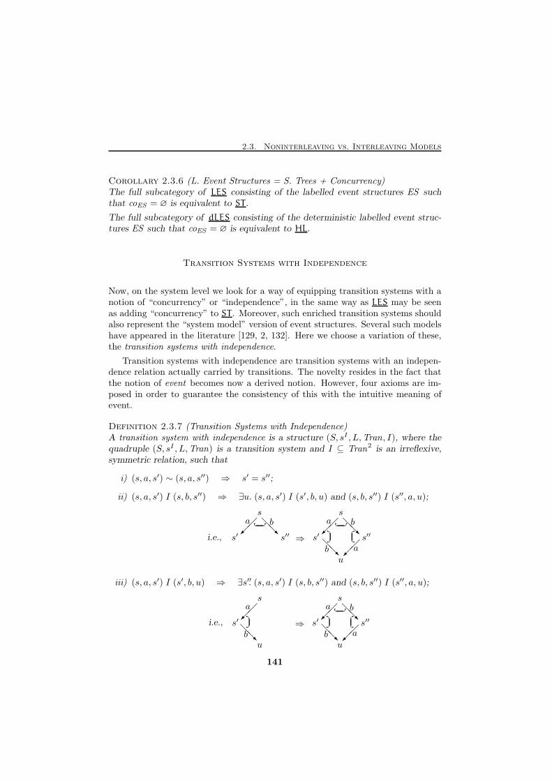
2.3. Noninterleaving vs. Interleaving Models
Corollary 2.3.6 (L. Event Structures = S. Trees + Concurrency)The full subcategory of LES consisting of the labelled event structures ES suchthat coES = ∅ is equivalent to ST .
The full subcategory of dLES consisting of the deterministic labelled event struc-tures ES such that coES = ∅ is equivalent to HL.
Transition Systems with Independence
Now, on the system level we look for a way of equipping transition systems with anotion of “concurrency” or “independence”, in the same way as LES may be seenas adding “concurrency” to ST . Moreover, such enriched transition systems shouldalso represent the “system model” version of event structures. Several such modelshave appeared in the literature [129, 2, 132]. Here we choose a variation of these,the transition systems with independence.
Transition systems with independence are transition systems with an indepen-dence relation actually carried by transitions. The novelty resides in the fact thatthe notion of event becomes now a derived notion. However, four axioms are im-posed in order to guarantee the consistency of this with the intuitive meaning ofevent.
Definition 2.3.7 (Transition Systems with Independence)A transition system with independence is a structure (S, sI , L,Tran, I), where thequadruple (S, sI , L,Tran) is a transition system and I ⊆ Tran2 is an irreflexive,symmetric relation, such that
i) (s, a, s′) ∼ (s, a, s′′) ⇒ s′ = s′′;
ii) (s, a, s′) I (s, b, s′′) ⇒ ∃u. (s, a, s′) I (s′, b, u) and (s, b, s′′) I (s′′, a, u);
i.e.,
@@R
��
s
s′ s′′
a b� � � ��� ��⇒@@R
��
@@R
��
s
s′ s′′
u
a b
b a
iii) (s, a, s′) I (s′, b, u) ⇒ ∃s′′. (s, a, s′) I (s, b, s′′) and (s, b, s′′) I (s′′, a, u);
i.e.,@@R
��
s
s′
u
a
b
�� � ��� ��⇒@@R
��
@@R
��
s
s′ s′′
u
a b
b a
141
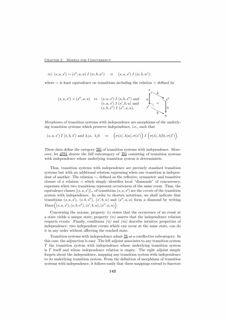
Chapter 2. Models for Concurrency
iv) (s, a, s′) ∼ (s′′, a, u) I (w, b, w′) ⇒ (s, a, s′) I (w, b, w′);
where ∼ is least equivalence on transitions including the relation ≺ defined by
(s, a, s′) ≺ (s′′, a, u) ⇔ (s, a, s′) I (s, b, s′′) and(s, a, s′) I (s′, b, u) and(s, b, s′′) I (s′′, a, u). HHHHj ?
HHHHj
? ≺
s
s′
u
s′′
b
b
a
a
��
Morphisms of transition systems with independence are morphisms of the underly-ing transition systems which preserve independence, i.e., such that
(s, a, s′) I (s, b, s′) and λ↓a, λ↓b ⇒(σ(s), λ(a), σ(s′)
)I(σ(s), λ(b), σ(s′)
).
These data define the category TSI of transition systems with independence. More-over, let dTSI denote the full subcategory of TSI consisting of transition systemswith independence whose underlying transition system is deterministic.
Thus, transition systems with independence are precisely standard transitionsystems but with an additional relation expressing when one transition is indepen-dent of another. The relation ∼, defined as the reflexive, symmetric and transitiveclosure of a relation ≺ which simply identifies local “diamonds” of concurrency,expresses when two transitions represent occurrences of the same event. Thus, theequivalence classes [(s, a, s′)]∼ of transitions (s, a, s′) are the events of the transitionsystem with independence. In order to shorten notations, we shall indicate thattransitions (s, a, s′), (s, b, s′′), (s′, b, u) and (s′′, a, u) form a diamond by writing
Diam((s, a, s′), (s, b, s′′), (s′, b, u), (s′′, a, u)
).
Concerning the axioms, property (i) states that the occurrence of an event ata state yields a unique state; property (iv) asserts that the independence relationrespects events. Finally, conditions (ii) and (iii) describe intuitive properties ofindependence: two independent events which can occur at the same state, can doit in any order without affecting the reached state.
Transition systems with independence admit TS as a coreflective subcategory. Inthis case, the adjunction is easy. The left adjoint associates to any transition systemT the transition system with independence whose underlying transition systemis T itself and whose independence relation is empty. The right adjoint simplyforgets about the independence, mapping any transition system with independenceto its underlying transition system. From the definition of morphisms of transitionsystems with independence, it follows easily that these mappings extend to functors
142
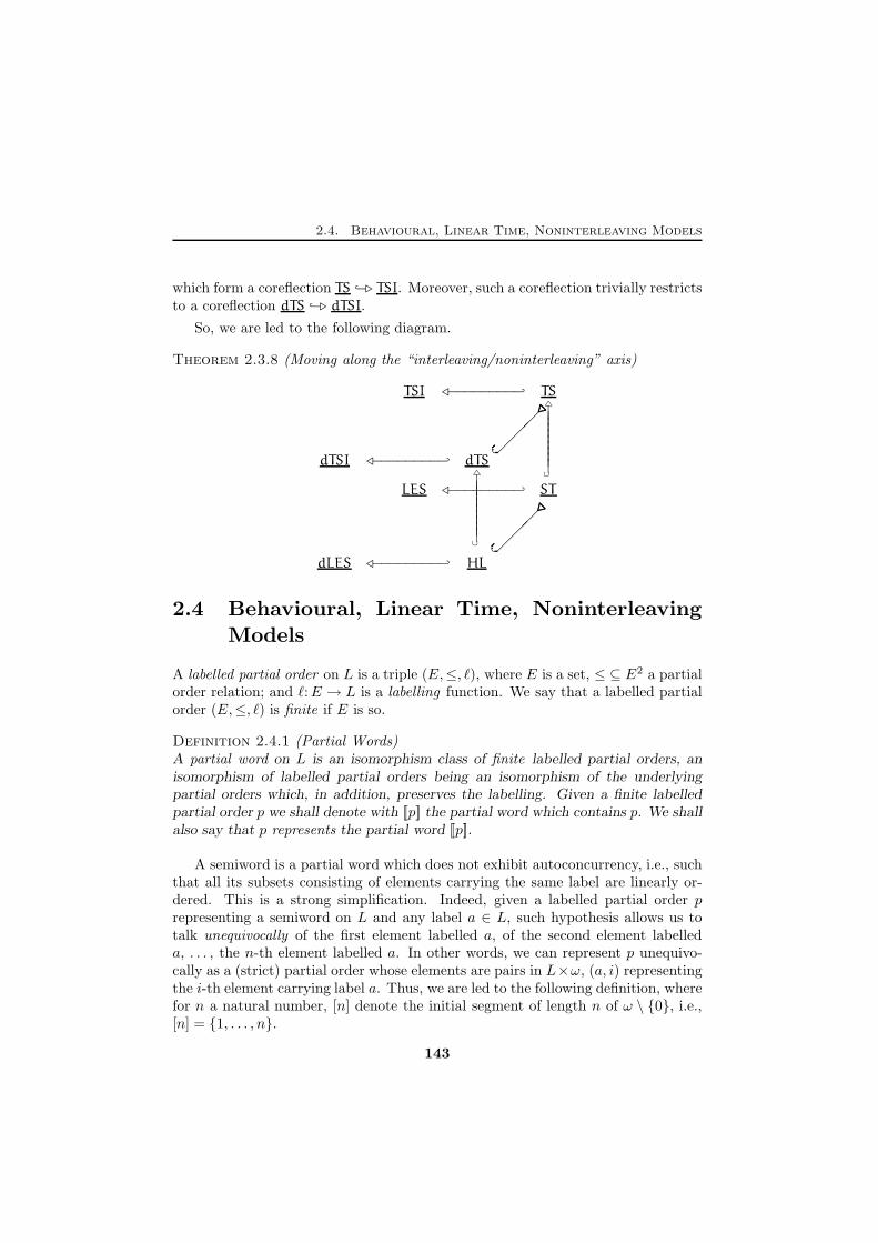
2.4. Behavioural, Linear Time, Noninterleaving Models
which form a coreflection TS −⊲ TSI. Moreover, such a coreflection trivially restrictsto a coreflection dTS −⊲ dTSI.
So, we are led to the following diagram.
Theorem 2.3.8 (Moving along the “interleaving/noninterleaving” axis)
dTSI ⊳−−−−−−−−− dTS���
....................................................
..........�△
||||||||||∪
dLES ⊳−−−−−−−−− HL���
....................................................
..........�
TSI ⊳−−−−−−−−− TS△
||||||||||∪
LES ⊳−−−−−−−−− ST
2.4 Behavioural, Linear Time, NoninterleavingModels
A labelled partial order on L is a triple (E,≤, ℓ), where E is a set, ≤ ⊆ E2 a partialorder relation; and ℓ:E → L is a labelling function. We say that a labelled partialorder (E,≤, ℓ) is finite if E is so.
Definition 2.4.1 (Partial Words)A partial word on L is an isomorphism class of finite labelled partial orders, anisomorphism of labelled partial orders being an isomorphism of the underlyingpartial orders which, in addition, preserves the labelling. Given a finite labelledpartial order p we shall denote with [[p]] the partial word which contains p. We shallalso say that p represents the partial word [[p]].
A semiword is a partial word which does not exhibit autoconcurrency, i.e., suchthat all its subsets consisting of elements carrying the same label are linearly or-dered. This is a strong simplification. Indeed, given a labelled partial order prepresenting a semiword on L and any label a ∈ L, such hypothesis allows us totalk unequivocally of the first element labelled a, of the second element labelleda, . . . , the n-th element labelled a. In other words, we can represent p unequivo-cally as a (strict) partial order whose elements are pairs in L×ω, (a, i) representingthe i-th element carrying label a. Thus, we are led to the following definition, wherefor n a natural number, [n] denote the initial segment of length n of ω \ {0}, i.e.,[n] = {1, . . . , n}.
143
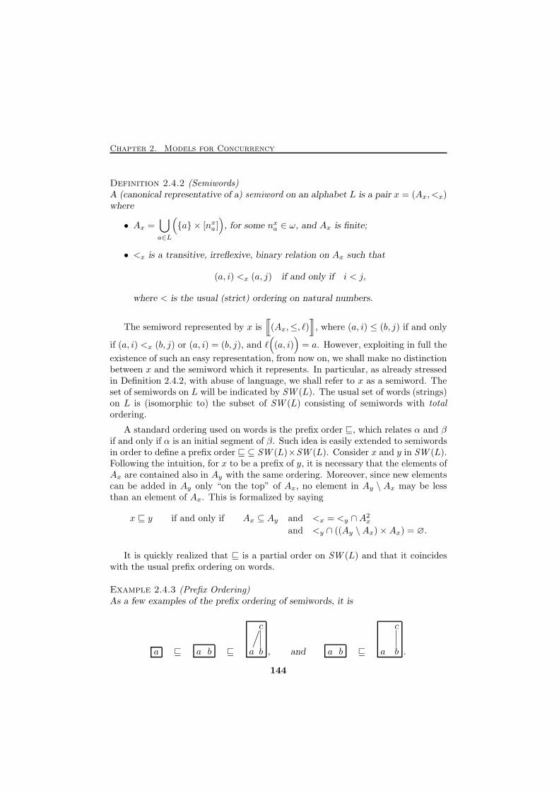
Chapter 2. Models for Concurrency
Definition 2.4.2 (Semiwords)A (canonical representative of a) semiword on an alphabet L is a pair x = (Ax, <x)where
• Ax =⋃
a∈L
({a} × [nxa]
), for some nxa ∈ ω, and Ax is finite;
• <x is a transitive, irreflexive, binary relation on Ax such that
(a, i) <x (a, j) if and only if i < j,
where < is the usual (strict) ordering on natural numbers.
The semiword represented by x is[[(Ax,≤, ℓ)
]], where (a, i) ≤ (b, j) if and only
if (a, i) <x (b, j) or (a, i) = (b, j), and ℓ((a, i)
)= a. However, exploiting in full the
existence of such an easy representation, from now on, we shall make no distinctionbetween x and the semiword which it represents. In particular, as already stressedin Definition 2.4.2, with abuse of language, we shall refer to x as a semiword. Theset of semiwords on L will be indicated by SW (L). The usual set of words (strings)on L is (isomorphic to) the subset of SW (L) consisting of semiwords with totalordering.
A standard ordering used on words is the prefix order ⊑, which relates α and βif and only if α is an initial segment of β. Such idea is easily extended to semiwordsin order to define a prefix order ⊑ ⊆ SW (L)×SW (L). Consider x and y in SW (L).Following the intuition, for x to be a prefix of y, it is necessary that the elements ofAx are contained also in Ay with the same ordering. Moreover, since new elementscan be added in Ay only “on the top” of Ax, no element in Ay \ Ax may be lessthan an element of Ax. This is formalized by saying
x ⊑ y if and only if Ax ⊆ Ay and <x = <y ∩A2x
and <y ∩ ((Ay \Ax)×Ax) = ∅.
It is quickly realized that ⊑ is a partial order on SW (L) and that it coincideswith the usual prefix ordering on words.
Example 2.4.3 (Prefix Ordering)As a few examples of the prefix ordering of semiwords, it is
a ⊑ a b ⊑
/
a
c∣∣∣b , and a b ⊑ a
c∣∣∣b .
144
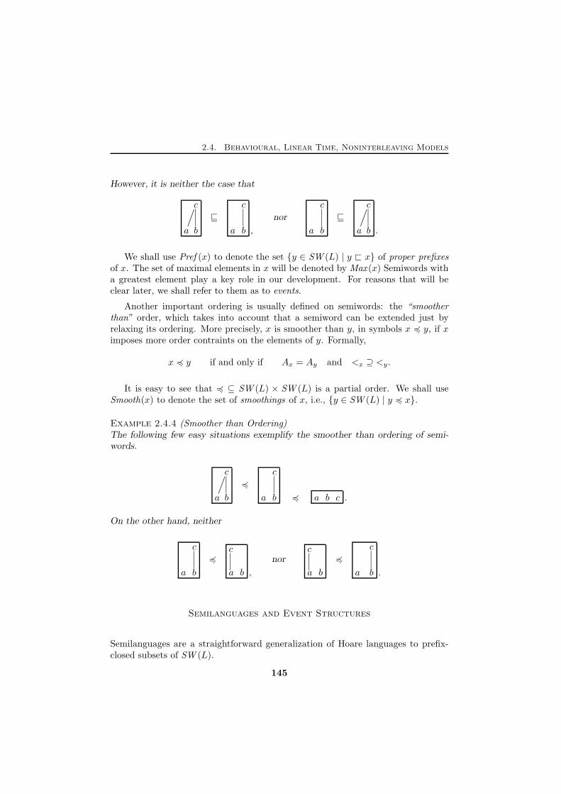
2.4. Behavioural, Linear Time, Noninterleaving Models
However, it is neither the case that
/
a
c∣∣∣b
⊑
a
c∣∣∣b ,
nor
a
c∣∣∣b
⊑/
a
c∣∣∣b .
We shall use Pref (x) to denote the set {y ∈ SW (L) | y ⊏ x} of proper prefixesof x. The set of maximal elements in x will be denoted by Max (x) Semiwords witha greatest element play a key role in our development. For reasons that will beclear later, we shall refer to them as to events.
Another important ordering is usually defined on semiwords: the “smootherthan” order, which takes into account that a semiword can be extended just byrelaxing its ordering. More precisely, x is smoother than y, in symbols x 4 y, if ximposes more order contraints on the elements of y. Formally,
x 4 y if and only if Ax = Ay and <x ⊇ <y.
It is easy to see that 4 ⊆ SW (L) × SW (L) is a partial order. We shall useSmooth(x) to denote the set of smoothings of x, i.e., {y ∈ SW (L) | y 4 x}.
Example 2.4.4 (Smoother than Ordering)The following few easy situations exemplify the smoother than ordering of semi-words.
/
a
c∣∣∣b
4a
c∣∣∣b 4 a b c .
On the other hand, neither
a
c∣∣∣b
4c∣∣∣a b ,
norc∣∣∣a b
4a
c∣∣∣b .
Semilanguages and Event Structures
Semilanguages are a straightforward generalization of Hoare languages to prefix-closed subsets of SW (L).
145
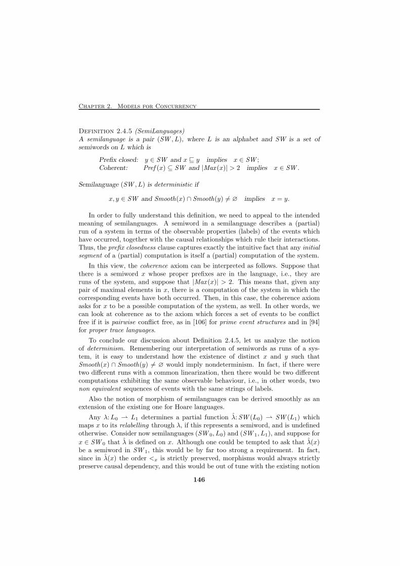
Chapter 2. Models for Concurrency
Definition 2.4.5 (SemiLanguages)A semilanguage is a pair (SW , L), where L is an alphabet and SW is a set ofsemiwords on L which is
Prefix closed: y ∈ SW and x ⊑ y implies x ∈ SW ;Coherent: Pref (x) ⊆ SW and |Max (x)| > 2 implies x ∈ SW .
Semilanguage (SW , L) is deterministic if
x, y ∈ SW and Smooth(x) ∩ Smooth(y) 6= ∅ implies x = y.
In order to fully understand this definition, we need to appeal to the intendedmeaning of semilanguages. A semiword in a semilanguage describes a (partial)run of a system in terms of the observable properties (labels) of the events whichhave occurred, together with the causal relationships which rule their interactions.Thus, the prefix closedness clause captures exactly the intuitive fact that any initialsegment of a (partial) computation is itself a (partial) computation of the system.
In this view, the coherence axiom can be interpreted as follows. Suppose thatthere is a semiword x whose proper prefixes are in the language, i.e., they areruns of the system, and suppose that |Max (x)| > 2. This means that, given anypair of maximal elements in x, there is a computation of the system in which thecorresponding events have both occurred. Then, in this case, the coherence axiomasks for x to be a possible computation of the system, as well. In other words, wecan look at coherence as to the axiom which forces a set of events to be conflictfree if it is pairwise conflict free, as in [106] for prime event structures and in [94]for proper trace languages.
To conclude our discussion about Definition 2.4.5, let us analyze the notionof determinism. Remembering our interpretation of semiwords as runs of a sys-tem, it is easy to understand how the existence of distinct x and y such thatSmooth(x) ∩ Smooth(y) 6= ∅ would imply nondeterminism. In fact, if there weretwo different runs with a common linearization, then there would be two differentcomputations exhibiting the same observable behaviour, i.e., in other words, twonon equivalent sequences of events with the same strings of labels.
Also the notion of morphism of semilanguages can be derived smoothly as anextension of the existing one for Hoare languages.
Any λ:L0 ⇀ L1 determines a partial function λ:SW (L0) ⇀ SW (L1) whichmaps x to its relabelling through λ, if this represents a semiword, and is undefinedotherwise. Consider now semilanguages (SW 0, L0) and (SW 1, L1), and suppose for
x ∈ SW 0 that λ is defined on x. Although one could be tempted to ask that λ(x)be a semiword in SW 1, this would be by far too strong a requirement. In fact,since in λ(x) the order <x is strictly preserved, morphisms would always strictlypreserve causal dependency, and this would be out of tune with the existing notion
146
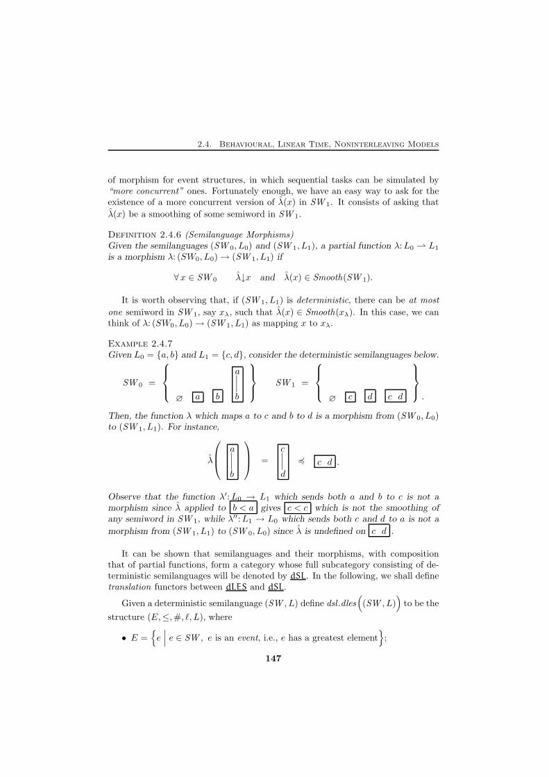
2.4. Behavioural, Linear Time, Noninterleaving Models
of morphism for event structures, in which sequential tasks can be simulated by“more concurrent” ones. Fortunately enough, we have an easy way to ask for theexistence of a more concurrent version of λ(x) in SW 1. It consists of asking that
λ(x) be a smoothing of some semiword in SW 1.
Definition 2.4.6 (Semilanguage Morphisms)Given the semilanguages (SW 0, L0) and (SW 1, L1), a partial function λ:L0 ⇀ L1
is a morphism λ: (SW0, L0)→ (SW 1, L1) if
∀x ∈ SW 0 λ↓x and λ(x) ∈ Smooth(SW 1).
It is worth observing that, if (SW 1, L1) is deterministic, there can be at most
one semiword in SW 1, say xλ, such that λ(x) ∈ Smooth(xλ). In this case, we canthink of λ: (SW0, L0)→ (SW 1, L1) as mapping x to xλ.
Example 2.4.7Given L0 = {a, b} and L1 = {c, d}, consider the deterministic semilanguages below.
SW 0 =
∅ a b
a∣∣∣b
SW 1 =
∅ c d c d
.
Then, the function λ which maps a to c and b to d is a morphism from (SW 0, L0)to (SW 1, L1). For instance,
λ
a∣∣∣b
=c∣∣∣d
4 c d .
Observe that the function λ′:L0 → L1 which sends both a and b to c is not amorphism since λ applied to b < a gives c < c which is not the smoothing ofany semiword in SW 1, while λ′′:L1 → L0 which sends both c and d to a is not a
morphism from (SW 1, L1) to (SW 0, L0) since λ is undefined on c d .
It can be shown that semilanguages and their morphisms, with compositionthat of partial functions, form a category whose full subcategory consisting of de-terministic semilanguages will be denoted by dSL. In the following, we shall definetranslation functors between dLES and dSL.
Given a deterministic semilanguage (SW , L) define dsl .dles((SW , L)
)to be the
structure (E,≤,#, ℓ, L), where
• E ={e∣∣∣ e ∈ SW , e is an event, i.e., e has a greatest element
};
147
Chapter 2. Models for Concurrency
• ≤ = ⊑ ∩ E2;
• # ={(e, e′) ∈ E2
∣∣∣ e and e′ are incompatible wrt ⊑};
• ℓ(e) is the label of the greatest element of e.
Theorem 2.4.8dsl .dles
((SW , L)
)is a deterministic labelled event structure.
Consider now a deterministic labelled event structure DES = (E,≤,#, ℓ, L).Define dles .dsl (DES ) to be the structure (SW , L), where
SW ={[[
(c,≤ ∩ c2, ℓ|c)]] ∣∣∣ c is a finite configuration of DES
}.
Theorem 2.4.9dles .dsl (DES ) is a deterministic semilanguage.
It can be shown that dsl.dles and dles.dsl extend to functors which when com-posed with each other yield functors naturally isomorphic to identity functors. Inother words, they form an adjoint equivalence [90, chap. III, pg. 91], i.e., an adjunc-tion which is both a reflection and a coreflection. It is worthwhile noticing thatthis implies that the mappings dsl.dles and dles.dsl constitute a bijection betweendeterministic semilanguages and isomorphism classes of deterministic labelled eventstructures—isomorphism being identity up to the names of events.
Theorem 2.4.10The categories dSL and dLES are equivalent.
In fact, dropping the axiom of coherence in Definition 2.4.5 we get semilanguagesequivalent to labelled stable event structures [143].
Trace Languages and Event Structures
Generalized trace languages extend trace languages by considering an independencerelation which may vary while the computation is progressing. Of course, we needa few axioms to guarantee the consistency of such an extension.
Definition 2.4.11 (Generalized Trace Languages)A generalized trace language is a triple (M, I, L), where L is an alphabet, M ⊆ L∗
148
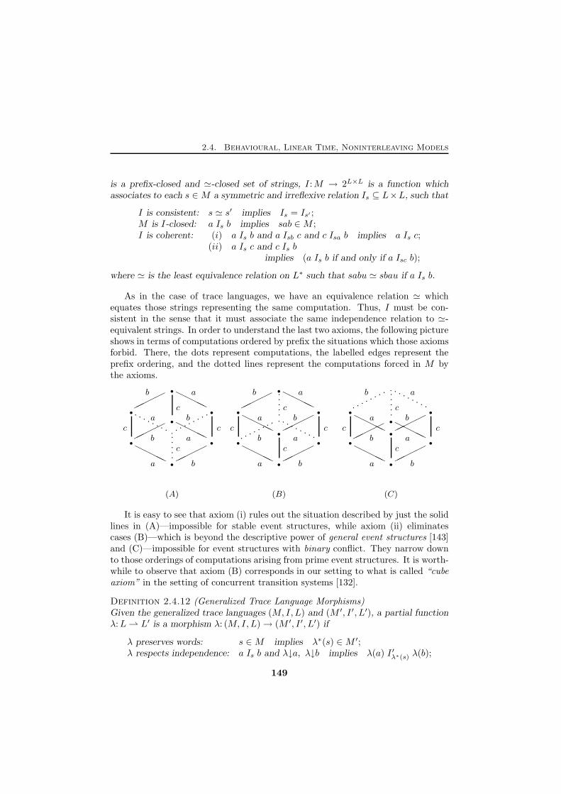
2.4. Behavioural, Linear Time, Noninterleaving Models
is a prefix-closed and ≃-closed set of strings, I:M → 2L×L is a function whichassociates to each s ∈M a symmetric and irreflexive relation Is ⊆ L×L, such that
I is consistent: s ≃ s′ implies Is = Is′ ;M is I-closed: a Is b implies sab ∈M ;I is coherent: (i) a Is b and a Isb c and c Isa b implies a Is c;
(ii) a Is c and c Is bimplies (a Is b if and only if a Isc b);
where ≃ is the least equivalence relation on L∗ such that sabu ≃ sbau if a Is b.
As in the case of trace languages, we have an equivalence relation ≃ whichequates those strings representing the same computation. Thus, I must be con-sistent in the sense that it must associate the same independence relation to ≃-equivalent strings. In order to understand the last two axioms, the following pictureshows in terms of computations ordered by prefix the situations which those axiomsforbid. There, the dots represent computations, the labelled edges represent theprefix ordering, and the dotted lines represent the computations forced in M bythe axioms.
HHHH
����
����
HHHH
HHHH
����
HHHH
HHHH
����HHHH
����
����HHHH
HHHH
����HHHH
����
����
. . . . . . . ......
................
.
.
.
.
.. . . . . . . .
........
. . . . . . . .
.
.
.
.
.
•
• •
•
·
• •
•
•
• •
·
•
• •
•
•
• •
•
•
• •
·
c
c c
cb
a b
ab
b
a
a
c
c c
cb
a b
ab
b
a
a
c
c c
c
b
b
b
b
a
a
a
a
(A) (B) (C)
It is easy to see that axiom (i) rules out the situation described by just the solidlines in (A)—impossible for stable event structures, while axiom (ii) eliminatescases (B)—which is beyond the descriptive power of general event structures [143]and (C)—impossible for event structures with binary conflict. They narrow downto those orderings of computations arising from prime event structures. It is worth-while to observe that axiom (B) corresponds in our setting to what is called “cubeaxiom” in the setting of concurrent transition systems [132].
Definition 2.4.12 (Generalized Trace Language Morphisms)Given the generalized trace languages (M, I, L) and (M ′, I ′, L′), a partial functionλ:L ⇀ L′ is a morphism λ: (M, I, L)→ (M ′, I ′, L′) if
λ preserves words: s ∈M implies λ∗(s) ∈M ′;λ respects independence: a Is b and λ↓a, λ↓b implies λ(a) I ′λ∗(s) λ(b);
149
Chapter 2. Models for Concurrency
where λ∗ is defined by λ∗(ǫ) = ǫ and λ∗(sa) =
{λ∗(s)λ(a) if λ↓aλ∗(s) otherwise.
Generalized trace languages and their morphisms, under the usual compositionof partial functions, form the category GTL.
A derived notion of event in generalized trace languages can be captured by therelation ∼ defined as the least equivalence such that
a Is b implies sa ∼ sba and s ≃ s′ implies sa ∼ s′a.
The events occurring in s ∈M , denoted by Ev (s), are the ∼-classes a represen-tative of which occurs as a non empty prefix of s, i.e.,
{[u]∼
∣∣∣ u is a non empty prefix of s}.
It can be shown that s ≃ s′ if and only if Ev (s) = Ev(s′). Extending the notation,we shall write Ev(M) to denote the events of (M, I, L), i.e., the ∼-equivalenceclasses of non empty strings in M .
Now, given a generalized trace language (M, I, L) define gtl .dles((M, I, L)
)to
be the structure (Ev(M),≤,#, ℓ, L), where
• [s]∼ ≤ [s′]∼ if and only if ∀u ∈M, [s′]∼ ∈ Ev(u) implies [s]∼ ∈ Ev(u);
• [s]∼ # [s′]∼ if and only if ∀u ∈M, [s]∼ ∈ Ev (u) implies [s′]∼ 6∈ Ev (u);
• ℓ([s]∼
)= a if and only if s = s′a.
Theorem 2.4.13gtl .dles
((M, I, L)
)is a deterministic labelled event structure.
On the other hand, in order to define a generalized trace language from a de-terministic labelled event structure DES = (E,≤,#, ℓ, L), consider
M ={ℓ∗(e1 · · · en)
∣∣∣ {e1, . . . , en} ⊆ E and {e1, . . . , ei−1} ⊢ ei, i = 1, . . . , n}.
Since DES is deterministic, any s ∈ M identifies unequivocally a string of eventsSec(s) = e1 · · · en ∈ E
∗ such that {e1, . . . , ei−1} ⊢ ei, i = 1, . . . , n, and such thatℓ∗(e1 · · · en) = s. Now, for any s ∈M , take
Is ={
(a, b)∣∣∣ sab ∈M, Sec(sab) = xe0e1 and e0 co e1
}.
Then, define (M, I, L) to be dles .gtl (DES ).
150
2.5. Transition Systems with Independence and Labelled Event Structures
Theorem 2.4.14dles .gtl(DES ) is a generalized trace language.
As in the case treated in the previous section, dles.gtl and gtl.dles extend tofunctors between GTL and dLES which form an adjoint equivalence. Such an equiv-alence restricts to an isomorphism of generalized trace languages and isomorphismclasses of deterministic labelled event structures.
Theorem 2.4.15Categories GTL and dLES are equivalent.
The result extends to labelled stable event structures by dropping the ‘only if ’implication in part (ii) of the coherence axiom of Definition 2.4.11. Of course, itfollows from Theorem 2.4.10 and Theorem 2.4.15 that dSL and GTL are equivalent.In [125], we also define direct translations between such categories.
2.5 Transition Systems with Independence andLabelled Event Structures
In this section, we show that transition systems with independence are an extensionof labelled event structures to a system model, by showing that there exists acoreflection from LES to TSI. To simplify our task, we split such a coreflection intwo parts. First, we define the unfolding of transition systems with independence.To this aim, we introduce the category oTSI of occurrence transition systems withindependence. Later, we shall show that labelled event structures are coreflectivein oTSI, thus obtaining
LES −−−−−−−⊲ oTSI −−−−−−−⊲ TSI.
Definition 2.5.1 (Occurrence Transition Systems with Independence)An occurrence transition system with independence is a transition system with in-dependence OTI = (S, sI , L,Tran, I) which is reachable, acyclic and such that
(s′, a, u) 6= (s′′, b, u) ∈ Tran implies∃s. (s, b, s′) I (s, a, s′′) and (s, b, s′) I (s′, a, u)
and (s, a, s′′) I (s′′, b, u),
or, in other words, (s′, a, u) and (s′′, b, u) form the bottom of a concurrency diamond
Diam((s, a, s′′), (s, b, s′)(s′′, b, u), (s′, a, u)
).
Let oTSI denote the full subcategory of TSI whose objects are occurrence transitionsystems with independence.
151
Chapter 2. Models for Concurrency
Given a transition system with independence TI , define ≃ ⊆ Path(TI )2 to bethe least equivalence relation such that
πs(s, a, s′)(s′, b, u)πv ≃ πs(s, b, s′′)(s′′, a, u)πv
if Diam((s, a, s′), (s, b, s′′)(s′, b, u), (s′′, a, u)
).
Lemma 2.5.2Given an occurrence transition system with independence OTI , let u be a stateand πu, π
′u paths leading to it. Then πu ≃ π′u.
Proof. By induction on the minimum length among those of πu and π′u.
If |πu| = |π′u| = 0, then πu = ǫ = π′u.
Suppose that πu = πs′(s′, a, u), π′u = πs′′(s
′′, b, u) and suppose that |πs′ | ≤ |πs′′ |.Then, necessarily, it must be
Diam((s, a, s′′), (s, b, s′), (s′, a, u), (s′′, b, u)
),
for some s ∈ SOTI .
Since OTI is reachable, there exists a path π0 = πs(s, b, s′). Since the length of πs′ is
n−1, we have that min{|π0|, |πs′ |} ≤ n−1. So, we can apply the induction hypothesis
and conclude that πs′ ≃ π0. From the definition of ≃, it follows that π0 has length
n − 1. Thus, π1 = πs(s, a, s′′) has length n − 1 and, by induction, π1 ≃ πs′′ . So,
πu = πs′(s′, a, u) ≃ πs(s, b, s
′)(s′, a, u) ≃ πs(s, a, s′′)(s′′, b, u) ≃ πs′′(s
′′, b, u) = π′u. X
Such a lemma has the following corollary.
Corollary 2.5.3All the paths leading to the same state of an occurrence transition system withindependence have the same length.
It is now easy to prove the following basic properties.
Corollary 2.5.4Occurrence transition systems with independence do not contain infinite sequencesof transitions ending in a state.
Proof. Suppose that OTI admits an infinite chain of the kind s0a1←− s1
a2←− s2a3←− · · ·.
Since OTI is reachable, there exists a path πs0 in Path(OTI ). Let us suppose that
|πs0 | = n. Then consider the first n + 1 elements of the chain s0a1←− s1 · · ·
an←− sn.
Then, there exists a path πsn which when composed with snan−→ · · ·
a0−→ s0 gives a
path π′s0 whose length is greater than n. This contradicts Lemma 2.5.2. X
The same technique used in the last proof shows the following corollary.
152
2.5. Transition Systems with Independence and Labelled Event Structures
Corollary 2.5.5Any pair of sequences of transitions leading from state s to state s′ of OTI havethe same length.
Proof. If there where sa1−→ · · ·
an−→ s′ and sb1−→ · · ·
bm−→ s′ with n 6= m, since s is
reachable, we would have two paths leading to s′ of different length. X
Corollary 2.5.6Any pair of sequences leading from state s to state s′ of OTI contain the samenumber of representatives from any ∼-equivalence class.
Proof. First suppose that s is the initial state sIOTI . Then the sequences are two pathsleading to the same state and therefore, by Lemma 2.5.2, they are ≃-equivalent. Inthe case πs(s, a, s
′)(s′, b, u)πs′ ≃ πs(s, b, s′′)(s′′, a, u)πs′ , the result is immediate, since
(s, a, s′) ∼ (s′′, a, u) and (s, b, s′′) ∼ (s′, b, u). In the general case, the result follows byapplying transitively the previous argument.
Now, consider two sequences from a generic s to s′, say σs→s′ and σ′s→s′ . If there were
a ∼-class whose elements occur a different number of times in σs→s′ and σ′s→s′ , then
the same would happen for the paths πsσs→s′ and πsσ′s→s′ , and that would contradict
what we have just shown in the first part of this proof. X
Corollary 2.5.7If (s, a, s′) and (s, b, s′) are transitions of OTI , then a = b.
Proof. Since πs(s, a, s′) ≃ πs(s, b, s
′), it must be (s, a, s′) ∼ (s, b, s′) and so a = b. X
Some other interesting results which do not depend directly from Lemma 2.5.2follow.
Lemma 2.5.8For any (s′, a, u) 6= (s′′, a, u) ∈ TranOTI , it is (s′, a, u) 6∼ (s′′, a, u).
Proof. Suppose that (s′, a, u) ∼ (s′′, a, u). Since s′ 6= s′′, by definition of occurrence
transition system with independence, there exist a state s and transitions (s, a, s′) and
(s, a, s′′) which form a diamond. Then, (s, a, s′) ∼ (s′′, a, u) ∼ (s′, a, u) ∼ (s, a, s′′),
and therefore, by axiom (i) in Definition 2.3.7, s′ = s′′. Absurd. X
Corollary 2.5.9Given (s′, a, u) 6= (s′′, b, u) ∈ TranOTI , there exist unique s, (s, b, s′) and (s, a, s′′)
such that Diam((s, b, s′), (s, a, s′′), (s′, a, u), (s′′, b, u)
).
Proof. Suppose that Diam((s, b, s′), (s, a, s′′), (s′, a, u), (s′′, b, u)
)for s 6= s. Then we
have (s, a, s′′) ∼ (s′, a, u) ∼ (s, a, s′′), contradicting the previous lemma. Absurd. X
153
Chapter 2. Models for Concurrency
Summing up, these results tell us that occurrence transition systems with in-dependence are particularly well structured. In particular, they imply that in anoccurrence transition system with independence each diamond of concurrency isnot degenerate, i.e., it consists of four distinct states.
The next step is to show that in a path of an occurrence transition system withindependence at most one representative of a ∼-class may appear. Given a path π
and an equivalence class [(s, a, s′)]∼, let N(π, [(s, a, s′)]∼
)be the number of repre-
sentatives of [(s, a, s′)]∼ occurring in π. Of course, we know from Corollary 2.5.6that such a number depends on π only by means of the state it reaches. Therefore,
we shall write simply N(x, [(s, a, s′)]∼
), for x ∈ SOTI . Moreover, let s
a←→ s′
stand for sa−→ s′ or s
a←− s′. Then we have the following result.
Lemma 2.5.10Consider a sequence of states σ = s0
a1←→ s1a2←→ s2 · · ·
an←→ sn. Then
N(sn, [(s, a, s
′)]∼
)= N
(s0, [(s, a, s
′)]∼
)
+∣∣∣{(si, ai+1, si+1) | (si, ai+1, si+1) ∼ (s, a, s′)
}∣∣∣
−∣∣∣{(si+1, ai+1, si) | (si+1, ai+1, si) ∼ (s, a, s′)
}∣∣∣.
Proof. By induction on n, the length of σ. For n = 0, σ is empty and the thesis istrivially true. Suppose then that the thesis holds for sequences of length n− 1. Thereare two cases: sn−1
an−→ sn or snan−→ sn−1.
@@@R �
������
����
. .. .
. . . . . . . .
••
• •
s0
sn−1
sn
a1
an
(case sn−1an−→ sn.)
If (sn−1, an, sn) 6∼ (s, a, s′) then
N(sn, [(s, a, s
′)]∼
)=
N(sn−1, [(s, a, s
′)]∼
),
and since nothing is added to or sub-tracted from the right hand term,
the equality holds. If otherwise (sn−1, an, sn) ∼ (s, a, s′), then
N(sn, [(s, a, s
′)]∼
)= N
(sn−1, [(s, a, s
′)]∼
)+ 1,
and the equality stays since 1 is added also to the righthand term. So, the inductionhypothesis is mantained.
154
2.5. Transition Systems with Independence and Labelled Event Structures
@@@R
���
���
����
. .. .
. . . . . . . .
••
• •
s0
sn−1
sn
a1
an
(case snan−→ sn−1.)
Again, if (sn−1, an, sn) 6∼ (s, a, s′)
the terms on both the sides of the
equation are unchanged considering
the n-th transition, and the result
holds by induction. Otherwise if
(sn−1, an, sn) ∼ (s, a, s′), then N(sn, [(s, a, s
′)]∼
)= N
(sn−1, [(s, a, s
′)]∼
)− 1. This
time 1 is subtracted from the right hand term, and therefore the induction hypothesis
is mantained. X
Then, we have the following important corollary.
Corollary 2.5.11Given a path π ∈ Path(OTI ), at most one representative of any ∼-equivalence classcan occur in π.
Proof. Suppose that (s, a, s′) ∼ (s, a, s′) occur both in π. By definition of ∼, it must
exist a sequence σ =(s = s0
a0←→ · · ·an←→ sn = s
), as shown it the following figure.
PPPq
PPPqPPPq
PPPq ���)
���) ���)
���) PPPq
PPPqPPPq
PPPq
?
??
??
??
??
?
. . . . .
. . . . . . .
. . . . .
. . .
. . . . .
s
s′
s1si−1
si
si+1
sk−1
sk
sk+1
sn−1
s′
s•
•
•
•
•
•
•
•
≺
≺ ≻
≻ ≺
≺
a
aa
a
aa
a
aa
a
Without loss of generality, we can assume π = π′(s, a, s′)σ′(s, a, s′)σ′′, i.e., that(s, a, s′) occurs before than (s, a, s′). Now, since (s, a, s′) appears in π after states, we have
N(s, [(s, a, s′)]∼
)< N
(s, [(s, a, s′)]∼
).
By the previous lemma, we have that in σ at least a representative of [(s, a, s′)]∼ mustoccur “positively”, say (sk, ak+1, sk+1) ∼ (s, a, s′). Therefore, we have a diamond
Diam((sk, ak+1, sk+1), (sk, a, sk), (sk+1, a, sk+1), (sk, ak+1, sk+1)
)
where, for the properties already shown, it must be sk 6= sk. This is absurd, because
(sk, ak+1, sk+1) ∼ (sk, a, sk) breaks axiom (i) of transition systems with independence.
X
155
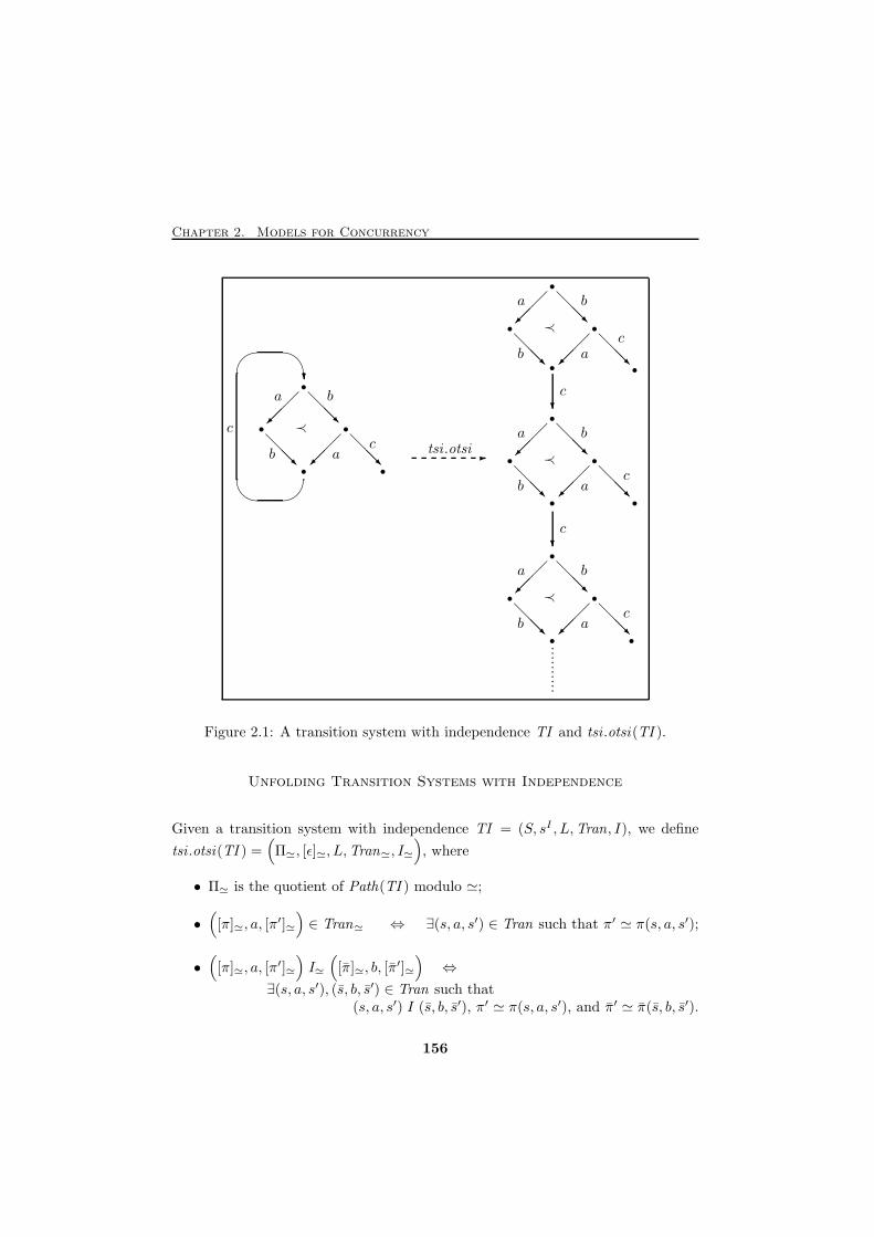
Chapter 2. Models for Concurrency
� �
� �
?
@@@R
@@@R
���
���
@@@R
-
@@@R
@@@R
���
���
@@@R
@@@R
@@@R
���
���
@@@R
?
..........
@@@R
@@@R
���
���
@@@R
?•
• •
• •≺
a b
c
b a
c
c tsi .otsi
•
• •≺
• •
•
• •≺
•
•
• •
• •≺
•
a b
a
a
b
c
a
a b
c
c
a
b
b
b
c
Figure 2.1: A transition system with independence TI and tsi .otsi(TI ).
Unfolding Transition Systems with Independence
Given a transition system with independence TI = (S, sI , L,Tran, I), we define
tsi .otsi(TI ) =(Π≃, [ǫ]≃, L,Tran≃, I≃
), where
• Π≃ is the quotient of Path(TI ) modulo ≃;
•([π]≃, a, [π
′]≃
)∈ Tran≃ ⇔ ∃(s, a, s′) ∈ Tran such that π′ ≃ π(s, a, s′);
•([π]≃, a, [π
′]≃
)I≃
([π]≃, b, [π
′]≃
)⇔
∃(s, a, s′), (s, b, s′) ∈ Tran such that(s, a, s′) I (s, b, s′), π′ ≃ π(s, a, s′), and π′ ≃ π(s, b, s′).
156
2.5. Transition Systems with Independence and Labelled Event Structures
Proposition 2.5.12The transition system tsi .otsi(TI ) is an occurrence transition system with inde-pendence.
Proof. We show only the condition in Definition 2.5.1 of occurrence transition systems
with independence. Suppose that([π′]≃, b, [π]≃
)6=([π′′]≃, a, [π]≃
). Then, we have
π ≃ π′(s′, b, u) ≃ π′′(s′′, a, u) with π′ 6= π′′. By definition of ≃, it must exist π such
that π′(s′, b, u) ≃ π(s, a, s′)(s′, b, u) and π′′(s′′, a, u) ≃ π(s, b, s′′)(s′′, a, u). Moreover,
it must be π(s, a, s′) ≃ π′ and π(s, b, s′′) ≃ π′′. Therefore,([π]≃, a, [π(s, a, s′)]≃
)and
([π]≃, b, [π(s, b, s′′)]≃
)close the diamond. X
Figure 2.1 shows a simple example of unfolding of a transition system withindependence. Next, we want to show that tsi .otsi extends to a functor for TSI tooTSI which is right adjoint to the inclusion functor oTSI → TSI. As a candidate forthe counit of such an adjunction, consider the mapping (σε, id): tsi .otsi(TI )→ TIwhere
σε(ǫ) = sITI and σε
([πs]≃
)= s.
By Lemma 2.5.2, we know that σε is well-defined. Then, it is not difficult to seethat (σε, id) is a morphism of transition systems with independence.
Proposition 2.5.13 ( (σε, id): tsi .otsi(TI )→ TI is couniversal)For any occurrence transition system with independence OTI , transition systemwith independence TI and morphism (σ, λ):OTI → TI , there exists a uniquek:OTI → tsi .otsi(TI ) in oTSI such that (σε, id) ◦ k = (σ, λ).
tsi .otsi(TI ) TI
OTI
(σε,id) //
k
OO
(σ,λ)llllllllllllll 66Proof. Clearly, in order for the diagram to commute, k must be of the form (σ, λ).
Consider the map σ(s) = [σλ(πs)]≃, where σλ: Path(OTI )→ Path(TI ) is given by
σλ(ǫ) = ǫ; σλ
(πs(s, a, s
′))
=
{σλ(πs)
(σ(s), λ(a), σ(s′)
)if λ↓a
σλ(πs) otherwise.
This definition is well-given: fixed s, let πs and πs′ be two paths leading to s. Then,since OTI is an occurrence transition system with independence, it is πs ≃ πs′ , andsince (σ, λ) is a morphism, it is σλ(πs) ≃ σλ(πs′). In order to show this last statement,
157
Chapter 2. Models for Concurrency
it is enough to prove that
πs(s, a, s′)(s′, b, u)πv ≃ πs(s, b, s
′′)(s′′, a, u)πv
⇒ σλ(πs)σλ
((s, a, s′)(s′, b, u)
)σλ(πv)
≃ σλ(πs)σλ
((s, b, s′′)(s′′, a, u)
)σλ(πv).
There are four cases:
i) λ↑a, λ↑b: then σλ
((s, a, s′)(s′, b, u)
)= ǫ = σλ
((s, b, s′′)(s′′, a, u)
)and the thesis
follows easily.
ii) λ↓a, λ↑b: then
σλ
((s, a, s′)(s′, b, u)
)=
(σ(s), λ(a), σ(s′)
)
=(σ(s′′), λ(a), σ(u)
)= σλ
((s, b, s′′)(s′′, a, u)
)
and again the thesis follows.
iii) λ↑a, λ↓b: as for the previous point.
iv) λ↓a, λ↓b: then the thesis follows directly from the definition of morphism, since
it is Diam((s, a, s′)(s, b, s′′)(s′, b, u)(s′′, a, u)
)and in this case diamonds are pre-
served.
Let us show that (σ, λ) is indeed a morphism of occurrence transition systems withindependence.
i) σ(sIOTI ) = [ǫ]≃.
ii) Consider (s, a, s′) ∈ TranOTI , and suppose λ↓a. Since OTI is reachable, we
have πs(s, a, s′) ∈ Path(OTI ), and σλ(πs)
(σ(s), λ(a), σ(s′)
)in Path(TI ). Thus,
([σλ(πs)]≃, λ(a), [σλ(πs(s, a, s
′))]≃
)∈ Tran≃, i.e.,
(σ(s), λ(a), σ(s′)
)∈ Tran≃.
iii) If (s, a, s′) IOTI (s, b, s′),(σ(s), λ(a), σ(s′)
)ITI
(σ(s), λ(b), σ(s′)
), and reason-
ing as before, we get(σ(s), λ(a), σ(s′)
)I≃
(σ(s), λ(b), σ(s′)
).
In order to show that the diagram commutes, it is enough to observe that each s is
mapped to a ≃-class of paths leading to σ(s). Therefore, σε◦σ(s) = σ(s). The uniquess
of (σ, λ) is easily obtained following the same argument. In fact, the behaviour of σ
is compelled on any s: sIOTI must be mapped to [ǫ]≃, while a generic s must mapped
to a ≃-equivalence class of paths leading to σ(s). But we know that there is a unique
such class. X
Corollary 2.5.14The construction tsi .otsi extends to a functor from TSI to oTSI which is rightadjoint to the inclusion oTSI → TSI.
158
2.5. Transition Systems with Independence and Labelled Event Structures
It will be useful later to notice that this coreflection cuts down to a coreflectionsdoTSI −⊲ dTSI, where doTSI is the full subcategory of oTSI consisting of determin-istic transition systems. In order to achieve this result, it is clearly enough to showthat tsi .otsi maps objects from dTSI to doTSI.
Proposition 2.5.15If TI is deterministic, then tsi .otsi(TI ) is deterministic.
Proof. Suppose that([π]≃, a, [π
′]≃
)and
([π]≃, a, [π
′′]≃
)are in Tran≃. Then, it must
be π′ ≃ πs(s, a, s′) and π′′ ≃ πs(s, a, s
′′), for (s, a, s′), (s, a, s′′) ∈ Tran . Then we have
s′ = s′′ and so π′ ≃ π′′. X
Occurrence TSI’s and Labelled Event Structures
In this subsection we complete the construction of the coreflections LES −⊲ TSI
and dLES −⊲ dTSI by showing the existence of coreflections LES −⊲ oTSI anddLES −⊲ doTSI.
Consider a labelled event structure ES = (E,≤,#, ℓ, L). Define les .otsi(ES ) tobe the transition system with independence of the finite configurations of ES , i.e.,
les .otsi(ES ) =(LF (ES ),∅, L,Tran, I
),
where
• LF (ES ) is the set of finite configuration of ES ;
• (c, a, c′) ∈ Tran if and only if c = c′ \ {e} and ℓ(e) = a;
• (c, a, c′) I (c, b, c′) if and only if (c′ \ c) co (c′ \ c).
By definition, les .otsi(ES ) is clearly an acyclic, reachable transition system.Moreover, I ⊆ Tran2 is symmetric and irreflexive, since co is such. In order toshow that it is an occurrence transition system with independence, it is importantthe following characterization of the relation ∼.
Lemma 2.5.16Given (c, a, c′) and (c, a, c′) ∈ Tran, we have (c, a, c′) ∼ (c, a, c′) ∈ Tran if and onlyif (c′ \ c) = (c′ \ c).
Proof. (⇒). It is enough to show that
Diam((c, a, c′), (c, b, c), (c′, b, c′), (c, a, c′)
)implies (c′ \ c) = (c′ \ c).
159
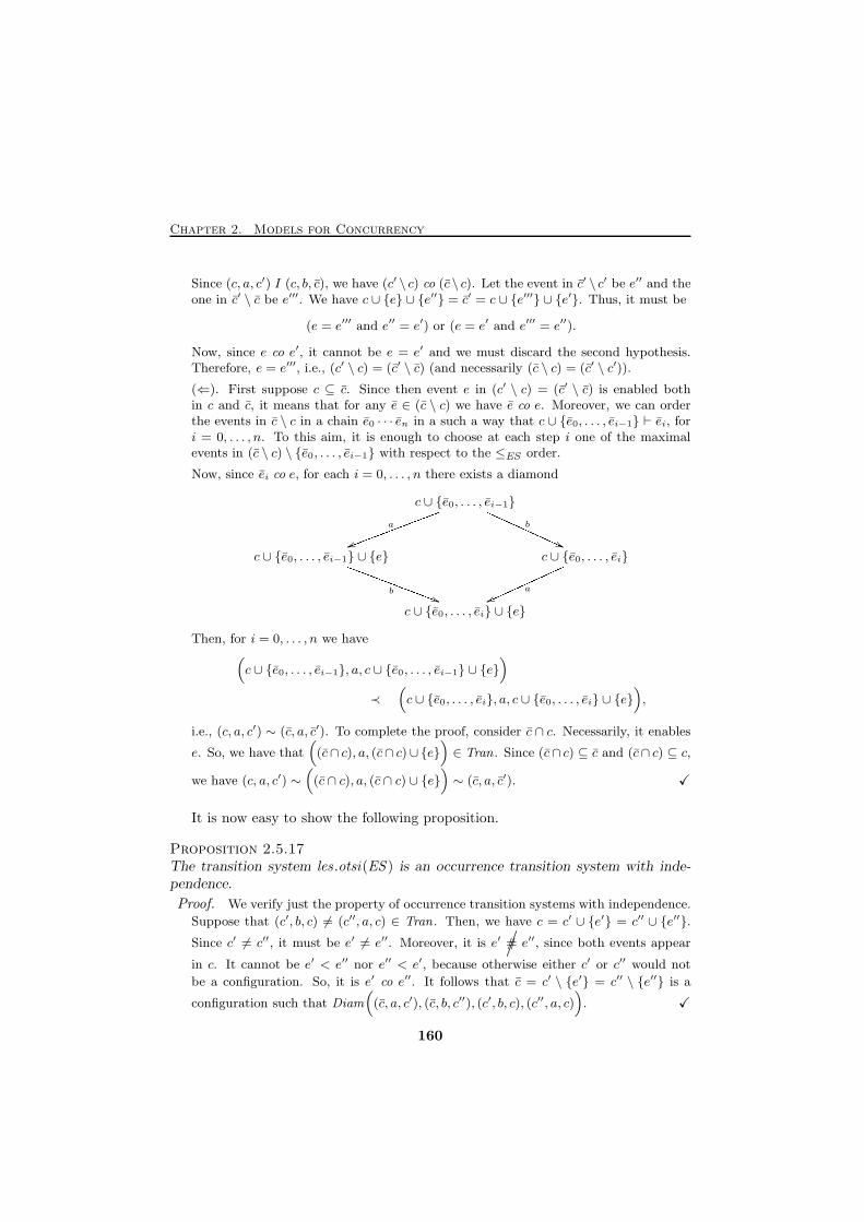
Chapter 2. Models for Concurrency
Since (c, a, c′) I (c, b, c), we have (c′ \ c) co (c \ c). Let the event in c′ \ c′ be e′′ and theone in c′ \ c be e′′′. We have c ∪ {e} ∪ {e′′} = c′ = c ∪ {e′′′} ∪ {e′}. Thus, it must be
(e = e′′′ and e′′ = e′) or (e = e′ and e′′′ = e′′).
Now, since e co e′, it cannot be e = e′ and we must discard the second hypothesis.Therefore, e = e′′′, i.e., (c′ \ c) = (c′ \ c) (and necessarily (c \ c) = (c′ \ c′)).
(⇐). First suppose c ⊆ c. Since then event e in (c′ \ c) = (c′ \ c) is enabled bothin c and c, it means that for any e ∈ (c \ c) we have e co e. Moreover, we can orderthe events in c \ c in a chain e0 · · · en in a such a way that c ∪ {e0, . . . , ei−1} ⊢ ei, fori = 0, . . . , n. To this aim, it is enough to choose at each step i one of the maximalevents in (c \ c) \ {e0, . . . , ei−1} with respect to the ≤ES order.
Now, since ei co e, for each i = 0, . . . , n there exists a diamond
c ∪ {e0, . . . , ei−1}
c ∪ {e0, . . . , ei−1} ∪ {e} c ∪ {e0, . . . , ei}
c ∪ {e0, . . . , ei} ∪ {e}
a
uukkkkkkkkkkkkk b
PPPPPPPPPPP ((b
SSSSSSSSSSSSS)) avvnnnnnnnnnnn
Then, for i = 0, . . . , n we have(c ∪ {e0, . . . , ei−1}, a, c ∪ {e0, . . . , ei−1} ∪ {e}
)
≺(c ∪ {e0, . . . , ei}, a, c ∪ {e0, . . . , ei} ∪ {e}
),
i.e., (c, a, c′) ∼ (c, a, c′). To complete the proof, consider c ∩ c. Necessarily, it enables
e. So, we have that((c∩ c), a, (c∩ c)∪{e}
)∈ Tran . Since (c∩ c) ⊆ c and (c∩ c) ⊆ c,
we have (c, a, c′) ∼((c ∩ c), a, (c ∩ c) ∪ {e}
)∼ (c, a, c′). X
It is now easy to show the following proposition.
Proposition 2.5.17The transition system les .otsi(ES ) is an occurrence transition system with inde-pendence.
Proof. We verify just the property of occurrence transition systems with independence.
Suppose that (c′, b, c) 6= (c′′, a, c) ∈ Tran . Then, we have c = c′ ∪ {e′} = c′′ ∪ {e′′}.
Since c′ 6= c′′, it must be e′ 6= e′′. Moreover, it is e′/# e′′, since both events appear
in c. It cannot be e′ < e′′ nor e′′ < e′, because otherwise either c′ or c′′ would not
be a configuration. So, it is e′ co e′′. It follows that c = c′ \ {e′} = c′′ \ {e′′} is a
configuration such that Diam((c, a, c′), (c, b, c′′), (c′, b, c), (c′′, a, c)
). X
160
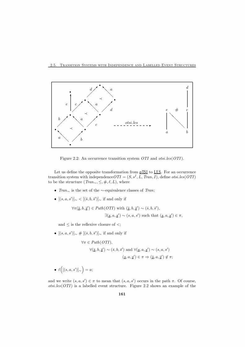
2.5. Transition Systems with Independence and Labelled Event Structures
@@@I
����
@@@I
����
@@@I
����
����
@@@I
����
- @@@@
6
����
•
•
b
a b
a
•
•
•
•
a
•
•
a
≺
≺
≺ •
c
d
otsi .les
a b
c
d
e c
d
e #
Figure 2.2: An occurrence transition system OTI and otsi .les(OTI ).
Let us define the opposite transformation from oTSI to LES. For an occurrencetransition system with independenceOTI = (S, sI , L,Tran, I), define otsi .les(OTI )to be the structure (Tran∼,≤,#, ℓ, L), where
• Tran∼ is the set of the ∼-equivalence classes of Tran;
• [(s, a, s′)]∼ < [(s, b, s′)]∼ if and only if
∀π(s, b, s′) ∈ Path(OTI ) with (s, b, s′) ∼ (s, b, s′),
∃(s, a, s′) ∼ (s, a, s′) such that (s, a, s′) ∈ π,
and ≤ is the reflexive closure of <;
• [(s, a, s′)]∼ # [(s, b, s′)]∼ if and only if
∀π ∈ Path(OTI ),
∀(s, b, s′) ∼ (s, b, s′) and ∀(s, a, s′) ∼ (s, a, s′)
(s, a, s′) ∈ π ⇒ (s, a, s′) 6∈ π;
• ℓ([(s, a, s′)]∼
)= a;
and we write (s, a, s′) ∈ π to mean that (s, a, s′) occurs in the path π. Of course,otsi .les(OTI ) is a labelled event structure. Figure 2.2 shows an example of the
161
Chapter 2. Models for Concurrency
labelled event structure associated to an occurrence transition system with inde-pendence.
Next, we need to extend otsi.les to a functor. Given (σ, λ):OTI 0 → OTI 1,
define otsi .les((σ, λ)
)= (ησ, λ), where
ησ
([(s, a, s′)]∼
)=
{ [(σ(s), λ(a), σ(s′)
)]
∼if λ↓a
↑ otherwise.
In the proof of Proposition 2.5.13, it has been shown implicitly that (s, a, s′) ≺
(s, a, s′) and λ↓a implies(σ(s), λ(a), σ(s′)
)∼(σ(s), λ(a), σ(s′)
). Then ησ is well-
given.
Proposition 2.5.18Given a transition system with independence morphism (σ, λ):OTI 0 → OTI 1,
otsi .les((σ, λ)
): otsi .les(OTI 0)→ otsi .les(OTI 1) is a labelled event structure mor-
phism.
Proof. We show the properties of labelled event structure morphisms.
i) ⌊ησ(e)⌋ ⊆ ησ(⌊e⌋).
Consider e =[(σ(s), λ(a), σ(s′)
)]
∼in otsi .les(OTI 1) and [(s, b, s′)]∼ ≤ e. Since
OTI 1 is reachable there is a path πσ(s)
(σ(s), λ(a), σ(s′)
), where πσ(s) necessarily
contains (s, b, s′) ∼ (s, b, s′), and there exists a path πs(s, a, s′) ∈ Path(OTI 0) whose
image through (σ, λ) is πσ(s)
(σ(s), λ(a), σ(s′)
). Then, we must have a transition
(x, c, y) ∈ πs such that(σ(x), λ(c), σ(y)
)=(s, b, s′
). Clearly, we have that
ησ
([(x, c, y)]∼
)= [(s, b, s′)]∼. Thus, we need to show that
[(x, c, y)]∼ < [(s, a, s′)]∼.
Consider (s′′, a, s′′′) ∼ (s, a, s′). Since λ↓a, it is(σ(s′′), λ(a), σ(s′′′)
)∈ TranOTI 1
, and
since (σ, λ) is a morphism,(σ(s′′), λ(a), σ(s′′′)
)∼(σ(s), λ(a), σ(s′)
). It follows that
for each path πσ(s′′)
(σ(s′′), λ(a), σ(s′′′)
)there exists (s′′, b, s′′′) ∼ (s, b, s′) occurring in
πσ(s′′). Therefore, there exists a path πs′′(s′′, a, s′′′) such that there is (x′, d, y′) ∈ πs′′
and(σ(x′), λ(d), σ(y′)
)= (s′′, b, s′′′) ∼ (s, b, s′). Now, since by the properties of
occurrence transition systems with independence in any other path πs′′′ it must exista transition ∼-equivalent to (x′, d, y′), it is enough to show that
(x′, d, y′) ∼ (x, c, y).
162
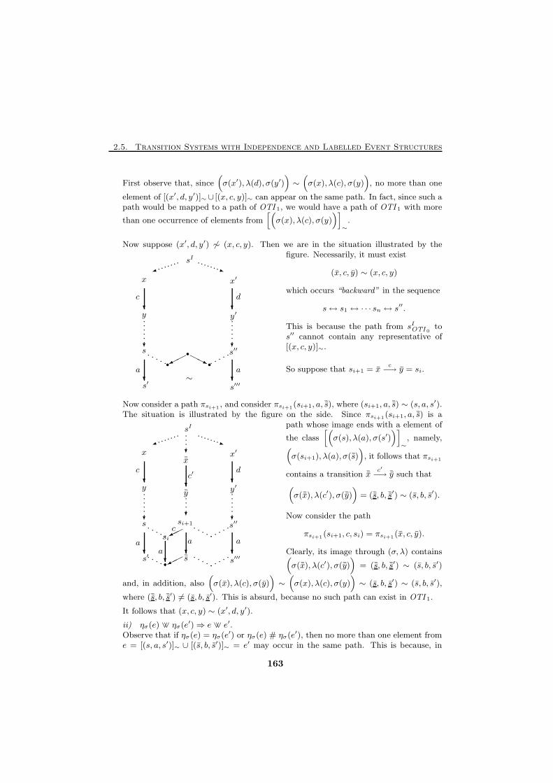
2.5. Transition Systems with Independence and Labelled Event Structures
First observe that, since(σ(x′), λ(d), σ(y′)
)∼(σ(x), λ(c), σ(y)
), no more than one
element of [(x′, d, y′)]∼∪ [(x, c, y)]∼ can appear on the same path. In fact, since such apath would be mapped to a path of OTI 1, we would have a path of OTI 1 with more
than one occurrence of elements from[(σ(x), λ(c), σ(y)
)]
∼.
?
......
?
?
?
?
?
......
)........ q
........
HHj���. . . . .
.....a
c
x
y
s
s′
•
sI
∼
•
•
x′
y′
s′′′
s′′
a
d
Now suppose (x′, d, y′) 6∼ (x, c, y). Then we are in the situation illustrated by thefigure. Necessarily, it must exist
(x, c, y) ∼ (x, c, y)
which occurs “backward” in the sequence
s↔ s1 ↔ · · · sn ↔ s′′.
This is because the path from sIOTI 0to
s′′ cannot contain any representative of[(x, c, y)]∼.
So suppose that si+1 = xc−→ y = si.
?
......?
......
)........ q
........
���
���
?
....
?
....
. . . . .
. . . . .
.....
.....
. . . . .
. . . . .
? ?
? ?
?
?
?
a
c
x
y
s
s′a
si
•
csi+1
sI
c′
¯y
¯s
¯x
a
x′
y′
s′′′
s′′
a
d
Now consider a path πsi+1 , and consider πsi+1(si+1, a, ¯s), where (si+1, a, ¯s) ∼ (s, a, s′).The situation is illustrated by the figure on the side. Since πsi+1(si+1, a, ¯s) is a
path whose image ends with a element of
the class[(σ(s), λ(a), σ(s′)
)]
∼, namely,
(σ(si+1), λ(a), σ(¯s)
), it follows that πsi+1
contains a transition ¯xc′
−→ ¯y such that
(σ(¯x), λ(c′), σ(¯y)
)= (¯s, b, ¯s′) ∼ (s, b, s′).
Now consider the path
πsi+1(si+1, c, si) = πsi+1(x, c, y).
Clearly, its image through (σ, λ) contains(σ(¯x), λ(c′), σ(¯y)
)= (¯s, b, ¯s′) ∼ (s, b, s′)
and, in addition, also(σ(x), λ(c), σ(y)
)∼(σ(x), λ(c), σ(y)
)∼ (s, b, s′) ∼ (s, b, s′),
where (¯s, b, ¯s′) 6= (s, b, s′). This is absurd, because no such path can exist in OTI 1.
It follows that (x, c, y) ∼ (x′, d, y′).
ii) ησ(e) ∨∨ ησ(e′)⇒ e ∨∨ e′.
Observe that if ησ(e) = ησ(e′) or ησ(e) # ησ(e
′), then no more than one element frome = [(s, a, s′)]∼ ∪ [(s, b, s′)]∼ = e′ may occur in the same path. This is because, in
163
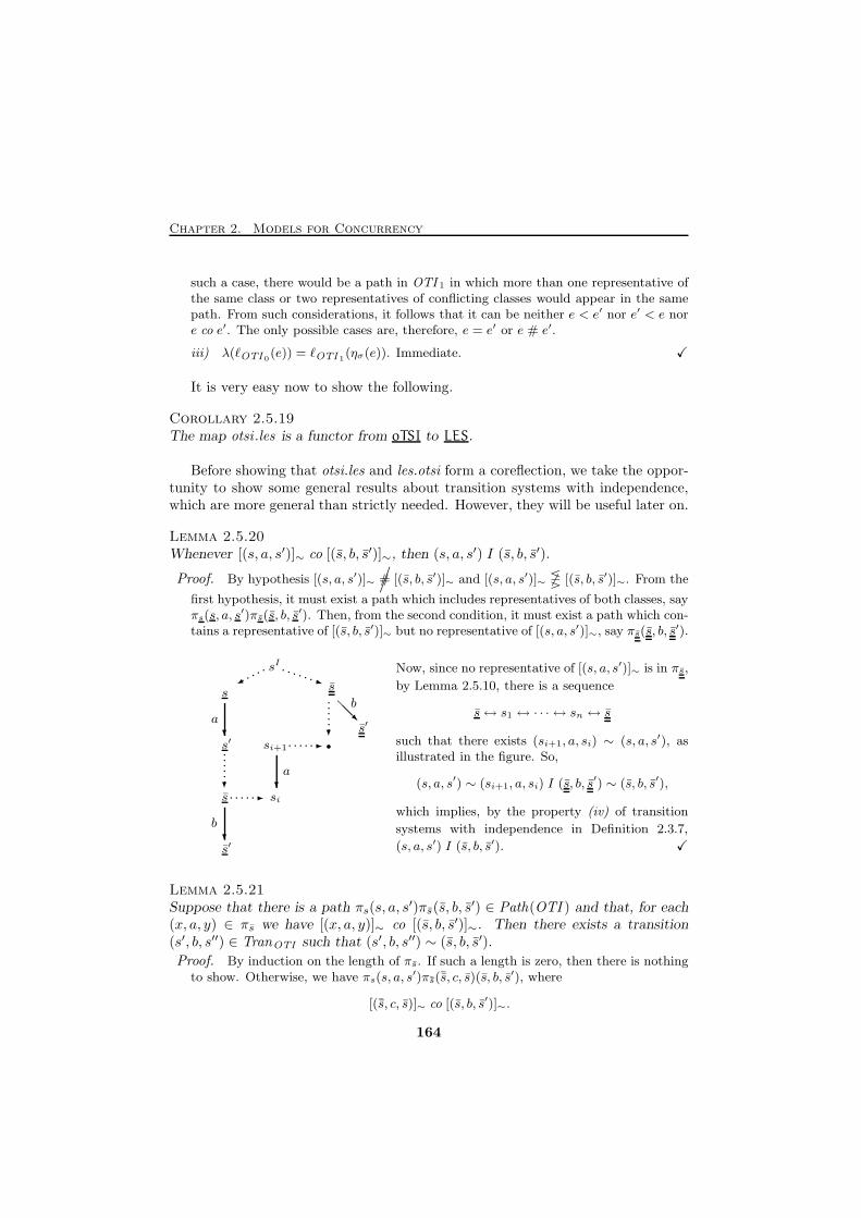
Chapter 2. Models for Concurrency
such a case, there would be a path in OTI 1 in which more than one representative ofthe same class or two representatives of conflicting classes would appear in the samepath. From such considerations, it follows that it can be neither e < e′ nor e′ < e nore co e′. The only possible cases are, therefore, e = e′ or e # e′.
iii) λ(ℓOTI 0(e)) = ℓOTI 1
(ησ(e)). Immediate. X
It is very easy now to show the following.
Corollary 2.5.19The map otsi .les is a functor from oTSI to LES.
Before showing that otsi.les and les.otsi form a coreflection, we take the oppor-tunity to show some general results about transition systems with independence,which are more general than strictly needed. However, they will be useful later on.
Lemma 2.5.20Whenever [(s, a, s′)]∼ co [(s, b, s′)]∼, then (s, a, s′) I (s, b, s′).
Proof. By hypothesis [(s, a, s′)]∼
/# [(s, b, s′)]∼ and [(s, a, s′)]∼ 6⋚ [(s, b, s′)]∼. From the
first hypothesis, it must exist a path which includes representatives of both classes, sayπs(s, a, s
′)πs(s, b, s′). Then, from the second condition, it must exist a path which con-
tains a representative of [(s, b, s′)]∼ but no representative of [(s, a, s′)]∼, say πs(s, b, s′).
?
?@@R
�..... q
. . . . . . .
?
......-. . . . . .
-. . . . . .?
......
?s′
s
sI
si
•
a
a
s
s′
s
s′
b
b
si+1
Now, since no representative of [(s, a, s′)]∼ is in πs,
by Lemma 2.5.10, there is a sequence
s↔ s1 ↔ · · · ↔ sn ↔ s
such that there exists (si+1, a, si) ∼ (s, a, s′), asillustrated in the figure. So,
(s, a, s′) ∼ (si+1, a, si) I (s, b, s′) ∼ (s, b, s′),
which implies, by the property (iv) of transition
systems with independence in Definition 2.3.7,
(s, a, s′) I (s, b, s′). X
Lemma 2.5.21Suppose that there is a path πs(s, a, s
′)πs(s, b, s′) ∈ Path(OTI ) and that, for each
(x, a, y) ∈ πs we have [(x, a, y)]∼ co [(s, b, s′)]∼. Then there exists a transition(s′, b, s′′) ∈ TranOTI such that (s′, b, s′′) ∼ (s, b, s′).
Proof. By induction on the length of πs. If such a length is zero, then there is nothingto show. Otherwise, we have πs(s, a, s
′)π¯s(¯s, c, s)(s, b, s′), where
[(¯s, c, s)]∼ co [(s, b, s′)]∼.
164
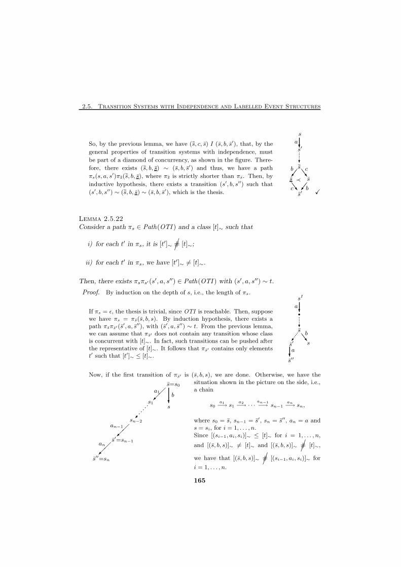
2.5. Transition Systems with Independence and Labelled Event Structures
��/ SSw
SSw ��/
?......
?
s
s′a
¯s
≺s s
s′
b c
c b
So, by the previous lemma, we have (¯s, c, s) I (s, b, s′), that, by the
general properties of transition systems with independence, must
be part of a diamond of concurrency, as shown in the figure. There-
fore, there exists (¯s, b, s) ∼ (s, b, s′) and thus, we have a path
πs(s, a, s′)π¯s(¯s, b, s), where π¯s is strictly shorter than πs. Then, by
inductive hypothesis, there exists a transition (s′, b, s′′) such that
(s′, b, s′′) ∼ (¯s, b, s) ∼ (s, b, s′), which is the thesis. X
Lemma 2.5.22Consider a path πs ∈ Path(OTI ) and a class [t]∼ such that
i) for each t′ in πs, it is [t′]∼
/# [t]∼;
ii) for each t′ in πs, we have [t′]∼ 6= [t]∼.
Then, there exists πsπs′(s′, a, s′′) ∈ Path(OTI ) with (s′, a, s′′) ∼ t.
Proof. By induction on the depth of s, i.e., the length of πs.
SSw
?
/......
?......
?
sI
a•
sb
ss′
s′′
a
If πs = ǫ, the thesis is trivial, since OTI is reachable. Then, supposewe have πs = πs(s, b, s). By induction hypothesis, there exists apath πsπs′(s
′, a, s′′), with (s′, a, s′′) ∼ t. From the previous lemma,we can assume that πs′ does not contain any transition whose classis concurrent with [t]∼. In fact, such transitions can be pushed afterthe representative of [t]∼. It follows that πs′ contains only elementst′ such that [t′]∼ ≤ [t]∼.
��
��
......
?
��
s=s0a1
bs1
s
sn−2an−1
s′=sn−1an
s′′=sn
Now, if the first transition of πs′ is (s, b, s), we are done. Otherwise, we have thesituation shown in the picture on the side, i.e.,a chain
s0a1−→ s1
a2−→ · · ·an−1−→ sn−1
an−→ sn,
where s0 = s, sn−1 = s′, sn = s′′, an = a ands = si, for i = 1, . . . , n.Since [(si−1, ai, si)]∼ ≤ [t]∼ for i = 1, . . . , n,
and [(s, b, s)]∼ 6= [t]∼ and [(s, b, s)]∼
/# [t]∼,
we have that [(s, b, s)]∼
/# [(si−1, ai, si)]∼ for
i = 1, . . . , n.
165
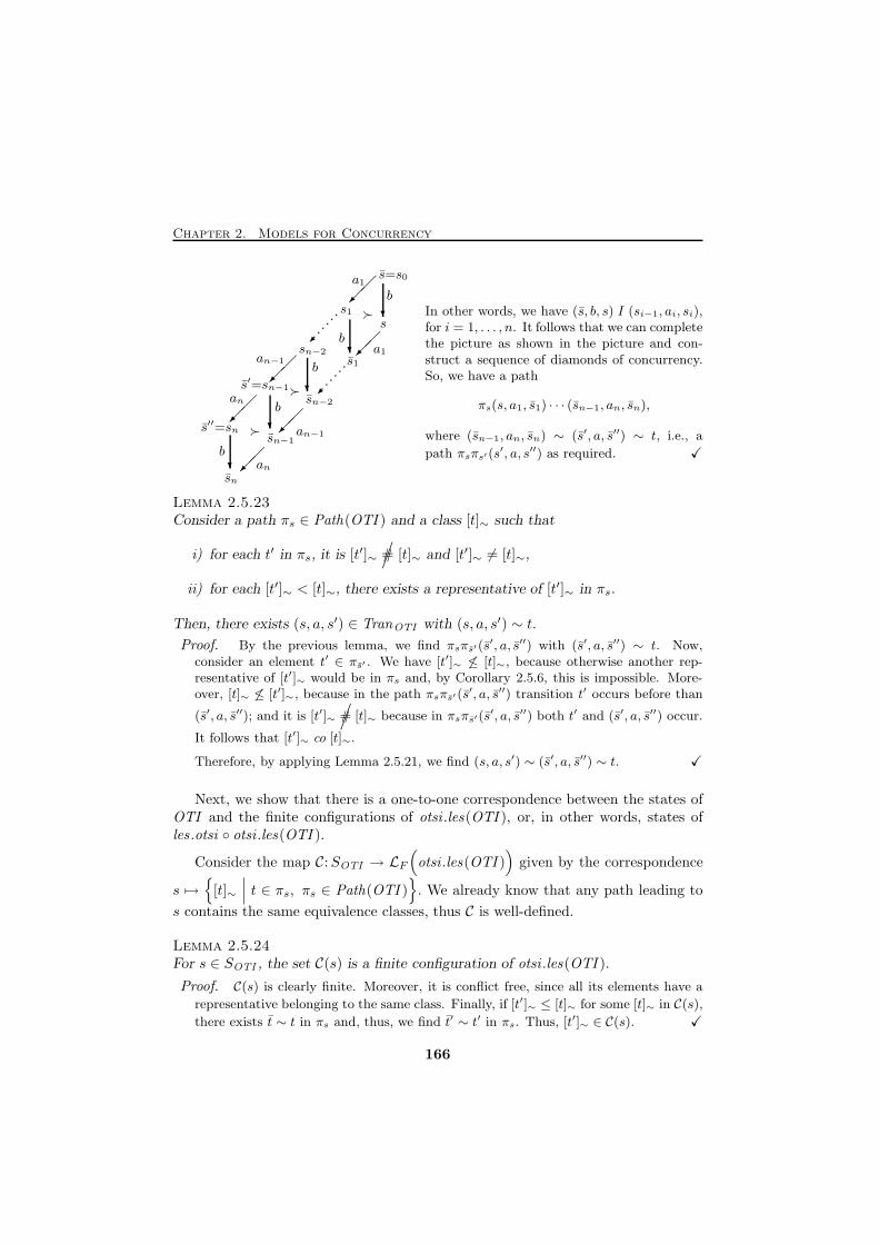
Chapter 2. Models for Concurrency
......
?
?
?
?
?��
��
��
��
��
��
......
s=s0a1
bs1 ≻
sb
sn−2 a1an−1 s1b
s′=sn−1≻an sn−2b
≻ an−1s′′=sn
sn−1
ban
sn
In other words, we have (s, b, s) I (si−1, ai, si),for i = 1, . . . , n. It follows that we can completethe picture as shown in the picture and con-struct a sequence of diamonds of concurrency.So, we have a path
πs(s, a1, s1) · · · (sn−1, an, sn),
where (sn−1, an, sn) ∼ (s′, a, s′′) ∼ t, i.e., a
path πsπs′(s′, a, s′′) as required. X
Lemma 2.5.23Consider a path πs ∈ Path(OTI ) and a class [t]∼ such that
i) for each t′ in πs, it is [t′]∼
/# [t]∼ and [t′]∼ 6= [t]∼,
ii) for each [t′]∼ < [t]∼, there exists a representative of [t′]∼ in πs.
Then, there exists (s, a, s′) ∈ TranOTI with (s, a, s′) ∼ t.
Proof. By the previous lemma, we find πsπs′(s′, a, s′′) with (s′, a, s′′) ∼ t. Now,
consider an element t′ ∈ πs′ . We have [t′]∼ 6≤ [t]∼, because otherwise another rep-resentative of [t′]∼ would be in πs and, by Corollary 2.5.6, this is impossible. More-over, [t]∼ 6≤ [t′]∼, because in the path πsπs′(s
′, a, s′′) transition t′ occurs before than
(s′, a, s′′); and it is [t′]∼
/# [t]∼ because in πsπs′(s
′, a, s′′) both t′ and (s′, a, s′′) occur.
It follows that [t′]∼ co [t]∼.
Therefore, by applying Lemma 2.5.21, we find (s, a, s′) ∼ (s′, a, s′′) ∼ t. X
Next, we show that there is a one-to-one correspondence between the states ofOTI and the finite configurations of otsi .les(OTI ), or, in other words, states ofles .otsi ◦ otsi .les(OTI ).
Consider the map C:SOTI → LF(otsi .les(OTI )
)given by the correspondence
s 7→{[t]∼
∣∣∣ t ∈ πs, πs ∈ Path(OTI )}. We already know that any path leading to
s contains the same equivalence classes, thus C is well-defined.
Lemma 2.5.24For s ∈ SOTI , the set C(s) is a finite configuration of otsi .les(OTI ).
Proof. C(s) is clearly finite. Moreover, it is conflict free, since all its elements have a
representative belonging to the same class. Finally, if [t′]∼ ≤ [t]∼ for some [t]∼ in C(s),
there exists t ∼ t in πs and, thus, we find t′ ∼ t′ in πs. Thus, [t′]∼ ∈ C(s). X
166
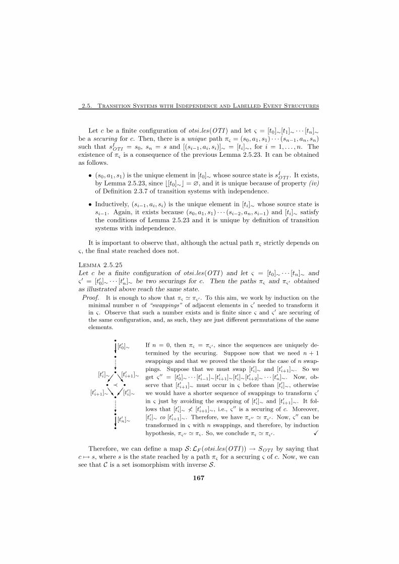
2.5. Transition Systems with Independence and Labelled Event Structures
Let c be a finite configuration of otsi .les(OTI ) and let ς = [t0]∼[t1]∼ · · · [tn]∼be a securing for c. Then, there is a unique path πς = (s0, a1, s1) · · · (sn−1, an, sn)such that sIOTI = s0, sn = s and [(si−1, ai, si)]∼ = [ti]∼, for i = 1, . . . , n. Theexistence of πς is a consequence of the previous Lemma 2.5.23. It can be obtainedas follows.
• (s0, a1, s1) is the unique element in [t0]∼ whose source state is sIOTI . It exists,by Lemma 2.5.23, since ⌊[t0]∼⌋ = ∅, and it is unique because of property (iv)of Definition 2.3.7 of transition systems with independence.
• Inductively, (si−1, ai, si) is the unique element in [ti]∼ whose source state issi−1. Again, it exists because (s0, a1, s1) · · · (si−2, an, si−1) and [ti]∼ satisfythe conditions of Lemma 2.5.23 and it is unique by definition of transitionsystems with independence.
It is important to observe that, although the actual path πς strictly depends onς, the final state reached does not.
Lemma 2.5.25Let c be a finite configuration of otsi .les(OTI ) and let ς = [t0]∼ · · · [tn]∼ andς ′ = [t′0]∼ · · · [t
′n]∼ be two securings for c. Then the paths πς and πς′ obtained
as illustrated above reach the same state.
Proof. It is enough to show that πς ≃ πς′ . To this aim, we work by induction on theminimal number n of “swappings” of adjacent elements in ς ′ needed to transform itin ς. Observe that such a number exists and is finite since ς and ς ′ are securing ofthe same configuration, and, as such, they are just different permutations of the sameelements.
��/ SSw
SSw ��/
?......
?
......
?
?
•
•
•
• •
•
•
•
≺
[t′0]∼
[t′i]∼ [t′i+1]∼
[t′i+1]∼ [t′i]∼
[t′n]∼
If n = 0, then πς = πς′ , since the sequences are uniquely de-
termined by the securing. Suppose now that we need n + 1
swappings and that we proved the thesis for the case of n swap-
pings. Suppose that we must swap [t′i]∼ and [t′i+1]∼. So we
get ς ′′ = [t′0]∼ · · · [t′i−1]∼[t′i+1]∼[t′i]∼[t′i+2]∼ · · · [t
′n]∼. Now, ob-
serve that [t′i+1]∼ must occur in ς before than [t′i]∼, otherwise
we would have a shorter sequence of swappings to transform ς ′
in ς just by avoiding the swapping of [t′i]∼ and [t′i+1]∼. It fol-
lows that [t′i]∼ 6< [t′i+1]∼, i.e., ς ′′ is a securing of c. Moreover,
[t′i]∼ co [t′i+1]∼. Therefore, we have πς′′ ≃ πς′ . Now, ς ′′ can be
transformed in ς with n swappings, and therefore, by induction
hypothesis, πς′′ ≃ πς . So, we conclude πς ≃ πς′ . X
Therefore, we can define a map S:LF (otsi .les(OTI )) → SOTI by saying thatc 7→ s, where s is the state reached by a path πς for a securing ς of c. Now, we cansee that C is a set isomorphism with inverse S.
167
Chapter 2. Models for Concurrency
Lemma 2.5.26S = C−1.Proof. Consider C(s) = {[t]∼ | t ∈ πs} and consider the sequence ς = [t0]∼ · · · [tn]∼
such that πs = t0 · · · tn. This is clearly a securing of C(s), whose associated path πςis πs itself. This is because of the uniqueness of πς as shown earlier. So, we haveS(C(s)) = s.
On the other hand, suppose S(c) = s. Among the paths leading to s, consider πς ,
where ς = [t0]∼ · · · [tn]∼ is any securing of c. Then, we may use πς to calculate
C(S(c)) = {[t]∼ | t ∈ πς} = {[ti]∼ | i = 0, . . . , n} = c. X
It is worthwhile to observe that C and S give rise to morphisms of transitionsystems which are each other’s inverse. First observe that S(∅) = sIOTI , since theunique path associated with the unique securing of the empty configuration, is theempty path. Moreover, C(sIOTI ) = ∅, since the unique path leading to sIOTI inOTI is the empty path. Moreover, we have the following easy lemma.
Lemma 2.5.27Let OTI be a transition system with independence. Then
i) If (s, a, s′) is a transition of OTI , then(C(s), a, C(s′)
)is a transition of
les .otsi ◦ otsi .les(OTI ).
ii) If (c, a, c′) is a transition of les .otsi ◦ otsi .les(OTI ),(S(c), a,S(c′)
)is a tran-
sition of OTI .
This means that (C, id) from OTI to les .otsi ◦ otsi .les(OTI ) and (S, id) fromles .otsi ◦ otsi .les(OTI ) to OTI are morphisms of transition systems. Moreover,(S, id) = (C, id)−1. Recall that (c, a, c′) I (c, b, c′) implies, by definition of les.otsi,that (c′ \ c) = [t]∼ co [t]∼ = (c′ \ c). From the previous Lemma 2.5.27 we thereforehave that
[t]∼ =[(S(c), a,S(c′)
)]
∼co[(S(c), b,S(c′)
)]
∼= [t]∼
and then, from Lemma 2.5.20,(S(c), a,S(c′)
)I(S(c), b,S(c′)
). In other words,
we have proved the following.
Proposition 2.5.28(S, id) is a transition system with independence morphism.
However, (C, id) is not a morphism in TSI. It follows that (S, id), in general,is not an isomorphism of transition systems with independence. Consider now theproperty:
t I t′ ⇒ ∃s. (s, a, s′) ∼ t and (s, b, s′′) ∼ t′. (E)
168
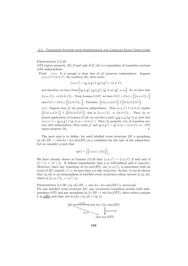
2.5. Transition Systems with Independence and Labelled Event Structures
Proposition 2.5.29OTI enjoys property (E) if and only if (C, id) is a morphism of transition systemswith independence.
Proof. (⇒). It is enough to show that (C, id) preserves independence. Suppose(s, a, s′) I (s, b, s′). By condition (E), there exists
(s, a, s′) ∼ (s, a, s′) I (s, b, s′′) ∼ (s, b, s′),
and therefore, we have Diam((s, a, s′), (s, b, s′′), (s′, b, u), (s′′, a, u)
). So, we have that
[(s, a, s′)]∼ co [(s, b, s′)]∼. From Lemma 2.5.27, we have C(s′) = C(s) ∪{
[(s, a, s′)]∼
}
and C(s′) = C(s) ∪{
[(s, b, s′)]∼
}. Therefore,
(C(s), a, C(s′)
)I(C(s), b, C(s′)
).
(⇐). Suppose that (C, id) preserves independence. Then (s, a, s′) I (s, b, s′) implies(C(s), a, C(s′)
)I(C(s), b, C(s′)
), that is [(s, a, s′)]∼ co [(s, b, s′)]∼. Then, by re-
peated applications of Lemma 2.5.23, we can find a path πs(s, a, s′)(s′, b, u) such that
(s, a, s,′ ) ∼ (s, a, s′) I (s′, b, u) ∼ (s, b, s,′ ). Then, by property (iii) of transition sys-
tem with independence, there exists s′′ and (s, b, s′′) ∼ (s′, b, u) ∼ (s, b, s′), i.e., OTI
enjoys property (E). X
The next step is to define, for each labelled event structure ES a morphism(η, id):ES → otsi .les ◦ les .otsi(ES ) as a candidate for the unit of the adjunction.Let us consider η such that
η(e) =[(c, a, c ∪ {e}
)]
∼.
We have already shown in Lemma 2.5.16 that (c, a, c′) ∼ (c, a, c′) if and only if(c′ \ c) = (c′ \ c). It follows immediately that η is well-defined and is injective.Moreover, since any transition of les .otsi(ES ), say (c, a, c′), is associated with anevent of ES , namely, c′\c, we have that η is also surjective. In fact, it can be shownthat (η, id) is an isomorphism of labelled event structures whose inverse is (η, id),where η: [(c, a, c′)]∼ 7→ (c′ \ c).
Proposition 2.5.30 ( (η, id ):ES → otsi .les ◦ les .otsi(ES ) is universal)For any labelled event structure ES , any occurrence transition system with inde-pendence OTI and any morphism (η, λ):ES → otsi .les(OTI ), there exists a uniquek in oTSI such that otsi .les(k) ◦ (η, id) = (η, λ).
ES otsi .les ◦ les .otsi(ES )
otsi .les(OTI )
(η,id) //
(η,λ)
TTTTTTTTTTTTTTTTT )) otsi.les(k)
��
169
Chapter 2. Models for Concurrency
Proof. Let us define k: les.otsi (ES) → OTI . Clearly, in order to make the diagramcommute, k must be of the form (σ, λ), for some σ. Let us consider σ: c 7→ S(η(c)),i.e.,
(σ, λ) = (S , id) ◦ (η, λ): les.otsi(ES)→ les.otsi (otsi .les(OTI ))→ OTI .
Then, we have immediately that σ is well-defined and that (σ, λ) is a transition systemwith independence morphism.
Now, we show that the diagram commutes. We verify that ησ ◦ η = ηS ◦ ηη ◦ η = η.Consider e ∈ EES and let a be ℓ(e). If λ↑a, then η↑a and ηη↑a and, therefore, bothsides of the above equality are undefined. Suppose otherwise that λ↓a. We have
eη7→[(c, a, c ∪ {e})
]
∼
ηη7→
[(η(c), λ(a), η(c) ∪ {η(e)}
)]
∼
ηS7→[(S(η(c)), λ(a),S(η(c) ∪ {η(e)})
)]
∼
=[(σ(c), λ(a), σ(c ∪ {e})
)]
∼.
Observe that(η(c), λ(a), η(c)∪{η(e)}
)belongs to les.otsi ◦otsi .les(OTI ) and is asso-
ciated with the event η(e) of otsi .les(OTI ). Then, from Lemma 2.5.27, we have that[(S(η(c)), λ(a),S(η(c) ∪ {η(e)})
)]
∼= η(e).
The last step to prove the universality of (η, id) is to show that k is the unique transi-
tion system with independence morphism from les.otsi (ES) to OTI which makes the
diagram commute. Let us suppose that there is k′ which does so. It must necessarily
be k′ = (σ′, λ). Observe from the first part of the proof that in order for the diagram to
commute, it must be ησ′
([(c, a, c ∪ {e})
]
∼
)=[(σ′(c), λ(a), σ′(c∪ {e})
)]
∼= η(e) =
[(σ(c), λ(a), σ(c ∪ {e})
)]
∼, for any e such that λ↓ℓ(e). Now, it is easy to show by
induction on the cardinality of c, that σ′ = σ. X
Therefore, we have the following corollary.
Corollary 2.5.31 ( les .otsi ⊣ otsi .les)The map les .otsi extends to a functor from LES to oTSI which is left adjoint tootsi .les . Since the unit of the adjunction is an isomorphism, the adjunction is acoreflection.
Next, we show that (S, id) is the counit of this coreflection. Actually, the taskis fairly easy now: by general results in Category Theory [90, chap. IV, pg. 81], thecounit of an adjunction can be determined through the unit as the unique morphism
170
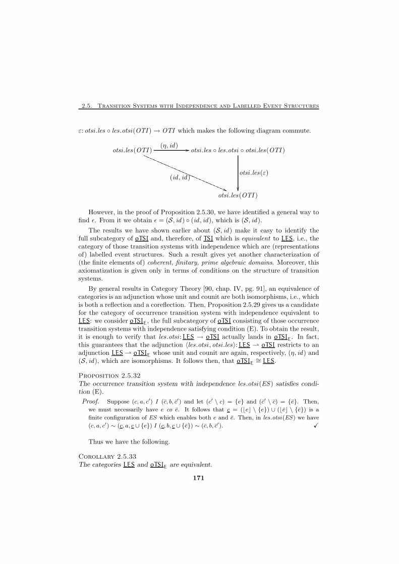
2.5. Transition Systems with Independence and Labelled Event Structures
ε: otsi .les ◦ les .otsi(OTI )→ OTI which makes the following diagram commute.
otsi .les(OTI ) otsi .les ◦ les .otsi ◦ otsi .les(OTI )
otsi .les(OTI )
(η, id) //
(id , id)
QQQQQQQQQQQQQQQQQQQQQQQQQ (( otsi .les(ε)
��
However, in the proof of Proposition 2.5.30, we have identified a general way tofind ǫ. From it we obtain ǫ = (S, id ) ◦ (id , id), which is (S, id ).
The results we have shown earlier about (S, id) make it easy to identify thefull subcategory of oTSI and, therefore, of TSI which is equivalent to LES, i.e., thecategory of those transition systems with independence which are (representationsof) labelled event structures. Such a result gives yet another characterization of(the finite elements of) coherent, finitary, prime algebraic domains. Moreover, thisaxiomatization is given only in terms of conditions on the structure of transitionsystems.
By general results in Category Theory [90, chap. IV, pg. 91], an equivalence ofcategories is an adjunction whose unit and counit are both isomorphisms, i.e., whichis both a reflection and a coreflection. Then, Proposition 2.5.29 gives us a candidatefor the category of occurrence transition system with independence equivalent toLES: we consider oTSIE, the full subcategory of oTSI consisting of those occurrencetransition systems with independence satisfying condition (E). To obtain the result,it is enough to verify that les .otsi : LES → oTSI actually lands in oTSIE. In fact,this guarantees that the adjunction 〈les .otsi , otsi .les〉: LES ⇀ oTSI restricts to anadjunction LES ⇀ oTSIE whose unit and counit are again, respectively, (η, id) and(S, id), which are isomorphisms. It follows then, that oTSIE
∼= LES.
Proposition 2.5.32The occurrence transition system with independence les .otsi(ES ) satisfies condi-tion (E).
Proof. Suppose (c, a, c′) I (c, b, c′) and let (c′ \ c) = {e} and (c′ \ c) = {e}. Then,
we must necessarily have e co e. It follows that c = (⌊e⌋ \ {e}) ∪ (⌊e⌋ \ {e}) is a
finite configuration of ES which enables both e and e. Then, in les.otsi (ES) we have
(c, a, c′) ∼ (c, a, c ∪ {e}) I (c, b, c ∪ {e}) ∼ (c, b, c′). X
Thus we have the following.
Corollary 2.5.33The categories LES and oTSIE are equivalent.
171
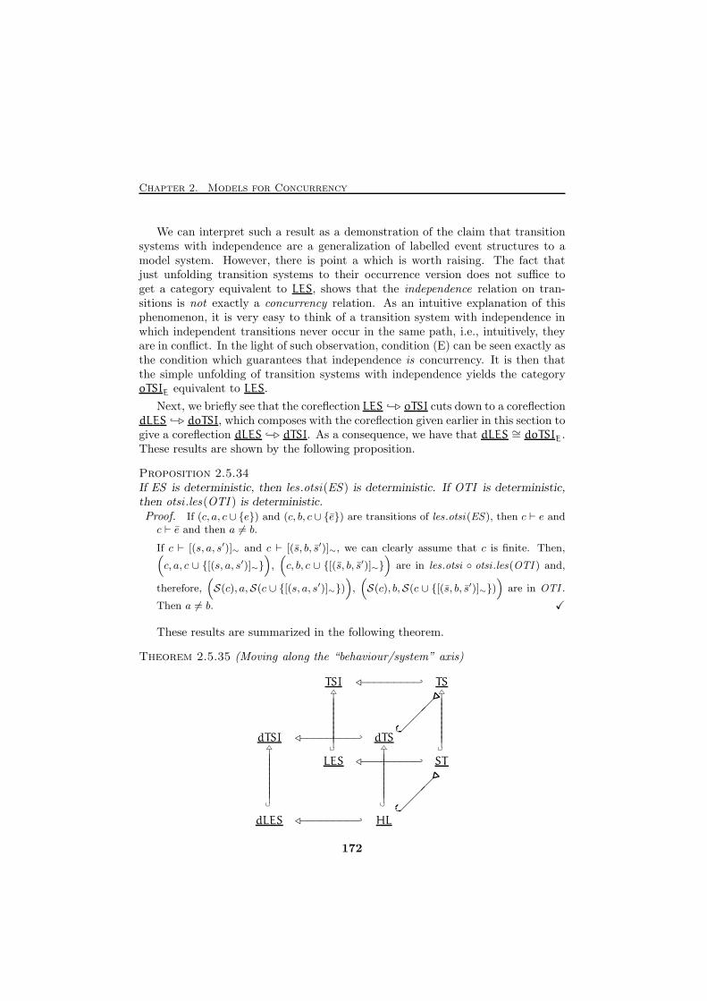
Chapter 2. Models for Concurrency
We can interpret such a result as a demonstration of the claim that transitionsystems with independence are a generalization of labelled event structures to amodel system. However, there is point a which is worth raising. The fact thatjust unfolding transition systems to their occurrence version does not suffice toget a category equivalent to LES, shows that the independence relation on tran-sitions is not exactly a concurrency relation. As an intuitive explanation of thisphenomenon, it is very easy to think of a transition system with independence inwhich independent transitions never occur in the same path, i.e., intuitively, theyare in conflict. In the light of such observation, condition (E) can be seen exactly asthe condition which guarantees that independence is concurrency. It is then thatthe simple unfolding of transition systems with independence yields the categoryoTSIE equivalent to LES.
Next, we briefly see that the coreflection LES −⊲ oTSI cuts down to a coreflectiondLES −⊲ doTSI, which composes with the coreflection given earlier in this section togive a coreflection dLES −⊲ dTSI. As a consequence, we have that dLES ∼= doTSIE.These results are shown by the following proposition.
Proposition 2.5.34If ES is deterministic, then les .otsi(ES ) is deterministic. If OTI is deterministic,then otsi .les(OTI ) is deterministic.Proof. If (c, a, c ∪ {e}) and (c, b, c ∪ {e}) are transitions of les.otsi (ES), then c ⊢ e andc ⊢ e and then a 6= b.
If c ⊢ [(s, a, s′)]∼ and c ⊢ [(s, b, s′)]∼, we can clearly assume that c is finite. Then,(c, a, c ∪ {[(s, a, s′)]∼}
),(c, b, c ∪ {[(s, b, s′)]∼}
)are in les.otsi ◦ otsi .les(OTI ) and,
therefore,(S(c), a,S(c ∪ {[(s, a, s′)]∼})
),(S(c), b,S(c ∪ {[(s, b, s′)]∼})
)are in OTI .
Then a 6= b. X
These results are summarized in the following theorem.
Theorem 2.5.35 (Moving along the “behaviour/system” axis)
dTSI ⊳−−−−−−−−− dTS���
....................................................
..........�△
||||||||||∪
△
||||||||||∪
dLES ⊳−−−−−−−−− HL
���
....................................................
..........�
TSI ⊳−−−−−−−−− TS△
||||||||||∪
△
||||||||||∪
LES ⊳−−−−−−−−− ST
172
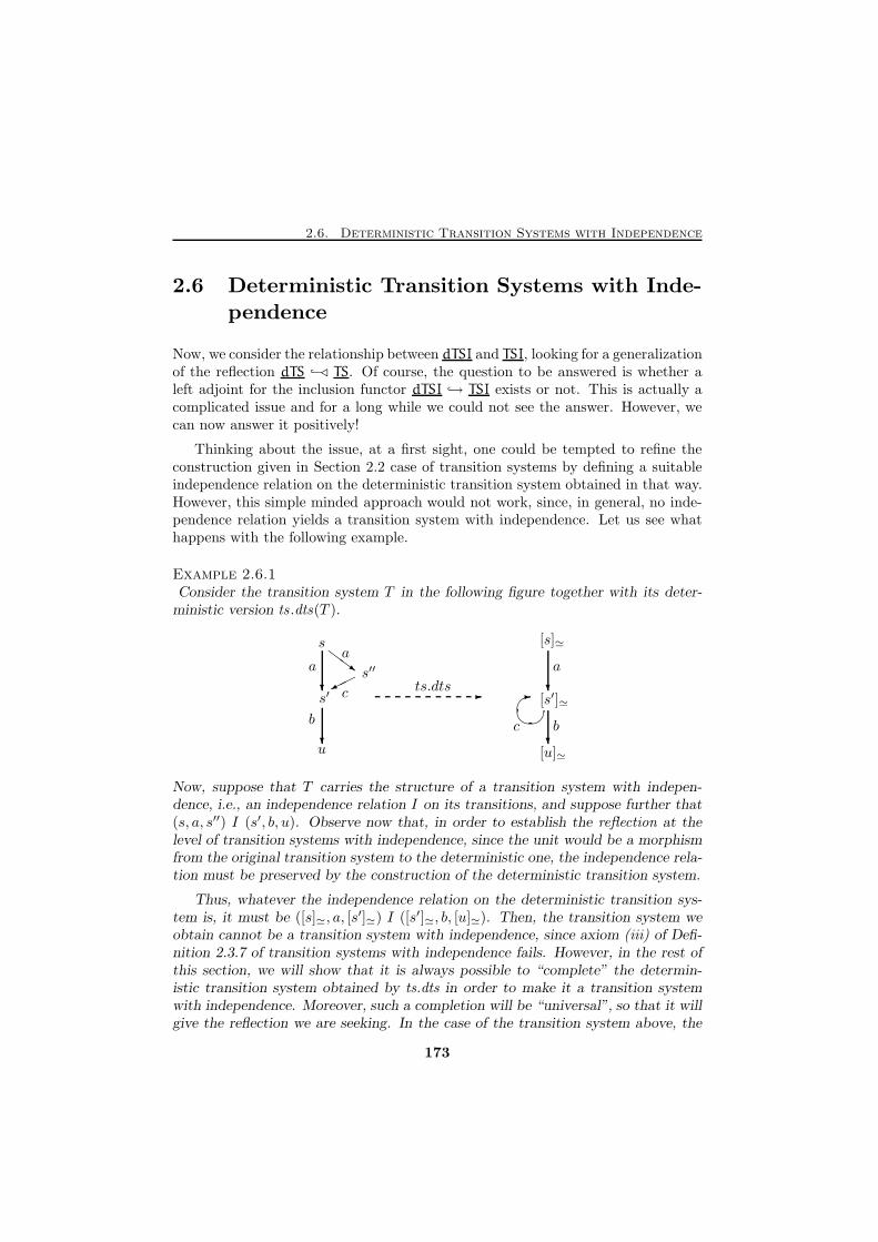
2.6. Deterministic Transition Systems with Independence
2.6 Deterministic Transition Systems with Inde-
pendence
Now, we consider the relationship between dTSI and TSI, looking for a generalizationof the reflection dTS −⊳ TS. Of course, the question to be answered is whether aleft adjoint for the inclusion functor dTSI → TSI exists or not. This is actually acomplicated issue and for a long while we could not see the answer. However, wecan now answer it positively!
Thinking about the issue, at a first sight, one could be tempted to refine theconstruction given in Section 2.2 case of transition systems by defining a suitableindependence relation on the deterministic transition system obtained in that way.However, this simple minded approach would not work, since, in general, no inde-pendence relation yields a transition system with independence. Let us see whathappens with the following example.
Example 2.6.1Consider the transition system T in the following figure together with its deter-
ministic version ts .dts(T ).
s′
s
u
s′′
b
a
c
a
� �-
? ?
?
ZZ~��� - ?
[s]≃
ts.dts
[u]≃
[s′]≃
b
a
c
Now, suppose that T carries the structure of a transition system with indepen-dence, i.e., an independence relation I on its transitions, and suppose further that(s, a, s′′) I (s′, b, u). Observe now that, in order to establish the reflection at thelevel of transition systems with independence, since the unit would be a morphismfrom the original transition system to the deterministic one, the independence rela-tion must be preserved by the construction of the deterministic transition system.
Thus, whatever the independence relation on the deterministic transition sys-tem is, it must be ([s]≃, a, [s
′]≃) I ([s′]≃, b, [u]≃). Then, the transition system weobtain cannot be a transition system with independence, since axiom (iii) of Defi-nition 2.3.7 of transition systems with independence fails. However, in the rest ofthis section, we will show that it is always possible to “complete” the determin-istic transition system obtained by ts.dts in order to make it a transition systemwith independence. Moreover, such a completion will be “universal”, so that it willgive the reflection we are seeking. In the case of the transition system above, the
173
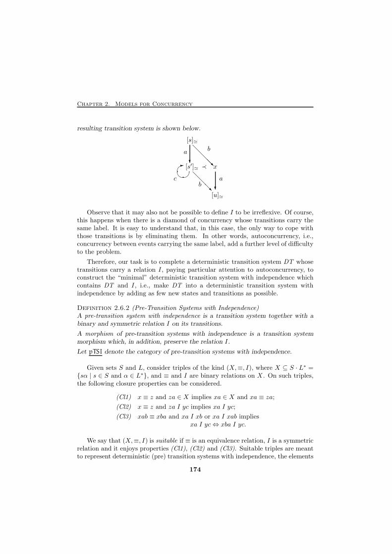
Chapter 2. Models for Concurrency
resulting transition system is shown below.
@@@@R?
@@@R ?
� �- x[s′]≃
[s]≃
≺
a
c
[u]≃
a
b
b
Observe that it may also not be possible to define I to be irreflexive. Of course,this happens when there is a diamond of concurrency whose transitions carry thesame label. It is easy to understand that, in this case, the only way to cope withthose transitions is by eliminating them. In other words, autoconcurrency, i.e.,concurrency between events carrying the same label, add a further level of difficultyto the problem.
Therefore, our task is to complete a deterministic transition system DT whosetransitions carry a relation I, paying particular attention to autoconcurrency, toconstruct the “minimal” deterministic transition system with independence whichcontains DT and I, i.e., make DT into a deterministic transition system withindependence by adding as few new states and transitions as possible.
Definition 2.6.2 (Pre-Transition Systems with Independence)A pre-transition system with independence is a transition system together with abinary and symmetric relation I on its transitions.
A morphism of pre-transition systems with independence is a transition systemmorphism which, in addition, preserve the relation I.
Let pTSI denote the category of pre-transition systems with independence.
Given sets S and L, consider triples of the kind (X,≡, I), where X ⊆ S · L∗ ={sα | s ∈ S and α ∈ L∗}, and ≡ and I are binary relations on X . On such triples,the following closure properties can be considered.
(Cl1) x ≡ z and za ∈ X implies xa ∈ X and xa ≡ za;
(Cl2) x ≡ z and za I yc implies xa I yc;
(Cl3) xab ≡ xba and xa I xb or xa I xab impliesxa I yc⇔ xba I yc.
We say that (X,≡, I) is suitable if ≡ is an equivalence relation, I is a symmetricrelation and it enjoys properties (Cl1), (Cl2) and (Cl3). Suitable triples are meantto represent deterministic (pre) transition systems with independence, the elements
174
2.6. Deterministic Transition Systems with Independence
in X representing both states and transitions. Namely, xa represents the statereached from (the state corresponding to) x with an a-labelled transition, and thattransition itself. Thus, equivalence ≡ relate paths which lead to the same stateand relation I expresses independence of transitions. With this understanding,(Cl1) means that from any state there is at most one a-transition, while (Cl2) saysthat I acts on transitions rather than on their representation. Finally, (Cl3)—the analogous of axiom (iv) of transition systems with independence—tells thattransitions on the opposite edges of a diamond behave the same with respect to I.
For x ∈ S · L∗ and a ∈ L, let x↾a denote the pruning of x with respect to a.Formally,
s↾a = s and (xb)↾a =
{x↾a if a = b
(x↾a)b otherwise
Of course, (x↾a)↾b = (x↾b)↾a and thus it is possibile to use unambiguously x↾Afor A ⊆ L. Given X ⊆ S ·L∗, we use X↾A to denote the set {x↾A | x ∈ X} and fora binary relation R on X R↾A will be {(x↾A, y↾A) | (x, y) ∈ R}.
For a transition system with independence TI = (S, sI , L,Tran, I), we definethe sequence a triples (Si,≡i, Ii), for i ∈ ω, inductively as follows. For i = 0,(S0,≡0, I0) is the least (with respect to componentwise set inclusion) suitable triplesuch that
S ∪{sa∣∣∣ (s, a, u) ∈ Tran
}⊆ S0;
{(sa, u)
∣∣∣ (s, a, u) ∈ Tran}⊆ ≡0;
and {(sa, s′b)
∣∣∣ (s, a, u) I (s′, b, u′)}⊆ I0;
and, for i > 0, (Si,≡i, Ii) is the least suitable triple such that
(ℑ) Si−1↾Ai−1 ⊆ Si; ≡i−1↾Ai−1 ⊆ ≡i; (Ii−1 \ TAi−1)↾Ai−1 ⊆ Ii;
(D1) xa, xb ∈ Si−1↾Ai−1 and xa (Ii−1 \TAi−1)↾Ai−1 xbimplies xab, xba ∈ Si and xab ≡i xba;
(D2) xa, xab ∈ Si−1↾Ai−1 and xa (Ii−1 \TAi−1)↾Ai−1 xabimplies xb, xba ∈ Si and xab ≡i xba;
where Ai = {a ∈ L | xa Ii xa} and TAi = {(xa, yb) ∈ Ii | a ∈ Ai or b ∈ Ai}.
The inductive step extends a triple towards a transition system with indepen-dence by means of the rules (D1) and (D2), whose intuitive meaning is clearly thatof closing possibly incomplete diamonds. The process could create autoindependenttransitions which must be eliminated. This is done by (ℑ) which drops them andadjusts ≡i and Ii.
A simple inspection of the rules shows that if a ∈ Ai, then it will never appearagain in the sequence. Thus, if x is removed from Si, it will not be reintroduced,
175
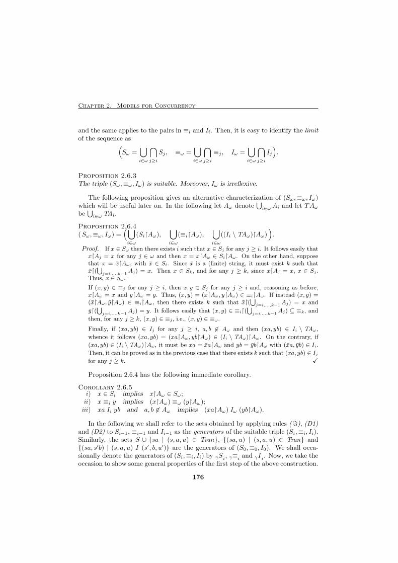
Chapter 2. Models for Concurrency
and the same applies to the pairs in ≡i and Ii. Then, it is easy to identify the limitof the sequence as
(Sω =
⋃
i∈ω
⋂
j≥i
Sj , ≡ω =⋃
i∈ω
⋂
j≥i
≡j , Iω =⋃
i∈ω
⋂
j≥i
Ij
).
Proposition 2.6.3The triple (Sω,≡ω, Iω) is suitable. Moreover, Iω is irreflexive.
The following proposition gives an alternative characterization of (Sω,≡ω, Iω)which will be useful later on. In the following let Aω denote
⋃i∈ω Ai and let TAω
be⋃i∈ω TAi.
Proposition 2.6.4(Sω,≡ω, Iω) =
(⋃
i∈ω
(Si↾Aω),⋃
i∈ω
(≡i↾Aω),⋃
i∈ω
((Ii \ TAω)↾Aω)).
Proof. If x ∈ Sω then there exists i such that x ∈ Sj for any j ≥ i. It follows easily thatx↾Aj = x for any j ∈ ω and then x = x↾Aω ∈ Si↾Aω. On the other hand, supposethat x = x↾Aω, with x ∈ Si. Since x is a (finite) string, it must exist k such thatx↾(⋃j=i,...,k−1
Aj) = x. Then x ∈ Sk, and for any j ≥ k, since x↾Aj = x, x ∈ Sj .Thus, x ∈ Sω.
If (x, y) ∈ ≡j for any j ≥ i, then x, y ∈ Sj for any j ≥ i and, reasoning as before,x↾Aω = x and y↾Aω = y. Thus, (x, y) = (x↾Aω, y↾Aω) ∈ ≡i↾Aω. If instead (x, y) =(x↾Aω, y↾Aω) ∈ ≡i↾Aω, then there exists k such that x↾(
⋃j=i,...,k−1
Aj) = x and
y↾(⋃j=i,...,k−1
Aj) = y. It follows easily that (x, y) ∈ ≡i↾(⋃j=i,...,k−1
Aj) ⊆ ≡k, and
then, for any j ≥ k, (x, y) ∈ ≡j , i.e., (x, y) ∈ ≡ω.
Finally, if (xa, yb) ∈ Ij for any j ≥ i, a, b 6∈ Aω and then (xa, yb) ∈ Ii \ TAω,
whence it follows (xa, yb) = (xa↾Aω, yb↾Aω) ∈ (Ii \ TAω)↾Aω. On the contrary, if
(xa, yb) ∈ (Ii \ TAω)↾Aω, it must be xa = xa↾Aω and yb = yb↾Aω with (xa, yb) ∈ Ii.
Then, it can be proved as in the previous case that there exists k such that (xa, yb) ∈ Ijfor any j ≥ k. X
Proposition 2.6.4 has the following immediate corollary.
Corollary 2.6.5i) x ∈ Si implies x↾Aω ∈ Sω;ii) x ≡i y implies (x↾Aω) ≡ω (y↾Aω);iii) xa Ii yb and a, b 6∈ Aω implies (xa↾Aω) Iω (yb↾Aω).
In the following we shall refer to the sets obtained by applying rules (ℑ), (D1)and (D2) to Si−1, ≡i−1 and Ii−1 as the generators of the suitable triple (Si,≡i, Ii).Similarly, the sets S ∪ {sa | (s, a, u) ∈ Tran}, {(sa, u) | (s, a, u) ∈ Tran} and{(sa, s′b) | (s, a, u) I (s′, b, u′)} are the generators of (S0,≡0, I0). We shall occa-sionally denote the generators of (Si,≡i, Ii) by γSi, γ≡i and γIi. Now, we take theoccasion to show some general properties of the first step of the above construction.
176
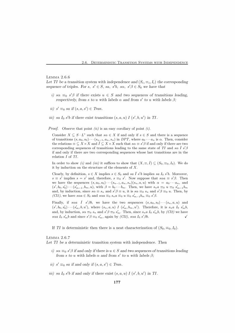
2.6. Deterministic Transition Systems with Independence
Lemma 2.6.6Let TI be a transition system with independence and (Si,≡i, Ii) the correspondingsequence of triples. For s, s′ ∈ S, sa, s′b, sα, s′β ∈ S0 we have that
i) sα ≡0 s′β if there exists u ∈ S and two sequences of transitions leading,respectively, from s to u with labels α and from s′ to u with labels β;
ii) s′ ≡0 sa if (s, a, s′) ∈ Tran.
iii) sa I0 s′b if there exist transitions (s, a, u) I (s′, b, u′) in TI .
Proof. Observe that point (ii) is an easy corollary of point (i).
Consider X ⊆ S · L∗ such that sα ∈ X if and only if s ∈ S and there is a sequenceof transitions (s, a0, s0) · · · (sn−1, an, sn) in DPT , where a0 · · · an is α. Then, considerthe relations ≡ ⊆ X×X and I ⊆ X×X such that sα ≡ s′β if and only if there are twocorresponding sequences of transitions leading to the same state of TI and sα I s′βif and only if there are two corresponding sequences whose last transitions are in therelation I of TI .
In order to show (i) and (iii) it suffices to show that (X,≡, I) ⊆ (S0,≡0, I0). We doit by induction on the structure of the elements of X.
Clearly, by definition, s ∈ X implies s ∈ S0 and sa I s′b implies sa I0 s′b. Moreover,
s ≡ s′ implies s = s′ and, therefore, s ≡0 s′. Now suppose that sαa ≡ s′β. Then
we have the sequences (s, a0, s0) · · · (sn−1, an, sn)(sn, a, u) with α = a0 · · · an, and(s′, b0, s
′0) · · · (s
′m−1, bm, u), with β = b0 · · · bm. Then, we have sna ≡0 u ≡0 s
′m−1bm
and, by induction, since sα ≡ sn and s′β ≡ u, it is sα ≡0 sn and s′β ≡0 u. Then, by(Cl1), we have sαa ∈ S0 and sαa ≡0 sna ≡0 u ≡0 s
′m−1bm ≡0 s
′β.
Finally, if sαa I s′βb, we have the two sequences (s, a0, s0) · · · (sn, a, u) and
(s′, b0, s′0) · · · (s
′m, b, u
′), where (sn, a, u) I (s′m, bm, u′). Therefore, it is sna I0 s′mb,
and, by induction, sα ≡0 sn and s′β ≡0 s′m. Then, since sna I0 s
′mb, by (Cl2) we have
sαa I0 s′mb and since s′β ≡0 s
′m, again by (Cl2), sαa I0 s
′βb. X
If TI is deterministic then there is a neat characterization of (S0,≡0, I0).
Lemma 2.6.7Let TI be a deterministic transition system with independence. Then
i) sα ≡0 s′β if and only if there is u ∈ S and two sequences of transitions leading
from s to u with labels α and from s′ to u with labels β;
ii) s′ ≡0 sa if and only if (s, a, s′) ∈ Tran .
iii) sa I0 s′b if and only if there exist (s, a, u) I (s′, b, u′) in TI .
177
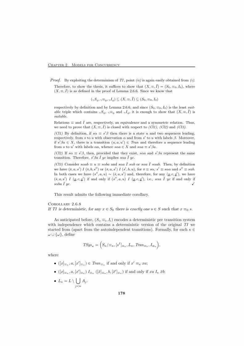
Chapter 2. Models for Concurrency
Proof. By exploiting the determinism of TI , point (ii) is again easily obtained from (i).
Therefore, to show the thesis, it suffices to show that (X,≡, I) = (S0,≡0, I0), where(X,≡, I) is as defined in the proof of Lemma 2.6.6. Since we know that
(γS0, γ≡0, γI0) ⊆ (X,≡, I) ⊆ (S0,≡0, I0)
respectively by definition and by Lemma 2.6.6, and since (S0,≡0, I0) is the least suit-able triple which contains γS0, γ≡0 and γI0, it is enough to show that (X,≡, I) issuitable.
Relations ≡ and I are, respectively, an equivalence and a symmetric relation. Thus,we need to prove that (X,≡, I) is closed with respect to (Cl1), (Cl2) and (Cl3).
(Cl1) By definition, if sα ≡ s′β then there is a state u and two sequences leading,respectively, from s to u with observation α and from s′ to u with labels β. Moreover,if s′βa ∈ X, there is a transition (u, a, u′) ∈ Tran and therefore a sequence leadingfrom s to u′ with labels αa, whence sαa ∈ X and sαa ≡ s′βa.
(Cl2) If sα ≡ s′β, then, provided that they exist, sαa and s′βa represent the sametransition. Therefore, s′βa I yc implies sαa I yc.
(Cl3) Consider sαab ≡ u ≡ sαba and sαa I sαb or sαa I sαab. Then, by definition
we have (s, a, s′) I (s, b, s′′) or (s, a, s′) I (s′, b, u), for s ≡ sα, s′ ≡ sαa and s′′ ≡ sαb.
In both cases we have (s′′, a, u) ∼ (s, a, s′) and, therefore, for any (s, c, s′), we have
(s, a, s′) I (s, c, s′) if and only if (s′′, a, u) I (s, c, s′), i.e., sαa I yc if and only if
sαba I yc. X
This result admits the following immediate corollary.
Corollary 2.6.8If TI is deterministic, for any x ∈ S0 there is exactly one s ∈ S such that x ≡0 s.
As anticipated before, (Si,≡i, Ii) encodes a deterministic pre transition systemwith independence which contains a deterministic version of the original TI westarted from (apart from the autoindependent transitions). Formally, for each κ ∈ω ∪ {ω}, define
TSysκ =(Sκ/≡κ, [s
I ]≡κ, Lκ,Tran≡κ
, I≡κ
),
where
• ([x]≡κ, a, [x′]≡κ
) ∈ Tran≡κif and only if x′ ≡κ xa;
• ([x]≡κ, a, [x′]≡κ
) I≡κ([x]≡κ
, b, [x′]≡κ) if and only if xa Iκ xb;
• Lκ = L \⋃
j<κ
Aj .
178
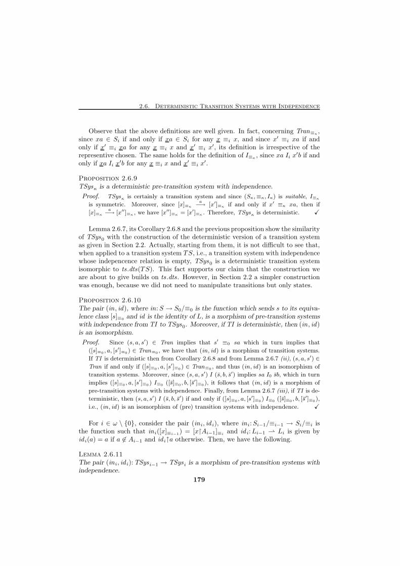
2.6. Deterministic Transition Systems with Independence
Observe that the above definitions are well given. In fact, concerning Tran≡κ,
since xa ∈ Si if and only if xa ∈ Si for any x ≡i x, and since x′ ≡i xa if andonly if x′ ≡i xa for any x ≡i x and x′ ≡i x′, its definition is irrespective of therepresentive chosen. The same holds for the definition of I≡κ
, since xa Ii x′b if and
only if xa Ii x′b for any x ≡i x and x′ ≡i x′.
Proposition 2.6.9TSysκ is a deterministic pre-transition system with independence.
Proof. TSysκ is certainly a transition system and since (Sκ,≡κ, Iκ) is suitable, I≡κ
is symmetric. Moreover, since [x]≡κ
a−→ [x′]≡κ if and only if x′ ≡κ xa, then if
[x]≡κ
a−→ [x′′]≡κ , we have [x′′]≡κ = [x′]≡κ . Therefore, TSysκ is deterministic. X
Lemma 2.6.7, its Corollary 2.6.8 and the previous proposition show the similarityof TSys0 with the construction of the deterministic version of a transition systemas given in Section 2.2. Actually, starting from them, it is not difficult to see that,when applied to a transition system TS, i.e., a transition system with independencewhose indepencence relation is empty, TSys0 is a deterministic transition systemisomorphic to ts .dts(TS). This fact supports our claim that the construction weare about to give builds on ts .dts. However, in Section 2.2 a simpler constructionwas enough, because we did not need to manipulate transitions but only states.
Proposition 2.6.10The pair (in , id), where in:S → S0/≡0 is the function which sends s to its equiva-lence class [s]≡0 and id is the identity of L, is a morphism of pre-transition systemswith independence from TI to TSys0. Moreover, if TI is deterministic, then (in , id)is an isomorphism.
Proof. Since (s, a, s′) ∈ Tran implies that s′ ≡0 sa which in turn implies that
([s]≡0 , a, [s′]≡0) ∈ Tran≡0 , we have that (in, id) is a morphism of transition systems.
If TI is deterministic then from Corollary 2.6.8 and from Lemma 2.6.7 (ii), (s, a, s′) ∈
Tran if and only if ([s]≡0 , a, [s′]≡0) ∈ Tran≡0 , and thus (in, id) is an isomorphism of
transition systems. Moreover, since (s, a, s′) I (s, b, s′) implies sa I0 sb, which in turn
implies ([s]≡0 , a, [s′]≡0) I≡0 ([s]≡0 , b, [s
′]≡0), it follows that (in, id) is a morphism of
pre-transition systems with independence. Finally, from Lemma 2.6.7 (iii), if TI is de-
terministic, then (s, a, s′) I (s, b, s′) if and only if ([s]≡0 , a, [s′]≡0) I≡0 ([s]≡0 , b, [s
′]≡0),
i.e., (in, id) is an isomorphism of (pre) transition systems with independence. X
For i ∈ ω \ {0}, consider the pair (in i, id i), where in i:Si−1/≡i−1 → Si/≡i isthe function such that ini([x]≡i−1) = [x↾Ai−1]≡i
and id i:Li−1 ⇀ Li is given byid i(a) = a if a 6∈ Ai−1 and id i↑a otherwise. Then, we have the following.
Lemma 2.6.11The pair (in i, id i):TSysi−1 → TSysi is a morphism of pre-transition systems withindependence.
179
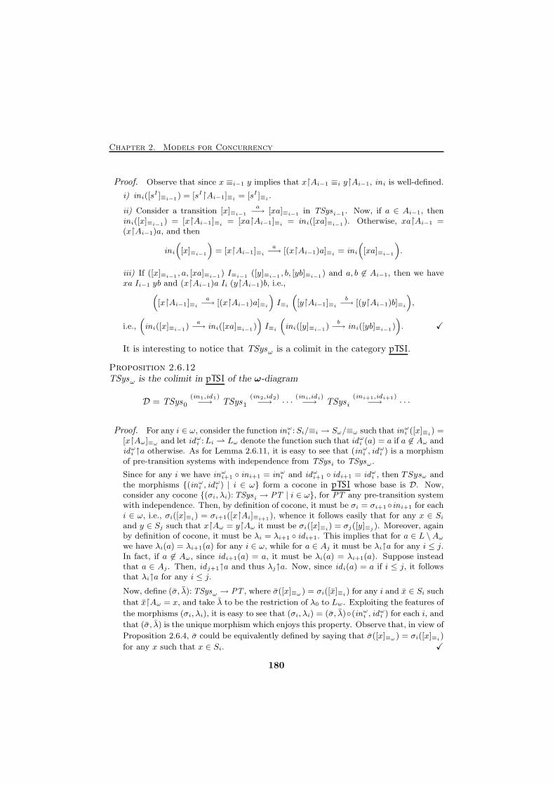
Chapter 2. Models for Concurrency
Proof. Observe that since x ≡i−1 y implies that x↾Ai−1 ≡i y↾Ai−1, ini is well-defined.
i) ini([sI ]≡i−1) = [sI↾Ai−1]≡i = [sI ]≡i .
ii) Consider a transition [x]≡i−1
a−→ [xa]≡i−1 in TSysi−1. Now, if a ∈ Ai−1, then
ini([x]≡i−1) = [x↾Ai−1]≡i = [xa↾Ai−1]≡i = ini([xa]≡i−1). Otherwise, xa↾Ai−1 =(x↾Ai−1)a, and then
ini
([x]≡i−1
)= [x↾Ai−1]≡i
a−→ [(x↾Ai−1)a]≡i = ini
([xa]≡i−1
).
iii) If ([x]≡i−1 , a, [xa]≡i−1) I≡i−1 ([y]≡i−1 , b, [yb]≡i−1) and a, b 6∈ Ai−1, then we havexa Ii−1 yb and (x↾Ai−1)a Ii (y↾Ai−1)b, i.e.,
([x↾Ai−1]≡i
a−→ [(x↾Ai−1)a]≡i
)I≡i
([y↾Ai−1]≡i
b−→ [(y↾Ai−1)b]≡i
),
i.e.,(ini([x]≡i−1)
a−→ ini([xa]≡i−1)
)I≡i
(ini([y]≡i−1)
b−→ ini([yb]≡i−1)
). X
It is interesting to notice that TSysω is a colimit in the category pTSI.
Proposition 2.6.12TSysω is the colimit in pTSI of the ω-diagram
D = TSys0
(in1,id1)−→ TSys1
(in2,id2)−→ · · ·
(ini,idi)−→ TSysi
(ini+1,idi+1)−→ · · ·
Proof. For any i ∈ ω, consider the function inωi :Si/≡i → Sω/≡ω such that inωi ([x]≡i) =[x↾Aω]≡ω and let idωi :Li ⇀ Lω denote the function such that idωi (a) = a if a 6∈ Aω andidωi ↑a otherwise. As for Lemma 2.6.11, it is easy to see that (inωi , id
ωi ) is a morphism
of pre-transition systems with independence from TSysi to TSysω.
Since for any i we have inωi+1 ◦ ini+1 = inωi and idωi+1 ◦ id i+1 = idωi , then TSysω andthe morphisms {(inωi , id
ωi ) | i ∈ ω} form a cocone in pTSI whose base is D. Now,
consider any cocone {(σi, λi):TSysi → PT | i ∈ ω}, for PT any pre-transition systemwith independence. Then, by definition of cocone, it must be σi = σi+1 ◦ini+1 for eachi ∈ ω, i.e., σi([x]≡i) = σi+1([x↾Ai]≡i+1), whence it follows easily that for any x ∈ Siand y ∈ Sj such that x↾Aω = y↾Aω it must be σi([x]≡i) = σj([y]≡j ). Moreover, againby definition of cocone, it must be λi = λi+1 ◦ id i+1. This implies that for a ∈ L \Aωwe have λi(a) = λi+1(a) for any i ∈ ω, while for a ∈ Aj it must be λi↑a for any i ≤ j.In fact, if a 6∈ Aω, since id i+1(a) = a, it must be λi(a) = λi+1(a). Suppose insteadthat a ∈ Aj . Then, idj+1↑a and thus λj↑a. Now, since id i(a) = a if i ≤ j, it followsthat λi↑a for any i ≤ j.
Now, define (σ, λ):TSysω → PT , where σ([x]≡ω ) = σi([x]≡i) for any i and x ∈ Si such
that x↾Aω = x, and take λ to be the restriction of λ0 to Lw. Exploiting the features of
the morphisms (σi, λi), it is easy to see that (σi, λi) = (σ, λ)◦(inωi , idωi ) for each i, and
that (σ, λ) is the unique morphism which enjoys this property. Observe that, in view of
Proposition 2.6.4, σ could be equivalently defined by saying that σ([x]≡ω ) = σi([x]≡i)
for any x such that x ∈ Si. X
180
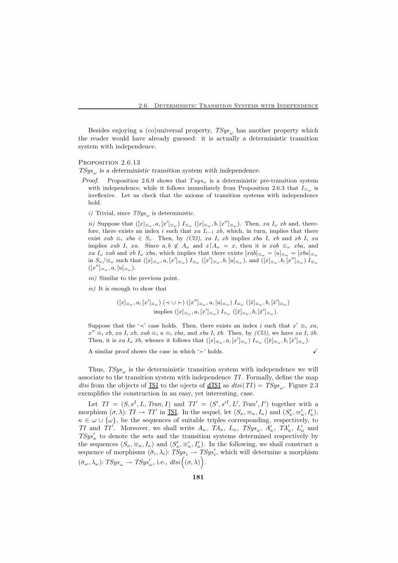
2.6. Deterministic Transition Systems with Independence
Besides enjoying a (co)universal property, TSysω has another property whichthe reader would have already guessed: it is actually a deterministic transitionsystem with independence.
Proposition 2.6.13TSysω is a deterministic transition system with independence.
Proof. Proposition 2.6.9 shows that Tsysω is a deterministic pre-transition systemwith independence, while it follows immediately from Proposition 2.6.3 that I≡ω isirreflexive. Let us check that the axioms of transition systems with independencehold.
i) Trivial, since TSysω is deterministic.
ii) Suppose that ([x]≡ω , a, [x′]≡ω ) I≡ω ([x]≡ω , b, [x
′′]≡ω ). Then, xa Iω xb and, there-fore, there exists an index i such that xa Ii−1 xb, which, in turn, implies that thereexist xab ≡i xba ∈ Si. Then, by (Cl3), xa Ii xb implies xba Ii xb and xb Ii xaimplies xab Ii xa. Since a, b 6∈ Aω and x↾Aω = x, then it is xab ≡ω xba, andxa Iω xab and xb Iω xba, which implies that there exists [xab]≡ω = [u]≡ω = [xba]≡ω
in Sω/≡ω such that ([x]≡ω , a, [x′]≡ω ) I≡ω ([x′]≡ω , b, [u]≡ω ), and ([x]≡ω , b, [x
′′]≡ω ) I≡ω
([x′′]≡ω , a, [u]≡ω ).
iii) Similar to the previous point.
iv) It is enough to show that
([x]≡ω , a, [x′]≡ω ) (≺ ∪ ≻) ([x′′]≡ω , a, [u]≡ω ) I≡ω ([x]≡ω , b, [x
′]≡ω )
implies ([x]≡ω , a, [x′]≡ω ) I≡ω ([x]≡ω , b, [x
′]≡ω ).
Suppose that the ‘≺’ case holds. Then, there exists an index i such that x′ ≡i xa,x′′ ≡i xb, xa Ii xb, xab ≡i u ≡i xba, and xba Ii xb. Then, by (Cl3), we have xa Ii xb.Then, it is xa Iω xb, whence it follows that ([x]≡ω , a, [x
′]≡ω ) I≡ω ([x]≡ω , b, [x′]≡ω ).
A similar proof shows the case in which ‘≻’ holds. X
Thus, TSysω is the deterministic transition system with independence we willassociate to the transition system with independence TI . Formally, define the mapdtsi from the objects of TSI to the ojects of dTSI as dtsi(TI ) = TSysω. Figure 2.3exemplifies the construction in an easy, yet interesting, case.
Let TI = (S, sI , L,Tran, I) and TI ′ = (S′, s′I , L′,Tran ′, I ′) together with amorphism (σ, λ):TI → TI ′ in TSI. In the sequel, let (Sκ,≡κ, Iκ) and (S′κ,≡
′κ, I′κ),
κ ∈ ω ∪ {ω}, be the sequences of suitable triples corresponding, respectively, toTI and TI ′. Moreover, we shall write Aκ, TAκ, Lκ, TSysκ, A
′κ, TA′κ, L
′κ and
TSys ′κ to denote the sets and the transition systems determined respectively bythe sequences (Sκ,≡κ, Iκ) and (S′κ,≡
′κ, I′κ). In the following, we shall construct a
sequence of morphisms (σi, λi):TSys i → TSys ′i, which will determine a morphism
(σω, λω):TSysω → TSys ′ω , i.e., dtsi((σ, λ)
).
181
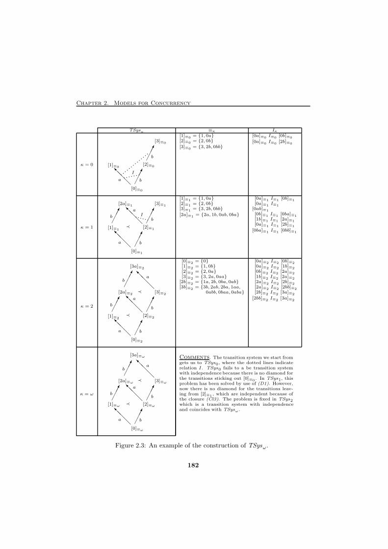
Chapter 2. Models for Concurrency
TSysκ ≡κ Iκ
κ = 0����
@@@I
����. . . . . . ....
......
.....
[0]≡0
[2]≡0
I
[3]≡0
a b
b
[1]≡0
[1]≡0 = {1, 0a}[2]≡0 = {2, 0b}
[3]≡0 = {3, 2b, 0bb}
[0a]≡0 I≡0 [0b]≡0
[0a]≡0 I≡0 [2b]≡0
κ = 1����
@@@I
@@@I
����
����
......
[0]≡1
[2]≡1
[3]≡1
a
I
b
b
[1]≡1
[2a]≡1
≺
a
b
[1]≡1 = {1, 0a}[2]≡1 = {2, 0b}[3]≡1 = {3, 2b, 0bb}
[2a]≡1 = {2a, 1b, 0ab, 0ba}
[0a]≡1 I≡1 [0b]≡1[0a]≡1 I≡1
[0ab]≡1[0b]≡1 I≡1 [0ba]≡1[1b]≡1 I≡1 [2a]≡1[0a]≡1 I≡1 [2b]≡1
[0ba]≡1 I≡1 [0bb]≡1
κ = 2����
@@@I
@@@I
����
@@@I
����
����
[0]≡2
[2]≡2
[3]≡2
a b
a
b
[1]≡2
[2a]≡2
≺
a
b
[3a]≡2
≺
b
[0]≡2 = {0}[1]≡2 = {1, 0b}[2]≡2 = {2, 0a}[3]≡2 = {3, 2a, 0aa}
[2b]≡2 = {1a, 2b, 0ba, 0ab}[3b]≡2 = {3b, 2ab, 2ba, 1aa,
0abb, 0baa, 0aba}
[0a]≡2 I≡2 [0b]≡2[0a]≡2 I≡2 [1b]≡2[0b]≡2 I≡2 [2a]≡2[1b]≡2 I≡2 [2a]≡2[2a]≡2 I≡2 [2b]≡2[2a]≡2 I≡2 [2bb]≡2[2b]≡2 I≡2 [3a]≡2
[2bb]≡2 I≡2 [3a]≡2
κ = ω����
@@@I
@@@I
����
@@@I
����
����
[0]≡ω
[2]≡ω
[3]≡ω
a b
a
b
[1]≡ω
[2a]≡ω
≺
a
b
[3a]≡ω
≺
b
Comments. The transition system we start fromgets us to TSys0, where the dotted lines indicaterelation I. TSys0 fails to a be transition systemwith independence because there is no diamond forthe transitions sticking out [0]≡0 . In TSys1, thisproblem has been solved by use of (D1). However,now there is no diamond for the transitions leav-ing from [2]≡1 , which are independent because ofthe closure (Cl3). The problem is fixed in TSys2which is a transition system with independenceand coincides with TSysω .
Figure 2.3: An example of the construction of TSysω.
182
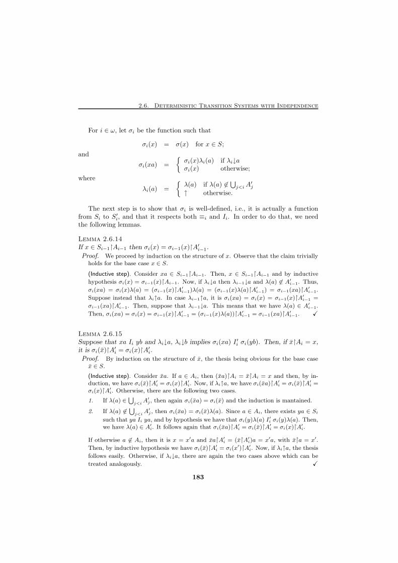
2.6. Deterministic Transition Systems with Independence
For i ∈ ω, let σi be the function such that
σi(x) = σ(x) for x ∈ S;
and
σi(xa) =
{σi(x)λi(a) if λi↓aσi(x) otherwise;
where
λi(a) =
{λ(a) if λ(a) 6∈
⋃j<iA
′j
↑ otherwise.
The next step is to show that σi is well-defined, i.e., it is actually a functionfrom Si to S′i, and that it respects both ≡i and Ii. In order to do that, we needthe following lemmas.
Lemma 2.6.14If x ∈ Si−1↾Ai−1 then σi(x) = σi−1(x)↾A′i−1.
Proof. We proceed by induction on the structure of x. Observe that the claim triviallyholds for the base case x ∈ S.
(Inductive step). Consider xa ∈ Si−1↾Ai−1. Then, x ∈ Si−1↾Ai−1 and by inductive
hypothesis σi(x) = σi−1(x)↾Ai−1. Now, if λi↓a then λi−1↓a and λ(a) 6∈ A′i−1. Thus,
σi(xa) = σi(x)λ(a) = (σi−1(x)↾A′i−1)λ(a) = (σi−1(x)λ(a)↾A′i−1) = σi−1(xa)↾A′i−1.
Suppose instead that λi↑a. In case λi−1↑a, it is σi(xa) = σi(x) = σi−1(x)↾A′i−1 =
σi−1(xa)↾A′i−1. Then, suppose that λi−1↓a. This means that we have λ(a) ∈ A′i−1.
Then, σi(xa) = σi(x) = σi−1(x)↾A′i−1 = (σi−1(x)λ(a))↾A′i−1 = σi−1(xa)↾A′i−1. X
Lemma 2.6.15Suppose that xa Ii yb and λi↓a, λi↓b implies σi(xa) I
′i σi(yb). Then, if x↾Ai = x,
it is σi(x)↾A′i = σi(x)↾A′i.Proof. By induction on the structure of x, the thesis being obvious for the base casex ∈ S.
(Inductive step). Consider xa. If a ∈ Ai, then (xa)↾Ai = x↾Ai = x and then, by in-duction, we have σi(x)↾A′i = σi(x)↾A′i. Now, if λi↑a, we have σi(xa)↾A′i = σi(x)↾A′i =σi(x)↾A′i. Otherwise, there are the following two cases.
1. If λ(a) ∈⋃j<i
A′j , then again σi(xa) = σi(x) and the induction is mantained.
2. If λ(a) 6∈⋃j<i
A′j , then σi(xa) = σi(x)λ(a). Since a ∈ Ai, there exists ya ∈ Si
such that ya Ii ya, and by hypothesis we have that σi(y)λ(a) I ′i σi(y)λ(a). Then,we have λ(a) ∈ A′i. It follows again that σi(xa)↾A′i = σi(x)↾A′i = σi(x)↾A′i.
If otherwise a 6∈ Ai, then it is x = x′a and xa↾A′i = (x↾A′i)a = x′a, with x↾a = x′.
Then, by inductive hypothesis we have σi(x)↾A′i = σi(x′)↾A′i. Now, if λi↑a, the thesis
follows easily. Otherwise, if λi↓a, there are again the two cases above which can be
treated analogously. X
183
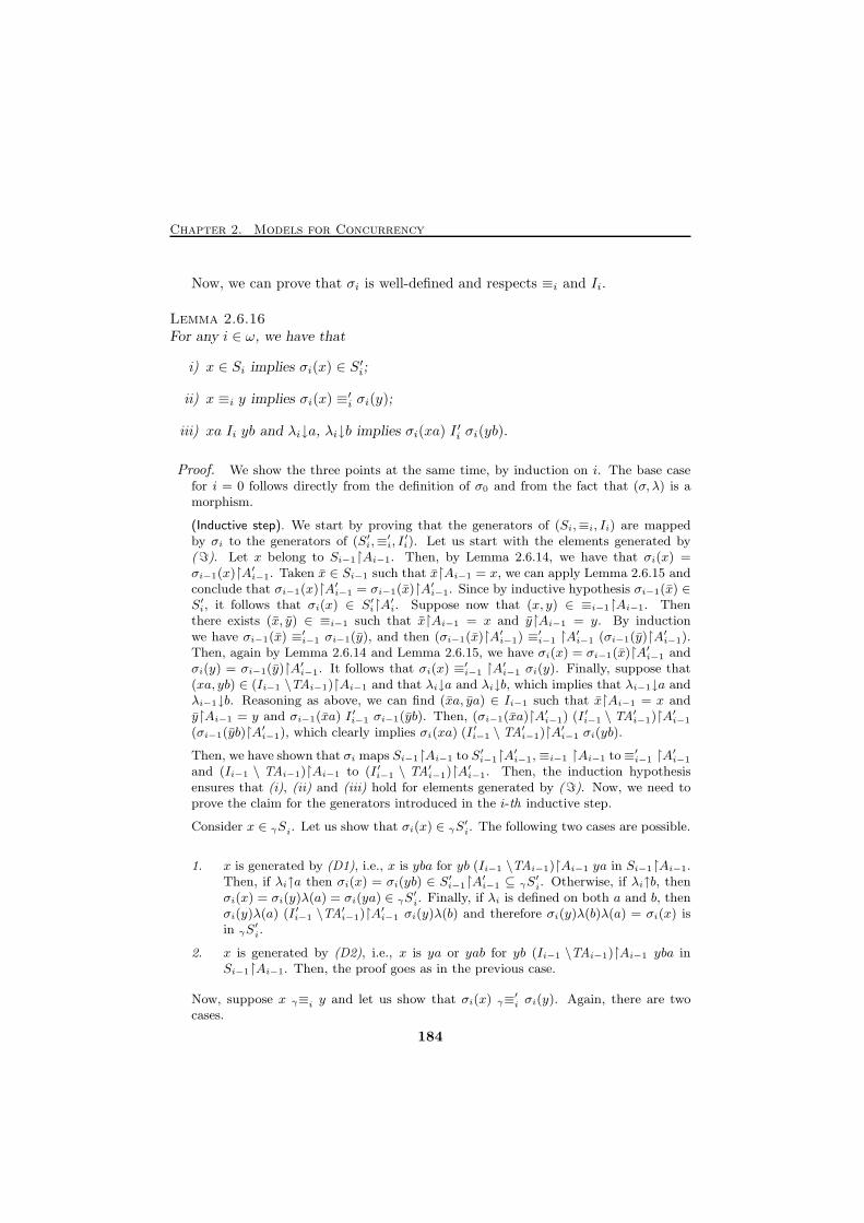
Chapter 2. Models for Concurrency
Now, we can prove that σi is well-defined and respects ≡i and Ii.
Lemma 2.6.16For any i ∈ ω, we have that
i) x ∈ Si implies σi(x) ∈ S′i;
ii) x ≡i y implies σi(x) ≡′i σi(y);
iii) xa Ii yb and λi↓a, λi↓b implies σi(xa) I′i σi(yb).
Proof. We show the three points at the same time, by induction on i. The base casefor i = 0 follows directly from the definition of σ0 and from the fact that (σ, λ) is amorphism.
(Inductive step). We start by proving that the generators of (Si,≡i, Ii) are mappedby σi to the generators of (S′i,≡
′i, I′i). Let us start with the elements generated by
(ℑ). Let x belong to Si−1↾Ai−1. Then, by Lemma 2.6.14, we have that σi(x) =σi−1(x)↾A′i−1. Taken x ∈ Si−1 such that x↾Ai−1 = x, we can apply Lemma 2.6.15 andconclude that σi−1(x)↾A′i−1 = σi−1(x)↾A′i−1. Since by inductive hypothesis σi−1(x) ∈S′i, it follows that σi(x) ∈ S′i↾A′i. Suppose now that (x, y) ∈ ≡i−1↾Ai−1. Thenthere exists (x, y) ∈ ≡i−1 such that x↾Ai−1 = x and y↾Ai−1 = y. By inductionwe have σi−1(x) ≡
′i−1 σi−1(y), and then (σi−1(x)↾A′i−1) ≡
′i−1 ↾A′i−1 (σi−1(y)↾A′i−1).
Then, again by Lemma 2.6.14 and Lemma 2.6.15, we have σi(x) = σi−1(x)↾A′i−1 andσi(y) = σi−1(y)↾A′i−1. It follows that σi(x) ≡
′i−1 ↾A′i−1 σi(y). Finally, suppose that
(xa, yb) ∈ (Ii−1 \TAi−1)↾Ai−1 and that λi↓a and λi↓b, which implies that λi−1↓a andλi−1↓b. Reasoning as above, we can find (xa, ya) ∈ Ii−1 such that x↾Ai−1 = x andy↾Ai−1 = y and σi−1(xa) I
′i−1 σi−1(yb). Then, (σi−1(xa)↾A′i−1) (I ′i−1 \ TA′i−1)↾A′i−1
(σi−1(yb)↾A′i−1), which clearly implies σi(xa) (I ′i−1 \ TA′i−1)↾A′i−1 σi(yb).
Then, we have shown that σi maps Si−1↾Ai−1 to S′i−1↾A′i−1, ≡i−1 ↾Ai−1 to≡′i−1 ↾A′i−1
and (Ii−1 \ TAi−1)↾Ai−1 to (I ′i−1 \ TA′i−1)↾A′i−1. Then, the induction hypothesisensures that (i), (ii) and (iii) hold for elements generated by (ℑ). Now, we need toprove the claim for the generators introduced in the i-th inductive step.
Consider x ∈ γSi. Let us show that σi(x) ∈ γS′i. The following two cases are possible.
1. x is generated by (D1), i.e., x is yba for yb (Ii−1 \TAi−1)↾Ai−1 ya in Si−1↾Ai−1.Then, if λi↑a then σi(x) = σi(yb) ∈ S
′i−1↾A′i−1 ⊆ γS
′i. Otherwise, if λi↑b, then
σi(x) = σi(y)λ(a) = σi(ya) ∈ γS′i. Finally, if λi is defined on both a and b, then
σi(y)λ(a) (I ′i−1 \TA′i−1)↾A′i−1 σi(y)λ(b) and therefore σi(y)λ(b)λ(a) = σi(x) isin γS
′i.
2. x is generated by (D2), i.e., x is ya or yab for yb (Ii−1 \TAi−1)↾Ai−1 yba inSi−1↾Ai−1. Then, the proof goes as in the previous case.
Now, suppose x γ≡i y and let us show that σi(x) γ≡′i σi(y). Again, there are two
cases.
184
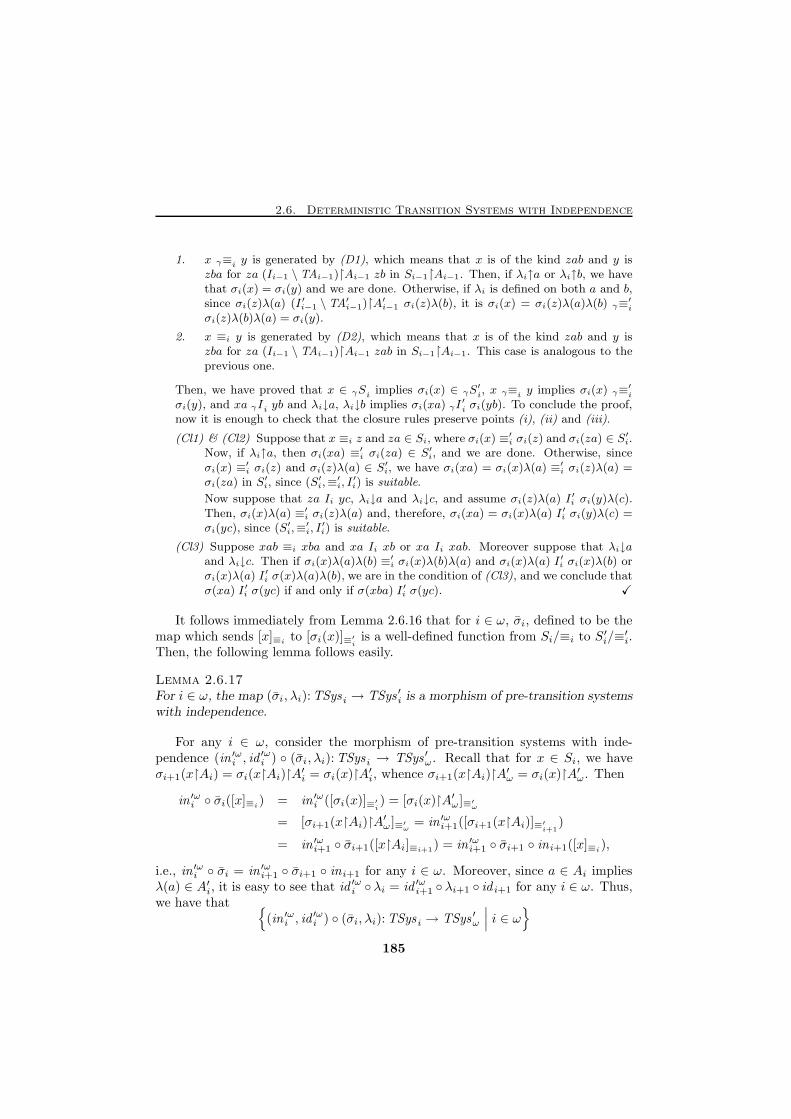
2.6. Deterministic Transition Systems with Independence
1. x γ≡i y is generated by (D1), which means that x is of the kind zab and y iszba for za (Ii−1 \ TAi−1)↾Ai−1 zb in Si−1↾Ai−1. Then, if λi↑a or λi↑b, we havethat σi(x) = σi(y) and we are done. Otherwise, if λi is defined on both a and b,since σi(z)λ(a) (I ′i−1 \ TA′i−1)↾A′i−1 σi(z)λ(b), it is σi(x) = σi(z)λ(a)λ(b) γ≡
′i
σi(z)λ(b)λ(a) = σi(y).
2. x ≡i y is generated by (D2), which means that x is of the kind zab and y iszba for za (Ii−1 \ TAi−1)↾Ai−1 zab in Si−1↾Ai−1. This case is analogous to theprevious one.
Then, we have proved that x ∈ γSi implies σi(x) ∈ γS′i, x γ≡i y implies σi(x) γ≡
′i
σi(y), and xa γIi yb and λi↓a, λi↓b implies σi(xa) γI′i σi(yb). To conclude the proof,
now it is enough to check that the closure rules preserve points (i), (ii) and (iii).
(Cl1) & (Cl2) Suppose that x ≡i z and za ∈ Si, where σi(x) ≡′i σi(z) and σi(za) ∈ S
′i.
Now, if λi↑a, then σi(xa) ≡′i σi(za) ∈ S′i, and we are done. Otherwise, since
σi(x) ≡′i σi(z) and σi(z)λ(a) ∈ S′i, we have σi(xa) = σi(x)λ(a) ≡′i σi(z)λ(a) =
σi(za) in S′i, since (S′i,≡′i, I′i) is suitable.
Now suppose that za Ii yc, λi↓a and λi↓c, and assume σi(z)λ(a) I ′i σi(y)λ(c).Then, σi(x)λ(a) ≡′i σi(z)λ(a) and, therefore, σi(xa) = σi(x)λ(a) I ′i σi(y)λ(c) =σi(yc), since (S′i,≡
′i, I′i) is suitable.
(Cl3) Suppose xab ≡i xba and xa Ii xb or xa Ii xab. Moreover suppose that λi↓aand λi↓c. Then if σi(x)λ(a)λ(b) ≡′i σi(x)λ(b)λ(a) and σi(x)λ(a) I ′i σi(x)λ(b) orσi(x)λ(a) I ′i σ(x)λ(a)λ(b), we are in the condition of (Cl3), and we conclude thatσ(xa) I ′i σ(yc) if and only if σ(xba) I ′i σ(yc). X
It follows immediately from Lemma 2.6.16 that for i ∈ ω, σi, defined to be themap which sends [x]≡i
to [σi(x)]≡′i
is a well-defined function from Si/≡i to S′i/≡′i.
Then, the following lemma follows easily.
Lemma 2.6.17For i ∈ ω, the map (σi, λi):TSysi → TSys ′i is a morphism of pre-transition systemswith independence.
For any i ∈ ω, consider the morphism of pre-transition systems with inde-pendence (in ′ωi , id
′ωi ) ◦ (σi, λi):TSysi → TSys ′ω. Recall that for x ∈ Si, we have
σi+1(x↾Ai) = σi(x↾Ai)↾A′i = σi(x)↾A′i, whence σi+1(x↾Ai)↾A′ω = σi(x)↾A′ω. Then
in ′ωi ◦ σi([x]≡i) = in ′ωi ([σi(x)]≡′
i) = [σi(x)↾A′ω ]≡′
ω
= [σi+1(x↾Ai)↾A′ω ]≡′ω
= in ′ωi+1([σi+1(x↾Ai)]≡′i+1
)
= in ′ωi+1 ◦ σi+1([x↾Ai]≡i+1) = in ′ωi+1 ◦ σi+1 ◦ ini+1([x]≡i),
i.e., in ′ωi ◦ σi = in ′ωi+1 ◦ σi+1 ◦ ini+1 for any i ∈ ω. Moreover, since a ∈ Ai impliesλ(a) ∈ A′i, it is easy to see that id ′ωi ◦λi = id ′ωi+1 ◦ λi+1 ◦ id i+1 for any i ∈ ω. Thus,we have that {
(in ′ωi , id′ωi ) ◦ (σi, λi):TSys i → TSys ′ω
∣∣∣ i ∈ ω}
185
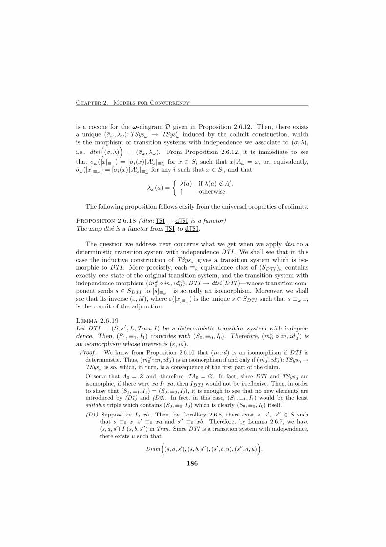
Chapter 2. Models for Concurrency
is a cocone for the ω-diagram D given in Proposition 2.6.12. Then, there existsa unique (σω, λω):TSysω → TSys ′ω induced by the colimit construction, whichis the morphism of transition systems with independence we associate to (σ, λ),
i.e., dtsi((σ, λ)
)= (σω , λω). From Proposition 2.6.12, it is immediate to see
that σω([x]≡ω) = [σi(x)↾A′ω ]≡′
ωfor x ∈ Si such that x↾Aω = x, or, equivalently,
σω([x]≡ω) = [σi(x)↾A′ω]≡′
ωfor any i such that x ∈ Si, and that
λω(a) =
{λ(a) if λ(a) 6∈ A′ω↑ otherwise.
The following proposition follows easily from the universal properties of colimits.
Proposition 2.6.18 ( dtsi : TSI→ dTSI is a functor)The map dtsi is a functor from TSI to dTSI.
The question we address next concerns what we get when we apply dtsi to adeterministic transition system with independence DTI . We shall see that in thiscase the inductive construction of TSysω gives a transition system which is iso-morphic to DTI . More precisely, each ≡ω-equivalence class of (SDTI )ω containsexactly one state of the original transition system, and the transition system withindependence morphism (inω0 ◦ in , idω0 ):DTI → dtsi(DTI )—whose transition com-ponent sends s ∈ SDTI to [s]≡ω
—is actually an isomorphism. Moreover, we shallsee that its inverse (ε, id), where ε([x]≡ω
) is the unique s ∈ SDTI such that s ≡ω x,is the counit of the adjunction.
Lemma 2.6.19Let DTI = (S, sI , L,Tran, I) be a deterministic transition system with indepen-dence. Then, (S1,≡1, I1) coincides with (S0,≡0, I0). Therefore, (inω0 ◦ in , idω0 ) isan isomorphism whose inverse is (ε, id).
Proof. We know from Proposition 2.6.10 that (in, id) is an isomorphism if DTI isdeterministic. Thus, (inω0 ◦in , id
ω0 ) is an isomorphism if and only if (inω0 , id
ω0 ):TSys0 →
TSysω is so, which, in turn, is a consequence of the first part of the claim.
Observe that A0 = ∅ and, therefore, TA0 = ∅. In fact, since DTI and TSys0 areisomorphic, if there were xa I0 xa, then IDTI would not be irreflexive. Then, in orderto show that (S1,≡1, I1) = (S0,≡0, I0), it is enough to see that no new elements areintroduced by (D1) and (D2). In fact, in this case, (S1,≡1, I1) would be the leastsuitable triple which contains (S0,≡0, I0) which is clearly (S0,≡0, I0) itself.
(D1) Suppose xa I0 xb. Then, by Corollary 2.6.8, there exist s, s′, s′′ ∈ S suchthat s ≡0 x, s′ ≡0 xa and s′′ ≡0 xb. Therefore, by Lemma 2.6.7, we have(s, a, s′) I (s, b, s′′) in Tran . Since DTI is a transition system with independence,there exists u such that
Diam((s, a, s′), (s, b, s′′), (s′, b, u), (s′′, a, u)
),
186
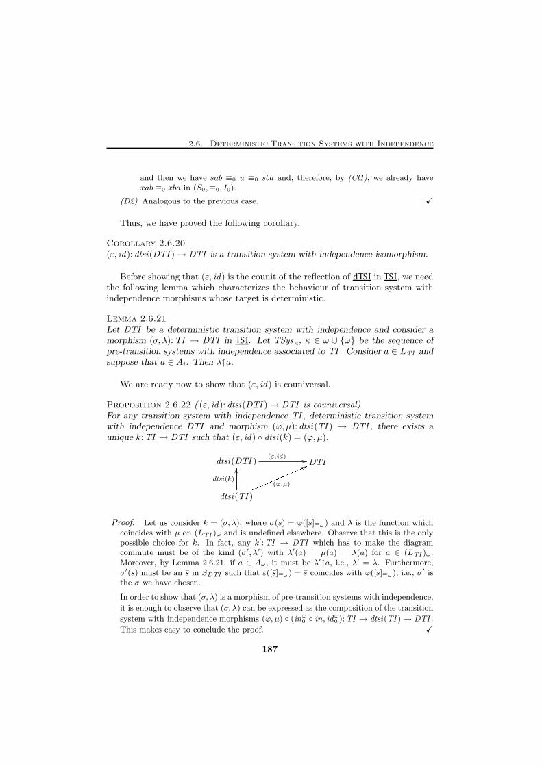
2.6. Deterministic Transition Systems with Independence
and then we have sab ≡0 u ≡0 sba and, therefore, by (Cl1), we already havexab ≡0 xba in (S0,≡0, I0).
(D2) Analogous to the previous case. X
Thus, we have proved the following corollary.
Corollary 2.6.20(ε, id): dtsi(DTI )→ DTI is a transition system with independence isomorphism.
Before showing that (ε, id) is the counit of the reflection of dTSI in TSI, we needthe following lemma which characterizes the behaviour of transition system withindependence morphisms whose target is deterministic.
Lemma 2.6.21Let DTI be a deterministic transition system with independence and consider amorphism (σ, λ):TI → DTI in TSI. Let TSysκ, κ ∈ ω ∪ {ω} be the sequence ofpre-transition systems with independence associated to TI . Consider a ∈ LTI andsuppose that a ∈ Ai. Then λ↑a.
We are ready now to show that (ε, id) is couniversal.
Proposition 2.6.22 ( (ε, id): dtsi(DTI )→ DTI is couniversal)For any transition system with independence TI , deterministic transition systemwith independence DTI and morphism (ϕ, µ): dtsi(TI ) → DTI , there exists aunique k:TI → DTI such that (ε, id) ◦ dtsi(k) = (ϕ, µ).
dtsi(DTI ) DTI
dtsi(TI )
(ε,id) //
dtsi(k)
OO
(ϕ,µ)mmmmmmmmmmmmm66Proof. Let us consider k = (σ, λ), where σ(s) = ϕ([s]≡ω ) and λ is the function which
coincides with µ on (LTI )ω and is undefined elsewhere. Observe that this is the onlypossible choice for k. In fact, any k′:TI → DTI which has to make the diagramcommute must be of the kind (σ′, λ′) with λ′(a) = µ(a) = λ(a) for a ∈ (LTI )ω.Moreover, by Lemma 2.6.21, if a ∈ Aω, it must be λ′↑a, i.e., λ′ = λ. Furthermore,σ′(s) must be an s in SDTI such that ε([s]≡ω ) = s coincides with ϕ([s]≡ω ), i.e., σ′ isthe σ we have chosen.
In order to show that (σ, λ) is a morphism of pre-transition systems with independence,
it is enough to observe that (σ, λ) can be expressed as the composition of the transition
system with independence morphisms (ϕ, µ) ◦ (inω0 ◦ in, idω0 ):TI → dtsi(TI )→ DTI .
This makes easy to conclude the proof. X
187
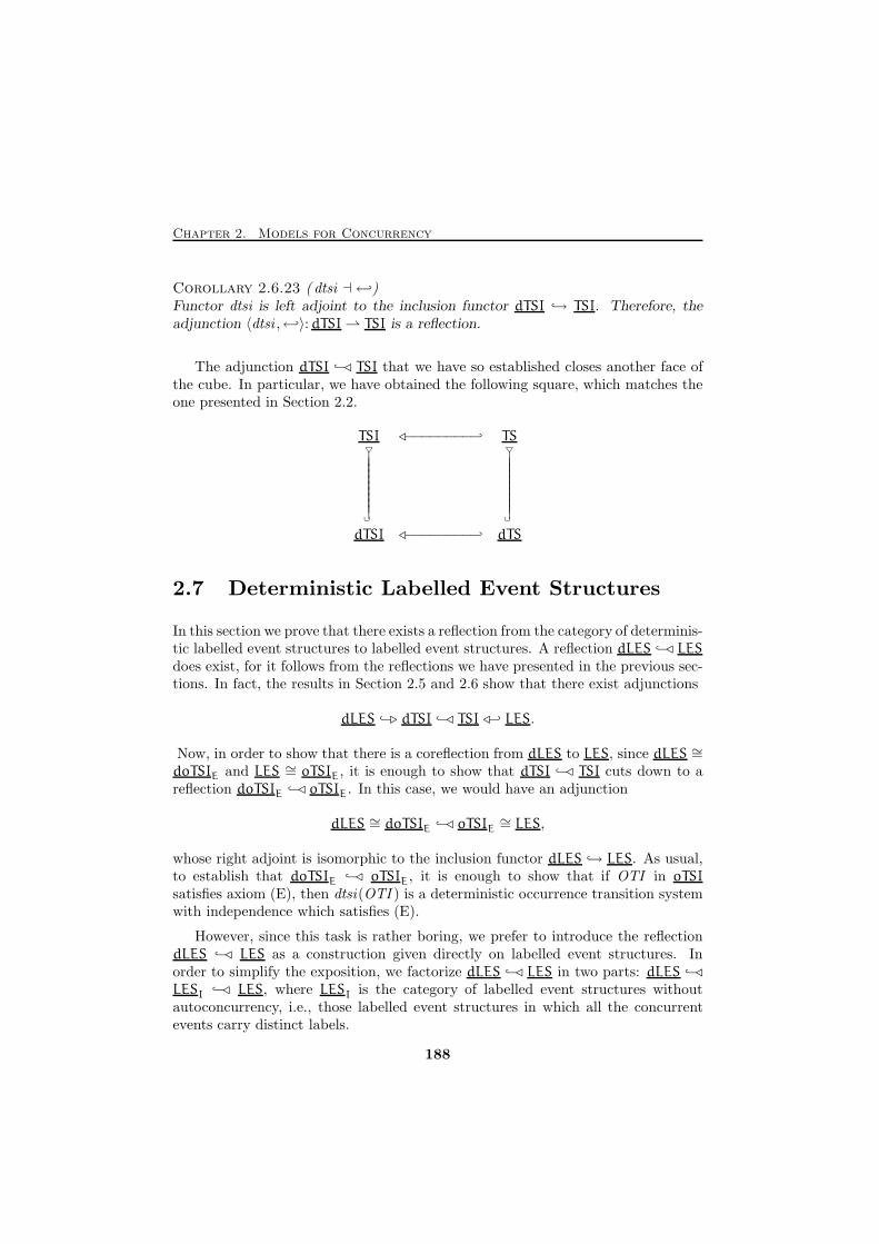
Chapter 2. Models for Concurrency
Corollary 2.6.23 ( dtsi ⊣ ←)Functor dtsi is left adjoint to the inclusion functor dTSI → TSI. Therefore, theadjunction 〈dtsi , ←〉: dTSI ⇀ TSI is a reflection.
The adjunction dTSI −⊳ TSI that we have so established closes another face ofthe cube. In particular, we have obtained the following square, which matches theone presented in Section 2.2.
TSI ⊳−−−−−−−−− TS▽
||||||||||∪
▽
||||||||||∪
dTSI ⊳−−−−−−−−− dTS
2.7 Deterministic Labelled Event Structures
In this section we prove that there exists a reflection from the category of determinis-tic labelled event structures to labelled event structures. A reflection dLES −⊳ LES
does exist, for it follows from the reflections we have presented in the previous sec-tions. In fact, the results in Section 2.5 and 2.6 show that there exist adjunctions
dLES −⊲ dTSI −⊳ TSI ⊳− LES.
Now, in order to show that there is a coreflection from dLES to LES, since dLES ∼=doTSIE and LES ∼= oTSIE, it is enough to show that dTSI −⊳ TSI cuts down to areflection doTSIE −⊳ oTSIE. In this case, we would have an adjunction
dLES ∼= doTSIE −⊳ oTSIE∼= LES,
whose right adjoint is isomorphic to the inclusion functor dLES → LES. As usual,to establish that doTSIE −⊳ oTSIE, it is enough to show that if OTI in oTSI
satisfies axiom (E), then dtsi(OTI ) is a deterministic occurrence transition systemwith independence which satisfies (E).
However, since this task is rather boring, we prefer to introduce the reflectiondLES −⊳ LES as a construction given directly on labelled event structures. Inorder to simplify the exposition, we factorize dLES −⊳ LES in two parts: dLES −⊳LESI −⊳ LES, where LESI is the category of labelled event structures withoutautoconcurrency, i.e., those labelled event structures in which all the concurrentevents carry distinct labels.
188
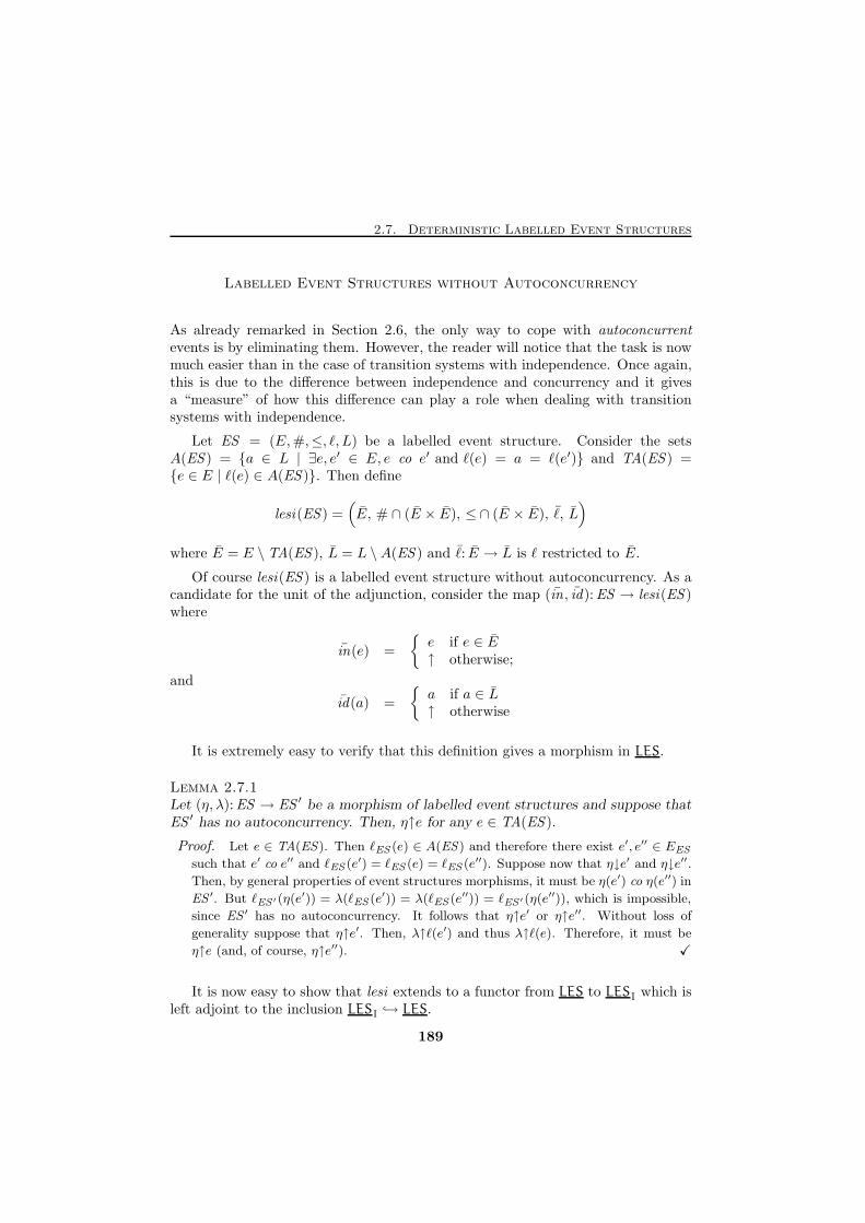
2.7. Deterministic Labelled Event Structures
Labelled Event Structures without Autoconcurrency
As already remarked in Section 2.6, the only way to cope with autoconcurrentevents is by eliminating them. However, the reader will notice that the task is nowmuch easier than in the case of transition systems with independence. Once again,this is due to the difference between independence and concurrency and it givesa “measure” of how this difference can play a role when dealing with transitionsystems with independence.
Let ES = (E,#,≤, ℓ, L) be a labelled event structure. Consider the setsA(ES ) = {a ∈ L | ∃e, e′ ∈ E, e co e′ and ℓ(e) = a = ℓ(e′)} and TA(ES ) ={e ∈ E | ℓ(e) ∈ A(ES )}. Then define
lesi(ES ) =(E, # ∩ (E × E), ≤ ∩ (E × E), ℓ, L
)
where E = E \ TA(ES ), L = L \A(ES ) and ℓ: E → L is ℓ restricted to E.
Of course lesi(ES ) is a labelled event structure without autoconcurrency. As acandidate for the unit of the adjunction, consider the map (in , id):ES → lesi(ES )where
in(e) =
{e if e ∈ E↑ otherwise;
and
id(a) =
{a if a ∈ L↑ otherwise
It is extremely easy to verify that this definition gives a morphism in LES.
Lemma 2.7.1Let (η, λ):ES → ES ′ be a morphism of labelled event structures and suppose thatES ′ has no autoconcurrency. Then, η↑e for any e ∈ TA(ES ).
Proof. Let e ∈ TA(ES). Then ℓES (e) ∈ A(ES) and therefore there exist e′, e′′ ∈ EES
such that e′ co e′′ and ℓES (e′) = ℓES (e) = ℓES (e′′). Suppose now that η↓e′ and η↓e′′.
Then, by general properties of event structures morphisms, it must be η(e′) co η(e′′) in
ES ′. But ℓES ′(η(e′)) = λ(ℓES (e′)) = λ(ℓES (e′′)) = ℓES ′(η(e′′)), which is impossible,
since ES ′ has no autoconcurrency. It follows that η↑e′ or η↑e′′. Without loss of
generality suppose that η↑e′. Then, λ↑ℓ(e′) and thus λ↑ℓ(e). Therefore, it must be
η↑e (and, of course, η↑e′′). X
It is now easy to show that lesi extends to a functor from LES to LESI which isleft adjoint to the inclusion LESI → LES.
189

Chapter 2. Models for Concurrency
Proposition 2.7.2 ( (in , id):ES → lesi(ES ) is universal)For any labelled event structure ES , any labelled event structure without au-toconcurrency ES ′ and any morphism (η, λ):ES → ES ′, there exists a unique(η, λ): lesi(ES )→ ES ′ in LESI such that (η, λ) ◦ (in , id) = (η, λ).
ES lesi(ES )
ES ′
(in,id) //
(η,λ)
PPPPPPPPPPPPP(( (η,λ)
��
Proof. Consider η: EES → EES ′ and λ: LES → LES ′ to be, respectively, η restricted
to EES and λ restricted to LES . Exploiting Lemma 2.7.1 it is not difficult to conclude
the proof. X
Therefore, we have the following corollary.
Corollary 2.7.3 ( lesi ⊣ ←)The map lesi extends to a functor from LES to LESI which is left adjoint to theinclusion functor LESI → LES. Therefore, the adjunction 〈lesi , ←〉: LES ⇀ LESI isa reflection.
Deterministic Labelled Event Structures
Let us now turn our attention to dLES −⊳ LESI. Given a labelled event structurewithout autoconcurrency ES = (E,≤,#, ℓ, L), consider the sequence of relations(∼i,≤i,#i), for i ∈ ω, where
• ∼0 ={(e, e)
∣∣∣ e ∈ E}; ≤0 = ≤; #0 = #;
and, for i > 0,
• ∼i is the least equivalence on E such that
i) ∼i−1 ⊆ ∼i;
ii) e 6≤i−1 e′, e′ 6≤i−1 e, ℓ(e) = ℓ(e′)
⌊e⌋≤i−1
/#i−1⌊e′⌋≤i−1
\ {e′} and
⌊e⌋≤i−1
/#i−1⌊e′⌋≤i−1
\ {e′}
implies e ∼i e′,
where ⌊e⌋≤iis a shorthand for {e′ ∈ E | e′ ≤i e} and, for x, y ⊆ E, x
/#iy
stands for ∀ e ∈ x, ∀ e′ ∈ y, not e #i e′.
190
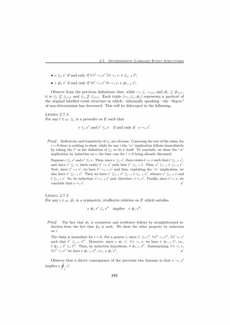
2.7. Deterministic Labelled Event Structures
• e ≤i e′ if and only if ∀ e′ ∼i e′ ∃ e ∼i e. e ≤i−1 e′;
• e #i e′ if and only if ∀e′ ∼i e′ ∀e ∼i e. e #i−1 e
′;
Observe from the previous definitions that, while ∼i ⊆ ∼i+1 and #i ⊇ #i+1,it is ≤i * ≤i+1 and ≤i + ≤i+1. Each triple (∼i,≤i,#i) represents a quotient ofthe original labelled event structure in which—informally speaking—the “degree”of non-determinism has decreased. This will be delevoped in the following.
Lemma 2.7.4For any i ∈ ω, ≤i is a preorder on E such that
e ≤i e′ and e′ ≤i e if and only if e ∼i e
′.
Proof. Reflexivity and transitivity of≤i are obvious. Concernig the rest of the claim, fori = 0 there is nothing to show, while for any i the ‘⇐’ implication follows immediatelyby taking the e′ in the definition of ≤i to be e itself. To conclude, we show the ‘⇒’implication by induction on i, the base case for i = 0 being already discussed.
Suppose e ≤i e′ and e′ ≤i e. Then, since e ≤i e
′, there exists e ∼i e such that e ≤i−1 e′,
and since e′ ≤i e, there exists e′ ∼i e′ such that e′ ≤i−1 e. Thus, e′ ≤i−1 e ≤i−1 e
′.
Now, since e′ ∼i e′, we have e′ ∼i−1 e
′ and thus, exploiting the ‘⇐’ implication, we
also have e′ ≤i−1 e′. Then we have e′ ≤i−1 e
′ ≤i−1 e ≤i−1 e′, whence e′ ≤i−1 e and
e ≤i−1 e′. So, by induction, e ∼i−1 e
′ and, therefore, e ∼i e′. Finally, since e ∼i e, we
conclude that e ∼i e′. X
Lemma 2.7.5For any i ∈ ω, #i is a symmetric, irreflexive relation on E which satisfies
e #i e′ ≤i e
′′ implies e #i e′′.
Proof. The fact that #i is symmetric and irreflexive follows by straightforward in-duction from the fact that #0 is such. We show the other property by inductionon i.
The claim is immediate for i = 0. For a generic i, since e′ ≤i e′′, ∀ e′′ ∼i e
′′, ∃ e′ ∼i e′
such that e′ ≤i−1 e′′. Moreover, since e #i e′, ∀ e ∼i e, we have e #i−1 e′, i.e.,
e #i−1 e′ ≤i e
′′. Then, by induction hypothesis, e #i−1 e′′. Summarizing, ∀ e ∼i e,
∀ e′′ ∼i e′′ we have e #i−1 e
′′, i.e., e #i e′′. X
Observe that a direct consequence of the previous two lemmas is that e ∼i e′
implies e/#ie′.
191
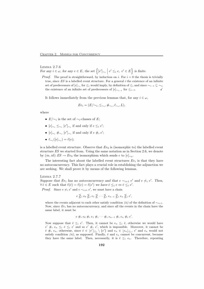
Chapter 2. Models for Concurrency
Lemma 2.7.6For any i ∈ ω, for any e ∈ E, the set
{[e′]∼i
∣∣∣ e′ ≤i e, e′ ∈ E}
is finite.
Proof. The proof is straightforward, by induction on i. For i = 0 the thesis is trivially
true, since ES is a labelled event structure. For a general i the existence of an infinite
set of predecessors of [e]∼i for ≤i would imply, by definition of ≤i and since ∼i−1 ⊆ ∼i,
the existence of an infinite set of predecessors of [e]∼i−1 for ≤i−1. X
It follows immediately from the previous lemmas that, for any i ∈ ω,
Ev i = (E/∼i,≤∼i,#∼i
, ℓ∼i, L),
where
• E/∼i is the set of ∼i-classes of E;
• [e]∼i≤∼i
[e′]∼iif and only if e ≤i e
′;
• [e]∼i#∼i
[e′]∼iif and only if e #i e
′;
• ℓ∼i([e]∼i
) = ℓ(e);
is a labelled event structure. Observe that Ev0 is (isomorphic to) the labelled eventstructure ES we started from. Using the same notation as in Section 2.6, we denoteby (in , id):ES → Ev0 the isomorphism which sends e to [e]∼0 .
The interesting fact about the labelled event structures Ev i is that they haveno autoconcurrency. This fact plays a crucial role in establishing the adjunction weare seeking. We shall prove it by means of the following lemmas.
Lemma 2.7.7Suppose that Ev i has no autoconcurrency and that e ∼i+1 e
′ and e 6∼i e′. Then,∀ e ∈ E such that ℓ(e) = ℓ(e) = ℓ(e′) we have e ≤i e⇔ e ≤i e′.
Proof. Since e 6∼i e′ and e ∼i+1 e
′, we must have a chain
e 6⋚i e0 6⋚i e1 6⋚ · · · 6⋚i en−1 6⋚i en 6⋚i e′,
where the events adjacent to each other satisfy condition (ii) of the definition of ∼i+1.Now, since Ev i has no autoconcurrency, and since all the events in the chain have thesame label, it must be
e #i e0 #i e1 #i · · · #i en−1 #i en #i e′.
Now suppose that e ≤i e′. Then, it cannot be en ≤i e, otherwise we would have
e′ #i en ≤i e ≤i e′ and so e′ #i e
′, which is impossible. Moreover, it cannot bee #i en, otherwise, since e ∈ ⌊e′⌋≤i
\ {e′} and en ∈ ⌊en⌋≤i, e′ and en would not
satisfy condition (ii), as supposed. Finally, e and en cannot be concurrent, becausethey have the same label. Then, necessarily, it is e ≤i en. Therefore, repeating
192
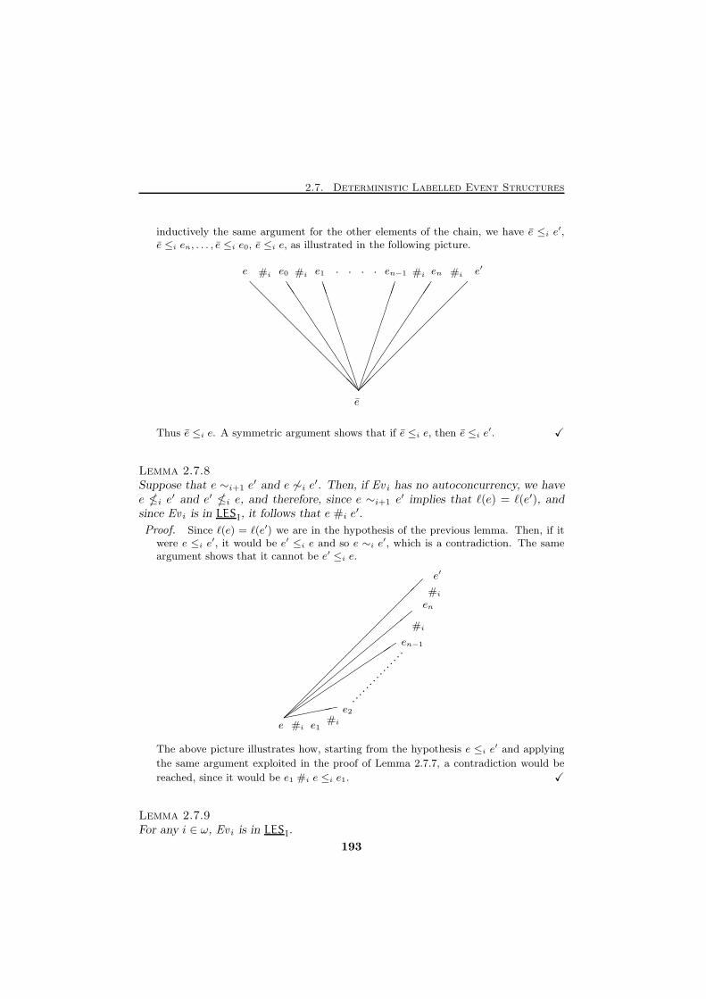
2.7. Deterministic Labelled Event Structures
inductively the same argument for the other elements of the chain, we have e ≤i e′,
e ≤i en, . . . , e ≤i e0, e ≤i e, as illustrated in the following picture.
BBBBBBBBBB
����������
JJJJJJJJJJ@
@@@@@@@@@
����������
. . . .
e′enen−1
e
e1e0e #i #i #i #i
Thus e ≤i e. A symmetric argument shows that if e ≤i e, then e ≤i e′. X
Lemma 2.7.8Suppose that e ∼i+1 e
′ and e 6∼i e′. Then, if Ev i has no autoconcurrency, we havee �i e
′ and e′ �i e, and therefore, since e ∼i+1 e′ implies that ℓ(e) = ℓ(e′), and
since Ev i is in LESI, it follows that e #i e′.
Proof. Since ℓ(e) = ℓ(e′) we are in the hypothesis of the previous lemma. Then, if itwere e ≤i e
′, it would be e′ ≤i e and so e ∼i e′, which is a contradiction. The same
argument shows that it cannot be e′ ≤i e.
,,,,,,,,,,,
������������
...............
����������
e e1
e2
en−1
en
e′
#i#i
#i
#i
The above picture illustrates how, starting from the hypothesis e ≤i e′ and applying
the same argument exploited in the proof of Lemma 2.7.7, a contradiction would be
reached, since it would be e1 #i e ≤i e1. X
Lemma 2.7.9For any i ∈ ω, Ev i is in LESI.
193
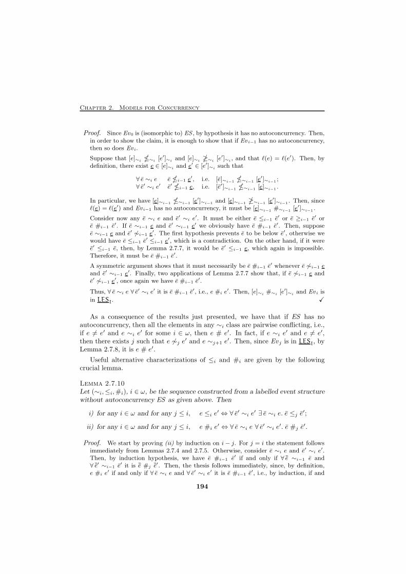
Chapter 2. Models for Concurrency
Proof. Since Ev0 is (isomorphic to) ES , by hypothesis it has no autoconcurrency. Then,in order to show the claim, it is enough to show that if Ev i−1 has no autoconcurrency,then so does Ev i.
Suppose that [e]∼i �∼i [e′]∼i and [e]∼i �∼i [e′]∼i , and that ℓ(e) = ℓ(e′). Then, bydefinition, there exist e ∈ [e]∼i and e′ ∈ [e′]∼i such that
∀ e ∼i e e �i−1 e′, i.e. [e]∼i−1 �∼i−1 [e′]∼i−1 ;
∀ e′ ∼i e′ e′ �i−1 e, i.e. [e′]∼i−1 �∼i−1 [e]∼i−1 .
In particular, we have [e]∼i−1 �∼i−1 [e′]∼i−1 and [e]∼i−1 �∼i−1 [e′]∼i−1 . Then, sinceℓ(e) = ℓ(e′) and Ev i−1 has no autoconcurrency, it must be [e]∼i−1 #∼i−1 [e′]∼i−1 .
Consider now any e ∼i e and e′ ∼i e′. It must be either e ≤i−1 e
′ or e ≥i−1 e′ or
e #i−1 e′. If e ∼i−1 e and e′ ∼i−1 e
′ we obviously have e #i−1 e′. Then, suppose
e ∼i−1 e and e′ 6∼i−1 e′. The first hypothesis prevents e to be below e′, otherwise we
would have e ≤i−1 e′ ≤i−1 e
′, which is a contradiction. On the other hand, if it weree′ ≤i−1 e, then, by Lemma 2.7.7, it would be e′ ≤i−1 e, which again is impossible.Therefore, it must be e #i−1 e
′.
A symmetric argument shows that it must necessarily be e #i−1 e′ whenever e 6∼i−1 e
and e′ ∼i−1 e′. Finally, two applications of Lemma 2.7.7 show that, if e 6∼i−1 e and
e′ 6∼i−1 e′, once again we have e #i−1 e
′.
Thus, ∀ e ∼i e ∀ e′ ∼i e
′ it is e #i−1 e′, i.e., e #i e
′. Then, [e]∼i #∼i [e′]∼i and Ev i is
in LESI. X
As a consequence of the results just presented, we have that if ES has noautoconcurrency, then all the elements in any ∼i class are pairwise conflicting, i.e.,if e 6= e′ and e ∼i e′ for some i ∈ ω, then e # e′. In fact, if e ∼i e′ and e 6= e′,then there exists j such that e 6∼j e
′ and e ∼j+1 e′. Then, since Ev j is in LESI, by
Lemma 2.7.8, it is e # e′.
Useful alternative characterizations of ≤i and #i are given by the followingcrucial lemma.
Lemma 2.7.10Let (∼i,≤i,#i), i ∈ ω, be the sequence constructed from a labelled event structurewithout autoconcurrency ES as given above. Then
i) for any i ∈ ω and for any j ≤ i, e ≤i e′ ⇔ ∀ e′ ∼i e
′ ∃ e ∼i e. e ≤j e′;
ii) for any i ∈ ω and for any j ≤ i, e #i e′ ⇔ ∀ e ∼i e ∀ e′ ∼i e′. e #j e
′.
Proof. We start by proving (ii) by induction on i− j. For j = i the statement followsimmediately from Lemmas 2.7.4 and 2.7.5. Otherwise, consider e ∼i e and e′ ∼i e
′.Then, by induction hypothesis, we have e #i−1 e′ if and only if ∀ ¯e ∼i−1 e and∀ ¯e′ ∼i−1 e
′ it is ¯e #j ¯e′. Then, the thesis follows immediately, since, by definition,e #i e
′ if and only if ∀ e ∼i e and ∀ e′ ∼i e′ it is e #i−1 e
′, i.e., by induction, if and
194
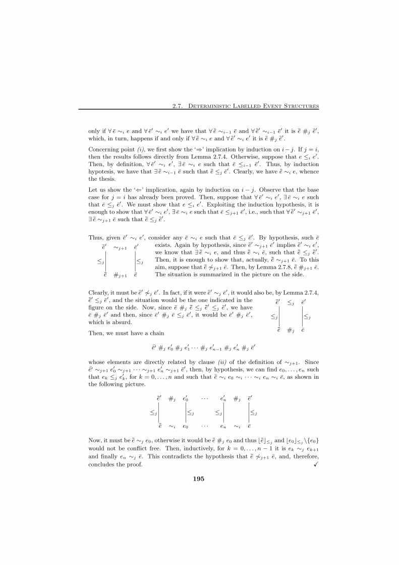
2.7. Deterministic Labelled Event Structures
only if ∀ e ∼i e and ∀ e′ ∼i e′ we have that ∀ ¯e ∼i−1 e and ∀ ¯e′ ∼i−1 e
′ it is ¯e #j ¯e′,which, in turn, happens if and only if ∀ ¯e ∼i e and ∀ ¯e′ ∼i e
′ it is ¯e #j ¯e′.
Concerning point (i), we first show the ‘⇒’ implication by induction on i− j. If j = i,then the results follows directly from Lemma 2.7.4. Otherwise, suppose that e ≤i e
′.Then, by definition, ∀ e′ ∼i e
′, ∃ e ∼i e such that e ≤i−1 e′. Thus, by inductionhypotesis, we have that ∃ ¯e ∼i−1 e such that ¯e ≤j e
′. Clearly, we have ¯e ∼i e, whencethe thesis.
Let us show the ‘⇐’ implication, again by induction on i − j. Observe that the basecase for j = i has already been proved. Then, suppose that ∀ e′ ∼i e
′, ∃ e ∼i e suchthat e ≤j e
′. We must show that e ≤i e′. Exploiting the induction hypothesis, it is
enough to show that ∀ e′ ∼i e′, ∃ e ∼i e such that e ≤j+1 e
′, i.e., such that ∀ ¯e′ ∼j+1 e′,
∃ ¯e ∼j+1 e such that ¯e ≤j ¯e′.
¯e′ ∼j+1 e′
≤j
∣∣∣∣∣
∣∣∣∣∣≤j
¯e #j+1 e
Thus, given e′ ∼i e′, consider any e ∼i e such that e ≤j e
′. By hypothesis, such eexists. Again by hypothesis, since ¯e′ ∼j+1 e
′ implies ¯e′ ∼i e′,
we know that ∃ ¯e ∼i e, and thus ¯e ∼i e, such that ¯e ≤j ¯e′.Then, it is enough to show that, actually, ¯e ∼j+1 e. To thisaim, suppose that ¯e 6∼j+1 e. Then, by Lemma 2.7.8, ¯e #j+1 e.The situation is summarized in the picture on the side.
¯e′ ≤j e′
≤j
∣∣∣∣∣
∣∣∣∣∣≤j
¯e #j e
Clearly, it must be ¯e′ 6∼j e′. In fact, if it were ¯e′ ∼j e
′, it would also be, by Lemma 2.7.4,¯e′ ≤j e
′, and the situation would be the one indicated in thefigure on the side. Now, since e #j ¯e ≤j ¯e′ ≤j e
′, we havee #j e
′ and then, since e′ #j e ≤j e′, it would be e′ #j e
′,which is absurd.
Then, we must have a chain
¯e′ #j e′0 #j e
′1 · · · #j e
′n−1 #j e
′n #j e
′
whose elements are directly related by clause (ii) of the definition of ∼j+1. Since¯e′ ∼j+1 e
′0 ∼j+1 · · · ∼j+1 e
′n ∼j+1 e
′, then, by hypothesis, we can find e0, . . . , en suchthat ek ≤j e
′k, for k = 0, . . . , n and such that ¯e ∼i e0 ∼i · · · ∼i en ∼i e, as shown in
the following picture.
¯e′ #j e′0 · · · e′n #j e′
≤j
∣∣∣∣∣
∣∣∣∣∣≤j ≤j
∣∣∣∣∣
∣∣∣∣∣≤j
¯e ∼i e0 · · · en ∼i e
Now, it must be ¯e ∼j e0, otherwise it would be ¯e #j e0 and thus ⌊¯e⌋≤jand ⌊e0⌋≤j
\{e0}
would not be conflict free. Then, inductively, for k = 0, . . . , n − 1 it is ek ∼j ek+1
and finally en ∼j e. This contradicts the hypothesis that ¯e 6∼j+1 e, and, therefore,
concludes the proof. X
195
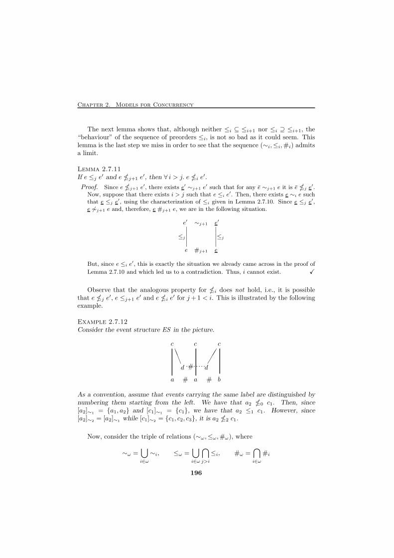
Chapter 2. Models for Concurrency
The next lemma shows that, although neither ≤i ⊆ ≤i+1 nor ≤i ⊇ ≤i+1, the“behaviour” of the sequence of preorders ≤i, is not so bad as it could seem. Thislemma is the last step we miss in order to see that the sequence (∼i,≤i,#i) admitsa limit.
Lemma 2.7.11If e ≤j e′ and e �j+1 e
′, then ∀ i > j. e �i e′.
Proof. Since e �j+1 e′, there exists e′ ∼j+1 e
′ such that for any e ∼j+1 e it is e �j e′.
Now, suppose that there exists i > j such that e ≤i e′. Then, there exists e ∼i e such
that e ≤j e′, using the characterization of ≤i given in Lemma 2.7.10. Since e ≤j e
′,e 6∼j+1 e and, therefore, e #j+1 e, we are in the following situation.
e′ ∼j+1 e′
≤j
∣∣∣∣∣
∣∣∣∣∣≤j
e #j+1 e
But, since e ≤i e′, this is exactly the situation we already came across in the proof of
Lemma 2.7.10 and which led us to a contradiction. Thus, i cannot exist. X
Observe that the analogous property for �i does not hold, i.e., it is possiblethat e �j e
′, e ≤j+1 e′ and e �i e
′ for j+1 < i. This is illustrated by the followingexample.
Example 2.7.12Consider the event structure ES in the picture.
LLL
���
. . . . . . . .
a
c
d d
a
c
b
c
#
# #
As a convention, assume that events carrying the same label are distinguished bynumbering them starting from the left. We have that a2 �0 c1. Then, since[a2]∼1 = {a1, a2} and [c1]∼1 = {c1}, we have that a2 ≤1 c1. However, since[a2]∼2 = [a2]∼1 while [c1]∼2 = {c1, c2, c3}, it is a2 �2 c1.
Now, consider the triple of relations (∼ω,≤ω,#ω), where
∼ω =⋃
i∈ω
∼i, ≤ω =⋃
i∈ω
⋂
j>i
≤i, #ω =⋂
i∈ω
#i
196
2.7. Deterministic Labelled Event Structures
or, equivalenty, ≤ω is defined by
e ≤ω e′ if and only if ∃ k ∀ i > k e ≤i e
′.
Thanks to Lemma 2.7.11, it is immediate to show that ≤ω enjoys the followingrelevant property.
Lemma 2.7.13e �ω e
′ if and only if ∃ k. ∀ i > k e �i e′.
Proof. By definition, e �ω e′ if and only if ∀ k ∃ i > k. e �i e′. Then, the ‘⇐’
implication is obviously true. Suppose that e �ω e′ and for k = 0 let i0 be the first
index such that e �i0 e′. Now, if ∀ i > i0 it is e �i e
′ we are done. Otherwise let
k0 > i0 be an index such that e ≤k0 e′. Then, we can find i1 > k0 such that e �i1 e
′
and, from Lemma 2.7.11, we know that ∀ i > i1 it must be e �i e′. X
The following characterization of ≤ω derives easily from Lemma 2.7.10 andLemma 2.7.13.
Lemma 2.7.14For any j ∈ ω, e ≤ω e′ if and only if ∀ e′ ∼ω e′ ∃ e ∼ω e. e ≤j e′.
Proof. Suppose that e ≤ω e′. Then, there exists k such that for any i > k it is e ≤i e
′.Then, chosen any j and exploiting Lemma 2.7.10, ∀ i > max{j, k} ∀ e′ ∼i e
′ ∃ e ∼ie. e ≤j e
′, whence it immediately follows that ∀ e′ ∼ω e′ ∃ e ∼ω e. e ≤j e
′.
In order to show the inverse implication, we start by showing that, if ∀ e′ ∼ω e′ ∃ e ∼ω e
such that e ≤j e′ holds for a particular j, then it holds for all j ∈ ω. It is immediately
clear from the definitions that
∀ e′ ∼ω e′ ∃ e ∼ω e. e ≤j e
′ implies ∀ e′ ∼ω e′ ∃ e ∼ω e. e ≤j−1 e
′.
Therefore, it is enough to show—with a proof similar to the one of Lemma 2.7.10—that
∀ e′ ∼ω e′ ∃ e ∼ω e. e ≤j e
′ implies ∀ e′ ∼ω e′ ∃ e ∼ω e. e ≤j+1 e
′.
Consider e′ ∼ω e. Then, we know that ∃ e ∼ω e such that e ≤j e′. Now, for any
¯e′ ∼j+1 e′, again from the hypothesis, we can find ¯e ∼ω e ∼ω e such that ¯e ≤j ¯e′.
Now, assuming that ¯e #j+1 e and reasoning as in the proof of Lemma 2.7.10 wouldlead to a contradiction. Therefore, it must be ¯e ∼j+1 e. Then, we have shown that∀ ¯e′ ∼j+1 e′ ∃ ¯e ∼j−1 e such that ¯e ≤j ¯e′, i.e., e ≤j+1 e′, and thus we have that∀ e′ ∼ω e
′ ∃ e ∼ω e. e ≤j+1 e′.
To conclude the proof suppose that ∀ e′ ∼ω e′ ∃ e ∼ω e such that e ≤j e
′. Then, inparticular ∀ j ∈ ω ∃ ej ∼ω e such that ej ≤j e
′. We claim that the sequence of theej ’s cannot be such that ∀ k ∃ j > k. ek 6∼j ej . In fact, if this were the case, then wecould build the following subsequence ejn , n ∈ ω, of the ej ’s.
197
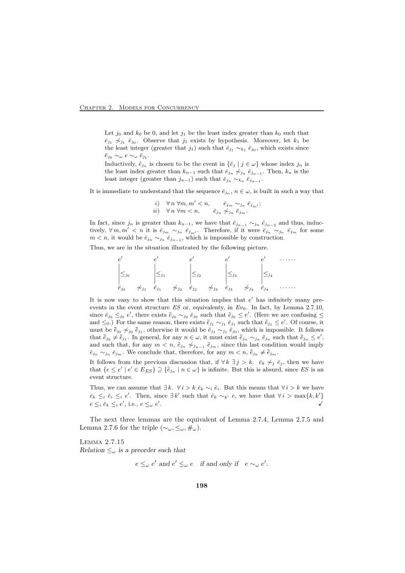
Chapter 2. Models for Concurrency
Let j0 and k0 be 0, and let j1 be the least index greater than k0 such thatej1 6∼j1 ej0 . Observe that j1 exists by hypothesis. Moreover, let k1 bethe least integer (greater that j1) such that ej1 ∼k1 ej0 , which exists sinceej0 ∼ω e ∼ω ej1 .
Inductively, ejn is chosen to be the event in {ej | j ∈ ω} whose index jn isthe least index greater than kn−1 such that ejn 6∼jn ejn−1 . Then, kn is theleast integer (greater than jn−1) such that ejn ∼kn ejn−1 .
It is immediate to understand that the sequence ejn , n ∈ ω, is built in such a way that
i) ∀n ∀m,m′ < n, ejm ∼jn ejm′ ;ii) ∀n ∀m < n, ejn 6∼jn ejm .
In fact, since jn is greater than kn−1, we have that ejn−1 ∼jn ejn−2 and thus, induc-tively, ∀m,m′ < n it is ejm ∼jn ejm′ . Therefore, if it were ejn ∼jn ejm for somem < n, it would be ejn ∼jn ejn−1 , which is impossible by construction.
Thus, we are in the situation illustrated by the following picture.
e′ e′ e′ e′ e′ · · · · · ·∣∣∣∣∣≤j0
∣∣∣∣∣≤j1
∣∣∣∣∣≤j2
∣∣∣∣∣≤j3
∣∣∣∣∣≤j4
ej0 6∼j1 ej1 6∼j2 ej2 6∼j3 ej3 6∼j4 ej4 · · · · · ·
It is now easy to show that this situation implies that e′ has infinitely many pre-events in the event structure ES or, equivalenty, in Ev0. In fact, by Lemma 2.7.10,since ej0 ≤j0 e
′, there exists ¯ej0 ∼j0 ej0 such that ¯ej0 ≤ e′. (Here we are confusing ≤and ≤0.) For the same reason, there exists ¯ej1 ∼j1 ej1 such that ¯ej1 ≤ e
′. Of course, itmust be ¯ej0 6∼j0 ¯ej1 , otherwise it would be ej1 ∼j1 ej0 , which is impossible. It followsthat ¯ej0 6= ¯ej1 . In general, for any n ∈ ω, it must exist ¯ejn ∼jn ejn such that ¯ejn ≤ e
′,and such that, for any m < n, ¯ejn 6∼jn−1
¯ejm , since this last condition would implyejn ∼jn ejm . We conclude that, therefore, for any m < n, ¯ejn 6= ¯ejm .
It follows from the previous discussion that, if ∀ k ∃ j > k. ek 6∼j ej , then we havethat {e ≤ e′ | e′ ∈ EES} ⊇ {¯ejn | n ∈ ω} is infinite. But this is absurd, since ES is anevent structure.
Thus, we can assume that ∃ k. ∀ i > k ek ∼i ei. But this means that ∀ i > k we have
ek ≤i ei ≤i e′. Then, since ∃ k′ such that ek ∼k′ e, we have that ∀ i > max{k, k′}
e ≤i ek ≤i e′, i.e., e ≤ω e
′. X
The next three lemmas are the equivalent of Lemma 2.7.4, Lemma 2.7.5 andLemma 2.7.6 for the triple (∼ω,≤ω,#ω).
Lemma 2.7.15Relation ≤ω is a preorder such that
e ≤ω e′ and e′ ≤ω e if and only if e ∼ω e
′.
198
2.7. Deterministic Labelled Event Structures
Proof. That ≤ω is a preorder is easily shown from the definition, exploiting the factthat, for any i ∈ ω, ≤i is a preorder.
Now suppose that e ≤ω e′ and e′ ≤ω e. Then, there exists i such that e ≤i e′ and
e′ ≤i e. Thus, by Lemma 2.7.4, e ∼i e′ whence e ∼ω e
′. On the contrary, if e ∼ω e′,
then there exists k such that ∀ i > k e ∼i e′. Then, again by the same lemma, for any
i > k, e ≤i e′ and e′ ≤i e, i.e., e ≤ω e
′ and e′ ≤ω e. X
Lemma 2.7.16Relation #ω is symmetric, irreflexive and such that
e #ω e′ ≤ω e
′′ implies e #ω e′′.
Proof. Since for any i ∈ ω #i is symmetric and irreflexive and since #ω =⋂i∈ω
#i,the first part of the claim is immediate.
Suppose that e #ω e′ and e′ ≤ω e
′′. By definition of #ω, for any i ∈ ω we have e #i e′.
Moreover, there exists k such that ∀ i > k it is e′ ≤i e′′. Thus, ∀ i > k we have e #i e
′
and e′ ≤i e′′, i.e., by Lemma 2.7.5, e #i e
′′. Then, since #i ⊆ #i−1 we have e #i e′′
for any i ∈ ω, i.e., e #ω e′′. X
Lemma 2.7.17For any e ∈ E, the set
{[e′]∼ω
∣∣∣ e′ ≤ω e, e′ ∈ E}
is finite.
Proof. If [e′]∼ω ≤∼ω [e]∼ω , then there exists e′ ∼ω e′ such that e′ ≤0 e. Moreover,
if [e′]∼ω 6= [e]∼ω , then clearly e′ 6= e. Hence, if we have infinitely many events in{[e′]∼ω
∣∣∣ e′ ≤ω e}
, we also have infinitely many events in{
[e′]∼0
∣∣∣ e′ ≤0 e}
, which,
by Lemma 2.7.6, is impossible. X
Then, we can define a labelled event structure Evω out of the triple (∼ω,≤ω,#ω)exactly as for the Ev i’s: Evω is the event structure (E/∼ω,≤∼ω
,#∼ω, ℓ∼ω
, L),where
• E/∼ω is the set of ∼ω-classes of E;
• [e]∼ω≤∼ω
[e′]∼ωif and only if e ≤ω e′;
• [e]∼ω#∼ω
[e′]∼ωif and only if e #ω e
′;
• ℓ∼ω([e]∼ω
) = ℓ(e).
Similarly to the case of the sequence TSysi, i ∈ ω, presented in Section 2.6, eventstructures Ev i are related to each other by inclusion morphisms. For i ∈ ω \ {0},
let ini:E/∼i−1 → E/∼i be the function such that in i
([e]∼i−1
)= [e]∼i
. Then we
have the following.
199
Chapter 2. Models for Concurrency
Lemma 2.7.18For any i ∈ ω \ {0}, (ini, id):Ev i−1 → Ev i is a labelled event structure morphism.
Proof. Axiom (iii) of Definition 2.3.1 of labelled event structure morphisms triviallyholds for (ini, id i). Let us check axioms (i) and (ii).
i) ini
(⌊[e]∼i−1
⌋
≤i−1
)⊆⌊ini
([e]∼i−1
)⌋
≤i
, i.e., for any [e′]∼i ≤∼i [e]∼i there
exists [e′]∼i−1 ≤∼i−1 [e]∼i−1 such that [e′]∼i = [e′]∼i . But this is immediatebecause e′ ≤i e implies, by definition of ≤i, that there exists e′ ∼i e
′ such thate′ ≤i−1 e.
ii) ini
([e]∼i−1
)∨∨ ini
([e′]∼i−1
)implies [e]∼i−1 ∨∨ [e′]∼i−1 , i.e., [e]∼i ∨∨ [e′]∼i
implies [e]∼i−1 ∨∨ [e′]∼i−1 . Clearly, by definition, [e]∼i #∼i [e′]∼i implies[e]∼i−1 #∼i−1 [e′]∼i−1 .
Now suppose that [e]∼i = [e′]∼i but [e]∼i−1 6= [e′]∼i−1 . Then, we have e ∼i e′ but
e 6∼i−1 e′. Then, by Lemma 2.7.8, we have e #i−1 e
′, i.e., [e]∼i−1 #∼i−1 [e′]∼i−1 .X
Next, we shall show that Evω is the colimit of the ω-diagram formed by theEv i’s. For any i ∈ ω, consider the mapping inωi :E/∼i → E/∼ω which, for anye ∈ E, sends [e]∼i
to [e]∼ω.
Lemma 2.7.19For any i ∈ ω, (inωi , id):Ev i → Evω is a labelled event structure morphism
Proof. The proof is formally identical to that of Lemma 2.7.18. With respect to
Definition 2.3.1, property (i), i.e., inωi
(⌊[e]∼i
⌋
≤i
)⊆⌊inωi
([e]∼i
)⌋
≤ω
, derives im-
mediately from Lemma 2.7.10; property (ii), i.e., inωi
([e]∼i
)∨∨ inωi
([e′]∼i
)implies
[e]∼i ∨∨ [e′]∼i derives immediately from Lemma 2.7.8; and property (iii) is trivially
true. X
Proposition 2.7.20Evω is the colimit in LESI of the ω-diagram
D = Ev0(in1,id)−→ Ev1
(in2,id)−→ · · ·
(ini−1,id)−→ Ev i
(ini,id)−→ · · ·
Proof. Since for any 1 < j < i it is inωj = inωi ◦ ini ◦ · · · ◦ inj+1, then {(inωi , id):Ev i →Evω | i ∈ ω} is a cocone with base D.
Consider now any other cocone {(ηi, λi):Ev i → ES | i ∈ ω} for D, ES being any objectin LESI. Since for any i it is (ηi, λi) = (ηi+1, λi+1) ◦ (ini+1, id), it must necessarily
200
2.7. Deterministic Labelled Event Structures
be λi = λ0 = λ and ηi
([e]∼i
)= ηi+1
([e]∼i+1
), for any i. Thus, we can define
η:E/∼ω → EES by η([e]∼ω
)= η0
([e]∼0
). Clearly, we have that
η([e]∼ω
)= η0
([e]∼0
)= ηi
([e]∼i
),
i.e., for any i, ηi = η ◦ inωi , and, moreover, η is clearly the unique mapping for whichthat happens. Thus, to conclude the proof, we only miss to show that (η, λ):Evω → ESis a labelled event structure morphism.
Again, axiom (iii) of Definition 2.3.1 trivially holds by definition. Let us show axioms(i) and (ii).
i) Consider e ∈ EES such that e ≤ η([e]∼ω
). Then, by definition, for each i,
e ≤ ηi
([e]∼i
)and, since (ηi, λi) is a morphism, for any i there exists ¯ei ∈ E such
that ¯ei ≤i e and ηi
([¯ei]∼i
)= e. Thus, we are in the same situation we came
across while proving Lemma 2.7.14. And in fact, reasoning as in that proof, wehave that there can be only finitely many ¯ei which are not in the relation ∼ω,i.e., there must be a k such that ¯ek ≤i e for any i > k. Then, ¯ek ≤ω e and
η([¯ek]∼ω
)= ηk
([¯ek]∼k
)= e.
ii) Suppose that η([e]∼ω
)∨∨ η
([e′]∼ω
). Then, clearly, for any i ∈ ω we have that
ηi
([e]∼i
)∨∨ ηi
([e′]∼i
). Now, if there exists i such that [e]∼i = [e′]∼i , then
[e]∼ω = [e′]∼ω . Otherwise, [e]∼i #∼i [e′]∼i for any i ∈ ω, i.e., [e]∼ω #∼ω [e′]∼ω .In both cases, [e]∼ω ∨∨ [e′]∼ω and we are done. X
Exploiting the characterizations of ≤ω previously given, it is not difficult toshow the following.
Lemma 2.7.21Evω is deterministic.
Proof. Consider a configuration cω of Evω and two events [e]∼ω 6= [e′]∼ω enabled atcω, i.e., such that cω ⊢ [e]∼ω and cω ⊢ [e′]∼ω . We shall show that there exist i and aconfiguration ci of Ev i in which [e]∼i and [e′]∼i are enabled. Since [e]∼i+1 6= [e′]∼i+1 ,
which follows from the fact that [e]∼ω 6= [e′]∼ω , and since [e]∼i 6⋚i [e′]∼i , which followsfrom the fact that both are enabled at ci, it must necessarily be
ℓ∼ω
([e]∼ω
)= ℓ∼i
([e]∼i
)6= ℓ∼i
([e′]∼i
)= ℓ∼ω
([e′]∼ω
),
which shows that Evω is deterministic.
Suppose that [e]∼ω ≤∼ω [e]∼ω . Then, there exists k such that ∀ j > k [e]∼j ≤∼j [e]∼j .
Since the set⌊[e]∼ω
⌋
≤ω
is finite, we can find k′ such that for any j > k′ [e]∼ω ≤∼ω
201
Chapter 2. Models for Concurrency
[e]∼ω implies [e]∼j ≤∼j [e]∼j . If otherwise [e]∼ω �∼ω [e]∼ω and [e]∼k′ ≤∼k′ [e]∼k′ ,
there exists j > k such that [e]∼j �∼j [e]∼j . Now, observe that there can be onlyfinitely many such [e]∼k
. In fact, if it were not, reasoning as done in previous proofs,and exploiting Lemmas 2.7.10 and 2.7.13, we would easily derive a contradiction show-ing that e has infinitely many pre-events in Ev0. Then, we can find k′′ such that forany j > k′′
[e]∼ω ≤∼ω [e]∼ω ⇔ [e]∼j ≤∼j [e]∼j .
In the same way, we can find ¯k′′ such that for any j > ¯k′′, [e]∼ω ≤∼ω [e′]∼ω if and only
if [e]∼j ≤∼j [e′]∼j . Thus, considering k = max{k′′, ¯k′′} we have that for any i > k
[e]∼ω ∈⌊[e]∼ω
⌋
≤ω
⇔ [e]∼i ∈⌊[e]∼i
⌋
≤i
and
[e]∼ω ∈⌊[e′]∼ω
⌋
≤ω
⇔ [e]∼i ∈⌊[e′]∼i
⌋
≤i
.
Now, consider [e]∼k≤k [e]∼k
and [e′]∼k≤k [e′]∼k
. Clearly, it is still possible that
[e]∼k#∼k
[e′]∼k. However, since [e]∼ω
/#∼ω
[e′]∼ω , it must exist k such that for any
i > k [e]∼i
/#∼i
[e′]∼i . Then, since there can be only finitely many such pairs, we can
find an integer i (greater than k) such that the set⌊[e]∼i
⌋
≤i
∪⌊[e′]∼i
⌋
≤i
is conflict
free (wrt. to #∼i).
It is immediate now to see that
ci =(⌊
[e]∼i
⌋
≤i
\{
[e]∼i
})∪(⌊
[e′]∼i
⌋
≤i
\{
[e′]∼i
})
is a configuration of Ev i which enables [e]∼i and [e′]∼i . X
As it was probably clear from a while, the object component of the functordles : LESI → dLES is the function which maps a labelled event structure withoutautoconcurrency ES to the deterministic event structure Evω limit of the sequenceof event structures Ev i built from it.
An example of the construction is given in Figure 2.4, in which we also show howthe construction of the deterministic transition system with independence works onthe transition system of configurations of ES . Now, the last step we miss is to showthat dles can be extended to a functor which is left adjoint to the inclusion functordLES → LESI. This is done in the following proposition.
Proposition 2.7.22 ( (inω0 ◦ in , id):ES → dles(ES ) is universal)For any labelled event structure without autoconcurrency ES , any deterministiclabelled event structure DES and any (η, λ):ES → DES , there exists a unique
202
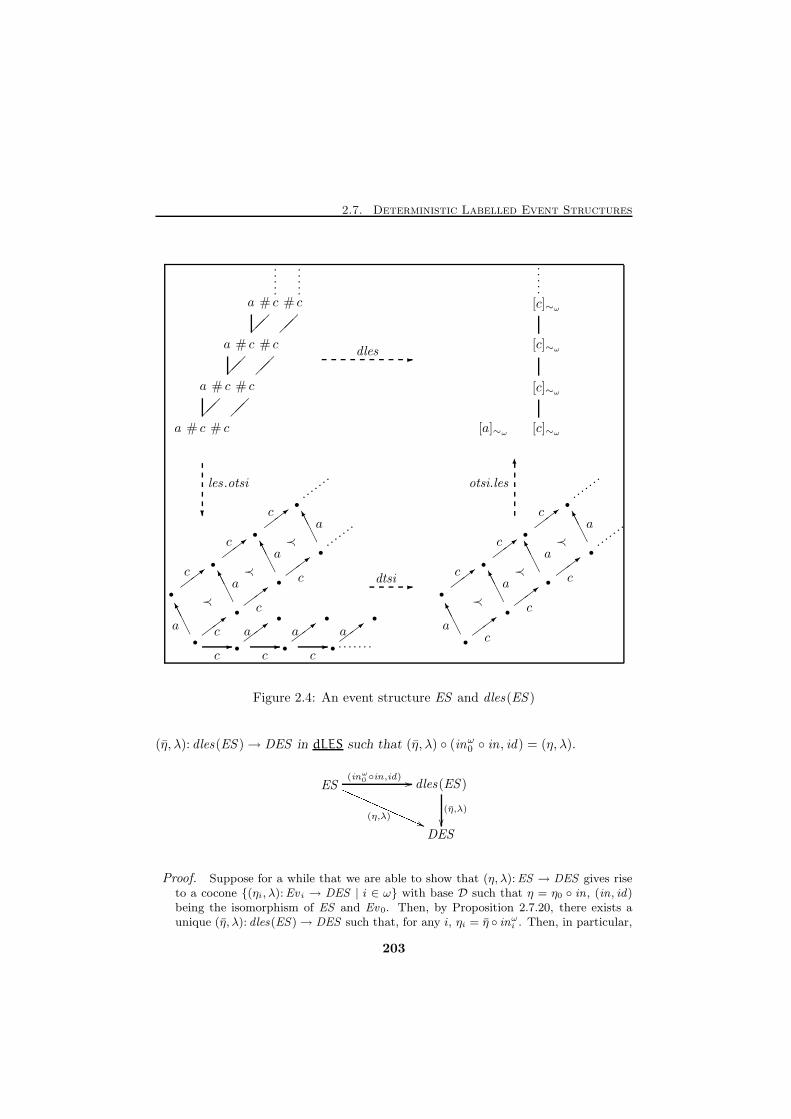
2.7. Deterministic Labelled Event Structures
�� ��
�� ��
�� ��
AAAK
��>
��>
AAAK
��>
AAAK
��>
��>
AAAK
- -��>
��>- �
�>
��>
dles -
dtsi-
otsi.les6
les .otsi
?
..
..
.
..
..
.
..
..
.
......
.
......
.
. . . . . . .
......
.
......
.
AAAK
��>
��>
AAAK
��>
��>
AAAK
��>
��>
AAAK
•
•
•
•
•
•
•
• •
• •
•
•
•
•
•
•
•
•
•
•
•
# #
# #
# #
# #
ca c
ca c
ca c
ca c
a
≺
ac ≺
ac ≺
ac
c
c a a a
c
c c c
[a]∼ω[c]∼ω
[c]∼ω
[c]∼ω
[c]∼ω
a
≺
ac
c
≺
ac
c
≺
ac
c
Figure 2.4: An event structure ES and dles(ES )
(η, λ): dles(ES )→ DES in dLES such that (η, λ) ◦ (inω0 ◦ in, id) = (η, λ).
ES dles(ES )
DES
(inω0 ◦in,id) //
(η,λ)
QQQQQQQQQQQQQ (( (η,λ)
��
Proof. Suppose for a while that we are able to show that (η, λ):ES → DES gives riseto a cocone {(ηi, λ):Ev i → DES | i ∈ ω} with base D such that η = η0 ◦ in, (in, id)being the isomorphism of ES and Ev0. Then, by Proposition 2.7.20, there exists aunique (η, λ): dles(ES)→ DES such that, for any i, ηi = η ◦ inωi . Then, in particular,
203
Chapter 2. Models for Concurrency
η0 = η ◦ inω0 , and thus
(η, λ) = (η0 ◦ in, λ) = (η, λ) ◦ (inω0 ◦ in, id).
In other words, η:EES/∼ω → EDES given, as in the proof of Proposition 2.7.20, by
η([e]∼ω
)= η(e) would be such that (η, λ) makes the diagram commute.
The hypothesis above is sufficient also to show the uniqueness of (η, λ). Suppose infact that there exists ¯η such that η = ¯η ◦ (inω0 ◦ in), then it is η0 = ¯η ◦ inω0 . It followsthat, for any i,
ηi
([e]∼i
)= (η ◦ inωi )
([e]∼i
)= (η ◦ inω0 )
([e]∼0
)
= (¯η ◦ inω0 )([e]∼0
)= (¯η ◦ inωi )
([e]∼i
),
i.e., for any i it is ηi = ¯η ◦ inωi . Then, by definition of colimit, it is ¯η = η.
Thus, we only need to show that the cocone {(ηi, λ):Ev i → DES | i ∈ ω} actuallyexists. However, by defining for any integer i the mapping ηi:EES/∼i → EDES by
ηi
([e]∼i
)= η(e), we obviously have a cocone {(ηi, λ) | i ∈ ω} as required. So, we just
need to prove that (ηi, λ) is a well-defined labelled event structure morphism from Ev ito DES . We shall do it by induction on i.
For i = 0 everything is fine, since (η0, λ) is the composition of two morphisms, namely(η, λ) ◦ (in−1, id). So, assuming that (ηi, λ) is a well-defined morphism from Ev i toDES , let us show that (ηi+1, λ):Ev i+1 → DES is such.
To show that ηi+1 is well-defined, it is enough to show that η(e) = η(e′) whenever eand e′ are related directly from condition (ii) of the definition of ∼i+1. Since ∼i+1 isan equivalence generated by that unique rule starting from ∼i, the other cases followimmediately using the inductive hypothesis. Thus, it is e 6⋚i e
′, ℓ(e) = ℓ(e′) and
⌊e⌋≤i\ {e} 6#i ⌊e
′⌋≤iand ⌊e⌋≤i
6#i ⌊e′⌋≤i\ {e′}.
First observe that η↓e if and only if λ↓ℓ(e) if and only if λ↓ℓ(e′) if and only if η↓e′.Thus, ηi+1 is defined or not on a class [e]∼i+1 irrespectively of the representativechosen. Suppose then that η is defined on e. Thus ηi is defined on both [e]∼i and[e′]∼i . By general properties of event structure morphisms,
ηi
((⌊e⌋≤i
\ {e})∪(⌊e′⌋≤i
\ {e′}))
is a configuration of DES which enables both ηi
([e]∼i
)and ηi
([e′]∼i
). Then, since
those two events have the same label in DES , which is deterministic, it follows that
ηi
([e]∼i
)= ηi
([e′]∼i
).
Let us show now that (ηi+1, λ) is a morphism.
i)⌊ηi+1
([e]∼i+1
)⌋
≤⊆ ηi+1
(⌊[e]∼i+1
⌋
≤∼i+1
).
204
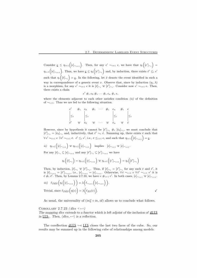
2.7. Deterministic Labelled Event Structures
Consider e ≤ ηi+1
([e]∼i+1
). Then, for any e′ ∼i+1 e, we have that ηi
([e′]∼i
)=
ηi+1
([e]∼i+1
). Thus, we have e ≤ ηi
([e′]∼i
)and, by induction, there exists e′ ≤i e
′
such that ηi
([e]∼i
)= e. In the following, let x denote the event identified in such a
way in correspondence of a generic event x. Observe that, since by induction (ηi, λ)is a morphism, for any e′ ∼i+1 e it is [e]∼i ∨∨ [e′]∼i . Consider now e′ ∼i+1 e. Then,there exists a chain
e′ #i e0 #i · · · #i en #i e,
where the elements adjacent to each other satisfies condition (ii) of the definitionof ∼i+1. Thus we are led to the following situation.
e′ #i e0 #i · · · #i en #i e∣∣∣∣∣≤i
∣∣∣∣∣≤i
∣∣∣∣∣≤i
∣∣∣∣∣≤i
e′ ∨∨ e0 ∨∨ · · · ∨∨ en ∨∨ e
However, since by hypothesis it cannot be [e′]∼i #i [e0]∼i , we must conclude that[e′]∼i = [e0]∼i and, inductively, that e′ ∼i e. Summing up, there exists e such that
∀ e′ ∼i+1 e ∃ e′ ∼i+1 e. e
′ ≤i e′, i.e., e ≤i+1 e, and such that ηi+1
([e]∼i+1
)= e.
ii) ηi+1
([e]∼i+1
)∨∨ ηi+1
([e]∼i+1
)implies [e]∼i+1 ∨∨ [e]∼i+1 .
For any [e]∼i ⊆ [e]∼i+1 and any [e′]∼i ⊆ [e′]∼i+1 we have
ηi
([e]∼i
)= ηi+1
([e]∼i+1
)∨∨ ηi+1
([e′]∼i+1
)= ηi
([e′]∼i
)
Then, by induction, [e]∼i ∨∨ [e′]∼i . Thus, if [e]∼i = [e′]∼i for any such e and e′, itis [e]∼i+1 = [e′]∼i+1 , i.e., [e]∼i+1 = [e]∼i+1 . Otherwise, ∀ e ∼i+1 e ∀ e
′ ∼i+1 e′ it is
e #i e′. Then, by Lemma 2.7.10, we have e #i+1 e
′. In both cases, [e]∼i+1 ∨∨ [e]∼i+1 .
iii) ℓDES
(ηi
([e]∼i+1
))= λ(ℓ∼i+1
([e]∼i+1
)).
Trivial, since ℓDES
(η(e)
)= λ(ℓES (e)
). X
As usual, the universality of (inω0 ◦ in , id) allows us to conclude what follows.
Corollary 2.7.23 ( dles ⊣ ←)The mapping dles extends to a functor which is left adjoint of the inclusion of dLES
in LESI. Then, 〈dles , ←〉 is a reflection.
The coreflection dLES −⊳ LES closes the last two faces of the cube. So, ourresults may be summed up in the following cube of relationships among models.
205
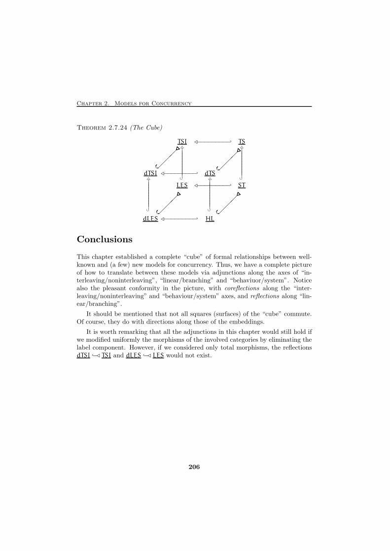
Chapter 2. Models for Concurrency
Theorem 2.7.24 (The Cube)
dTSI
���
....................................................
..........�⊳−−−−−−−−− dTS
���
....................................................
..........�△
||||||||||∪
△
||||||||||∪
dLES���
....................................................
..........�⊳−−−−−−−−− HL
���
....................................................
..........�
TSI ⊳−−−−−−−−− TS△
||||||||||∪
△
||||||||||∪
LES ⊳−−−−−−−−− ST
Conclusions
This chapter established a complete “cube” of formal relationships between well-known and (a few) new models for concurrency. Thus, we have a complete pictureof how to translate between these models via adjunctions along the axes of “in-terleaving/noninterleaving”, “linear/branching” and “behaviuor/system”. Noticealso the pleasant conformity in the picture, with coreflections along the “inter-leaving/noninterleaving” and “behaviour/system” axes, and reflections along “lin-ear/branching”.
It should be mentioned that not all squares (surfaces) of the “cube” commute.Of course, they do with directions along those of the embeddings.
It is worth remarking that all the adjunctions in this chapter would still hold ifwe modified uniformly the morphisms of the involved categories by eliminating thelabel component. However, if we considered only total morphisms, the reflectionsdTSI −⊳ TSI and dLES −⊳ LES would not exist.
206
Chapter 3
Infinite Computations
Abstract. For any cardinal ℵ, there exists a KZ-doctrine on the 2-category of thelocally small categories whose algebras are exactly the categories which admits all thecolimits indexed by chains of cardinality not greater than ℵ. The chapter presents a widesurvey of this topic.
In addition, we show that this inductive completion KZ-doctrine lifts smoothly to KZ-doctrines on (many variations of) the 2-categories of monoidal and symmetric monoidalcategories, thus yielding, in particular, a universal construction of colimits of ω-chainsin those categories. Since the processes of Petri nets may be axiomatized in terms ofsymmetric monoidal categories this result provides a universal construction of the algebraof infinite processes of a Petri net.
So that we may say that the door is now opened . . .to a new method . . .which in future years
will command the attention of other minds.
Galileo Galilei
Tra questa immensita s’annega il pensier mio:e il naufragar mi e dolce in questo mare.
Giacomo Leopardi
L’infinito e drasticamente diversoda tutte le cose finite.
Antonino Zichichi, L’infinito
This chapter is based on joint work with Jose Meseguer and Ugo Montanari [123].
207

Chapter 3. Infinite Computations
208
Introduction
The idea of completing a mathematical stucture by adding to it some desirablelimit “points” is indeed a very natural one and it arises in many different fields ofmathematics, and in particular topology and partial order theory. Since categoriesare a generalization of the notion of partial orders, the issue of completing categoriesfor a given class of limits or colimits arose rather early in the development of thetheory (see [79] and references therein).
As far as computer science is concerned, the theory of complete partial ordersand associated completion techniques have assumed great relevance since the pio-neering work on semantics by D. Scott [128, 133]. In the last few years, however,many computing systems have been given a semantics through the medium of cat-egory theory, the general pattern being to look at objects as representing statesand at arrows as representing computations. It is therefore natural to expect thatthe theory of cocompletion of categories may play an interesting role in this kindof semantics. The main purpose of this chapter is to illustrate how this theoryfits well with the issue of infinite computations and, therefore, to make it moreeasily available to the computer science community. In a sense, by viewing cate-gories as generalized posets, this view of infinite computations is very natural andindeed generalizes to categories similar constructions for adding limits to posets.We motivate this further in terms of processes of Petri nets in Section 3.1.
Petri nets [109] are probably the most clear examplification of the categorical se-mantics pattern discussed above. They are unanimously considered among the mostrepresentative models for concurrency, since they are a fairly simple and naturalmodel of concurrent and distributed computation. Recent works [97, 16, 121, 122]have shown that the semantics of Petri nets can be understood in terms of symmet-ric monoidal categories—where objects are states, arrows processes, and the tensorproduct and the arrow composition model respectively the operations of paralleland sequential composition of processes. This yields an axiomatization of the causalbehaviour of nets as an essentially algebraic theory. However, when modeling per-petual systems, describing finite processes is not enough: we need to consider alsoinfinite behaviours. We remark that our interest here resides on processes of Petrinets, i.e., on structures able to describe concurrent computations taking into ac-count causality. More precisely, we aim at defining an algebra of net computationswhich includes infinite processes as well. To the best of our knowledge, this issueis still completely unexplored.
Although we are mainly interested in considering colimits of ω-chains, we shallpresent the theory of the cocompletion for filtered colimits of cardinality not greaterthan ℵ, where ℵ is an infinite cardinal. In particular, since ℵ-filtered cocompletenessis equivalent to the cocompleteness by colimits taken over chains of cardinality notgreater that ℵ, for ℵ = ω we have the ω-cocompletion as instantiation of the general
209
Chapter 3. Infinite Computations
theory. More precisely, for any infinite cardinal ℵ, we define a Kock-Zoberlain(KZ-)doctrine Ind( )ℵ on the 2-category of locally small categories such that thecategories admitting filtered colimits of cardinality ℵ are the algebras [76, 149]for the doctrine, while the Ind–homomorphisms are the functors which preservethose colimits. This result has already appeared in several different forms in theliterature, e.g. [71, 43] and the related [76, 79, 28, 149, 150, 137, 56, 58]. However,we aim at giving a simple and complete tutorial, which integrates the best featuresof the existing approaches and explores the application of these ideas to computerscience.
Concerning the organization of this chapter, in Section 3.2 we recall that, forany small category C, the category SetCop
of all presheaves on C may be consideredthe “free” cocompletion of C under all small colimits. This suggests immediatelya strategy for identifying the cocompletion of C for ℵ-filtered colimits, i.e., to lookfor an appropriate subcategory of SetCop
. Moreover, this approach generalizes alsoto locally small categories. This part of the theory is illustrated in Section 3.3.Then Section 3.5 gives the functors Ind( )ℵ bulding on the theory of KZ-doctrines,whose definitions and basic results are given in Section 3.4.
Getting back to our starting motivations about the process semantics of Petrinets, in Section 3.6 we study the application of the doctrine to symmetric monoidalcategories. Precisely, we show that the KZ-doctrine Ind( )ℵ lifts to KZ-doctrines re-spectively on any of the 2-categories of monoidal categories appearing in Table 3.1.This, from the technical point of view, is the main original contribution of thechapter. Finally, in Section 3.7, we discuss how this result generalizes the algebraicapproach to the process semantics of Petri nets discussed in detail in Chapter 1 tothe case in which infinite processes and composition operations on them are con-sidered. In particular, the infinite processes of a Petri net can in this way be givenan algebraic presentation which combines the essentially algebraic presentation ofmonoidal categories with the monadic presentation of their completion in terms ofKZ-doctrines. A further link with Chapter 1, and in particular with the results ofSection 1.9 about the relationships between process, unfolding, and algebraic viewsof net semantics is provided by showing that the arrows of the cocompletion of thecategory of decorated concatenable processes of N coincides with the configurationsof the event structure associated to N by the unfolding semantics.
However, the correspondence between infinite net processes obtained via thecocompletion doctrine and the algebraic theory of net processes is not as “precise”as one would like. In fact, in addition to the symmetric monoidality, the categoriesof processes of Petri nets satisfy further axioms which are, in general, not preservedby Ind( )ℵ. Therefore, although the arrows of the cocomplete category correspondprecisely to infinite computations, they do not enjoy the global structural propertiesof finite net processes, i.e., Ind( )ℵ does not restrict to an endofunctor on thecategory of categories of net processes. It is still an open problem whether a moresatisfactory solution to this problem can be found.
210
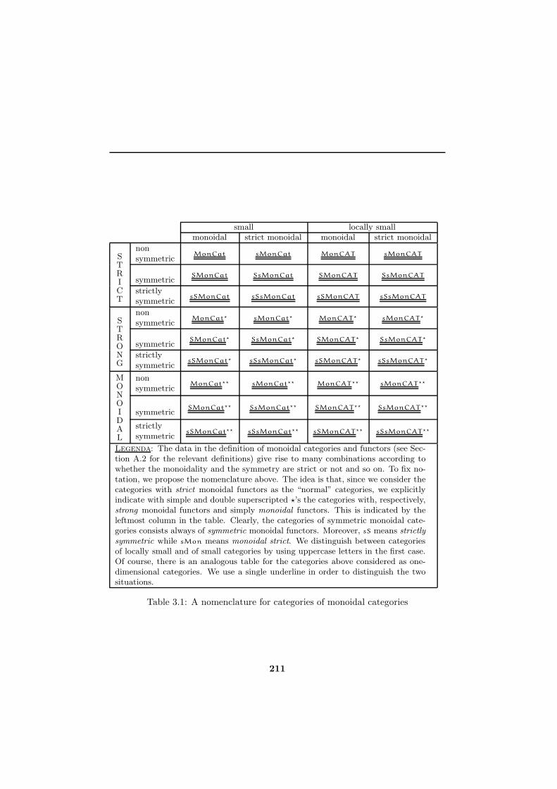
small locally smallmonoidal strict monoidal monoidal strict monoidal
STRICT
nonsymmetric
MonCat sMonCat MonCAT sMonCAT
symmetricSMonCat SsMonCat SMonCAT SsMonCAT
strictlysymmetric
sSMonCat sSsMonCat sSMonCAT sSsMonCAT
STRONG
nonsymmetric
MonCat⋆ sMonCat⋆ MonCAT⋆ sMonCAT⋆
symmetricSMonCat⋆ SsMonCat⋆ SMonCAT⋆ SsMonCAT⋆
strictlysymmetric
sSMonCat⋆ sSsMonCat⋆ sSMonCAT⋆ sSsMonCAT ⋆
MONOIDAL
nonsymmetric
MonCat⋆⋆ sMonCat⋆⋆ MonCAT⋆⋆ sMonCAT⋆⋆
symmetricSMonCat⋆⋆ SsMonCat⋆⋆ SMonCAT⋆⋆ SsMonCAT ⋆⋆
strictlysymmetric
sSMonCat⋆⋆ sSsMonCat⋆⋆ sSMonCAT⋆⋆ sSsMonCAT⋆⋆
Legenda: The data in the definition of monoidal categories and functors (see Sec-tion A.2 for the relevant definitions) give rise to many combinations according towhether the monoidality and the symmetry are strict or not and so on. To fix no-tation, we propose the nomenclature above. The idea is that, since we consider thecategories with strict monoidal functors as the “normal” categories, we explicitlyindicate with simple and double superscripted ⋆’s the categories with, respectively,strong monoidal functors and simply monoidal functors. This is indicated by theleftmost column in the table. Clearly, the categories of symmetric monoidal cate-gories consists always of symmetric monoidal functors. Moreover, sS means strictlysymmetric while sMon means monoidal strict. We distinguish between categoriesof locally small and of small categories by using uppercase letters in the first case.Of course, there is an analogous table for the categories above considered as one-dimensional categories. We use a single underline in order to distinguish the twosituations.
Table 3.1: A nomenclature for categories of monoidal categories
211
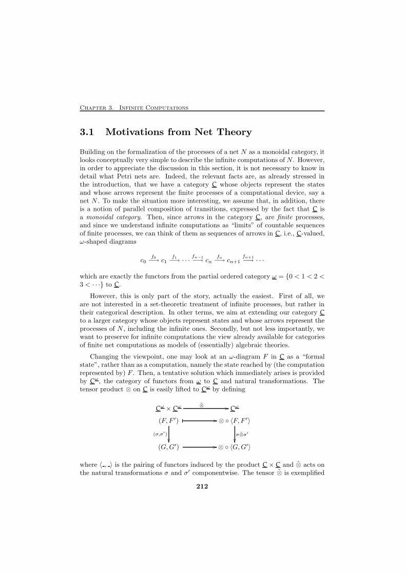
Chapter 3. Infinite Computations
3.1 Motivations from Net Theory
Building on the formalization of the processes of a net N as a monoidal category, itlooks conceptually very simple to describe the infinite computations of N . However,in order to appreciate the discussion in this section, it is not necessary to know indetail what Petri nets are. Indeed, the relevant facts are, as already stressed inthe introduction, that we have a category C whose objects represent the statesand whose arrows represent the finite processes of a computational device, say anet N . To make the situation more interesting, we assume that, in addition, thereis a notion of parallel composition of transitions, expressed by the fact that C isa monoidal category. Then, since arrows in the category C, are finite processes,and since we understand infinite computations as “limits” of countable sequencesof finite processes, we can think of them as sequences of arrows in C, i.e., C-valued,ω-shaped diagrams
c0f0−→ c1
f1−→ · · ·
fn−1−→ cn
fn−→ cn+1
fn+1−→ · · ·
which are exactly the functors from the partial ordered category ω = {0 < 1 < 2 <3 < · · ·} to C.
However, this is only part of the story, actually the easiest. First of all, weare not interested in a set-theoretic treatment of infinite processes, but rather intheir categorical description. In other terms, we aim at extending our category C
to a larger category whose objects represent states and whose arrows represent theprocesses of N , including the infinite ones. Secondly, but not less importantly, wewant to preserve for infinite computations the view already available for categoriesof finite net computations as models of (essentially) algebraic theories.
Changing the viewpoint, one may look at an ω-diagram F in C as a “formalstate”, rather than as a computation, namely the state reached by (the computationrepresented by) F . Then, a tentative solution which immediately arises is providedby Cω, the category of functors from ω to C and natural transformations. Thetensor product ⊗ on C is easily lifted to Cω by defining
(F, F ′) ⊗ ◦ 〈F, F ′〉
(G,G′) ⊗ ◦ 〈G,G′〉
� //
(σ,σ′)
��σ⊗σ′
��� //
CωCω × Cω⊗ //
where 〈 , 〉 is the pairing of functors induced by the product C× C and ⊗ acts onthe natural transformations σ and σ′ componentwise. The tensor ⊗ is exemplified
212
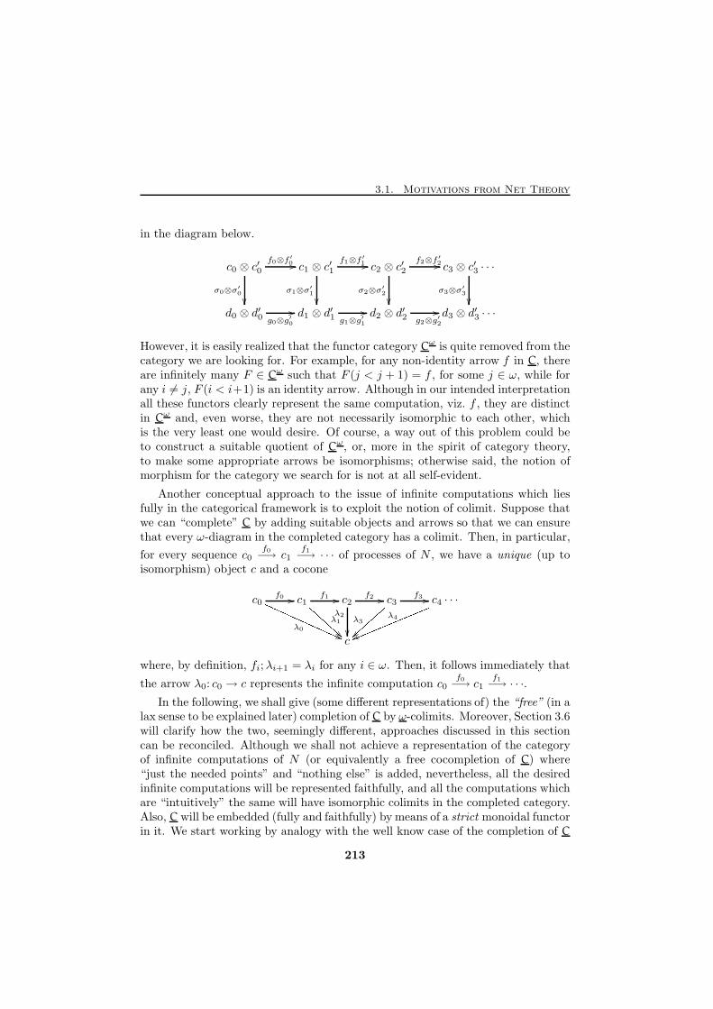
3.1. Motivations from Net Theory
in the diagram below.
c0 ⊗ c′0 c1 ⊗ c′1 c2 ⊗ c′2 c3 ⊗ c′3 · · ·
d0 ⊗ d′0 d1 ⊗ d′1 d2 ⊗ d′2 d3 ⊗ d′3 · · ·
f0⊗f′0 //
σ0⊗σ′0
��
f1⊗f′1 //
σ1⊗σ′1
��
f2⊗f′2//
σ2⊗σ′2
��σ3⊗σ
′3
��
g0⊗g′0
//g1⊗g
′1
//g2⊗g
′2
//
However, it is easily realized that the functor category Cω is quite removed from thecategory we are looking for. For example, for any non-identity arrow f in C, thereare infinitely many F ∈ Cω such that F (j < j + 1) = f , for some j ∈ ω, while forany i 6= j, F (i < i+1) is an identity arrow. Although in our intended interpretationall these functors clearly represent the same computation, viz. f , they are distinctin Cω and, even worse, they are not necessarily isomorphic to each other, whichis the very least one would desire. Of course, a way out of this problem could beto construct a suitable quotient of Cω, or, more in the spirit of category theory,to make some appropriate arrows be isomorphisms; otherwise said, the notion ofmorphism for the category we search for is not at all self-evident.
Another conceptual approach to the issue of infinite computations which liesfully in the categorical framework is to exploit the notion of colimit. Suppose thatwe can “complete” C by adding suitable objects and arrows so that we can ensurethat every ω-diagram in the completed category has a colimit. Then, in particular,
for every sequence c0f0−→ c1
f1−→ · · · of processes of N , we have a unique (up to
isomorphism) object c and a cocone
c0 c1 c2 c3 c4 · · ·
c
f0 //
λ0
QQQQQQQQQQQQQ((f1 //
λ1
BBBBBB!! f2 //λ2
��
f3 //
λ3
}}|||||| λ4
vvlllllllllllllwhere, by definition, fi;λi+1 = λi for any i ∈ ω. Then, it follows immediately that
the arrow λ0: c0 → c represents the infinite computation c0f0−→ c1
f1−→ · · ·.
In the following, we shall give (some different representations of) the “free” (in alax sense to be explained later) completion of C by ω-colimits. Moreover, Section 3.6will clarify how the two, seemingly different, approaches discussed in this sectioncan be reconciled. Although we shall not achieve a representation of the categoryof infinite computations of N (or equivalently a free cocompletion of C) where“just the needed points” and “nothing else” is added, nevertheless, all the desiredinfinite computations will be represented faithfully, and all the computations whichare “intuitively” the same will have isomorphic colimits in the completed category.Also, C will be embedded (fully and faithfully) by means of a strict monoidal functorin it. We start working by analogy with the well know case of the completion of C
213
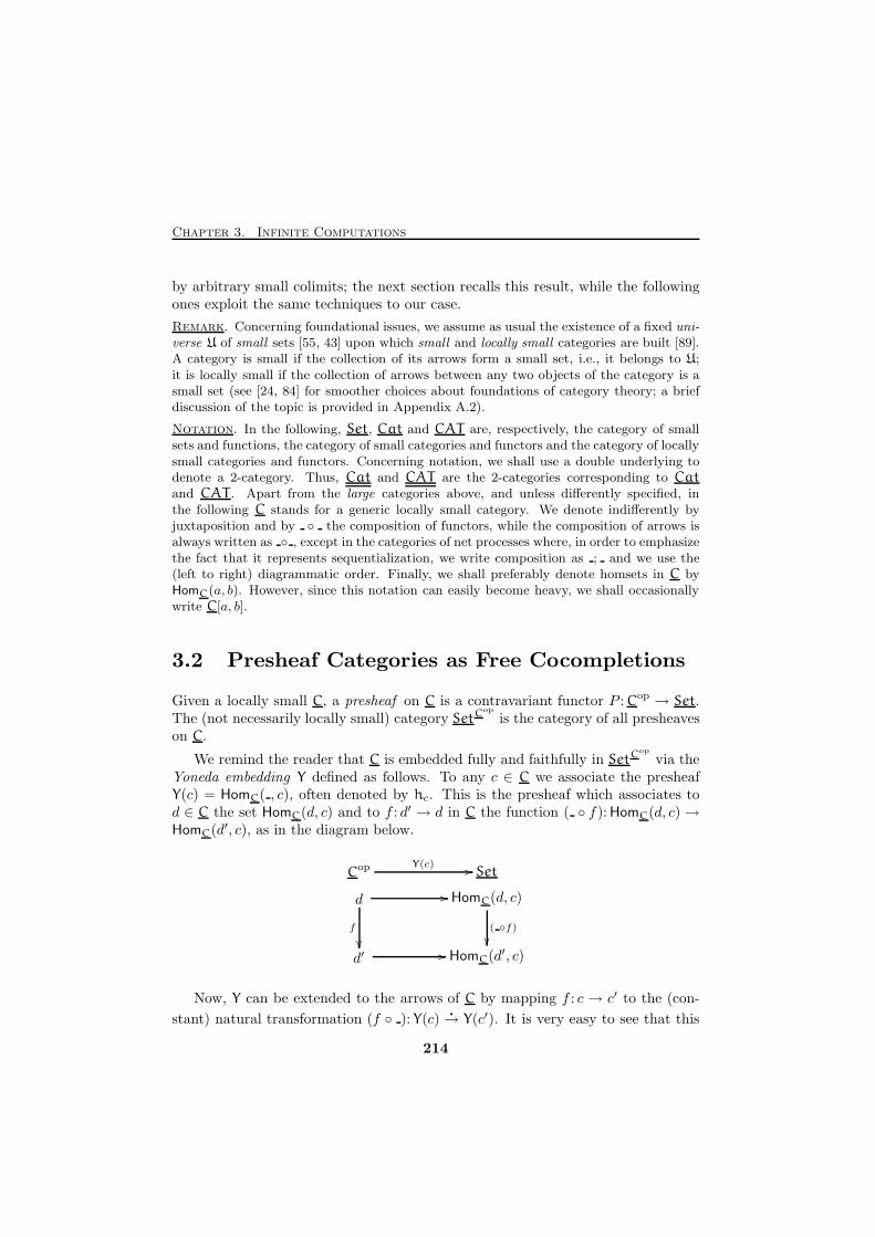
Chapter 3. Infinite Computations
by arbitrary small colimits; the next section recalls this result, while the followingones exploit the same techniques to our case.
Remark. Concerning foundational issues, we assume as usual the existence of a fixed uni-verse U of small sets [55, 43] upon which small and locally small categories are built [89].A category is small if the collection of its arrows form a small set, i.e., it belongs to U;it is locally small if the collection of arrows between any two objects of the category is asmall set (see [24, 84] for smoother choices about foundations of category theory; a briefdiscussion of the topic is provided in Appendix A.2).
Notation. In the following, Set, Cat and CAT are, respectively, the category of smallsets and functions, the category of small categories and functors and the category of locallysmall categories and functors. Concerning notation, we shall use a double underlying todenote a 2-category. Thus, Cat and CAT are the 2-categories corresponding to Catand CAT . Apart from the large categories above, and unless differently specified, inthe following C stands for a generic locally small category. We denote indifferently byjuxtaposition and by ◦ the composition of functors, while the composition of arrows isalways written as ◦ , except in the categories of net processes where, in order to emphasizethe fact that it represents sequentialization, we write composition as ; and we use the(left to right) diagrammatic order. Finally, we shall preferably denote homsets in C byHomC(a, b). However, since this notation can easily become heavy, we shall occasionallywrite C[a, b].
3.2 Presheaf Categories as Free Cocompletions
Given a locally small C, a presheaf on C is a contravariant functor P : Cop → Set.The (not necessarily locally small) category SetCop
is the category of all presheaveson C.
We remind the reader that C is embedded fully and faithfully in SetCop
via theYoneda embedding Y defined as follows. To any c ∈ C we associate the presheafY(c) = HomC( , c), often denoted by hc. This is the presheaf which associates tod ∈ C the set HomC(d, c) and to f : d′ → d in C the function ( ◦ f): HomC(d, c)→HomC(d′, c), as in the diagram below.
d HomC(d, c)
d′ HomC(d′, c)
� //
f
��( ◦f)
��� //
SetCop Y(c) //
Now, Y can be extended to the arrows of C by mapping f : c → c′ to the (con-
stant) natural transformation (f ◦ ): Y(c)�
→ Y(c′). It is very easy to see that this
214
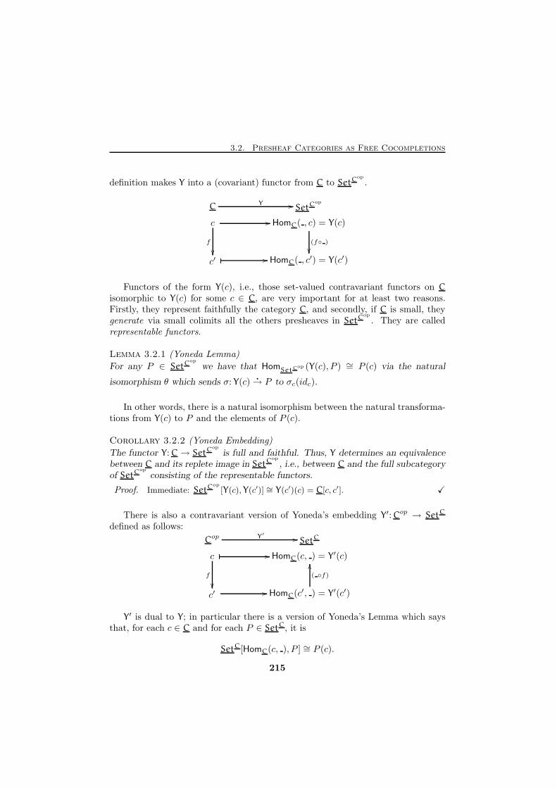
3.2. Presheaf Categories as Free Cocompletions
definition makes Y into a (covariant) functor from C to SetCop
.
c HomC( , c) = Y(c)
c′ HomC( , c′) = Y(c′)
� //
f
��(f◦ )
��� //
SetCopC Y //
Functors of the form Y(c), i.e., those set-valued contravariant functors on C
isomorphic to Y(c) for some c ∈ C, are very important for at least two reasons.Firstly, they represent faithfully the category C, and secondly, if C is small, theygenerate via small colimits all the others presheaves in SetCop
. They are calledrepresentable functors.
Lemma 3.2.1 (Yoneda Lemma)
For any P ∈ SetCop
we have that HomSetCop (Y(c), P ) ∼= P (c) via the natural
isomorphism θ which sends σ: Y(c)�
→ P to σc(idc).
In other words, there is a natural isomorphism between the natural transforma-tions from Y(c) to P and the elements of P (c).
Corollary 3.2.2 (Yoneda Embedding)
The functor Y: C→ SetCop
is full and faithful. Thus, Y determines an equivalencebetween C and its replete image in SetCop
, i.e., between C and the full subcategoryof SetCop
consisting of the representable functors.
Proof. Immediate: SetCop
[Y(c),Y(c′)] ∼= Y(c′)(c) = C[c, c′]. X
There is also a contravariant version of Yoneda’s embedding Y′: Cop → SetC
defined as follows:
c HomC(c, ) = Y′(c)
c′ HomC(c′, ) = Y′(c′)
� //
f
�� � //
SetCCopY′ //
( ◦f)
OO
Y′ is dual to Y; in particular there is a version of Yoneda’s Lemma which saysthat, for each c ∈ C and for each P ∈ SetC, it is
SetC[HomC(c, ), P ] ∼= P (c).
215
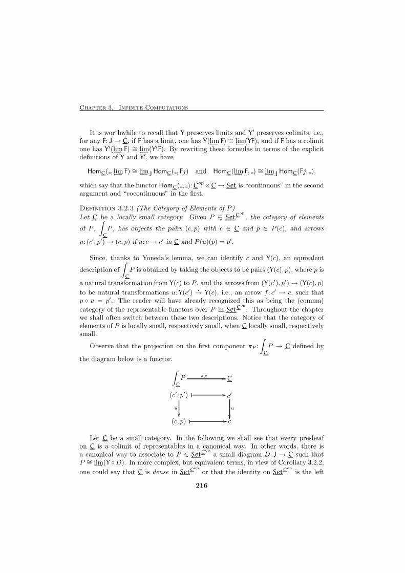
Chapter 3. Infinite Computations
It is worthwhile to recall that Y preserves limits and Y′ preserves colimits, i.e.,for any F: J→ C, if F has a limit, one has Y(lim←− F) ∼= lim←−(YF), and if F has a colimitone has Y′(lim−→ F) ∼= lim←−(Y′F). By rewriting these formulas in terms of the explicitdefinitions of Y and Y′, we have
HomC( , lim←− F) ∼= lim←−J HomC( , Fj) and HomC(lim−→ F, ) ∼= lim←−J HomC(Fj, ),
which say that the functor HomC( , ): Cop×C→ Set is “continuous” in the secondargument and “cocontinuous” in the first.
Definition 3.2.3 (The Category of Elements of P )
Let C be a locally small category. Given P ∈ SetCop
, the category of elements
of P ,
∫
C
P , has objects the pairs (c, p) with c ∈ C and p ∈ P (c), and arrows
u: (c′, p′)→ (c, p) if u: c→ c′ in C and P (u)(p) = p′.
Since, thanks to Yoneda’s lemma, we can identify c and Y(c), an equivalent
description of
∫
C
P is obtained by taking the objects to be pairs (Y(c), p), where p is
a natural transformation from Y(c) to P , and the arrows from (Y(c′), p′)→ (Y(c), p)
to be natural transformations u: Y(c′)�
→ Y(c), i.e., an arrow f : c′ → c, such thatp ◦ u = p′. The reader will have already recognized this as being the (comma)
category of the representable functors over P in SetCop
. Throughout the chapterwe shall often switch between these two descriptions. Notice that the category ofelements of P is locally small, respectively small, when C locally small, respectivelysmall.
Observe that the projection on the first component πP :
∫
C
P → C defined by
the diagram below is a functor.
(c′, p′) c′
(c, p) c
� //
u
��u
��� //
C
∫
C
P πP //
Let C be a small category. In the following we shall see that every presheafon C is a colimit of representables in a canonical way. In other words, there isa canonical way to associate to P ∈ SetCop
a small diagram D: J → C such thatP ∼= lim−→(Y ◦D). In more complex, but equivalent terms, in view of Corollary 3.2.2,
one could say that C is dense in SetCop
or that the identity on SetCop
is the left
216
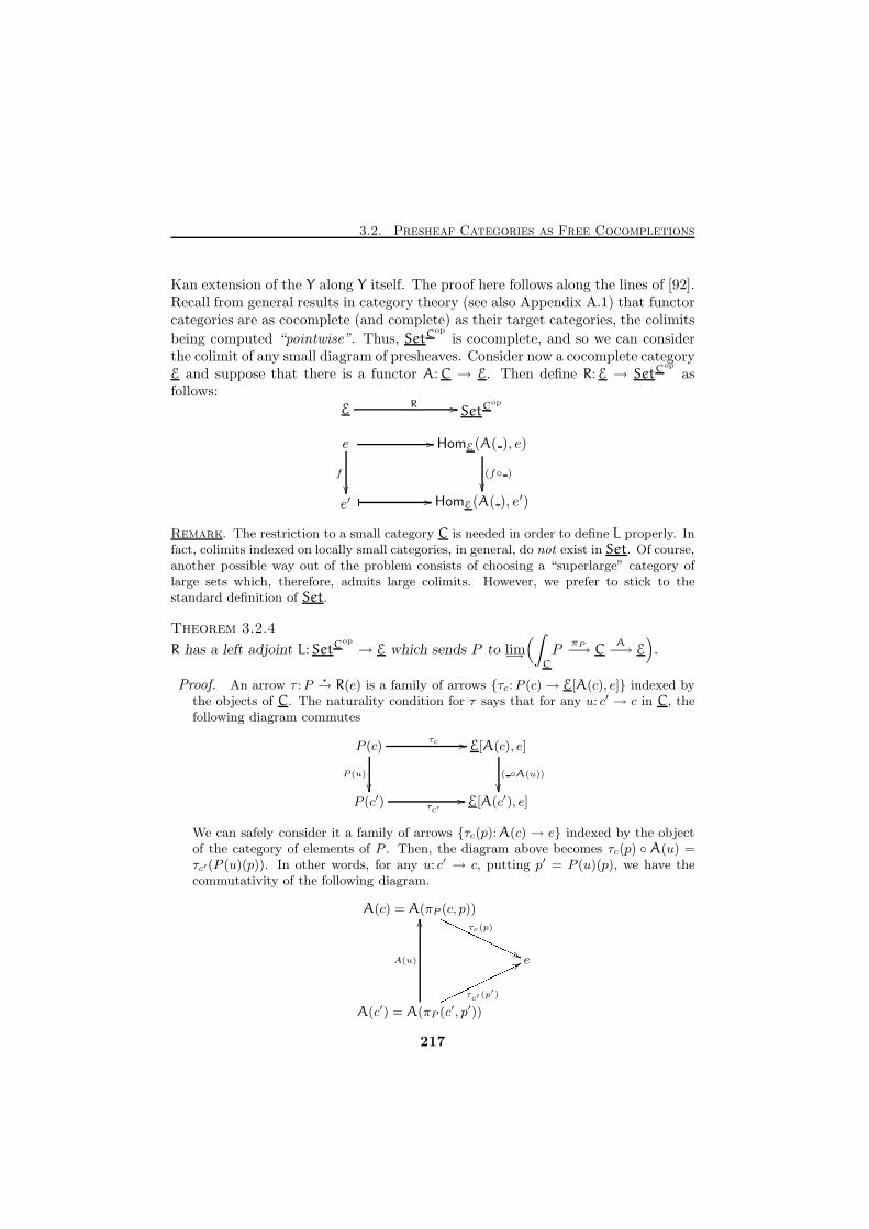
3.2. Presheaf Categories as Free Cocompletions
Kan extension of the Y along Y itself. The proof here follows along the lines of [92].Recall from general results in category theory (see also Appendix A.1) that functorcategories are as cocomplete (and complete) as their target categories, the colimits
being computed “pointwise”. Thus, SetCop
is cocomplete, and so we can considerthe colimit of any small diagram of presheaves. Consider now a cocomplete categoryE and suppose that there is a functor A: C → E. Then define R: E → SetCop
asfollows:
e HomE(A( ), e)
e′ HomE(A( ), e′)
� //
f
��(f◦ )
��� //
SetCopE
R //
Remark. The restriction to a small category C is needed in order to define L properly. Infact, colimits indexed on locally small categories, in general, do not exist in Set. Of course,another possible way out of the problem consists of choosing a “superlarge” category oflarge sets which, therefore, admits large colimits. However, we prefer to stick to thestandard definition of Set.
Theorem 3.2.4
R has a left adjoint L: SetCop
→ E which sends P to lim−→
(∫
C
PπP−→ C
A−→ E
).
Proof. An arrow τ :P�
→ R(e) is a family of arrows {τc:P (c) → E[A(c), e]} indexed bythe objects of C. The naturality condition for τ says that for any u: c′ → c in C, thefollowing diagram commutes
P (c) E[A(c), e]
P (c′) E[A(c′), e]
τc //
P (u)
��( ◦A(u))
��τc′
//
We can safely consider it a family of arrows {τc(p):A(c) → e} indexed by the objectof the category of elements of P . Then, the diagram above becomes τc(p) ◦ A(u) =τc′(P (u)(p)). In other words, for any u: c′ → c, putting p′ = P (u)(p), we have thecommutativity of the following diagram.
A(c) = A(πP (c, p))
e
A(c′) = A(πP (c′, p′))
τc(p)PPPPPPPPPPP''
τc′ (p′)nnnnnnnnnnn77A(u)
OO
217
Chapter 3. Infinite Computations
In other words,{τc(p) | (c, p) ∈
∫
C
P}
is a cocone for A ◦ πP . Since we have this
correspondence between natural transformations from P to R(e) and cocones for A◦πPwith vertex e, it follows easily from the universal property of colimits that there is a
natural bijection between natural transformations from P to R(e) and arrows from
lim−→
(A ◦ πP ) to e, i.e., SetCop
[P,R(e)] ∼= E[L(P ), e], which means that L ⊣ R. X
Corollary 3.2.5Every presheaf is a colimit of representable functors.
Proof. Apply the previous theorem with SetCop
in place of E and Y in place of A.
Observe that then we have L,R:SetCop
→ SetCop
. Now, by definition, R(P )(c) =
SetCop
[Y(c), P ] and then, by Yoneda’s lemma, R(P )(c) ∼= P (c) for any c ∈ C and any
P ∈ SetCop
. If follows that R ∼= IdSetCop . Now, the identity is left adjoint to itself
and since adjoints are unique up to isomorphisms and since we know that L is leftadjoint to R and, therefore, to the identity, we conclude that L ∼= Id
SetCop . Therefore
P ∼= L(P ) = lim−→
(∫
C
PπP−→ C
Y−→ SetCop
)= lim−→
(Y ◦ πP
).
X
An application of this result is that the morphisms in SetCop
can be character-ized as follows:
SetCop
[P,Q] ∼= SetCop[lim−→
(∫
C
PY◦πP−→ SetCop
), Q]
∼= lim←−c∈∫P
SetCop
[hc, Q] ∼= lim←−c∈∫PQ(c).
We have also the following corollary that states that SetCop
is “universal” upto isomorphism and bring us back to the issue of cocompletion of categories.
Corollary 3.2.6Let C be a small category. Then, for any cocomplete category E and any functorA: C → E, there is a functor L: SetCop
→ E which preserves the colimits and suchthat the following diagram commutes.
SetCopE
C
L //
Y/� OO Appppppppppppp77Moreover, L is unique up to isomorphisms.
218
3.3. ℵ-Filtered Cocompletion
Proof. Let us consider L(P ) = lim−→
(∫
C
PπP−→ C
A−→ E
). Since L is a left adjoint, it
preserves colimits. Now, let us show that the diagram commutes. If P is representable,then P ∼= Y(c) for some c ∈ C. It is then easy to realize that the category of elementsof P has a terminal object, namely the object (c, idc). Thus, without loss of generality,may assume that
L(Y(c)) = lim−→
(A ◦ πY(c)) = A(πY(c)(c, idc)) = A(c),
i.e., the diagram commutes.
Now, suppose that K:SetCop
→ E renders the diagram commutative and preservescolimits. Then, since for any presheaf P we have P ∼= lim
−→(Y ◦ πP ), it is
L(P ) ∼= L(lim−→
(Y ◦ πP )) ∼= lim−→
(L ◦ Y ◦ πP ) = lim−→
(A ◦ πP )
= lim−→
(K ◦ Y ◦ πP ) ∼= K(lim−→
(Y ◦ πP )) ∼= K(P ),
and thus K ∼= L. X
Observe that the above construction does not give rise to an adjunction fromCat to some “superlarge” category of large cocomplete categories for at least tworeasons. First, there are problems of cardinality, since SetCop
is not necessarilysmall and thus there is no evident forgetful functor which could make it so. Equallyimportant, and more relevant from our point of view, is that the free constructionabove is defined only up to equivalences. We shall get back to this point later.
3.3 ℵ-Filtered Cocompletion
In this section we apply the techniques of Section 3.2 to the case of the ℵ-chaincocompletion. The understanding of SetCop
as the “free” completion of a smallcategory C by arbitrary small colimits gives a strong hint on what the completionof C by ℵ-chains, say Cℵ, should be: the full subcategory of SetCop
which contains
the representables and their ℵ-chain colimits in SetCop
. We shall see that this isindeed the case, i.e., that Cℵ is closed for colimits of ℵ-chains and it is “universal”(in the weak sense above) among the ℵ-chain cocomplete categories which extends
C. Moreover, since the definition of Cℵ makes sense for any locally small category,the following theory applies to any such C.
Although chains are pretty simple structures, they are rather uncomfortableto manage, at least in our context, since, as categories, they are very stronglyrestricted. For instance, one cannot form products and coproducts of chains. Thissituation, however, is common to other fields of mathematics, like partial ordertheory and topology, where one uses the—equivalent in many contexts—notion ofdirected set [93, 52, 61, 133]. Thus, as a first step, we abandon ℵ-chains and we
219
Chapter 3. Infinite Computations
broaden the class of index categories we use for the colimits, but, as we shall see,this will not change the kind of cocompleteness Cℵ will have. Of course, as in manyexamples in the literature, e.g. [43, 58], we use filtered categories, which are thecategorical correspondent of directed sets.
Chains versus Directed Partial Orders
In this subsection we recall the relevant results about the equivalence of the no-tions of chain-completeness and direct-completeness for posets. By applying tocategories, one sees that a category admits all the colimits indexed over chains ifand only if it admits all colimits indexed by directed sets. The development herefollows [52, 130, 93]. Our reference for set theory is [55].
Definition 3.3.1A non-empty subset D of a partial order P is directed if any pair of elements in Dhas an upper bound in D. Equivalently, D is directed if it contains an upper boundof any of its finite subsets. A chain is a non-empty partial order which is totallyordered.
P is ℵ-directed complete if P has the least upper bound of any directed subsetof cardinality not greater than ℵ. It is directed complete if it has the least upperbound of any directed subset. P is ℵ-chain complete if P has the least upper boundof any chain of cardinality not greater than ℵ. It is chain complete if it has theleast upper bound of any chain.
Directed sets and chains are, as usual, required not to be empty. This is becausethe least upper bound of an empty set, if it exists, is the least element of the posetand in many applications—and in particular here—one desires to consider limitswithout requiring the existence of such an element.
Lemma 3.3.2Let D be an infinite directed set. Then, there exists a transfinite sequence {Dα}αof directed subsets of D, with α < |D|, such that
i) For any α
• If α is finite so is Dα;
• If α is infinite, then |Dα| = |α| (and therefore |Dα| < |D|).
ii) For any ordinals α < β < |D|, Dα ⊂ Dβ .
iii) D =⋃αDα.
Proof. Let γ be the cardinality of D. Remember that the cardinals correspond to theleast ordinal of a given cardinality. Let {xα}α<γ be a well-ordering of D and for each
220
3.3. ℵ-Filtered Cocompletion
finite subset F of D, let uF denote an upper bound of F in D. Then consider thecountable sequence
D0 = {x0};
Di+1 = Di ∪{yi+1, uDi∪{yi+1}
};
where yi+1 is the least element of D \Di (wrt. to the order {xα}α<γ). Of course, forany i ∈ ω, Di is finite of cardinality greater or equal to i, is directed, and for any j > iwe have Di ⊂ Dj . Let Dω be
⋃i<ω
Di. Now, if γ = ω, we are done. In fact, Dω ⊆ Dby construction, while if x ∈ D, then x = xj for some j and therefore x ∈ Dj ⊆ Dω,whence it follows Dω = D.
Suppose instead that γ > ω. Consider now β < γ and suppose that the sequence{Dα}α<β enjoys properties (i) and (ii) above. We show that the sequence can beextended to β. There are the following two cases.
(a) If β is a limit ordinal, then define Dβ =⋃α<β
Dα. Then, for any α < β it
is Dα ⊂ Dβ . Moreover, since |Dα| = |α| and since β =⋃α<β
α, we have |Dβ | =
Σα<β |α| = |β| × sup |α| = |β| × |β| = |β|.
(b) β = δ + 1. Then consider the countable sequence
Dβ,0 = Dδ ∪ {y′β}, y
′β being the least element in D \Dδ;
Dβ,i+1 = Dβ,i ∪{uF | F ⊂ Dβ,i, F finite
};
and take Dβ =⋃i<ω
Dβ,i. Let S be a finite subset of Dβ . Then, S ⊂ Dβ,i for some iand, therefore, uF ∈ Dβ,i+1. It follows that Dβ is directed. Moreover, |Dβ,i| = |Dδ |,since the set of the finite subsets of X has the same cardinality as X. Then |Dβ | =ω × |Dδ | = |Dδ | = |δ| = |δ + 1| = |β|. Finally, we of course have Dδ ⊂ Dβ .
Now, the thesis follows by transfinite induction. X
The relevance of the previous lemma shows in the proof of the following.
Corollary 3.3.3P is ℵ-directed complete if and only if P is ℵ-chain complete.
Proof. One implication is obvious, since chains are directed sets. Let us show the otherimplication.
Suppose that the conclusion is false, i.e., that there exists a directed D ⊆ P with
|D| ≤ ℵ such that supD does not exist. Observe that D cannot be finite, since a
finite directed set always has a least upper bound: its greatest element. Clearly, we
can assume that every D′ ⊂ D with |D′| < |D| has a least upper bound. Then we are
in the hypothesis of Lemma 3.3.2. Let {Dα}, with α < |D|, be the sequence obtained
by applying it to D. Since |Dα| < |D|, supDα exists in P . Therefore we have a chain
{supDα}α<|D| of cardinality |D|. Then, sup{supDα}α<|D| exists and it is clearly the
least upper bound of D. X
221
Chapter 3. Infinite Computations
The previous proof depends heavily on the axiom of choice, because of thewell-ordering chosen for D. Observe that Corollary 3.3.3 does not say that fromany directed set we can extract a cofinal subchain, which is in fact false. (For acounterexample see e.g. [130].)
Corollary 3.3.4P is directed complete if and only if P is chain complete.
Proof. Immediate from Corollary 3.3.3. X
Next, we apply Lemma 3.3.2 to the notion of cocompleteness in categories. Sincean ordinal number α is an ordered set, which in turn is a category, we can considerfunctors F :α → C. We shall refer to such functors as chain functors, or simplychains. We call F a ℵ-chain functor, or simply ℵ-chain, if α = ℵ, where | | givesthe cardinality of sets. Similarly, for D a directed set, a functor F :D → C is calleddirected functor. If |D| ≤ ℵ then F is called ℵ-directed.
Definition 3.3.5A category C is (ℵ-)directed cocomplete if it admits colimits of all (ℵ-)directedfunctors. It is (ℵ-)chain cocomplete if it has colimits of all (ℵ-)chain functors.
Of course, as in the case of posets, for ℵ finite, the ℵ-directed and ℵ-chaincocompleteness are trivial notions, since they are enjoyed by any category.
Remarkably, the notion of colimits indexed over directed posets is a prettypowerful one—indeed it was the original definition of colimits in category theory. Infact, if C has all finite coproducts and colimits of directed sets, then it is cocomplete,i.e., it has all small colimits [90, chap. IX, pp. 208].
Proposition 3.3.6C is ℵ-directed cocomplete if and only if it is ℵ-chain cocomplete.Proof. Once again one implication is trivial. Let us show that when C admits colimits
of all ℵ-chains it has colimits of all ℵ-directed functors. If ℵ is finite the thesis is trivial;so suppose ℵ infinite. Let F :D → C be a ℵ-directed functor. If F is n-directed thenD has a greatest element, say d, and, therefore, F has a colimit, namely Fd with theobvious limit cocone.
Now suppose that a colimit exists for any β-directed functor with β < γ ≤ ℵ, γan infinite cardinal, and let |D| be γ in F :D → C. Applying Lemma 3.3.2, we get asequence {Dα}α<γ with Dα ⊂ D, |Dα| = |α| < γ, Dα directed and
⋃α<γ
Dα = D. Let
inα:Dα → D denote the injection of Dα in D. For any α < γ, let Fα:Dαinα→ D
F−→ C
be the restriction of F to Dα and let σα:Fα�
→ cα be a colimit for Fα. Now, observe
that for any α ≤ β, since Dα ⊆ Dβ , we have (σβ)α:Fα�
→ cβ , where (σβ)α is therestriction of σβ to Dα. Then, by definition of colimit, there exists a unique inducedarrow fα,β : cα → cβ such that
fα,β ◦ (σα)d = (σβ)d for any d ∈ Dα. (3.1)
222
3.3. ℵ-Filtered Cocompletion
It follows, again from the universal property of colimits, that the following definitiondefines a functor G: γ → C.
Gα = cα for any α ∈ γ; G(α ≤ β) = fα,β .
Since G is a γ-chain we can consider lim−→
G in C. Let λ:G�
→ c be the limit cocone.We claim that c is lim
−→DF .
Next we define a cocone σ:F�
→ c for F and we show that it is the limit cocone. Sincefor any d ∈ D there exists α such that d ∈ Dα, the obvious choice is σd = λα ◦ (σα)d.Observe that σd is irrespective of the choice of α. In fact, suppose d ∈ Dβ and letσ′d be λβ ◦ (σβ)d. Without loss of generality suppose α ≤ β. Then, since we have
λ:G�
→ c, it is λα = λβ ◦ fα,β . Moreover, by construction, (σβ)d = fα,β ◦ (σα)d. Then,λβ ◦ (σβ)d = λβ ◦ fα,β ◦ (σα)d = λα ◦ (σα)d = σd. Thus, σ is well-given. Let us seethat it is a cocone. Suppose d ≤ e in D. Let α be large enough so that d, e ∈ Dα.Now, since we have σα:Fα → cα, it is (σα)d = (σα)e ◦Fα(d ≤ e) and then, taking intoaccount also that Fα(d ≤ e) = F (d ≤ e), it is λα ◦ (σα)d = λα ◦ (σα)e ◦F (d ≤ e) whichis σd = σe ◦ F (d ≤ e).
Then, we only miss to show that σ is universal. Let η:F�
→ c′ be a cocone with vertex
c′ for F . In particular, for any α ∈ γ, η restricts on Dα to (η)α:Dα�
→ c′, and thus it
exists a unique να: cα → c induced by the colimit, i.e., such that να ◦ (σα)d = ηd for
any d ∈ Dα. Let us show that the collection of the ν’s form a cocone with vertex c′ for
G. We must show that, for any α ≤ β, να = νβ ◦ fα,β which comes as follows: for any
α ≤ β, and for any d ∈ Dα, we have by (3.1) that νβ ◦ fα,β ◦ (σα)d = νβ ◦ (σβ)d = ηd,
which is enough since να is the unique arrow with this property. Thus, we have
shown that a cocone η:F�
→ c′ determines a unique ν:G�
→ c′. Then, by universality
of λ, there exists a unique k: c → c′ such that να = k ◦ λα for any α ∈ γ, which
implies να ◦ (σα)d = k ◦ λα ◦ (σα)d for any α ∈ γ and for any d ∈ Dα, which implies
ηd = k ◦ λα ◦ (σα)d for any α ∈ γ and for any d ∈ Dα, which is ηd = k ◦ σd for
any d ∈ D. The construction itself shows that k is the unique morphism from c to c′
enjoying this property, and thus the proof is concluded. X
A particular case which will interest us in the following is the one where ℵ is ω.Of course, we have the following corollary.
Corollary 3.3.7C is directed cocomplete if and only if C is chain cocomplete.
Proof. Immediate from Proposition 3.3.6. X
Filtered Categories and Cofinal Functors
In this subsection we broaden further the kind of index categories over which col-imits are considered. In particular, we recall the basic facts about filtered categories
223
Chapter 3. Infinite Computations
and cofinal functors. Moreover, we state results which show that requiring the ex-istence of colimits indexed by filtered categories is not stronger than requiring theexistence of colimits indexed by directed sets and, therefore, of chain colimits.
Definition 3.3.8 (Filtered Categories)A category J is filtered if it is not empty and
i) for all j, j′ ∈ J there exists k and u: j → k, v: j′ → k, i.e.,j
kj′
uPPP''vooo77 .
ii) for all i ju //v
// in J, there exists w: j → k such that w ◦ u = w ◦ v, i.e.,
i ju //v
// w−→ k is commutative.
A functor F: J→ C is filtered if J is filtered. By filtered colimits we mean colimitsof filtered functors.
The following propositions list some of the good properties enjoyed by filteredcategories.
Proposition 3.3.9The cartesian product of filtered categories is filtered.
Proof. Immediate. X
A good point is that filtered colimits in Set are easily characterized.
Proposition 3.3.10Let F: J → Set be filtered and suppose that J is small. Consider the set
∐j∈J Fj
and the binary relation R on it defined as follows
in i(x) R inj(y) ⇔ ∃k ∈ J andi
kj
uPPP''vppp77 such that F(u)(x) = F(v)(y).
Then
i) R is an equivalence relation;
ii)(∐
j∈J Fj) /R ∼= lim−→J F;
iii) Given x, y ∈ Fk, then ink(x) R ink(y) if and only if there exists u: k → hsuch that F(u)(x) = F(u)(y).
224
3.3. ℵ-Filtered Cocompletion
Proof. (i). R is manifestly reflexive and symmetric. Let us show that it is symmetric.Suppose ini(x) R inj(y) via u: i→ h and v: j → h, and suppose that inj(y) R ink(z)via v′: j → h′ and u′: k → h′. Using jointly the properties (i) and (ii) of filteredcategories, we find w:h → m and w′:h′ → m such that w ◦ v = w′ ◦ v. Now wehave F(w ◦ u)(x) = F(w)(F(u)(x)) = F(w)(F(v)(y)) = F(w ◦ v)(y) = F(w′ ◦ v′)(y) =F(w′)(F(v′)(y)) = F(w′)(F(u′)(z)) = F(w′ ◦ u′)(z), i.e., ini(x) R ink(z) via w and w′.This is summarized by the following picture.
i j k
h h′
m
u
<<<<<<�� v�������� v′
�������� u′
��������w
� � � w′~~} } }(ii). For any j ∈ J, let σj be the composition of the injection of Fj in
∐j∈J Fj with the
quotient map∐j∈J Fj 7→
(∐j∈J Fj
) /R. Since for any u: i→ j in J, it is obviously
ini(x) R inj(F(u)(x)) via u and id j , we have σi = σj ◦ F(u). Thus, the collection of
the σ’s is a cocone σ: F�
→(∐
j∈J Fj) /R which is easily shown to be universal. In
fact, if η: F�
→ X is another cocone, by definition it must be ηi(x) = ηj(y) wheneverini(x) R inj(y) whence the result follows at once.
(iii). Obvious from point (i) and condition (ii) of Definition 3.3.8. X
Proposition 3.3.11The category of small filtered categories has all small filtered colimits.
Proof. It is easy to see that the characterization of indexed colimits in Set given by
Proposition 3.3.10 can be extended to Cat-valued filtered functors. Then, it is easy to
show that the category resulting as colimit of a filtered diagram of filtered categories
is itself filtered. X
Cofinal subcategories are the categorical generalization of the set-theoretic no-tion of cofinal chains. Intuitively, a subcategory I of J is cofinal in J if the colimitof any J-indexed diagram coincides with the colimit of the same diagram restrictedto I. Of course, there is no conceptual need to limit oneself to subcategories, andthat is why one introduces cofinal functors.
Definition 3.3.12 (Cofinal Functors)A functor φ: I→ J is cofinal if for any functor F: J→ C
lim−→ I(F ◦ φ) exists ⇒ lim−→J F exists and lim−→ I(F ◦ φ) ∼= lim−→J F,
225
Chapter 3. Infinite Computations
the isomorphism being via the canonical comparison map lim−→ I(F ◦ φ) → lim−→J F
induced by the colimit.
A subcategory I of J is cofinal if the inclusion functor is cofinal.
Of course the name is inherited from the corresponding notion in set theoryand the “co” prefix has nothing to do with duality in categories. For this reason,MacLane [90, chap. IX] and others use the term “final” to name the concept.However, once the reader has been warned about this mismatch, we prefer to keepusing the classical terminology.
The proof of the following proposition is immediate.
Proposition 3.3.13The composition of cofinal functors is a cofinal functor.
The following key lemma gives a characterization of cofinal functors betweenfiltered categories.
Lemma 3.3.14For a functor φ: I→ J the following properties can be stated:
F1: for any j ∈ J, there exists i ∈ I such that HomJ(j, φi) 6= ∅.
F2: for any i ∈ I and for any j φif //g
// in J, there exists h: i → k in I such
that φh ◦ f = φh ◦ g.
Then, we have the following facts:
i) if φ is cofinal, then F1 holds;
ii) if I is filtered, then φ is cofinal if and only if F1 and F2 hold and, in thiscase, J is also filtered;
iii) if J is filtered and φ is full and faithful, then φ is cofinal if and only if F1holds, and, in this case, I is also filtered.
Proof. Let us consider the Yoneda’s embedding Y: J → SetJop
. Without loss of gen-erality, we can assume that Set is based on a universe U such that I and J are smallwith respect to U. In fact, if this were not the case we could replace Set with a largercategory and the following arguments would apply unchanged. Then, we can considerthe lim
−→ I(Y ◦ φ), which exists by the hypothesis above. Since φ is cofinal, this impliesthat lim
−→J Y exists.
Now, in order to show that F1 is a necessary condition, suppose that there exists ∈ Jsuch that, for any i ∈ I, HomJ(, φi) = ∅. Then, again by cofinality of φ, it must be
lim−→ I(Y ◦ φ) = lim
−→ i∈I HomJ( , φi) ∼= lim−→ j∈J HomJ( , j) = lim
−→J Y.
226
3.3. ℵ-Filtered Cocompletion
But this is impossible, since(lim−→ i∈I HomJ( , φi)
) ∼= lim
−→ ı∈I HomJ(, φi) = ∅ by hy-
pothesis on , while(lim−→ j∈J HomJ( , j)
) ∼= lim
−→ j∈J HomJ(, j) 6= ∅, since it must at
least contain an element to match id ∈ HomJ(, ).
Assume now that I be filtered. Let us see that J is filtered. Consider j, j′ ∈ J. Then,
by F1, we can find ju−→ φi and j′
u′
−→ φi′ in J, and since I is filtered we have iw′
−→ k
and i′w′
−→ k in I whose image via φ givesj
φk
j′
φw◦uQQQ((φw′◦u′nnn66 . Thus, property (i) of the definition
of filtered categories is shown.
In order to show the other condition, we need the following lemma: for any k ∈ I it islim−→ I HomI(k, ) = {∗}. Observe that this is an easy consequence of the (contravariant)Yoneda’s Lemma: let ∆(S): I→ Set be the constant functor which returns the set S;then
SetI[HomI(k, ),∆(S)] ∼= S ∼= Set[{∗}, S],
which is the required adjointness condition for colimits. Consider now ′f //g
// and
take x: ′ → φı, which exists by F1. Then, lim−→ i∈I HomI(, φi) = lim
−→ j∈J HomJ(, j)
by cofinality of φ, which is {∗} by the previous argument. Then, by point (iii) ofProposition 3.3.10, since x ◦ f, x ◦ g ∈ HomI(, φı) and x ◦ f R x ◦ g, it must existh: ı→ k in I such that φh ◦ x ◦ f = φh ◦ x ◦ g. Thus, φh ◦ x equalizes1 f and g and the
second condition of filteredness is shown. Now, if we consider φıf //g
// , reasoning
as above, we find h: ı → k such that φh ◦ f = φh ◦ g. Thus, the necessity of F2 isshown.
Next, we see that F1 and F2 are sufficient to ensure that φ is cofinal. Let F: J → Cbe a functor and suppose that c = lim
−→(F ◦ φ). It is possible to show that there is a
one-to-one correspondence between cocones with base F ◦ φ and vertex c and cocones
with base F and vertex c. Let σ: F ◦ φ�
→ c. Now, for j ∈ J, chosen u: j → φi, defineτj = σi ◦Fu. First, we have to show that τj does not depend on the choice of u: j → φi.In fact, if u′: j → φi′, since I is filtered, we can find x: i→ k and y: i′ → k. Moreover,by F2 we can find h: k → z such that φh ◦ φx ◦ u = φh ◦ φy ◦ u′. Then
τ ′j = σi′ ◦ Fu′ = σk ◦ Fφy ◦ Fu′
= σz ◦ Fφh ◦ Fφy ◦ Fu′
= σz ◦ Fφh ◦ Fφx ◦ Fu
= σk ◦ Fφx ◦ Fu
= σi ◦ Fu = τj
1Here and in the following the term equalizer is used in its English sense, not in the categoricalone.
227
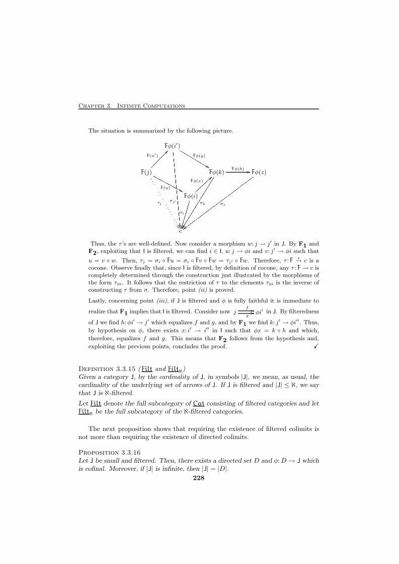
Chapter 3. Infinite Computations
The situation is summarized by the following picture.
F(j) Fφ(k) Fφ(z)
c
Fφ(i′)
σi′
"""""""""""""""""""""""" ��Fφ(y)
LLLLLLLLL%%F(u′)
??������τj
��
� � � � � � � � � � � � � � � � � � � � � � � � � � � � � � � � � � � � � � � σk
������������������Fφ(h) //
σz
{{wwwwwwwwwwwwwwwwwwwww
Fφ(i)
σi
���������Fφ(x)}}}}}>>F(u)
NNNNNNNNN &&Thus, the τ ’s are well-defined. Now consider a morphism w: j → j′ in J. By F1 andF2, exploiting that I is filtered, we can find i ∈ I, u: j → φi and v: j′ → φi such that
u = v ◦ w. Then, τj = σi ◦ Fu = σi ◦ Fv ◦ Fw = τj′ ◦ Fw. Therefore, τ :F�
→ c is acocone. Observe finally that, since I is filtered, by definition of cocone, any τ : F→ c iscompletely determined through the construction just illustrated by the morphisms ofthe form τφi. It follows that the restriction of τ to the elements τφi is the inverse ofconstructing τ from σ. Therefore, point (ii) is proved.
Lastly, concerning point (iii), if J is filtered and φ is fully faithful it is immediate to
realize that F1 implies that I is filtered. Consider now j φi′f //g
// in J. By filteredness
of J we find h:φi′ → j′ which equalizes f and g, and by F1 we find k: j′ → φi′′. Thus,
by hypothesis on φ, there exists x: i′ → i′′ in I such that φx = k ◦ h and which,
therefore, equalizes f and g. This means that F2 follows from the hypothesis and,
exploiting the previous points, concludes the proof. X
Definition 3.3.15 ( Filt and Filtℵ)Given a category J, by the cardinality of J, in symbols |J|, we mean, as usual, thecardinality of the underlying set of arrows of J. If J is filtered and |J| ≤ ℵ, we saythat J is ℵ-filtered.
Let Filt denote the full subcategory of Cat consisting of filtered categories and letFiltℵ be the full subcategory of the ℵ-filtered categories.
The next proposition shows that requiring the existence of filtered colimits isnot more than requiring the existence of directed colimits.
Proposition 3.3.16Let J be small and filtered. Then, there exists a directed set D and φ:D → J whichis cofinal. Moreover, if |J| is infinite, then |J| = |D|.
228
3.3. ℵ-Filtered Cocompletion
Proof. First suppose that J has no greatest object, i.e., that for any j ∈ J it is possible tofind j′ ∈ J, j′ 6= j, such that HomJ(j, j′) 6= ∅. D consists of all the finite subcategoriesA of J which have a unique terminal object ordered by inclusion. Of course, one definesφ(A) to be its terminal object. Moreover, if A ⊆ B, there is a unique arrow f in Bsuch that f :φ(A)→ φ(B), and one defines φ(A ⊆ B) to be such an arrow.
For A and B in D an upper bound is identified as follows. Let a and b be the terminalobjects of, respectively, A and B. Since J is filtered one can find u: a→ j and v: b→ j.Then consider the category E whose objects are the union of those of A and B plus jand whose arrows are the union of those of A and B plus u and v. Clearly, E is a finitesubcategory of J with a unique terminal object and is an upper bound for A and B.Thus, D is directed.
In order to show that φ is cofinal we use point (ii) of Lemma 3.3.14. It is obvious thatF1 holds: for any j ∈ J consider the subcategory of J consisting of the only j with its
identity arrow. Verifying that F2 holds requires a bit more of work. Let j φ(A)f //g
//
be in J. Since J is filtered, we can find u:φ(A) → j′ which equalizes them. Since weassume that J has no greatest object, we can suppose that j′ is different from φ(A). Itfollows that j′ cannot be an object of A and that the subcategory B obtained from Aby adding the new object j′ and the arrow u belongs to D. Moreover, φ(A ⊆ B) = uequalizes f and g as required.
We miss the case in which J has a greatest element. In this case one considers the
category ω × J, which is filtered and does not have a greatest object. Then one finds
Dφ−→ ω × J, with φ cofinal and compose it with the projection ω × J
π−→ J, which is
manifestly cofinal because of Lemma 3.3.14, point (iii). Thus, Dπ◦φ−→ J is cofinal. The
statement about cardinalities follows at once, since the set of finite subcategories of J
has the same cardinality as J if this is infinite. X
Recall that we say that a functor F: J → C is filtered if J ∈ Filt. Moreover, ifJ ∈ Filtℵ, then F is ℵ-filtered. A category C is ℵ-filtered cocomplete if it admitscolimits of all ℵ-filtered functors, and it filtered cocomplete if it has colimits of allfiltered functors.
Corollary 3.3.17A category C is ℵ-filtered cocomplete if and only if it is ℵ-directed cocomplete, ifand only if it is ℵ-chain cocomplete.
A category C is filtered cocomplete if and only if is directed cocomplete, if and onlyif it is chain cocomplete.
Proof. Concerning the first claim, the second double implication is Proposition 3.3.6and one direction of the first one is trivial. The other direction follows immediatelyby Proposition 3.3.16 as follows. Let C be directed complete and consider F: J → C.Suppose that ℵ is infinite. Then, we can find a directed D and φ:D → J such that|D| = |J| and φ is cofinal. Then, Fφ:D → C has a colimit and therefore, by cofinality,lim−→
F exists in C. Suppose instead that ℵ is finite. If J has no greatest object, the
229
Chapter 3. Infinite Computations
D obtained from Proposition 3.3.16 is finite and the argument above can be applied,since the colimits indexed by finite D’s always exist in C. Finally, if J has a greatestobject, take φ to be the functor which maps the singleton set to such an object. Ofcourse φ is cofinal, and thus we can apply again the argument above. (Observe thatthis just proves that, as in the case of directed colimits, finite filtered colimits are atrivial notion, since they exist in any category C.)
The second statement is proved similarly. X
Exploiting further the notion of cofinal functor, we can still broaden further theclass of index categories over which we shall consider colimits. We shall do so bybeing as lax as possible with respect to cardinalities.
Definition 3.3.18 (Essentially ℵ-Filtered Categories)A category J is essentially ℵ-filtered if it is locally small and if there exists I ∈ Filtℵtogether with φ: I → J which is cofinal. J is essentially filtered if it is essentiallyℵ-filtered for some cardinal ℵ.
Let E-Filt be the full subcategory of CAT consisting of the essentially filteredcategories. E-Filtℵ denotes the full subcategory of E-Filt consisting of the essentiallyℵ-filtered categories.
We say that C is essentially (ℵ-)filtered cocomplete if it admits colimits of allfunctors indexed over essentially (ℵ-)filtered categories. Then, we have the followingimmediate corollary which closes this subsection and allows us in the rest of thechapter to use the quite liberal essentially ℵ-filtered categories in place of ℵ-chainswithout changing the kind of cocompleteness of the category involved.
Corollary 3.3.19A category C is essentially (ℵ-)filtered cocomplete if and only if it is (ℵ-)filteredcocomplete if and only if it is (ℵ-)directed cocomplete if and only if it is (ℵ-)chaincocomplete.
Proof. The missing step is to prove that if C is (ℵ-)filtered cocomplete then it is
essentially (ℵ)-filtered cocomplete. But this follows immediately from Corollary 3.3.17
and from the definition of cofinal functor. X
Thus, although we shall preferably use the (ℵ-)filtered alternative, the previouscorollary allows us to use the terms above interchangeably.
Remark. We have already observed that the notion of cocompleteness coincide (trivially)for all the finite cardinals. However, this is just a limit case of a general situation: if ℵand ℵ′ are infinite cardinals having the same cofinality, then C is ℵ-filtered cocompleteif and only if it is ℵ′-filtered cocomplete. Clearly, different regular cardinals give rise todifferent notions of cocompleteness.
230
3.3. ℵ-Filtered Cocompletion
ℵ-Ind-Representable Functors
We are ready now to give the results about the chain cocompletion, or equivalentlythe essentially filtered cocompletion, of C.
Definition 3.3.20 (ℵ-Ind-Representable Functors)
Given a locally small category C, let Cℵ denote the full subcategory of SetCop
whichcontains the representables hc, c ∈ C, and lim−→ YF for any ℵ-chain functor F:α→ C,Y being the Yoneda’s embedding.
Similarly, C denotes the full subcategory of SetCop
which contains the representableshc and lim−→ YF for any chain functor F.
The presheaves in Cℵ are called ℵ-ind-representable (ind standing for inductively),
those in C are called the ind-representable functors.
Observe that, in view of the development in the previous sections, C (Cℵ) can
be equivalently defined as the full subcategory of SetCop
which contains the rep-resentables and lim−→(YF) for any F: J → C, where J ∈ E-Filt (J ∈ E-Filtℵ). In thefollowing, we shall use often this equivalent description.
Proposition 3.3.21The categories Cℵ and C are locally small.
Proof. Since Cℵ is a full subcategory of C, it is enough to prove the result for C. Given
P and Q in C we can assume they are of the form P ∼= lim−→ I hci and Q ∼= lim
−→J hcj , forI, J ∈ Filt. Then,
C[P,Q] = SetCop
[P,Q]
∼= SetCop
[lim−→ I hci , lim−→J hcj ]
∼= lim←− I SetCop
[hci , lim−→J hcj ] (since Y′ preserves colimits)
∼= lim←− I
(lim−→J hcj
)ci (by the Yoneda’s lemma)
∼= lim←− I lim−→J HomC(ci, cj).
Thus, as a lim←−
lim−→
construction in Set indexed by small categories, HomC
(P,Q) is a
small set. X
The following is an interesting property of ind-representables.
Proposition 3.3.22ℵ-ind-representable functors preserve finite colimits.
Proof. Let I be finite and consider F: I→ C such that lim−→
F exists. Let us show that for
every P be in Cℵ it is lim←−
(P ◦ F) ∼= P (lim−→
F).
231
Chapter 3. Infinite Computations
First observe that this is true for the representable functors.
hc(lim−→ F) = HomC(lim−→
F, c)
∼= lim←−
HomC(F, c) (since Y′ preserves colimits)
∼= lim←−
(hc ◦ F)
Now, if P is ℵ-ind-representable, then P = lim−→J hcj . Therefore,
(lim−→J hcj )(lim−→ I F) = lim
−→J(hcj (lim−→ I F)) = lim−→J lim
←− I(hcj ◦ F)
∼= lim←− I lim
−→J(hcj ◦ F)
= lim←− I((lim−→J hcj ) ◦ F) = lim
←− I(P ◦ F),
the key passage being because finite limits and filtered colimits commute in Set. X
We have seen in Section 3.2 that the Yoneda’s embedding Y preserves arbitrarysmall limits. If we look at Y as a functor from C to the category of (ℵ-)ind-representable functors, we can show that Y preserves finite colimits. However, it isfalse that Y preserves filtered colimits which exist in C, i.e., c = lim−→ F in C does notimply hc ∼= lim−→(YF).
Proposition 3.3.23Y: C→ C (Y: C→ Cℵ) preserves finite colimits
Proof. Let c = lim−→ I ci. Then, for any P ∈ C, supposing that P ∼= lim
−→K hxk, we have
SetCop
[hc, P ] ∼= P (c) ∼= (lim−→K hxk
)c ∼= lim−→K HomC(c, xk)
∼= lim−→K HomC(lim
−→ I ci, xk)∼= lim−→K lim
←− I HomC(ci, xk)
∼= lim←− I lim−→K HomC(ci, xk) ∼= lim
←− I SetCop
[hci , lim−→K hxk]
∼= SetCop
[lim−→ I hci , P ].
It follows that Y(lim−→ I ci)
∼= lim−→ I Y(ci). X
Now, we see that the results about SetCop
in Section 3.2 can be mimicked forCℵ. The key fact is the following proposition, which gives us a canonical way tosee every ℵ-ind-representable functor as an essentially ℵ-filtered diagram in C.
Proposition 3.3.24
A presheaf P on C is ℵ-ind-representable if and only if
∫
C
P is essentially ℵ-filtered.
Proof. Since for any presheaf P we have P ∼= lim−→
(∫
C
PπP−→ C
Y−→ SetCop
), one
implication is obvious.
Therefore, if the category of elements of P is essentially ℵ-filtered then P is in Cℵ.
232
3.3. ℵ-Filtered Cocompletion
Suppose now that P ∼= lim−→ I hci , where I is essentially ℵ-filtered and let λi:hci → P be
the components of the limit cocone. Let (c, p) and (c′, p′) be objects of
∫
C
P . Recall
that p and p′ can be thought of as morphisms p:hc�
→ P and p′: hc′�
→ P , and since
SetCop
[hc, P ] ∼= lim−→ I HomC(c, ci), from the characterization of set-valued filtered col-
imits of Proposition 3.3.10, these transformations must come from morphisms f : c→ ciand g: c′ → cj in C, for i, j ∈ I, such that p = λi ◦ (f ◦ ) and p′ = λj ◦ (g ◦ ). Thus we
have (c, p)f−→ (ci, λi) and (c′, p′)
g−→ (cj , λj) in
∫
C
P . Now, since I is filtered, we can
find k in I and h: cj → ck and h′: c′j → ck in C. Consider (ck, λk). Of course, we have
λi = λk ◦ (h ◦ ) and λj = λk ◦ (h′ ◦ ) and thus we have (c, p)f−→ (ci, λi)
h−→ (ck, λk)
and (c′, p′)g−→ (cj , λj)
h′
−→ (ck, λk) in
∫
C
P . This is summarized by the following
picture.
hc hcihcj hc′
hck
P
p
BBBBBBBBBBBBBBB!!(f◦ ) //
h
BBBBBB!!λi
1111111111111�� h′
}}||||||λj
�� p′
}}{{{{{{{{{{{{{{{(g◦ )oo
λk
��
Consider now (c, p) (c′, p′)f //g
// . Recall that by definition of morphism in the cat-
egory of elements of P , p′ ◦ (f ◦ ) = p = p′ ◦ (g ◦ ). Reasoning as before we
get that p′ corresponds to h: c′ → ci such that (c′, p′)h−→ (ci, λi). Then we have
λi ◦ (h ◦ f ◦ ) = λi ◦ (h ◦ g ◦ ) By the characterization of filtered colimits in Set ofProposition 3.3.10 this means that it must exist an arrow i→ j in the index category I
whose image in C, say k, equalizes h◦f and h◦g. It follows that (hci , λi)k−→ (hcj , λj)
equalizes f and g in
∫
C
P . This is illustrated below.
hc
hc′
hci
F hcj
(f◦ )
��(g◦ )
��
p′
��
(h◦ )
BBBBBB!!λi
~~|||||| (k◦ )
BBBBBB λjoo
233
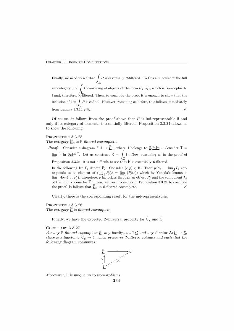
Chapter 3. Infinite Computations
Finally, we need to see that
∫
C
P is essentially ℵ-filtered. To this aim consider the full
subcategory J of
∫
C
P consisting of objects of the form (ci, λi), which is isomorphic to
I and, therefore, ℵ-filtered. Then, to conclude the proof it is enough to show that the
inclusion of J in
∫
C
P is cofinal. However, reasoning as before, this follows immediately
from Lemma 3.3.14 (iii). X
Of course, it follows from the proof above that P is ind-representable if andonly if its category of elements is essentially filtered. Proposition 3.3.24 allows usto show the following.
Proposition 3.3.25The category Cℵ is ℵ-filtered cocomplete.
Proof. Consider a diagram F: J → Cℵ, where J belongs to E-Filtℵ. Consider T =
lim−→J F in SetCop
. Let us construct K =
∫
C
T . Now, reasoning as in the proof of
Proposition 3.3.24, it is not difficult to see that K is essentially ℵ-filtered.
In the following let Pj denote Fj. Consider (c, p) ∈ K. Then p:hc → lim−→J Pj cor-
responds to an element of (lim−→J Pj)c = lim
−→J(Pj(c)) which by Yoneda’s lemma is
lim−→J Hom(hc, Pj). Therefore, p factorizes through an object Pj and the component λjof the limit cocone for T . Then, we can proceed as in Proposition 3.3.24 to conclude
the proof. It follows that Cℵ in ℵ-filtered cocomplete. X
Clearly, there is the corresponding result for the ind-representables.
Proposition 3.3.26The category C is filtered cocomplete.
Finally, we have the expected 2-universal property for Cℵ and C.
Corollary 3.3.27For any ℵ-filtered cocomplete E, any locally small C and any functor A: C → E,there is a functor L: Cℵ → E which preserves ℵ-filtered colimits and such that thefollowing diagram commutes.
Cℵ E
C
L //
Y/� OO Arrrrrrrrrrrr 88Morevover, L is unique up to isomorphisms.
234
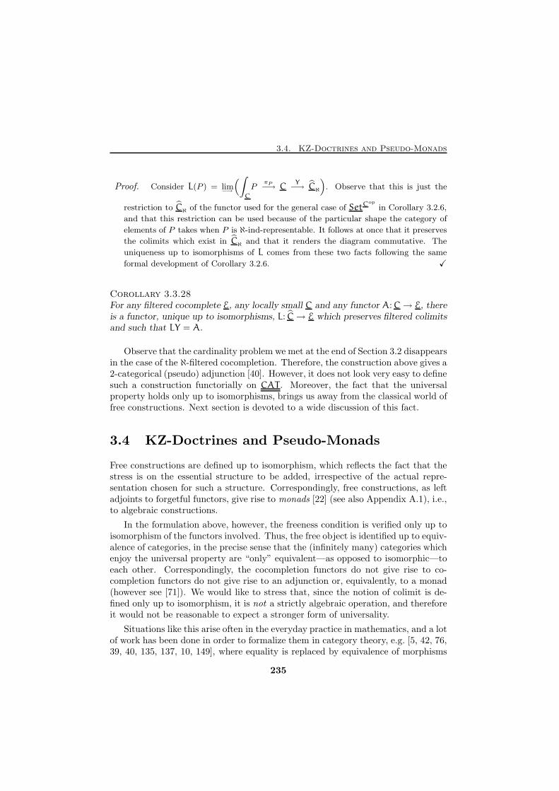
3.4. KZ-Doctrines and Pseudo-Monads
Proof. Consider L(P ) = lim−→
(∫
C
PπP−→ C
Y−→ Cℵ
). Observe that this is just the
restriction to Cℵ of the functor used for the general case of SetCop
in Corollary 3.2.6,
and that this restriction can be used because of the particular shape the category of
elements of P takes when P is ℵ-ind-representable. It follows at once that it preserves
the colimits which exist in Cℵ and that it renders the diagram commutative. The
uniqueness up to isomorphisms of L comes from these two facts following the same
formal development of Corollary 3.2.6. X
Corollary 3.3.28For any filtered cocomplete E, any locally small C and any functor A: C→ E, thereis a functor, unique up to isomorphisms, L: C→ E which preserves filtered colimitsand such that LY = A.
Observe that the cardinality problem we met at the end of Section 3.2 disappearsin the case of the ℵ-filtered cocompletion. Therefore, the construction above gives a2-categorical (pseudo) adjunction [40]. However, it does not look very easy to definesuch a construction functorially on CAT . Moreover, the fact that the universalproperty holds only up to isomorphisms, brings us away from the classical world offree constructions. Next section is devoted to a wide discussion of this fact.
3.4 KZ-Doctrines and Pseudo-Monads
Free constructions are defined up to isomorphism, which reflects the fact that thestress is on the essential structure to be added, irrespective of the actual repre-sentation chosen for such a structure. Correspondingly, free constructions, as leftadjoints to forgetful functors, give rise to monads [22] (see also Appendix A.1), i.e.,to algebraic constructions.
In the formulation above, however, the freeness condition is verified only up toisomorphism of the functors involved. Thus, the free object is identified up to equiv-alence of categories, in the precise sense that the (infinitely many) categories whichenjoy the universal property are “only” equivalent—as opposed to isomorphic—toeach other. Correspondingly, the cocompletion functors do not give rise to co-completion functors do not give rise to an adjunction or, equivalently, to a monad(however see [71]). We would like to stress that, since the notion of colimit is de-fined only up to isomorphism, it is not a strictly algebraic operation, and thereforeit would not be reasonable to expect a stronger form of universality.
Situations like this arise often in the everyday practice in mathematics, and a lotof work has been done in order to formalize them in category theory, e.g. [5, 42, 76,39, 40, 135, 137, 10, 149], where equality is replaced by equivalence of morphisms
235
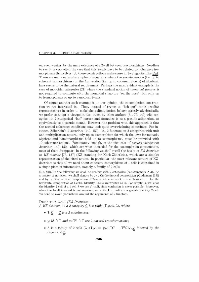
Chapter 3. Infinite Computations
or, even weaker, by the mere existence of a 2-cell between two morphisms. Needlessto say, it is very often the case that this 2-cells have to be related by coherence iso-morphisms themselves. So these constructions make sense in 3-categories, like Cat.There are many natural examples of situations where the pseudo version (i.e. up tocoherent isomorphisms) or the lax version (i.e. up to coherent 2-cells) of algebraiclaws seems to be the natural requirement. Perhaps the most evident example is thecase of monoidal categories [21] where the standard notion of monoidal functor isnot required to commute with the monoidal structure “on the nose”, but only upto isomorphisms or up to canonical 2-cells.
Of course another such example is, in our opinion, the cocompletion construc-tion we are interested in. Thus, instead of trying to “fish out” some peculiarrepresentatives in order to make the colimit notion behave strictly algebraically,we prefer to adopt a viewpoint also taken by other authors [71, 76, 149] who rec-ognize its 2-categorical “lax” nature and formalize it as a pseudo-adjunction, orequivalently as a pseudo-monad. However, the problem with this approach is thatthe needed coherence conditions may look quite overwhelming sometimes. For in-stance, Zoberlein’s 2-doctrines [149, 150], i.e., 2-functors on 2-categories with unitand multiplication natural only up to isomorphism for which the laws for monads,algebras and homomorphisms hold up to isomorphisms, must be provided with19 coherence axioms. Fortunately enough, in the nice case of coquasi-idempotentdoctrines [149, 150], which are what is needed for the cocompletion construction,most of them disappear. In the following we shall recall the basics of KZ-doctrinesor KZ-monads [76, 137] (KZ standing for Kock-Zoberlein), which are a simplerrepresentation of the cited notion. In particular, the most relevant feature of KZ-doctrines is that all we need about coherent isomorphisms of 1-cells is contained ina single piece of information, namely a family of 2-cells.
Remark. In the following we shall be dealing with 2-categories (see Appendix A.3). Asa matter of notation, we shall denote by ∗ the horizontal composition (Godement [35])and by � the vertical composition of 2-cells, while we stick to the classical ◦ for thehorizontal composition of 1-cells. Identity 1-cells are written as idC , or simply id, while forthe identity 2-cell of a 1-cell f we use f itself, since confusion is never possible. Moreover,when the 1-cell involved is not relevant, we write 1 to indicate a generic identity 2-cell.We tend to avoid parenthesis around the arguments of 2-functors.
Definition 3.4.1 (KZ-Doctrines)A KZ-doctrine on a 2-category C is a tuple (T , y,m, λ), where
• T : C→ C is a 2-endofunctor;
• y: Id�
→ T and m: T2 �
→ T are 2-natural transformations;
• λ is a family of 2-cells {λC : TyC ⇒ yTC : TC → T2C}C∈C indexed by the
objects of C;
236
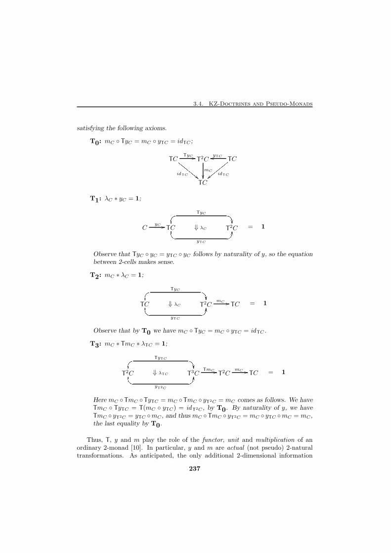
3.4. KZ-Doctrines and Pseudo-Monads
satisfying the following axioms.
T0: mC ◦ TyC = mC ◦ yTC = idTC ;
TC T2C TC
TC
idTC
EEEEEEE""TyC //
mC
��idTC||yyyyyyyyTCoo
T1: λC ∗ yC = 1;
C TC ⇓ λC T2CyC //
# "TyC
�� !yTC
OO = 1
Observe that TyC ◦ yC = yTC ◦ yC follows by naturality of y, so the equationbetween 2-cells makes sense.
T2: mC ∗ λC = 1;
TC ⇓ λC T2C TC
# "TyC
�� !yTC
OOmC // = 1
Observe that by T0 we have mC ◦ TyC = mC ◦ yTC = idTC .
T3: mC ∗ TmC ∗ λTC = 1;
T2C ⇓ λTC T3C T2C TC
# "TyTC
�� !y
T2C
OOTmC // mC // = 1
Here mC ◦ TmC ◦ TyTC = mC ◦ TmC ◦ yT2C = mC comes as follows. We haveTmC ◦ TyTC = T(mC ◦ yTC) = idT2C , by T0. By naturality of y, we haveTmC ◦ yT2C = yTC ◦mC , and thus mC ◦ TmC ◦ yT2C = mC ◦ yTC ◦mC = mC ,the last equality by T0.
Thus, T , y and m play the role of the functor, unit and multiplication of anordinary 2-monad [10]. In particular, y and m are actual (not pseudo) 2-naturaltransformations. As anticipated, the only additional 2-dimensional information
237

Chapter 3. Infinite Computations
around is λ and every coherence isomorphism is obtained from it. Axiom T0corresponds to the unit law of monads, that therefore holds strictly also in KZ-doctrines. Axioms T1, T2 and T3 express the coherence of λ with the unit andthe multiplication. Observe that there is no explicit mention of a pseudo form of themultiplication law. However, we shall see later that this is indeed the case and, forany C ∈ C, there exists an isomorphism µC :mC ◦ TmC ⇒ mC ◦mTC : T3C → TC.
T3C T2C
T2C TC
TmC //
mTC
��mC
��mC
//
µC
{� ��������Proposition 3.4.2For any C ∈ C we have a reflectionmC ⊣ yTC : T2C ⇀ TC, the unit of the adjunctionbeing TmC ∗ λTC : idT2C ⇒ yTC ◦mC .
Proof. Here and in the following, we denote by η and ε respectively the unit and counitof a generic adjunction. Let us check that the triangular identities hold. Rememberthat for a reflection the counit is the identity 2-cell.
T2C T2C
TC TC
id //
mC
EEEEEE ""⇓ η mC
EEEEEE""yTCyyyyyy<<id
//⇓ 1
= mC ∗ TmC ∗ λC = 1, by T3.
T2C T2C
TC TC
id //
mC
EEEEEE ""⇓ ηyTCyyyyyy<<id
//⇓ 1
yTCyyyyyy<< = TmC ∗ λTC ∗ yTC = 1, by T1.
X
Definition 3.4.3 ( T -Algebras)An algebra for T is an object A ∈ C together with a structure map a: TA → Awhich is a reflection left adjoint for yA:A→ TA.
Thus, structures are adjoints to units [76]. Observe that, since a ⊣ yA is areflection, we have a ◦ yA = id . Therefore, as in the case of the KZ-doctrine itself,the unit law for the structure of an algebra holds strictly. Since we have mC ⊣ yTC ,for any C ∈ C there is a “free” algebra on C, namely (TC,mC).
In order to define T -homomorphisms, we need to recall the well known conceptof 2-cells mates under adjunctions (see, e.g., [69]). It is based on the operation of
238
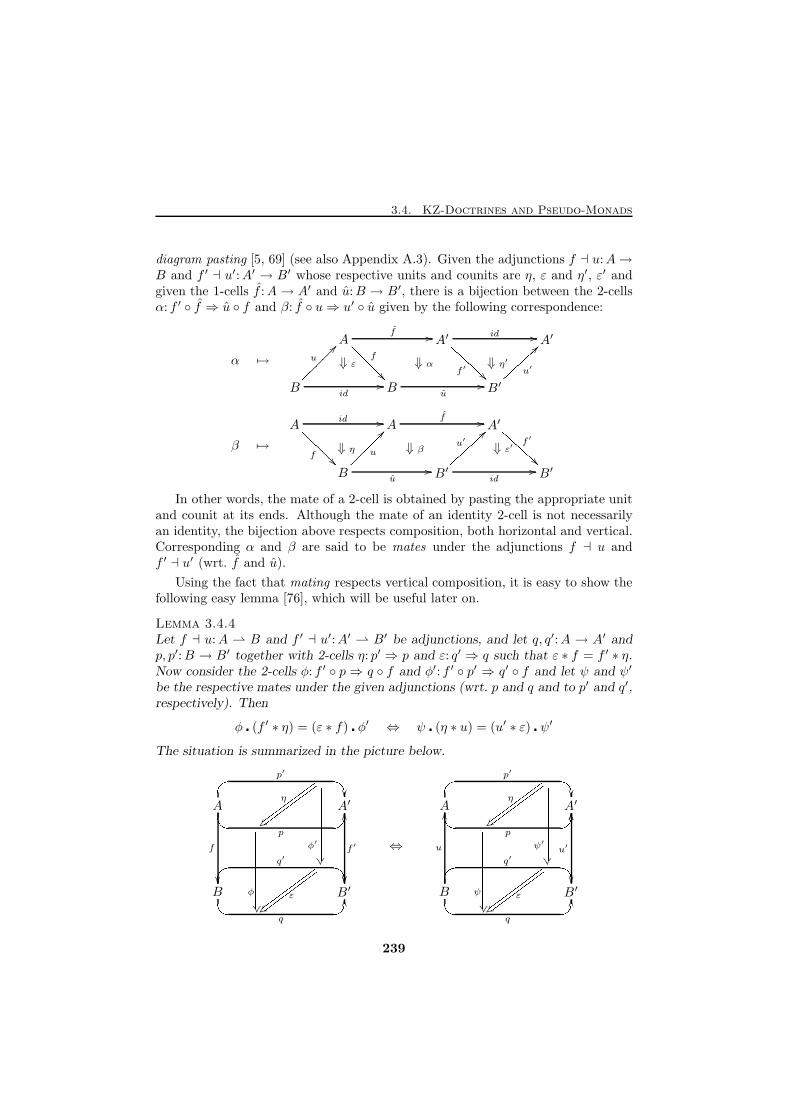
3.4. KZ-Doctrines and Pseudo-Monads
diagram pasting [5, 69] (see also Appendix A.3). Given the adjunctions f ⊣ u:A→B and f ′ ⊣ u′:A′ → B′ whose respective units and counits are η, ε and η′, ε′ andgiven the 1-cells f :A→ A′ and u:B → B′, there is a bijection between the 2-cellsα: f ′ ◦ f ⇒ u ◦ f and β: f ◦ u⇒ u′ ◦ u given by the following correspondence:
α 7→
A A′ A′
B B B′
f //
f
?????�� f ′
BBBBBB id //
⇓ εu����� ??id
//
⇓ α
u//
u′|||||| >>⇓ η′
β 7→
A A A′
B B′ B′
id //
f
?????�� f //
f ′BBBBBB ⇓ η u�����??
u//
⇓ β
id//
u′||||||>> ⇓ ε′In other words, the mate of a 2-cell is obtained by pasting the appropriate unit
and counit at its ends. Although the mate of an identity 2-cell is not necessarilyan identity, the bijection above respects composition, both horizontal and vertical.Corresponding α and β are said to be mates under the adjunctions f ⊣ u andf ′ ⊣ u′ (wrt. f and u).
Using the fact that mating respects vertical composition, it is easy to show thefollowing easy lemma [76], which will be useful later on.
Lemma 3.4.4Let f ⊣ u:A ⇀ B and f ′ ⊣ u′:A′ ⇀ B′ be adjunctions, and let q, q′:A → A′ andp, p′:B → B′ together with 2-cells η: p′ ⇒ p and ε: q′ ⇒ q such that ε ∗ f = f ′ ∗ η.Now consider the 2-cells φ: f ′ ◦ p ⇒ q ◦ f and φ′: f ′ ◦ p′ ⇒ q′ ◦ f and let ψ and ψ′
be the respective mates under the given adjunctions (wrt. p and q and to p′ and q′,respectively). Then
φ � (f ′ ∗ η) = (ε ∗ f) � φ′ ⇔ ψ � (η ∗ u) = (u′ ∗ ε) � ψ′
The situation is summarized in the picture below.
A A′
B B′
# "p′
�� !p
OO
f
��
η
w� wwwwwwwwwwwwwwwwf ′
��# "q′
�� !q
OOε
w� wwwwwwwwwwwwwwwwφ
��
������������������������ φ′
��
������������������������ ⇔
A A′
B B′
# "p′
�� !p
OOη
w� wwwwwwwwwwwwwwww# "q′
�� !q
OO
u
OO
ε
w� wwwwwwwwwwwwwwwwψ
��
������������������������ ψ′
��
������������������������ u′
OO
239
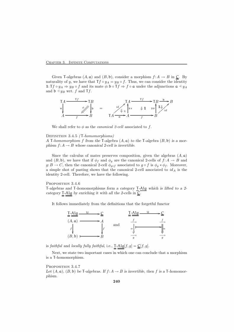
Chapter 3. Infinite Computations
Given T -algebras (A,a) and (B,b), consider a morphism f :A → B in C. Bynaturality of y, we have that Tf ◦ yA = yB ◦ f . Thus, we can consider the identity1: Tf ◦ yA ⇒ yB ◦ f and its mate φ: b ◦ Tf ⇒ f ◦ a under the adjunctions a ⊣ yAand b ⊣ yB wrt. f and Tf .
TA TB
A B
Tf //
a
��b
��f
//
φ
{� �������� =
TA TB B
TA A B
Tf // b //
⇓ ηidzzzzzz<<
a//
⇓ 1
f//
yA
OO
id|||||| ==yB
OO1⇓
We shall refer to φ as the canonical 2-cell associated to f .
Definition 3.4.5 ( T -homomorphisms)A T -homomorphism f from the T -algebra (A,a) to the T -algebra (B,b) is a mor-phism f :A→ B whose canonical 2-cell is invertible.
Since the calculus of mates preserves composition, given the algebras (A,a)and (B,b), we have that if φf and φg are the canonical 2-cells of f :A → B andg:B → C, then the canonical 2-cell φg◦f associated to g ◦ f is φg ∗ φf . Moreover,a simple shot of pasting shows that the canonical 2-cell associated to idA is theidentity 2-cell. Therefore, we have the following.
Proposition 3.4.6T -algebras and T -homomorphisms form a category T -Alg which is lifted to a 2-category T -Alg by enriching it with all the 2-cells in C.
It follows immediately from the definitions that the forgetful functor
(A,a) A
(B,b) B
� //
f
��f
��� //
CT -Alg U //
and
f−→
f−→
−→g
−→g
α
��
���������� α
��
����������� //
CT -Alg U //
is faithful and locally fully faithful, i.e., T -Alg[f, g] = C[f, g].
Next, we state two important cases in which one can conclude that a morphismis a T -homomorphism.
Proposition 3.4.7Let (A,a), (B,b) be T -algebras. If f :A→ B is invertible, then f is a T -homomor-phism.
240
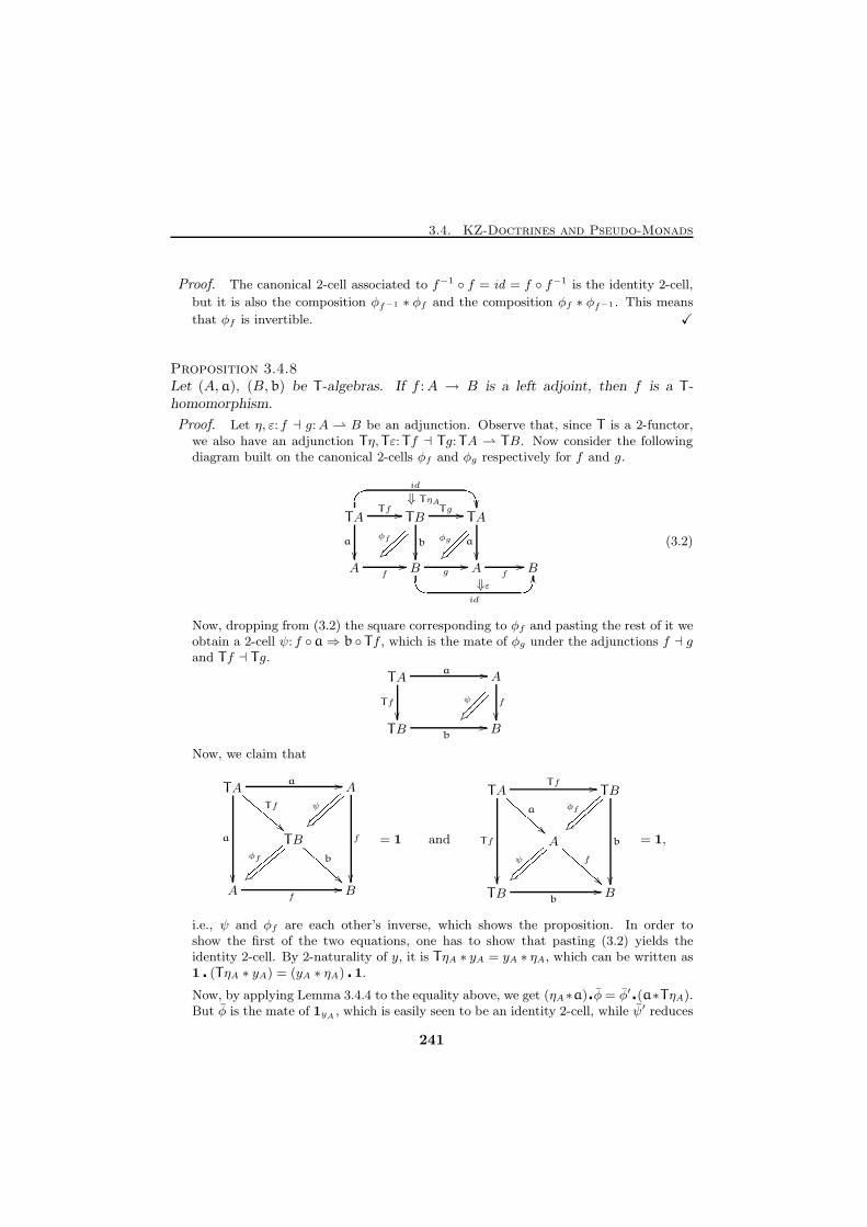
3.4. KZ-Doctrines and Pseudo-Monads
Proof. The canonical 2-cell associated to f−1 ◦ f = id = f ◦ f−1 is the identity 2-cell,
but it is also the composition φf−1 ∗ φf and the composition φf ∗ φf−1 . This means
that φf is invertible. X
Proposition 3.4.8Let (A,a), (B,b) be T -algebras. If f :A → B is a left adjoint, then f is a T -homomorphism.
Proof. Let η, ε: f ⊣ g:A ⇀ B be an adjunction. Observe that, since T is a 2-functor,we also have an adjunction Tη, Tε: Tf ⊣ Tg:TA ⇀ TB. Now consider the followingdiagram built on the canonical 2-cells φf and φg respectively for f and g.
TA TB TA
A B A B
# "id
��Tf //
a
��
⇓ TηA
b
��
Tg //
a
��f
//
φf
z� }}}}}}}} !id
OOg//
φg
{� ��������⇓ε
f//
(3.2)
Now, dropping from (3.2) the square corresponding to φf and pasting the rest of it weobtain a 2-cell ψ: f ◦a⇒ b ◦ Tf , which is the mate of φg under the adjunctions f ⊣ gand Tf ⊣ Tg.
TA A
TB B
a //
Tf
��f
��b
//
ψ
{� ��������Now, we claim that
TA A
TB
A B
a //
a
��
Tf
DDDDDD!!f
��
ψ
y� ||||||||||b
BBBBBB !!φf
x� zzzzzzzzzzf
//
= 1 and
TA TB
A
TB B
Tf //
a
BBBBBB!!Tf
��
b
��
φf
y� ||||||||||f
BBBBBB!!ψ
y� ||||||||||b
//
= 1,
i.e., ψ and φf are each other’s inverse, which shows the proposition. In order toshow the first of the two equations, one has to show that pasting (3.2) yields theidentity 2-cell. By 2-naturality of y, it is TηA ∗ yA = yA ∗ ηA, which can be written as1 � (TηA ∗ yA) = (yA ∗ ηA) � 1.
Now, by applying Lemma 3.4.4 to the equality above, we get (ηA∗a)�φ = φ′ �(a∗TηA).But φ is the mate of 1yA , which is easily seen to be an identity 2-cell, while ψ′ reduces
241
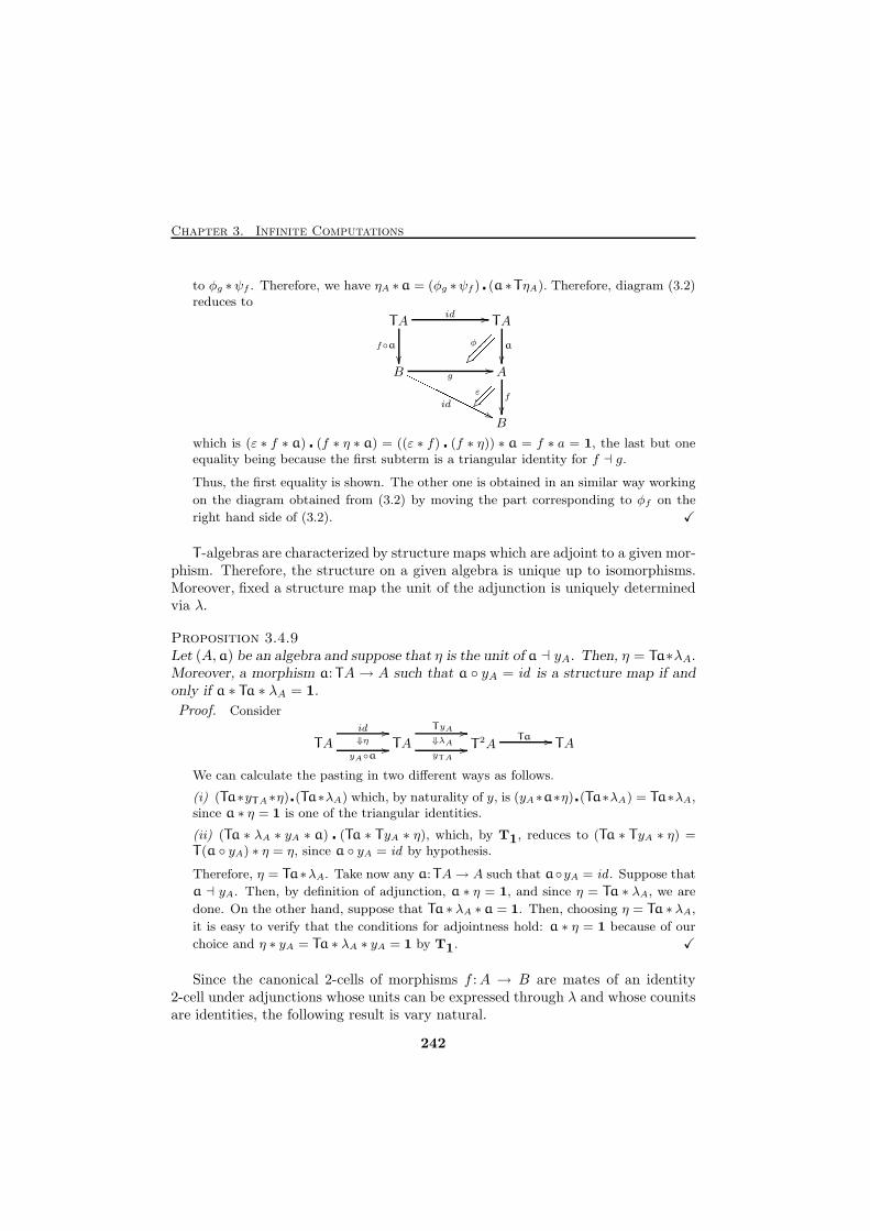
Chapter 3. Infinite Computations
to φg ∗ψf . Therefore, we have ηA ∗a = (φg ∗ψf ) � (a ∗TηA). Therefore, diagram (3.2)reduces to
TA TA
B A
B
id //
f◦a
��a
��g
//
id
OOOOOOOOOOOO''φ
{� ��������f
��
ε
{� ������which is (ε ∗ f ∗ a) � (f ∗ η ∗ a) = ((ε ∗ f) � (f ∗ η)) ∗ a = f ∗ a = 1, the last but oneequality being because the first subterm is a triangular identity for f ⊣ g.
Thus, the first equality is shown. The other one is obtained in an similar way working
on the diagram obtained from (3.2) by moving the part corresponding to φf on the
right hand side of (3.2). X
T -algebras are characterized by structure maps which are adjoint to a given mor-phism. Therefore, the structure on a given algebra is unique up to isomorphisms.Moreover, fixed a structure map the unit of the adjunction is uniquely determinedvia λ.
Proposition 3.4.9Let (A,a) be an algebra and suppose that η is the unit of a ⊣ yA. Then, η = Ta∗λA.Moreover, a morphism a: TA→ A such that a ◦ yA = id is a structure map if andonly if a ∗ Ta ∗ λA = 1.
Proof. Consider
TA TA T2A TAid⇓η
//
yA◦a//
TyA
⇓λA
//
yTA
//Ta //
We can calculate the pasting in two different ways as follows.
(i) (Ta∗yTA∗η)�(Ta∗λA) which, by naturality of y, is (yA∗a∗η)�(Ta∗λA) = Ta∗λA,since a ∗ η = 1 is one of the triangular identities.
(ii) (Ta ∗ λA ∗ yA ∗ a) � (Ta ∗ TyA ∗ η), which, by T1, reduces to (Ta ∗ TyA ∗ η) =T (a ◦ yA) ∗ η = η, since a ◦ yA = id by hypothesis.
Therefore, η = Ta∗λA. Take now any a:TA→ A such that a◦yA = id . Suppose that
a ⊣ yA. Then, by definition of adjunction, a ∗ η = 1, and since η = Ta ∗ λA, we are
done. On the other hand, suppose that Ta ∗ λA ∗a = 1. Then, choosing η = Ta ∗ λA,
it is easy to verify that the conditions for adjointness hold: a ∗ η = 1 because of our
choice and η ∗ yA = Ta ∗ λA ∗ yA = 1 by T1. X
Since the canonical 2-cells of morphisms f :A → B are mates of an identity2-cell under adjunctions whose units can be expressed through λ and whose counitsare identities, the following result is vary natural.
242
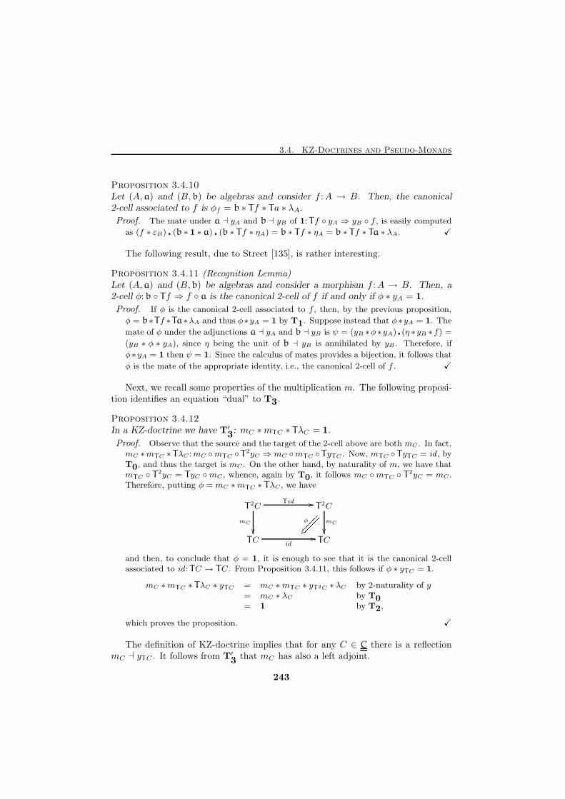
3.4. KZ-Doctrines and Pseudo-Monads
Proposition 3.4.10Let (A,a) and (B,b) be algebras and consider f :A → B. Then, the canonical2-cell associated to f is φf = b ∗ Tf ∗ Ta ∗ λA.
Proof. The mate under a ⊣ yA and b ⊣ yB of 1: Tf ◦ yA ⇒ yB ◦ f , is easily computed
as (f ∗ εB) � (b ∗ 1 ∗ a) � (b ∗ Tf ∗ ηA) = b ∗ Tf ∗ ηA = b ∗ Tf ∗ Ta ∗ λA. X
The following result, due to Street [135], is rather interesting.
Proposition 3.4.11 (Recognition Lemma)Let (A,a) and (B,b) be algebras and consider a morphism f :A → B. Then, a2-cell φ: b ◦ Tf ⇒ f ◦ a is the canonical 2-cell of f if and only if φ ∗ yA = 1.
Proof. If φ is the canonical 2-cell associated to f , then, by the previous proposition,
φ = b∗Tf ∗Ta∗λA and thus φ∗yA = 1 by T1. Suppose instead that φ∗yA = 1. The
mate of φ under the adjunctions a ⊣ yA and b ⊣ yB is ψ = (yB ∗φ∗yA) � (η ∗yB ∗f) =
(yB ∗ φ ∗ yA), since η being the unit of b ⊣ yB is annihilated by yB . Therefore, if
φ∗yA = 1 then ψ = 1. Since the calculus of mates provides a bijection, it follows that
φ is the mate of the appropriate identity, i.e., the canonical 2-cell of f . X
Next, we recall some properties of the multiplication m. The following proposi-tion identifies an equation “dual” to T3.
Proposition 3.4.12In a KZ-doctrine we have T′3: mC ∗mTC ∗ TλC = 1.
Proof. Observe that the source and the target of the 2-cell above are both mC . In fact,mC ∗mTC ∗ TλC :mC ◦mTC ◦ T
2yC ⇒ mC ◦mTC ◦ TyTC . Now, mTC ◦ TyTC = id , byT0, and thus the target is mC . On the other hand, by naturality of m, we have thatmTC ◦ T2yC = TyC ◦mC , whence, again by T0, it follows mC ◦mTC ◦ T2yC = mC .Therefore, putting φ = mC ∗mTC ∗ TλC , we have
T2C T2C
TC TC
T id //
mC
��mC
��id
//
φ
{� ��������and then, to conclude that φ = 1, it is enough to see that it is the canonical 2-cellassociated to id : TC → TC. From Proposition 3.4.11, this follows if φ ∗ yTC = 1.
mC ∗mTC ∗ TλC ∗ yTC = mC ∗mTC ∗ yT2C ∗ λC by 2-naturality of y= mC ∗ λC by T0
= 1 by T2,
which proves the proposition. X
The definition of KZ-doctrine implies that for any C ∈ C there is a reflectionmC ⊣ yTC . It follows from T′3 that mC has also a left adjoint.
243
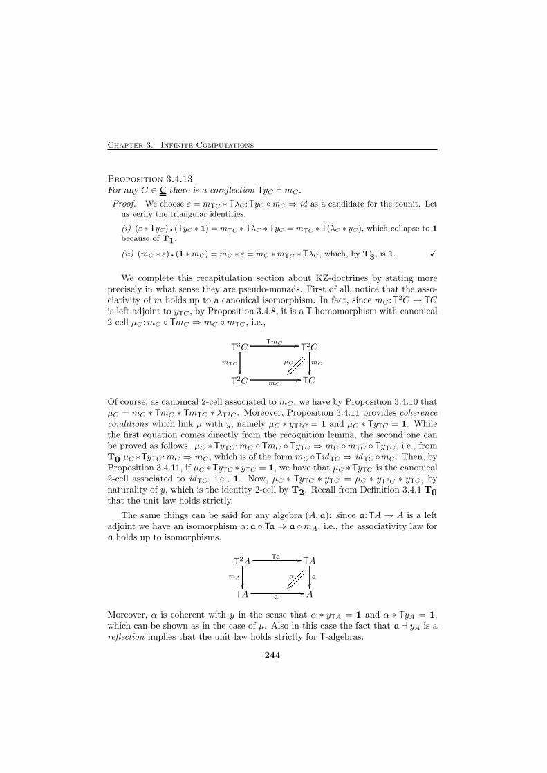
Chapter 3. Infinite Computations
Proposition 3.4.13For any C ∈ C there is a coreflection TyC ⊣ mC .
Proof. We choose ε = mTC ∗ TλC : TyC ◦mC ⇒ id as a candidate for the counit. Letus verify the triangular identities.
(i) (ε ∗ TyC) � (TyC ∗ 1) = mTC ∗ TλC ∗ TyC = mTC ∗ T (λC ∗ yC), which collapse to 1
because of T1.
(ii) (mC ∗ ε) � (1 ∗mC) = mC ∗ ε = mC ∗mTC ∗ TλC , which, by T′3, is 1. X
We complete this recapitulation section about KZ-doctrines by stating moreprecisely in what sense they are pseudo-monads. First of all, notice that the asso-ciativity of m holds up to a canonical isomorphism. In fact, since mC : T2C → TCis left adjoint to yTC , by Proposition 3.4.8, it is a T -homomorphism with canonical2-cell µC :mC ◦ TmC ⇒ mC ◦mTC , i.e.,
T3C T2C
T2C TC
TmC //
mTC
��mC
��mC
//
µC
{� ��������Of course, as canonical 2-cell associated to mC , we have by Proposition 3.4.10 thatµC = mC ∗ TmC ∗ TmTC ∗ λT2C . Moreover, Proposition 3.4.11 provides coherenceconditions which link µ with y, namely µC ∗ yT2C = 1 and µC ∗ TyTC = 1. Whilethe first equation comes directly from the recognition lemma, the second one canbe proved as follows. µC ∗ TyTC :mC ◦ TmC ◦ TyTC ⇒ mC ◦mTC ◦ TyTC , i.e., fromT0 µC ∗TyTC :mC ⇒ mC , which is of the form mC ◦T idTC ⇒ idTC ◦mC . Then, byProposition 3.4.11, if µC ∗ TyTC ∗ yTC = 1, we have that µC ∗ TyTC is the canonical2-cell associated to idTC , i.e., 1. Now, µC ∗ TyTC ∗ yTC = µC ∗ yT2C ∗ yTC , bynaturality of y, which is the identity 2-cell by T2. Recall from Definition 3.4.1 T0that the unit law holds strictly.
The same things can be said for any algebra (A,a): since a: TA → A is a leftadjoint we have an isomorphism α: a ◦ Ta ⇒ a ◦mA, i.e., the associativity law fora holds up to isomorphisms.
T2A TA
TA A
Ta //
mA
��a
��a
//
α
{� ��������Moreover, α is coherent with y in the sense that α ∗ yTA = 1 and α ∗ TyA = 1,which can be shown as in the case of µ. Also in this case the fact that a ⊣ yA is areflection implies that the unit law holds strictly for T -algebras.
244
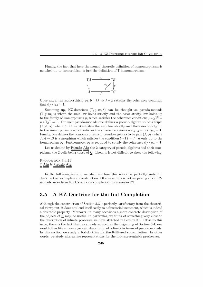
3.5. A KZ-Doctrine for the Ind Completion
Finally, the fact that here the monad-theoretic definition of homomorphisms ismatched up to isomorphism is just the definition of T -homomorphism.
TA TB
A TC
Tf //
a
��b
��f
//
φf
{� ��������Once more, the isomorphism φf : b ◦ Tf ⇒ f ◦ a satisfies the coherence conditionthat φf ∗ yA = 1.
Summing up, KZ-doctrines (T , y,m, λ) can be thought as pseudo-monads(T , y,m, µ) where the unit law holds strictly and the associativity law holds upto the family of isomorphisms µ, which satisfies the coherence conditions µ ∗ yT2 =µ ∗ TyT = 1. For such pseudo-monads one defines a pseudo-algebra to be a triple(A,a, α), where a: TA → A satisfies the unit law strictly and the associativity upto the isomorphism α which satisfies the coherence axioms α ∗ yTA = α ∗ TyA = 1.Finally, one defines the homomorphisms of pseudo-algebras to be pair (f, φf ) wheref :A→ B is a morphism which satisfies the condition b ◦ Tf = f ◦ a only up to theisomorphism φf . Furthermore, φf is required to satisfy the coherence φf ∗ yA = 1.
Let us denote by Pseudo-Alg the 2-category of pseudo-algebras and their mor-
phisms, the 2-cells being those of C. Then, it is not difficult to show the following.
Proposition 3.4.14T -Alg ∼= Pseudo-Alg
In the following section, we shall see how this notion is perfectly suited todescribe the cocompletion construction. Of course, this is not surprising since KZ-monads arose from Kock’s work on completion of categories [71].
3.5 A KZ-Doctrine for the Ind Completion
Although the construction of Section 3.3 is perfectly satisfactory from the theoreti-cal viewpoint, it does not lend itself easily to a functorial treatment, which is indeeda desirable property. Moreover, in many occasions a more concrete description ofthe objects of C may be useful. In particular, we think of something very close tothe description of infinite processes we have sketched in Section 3.1. Close to thisissue, there is the fact that, as already noticed at the beginning of Section 3.4, onewould often like a more algebraic description of colimits in terms of pseudo monads.In this section we study a KZ-doctrine for the ℵ-filtered cocompletion. In otherwords, we study alternative representations for the ind-representable presheaves.
245
Chapter 3. Infinite Computations
Remark. Since the case of ℵ finite is trivial, in the following we implicitly assume thatℵ is infinite. Moreover, since everything which follows is parametric with respect to ℵ,we shall mention it explicitly only when unavoidable. However, the reader should keep inmind that every statement below about “filtered” objects can safely be restated in termsof “ℵ-filtered” objects.
Ind Objects
The following definition of ind-object follows the same simple idea about represen-tation of infinite computations we discussed in Section 3.1.
Definition 3.5.1 (Ind-objects)A functor X : J→ C is an ind-object if J is small and filtered. If |J| ≤ ℵ, then X isa ℵ-ind-object.
We shall identify ind-objectsX : I→ C and Y : J→ C if there exists a cofinal φ: I→ J
whose object component is an isomorphism and such that Y ◦ φ = X .
Thus, ind-objects are nothing but filtered diagrams in C. We can think of ind-objects as “syntactic” representations of ind-representable functors. In particular,we shall say that the ind-object X : I→ C represents the ind-representable functor
L(X) = lim−→(IX−→ C
Y−→ C) ∼= lim−→ i∈I HomC( , X(i)).
Observe then that the imposed equalities are perfectly harmless because theyidentify objects which represent isomorphic presheaves.
In order to simplify notation, we shall often use the so-called indexed notationfor ind-objects. We write (Xi)i∈I for X : I → C with X(i) = Xi. Admittedlythis notation is rather poor but it will not be misleading, and therefore it will beacceptable, provided one never forgets that we are not handling sequences or chainsof objects, but filtered diagrams in C. Of course, given an ind-object (Xi)i∈I, wereserve the right to use X also in every context in which a functor is expected.
As already observed in Section 3.1, the key point is the definition of morphismsfor ind-objects. The right notion should be such that it identifies, i.e., it makesisomorphic, ind-objects which intuitively should be the same. Moreover, it has tomake the category of ind-objects filtered cocomplete. Clearly, the theory exposedin Section 3.3 allows us to identify such notion of morphism immediately.
Definition 3.5.2The category Ind(C) is the category whose objects are the ind-objects of C, andwhose homsets are defined by
HomInd(C)(X,Y ) = HomC(L(X),L(Y )).
The category Ind(C)ℵ is the full subcategory of Ind(C) whose object are ℵ-filteredfunctors.
246
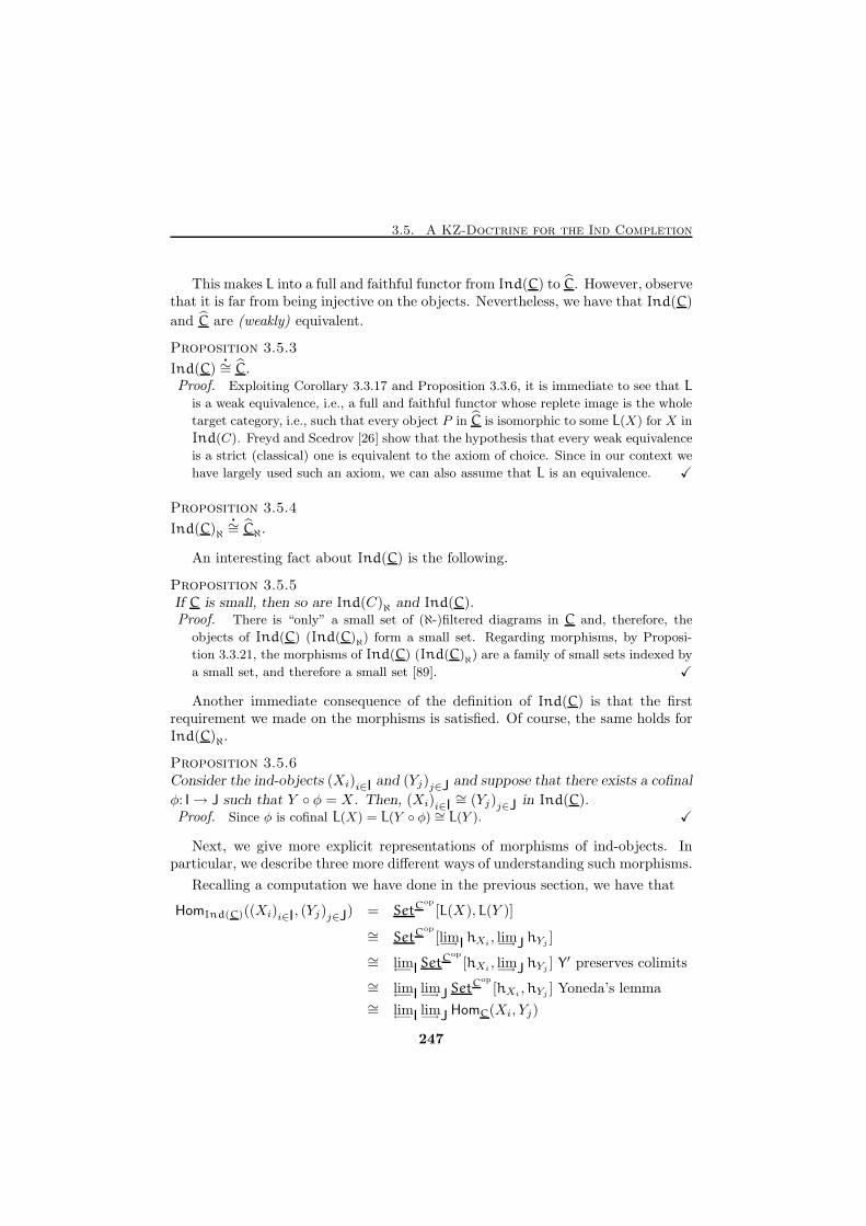
3.5. A KZ-Doctrine for the Ind Completion
This makes L into a full and faithful functor from Ind(C) to C. However, observethat it is far from being injective on the objects. Nevertheless, we have that Ind(C)
and C are (weakly) equivalent.
Proposition 3.5.3
Ind(C)�
∼= C.Proof. Exploiting Corollary 3.3.17 and Proposition 3.3.6, it is immediate to see that L
is a weak equivalence, i.e., a full and faithful functor whose replete image is the whole
target category, i.e., such that every object P in C is isomorphic to some L(X) for X in
Ind(C). Freyd and Scedrov [26] show that the hypothesis that every weak equivalence
is a strict (classical) one is equivalent to the axiom of choice. Since in our context we
have largely used such an axiom, we can also assume that L is an equivalence. X
Proposition 3.5.4
Ind(C)ℵ�
∼= Cℵ.
An interesting fact about Ind(C) is the following.
Proposition 3.5.5If C is small, then so are Ind(C)ℵ and Ind(C).Proof. There is “only” a small set of (ℵ-)filtered diagrams in C and, therefore, the
objects of Ind(C) (Ind(C)ℵ) form a small set. Regarding morphisms, by Proposi-
tion 3.3.21, the morphisms of Ind(C) (Ind(C)ℵ) are a family of small sets indexed by
a small set, and therefore a small set [89]. X
Another immediate consequence of the definition of Ind(C) is that the firstrequirement we made on the morphisms is satisfied. Of course, the same holds forInd(C)ℵ.
Proposition 3.5.6Consider the ind-objects (Xi)i∈I and (Yj)j∈J and suppose that there exists a cofinal
φ: I→ J such that Y ◦ φ = X . Then, (Xi)i∈I∼= (Yj)j∈J in Ind(C).
Proof. Since φ is cofinal L(X) = L(Y ◦ φ) ∼= L(Y ). X
Next, we give more explicit representations of morphisms of ind-objects. Inparticular, we describe three more different ways of understanding such morphisms.
Recalling a computation we have done in the previous section, we have that
HomInd(C)((Xi)i∈I, (Yj)j∈J) = SetCop
[L(X),L(Y )]
∼= SetCop
[lim−→ I hXi, lim−→J hYj
]
∼= lim←− I SetCop
[hXi, lim−→J hYj
] Y′ preserves colimits
∼= lim←− I lim−→J SetCop
[hXi,hYj
] Yoneda’s lemma∼= lim←− I lim−→J HomC(Xi, Yj)
247
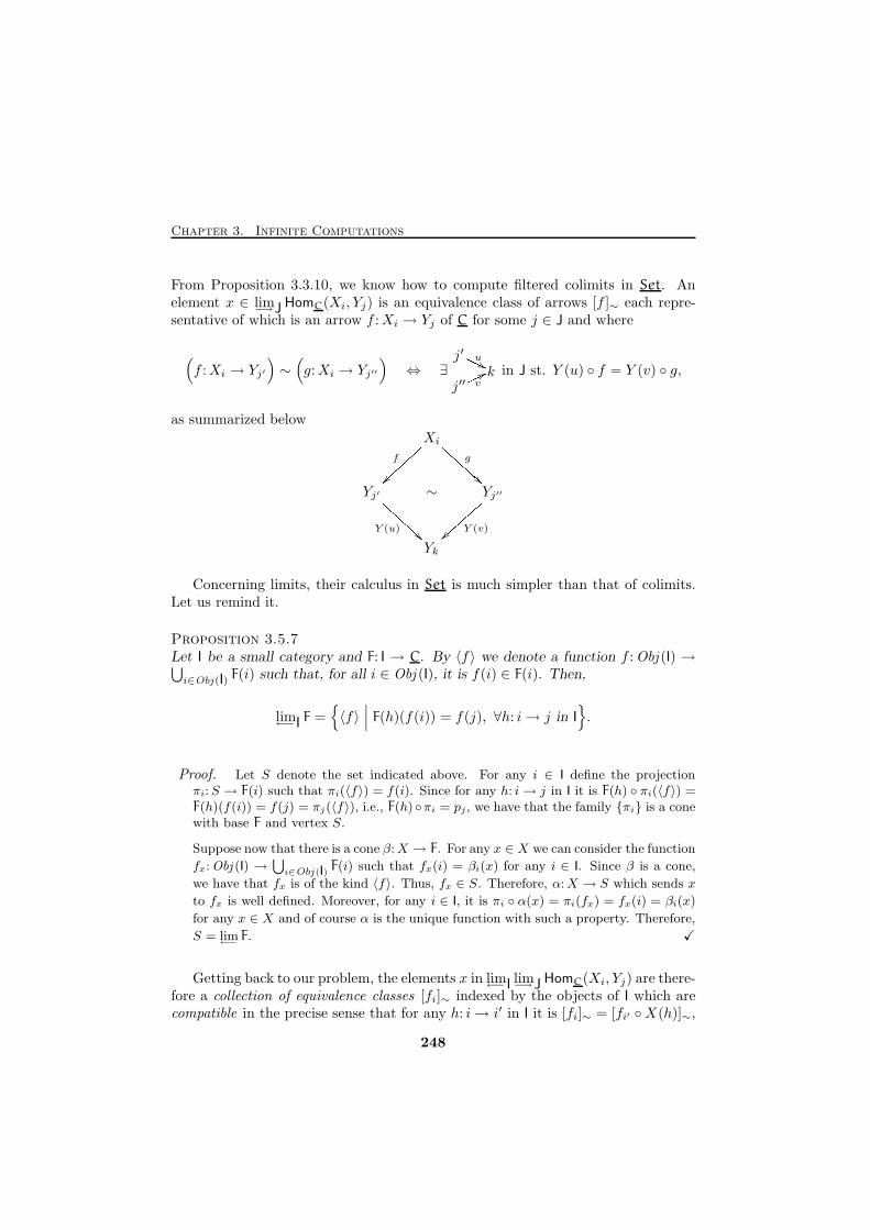
Chapter 3. Infinite Computations
From Proposition 3.3.10, we know how to compute filtered colimits in Set. Anelement x ∈ lim−→J HomC(Xi, Yj) is an equivalence class of arrows [f ]∼ each repre-sentative of which is an arrow f :Xi → Yj of C for some j ∈ J and where
(f :Xi → Yj′
)∼(g:Xi → Yj′′
)⇔ ∃
j′
kj′′
uPPP ''vnnn77 in J st. Y (u) ◦ f = Y (v) ◦ g,
as summarized below
Xi
Yj′ ∼ Yj′′
Yk
f
~~}}}}}} g
BBBBBB!!Y (u)
AAAAAA Y (v)}}||||||Concerning limits, their calculus in Set is much simpler than that of colimits.
Let us remind it.
Proposition 3.5.7Let I be a small category and F: I → C. By 〈f〉 we denote a function f :Obj (I) →⋃i∈Obj(I) F(i) such that, for all i ∈ Obj (I), it is f(i) ∈ F(i). Then,
lim←− I F ={〈f〉
∣∣∣ F(h)(f(i)) = f(j), ∀h: i→ j in I}.
Proof. Let S denote the set indicated above. For any i ∈ I define the projectionπi:S → F(i) such that πi(〈f〉) = f(i). Since for any h: i→ j in I it is F(h) ◦ πi(〈f〉) =F(h)(f(i)) = f(j) = πj(〈f〉), i.e., F(h)◦πi = pj , we have that the family {πi} is a conewith base F and vertex S.
Suppose now that there is a cone β:X → F. For any x ∈ X we can consider the function
fx:Obj (I) →⋃i∈Obj (I) F(i) such that fx(i) = βi(x) for any i ∈ I. Since β is a cone,
we have that fx is of the kind 〈f〉. Thus, fx ∈ S. Therefore, α:X → S which sends x
to fx is well defined. Moreover, for any i ∈ I, it is πi ◦ α(x) = πi(fx) = fx(i) = βi(x)
for any x ∈ X and of course α is the unique function with such a property. Therefore,
S = lim←−
F. X
Getting back to our problem, the elements x in lim←− I lim−→J HomC(Xi, Yj) are there-fore a collection of equivalence classes [fi]∼ indexed by the objects of I which arecompatible in the precise sense that for any h: i→ i′ in I it is [fi]∼ = [fi′ ◦X(h)]∼,
248
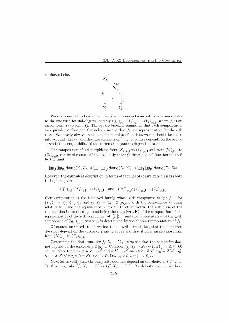
3.5. A KZ-Doctrine for the Ind Completion
as shown below.Xi
Xj′
Yj Yj′
fi
��
X(h)BBBBBB!!
fi′
��
∼
We shall denote this kind of families of equivalence classes with a notation similarto the one used for ind-objects, namely ([fi])i∈I: (Xi)i∈I → (Yj)j∈J, where fi is anarrow from Xi to some Yj . The square brackets remind us that each component isan equivalence class and the index i means that fi is a representative for the i-thclass. We nearly always avoid explicit mention of ∼. However it should be takeninto account that ∼, and thus the elements of [fi]∼, of course depends on the actualJ, while the compatibility of the various components depends also on I.
The composition of ind-morphisms from (Xi)i∈I to (Yj)j∈J and from (Yj)j∈J to
(Zk)k∈K can be of course defined explicitly through the canonical function inducedby the limit
lim←−J lim−→K HomC(Yj , Zk)× lim←− I lim−→J HomC(Xi, Yj)→ lim←− I lim−→K HomC(Xi, Zk).
However, the equivalent description in terms of families of equivalence classes aboveis simpler: given
([fi])i∈I: (Xi)i∈I → (Yj)j∈J and ([gj ])j∈J: (Yj)j∈J → (Zk)k∈K,
their composition is the I-indexed family whose i-th component is [g ◦ f ]∼′ for(f :Xi → Yj) ∈ [fi]∼ and (g:Yj → Zk) ∈ [gj]∼′ , with the equivalence ∼ beingrelative to J and the equivalence ∼′ to K. In other words, the i-th class of thecomposition is obtained by considering the class (wrt. K) of the composition of onerepresentative of the i-th component of ([fi])i∈I and one representative of the ji-thcomponent of ([gj ])j∈J, where ji is determined by the chosen representative of fi.
Of course, one needs to show that this is well-defined, i.e., that the definitiondoes not depend on the choice of f and g above and that it gives an ind-morphismfrom (Xi)i∈I to (Zk)k∈K.
Concerning the first issue, for fi:Xi → Yj , let us see that the composite doesnot depend on the choice of g ∈ [gj]∼. Consider (gj :Yj → Zk) ∼ (g′j :Yj → Zk′). Ofcourse, since there exist u: k → k′′ and v: k′ → k′′ such that Z(u) ◦ gi = Z(v) ◦ g′i,we have Z(u) ◦ gj ◦ fi = Z(v) ◦ g′j ◦ fi, i.e., [gj ◦ fi]∼ = [g′j ◦ fi]∼.
Now, let us verify that the composite does not depend on the choice of f ∈ [fi]∼.To this aim, take (fi:Xi → Yj) ∼ (f ′i :Xi → Yj′). By definition of ∼, we have
249
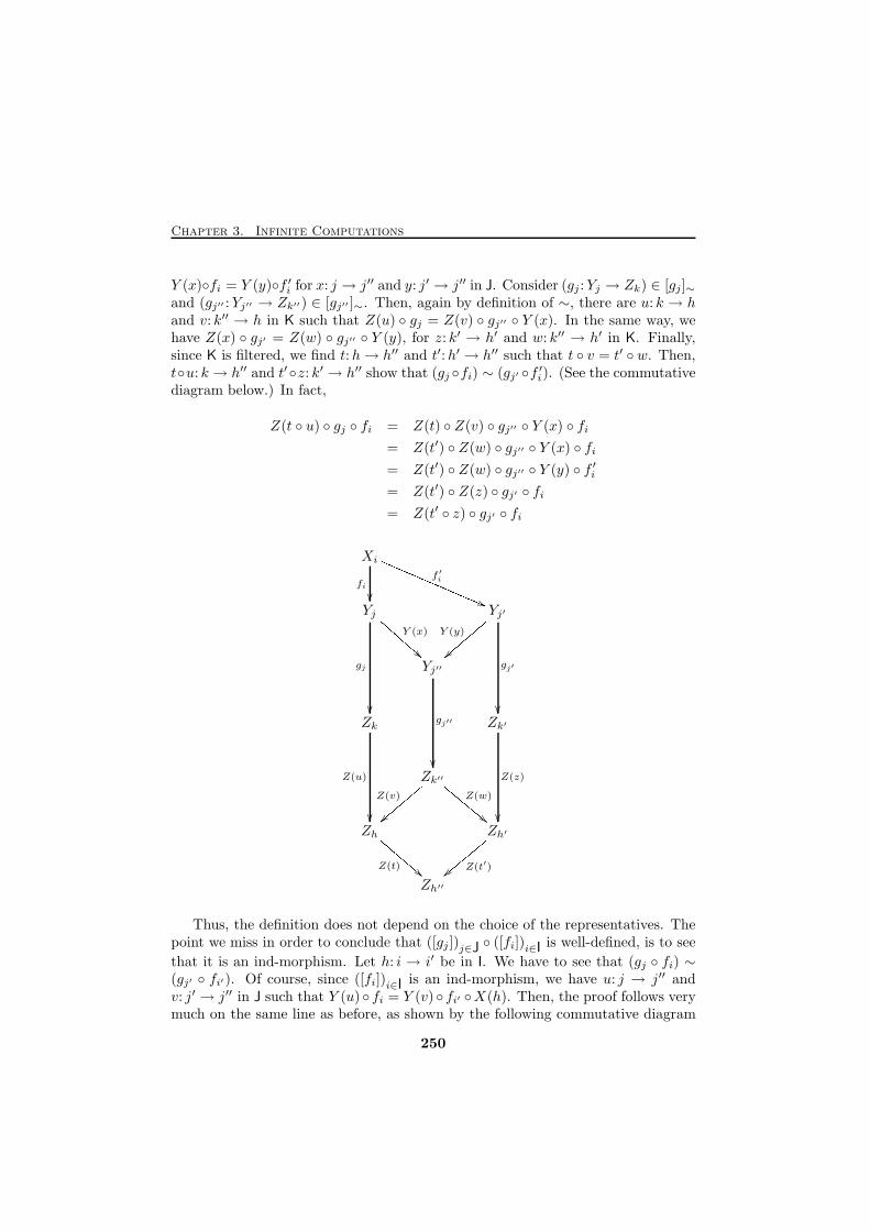
Chapter 3. Infinite Computations
Y (x)◦fi = Y (y)◦f ′i for x: j → j′′ and y: j′ → j′′ in J. Consider (gj :Yj → Zk) ∈ [gj]∼and (gj′′ :Yj′′ → Zk′′) ∈ [gj′′ ]∼. Then, again by definition of ∼, there are u: k → hand v: k′′ → h in K such that Z(u) ◦ gj = Z(v) ◦ gj′′ ◦ Y (x). In the same way, wehave Z(x) ◦ gj′ = Z(w) ◦ gj′′ ◦ Y (y), for z: k′ → h′ and w: k′′ → h′ in K. Finally,since K is filtered, we find t:h→ h′′ and t′:h′ → h′′ such that t ◦ v = t′ ◦ w. Then,t◦u: k→ h′′ and t′◦z: k′ → h′′ show that (gj ◦fi) ∼ (gj′ ◦f
′i). (See the commutative
diagram below.) In fact,
Z(t ◦ u) ◦ gj ◦ fi = Z(t) ◦ Z(v) ◦ gj′′ ◦ Y (x) ◦ fi
= Z(t′) ◦ Z(w) ◦ gj′′ ◦ Y (x) ◦ fi
= Z(t′) ◦ Z(w) ◦ gj′′ ◦ Y (y) ◦ f ′i= Z(t′) ◦ Z(z) ◦ gj′ ◦ fi
= Z(t′ ◦ z) ◦ gj′ ◦ fi
Xi
Yj Yj′
Yj′′
Zk Zk′
Zk′′
Zh Zh′
Zh′′
fi
��
f ′i
QQQQQQQQQQQQQQQ((gj
��
Y (x)
CCCCCC!!gj′
��
Y (y)
}}{{{{{{gj′′
��Z(u)
��
Z(z)
��
Z(v)
}}zzzzzz Z(w)DDDDDD""
Z(t)
DDDDDD !! Z(t′)||zzzzzzThus, the definition does not depend on the choice of the representatives. The
point we miss in order to conclude that ([gj ])j∈J ◦ ([fi])i∈I is well-defined, is to see
that it is an ind-morphism. Let h: i → i′ be in I. We have to see that (gj ◦ fi) ∼(gj′ ◦ fi′). Of course, since ([fi])i∈I is an ind-morphism, we have u: j → j′′ andv: j′ → j′′ in J such that Y (u) ◦ fi = Y (v) ◦ fi′ ◦X(h). Then, the proof follows verymuch on the same line as before, as shown by the following commutative diagram
250
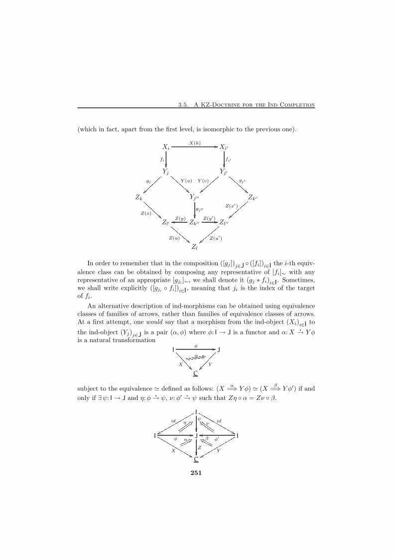
3.5. A KZ-Doctrine for the Ind Completion
(which in fact, apart from the first level, is isomorphic to the previous one).
Xi Xi′
Yj Yj′
Zk Yj′′ Zk′
Zl′ Zk′′ Zl′′
Zl
fi
��
X(h) //
fi′
��
gj
~~}}}}}} Y (u)
CCCCCC!! Y (v)
}}{{{{{{ gj′
CCCCCC!!Z(x)
AAAAAA gj′′
��
Z(x′)
}}{{{{{{Z(u)
DDDDDD!!Z(y)oo Z(y′) //
Z(u′)||zzzzzzIn order to remember that in the composition ([gj ])j∈J ◦ ([fi])i∈I the i-th equiv-
alence class can be obtained by composing any representative of [fi]∼ with anyrepresentative of an appropriate [gji ]∼, we shall denote it (gj ∗ fi)i∈I. Sometimes,we shall write explicitly ([gji ◦ fi])i∈I, meaning that ji is the index of the targetof fi.
An alternative description of ind-morphisms can be obtained using equivalenceclasses of families of arrows, rather than families of equivalence classes of arrows.At a first attempt, one would say that a morphism from the ind-object (Xi)i∈I to
the ind-object (Yj)j∈J is a pair (α, φ) where φ: I → J is a functor and α:X�
→ Y φis a natural transformation
I J
C
φ //
X
<<<<<< �� Y
��������α -6ddddddddddddsubject to the equivalence ≃ defined as follows: (X
α=⇒ Y φ) ≃ (X
β=⇒ Y φ′) if and
only if ∃ψ: I→ J and η:φ�
→ ψ, ν:φ′�
→ ψ such that Zη ◦ α = Zν ◦ β.
I
I J I
C
id
xxqqqqqqqqqqq id
MMMMMMMMMMM &&ψ
��φ
//
X
LLLLLLLLLLL&&η 6>uuuuuuuu ν`h IIIIIIIIZ
��
φ′oo
Y
xxrrrrrrrrrrrα 3;oooooo βck OOOOOO251
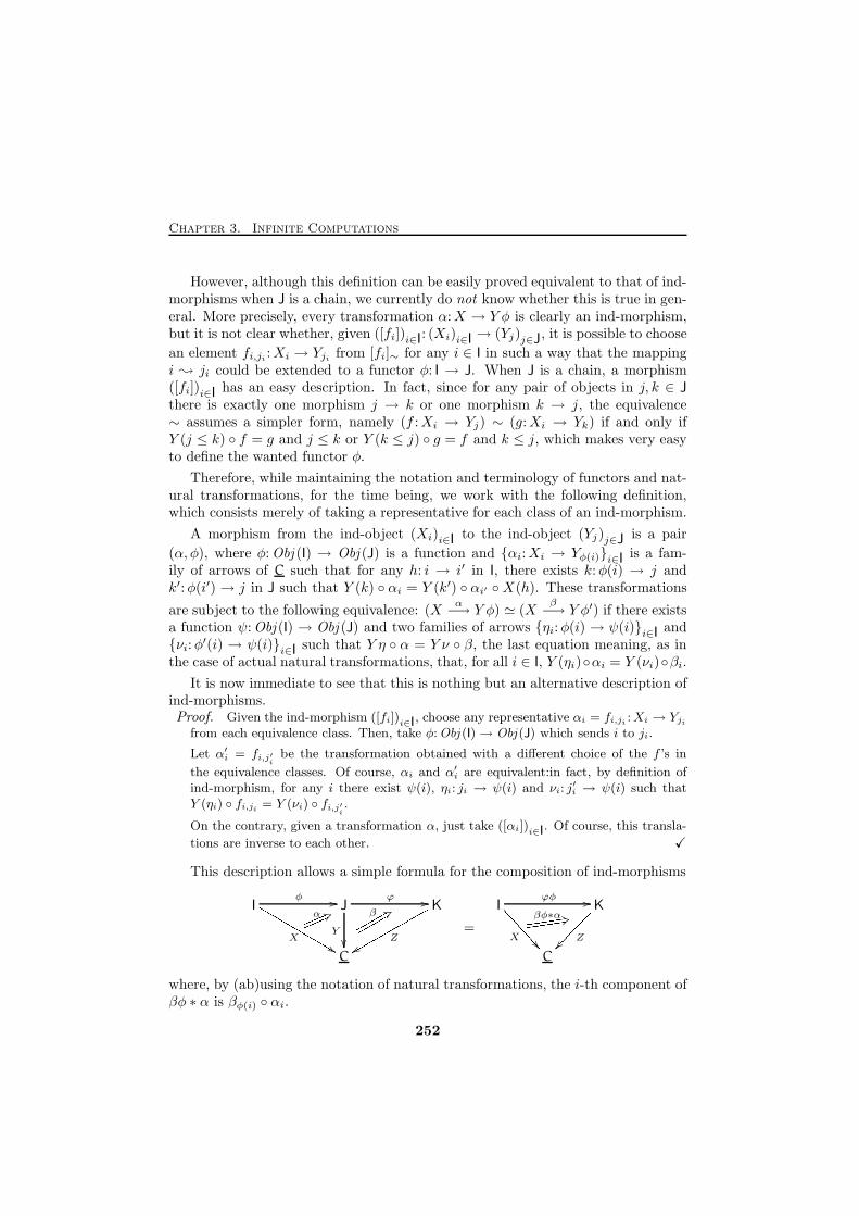
Chapter 3. Infinite Computations
However, although this definition can be easily proved equivalent to that of ind-morphisms when J is a chain, we currently do not know whether this is true in gen-eral. More precisely, every transformation α:X → Y φ is clearly an ind-morphism,but it is not clear whether, given ([fi])i∈I: (Xi)i∈I → (Yj)j∈J, it is possible to choose
an element fi,ji :Xi → Yji from [fi]∼ for any i ∈ I in such a way that the mappingi ; ji could be extended to a functor φ: I → J. When J is a chain, a morphism([fi])i∈I has an easy description. In fact, since for any pair of objects in j, k ∈ J
there is exactly one morphism j → k or one morphism k → j, the equivalence∼ assumes a simpler form, namely (f :Xi → Yj) ∼ (g:Xi → Yk) if and only ifY (j ≤ k) ◦ f = g and j ≤ k or Y (k ≤ j) ◦ g = f and k ≤ j, which makes very easyto define the wanted functor φ.
Therefore, while maintaining the notation and terminology of functors and nat-ural transformations, for the time being, we work with the following definition,which consists merely of taking a representative for each class of an ind-morphism.
A morphism from the ind-object (Xi)i∈I to the ind-object (Yj)j∈J is a pair
(α, φ), where φ:Obj (I) → Obj (J) is a function and {αi:Xi → Yφ(i)}i∈I is a fam-ily of arrows of C such that for any h: i → i′ in I, there exists k:φ(i) → j andk′:φ(i′) → j in J such that Y (k) ◦ αi = Y (k′) ◦ αi′ ◦X(h). These transformations
are subject to the following equivalence: (Xα−→ Y φ) ≃ (X
β−→ Y φ′) if there exists
a function ψ:Obj (I) → Obj (J) and two families of arrows {ηi:φ(i) → ψ(i)}i∈I and
{νi:φ′(i) → ψ(i)}i∈I such that Y η ◦ α = Y ν ◦ β, the last equation meaning, as in
the case of actual natural transformations, that, for all i ∈ I, Y (ηi)◦αi = Y (νi)◦βi.
It is now immediate to see that this is nothing but an alternative description ofind-morphisms.Proof. Given the ind-morphism ([fi])i∈I, choose any representative αi = fi,ji :Xi → Yji
from each equivalence class. Then, take φ:Obj (I)→ Obj (J) which sends i to ji.
Let α′i = fi,j′i
be the transformation obtained with a different choice of the f ’s in
the equivalence classes. Of course, αi and α′i are equivalent:in fact, by definition ofind-morphism, for any i there exist ψ(i), ηi: ji → ψ(i) and νi: j
′i → ψ(i) such that
Y (ηi) ◦ fi,ji = Y (νi) ◦ fi,j′i.
On the contrary, given a transformation α, just take ([αi])i∈I. Of course, this transla-
tions are inverse to each other. X
This description allows a simple formula for the composition of ind-morphisms
I J K
C
φ //
X
LLLLLLLLLLL&& ϕ //
Y
�� Z
xxqqqqqqqqqqqβ 4<qqqqqqqqqqα 2:mmmmmmmm =
I K
C
ϕφ //
X
<<<<<<�� Z
�������βφ∗α -6ddddddddddddwhere, by (ab)using the notation of natural transformations, the i-th component ofβφ ∗ α is βφ(i) ◦ αi.
252
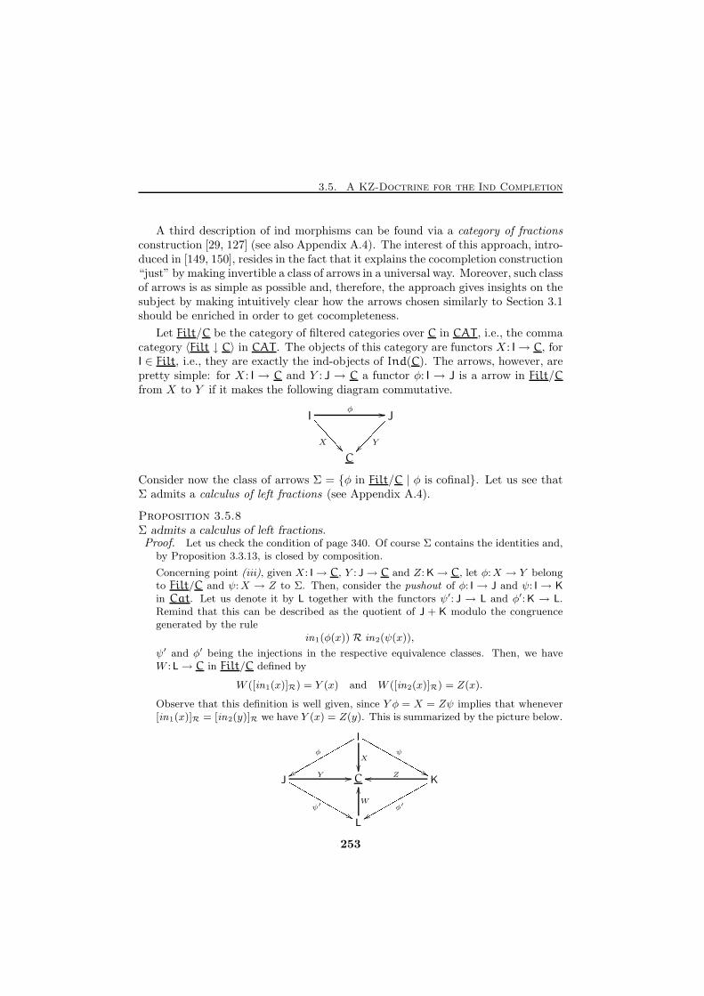
3.5. A KZ-Doctrine for the Ind Completion
A third description of ind morphisms can be found via a category of fractionsconstruction [29, 127] (see also Appendix A.4). The interest of this approach, intro-duced in [149, 150], resides in the fact that it explains the cocompletion construction“just” by making invertible a class of arrows in a universal way. Moreover, such classof arrows is as simple as possible and, therefore, the approach gives insights on thesubject by making intuitively clear how the arrows chosen similarly to Section 3.1should be enriched in order to get cocompleteness.
Let Filt/C be the category of filtered categories over C in CAT , i.e., the commacategory 〈Filt ↓ C〉 in CAT . The objects of this category are functors X : I→ C, forI ∈ Filt, i.e., they are exactly the ind-objects of Ind(C). The arrows, however, arepretty simple: for X : I → C and Y : J → C a functor φ: I → J is a arrow in Filt/Cfrom X to Y if it makes the following diagram commutative.
I J
C
φ //
X
<<<<<< �� Y
��������Consider now the class of arrows Σ = {φ in Filt/C | φ is cofinal}. Let us see thatΣ admits a calculus of left fractions (see Appendix A.4).
Proposition 3.5.8Σ admits a calculus of left fractions.Proof. Let us check the condition of page 340. Of course Σ contains the identities and,
by Proposition 3.3.13, is closed by composition.
Concerning point (iii), given X: I→ C, Y : J→ C and Z: K→ C, let φ:X → Y belongto Filt/C and ψ:X → Z to Σ. Then, consider the pushout of φ: I → J and ψ: I → Kin Cat. Let us denote it by L together with the functors ψ′: J → L and φ′:K → L.Remind that this can be described as the quotient of J + K modulo the congruencegenerated by the rule
in1(φ(x)) R in2(ψ(x)),
ψ′ and φ′ being the injections in the respective equivalence classes. Then, we haveW :L→ C in Filt/C defined by
W ([in1(x)]R) = Y (x) and W ([in2(x)]R) = Z(x).
Observe that this definition is well given, since Y φ = X = Zψ implies that whenever[in1(x)]R = [in2(y)]R we have Y (x) = Z(y). This is summarized by the picture below.
I
J C K
L
φ
xxqqqqqqqqqqqq ψ
MMMMMMMMMMMM &&X
��Y //
ψ′
MMMMMMMMMMM && Zoo
φ′
xxqqqqqqqqqqqW
OO
253
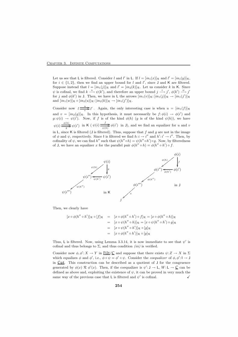
Chapter 3. Infinite Computations
Let us see that L is filtered. Consider l and l′ in L. If l = [ini(x)]R and l′ = [ini(y)]R,for i ∈ {1, 2}, then we find an upper bound for l and l′, since J and K are filtered.Suppose instead that l = [in1(j)]R and l′ = [in2(k)]R. Let us consider k in K. Since
ψ is cofinal, we find ku−→ ψ(k′), and therefore an upper bound j
v−→ j′, φ(k′)
w−→ j′
for j and φ(k′) in J. Then, we have in L the arrows [in1(v)]R: [in1(j)]R → [in1(j′)]R
and [in1(w)]R ◦ [in2(u)]R: [in2(k)]R → [in1(j′)]R.
Consider now l l′u //v
// . Again, the only interesting case is when u = [in1(f)]R
and v = [in2(g)]R. In this hypothesis, it must necessarily be f :φ(i) → φ(i′) andg:ψ(i) → ψ(i′). Now, if f is of the kind φ(h) (g is of the kind ψ(h)), we have
ψ(i) ψ(i′)φ(h) //g
// in K ( ψ(i) φ(i′)f //
ψ(h)// in J), and we find an equalizer for u and v
in L, since K is filtered (J is filtered). Thus, suppose that f and g are not in the imageof φ and ψ, respectively. Since I is filtered we find h: i→ i′′ and h′: i′ → i′′. Then, bycofinality of ψ, we can find h′′ such that ψ(h′′ ◦h) = ψ(h′′ ◦h′)◦g. Now, by filterednessof J, we have an equalizer x for the parallel pair φ(h′′ ◦ h) = φ(h′′ ◦ h′) ◦ f .
ψ(i)
ψ(i′′) ψ(i′)
ψ(i′′′) in K
g
��
ψ(h)
{{xxxxxxxψ(h′′){{wwwwwww ψ(h′)
oo
φ(i)
φ(i′′) φ(i′)
φ(i′′′) in J
j
f
��
φ(h)
||xxxxxxxφ(h′′){{wwwwwww φ(h′)
oo
x
}}{{{{{{Then, we clearly have
[x ◦ φ(h′′ ◦ h′)]R ◦ [f ]R = [x ◦ φ(h′′ ◦ h′) ◦ f ]R = [x ◦ φ(h′′ ◦ h)]R
= [x ◦ ψ(h′′ ◦ h)]R = [x ◦ ψ(h′′ ◦ h′) ◦ g]R
= [x ◦ ψ(h′′ ◦ h′)]R ◦ [g]R
= [x ◦ φ(h′′ ◦ h′)]R ◦ [g]R
Thus, L is filtered. Now, using Lemma 3.3.14, it is now immediate to see that ψ′ iscofinal and thus belongs to Σ, and thus condition (iii) is verified.
Consider now φ, φ′:X → Y in Filt/C and suppose that there exists ψ:Z → X in Σ
which equalizes φ and φ′, i.e., φ ◦ ψ = φ′ ◦ ψ. Consider the coequalizer of φ, φ′: I → J
in Cat. This construction can be described as a quotient of J for the congruence
generated by φ(x) R φ′(x). Then, if the coequalizer is ψ′: J → L, W :L → C can be
defined as above and, exploiting the existence of ψ, it can be proved in very much the
same way of the previous case that L is filtered and ψ′ is cofinal. X
254
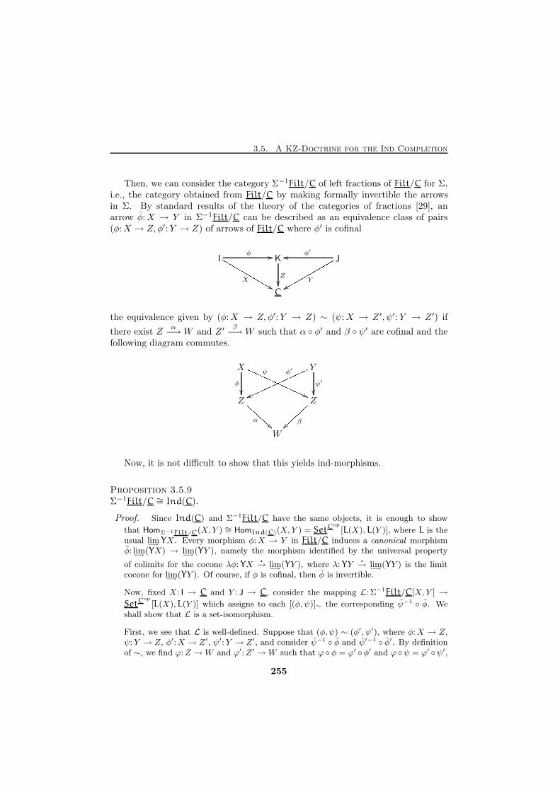
3.5. A KZ-Doctrine for the Ind Completion
Then, we can consider the category Σ−1Filt/C of left fractions of Filt/C for Σ,i.e., the category obtained from Filt/C by making formally invertible the arrowsin Σ. By standard results of the theory of the categories of fractions [29], anarrow φ:X → Y in Σ−1Filt/C can be described as an equivalence class of pairs(φ:X → Z, φ′:Y → Z) of arrows of Filt/C where φ′ is cofinal
I K J
C
φ //
X
LLLLLLLLLLL&& Z
�� Y
xxqqqqqqqqqqqφ′
oo
the equivalence given by (φ:X → Z, φ′:Y → Z) ∼ (ψ:X → Z ′, ψ′:Y → Z ′) if
there exist Zα−→W and Z ′
β−→W such that α ◦ φ′ and β ◦ ψ′ are cofinal and the
following diagram commutes.
X Y
Z Z
W
φ
��
ψPPPPPPPPPPPPP((φ′
vvnnnnnnnnnnnnn ψ′
��
α
BBBBBB β~~}}}}}}Now, it is not difficult to show that this yields ind-morphisms.
Proposition 3.5.9Σ−1Filt/C ∼= Ind(C).
Proof. Since Ind(C) and Σ−1Filt/C have the same objects, it is enough to show
that HomΣ−1Filt/C(X,Y ) ∼= HomInd(C)(X,Y ) = SetCop
[L(X),L(Y )], where L is theusual lim
−→YX. Every morphism φ:X → Y in Filt/C induces a canonical morphism
φ: lim−→
(YX) → lim−→
(YY ), namely the morphism identified by the universal property
of colimits for the cocone λφ:YX�
→ lim−→
(YY ), where λ:YY�
→ lim−→
(YY ) is the limitcocone for lim
−→(YY ). Of course, if φ is cofinal, then φ is invertible.
Now, fixed X: I → C and Y : J → C, consider the mapping L: Σ−1Filt/C[X, Y ] →
SetCop
[L(X),L(Y )] which assigns to each [(φ, ψ)]∼ the corresponding ψ−1 ◦ φ. Weshall show that L is a set-isomorphism.
First, we see that L is well-defined. Suppose that (φ,ψ) ∼ (φ′, ψ′), where φ:X → Z,ψ:Y → Z, φ′:X → Z′, ψ′:Y → Z′, and consider ψ−1 ◦ φ and ψ′−1 ◦ φ′. By definitionof ∼, we find ϕ:Z →W and ϕ′:Z′ →W such that ϕ ◦φ = ϕ′ ◦φ′ and ϕ ◦ψ = ϕ′ ◦ψ′,
255
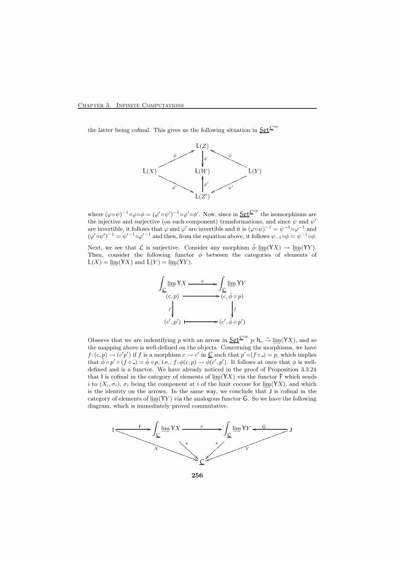
Chapter 3. Infinite Computations
the latter being cofinal. This gives us the following situation in SetCop
L(Z)
L(X) L(W ) L(Y )
L(Z′)
ϕ
��
φnnnnnnnnnnn77φ′
PPPPPPPPPPP'' ψ
ggPPPPPPPPPPPψ′
wwnnnnnnnnnnnϕ′
OO
where (ϕ◦ψ)−1◦ϕ◦φ = (ϕ′◦ψ′)−1◦ϕ′◦φ′. Now, since in SetCop
the isomorphisms arethe injective and surjective (on each component) transformations, and since ψ and ψ′
are invertible, it follows that ϕ and ϕ′ are invertible and it is (ϕ◦ψ)−1 = ψ−1◦ϕ−1 and(ϕ′◦ψ′)−1 = ψ′−1◦ϕ′−1 and then, from the equation above, it follows ψ−1◦φ = ψ−1◦φ.
Next, we see that L is surjective. Consider any morphism φ: lim−→
(YX) → lim−→
(YY ).Then, consider the following functor φ between the categories of elements ofL(X) = lim
−→(YX) and L(Y ) = lim
−→(YY ).
(c, p) (c, φ ◦ p)
(c′, p′) (c′, φ ◦ p′)
� //
f
��f
��� //
∫
C
lim−→
YY
∫
C
lim−→
YX φ //
Observe that we are indentifying p with an arrow in SetCop
p:hc�
→ lim−→
(YX), and sothe mapping above is well-defined on the objects. Concerning the morphisms, we havef : (c, p)→ (c′p′) if f is a morphism c→ c′ in C such that p′ ◦ (f ◦ ) = p, which impliesthat φ ◦ p′ ◦ (f ◦ ) = φ ◦ p, i.e., f :φ(c, p)→ φ(c′, p′). It follows at once that φ is well-defined and is a functor. We have already noticed in the proof of Proposition 3.3.24that I is cofinal in the category of elements of lim
−→(YX) via the functor F which sends
i to (Xi, σi), σi being the component at i of the limit cocone for lim−→
(YX), and whichis the identity on the arrows. In the same way, we conclude that J is cofinal in thecategory of elements of lim
−→(YY ) via the analogous functor G. So we have the following
diagram, which is immediately proved commutative.
I J
C
X
SSSSSSSSSSSSSSSSSSSSSSSSS))F //∫
C
lim−→
YX
πBBBBBB φ //
∫
C
lim−→
YY
π
~~}}}}}} Y
uukkkkkkkkkkkkkkkkkkkkkkkkkGoo
256
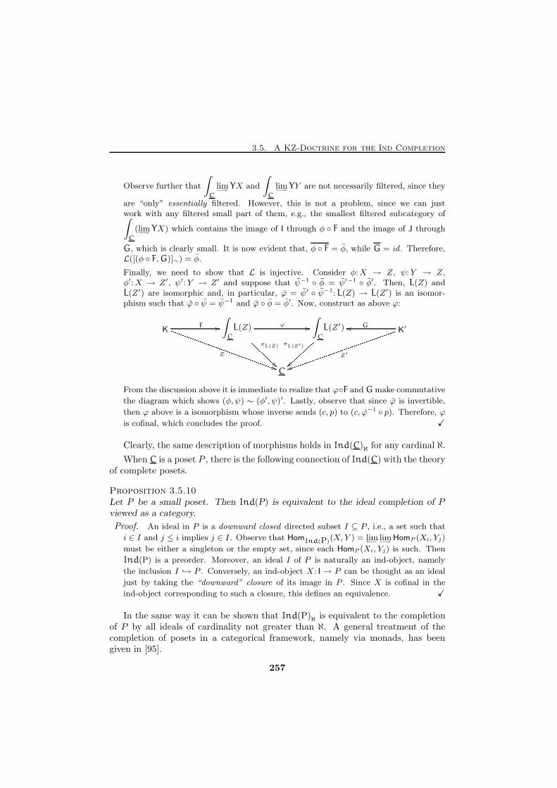
3.5. A KZ-Doctrine for the Ind Completion
Observe further that
∫
C
lim−→
YX and
∫
C
lim−→
YY are not necessarily filtered, since they
are “only” essentially filtered. However, this is not a problem, since we can justwork with any filtered small part of them, e.g., the smallest filtered subcategory of∫
C
(lim−→
YX) which contains the image of I through φ ◦ F and the image of J through
G, which is clearly small. It is now evident that, φ ◦ F = φ, while G = id . Therefore,L([(φ ◦ F,G)]∼) = φ.
Finally, we need to show that L is injective. Consider φ:X → Z, ψ:Y → Z,φ′:X → Z′, ψ′:Y → Z′ and suppose that ψ−1 ◦ φ = ψ′−1 ◦ φ′. Then, L(Z) andL(Z′) are isomorphic and, in particular, ϕ = ψ′ ◦ ψ−1:L(Z) → L(Z′) is an isomor-phism such that ϕ ◦ ψ = ψ−1 and ϕ ◦ φ = φ′. Now, construct as above ϕ:
K
∫
C
L(Z)
∫
C
L(Z′) K′
C
Z
SSSSSSSSSSSSSSSSSSSSSSS))F //
πL(Z)AAAAAA ϕ //
πL(Z′)
~~|||||| Z′
uujjjjjjjjjjjjjjjjjjjjjjjjGoo
From the discussion above it is immediate to realize that ϕ◦F and G make commutative
the diagram which shows (φ, ψ) ∼ (φ′, ψ)′. Lastly, observe that since ϕ is invertible,
then ϕ above is a isomorphism whose inverse sends (c, p) to (c, ϕ−1 ◦ p). Therefore, ϕ
is cofinal, which concludes the proof. X
Clearly, the same description of morphisms holds in Ind(C)ℵ for any cardinal ℵ.
When C is a poset P , there is the following connection of Ind(C) with the theoryof complete posets.
Proposition 3.5.10Let P be a small poset. Then Ind(P) is equivalent to the ideal completion of Pviewed as a category.
Proof. An ideal in P is a downward closed directed subset I ⊆ P , i.e., a set such that
i ∈ I and j ≤ i implies j ∈ I . Observe that HomInd(P)(X,Y ) = lim
←−lim−→
HomP (Xi, Yj)
must be either a singleton or the empty set, since each HomP (Xi, Yj) is such. Then
Ind(P) is a preorder. Moreover, an ideal I of P is naturally an ind-object, namely
the inclusion I → P . Conversely, an ind-object X: I → P can be thought as an ideal
just by taking the “downward” closure of its image in P . Since X is cofinal in the
ind-object corresponding to such a closure, this defines an equivalence. X
In the same way it can be shown that Ind(P)ℵ is equivalent to the completionof P by all ideals of cardinality not greater than ℵ. A general treatment of thecompletion of posets in a categorical framework, namely via monads, has beengiven in [95].
257
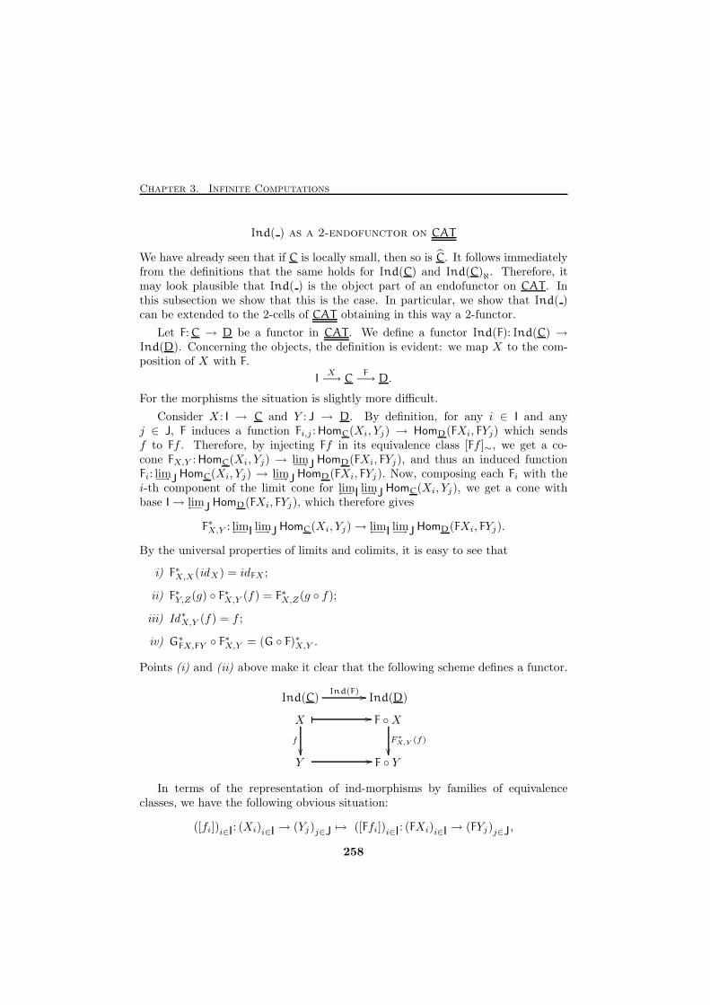
Chapter 3. Infinite Computations
Ind( ) as a 2-endofunctor on CAT
We have already seen that if C is locally small, then so is C. It follows immediatelyfrom the definitions that the same holds for Ind(C) and Ind(C)ℵ. Therefore, itmay look plausible that Ind( ) is the object part of an endofunctor on CAT . Inthis subsection we show that this is the case. In particular, we show that Ind( )can be extended to the 2-cells of CAT obtaining in this way a 2-functor.
Let F: C → D be a functor in CAT . We define a functor Ind(F): Ind(C) →Ind(D). Concerning the objects, the definition is evident: we map X to the com-position of X with F.
IX−→ C
F−→ D.
For the morphisms the situation is slightly more difficult.
Consider X : I → C and Y : J → D. By definition, for any i ∈ I and anyj ∈ J, F induces a function Fi,j : HomC(Xi, Yj) → HomD(FXi, FYj) which sendsf to Ff . Therefore, by injecting Ff in its equivalence class [Ff ]∼, we get a co-cone FX,Y : HomC(Xi, Yj) → lim−→J HomD(FXi, FYj), and thus an induced functionFi: lim−→J HomC(Xi, Yj) → lim−→J HomD(FXi, FYj). Now, composing each Fi with thei-th component of the limit cone for lim←− I lim−→J HomC(Xi, Yj), we get a cone withbase I→ lim←−J HomD(FXi, FYj), which therefore gives
F∗X,Y : lim←− I lim−→J HomC(Xi, Yj)→ lim←− I lim−→J HomD(FXi, FYj).
By the universal properties of limits and colimits, it is easy to see that
i) F∗X,X(idX) = idFX ;
ii) F∗Y,Z(g) ◦ F∗X,Y (f) = F∗X,Z(g ◦ f);
iii) Id∗X,Y (f) = f ;
iv) G∗FX,FY ◦ F∗X,Y = (G ◦ F)∗X,Y .
Points (i) and (ii) above make it clear that the following scheme defines a functor.
X F ◦X
Y F ◦ Y
� //
f
��F∗
X,Y (f)
��� //
Ind(D)Ind(C)Ind(F) //
In terms of the representation of ind-morphisms by families of equivalenceclasses, we have the following obvious situation:
([fi])i∈I: (Xi)i∈I → (Yj)j∈J 7→ ([Ffi])i∈I: (FXi)i∈I → (FYj)j∈J,
258
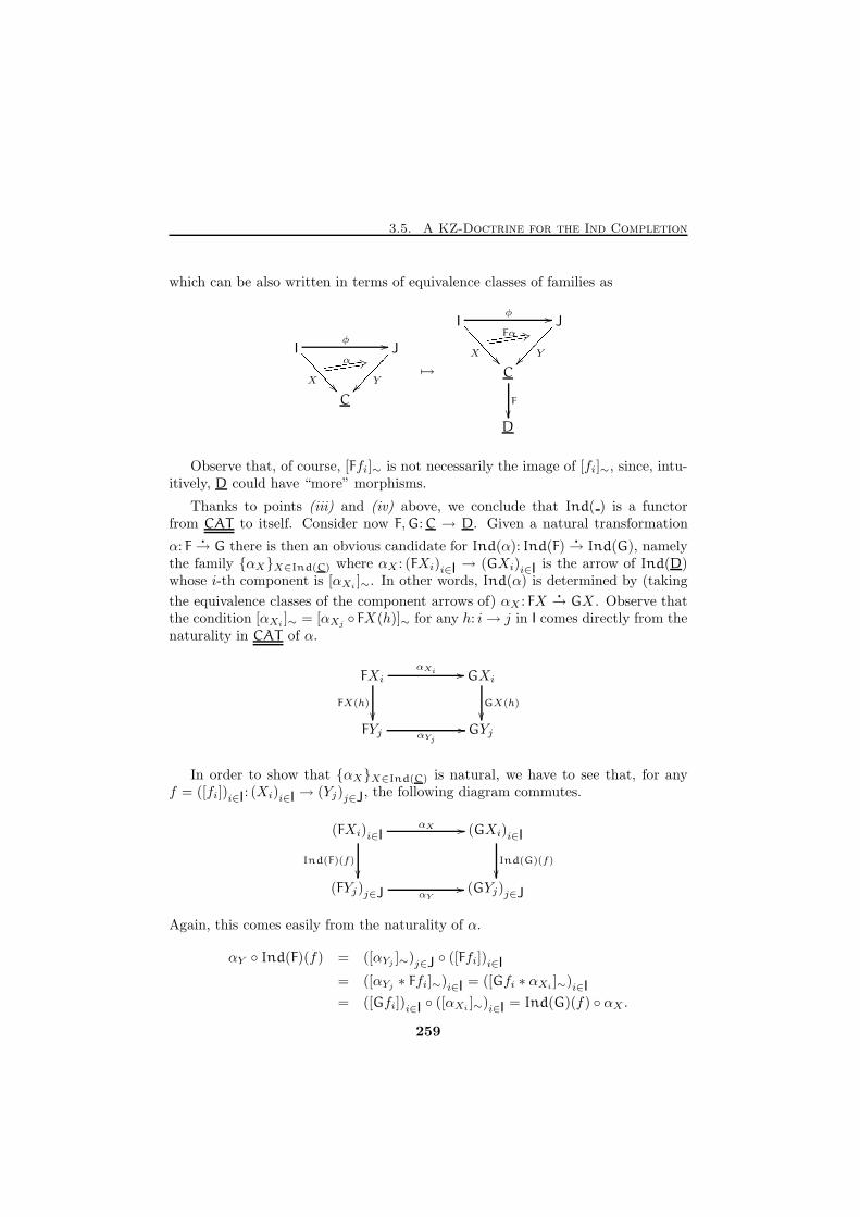
3.5. A KZ-Doctrine for the Ind Completion
which can be also written in terms of equivalence classes of families as
I J
C
φ //
X
<<<<<<�� Y
��������α -6dddddddddddd 7→
I J
C
D
φ //
X
====== �� Y
��������Fα -6ddddddddddddF
��
Observe that, of course, [Ffi]∼ is not necessarily the image of [fi]∼, since, intu-itively, D could have “more” morphisms.
Thanks to points (iii) and (iv) above, we conclude that Ind( ) is a functorfrom CAT to itself. Consider now F,G: C → D. Given a natural transformation
α: F�
→ G there is then an obvious candidate for Ind(α): Ind(F)�
→ Ind(G), namelythe family {αX}X∈Ind(C) where αX : (FXi)i∈I → (GXi)i∈I is the arrow of Ind(D)whose i-th component is [αXi
]∼. In other words, Ind(α) is determined by (taking
the equivalence classes of the component arrows of) αX : FX�
→ GX . Observe thatthe condition [αXi
]∼ = [αXj◦ FX(h)]∼ for any h: i→ j in I comes directly from the
naturality in CAT of α.
FXi GXi
FYj GYj
FX(h)
��
αXi //
GX(h)
��αYj
//
In order to show that {αX}X∈Ind(C) is natural, we have to see that, for anyf = ([fi])i∈I: (Xi)i∈I → (Yj)j∈J, the following diagram commutes.
(FXi)i∈I (GXi)i∈I
(FYj)j∈J (GYj)j∈J
Ind(F)(f)
��
αX //
Ind(G)(f)
��
αY
//
Again, this comes easily from the naturality of α.
αY ◦ Ind(F)(f) = ([αYj]∼)
j∈J ◦ ([Ffi])i∈I
= ([αYj∗ Ffi]∼)
i∈I = ([Gfi ∗ αXi]∼)
i∈I= ([Gfi])i∈I ◦ ([αXi
]∼)i∈I = Ind(G)(f) ◦ αX .
259
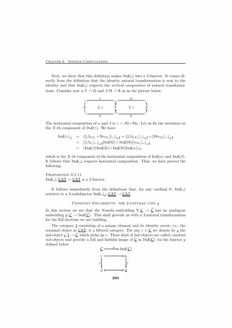
Chapter 3. Infinite Computations
Next, we show that this definition makes Ind( ) into a 2-functor. It comes di-rectly from the definition that the identity natural transformation is sent to theidentity and that Ind( ) respects the vertical composition of natural transforma-
tions. Consider now α: F�
→ G and β: H�
→ K as in the picture below.
X ⇓ α Y ⇓ β Z
# "F
�� !G
OO
# "H
�� !K
OO
The horizontal composition of α and β is γ = βG ◦Hα. Let us fix the attention onthe X-th component of Ind(γ). We have
Ind(γ)X = ([(βGXi◦HαXi
)]∼)i∈I = ([(βGXi
]∼)i∈I ◦ ([HαXi
]∼)i∈I
= ([(βXi]∼)
i∈IInd(G) ◦ Ind(H)([αXi]∼)
i∈I
= (Ind(β)Ind(G) ◦ Ind(H)Ind(α))X ,
which is the X-th component of the horizontal composition of Ind(α) and Ind(β).It follows that Ind( ) respects horizontal composition. Thus, we have proved thefollowing.
Proposition 3.5.11Ind( ): CAT → CAT is a 2-functor.
It follows immediately from the definitions that, for any cardinal ℵ, Ind( )restricts to a 2-endofunctor Ind( )ℵ: CAT → CAT .
Constant Ind-objects: the 2-natural unit y
In this section we see that the Yoneda embedding Y: C → C has an analogousembedding y: C → Ind(C). This shall provide us with a 2-natural transformationfor the KZ-doctrine we are building.
The category 1 consisting of a unique element and its identity arrow, i.e., theterminal object in CAT , is a filtered category. For any c ∈ C we denote by c theind-object c: 1→ C which picks up c. These kind of ind-objects are called constantind-objects and provide a full and faithful image of C in Ind(C) via the functor ydefined below.
c c
d d
� //
f
��f
��� //
Ind(C)Cy //
260
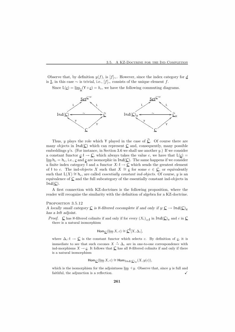
3.5. A KZ-Doctrine for the Ind Completion
Observe that, by definition y(f), is [f ]∼. However, since the index category for dis 1, in this case ∼ is trivial, i.e., [f ]∼ consists of the unique element f .
Since L(c) = lim−→1(Y ◦ c) = hc, we have the following commuting diagrams.
SetCop
Ind(C) C
C
Luuuuuuuu::∼oo //
L
aaCCCCCCCy
ddJJJJJJJJJ Yzzzzzzz<<SetCop
Ind(C)ℵ Cℵ
C
Ltttttttt::∼oo //
L
bbEEEEEEEy
eeKKKKKKKKK Yxxxxxxx<<Thus, y plays the role which Y played in the case of C. Of course there are
many objects in Ind(C) which can represent C and, consequently, many possibleembeddings y’s. (For instance, in Section 3.6 we shall use another y.) If we considera constant functor c: I → C, which always takes the value c, we have that L(c) =lim−→ hc = hc, i.e., c and c are isomorphic in Ind(C). The same happens if we considera finite index category I and a functor X : I → C which sends the greatest elementof I to c. The ind-objects X such that X ∼= c for some c ∈ C, or equivalentlysuch that L(X) ∼= hc, are called essentially constant ind-objects. Of course, y is anequivalence of C and the full subcategory of the essentially constant ind-objects inInd(C).
A first connection with KZ-doctrines is the following proposition, where thereader will recognize the similarity with the definition of algebra for a KZ-doctrine.
Proposition 3.5.12A locally small category C is ℵ-filtered cocomplete if and only if y: C → Ind(C)ℵhas a left adjoint.
Proof. C has ℵ-filtered colimits if and only if for every (Xi)i∈I in Ind(C)ℵ and c in Cthere is a natural isomorphism
HomC(lim−→
X, c) ∼= CI[X,∆c],
where ∆c: I → C is the constant functor which selects c. By definition of c, it is
immediate to see that such cocones X�
→ ∆c are in one-to-one correspondence withind-morphisms X → c. It follows that C has all ℵ-filtered colimits if and only if thereis a natural isomorphism
HomC(lim−→
X, c) ∼= HomInd(C)ℵ(X, y(c)),
which is the isomorphism for the adjointness lim−→⊣ y. Observe that, since y is full and
faithful, the adjunction is a reflection. X
261
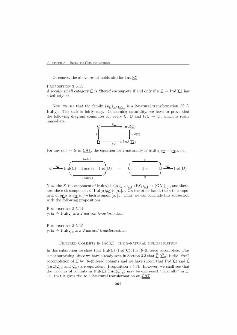
Chapter 3. Infinite Computations
Of course, the above result holds also for Ind(C)
Proposition 3.5.13A locally small category C is filtered cocomplete if and only if y: C → Ind(C) hasa left adjoint.
Now, we see that the family {yC}C∈CAT is a 2-natural transformation Id�
→
Ind( ). The task is fairly easy. Concerning naturality, we have to prove thatthe following diagram commutes for every C, D and F: C → D, which is reallyimmediate.
C Ind(C)
D Ind(D)
F
��
yC //
Ind(F)
��yD
//
For any α: F→ G in CAT , the equation for 2-naturality is Ind(α)yC = yDα, i.e.,
C Ind(C) ⇓Ind(α) Ind(D)yC //
# "Ind(F)
�� !Ind(G)
OO = C ⇓ α D Ind(D)
# "F
�� !G
OOyD //
Now, theX-th component of Ind(α) is ([αXi]∼)
i∈I: (FXi)i∈I → (GXi)i∈I, and there-fore the c-th component of Ind(α)yC is [αc]∼. On the other hand, the c-th compo-nent of yDα is yD(αc) which is again [αc]∼. Thus, we can conclude this subsectionwith the following propositions.
Proposition 3.5.14y: Id
�
→ Ind( ) is a 2-natural transformation.
Proposition 3.5.15y: Id
�
→ Ind( )ℵ is a 2-natural transformation.
Filtered Colimits in Ind(C): the 2-natural multiplication
In this subsection we show that Ind(C) (Ind(C)ℵ) is (ℵ-)filtered cocomplete. This
is not surprising, since we have already seen in Section 3.3 that C (Cℵ) is the “free”
cocompletion of C by (ℵ-)filtered colimits and we have shown that Ind(C) and C
(Ind(C)ℵ and Cℵ) are equivalent (Proposition 3.5.3). However, we shall see thatthe calculus of colimits in Ind(C) (Ind(C)ℵ) may be expressed “naturally” in C,i.e., that it gives rise to a 2-natural transformation on CAT .
262
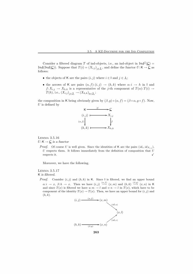
3.5. A KZ-Doctrine for the Ind Completion
Consider a filtered diagram T of ind-objects, i.e., an ind-object in Ind2(C) =Ind(Ind(C)). Suppose that T (i) = (Xi,j)j∈Ji
, and define the functor U : K→ C asfollows:
• the objects of K are the pairs (i, j) where i ∈ I and j ∈ Ji;
• the arrows of K are pairs (α, f): (i, j) → (h, k) where α: i → h in I andf :Xi,j → Xh,k is a representative of the j-th component of T (α):T (i) →T (h), i.e., (Xi,j)j∈Ji
→ (Xh,k)k∈Jh;
the composition in K being obviously given by (β, g) ◦ (α, f) = (β ◦ α, g ◦ f). Now,U is defined by
(i, j) Xi,j
(h, k) Xh,k
� //
(α,f)
��f
��� //
CKU //
Lemma 3.5.16U : K→ C is a functor
Proof. Of course U is well given. Since the identities of K are the pairs (id i, idXi,j ),
U respects them. It follows immediately from the definition of composition that U
respects it. X
Moreover, we have the following.
Lemma 3.5.17K is filtered.
Proof. Consider (i, j) and (h, k) in K. Since I is filtered, we find an upper bound
α: i → x, β: h → x. Then we have (i, j)(α,f)−→ (x,m) and (h, k)
(β,g)−→ (x, n) in K
and since T (x) is filtered we have u:m → l and v:n → l in T (x), which have to becomponent of the identity T (x)→ T (x). Then, we have an upper bound for (i, j) and(h, k).
(i, j) (x,m)
(x, l)
(h, k) (x, n)
(α,f) //
(id ,u)
GGGGGGG##(β,g)
//(id ,v)wwwwwww ;;
263
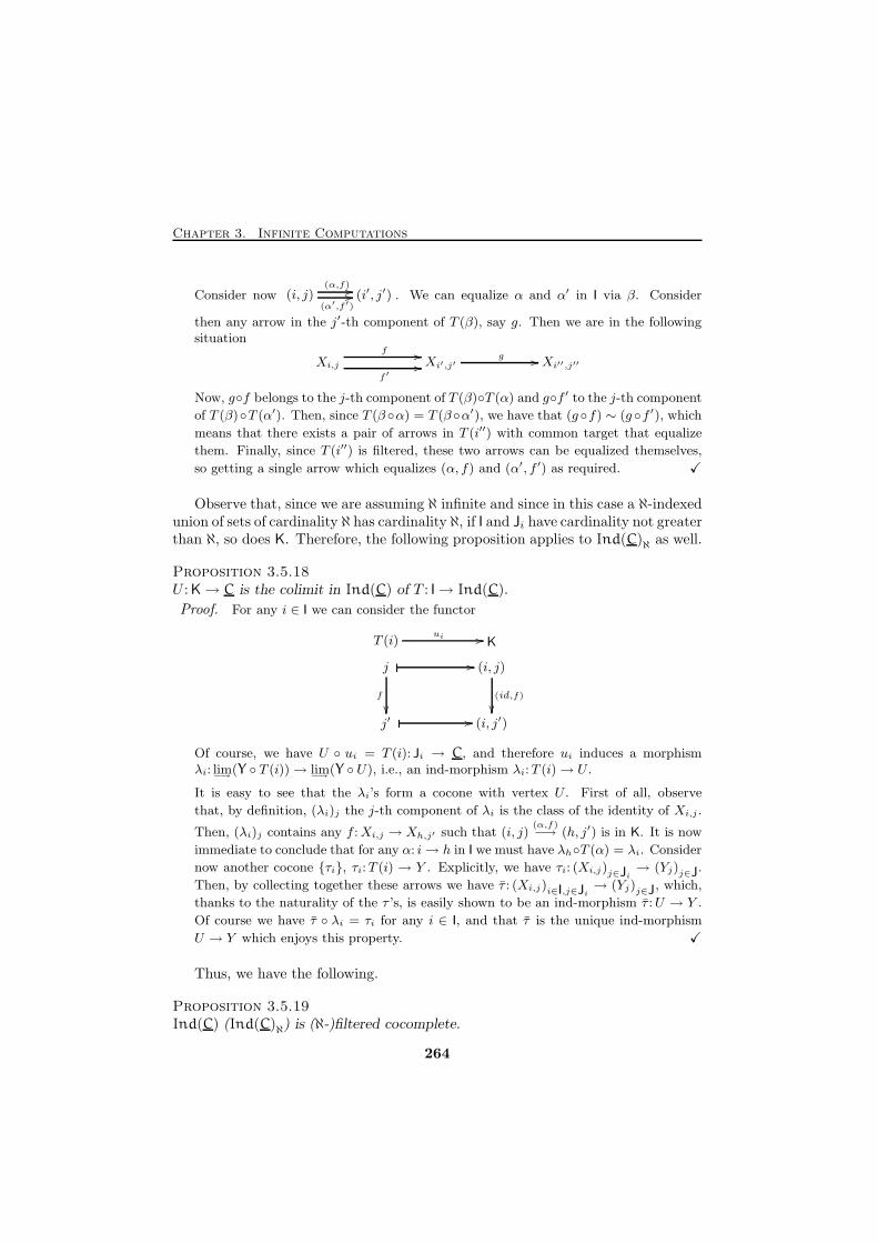
Chapter 3. Infinite Computations
Consider now (i, j) (i′, j′)(α,f) //
(α′,f ′)// . We can equalize α and α′ in I via β. Consider
then any arrow in the j′-th component of T (β), say g. Then we are in the followingsituation
Xi,j Xi′,j′ Xi′′,j′′f //
f ′//
g //
Now, g◦f belongs to the j-th component of T (β)◦T (α) and g◦f ′ to the j-th component
of T (β)◦T (α′). Then, since T (β ◦α) = T (β ◦α′), we have that (g ◦f) ∼ (g ◦f ′), which
means that there exists a pair of arrows in T (i′′) with common target that equalize
them. Finally, since T (i′′) is filtered, these two arrows can be equalized themselves,
so getting a single arrow which equalizes (α, f) and (α′, f ′) as required. X
Observe that, since we are assuming ℵ infinite and since in this case a ℵ-indexedunion of sets of cardinality ℵ has cardinality ℵ, if I and Ji have cardinality not greaterthan ℵ, so does K. Therefore, the following proposition applies to Ind(C)ℵ as well.
Proposition 3.5.18U : K→ C is the colimit in Ind(C) of T : I→ Ind(C).
Proof. For any i ∈ I we can consider the functor
j (i, j)
j′ (i, j′)
� //
f
��(id,f)
��� //
KT (i)ui //
Of course, we have U ◦ ui = T (i): Ji → C, and therefore ui induces a morphismλi: lim−→(Y ◦ T (i))→ lim
−→(Y ◦ U), i.e., an ind-morphism λi:T (i)→ U .
It is easy to see that the λi’s form a cocone with vertex U . First of all, observe
that, by definition, (λi)j the j-th component of λi is the class of the identity of Xi,j .
Then, (λi)j contains any f :Xi,j → Xh,j′ such that (i, j)(α,f)−→ (h, j′) is in K. It is now
immediate to conclude that for any α: i→ h in I we must have λh◦T (α) = λi. Consider
now another cocone {τi}, τi:T (i) → Y . Explicitly, we have τi: (Xi,j)j∈Ji→ (Yj)j∈J.
Then, by collecting together these arrows we have τ : (Xi,j)i∈I,j∈Ji→ (Yj)j∈J, which,
thanks to the naturality of the τ ’s, is easily shown to be an ind-morphism τ :U → Y .
Of course we have τ ◦ λi = τi for any i ∈ I, and that τ is the unique ind-morphism
U → Y which enjoys this property. X
Thus, we have the following.
Proposition 3.5.19Ind(C) (Ind(C)ℵ) is (ℵ-)filtered cocomplete.
264
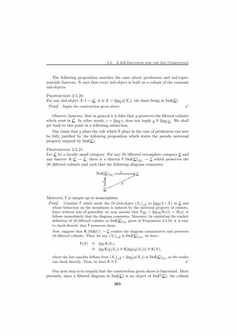
3.5. A KZ-Doctrine for the Ind Completion
The following proposition matches the ones about presheaves and ind-repre-sentable functors. It says that every ind-object is built as a colimit of the constantind-objects.
Proposition 3.5.20For any ind-object X : I→ C, it is X = lim−→ I y(Xi), the limit being in Ind(C).
Proof. Apply the construction given above. X
Observe, however, that in general it is false that y preserves the filtered colimitswhich exist in C. In other words, c = lim−→ I ci does not imply c ∼= lim−→ I ci. We shallget back to this point in a following subsection.
Our claim that y plays the role which Y plays in the case of presheaves can nowbe fully justified by the following proposition which states the pseudo universalproperty enjoyed by Ind(C).
Proposition 3.5.21Let C be a locally small category. For any (ℵ-)filtered cocomplete category E andany functor A: C → E, there is a functor F: Ind(C)(ℵ) → E which preserves the
(ℵ-)filtered colimits and such that the following diagram commutes.
Ind(C)(ℵ) E
C
F //
y/� OO Annnnnnnnnnnnnnn77Moreover, F is unique up to isomorphism.
Proof. Consider F which sends the (ℵ-)ind-object (Xi)i∈I to lim−→ I(A ◦ X) in E and
whose behaviour on the morphisms is induced by the universal property of colimits.Since without loss of generality we may assume that F(c) = lim
−→y(A(c)) = A(c), it
follows immediately that the diagram commutes. Moreover, by exploiting the explicitdefinition of (ℵ-)filtered colimits in Ind(C)(ℵ) given in Proposition 3.5.18, it is easy
to check directly that F preserves them.
Now, suppose that K: Ind(C) → E renders the diagram commutative and preserves(ℵ-)filtered colimits. Then, for any (Xi)i∈I in Ind(C)(ℵ), we have:
F(X) ∼= lim−→
A(Xi)
∼= lim−→
K(y(Xi)) ∼= K(lim−→
(y(Xi))) ∼= K(X),
where the last equality follows from (Xi)i∈I = lim−→ I(y(Xi)) in Ind(C)(ℵ), as the reader
can check directly. Thus, we have K ∼= F. X
Our next step is to remark that the construction given above is functorial. Moreprecisely, since a filtered diagram in Ind(C) is an object of Ind2(C), the colimit
265
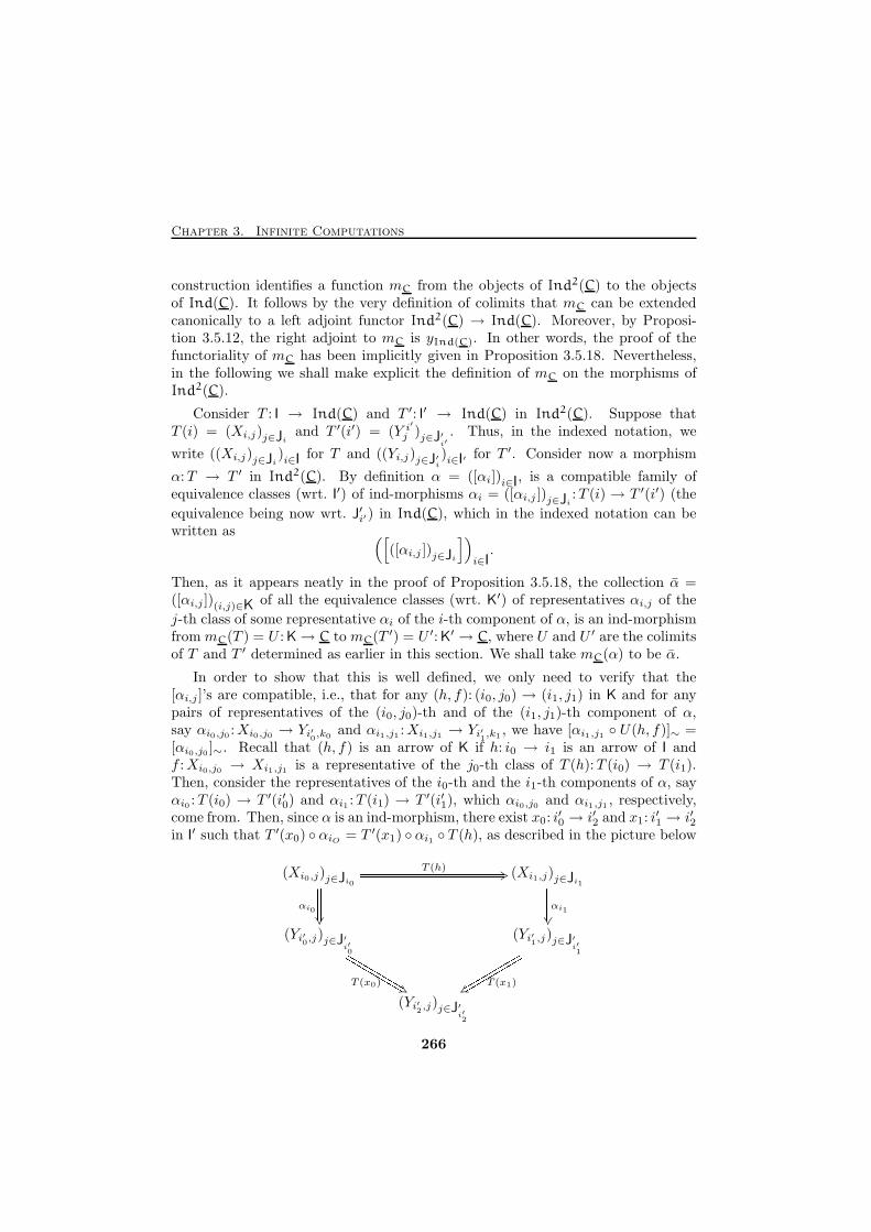
Chapter 3. Infinite Computations
construction identifies a function mC from the objects of Ind2(C) to the objectsof Ind(C). It follows by the very definition of colimits that mC can be extendedcanonically to a left adjoint functor Ind2(C) → Ind(C). Moreover, by Proposi-tion 3.5.12, the right adjoint to mC is yInd(C). In other words, the proof of thefunctoriality of mC has been implicitly given in Proposition 3.5.18. Nevertheless,in the following we shall make explicit the definition of mC on the morphisms ofInd2(C).
Consider T : I → Ind(C) and T ′: I′ → Ind(C) in Ind2(C). Suppose thatT (i) = (Xi,j)j∈Ji
and T ′(i′) = (Y i′
j )j∈J′
i′. Thus, in the indexed notation, we
write ((Xi,j)j∈Ji)i∈I for T and ((Yi,j)j∈J′
i
)i∈I′ for T ′. Consider now a morphism
α:T → T ′ in Ind2(C). By definition α = ([αi])i∈I, is a compatible family ofequivalence classes (wrt. I′) of ind-morphisms αi = ([αi,j ])j∈Ji
:T (i) → T ′(i′) (the
equivalence being now wrt. J′i′) in Ind(C), which in the indexed notation can bewritten as ([
([αi,j ])j∈Ji
])
i∈I.
Then, as it appears neatly in the proof of Proposition 3.5.18, the collection α =([αi,j ])(i,j)∈K of all the equivalence classes (wrt. K′) of representatives αi,j of the
j-th class of some representative αi of the i-th component of α, is an ind-morphismfrom mC(T ) = U : K→ C to mC(T ′) = U ′: K′ → C, where U and U ′ are the colimitsof T and T ′ determined as earlier in this section. We shall take mC(α) to be α.
In order to show that this is well defined, we only need to verify that the[αi,j ]’s are compatible, i.e., that for any (h, f): (i0, j0) → (i1, j1) in K and for anypairs of representatives of the (i0, j0)-th and of the (i1, j1)-th component of α,say αi0,j0 :Xi0,j0 → Yi′
0,k0 and αi1,j1 :Xi1,j1 → Yi′
1,k1 , we have [αi1,j1 ◦ U(h, f)]∼ =
[αi0,j0 ]∼. Recall that (h, f) is an arrow of K if h: i0 → i1 is an arrow of I andf :Xi0,j0 → Xi1,j1 is a representative of the j0-th class of T (h):T (i0) → T (i1).Then, consider the representatives of the i0-th and the i1-th components of α, sayαi0 :T (i0) → T ′(i′0) and αi1 :T (i1) → T ′(i′1), which αi0,j0 and αi1,j1 , respectively,come from. Then, since α is an ind-morphism, there exist x0: i
′0 → i′2 and x1: i
′1 → i′2
in I′ such that T ′(x0) ◦ αiO = T ′(x1) ◦ αi1 ◦ T (h), as described in the picture below
(Xi0,j)j∈Ji0(Xi1,j)j∈Ji1
(Yi′0,j)j∈J′
i′0
(Yi′1,j)j∈J′
i′1
(Yi′2,j)j∈J′
i′2
T (h) +3________________________________________αi0
��
���������� αi1
��
����������T (x0) !*
LLLLLLLLLLLLLLLL T (x1)t} rrrrrrrrrrrrrrrr266
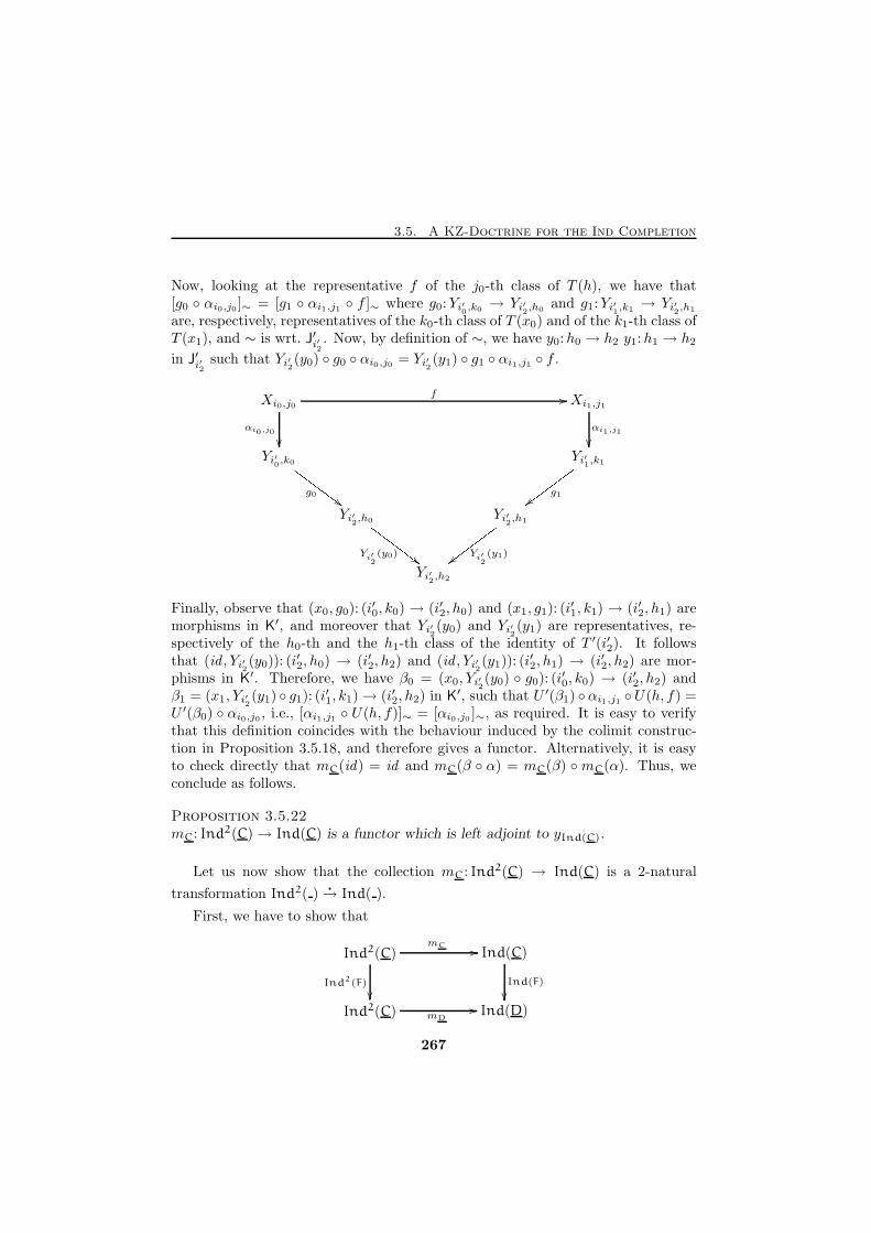
3.5. A KZ-Doctrine for the Ind Completion
Now, looking at the representative f of the j0-th class of T (h), we have that[g0 ◦ αi0,j0 ]∼ = [g1 ◦ αi1,j1 ◦ f ]∼ where g0:Yi′
0,k0 → Yi′
2,h0
and g1:Yi′1,k1 → Yi′
2,h1
are, respectively, representatives of the k0-th class of T (x0) and of the k1-th class ofT (x1), and ∼ is wrt. J′i′
2. Now, by definition of ∼, we have y0:h0 → h2 y1:h1 → h2
in J′i′2such that Yi′
2(y0) ◦ g0 ◦ αi0,j0 = Yi′
2(y1) ◦ g1 ◦ αi1,j1 ◦ f .
Xi0,j0 Xi1,j1
Yi′0,k0 Yi′1,k1
Yi′2,h0
Yi′2,h1
Yi′2,h2
f //
αi0,j0
��αi1,j1
��
g0
GGGGGGG## g1{{wwwwwww
Yi′2(y0)
GGGGGGG ## Yi′2(y1){{wwwwwww
Finally, observe that (x0, g0): (i′0, k0) → (i′2, h0) and (x1, g1): (i
′1, k1) → (i′2, h1) are
morphisms in K′, and moreover that Yi′2(y0) and Yi′
2(y1) are representatives, re-
spectively of the h0-th and the h1-th class of the identity of T ′(i′2). It followsthat (id , Yi′2 (y0)): (i
′2, h0) → (i′2, h2) and (id , Yi′2(y1)): (i
′2, h1) → (i′2, h2) are mor-
phisms in K′. Therefore, we have β0 = (x0, Yi′2(y0) ◦ g0): (i′0, k0) → (i′2, h2) and
β1 = (x1, Yi′2 (y1) ◦ g1): (i′1, k1)→ (i′2, h2) in K′, such that U ′(β1) ◦αi1,j1 ◦U(h, f) =
U ′(β0) ◦ αi0,j0 , i.e., [αi1,j1 ◦ U(h, f)]∼ = [αi0,j0 ]∼, as required. It is easy to verifythat this definition coincides with the behaviour induced by the colimit construc-tion in Proposition 3.5.18, and therefore gives a functor. Alternatively, it is easyto check directly that mC(id) = id and mC(β ◦ α) = mC(β) ◦mC(α). Thus, weconclude as follows.
Proposition 3.5.22mC: Ind2(C)→ Ind(C) is a functor which is left adjoint to yInd(C).
Let us now show that the collection mC: Ind2(C) → Ind(C) is a 2-natural
transformation Ind2( )�
→ Ind( ).
First, we have to show that
Ind2(C) Ind(C)
Ind2(C) Ind(D)
mC //
Ind2(F)
��Ind(F)
��mD
//
267
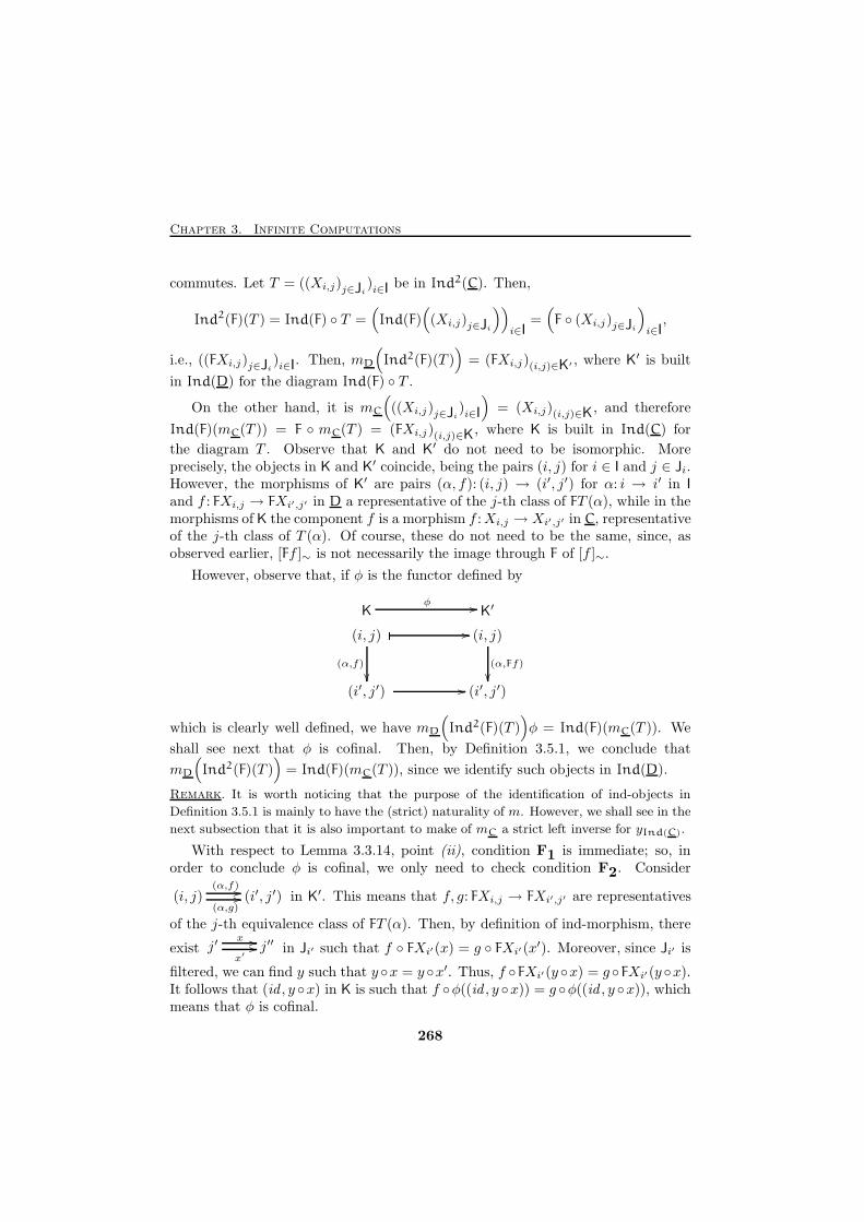
Chapter 3. Infinite Computations
commutes. Let T = ((Xi,j)j∈Ji)i∈I be in Ind2(C). Then,
Ind2(F)(T ) = Ind(F) ◦ T =(Ind(F)
((Xi,j)j∈Ji
))
i∈I=(F ◦ (Xi,j)j∈Ji
)
i∈I,
i.e., ((FXi,j)j∈Ji)i∈I. Then, mD
(Ind2(F)(T )
)= (FXi,j)(i,j)∈K′ , where K′ is built
in Ind(D) for the diagram Ind(F) ◦ T .
On the other hand, it is mC
(((Xi,j)j∈Ji
)i∈I
)= (Xi,j)(i,j)∈K, and therefore
Ind(F)(mC(T )) = F ◦ mC(T ) = (FXi,j)(i,j)∈K, where K is built in Ind(C) for
the diagram T . Observe that K and K′ do not need to be isomorphic. Moreprecisely, the objects in K and K′ coincide, being the pairs (i, j) for i ∈ I and j ∈ Ji.However, the morphisms of K′ are pairs (α, f): (i, j) → (i′, j′) for α: i → i′ in I
and f : FXi,j → FXi′,j′ in D a representative of the j-th class of FT (α), while in themorphisms of K the component f is a morphism f :Xi,j → Xi′,j′ in C, representativeof the j-th class of T (α). Of course, these do not need to be the same, since, asobserved earlier, [Ff ]∼ is not necessarily the image through F of [f ]∼.
However, observe that, if φ is the functor defined by
(i, j) (i, j)
(i′, j′) (i′, j′)
� //
(α,f)
��(α,Ff)
��� //
K′Kφ //
which is clearly well defined, we have mD
(Ind2(F)(T )
)φ = Ind(F)(mC(T )). We
shall see next that φ is cofinal. Then, by Definition 3.5.1, we conclude that
mD
(Ind2(F)(T )
)= Ind(F)(mC(T )), since we identify such objects in Ind(D).
Remark. It is worth noticing that the purpose of the identification of ind-objects in
Definition 3.5.1 is mainly to have the (strict) naturality of m. However, we shall see in the
next subsection that it is also important to make of mC a strict left inverse for yInd(C).
With respect to Lemma 3.3.14, point (ii), condition F1 is immediate; so, inorder to conclude φ is cofinal, we only need to check condition F2. Consider
(i, j) (i′, j′)(α,f) //(α,g)
// in K′. This means that f, g: FXi,j → FXi′,j′ are representatives
of the j-th equivalence class of FT (α). Then, by definition of ind-morphism, there
exist j′ j′′x //x′
// in Ji′ such that f ◦ FXi′(x) = g ◦ FXi′ (x′). Moreover, since Ji′ is
filtered, we can find y such that y ◦x = y ◦x′. Thus, f ◦FXi′(y ◦x) = g ◦FXi′(y ◦x).It follows that (id , y ◦x) in K is such that f ◦φ((id , y ◦x)) = g ◦φ((id , y ◦x)), whichmeans that φ is cofinal.
268

3.5. A KZ-Doctrine for the Ind Completion
Consider now a morphism α =([
([αi,j ])j∈Ji
])
i∈Ifrom T to T ′ in Ind2(C).
Then,
Ind2(F)(α) =([
Ind(F)(([αi,j ])j∈Ji)])
i∈I=([
([F(αi,j)])j∈Ji
])
i∈I,
and thus mD
(Ind2(F)(α)
)= ([F(αi,j)])(i,j)∈K′ , K′, as before, being built in Ind(D)
for Ind(F) ◦ T . Following the other edge of the diagram, we have
Ind(F)(mC(α)) = Ind(F)(([αi,j ])(i,j)∈K
)= ([F(αi,j ]))(i,j)∈K,
for K in Ind(D) built for T . We shall show that these morphisms are the same.
Let K0 and K′0 be the categories built along the two different edges of thediagram for T ′ and let ∼ and ∼′ indicate, respectively, the equivalences wrt. K0 andwrt. K′0. We know that K0 and K′0 have the same elements and that there is a cofinalφ: K0 → K′0. Of course, if f ∼ g then f ∼′ g. Therefore, [F(αi,j)]∼ ⊆ [F(αi,j)]∼′ .Now, suppose that (F(αi,j):Xi,j → i0, j0) ∼′ (f :Xi,j → Xi1,j1). Then, there exist
(β0, g0): (i0, j0)→ (i2, j2) and (β1, g1): (i1, j1)→ (i2, j2)
such that g0 ◦ F(αi,j) = g1 ◦ f . Since (i0, j0) and (i2, j2) belong to K0, we findan upper bound (γ0, x0): (i0, j0) → (i3, j3) and (γ1, x1): (i2, j2) → (i3, j3) in K0.Then, consider the pair of arrows φ((γ0, x0)) = (γ0, F(x0)): (i0, j0) → (i3, j3) andφ((γ1, x1)) = (γ1, F(x1)): (i2, j2) → (i3, j3) in K′0. These arrows provide a parallelpair of arrows in K′0, namely (γ1, F(x1)) ◦ (β0, g0) and (γ0, F(x0)), and since φ iscofinal we find (δ0, y0): (i3, j3)→ (i5, j5) such that
φ((δ0, y0)) ◦ (γ0, F(x0)) = φ((δ0, y0)) ◦ (γ1, F(x1)) ◦ (β0, g0),
i.e., (δ0 ◦ γ0, F(y0 ◦ x0)) = (δ0 ◦ γ1 ◦ β0, F(y0 ◦ x1) ◦ g0).
Applying the same argument above to (i2, j2) and (i1, j1), one finds the arrows(γ2, x2): (i1, j1) → (i4, j4) and (γ1, x1): (i2, j2) → (i4, j4) in K0, and then an upperbound (δ1, y1): (i4, j4)→ (i6, j6) such that
φ((δ1, y1)) ◦ (γ2, F(x2)) = φ((δ1, y1)) ◦ (γ1, F(x1)) ◦ (β1, g1),
which is (δ1 ◦ γ2, F(y1 ◦ x2)) = (δ1 ◦ γ1 ◦ β1, F(y1 ◦ x1) ◦ g1).
Finally, since K0 is filtered, we have
(δ2, y2): (i5, j5)→ (i7, j7) and (δ3, y3): (i6, j6)→ (i7, j7)
such that (δ2, y2) ◦ (δ0, y0) ◦ (γ1, x1) = (δ3, y3) ◦ (δ1, y1) ◦ (γ1, x1), which means that(δ2 ◦ δ0 ◦ γ1, y2 ◦ y0 ◦ x1) = (δ3 ◦ δ1 ◦ γ1, y3 ◦ y1 ◦ x1). Then, we have the following
269

Chapter 3. Infinite Computations
commutative diagram in D.
(i, j)
(i0, j0) (i1, j1)
(i2, j2)
(i3, j3) (i4, j4)
(i5, j5) (i6, j6)
(i7, j7)
f
IIIIIIII $$F(αi,j)
zzuuuuuuuu(γ0,F(x0))
��
(β0,g0)IIIIIIII$$
(γ2,F(x2))
��
(β1,g1)
zzuuuuuuuu(γ1,F(x1))zzuuuuuuuu (γ1,F(x1))
IIIIIIII $$(δ0,F(y0))
��(δ1,F(y1))
��
(δ2,F(y2))
IIIIIIII$$ (δ3,F(y3))zzuuuuuuuuNow, consider (δ2◦δ0◦γ0, y2◦y0◦x0) from (i0, j0) to (i7, j7) and (δ3◦δ1◦γ2, y3◦y1◦x2)from (i1, j1) to (i7, j7) in K. We claim that these morphisms show that F(αi,j) ∼ f .In fact,
F(y2 ◦ y0 ◦ x0) ◦ F(αi,j) = F(y2) ◦ F(y0) ◦ F(x0) ◦ F(αi,j)
= F(y2) ◦ F(y0) ◦ F(x1) ◦ g0 ◦ F(αi,j)
= F(y2) ◦ F(y0) ◦ F(x1) ◦ g1 ◦ f
= F(y3) ◦ F(y1) ◦ F(x1) ◦ g1 ◦ f
= F(y3) ◦ F(y1) ◦ F(x2) ◦ f
= F(y3 ◦ y1 ◦ x2) ◦ f.
Thus, we conclude that [F(αi,j)]∼ = [F(αi,j)]∼′ . In order to complete the identifica-tion of the two morphisms above, we should that show that the ∼-classes of F(αi,j),which by definition are compatible wrt. K, i.e., for morphisms (β, g): (i, j)→ (i′, j′)in K, are compatible also wrt. K′. However, we omit this proof which can be doneexactly as the previous one thanks to the fact that also in this case there exists acofinal φ: K→ K′ which is the identity on the objects.
Remark. We would like to stress that the result above proves the naturality of the iden-tification of ind-objects imposed in Definition 3.5.1. In fact, it is important to notice thatthe proof given above does not rely on the fact that φ:K → K′ is the identity on theobjects, but just on the fact that it is an isomorphism. Thus, the proof above applies toall the ind-objects identified via the cofinal φ.
270
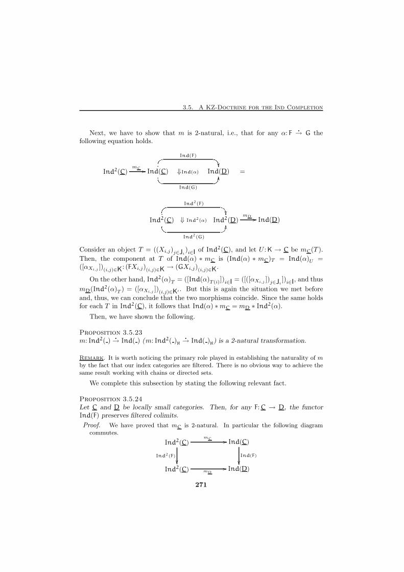
3.5. A KZ-Doctrine for the Ind Completion
Next, we have to show that m is 2-natural, i.e., that for any α: F�
→ G thefollowing equation holds.
Ind2(C) Ind(C) ⇓Ind(α) Ind(D)mC //
# "Ind(F)
�� !Ind(G)
OO =
Ind2(C) ⇓ Ind2(α) Ind2(D) Ind(D)
# "Ind2(F)
�� !Ind2(G)
OOmD //
Consider an object T = ((Xi,j)j∈Ji)i∈I of Ind2(C), and let U : K → C be mC(T ).
Then, the component at T of Ind(α) ∗ mC is (Ind(α) ∗ mC)T = Ind(α)U =([αXi,j
])(i,j)∈K: (FXi,j)(i,j)∈K → (GXi,j)(i,j)∈K.
On the other hand, Ind2(α)T = ([Ind(α)T (i)])i∈I = ([([αXi,j])j∈Ji
])i∈I, and thus
mD(Ind2(α)T ) = ([αXi,j])(i,j)∈K′ . But this is again the situation we met before
and, thus, we can conclude that the two morphisms coincide. Since the same holdsfor each T in Ind2(C), it follows that Ind(α) ∗mC = mD ∗ Ind2(α).
Then, we have shown the following.
Proposition 3.5.23m: Ind2( )
�
→ Ind( ) (m: Ind2( )ℵ�
→ Ind( )ℵ) is a 2-natural transformation.
Remark. It is worth noticing the primary role played in establishing the naturality of mby the fact that our index categories are filtered. There is no obvious way to achieve thesame result working with chains or directed sets.
We complete this subsection by stating the following relevant fact.
Proposition 3.5.24Let C and D be locally small categories. Then, for any F: C → D, the functorInd(F) preserves filtered colimits.
Proof. We have proved that mC is 2-natural. In particular the following diagramcommutes.
Ind2(C) Ind(C)
Ind2(C) Ind(D)
mC //
Ind2(F)
��Ind(F)
��mD
//
271
Chapter 3. Infinite Computations
However, since mC is an explicit choice of colimits and the colimits of a given diagram
are isomorphic, this can be read as Ind(F) ◦ lim−→C
∼= lim−→D
◦Ind2(F), i.e., Ind(F)
preserves filtered colimits. X
Of course, the same holds for Ind( )ℵ.
Some Remarks on Ind(C)
This subsection states some further results which, although not central in our in-terest, may have future applications and, therefore, be useful. We omit all theproofs.
We have noticed earlier that y does not preserve colimits. The following is ageneral statement of the properties of y with respect to preservation of limits.
Proposition 3.5.25For any C, consider the embedding y: C → Ind(C) (y: C → Ind(C)ℵ). Then, wehave the following.
i) y preserves limits.
ii) y preserves finite colimits.
iii) The following are equivalent:
(a) y preserves (ℵ-)filtered colimits;
(b) y is an equivalence of categories;
(c) C has filtered colimits and y preserves them;
(d) C has filtered colimits and for any c the functor HomC(c, ) preservesthem.
One of the most interesting issue in order theory (domain theory) is that, froma complete poset, it is often possible—by considering some special elements—toextract a poset whose completion gives back the complete poset. Examples of thissituation are the principal ideals in a lattice, the algebraic elements of a Scott’sdomain and the prime algebraic elements in Berry’s dI-domains. There is a similarissue also on the categorical ground which allows, in some cases, to get back fromInd(C) a category which is equivalent to C. The following notions are studied ingreat detail in e.g. [28, 64].
Let D be a ℵ-filtered cocomplete category. An object c ∈ D is (ℵ-)finitely pre-sentable if the functor Y′(c) = HomD(c, ): Dop → Set preserves ℵ-filtered colimits.Let DF denote the subcategory of D consisting of the finitely presentable (fp) ob-jects. A category D is (ℵ-)locally finitely presentable (lfp) if DF contains a basewhich generates D by (ℵ-)filtered colimits. In other words, D is locally finitely
272
3.5. A KZ-Doctrine for the Ind Completion
presentable if Ind(DF )�
∼= D (Ind(DF )ℵ�
∼= D). The following is stated for Ind(C),but, of course, it holds also for Ind(C)ℵ.
Proposition 3.5.26For any c ∈ C, y(c) is finitely presentable in Ind(C).
If the idempotents split in C, then Ind(C) is lfp and Ind(C)F�
∼= C, since it is thesubcategory of the essentially constants ind-objects.
The Ind KZ-Doctrine
In this subsection we sum up the results by showing that the data Ind( ) (Ind( )ℵ),y, and m determine a KZ-doctrine on CAT . We treat mainly the case of Ind( ),but everything below can be restated for Ind( )ℵ.
We have shown in the previous subsection that Ind( ) is a 2-functor and thaty and m are 2-natural transformations. We still need to give the family of 2-cellsλC. Recall that, by Proposition 3.5.22, we have a reflection mC ⊣ yInd(C). Let
ηC: id Ind2(C)�
→ yInd(C) ◦mC be the unit of this adjunction. Then, we take λC tobe ηC ∗ Ind(yC). For general reasons, we know that ηC gives the limit cocones. Letus give it explicitly.
Given T = ((Xi,j)j∈Ji)i∈I, we have mC(T ) = (Xi,j)(i,j)∈K and therefore we
have yInd(C)(mC(T )) = ((Xi,j)(i,j)∈K)1, where we use the notation (T )1 for the
singleton diagram of value T . Thus, ηT is an I-indexed family of ind-morphismsαi in Ind(C), where αi is the “inclusion” of T (i) in the colimit of T , which is theJi-indexed family of the equivalence classes (wrt. K) of the identities of Xi,j . Inother words, we have ηT = ([([idXi,j
])j∈Ji
])i∈I: ((Xi,j)j∈Ji
)i∈I → ((Xi,j)(i,j)∈K)1.
Thus, we can conclude the triangular identities, which in the particular case of areflection take the form
ηC ∗ yInd(C) = 1 and mC ∗ ηC = 1.
Let us verify the KZ-doctrine axioms in Definition 3.4.1.
T0: mC ◦ yInd(C) = id and mC ◦ Ind(yC) = id .
mC
(yInd(C)
((Xi)i∈I
))= mC
(((Xi)i∈I)1
)= (Xi)(∗,i)∈K. Once again, K deter-
mined from 1 and I is not isomorphic to I. In fact, its objects are pairs (∗, i) and its
morphisms are pairs (∗, i)(id ,f)−→ (∗, i′), where f is a representative of the i-th class
wrt. I of the identity on (Xi)i∈I. Thus, although every f : i → i′ in I correspondsto (id , f) in K, the converse is not true. However, the embedding φ: I → K, whichsends i to (∗, i) and f to (id , f), is easily shown to be cofinal. Thus, the last formula
273
Chapter 3. Infinite Computations
is equal to (Xi)i∈I. The same formal steps prove that mC ◦ yInd(C) is the identityalso on the morphisms.
mC
(Ind(yC)((Xi)i∈I)
)= mC
(((Xi)1)
i∈I
)= (Xi)(i,∗)∈K. This time the objects of
K are pairs (i, ∗) for i ∈ I and the morphisms are pairs (α, k) where α: i→ i′ is in I
and k is a representative of the unique equivalence class wrt. 1 of X(α). However,because of the particular form of 1 there is a unique representative in that class.Therefore, in this case, K is isomorphic to I. Thus, the last formula is equal to(Xi)i∈I. The same argument can be used for the morphisms of Ind(C) to showmC ◦ Ind(yC) = id , as required.
Observe now that Ind(yC): Ind(C)→ Ind2(C), and thus
λC = ηC ∗ Ind(yC): Ind(yC)�
→ yInd2(C) ◦mC ◦ Ind(yInd(C)) = yInd2(C),
as required.
Let us proceed to show that the remaining KZ-doctrine axioms hold in ourcontext.
T1: λC ∗ yC = 1.
The left hand side of the equation actually is ηC ∗ Ind(yC)∗yC, which by naturalityof y is ηC ∗ yInd(C) ∗ yC. But the last two elements of this composition are one ofthe triangular identities for the adjunction, and therefore the formula above is anidentity 2-cell.
T2: mC ∗ λC = 1.
The left hand side of the equation is mC ∗ ηC ∗ Ind(yC), and using the othertriangular identity we again can show that it equals 1.
T3: mC ∗ Ind(mC) ∗ λInd2(C) = 1.
Consider T = ((Xi,j)j∈Ji)∈I. We have Ind(yInd(C))(T ) = (((Xi,j)j∈Ji
)1)i∈I. Thus,
the unit ηInd(C) at this object is the I-indexed family α of equivalence classes [αi]whose representatives are ind-morphisms
αi: ((Xi,j)j∈Ji)1 → ((Xi,j)j∈Ji
)(i,∗)∈K0,
where K0 is built by mInd(C) for I and 1. Each αi has a unique component which,by definition, is the equivalence class (wrt. K) of the identity ind-morphism of(Xi,j)j∈Ji
. Then Ind(mC)(α) is the I-indexed family β of equivalence classes [βi]whose representatives are ind-morphisms
βi: (Xi,j)(∗,j)∈Hi→ ((Xi,j)j∈Ji
)(i,∗,j)∈Li,
where Hi is built by mC for 1, and Ji and Li corresponds to K0 and Ji. Observe thateach component of βi is the equivalence class (wrt. Li) of the identity of Xi,j in C.
274
3.5. A KZ-Doctrine for the Ind Completion
Finally, we must compute mC(β). We have the index categories K built from I andthe Hi’s and K′ built from 1 and the Li’s. Thus, mC(β) is a (i, ∗, j) ∈ K-indexedfamily γ whose components are equivalence classes (wrt. K′) of the identity arrowof Xi,j . Now let K′′ be the index category for mC(T ). Of course, K, K′ and K′′ allhave isomorphic sets of objects and, as usual, it is not difficult to show that thereexist cofinal functors φ: K′ → K and φ′: K′′ → K. It follows that the componentat T of mC ∗ Ind(mC) ∗ ηIndC ∗ Ind(yInd2(C)) = mC ∗ Ind(mC) ∗ λInd2(C) is theidentity of mC(T ), i.e., mC ∗ Ind(mC) ∗ λInd2(C) = 1, as required.
Thus, we have proved the following.
Proposition 3.5.27(Ind( ), y,m, {λC}C∈CAT
)is a KZ-doctrine on CAT , the category of locally small
categories.
Of course, the same holds for Ind( )ℵ.
Proposition 3.5.28(Ind( )ℵ, y,m, {λC}C∈CAT
)is a KZ-doctrine on CAT , the category of locally small
categories.
Moreover, by Proposition 3.5.5, we also have the following results concerningCat, the category of the small categories.
Proposition 3.5.29(Ind( ), y,m, {λC}C∈Cat
)is a KZ-doctrine on Cat.
Proposition 3.5.30(Ind( )ℵ, y,m, {λC}C∈Cat
)is a KZ-doctrine on Cat.
We now turn our attention to the category Ind-Alg of Ind( )-algebras. By
Definition 3.4.3, an algebra is a category A together with a functor a: Ind(A) →A which is a reflection left adjoint for yA: A → Ind(A). By Proposition 3.5.12we conclude immediately that the algebras are exactly the locally small filteredcocomplete categories with a choice a of colimits. Recall that, by the generaltheory of KZ-doctrines, the same category A gives rise to different algebras onlyvia isomorphic a’s, i.e., via different choices of colimits in A.
As usual, the same holds for Ind( )ℵ, whose algebras are the locally small ℵ-filtered cocomplete categories with a choice of colimits.
Let us consider the Ind-homomorphisms. From the theory in Section 3.4 weknow that F: A → B is a morphism of the algebras (A,a) and (B,b) if and only if
275
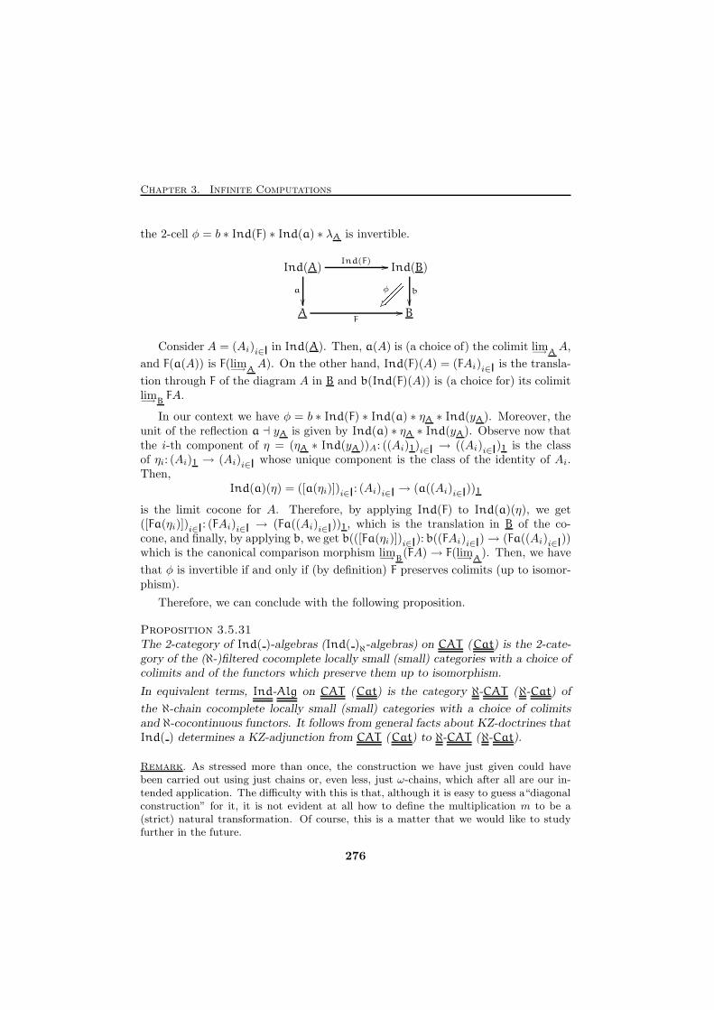
Chapter 3. Infinite Computations
the 2-cell φ = b ∗ Ind(F) ∗ Ind(a) ∗ λA is invertible.
Ind(A) Ind(B)
A B
Ind(F) //
a
��b
��
F//
φ
{� ��������Consider A = (Ai)i∈I in Ind(A). Then, a(A) is (a choice of) the colimit lim−→A
A,
and F(a(A)) is F(lim−→AA). On the other hand, Ind(F)(A) = (FAi)i∈I is the transla-
tion through F of the diagram A in B and b(Ind(F)(A)) is (a choice for) its colimitlim−→B
FA.
In our context we have φ = b ∗ Ind(F) ∗ Ind(a) ∗ ηA ∗ Ind(yA). Moreover, theunit of the reflection a ⊣ yA is given by Ind(a) ∗ ηA ∗ Ind(yA). Observe now thatthe i-th component of η = (ηA ∗ Ind(yA))A: ((Ai)1)
i∈I → ((Ai)i∈I)1 is the classof ηi: (Ai)1 → (Ai)i∈I whose unique component is the class of the identity of Ai.Then,
Ind(a)(η) = ([a(ηi)])i∈I: (Ai)i∈I → (a((Ai)i∈I))1
is the limit cocone for A. Therefore, by applying Ind(F) to Ind(a)(η), we get([Fa(ηi)])i∈I: (FAi)i∈I → (Fa((Ai)i∈I))1, which is the translation in B of the co-cone, and finally, by applying b, we get b(([Fa(ηi)])i∈I): b((FAi)i∈I)→ (Fa((Ai)i∈I))which is the canonical comparison morphism lim−→B
(FA)→ F(lim−→A). Then, we have
that φ is invertible if and only if (by definition) F preserves colimits (up to isomor-phism).
Therefore, we can conclude with the following proposition.
Proposition 3.5.31The 2-category of Ind( )-algebras (Ind( )ℵ-algebras) on CAT (Cat) is the 2-cate-gory of the (ℵ-)filtered cocomplete locally small (small) categories with a choice ofcolimits and of the functors which preserve them up to isomorphism.
In equivalent terms, Ind-Alg on CAT (Cat) is the category ℵ-CAT (ℵ-Cat) of
the ℵ-chain cocomplete locally small (small) categories with a choice of colimitsand ℵ-cocontinuous functors. It follows from general facts about KZ-doctrines thatInd( ) determines a KZ-adjunction from CAT (Cat) to ℵ-CAT (ℵ-Cat).
Remark. As stressed more than once, the construction we have just given could havebeen carried out using just chains or, even less, just ω-chains, which after all are our in-tended application. The difficulty with this is that, although it is easy to guess a“diagonalconstruction” for it, it is not evident at all how to define the multiplication m to be a(strict) natural transformation. Of course, this is a matter that we would like to studyfurther in the future.
276
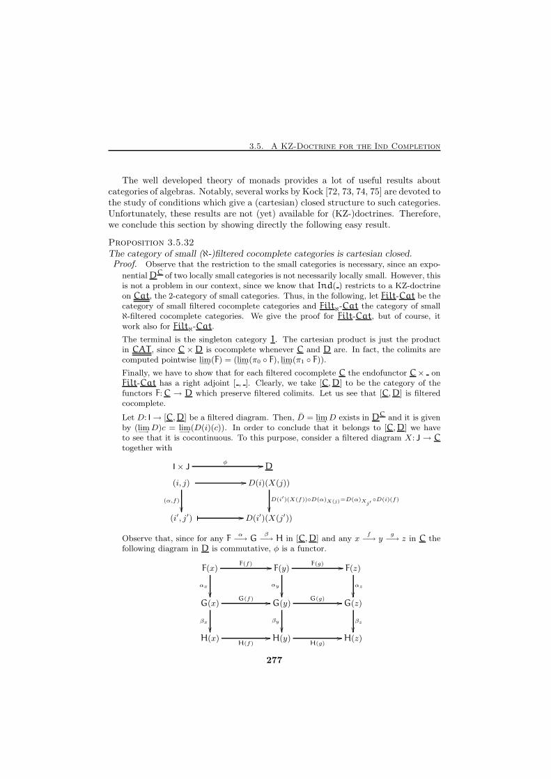
3.5. A KZ-Doctrine for the Ind Completion
The well developed theory of monads provides a lot of useful results aboutcategories of algebras. Notably, several works by Kock [72, 73, 74, 75] are devoted tothe study of conditions which give a (cartesian) closed structure to such categories.Unfortunately, these results are not (yet) available for (KZ-)doctrines. Therefore,we conclude this section by showing directly the following easy result.
Proposition 3.5.32The category of small (ℵ-)filtered cocomplete categories is cartesian closed.Proof. Observe that the restriction to the small categories is necessary, since an expo-
nential DC of two locally small categories is not necessarily locally small. However, thisis not a problem in our context, since we know that Ind( ) restricts to a KZ-doctrineon Cat, the 2-category of small categories. Thus, in the following, let Filt-Cat be thecategory of small filtered cocomplete categories and Filtℵ-Cat the category of smallℵ-filtered cocomplete categories. We give the proof for Filt-Cat, but of course, itwork also for Filtℵ-Cat.
The terminal is the singleton category 1. The cartesian product is just the productin CAT , since C ×D is cocomplete whenever C and D are. In fact, the colimits arecomputed pointwise lim
−→(F) = (lim
−→(π0 ◦ F), lim
−→(π1 ◦ F)).
Finally, we have to show that for each filtered cocomplete C the endofunctor C× onFilt-Cat has a right adjoint [ , ]. Clearly, we take [C,D] to be the category of thefunctors F: C → D which preserve filtered colimits. Let us see that [C,D] is filteredcocomplete.
Let D: I→ [C,D] be a filtered diagram. Then, D = lim−→
D exists in DC and it is givenby (lim
−→D)c = lim
−→(D(i)(c)). In order to conclude that it belongs to [C,D] we have
to see that it is cocontinuous. To this purpose, consider a filtered diagram X: J → Ctogether with
(i, j) D(i)(X(j))
(i′, j′) D(i′)(X(j′))
� //
(α,f)
��D(i′)(X(f))◦D(α)X(j)=D(α)X
j′◦D(i)(f)
��� //
DI× Jφ //
Observe that, since for any Fα−→ G
β−→ H in [C,D] and any x
f−→ y
g−→ z in C the
following diagram in D is commutative, φ is a functor.
F(x) F(y) F(z)
G(x) G(y) G(z)
H(x) H(y) H(z)
F(f) //
αx
��
F(g) //
αy
��αz
��G(f) //
βx
��
G(g) //
βy
��βz
��
H(f)//
H(g)//
277
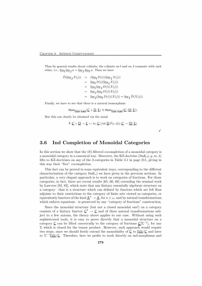
Chapter 3. Infinite Computations
Thus by general results about colimits, the colimits on I and on J commute with eachother, i.e., lim
−→ I lim−→J φ = lim−→J lim
−→ I φ. Then we have
D(lim−→JX(j)) = (lim
−→ ID(i))(lim−→JX(j))
= lim−→ ID(i)(lim
−→JX(j))
= lim−→ I lim−→JD(i)(X(j))
= lim−→J lim
−→ ID(i)(X(j))
= lim−→J(lim
−→ ID(i))(X(j)) = lim−→J D(X(j)).
Finally, we have to see that there is a natural isomorphism
HomFilt-Cat(C×D,E) ∼= HomFilt-Cat(C, [D,E]).
But this can clearly be obtained via the usual
F: C×D→ E ; λc:C.(λd:D.F(c, d)):C→ [D,E].
X
3.6 Ind Completion of Monoidal Categories
In this section we show that the (ℵ)-filtered cocompletion of a monoidal category isa monoidal category in a canonical way. Moreover, the KZ-doctrine (Ind( ), y,m, λ)lifts to KZ-doctrines on any of the 2-categories in Table 3.1 in page 211, giving inthis way their “free” cocompletion.
This fact can be proved in some equivalent ways, corresponding to the differentcharacterization of the category Ind( ) we have given in the previous sections. Inparticular, a very elegant approach is to work on categories of fractions. For thosecategories, in fact, there are recent results [65, 66, 68] extending the seminal workby Lawvere [82, 83], which state that any finitary essentially algebraic structure ona category—that is a structure which can defined by functors which are left Kanadjoints to their restrictions to the category of finite sets viewed as categories, orequivalently functors of the kind An → A, for n ∈ ω, and by natural transformationswhich enforce equations—is preserved by any “category of fractions” construction.
Since the monoidal structure (but not a closed monoidal one!) on a categoryconsists of a finitary functor C2 → C and of three natural transformations sub-ject to a few axioms, the theory above applies to our case. Without using suchsophisticated tools, it is easy to prove directly that a monoidal structure on acategory C can be lifted canonically to the category of fractions C[Σ−1], for anyΣ which is closed for the tensor product. However, such approach would requiretwo steps, since we should firstly extend the monoidality of C to Filt/C and laterto Σ−1Filt/C. Therefore, here we prefer to work directly on ind-morphisms and
278
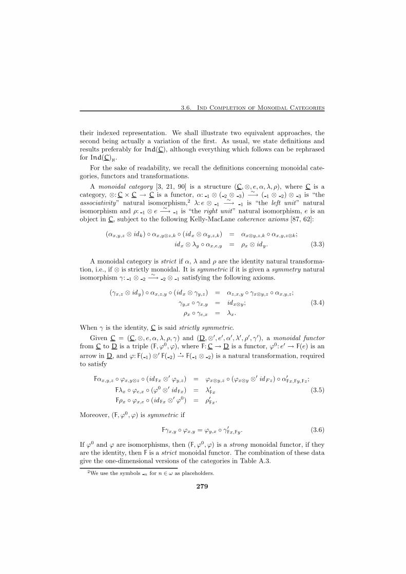
3.6. Ind Completion of Monoidal Categories
their indexed representation. We shall illustrate two equivalent approaches, thesecond being actually a variation of the first. As usual, we state definitions andresults preferably for Ind(C), although everything which follows can be rephrasedfor Ind(C)ℵ.
For the sake of readability, we recall the definitions concerning monoidal cate-gories, functors and transformations.
A monoidal category [3, 21, 90] is a structure (C,⊗, e, α, λ, ρ), where C is acategory, ⊗: C × C → C is a functor, α: 1 ⊗ ( 2 ⊗ 3)
∼−→ ( 1 ⊗ 2) ⊗ 3 is “the
associativity” natural isomorphism,2 λ: e ⊗ 1∼−→ 1 is “the left unit” natural
isomorphism and ρ: 1 ⊗ e∼−→ 1 is “the right unit” natural isomorphism, e is an
object in C, subject to the following Kelly-MacLane coherence axioms [87, 62]:
(αx,y,z ⊗ idk) ◦ αx,y⊗z,k ◦ (idx ⊗ αy,z,k) = αx⊗y,z,k ◦ αx,y,z⊗k;
idx ⊗ λy ◦ αx,e,y = ρx ⊗ idy. (3.3)
A monoidal category is strict if α, λ and ρ are the identity natural transforma-tion, i.e., if ⊗ is strictly monoidal. It is symmetric if it is given a symmetry naturalisomorphism γ: 1 ⊗ 2
∼−→ 2 ⊗ 1 satisfying the following axioms.
(γx,z ⊗ idy) ◦ αx,z,y ◦ (idx ⊗ γy,z) = αz,x,y ◦ γx⊗y,z ◦ αx,y,z;
γy,x ◦ γx,y = idx⊗y; (3.4)
ρx ◦ γe,x = λx.
When γ is the identity, C is said strictly symmetric.
Given C = (C,⊗, e, α, λ, ρ, γ) and (D,⊗′, e′, α′, λ′, ρ′, γ′), a monoidal functorfrom C to D is a triple (F, ϕ0, ϕ), where F: C→ D is a functor, ϕ0: e′ → F(e) is an
arrow in D, and ϕ: F( 1)⊗′ F( 2)�
→ F( 1 ⊗ 2) is a natural transformation, requiredto satisfy
Fαx,y,z ◦ ϕx,y⊗z ◦ (idFx ⊗′ ϕy,z) = ϕx⊗y,z ◦ (ϕx⊗y ⊗
′ idFz) ◦ α′Fx,Fy,Fz;
Fλx ◦ ϕe,x ◦ (ϕ0 ⊗′ idFx) = λ′Fx (3.5)
Fρx ◦ ϕx,e ◦ (idFx ⊗′ ϕ0) = ρ′Fx.
Moreover, (F, ϕ0, ϕ) is symmetric if
Fγx,y ◦ ϕx,y = ϕy,x ◦ γ′Fx,Fy. (3.6)
If ϕ0 and ϕ are isomorphisms, then (F, ϕ0, ϕ) is a strong monoidal functor, if theyare the identity, then F is a strict monoidal functor. The combination of these datagive the one-dimensional versions of the categories in Table A.3.
2We use the symbols n for n ∈ ω as placeholders.
279
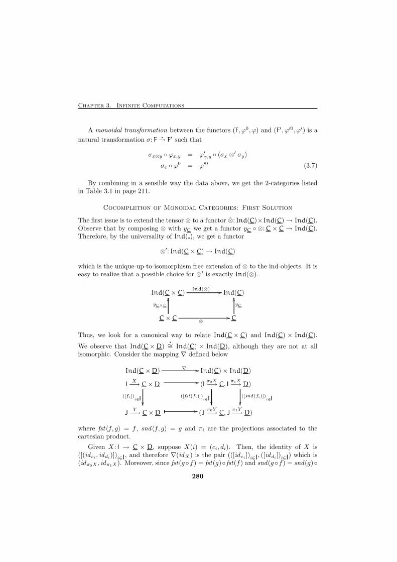
Chapter 3. Infinite Computations
A monoidal transformation between the functors (F, ϕ0, ϕ) and (F′, ϕ′0, ϕ′) is a
natural transformation σ: F�
→ F′ such that
σx⊗y ◦ ϕx,y = ϕ′x,y ◦ (σx ⊗′ σy)
σe ◦ ϕ0 = ϕ′0 (3.7)
By combining in a sensible way the data above, we get the 2-categories listedin Table 3.1 in page 211.
Cocompletion of Monoidal Categories: First Solution
The first issue is to extend the tensor ⊗ to a functor ⊗: Ind(C)×Ind(C)→ Ind(C).Observe that by composing ⊗ with yC we get a functor yC ◦ ⊗: C × C → Ind(C).Therefore, by the universality of Ind( ), we get a functor
⊗′: Ind(C× C)→ Ind(C)
which is the unique-up-to-isomorphism free extension of ⊗ to the ind-objects. It iseasy to realize that a possible choice for ⊗′ is exactly Ind(⊗).
Ind(C× C) Ind(C)
C× C C
Ind(⊗) //
yC×C
OO
⊗//
yC
OO
Thus, we look for a canonical way to relate Ind(C× C) and Ind(C) × Ind(C).
We observe that Ind(C×D)�
∼= Ind(C) × Ind(D), although they are not at allisomorphic. Consider the mapping ∇ defined below
IX−→ C×D (I
π0X−→ C, Iπ1X−→ D)
JY−→ C×D (J
π0Y−→ C, Jπ1Y−→ D)
([fi])i∈I
��
� //
([fst(fi)])i∈I
��([snd(fi)])
i∈I��� //
Ind(C)× Ind(D)Ind(C×D) ∇ //
where fst〈f, g〉 = f , snd〈f, g〉 = g and πi are the projections associated to thecartesian product.
Given X : I → C × D, suppose X(i) = (ci, di). Then, the identity of X is([(id ci
, iddi)])i∈I, and therefore ∇(idX) is the pair (([id ci
])i∈I, ([iddi
])i∈I) which is
(idπ0X , idπ1X). Moreover, since fst(g◦f) = fst(g)◦ fst(f) and snd(g◦f) = snd(g)◦
280
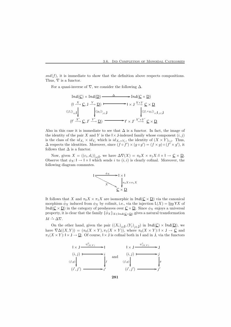
3.6. Ind Completion of Monoidal Categories
snd(f), it is immediate to show that the definition above respects compositions.Thus, ∇ is a functor.
For a quasi-inverse of ∇, we consider the following ∆.
(IX−→ C, J
Y−→ D) I× J
X×Y−→ C×D
(I′X′
−→ C, J′Y ′
−→ D) I′ × J′X′×Y ′
−→ C×D
� //
([fi])i∈I
��([gj ])
j∈J��
([fi×gj ])i∈I,j∈J
��� //
Ind(C×D)Ind(C)× Ind(D) ∆ //
Also in this case it is immediate to see that ∆ is a functor. In fact, the image ofthe identity of the pair X and Y is the I× J-indexed family whose component (i, j)is the class of the idXi
× idYjwhich is idXi×Yj
, the identity of (X × Y )i,j . Thus,∆ respects the identities. Moreover, since (f ◦ f ′)× (g ◦ g′) = (f × g) ◦ (f ′ × g′), itfollows that ∆ is a functor.
Now, given X = ((ci, di))i∈I, we have ∆∇(X) = π0X × π1X : I × I → C × D.Observe that φX : I → I × I which sends i to (i, i) is clearly cofinal. Moreover, thefollowing diagram commutes.
I I× I
C×D
φX //
X
OOOOOOOOOOOO'' π0X×π1X
��
It follows that X and π0X × π1X are isomorphic in Ind(C×D) via the canonicalmorphism φX induced from φX by colimit, i.e., via the injection L(X) = lim−→ YX ofInd(C×D) in the category of presheaves over C×D. Since φX enjoys a universalproperty, it is clear that the family {φX}X∈Ind(C×D) gives a natural transformation
Id�
→ ∆∇.
On the other hand, given the pair ((Xi)i∈I, (Yj)j∈J) in Ind(C) × Ind(D), we
have ∇∆((X,Y )) = (π0(X × Y ), π1(X × Y )), where π0(X × Y ): I × J → C andπ1(X ×Y ): I× J→ D. Of course, I× J is cofinal both in I and in J, via the functors
(i, j) i
(i′, j′) i′
� //
(f,g)
��f
��� //
II× Jψ0
(X,Y ) //
and(i, j) j
(i′, j′) j′
� //
(f,g)
��g
��� //
JI× Jψ1
(X,Y ) //
281
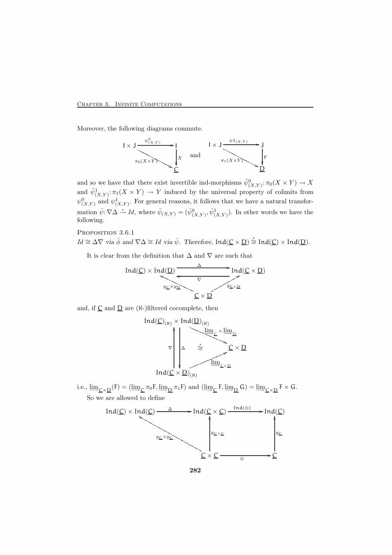
Chapter 3. Infinite Computations
Moreover, the following diagrams commute.
I× J I
C
ψ0(X,Y ) //
π0(X×Y )
NNNNNNNNNNN '' X
��and
I× J J
D
ψ1(X,Y ) //
π1(X×Y )
NNNNNNNNNNN'' Y
��
and so we have that there exist invertible ind-morphisms ψ0(X,Y ):π0(X × Y ) → X
and ψ1(X,Y ):π1(X × Y ) → Y induced by the universal property of colimits from
ψ0(X,Y ) and ψ1
(X,Y ). For general reasons, it follows that we have a natural transfor-
mation ψ:∇∆�
→ Id , where ψ(X,Y ) = (ψ0(X,Y ), ψ
1(X,Y )). In other words we have the
following.
Proposition 3.6.1
Id ∼= ∆∇ via φ and ∇∆ ∼= Id via ψ. Therefore, Ind(C×D)�
∼= Ind(C)× Ind(D).
It is clear from the definition that ∆ and ∇ are such that
Ind(C)× Ind(D) Ind(C×D)
C×D
∆ //
∇oo
yC×yD
ggPPPPPPPPPPP yC×Dqqqqqqqqq 88and, if C and D are (ℵ-)filtered cocomplete, then
Ind(C)(ℵ) × Ind(D)(ℵ)
C×D
Ind(C×D)(ℵ)
lim−→C× lim−→D
QQQQQQQQQQQQ((∆
��
∇
OO
lim−→C×Dmmmmmmmmmmmm66�
∼=
i.e., lim−→C×D(F) = (lim−→C
π0F, lim−→Dπ1F) and (lim−→C
F, lim−→DG) = lim−→C×D
F×G.
So we are allowed to define
Ind(C)× Ind(C) Ind(C× C) Ind(C)
C× C C
∆ // Ind(⊗) //
yC×yC
ffMMMMMMMMMMMMMMMMMMMM yC×C
OO
⊗//
yC
OO
282
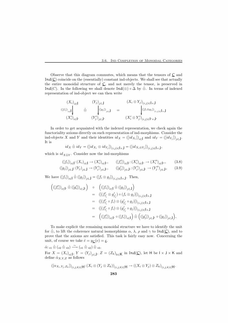
3.6. Ind Completion of Monoidal Categories
Observe that this diagram commutes, which means that the tensors of C andInd(C) coincide on the (essentially) constant ind-objects. We shall see that actuallythe entire monoidal structure of C, and not merely the tensor, is preserved inInd(C). In the following we shall denote Ind(⊗) ◦ ∆ by ⊗. In terms of indexedrepresentation of ind-object we can then write
(Xi)i∈I
(X ′i)i∈I′
([fi])i∈I
��⊗
(Yj)j∈J
(Y ′j )j∈J′
([gj ])j∈J
��=
(Xi ⊗ Yj)(i,j)∈I×J
(X ′i ⊗ Y′j )(i,j)∈I′×J′
([fi⊗gj ])(i,j)∈I×J
��
In order to get acquainted with the indexed representation, we check again thefunctoriality axioms directly on such representation of ind-morphisms. Consider theind-objects X and Y and their identities idX = ([idXi
])i∈I and idY = ([idYj
])j∈J.
It isidX ⊗ idY = ([idXi
⊗ idYj])(i,j)∈I×J = ([idXi⊗Yj
])(i,j)∈I×J,
which is idX⊗Y . Consider now the ind-morphisms
([fi])i∈I: (Xi)i∈I → (X ′i)i∈I′ , ([f ′i ])i∈I′ : (X′i)i∈I′ → (X ′′i )
i∈I′′ , (3.8)
([gj ])j∈J: (Yj)j∈J → (Y ′j )j∈J′ , ([g′j ])j∈J′ : (Y′j )j∈J′ → (Y ′′j )
j∈J′′ (3.9)
We have ([fi])i∈I ⊗ ([gj ])j∈J = ([fi ⊗ gj])(i,j)∈I×J. Then,
(([f ′i ])i∈I′ ⊗ ([g′i])i∈J′
)◦
(([fi])i∈I ⊗ ([gj ])j∈J
)
= ([(f ′i′i⊗ g′j′
j) ◦ (fi ⊗ gj)])(i,j)∈I×J
= ([(f ′i′i◦ fi)⊗ (g′j′
j◦ gj)])(i,j)∈I×J
= ([(f ′i′i◦ fi)⊗ (g′j′
j◦ gj)])(i,j)∈I×J
=(([f ′i ])i∈I′ ◦ ([fi])i∈I
)⊗(([g′j ])j∈J′ ◦ ([gj ])j∈J
),
To make explicit the remaining monoidal structure we have to identify the unitfor ⊗, to lift the coherence natural isomorphisms α, λ, ρ and γ to Ind(C), and toprove that the axioms are satisfied. This task is fairly easy now. Concerning theunit, of course we take e = yC(e) = e.
α: 1 ⊗ ( 2 ⊗ 3)∼−→ ( 1 ⊗ 2) ⊗ 3.
For X = (Xi)i∈I, Y = (Yj)j∈J, Z = (Zk)k∈K in Ind(C), let H be I × J × K anddefine αX,Y,Z as follows
([αXi,Yj ,Zk])(i,j,k)∈H: (Xi ⊗ (Yj ⊗ Zk))(i,j,k)∈H → ((Xi ⊗ Yj)⊗ Zk)(i,j,k)∈H.
283
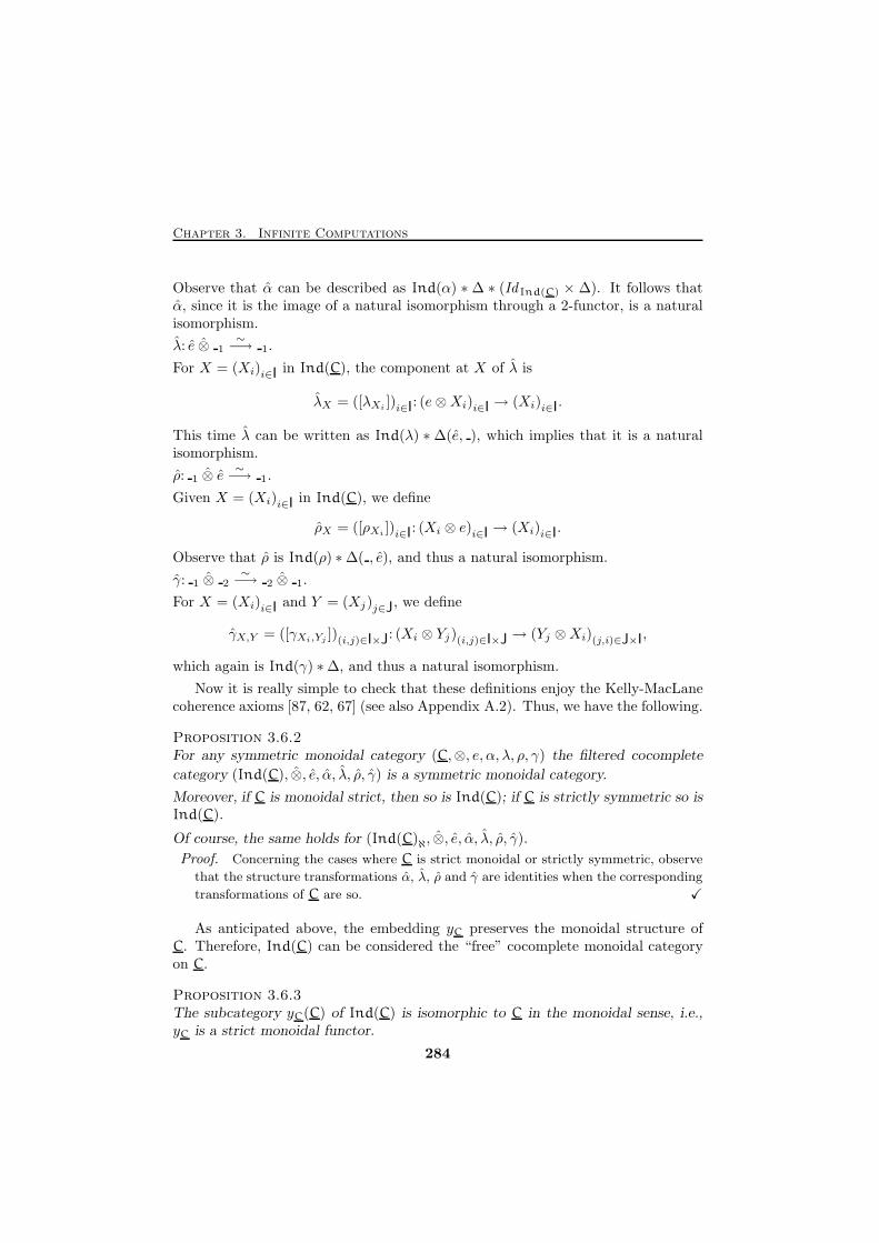
Chapter 3. Infinite Computations
Observe that α can be described as Ind(α) ∗ ∆ ∗ (IdInd(C) × ∆). It follows thatα, since it is the image of a natural isomorphism through a 2-functor, is a naturalisomorphism.
λ: e ⊗ 1∼−→ 1.
For X = (Xi)i∈I in Ind(C), the component at X of λ is
λX = ([λXi])i∈I: (e⊗Xi)i∈I → (Xi)i∈I.
This time λ can be written as Ind(λ) ∗∆(e, ), which implies that it is a naturalisomorphism.
ρ: 1 ⊗ e∼−→ 1.
Given X = (Xi)i∈I in Ind(C), we define
ρX = ([ρXi])i∈I: (Xi ⊗ e)i∈I → (Xi)i∈I.
Observe that ρ is Ind(ρ) ∗∆( , e), and thus a natural isomorphism.
γ: 1 ⊗ 2∼−→ 2 ⊗ 1.
For X = (Xi)i∈I and Y = (Xj)j∈J, we define
γX,Y = ([γXi,Yj])(i,j)∈I×J: (Xi ⊗ Yj)(i,j)∈I×J → (Yj ⊗Xi)(j,i)∈J×I,
which again is Ind(γ) ∗∆, and thus a natural isomorphism.
Now it is really simple to check that these definitions enjoy the Kelly-MacLanecoherence axioms [87, 62, 67] (see also Appendix A.2). Thus, we have the following.
Proposition 3.6.2For any symmetric monoidal category (C,⊗, e, α, λ, ρ, γ) the filtered cocomplete
category (Ind(C), ⊗, e, α, λ, ρ, γ) is a symmetric monoidal category.
Moreover, if C is monoidal strict, then so is Ind(C); if C is strictly symmetric so isInd(C).
Of course, the same holds for (Ind(C)ℵ, ⊗, e, α, λ, ρ, γ).
Proof. Concerning the cases where C is strict monoidal or strictly symmetric, observe
that the structure transformations α, λ, ρ and γ are identities when the corresponding
transformations of C are so. X
As anticipated above, the embedding yC preserves the monoidal structure ofC. Therefore, Ind(C) can be considered the “free” cocomplete monoidal categoryon C.
Proposition 3.6.3The subcategory yC(C) of Ind(C) is isomorphic to C in the monoidal sense, i.e.,yC is a strict monoidal functor.
284
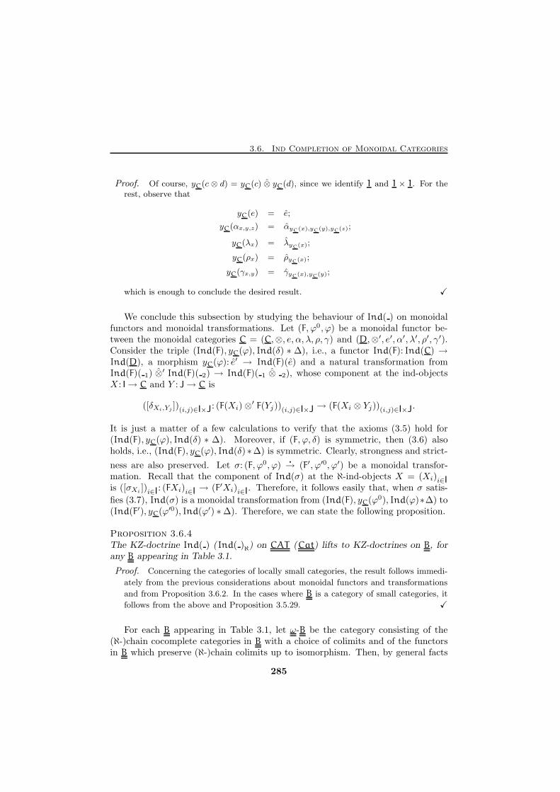
3.6. Ind Completion of Monoidal Categories
Proof. Of course, yC(c ⊗ d) = yC(c) ⊗ yC(d), since we identify 1 and 1 × 1. For therest, observe that
yC(e) = e;
yC(αx,y,z) = αyC(x),yC(y),yC(z);
yC(λx) = λyC(x);
yC(ρx) = ρyC(x);
yC(γx,y) = γyC(x),yC(y);
which is enough to conclude the desired result. X
We conclude this subsection by studying the behaviour of Ind( ) on monoidalfunctors and monoidal transformations. Let (F, ϕ0, ϕ) be a monoidal functor be-tween the monoidal categories C = (C,⊗, e, α, λ, ρ, γ) and (D,⊗′, e′, α′, λ′, ρ′, γ′).Consider the triple (Ind(F), yC(ϕ), Ind(δ) ∗ ∆), i.e., a functor Ind(F): Ind(C) →Ind(D), a morphism yC(ϕ): e′ → Ind(F)(e) and a natural transformation fromInd(F)( 1) ⊗′ Ind(F)( 2) → Ind(F)( 1 ⊗ 2), whose component at the ind-objectsX : I→ C and Y : J→ C is
([δXi,Yj])(i,j)∈I×J: (F(Xi)⊗
′ F(Yj))(i,j)∈I×J → (F(Xi ⊗ Yj))(i,j)∈I×J.
It is just a matter of a few calculations to verify that the axioms (3.5) hold for(Ind(F), yC(ϕ), Ind(δ) ∗ ∆). Moreover, if (F, ϕ, δ) is symmetric, then (3.6) alsoholds, i.e., (Ind(F), yC(ϕ), Ind(δ) ∗∆) is symmetric. Clearly, strongness and strict-
ness are also preserved. Let σ: (F, ϕ0, ϕ)�
→ (F′, ϕ′0, ϕ′) be a monoidal transfor-mation. Recall that the component of Ind(σ) at the ℵ-ind-objects X = (Xi)i∈Iis ([σXi
])i∈I: (FXi)i∈I → (F′Xi)i∈I. Therefore, it follows easily that, when σ satis-
fies (3.7), Ind(σ) is a monoidal transformation from (Ind(F), yC(ϕ0), Ind(ϕ)∗∆) to(Ind(F′), yC(ϕ′0), Ind(ϕ′) ∗∆). Therefore, we can state the following proposition.
Proposition 3.6.4The KZ-doctrine Ind( ) (Ind( )ℵ) on CAT (Cat) lifts to KZ-doctrines on B, forany B appearing in Table 3.1.
Proof. Concerning the categories of locally small categories, the result follows immedi-
ately from the previous considerations about monoidal functors and transformations
and from Proposition 3.6.2. In the cases where B is a category of small categories, it
follows from the above and Proposition 3.5.29. X
For each B appearing in Table 3.1, let ω-B be the category consisting of the(ℵ-)chain cocomplete categories in B with a choice of colimits and of the functorsin B which preserve (ℵ-)chain colimits up to isomorphism. Then, by general facts
285
Chapter 3. Infinite Computations
in the theory of KZ-doctrines, we have that any B in Table 3.1, Ind( ) (Ind( )ℵ)determines a KZ-adjunction from B to ω-B.
Cocompletion of Monoidal Categories: Second Solution
The extension of the monoidal structure of C to Ind(C) given in the previous subsec-tion may look rather far from our intended interpretation motivated in Section 3.1.For instance, the tensor of two ω-chains is (represented by) a two-dimensional struc-ture ω × ω. However, this is just a comfortable representation for the tensor. Onecould consider another representation taking for example the “diagonal” cofinalchain in ω×ω, which is isomorphic as ind-object to the “whole square”, and whichcorresponds to the motivating diagram shown in Section 3.1. In this subsection,we study an alternative description of the monoidal structure of Ind(C) which ismore intuitive and better suited for our intend applications. Since to be ℵ-filteredcocomplete is equivalent to be ℵ-chain cocomplete, we could consider the subcate-gory of Ind(C) consisting of ℵ-chains. This choice essentially does not change thecategory. However, it is not clear whether we could or not define a KZ-doctrine outof it, because of the problem with the multiplication we have already mentioned.In the following, we focus only on ω-chains.
Let Cω be the full subcategory of Ind(C) consisting of the ind-objects indexedby ω. Then we have the following.
Proposition 3.6.5
Cω�
∼= Ind(C)ω.
Proof. The inclusion functor Cω → Ind(C)ω is by definition full and faithfull. Weshow that is replete image is Ind(C). Then, by exploting the results of [26] as inProposition 3.5.3, we have the desired result.
Let X be an ω-ind-object, i.e., a countable filtered diagram in C. We have to showthat it is isomorphic in Ind(C)ω to an ω-chain. By applying the lemma (from [43])stated in Proposition 3.3.17, and thanks to Proposition 3.5.6, we may assume that Xis indexed over a countable directed set D. Then, using the lemma (from [93]) givenin Proposition 3.3.6, we find a countable sequence of finite directed subsets {Di}i∈ωsuch that, Di ⊂ Di+1, for any i ∈ ω, and D =
⋃i∈ω
Di. Then, we can extract from{Di}i∈ω a sequence of {ci}i∈ω, where ci is the greatest element of Di, which existssince Di is directed and finite. Now, define the functors φ:ω → D and Y :ω → C asfollows:
φ(i) = ci and Y (i < i+ 1) = ci < ci+1;
Y (i) = X(ci) and Y (i < i+ 1) = X(ci < ci+1).
Clearly, by Lemma 3.3.14 (iii), we have that φ is cofinal, and since Y φ = X, by
Proposition 3.5.6, we conclude that X and Y are isomorphic in Ind(C)ω. Since Y is
an ω-chain, this concludes the proof. X
286
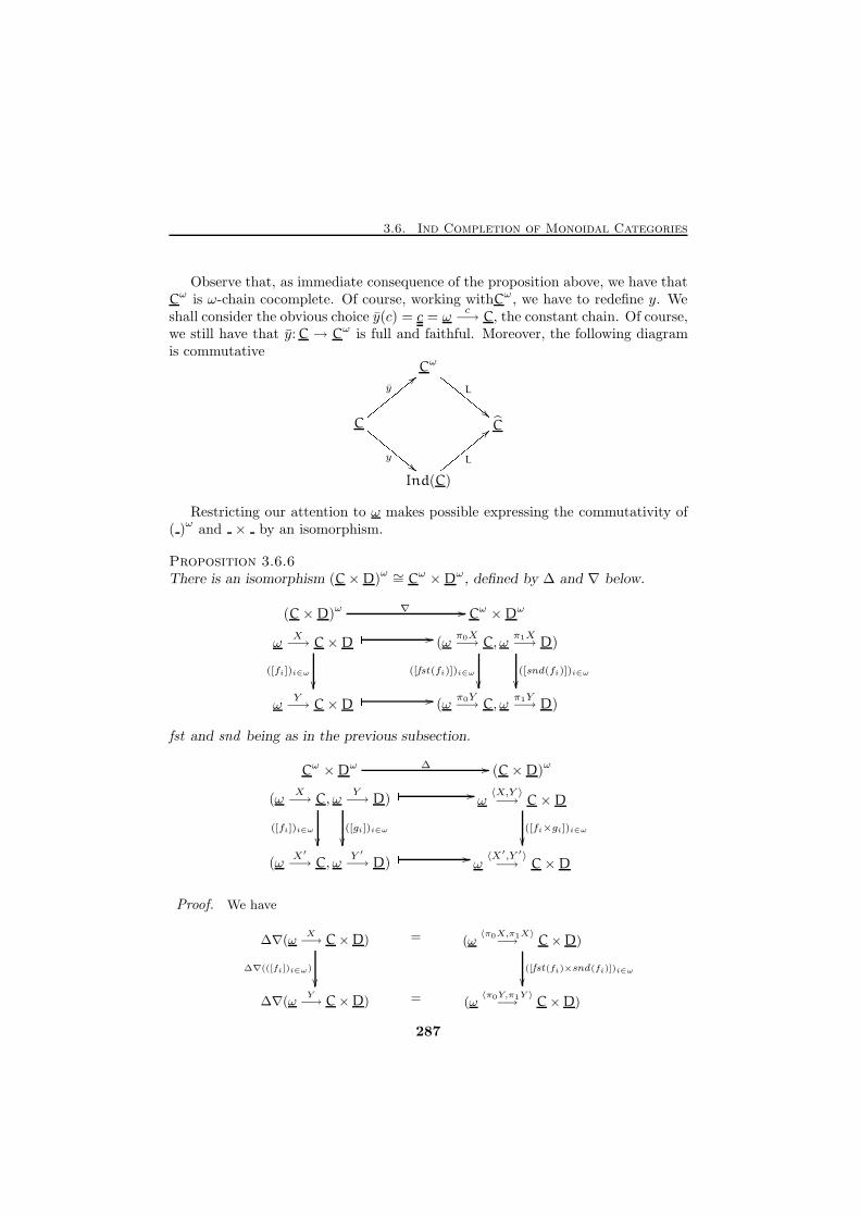
3.6. Ind Completion of Monoidal Categories
Observe that, as immediate consequence of the proposition above, we have thatCω is ω-chain cocomplete. Of course, working withCω , we have to redefine y. Weshall consider the obvious choice y(c) = c = ω
c−→ C, the constant chain. Of course,
we still have that y: C → Cω is full and faithful. Moreover, the following diagramis commutative
Cω
C C
Ind(C)
L
EEEEEEE""yyyyyyyy <<y
EEEEEEE"" Lyyyyyyy<<Restricting our attention to ω makes possible expressing the commutativity of
( )ω
and × by an isomorphism.
Proposition 3.6.6There is an isomorphism (C×D)
ω ∼= Cω ×Dω , defined by ∆ and ∇ below.
ωX−→ C×D (ω
π0X−→ C, ωπ1X−→ D)
ωY−→ C×D (ω
π0Y−→ C, ωπ1Y−→ D)
([fi])i∈ω
��
� //
([fst(fi)])i∈ω
��([snd(fi)])i∈ω
��� //
Cω ×Dω(C×D)ω ∇ //
fst and snd being as in the previous subsection.
(ωX−→ C, ω
Y−→ D) ω
〈X,Y 〉−→ C×D
(ωX′
−→ C, ωY ′
−→ D) ω〈X′,Y ′〉−→ C×D
� //
([fi])i∈ω
��([gi])i∈ω
��([fi×gi])i∈ω
��� //
(C×D)ωCω ×Dω ∆ //
Proof. We have
∆∇(ωX−→ C×D) = (ω
〈π0X,π1X〉−→ C×D)
∆∇(ωY−→ C×D) = (ω
〈π0Y,π1Y 〉−→ C×D)
∆∇(([fi])i∈ω)
��([fst(fi)×snd(fi)])i∈ω
��
287
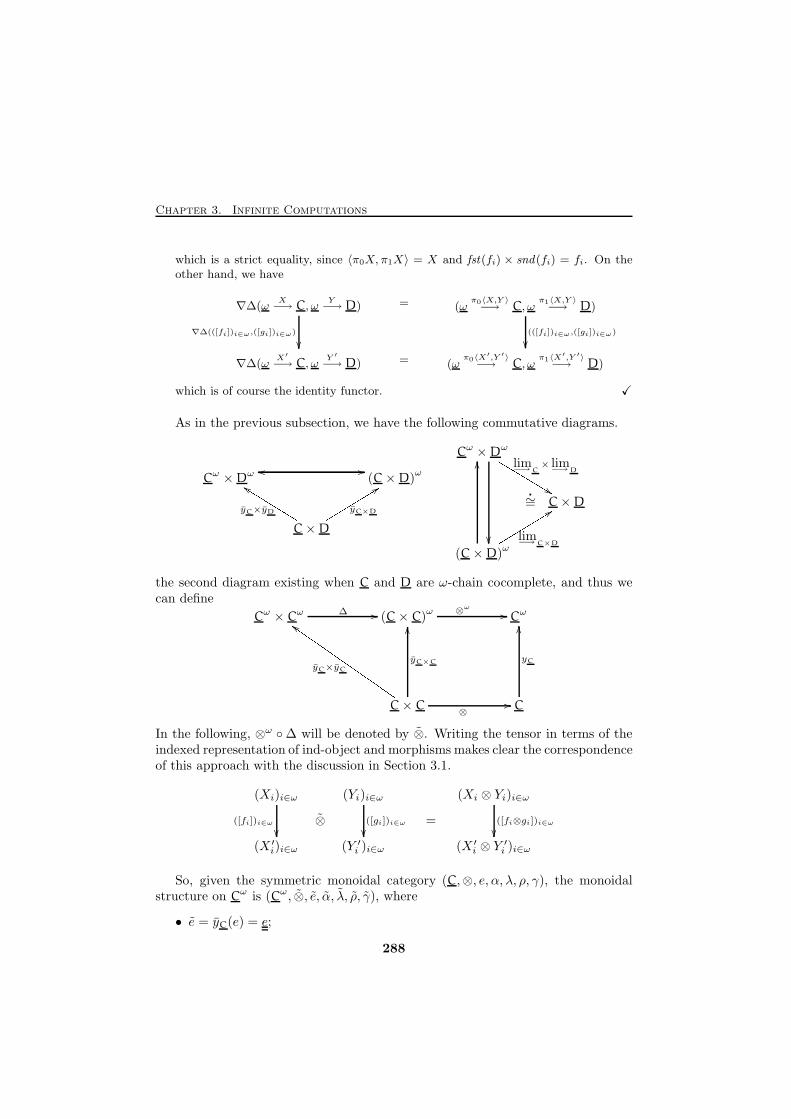
Chapter 3. Infinite Computations
which is a strict equality, since 〈π0X, π1X〉 = X and fst(fi) × snd(fi) = fi. On theother hand, we have
∇∆(ωX−→ C, ω
Y−→ D) = (ω
π0〈X,Y 〉−→ C, ω
π1〈X,Y 〉−→ D)
∇∆(ωX′
−→ C, ωY ′
−→ D) = (ωπ0〈X
′,Y ′〉−→ C, ω
π1〈X′,Y ′〉−→ D)
∇∆(([fi])i∈ω,([gi])i∈ω)
��(([fi])i∈ω,([gi])i∈ω)
��
which is of course the identity functor. X
As in the previous subsection, we have the following commutative diagrams.
Cω ×Dω (C×D)ω
C×D
//oo
yC×yD
eeKKKKKKKK yC×Drrrrrrrr99 Cω ×Dω
C×D
(C×D)ω
lim−→C× lim−→D
LLLLLLLLL%%��
OO
lim−→C×Drrrrrrrr 99�
∼=
the second diagram existing when C and D are ω-chain cocomplete, and thus wecan define
Cω × Cω (C× C)ω
Cω
C× C C
∆ // ⊗ω
//
yC×yC
ddIIIIIIIIIIIIIIII yC×C
OO
⊗//
yC
OO
In the following, ⊗ω ◦∆ will be denoted by ⊗. Writing the tensor in terms of theindexed representation of ind-object and morphisms makes clear the correspondenceof this approach with the discussion in Section 3.1.
(Xi)i∈ω
(X ′i)i∈ω
([fi])i∈ω
��⊗
(Yi)i∈ω
(Y ′i )i∈ω
([gi])i∈ω
��=
(Xi ⊗ Yi)i∈ω
(X ′i ⊗ Y′i )i∈ω
([fi⊗gi])i∈ω
��
So, given the symmetric monoidal category (C,⊗, e, α, λ, ρ, γ), the monoidalstructure on Cω is (Cω, ⊗, e, α, λ, ρ, γ), where
• e = yC(e) = e;
288
3.7. Applications to Petri Nets
• αX,Y,Z = ([αXi,Yi,Zi])i∈ω ;
• λX = ([λXi])i∈ω ;
• ρX = ([ρXi])i∈ω ;
• γX,Y = ([γXi,Yi])i∈ω.
Showing that these data form a symmetric monoidal category is a routine task.Therefore, we can summarize the results in the following propositions.
Proposition 3.6.7For any symmetric monoidal category (C,⊗, e, α, λ, ρ, γ) the ω-filtered cocompletecategory (Cω, ⊗, e, α, λ, ρ, γ) is a symmetric monoidal category.
Moreover, if C is monoidal strict, then so is Cω ; if C is strictly simmetric so is Cω.
Proposition 3.6.8The subcategory yC(C) of Cω is isomorphic to C in the monoidal sense, i.e., yC isa strict monoidal functor.
Proposition 3.6.9Cω is, up to equivalence, the free ω-chain cocomplete monoidal category on C.Proof. It follows easily from Proposition 3.6.5 and the pseudo universal property of
Ind(C)ω (see, e.g., Proposition 3.5.21). X
Of course, the results above can be restated for any chain α and the correspond-ing subcategory Cα of Ind(C).
3.7 Applications to Petri Nets
The previous sections have shown how we can build the (pseudo) free (ℵ)-filteredcocomplete category Ind(C) over a given C. In particular, in Section 3.6 we haveproved that the construction lifts to a KZ-doctrine on SsMonCat, giving in this waythe completion of symmmetric strict monoidal categories (SSMC’s). The theorieswe have formalized and the arguments we have discussed in Chapter 1 of this thesis,and in particular in Sections 1.1, 1.2, 1.3 and 1.9 support the claim that this resultbrings us close again to Petri nets. This section, which matches in style Section 3.1,explains further these facts.
It is important to observe that Petri nets are not precisely symmetric strictmonoidal categories, since they enjoy other important axioms, the principal onebeing the free monoidal structure on the objects. In order to fix the ideas, we recallthat Chapter 1 presented four relevant monoidal constructions for net computa-tions, namely
289
Chapter 3. Infinite Computations
i) T [N ], which gives a CatPetri object, i.e., a strictly symmetric strict monoidalcategory whose objects form a free commutative monoid, corresponding tothe notion of commutative processes of N (see Definition 1.1.7 and Proposi-tion 1.1.12).
ii) P [N ], which gives the symmetric strict monoidal category obtained by quo-tienting the free symmetric strict monoidal category on N via the axioms
γa,b = ida⊗b if a, b ∈ S and a 6= b,
(id ⊗ γa,a ⊗ id); t = t if t ∈ T and a ∈ S,
t; (id ⊗ γa,a ⊗ id) = t if t ∈ T and a ∈ S,
and corresponds to the concatenable processes of N . (See Definition 1.1.16,Propositions 1.1.19, and 1.2.5 and Corollary 1.2.7.) We shall refer to thecategory of small symmetric monoidal categories with the properties aboveas CatProc.
iii) DP [N ], which is as above, but satisfying only the first two axioms, and cor-responds to the decorated concatenable processes of N . (See Definition 1.9.13and Proposition 1.9.14.) Let CatDecProc denote the category of the smallcategories with the properties above.
iv) Q[N ], which gives the quotient of the free symmetric strict monoidal categoryon the graph of the “linearizations” of the transitions of N modulo the axiom
s; tu′,v′ ; s = tu,v for s:u→ u′, s′: v′ → v symmetries.
and corresponds to the strong concatenable processes of N . (See Defini-tion 1.3.8 and Proposition 1.4.5.) Proposition 1.1.19). We shall refer to thecategory of small symmetric monoidal categories with the properties aboveas CatStrProc.
Since we already know that the monoidal structure of such categories is pre-served by the ℵ-ind-completion process, the remaining question is whether theadditional structure is preserved by the (ℵ-)ind-completion or, in other words, ifInd( ) lifts to KZ-monads on CatPetri, CatProc, CatDecProc and CatStrProc.Clearly, this would be the best possible result from our point of view, since it wouldallow a full application of the theory of the cocompletion of monoidal categoriesto the case of Petri nets, thus giving a full account of infinite behaviours of nets.Unfortunately, this is not the case. More precisely, only the objects of CatPetri arerather close to keep their structure under the cocompletion construction. In fact, weknow from Proposition 3.6.2 that Ind(T [N ]) is a strictly symmetric strict monoidalcategory. However, Ind(T [N ]) does not belong to CatPetri since its monoid of ob-jects is not free. The situation is worse for the other categories. Observe, in fact,
290

3.7. Applications to Petri Nets
that when C is not strictly symmetric, then the primary requirement about themonoid of objects being commutative fails immediately. In fact, in this case, thetensor of diagrams in general will not be commutative because of the arrows.
Thus, Ind( ) does not restrict to an endofunctor on the categories we are mainlyconcerned with. A possible way out of this problem, which is currently under in-vestigation, consists of looking for an alternative presentation of the cocompletiondoctrine, i.e., for a doctrine whose functor is isomorphic to Ind( ) but better suitedfor the case of Petri nets. For the time being, however, we present some consid-erations about the relationships between Petri nets and the cocompletion of theircategories of processes which aim at showing that, at the level of a single net,Ind( ) behaves as expected, giving a faithful description of infinite processes. Inparticular, we shall present the following considerations about the relationships be-tween Petri nets and the cocompletion of their categories of processes. We shallfocus on decorated concatenable processes, although all the following, apart fromProposition 3.7.4, applies also to T [ ], P [ ] and Q[ ]. Consider again the diagram
Petri SsMonCat
MPetri∗ PreOrd
PTNets DecOcc Occ PES
DP[ ] //
〈uN↓ 〉NNNNNNNNNN&&OO
��
U [ ]//
F [ ]//
E[ ]//
LF [ ]pppppppppp88 (1.26)
of Section 1.9, where we have shown that for any net (N, uN ) in MPetri∗ we havethat the decorated concatenable processes of N leaving from u coincide with thefinite marked processes of FU [N ], i.e., with the finite configurations of EFU [N ].
As a simple application of the theory illustrated in this chapter, we shall extendthe result to infinite processes and infinite configurations, as shown by the diagrambelow.
Cat
Petri SsMonCat
MPetri∗ PreOrd
PTNets DecOcc Occ PES
〈uN↓ 〉
<<<<<<<<<<<<< ��DP[ ] //
Ind(P[N ])ωffffffffffffffffffffffffffffffff22〈uN↓ 〉
NNNNNNNNNN&&OO
��
U [ ]//
F [ ]//
E[ ]//
LF [ ]pppppppppp88 (3.10)
291
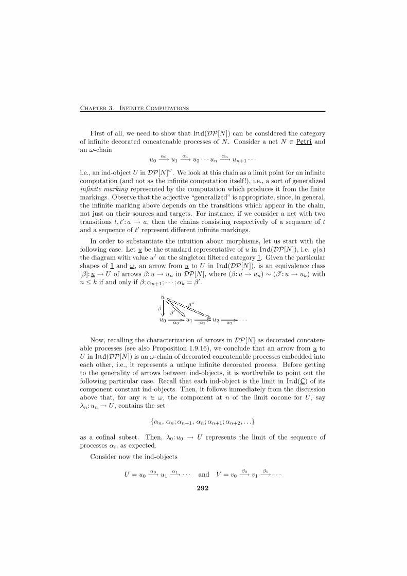
Chapter 3. Infinite Computations
First of all, we need to show that Ind(DP [N ]) can be considered the categoryof infinite decorated concatenable processes of N . Consider a net N ∈ Petri andan ω-chain
u0α0−→ u1
α1−→ u2 · · ·unαn−→ un+1 · · ·
i.e., an ind-object U in DP [N ]ω. We look at this chain as a limit point for an infinite
computation (and not as the infinite computation itself!), i.e., a sort of generalizedinfinite marking represented by the computation which produces it from the finitemarkings. Observe that the adjective “generalized” is appropriate, since, in general,the infinite marking above depends on the transitions which appear in the chain,not just on their sources and targets. For instance, if we consider a net with twotransitions t, t′: a → a, then the chains consisting respectively of a sequence of tand a sequence of t′ represent different infinite markings.
In order to substantiate the intuition about morphisms, let us start with thefollowing case. Let u be the standard representative of u in Ind(DP [N ]), i.e. y(u)the diagram with value uI on the singleton filtered category 1. Given the particularshapes of 1 and ω, an arrow from u to U in Ind(DP[N ]), is an equivalence class[β]:u → U of arrows β:u → un in DP [N ], where (β:u → un) ∼ (β′:u → uk) withn ≤ k if and only if β;αn+1; · · · ;αk = β′.
u
u0 u1 u2 · · ·
β
��
����������β′
�%
CCCCCCCCCCCC β′′
$,
QQQQQQQQQQQQQQQQQQQQQQQQQQα0
//α1
//α2
//
Now, recalling the characterization of arrows in DP [N ] as decorated concaten-able processes (see also Proposition 1.9.16), we conclude that an arrow from u toU in Ind(DP [N ]) is an ω-chain of decorated concatenable processes embedded intoeach other, i.e., it represents a unique infinite decorated process. Before gettingto the generality of arrows between ind-objects, it is worthwhile to point out thefollowing particular case. Recall that each ind-object is the limit in Ind(C) of itscomponent constant ind-objects. Then, it follows immediately from the discussionabove that, for any n ∈ ω, the component at n of the limit cocone for U , sayλn:un → U , contains the set
{αn, αn;αn+1, αn;αn+1;αn+2, . . .}
as a cofinal subset. Then, λ0:u0 → U represents the limit of the sequence ofprocesses αi, as expected.
Consider now the ind-objects
U = u0α0−→ u1
α1−→ · · · and V = v0β0−→ v1
β1−→ · · ·
292
3.7. Applications to Petri Nets
and an arrow ([σi])i∈ω :U → V . As explained above, each component [σi] repre-sents an infinite process leaving from ui, i.e., leaving from the i-th approximationof the generalized marking U . Now, the “compatibility” condition on the com-ponents of ([σi])i∈ω means that for any n ≤ k and for any σi:un → vn′ andσk:uk → vk′ , representatives of, respectively, the i-th and the k-th componentof the ind-morphism, assuming without loss of generality n′ ≤ k′, we must haveαn; · · · ;αk−1;σk = σn;βn′ ; · · · ;βk′−1. It follows that the infinite processes (corre-sponding to) [σi] form a sequence of embedded processes which leave from betterand better approximations of U . Then, this chain admits a colimit process whichis the decorated infinite process corresponding to ([σi])i∈ω . In other words, mor-phisms from generalized infinite markings are defined via continuity from “finite”approximation morphisms. The same, of course, happens for the composition ofdecorated infinite processes.
It is now easy to translate the previous informal discussion into a formal proofof the following.
Of course, the previous informal discussion could be easily translated into aformal proof of the fact that P [N ]ω captures the usual intuitive notion of infiniteprocesses, thus yielding a smooth extension of the algebraic theory of Petri netsof [97, 16] to an axiomatization in terms of monoidal categories of the infinite causalbehaviour of N . For the purpose of this section, however, we simply claim that thefollowing definitions are completely adequate.
Definition 3.7.1Ind(T [N ])ω is, up to equivalence, the (strictly symmetric strict monoidal) categoryof infinite commutative processes of N .
Ind(P [N ])ω is, up to equivalence, the (symmetric strict monoidal) category ofinfinite concatenable processes of N .
Ind(DP [N ])ω is, up to equivalence, the (symmetric strict monoidal) category ofinfinite decorated concatenable processes of N .
Ind(Q[N ])ω is, up to equivalence, the (symmetric strict monoidal) category ofinfinite strong concatenable processes of N .
Moreover, since Cω and Ind(C) are equivalent categories, we have also thefollowing proposition.
Proposition 3.7.2T [N ]
ωis the category of infinite commutative processes of N .
P [N ]ω
is the category of infinite concatenable processes of N .
DP [N ]ω is the category of infinite decorated concatenable processes of N .
Q[N ]ω is the category of infinite strong concatenable processes of N .
293
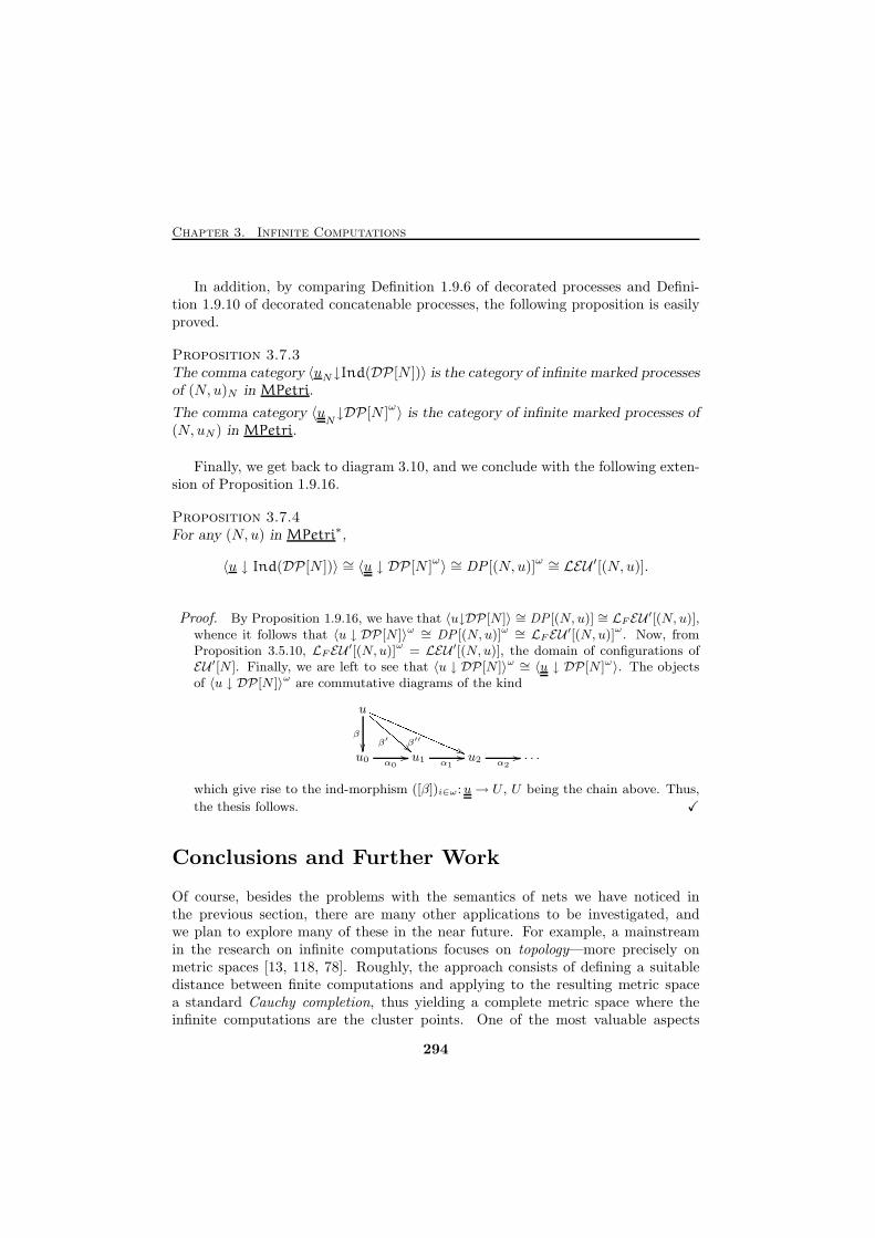
Chapter 3. Infinite Computations
In addition, by comparing Definition 1.9.6 of decorated processes and Defini-tion 1.9.10 of decorated concatenable processes, the following proposition is easilyproved.
Proposition 3.7.3The comma category 〈uN↓Ind(DP [N ])〉 is the category of infinite marked processesof (N, u)N in MPetri.
The comma category 〈uN↓DP[N ]
ω〉 is the category of infinite marked processes of(N, uN) in MPetri.
Finally, we get back to diagram 3.10, and we conclude with the following exten-sion of Proposition 1.9.16.
Proposition 3.7.4For any (N, u) in MPetri∗,
〈u ↓ Ind(DP [N ])〉 ∼= 〈u ↓ DP [N ]ω〉 ∼= DP [(N, u)]
ω ∼= LEU ′[(N, u)].
Proof. By Proposition 1.9.16, we have that 〈u↓DP [N ]〉 ∼= DP [(N, u)] ∼= LFEU′[(N, u)],
whence it follows that 〈u ↓ DP [N ]〉ω ∼= DP [(N, u)]ω ∼= LF EU′[(N, u)]
ω. Now, from
Proposition 3.5.10, LF EU′[(N,u)]
ω= LEU ′[(N,u)], the domain of configurations of
EU ′[N ]. Finally, we are left to see that 〈u ↓ DP [N ]〉ω ∼= 〈u ↓ DP [N ]ω〉. The objectsof 〈u ↓ DP [N ]〉ω are commutative diagrams of the kind
u
u0 u1 u2 · · ·
β
�� β′
CCCCCC!!β′′
QQQQQQQQQQQQQ((α0
//α1
//α2
//
which give rise to the ind-morphism ([β])i∈ω:u→ U , U being the chain above. Thus,
the thesis follows. X
Conclusions and Further Work
Of course, besides the problems with the semantics of nets we have noticed inthe previous section, there are many other applications to be investigated, andwe plan to explore many of these in the near future. For example, a mainstreamin the research on infinite computations focuses on topology—more precisely onmetric spaces [13, 118, 78]. Roughly, the approach consists of defining a suitabledistance between finite computations and applying to the resulting metric spacea standard Cauchy completion, thus yielding a complete metric space where theinfinite computations are the cluster points. One of the most valuable aspects
294
3.7. Applications to Petri Nets
of this approach is that, by choosing appropriate metrics, it is possible to factorout those infinite computations which do not enjoy certain properties, in particularfairness properties [18]. It is indeed a very interesting question whether these resultscan be recovered in the categorical framework building on the seminal paper [85].
Moreover, since by now there are several categorical approaches to the semanticsof computing systems in which objects represent states and arrows computations,this also yields a general method to construct and manipulate infinite computationsof those systems. A notable example is given by Meseguer’s concurrent rewritingsystems [96]. This issue deserves to be fully investigated in future.
295

Chapter 3. Infinite Computations
296
Bibliography
[1] M. Barr, and C. Wells.Toposes, Triples and Theories. Grundlehren der Mathematik, Springer-Verlag, 1985.
[2] M.A. Bednarczyk.Categories of Asynchronous Transition Systems. PhD Thesis, University of Sussex,1988.
[3] J. Benabou.Categories with Multiplication. Comptes Rendue Academie Science Paris, n. 256,pp. 1887–1890, 1963.
[4] J. Benabou.Des categories fibrees. Draft of Lectures. Manuscript.
[5] J. Benabou.Introduction to Bicategories. LNM n. 40, J. Tits, Ed., pp. 1–77, Springer-Verlag,1967.
[6] J. Benabou.Fibered Categories and the Foundations of Naive Category Theory. Journal ofSymbolic Logic, n. 40, pp. 10–37, Association for Symbolic Logic, 1985.
[7] P. Bernays.A system of axiomatic set theory: I–VII. Journal of Symbolic Logic, Associationfor Symbolic Logic, n. 2, pp. 65–77, 1937, n. 6, pp. 1–17, 1941, n. 7, pp. 65–89,1942, n. 7, pp. 133–145, 1942, n. 8, pp. 89–106, 1943, n. 13, pp. 65–79, 1948, n. 19,pp. 81–96, 1954.
[8] G. Berry.Stable Models of Typed λ-calculi. In Proceedings ICALP ‘78, LNCS n. 62,G. Ausiello, C. Bohm, Eds., pp. 72–89, Springer Verlag, 1978.
[9] E. Best, and R. Devillers.Sequential and Concurrent Behaviour in Petri Net Theory. Theoretical ComputerScience, n. 55, pp. 87–136, Elsevier, 1987.
297
Bibliography
[10] R. Blackwell, G.M. Kelly, and A.J.Power.Two-Dimensional Monad Theory. Journal Pure and Applied Algebra, n. 59, pp. 1–41, North-Holland, 1989.
[11] W. Burnside.Theory of Groups of Finite Order. Cambridge University Press, 1911.
[12] H. Carstensen, and R. Valk.Infinite Behaviours and Fairness in Petri Nets. In Advances in Petri Nets ‘84,LNCS n. 188, G. Rozenberg, H. Genrich, G. Roucairol, Eds., pp. 83–100, Springer-Verlag, 1985.
[13] P. Darondeau, D. Nolte, L. Priese, and S. Yoccoz.Fairness, Distances and Degrees. Theoretical Computer Science, n. 97, pp. 131–142,Elsevier, 1992.
[14] B. Day, and G.M. Kelly.Enriched Functors Categories. Reports of the Midwest Category Seminar, M. Barr,Ed., LNM n. 106, pp. 178–191, Springer-Verlag, 1969.
[15] P. Degano, R. De Nicola, and U. Montanari.A Distributed Operational Semantics for CCS based on Condition/Event Systems.Acta Informatica, n. 26, pp. 59–91, Springer International 1988.
[16] P. Degano, J. Meseguer, and U. Montanari.Axiomatizing Net Computations and Processes. In Proceedings of the 4th LICSSymposium, pp. 175–185, IEEE Computer Society Press, 1989.
[17] P. Degano, J. Meseguer, and U. Montanari.Axiomatizing the Algebra of Net Computations and Processes. Technical ReportSRI–CSL–90–12, SRI International, Computer Science Laboratory, 1990, and Tech-nical Report TR 1/91 Dipartimento Informatica, Universita di Pisa, 1991.
[18] P. Degano, and U. Montanari.Liveness Properties as Convergence in Metric Spaces. In Proceedings of STOC 84,pp. 31–38, ACM Press, 1984.
[19] P. Degano, and U. Montanari.Concurrent Histories: A Basis for Observing Distributed Systems. Journal of Com-puter and System and Sciences, n. 34, pp. 422–461, Academic Press, 1987.
[20] M. Droste.Event Structures and Domains. Theoretical Computer Science, n. 68, pp. 37–47,Elsevier, 1989.
[21] S. Eilenberg, and G.M. Kelly.Closed Categories. In Proceedings of the Conference on Categorical Algebra, LaJolla, S. Eilenberg, Ed., pp. 421–562, Springer, 1966.
298
Bibliography
[22] S. Eilenberg, and J.C. Moore.Adjoints Functors and Triples. Illinois Journal of Mathematics, n. 9, pp. 381–398,University of Illinois at Urbana, Champagne, 1965.
[23] J. Engelfriet.Branching Processes of Petri Nets. Acta Informatica, n. 28, pp. 575–591, SpringerInternational, 1991.
[24] S. Feferman.Set-Theorical Foundation of Category Theory. Reports of the Midwest CategorySeminar, LNM n. 106, M. Barr, Ed., pp. 201–247, Springer-Verlag, 1969.
[25] A. Fraenkel.Abstract Set Theory. North-Holland, Amsterdam, 1953.
[26] P. Freyd, and A. Scedrov.Categories and Allegories. North-Holland, 1990.
[27] P. Gabriel.Des categories abeliennes. Bulletin Societe Mathematique France, n. 90, pp. 323–448, 1962.
[28] P. Gabriel, and F. Ulmer.Lokal prasentierbare Kategorien, LNM n. 221, Springer-Verlag, 1971.
[29] P. Gabriel, and M. Zisman.Calculus of Fractions and Homotopy Theory. Ergebnisse der Mathematik und ihrerGrenzgebiete, Springer-Verlag, 1967.
[30] H.J. Genrich, K. Lautenbach, and P.S. Thiagarajan.Elements of General Net Theory. Net Theory and Applications, LNCS n. 84,W. Brauer, Ed., pp. 21–163, Springer Verlag, 1980.
[31] G. Gentzen.Untersuchungen uber das logische Schliessen I. Mathematische Zeitschrift, n. 39,pp. 176–210, Springer-Verlag, 1934.
[32] G. Gentzen.Untersuchungen uber das logische Schliessen II. Mathematische Zeitschrift, n. 39,pp. 405–431, Springer-Verlag, 1934.
[33] J. Gischer.The Equational Theory of Pomsets. Theoretical Computer Science, n. 61, pp. 199–224, Elsevier, 1988.
[34] K. Godel.The consistency of the axiom of choice and the generalized continuum hypothesis.Annals of Mathematics Studies, n. 3, Princeton, 1940.
299
Bibliography
[35] R. Godement.Topologie Algebrique et Theorie des Faisceaux. Harman, Paris, 1958.
[36] U. Goltz, and W. Reisig.The Non-Sequential Behaviour of Petri Nets. Information and Computation, n. 57,pp. 125–147, Academic Press, 1983.
[37] R. Gorrieri, and U. Montanari.Scone: A Simple Calculus of Nets. In Proceedings of CONCUR ‘90, LNCS n. 458,J.C.M. Baeten, J.W. Klop, Eds., pp. 2–31, Springer-Verlag, 1990.
[38] J. Grabowski.On Partial Languages. Fundamenta Informaticae, n. 4, pp. 428–498, IOS Press,1981.
[39] J.W. Gray.2-Algebraic Theories and Triples. Cahiers de Topologie et Geometrie Differentielle,n. 14, pp. 178–180, Amiens, 1973.
[40] J.W. Gray.Formal Category Theory: Adjointness for 2-Categories. LNM n. 391, Springer-Verlag, 1974.
[41] A. Grothendieck.Technique de descente et theoremes d’existence en geometrie algebrique II. Semi-naire Bourbaki 12, expose 195, Secretariat Mathematique, Paris, 1961.
[42] A. Grothendieck.Categories fibrees et descente. Seminaire de Geometrie Algebrique. Institut desHaute Etudes Scientifiques, Paris, 1961.
[43] A. Grothendieck, and J. Verdier.Theorie de Topos et Cohomologie Etale de Schemas, Expose I. Seminaire deGeometrie Algebrique 4. LNM n. 269, pp. 1–217, Springer-Verlag, 1972.
[44] J. Gunawardena.Geometric Logic, Causality and Event Structures. In Proceedings of CONCUR ‘91,LNCS n. 527, J.C.M. Baeten, J.F. Groote, Eds., pp. 266–280, Springer-Verlag, 1991.
[45] J. Gunawardena.Causal Automata. Theoretical Computer Science, n. 101, pp. 265–288, Elsevier,1992.
[46] J. Gunawardena.A Generalized Event Structure for the Muller Unfolding of a Safe Net. In Proceed-ings of CONCUR ‘93, LNCS n. 715, E. Best, Ed., pp. 278–292, Springer-Verlag,1993.
[47] M. Hennessy.Algebraic Theory of Processes. Cambridge, Massachusetts, 1988.
300
Bibliography
[48] C.A.R. Hoare.Communicating Sequential Processes. Englewood Cliffs, 1985.
[49] H.J. Hoogeboom, and G. Rozenberg.Infinitary Languages: Basic Theory and Applications to Concurrent Systems. InCurrent Trends in Concurrency, LNCS n. 224, J.W. de Bakker, W.P. de Roever,G. Rozenberg, Eds., pp. 266–342, Springer-Verlag, 1986.
[50] P.W. Hoogers, H.C.M. Kleijn, and P.S. Thiagarajan.A Trace Semantics for Petri Nets. In Proceedings of ICALP ‘92, LNCS n. 623,W. Kuich, Ed., pp. 595–604, Springer-Verlag, 1992.
[51] P.W. Hoogers, H.C.M. Kleijn, and P.S. Thiagarajan.Local Event Structures and Petri Nets. In Proceedings of CONCUR ‘93, LNCSn. 715, E. Best, Ed., pp. 462–476, Springer-Verlag, 1993.
[52] T. Iwamura.A lemma on directed sets. Zenkoku Shijo Sugaku Danwakai, n. 262, pp. 107–111,1944.
[53] B. Jacobs.Semantics of Weakening and Contraction. To appear in Annals of Pure and AppliedLogic, North-Holland, 1994.
[54] C.B. Jay.The Structure of Free Closed Categories. LFCS Report Series, ECS-LFCS-89–92,Department of Computer Science, University of Edinburgh, 1989.
[55] T. Jech.Set Theory. Academic Press, 1978.
[56] P. Johnstone.Stone Spaces. Cambridge University Press, 1982.
[57] P. Johnstone.Topos Theory. Academic Press, London, 1977.
[58] P. Johnstone, and A. Joyal.Continuous Categories and Exponentiable Toposes. Journal Pure and Applied Al-gebra, n. 25, pp. 255–296, North-Holland, 1982.
[59] D.M. Kan.Adjoint Functors. Transactions of the American Mathematical Society, n. 87,pp. 294–329, AMS, 1958.
[60] R.M. Keller.Formal Verification of Parallel Programs. Communications of the ACM, n. 19, vol. 7,pp. 371–384, ACM Press, 1976.
301
Bibliography
[61] J. Kelley.General Topology. D. Van Nostrand Company, Princeton, 1955.
[62] G.M. Kelly.On MacLane’s Conditions for Coherence of Natural Associativities, Commutativi-ties, etc. Journal of Algebra, n. 1, pp. 397–402, Academic Press, 1964.
[63] G.M. Kelly.Basic Concepts of Enriched Category Theoy. London Mathematical Society, LN Se-ries, n. 64, 1982.
[64] G.M. Kelly.Structures defined by finite limits in the enriched context, I. Cahiers de Topologieet Geometrie Differentielle, n. 23, pp. 3–42, Amiens, 1982.
[65] G.M. Kelly, and S. Lack.Finite-product-preserving functors, Kan extensions, and strongly-finitary 2-monads.Research Report 92–29 School of Mathematics and Statistics, The University ofSidney, 1992.
[66] G.M. Kelly, S. Lack, and R.F.C. Walters.Coinverters and categories of fractions for categories with structure. Research Re-port 92–30 School of Mathematics and Statistics, The University of Sidney, 1992.
[67] G.M. Kelly, and S. MacLane.Coherence in Closed Categories. Journal Pure and Applied Algebra, n. 1, pp. 97–140, North-Holland, 1971.
[68] G.M. Kelly, and A.J. Power.Adjunctions whose counits are coequalizers, and presentations of finitary enrichedmonads. Research Report 90–22 School of Mathematics and Statistics, The Univer-sity of Sidney, 1990.
[69] G.M. Kelly, and R. Street.Review of the elements of 2-categories. In Category Seminar Sidney, LNM n. 420,G.M. Kelly, Ed., pp. 75–103, Springer-Verlag, 1974.
[70] H. Kleisli.Every standard construction is induced by a pair of adjoint functors. In Proceedingsof the American Mathematical Society, n. 16, pp. 544–546, AMS, 1965.
[71] A. Kock.Limit Monads in Categories. Preprint Series, Aarhus Matematisk Institut, n. 6,Aarhus University, Denmark, 1967.
[72] A. Kock.Monads on Symmetric Monoidal Closed Categories. Archiv der Mathematik, n. 21,pp. 1–10, Birkhauser-Verlag, 1970.
302
Bibliography
[73] A. Kock.Closed Categories generated by Commutative Monads. Journal of the AustralianMathematical Society, n. 12, pp. 405–424, 1971.
[74] A. Kock.Bilinearity and Cartesian Closed Monads. Mathematica Scandinavica, n. 29,pp. 161–174, Societates Mathematicæ Daniæ Fenniæ Islandiæ Norvegiæ Sveciæ,1971.
[75] A. Kock.Strong Functors and Monoidal Monads. Archiv der Mathematik, n. 23, pp. 113–120,Birkhauser-Verlag, 1972.
[76] A. Kock.Monads for which structures are adjoints to units. Preprint Series, Aarhus Matem-atisk Institut, n. 35, Aarhus University, Denmark, 1973. Latest version: fall 1993.To appear in Journal of Pure and Applied algebra
[77] M. Kwiatkowska.Defining Process Fairness for Non-Interleaving Concurrency. In Proceedings ofFST&TCS, LNCS n. 472, K.V. Nori, C.E.V. Madhavan, Eds., pp. 286–300,Springer-Verlag, 1990.
[78] M. Kwiatkowska.On Topological Characterization of Behavioural Properties. Topology and CategoryTheory in Computer Science, pp. 153–177, Clarendon Press, Oxford, 1991.
[79] J. Lambek.Completion of Categories, LNM n. 24, Springer-Verlag, 1966.
[80] J. Lambek.Deductive Systems and Categories I. Syntactic Calculus and Residuated Categories.Mathematical Systems Theory, n. 2, pp. 287–318, Springer-Verlag, 1968.
[81] J. Lambek.Deductive Systems and Categories II. Standard Costructions and Closed Categories.In Proceedings of Category Theory, Homology Theory and their Applications I,LNM n. 86, pp. 76–122, Springer-Verlag, 1969.
[82] W. Lawvere.Functorial Semantics of Algebraic Theories. Proceedings of the National Academyof Science, n. 50, pp. 869–872, 1963.
[83] W. Lawvere.Functorial Semantics of Algebraic Theories. PhD Thesis, Columbia University, NewYork, 1963.
[84] F.W. Lawvere.The Category of Categories as a Foundation of Mathematics. In Proceedings of theConference on Categorical Algebra, La Jolla, S. Eilenberg, Ed., pp. 1–21, Springer,1966.
303
Bibliography
[85] F.W. Lawvere.Metric Spaces, Generalized Logic, and Closed Categories. Rendiconti del SeminarioMatematico e Fisico di Milano, n. 43, pp. 135–166, 1973.
[86] S. MacLane.Locally small categories and the foundation of set theory. Infinitistic Methods,pp. 25–43, Oxford, 1961.
[87] S. MacLane.Natural Associativity and Commutativity. Rice University Studies, n. 49, pp. 28–46,1963.
[88] S. MacLane.Categorical Algebra. Bulletin American Mathematical Society, n. 71, pp. 40–106,AMS, 1965.
[89] S. MacLane.One Universe as a Foundation of Category Theory. Reports of the Midwest CategorySeminar, LNM n. 106, M. Barr, Ed., pp. 192–200, Springer-Verlag, 1969.
[90] S. MacLane.Categories for the Working Mathematician. Springer-Verlag, 1971.
[91] S. MacLane. Why commutative diagrams coincide with equivalent proofs. Sym-posium on Algebraic Topology in honor of Jose Adem, S. Gitler, Ed., ConteporaryMathematics n. 12, pp. 387–401, American Mathematical Society, 1982.
[92] S. MacLane, and I. Moerdijk.Sheaves in Geometry and Logic: A First Introduction to Topos Theory. Springer-Verlag, 1992.
[93] G. Markowsky.Chain-complete posets and directed sets with applications. Algebra Universalis,n. 6, pp. 53–68, Birkhauser-Verlag, 1976.
[94] A. Mazurkiewicz.Basic Notions of Trace Theory. In lecture notes for the REX summerschool intemporal logic, LNCS n. 354, J.W. de Bakker, W.P. de Roever, G. Rozenberg,Eds., pp. 285–363, Springer-Verlag, 1988.
[95] J. Meseguer.Order Completion Monads. Algebra Universalis, n. 16, pp. 63–82, Birkhauser-Verlag, 1983.
[96] J. Meseguer.Conditional Rewriting Logic as a Unified Model of Concurrency. Theoretical Com-puter Science, n. 96, pp. 72–156, Elsevier, 1992.
[97] J. Meseguer, and U. Montanari.Petri Nets are Monoids. Information and Computation, n. 88, pp. 105–154, Aca-demic Press, 1990.
304
Bibliography
[98] J. Meseguer, U. Montanari, and V. Sassone.On the Semantics of Petri Nets. In Proceedings of CONCUR ‘92, LNCS, n. 630,R. Cleaveland, Ed., pp. 286–301, Springer-Verlag, 1992.
[99] J. Meseguer, U. Montanari and V. Sassone.On the Semantics of Place/Transition Petri Nets. Technical Report TR 27/92Dipartimento Informatica, Universita di Pisa, 1992, and Technical Report SRI–CSL–92–09, SRI International, Computer Science Laboratory, 1992.
[100] J. Meseguer, U. Montanari, and V. Sassone.On the Model of Computation of Place/Transitions Petri Nets. To appear in theproceedings of the 15th International Conference on Application and Theory ofPetri Nets, LNCS Series, Springer-Verlag, 1994.
[101] J. Meseguer, U. Montanari, and V. Sassone.Process versus Unfolding Semantics for Place/Transitions Petri Nets. To appearas Technical Report Dipartimento Informatica, Universita di Pisa, and TechnicalReport SRI International, Computer Science Laboratory, 1994.
[102] R. Milner.Communication and Concurrency. Prentice-Hall, 1989.
[103] B. Mitchell.Theory of Categories. Academic Press, 1965.
[104] E.H. Moore.Concerning the abstract group of order k! isomorphic with the symmetric substi-tution group on k letters. Proceedings of the London Mathematical Society, n. 28,pp. 357–366, 1897.
[105] M. Mukund.Petri Nets and Step Transition Systems. International Journal of Foundations ofComputer Science, n. 3, pp. 443–478, World Scientific, 1992.
[106] M. Nielsen, G. Plotkin, and G. Winskel.Petri Nets, Event Structures and Domains, Part 1. Theoretical Computer Science,n. 13, pp. 85–108, Elsevier, 1981.
[107] M. Nielsen, G. Rozenberg, and P.S. Thiagarajan.Behavioural Notions for Elementary Net Systems. Distributed Computing, n. 4,pp. 45–57, Springer International, 1990.
[108] E.R. Olderog.A Petri Net Semantics for CCSP. In Advances in Petri Nets, LNCS, n. 255,W. Brauer, W. Reisig, G. Rozenberg, Eds., pp. 196–223, Springer-Verlag, 1987.
[109] C.A. Petri.Kommunikation mit Automaten. PhD thesis, Institut fur Instrumentelle Mathe-matik, Bonn, Germany, 1962.
305
Bibliography
[110] C.A. Petri.Concepts of Net Theory. In Proceedings of MFCS ‘73, pp. 137–146, MathematicsInstitute of the Slovak Academy of Science, 1973.
[111] C.A. Petri.Non-Sequential Processes. Interner Bericht ISF–77–5, Gesellschaft fur Mathematikund Datenverarbeitung, Bonn, FRG, 1977.
[112] M. Pinna, and A. Poigne.On the Nature of Events. In Proceedings of MFCS ‘92, LNCS. 629, I.M. Havel,V. Koubek, Eds., pp. 430–441, Springer-Verlag, 1992.
[113] G. Plotkin.A Structural Approach to Operational Semantics. Technical report DAIMI FN-19,Computer Science Department, Aarhus University, 1981.
[114] V. Pratt.Modeling Concurrency with Partial Orders. International Journal of Parallel Pro-cessing, n. 15, pp. 33–71, Plenum Press, 1986.
[115] V. Pratt.Modeling Concurrency with Geometry. In Proceedings of POPL ‘91, pp. 311–322,ACM Press, 1991.
[116] V. Pratt.The Duality between Time and Information. In Proceedings of CONCUR ‘92,LNCS n. 630, R. Cleaveland, Ed., pp. 237–253, Springer-Verlag, 1992.
[117] V. Pratt.Event Spaces and their Linear Logic. In AMAST ‘91: Algebraic Methodology andSoftware Technology, Workshops in Computing, pp. 1–23, Springer-Verlag, 1992.
[118] L. Priese, and D. Nolte.Strong Fairness and Ultra Metrics. Theoretical Computer Science, n. 99, pp. 121–140, Elsevier, 1992.
[119] W. Reisig.Petri Nets. Springer-Verlag, 1985.
[120] G. Rozenberg, and P.S. ThiagarajanPetri nets: Basic notions, Structure, Behaviour. Current Trends in Concurrency,LNCS. n. 224, J.W. de Bakker, W.P. de Roever, G. Rozenberg, Eds., pp. 585–668,Springer-Verlag, 1986.
[121] V. Sassone.Some Remarks on Concatenable Processes of Petri Nets. To appear as TechnicalReport of Dipartimento di Informatica, Universita di Pisa, 1994.
[122] V. Sassone.Strong Concatenable Processes of Petri Nets. To appear as Technical Report ofDipartimento di Informatica, Universita di Pisa, 1994.
306
Bibliography
[123] V. Sassone, J. Meseguer, and U. Montanari.ω-Ind Completion of Monoidal Categories and Infinite Petri Net Computations.Presentation at the Workshop on Topology and Completion in Sematics, InstituteBlaise Pascal, November 1993, Chartres, France.
[124] V. Sassone, M. Nielsen, and G. Winskel.A Classification of Models for Concurrency. In Proceedings of Fourth InternationalConference on Concurrency Theory, CONCUR ‘93, LNCS n. 715, E. Best, Ed.,pp. 82–96, Springer-Verlag, 1993. To appear as Technical Report DAIMI, ComputerScience Department, Aarhus University, 1993.
[125] V. Sassone, M. Nielsen, and G. Winskel.Deterministic Behavioural Models for Concurrency. In Proceedings of 18th In-ternational Symposium on the Mathematical Foundations of Computer Science,MFCS ‘93, LNCS n. 711, A.M. Borzyszkowski, S. Sokolowski, Eds., pp. 682–692,Springer-Verlag, 1993. To appear as Technical Report DAIMI, Computer ScienceDepartment, Aarhus University, 1993.
[126] V. Sassone, M. Nielsen, G. Winskel.Relationships between Models for Concurrency. In Proceedings of REX School ’93.To appear in LNCS series, Springer-Verlag, 1993.
[127] H. Schubert.Categories. Springer-Verlag, 1972.
[128] D. Scott.Outline of a Mathematical Theory of Computation. In Proceedings of the 4thAnnual Princeton Conference on Information Science and Systems, pp. 169–176,1970.
[129] M.W. Shields.Concurrent Machines. Computer Journal, n. 28, pp. 449–465, Oxford UniversityPress, 1985.
[130] L.A. Skornyakov.Complemented Modular Lattices and Regular Rings. Oliver and Boyd, Edinburgh,1964.
[131] P. Starke.Traces and Semiwords. LNCS, n. 208, A. Skowron, Ed., pp. 332–349, Springer-Verlag, 1985.
[132] A. Stark.Concurrent Transition Systems. Theoretical Computer Science, n. 64, pp. 221–269,Elsevier, 1989.
[133] J. Stoy.Denotational Semantics: The Scott-Strachey Approach to Programming Languages.The MIT Press, 1977.
307
Bibliography
[134] R. Street.Two constructions on lax functors. Cahiers de Topologie et Geometrie Differentielle,n. 13, pp. 217–264, Amiens, 1972.
[135] R. Street.Fibrations and the Yoneda’s Lemma in 2-Categories. In Category Seminar Sidney,LNM n. 420, G.M. Kelly, Ed., pp. 104–133, Springer-Verlag, 1974.
[136] P. Suppes.Axiomatic Set Theory. D. Van Nostrand Company, 1960. Annals of MathematicalStudies, n. 3, Princeton, 1951.
[137] R. Street.Fibrations in Bicategories. Cahiers de Topologie et Geometrie Differentielle, n. 21,pp. 111–160, Amiens, 1980.
[138] R. Valk.Infinite Behaviour of Petri Nets. Theoretical Computer Science, n. 25, pp. 311–341,Elsevier, 1983.
[139] R. Van Glabbeek, and F. Vaandrager.Petri Net Models for Algebraic Theories of Concurrency. In Proceedings of PARLE,LNCS, n. 259, J.W. de Bakker, A.J. Nijman, P.C. Treleaven, Eds., pp. 224–242,Springer-Verlag, 1987.
[140] G. Winskel.Event Structure Semantics of CCS and Related Languages. In Proceedings ofICALP ‘82, LNCS n. 140, M. Nielsen, E.M. Schmidt, Eds., pp. 561–567, Springer-Verlag, 1982. Expanded version available as technical report DAIMI PB-159, Com-puter Science Department, Aarhus University.
[141] G. Winskel.A New Definition of Morphism on Petri Nets. In Proceedings of STACS ‘84, LNCS,n. 166, M. Fontet, K. Mehlhorn, Eds., pp. 140–150, Springer-Verlag, 1984.
[142] G. Winskel.Synchronization Trees. Theoretical Computer Science, n. 34, pp. 33–82, Elsevier,1985.
[143] G. Winskel.Event Structures. In Advances in Petri Nets, LNCS, n. 255, W. Brauer, W. Reisig,G. Rozenberg, Eds., pp. 325–392, Springer-Verlag, 1987.
[144] G. Winskel.Petri Nets, Algebras, Morphisms and Compositionality. Information and Compu-tation, n. 72, pp. 197–238, Academic Press, 1987.
[145] G. Winskel.A category of labelled Petri nets compositional proof system. In Proceedings ofLICS ‘88, pp. 142–154, IEEE Computer Society Press, 1988.
308
Bibliography
[146] G. Winskel, and M. Nielsen.Models for Concurrency. To appear in the Handbook of Logic in Computer Science.A draft appears as technical report DAIMI PB-429, Computer Science Department,Aarhus University, 1992.
[147] E. Zermelo.Uber Grenzzhlen und Mengenbereiche. Fundamenta Mathematicae, n. 16, pp. 29–47, Polska Akademia Nauk, 1930.
[148] G.Q. Zhang.Logics of Domains. Progress in Theoretical Computer Science, Birkhauser-Verlag,1991. Appears also as PhD Thesis, University of Cambridge and DAIMI PB–298,Aarhus University, 1989.
[149] V. Zoberlein.Doctrines on 2-categories. Mathematische Zeitschrift n. 148, pp. 267–279, Springer-Verlag, 1976.
[150] V. Zoberlein.Doktrinen auf 2-Kategorien. PhD Thesis, Universitat Dusseldorf, 1974.
Let us come to references to authors.You have nothing else to do but
to look for a book that quotes them all, from A to Z.Then you put this same alphabet in yours.
Perhaps there will be even someone silly enoughto believe that you have made use of them all
in your simple and straightforward story.
Miguel de Cervantes, Don Quixote
309

Bibliography
310
Appendices
These appendices are mainly intended to fix the basic notations, even though we triedto stick always to the standard ones. They also can serve as a quick reference to simplecategorical notions not quite diffused among the computer scientists, such as monoidalcategories, 2-categories and categories of fractions.
Se comprendere e impossibile,conoscere e necessario.
Primo Levi, I sommersi ed i salvati
Neglect of mathematicsworks injury to all knowledge,since he who is ignorant of it
cannot know the other sciencesor the things of this world.
Roger Bacon
There is no branch of mathematics,however abstract,
which may not some day be appliedto phenomena of the real world.
Nikolai Ivanovich Lobachevsky
311

Appendices
312
A.1. Categories
A.1 Categories
In this section, we recall the classical concepts from Category Theory that we usein the paper. The appendix is not intended to be an introduction to the theory,but rather to fix the notation. For a complete introduction to category theory thereader is referred to [90, 1, 103, 127, 26, 92].
We assume, as in [90, 89], the existence of a universe U of small sets uponwhich categories are built. In particular, U is a set, whose elements are called smallsets, which is closed under the usual set theoretic constructions. The idea is thatU is “big enough” in order for the small categories to model all the “ordinary”mathematical objects. Therefore, a set theory which contains U is “big enough” toconstruct all the “needed” categories. In order to be more precise about U and itsrole in the foundations of category theory, the following discussion—in which someknowledge of set theory is assumed—can be useful. The uninterested reader maysafely skip the remark below.
Remark. The issue of foundations for category theory raised some problems for the settheoretic approach to the foundations of mathematics, in the precise sense of providingan example in which set theory, in the classical formulations of Zermelo-Fraenkel [147, 25]and Godel-Bernays [7, 34] (see [55, 136] for a thorough exposition), does not fit directlyto the common practise of (naive) category theory. The need of foundations arises fromthe facts that the definition of category is based on the notion of set—actually it includesthat of sets—and it is self-applicative, i.e., that the collection of all categories has itselfthe structure of a category. Clearly, considering such totalities as the category of all sets,of all groups, of all categories, and so on, leads to the usual paradoxes. But of course,this is not new at all! Similar situations arise often and they are well-known to logicians,as for instance in the cases of the set structure of the collection of all sets, the well-ordering structure of well-orderings, the semigroup structure of semigroups, and so on.This consideration, together with the fact that “being a category” can be simply viewedas a first order property of sets, has prevented logicians to take seriously the matter for along while.
However, the novelty presented by categories is that category theorist intend (well, acategorist would say “need” and a logician “want”) to consider the aforesaid illegitimatecategories very seriously. In other words, the key resides in the fact that category theoryaim at working in the “small”, i.e., at describing mathematical objects via categories,and in the “large”, i.e., at studying the global structure of the collection of such objects.Therefore, any foundation for category theory, in order to be useful and to reflect the veryaspiration of the theory, has to take into account this issue.
The first approaches to the foundations of category theory consisted, as directly suggestedby the discussion above, of working with the Godel-Bernays axiomatization of set theory,were both the notions of set and class are present. Details can be found in [86]. Thissolution, however, is not satisfactory at all, since it does not allow to construct functorcategories. In fact, the collection of all class functions between two classes is not a class.This easy observation makes it clear that the axioms of set theory have to be strengthenif one wants to fullfil the requirements. The Grothendieck school has suggested then
313
Appendices
to postulate the existence of a hierarchy of universes [27, 43] by means of which allthe paradoxes are avoided: considering the collection of all sets of a universe, or similarconstructions, brings to a larger universe. Although this provides sound foundations basedon a simple intuition, it still does not allow to consider the category of all sets, whilepresenting the annoying need of relating different universes. In other words, the approachis probably more complicated than needed, especially with respect to its achievements. Infact, as pointed out by MacLane [89], one can dispense with the hierarchy above and enrichsystem ZFC with axioms which guarantee the existence of a single universe U playing therole already mentioned. This approach has the clear advantages of abandoning classes andbeing as simple as possible. Yet, the admissible collections are only those consisting of“small objects”. Working on the same guidelines, Feferman [24] axiomatizes very smoothlythe notion of small sets, under fairly weak conditions, by enriching the language of ZFCwith a new symbol S representing the set of small sets and five axioms. Remarkably,Feferman’s system allows to show the following relevant facts about the set of small setswhich fully justify the claim that they are “enough” to model the “ordinary” mathematicalobjects.
• U is an initial segment of the cumulative hierarchy Rα, where, for any ordinal α, Rα
is obtained by iterating α times the cumulative power set operator R:x 7→ x∪℘(x).
• There exists the smaller ordinal σ which does not belong to S; moreover σ is a limitordinal greater that ω and S = Rσ.
• If α < σ then ℵα < σ; therefore
ℵ0,ℵ1, . . . ,ℵℵ0 ,ℵℵ1 , . . .ℵℵℵ0, . . .
can all be proved to belong to S.
The current trends in the mathematical development clearly show the growth of the con-viction that the relevant features of mathematical objects are those given by their abstractstucture rather than those residing in the individuality of the elements they are made of.This brings immediately to the consideration that such a viewpoint should be reflected,if possible, by providing a foundation for mathematics in which membership and sets donot play any role. It is self-evident that, if such a foundation is to exist, it must be dealtwith category theory. Therefore, instead of trying to found category theory on set the-ory, one could try to establish an axiomatic theory of categories upon which the wholemathematics could be based. The considerable amount of work recently devoted to topostheory [57, 92] seems to indicate that the latter may be possible.
A very interesting attempt along the lines discussed above is Lawvere’s axiomatizationof the category of all categories [84]. Although it is somehow incomplete in the sensethat it still needs some metatheorems supporting the claim of adequacy for the proposedaxiomatization, the cited work has, at the very least, the merit of giving good insights onthe structure of the category of categories. In [6], Benabou moves from very well motivatedand strong criticisms to the set theoretic approaches to category theory illustrating, inparticular, the misjudged relevance of enriching the language of set theory in order to makedefinable the usual categorical constructions. Moreover, he proposes fibrations [42, 41, 4]as a natural vehicle to provide foundations of category theory independently of sets. As
314
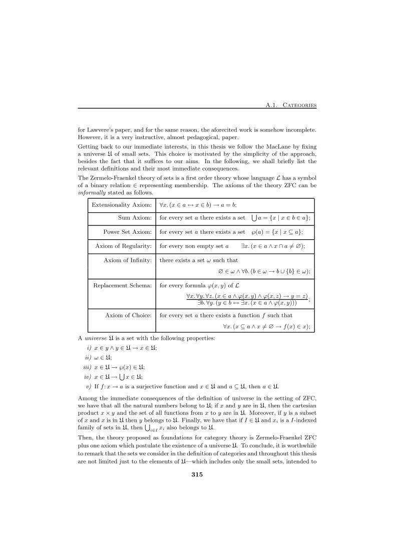
A.1. Categories
for Lawvere’s paper, and for the same reason, the aforecited work is somehow incomplete.However, it is a very instructive, almost pedagogical, paper.
Getting back to our immediate interests, in this thesis we follow the MacLane by fixinga universe U of small sets. This choice is motivated by the simplicity of the approach,besides the fact that it suffices to our aims. In the following, we shall briefly list therelevant definitions and their most immediate consequences.
The Zermelo-Fraenkel theory of sets is a first order theory whose language L has a symbolof a binary relation ∈ representing membership. The axioms of the theory ZFC can beinformally stated as follows.
Extensionality Axiom: ∀x. (x ∈ a↔ x ∈ b)→ a = b;
Sum Axiom: for every set a there exists a set⋃a = {x | x ∈ b ∈ a};
Power Set Axiom: for every set a there exists a set ℘(a) = {x | x ⊆ a};
Axiom of Regularity: for every non empty set a ∃x. (x ∈ a ∧ x ∩ a 6= ∅);
Axiom of Infinity: there exists a set ω such that
∅ ∈ ω ∧ ∀b. (b ∈ ω → b ∪ {b} ∈ ω);
Replacement Schema: for every formula ϕ(x, y) of L
∀x.∀y.∀z. (x ∈ a ∧ ϕ(x, y) ∧ ϕ(x, z)→ y = z)∃b.∀y. (y ∈ b↔ ∃x. (x ∈ a ∧ ϕ(x, y)))
;
Axiom of Choice: for every set a there exists a function f such that
∀x. (x ⊆ a ∧ x 6= ∅→ f(x) ∈ x);
A universe U is a set with the following properties:
i) x ∈ y ∧ y ∈ U→ x ∈ U;
ii) ω ∈ U;
iii) x ∈ U→ ℘(x) ∈ U;
iv) x ∈ U→⋃x ∈ U;
v) If f :x→ a is a surjective function and x ∈ U and a ⊆ U, then a ∈ U.
Among the immediate consequences of the definition of universe in the setting of ZFC,we have that all the natural numbers belong to U; if x and y are in U, then the cartesianproduct x× y and the set of all functions from x to y are in U. Moreover, if y is a subsetof x and x is in U then y belongs to U. Finally, we have that if I ∈ U and xi is a I-indexedfamily of sets in U, then
⋃i∈I
xi also belongs to U.
Then, the theory proposed as foundations for category theory is Zermelo-Fraenkel ZFC
plus one axiom which postulate the existence of a universe U. To conclude, it is worthwhile
to remark that the sets we consider in the definition of categories and throughout this thesis
are not limited just to the elements of U—which includes only the small sets, intended to
315
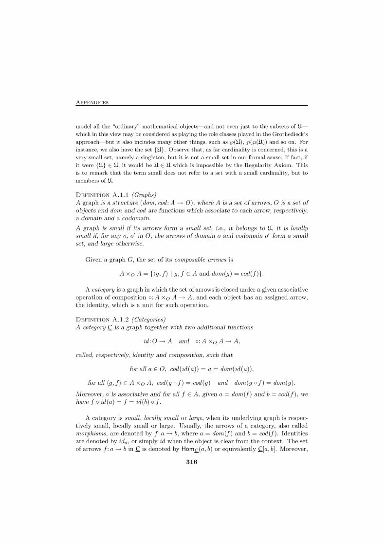
Appendices
model all the “ordinary” mathematical objects—and not even just to the subsets of U—
which in this view may be considered as playing the role classes played in the Grothedieck’s
approach—but it also includes many other things, such as ℘(U), ℘(℘(U)) and so on. For
instance, we also have the set {U}. Observe that, as far cardinality is concerned, this is a
very small set, namely a singleton, but it is not a small set in our formal sense. If fact, if
it were {U} ∈ U, it would be U ∈ U which is impossible by the Regularity Axiom. This
is to remark that the term small does not refer to a set with a small cardinality, but to
members of U.
Definition A.1.1 (Graphs)A graph is a structure (dom, cod :A → O), where A is a set of arrows, O is a set ofobjects and dom and cod are functions which associate to each arrow, respectively,a domain and a codomain.
A graph is small if its arrows form a small set, i.e., it belongs to U, it is locallysmall if, for any o, o′ in O, the arrows of domain o and codomain o′ form a smallset, and large otherwise.
Given a graph G, the set of its composable arrows is
A×O A = {〈g, f〉 | g, f ∈ A and dom(g) = cod(f)}.
A category is a graph in which the set of arrows is closed under a given associativeoperation of composition ◦:A ×O A → A, and each object has an assigned arrow,the identity, which is a unit for such operation.
Definition A.1.2 (Categories)A category C is a graph together with two additional functions
id :O→ A and ◦:A×O A→ A,
called, respectively, identity and composition, such that
for all a ∈ O, cod(id(a)) = a = dom(id(a)),
for all 〈g, f〉 ∈ A×O A, cod(g ◦ f ) = cod(g) and dom(g ◦ f ) = dom(g).
Moreover, ◦ is associative and for all f ∈ A, given a = dom(f ) and b = cod(f), wehave f ◦ id(a) = f = id(b) ◦ f .
A category is small , locally small or large, when its underlying graph is respec-tively small, locally small or large. Usually, the arrows of a category, also calledmorphisms, are denoted by f : a→ b, where a = dom(f ) and b = cod(f ). Identitiesare denoted by ida, or simply id when the object is clear from the context. The setof arrows f : a→ b in C is denoted by HomC(a, b) or equivalently C[a, b]. Moreover,
316
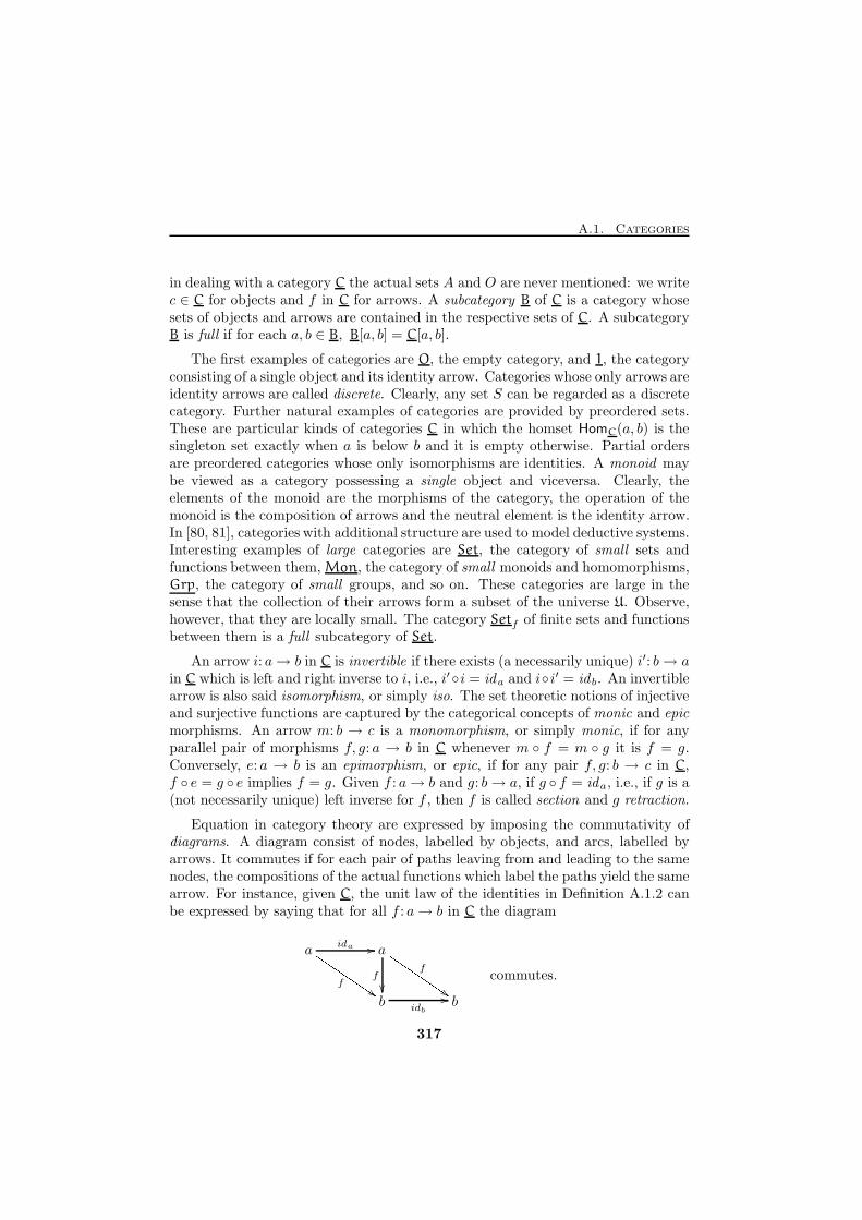
A.1. Categories
in dealing with a category C the actual sets A and O are never mentioned: we writec ∈ C for objects and f in C for arrows. A subcategory B of C is a category whosesets of objects and arrows are contained in the respective sets of C. A subcategoryB is full if for each a, b ∈ B, B[a, b] = C[a, b].
The first examples of categories are O, the empty category, and 1, the categoryconsisting of a single object and its identity arrow. Categories whose only arrows areidentity arrows are called discrete. Clearly, any set S can be regarded as a discretecategory. Further natural examples of categories are provided by preordered sets.These are particular kinds of categories C in which the homset HomC(a, b) is thesingleton set exactly when a is below b and it is empty otherwise. Partial ordersare preordered categories whose only isomorphisms are identities. A monoid maybe viewed as a category possessing a single object and viceversa. Clearly, theelements of the monoid are the morphisms of the category, the operation of themonoid is the composition of arrows and the neutral element is the identity arrow.In [80, 81], categories with additional structure are used to model deductive systems.Interesting examples of large categories are Set, the category of small sets andfunctions between them, Mon, the category of small monoids and homomorphisms,Grp, the category of small groups, and so on. These categories are large in thesense that the collection of their arrows form a subset of the universe U. Observe,however, that they are locally small. The category Setf of finite sets and functionsbetween them is a full subcategory of Set.
An arrow i: a→ b in C is invertible if there exists (a necessarily unique) i′: b→ ain C which is left and right inverse to i, i.e., i′◦i = ida and i◦i′ = idb. An invertiblearrow is also said isomorphism, or simply iso. The set theoretic notions of injectiveand surjective functions are captured by the categorical concepts of monic and epicmorphisms. An arrow m: b → c is a monomorphism, or simply monic, if for anyparallel pair of morphisms f, g: a → b in C whenever m ◦ f = m ◦ g it is f = g.Conversely, e: a → b is an epimorphism, or epic, if for any pair f, g: b → c in C,f ◦ e = g ◦ e implies f = g. Given f : a→ b and g: b→ a, if g ◦ f = ida, i.e., if g is a(not necessarily unique) left inverse for f , then f is called section and g retraction.
Equation in category theory are expressed by imposing the commutativity ofdiagrams. A diagram consist of nodes, labelled by objects, and arcs, labelled byarrows. It commutes if for each pair of paths leaving from and leading to the samenodes, the compositions of the actual functions which label the paths yield the samearrow. For instance, given C, the unit law of the identities in Definition A.1.2 canbe expressed by saying that for all f : a→ b in C the diagram
a a
b b
ida //
f
IIIIIIIII $$f �� f
IIIIIIIII $$idb
//
commutes.
317
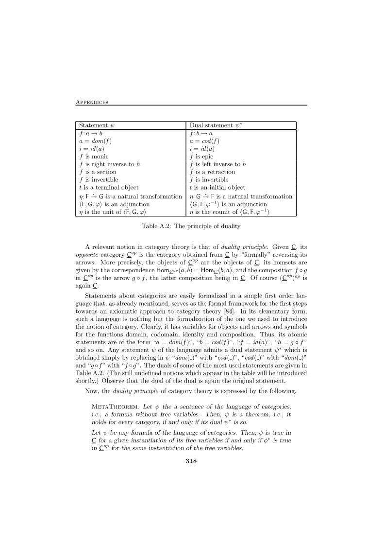
Appendices
Statement ψ Dual statement ψ∗
f : a→ b f : b→ aa = dom(f ) a = cod(f )i = id(a) i = id(a)f is monic f is epicf is right inverse to h f is left inverse to hf is a section f is a retractionf is invertible f is invertiblet is a terminal object t is an initial object
η: F�
→ G is a natural transformation η: G�
→ F is a natural transformation〈F,G, ϕ〉 is an adjunction 〈G, F, ϕ−1〉 is an adjunctionη is the unit of 〈F,G, ϕ〉 η is the counit of 〈G, F, ϕ−1〉
Table A.2: The principle of duality
A relevant notion in category theory is that of duality principle. Given C, itsopposite category Cop is the category obtained from C by “formally” reversing itsarrows. More precisely, the objects of Cop are the objects of C, its homsets aregiven by the correspondence HomCop(a, b) = HomC(b, a), and the composition f ◦ gin Cop is the arrow g ◦ f , the latter composition being in C. Of course (Cop)op isagain C.
Statements about categories are easily formalized in a simple first order lan-guage that, as already mentioned, serves as the formal framework for the first stepstowards an axiomatic approach to category theory [84]. In its elementary form,such a language is nothing but the formalization of the one we used to introducethe notion of category. Clearly, it has variables for objects and arrows and symbolsfor the functions domain, codomain, identity and composition. Thus, its atomicstatements are of the form “a = dom(f )”, “b = cod(f )”, “f = id(a)”, “h = g ◦ f”and so on. Any statement ψ of the language admits a dual statement ψ∗ which isobtained simply by replacing in ψ “dom( )” with “cod( )”, “cod( )” with “dom( )”and “g◦f” with “f ◦g”. The duals of some of the most used statements are given inTable A.2. (The still undefined notions which appear in the table will be introducedshortly.) Observe that the dual of the dual is again the original statement.
Now, the duality principle of category theory is expressed by the following.
MetaTheorem. Let ψ the a sentence of the language of categories,i.e., a formula without free variables. Then, ψ is a theorem, i.e., itholds for every category, if and only if its dual ψ∗ is so.
Let ψ be any formula of the language of categories. Then, ψ is true inC for a given instantiation of its free variables if and only if φ∗ is truein Cop for the same instantiation of the free variables.
318
A.1. Categories
This principle implies that it is never necessary to prove a statement and itsdual. For instance, the proof that f is monic in a category C is also a proof thatf is epic in Cop. Of course, since definitions may be dualizated as well, everynotion “X” introduced in the theory comes with a “dual” notion “coX”. Instancesof this pattern are products and coproduct, equalizers and coequalizers, limits andcolimits, and many more.
Functors are essentially morphisms of categories, in the informal sense that theyare mappings which respect the relevant structure of categories.
Definition A.1.3 (Functors)A functor F: A → B is a function which maps objects of A to objects of B andarrows in A to arrows in B, in such a way that
i) for all f : a→ b in A, F(f): F(a)→ F(b) in B;
ii) for all a ∈ A, F(ida) = idF(a);
iii) for all composable pairs 〈g, f〉, F(g ◦ f) = F(g) ◦ F(f) .
A functor F: A → B is full if, for all a, b ∈ A, its restriction to HomA(a, b) is asurjective function., i.e., if for any g: F(a) → F(b) in B there exists f : a → b in A
such that F(f) = g. Analogously, F is faithful, or an embedding, if for any parallelpair f, g: a → b in A, if F(f) = F(g) then f = g, i.e, if F restricted to any homsetHomA(a, b) is injective. A functor F which is full and faithful is also called a fullembedding.
Since some situations of great relevance occur frequently in the categorical prac-tise, there are some kinds of functors which are named after their characteristics,as in the case of the aforesaid embeddings and in the case of forgetful and inclusionfunctors. Given a category B whose objects are objects of A with some additionalstructure and whose morphisms are the morphisms of A which in addition preservesuch structure, a functor from B to A which sends each object to its “underlying”A-object a category and each morphism to its A-version is called a forgetful functor.Strictly speaking, an inclusion functor is a functor from a subcategory A of B to B
whose object and arrow components are all set inclusions. However, it is easy torealize that the key feature of such functors is that they are full and faithful, i.e.,full embeddings, and, in addition, they are injective on the objects. Thus, with alittle abuse, one often refers to any functor with this properties as to an inclusion
A functor F: Aop → B is usually called a contravariant functor from A to B. Infact, looking at them as “mappings” from A to B, for f : a→ b in A, we have thatF(f): F(b)→ F(a) and F(g ◦ f) = F(f) ◦ F(g), whence their name.
A composition operation for functors is easily obtained by composing their ob-ject and arrows components as functions. It is immediate to see that this operation
319
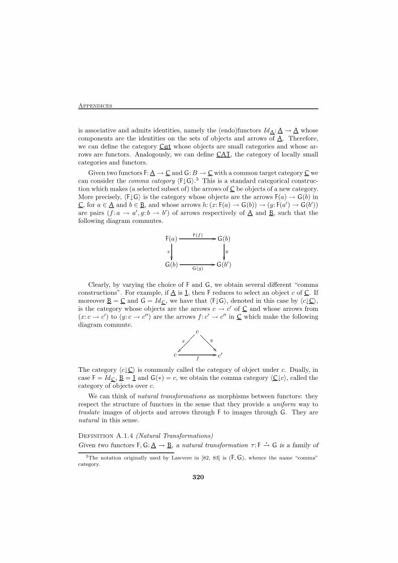
Appendices
is associative and admits identities, namely the (endo)functors IdA: A→ A whosecomponents are the identities on the sets of objects and arrows of A. Therefore,we can define the category Cat whose objects are small categories and whose ar-rows are functors. Analogously, we can define CAT , the category of locally smallcategories and functors.
Given two functors F: A→ C and G:B → C with a common target category C wecan consider the comma category 〈F↓G〉.3 This is a standard categorical construc-tion which makes (a selected subset of) the arrows of C be objects of a new category.More precisely, 〈F↓G〉 is the category whose objects are the arrows F(a)→ G(b) inC, for a ∈ A and b ∈ B, and whose arrows h: (x: F(a)→ G(b))→ (y: F(a′)→ G(b′))are pairs (f : a → a′, g: b → b′) of arrows respectively of A and B, such that thefollowing diagram commutes.
F(a) G(b)
G(b) G(b′)
x
��
F(f) //
y
��
G(g)//
Clearly, by varying the choice of F and G, we obtain several different “commaconstructions”. For example, if A is 1, then F reduces to select an object c of C. Ifmoreover B = C and G = IdC, we have that 〈F↓G〉, denoted in this case by 〈c↓C〉,is the category whose objects are the arrows c → c′ of C and whose arrows from(x: c → c′) to (y: c → c′′) are the arrows f : c′ → c′′ in C which make the followingdiagram commute.
c
c c′
x�������� y
?????��f
//
The category 〈c↓C〉 is commonly called the category of object under c. Dually, incase F = IdC, B = 1 and G(∗) = c, we obtain the comma category 〈C↓c〉, called thecategory of objects over c.
We can think of natural transformations as morphisms between functors: theyrespect the structure of functors in the sense that they provide a uniform way totraslate images of objects and arrows through F to images through G. They arenatural in this sense.
Definition A.1.4 (Natural Transformations)
Given two functors F,G: A → B, a natural transformation τ : F�
→ G is a family of
3The notation originally used by Lawvere in [82, 83] is (F,G), whence the name “comma”category.
320
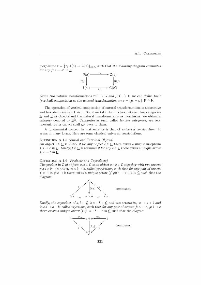
A.1. Categories
morphisms τ = {τa: F(a) → G(a)}a∈A such that the following diagram commutesfor any f : a→ a′ in B.
F(a) G(a)
F(a′) G(a′)
τa //
F(f)
��G(f)
��τa′
//
Given two natural transformations τ : F�
→ G and µ: G�
→ H we can define their
(vertical) composition as the natural transformation µ ◦ τ = {µa ◦ τa}: F�
→ H.
The operation of vertical composition of natural transformations is associative
and has identities IdF : F�
→ F. So, if we take the functors between two categoriesA and B as objects and the natural transformations as morphisms, we obtain acategory denoted by BA. Categories as such, called functor categories, are veryrelevant. Later on, we shall get back to them.
A fundamental concept in mathematics is that of universal construction. Itarises in many forms. Here are some classical universal constructions.
Definition A.1.5 (Initial and Terminal Objects)An object i ∈ C is initial if for any object c ∈ C there exists a unique morphismf : i→ c in C. Dually, t ∈ C is terminal if for any c ∈ C there exists a unique arrowf : c→ t in C.
Definition A.1.6 (Products and Coproducts)The product in C of objects a, b ∈ C is an object a×b ∈ C together with two arrowsπa: a× b→ a and πb: a× b→ b, called projections, such that for any pair of arrowsf : c → a, g: c → b there exists a unique arrow 〈f, g〉: c → a × b in C such that thediagram
c
a a× b b
f
}}{{{{{{{{{ g
CCCCCCCCC !!〈f,g〉
��πa
ooπb
//
commutes.
Dually, the coproduct of a, b ∈ C is a + b ∈ C and two arrows ina: a → a + b andinb: b→ a+ b, called injections, such that for any pair of arrows f : a→ c, g: b→ cthere exists a unique arrow [f, g]: a+ b→ c in C such that the diagram
a a+ b b
c
ina //
f
CCCCCCCCC!! [f,g]
��
inboo
g
}}{{{{{{{{{ commutes.
321
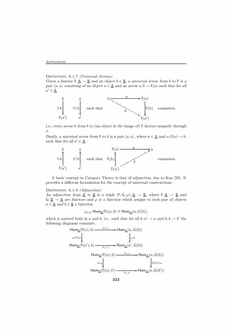
Appendices
Definition A.1.7 (Universal Arrows)Given a functor F: A → B and an object b ∈ B, a universal arrow from b to F is apair 〈a, u〉 consisting of an object a ∈ A and an arrow u: b→ F(a) such that for alla′ ∈ A
b
F(a′)
∀ k
��
a
a′
∃ !h
��
such that
b F(a)
F(a′)
u //
k
NNNNNNNNNNNNNNNN&& F(h)
��
commutes.
i.e., every arrow k from b to (an object in the image of) F factors uniquely throughu.
Dually, a universal arrow from F to b is a pair 〈a, u〉, where a ∈ A and u: F(a)→ b,such that for all a′ ∈ A
b
F(a′)
∀ k
OO a
a′
∃ !h
OO
such that
F(a) b
F(a′)
u //
F(h)
OO
kpppppppppppppppp88 commutes.
A basic concept in Category Theory is that of adjunction, due to Kan [59]. Itprovides a different formulation for the concept of universal constructions.
Definition A.1.8 (Adjunction)An adjunction from A to B is a triple 〈F,G, ϕ〉: A ⇀ B, where F: A → B andG: B → A are functors and ϕ is a function which assigns to each pair of objectsa ∈ A and b ∈ B a bijection
ϕa,b: HomB(F(a), b) ∼= HomA(a,G(b)),
which is natural both in a and b, i.e., such that for all k: a′ → a and h: b → b′ thefollowing diagrams commute.
HomB(F(a), b) HomA(a,G(b))
HomB(F(a′), b) HomA(a′,G(b))
ϕa,b //
◦F(k)
��◦k
��ϕa′,b
//
HomB(F(a), b) HomA(a,G(b))
HomB(F(a), b′) HomA(a,G(b′))
ϕa,b //
h◦
��G(h)◦
��ϕa,b′
//
322
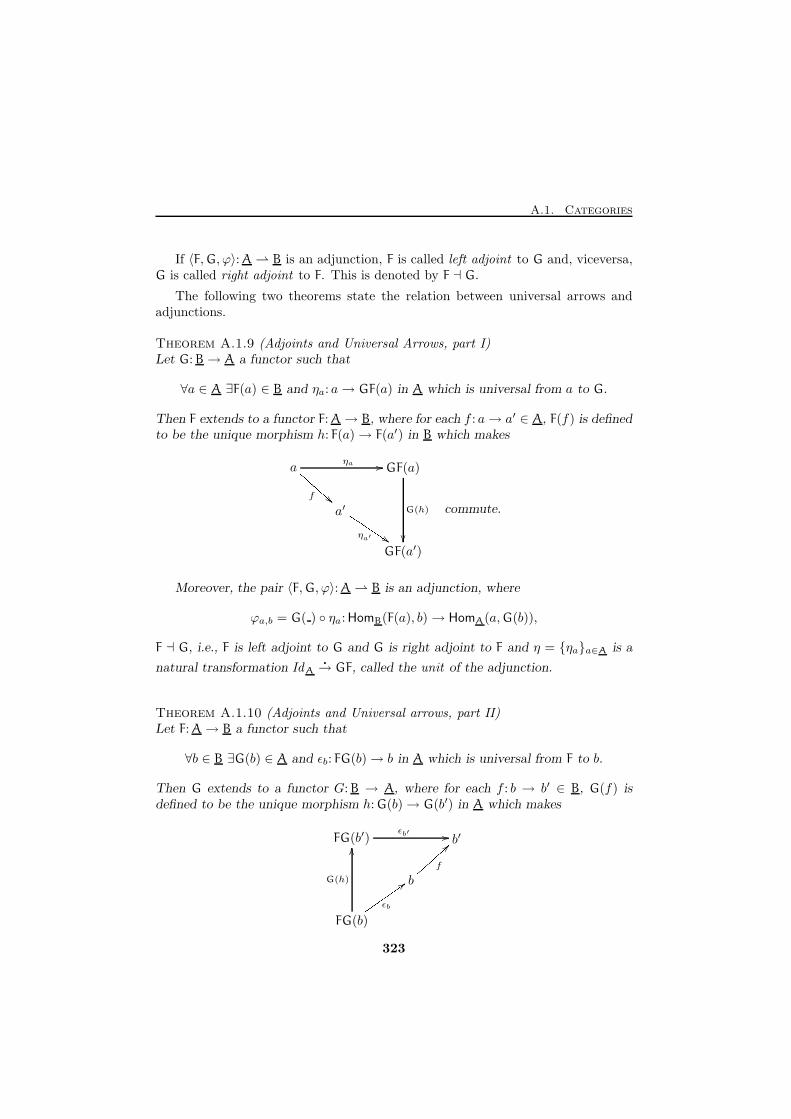
A.1. Categories
If 〈F,G, ϕ〉: A ⇀ B is an adjunction, F is called left adjoint to G and, viceversa,G is called right adjoint to F. This is denoted by F ⊣ G.
The following two theorems state the relation between universal arrows andadjunctions.
Theorem A.1.9 (Adjoints and Universal Arrows, part I)Let G: B→ A a functor such that
∀a ∈ A ∃F(a) ∈ B and ηa: a→ GF(a) in A which is universal from a to G.
Then F extends to a functor F: A→ B, where for each f : a→ a′ ∈ A, F(f) is definedto be the unique morphism h: F(a)→ F(a′) in B which makes
a GF(a)
a′
GF(a′)
ηa //
f
CCCCC!!G(h)
��ηa′
JJJJJJ $$ commute.
Moreover, the pair 〈F,G, ϕ〉: A ⇀ B is an adjunction, where
ϕa,b = G( ) ◦ ηa: HomB(F(a), b)→ HomA(a,G(b)),
F ⊣ G, i.e., F is left adjoint to G and G is right adjoint to F and η = {ηa}a∈A is a
natural transformation IdA�
→ GF, called the unit of the adjunction.
Theorem A.1.10 (Adjoints and Universal arrows, part II)Let F: A→ B a functor such that
∀b ∈ B ∃G(b) ∈ A and ǫb: FG(b)→ b in A which is universal from F to b.
Then G extends to a functor G: B → A, where for each f : b → b′ ∈ B, G(f) isdefined to be the unique morphism h: G(b)→ G(b′) in A which makes
FG(b′) b′
b
FG(b)
ǫb′ //
f||||| >>G(h)
OO
ǫbuuuuuu::323
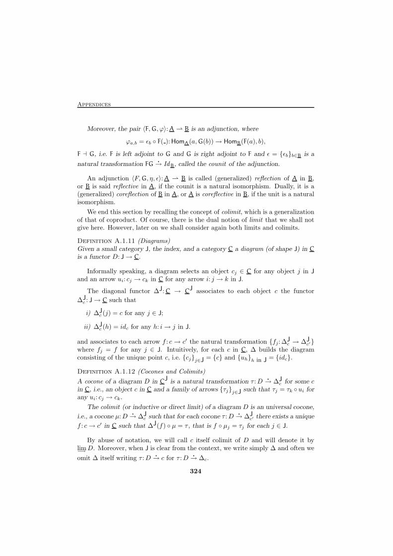
Appendices
Moreover, the pair 〈F,G, ϕ〉: A ⇀ B is an adjunction, where
ϕa,b = ǫb ◦ F( ): HomA(a,G(b))→ HomB(F(a), b),
F ⊣ G, i.e. F is left adjoint to G and G is right adjoint to F and ǫ = {ǫb}b∈B is a
natural transformation FG�
→ IdB, called the counit of the adjunction.
An adjunction 〈F,G, η, ǫ〉: A ⇀ B is called (generalized) reflection of A in B,or B is said reflective in A, if the counit is a natural isomorphism. Dually, it is a(generalized) coreflection of B in A, or A is coreflective in B, if the unit is a naturalisomorphism.
We end this section by recalling the concept of colimit, which is a generalizationof that of coproduct. Of course, there is the dual notion of limit that we shall notgive here. However, later on we shall consider again both limits and colimits.
Definition A.1.11 (Diagrams)Given a small category J, the index, and a category C a diagram (of shape J) in C
is a functor D: J→ C.
Informally speaking, a diagram selects an object cj ∈ C for any object j in J
and an arrow ui: cj → ck in C for any arrow i: j → k in J.
The diagonal functor ∆J: C → CJ associates to each object c the functor
∆Jc : J→ C such that
i) ∆Jc (j) = c for any j ∈ J;
ii) ∆Jc (h) = idc for any h: i→ j in J.
and associates to each arrow f : c → c′ the natural transformation {fj: ∆Jc → ∆J
c′}where fj = f for any j ∈ J. Intuitively, for each c in C, ∆ builds the diagramconsisting of the unique point c, i.e. {cj}j∈J = {c} and {uh}h in J = {idc}.
Definition A.1.12 (Cocones and Colimits)
A cocone of a diagram D in CJ is a natural transformation τ :D�
→ ∆Jc for some c
in C, i.e., an object c in C and a family of arrows {τj}j∈J such that τj = τk ◦ ui forany ui: cj → ck.
The colimit (or inductive or direct limit) of a diagram D is an universal cocone,
i.e., a cocone µ:D�
→ ∆Jc such that for each cocone τ :D
�
→ ∆Jc′ there exists a unique
f : c→ c′ in C such that ∆J(f) ◦ µ = τ , that is f ◦ µj = τj for each j ∈ J.
By abuse of notation, we will call c itself colimit of D and will denote it bylim−→ D. Moreover, when J is clear from the context, we write simply ∆ and often we
omit ∆ itself writing τ :D�
→ c for τ :D�
→ ∆c.
324
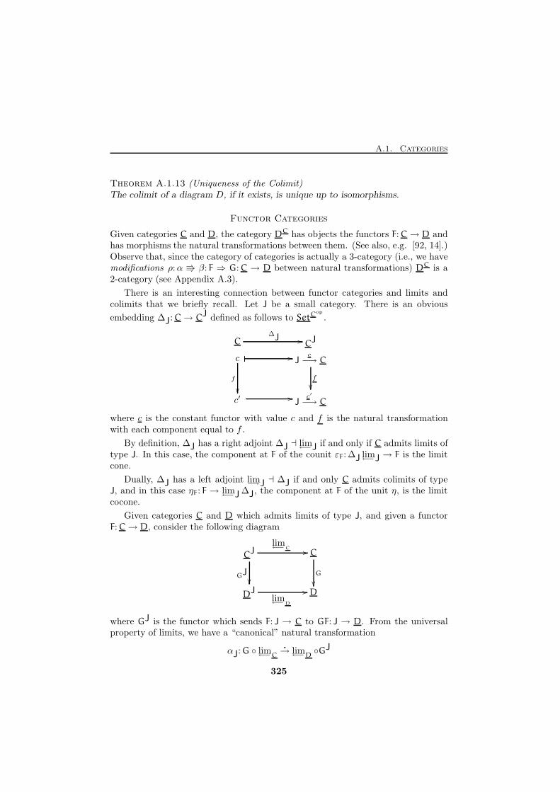
A.1. Categories
Theorem A.1.13 (Uniqueness of the Colimit)The colimit of a diagram D, if it exists, is unique up to isomorphisms.
Functor Categories
Given categories C and D, the category DC has objects the functors F: C→ D andhas morphisms the natural transformations between them. (See also, e.g. [92, 14].)Observe that, since the category of categories is actually a 3-category (i.e., we havemodifications ρ:α ⇛ β: F ⇒ G: C → D between natural transformations) DC is a2-category (see Appendix A.3).
There is an interesting connection between functor categories and limits andcolimits that we briefly recall. Let J be a small category. There is an obvious
embedding ∆J: C→ CJ defined as follows to SetCop
.
c Jc−→ C
c′ Jc′
−→ C
� //
f
��
f
��� //
CJC∆J //
where c is the constant functor with value c and f is the natural transformationwith each component equal to f .
By definition, ∆J has a right adjoint ∆J ⊣ lim←−J if and only if C admits limits oftype J. In this case, the component at F of the counit εF: ∆J lim←−J → F is the limitcone.
Dually, ∆J has a left adjoint lim−→J ⊣ ∆J if and only C admits colimits of typeJ, and in this case ηF: F → lim←−J ∆J, the component at F of the unit η, is the limitcocone.
Given categories C and D which admits limits of type J, and given a functorF: C→ D, consider the following diagram
CJ C
DJ D
lim←−C //
GJ��
G
��
lim←−D
//
where GJ is the functor which sends F: J → C to GF: J → D. From the universalproperty of limits, we have a “canonical” natural transformation
αJ: G ◦ lim←−C
�
→ lim←−D◦GJ
325
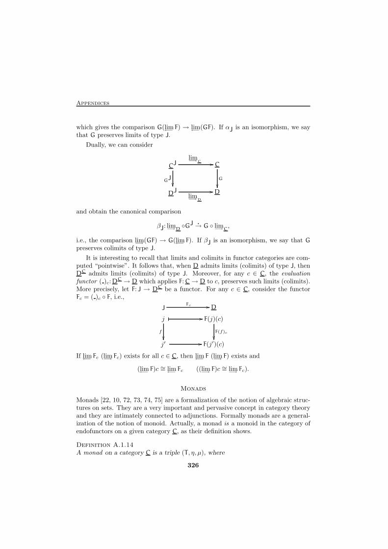
Appendices
which gives the comparison G(lim←− F) → lim←−(GF). If αJ is an isomorphism, we saythat G preserves limits of type J.
Dually, we can consider
CJ C
DJ D
lim−→C //
GJ��
G
��
lim−→D
//
and obtain the canonical comparison
βJ: lim−→D◦GJ �
→ G ◦ lim−→C,
i.e., the comparison lim−→(GF) → G(lim←− F). If βJ is an isomorphism, we say that G
preserves colimits of type J.
It is interesting to recall that limits and colimits in functor categories are com-puted “pointwise”. It follows that, when D admits limits (colimits) of type J, thenDC admits limits (colimits) of type J. Moreover, for any c ∈ C, the evaluationfunctor ( )c: D
C → D which applies F: C→ D to c, preserves such limits (colimits).More precisely, let F: J → DC be a functor. For any c ∈ C, consider the functorFc = ( )c ◦ F, i.e.,
j F(j)(c)
j′ F(j′)(c)
� //
f
��F(f)c
��� //
DJFc //
If lim←− Fc (lim−→ Fc) exists for all c ∈ C, then lim←− F (lim−→ F) exists and
(lim←− F)c ∼= lim←− Fc ((lim−→ F)c ∼= lim−→ Fc).
Monads
Monads [22, 10, 72, 73, 74, 75] are a formalization of the notion of algebraic struc-tures on sets. They are a very important and pervasive concept in category theoryand they are intimately connected to adjunctions. Formally monads are a general-ization of the notion of monoid. Actually, a monad is a monoid in the category ofendofunctors on a given category C, as their definition shows.
Definition A.1.14A monad on a category C is a triple (T , η, µ), where
326
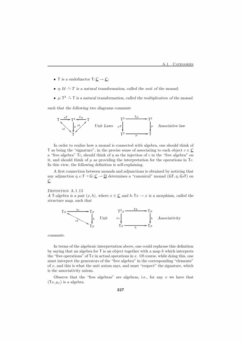
A.1. Categories
• T is a endofunctor T : C→ C;
• η: Id�
→ T is a natural transformation, called the unit of the monad;
• µ: T2 �
→ T is a natural transformation, called the multiplication of the monad.
such that the following two diagrams commute
T T2 T
T
ηT //
id
__�������� µ�� Tηoo
id
??
��~~~~~~ Unit Laws
T3 T2
T2 T
Tµ //
µT
��µ
��µ
//
Associative law
In order to realize how a monad is connected with algebra, one should think ofT as being the “signature”, in the precise sense of associating to each object c ∈ C
a “free algebra” Tc, should think of η as the injection of c in the “free algebra” onit, and should think of µ as providing the interpretation for the operations in Tc.In this view, the following definition is self-explaining.
A first connection between monads and adjunctions is obtained by noticing thatany adjunction η, ǫ: F ⊣ G: C ⇀ D determines a “canonical” monad (GF, η,GǫF) onC.
Definition A.1.15A T -algebra is a pair (x, h), where x ∈ C and h: Tx→ x is a morphism, called thestructure map, such that
Tx Tx
Tx
ηx //
id
ggNNNNNNNNNNN'' h
��Unit
T2x Tx
Tx Tx
Th //
µx
��h
��h
//
Associativity
commute.
In terms of the algebraic interpretation above, one could rephrase this definitionby saying that an algebra for T is an object together with a map h which interpretsthe “free operations” of Tx in actual operations in x. Of course, while doing this, onemust interpret the generators of the “free algebra” in the corresponding “elements”of x, and this is what the unit axiom says, and must “respect” the signature, whichis the associativity axiom.
Observe that the “free algebras” are algebras, i.e., for any x we have that(Tx, µx) is a algebra.
327
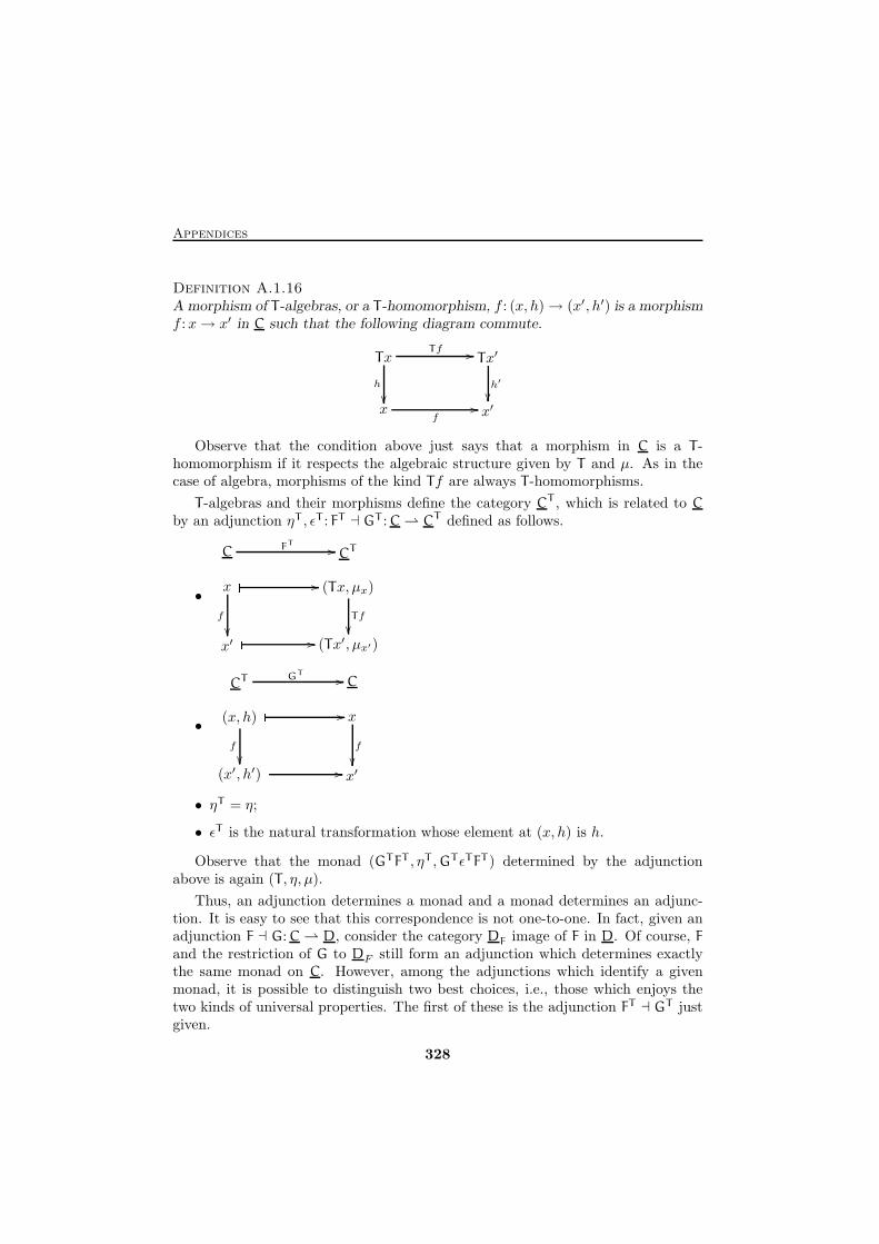
Appendices
Definition A.1.16A morphism of T -algebras, or a T -homomorphism, f : (x, h)→ (x′, h′) is a morphismf :x→ x′ in C such that the following diagram commute.
Tx Tx′
x x′
Tf //
h
��h′
��f
//
Observe that the condition above just says that a morphism in C is a T -homomorphism if it respects the algebraic structure given by T and µ. As in thecase of algebra, morphisms of the kind Tf are always T -homomorphisms.
T -algebras and their morphisms define the category CT , which is related to C
by an adjunction ηT , ǫT : FT ⊣ GT : C ⇀ CT defined as follows.
•x (Tx, µx)
x′ (Tx′, µx′)
� //
f
��Tf
��� //
CTC FT //
•(x, h) x
(x′, h′) x′
� //
f
��f
��� //
CCT GT //
• ηT = η;
• ǫT is the natural transformation whose element at (x, h) is h.
Observe that the monad (GTFT , ηT ,GT ǫTFT ) determined by the adjunctionabove is again (T , η, µ).
Thus, an adjunction determines a monad and a monad determines an adjunc-tion. It is easy to see that this correspondence is not one-to-one. In fact, given anadjunction F ⊣ G: C ⇀ D, consider the category DF image of F in D. Of course, F
and the restriction of G to DF still form an adjunction which determines exactlythe same monad on C. However, among the adjunctions which identify a givenmonad, it is possible to distinguish two best choices, i.e., those which enjoys thetwo kinds of universal properties. The first of these is the adjunction FT ⊣ GT justgiven.
328
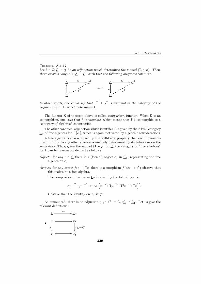
A.1. Categories
Theorem A.1.17Let F ⊣ G: C ⇀ A be an adjunction which determines the monad (T , η, µ). Then,there exists a unique K: A→ CT such that the following diagrams commute.
A CT
C
K //
F
OO
FTqqqqqqqqqqq88 and
A CT
C
K //
G
�� GT
xxqqqqqqqqqqqIn other words, one could say that FT ⊣ GT is terminal in the category of theadjunctions F ⊣ G which determines T .
The functor K of theorem above is called comparison functor. When K is anisomorphism, one says that F is monadic, which means that F is isomorphic to a“category of algebras” construction.
The other canonical adjunction which identifies T is given by the Kleisli categoryCT of free algebras for T [70], which is again motivated by algebraic considerations.
A free algebra is characterized by the well-know property that each homomor-phism from it to any other algebra is uniquely determined by its behaviour on thegenerators. Thus, given the monad (T , η, µ) on C, the category of “free algebras”for T can be reasonably defined as follows:
Objects: for any c ∈ C there is a (formal) object cT in CT , representing the freealgebra on c;
Arrows: for any arrow f : c → Tc′ there is a morphism f∗: cT → c′T ; observe thatthis makes cT a free algebra.
The composition of arrow in CT is given by the following rule
xTf∗
−→ yTg∗
−→ zT ;
(x
f−→ Ty
Tg−→ T2z
µz−→ Tz
)∗.
Observe that the identity on xT is η∗x
As announced, there is an adjuction ηT , ǫT : FT ⊣ GT : C ⇀ CT . Let us give therelevant definitions.
•x xT
x′ x′T
� //
f
��(ηx′◦f)∗
��� //
CTCFT //
329
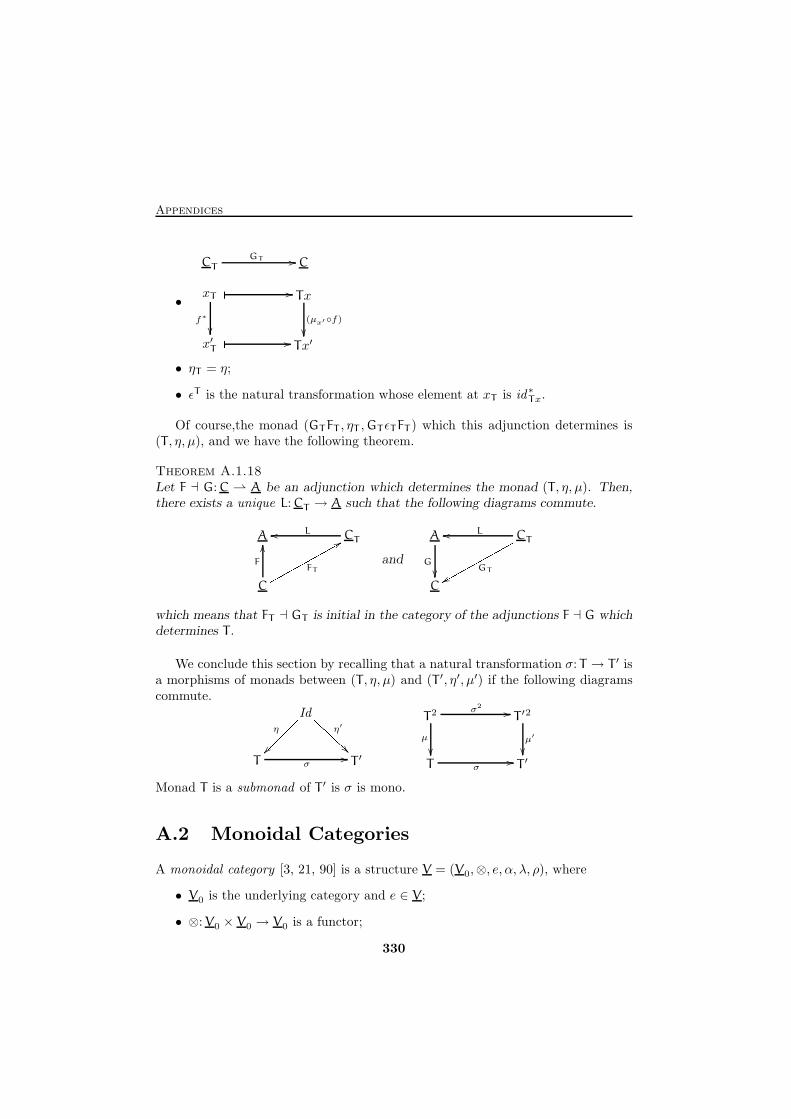
Appendices
•xT Tx
x′T Tx′
� //
f∗
��(µx′◦f)
��� //
CCTGT //
• ηT = η;
• ǫT is the natural transformation whose element at xT is id∗Tx.
Of course,the monad (GT FT , ηT ,GT ǫTFT ) which this adjunction determines is(T , η, µ), and we have the following theorem.
Theorem A.1.18Let F ⊣ G: C ⇀ A be an adjunction which determines the monad (T , η, µ). Then,there exists a unique L: CT → A such that the following diagrams commute.
A CT
C
Loo
F
OO
FTqqqqqqqqqqq88 and
A CT
C
G
��
Loo
GT
xxqqqqqqqqqqqwhich means that FT ⊣ GT is initial in the category of the adjunctions F ⊣ G whichdetermines T .
We conclude this section by recalling that a natural transformation σ: T → T ′ isa morphisms of monads between (T , η, µ) and (T ′, η′, µ′) if the following diagramscommute.
Id
T T ′
η
��~~~~~~ η′AAAAAA
σ//
T2 T ′2
T T ′
σ2 //
µ
��µ′
��σ
//
Monad T is a submonad of T ′ is σ is mono.
A.2 Monoidal Categories
A monoidal category [3, 21, 90] is a structure V = (V0,⊗, e, α, λ, ρ), where
• V0 is the underlying category and e ∈ V ;
• ⊗: V0 × V0 → V0 is a functor;
330
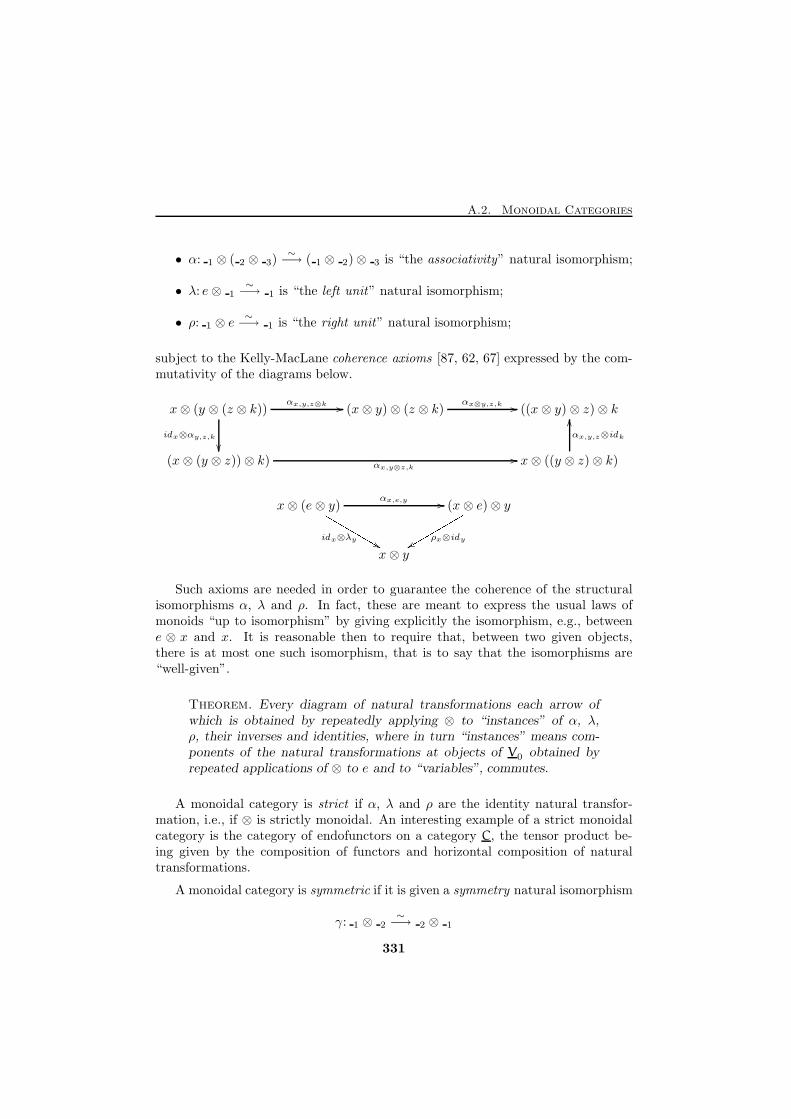
A.2. Monoidal Categories
• α: 1 ⊗ ( 2 ⊗ 3)∼−→ ( 1 ⊗ 2)⊗ 3 is “the associativity” natural isomorphism;
• λ: e⊗ 1∼−→ 1 is “the left unit” natural isomorphism;
• ρ: 1 ⊗ e∼−→ 1 is “the right unit” natural isomorphism;
subject to the Kelly-MacLane coherence axioms [87, 62, 67] expressed by the com-mutativity of the diagrams below.
x⊗ (y ⊗ (z ⊗ k)) (x⊗ y)⊗ (z ⊗ k) ((x⊗ y)⊗ z)⊗ k
(x ⊗ (y ⊗ z))⊗ k) x⊗ ((y ⊗ z)⊗ k)
idx⊗αy,z,k
��
αx,y,z⊗k // αx⊗y,z,k //
αx,y⊗z,k
//
αx,y,z⊗idk
OO
x⊗ (e⊗ y) (x ⊗ e)⊗ y
x⊗ y
αx,e,y //
idx⊗λy
LLLLLLLLL&& ρx⊗idyxxrrrrrrrrrSuch axioms are needed in order to guarantee the coherence of the structural
isomorphisms α, λ and ρ. In fact, these are meant to express the usual laws ofmonoids “up to isomorphism” by giving explicitly the isomorphism, e.g., betweene ⊗ x and x. It is reasonable then to require that, between two given objects,there is at most one such isomorphism, that is to say that the isomorphisms are“well-given”.
Theorem. Every diagram of natural transformations each arrow ofwhich is obtained by repeatedly applying ⊗ to “instances” of α, λ,ρ, their inverses and identities, where in turn “instances” means com-ponents of the natural transformations at objects of V0 obtained byrepeated applications of ⊗ to e and to “variables”, commutes.
A monoidal category is strict if α, λ and ρ are the identity natural transfor-mation, i.e., if ⊗ is strictly monoidal. An interesting example of a strict monoidalcategory is the category of endofunctors on a category C, the tensor product be-ing given by the composition of functors and horizontal composition of naturaltransformations.
A monoidal category is symmetric if it is given a symmetry natural isomorphism
γ: 1 ⊗ 2∼−→ 2 ⊗ 1
331
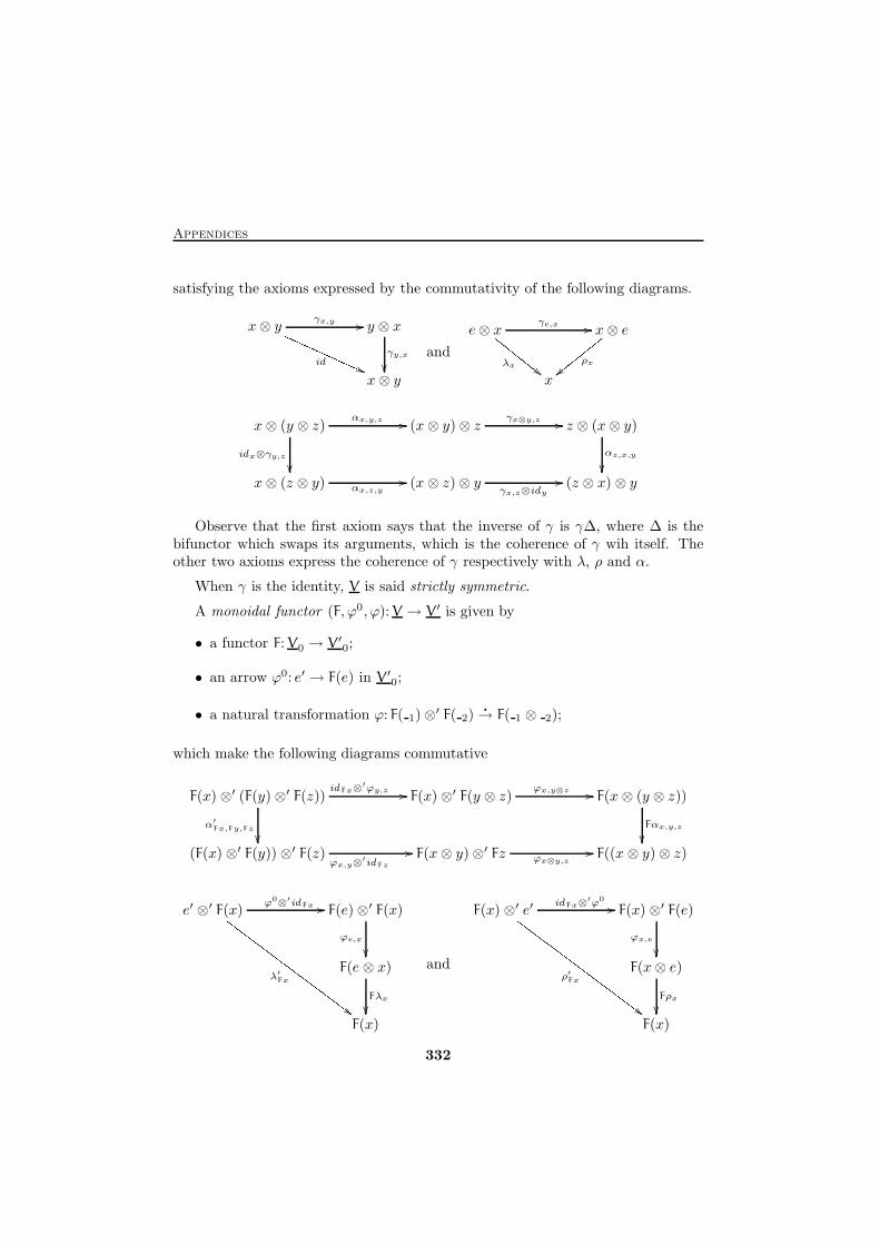
Appendices
satisfying the axioms expressed by the commutativity of the following diagrams.
x⊗ y y ⊗ x
x⊗ y
γx,y //
id
QQQQQQQQQQQ(( γy,x
��and
e⊗ x x⊗ e
xλx
EEEEEEE ""γe,x //
ρx
||yyyyyyyx⊗ (y ⊗ z) (x ⊗ y)⊗ z z ⊗ (x⊗ y)
x⊗ (z ⊗ y) (x ⊗ z)⊗ y (z ⊗ x) ⊗ y
idx⊗γy,z
��
αx,y,z // γx⊗y,z //
αz,x,y
��αx,z,y
//γx,z⊗idy
//
Observe that the first axiom says that the inverse of γ is γ∆, where ∆ is thebifunctor which swaps its arguments, which is the coherence of γ wih itself. Theother two axioms express the coherence of γ respectively with λ, ρ and α.
When γ is the identity, V is said strictly symmetric.
A monoidal functor (F, ϕ0, ϕ): V → V ′ is given by
• a functor F: V0 → V ′0;
• an arrow ϕ0: e′ → F(e) in V ′0;
• a natural transformation ϕ: F( 1)⊗′ F( 2)�
→ F( 1 ⊗ 2);
which make the following diagrams commutative
F(x) ⊗′ (F(y)⊗′ F(z)) F(x) ⊗′ F(y ⊗ z) F(x ⊗ (y ⊗ z))
(F(x) ⊗′ F(y)) ⊗′ F(z) F(x⊗ y)⊗′ Fz F((x ⊗ y)⊗ z)
idFx⊗′ϕy,z //
α′Fx,Fy,Fz
��
ϕx,y⊗z //
Fαx,y,z
��
ϕx,y⊗′idFz
//ϕx⊗y,z
//
e′ ⊗′ F(x) F(e)⊗′ F(x)
F(e⊗ x)
F(x)
ϕ0⊗′idFx //
λ′Fx
GGGGGGGGGGGGGGGGG##ϕe,x
��
Fλx
��
and
F(x) ⊗′ e′ F(x) ⊗′ F(e)
F(x⊗ e)
F(x)
idFx⊗′ϕ0
//
ρ′Fx
GGGGGGGGGGGGGGGGG ##ϕx,e
��
Fρx
��
332
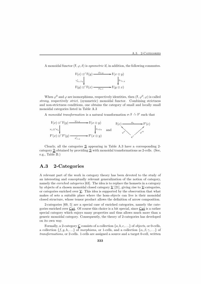
A.3. 2-Categories
A monoidal functor (F, ϕ, δ) is symmetric if, in addition, the following commutes.
F(x) ⊗′ F(y) F(x ⊗ y)
F(y)⊗′ F(x) F(y ⊗ x)
ϕx,y //
γ′Fx,Fy
��Fγx,y
��ϕy,x
//
When ϕ0 and ϕ are isomorphisms, respectively identities, then (F, ϕ0, ϕ) is calledstrong, respectively strict, (symmetric) monoidal functor. Combining strictnessand non-strictness conditions, one obtains the category of small and locally smallmonoidal categories listed in Table A.3
A monoidal transformation is a natural transformation σ: F�
→ F′ such that
F(x)⊗′ F(y) F(x⊗ y)
F′(x)⊗′ F′(y) F′(x⊗ y)
ϕx,y //
σx⊗′σy
��σx⊗y
��
ϕ′x,y
//
and
F(e) F′(e)
e′
σe //
ϕ0
``BBBBBB ϕ′0{{{{{{ ==Clearly, all the categories B appearing in Table A.3 have a corresponding 2-
category B obtained by providing B with monoidal transformations as 2-cells. (See,e.g., Table B.)
A.3 2-Categories
A relevant part of the work in category theory has been devoted to the study ofan interesting and conceptually relevant generalization of the notion of category,namely the enriched categories [63]. The idea is to replace the homsets in a categoryby objects of a chosen monoidal closed category V [21], giving rise to V-categories,or categories enriched over V . This idea is supported by the observation that whatmakes of sets a suitable place where the hom-objects can live is their monoidalclosed structure, whose tensor product allows the definition of arrow composition.
2-categories [69, 5] are a special case of enriched categories, namely the cate-gories enriched over Cat. Of course this choice is a bit special, since Cat is a ratherspecial category which enjoys many properties and thus allows much more than ageneric monoidal category. Consequently, the theory of 2-categories has developedon its own way.
Formally, a 2-category C consists of a collection {a, b, c, . . .} of objects, or 0-cells,a collection {f, g, h, . . .} of morphisms, or 1-cells, and a collection {α, β, γ, . . .} oftransformations, or 2-cells. 1-cells are assigned a source and a target 0-cell, written
333
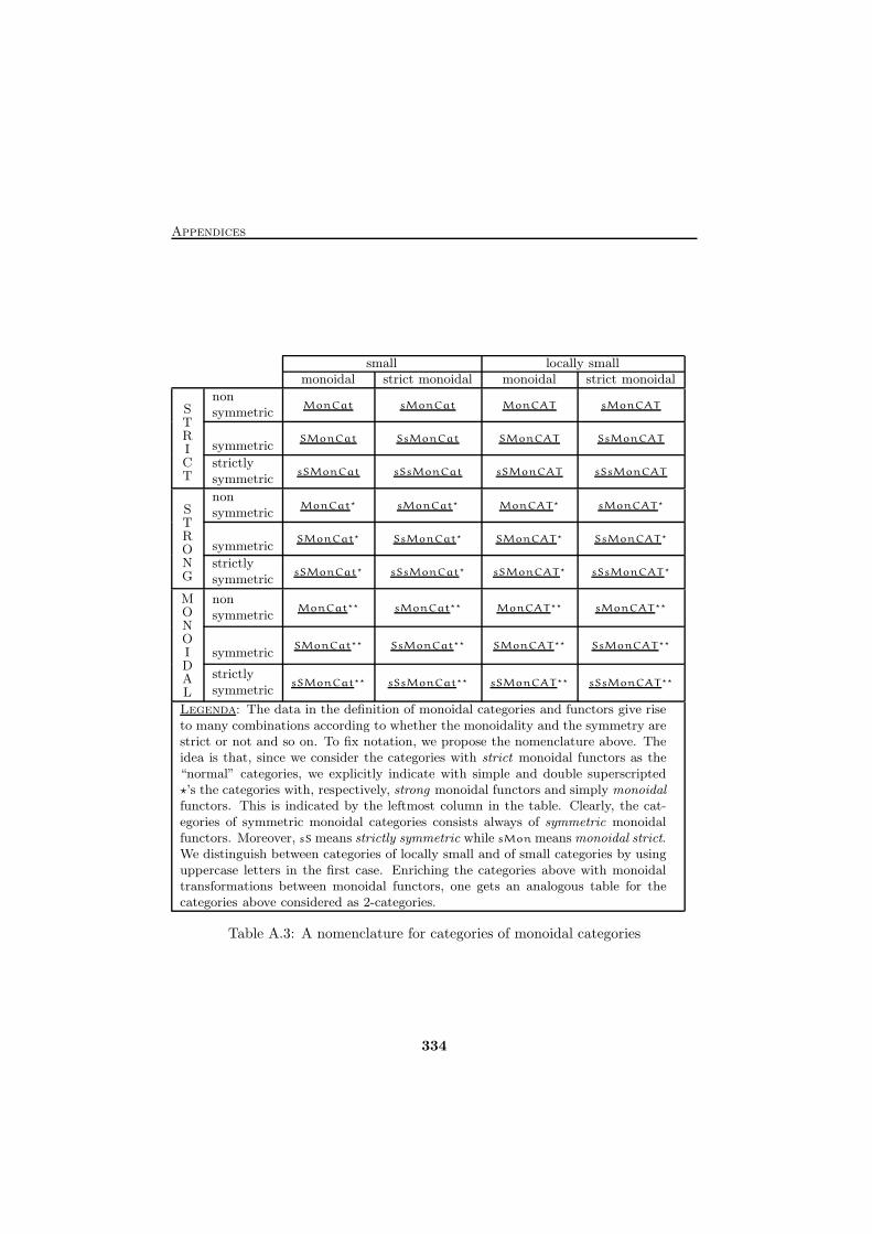
Appendices
small locally smallmonoidal strict monoidal monoidal strict monoidal
STRICT
nonsymmetric
MonCat sMonCat MonCAT sMonCAT
symmetricSMonCat SsMonCat SMonCAT SsMonCAT
strictlysymmetric
sSMonCat sSsMonCat sSMonCAT sSsMonCAT
STRONG
nonsymmetric
MonCat⋆ sMonCat⋆ MonCAT⋆ sMonCAT⋆
symmetricSMonCat⋆ SsMonCat⋆ SMonCAT⋆ SsMonCAT⋆
strictlysymmetric
sSMonCat⋆ sSsMonCat⋆ sSMonCAT⋆ sSsMonCAT ⋆
MONOIDAL
nonsymmetric
MonCat⋆⋆ sMonCat⋆⋆ MonCAT⋆⋆ sMonCAT⋆⋆
symmetricSMonCat⋆⋆ SsMonCat⋆⋆ SMonCAT⋆⋆ SsMonCAT ⋆⋆
strictlysymmetric
sSMonCat⋆⋆ sSsMonCat⋆⋆ sSMonCAT⋆⋆ sSsMonCAT⋆⋆
Legenda: The data in the definition of monoidal categories and functors give riseto many combinations according to whether the monoidality and the symmetry arestrict or not and so on. To fix notation, we propose the nomenclature above. Theidea is that, since we consider the categories with strict monoidal functors as the“normal” categories, we explicitly indicate with simple and double superscripted⋆’s the categories with, respectively, strong monoidal functors and simply monoidalfunctors. This is indicated by the leftmost column in the table. Clearly, the cat-egories of symmetric monoidal categories consists always of symmetric monoidalfunctors. Moreover, sS means strictly symmetric while sMon means monoidal strict.We distinguish between categories of locally small and of small categories by usinguppercase letters in the first case. Enriching the categories above with monoidaltransformations between monoidal functors, one gets an analogous table for thecategories above considered as 2-categories.
Table A.3: A nomenclature for categories of monoidal categories
334
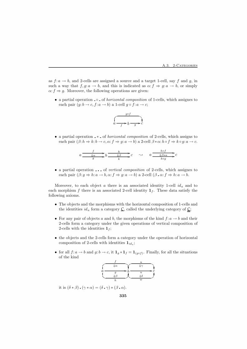
A.3. 2-Categories
as f : a → b, and 2-cells are assigned a source and a target 1-cell, say f and g, insuch a way that f, g: a → b, and this is indicated as α: f ⇒ g: a → b, or simplyα: f ⇒ g. Moreover, the following operations are given:
• a partial operation ◦ of horizontal composition of 1-cells, which assignes toeach pair (g: b→ c, f : a→ b) a 1-cell g ◦ f : a→ c;
a b c
# "g◦f
��f
//g
//
• a partial operation ∗ of horizontal composition of 2-cells, which assigns toeach pair (β:h⇒ k: b→ c, α: f ⇒ g: a→ b) a 2-cell β ∗α:h◦ f ⇒ k ◦ g: a→ c.
a b cf
⇓α//
g//
h
⇓β//
k// ; a c
h◦f
⇓β∗α//
k◦g//
• a partial operation � of vertical composition of 2-cells, which assignes toeach pair (β: g ⇒ h: a→ b, α: f ⇒ g: a→ b) a 2-cell (β � α: f ⇒ h: a→ b.
Moreover, to each object a there is an associated identity 1-cell ida and toeach morphism f there is an associated 2-cell identity 1f . These data satisfy thefollowing axioms.
• The objects and the morphisms with the horizontal composition of 1-cells andthe identities ida form a category C, called the underlying category of C;
• For any pair of objects a and b, the morphisms of the kind f : a→ b and their2-cells form a category under the given operations of vertical composition of2-cells with the identities 1f ;
• the objects and the 2-cells form a category under the operation of horizontalcomposition of 2-cells with identities 1ida
;
• for all f : a→ b and g: b→ c, it 1g ∗ 1f = 1(g◦f). Finally, for all the situationsof the kind
a b c
# "f
⇓α ��g
// !h
⇓βOO
# "u
⇓γ��
u// !
w
⇓δ
OO
it is (δ ∗ β) � (γ ∗ α) = (δ � γ) ∗ (β � α).
335
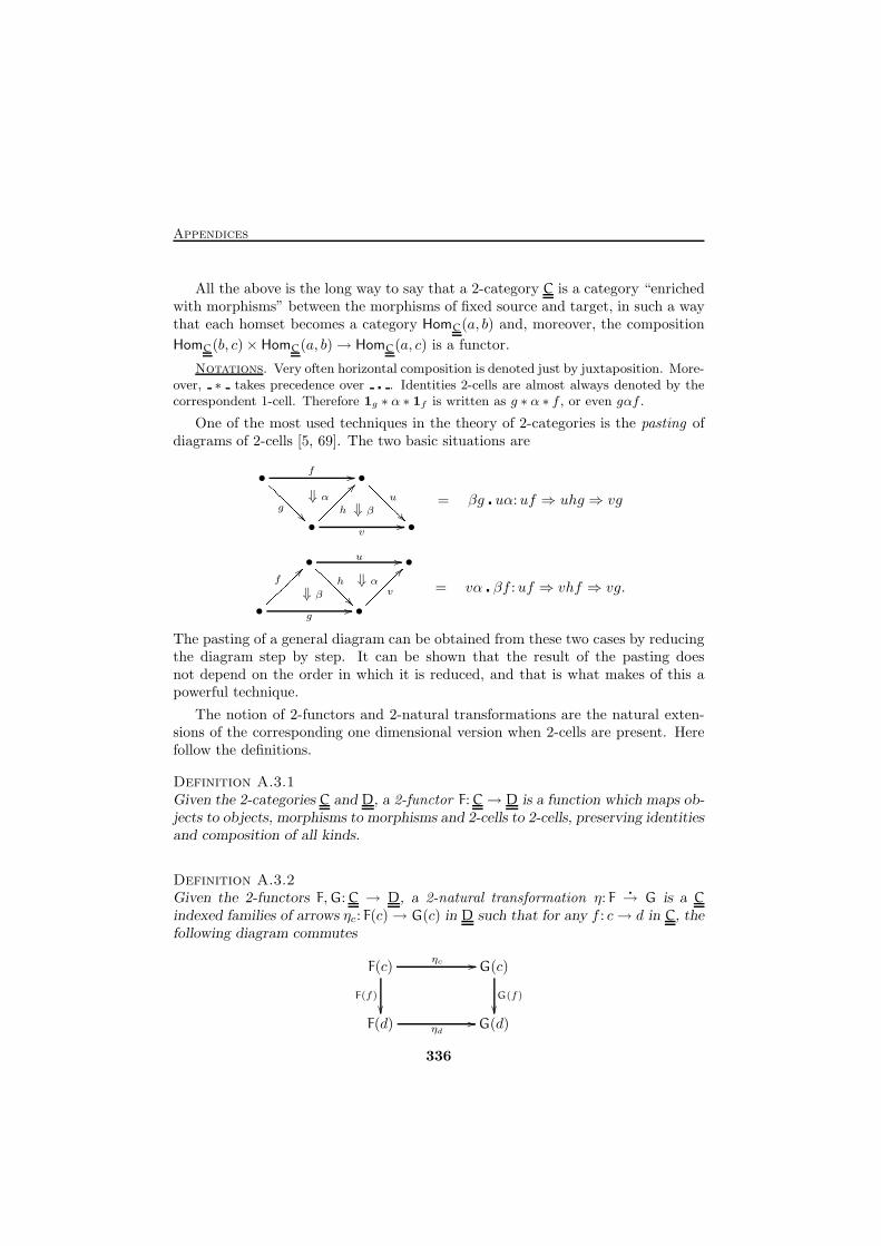
Appendices
All the above is the long way to say that a 2-category C is a category “enrichedwith morphisms” between the morphisms of fixed source and target, in such a waythat each homset becomes a category HomC(a, b) and, moreover, the composition
HomC(b, c)× HomC(a, b)→ HomC(a, c) is a functor.
Notations. Very often horizontal composition is denoted just by juxtaposition. More-over, ∗ takes precedence over � . Identities 2-cells are almost always denoted by thecorrespondent 1-cell. Therefore 1g ∗ α ∗ 1f is written as g ∗ α ∗ f , or even gαf .
One of the most used techniques in the theory of 2-categories is the pasting ofdiagrams of 2-cells [5, 69]. The two basic situations are
• •
• •
f //
g
����� �� ⇓ α u
����� ��h~~~~~??v
//⇓ β
= βg � uα:uf ⇒ uhg ⇒ vg
• •
• •
u //
h
����� �� ⇓ αf~~~~~??g
//⇓ β v~~~~~?? = vα � βf :uf ⇒ vhf ⇒ vg.
The pasting of a general diagram can be obtained from these two cases by reducingthe diagram step by step. It can be shown that the result of the pasting doesnot depend on the order in which it is reduced, and that is what makes of this apowerful technique.
The notion of 2-functors and 2-natural transformations are the natural exten-sions of the corresponding one dimensional version when 2-cells are present. Herefollow the definitions.
Definition A.3.1Given the 2-categories C and D, a 2-functor F: C→ D is a function which maps ob-jects to objects, morphisms to morphisms and 2-cells to 2-cells, preserving identitiesand composition of all kinds.
Definition A.3.2Given the 2-functors F,G: C → D, a 2-natural transformation η: F
�
→ G is a C
indexed families of arrows ηc: F(c)→ G(c) in D such that for any f : c→ d in C, thefollowing diagram commutes
F(c) G(c)
F(d) G(d)
ηc //
F(f)
��G(f)
��ηd
//
336
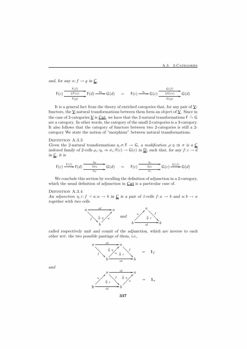
A.3. 2-Categories
and, for any α: f → g in C,
F(c) F(d) G(d)
F(f)
⇓F(α)//
F(g)//
ηd // = F(c) G(c) G(d)ηc //
G(f)
⇓G(α)//
G(g)//
It is a general fact from the theory of enriched categories that, for any pair of V-functors, the V-natural transformations between them form an object of V. Since in
the case of 2-categories V is Cat, we have that the 2-natural transformations F�
→ G
are a category. In other words, the category of the small 2-categories is a 3-category.It also follows that the category of functors between two 2-categories is still a 2-category We state the notion of “morphism” between natural transformations.
Definition A.3.3Given the 2-natural transformations η, σ: F → G, a modification ρ: η ⇛ σ is a C
indexed family of 2-cells ρc: ηc ⇒ σc: F(c)→ G(c) in D, such that, for any f : c→ din C, it is
F(c) F(d) G(d)F(f) //
ηd
⇓ρd
//
σd
// = F(c) G(c) G(d)ηc
⇓ρc
//
σc
//G(f) //
We conclude this section by recalling the definition of adjunction in a 2-category,which the usual definition of adjunction in Cat is a particular case of.
Definition A.3.4An adjunction η, ε: f ⊣ u: a → b in C is a pair of 1-cells f : a → b and u: b → atogether with two cells
a a
b
id //
f
>>>>>> ��⇓ η u
??������ and
a
b b
f
>>>>>>��⇓ εu
??������id
//
called respectively unit and counit of the adjunction, which are inverse to eachother wrt. the two possible pastings of them, i.e.,
a a
b b
id //
f
>>>>>>�� ⇓ η f
>>>>>>��u
??������id
//⇓ ε
= 1f
anda a
b b
id //
f
>>>>>> �� ⇓ ηu
??�����id
//⇓ ε u
??������ = 1u
337
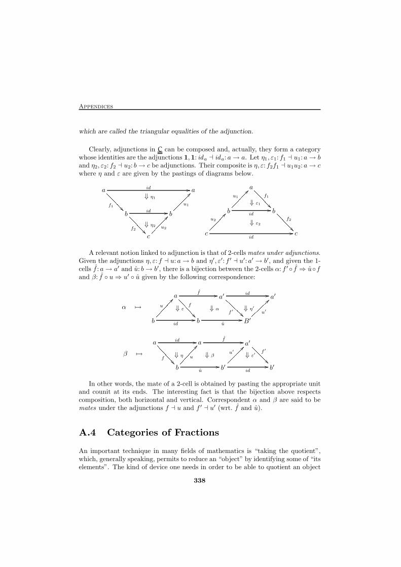
Appendices
which are called the triangular equalities of the adjunction.
Clearly, adjunctions in C can be composed and, actually, they form a categorywhose identities are the adjunctions 1,1: ida ⊣ ida: a→ a. Let η1, ε1: f1 ⊣ u1: a→ band η2, ε2: f2 ⊣ u2: b→ c be adjunctions. Their composite is η, ε: f2f1 ⊣ u1u2: a→ cwhere η and ε are given by the pastings of diagrams below.
a a
b b
c
f1
>>>>>> �� id //
id //
f2
>>>>>> �� u1
??������⇓ η1
⇓ η2 u2
@@������a
b b
c c
f1
>>>>>> ��⇓ ε1
⇓ ε2
u1
??������id
//
f2
>>>>>> ��id
//
u2
@@������A relevant notion linked to adjunction is that of 2-cells mates under adjunctions.
Given the adjunctions η, ε: f ⊣ u: a→ b and η′, ε′: f ′ ⊣ u′: a′ → b′, and given the 1-cells f : a→ a′ and u: b→ b′, there is a bijection between the 2-cells α: f ′ ◦ f ⇒ u◦fand β: f ◦ u⇒ u′ ◦ u given by the following correspondence:
α 7→
a a′ a′
b b B′
f //
f
====== �� f ′
AAAAAA id //
⇓ εu
@@������id
//
⇓ α
u//
u′}}}}}} >>⇓ η′
β 7→
a a a′
b b′ b′
id //
f
======�� f //
f ′?????��⇓ η u
@@������u
//
⇓ β
id//
u′�����?? ⇓ ε′In other words, the mate of a 2-cell is obtained by pasting the appropriate unit
and counit at its ends. The interesting fact is that the bijection above respectscomposition, both horizontal and vertical. Correspondent α and β are said to bemates under the adjunctions f ⊣ u and f ′ ⊣ u′ (wrt. f and u).
A.4 Categories of Fractions
An important technique in many fields of mathematics is “taking the quotient”,which, generally speaking, permits to reduce an “object” by identifying some of “itselements”. The kind of device one needs in order to be able to quotient an object
338
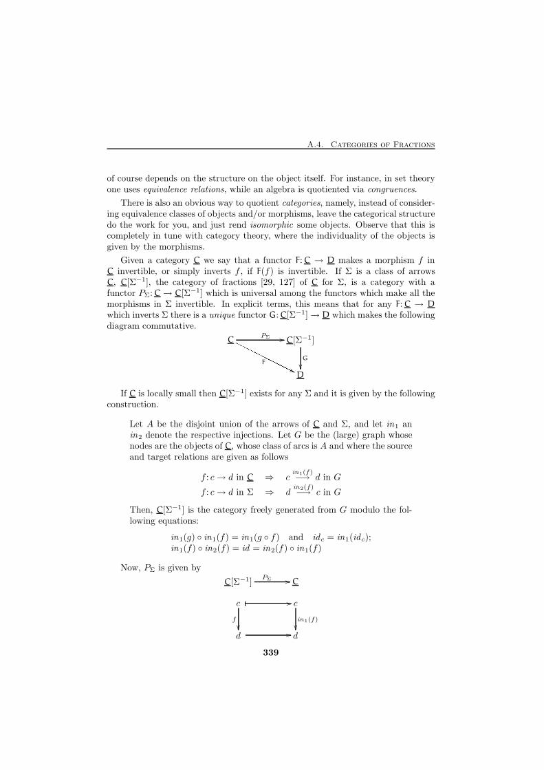
A.4. Categories of Fractions
of course depends on the structure on the object itself. For instance, in set theoryone uses equivalence relations, while an algebra is quotiented via congruences.
There is also an obvious way to quotient categories, namely, instead of consider-ing equivalence classes of objects and/or morphisms, leave the categorical structuredo the work for you, and just rend isomorphic some objects. Observe that this iscompletely in tune with category theory, where the individuality of the objects isgiven by the morphisms.
Given a category C we say that a functor F: C → D makes a morphism f inC invertible, or simply inverts f , if F(f) is invertible. If Σ is a class of arrowsC, C[Σ−1], the category of fractions [29, 127] of C for Σ, is a category with afunctor PΣ: C→ C[Σ−1] which is universal among the functors which make all themorphisms in Σ invertible. In explicit terms, this means that for any F: C → D
which inverts Σ there is a unique functor G: C[Σ−1]→ D which makes the followingdiagram commutative.
C C[Σ−1]
D
PΣ //
F
OOOOOOOOOOOOO'' G
��
If C is locally small then C[Σ−1] exists for any Σ and it is given by the followingconstruction.
Let A be the disjoint union of the arrows of C and Σ, and let in1 anin2 denote the respective injections. Let G be the (large) graph whosenodes are the objects of C, whose class of arcs is A and where the sourceand target relations are given as follows
f : c→ d in C ⇒ cin1(f)−→ d in G
f : c→ d in Σ ⇒ din2(f)−→ c in G
Then, C[Σ−1] is the category freely generated from G modulo the fol-lowing equations:
in1(g) ◦ in1(f) = in1(g ◦ f) and idc = in1(idc);in1(f) ◦ in2(f) = id = in2(f) ◦ in1(f)
Now, PΣ is given by
c c
d d
� //
f
��in1(f)
��� //
CC[Σ−1]PΣ //
339
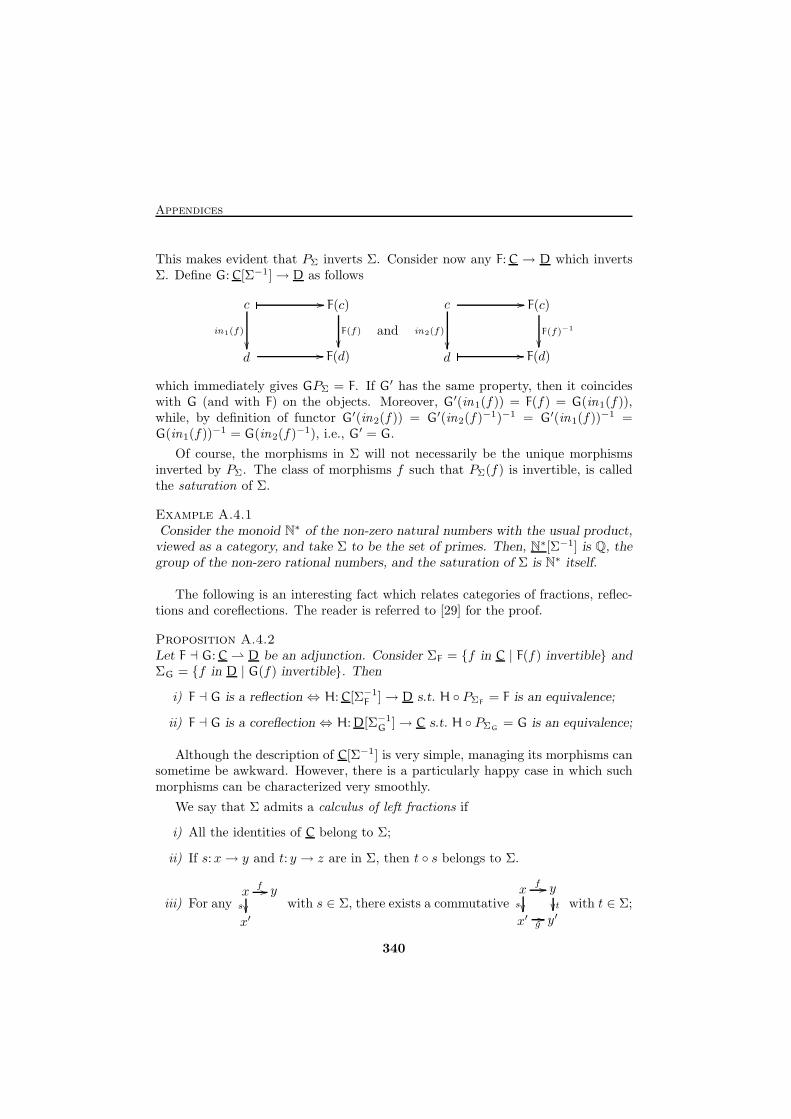
Appendices
This makes evident that PΣ inverts Σ. Consider now any F: C → D which invertsΣ. Define G: C[Σ−1]→ D as follows
c F(c)
d F(d)
� //
in1(f)
��F(f)
��� //
and
c F(c)
d F(d)
� //
in2(f)
��F(f)−1
��� //
which immediately gives GPΣ = F. If G′ has the same property, then it coincideswith G (and with F) on the objects. Moreover, G′(in1(f)) = F(f) = G(in1(f)),while, by definition of functor G′(in2(f)) = G′(in2(f)−1)−1 = G′(in1(f))−1 =G(in1(f))−1 = G(in2(f)−1), i.e., G′ = G.
Of course, the morphisms in Σ will not necessarily be the unique morphismsinverted by PΣ. The class of morphisms f such that PΣ(f) is invertible, is calledthe saturation of Σ.
Example A.4.1Consider the monoid N∗ of the non-zero natural numbers with the usual product,viewed as a category, and take Σ to be the set of primes. Then, N∗[Σ−1] is Q, thegroup of the non-zero rational numbers, and the saturation of Σ is N∗ itself.
The following is an interesting fact which relates categories of fractions, reflec-tions and coreflections. The reader is referred to [29] for the proof.
Proposition A.4.2Let F ⊣ G: C ⇀ D be an adjunction. Consider ΣF = {f in C | F(f) invertible} andΣG = {f in D | G(f) invertible}. Then
i) F ⊣ G is a reflection ⇔ H: C[Σ−1F ]→ D s.t. H ◦ PΣF
= F is an equivalence;
ii) F ⊣ G is a coreflection ⇔ H: D[Σ−1G ]→ C s.t. H ◦ PΣG
= G is an equivalence;
Although the description of C[Σ−1] is very simple, managing its morphisms cansometime be awkward. However, there is a particularly happy case in which suchmorphisms can be characterized very smoothly.
We say that Σ admits a calculus of left fractions if
i) All the identities of C belong to Σ;
ii) If s:x→ y and t: y → z are in Σ, then t ◦ s belongs to Σ.
iii) For anyx y
x′
f //s �� with s ∈ Σ, there exists a commutative
x y
x′ y′
f //s �� t��
g//
with t ∈ Σ;
340
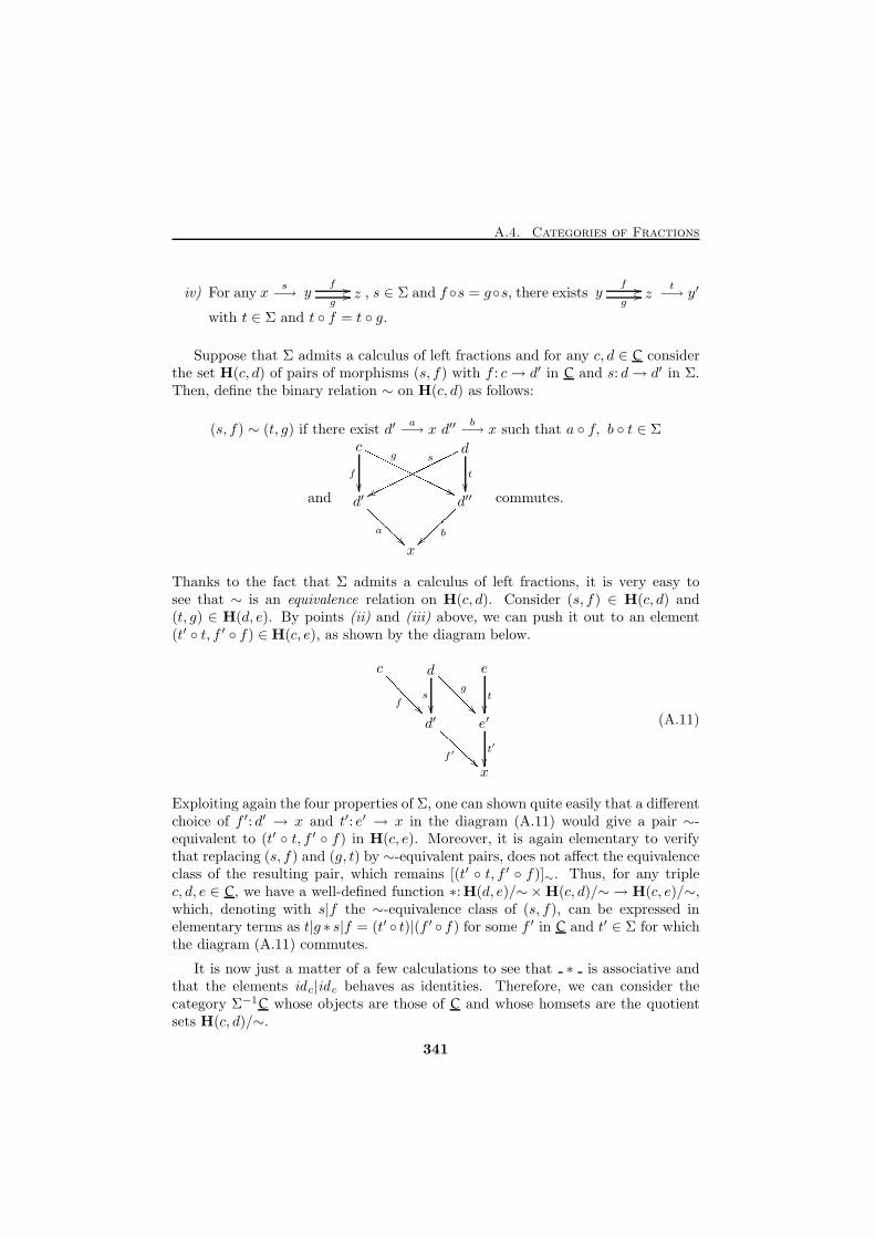
A.4. Categories of Fractions
iv) For any xs−→ y z
f //g
// , s ∈ Σ and f ◦s = g◦s, there exists y zf //g
//t−→ y′
with t ∈ Σ and t ◦ f = t ◦ g.
Suppose that Σ admits a calculus of left fractions and for any c, d ∈ C considerthe set H(c, d) of pairs of morphisms (s, f) with f : c→ d′ in C and s: d→ d′ in Σ.Then, define the binary relation ∼ on H(c, d) as follows:
(s, f) ∼ (t, g) if there exist d′a−→ x d′′
b−→ x such that a ◦ f, b ◦ t ∈ Σ
and
c d
d′ d′′
x
f
��
gOOOOOOOOOOOOO''s
wwooooooooooooo t
��
a
������� b~~}}}}}} commutes.
Thanks to the fact that Σ admits a calculus of left fractions, it is very easy tosee that ∼ is an equivalence relation on H(c, d). Consider (s, f) ∈ H(c, d) and(t, g) ∈ H(d, e). By points (ii) and (iii) above, we can push it out to an element(t′ ◦ t, f ′ ◦ f) ∈ H(c, e), as shown by the diagram below.
c d e
d′ e′
x
f
>>>>>> ��s �� g
??????�� t
��
f ′
AAAAAA t′�� (A.11)
Exploiting again the four properties of Σ, one can shown quite easily that a differentchoice of f ′: d′ → x and t′: e′ → x in the diagram (A.11) would give a pair ∼-equivalent to (t′ ◦ t, f ′ ◦ f) in H(c, e). Moreover, it is again elementary to verifythat replacing (s, f) and (g, t) by ∼-equivalent pairs, does not affect the equivalenceclass of the resulting pair, which remains [(t′ ◦ t, f ′ ◦ f)]∼. Thus, for any triplec, d, e ∈ C, we have a well-defined function ∗:H(d, e)/∼×H(c, d)/∼ → H(c, e)/∼,which, denoting with s|f the ∼-equivalence class of (s, f), can be expressed inelementary terms as t|g ∗ s|f = (t′ ◦ t)|(f ′ ◦ f) for some f ′ in C and t′ ∈ Σ for whichthe diagram (A.11) commutes.
It is now just a matter of a few calculations to see that ∗ is associative andthat the elements idc|id c behaves as identities. Therefore, we can consider thecategory Σ−1C whose objects are those of C and whose homsets are the quotientsets H(c, d)/∼.
341
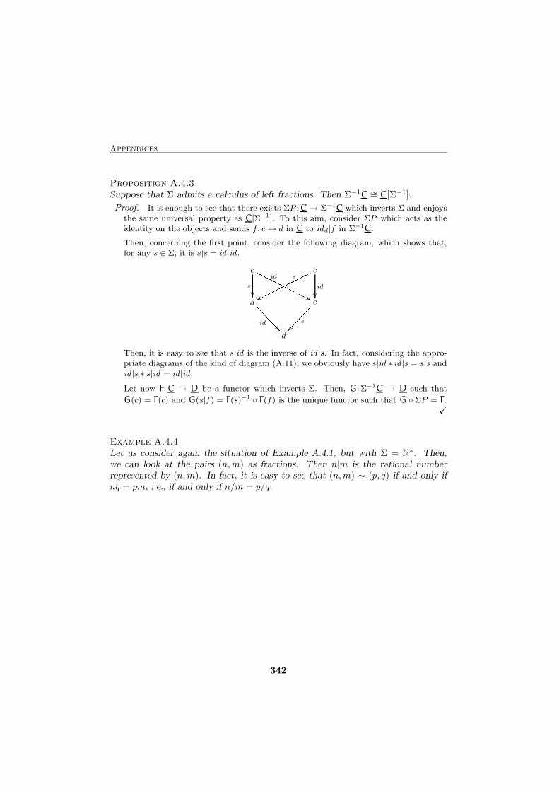
Appendices
Proposition A.4.3Suppose that Σ admits a calculus of left fractions. Then Σ−1C ∼= C[Σ−1].
Proof. It is enough to see that there exists ΣP :C→ Σ−1C which inverts Σ and enjoysthe same universal property as C[Σ−1]. To this aim, consider ΣP which acts as theidentity on the objects and sends f : c→ d in C to idd|f in Σ−1C.
Then, concerning the first point, consider the following diagram, which shows that,for any s ∈ Σ, it is s|s = id |id .
c c
d c
d
s
��
idOOOOOOOOOOOO ''s
wwoooooooooooo id
��
id
>>>>>> �� s
��������Then, it is easy to see that s|id is the inverse of id |s. In fact, considering the appro-priate diagrams of the kind of diagram (A.11), we obviously have s|id ∗ id |s = s|s andid |s ∗ s|id = id |id .
Let now F:C → D be a functor which inverts Σ. Then, G: Σ−1C → D such that
G(c) = F(c) and G(s|f) = F(s)−1 ◦ F(f) is the unique functor such that G ◦ ΣP = F.
X
Example A.4.4Let us consider again the situation of Example A.4.1, but with Σ = N∗. Then,we can look at the pairs (n,m) as fractions. Then n|m is the rational numberrepresented by (n,m). In fact, it is easy to see that (n,m) ∼ (p, q) if and only ifnq = pm, i.e., if and only if n/m = p/q.
342
Glossary
� , 236, 335
◦ , 335∗ , 236, 335
· ( )∗, 174↓ , 85, 132⊕
↓ , 85
⊢ , 139↾ , 175
γ≡i , 177
γIi , 177
⊑ , 144≺ , 70, 145
4 , 70, 145# , 70, 100, 138
∨∨ , 138co , 81, 138
〈 ↓ 〉, 19, 320( )+:DecOcc→ PTNets, 81
[ , ], 79( )⊕, 13
( )⊗, 45
( )0, 14( )M, 65
( )M∞ , 65, 66( )F , 80
( )R, 91[ ]i, 79, 143
⌊ ⌋, 100, 138[[ ]], 12, 65, 143
∆, 281, 287∇, 280, 287
Π(n), 23Σ+, 94
ΣP , 94Σ∅, 95
Σ{t}, 95Σ−1C, 341
Θ(n), 83∂iN , 13, 68λ, 133, 246
λ∗, 150γσ, 60
γSi, 177ω, 84
S, 314U, 214, 313s
a←→ s′, 154
u[α〉v, 15
u0[α0〉 · · · [αn〉un+1, 17∫
C
P , 216
(Xi)i∈I, 246(X,≡, I), 174
(Si,≡i, Ii), 176(Sω,≡ω, Iω), 176(∼i,≤i,#i), 190
(∼ω,≤ω,#ω), 196ℵ-CAT , 276ℵ-Cat, 276(ℵ)-lfp 272
O, 3171, 260, 3171, 236, 335
A(ES), 189Act(π), 134Act(T ), 134C, 166
C, 231
Cℵ, 231Cω, 286
343
Glossary
C[Σ−1], 339C[a, b], 214CAT , 214CAT , 214CMonPetri, 16CP[N ], 28CQ[N ], 58C/R, 33CT , 328
CT , 329Cat, 214, 320CatPetri, 17Co( ), 81Colim( ), 84D, 84D[ ]:Occ→ DecOcc, 95DCP , 114DCP[N ], 114DES , 148DP [N ], 110DT , 134DecOcc, 80Diam(x, y, z, t), 142Dom, 102E 168E [ ]:Occ→ PES, 101ES 100, 138Ev(s), 150Ev i, 192Evω, 199F [ ]: DecOcc→ Occ, 93F( ):Petri→ SSMC⊕, 30Filt, 228Filtℵ, 228G:SSMC⊗ → Petri, 54Graph, 12HL, 133HomC(a, b), 214
I ⊆ Tran2, 141Is ⊆ L× L, 149Ind(C), 246Ind(C)ℵ, 246Ind(F), 258Ind(α), 259Ind2(C), 263L(ES), 101, 139
L[ ]: PES→ Dom, 102
L( ): C→ Ind(C), 246LES, 138LESI, 188MPetri, 15MPetri∗, 107
MPetri∗, 20MPetri0, 15MProcf [(N,u)], 20MProcNets, 20MProc[(N,u)], 20M(u), 50
Max (x), 145N ( , ), 154N [ ]: PES→ Occ, 101Net, 69OTI , 151Occ, 70
PES, 100PROP, 22P [N ], 25PTNets, 66Petri, 13Petri∗, 18
Petri0, 15Pr:Dom→ PES, 103Pref (x), 145Proc[N ], 19Procf [N ], 19ProcNets, 19
Pseudo-Alg, 245
Q[ ]:Petri→ SSMC⊗, 50
R, 54R[N ], 68S , 167Sxk , 97S, 50S [ ]: Petri→ CMonPetri, 16S [N ], 16, 88
SCP , 57SS [N ], 16SSMC, 21SSMC⊕, 22SSMC⊗, 54ST , 132
344
Glossary
SW (L), 144
Safe, 68Sec(ES), 139Smooth(x), 145
SsMonCat, 22Sym∗N , 50Sym∗S, 45
SymN , 25SymC, 22Path(T ), 133
Set, 11, 214
SetCop
, 214
T , 131T -Alg, 240T -Alg, 240
TA(ES), 189TI , 152TS, 132
TSI, 142TSysκ, 178T [ ]:Petri→ CatPetri, 17
U [ ]:PTNets→ DecOcc, 86U( ):SSMC⊕ → Petri, 30U(k)[N ], 85
Y:C→ SetCop
, 214
dLES, 139doTSI, 159dTS, 135dTSI, 142
dles( ):LESI → dLES, 202dles.dsl( ):dLES→ dSL, 148dles.gtl( ):dLES→ GTL, 150
dsl .dles( ):dSL→ dLES, 147dts.hl ( ):dTS→ HL, 136dtsi( ): TSI→ dTSI, 181
gop∅
, 80gop{t}
, 80gcd, 94
gtl .dles( ):GTL→ dLES, 150hc, 214hl .dts( ):HL→ dTS, 136
hl .st( ):HL→ ST , 134inS , 52inSN , 52les.otsi( ):LES→ oTSI, 159
les.st( ):LES→ ST , 140lesi( ):LES→ LESI, 189lcm(ni,mj), 73max(Θ), 27min(Θ), 20, 27otsi .les( ):oTSI→ LES, 161oTSI, 151oTSIE, 171pTSI, 174st .hl ( ):ST → HL, 134st .les( ):ST → LES, 139ts.dts( ): TS→ dTS, 135ts.st( ): TS→ ST , 133tsi .otsi ( ): TSI→ oTSI, 156y:C→ Ind(C), 261
345

Glossary
346
Index
(ℵ-)finitely presentable objects, 272( )M∞–homomorphism 66, 67σ-interchange symmetry, 602-categories, 333
2-functors, 3362-natural transformations, 336CP[N ], 28
operations in CP [N ], 28, 29symmetries CP[N ], 29transitions CP [N ], 29
CP[N ] and P [N ] are isomorphic, 29CQ[N ], 58
operations CQ[N ], 57, 58symmetries CQ[N ], 58transitions CQ[N ], 59
CQ[N ] and Q[N ] are isomorphic, 61
D[ ] from Occ to DecOcc 95DP [N ] 113, 117DCP[N ], 113
operations DCP[N ], 114, 115symmetries DCP[N ], 115transitions DCP[N ], 115
DCP[N ] and DP [N ] are isomorphic, 117
(E), condition, 168Evω is deterministic, 201Evω is a colimit in LESI, 200F [ ] from DecOcc to Occ, 93Filt/C, 253G[ ] from SSMC⊗ to Petri, 55
Hoare languages, 133Ind( )ℵ KZ-doctrine, 273, 275Ind( ) KZ-doctrine, 273, 275
Ind( ) on functors, 258Ind( ) on 2-cells, 259Ind-algebras, 275
KZ-doctrines, 236
(ℵ-)cocompletion KZ-doctrine, 276P [N ], 37, 39, 40, 40Petri categories 17Petri commutative monoids 16
Petri nets, 13Petri categories, 17PT Nets, 66
morphisms of PT nets, 67remarks on PTNets, 67unfoldings of PT nets, 85, 86
decorated occurrence nets, 80free SSMC on a net, 32marked Petri nets, 15
morphisms of marked nets, 15pointed Petri nets, 15
morphisms of pointed nets, 15
morphisms of petri nets, 13, 15, 67safe nets 68steps, 15, 68step sequences, 16, 68step sequences for PT nets, 68
Petri symmetric categories, 54Q[ ], 50, 51, 52, 54, 56
SymN , 23SymN is a SSMC, 25axiomatization of SymN , 36
Sym∗S , 45Sym∗S is a SSMC, 46Sym∗S is free, 47, 50
Sym∗N , 50T -algebras 327
in KZ doctrine 238T -homomorphisms 327
in KZ doctrine 240TSysω 180, 181
is a colimit in pTSI, 180
347
Index
Yoneda embedding, 214, 215contravariant embedding, 215
Yoneda lemma, 215adjunctions, 322
adjoints and universal arrows, 323associativity isomorphisms, 331behaviour/system axis, 172block functions, 79calculus of left fractions, 253, 340canonical 2-cell of f 240categories, 316
(ℵ-)chain cocomplete, 220, 222(ℵ-)directed cocomplete, 220, , 222(ℵ-)filtered cocomplete, 229(ℵ-)finitely locally presentable, 272Kleisli category, 329Petri categories, 17PROP categories, 22category of fractions, 252, 339category of left fractions 341category of the elements of P , 216category of the objects over c, 320category of the object under c, 320comma category, 107, 320discrete categories, 317duality of categories, 318essentially (ℵ-)filtered, 230filtered categories, 224large categories, 214locally small categories, 214monoidal categories, 330monoidal quotient categories, 33small categories, 214strict monoidal categories, 331symmetric monoidal categories, 331SSMC, 332symmetric Petri categories, 54
chain functors, 222chains, 220cocones, 324cofinal functors, 225cofinal subcategories, 225coherence axioms, 331coherence theorem, 331colimits, 324colimits of ind-objects, 264
comma category, 320
commutative monoids monad, 12, 52
commutative processes, 18
comparison functor, 329
concatenable processes, 25, 27, 29
concatenation, 27
parallel composition, 28
concurrent elements of a net, 81
configurations of an event structure, 138
contravariant functors, 319
coproducts, 321
in DecOcc, 92, 93
in Occ, 78
in PTNets, 73, 74
in Safe, 77
coreflections, 324
counits of adjunctions, 324
decorated processes, 110
decorated concatenable processes, 113
axiomatization, 117
operations, 113, 114
decorated occurrence nets, 80
morphisms, 80, 81
products, 90, 92
coproducts, 92, 93
structure, 83
depth of the elements of a net, 83
deterministic labelled event structures,139
deterministic occurrence nets, 18
deterministic semilanguages, 145
deterministic transition systems, 134
diagrams, 324
directed sets, 102, 220
discrete categories, 317
doTSI −⊲ dTSI, 159
duality of categories, 318
epic morphisms, 317
event structures, 100
configurations, 100
deterministic, 139
labelled, 138
morphisms, 100
events
in generalized trace languages, 150
348
Index
in transition systems with indepen-dence, 142
f -indexed orderings, 26faithful functor, 319family of a, 80filtered categories, 224filtered colimits in Set, 224domains, 102
algebraic, 102coherent, 102finitary, 102prime algebraic, 102
finite multisets, 12folding morphisms of nets, 87folding of FU [N ] into N , 111forward branching, 69foundations of categories, 214, 313free SSMC on N 32from to
DecOcc 7→ PTNets 8Dom 7→ PES 103GTL 7→ LES 150HL 7→ dTS 136HL 7→ ST 134LES 7→ dLES 188LES 7→ dLES 189LES 7→ dSL 148LES 7→ GTL 150LES 7→ LESI 190LES 7→ oTSI 159LES 7→ ST 140LESI 7→ dLES 196LESI 7→ dLES 202, 205Occ 7→ PES 101PES 7→ Occ 101PES 7→ Dom 102PES 7→ Dom 102ST 7→ HL 134ST 7→ LES 139TS 7→ ST 133TSI 7→ dTSI 181TSI 7→ dTSI 186TSI 7→ dTSI 188TSI 7→ oTSI 156dLES 7→ dTSI 172doTSI 7→ dTSI 159
dSL 7→ dLES 147dTS 7→ HL 136dTSI 7→ dLES 172dTSI 7→ doTSI 159oTSI 7→ LES 161
functor, 319cofinal functor, 225(ℵ-)chain functor, 222(ℵ-)directed functor, 222embedding, 319(ℵ-)ind-representable functor, 231forgetful functor, 319faithful, 319full, 319left adjoint functor, 323monadic adjoint functor, 329representable functor, 215right adjoint functor, 323
embedding, 319full embedding, 319generalized trace languages, 148graph, 12graphs, 316horizontal composition of 1-cells, 335horizontal composition of 2-cells, 335ind-morphisms, 248, 251, 252ind-objects, 246ind-representable functors, 231indexed notation for ind-objects, 246infinite multise monad, 66infinite multisets, 66initial marking, 66, 67initial object, 321interchange permutation, 45interleaving surface, 137interleaving/noninterleaving axis, 143invertible arrows, 317labelled event structures, 138
configurations, 138deterministic, 139morphisms, 138
labelled partial orders, 143labelled transition systems, 131languages of prime strings, 94left adjoint functors, 323left unit isomorphisms, 331
349
Index
linear/branching axis, 206linearization of multisets, 52lifting monad, 14lluf subcategory, 18marked petri nets, 15marked process, 20marked process nets, 20mates under adjunctions, 239, 338modification, 337, 325monads, 326monadic functor, 329monic morphisms, 317monoidal
categories, 330functors, 332natural isomorphisms, 52, 54quotient categories, 33transformations 333
monoids monad 45, 52morphisms
of generalized trace languages, 149of labelled event structure, 138of labelled transition system, 132of monads, 52, 330of occurrence nets, 88, 107
preserve concurrency, 88of pre-transition systems with inde-
pendence, 174of PT nets, 67of prime algebraic domains, 102of prime event structures, 100of safe nets, 68of semilanguages 146, 147of transition system with indepen-
dence, 142multisets, 65
finite, 12infinite, 66linearization of multiset, 52underlying a string, 50with infinite multiplicities, 65
natural transformations, 320nondeterministic composition of nets, 75oTSIE and LES are equivalent, 171objects under c, 107occurrence nets, 69
deterministic occurrence nets, 18
occurrence transition systems with inde-pendence, 151
opposite category, 318
parallel composition of nets, 70
with synchronization, 71
partial words, 143
pasting diagram of 2-cells 336
permutation 23, 34, 45, 47, 60
operations on permutations, 45
pointed Petri nets, 15
pre-transition systems withindependence, 174
prefix order on SW (L), 144
prime algebraic domains, 101
prime event structures, 100
prime strings, 94
processes, 19
process nets, 18
product and permutation categories, 22
products 321
in DecOcc, 90, 91
in PTNets, 70, 71
pruning of a string, 175
pseudo-functor, 51, 53
reachable markings, 68
reflection, 324
reflective subcategory, 324
representable functors, 215
retractions, 317
right unit isomorphisms, 331
safe nets, 68
sections, 317
securing for a configuration, 139
semilanguages, 145
coherence axiom for semilanguages,146
deterministic semilanguages, 145
semiwords, 144
small categories, 214
small sets, 313
“smoother than” ordering, 145
steps, 15, 68
step sequences, 16, 68
strict monoidal categories, 331
350
Index
strictly symmetric monoidal categories,332
strong concatenable processes, 57, 61composition, 57parallel composition, 58
subcategory, 317cofinal subcategories, 225coreflective subcategory, 324full subcategory, 317lluf subcategory, 18reflective subcategory, 324
submonad, 330subnets of a net, 83suitable triples, 174symmetric Petri category, 53symmetric group of order n!, 23symmetric monoidal category, 331symmetric monoidal functors, 332symmetric strict monoidal category, 21symmetries, 22
in DCP[N ] 114in CQ[N ], 58
symmetry isomorphisms, 332synchronization trees, 132terminal object, 321transition systems with
independence, 141transitions
in in CP[N ] 29transitions in CQ[N ] 59transitions in DCP[N ] 115
transposition, 23, 34, 60unfolding semantics, 99unfoldings
of PT nets, 85, 86of safe nets, 90of transition systems 133of transition systems with indepen-
dence, 156units of the adjunction, 323unit of a monadm 327universal arrowsm 322universe, 313, 315universe of small sets, 214vector of permutations, 23vertical composition of 2-cells, 335
vperms, 23operations on vperms, 23
351