The lattice Boltzmann equation: A new tool for computational fluid-dynamics

Physica D 47 (1991) 219-230 North-Holland

THE LATTICE BOLTZMANN EQUATION: A NEW TOOL FOR COMPUTATIONAL FLUID-DYNAMICS

Sauro SUCCI a, Roberto BENZI b and Francisco H I G U E R A c alBM European Center for Scientific and Engineering Computing, Via Giorgione 159, 00147 Rome, Italy bUniversith di Roma "Tor Vergata", Via Orazio Raimondo, 00173 Rome, Italy CSchool of Aeronautics, Universidad Politecnica de Madrid, Pza Cardenal Cisneros 3, 28040 Madrid, Spain

Received 20 October 1989

We present a series of applications which demonstrate that the lattice Boltzmann equation is an adequate computational tool to address problems spanning a wide spectrum of fluid regimes, ranging from laminar to fully turbulent flows in two and three dimensions.

1. Introduction

Recently, a new computational technique, based on the resolution of a Boltzmann equation in a discrete lattice with appropriate symmetries, has been proposed as an alternative tool to inves- tigate problems in the domain of two- and three- dimensional fluid dynamics [1, 2]. The lattice Boltzmann equation (LBE) is essentially the kinetic equation resulting from ensemble-averaging of the discrete dynamics of the Fr isch-Hass lacher- Pomeau (FHP) cellular automaton (and its gener- alizations) [3] supplemented with the assumption of molecular chaos. The idea is that instead of solving the Boolean equations which govern the microdynamical evolution of the cellular automaton (the analogue of Hamilton equations in classical mechanics) one only aims to follow the evolution of the mean populations living in the lattice. A definite advantage of the LBE formulation is the suppression of the large amount of noise which usually plagues cellular automata (CA) simulations. In addition, a quasi-linear version of LBE allows a straightforward implementation of

three-dimensional cases which is known to be highly problematic in the Boolean version.

The price to pay for that is twofold: on the theoretical side one loses the possibility of looking at many-body correlations that are by definition discarded in the Boltzmann approach. On the practical side, since the mean populations are real-valued non-negative quantities, the resulting simulations rely upon floating-point algebra, thus losing the important property of CA models to be exactly solvable on a digital computer (this problem however can probably be circumvented by using a fixed point representation of the mean populations).

Whether the advantages outweigh the disad- vantages is a question which cannot be answered in general; what can be stated is that, with the present state of the art, purely hydrodynamic situations are handled much more economically by the LB rather than by the CA method over virtually the whole range of Reynolds numbers attainable on present-day computers. Obviously such a conclusion only pertains to general purpose computing environments (i.e. computers with

0167-2789/91/$03.50 © 1991 - Elsevier Science Publishers B.V. (North-Holland)

220 S. Succi et aL / The lattice Boltzmann equation

no hardware optimization for Boolean algebra) and any extrapolation to different situations is by no means justified.

2. The lattice Boltzmann equation

Owing to mass and momentum conservation, the collision term fulfills the following relations:

b b

E ~'~i = 0, E ~-~iCi = O. (3) i=1 i=1

Lattice gas hydrodynamics (LGH) is based on a special class of cellular automata whose dynamics is governed by local rules based on mass and momentum conservation. These automata can be viewed as a set of pseudo-particles which are constrained to move with a unit speed and a unit mass along the links of a regular lattice, in such a way that the state of the automaton is entirely specified in terms of a set of Boolean variables ni~ which take the value one or zero according to whether the j th site holds a particle moving along the ith link or not. The interaction between the pseudo-particles is governed by a set of collision rules which, site by site, mimic the momentum transfer occurring between molecules in a real fluid. In addition, an exclusion principle holds, by which the simultaneous presence of two or more particles with the same speed at the same spatial location is forbidden.

These simple prescriptions allow one to con- struct the microdynamical equations which govern the evolution of the Boolean field ni(x,t). These take the form

Tini=-ni(xj+ci,t+ 1) -ni(xy, t ) =f2i(n), (1)

where c i (i = 1 , . . . , b) is the set of unit vectors connecting a given site of the lattice to its b neighbors and the term J2 i represents the change in the ith occupation number due to the colli- sional interaction. This can be written as

b ~-~i = E ( S [ - - s i ) A s s , H n ? ( I - - n j ) 1-sj, (2)

ss' j~ 1

where Ass, is the matrix element mediating the collision transforming the input state s into s', s and s' being Boolean strings of b bits.

Starting from the microdynamical equations (1) and taking the appropriate limits of small Mach and small Knudsen numbers [5], one ends up with a set of macroscopic equations for the density and the velocity of the automaton fluid which, as a consequence of the aforementioned conservation laws, take the same structure of the Navier- Stokes equations.

As a matter of fact, in order to obtain exactly the Navier-Stokes equations, the lattice has to be symmetric enough to guarantee the isotropy of fourth-order tensors. This is the case for the hexagonal FHP lattice in two dimensions and for

the face-centered hypercube (FCHC) in four dimensions. In addition, the lack of translational symmetry of the discrete lattice becomes manifest through the appearance of a density-dependent factor g(d) in front of the advective term of the Navier-Stokes equations. This anomaly is, however, easily removed by a simple rescaling of the time variable t ~ t/g.

Eq. (1) is very appealing from the computational viewpoint in that it lends itself to massive vector and parallel computing. In addition, all the operations can be performed in Boolean logic so that the resulting simulations are automatically freed from the round-off and truncation errors, which commonly affect standard floating-point simulations. This simplicity has, however, a price; first, the fact that to recover smooth hydrodynamics a large amount of automata are needed (the well-known problem of noise common to any particle method) and second, the implementation of the collision operator O i in three dimensions. In two dimensions, where b = 6 (hexagonal lattice), g2 i can be expressed in closed form as a combination of the appropriate elementary Boolean operators. In three dimensions there is no lattice for single-speed particles possessing the

S. Succi et al. / The lattice Boltzmann equation 221

symmetries required to ensure isotropy at a macroscopic level and the remedy is to use a four-dimensional face-centered hypercube (FCHC), which is subsequently projected back in three dimensions, resulting in multiple (two) speeds. In the FCHC lattice each node of the lattice is coupled to 24 neighbors. Owing to this large number of neighbors, no closed Boolean expression for the collision operator can be found so that ~/ has to be coded via a pre-constructed lookup table mapping the input state s onto the output state s'. Since these states are represented by strings of 24 bits, this means working with a 48 Mbyte large lookup table which has to be accessed randomly, thus rendering the corresponding algorithm very memory intensive even on a large mainframe [6].

The lattice Boltzmann equation is a possible way out of these problems (even though other solutions start to be available [7]). In the Boltzmann approach the occupation numbers n~ are replaced by corresponding mean populations N i = ( n i ) , where the angular brackets denote ensemble averaging. This means that instead of following each pseudo-particle in detail, one is only interested in the story of an average particle. By supplementing this averaging procedure with some further statistical assumptions (molecular chaos), one derives a lattice Boltzmann equation which has exactly the same form as eq. (1) with the occupation numbers n; replaced by the mean populations N~. This yields

T/V~ = D, (N) . (4)

that eq. (4) contains much less physical information than eq. (1): in particular all the physics related to particle correlations is lost.

In summary, the successful application of LBE hinges on the fact that in many practical situations the information lost in the averaging procedure does not significantly affect the large-scale hydrodynamic behavior of the automaton fluid.

3. LBE with enhanced collisions

The LBE is a nonJinear finite difference equation (even though it does not result from the discretization of any partial differential equation!). An immediate practical problem associated with its numerical resolution concerns the manipulation of polynomials of order b, which can give rise to severe round-off errors in three dimensions (b = 24). A partial alleviation of this problem is obtained by linearizing the collision operator D i around the uniform steady state N i = d, d being the density per link of the discrete fluid. This leads to the following difference equa-' tion

b

TiNi = E ff~ij(N/-Njequi'), (5) j=l

where 12ii = O D i / a N j at N/= d, is given by

~'~ij = ~ , ( s , - s i ) d P - l ( 1 - d ) b - p - l A , , , ( s : - s : ) , S S p

(6)

The advantage of eq. (4) over eq. (1) is that the functions N/ (which are no longer Boolean but real variables) are now smooth functions of space and time because the single-particle fluctuations have been averaged out by the very definition of the mean populations N/. Another practical advantage is that 3D hydrodynamics can be simu- lated without using the huge lookup table required by the Boolean version, as we will detail in the sequel. On the other hand, it is also clear

p being the number of particles involved in the collision and .Nj equil the (Fermi-Dirac or Bose- Einstein) equilibrium distribution expanded to the second order in the local velocity field u. By taking advantage of the symmetries of the problem, it can be shown that, despite its apparent linearity, eq. (5) accounts for second-order terms in the expansion of the collision operator as a function of the local flow speed u. Since the validity of the LGH method is in any case limited

222 S. Succi et al. / The lattice Boltzmann equation

to low-speed (i.e. low Mach numbers) regimes, it follows that eq. (5) is indeed compatible with the aim of a large-scale description of the automaton fluid.

Very recently, we proposed a new class of lattice Boltzmann equations which can be used to achieve maximum efficiency regardless of the collision rules [8]. For this purpose, let us consider the matrix element ~ i j representing the change due to collisions of the ith population about the reference state as induced by a unit change in the j th population. Due to the isotropy of the reference state, g2ig only depends on the angle between directions i and j, which has only a limited set of values for a given lattice. So, for the 2D triangular lattice the values of the angles are 0 °, 60 °, 120 °, 180 ° while for the 4D FCHC lattice one has 0 °, 60 °, 90 °, 120 °, and 180 °. Accordingly, the number of possibly different elements Oij is four for the 6-particle FHP and five for 24-particle FCHC models, respectively.

The number of independent matrix elements is further decreased by the conditions of conservation of mass and momentum, requiring that D + 1 eigenvalues of the collision operator be zero (Goldstone modes) with the corresponding null subspace being spanned by the D + 1 vectors,

V0"= ( l i ) , Va = (ciot) ,

i = 1 . . . . , b , a = l . . . . . D . (7 )

For FCHC models these conditions lead to the relations

a o + 8a6o + 6a9o + 8a12 0 "4- al8 O = O,

FCHC models, the non-zero eigenvalues are

A = a 0 - 2a90 + a180, 3

o" = 7 (a 0 - a180) , 3

r = 2(ao + 6a9o + al8o), (9)

with multiplicities 9, 8 and 2. In both cases the eigenvectors are independent of the values of the matrix elements. In particular, the eigenvectors associated with the eigenvalue A are the ½D(D + 1 ) - 1 linearly independent elements of the set

Vat3 = Qia~ =- Cic~Cil3 - ( c 2 / / O ) ( ~ a / 3 •

We are now in a position to appreciate the impressive reduction of computational complexity one achieves in passing from the Boolean dynamics, eq. (1), to the quasi-linear LBE, eq. (4). In the former case, one has to employ the huge (48 Mbyte) matrix Ass, while with LBE, one only needs the b × b matrix g2ii, which, as we have just seen, can be expressed in terms of only three parameters, namely its non-zero eigenvalues A, o-, ~-. These can be chosen at will, with the only proviso that they be negative. Also, the eigenvalue A can be tuned to minimize the viscosity according to relation

V = - - 3 ( 13+ l /A ) . (10)

On account of this, all the simulations presented in the sequel have been performed on the basis of eq. (4), with either the "classical" FCHC collision operator, eq. (6), or its "enhanced" version, eqs. (8)-(10).

a 0 + 4 a 6 0 - 4a120- a180--- 0, (8) 4. Applications

where a o are the matrix elements linking pairs of directions that make an angle 0.

The eigenvalues and eigenvectors of these ma- trices are easily computed by exploiting the fact that g2ij is a circulant matrix [9]. For 24-particle

4.1. Application 1: Three-dimensional flows in complex geometries

One of the most advocated merits of the LG method, besides the fact of being ideal candidate

S. Succi et at / The lattice Boltzmann equation 223

for massive vector and parallel computing, is its flexibility with respect to complex geometries. This is easily understood by recalling that, even though based on a very stylized cellular automaton dynamics, the LG method is basically a particle tracking technique, and as such, it allows one to treat the intricacies associated with complex boundary conditions in simple terms of particle reflections and bounces at appropriate spatial locations flagged as wall sites. These properties point to the LG method as to an excellent candidate to address a long-standing problem in the physics of random' media, namely the calculation of transport coefficients in terms of the medium's microscopic geometry. Pioneering work along these lines has been developed by Rothman [10], who applied the six-bit FHP Boolean automaton to the study of two-dimensional flows in porous media.

Very recently, we have been able to extend Rothman's work to three-dimensional cases [11]. The simulation of the random medium was performed on a small resolution (323) cubic lattice at a density per link d = 0.328 with the standard FCHC scheme. The complex medium was mod- elled as a random sequence of elementary blocks of four units in size distributed in such a way that no free pore with a cross section smaller than 4 × 4 lattice units was allowed. This size was determined by a preliminary series of tests aiming to ascertain under which parameter conditions LBE is able to quantitatively reproduce a Poiseuille flow in a square channel. On the sur- faces of the blocks, as well as on the lateral wails, no-slip boundary conditions were imposed, i.e. particles impinging along a given direction were reflected back into the fluid along the opposite direction. Along the streaming direction (x) periodic conditions were applied.

The first goal of this investigation was to test the validity of Darcy's law

U = - ( k / t x ) G , (11)

k being the permeability of the medium and IX

the dynamic viscosity. This was done by varying the total pressure gradient G = ~ ( p - p f x ) / ~ x

via the input parameter f , which represents the force per unit mass imparted to the fluid.

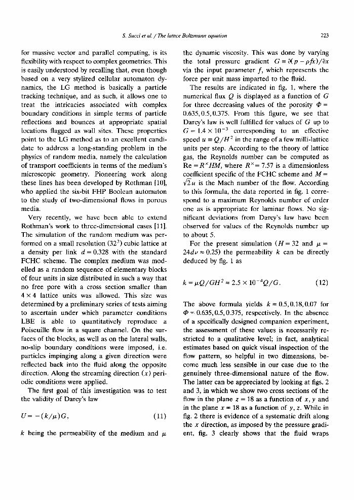
The results are indicated in fig. 1, where the numerical flux Q is displayed as a function of G for three decreasing values of the porosity qb = 0.635,0.5,0.375. From this figure, we see that Darcy's law is well fulfilled for values of G up to G = 1 .4× 10 -3 corresponding to an effective speed u = Q / H 2 in the range of a few milli-lattice units per step. According to the theory of lattice gas, the Reynolds number can be computed as Re = R ×HM, where R ×= 7.57 is a dimensionless coefficient specific of the FCHC scheme and M = v~u is the Mach number of the flow. According to this formula, the data reported in fig. 1 corre- spond to a maximum Reynolds number of order one as is appropriate for laminar flows. No significant deviations from Darcy's law have been observed for values of the Reynolds number up to about 5.

For the present simulation ( H = 32 and IX = 24d~ = 0.25) the permeability k can be directly deduced by fig. 1 as

k = I X Q / G H 2 = 2.5 x I O - 4 Q / G . (12)

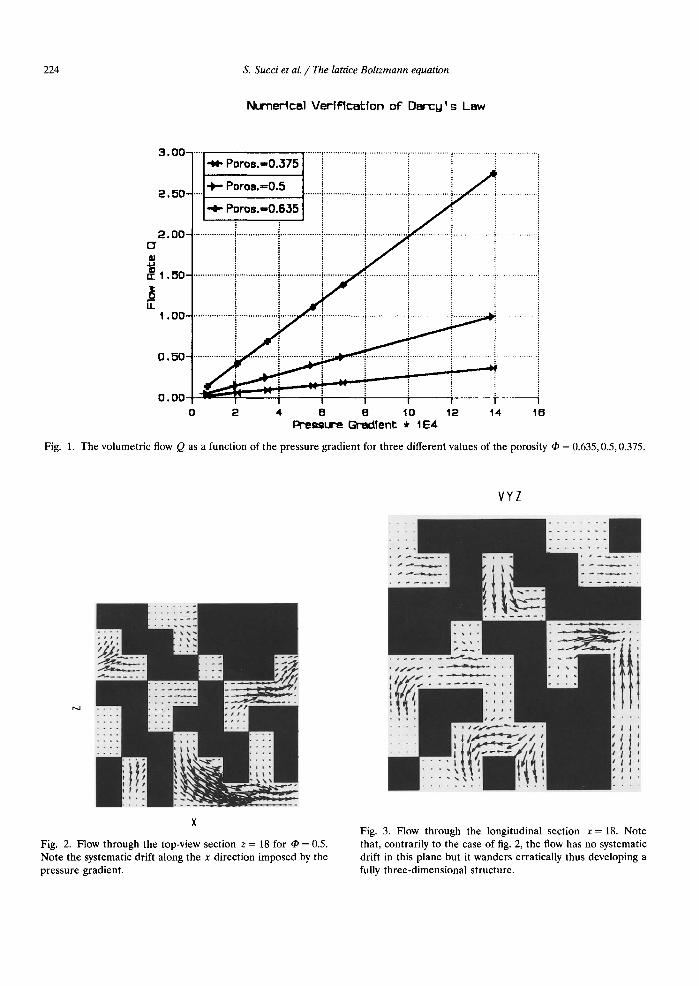
The above formula yields k =0.5,0.18,0.07 for qb = 0.635, 0.5, 0.375, respectively. In the absence of a specifically designed companion experiment, the assessment of these values is necessarily re- stricted to a qualitative level; in fact, analytical estimates based on quick visual inspection of the flow pattern, so helpful in two dimensions, become much less sensible in our case due to the genuinely three-dimensional nature of the flow. The latter can be appreciated by looking at figs. 2 and 3, in which we show two cross sections of the flow in the plane z = 18 as a function of x, y and in the plane x = 18 as a function of y, z. While in fig. 2 there is evidence of a systematic drift along the x direction, as imposed by the pressure gradient, fig. 3 clearly shows that the fluid wraps


Numer4cel Verlf~catlon of Dercu's Law

3 . 0 0 -

2 . 5 0 -

2.00- O W

er 1 . 5 0 -

LL 4.00-

0.50-~

O.OO

.... "¢¢* Poron.zO.375 ....... i .................. i .................. i .................. ! .................. i .................. !

. . . . . . . . . . . . . . . . . . i . . . . . . . . . . . . . . . . . . i . . . . . . . . . . . . . . . . . . . . . . . . . . . . . . . . . . . . :, . . . . . . . . . . . . . . . . . . ' . . . . . . . . . . . . . . . . ~ . . . . . . . . . . . . . " . . . . . . . . . . . . . . . . i

I D

i

-" I I I I

0 2 4 B B 10 12 14 16 Pceggure G r ~ l e n t * I E4

Fig. 1. The volumetric flow Q as a function of the pressure gradient for three different values of the porosity qb = 0.635, 0.5, 0.375.

VYZ

VXZ

Fig. 2. Flow through the top-view section z = 18 for q0 = 0.5. Note the systematic drift along the x direction imposed by the pressure gradient.

N

Fig. 3. Flow through the longitudinal section x = 18. Note that, contrarily to the case of fig. 2, the flow has no systematic drift in this plane but it wanders erratically thus developing a fully three-dimensional structure.

S. Succi et al. / The lattice Boltzmann equation 225

around the solid obstacles along any of the three directions available to the motion.

A semi-qualitative comparison with theoretical results based on simple pictures of shrinking-tube and grain-consolidation models, showed that the numerical simulations yield a permeability which agrees with analytical estimates within about a factor two.

Apart from the quantitative aspects, the main result of this study is the demonstration of the adherence of the LB model to Darcy's law for a three-dimensional flow through a complex medium. The simulation or real rocks is likely to require mesh sizes of the order of 128 cubed, with a corresponding increase of almost two or- ders of magnitude in computing power. Given the fact that, on a IBM 3090/VF, the LBE scheme is processed at a rate of about 0.1 Msi tes /s (with a single processor), running, say, a thousand steps on a 1283 lattice will take approximately 10 h CPU time. This figure can be easily brought down to a couple of hours by running on a six-headed 3090 multiprocessor. Hence, the problem is already feasible on a present-day supercomputer even though, for parametric studies, a significant improvement of these processing speeds is cer- tainly desirable.

181), are placed normal to the flow stream and spaced 6.6 times the channel half-width. This spacing is about three times the wavelength of the channel which needs to be excited in order to destabilize the least stable mode of the Poiseuille flow. The Reynolds number of the system is de- fined as Re = U H / 2 u , where H is the width of the channel and U is the maximum velocity of a Poiseuille flow leading to the same flux as the actual flow.

The laminar-turbulent transition can be de- scribed within the framework of Landau's theory, with the amplitude of the primary bifurcated mode A = p e i° playing the role of the order parameter. The dynamics of the transition is de- scribed by Landau's equations

= SrP - L r P 3,

= S i - L i p 2, (13)

where S and L are two complex coefficients which characterize the transition. In the vicinity of the critical point (S r = 0), they can be taken in the form S r = a r and S i = S o + ~ r , where r = ( R e - R e c ) / R e ~ is the reduced Reynolds number. Above the critical threshold ( r > 0), the steady-state solution of eqs. (13) reads

4.2. Application 2: Bifurcations o f a

two-dimensional Poiseuille f low

It has recently been shown that by exciting obstacle-induced shear-layer instabilities it is possible to promote fluid turbulence in a Poiseuille flow well below the critical Reynolds number of the same flow in a free channel [12]. Apart from the practical motivation of minimizing the cost of mechanical power versus thermal transport, the study of these instabilities provides an interesting scenario of a transition from laminar to turbulent regimes at moderate values of the Reynolds number, typically of the order of hundred. We have studied this problem by considering a plane channel containing a periodic array of identical plates. The plates, one fifth of the channel width ( H =

p ~ S r ~ f ~ r OC r 0"5 ,

to = 0 = S O + ( fl - a L i / L r ) r , (14)

which shows the typical mean-field theory critical exponent 0.5.

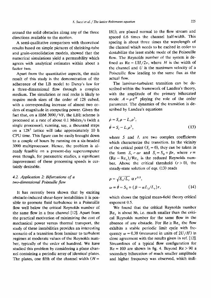
We found that the critical Reynolds number Re c is about 86, i.e. much smaller than the critical Reynolds number for the same flow in the absence of any obstacle. For Re > Re c the flow exhibits a stable periodic limit cycle with frequency to = 0.38 (measured in units of 2 U / H ) in close agreement with the results given in ref. [12]. Streamlines of a typical flow configuration for Re -- 100 are shown in fig. 4. Beyond Re > 90 a secondary bifurcation of much smaller amplitude and higher frequency was observed, which indi-


Fig. 4. Streamlines of the unstable Poiseuille flow at Re = 100.

cates the onset of fully developed turbulence not describable by eqs. (13).

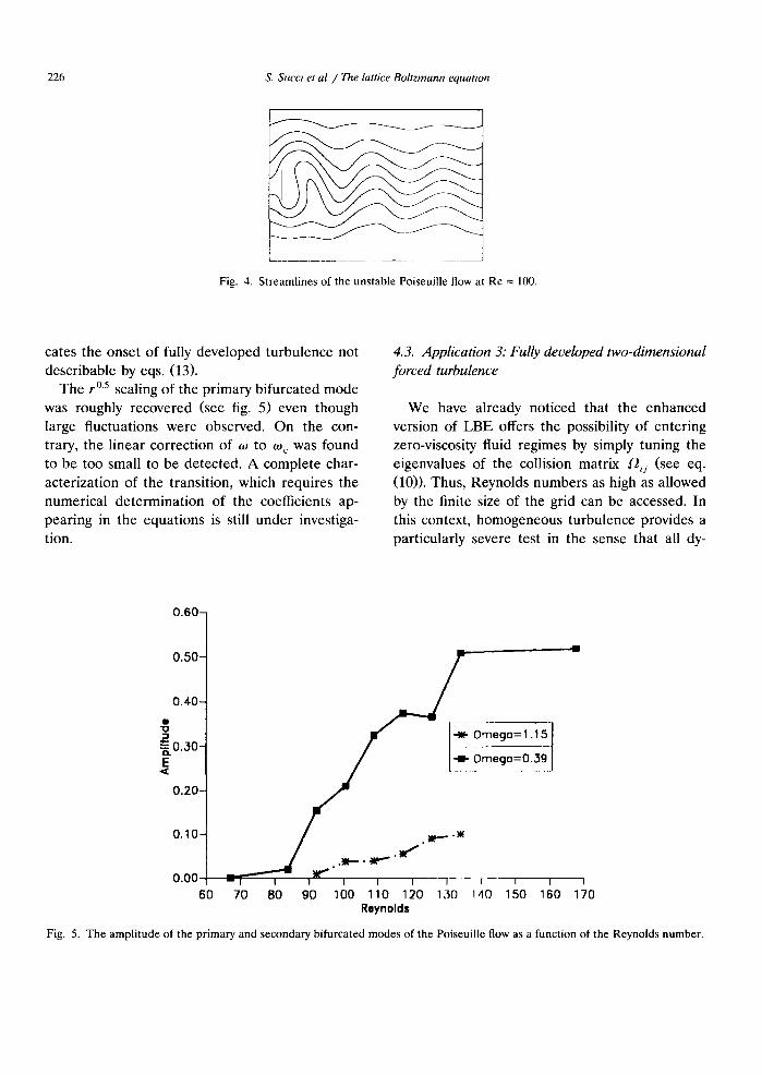
The r °5 scaling of the primary bifurcated mode was roughly recovered (see fig. 5) even though large fluctuations were observed. On the con- trary, the linear correction of to to toc was found to be too small to be detected. A complete char- acterization of the transition, which requires the numerical determination of the coefficients ap- pearing in the equations is still under investigation.

4.3. Application 3: Fully deueloped two-dimensional forced turbulence

W e have already noticed that the enhanced version of LBE offers the possibility of entering zero-viscosity fluid regimes by simply tuning the eigenvalues of the collision matrix .Oij (see eq. (10)). Thus, Reynolds numbers as high as allowed by the finite size of the grid can be accessed. In this context, homogeneous turbulence provides a particularly severe test in the sense that all dy-

0 . 6 0 -

0.50-

0.40-

m "o

~ 0 . 3 0 - E

0 . 2 0 -

0.10-

0.00 i 60 170

? ego=llS [41- Omega=O.39

- ~ ~ ~ ~ ~ ~ -~ - . . . . . ~__ ,

70 80 go 100 110 120 130 140 150 160 Reynolds

Fig. 5. The ampli tude of the primary and secondary bifurcated modes of the Poiseuille flow as a function of the Reynolds number.

S. Succi et aL / The lattice Boltzmann equation 227

namical scales ranging from the macroscopic scale L to the dissipative scale l = L Re -°'5 are effec- tively excited. It is therefore of primary interest to test the ability of LBE to reproduce the basic physics of fully turbulent flows and possibly esti- mate its computational efficiency with respect to other conventional techniques. For this purpose, we have studied a two-dimensional flow in a square box of size 2rr with periodic boundary conditions and a periodic long-wave forcing of the type F = F o s i n ( 2 1 r p y / L ) along the x axis on the wavenumber p = 4.

As a first instance we have compared the physical results obtained by running the LBE and a pseudo-spectral code in a 642 grid, i.e. at a mod- erately low resolution. It is worth mentioning that this comparison is particularly severe since the spectral methods are probably the most well- established numerical technique for this kind of problems.

The spectral viscosity was fixed at the minimum value compatible with the grid resolution, that is to say v - U A x . The spectral time step was At = 0.01, corresponding to 1/382 LBE units after the appropriate scaling between spectral and lattice

units (subscripts sp and B refer to spectral and Boltzmann, respectively):

Lsp = ( 2 a r / N ) L B , Usp = 25UB,

where N is the number of grid points /dimension in the Boltzmann simulation and the factor 25 between speeds stems from the requirement that the maximum speed produced by the force F corresponds to U B = 0.2 (complete details are given in ref. [13]).

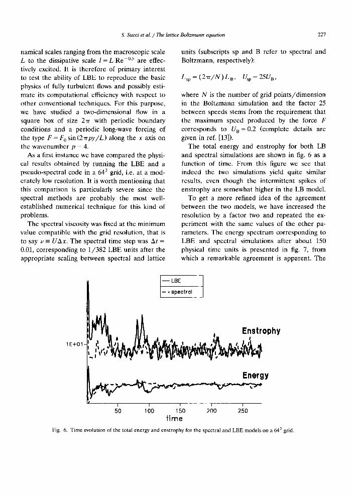
The total energy and enstrophy for both LB and spectral simulations are shown in fig. 6 as a function of time. From this figure we see that indeed the two simulations yield quite similar results, even though the intermittent spikes of enstrophy are somewhat higher in the LB model.

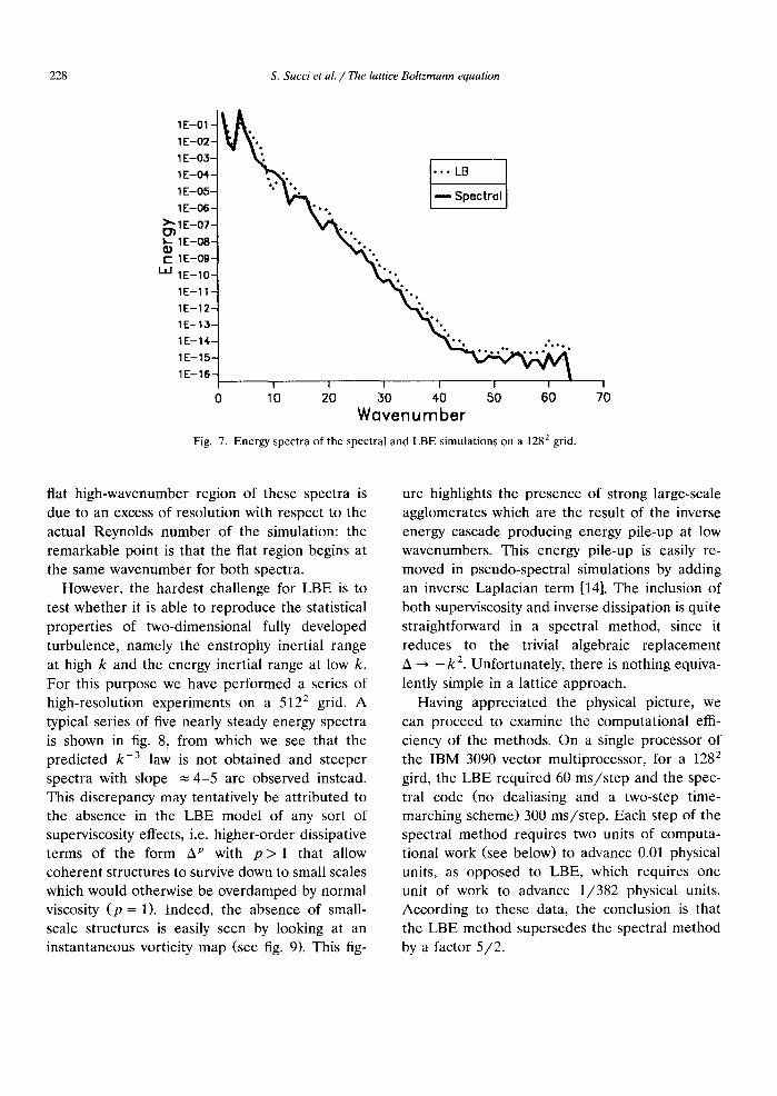
To get a more refined idea of the agreement between the two models, we have increased the resolution by a factor two and repeated the experiment with the same values of the other parameters. The energy spectrum corresponding to LBE and spectral simulations after about 150 physical time units is presented in fig. 7, from which a remarkable agreement is apparent. The

- - L B E

- - ,, B p e c t r o

I1 , Enstrophy 1 +o1 ,,, : ._., , , , / / 1 , . , , .

[ ; . . ; , , ' , , , , ,

I I I . . . . . . . . . . ] - - - - - I

50 1 O0 1 SO 200 250

t ime

Fig. 6. Time evolution of the total energy and enstrophy for the spectral and LBE models on a 642 grid.


1E-01 -

1 E - 0 2 -

1 E - 0 3 -

1E-04 -

1E-O5-

1E-06-

.1 E - 0 7 -

I..- 1 E - 0 8 -

I - 1 E - O 9 -

LLI 1E - lO -

1E-11-

1E-12-

1E-13-

1E-14-

1E-15-

1E-16-

I

I I I I I I

0 10 20 30 40 50 60 Wavenumber

Fig. 7. Energy spectra of the spectral and LBE simulations on a 1282 grid.

70

flat high-wavenumber region of these spectra is due to an excess of resolution with respect to the actual Reynolds number of the simulation: the remarkable point is that the fiat region begins at the same wavenumber for both spectra.

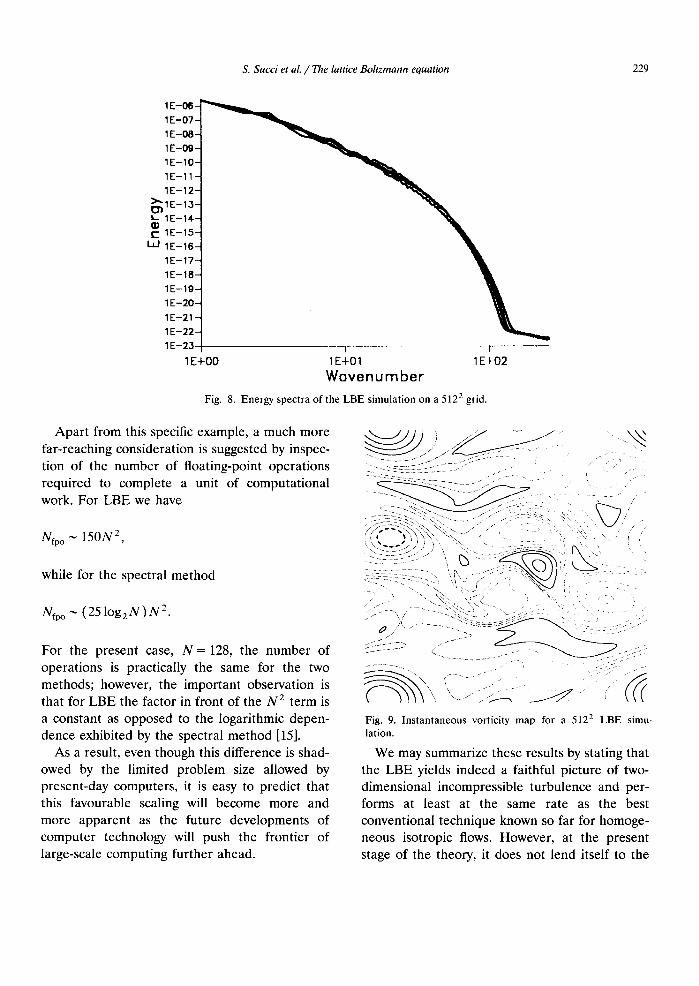
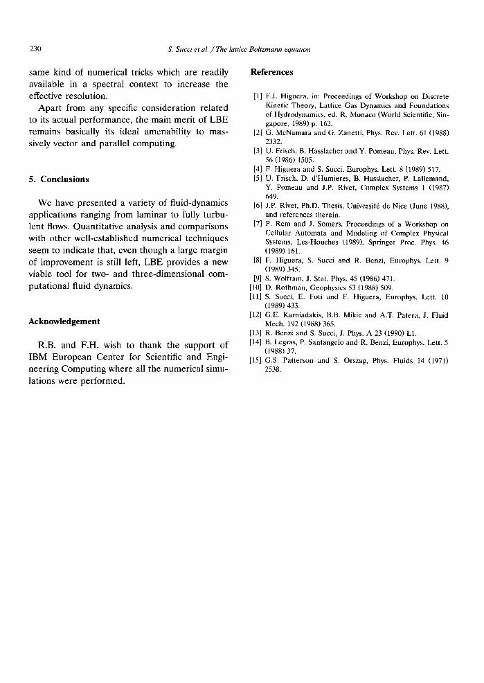
However, the hardest challenge for LBE is to test whether it is able to reproduce the statistical properties of two-dimensional fully developed turbulence, namely the enstrophy inertial range at high k and the energy inertial range at low k. For this purpose we have performed a series of high-resolution experiments on a 5122 grid. A typical series of five nearly steady energy spectra is shown in fig. 8, from which we see that the predicted k -3 law is not obtained and steeper spectra with slope ---4-5 are observed instead. This discrepancy may tentatively be attributed to the absence in the LBE model of any sort of superviscosity effects, i.e. higher-order dissipative terms of the form AP with p > 1 that allow coherent structures to survive down to small scales which would otherwise be overdamped by normal viscosity (p = 1). Indeed, the absence of small- scale structures is easily seen by looking at an instantaneous vorticity map (see fig. 9). This fig-

ure highlights the presence of strong large-scale agglomerates which are the result of the inverse energy cascade producing energy pile-up at low wavenumbers. This energy pile-up is easily removed in pseudo-spectral simulations by adding an inverse Laplacian term [14]. The inclusion of both superviscosity and inverse dissipation is quite straightforward in a spectral method, since it reduces to the trivial algebraic replacement A ~ - k 2. Unfortunately, there is nothing equiva- lently simple in a lattice approach.

Having appreciated the physical picture, we can proceed to examine the computational efficiency of the methods. On a single processor of the IBM 3090 vector multiprocessor, for a 1282 gird, the LBE required 60 ms / s tep and the spectral code (no dealiasing and a two-step time- marching scheme) 300 ms/s tep. Each step of the spectral method requires two units of computational work (see below) to advance 0.01 physical units, as opposed to LBE, which requires one unit of work to advance 1/382 physical units. According to these data, the conclusion is that the LBE method supersedes the spectral method by a factor 5 /2 .

S. Succi et aL / The lattice Boltzmann equation 229

1 E - 0 6 -

1 E - 0 7 -

1 E -OB-

1E-Og-

1 E - 1 0 -

1 E - 1 1 -

1 E - 1 2 -

~ 1E--13-

L_ I E - 1 4 -

t " I E - 1 5 - l.a_l I E - 1 6 -

I E - 1 7 -

I E - 1 8 -

I E - I g -

I E - 2 0 -

IE -21 -

I E - 2 2 -

1E-23 i . . . . . . . . . . . . i

I E+O0 I E+01 I E+02 Wavenumber

Fig. 8. Energy spectra o f the L B E s imulat ion on a 5]22 grid.

Apart from this specific example, a much more far-reaching consideration is suggested by inspection of the number of floating-point operations required to complete a unit of computational work. For LBE we have

Nfp o ~ 1 5 0 N 2,

while for the spectral method

Nfp o ~ (25 l o g 2 N ) N 2.

For the present case, N = 128, the number of operations is practically the same for the two methods; however, the important observation is that for LBE the factor in front of the N2 term is a constant as opposed to the logarithmic depen- dence exhibited by the spectral method [15].

As a result, even though this difference is shad- owed by the limited problem size allowed by present-day computers, it is easy to predict that this favourable scaling will become more and more apparent as the future developments of computer technology will push the frontier of large-scale computing further ahead.

::

o

~ , i ............................ ̧ .I¸

Fig. 9. Instantaneous vorticity map for a 5122 LBE simulation.

We may summarize these results by stating that the LBE yields indeed a faithful picture of two- dimensional incompressible turbulence and per- forms at least at the same rate as the best conventional technique known so far for homogeneous isotropic flows. However, at the present stage of the theory, it does not lend itself to the


same kind of numerical tricks which are readily available in a spectral context to increase the effective resolution.

Apart from any specific consideration related to its actual performance, the main merit of LBE remains basically its ideal amenability to mas- sively vector and parallel computing.

5. Conclusions

We have presented a variety of fluid-dynamics applications ranging from laminar to fully turbulent flows. Quantitative analysis and comparisons with other well-established numerical techniques seem to indicate that, even though a large margin of improvement is still left, LBE provides a new viable tool for two- and three-dimensional computational fluid dynamics.

Acknowledgement

R.B. and F.H. wish to thank the support of IBM European Center for Scientific and Engi- neering Computing where all the numerical simulations were performed.

References

[1] F.J. Higuera, in: Proceedings of Workshop on Discrete Kinetic Theory, Lattice Gas Dynamics and Foundations of Hydrodynamics, ed. R. Monaco (World Scientific, Sin- gapore, 1989)p, 162.

[2] G. McNamara and G. Zanetti, Phys. Rev. Lett. 61 (1988) 2332.

[3] U. Frisch, B. Hasslacher and Y. Pomeau, Phys. Rev. Lett. 56 (1986) 1505.

[4] F. Higuera and S. Succi, Europhys. Lett. 8 (1989) 517. [5] U. Frisch, D. d'Humieres, B. Hasslacher, P. Lallemand,

Y. Pomeau and J.P. Rivet, Complex Systems 1 (1987) 649.

[6] J.P. Rivet, Ph.D. Thesis, Universit6 de Nice (June 1988), and references therein.

[7] P. Rem and J. Somers, Proceedings of a Workshop on Cellular Automata and Modeling of Complex Physical Systems, Les-Houches (1989), Springer Proc. Phys. 46 (1989) 161.

[8] F. Higuera, S. Succi and R. Benzi, Europhys. Lett. 9 (1989) 345.

[9] S. Wolfram, J. Star. Phys. 45 (1986) 471. [10] D. Rothman, Geophysics 53 (1988) 509. [11] S. Succi, E. Foti and F. Higuera, Europhys. Lett. 10

(1989) 433. [12] G.E. Karniadakis, B.B. Mikic and A.T. Patera, J. Fluid

Mech. 192 (1988) 365. [13] R. Benzi and S. Succi, J. Phys. A 23 (1990) L1. [14] B. Legras, P. Santangelo and R. Benzi, Europhys. Lett. 5

(1988) 37. [15] G.S. Patterson and S. Orszag, Phys. Fluids 14 (1971)

2538.

The lattice Boltzmann equation: A new tool for computational fluid-dynamics

Documents

Transcript of The lattice Boltzmann equation: A new tool for computational fluid-dynamics