Computers & Fluids 39 (2010) 568–591

Contents lists available at ScienceDirect

Computers & Fluids

journal homepage: www.elsevier .com/locate /compfluid

Comparison of the lattice Boltzmann and pseudo-spectral methods for decayingturbulence: Low-order statistics

Yan Peng a, Wei Liao a, Li-Shi Luo a,*, Lian-Ping Wang b

a Department of Mathematics & Statistics, Center for Computational Sciences, Old Dominion University, Norfolk, VA 23529, USAb Department of Mechanical Engineering, University of Delaware, 126 Spencer Laboratory, Newark, DE 19716-3140, USA

a r t i c l e i n f o

Article history:Received 20 February 2009Received in revised form 16 June 2009Accepted 6 October 2009Available online 10 November 2009

Keywords:Lattice Boltzmann equationPseudo-spectral methodIncompressible flowDecaying turbulenceLow-order statisticsInstantaneous flow fields

0045-7930/$ - see front matter � 2009 Elsevier Ltd. Adoi:10.1016/j.compfluid.2009.10.002

* Corresponding author. Tel.: +1 757 683 5295; faxE-mail addresses: ypeng@odu.edu (Y. Peng), wlia

odu.edu (L.-S. Luo), lwang@udel.edu (L.-P. Wang).URL: http://www.lions.odu.edu/lluo (L.-S. Luo).

a b s t r a c t

We conduct a detailed comparison of the lattice Boltzmann equation (LBE) and the pseudo-spectral (PS)methods for direct numerical simulations (DNS) of the decaying homogeneous isotropic turbulence in athree-dimensional periodic cube. We use a mesh size of N3 ¼ 1283 and the Taylor micro-scale Reynoldsnumber 24:35 6 Rek 6 72:37, and carry out all simulations to t � 30s0, where s0 is the turbulence turn-over time. In the PS method, the second-order Adam–Bashforth scheme is used to numerically integratethe nonlinear term while the viscous term is treated exactly. We compare the following quantities com-puted by the LBE and PS methods: instantaneous velocity u and vorticity x fields, and statistical quanti-ties such as, the total energy KðtÞ and the energy spectrum Eðk; tÞ, the dissipation rate eðtÞ, the root-mean-squared (rms) pressure fluctuation dpðtÞ and the pressure spectrum Pðk; tÞ, and the skewness and flatnessof the velocity derivative. Our results show that the LBE method performs very well when compared tothe PS method in terms of accuracy and efficiency: the instantaneous flow fields, u and x, and all the sta-tistical quantities — except the rms pressure fluctuation dpðtÞ and the pressure spectrum Pðk; tÞ — com-puted from the LBE and PS methods agree well with each other, provided that the initial flow field isadequately resolved by both methods. We note that dpðtÞ and Pðk; tÞ computed from the two methodsagree with each other in a period of time much shorter than that for other quantities, indicating thatthe pressure field p computed by using the LBE method is less accurate than other quantities. The skew-ness and flatness computed from the LBE method contain high-frequency oscillations due to acousticwaves in the system, which are absent in PS methods. Our results indicate that the resolution require-ment for the LBE method is dx=g0 6 1:0, approximately twice of the requirement for PS methods, wheredx and g0 are the grid spacing and the initial Kolmogorov length, respectively. Overall, the LBE method isshown to be a reliable and accurate method for the DNS of decaying turbulence.

� 2009 Elsevier Ltd. All rights reserved.

1. Introduction tice Boltzmann method (e.g., [16–18]) for DNS of decaying homo-

Homogeneous isotropic turbulence in three-dimensions (3D) isa canonical case in turbulence theory (cf. [1,2] and referencestherein). To date, pseudo-spectral (PS) methods [3,4] remain asthe most accurate numerical tool for direct numerical simulations(DNS) of homogeneous isotropic turbulence (HIT) (e.g., [5–15]).While PS methods are the preferred method for DNS of flows withsimple geometries, such as the channel flow with flat walls or tur-bulence in a cube with periodic boundary conditions, PS methodsmay be difficult to apply for flows with complex geometries ofengineering significance. Development of accurate and efficientmethods for DNS of turbulent flows is one of the most active areasin computational fluid dynamics. In this work, we will use the lat-

ll rights reserved.

: +1 757 683 3885.o@odu.edu (W. Liao), lluo@

geneous isotropic turbulence (DHIT) in three-dimensions (3D).The purpose of the present work is to validate the lattice

Boltzmann method for DNS of decaying turbulence in three dimen-sions. The focus of this work is on the accuracy and efficiency of theinterested numerical methodology, but not on the physics of tur-bulence. The validation will be carried out by conducting a detailedcomparison of the lattice Boltzmann and the pseudo-spectralmethods in terms of accuracy and efficiency for decaying turbu-lence in 3D. The lattice Boltzmann method has been applied forDNS of homogeneous turbulence [19–29]. In particular, there hasbeen previous studies using the LBE method for DNS of decayingturbulence [19–24]. However, the previous studies [19–24] offeronly qualitative comparisons for a very limited number of low-or-der statistical quantities such as the total kinetic energy KðtÞ, thedissipation rate eðtÞ, and the energy spectrum Eðk; tÞ in a relativelyshort period of time. We note that there are some comparativestudies of finite-difference and spectral methods [30,31], whichare restricted low-order turbulence statistics.

Y. Peng et al. / Computers & Fluids 39 (2010) 568–591 569

In this work we will compare in detail the lattice Boltzmann andpseudo-spectral methods for decaying turbulence in 3D by com-puting a number of low-order statistical quantities, in addition toKðtÞ, eðtÞ, and Eðk; tÞ, such as the skewness and the flatness, andthe pressure spectrum Pðk; tÞ. In addition, we will compare theinstantaneous velocity and vorticity fields obtained by the twomethods. The simulations will be carried out for about 30s0, wheres0 is the turbulence turnover time. The direct comparison will al-low us to investigate, first, the differences between the two meth-ods and, second, the effects of the differences on the quantitiesrelevant to decaying turbulence.

The remainder of this paper is organized as follows. Section 2succinctly describes the lattice Boltzmann and pseudo-spectralmethods. Section 3 gives a brief discussion of the decaying turbu-lence, its initial conditions, and the quantities to be computed. Sec-tion 4 presents our results as the following. Section 4.1 describesthe parameters and conditions used in our simulations. Section 4.2compares the instantaneous velocity and vorticity fields obtainedby using the LBE and PS methods with a grid size N3 ¼ 1283 andthe Taylor micro-scale Reynolds number Rek � 24:35. Section 4.3presents the statistical quantities computed by using the twomethods. Section 4.4 analyzes the acoustic waves in the LBE simu-lations, which are absent in the PS simulations. Section 4.5 inves-tigates the dependence of instantaneous flow fields andstatistical quantities on the viscosity m or the Reynolds numberRek. Various results with 24:35 6 Rek 6 72:37 will be discussed.Section 4.6 compares the computational efficiency of the twomethods. Finally, Section 5 summarizes our results and concludesthe paper.

2. Numerical methods

2.1. The lattice Boltzmann equation

We use the lattice Boltzmann equation with the multiple-relaxation-time (MRT) collision model [32–36] and 19 discretevelocities in three dimensions, i.e., the D3Q19 model [35]. TheMRT-LBE can be concisely written as the following:

fðxj þ cdt; tn þ dtÞ ¼ fðxj; tnÞ �M�1 � S � ½m�mðeqÞ�; ð1Þ

where the symbols in bold-font are Q-tuple vectors in RQ for a mod-el with Q discrete velocities,

fðxj; tnÞ :¼ ðf0ðxj; tnÞ; f 1ðxj; tnÞ; . . . ; fbðxj; tnÞÞy;fðxj þ cdt; tn þ dtÞ :¼ ðf0ðxj; tn þ dtÞ; f 1ðxj þ c1dt; tn þ dtÞ;

. . . ; fbðxj þ cbdt; tn þ dtÞÞy;mðxj; tnÞ :¼ ðm0ðxj; tnÞ; m1ðxj; tnÞ; . . . ;mbðxj; tnÞÞy;mðeqÞðxj; tnÞ :¼ ðmðeqÞ

0 ðxj; tnÞ; mðeqÞ1 ðxj; tnÞ; . . . ;mðeqÞ

b ðxj; tnÞÞy;

y denotes transpose, fi is the discrete particle density distributionfunction corresponding to the discrete velocity ci; i 2 f0; 1; . . . ; bg,and mi is the ith moment. The Q � Q matrix M transforms f to m:

m ¼ M � f; f ¼ M�1 �m: ð2Þ

By construction the transform matrix M has the propertythat M �My is diagonal, thus M�1 can be easily obtained[33,35,36].

For the D3Q19 model [35], the 19 discrete velocities are

ci ¼ð0; 0; 0Þ; i ¼ 0;ð�1; 0; 0Þc; ð0; �1; 0Þc; ð0; 0; �1Þc; i ¼ 1—6;ð�1; �1; 0Þc; ð�1; 0; �1Þc; ð0; �1; �1Þc; i ¼ 7—18;

8><>:

ð3Þ

where c :¼ dx=dt. The corresponding 19 moments are

m :¼ ðdq; e; �; jx; qx; jy; qy; jz; qz;3pxx;3pxx; pww;pww;

pxy; pyz;pxz;mx;my;mzÞy ¼ ðm0;m1; . . . ; m18Þy; ð4Þ

where dq is the density fluctuation, the density

q :¼ q0 þ dq; q0 ¼ 1; ð5Þ

and q0 is the mean density. The effect due to round-off error can bereduced by using dq instead of q in the LBE simulations [37]. Theequilibria of the moments are functions of the conserved quantitiesin the system, i.e., the density fluctuation dq and the flow momen-tum j ¼ ðjx; jy; jzÞ :¼ q0u [35]:

dq ¼XQ�1

i¼0

fi; j :¼ q0u ¼XQ�1

i¼0

fici; ð6Þ

where we have applied the approximation for incompressible flows,i.e.,

j ¼ qu � q0u ¼ u: ð7Þ

That is, we assume that in theory jdqj � 1, therefore we can ne-glect the coupling terms between dq and u. The equilibria of thenon-conserved moments in the D3Q19 model for athermal flowsare [35]:

eðeqÞ ¼ �11dqþ 19q0

j � j; ð8aÞ

�ðeqÞ ¼ 3dq� 112q0

j � j; ð8bÞ

qðeqÞx ¼ �2

3jx; qðeqÞ

y ¼ �23

jy; qðeqÞz ¼ �2

3jz; ð8cÞ

pðeqÞxx ¼

13q0

2j2x � j2

y þ j2z

� �h i; pðeqÞ

ww ¼1q0

j2y � j2

z

h i; ð8dÞ

pðeqÞxy ¼

1q0

jxjy; pðeqÞyz ¼

1q0

jyjz; pðeqÞxz ¼

1q0

jxjz; ð8eÞ

pðeqÞxx ¼ �

12

pðeqÞxx ; pðeqÞ

ww ¼ �12

pðeqÞww ; ð8fÞ

mðeqÞx ¼ mðeqÞ

y ¼ mðeqÞz ¼ 0; ð8gÞ

where j � j :¼ j2x þ j2

y þ j2z ¼ u2

x þ u2y þ u2

z . The significance of the mo-ments has been discussed previously [33,35,36].

The diagonal relaxation matrix S is positive and its diagonal ele-ments are relaxation rates, which must satisfy the stability condi-tion si > 1=2 for all non-conserved moments [33,35,36],

S ¼ diagð0; s1; s2;0; s4;0; s4;0; s4; s9; s10; s9; s10; s13; s13; s13; s16; s16; s16Þ¼ diagð0; se; s�; 0; sq; 0; sq;0; sq; sm; sp; sm; sp; sm; sm; sm; sm; sm; smÞ:

ð9Þ

The speed of sound of the D3Q19 model is cs ¼ 1=ffiffiffi3p� �

c and theshear viscosity m and the bulk viscosity f are

m ¼ 13

1sm� 1

2

� �cdx; ð10aÞ

f ¼ ð5� 9c3s Þ

91se� 1

2

� �cdx: ð10bÞ

With the equilibria of Eqs. (8g), if all of the relaxation rates,fsiji ¼ 0; . . . ;18g, are set to be a single value 1=s, i.e., S ¼ s�1I,where I is Q � Q identity matrix, then the model is equivalent tothe D3Q19 LBGK model of which the equilibria are the second-or-der Taylor expansion of the Maxwellian distribution function in u.Except sm, which is determined by the viscosity m, other relaxationrates si may be determined by linear stability analysis [33,35,36].The specific values of si used in our simulations will be givenexplicitly in Section 4.1.

570 Y. Peng et al. / Computers & Fluids 39 (2010) 568–591

The LBE algorithm consists of two steps: collision and advection.For a given LBE model, the collision is the only step involving arith-metic operations, and the number of arithmetic operations at eachgrid node is fixed, while the advection moves data from one gridnode to another with no arithmetic operation. However, advectiondoes cost CPU time for passing data. Thus, the best way to implementLBE code is to combine the collision and advection in one step so thatdata passing time overlaps with the CPU time for floating point oper-ations. In the present work, we still implement collision and advec-tion into two do loops so that the code is easier to modularize andmaintain. Obviously, for a system of size N3, the overall computa-tional cost of the LBE method is of OðN3Þ per time step.

2.2. The pseudo-spectral method

The pseudo-spectral (PS) method solves the incompressible Na-vier–Stokes equations in a cubic domain of size L3 with periodicboundary conditions:

@tuþ u � $u ¼ �$pþ mr2u; x 2 ½0; L�3; ð11aÞ$ � u ¼ 0; ð11bÞ

where the velocity field uðx; tÞ is represented as a finite Fourierseries

uðx; tÞ ¼X

k

~uðk; tÞeık�x; ð12Þ

where ı :¼ffiffiffiffiffiffiffi�1p

. Usually, L ¼ 2p, the grid resolution N in eachdimension is an even number, and the grid spacing is dx ¼ 2p=N.The wavenumber ki; i 2 fx; y; zg, in each dimension varies between�N=2þ 1 and N=2 and the largest wavenumber is kN ¼ N=2. Thefast Fourier transform (FFT) is used to compute ~u. We use the opensource package FFTW 2.1.5 (cf. http://www.fftw.org) for FFT withMPI (cf. http://www-unix.mcs.anl.gov/mpi and http://comput-ing.llnl.gov/tutorials/mpi) in our simulations.

For pseudo-spectral methods, in order to reduce computationalcost, the nonlinear advection term u � $u term is evaluated in phys-ical space as the following. Both the velocity ~u and the vorticity ~x

in Fourier space are transformed by the inverse FFT back to phys-ical space to form the nonlinear term x� u, which is then trans-formed back to wavenumber space k. The de-aliasing isaccomplished by nullifying ~uðk; tÞ for jkj > N=3 at each time step.

The incompressible Navier–Stokes equation can be re-writtenin k space as the following:

@t ~uþ mk2 ~u ¼ �eT?; ð13Þ

where eT is the Fourier transform of x� u,

eT? :¼ eT � ðeT � k̂Þk̂;and k̂ is the unit vector parallel to k. Eq. (13) can be further writtenas

@tð~uemk2tÞ ¼ �eT?emk2t : ð14Þ

We will apply the second-order Adams–Bashforth scheme fortime integration of the above equation:

~uðt þ dtÞ ¼ ~uðtÞ � 12

dt 3eT?ðtÞ � eT?ðt � dtÞe�mk2dth i� �

e�mk2dt : ð15Þ

Eq. (13) circumvents the need to directly solve the Poisson equationfor the pressure p by noting the fact that

~p ¼ ıeT kk� ~j; eT k :¼ k̂ � eT ; ð16Þ

where ~j is the Fourier transform of the kinetic energy u � u=2.Therefore, the pressure p is obtained by computing the inverse Fou-rier transform of ~p given by the above equation.

For homogeneous turbulence with a mesh of size N3, the com-putational cost of the pseudo-spectral method is of the orderOðN3 ln NÞ per time step, while that of the LBE method is ofOðN3Þ. For homogeneous turbulence, pseudo-spectral methodsare the chosen method for their superiority in spatial accuracy.

3. Decaying homogeneous isotropic turbulence in a 3D cube

The decaying homogeneous isotropic turbulence (DHIT) in athree-dimensional cube of the size L3 ¼ ð2pÞ3 with periodic bound-ary conditions in all three directions is a canonical problem in tur-bulence theory. It has been used as a standard test case to validatenumerical schemes for direct numerical simulations. In the DHIT,an initial energy spectrum is given in Fourier space k. In the pres-ent work, the following initial spectrum is used:

E0ðkÞ :¼ Eðk; t ¼ 0Þ ¼ Ak4e�0:14k2; k 2 ½ka; kb�; ð17Þ

where the magnitude A and the range of the initial energy spectrum½ka; kb� determine the initial total kinetic energy K0 in the simula-tion. The divergence-free initial velocity field u0, i.e., $ � u0 ¼ 0, isgenerated in Fourier space k according to Rogallo’s procedure [38]:

~u0ðkÞ¼akk2þbk1k3

kffiffiffiffiffiffiffiffiffiffiffiffiffiffiffiffiffiffiðk2

1þk22Þ

q0B@

1CAk̂1þ

bk2k3�ak1k

kffiffiffiffiffiffiffiffiffiffiffiffiffiffiffiffiffiffiðk2

1þk22Þ

q0B@

1CAk̂2�

bffiffiffiffiffiffiffiffiffiffiffiffiffiffiffiffiffiffiðk2

1þk22Þ

qk

0@

1Ak̂3;

ð18Þ

where a ¼ffiffiffiffiffiffiffiffiffiffiffiffiffiffiffiffiffiffiffiffiffiffiffiffiE0ðkÞ=4pk2

qeıh1 cos /;b ¼

ffiffiffiffiffiffiffiffiffiffiffiffiffiffiffiffiffiffiffiffiffiffiffiffiE0ðkÞ=4pk2

qeıh2 sin /; h1; h2

and / are uniform random variables between 0 and 2p; ı :¼ffiffiffiffiffiffiffi�1p

;and k̂1, k̂2, and k̂3 are the unit vectors along three axis in k-space.The turbulent fluctuating velocity field u has a zero mean, i.e.,hui ¼ 0, and is characterized by its root-mean-squared (rms) value:

u0 :¼ 1ffiffiffi3p

ffiffiffiffiffiffiffiffiffiffiffiffiffiffihu � ui

p; ð19Þ

where h�i designates ensemble average, which can be carried out asvolume average in either physical space x or spectral space k.

We will compare instantaneous velocity field uðxj; tnÞ and vor-ticity field xðxj; tnÞ obtained from the LBE and PS methods. The vor-ticity fields xðxj; tnÞ in both methods will be computed in spectralspace k by the inverse FFT of ~x ¼ �ık� ~u. We compute the energyspectrum Eðk; tÞ and the compensated spectrum WðkÞ of the veloc-ity field uðx; tÞ,

Eðk; tÞ :¼ 12

~uðk; tÞ � ~uyðk; tÞ; ð20aÞ

WðkÞ :¼ eðkÞ�2=3k5=3EðkÞ; ð20bÞ

and other statistical quantities pertinent to DHIT:

KðtÞ :¼ 12hu � ui ¼

ZdkEðk; tÞ; ð21aÞ

XðtÞ :¼ hð$uÞ2i ¼Z

dkk2Eðk; tÞ; ð21bÞ

eðtÞ :¼ 2mXðtÞ; g :¼ffiffiffiffiffiffiffiffiffiffim3=e4

q; ð21cÞ

SuiðtÞ ¼ hð@iuiÞ3i

hð@iuiÞ2i3=2 ; SuðtÞ ¼13

Xi

Sui; ð21dÞ

FuiðtÞ ¼ hð@iuiÞ4i

hð@iuiÞ2i2; FuðtÞ ¼

13

Xi

Fui; ð21eÞ

where KðtÞ;XðtÞ, and eðtÞ are the total kinetic energy, the enstrophy,and the dissipation rate, respectively; g is the Kolmogorov lengthscale; Sui

ðtÞ is the skewness computed from @iui; i 2 fx; y; zg, andSuðtÞ is the skewness averaged over three directions; and Fui

ðtÞ is

Y. Peng et al. / Computers & Fluids 39 (2010) 568–591 571

the flatness computed from ui and FuðtÞ is the flatness averaged overthree directions. We also compute the pressure spectrum PðkÞ,

hðdpÞ2i ¼Z

dkPðkÞ; ð22Þ

where dp is the pressure fluctuation. For the DHIT, the Taylor micro-scale Reynolds number Rek is used to characterize the flow:

Rek :¼ u0km; k :¼

ffiffiffiffiffiffiffi152X

ru0; ð23Þ

where k is the transverse Taylor micro-scale length.Because the LBE method is intrinsically a compressible flow sol-

ver, we monitor the rms velocity divergence

H0ðtÞ :¼ffiffiffiffiffiffiffiffiffiffiffiffiffiffiffiffiffiffiffiffihð$ � uÞ2i

q: ð24Þ

Note that for incompressible flows, $ � u ¼ 0, thus H0 ¼ 0 andX ¼ hx � xi=2, where x :¼ $� u is the vorticity. We also monitorthe Mach number in the LBE simulations,

Ma ¼ ucs; cs ¼

ffiffiffiffiffiffiRTp

; ð25Þ

where RT ¼ 13 c2 and c :¼ dx=dt.

4. Results

4.1. Parameters and flow conditions

To compare two significantly different methods such as the LBEand PS methods, we must first properly choose a number of param-eters used in the simulation so that the comparison is meaningful.First of all, the simulations carried out to compare the two methodsshould have the same system size L3 ¼ ð2pÞ3 and the grid resolu-tion N3, the initial Taylor micro-scale Reynolds number Rek, andthe dimensionless time step size dt0 normalized by the turbulenceturnover time s0 ¼ K0=e0. The grid spacing is dx ¼ 2p=N. In the LBEmethod, all quantities are in the units of dx ¼ dt ¼ 2p=N. In the PSmethod, dx ¼ 2p=N, the initial kinetic energy K0 is always set to 1,therefore the initial rms velocity is u00 ¼

ffiffiffiffiffiffiffiffi2=3

p. With equal initial

Rek and the dimensionless time step size dt0, both the viscosity mand the time step size dt in the PS calculations must be relatedto their LBE counterpart as the following:

mPS ¼mLBEffiffiffiffiffiffi

K0p ; dtPS ¼

ffiffiffiffiffiffiK0

pdtLBE; ð26Þ

where K0 is the initial total kinetic energy in the LBE simulationcomputed from Eq. (17) with given parameter values of A; ka andkb. Table 1 summarizes the relationships between various quanti-ties in the LBE and PS methods.

For the initial energy spectrum E0ðkÞ given by Eq. (17), we useA ¼ 1:4293� 10�4; ka ¼ 3, and kb ¼ 8, thus the initial kinetic en-ergy is K0 � 1:0130� 10�2, the rms velocity is u0 � 8:2181� 10�2,and the initial enstrophy is X0 � 0:2077.

For the LBE method, we must ensure that the local Mach num-ber Ma is small enough so that the LBE method is well within theincompressible flow region. With the initial energy spectrum and

Table 1Parameters used in the lattice Boltzmann (LBE) and pseudo-spectral (PS) methods. K0

and e0 are the initial total kinetic energy and dissipation rate in the LBE simulations,respectively, computed from the initial spectrum E0ðkÞ given by Eq. (17) withparameters A; ka, and kb.

Method K0 u00 m L dx dt dt0

LBE K0ffiffiffiffiffiffiffiffiffiffiffiffiffiffi2K0=3

p m 2p 2p=N 2p=N 2pe0=K0N

PS 1ffiffiffiffiffiffiffiffi2=3

pm=

ffiffiffiffiffiffiK0p

2p 2p=N 2pffiffiffiffiffiffiK0p

=N 2pe0=K0N

parameters given above, we can ensure that the maximum localMach number Mamax ¼ ku0kmax=cs 6 0:15 for the initial velocityfield u0, where cs ¼ 1=

ffiffiffi3p� �

c is the sound speed in the LBE model.The viscosity used in the LBE simulations is m ¼ ð1=600Þcdx. Withthe initial energy spectrum E0ðkÞ and the viscosity m given above,the Taylor micro-scale Reynolds Rek � 24:35.

In the LBE simulations, we set the values of the relaxation ratesfor all non-conserved moments, except the stresses, as si ¼ 1:8 –sm. We have also tested other values of si – sm, and have found that,within a certain range, they have little noticeable effect on the re-sults of DHIT.

For homogeneous isotropic turbulence with a given Rek, the re-quired resolution for DNS in 3D using spectral methods can be esti-mated as (cf. [39,1]):

N P 0:4Re3=2k : ð27Þ

The above formula can be re-written in terms of the Kolmogo-rov length scale g normalized by the grid spacing dx [1]:

gdx

P1

2:1� 0:476: ð28Þ

Since the lattice Boltzmann method is formally a second-ordermethod [40,41], the resolution requirement for the LBE methodwould not be the same as the above criterion (28) for spectralmethods, which are exponentially accurate. Thus, for the LBE meth-od we should consider a resolution criterion more stringent thanEq. (28), such as

gdx

P 1:0: ð29Þ

The above criterion is consistent with previous empirical obser-vations (cf. [42,43]) and will be tested in our simulations.

4.2. Instantaneous velocity and vorticity fields

First, we will directly compare instantaneous flow fields ob-tained with the LBE and PS methods with Rek � 24:35. The initialvelocity fields used in both the LBE and PS methods are identicalexcept an overall scaling factor, as discussed in the previous sec-tion. That is, one single random velocity field is generated withthe energy spectrum of Eq. (17), then it is rescaled such thatu00 ¼

ffiffiffiffiffiffiffiffi2=3

pfor the PS method, and Mamax 6 0:15 for the LBE meth-

od. For the PS method, the pressure p is obtained by solving thePoisson equation in the spectral space. As for the LBE method, pis obtained by using an iterative procedure which solves thePoisson equation consistent with the LBE method [44]. Before wecompare the results obtained by the LBE and PS methods, weshould bear in mind that these two methods are different fromeach other. Specifically, the PS method solves the incompressibleNavier–Stokes equation with an exponential accuracy in space forall flow variables, while the LBE method is formally second-orderaccurate in space for the velocity field u and only first-order accu-rate for the pressure field p [40,41]. As for the accuracy in time, thePS method is second-order, while formally the LBE method is onlyfirst-order [41]. In some way the LBE method can be viewed as aNavier–Stokes solver with artificial compressibility.

We first show the evolution of the magnitude of the velocityfield normalized by its initial rms value k�uk :¼ u=u00

on. The sys-tem size is 1283 and the Taylor micro-scale Reynolds number isRek � 24:35 unless it is otherwise stated. We compare results fromthree runs with an identical initial velocity field apart from anoverall constant factor: the LBE method, the PS method with thedimensionless time step size dt0 equal to that of the LBE method(labeled as PS1), and the PS method with the dimensionless timestep size equal to one third of that in the LBE method (labeled asPS2). The dimensionless time step size, normalized by the

572 Y. Peng et al. / Computers & Fluids 39 (2010) 568–591

turbulence turnover time s0 ¼ K0=e0, is dt0 ¼ 4pmX0=NK0 �2:892� 10�3. All runs stop at t0 � 30, when the total kinetic energyK decays almost four orders of magnitude, and the rms velocity u0

decays almost two orders of magnitude.The results for the evolution of k�uk on the xy plane z ¼ p are

shown in Fig. 1. We compare the results obtained by the three runsin four instances: t0 � 4:048; 8:095; 16:189, and 29.949. Even atthe latest time t0 � 29:949, the velocity field �u obtained from theLBE method is very similar to those obtained from the PS methodwith an equal time step size dt0 or a smaller one (i.e., dt0=3): bothmagnitudes and locations of vortices in the velocity fields obtainedby different methods are very close to each other.

The agreement between the flow fields is further demonstratedwith the evolution of the vorticity field normalized by the initialrms velocity k�xk :¼ xkL=u00

on a plane. The vorticity fields for bothLBE and PS simulations are computed in spectral spacek; ~x ¼ �ık� ~u, and then by using the inverse FFT to transfer ~x backto physical space x. The results of k�xk are shown in Fig. 2. Clearly,at t0 � 29:949, the difference between the LBE and PS vorticityfields is visible in Fig. 2. While the basic features of the vorticityfields obtained from the LBE and PS methods remain quite similar,in terms of vortex shapes and locations, the LBE and PS resultsclearly deviate from each other more and more as time evolves.

We also show the evolutions of velocity and vorticity magni-tude iso-surfaces in three dimensions in Figs. 3 and 4, respectively.We show the iso-surfaces of velocity and vorticity magnitudes inthree times: t0 ¼ 0:1348;0:2359, and 0.5730, corresponding tothe times before, about, and after the dissipation rate eðt0Þ attainsits maximum (cf. Fig. 7 in the next section). We note that the flowfeatures obtained by using the LBE and PS methods agree well witheach other, even in small scales of a few grid spacings. It should bestressed that for a strongly nonlinear system, such as the Navier–Stokes equation, a small difference in the initial conditions cangrow exponentially in time. Therefore, it is remarkable that theflow fields computed from the LBE and PS methods should agreewith each other so well, as shown in Figs. 1–4. The differences be-tween the flow fields obtained by the LBE and PS methods will befurther quantified in Section 4.5.

4.3. Statistical quantities

We now compare the statistical quantities of the decayinghomogeneous isotropic turbulence (DHIT) obtained by using theLBE and PS methods. In Fig. 5 we first show the energy spectraEðk; t0Þ and the compensated spectra Wðk; t0Þ. The results obtainedwith the LBE and PS methods with an equal time step size agreevery well with each other. In fact, they show no visible differencein the spectra. If the compensated spectra is rescaled to Wðkg; t0Þ,it can be shown that when kg > 2, i.e., in small scales, the compen-sated spectra Wðkg; t0Þ collapse to a single curve which is timeindependent, as expected [1].

To quantify the differences between the results obtained fromdifferent methods, we compute the following difference betweenthe spectra Eðk; t0Þ:

DEðk; t0Þ ¼ kE1ðk; t0Þ � E2ðk; t0Þk; ð30Þ

where the subscripts ‘‘1” and ‘‘2” denote different methods. Weshow the results of DEðk; t0Þ for the LBE vs. PS1 (left) and PS1 vs.PS2 (right) in Fig. 6. Clearly DEðk; t0Þ for LBE vs. PS1 is very similarto that for PS1 vs. PS2, as shown in Fig. 6. Also, the differences ofthe spectra DEðk; t0Þ are very similar to the spectra Eðk; t0Þthemselves.

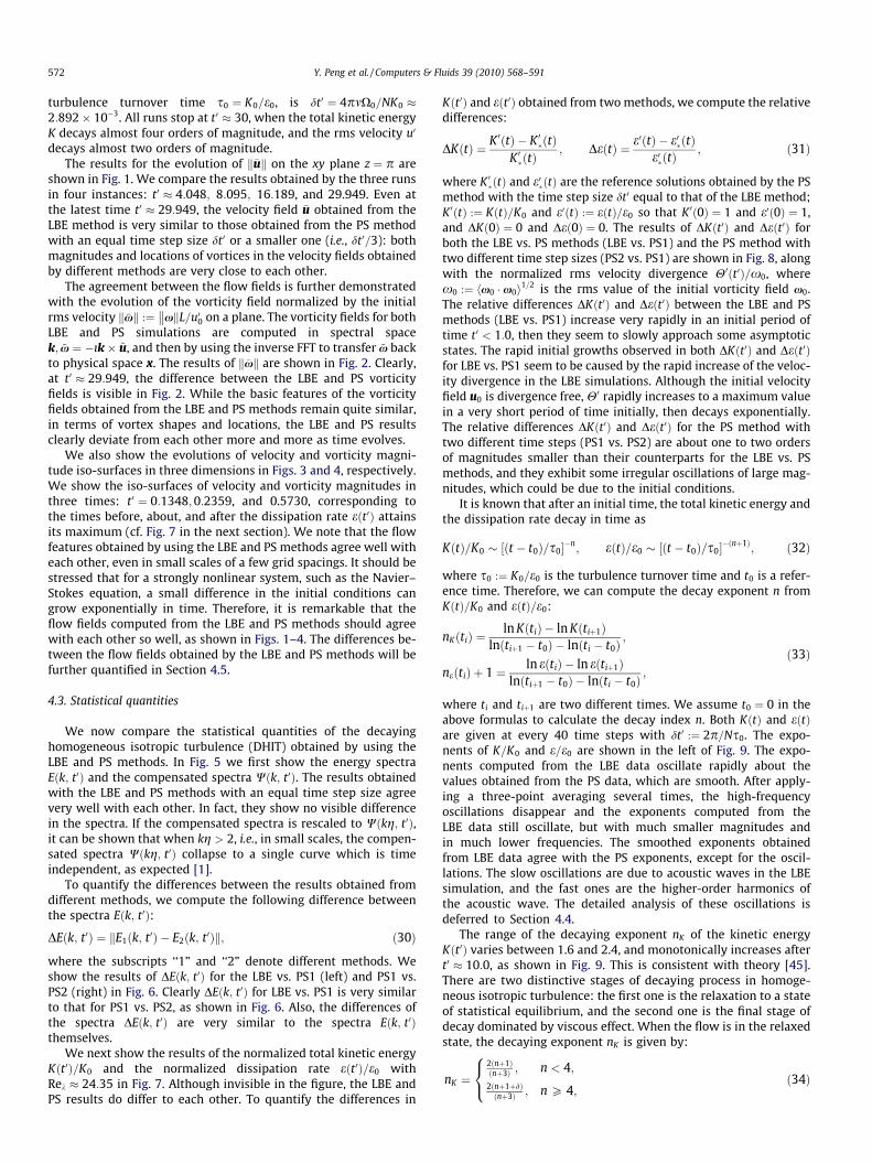
We next show the results of the normalized total kinetic energyKðt0Þ=K0 and the normalized dissipation rate eðt0Þ=e0 withRek � 24:35 in Fig. 7. Although invisible in the figure, the LBE andPS results do differ to each other. To quantify the differences in

Kðt0Þ and eðt0Þ obtained from two methods, we compute the relativedifferences:

DKðtÞ ¼ K 0ðtÞ � K 0ðtÞK 0ðtÞ

; DeðtÞ ¼ e0ðtÞ � e0ðtÞe0ðtÞ

; ð31Þ

where K 0ðtÞ and e0ðtÞ are the reference solutions obtained by the PSmethod with the time step size dt0 equal to that of the LBE method;K 0ðtÞ :¼ KðtÞ=K0 and e0ðtÞ :¼ eðtÞ=e0 so that K 0ð0Þ ¼ 1 and e0ð0Þ ¼ 1,and DKð0Þ ¼ 0 and Deð0Þ ¼ 0. The results of DKðt0Þ and Deðt0Þ forboth the LBE vs. PS methods (LBE vs. PS1) and the PS method withtwo different time step sizes (PS2 vs. PS1) are shown in Fig. 8, alongwith the normalized rms velocity divergence H0ðt0Þ=x0, wherex0 :¼ hx0 � x0i1=2 is the rms value of the initial vorticity field x0.The relative differences DKðt0Þ and Deðt0Þ between the LBE and PSmethods (LBE vs. PS1) increase very rapidly in an initial period oftime t0 < 1:0, then they seem to slowly approach some asymptoticstates. The rapid initial growths observed in both DKðt0Þ and Deðt0Þfor LBE vs. PS1 seem to be caused by the rapid increase of the veloc-ity divergence in the LBE simulations. Although the initial velocityfield u0 is divergence free, H0 rapidly increases to a maximum valuein a very short period of time initially, then decays exponentially.The relative differences DKðt0Þ and Deðt0Þ for the PS method withtwo different time steps (PS1 vs. PS2) are about one to two ordersof magnitudes smaller than their counterparts for the LBE vs. PSmethods, and they exhibit some irregular oscillations of large mag-nitudes, which could be due to the initial conditions.

It is known that after an initial time, the total kinetic energy andthe dissipation rate decay in time as

KðtÞ=K0 ½ðt � t0Þ=s0��n; eðtÞ=e0 ½ðt � t0Þ=s0��ðnþ1Þ

; ð32Þ

where s0 :¼ K0=e0 is the turbulence turnover time and t0 is a refer-ence time. Therefore, we can compute the decay exponent n fromKðtÞ=K0 and eðtÞ=e0:

nKðtiÞ ¼ln KðtiÞ � ln Kðtiþ1Þ

lnðtiþ1 � t0Þ � lnðti � t0Þ;

neðtiÞ þ 1 ¼ ln eðtiÞ � ln eðtiþ1Þlnðtiþ1 � t0Þ � lnðti � t0Þ

;

ð33Þ

where ti and tiþ1 are two different times. We assume t0 ¼ 0 in theabove formulas to calculate the decay index n. Both KðtÞ and eðtÞare given at every 40 time steps with dt0 :¼ 2p=Ns0. The expo-nents of K=K0 and e=e0 are shown in the left of Fig. 9. The expo-nents computed from the LBE data oscillate rapidly about thevalues obtained from the PS data, which are smooth. After apply-ing a three-point averaging several times, the high-frequencyoscillations disappear and the exponents computed from theLBE data still oscillate, but with much smaller magnitudes andin much lower frequencies. The smoothed exponents obtainedfrom LBE data agree with the PS exponents, except for the oscil-lations. The slow oscillations are due to acoustic waves in the LBEsimulation, and the fast ones are the higher-order harmonics ofthe acoustic wave. The detailed analysis of these oscillations isdeferred to Section 4.4.

The range of the decaying exponent nK of the kinetic energyKðt0Þ varies between 1.6 and 2.4, and monotonically increases aftert0 � 10:0, as shown in Fig. 9. This is consistent with theory [45].There are two distinctive stages of decaying process in homoge-neous isotropic turbulence: the first one is the relaxation to a stateof statistical equilibrium, and the second one is the final stage ofdecay dominated by viscous effect. When the flow is in the relaxedstate, the decaying exponent nK is given by:

nK ¼2ðnþ1Þðnþ3Þ ; n < 4;

2ðnþ1þdÞðnþ3Þ ; n P 4;

8<: ð34Þ

Fig. 1. Evolution of velocity field with Rek � 24:35 and N3 ¼ 1283. Contours of kuk=u00 on the plane z ¼ p. Left column: LBE (thick red lines) vs. PS1 (thin dashed green lines)with equal dt0; center column: LBE (thick red lines) vs. PS2 (thin dashed blue lines) with dt0LBE ¼ 3dt0PS; and right column: PS1 (thick green lines) vs. PS2 (thin dashed bluelines). From top to bottom: t0 ¼ 4:048169;8:095571;16:18959, and 29.94941. (For interpretation of the references to colour in this figure legend, the reader is referred to theweb version of this article.)

Y. Peng et al. / Computers & Fluids 39 (2010) 568–591 573

where both n and d are determined by the asymptotic properties ofthe initial energy spectrum:

limk!0

Eðk; t ¼ 0Þ ¼ A0kn; ð35aÞ

limt!1

A0 ¼ t�d: ð35bÞ

It is observed that the effect of d on nK is rather weak (ca. 2%)[45]. In the final stage of decay,

Fig. 2. Evolution of the vorticity field with Rek � 24:35. Contours of kxkL=u00 on the plane z ¼ p. Similar to Fig. 1.

574 Y. Peng et al. / Computers & Fluids 39 (2010) 568–591

nK ¼12ðnþ 1Þ: ð36Þ

We use n ¼ 4 here, as given by Eq. (17), thusnK � 10=7 � 1:43 for the relaxed state and nK ¼ 5=2 ¼ 2:5 forthe final state. The results of nKðt0Þ in Fig. 9 show that flow doesgo through a nonlinear relaxation and approaches to the final

state of decay, as nK becomes close to 2.5 from below. Giventhe significant difference between the two methods, it is remark-able that nKðt0Þ’s computed from both simulations agree so wellwith each other.

We compare the rms pressure fluctuation dp0 obtained by theLBE and PS methods in Fig. 10(left). While the general feature ofthe rms pressures obtained by the LBE and PS methods are similar,

Fig. 3. Evolution of velocity magnitude iso-surface kuk=u00 ¼ 2:0. Rek � 24:35 and N3 ¼ 1283. From left to right: t0 ¼ 0:1348; 0:2359, and 0.5730. LBE (top row) vs. PS(bottom).

Y. Peng et al. / Computers & Fluids 39 (2010) 568–591 575

their quantitative differences are considerable. First, the LBE resultis oscillatory because of the acoustic waves in the system, whichare absent in the PS simulations. And second, the LBE result decaysslightly faster than the PS one initially, which is not visible in thefigure. There are at least two obvious contributing factors respon-sible for the differences between the LBE and PS pressure fluctua-tion. First and foremost, the LBE method does not solve the Poissonequation for the pressure p, which evolves as density fluctuationsthrough the equation of state. The initial pressure fields are notidentical in the LBE and PS methods, while the initial velocity fieldsare identical apart from an overall scaling factor. Nevertheless, wedo find that the initial rms pressure fluctuations dp00 in both the LBEand PS simulations are very close to each other; they differ by lessthan 0.7%. Second, the LBE method has a non-zero bulk viscosity fwhich is merely a numerical artifact. The bulk viscosity f in the LBEmethod affects the attenuation of acoustic waves in the system anddirectly contributes to the dissipation of the pressure fluctuations.Because the LBE method does not solve the Poisson equation andcannot enforce the divergence-free condition for the velocity fieldas in the PS method, the divergence of the velocity is not zero in theLBE simulations.

In Fig. 10(right) we show the pressure spectrum Pðk; t0Þ. For ashort period of time up to t0 � 1:0, the pressure spectrum Pðk; t0Þobtained by the LBE method agrees with that obtained by the PSmethod quantitatively. However, as time goes, the LBE result devi-ates more and more from the PS results for small k, that is, the LBEmethod does not accurately capture large-scale pressure fluctua-tions in simulations. It is interesting to note that the deterioratingpressure field in the LBE simulation seems to have little effect onthe quality of the velocity and vorticity fields.

The skewness and flatness (or kurtosis) are the third-order andfourth-order moments of $u, respectively, and the skewness is re-lated to the fourth-order derivative of the velocity field. For a sec-ond-order accurate method such as the LBE, computing higher-order velocity-derivatives can be a challenging task. In Fig. 11,we compare both the skewness and the flatness computed from@xux; @yuy; @zuz and their averaged value in the LBE and PS simula-tions. When t0 < 8:0, the LBE and PS results agree well with eachother, especially the averaged skewness Su and flatness Fu,although the LBE results have high-frequency oscillations due tothe acoustic waves in the system. The magnitudes of the oscilla-tions grow in time as the velocity field decays, because numericaldifferentiation amplifies fluctuations; the higher the order of thederivatives, the greater the amplification. When high-frequencyoscillations are filtered out by simple smoothing through averag-ing, the LBE results indeed agree very well with the PS results, asshown in the bottom row of Fig. 11. This indicates once again thatthe LBE pressure fluctuations due to the ‘‘artificial” compressibilitydo not adversely affect the averaged quantities in the simulation.

4.4. Acoustic oscillation in LBE results

One salient distinction between the LBE and PS methods is thatthe former is (weakly) compressible while the latter is incompress-ible. In the LBE method, density fluctuations are intrinsic. Also, thespeed of sound is very slow, cs ¼ 1=

ffiffiffi3p� �

c ðc :¼ dx=dtÞ. We willshow that intrinsic density fluctuations in the LBE method areresponsible for the oscillations observed in various statisticalquantities we show in the previous section.

Fig. 5. The energy spectra Eðk; t0Þ (left) and the compensated spectra Wðk; t0Þ (right) with Rek � 24:35 and N3 ¼ 1283. The lines and symbols are the LBE and PS1 results,respectively.

Fig. 4. Evolution of vorticity magnitude iso-surface kxkL=u00 ¼ 13:0. Rek � 24:35 and N3 ¼ 1283. From left to right: t0 ¼ 0:1348; 0:2359, and 0.5730. LBE (top row) vs. PS(bottom).

576 Y. Peng et al. / Computers & Fluids 39 (2010) 568–591

Given the dimension of the cube is L ¼ 2p and the speed ofsound is cs ¼ 1=

ffiffiffi3p� �

c, the period of the acoustic wave normal-ized by the turbulence turnover time s0 ¼ K0=e0 isT 0 ¼ 2p

ffiffiffi3p

e0=K0, and the normalized basic acoustic frequencyis f 0 :¼ 1=T 0 ¼ K0=2p

ffiffiffi3p

e0. For the case of Rek � 24:35, the fun-damental frequency of the sound wave should be aboutf 0s � 1:3444.

To identify the sources of oscillations in various quantities ob-tained by the LBE method, we carry out the following analysis.First, an interested quantity is decomposed into a smooth slow-varying component, which can be obtained by, e.g., local averaging,and a fast-oscillating component with zero mean value over time.Then the FFT is applied to compute the power spectrum of the fast-oscillating component in the frequency domain f 0.

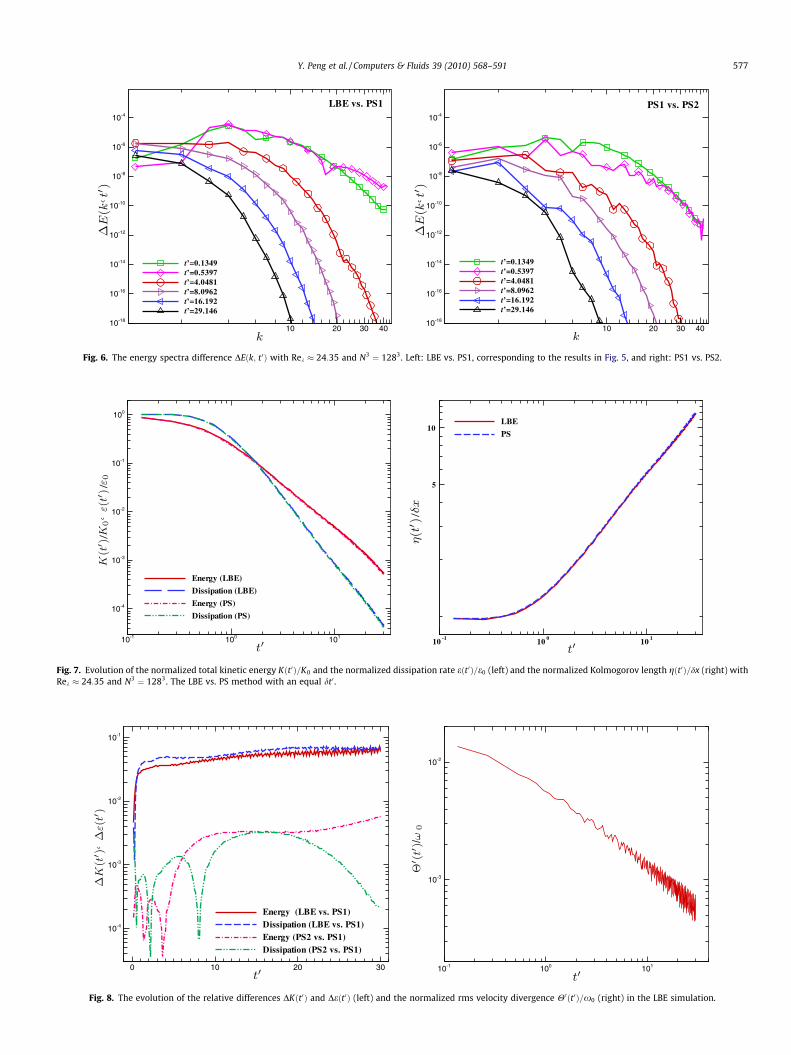
Fig. 6. The energy spectra difference DEðk; t0Þ with Rek � 24:35 and N3 ¼ 1283. Left: LBE vs. PS1, corresponding to the results in Fig. 5, and right: PS1 vs. PS2.

Fig. 7. Evolution of the normalized total kinetic energy Kðt0Þ=K0 and the normalized dissipation rate eðt0Þ=e0 (left) and the normalized Kolmogorov length gðt0Þ=dx (right) withRek � 24:35 and N3 ¼ 1283. The LBE vs. PS method with an equal dt0 .

Fig. 8. The evolution of the relative differences DKðt0Þ and Deðt0 Þ (left) and the normalized rms velocity divergence H0ðt0Þ=x0 (right) in the LBE simulation.

Y. Peng et al. / Computers & Fluids 39 (2010) 568–591 577

Fig. 9. Decaying exponents nK and ne computed from Kðt0Þ=K0 and eðt0Þ=e0, respectively, corresponding to Fig. 7. Left: the results computed from Eq. (33) and right: the LBEresults smoothed by local averaging.

Fig. 10. The rms pressure fluctuation dp0ðt0Þ=dp00 (left) and the pressure spectra Pðk; t0Þ (right), LBE vs. PS1.

578 Y. Peng et al. / Computers & Fluids 39 (2010) 568–591

We first show in Fig. 12 the power spectra of fluctuations of thedecay exponent n computed from the total energy Kðt0Þ and thedissipation rate eðt0Þ by using the finite-difference formulas (33),corresponding to Fig. 9(left). The first and second peaks of bothn̂Kðf 0Þ and n̂eðf 0Þ are f 0 � 1:3316 and 2.6632, respectively. The firstpeak corresponds to the fundamental frequency f 0s of the acousticwave, and the second one to the second harmonic frequency 2f 0s .The second harmonic is much more intense than the fundamentalone because both Kðt0Þ and eðt0Þ are related to u � u. The spectra inFig. 12 clearly show that the acoustic wave in the LBE simulation isresponsible for the oscillations in nK and ne of Fig. 9(left).

We next show in Fig. 13 the power spectra of oscillating compo-nents of the rms pressure fluctuation dp0ðt0Þ and the rms velocitydivergence H0ðt0Þ. Both these spectra are very much similar to theprevious ones, for they are also related to u � u. It is interesting tonote that the strength of the fundamental frequency f 0s for therms pressure fluctuation dp0ðt0Þ is very weak.

Finally, we show in Fig. 14 the spectral analysis for the skewnessand flatness of the LBE simulations. The spectra of the skewness andthe flatness have more peaks than, for example, that of the rms pres-sure. There are four most prominent peaks, labeled by A, B, C and D,situated at f 0A � 1:360 � f 0s ; f 0B � 1:968; f 0C � 2:315 and f 0D � 2:750 �

2f 0s , respectively. Clearly, f 0A and f 0D correspond to the basic and secondharmonic frequencies of the acoustic wave in the system. However,it is not so clear what the other peak frequencies correspond to. Wesuspect that the frequency f 0B corresponds to the wave travelingalong the diagonals of a plane parallel to the faces of the cube, andf 0C to the diagonals of the cube, because f 0B �

ffiffiffi2p

f 0s ¼ 2css0=ffiffiffi2p

L andf 0C �

ffiffiffi3p

f 0s ¼ 3css0=ffiffiffi3p

L. In addition, f 0 � f 0B=2 � 0:984; f 0C=3 � 0:772and 2f 0C=3 � 1:54 can be seen in the frequency spectrum of the skew-ness, shown in Fig. 14 (left): the subharmonics f 0B=2 and f 0C=3 on theleft of peak A are labeled as a and b, respectively; peak d, betweenpeak A and peak B, is about f 0 � 2f 0C=3; and peak e, on the right of peakD, is f 0 � 3f 0B=2.

To definitively identify the source of oscillations in the LBE sim-ulations, we perform the following test. Besides the accuracy, thegreatest distinction between the LBE and PS methods is treatmentof pressure p. The PS method solves the Poisson equation for thepressure p in k-space, while the LBE method relates the pressurep to the density q through the equation of state p ¼ c2

s q, thus den-sity fluctuations are essential in LBE simulations. To mitigate theeffect of density fluctuations, we alter the LBE algorithm as follows.Instead of the simple advection–collision algorithm, we apply aniterative algorithm [44] to consistently solve the Poisson equation

Fig. 11. The skewness (left) and the flatness (right) with Rek � 24:35 and N3 ¼ 1283. The LBE (thin lines) vs. PS1 (thick patterned lines). In the bottom row, the LBE data (thinline with symbols) have been smoothed.

Fig. 12. The power spectra of the fluctuations in the decay exponent nðt0Þ computed from the total energy Kðt0Þ (left) and the dissipation rate eðt0Þ (right) of the LBE simulation,corresponding to the data in Fig. 9 (left). Rek � 24:35 and N3 ¼ 1283.

Y. Peng et al. / Computers & Fluids 39 (2010) 568–591 579

Fig. 13. The power spectra of the rms pressure fluctuation cdp0 ðf 0Þ (left) and the rms velocity divergence cH0 ðf 0 Þ (right), corresponding to Fig. 10 (left) and Fig. 8, respectively.Rek � 24:35 and N3 ¼ 1283.

Fig. 14. The power spectra of the oscillating components of the skewness (left) and the flatness (right), corresponding to the data of Fig. 11 left and right, respectively.Rek � 24:35 and N3 ¼ 1283.

580 Y. Peng et al. / Computers & Fluids 39 (2010) 568–591

after each collision step. That is, after each advection–collisionstep, the local velocity field uðxj; tiÞ is kept unchanged while thecollision step is repeated for, say, 20 times, to obtain the densityqðxj; tiÞ. Then the advection–collision is repeated again. The resultfor the skewness Suðt0Þ obtained in this test is shown in Fig. 15. InFig. 15, we show the skewness Suðt0Þ obtained by the PS and LBEmethod, corresponding to the data shown in Fig. 11(left), and bythe advection–collision-iteration scheme. Clearly, the oscillationsin Suðt0Þ have been completely eliminated by the advection–colli-sion-iteration scheme. This conclusively proves that density fluctu-ations are the source of the oscillations in the statistical quantitiesobtained by using the LBE method. While the advection–collision-iteration scheme can eliminate the acoustic oscillations, thescheme is inaccurate and unstable, as indicated in Fig. 15: aftert0 � 3:3, the simulation diverges.

While the advection–collision-iteration scheme is useful toidentify the source of oscillations in the LBE simulations, it cannotbe used to reduce the oscillation because it is neither accurate norstable, as shown by the results of Fig. 15. Given the compressiblenature of the LBE method, our options to reduce the acoustic effect

in LBE simulations are rather limited. We do not want to use asmaller Mach number because that effectively reduces the CFLnumber and hence the efficiency. Since the equilibria are relatedto the second-order Taylor expansion of the Maxwellian in u[16,17], we can consider using a higher-order expansion in u forthe equilibria. We test the equilibria including the terms of Oðu3Þ,and results are shown in Fig. 16. In Fig. 16 we compare the skew-ness Suðt0Þ and the flatness Fuðt0Þ computed from the LBE schemewith the second-order and third-order equilibria. Clearly, thethird-order equilibria reduce the magnitude of oscillations in bothSu and Fu only very little.

4.5. Effects due to the viscosity or the Reynolds number

To investigate the effect of the viscosity m or the Reynolds num-ber on the results obtained from the LBE and PS methods, we con-duct simulations with different values of the viscosity m, and fixedmesh size N3 ¼ 1283 and the initial energy spectrum E0ðkÞ, result-ing in different Taylor micro-scale Reynolds numbers. The values of

Fig. 15. The oscillations due to the acoustics in the LBE simulation. The skewnessSuðt0Þ computed by using the LBE (thin line), PS (thick line) and the LBE withadvection–collision-iteration scheme (line with symbols).

Table 2The viscosity m, the initial Taylor micro-scale Reynolds number Rek , and the initialKolmogorov length scale g0 in the simulations.

m 1/600 1/1000 3/4000 1/1600 1/1800

Rek 24.35 40.67 54.23 65.07 72.37g0=dx 1.036 0.802 0.695 0.634 0.598

Y. Peng et al. / Computers & Fluids 39 (2010) 568–591 581

Rek; m and the normalized initial Kolmogorov length scale g0=dxused in the simulations are given in Table 2.

It is important to note that with the initial spectrum given byEq. (17), the required resolution in the simulation is explicitlyspecified by kb. However, as the flow evolves, all the modes in kspace are filled immediately. The dissipation rate eðtÞ will reach amaximum before it decays monotonically. The Kolmogorov scalegðtÞ will attain a minimum when eðtÞ reaches its maximum. Theminimum of gðtÞ is not too far from its initial value g0. For this rea-son g0 is given in Table 2 as a reference value.

We first investigate the Reynolds-number dependence of thedifference between instantaneous flow fields obtained from theLBE and PS methods by comparing the flow fields with the Rey-nolds numbers Rek � 40:67 at t0 � 4:0400 and Rek � 72:37 att0 � 4:0869. The results are shown in Figs. 17 and 18 forRek � 40:67 and 72.37, respectively. For the case of Rek � 40:67shown in Fig. 17, the LBE flow fields are clearly different fromthe PS ones, although strong correlations can still be observed,while the PS results obtained with different time step sizes stillagree with each other rather well. As for the case of Rek � 72:37shown in Fig. 18, the LBE flow fields have very little resemblance

Fig. 16. The effect of the equilibria on the skewness Suðt0 Þ (left) and the flatness Fuðt0Þ. Thorder equilibria (thin red lines). (For interpretation of the references to colour in this fig

to the PS ones. However, the flow fields obtained by the PS methodwith different time step sizes still exhibit a much better resem-blance to each other than the fields obtained by two differentmethods. Clearly, the differences between the flow fields obtainedwith different methods or with different time step sizes increase asthe Reynolds number Rek increases.

To quantify the difference between the flow fields obtained byusing different methods, we compute the L2-norm of the differencebetween two flow fields:

kd�vk :¼ k�v1 � �v2k; ð37Þ

where �v :¼ v=u00;v is either the velocity or vorticity field, u00 is theinitial rms velocity, and �v1 and �v2 are flow fields obtained by meth-ods ‘‘1” and ‘‘2”, respectively. We compute the flow field differenceswith the five Reynolds numbers given in Table 2. Again, we comparethe results obtained by the LBE method and the PS method with twodifferent time step sizes, and the results for kd�uðt0Þk and kd�xðt0Þk areshown in Fig. 19.

The following observations of the flow field differences can bemade. First, for the velocity difference kd�uðt0Þk, after a short initialperiod of time, they all appear to grow linearly in time. The slope ofkd�uðt0Þk, i.e., dkd�uk=dt0, clearly depends on the Reynolds numberRek; the slope increases as Rek increases. It should be noted thatwith the resolution N3 and time step size dt0 fixed, the velocity dif-ference kd�uðt0Þk appears to saturate, as indicated in the case of LBEvs. PS method with an equal time step size dt0 (labeled as PS1 in thefigure), shown in the first figure in left column of Fig. 19. The re-sults of kd�uðt0Þk for Rek � 65:07 and 72.37 almost overlap witheach other. However, when the results with the time step size ofdt0 are compared with the results with PS method with the timestep size of dt0=3 (labeled as PS2 in the figure), the velocity differ-ences kd�uðt0Þk are in fact distinguishable for both cases ofRek � 65:07 and 72.37. We note that the maximum Reynolds num-ber estimated by Eq. (27) is about Rek max 47:8, thus bothRek � 65:07 and 72.37 exceed this maximum value of Rek allowedby the given resolution of N3 ¼ 1283. In other words, when the

e results with the second-order equilibria (thick blue lines) vs. that with the third-ure legend, the reader is referred to the web version of this article.)

Fig. 17. Instantaneous velocity kuk=u00 (top) and vorticity kxkL=u00 (bottom) fields with Rek � 40:67 at t0 � 4:05. Contours on the plane z ¼ p. From left to right: LBE (thick redlines) vs. PS1 (thin dashed green lines), LBE (thick red lines) vs. PS2 (thin dashed blue lines), and PS1 (thick green lines) vs. PS2 (thin dashed blue lines). (For interpretation ofthe references to colour in this figure legend, the reader is referred to the web version of this article.)

Fig. 18. Instantaneous velocity kuk=u00 (top) and vorticity kxkL=u00 (bottom) fields with Rek � 72:37 at t0 � 4:05. Contours on the xy plane z ¼ p. From left to right: LBE (thickred lines) vs. PS1 (thin dashed green lines), LBE (thick red lines) vs. PS2 (thin dashed blue lines), and PS1 (thick green lines) vs. PS2 (thin dashed blue lines). (For interpretationof the references to colour in this figure legend, the reader is referred to the web version of this article.)

582 Y. Peng et al. / Computers & Fluids 39 (2010) 568–591

Y. Peng et al. / Computers & Fluids 39 (2010) 568–591 583

initial flow field is under-resolved, the velocity difference kd�uðt0Þkdoes not depend on the Reynolds number as strongly as whenthe flow is well resolved.

The evolution of the vorticity difference kd�xðt0Þk behaves dras-tically different from the velocity difference kd�uðt0Þk. The vorticity

Fig. 19. Evolution of kd�uðt0Þk (left) and kd�xðt0Þk (right). From

difference kd�xðt0Þk for different methods and different time stepsizes dt0 increases rapidly in an initial period of time, up tot0 � 2:0, and then reaches a saturated final value depending onthe Reynolds number Rek, as shown in the right column ofFig. 19. Clearly, the saturated value of kd�xðt0Þk increases as the Rey-

top to bottom: LBE vs. PS1, LBE vs. PS2, and PS1 vs. PS2.

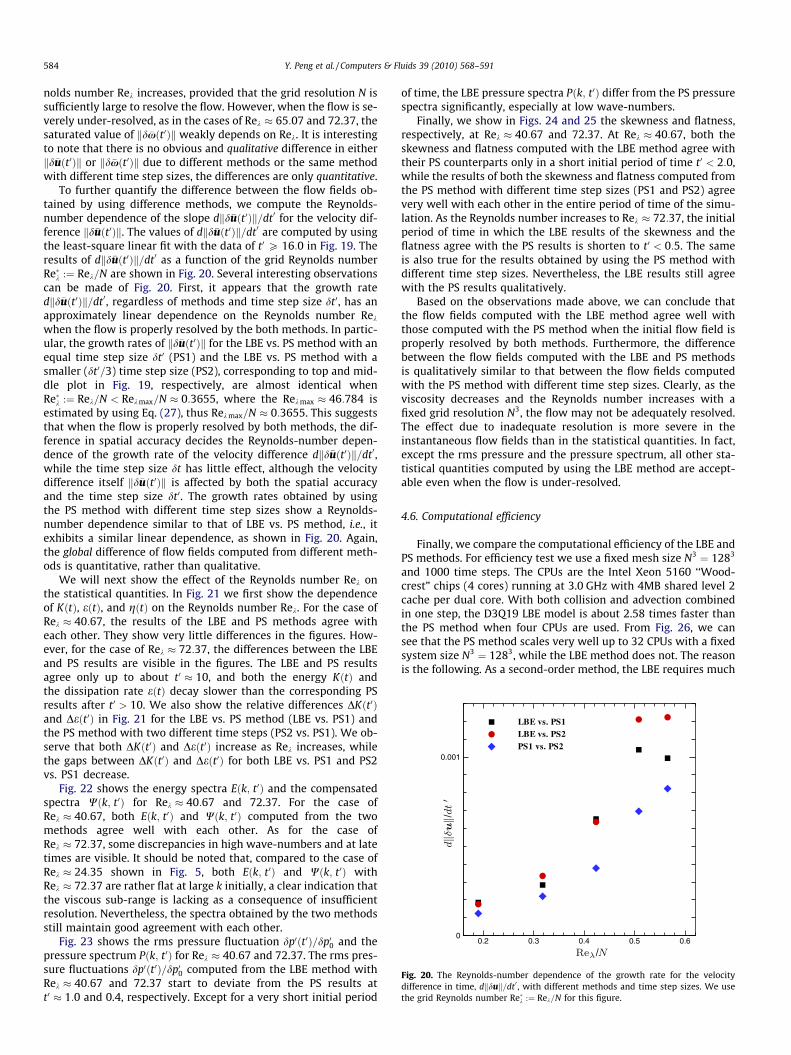
Fig. 20. The Reynolds-number dependence of the growth rate for the velocitydifference in time, dkduk=dt0 , with different methods and time step sizes. We usethe grid Reynolds number Rek :¼ Rek=N for this figure.

584 Y. Peng et al. / Computers & Fluids 39 (2010) 568–591

nolds number Rek increases, provided that the grid resolution N issufficiently large to resolve the flow. However, when the flow is se-verely under-resolved, as in the cases of Rek � 65:07 and 72.37, thesaturated value of kd�xðt0Þk weakly depends on Rek. It is interestingto note that there is no obvious and qualitative difference in eitherkd�uðt0Þk or kd�xðt0Þk due to different methods or the same methodwith different time step sizes, the differences are only quantitative.

To further quantify the difference between the flow fields ob-tained by using difference methods, we compute the Reynolds-number dependence of the slope dkd�uðt0Þk=dt0 for the velocity dif-ference kd�uðt0Þk. The values of dkd�uðt0Þk=dt0 are computed by usingthe least-square linear fit with the data of t0 P 16:0 in Fig. 19. Theresults of dkd�uðt0Þk=dt0 as a function of the grid Reynolds numberRek :¼ Rek=N are shown in Fig. 20. Several interesting observationscan be made of Fig. 20. First, it appears that the growth ratedkd�uðt0Þk=dt0, regardless of methods and time step size dt0, has anapproximately linear dependence on the Reynolds number Rek

when the flow is properly resolved by the both methods. In partic-ular, the growth rates of kd�uðt0Þk for the LBE vs. PS method with anequal time step size dt0 (PS1) and the LBE vs. PS method with asmaller (dt0=3) time step size (PS2), corresponding to top and mid-dle plot in Fig. 19, respectively, are almost identical whenRek :¼ Rek=N < Rek max=N � 0:3655, where the Rek max � 46:784 isestimated by using Eq. (27), thus Rek max=N � 0:3655. This suggeststhat when the flow is properly resolved by both methods, the dif-ference in spatial accuracy decides the Reynolds-number depen-dence of the growth rate of the velocity difference dkd�uðt0Þk=dt0,while the time step size dt has little effect, although the velocitydifference itself kd�uðt0Þk is affected by both the spatial accuracyand the time step size dt0. The growth rates obtained by usingthe PS method with different time step sizes show a Reynolds-number dependence similar to that of LBE vs. PS method, i.e., itexhibits a similar linear dependence, as shown in Fig. 20. Again,the global difference of flow fields computed from different meth-ods is quantitative, rather than qualitative.

We will next show the effect of the Reynolds number Rek onthe statistical quantities. In Fig. 21 we first show the dependenceof KðtÞ, eðtÞ, and gðtÞ on the Reynolds number Rek. For the case ofRek � 40:67, the results of the LBE and PS methods agree witheach other. They show very little differences in the figures. How-ever, for the case of Rek � 72:37, the differences between the LBEand PS results are visible in the figures. The LBE and PS resultsagree only up to about t0 � 10, and both the energy KðtÞ andthe dissipation rate eðtÞ decay slower than the corresponding PSresults after t0 > 10. We also show the relative differences DKðt0Þand Deðt0Þ in Fig. 21 for the LBE vs. PS method (LBE vs. PS1) andthe PS method with two different time steps (PS2 vs. PS1). We ob-serve that both DKðt0Þ and Deðt0Þ increase as Rek increases, whilethe gaps between DKðt0Þ and Deðt0Þ for both LBE vs. PS1 and PS2vs. PS1 decrease.

Fig. 22 shows the energy spectra Eðk; t0Þ and the compensatedspectra Wðk; t0Þ for Rek � 40:67 and 72.37. For the case ofRek � 40:67, both Eðk; t0Þ and Wðk; t0Þ computed from the twomethods agree well with each other. As for the case ofRek � 72:37, some discrepancies in high wave-numbers and at latetimes are visible. It should be noted that, compared to the case ofRek � 24:35 shown in Fig. 5, both Eðk; t0Þ and Wðk; t0Þ withRek � 72:37 are rather flat at large k initially, a clear indication thatthe viscous sub-range is lacking as a consequence of insufficientresolution. Nevertheless, the spectra obtained by the two methodsstill maintain good agreement with each other.

Fig. 23 shows the rms pressure fluctuation dp0ðt0Þ=dp00 and thepressure spectrum Pðk; t0Þ for Rek � 40:67 and 72.37. The rms pres-sure fluctuations dp0ðt0Þ=dp00 computed from the LBE method withRek � 40:67 and 72.37 start to deviate from the PS results att0 � 1:0 and 0.4, respectively. Except for a very short initial period

of time, the LBE pressure spectra Pðk; t0Þ differ from the PS pressurespectra significantly, especially at low wave-numbers.

Finally, we show in Figs. 24 and 25 the skewness and flatness,respectively, at Rek � 40:67 and 72.37. At Rek � 40:67, both theskewness and flatness computed with the LBE method agree withtheir PS counterparts only in a short initial period of time t0 < 2:0,while the results of both the skewness and flatness computed fromthe PS method with different time step sizes (PS1 and PS2) agreevery well with each other in the entire period of time of the simu-lation. As the Reynolds number increases to Rek � 72:37, the initialperiod of time in which the LBE results of the skewness and theflatness agree with the PS results is shorten to t0 < 0:5. The sameis also true for the results obtained by using the PS method withdifferent time step sizes. Nevertheless, the LBE results still agreewith the PS results qualitatively.

Based on the observations made above, we can conclude thatthe flow fields computed with the LBE method agree well withthose computed with the PS method when the initial flow field isproperly resolved by both methods. Furthermore, the differencebetween the flow fields computed with the LBE and PS methodsis qualitatively similar to that between the flow fields computedwith the PS method with different time step sizes. Clearly, as theviscosity decreases and the Reynolds number increases with afixed grid resolution N3, the flow may not be adequately resolved.The effect due to inadequate resolution is more severe in theinstantaneous flow fields than in the statistical quantities. In fact,except the rms pressure and the pressure spectrum, all other sta-tistical quantities computed by using the LBE method are accept-able even when the flow is under-resolved.

4.6. Computational efficiency

Finally, we compare the computational efficiency of the LBE andPS methods. For efficiency test we use a fixed mesh size N3 ¼ 1283

and 1000 time steps. The CPUs are the Intel Xeon 5160 ‘‘Wood-crest” chips (4 cores) running at 3.0 GHz with 4MB shared level 2cache per dual core. With both collision and advection combinedin one step, the D3Q19 LBE model is about 2.58 times faster thanthe PS method when four CPUs are used. From Fig. 26, we cansee that the PS method scales very well up to 32 CPUs with a fixedsystem size N3 ¼ 1283, while the LBE method does not. The reasonis the following. As a second-order method, the LBE requires much

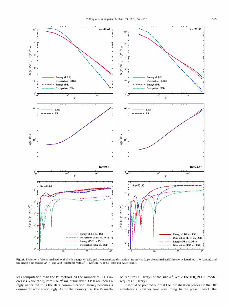
Fig. 21. Evolution of the normalized total kinetic energy Kðt0Þ=K0 and the normalized dissipation rate eðt0Þ=e0 (top), the normalized Kolmogorov length gðt0Þ=dx (center), andthe relative differences DKðt0Þ and Deðt0Þ (bottom), with N3 ¼ 1283;Rek � 40:67 (left) and 72.37 (right).

Y. Peng et al. / Computers & Fluids 39 (2010) 568–591 585

less computation than the PS method. As the number of CPUs in-creases while the system size N3 maintains fixed, CPUs are increas-ingly under fed thus the data communication latency becomes adominant factor accordingly. As for the memory use, the PS meth-

od requires 13 arrays of the size N3, while the D3Q19 LBE modelrequires 19 arrays.

It should be pointed out that the initialization process in the LBEsimulations is rather time consuming. In the present work, the

586 Y. Peng et al. / Computers & Fluids 39 (2010) 568–591

initialization takes almost as long as the simulation time, i.e., about30s0, where s0 is the turbulence turnover time, to satisfy the fol-lowing criterion:

maxxj

kdqðxj; tn þ 1Þ � dqðxj; tnÞk 6 10�8:

To significantly shorten the time required to obtain accurateinitial conditions in LBE simulations, either multigrid [46–48] orsome implicit time integration [49] techniques must be used.

5. Discussion and conclusions

In this work we carry out a detailed comparison of the latticeBoltzmann and the pseudo-spectral methods for direct numericalsimulations of decaying turbulence in three dimensions. We com-pare instantaneous flow fields and low-order statistical quantitiescomputed by using these two methods. The computed instanta-neous flow fields are the velocity field uðx; tÞ and the vorticity fieldxðx; tÞ. It is interesting to note that, while there have been numer-ous studies comparing turbulence statistics obtained by using fi-nite-difference and spectral methods, to the best of knowledge,no detailed comparison of instantaneous flow fields has beenmade. Our results show that, with the Reynolds number Rek fixed,the L2-normed difference kduk :¼ kuLBE � uPSk between the LBE and

Fig. 22. The energy spectra Eðk; tÞ (left) and the compensated spectra Wðk; t0Þ (right) withvs. PS1 (thick patterned lines).

PS velocity fields appear to grow linearly in time. Furthermore, thegrowth rate dkduk=dt seems to depend linearly on Rek in a certainrange Rek depending on the methods which are compared. As theReynolds number Rek increases beyond certain point, the growthrate dkduk=dt will saturate eventually. The same is also observedfor the velocity difference between the velocity fields obtainedby the PS method with different time step sizes. As for the vorticityfield xðx; tÞ, the L2-normed difference kdxk :¼ kxLBE � xPSk be-tween the LBE and PS vorticity fields exhibits a behavior entirelydifferent from that of the velocity difference kduk. The vorticity dif-ference kdxk grows very rapidly in an initial period of time t0 < 2:0,then increases gradually to a plateau in a later time. It is interestingto note that the same phenomenon is also observed in the vorticitydifference between the vorticity fields obtained by the PS methodwith different time step sizes.

For the low-order statistical quantities, our results show thatthe energy spectrum Eðk; tÞ, the total kinetic energy KðtÞ, and thedissipation rate eðtÞ obtained by the two methods agree verywell up to t0 � 30 when the initial velocity field is well resolvedby both methods, i.e., dx=g0 6 1:0. This resolution criterion isconsistent with previous empirical observations (cf. [42,43]).For the case of initial Rek ¼ 24:35, the relative differences in bothKðtÞ and eðtÞ computed by the LBE and PS methods are no morethan 5% when t0 � 30, after both KðtÞ and eðtÞ decay almost four

N3 ¼ 1283;Rek � 40:67 (top) and 72.37 (bottom). The LBE (thin lines with symbols)

Fig. 23. The rms pressure fluctuation dp0ðt0Þ=dp00 (left) and the pressure spectra Pðk; t0Þ (right), with Re � 40:67 (top) and 70.37 (bottom). LBE vs. PS1.

Y. Peng et al. / Computers & Fluids 39 (2010) 568–591 587

orders of magnitude. This is not surprising, because the flowfields are well captured in the LBE calculation in this case. How-ever, when the initial flow is under-resolved in the LBE simula-tions, such as in the case of initial Rek � 72:37 and g0=dx �0:598;KðtÞ and eðtÞ computed from the two methods show visi-ble discrepancies after t0 > 10, and the relative differences in KðtÞand eðtÞ computed by the LBE and PS methods increase to about40% when t0 > 20. However, even in the case of Rek ¼ 72:37,both KðtÞ and eðtÞ computed from the two methods agree wellwhen t0 � 10. In general, the relative differences DKðtÞ andDeðtÞ for the LBE vs. PS method are greater than their counter-parts for the PS method with different dt0. However, the differ-ences between DKðtÞ and DeðtÞ for the LBE vs. PS method, andtheir counterparts for the PS method with different dt0, decreaseas the Reynolds number Rek increases.

The greatest difference between statistical quantities computedby using the LBE and PS methods is the pressure spectrum Pðk; t0Þ,due to significantly different treatments of the pressure field pðx; tÞin these two methods. It can be shown that the spatial accuracy ofthe pressure field p solved by the LBE method is formally first-or-der. As shown in the present work, even when the flow is well re-solved initially by both methods, i.e., dx=g0 6 1:0, the rms pressurefluctuations obtained by the LBE and PS methods agree with eachother very well only for a relatively short period of time t0 < 2:0.

Consequently the pressure spectra Pðk; t0Þ computed by using thetwo methods also agree with each other in the same short periodof time. Increasing the grid Reynolds number Rek=N would de-crease this initial period of time within which the pressures com-puted by using the two methods agree with each other. Beyondthis initial period of time, the quality of the LBE pressure field dete-riorates and is dominated by density fluctuations of very high fre-quencies and short wavelengths, comparable to that of the timestep size dt and the grid spacing dx, respectively. In spite of thedeterioration of the pressure field, both velocity and vorticity fieldsare well captured in the LBE simulations.

For the skewness and flatness of the velocity derivative, the ef-fect due to acoustic waves intrinsic to the LBE method is conspicu-ous: the pressure fluctuations induce high-frequency oscillations inthe skewness and the flatness computed by using the LBE method,which are absent in the PS results. Nevertheless, when the high-fre-quency oscillations are filtered out, the LBE results agree well withthe PS results up to t � 30s0 when the initial flow field is well re-solved by both methods, as in the case of Rek � 24:35.

Based on our results, we can conclude that, overall, the latticeBoltzmann method performs very well when compared with thepseudo-spectral method for DNS of decaying turbulence whenthe flow is properly resolved. Specifically, the LBE simulationscan reliably produce accurate results for instantaneous velocity

Fig. 24. The skewness with Rek � 40:67 (left) 72.37 (right). N3 ¼ 1283. LBE vs. PS1 (top), smoothed LBE vs. PS1 (center), and PS2 vs. PS1 (bottom).

588 Y. Peng et al. / Computers & Fluids 39 (2010) 568–591

and vorticity fields and low-order statistical quantities includingthe total energy KðtÞ, the dissipation rate eðtÞ, the energy spectrumEðk; tÞ, the skewness and the flatness for an extended period oftime, provided that the initial flow field is well resolved with thecriterion that dx=g0 6 1:0, which is about twice of the resolution

requirement for spectral methods. This is consistent with theobservation made in a previous study comparing finite-differenceand spectral methods [42,43,31]. Consequently the LBE method de-mands a computational effort about 16 times greater than that ofthe pseudo-spectral method (a factor of two from each spatial

Fig. 25. The flatness with Rek � 40:67 (left) 72.37 (right). N3 ¼ 1283. LBE vs. PS1 (top), smoothed LBE vs. PS1 (center), and PS2 vs. PS1 (bottom).

Y. Peng et al. / Computers & Fluids 39 (2010) 568–591 589

dimension and another one from time stepping, to maintain thesame CFL number in both systems). However, this is expected be-cause the LBE method is only a second-order scheme. The pressurefield obtained by using the LBE method is much less satisfactory.The rms pressure dp0ðtÞ and the pressure spectrum Pðk; tÞ obtained

by using the LBE method are accurate in a time interval muchshorter than that for the velocity field and other statistical quanti-ties. This is somewhat expected because the LBE method does notsolve the Poisson equation for the pressure, and this is true of alllow-order schemes which do not solve the Poisson equation

Fig. 26. Parallel efficiency, LBE (squares) vs. PS (bullets) method.

590 Y. Peng et al. / Computers & Fluids 39 (2010) 568–591

accurately. To improve the accuracy of the LBE method for thepressure field, one must, in some way, consider solving the Poissonequation effectively and efficiently while preserving other key fea-tures of the LBE method, including its conservativeness, isotropy,and low numerical dissipation in small scales [33,36]. This willbe a subject of our future research.

Finally, we would like to comment on the significance of thiswork. In a larger sense, our work attempts to address the followingquestion: what should we understand by ‘‘direct numerical simula-tions” for turbulence? For many, DNS may simply mean a numericalmethod without explicit turbulence modeling. However, it is moreappropriate to restrict the term ‘‘DNS” to schemes which demonstra-bly resolve everything up to the smallest dynamically relevant scale.In this sense, spectral-type methods are the best methods to perform‘‘DNS”, and we have shown in this work that, although the LBE meth-od is inferior to pseudo-spectral methods in terms of accuracy, it cannevertheless be used as an adequate ‘‘DNS” tool. We believe that thesuccess of the LBE method as a DNS tool can be specifically attributedto the following features of the LBE. First, the LBE method has rela-tively low numerical dissipations even at the scales of grid spacing[33,36], which is difficult to achieve for low-order schemes. Second,the LBE method is isotropic, that is, its accuracy does not depend onthe angle with respect to mesh lines [33,36]. The isotropy ensuresthe conservation of angular momentum (or vorticity) numerically.And third, the LBE method has relatively small numerical dispersiveeffects [33], which are certainly less than what is observed in con-ventional CFD methods of second-order accuracy [50,51]. These in-sights can serve as guidelines to construct accurate numericalschemes for DNS of turbulence.

Acknowledgments

We are grateful to Regionales RechenZentrum Erlangen (RRZE)at University of Erlangen for providing computational resourcesto us, and to Dr. T. Zeiser at RRZE for his help on numerous issuesrelated to computing. We thank Dr. Pierre Lallemand for helpfuldiscussions on efficient implementations of the LBE code. L.-S.Luo thank Prof. George Karniadakis and Dr. Robert Rubinstein formany insightful discussions; and Prof. Yukio Kaneda, Dr. RobertRubinstein, and Prof. Gretar Tryggvason for bringing our attentionto references [31,45,30], respectively. Y. Peng, W. Liao, and L.-S. Luoacknowledge the support from the US Department of Defense un-der AFOSR-MURI project ‘‘Hypersonic Transition and Turbulencewith Non-equilibrium Thermochemistry” (Dr. J. Schmisseur, Pro-

gram Manager). L.-P. Wang acknowledges support by National Sci-ence Foundation (under contract ATM-0527140) and by NationalNatural Science Foundation of China (Project No. 10628206).

References

[1] Pope SB. Turbulent flows. Cambridge, UK: Cambridge University Press; 2000.[2] Sagaut P, Cambon C. Homogeneous turbulence dynamics. New

York: Cambridge University Press; 2008.[3] Orszag SA, Patterson GS. Numerical simulation of three-dimensional

homogeneous isotropic turbulence. Phys Rev Lett 1972;28(2):76–9.[4] Canuto CG, Hussaini MY, Quarteroni A, Zang TA. Spectral methods: evolution to

complex geometries and applications to fluid dynamics. New York: Springer;2007.

[5] Vincent A, Meneguzzi M. The spatial structure and statistical properties ofhomogeneous turbulence. J Fluid Mech 1991;225:1–20.

[6] Jiménez J, Wray A, Saffman PG, Rogallo R. The structure of intense vorticity inisotropic turbulence. J Fluid Mech 1993;255:65–90.

[7] Wang L-P, Chen S-Y, Brasseur JG, Wyngaard JC. Examination of hypotheses inthe Kolmogorov refined turbulence theory through high-resolutionsimulations 1. Velocity field. J Fluid Mech 1996;309:113–56.

[8] Jiménez J, Wray A. On the characteristics of vortex filaments in isotropicturbulence. J Fluid Mech 1998;273:255–85.

[9] Gotoh T, Fukayama D. Pressure spectrum in homogeneous turbulence. PhysRev Lett 2001;86(17):3775–8.

[10] Kaneda Y, Ishihara T, Yokokawa M, Itakura K, Uno A. Energy dissipation rateand energy spectrum in high resolution direct numerical simulations ofturbulence in a periodic box. Phys Fluids 2003;15(2):L21–4.

[11] Yoshida K, Yamaguchi J, Kaneda Y. Regeneration of small eddies by dataassimilation in turbulence. Phys Rev Lett 2005;94(1):014501.

[12] Ishida T, Davidson PA, Kaneda Y. On the decay of isotropic turbulence. J FluidMech 2006;564:455–75.

[13] Kaneda Y, Ishihara T. High-resolution direct numerical simulation ofturbulence. J Turbul 2006;7(20):1–17.

[14] Donzis DA, Yeung PK, Sreenivasan KR. Dissipation and enstrophy in isotropicturbulence: resolution effects and scaling in direct numerical simulations.Phys Fluids 2008;20(4):045108.

[15] Ishihara T, Gotoh T, Kaneda Y. Study of high-Reynolds number isotropicturbulence by direct numerical simulations. Annu Rev Fluid Mech2009;41:165–80.

[16] He X, Luo L-S. A priori derivation of the lattice Boltzmann equation. Phys Rev E1997;55(6):R6333–6.

[17] He X, Luo L-S. Theory of lattice Boltzmann method: from the Boltzmannequation to the lattice Boltzmann equation. Phys. Rev. E 1997;56(6):6811–7.

[18] Yu DZ, Mei R, Luo L-S, Shyy W. Viscous flow computations with the method oflattice Boltzmann equation. Prog Aerospace Sci 2003;39(5):329–67.

[19] Chen S, Wang Z, Shan X, Doolen GD. Lattice Boltzmann computational fluiddynamics in three dimensions. J Stat Phys 1992;68(3/4):379–400.

[20] Treviño C, Higuera F. Lattice Boltzmann and spectral simulations of nonlinearstability of Kolmogorov flows. Revista Mexicana de Fisica 1994;40(6):878–90.

[21] Luo L-S, Qi D, Wang L-P. Applications of the lattice Boltzmann method to complexand turbulent flows. In: Breuer M, Durst F, Zenger C, editors. High performancescientific and engineering computing. Lecture notes in computational science andengineering, vol. 21. Berlin: Springer; 2002. p. 123–30.

[22] Yu HD, Girimaji SS, Luo L-S. Lattice Boltzmann simulations of decayinghomogeneous isotropic turbulence. Phys Rev E 2005;71(1):016708.

[23] Yu HD, Girimaji SS, Luo L-S. DNS and LES of decaying isotropic turbulence withand without frame rotation using lattice Boltzmann method. J Comput Phys2005;209(2).

[24] Yu DZ, Girimaji SS. Direct numerical simulations of homogeneous turbulencesubject to periodic shear. Phys Rev E 2005;71(1):016708.

[25] Yu DZ, Girimaji SS. DNS of homogeneous shear turbulence revisited with thelattice Boltzmann method. J Turbul 2005;6(6).

[26] Hazi G. Bias in the direct numerical simulation of isotropic turbulence usingthe lattice Boltzmann method. Phys Rev E 2005;71(3):036705.

[27] Izawa WA Kareem S, Xiong AK, Fukunishi Y. Identification of multi-scalecoherent eddy structures in a homogeneous isotropic turbulence. Prog ComputFluid Dyn 2006;6(7):402–8.

[28] ten Cate A, van Vliet E, Derksen JJ, Van den Akker HEA. Application of spectralforcing in lattice-Boltzmann simulations of homogeneous turbulence. Comput.Fluids 2006;35(10):1239–51.

[29] Burattini P, Lavoie P, Agrawal A, Djenidi L, Antonia RA. Power law of decayinghomogeneous isotropic turbulence at low Reynolds number. Phys. Rev. E2006;73(6):066304.

[30] Orlandi P. Fluid flow phenomena. Dordrecht: Kluwer; 2000.[31] Yoshimatsu K, Ishihara T, Kaneda Y, Nakai S, Nishida H, Satofuka N.

Comparison of a spectral method with a higher-order finite differencemethod in direct numerical simulations of three-dimensional homogeneousturbulence. Trans Jpn Soc Mech Eng Ser B 2003;69(679):13–8 [in Japanese].

[32] d’Humières D. Generalized lattice-Boltzmann equations. In: Shizgal BD, WeaveDP, editors. Rarefied gas dynamics: theory and simulations. Progress inastronautics and aeronautics, vol. 159. Washington, DC: AIAA; 1992. p. 450–8.

[33] Lallemand P, Luo L-S. Theory of the lattice Boltzmann method: dispersion,dissipation, isotropy, Galilean invariance, and stability. Phys Rev E2000;61(6):6546–62.

Y. Peng et al. / Computers & Fluids 39 (2010) 568–591 591

[34] d’Humières D, Bouzidi M, Lallemand P. Thirteen-velocity three-dimensionallattice Boltzmann model. Phys Rev E 2001;63:066702.

[35] d’Humières D, Ginzburg I, Krafczyk M, Lallemand P, Luo L-S. Multiple-relaxation-time lattice Boltzmann models in three-dimensions. Philos TransRoy Soc Lond A 2002;360(1792):437–51.

[36] Lallemand P, Luo L-S. Theory of the lattice Boltzmann method: acoustic andthermal properties in two and three dimensions. Phys Rev E 2003;68(3):036706.

[37] He X, Luo L-S. Lattice Boltzmann model for the incompressible Navier–Stokesequation. J Stat Phys 1997;88:927–44.

[38] Rogallo RS. Numerical experiments in homogeneous turbulence. TechnicalReport TM-8135, NASA; 1981.

[39] Yeung PK, Pope SB. Lagrangian statistics from direct numerical simulations ofisotropic turbulence. J Fluid Mech 1989;207:531–86.

[40] Junk M, Klar A. Discretizations for the incompressible Navier–Stokes equationsbased on the lattice Boltzmann method. SIAM J Sci Comput 2000;22:1–19.

[41] Junk M, Klar A, Luo L-S. Asymptotic analysis of the lattice Boltzmann equation.J Comput Phys 2005;210(2):676–704.

[42] Kristoffersen R, Andersson HI. Direct simulations of low-Reynolds-numberturbulent flow in a rotating channel. J Fluid Mech 1993;256:163–97.

[43] Moin P, Mahesh K. Direct numerical simulation: a tool in turbulence research.Annu Rev Fluid Mech 1998;30:539–78.

[44] Mei R, Luo L-S, Lallemand P, d’Humières D. Consistent initial conditions forlattice Boltzmann simulations. Comput Fluids 2006;35:855–62.

[45] Clark TT, Zemarch C. Symmetries and the approach to statistical equilibrium inisotropic turbulence. Phys Fluids 1998;10(11):2846–58.

[46] Tölke J, Krafczyk M, Rank E. A multigrid solver for the discrete Boltzmannequation. J Stat Phys 2002;107:573–91.

[47] Mavriplis DJ. Multigrid solution of the steady-state lattice Boltzmannequation. Comput Fluids 2005;35(8/9):793–804.

[48] Mavriplis DJ. Exploring alternative approaches to computational fluiddynamics. Int J Comput Fluid Dyn 2005;19(8):613–20.

[49] Tölke J, Krafczyk M, Schulz M, Rank E, Berrios R. Implicit discretization andnonuniform mesh refinement approaches for FD discretizations of LBGKmodels. Int J Mod Phys C 1998;9:1143–57.

[50] Wilde A. Calculation of sound generation and radiation from instationaryflows. Comput Fluids 2006;35(8/9):986–93.

[51] Marı́e S, Ricot D, Sagaut P. Comparison between lattice Boltzmann method andNavier–Stokes high-order schemes for computational aeroacoustics. J ComputPhys 2009;228(4):1056–70.