An alternative method for simulating particle suspensions using lattice Boltzmann

An alternative method for simulating particlesuspensions using lattice Boltzmann

Luıs Orlando Emerich dos Santos

Center of Mobility Engineering, Federal University of Santa Catarina,88040-900, Florianopolis, Santa Catarina, Brazil

E-mail: [email protected]

Paulo Cesar Philippi

Mechanical Engineering Department, Federal University of Santa Catarina,88040-900, Florianopolis, Santa Catarina, Brazil

E-mail: [email protected]

Abstract. In this study, we propose an alternative way to simulate particlesuspensions using the lattice Boltzmann method. The main idea is to impose thenon-slip boundary condition in the lattice sites located on the particle boundaries.The focus on the lattice sites, instead of the links between them, as done in themore used methods, represents a great simplification in the algorithm. A fullydescription of the method will be presented, in addition to simulations comparingthe proposed method with other methods and, also, with experimental results.

Keywords: Lattice Boltzmann method, Particulate flow, Particle-fluid interactions

1. Introduction

Particulate flows are found in many industrial processes [1, 2, 3, 4], and have beensubjected to considerable scientific investigation. Recently, computer simulations havebecome an effective tool in these studies and several methods have been applied,such as finite element method [5], Lagrange-multipliers [2, 3], direct forcing method[6], lattice Boltzmann methods [1, 4, 7, 8, 9, 10, 11, 12, 13, 14, 15, 16], solving theStokes equation near the particles (Physalis) [17] and combining two or more methods[14, 18, 19].In this study, we propose an alternative way to simulate suspensions using the latticeBoltzmann method. The main idea is to impose the non-slip boundary condition inthe lattice sites representing the particle boundaries. The focus on lattice sites, insteadof the link between them, as done in the more used methods [11], represents a greatsimplification in the algorithm. Similar approaches, focusing on the lattice sites werealready tried [1], although without popularity due, probably, to difficulties several inthe implementation.Its important to mention that the simplifications we propose can reduce the accuracyin describing the details of the flow near the particles, and these details can or cannot

arX

iv:1

105.

2904

v1 [

phys

ics.

com

p-ph

] 1

4 M

ay 2

011

An alternative method for simulating particle suspensions using lattice Boltzmann 2

),( tfi x

Figure 1. The D2Q9 lattice, used in two-dimensional simulations. The arrowsrepresent the distributions fi(x, t), and circles represent the lattice sites.

be important, depending on the problem one wants to simulate. In the simulations wehave done until now, in despite of the simplifications, the results we obtain are similarto the results obtained by other methods (see section 3).

2. The model

In this section we introduce the lattice Boltzmann method and present the modeldescribing the particle-fluid interaction. Interactions among particles and between aparticle and a solid surface will also be discussed in this section.

2.1. The lattice Boltzmann model

The lattice-Boltzmann method (LBM) is based on the discretization of theBoltzmann’s mesoscopic equation[20, 21, 22], usually with the BGK approach forthe collision operator (for a comprehensive review see [23]). In the LBM scale, thesystem is described using a single particle distribution function, fi(x, t), representingthe number of particles with velocity ci at the site x and time t, where i = 0, ..., b. Theparticles are restricted to a discrete lattice, in a manner that each group of particles canmove only in a finite number b of directions and with a limited number of velocities (seeFig. 1). Therefore, physical and velocity space are discretized. The local macroscopicproperties such as total mass (the particle mass, m, is assumed unitary), ρ(x, t), andtotal momentum, ρ(x, t)u(x, t), can be obtained from the distribution function in thefollowing way:

ρ(x, t) =∑i

fi(x, t), (1)

ρ(x, t)u(x, t) =∑i

fi(x, t)ci. (2)

The Lattice Boltzmann equation, that is, the discrete version of the Boltzmannequation with the BGK collision, operator is written

fi(x + δtci, t+ δt) − fi(x, t) = −δtτ

[fi(x, t) − feqi (ρ,u)] (3)


Figure 2. Boundary sites characterizing a particle. The boundary sites (BS) aredepicted in dark gray and the internal sites (IS), in dark. The particle’s boundaryare regard to be between the IS and BS sites.

where, δt is the time step and feqi (ρ,u) is a polynomial approximation of the Maxwell-Boltzmann equilibrium distribution [24, 20, 21, 22], a function of the local variablesρ(x, t) and u(x, t). It can be shown, through a Chapman-Enskog analysis, that thissystem macroscopically will evolve according to the Navier-Stokes equations with akinematic viscosity given by

ν = c2s (τ − 1/2) , (4)

where cs is the sound velocity, a constant depending on the set of velocities ci.

2.2. Particle-fluid interaction

The basic idea of the method is that the fluid in contact with a solid surface mustacquire the velocity of this surface, considering the non-slip condition. Keeping thisin mind, a set of boundary sites can be used to describe the particle. This approachis similar to the one presented in [7] and [11], although we focus in the lattice sitesand not in the links between them. We denote boundary sites (BS) the particle sitesin contact with fluid, and internal sites (IS) the particle sites in contact with theboundary sites (see Fig.2). The particle’s boundary is regarded to be halfway betweenthe IS and the BS sites. A particle will be represented by its central position xp, aradius rp, a mass mp and a moment of inertia Ip. Its velocity will be denoted up, andthe angular velocity ωp. Only spherical particles will be considered.

The presence of a particle will be represented only by its effects on the fluid incontact with the particle, altering the dynamics of the sites BS and IS. The position ofthese sites will be denoted by xB and xI , respectively, and its integer counterpart (orthe nearest integer of each component of the vectors) by [xB ] and [xI ], respectively.Velocities and densities in the sites [xB ] and [xI ] will be denoted uB , uI and ρB ,ρI . We emphasize that all sites will be updated by the usual collision/propagationsteps, but the IS and BS sites, in addition to these steps, will be submitted to a setof substeps included between the collision and the propagation steps. These substepsare presented in the sequence.


• Particle-fluid momentum transfer

This substep is executed only in the BS sites. As was previously mentioned, thevelocity in the BS sites must acquire the particle’s velocity. This velocity, consideringthe angular velocity, is

u′B = up + (xB − xp) × ωp. (5)

To impose this velocity in the fluid, that is in lattice sites, the equilibriumdistribution is employed, setting fi ([xB ] , t) = feqi (ρ,u′B).

Naming pB = ρBuB the linear momentum of a BS site, we compute

∆pB = ρB(u′B − uB), (6)

and

∆lB = ρB(xB − xp) × (u′B − uB), (7)

where ∆lB represents the change in the angular momentum caused by the change inthe linear momentum ∆pB .

Finishing this step we have the total momentum exchanged, ∆PB and ∆LB :

∆PB =∑BS

∆pB (8)

∆LB =∑BS

∆lB (9)

• Particle’s acceleration

This substep accounts for the change in particles velocity caused by fluid.According to the Newton’s third law of motion, we simply compute

u′p = up − ∆PB/mp, (10)

ω′p = ωp − ∆LB/Ip, (11)

u′I = u′p + (xI − xp) × ω′p. (12)

• Updating of particle’s position

Due to the spherical symmetry it is not necessary to take into account the rotationof the particles. The position is updated by doing:

x′p = xp + δtu′p. (13)

The positions of boundary and internal sites, also, must be updated:

x′B = xB + δtu′p; (14)

x′I = xI + δtu′p. (15)

Clearly, this procedure includes errors of order (δ2t ), more precise procedures couldbe employed. Nevertheless, there is a lot of imprecision in describing the shape of theparticle, therefore it is not necessary to be so precise in updating particle’s position.

• Velocity of the internal sites


To impose this velocity the equilibrium distribution is employed again, settingfi ([x′I ] , t) = feqi (ρ,u′I).

Some comments are necessary to clarity the physics behind these sub-steps. Con-sider a particule that is found with a velocity up different of the fluid velocity aroundit, in the beginning of the particle-fluid interaction step. This situation never occursin the continuum but this is possible in discrete models due to the discretization oftime. Particle and fluid must then exchange linear and angular momentum until thefluid around the particle acquires the velocity of the particle surface. In this pro-cess the particle velocity also changes due to the fluid reaction on the particle and inaccordance with Newton’s third law of motion. Action and reaction happen simul-taneously in the physical process, but in the discrete case this occurs in steps 1 and2. In the first step the particle transfers linear and angular momentum to the fluid.In consequence the fluid in contact with the particle surface particle accelerates untilhave acquired the same particle velocity. As it was earlier mentioned two hypothesesare used for this step: non-slipping on the particle surface and the hypotheses thatthe fluid-particle equilibration takes a time interval smaller than the time step usedin the simulation. This enables the use of an equilibrium distribution to impose thevelocities. With the fluid velocity altered, we then calculate the change in the linearand angular momentum of the fluid due to this acceleration. These variations mustbe the same as the corresponding changes for the particle, in accordance with theNewton’s third law. We then proceed to step 2 and recalculate the particle velocity.The velocity to be imposed in sites IS is also calculated in accordance with the newparticle velocity.

In a third step, the position of the particle and sites IS and BS are changed. Thespherical symmetry of the particles eases this step since only the translation velocitiesare taken into account in the calculation of the new positions. It must be stressedthat although sites BS belong to the fluid phase, they have their position changed inaccordance with the particle velocity. Indeed, these sites are in the particle boundaryand must follow its displacement. In other words the displacement of the boundarysites is independent of the fluid particles that are occupying these sites, in a giveninstant.

Finally, in a fourth step, we impose the velocity u′I to the sites IS. This stepis important because during the propagation step the information in these sitesis transferred to the adjacent sites BS. Therefore, the sites BS will have theirvelocity composed by the particle and fluid velocities and will define a new change ofmomentum in the following time step.

2.3. Interaction between particles

Especially in simulations involving a great number of particles, as the simulationpresented in subsection 3.4, the interaction between particles must carefully be ad-dressed. There are many techniques to treat these interactions, possibly the mostpopular approach is to introduce a repulsive force between particles when the gap be-tween becomes smaller than a given threshold[14]. We chose another approach in thiswork, treating the collisions as occurring between completely rigid particles (hard-corecollisions). In this way it is not necessary to set the parameters of repulsive forces.We simply impose (see Fig.3)


Figure 3. Collision between two particles, A and B. The arrows indicate thenormal and tangential velocities before and after the collision. The velocities arerepresented in the center of mass reference frame.

v′An = −vAn, (16)

v′Bn = −vBn, (17)

v′At = vAt, (18)

v′Bt = vBt, (19)

where all velocities are represented in the center of mass reference frame. Thisimposition must be done before updating particles’ positions, that is, it can beconsidered as part of the particle’s acceleration substep.It’s necessary to underline that the way we chose to introduce the particle-particleinteraction is not new, nor regarded as part of the method. Moreover, this choicewas done considering solely the easeness in the implementation. In accordance withthe Reynolds number, volume fraction of the particles and the involved force, moreelaborated techniques, employing lubrication[8] or spring forces[25] may reveal to benecessary.

3. Validation

Four cases are presented in order to validate the model. The first case simulatedwas the flow around a massive two-dimensional particle. The particle’s mass waschosen in such way that it doesn’t move, therefore it’s possible to compare the flowaround the two dimensional particle and the flow around a solid cylinder, simulatedusing bounce-back. The drag coefficient for a massive particle was also computedconsidering several Reynolds number and compared with drag coefficients obtainedby other methods. The second case simulated was the flow of a neutrally buoyanttwo-dimensional particle in a shear flow, the results are compared with the resultspresented by Feng and Michaelides[14]. A simulation of a sphere settling in a closedbox was done in order to validate the model in a three-dimensional simulation. Theresults obtained was compared with the ones presented by ten Cate et al.[26]. Finally,it was simulated the sedimentation of 504 two-dimensional particles in an enclosure.


1200 sites

300

site

s

D=98 sites

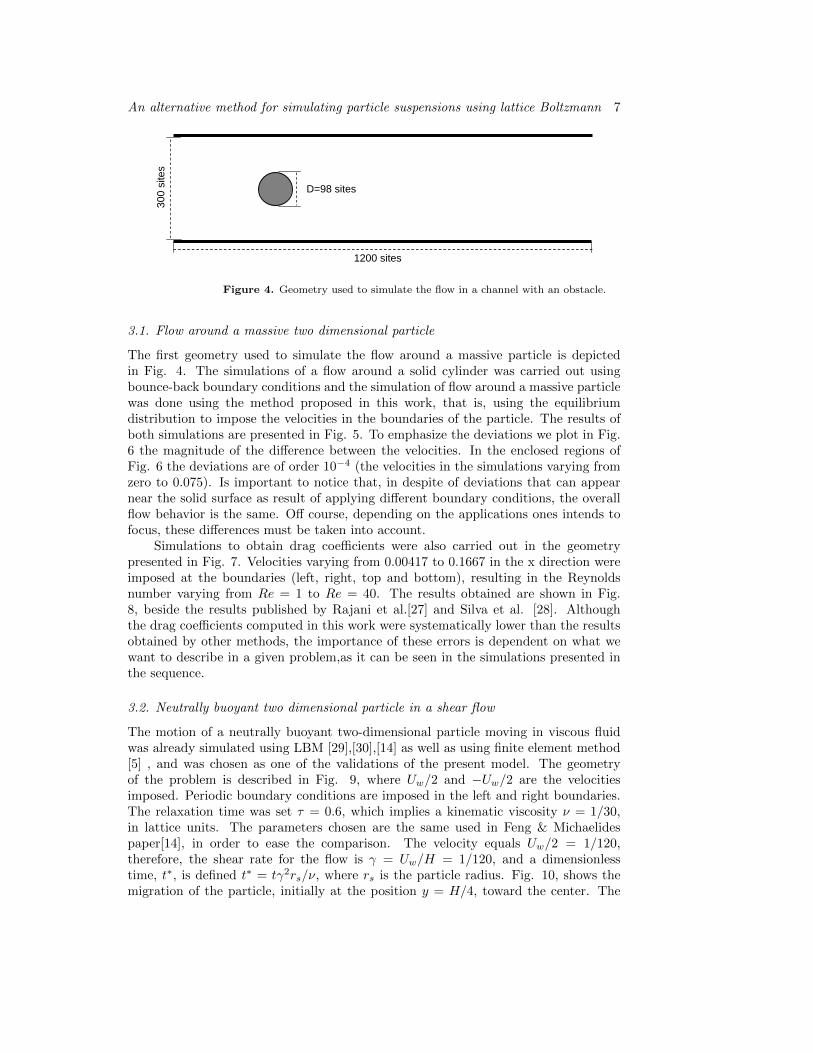
Figure 4. Geometry used to simulate the flow in a channel with an obstacle.

3.1. Flow around a massive two dimensional particle

The first geometry used to simulate the flow around a massive particle is depictedin Fig. 4. The simulations of a flow around a solid cylinder was carried out usingbounce-back boundary conditions and the simulation of flow around a massive particlewas done using the method proposed in this work, that is, using the equilibriumdistribution to impose the velocities in the boundaries of the particle. The results ofboth simulations are presented in Fig. 5. To emphasize the deviations we plot in Fig.6 the magnitude of the difference between the velocities. In the enclosed regions ofFig. 6 the deviations are of order 10−4 (the velocities in the simulations varying fromzero to 0.075). Is important to notice that, in despite of deviations that can appearnear the solid surface as result of applying different boundary conditions, the overallflow behavior is the same. Off course, depending on the applications ones intends tofocus, these differences must be taken into account.

Simulations to obtain drag coefficients were also carried out in the geometrypresented in Fig. 7. Velocities varying from 0.00417 to 0.1667 in the x direction wereimposed at the boundaries (left, right, top and bottom), resulting in the Reynoldsnumber varying from Re = 1 to Re = 40. The results obtained are shown in Fig.8, beside the results published by Rajani et al.[27] and Silva et al. [28]. Althoughthe drag coefficients computed in this work were systematically lower than the resultsobtained by other methods, the importance of these errors is dependent on what wewant to describe in a given problem,as it can be seen in the simulations presented inthe sequence.

3.2. Neutrally buoyant two dimensional particle in a shear flow

The motion of a neutrally buoyant two-dimensional particle moving in viscous fluidwas already simulated using LBM [29],[30],[14] as well as using finite element method[5] , and was chosen as one of the validations of the present model. The geometryof the problem is described in Fig. 9, where Uw/2 and −Uw/2 are the velocitiesimposed. Periodic boundary conditions are imposed in the left and right boundaries.The relaxation time was set τ = 0.6, which implies a kinematic viscosity ν = 1/30,in lattice units. The parameters chosen are the same used in Feng & Michaelidespaper[14], in order to ease the comparison. The velocity equals Uw/2 = 1/120,therefore, the shear rate for the flow is γ = Uw/H = 1/120, and a dimensionlesstime, t∗, is defined t∗ = tγ2rs/ν, where rs is the particle radius. Fig. 10, shows themigration of the particle, initially at the position y = H/4, toward the center. The


Figure 5. Top:flow around a solid cylinder. Bottom: flow around a massiveparticle. The velocities vary from zero (black) to 0.075 (white)

.

Figure 6. The difference in the velocities considering the simulations using asolid cylinder and a massive particle. In the enclosed region the errors are oforder O(10−4), outside the errors are smaller than this.


1200 sites

720

site

s

D=40 sites

x

y

Figure 7. The geometry used to compute the drag coefficient of the 2D particle.

Figure 8. Drag coefficients for Reynolds number varying from one to forty. Theresults computed using the proposed model are compared with the work by Rajaniet al. [27] (Reynolds from one to five) and Silva et al. [28] (Reynolds from ten toforty).


Figure 9. Schematic depiction of the problem simulated: a neutrally buoyanttwo dimensional particle in a shear flow

0.2

0.3

0.4

0.5

0.6

0 20 40 60 80 100 120

Dimensionless time t*

y/H

y/H

IB-LBM by Feng and Michaelides (2003)

LBM by Feng at al. (2002)

FEM by Feng at al. (1994)

Figure 10. A neutrally buoyant particle in a shear flow – comparison of theresults obtained using the proposed model for fluid-solid interaction and previousmodels. The y-axis shows the particle’s position with respect to the lateral ofchannel divided it’s width H.

agreement between the results using the proposed model and the previous models arequite good.

3.3. A sphere settling in a closed box

In this subsection the trajectory and velocity of a sphere settling in a closed boxis simulated using the model here prosed and compared with experimental resultsobtained by Cate et al. [26]. The settling sphere has a diameter of D = 15mmand density ρ = 1120kg/m3. The container dimensions are depth×width×height=


100 mm

160

mm

D=15 mm

100 sites16

0 si

tes

D=15 sites

H=1

20m

m

H=1

20si

tes

Figure 11. Schematic depiction of the geometry used in the experiments (left)and in the simulations (right).

100× 100× 160mm (see Fig. 11). Four cases were simulated considering the differentdensities and viscosities of the fluid in which the sphere will settle, corresponding to aReynolds number varying from Re = 1.5 to Re = 32.2. The fluid characteristics andthe parameters used in the simulations are shown in Table 1.

Table 1. Fluid properties in the experiment and parameters used in simulations.

ρf [kg/m3] µf [10−3Ns/m2] τ δt[10−3s]Case E1 970 373 0.9 0.347Case E2 965 212 0.9 0.607Case E3 962 113 0.8 0.851Case E4 960 58 0.9 2.207

Figure 12 and 13 present comparisons between simulation and experiment for thetrajectories and velocities of the settling particle, respectively.

3.4. 504 particles settling in a closed box

The problem of a large number of particles settling in a closed 2D box was alreadysimulated by other methods [2], [14]. All the parameters were chosen in order tocompare with the previous works. That is, 504 circular particles with diameterD = 0.625cm settling in box having 10−2m width and 10−2m height. The fluidand particle densities are ρf = 1000kg/m3 and ρp = 1010kg/m3, respectively, andthe fluid kinematic viscosity is νf = 10−6m2/s. Representing the box by 512 × 512sites and using a relaxation time τ = 0.9915 we will have a time step of 0.00025s.The process of sedimentation simulated from the initial state to 24s is presented in


0

1

2

3

4

5

6

7

8

9

0 0.5 1 1.5 2 2.5 3 3.5 4 4.5

t[s]

H/D

Case E1 simulatedCase E2 simulatedCase E3 simulatedCase E4 simulatedCase E1 experimentalCase E2 experimentalCase E3 experimentalCase E4 experimental

Figure 12. The position of the particle settling in a closed box. The simulatedresults are compared with the experimental results from Cate el al. (2002). They-axis presents particle’s position H (see Fig. 11), divided by it’s diameter D. Thex-axis shows time in seconds.

-0.14

-0.12

-0.1

-0.08

-0.06

-0.04

-0.02

0

0 0.5 1 1.5 2 2.5 3 3.5 4 4.5

t[s]

u[m

/s] Case E1 simulated

Case E2 simulatedCase E3 simulatedCase E4 simulatedCase E1 experimentalCase E2 experimentalCase E3 experimentalCase E4 experimental

Figure 13. Comparison between simulation and the experimental results fromCate el al. (2002). The y-axis shows the velocity of the settling particle in metersper second and the x-axis indicates time in seconds.


t=0s t=1s t=2s

Figure 14. Configurations of the settling particles.

t=3s t=4s t=5s


t=8s t=12s t=24s


Fig. 14, Fig. 15 and Fig. 16. The figures show the development of a Rayleigh–Taylor instability and are, qualitatively, in agreement with the previous works. Thedifferences between the three simulations (the one presented here and the simulationsof refs. [2] and [14]) are, possibly, a result of the differences in treating the collisionsbetween particles and differences arising from compressibility effects that are presentin the lattice Boltzmann methods.


4. Conclusion

In this study an alternative and simpler way to simulate particle-fluid interactions isproposed. The lattice Boltzmann method is employed to simulate the fluid flow andthe particles are simulated using the Newton’s law. The coupling is made applyingthe equilibrium distribution function to assure the non-slip condition near the solidsurfaces. Several simulations are presented showing that the method can simulateparticle-fluid interactions with a precision comparable with other methods.

References

[1] O. Behrend, “Solid–fluid boundaries in particle suspension simulations via the lattice boltzmannmethod,” Physical Review E 52, pp. 1164–1175, 1995.

[2] R. Glowinski, T. W. Pan, T. I. Hesla, and D. D. Joseph, “A distributed lagrangemultiplier/fictitious domain method for particulate flows,” International Journal ofMultiphase Flow 25, pp. 755–794, 1999.

[3] N. Patankar, P. Singh, D. Joseph, R. Glowinski, and T. W. Pan, “A new formulation of thedistributed lagrange multiplier/ fictitious domain method for particulate flows,” InternationalJournal of Multiphase Flow 26, pp. 1509–1524, 2000.

[4] E.-J. Ding and C. K. Aidun, “Extension of the lattice-boltzmann method for direct simulationof suspended particles near contact,” Journal of Statistical Physics 112, pp. 685–708, August2003.

[5] J. Feng, H. H. Hu, and D. D. Joseph, “Direct simulation of initial-value problems for themotion of solid bodies in a newtonian fluid .2. couette and poiseuille flows,” Journal of FluidMechanics 277, pp. 271–301, 1994.

[6] Z. Yu and X. Shao, “A direct-forcing fictitious domain method for particulate flows,” Journalof Computational Physics 227, pp. 292–314, 2007.

[7] A. Ladd, “Numerical simulation of particulate suspension via a discretized boltzmann-equation.1. theoretical foundation,” Journal of Fluid Mechanics 271, pp. 285–309, 1994.

[8] A. Ladd, “Numerical simulation of particulate suspension via a discretized boltzmann-equation.2. numerical results,” Journal of Fluid Mechanics 271, pp. 311–339, 1994.

[9] C. Aidun and Y. Lu, “Lattice boltzmann simulation of solid particles suspended in a fluid,”Journal of Statistical Physics 81, pp. 49–59, 1995.

[10] C. Aidun, Y. Lu, and E.-J. Ding, “Direct analysis of particulate suspensions with inertia usingthe discrete boltzmann equation,” Journal of Fluid Mechanics 373, pp. 287–311, 1998.

[11] A. J. C. Ladd and R. Verberg, “Lattice-boltzmann simulations of particle-fluid suspensions,”Journal of Statistical Physics 104, pp. 1191–1251, September 2001.

[12] B. Chopard and S. Marconi, “Lattice boltzmann solid particles in a lattice boltzmann fluid,”Journal of Statistical Physics 107, pp. 23–37, April 2002.

[13] N.-Q. Nguyen and A. J. C. Ladd, “Lubrication corrections for lattice-boltzmann simulations ofparticle suspensions,” Physical Review E 66, p. 046708, 2002.

[14] Z.-G. Feng and E. E. Michaelides, “The immersed boundary-lattice boltzmann method forsolving fluid-particles interaction problems,” Journal of Computational Physics 195, pp. 602–628, 2004.

[15] N.-Q. Nguyen and A. J. C. Ladd, “Sedimentation of hard-sphere suspensions at low reynoldsnumber,” Journal of Fluid Mechanics 525, pp. 73–104, 2005.

[16] J. Kromkamp, D. van den Ende, D. Kandhai, R. van der Sman, and R. Boom, “Lattice boltzmannsimulation of 2d and 3d non-brownian suspensions in couette flow,” Chemical EngineeringScience 61, pp. 858–873, 2006.

[17] Z. Zhang and A. Prosperetti, “A second-order method for three-dimensional particle simulation,”Journal of Computational Physics 210, pp. 292–324, 2005.

[18] Z.-G. Feng and E. E. Michaelides, “Proteus: a direct forcing method in the simulations ofparticulate flows,” Journal of Computational Physics 202, pp. 20–51, 2005.

[19] Z. Wang, J. Fan, and K. Luo, “Combined multi-direct forcing and immersed boundary methodfor simulating flows with moving particles,” International Journal of Multiphase Flow 34(3),pp. 283–302, 2008.

[20] X. He and L. Luo, “A priori derivation of the lattice boltzmann equation,” Physical ReviewE 55(6), pp. R6333–R6336, 1997.


[21] X. Shan, X.-F. Yuan, and H. Chen, “Kinetic theory representation of hydrodynamics: a waybeyond navier-stokes equation,” Journal of Fluid Mechanics 550, pp. 413–441, 2006.

[22] P. C. Philippi, L. A. Hegele, L. O. E. dos Santos, and R. Surmas, “From the continuous tothe lattice boltzmann equation: The discretization problem and thermal models,” PhysicalReview E 73(5), p. 056702, 2006.

[23] S. Succi, The Lattice Boltzmann Equation for Fluid Dynamics and Beyond, Oxford UniversityPress, 2001.

[24] T. Abe, “Derivation of the lattice boltzmann method by means of the discrete ordinate methodfor the boltzmann equation,” Journal of Computational Physics 131(1), pp. 241–246, 1997.

[25] K. Hofler and S. Schwarzer, “Navier-stokes simulation with constraint forces: Finite-differencemethod for particle-laden flows and complex geometries,” Physical Review E 61(6), pp. 7146–7160, 2000.

[26] A. ten Cate, C. H. Nieuwstad, J. J. Derksen, and H. E. A. V. den Akker, “Particle imagingvelocimetry experiments and lattice-boltzmann simulations on a single sphere settling undergravity,” Physics of Fluids 14, pp. 4012–4025, November 2002.

[27] B. Rajani, A. Kandasamy, and S. Majumdar, “Numerical simulation of laminar flow past acircular cylinder,” Applied Mathematical Modelling 33, pp. 1228–1247, 2009.

[28] A. L. E. Silva, A. Silveira-Neto, and J. Damasceno, “Numerical simulation of two-dimensional flows over a circular cylinder using the immersed boundary method,” Journalof Computational Physics 189, pp. 351–370, 2003.

[29] Z.-G. Feng and E. E. Michaelides, “Hydrodynamic force on spheres in cylindrical and prismaticenclosures,” International Journal of Multiphase Flow 28, pp. 479–496, 2002.

[30] Z.-G. Feng and E. E. Michaelides, “Interparticle forces and lift on a particle attached to a solidboundary in suspension flow,” Physics of Fluids 14, pp. 49–60, January 2002.

An alternative method for simulating particle suspensions using lattice Boltzmann

Documents

Transcript of An alternative method for simulating particle suspensions using lattice Boltzmann