Active Suspensions

Active Suspensions

Dott. Alessio Romano

Dott. Carlo Mure’

Dott. Jacopo Sini

Dott. Vincenzo Lo Schiavo

Politecnico di Torino

Automotive Control Systems

16 January 2015

Summary

Market

Suspension description

Matlab/Simulink implementation

CarSim implementation and simulation

Future solutions

Technology

Conclusions

Introduction

Introduction

Introduction

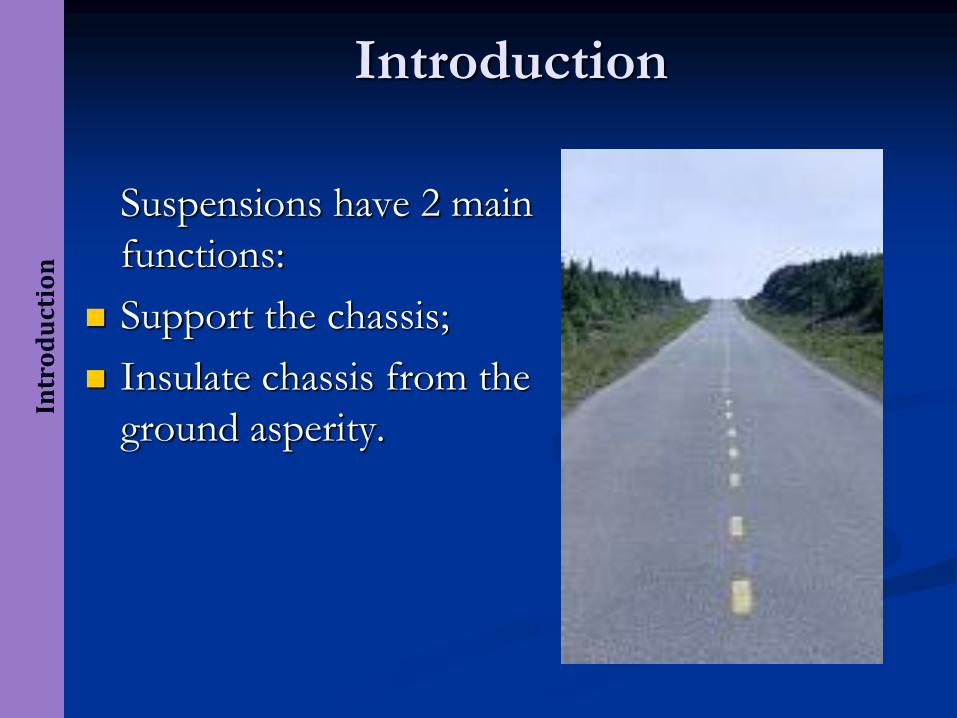
Suspensions have 2 main

functions:

Support the chassis;

Insulate chassis from the

ground asperity.

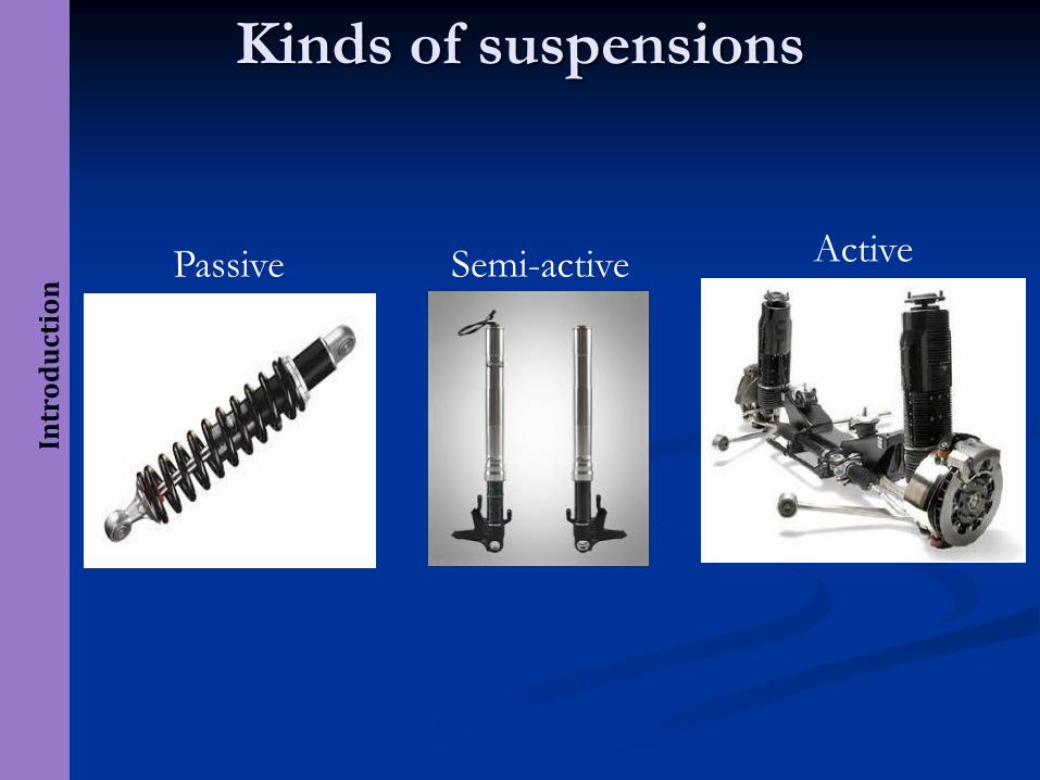
Passive ActiveSemi-active

Kinds of suspensionsIntroduction

Introdcution

Unfortunately the suspensions’ designer have

to satisfy two incompatible requirements

Comfort : «soft» suspension can modify fastly its

length reducing the acceleration of the sprung mass,

but at same time it reduces the force exchanged

between ground and tires.

Handling: «rigid» suspension guarantees better

adherence of tires, but applies bigger vertical

acceleration to the sprung mass.

Active suspensions are the best way to manage this

trade-off

Introdcution

Standards for comfort evaluation

RMS vertical acceleration level [m/s2] Degree of comfort

(1) < 0,315 Not uncomfortable

(2) 0,315 – 0,63 A little uncomfortable

(3) 0,5 – 1 Fairly uncomfortable

(4) 0,8-1,6 Uncomfortable

(5) 1,25-2,5 Very uncomfortable

(6) > 2 Extremely uncomfortable

RMS vertical acceleration level and degree of comfort

From ISO 2631-1 1997: Mechanical vibration and shock

Introdcution

Standards for comfort evaluation

Minimum tolerance

between 4 Hz (25.13

rad/s) and 8 Hz

(50.26 rad/s) due to

vertical resonance of

the abdominal

cavity.

Small inflection

between 10 Hz

(62.83 rad/s) and 20

Hz (125.66 rad/s)

due for example to

head resonance at 10

Hz.

They were adopted by the following constructors:

Lotus (Ayrton Senna) ;

Williams-Renault (Nigel Mansell and Riccardo Patrese) with a

neural network controller able to make more than 60 asset

variations per second and to keep the vehicle at less than 1 cm

from ground to keep the ground effect.

Introduction

History

First active suspensions were designed by an English

engineer in 1985. Their first use took place in Formula 1

in 1987.

Introduction

In 1993 Alex Zanardi was involved in a terrible accident caused

by an erroneous operation of the active suspensions system.

In 1994 active suspension was forbidden for safety and sport

reasons (their high efficacy gave too many advantages to the

users): the active suspension research ended.

Today some manufacturers develop active suspensions for their

high-performance cars and motorbikes.

Market

Passive suspensions are largely used in vehicles thanks to

their simplicity and low cost.

Passive suspensions

Market

The semi-active suspensions use a parallel of a spring and a

damper but it is possible to tune the damping factor.

Semi-active suspensions

Market

Active suspensions use an actuator to generate a tunable force F(t).

First commercial active suspensions system was implemented in 1991

by Toyota in the Soarer UZZ 32.

Active suspensions - I

Market

Another vehicle that uses active suspensions is the

Mercedes-Benz SL500.

Active suspensions - II

Vehicles

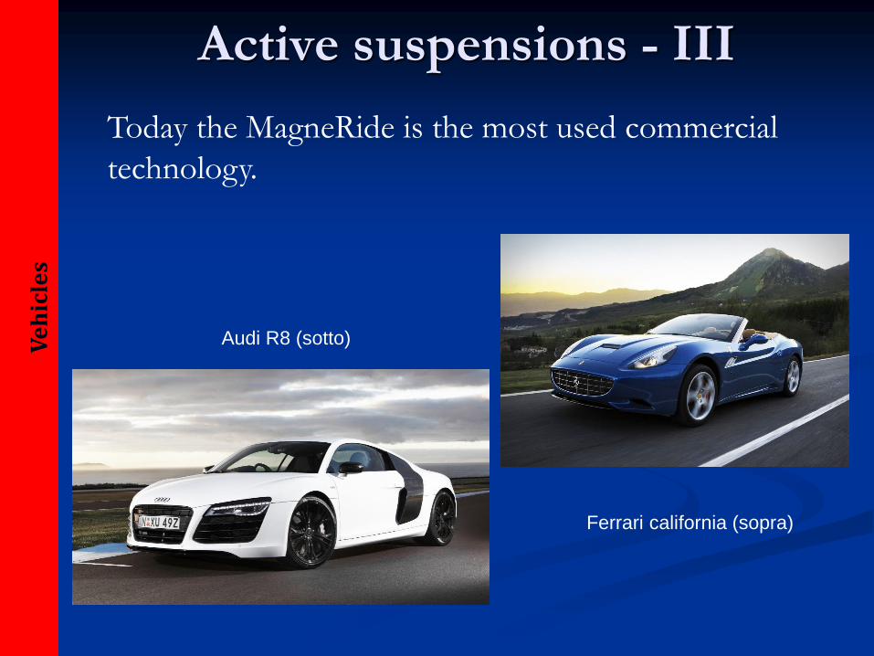
Today the MagneRide is the most used commercial

technology.

Ferrari california (sopra)

Audi R8 (sotto)

Active suspensions - III

Description

Physical modelVehicles are very complex systems.

Among the most important things to consider are:

Suspensions geometry;

Coupled behavior.

The most used models are

the following ones:

Quarter-Car;

Half-Car;

Full Car.

Description

ACTIVE SEMI-ACTIVE PASSIVE

Quarter-car representation

Matlab/Simulinkimplementation

Suspensions control

We implemented two control methods:

Loop shaping, controlling firstly the

vertical acceleration and secondly the

handling;

H-infinity, in order to optimize acceleration

and handling performances contemporarily.


We started from the implementation of the quarter-car

physical model in Simulink, modelled by Euler-Newton

equations.

Simulation model


Here are the values of the physical quantities involved:

Simulation model

mb = 300 kg

mw = 60 kg

bs = 1000 N/m/s

ks = 16000 N/m

kt = 190000 N/m

Bt = 0 N/m/s


Loop shaping controller of acceleration

Input (u): actuator force.

Disturbance (w): we chose to consider as disturbance a

10cm step.

Output (y): sprung mass (car body) acceleration.

Target: setting time < 1 second, small overshoot,

rejection of road profile disturbance.



Starting from the Simulink model, we computed the

transfer functions from output to input and from

output to disturbance.

Matlab/Simulinkimplementation Starting from the Bode diagram, we computed some control laws.

First target was the open loop stability.


In the Bode diagram we have a

positive +40 dB/decade slope:

the system has two zeros in the

origin. The resonance peak is

caused by the two pure

imaginary zeros at 56,3 rad/s.

With our controller we have infinite

gain margin and phase margin

equal to 50,8 at 54.8 rad/s (crossover

frequency).

Stability is verified!


After the open loop function, we need to analyze the Bode diagram of sensitivity

and complementary sensitivity functions.


As we can see, the complementary sensitivity function (azure) acts

like a low-pass filter (65 rad/s). The sensitivity (green) has a good

attenuation of the disturbance on all the frequencies, except at 40 rad/s.

Matlab/Simulinkimplementation Closed loop analysis


The crossover frequency is equal to 11 rad/s.

The gain margin is 85.9dB and the phase margin is infinite.


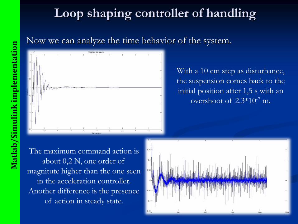
Now we can analyze the time behavior of the system.


With a 10 cm step as disturbance,

the acceleration becomes null

after about 1 s with an overshoot

of 3.44*10-5 m/s2.

The maximum command action is

about 0.015 N.

In constant speed condition, we

have the same behavior for the

power.


The interesting point is to notice that the jounce behavior in

this control system is not very good.



Loop shaping controller of handling

Now we can optimize the handling of the vehicle.

The targets are the same of the previous controller:

setting time around 1s, small overshoot, rejection of

road profile disturbance.

Input (u): actuator force.

Disturbance (w): we chose to consider as disturbance a 10cm

step.

Output(y): In the literature there are lots of discussions about

which parameter maximizes the handling*.

As a lot of authors, we considered the relative

displacement between the sprung and the unsprung

masses, i.e. the suspension elongation.

*Probably the best parameter is the tire deformation, but the

measurements are very difficult.



Starting from the Simulink model, we computed the transfer

functions from output to input and from output to disturbance.

Matlab/Simulinkimplementation Starting from the Bode diagram, we computed some control laws.

First target is the open loop stability.


Also in this case, we have a

resonance peak caused by

two pure imaginary

zeros at about 23 rad/s.

In open loop we have infinite

gain margin and phase

margin equal to 66 at 137

rad/s (crossover frequency).

Stability is verified!

Matlab/Simulinkimplementation After the open loop function, we need to analyze the Bode diagram of sensitivity

and complementary sensitivity function.


As we can see, the complementary sensitivity function (azure) acts

like a low-pass filter 102 rad/s. The sensitivity (green) has a good

attenuation of the disturbance on all the frequencies, expect at 60 rad/s.

Matlab/Simulinkimplementation Closed loop analysis


The crossover frequency is equal to 55 rad/s.

The gain margin is 95,3 dB and the phase margin is infinite.

Matlab/Simulinkimplementation Now we can analyze the time behavior of the system.


With a 10 cm step as disturbance,

the suspension comes back to the

initial position after 1,5 s with an

overshoot of 2.3*10-7 m.

The maximum command action is

about 0,2 N, one order of

magnitute higher than the one seen

in the acceleration controller.

Another difference is the presence

of action in steady state.

Matlab/Simulinkimplementation As before it’s interesting to see the acceleration behavior in this controller.


This kind of acceleration profile is not very comfortable for the

passengers.



Observation

In this control we have a lot of simplifications; for example

the geometry is simple and a filter to the road disturbance is

applied.

Nevertheless, it’s well evident that optimizing one of the two

specifications, the other one is not satisfied.

For this reason, we focused our attention on the

H-infinity control.


H-infinity control

Main problem : there are two conflicting objectives, that

are passenger comfort and road holding.

Solution: the H-infinity control is aimed to find a

compromise between them.


H-infinity control

Factors that influence the control design :

•Characteristics of the road disturbance;

•Quality of the sensor measurements for feedback;

•Limits on the available control force.


H-infinity control

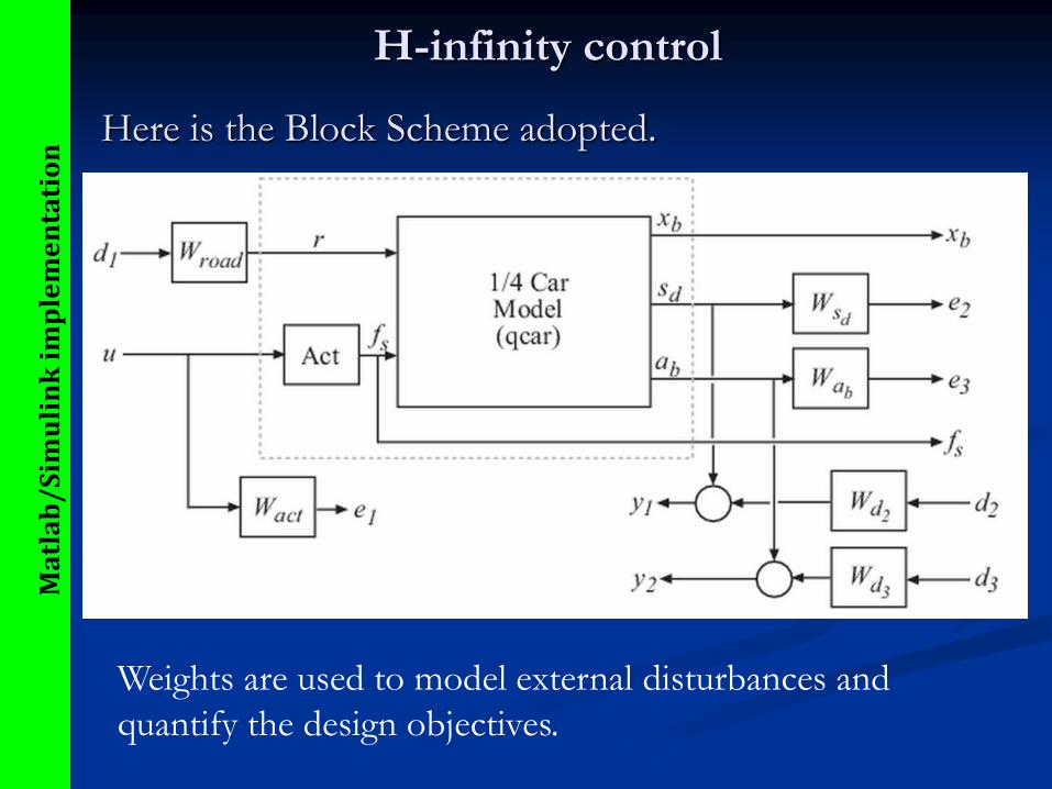
Here is the Block Scheme adopted.

Weights are used to model external disturbances and

quantify the design objectives.


H-infinity control

Here are the weight function used:

•Wroad = 0.07

•.

•Wd2=0.01, Wd3=0.5

•Wsd = β/HandlingTarget, where

•Wab = (1-β)/ComfortTarget, where

In particular β is a blending parameter, used to modulate the

trade-off. The Matlab command used to introduce β is the

following one:

β = reshape([0.01 0.5 0.99],[1 1 3]).

We use the command hinfsyn to compute an H-infinity controller

for each value of the blending parameter, β.


H-infinity control

Here are the plots of the closed-loop targets compared to the

open-loop responses in the frequency domain.

-80

-70

-60

-50

-40

-30

-20

-10

0

10

20

From: d1

To: sd

100

101

102

103

-100

-50

0

50

To: ab

Response to road disturbance

Frequency (rad/s)

Magnitu

de (

dB

)

Open-loop

Closed-loop target


H-infinity control

Here is the comparison between the different frequency responses

from the road disturbance to sd,xb and ab for the passive and

active suspensions, according to what we found in the literature.

-50

0

50

From: r

To: xb

-40

-30

-20

-10

0

10

20

To: sd

100

101

102

0

10

20

30

40

50

60

To: ab

Body travel, suspension deflection, and body acceleration due to road

Frequency (rad/s)

Magnitu

de (

dB

)

Open-loop

Comfort

Balanced

Handling


H-infinity control

Here is the comparison between the different frequency responses

from the road disturbance to sd and ab for the passive and active

suspensions, after the implementation of our controller.

56.27 rad/s is called the tire-hop frequency and it is the frequency of

the imaginary-axis zero of the transfer function from actuator to

acceleration.


H-infinity control

To further evaluate the three designs, we performed time-domain

simulations using the following road disturbance signal r(t):

r(t)=a(1−cos8πt), 0≤t≤0.25

r(t)=0 otherwise.

This signal corresponds to a road bump of height 5 cm.

Time-domain evaluation


H-infinity control

Here are the time-domain responses of the closed-loop models to

the road disturbance signal, according to what we found in the

literature.

0 0.1 0.2 0.3 0.4 0.5 0.6 0.7 0.8 0.9 1-0.04

-0.02

0

0.02

0.04

0.06

0.08

0.1Body travel

xb (

m)

0 0.1 0.2 0.3 0.4 0.5 0.6 0.7 0.8 0.9 1-20

-15

-10

-5

0

5

10Body acceleration

ab (

m/s

2)

0 0.1 0.2 0.3 0.4 0.5 0.6 0.7 0.8 0.9 1-0.1

-0.05

0

0.05

0.1Suspension deflection

Time (s)

sd (

m)

0 0.1 0.2 0.3 0.4 0.5 0.6 0.7 0.8 0.9 1-0.4

-0.3

-0.2

-0.1

0

0.1

0.2

0.3

Control force

Time (s)

f s (

N)

Open-loop

Comfort

Balanced

Suspension

Road Disturbance


H-infinity control

Here are the time-domain responses of the closed-loop models to the

road disturbance signal, after the implementation of our controller.

0 1 2 3 4 5 6 7 8 9 10-4

-3

-2

-1

0

1

2

3

4Body acceleration

ab (

m/s

2)

Open-loop

Comfort

Balanced

Suspension

Road Disturbance

0.05 0.1 0.15 0.2 0.25 0.3

-0.5

0

0.5

1

1.5

Body acceleration

ab (

m/s

2)

Open-loop

Comfort

Balanced

Suspension

Road Disturbance


H-infinity control

0 1 2 3 4 5 6 7 8 9 10-0.08

-0.06

-0.04

-0.02

0

0.02

0.04

0.06Suspension deflection

Time (s)

sd (

m)

Open-loop

Comfort

Balanced

Suspension

Road Disturbance

0 1 2 3 4 5 6 7 8 9 10-0.2

-0.15

-0.1

-0.05

0

0.05

0.1

0.15Control force

Time (s)

f s (

N)

Open-loop

Comfort

Balanced

Suspension

Road Disturbance

CarSim

implementation

Carsim Simulation

We also implemented our designed control on CarSim(shortly

C.S.) Program.

First, we selected C.S. dataset “Semi-Active Suspension”

Controller in order to study how it worked.

The control is for a semi-active suspension and for this reason it

aims to find the damping factor and then the force to apply

to each wheel.

CarSim

implementation

The inputs used by the software for each wheel are the following

ones: tire deformation, jounce, wheel velocity, body velocity

and jounce rate.

Carsim Control

Where

•K1= - 14184;

• K2= 8624;

• K3= 1088;

• K4= - 2504

•Gain4 = 2.5

•Gains 5,6,7 and 8 are

the spring stiffnesses

•Gain9 = 1

CarSim

implementation

The first four inputs are multiplied by different gain K1=

- 14184; K2= 8624; K3= 1088; K4= - 2504; then they

are summed together and moltiplied by gain1=1. The

jounce signals are also divided and moltiplied by the

spring stiffness (front and rear) in order to find the

force on each suspension, then reunited.

After this operation it sums the two signals, compute the

product between the sign of the jounce rate and

moltiply by the gain2=2.5 and find the damping factor.

Finally it compute the product between the jounce rate

and the found damping factor in order to find the

force to apply at each wheel.

CarSim

implementation

Comfort Control implementation

We implemented our comfort control and simulated it.

First of all, in order to be really close to our simulation

conditions, we changed the default parameters of the dataset

with our parameters:

unsprung mass (60 kg);

car weight with passenger (1500 kg),

suspensions and tires stiffnesses (respectively 16 N/mm and

190 N/mm).

CarSim

implementation

Here is the Simulink Scheme Block adopted.

Procedure : “bump(very sharp 3.5 cm high,40 cm long)” ,

reshaped as 5 cm step.

The constant velocity of the car was set to 35 km/h.

CarSim

implementation

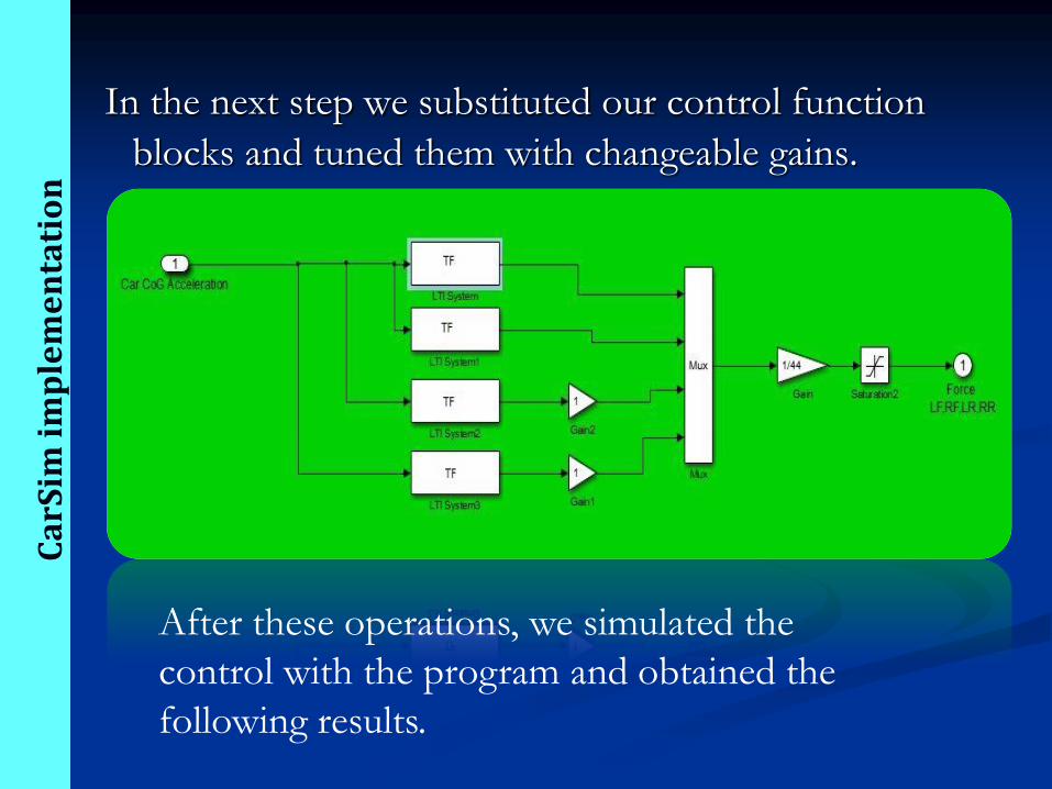
In the next step we substituted our control function

blocks and tuned them with changeable gains.

After these operations, we simulated the

control with the program and obtained the

following results.

CarSim

implementation

Plots

0 5 10 15 20 25 30 35 40-0.08

-0.06

-0.04

-0.02

0

0.02

0.04

0.06

0.08

0.1

time [t]

Suspensio

n d

eflection [

m]

front wheels

rear wheels

Suspension deflection

CarSim

implementation

Plots

Vertical acceleration

0 5 10 15-0.8

-0.6

-0.4

-0.2

0

0.2

0.4

0.6

0.8

time [t]

Vehic

le v

ert

ical accele

ration [

g]

0 5 10 15 20 25 30 35 40-50

0

50

100

150

200

250

300

350

400

450

time [t]

Forc

e [

N]

CarSim

implementation

Plots

Force

CarSim

implementation

Consideration

The results of our simulation weren’t the expected ones

and so the controller had to be revised.

However, there are several considerations to make:

- Differences in the physical model (combinated

behavior, geometry, etc.) ;

- Parameters modification (damper characteristcs);

- Different internal logical working principle of the

program ( units of measurement, discrete or

continuous time, etc.)

CarSim

implementation

Handling control

We performed another test on CarSim, based on the handling

control. In this case, we didn’t modify any parameter of the

car, given in the original dataset:

Sprung mass = 1370 kg;

Unsprung mass = 80 kg (for each “quarter”);

Spring rate of the front wheels =153 N/mm;

Spring rate of the rear wheels =82 N/mm;

Damper compression/jounce ratio of the front wheels =

0.65144;

Damper compression/jounce ratio of the rear wheels = 0.797;

CarSim

implementation

Handling control

Procedure : “Small,smooth bump”.

The constant velocity of the car was set to 50 km/h and the path

station length was set to 200 m.

94 96 98 100 102 104 106

0

0.005

0.01

0.015

0.02

0.025

0.03

path lenght [m]

bum

p h

eig

ht

[m]

CarSim

implementation

Handling control

We used a two-lead controller with a constant gain equal to 30:

CarSim

implementation

Plots

Suspension deflection

0 5 10 15 20 25 30-0.04

-0.03

-0.02

-0.01

0

0.01

0.02

0.03

time [t]

Suspensio

n d

eflection [

m]

rear wheels

front wheels

CarSim

implementation

Plots

Vertical acceleration

0 5 10 15 20 25 30-0.8

-0.6

-0.4

-0.2

0

0.2

0.4

0.6

time [t]

Vehic

le v

ert

ical accele

ration [

g]

CarSim

implementation

Plots

Force

0 5 10 15 20 25 30-1500

-1000

-500

0

500

1000

1500

time [t]

Forc

e [

N]

rear wheels

front wheels

Technology

Hydraulic actuator

A possible solution is the use of an oil

dynamic actuator.

These actuators can generate the required

forces but they are so big that can be

difficult to find the necessary free space in

a car.

The nominal actuator dynamics can be

represented by the first-order transfer

function:

The maximum displacement is 0.05 m.

Technology

Linear magnetic actuators

Recently manufacturers started to use linear magnetic actuators.

This kind of actuators guarantees faster response than the one of the

hydraulic ones.

Another advantage in the use of electronic system is the possibility the

store energy instead of dissipating it, increasing the efficiency of

the system.

The disadvantage of this solution is the low force that these actuators

can generate.

Future

Ground profile measure

A possible innovative solution can be an anticipated

measure of the ground profile variation.

In this way we can anticipate the tune of our

suspension and have a more precise control.

Future

Another idea can be splitting comfort and handling on two

different elements. The vehicle suspension system can be

designed to maximize the handling, and a new suspension under

the seat can be used to filter the chassis vibration.

This solution is usually used in heavy vehicles.

Damping seat

Conclusions

Conclusions

Evidence of the comfort/handling comprimise;

H-infinity as best control method for the analysis and

the resolution of the compromise;

Difference between project and simulation;

Pratical realization problem;

Deeper analysis of the future solution.

In conclusion we can resume these points:

The problem could be further developed and

improved in different ways

Bibliography

o “Automotive Control System” U.Kiencke,

L.Nielsen;

o “Introduzione al Controllo Ottimo” S.A.Malan,

G.Fiorio;

o “Modellistica, analisi e controllo di sospensioni

attive per autoveicoli” Ing. A. Pisano;

o Different thesies on the web

o www.mathworks.com

Thank you for your attention

Politecnico di Torino

Active Suspensions

Documents

Transcript of Active Suspensions