1

Thermal Diffusivity and Viscosity of Suspensions of

Disc Shaped Nanoparticles

Susheel S. Bhandari and K. Muralidhar

Department of Mechanical Engineering

Indian Institute of Technology Kanpur

Kanpur 208016 INDIA

and

Yogesh M. Joshi*

Department of Chemical Engineering

Indian Institute of Technology Kanpur

Kanpur 208016 INDIA

* Corresponding author, email: joshi@iitk.ac.in

2

Abstract

In this work we conduct a transient heat conduction experiment with an

aqueous suspension of nanoparticle disks of Laponite JS, a sol forming grade,

using laser light interferometry. The image sequence in time is used to measure

thermal diffusivity and thermal conductivity of the suspension. Imaging of the

temperature distribution is facilitated by the dependence of refractive index of

the suspension on temperature itself. We observe that with the addition of 4

volume % of nano-disks in water, thermal conductivity of the suspension

increases by around 30%. A theoretical model for thermal conductivity of the

suspension of anisotropic particles by Fricke as well as by Hamilton and

Crosser explains the trend of data well. In turn, it estimates thermal

conductivity of the Laponite nanoparticle itself, which is otherwise difficult to

measure in a direct manner. We also measure viscosity of the nanoparticle

suspension using a concentric cylinder rheometer. Measurements are seen to

follow quite well, the theoretical relation for viscosity of suspensions of oblate

particles that includes up to two particle interaction. This result rules out the

presence of clusters of particles in the suspension. The effective viscosity and

thermal diffusivity data show that the shape of the particle has a role in

determining enhancement of thermophysical properties of the suspension.

3

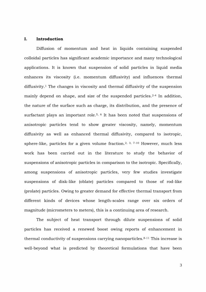
I. Introduction

Diffusion of momentum and heat in liquids containing suspended

colloidal particles has significant academic importance and many technological

applications. It is known that suspension of solid particles in liquid media

enhances its viscosity (i.e. momentum diffusivity) and influences thermal

diffusivity.1 The changes in viscosity and thermal diffusivity of the suspension

mainly depend on shape, and size of the suspended particles.2-4 In addition,

the nature of the surface such as charge, its distribution, and the presence of

surfactant plays an important role.5, 6 It has been noted that suspensions of

anisotropic particles tend to show greater viscosity, namely, momentum

diffusivity as well as enhanced thermal diffusivity, compared to isotropic,

sphere-like, particles for a given volume fraction.2, 3, 7-10 However, much less

work has been carried out in the literature to study the behavior of

suspensions of anisotropic particles in comparison to the isotropic. Specifically,

among suspensions of anisotropic particles, very few studies investigate

suspensions of disk-like (oblate) particles compared to those of rod-like

(prolate) particles. Owing to greater demand for effective thermal transport from

different kinds of devices whose length-scales range over six orders of

magnitude (micrometers to meters), this is a continuing area of research.

The subject of heat transport through dilute suspensions of solid

particles has received a renewed boost owing reports of enhancement in

thermal conductivity of suspensions carrying nanoparticles.8-11 This increase is

well-beyond what is predicted by theoretical formulations that have been

4

validated and known to work well for stable suspensions of larger particles.

Such anomalous increase in thermal conductivity has been attributed by

various authors to factors such as enhanced Brownian diffusivity,12 phonon

transport,11 layering of liquid molecules over the particle surface,13 and fractal

cluster formation.6, 14 Recent literature, however, indicates consensus on the

possibility of cluster formation of nanoparticles as the factor responsible for the

anomalous enhancement in thermal conductivity.9 A major limitation in many

studies that analyze enhancement of thermal conductivity in nanofluids by

using theoretical models is unavailability of thermal conductivity of the

nanoparticles. In such cases assumption of thermal conductivities over a

certain range facilitates comparison of the trend. Interestingly, careful and

independent investigations on this subject do not subscribe to the claim of

anomalous enhancement of thermal conductivity beyond the theoretical.15, 16

Poulikakos and coworkers15 carefully studied the effect of particle size,

concentration, method of stabilization and clustering on thermal transport in

gold nanofluid. A maximum enhancement of 1.4 % was reported for 0.11

volume % suspension of 40 nm diameter particles in water suggesting no

apparent anomaly.

In general, if thermal conductivity of the suspended particles is

significantly greater than that of suspending liquid, increase in the aspect ratio

is expected to cause substantial enhancement in thermal conductivity of the

suspension. This is due to the fact that for the same volume fraction,

anisotropy allows thermal transport over greater length-scales through

5

elongated shape and greater surface area of the suspended particles. Here, the

aspect ratio is defined in such a way that it is less than unity for oblate

particles and greater than unity for the prolate. Based on Hamilton and

Crosser theory,3 Keblinski and coworkers17 suggested that for equal volume

fractions, a 10 fold enhancement in thermal conductivity is obtained when the

aspect ratio of the anisotropic particle is around 100 (or 1/100). A good

amount work has been carried out in the literature to investigate thermal

properties of carbon nanotube suspensions in a variety of solvents. 8-11 Owing

to different aspect ratios, solvents and type of nanotubes (single or multiwall),

there is considerable spread in the data. The reported values range from 10 %

to over 150 % enhancement in the thermal conductivity for 1 volume %

concentration.13, 18-23 On the other hand, experiments with aqueous suspension

of titanate nanotubes having an aspect ratio of 10 is reported to show very

moderate enhancement of around 3 % for 2.5 weight % suspension.24 Recently

Cherkasova and Shan25 studied thermal conductivity behavior of suspension of

whiskers having various aspect ratios (up to 10) and observed that for constant

total volume fraction thermal conductivity increases with increase in the aspect

ratio. The experimental data showed good agreement with effective medium

theory of Nan and coworkers26 which accounts for interfacial resistance in the

conventional theories.

Compared to suspensions of rod-like particles, less work has been

reported for suspensions of disk-like particles. Singh and coworkers 27 studied

heat transfer behavior of aqueous suspension of silicon carbide having oblate

6

shape and aspect ratio of around 1/4. They typically observed 30 %

enhancement for 7 volume % concentration. The authors analyzed the data

using Hamilton and Crosser theory3 and found a correlation between them.

Khandekar and coworkers28 employed various spherical nanoparticle as well as

Laponite JS (oblate shape, aspect ratio 1/25) based nanofluids in closed two

phase thermosyphon and observed its heat transport behavior to be inferior to

that of pure water in all cases. However, in a thermosyphon, in addition to

thermal conductivity, fluid viscosity, wettability of the liquid on the surface of

the apparatus, and roughness of the surface compared to particle dimensions

also play an important role.28 Recently, Bhandari and coworkers29 reported

transient heat transport behavior of a suspension of gel forming grade of

nanoclay called Laponite RD, which has a soft solid-like consistency.

Interestingly for about 1 volume % concentration of clay over 30 %

enhancement in thermal conductivity was observed. Unlike the previous

examples, this system is in solid state with finite elastic modulus (and infinite

viscosity).29 Recently many groups have studied heat transport in nanofluids

composed of graphene. It has negligible thickness compared to its lateral

dimensions and an extreme aspect ratio. Most studies employ water as the

suspending medium. In order to render graphene hydrophilic, a

functionalization step is carried out. For functionalized graphene – water

nanofluids, thermal conductivity enhancement of 15 to 25 % is observed for

around 0.05 volume %.30-32 Other studies employ water soluble solvents such

as ethylene glycol33 and alcohol34 and report similar enhancement as for water.

7

Although most studies on graphene nanofluid report thermal conductivity

enhancement with increase temperature,30-32, 35 one study reports it to remain

constant.34 Dhar et al.36 and Martin-Gallego et al.37 have analyzed thermal

conductivity enhancement in graphene nanofluid and emphasized the

importance of phonon transport. Two studies have compared the effect of

particle shape, namely, prolate vis á vis oblate on the thermal conductivity

enhancement at a given concentration using carbon nanotube and graphene

nanofluids. Interestingly, Martin-Gallego et al.37 observe enhancement in both

the systems to be comparable while Wang and coworkers35 report graphene

nanofluid to perform better than nanotube suspension.

In the present work, we study transient heat transport behavior of an

aqueous suspension of sol forming nanoclay - Laponite JS, which is an

anisotropic, disk-shaped nanoparticle, using laser light interferometry.

II. Viscosity and thermal conductivity of suspension of oblate spheroids

In the limit of very low volume fractions (f < 0.03) an expression of

viscosity of suspension having spherical particles is due to Einstein and is

given by:38

( )1 2.5sh h f= +

where sh is viscosity of the Newtonian solvent in which the particles having

volume fraction f are suspended. This expression was obtained by estimating

dissipation associated with flow around the sphere and assumes flow field

8

around one sphere is not influenced by the presence of other spheres in the

vicinity (therefore, the dilute limit). This expression was modified by

incorporating hydrodynamic interactions associated with two–body interactions

by Batchelor and Green.39 The two body interaction leads to a contribution to

h proportional to 2f .

For a suspension containing monodispersed particles, the general

expression for low shear viscosity irrespective of the aspect ratio of the particles

can be written as:40, 41

( )2 31 21r

s

C C Oh

h f f fh

= = + + + , (1)

where 1C and 2C respectively represent one and two body interactions and the

volume fraction f . In this expression, 1 0C hé ù= ë û and

22 0HC k hé ù= ë û , where

0hé ùë û is

an intrinsic viscosity in the limit of low shear rates. Parameter Hk is the

Huggins coefficient, which relates viscosity originating from two body

interactions to that of viscosity associated with the infinite dilution limit where

two body interactions are negligible. For particles having hard core

interactions, the theoretical value of Huggins coefficient has been estimated to

be Hk »1 for spheres.40 Theoretical value for disk-like particles is not available

in the literature. Equation (1) with up to two body interaction ( 2f term) term

holds good for f £0.1.

9

In this work we study viscosity behavior of oblate spheroidal particles.

We assume d and a to be the length-scales associated with short and long axis

of the spheroid respectively. For a disk, d and a can be considered as a

thickness and diameter respectively. Intrinsic viscosity 0

hé ùë û , a dimensionless

quantity, is a function of the aspect ratio pr ( /d a= <1) and is given by the

expression:41, 42

( )0

15 321 0.628

2 15 1 0.075p

pp p

rr

r rh

p

æ ö- ÷çé ù ÷ç= + - - ÷çë û ÷÷ç -è ø. (2)

It can be seen that intrinsic viscosity expressed by Equation (2) is sensitive to

the aspect ratio of the particle. It is inherently assumed in Equations (1) and (2)

that particle orientation is isotropic, and therefore these equations are

applicable only in the limit of small rotational Peclet number ( )1Pe << defined

as,38

34

3sdPekT

h g=

. (3)

In Equation (3), g is shear rate, k is Boltzmann constant, sh is solvent

viscosity and T is temperature.

The expression for electrical conductivity of a suspension containing

oblate non-polarizable spheroidal particles is due to Fricke.2 In this analysis, a

single particle was placed in a unit cell, subjected to a unit potential difference,

and analyzed in terms of Poisson’s equation for a two-phase system. The

influence of all other particles in the suspension on the near field of the single

10

particle was taken to be equal to the mean value for the entire suspension. The

prediction of electrical conductivity was seen to match very well with that of

dog’s blood for concentration of red corpuscles up to 90% in serum, the

particles being treated as oblate spheroids. Treating thermal conductivity as

analogous to electrical conductivity, the effective thermal conductivity of a

suspension containing oblate spheroidal particles is given by:2, 25

( ) ( )( )( ) ( )1 1 1

1 1e s

n nk k

n

z z f

z z f

é ù+ - + - -ê ú= ê ú+ - - -ê úë û, (4)

where sk is thermal conductivity of the solvent, p sk kz = is particle-to-solvent

conductivity ratio, and pk is thermal conductivity of the particles. Parameter n

is a shape factor given by:

( )( )

1

1n

b z

z b

-=

- -, (5)

Here b is:

( )( )

( )( )( )

4 1 113 2 1 1 1 1M M

z zb

z z

é ùê úê úê úë û

- -= +

+ - + - -, (6)

and

3

2 sin 2cos

2 sinM

j jj

j-

= , (7)

where 1cos ( )prj -= .

Rather than extending the expression derived for electric conductivity to

thermal conductivity as carried out by Fricke,2 Hamilton and Crosser3 obtained

11

effective thermal conductivity of a two component heterogeneous system by

expressing it in terms of ratios of average temperature gradient in both the

phases. They obtained the average gradient ratio by using expressions

developed by Maxwell7 and Fricke,2 which led to the identical expression for ek

as given by Equation (4) but a different shape factor:3

3n = Y , (8)

where Y is sphericity expressed as the ratio of surface area of a sphere having

the same volume as the particle to that of surface area of the particle. For a

disk having diameter a and thickness d (aspect ratio pr /d a= ), sphericity is

given by the expression:

( )2 32 3 4

1p

p

r

rY =

+. (9)

The major difference between the analysis of Fricke and Hamilton and Crosser

is the way effect of shape is incorporated. The latter considers the shape factor

to be an empirical constant and expresses it as: 3n = Y . On the other hand, in

the Fricke expression shape factor is a function of thermal conductivities of

particle as well as base fluid in addition to the aspect ratio. The expression by

Hamilton and Crosser shows thermal conductivity of suspension to be slightly

higher than that of Fricke for a given volume fraction of suspended particles.

Both the expressions yield the Maxwell relation in the limit of spherical shape

of the particle (aspect ratio of unity).

12

Similar to the expression for viscosity, a necessary condition for the

application of Fricke model as well as Hamilton and Crosser model is an

isotropic distribution of orientations of the disk-shaped particles. This

requirement is ensured at the low Peclet number limit 1Pe << . In addition,

sufficient time is needed to be given to the suspension in an experiment to

stabilize so that Brownian motions randomize the orientation of clay discs and

erase the shear history.

While the Fricke model is for electrical conductivity, it has been used to

estimate thermal conductivity from the following thermodynamic perspective.

Natural phenomena follow a cause-effect relationship that is expressible as in

terms of forces and fluxes. It is a linear relation for electrical, thermal,

hydraulic and other situations. Thus, one can have expressions for electrical,

thermal, and hydraulic resistance and conductivity. Though the conductivities

do not match in dimensional form, we can expect nondimensional

conductivities of thermal and electrical systems scaled by a reference to match

in quantitative terms.

III. Determination of thermal diffusivity from an unsteady experiment

Consider a horizontal layer of the aqueous suspension in one dimension

of thickness H maintained initially at constant temperature CT . At time 0t > ,

the temperature of the top surface is suddenly raised to HT ( CT> ).

Consequently heat diffuses from the top plate towards the bottom plate. The

13

configuration is gravitationally stable in density. Hence, convection currents

are absent and heat transfer is determined by pure diffusion. Combining

Fourier’s law of heat conduction with the first law of thermodynamics, the

governing equation for temperature is given by,1

2

2

q qt y

¶ ¶=

¶ ¶. (10)

Here ( ) ( )C H CT T T Tq = - - is dimensionless temperature, 2t Ht a= is

dimensionless time, y Hy = is a dimensionless coordinate measured from the

lower surface. In addition, t is time and a is thermal diffusivity of the

suspension. The initial and boundary conditions associated with Equation (8)

are:29

0q = 0t £

1q = 0t > , 1y = (11)

0q = 0t > , 0y =

Equation (10) can be analytically solved for a constant thermal diffusivity

medium subject to conditions described by Equation (11) to yield:29

( ) ( )1 2 22 ( 1) sin expn

n

n n nq y p py p t+é ù= - - -ê úë ûå , for n =1, 2, 3 … (12)

Over the range of temperatures discussed in Section IV, thermal diffusivity

changes by less than 0.5% and the constant diffusivity approximation is valid.

According to Equation (12), the only material property that fixes the evolution

of the temperature field is thermal diffusivity a .

14

We describe in Section IV the experimental procedure to obtain

temperature within the suspension as a function of position (y ) and time.

Using an inverse technique, we fit Equation (12) to the experimentally obtained

temperature data so as to estimate thermal diffusivity. The technique relies on

the method of least squares where the variance of the measured temperature

relative to the analytical is minimized with respect to diffusivity as a parameter.

In the limit of steady state (t ¥ ), Equation (12) becomes independent of

thermal diffusivity. Hence, with increase in time, the fit of Equation (12) to the

experimental data becomes progressively less sensitive to the choice of a . In

addition, with the approach of steady state, temperature field in the aqueous

suspension is affected by the thermal properties of the confining surfaces. At

the other extreme of small values of t , temperature gradients near the heated

boundary are large and optical measurements are contaminated by refraction

errors. Hence, with small time data, uncertainty associated with the estimated

thermal diffusivity from Equation (12) is expected to be large. It can be

concluded that the regression of experimental data against the analytical

solution is most appropriate only at intermediate times. The conventional least

squares procedure is thus modified to an equivalent weighted least squares

procedure to highlight the data within a certain sensitivity interval, as

discussed below.

15

Let ja ( )1, 2,...j m= parameters be determined from measurement data

iY ( )1,2,...i n m= > using a mathematical model ( )i jT a by a least squares

procedure. The process of minimizing the error functional:

( )21( )

nj i ii

E a Y T-

= -å (13)

leads to the system of algebraic equations:43

{ }1

{ } T Tj ia J J J Y

-é ù= ê úë û . (14)

Here, J is a Jacobian matrix defined as

iij

j

TJ

a

¶=

¶. (15)

Equation (14) shows that uncertainty in the estimated parameters ja depends

on the condition number of the matrix TJ J since its inverse multiplies the

measured data iY . Specifically, the condition number should be large for

uncertainty to be small. This requirement leads to the result that the diagonal

entries of the matrix TJ J should be large. In this context, the Jacobian is

referred to as sensitivity in the literature.44

During estimation of a single parameter, namely thermal diffusivity from

spatio-temporal data of temperature, sensitivity estimates can be alternatively

derived as follows. In analogy to Equation (15), the sensitivity parameter for the

suspension as a whole is obtained by integrating over the layer thickness and

is given by:44

16

( )0

,H

tT

S t dyaa

¶=

¶ò . (16)

By differentiating Equation (12), the dimensionless form of the sensitivity

parameter tS is given by the expression:

( ) ( ) ( ) ( )2 1 2 2 2

1

2 1 1 expn nR t

t RnH C

SS n

H T T

at a p t

¥+ +

=

é ù= = - - + - -ê ú- ë ûå , (17)

where Ra is thermal diffusivity of a reference material (water in the present

study), Ra a a= , and 2RR t Ht a= .

Analogous to time, a fit to the experimental data closer to either of the

boundaries in not sensitive to the choice of a . The loss of sensitivity arises

from the fact that the walls are at constant temperature, independent of the

material diffusivity. Following Equation (16), sensitivity associated with the

experimental data as a function of the spatial coordinate can be estimated by

integrating with respect to time and is given by:

( )0

,yT

S y dtaa

¥ ¶=

¶ò . (18)

However, in Equation (18) rather than integrating T a¶ ¶ over the entire

duration of experiment, we integrate the same over only that duration where

sensitivity estimated from equations (16) and (17) is very high (typically above

90 % of the maximum in sensitivity). If interval between 1t and 2t represents

that window of high sensitivity, Equation (18) can be modified to:

( ) 2

1

,t

y t

TS y dta

a¶

=¶ò . (19)

17

In a manner similar to Equation (17), the dimensionless sensitivity parameter

yS for spatial sensitivity of data is given by:

yS =( )( )2 1

y R

H C

S

T T t t

a=

- - ( ) ( ) ( )2

2 1

1 21 sinn

nnR R

n An

pypa t t

+-

- å , (20)

where nA is given by:

( ) ( )2 22 2 1 12 2 2 2

1 1exp expn R R R RA n n

n nt a t t a t

a p a p

æ ö æ ö÷ ÷ç ç= + - - + -÷ ÷ç ç÷ ÷÷ ÷ç çè ø è ø. (21)

In order to obtain a dependable value of a , Equation (12) is fitted to the

experimental data in that window of y and t , where sensitivity, defined by

Equations (17) and (20) is high. In addition, uncertainty in the estimated

properties is determined by conducting statistically independent experiments.

IV. Materials, sample preparation and experimental protocol

In the present study, we use an aqueous suspension of Laponite JS®

(sodium magnesium fluorosilicate), which is a sol forming variant of Laponite

clay.45 Laponite particles are disk-like with diameter 25 nm and thickness 1

nm with very little size/shape distribution.46 In a single layer of Laponite, two

tetrahedral silica layers sandwich an octahedral magnesia layer.47 A particle of

Laponite can, therefore, be considered as a single crystal. Face of Laponite

particle is negatively charged while the edge has weak positive charge. Laponite

JS used in the present work was procured from Southern Clay Products Inc.

Laponite JS contains premixed tetrasodium pyrophosphate which prevents

aggregation of the particles thereby providing stability to the sol. It should be

18

noted that in our previous communication,29 we had investigated gel forming

grade: Laponite RD, which does not have tetrasodium pyrophosphate and

therefore transforms into a soft solid with infinite viscosity and finite modulus.

The suspension of Laponite JS used in this work, on the other hand, is a free

flowing liquid with viscosity comparable to water. According to the

manufacturer, suspension of Laponite JS is stable against aggregation over

duration of months for much larger concentrations than used in the present

work.45 Predetermined quantity of white powder of Laponite was mixed with

ultrapure water using an ultra Turrex drive as stirrer. Water was maintained at

pH=10 to ensure chemical stability of the Laponite particles.48 Laponite JS

forms a stable and clear suspension in water that remains unaltered for several

months. Laponite JS suspension prepared using this procedure was used for

rheology and interferometry experiments. The ionic conductivity and pH of the

suspension after incorporation of Laponite JS are reported in Table 1. While pH

remains practically constant, conductivity increases as expected with Laponite

concentration.

Rheological experiments were carried out in a concentric cylinder

geometry (diameter of inner cylinder 26.663 mm and thickness of the annular

region 1.08 mm) using Anton Paar MCR 501 rheometer (stress controlled

rheometer with minimum torque of 0.020.001 µNm). Viscosity is measured

over a range of shear rates 25/s to 140/s and is observed to be constant over

this range. We ensured absence of Taylor-Couette instability in the annular gap

during the measurement of viscosity over this shear rate range.

19

Transient heat transfer experiments were performed using a Mach-

Zehnder interferometer. A schematic drawing of the setup is shown in Figure 1.

In this setup the collimated laser beam [632.8 nm, 35 mW He-Ne laser (Spectra

Physics)] is split using a beam splitter and passed through the test and the

reference chambers as shown in Figure 1. Subsequently, the beams are

superimposed, and the resulting image is recorded by a CCD camera. Owing to

the optical path difference generated between the beams passing through the

test and the reference sections an interference pattern is formed. Before

beginning the experiment, the test chamber was filled with Laponite JS

suspension having a certain concentration. The reference chamber was filled

with glucose solution. The concentration of the glucose solution in the

reference chamber was varied in such a way that it matched the refractive

index of Laponite suspension in the test chamber at temperature CT . This step

ensured balancing of the optical path lengths of the light beams passing

through the reference and the test chambers. Superposition of the two light

beams resulted in constructive interference with a bright spot on the screen.

This state of the interferometer is referred as the infinite fringe setting.

Subsequent to attainment of thermal equilibrium between the test and the

reference sections of the apparatus, the temperature of the top plate was raised

to HT . Soon after the top plate temperature is raised to HT , heat diffuses

towards the lower surface, causing an increase in temperature within the

medium. Consequently, refractive index of the suspension is altered,

generating an optical path difference between the beams passing through the

20

test and the reference chambers. Superposition of the two light beams leads to

an interference pattern.

In the present set of experiments, we maintained CT between 19 and

20 , while HT is varied between 21 and 23°C. The horizontal bounding

surfaces of the test cell were made of 1.6mm copper sheets. Temperatures were

maintained constant by circulating water over these surfaces from constant

temperature baths. The lower surface was baffled to form a tortuous flow path

in addition to creating a fin effect. Constant temperature baths maintained

temperature constant to within +0.1°C. Direct measurement by thermocouples

did not reveal any (measurable) spatial temperature variation. These

temperatures were constant to within +0.1°C during the experimental duration

of 4-5 hours. Experiments were carried out in an air-conditioned room where

temperature was constant to within +1.0°C. The bounding surfaces reached

their respective temperatures in 1-2 minutes. This delay is negligible in

comparison to the experimental duration of 4-5 hours. The time constant of the

diffusion process can be estimated as 2H a 4.6 hours.

We study below the effect of concentration of Laponite JS up to 4 volume

% in water. For each concentration, a minimum of three experiments were

carried out to examine repeatability. In order to analyze results of laser

interferometry, the temperature dependence of refractive index of the Laponite

suspension at each concentration is required. In the present work, a

21

refractometer (Abbemat 500, Anton Paar) was used to measure refractive index

of the suspension at various temperatures.

V. Results and Discussion

Viscosity of the suspension

In Figure 2 we plot effective viscosity of the aqueous suspension as a

function of volume fraction of Laponite JS. It can be seen that viscosity, shown

as circles, increases with volume fraction, such that for 4% volume fraction of

Laponite, viscosity is three times that of water. Note that the uncertainty band

is quite small. In Section II we discussed the need to enforce a limit of 1Pe <<

to ensure random (isotropic) orientation of the clay disks for Equations (1) to

hold. This assumption can now be examined. For sh =10–3 Pa-s, d = 25 nm,

g =100/s, and T =300 K, we get Pe 0.0005, which is considerably smaller

than unity. Hence, the particle orientation is randomized and there are no

preferred directions for thermal diffusivity. Further, the system is

gravitationally stable (bottom heavy) and convection is not present. Hence,

random orientation of the original medium is preserved during the conduction

heat transfer experiment.

It can be seen that Equation (1) fits the data very well, which is

represented by a solid line. In the inset we plot ( ) ( )s s Lh h h f- as a function of

concentration of Laponite. The linear fit to the data in the inset in rearranged

Equation (1) is given by: ( ) ( ) 0 2[ ]s s L Ch h h f h f- = + , whose intercept on the

22

vertical axis lead to intrinsic viscosity 0[ ]h . Equation (2) relates intrinsic

viscosity 0[ ]h to the aspect ratio of oblate particles. Remarkably value of

0[ ]h =18.62 obtained from linear fit leads to 1/ pr =25.7 which is very close to the

value of 25 reported in the literature from independent measurements.45, 46 The

fit of the data also yields Huggins coefficient Hk =2 for disk like particles of

Laponite. Importantly, a good fit of the experimental data is obtained to the

viscosity relation based on classical theory. It confirms the aspect ratio of the

particle independently and rules out the presence of clusters of disk-like

particles within the suspension. For this reason, measured thermal

conductivity data in the following section have been compared with well-

established models of HC and Fricke.

Thermal diffusivity of the suspension

Next, we discuss thermal diffusivity measurements based on

interferometry experiments. Subsequent to a step increase in temperature of

the top surface, one dimensional diffusion of heat is initiated towards the cold

plate of the test section. An increase in temperature of the suspension changes

its density, and hence the refractive index. This alters the optical path length of

the beam of light passing through the test section in comparison with the

reference, producing an interference pattern on superposition. It is noted here

that diffusivity changes in the range 21–23°C are small enough from a

modeling perspective (Equation 12). However, density and refractive changes

23

are large enough to create a measurable optical path difference needed for the

formation of interferograms. Measurement sensitivity is further enhanced by

having a test cell that is long in the viewing direction.

The time evolution of the interference pattern is shown in Figure 3. In the

beginning, the fringe pattern at time t =0 reveals an infinite fringe setting,

corresponding to constructive interference when equal path lengths are

obtained in the light beam passing through test and reference sections. As heat

diffuses from the top surface into the suspension, fringes appear in its

neighborhood, and migrate with time towards the lower surface. In the limit of

large times, steady state sets in and fringes get distributed throughout the

field. The temperature difference associated with two consecutive fringes ( TeD )

can be estimated from the knowledge of variation of refractive index with

temperature dn dT , wavelength of light l , length of the test cell L , and is given

by principles of wave optics as:49

( )/T Ldn dTe lD = . (22)

Equation (22) assumes that the passage of the light ray is straight and beam

bending due to refraction is small. Refraction would be strong in the initial

stages when temperature (and hence, refractive index) gradient near the top

wall is large. Explicit calculations with a generalized form49 of Equation 22

showed that for times greater than 20 minutes, refraction error is less than 1%

and Equation (22) is applicable. This requirement is fulfilled during data

analysis in a statistical framework using the sensitivity function. In Figure (4),

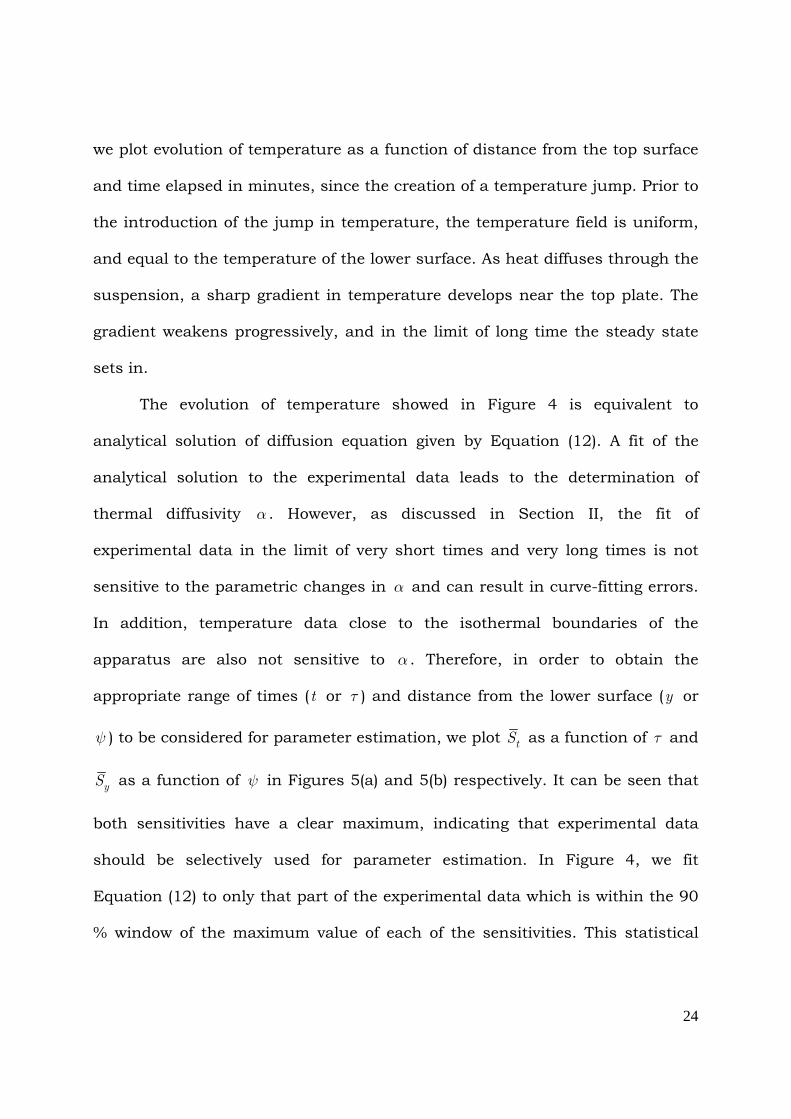
24

we plot evolution of temperature as a function of distance from the top surface

and time elapsed in minutes, since the creation of a temperature jump. Prior to

the introduction of the jump in temperature, the temperature field is uniform,

and equal to the temperature of the lower surface. As heat diffuses through the

suspension, a sharp gradient in temperature develops near the top plate. The

gradient weakens progressively, and in the limit of long time the steady state

sets in.

The evolution of temperature showed in Figure 4 is equivalent to

analytical solution of diffusion equation given by Equation (12). A fit of the

analytical solution to the experimental data leads to the determination of

thermal diffusivity a . However, as discussed in Section II, the fit of

experimental data in the limit of very short times and very long times is not

sensitive to the parametric changes in a and can result in curve-fitting errors.

In addition, temperature data close to the isothermal boundaries of the

apparatus are also not sensitive to a . Therefore, in order to obtain the

appropriate range of times (t or t ) and distance from the lower surface (y or

y ) to be considered for parameter estimation, we plot tS as a function of t and

yS as a function of y in Figures 5(a) and 5(b) respectively. It can be seen that

both sensitivities have a clear maximum, indicating that experimental data

should be selectively used for parameter estimation. In Figure 4, we fit

Equation (12) to only that part of the experimental data which is within the 90

% window of the maximum value of each of the sensitivities. This statistical

25

procedure reliably estimates thermal diffusivity as a function of volume fraction

of Laponite JS.

Thermal conductivity of the suspension

Thermal conductivity enhancement in nanofluids has been a subject of

many studies over the past decade. Apart from solvent selection, types of

nanoparticles, their sizes, and to a lesser extent, their shape have been

explored. The measurement technique – point, line or volumetric, influences

the conductivity prediction. It is, therefore, not surprising that contradictory

opinions have been expressed in the literature. In this context, knowledge of

physicochemical behavior of colloidal suspensions is also necessary. A rigorous

study that employs thermal conductivity measurement in a stable suspension

of anisotropic particles and comparison with available theories helps in further

understanding of the subject.

We obtain thermal conductivity of the suspension using fitted values of

thermal diffusivity. The two are related as Pk Cr a= , where r is density of

suspension while PC is its heat capacity at constant pressure. Heat capacity of

Laponite clay is known to be 1.03 kJ/(kg-K),38-39 while that of water is 4.18

kJ/(kg-K). Heat capacity of the suspension is estimated by using the rule of

mixtures:50, 51

, , ,P sus L P L W PWC w C w C= + , (23)

26

where w is mass fraction, PC is heat capacity at constant pressure, and

subscripts L and W represent Laponite and water respectively. In Figure 6 we

plot thermal conductivity of the suspension normalized by thermal conductivity

of water as a function of volume fraction of Laponite. It can be seen that

thermal conductivity increases with increase in concentration of Laponite. An

increase of around 30 % is observed for a volume fraction of 4 %.

In Section II, we describe models for thermal conductivity proposed by

Fricke2 and Hamilton and Crosser3 for a Brownian suspension of disk-like

particles. Accordingly, the effective thermal conductivity of the suspension is

represented by Equations (4) to (7) and Equations (4), (8) and (9) respectively.

In order to estimate effective thermal conductivity, thermal conductivity of a

single particle of Laponite is necessary, which is not available in the literature.

In addition, owing to its nanoscopic size and anisotropic shape, it is expected

that thermal conductivity of the Laponite crystal would be difficult to measure

using conventional techniques. Owing to a layered structure of the particle,

comprising outer silica layers that sandwich magnesia layer, a particle of

Laponite is expected to have a high thermal conductivity.

In Figure 6, we plot a fit of Fricke model (Equations 4 to 7) and Hamilton

and Crosser model (Equations 4, 8 and 9) to the experimental data. It can be

seen that model shows a good fit to the suspension thermal conductivity for

p fk k =13. Since thermal conductivity of water is 0.58 W/(m-K), the estimated

thermal conductivity of the Laponite particle comes out to be around 7.54

W/(m-K). Interestingly crystalline silica is known to have thermal conductivity

27

of 14 W/(m-K).52 This suggests that the estimated value of thermal conductivity

of Laponite particle is plausible. Figure 6 also shows prediction of Maxwell

model (Equation 4) for suspension of isotropic particles (n =3) for p fk k =13. It

can be seen that, owing anisotropy, Laponite JS suspension substantial

improvement over suspension of isotropic particles that obey Maxwellian

behavior. As discussed in previously such enhancement can be attributed to

increased thermal transport due to greater length-scale and surface area

associated with anisotropic particle than that of isotropic particles.

As discussed in Section I on introduction to the present study, a

significant amount of research in the literature report the effect of

incorporation of nanoparticles in liquid media on thermal conductivity. Some

studies claim an anomalous increase in thermal conductivity that cannot be

explained by the existing effective medium theories. It is now believed that an

anomalous enhancement can be attributed to formation of a cluster with

fractal-like behavior. In the present work, an excellent fit of the viscosity

relation based on two body interaction to the experimental data rules out the

possibility of cluster formation.

The thermal conductivity data based on unsteady heat conduction is less

conclusive. The degree of enhancement of thermal conductivity of the aqueous

suspension of Laponite and its match with theory relies on the knowledge of

the particle thermal conductivity. The possibility of an anomalous increase can

be ruled out only with an independent estimation of thermal conductivity of the

Laponite particle. Nonetheless, qualitative agreement of the Fricke model and

28

Hamilton and Crosser model with experimental data is encouraging. In view of

the fact that the estimated value of Laponite thermal conductivity is plausible,

reference to any other mechanism to support anomalous enhancement is not

necessary. Following the correct prediction of viscosity, the effective medium

theory may now be taken as applicable in the context of energy transfer.

Consequently, the theoretical models combined with the measured thermal

diffusivity data provide a method of estimating the particle thermal

conductivity itself.

Thermal fluctuations

The role of Brownian motion on the enhancement of thermal

conductivity has been assessed thoroughly in the literature. Careful analysis

by Fan and Wang9 (and references therein) clearly rule out this possibility. On

thermophoresis, Piazza and Parola53 discuss thermophoretic diffusivity to be

comparable (or smaller) than mass diffusivity of Laponite in water. The mass

diffusivity itself is several orders of magnitude smaller than thermal diffusivity.

In addition the gradient of temperature in the thermal cell used in the present

work is small, being around 2K at 300K over a distance of 50mm. These factors

suggest that thermophoresisis has negligible contribution to the overall heat

transport.

Anisotropic particles at the nanoscale have significant advantages over

microscopic particles. Owing to their small size, thermal fluctuations of

internal energy eliminate chances of sedimentation and enhance stability of the

29

suspension. Furthermore, thermal factors keep small anisotropic particles

isotropically orientated, making thermal conductivity an isotropic quantity.

Larger anisotropic particles, on the other hand, would take longer to randomize

their orientation.

VI. Conclusions

We measure viscosity of an aqueous suspension of Laponite JS and

observe that it increases with particle concentration. Effective medium theory

for viscosity of suspensions of anisotropic particles fit the experimental data

very well. In addition intrinsic viscosity estimated from the fit correctly predicts

the aspect ratio of the Laponite particles. This suggests absence of formation of

any particle clusters in the suspension. We measure thermal diffusivity from a

transient heat conduction experiment using laser light interferometry, wherein

temperature dependence of refractive index of the suspension is utilized for

image formation. Typically for incorporation of 4 volume % of nanodisks,

around 30 % enhancement in thermal conductivity is observed in the

temperature range of 21-23°C. Similar enhancements can be expected at other

temperatures that are close to the ambient. The Fricke model as well as the

Hamilton and Crosser model for thermal conductivity of suspension of

anisotropic particles explain the trend of the experimental data quite well. The

fit requires information of particle thermal conductivity. A retrieved value of the

Laponite thermal conductivity is seen to be realistic.

30

Acknowledgement: This work was supported by Department of Science and

Technology, Government of India.

References

(1) Deen, W. M. Analysis of Transport Phenomena; Oxford University Press: New York, 1998. (2) Fricke, H. A Mathematical Treatment of the Electric Conductivity and Capacity of Disperse Systems I. The Electric Conductivity of a Suspension of Homogeneous Spheroids. Phys. Rev. 1924, 24, 575. (3) Hamilton, R. L.; Crosser, O. K. Thermal Conductivity of Heterogeneous Two-component Systems. Ind. Eng. Chem. Fundam. 1962, 1, 187. (4) Chopkar, M.; Sudarshan, S.; Das, P.; Manna, I. Effect of Particle Size on Thermal Conductivity of Nanofluid. Metall. Mater. Trans. A 2008, 39A, 1535 (5) Pilkington, G. A.; Briscoe, W. H. Nanofluids Mediating Surface Forces. Adv. Colloid Interface Sci. 2012, 179-182, 68. (6) Gao, J. W.; Zheng, R. T.; Ohtani, H.; Zhu, D. S.; Chen, G. Experimental Investigation of Heat Conduction Mechanisms in Nanofluids. Clue on Clustering. Nano Lett. 2009, 9, 4128. (7) Maxwell, J. C. A Treatise on Electricity and Magnetism; Clarendon Press: Oxford, 1891. (8) Eastman, J. A.; Phillpot, S. R.; Choi, S. U. S.; Keblinski, P. Thermal Transport in Nanofluids. Annu. Rev. Mater. Res. 2004, 34, 219. (9) Fan, J.; Wang, L. Review of Heat Conduction in Nanofluids. J. Heat Transfer 2011, 133, 040801. (10) Keblinski, P.; Prasher, R.; Eapen, J. Thermal Conductance of Nanofluids: Is the Controversy Over? J. Nanopart. Res. 2008, 10, 1089. (11) Kleinstreuer, C.; Feng, Y. Experimental and Theoretical Studies of Nanofluid Thermal Conductivity Enhancement: A Review. Nanoscale Res Lett 2011, 6, 229. (12) Kumar, D. H.; Patel, H. E.; Kumar, V. R. R.; Sundararajan, T.; Pradeep, T.; Das, S. K. Model for Heat Conduction in Nanofluids. Phys. Rev. Lett. 2004, 93, 144301. (13) Choi, S. U. S.; Zhang, Z. G.; Yu, W.; Lockwood, F. E.; Grulke, E. A. Anomalous Thermal Conductivity Enhancement in Nanotube Suspensions. Appl. Phys. Lett. 2001, 79, 2252. (14) Prasher, R.; Phelan, P. E.; Bhattacharya, P. Effect of Aggregation Kinetics on the Thermal Conductivity of Nanoscale Colloidal Solutions (Nanofluid). Nano Lett. 2006, 6, 1529. (15) Shalkevich, N.; Escher, W.; Buergi, T.; Michel, B.; Ahmed, L.; Poulikakos, D. On the Thermal Conductivity of Gold Nanoparticle Colloid. Langmuir 2010, 26, 663. (16) Buongiorno, J.; Venerus, D. C.; Prabhat, N.; McKrell, T.; Townsend, J.; Christianson, R.; Tolmachev, Y. V.; Keblinski, P.; Hu, L. W.; Alvarado, J. L.; Bang, I. C.; Bishnoi, S. W.; Bonetti, M.; Botz, F.; Cecere, A.; Chang, Y.; Chen, G.; Chen, H.; Chung, S. J.; Chyu, M. K.; Das, S. K.; Di Paola, R.; Ding, Y.; Dubois, F.; Dzido, G.; Eapen, J.; Escher, W.; Funfschilling, D.; Galand, Q.; Gao, J.; Gharagozloo, P. E.; Goodson, K. E.; Gutierrez, J. G.; Hong, H.; Horton, M.; Hwang, K. S.; Iorio, C. S.; Jang, S. P.; Jarzebski, A. B.; Jiang, Y.; Jin, L.; Kabelac, S.; Kamath, A.; Kedzierski, M. A.; Kieng, L. G.; Kim, C.; Kim, J. H.; Kim, S.; Lee, S. H.; Leong, K. C.; Manna, I.; Michel, B.; Ni, R.; Patel, H. E.; Philip, J.; Poulikakos, D.; Reynaud, C.; Savino, R.; Singh, P.

31

K.; Song, P.; Sundararajan, T.; Timofeeva, E.; Tritcak, T.; Turanov, A. N.; Van Vaerenbergh, S.; Wen, D.; Witharana, S.; Yang, C.; Yeh, W. H.; Zhao, X. Z.; Zhou, S. Q. A Benchmark Study on the Thermal Conductivity of Nanofluids. J. Appl. Phys. 2009, 106, 094312. (17) Keblinski, P.; Phillpot, S. R.; Choi, S. U. S.; Eastman, J. A. Mechanisms of Heat Flow in Suspensions of Nano-sized Particles (Nanofluids). Int. J. Heat Mass Transfer 2002, 45, 855. (18) Assael, M. J.; Chen, C. F.; Metaxa, I.; Wakeham, W. A. Thermal Conductivity of Suspensions of Carbon Nanotubes in Water. Int. J. Thermophys. 2004, 25, 971. (19) Assael, M. J.; Metaxa, I. N.; Arvanitidis, J.; Christofilos, D.; Lioutas, C. Thermal Conductivity Enhancement in Aqueous Suspensions of Carbon Multi-walled and Double-walled Nanotubes in the Presence of Two Different Dispersants. Int. J. Thermophys. 2005, 26, 647. (20) Ding, Y.; Alias, H.; Wen, D.; Williams, R. Heat Transfer of Aqueous Suspensions of Carbon Nanotubes (CNT Nanofluids). Int. J. of Heat Mass Transfer 2006, 49, 240 (21) Liu, M. S.; Ching-Cheng Lin, M.; Huang, I. T.; Wang, C. C. Enhancement of Thermal Conductivity with Carbon Nanotube for Nanofluids. Int Commun Heat Mass 2005, 32, 1202. (22) Xie, H.; Lee, H.; Youn, W.; Choi, M. Nanofluids Containing Multiwalled Carbon Nanotubes and Their Enhanced Thermal Conductivities. J. Appl. Phys. 2003, 94, 4967. (23) Biercuk, M. J.; Llaguno, M. C.; Radosavljevic, M.; Hyun, J. K.; Johnson, A. T.; Fischer, J. E. Carbon Nanotube Composites for Thermal Management. Appl. Phys. Lett. 2002, 80, 2767-2769. (24) Putnam, S. A.; Cahill, D. G.; Braun, P. V.; Ge, Z.; Shimmin, R. G. Thermal Conductivity of Nanoparticle Suspensions. J. Appl. Phys. 2006, 99, 084308. (25) Cherkasova, A. S.; Shan, J. W. Particle Aspect-ratio Effects on the Thermal Conductivity of Micro- and Nanoparticle Suspensions. J. Heat Transfer 2008, 130, 082406. (26) Nan, C. W.; Birringer, R.; Clarke, D. R.; Gleiter, H. Effective Thermal Conductivity of Particulate Composites with Interfacial Thermal Resistance. J. Appl. Phys. 1997, 81, 6692. (27) Singh, D.; Timofeeva, E.; Yu, W.; Routbort, J.; France, D.; Smith, D.; Lopez-Cepero, J. An Investigation of Silicon Carbide-water Nanofluid for Heat Transfer Applications. J. Appl. Phys. 2009, 15, 064306. (28) Khandekar, S.; Joshi, Y. M.; Mehta, B. Thermal Performance of Closed Two-phase Thermosyphon Using Nanofluids. Int J Therm Sci 2008, 47, 659. (29) Bhandari, S. S.; Muralidhar, K.; Joshi, Y. M. Enhanced Thermal Transport Through a Soft Glassy Nanodisk Paste. Phys. Rev. E 2013, 87, 022301. (30) Kole, M.; Dey, T. K. Investigation of Thermal Conductivity, Viscosity, and Electrical Conductivity of Graphene Based Nanofluids. J. Appl. Phys. 2013, 113, 084307. (31) Baby, T. T.; Ramaprabhu, S. Enhanced Convective Heat Transfer Using Graphene Dispersed Nanofluids. Nanoscale Res. Lett. 2011, 6, 289. (32) Ghozatloo, A.; Shariaty-Niasar, M.; Rashidi, A. M. Preparation of Nanofluids from Functionalized Graphene by New Alkaline Method and Study on the Thermal Conductivity and Stability. Int Commun Heat Mass 2013, 42, 89. (33) Yu, W.; Xie, H.; Wang, X. Significant Thermal Conductivity Enhancement for Nanofluids Containing Graphene Nanosheets. Phys. Lett. A 2011, 375, 1323. (34) Sun, Z.; Pöller, S.; Huang, X.; Guschin, D.; Taetz, C.; Ebbinghaus, P.; Masa, J.; Erbe, A.; Kilzer, A.; Schuhmann, W.; Muhler, M. High-yield Exfoliation of Graphite in Acrylate Polymers: A Stable Few-layer Graphene Nanofluid with Enhanced Thermal Conductivity. Carbon 2013, 64, 288.

32

(35) Wang, F.; Han, L.; Zhang, Z.; Fang, X.; Shi, J.; Ma, W. Surfactant-free Ionic Liquid-based Nanofluids with Remarkable Thermal Conductivity Enhancement at Very Low Loading of Graphene. Nanoscale Res Lett 2012, 7. (36) Dhar, P.; Sen Gupta, S.; Chakraborty, S.; Pattamatta, A.; Das, S. K. The Role of Percolation and Sheet Dynamics During Heat Conduction in Poly-dispersed Graphene Nanofluids. Appl. Phys. Lett. 2013, 102. (37) Martin-Gallego, M.; Verdejo, R.; Khayet, M.; de Zarate, J. M. O.; Essalhi, M.; Lopez-Manchado, M. A. Thermal Conductivity of Carbon Nanotubes and Graphene in Epoxy Nanofluids and Nanocomposites. Nanoscale Res Lett 2011, 6, 1. (38) Larson, R. G. The Structure and Rheology of Complex Fluids; Clarendon Press: Oxford, 1999. (39) Batchelor, G. K.; Green, J. T. The Determination of the Bulk Stress in a Suspension of Spherical Particles to Order c2. J. Fluid Mech. 1972, 56, 401. (40) Batchelor, G. K. The Effect of Brownian Motion on the Bulk Stress in a Suspension of Spherical Particles. J. Fluid Mech. 1977, 83, 97. (41) van der Kooij, F. M.; Boek, E. S.; Philipse, A. P. Rheology of Dilute Suspensions of Hard Platelike Colloids. J. Colloid Interface Sci. 2001, 235, 344. (42) Low, P. F. Clay-Water Interface and its Rheological Implications; The Clay Minerals Soc.: Boulder, CO, 1992. (43) Chapra, S. C.; Canale, R. P. Numerical Methods for Engineers; 5 ed.; McGraw Hill: New York, 2006. (44) Ozisik, M. N.; Orlande, H. R. B. Inverse Heat Transfer: Fundamentals and Applications; Taylor and Francis: New York, 2000. (45) http://www.laponite.com (46) Kroon, M.; Wegdam, G. H.; Sprik, R. Dynamic Light Scattering Studies on the Sol-gel Transition of a Suspension of Anisotropic Colloidal Particles. Phys. Rev. E 1996, 54, 6541. (47) Shahin, A.; Joshi, Y. M. Physicochemical Effects in Aging Aqueous Laponite Suspensions. Langmuir 2012, 28, 15674. (48) Thompson, D. W.; Butterworth, J. T. The Nature of Laponite and its Aqueous Dispersions. J. Colloid Interface Sci. 1992, 151, 236. (49) Goldstein, R. J. Fluid Mechanics Measurements; Second ed.; Taylor and Francis: New York, 1996. (50) Buongiorno, J. Convective Transport in Nanofluids. J. Heat Transfer 2005, 128, 240. (51) O'Hanley, H.; Buongiorno, J.; McKrell, T.; Hu, L.-w. Measurement and Model Validation of Nanofluid Specific Heat Capacity with Differential Scanning Calorimetry. Adv. Mech. Eng. 2012, 2012, 181079. (52) Ardebili, H.; Pech, M. Encapsulation Technologies for Electronic Applications; Elsevier: Oxford, 2009. (53) Piazza, R.; Parola, A. Thermophoresis in Colloidal Suspensions. J. Phys.: Condens. Matter 2008, 20, 153102.

33

Table 1. Ionic conductivity and pH of Laponite JS suspension

Initial water+NaOH

(10pH) solution

Concentration of Laponite JS (Volume %)

0.6 1 1.4 2.4 4

pH 10 9.996 9.983 9.917 9.993 10

Conductivity (mS/cm) 2.911×102 1.933 2.995 3.738 6.205 8.984

34

Figure 1. Schematic Drawing of a Differentially Heated Test Cell Integrated

with the Mach-Zehnder Interferometer. 1, Laser; 2, Spatial Filter; 3, Plano

Convex Lens; 4, Beam Splitters 4(a), 4(b); 5, Mirrors 5(a), 5(b); 6, Compensation

Chamber; 7, Hot Water Bath; 8, Cold Water Bath; 9, Optical Cavity; 10, Optical

Window; 11, Screen; 12, CCD Camera; 13, Computer.

35

0 1 2 3 4

1.0

1.5

2.0

2.5

3.0

0 1 2 3 4

20

30

40

50

fL [Volume %]

h-h s

)/(h

sfL

)

fL [Volume %]

hm

Pas

Figure 2. Viscosity (open circles) of suspension is plotted as a function of

volume % of Laponite JS in water obtained at 25°C. Solid line is a fit of

Equation (1) for oblate particle suspension. Dotted line is prediction of viscosity

of suspension having spherical particles. In the inset ( ) ( )s s Lh h h f- is plotted

as a function of volume % of Laponite. The solid line in the inset is the same fit

of Equation (1) shown in the main figure. The intercept of the line on the

vertical axis (limit of 0Lf ) is intrinsic viscosity.

36

0 min 2 min 6 min 10 min

15 min 20 min 25 min 30 min

40 min 50 min 60 min 120 min

Figure 3: Evolution of interference pattern as a function of time for 2.4 volume

% aqueous Laponite JS suspension. The upper and lower surfaces were

maintained at 21.7°C and 19.7°C respectively.

37

0.0 0.2 0.4 0.6 0.8 1.00.0

0.2

0.4

0.6

0.8

1.0 10 15 20 30 40 120 min

y

q

Figure 4. Evolution of normalized temperature (q ) is plotted as a function of

normalized distance from the bottom plate (y ) for the interference patterns

shown in Figure 3 (2.4 volume %). Symbols represent the experimental data

obtained at different times (in minutes) while the lines are fits of the analytical

solution (Equation (12)) at different times to the experimental data. In 90%

sensitivity window in time and spatial domain the coefficient of determination

( 2R ) for the fits for 30 and 40 min data are 0.9826 and 0.9645 respectively.

38

0.0 0.1 0.2 0.3 0.4

0.00

0.02

0.04

0.06

0.08

0.10

0.12

0.14

0.16

0.18

a

a=1.2

a=1.4

tR

15

20 25 30

40

50

60min

St

(a)

0.0 0.2 0.4 0.6 0.8 1.00.00

0.05

0.10

0.15

0.20

0.25

a

a=1.2

a=1.4

y

Sy

(b)

Figure 5. Normalized sensitivities tS and yS are plotted as a function of

dimensionless time (a), and dimensionless distance from the bottom plate (b)

respectively. In figure 4 we fit only that part of the data which lies within the 90

% of the window of the maximum value.

39

0 1 2 3 4 5

1.0

1.1

1.2

1.3

1.4

fL [volume %]

k e/k

f

kp/k

f=13

Figure 6. Thermal conductivity as a function of concentration of Laponite JS.

Symbols represent the experimental data, solid line represents analytical

solution due to Fricke (Equations 4 to 7), while dashed line represents

analytical expression due to Hamilton and Crosser (Equations 4, 8 and 9) for

pr =1/25. Dotted line is a solution of Maxwell equation (Equation 4) for

suspension of spherical particles (n =3). For all the cases conductivity ratio is:

p fk k =13.