arX

iv:1

003.

1825

v3 [

gr-q

c] 2

0 A

pr 2

010

Shear Viscosity in the Postquasistatic Approximation

C. PeraltaDeutscher Wetterdienst, Frankfurter Str. 135, 63067 Offenbach, Germany∗

L. RosalesLaboratorio de Fısica Computacional, Universidad Experimental Politecnica “Antonio Jose de Sucre”, Puerto Ordaz, Venezuela

B. Rodrıguez–MuellerComputational Science Research Center, College of Sciences,

San Diego State University, San Diego, California, USA

W. BarretoCentro de Fısica Fundamental, Facultad de Ciencias, Universidad de Los Andes, Merida, Venezuela

(Dated: June 21, 2013)

We apply the postquasistatic approximation, an iterative method for the evolution of self–gravitating spheres of matter, to study the evolution of anisotropic non–adiabatic radiating and dis-sipative distributions in General Relativity. Dissipation is described by viscosity and free–streamingradiation, assuming an equation of state to model anisotropy induced by the shear viscosity. Wematch the interior solution, in non–comoving coordinates, with the Vaidya exterior solution. Twosimple models are presented, based on the Schwarzschild and Tolman VI solutions, in the non–adiabatic and adiabatic limit. In both cases the eventual collapse or expansion of the distributionis mainly controlled by the anisotropy induced by the viscosity.

PACS numbers: 04.25.-g,04.25.D-,0.40.-b

I. INTRODUCTION

In order to study astrophysical fluid dynamics one canget complicated models incorporating realistic transportmechanisms and equations of state. The simplest casewith mass, spherical symmetry, despite its simplicity,still remains an interesting problem in numerical rela-tivity, specially when including dissipation. Dissipationdue to the emission of massless particles (photons and/orneutrinos) is a characteristic process in the evolution ofmassive stars. It seems that the only plausible mecha-nism to carry away the bulk of the binding energy of thecollapsing star, leading to a black hole or neutron star,is neutrino emission [1]. Viscosity may be important inthe neutrino trapping during gravitational collapse [2–4],which is expected to occur when the central density is ofthe order 1011–1012g cm−3. Although the mean free pathof the neutrinos is much greater than for others particles,the radiative Reynolds number of the trapped neutrinosis nevertheless small at high density [5], rendering viscousthe core fluid [6], [1].

Numerical Relativity is expected to keep its power tosolve problems and generate new, interesting physics,when dissipative distributions of matter are considered.In fact, numerical methods in General Relativity havebeen proven to be extremely valuable for the investi-gation of strong field scenarios (see [7] and references

∗Also at: School of Physics, University of Melbourne, Parkville,

VIC 3010, Australia

therein). For instance, these methods and frameworkshave (i) revealed unexpected phenomena [8], (ii) enabledthe simulation of binary black holes (neutron stars) [9, 10]and (iii) allowed the development of relativistic hydrody-namic solvers [11], among other achievements. Currently,the main limitation for Numerical Relativity is the com-putational demand for 3D evolution [12]. The addition ofa test-bed for studying dissipation mechanisms and othertransport processes in order to later incorporate theminto a more sophisticated numerical framework (ADM orcharacteristic) is a necessity.

In this paper, we study a selfgravitating spherical dis-tribution of matter containing a dissipative fluid. Wefollow the method proposed in [13], which introduces aset of conveniently defined “effective” variables (effectivepressure and energy density), where their radial depen-dence is chosen on heuristic grounds. In essence this isequivalent to going one step further from the quasistaticregime, and the method has been named the postqua-sistatic approximation (PQSA) after [14]. The essenceof the PQSA was first proposed in [15] using radiativeBondi coordinates and it has been extensively used byHerrera and collaborators [16–23]. By quasistatic ap-proximation we mean that the effective variables coin-cide with the corresponding physical variables (pressureand energy density). However, in Bondi coordinates thenotion of quasistatic approximation is not evident: thesystem goes directly from static to postquasistatic evolu-tion. In an adiabatic and slow evolution we can catch–upthat phase, clearly seen in non–comoving coordinates.This can be achieved using Schwarzschild coordinates[14]. Here we study radiating viscous fluid spheres in

2

the streaming out limit with the PQSA approach whichallow us to departure from equilibrium in non–comovingcoordinates. These systems have been studied using themethod described in [15] for the radiative shear viscos-ity problem and its effect on the relativistic gravitationalcollapse [24–28]. We do not consider temperature pro-files to determine which processes can take place duringthe collapse. For that purpose, transport equations inthe relaxation time approximation have been proposedto avoid pathological behaviors (see for instance [22] andreferences therein). These issues will be considered ina future investigation. In order to develop a numericalsolver which incorporates in a realistic way dissipationfollowing the Muller-Israel-Stewart theory [29–32] it isfirst necessary to know, to zeroth level of approximation,viscosity profiles like the ones presented in this investiga-tion. The physical consequences of considering dissipa-tion by means of an appropriate causal procedure havebeen stated analytically in several papers by Herrera andcollaborators (see for example [33–36]).

To the best of our knowledge, no author has under-taken in practice the dissipative matter problem in nu-merical relativity. Our purpose here is to show how vis-cosity processes can be considered as anisotropy and howthe PQSA works in this context. Our results partiallyconfirm previous investigations [25, 26]. The novelty hereis in the use of the PQSA to study dissipative scenarios.The results indicate that an observer using radiation co-ordinates does not ”see” some details when shear viscos-ity is considered. The final goal is to eventually study thesame problem using the Muller-Israel-Stewart theory fordissipative system, which is highly nontrivial in sphericalsymmetry.

In standard numerical relativity, in order to deal withmatter both in ADM 3+1 [37] and in the characteristicformulations [11], Bondian observers have been used im-plicitly. This has been noted recently, and the methodhas been proposed as a test bed in numerical relativity[38]. The systematic use of local Minkowskian and co-moving observers in the PQSA, named Bondians, wasused to reveal a central equation of state in adiabaticscenarios [39], and to couple matter with radiation [40].Since Bondian observers are a fundamental part of thePQSA and all its applications in the characteristic for-mulation we are currently trying to transfer all the expe-rience gained using this approach to include more real-istic effects in the dynamics of the fluid using the ADM3+1 formulation, the most popular method in numericalrelativity. Besides introducing a more realistic time scalein the problem with matter the intention is to promotethe PQSA (and any of its applications) as a test bed inthe ADM 3+1 and characteristic approaches.

The plan for this paper is as follows: In Section §IIwe present the field equations and matching conditionsat the surface of the distribution. We explain the PQSAand write a set of surface equations, in Section §III. InSection §IV we illustrate the method presenting four sim-ple models based on the Schwarzschild and Tolman VI in-

terior solutions. Finally, we discuss the results in Section§V.

II. FIELD EQUATIONS FOR BONDIAN

FRAMES AND MATCHING

To write the Einstein field equations we use the lineelement in Schwarzschild–like coordinates

ds2 = eνdt2 − eλdr2 − r2(

dθ2 + sin 2θdφ2)

, (1)

where ν = ν(t, r) and λ = λ(t, r), with (t, r, θ, φ) ≡(0, 1, 2, 3).In order to get physical input we introduce the

Minkowski coordinates (τ, x, y, z) by [41]

dτ = eν/2dt, dx = eλ/2dr, dy = rdθ, dz = r sin θdφ, (2)

In these expressions ν and λ are constants, because theyhave only local values.Next we assume that, for an observer moving relative

to these coordinates with velocity ω in the radial (x)direction, the space contains

• a viscous fluid of density ρ, pressure p, effective bulkpressure pζ and effective shear pressure pη, and

• unpolarized radiation of energy density ǫ.

For this moving observer, the covariant energy tensorin Minkowski coordinates is thus

ρ+ ǫ −ǫ 0 0−ǫ p+ ǫ− pζ − 2pη 0 00 0 p− pζ + pη 00 0 0 p− pζ + pη

.

(3)Note that from (2) the velocity of matter in

Schwarzschild coordinates is

dr

dt= ωe(ν−λ)/2. (4)

Making a Lorentz boost and defining p ≡ p− pζ , pr ≡p − 2pη, pt ≡ p + pη and ǫ ≡ ǫ(1 + ω)/(1 − ω) we writethe field equations in relativistic units (G = c = 1) asfollows:

ρ =1

8πr

[

1

r− e−λ

(

1

r− λ,r

)]

, (5)

p =1

8πr

[

e−λ

(

1

r+ ν,r

)

− 1

r

]

, (6)

pt =1

32πe−λ[2ν,rr + ν2,r − λ,rν,r +

2

r(ν,r − λ,r)]

− e−ν [2λ,tt + λ,t(λ,t − ν,t)], (7)

3

S = − λ,t8πr

e−1

2(ν+λ), (8)

where the comma (,) represents partial differentiationwith respect to the indicated coordinate and the effec-tive variables ρ, S, known as conservation variables aswell, and p, the flux variable,

ρ =ρ+ prω

2

1− ω2+ ǫ, (9)

S = (ρ+ pr)ω

1− ω2+ ǫ (10)

and

p =pr + ρω2

1− ω2+ ǫ. (11)

Equations (5)–(8) are formally the same as for ananisotropic fluid in the streaming out approximation [26].At this point, for the sake of completeness, we write the

effective viscous pressures in terms of the bulk viscosityζ, the volume expansion Θ, the shear viscosity η and thescalar shear σ

pζ = ζΘ, (12)

pη =2√3ησ, (13)

where

Θ =1

(1− ω2)1/2

[

e−ν/2

(

λ,t2

+ωω,t

1− ω2

)

+e−λ/2

(

ν,r2ω +

1 + ω2

1− ω2ω,r +

2ω

r

)]

(14)

and

σ = ±√3

(

Θ

3− e−λ/2

r

ω√1− ω2

)

. (15)

We have four field equations for five physical variables(ρ, pr, ǫ, ω and pt) and two geometrical variables (ν andλ). Obviously, we require additional assumptions to han-dle the problem consistently. However, we discuss firstthe matching with an exterior solution and the surfaceequations that govern the dynamics.

We describe the exterior space–time by the Vaidyametric

ds2 =

(

1− 2M(u)

R

)

du2+2dudR−R2(

dθ2 + sin2 θdφ2)

,

(16)where u is a time–like coordinate so that u = constantrepresents, asymptotically, null cones open to the future

and R is a null coordinate (gRR = 0). The relation-ship at the surface between the coordinates (t,r,θ,φ) and(u,R,θ,φ) is

u = t− r − 2M ln( r

2M − 1)

, R = r. (17)

The exterior and interior solutions are separated bythe surface r = a(t). In order to match both regionson this surface we use the Darmois junction conditions.Demanding the continuity of the first fundamental form,we obtain

e−λa = 1− 2MRa

(18)

and

νa = −λa. (19)

From now on the subscript a indicates that the quantityis evaluated at the surface. Now, instead of writing thejunction conditions as usual, we demand the continuityof the first fundamental form and the continuity of theindependent components of the energy–momentum flow[42]. This last condition guarantees the absence of sin-gular behaviors on the surface. It is easy to check that

pa = pζa + 2pηa, (20)

which expresses the discontinuity of the radial pressurein the presence of viscous processes.Before proceeding with the description of the method

it is convenient to rewrite some equations and introduceone equation of state.Defining the mass function as

e−λ = 1− 2m/r, (21)

and substituting (21) into (5) and (8) we obtain, aftersome arrangements,

dm

dt= −4πr2

[

dr

dtpr + ǫ(1− ω)(1− 2m/r)1/2eν/2

]

.

(22)This equation, known as the momentum constraint in theADM 3+1 formulation, expresses the power across anymoving spherical shell.Equation (7) can be written as T µ

1;µ = 0 or equivalently,after a lengthly calculation

p,r +(ρ+ p)(4πr3p+m)

r(r − 2m)+

2

r(p− pt) =

e−ν

4πr(r − 2m)

(

m,tt +3m2

,t

r − 2m− m,tν,t

2

)

. (23)

This last equation corresponds to a generalization ofthe hydrostatic support equation, that is, the Tolman–Oppenheimer–Volkoff (TOV) equation. It can be shown

4

that equation (23) is equivalent to the equation of mo-tion for the fluid in conservative form in the standardADM 3+1 formulation [38]. Equation (23) leads to thethird equation at the surface (see next section); up to thispoint is completely general within spherical symmetry.To close this section we have to mention that we

assume the following equation of state [26] for non–adiabatic modeling [43]

pt − pr =C(p+ ρ)(4πr3p+m)

(r − 2m)(24)

where C is a constant.

4.2

4.3

4.4

4.5

4.6

4.7

4.8

4.9

5

0 1 2 3 4 5 6 7 8 9 10

Radius

Time

FIG. 1: Evolution of the radius A(t) for the Schwarzschild–like model I. The initial conditions are A(0) = 5.0, F (0) = 0.6,Ω(0) = −0.1.

III. THE POSTQUASISTATIC

APPROXIMATION AND THE SURFACE

EQUATIONS

Feeding back (9) and (11) and using (21) into (5) and(6), these two field equations may be formally integratedto obtain

m =

∫ r

0

4πr2ρ dr (25)

which is the Hamiltonian constraint in the ADM 3+1formulation and

ν = νa +

∫ r

a

2(4πr3p+m)

r(r − 2m)dr, (26)

the polar slicing condition, from where it is obvious thatfor a given radial dependence of the effective variables,the radial dependence of the metric functions becomescompletely determined.

1.4

1.6

1.8

2

2.2

2.4

2.6

2.8

3

0 1 2 3 4 5 6 7 8 9 10

Energy density

Time

r/a=0.2r/a=0.4r/a=0.6r/a=0.8r/a=1.0

FIG. 2: Evolution of the energy density ρ (multiplied by 103)for the Schwarzschild–like model I. The initial conditions areA(0) = 5.0, F (0) = 0.6, Ω(0) = −0.1, with h = 0.99.

-0.5

0

0.5

1

1.5

2

2.5

3

0 1 2 3 4 5 6 7 8 9 10

Radial pressure

Time

r/a=0.2r/a=0.4r/a=0.6r/a=0.8r/a=1.0

FIG. 3: Evolution of the radial pressure pr (multiplied by 103)for the Schwarzschild–like model I. The initial conditions areA(0) = 5.0, F (0) = 0.6, Ω(0) = −0.1, with h = 0.99.

As defined in [14] the postquasistatic regime is a sys-tem out of equilibrium (or quasiequilibrium; see [34])but whose effective variables share the same radial de-pendence as the corresponding physical variables in thestate of equilibrium (or quasiequilibrium). Alternatively,we can say that the system in the postquasistatic regimeis characterized by metric functions of the static (qua-sistatic) regime. The rationale behind this definition isnot difficult to catch: we look for a regime which, al-though out of equilibrium, it is the closest to quasistaticevolution.

5

-0.5

0

0.5

1

1.5

2

2.5

3

0 1 2 3 4 5 6 7 8 9 10

Tangential pressure

Time

r/a=0.2r/a=0.4r/a=0.6r/a=0.8r/a=1.0

FIG. 4: Evolution of the tangential pressure pt (multiplied by103) for the Schwarzschild–like model I. The initial conditionsare A(0) = 5.0, F (0) = 0.6, Ω(0) = −0.1, with h = 0.99.

-0.45

-0.4

-0.35

-0.3

-0.25

-0.2

-0.15

-0.1

-0.05

0

0 1 2 3 4 5 6 7 8 9 10

Local radial velocity

Time

r/a=0.2r/a=0.4r/a=0.6r/a=0.8r/a=1.0

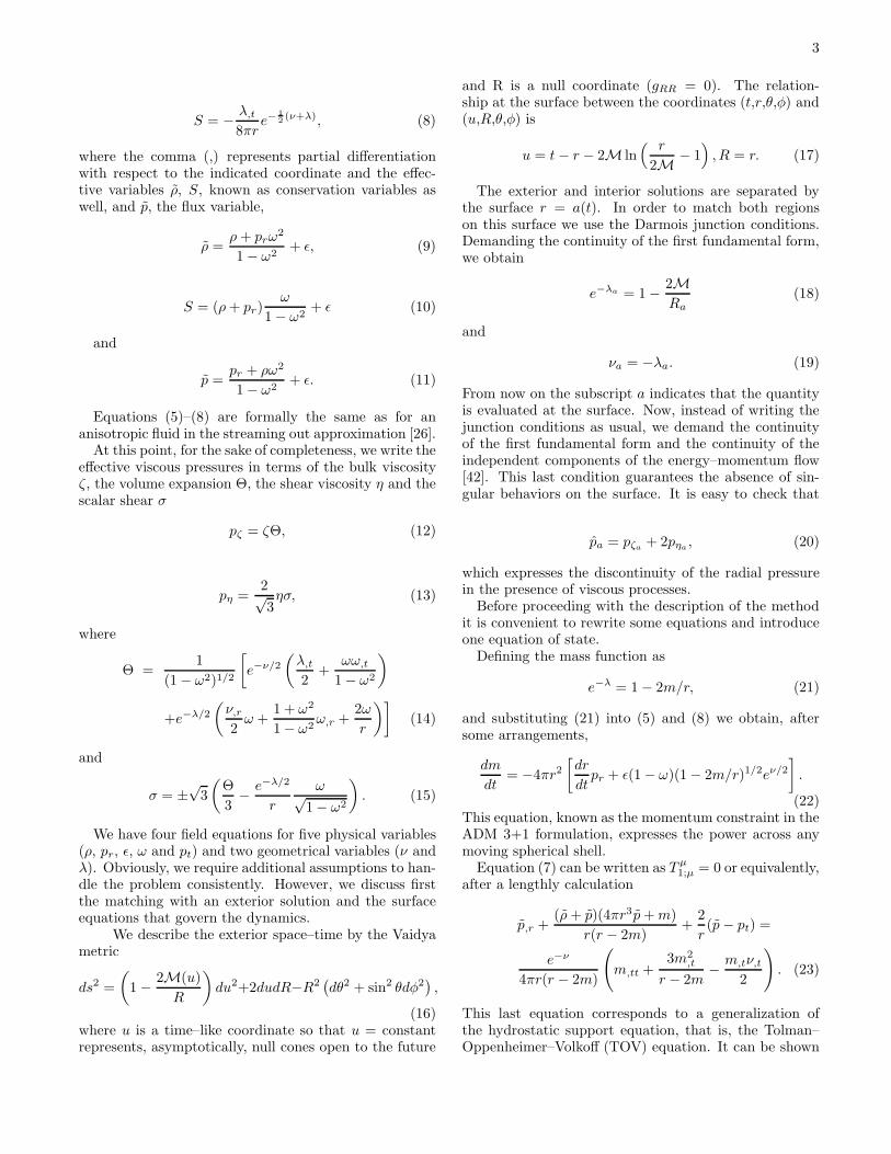
FIG. 5: Evolution of the local velocity ω for theSchwarzschild–like model I. The initial conditions are A(0) =5.0, F (0) = 0.6, Ω(0) = −0.1, with h = 0.99.

A. The PQSA protocol

We outline here the PQSA approach:

1. Take an interior solution to Einstein’s field equa-tions, representing a fluid distribution of matter inequilibrium, with static solutions

ρst. = ρ(r), pst. = p(r).

2. Assume that the r dependence of ρ and p is thesame as that of ρst. and pst., respectively.

-1

0

1

2

3

4

5

0 1 2 3 4 5 6 7 8 9 10

Radiation flux

Time

r/a=0.2r/a=0.4r/a=0.6r/a=0.8r/a=1.0

FIG. 6: Evolution of the radiation flux ǫ (multiplied by 104)for the Schwarzschild–like model I. The initial conditions areA(0) = 5.0, F (0) = 0.6, Ω(0) = −0.1, with h = 0.99.

-0.55

-0.5

-0.45

-0.4

-0.35

-0.3

-0.25

-0.2

-0.15

-0.1

-0.05

0

0 1 2 3 4 5 6 7 8 9 10

Expansion

Time

r/a=0.2r/a=0.4r/a=0.6r/a=0.8r/a=1.0

FIG. 7: Evolution of the expansion Θ for the Schwarzschild–like model I. The initial conditions are A(0) = 5.0, F (0) = 0.6,Ω(0) = −0.1, and h = 0.99.

3. Using equations (25) and (26), with the r depen-dence of p and ρ, one gets m and ν up to somefunctions of t, which will be specified below.

4. For these functions of t one has three ordinary dif-ferential equations (hereafter referred to as the sur-face equations), namely:

(a) Equation (4) evaluated at r = a;

(b) Equation (22) evaluated at r = a;

(c) Equation T ν1;ν = 0 evaluated at r = a.

6

-0.02

0

0.02

0.04

0.06

0.08

0.1

0.12

0.14

0.16

0.18

0 1 2 3 4 5 6 7 8 9 10

Shear

Time

r/a=0.2r/a=0.4r/a=0.6r/a=0.8r/a=1.0

FIG. 8: Evolution of the shear σ for the Schwarzschild–likemodel I. The initial conditions are A(0) = 5.0, F (0) = 0.6,Ω(0) = −0.1, and h = 0.99.

-5

-4.5

-4

-3.5

-3

-2.5

-2

-1.5

-1

-0.5

0 1 2 3 4 5 6 7 8 9 10

log10(Shear viscosity)

Time

r/a=0.6r/a=0.7r/a=0.8r/a=0.9r/a=1.0

FIG. 9: Evolution of the shear viscosity η for theSchwarzschild–like model I. The initial conditions are A(0) =5.0, F (0) = 0.6, Ω(0) = −0.1, with h = 0.99.

5. Depending on the kind of matter under consider-ation, the system of surface equations describedabove may be closed with the additional informa-tion provided by the transport equation and/orthe equation of state for the anisotropic pressureand/or eventual additional information about someof the physical variables evaluated on the surface ofthe boundary (e.g. the luminosity).

6. Once the system of surface equations is closed, itcan be integrated for any initial data.

7. Feeding back the result of integration in the expres-sions for m and ν, these two functions are com-pletely determined.

8. With the input from point 7, and using the fieldequations, together with the equation of stateand/or transport equation, all physical variablescan be found everywhere inside the matter distri-bution.

As it should be clear from the above, the crucial pointin the algorithm is the system of equations at the surfaceof the distribution. We specify it in the next section.

B. Surface equations

Evaluating (22) at the surface and using the boundarycondition (20), the energy loss is given by

ma = −4πa2ǫa(1− 2ma/a)(1− ωa). (27)

Hereafter the overdot indicates d/dt and the a subscriptindicates that quantity is evaluated at the surface r =a(t).The evolution of the boundary is governed by equation

(4) evaluated at the surface

a = (1− 2ma/a)ωa. (28)

Scaling the total mass ma, the radius a and the time–likecoordinate by the initial mass ma(t = 0) ≡ ma(0),

A ≡ a/ma(0), M ≡ ma/ma(0), t/ma(0) → t,

and defining

F ≡ 1− 2M

A, (29)

Ω ≡ ωa, (30)

E ≡ 4πa2ǫa(1 − Ω), (31)

the surface equations can be written as

A = FΩ, (32)

F =F

A[(1− F )Ω + 2E] . (33)

Equations (32) and (33) are general within spherical sym-metry.We need a third surface equation to specify the dy-

namics completely for any set of initial conditions and agiven luminosity profile E(t). For this purpose we canuse the field equation (7) or the conservation equation,(23), written in terms of the effective variables, which isclearly model–dependent.

7

4.6

4.65

4.7

4.75

4.8

4.85

4.9

4.95

5

0 2 4 6 8 10

Radii

Time

h=0.70h=0.80h=0.90h=0.95h=0.98h=1.00

FIG. 10: Evolution of the radius A(t) for the Schwarzschild–like model II. The initial conditions are A(0) = 5, F (0) = 0.6,Ω(0) = −0.01.

-0.05

-0.045

-0.04

-0.035

-0.03

-0.025

-0.02

-0.015

-0.01

-0.005

0

0 1 2 3 4 5 6 7 8 9 10

Local radial velocity

Time

r/a=0.2r/a=0.4r/a=0.6r/a=0.8r/a=1.0

FIG. 11: Evolution of the local radial velocity ω for theSchwarzschild–like model II. The initial conditions are A(0) =5, F (0) = 0.6, Ω(0) = −0.01, and h = 0.9.

IV. EXAMPLES

We illustrate the PQSA method with four examplesbased on the Schwarzschild and Tolman VI interior so-lutions. Additionally, we consider two correspondingadiabatic models, that is, without free–streaming butanisotropic (viscous). Although greatly simplified, theadiabatic models lead to non-trivial results, which allowto understand our results better.

-0.5

0

0.5

1

1.5

2

2.5

3

3.5

0 1 2 3 4 5 6 7 8 9 10

Shear viscosity

Time

r/a=0.2r/a=0.4r/a=0.6r/a=0.8r/a=1.0

FIG. 12: Evolution of the shear viscosity η (multiplied by 102)for the Schwarzschild–like model II. The initial conditions areA(0) = 5, F (0) = 0.6, Ω(0) = −0.01, and h = 0.9.

A. Schwarzschild–like model I: non–adiabatic

We consider here a very simple model inspired by thewell-known Schwarzschild interior solution [44]. We take

ρ = f(t), (34)

where f is an arbitrary function of t. The expression forp is

p+ 13 ρ

p+ ρ=

(

1− 8π

3ρr2)h/2

k(t), (35)

where k is a function of t to be defined from the boundarycondition (20), which now reads, in terms of the effectivevariables, as

pa = ρaΩ2 + ǫa(1 + Ω)2. (36)

Thus, (35) and (36) give

ρ =3(1− F )

8πa2, (37)

p =ρ

3

χSFh/2 − 3ψSξ

ψSξ − χSFh/2

, (38)

with

ξ = [1− (1− F )(r/a)2]h/2

where h = 1− 2C and

χS = 3(Ω2 + 1)(1− F ) + 2E(1 + Ω),

8

ψS = (3Ω2 + 1)(1− F ) + 2E(1 + Ω).

Using (21) and (26) it is easy to obtain expressions form and ν:

m = ma(r/a)3, (39)

eν =

χSFh/2 − ψSξ

2(1− F )

2/h

. (40)

In order to write down explicitely the surface equationsfor this example, we evaluate the equation (23) at thesurface, obtaining

Ω = [8EF − Ω2 + 10Ω2F − 6EΩ+ 2EΩ2 + 3Ω4 − 8E2

− 9Ω2F 2 − 6Ω4F + 8EΩ3 + 3F 2Ω4 + 4E2Ω+ 4E2Ω2

+ 4EA+ 6FEΩ− 2FΩ2E − 8FΩ3E)

/ (2A(F − 1)) (41)

It is interesting to note that this equation is the sameas in the isotropic case (pr = pt). This is a direct con-sequence of the chosen equation of state combined withincompressibility of the fluid; it is not a general result, aswe will see for the next models. Equation (41), togetherwith (32) and (33), constitute the system of differentialequations at the surface for this model. It is necessaryto specify one the luminosity as a function of t and theinitial data. We choose E to be a gaussian

E = E0e−(t−t0)

2/Σ2

,

with E0 = Mr/√Σπ, t0 = 5.0 and Σ = 0.25, which

corresponds to a pulse radiating away Mr = 1/10 of theinitial mass.We solve equations (32), (33), and (41) using a fourth

order Runge-Kutta method. The physical variables (ρ,p, ω, η, ǫ) are obtained from the field equations (5)–(8)and the equation of state (24). Note that we have to useequations (14) and (15) and some additional numericalwork to determine η. We take as initial conditionsA(0) =5, M(0) = 1, Ω(0) = −0.1, with h = 0.99.Figure 1 shows the evolution of the radius of the dis-

tribution. Figures 2–6 display the physical variables (ρ,pr, pt, ω, ǫ), figures 7–8 the kinematic variables Θ andσ, and figure 9 the shear viscosity η, for different regions.It is evident that the emission of energy decreases theenergy density and the shear viscosity, but increases thepressure; while the collapse is briefly accelerated. It isinteresting to note that after the gaussian emission thedistribution recovers staticity slowly, probably in a qua-sistatic regime. In this model pt > pr, which means2√3ση > 0 (h = 0.99). It is important to mention that

in this model, a shear viscosity η > 0 is only possible ifwe choose the negative root in (15). Physically mean-ingful values of shear viscosity (η > 0) are obtained for

regions r/a ≈ 0.6 → 1. This means that the inner coreis not viscous but anisotropic. The rest of the kinematicvariables (Θ and σ), shown in Figures 7–8, follow theevolution of the radius of the distribution, with Θ (σ)decreasing (increasing) faster as the radius decreases ata faster rate for 4 <∼ t <∼ 6.

7.6

7.65

7.7

7.75

7.8

7.85

7.9

7.95

8

0 1 2 3 4 5 6 7 8 9 10

Radii

Time

h=0.7h=0.8h=0.9h=1.0

FIG. 13: Evolution of the radii for the Tolman VI-like modelIII. The initial conditions are A(0) = 8.0, F (0) = 0.75, Ω(0) =−0.1.

-0.2

-0.15

-0.1

-0.05

0

0.05

0.1

0 1 2 3 4 5 6 7 8 9 10

Local radial velocity

Time

r/a=0.2r/a=0.4r/a=0.6r/a=0.8r/a=1.0

FIG. 14: Evolution of the local radial velocity ω for the Tol-man VI-like model III The initial conditions are A(0) = 8.0,F (0) = 0.75, Ω(0) = −0.1, with h = 0.95.

B. Schwarzschild–like model II: adiabatic

We construct this model with the same effective vari-ables and metric functions as the aforestudied model I,

9

0

0.5

1

1.5

2

2.5

0 1 2 3 4 5 6 7 8 9 10

Shear viscosity

Time

r/a=0.2r/a=0.4r/a=0.6r/a=0.8r/a=1.0

FIG. 15: Evolution of the shear viscosity η (multiplied by104) for the Tolman VI-like model III. The initial conditionsare A(0) = 8, F (0) = 0.75, Ω(0) = −0.1, with h = 0.95.

but now the radiation flux is zero everyhere; thereforethis model is adiabatic. Obviously we do not need nowan equation of state because all physical variables aredetermined algebraically from the field equations. How-ever some measure of tangential stress at the surface isrequired to evolve the system. We opt for a tangentialpressure equal to the radial pressure just at the surface,pt|a = pr|a. The third surface equation in this case is

Ω = − 1

2A(4hΩ2F − Ω2F + hF − 6Ω4F + 3hΩ4F

− F − 3hΩ4 − 4hΩ2 − 3Ω2 + 1− h+ 6Ω4) (42)

Observe that this expression explicitly depends on theanisotropic parameter h. In this case we integrate thesystem for the initial conditions A(0) = 5, M(0) = 1 andΩ = −0.01. Figure 10 shows the radius of the distribu-tion for different values of h. Figures 11–12 display theradial velocity and the shear viscosity for h = 0.9. Inthis case anisotropy manifests clearly at the surface. Aslong as pt is greater than pr the collapse accelerates. Thesame occurs for 0.7 ≤ h ≤ 1.0, as we go deeper in the

distribution the inner shells collapse faster. The fffec-tive gravitation is therefore enhanced by the anisotropyinduced by the viscosity. Inner regions have a greatershear viscosity in this model (∼ 10-105 times the valuesfound in model I).

C. Tolman VI–like model III: non–adiabatic

In this subsection we revise the model obtained fromTolman’s solution VI [45]. Let us take

ρ =g

r2, (43)

p =gK(1− 9α(r/a)

√

4−3h)

3(K/I − 9α(r/a)√

4−3h)hr2, (44)

where K and I are defined as

K = 8− 3h+ 4√4− 3h,

I = 8− 3h− 4√4− 3h.

g and α are functions of t, which can be determined using(36). Therefore

g =3(1− F )

24π(45)

α =3h(1− F )−Kβ

9[3h(1− F )− Iβ](46)

where

β = (1 − F )Ω2 + 2E(1 + Ω).

Using (21) and (26) we obtain

m = ma(r/a) (47)

and

ν = lnF +8πg

F

(

1 +I

3h

)

ln(r/a) +8πg

3hF√4− 3h

I ln

(

(K/I − 9α)a√

4−3h

(K/I)a√

4−3h − 9αr√

4−3h

)

+K ln

(

(K/I)a√

4−3h − 9αr√

4−3h

a√

4−3h(K/I − 9α)

)

(48)

Evaluating equation (23) at the surface we can obtain an equation for Ω (too long to display here).Integrating the system of equations at the surface for the initial conditions A(0) = 8 and Ω = −0.1, withMr = 10−2,

we obtain figures 13, 14 and 15. We obtain similar results as in model II but in a different fashion. The bigger the

10

difference between the tangential (viscous) pressure pt and the radial pressure pr (as h decreases), the more violentlythe distribution explodes. It is striking that now all the spherical shells tend to reach the same instantaneous localradial velocity when the system goes to faster collapse with emission of energy across de boundary surface. At leastlocally, the “acceleration” of all the shells goes to zero at the same time; again the same instantaneous local radialvelocity (negative) is reached before a final bouncing per shell from outer to inner.

D. Tolman VI–like model IV: adiabatic

We construct this model with the same effective variables and metric functions as in model III, but now the radiationflux is zero everyhere; therefore this model is adiabatic. Obviously we do not need now an equation of state becauseall physical variables are determined algebraically from the field equations. However some measure of tangential stressat the surface is required to evolve the system. We opt for a tangential pressure equal to the radial pressure just atthe surface, pt|a = pr|a, as in model II. The third surface equation in this case is

Ω = (−9Ω4Kh2I2F +Ω4FI2K3 + 9Ω4K2h2IF + 6Ω4FI2K2h√4− 3h− 243FIh4Ω2 − I3K2FΩ4

− 81Fh4I + 54FIKh3√4− 3h+ 243Kh4Ω2F − 18Ω2FI2Kh2

√4− 3h− 18Ω2FIK2h2

√4− 3h

+ 81Fh4K − 18h2I2FKΩ2 + 18Fh2K2Ω2I + 9Ω4Kh2I2 − 9Ω4K2h2I − 18h2K2Ω2I + 18h2I2KΩ2

+ I3K2Ω4 − 81h4K − I2Ω4K3 + 81h4I + 81Kh4Ω2 − 81Ih4Ω2)/[162(K − I)h4A] (49)

Integrating the system for the initial conditions A(0) = 8and Ω = −0.1, figure 13 shows the radius of the distri-bution for different values of h. Figures 16–18 displaythe radial velocity and the shear viscosity for h = 0.9.After some numerical experimentation some non–trivialresults arise, and we relax the condition pt > pr. At thesurface we do not find any novelty. The most violent ex-plosion occurs as pr >> pt. In this adiabatic but viscous(anisotropic) model all the shells bounce at the same timeto irrupt from inner regions to outer regions with an ap-parently linear dependence with time. The outer shellsof matter are ejected faster and earlier than the innerones. This sort of behavior was reported several yearsago studying in Bondi coordinates the collapse of radiat-ing distributions with an extreme transport mechanismas diffusion [46]. However, the shear viscosity profiles in-dicate that i) bouncing is not allowed at all and ii) someinner regions are forbidden, otherwise the shear viscos-ity profiles become negative or/and infinite (see Figure18). This situation is general and independent of theanisotropy parameter h.

V. CONCLUSIONS

We consider a selfgravitating spherical distribution ofmatter containing a dissipative fluid. The use of thePQSA with non–comoving coordinates allow us to studyviscous fluid spheres in the streaming out limit as theyjust depart from equilibrium. From this point of view,the PQSA can also be seen as a nonlinear perturbativemethod to test the stability of solutions in equilibrium.

For the non–adiabatic Schwarzschild model the distri-bution evolves to a final state with a non–viscous and

7.5

7.6

7.7

7.8

7.9

8

8.1

8.2

8.3

8.4

0 2 4 6 8 10

Radii

Time

h=0.7h=1.0h=1.3

FIG. 16: Evolution of the radii for the Tolman VI-like modelIV. The initial conditions are A(0) = 8.0, F (0) = 0.75, Ω(0) =−0.1.

anisotropic inner core. Surprisingly, in this model theevolution of the local radial velocity at the surface isthe same in the isotropic (pt = pr) case, a fortuitouscoincidence due to the chosen equation and state andthe incompressibility of the fluid. For the adiabaticSchwarzschild model the final core is up to 105 timesmore viscous, and the anisotropy appears explicitly in allthe evolution equations. The higher viscosity of the coreincreases the effective gravity and the collapse is faster,as long as pt > pr.

Both of the Tolman VI models lead to a distribu-

11

-0.1

-0.08

-0.06

-0.04

-0.02

0

0.02

0.04

0.06

0.08

0 2 4 6 8 10

Local radial velocity

Time

r/a=0.2r/a=0.4r/a=0.6r/a=0.8r/a=1.0

FIG. 17: Evolution of the local radial velocity ω for the Tol-man VI-like model IV. The initial conditions are A(0) = 8.0,F (0) = 0.75, Ω(0) = −0.1, with h = 0.95.

-2

-1.5

-1

-0.5

0

0.5

1

1.5

2

0 2 4 6 8 10

Shear Viscosity

Time

r/a=0.2r/a=0.4r/a=0.6r/a=0.8r/a=1.0

FIG. 18: Evolution of the shear viscosity η for the TolmanVI-like model IV. The initial conditions are A(0) = 8, F (0) =0.75, Ω(0) = −0.1, with h = 0.95.

tion which initially collapses and then bounces andexpands indefinitely. The Tolman VI non–adiabaticmodel shares some of the characteristics of the adiabaticSchwarzschild. Before the final bouncing, as pt > pr thecollapse is accelerated. For the non–adiabatic case someregions of the parameter space are forbidden, since theshear viscosity profiles become unphysical. In this casethe bouncing is not allowed and the distribution collapsesindefinitely.

A forthcoming paper considers the dissipation by heatflow, in order to isolate effects similar to the ones stud-ied in the present investigation, but with different mech-anisms. Also, a work in progress considers heat flow andanisotropy induced by electric charge, pointing to themost realistic numeric modeling in this area [47]. Al-though they are not entirely new, the results presentedhere constitute a first cut to more general situations us-ing the PQSA, including dissipation, anisotropy, electriccharge, heat flow, viscosity, radiation flux, superficial ten-sion, temperature profiles and study their influence onthe gravitational collapse. This investigation is an essen-tial part of a long-term project which tries to incorporatethe Muller–Israel–Stewart theory for dissipation and de-viations from spherical symmetry, specially when con-sidering electrically charged distributions. Besides beinginteresting in their own right, we believe that sphericallysymmetric fluid models are useful as a test bed for moregeneral solvers in numerical relativity [39, 40]. A general3D code must be able to reproduce situations closer toequilibrium.

Acknowledgments

WB was on sabbatical leave from Universidad de LosAndes while finishing this work. CP acknowledges thecomputing resources provided by the Victorian Partner-ship for Advanced Computation (VPAC).

[1] D. Kazanas and D. N. Schramm, in Sources of Grav-

itational Radiation, edited by L. L. Smarr (1979), pp.345–354.

[2] W. D. Arnett, Astrophys. J. 218, 815 (1977).[3] G. E. Brown, in NATO ASIC Proc. 90: Supernovae: A

Survey of Current Research, edited by M. J. Rees andR. J. Stoneham (1982), pp. 13–33.

[4] H. A. Bethe, in NATO ASIC Proc. 90: Supernovae: A

Survey of Current Research, edited by M. J. Rees andR. J. Stoneham (1982), pp. 35–52.

[5] D. Mihalas and B. Weibel Mihalas, Foundations of radia-tion hydrodynamics (New York: Oxford University Press,1984, 1984).

[6] D. Kazanas, Astrophys. J., Lett. 222, L109 (1978).[7] L. Lehner, Class. Quantum Grav. 18, 25 (2001).[8] M. W. Choptuik, Phys. Rev. Lett. 70, 9 (1993).[9] F. Pretorius, Phys. Rev. Lett. 95, 121101 (2005).

[10] L. Baiotti, B. Giacomazzo, and L. Rezzolla, Phys. Rev.D 78, 084033 (2008).

[11] J. A. Font, Living Rev. Relativ. 6, 4 (2003).

12

[12] J. Winicour, Living Rev. Relativ. 8, 10 (2005).[13] W. Barreto, B. Rodrıguez, and H. Martınez, Astrophys.

Space. Sci. 282, 581 (2002).[14] L. Herrera, W. Barreto, A. Di Prisco, and N. O. Santos,

Phys. Rev. D 65, 104004 (2002).[15] L. Herrera, J. Jimenez, and G. J. Ruggeri, Phys. Rev. D

22, 2305 (1980).[16] L. Herrera and L. A. Nunez, Fund. Cosm. Phys. 14, 235

(1990).[17] W. Barreto and L. A. Nunez, Astrophys. Space. Sci. 178,

261 (1991).[18] W. Barreto, L. Herrera, and L. Nunez, Astrophys. J. 375,

663 (1991).[19] W. Barreto, L. Herrera, and N. Santos, Astrophys. Space.

Sci. 187, 271 (1992).[20] R. Aquilano, W. Barreto, and L. A. Nunez, Gen. Relat.

Gravit. 26, 537 (1994).[21] L. Herrera, A. Melfo, L. A. Nunez, and A. Patino, As-

trophys. J. 421, 677 (1994).[22] J. Martınez, Phys. Rev. D 53, 6921 (1996).[23] W. Barreto and A. da Silva, Gen. Relat. Gravit. 28, 735

(1996).[24] L. Herrera, J. Jimenez, and W. Barreto, Can. J. Phys.

67, 855 (1989).[25] W. Barreto and S. Rojas, Astrophys. Space. Sci. 193,

201 (1992).[26] W. Barreto, Astrophys. Space. Sci. 201, 191 (1993).[27] W. Barreto and L. Castillo, J. Math. Phys. 36, 5789

(1995).[28] W. Barreto, J. Ovalle, and B. Rodrıguez, Gen. Relat.

Gravit. 30, 15 (1998).[29] I. Muller, Z. Phys. 198, 329 (1967).[30] W. Israel, Ann. Phys. 100, 310 (1976).[31] W. Israel and J. M. Stewart, Phys. Lett. A 58, 213

(1976).[32] W. Israel and J. M. Stewart, Ann. Phys. 118, 341 (1979).[33] L. Herrera, A. Di Prisco, J. L. Hernandez-Pastora,

J. Martın, and J. Martınez, Class. Quantum Grav. 14,2239 (1997).

[34] L. Herrera and J. Martınez, J. Math. Phys. 39, 3260(1998).

[35] L. Herrera, A. di Prisco, J. Martin, J. Ospino, N. O.Santos, and O. Troconis, Phys. Rev. D 69, 084026 (2004).

[36] L. Herrera, A. di Prisco, and W. Barreto, Phys. Rev. D73, 024008 (2006).

[37] D. W. Neilsen and M. W. Choptuik, Class. QuantumGrav. 17, 733 (2000).

[38] W. Barreto, Phys. Rev. D 79, 107502 (2009).[39] W. Barreto, L. Castillo, and E. Barrios, Phys. Rev. D

80, 084007 (2009).[40] W. Barreto, L. Castillo, and E. Barrios, To appear in

Gen. Relat. Gravit. (2010).[41] R. A. Lyttleton and H. Bondi, Mon. Not. R. Astron. Soc.

128, 207 (1964).[42] L. Herrera and A. Di Prisco, Phys. Rev. D 55, 2044

(1997).[43] M. Cosenza, L. Herrera, M. Esculpi, and L. Witten, Phys.

Rev. D 25, 2527 (1982).[44] K. Schwarzschild, Abh. Konigl. Preuss. Akad. Wis-

senschaften Jahre 1906,92, Berlin,1907 pp. 189–196(1916).

[45] R. C. Tolman, Phys. Rev. 55, 364 (1939).[46] W. Barreto, L. Herrera, and N. Santos, Astrophys. J.

344, 158 (1989).[47] A. Di Prisco, L. Herrera, G. Le Denmat, M. McCallum,

and N. Santos, Phys. Rev. D 76, 064017 (2007).