INTERFACIAL TENSION AND VISCOSITY OF RESERVOIR ...
302
INTERFACIAL TENSION AND VISCOSITY OF RESERVOIR FLUIDS by ABHIJIT YESHWANT DANDEKAR Submitted for the Degree of Doctor of Philosophy Department of Petroleum Engineering Heriot-Watt University Edinburgh, UK February 1994 This copy of the thesis has been supplied on condition that anyone who consults it is understood to recognise that the copyright rests with its author and no information derived from it may be published without prior written consent of the author or the University (as may be appropriate).
-
Upload
khangminh22 -
Category
Documents
-
view
0 -
download
0
Transcript of INTERFACIAL TENSION AND VISCOSITY OF RESERVOIR ...
INTERFACIAL TENSION AND VISCOSITY
OF RESERVOIR FLUIDS
by
ABHIJIT YESHWANT DANDEKAR
Submitted for the Degree of Doctor of Philosophy
Department of Petroleum Engineering
Heriot-Watt University
Edinburgh, UK
February 1994
This copy of the thesis has been supplied on condition that anyone who consults it is
understood to recognise that the copyright rests with its author and no information
derived from it may be published without prior written consent of the author or the
University (as may be appropriate).

Dedicated to my Beloved Grandfather.
ABSTRACT
Interfacial tension (IFT) and viscosity are the two important fluid properties which
have a particular significance in various reservoir engineering calculations and
mathematical simulations. Therefore, there exists a need to develop practical
methods to accurately determine them for reservoir fluids particularly for application
to gas injection schemes and development of gas condensate reservoirs.
Part A of this thesis on interfacial tension presents a novel technique for measuring
this property, which has the advantage of carrying out the simultaneous
measurements of interfacial tension along with other phase properties, without any
extra efforts. The developed expression relating the interfacial tension to other
measurable properties is simple and rigorous and hence, does not involve any
empiricism. Results on various binary and multicomponent synthetic hydrocarbon
mixtures, and real gas condensate fluids using the above technique have been
presented along with literature data in order to demonstrate the accuracy and
reliability of the method. Similarly, interfacial tension data determined by the
conventional pendant drop technique on real volatile and black oil fluids has also
been furnished.
A critical evaluation of the predictive techniques for interfacial tension, namely; the
scaling law and the parachor method has also been presented using a large number of
data on interfacial tension of binary hydrocarbon mixtures from literature. Based on
this evaluation and employing the same literature data on interfacial tension of binary
hydrocarbon mixtures modifications of the existing predictive techniques are
proposed by relating the exponents in the equations to the molar density difference
between the vapour and liquid phases. Results obtained for various multicomponent
synthetic hydrocarbon mixtures and real reservoir fluids, by implementing the above
mentioned modifications have shown significant improvement compared to the
original methods.
Part B of this thesis on viscosity presents a comparative study for pure hydrocarbon
components and their mixtures by using various viscosity prediction methods. Also
presented is a tuning study on various real reservoir fluids by employing the popularly
used residual viscosity and corresponding states methods respectively. The
drawbacks of these techniques have also been highlighted.
The residual viscosity method is critically evaluated and it has been proved that the
variation of residual viscosity with respect to reduced density is not uniform for all
fluids, particularly in the dense fluid phase. Based on a large number of data on pure
hydrocarbon compounds in the dense fluid phase from literature, the residual method
is modified by relating the residual viscosity of a fluid to its molecular weight along
with its reduced density in dense fluid phase conditions. The modified method has
been applied to various pure hydrocarbon compounds and their mixtures, and real
reservoir fluids. The superiority of the new method has been demonstrated by
comparing the results with those of the original methods and those based on the
principle of corresponding states.
TABLE OF CONTENTS
TABLE OF CONTENTS i
LIST OF SYMBOLS iv
LIST OF TABLES vii LIST OF FIGURES xiii ACKNOWLEDGEMENTS xvi INTRODUCTION xviii
CHAPTER 1: INTRODUCTION - INTERFACIAL TENSION 1
1.1 INTRODUCTION 1
1.2 SIGNIFICANCE OF INTERFACIAL TENSION IN RESERVOIR
ENGINEERING
1.3 EFFECT OF TEMPERATURE ON INTERFACIAL TENSION
1.4 EFFECT OF PRESSURE ON INTERFACIAL TENSION
REFERENCES
CHAPTER 2: EXPERIMENTAL TECHNIQUES
MEASURING INTERFACIAL TENSION
2.1 INTRODUCTION
2.2
2.3
PENDANT DROP TECHNIQUE
1
5
5
6
FOR
8
8
8
2.2.1 Discussion of Results on Pendant Drop Device in the Gas Condensate
Equilibrium Cell 9
2.2.2 Pendant Drop Device in the Vapour - Liquid - Equilibrium ( V-L-E )
Cell 10
LASER LIGHT SCATTERING TECHNIQUE
2.4 CAPILLARY RISE TECHNIQUE
2.5 THE RING METHOD
12
13
15
1
REFERENCES 15
CHAPTER 3: DEVELOPMENT OF A NOVEL TECHNIQUE FOR
MEASURING INTERFACIAL TENSION OF GAS CONDENSATE
SYSTEMS 18
3.1 INTRODUCTION 18
3.2 EXPERIMENTAL SET-UP FOR GAS CONDENSATE CELL 19
3.3 EXPERIMENTAL SET-UP FOR V-L-E APPARATUS 21
3.4 LITERATURE SURVEY 23
3.4.1 Theoretical Background of the Developed Technique 24
3.5 INTERFACIAL TENSION MEASUREMENTS OF SYNTHETIC
MIXTURES 28
3.5.1 Methane-n-Butane System 28
3.5.2 Methane-n-Decane System 29
3.5.3 Methane-Propane System 31
3.5.4 Carbon Dioxide-n-Tetradecane System 32
3.5.5 Methane-Propane-n-Decane System 33
3.5.6 Methane-Carbon Dioxide-Propane-n-Pentane-n-Decane-n-Hexadecane
System 34
3.5.7 Interfacial Tension Measurements on a Synthetic Near Critical Fluid34
3.6 INTERFACIAL TENSION MEASUREMENTS OF REAL RESERVOIR
FLUIDS 35
3.6.1 Gas Condensate Fluid C3 35
3.6.2 Real Volatile Oil (A) 37
3.6.3 Real Black Oil RFS-1 38
3.6.4 Near Critical Fluid 39
3.7 ERROR ANALYSIS 40
REFERENCES 42
11
CHAPTER 4: PREDICTIVE TECHNIQUES FOR INTERFACIAL
TENSION 45 4.1 INTRODUCTION 45
4.2 PARACHOR METHOD 45
4.2.1 Hough and Stegemeier's Method 48
4.2.2 Sugden's Parachor 49
4.2.2 Fanchi's Method for estimating Parachor 50
4.3 SCALING LAW 52
4.4 GRADIENT THEORY 57
REFERENCES 60
CHAPTER 5: IMPROVEMENT OF PREDICTIVE TECHNIQUES
FOR INTERFACIAL TENSION - SCALING LAW AND
PARACHOR METHOD 63
5.1 INTRODUCTION 63
5.2 COMPARISON OF PREDICTED AND MEASURED INTERFACIAL
TENSION DATA 63
5.3 PROPOSED MODIFICATION OF SCALING LAW AND PARACHOR
METHOD 64
5.4 EXPERIMENTAL RESULTS 66
5.5 INTERFACIAL TENSION PREDICTIONS OF REAL RESERVOIR
FLUIDS 67
REFERENCES 69
CHAPTER 6: CONCLUSIONS AND RECOMMENDATIONS
6.1 CONCLUSIONS
6.2 RECOMMENDATIONS
72
72
74
111
LIST OF SYMBOLS
Nomenclature
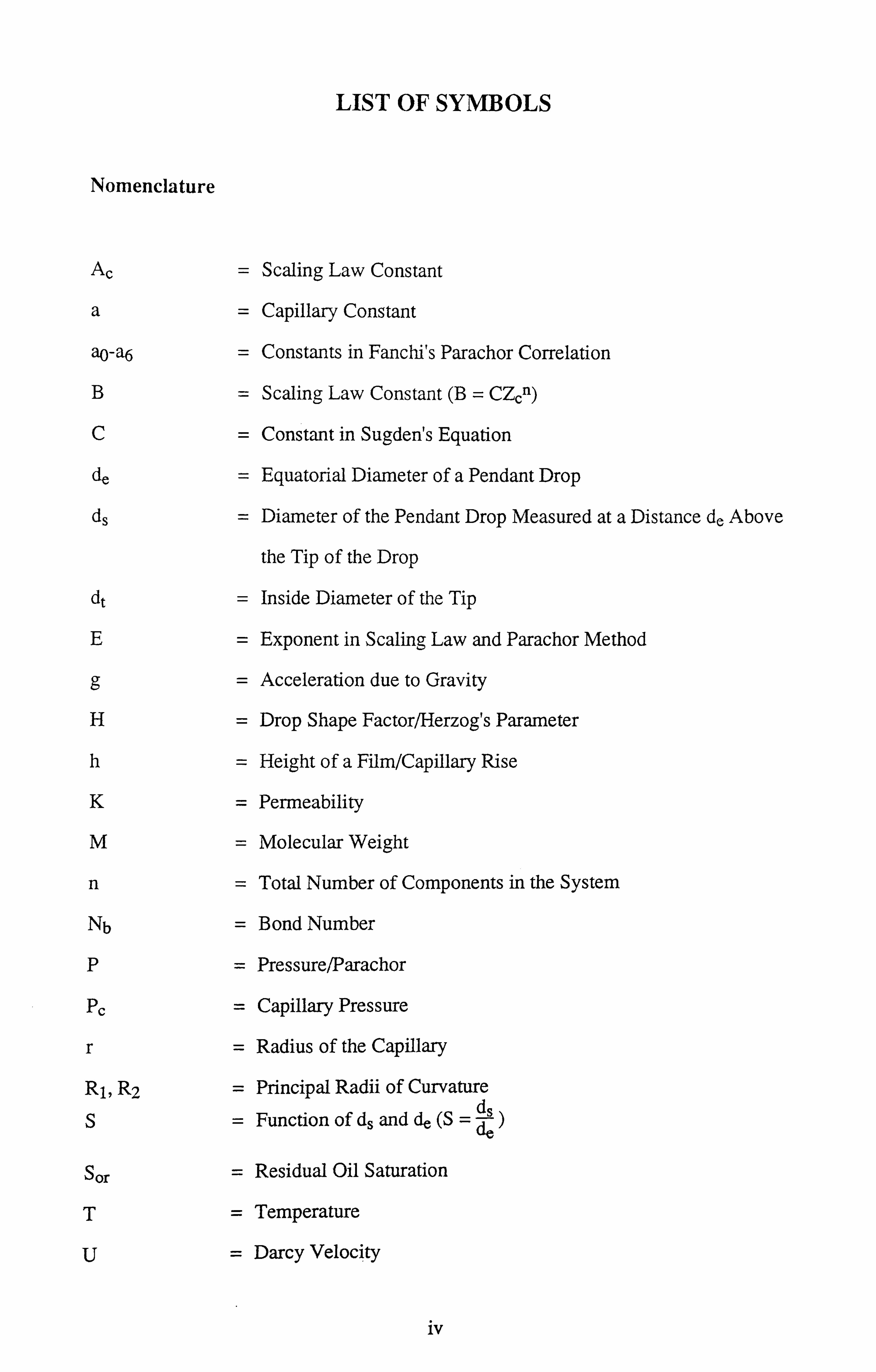
Ac = Scaling Law Constant
a= Capillary Constant
ap-a6 = Constants in Fanchi's Parachor Correlation
B= Scaling Law Constant (B = CZcn)
C= Constant in Sugden's Equation
de = Equatorial Diameter of a Pendant Drop
ds = Diameter of the Pendant Drop Measured at a Distance de Above
the Tip of the Drop
dt = Inside Diameter of the Tip
E= Exponent in Scaling Law and Parachor Method
g= Acceleration due to Gravity
H= Drop Shape Factor/Herzog's Parameter
h= Height of a Film/Capillary Rise
K= Permeability
M= Molecular Weight
n= Total Number of Components in the System
Nb = Bond Number
P= Pressure/Parachor
PC = Capillary Pressure
r= Radius of the Capillary
R1, R2 = Principal Radii of Curvature
S= Function of ds and de (S = ds de
Sor = Residual Oil Saturation
T= Temperature
U= Darcy Velocity
iv

V = Volume
X = Liquid Phase Mole Fraction
Y = Vapour Phase Mole Fraction
Z = Compressibility Factor
Greek Letters
ac = Riedel Parameter
ß = Scaling Law Exponential Constant
= Partial Differential
A = Difference Operator
µ = Viscosity
p = Density
G = Interfacial Tension
8 = Scaling Law Exponential Constant
Subscripts
a = Capillary Constant/Atmospheric
b = Boiling Point
c = Critical Value
i = Component Index
1 = Liquid Phase
m = Molar/Mixture
n = Number of Components
r = Reduced Value
v = Vapour Phase
V

Abbreviations
AAD = Average Absolute Deviation
CCE = Constant Composition Expansion
CVD = Constant Volume Depletion
FOR = Enhanced Oil Recovery
EOS = Equations of State
GOR = Gas Oil Ratio
HWU = Heriot-Watt University
IFT = Interfacial Tension
MBC = Multiple Backward Contact
MFC = Multiple Forward Contact
PR = Peng-Robinson
STDEV = Standard Deviation
V-L-E = Vapour-Liquid-Equilibrium
vi

LIST OF TABLES
Table 2.2.1 List of IFT Data Measured by Pendant Drop Technique. Table 2.2.2 Tabulated Values of the Drop Shape Factors, H,
(from Reference
2).
Table 2.2.1.1 Interfacial Tension Data of Methane-n-Butane System at 80°C.
Table 2.2.1.2 Interfacial Tension Data of Methane-n-Decane System at 71.1°C.
Table 3.5.1.1(a) Liquid Phase Compositions and Densities at 80°C for the Methane-
n-Butane System.
Table 3.5.1.1(b) Vapour Phase Compositions and Densities at 80°C for the Methane-
n-Butane System.
Table 3.5.1.2 Film Heights Measured at Each Pressure Stage for the Methane-n-
Butane System at 80°C.
Table 3.5.1.3 Data on Interfacial Tension for the Methane-n-Butane System at
80°C.
Table 3.5.2.1 (*iquid Phase Compositions and Densities at 71.1°C for the
Methane-n-Decane System.
Table 3.5.2.1 (byapour Phase Compositions and Densities at 71.1 °C for the
Methane-n-Decane System.
Table 3.5.2.2 Data on Interfacial Tension for the Methane-n-Decane System at
71.1°C.
Table 3.5.3.1 (41iquid Phase Compositions and Densities at 33.6°C for the
Methane-Propane System.
Table 3.5.3.1 (byapour Phase Compositions and Densities at 33.6°C for the
Methane-Propane System.
Table 3.5.3.2 Data of Haniff and Pearce [ 19I, on Interfacial Tension Interpolated,
for the Density Differences Measured in our Laboratory, from
Figure (3.5.3.1).
Table 3.5.3.3 Data on Interfacial Tension for the Methane-Propane System at
33.6°C.
VII
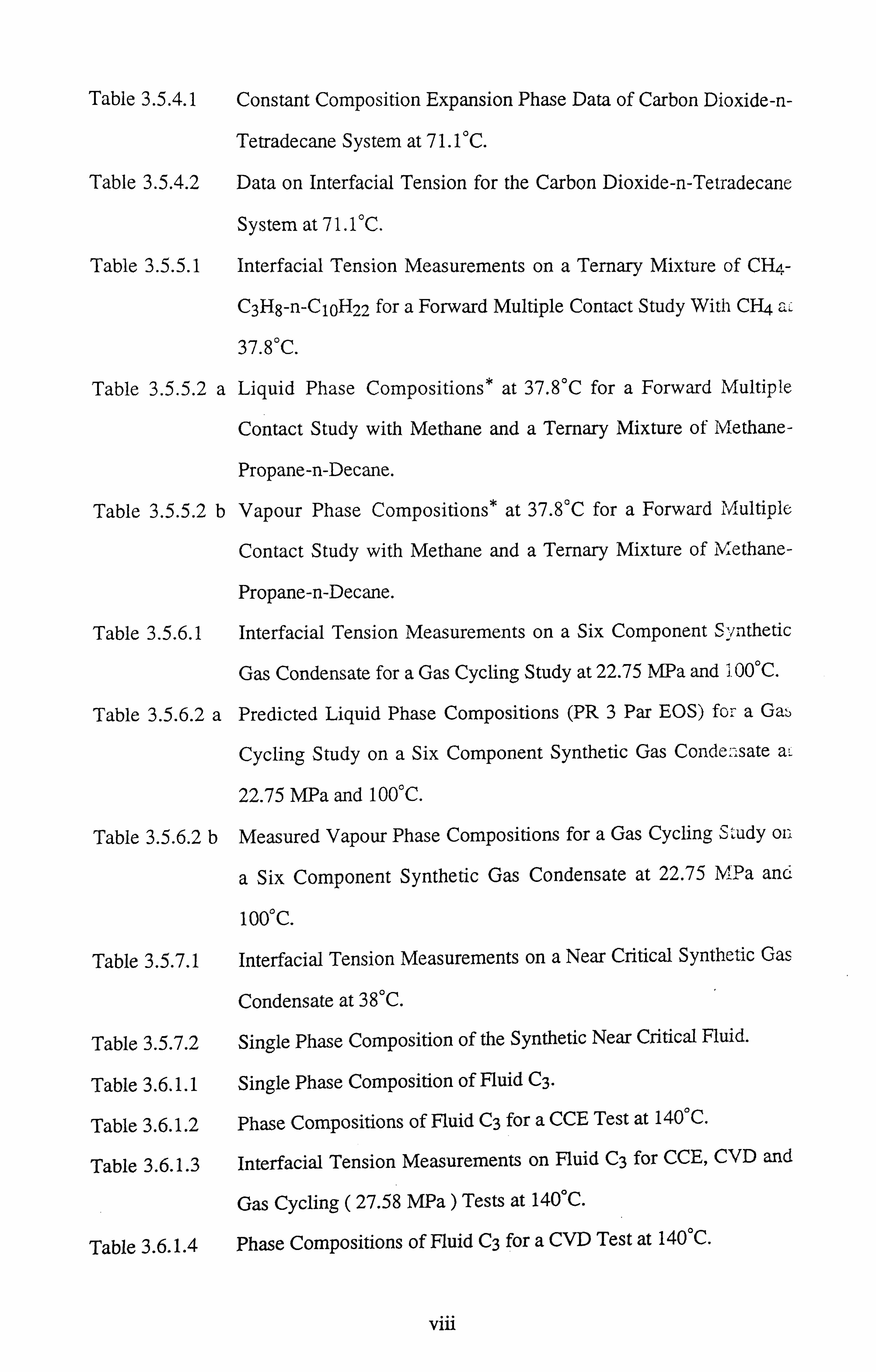
Table 3.5.4.1 Constant Composition Expansion Phase Data of Carbon Dioxide-n-
Tetradecane System at 7 1.1 °C.
Table 3.5.4.2 Data on Interfacial Tension for the Carbon Dioxide-n-Tetradecane
System at 7 1. VC -
Table 3.5.5.1 Interfacial Tension Measurements on a Ternary Mixture of CH4-
C3Hg-n-C10H22 for a Forward Multiple Contact Study With CH4 aL
37.8°C.
Table 3.5.5.2 a Liquid Phase Compositions* at 37.8°C for a Forward Multiple
Contact Study with Methane and a Ternary Mixture of Methane-
Propane-n-Decane.
Table 3.5.5.2 b Vapour Phase Compositions* at 37.8°C for a Forward Multiple
Contact Study with Methane and a Ternary Mixture of Methane-
Propane-n-Decane.
Table 3.5.6.1 Interfacial Tension Measurements on a Six Component Synthetic
Gas Condensate for a Gas Cycling Study at 22.75 MPa and x. 00°C.
Table 3.5.6.2 a Predicted Liquid Phase Compositions (PR 3 Par EOS) for a Gaz)
Cycling Study on a Six Component Synthetic Gas Conde : sate a
22.75 MPa and 100°C.
Table 3.5.6.2 b Measured Vapour Phase Compositions for a Gas Cycling Study on
a Six Component Synthetic Gas Condensate at 22.75 N'-. -. Pa and
100°C.
Table 3.5.7.1 Interfacial Tension Measurements on a Near Critical Synthetic Gas
Condensate at 38°C.
Table 3.5.7.2 Single Phase Composition of the Synthetic Near Critical Fluid.
Table 3.6.1.1 Single Phase Composition of Fluid C3.
Table 3.6.1.2 Phase Compositions of Fluid C3 for a CCE Test at 140°C.
Table 3.6.1.3 Interfacial Tension Measurements on Fluid C3 for CCE, CVD and
Gas Cycling ( 27.58 MPa) Tests at 140°C.
Table 3.6.1.4 Phase Compositions of Fluid C3 for a CVD Test at 140°C.
Vlll

Table 3.6.1.5 Vapour Phase Compositions of Fluid C3 for a Gas Cycling Test
with Methane at 27.58 MPa and 140°C.
Table 3.6.2.1 Single Phase Composition of Real Volatile Oil (A).
Table 3.6.2.2 Phase Compositions of Real Volatile Oil (A) for a CCE Test at
100°C.
Table 3.6.2.3 Interfacial Tension Measurements on Real Volatile Oil (A) for a
CCE Test at 100°C.
Table 3.6.2.4 Interfacial Tension Measurements on Real Volatile Oil (A) for a
Backward Multiple Contact Study with CH4+C02 at 35.26 MPa
and 100°C.
Table 3.6.2.5 Predicted Phase Compositions of Real Volatile Oil (A) for a MBC
Study with CI4+C02 at 35.26 MPa and 100°C.
Table 3.6.3.1 Single Phase Composition of Real Black Oil RFS-1.
Table 3.6.3.2 Phase Compositions for a Real Black Oil RFS-1 for a Four Stage
Backward Contact Study with CH4 at 34.58 MPa and 100°C.
Table 3.6.3.3 Interfacial Tension Measurements on a Real Black Oil RES-1 for a
Backward Multiple Contact Study with CH4 at 34.58 MPa and
100°C.
Table 3.6.3.4 Phase Compositions for a Real Black Oil RFS-1 for a Three Stage
Forward Contact Study with CH4 at 34.58 MPa and 100°C.
Table 3.6.3.5 Interfacial Tension Measurements on a Real Black Oil RFS-1 for a
Forward Multiple Contact Study with CH4 at 34.58 MPa and
100°C.
Table 3.6.3.6 Phase Compositions for a Real Black Oil RFS-1 for a Three Stage
Forward Contact Study with CH4 (79.86 mole %) and Carbon
Dioxide (20.14 mole %) at 34.58 MPa and 100°C.
Table 3.6.3.7 Interfacial Tension Measurements on a Real Black Oil RFS-1 for a
Forward Multiple Contact Study with CH4 (79.86 mole %) and
Carbon Dioxide (20.14 mole %) at 34.58 MPa and 100°C.
ix

Table 3.6.4.1 Interfacial Tension Measurements on a Real Near Critical Fluid at
Various Temperatures.
Table 3.6.4.2 Single Phase Composition of Real Near Critical Fluid.
Table 3.7.1 Error Analysis for the Gas-Liquid Interface Technique.
Table 3.7.2 Error Analysis for the Pendant Drop Interface Technique.
Table 5.2.1 (a) Liquid Phase Compositions and Densities at 30°C for a Five
Component Mixture.
Table 5.2.1 (b) Vapour Phase Compositions and Densities at 30°C for a Five
Component Mixture.
Table 5.2.2 (a) Liquid Phase Compositions and Densities at 35°C for a Five
Component Mixture, (Predicted Compositional Data and
Interpolated Density Data).
Table 5.2.2 (b) Vapour Phase Compositions and Densities at 35°C for a Five
Component Mixture, (Predicted Compositional Data and
Interpolated Density Data).
Table 5.2.3 (a) Liquid Phase Compositions and Densities at 40°C for a Five
Component Mixture, (Predicted Compositional Data and Measured
Density Data).
Table 5.2.3 (b) Vapour Phase Compositions and Densities at 40°C for a Five
Component Mixture, (Predicted Compositional Data and Measured
Density Data).
Table 5.2.4 (a) Liquid Phase Compositions and Densities at 80°C for a Five
Component Mixture.
Table 5.2.4 (b) Vapour Phase Compositions and Densities at 80°C for a Five
Component Mixture.
Table 5.2.5 Phase Compositions and Densities at 65.5°C for a Twenty
Component Mixture.
Table 5.2.6 Phase Compositions and Densities at 93.3°C for a Twenty
Component Mixture.
X
Table 5.2.7 Phase Compositions and Densities at 121.1 °C for a Twenty
Component Mixture.
Table 5.2.8 Interfacial Tension Data for a Five Component Mixture at 30°C
Using the Original Scaling Law and Parachor Method and the
Hough - Stegemeier's Parachor Method.
Table 5.2.9 Interfacial Tension Data for a Five Component Mixture at 35°C
Using the Original Scaling Law and Parachor Method and the
Hough - StegemeierIs Parachor Method.
Table 5.2.10 Interfacial Tension Data for a Five Component Mixture at 40°C
Using the Original Scaling Law and Parachor Method and the
Hough - Stegemeier's Parachor Method.
Table 5.2.11 Interfacial Tension Data for a Five Component Mixture at 80°C
Using the Original Scaling Law and Parachor Method and the
Hough - Stegemeier's Parachor Method.
Table 5.2.12 Interfacial Tension Data for a Twenty Component- Mixture at
65.5°C Using the Original Scaling Law and Parachor Method and
the Hough - Stegemeier's Parachor Method.
Table 5.2.13 Interfacial Tension Data for a Twenty Component Mixture at
93.3°C Using the Original Scaling Law and Parachor Method and
the Hough - Stegemeier's Parachor Method.
Table 5.2.14 Interfacial Tension Data for a Twenty Component Mixture at
121.1 °C Using the Original Scaling Law and Parachor Method and
the Hough - Stegemeier's Parachor Method.
Table 5.3.1 Literature IFT Data Used in the Modification.
Table 5.4.1 Compositions of Tested Fluids.
Table 5.4.2 Interfacial Tension Data for Fluid A Using the Original and
Modified Scaling Law and Parachor Method.
Table 5.4.3 Interfacial Tension Data for Fluid B Using the Original and
Modified Scaling Law and Parachor Method.
xi
Table 5.4.4 Interfacial Tension Data for Fluid C Using the Original and
Modified Scaling Law and Parachor Method.
Table 5.4.5 Interfacial Tension Data for Fluid D Using the Original and
Modified Scaling Law and Parachor Method.
Table 5.4.6 Interfacial Tension data for a Gas Injection Study on a Six
Component Synthetic Gas Condensate at 22.75 MPa and 100°C
Using Original and Modified Scaling Law and Parachor Method.
Table 5.4.7 Interfacial Tension data for a Forward Multiple Contact Study With
CH4 and a Ternary Mixture of CH4-C3-n-C1 at 37.8°C Using
Original and Modified Scaling Law and Parachor Method.
Table 5.4.8 Interfacial Tension data for a Ternary Mixture of CO2+n-C4+n-Cio
at 71.1°C[14] Using the Original and Modified Scaling Law and
Parachor Method.
Table 5.4.9 Overall Statistical Analysis of IFT Prediction on Synthetic
Hydrocarbon Mixtures.
Table 5.5.1 Prediction of IFT for Fluid C3 Using Original and Modified Scaling
Law and Parachor Method for CCE, CVD and Gas Cycling Tests.
Table 5.5.2 Prediction of IFT for Real Volatile Oil (A) Using Original and
Modified Scaling Law and Parachor Method for CCE, and Four
Stage Backward Contact Study.
Table 5.5.3 Prediction of III' for Real Black Oil, RFS -1 Using Original and
Modified Scaling Law and Parachor Method for Various Multiple
Contact Tests.
Table 5.5.4 Prediction of IFT for Oil -C from Reference [15] Using Original
and Modified Scaling Law and Parachor Method.
Table 5.5.5 Overall Statistical Analysis of IFT Prediction for 29 Data Points on
Real Reservoir Fluids.
Xll
LIST OF FIGURES
Figure 1.2.1 Dependence of Residual Oil Saturation on Capillary Number (from
Reference 12).
Figure 1.3.1 Effect of Temperature on Interfacial Tension of Pure Hydrocarbons
(from Reference 13).
Figure 1.3.2 Effect of Temperature on Interfacial Tension of Pure Hydrocarbons
(from Reference 13).
Figure 1.3.3 Interfacial Tension as a Function of Reduced Temperature for Pure
Hydrocarbons and Mixtures (from Reference 13).
Figure 1.4.1 Interfacial Tension of a Methane-Propane System (from Reference
13).
Figure 1.4.2 Interfacial Tension of Crude Oils (from Reference 13).
Figure 1.4.3 Effect of Pressure on a Real Gas Condensate Fluid C3 at 140°C
(Chapter 3, Section 3.6.1).
Figure 2.2.1 Pendant Drop Hanging from a Tube, in Vapour.
Figure 2.2.1.1 Schematic of the Pendant Drop Device in the Gas Condensate Cell
of Heriot-Watt University
Figure 2.2.2.1 Schematic of Pendant Drop in the V-L-E Facility.
Figure 2.5.1 The Ring Method (from Reference 20).
Figure 2.5.2 Correction Factor Plots for the Ring Method (from Reference 21).
Figure 3.1.1 Gas Liquid Interface Below the Dew Point.
Figure 3.1.2 Gas Liquid Interface Below the Dew Point.
Figure 3.1.3 Gas Liquid Interface Below the Dew Point.
Figure 3.1.4 Gas Liquid Interface Below the Dew Point.
Figure 3.2.1 Gas-Condensate Equilibrium Cell Set-Up.
Figure 3.2.2 Cross Sectional Top View of the Sapphire Window.
Figure 3.2.3 Side View of the Gas-Liquid Interface.
Figure 3.2.4 Front View of the Gas-Liquid Interface (as seen on the TV
Monitor).
xill

Figure 3.2.5 General View of the Condensate Facility.
Figure 3.2.6 The Condensate Cell in its Enclosure.
Figure 3.2.7 The Pumping Rig.
Figure 3.2.8 The ROP Mercury Pumps.
Figure 3.2.9 Instrumentation Cabinets.
Figure 3.3.1 Vapour-Liquid-Equilibrium (V-L-E) Facility.
Figure 3.4.1.1 Schematic of a Liquid Surface.
Figure 3.4.1.2 Pressure Differential Across a Capillary.
Figure 3.4.1.3 Rise of a Condensate Over the Cell Window.
Figure 3.5.2.1 Comparison of the Liquid-Gas Density Difference for the C;. -nCio
Mixture at 71.1 °C.
Figure 3.5.2.2 Comparison of the IFT Data Using the Literature -Density
Differences for the C1-nC10 Mixture at 71.1°C.
Figure 3.5.2.3 Comparison of the IFT Data Using Density Data Measured in this
Laboratory for the C 1-nC 10 Mixture at 71.1 °C.
Figure 3.5.3.1 Data of Haniff and Pearce[19], on IFT of Methane-Propane Mixture
at 33.6°C.
Figure 3.5.4.1 Comparison of Density Difference Data, for the Carbon Dioxide-n-
Tetradecane System at 71.1 °C.
Figure 3.5.4.2 Variation of IFT With Density Difference, for the C02-nC14.
Mixture at 71.1 °C.
Figure 3.5.7.1 Interfacial Tension Data on a Near Critical Synthetic Gas
Condensate at 38°C.
Figure 3.6.4.1 Interfacial Tension Data on a Real Near Critical Fluid at Various
Temperatures.
Figure 4.2.1 Plot of Carbon Number vs. Parachor for normal Alkanes (from
Reference 8).
Figure 5.3.1 Deviations of Predicted I. F. T. by Scaling Law for Binary Systems.
xiv
Figure 5.3.2 Deviations of Predicted I. F. T. by Parachor Method for Binary
Systems.
Figure 5.4.1 Variations of IFT with Pressure for Five-Component Gas
Condensate.
Figure 5.4.2 IFT data for a Gas Cycling Study with CH4+ CO2 on a Si:
Component Synthetic Gas Condensate at 22.75 MPa and 100°C.
Figure 5.4.3 IFT data for a Ternary Mixture of C02+nC4+nCl0 at 71.1°C[14].
Figure 5.5.1 IFT Data for Fluid C3 for a CCE Test at 140°C.
Figure 5.5.2 IFT Data on Gas Cycling Test with Methane and Fluid C3 at 140°C.
xv

ACKNOWLEDGEMENTS
First of all, I am extremely grateful to Professors Ali Danesh, Dabir Tehrani and
Adrian Todd for providing me this excellent opportunity to study under their
guidance.
To Professor Ali Danesh I am highly indebted for his continual interest and
invaluable guidance in my wor',:. His expertise and profound knowledge of the
subject have all been important factors in the consummation of this work.
I would like to express my special appreciation to Professor Dabir Tehrani for his
constructive criticism and suggestions in the course of the research reported here.
I would also like to thank Professor Adrian Todd for his interest in my work and
providing continual encouragement during the course of this study.
On the experimental side, I am particularly indebted to Ian Baille, Keith Bell and Ken
Malcolm for performing all of the high-pressure and high-temperature PVT tests on
various synthetic and real reservoir fluids, from which all of the interfacial tension
data reported in this work were generated. I would also like to thank Jim Pantling for
his novel design and construction contributions to many associated items of
equipment used in this study.
Sincere thanks are extended to Andrew Kidd, David Parker and Radheshyam Sarkar
for their invaluable assistance in computer related problems, and to Donghai Xu for
providing me the FPE (Fluid Phase Equilibria) program for phase behaviour
calculations.
xvi

I sincerely thank to all of my family members and friends who gave me moral support
and encouragement during the course of this study.
Finally, I am very grateful to the oil companies who supported the various projects,
without which the production of this manuscript would have been doubtful to say the
least.
xvii

INTRODUCTION
As a contribution to a major reservoir fluids study project in the Department of
Petroleum Engineering at Heriot-Watt University the author was assigned to conduct
research in interfacial tension (IFT) between hydrocarbon vapours and liquids and the
viscosity of hydrocarbon fluids both at a wide range of temperature, pressure and
compositions. The basic objective of this work was to develop and evaluate reliable
techniques for measuring and predicting these two properties of reservoir fluids.
This thesis, therefore, is composed of two main parts:
Part A- Interfacial Tension (IFT)
Part B- Viscosity
The following main points summarise the work reported in this thesis in the above
two areas:
A- INTERFACIAL TENSION
Chapter 1 Deals with various definitions of interfacial tension, and its
significance in reservoir engineering. Work carried out by various
researchers on studying the effect of interfacial tension on increased oil
recovery, for example, by reduction in the capillary pressure and
increase in gravity drainage is discussed in detail here. Also discussed
here is the effect of temperature and pressure on interfacial tension,
and various examples from the literature and the results reported in this
xvin
work are furnished to study the effect of these variables on interfacial
tension.
Chapter 2 Various techniques for measuring interfacial tension are reviewed in
this chapter. Interfacial tension between the oil and gas phases is
normally measured by the conventional pendant drop technique in the
petroleum industry. An assessment of the pendant drop device
installed in the gas condensate cell and the vapour-liquid equilibrium
(V-L-E) apparatus of Heriot-Watt University is presented in detail.
The other experimental techniques which are reviewed in this chapter
are the, newly developed Laser Light Scattering technique (LLS),
which is considered to be highly accurate and reliable for determining
very low interfacial tension values. Also discussed are the
conventional methods of measuring the interfacial tension by the
capillary rise technique and the ring method. The meniscus method is
saved for a more detailed treatment in the next chapter.
Chapter 3A novel technique developed during the course of this study, based on
the rise of a liquid film over a flat vertical wall, called the gas-liquid
curvature technique or the meniscus method is discussed and presented
in detail. This chapter also provides a large number of accurate and
reliable data measured on interfacial tension of synthetic, binary and
multicomponent hydrocarbon mixtures, gas condensates, volatile and
black oil systems using the meniscus method and the conventional
pendant drop technique. All the data reported were generated at a
wide range of temperature and pressure conditions from the
experiments performed on the above mentioned fluids in the gas
condensate and the vapour liquid equilibrium (V-L-E) facilities. An
xix
error analysis for the meniscus technique and the pendant drop method is furnished at the end of the chapter.
Chapter 4 This chapter covers the techniques for prediction of interfacial tension
(IFT) using other available fluid data such as density and parachor.
Interfacial tension of reservoir fluids is commonly predicted by the
scaling law and the parachor method in the petroleum industry. These
two popularly used methods are reviewed in details in this chapter.
Some of the non-conventional methods such as the gradient theory of
inhomogeneous fluids is also discussed. Although the method has not
been thoroughly studied for engineering purposes, it is presented in
this chapter for the purpose of completeness of the review of the
predictive techniques.
Chapter 5A critical evaluation of the scaling law and the parachor method, based
on a large number of data from the literature on binary hydrocarbon
mixtures at a wide range of temperature and pressure conditions is
presented in this chapter. It is shown that both methods underpredict
the interfacial tension at high pressure conditions (low IFT) and
overpredict at low pressure conditions (high IFT). The two methods
are modified by making the exponents in the scaling law and the
parachor method a function of the molar density difference between
the vapour and the liquid phases. The accuracy of the modified
methods is demonstrated by applying them to both synthetic
multicomponent hydrocarbon mixtures and real reservoir fluids at
wide range of temperature and pressure conditions.
Chapter 6 The conclusions drawn from the study are presented along with
recommendations for future work.
xx

B- VISCOSITY
The study carried out on viscosity can be summarised as follows:
Chapter 1 General aspects of viscosity such as definition, the effect of
temperature, pressure and composition are discussed in this chapter.
Also presented is the significance of viscosity in reservoir engineering
and fluid mechanics.
Chapter 2A detailed review of the various viscosity correlations is presented in
this chapter. Broadly the viscosity of reservoir fluids can be predicted
by either the residual viscosity method or the principle of
corresponding states method. However, the most commonly used
method in the compositional reservoir simulators is the residual
viscosity method, which has gained popularity due to its simplicity and
is fairly easily tuned to the experimental data. The one reference, two
reference and the extended principle of corresponding states methods
have not achieved the same degree of success, yet due to their complex
mathematical formulations.
Chapter 3 Many viscosity correlations relate the viscosity of the fluid to its
density, especially the residual viscosity method. Most of these
correlations show a high degree of sensitivity to the values of density
used in the pertinent correlations. Hence, this chapter is aptly
dedicated to the review of two equations of state (EOS) for estimating
the density of hydrocarbon liquids and vapours for use in the viscosity
correlations. Also presented is a small section showing the importance
of accurate and reliable density values used in the viscosity
correlations.
xxi

Chapter 4A comparative study carried out on various predictive techniques using
a large number of data on pure hydrocarbons and their mixtures is
presented here. Also furnished is a useful tuning study carried out on
the residual viscosity method and the principle of corresponding states
method using a number of data sets on viscosity of real reservoir
fluids.
Chapter 5 Conclusions drawn from chapter 4 once again confirmed that the
residual viscosity method was the simplest and most efficient
technique for estimating the viscosity of gas and liquid phases alike.
However, the study also revealed certain drawbacks (large
underprediction of viscosity of dense phase fluids) of this approach,
which are demonstrated in this chapter. Based on these conclusions a
modification of the residual viscosity method is presented, which has
significantly improved the performance of this method. The accuracy
of the modified method is demonstrated by applying it to pure
hydrocarbons, their mixtures and real reservoir fluids and the results
are also compared with the two most popularly used methods from the
group of principle of corresponding states.
Chapter 6 The conclusions drawn from this study and the recommendations for
future work are provided in this chapter.
xxl

PART A- INTERFACIAL TENSION

CHAPTER 1: INTRODUCTION INTERFACIAL TENSION
1.1 : INTRODUCTION
Surface forces play a major role in multiphase flow of gas - liquid systems in hydrocarbon
reservoirs and pipelines. A quantitative index of the molecular behaviour at the interface is
defined as the interfacial tension (IFT), defined as the force exerted at the interface per unit length usually expressed in the units of dyne/cm (mN/m). Various definitions have been
reported for this surface property such as -
1) Measure of the specific surface free energy between two phases having
different compositions ll (erg/cm2).
2) Boundary tension at an interface between a liquid and a gas or vapour[2]
(mN/m)"
3) Measure of free energy of a fluid interface[2] (erg/cm2).
Nearly all of the common specific properties of fluids, such as density, boiling and freezing
points, viscosity and thermal conductivity, are properties of the main body of fluids, whereas
interfacial tension is the best known property of fluid interfaces. In this chapter the
significance of interfacial tension in reservoir engineering and the effect of temperature and
pressure on interfacial tension is described. In earlier periods the IFT was simply referred to
as 'surface tension' when the tension between liquid and air or liquid and its vapour at
atmospheric conditions was considered.
1.2 : SIGNIFICANCE OF INTERFACIAL TENSION IN RESERVOIR ENGINEERING
Interfacial tension (IFT) is a very important property as the relative magnitudes of surface,
gravitational and viscous forces affect the recovery of reservoir fluids. It has been well
1
established that the relative permeability relationships which determine the flow behaviour of
reservoir fluids strongly depend on the IFT at high pressure conditions.
Lowering of IFT between fluid phases play a particularly important role in the success of most
tertiary recovery processes in hydrocarbon reservoirs. In miscible systems, for example,
enhanced hydrocarbon recovery relies on the interaction between the displacing and the in -
place fluids producing near zero IFT. Here, mixing and mass transfer take place across the
phase boundary producing changes in fluid properties which lead to thermodynamic
miscibility and reduced capillary pressures. This results in low liquid saturation, and is the
ultimate objective in such processes as, miscible and surfactant flooding.
For a particular class of reservoirs, gas condensates, hydrocarbons exist as a single phase
above the dew point. During depletion when the pressure falls below the dew - point the fluid
in pores separates into its constituent liquid and vapour phases. Here, the composition and
hence the IFT between the phases varies with pressure. The volume of liquid condensing in
the formation is often very small, which may lead to permanently trapped liquid hydrocarbon,
and reduced gas flow to the producing well. Such situations often result in a loss of revenue,
and can present technical difficulties, since in extreme cases liquid build up near the wells can
stop gas production altogether. Improved recovery methods for these reservoirs include gas
recycling, full and partial pressure maintenance, and possibly water flooding. Laboratory
experiments [3,4,5,14,15] using condensate fluids show that flow rates are considerably
improved and residual saturation's of liquids much reduced when IFT is low (< 0.04 mN/m).
These works demonstrate the importance of low IFT in correlating improved flow rates and
lower residual saturation's with fluid composition, and hence reservoir pressures.
Wagner and Leach[6] studied the effects of IFT on displacement efficiency by performing
immiscible displacement tests in a consolidated sandstone core over the IIF7 range from less
than 0.01 to 5 mN/m to better define how IFT reduction can lead to increased oil recovery.
Their study revealed that displacement efficiency under both oil - wet and water - wet
conditions can be markedly improved by a sufficient reduction in IFT. In the particular
medium used by them and the low pressure gradients employed, the reduction of IFT below
2
about 0.07 mN/rn, resulted in large increases in displacement efficiencies. They obtained
increased recoveries at pressure gradients which were well below those which can exist in the
interwell area of a reservoir under water flood. Also, experiments have shown that the
residual oil, Sor, is related to the capillary number, 6, where t is the viscosity, v is the
velocity and ß is the interfacial tension. In case of an immiscible displacement, the effect of
oil/water interfacial tension on residual oil saturation can be illustrated by Figure 1.2.1112].
Where the oil saturation is plotted vs. capillary number, which is an approximate measure of
the ratio of viscous to capillary forces. Over ranges of velocity, oil viscosity, and oil/water
1'T found in conventional waterflooding, residual oil saturation is insensitive to capillary
number. Figure 1.2.1 shows that a drastic reduction in IFT between oil and water, by several
orders of magnitude or more, would be required to achieve a significant reduction in Sor"
However, in case of a miscible displacement the interfacial tension effect is even more
pronounced, since the objective is to achieve miscibility and hence by eliminating the IFT
completely between the displacing fluid and the oil (capillary number infinite), residual on
saturation can be reduced to its minimal value.
Alonso and Nectoux[7] investigated the primary depletion of a near critical fluid in a very rich
gas condensate reservoir. It was reported from their study that gravity segregation of liquids
was important when the IFT was low. As the IFT increases the gravitational forces are
overtaken by the capillary forces which result in a classical gas - drive type experiment. It has
also been observed that the mode of drainage mainly relies on the density differences and IF f
between gas and oil phases.
A dimensionless number which defines the ratios of gravitational to surface forces, is called
'the Bond number' and is defined by :
Nb_pgk
Where,
Nb = the Bond number
Ap = the density difference between the vapour and liquid.
(1.2.1;
3

40
a 30
z O
D < 20
0 J
C 10 w
0- 10-8
CORE PLUGS FROM A ROCKY MOUNTAIN RESERVOIR
_ (EXTRACTED)
BEREA SANDSTONE SAMPLE 1
BEREA SANDSTONE SAMPLE 2
i0-7 10-6 10-5 lQ-4 10-3
CAPILLARY NUMBER, Uµ 10-2 10-
Figure 1.2.1 - Dependence of Residual Oil Saturation on Capillary Number (from Reference 12).

g= the acceleration due to gravity
k= permeability and
6= the interfacial tension
one can see from Eq. 1.2.1 that the lower the IFT the greater is the gravitational influence.
In gas - condensate systems the initial IFT is very low and approaches zero in the critical
region, but it increases rapidly as the pressure falls below the dew - point. Therefore when
the initial IFT is very low this should allow a more efficient drainage of condensate as shown
by the Bond number.
Another quantity which defines the IFT effects on the recovery, is the capillary pressure. The
residual oil remaining in the rock after oil is displaced with water or gas is greatly dependen
on the capillary forces. The capillary pressure itself is a function of interfacial tension and the
principal radii of curvature through Young-Laplace Eq. as follows :
PC =6( 1;
+1 R R2ý
Where,
Pc = the capillary pressure
a= the interfacial tension and
RI & R2 = the principal radii of curvature
(1.2.2)
Reduction of interfacial tension will decrease the capillary pressure which will reduce the
residual oil saturation. In any two phase system, as the wetting phase saturation increases the
capillary pressure decreases. In a gas condensate system, however, the IFT initially is very
small and increases as the pressure decreases, which tends to increase the capillary pressure.
As can be seen from Eq. 1.2.2, when the IFT is low, the capillary pressure will be
suppressed and the pores may be unable to retain the condensate wetting phase. As the IFT
increases the ability of capillary forces to retain condensate will increase, until the radius of
mean curvature of the condensate reaches a maximum and the pore is full.
4
Hence, when a gas - condensate reservoir is depleted gravitational forces can be initially
dominant, but become balanced by capillary forces as the IFT increases. A gas - condensate
recovery project conducted in the Department of Petroleum Engineering of this.
University [8,9], performed experiments, in two dimensional glass micromodels and different
types of sandstone cores concluded that the, gravity drainage of condensate was most
effective at very low IFTs, but occurs throughout the region of retrograde condensation. The
increase of IFT resulted in retention of the condensate by capillary forces and the flow o
condensate become capillary controlled[8,9I.
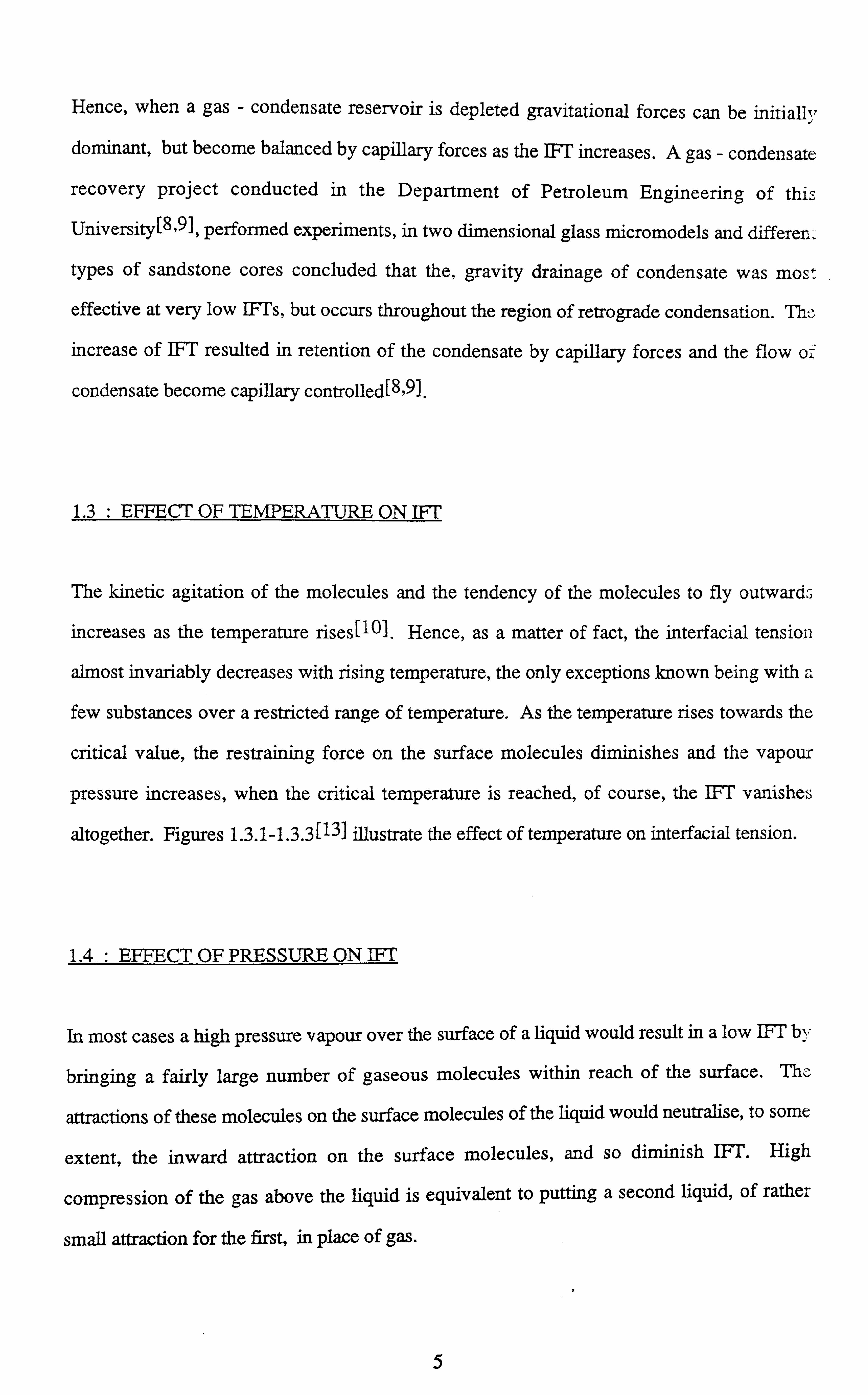
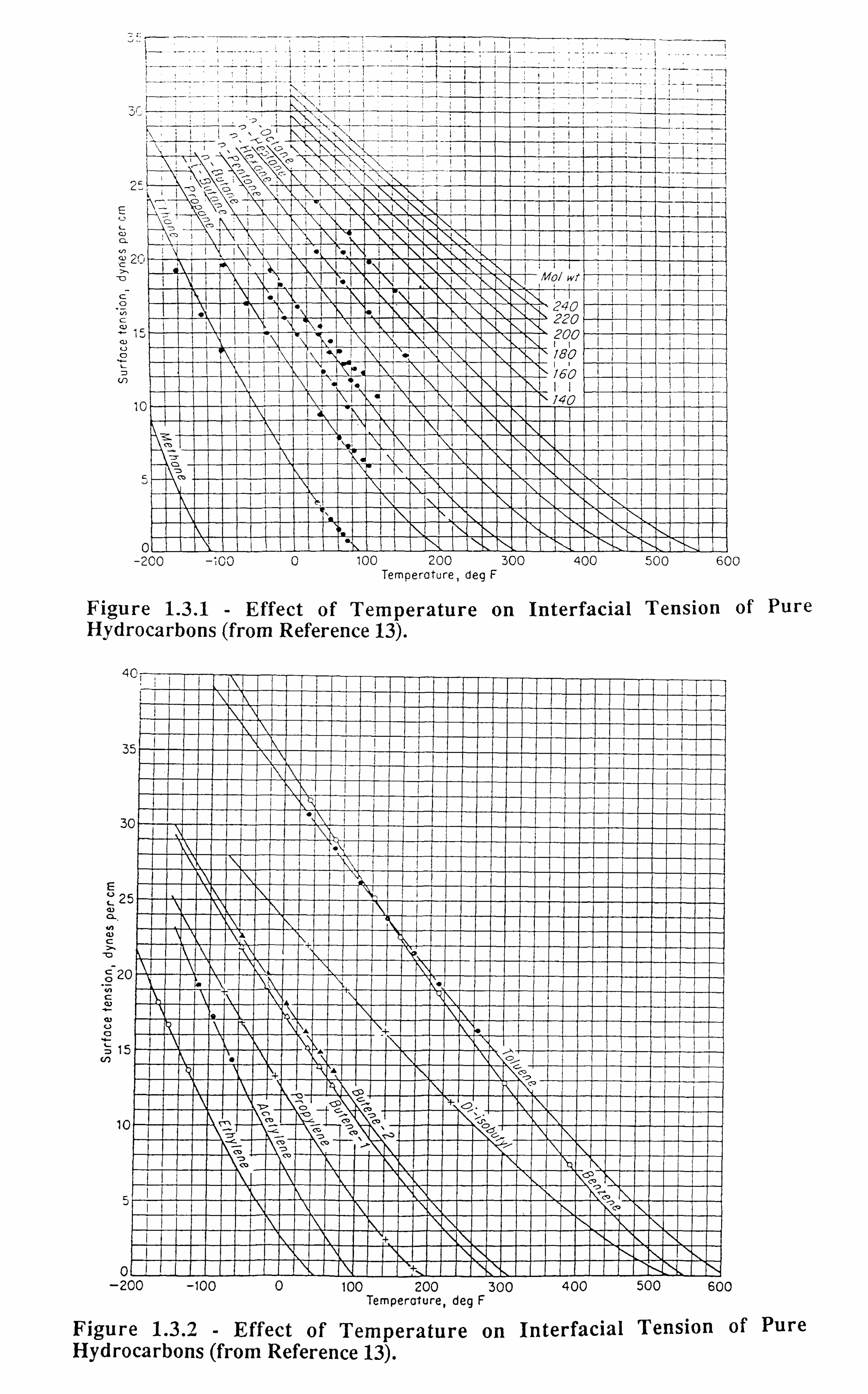
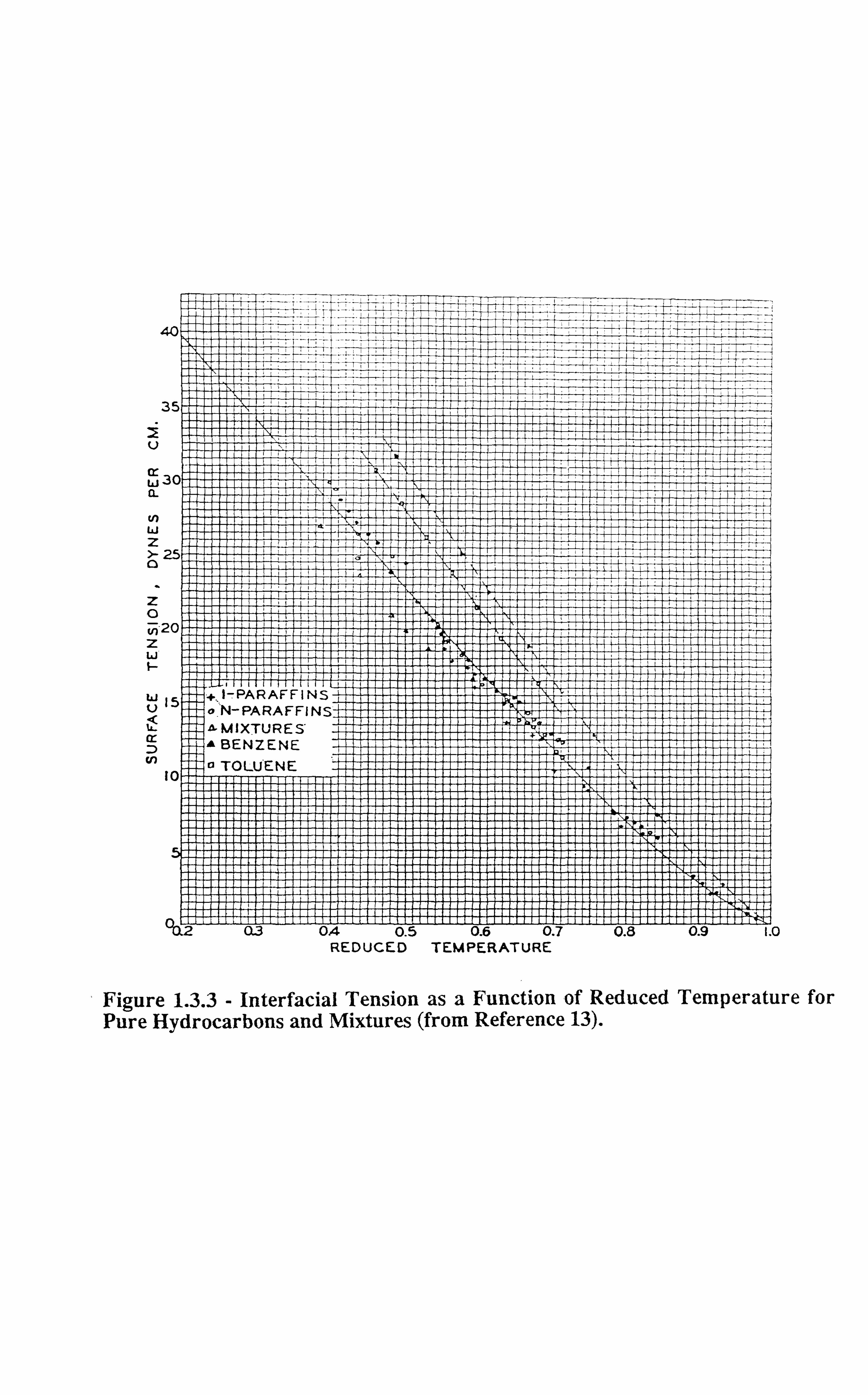
1.3 : EFFECT OF TEMPERATURE ON IFT
The kinetic agitation of the molecules and the tendency of the molecules to fly outwards
increases as the temperature rises[10I. Hence, as a matter of fact, the interfacial tension
almost invariably decreases with rising temperature, the only exceptions known being with a
few substances over a restricted range of temperature. As the temperature rises towards the
critical value, the restraining force on the surface molecules diminishes and the vapour
pressure increases, when the critical temperature is reached, of course, the IC'I' vanishes
altogether. Figures 1.3.1-1.3.3[13] illustrate the effect of temperature on interfacial tension.
1.4 : EFFECT OF PRESSURE ONIFT
In most cases a high pressure vapour over the surface of a liquid would result in a low IF'T by
bringing a fairly large number of gaseous molecules within reach of the surface. The
attractions of these molecules on the surface molecules of the liquid would neutralise, to some
extent, the inward attraction on the surface molecules, and so diminish IFT. High
compression of the gas above the liquid is equivalent to putting a second liquid, of rather
small attraction for the first, in place of gas.
5
Jr
2`
E
a- c 2C-
T 7D
0 U, t
a
1c
U1 II 11 1III11III Tl 1I1II --. II 'f, IYI1III '}-- 1If Tel V1
-200 -1C0 0 100 200 300 400 500 600 Temperature, deg F
Figure 1.3.1 - Effect of Temperature on Interfacial Tension of Pure Hydrocarbons (from Reference 13).
11 n
3'.
3(
E
C- N N C
ö 2C
C w
d U O
w
15
10
5
0lLIIIIIIIII L'il 11 V11I +ý III I' N 11 IIIIIIII -L l IN -200 -100 0 100 200 300 400 500 600
Temperature, deg F
Figure 1.3.2 - Effect of Temperature on Interfacial Tension of Pure Hydrocarbons (from Reference 13).
ý ý; ýticI II t LI
'
J
I ýý-
ýý ýý
!
I(
I "' "I ý;
! i t I
f ý
-I I It III II i I I I
' "
Mo/ wt L
" " I 240 i t.
220 t t ! 200
t ýI I "' 180 ;1 - j I I 60 _
'. I 140 I {
11 1 IN N I il l I l l !I t i
ö tl i
44
3
V
W3 CL
W Z
Q
Z 0
u, 2l Z LJ
tJ 0
W D in
I ý
^ý II j ý I II Imo' I
rý r
I
. I I II 5 II. I I 17
' . I I
I if O
I I
I
' 1 I 'i
ý I 1
5 I4 I I I I I
l i f , 1 -Ti I I 1
I 1I
- I T L- - kL
1 1 F V- 1T
5
J
11
f.. I-PARAFFINS o ̀ N-PARAFFINS
MIXTURES BENZENE
° TOLUENE T - if Ti
1
i f I J i l l
L - - - - .I L I L. -I L - 2 I I I - - 0 Q
- - Q2 03 04 0.5 0.6 'T T Ti I
0.7 0.8 0.9 - , 1! REDUCED TEMPERATURE
Figure 1.3.3 - Interfacial Tension as a Function of Reduced Temperature for Pure Hydrocarbons and Mixtures (from Reference 13).

14
I2
E L)10
ä8
C Z- 0 C c6
0 U 0
L J
2
0 0
O
/lS O
lS
-0
3O
9S
6S ý4
90 194 200 400 600 800 1000 1200 1400 1600
Pressure, psis
Figure 1.4.1 - Interfacial Tension of a Methane-Propane System (from Reference 13).
3C
2`
E
2C
T
OC 1S
N C
° 1C
5
OL 0
88deg F Schwartz expert " 95deg F Jones exper. 0 120 de F Standin g g
and Katz co%
0 ( 10
1000 2000 3000 4000 5000 6000 Soturotion pressure, psis
Figure 1.4.2 - Interfacial Tension of Crude Oils (from Reference 13).

7
6
5
4
3
aý 2
1
0 0 10 20 30
Pressure, MPa
Figure 1.4.3 - Effect of Pressure on a Real Gas Condensate Fluid C3 at 140 deg C (Chapter 3, Section 3.6.1).
r1r wýriý
Kundt's measurements[ 111 confirm this expectation and show decrease in the IFT of several
common liquids, with increase of pressure of the gas above them; the decrease amounted to
some 50 % in some cases at about 150 atm. The amount of decrease in IFT as the result of a
given amount of increase in pressure depends on the type of gas in contact with liquid. For
example, when IFT between hydrogen and diethyl ether (DEE) is compared with IF T between
air and DEE and carbon dioxide and DEE, for a given increase in pressure, the decrease in
IFT of hydrogen-DEE will be less than this decrease in IFT of air-DEE, which in turn will be
less than the decrease in IF-7 of carbon dioxide-DEE[111. Figure 1.4.1 and 1.4.2 show the
effect of pressure on interfacial tension for a methane-propane system and crude oils
respectively[ 131 and Figure 1.4.3 illustrates the effect of pressure on a real gas condensate
fluid (results for this fluid C3 are discussed in Chapter 3, Section 3.6.1).
References
1) Hough, E. W., Wood, B. B. and Rzasa, M. J.: "Adsorption at H20, - He,
-CH4, -N2 Interfaces at Pressures to 15,000 PSIA", J. Phys. Chem., Vol. 56,
pp. 996, (1952).
2) Andreas, 7. M., Hauser, E. A. and Tucker, W. B.: "Boundary Tension by
Pendant Drops", Presented at the Fiftieth Colloid Symposium, held at
Cambridge, Massachusetts, (Jun., 1938).
3) Bardon, C. and Longeron, .: "Influence of Very Low Interfacial Tensions on
Relative Permeability", Society of Petroleum Engineers Journal (SPED), pp.
391-401, (Oct., 1980).
4) Asar, H. K.: "Influence of Interfacial Tension on Gas Oil Relative Permeability
in Gas- Condensate Systems", PhD Thesis, University of Southern
California, (May, 1980).
5) Amafuele, J. O., and Handy, L. L.: "The Effect of Interfacial Tension on
Relative Oil Water Permeabilities on Consolidated Porous Media", Society of
Petroleum Engineers Journal (SPED), pp 371-381 (June, 1982).
6
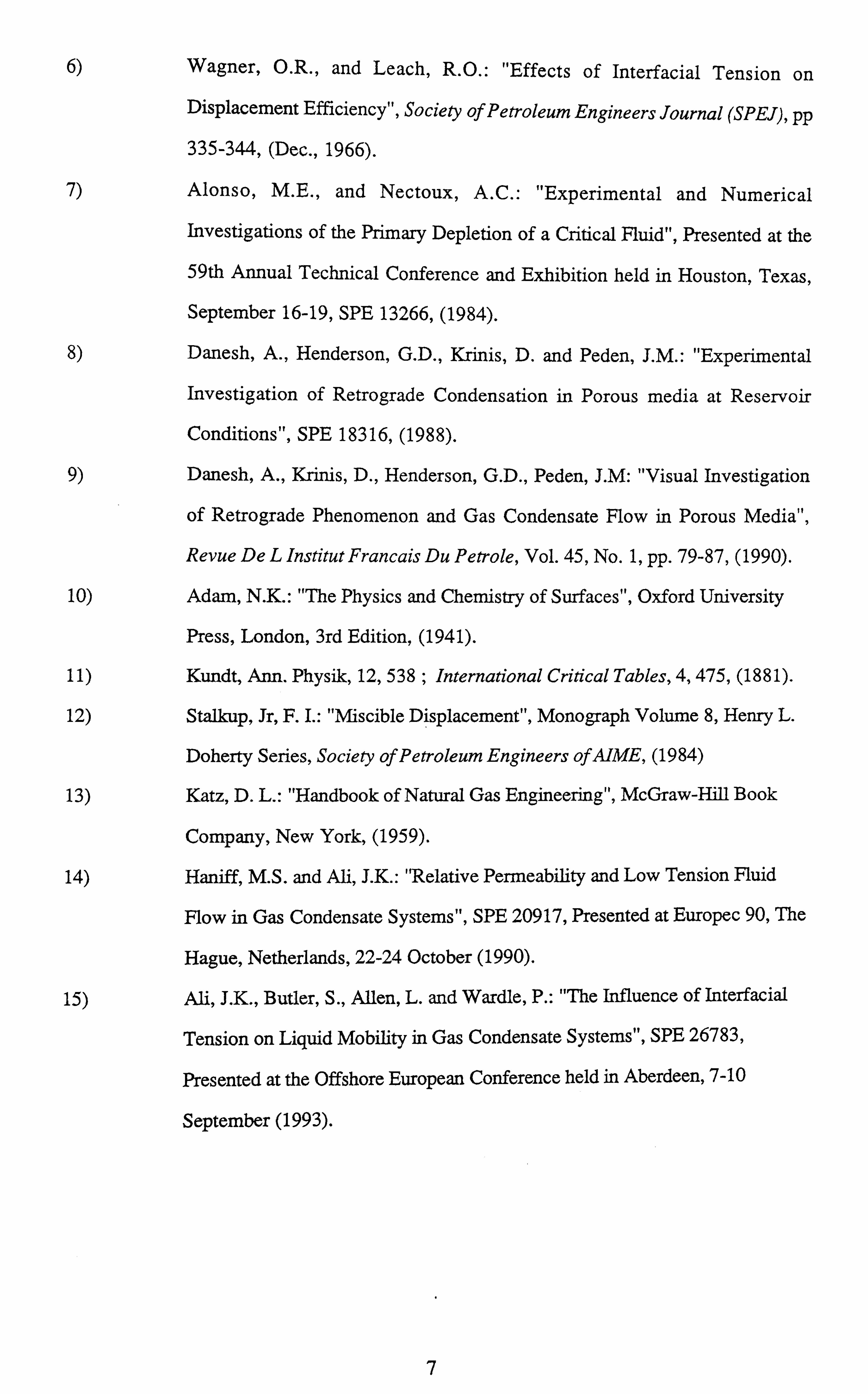
6) Wagner, O. R., and Leach, R. O.: "Effects of Interfacial Tension on Displacement Efficiency", Society of Petroleum Engineers Journal (SPED), pp
335-344, (Dec., 1966).
7) Alonso, M. E., and Nectoux, A. C.: "Experimental and Numerical
Investigations of the Primary Depletion of a Critical Fluid", Presented at the
59th Annual Technical Conference and Exhibition held in Houston, Texas,
September 16-19, SPE 13266, (1984).
8) Danesh, A., Henderson, G. D., Krinis, D. and Peden, J. M.: "Experimental
Investigation of Retrograde Condensation in Porous media at Reservoir
Conditions", SPE 18316, (1988).
9) Danesh, A., Krinis, D., Henderson, G. D., Peden, J. M: "Visual Investigation
of Retrograde Phenomenon and Gas Condensate Flow in Porous Media",
Revue De L Institut Francais Du Petrole, Vol. 45, No. 1, pp. 79-87, (1990).
10) Adam, N. K.: "The Physics and Chemistry of Surfaces", Oxford University
Press, London, 3rd Edition, (1941).
11) Kundt, Ann. Physik, 12,538 ; International Critical Tables, 4,475, (1881).
12) Stalkup, Jr, F. I.: "Miscible Displacement", Monograph Volume 8, Henry L.
Doherty Series, Society of Petroleum Engineers of ATME, (1984)
13) Katz, D. L.: "Handbook of Natural Gas Engineering", McGraw-Hill Book
Company, New York, (1959).
14) Haniff, M. S. and Ali, J. K.: "Relative Permeability and Low Tension Fluid
Flow in Gas Condensate Systems", SPE 20917, Presented at Europec 90, The
Hague, Netherlands, 22-24 October (1990).
15) Ali, J. K., Butler, S., Allen, L. and Wardle, P.: "The Influence of Interfacial
Tension on Liquid Mobility in Gas Condensate Systems", SPE 26783,
Presented at the Offshore European Conference held in Aberdeen, 7-10
September (1993).
7
CHAPTER 2: EXPERIMENTAL TECHNIQUES FOR MEASURING INTERFACIAL TENSION
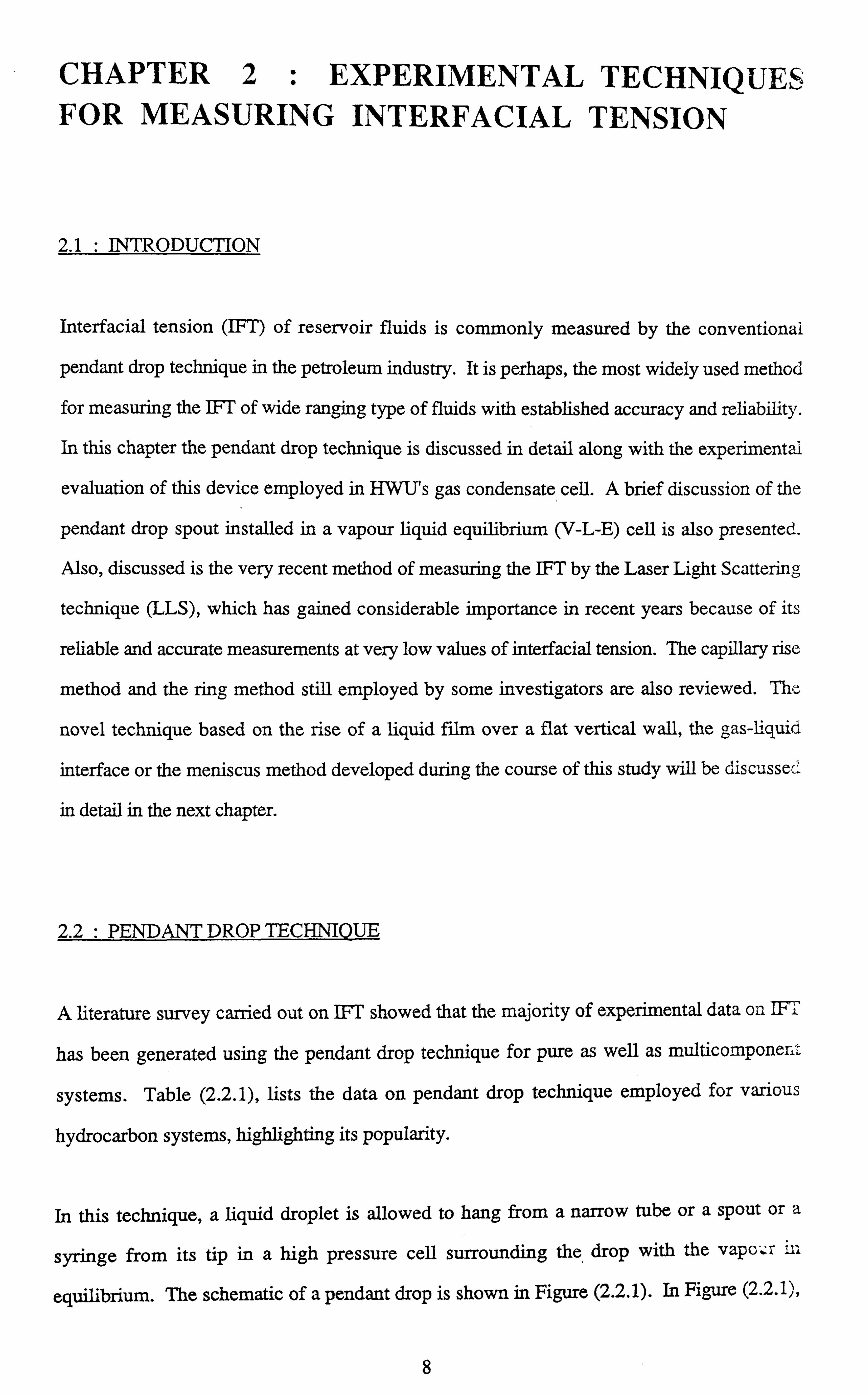
2.1 : INTRODUCTION
Interfacial tension (IFT) of reservoir fluids is commonly measured by the conventional
pendant drop technique in the petroleum industry. It is perhaps, the most widely used method
for measuring the IFT of wide ranging type of fluids with established accuracy and reliability.
In this chapter the pendant drop technique is discussed in detail along with the experimental
evaluation of this device employed in HWU's gas condensate cell. A brief discussion of the
pendant drop spout installed in a vapour liquid equilibrium (V-L-E) cell is also presented.
Also, discussed is the very recent method of measuring the IFT by the Laser Light Scattering
technique (LLS), which has gained considerable importance in recent years because of its
reliable and accurate measurements at very low values of interfacial tension. The capillary rise
method and the ring method still employed by some investigators are also reviewed. The
novel technique based on the rise of a liquid film over a flat vertical wall, the gas-liquid
interface or the meniscus method developed during the course of this study will be discussed
in detail in the next chapter.
2.2 : PENDANT DROP TECHNIQUE
A literature survey carried out on IC'I' showed that the majority of experimental data on IF T
has been generated using the pendant drop technique for pure as well as multicomponen
systems. Table (2.2.1), lists the data on pendant drop technique employed for various
hydrocarbon systems, highlighting its popularity.
In this technique, a liquid droplet is allowed to hang from a narrow tube or a spout or a
syringe from its tip in a high pressure cell surrounding the drop with the vapor in
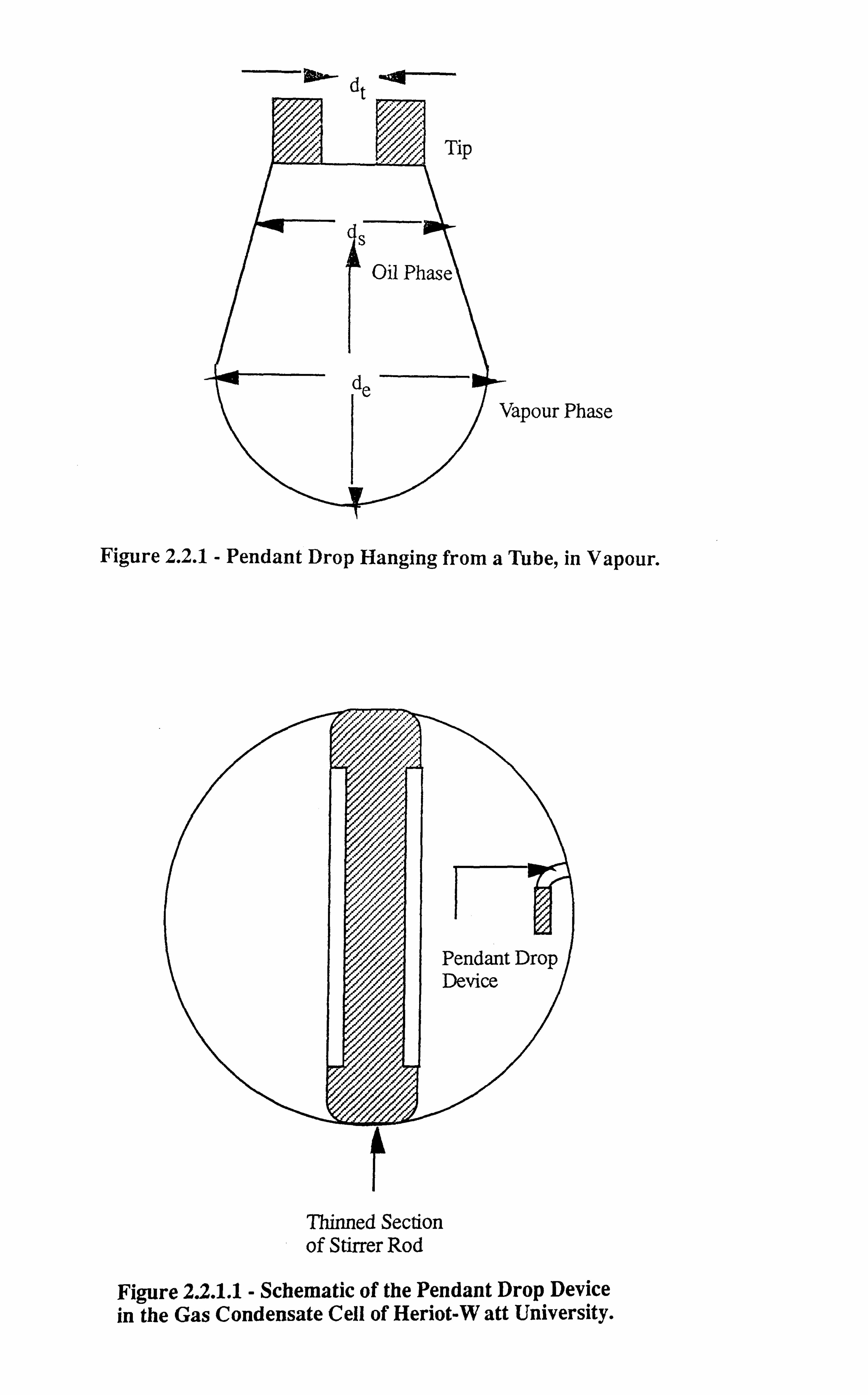
equilibrium. The schematic of a pendant drop is shown in Figure (2.2.1). In Figure (2.2.1),
8
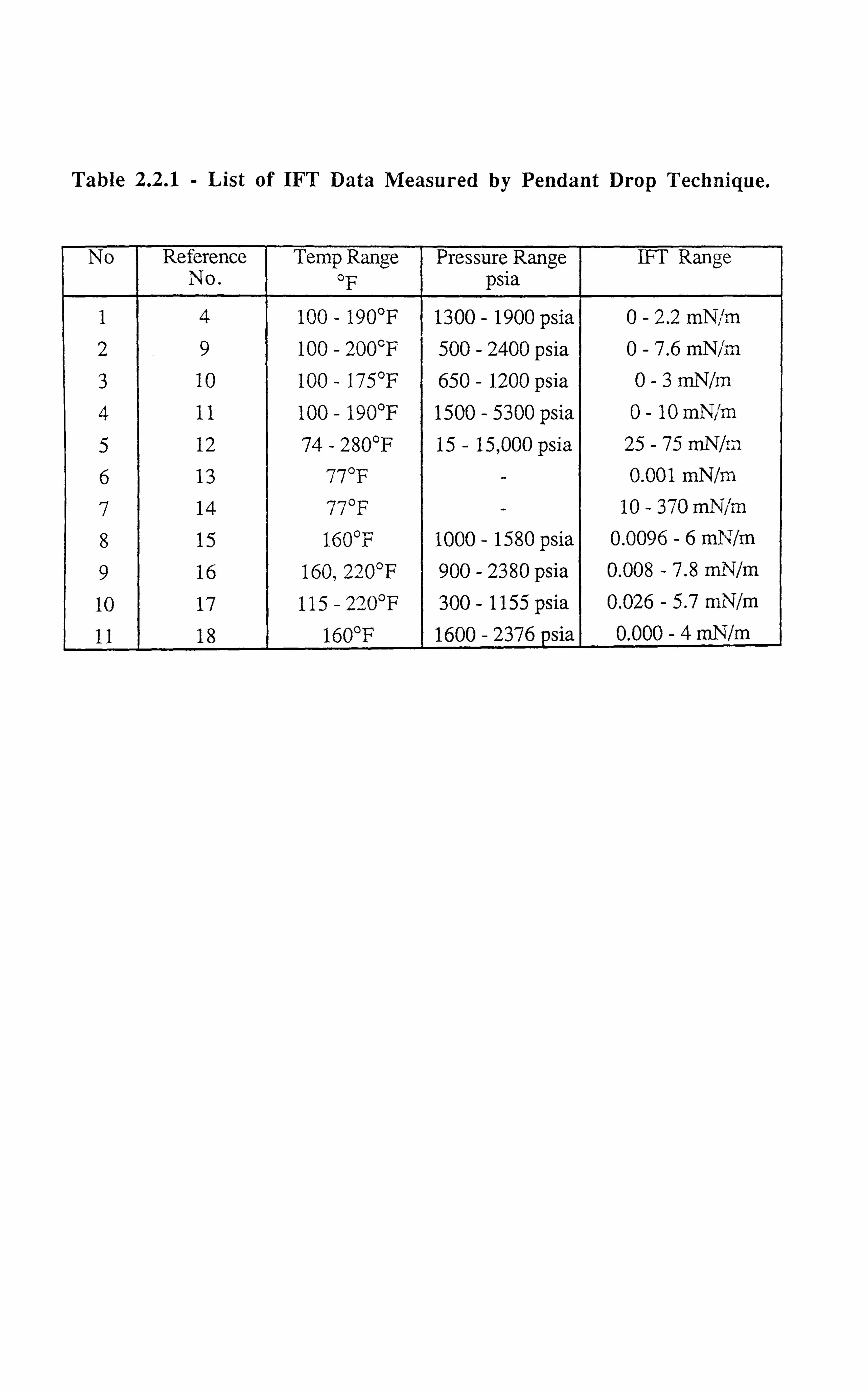
Table 2.2.1 - List of IFT Data Measured by Pendant Drop Technique.
No Reference No.
Temp Range °F
Pressure Range psia
IFT Range
1 4 100 - 190°F 1300 - 1900 psia 0-2.2 mN; rn 2 9 100 - 200°F 500 - 2400 psia 0-7.6 mN/ýr 3 10 100 - 175°F 650 - 1200 psia 0-3 mN/m 4 11 100 - 190°F 1500 - 5300 psia 0- 10 mNJm 5 12 74 - 280°F 15 - 15,000 psia 25 - 75 mN/:: 1 6 13 77°F - 0.001 mN/m, 7 14 77°F - 10-370mNim
8 15 160°F 1000 - 1580 psia 0.0096 -6 mN/m 9 16 160,220°F 900 - 2380 psia 0.008 - 7.8 mN/m 10 17 115 - 22 0°F 300 - 1155 psia 0.026 - 5.7 mN/m
11 18 160°F 1600 - 2376 sia 0.000 -4 mN/m
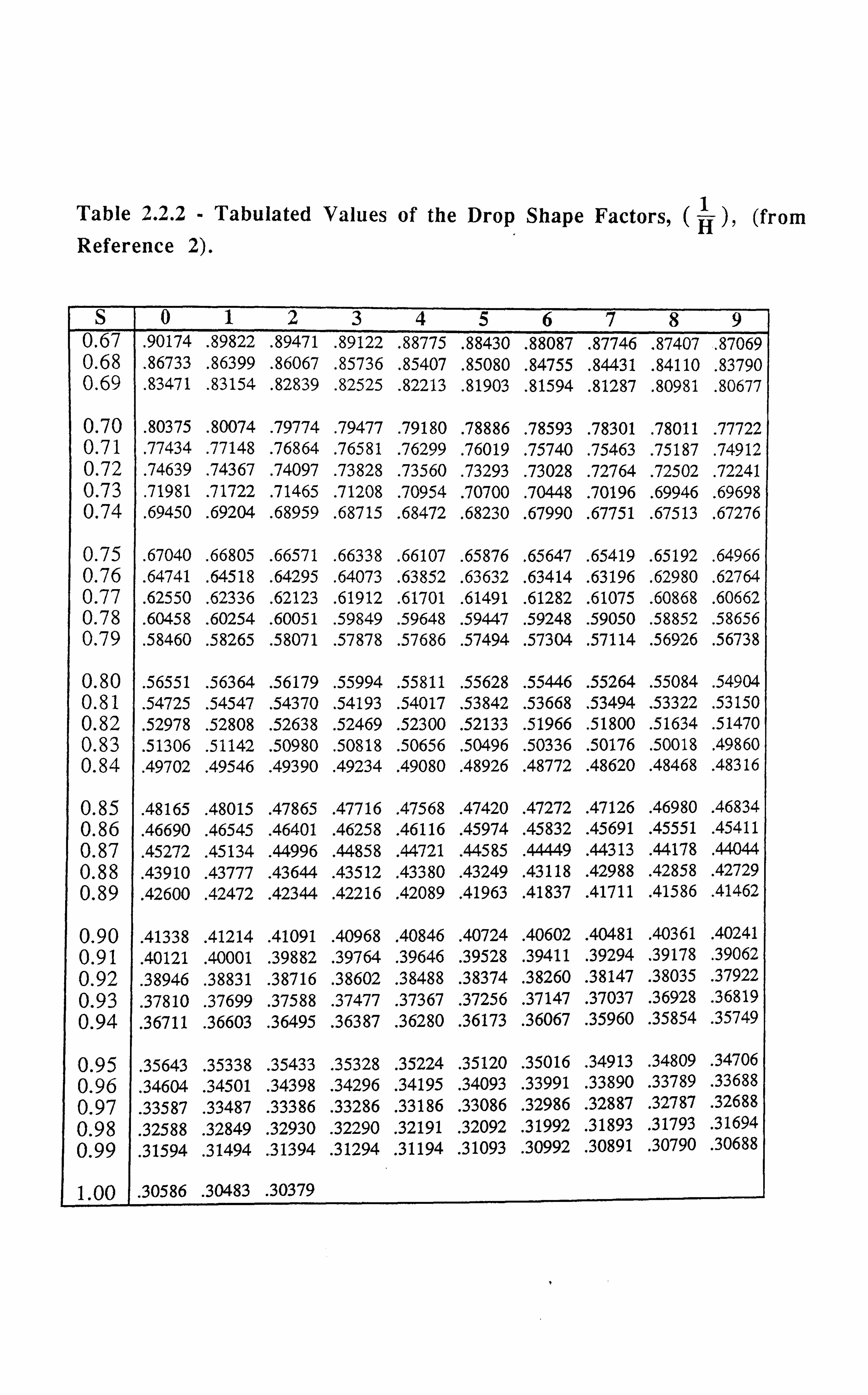
Table 2.2.2 - Tabulated Values of the Drop Shape Factors, (H ), (from Reference 2).
S 0 1 2 3 4 5 6 7 8 9 0.67
. 90174 . 89822 . 89471 . 89122 . 88775 . 88430 . 88087 . 87746 . 87407 . 87069 0.68
. 86733 . 86399 . 86067 . 85736 . 85407 . 85080 . 84755 . 84431 . 84110 .
83790 0.69
. 83471 . 83154 . 82839 . 82525 . 82213 . 81903 . 81594 . 81287 . 80981 . 80677
0.70 . 80375 . 80074 . 79774 . 79477 . 79180 . 78886 . 78593 . 78301 . 78011 . 77722
0.71 . 77434 . 77148 . 76864 . 76581 . 76299 . 76019 . 75740 . 75463 . 75187 . 74912
0.72 . 74639 . 74367 . 74097 . 73828 . 73560 . 73293 . 73028 . 72764 . 72502 . 72241
0.73 . 71981 . 71722 . 71465 . 71208 . 70954 . 70700 . 70448 . 70196 . 69946 . 69698
0.74 . 69450 . 69204 . 68959 . 68715 . 68472 . 68230 . 67990 . 67751 . 67513 . 67276
0.75 . 67040 . 66805 . 66571 . 66338 . 66107 . 65876 . 65647 . 65419 . 65192 . 64966
0.76 . 64741 . 64518 . 64295 . 64073 . 63852 . 63632 . 63414 . 63196 . 62980 . 62764
0.77 . 62550 . 62336 . 62123 . 61912 . 61701 . 61491 . 61282 . 61075 . 60868 . 60662
0.78 . 60458 . 60254 . 60051 . 59849 . 59648 . 59447 . 59248 . 59050 . 58852 . 58656
0.79 . 58460 . 58265 . 58071 . 57878 . 57686 . 57494 . 57304 . 57114 . 56926 . 56738
0.80 . 56551 . 56364 . 56179 . 55994 . 55811 . 55628 . 55446 . 55264 . 55084 . 54904
0.81 . 54725 . 54547 . 54370 . 54193 . 54017 . 53842 . 53668 . 53494 . 53322 . 53150
0.82 . 52978 . 52808 . 52638 . 52469 . 52300 . 52133 . 51966 . 51800 . 51634 . 51470
0.83 . 51306 . 51142 .
50980 . 50818 . 50656 . 50496 . 50336 . 50176 . 50018 . 49860
0.84 . 49702 . 49546 . 49390 . 49234 . 49080 . 48926 . 48772 . 48620 . 48468 . 48316
0.85 . 48165 . 48015 . 47865 . 47716 . 47568 . 47420 . 47272 . 47126 . 46980 . 46834
0.86 . 46690 . 46545 . 46401 . 46258 . 46116 . 45974 . 45832 . 45691 . 45551 . 45411
0.87 . 45272 . 45134 . 449 96 . 44958 . 44721 . 445 85 . 44449 . 44313 . 44178 . 44044
0.88 . 43910 . 43777 . 43644 . 43512 . 43380 . 43249 . 43118 . 42988 . 42858 . 42729
0.89 . 42600 . 42472 . 42344 . 42216 . 42089 . 41963 . 41837 . 41711 . 41586 . 41462
0.90 . 41338 . 41214 . 41091 . 40968 . 40846 . 40724 . 40602 . 40481 . 40361 . 40241
0.91 . 40121 . 40001 . 39882 . 39764 . 39646 . 39528 . 39411 . 39294 . 39178 . 39062
0.92 . 38946 . 38831 . 38716 . 38602 . 38488 . 38374 . 38260 . 38147 . 38035 . 37922
0.93 . 37810 . 37699 . 37588 . 37477 . 37367 . 37256 . 37147 . 37037 . 36928 . 36819 0.94
. 36711 . 36603 . 36495 . 36387 . 36280 . 36173 . 36067 . 35960 . 35854 . 35749
0.95 . 35643 . 35338 . 35433 . 35328 . 35224 . 35120 . 35016 . 34913 . 34809 . 34706
0.96 . 34604 . 34501 . 34398 . 34296 . 34195 . 34093 . 33991 . 33890 . 33789 . 33688 0.97
. 33587 . 33487 . 33386 . 33286 . 33186 . 33086 . 32986 . 32887 . 32787 . 32688 0.98
. 32588 . 32849 . 32930 . 32290 . 32191 . 32092 . 31992 . 31893 . 31793 . 31694 0.99
. 31594 . 31494 . 31394 . 31294 . 31194 . 31093 . 30992 . 30891 . 30790 . 30688
1.00 . 30586 . 30483 . 30379

de is called the equatorial diameter or the maximum horizontal diameter of the drop, ds is the
diameter of the drop measured at a distance de above the tip of the drop and dt is the tip inside
diameter as observed on a photographic image. The quantity dtw is already known which
represents the original tip inside diameter which is taken as a reference value for calculating
the magnification. The drop dimensions are correlated by balancing the gravitational and
surface forces to give the IFT in the form given below :
d2 (Pl-Pv) (2.2.1,
Where,
g= acceleration due to gravity
6 interfacial tension
pi & pv = liquid and vapour phase densities (mass) respectively
in Eq. 2.2.1, H, which is a function of S=, is called the drop shape factor, the values o
which have been derived using the Laplace/Young equation as applied to the drops and
reported by several workers[1'2] against S.
Hence the values of H can be known after measuring the drop dimensions and subsequently
calculating the value of S. Table (2.2.2), gives the tabulated values of 1H
vs. S from
Reference[2].
2.2.1 : Discussion of Results on Pendant Drop Device in the Gas Condensate Equilibrium
Cell
As an initial approach towards the measurement of interfacial tension between gas and
condensate phases in equilibrium, a pendant drop device was installed in the gas condensate
cell as shown in Figure (2.2.1.1). The device installed consisted of a spout attached to the
orifice of a regulating valve which is located in the wall of the cell adjacent to the window.
The valve forms the part of the direct sampling system (see Section 3.2 for details of the
9
Tapour Phase
Figure 2.2.1 - Pendant Drop Hanging from a Tube, in Vapour.
Thinned Section of Stirrer Rod
Figure 2.2.1.1 - Schematic of the Pendant Drop Device in the Gas Condensate Cell of Heriot-W att University.
---loo -- dt -4-
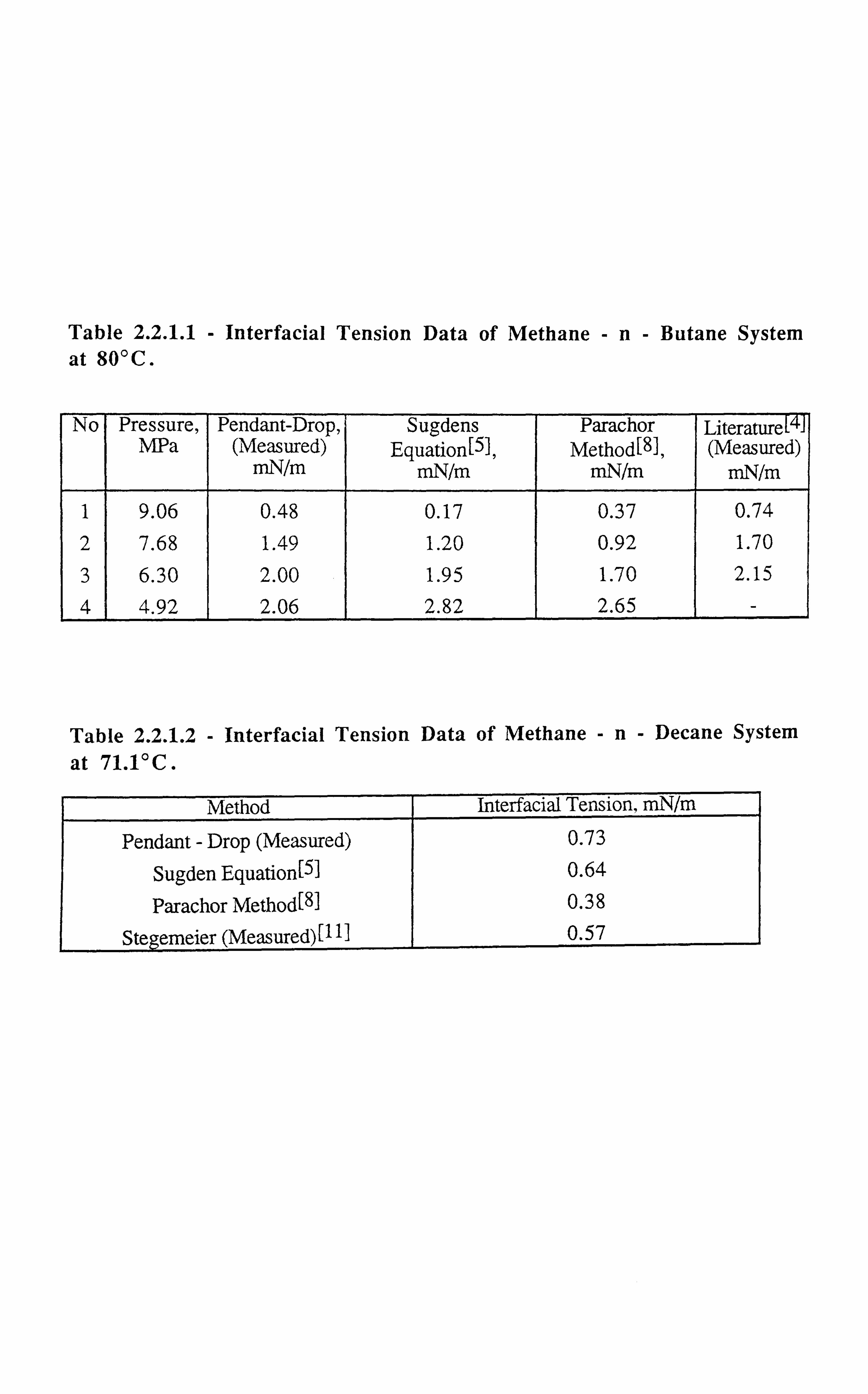
Table 2.2.1.1 - Interfacial Tension Data of Methane -n- Butane System at 80°C.
No Pressure, Pendant-Drop, Sugdens Parachor Literature MPa (Measured) Equation[s], Method[8}, (Measured)
mN/m mN/m mN/m mN/m
1 9.06 0.48 0.17 0.37 0.74 2 7.68 1.49 1.20 0.92 1.70 3 6.30 2.00 1.95 1.70 2.15 4 4.92 2.06 2.82 2.65 -
Table 2.2.1.2 - Interfacial Tension Data of Methane -n- Decane System
at 71.1°C.
Method Interfacial Tension, mN/m
Pendant - Drop (Measured) 0.73
Sugden Equation[5] 0.64
Parachor Method[811 0.38
Stegemeier (Measured)1111 0.57
experimental facility) and by manipulation of fluids contained within the circulation loop it is
possible to suspend a drop of liquid at the tip of the spout. Interfacial tension can then b;
calculated after measuring the drop dimensions as mentioned in the previous section. In order
to test the pendant drop facility incorporated into the cell two binary systems namely methane-
n-butane and methane-n-decane, at 80°C and 71.1°C respectively, were studied.
The methane-n-butane system exhibited retrograde condensation and had a two phase region
between 4.92 MPa and 11.09 MPa. IFTs in the range of 0.5 to 2 mN/m were measured by
the pendant drop technique. Table (2.2.1.1), lists the IFT measurements by the pendant drop
device and those reported in the literature[4], along with those calculated by the predictive
techniques [5,8]. The measured methane and n- decane interfacial tension at 71.1°C and
31.11 MPa and the value given by Stegemeier et. al. [ 11 ] along with predicted values arc,
tabulated in Table (2.2.1.2). Reasonable agreement between the values obtained from our
measurements, predicted values and reported by Stegemeier et. al. [111 can be seen. As it cri .
be seen from Table (2.2.1.1), the values matched reasonably well at high IFTs but it was
found that the lowest limit of IFT measurable by our pendant drop method was 1 dyne/cm.
The measurement of IFT at fairly low values requires very small diameter drops to be formed
which was very difficult with the present spout size which was 0.65 mm. The insertion of a
spout of smaller size would involve large changes in the cell structure which was thought to
be unfeasible. So the pendant drop method merely served the purpose of quantitative
assessment. And the values measured by our pendant drop spout at low values could not be
quoted with certainty. These were the initial results which proved to be conducive for the
development of a novel technique based on the rise of a film of liquid over a flat vertical wall.
A complete account of this method with the obtained results are furnished in the next chapter.
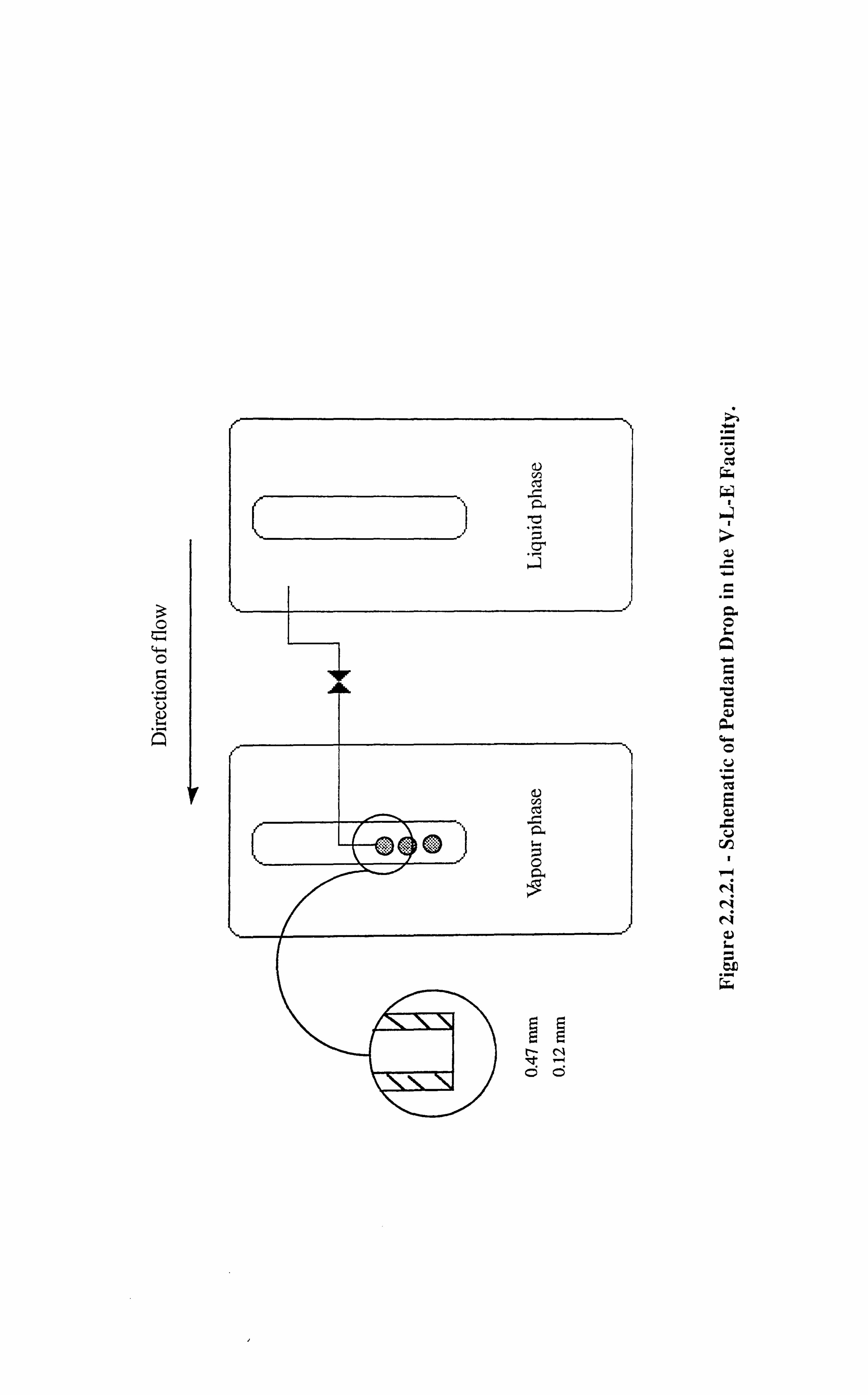
2.2.2 : Pendant Drop Device in the Vapour-Liquid Equilibrium (V-L-E) Cell
A pendant drop spout was installed in the V-L-E cell in order to carry out the measurement of
interfacial tension during the processes of gas injection involving real volatile and black oils.
The details of the arrangement are shown in Figure 2.2.2.1 which shows the pendant drop
10
3 C
0 0 U
Q
.r
"r U
W
U r" r,
C .r
l.. iM Q
i.. l
i. ý
Fro
Q "r i. ý
E C. )
rV^1
cV N N
i. .. r
.... Gý

tubing, pipework and isolation valve, that are introduced between two, 200 cc Ruska
windowed VLE cells, in such a way that liquid phase could be introduced and dropped
through its equilibrium vapour, via a small bore (0.47 mm external diameter, 0.12 mm
internal diameter) stainless steel capillary tube. By extending the horizontal length of this
pipe, a droplet of the liquid could be dropped from its distal tip. This event and the vapour-
liquid interface boundary could then be video recorded and subsequently dimensioned using
the VMS scalar unit for IFT calculations.
It was first decided to test the validity of the developed gas-liquid curvature (meniscus)
method and the installed pendant drop method by measuring interfacial tension data for a
known system for which values in the literature would be available. So that these
measurement techniques could be applied with confidence to the injection processes for
determining the interfacial tension. A binary mixture of methane-n-decane at 71.1 °C was
selected for this purpose. Stegemier[l 1] has measured IFT of this binary mixture at different
isotherms by the pendant drop technique. The range of IFTs reported is from 0.002-10
dyne/cm. A detailed discussion of the experiment carried out is provided in Chapter 3.
Interfacial tension measurements were carried out at various pressures below the dew point of
35.3 MPa. Both the pendant drop and gas-liquid meniscus methods were found to be in
reasonable agreement with the data presented in the literature. Plots for comparison are
presented in Chapter 3. This exercise proved that the meniscus method could also be applied
in the V-L-E cell for condensate type fluids with near zero contact angles and at the same time
validated the newly installed pendant drop device.
It was then decided to test both the methods for a real volatile oil system. This oil was flashed
at several pressures below its bubble point of 34.92 MPa at 100°C. The IFTs were measured
similar to the previous experiment at three different pressures and were compared with those
predicted by the modified parachor method (no previous measurements were reported fo: this
system). This comparison indicated that the values measured by the pendant drop were in
reasonable agreement with those predicted whereas the meniscus values were significantly
low. This is apparently due to the partial wetting (90° > contact angle > 0°) of the cell
windows by the oil phase (also contact angle increases as IFT increases) as against the
It
11
condensate phase which exhibits a full wetting behaviour. Perfect wetting has been one of the
assumption in developing the expression for the gas-liquid curvature technique. Another
explanation for these differences is because of the presence of surface active agents such as
asphaltenes in the oil systems. Hence it was decided to use the pendant drop method for these
wetting type of fluids in future studies. A detailed description of this experiment involving
the real volatile oil is furnished in Chapter 3.
2.3 : LASER LIGHT SCATTERING TECIIQUE
Laser Light Scattering (LLS) technique is a fairly new technique especially suited for
measuring IFTs near the critical point or at very high pressures. Recently Pearce and
Haniff[6], measured the IFT of a methane-propane binary mixture by LLS technique in th--
range of 0.001 to 1 mN%m. Similarly the same authors[71, have measured EFT of a carbon
dioxide system near the critical region in the range of 0.01 to 2 mN/m.
Measurement of surface properties such as the interfacial tension, and viscosity by the LLS
technique is based on the thermally excited waves which exist at the interface separating the
vapour and liquid phases. These waves are studied by measuring the statistical properties of
the light scattered at the interface using the LLS technique. A laser beam is focused on to the
surface of the liquid, such that both the reflected and scattered light are collected at a photo
multiplier. A recently developed technique called the photon correlation spectroscopy is used
to detect the signals. Here, the scattered and reflected lights are mixed to produce a bea:
frequency which can be measured using either a spectrum analyser to produce a power
spectrum in the frequency domain or an auto-correlator to give a correlation function in the
time domain. The correlation functions or power spectra thus provides the characteristics of
the surface waves. In order to interpret the correlation functions one uses a dispersion
equation which relates the properties of the fluid to a description of the wave propagations.
Finally the correlation function is solved by a numerical procedure, since it does not have any
analytical solutions, to give the values of interfacial tension and viscosity directly.
12

As far as the advantages of the LLS technique are concerned, it is a non - perturbative
technique, needs only a small volume of liquid for measurements, and it is also capable of
measuring interfacial tensions close to the critical point[6'7]. The LLS technique requires density data of equilibrated phases. Compositional data on the fluids tested are also needed if
predictive methods are to be evaluated against experimental IFT data. The measurements of IFT by the LLS technique are required to be carried out in the specific apparatus where it is
difficult to match the same compositions that exist in the equipment for conventional phase behaviour measurements. However, compared to the LLS technique, the set-up described in
this thesis which directly provides all the density, compositional and volumetric data required
for measurement and prediction of the interfacial tension is much more convenient and
practical.
2.4 : CAPILLARY RISE TECHNIQUE
The capillary rise method is another technique employed for measuring interfacial tension
which relies on the fundamentals of capillarity and uses some basic equations to measure the
IFT from it. Weinaug and Katz[8l, have measured the IFIs of the methane-propane binary
mixture at various temperature and pressure conditions using the capillary rise method. Ms
method basically involves the use of a fine capillary tube through which a liquid is allowed to
rise, this particular rise is predominantly dependant upon the interfacial tension, or the
adhesive and cohesive forces. The surface force of IFT is then balanced against the liquid
head which enables to define the following relationship :
2irrß' = irr2h (1-Pv)g (2.4.1)
the quantity on the left hand side of the Eq. 2.4.1, is the force due to IFT and that on the right
hand side is the force due to the liquid head which allows the calculation of IFT:
phr 2
(2.4.2)
13
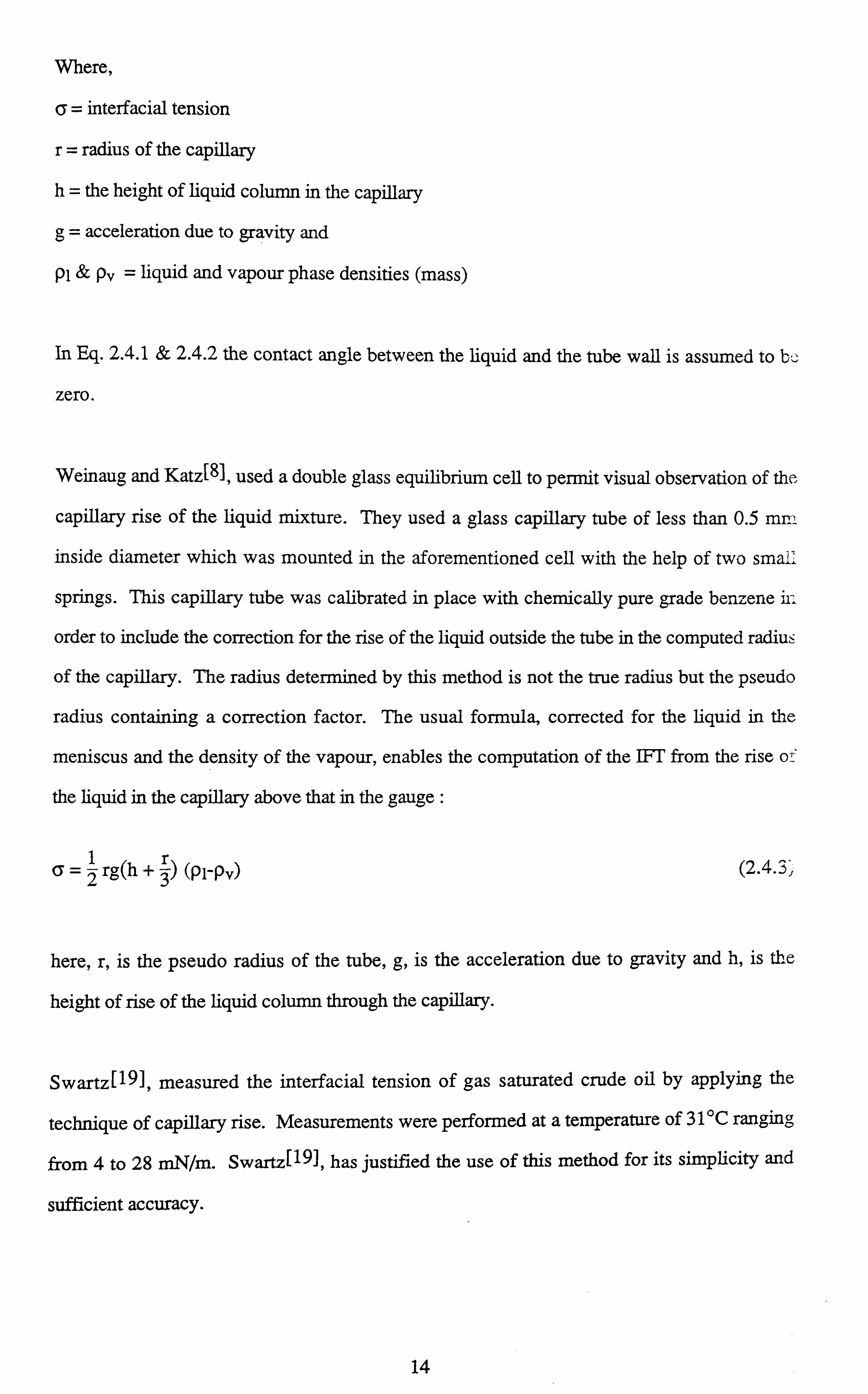
Where,
6= interfacial tension
r= radius of the capillary
h= the height of liquid column in the capillary
g= acceleration due to gravity and
pi & pv = liquid and vapour phase densities (mass)
In Eq. 2.4.1 & 2.4.2 the contact angle between the liquid and the tube wall is assumed to b:
zero.
Weinaug and Katz[8], used a double glass equilibrium cell to permit visual observation of the.
capillary rise of the liquid mixture. They used a glass capillary tube of less than 0.5 mm
inside diameter which was mounted in the aforementioned cell with the help of two small
springs. This capillary tube was calibrated in place with chemically pure grade benzene iii
order to include the correction for the rise of the liquid outside the tube in the computed radius
of the capillary. The radius determined by this method is not the true radius but the pseudo
radius containing a correction factor. The usual formula, corrected for the liquid in the
meniscus and the density of the vapour, enables the computation of the IFT from the rise o
the liquid in the capillary above that in the gauge :
6=2rgCh+3) (P1-Pv) (2.4.3)
here, r, is the pseudo radius of the tube, g, is the acceleration due to gravity and h, is the
height of rise of the liquid column through the capillary.
Swartz[19], measured the interfacial tension of gas saturated crude oil by applying the
technique of capillary rise. Measurements were performed at a temperature of 31 °C ranging
from 4 to 28 mN/m. Swartz[191, has justified the use of this method for its simplicity and
sufficient accuracy.
14

-' '//
" 17T7+r
/I / �/. ////i/i
Figure 2.5.1 - The Ring Method (from Reference 20).
1.
1.1
1.0
f
0.9
0.8
0.7
R/r = 80
50
"".... 40 13.5 30
012345 R3/V
Figure 2.5.2 - Correction Factor Plots for. the Ring Method (from Reference 21).
To Balance

Although this method appears to be simple for application, its use at very high pressure
conditions, where the IFT is small, is not practical as the rise of liquid in the capillary tube is
very small.
2.5 : THE RING METHOD
The ring method is generally attributed to du Nouy{20I. The method belongs to the family of detachment methods, where a first approximation to the detachment force is given by the
surface tension multiplied by the periphery of the surface detached. Thus, for a ring, as
illustrated in Figure (2.5.1),
Wtot = Wring + 41rRa (2.5.1)
Harkins and Jordan[21I found, however, that Eq. 2.5.1 was generally in serious error and
worked out an empirical correction factor, which is given by the following expression:
f=\Pý=f (R3 >R) (2.5.2)
where p denoted the "ideal" surface tension calculated from Eq. 2.5.1 and V is the meniscus
volume. Figure (2.5.2) shows the correction factor plots for the ring method. Eq. 2.5.1 &
2.5.2 used in conjunction with Figure (2.5.2) can be used to determine the interfacial tension.
References
1) Andreas, J. M., Hauser, E. A., and Tucker, W. B.: "Boundary Tension by
Pendant Drops", Presented at the Fiftieth Colloid Symposium, held at
Cambridge, Massachusetts, (Jun., 1938).
2) Niederhauser, D. O. and Bartell, F. E.: "A Corrected Table for Calculation of
Boundary Tensions by Pendant Drop Method", Research on Occurrence and
15

Recovery of Petroleum, A Contribution from API Research Project 27, pp.
114-146, (Mar., 1947).
3) Bashforth, F. and Adams, J. C.: "An Attempt to test the Theories of Capillary
Action", University Press, Cambridge, England, (1883).
4) Pennington, B. F. and. Hough, E. W.: "Interfacial Tension of the Methane
Normal Butane System", Producers Monthly, pp. 4, (Jul., 1965).
5) Hough, E. W. and Warren, H. G.: "Correlation of Interfacial Tension of
Hydrocarbons", Society of Petroleum Engineers Journal (SPEJ), pp. 345-
349, (Dec., 1966).
6) Haniff, M. S. and Pearce, A. 3.: "Measuring Interfacial Tension in a Methane -
Propane Gas - Condensate System Using a Laser Light Scattering Technique",
SPE 19025, (1988).
7) Pearce, A. J. and Haniff, M. S.: "Light Scattering Experiments from a Carbon
Dioxide Surface Near the Critical Point :A Data Reduction Procedure", J. Col.
& Int. Sci., Vol. 119, No. 2, pp. 315-325, (Oct., 1987).
8) Weinaug, C. F. and Katz, D. L.: "Surface Tension of Methane - Propane
Mixtures", Industrial & Engineering Chemistry (I & EC), Vol. 35, No. 2, pp.
239-247, (Feb., 1943).
9) Stegemeier, G. L. and Hough, E. W.: "Interfacial Tension of the Methane
Normal Pentane System", Producers Monthly, pp. 6-9, (Nov., 1961).
10) Brauer, E. B. and Hough, E. W.: "'Interfacial Tension of the Normal Butane
Carbon Dioxide System", Producers Monthly, pp. 13, (Aug., 1965).
11) Stegemeier, G. L., Pennington, B. F., Brauer, E. B. and Hough, E. W.:
"Interfacial Tension of the Methane - Normal Decane System", Society of
Petroleum Engineers Journal (SPED), pp. 257-260, (Sep., 1980).
12) Hough, E. W., Rzasa, M. J. and Wood, B. B.: "Interfacial Tensions At
Reservoir Pressures and Temperatures; Apparatus and the Water - Methane
System", Petroleum Transactions of AJME, Vol. 192,. pp. 58-60, (1951).
13) Jennings, H. Y. Jr.: "Apparatus for Measuring Very Low Interfacial
Tensions", The Review of Scientific Instruments, Vol. 28, No. 10, pp. 774-
777, (Oct., 1957).
16
14) Andreas, J. M., Hauser, E. A. and Tucker, W. B.: "Boundary Tension b -v Pendant Drops", Presented at the Fiftieth Colloid Symposium, held a_ Cambridge, Massachusetts, pp. 9-11, (Jun., 1938).
15) Nagarajan, N. and Robinson, R. L. Jr.: "Equilibrium Phase Compositions,
Phase Densities, and Interfacial Tensions for CO2 + Hydrocarbon Systems. 3.
CO2 + Cyclohexane. 4. CO2 + Benzene", Journal of Chemical and
Engineering Data, Vol. 32, No. 3, pp. 369-371, (1987).
16) Nagarajan, N. and Robinson, R. L. Jr.: "Equilibrium Phase Compositions,
Phase Densities, and Interfacial Tensions for CO2 + Hydrocarbon Systems. 2.
CO2 +n- Decane", Journal of Chemical and Engineering Data, Vol. 31,
No. 2, pp. 168-171, (1986).
17) Hsu, Jack, J. C, Nagarajan, N. and Robinson, R. L. Jr.: "Equilibrium Phase
Compositions, Phase Densities, and Interfacial Tensions for CO2 +
Hydrocarbon Systems. 1. CO2 +n- Butane", Journal of Chemical and
Engineering Data, Vol. 30, No. 4, pp. 485-491, (1985).
18) Gasem, K. A. M., Dickson, K. B., Dulcamara, P. B., Nagarajan, N. and
Robinson, R. L. Jr.: "Equilibrium Phase Compositions, Phase Densities, and
Interfacial Tensions for C02 + Hydrocarbon Systems. 5. C02 +n-
Tetradecane", Journal of Chemical and Engineering Data, Vol. 34, No. 2, pp.
191-195, (1989).
19) Swartz, C. A.: "The Variation in the Surface Tension of Gas Saturated
Petroleum With Pressure of Saturation", Physics, Vol. 1, pp. 245-253, (Oct.,
1931).
20) du Nouy, P. Lecomte, J. Gen. Physiol., 1,521 (1919).
21) Harkins, W. D. and Jordan, H. F.: "A Method for the Determination of Surface
Tension and Interfacial Tension from the Maximum Pull on a Ring", J. Am.
Chem. Soc., 52,1751, (1930).
17

CHAPTER 3: DEVELOPMENT OF A NOVEL TECHNIQUE FOR MEASURING INTERFACIAL TENSION OF GAS CONDENSATE SYSTEMS
3.1 : INTRODUCTION
As discussed earlier in Section 2.2.1, a narrow spout was inserted in the gas condensate port
at the neck to form liquid droplets by pumping condensate through the analysis loop. The
droplets were observed through the window, magnified and recorded on video. A number of fluids for which literature IFT data were available, were tested. The measured results agreed
with the literature data for fluids with interfacial tension higher than about 1mN/m. 'Pile spout
diameter was however, too large to yield properly shaped droplets at low IFT. Although the
unit could be improved by inserting a thin wire in the spout, to form smaller droplets, the
method was abandoned in favour of the gas-liquid meniscus technique at low IFT conditions,
which is discussed in detail in this chapter.
The gas - liquid interface, as seen on a monitor, during a pressure depletion study of a gas
condensate is presented in Figures (3.1.1) to (3.1.4). The thick black band running vertically
through the window is the stirrer shaft which is used to enhance the achievement of
equilibrium between the two phases. The clear area in the upper half of the window is the gas
phase and the hazy area in the lower part is the liquid phase. The horizontal black band in the
centre of the window is the gas - liquid meniscus as seen on the monitor. Note the changes in
the gas - liquid interface thickness as the pressure is reduced below the dew - point. As
pressure declines during the process of depletion for a retrograde condensation, compositional
changes in the gas and liquid phases give rise to increase in interfacial tension between the
two phases. At pressures close to the dew - point, Figure (3.1.1), the interface is thin and
flat. As pressure falls further below the dew - point, Figure (3.1.2), and Figure (3.1.3), the
interface curvature steadily increases as shown by thickening of the band, until at pressures
much below the dew - point, Figure (3.1.4), where the interface exhibits a considerable
amount of curvature.
18
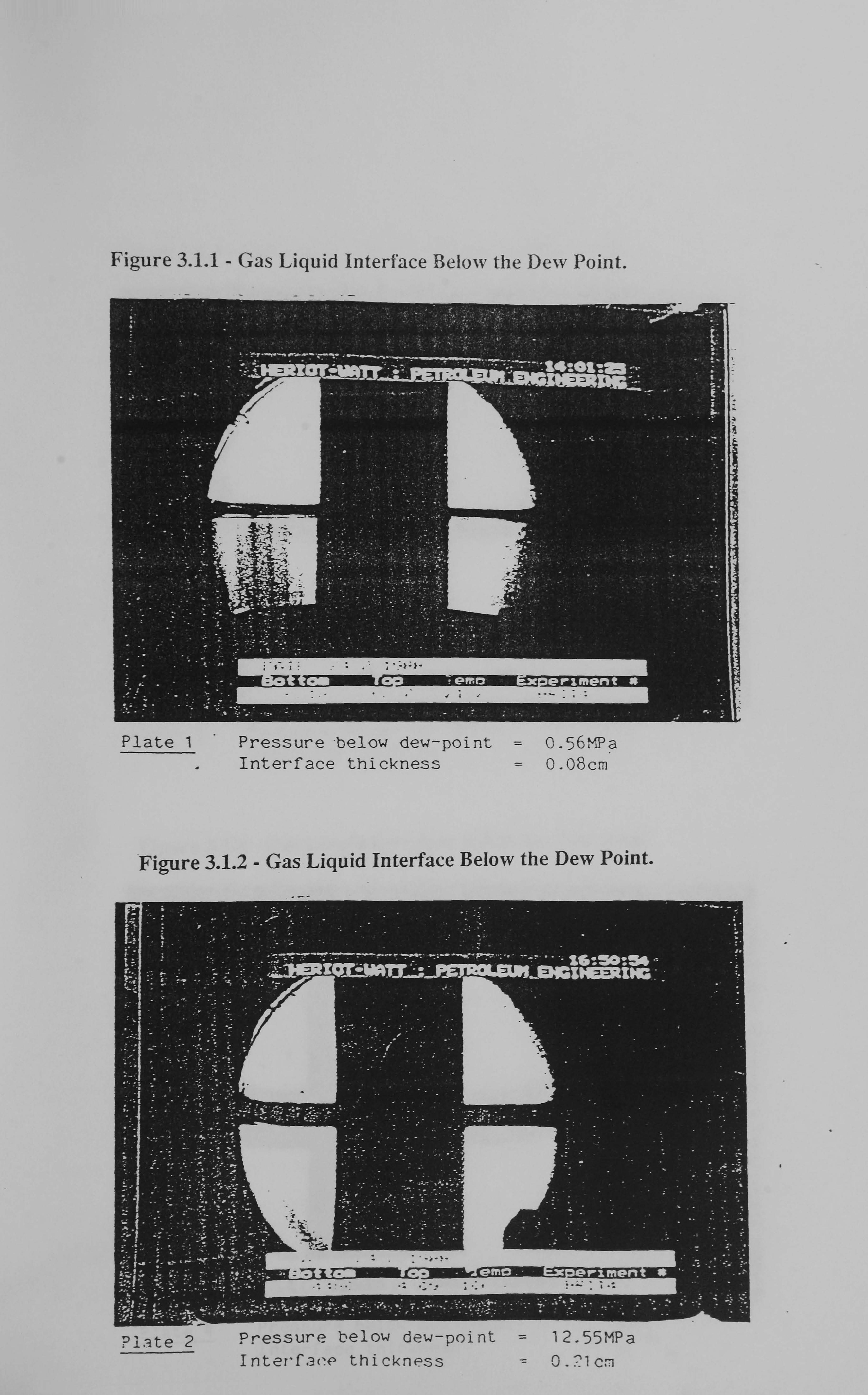
Figure 3.1.1 - Gas Liquid Interface Below the Dew Point.
Figure 3.1.2 - Gas Liquid Interface Below the Dew Point.
Plate 1 Pressure below dew-point = 0.56MPa Interface thickness = 0.08cm
? late 2 Pressure below dew-point 1 2.55MPa I ntevface thickness =0.: '1 cm.
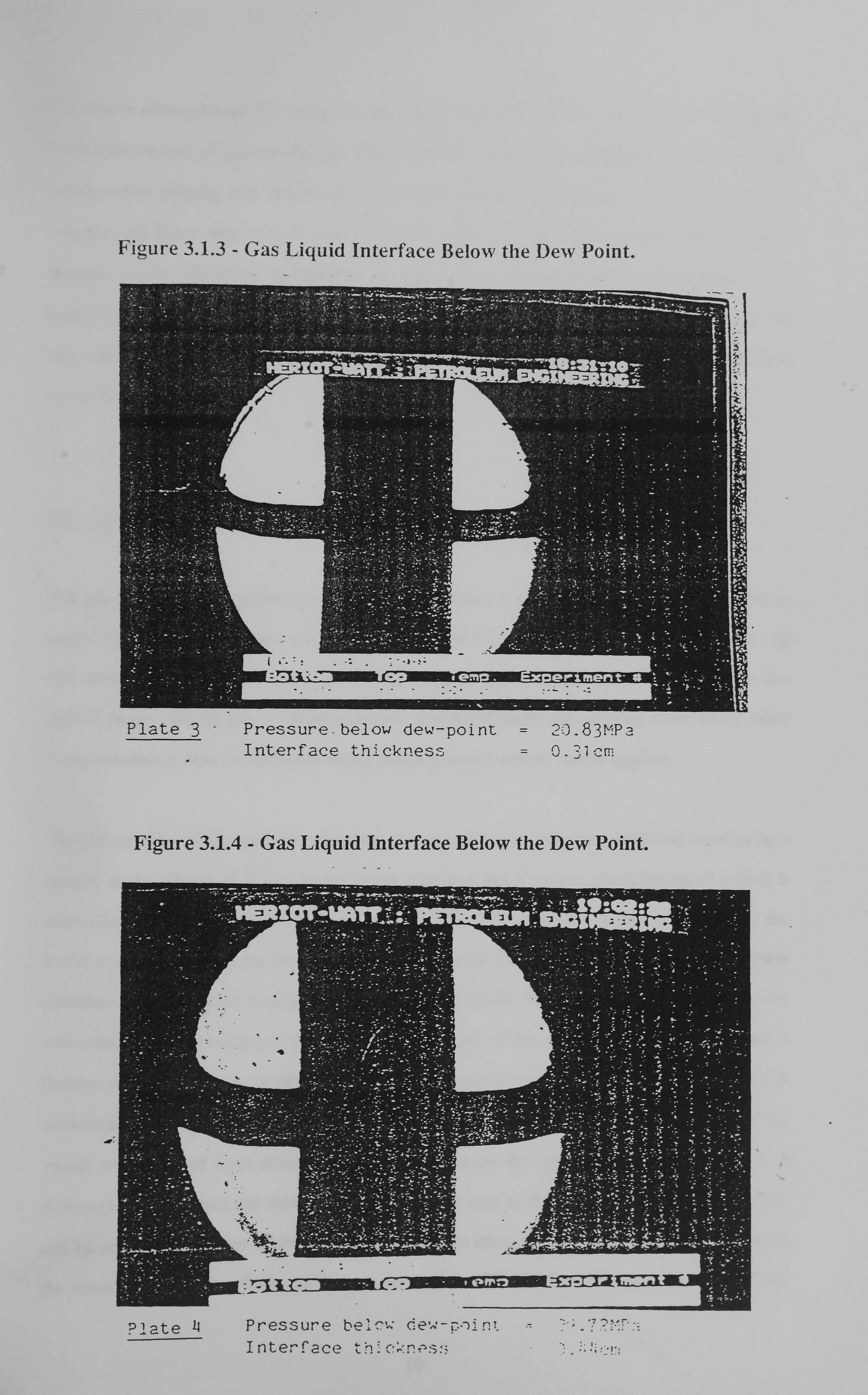
Figure 3.1.3 - Gas Liquid Interface Below the Dew Point.
Figure 3.1.4 - Gas Liquid Interface Below the Dew Point.
. W.
Plate 3 Pressure. below dew-point = 2D3MPa Interface thickness =J_ 3i cm
Plate 4 Pressure hei^,: ce: -º: "ý Interface

The above observations led to the development of a novel technique for determining the
interfacial tension of gas condensate fluids tested in the gas condensate facility. It was also
attempted to employ this technique in the vapour-liquid equilibrium (V-L-E) facility for
volatile and black oils, but, it was unsuccessful due to the contact angle considerations
(Section 2.2.2). However, the method was successfully applied in the V-L-E facility for gas
condensate type fluids (Section 3.5.2). Interfacial tension data measured on various binary
and multicomponent synthetic hydrocarbon mixtures and real reservoir fluids is presented in
this chapter.
3.2 : EXPERIMENTAL SET - UP FOR GAS CONDENSATE CELL
The gas - condensate equilibrium cell used in the study is manufactured by A. C. B. of France
under license from Elf. This cell has been modified in certain areas from its original set - up
and made more flexible to use in the P-V-T study of gas - condensates. The equipment is a
typical large volume gas - condensate cell, and equipment with similar features by other
manufacturers is also available for which the proposed methods can be applied.
The cell consists of a large upper chamber and a small lower chamber connected together by a
narrow neck, Figure (3.2.1). In the upper chamber lies a piston, the position of which is
controlled by pumping mercury into the top of the cell. Mercury is also pumped into the
lower chamber through the bottom of the cell, thereby forming a 'liquid piston' in the lower
chamber. The volume available to hydrocarbon fluids within the cell can therefore be
controlled by the pumping of the mercury into or out of the cell. The cell is housed into a
thermo-static enclosure, in which the air can be cooled or heated. Visual information is
achieved by means of two sapphire windows mounted opposite each other in the neck of the
vessel with a fitted light source and a TV camera on the opposite sides, Figure (3.2.1).
Although the windows are small, approximately 10 mm in diameter, visual information can
still be achieved by virtue of the magnification of the image which is approximately 32 times
the actual dimensions, which can be seen on a colour TV monitor. The gas - condensate (or
19
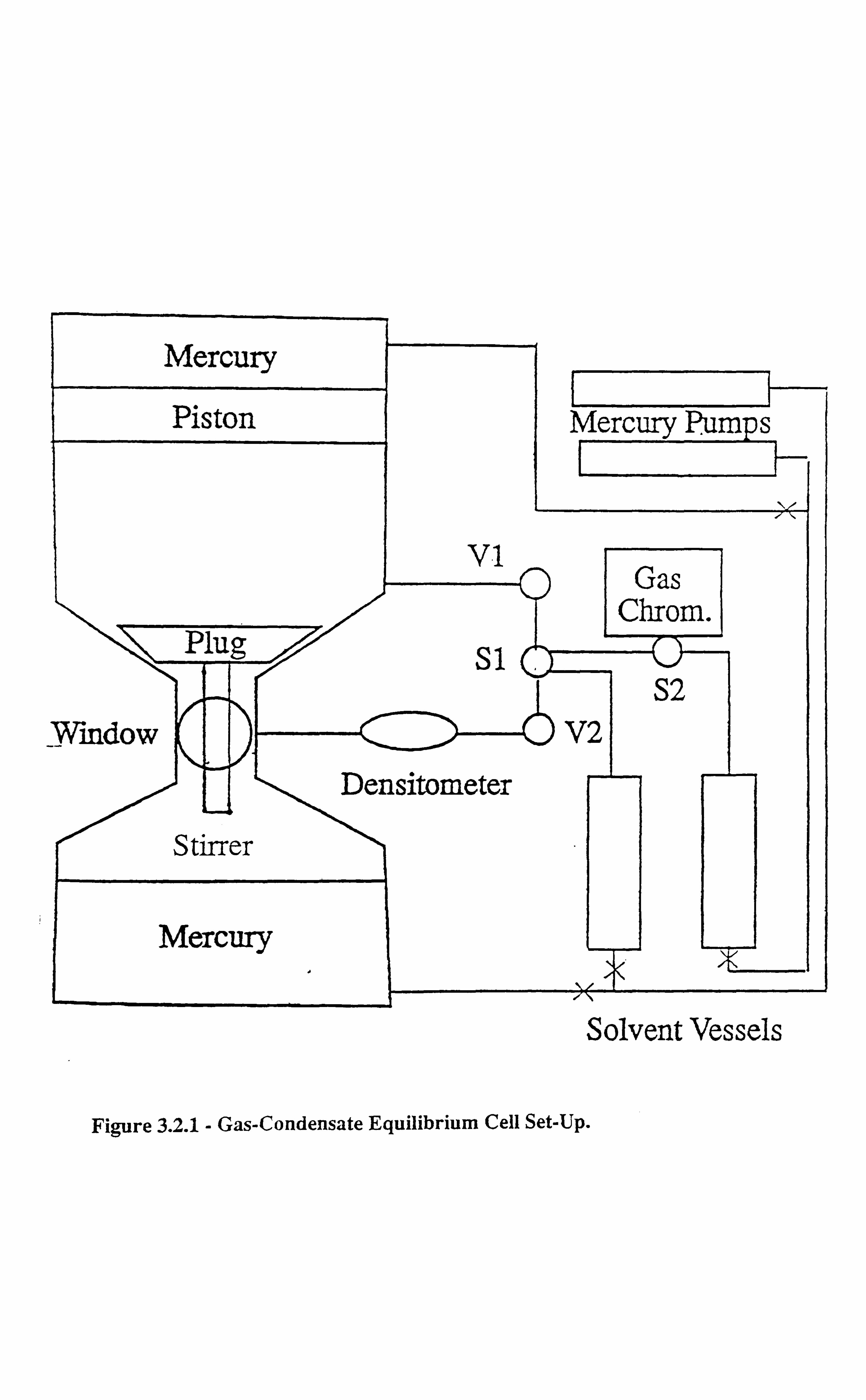
Mercury
Piston Mercury Pumps F
-J-
V-l
Plu Si
Gas Chrom.
S2 Window
Stirrer
Mercury
V2
Densitometer
Solvent Vessels
Figure 3.2.1 - Gas-Condensate Equilibrium Cell Set-Up.
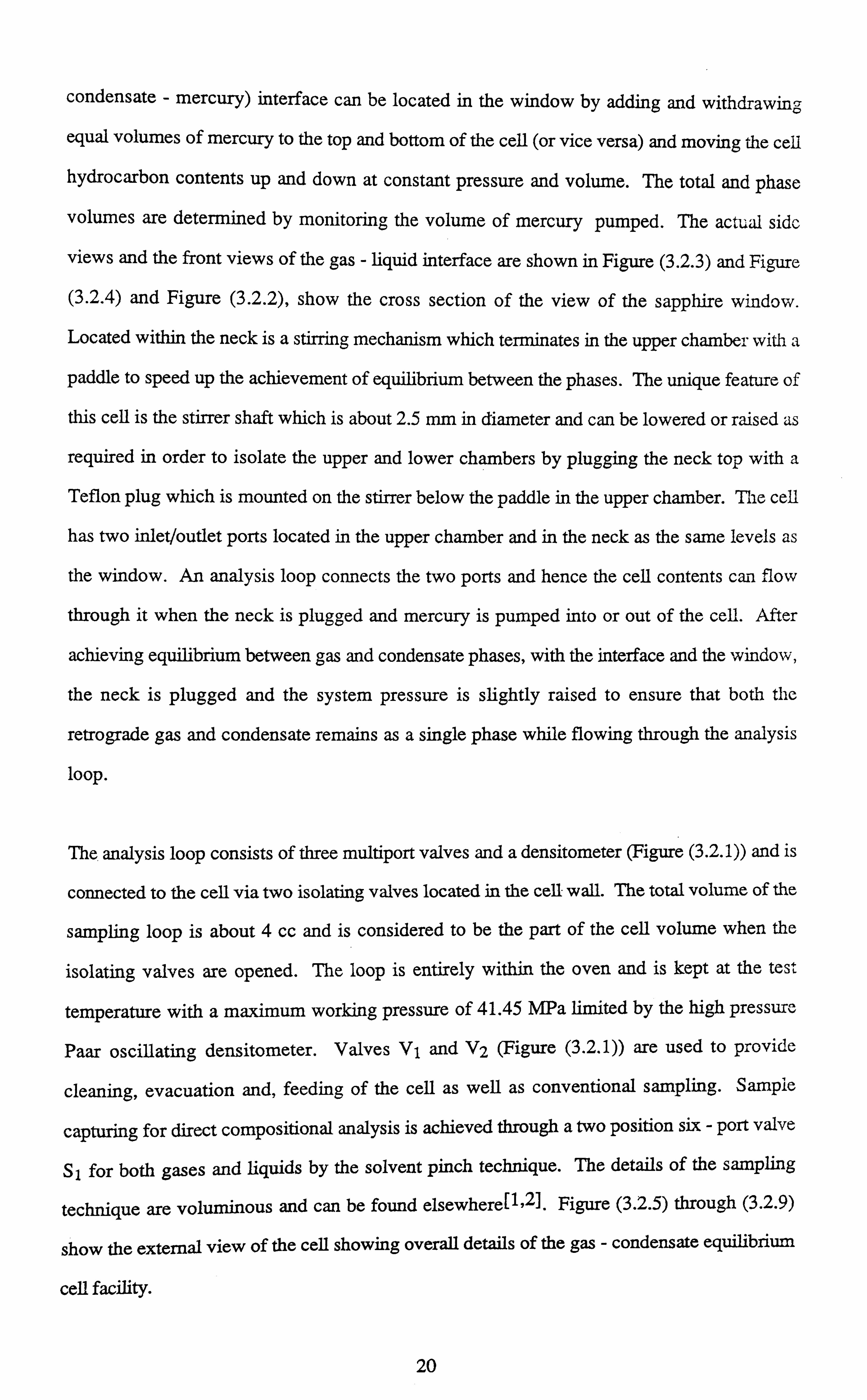
condensate - mercury) interface can be located in the window by adding and withdrawing
equal volumes of mercury to the top and bottom of the cell (or vice versa) and moving the cell
hydrocarbon contents up and down at constant pressure and volume. The total and phase
volumes are determined by monitoring the volume of mercury pumped. The actual side
views and the front views of the gas - liquid interface are shown in Figure (3.2.3) and Figure
(3.2.4) and Figure (3.2.2), show the cross section of the view of the sapphire window.
Located within the neck is a stirring mechanism which terminates in the upper chamber with a
paddle to speed up the achievement of equilibrium between the phases. The unique feature of
this cell is the stirrer shaft which is about 2.5 mm in diameter and can be lowered or raised as
required in order to isolate the upper and lower chambers by plugging the neck top with a
Teflon plug which is mounted on the stirrer below the paddle in the upper chamber. The cell
has two inlet/outlet ports located in the upper chamber and in the neck as the same levels as
the window. An analysis loop connects the two ports and hence the cell contents can flow
through it when the neck is plugged and mercury is pumped into or out of the cell. After
achieving equilibrium between gas and condensate phases, with the interface and the window,
the neck is plugged and the system pressure is slightly raised to ensure that both the
retrograde gas and condensate remains as a single phase while flowing through the analysis
loop.
The, analysis loop consists of three multiport valves and a densitometer (Figure (3.2.1)) and is
connected to the cell via two isolating valves located in the cell wall. The total volume of the
sampling loop is about 4 cc and is considered to be the part of the cell volume when the
isolating valves are opened. The loop is entirely within the oven and is kept at the test
temperature with a maximum working pressure of 41.45 MPa limited by the high pressure
Paar oscillating densitometer. Valves V1 and V2 (Figure (3.2.1)) are used to provide
cleaning, evacuation and, feeding of the cell as well as conventional sampling. Sample
capturing for direct compositional analysis is achieved through a two position six - port valve
S1 for both gases and liquids by the solvent pinch technique. The details of the sampling
technique are voluminous and can be found elsewhere[1L2]. Figure (3.2.5) through (3.2.9)
show the external view of the cell showing overall details of the gas - condensate equilibrium
cell facility.
20

Sapphire Window Walls
Camer; Monochromatic Light Source
Figure 3.2.2 - Cross Sectional Top View of the Sapphire Window.
Gas Phase
Liquid Phase Meniscus
Band
Figure 3.2.3 - Side View of the Gas-Liquid Interface.
Gas Phase
Liquid Phase
Stirrer Stem Gas-Liquid Interface
Figure 3.2.4 - Front View of the Gas-Liquid Interface (as seen on the TV monitor).
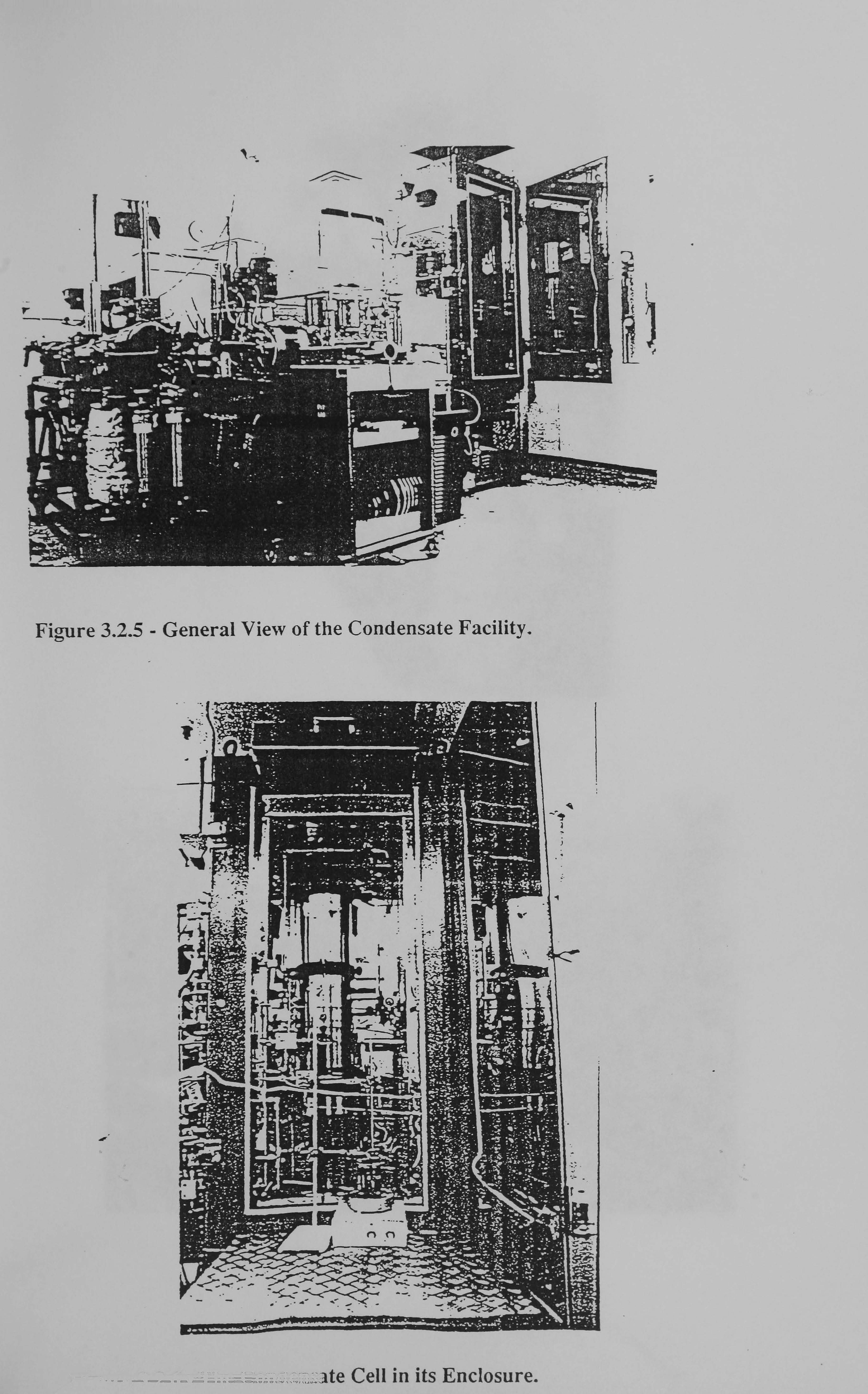
Figure 3.2.5 - General View of the Condensate Facility.
ýý
ate Cell in its Enclosure.
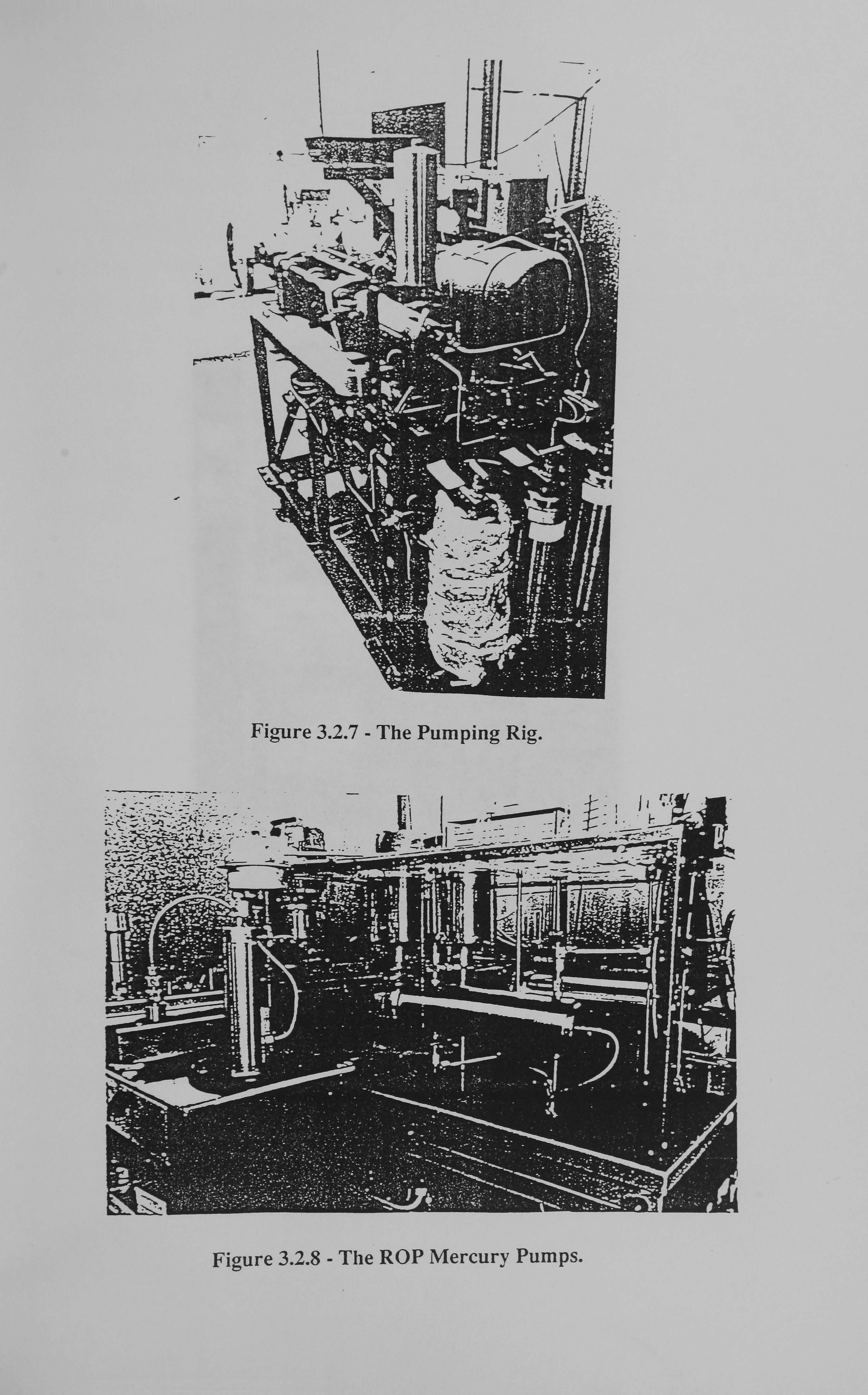
'4ý ýý-
zrZ
tý ý- ý, -. r
Figure 3.2.7 - The Pumping Rig.
Figure 3.2.8 - The ROP Mercury Pumps.
Y.

"of ýlý`ý=.
Figure 3.2.9 - Instrumentation Cabinets.
An Olympus High Precision Video Scaling Unit (VMS300) is used to assist with the
measurement of meniscus width (film height) for use in the calculation of IFT. This allows
two horizontal and two vertical lines to be superimposed onto either a TV monitor or directly
recorded onto video cassette. The unit has proved to be a quick and accurate method for
measurement of the meniscus width. The unit can measure to ± 0.01 1mm on the horizontal
scale and to ± 0.008mm on the vertical scale. The image of the meniscus is magnified by 32
times its actual size and the actual diameter of the stirrer (2.5mm) is used to calibrate the scalar
unit. A Time Base Corrector (TBC) is also used to stabilise and synchronise the signal from
the Video Cassette Recorder (VCR) through the VMS300 scaling unit to improve the quality
of the image obtained. Readings are taken for each pressure point below the dew - point
where the IFT measurements are desired.
3.3 : EXPERIMENTAL SET - UP FOR VAPOUR-LIQUID-EQUILIBRIUM (V-L-E)
APPARATUS
The V-L-E apparatus is a two-cell PVT rig which is used to study the phase behaviour of
black and volatile oils, experimentally, in simulated gas injection processes. Forward and
backward contact experiments can be performed to investigate the leading and trailing edge,
respectively, of a gas displacement. At present the V-L-E experimental facility is configured
to perform :
1) Phase volume measurement
2) Phase density measurement
3) Phase compositional analysis and
4) Interfacial tension (IFT) measurements using the pendant drop and meniscus techniques.
More conventional PVT tests may of course be performed; saturation pressure determination,
gas oil ratio (GOR) measurement and oil formation volume factor estimation, for instance.
Experimental operating limits for temperature and pressure are, at present, 100°C and 34.6
MPa respectively.
21
The schematic of the V-L-E experimental facility is shown in Figure 3.3.1. Two, 200cc Ruska VLE windowed cells mounted within a thermostatically controlled airbath, controllable to within ± 0.1°C, are employed to contain the experimental fluids. Each VLE cell is fitted, front and rear with high pressure glass windows, to assist in phase volume, liquid droplet and meniscus (for IFT) measurements. Viewing the vapour/liquid interface is further aided by lighting from the rear of the cells, while viewing from the front with a magnifying boroscope.
The event of falling of a liquid droplet through its equilibrium vapour is recorded on a video
cassette along with the gas-liquid meniscus for IFT calculations. The droplet and the
meniscus are later dimensioned by the previously mentioned VMS300 scalar unit. The image
of a droplet is magnified by 53 times of its actual size. The external diameter of the pendant drop spout (0.47mm) is used to calibrate the scalar unit.
Once the interface has been identified the distance from the interface to the cell top can be
measured by a linear transducer, mounted on the boroscope traversing stage. The measured
distance is then translated to volume, each cell having a slightly different calibration
conversion factor. To accelerate equilibrium after, say injecting a gas into an oil, or, dropping
the system pressure, to determine the saturation pressure of a fluid contained within one of the
VLE cells, they are mounted on a plate which can be rotated. This also allows for the total
inversion of the cells for phase volume measurement, where large vapour volumes are
involved. Communication between the V-L-E cells is by pipework, which has been kept as
short as possible, to minimise phase disruption when filling the route. Incorporated within
the pipework is a calibrated oscillating density cell (Anton Paar) and an high pressure liquid
chromatography (HPLC) sampling valve (Valco). The density cell, as well as giving
measurements of phase densities also indicates when the phase is homogeneous, by
displaying a steady reading over time. When the sample is homogeneous it may be analysed
compositionally. Each analysis only removes approximately 0.2cc of fluid. By operating the
HPLC valve the sample fluid is introduced, as a slug, into a mobile solvent transport column.
After a pre-set time the centre of the fluid slug will be present inside a second HPLC valve
fitted with a 0.6microlitre internal valve capacity. When operated this valve injects that
fraction of the fluid directly into the column of an Hewlett Packard 5880A gas chromatograph
22
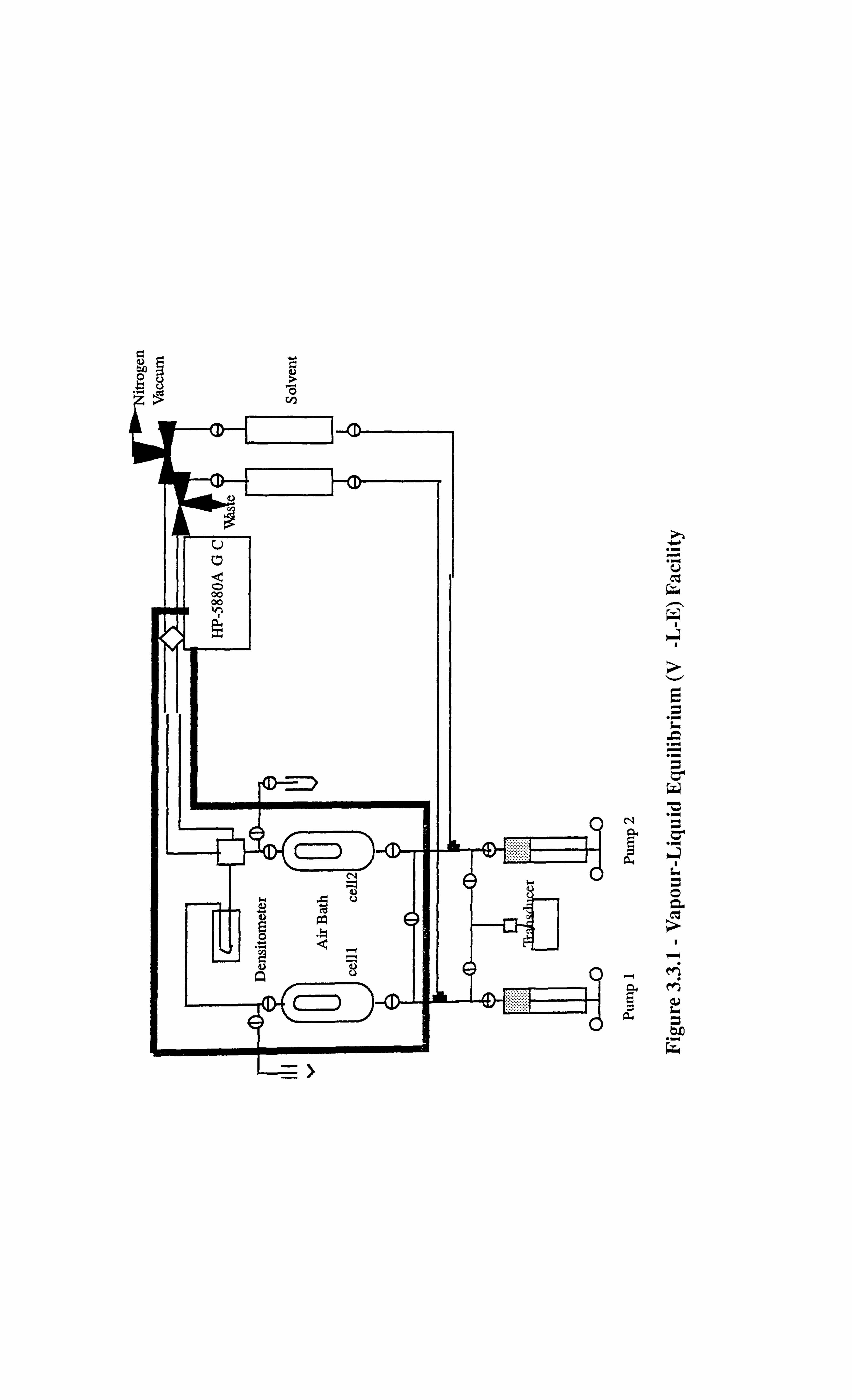
cz
G=a
a
E s. lý
a" Gz7 ,. ý N
,a L
O G
ry
r-o ,AM
M

fitted with a flame ionisation detector (FID). The description of this V-L-E facility is also available elsewhere in more details[2].
3.4 : LITERATURE SURVEY
Groenveld[3], studied the withdrawal of flat plates from the liquid bath which had a
significant importance in the processes of dip coating, lubrication, freezing and, drying rolls,
and in the coating of photographic film and paper. He proposed a new theory for withdrawal from viscous Newtonian liquids by vertical plates. In his work the thickness of the liquid
layer on the withdrawn plate was determined experimentally by a light adsorption method. But his work was more relevant as far as the textile and certain chemical engineering
applications were concerned.
Wilson and Jones[4], studied a similar phenomenon concerning the case of liquid film
running down a vertical wall and entering a large pool creating horizontal ripples, he also
studied a case similar to that of Groenveld[31, in which a case of flat vertical wall running
downwards through a liquid column was analysed, but both the cases studied were relevant to
other applications whereas our case was, in which the wall was stationary and the liquid film
was moving.
Similarly other researchers have done an extensive work in the area of withdrawal of flat
plates from liquid columns[5,6,7]. Extensive research has also been carried out concerning
the withdrawal of cylinders from liquid baths, mostly considering the Newtonian
fluids[8,9,10],
White and Tallmadge[111, considered the case of static meniscus on the outside of cylinders
and a special case of meniscus outside the flat plate. They also derived an equation relating
the meniscus profile and the film height. Kennedy and Burley{121, applied the geometry of
fluid interfaces in the shape of figures of revolution to external fluid dynamics. The work of
the above two researchers are closely related to the observations made in our work, hence,
applied to derive a rigorous relationship for measuring interfacial tension.
23
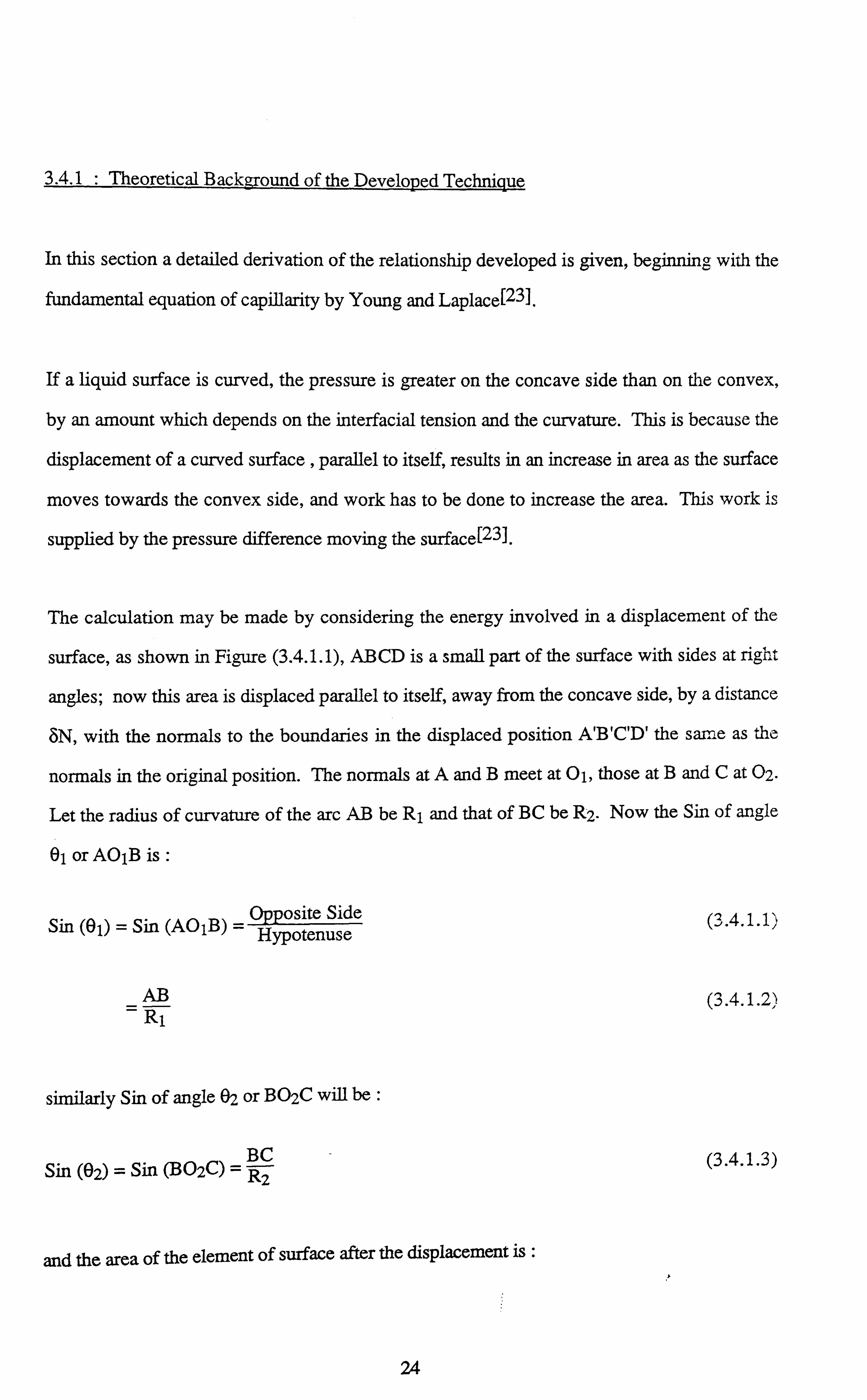
3.4.1 : Theoretical Background of the Developed Technique
In this section a detailed derivation of the relationship developed is given, beginning with the
fundamental equation of capillarity by Young and Laplace[23].
If a liquid surface is curved, the pressure is greater on the concave side than on the convex,
by an amount which depends on the interfacial tension and the curvature. This is because the
displacement of a curved surface , parallel to itself, results in an increase in area as the surface
moves towards the convex side, and work has to be done to increase the area. This work is
supplied by the pressure difference moving the surface[23].
The calculation may be made by considering the energy involved in a displacement of the
surface, as shown in Figure (3.4.1.1), AB CD is a small part of the surface with sides at right
angles; now this area is displaced parallel to itself, away from the concave side, by a distance
SN, with the normals to the boundaries in the displaced position A'B'C'D' the same as the
normals in the original position. The normals at A and B meet at 01, those at B and C at 02.
Let the radius of curvature of the arc AB be R1 and that of BC be R2. Now the Sin of angle
01 orAO1Bis:
Sin(61)=Sin(AOIB)_OppositeSide Hypotenuse
AB
R1
similarly Sin of angle 02 or BO2C will be :
BC Sin (82) = Sin (BO2C) = R2
and the area of the element of surface after the displacement is :
(3.4.1.1)
(3.4.1.2)
(3.4.1.3)
24
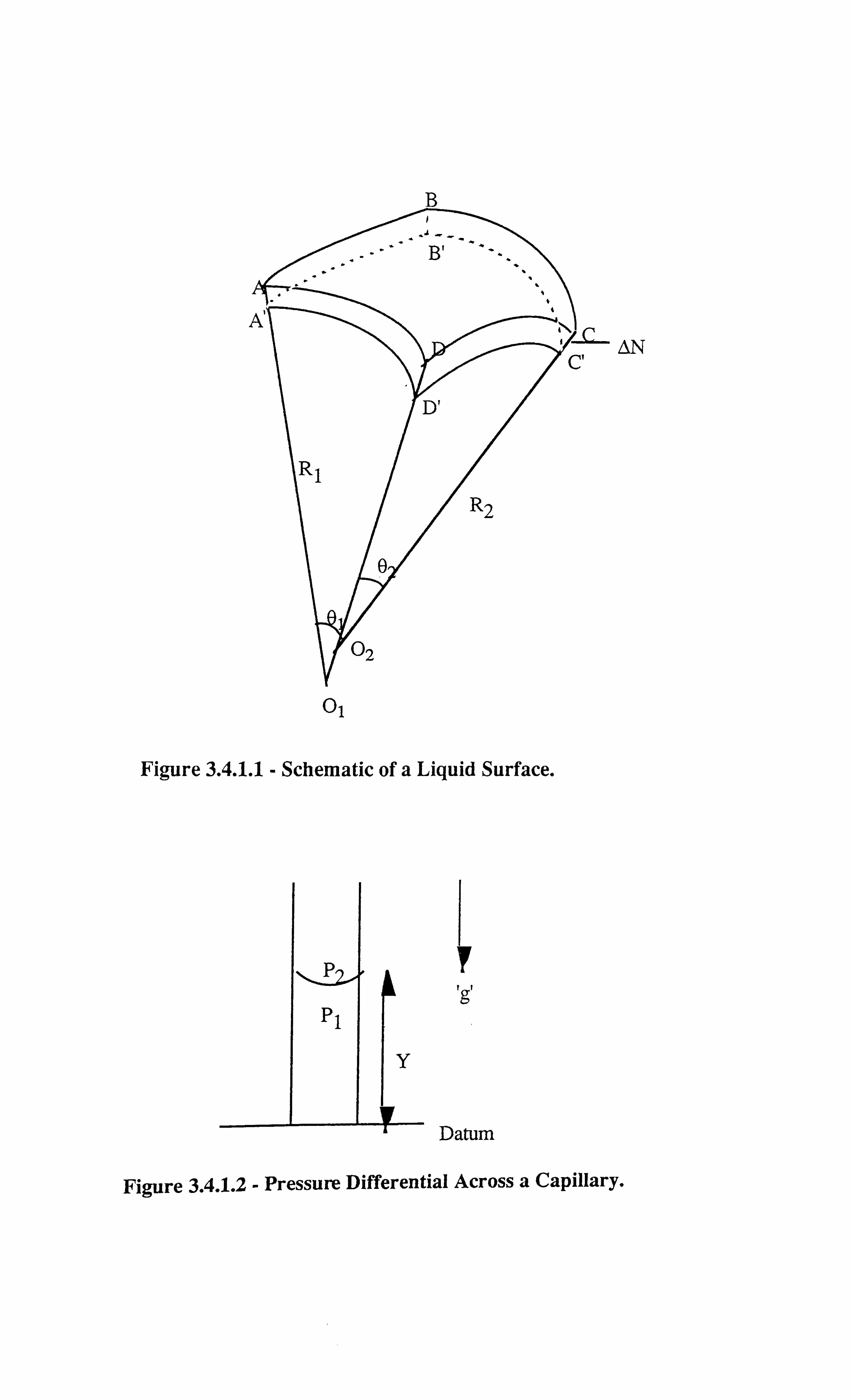
AN
01
Figure 3.4.1.1 - Schematic of a Liquid Surface.
t 9
Datum
Figure 3.4.1.2 - Pressure Differential Across a Capillary.
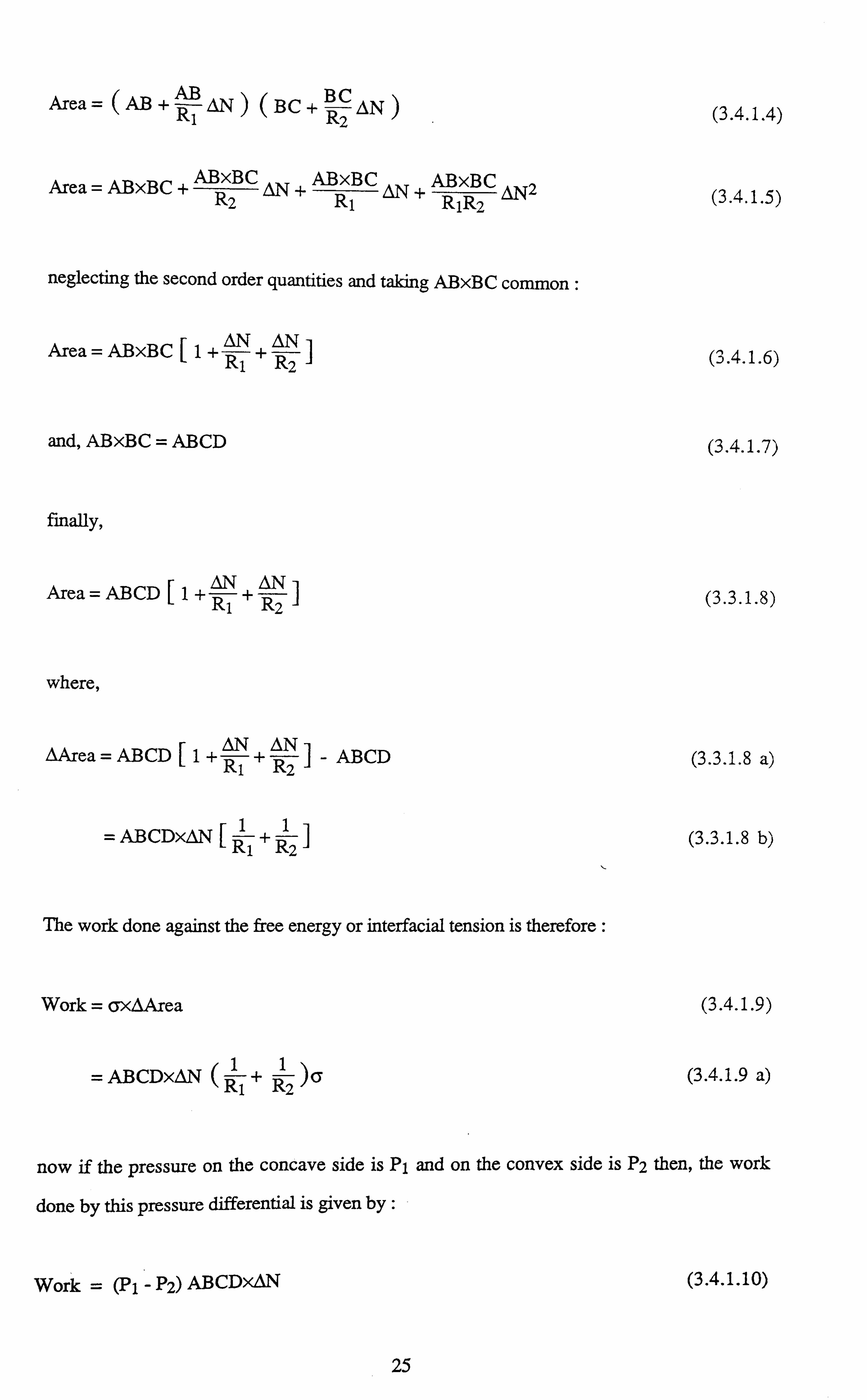
Area= (AB+R AN) (BC +R AN) (3.4.1.4) 12
Area = ABxBC +R BC
AN + `4BR BC AN +
ABxBC AN2 (3.4.1.5) 1 R1R2 )
neglecting the second order quantities and taking ABxBC common :
Area =ABxBCL1+R +RNj (3.4.1.6) 1 R2
and, ABxBC = ABCD (3.4.1.7)
finally,
Area =ABCD[1+R +R (3.3.1.8)
where,
DArea = ABCD [1+R+Ri- ABCD (3.3.1.8 a)
= ABCDxON [1 +1] (3.3.1.8 b) Ri R2
The work done against the free energy or interfacial tension is therefore :
Work = ßxzArea (3.4.1.9)
= ABCDxiN Rl
+1)6 (3.4.1.9 a)
now if the pressure on the concave side is P1 and on the convex side is P2 then, the work
done by this pressure differential is given by :
Work = (p, - P2) AB CDX N (3.4.1.1 0)
25
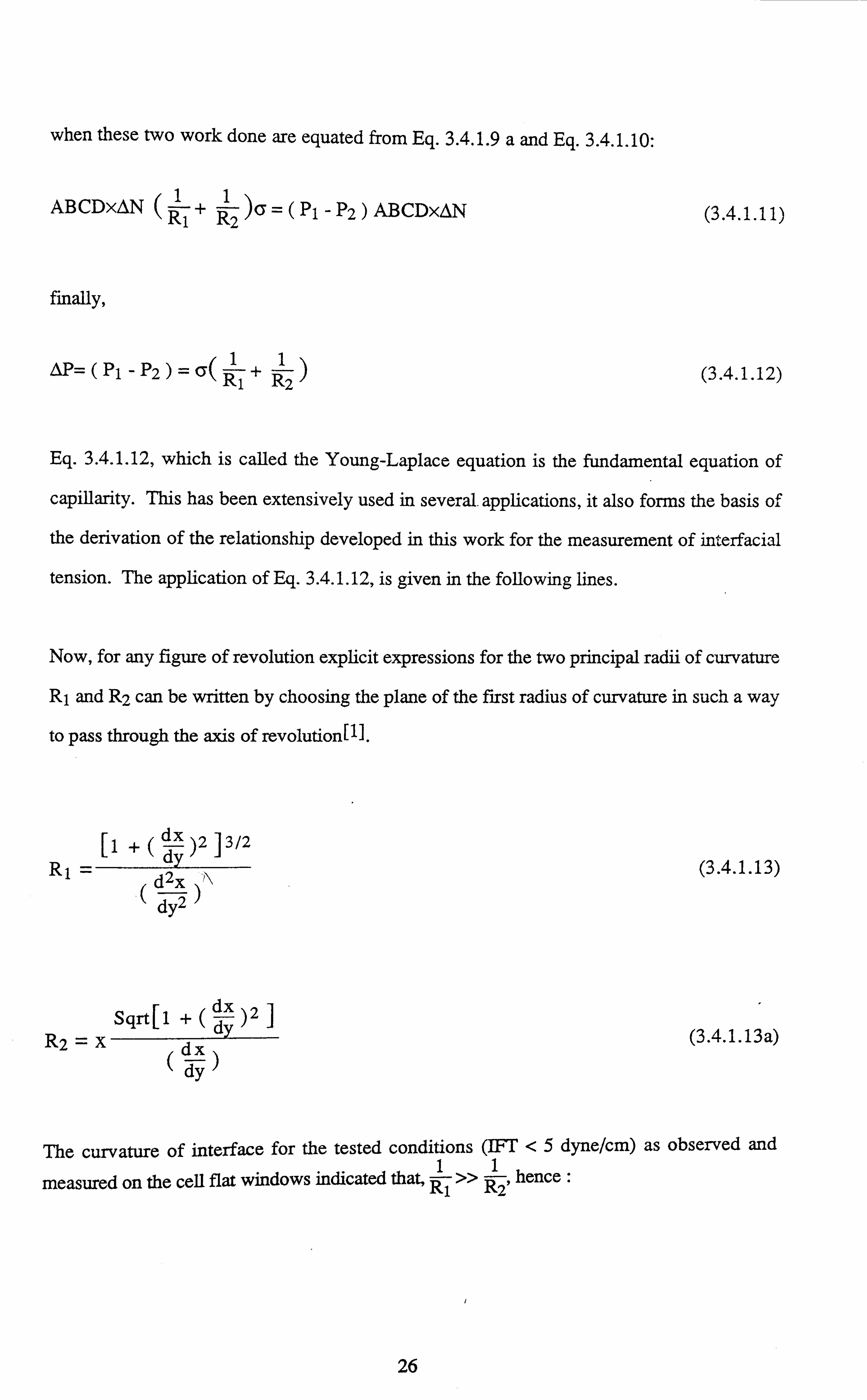
when these two work done are equated from Eq. 3.4.1.9 a and Eq. 3.4.1.10:
ABCDxAN (---+ 1
)=Pi-P2ABCDXN
finally,
AP=(P1-P2)=6( + R2ý
(3.4.1.1 1)
(3.4.1.1 2)
Eq. 3.4.1.12, which is called the Young-Laplace equation is the fundamental equation of
capillarity. This has been extensively used in several. applications, it also forms the basis of
the derivation of the relationship developed in this work for the measurement of interfacial
tension. The application of Eq. 3.4.1.12, is given in the following lines.
Now, for any figure of revolution explicit expressions for the two principal radii of curvature
R1 and R2 can be written by choosing the plane of the first radius of curvature in such a way
to pass through the axis of revolution[ll.
+(dx)2] 3/2
R1. y (3.4.1.13) 12X \ dy
sgrt[1 +(dx)2] R2 =x dx
(3.4.1.13a)
dy
The curvature of interface for the tested conditions (IFT <5 dyne/cm) as observed and
measured on the cell flat windows indicated that, Rl
» R2, hence :
26

d2x
dy 0P =
Iý + (dx )2 1 3/2 dy
(3.4.1.1 4)
the pressure differential across the interface is balanced by the gravity at each point see Figure
(3.4.1.2), hence we can write :
OP=(P1-pv)gy (3.4.1.15)
Eq. 3.4.1.14 and 3.4.1.15 can thus be equated which gives:
2 ý
(Pl-Pv) gY d y2
+(dx)2]3/2 dy
after introducing capillary constant, a, and making the left hand side of Eq. 3.4.1.16
dimensionless we get :
a= 2a ] 1/2 (3.4.1.17)
C P1-Pv) g
d2X ) dy = 2Y (3.4.1.18)
ý1+(dY)2] 3/2
where, Y=a and X=ä, the contact angle, 8, on the window from `Figure (3.4.1.3) for gas -
condensate is defined by :
tan(O)=-d , atX=O
Now substituting Eq. 3.4.1.19 in Eq. 3.4.1.18 and solving for Y gives :
(3.4.1.19)
27
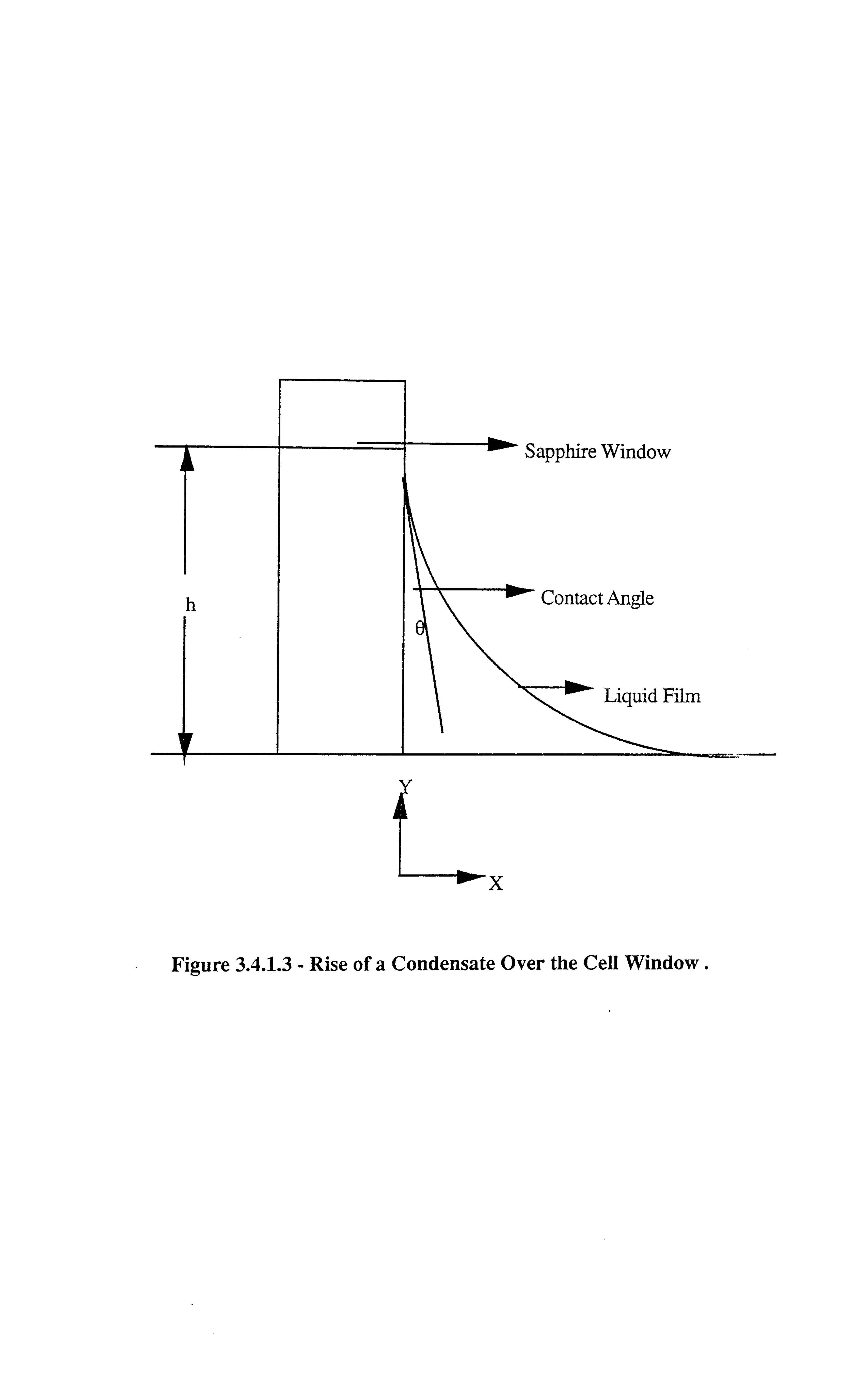
x
Figure 3.4.1.3 - Rise of a Condensate Over the Cell Window.
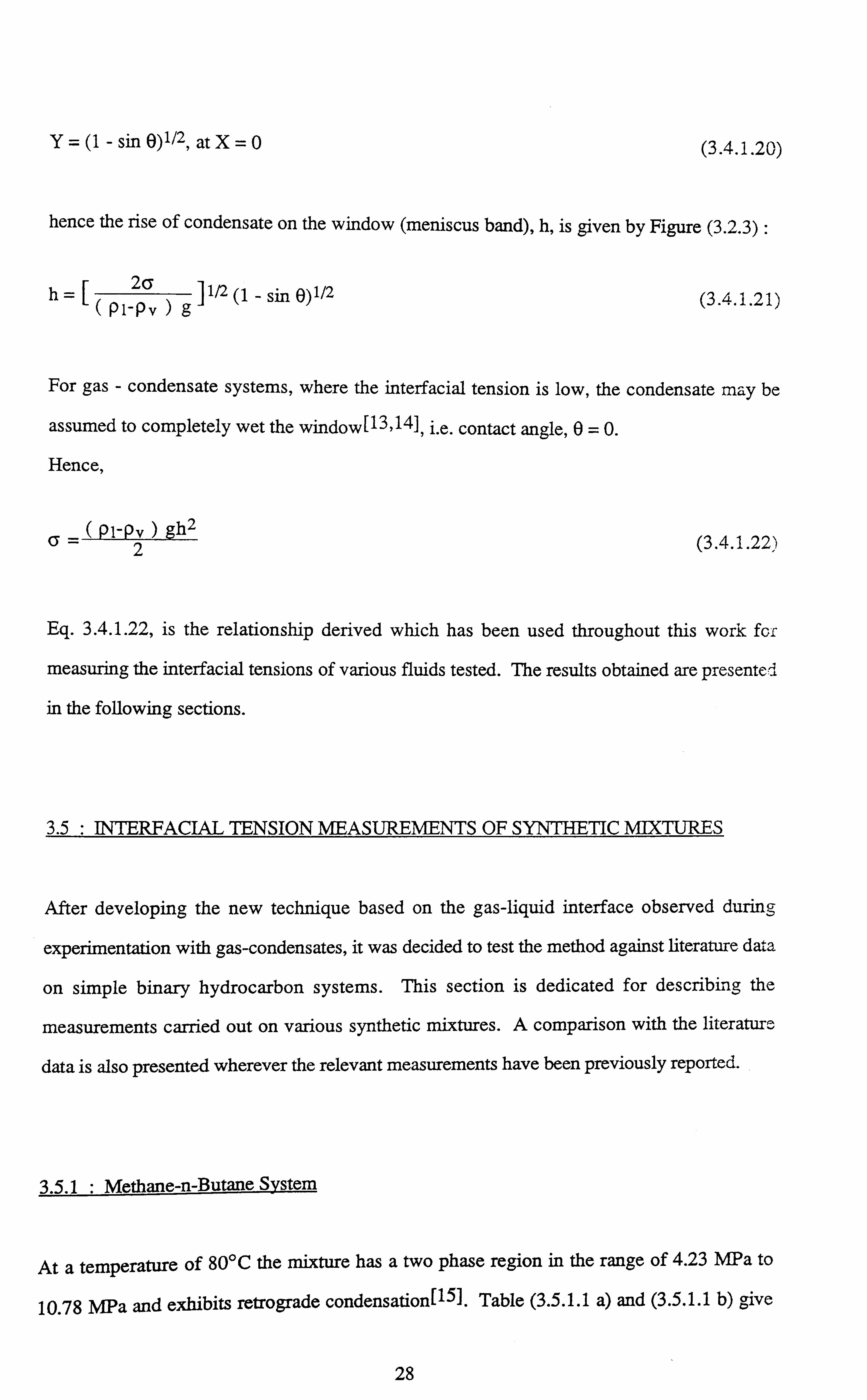
Y=(1-sin6)1/2, atX=O (3.4.1.20)
hence the rise of condensate on the window (meniscus band), h, is given by Figure (3.2.3) :
26 h=ý (P1-Pv -
]1/2 )g - sin 0)1/2 (3.4.1.21)
For gas - condensate systems, where the interfacial tension is low, the condensate may be
assumed to completely wet the window[13,14], i. e. contact angle, 0=0.
Hence,
6_Cpi-P2)gh2 (3.4.1.22)
Eq. 3.4.1.22, is the relationship derived which has been used throughout this work for
measuring the interfacial tensions of various fluids tested. The results obtained are presente d
in the following sections.
3.5 : INTERFACIAL TENSION MEASUREMENTS OF SYNTHETIC MIXTURES
After developing the new technique based on the gas-liquid interface observed during
experimentation with gas-condensates, it was decided to test the method against literature data
on simple binary hydrocarbon systems. This section is dedicated for describing the
measurements carried out on various synthetic mixtures. A comparison with the literature
data is also presented wherever the relevant measurements have been previously reported.
3.5.1 : Methane-n-Butane System
At a temperature of 80°C the mixture has a two phase region in the range of 4.23 MPa to
10.78 MPa and exhibits retrograde condensation[ l5]. Table (3.5.1.1 a) and (3.5.1.1 b) give
28
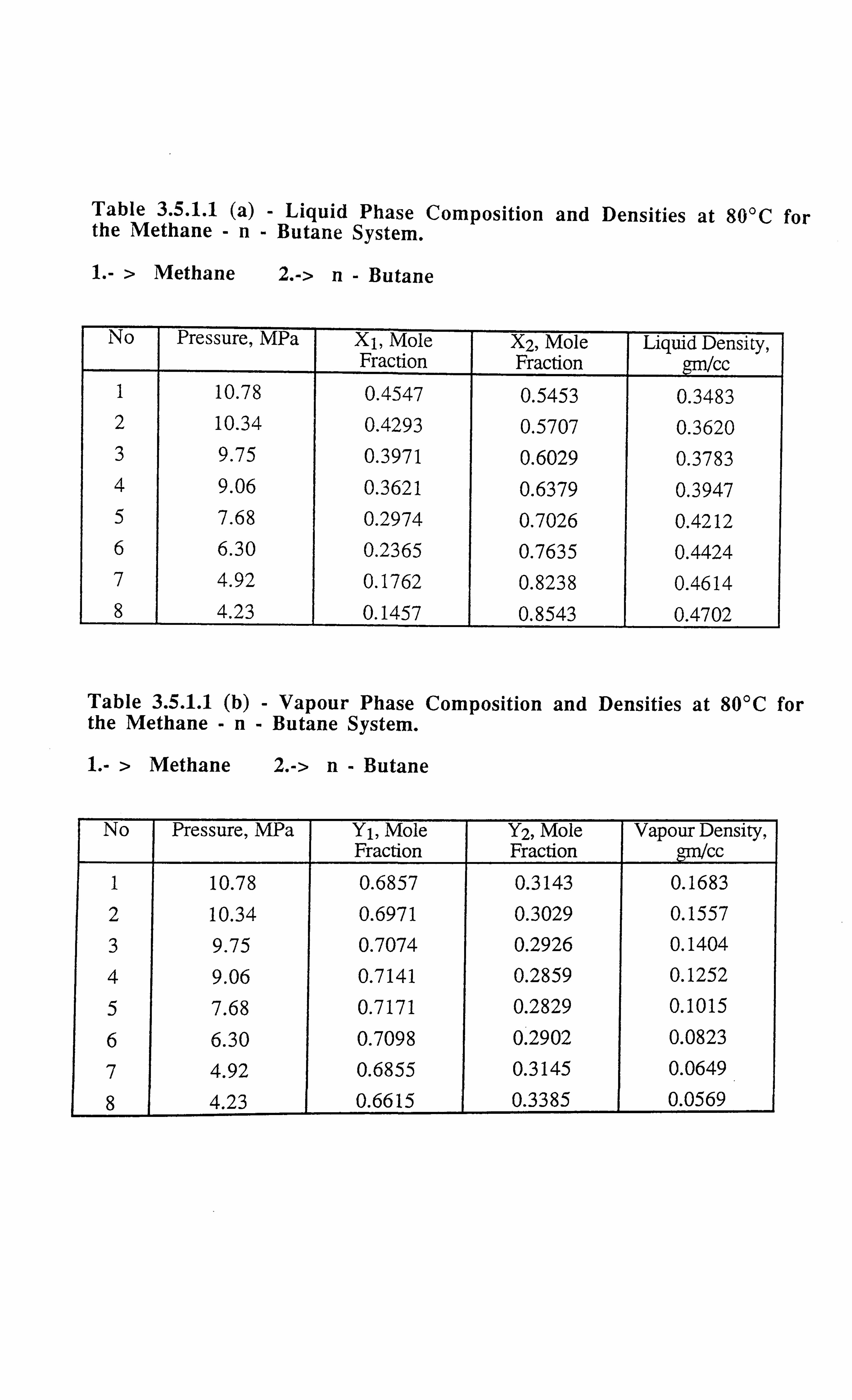
Table 3.5.1.1 (a) - Liquid Phase Composition and Densities at 80°C for the Methane -n- Butane System.
I. - > Methane 2. -> n- Butane
No Pressure, MPa X1, Mole Fraction
X2, Mole Fraction
Liquid Density, gm1cc
1 10.78 0.4547 0.5453 0.3483 2 10.34 0.4293 0.5707 0.3620 3 9.75 0.3971 0.6029 0.3783 4 9.06 0.3621 0.6379 0.3947 5 7.68 0.2974 0.7026 0.4212 6 6.30 0.2365 0.7635 0.4424 7 4.92 0.1762 0.8238 0.4614 8 4.23 0.1457 0.8543 0.4702
Table 3.5.1.1 (b) - Vapour Phase Composition and Densities at 80°C for the Methane -n- Butane System.
1. - > Methane 2. -> n- Butane
No Pressure, MPa Y1, Mole Fraction
Y2, Mole Fraction
Vapour Density, gm1cc
1 10.78 0.6857 0.3143 0.1683
2 10.34 0.6971 0.3029 0.1557
3 9.75 0.7074 0.2926 0.1404
4 9.06 0.7141 0.2859 0.1252
5 7.68 0.7171 0.2829 0.1015
6 6.30 0.7098 0.2902 0.0823
7 4.92 0.6855 0.3145 0.0649
8 4.23 0.6615 0.3385 0.0569
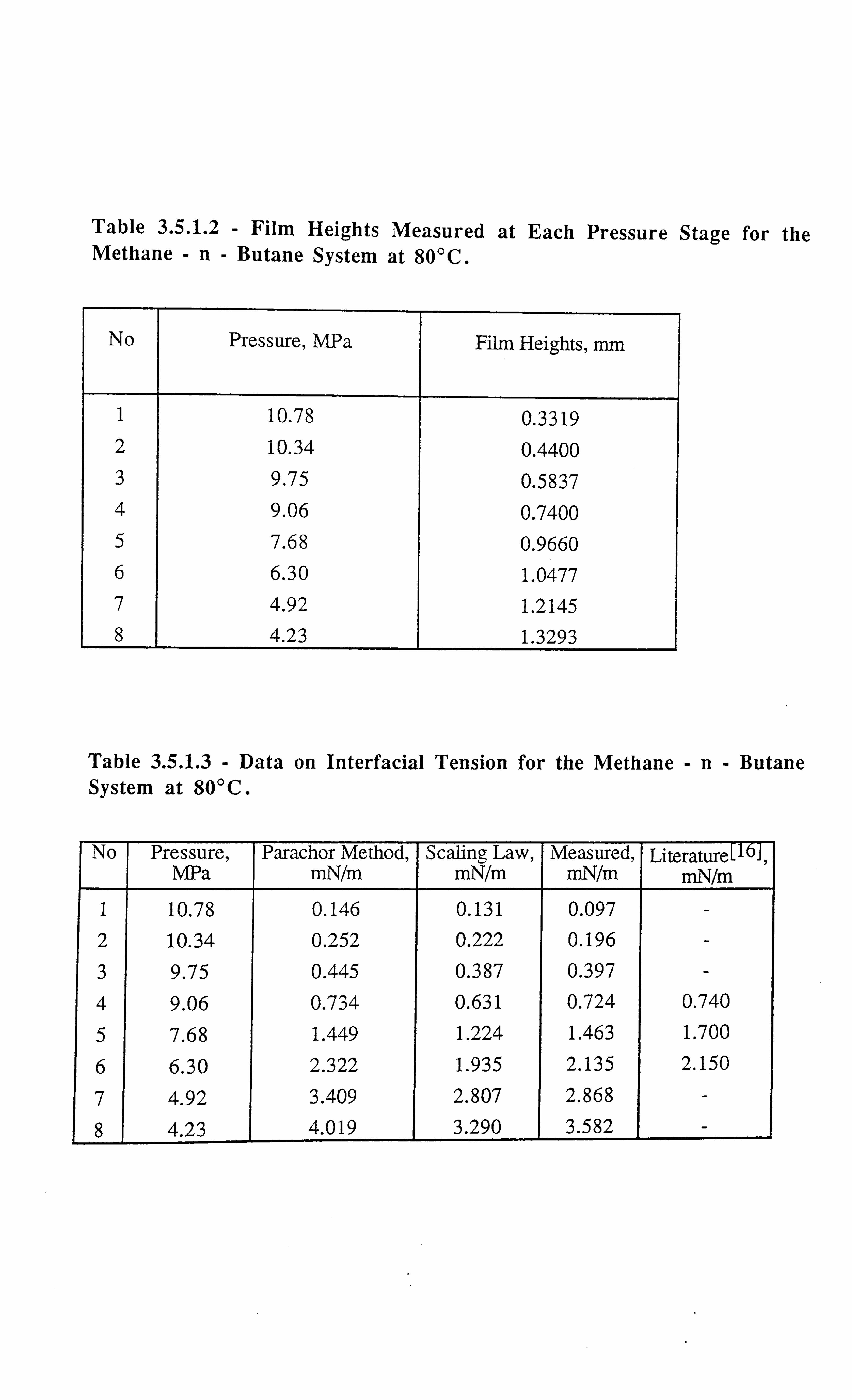
Table 3.5.1.2 - Film Heights Measured at Each Pressure Stage for the Methane -n- Butane System at 800C.
No Pressure, MPa Film Heights, mm
1 10.78 0.3319 2 10.34 0.4400 3 9.75 0.5837 4 9.06 0.7400 5 7.68 0.9660 6 6.30 1.0477 7 4.92 1.2145 8 4.23 1.3293
Table 3.5.1.3 - Data on Interfacial Tension for the Methane -n- Butane System at 80°C.
No Pressure, MPa
Parachor Method, mN/m
Scaling Law, mN/m
Measured, mN/m
Literature [16], mN/m
1 10.78 0.146 0.131 0.097 - 2 10.34 0.252 0.222 0.196 - 3 9.75 0.445 0.387 0.397 - 4 9.06 0.734 0.631 0.724 0.740
5 7.68 1.449 1.224 1.463 1.700
6 6.30 2.322 1.935 2.135 2.150
7 4.92 3.409 2.807 2.868 - 8 4.23 4.019 3.290 3.582 -
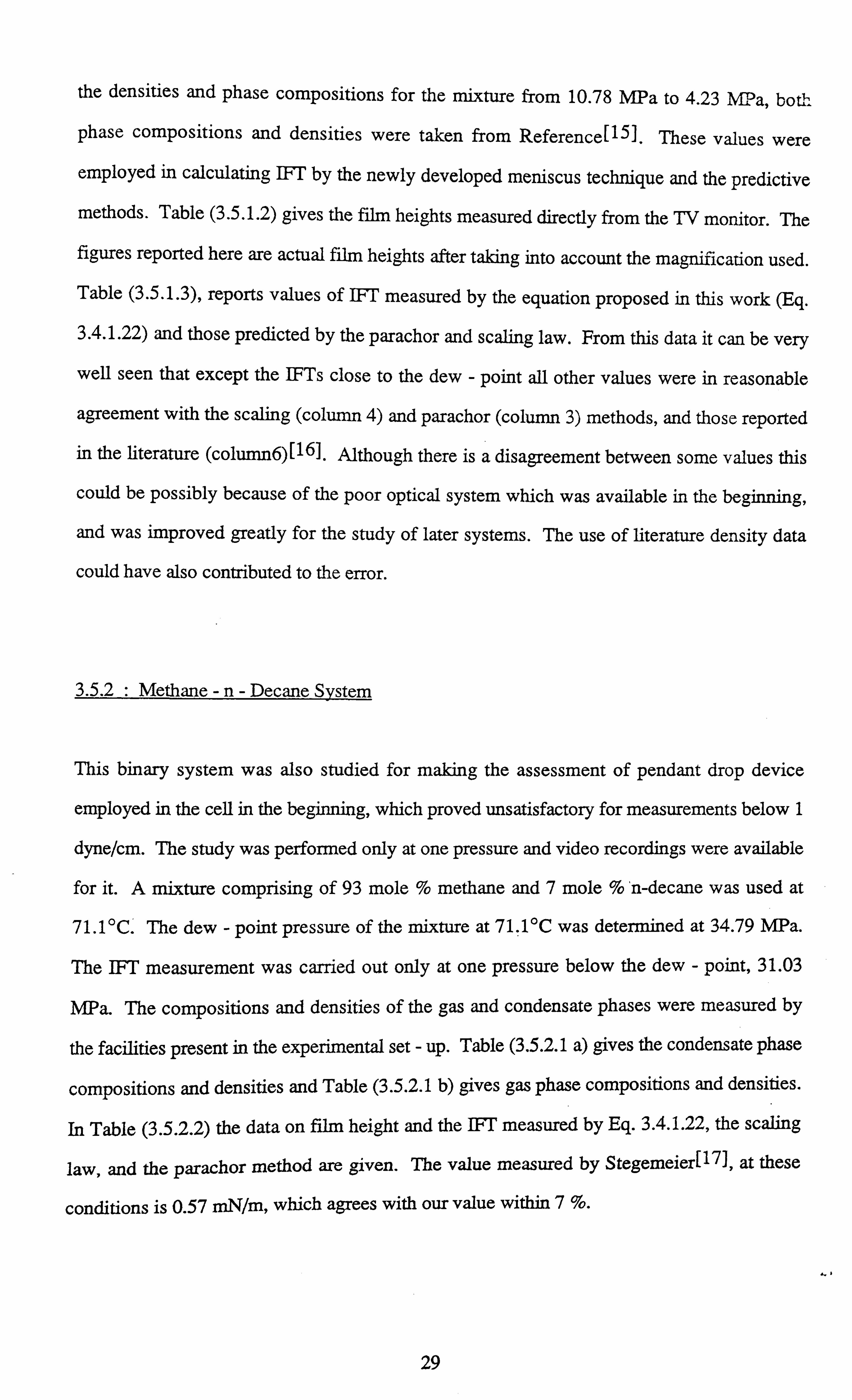
the densities and phase compositions for the mixture from 10.78 MPa to 4.23 MPa, bot'
phase compositions and densities were taken from Reference[151. These values were
employed in calculating IFT by the newly developed meniscus technique and the predictive
methods. Table (3.5.1.2) gives the film heights measured directly from the TV monitor. The
figures reported here are actual film heights after taking into account the magnification used. Table (3.5.1.3), reports values of IFT measured by the equation proposed in this work (Eq.
3.4.1.22) and those predicted by the parachor and scaling law. From this data it can be very
well seen that except the IFTs close to the dew - point all other values were in reasonable
agreement with the scaling (column 4) and parachor (column 3) methods, and those reported
in the literature (column6)[16]. Although there is a disagreement between some values this
could be possibly because of the poor optical system which was available in the beginning,
and was improved greatly for the study of later systems. The use of literature density data
could have also contributed to the error.
3.5.2 : Methane -n- Decane System
This binary system was also studied for making the assessment of pendant drop device
employed in the cell in the beginning, which proved unsatisfactory for measurements below 1
dyne/cm. The study was performed only at one pressure and video recordings were available
for it. A mixture comprising of 93 mole % methane and 7 mole % 'n-decane was used at
71.1 °C. The dew - point pressure of the mixture at 71.1 °C was determined at 34.79 MPa.
The IFT measurement was carried out only at one pressure below the dew - point, 31.03
MPa. The compositions and densities of the gas and condensate phases were measured by
the facilities present in the experimental set - up. Table (3.5.2.1 a) gives the condensate phase
compositions and densities and Table (3.5.2.1 b) gives gas phase compositions and densities.
In Table (3.5.2.2) the data on film height and the IFT measured by Eq. 3.4.1.22, the scaling
law, and the parachor method are given. The value measured by Stegemeier[17], at these
conditions is 0.57 mN/m, which agrees with our value within 7 %.
29

Table 3.5.2.1 (a) - Liquid Phase Compositions and Densities at 71.1°C for the Methane -n- Decane System.
l. - > Methane 2. - >n- Decane
Preussure, MPa
X1, Mole Fraction X2, Mole Fraction Liquid Density, gm/cc
31.03 0.7724 0.2276 0.5110
Table 3.5.2.1 (b) - Vapour Phase Compositions and Densities at 71.1°C for the Methane -n- Decane System.
1. - > Methane 2. - >n- Decane
Preussure, MPa Y1, Mole Fraction Y2, Mole Fraction Va or Density, cc 31.03 0.9635 0.0365 0.2360
Table 3.5.2.2 - Data on Interfacial Tension for the Methane -n- Decane System at 71.1'C.
Pressure, MPa
Film Height, mm
Parachor Method, mN/m
Scaling Law, mN/m
Measured, mN/m
Reference[17], n /m
31.03 0.625 0.480 0.590 0.530 0.570

The above mixture was previously studied in the gas condensate PVT cell. The following
lines describe the experiment carried out on the same system in the V-L-E cell for validating
the gas-liquid interface technique and the pendant drop technique by comparing both
measurements with the literature data.
As mentioned previously Stegemeier[17] has measured IFT of the methane-n-decane systeü.
at different isotherms by the pendant drop method. The measurements at 71.1°C were
selected for comparison since the data had a wide range of IFTs from 0.002-10 dyne/cm, and
the temperature most suited the operating conditions of the V-L-E cell. A mixture of methane
(89 mole %) and n-decane (11 mole %) was prepared gravimetrically and introduced into the
cell. The mixture did not pass through an exact critical pressure but reached a near critical
dew-point of 35.30 MPa. A"constant composition expansion test was performed at pressures
ranging from 34.47 to 10.34 MPa. The entire experiment was video recorded and the
measurements of gas-liquid interface and the droplets for the pendant drop were carried out by
the VMS300 video scalar unit. Density was measured of both the liquid and vapour phases
except for a few high pressure data points where the liquid density could not be measured due
to operational problems of the densitometer. These data were however obtained by
interpolation or extrapolation of the available measurements. A comparison between the
density differences measured in this work and by Sage and Lacey[18] is shown in Figure
3.5.2.1, which shows a reasonably good agreement. The average differences between both
liquid and vapour phase densities were less than 1.5 % compared to Sage and Lacey[18].
Interfacial tension data were calculated using both sets of density differences and are shown in
Figures 3.5.2.2 and 3.5.2.3. The average differences between IFT values measured by the
pendant drop method and those reported in Reference 17 were less than 10 %. These plots
prove the reliability of the IFT measurements carried out in the VLE apparatus using both
methods, which also proves the fact that the gas-liquid interface technique can also be applied
to the V-L-E rig for model fluids.
30
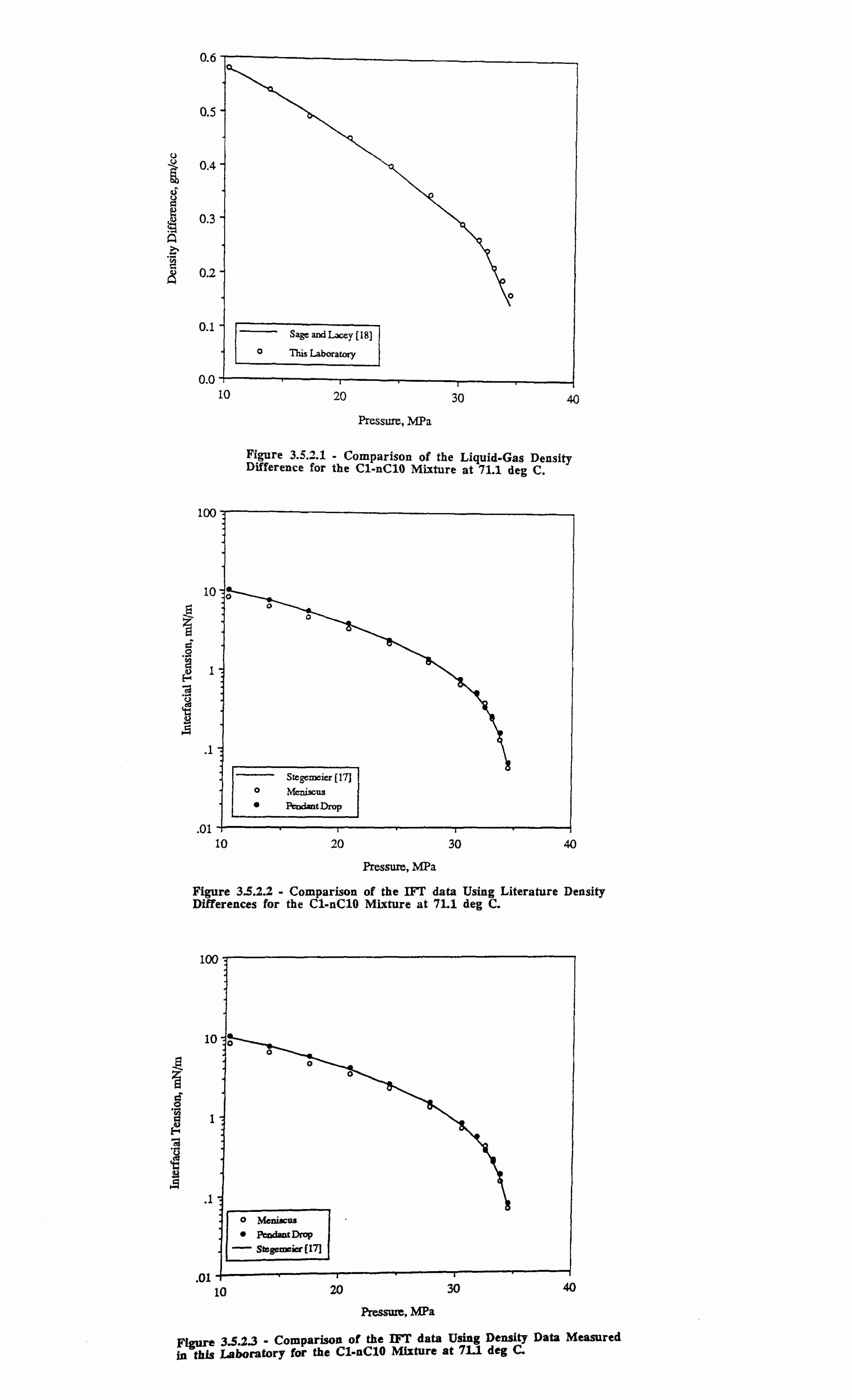
0.6
0.5
0.4 6§
a 0.3
0.2
0.1
0.0 -t- 10
100
10
a I.,
H1
.1
. 01
20 30 40
Pressure, MPa
Figure 3.5.2.1 - Comparison of the Liquid-Gas Density Difference for the Cl-nC10 Mixture at 71.1 deg C.
Stegcmaier (17] o Meniscus " Pendant Drop
10 20 30 40
Pressure, MPa
Figure 3.5.2.2 - Comparison of the IFT data Using Literature Density Differences for the CI-nC10 Mixture at 711 deg C.
10(
is
8 d 0
1 F
S 1
_01
0
o Meniscus
" Pentiont Drop
- Stegemeier(17]
iQ 20 30 40
Pressure, MPa
Figure 3.5.2.3 - Comparison of the 1FT data Using Density Data Measured
in this Laboratory for the Cl-nC10 Mixture at 711 deg C.
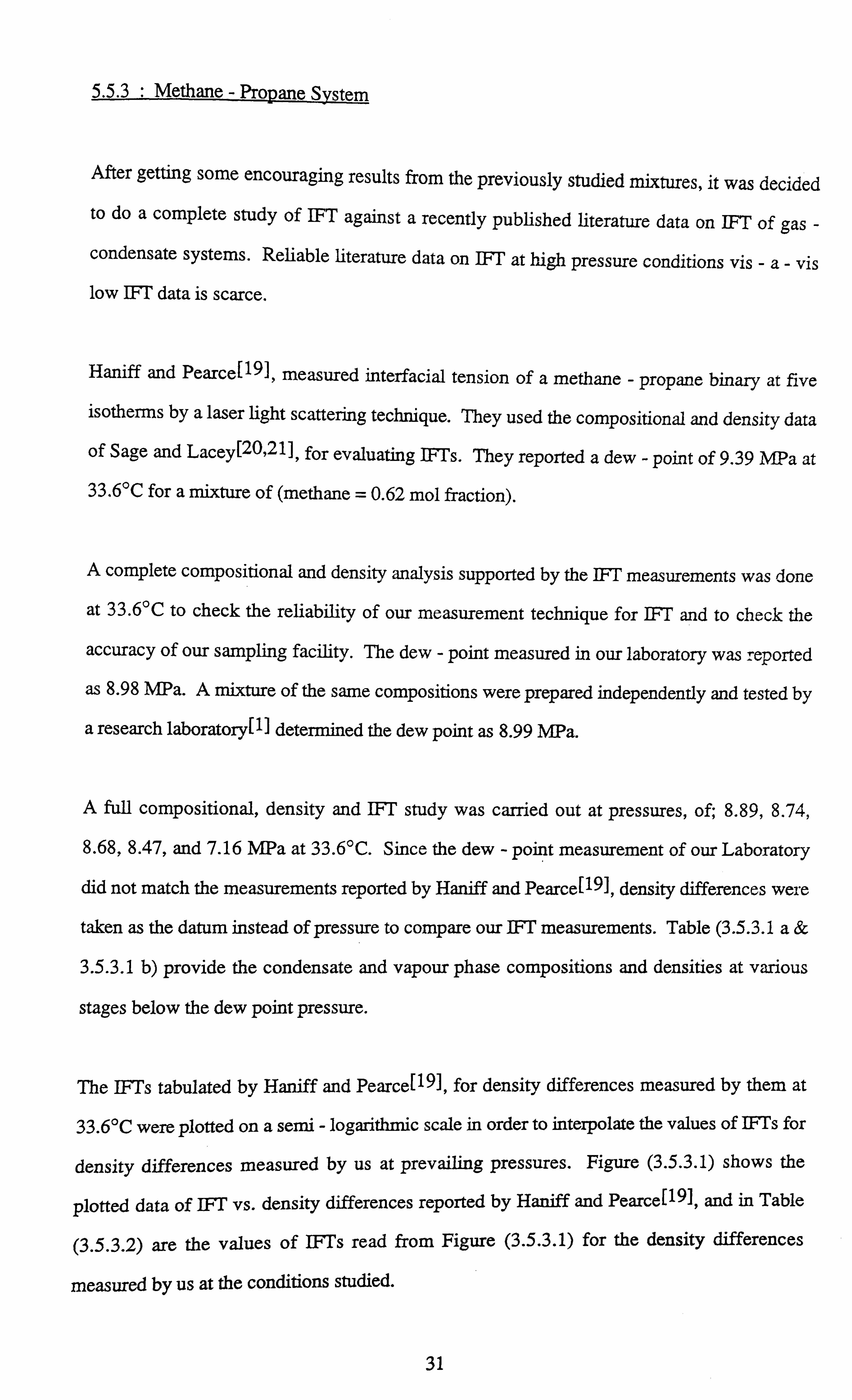
5.5.3 : Methane - Propane S, stem
After getting some encouraging results from the previously studied mixtures, it was decided
to do a complete study of IFT against a recently published literature data on IFT of gas - condensate systems. Reliable literature data on IFT at high pressure conditions vis -a- vis low IFT data is scarce.
Haniff and Pearce[19I, measured interfacial tension of a methane - propane binary at five
isotherms by a laser light scattering technique. They used the compositional and density data
of Sage and Lacey[2O, 21], for evaluating IFTs. They reported a dew - point of 9.39 MPa at 33.6°C for a mixture of (methane = 0.62 mol fraction).
A complete compositional and density analysis supported by the IFT measurements was done
at 33.6°C to check the reliability of our measurement technique for IFI' and to check the
accuracy of our sampling facility. The dew - point measured in our laboratory was reported
as 8.98 MPa. A mixture of the same compositions were prepared independently and tested by
a research laboratory[ 11 determined the dew point as 8.99 MPa.
A full compositional, density and IFT study was carried out at pressures, of; 8.89,8.74,
8.68,8.47, and 7.16 MPa at 33.6°C. Since the dew - point measurement of our Laboratory
did not match the measurements reported by Haniff and Pearce[191, density differences were
taken as the datum instead of pressure to compare our IFT measurements. Table (3.5.3.1 a&
3.5.3.1 b) provide the condensate and vapour phase compositions and densities at various
stages below the dew point pressure.
The IF°Ts tabulated by Haniff and Pearce[191, for density differences measured by them at
33.6°C were plotted on a semi - logarithmic scale in order to interpolate the values of IFTs for
density differences measured by us at prevailing pressures. Figure (3.5.3.1) shows the
plotted data of IFT vs. density differences reported by Haniff and Pearce{191, and in Table
(3.5.3.2) are the values of IFTs read from Figure (3.5.3.1) for the density differences
measured by us at the conditions studied.
31
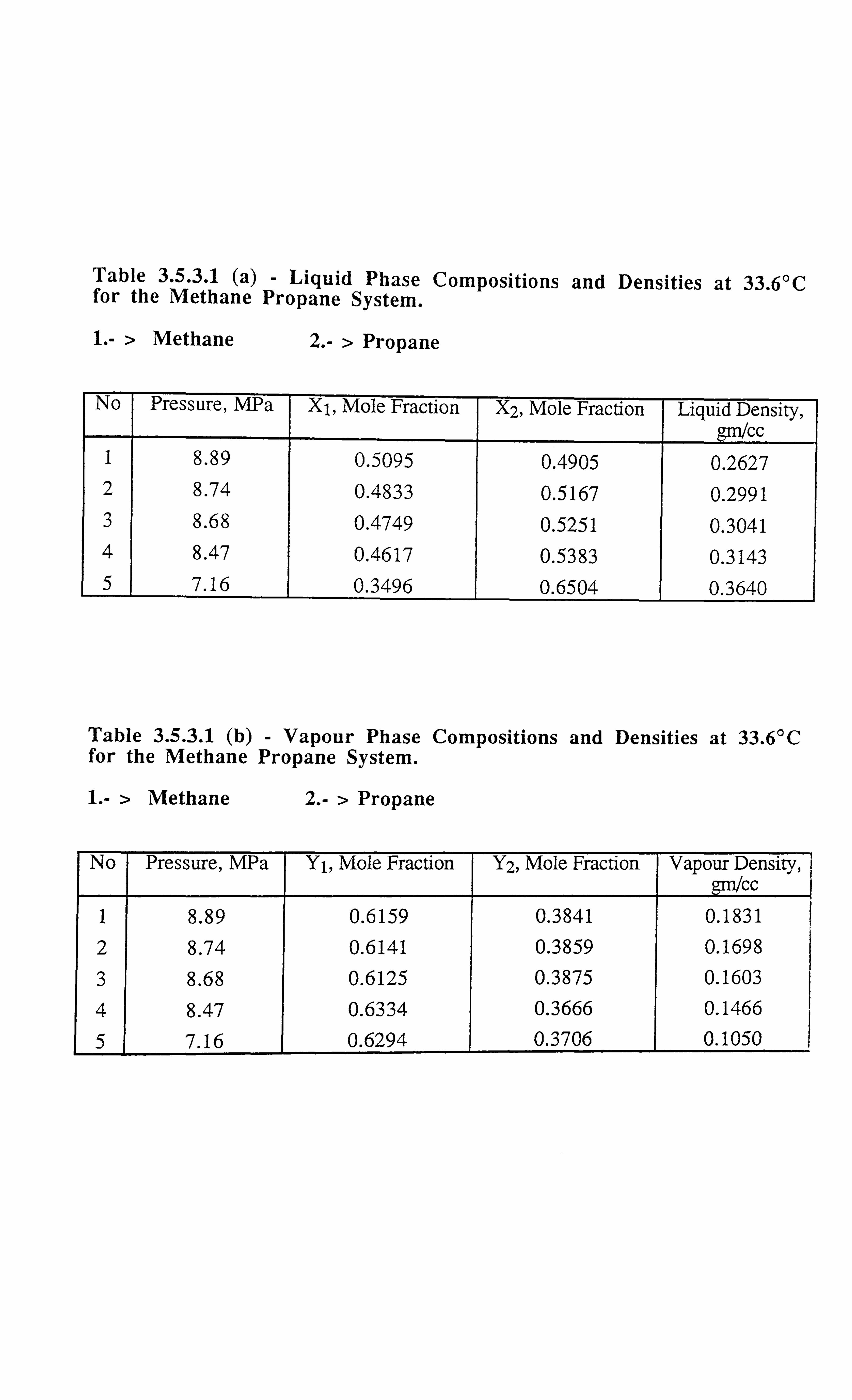
Table 3.5.3.1 (a) for the Methane
1. - > Methane
- Liquid Phase Compositions and Densities at 33.6°C Propane System.
2. - > Propane
No Pressure, MPa X1, Mole Fraction X2, Mole Fraction Liquid Density, cc
1 8.89 0.5095 0.4905 0.2627 2 8.74 0.4833 0.5167 0.2991 3 8.68 0.4749 0.5251 0.3041 4 8.47 0.4617 0.5383 0.3143 5 7.16 0.3496 0.6504 0.3640
Table 3.5.3.1 (b) for the Methane
1. - > Methane
- Vapour Phase Compositions and Densities at 33.6°C Propane System.
2. - > Propane
No Pressure, MPa Y1, Mole Fraction Y2, Mole Fraction Vapour Density, gm/Cc
1 8.89 0.6159 0.3841 0.1831 2 8.74 0.6141 0.3859 0.1698
3 8.68 0.6125 0.3875 0.1603 4 8.47 0.6334 0.3666 0.1466
5 7.16 0.6294 0.3706 0.1050

Table 3.5.3.2 - Data of Haniff and Pearce[19I, on Interfacial Tension Interpolated, for the Density Differences Measured in our Laboratory, from Figure (3.3.3.1).
No Density Difference, gm/cc Interfacial Tension, mN/m 1 0.0796 0.018 2 0.1293 0.058 3 0.1438 0.077 4 0.1677 0.122 5 0.2590 0.662
Table 3.5.3.3 - Data on Interfacial Tension for the Methane - Propane System at 33.6'C.
No Pressure, MPa
Film Heights,
mm
Scaling Law, mN/m
Parachor Method, mN/m
Measured mN/m
Haniff and* Pearce[191,
mN/m 1 8.89 0.2221 0.006 0.006 0.019 0.018
2 8.74 0.2902 0.045 0.045 0.054 0.058
3 8.68 0.3169 0.070 0.069 0.071 0.077
4 8.47 0.4695 0.126 0.127 0.181 0.122
5 7.16 0.8165 0.656 0.685 0.847 0.662
* From Table 3.5.3.2 above

Z
c 0
aý H
U 421 N
1
.1
. 01
. 001
ý' IFT, mN/m
0.0 0.1 0.2
Phase Density Difference, gm/cc
Figure 3.5.3.1 - Data of Haniff and Pearce [19], on IFT of Methane-Propane Mixture at 33.6 deg C.
0.3
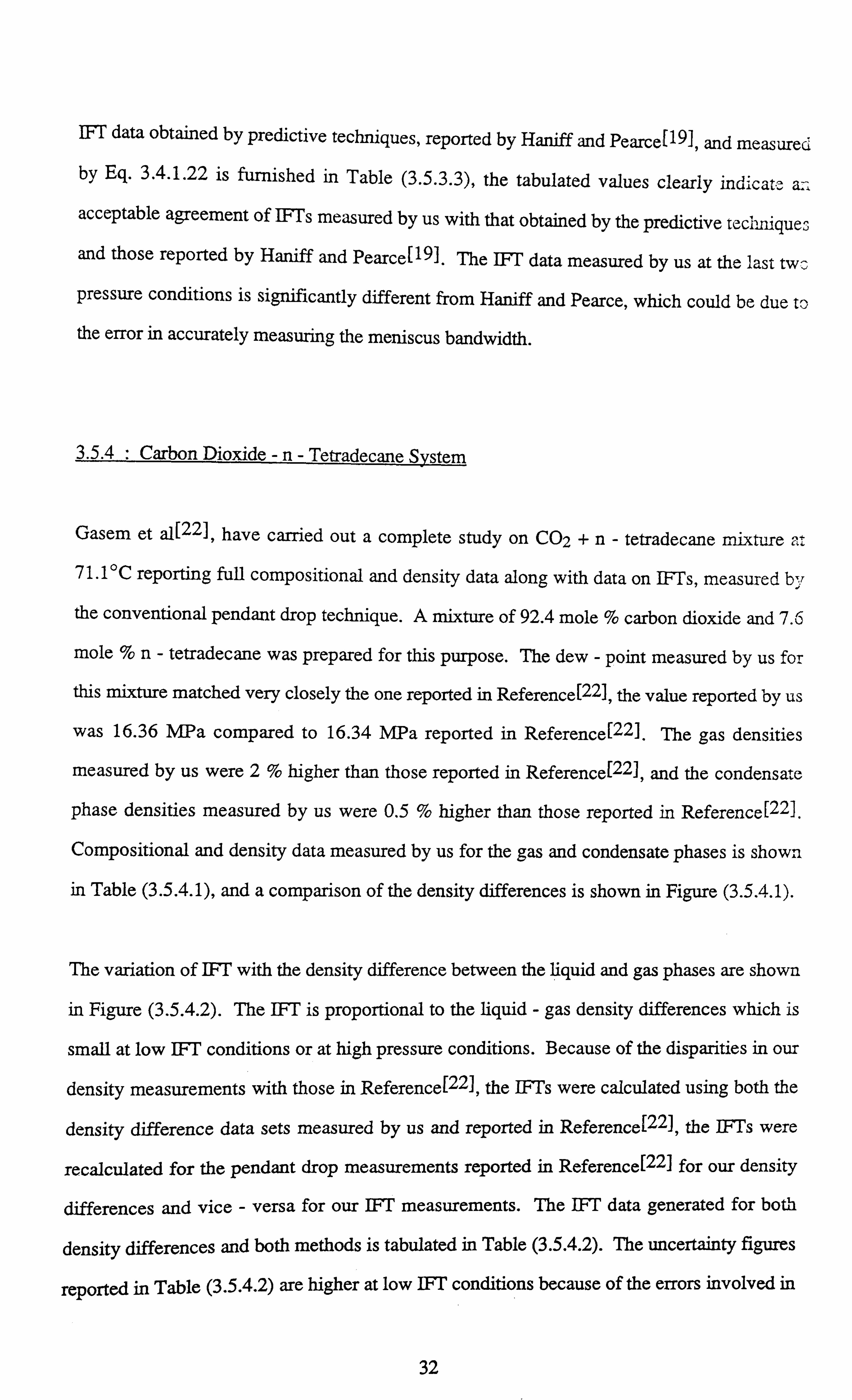
IFT data obtained by predictive techniques, reported by Haniff and Pearce[191, and measured by Eq. 3.4.1.22 is furnished in Table (3.5.3.3), the tabulated values clearly indicate a. -, acceptable agreement of IFTs measured by us with that obtained by the predictive tech uques
and those reported by Haniff and Pearce[191I. The IFT data measured by us at the last twc
pressure conditions is significantly different from Haniff and Pearce, which could be due to
the error in accurately measuring the meniscus bandwidth.
3.5.4 Carbon Dioxide - n_- Tetradecane System
Gasem et al[22], have carried out a complete study on CO2 +n- tetradecane mixture ot 71.1 °C reporting full compositional and density data along with data on IF'Ts, measured by
the conventional pendant drop technique. A mixture of 92.4 mole % carbon dioxide and 7.6
mole %n- tetradecane was prepared for this purpose. The dew - point measured by us for
this mixture matched very closely the one reported in Reference{221, the value reported by us
was 16.36 MPa compared to 16.34 MPa reported in Reference[22]. The gas densities
measured by us were 2% higher than those reported in Reference{22], and the condensate
phase densities measured by us were 0.5 % higher than those reported in Reference[22].
Compositional and density data measured by us for the gas and condensate phases is shown
in Table (3.5.4.1), and a comparison of the density differences is shown in Figure (3.5.4.1).
The variation of IFT with the density difference between the liquid and gas phases are shown
in Figure (3.5.4.2). The IFT is proportional to the liquid - gas density differences which is
small at low IFT conditions or at high pressure conditions. Because of the disparities in our
density measurements with those in Reference[22] , the IFTs were calculated using both the
density difference data sets measured by us and reported in Reference[22], the IFTs were
recalculated for the pendant drop measurements reported in Reference[22] for our density
differences and vice - versa for our IFT measurements. The IFT data generated for both
density differences and both methods is tabulated in Table (3.5.4.2). The uncertainty figures
reported in Table (3.5.4.2) are higher at low IFT conditions because of the errors involved in
32
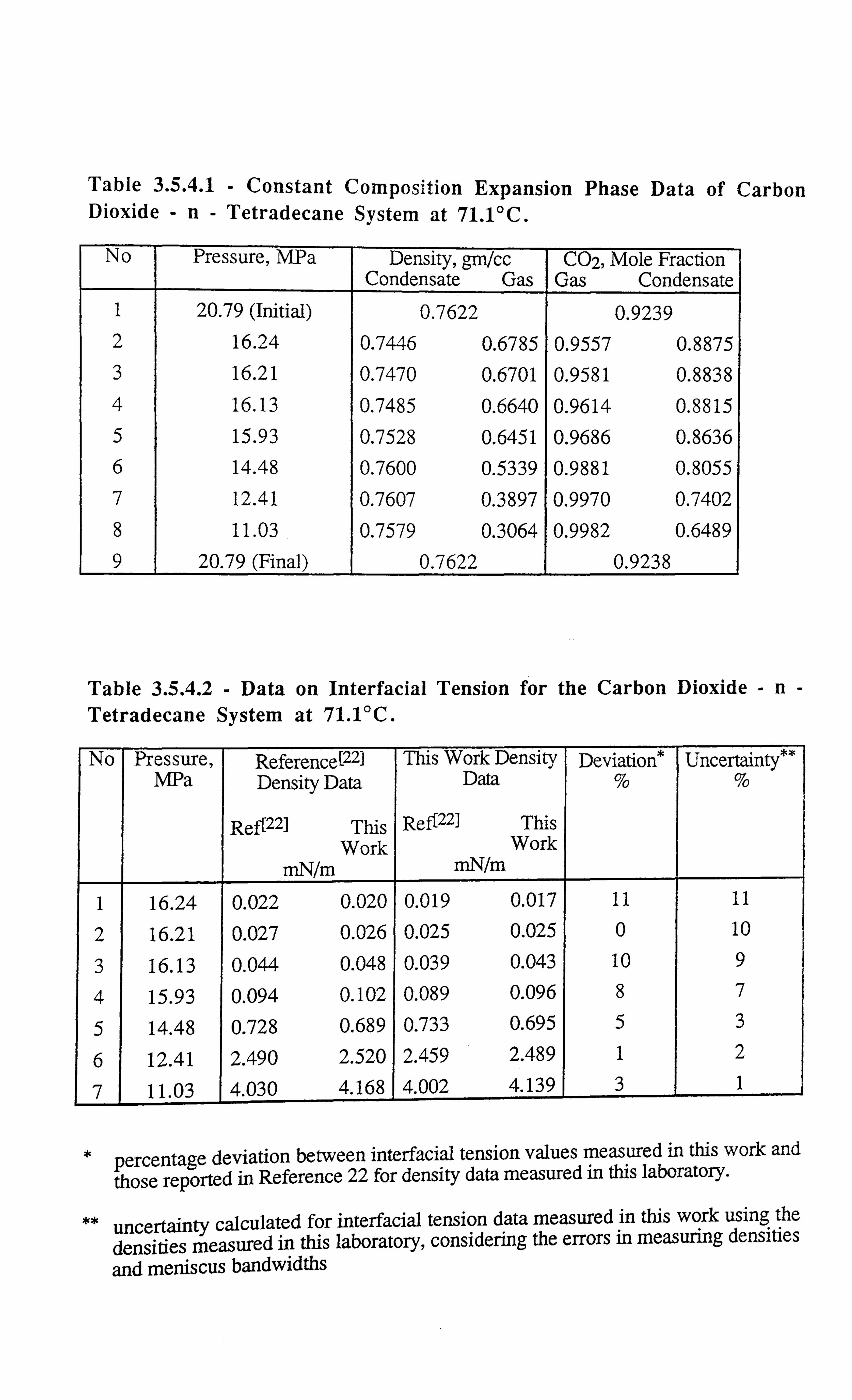
Table 3.5.4.1 - Constant Composition Expansion Phase Data of Carbon Dioxide -n- Tetradecane System at 71.1'C.
No Pressure, MPa Density, gm/cc Condensate Gas
C02, Mole Fraction Gas Condensate
1 20.79 (Initial) 0.7622 0.9239 2 16.24 0.7446 0.6785 0.9557 0.8875 3 16.21 0.7470 0.6701 0.9581 0.8838 4 16.13 0.7485 0.6640 0.9614 0.8815 5 15.93 0.7528 0.6451 0.9686 0.8636 6 14.48 0.7600 0.5339 0.9881 0.8055
7 12.41 0.7607 0.3897 0.9970 0.7402 8 11.03 0.7579 0.3064 0.9982 0.6489 9 20.79 (Final) 0.7622 0.9238
Table 3.5.4.2 - Data on Interfacial Tension for the Carbon Dioxide -n- Tetradecane System at 71.1°C.
No Pressure, Reference[221 This Work Density Deviation* Uncertainty** M'a Density Data Data % %
Ref"2211 This Ref{221 This Work Work
n N/m mN/m
1 16.24 0.022 0.020 0.019 0.017 11 11
2 16.21 0.027 0.026 0.025 0.025 0 10
3 16.13 0.044 0.048 0.039 0.043 10 9
4 15.93 0.094 0.102 0.089 0.096 8 7
5 14.48 0.728 0.689 0.733 0.695 5 3
6 12.41 2.490 2.520 2.459 2.489 1 2
7 11.03 4.030 4.168 4.002 4.139 3 1
* percentage deviation between interfacial tension values measured in this work and
those reported in Reference 22 for density data measured in this laboratory.
** uncertainty calculated for interfacial tension data measured in this work using the
densities measured in this laboratory, considering the errors in measuring densities
and meniscus bandwidths

0.5
This Work
................ Gasem et. al. [22] 0.4
U
U
0.3 2
0.2 A aý
0.1
0.0t 11 12 13 14 15
Pressure, MPa
16 17
Figure 3.5.4.1 - Comparison of Density Difference Data, for the Carbon Dioxide -n- Tetradecane System at 71.1 deg C.
10
1 z E C O
cd
S
-o- IFF, mN/m
. 01 `- 0.0 0.1 0.2 0.3 0.4
Phase Density Difference, gm/cc
0.5
Figure 3.5.4.2 - Variation of IFT With Density Difference, for the C02-n C14 Mixture at 71.1 deg C.
measuring the film heights at these conditions, which are quite small, subsequently these
uncertainties reduce at high IFT conditions since the errors in measuring the film heights gel,
minimised at low pressure or high IFT conditions.
The results in Table (3.5.4.2), clearly indicate the reliability and accuracy of our proposed
measurement technique also highlighting its simplicity in carrying out the measurements and
the ease with which reliable IFT data can be generated.
3.5.5 : Methane-Propane-n-Decane System
A four stage forward contact study was conducted in the vapour-Liquid-equilibrium (V-L-E)
apparatus, between pure methane and a ternary mixture comprising of methane, propane and
normal decane. ' This study was performed to generate data on phase densities, phase volumes
and interfacial tensions to support the work on dynamic validation of phase behaviour models.
A ternary mixture comprising of methane (46 mole %), propane (39 mole %) and normal
decane (15 mole %) was contacted with pure methane at 20.68 MPa and 37.78°C. The event
of suspending the liquid droplets into its surrounding equilibrium vapour and the meniscus at
the interface were video recorded for IFT measurements. The liquid and vapour phase
densities at equilibrium were also measured. The experiment progressed to the second stage
in which the equilibrium vapour was retained to contact with a fresh liquid. However the
second contact resulted in complete miscibility. The experiment was stopped at this stage and
a pressure of 13.79 MPa was selected to carry out the necessary number of contacts required
for the dynamic validation study. The experiment was continued for four stages. The phase
densities, pendant drops and meniscus widths were recorded at each contact point. The video
recordings were later dimensioned to measure the interfacial tension for both the pendant drop
and the meniscus technique. The measured IFT values and phase densities are furnished in
Table 3.5.5.1. The predicted liquid and vapour phase compositions are provided in Table
3.5.5.2 a and 3.5.5.2 b respectively.
33
3.5.6: Methane-Carbon Dioxide-Propane-n-Pentane-n-Decane-n-Hexadecane System
A series of constant composition expansion (CCE) and gas cycling tests were performed on a
six component synthetic mixture comprising of C02, CH4, C3H8, nC5, nC10 and nC16. The
tests were carried out at a temperature of 100°C and 22.75 MPa. Interfacial tension data was
measured using the gas-liquid interface technique during the cycling test with a gas composed
of 59.35% CH4 and 40.65% CO2 at 22.75 MPa. The measured IFT data and phase densities
are provided in Table 3.5.6.1. The predicted liquid phase compositions are given in Table
3.5.6.2 a and measured vapour phase compositions are provided in Table 3.5.6.2 b.
3.5.7 Interfacial Tension Measurements on a Synthetic Near Critical Fluid
A complete set of tests were planned for a near critical real reservoir fluid to be tested in
the VLE and gas condensate experimental facilities. As a forerunner to that a six component
synthetic mixture comprised of methane, ethane, propane and normal pentane, octane and
decane, was gravimetrically prepared. A constant composition expansion (CCE) test was
performed on this fluid at 38.0°C in the gas-condensate PVT cell. The mixture exhibited a
near critical dew point of about 33 MPa. The phase volumes, densities and meniscus widths
were recorded from 31.72 to 24.13 MPa. The meniscus widths were later dimensioned using
a video scalar unit from which the IFT values were measured. The values of interfacial
tension for this near critical fluid ranged from 0.0017 to 0.235 dyn%m and are furnished for
various points of CCE in Table 3.5.7.1 and Figure 3.5.7.1. The single phase composition
for this fluid is given in Table 3.5.7.2, however, no measurements or predictions for the two
phase compositions for this fluid were carried out.
34

Table 3.5.5.1 - Interfacial Tension Measurements on a Ternary Mixture of C H4- C3H8-n-C10H22 for a Forward Multiple Contact Study With CH4 at 37.8°C.
Stage Number Liquid Density gm/cc
Vapour Density gm/cc
Measured IFT mN/m
20.68 MPa
1 0.4918 0.2442 0.457
13.79 MPa
1 0.5495 0.1493 2.375 2 0.4964 0.1794 1.166 3 0.4894 0.1914 0.907 4 0.4874 0.2003 0.697
Table 3.5.6.1 - Interfacial Tension Measurements on a Six Component Synthetic Gas Condensate for a Gas Cycling Study at 22.75 MPa and 100°C.
Stage Number Liquid Density Vapour Density Measured IFT gm/cc gm/cc mN/m
0 0.5700 0.2410 0.853 1 0.6050 0.2390 1.359 2 0.6260 0.2390 1.742 3 0.6400 0.2360 2.123 4 0.6490 0.2380 2.347
Table 3.5.7.1 - Interfacial Tension Measurements on a Near Critical Synthetic
Gas Condensate at 38°C.
Pressure (MPa) Liquid Density Vapour Density Measured IFT gm/cc gm/cc mN/rn
31.72 0.5013 0.3733 0.002 30.34 0.5245 0.3431 0.010 28.96 0.5456 0.3219 0.037 27 58 0.5567 0.3095 0.078
. 24.13 0.5749 0.2880 0.235
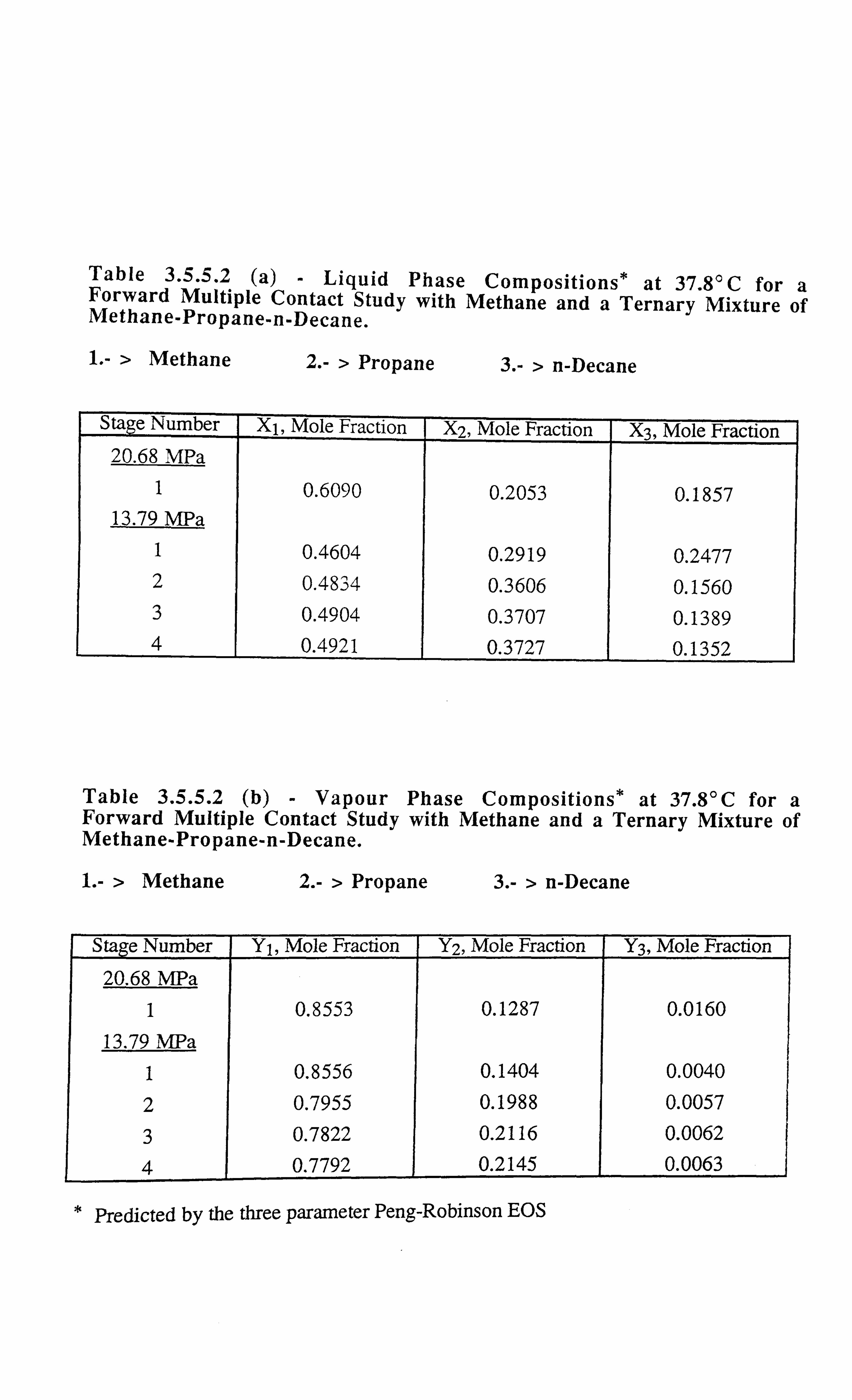
Table 3.5.5.2 (a) - Liquid Phase Compositions* at 37.8°C for a Forward Multiple Contact Study with Methane and a Ternary Mixture of Methane-Propane-n-Decane.
1. - > Methane 2. - > Propane 3. - > n-Decane
Stage Number Xi, Mole Fraction X2, Mole Fraction X3, Mole Fraction 20.68 MPa
1 0.6090 0.2053 0.1857 13.79 MPa
1 0.4604 0.2919 0.2477 2 0.4834 0.3606 0.1560 3 0.4904 0.3707 0.1389 4 0.4921 0.3727 0.1352
Table 3.5.5.2 (b) - Vapour Phase Compositions* at 37.8°C for a Forward Multiple Contact Study with Methane and a Ternary Mixture of Methane-Propane-n-Decane.
1. - > Methane 2. - > Propane 3. - > n-Decane
Stage Number Yl, Mole Fraction Y2, Mole Fraction Y3, Mole Fraction
20.68 MPa
1 0.8553 0.1287 0.0160
13.79 MPa
1 0.8556 0.1404 0.0040
2 0.7955 0.1988 0.0057
3 0.7822 0.2116 0.0062
4 0.7792 0.2145 0.0063
* Predicted by the three parameter Peng-Robinson EOS
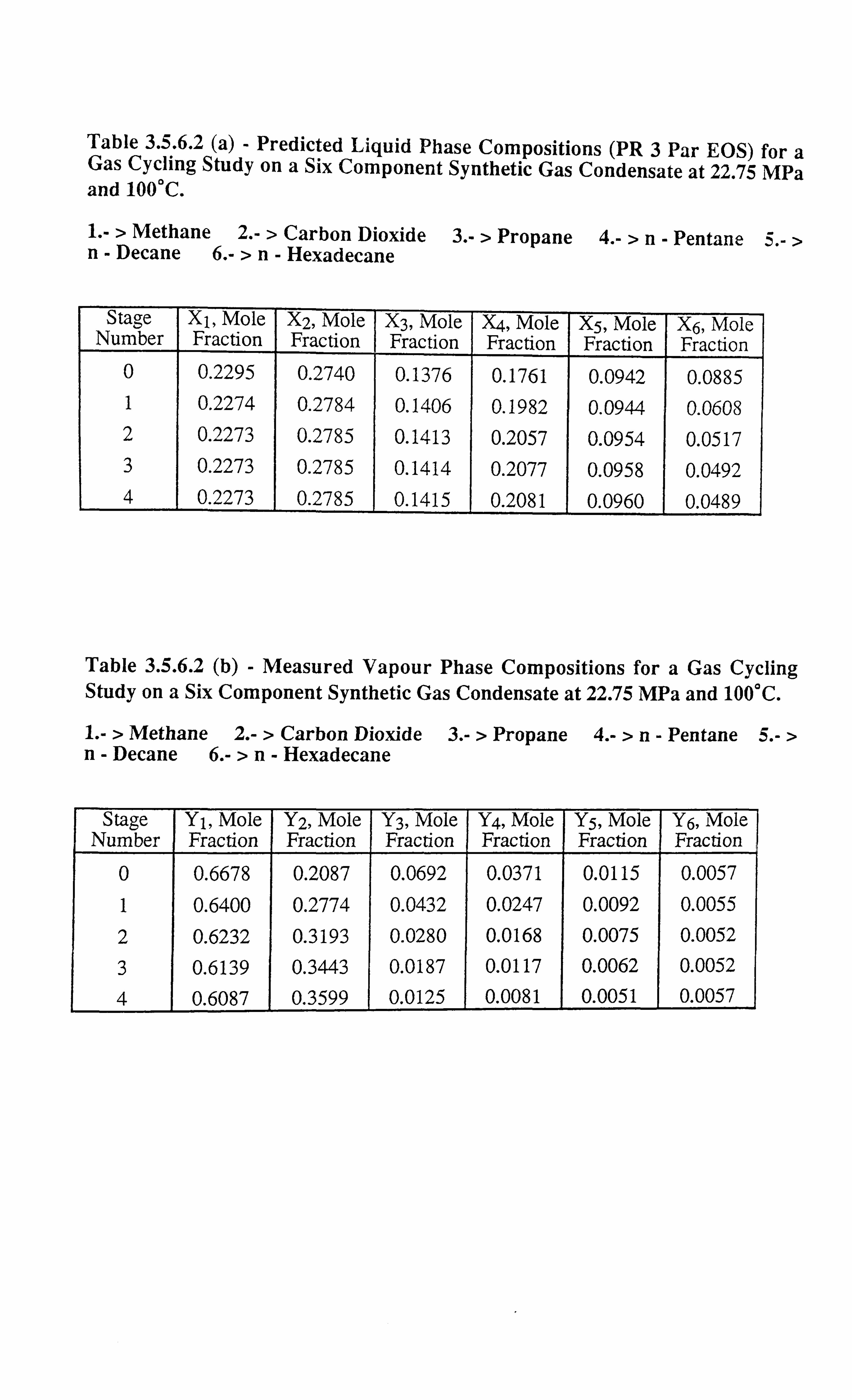
Table 3.5.6.2 (a) - Predicted Liquid Phase Compositions (PR 3 Par EOS) for a Gas Cycling Study on a Six Component Synthetic Gas Condensate at 22.75 MPa and 100°C.
1. - > Methane 2. - > Carbon Dioxide 3. - > Propane 4. - >n- Pentane 5. - > n- Decane 6. - >n- Hexadecane
Stage Number
X1, Mole Fraction
X2, Mole Fraction
X3, Mole Fraction
X4, Mole Fraction
X5, Mole Fraction
X6, Mole Fraction
0 0.2295 0.2740 0.1376 0.1761 0.0942 0.0885 1 0.2274 0.2784 0.1406 0.1982 0.0944 0.0608 2 0.2273 0.2785 0.1413 0.2057 0.0954 0.0517 3 0.2273 0.2785 0.1414 0.2077 0.0958 0.0492 4 0.2273 0.2785 0.1415 0.2081 0.0960 0.0489
Table 3.5.6.2 (b) - Measured Vapour Phase Compositions for a Gas Cycling Study on a Six Component Synthetic Gas Condensate at 22.75 MPa and 100°C.
1. - > Methane 2. - > Carbon Dioxide 3. - > Propane 4. - >n- Pentane 5. - > n- Decane 6. - >n- Hexadecane
Stage Number
Y1, Mole Fraction
Y2, Mole Fraction
Y3, Mole Fraction
Y4, Mole Fraction
Y5, Mole Fraction
Y6, Mole Fraction
0 0.6678 0.2087 0.0692 0.0371 0.0115 0.0057 1 0.6400 0.2774 0.0432 0.0247 0.0092 0.0055
2 0.6232 0.3193 0.0280 0.0168 0.0075 0.0052
3 0.6139 0.3443 0.0187 0.0117 0.0062 0.0052
4 0.6087 0.3599 0.0125 0.0081 0.0051 0.0057

Table 3.5.7.2 - Single Phase Composition of the Synthetic Near Critical Fluid.
Component Mole %
Methane 76.58
Ethane 7.79
Propane 5.17
n-Pentane 3.95
n-Octane 2.80
n-Hexadecane 3.71
Total 100
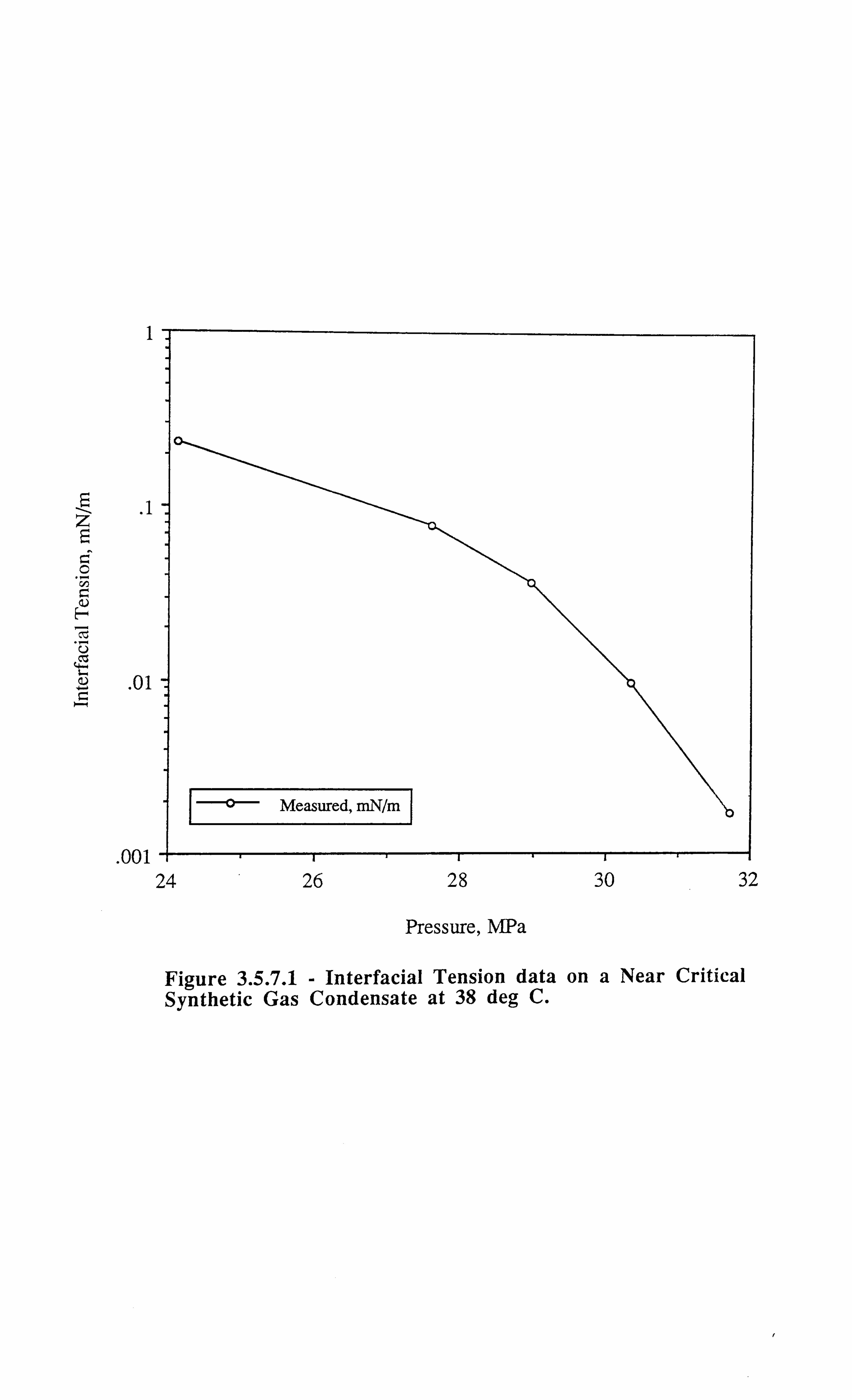
1
.1 z
O . r. COO
a) E
U
. 01
. 001 24 26 28 30 32
Pressure, MPa
Figure 3.5.7.1 - Interfacial Tension data on a Near Critical Synthetic Gas Condensate at 38 deg C.
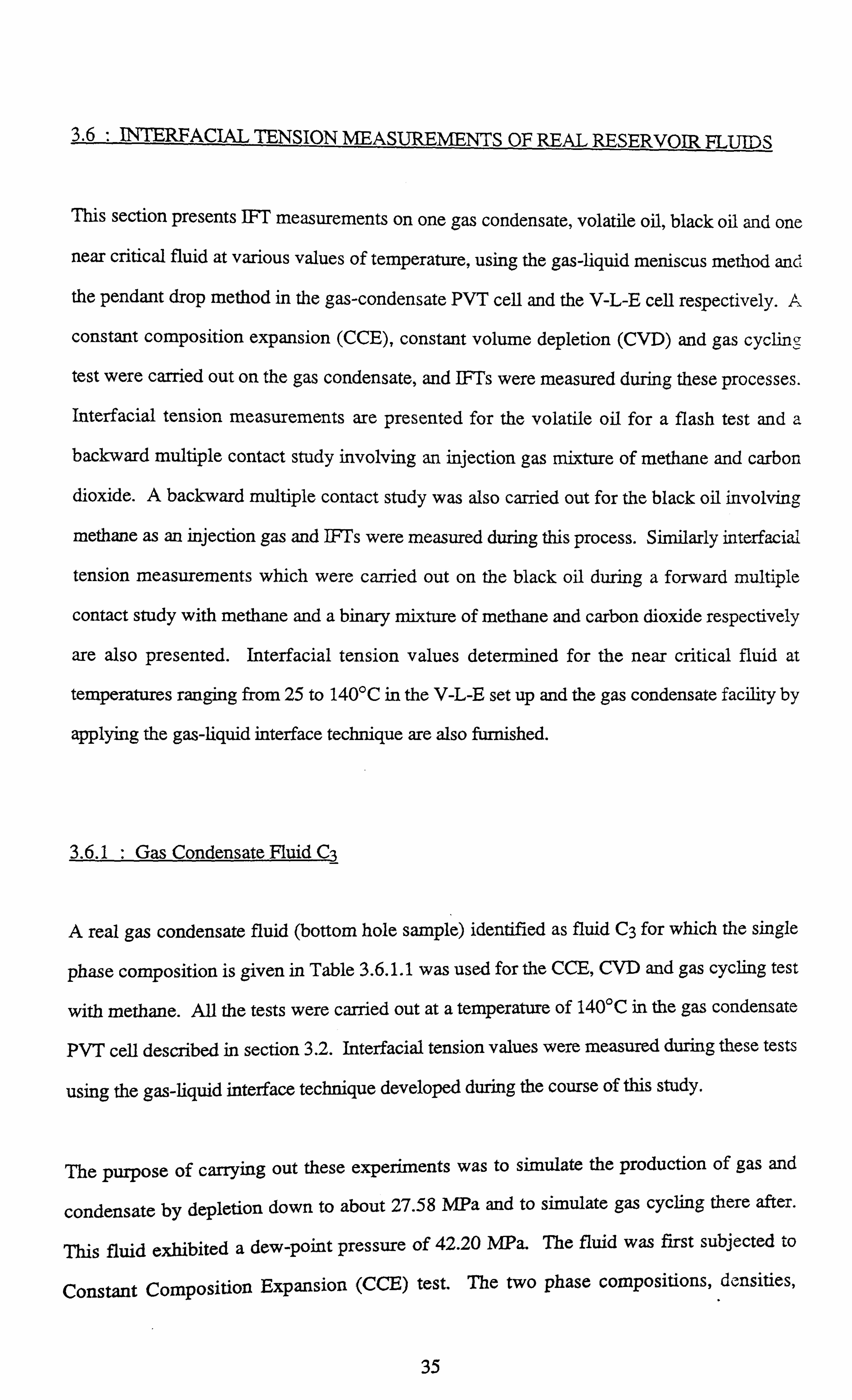
3.6 : INTERFACAL TENSION MEASUREMENTS OF REAL RESERVOIR FLUIDS
This section presents IFT measurements on one gas condensate, volatile oil, black oil and one
near critical fluid at various values of temperature, using the gas-liquid meniscus method and
the pendant drop method in the gas-condensate PVT cell and the V-L-E cell respectively. A
constant composition expansion (CCE), constant volume depletion (CVD) and gas cycling
test were carried out on the gas condensate, and IFTs were measured during these processes.
Interfacial tension measurements are presented for the volatile oil for a flash test and a
backward multiple contact study involving an injection gas mixture of methane and carbon
dioxide. A backward multiple contact study was also carried out for the black oil involving
methane as an injection gas and IFTs were measured during this process. Similarly interfacial
tension measurements which were carried out on the black oil during a forward multiple
contact study with methane and a binary mixture of methane and carbon dioxide respectively
are also presented. Interfacial tension values determined for the near critical fluid at
temperatures ranging from 25 to 140°C in the V-L-E set up and the gas condensate facility by
applying the gas-liquid interface technique are also furnished.
3.6.1: Gas Condensate Fluid Ca
A real gas condensate fluid (bottom hole sample) identified as fluid C3 for which the single
phase composition is given in Table 3.6.1.1 was used for the CCE, CVD and gas cycling test
with methane. All the tests were carried out at a temperature of 140°C in the gas condensate
PVT cell described in section 3.2. Interfacial tension values were measured during these tests
using the gas-liquid interface technique developed during the course of this study.
The purpose of carrying out these experiments was to simulate the production of gas and
condensate by depletion down to about 27.58 MPa and to simulate gas cycling there after.
This fluid exhibited a dew-point pressure of 42.20 MPa. The fluid was first subjected to
Constant Composition Expansion (CCE) test. The two phase compositions, densities,
35
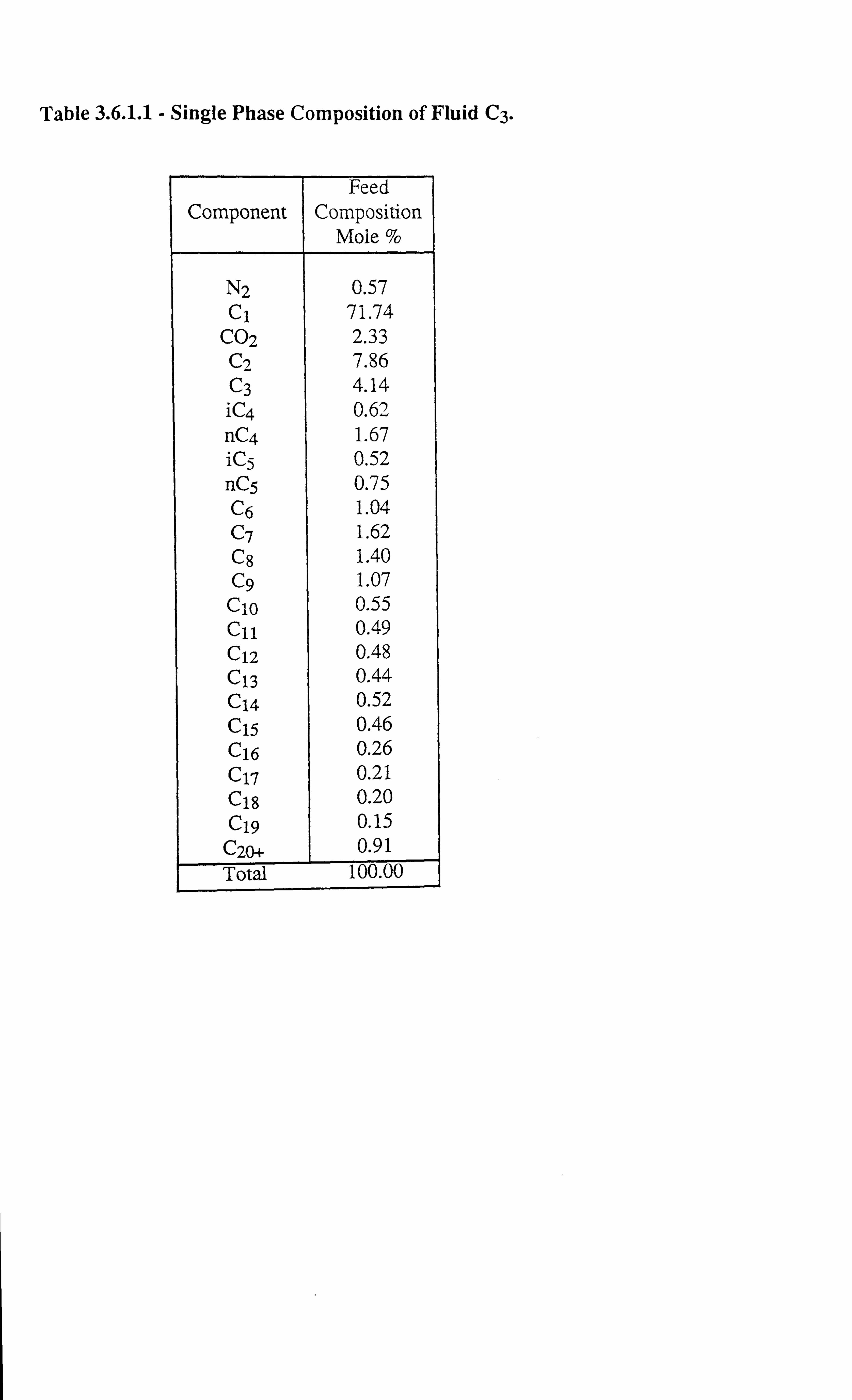
Table 3.6.1.1 - Single Phase Composition of Fluid C3.
Component Feed
Composition Mole %
N2 0.57 Cl 71.74
CO2 2.33 C2 7.86 C3 4.14 iC4 0.62 nC4 1.67 iC5 0.52 nC5 0.75 C6 1.04 C7 1.62 C8 1.40 C9 1.07 C10 0.55 C11 0.49 C12 0.48 C13 0.44 C14 0.52 C15 0.46 C16 0.26 C17 0.21 C18 0.20 C19 0.15
C20+ 0.91 Total 100.00
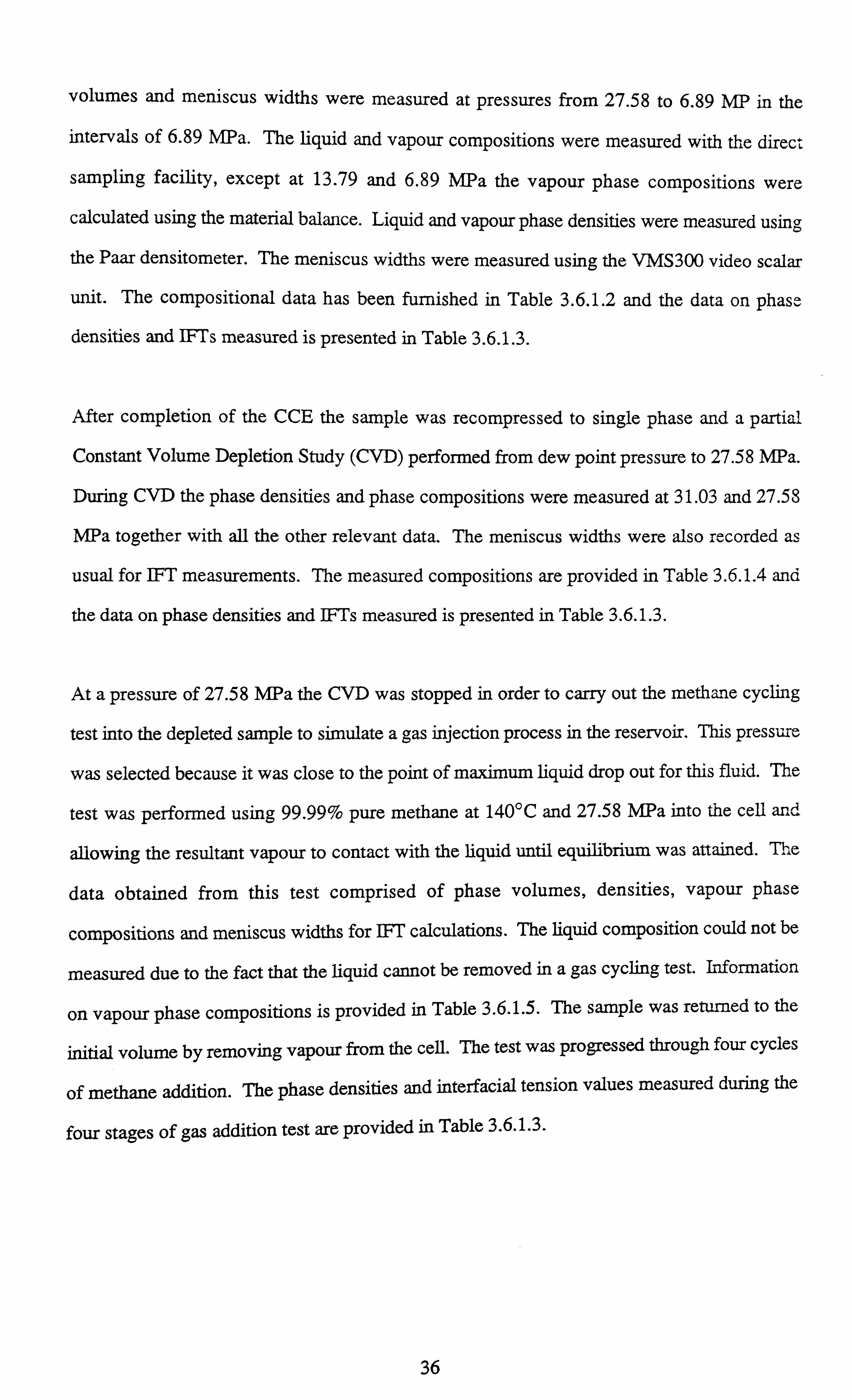
volumes and meniscus widths were measured at pressures from 27.58 to 6.89 MP in the
intervals of 6.89 MPa. The liquid and vapour compositions were measured with the direct
sampling facility, except at 13.79 and 6.89 MPa the vapour phase compositions were
calculated using the material balance. Liquid and vapour phase densities were measured using
the Paar densitometer. The meniscus widths were measured using the VMS300 video scalar
unit. The compositional data has been furnished in Table 3.6.1.2 and the data on phase
densities and IFTs measured is presented in Table 3.6.1.3.
After completion of the CCE the sample was recompressed to single phase and a partial
Constant Volume Depletion Study (CVD) performed from dew point pressure to 27.58 MPa.
During CVD the phase densities and phase compositions were measured at 31.03 and 27.58
MPa together with all the other relevant data. The meniscus widths were also recorded as
usual for IFT measurements. The measured compositions are provided in Table 3.6.1.4 and
the data on phase densities and IFTs measured is presented in Table 3.6.1.3.
At a pressure of 27.58 MPa the CVD was stopped in order to carry out the methane cycling
test into the depleted sample to simulate a gas injection process in the reservoir. This pressure
was selected because it was close to the point of maximum liquid drop out for this fluid. The
test was performed using 99.99% pure methane at 140°C and 27.58 MPa into the cell and
allowing the resultant vapour to contact with the liquid until equilibrium was attained. The
data obtained from this test comprised of phase volumes, densities, vapour phase
compositions and meniscus widths for IFI' calculations. The liquid composition could not be
measured due to the fact that the liquid cannot be removed in a gas cycling test. Information
on vapour phase compositions is provided in Table 3.6.1.5. The sample was returned to the
initial volume by removing vapour from the cell. The test was progressed through four cycles
of methane addition. The phase densities and interfacial tension values measured during the
four stages of gas addition test are provided in Table 3.6.1.3.
36
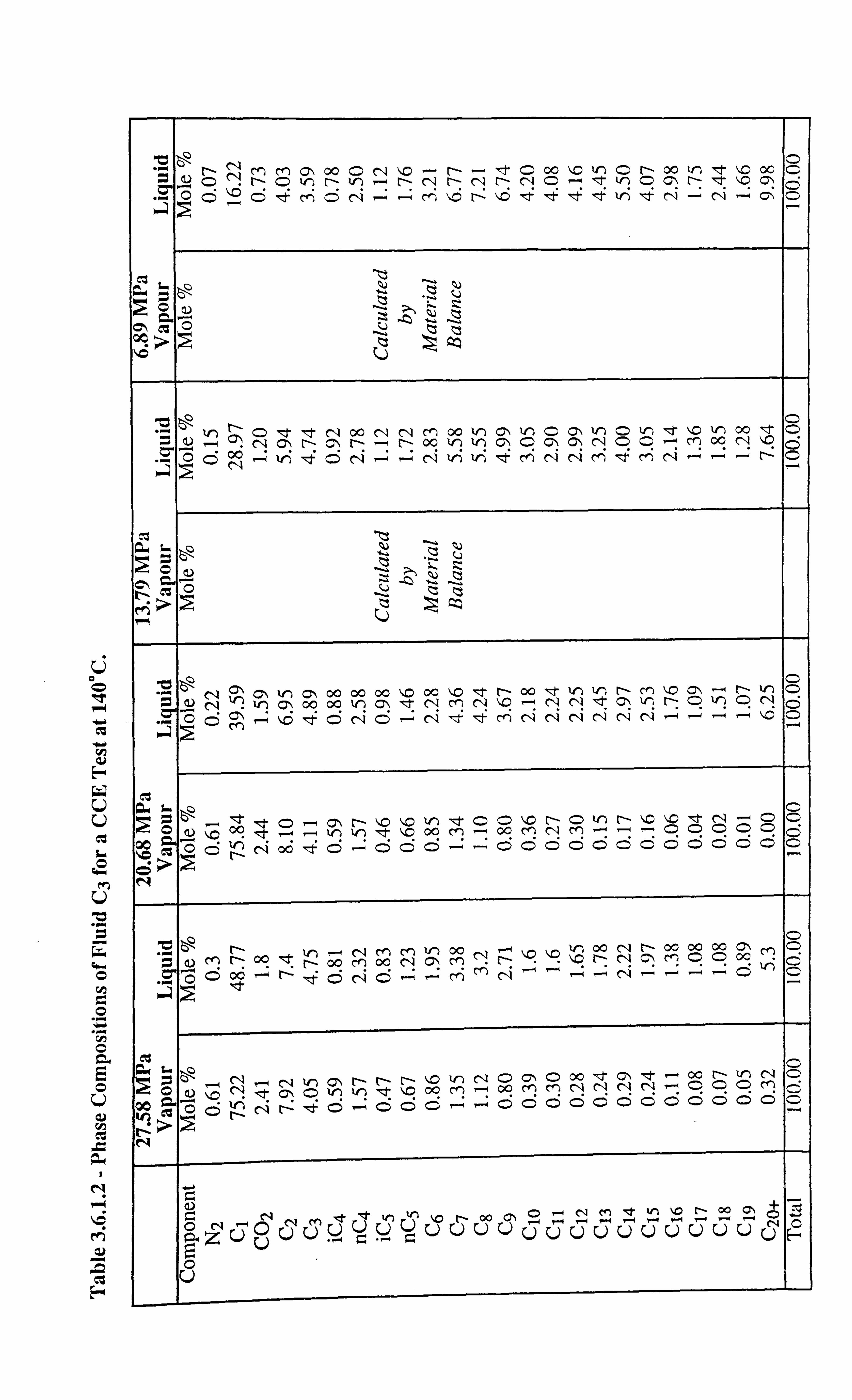
'C NM ch C7-, 00 ON IO -N- d- O 00 \O un CN 00 to - \D 00 Ö
tea,, ONO Nin -NNNNNN O- C C\ N d- 1,0 O, \
a5 O- 6 d' M6N 14 1. M `O N \O d' d' mot' 4 ti 4 N- N --; O
0
U 9.4
4° M
U
ýTW
O
E O
C3
0 U -- ;, ý,
.ýv
It N 00 NN cM 00 to ON kn CCVO Ln ct ýO V, ) oc 01,
-N C\ N C\ NN 00 to Vn O\ C C\ C\ NCC'M 00 N ýD ON -+ Ni ýt MNNM d- MN r-+ '-' ý`' 00 ON
Ate'' ý , moo
112
CD
N p. ' in c-, o0 00 00 \, O oc \O 1 C- oc d' vý vý NM ýD Oý r-+ N In O N I? ºn cN o0 0o in ON 4NmN LO NNd: U I1 O to ON
r-+ '--*-- CO N d' mot' MNNNNNN . '. 0p M- o it ON6-:
m
-c t- `O �O ýn d' CC \C t- C In [- \O \, O d' N-CÖ C ¢N ýp in in d' \Z 00 M- oo MNM r-" - . -. CCCCO p ýj app
p-2CÖ --+ -CCCCCCCCCCCCÖ
N 00 d" 'ý NMM If) 00 N r-+ if) 00 NN 00 00 00 Cl\ M
NN 00 cn 00 N O\ MN \IO r: N C\ MOO oc 00
vi
r--, N-N v) t- t i- \O in NO CIN O 00 'ý C\ IRt ---4 00 r- in NC
OyN d- p in to d- ýp oo M- oc cn mNNNNOOM ýO etY OONN mot' O ý+ OOC *-" OOO6CCO0C: ) 6
Q ý--ý NMv1 ýD lý o_O cý p ýY
äZÜýÜÜV ýÜ ÜÜÜÜUUUUUUUUUU c
F
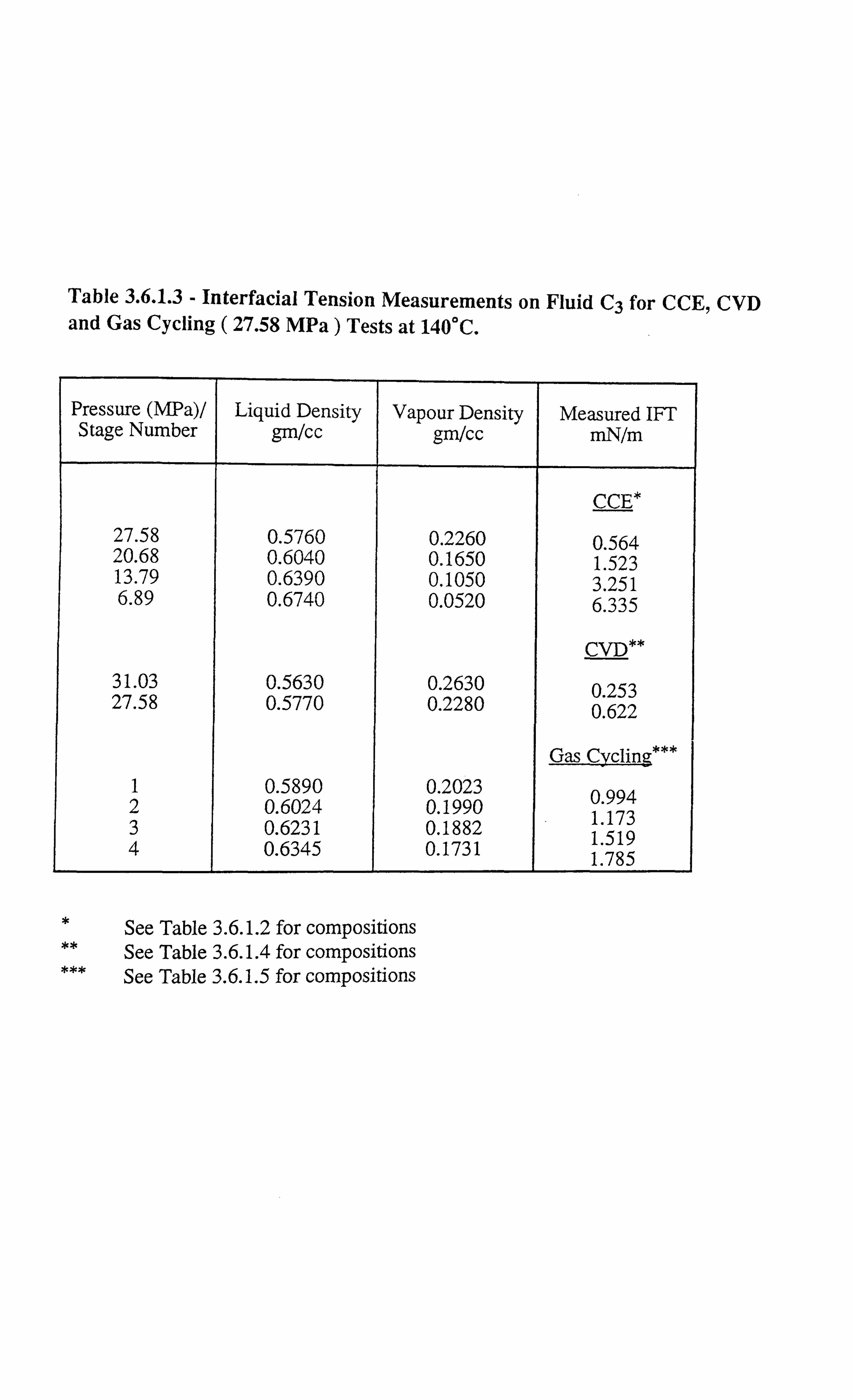
Table 3.6.1.3 - Interfacial Tension Measurements on Fluid C3 for CCE, CVD and Gas Cycling ( 27.58 MPa) Tests at 140°C.
Pressure (MPa)/ Stage Number
Liquid Density gm/cc
Vapour Density gm/cc
Measured IFT mN/m
CCE* 27.58 0.5760 0.2260 0.564 20.68 0.6040 0.1650 1.523 13.79 0.6390 0.1050 3.251 6.89 0.6740 0.0520 6.335
CVD**
31.03 0.5630 0.2630 253 0 27.58 0.5770 0.2280 . 0.622
Gas Cycling***
1 0.5890 0.2023 994 0 2 0.6024 0.1990 . 1 173 3 0.6231 0.1882 . 1 519 4 0.6345 0.1731 . 1.785
* See Table 3.6.1.2 for compositions ** See Table 3.6.1.4 for compositions *** See Table 3.6.1.5 for compositions
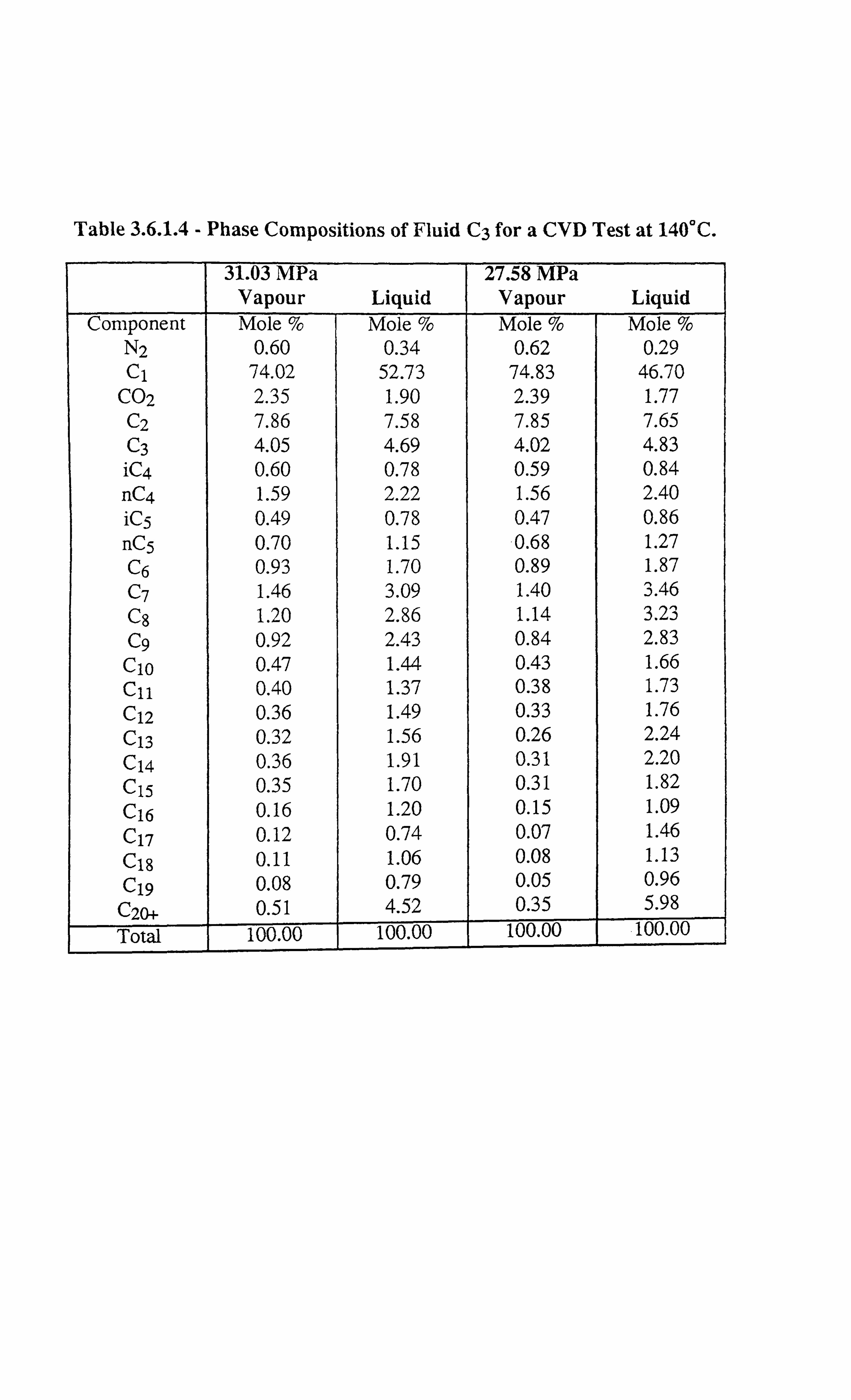
Table 3.6.1.4 - Phase Compositions of Fluid C3 for a CVD Test at 140°C.
31.03 MPa Vapour Liquid
27.58 MPa Vapour Liquid
Component Mole % Mole % Mole % Mole % N2 0.60 0.34 0.62 0.29 Cl 74.02 52.73 74.83 46.70
C02 2.35 1.90 2.39 1.77 C2 7.86 7.58 7.85 7.65 C3 4.05 4.69 4.02 4.83 iC4 0.60 0.78 0.59 0.84 nC4 1.59 2.22 1.56 2.40 iC5 0.49 0.78 0.47 0.86 nC5 0.70 1.15 0.68 1.27 C6 0.93 1.70 0.89 1.87 C7 1.46 3.09 1.40 3.46 C8 1.20 2.86 1.14 3.23 C9 0.92 2.43 0.84 2.83 C10 0.47 1.44 0.43 1.66 C11 0.40 1.37 0.38 1.73 C12 0.36 1.49 0.33 1.76 C13 0.32 1.56 0.26 2.24 C14 0.36 1.91 0.31 2.20 C15 0.35 1.70 0.31 1.82 C16 0.16 1.20 0.15 1.09 C17 0.12 0.74 0.07 1.46 Cig 0.11 1.06 0.08 1.13 C 19 0.08 0.79 0.05 0.96
C20+ 0.51 4.52 0.35 5.98 Total 100.00 100.00 100.00 100.00

Table 3.6.1.5 - Vapour Phase Compositions of Fluid C3 for a Gas Cycling Test with Methane at 27.58 MPa and 140°C.
Stage 1 Stage 2 Stage 3 Stage 4 Component Mole% Mole% Mole% Mole%
N2 0.66 0.67 0.70 0.72 C1 81.54 83.27 85.98 89.26
C02 1.76 1.56 1.24 0.82 C2 5.89 5.26 4.25 3.11 C3 2.94 2.63 2.12 1.53 iC4 0.44 0.39 0.32 0.23 nC4 1.16 1.05 0.85 0.63 iC5 0.36 0.32 0.26 0.20 nC5 0.51 0.46 0.38 0.28 C6 0.65 0.59 0.50 0.40 C7 0.99 0.91 0.78 0.64 C8 0.79 0.74 0.65 0.55 C9 0.60 0.55 0.49 0.42
C10 0.29 0.28 0.25 0.21 Ct 1 0.25 0.23 0.21 0.18 C12 0.22 0.21 0.19 0.16 C13 0.23 0.21 0.20 0.17 C14 0.17 0.16 0.14 0.12 C15 0.17 0.16 0.15 0.13 C16 0.08 0.07 0.07 0.06 C17 0.05 0.05 0.05 0.03 C18 0.04 0.04 0.04 0.02 C19 0.03 0.02 0.02 0.02
C20. + 0.19 0.17 0.16 0.11 F Total 100.00 100.00 100.00 100.00

3.6.2: Real Volatile Oil Volatile Oil (A)
A real volatile oil sample was used for carrying out the flash (CCE) and a backward multiple
contact study using a mixture of methane and carbon dioxide. The single phase feed
composition of the oil is available in Table 3.6.2.1. Both CCE and the contact study were
carried out at a temperature of 100°C. These tests were performed in the vapour-liquid-
equilibrium facility (V-L-E) cell described in Section 3.3. The interfacial tension data was
measured using the pendant drop method because the gas-liquid interface technique was
found unsuitable due to the contact angle considerations as mentioned in Section 2.2.2 of the
previous chapter.
A flash test was performed on this oil at 100°C below the saturation pressure of 34.92 MVIPa.
The test was conducted from 6.89 to 35.26 MPa. The phase volumes, densities and
compositions were measured at 6.89,10.34 and 13.79 MPa. The two phase compositions
are presented in Table 3.6.2.2. The event of falling of a droplet into its surrounding
equilibrium vapour was recorded at the three pressures mentioned above. These tapes were
later used for dimensioning the drops, using the VMS300 video scalar unit to calculate the
pendant drop IFT. The measured liquid and vapour phase densities and IFT values are
furnished in Table 3.6.2.3.
Application of gas injection in the field, to both maintain reservoir pressure and as an aid to
enhanced oil recovery (EOR) has been popular for many years now. A series of multiple
contact experiments are conducted to study the effect of mass transfer between the original
injection gas and the reservoir oil as the fluids migrate towards the production well. A four
stage backward contact study was carried out on the real volatile oil employing an injection
gas mixture of methane (60 mole %) and carbon dioxide (40 mole %) at 35.26MPa and
100°C.
A previously calculated amount of oil was loaded into the cell and was allowed to contact the
fresh injection gas in the first stage. The phase densities were measured and the equilibrium
liquid was allowed to flow through the spout into its equilibrium vapour for interfacial tension
37
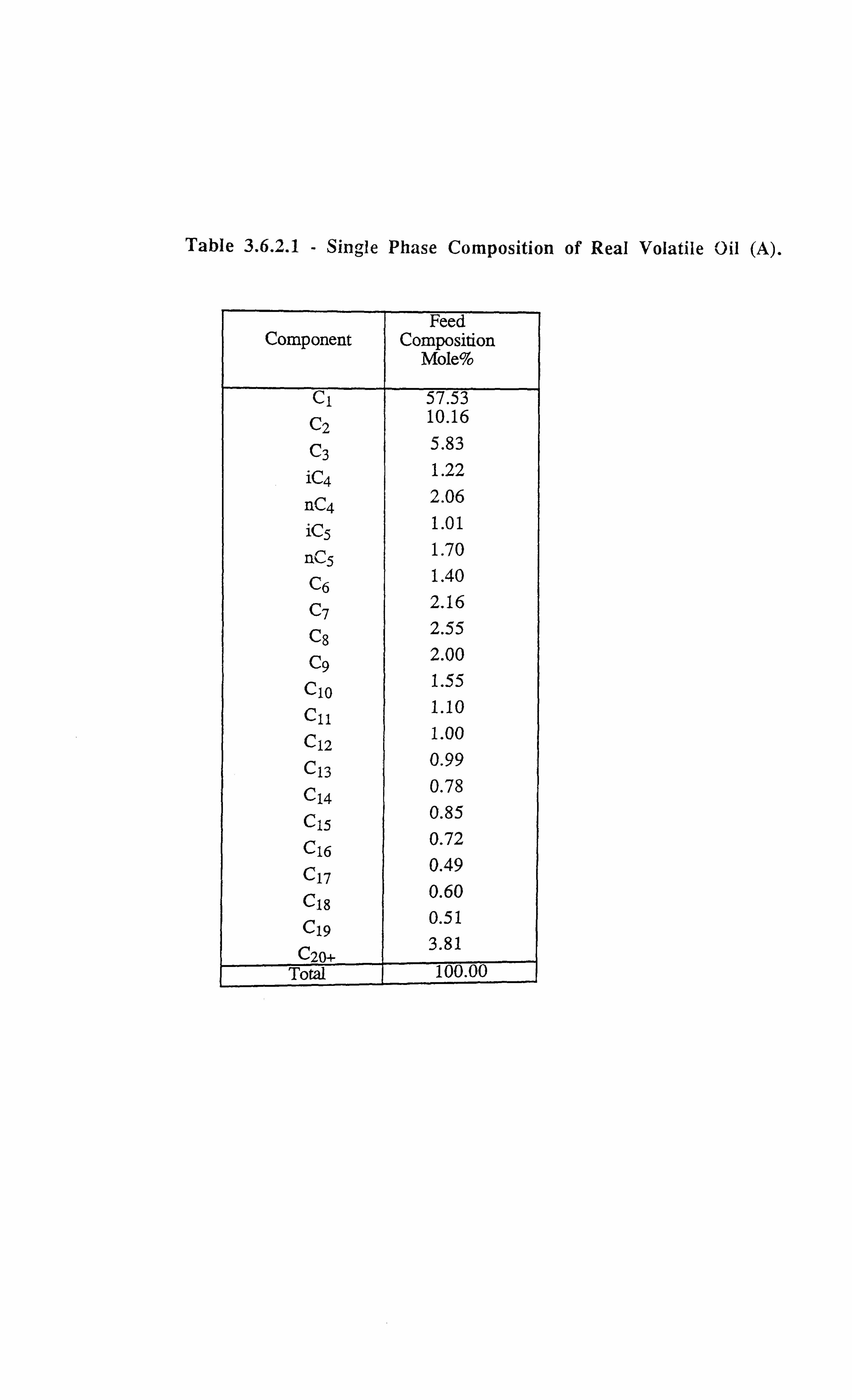
Table 3.6.2.1 - Single Phase Composition of Real Volatile Oil (A).
Component Feed
Composition Mole%
Cl 57.53 C2 10.16
C3 5.83
iC4 1.22
nC4 2.06
iC5 1.01
nC5 1.70
C6 1.40
C7 2.16
C8 2.55
C9 2.00
C10 1.55
Cil 1.10
C12 1.00
C13 0.99
C14 0.78
C15 0.85
C16 0.72
C17 0.49
C18 0.60
C19 0.51
C20+ 3.81
Total 100.00

0
rA
r1
E
N
M 4i
ctt E"ý
CD lý !ý --ý cT c V) c d' Cn O M N O N mot' M ýO cn C Z d) '-+ N C Q1 CT crl CT 00 N C d` 00 N 'O Vý 00 M r-+ 40 0o M C 00 VI © N M ý-0 N N *-+ oG N M ýt tT ýO d` 0 , lý [- -+ M N M M tin tý t+ý cri N N N N -- "-; , -; , --+ c5 CD C
CD ' C M
V_ ^ M oo O
N CT
- vn d-
N N
O C in O O O O C O O O C O C rn ý cT O O O O O O C O O O C O C O = - - C ýO r oo M Vý O C O O O O O O O O O O
°0° = '0
cq (-i `(j Z; -Z Cj -- C - -4 cC c5 c5 c7 C C C 0 C © Ö c5 ö
.ý - Ir) \, O C- V') M '
- d- - in tý O N O \Z M 00 ýt t- [ý \lD Ö
'O 00 Vn cM ý, O cß 1 t r--+ N - u-) tr, CT Oý mot- N mot' Oý In e e C <T mt 00 e cT mt Olý O c1 N \, O e c) C r-+ IC M d. N M N ßi'3 N M M N d' \O N N N N N N C O
r-,
cri
O \ 1- in M tiO r- r- C ' N CD CD CD CD CD CD CD CD CD CD CD O ý rn M O O tn M N CT oo N M O C O O C O O O O O O O CZ - Ln CT d. In O\ In r-+ N e O CD O O O C CD CD CD CD CD
v; Ö -+ cý Ö Ö '-+ Ö C Ö Ö C> Ö C5 Ö © Ö © Ö C
r-1
= C 00 C C N ir) N Lt Z ýlO V) cý N in Ca N C v', ý N O C rn
Ö
= - ro- [- M M N N r+ M O \, O r- \Z 00 00 -+ N l 00 N \O -+ N O
a . 0 cn r- N O N M 00 M - CD 00 N In r--+ N N d'
'" N Cr N r--ý M i CM N d' ýn d' N N N N --+ r-+ --ý -4 oc O
O O O 00 O N C> cO Cl% CD d' 1- 0 0 0 0 0 0 0 C
rý p N ý ýy d- tn , -- 'C 00 t'- t- ý r-+ V CD CD CD CD CD CD CD O = _-w -4 00 M to oo \Q N 00 \, O c*) N N - O O O O O C C M ý r-+ O O 0 0 0 C O Ö O O O Ö O O O O Ö O
Q 0 ^' N ch d" 'n U
ýo 00 0, . - r-4 - - - in - r- 00 O\ U ý,, ý ý} U ý ý U U U V U V U V U V U U U U j' ý ý.,
Ü

Table 3.6.2.3 - Interfacial Tension Measurements on Real Volatile Oil (A) for a CCE* test at 100°C.
No Pressure Liquid Density Vapour Density Measured IFT MPa gm/cc gm/cc mN/m
1 13.79 0.6900 0.1170 7.046
2 10.34 0.7060 0.0860 10.313
3 6.849 0.7260 0.0580 13.519
* See Table 3.6.2.2 for compositions
Table 3.6.2.4 - Interfacial Tension Measurements on Real Volatile Oil (A) for a Backward Multiple Contact Study* * with CH4+CO2 at 35.26 MPa and 100°C.
Stage No Liquid Density /cc
Vapour Density gm/cc
Measured IFT mN/m
1 0.6378 0.3581 0.663
2 0.6898 0.3660 1.420
3 0.7248 0.3636 2.170
4 0.7565 0.3505 3.239
** See Table 3.6.2.5 for compositions
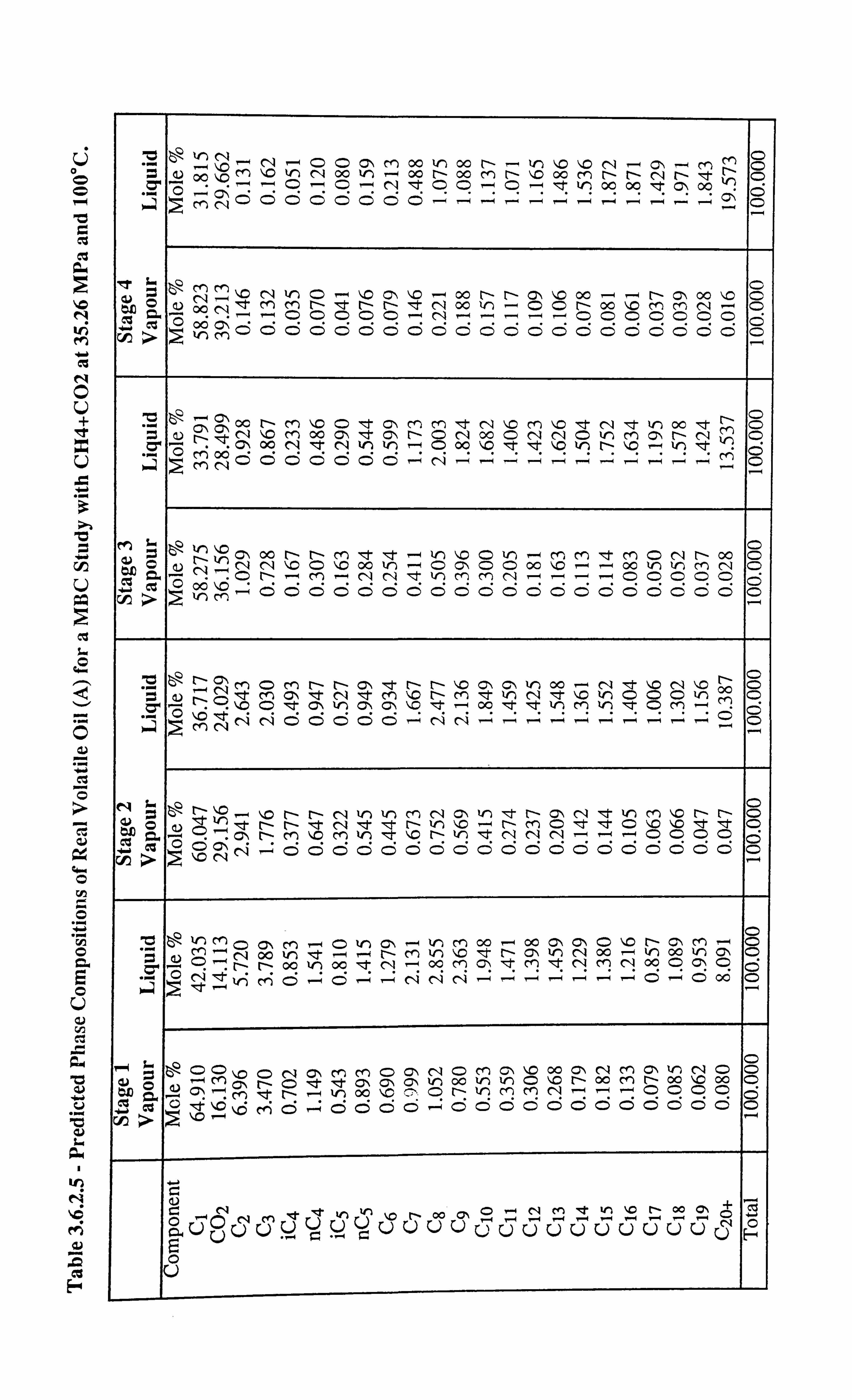
U 0 0 b
\o N
M
N
V
x U
3
U
cý L
a2
.. r
Gý
GG O
r
0
0
0 a. 0 U
zý aý V
V L
a Il) N
cts E"4
-ý --ý N -- C C M oo to oo In ýo ý, O N Ch *-- M M C
pp `p M ý V') N o0 v'l - 00 N oo M N C 00 M N N N N 'f r- a --ý O CD - C - N d. C C C 7t tn 00 00 C> oo O ;ý c,., °ciö ö ö ö ö 0 0 0 Z , -Z - - - -ý - -. - - - -ý
ý o
y N N in C r-+ \, O \, O - 00 N N cý \, O 00 - -4 N C\ oo '0 C
N Mt 00 M c N N N e N 00 V) - C C N 00 \D M M N - C C. -
ll r--m O O C C C 9-4 N r-+ r- C C C C C C O
cu od MC O O C C C O C C C O O C C C C C C C C C O
00 N M 1%c C lt C\ M M le N \lO M \IC lt N le l(1) oo d' M C N \Z cM 00 Oý t C N O N 00 O N N O 'n M C N N O O\ 00 N d' (N v) r-+ O oo ýc 'zt' ýO V-ý N ýo r-+ ýn d'
MNÖ Ö Ö Ö Ö Ö Ö r--ý rj
C
M = Zw C, r- Oý 00 N N rM d- d- ý in \O C V) "- M M M C N N oo
C O NN \, O O \O 00 N _ O O\ O O oo \, O Ö O
42 O N O C C C Z O C C O C O O C O C O C C O C C C C C C
C
= e, r- NM O M N N O d' N N \D O\ Cý in 00 , -" N d- \O N \Z r- Ö
i O ýfi r M ýt N ýt M tý M d- ýn N '
\O in '
O O O to M O - C d' O\ to clý Ol\ \, O r-+ 00 d- v ) M V ) - C M
,.. ý MN tV rV Ö Ö Ö Ö Ö r-+ N tV , -- r-- , -- "4 r+ .4 -
c O 2
N = C t `O Iý t- N u-ý M N O, in d' lý N d- V-) M �O t- [- C
O O le ir) d' N d' N d' d' N ýO r--ý '
N M C mt d' C \O 0 lKt le C ¢, M \Z d' ýO r- d N N N - r--1 C C C O
CD N (mal r-+ Ö Ö Ö Ö Ö Ö Ö Ö (:: 5 Ö Ö Ö Ö Ö Ö Ö Ö Ö Ö C
'C? 1. -) M C., rn T-+ O ý Oý "-4 to M oo -+ oo O\ Oh O ýO r-- c> M ý O 'E U MN 00 in ýt - --+ N M vý `O d' N C\ In N 00 yr 00 In
l C C
= --4 O [ý tý 00 u) oo d: N oo M Vý e M e N M N 00 C O ý C 0 cq -e tri M O O Q O oÖ C
OO \lo O N a\ M M O N O M Gý \O 00 O, \ N M OIN in N C C
O O M N O ýt d' to 00 to VI O M
'Z N
N 00 M N O
00 O
"O O
oo C
O u M in 00 O N M
'. ' c n -e \Zý M Ö --ý 0 0 0 O ý Ö Ö Ö Ö Ö Ö Ö Ö Ö Ö Ö Ö Ö
cn
I
° �t 'nt vl O N 00 O\ O '-+ N M d' ýO N 00 Oý +
A , Výýj ýj U V ý V V V U L Ü V 0 0 0 0 0 0 0 ý,
0 V
measurement. The equilibrium liquid phase was kept intact and was allowed to come in
contact with the fresh injection gas in the second stage and this process continued till the
vapour phase remained similar to the original gas that is being injected. The measured liquid
and vapour phase densities and interfacial tension data is furnished in Table 3.6.2.4 for all
four stages. The predicted liquid and vapour phase compositions are provided in Table
3.6.2.5.
3.6.3 : Real Black Oil RFS-1
Three multiple contact tests were performed on the real black oil RFS-1 at 34.58 MPa and
100°C. Similar to the previously mentioned backward contact study on the real volatile oil, a
four stage backward contact study was performed with pure methane as an injection gas, and
two multiple forward contacts were performed with pure methane and a mixture of methane
(79.86 mole %) and carbon dioxide (20.14 mole %) respectively. These experiments were
conducted in the vapour-liquid-equilibrium (V-L-E) facility.
The original single phase liquid composition of the real black oil is given in Table 3.6.3.1.
About 100cc of this oil were loaded into one of the windowed PVT cells. Into this oil about
70cc of pure methane was injected. The mixture was then taken to equilibrium, at 34.58 MPa
and the phase volumes, densities and compositions were recorded. The contact study was
performed for altogether four stages till the resultant equilibrium vapour phase composition
was virtually equal to 100 % methane. The two phase compositions are presented in Table
3.6.3.2. The event of equilibrium liquid droplets suspended on the pendant drop spout
surrounded by its equilibrium vapour phase was recorded for each stage. The video
recordings were subsequently employed to dimension the droplets and calculate the interfacial
tension from it. The liquid and vapour phase densities and interfacial tension values for this
test are provided in Table 3.6.3.3.
In the first forward contact test, about 50cc of the original RFS-1 oil were loaded into one of
the windowed PVT cells. Into this oil about 120cc of pure methane was injected. The
38
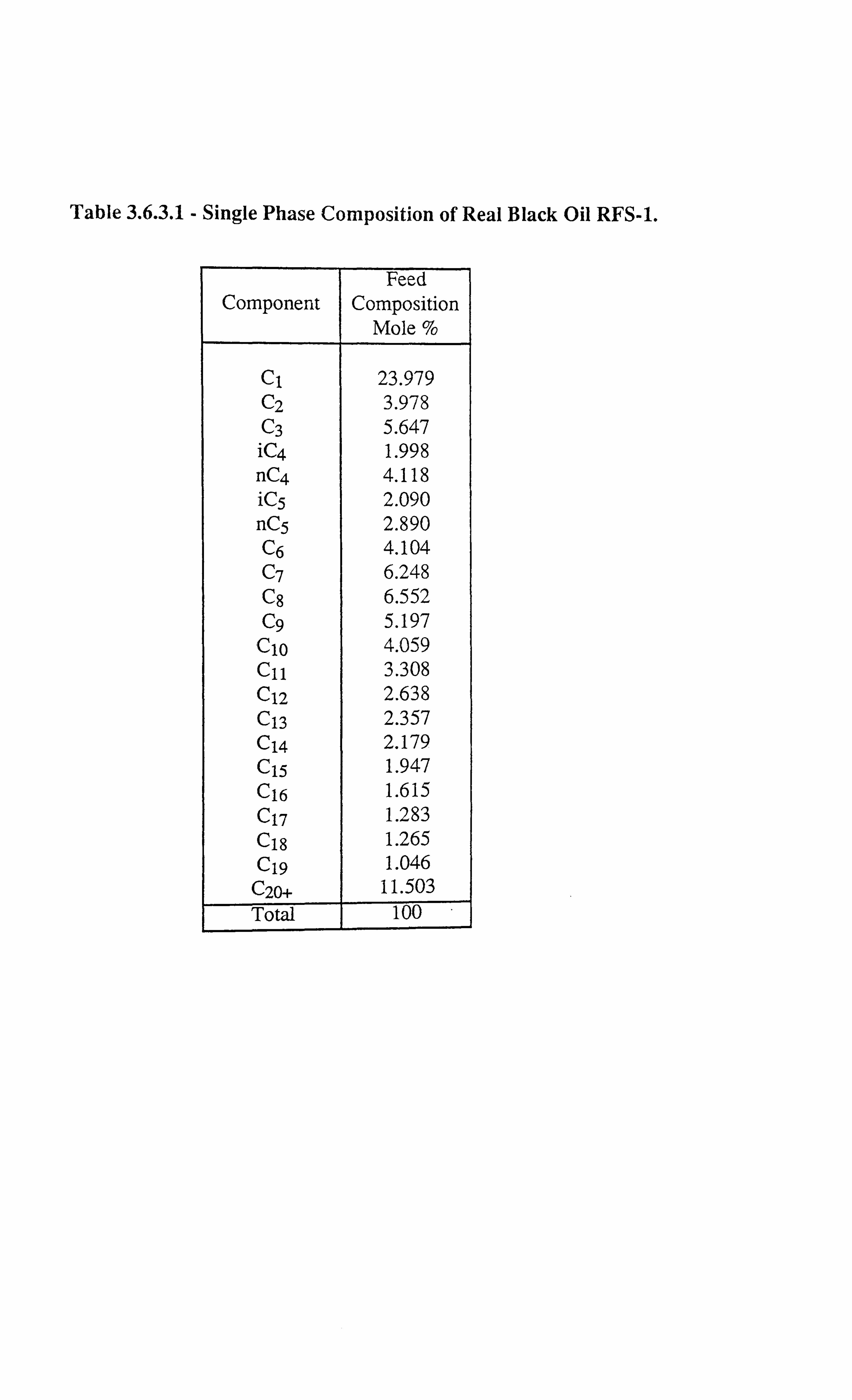
Table 3.6.3.1 - Single Phase Composition of Real Black Oil RFS-1.
Component Feed
Composition Mole %
Cl 23.979 C2 3.978 C3 5.647 iC4 1.998 nC4 4.118 iC5 2.090 nC5 2.890 C6 4.104 C7 6.248 C8 6.552 C9 5.197 C10 4.059 C11 3.308 C12 2.638 C13 2.357 C14 2.179 C15 1.947 C16 1.615 C17 1.283 C18 1.265 C19 1.046
C20. ß 11.503 Total 100

C/1
L
G! i
bA C. d
cn
L
42
L
E O
M
M cu
P. m .Q
ce &. 4
U 0 0
cý a co tn M
U
0-1
.o ýc>Oýý CD '
c>le -
I- \lO MOO r- V) \lpOl\ t-\Oývn00 IIZ - clq O O Uý00 :1 cfl N C\ \, O N1nC MOM[-O C'r NC ir) O O N r-+ MN M c1 c\ \z d -e vý cýc, pý \, OMMN "" O O O OO O O NN "-+N
Ö
M M M O d' V' V)cn cýin 00 \0 Cfl00M V O ý oO O l- tý `OCD gt tr- ý r-- I- ocýt N ootýýO M O m LL 3 O r-+ CD -- - rn V) výýtM NNr- -- -+000 [ c5 In Ö Ö Ö ÖÖ Ö Ö Ö ÖÖÖ ÖÖÖÖÖ ÖÖÖÖ Ö O
.a e, ýN 1- 0 \OM ýt' M MýDOOý MIýO-d' O\Oýt'N N O cnO\ N o0 tt M - O V ooO\O - NNM 0 00NM -t O
a N ID N \lO ýt ýIO M d- O '10 to O Ol\ 00 00 \, O in r-+ O '~ ýO O O OO O r-+ N MNN Nýý' ýýr-+-
Ö
M A, in l- ýt \, CN -ý C N 000 \ vi CD ýC00 NMMN N Ö 00 In r- nO r- oo 0O d-CD r- M00 ern 0O l-CD CD oO Vn O N d' -ý MN (: q In t- I- \, Oe M NNNr-+ r-+CD 0ý c5 O Ö O OO O Ö O OOO OÖ C5 ÖÖ ÖÖ00 0 O
ý N .O d'�t ý "f' d' NOt( 00ood' r'ý00rnýO N Ö
O O . O v-) eO O M oc oov-C\ 00 ONNC 'tr ývn N O - oo d. in NN CD r- C% le ood' cý r- ýD\lOM Mclý Oýo0 > c5
". " cl c 5 C '- N MNN ÖOÖ Cý O
N L' C O O 00 fl n00 -+ [- cT OLO e CNC OC CýNCh ý01 0ý M1- cý CI� - MVn00 r-+MI-1, ON 000D --SOO N O
[- CD M [-M d" [ý CD CD Iýi e MNNN - --0 0 c3 0 0 00 0 0 --ý OO OOOOO OOOO O
;O oM N N N N ý d' tý NN cnool - e Cý Ö
,ý N Ö Ö N N N N _ _ r r P--4 M N M Ö O \O OC
. '" ýý
N O "-ý -; Ný c flNN "-- _; ter: - -; 000 C O
s. = , ooý M OO\, O NNCD Oý I-CD 0 i oIn 00 lý' -, O ý -- Z ý- CD r, vi \, O ý 00
' ý _ _
MN t _ ý--ýýp . C
U ,, ,
; 00 NN N NýO tý e t Oý nýtM 2 m O
ý., fir--+ N Ö --ýÖ Ö ý ý r-,
Ö ÖÖÖ ÖÖ ÖÖÖÖ - O
C
p '"'' N
UU M
U rt
V d'n
ýU ý e V
t, V
00 O\ UV
----
UVUU -- 00 -
UUVU p j
`3
° U U ý F ., rz 0 U

Table 3.6.3.3 - Interfacial Tension Measurements on a Real Black Oil RFS-1 for a Backward Multiple Contact Study with CH4 at 34.58 MPa and 100°C (Compositions in Table 3.6.3.2).
Stage No Liquid Density Vapour Density Measured IFT* gm/cc gm/cc mN/m
2 0.6870 0.2390 2.189
3 0.7200 0.2170 3.319
4 0.7460 0.2060 4.515
* insufficient vapour in equilibrium did not allow IFT measurements for stage 1
Table 3.6.3.5 - Interfacial Tension Measurements on a Real Black Oil RFS-1 for a Forward Multiple Contact Study with CH4 at 34.58 MPa and 100°C (Compositions in Table 3.6.3.4).
Stage No Liquid Density Vapour Density Measured IFT gm/cc gm/cc mN/m
1 0.6920 0.2370 2.091
2 0.6420 0.2780 0.987
3 0.6110 0.3100 0.437
Table 3.6.3.7 - Interfacial Tension Measurements on a Real Black Oil RFS-1 for
a Forward Multiple Contact Study with CH4 (79.86 mole %) and Carbon
Dioxide (20.14 mole %) at 34.58 MPa and 100°C (Compositions in Table 3.6.3.6).
Stage No Liquid Density Vapour Density Measured IFT** gm/cc gm/cc mN/m
1 0.7070 0.3110 1.168
2 0.6430 0.3570 0.325
** insufficient vapour in equilibrium did not allow IFT measurements for stage
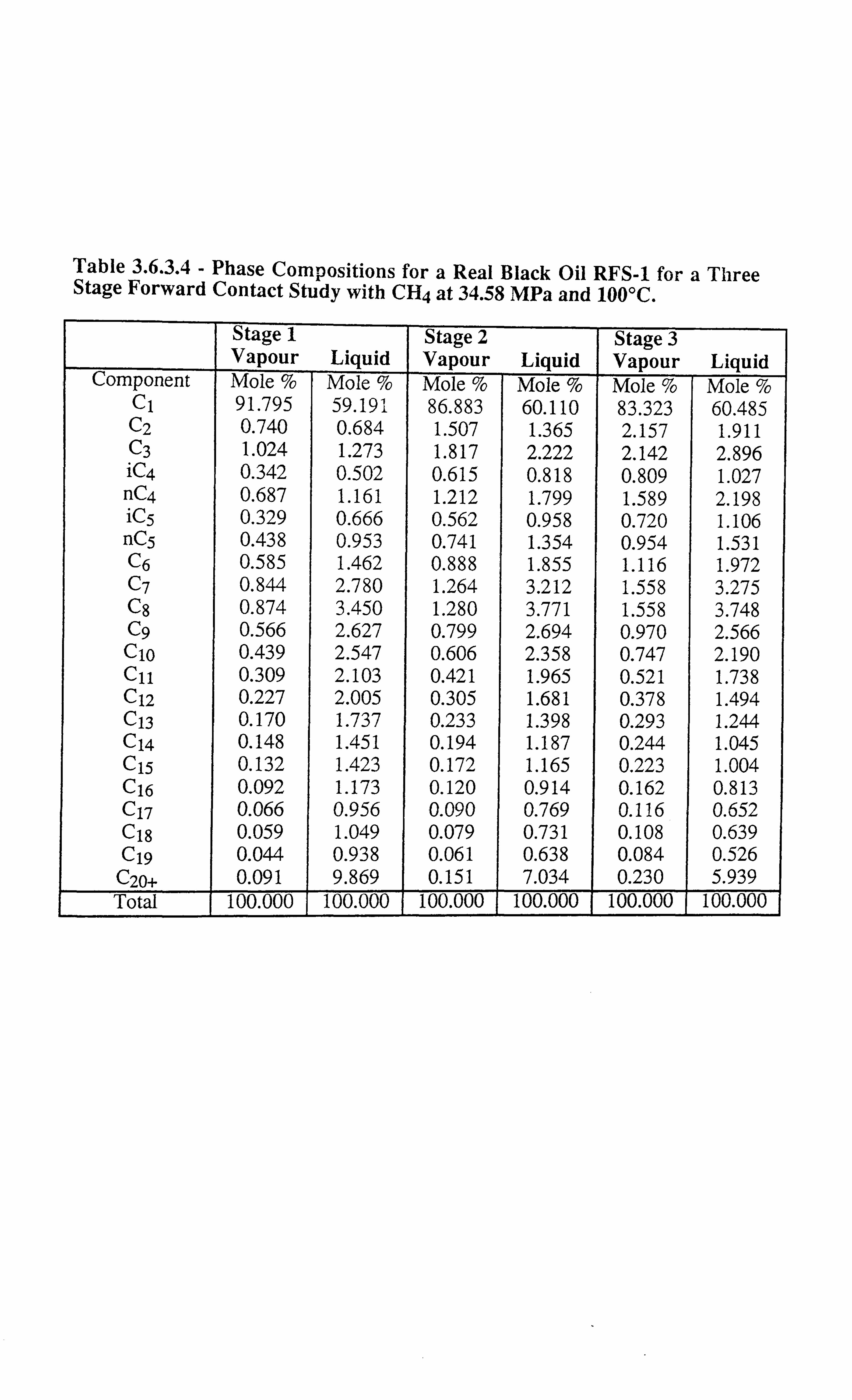
Table 3.6.3.4 - Phase Compositions for a Real Black Oil RFS-1 for a Three Stage Forward Contact Study with CH4 at 34.58 MPa and 100°C.
Stage 1 Vapour Liquid
Stage 2 Vapour Liquid
Stage 3 Vapour Liquid
Component Mole % Mole % Mole % Mole % Mole % Mole %- Cl 91.795 59.191 86.883 60.110 83.323 60.485 C2 0.740 0.684 1.507 1.365 2.157 1.911 C3 1.024 1.273 1.817 2.222 2.142 2.896 iC4 0.342 0.502 0.615 0.818 0.809 1.027 nC4 0.687 1.161 1.212 1.799 1.589 2.198 iC5 0.329 0.666 0.562 0.958 0.720 1.106 nC5 0.438 0.953 0.741 1.354 0.954 1.531 C6 0.585 1.462 0.888 1.855 1.116 1.972 C7 0.844 2.780 1.264 3.212 1.558 3.275 C8 0.874 3.450 1.280 3.771 1.558 3.748 C9 0.566 2.627 0.799 2.694 0.970 2.566 C10 0.439 2.547 0.606 2.358 0.747 2.190 C11 0.309 2.103 0.421 1.965 0.521 1.738 C12 0.227 2.005 0.305 1.681 0.378 1.494 C13 0.170 1.737 0.233 1.398 0.293 1.244 C14 0.148 1.451 0.194 1.187 0.244 1.045 C15 0.132 1.423 0.172 1.165 0.223 1.004 C16 0.092 1.173 0.120 0.914 0.162 0.813 C17 0.066 0.956 0.090 0.769 0.116 0.652 C18 0.059 1.049 0.079 0.731 0.108 0.639 C19 0.044 0.938 0.061 0.638 0.084 0.526
C20+ 0.091 9.869 0.151 7.034 0.230 5.939 Total 100.000 100.000 100.000 100.000 100.000 100.000

Table 3.6.3.6 - Phase Compositions for a Real Black Oil RFS-1 for a Three Stage Forward Contact Study with CH4 (79.86 mole %) and Carbon Dioxide (20.14 mole %) at 34.58 MPa and 100°C.
Stage 1 Stage 2 Stage 3 Vapour Liquid Vapour Liquid Vapour Liquid
Component Mole % Mole % Mole % Mole % Mole % Mole % Cl 73.763 48.830 70.706 51.221 67.920 53.904
CO2 16.897 14.329 14.039 12.176 11.322 10.553 C2 0.766 0.727 1.513 1.412 2.184 2.039 C3 1.087 1.288 2.031 2.249 2.809 2.952 iC4 0.368 0.490 0.674 0.810 0.920 1.021 nC4 0.745 1.125 1.347 1.763 1.820 2.137 iC5 0.358 0.625 0.629 0.915 0.842 1.058 nC5 0.473 0.887 0.828 1.268 1.115 1.444 C6 0.632 1.336 1.034 1.730 1.345 1.849 C7 0.922 2.479 1.448 2.896 1.895 2.935 C8 0.994 3.152 1.534 3.455 2.012 3.349 C9 0.656 2.377 0.975 2.430 1.287 2.272 C10 0.525 2.174 0.763 2.150 1.016 1.940 C11 0.378 1.862 0.537 1.655 0.730 1.463 C12 0.288 1.667 0.397 1.384 0.540 1.198 C13 0.231 1.509 0.318 1.259 0.432 1.070 C14 0.195 1.334 0.261 1.074 0.358 0.891 C15 0.180 1.346 0.229 1.018 0.348 0.833 C16 0.127 1.092 0.169 0.814 0.226 0.659 C17 0.100 0.959 0.127 0.678 0.193 0.534 C18 0.086 0.915 0.114 0.668 0.176 0.525 C19 0.068 0.785 0.090 0.579 0.140 0.442
C20+ 0.161 8.713 0.236 6.397 0.370 4.934 Total 100.000 100.000 100.000 100.000 100.000 100.000
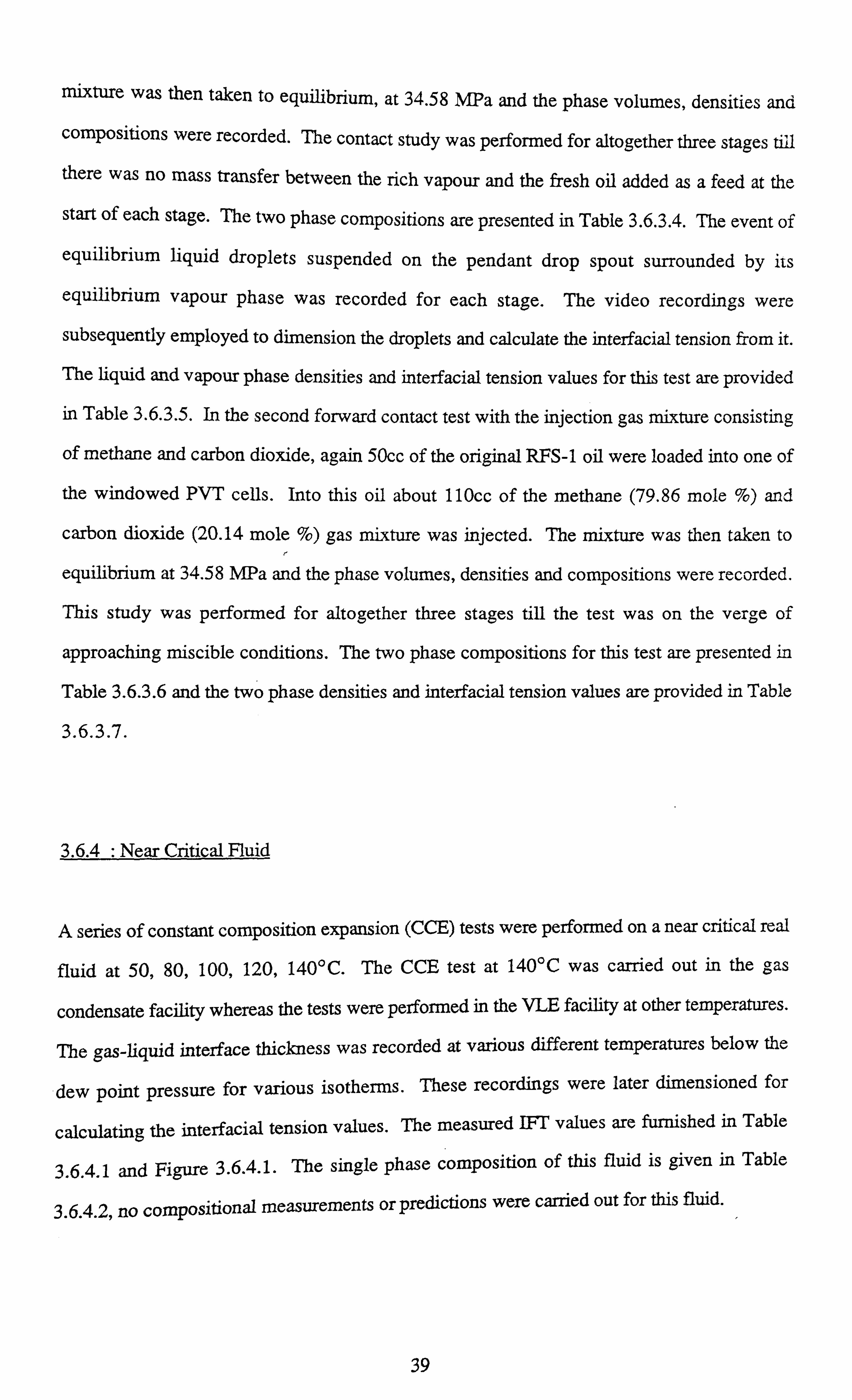
mixture was then taken to equilibrium, at 34.58 MPa and the phase volumes, densities and
compositions were recorded. The contact study was performed for altogether three stages till
there was no mass transfer between the rich vapour and the fresh oil added as a feed at the
start of each stage. The two phase compositions are presented in Table 3.6.3.4. The event of
equilibrium liquid droplets suspended on the pendant drop spout surrounded by its
equilibrium vapour phase was recorded for each stage. The video recordings were
subsequently employed to dimension the droplets and calculate the interfacial tension from it.
The liquid and vapour phase densities and interfacial tension values for this test are provided
in Table 3.6.3.5. In the second forward contact test with the injection gas mixture consisting
of methane and carbon dioxide, again 50cc of the original RFS-1 oil were loaded into one of
the windowed PVT cells. Into this oil about 110cc of the methane (79.86 mole %) and
carbon dioxide (20.14 mole %) gas mixture was injected. The mixture was then taken to
equilibrium at 34.58 MPa and the phase volumes, densities and compositions were recorded.
This study was performed for altogether three stages till the test was on the verge of
approaching miscible conditions. The two phase compositions for this test are presented in
Table 3.6.3.6 and the two phase densities and interfacial tension values are provided in Table
3.6.3.7.
3.6.4 : Near Critical Fluid
A series of constant composition expansion (CCE) tests were performed on a near critical real
fluid at 50,80,100,120,140°C. The CCE test at 140°C was carried out in the gas
condensate facility whereas the tests were performed in the VLE facility at other temperatures.
The gas-liquid interface thickness was recorded at various different temperatures below the
dew point pressure for various isotherms. These recordings were later dimensioned for
calculating the interfacial tension values. The measured IFT values are furnished in Table
3.6.4.1 and Figure 3.6.4.1. The single phase composition of this fluid is given in Table
3.6.4.2, no compositional measurements or predictions were carried out for this fluid.
39
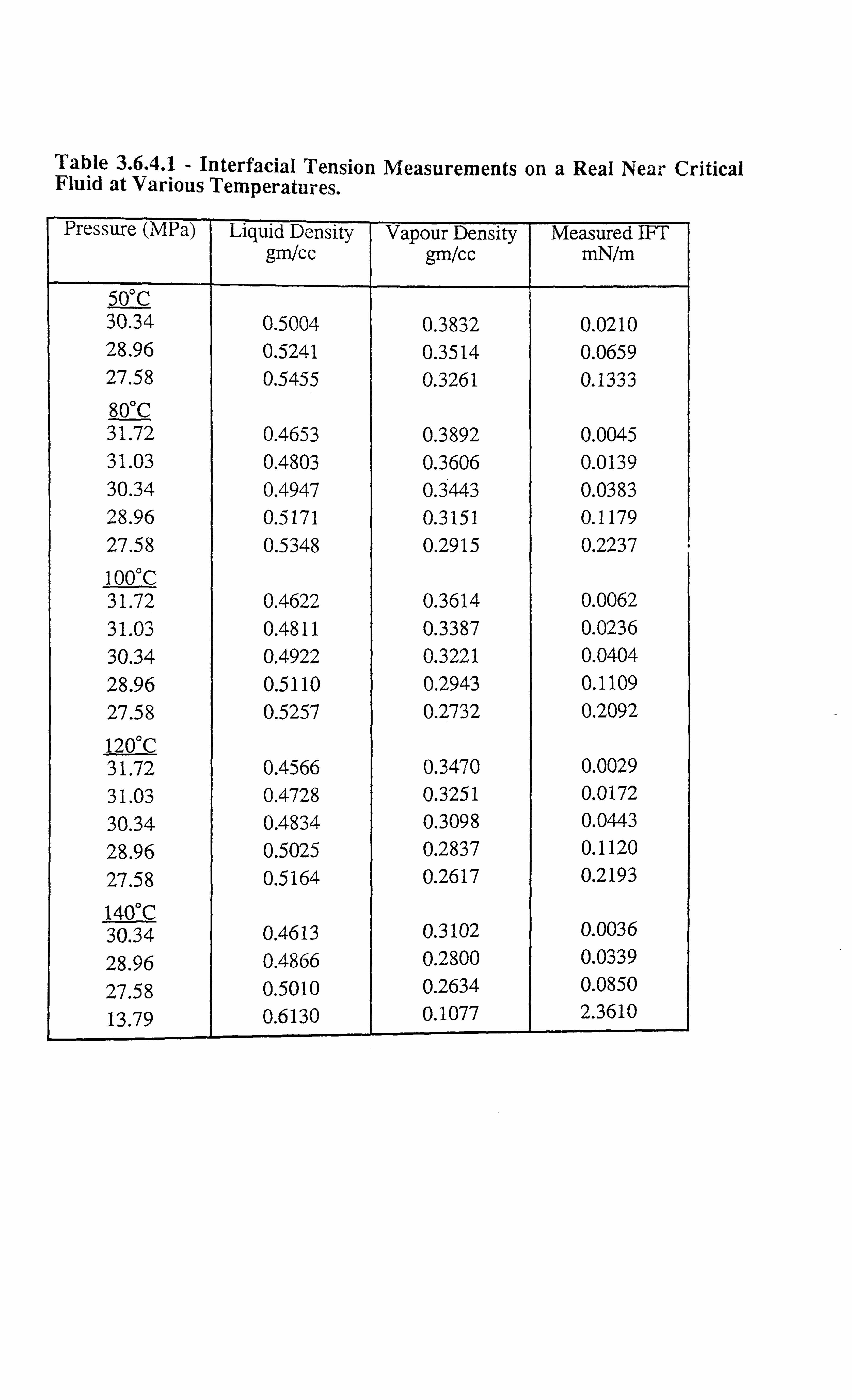
Table 3.6.4.1 - Interfacial Tension Measurements on a Real Near Critical Fluid at Various Temperatures.
Pressure (MPa) Liquid Density gm/cc
Vapour Density gm/cc
Measured IFT mN/m
50°C 30.34 0.5004 0.3832 0.0210 28.96 0.5241 0.3514 0.0659 27.58 0.5455 0.3261 0.1333 80°C 31.72 0.4653 0.3892 0.0045 31.03 0.4803 0.3606 0.0139 30.34 0.4947 0.3443 0.0383 28.96 0.5171 0.3151 0.1179 27.58 0.5348 0.2915 0.2237
100°C 31.72 0.4622 0.3614 0.0062 31.03 0.4811 0.3387 0.0236 30.34 0.4922 0.3221 0.0404 28.96 0.5110 0.2943 0.1109 27.58 0.5257 0.2732 0.2092
120°C 31.72 0.4566 0.3470 0.0029 31.03 0.4728 0.3251 0.0172 30.34 0.4834 0.3098 0.0443
28.96 0.5025 0.2837 0.1120 27.58 0.5164 0.2617 0.2193
140°C 30.34 0.4613 0.3102 0.0036
28.96 0.4866 0.2800 0.0339
27.58 0.5010 0.2634 0.0850
13.79 0.6130 0.1077 2.3610
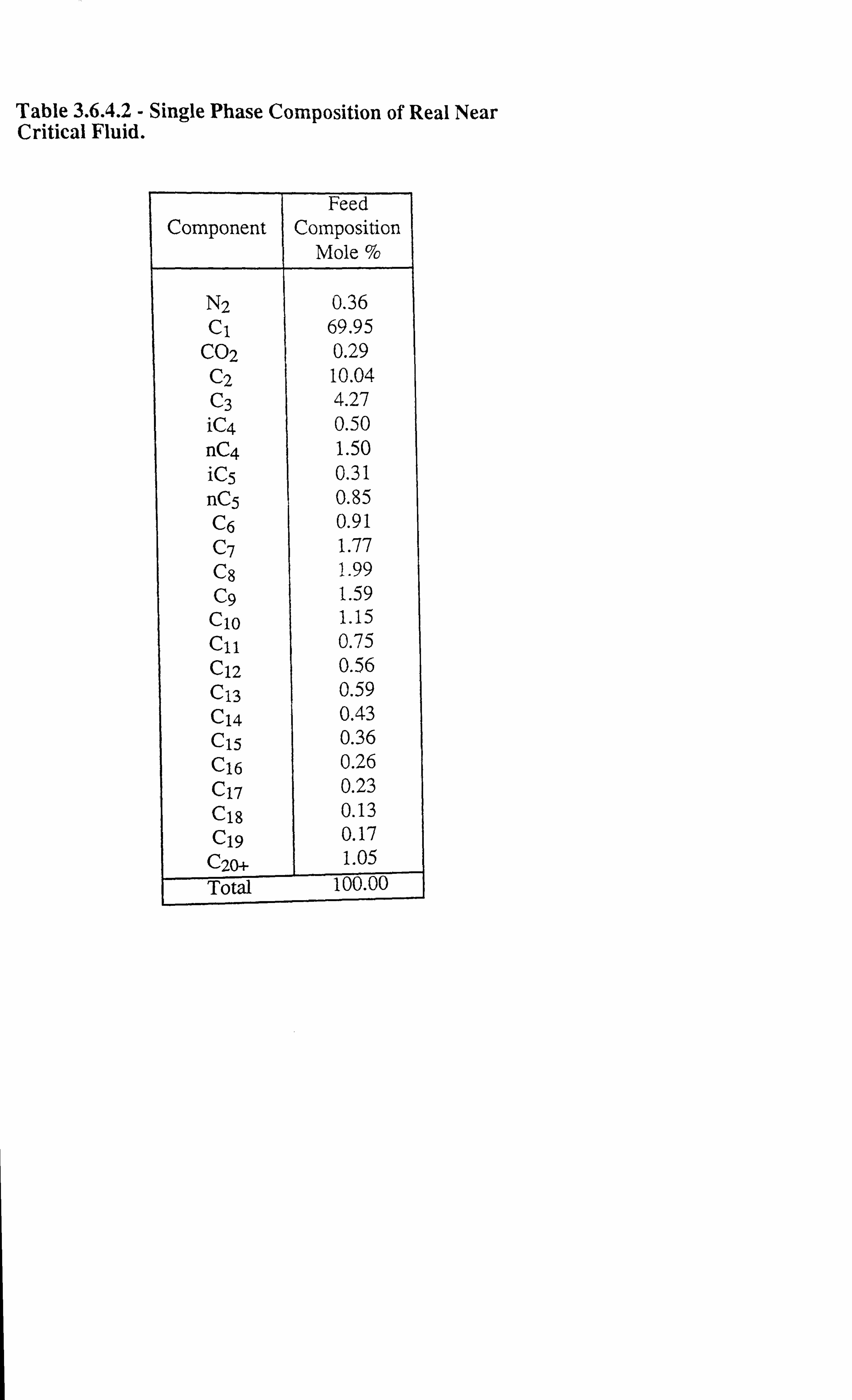
Table 3.6.4.2 - Single Phase Composition of Real Near Critical Fluid.
Component Feed
Composition Mole %
N2 0.36 Cl 69.95
CO2 0.29 C2 10.04 C3 4.27 iC4 0.50 nC4 1.50 iC5 0.31 nC5 0.85 C6 0.91 C7 1.77 C8 1.99 C9 1.59 C10 1.15 X11 0.75 C12 0.56 C13 0.59 C14 0.43 C15 0.36 C16 0.26 C17 0.23 C18 0.13 C19 0.17
C20. 1.05 Total 100.00

r_ -ZZ Z E O
cn
U 451 GJ
10
1
.1
. 01
nni
'- 50 deg C ý'- 80 deg C --0- 100 deg C
fr 120 deg C A 140degC
1
. VV1
10 20
Pressure, MPa
30 4C
Figure 3.6.4.1 - Interfacial Tension data on a Real ` gar Critical Fluid at Various Temperatures.
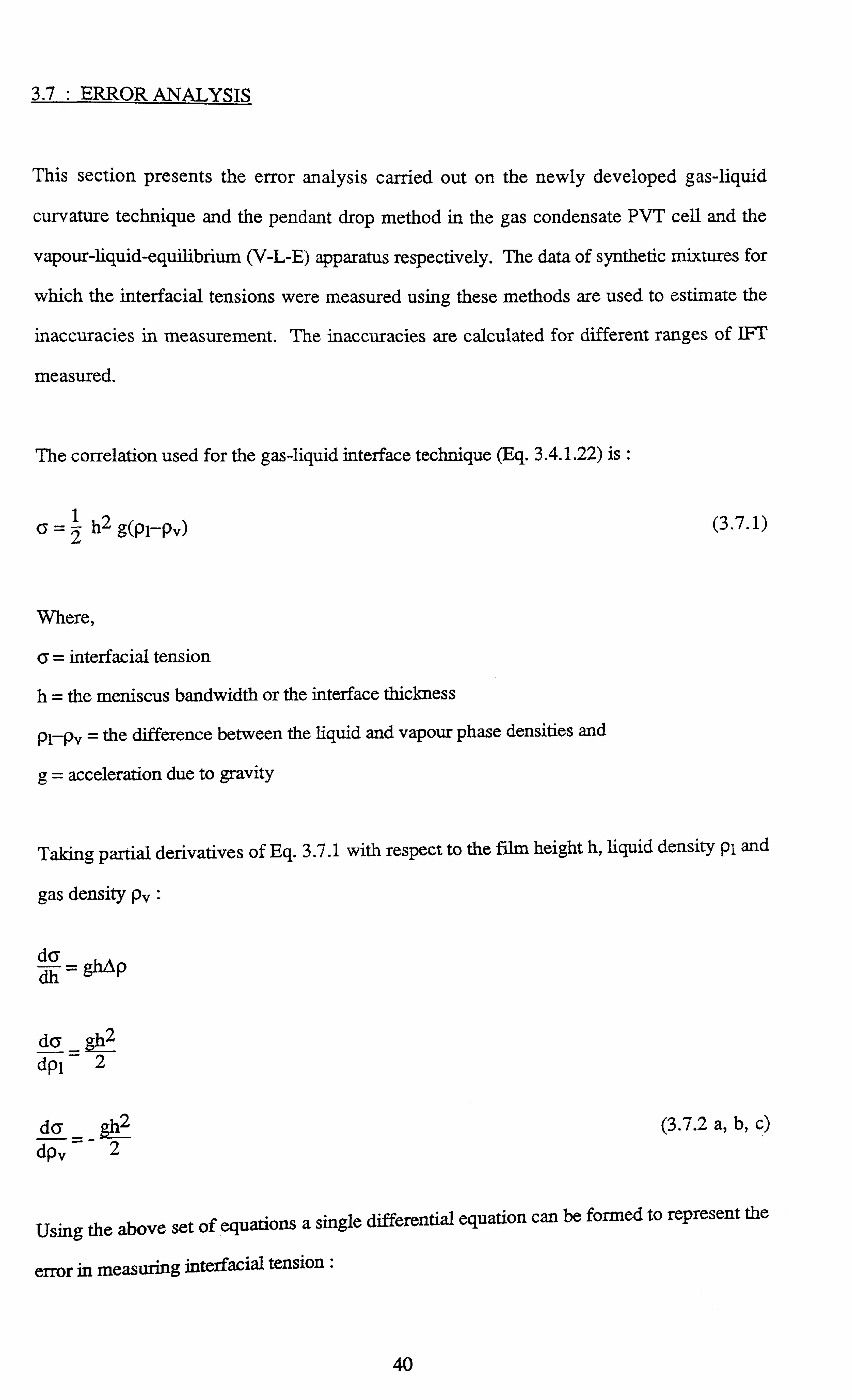
3.7 : ERROR ANALYSIS
This section presents the error analysis carried out on the newly developed gas-liquid
curvature technique and the pendant drop method in the gas condensate PVT cell and the
vapour-liquid-equilibrium (V-L-E) apparatus respectively. The data of synthetic mixtures for
which the interfacial tensions were measured using these methods are used to estimate the
inaccuracies in measurement. The inaccuracies are calculated for different ranges of IFT
measured.
The correlation used for the gas-liquid interface technique (Eq. 3.4.1.22) is :
ß=2 h2 g(Pi-Pv)
Where,
6= interfacial tension
h= the meniscus bandwidth or the interface thickness
pl-pv = the difference between the liquid and vapour phase densities and
g= acceleration due to gravity
(3.7.1)
Taking partial derivatives of Eq. 3.7.1 with respect to the film height h, liquid density pl and
gas density pv :
da - ghAp dh
da_gh2 dpl- 2
dß gh2 dpv 2
(3.7.2 a, b, c)
Using the above set of equations a single differential equation can be formed to represent the
error in measuring interfacial tension :
40
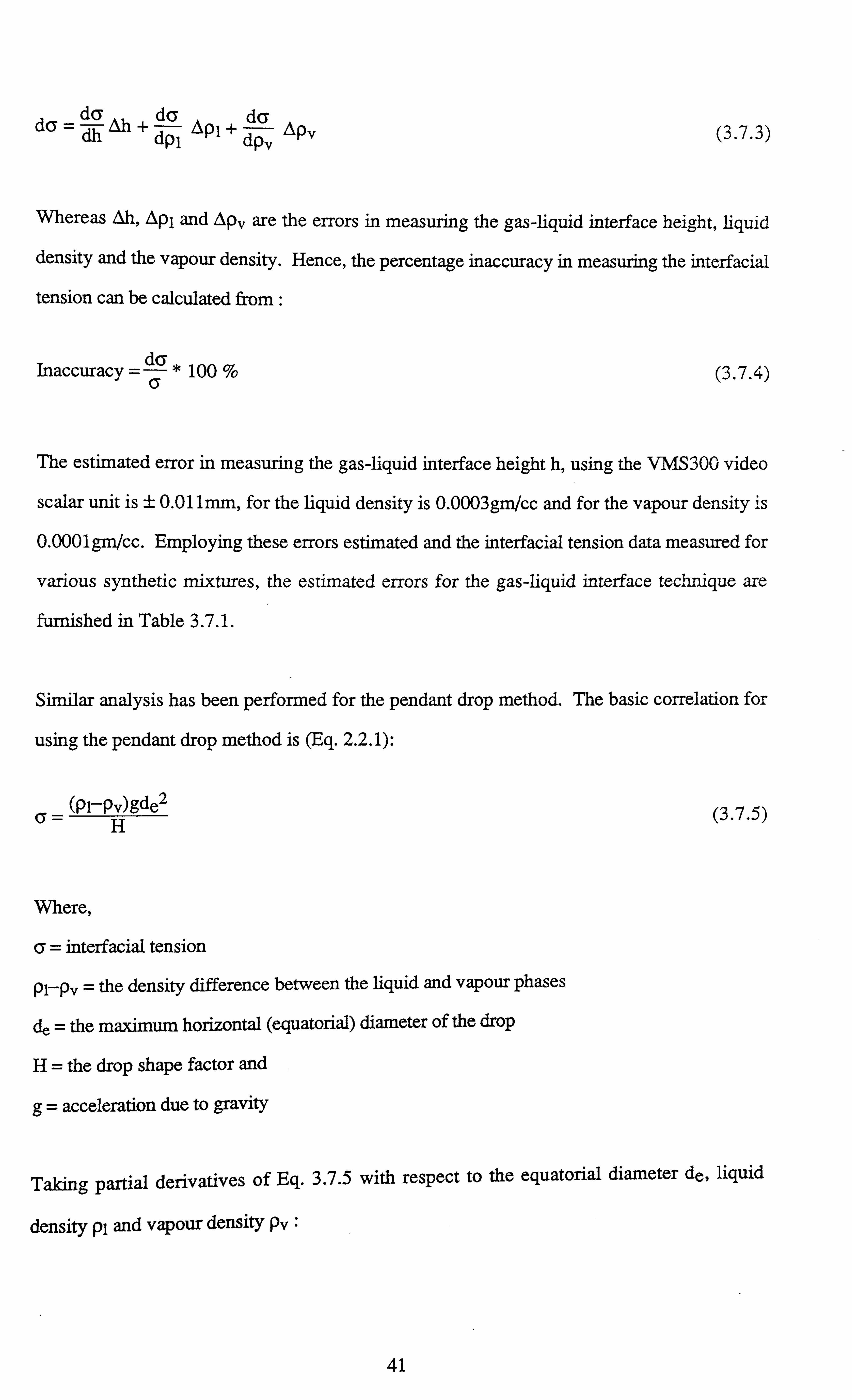
da = oh + da
PI Ap, + dPdßý opv (3.7.3)
Whereas Oh, Apl and App are the errors in measuring the gas-liquid interface height, liquid
density and the vapour density. Hence, the percentage inaccuracy in measuring the interfacial
tension can be calculated from :
Inaccuracy = ä6
* 100 % (3.7.4)
The estimated error in measuring the gas-liquid interface height h, using the VMS300 video
scalar unit is ± 0.011mm, for the liquid density is 0.0003gm/cc and for the vapour density is
0.0001gm/cc. Employing these errors estimated and the interfacial tension data measured for
various synthetic mixtures, the estimated errors for the gas-liquid interface technique are
furnished in Table 3.7.1.
Similar analysis has been performed for the pendant drop method. The basic correlation for
using the pendant drop method is (Eq. 2.2.1):
6= (Pl-Pv)gde2
H
Where,
6= interfacial tension
pi-pv = the density difference between the liquid and vapour phases
de = the maximum horizontal (equatorial) diameter of the drop
H= the drop shape factor and
g= acceleration due to gravity
(3.7.5)
Taking partial derivatives of Eq. 3.7.5 with respect to the equatorial diameter de, liquid
density pi and vapour density pv :
41
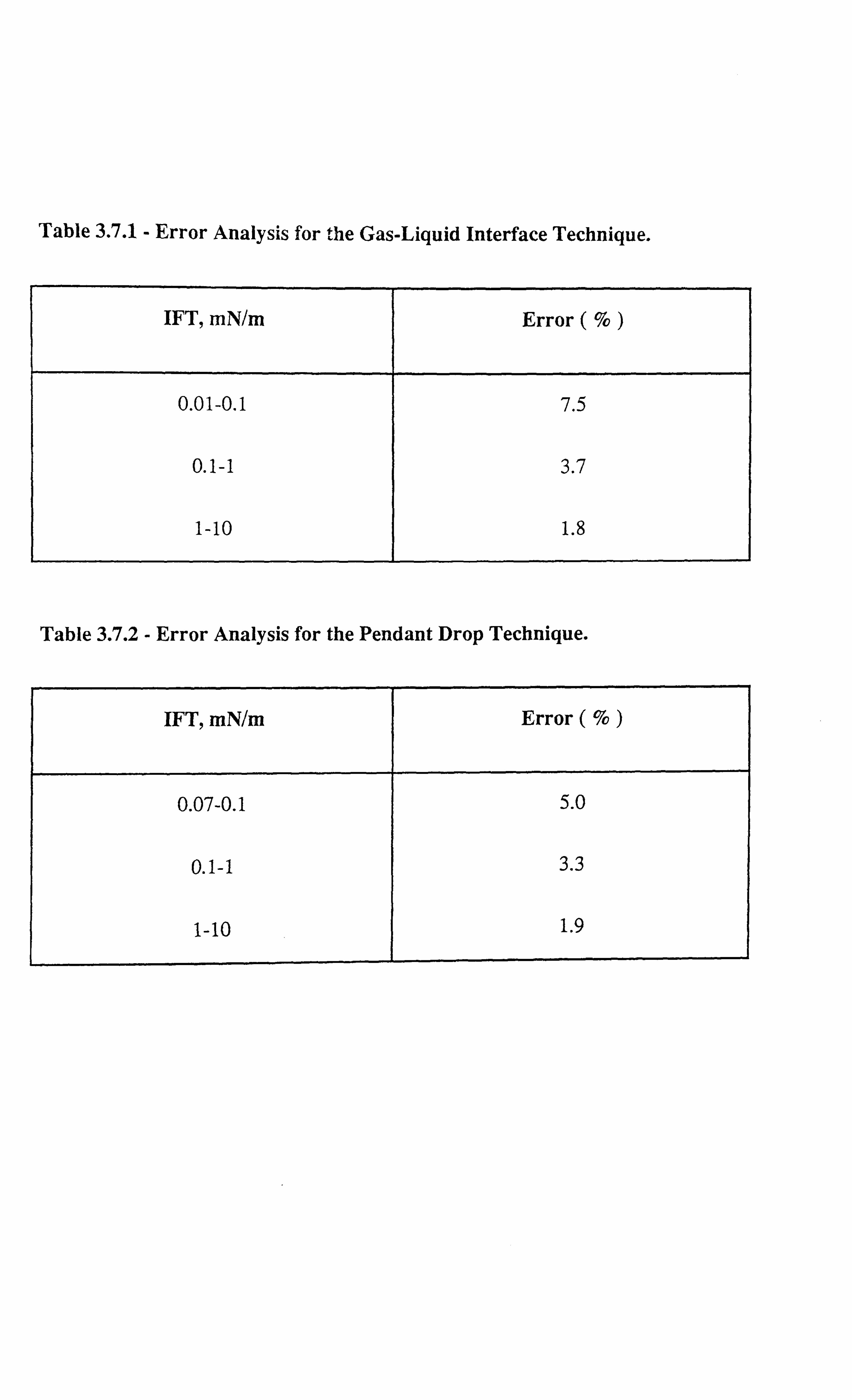
Table 3.7.1 - Error Analysis for the Gas-Liquid Interface Technique.
IFT, mN/m Error (%o )
0.01-0.1 7.5
0.1-1 3.7
1-10 1.8
Table 3.7.2 - Error Analysis for the Pendant Drop Technique.
IFT, mN/m Error (%}
0.07-0.1 5.0
0.1-1 3.3
1-10 1.9
_ da 2L pgde dde H
dß' gde2 dpi H
d6 _
gde2 dpi- H (3.7.6 a, b, c)
Similar to Eq. 3.7.3 we have :
dß = da Ode + da Pl
Apl + dPd6ý Apv (3.7.7)
Whereas dde, AN and Opi are the errors in measuring the equatorial diameter, liquid and
vapour density. The estimated error in measuring de is ± 0.008mm, for the liquid density is
0.0003 gm/cc and for the vapour density is 0.0001 gm/cc. Hence from Eq. 3.7.4 the errors for the pendant drop method can also be estimated and are presented in Table 3.7.2.
References
1) Danesh, A., Todd, A. C., Somerville, J. and Dandekar, A.: "Direct
Measurement of Interfacial Tension, Density, Volume, and Compositions of
Gas - Condensate System", Trans IChem E, Vol. 68, Part A, pp. 325-330,
(Jul., 1990).
2) Danesh, A. and Todd, A. C.: "A Novel Sampling Method for Compositional
Analysis of High Pressure Fluids", Fluid Phase Equilibria, Vol. 57, pp. 161-
171, (1990).
3) Groenveld, P.: "High Capillary Number Withdrawal from Viscous Newtonian
Liquids by Flat Plates", Chemical Engineering Science, Vol. 25, pp. 33-40,
(1970).
4) Wilson, S. D. R. and Jones, A. F.: "The Entry of a Falling Film into a Pool and
Air Entrainment Problem", J. Fluid Mech., Vol. 128, pp. 219-230, (1983).
Al

5) Lee, Chien. Y. and Tallmadge, J. A.: "Meniscus Shapes in Withdrawal of Flat
Sheets from Liquid Baths. 2. A Quasi - one - Dimensional Flow Model for
Low Capillary Numbers", Industrial & Engineering Chemistry (1 & EC)
Fundamentals, Vol. 14, No. 2, pp. 120-126, (1975).
6) Inverarity, G.: "Dynamic Wetting of Glass Fibre and Polymer Fibre", British
Polymer Journal, Vol. 1, pp. 245-251, (Nov., 1969).
7) Burley, R. and Kennedy, B. S.: "A Study of the Dynamic Wetting Behaviour
of Polyester Tapes", The British Polymer Journal, pp. 140-143, (Dec., 1976).
8) White, D. A. and Tallmadge, J. A.: "A Theory of Withdrawal of Cylinders
from Liquid Baths", AIChEJ? Vol. 12, No. 2, (Mar., 1966).
9) Tallmadge, J. A. and White, D. A.: "Film Properties and Design Procedures in
Cylinder Withdrawal", Industrial & Engineering Chemistry (I & EC) Process
Design & Development, Vol. 7, No. 4, pp. 503-508, (Oct., 1968).
10) White, D. A. and Tallmadge, J. A.: "A Gravity Corrected Theory for Cylinder
Withdrawal", AIChEJ, Vol. 13, No. 4, pp. 745-750, (Jul., 1967).
11) White, D. A. and Tallmadge, J. A.: "Static Menisci on the Outside of
Cylinders", J. Fluid Mech. Vol. 23, Part 2, pp. 325-335, (1965).
12) Kennedy, B. S. and Burley, R.: "Dynamic Fluid Interface Displacement and
Prediction of Air Entrainment", J. Col. & Int. Sci., Vol. 62, No. 1, pp. 48-62,
(Oct., 1977).
13) Danesh, A., Henderson, G. D., Krinis, D. and Peden J. M.: Paper Presented at
the SPE 63 rd Annual Tech. Conf., Houston, Texas, SPE 18316, (1988).
14) Cahn, J. W.: "Critical Point Wetting", The J. Chem. Physics, Vol. 66, No. 8,
pp. 3667-3672, (April, 1977).
15) Sage, B. H., Hicks, B. L. and Lacey, W. N.: "Phase Equilibria in Hydrocarbon
Systems, The Methane -n- Butane System in the Two Phase Region",
Industrial & Engineering Chemistry (I & EC), Vol. 32, No. 8, pp. 1088-
1091.
16) Pennington, B. F. and Hough, E. W.: "Interfacial Tension of the Methane -
Normal Butane System", Producers Monthly, pp. 4, (Jul., 1965).
43

17) Stegemeier, G. L., Pennington, B. F., Brauer, E. B. and Hough, E. W.:
"Interfacial Tension of the Methane - Normal Decane System", Society of
Petroleum Engineers Journal (SPEJ), pp. 257-260, (Sep., 1962). 18) Sage, B. H. and Lacey, W. N.: "Thermodynamic Properties of the Lighter
Paraffin Hydrocarbons and Nitrogen", API, New York, (1950).
19) Haniff, M. S. and Pearce, A. J.: "Measuring Interfacial Tension in a Methane - Propane Gas - Condensate System Using a Laser Light Scattering Technique",
SPE 19025, (1988).
20) Sage, B. H, Lacey, W. N. and Schaefsma, J. G.: "Phase Equilibria in
Hydrocarbon Systems", Industrial & Engineering Chemistry (I & EC), Vol.
26, pp. 214-217, (1934).
21) Reamer, H. H, Sage, B. H. and Lacey, W. N.: "Phase Equilibria in
Hydrocarbon Systems", Industrial & Engineering Chemistry (I & EC), Vol.
42, pp. 534-539, (1950).
22) Gasem, K. A. M., Dickson, K. B., Dulcamara, P. B., Nagarajan, N. and
Robinson, R. L. Jr.: "Equilibrium Phase Compositions, Phase Densities, and
Interfacial Tensions for CO2 + Hydrocarbon Systems. 5. CO2 +n-
Tetradecane", J. Chem & Engg. Data, Vol. 34, No. 2, pp. 191-195, (1989).
23) Adam, N. K.: "The Physics and Chemistry of Surfaces", Oxford University
Press, London, 3rd Edition, (1941).
44
CHAPTER 4 PREDICTIVE TECHNIQUES FOR INTERFACIAL TENSION
4.1 : INTRODUCTION
In this chapter some of the predictive techniques for estimating the interfacial tension (EFT) are
reviewed in details. The IFT of hydrocarbon mixtures at high pressures can be estimated by
several methods. Although all the methods have theoretical foundations, they rely to certain
extent on experimentally determined parameters.
The lack of reliable experimental data and the need for good IFT values have sustained a
continuous interest for past sixty years in the development of correlations to predict this
property. Several methods have been devised which make use of the various properties of the
fluids, such as density [2,3,4,5], liquid compressibility[6'71, and the enthalpy of
vaporisation[8]. More recently, Sivaraman et. al. {91, used the latent heat of vaporisation to
predict IFT of pure alkanes, napthenic and aromatic compounds over a wide range of
temperature from freezing to the critical point of the fluids. Here the most widely used
correlations in the petroleum industry are discussed in details.
4.2 : PARACHOR METHOD
This is the most commonly used method, which correlates the density difference of the liquid
and vapour phases with the IFT. It was first developed by Macleod[3], for pure component
systems, and later modified by Sugden[4], who introduced the parachor concept. Weinaug
and Katz[51, introduced simple mixing rules to allow the prediction of the IFT of mixtures.
It was first observed by Macleod[3], that the interfacial tension (6) of pure components was
related to the density difference between the liquid and saturated vapour by the expression :
45

6=C(Ap)E
Eq. 4.2.1, was later modified by Sugden[4], to obtain the following:
6ý�E _ [P] M
(4.2.1, '
(4.2.2
The quantity [P], is the property called parachor, which is the property of each compound m- is discussed further in Section 4.2.1. E, is the exponent equal to 4 as proposed c,
Macleod[3], in the original Eq. 4.2.2, and M, is the molecular weight of the pure compoun__.
Weinaug and Katz[51, improved Eq. 4.2.2 to make it applicable to mixtures and proposed t_
following:
n
ßl/E _ Plm(Pixi) - Pvm(PiYi) (4.2.
Where,
6= interfacial tension
E= the exponent ;=4
pim = the molar liquid density
Pi = the parachor of the ith component
Xi = liquid mole fraction of the ith component
pvm = the molar vapour density and
Yi = vapour mole fraction of the ith component
It is evident that a simple molar mixing rule is used to obtain the parachors of the liquid
(ZPiXi) and the vapour (EPiYi) respectively. For prediction of IFT of hydrocarbons, the
compositional and density data obtained either from experimentation or from EOS models can
be used. The parachor values for various pure components have been reported by several
authors[4,5,8]. Hough and Stegemeier{8}, have given a plot of parachor against the carbon
numbers for normal paraffins ranging from C1 to C20 (Figure 4.2.1), it follows a well
46
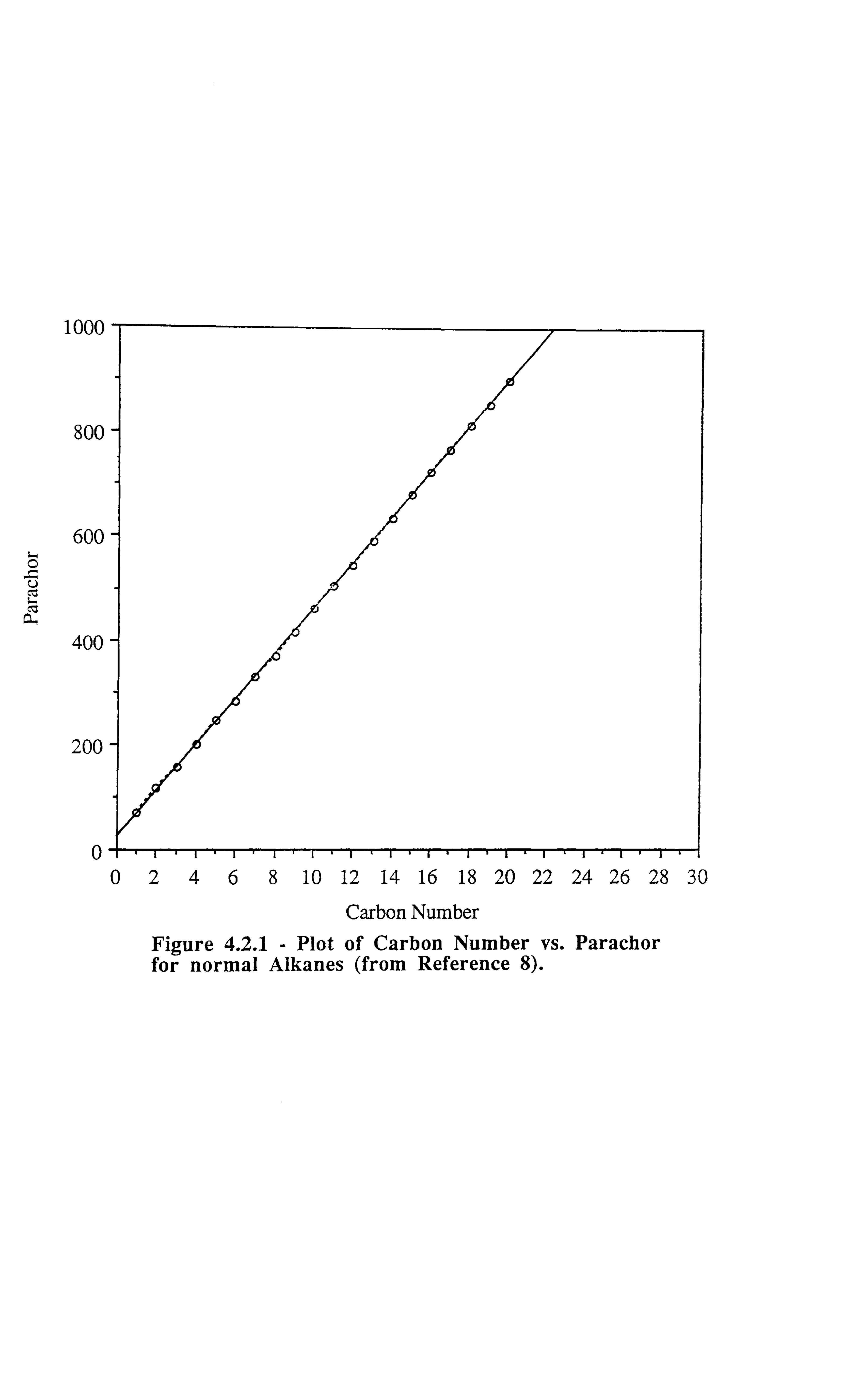
O
U CC$
cý
1000
800
600
400
200
0 02468 10 12 14 16 18 20 22 24 26 28 30
Carbon Number Figure 4.2.1 - Plot of Carbon Number vs. Parachor for normal Alkanes (from Reference 8).

defined linear relationship which can be used for evaluating parachor values for normal
paraffins hydrocarbons for predicting IFTs using Eq. 4.2.2 or 4.2.3. From Figure 4.2.1:
Pa = 23.85 + 43.73CN
where,
Pa = parachor of a normal paraffin and
CN = carbon number
(4.2.4)
This method is suitable only for synthetic mixtures with well defined compositions.
However, for the real reservoir fluids the exact composition is usually not known. All
isomers are combined in groups such as C6's, C7's etc. To obtain the parachors for such
groups, correlations of parachors with molecular weight of the hydrocarbon compounds were
introduced by Katz and Monroe[22], Figure 4.2.2. They measured the surface tension of
C7+ residues of various crudes to prepare Figure 4.2.2. However, it has been indicated by
Firoozabadi et. al. 1111 that this approach underestimates the interfacial tension in a certain
range. This could be attributed to the limited range of data employed in the approach of Katz
et. al. [22]. In order to circumvent this problem, Firoozabadi et al1111, determined parachors
of a wide range of crude oil fractions with a broad band of molecular weights and proposed
the following correlation (Figure 4.2.3):
P6=-11.4+3.23 M-0.0022 M2
Where,
Pu = the parachor of the plus fraction of a real reservoir fluid and
M= the molecular weight of the plus fraction of a real reservoir fluid
(4.2.5)
Eq. 4.2.5, should not be used to evaluate parachor of the oil heavy end, which generally
contains a high concentration of asphaltic materials.
47

11000
900
800
70C
s " n-Porcffins Q Hepfones plus cf Ref 3- 68 � j_-_. _ Goso�ines
Crude oi� -- -f iII ýi
ý1 tii
60C
0 ö 50C 0
40C
300
200
101
ý- 0 100 200 300 400
Molecular weight
Figure 4.2.2 - Parachors for Hydrocarbons (from Reference 22).
1200
y $00 0 s V ß L tq
a 400
n
" Crude A cuts " Crude B cuts A Crude C cuts " Crude D last cut "
" N-Paraffins
0 200 400 600
Molecular weight
Figure 4.2.3 - Parachors vs. Molecular Weight for Crude Cuts and n-Paraffins. (from Reference 11).
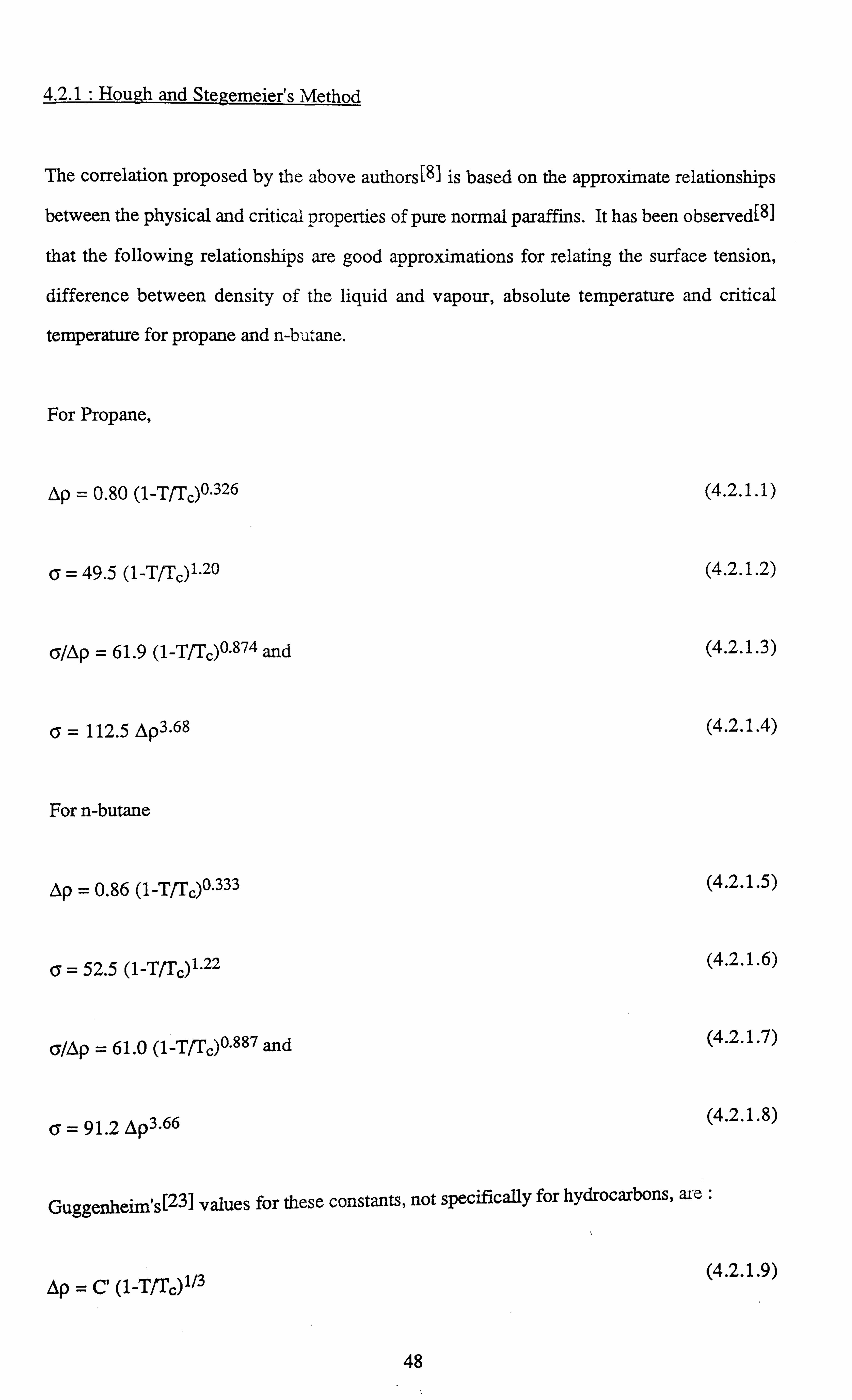
4.2.1: Hough and Stegemeier's Method
The correlation proposed by the above authors[g] is based on the approximate relationships
between the physical and critical properties of pure normal paraffins. It has been observed[8]
that the following relationships are good approximations for relating the surface tension,
difference between density of the liquid and vapour, absolute temperature and critical
temperature for propane and n-butane.
For Propane,
Op = 0.80 (1-T/TC)0.326 (4.2.1.1)
ß= 49.5 (1-T/T )1.20 (4.2.1.2)
6/Op = 61.9 (1-T/Tc)0.874 and (4.2.1.3)
6= 112.5 A p3.68 (4.2.1.4)
For n-butane
Ap = 0.86 (1-T/T )0.333 (4.2.1.5)
a= 52.5 (1-TfT )1.22 (4.2.1.6)
ß/Ap = 61.0 (1-T/TC)0.887 and (4.2.1.7)
ß= 91.2 Ap3.66
Guggenheim's[231 values for these constants, not specifically for hydrocarbons, are :
(4.2.1.9) ep = C' (1-T/TC)1/3
48
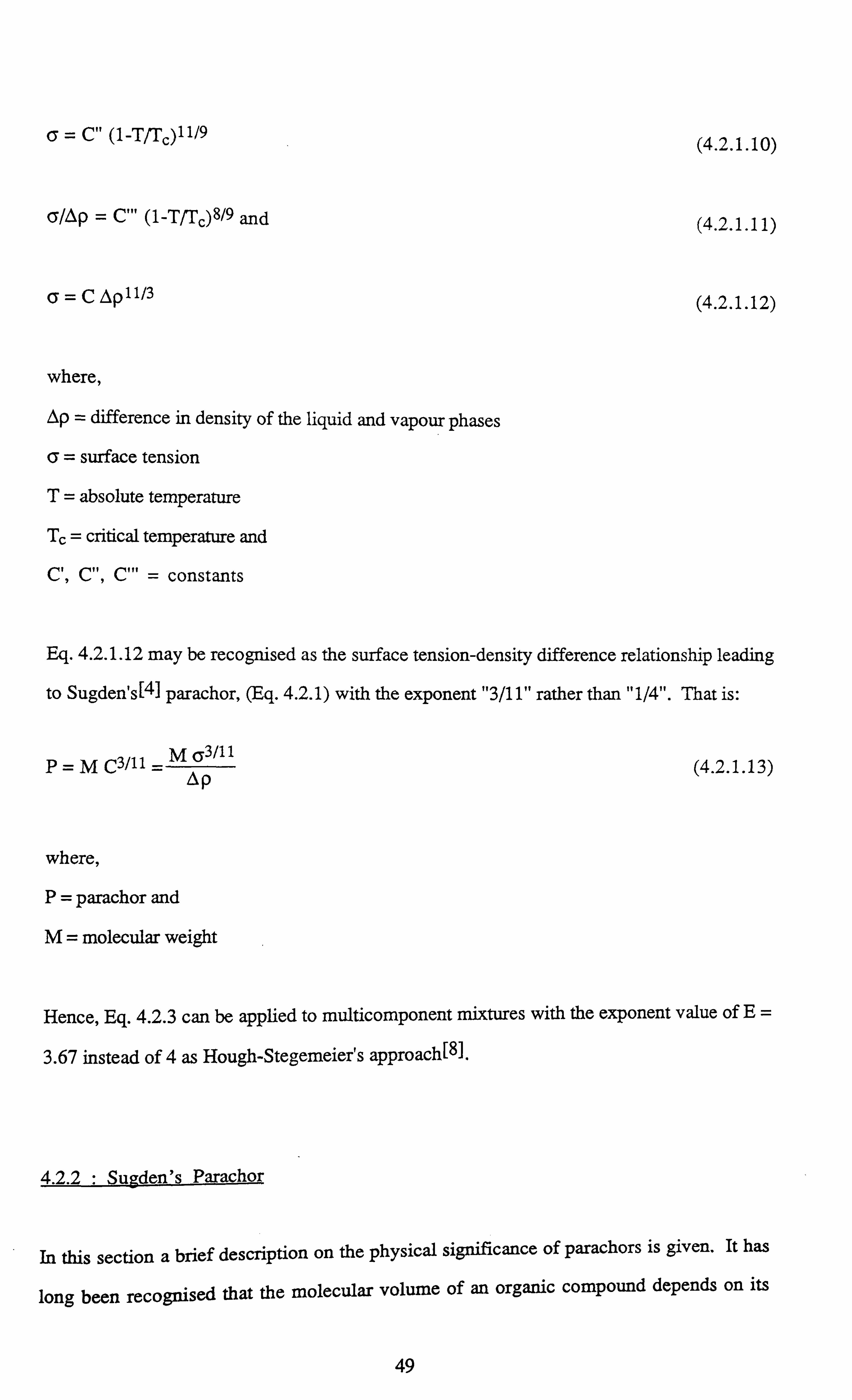
cs = C" (1-T, /Tc)11/9 (4.2.1.10)
CF/Op = C'"" (1-T/Tc)8/9 and (4.2.1.11)
6=C Lp 11/3 (4.2.1.12)
where,
Op = difference in density of the liquid and vapour phases
6= surface tension
T= absolute temperature
Tc = critical temperature and
Cl, C", C"' = constants
Eq. 4.2.1.12 may be recognised as the surface tension-density difference relationship leading
to Sugden's[4] parachor, (Eq. 4.2.1) with the exponent "3/11" rather than "1/4". That is:
M 63/11 P=M03/11= Ap
where,
P= parachor and
M= molecular weight
(4.2.1.1 3)
Hence, Eq. 4.2.3 can be applied to multicomponent mixtures with the exponent value of E_
3.67 instead of 4 as Hough-Stegemeier's approach[8].
4.2.2 " Sugden's Parachor
In this section a brief description on the physical significance of parachors is given. It has
long been recognised that the molecular volume of an organic compound depends on its
49

chemical constituents, and may be used in the case of liquids of uncertain constitution as a
guide to estimate their composition. The principle underlying this view is that different atomic
groupings have characteristic shapes and sizes and will therefore probably occupy
characteristic volumes in liquids, the total volume of the liquid being the sum of the
characteristic volumes of the separate groups of the molecules. The difficulty in practical
application has always been that the volumes of liquids change with temperature, as the
thermal motions of the molecules gradually overcome the cohesional forces between them,
and no really satisfactory basis for choosing the correct temperature at which to compare the
, however pointed out that molecular volumes was found for a long time. Sugden[ 14]
MacLeod's[3], relationship of density difference against IFT can form a good basis for the
comparison of molecular volumes under conditions where the effect of temperature is
neutralised by taking into account the IFT.
Now from Eq. 4.2.2 the constant [P] equals :
O 61/E P
(4.2.2.1)
the right hand side of the Eq. 4.2.2.1, is the product of IFT raised to a quarter (when a value
of, Ems, is taken) and the molecular volume which is molecular weight divided by the density
difference between liquid and vapour phase.
This particular term [P] on the left hand side of Eq. 4.2.2.1 has been termed by Sugden[14],
as ̀ parachor'. Parachor is a property independent from pressure and temperature. Hence, by
experimentation the parachor can be evaluated for each pure compound if the measured
interfacial tension, density difference between liquid and vapour phases, and the molecular
weights are substituted in Eq. 4.2.2.1.
4.2.3 " Fanchi's Method for Estimating Parachor
Fanchi[12], performed a linear regression analysis relating the critical properties (Vc and Tc)
and parachor of normal paraffins ranging from C1 to C7 to develop an expression for the
50
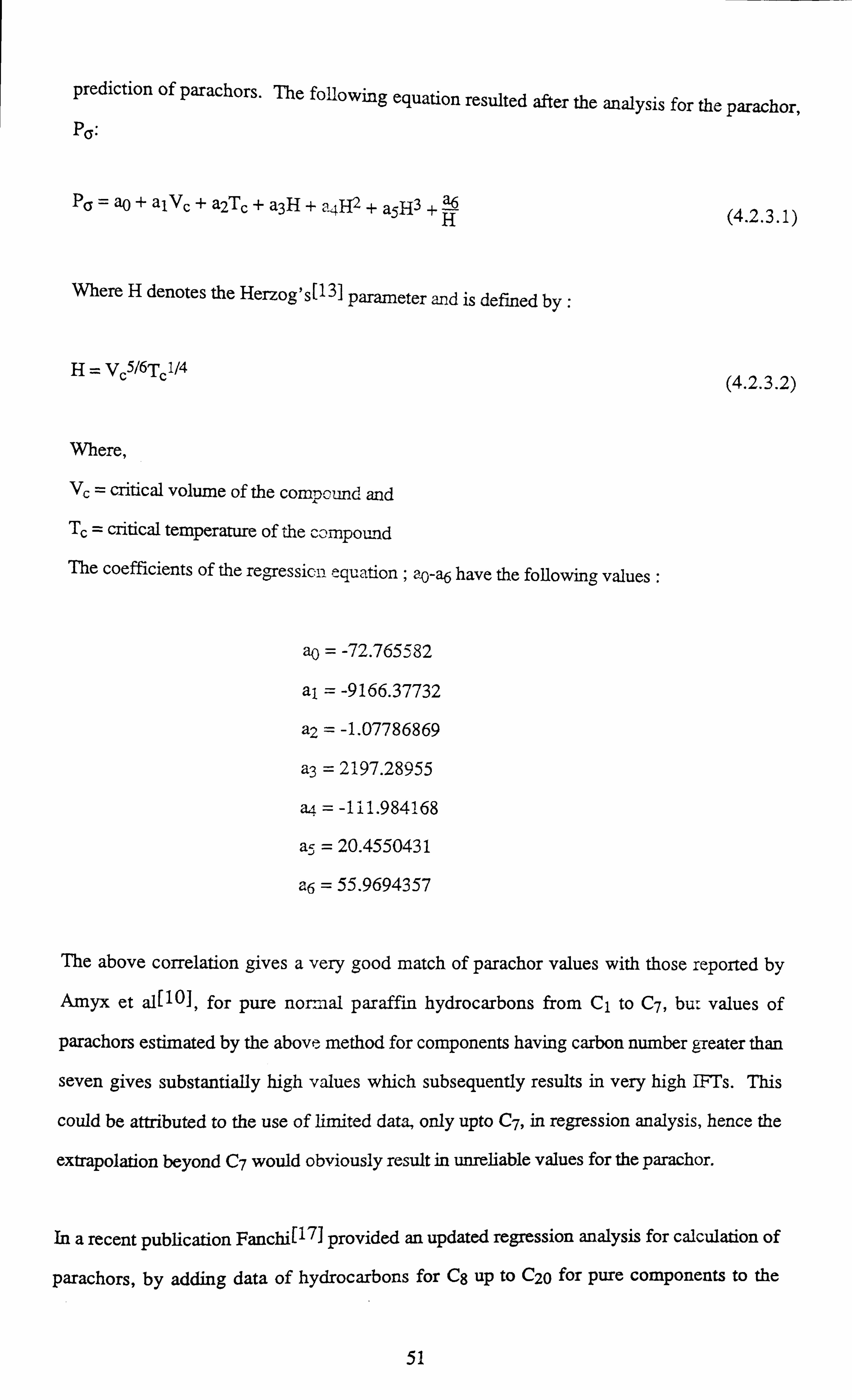
prediction of parachors. The following equation resulted after the analysis for the parachor, P6:
Pa= ap+alVc+a2Tc+a3H+a4H2 +a5H3+4 (4.2.3.1)
Where H denotes the Herzog's[131 parameter and is defined by :
H= VC5/6Tc'/4 (4.2.3.2)
Where,
V, = critical volume of the compound and
Tc = critical temperature of the Compound
The coefficients of the regressions equation ; ap-a6 have the following values :
an = -72.765582
al = -9166.37732
a2 = -1.07786869
a3 = 2197.28955
a: = -111.984168
a5 = 20.4550431
26 = 55.9694357
The above correlation gives a very good match of parachor values with those reported by
Amyx et a11101, for pure normal paraffin hydrocarbons from C1 to C7, bu: values of
parachors estimated by the above method for components having carbon number greater than
seven gives substantially high values which subsequently results in very high IFTs. This
could be attributed to the use of limited data, only upto C7, in regression analysis, hence the
extrapolation beyond C7 would obviously result in unreliable values for the parachor.
In a recent publication Fanchi[17] provided an updated regression analysis for calculation of
parachors, by adding data of hydrocarbons for C8 up to C20 for pure components to the
51
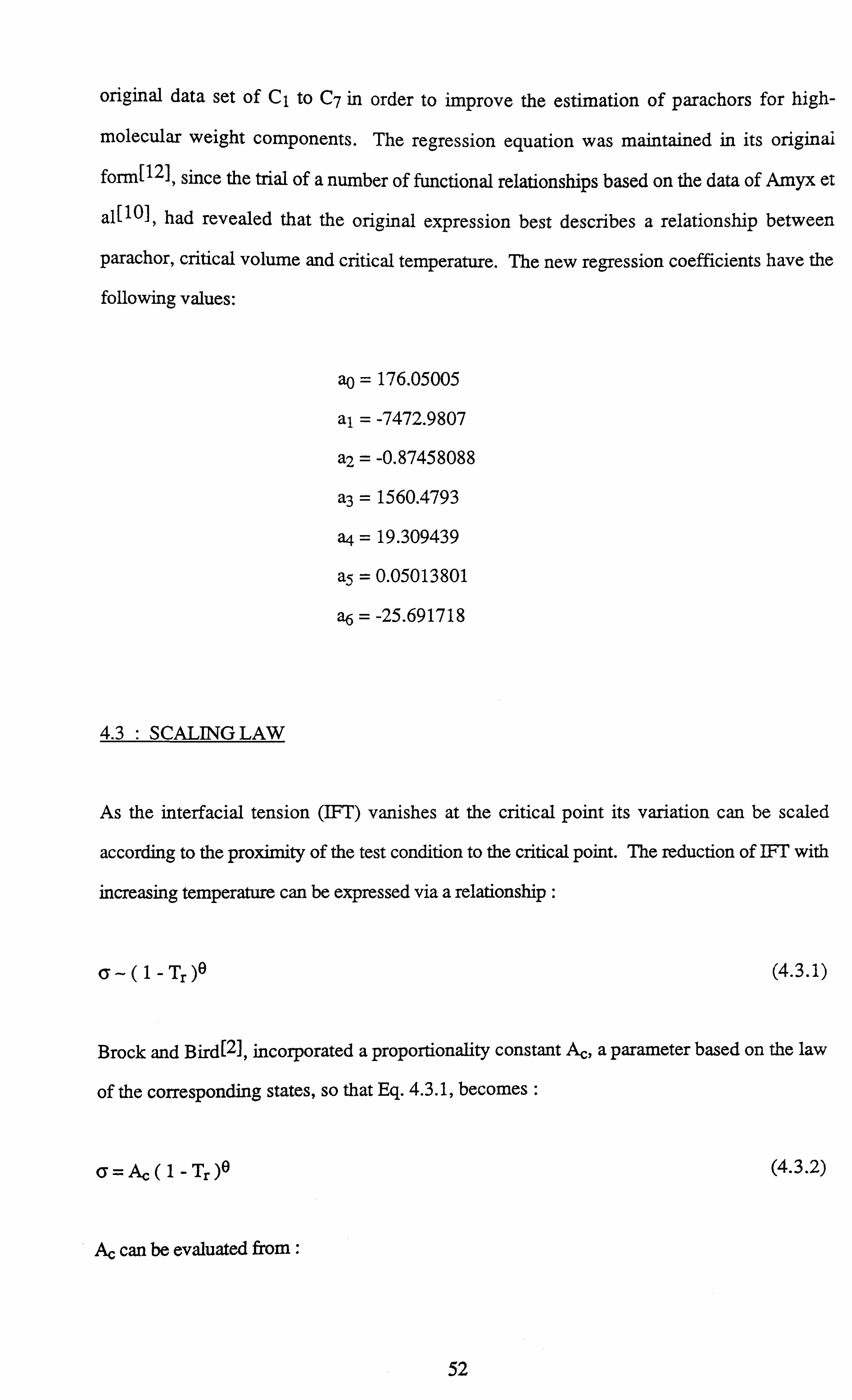
original data set of C1 to C7 in order to improve the estimation of parachors for high-
molecular weight components. The regression equation was maintained in its original
form[12], since the trial of a number of functional relationships based on the data of Amyx et
al[10], had revealed that the original expression best describes a relationship between
parachor, critical volume and critical temperature. The new regression coefficients have the
following values:
an = 176.05005
al = -7472.9807
a2 = -0.87458088
a3 = 1560.4793
a4 = 19.309439
a5 = 0.05013801
a6 = -25.691718
4.3 : SCALING LAW
As the interfacial tension (IFT) vanishes at the critical point its variation can be scaled
according to the proximity of the test condition to the critical point. The reduction of IFT with
increasing temperature can be expressed via a relationship :
6--(1-Tr)e (4.3.1)
Brock and Bird[2], incorporated a proportionality constant Ac, a parameter based on the law
of the corresponding states, so that Eq. 4.3.1, becomes :
6=Ac(1 -Tr)9
Ac can be evaluated from :
(4.3.2)
52

AG = Pct/3Tc1/3 (0.133ac - 0.281 )
and0= 11
(4.3.3)
the Riedel parameter, ac, is directly obtained from Reid and Sherwood[16], or it can be
evaluated from the following expression suggested by Miller[15]:
ac = 0.9076
Where,
T, binPc 1.0 +
Pa
1 _Tb
interfacial tension
Tr = reduced temperature
6= the scaling law constant exponent
Ac = proportionality constant, defined by Eq. 4.3.3
Pc = critical pressure
TT = critical temperature
occ = the Riedel parameter, defined by Eq. 4.3.4
Tb = boiling temperature and
Pa = atmospheric pressure
(4.3.4)
Lee and Chien[151 replaced the quantity of scale temperature by proposing density difference
as:
(Pi - Pv) - (Tc -T)
substituting ((3 = 6) into Eq. 4.3.5 and introducing a proportionality constant B':
(Pl - Pv) = B'(Tc - T)ß
(4.3.5}
(4.3.6)
53
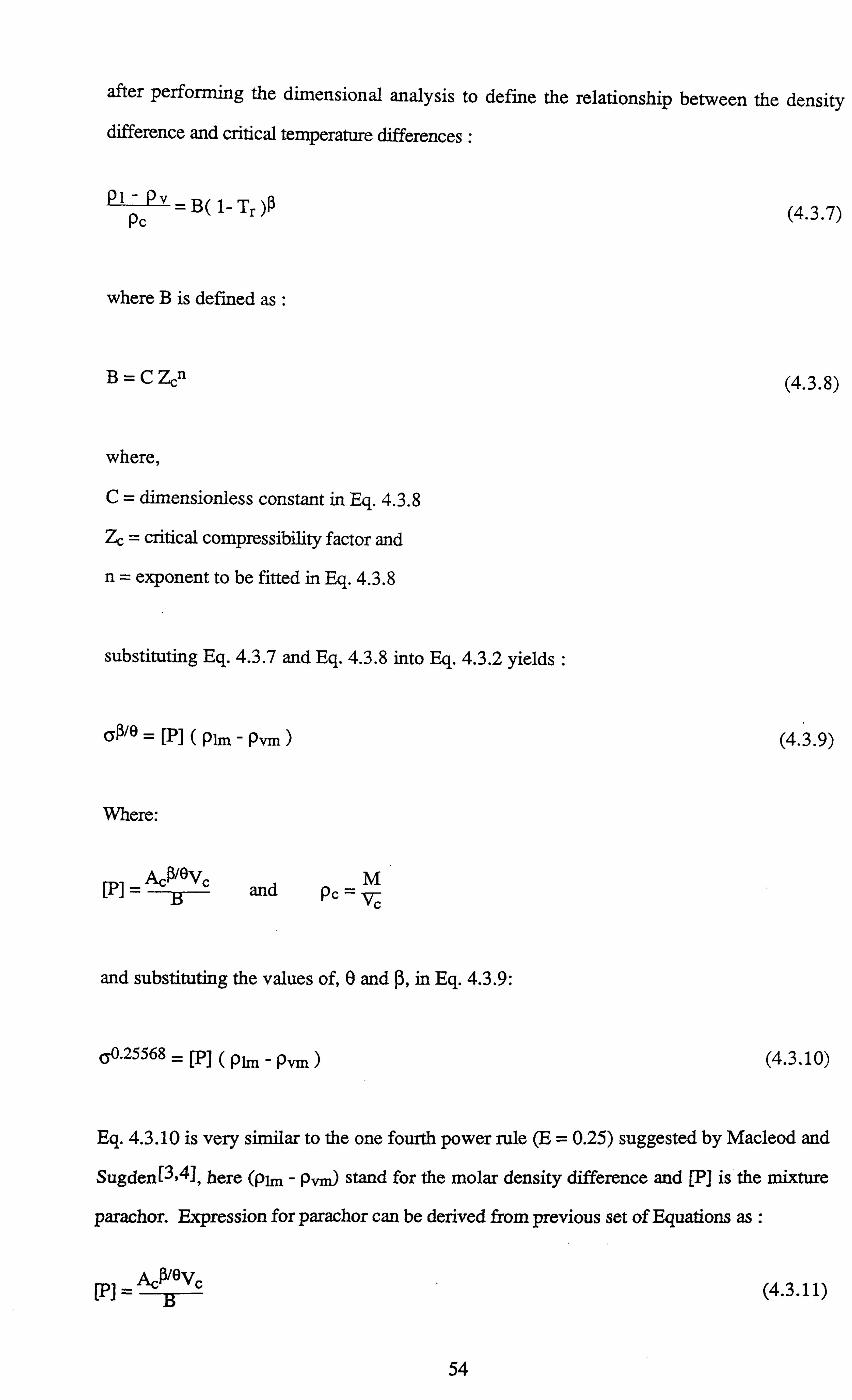
after performing the dimensional analysis to define the relationship between the density
difference and critical temperature differences :
Pi Pc
Pv =B( 1-Tr)ß (4.3.7)
where B is defined as :
B=CZýn (4.3.8)
where,
C= dimensionless constant in Eq. 4.3.8
Zc = critical compressibility factor and
n= exponent to be fitted in Eq. 4.3.8
substituting Eq. 4.3.7 and Eq. 4.3.8 into Eq. 4.3.2 yields :
6ßý8 . ['] (Phn - Pvm) (4.3.9)
Where:
['l = A. cWey and PC _M vc-
and substituting the values of, 0 and ß, in Eq. 4.3.9:
60.25568 = [p] (P1m - Pvm) (4.3.10)
Eq. 4.3.10 is very similar to the one fourth power rule (E = 0.25) suggested by Macleod and
Sugden[3,4], here (pim - p, ) stand for the molar density difference and [P] is the mixture
parachor. Expression for parachor can be derived from previous set of Equations as :
ýßievc [ý]=- F- (4.3.1 1)
54
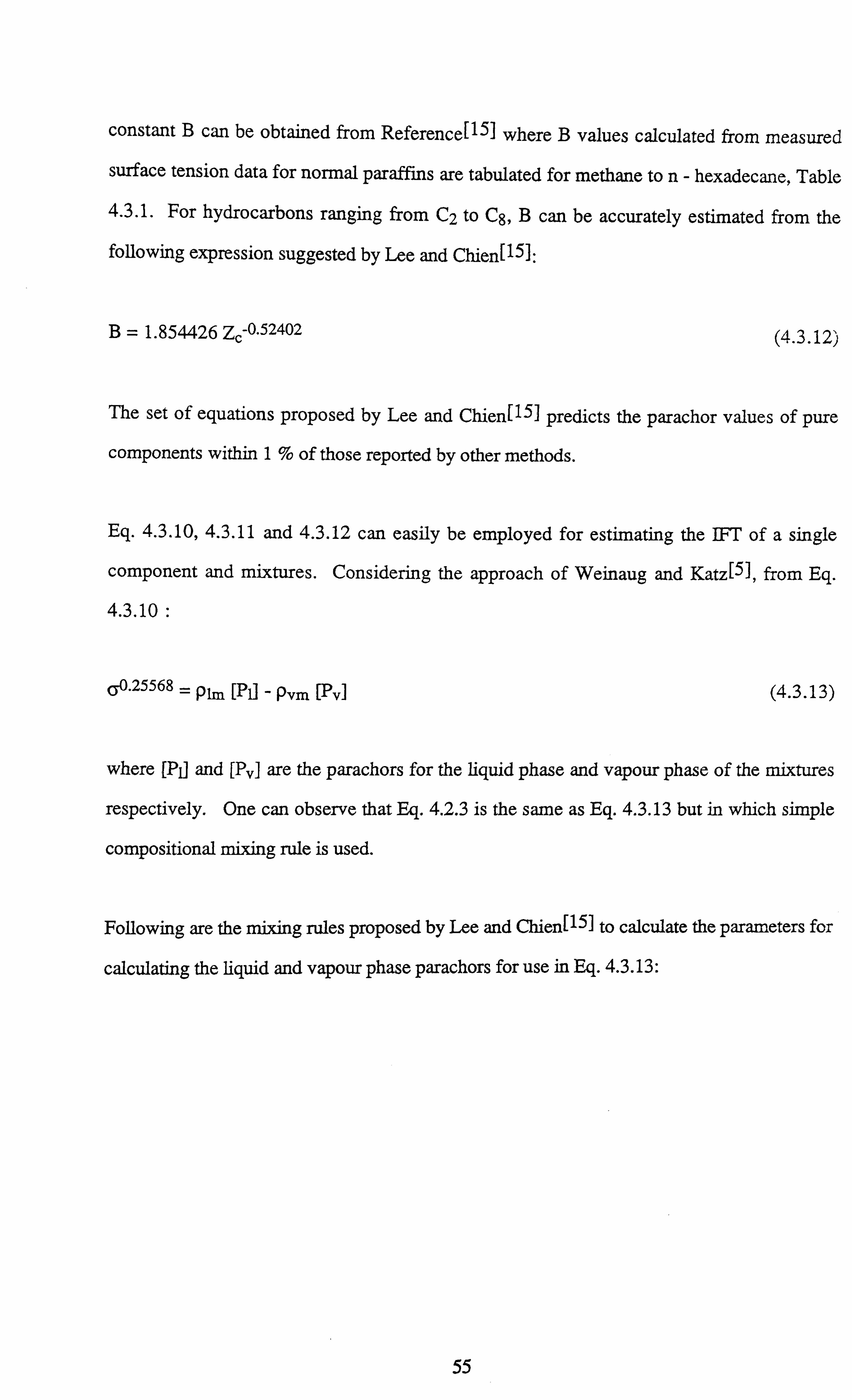
constant B can be obtained from Reference[151 where B values calculated from measured
surface tension data for normal paraffins are tabulated for methane to n- hexadecane, Table
4.3.1. For hydrocarbons ranging from C2 to C8, B can be accurately estimated from the
following expression suggested by Lee and Chien[15]:
B=1.854426 ZC-0.52402 (4.3.12'
The set of equations proposed by Lee and Chien[15] predicts the parachor values of pure
components within 1% of those reported by other methods.
Eq. 4.3.10,4.3.11 and 4.3.12 can easily be employed for estimating the IFT of a single
component and mixtures. Considering the approach of Weinaug and Katz[5J, from Eq.
4.3.10 :
60.25568 = pun [p1] - pvm [Pv] (4.3.13)
where {Pi] and [Pv] are the parachors for the liquid phase and vapour phase of the mixtures
respectively. One can observe that Eq. 4.2.3 is the same as Eq. 4.3.13 but in which simple
compositional mixing rule is used.
Following are the mixing rules proposed by Lee and Chien[15] to calculate the parameters for
calculating the liquid and vapour phase parachors for use in Eq. 4.3.13:
55

Table 4.3.1 - Calculated Values of B from Measured Surface Tension Data for normal Paraffins (from Reference 15).
Compound B
CH4 3.409
C2H6 3.630 C3H8 3.681
nC4 3.687
nC5 3.695
nC6 3.726
nC8 3.852
nC9 3.865
nClp 3.855 nCl l 3.641
nC12 3.815 nC13 3.872 nC14 3.820
nC15 3.795 nC l6 3.822

Vii = xi Yi
1=1 1
n
Bl=LXiBi i=1
n Pcl =
ýj Xi Pci
i=1
n
lcl = IxiTci
i=1
cl = ý`iaci
i=1
n
vcv Yivci
n
By _ YiB;
Pcv YiPci
Tcv _ YiTci
c, = lyi(Xci i=I
(4.3.14 - 4.3.18)
(4.3.19 - 4.3.23)
Eq. 4.3.14 to 4.3.18 can be employed to get the liquid phase parameters, to be used in the
Eq. 4.3.11, for the liquid phase mixture :
[p1J = AcIP"'Vcl
(4.3.24) 1
and Eq. 4.3.19 to 4.3.23 can be employed to get the vapour phase parameters:
[Pv] = AcvP/OVcy
(4.3.25) By
and for Acl, and Ac,
Act = Pc12/3Tc11/3 ( 0.1330cci - 0.281) (4.3.26)
56
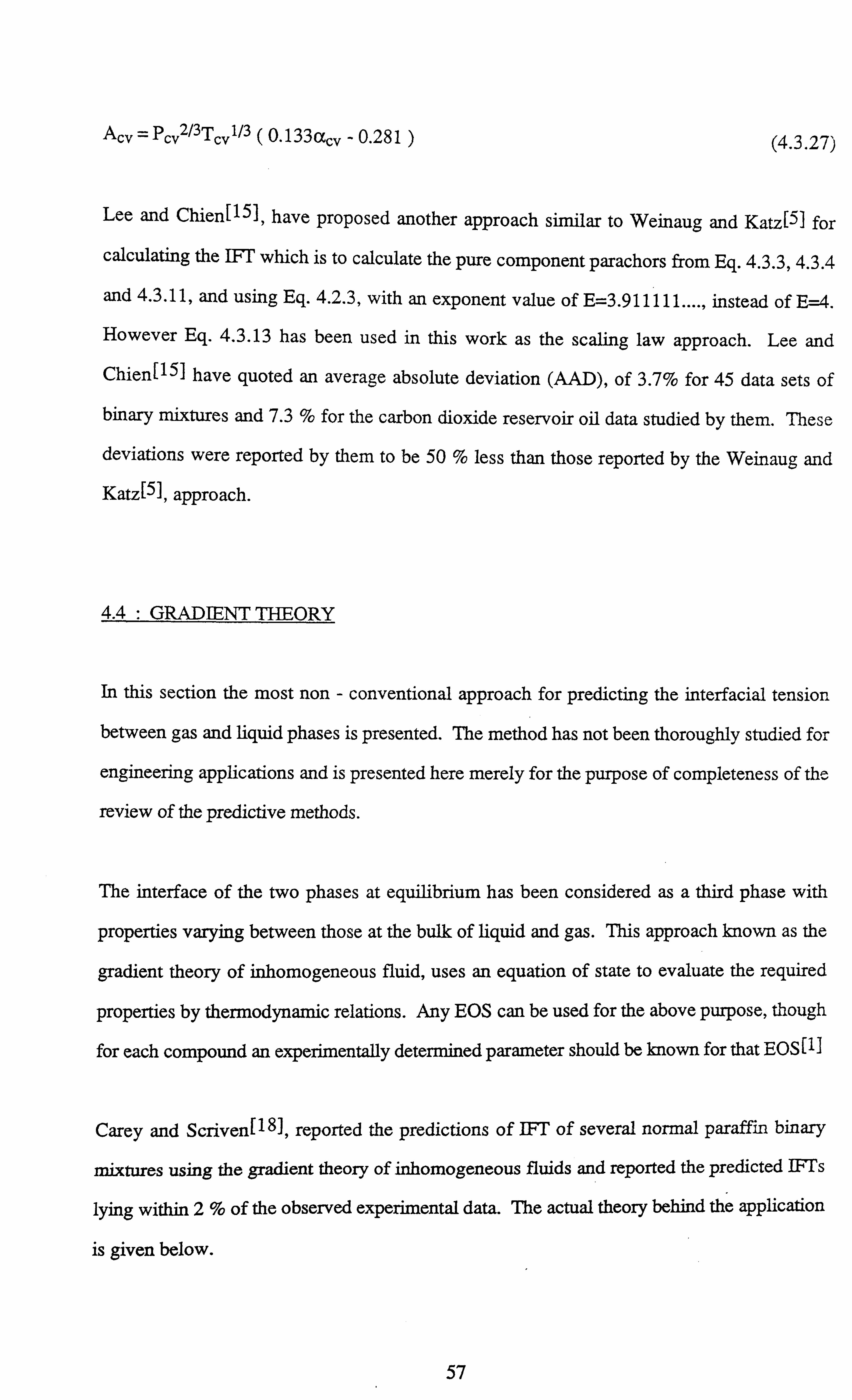
Acv - pCV2/3Tcv1/3 ( 0.133acv - 0.281) (4.3.27)
Lee and Chien[15], have proposed another approach similar to Weinaug and Katz[5] for
calculating the IFT which is to calculate the pure component parachors from Eq. 4.3.3,4.3.4
and 4.3.11, and using Eq. 4.2.3, with an exponent value of E=3.911111...., instead of E=4.
However Eq. 4.3.13 has been used in this work as the scaling law approach. Lee and
Chien{151 have quoted an average absolute deviation (AAD), of 3.7% for 45 data sets of binary mixtures and 7.3 % for the carbon dioxide reservoir oil data studied by them. These
deviations were reported by them to be 50 % less than those reported by the Weinaug and
Katz[5J, approach.
4.4 : GRADIENT THEORY
In this section the most non - conventional approach for predicting the interfacial tension
between gas and liquid phases is presented. The method has not been thoroughly studied for
engineering applications and is presented here merely for the purpose of completeness of the
review of the predictive methods.
The interface of the two phases at equilibrium has been considered as a third phase with
properties varying between those at the bulk of liquid and gas. This approach known as the
gradient theory of inhomogeneous fluid, uses an equation of state to evaluate the required
properties by thermodynamic relations. Any EOS can be used for the above purpose, though
for each compound an experimentally determined parameter should be known for that EOS III
Carey and Scrivenl18J, reported the predictions of ICI' of several normal paraffin binary
mixtures using the gradient theory of inhomogeneous fluids and reported the predicted =s
lying within 2% of the observed experimental data. The actual theory behind the application
is given below.
57
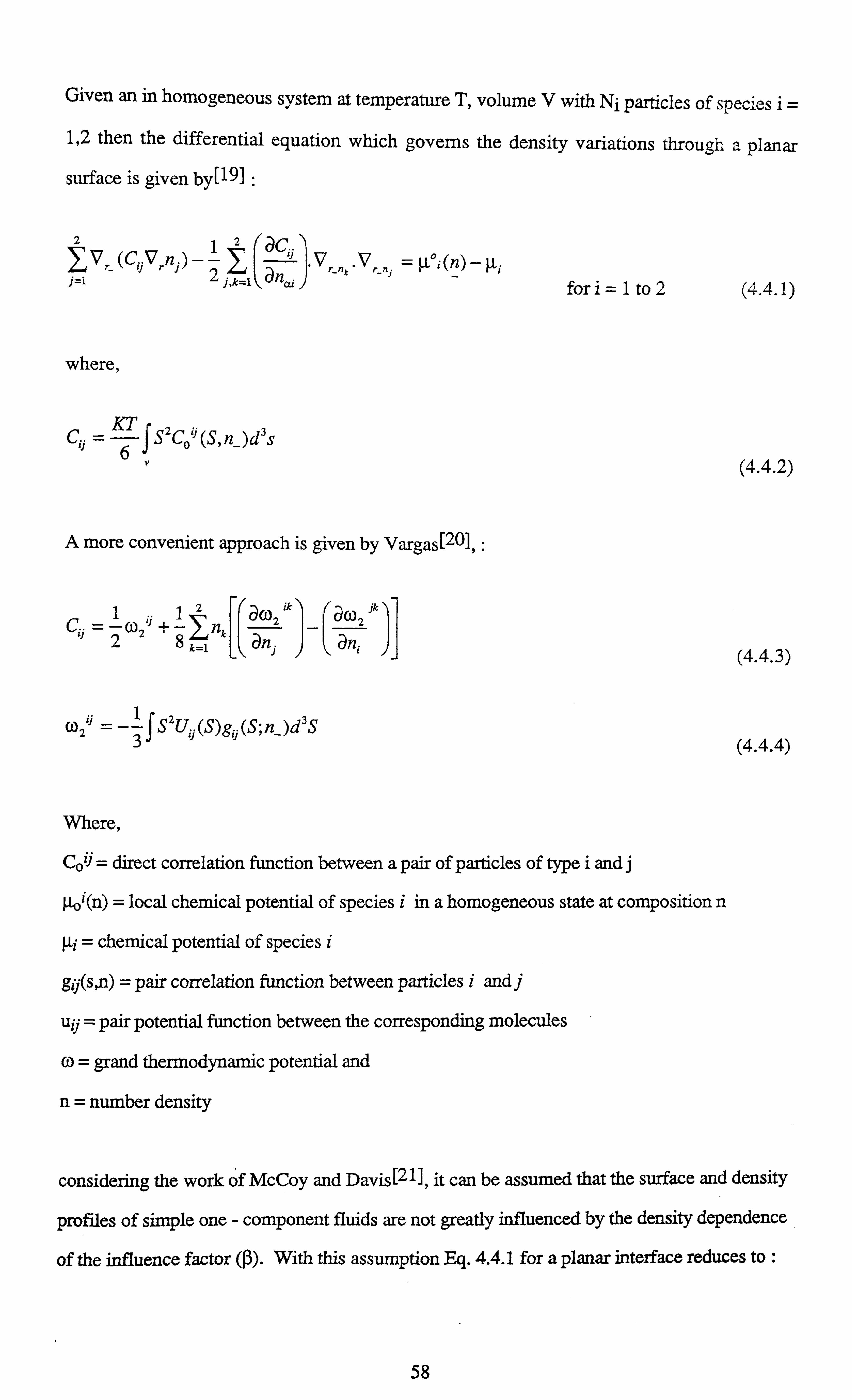
Given an in homogeneous system at temperature T, volume V with Ni particles of species i=
1,2 then the differential equation which governs the density variations through a planar
surface is given by[19J :
212 ýC=i yr (Cijvrnj)
-2 ýn
}Vrak
V !. Lot (n) - µi j=1 I. k=1 aj
where,
CGS =f S2C0`'(S, n_)d3s
6 v
A more convenient approach is given by Vargas[20], :
1 tl
12 x0)2 ik &o2 jk Cij
- -w2 +-nk - 28
k=1 a%Z
j an,
w2`' J S2U (S)g=; (S; n_ )d 3S 3
Where,
Cot. = direct correlation function between a pair of particles of type i and j
p, '(n) = local chemical potential of species i in a homogeneous state at composition n
µi = chemical potential of species i
glj(s, n) = pair correlation function between particles i and j
ulj = pair potential function between the corresponding molecules
w= grand thermodynamic potential and
n= number density
(4.4.2)
(4.4.3)
(4.4.4)
considering the work of McCoy and Davis [211, it can be assumed that the surface and density
profiles of simple one - component fluids are not greatly influenced by the density dependence
of the influence factor (ß). With this assumption Eq. 4.4.1 for a planar interface reduces to :
for i=1 to 2 (4.4.1)
58

d2 CIJ
2j, µoj(n_)-µt, i=1,2 1=I
Cj j for species 1&2 can be given as :
C12 =ß ClIC22 (4.4.6)
where, (3, is an adjustable parameter, C11 and C22 are to be determined from the pure
component interfacial tension data. Hence IFT equation corresponding to Eq. 4.4.1, is giver.
by [19,20], :
6=I Ci' dx dx
_°° ij=1 (4.4.7'
n, 2 (dn 6=J
j2[o(n) - w(n_b)] jCki dk i dni
nil i, k=1 dni 'ni (4.4.8)
Eq. 4.4.8 is a profile independent equation. Where nil & ni2 are the bulk densities for
species i which are computed via equalities of bulk pressures and chemical potentials for each
species. co(n), represents the grand thermodynamic potential defined by :
co(n-) _ .f0 (n_) - ).. fldLt
(4.4.9)
Where fO(n_) the local Helmholtz free energy density of homogeneous fluid at composition
(n-) can be determined from an EOS.
A more detailed application of Eq. 4.4.7 or 4.4.8 for prediction of interfacial tension of
mixtures is given in Reference[18]. As the method relies significantly on the empiricism,
defined by Eq. 4.4.6, and major thermodynamic calculations, it has not been widely applied.
59
References
1) Nitsche, J. M., Teletzke, G. E., Scriven, L. E., and Davis, H. T.: "Behaviour of
Water, Carbon dioxide and Decane", Fluid Phase Equilibria, Vol. 14, pp. 203-
208, (1980).
2) Brock, J. R. and Bird, R. B.: "Surface Tension and the Principle of
Corresponding states", AIChEJ, Vol. 1, No. 2, pp. 174-177, (Jun., 1955).
3) MaCleod, D. B.: "On a Relation Between Surface Tension, Density",
Transactions of Faraday Soc., Vol. 19, pp. 38-43, (1923).
4) Sugden S.: "A Relation between Surface Tension, Density and, Chemical
Composition", J. Chem. Soc., Vol. 168, pp. 1177-1189, (1924).
5) Weinaug, C. F. and Katz, D. L.: "Surface Tension of Methane - Propane
Mixtures", Industrial & Engineering Chemistry (I & EC), pp. 239-246,
(1943).
6) Mayer, S. W.: "A Molecular Parameter Relationship between Surface Tension
and Liquid Compressibility", J. Phys. Chem., Vol. 67, pp. 2160-2164,
(1963).
7) Sanchez, I. C.: "Liquids : Surface Tension, Compressibility and Invariants", J.
Chem Phys., Vol. 79, pp. 405-415, (1983).
8) Hough, E. W. and Stegerneier, G. 1.: "Correlation of Surface and Interfacial
Tension of Light Hydrocarbons in the Critical Region", Society of Petroleum
Engineers Journal (SPEJ), pp. 259-263, (Dec., 1961).
9) Sivaraman, A., Ziga, J. and Kobayashi, R.: "Correlation for Prediction of
Interfacial Tensions of Pure Alkane, Napthenic and Aromatic Compounds
between their Freezing and Critical Points", Fluid Phase Equilibria, Vol. 18,
pp. 225-235, (1984).
10) Amyx, J. W., Bass, D. M. and Whiting, R. L.: "Petroleum Reservoir
Engineering", McGraw Hill, pp. 306-308, (1960).
60
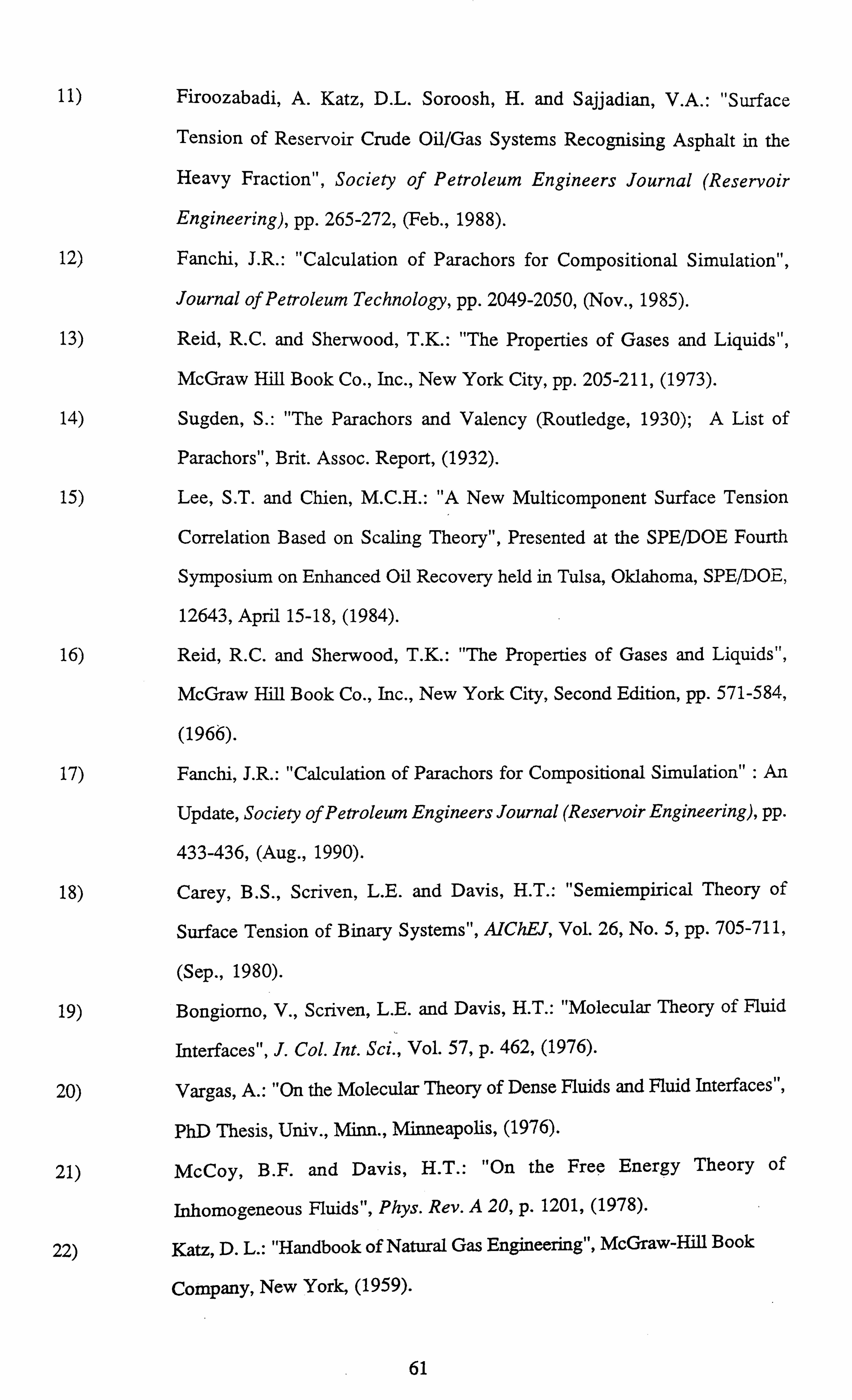
11) Firoozabadi, A. Katz, D. L. Soroosh, H. and Sajjadian, V. A.: "Surface
Tension of Reservoir Crude Oil/Gas Systems Recognising Asphalt in the
Heavy Fraction", Society of Petroleum Engineers Journal (Reservoir
Engineering), pp. 265-272, (Feb., 1988).
12) Fanchi, J. R.: "Calculation of Parachors for Compositional Simulation",
Journal of Petroleum Technology, pp. 2049-2050, (Nov., 1985).
13) Reid, R. C. and Sherwood, T. K.: "The Properties of Gases and Liquids",
McGraw Hill Book Co., Inc., New York City, pp. 205-211, (1973).
14) Sugden, S.: "The Parachors and Valency (Routledge, 1930); A List of
Parachors", Brit. Assoc. Report, (1932).
15) Lee, S. T. and Chien, M. C. H.: "A New Multicomponent Surface Tension
Correlation Based on Scaling Theory", Presented at the SPE/DOE Fourth
Symposium on Enhanced Oil Recovery held in Tulsa, Oklahoma, SPE/DOE,
12643, April 15-18, (1984).
16) Reid, R. C. and Sherwood, T. K.: "The Properties of Gases and Liquids",
McGraw Hill Book Co., Inc., New York City, Second Edition, pp. 571-584,
(1966).
17) Fanchi, J. R.: "Calculation of Parachors for Compositional Simulation" : An
Update, Society of Petroleum Engineers Journal (Reservoir Engineering), pp.
433-436, (Aug., 1990).
18) Carey, B. S., Scriven, L. E. and Davis, H. T.: "Semiempirical Theory of
Surface Tension of Binary Systems", AIChEJ, Vol. 26, No. 5, pp. 705-711,
(Sep., 1980).
19) Bongiorno, V., Scriven, L. E. and Davis, H. T.: "Molecular Theory of Fluid
Interfaces", J. Col. Int. Sci., Vol. 57, p. 462, (1976).
20) Vargas, A.: "On the Molecular Theory of Dense Fluids and Fluid Interfaces",
PhD Thesis, Univ., Minn., Minneapolis, (1976).
21) McCoy, B. F. and Davis, H. T.: "On the Free Energy Theory of
Inhomogeneous Fluids", Phys. Rev. A 20, p. 1201, (1978).
22) Katz, D. L.: "Handbook of Natural Gas Engineering", McGraw-Hill Book
Company, New York, (1959).
61
23) Guggenheim, E. A.: "Thermodynamics", Third Ed., North Holland
Publishing Co., Amsterdam, (1957).
62
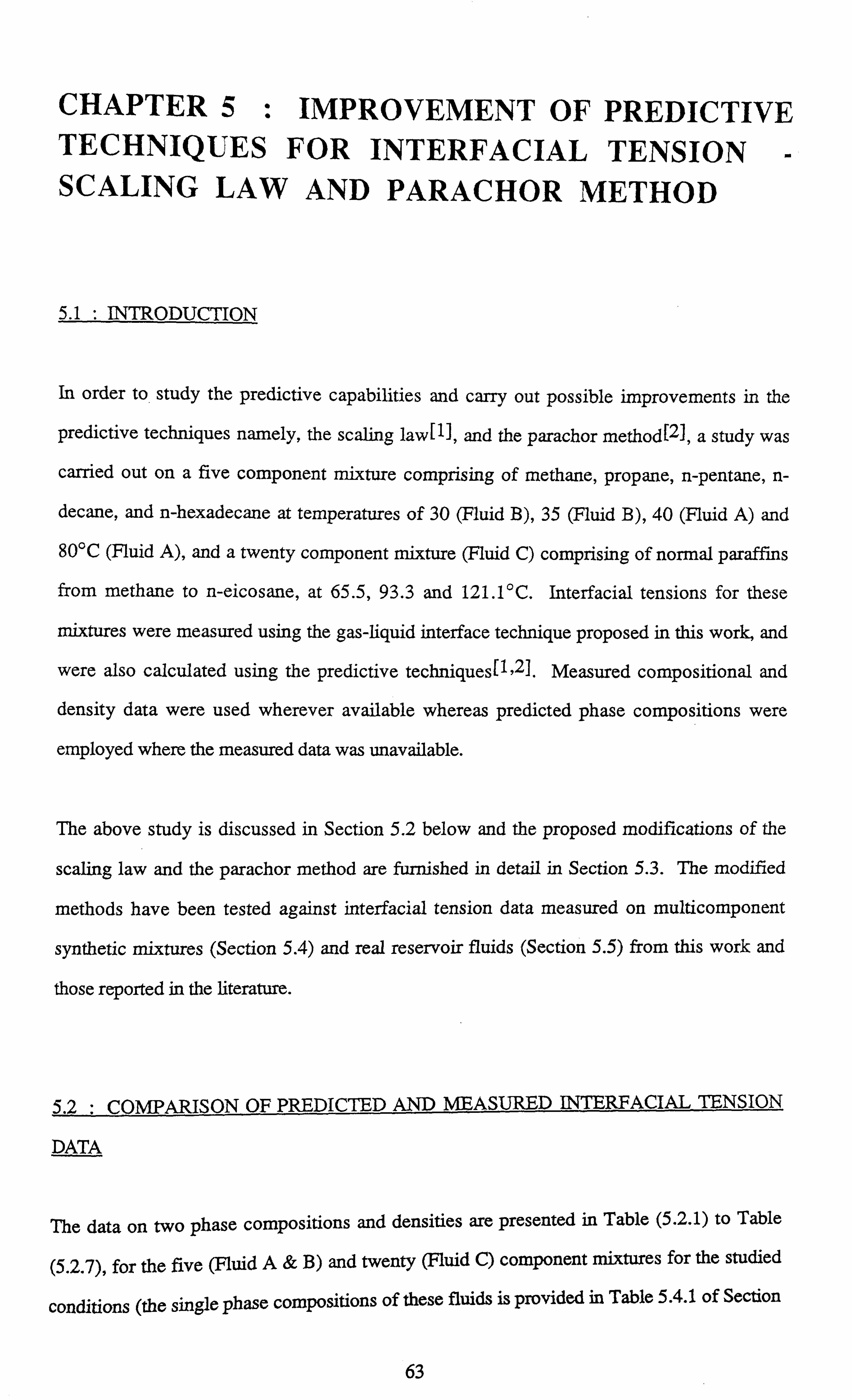
CHAPTER 5: IMPROVEMENT OF PREDICTIVE TECHNIQUES FOR INTERFACIAL TENSION SCALING LAW AND PARACHOR METHOD
5.1 : INTRODUCTION
In order to study the predictive capabilities and carry out possible improvements in the
predictive techniques namely, the scaling law[l], and the parachor methodr2i1, a study was
carried out on a five component mixture comprising of methane, propane, n-pentane, n-
decane, and n-hexadecane at temperatures of 30 (Fluid B), 35 (Fluid B), 40 (Fluid A) and
80°C (Fluid A), and a twenty component mixture (Fluid C) comprising of normal paraffins
from methane to n-eicosane, at 65.5,93.3 and 121.1°C. Interfacial tensions for these
mixtures were measured using the gas-liquid interface technique proposed in this work, and
were also calculated using the predictive techniques[ 1'2]. Measured compositional and
density data were used wherever available whereas predicted phase compositions were
employed where the measured data was unavailable.
The above study is discussed in Section 5.2 below and the proposed modifications of the
scaling law and the parachor method are furnished in detail in Section 5.3. The modified
methods have been tested against interfacial tension data measured on multicomponent
synthetic mixtures (Section 5.4) and real reservoir fluids (Section 5.5) from this work and
those reported in the literature.
5.2 : COMPARISON OF PREDICTED AND MEASURED INTERFACIAL TENSION
DATA
The data on two phase compositions and densities are presented in Table (5.2.1) to Table
(5.2.7), for the five (Fluid A& B) and twenty (Fluid C) component mixtures for the studied
conditions (the single phase compositions of these fluids is provided in Table 5.4.1 of Section
63
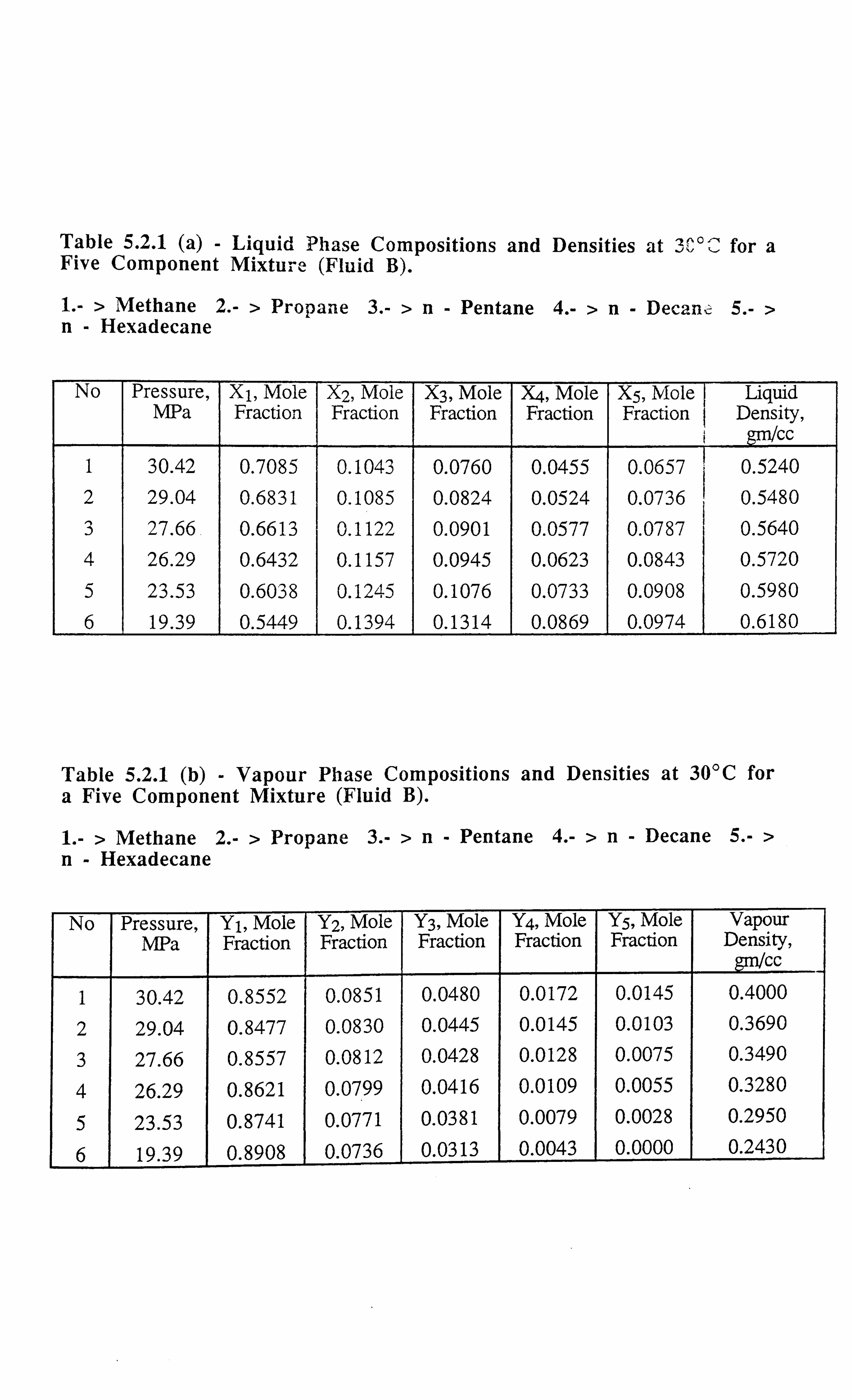
Table 5.2.1 (a) - Liquid Phase Compositions and Densities at 3ý, °C for a Five Component Mixture (Fluid B).
1. - > Methane 2. - > Propane 3. - >n- Pentane 4. - >n- Decant 5. - > n- Hexadecane
No Pressure, MPa
X1, Mole Fraction
X2, Mole Fraction
X3, Mole Fraction
X4, Mole Fraction
X5, Mole Fraction
Liquid Density,
cc 1 30.42 0.7085 0.1043 0.0760 0.0455 0.0657 0.5240 2 29.04 0.6831 0.1085 0.0824 0.0524 0.0736 0.5480
3 27.66. 0.6613 0.1122 0.0901 0.0577 0.0787 0.5640 4 26.29 0.6432 0.1157 0.0945 0.0623 0.0843 0.5720
5 23.53 0.6038 0.1245 0.1076 0.0733 0.0908 0.5980
6 19.39 0.5449 0.1394 0.1314 0.0869 0.0974 0.6180
Table 5.2.1 (b) - Vapour Phase Compositions and Densities at 30°C for a Five Component Mixture (Fluid B).
1. - > Methane 2. - > Propane 3. - >n- Pentane 4. - >n- Decane 5. - > n- Hexadecane
No Pressure, MPa
Y1, Mole Fraction
Y2, Mole Fraction
Y3, Mole Fraction
Y4, Mole Fraction
Y5, Mole Fraction
Vapour Density,
gm/qc
1 30.42 0.8552 0.0851 0.0480 0.0172 0.0145 0.4000
2 29.04 0.8477 0.0830 0.0445 0.0145 0.0103 0.3690
3 27.66 0.8557 0.0812 0.0428 0.0128 0.0075 0.3490
4 26.29 0.8621 0.0799 0.0416 0.0109 0.0055 0.3280
5 23.53 0.8741 0.0771 0.0381 0.0079 0.0028 0.2950
6 19.39 0.8908 0.0736 0.0313 0.0043 0.0000 0.2430
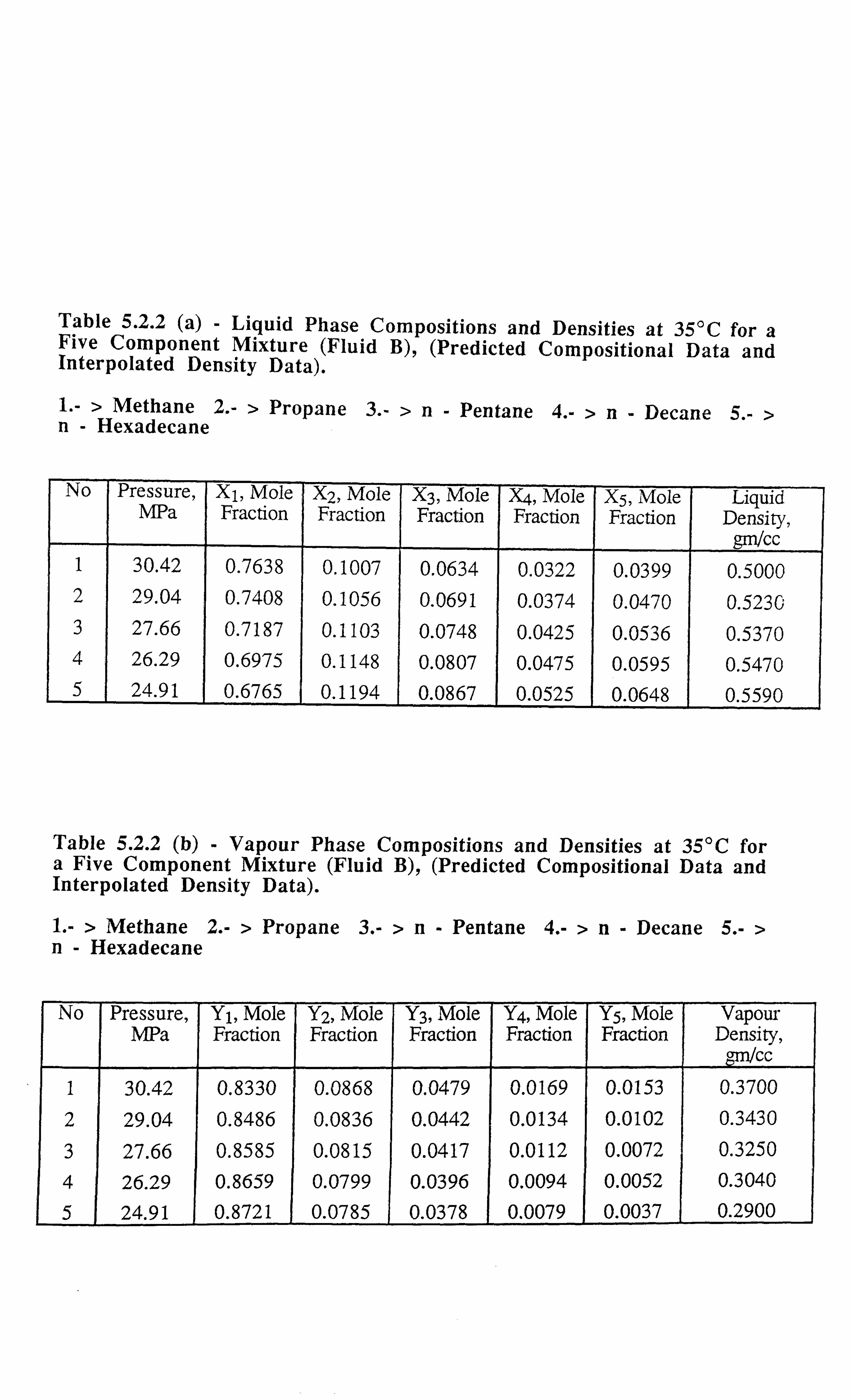
Table 5.2.2 (a) - Liquid Phase Compositions and Densities at 35°C for a Five Component Mixture (Fluid B), (Predicted Compositional Data and Interpolated Density Data).
1. - > Methane 2. - > Propane 3. - >n- Pentane 4. - >n- Decane 5. - > n- Hexadecane
No Pressure, MPa
X1, Mole Fraction
X2, Mole Fraction
X3, Mole Fraction
X4, Mole Fraction
X5, Mole Fraction
Liquid Density, gm/cc
1 30.42 0.7638 0.1007 0.0634 0.0322 0.0399 0.5000 2 29.04 0.7408 0.1056 0.0691 0.0374 0.0470 0.5230 3 27.66 0.7187 0.1103 0.0748 0.0425 0.0536 0.5370 4 26.29 0.6975 0.1148 0.0807 0.0475 0.0595 0.5470 5 24.91 0.6765 0.1194 0.0867 0.0525 0.0648 0.5590
Table 5.2.2 (b) - Vapour Phase Compositions and Densities at 35°C for a Five Component Mixture (Fluid B), (Predicted Compositional Data and Interpolated Density Data).
1. - > Methane 2. - > Propane 3. - >n- Pentane 4. - >n- Decane 5. - > n- Hexadecane
No Pressure, MPa
Y1, Mole Fraction
Y2, Mole Fraction
Y3, Mole Fraction
Y4, Mole Fraction
Y5, Mole Fraction
Vapour Density,
gm1cc 1 30.42 0.8330 0.0868 0.0479 0.0169 0.0153 0.3700 2 29.04 0.8486 0.0836 0.0442 0.0134 0.0102 0.3430 3 27.66 0.8585 0.0815 0.0417 0.0112 0.0072 0.3250 4 26.29 0.8659 0.0799 0.0396 0.0094 0.0052 0.3040
5 24.91 0.8721 0.0785 0.0378 0.0079 0.0037 0.2900
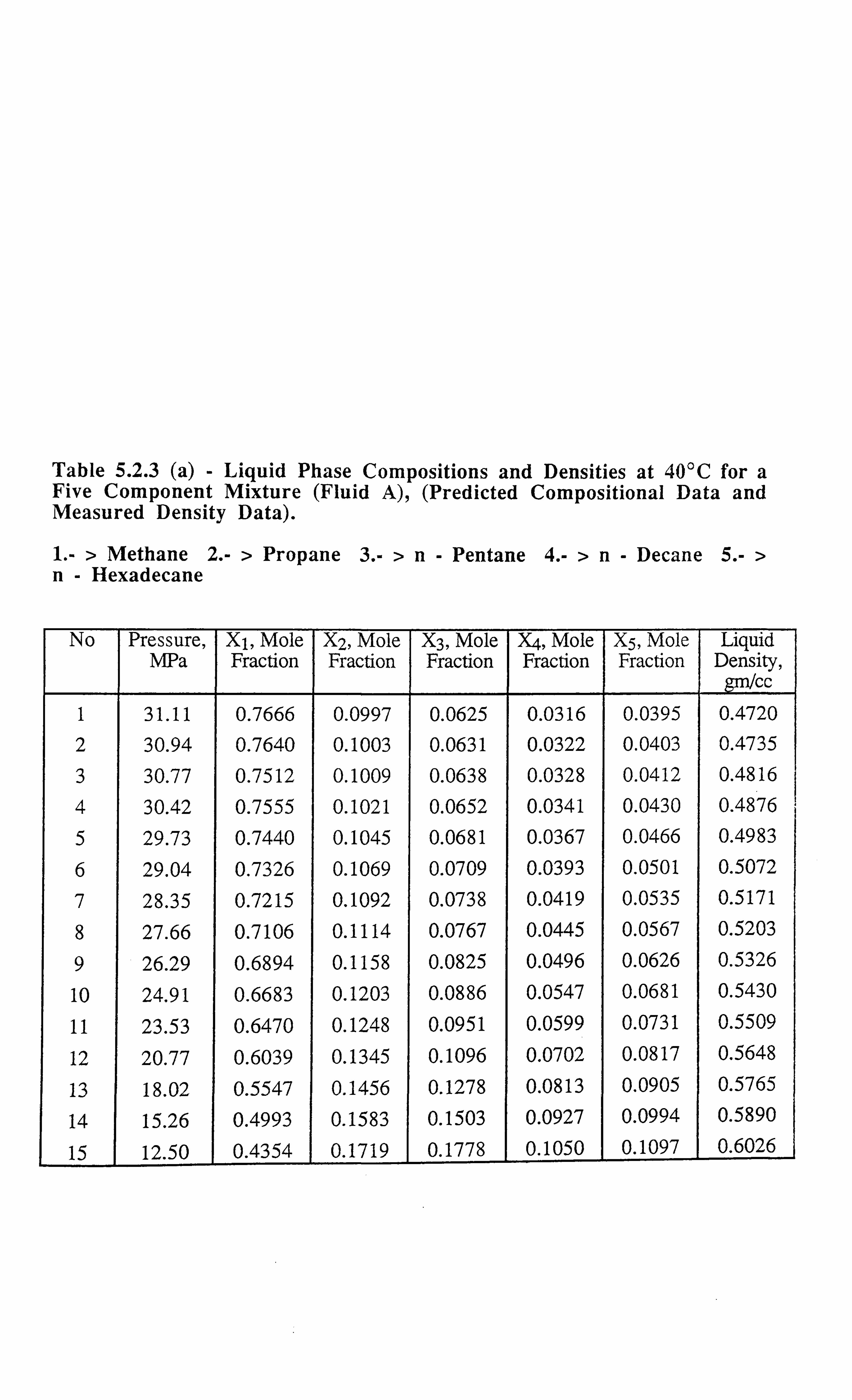
Table 5.2.3 (a) - Liquid Phase Compositions and Densities at 40°C for a Five Component Mixture (Fluid A), (Predicted Compositional Data and Measured Density Data).
1. - > Methane 2. - > Propane 3. - >n- Pentane 4. - >n- Decane 5. - > n- Hexadecane
No Pressure, MPa
X1, Mole Fraction
X2, Mole Fraction
X3, Mole Fraction
X4, Mole Fraction
X5, Mole Fraction
Liquid Density,
gm/Cc
1 31.11 0.7666 0.0997 0.0625 0.0316 0.0395 0.4720
2 30.94 0.7640 0.1003 0.0631 0.0322 0.0403 0.4735
3 30.77 0.7512 0.1009 0.0638 0.0328 0.0412 0.4816
4 30.42 0.7555 0.1021 0.0652 0.0341 0.0430 0.4876 5 29.73 0.7440 0.1045 0.0681 0.0367 0.0466 0.4983
6 29.04 0.7326 0.1069 0.0709 0.0393 0.0501 0.5072
7 28.35 0.7215 0.1092 0.0738 0.0419 0.0535 0.5171
8 27.66 0.7106 0.1114 0.0767 0.0445 0.0567 0.5203
9 26.29 0.6894 0.1158 0.0825 0.0496 0.0626 0.5326
10 24.91 0.6683 0.1203 0.0886 0.0547 0.0681 0.5430
11 23.53 0.6470 0.1248 0.0951 0.0599 0.0731 0.5509
12 20.77 0.6039 0.1345 0.1096 0.0702 0.0817 0.5648
13 18.02 0.5547 0.1456 0.1278 0.0813 0.0905 0.5765
14 15.26 0.4993 0.1583 0.1503 0.0927 0.0994 0.5890
15 12.50 0.4354 0.1719 0.1778 0.1050 0.1097 0.6026
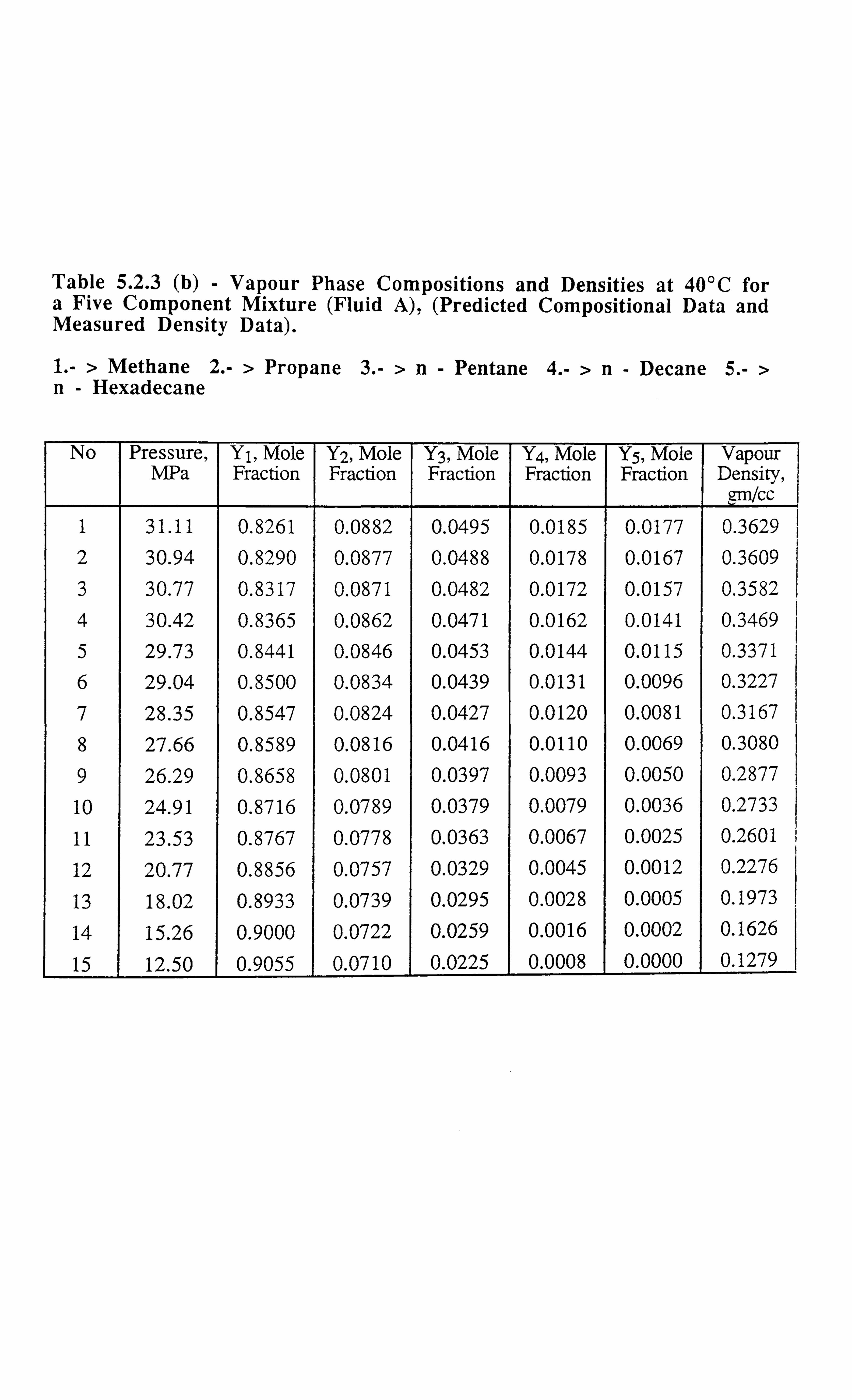
Table 5.2.3 (b) - Vapour Phase Compositions and Densities at 40°C for a Five Component Mixture (Fluid A), (Predicted Compositional Data and Measured Density Data).
1. - > Methane 2. - > Propane 3. - >n- Pentane 4. - >n- Decane 5. - > n- Hexadecane
No Pressure, MPa
Y1, Mole Fraction
Y2, Mole Fraction
Y3, Mole Fraction
Y4, Mole Fraction
Y5, Mole Fraction
Vapour Density,
gm/cc 1 31.11 0.8261 0.0882 0.0495 0.0185 0.0177 0.3629
2 30.94 0.8290 0.0877 0.0488 0.0178 0.0167 0.3609
3 30.77 0.8317 0.0871 0.0482 0.0172 0.0157 0.3582 4 30.42 0.8365 0.0862 0.0471 0.0162 0.0141 0.3469
5 29.73 0.8441 0.0846 0.0453 0.0144 0.0115 0.3371
6 29.04 0.8500 0.0834 0.0439 0.0131 0.0096 0.3227
7 28.35 0.8547 0.0824 0.0427 0.0120 0.0081 0.3167 8 27.66 0.8589 0.0816 0.0416 0.0110 0.0069 0.3080
9 26.29 0.8658 0.0801 0.0397 0.0093 0.0050 0.2877 10 24.91 0.8716 0.0789 0.0379 0.0079 0.0036 0.2733
11 23.53 0.8767 0.0778 0.0363 0.0067 0.0025 0.2601
12 20.77 0.8856 0.0757 0.0329 0.0045 0.0012 0.2276
13 18.02 0.8933 0.0739 0.0295 0.0028 0.0005 0.1973
14 15.26 0.9000 0.0722 0.0259 0.0016 0.0002 0.1626
15 12.50 0.9055 0.0710 0.0225 0.0008 0.0000 0.1279
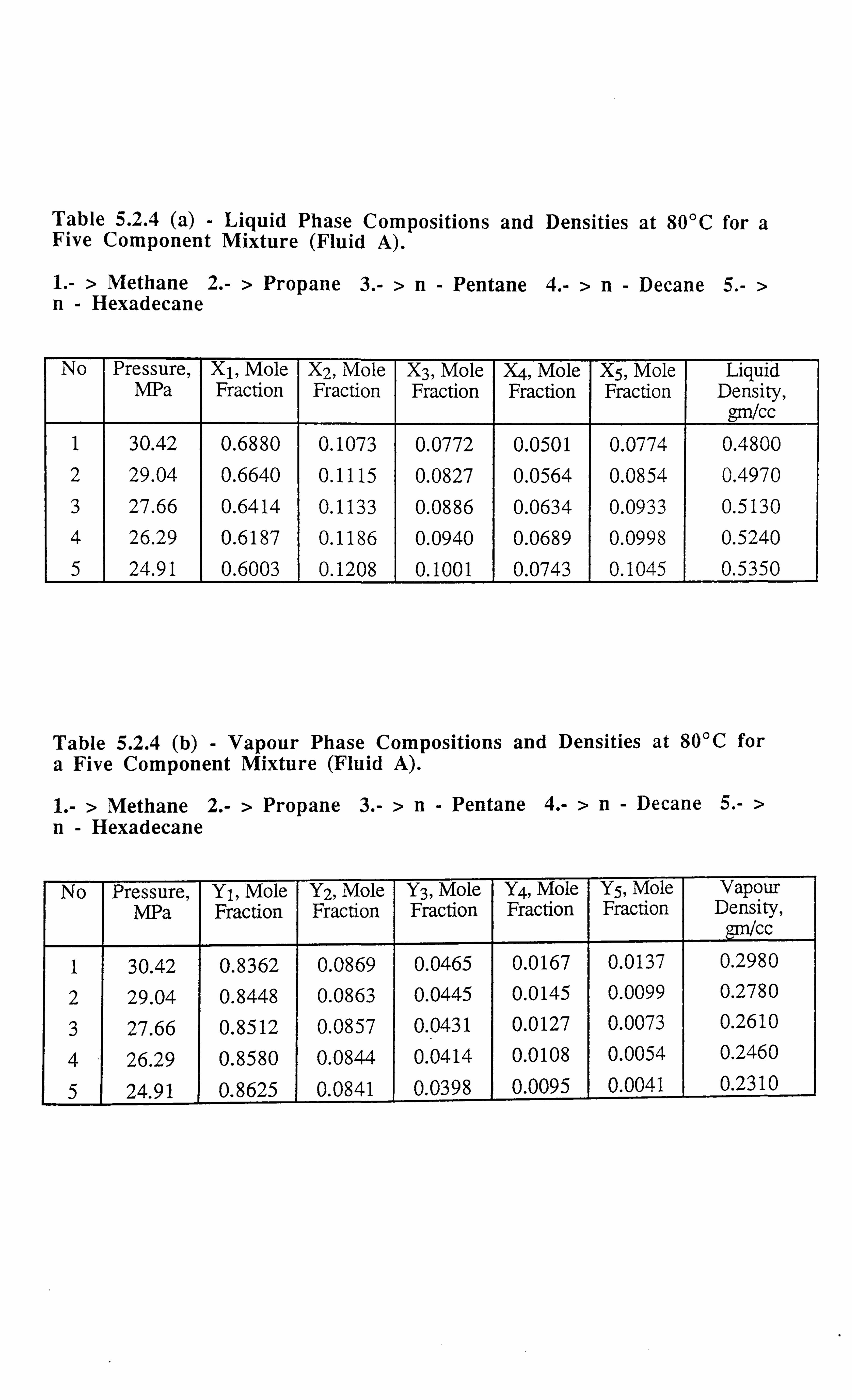
Table 5.2.4 (a) - Liquid Phase Compositions and Densities at 80°C for a Five Component Mixture (Fluid A).
1. - > Methane 2. - > Propane 3. - >n- Pentane 4. - >n- Decane 5. - > n- Hexadecane
No Pressure, MPa
X1, Mole Fraction
X2, Mole Fraction
X3, Mole Fraction
X4, Mole Fraction
X5, Mole Fraction
Liquid Density,
gm/cc 1 30.42 0.6880 0.1073 0.0772 0.0501 0.0774 0.4800 2 29.04 0.6640 0.1115 0.0827 0.0564 0.0854 0.4970 3 27.66 0.6414 0.1133 0.0886 0.0634 0.0933 0.5130 4 26.29 0.6187 0.1186 0.0940 0.0689 0.0998 0.5240
5 24.91 0.6003 0.1208 0.1001 0.0743 0.1045 0.5350
Table 5.2.4 (b) - Vapour Phase Compositions and Densities at 80°C for a Five Component Mixture (Fluid A).
1. - > Methane 2. - > Propane 3. - >n- Pentane 4. - >n- Decane 5. - > n- Hexadecane
No Pressure, MPa
Y1, Mole Fraction
Y2, Mole Fraction
Y3, Mole Fraction
Y4, Mole Fraction
Y5, Mole Fraction
Vapour Density,
gm/Cc
1 30.42 0.8362 0.0869 0.0465 0.0167 0.0137 0.2980
2 29.04 0.8448 0.0863 0.0445 0.0145 0.0099 0.2780
3 27.66 0.8512 0.0857 0.0431 0.0127 0.0073 0.2610
4 26.29 0.8580 0.0844 0.0414 0.0108 0.0054 0.2460
5 24.91 0.8625 0.0841 0.0398 0.0095 0.0041 0.2310
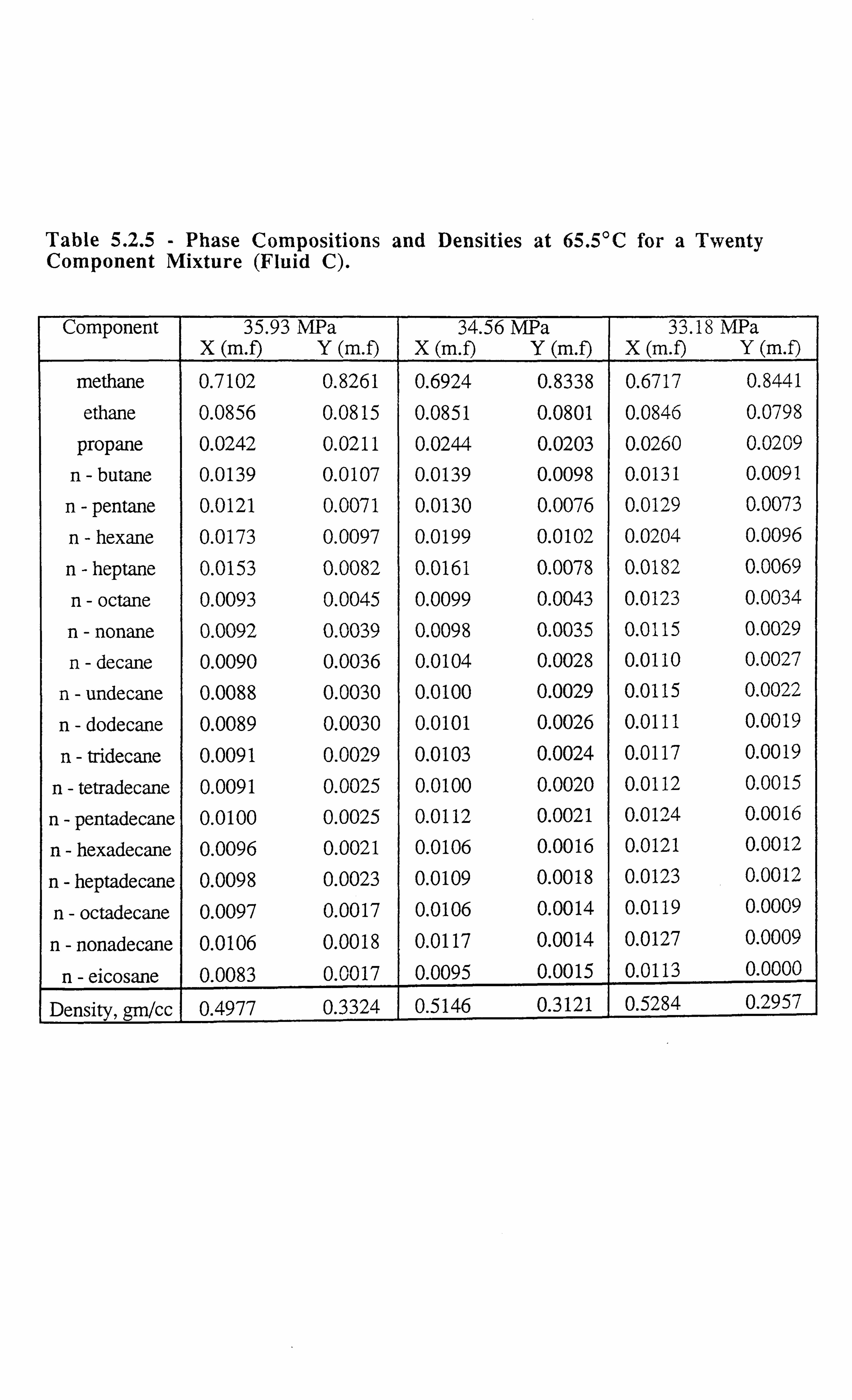
Table 5.2.5 - Phase Compositions and Densities at 65.5°C for a Twenty Component Mixture (Fluid C).
Component 35.93 MPa X (m. f) Y (m. f)
34.56 MPa X (m. f) Y (m. f)
33.18 X (m. f)
MPa Y (m. f)
methane 0.7102 0.8261 0.6924 0.8338 0.6717 0.8441
ethane 0.0856 0.0815 0.0851 0.0801 0.0846 0.0798
propane 0.0242 0.0211 0.0244 0.0203 0.0260 0.0209
n- butane 0.0139 0.0107 0.0139 0.0098 0.0131 0.0091
n- pentane 0.0121 0.0071 0.0130 0.0076 0.0129 0.0073
n- hexane 0.0173 0.0097 0.0199 0.0102 0.0204 0.0096
n- heptane 0.0153 0.0082 0.0161 0.0078 0.0182 0.0069
n- octane 0.0093 0.0045 0.0099 0.0043 0.0123 0.0034
n- nonane 0.0092 0.0039 0.0098 0.0035 0.0115 0.0029
n- decane 0.0090 0.0036 0.0104 0.0028 0.0110 0.0027
n- undecane 0.0088 0.0030 0.0100 0.0029 0.0115 0.0022
n- dodecane 0.0089 0.0030 0.0101 0.0026 0.0111 0.0019
n- tridecane 0.0091 0.0029 0.0103 0.0024 0.0117 0.0019
n- tetradecane 0.0091 0.0025 0.0100 0.0020 0.0112 0.0015
n- pentadecane 0.0100 0.0025 0.0112 0.0021 0.0124 0.0016
n- hexadecane 0.0096 0.0021 0.0106 0.0016 0.0121 0.0012
n- heptadecane 0.0098 0.0023 0.0109 0.0018 0.0123 0.0012
n- octadecane 0.0097 0.0017 0.0106 0.0014 0.0119 0.0009
n- nonadecane 0.0106 0.0018 0.0117 0.0014 0.0127 0.0009
n- eicosane 0.0083 0.0017 0.0095 0.0015 0.0113 0.0000
Density, gm%c 0.4977 0.3324 0.5146 0.3121 0.5284 0.2957
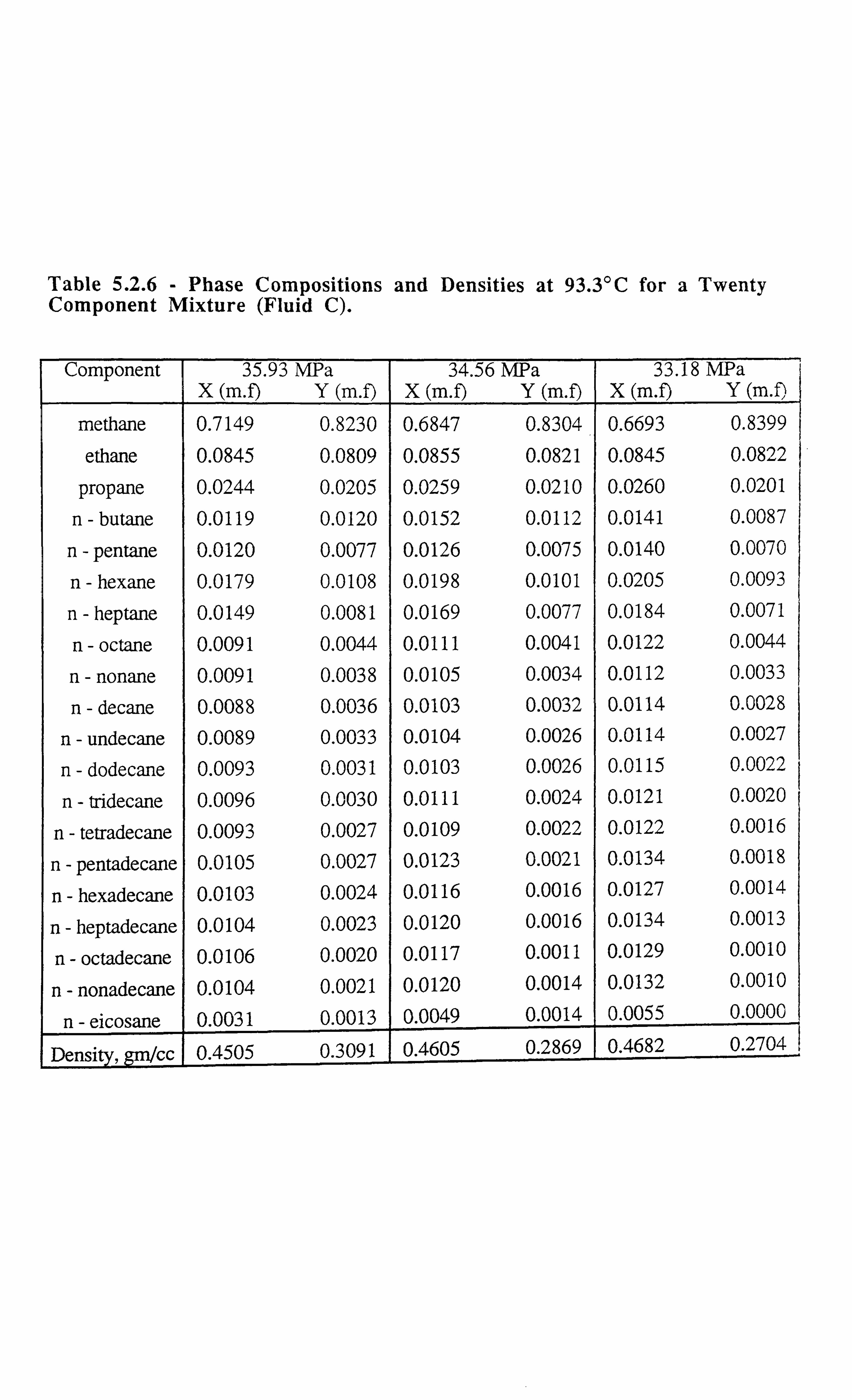
Table 5.2.6 - Phase Compositions and Densities at 93.3°C for a Twenty Component Mixture (Fluid Q.
Component 35.93 X (m. f)
MPa Y (m. f)
34.56 MPa X (m. f) Y (m. )
33.18 MPa X (m. f) Y (m. f)
methane 0.7149 0.8230 0.6847 0.8304 0.6693 0.8399
ethane 0.0845 0.0809 0.0855 0.0821 0.0845 0.0822
propane 0.0244 0.0205 0.0259 0.0210 0.0260 0.0201
n- butane 0.0119 0.0120 0.0152 0.0112 0.0141 0.0087
n- pentane 0.0120 0.0077 0.0126 0.0075 0.0140 0.0070
n- hexane 0.0179 0.0108 0.0198 0.0101 0.0205 0.0093
n- heptane 0.0149 0.0081 0.0169 0.0077 0.0184 0.0071
n- octane 0.0091 0.0044 0.0111 0.0041 0.0122 0.0044
n- nonane 0.0091 0.0038 0.0105 0.0034 0.0112 0.0033
n- decane 0.0088 0.0036 0.0103 0.0032 0.0114 0.0028
n- undecane 0.0089 0.0033 0.0104 0.0026 0.0114 0.0027
n- dodecane 0.0093 0.0031 0.0103 0.0026 0.0115 0.0022
n- tridecane 0.0096 0.0030 0.0111 0.0024 0.0121 0.0020
n- tetradecane 0.0093 0.0027 0.0109 0.0022 0.0122 0.0016
n- pentadecane 0.0105 0.0027 0.0123 0.0021 0.0134 0.0018
n- hexadecane 0.0103 0.0024 0.0116 0.0016 0.0127 0.0014
n- heptadecane 0.0104 0.0023 0.0120 0.0016 0.0134 0.0013
n- octadecane 0.0106 0.0020 0.0117 0.0011 0.0129 0.0010
n- nonadecane 0.0104 0.0021 0.0120 0.0014 0.0132 0.0010
n- eicosane 0.0031 0.0013 0.0049 0.0014 0.0055 0.0000
cc Density 0.4505 0.3091 0.4605 0.2869 0.4682 0.2704 1
,

Table 5.2.7 - Phase Compositions and Densities at 121.1°C for a Twenty Component Mixture (Fluid Q.
Component 35.25 MPa X (m. f) Y (m. f)
33.87 MPa X (m. fl Y (m. f)
32.49 MPa X (m. f) Y (m. f)
methane 0.7091 0.8236 0.6723 0.8378 0.6545 0.8441
ethane 0.0854 0.0823 0.0836 0.0796 0.0834 0.0802
propane 0.0240 0.0195 0.0254 0.0200 0.0249 0.0193
n- butane 0.0126 0.0105 0.0148 0.0098 0.0142 0.0094
n- pentane 0.0112 0.0082 0.0124 0.0072 0.0131 0.0072
n- hexane 0.0172 0.0108 0.0194 0.0100 0.0209 0.0101
n- heptane 0.0147 0.0083 0.0172 0.0075 0.0184 0.0069
n- octane 0.0092 0.0048 0.0111 0.0042 0.0114 0.0036
n- nonane 0.0090 0.0037 0.0104 0.0034 0.0116 0.0031
n- decane 0.0091 0.0038 0.0108 0.0029 0.0119 0.0025
n- undecane 0.0086 0.0032 0.0109 0.0025 0.0121 0.0022
n- dodecane 0.0088 0.0029 0.0110 0.0023 0.0119 0.0026
n- tridecane 0.0092 0.0027 0.0114 0.0022 0.0126 0.0018
n- tetradecane 0.0093 0.0025 0.0118 0.0021 0.0128 0.0015
n- pentadecane 0.0103 0.0027 0.0129 0.0019 0.0144 0.0015
n- hexadecane 0.0098 0.0022 0.0126 0.0016 0.0139 0.0012
n- heptadecane 0.0104 0.0022 0.0133 0.0015 0.0143 0.0011
n- octadecane 0.0101 0.0021 0.0131 0.0013 0.0143 0.0008
n- nonadecane 0.0113 0.0020 0.0141 0.0012 0.0155 0.0007
n- eicosane 0.0103 0.0019 0.0115 0.0012 0.0135 0.0000
cc Density 0.4395 0.2899 0.4676 0.2674 0.4897 0.2484 ,

Table 5.2.8 - Interfacial Tension Data for a Five 30'C (Fluid B) Using the Original Scaling Law and the Hough - Stegemeier's Parachor Method.
Component Mixture at and Parachor Method
No Pressure, MPa
Measured, mN/m
Scaling Law, mN/m
Parachor Method, mN/m
Hough - Stegemeier's Parachor Method,
mN/m 1 30.42 0.026 0.012 0.011 0.016 2 29.04 0.083 0.058 0.062 0.080 3 27.66 0.185 0.130 0.140 0.165 4 26.29 0.321 0.227 0.245 0.275 5 23.53 0.607 0.585 0.642 0.665 6 19.39 1.255 1.500 1.680 1.600
Table 5.2.9 - Interfacial Tension Data for a Five Component Mixture at 35'C (Fluid B) Using the Original Scaling Law and Parachor Method and the Hough - Stegemeier's Parachor Method.
No Pressure, MPa
Measured, mN/m
Scaling Law, mN/m
Parachor Method, mN/m
Hough - Stegemeier`s Parachor Method,
mN/m
1 30.42 0.031 0.029 0.029 0.039
2 29.04 0.116 0.097 0.099 0.119 3 27.66 0.192 0.174 0.181 0.208
4 26.29 0.320 0.295 0.312 0.343
5 24.91 0.450 0.434 0.464 0.494
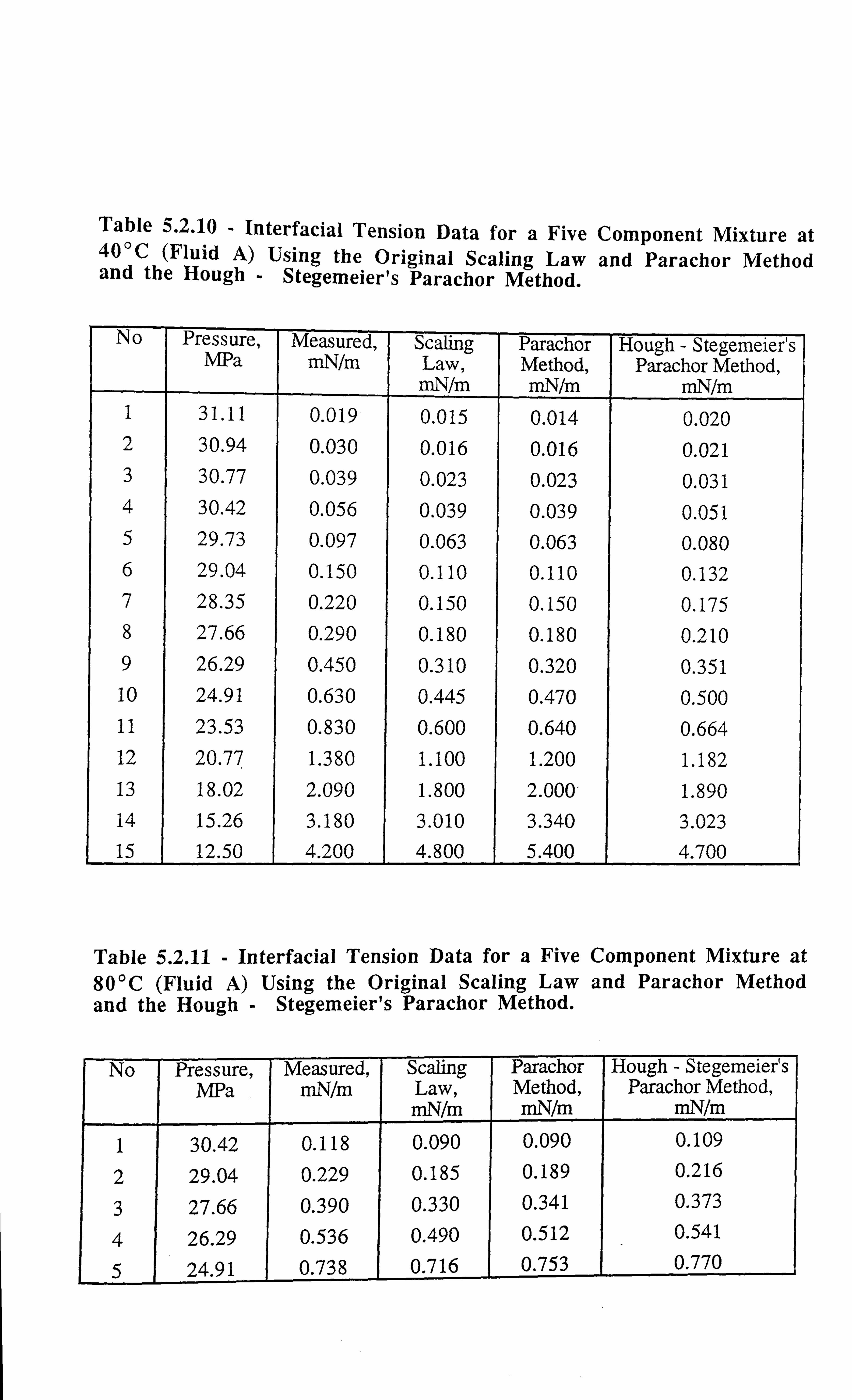
Table 5.2.10 - Interfacial Tension Data for a Five Component Mixture at 40'C (Fluid A) Using the Original Scaling Law and Parachor Method and the Hough - Stegemeier's Parachor Method.
No Pressure, MPa
Measured, mN/m
Scaling Law, mN/m
Parachor Method, mN/m
Hough - Stegemeier's Parachor Method,
mN/m 1 31.11 0.019 0.015 0.014 0.020 2 30.94 0.030 0.016 0.016 0.021 3 30.77 0.039 0.023 0.023 0.031 4 30.42 0.056 0.039 0.039 0.051 5 29.73 0.097 0.063 0.063 0.080 6 29.04 0.150 0.110 0.110 0.132 7 28.35 0.220 0.150 0.150 0.175 8 27.66 0.290 0.180 0.180 0.210 9 26.29 0.450 0.310 0.320 0.351 10 24.91 0.630 0.445 0.470 0.500 11 23.53 0.830 0.600 0.640 0.664 12 20.77 1.380 1.100 1.200 1.182 13 18.02 2.090 1.800 2.000 1.890 14 15.26 3.180 3.010 3.340 3.023 15 12.50 4.200 4.800 5.400 4.700
Table 5.2.11 - Interfacial Tension Data for a Five Component Mixture at 80'C (Fluid A) Using the Original Scaling Law and Parachor Method and the Hough - Stegemeier's Parachor Method.
No Pressure, MPa
Measured, mN/m
Scaling Law, mN/m
Parachor Method, mN/m
Hough - Stegemeier°s Parachor Method,
mN/m
1 30.42 0.118 0.090 0.090 0.109
2 29.04 0.229 0.185 0.189 0.216
3 27.66 0.390 0.330 0.341 0.373
4 26.29 0.536 0.490 0.512 0.541
5 24.91 0.738 0.716 0.753 0.770
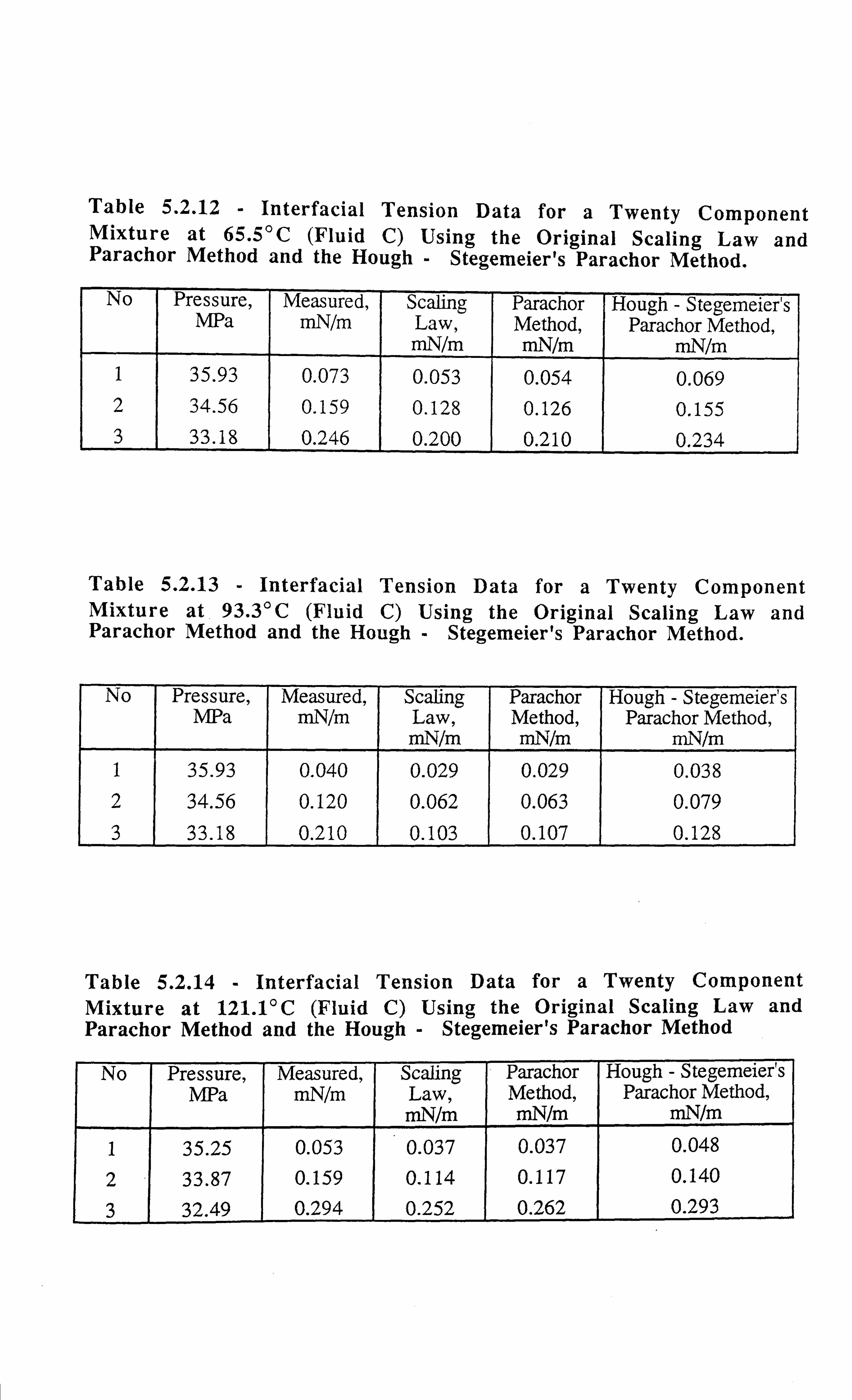
Table 5.2.12 - Interfacial Tension Data for a Twenty Component Mixture at 65.5°C (Fluid C) Using the Original Scaling Law and Parachor Method and the Hough - Stegemeier's Parachor Method.
No Pressure, Measured, Scaling Parachor Hough - Stegemeier's MPa mN/m Law, Method, Parachor Method,
mN/m mN/m mN/m 1 35.93 0.073 0.053 0.054 0.069 2 34.56 0.159 0.128 0.126 0.155 3 33.18 0.246 0.200 0.210 0.234
Table 5.2.13 - Interfacial Tension Data for a Twenty Component Mixture at. 93.3°C (Fluid C) Using the Original Scaling Law and Parachor Method and the Hough - Stegemeier's Parachor Method.
No Pressure, Measured, Scaling Parachor Hough - Stegemeier's MPa mN/m Law, Method, Parachor Method,
mN/m mN/m mN/m 1 35.93 0.040 0.029 0.029 0.038
2 34.56 0.120 0.062 0.063 0.079 3 33.18 0.210 0.103 0.107 0.128
Table 5.2.14 - Interfacial Tension Data for a Twenty Component Mixture at 121.1°C (Fluid C) Using the Original Scaling Law and Parachor Method and the Hough - Stegemeier's Parachor Method
No Pressure, Measured, Scaling Parachor Hough - Stegemeier's MPa mN/m Law, Method, Parachor Method,
mN/m mN/m mN/m
1 35.25 0.053 0.037 0.037 0.048
2 33.87 0.159 0.114 0.117 0.140
3 32.49 0.294 0.252 0.262 0.293
5.4). The interfacial tension data measured and predicted 1'2I has been tabulated through
Table (5.2.8) to Table (5.2.14), for these mixtures studied at various conditions. The tables
also show a column of the EIF7s predicted by using the Hough and Stegemeier's[3], method
(Section 4.2.1, Chapter 4). This method basically uses the same principle as the parachor
method[2], except that the exponent value used in this approach[3], is, E=3.67, instead of,
E=4.
From, the presented IFT data, Table (5.2.8) to Table (5.2.14), it can be seen that the IFTs
predicted by using the Hough and Stegmeiers[3], method (E=3.67) are in reasonable
agreement with the values measured by us (the reliability of which has already been
established[4]). Whereas the original scaling law and parachor methods[1L21, seem to
underestimate the IFI's at high pressure conditions or at low IFTs, and overestimate the IFTs
at low pressure conditions or high IFT conditions. The predictions agree, however, in some
cases for the intermediate range, i. e., 0.5 -1 mN/m. Hence, one can conclude from the
presented IFT data that the exponents suggested in the scaling law (E=3.911111... ){1], and
that suggested in the parachor method (E=4)[2], do not represent a universal value of
exponent for the entire range of IFTs.
5.3 : PROPOSED MODIFICATION OF SCALING LAW AND PARACHOR METHOD
In this section a modification based on the molar and mass density difference dependence of
the exponents for the scaling law[l] and parachor method[2] has been proposed. For this
purpose reliable literature data on measured IFTs for seven binaries were collected for the
analysis. The binaries were, C1-C3[2], C1-nC4[5], C1-nC5[6], C1-nC10[7], C02-nC4[8],
C02-nC10[9] & C02-nCl4C10]. Interfacial tensions ranging from 0.001 - 10 mN/m
comprised the data set of 213 points (Table 5.3.1), so that a wide ranging modification could
be proposed. All the IFT data[5,6,7,8,9,10], had been measured by the conventional pendant
drop method, only for the C1-C3[2], binary the IFTs were measured by the capillary rise
method.
64
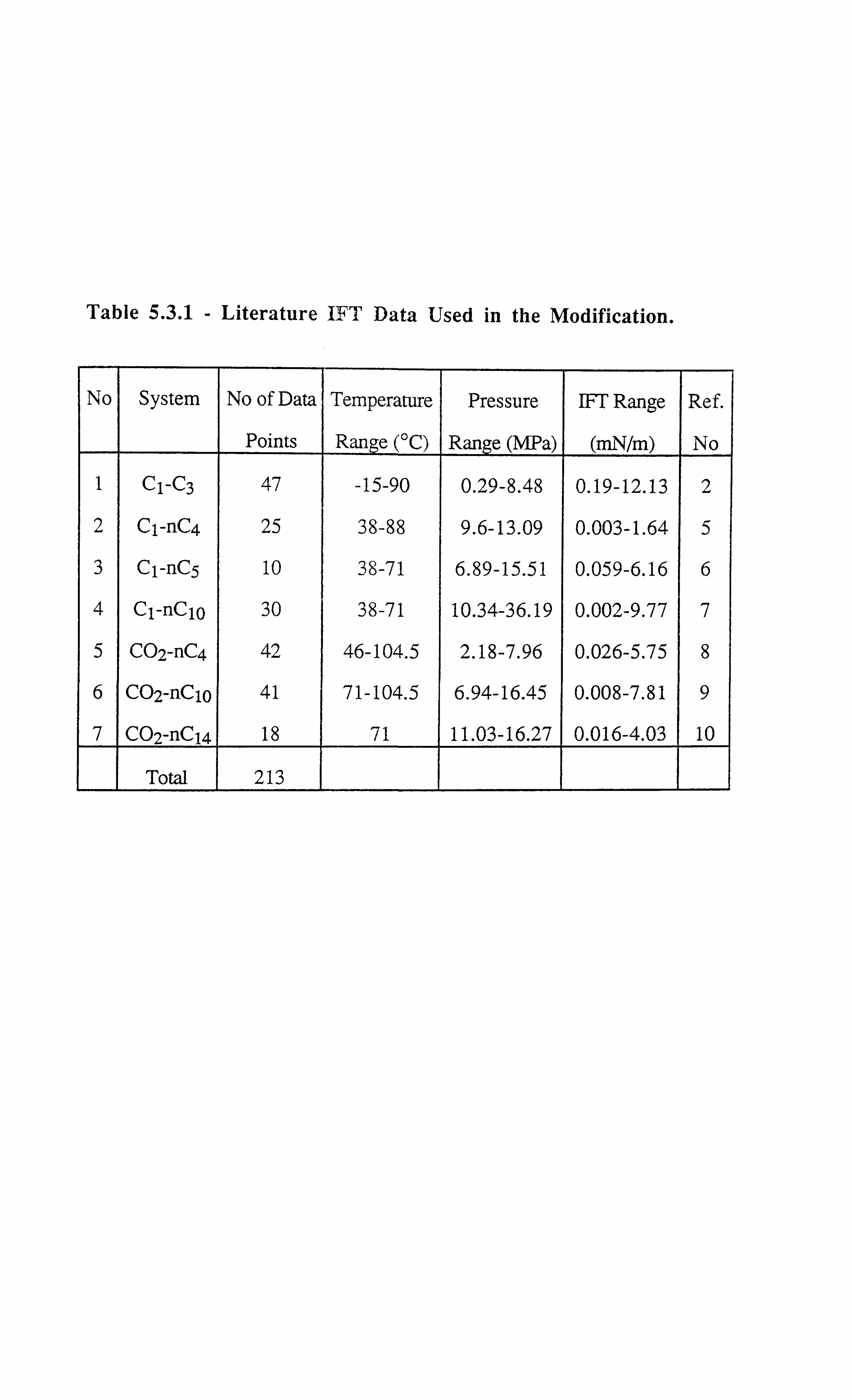
Table 5.3.1 - Literature IFT Data Used in the Modification.
No System No of Data
Points
Temperature
Range (°C)
Pressure
Range (MPa)
IFT Range
(mN/m)
Ref.
No
1 Cl-C3 47 -15-90 0.29-8.48 0.19-12.13 2
2 C1-nC4 25 38-88 9.6-13.09 0.003-1.64 5
3 C1-nC5 10 38-71 6.89-15.51 0.059-6.16 6
4 C1-nC10 30 38-71 10.34-36.19 0.002-9.77 7
5 C02-nC4 42 46-104.5 2.18-7.96 0.026-5.75 8
6 C02-nClp 41 71-104.5 6.94-16.45 0.008-7.81 9
7 C02-nC14 18 71 11.03-16.27 0.016-4.03 10
Total 213

For all the IFT data points under consideration the molar and mass density differences were
evaluated from the data sources [2,5,6,7,8,9,101. The interfacial tensions were also predicted
by using the Lee-Chien scaling law[ I] and Weinaug-Katz parachor method[2I by employing
the compositional and density data available from the same IFT data source. The percentage
deviations [ 100((Tpred-ßexp)/ßexp] of predicted results by the scaling law and parachor method
for all the binary systems are shown in Figures 5.3.1 and 5.3.2 respectively. Note that the
performances of both methods are quite similar. The scaling law, however, shows more
scatter particularly at low IFT.
Although the scaling law provides a value for the exponent E based on a mainly theoretical
approach, the exponent has been generally treated as an empirical parameter. The results
shown in Figures 5.3.1 and 5.3.2 indicate the performance of both methods can be
significantly improved by relating E to the IFT[13].
Subsequently the values of exponents were evaluated for both the scaling law{l11, and
parachor method[2], by matching the predictions with the measured IFT data. A considerable
scatter in the values of exponents was observed, however majority of the values lied between
3&4. This supports the conclusion that the exponents proposed in the original predictive
techniques fail to represent the universal values of E. The value of E in this work was
considered to be a function of the liquid-vapour molar density difference. The relation was
determined for both methods by regressing E to minimise the deviations of the predicted
results. The developed correlations of this work are :
Modified Lee-Chien Method :
E=3.535 + 17.76 (pes-pvm) (5.3.1)
Modified Weinaug-Katz Method :
E=3.583 + 0.16 (pim-pvm) (5.3.2)
65.
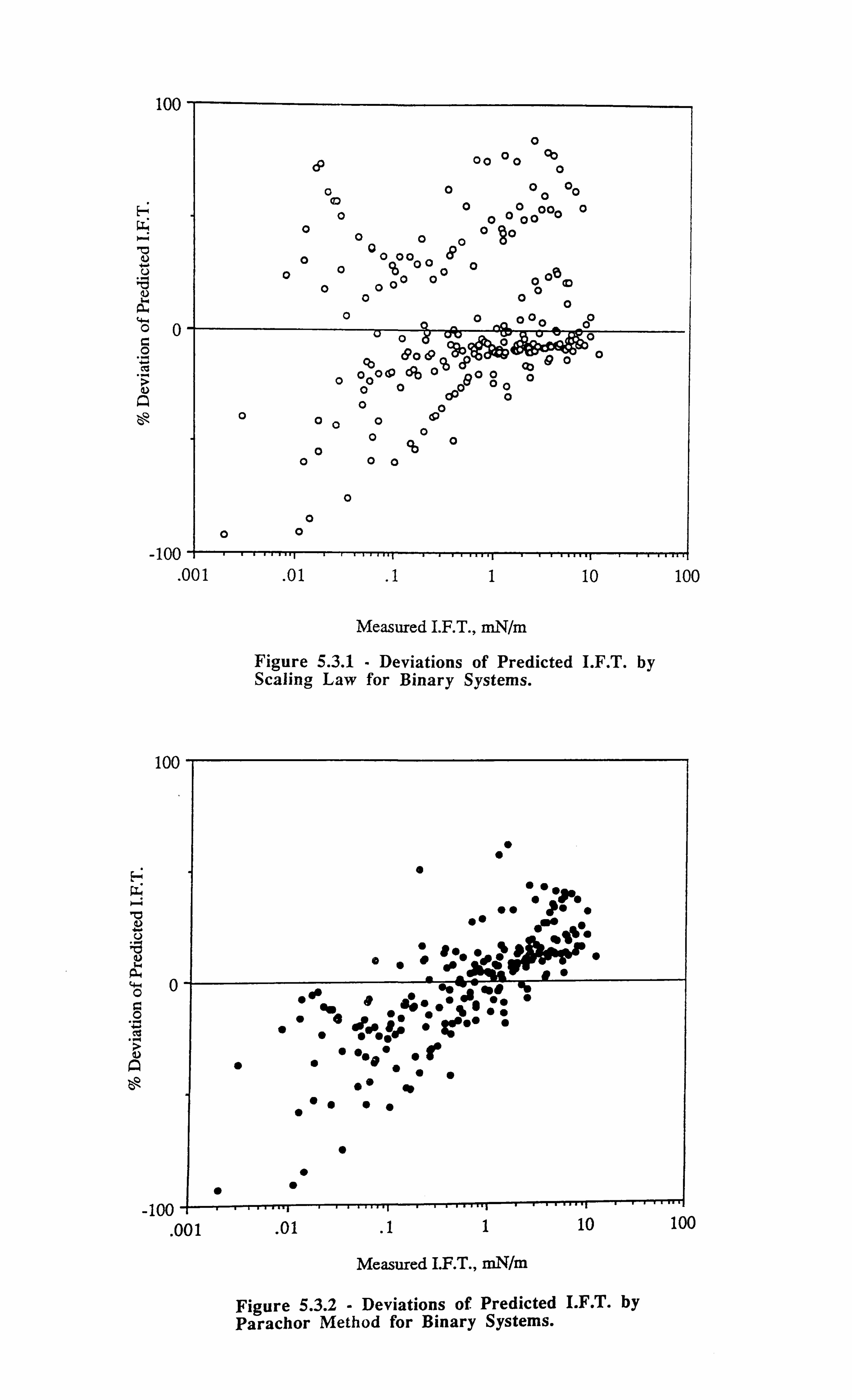
100
Eý w
0 °O °°
8o
000o 00 00 00 0 0 0000 0
0000o to
00o 00 8 00C°Q°0 0e
0° 0m 000o00
°0 000 °o ACL °0 (90(9 Bo 0 Cb 00 00 (b
0 o°oP ° go 0o
°0 dP° 00
0 0o
00°°0°0 0
000
0 0
00
aý U
a w op c 0
aý Q el
-100 -t-
. 001
E-ý w
'C ar U
a)
0
A el
. 01 .11 10 100
Measured I. F. T., mN/m
Figure 5.3.1 - Deviations of Predicted I. F. T. by Scaling Law for Binary Systems.
" "
. " ".
" iii "" ý" "
"" f" .
"
®"ý: ýi. " Ire* 0
". . '''.; r " ".. ' .
ý'
." ,".
"
" -100 --
. 001 . 01 .11 10 100
Measured I. F. T., mN/m
Figure 5.3.2 - Deviations of Predicted I. F. T. by Parachor Method for Binary Systems.
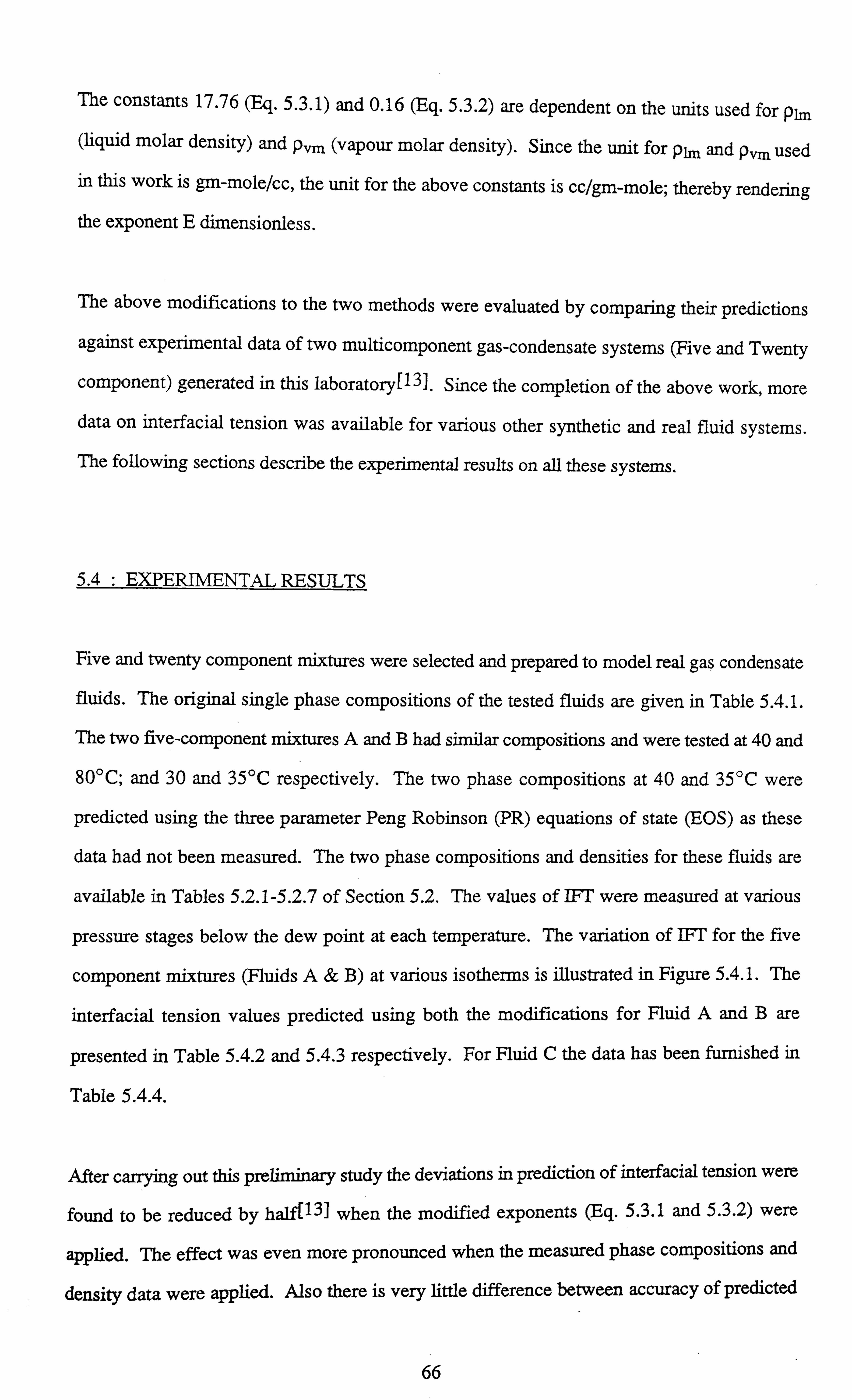
The constants 17.76 (Eq. 5.3.1) and 0.16 (Eq. 5.3.2) are dependent on the units used for p1m (liquid molar density) and pvm (vapour molar density). Since the unit for p1m and pvm used in this work is gm-mole/cc, the unit for the above constants is cc/gm-mole; thereby rendering
the exponent E dimensionless.
The above modifications to the two methods were evaluated by comparing their predictions
against experimental data of two multicomponent gas-condensate systems (Five and Twenty
component) generated in this laboratory[13]. Since the completion of the above work, more
data on interfacial tension was available for various other synthetic and real fluid systems.
The following sections describe the experimental results on all these systems.
5.4 : EXPERIMENTAL RESULTS
Five and twenty component mixtures were selected and prepared to model real gas condensate
fluids. The original single phase compositions of the tested fluids are given in Table 5.4.1.
The two five-component mixtures A and B had similar compositions and were tested at 40 and
80°C; and 30 and 35°C respectively. The two phase compositions at 40 and 35°C were
predicted using the three parameter Peng Robinson (PR) equations of state (EOS) as these
data had not been measured. The two phase compositions and densities for these fluids are
available in Tables 5.2.1-5.2.7 of Section 5.2. The values of IFT were measured at various
pressure stages below the dew point at each temperature. The variation of IFT for the five
component mixtures (Fluids A& B) at various isotherms is illustrated in Figure 5.4.1. The
interfacial tension values predicted using both the modifications for Fluid A and B are
presented in Table 5.4.2 and 5.4.3 respectively. For Fluid C the data has been furnished in
Table 5.4.4.
After carrying out this preliminary study the deviations in prediction of interfacial tension were
found to be reduced by half[131 when the modified exponents (Eq. 5.3.1 and 5.3.2) were
applied. The effect was even more pronounced when the measured phase compositions and
density data were applied. Also there is very little difference between accuracy of predicted
66

Table 5.4.1 - Compositions of Tested Fluids.
Component Fluid A Mole(%)
Fluid B Mole (%)
Fluid D Mole (%)
CO2 0.00 0.00 21.55 Cl 82.05 82.32 64.55 C3 8.95 8.71 6.96
nC5 5.00 5.05 3.63
nCjO 1.99 1.98 1.66 nC16 2.01 1.94 1.65
Fluid C (20-Component System)
Component Mole (%)
Cl 80.11 CZ 8.23 C3 2.11
nC4 1.07
nC5 0.80
nC6 1.20
nC7 0.96
nC8 0.55
nC9 0.49
nC1o 0.48
nCi 1 0.45
nCl2 0.44
nCl3 0.44
nC14 0.41
nCl5 0.41
nCl6 0.39
nC17 0.38
nC18 0.37
nC19 0.36
nC20 0.35
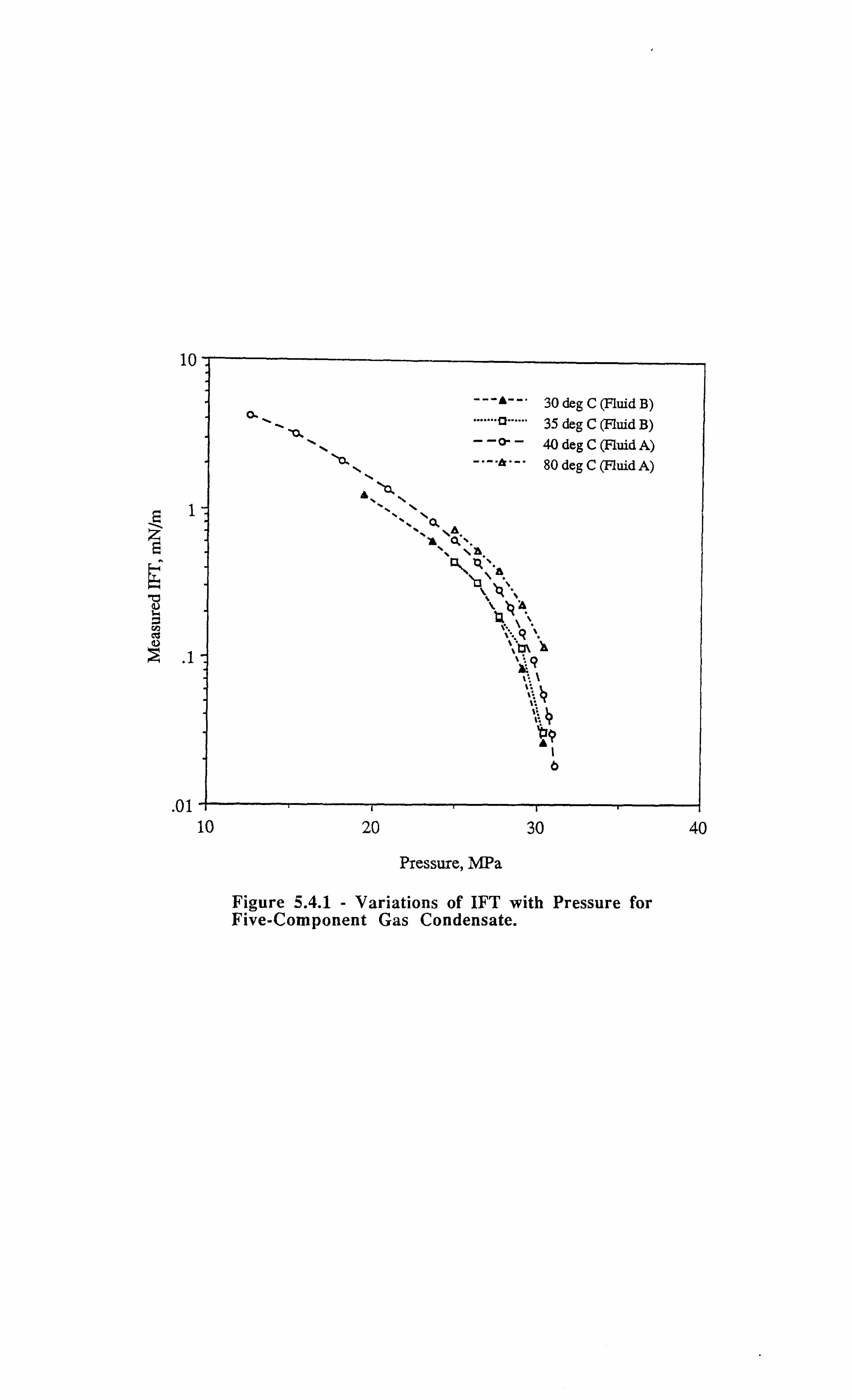
10
---A--
I
"O aý
cý aý ý
.1
. 01
..... "g...... 35 deg C (Fluid B) ýý--Q- 40 deg C (Fluid A)
80 deg C (Fluid A)
CL 30 deg C (Fluid B)
-A 4
v,
"
10 20 30 40
Pressure, MPa
Figure 5.4.1 - Variations of IFT with Pressure for Five-Component Gas Condensate.

Table 5.4.2 - Interfacial Tension Data for Fluid A* Using Original and Modified Scaling Law and Parachor Methods.
No Pressure Measured Scaling Law, Parachor Method, MPa IILN/I mN/m mN/m
Original Modified Original Modified
Temperature = 40°C 1 31.11 0.019 0.015 0.022 0.014 0.022 2 30.94 0.030 0.016 0.025 0.016 0.025 3 30.77 0.039 0.023 0.034 0.023 0.034 4 30.42 0.056 0.039 0.054 0.039 0.054 5 29.73 0.097 0.063 0.083 0.063 0.085 6 29.04 0.150 0.110 0.133 0.110 0.137 7 28.35 0.220 0.150 0.173 0.150 0.179 8 27.66 0.290 0.180 0.207 0.180 0.216 9 26.29 0.450 0.310 0.343 0.320 0.360 10 24.91 0.630 0.445 0.484 0.470 0.512 11 23.53 0.830 0.600 0.629 0.640 0.669 12 20.77 1.380 1.100 1.099 1.200 1.178 13 18.02 2.090 1.800 1.716 2.000 1.850
14 15.26 3.180 3.010 2.736 3.340 2.950 15 12.50 4.200 4.800 4.215 5.400 4.516
AAD** % 27.5 16.6 26.9 14.2 STDEV % 14.7 11.0 18.9 10.5
Temperature = 80°C
1 30.42 0.118 0.090 0.114 0.090 0.115 2 29.04 0.229 0.185 0.220 0.189 0.225
3 27.66 0.390 0.330 0.371 0.341 0.382
4 26.29 0.536 0.490 0.529 0.512 0.549
5 24.91 0.738 0.716 0.744 0.753 0.776
AAD % 14.0 2.9 12.1 2.8
STDEV % 7.4 2.0 9.1 3.0
* The single phase composition of this fluid is provided in Table 5.4.1, and the
two phase compositions are available in Tables 5.2.3 and 5.2.4 respectively. ** Average Absolute Deviation (AAD) and Standard Deviation (STDEV) are
defined in Table 5.4.9.

Table 5.4.3 - Interfacial Tension Data for Fluid B* Using Original and Modified Scaling Law and Parachor Method.
No Pressure Measured Scaling Law, Parachor Method, MPa mN/m mN/m mN/m
Original Modified Original Modified
Temperature = 30°C 1 30.42 0.026 0.012 0.019 0.011 0.018 2 29.04 0.083 0.058 0.080 0.062 0.083 3 27.66 0.185 0.130 0.164 0.140 0.171 4 26.29 0.321 0.227 0.268 0.245 0.284 5 23.53 0.607 0.585 0.623 0.642 0.672 6 19.39 1.255 1.500 1.445 1.680 1.589
. AAD % 27.7 12.7 28.4 14.5
STDEV % 23.3 13.5 28.6 18.0
Temperature = 35°C
1 30.42 0.031 0.029 0.041 0.029 0.041
2 29.04 0.116 0.097 0.122 0.099 0.126
3 27.66 0.192 0.174 0.207 0.181 0.216
4 26.29 0.320 0.295 0.335 0.312 0.352
5 24.91 0.450 0.434 0.474 0.464 0.503
AAD % 8.7 11.1 6.5 15.0
STDEV % 4.3 10.7 5.8 8.7
The single phase composition of this fluid is provided in Table 5.4.1, and the
two phase compositions are available in Tables 5.2.1 and 5.2.2 respectively.

Table 5.4.4 - Interfacial Tension Data for Fluid C* Using Original and Modified Scaling Law and Parachor Method.
Pressure Measured Scaling Law, Parachor Method, MPa mN/m mN/m mN/m
Original Modified Original Modified
Temperature = 65.5°C 35.93 0.073 0.053 0.072 0.054 0.073 34.56 0.159 0.128 0.153 0.126 0.158 33.18 0.246 0.200 0.238 0.210 0.247
AAD % 21.9 2.8 20.5 0.3 STDEV % 12.8 1.0 12.7 0.4
Temperature = 93.3°C 35.93 0.040 0.029 0.041 0.029 0.042 34.56 0.120 0.062 0.085 0.063 0.086
33.18 0.210 0.103 0.130 0.107 0.135
AAD % 42.3 23.3 41.3 23.0
STDEV % 25.1 16.0 24.5 15.3
Temperature = 121.1 °C
35.25 0.053 0.037 0.052 0.037 0.052
33.87 0.159 0.114 0.143 0.117 0.147 32.49 0.294 0.252 0.291 0.262 0.301
AAD % 24.3 4.3 22.5 3.9
STDEV % 14.6 3.4 13.9 2.7
The single phase composition of this fluid is provided in Table 5.4.1, and the
two phase compositions are available in Tables 5.2.5,5.2.6 and 5.2.7.

results by the scaling law and the parachor method both with the original and the modified
correlations.
These modifications have also been applied to a further amount of data on synthetic mixtures.
Table 5.4.5 shows the comparison of measured (during a CCE test) and predicted interfacial
tension data for a six component synthetic gas condensate mixture, referred to as Fluid D in
Table 5.4.1, at 100°C. The two phase compositions were predicted from the three parameter
PR EOS whereas measured density data were used for IFT calculations. The constant
composition expansion (CCE) experiment was carried out in the gas condensate cell and the
IFT data was determined by the gas-liquid curvature technique. Figure 5.4.2 and Table 5.4.6
present the comparison of measured and predicted interfacial tension for a gas cycling study
for a six component synthetic gas condensate mixture at 100°C and 22.75 MPa (Section
3.5.6). Liquid phase compositions predicted by the three parameter PR EOS were used along
with measured vapour phase compositions and densities. Table 5.4.7 shows the comparison
of IFT data for a multiple contact study carried out on a ternary mixture of CH4-C3-n-C10
(Section 3.5.5) with pure methane at 37.8°C. Two phase compositions were predicted from
the three parameter PR EOS whereas measured density data were used for IFT calculations.
Figure 5.4.3 and Table 5.4.8 shows interfacial tension values predicted for a ternary mixture
of C02-n-C4-n-C10[14] at 71.1°C. The calculations were performed using the measured
phase compositions and density data provided in the literature[14]. An overall statistical
analysis for 65 data points was performed for the original and modified scaling law and
parachor methods and is furnished in Table 5.4.9. Also shown in Table 5.4.9 gives the
deviations for all the methods for various different ranges of interfacial tension. This clearly
indicates the superiority of the proposed modifications and it can also be seen that the simple
introduction of a density dependent exponent has significantly improved the prediction
performance of the scaling law and the parachor method.
5.5 : INTERFACIAL TENSION PREDICTIONS OF REAL RESERVOIR FLUIDS
A comparative study for real reservoir fluids has also been carried out using the scaling lawfll
and the parachor method[21. The interfacial tension predictions were carried out for the real
67

Table 5.4.5 - Interfacial Tension Data for Fluid D* Using Original and Modified Scaling Law and Parachor Method.
No Pressure Measured Scaling Law, Parachor Method, MPa mN/m mN/m mN/m
Original Modified Original Modified 1 28.34 0.078 0.115 0.142 0.087 0.113 2 25.61 0.362 0.450 0.486 0.364 0.404 3 18.73 1.622 2.000 1.877 1.797 1.690
AAD % 31.7 44.0 7.6 20.2 STDEV % 11.1 27.9 5.0 17.7
ý` See Table 5.4.1 for single phase composition.
Table 5.4.6 - Interfacial Tension data for a Gas Injection Study on a Six Component Synthetic Gas Condensate" at 22.75 Mpa and 100°C Using Original and Modified Scaling Law and Parachor Method.
No Stage No.
Measured mN/m
Scaling Law, mN/m
Original Modified
Parachor Method, mN/m
Original Modified
1 0 0.853 1.300 1.260 1.202 1.180
2 1 1.359 1.742 1.653 1.681 1.593
3 2 1.742 2.249 2.090 2.260 2.080
4 3 2.123 2.744 2.514 2.799 2.514
5 4 2.347 3.004 2.732 3.086 2.744
AAD % 33.4 24.8 31.5 22.1
STDEV % 15.5 12.3 14.3 10.5
** Tests carried out on this fluid are discussed in Section 3.5.6, Chapter 3.
The two phase densities and compositions are available in Table 3.5.6.1
and 3.5.6.2 respectively.
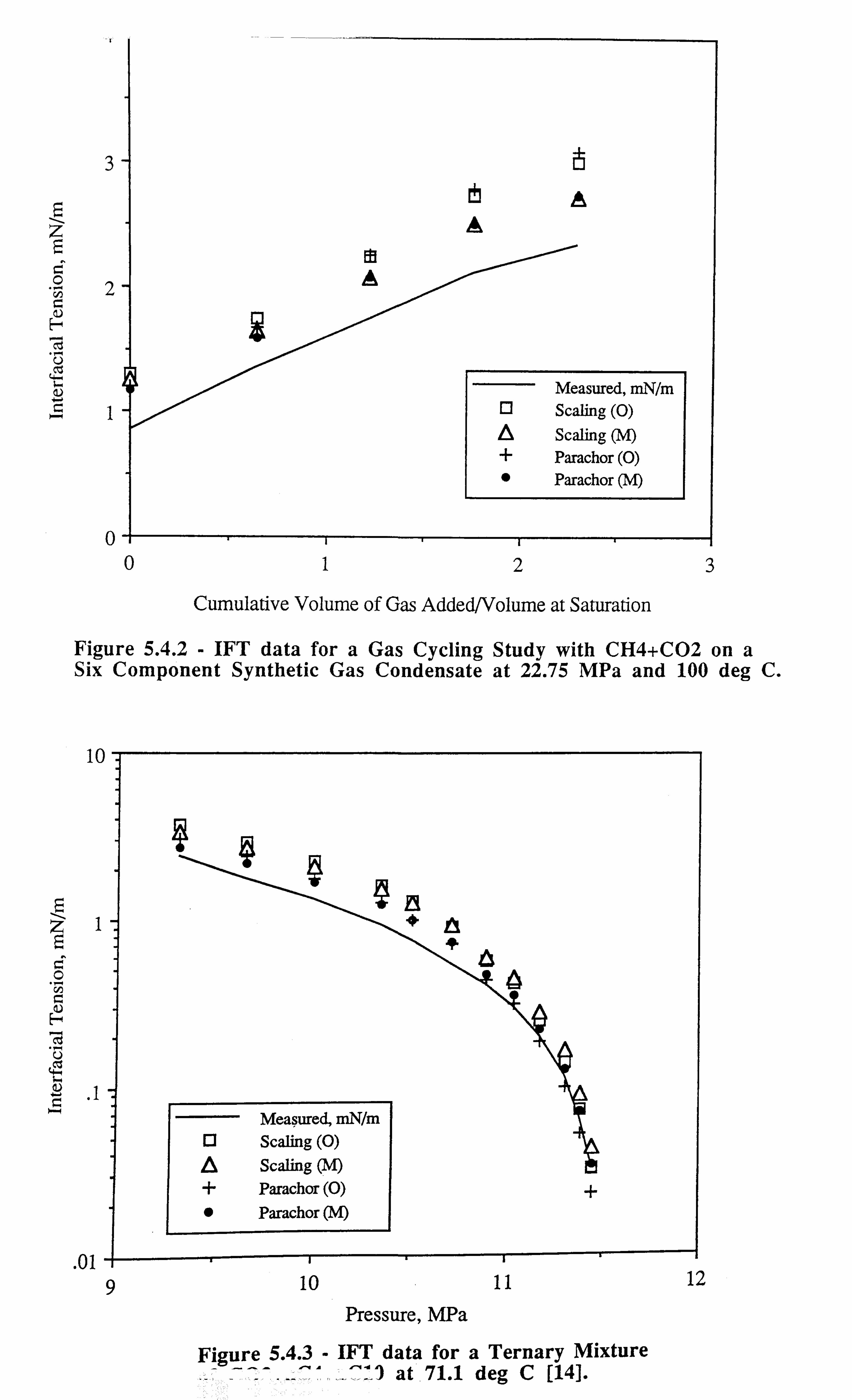
_T
E
3
z E O2
w
1
A A
Measured, mN/m Q Scaling (0) A Scaling (M) + Parachor (0) " Parachor (M)
0 0123
Cumulative Volume of Gas Added/Volume at Saturation
Figure 5.4.2 - IFT data for a Gas Cycling Study with CH4+CO2 on a Six Component Synthetic Gas Condensate at 22.75 MPa and 100 deg C.
1C
z1 E O
G H
cý . r, U
I
°' .1
En
e
8
e-, ý
ee
a
. 01 -1 9
+
Measured, mN/m Q Scaling (0)
Scaling (M) + Parachor (0) " Parachor (M)
10 11 12
Pressure, MPa
Figure 5.4 .3- IFT data for a Ternary Mixture at 71.1 deg C [14].
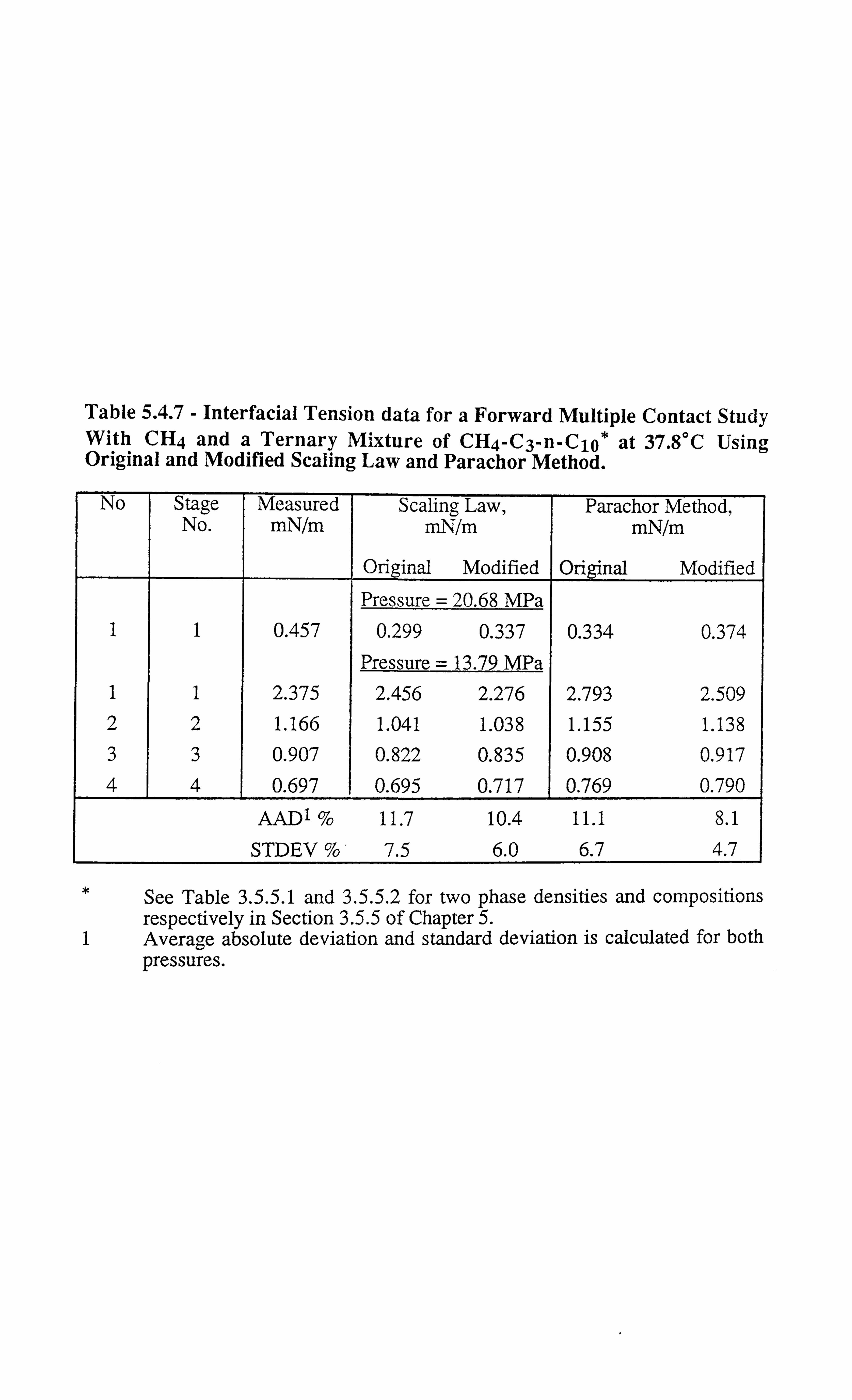
Table 5.4.7 - Interfacial Tension data for a Forward Multiple Contact Study With CH4 and a Ternary Mixture of CH4-C3-n-Cj 0 at 37.8°C Using Original and Modified Scaling Law and Parachor Method.
No Stage Measured Scaling Law, Parachor Method, No. mN/m mN/m mN/m
Original Modified Original Modified
Pressure = 20.68 MPa 1 1 0.457 0.299 0.337 0.334 0.374
Pressure = 13.79 MPa 1 1 2.375 2.456 2.276 2.793 2.509 2 2 1.166 1.041 1.038 1.155 1.138 3 3 0.907 0.822 0.835 0.908 0.917 4 4 0.697 0.695 0.717 0.769 0.790
AAD 1% 11.7 10.4 11.1 8.1
STDEV % 7.5 6.0 6.7 4.7
See Table 3.5.5.1 and 3.5.5.2 for two phase densities and compositions respectively in Section 3.5.5 of Chapter 5.
1 Average absolute deviation and standard deviation is calculated for both pressures.
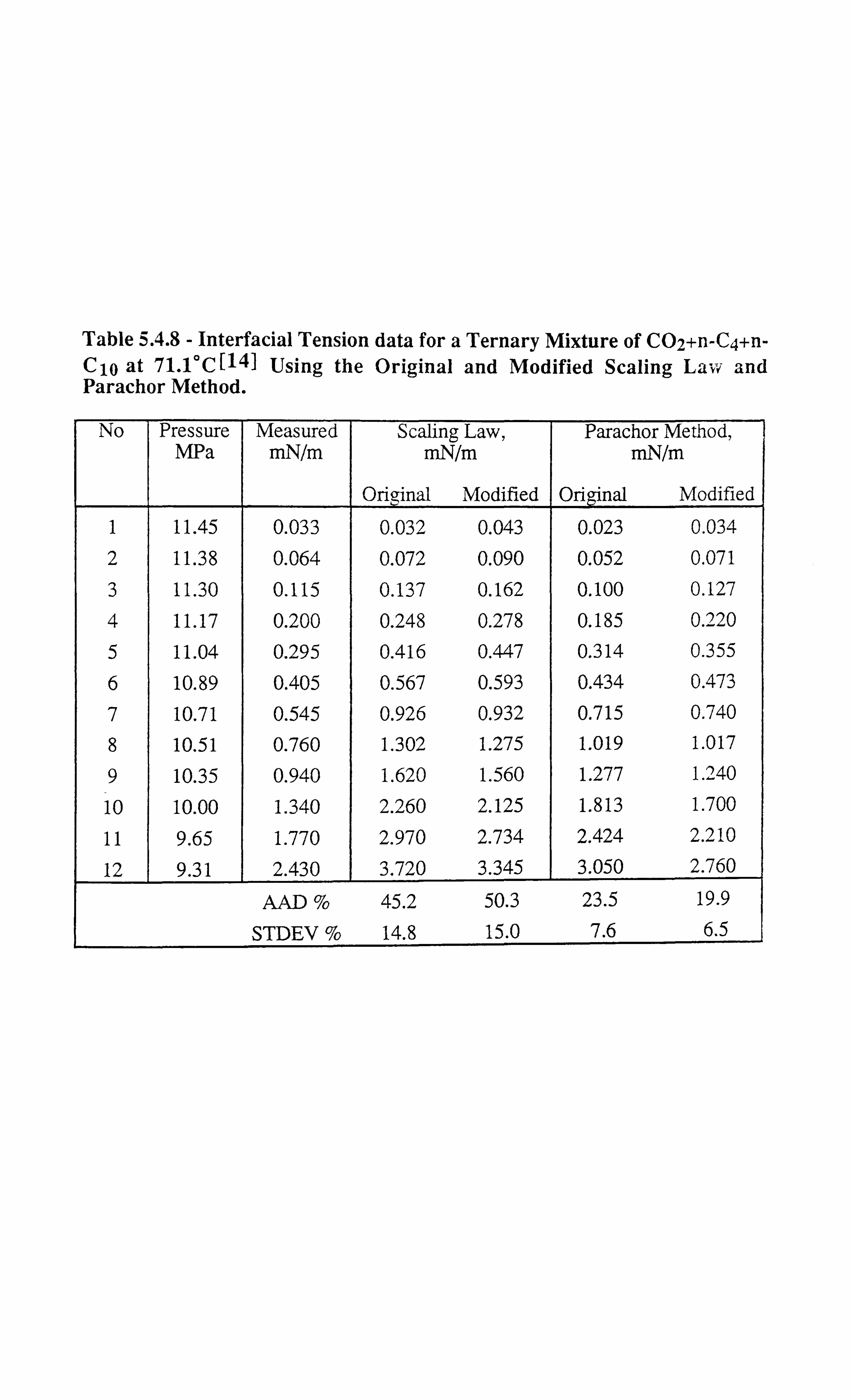
Table 5.4.8 - Interfacial Tension data for a Ternary Mixture of C02+n-C4+n- C10 at 71.1°C[14] Using the Original and Modified Scaling Law and Parachor Method.
No Pressure MPa
Measured mN/m
Scaling Law, mN/m
Original Modified
Parachor Method, mN/m
Original Modified
1 11.45 0.033 0.032 0.043 0.023 0.034
2 11.38 0.064 0.072 0.090 0.052 0.071
3 11.30 0.115 0.137 0.162 0.100 0.127
4 11.17 0.200 0.248 0.278 0.185 0.220
5 11.04 0.295 0.416 0.447 0.314 0.355
6 10.89 0.405 0.567 0.593 0.434 0.473 7 10.71 0.545 0.926 0.932 0.715 0.740
8 10.51 0.760 1.302 1.275 1.019 1.017
9 10.35 0.940 1.620 1.560 1.277 1.240
10 10.00 1.340 2.260 2.125 1.813 1.700
11 9.65 1.770 2.970 2.734 2.424 2.210
12 9.31 2.430 3.720 3.345 3.050 2.760
AAD % 45.2 50.3 23.5 19.9
STDEV % 14.8 15.0 7.6 6.5
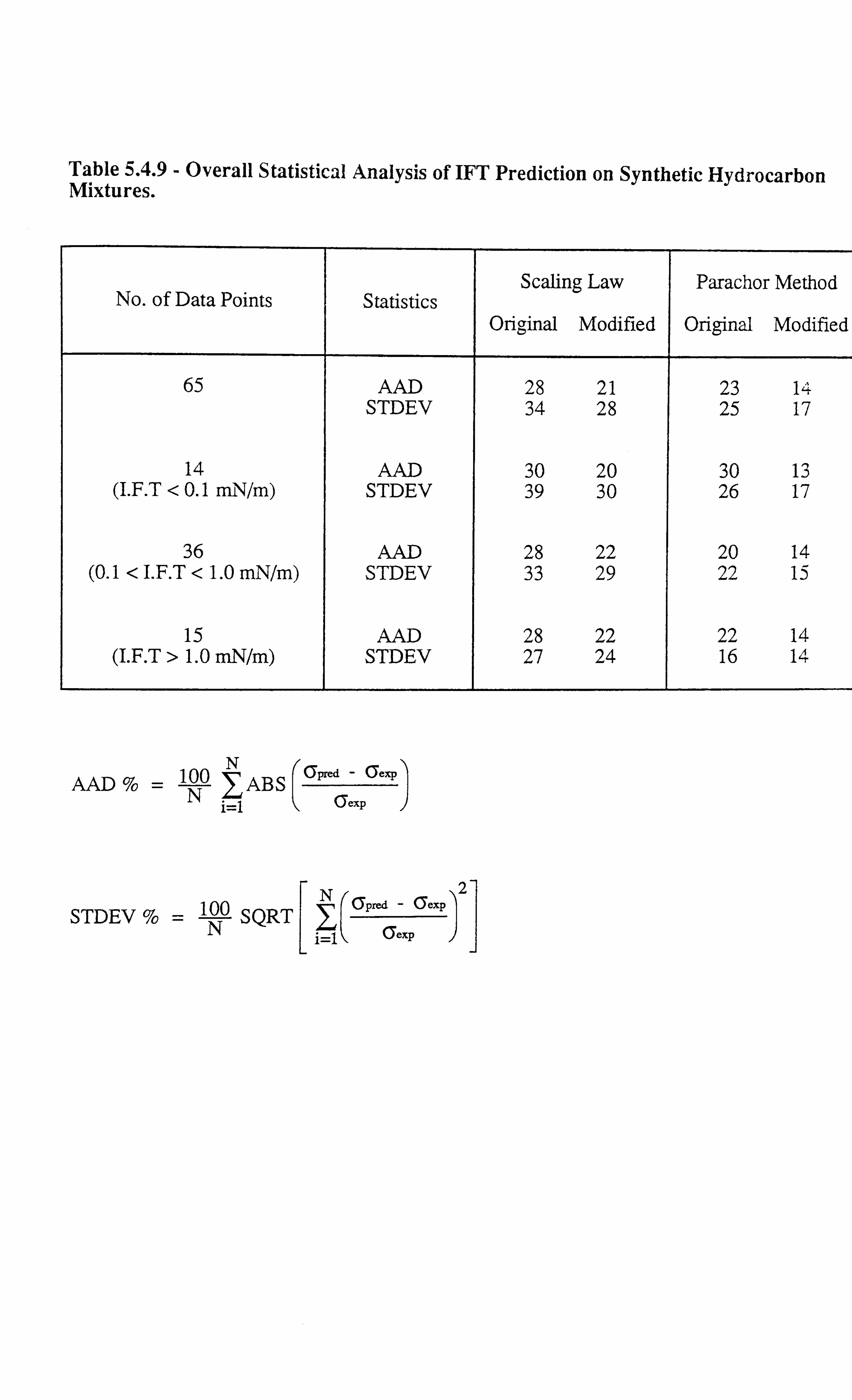
Table 5.4.9 - Overall Statistical Analysis of IFT Prediction on Synthetic Hydrocarbon Mixtures.
No. of Data Points Statistics Scaling Law
Original Modified
Parachor Method
Original Modified
65 AAD 28 21 23 1 STDEV 34 28 25 17
14 AAD 30 20 30 13 (I. F. T < 0.1 mN/m) STDEV 39 30 26 17
36 AAD 28 22 20 14 (0.1 < I. F. T < 1.0 mN/m) STDEV 33 29 22 15
15 AAD 28 22 22 14 (I. F. T > 1.0 mN/m) STDEV 27 24 16 14
N 6pmd - Gexp
AAD %= 100 LABS 1-1
6exp
STDEV %= 1N SQRT
L 6pred - 6ezp
i=1 heap

gas condensate fluid C3 (Section 3.6.1, Chapter 3), the real volatile oil (A) (Section 3.6.2,
Chapter 3), the real black oil RFS-1 (Section 3.6.3, Chapter 3) and one data (named as Oil-C
in Reference 15) set from the literature[151. The parachor value and the B parameter used in
the scaling law for the last fraction of each fluid was determined by matching to one measured
IFT data point. This approach has been recommended by other investigators[ 151 as the
generalised correlations for these parameters are not valid for the plus fraction of real reservoir
fluids apparently due to the presence of heavy surface active compounds of asphaltic nature.
These values were then applied to predict the IFT at other conditions for each mixture.
The predicted values of interfacial tension for the real gas condensate fluid C3 are provided in
Table 5.5.1 and Figures 5.5.1 and 5.5.2. The parameters of the last fraction were determined
by matching the measured value of 0.622 mN/m for the constant volume depletion (CVD) test
at 27.58 MPa and 140°C. These values were employed in calculating the IFT at other
conditions for CCE, CVD and gas cycling tests. Measured phase densities and compositions
were utilised in all calculations except for the gas cycling test where the liquid compositions
were predicted as the liquid was not removed for sampling during the test. Information on
two phase densities and compositions is available in Section 3.6.1 of Chapter 3.
Table 5.5.2 presents the comparison of predicted interfacial tension values with those
measured by the pendant drop method for the real volatile oil (A) for the flash and four stage
backward contact experiment at 100°C. The heavy end values were determined at an IFT
value of 0.663 mN/m for the second stage of the four stage backward contact test. These
values were then utilised in predicting the IFT for other conditions of the test and the flash
experiment. Predicted phase compositions and measured density values were used for the
IFT calculations for the four stage backward contact test. Measured phase compositions and
densities were used for the flash test. Two phase densities and compositions are provided in
Section 3.6.2 of Chapter 3.
A comparison between the measured and predicted interfacial tension data for the real black oil
RFS-1 for various multiple contact tests at 34.58 MPa and 100°C has been presented in Table
5.5.3. Similar to the volatile oil the heavy end values were determined at an IFT value of
68

Table 5.5.1 - Prediction of IFT for Fluid C31 Using Original and Modified Scaling Law and Parachor Method for CCE, CVD and Gas Cycling Tests.
No Pressure/Stage Measured Scaling Law, Parachor Method, No. mN/m mN/m mN/m MPa
Original Modified Original Modified
CCE* 1 27.58 0.564 0.691 0.687 0.650 0.649 2 20.68 1.523 1.746 1.593 1.760 1.595 3 13.79 3.251 3.831 3.275 4.288 3.562 4 6.89 6.335 6.366 5.234 8.275 6.434
AAD % 13.9 11.1 23.3 7.8 STDEV % 8.1 7.1 12.3 4.6
CVD** 1 31.03 0.253 0.383 0.404 0.344 0.367
2 27.58 0.622 0.622 0.622 0.622 0.622 AAD % 25.6 29.7 17.9 22.4
STDEV % 18.1 29.7 17.9 22.4
Gas Cycling***
1 1 0.994 1.094 1.043 1.002 0.956
2 2 1.173 1.264 1.189 1.166 1.097
3 3 1.519 1.593 1.456 1.535 1.394
4 4 1.785 1.804 1.621 1.907 1.692
AAD % 5.9 4.9 2.3 5.9
STDEV % 3.4 2.8 1.7 3.1
1 See Table 3.6.1.1 for single phase compositions * See Table 3.6.1.2 for compositions and Table 3.6.1.3 for densities ** See Table 3.6.1.4 compositions and Table 3.6.1.3 for densities *** See Table 3.6.1.5 for compositions and Table 3.6.1.3 for densities
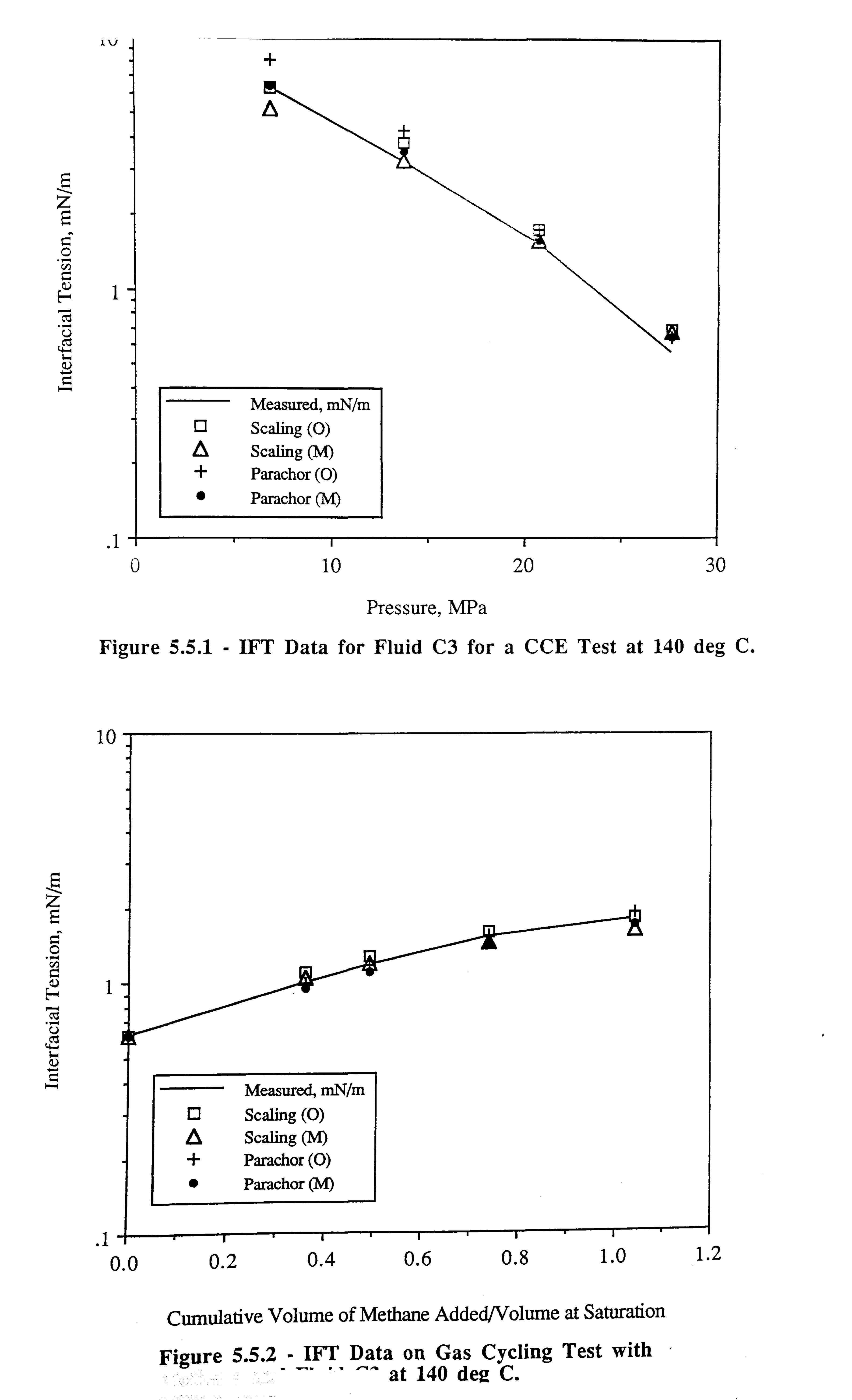
IV
+
I
j
z
0 . -. F; 1
U w
C
Measured, mN/m Q Scaling (0)
Scaling (M)
-ý- Parachor (0) " Parachor (M)
A
.1- 0 10 20 30
Pressure, MPa
Figure 5.5.1 - IFT Data for Fluid C3 for a CCE Test at 140 deg C.
10
Z
C C
C N
cý U
iý
C
1
--- Measured, mN/m Q Scaling (0)
Scaling (M)
-F Parachor (0)
" Parachor (M)
. 1-- 0.0 0.2 0.4 0.6 0.8 1.0
Cumulative Volume of Methane Added/Volume at Saturation
Figure 5.5.2 IFT Data on Gas Cycling Test with ' "" at 140 deg C.
1.2

Table 5.5.2 - Prediction of IFT for Real Volatile Oil (A)1 Using Original and Modified Scaling Law and Parachor Method for CCE, and Four Stage Backward Contact Study.
No Pressure/Stage Measured Scaling Law, Parachor Method, No. mN/m mN/m mN/m MPa
Original Modified Original Modified
CCE* 1 13.79 7.046 10.129 8.042 10.318 7.924 2 10.34 10.313 14.138 10.980 14.207 10.564 3 6.89 13.519 19.617 14.912 19.500 14.036
AAD % 41.9 10.3 42.8 6.2
STDEV % 24.3 6.2 24.8 4.4
Multiple Contact**
1 1 0.663 0.663 0.663 0.663 0.663 2 2 1.420 1.755 1.558 1.593 1.453 3 3 2.170 3.540 2.853 2.958 2.526 4 4 3.239 7.456 5.326 5.545 4.418
AAD % 54.2 26.4 29.9 13.8
STDEV % 36.6 18.1 20.2 10.0
1 See Table 3.6.2.1 for single phase compositions See Table 3.6.2.2 for compositions and Table 3.6.2.3 for densities
** See Table 3.6.2.5 for compositions and Table 3.6.2.4 for densities
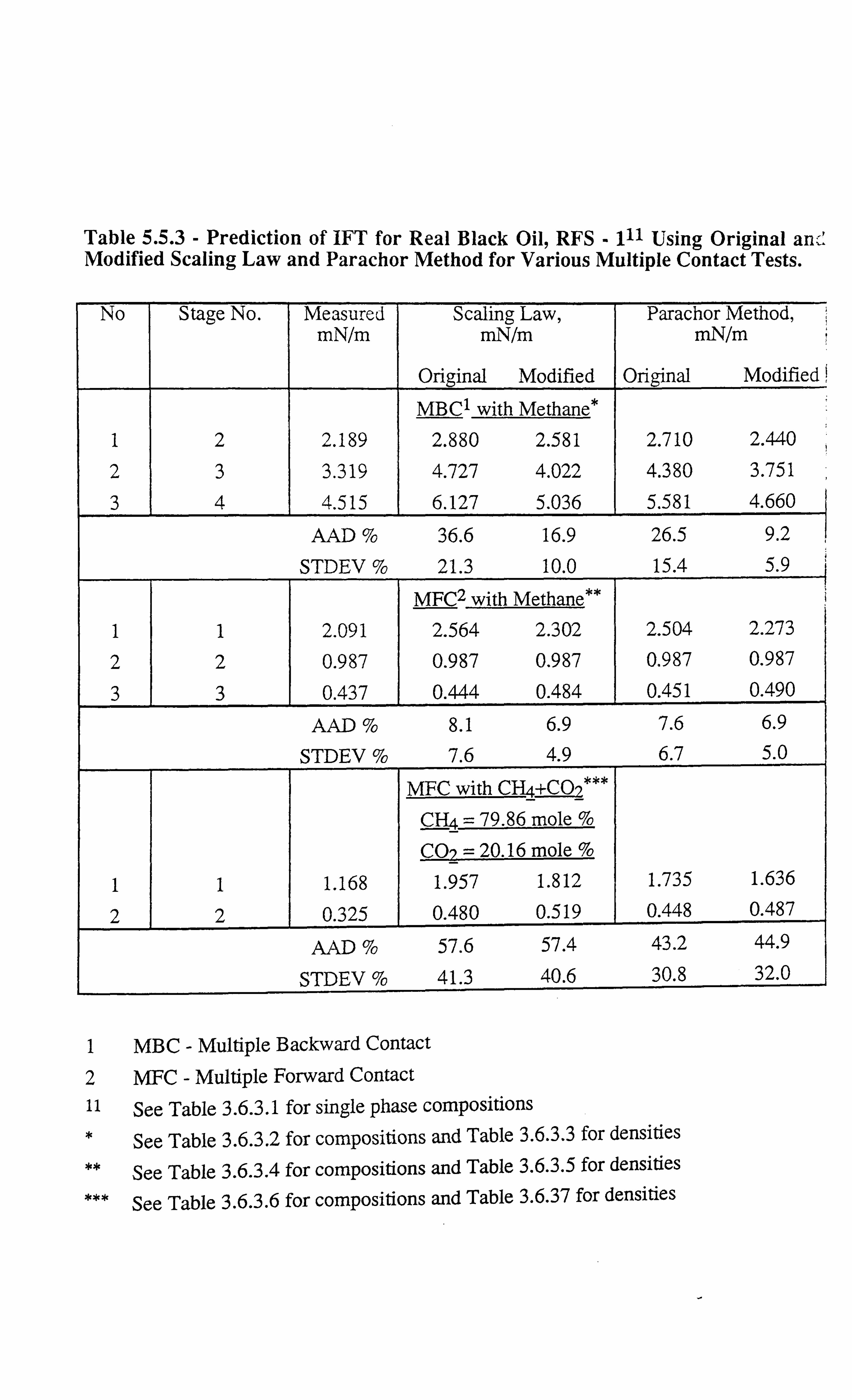
Table 5.5.3 - Prediction of IFT for Real Black Oil, RFS - 111 Using Original any' Modified Scaling Law and Parachor Method for Various Multiple Contact Tests.
No Stage No. Measured Scaling Law, Parachor Method, mN/m mN/m mN/m
Original Modified Original Modified
MBC1 with Methane*
1 2 2.189 2.880 2.581 2.710 2.440
2 3 3.319 4.727 4.022 4.380 3.751
3 4 4.515 6.127 5.036 5.581 4.660
AAD % 36.6 16.9 26.5 9.2 STDEV % 21.3 10.0 15.4 5.9
MFC2 with Methane**
1 1 2.091 2.564 2.302 2.504 2.273
2 2 0.987 0.987 0.987 0.987 0.987
3 3 0.437 0.444 0.484 0.451 0.490
AAD % 8.1 6.9 7.6 6.9
STDEV % 7.6 4.9 6.7 5.0
MFC with CH4+CO2***
CHa = 79.86 mole %
CO? = 20.16 mole %
1 1 1.168 1.957 1.812 1.735 1.636
2 2 0.325 0.480 0.519 0.448 0.487
AAD % 57.6 57.4 43.2 44.9
STDEV % 41.3 40.6 30.8 32.0
1 MBC - Multiple Backward Contact
2 MFC - Multiple Forward Contact
11 See Table 3.6.3.1 for single phase compositions * See Table 3.6.3.2 for compositions and Table 3.6.3.3 for densities
** See Table 3.6.3.4 for compositions and Table 3.6.3.5 for densities
*** See Table 3.6.3.6 for compositions and Table 3.6.37 for densities
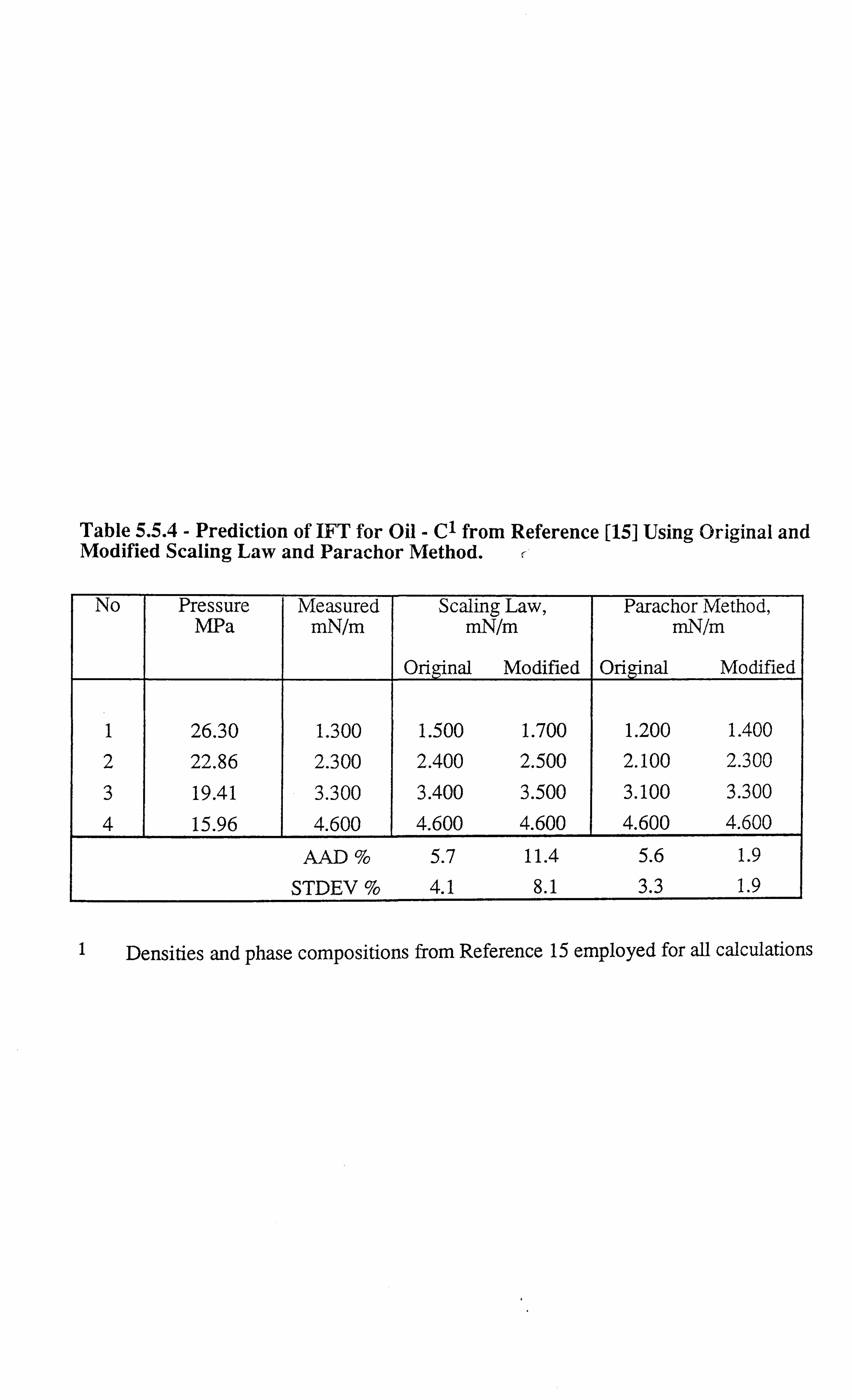
Table 5.5.4 - Prediction of IFT for Oil - C1 from Reference [15] Using Original and Modified Scaling Law and Parachor Method. r
No Pressure MPa
Measured mN/m
Scaling Law, mN/m
Original Modified
Parachor Method, mN/m
Original Modified
1 26.30 1.300 1.500 1.700 1.200 1.400
2 22.86 2.300 2.400 2.500 2.100 2.300
3 19.41 3.300 3.400 3.500 3.100 3.300
4 15.96 4.600 4.600 4.600 4.600 4.600
AAD % 5.7 11.4 5.6 1.9
STDEV % 4.1 8.1 3.3 1.9
Densities and phase compositions from Reference 15 employed for all calculations
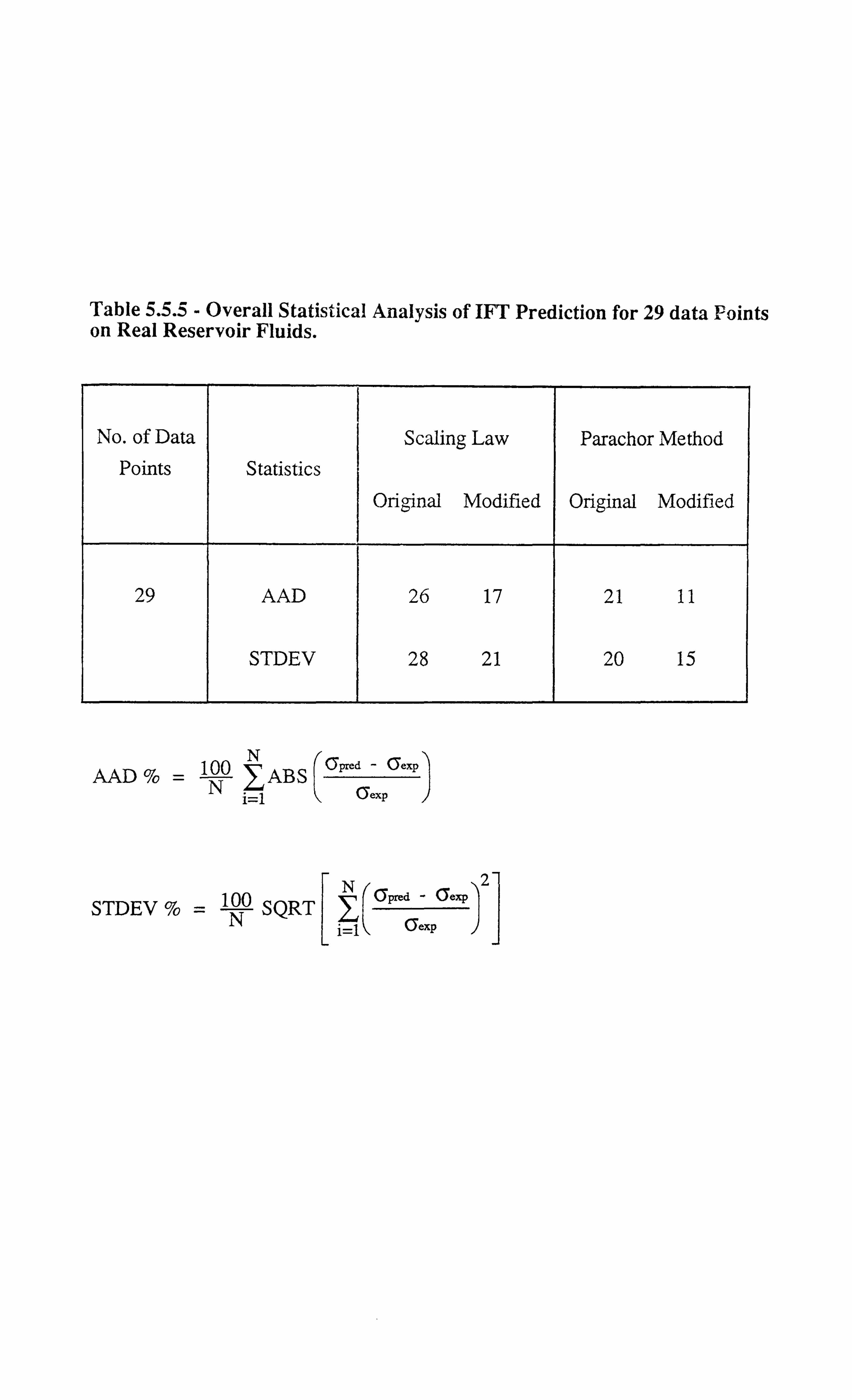
Table 5.5.5 - Overall Statistical Analysis of IFT Prediction for 29 data Points on Real Reservoir Fluids.
No. of Data I
Scaling Law Parachor Method Points Statistics
Original Modified Original Modified
29 AAD 26 17 21 11
STDEV 28 21 20 15
AAD% = 100 N
ABS N i=1
STDEV %=
6pred -
6exp
6exp
1N SQRTI
L N2 6pred - ßexp
1=1 6exp
0.987 mN/m for the second stage of the multiple forward contact test using pure methane as
an injection gas. Measured phase compositions and densities were employed for all =
predictions. All the data on two phase densities and compositions is furnished in Section
3.6.3 of Chapter 3. These tuned parameters were subsequently employed to predict the IFT
at other contact stages.
Table 5.5.4 shows the predictions for Oil-C at 82°C from Reference 15. The heavy end
values were determined at an IFT value of 4.6 mN/m and were used in prediction at other
conditions. Two phase compositions and densities provided in Reference 15 were employed
for all the 11-7 calculations. The overall statistical analysis of all the data of Tables 5.5.1 to
5.5.4 for the original and modified scaling law and the parachor method has been provided in
Table 5.5.5. The modified methods clearly show a better overall performance than the
original methods.
References
1) Lee, S. T. and Chien, M. C. H.: "A New Multicomponent Surface Tension
Correlation Based on Scaling Theory", Presented at the SPE/DOE Fourth
Symposium on Enhanced Oil Recovery held in Tulsa, Oklahoma, SPE/DOE,
12643, April 15-18, (1984).
2) Weinaug, C. F. and Katz, D. L.: "Surface Tension of Methane - Propane
Mixtures", Industrial & Engineering Chemistry (I & EC), pp. 239-246,
(1943).
3) Hough, E. W. and Stegemeier, G. L.: "Correlation of Surface Tension of Light
Hydrocarbons in the Critical Region", Society of Petroleum Engineers Journal
(SPEJ), pp. 259-263, (Dec., 1961).
4) Danesh, A., Todd, A. C., Somerville, J. and Dandekar, A.: "Direct
Measurement of Interfacial Tension, Density, Volume, and Compositions of
Gas - Condensate System", Trans IChem E, Vol. 68, Part A, (Jul., 1990).
69

5) Pennington, B. F. and Hough, E. W.: "Interfacial Tension of the Methane - Normal Butane System", Producers Monthly, pp. 4, (Jul., 1965).
6) Stegemeier, G. L. and Hough, E. W.: "Interfacial Tension of the Methane - Normal Pentane System", Producers Monthly, pp. 6-9, (Nov., 1961).
7) Stegemeier, G. L., Pennington, B. F., Brauer, E. B. and Hough, E. W.:
"Interfacial Tension of the Methane - Normal Decane System", Society of Petroleum Engineers Journal (SPED), pp. 257-260, (Sep., 1962).
8) Hsu, Jack, J. C, Nagarajan, N. and Robinson, R. L. Jr.: "Equilibrium Phase
Compositions, Phase Densities, and Interfacial Tensions for CO2 +
Hydrocarbon Systems. 1. CO2 +n- Butane", J. Chem. & Engg. Data., Vol.
30, No. 4, pp. 485-491, (1985).
9) Nagarajan, N. and Robinson, R. L. Jr.: "Equilibrium Phase Compositions,
Phase Densities, and Interfacial Tensions for CO2 + Hydrocarbon Systems. 2.
CO2 +n- Decane", J. Chem. & Engg. Data., Vol. 31, No. 2, pp. 168-171,
(1986).
10) Gasem, K. A. M., Dickson, K. B., Dulcamara, P. B., Nagarajan, N. and
Robinson, R. L. Jr.: "Equilibrium Phase Compositions, Phase Densities, and
Interfacial Tensions for CO2 + Hydrocarbon Systems. 5. CO2 +n-
Tetradecane", J. Chem. & Engg. Data., Vol. 34, No. 2, pp. 191-195, (1989).
11) Sage, B. H. and Lacey, W. N.: "Thermodynamic Properties of the Lighter
Paraffin Hydrocarbons and Nitrogen", New York, API, (1950).
12) Reid, R. C. and Sherwood, T. K.: "The Properties of Gases and Liquids",
Second Edition, McGraw Hill Book Co., New York (1973).
13) Danesh, A. S., Dandekar, A. Y., Todd, A. C. and Sarkar, R.: "A Modified
Scaling Law and Parachor Method Approach for Improved Prediction of
Interfacial Tension of Gas-Condensate Systems", Presented at the 66th Annual
Technical Conference and Exhibition of the Society of Petroleum Engineers
held in Dallas, Texas, October 6-9, SPE 22710, (1991).
14) Nagarajan, N., Gasem, K. A. M. and Robinson, R. L.: "Equilibrium Phase
Compositions, Phase Densities, and Interfacial Tensions for
70
CO2+Hydrocarbon Systems. 6. C02+n-Butane+n-Decane", J. Chem. Eng.
Data, Vol. 35, No. 35, pp. 228-231, (1990).
15) Firoozabadi, A., Katz, D. L., Soroosh, H. and Sajjadian, V. A.: "Surface
Tension of Reservoir Crude-Oil/Gas Systems Recognising the Asphalt in the
Heavy Fraction", Society of Petroleum Engineers Journal (Reservoir
Engineering), pp. 265-272, (Feb., 1988).
71
CHAPTER 6: CONCLUSIONS AND RECOMMENDATIONS
6.1 : CONCLUSIONS
Various techniques for measuring the interfacial tension between hydrocarbon vapour and
liquid phases have been evaluated in this work. It has been shown that the pendant drop
method which is widely used in the petroleum industry for measuring IFT, proves to be a
useful technique for measuring IFT at high values or low pressures but it is rather inaccurate
for measuring IFT at low values or high pressure conditions. A novel technique based on the
liquid-vapour interface curvature is introduced in this work to measure the interfacial tension
of hydrocarbon fluids along with other properties with a minimum effort. The IFT values
measured by the above technique have been compared with literature data wherever possible
and their reliability demonstrated. The following main conclusions can be drawn from the
work carried out on IFT measurements :
1.
2.
3.
A large amount of accurate and highly valuable data on interfacial tension, of
synthetic hydrocarbon mixtures and real reservoir fluids, at high pressure and high
temperature conditions has been generated in this work along with the commonly
available data on phase compositions, densities and volumes.
The measurement of gas-liquid interface curvature provides accurate interfacial
tension data with almost no extra effort if one has access to the equipment. The
relationship is rigorous and does not involve any empiricism and hence no need for
calibration. The simultaneous measurement of IFT, density and composition is
highly advantageous. It provides accurate IFT values and all the information
required to evaluate and improve IFT prediction methods.
The gas-liquid curvature technique developed in this work is now routinely employed
in the gas condensate PVT cell for measuring the IFT data for gas condensate type
72

fluids. Similarly the pendant drop method is now trivially used in the VLE cell to
measure the IFT data for volatile oil and black oil systems.
4. Interfacial tension varies with density difference between liquid and gas phases in
direct proportion, and hence accurate density data is essential for a reliable
measurement of interfacial tension, especially at high pressure conditions.
The two most widely used methods of predicting the interfacial tension in the petroleum
industry i. e. the scaling law and the parachor methods have been evaluated in this work. It
has been shown that the exponent in the interfacial tension correlations is not a universal
constant as commonly assumed in the prediction methods. The methods have been modified
by relating the exponent value to the liquid-vapour density difference and the relevant
correlations have been developed. The following main conclusions can be drawn from this
study.
1. The Weinaug-Katz (parachor method) and the Lee-Chien (scaling law) correlations
predict the IFT of high pressure hydrocarbon systems with a comparable accuracy.
The first method is, however, superior particularly at low IFT conditions.
2. Both methods generally underpredict at low II' and overpredict at high IFT ranges,
with relatively accurate results around 1 mN/m.
3. The modification proposed in this work, which can be simply applied to both
methods has improved the predicted IFT.
4. The comparative study carried out on the original and modified scaling law and
parachor method using interfacial tension data measured in-house and from literature
on synthetic mixtures and real reservoir fluids has clearly demonstrated the
superiority of the proposed modifications.
73
6.2 : RECOMMENDATIONS
The proposed measurement technique for IFT should further be used for more real gas -
condensate fluids, at a wide range of temperature and pressure conditions, in order to obtain
more of reliable data on interfacial tension.
The modifications proposed in the predictive techniques namely the scaling law and the
parachor method are recommended for estimation of interfacial tension of synthetic
hydrocarbon mixtures and real reservoir fluids instead of the original ones.
4
74

PART B- VISCOSITY
ABSTRACT
Viscosity is an important property required in various reservoir engineering
calculations. It is commonly predicted by either, the residual viscosity method or the
principle of corresponding states method. Various correlations available for
estimation of viscosity are reviewed in this part of the thesis. Also discussed are the
various density correlations which are generally used for density dependent viscosity
correlations.
A comparative study for pure hydrocarbon components and their mixtures by using
various viscosity prediction methods is presented. Also presented is a tuning study on
various real reservoir fluids by employing the popularly used residual viscosity and
corresponding states methods respectively. The drawbacks of these techniques have
been highlighted.
The residual viscosity method is critically evaluated and it has been proved that the
variation of residual viscosity with respect to reduced density is not uniform for all
fluids, particularly in the dense fluid phase. Based on a large number of data on pure
hydrocarbon compounds in the dense fluid phase from literature, the residual method
is modified by relating the residual viscosity of a fluid to its molecular weight along
with its reduced density in dense fluid phase conditions. The modified method has
been applied to various pure hydrocarbon compounds and their mixtures, and real
reservoir fluids. The superiority of the new method has been demonstrated by
comparing the results with those of the original methods and those based on the
principle of corresponding states.
TABLE OF CONTENTS
TABLE OF CONTENTS i LIST OF SYMBOLS iv LIST OF TABLES
vii LIST OF FIGURES ix
CHAPTER 1: INTRODUCTION - VISCOSITY 1 1.1 DEFINITIONS 1
1.2 SIGNIFICANCE OF VISCOSITY IN RESERVOIR ENGINEERING 3
1.3 EFFECT OF TEMPERATURE AND PRESSURE ON VISCOSITY OF
PURE COMPONENTS 5
1.4 EFFECT OF TEMPERATURE, PRESSURE, AND COMPOSITION ON
VISCOSITY OF REAL RESERVOIR FLUIDS 7
REFERENCES 8
CHAPTER 2: THE AVAILABLE VISCOSITY CORRELATIONS 9 2.1 INTRODUCTION 9
2.2 RESIDUAL VISCOSITY CORRELATION 10
2.3 PRINCIPLE OF CORRESPONDING STATES (ONE REFERENCE
COMPONENT) 14
2.4 EXTENDED PRINCIPLE OF CORRESPONDING STATES METHOD
(TRAPP) 20
2.5 PRINCIPLE OF CORRESPONDING STATES (TWO REFERENCE
COMPONENTS) 25
2.6 LEE'S METHOD FOR VISCOSITY OF GASES 27
2.7 LITTLE AND KENNEDY'S METHOD FOR VISCOSITY OF LIQUIDS 29
REFERENCES 33
1

CHAPTER 3: REVIEW OF CORRELATIONS FOR DENSITY OF GASES AND LIQUIDS 36 3.1 INTRODUCTION 36
3.1.1 Significance of Density in the Residual Viscosity Correlation 36
3.2 ALANI AND KENNEDY METHOD FOR DENSITY OF LIQUIDS 37
3.3 SOAVE - REDLICH - KWONG EOS FOR PREDICTION OF GAS
DENSITY 41
REFERENCES 43
CHAPTER 4: COMPARATIVE STUDY OF PREDICTIVE
TECHNIQUES FOR VISCOSITY
4.1 INTRODUCTION
4.2 VISCOSITY OF PURE COMPONENTS
4.3 VISCOSITY OF MIXTURES
4.4 TUNING OF VISCOSITY CORRELATIONS
REFERENCES
CHAPTER 5: THE MODIFIED RESIDUAL
METHOD (THIS WORK)
45
45
45
46
48
50
VISCOSITY
53
5.1 INTRODUCTION 53
5.2 EVALUATION OF THE J-S-T AND THE L-B-C CORRELATIONS 53
5.3 DEVELOPMENT OF THE MODIFIED RESIDUAL VISCOSITY
CORRELATION 54
5.3.1 Continuity Between the Original and Modified Correlation 57
5.4 APPLICATION OF THE MODIFIED RESIDUAL VISCOSITY METHOD
TO SYNTHETIC HYDROCARBON MIXTURES 58
5.5 APPLICATION OF THE MODIFIED RESIDUAL VISCOSITY METHOD
TO REAL RESERVOIR FLUIDS 59
REFERENCES 60
11

CHAPTER 6: CONCLUSIONS AND RECOMMENDATIONS 63
6.1 CONCLUSIONS 63
6.2 RECOMMENDATIONS 64
111
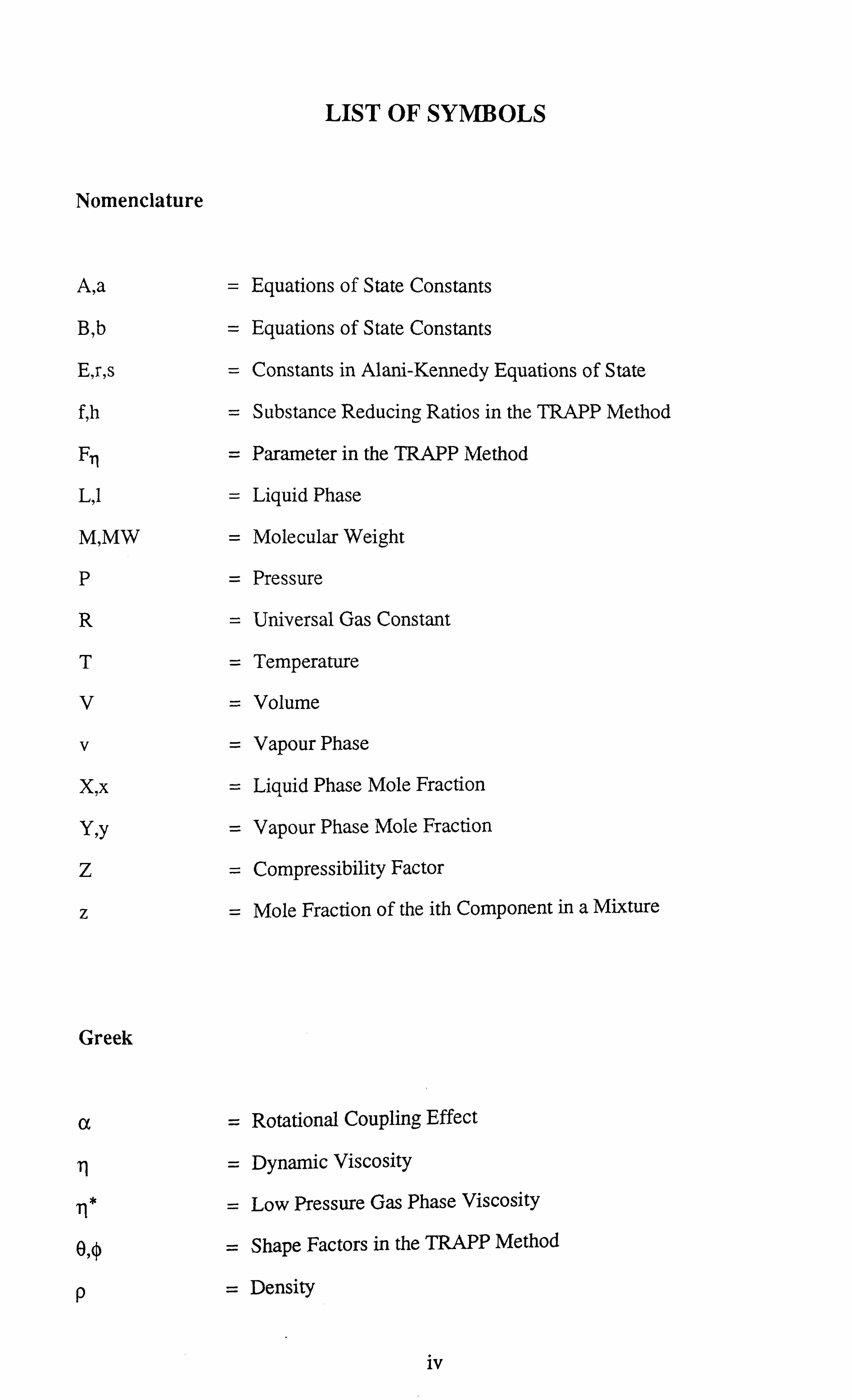
LIST OF SYMBOLS
Nomenclature
A, a = Equations of State Constants
B, b = Equations of State Constants
E, r, s = Constants in Alani-Kennedy Equations of State
f, h = Substance Reducing Ratios in the TRAPP Method
Fn = Parameter in the TRAPP Method
L, 1 = Liquid Phase
M, MW = Molecular Weight
P = Pressure
R = Universal Gas Constant
T = Temperature
V = Volume
v = Vapour Phase
X, x = Liquid Phase Mole Fraction
Y, y = Vapour Phase Mole Fraction
Z = Compressibility Factor
z = Mole Fraction of the ith Component in a Mixture
Greek
oc = Rotational Coupling Effect
11 = Dynamic Viscosity
7= Low Pressure Gas Phase Viscosity
O, 4 = Shape Factors in the TRAPP Method
p= Density
iv
G= Interfacial Tension
co = Acentric Factor
ý, k = Inverse of Critical Viscosity
Subscripts
c = Critical Value
C7+ = Plus Fraction of a Real Reservoir Fluid
i, j = Component Index
1 = Liquid
m = Molar/Mixture
mix = Mixture
n = Number of Components
o = Reference Component Indicator
r = Reduced Value
v = Vapour
Abbreviations
AAD = Average Absolute Deviation
ABS = Absolute Value
BIAS = Arithmetic Average of Percentage Deviations
FOR = Enhanced Oil Recovery
EOS = Equations of State
FPE = Fluid Phase Equilibria
J-S-T = Jossi-Stiel-Thodod
L-B-C = Lohrenz-Bray-Clark
V

PCS = Principle of Corresponding States
RV = Residual Viscosity
SG = Specific Gravity
STDEV = Standard Deviation
TRAPP = Transport Properties Prediction Program
VLE = Vapour-Liquid Equilibria
vi
LIST OF TABLES
Table 2.7.1 Empirical Constants in Eq. 2.7.7 for Pure Components for the Little
and Kennedy Method (from Reference 2).
Table 3.1.1.1 Effect of Density Inaccuracy on the Estimated Viscosity Using the
Lohrenz-Bray-Clark (LBC)[7] correlation (from Reference 9).
Table 3.2.1 Constants of Individual Pure Components for Alani and Kennedy
Correlation (from Reference 3).
Table 3.2.2 Comparison of Predicted Densities and Measured Densities for a
Binary Liquid Phase Mixture of Methane -n- Butane at 80°C.
Table 3.2.3 Comparison of Predicted Densities and Measured Densities for a
Carbon Dioxide and Synthetic Oil Mixture[s].
Table 3.3.1 Comparison of Predicted Densities and Measured Densities for a
Binary Vapour Mixture of Methane -n- Butane at 80°C.
Table 3.3.2 Comparison of Predicted Densities and Measured Densities for a
Low Ethane Natural Gas at 29.5°C.
Table 3.3.3 Comparison of Predicted Densities and Measured Densities for a
Low Ethane Natural Gas at 104.4°C.
Table 3.3.4 Comparison of Predicted Densities and Measured Densities for a
High Ethane Natural Gas at 25.9°C.
Table 3.3.5 Comparison of Predicted Densities and Measured Densities for a
High Ethane Natural Gas at 65.7°C.
Table 4.2.1 Typical Program Output for Viscosity Prediction of a Pure
Component.
Table 4.2.2 Average Absolute Deviations in Pure Component Viscosity
Predictions.
Table 4.3.1 Typical Program Output for Viscosity Prediction of Mixtures.
Table 4.3.2 Average Absolute Deviations in Mixture Viscosity Predictions.
vu

Table 4.4.1 Average Absolute Deviations of Predicted Viscosities of Real
Fluids.
Table 5.2.1 Effect of Simple and Cubic Mixing Rules on Prediction of
Viscosity Using the Lohrenz-Bray-Clark (L-B-C)[2] Correlation.
Table 5.3.1 Statistical analysis for the modified residual viscosity correlation
(Pure Components).
Table 5.4.1 Statistical analysis for the modified residual viscosity correlation
(Synthetic Mixtures).
Table 5.5.1 Statistical analysis for the modified residual viscosity correlation
(Real Reservoir Fluids).
yin

LIST OF FIGURES
Figure 1.1.1 Two Layers of a Fluid in Relative Motion.
Figure 1.3.1 Viscosity of Carbon Dioxide (from Reference 2).
Figure 1.3.2 Viscosity of Nitrogen (from Reference 2).
Figure 1.3.3 Generalised Phase Diagram for Gas Viscosity (from Reference 2).
Figure 1.3.4 Viscosities of Various Liquids as Functions of Temperature (from
Reference 2).
Figure 1.3.5 Effect of Pressure on the Viscosity of Liquids (from Reference 2).
Figure 1.4.1 Effect of Temperature on the Viscosity of a North Sea Oil at
Constant Pressure (27.76 MPa) and Constant Composition (from
Reference 4).
Figure 1.4.2 Effect of Pressure on the Viscosity of a North Sea Oil at Constant
Temperature (97.8°C) and Constant Composition (from Reference
5).
Figure 1.4.3 Effect of Pressure and Composition on Viscosity of a Synthetic
Near Critical Fluid at 38°C.
Figure 1.4.4 Effect of Composition on the Viscosity of a North Sea Oil at 71.1. °C
(from Reference 5).
Figure 2.2.1 Relationship Between Residual Viscosity Function and Reduced
Density (from Reference 7).
Figure 4.4.1 a Viscosity of North Sea Oil 1 at 97.8°C.
Figure 4.4.1 b Viscosity of North Sea Oil 1 at 97.8°C, All Methods Individually
Tuned at Bubble Point.
Figure 4.4.2 a Viscosity of North Sea Oil 2 at 93.3°C.
Figure 4.4.2 b Viscosity of North Sea Oil 2 at 93.3°C, All Methods Individually
Tuned at Bubble Point.
Figure 4.4.3 a Viscosity of North Sea Oil 3 at 71.1 T.
ix
Figure 4.4.3 b Viscosity of North Sea Oil 3 at 71.1°C, All Methods Individually
Tuned at Bubble Point.
Figure 4.4.4 a Viscosity of Malaysian Oil Mixture 4 at 125°F.
Figure 4.4.4 b Viscosity of Malaysian Oil 4 at 125°F, All Methods Individually
Tuned at Bubble Point.
Figure 4.4.5 a Viscosity of Malaysian Oil 5 at 196°F.
Figure 4.4.5 b Viscosity of Malaysian Oil 5 at 196°F, All Methods Individually
Tuned at Bubble Point.
Figure 4.4.6 a Viscosity of Malaysian Oil 6 at 187°F.
Figure 4.4.6 b Viscosity of Malaysian Oil 6 at 187°F, All Methods Individually
Tuned at Bubble Point.
Figure 4.4.7 a Viscosity of North Sea Fluid 7 at 353.2 K.
Figure 4.4.7 b Viscosity of North Sea Fluid 7 at 353.2 K, All Methods Individually
Tuned at Bubble Point.
Figure 5.2.1 Deviations of Calculated Viscosity from Experimental Value for the
J-S-T Method for the Pure Components Investigated.
Figure 5.2.2 Deviations of Calculated Viscosity from Experimental Value for the
L-B-C Correlation for Binary Mixtures.
Figure 5.3.1 Plot of Residual Viscosity vs. Reduced Density.
Figure 5.3.2 Dependence of Residual Viscosity on Molecular Weight.
Figure 5.3.3 Plot of loge(RV) vs. Reduced Density for the Group, nC6, Toluene
and nC8.
Figure 5.3.4 Plot of Coefficients of Individual Compounds vs. Molecular
Weight.
Figure 5.3.5 Deviations of Calculated Viscosity from Experimental Values for
Pure Components.
Figure 5.3.1.1 Continuity Between the Original and Modified Correlation for
nC10"
X

Figure 5.3.1.2 Continuity Between the Original and Modified Correlation for a
C02+nClp Binary Mixture.
Figure 5.4.1 Deviations of Calculated Viscosity from Experimental Value for
Synthetic Mixtures.
xi
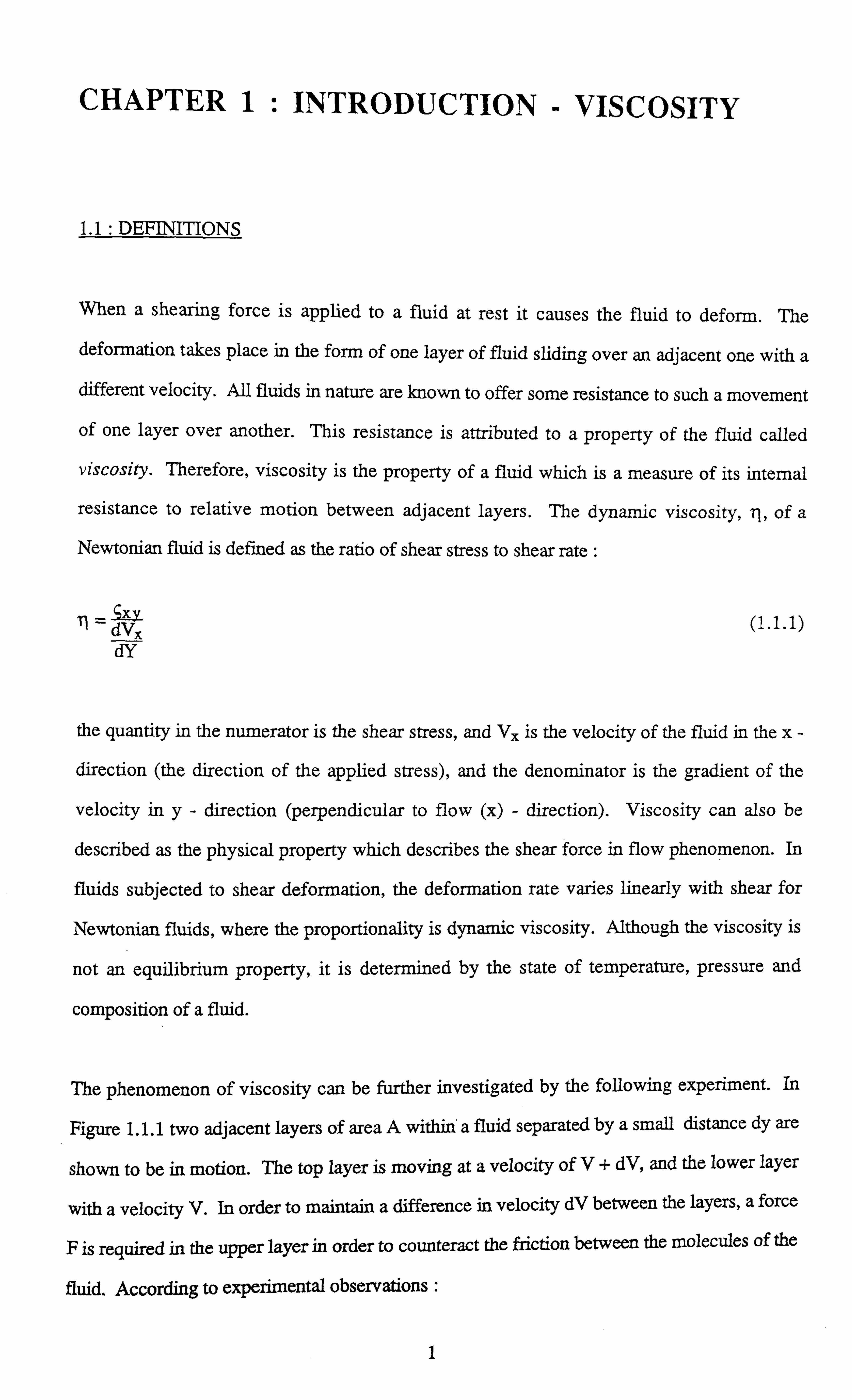
CHAPTER 1
1.1 : DEFINITIONS
: INTRODUCTION - VISCOSITY
When a shearing force is applied to a fluid at rest it causes the fluid to deform. The
deformation takes place in the form of one layer of fluid sliding over an adjacent one with a
different velocity. All fluids in nature are known to offer some resistance to such a movement
of one layer over another. This resistance is attributed to a property of the fluid called
viscosity. Therefore, viscosity is the property of a fluid which is a measure of its internal
resistance to relative motion between adjacent layers. The dynamic viscosity, TI, of a
Newtonian fluid is defined as the ratio of shear stress to shear rate :
1 dVx dY
(1.1.1)
the quantity in the numerator is the shear stress, and V. is the velocity of the fluid in the x-
direction (the direction of the applied stress), and the denominator is the gradient of the
velocity in y- direction (perpendicular to flow (x) - direction). Viscosity can also be
described as the physical property which describes the shear force in flow phenomenon. In
fluids subjected to shear deformation, the deformation rate varies linearly with shear for
Newtonian fluids, where the proportionality is dynamic viscosity. Although the viscosity is
not an equilibrium property, it is determined by the state of temperature, pressure and
composition of a fluid.
The phenomenon of viscosity can be further investigated by the following experiment. In
Figure 1.1.1 two adjacent layers of area A withini a fluid separated by a small distance dy are
shown to be in motion. The top layer is moving at a velocity of V+ dV, and the lower layer
with a velocity V. In order to maintain a difference in velocity dV between the layers, a force
F is required in the upper layer in order to counteract the friction between the molecules of the
fluid. According to experimental observations :
I

-º V+dV
(Iv
ýv
Figure 1.1.1 - Two Layers of a Fluid in Relative Motion.

F dV A-dY
or,
F_ dV A- 11 dY (1.1.2)
Where r is generally constant for a given (Newtonian) fluid at a given set of pressure and
temperature. Hence, another definition of viscosity is:
F A
dV dY
(1.1.3)
However, a wide range of industrially important liquids, such as solutions of high molecular
weight polymers, colloids, suspensions, and emulsions, exhibit more complex behaviour,
which is termed non-Newtonian in which case the ratio of shear stress to shear rate is not
constant. This work is limited to Newtonian fluids, i. e., fluids in which the viscosity, T, is
constant and is independent of either the magnitude of the shearing stress or velocity gradient
(rate of change in shear).
In the CGS system of units, force F is in dynes, area A is in sq. cm, differential velocity dV is
in cm/sec and the distance between the two layers dY is in cm, which gives :
_ dyne/cm2
TI (cm/sec)/cm
but, 1 dyne = gm cm therefore we get :
sect
11 g
cm sec
= poise (MI., -1T-1)
(1.1.4)
2
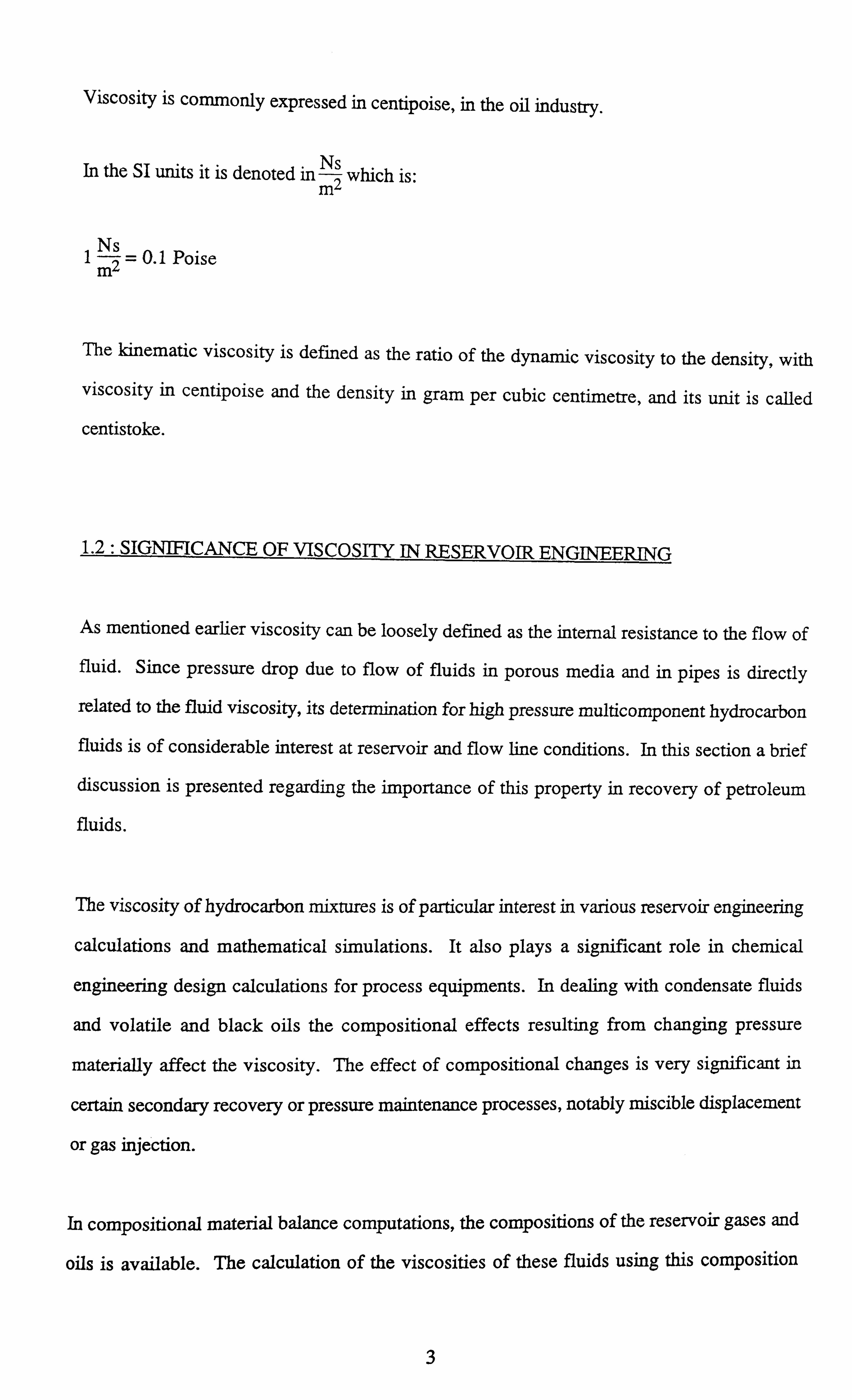
Viscosity is commonly expressed in centipoise, in the oil industry.
In the SI units it is denoted in mN2
which is:
1 Ns
= 0.1 Poise m
The kinematic viscosity is defined as the ratio of the dynamic viscosity to the density, with
viscosity in centipoise and the density in gram per cubic centimetre, and its unit is called
centistoke.
1.2 : SIGNIFICANCE OF VISCOSITY IN RESERVOIR ENGINEERING
As mentioned earlier viscosity can be loosely defined as the internal resistance to the flow of fluid. Since pressure drop due to flow of fluids in porous media and in pipes is directly
related to the fluid viscosity, its determination for high pressure multicomponent hydrocarbon
fluids is of considerable interest at reservoir and flow line conditions. In this section a brief
discussion is presented regarding the importance of this property in recovery of petroleum
fluids.
The viscosity of hydrocarbon mixtures is of particular interest in various reservoir engineering
calculations and mathematical simulations. It also plays a significant role in chemical
engineering design calculations for process equipments. In dealing with condensate fluids
and volatile and black oils the compositional effects resulting from changing pressure
materially affect the viscosity. The effect of compositional changes is very significant in
certain secondary recovery or pressure maintenance processes, notably miscible displacement
or gas injection.
In compositional material balance computations, the compositions of the reservoir gases and
oils is available. The calculation of the viscosities of these fluids using this composition
3

information is required for calculation of flowrates or pressure drops in reservoir due to flow
of these fluids.
Viscosity is of paramount importance as far as the processes of enhanced oil recovery (EOR)
are concerned, its significance is demonstrated in the following paragraphs. The mobility of a
fluid can be defined by the following simple equation:
kr _9
where
X= fluid mobility
kr = relative permeability and
µ= fluid viscosity
(1.2.1)
In the process of enhanced oil recovery, the mobility ratio in terms of the ratio of the mobility
of the displacing fluid to the mobility of the displaced fluid can be defined by :
M=1 X2
where
M= the mobility ratio
X1= mobility of the displacing fluid and
X2 = mobility of the displaced fluid
(1.2.2)
The higher the viscosity of the displacing fluid the lower will be its mobility and it will
provide a piston type and very efficient displacement mechanism (rather than fingering
through the displaced fluid). In polymer flooding the viscosity of the injected water is
expressly increased (by addition of polymers) to improve the displacement efficiency and
increase recovery.
4
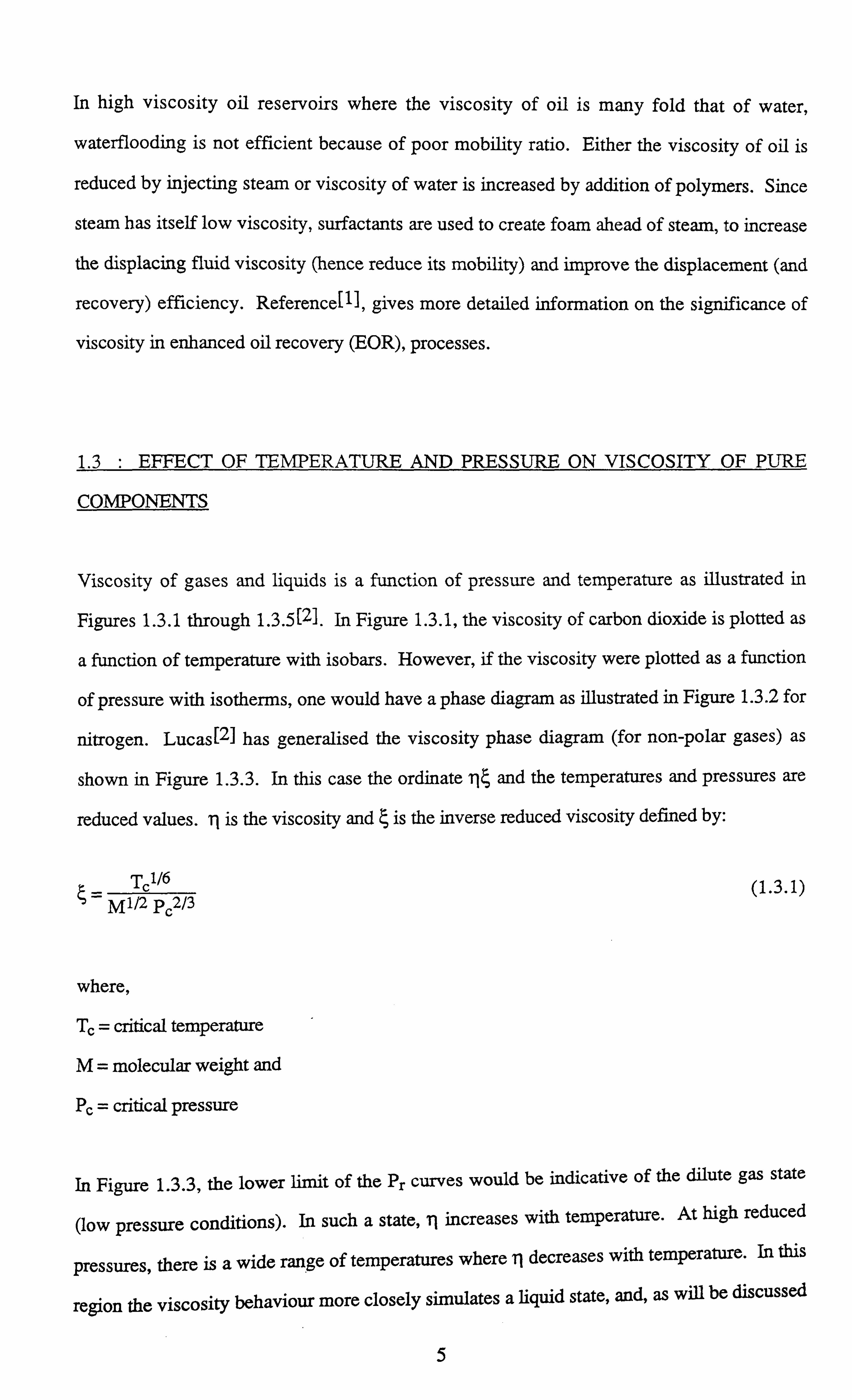
In high viscosity oil reservoirs where the viscosity of oil is many fold that of water,
waterflooding is not efficient because of poor mobility ratio. Either the viscosity of oil is
reduced by injecting steam or viscosity of water is increased by addition of polymers. Since
steam has itself low viscosity, surfactants are used to create foam ahead of steam, to increase
the displacing fluid viscosity (hence reduce its mobility) and improve the displacement (and
recovery) efficiency. Referenceill, gives more detailed information on the significance of
viscosity in enhanced oil recovery (EOR), processes.
1.3 : EFFECT OF TEMPERATURE AND PRESSURE ON VISCOSITY OF PURE
COMPONENTS
Viscosity of gases and liquids is a function of pressure and temperature as illustrated in
Figures 1.3.1 through 1.3.5 [21. In Figure 1.3.1, the viscosity of carbon dioxide is plotted as
a function of temperature with isobars. However, if the viscosity were plotted as a function
of pressure with isotherms, one would have a phase diagram as illustrated in Figure 1.3.2 for
nitrogen. Lucas[2] has generalised the viscosity phase diagram (for non-polar gases) as
shown in Figure 1.3.3. In this case the ordinate t1ý and the temperatures and pressures are
reduced values. il is the viscosity and 4 is the inverse reduced viscosity defined by:
Tc1/6 - M1/2 pc2/3
where,
Tc = critical temperature
M= molecular weight and
Pc = critical pressure
(1.3.1)
In Figure 1.3.3, the lower limit of the Pr curves would be indicative of the dilute gas state
(low pressure conditions). In such a state, ri increases with temperature. At high reduced
pressures, there is a wide range of temperatures where n decreases with temperature. In this
region the viscosity behaviour more closely simulates a liquid state, and, as will be discussed
5
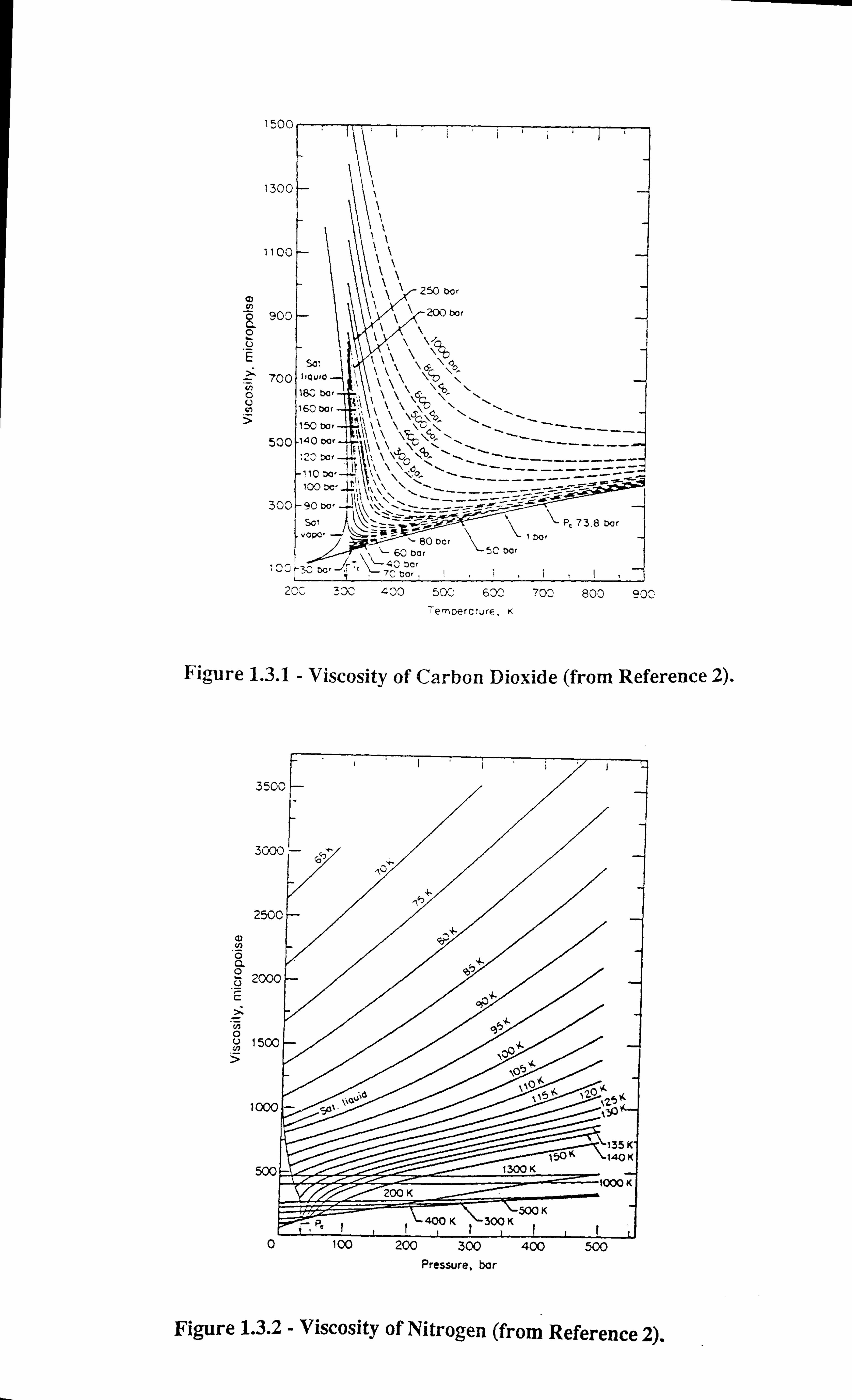
150,
1300
1100
CD 900
700
a U
> 500
300
'üý
1i 1\ 1\
`t 250 bor 1\
200 bar
1 Qý
Sal
iÖ� car \\ \`ý `
160 bcr t\ %J\ ? `ý\ \ýý
150 bar 140 oor
Sot P, 73.8 oar vapC"
ý 80 DCr tom'
r. ýý, . 60 oar 5C bCr
3,0 oo. r -4'v 50r 7CbC,,
20 330 X00 50C 630 700 800 °0C
em rc'urE, K
Figure 1.3.1 - Viscosity of Carbon Dioxide (from Reference 2).
35C
300
2501
av In 0 a
200{ C
y 0
1500
t (HOC
500
0
Figure 1.3.2 - Viscosity of Nitrogen (from Reference 2).
100 200 300 400 500 Pressure, bar
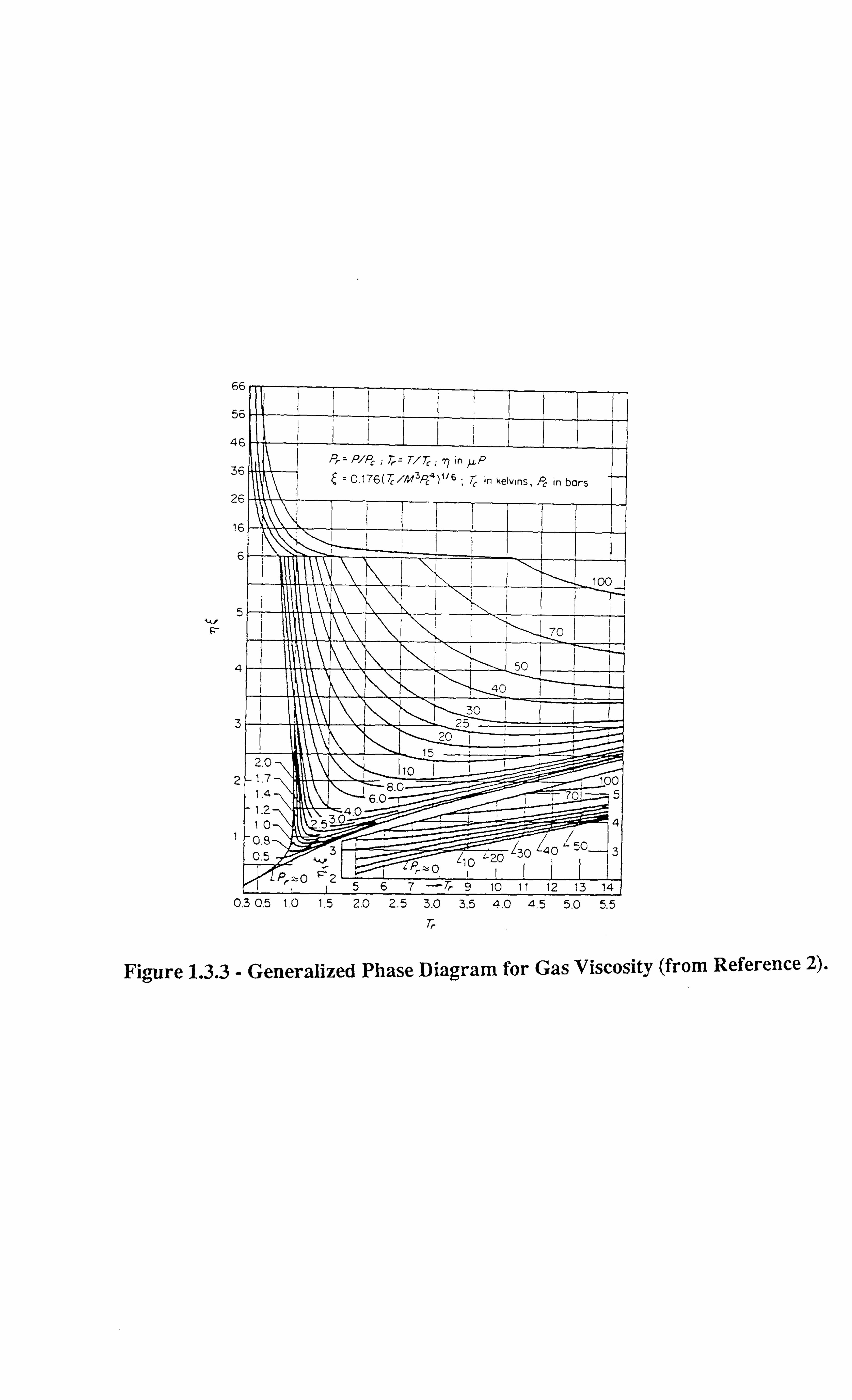
66
51
41
3i
2E
1E
2
1
Ii Pr =P1Pc; Tr =TI TinP
= 0.176(T/M3P°)'J6 ,T in kelvins, Pc in bars
00
70
r ( 0
`
40 30
25 20
2.0 15
10 1.7 1.4
100
6.08.0 70 -5 1.2 1.0
40
. 530 4
0.8 50 /40
3 1 3 0.5 30 Li0 2.20 , ", Pr ý0 L P' 0 ý2567 -Tr 9 10 11 12 13 14
0.3 0.5 1.0 1.5 2.0 2.5 3.0 3.5 4.0 4.5 5.0 5.5
Tr
Figure 1.3.3 - Generalized Phase Diagram for Gas Viscosity (from Reference 2).

in the following paragraph, an increase in temperature results in a decrease in viscosity.
Finally, at very high reduced temperatures, there again results a condition in which pressure
has little effect and viscosities increase with temperature.
The effect of increasing temperature on liquid viscosities is exactly opposite to that of the
effects on the gas viscosities at low values of pressure and high values of temperature (Figure
1.3.3). The rise in temperature of the liquid reduces its viscosity. Since liquids have more
compact molecules, with very low compressibility as compared to the gases, when the
temperature is raised, the molecules of the liquid start slowly moving away from each other,
thus reducing the affinity between them, which results in the reduction of viscosity.
Conversely, a reduction in temperature brings the liquid molecules closer and thus increases
the affinity which results in an increase in the viscosity. Simple expressions have been
formulated to show the effects of temperature on liquid viscosities[2]. For example Eq.
1.3.2, given below describes the viscosity of a liquid as a function of two constant parameters
A&B:
In 11L=A+; (1.3.2)
similarly equations involving three parameters are given as :
1nh1L=A+TBC (1.3.3)
values of constants A, B&C are calculated using experimental data and are tabulated in
Reference[2] for some pure compounds, which can be used for their viscosity prediction.
An increasing pressure causes an increase in viscosity for liquids and vice - versa. But this
effect on changes in pressure is only true when the composition of the liquid remains
constant. The effect of temperature and pressure on a liquid viscosity is shown in Figures
(1.3.4) and (1.3.5) respectively.
6
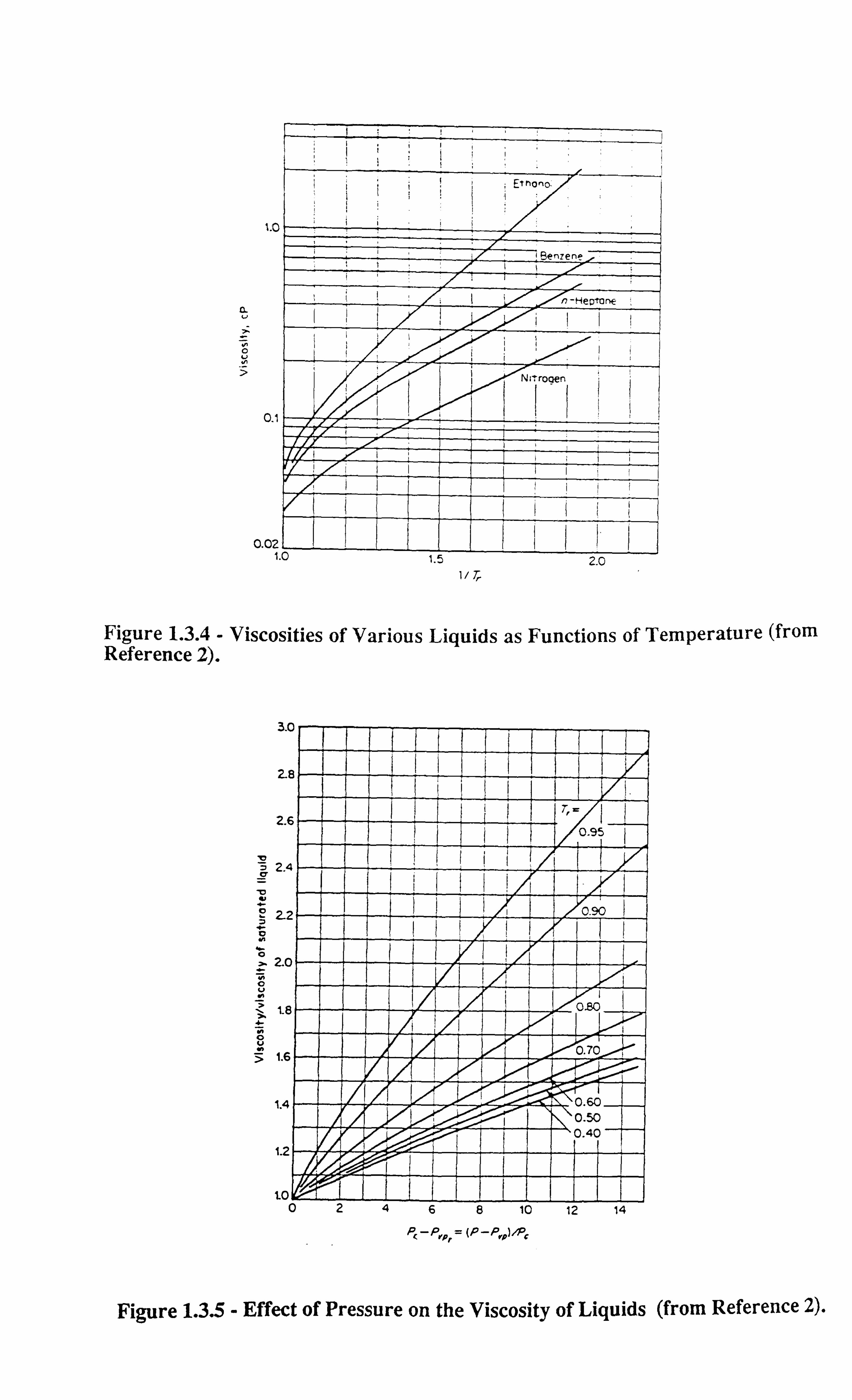
1.0
a u
_T N O v N
7
o_1
0.02 L. 1.0
1/r,
Figure 1.3.4 - Viscosities of Various Liquids as Functions of Temperature (from Reference 2).
c Q
t O
7 f O
O
h Q V
O V
>
J. V
28
0.95
2 4 . I
2.2 0.90 I I
2.0 I
18 0.80
1 6 0.70 .
1 4 I
I 60 0 .
I .
0.50
1.2 4 0.40
to u[g68 10 12 14
P(-Pyo, = (P-P, o) /P,
Figure 1.3.5 - Effect of Pressure on the Viscosity of Liquids (from Reference 2).
1.5 2.0

1.4 : EFFECT OF TEMPERATURE, PRESSURE, AND COMPOSITION ON
VISCOSITY OF REAL RESERVOIR FLUIDS
Figure 1.4.1 shows the effect of temperature on a typical North Sea crude oil[4] at a constant
composition and constant pressure. As expected, the plot indicates a decrease in the viscosity
as temperature increases. Figure 1.4.2 illustrates the effect of pressure on the viscosity of
another typical North Sea oil[ 51, at a constant temperature and constant composition. The plot
clearly shows the decrease in oil viscosity as pressure reduces.
However, the phenomenon observed in Figure 1.4.2 is not always valid when pressure drops
below the saturation pressure and as a result compositional changes take place which
significantly increase the oil viscosity despite reduction in pressure. Figure 1.4.3, shows the
effect of reduction in pressure on viscosity of a synthetic near critical gas - condensate in a
retrograde region. A decrease in pressure for a retrograde liquid in the retrograde region, the
reduction in pressure increases its viscosity. This is entirely because of the effect of changes
in the liquid phase composition and hence density as the pressure starts falling further and
further below the dew - point. For a retrograde mixture the mole fraction of heavier
components in the liquid phase increases by reduction in pressure below the dew - point.
Volatile oils and black oils exhibit similar behaviour, as observed in Figure 1.4.3, when
pressure falls below their bubble point pressure; i. e. the viscosity of the liberated gas keeps
decreasing with decrease in pressure whereas the viscosity of the remaining liquid keeps
increasing with decrease in pressure. The liberation of gas normally results in heavier and
more viscous liquid. Figure 1.4.4 shows the viscosity of a typical North Sea oil[5I graphed
against pressure at a constant temperature. The viscosity smoothly decreases as pressure is
reduced and approaches the bubble point and then suddenly increases inspite of reduction in
pressure and reaches a maximum value at atmospheric conditions. During the stages below
the bubble point pressure, significant changes in the liquid phase compositions occur
(increasing concentration of heavy components) which are responsible for the increasing
viscosity.
7
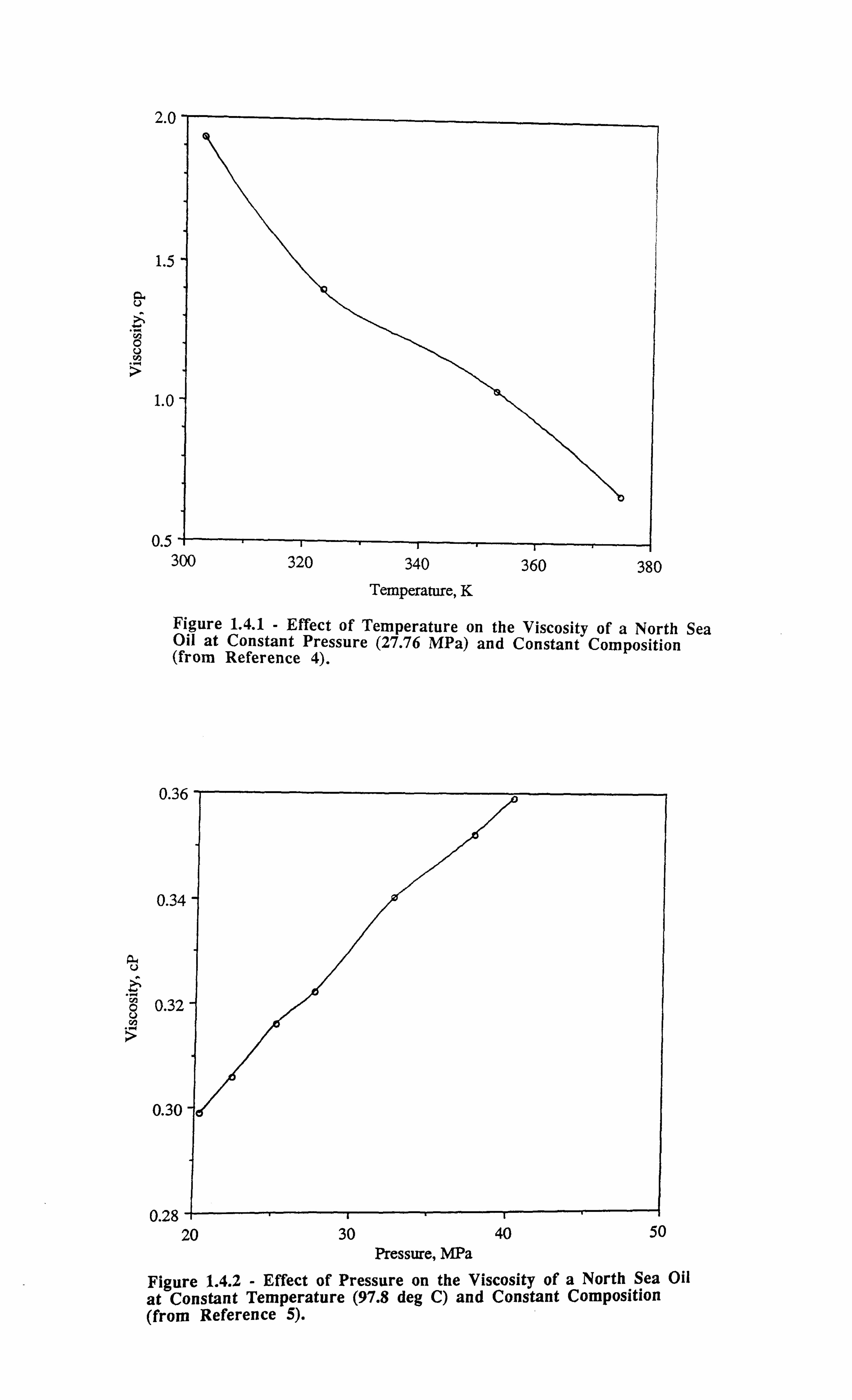
2. (
l. _`
C1. U
L'
C U y
1. C
0.5+- 300
Temperature, K
0.3E
Figure 1.4.1 - Effect of Temperature on the Viscosity of a North Sea Oil at Constant Pressure (27.76 MPa) and Constant Composition (from Reference 4).
0.34
ö 0.32 U y
0.30
0.28 -+- 20 30 40 50
Pressure, MPa
Figure 1.4.2 - Effect of Pressure on the Viscosity of a North Sea Oil at Constant Temperature (97.8 deg C) and Constant Composition (from Reference 5).
3/-u 34u 360 380

0.3
Liquid
Vapour
a U
1ý+ . r, 0 U
rý
0.2
0.1
i------------------------ --ýý'.
0.0 24 26 28 30 32
Pressure, MPa Figure 1.4.3 - Effect of Pressure and Composition on Viscosity of a Synthetic Near Critical Fluid at 38 deg C (from Section 3.5.7, Chapter 3, Part-A).
5
34
0 Measured
Cý U
ti O U
4 Bubble Point
3
21 0 100 200 300 400
Pressure, bars
Figure 1.4.4 - Effect of Composition on the Viscosity of a North Sea Oil at 71.1 deg C (from Reference 5).
References
1) Stewart, G. : "Enhanced Oil Recovery :A Technological Achievement in the
United States and Potential Application in the North Sea", Department of
Petroleum Engineering, Heriot - Watt University, (Jul., 1977).
2) Reid, R. C., Prausnitz, J. M. and Poling, B. E.: "The Properties of Gases and
Liquids", Fourth Edition, McGraw Hill Book Company, New York, (1987)
3) Ahrabi, F., Ashcroft, S. J. and Shearn, R. B.: "High Pressure Volumetric,
Phase Composition and Viscosity data for a North Sea Crude Oil and NGL",
Chem Eng. Res. Des, Vol. 65, pp. 63-73, (Jan., 1987).
4) Pedersen, K. S., Fredenslund, Aa. and Thomassen, P.: "Properties of Oils and
Natural Gases", Contributions in Petroleum Geology & Engineering, 5, Gulf
Publishing Company, (1989).
8
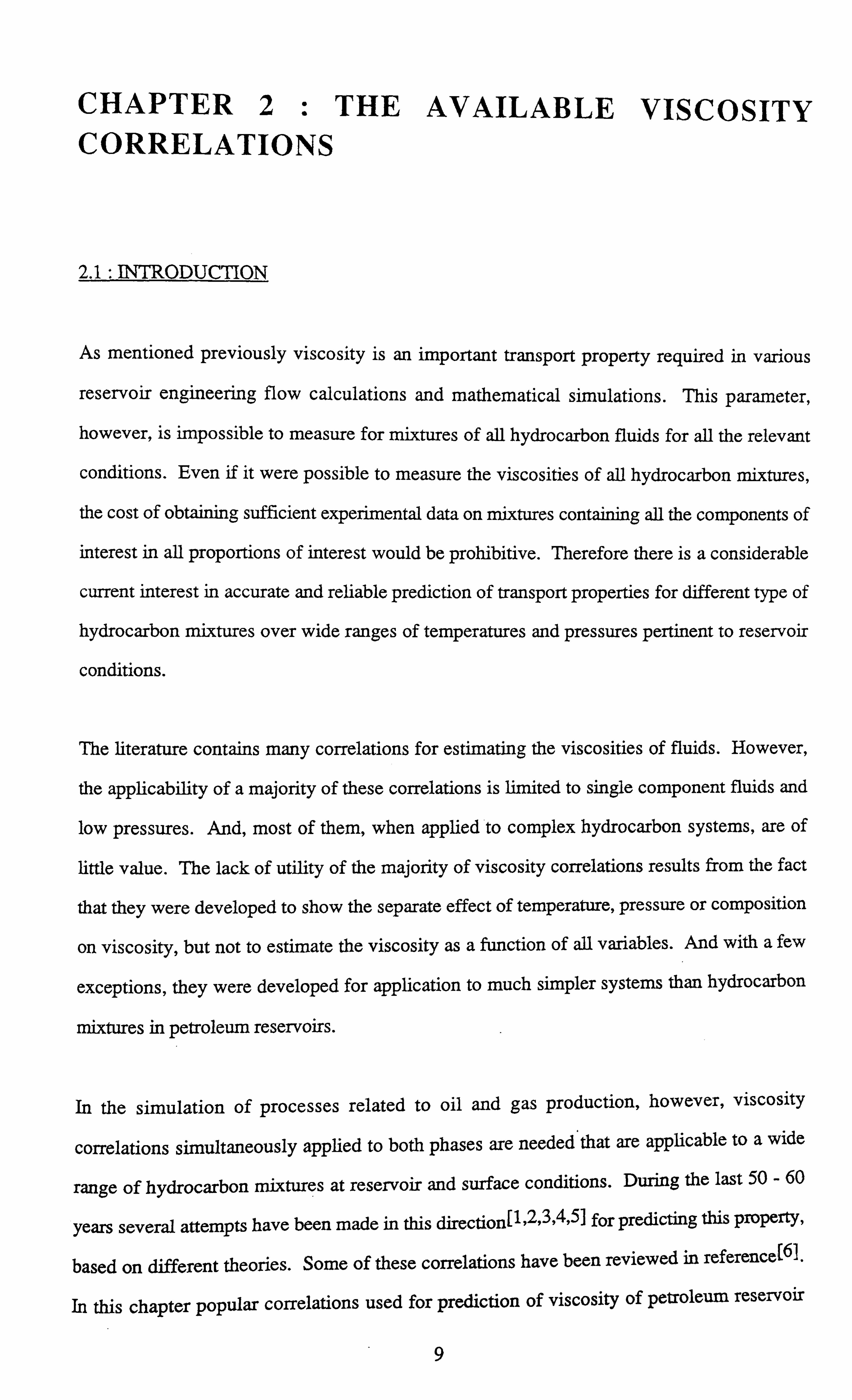
CHAPTER 2: THE AVAILABLE VISCOSITY CORRELATIONS
2.1: INTRODUCTION
As mentioned previously viscosity is an important transport property required in various
reservoir engineering flow calculations and mathematical simulations. This parameter,
however, is impossible to measure for mixtures of all hydrocarbon fluids for all the relevant
conditions. Even if it were possible to measure the viscosities of all hydrocarbon mixtures,
the cost of obtaining sufficient experimental data on mixtures containing all the components of
interest in all proportions of interest would be prohibitive. Therefore there is a considerable
current interest in accurate and reliable prediction of transport properties for different type of
hydrocarbon mixtures over wide ranges of temperatures and pressures pertinent to reservoir
conditions.
The literature contains many correlations for estimating the viscosities of fluids. However,
the applicability of a majority of these correlations is limited to single component fluids and
low pressures. And, most of them, when applied to complex hydrocarbon systems, are of
little value. The lack of utility of the majority of viscosity correlations results from the fact
that they were developed to show the separate effect of temperature, pressure or composition
on viscosity, but not to estimate the viscosity as a function of all variables. And with a few
exceptions, they were developed for application to much simpler systems than hydrocarbon
mixtures in petroleum reservoirs.
In the simulation of processes related to oil and gas production, however, viscosity
correlations simultaneously applied to both phases are needed that are applicable to a wide
range of hydrocarbon mixtures at reservoir and surface conditions. During the last 50 - 60
years several attempts have been made in this direction[ 1,2,3,4,5] for predicting this property,
based on different theories. Some of these correlations have been reviewed in reference[6].
In this chapter popular correlations used for prediction of viscosity of petroleum reservoir
9
fluids are reviewed in details. A comparative study for these methods is presented in Chapter
4. Greater emphasis is put on correlations applicable for predicting viscosities of both oil and
gas phases. Correlations reviewed in this chapter are, Lohrenz - Bray - Clark's residual
viscosity correlation, the principle of corresponding states (one reference component), the
extended principle of corresponding states (TRAPP), principle of corresponding states (two
reference components), Lee's method for viscosity of gases, and the Little & Kennedy's
method for the viscosity of oils.
2.2: RESIDUAL VISCOSITY CORRELATION
The viscosity correlation that has probably the most widespread use in flow models for
petroleum mixtures is the correlation of Jossi et. al[7], in the form suggested by Lohrenz et.
al[8], in which gas and liquid viscosities are related to a fourth - degree polynomial of the
reduced density. Jossi et. al[7], correlated viscosities of nitrogen, argon, carbon dioxide,
sulphur dioxide, methane, ethane, propane, i- butane, n- butane, and n- pentane in gaseous
and liquid phases, with reduced density by the use of dimensional analysis and the Abas -
Zade[9] equation for residual viscosity to produce a single generalised relationship which can
be used both graphically and analytically for single pure compounds.
Recent studies on the prediction of the transport properties of pure substances have been
primarily concerned with the viscosity and thermal conductivity of gases at normal
pressures [ 10I . Using a dimensional analysis approach and viscosity data reported in the
literature data for fifty-two non - polar gases and fifty-three polar gases, gave the relationships
which were developed for the viscosity, f* of any pure gas at moderate pressures (0.01013
MPa to 0.50 MPa). For non - polar gases the following relationships resulted :
r(*% = 34.0 E-05Tr0.94 for Tr <_ 1.5
and
(2.2.1)
10

11 *= 17.78 E-05[4.58Tr - 1.67]5/8 for Tr > 1.5 (2.2.2)
where
Tc1/6 ý' ý" Ml/2p, 2/3 (2.2.2 a)
A relationship for polar gases is not given here, since most of the petroleum reservoir fluids
exhibit non - polar behaviour. Critical properties and molecular weight of each compound
were used to calculate the viscosity reducing parameter, X. The residual viscosity (RV)
function, (rj-r1*)? , was evaluated using the experimental viscosity data in the dense gaseous
and liquid phase regions together with the viscosity data (rl*) at low pressure conditions or at
1 atm. The density data of these components in different thermodynamic regions were
obtained from the PVT data and were used to calculate the reduced density['f. In Figure
(2.2.1) the group (T-rL*)2, is plotted against the reduced density on log-log co-ordinates.
Precise details about the development of these correlations and the sources of the PVT and
viscosity data are given in Reference[7]. The following fourth degree polynomial was found
to represent accurately the relationship over the entire range of reduced densities :
[(ý-iý*)ý1, +10 4]11'4 = 0.1023+0.023364pr+0.058533pr2-0.040758pr3+0.0093324pr4 (2.2.3)
Where,
71 = viscosity of the fluid in centipoise
71* = gas phase viscosity of the same fluid at moderate pressure (e. g. 1 atm), in centipoise
X= inverse of the critical viscosity or viscosity reducing parameter, as defined by Eq. 2.2.2 a
p= density of the fluid, in gm/cc
PC = critical density of the fluid, in gm/cc
Pr =P the reduced density PC
Tc = critical temperature in Kelvin
Tr = reduced temperature
M= molecular weight of the fluid
11
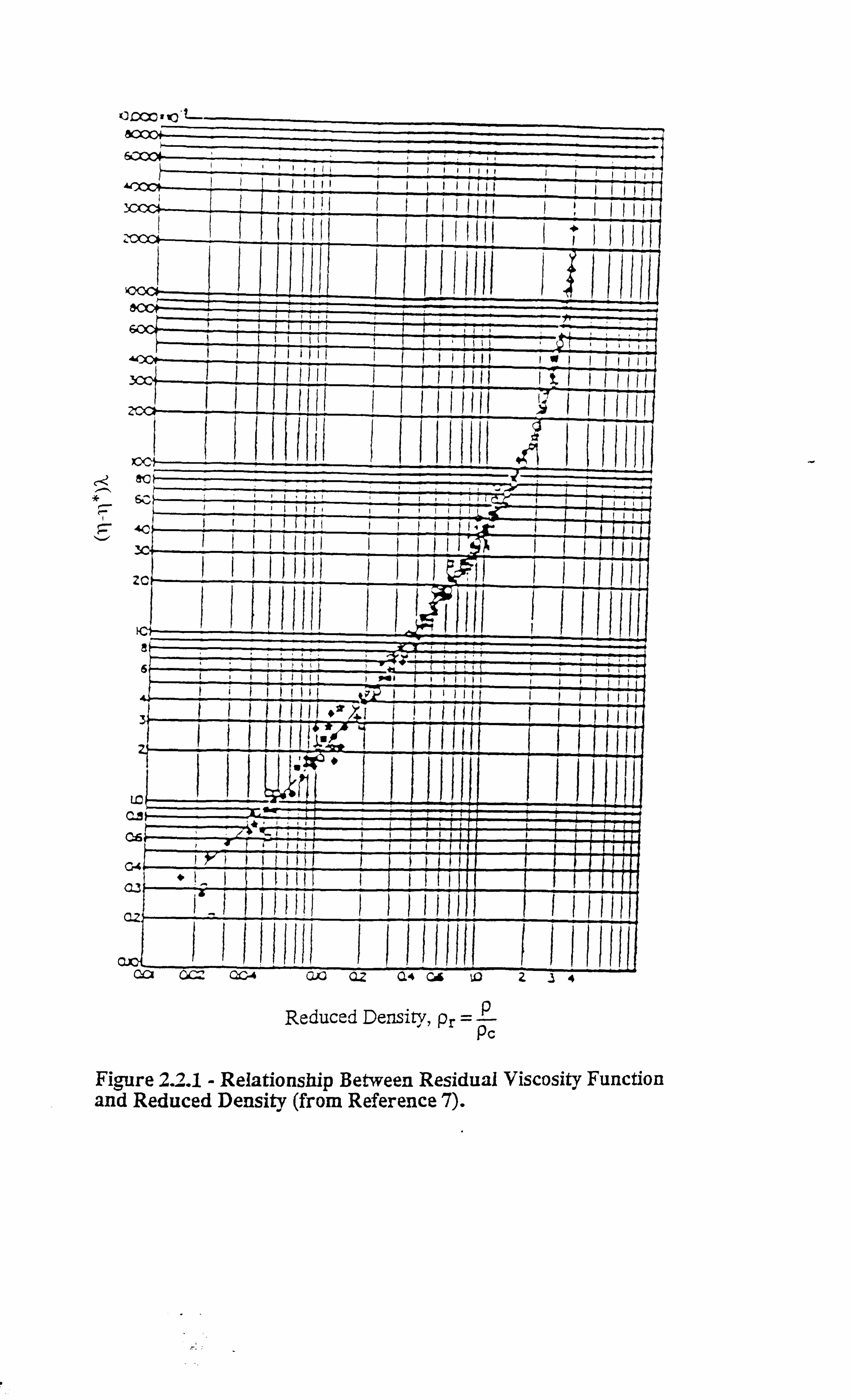
K3 ý)OC IF io'l-
acooo
vi '1.1II! I11II11I
V tºº IIIt lilt IIIIII li fl! I I I( IIII II VIII
ýt ififll L 41IýlII 4 'lll{14
--rt.. -...... _. _ý. ý 77
fI ºII! I 11 I fll ICIIII II 1 mI I 11111111 Iti 111 fill f T-1 -11111 IIf 111
cI. ItI!. I1. {. I_
ItIII
tIfII{IIIIfII
.'II 111111 II II II {I{II
2C II IHHll tI . i! IIl III
t1ttII1I via l11111III 11 f'f! E! IºI tyý+ III 111 III II rrI rfI IIº ""ý I ! III III (IIII II
IL Iý fit' IJ l 1111 jI1 Fl II L
C-9 i 'f 1I 1111
1111(I 111
11f I' 11 1
ºIIfI! fi I F-1. 0-4 MI Ll
ýI *! � I 1111 k !I!
-_ i, I I H H! I !I HI 1 Hill l Ga CC= QG4 ßA CZ 0-4 CA 1O 24
Reduced Density, Pr =p PC
Figure 2.2.1- Relationship Between Residual Viscosity Function and Reduced Density (from Reference 7).
Eq. 2.2.3, is however applicable only to all the pure single components investigated by Jossi
et. al[7], except hydrogen due to its quantum deviations, water and ammonia due to hydrogen
bonding which follow different trends compared to the normally behaving substances.
It was the effort of Lohrenz - Bray - Clark[8] in 1964 which made the application of Eq. 2.2.3
feasible for the prediction of viscosity of reservoir oils and gases. It in fact represented the
first attempt to relate viscosities of liquids and gases to composition, and was principally
designed for application to flow calculations. Lohrenz et. al[8] basically introduced several
mixing rules in the pure component viscosity correlations proposed by Jossi et. a1171,
discussed earlier, to make the method applicable for calculation of gas and liquid mixture
viscosities. According to Lohrenz et. al[811, Eq. 2.2.1 & 2.2.2 for a component, i, in the
mixture can be written as :
lli*Xi = 34.0 E-05Tri4.94, (TriS 1.5) (2.2.4)
T'li*Xi = 17.78 E-05[4.58Trj - 1.67]5/8ß (Tri > 1.5) (2.2.5)
where
=T= T"1/6 Tn Tci and ý_
Mi" 1ýPci "2ý (2.2.6 a&2.2.6 b)
hence for a mixture containing, n components, for ith component, Eq. 2.2.4,2.2.5,2.2.6 a
& 2.2.6 b should be used to calculate the reduced low pressure viscosity (rli*), reduced
temperature (Tri) and the viscosity reducing parameter (1.1). Temperature is in Kelvins and
pressure is in atmospheres and viscosity is in centipoise. Now using the information obtained
from the above equations, the low pressure viscosity of gas mixtures should be calculated,
the following simple molar mixing rules are used[111
n
Ixi7li*v-mi i=l
n 71 =I
xi Vm--i
i=l (2.2.7)
12
whereas the reduced density of the mixture is calculated from:
Pr=-p-7 Pc
in and
1. _I XýVCi
Pc i=1 iOC7+
+ Xc7+Vc7+
(2.2.8)
(2.2.8 a)
Mi and Vci are the molecular weight and critical molar volume of the ith component in the
mixture. Critical volume for a pseudo fraction, C7+ is estimated by the expression suggested by Lohrenz et. al[81l :
Vc7+ = 21.573 + 0.015122 Mc7+ - 27.656 SGc7+ + 0.0706151V. tc7+ SGc7+
Where,
Vc7+ = critical molar volume of the plus fraction
Mc7+ = molecular weight of the plus fraction and
SGc7+ = specific gravity of the plus fraction
(2.2.9)
viscosity reducing parameter, X, of the mixture is calculated by introducing simple molar
mixing rules into Eq. 2.2.6 b:
n1
[JXiTd]6 i=1
n1n2 [ýximI]Z[ýxiPi]3
(2.2.1 0)
Hence, calculation of gas or liquid mixture viscosity is accomplished by applying Eq. 2.2.4 -
2.2.10 to Eq. 2.2.3. The typical input data required to accomplish the viscosity calculation is,
compositions of gas or liquid phase, reliable density data of each phase, molecular weights of
each component in the mixture and the critical properties of each component in the mixture,
13
similar data for the pseudo fractions are also required for mixtures containing plus fractions.
Critical property data and other data for a majority of the pure hydrocarbon components and
organic compounds is listed in Reference 6, various methods for estimating the critical
temperature and pressure of the C7+ fraction are given in Reference 30.
The method is simple and fast in application and is easily tuned to experimental data.
However, it relies significantly on the density data of the fluid. Hence, it should always be
used in conjunction with an EOS known to predict the densities reliably, where measured
density data is not available. The weaknesses and strengths of this method compared with
other viscosity prediction techniques are given in Chapter 4.
2.3: PRINCIPLE OF CORRESPONDING STATES (ONE REFERENCE COMPONENT)
This is one of the recent methods published for predicting viscosities of gas and liquid phases
using the principle of corresponding states. The basic assumption behind the principle of
corresponding states is that any reduced property of a mixture or a pure component can be
expressed in terms of other reduced properties. For example, the reduced viscosity (TI/Tic)
can be expressed in terms of reduced pressure (P/Pc), reduced temperature (T/Tc) and reduced
density (p/pc). Moreover, to improve such correlations a reference component (generally
methane) is used as a pivot point.
In the principle of corresponding states (PCS), the reduced viscosity may be related to any
two reduced state properties such as reduced pressure, reduced temperature, reduced density,
or reduced volume. Hydrocarbon fluids, particularly complex mixtures, cannot be accurately
modelled by the above simple (PCS), hence correlations based on this approach include some
correction factors generally evaluated by matching the predicted and experimental data[12-151.
It was the work of Tham and Gubbins[16] in which they proposed the viscosity of a
component in terms of a correction factor in order to express the deviation from the simple
14
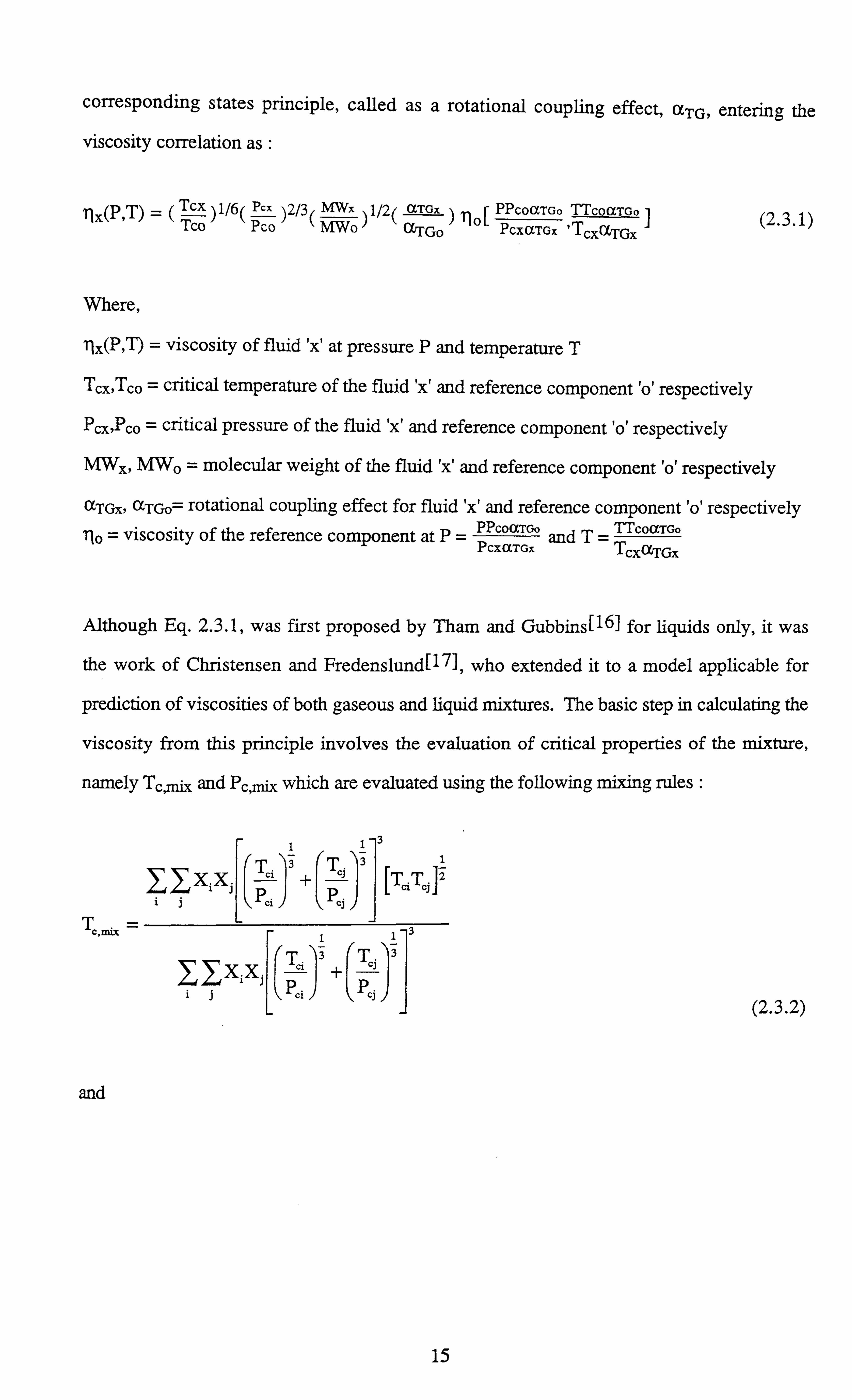
corresponding states principle, called as a rotational coupling effect, aTG, entering the
viscosity correlation as :
= TCX 1/6 Pcx 2/3 MVVz 1/2 06TGz PPCOCCTGo TTCOaTGo
ilx(P, Z') - (Tco) (Pco) (moo) () Flo C c Go PCXUTGx Tcxur'G.,
Where,
Tlx(P, T) = viscosity of fluid 'x' at pressure P and temperature T
TcxýTco = critical temperature of the fluid 'x' and reference component 'o' respectively
Pcx, Pco = critical pressure of the fluid 'x' and reference component 'o' respectively
MWx, MWo = molecular weight of the fluid 'x' and reference component 'o' respectively
aTG., aTG0= rotational coupling effect for fluid 'x' and reference component 'o' respectively rlo = viscosity of the reference component at P= PPcoaTCO
and T= T'coaTGo PCXaTGX TCxaTGx
Although Eq. 2.3.1, was first proposed by Tham and Gubbins[16] for liquids only, it was
the work of Christensen and Fredenslund[17], who extended it to a model applicable for
prediction of viscosities of both gaseous and liquid mixtures. The basic step in calculating the
viscosity from this principle involves the evaluation of critical properties of the mixture,
namely Tcn, ix and Pc, mix which are evaluated using the following mixing rules :
1 1-3 3
XiXi Týý
+
(T-i
[TiTjl
;P P-i T"Mix =1
1-3
T '' 3 XiXi P+'
; Psi P-;
and
(2.3.2)
15
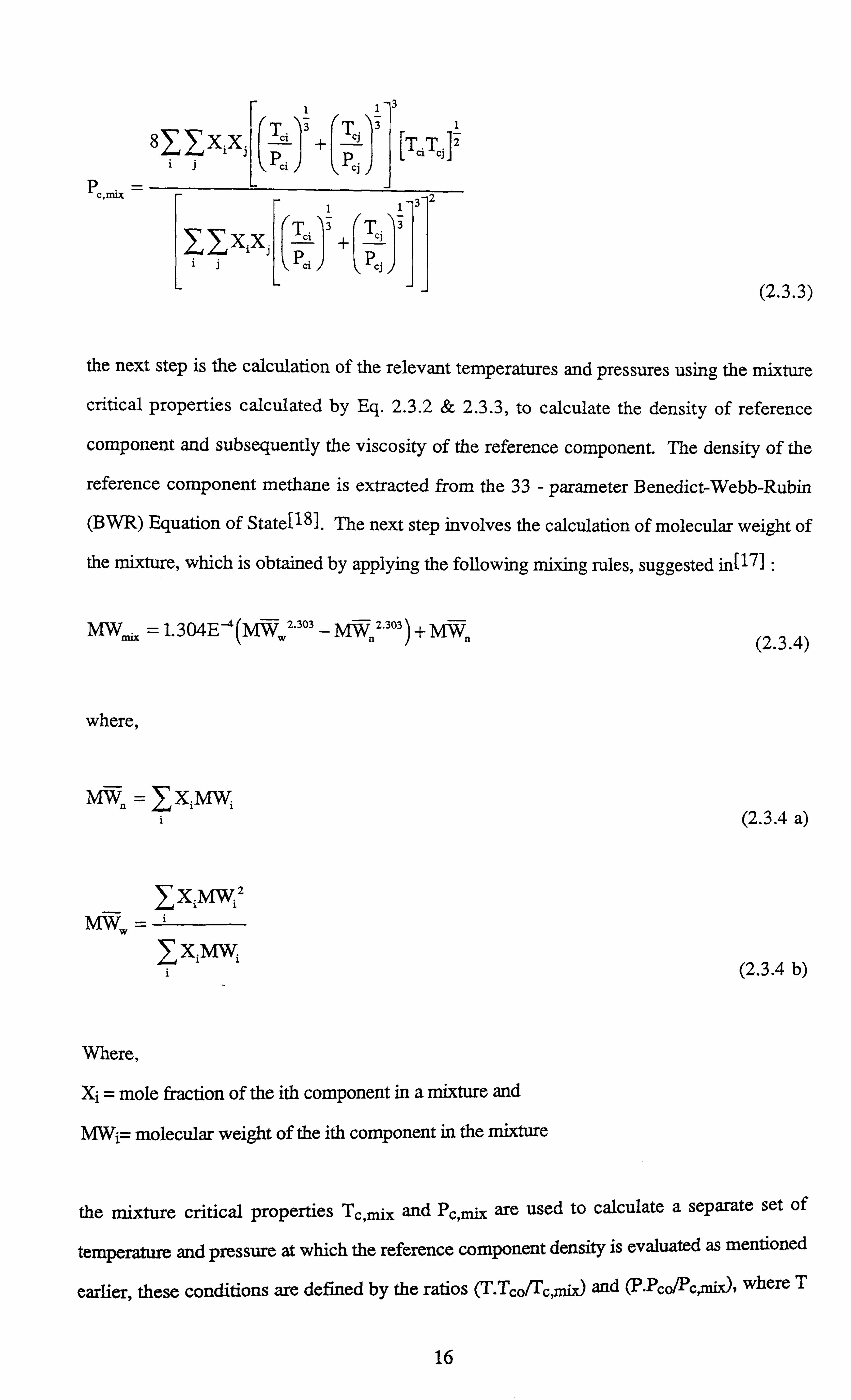
1 1-3
33
811 X. X. Tiý. `i [T. T. ]
i ci pc. ý pc,
mix 32 11 3
llxixj ýT-ili+ T;
i pci Pci
(2.3.3)
the next step is the calculation of the relevant temperatures and pressures using the mixture
critical properties calculated by Eq. 2.3.2 & 2.3.3, to calculate the density of reference
component and subsequently the viscosity of the reference component. The density of the
reference component methane is extracted from the 33 - parameter Benedict-Webb-Rubin
(BWR) Equation of State[18J. The next step involves the calculation of molecular weight of
the mixture, which is obtained by applying the following mixing rules, suggested in[171 :
MWmix =1.304E-` (MW,, 2.303 _A
ffn2.303) + MWA
where,
M Yin = XiM Wi
MW _
Where,
YX1M
12
Yximwi
Xi = mole fraction of the ith component in a mixture and
MWl molecular weight of the ith component in the mixture
(2.3.4)
(2.3.4 a)
(2.3.4 b)
the mixture critical properties Tc, mix and Pc, mix are used to calculate a separate set of
temperature and pressure at which the reference component density is evaluated as mentioned
earlier, these conditions are defined by the ratios (T. Tco/Tc, mix) and (P. P o/Pc, mix), where T
16
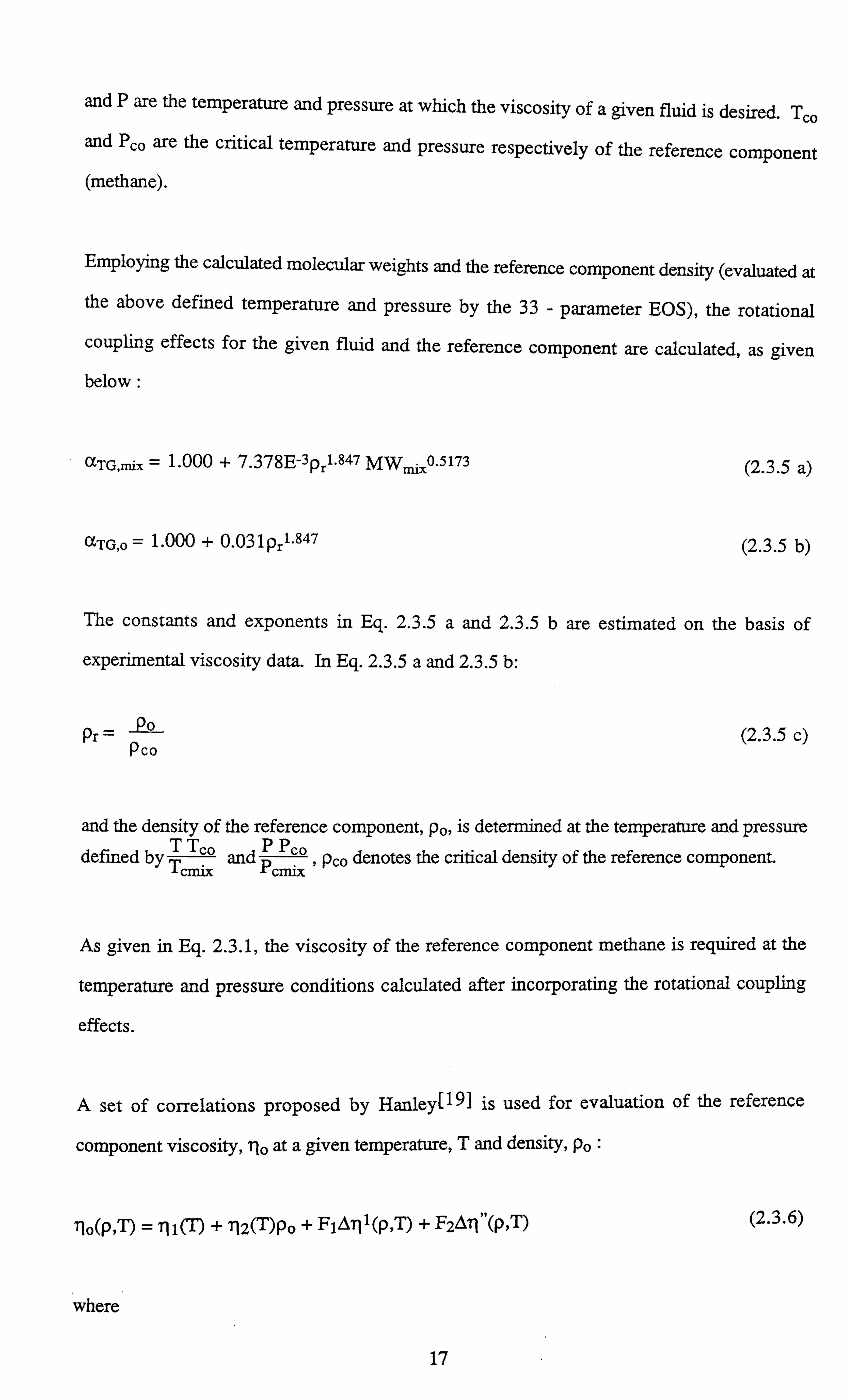
and P are the temperature and pressure at which the viscosity of a given fluid is desired. Teo
and Pco are the critical temperature and pressure respectively of the reference component (methane).
Employing the calculated molecular weights and the reference component density (evaluated at the above defined temperature and pressure by the 33 - parameter EOS), the rotational
coupling effects for the given fluid and the reference component are calculated, as given below :
XTG, m1x = 1.000 + 7.378E-3Pr1.847 MW 0.5173
OGTG, o = 1.000 + °. °31 Pr1.847
(2.3.5 a)
(2.3.5 b)
The constants and exponents in Eq. 2.3.5 a and 2.3.5 b are estimated on the basis of
experimental viscosity data. In Eq. 2.3.5 a and 2.3.5 b:
Pr Po Pco
(2.3.5 c)
and the density of the reference component, po, is determined at the temperature and pressure defined by
T Tco and
P Pco , pco denotes the critical density of the reference component. Tcmix Pcmix
As given in Eq. 2.3.1, the viscosity of the reference component methane is required at the
temperature and pressure conditions calculated after incorporating the rotational coupling
effects.
A set of correlations proposed by Hanley[191 is used for evaluation of the reference
component viscosity, ilo at a given temperature, T and density, po :
rlo(P, T) = T11 M+ r12(T)Po + F1AIll(p, T) + F2AII"(P, T)
where
(2.3.6)
17

fl 1(T) =A+B [C - loge(F)]2
constants A, B, C and F are:
A=1.696985927
B=-0.133372346
C=1.4
F= 168.0
the second function of Eq. 2.3.6 is given by :
(2.3.6 a)
712M = exp [j
1+ T]
[exp [0.1(2+2)+ Op0.5 J5
T'2 +
., ý
-1.0 (2.3.6 b)
constants jj to j7 have values :
ji = -10.3506 J2 = 17.5716
J3 = -3019.39
j4 = 188.7300
is = 0.0429036
J6 = 145.290
j7= 6127.68
whereas, 6, is defined as :
8_ (P0 - Pco Pco
and the third function, All' (p, T), in Eq. 2.3.6 is defined as
(2.3.6 c)
18
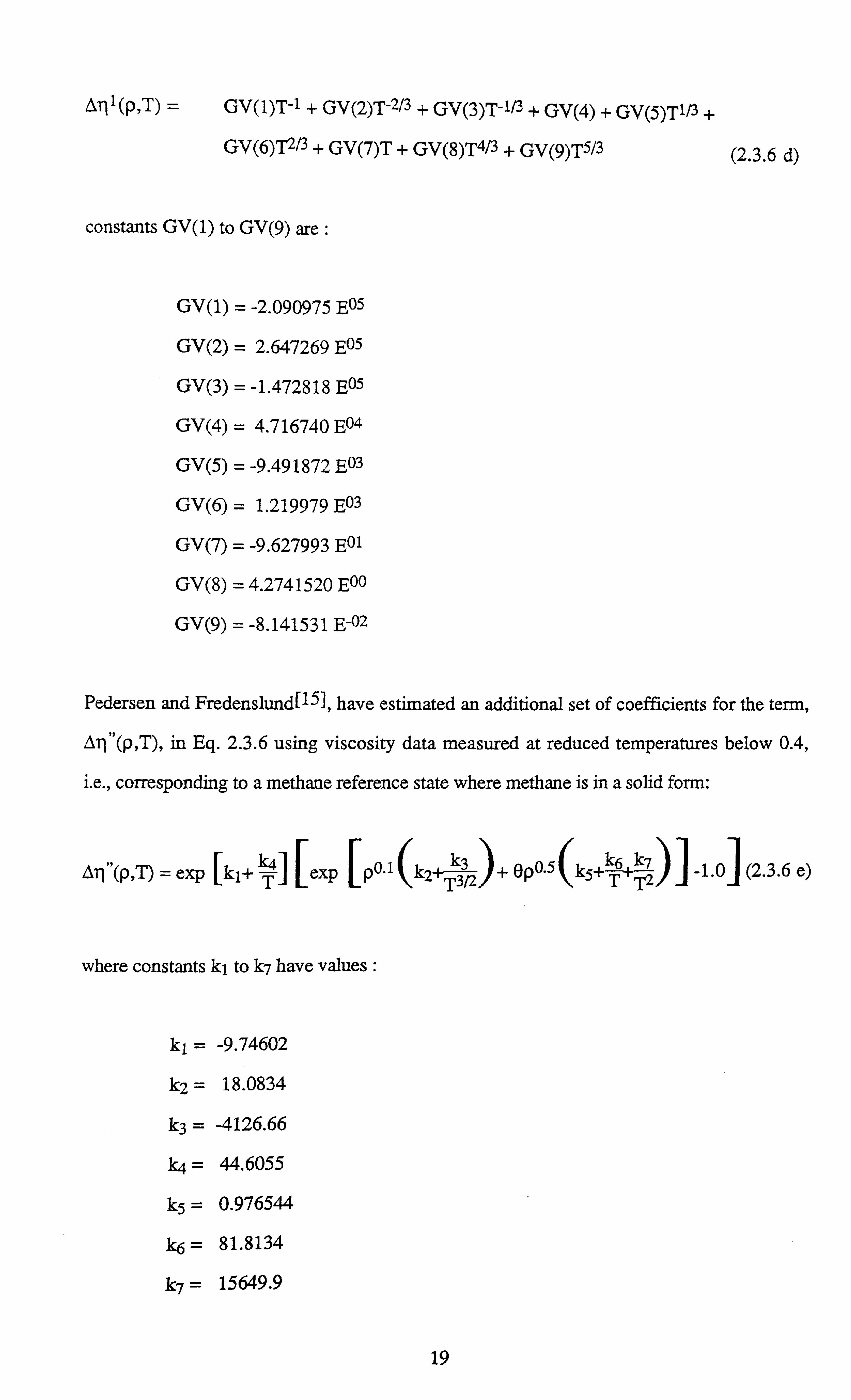
zTI I(p, T) = GV(1)T-1 + GV(2)T-2/3 + GV(3)T-113 + GV(4) + GV(5)Tl13 + GV(6)T213 + GV(7)T + GV(8)T4/3 + GV(9)T5/3
constants GV(1) to GV(9) are :
GV (1) = -2.090975 E05
GV(2) = 2.647269 E05
GV(3) = -1.472818 E05
GV(4) = 4.716740 E04
GV(5) = -9.491872 E03
GV(6) = 1.219979 E03
GV(7) = -9.627993 E01
GV(8) = 4.2741520 E00
GV(9) = -8.141531 E-02
(2.3.6 d)
Pedersen and Fredenslund[15I1, have estimated an additional set of coefficients for the term,
Ail "(p, T), in Eq. 2.3.6 using viscosity data measured at reduced temperatures below 0.4,
i. e., corresponding to a methane reference state where methane is in a solid form:
All �(p, T) = exp [k1+
T
[exp [pa1(k2ý, )+ 9p0.5 k5+ -1.0 (2.3.6
where constants ki to k7 have values :
kl = -9.74602
k2 = 18.0834
k3 = -4126.66
k4 = 44.6055
k5 = 0.976544
lk6 = 81.8134
k7 = 15649.9
19
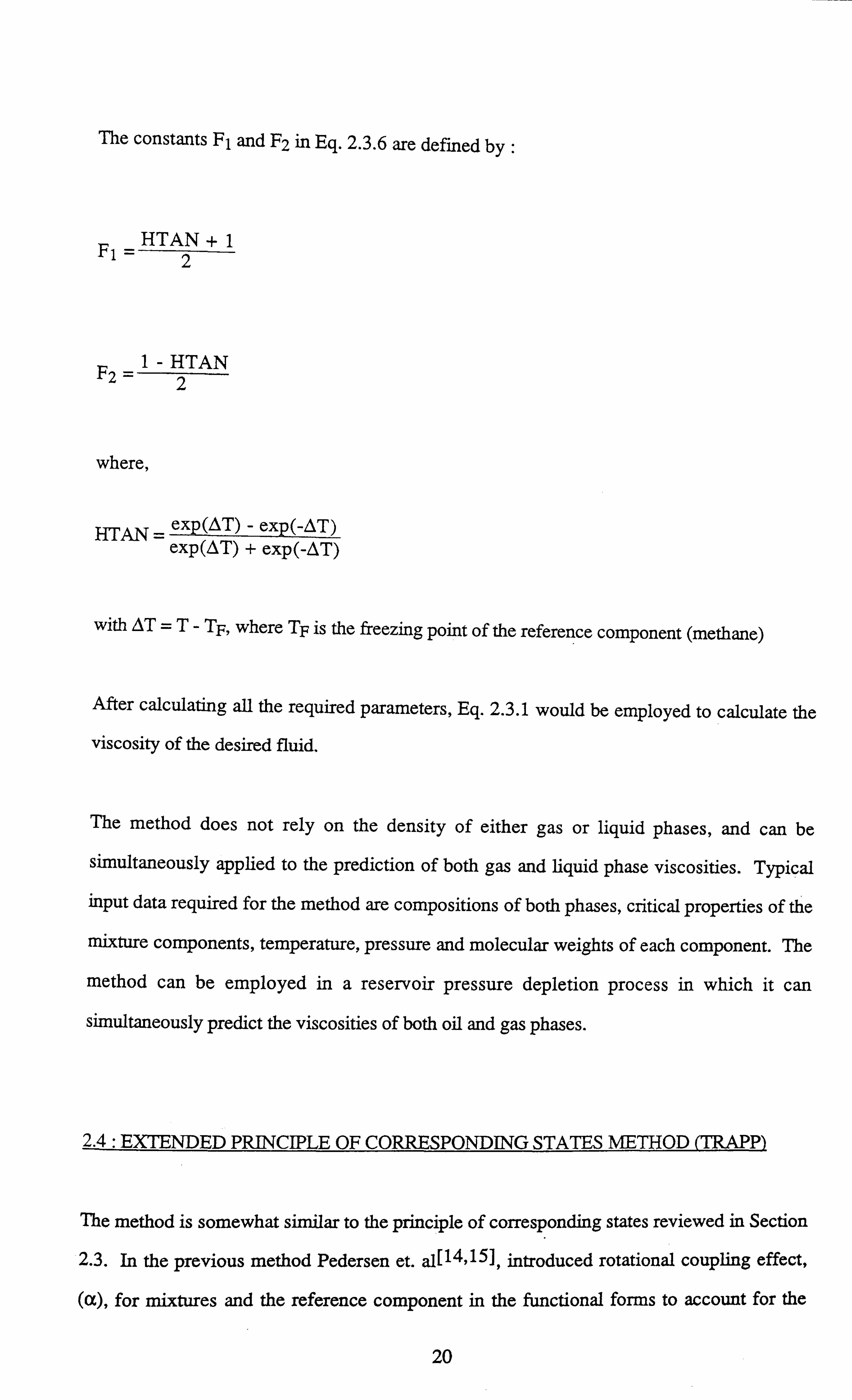
The constants F1 and F2 in Eq. 2.3.6 are defined by :
F1 _HTAN+ 1
2
F2: -- 1- HTAN
2
where,
H,, AN _ exp(dT) - exp(-OT) exp(OT) + exp(-QT)
with AT =T- TF, where TF is the freezing point of the reference component (methane)
After calculating all the required parameters, Eq. 2.3.1 would be employed to calculate the
viscosity of the desired fluid.
The method does not rely on the density of either gas or liquid phases, and can be
simultaneously applied to the prediction of both gas and liquid phase viscosities. Typical
input data required for the method are compositions of both phases, critical properties of the
mixture components, temperature, pressure and molecular weights of each component. The
method can be employed in a reservoir pressure depletion process in which it can
simultaneously predict the viscosities of both oil and gas phases.
2.4: EXTENDED PRINCIPLE OF CORRESPONDING STATES METHOD (TRAPP)
The method is somewhat similar to the principle of corresponding states reviewed in Section
2.3. In the previous method Pedersen et. x1[14,15], introduced rotational coupling effect,
(a), for mixtures and the reference component in the functional forms to account for the
20
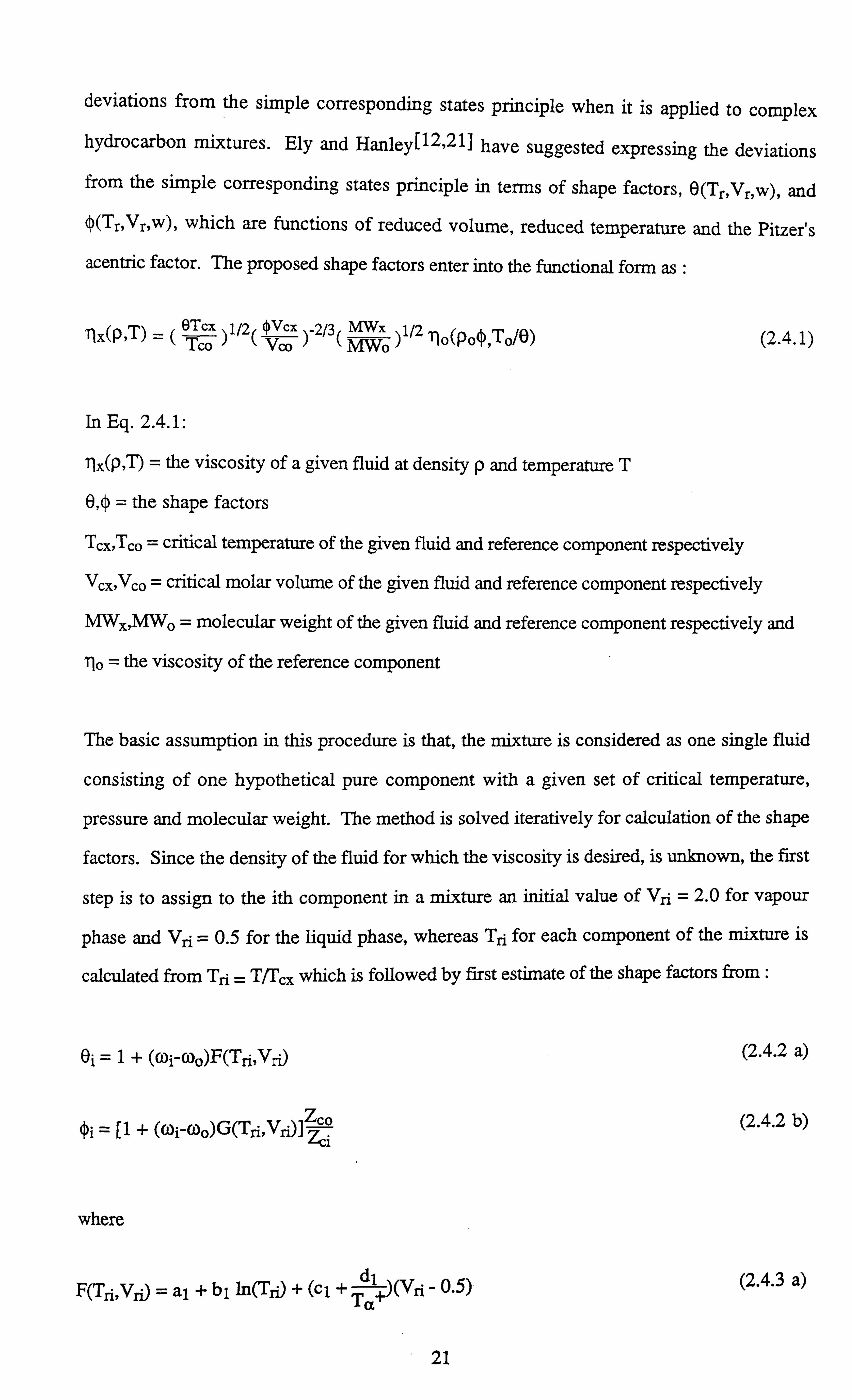
deviations from the simple corresponding states principle when it is applied to complex hydrocarbon mixtures. Ely and Hanley[12,211 have suggested expressing the deviations
from the simple corresponding states principle in terms of shape factors, 9(Tr, Vr, w), and ()(TT, VT, w), which are functions of reduced volume, reduced temperature and the Pitzer's
acentric factor. The proposed shape factors enter into the functional form as :
iix(P, T) _ (6Tcx )1/2( 4Vcx )-2/3ý MWx
)1/2 ýo(poo, Tofe) Tco Vco MWo
In Eq. 2.4.1:
(2.4.1)
flx(p, T) = the viscosity of a given fluid at density p and temperature T
8,0 = the shape factors
Tcx, Tco ý critical temperature of the given fluid and reference component respectively
vcx, Vco = critical molar volume of the given fluid and reference component respectively
MWx, MWo = molecular weight of the given fluid and reference component respectively and
, qo = the viscosity of the reference component
The basic assumption in this procedure is that, the mixture is considered as one single fluid
consisting of one hypothetical pure component with a given set of critical temperature,
pressure and molecular weight. The method is solved iteratively for calculation of the shape
factors. Since the density of the fluid for which the viscosity is desired, is unknown, the first
step is to assign to the ith component in a mixture an initial value of Vri = 2.0 for vapour
phase and Vri = 0.5 for the liquid phase, whereas Tri for each component of the mixture is
calculated from Tri = T%Tcx which is followed by first estimate of the shape factors from :
Oj, =1+ (coi-COO)F(Tri, Vri) (2.4.2 a)
ýi = ý1 + (wi-O)o)G(Tri, Vri)] ° (2.4.2 b) Zc,
where
F(Tri, Vri) = al + bi ln(Tri) + (cl +d +)(Vri - 0.5) (2.4.3 a)
Ta
21

G(Tri, Vri) = a2(Vri + b2) + C2(Vri + d2)IP(T
and the constants have the following values :
al = 0.090569
bl = -0.862762
cl = 0.316636
dl = -0.465684
a2 = 0.394901
b2 = -1.023545
C2 = -0.932813
d2 = -0.754639
(2.4.3 b)
and co,, are the acentric factors for ith component of the fluid and reference component 'o'
respectively, whereas Zvi and ZO are the critical compressibility factors of the ith component
of the fluid and the reference component respectively.
The next step is to calculate the substance reducing ratios, fi and hi using the following
equations and values obtained from Eq. 2.4.2 a and 2.4.2 b:
fi =[ Tci, ei (2.4.4 a) Tco
hi = [yc ]
0i (2.4.4 b)
where Td is the critical temperature of the ith component in the mixture and Vcl is the critical
volume of the ith component in the mixture. All the above expressions are proposed by Leach
and Leland[22,23].
The following mixing rules are employed for calculating the equivalent substance reducing
ratios for the mixture :
fx=h. -'j: 1: X Xjf ijhij
ij
22
(2.4.5 a)

bx = XiXJhii (2.4.5 b)
where fij and hij are calculated from:
fij = (fifj) 1/2 (2.4.6 a)
hij =g [hil/3 + hj1/3]3 (2.4.6 b)
fx and hx values calculated from Eq. 2.4.5 a and 2.4.5 b are used to calculate the equivalent temperature, Teq =x , and pressure, Peq = fP
hx at which the reference component density
x
(po) is calculated for the first guess, here P and T represent the pressure and temperature at
which the viscosity of the given fluid is desired. Again the 33-parameter Benedict-Webb-
Rubin (B WR) EOS[18] is used to calculate the methane density. This calculated methane
density is then converted into the density of the fluid for which the viscosity is desired from
the following:
Px = Po(Th e) (Vx =
MWx) (2.4.7) x Px
where,
MWx = Ximwi (2.4.8)
here MWX is the molecular weight of the mixture, MWi is the molecular weight of the ith
component in the mixture and Xi is the mole fraction of the ith component in the mixture. The
reduced temperature and the reduced volume are then recalculated and steps through Eq. 2.4.2
to 2.4.5 until convergence is achieved for fx and hx.
The density of methane at which the shape factor iteration loop converges is then used to
calculate the methane viscosity using correlations similar to those described in Section 2.3
23
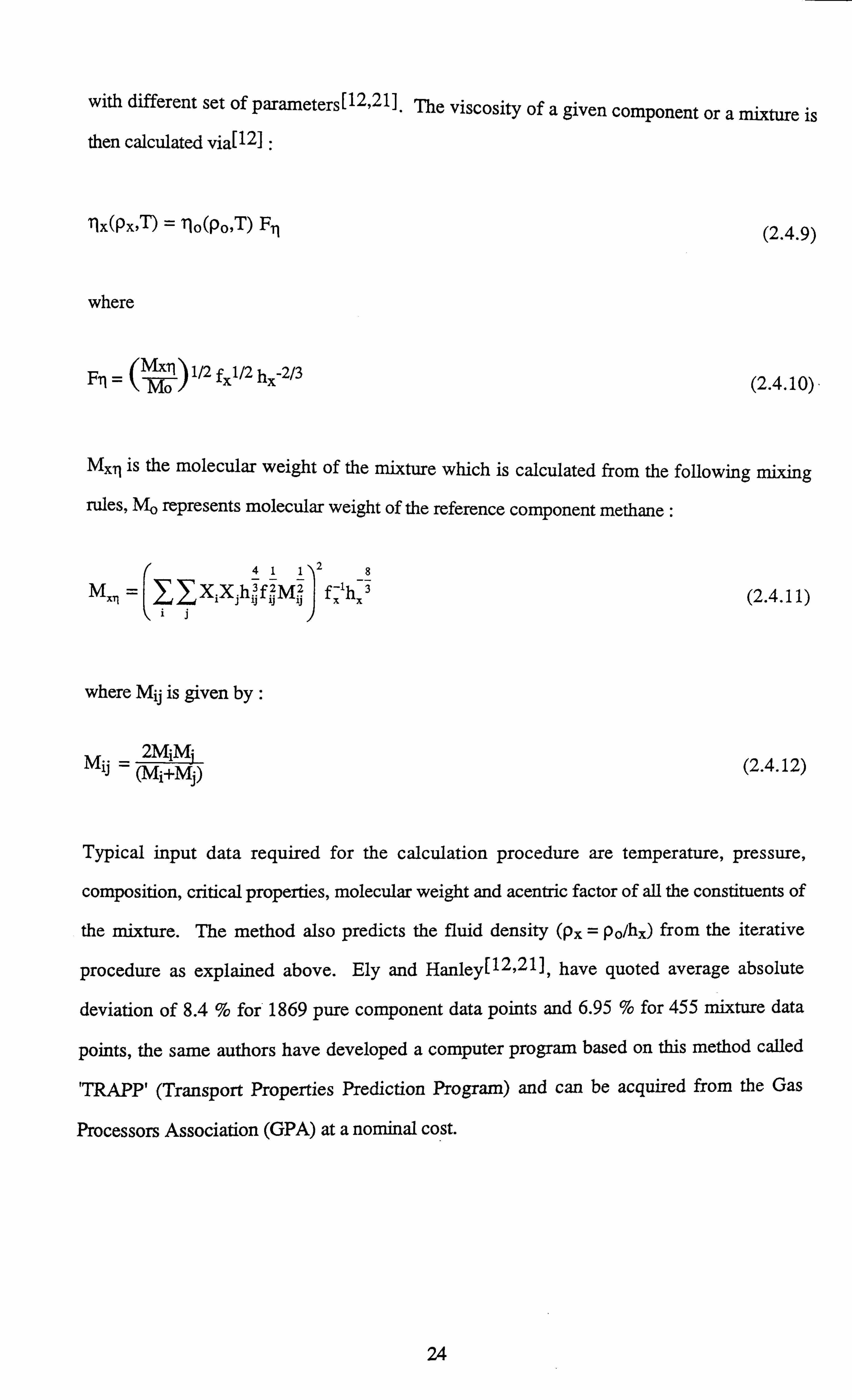
with different set of parameters [12,21]. The viscosity of a given component or a mixture is
then calculated via[12II :
Tlx(Px, T) = llo(Po, T) F� (2.4.9)
where
F (4n)1/2 fX1/2 hx-2'3 (2.4.10),
MX, q is the molecular weight of the mixture which is calculated from the following mixing
rules, MO represents molecular weight of the reference component methane :
41128
Mx, l _ XiXjh fMf z-lhx 3 (2.4.11)
where Mij is given by :
Mij = (M Mý
(2.4.12)
Typical input data required for the calculation procedure are temperature, pressure,
composition, critical properties, molecular weight and acentric factor of all the constituents of
the mixture. The method also predicts the fluid density (px = po/hx) from the iterative
procedure as explained above. Ely and HanleyV12,211, have quoted average absolute
deviation of 8.4 % for 1869 pure component data points and 6.95 % for 455 mixture data
points, the same authors have developed a computer program based on this method called
'TRAPP' (Transport Properties Prediction Program) and can be acquired from the Gas
Processors Association (GPA) at a nominal cost.
24

2.5: PRINCIPLE OF CORRESPONDING STATES (TWO REFERENCE COMPONENTS
It was seen that reliable predictions for mixtures similar to the prediction of the viscosity of
the reference component (methane) are usually obtained using the one reference, principle of
corresponding states method. However, for systems with components considerably different
in size and shape, substantial deviations may occur. Considering these implications, Petersen
et. al. [27] presented a method in 1991 based on the principle of corresponding states using
two reference components. The reduced viscosity (ru) of a given component (denoted by x)
is calculated using the following expression :
in TI, = In rlrl + MWX-MW'
In 71r2 1111'2-MW1 T''lr1
(2.5.1)
MW stands for molecular weight and subscripts 1 and 2 refer to the two reference
components. The functional form for Eq. 2.5.1 was originally suggested by Teja and
Rice[28] using the acentric factor instead of molecular weight. The reduced properties are
determined from :
Er- E=T, p, il (2.5.2)
Subscripts r and c indicate reduced and critical properties respectively. The critical viscosity,
11c is calculated from :
1k =C MW112Pc2/3Tc-1/6 (2.5.3)
Where, C is a constant, MW is the molecular weight, Pc is the critical pressure and Tc is the
critical temperature. The final form of the correlation can be derived by rearranging Eq. 2.5.1
and utilising Eq. 2.5.2:
Ti i1cxi11(T1, P1) [ 2(T2, P2)11c1 ]K
11c1 Tll(Tl, P1)rk2 (2.5.4)
25

The constant 'C' in Eq. 2.5.3 will cancel out on obtaining Eq. 2.5.4, where K represents the
slope of the straight line, in terms of molecular weight :
MWx-MW' K= MW2_MW1 (2.5.5)
ill and T12, are viscosities of the first and the second reference component and are evaluated at
conditions defined by :
Ti =T ,I ci i= 1,2 (2.5.6)
and
Pi=PPC1 i=1,2 (2.5.7) PCX
Where, T and P are the temperature and pressure at which viscosity calculations are desired.
The mixing rules employed to calculate the critical temperature (Tc, ) and pressure (Pox) of the
mixture are identical to those employed in the one reference method (Section 2.3). The
expressions for calculating the molecular weight are similar to those used in the one reference
method with a different set of parameters :
MWmix = MWn + 0.00867358 (MWW1.56079 -p Tn1.56079) (2.5.8)
MWw = F. ziMW 2 (2.5.9) £zjmwj
and
MWn = T-ZiMWi (2.5.10)
here zi is the mole fraction of the ith component in the mixture and MW1 is the molecular
weight of the ith component in the mixture.
26

The two reference components chosen are methane and n-decane. Decane is chosen as the
second reference due to the fact that it is the largest alkane for which sufficient amount of
transport and PVT data exists in the literature.
The reference component viscosities are calculated from the expressions similar to those in the
one reference method with different set of parameters[27] The reference component densities
are however, calculated from the new correlation developed by Petersen et. a1127] which is
based on the cubic Adachi-Lu-Sugie (ALS) equation of state in the form given by Jensen[29].
Typical input data required are critical temperature, pressure, molecular weight and
composition. The method is computationally much faster and superior compared to other
corresponding states methods. It, however, is not very accurate and reliable for fluids having
molecular weight more than decane due to that fact that the straight line functional form cannot
be successfully extrapolated beyond n-decane.
2.6 : LEE'S METHOD FOR VISCOSITY OF GASES
The methods discussed earlier were applicable for the simultaneous prediction of viscosity of
both gas and liquid phases, and thus were very self consistent in their predictive capabilities.
Apart from these methods there are certain methods which are specifically applicable for
estimating either the viscosity of gases or liquids only. In this section another widely used
method for predicting the viscosity of gases is reviewed.
In 1966 Lee et. al[l], developed a method for estimating viscosity of natural gases, the
method is based on experimental viscosity data of pure hydrocarbon gases and one binary gas
mixture. Viscosity is basically expressed in terms of the molecular weight, temperature and
the density. The original equation of Starling and Ellington[251, is used as a starting point:
r1= rloexPLXMPYMI (2.6.1)
27
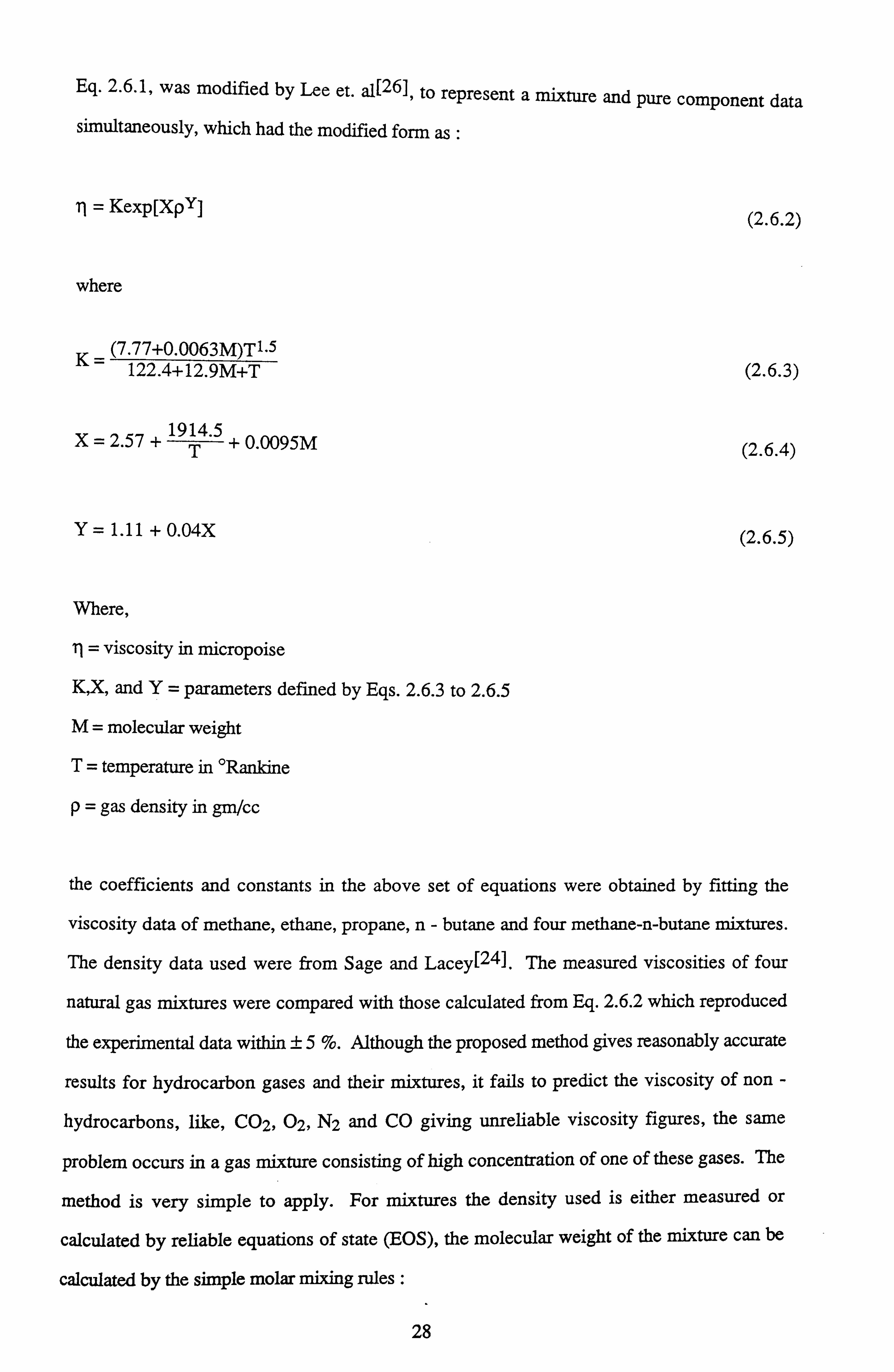
Eq. 2.6.1, was modified by Lee et. al[26], to represent a mixture and pure component data
simultaneously, which had the modified form as :
Tj = Kexp[Xpy] (2.6.2)
where
K_ (7.77+0.0063M)T1.5 122.4+12.9M+T (2.6.3)
X=2.57 + 19T4.5
+ 0.0095M (2.6.4)
Y= 1.11 +0.04X (2.6.5)
Where,
TI = viscosity in micropoise
K, X, and Y= parameters defined by Eqs. 2.6.3 to 2.6.5
M= molecular weight
T= temperature in °Rankine
gas density in gm/cc
the coefficients and constants in the above set of equations were obtained by fitting the
viscosity data of methane, ethane, propane, n- butane and four methane-n-butane mixtures.
The density data used were from Sage and Lacey[24]. The measured viscosities of four
natural gas mixtures were compared with those calculated from Eq. 2.6.2 which reproduced
the experimental data within ±5%. Although the proposed method gives reasonably accurate
results for hydrocarbon gases and their mixtures, it fails to predict the viscosity of non -
hydrocarbons, like, C02,02, N2 and CO giving unreliable viscosity figures, the same
problem occurs in a gas mixture consisting of high concentration of one of these gases. The
method is very simple to apply. For mixtures the density used is either measured or
calculated by reliable equations of state (EOS), the molecular weight of the mixture can be
calculated by the simple molar mixing rules :
28
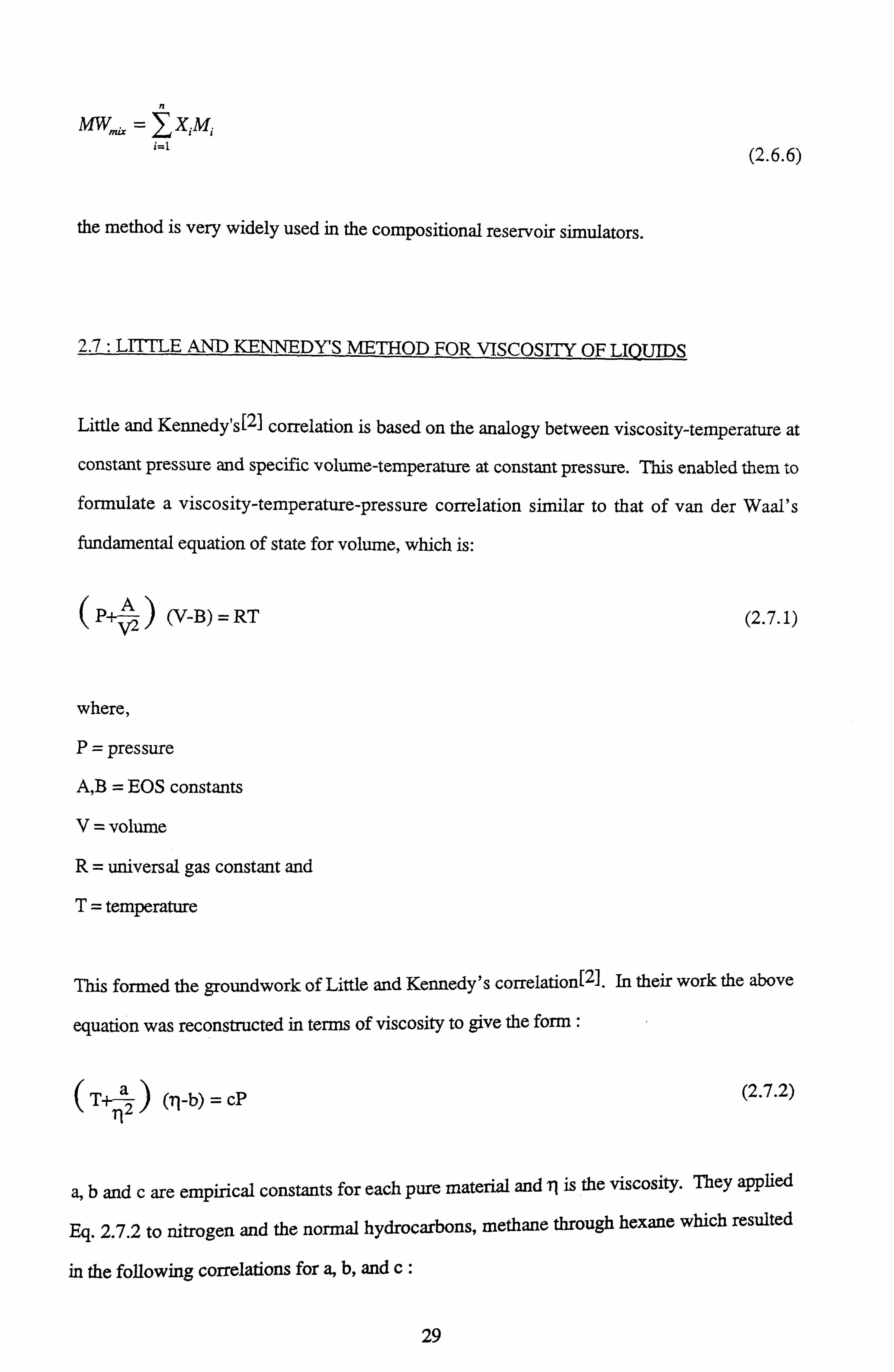
n
lYl lY - Iximi
i=1
the method is very widely used in the compositional reservoir simulators.
2.7: LITTLE AND KENNEDY'S METHOD FOR VISCOSITY OF LIQUIDS
(2.6.6)
Little and Kennedy's[2] correlation is based on the analogy between viscosity-temperature at
constant pressure and specific volume-temperature at constant pressure. This enabled them to
formulate a viscosity-temperature-pressure correlation similar to that of van der Waal's
fundamental equation of state for volume, which is:
P +-VA2 )
(V-B) = RT
where,
P= pressure
A, $ = EOS constants
V= volume
R= universal gas constant and
T= temperature
(2.7.1)
This formed the groundwork of Little and Kennedy's correlation[2]. In their work the above
equation was reconstructed in terms of viscosity to give the form :
(T) (rib) = cP
(2.7.2)
a, b and c are empirical constants for each pure material and 11 is the viscosity. They applied
Eq. 2.7.2 to nitrogen and the normal hydrocarbons, methane through hexane which resulted
in the following correlations for a, b, and c:
29

a= re-' (2.7.3 )
b= sPm (2.7.4)
c=tP-n (2.7.5 )
where,
r, k, s, m, t, and n= empirical constants for each pure component
(obtained from the data on nitrogen and methane through n-hexane)
P= pressure in psia
= viscosity in centipoise
Rearrangement of Eq. 2.7.2 - 2.7.5 gives :
(T+) sPm) - - (r1_ (tp-n)P (2.7.6)
or in a more convenient form :
, n3 - r12 (sPm
+ p-n+1 l+ ( re-k/P l- (re-k/P)(sPm)
_0 (2.7.7) TJTJT
The above cubic equation has three real roots 7c1,1r2 and 1t3 to satisfy the criteria such that :
(ri - in) (71 - TED (r1- 7t3) =0
The following set of rules are followed to calculate the viscosity of a pure hydrocarbon.
1.
2.
3.
In the single phase gas region the minimum of the roots I1,1t2 and 1t3 is used
if three real, unequal roots are obtained.
In the liquid or dense gas phase region, the maximum of the roots nl, 1t2 and
1r3 is used when three real, unequal roots are obtained.
Imaginary roots obtained in either region have no significance and should be
neglected.
30
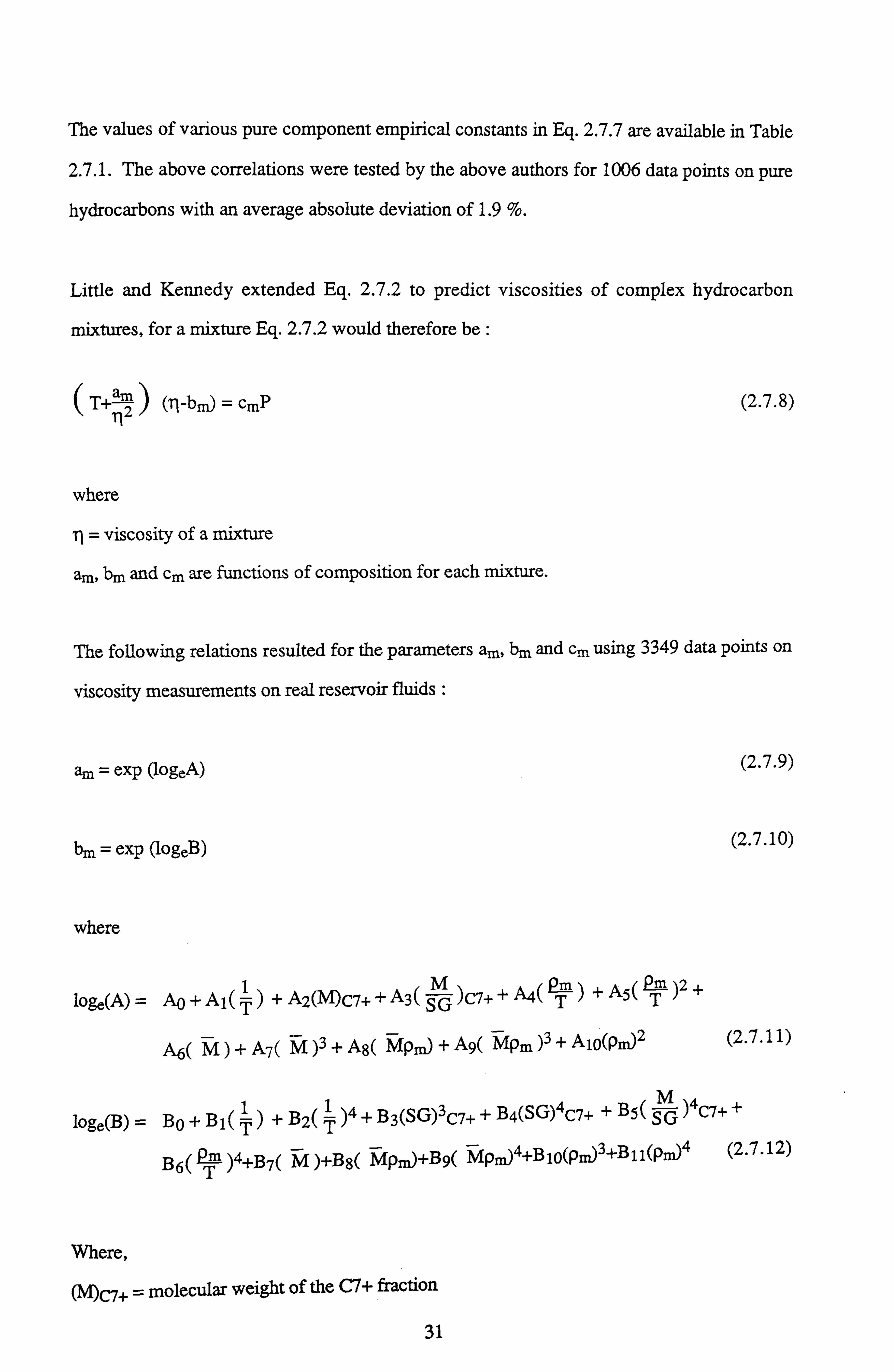
The values of various pure component empirical constants in Eq. 2.7.7 are available in Table
2.7.1. The above correlations were tested by the above authors for 1006 data points on pure
hydrocarbons with an average absolute deviation of 1.9 %.
Little and Kennedy extended Eq. 2.7.2 to predict viscosities of complex hydrocarbon
mixtures, for a mixture Eq. 2.7.2 would therefore be :
(T+) (7l-bm) = cmP
i
where
ii = viscosity of a mixture
am, bm and cm are functions of composition for each mixture.
(2.7.8)
The following relations resulted for the parameters am, bm and cm using 3349 data points on
viscosity measurements on real reservoir fluids :
am = exp (logeA) (2.7.9)
bm = exp (logeB) (2.7.10)
where
loge(A) = A0 + Al (1)+ A2(WC7+ + A3 ( SG )C7+ +() +A5(Pm)2+ T
Ab( M)+A7( NI)3+A8( MPm)+A9( MPm)3+A10(Pm)2 (2.7.11)
log =B+B +B2( 1 )4 + B3(SG)3C7+ + B4(SG)4C7+ + B5( -K)4 )4C7+ -! "
e(B) 01 T) T
B6(ß )4+B7( M)+Bg( Mpmj+B9( Mpm)4+B10(Pm)3+B11(Pm)4 (2.7.12) T
Where,
(M)C7+ _ molecular weight of the C7+ fraction
31
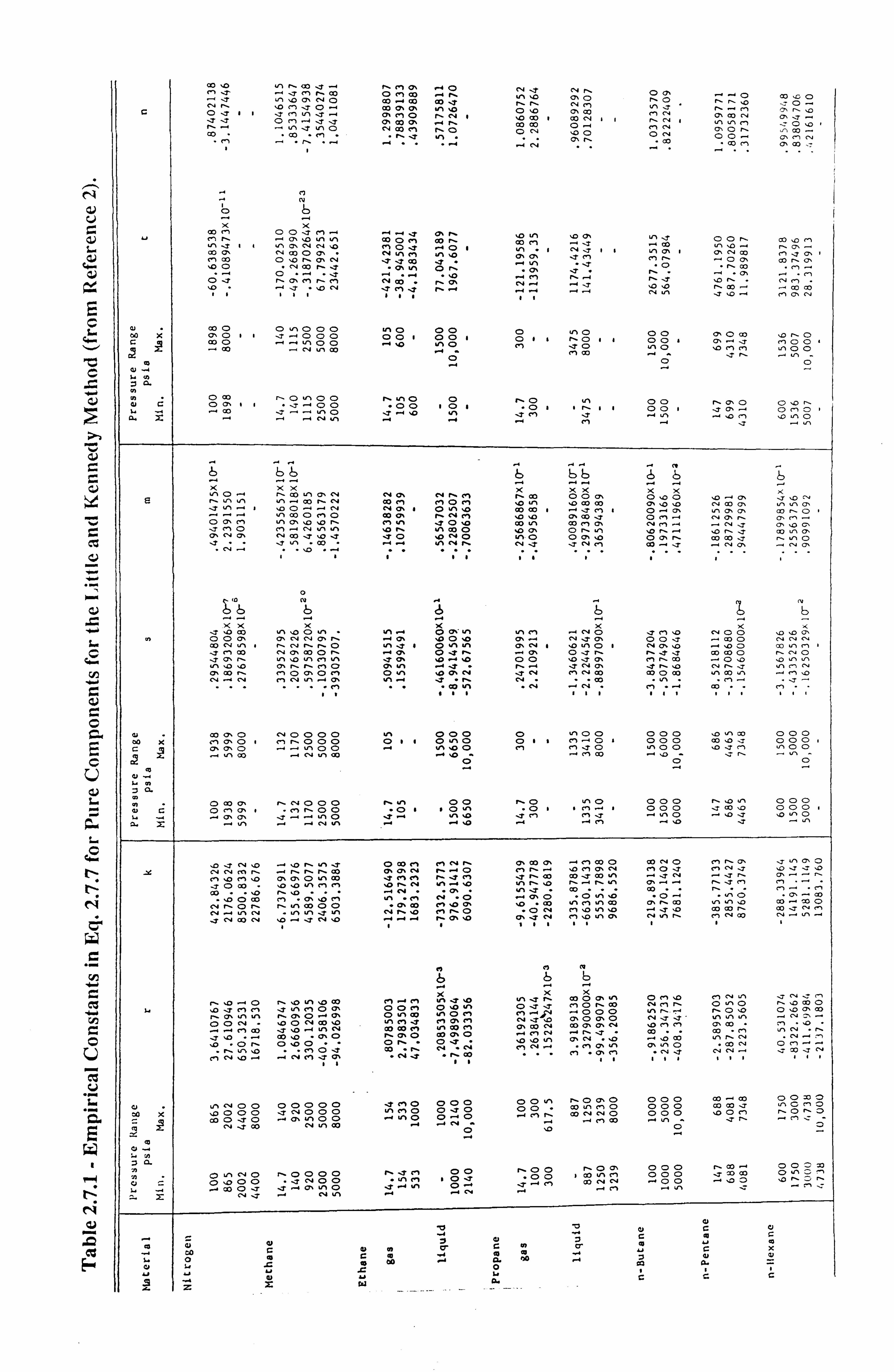
N Cd
4-
Ci
V
CJ
GC
CJ
CC
C L..
C
w
N"
C
.. r
C
L
E
r-i
E-0
CO .O �1 f- d0 i -4 N- 1"1 0' -4 0 NJ N f, J' -J c" N. CO 0 <'CO -4 N- to 'D <" CD O O O W
. ZT N^
J NO Co . -1 Co fü J h t- N 1D hO V1
n N- ý 0 T C OJ1I
O 0 <"1 Vl -
00 C% O' v1 .p O '. O O' OD .7 e-) C, 4
N- .. y / j J J
' O% C1 0 N- N/ p CO 1 CO N1I N- N
0% Co N CY, CT JJ N- -
Oc 1 . -1 ý7 ý7 '
Oý CA 0% . -i N- QO CO O -1 1
N 0
CO % ly to O V
' N a0 Pl r- 0 N 0
ON QON ýn CID
" CO "< 1 N- J vl " " Xl O O~ (" N
" Pl . --' . N- . -4 . -1 . .. -1 .4N . ý " <12 C1 " Il Q- CO .
N
ö b x
ý+ a (5( ý
CD CD IT en .4 I "... a 0%N 10 U 10 (Y, v, s c 1 N- . (7' SO V N v1 Co 0 t'1 Co n Co f'7 J .r CO 00 N- Co o, ac.. Y 1A Vl S [V N '. D <'1 O -7 ra O1 1 (5 NJ11 v1 T1 vl ýO r( O,
CO O' N CO O Q'. N IA M V1 Sp a O, N '. CJp,
crf Co O .O N- O' N IT J Co J" .ý v1 "J O (: N- ^
100 Na0 tom. 7 p (A ye O " J N Co .
- c -ý
.r c;
.. --1 .J N- O1 c"1 h (' 1
.. -4 (V .0 t'1 I N "--1 J , -ý (3 .ýN (N
c-1 N
N 7" '. D ýt c'1 ýt N- r1 N .1 ý
ýJ 1010 f- Co - r. Co CO 11 I11 111 I
N J 10 - In 0' G1 N
al 00 X
aD O o' O11
O In OOO -. -+O 00
In O 00 1
00 00 1
O vi 0 00 CD ýprýp G a)0 .-ý Vi 00 -ýO ýO O1/ c'1
N- C0011 O
0 01 C. . -+ C. J X00 t0 N vt Co ' J
c"1 Co In 0 10 c'1 r1 Ln 00
O O O
1. a1
vl 21 CO r- OýOO N-uyO O N-O vý 00 -C'rn0 0,0- ýý 00 / . 00 1O1 "O 1 1n14 00 1 J rn. ý Oo%0 ý7 1 1O J .r ýO vý J t'1 J . -r v'i .r .D In .O O -
b bb b b bb b b '
XX v ,O . -+ r. In v1
r- Co ul O+ N of 1 N
N 0% +
N f, cn rý Co 0O O' O .0O .0 -+ o+ J . - ao r- Co e 1 C0 P1 '0 In .o Co 0o Orn .0 .0 N OD rn In v\ rn J V1 . --1 1 '0 O "--1 . -+ tV N O' 1 Q Vl sD CO CO 1 . --1 S (" / O . --1 Os u'1 U O1 c0 N. O vl Co O c'1 O Co OI r- N c"1 sO 'O C% Co d O <'1 .. 4 cv O, N. a+ - O O' C'1 vi a' 'O sD N. e1 V1 .jO "O Co t! % CO f"1 OS N f'9 .1 . -. NJ Or 'O C,
J c%O m'r N In vn %0 r, v1 CO O . OO% O NýA sD r.. -. .ON. J Co vorn 0' N C' N Co S 'O ýt 10 IT 0 .0N0 In O 0 v1 .O O 0% N. co CO J NIO N J V1 . . -1 . -4 Vý N 1ý N ý7 J fV c'1 CO -T . -r cV as .-N O1
11 1 11 // 1 1 1 1
O
ýI b b b b ý b _ XX X X X K x
d 10 CO vl 10 O W% V1 r Q Oý v1 vl c'1 .ýNO IT c'7 10 NOO .O .O cý O0 O' 01 NN OsN r10% 10010 Os - NS O' OO IT . -+ Co O NNN CO N vy , N. N f. f, O Vl J1 Q V-1 uY TN1 10 vi O1 N p, Sp . --1 .pO CO u'1 C1 .1 na0 N C' 000 N. .r 0% Q IT r- -+O1 OJr N. JJ cD a00 N. cM0 .1 Q' N. Ln 10 vi Pl V% IT O' 10 . -+ 10 OO 10 a% P5 N. CO -O sO .D In ýn V1 sO '0 O5 1- N. (5 O O' Vl - 't N.. -1 IT N OS _7 t- 10 N N. J IS nN a. Co N. c-1 O Q+ O 1'1 O V\ 10 CA N dN cn N a0 Co 0 Co In Co VIN (V . "+ (V f'1 Nn . -U 05 1! 1 . -1 -j " N. CV " Co . Vý . l'1 - " -r . -"
... .".. Pl ." " CO vl "N -: CV c'1 " "ý CD .- cl-" 9t 886 118 841 101 111
o+ cD c
C1 w Lm
J n"
,n w L
G
Co C, C) d o, 0 I 0'. 0'. 0
Vl CO
p ap p. O en v+ 1 . -+ Oý
NOOOO cn ^000 "-+ --+ '00
. -1 N Vl 40
N. NOOp "c-in00 vl J --I "-+
N 1/'O1
In O11 "-+
nut "O /
J ""-1
OOO 0 4f% 0 N "0 O -4 '0
O+
OO 1 O"
"0 - ýQ
O O11 c"
r, CD "O 1
J 1'1 rl
CD CD e1 -+O / cý JO . -+ (_4 CO
v-% (D / c4- 1
c-1 J . -4 Pl
OOO 000 In 00 -. .pö
000 00 O .. v, % O
-, 0
. o'OD ao. a -z .0.
^'0 r% sCo 0
'. 0 - J
OOO 0 00 ýn 0o
O
000 000 O �- O
^ý J'1
.pN 'p "--1 'p n Vl J O CO 1'1 f"'. Nn O' Co O' ^' P1 0) O CO NO Pi N- O1 J Vl O' 0
Y NNMn N. N. n Co O'. Qý lV f`" """1 O f'1 n r-1 ýD C'1 Oý fV f"1 OJ C"1 NJ ýO ýT r ýD "
c'1 .0 en '0 0% a' O NA aD J r1 P1 h c"1 J N. Co co J Co In JN . --1 J rý '
Orn "-" ^ -
JO Co 'D .D 4n c-1 en '0 N. N 4A . "-/ .O Vl n 10 N. . --I N. ul 0, -- N. < 1 ( I -i --. n
`p . 10 n 'O n NO
en 7 . -" Oý O
c0 "O vý .O
a' "O "-4
N. ". "n p
t rn -- co
" .oO Co Nh0 N.
c"i . D nlnao00
" cý I "Os0) ch. 00' .o "aO v-t cilnCo rn^ao viln. o a)-COO
N N . -1 , r% cV - Vl V'1 JA Nn %0 c% nO "ON Cl sO V1 10
V% O' "--I J '0 N Y1 N
CO CID 1ý C'1 N Co
cý CO J
.7N 0) N '. O "r JN 10 "-1 . -1 . -1 n C% 10 0' JN Pl 'O . 1 I
I 1 1 /1/ 11 1
C
ý, b b
n ýp . --1 p npUQ CO C'. "-/ (" 1! 1 . 10 x
t! 1 '? h Co O O'. V'1 rlO na0
O C"1 10 N c-1 N.
C"1 N v'1 O'nO
JN N.. 0 a0O
L J c-1 c1 J /n c"'f OOH ý
OO1'1 Ovýa0
G"0 vº 1ýOo1
OJJ cl" -+OOO In rte... ^O'0 O. aa'm
ha. Invý n0%O"-+O I". c1 d (" Oýt"1 NJ O' O O' O NJ d' výIn In .ý (N . -"
CD (D cv - -1 rr o
"0O <v c0. D ) '0 .1 I/1 N CO CO l'1 u'. Co P1 O' CO N CO x> O' N 10 r'. Nl O' CID " ^l " "D
v . . iC J r.
- ao. o -rn0 nrn0 x0050 rnNý"
00O 0r. N
; cm
.DON. O O 'c 0 N. J N X10 ( (�1 N . -4 . t1 0' In rn In O " CO (N O c-ý -.
- N. " OJ "^ N N. N" a' Iry "NJ NN ZJ nl
'. 0 4 N ýO . --I 4". J Cý . "ý N C1 .T N 1/ 111 1II 1II
11 11
eý InN 00 00000 dl'ºO 000 001 0004+0 ýI^c"ýO
000 000 Co
"-o ýýs
00 a)C
00 X . 0000 JN000 cm (D OJO 0.0
00 . +rln CoNN O 000 "p0ý ý O ^O
' Co OJO -I0%U100 14 u10 1N .4 . -i cn CO . u1 J tý t 1 .: -
N .7 CO N 1/1 CO "-1 "-- ö O O
C1 v n
3a
In r40 ^0000 nJý 00 ^0O cy, 1
ýýý 000 JaCO O0
a) 0.000
J NOO u1tn 1 OJ '
. 00 ý (n J apNN "-+00 -, 00 `0^O ^
L -.. r 00 0 .7 J .ý O+ LM C) S. + u9 0 ^ N . -ý ,.. I c'1 .. a In d
.... N J (N U 1! 1 . "-1 N "4 rd
c b C C)
C 1p G
Co q)
0 G 0! of zr 0 r. U) c71 Co Z C Co X
i Co Co -4 (13 Co 00
-4 y L 0 Q
00 .+ O. m y
L. y ý 0
y L G C C 9 - ý. iii Z . .. _. _. _. ... _ _.
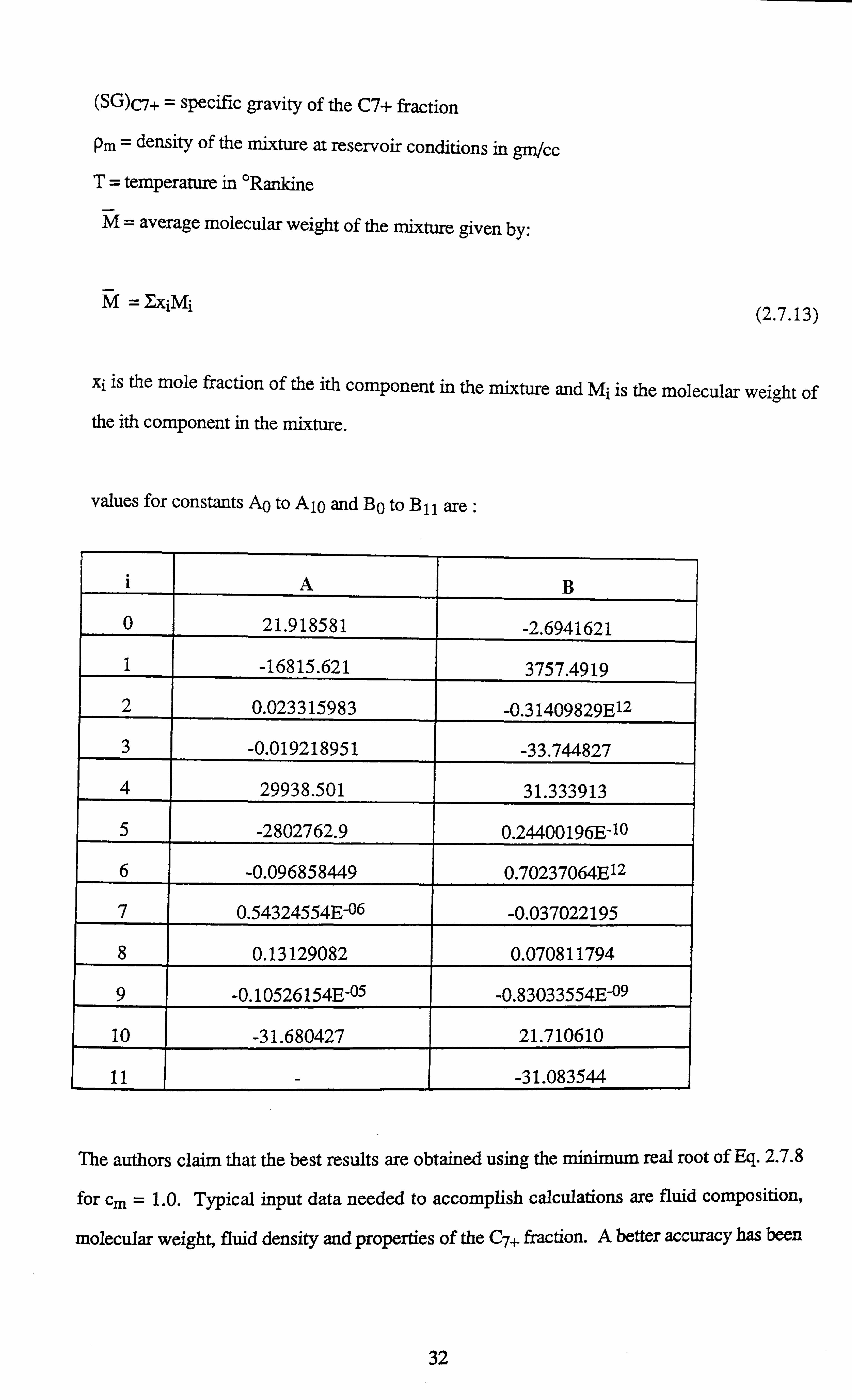
(SG)C7+ = specific gravity of the C7+ fraction
pm = density of the mixture at reservoir conditions in gm/cc T= temperature in °Rankine
M= average molecular weight of the mixture given by:
M= FxiMi (2.7.13)
xi is the mole fraction of the ith component in the mixture and Mi is the molecular weight of the ith component in the mixture.
values for constants AO to A10 and Bp to B11 are :
i A B
0 21.918581 -2.6941621 1 -16815.621 3757.4919
2 0.023315983 -0.31409829E12 3 -0.019218951 -33.744827
4 29938.501 31.333913
5 -2802762.9 0.24400196E-10
6 -0.096858449 0.70237064E12
7 0.54324554E-06 -0.037022195
8 0.13129082 0.070811794
9 -0.10526154E-05 -0.83033554E-09
10 -31.680427 21.710610
11 - -31.083544
The authors claim that the best results are obtained using the minimum real root of Eq. 2.7.8
for cm = 1.0. Typical input data needed to accomplish calculations are fluid composition,
molecular weight, fluid density and properties of the C7+ fraction. A better accuracy has been
32

claimed by the authors compared to the Lohrenz-Bray-Clark correlation[8]. The method is
known to be best suited for black oil applications.
References
1) Lee, A. L., Gonzalez, M. H. and Eakin, B. E.: "The Viscosity of Natural
Gases", Journal of Petroleum Technology, pp. 997 - 1000, (Aug., 1966).
2) Little, T. E. and Kennedy, H. T.: "A Correlation of the Viscosity of
Hydrocarbon Systems with Pressures, Temperature and Composition",
Society of Petroleum Engineers Journal (SPEJ), pp. 157 - 162, (Jun., 1968).
3) Eakin, B. E. and Ellington, R. T.: "Predicting the Viscosity of Pure Light
Hydrocarbons", Journal of Petroleum Technology, pp. 210 - 214, (Feb.,
1963).
4) Giddings, J. G. and Kobayashi, R.: "Correlation of the Viscosity of Light
Paraffin Hydrocarbons and Their Mixtures in the Liquid and Gaseous
Regions", Journal of Petroleum Technology, pp. 679 - 682, (Jun., 1964).
5) Twu, C. H.: "Generalised Methods for Predicting Viscosities of Petroleum
Fractions", AIChEJ, Vol. 32, No. 12, pp. 2091 - 2094, (Dec., 1986).
6) Reid, R. C., Prausnitz, J. M. and Poling, B. E.: "The Properties of Gases and
Liquids", Fourth Edition, McGraw Hill Book Company, New York (1989).
7) Jossi, J. A., Stiel, L. I. and Thodos, G.: "The Viscosity of Pure Substances in
the Dense Gaseous and Liquid Phases", AIChEJ, Vol. 8, pp. 59 - 63, (1962).
8) Lohrenz, J., Bray, B. G. and Clark, C. R.: "Calculating Viscosities of
Reservoir Fluids from Their Compositions", Journal of Petroleum
Technology, pp. 1171-1176, (Oct., 1964).
9) Abas - Zade, A. K., Zhur. Ekspl. i, Teoret. Fiz., 23,60, (1952).
10) Misic, Dragoslav, and George Thodos, AIChEJ, Vol. 7, pp. 264, (1961).
11) Herning, F. and Zipperer, L.: "Calculation of the Viscosity of Technical Gas
Mixtures from the Viscosity of Individual Gases", Gas U. Wasserfach, No.
49, (1936).
33
12) Ely, J. F. and Hanley, H. J. M.: "Prediction of Transport Properties 1, Viscosity of Fluids and Their Mixtures", Industrial & Engineering Chemistry
(I & EC) Fundamentals, Vol. 20, pp. 323-332, (1981).
13) Baltatu, M. E.: "Prediction of the Liquid Viscosity for Petroleum Fractions",
Industrial & Engineering Chemistry (I & EC) Process Design &
Development, Vol. 21, pp. 192-195, (1982).
14) Pedersen, K. S. et. al : "Viscosity of Crude Oils'", Chemical Engineering
Science, Vol. 39, pp. 1011-1016, (1984).
15) Pedersen, K. S. and Fredenslund, Aa.: "An Improved Corresponding States
Model for Prediction of Oil and Gas Viscosities and Thermal Conductivities",
Chemical Engineering Science, Vol. 42, pp. 182-186, (1987).
16) Tham, M. J. and Gubbins, K. E., Industrial & Engineering Chemistry (I &
EC) Fundamentals, Vol. 9, pp. 63, (1970).
17) Christensen, P. L. and Fredenslund, Aa., Chemical Engineering Science, Vol.
35, pp. 871, (1980).
18) McCarty, R. D.: "A Modified Benedict - Webb - Rubin Equation of State for
Methane Using Recent Experimental Data", Cryogenics, (May, 1974).
19) Hanley, H. J. M., McCarty, R. D. and Haynes, W. M.: "Equations for the
Viscosity and Thermal Conductivity Coefficients of Methane", Cryogenics,
(Jul., 1975).
20) Baltatu, M. E.: "Prediction of the Transport Properties of Petroleum
Fractions", Paper Presented at the 1984 Winter National Meeting of AIChE,
Atlanta, Georgia, (1984).
21) Ely, J. F. and. Hanley, H. J. M.: "Prediction of the Viscosity and Thermal
Conductivity in Hydrocarbon Mixtures - Computer Program, TRAPP",
Proceedings of the Sixtieth Annual Convention of Gas Processors
Association, pp. 20-29, (Mar., 1981).
22) Leach, J. W.: "Molecular Structure Corrections for Application of the Theory
of Corresponding States to Non - Spherical Pure Fluids and Mixtures", PhD
Thesis, Rice University, (1967).
34
23) Leach, J. W., Chappelear, P. S. and Leland, T. W., AIChEJ, Vol. 14, pp. 568, (1968).
24) Sage, B. H. and Lacey, W. N.: "Thermodynamic Properties of the Lighter
Paraffin Hydrocarbons and Nitrogen", API, New York, N. Y. (1950).
25) Starling, K. E. and Ellington, R. T.: "Viscosity Correlations for Non polar Fluids", AIChEJ, pp. 11-15, (Jan., 1964).
26) Lee, A. L., Starling, K. E., Dolan, J. P. and Ellington, R. T.: "Viscosity
Correlation for Light Hydrocarbon Systems", AIChEJ, pp. 694-697, (Sep.,
1964).
27) Aasberg-Petersen, K., Knudsen, K. and Fredenslund, A.: "Prediction of
Viscosities of Hydrocarbon Mixtures", Fluid Phase Equilibria, Vol. 70, pp.
293-308, (1991).
28) Teja, A. S. and Rice, P.: "Generalised Corresponding States Method for the
Viscosities of Liquid Mixtures", Industrial & Engineering Chemistry (I & EC)
Fundamentals, Vol. 20, pp. 77 (1981).
29) Jensen, B. H.: "Densities, Viscosities, and Phase Equilibria in Enhanced Oil
Recovery", PhD Thesis, Institut for Kemiteknik, the Technical University of
Denmark, (1987).
30) Pedersen, K. S., Fredenslund, Aa. and Thomassen, P.: "Properties of Oils and
Natural Gases", Contributions in Petroleum Geology & Engineering, 5, Gulf
Publishing Company, (1989).
35
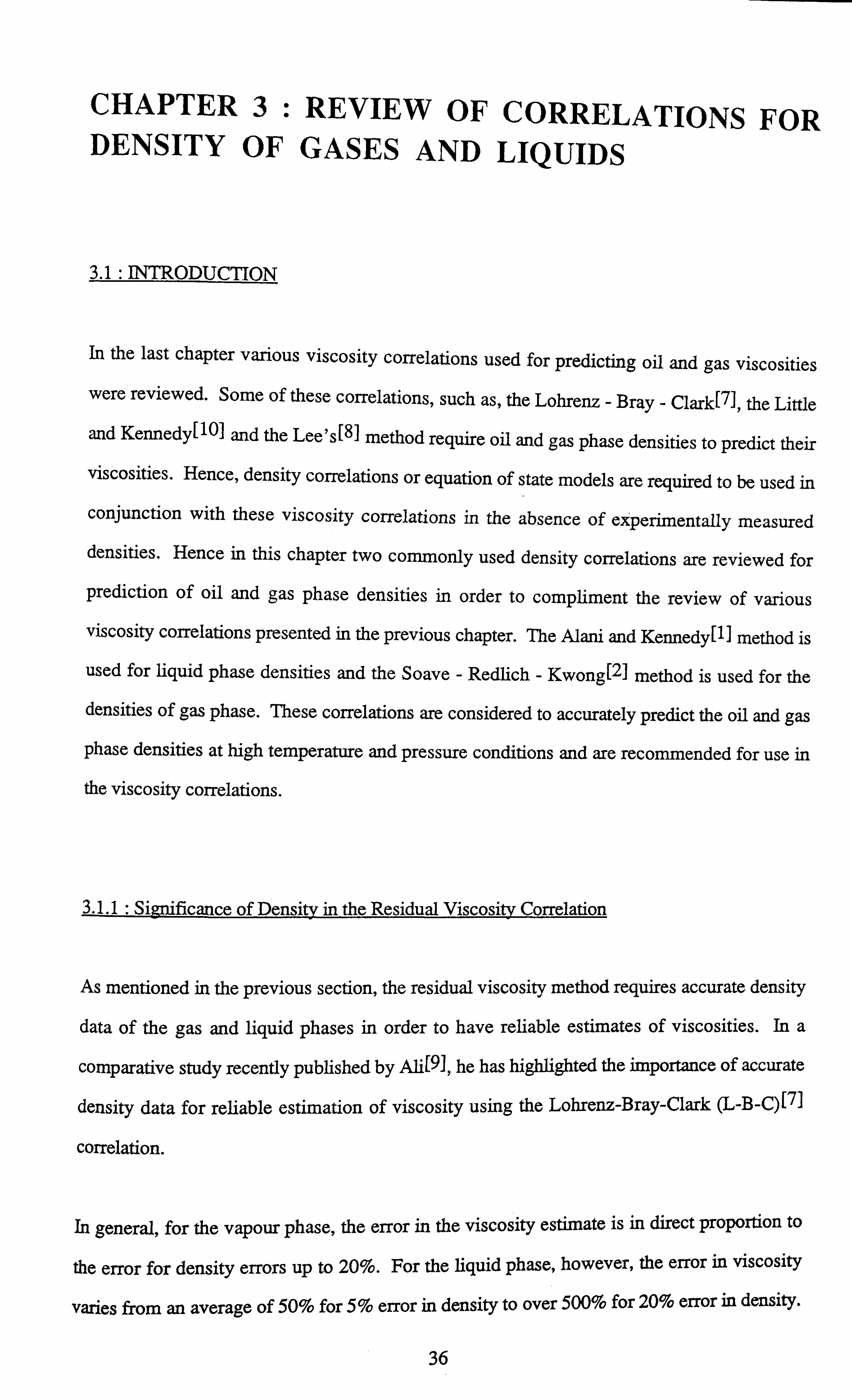
CHAPTER 3: REVIEW OF CORRELATIONS FOR DENSITY OF GASES AND LIQUIDS
3.1 : INTRODUCTION
In the last chapter various viscosity correlations used for predicting oil and gas viscosities
were reviewed. Some of these correlations, such as, the Lohrenz - Bray - Clark[7], the Little
and Kennedy[101 and the Lee's[8] method require oil and gas phase densities to predict their
viscosities. Hence, density correlations or equation of state models are required to be used in
conjunction with these viscosity correlations in the absence of experimentally measured densities. Hence in this chapter two commonly used density correlations are reviewed for
prediction of oil and gas phase densities in order to compliment the review of various
viscosity correlations presented in the previous chapter. The Alani and Kennedy{l ] method is
used for liquid phase densities and the Soave - Redlich - Kwong[2] method is used for the
densities of gas phase. These correlations are considered to accurately predict the oil and gas
phase densities at high temperature and pressure conditions and are recommended for use in
the viscosity correlations.
3.1.1: Significance of Density in the Residual Viscosity Correlation
As mentioned in the previous section, the residual viscosity method requires accurate density
data of the gas and liquid phases in order to have reliable estimates of viscosities. In a
comparative study recently published by Ali[91, he has highlighted the importance of accurate
density data for reliable estimation of viscosity using the Lohrenz-Bray-Clark (L-B-C)[71
correlation.
In general, for the vapour phase, the error in the viscosity estimate is in direct proportion to
the error for density errors up to 20%. For the liquid phase, however, the error in viscosity
varies from an average of 50% for 5% error in density to over 500% for 20% error in density.
36
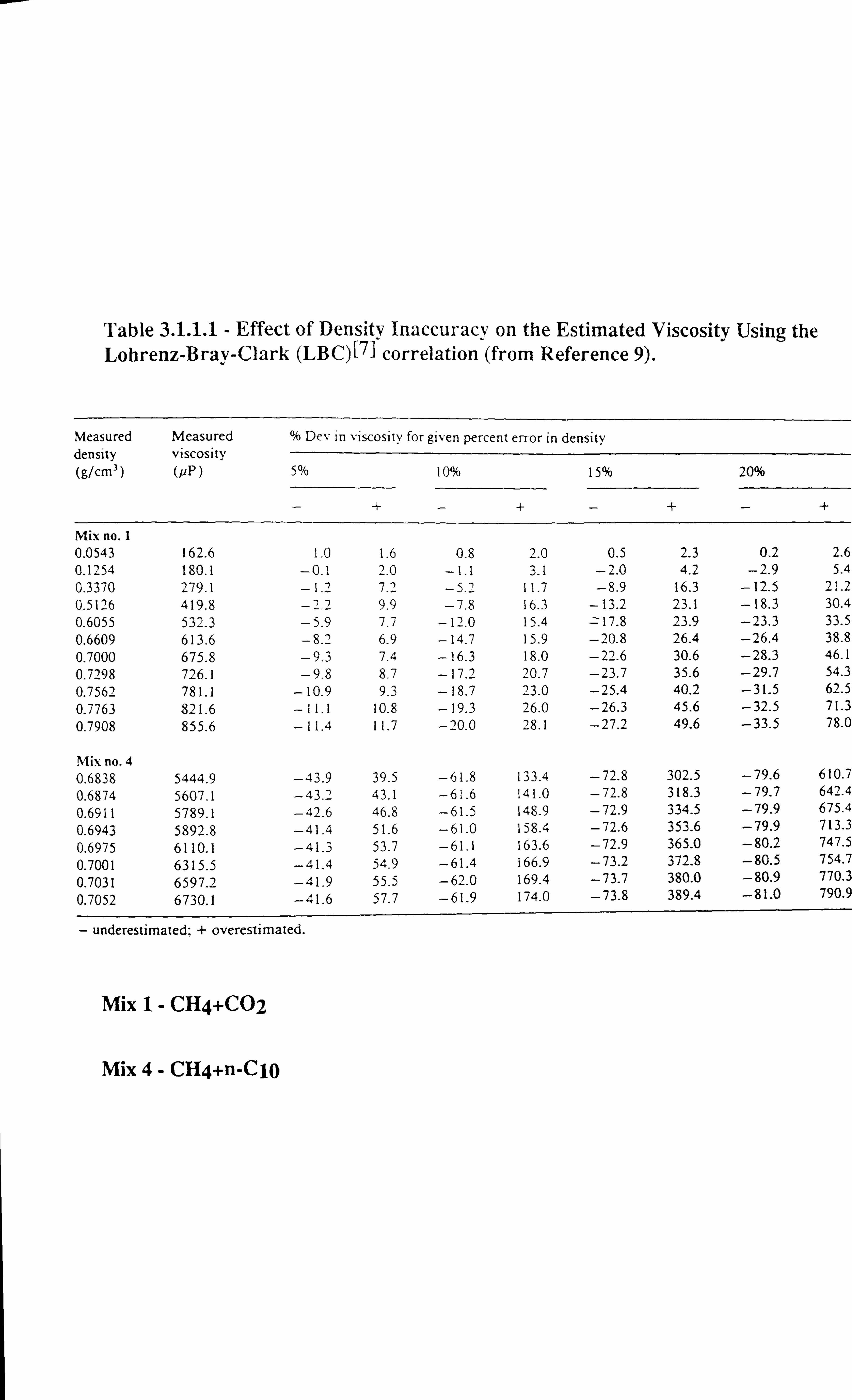
Table 3.1.1.1 - Effect of Density Inaccuracy on the Estimated Viscosity Using the Lohrenz-Bray-Clark (LBC)[7] correlation (from Reference 9).
Measured Measured Dev in viscosity for given percent error in density density viscosity (g/cm') (µP) 5% 10% 15% 20%
-+-+-+-+
Mix no. 1 0.0543 162.6 1.0 1.6 0.8 2.0 0.5 2.3 0.2 2.6 0.1254 180.1 -0.1 2.0 - 1.1 3.1 -2.0 4.2 -2.9 5.4 0.3370 279.1 -1.2 7.2 -5-2 11.7 -8.9 16.3 -12.5 21.2 0.5126 419.8 9.9 -7.8 16.3 -13.2 23.1 -18.3 30.4 0.6055 532.3 -5.9 7.7 -12.0 15.4 .. 17.8 23.9 -23.3 33.5 0.6609 613.6 -8.2 6.9 -14.7 15.9 -20.8 26.4 -26.4 38.8 0.7000 675.8 -9.3 7.4 -16.3 18.0 -22.6 30.6 -28.3 46.1 0.7298 726.1 -9.8 8.7 -17.2 20.7 -23.7 35.6 -29.7 54.3 0.7562 781.1 -10-9 9.3 -18.7 23.0 -25.4 40.2 -31.5 62.5 0.7763 821.6 - 11.1 10.8 -19.3 26.0 -26.3 45.6 -32.5 71.3 0.7908 855.6 -11.4 11.7 -20.0 28.1 -27.2 49.6 -33.5 78.0
Mix no. 4 0.6838 5444.9 -43.9 39.5 -61.8 133.4 -72.8 302.5 -79.6 610.7 0.6874 5607.1 -43.2 43.1 -61.6 141.0 -72.8 318.3 -79.7 642.4 0.6911 5789.1 -42.6 46.8 -61.5 148.9 -72.9 334.5 -79.9 675.4
0.6943 5892.8 -41.4 51.6 -61.0 158.4 -72-6 353.6 -79.9 713.3
0.6975 6110.1 -41.3 53.7 -61.1 163.6 -72.9 365.0 -80.2 747.5
0.7001 6315.5 -41.4 54.9 -61.4 166.9 -73.2 372.8 -80.5 754.7
0.7031 6597.2 -41.9 55.5 -62.0 169.4 -73.7 380.0 -80.9 770.3
0.7052 6730.1 -41.6 57.7 -61.9 174.0 -73.8 389.4 -81.0 790.9
- underestimated; + overestimated.
Mix 1- CH4+CO2
Mix 4- CH4+n-C10
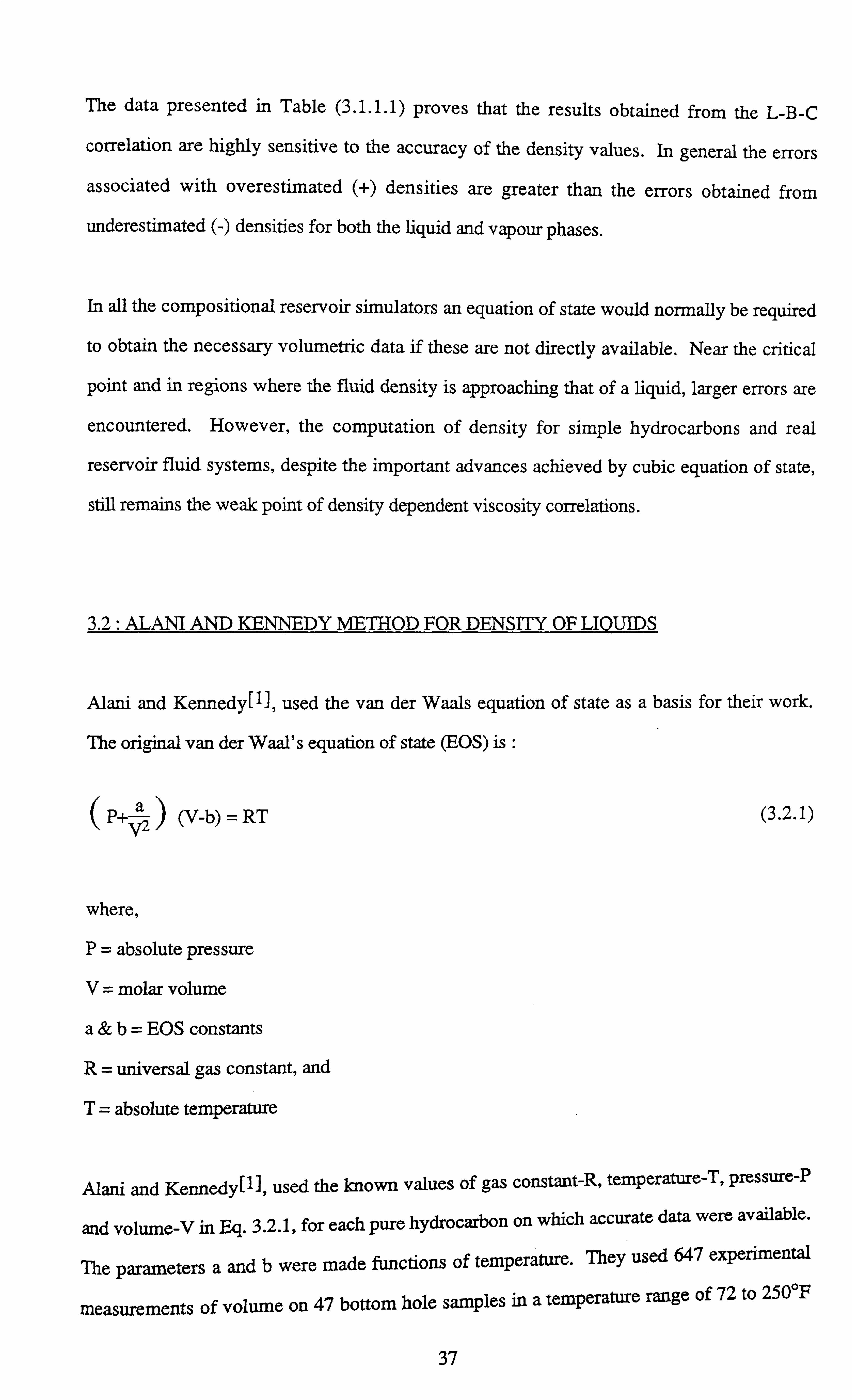
The data presented in Table (3.1.1.1) proves that the results obtained from the L-B-C
correlation are highly sensitive to the accuracy of the density values. In general the errors
associated with overestimated (+) densities are greater than the errors obtained from
underestimated (-) densities for both the liquid and vapour phases.
In all the compositional reservoir simulators an equation of state would normally be required
to obtain the necessary volumetric data if these are not directly available. Near the critical
point and in regions where the fluid density is approaching that of a liquid, larger errors are
encountered. However, the computation of density for simple hydrocarbons and real
reservoir fluid systems, despite the important advances achieved by cubic equation of state,
still remains the weak point of density dependent viscosity correlations.
3.2: ALANI AND KENNEDY METHOD FOR DENSITY OF LIQUIDS
Alani and Kennedy[lI, used the van der Waals equation of state as a basis for their work.
The original van der Waal's equation of state (EOS) is :
(P+; ý ) (V-b) =RT (3.2.1)
where,
P= absolute pressure
V= molar volume
a&b= EOS constants
R= universal gas constant, and
T= absolute temperature
Alani and Kennedytl], used the known values of gas constant-R, temperature-T, pressure-P
and volume-V in Eq. 3.2.1, for each pure hydrocarbon on which accurate data were available.
The parameters a and b were made functions of temperature. They used 647 experimental
measurements of volume on 47 bottom hole samples in a temperature range of 72 to 250°F
37
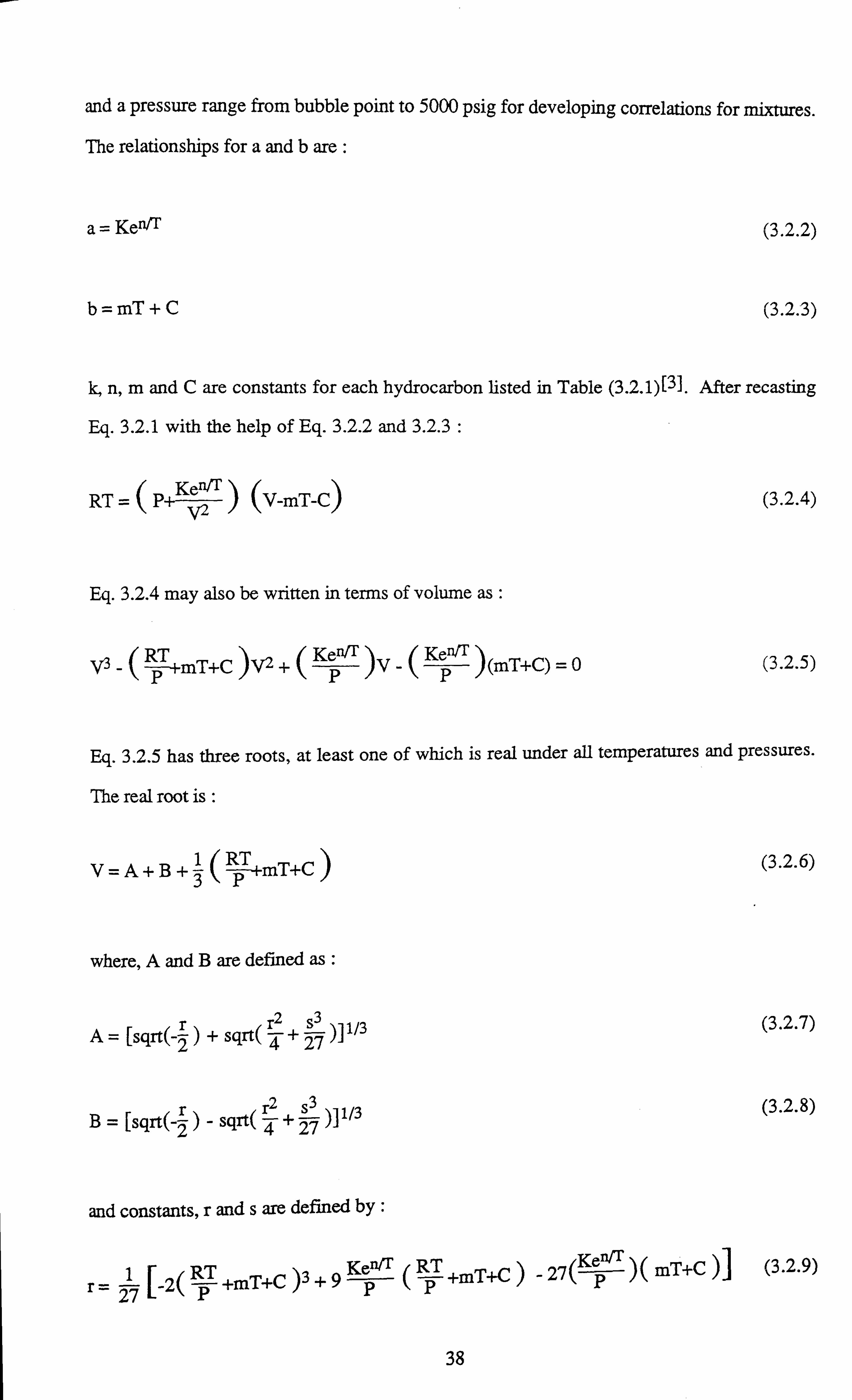
and a pressure range from bubble point to 5000 psig for developing correlations for mixtures.
The relationships for a and b are :
a= Ken/T (3.2.2)
b=mT+C (3.2.3)
k, n, m and C are constants for each hydrocarbon listed in Table (3.2.1)[3]. After recasting
Eq. 3.2.1 with the help of Eq. 3.2.2 and 3.2.3 :
RT =ýPý> (V-mT-C)
(3.2.4)
Eq. 3.2.4 may also be written in terms of volume as :
V3 RT MT+C) +(
KP )VKP )(mT+C)=0 (3.2.5) P
Eq. 3.2.5 has three roots, at least one of which is real under all temperatures and pressures.
The real root is :
V=A+B+1 (-T+mT+C, (3.2.6)
3
where, A and B are defined as :
23 A= [sgrt(-r) + sgrt(4 + 27
)] 1/3 (3.2.7) 2
B= [sgrt(-r) - sqrt( r2 + 27 )] 1/3 (3.2.8)
24
and constants, r and s are defined by :
27 P hhlr RT
+mT+C - 27(KeI'/T )C mT+C )1 (3.2.9)
-1 RT )3 Ke
r--[-2( +mT+C)+ 9ppp
38
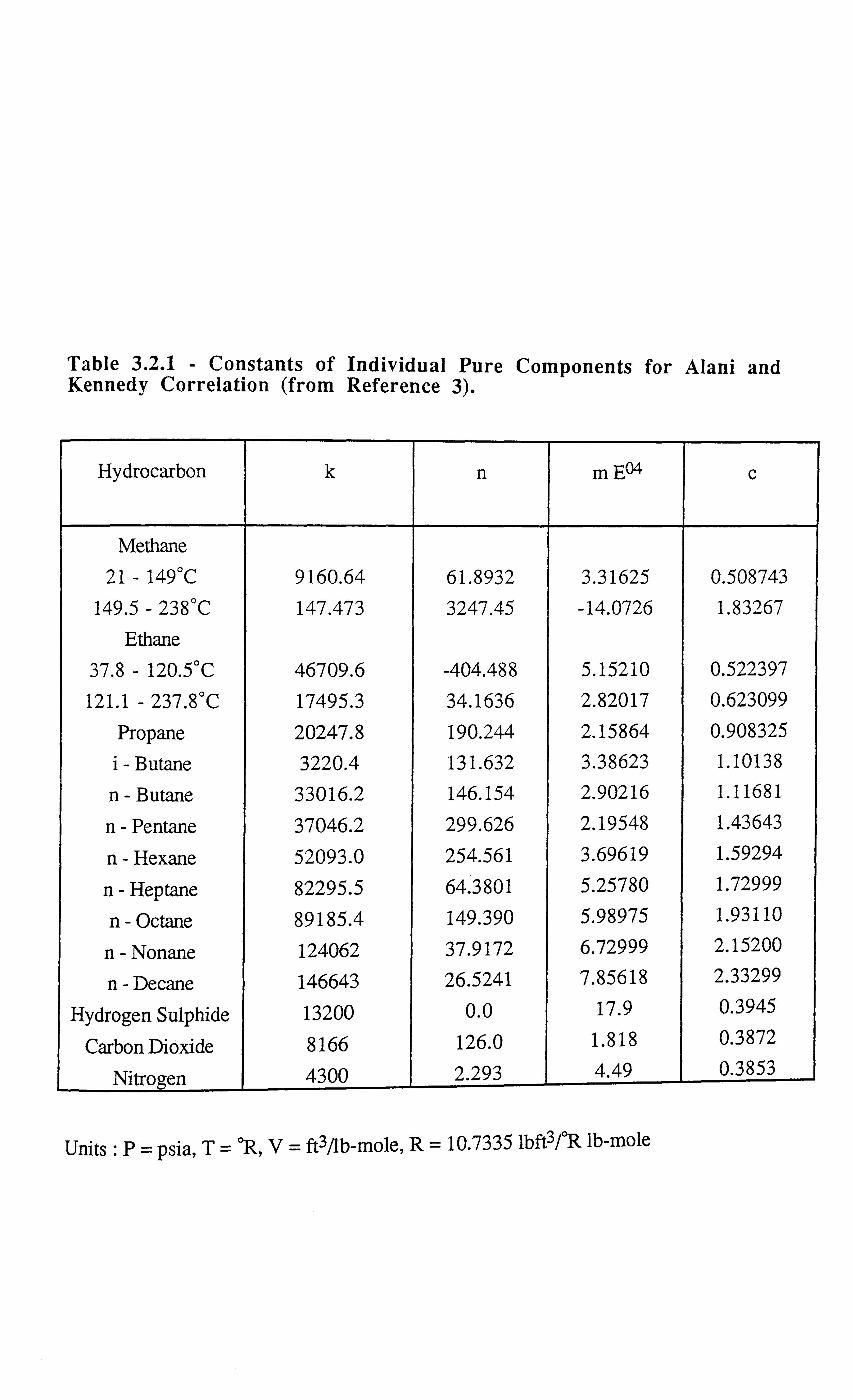
Table 3.2.1 - Constants of Individual Pure Components for Alani and Kennedy Correlation (from Reference 3).
Hydrocarbon k n m E04 c
Methane 21 - 149°C 9160.64 61.8932 3.31625 0.508743
149.5 - 238°C 147.473 3247.45 -14.0726 1.83267
Ethane
37.8 - 120.5°C 46709.6 -404.488 5.15210 0.522397
121.1 - 237.8°C 17495.3 34.1636 2.82017 0.623099 Propane 20247.8 190.244 2.15864 0.908325
i- Butane 3220.4 131.632 3.38623 1.10138
n- Butane 33016.2 146.154 2.90216 1.11681
n- Pentane 37046.2 299.626 2.19548 1.43643
n- Hexane 52093.0 254.561 3.69619 1.59294
n- Heptane 82295.5 64.3801 5.25780 1.72999
n- Octane 89185.4 149.390 5.98975 1.93110
n- Nonane 124062 37.9172 6.72999 2.15200
n- Decane 146643 26.5241 7.85618 2.33299
Hydrogen Sulphide 13200 0.0 17.9 0.3945
Carbon Dioxide 8166 126.0 1.818 0.3872
Nitrogen 4300 2.293 4.49 0.3853
Units :P= psia, T= °R, V= ft3/lb-mole, R =10.7335 lbft3/°R lb-mole

1 Kew' s=1
[3 P
(RT +mT+C )2] (3.2.10) P
r2 s3 The solution for the above root is obtained only if 4+ 27 > 0. The other two roots are then
imaginary and have no significance in determining liquid volumes.
Similarly, Eq. 3.2.5 has three real and unequal roots if r2 + s3 4 27 < 0. The minimum real root
in this case represents the volume as :
V=2E1/3Cos (e3 ý) +( PT+mT+C} (3.2.11)
where, E and Cos (6), are defined by :
ýT E=sgrt
[-27 (Kep -3 (PT+mT+C)2)3] (3.2.12)
1 KeWT 1 Ken/T RT 1 RT cos (8) =2p (mT+C) -6p (p +mT+C) + 27(p +mT+C)3
Ken/T sqrt - 27( p-3 (p-- +mT+C )2)3] (3.2.13)
Eq. 3.2.5 can be applied to pure components in its form given above and the liquid specific
volume can be obtained by solving the cubic equation for its minimum real root, among the
three roots obtained.
For a hydrocarbon mixture containing, n, number of components, the constants a and b can
be defined as :
n
am = Xiai i-1 (3.2.14)
n
bm = Xibi ; =1
(3.2.15)
39
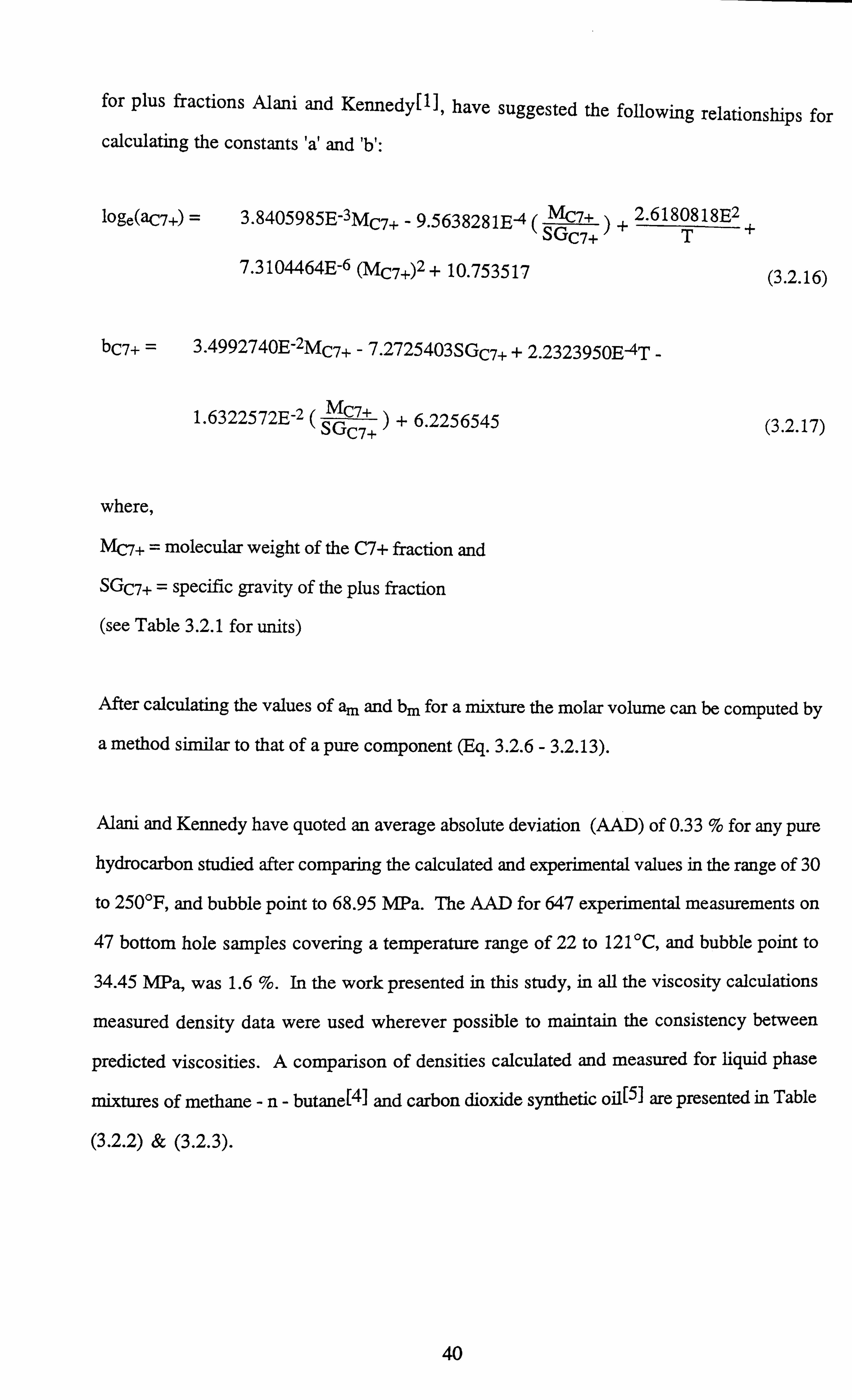
for plus fractions Alani and Kennedy[ l ], have suggested the following relationships for
calculating the constants 'a' and 'b':
10ge(aC7+) = 3.8405985E-3MC7+ - 9.5638281E-4 ( G7+ )+2.6180818E2 + SGC7+ T
7.3104464E-6 (MC7+)2 + 10.753517 (3.2.16)
bC7+ = 3.4992740E-2MC7+ - 7.2725403SGC7+ + 2.2323950E-4T -
1.6322572E-2 ( MC7 ++6.2256545 SG+ C7
where,
Mc7+ = molecular weight of the C7+ fraction and
SGC7+ = specific gravity of the plus fraction
(see Table 3.2.1 for units)
(3.2.17)
After calculating the values of am and bm for a mixture the molar volume can be computed by
a method similar to that of a pure component (Eq. 3.2.6 - 3.2.13).
Alani and Kennedy have quoted an average absolute deviation (AAD) of 0.33 % for any pure
hydrocarbon studied after comparing the calculated and experimental values in the range of 30
to 250°F, and bubble point to 68.95 MPa. The AAD for 647 experimental measurements on
47 bottom hole samples covering a temperature range of 22 to 121 °C, and bubble point to
34.45 MPa, was 1.6 %. In the work presented in this study, in all the viscosity calculations
measured density data were used wherever possible to maintain the consistency between
predicted viscosities. A comparison of densities calculated and measured for liquid phase
mixtures of methane -n- butane{41 and carbon dioxide synthetic of [5I are presented in Table
(3.2.2) & (3.2.3).
40
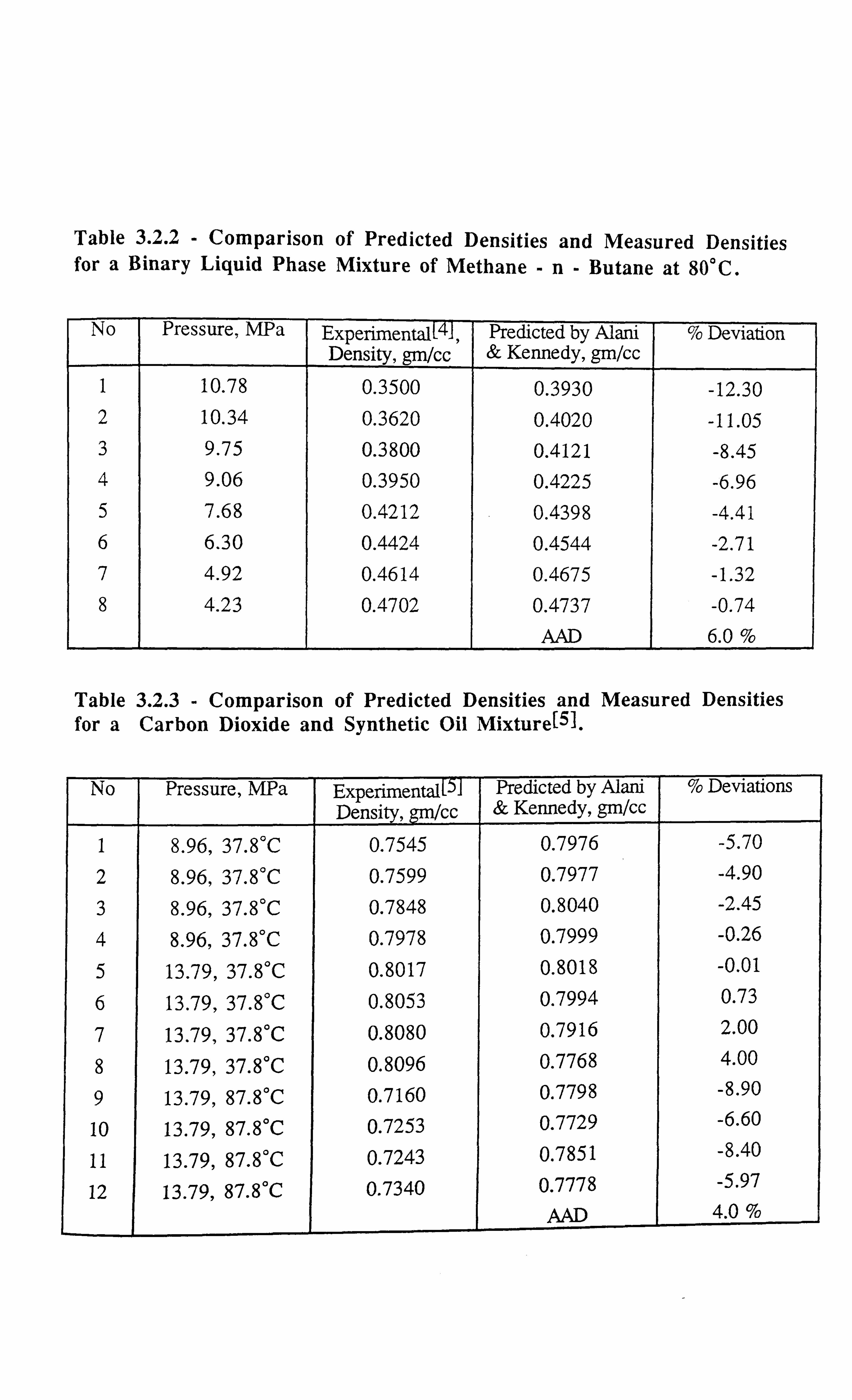
Table 3.2.2 - Comparison of Predicted Densities and Measured Densities for a Binary Liquid Phase Mixture of Methane - n- Butane at 80°C.
No Pressure, MPa Experimental [41, Density, gm/cc
Predicted by Alani & Kennedy, gm/cc
% Deviation
1 10.78 0.3500 0.3930 -12.30 2 10.34 0.3620 0.4020 -11.05 3 9.75 0.3800 0.4121 -8.45 4 9.06 0.3950 0.4225 -6.96 5 7.68 0.4212 0.4398 -4.41 6 6.30 0.4424 0.4544 -2.71 7 4.92 0.4614 0.4675 -1.32 8 4.23 0.4702 0.4737 -0.74
AAD 6.0%
Table 3.2.3 - Comparison of Predicted Densities and Measured Densities for a Carbon Dioxide and Synthetic Oil Mixture[51.
No Pressure, MPa Experimentall5l Density, gm/cc
Predicted by Alani & Kennedy, gm/cc
% Deviations
1 8.96,37.8°C 0.7545 0.7976 -5.70 2 8.96,37.8°C 0.7599 0.7977 -4.90 3 8.96,37.8°C 0.7848 0.8040 -2.45 4 8.96,37.8°C 0.7978 0.7999 -0.26 5 13.79,37.8°C 0.8017 0.8018 -0.01 6 13.79,37.8°C 0.8053 0.7994 0.73
7 13.79,37.8°C 0.8080 0.7916 2.00
8 13.79,37.8°C 0.8096 0.7768 4.00
9 13.79,87.8°C 0.7160 0.7798 -8.90
10 13.79,87.8°C 0.7253 0.7729 -6.60
11 13.79,87.8°C 0.7243 0.7851 -8.40
12 13.79,87.8°C 0.7340 0.7778 -5.97 AAD 4.0 %®
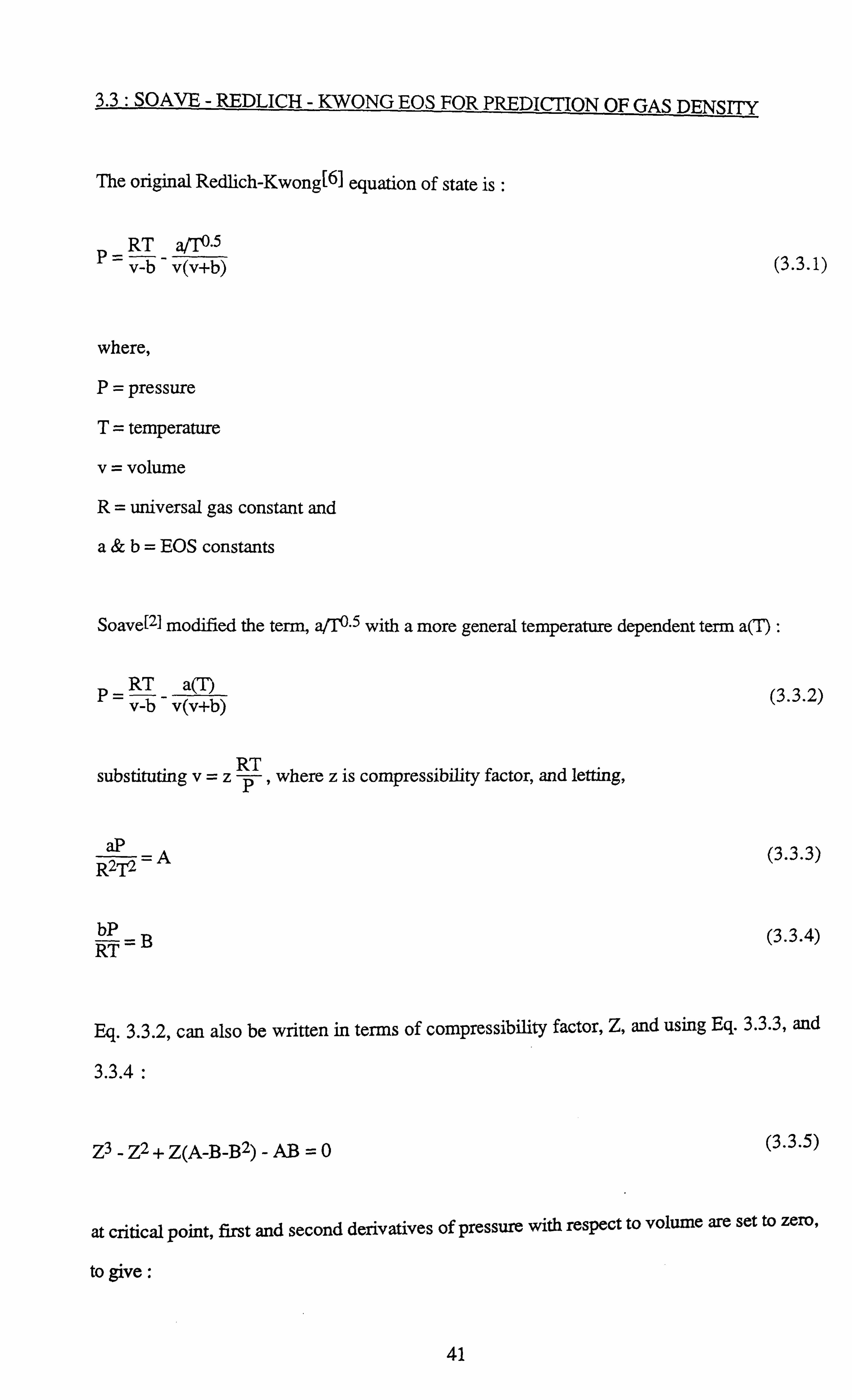
3.3: SOAVE - REDLICH - KWONG EOS FOR PREDICTION OF GAS DENSITY
The original Redlich-Kwong[6I equation of state is :
P RT afro 5
v-b v(v+b)
where,
P= pressure
T temperature
v= volume
R= universal gas constant and
a&b= EOS constants
(3.3.1)
Soave{2I1 modified the term, of I' 5 with a more general temperature dependent term a(T) :
P- _ RT
- a(T) (3.3.2)
v-b v(v+b)
substituting v=z PT , where z is compressibility factor, and letting,
=A (3.3.3 2
RT !B (3.3.4)
Eq. 3.3.2, can also be written in terms of compressibility factor, Z, and using Eq. 3.3.3, and
3.3.4 .
Z3 - Z2 + Z(A-B-B2) - AB =0 (3.3.5)
at critical point, first and second derivatives of pressure with respect to volume are set to zero,
to give:
41
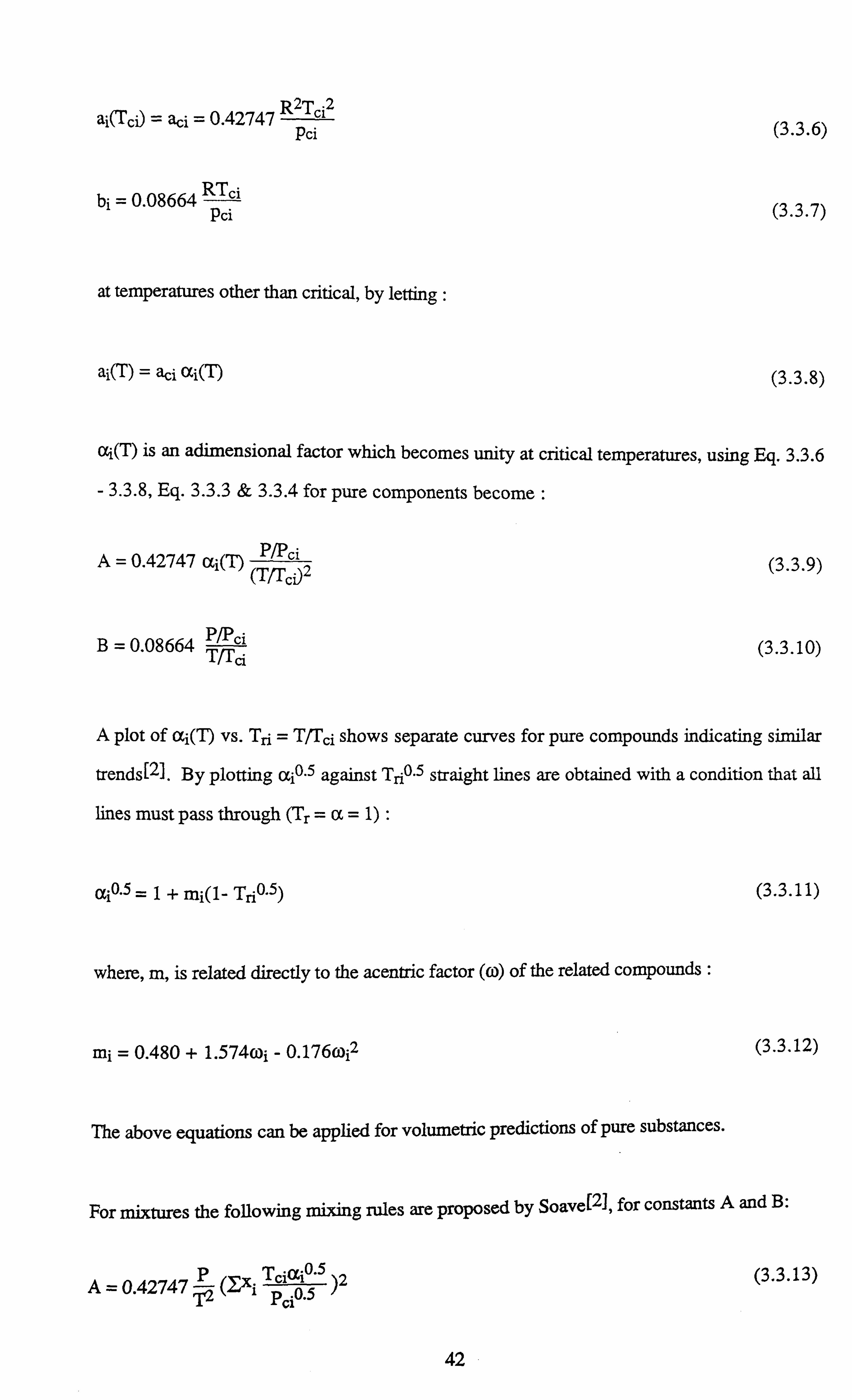
ai(rci) = aci = 0.42747 R2Tci2 Pci (3.3.6)
bi = 0.08664 RTci Pci (3.3.7)
at temperatures other than critical, by letting :
ai(T) = aci Cc1(T) (3.3.8)
al(T) is an adimensional factor which becomes unity at critical temperatures, using Eq. 3.3.6
- 3.3.8, Eq. 3.3.3 & 3.3.4 for pure components become :
A= 0.42747 ai(T) p/pci
3.3.9
B= P/pc' ci
(3.3.1 0) T/r
A plot of ai(T) vs. Tn = T[Fcl shows separate curves for pure compounds indicating similar
trends[2]. By plotting aiß"5 against Tri0.5 straight lines are obtained with a condition that all
lines must pass through (Tr =a= 1) :
alo. 5 =1+ mi(1- Trio. 5)
where, m, is related directly to the acentric factor (co) of the related compounds :
mi = 0.480 + 1.574tw1- 0.176co12
The above equations can be applied for volumetric predictions of pure substances.
(3.3.1 1)
(3.3.12)
For mixtures the following mixing rules are proposed by Soave[2l, for constants A and B:
05 2 A=0.42747 P (Yxi T p10.5 ci
(3.3.13)
42

Table 3.3.1 - Comparison of Predicted Densities and Measured Densities for a Binary Vapour Mixture of Methane -n- Butane at 80°C.
No Pressure, MPa Experimental [4], Density, gm/cc
Predicted by S-R-K,
cc
% Deviations
1 10.78 0.1683 0.1620 3.74 2 10.34 0.1557 0.1486 4.56 3 9.75 0.1404 0.1338 4.70 4 9.06 0.1252 0.1197 4.39 5 7.68 0.1015 0.0965 4.90 6 6.30 0.0823 0.0769 6.60 7 4.92 0.0649 0.0602 7.24 8 4.23 0.0569 0.0529 7.03
AAD 5.4%
Table 3.3.2 - Comparison of Predicted Densities and Measured Densities for a Low Ethane Natural Gas at 29.5°C.
No Pressure, MPa Experimental 181 , Density, gm/cc
Predicted by S-R-K,
gM/Cc
% Deviations
1 13.92 0.0991 0.1103 -11.30 2 27.69 0.2109 0.2006 4.90
3 31.18 0.2288 0.2167 5.30
4 34.61 0.2385 0.2307 3.27
5 41.52 0.2602 0.2543 2.27
6 48.38 0.2761 0.2734 0.98
7 55.36 0.2870 0.2897 -0.94 8 58.33 0.2941 0.2959 -0.61
AAD 3.7%

Table 3.3.3 - Comparison of Predicted Densities and Measured Densities for a Low Ethane Natural Gas at 104.4°C
.
No Pressure, MPa Experimental Density, gm/cc
Predicted by S-R-K,
cc
% Deviations
1 7.09 0.0396 0.0391 1.26 2 10.45 0.0582 0.0580 0.34 3 14.16 0.0747 0.0786 -5.22 4 20.85 0.1178 0.1137 3.48 5 27.68 0.1508 0.1455 3.51 6 38.09 0.1893 0.1857 1.90 7 44.78 0.2102 0.2070 1.52
AAD 2.5%
Table 3.3.4 - Comparison of Predicted Densities and Measured Densities for a High Ethane Natural Gas at 25.9°C.
No Pressure, MPa Experimental , Density, gm/cc Predicted
by S-R-K, cc
% Deviations
1 27.68 0.2746 0.2590 5.68
2 32.89 0.2976 0.2818 5.30 3 38.09 0.3172 0.3001 5.39
4 44.99 0.3384 0.3199 5.47 5 48.37 0.2474 0.3283 5.49
6 51.90 0.2554 0.3363 5.37
7 55.45 0.3642 0.3436 5.65
8 58.82 0.3741 0.3500 6.44
9 62.20 0.3791 0.3561 6.07
10 69.12 0.3906 0.3672 5.99
AAD 5.7
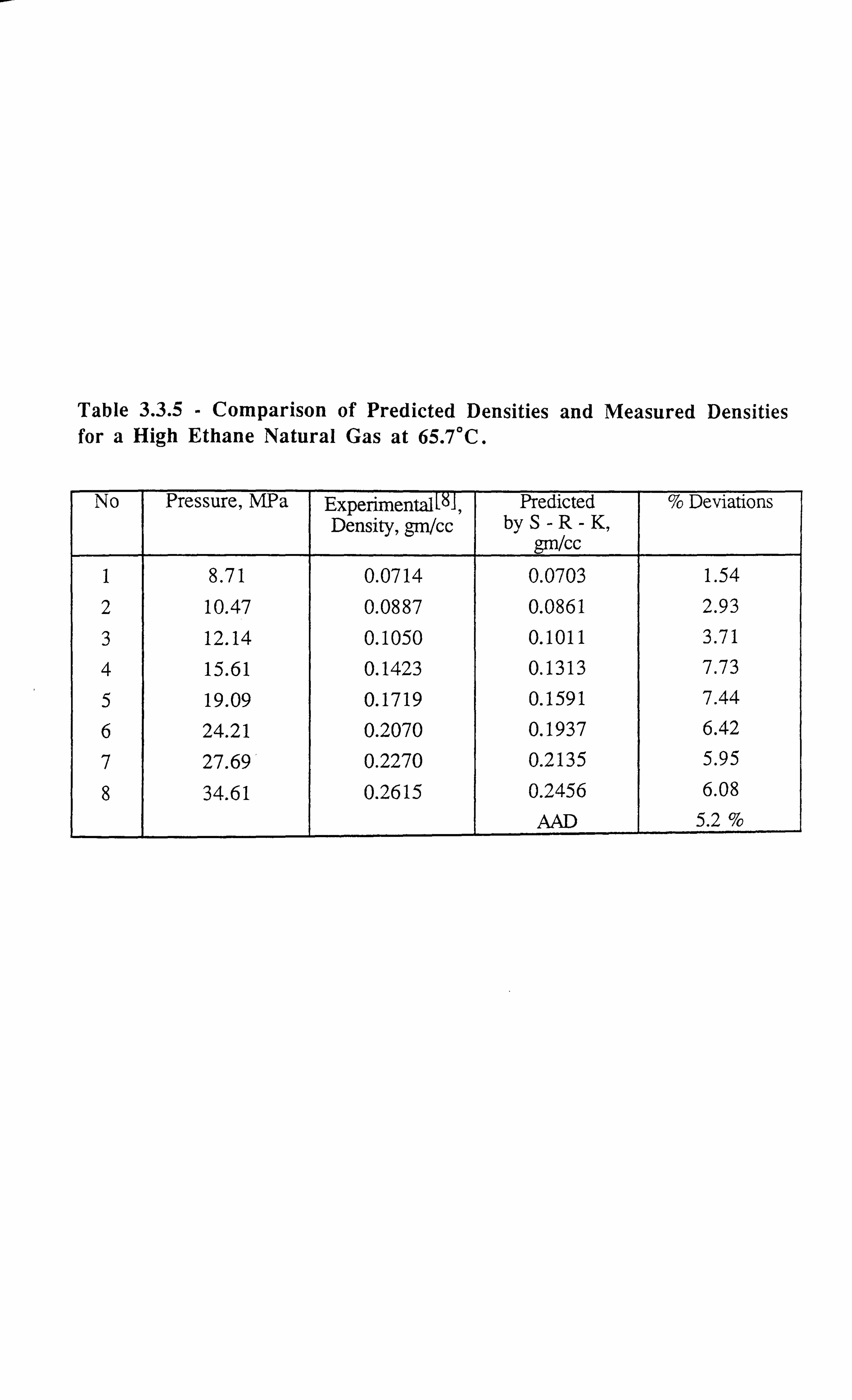
Table 3.3.5 - Comparison of Predicted Densities and Measured Densities for a High Ethane Natural Gas at 65.7°C.
No Pressure, MPa Experimental , Density, gm/cc
Predicted by S-R-K,
gm/cc
% Deviations
1 8.71 0.0714 0.0703 1.54
2 10.47 0.0887 0.0861 2.93
3 12.14 0.1050 0.1011 3.71
4 15.61 0.1423 0.1313 7.73
5 19.09 0.1719 0.1591 7.44
6 24.21 0.2070 0.1937 6.42
7 27.69 0.2270 0.2135 5.95
8 34.61 0.2615 0.2456 6.08 AAD 5.2 %
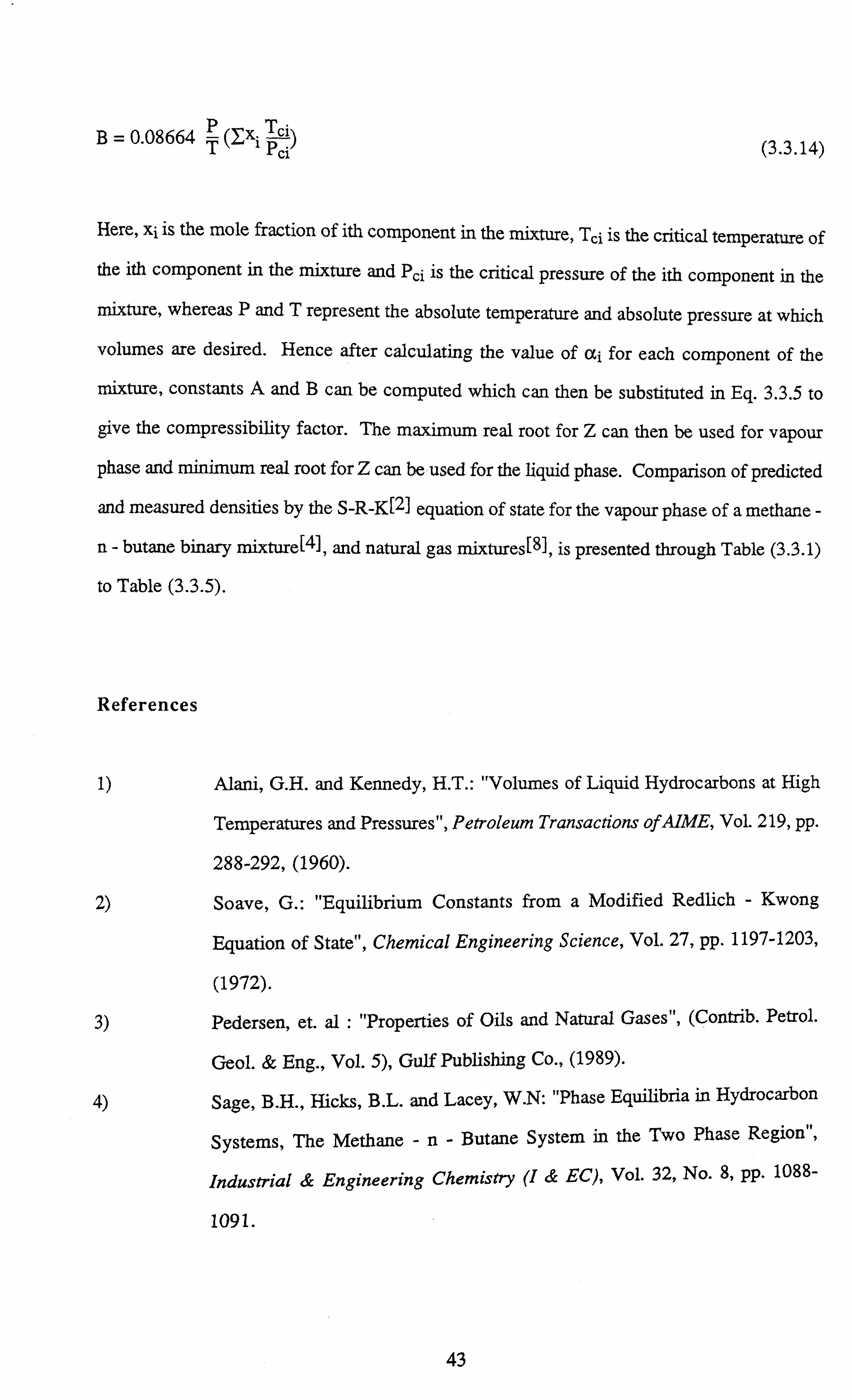
B=0.08664 p (EX, Pci) 3.3.14 ei {)
Here, xi is the mole fraction of ith component in the mixture, Tci is the critical temperature of
the ith component in the mixture and Pci is the critical pressure of the ith component in the
mixture, whereas P and T represent the absolute temperature and absolute pressure at which
volumes are desired. Hence after calculating the value of ai for each component of the
mixture, constants A and B can be computed which can then be substituted in Eq. 3.3.5 to
give the compressibility factor. The maximum real root for Z can then be used for vapour
phase and minimum real root for Z can be used for the liquid phase. Comparison of predicted
and measured densities by the S-R-K[2] equation of state for the vapour phase of a methane -
n- butane binary mixture[4], and natural gas mixtures! 8], is presented through Table (3.3.1)
to Table (3.3.5).
References
1) Alani, G. H. and Kennedy, H. T.: "Volumes of Liquid Hydrocarbons at High
Temperatures and Pressures", Petroleum Transactions ofAIME, Vol. 219, pp.
288-292, (1960).
2) Soave, G.: "Equilibrium Constants from a Modified Redlich - Kwong
Equation of State", Chemical Engineering Science, Vol. 27, pp. 1197-1203,
(1972).
3) Pedersen, et. al : "Properties of Oils and Natural Gases", (Contrib. Petrol.
Geol. & Eng., Vol. 5), Gulf Publishing Co., (1989).
4) Sage, B. H., Hicks, B. L. and Lacey, W. N: "Phase Equilibria in Hydrocarbon
Systems, The Methane -n- Butane System in the Two Phase Region",
Industrial & Engineering Chemistry (I & EC), Vol. 32, No. 8, pp. 1088-
1091.
43
5) Kovarik, F. S. and Taylor, M. A.: "Viscosity Measurements of High Pressure
C02/Hydrocarbon Mixtures", AIChE Annual Meeting, New York, (Nov., 15-
20,1987).
6) Redlich - Kwong, Chemical Review, Vol. 44, pp. 23, (1949).
7) Lohrenz, J., Bray, B. G. and Clark, C. R.: "Calculating Viscosities of
Reservoir Fluids from Their Compositions", Journal of Petroleum
Technology, pp. 1171-1176, (Oct., 1964).
8) Lee, A. L.: "Viscosity of Light Hydrocarbons", Monograph on API Research
Project 65, Published by API, New York, (1965).
9) Ali, J. K: "Evaluation of Correlations for Estimating the Viscosities of
Hydrocarbon Fluids", J. of Petroleum Science and Engineering, Vol. 5, pp.
351-369, (1991).
10) Little, J. E. and Kennedy, H. T.: "A Correlation of the Viscosity of
Hydrocarbon Systems with Pressures, Temperature and Composition",
Society of Petroleum Engineers Journal (SPEJ), pp. 157 - 162, (Jun., 1968).
44

CHAPTER 4 COMPARATIVE STUDY OF PREDICTIVE TECHNIQUES FOR VISCOSITY
4.1: INTRODUCTION
In this chapter a study conducted on evaluating the reliability and accuracy of the widely used
correlations is presented. Only viscosity correlations applicable to both the oil and gas phases
were considered for the study, namely, the Lohrenz - Bray - Clark[l] (Jossi-Stiel-Thodos{18]
for pure components) method, principle of corresponding states (one reference method) [2]
and the extended principle of corresponding states[3]. The Lee's method[4], although was
reviewed in this study, the results are not presented here because of two reasons, first, the
method is only applicable to gases and the viscosities predicted by it are almost identical to
those predicted by the other methods 11,2,3], secondly, the method was found inapplicable to
pure non - hydrocarbons, or mixtures of hydrocarbons with significantly large concentration
of non - hydrocarbons. The study has been conducted on both pure hydrocarbons and non -
hydrocarbons, and their mixtures at wide ranging temperature and pressure conditions.
However, a more complete study is presented in the next chapter which provides the
modification of the residual viscosity method, proposed in this work, for high reduced
density conditions. The comparative study recently carried out by Ali[161 is briefly
discussed. A brief study on the tuning of viscosity correlations for real reservoir fluids is also
presented.
4.2 : VISCOSITY OF PURE COMPONENTS
Pure normal paraffins ranging from methane to normal decane and non - hydrocarbons,
namely, carbon dioxide and nitrogen in both gaseous and liquid phases were considered for
the study. The data published by Stephan and Lucas[51, for the work of several researchers
was considered for comparing the measured and predicted values. Viscosity data presented in
Reference[s], is measured by a variety of conventional viscosity measurement equipment
45
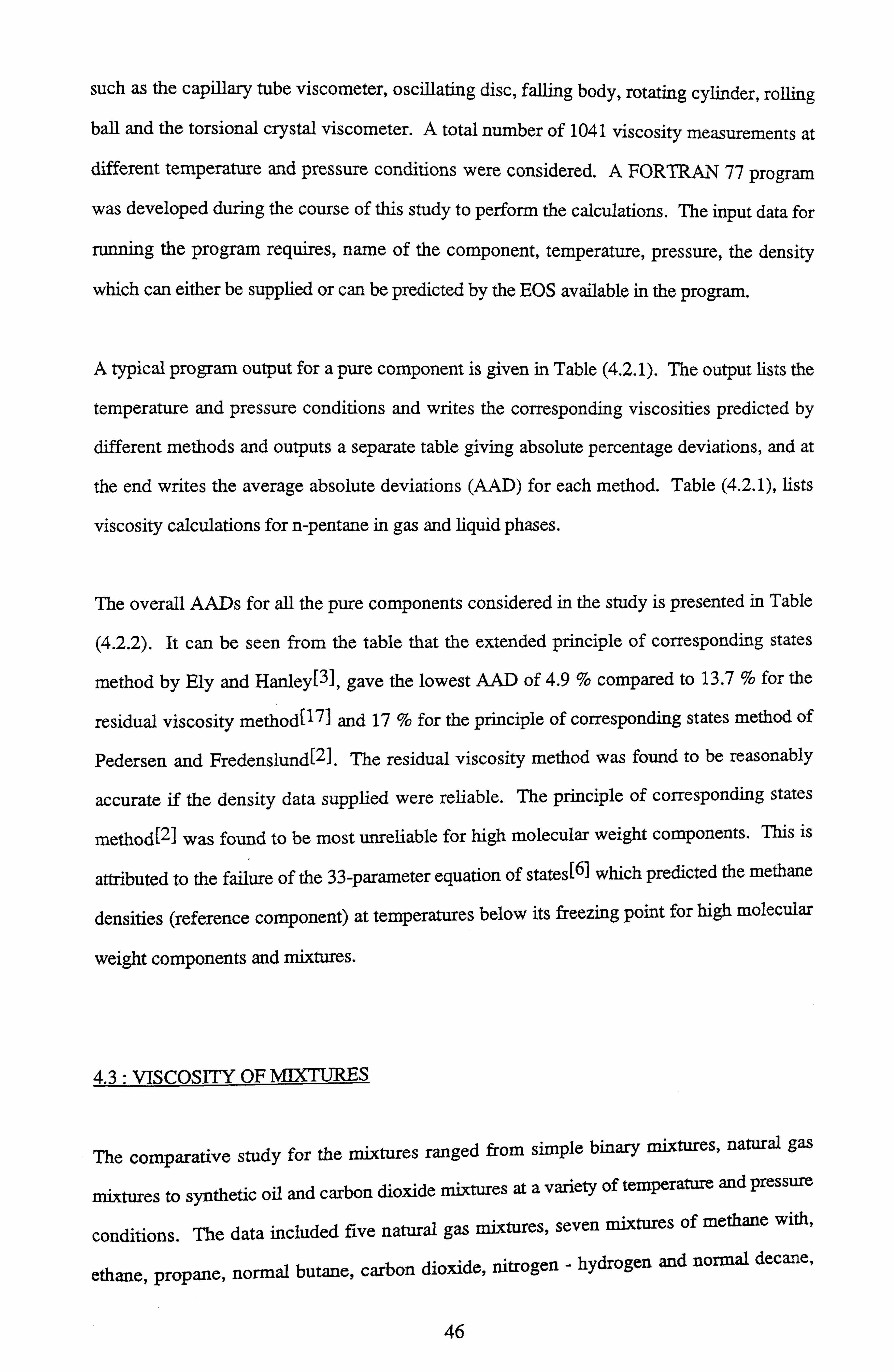
such as the capillary tube viscometer, oscillating disc, falling body, rotating cylinder, rolling
ball and the torsional crystal viscometer. A total number of 1041 viscosity measurements at
different temperature and pressure conditions were considered. A FORTRAN 77 program
was developed during the course of this study to perform the calculations. The input data for
running the program requires, name of the component, temperature, pressure, the density
which can either be supplied or can be predicted by the EOS available in the program.
A typical program output for a pure component is given in Table (4.2.1). The output lists the
temperature and pressure conditions and writes the corresponding viscosities predicted by
different methods and outputs a separate table giving absolute percentage deviations, and at
the end writes the average absolute deviations (AAD) for each method. Table (4.2.1), lists
viscosity calculations for n -pentane in gas and liquid phases.
The overall AADs for all the pure components considered in the study is presented in Table
(4.2.2). It can be seen from the table that the extended principle of corresponding states
method by Ely and Hanley[3], gave the lowest AAD of 4.9 % compared to 13.7 % for the
residual viscosity method[17] and 17 % for the principle of corresponding states method of
Pedersen and Fredenslund[2]. The residual viscosity method was found to be reasonably
accurate if the density data supplied were reliable. The principle of corresponding states
method[2] was found to be most unreliable for high molecular weight components. This is
attributed to the failure of the 33-parameter equation of states[6] which predicted the methane
densities (reference component) at temperatures below its freezing point for high molecular
weight components and mixtures.
4.3 : VISCOSITY OF NBXTLJRE-S
The comparative study for the mixtures ranged from simple binary mixtures, natural gas
mixtures to synthetic oil and carbon dioxide mixtures at a variety of temperature and pressure
conditions. The data included five natural gas mixtures, seven mixtures of methane with,
ethane, propane, normal butane, carbon dioxide, nitrogen - hydrogen and normal decane,
46
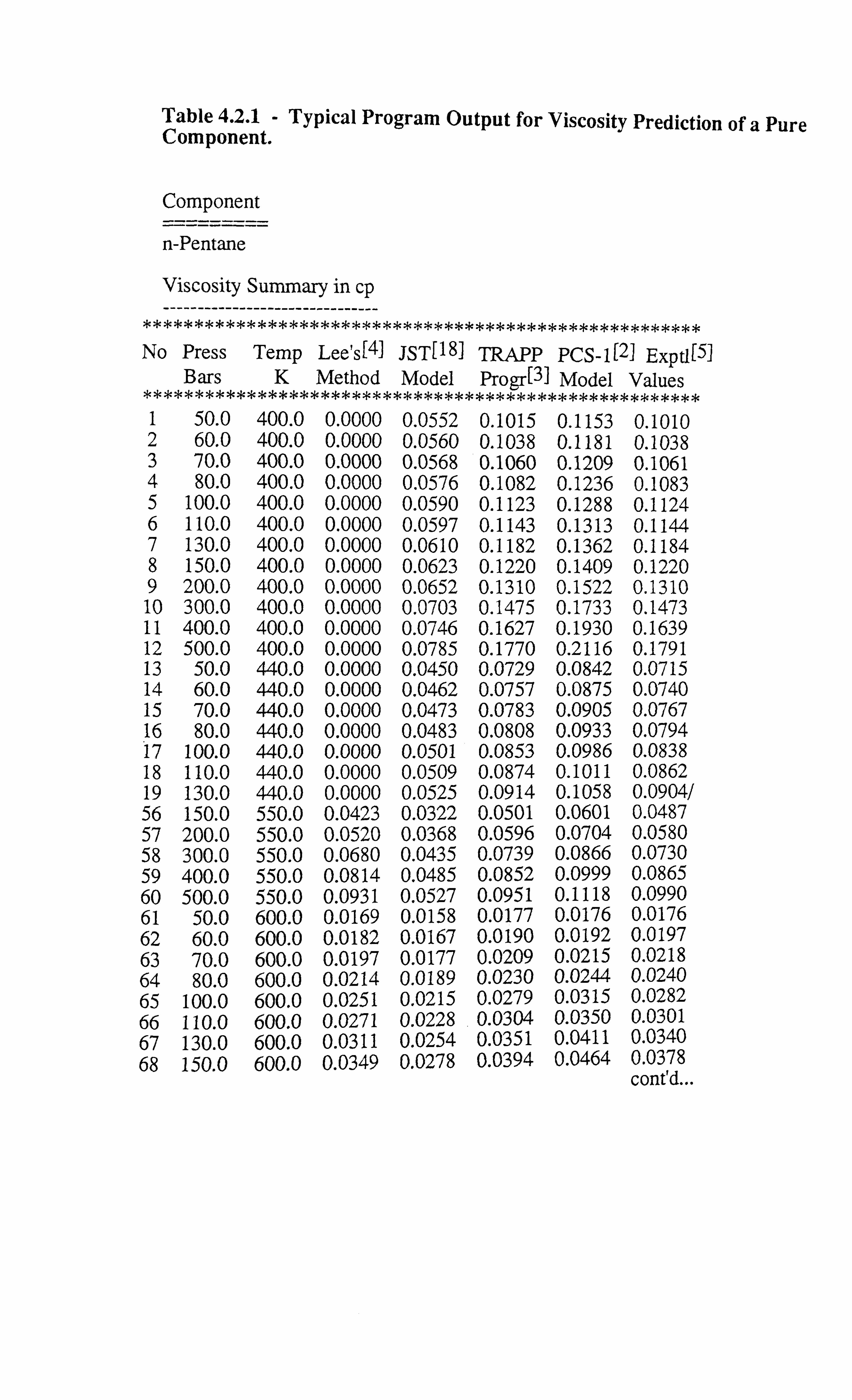
Table 4.2.1 - Typical Program Output for Viscosity Prediction of a Pure Component.
Component
n-Pentane
Viscosity Summary in cp ------------------------------- ****ýk**********************************************ý **
No Press Temp Lee's[4] JST{18] TRAPP PCS-1C21 Exptl{5] Bars K Method Model Progr[3] Model Values
1 50.0 400.0 0.0000 0.0552 0.1015 0.1153 0.1010 2 60.0 400.0 0.0000 0.0560 0.1038 0.1181 0.1038 3 70.0 400.0 0.0000 0.0568 0.1060 0.1209 0.1061 4 80.0 400.0 0.0000 0.0576 0.1082 0.1236 0.1083 5 100.0 400.0 0.0000 0.0590 0.1123 0.1288 0.1124 6 110.0 400.0 0.0000 0.0597 0.1143 0.1313 0.1144 7 130.0 400.0 0.0000 0.0610 0.1182 0.1362 0.1184 8 150.0 400.0 0.0000 0.0623 0.1220 0.1409 0.1220 9 200.0 400.0 0.0000 0.0652 0.1310 0.1522 0.1310 10 300.0 400.0 0.0000 0.0703 0.1475 0.1733 0.1473 11 400.0 400.0 0.0000 0.0746 0.1627 0.1930 0.1639 12 500.0 400.0 0.0000 0.0785 0.1770 0.2116 0.1791 13 50.0 440.0 0.0000 0.0450 0.0729 0.0842 0.0715 14 60.0 440.0 0.0000 0.0462 0.0757 0.0875 0.0740 15 70.0 440.0 0.0000 0.0473 0.0783 0.0905 0.0767 16 80.0 440.0 0.0000 0.0483 0.0808 0.0933 0.0794 17 100.0 440.0 0.0000 0.0501 0.0853 0.0986 0.0838 18 110.0 440.0 0.0000 0.0509 0.0874 0.1011 0.0862 19 130.0 440.0 0.0000 0.0525 0.0914 0.1058 0.0904/ 56 150.0 550.0 0.0423 0.0322 0.0501 0.0601 0.0487 57 200.0 550.0 0.0520 0.0368 0.0596 0.0704 0.0580 58 300.0 550.0 0.0680 0.0435 0.0739 0.0866 0.0730 59 400.0 550.0 0.0814 0.0485 0.0852 0.0999 0.0865 60 500.0 550.0 0.0931 0.0527 0.0951 0.1118 0.0990 61 50.0 600.0 0.0169 0.0158 0.0177 0.0176 0.0176 62 60.0 600.0 0.0182 0.0167 0.0190 0.0192 0.0197 63 70.0 600.0 0.0197 0.0177 0.0209 0.0215 0.0218 64 80.0 600.0 0.0214 0.0189 0.0230 0.0244 0.0240 65 100.0 600.0 0.0251 0.0215 0.0279 0.0315 0.0282 66 110.0 600.0 0.0271 0.0228 0.0304 0.0350 0.0301 67 130.0 600.0 0.0311 0.0254 0.0351 0.0411 0.0340 68 150.0 600.0 0.0349 0.0278 0.0394 0.0464 0.0378
cont'd...
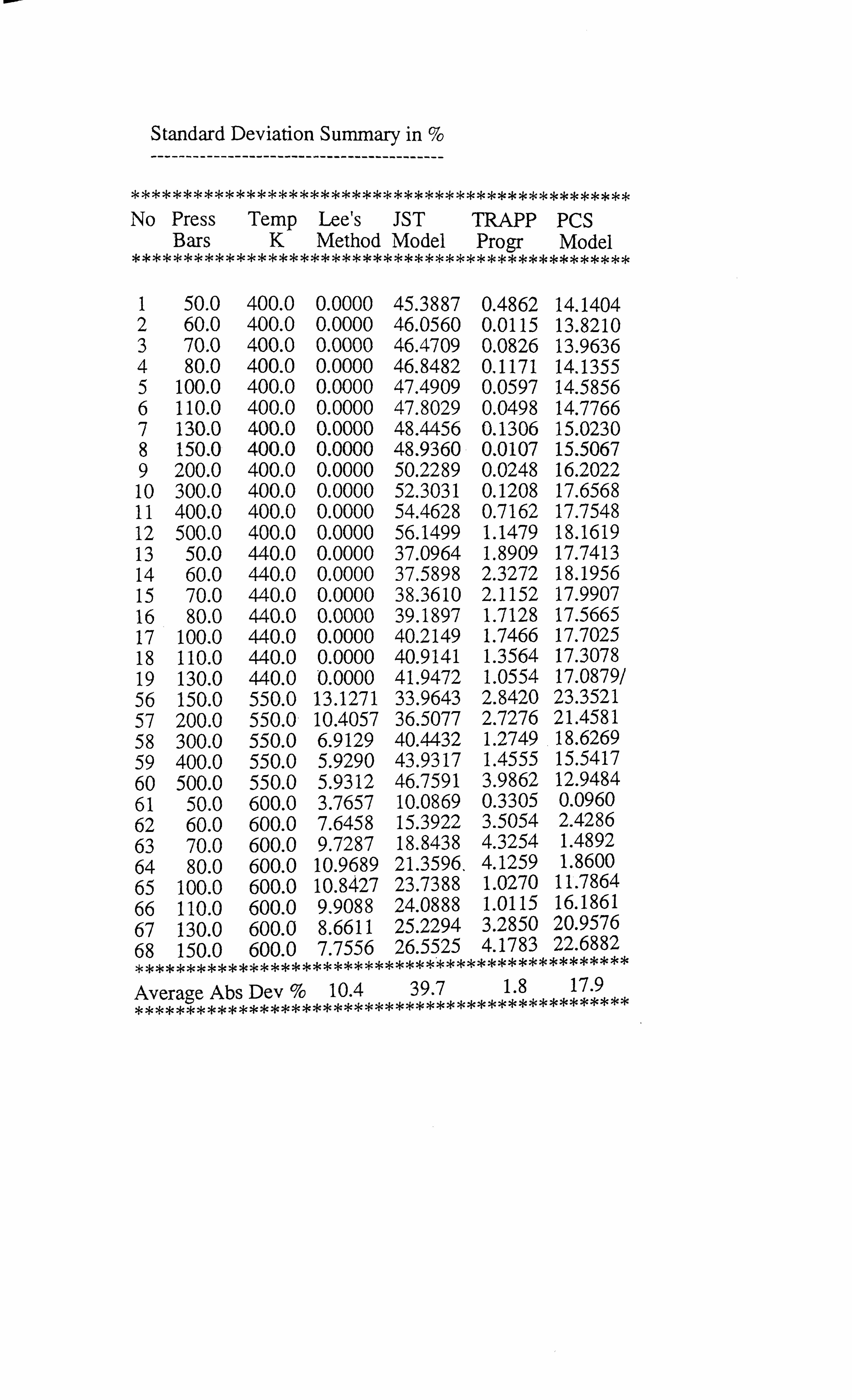
Standard Deviation Summary in % ------------------------------------------
************************************************
No Press Temp Lee's JST TRAPP PCS Bars K Method Model Progr Model
1 50.0 400.0 0.0000 45.3887 0.4862 14.1404 2 60.0 400.0 0.0000 46.0560 0.0115 13.8210 3 70.0 400.0 0.0000 46.4709 0.0826 13.9636 4 80.0 400.0 0.0000 46.8482 0.1171 14.1355 5 100.0 400.0 0.0000 47.4909 0.0597 14.5856 6 110.0 400.0 0.0000 47.8029 0.0498 14.7766 7 130.0 400.0 0.0000 48.4456 0.1306 15.0230 8 150.0 400.0 0.0000 48.9360 0.0107 15.5067 9 200.0 400.0 0.0000 50.2289 0.0248 16.2022 10 300.0 400.0 0.0000 52.3031 0.1208 17.6568 11 400.0 400.0 0.0000 54.4628 0.7162 17.7548 12 500.0 400.0 0.0000 56.1499 1.1479 18.1619 13 50.0 440.0 0.0000 37.0964 1.8909 17.7413 14 60.0 440.0 0.0000 37.5898 2.3272 18.1956 15 70.0 440.0 0.0000 38.3610 2.1152 17.9907 16 80.0 440.0 0.0000 39.1897 1.7128 17.5665 17 100.0 440.0 0.0000 40.2149 1.7466 17.7025 18 110.0 440.0 0.0000 40.9141 1.3564 17.3078 19 130.0 440.0 0.0000 41.9472 1.0554 17.0879/ 56 150.0 550.0 13.1271 33.9643 2.8420 23.3521 57 200.0 550.0 10.4057 36.5077 2.7276 21.4581 58 300.0 550.0 6.9129 40.4432 1.2749 18.6269 59 400.0 550.0 5.9290 43.9317 1.4555 15.5417 60 500.0 550.0 5.9312 46.7591 3.9862 12.9484 61 50.0 600.0 3.7657 10.0869 0.3305 0.0960 62 60.0 600.0 7.6458 15.3922 3.5054 2.4286 63 70.0 600.0 9.7287 18.8438 4.3254 1.4892 64 80.0 600.0 10.9689 21.3596. 4.1259 1.8600 65 100.0 600.0 10.8427 23.7388 1.0270 11.7864 66 110.0 600.0 9.9088 24.0888 1.0115 16.1861 67 130.0 600.0 8.6611 25.2294 3.2850 20.9576 68 150.0 600.0 7.7556 26.5525 4.1783 22.6882
Average Ab s Dev % 10.4 39.7 1.8 17.9

Table 4.2.2 - Average Absolute Deviations in Pure Component Viscosity Predictions.
Fluid N J-S-T TRAPP PCS-1 Methane (G) 97 1.86 1.68 1.98 Ethane (G) 88 4.29 2.99 2.51
Propane (G, L) 80 8.29 5.26 8.08 i- Butane (G, L) 59 10.49 8.93 11.56
n- Butane (G, L) 94 12.88 6.99 16.45
n- Pentane (G, L) 68 39.71 1.77 17.93
n- Hexane (L) 46 22.13 2.83 24.02
n- Heptane (L) 70 23.27 3.67 26.00
n- Octane (L) 48 17.17 5.67 33.61
n- Nonane (L) 94 13.38 2.62 36.11
n- Decane (L) 99 17.99 3.32 42.38 Nitrogen (G) 133 14.60 3.74 3.44
Carbon Dioxide (G) 65 5.46 9.51 10.33
OVERALL 1041 13.7 4.9 17.0
AADS (%)
ýpre-l exp
AAD (%) =
EABS Tlexp * 100
lexp - experimental viscosity
Tipre - predicted viscosity
N- number of data points
J-S-T : Jossi-Stiel-Thodos, residual viscosity correlation[17] TRAPP : Transport properties prediction program of Ely and Hanley[3]
2 PCS -1 : Principle of corresponding states method (one reference component)[ 1
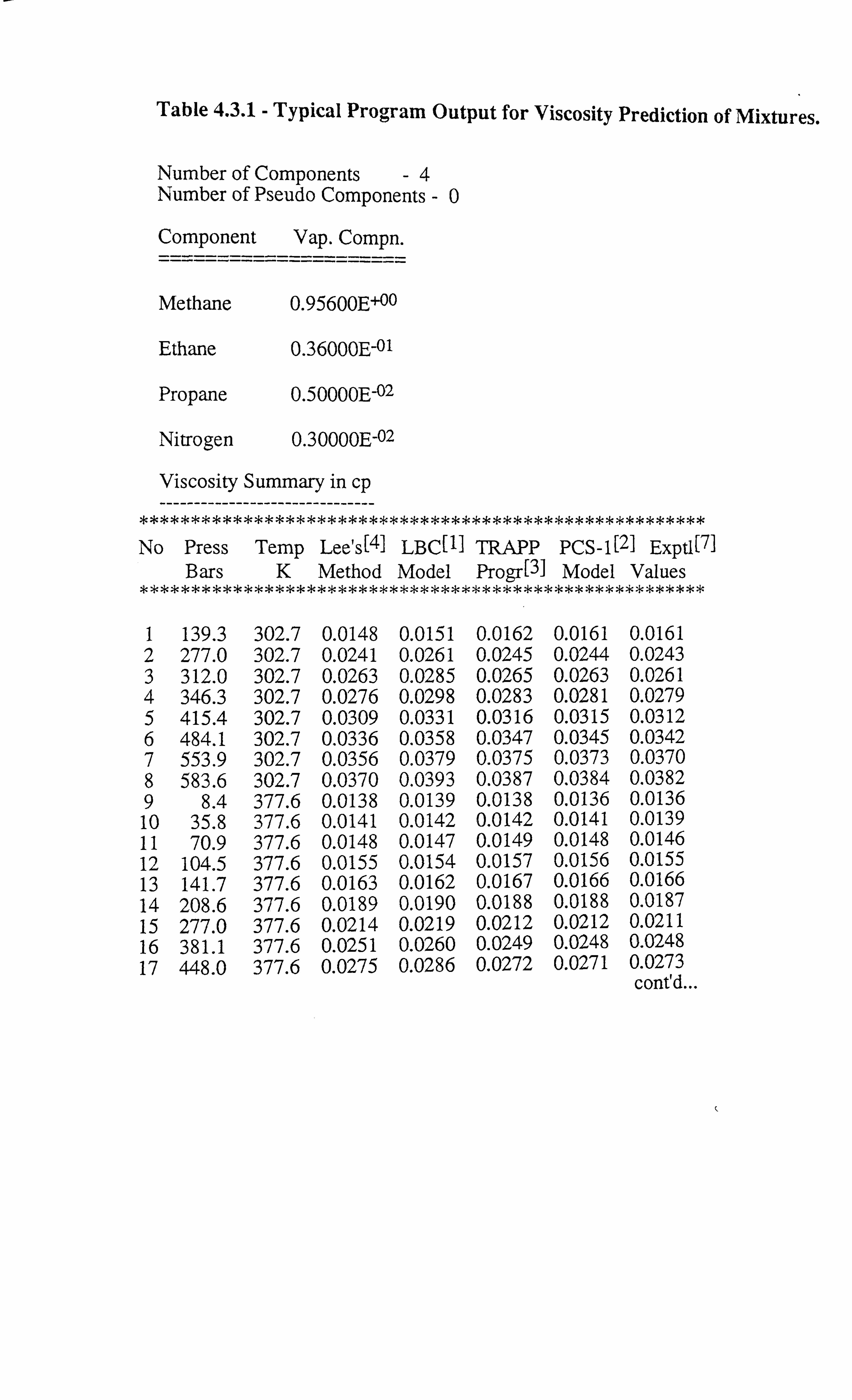
Table 4.3.1 - Typical Program Output for Viscosity Prediction of Mixtures.
Number of Components -4 Number of Pseudo Components -0
Component Vap. Compn. ----------------------
Methane 0.95600E+00
Ethane 0.36000E-01
Propane 0.50000E-02
Nitrogen 0.30000E-02
Viscosity Summary in cp ------------------------------- ***************************************ýk***************
No Press Temp Lee's[4] LBC[1II TRAPP PCS-1[2] Exptl[7] Bars K Method Model Progr[3] Model Values
1 139.3 302.7 0.0148 0.0151 0.0162 0.0161 0.0161 2 277.0 302.7 0.0241 0.0261 0.0245 0.0244 0.0243 3 312.0 302.7 0.0263 0.0285 0.0265 0.0263 0.0261 4 346.3 302.7 0.0276 0.0298 0.0283 0.0281 0.0279 5 415.4 302.7 0.0309 0.0331 0.0316 0.0315 0.0312 6 484.1 302.7 0.0336 0.0358 0.0347 0.0345 0.0342 7 553.9 302.7 0.0356 0.0379 0.0375 0.0373 0.0370 8 583.6 302.7 0.0370 0.0393 0.0387 0.0384 0.0382 9 8.4 377.6 0.0138 0.0139 0.0138 0.0136 0.0136 10 35.8 377.6 0.0141 0.0142 0.0142 0.0141 0.0139 11 70.9 377.6 0.0148 0.0147 0.0149 0.0148 0.0146 12 104.5 377.6 0.0155 0.0154 0.0157 0.0156 0.0155 13 141.7 377.6 0.0163 0.0162 0.0167 0.0166 0.0166 14 208.6 377.6 0.0189 0.0190 0.0188 0.0188 0.0187 15 277.0 377.6 0.0214 0.0219 0.0212 0.0212 0.0211 16 381.1 377.6 0.0251 0.0260 0.0249 0.0248 0.0248 17 448.0 377.6 0.0275 0.0286 0.0272 0.0271 0.0273
cont'd...

Standard Deviation Summary in %
***********************************************
No Press Temp Lee's LBC TRAPP PCS Bars K Method Model Progr Model
1 139.3 302.7 7.4860 5.9364 0.9632 0.5276 2 277.0 302.7 0.8070 7.5306 1.0466 0.6439 3 312.0 302.7 0.7309 9.0495 1.4021 0.9884 4 346.3 302.7 1.0926 6.8554 1.2994 0.8687 5 415.4 302.7 1.1906 6.0425 1.2775 0.7920 6 484.1 302.7 1.9733 4.6629 1.2656 0.7157 7 553.9 302.7 3.8841 2.3436 1.3183 0.7036 8 583.6 302.7 3.2336 2.9239 1.1339 0.4940 9 8.4 377.6 1.0031 2.1570 1.3173 0.1664 10 35.8 377.6 1.4665 2.0766 2.1366 1.0340 11 70.9 377.6 0.9712 0.7499 1.7524 0.7918 12 104.5 377.6 0.4279 0.2514 1.3070 0.5227 13 141.7 377.6 1.8876 2.6018 0.2649 0.3196 14 208.6 377.6 0.8857 1.4597 0.4116 0.0644 15 277.0 377.6 1.4965 3.7692 0.4931 0.2023 16 381.1 377.6 1.1708 4.9226 0.4015 0.1243 17 448.0 377.6 0.5323 4.5455 0.5459 0.7838
Average Ab s Dev % 1.8 4.0 1.1 0.6

Table 4.3.2 - Average Absolute Deviations in Mixture Viscosity Predictions.
Mixture N L-B-C III TRAPP PCS-1
Natural Gas J71 17 3.99 1.08 0.57 Natural Gas 2[7] 15 7.54 3.44 3.29
Natural Gas 3[41 19 1.61 0.98 0.65
Natural Gas 4[4] 23 3.05 2.22 2.28
Natural Gas 5[8] 94 6.16 4.24 4.06
CI - C2 (G, L), [9] 41 2.80 0.73 2.34
C1 - C3 (G, L), [10] 154 10.62 2.69 4.41
C1 - C4 (G, L), [7] 16 8.67 3.79 4.29
C1 - C10 (G, L), [73 71 18.39 5.33 16.32
C1- N2 (G, L), [11] 42 8.04 2.03 2.85
C1- C02 (G), [12] 102 3.59 3.10 8.18
C2 - CO2 (G, L), [13] 49 6.38 16.46 28.23
C10 - C02 (L), [14] 57 6.55 30.77 52.16
C1 - N2 - H2 (G), 181 50 8.74 3.39 4.41
CO2 -n C5 -n C10 -n 117 16.94 36.57 54.76
C16 -n C30 (L), 1151
OVERALL 867 8.6 10.2 16.6
AADs (%)
AAD (%) = JABS Tlexp * 100 (e1exp\
1lexp - experimental viscosity
Tipre - predicted viscosity
N- number of data points
L-B-C : Lohrenz-Bray-Clark, residual viscosity correlation[l] 3] TRAPP : Transport properties prediction program of Ely and Hanley[
[2] PCS -1 : Principle of corresponding states method (one reference component] [n] : References providing the source for the data
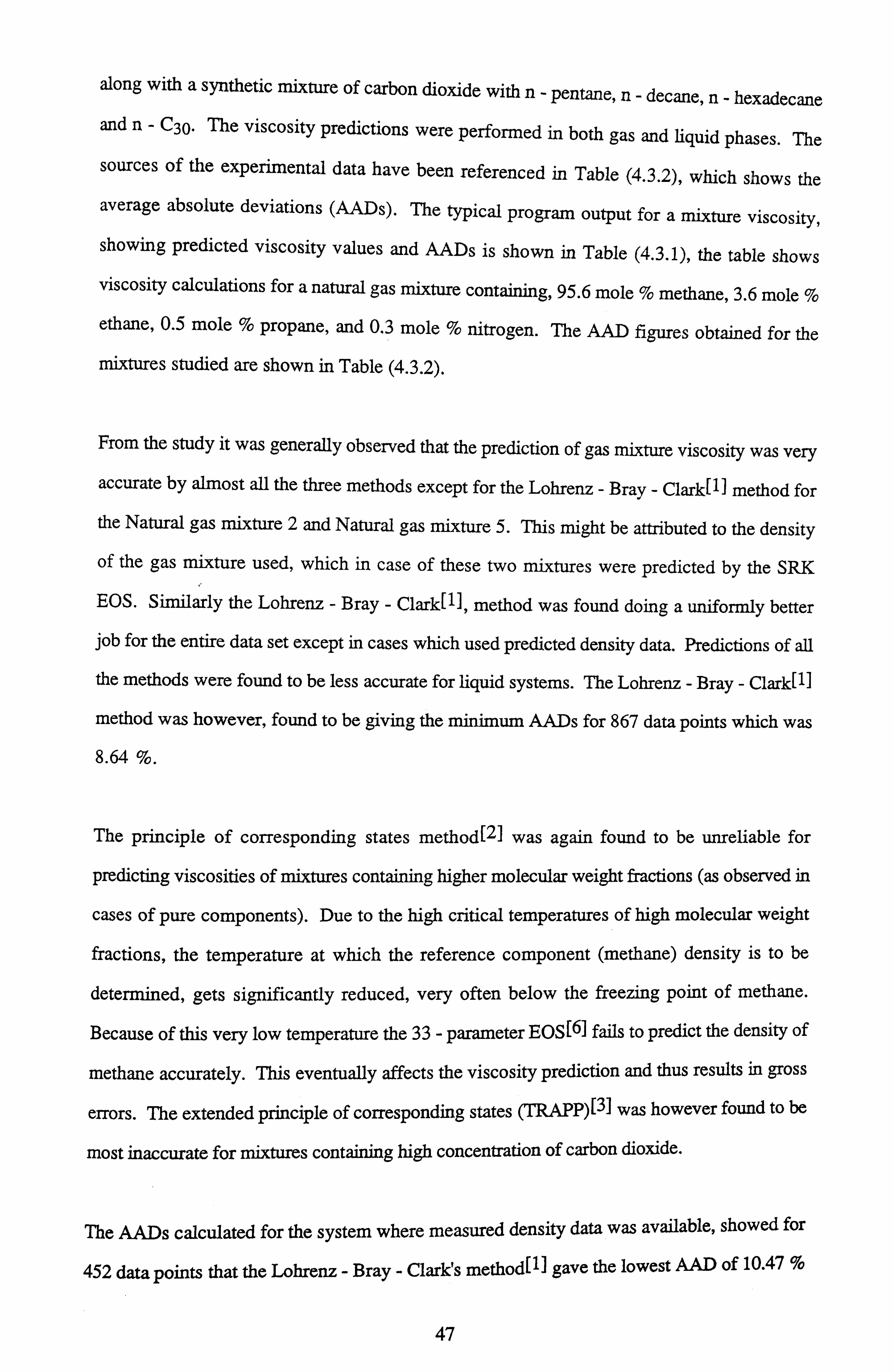
along with a synthetic mixture of carbon dioxide with n- pentane, n- decane, n- hexadecane
and n- C30. The viscosity predictions were performed in both gas and liquid phases. The
sources of the experimental data have been referenced in Table (4.3.2), which shows the average absolute deviations (AADs). The typical program output for a mixture viscosity, showing predicted viscosity values and AADs is shown in Table (4.3.1), the table shows viscosity calculations for a natural gas mixture containing, 95.6 mole % methane, 3.6 mole %
ethane, 0.5 mole % propane, and 0.3 mole % nitrogen. The AAD figures obtained for the
mixtures studied are shown in Table (4.3.2).
From the study it was generally observed that the prediction of gas mixture viscosity was very
accurate by almost all the three methods except for the Lohrenz - Bray - Clark[i] method for
the Natural gas mixture 2 and Natural gas mixture 5. This might be attributed to the density
of the gas mixture used, which in case of these two mixtures were predicted by the SRK
EOS. Similarly the Lohrenz - Bray - Clark[ll, method was found doing a uniformly better
job for the entire data set except in cases which used predicted density data. Predictions of all
the methods were found to be less accurate for liquid systems. The Lohrenz - Bray - Clark[ll
method was however, found to be giving the minimum AADs for 867 data points which was
8.64 %.
The principle of corresponding states method[21 was again found to be unreliable for
predicting viscosities of mixtures containing higher molecular weight fractions (as observed in
cases of pure components). Due to the high critical temperatures of high molecular weight
fractions, the temperature at which the reference component (methane) density is to be
determined, gets significantly reduced, very often below the freezing point of methane.
Because of this very low temperature the 33 - parameter EOS[61 fails to predict the density of
methane accurately. This eventually affects the viscosity prediction and thus results in gross
errors. The extended principle of corresponding states (TRAPP) [3] was however found to be
most inaccurate for mixtures containing high concentration of carbon dioxide.
The AADs calculated for the system where measured density data was available, showed for
452 data points that the Lohrenz - Bray - Clark's method 1 gave the lowest AAD of 10.47 %
47
compared to 16.55 % in case of the extended principle of corresponding states method[3l and 27.17 % in case of the original principle of corresponding states method[2]. However, when the AADs were calculated for the systems where the reference component (methane)
temperature remained above its freezing point showed for 471 data points that the principle of
corresponding states method[2] gave an AAD of 4.4 % and the extended principle of
corresponding states method[3I1 2.82 %, whereas for the Lohrenz - Bray - Clark's[l] method
the AAD figure was 6.80 %. Hence, it can be concluded that, if the density data available is
reliable, the Lohrenz - Bray - Clark's method[l] should be used for viscosity predictions. In
case of the lighter hydrocarbon mixtures the principle of corresponding states method[2], or
the extended principle of corresponding states method[3], is recommendable in the absence of
measured density data.
A comparative study recently carried out for evaluating the viscosity correlations by Ali[16]
draws conclusions similar to those presented in this work. Table 7 of Reference[16] confirms
that when accurate and reliable density data is available the residual viscosity method[1,17]
proves to be a useful tool for estimation of viscosity. However it is interesting to note that the
principle of corresponding states method[2] is also confirmed as a suitable model for
estimation of viscosities. It has the advantage of eliminating the need for density and is found
to combine the accuracy of extended principle of corresponding states method[3] and the
simplicity of the residual viscosity methodd1,171.
4.4: TUNING OF VISCOSITY CORRELATIONS
A brief study on tuning of the viscosity correlations was also carried out to complete the
comparative study on viscosity prediction methods. Each correlation was tuned (by altering
an uncertain parameter) so as it could reproduce the viscosity of the desired fluid at its bubble
point pressure. The various correlations were compared.
The methods studied were, the residual viscosity correlation of Lohrenz-Bray-Clark[l], the
principle of corresponding states method[2] (one reference component) and the principle of
48
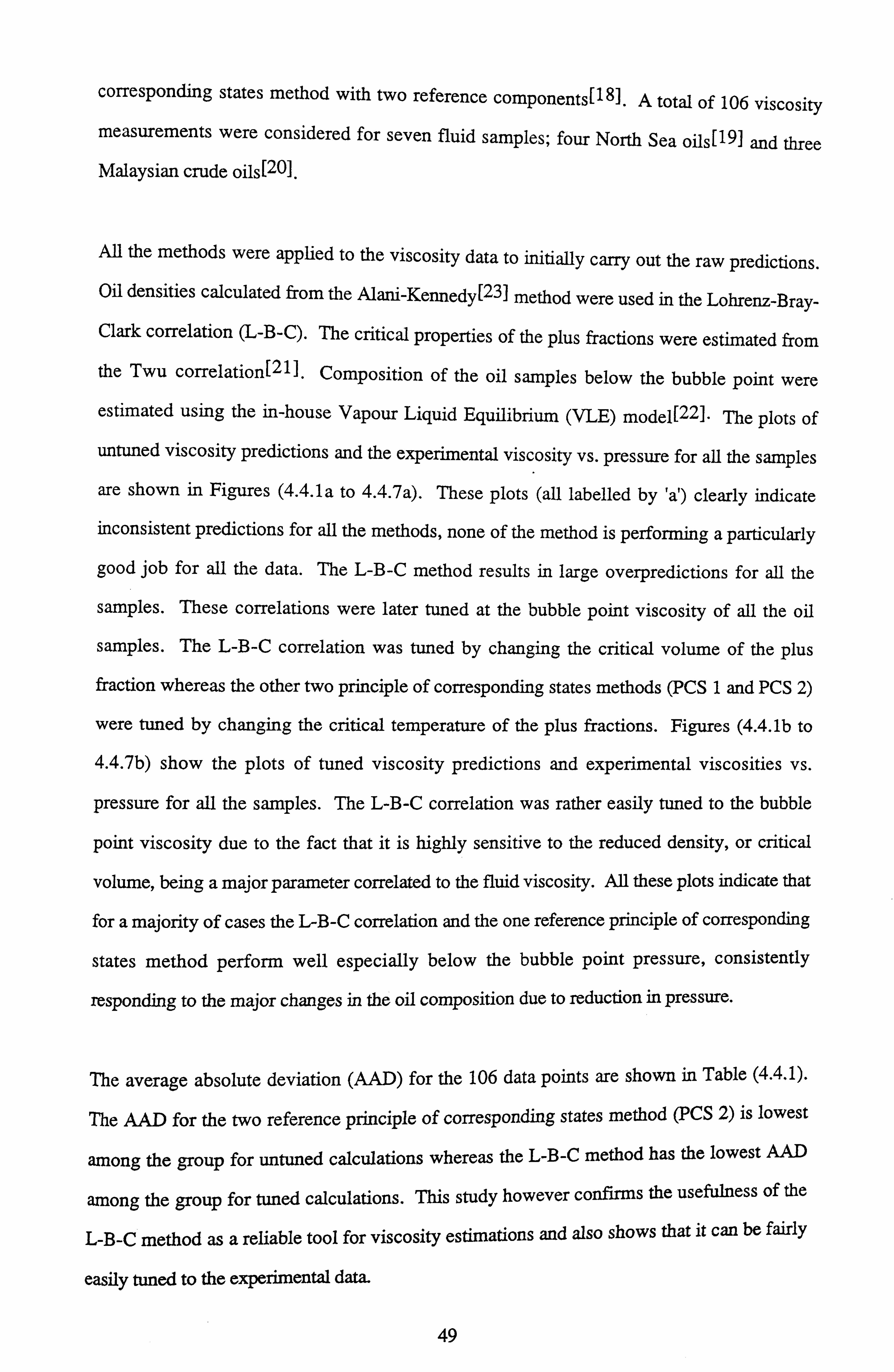
corresponding states method with two reference components[18]. A total of 106 viscosity measurements were considered for seven fluid samples; four North Sea oils[191 and three Malaysian crude oils [20].
All the methods were applied to the viscosity data to initially carry out the raw predictions. Oil densities calculated from the Alan-Kennedy[23] method were used in the Lohrenz-Bray-
Clark correlation (L-B-C). The critical properties of the plus fractions were estimated from
the Twu correlation[21]. Composition of the oil samples below the bubble point were
estimated using the in-house Vapour Liquid Equilibrium (VLE) model[22]. The plots of
untuned viscosity predictions and the experimental viscosity vs. pressure for all the samples
are shown in Figures (4.4.1a to 4.4.7a). These plots (all labelled by 'a') clearly indicate
inconsistent predictions for all the methods, none of the method is performing a particularly
good job for all the data. The L-B-C method results in large overpredictions for all the
samples. These correlations were later tuned at the bubble point viscosity of all the oil
samples. The L-B-C correlation was tuned by changing the critical volume of the plus
fraction whereas the other two principle of corresponding states methods (PCS 1 and PCS 2)
were tuned by changing the critical temperature of the plus fractions. Figures (4.4.1b to
4.4.7b) show the plots of tuned viscosity predictions and experimental viscosities vs.
pressure for all the samples. The L-B-C correlation was rather easily tuned to the bubble
point viscosity due to the fact that it is highly sensitive to the reduced density, or critical
volume, being a major parameter correlated to the fluid viscosity. All these plots indicate that
for a majority of cases the L-B-C correlation and the one reference principle of corresponding
states method perform well especially below the bubble point pressure, consistently
responding to the major changes in the oil composition due to reduction in pressure.
The average absolute deviation (AAD) for the 106 data points are shown in Table (4.4.1).
The AAD for the two reference principle of corresponding states method (PCS 2) is lowest
among the group for untuned calculations whereas the L-B-C method has the lowest AAD
among the group for tuned calculations. This study however confirms the usefulness of the
L-B-C method as a reliable tool for viscosity estimations and also shows that it can be fairly
easily tuned to the experimental data.
49
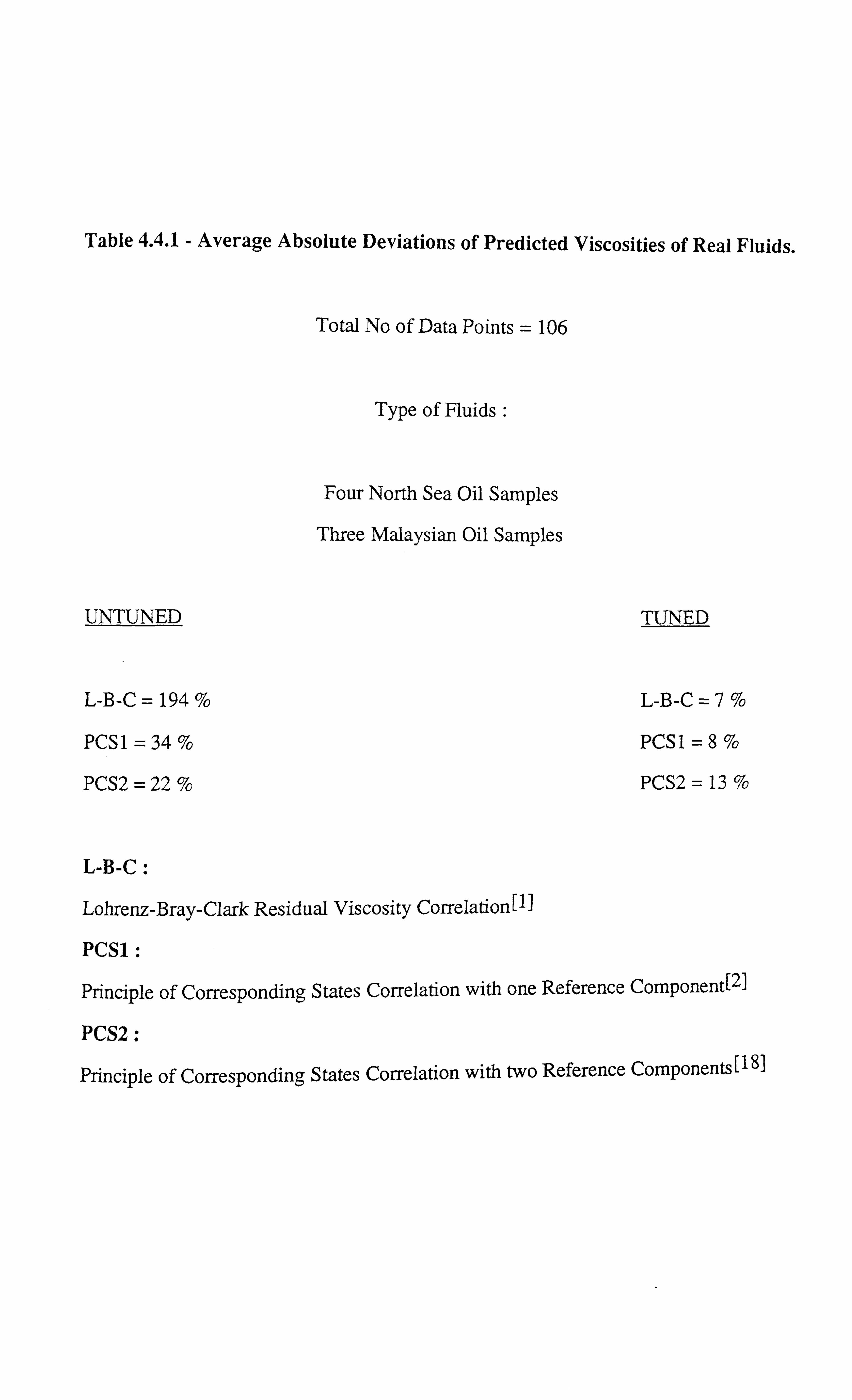
Table 4.4.1 - Average Absolute Deviations of Predicted Viscosities of Real Fluids.
Total No of Data Points = 106
Type of Fluids :
Four North Sea Oil Samples
Three Malaysian Oil Samples
UNTUNED
L-B-C=194%
PCS 1= 34 %
PCS2 = 22 %
L-B-C:
Lohrenz-Bray-Clark Residual Viscosity Correlation[1]
PCS1 :
TUNED
L-B-C =7%
PCS 1=8%
PCS2=13%
Principle of Corresponding States Correlation with one Reference Component[2]
PCS2 :
Principle of Corresponding States Correlation with two Reference Components I18]

04
L'
O U
.ý
1.6
1.4
1.2
Ow u
1.0
0 U
.. A 0.8
0.6
0.4
0..
0.2 --- 100 200 300 400 500
Pressure, bars
Figure 4.4.1a - Viscosity of North Sea Oil 1 at 97.8 deg C.
'T
0. Z
Measured
Tuned LBC
Tuned PCS 1
Tuned PCS2
Bubble Point "" T
. r:
0.2 100 200 300 400 500
Pressure, bars
Figure 4.4.1b - Viscosity of North Sea Oil 1 at 97.8 deg C All Methods Individually Tuned at Bubble Point.
0.3
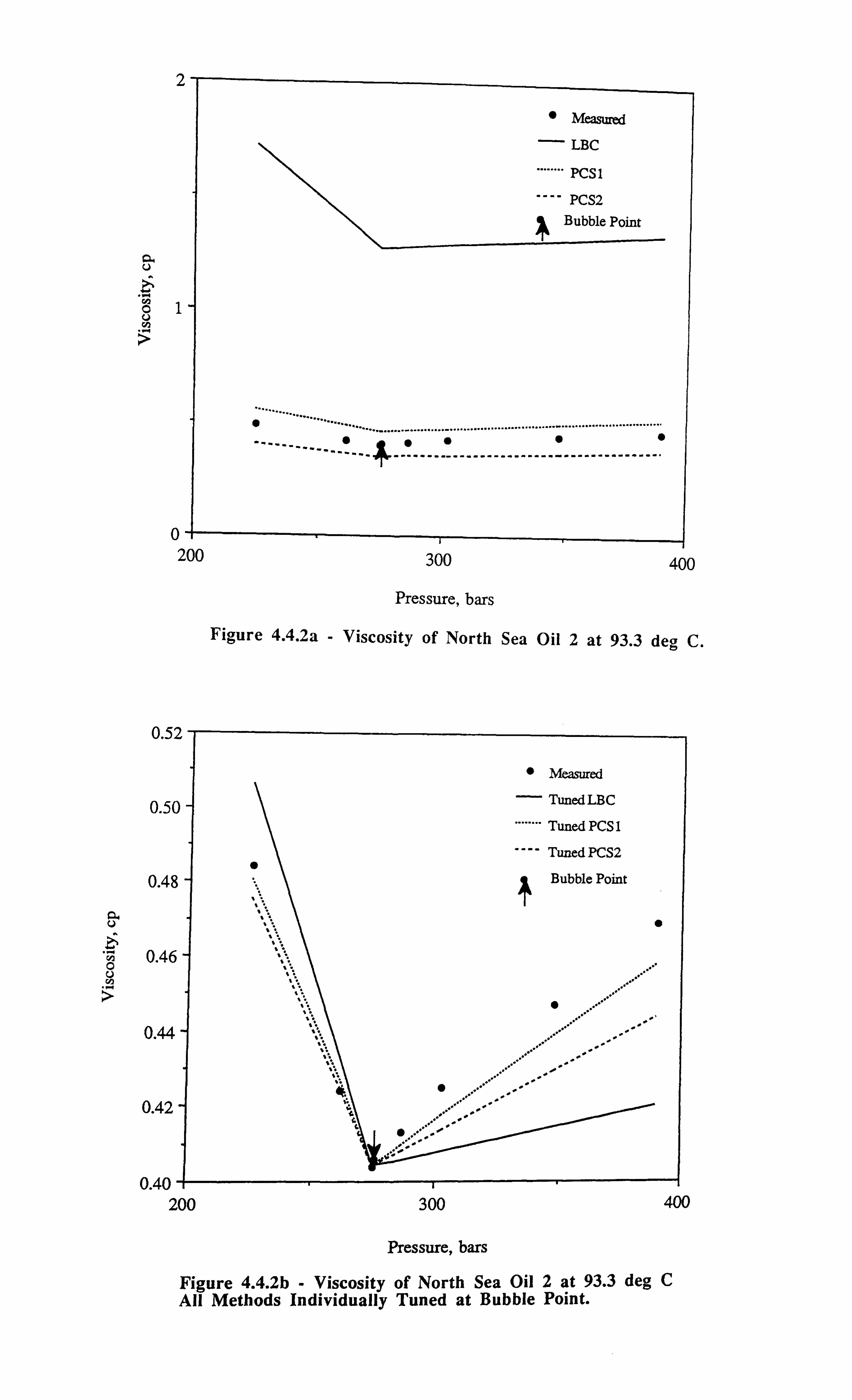
2
" Measured
LBC
..... PCS 1
PCS2 I Bubble Point
C14 U
ö1
.ý
.................
0 -f- 200 300 400
Pressure, bars
0.52
o..
0. Z
U
0.4
.ý
0.4
0.4
0.40 -1- 200
Pressure, bars
Figure 4.4.2b - Viscosity of North Sea Oil 2 at 93.3 deg C All Methods Individually Tuned at Bubble Point.
Figure 4.4.2a - Viscosity of North Sea Oil 2 at 93.3 deg C.
JUU 'tvv
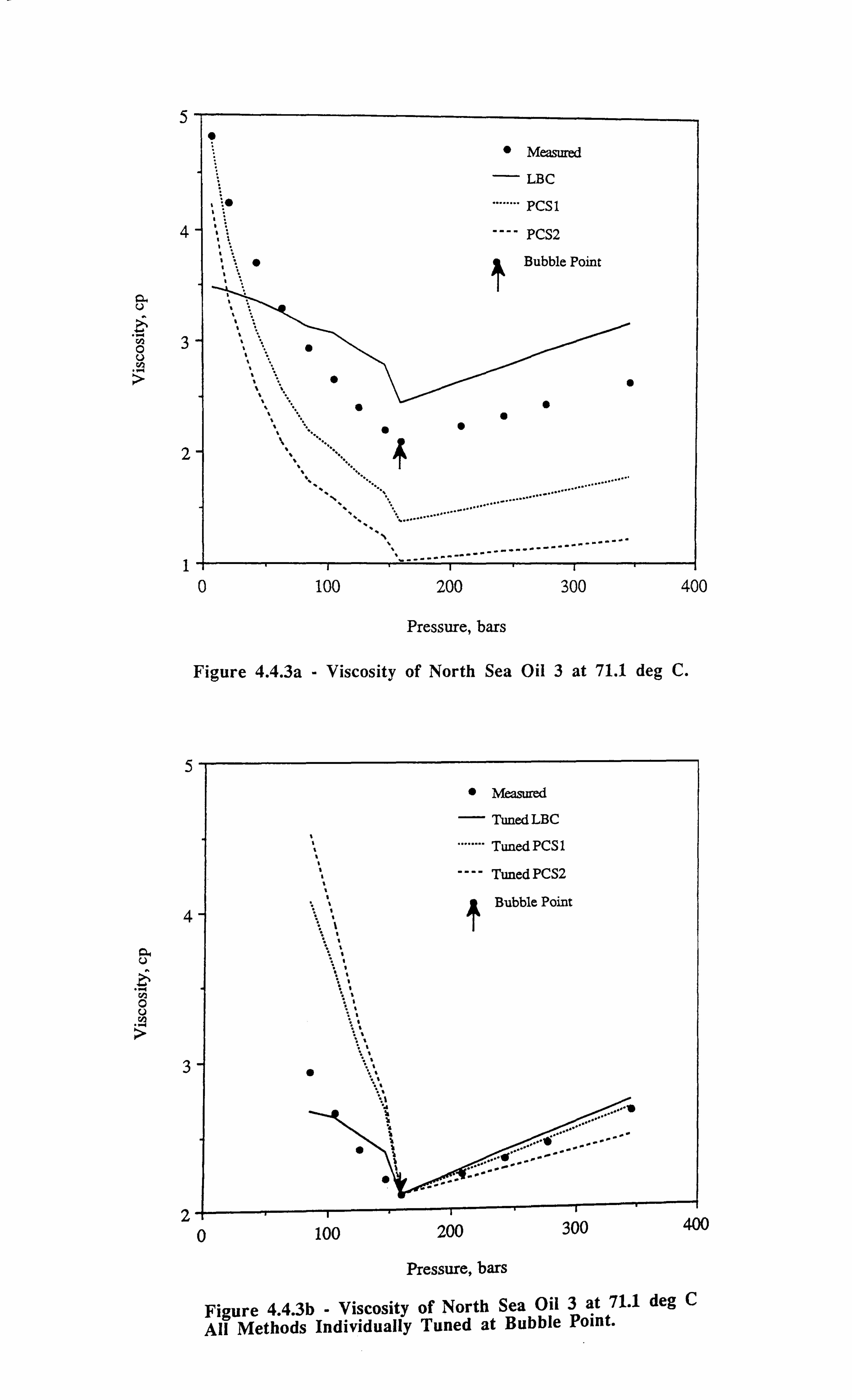
5 "
% 46
4
a U
L' ýý 3 0 U y .ý
" Measured
LBC
PCS 1
PCS2
Bubble Point
0
"
"
2
1
..
-- -----------
0 100 200 300 400
Pressure, bars
Figure 4.4.3a - Viscosity of North Sea Oil 3 at 71.1 deg C.
5
4
Q, C. )
I
.ý
3
0 100 200 300 4w
Pressure, bars
Figure 4.4.3b - Viscosity of North Sea Oil 3 at 71.1 deg C
All Methods Individually Tuned at Bubble Point.
2
" Measured
Tuned LBC
Tuned PCS I
Tuned PCS2
Bubble Point
0 '. ;
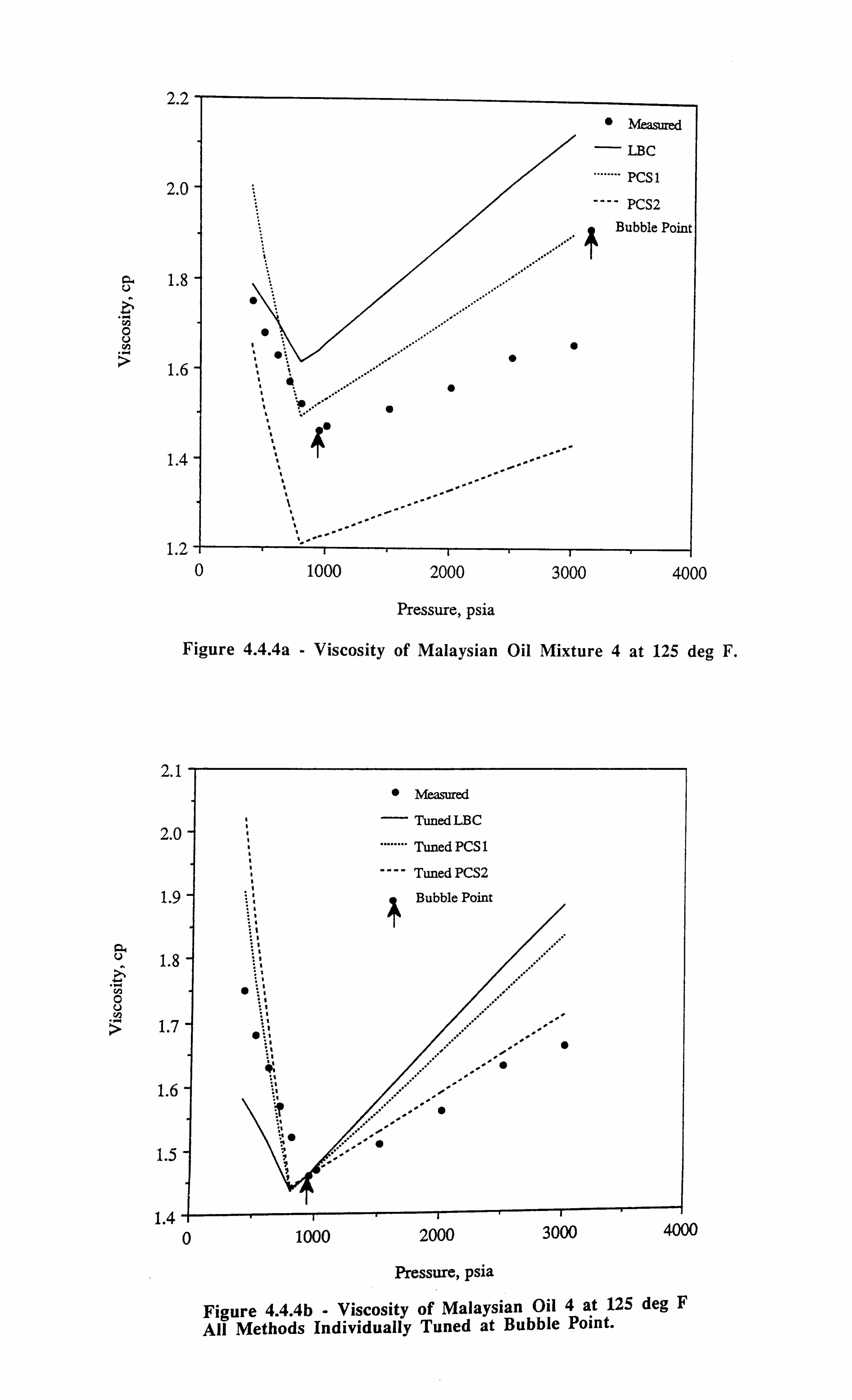
2.2-
2.0-
1.8
1.6-
1.4-
1.2
2.1
2.0
1.9
1.8
O U
1.7
1.6
1.5
1.4
,t " '!
t Meamzed
LBC
........ Pcsl
---- PCS2
" Bubble Point
0 1000 2000 3000 4000
Pressure, psia
Figure 4.4.4a - Viscosity of Malaysian Oil Mixture 4 at 125 deg F.
" Measured
Tuned LBC
Tuned PCS 1
Tuned PCS2
Bubble Point
wý"
} 7
0 1000 2000 3000 4000
Pressure, psia
Figure 4.4.4b - Viscosity of Malaysian Oil 4 at 125 deg F
All Methods Individually Tuned at Bubble Point.
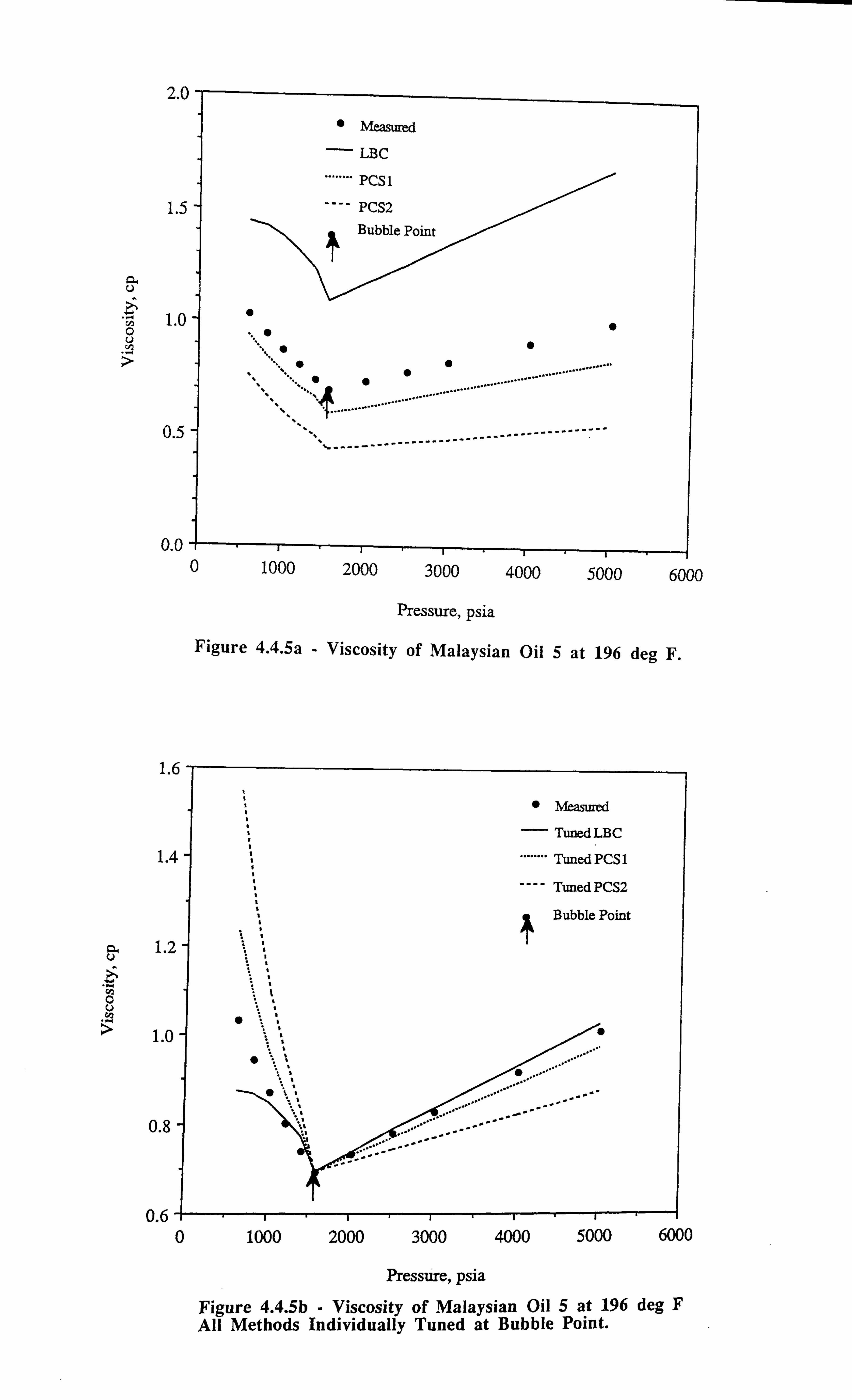
2.0
1.5
a U
1.0 O v
0.5
" Measured
LBC
PCS 1
PCS2 Bubble Point
" "
"" ;, '
"". ""
-------------------
----------------------
0.0 0 1000 2000 3000 4000 5000 6000
Pressure, psia
Figure 4.4.5a - Viscosity of Malaysian Oil 5 at 196 deg F.
1.1
1. ý
1.2
0 U CIO
1.0
0.8
0.6
" Measured
Tuned LBC
Tuned PCS 1
"- Tuned PCS2
Bubble Point
0 1000 2000 3000 4000 5000 6000
Pressure, psis
Figure 4.4.5b - Viscosity of Malaysian Oil 5 at 196 deg F All Methods Individually Tuned at Bubble Point.
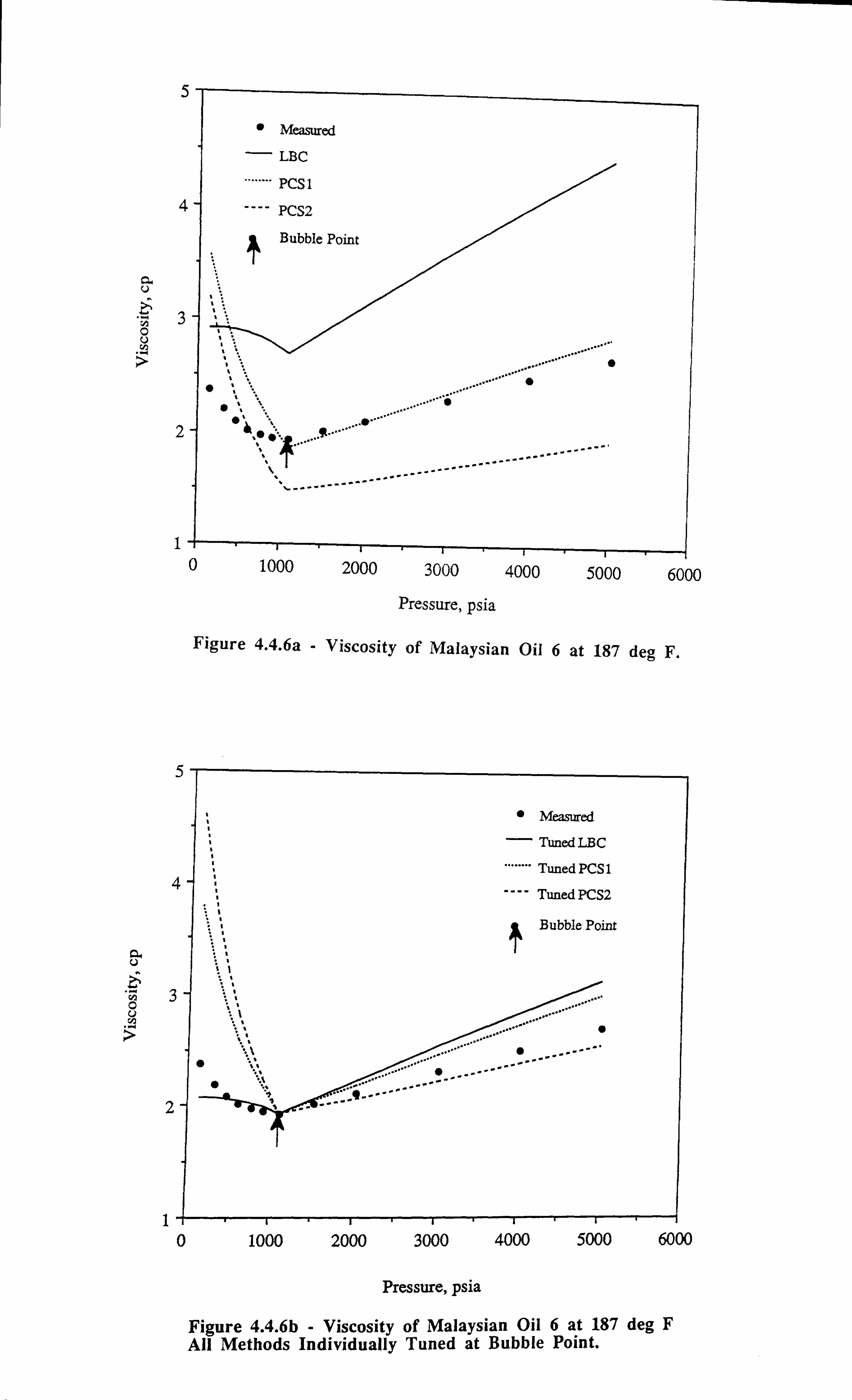
5
4
G U
"1 3 0 U
.ý rý
i
a 0
"- Ö Q
2
2
1 0 1000 2000 3000 4000 5000 6000
Pressure, psia
Figure 4.4.6a - Viscosity of Malaysian Oil 6 at 187 deg F.
r
,i " Measured
Tuned LBC
Tuned PCS 1
Tuned PCS2
Bubble Point
1t 0 1000 2000 3000 4000 5000 6000
Pressure, psia
Figure 4.4.6b - Viscosity of Malaysian Oil 6 at 187 deg F All Methods Individually Tuned at Bubble Point.
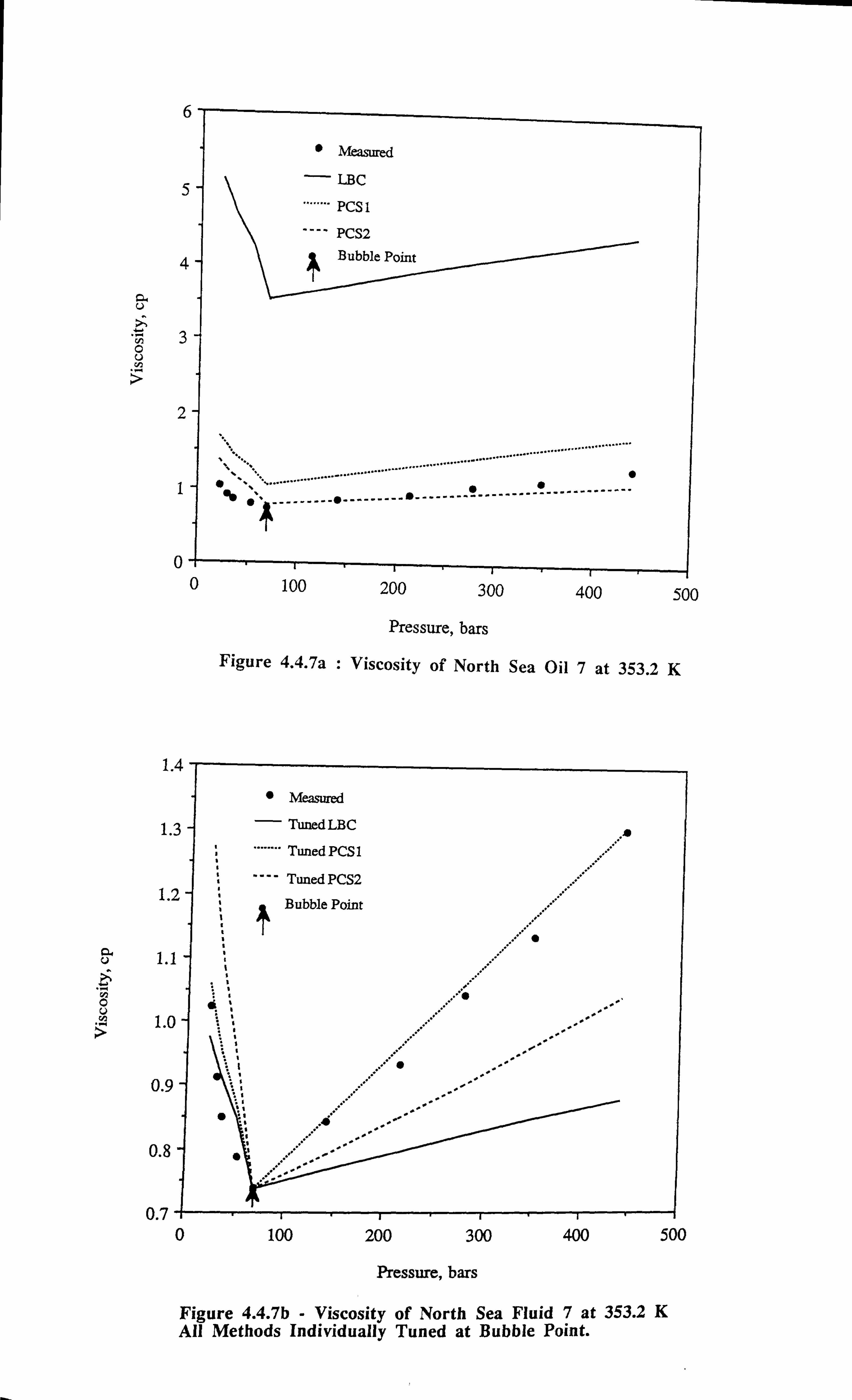
6
a U
rf O U
a
Measured
5 LBC
........ PCs 1
"-- PCS2
41 Bubble Point
3
2
1 `. ýý'
.... ....... ....... _ .... ............... " -"
0~ . ̀ ,; ti.. "___-ý---------ý-------- --- ^ ---- ----------- '"
0 0 100 200 300 400
Pressure, bars
500
Figure 4.4.7a : Viscosity of North Sea Oil 7 at 353.2 K
" Measured
Tuned LBC
Tuned PCS 1
Tuned PCS2
Bubble Point
1.4
1.3
1.2
1.0 '
............... .....................................
..
0.9
1 la -1
0.8 0
o. 7 0 100 200 300 400 500
Pressure, bars
Figure 4.4.7b - Viscosity of North Sea Fluid 7 at 353.2 K All Methods Individually Tuned at Bubble Point.
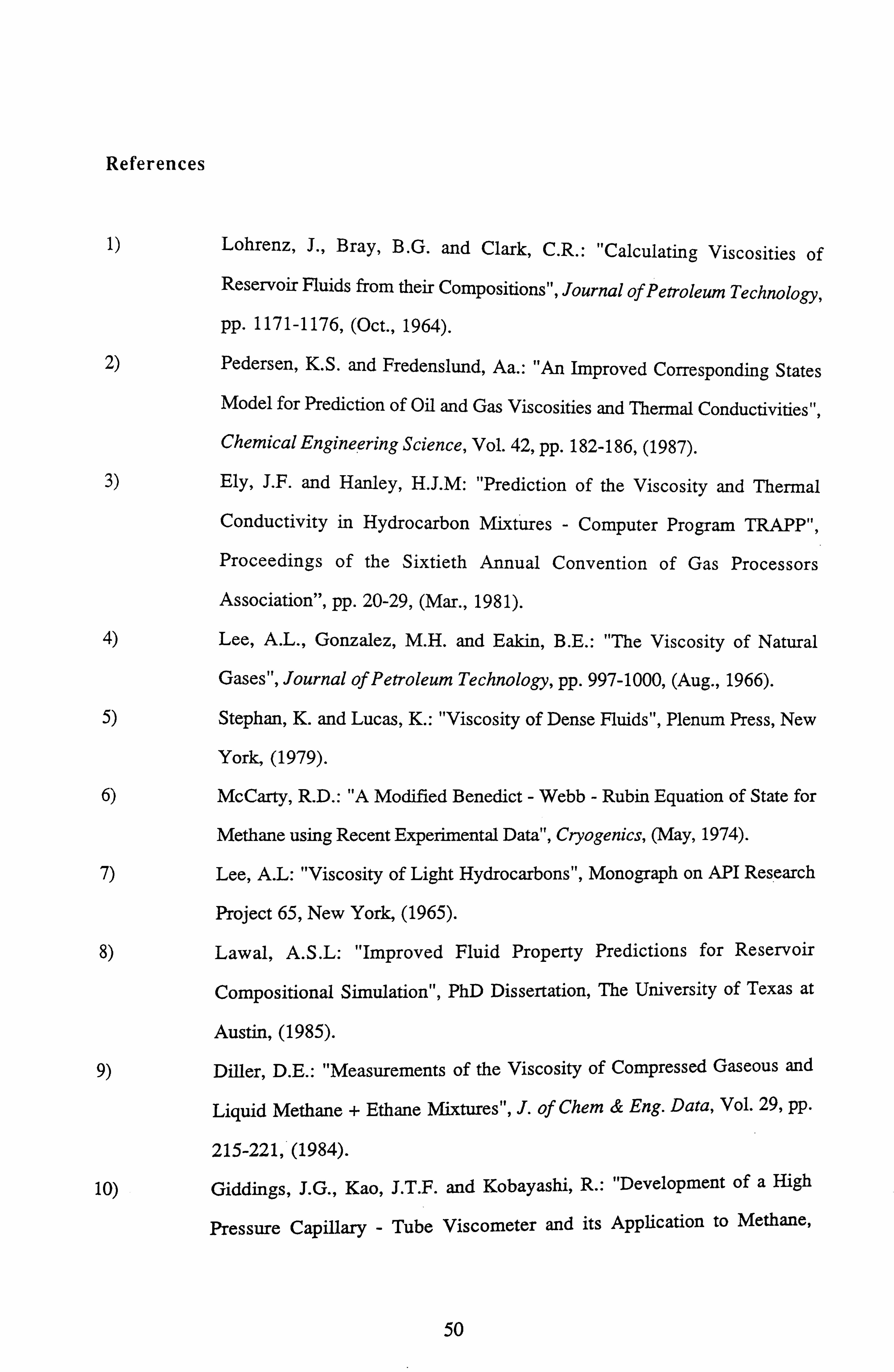
References
1) Lohrenz, J., Bray, B. G. and Clark, C. R.: "Calculating Viscosities of Reservoir Fluids from their Compositions", Journal of Petroleum Technology,
pp. 1171-1176, (Oct., 1964).
2) Pedersen, K. S. and Fredenslund, Aa.: "An Improved Corresponding States
Model for Prediction of Oil and Gas Viscosities and Thermal Conductivities",
Chemical Engineering Science, Vol. 42, pp. 182-186, (1987).
3) Ely, J. F. and Hanley, H. J. M: "Prediction of the Viscosity and Thermal
Conductivity in Hydrocarbon Mixtures - Computer Program TRAPP",
Proceedings of the Sixtieth Annual Convention of Gas Processors
Association", pp. 20-29, (Mar., 1981).
4) Lee, A. L., Gonzalez, M. H. and Eakin, B. E.: "The Viscosity of Natural
Gases", Journal of Petroleum Technology, pp. 997-1000, (Aug., 1966).
5) Stephan, K. and Lucas, K.: "Viscosity of Dense Fluids", Plenum Press, New
York, (1979).
6) McCarty, R. D.: "A Modified Benedict - Webb - Rubin Equation of State for
Methane using Recent Experimental Data", Cryogenics, (May, 1974).
7) Lee, A. L: "Viscosity of Light Hydrocarbons", Monograph on API Research
Project 65, New York, (1965).
8) Lawal, A. S. L: "Improved Fluid Property Predictions for Reservoir
Compositional Simulation", PhD Dissertation, The University of Texas at
Austin, (1985).
9) Diller, D. E.: "Measurements of the Viscosity of Compressed Gaseous and
Liquid Methane + Ethane Mixtures", J. of Chem & Eng. Data, Vol. 29, pp.
215-221, (1984).
10) Giddings, J. G., Kao, J. T. F. and Kobayashi, R.: "Development of a High
Pressure Capillary - Tube Viscometer and its Application to Methane,
50

Propane, and their Mixtures in the Gaseous and Liquid Regions", The Journal
of Chemical Physics, Vol. 45, No. 2, (Jul., 1966).
11) Diller, D. E.: "Measurements of the Viscosity of Compressed Gaseous and Liquid Nitrogen + Methane Mixtures", International J. Thermophysics, Vol.
3, No. 3, (1982).
12) Dewitt, K. J. and Thodos, G.: "Viscosities of Binary Mixtures in the Dense
Gaseous State: the Methane and Carbon Dioxide System", In: SPE Reprint
Ser. 13, Vol. 1, pp. 236-241, (1977).
13) Diller, D. E., Pollen, L. J. V. and Santos, F. V. D: "Measurements of the
Viscosities of Compressed Fluid and Liquid Carbon Dioxide + Ethane
Mixtures", J. of Chem & Eng. Data, Vol. 33, pp. 460-464, (1988).
14) Cullick, A. S. and Mathias, M. L.: "Densities and Viscosities of Carbon
Dioxide and n- Decane from 310 to 403 K, and, 7 to 30 MPa", J. of Chem &
Eng. Data, Vol. 29, pp. 393-396, (1984).
15) Kovarik, F. S. and Taylor, M. A.: "Viscosity Measurements of High - Pressure
CO2lHydrocarbon Mixtures", AIChE, Annual General Meeting, New York,
(1987).
16) Ali, J. K: "Evaluation of Correlations for Estimating the Viscosities of
Hydrocarbon Fluids", Journal of Petroleum Science and Engineering, Vol. 5,
pp. 351-369, (1991).
17) Jossi, J. A., Stiel, L. I. and Thodos, G.: "The Viscosity of Pure Substances in
the Dense Gaseous and Liquid Phases", AIChEJ, Vol. 8, pp. 59 - 63, (1962).
18) Aasberg-Petersen, K., Knudsen, K. and Fredenslund, A.: "Prediction of
Viscosities of Hydrocarbon Mixtures", Fluid Phase Equilibria, Vol. 70, pp.
293-308, (1991).
19) Pedersen, et. al : "Properties of Oils and Natural Gases", (Contrib. Petrol.
Geol. & Eng., Vol. 5), Gulf Publishing Co., (1989).
20) Omar, M. I.: "Private Communication". (1991)
21) Twu, C. H: "An Internally Consistent Correlation for Predicting the Critical
Properties and Molecular Weights of Petroleum and Coal-Tar Liquids", Fluid
Phase Equilibria, Vol. 16, pp. 137-150, (1984).
51
22) Xu, D.: "FPE, Predictions of Fluid Phase Equilibria", Department of
Petroleum Engineering, Heriot-Watt University, (1992).
23) Alan, G. H. and Kennedy, H. T.: "Volumes of Liquid Hydrocarbons at High
Temperatures and Pressures", Petroleum Transactions of ATME, Vol. 219, pp.
288-292, (1960).
52
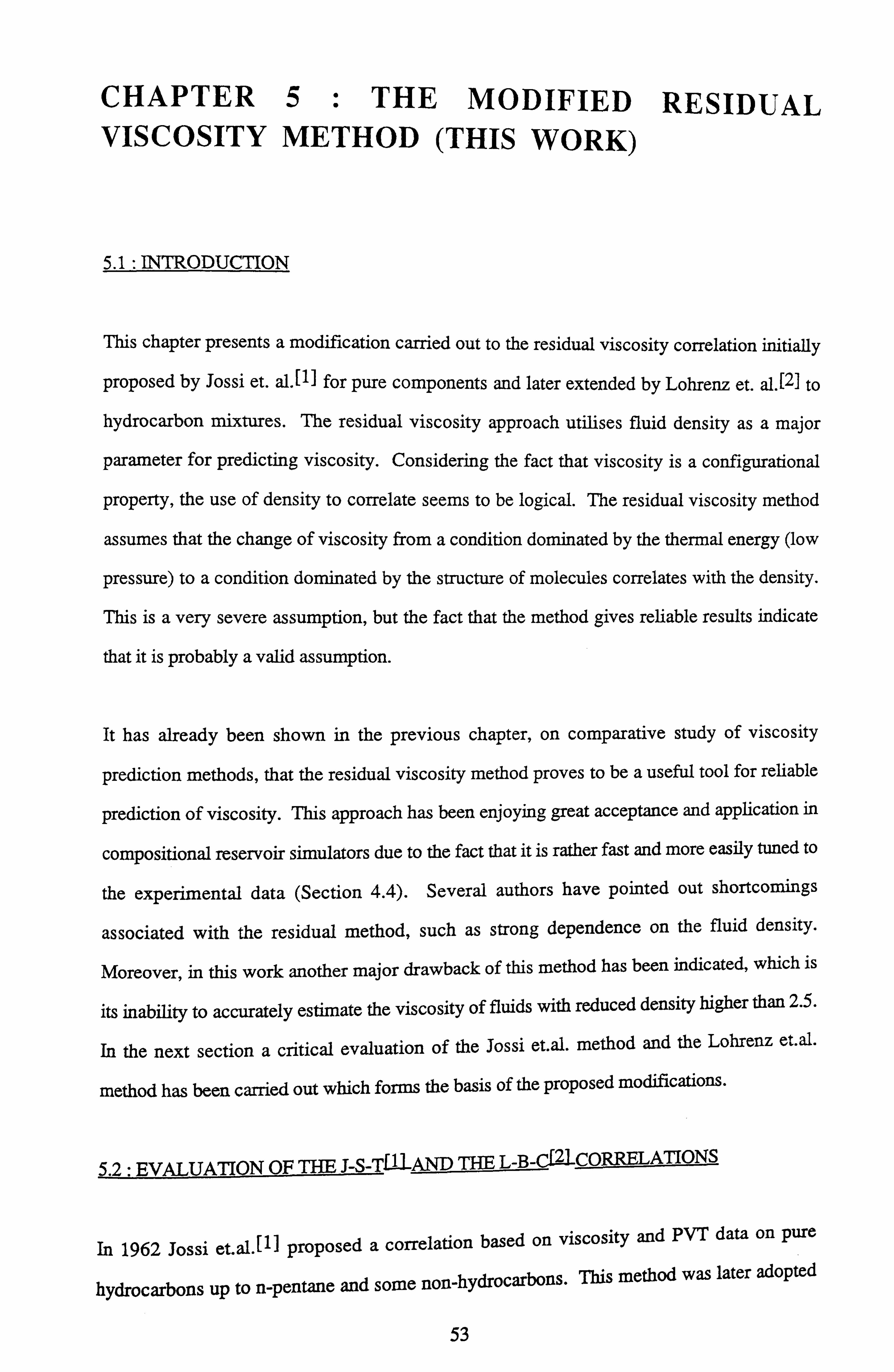
CHAPTER 5 THE MODIFIED RESIDUAL VISCOSITY METHOD (THIS WORK)
5.1 : INTRODUCTION
This chapter presents a modification carried out to the residual viscosity correlation initially
proposed by Jossi et. al. [11 for pure components and later extended by Lohrenz et. al. [2] to
hydrocarbon mixtures. The residual viscosity approach utilises fluid density as a major
parameter for predicting viscosity. Considering the fact that viscosity is a configurational
property, the use of density to correlate seems to be logical. The residual viscosity method
assumes that the change of viscosity from a condition dominated by the thermal energy (low
pressure) to a condition dominated by the structure of molecules correlates with the density.
This is a very severe assumption, but the fact that the method gives reliable results indicate
that it is probably a valid assumption.
It has already been shown in the previous chapter, on comparative study of viscosity
prediction methods, that the residual viscosity method proves to be a useful tool for reliable
prediction of viscosity. This approach has been enjoying great acceptance and application in
compositional reservoir simulators due to the fact that it is rather fast and more easily tuned to
the experimental data (Section 4.4). Several authors have pointed out shortcomings
associated with the residual method, such as strong dependence on the fluid density.
Moreover, in this work another major drawback of this method has been indicated, which is
its inability to accurately estimate the viscosity of fluids with reduced density higher than 2.5.
In the next section a critical evaluation of the Jossi et. al. method and the Lohrenz et-al.
method has been carried out which forms the basis of the proposed modifications.
5.2: EVALUATION OF THE J-S-T AND THE L-B-C -CORREI'ATIONS
In 1962 Jossi et. al. [11 proposed a correlation based on viscosity and PVT data on pure
hydrocarbons up to n-pentane and some non-hydrocarbons. This method was later adopted
53
by Lohrenz-Bray-Clarkl21 to develop their correlation for mixtures of hydrocarbon fluids. A
large number of data on pure components and mixtures were employed to check the
performance of these two correlations. Figure 5.2.1 shows the plot of percentage deviations
of calculated viscosity for pure components vs. reduced density using the J-S-T correlation. This graph clearly shows that viscosities can be predicted with reasonable accuracy for
reduced density up to about 2.5 and a general trend of large underpredictions (especially for
heavier components) is evident for reduced density greater than 2.5. This also indicates that
the method fails to recognise that the variation of residual viscosity with density is not
uniform for all components. Jossi et. al. have assumed in their work that for reduced densities
higher than 3.0 for components heavier than n-pentane the variation of residual viscosity with
respect to reduced density would correspond to their constructed plot. The drawback of this
assumption has been shown in the next section. A similar trend has been observed when the
L-B-C method is applied to hydrocarbon mixtures, showing reasonably reliable predictions
for reduced densities up to 2.5 and large underpredictions above 2.5. Figure 5.2.2 shows a
plot of percentage deviations of calculated viscosity vs. reduced density for various binary
mixtures.
However, it was also thought that these errors in predicted viscosity could be due to the use
of simple molar mixing rules (especially for critical volume, since the method is highly
sensitive to reduced density). Table 5.2.1 shows the results of viscosity prediction using two
different types of mixing rules for critical volume namely; the simple molar mixing rule and
the cubic mixing rule. However Table 5.2.1 proves the adequacy of the simple mixing rules
for the purpose of viscosity calculations.
53: DEVELOPMENT OF THE MODIFIED RESIDUAL VISCOSITY CORRELATION
The above evaluation of the J-S-T and the L-B-C correlation was conducive to propose a
modification of the residual viscosity approach for the dense fluid phases. The modification
has been carried out to the pure component correlation of J-S-T and subsequently applied to
hydrocarbon mixtures.
54
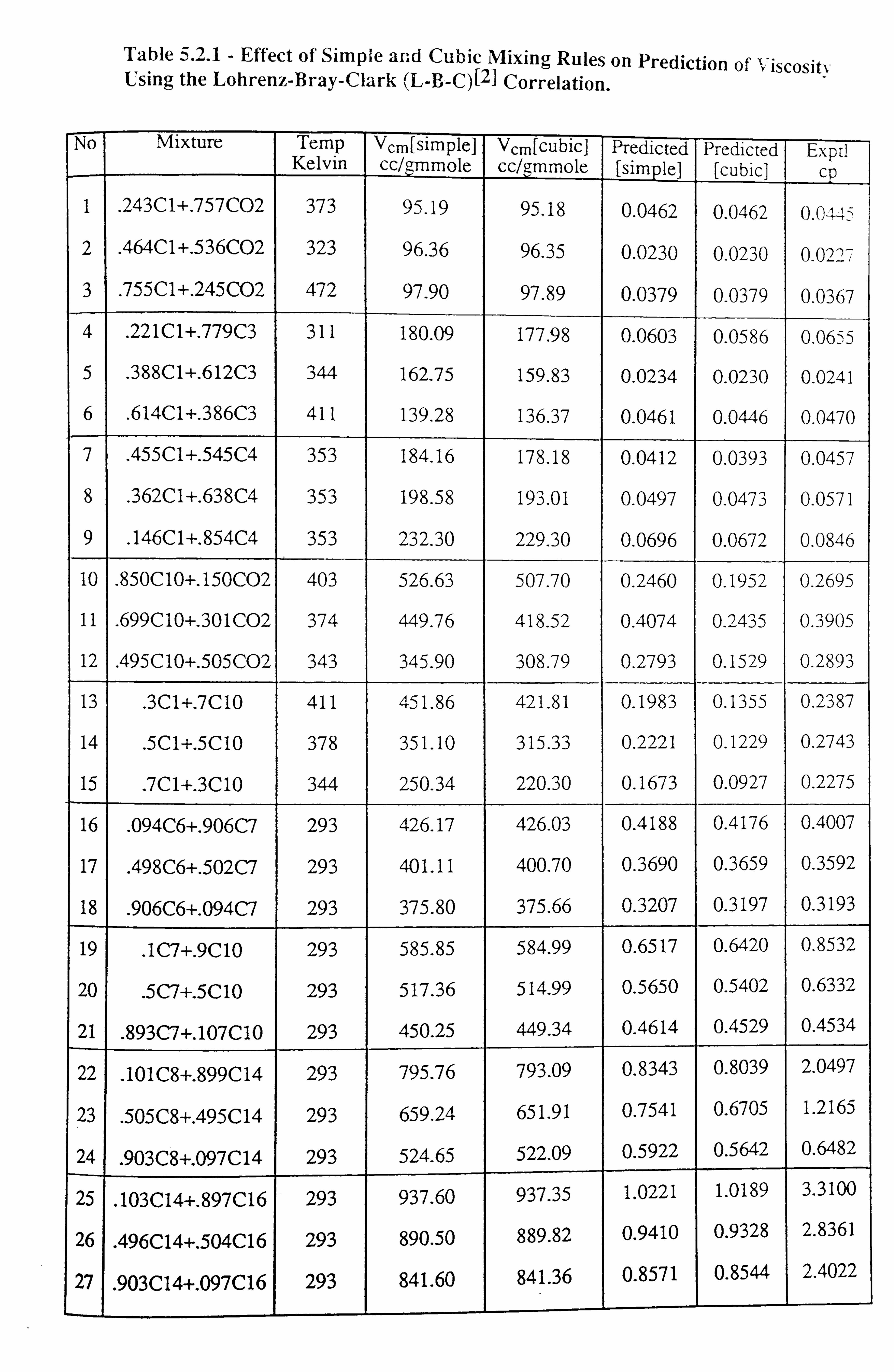
Table 5.2.1 - Effect of Simple and Cubic Mixing Rules on Prediction of V iscosity Using the Lohrenz-Bray-Clark (L-B-C)[2] Correlation.
No Mixture Temp Vcm[simple] Vcm[cubic] Predicted Predicted Exptl Kelvin cc/gmmole cc/gmmole [simple] [cubic] c
1 . 243C1+. 757C02 373 95.19 95.18 0.0462 0.0462 0.04-
2 . 464C1+. 536C02 323 96.36 96.35 0.0230 0.0230 0.0227
3 . 755C1+. 245C02 472 97.90 97.89 0.0379 0.0379 0.0367
4 . 221C1+. 779C3 311 180.09 177.98 0.0603 0.0586 0.06>5
5 . 388C1+. 612C3 344 162.75 159.83 0.0234 0.0230 0.0241
6 . 614C1+. 386C3 411 139.28 136.37 0.0461 0.0446 0.0470
7 . 455C1+. 545C4 353 184.16 178.18 0.0412 0.0393 0.0457
8 . 362C1+. 638C4 353 198.58 193.01 0.0497 0.0473 0.0571
9 . 146C1+. 854C4 353 232.30 229.30 0.0696 0.0672 0.0846
10 . 850C10+. 150002 403 526.63 507.70 0.2460 0.1952 0.2695
11 . 699C 10+. 301 CO2 374 449.76 418.52 0.4074 0.2435 0.3905
12 . 495C10+. 505C02 343 345.90 308.79 0.2793 0.1529 0.2893
13 . 3C1+. 7C10 411 451.86 421.81 0.1983 0.1355 0.2387
14 . 5C1+. 5C10 378 351.10 315.33 0.2221 0.1229 0.2743
15 . 7C1+. 3C10 344 250.34 220.30 0.1673 0.0927 0.2275
16 . 094C6+. 906C7 293 426.17 426.03 0.4188 0.4176 0.4007
17 . 498C6+. 502C7 293 401.11 400.70 0.3690 0.3659 0.3592
18 . 906C6+. 09407 293 375.80 375.66 0.3207 0.3197 0.3193
19 . 1C7+. 9C10 293 585.85 584.99 0.6517 0.6420 0.8532
20 . 5C7+. 5C10 293 517.36 514.99 0.5650 0.5402 0.6332
21 . 89307+. 107C10 293 450.25 449.34 0.4614 0.4529 0.4534
22 . 101C8+. 899C14 293 795.76 793.09 0.8343 0.8039 2.0497
23 . 505C8+. 495C14 293 659.24 651.91 0.7541 0.6705 1.2165
24 . 903C8+. 097C14 293 524.65 522.09 0.5922 0.5642 0.6482
25 . 103C14+. 897C16 293 937.60 937.35 1.0221 1.0189 3.3100
26 . 496C14+. 504C16 293 890.50 889.82 0.9410 0.9328 2.8361
27 . 903C14+. 097C16 293 841.60 841.36 0.8571 0.8544 2.4022
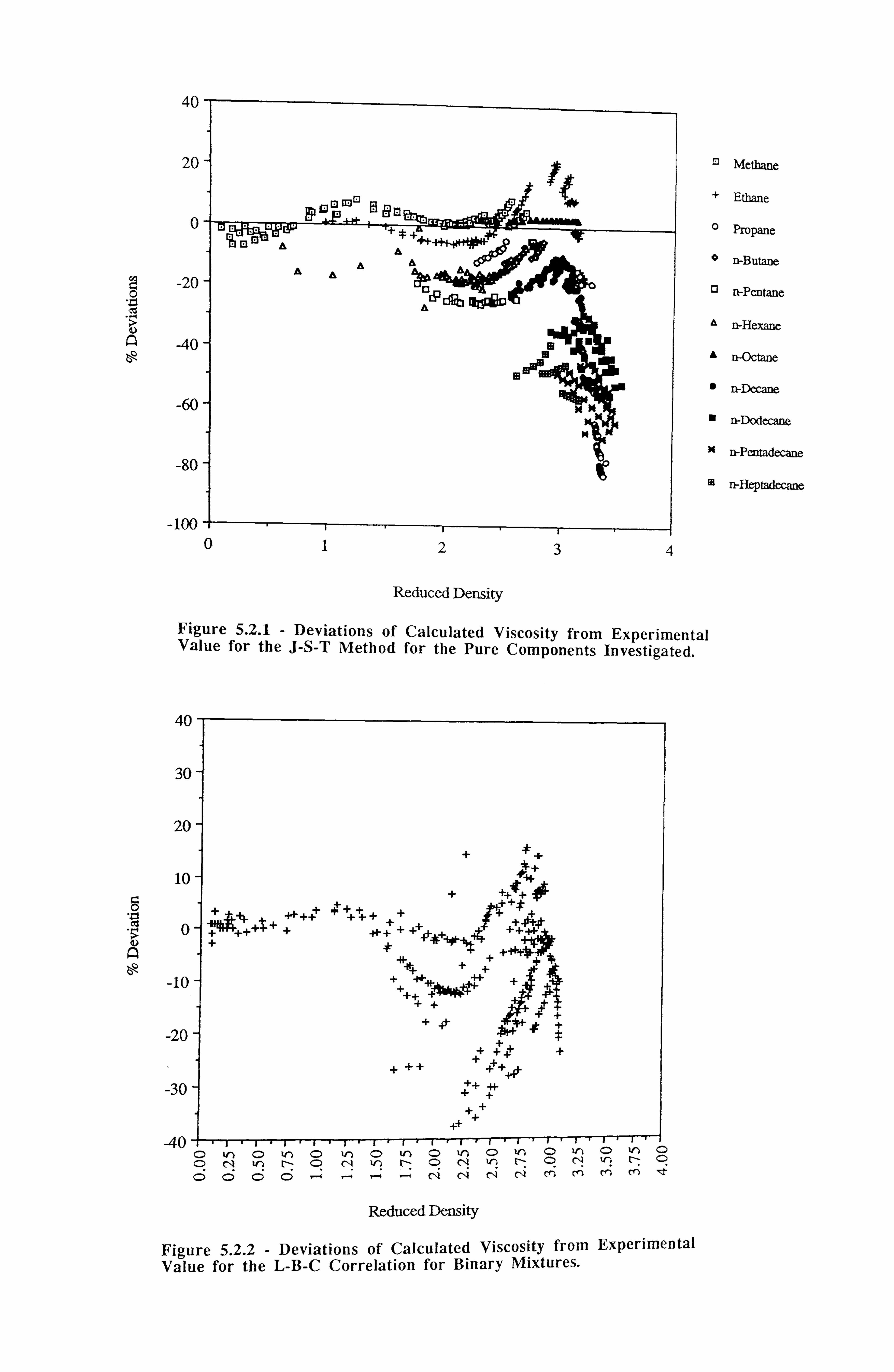
40
20
0
-20 0
A -40
-60
-80
-100 0
40
30
20
10
0
-10
-20
-30
-40
0 ll'E', ' a m'. ' -- -e/- 'w
_A -- ______________________________________________
1+A --
coo 4, ee ee q�ý
A i! R
CQý lld*D
1 2 3 4
I Methane
+ Ethane
o Propane
n-Butane
13 n-Pentane
n-Hexane
" . n-Octane
" n-Decane
n-Dodecane
n-Pentadecane
Ell n-Heptadecane
Reduced Density
Figure 5.2.1 - Deviations of Calculated Viscosity from Experimental Value for the J-S-T Method for the Pure Components Investigated.
+ #+ *+
++ ý+++ ++
++++ +"**++ + ý-+ + +, + ++-r} +# #$
+ 1+ +
++ + +++ +r +++
+++ +++ ++
++ ++
O to O vý O to O VI O ýn O ýn O ýn o 'n C-) C: ) r- ON l-- ON Iý ONu? r- a
OÖOO r-+ _; r+ CV NNNMMMM4
Reduced Density
Figure 5.2.2 - Deviations of Calculated Viscosity from Experimental Value for the L-B-C Correlation for Binary Mixtures.

A large number of data on viscosity[3,4,5] and PVT[3,4,6] in dense fluid phase conditions for heavy n-alkanes was amassed for this purpose. All the data was quality checked before
using them for modelling purposes. Figure 5.3.1 shows the plot of residual viscosity (RV),
(ij-ij*)?, against reduced density for various compounds [3,4,5]. Where, Ti is the fluid
viscosity, TI is the low pressure gas phase viscosity and ? is the inverse of critical viscosity
or viscosity reducing parameter defined by Eq. 2.2.2 a, Section 2.2. Along with all the
points a curve for the J-S-T correlation has also been shown (Eq. 2.2.3, Section 2.2). It is
evident from the graph that the points belonging to the group of (n-C6, Toluene and n-C8)
follow the same trend as the J-S-T curve and exhibit that RV is also a function of a molecular
property for heavier compounds. Note the gradual shifts in the RV curves as the alkane
number increases. Another important feature of Figure 5.3.1 shows that all the curves
converge at a reduced density of 2.5. This Figure is also indicative of the fact that the
hypothesis put forward by Jossi et. al. LlI that the variation of residual viscosity with respect to
the reduced density is uniform for all the substances is valid only for components up to
normal octane. Hence it can be concluded that the J-S-T correlation is valid for any range of
reduced density and components smaller with a molecular weight less than that of n-octane or
for any compounds with reduced density less than 2.5.
The above exercise formed the basic groundwork for the modification, the solution was
achieved in a very systematic way. In order to find out the dependence of RV on the
component property, values for RV were computed from Figure 5.3.1 for isoreduced density
values and were plotted against acentric factor. The formulation obtained by this method was
presented at the 7th European Improved Oil Recovery (IOR) Symposium in Moscow,
Russia[19I. However, later on the molecular weight was, chosen, instead of the acentric
factor as the correlating parameter because the former is a more readily available parameter
than acentric factor especially for the plus fractions of a real fluid. Figure 5.3.2 shows the
plot of RV vs. molecular weight for various isoreduced densities. The graph demonstrates
the dependency of RV on a component property. It is also interesting to note that the values
of RV converge to zero as molecular weight decreases.
55
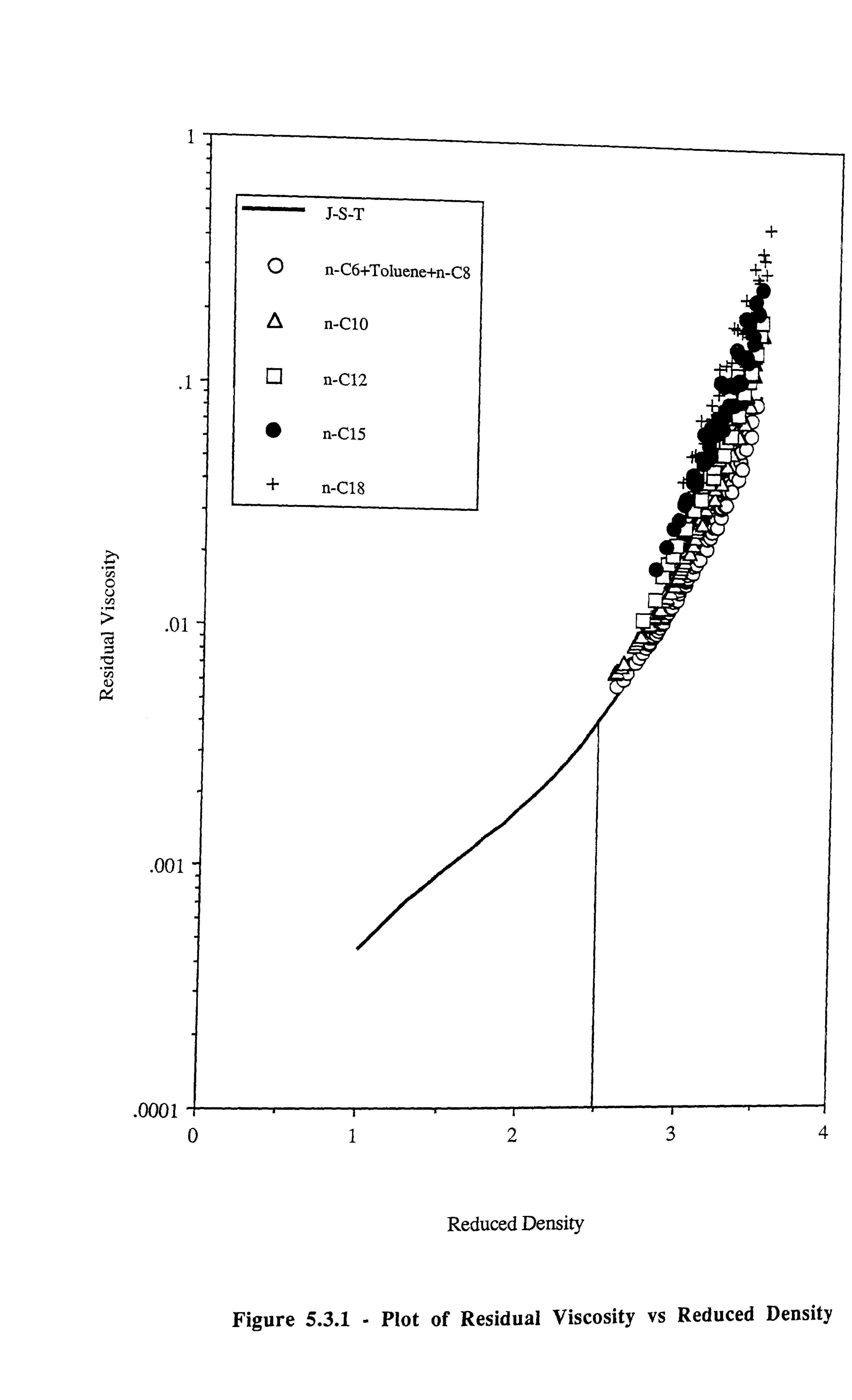
II
I "' J-S-T
, 2: 1 O U
Z
9
n-C6+Toluene+n-C8
n-C10
Q n-C12
n-C15
+ n-C18
. 01
. 001
. 0001-ý 0 12
Reduced Density
+
3 4
Figure 5.3.1 - Plot of Residual Viscosity vs Reduced Density
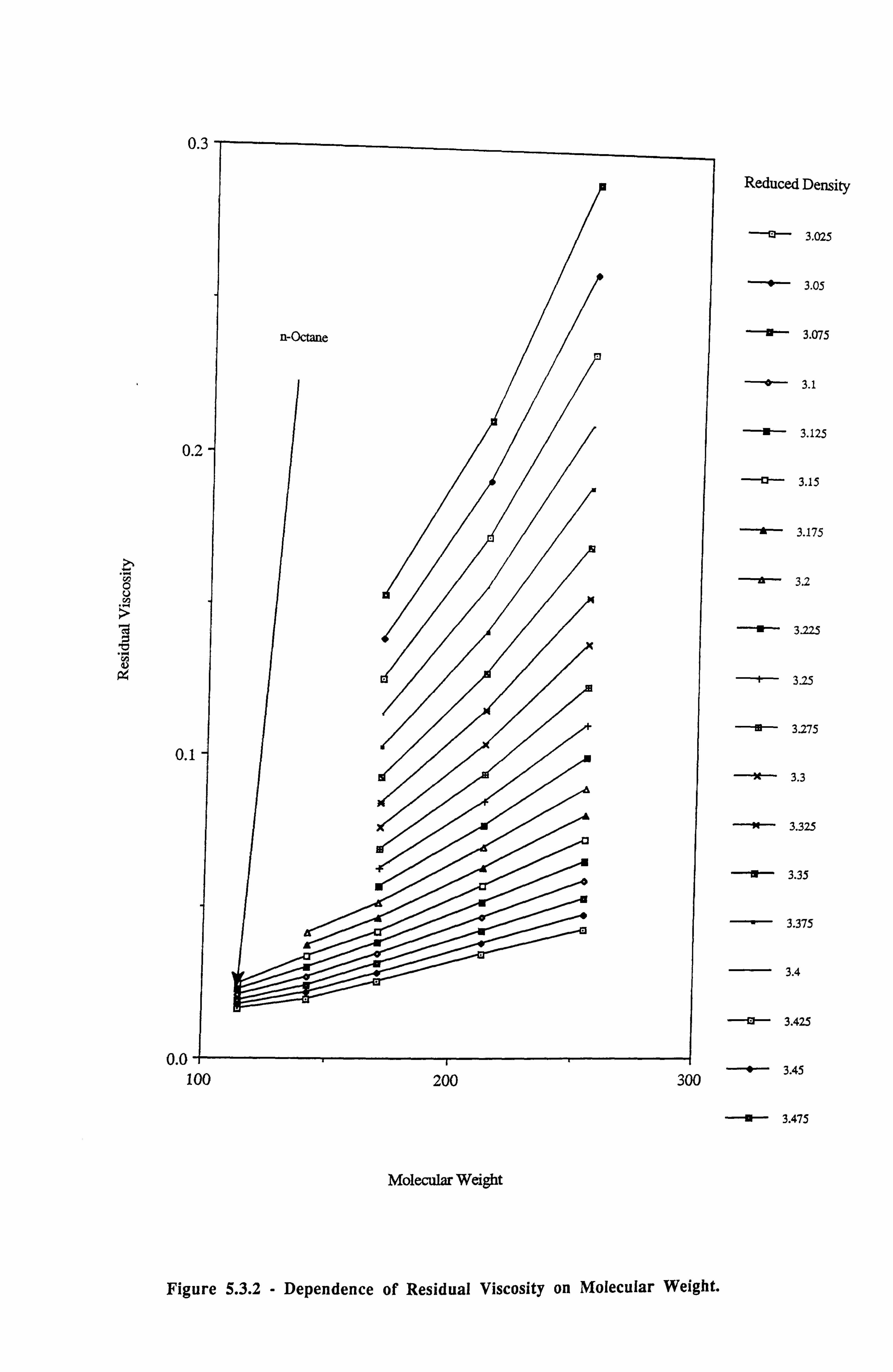
0.3
Reduced Density
0 U ti
'li
9
n -Octane
0.2
0.1
0.0 -+- 100 200
Molecular weight
il--ý
3.025
3.05
9-- 3.075
ý- 3.1
3.125
- 0-- 3.15
3.175
-' 1 3.2
3.225
ý- 3.25
-ý- 3.275
-'- 3.3
3.325
-ii 3.35
-ý- 3.375
3.4
-fl-- 3.425
-+-- 3.45 300
---¢- 3.475
Figure 5.3.2 - Dependence of Residual Viscosity on Molecular Weight.
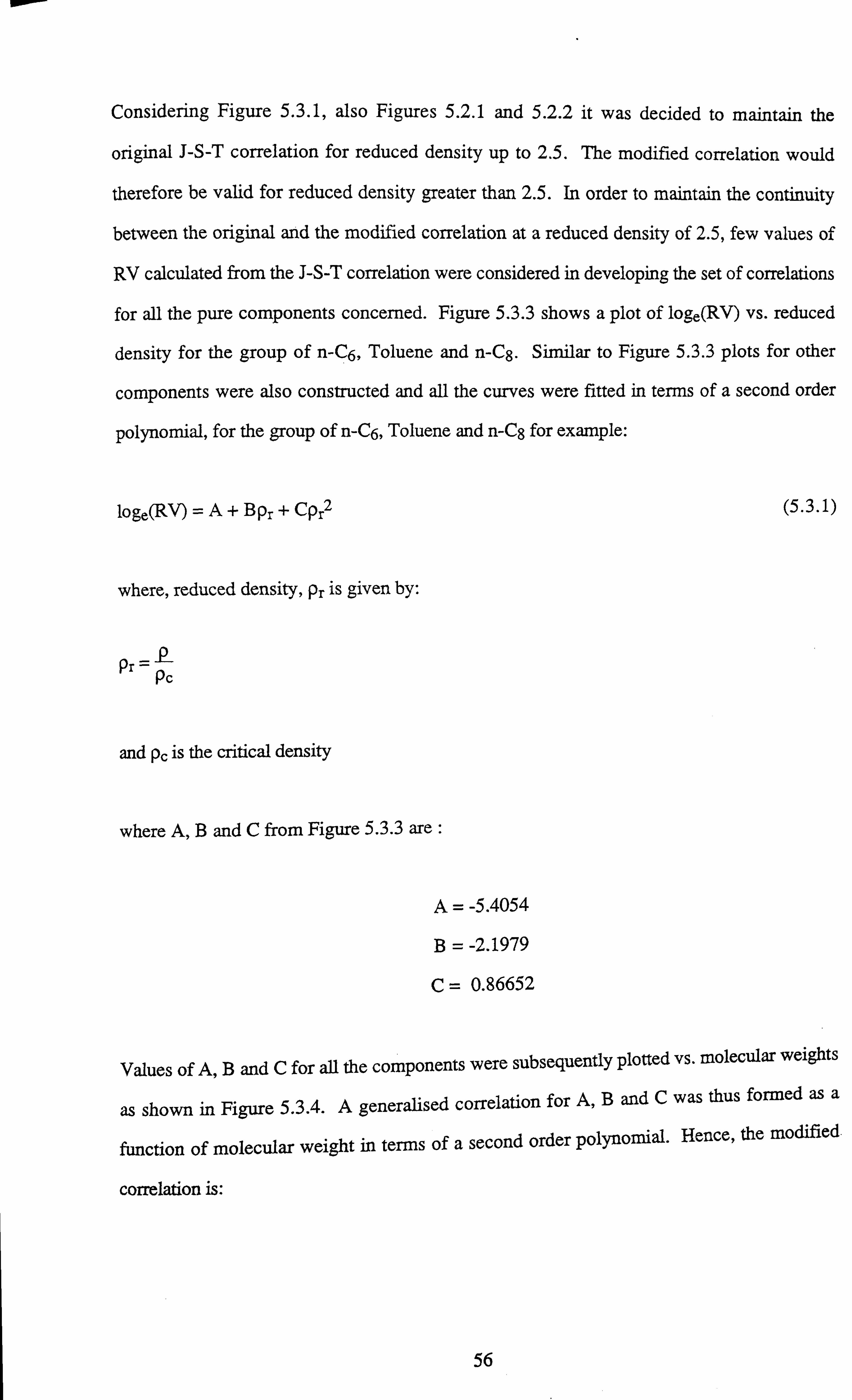
Considering Figure 5.3.1, also Figures 5.2.1 and 5.2.2 it was decided to maintain the
original J-S-T correlation for reduced density up to 2.5. The modified correlation would
therefore be valid for reduced density greater than 2.5. In order to maintain the continuity
between the original and the modified correlation at a reduced density of 2.5, few values of
RV calculated from the J-S-T correlation were considered in developing the set of correlations
for all the pure components concerned. Figure 5.3.3 shows a plot of loge(RV) vs. reduced
density for the group of n-C6, Toluene and n-Cg. Similar to Figure 5.3.3 plots for other
components were also constructed and all the curves were fitted in terms of a second order
polynomial, for the group of n-C6, Toluene and n-C8 for example:
loge(RV) =A+ BPr + Cpr2
where, reduced density, pr is given by:
Pr-Pc
and pc is the critical density
where A, B and C from Figure 5.3.3 are :
A= -5.4054 B= -2.1979
C=0.86652
(5.3.1)
Values of A, B and C for all the components were subsequently plotted vs. molecular weights
as shown in Figure 5.3.4. A generalised correlation for A, B and C was thus formed as a
function of molecular weight in terms of a second order polynomial. Hence, the modified
correlation is:
56
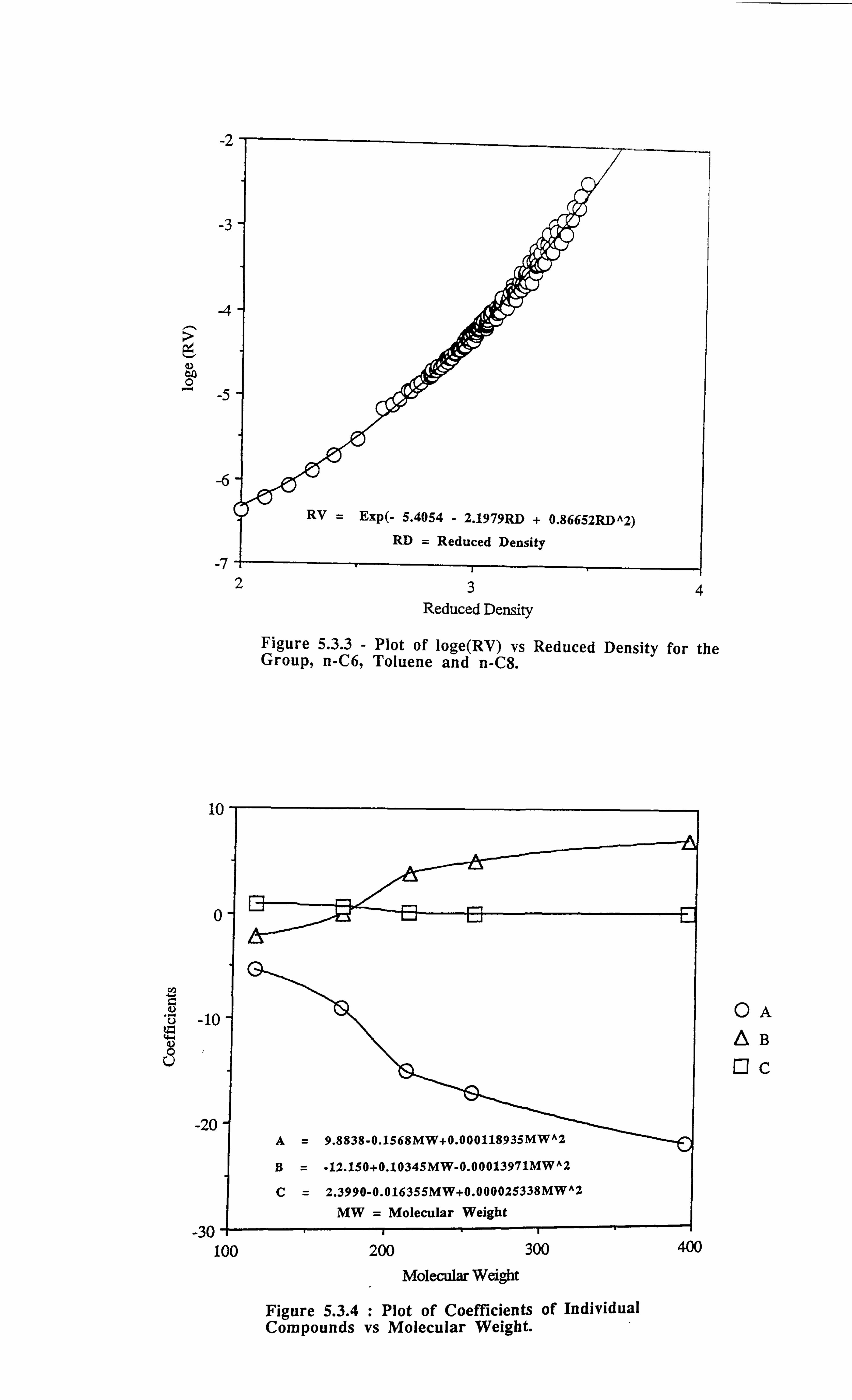
-2
-3
-4 I
-. " -5
-b
-7
1
Figure 5.3.3 - Plot of loge(RV) vs Reduced Density for the Group, n-C6, Toluene and n-C8.
C
-10
U
-20
-30 -f- 100
A=9.8838-0.1568MW+0.000118935MW^2
B= -12.150+0.10345MW-0.00013971MW^2
C=2.3990-0.016355MW+0.000025338MWA2
MW = Molecular Weight
200 300
Molecular Weight
Figure 5.3.4 Plot of Coefficients of Individual Compounds vs Molecular Weight.
400
OA 0s
Q
234
Reduced Density
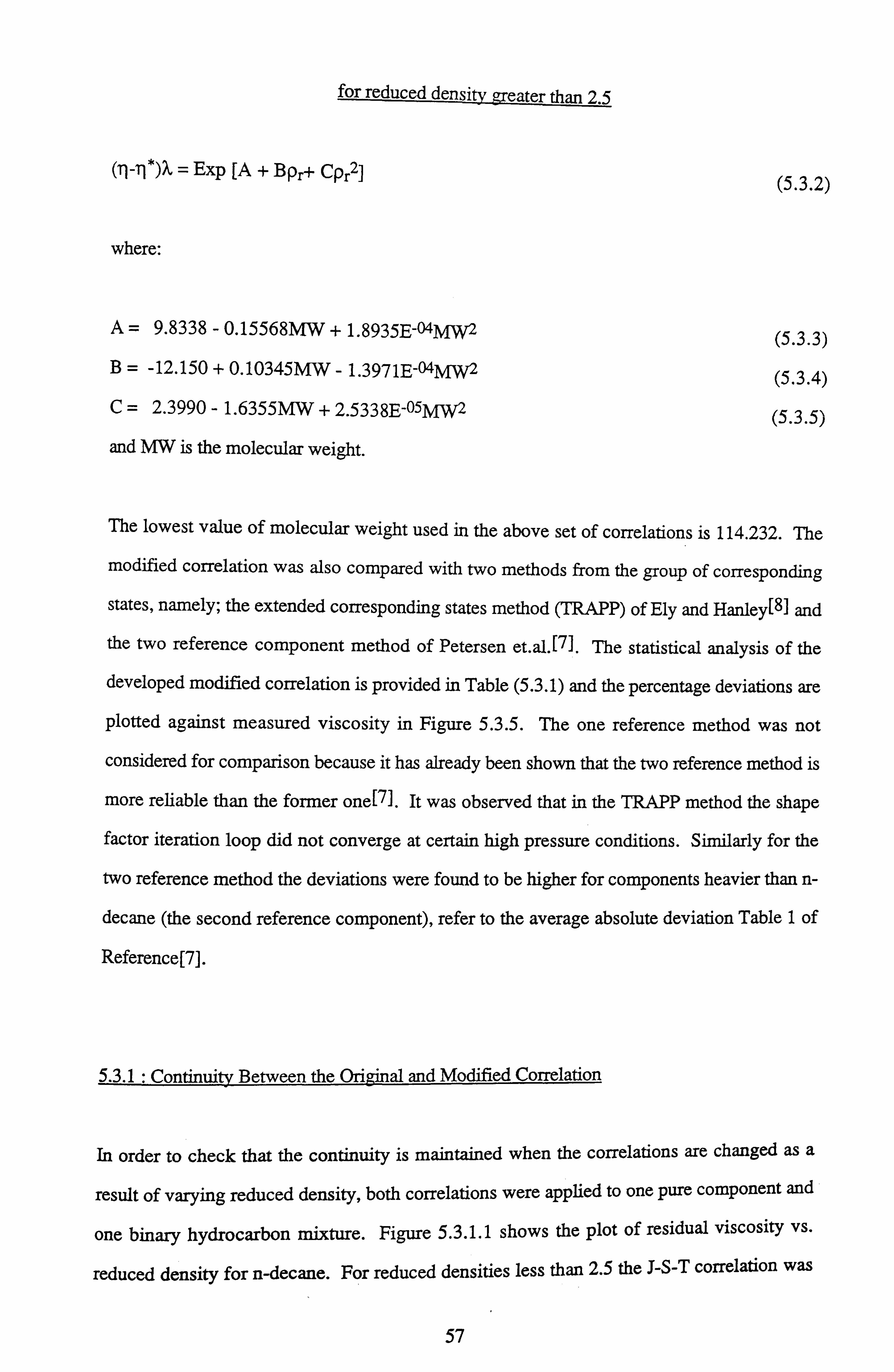
for reduced density eater than 2,5
(Tl-l1*)2L = Exp [A + Bpr+ CPr2] (5.3.2)
where:
A=9.8338 - 0.15568MW + 1.8935E-04MQ (5.3.3) B= -12.150 + 0.10345MW - 1.3971E-04MW2 (5.3.4) C=2.3990 - 1.6355MW + 2.5338E-05MW2 (5.3.5)
and MW is the molecular weight
The lowest value of molecular weight used in the above set of correlations is 114.232. The
modified correlation was also compared with two methods from the group of corresponding
states, namely; the extended corresponding states method (TRAPP) of Ely and Hanley[81 and
the two reference component method of Petersen et. al. [7]. The statistical analysis of the
developed modified correlation is provided in Table (5.3.1) and the percentage deviations are
plotted against measured viscosity in Figure 5.3.5. The one reference method was not
considered for comparison because it has already been shown that the two reference method is
more reliable than the former one[7]. It was observed that in the TRAPP method the shape
factor iteration loop did not converge at certain high pressure conditions. Similarly for the
two reference method the deviations were found to be higher for components heavier than n-
decane (the second reference component), refer to the average absolute deviation Table 1 of
Reference[7].
5.3.1 : Continuity Between the Original and Modified Correlation
In order to check that the continuity is maintained when the correlations are changed as a
result of varying reduced density, both correlations were applied to one pure component and
one binary hydrocarbon mixture. Figure 5.3.1.1 shows the plot of residual viscosity vs.
reduced density for n-decane. For reduced densities less than 2.5 the J-S-T correlation was
57
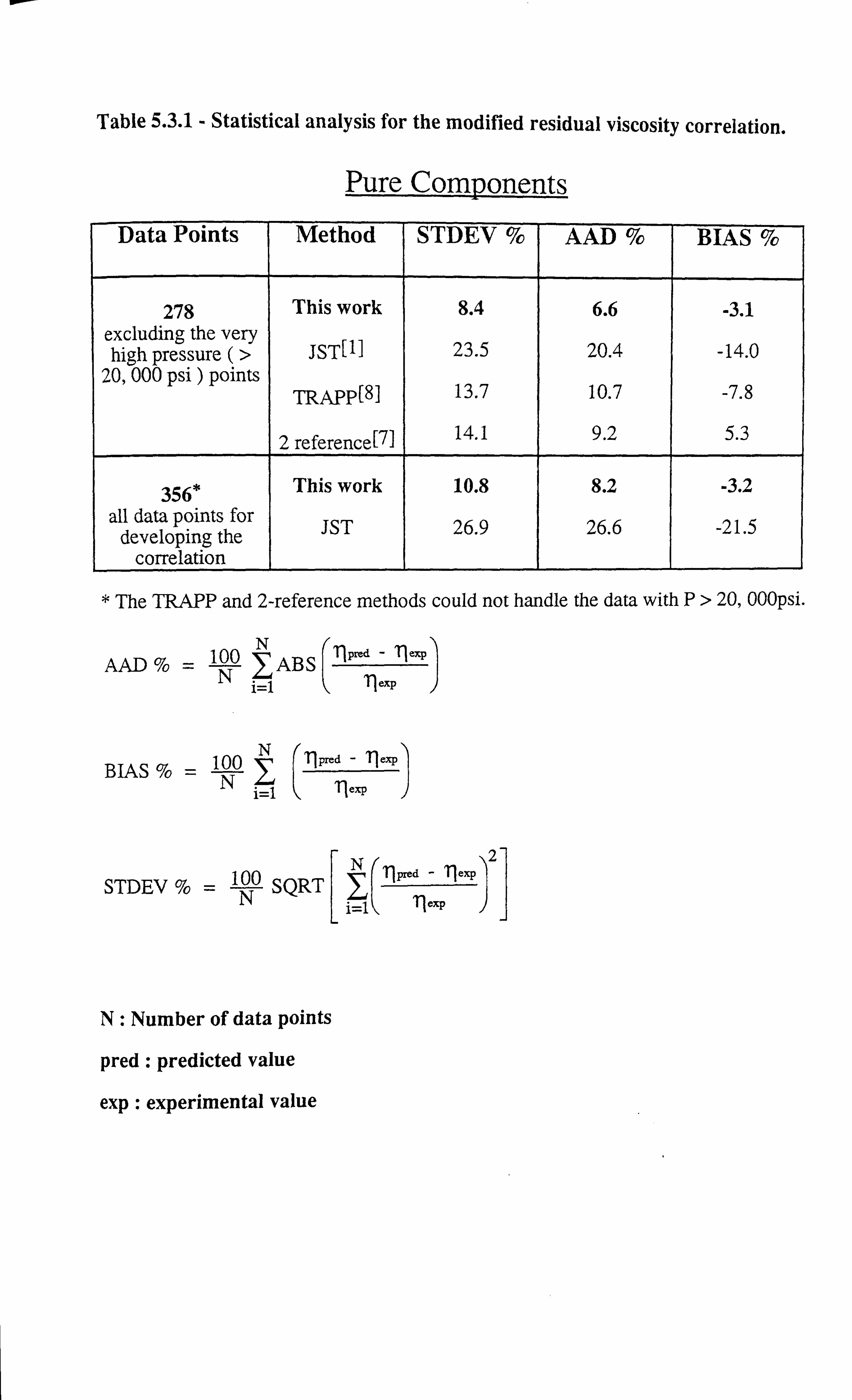
Table 5.3.1- Statistical analysis for the modified residual viscosity correlation.
Pure Components
Data Points Method STDEV % AAD % BIAS %
278 This work 8.4 6.6 -3.1 excluding the very high pressure (> JST[ 1] 23.5 20.4 -14.0
20,000 psi) points mipp[8] 13.7 10.7 -7.8
2 reference[7] 14.1 9.2 5.3
356* This work 10.8 8.2 -3.2 all data points for
JST 26 9 26 6 -21 5 developing the . . . correlation
* The TRAPP and 2-reference methods could not handle the data with P> 20,000psi.
N 11
AAD %= lo LABS fired - 11 ezp
1=1 ' 1exp
BIAS % 1oo ýPred - 11exp
e i=1 xp
100 N71pm(d_-_1exp2l
STDEV %=N SQRT i=1 l exp
N: Number of data points
pred : predicted value
exp : experimental value

100,
C O
Q s
o"
Q J-S-T O TRAPP
two-Reference ý' Modified
AA
'A A 2PA12, A
AA L*An& +A ++I
-ý ý- ++
-ý +
+, I+.
++
R
L
+++
+
13
-100 .1 1 10
Measured Viscosity, cp
Figure 5.3.5 - Deviations of Calculated Viscosity from Experimental Values for Pure Components.
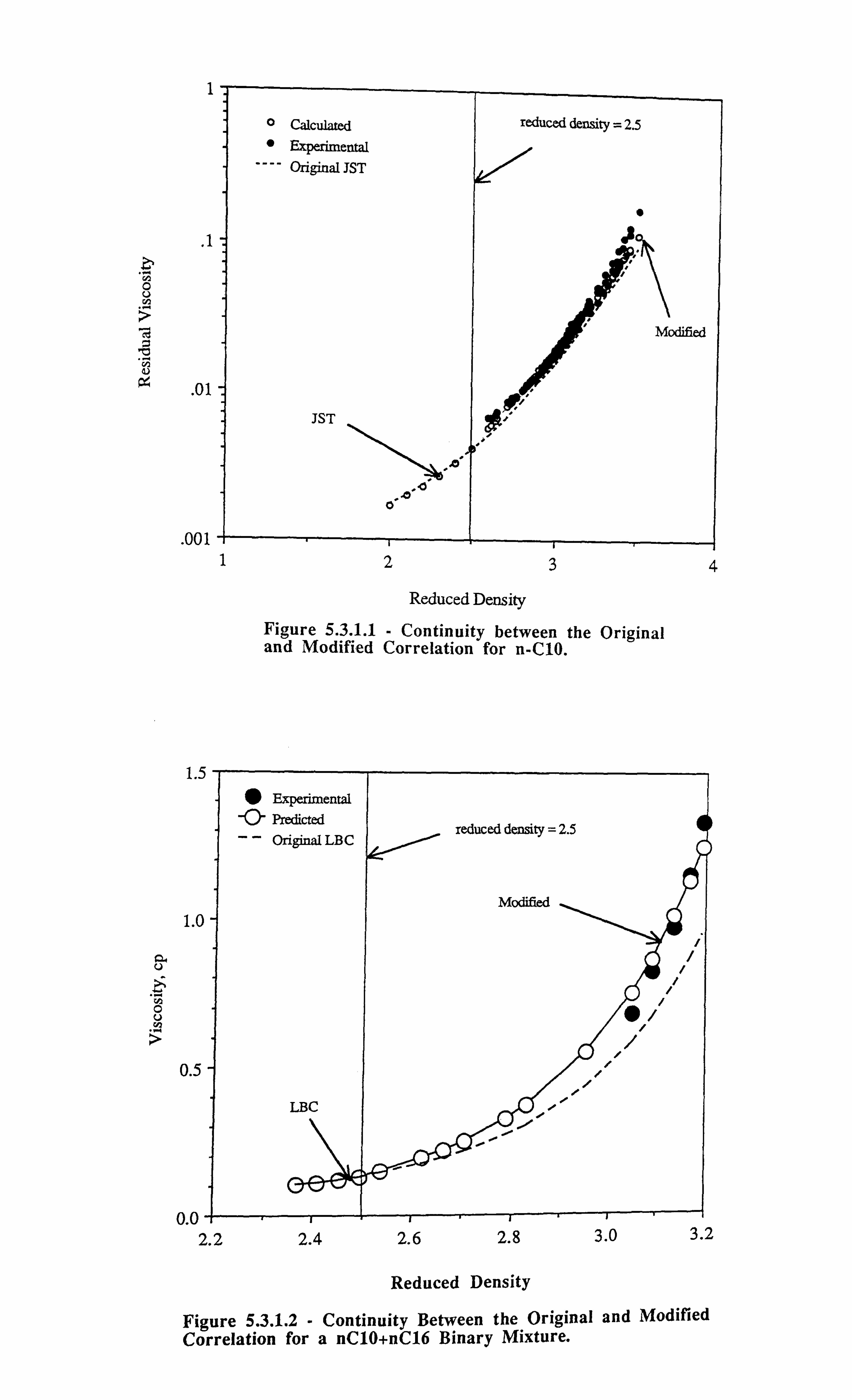
2: ' O U
cý b
N 9
1
.1
. 01
. 001-1 1
Reduced Density
Figure 5.3.1.1 - Continuity between the Original and Modified Correlation for n-C10.
a U
O U h
...,
1.5
1.0
0.5
Experimental '0' Predicted -- Original LB C
LBC
reduced density = 2.5
Modified
r
r r
r i i i i
00
0.0 2.2 2.4 2.6 2.8 3.0 3.2
Reduced Density
Figure 5.3.1.2 - Continuity Between the Original and Modified Correlation for a nC10+nC16 Binary Mixture.
234

applied and for reduced densities greater than 2.5 the modified correlation was used. The
Figure clearly illustrates the continuity maintained between the two correlations as the value of
reduced density changes, and a fairly smooth transition is achieved. Figure 5.3.1.2 shows
graph of viscosity against reduced density for a n-decane and n-hexadecane binary mixture.
The L-B-C correlation is applied to the reduced density data below 2.5 and the modified
correlation is applied to the reduced density data above 2.5. This plot again indicates
consistent predictions when the correlations are changed as a result of varying reduced
density.
5.4: APPLICATION OF THE MODIFIED RESIDUAL VISCOSITY METHOD TO
SYNTHETIC HYDROCARBON MIXTURES
The modified residual viscosity correlation, Eq. 5.3.2-5.3.5, was applied to several synthetic
hydrocarbon mixtures, ranging from simple binary mixtures to multicomponent
mixtures [9,10,11,12,16] at a wide range of temperature and pressure conditions. All the data
was quality checked prior to using it for comparison purposes. The experimental data used
for comparison is measured by various techniques. The data from Reference 9 on various
binary mixtures were measured by the Cannon-Ubeholde type viscometer which is generally
employed in estimating viscosities of viscosity standards which are used for calibrating the
rolling ball type viscometers. The viscosities of a binary mixture of carbon dioxide and n-
decane[l°i were obtained by the capillary tube viscometer. The viscosities of the binary
mixture of toluene and n-hexane[1 1] were measured by the falling body viscometer. A
conventional falling body viscometer similar to the rolling ball viscometer was used for
measuring viscosity of higher alkanes and its mixtures at high pressures and
temperatures[ 121. The viscosities of the binary mixture of methane and n-decaneV16] were
measured by the oscillation cup viscometer.
The data on measured density was available in all the sources corresponding to the viscosity
measurements except Reference 12 in which case the densities were calculated using the API
method[131 for the binary mixture of n-decane-n-hexadecane and the quaternary mixture of n-
58
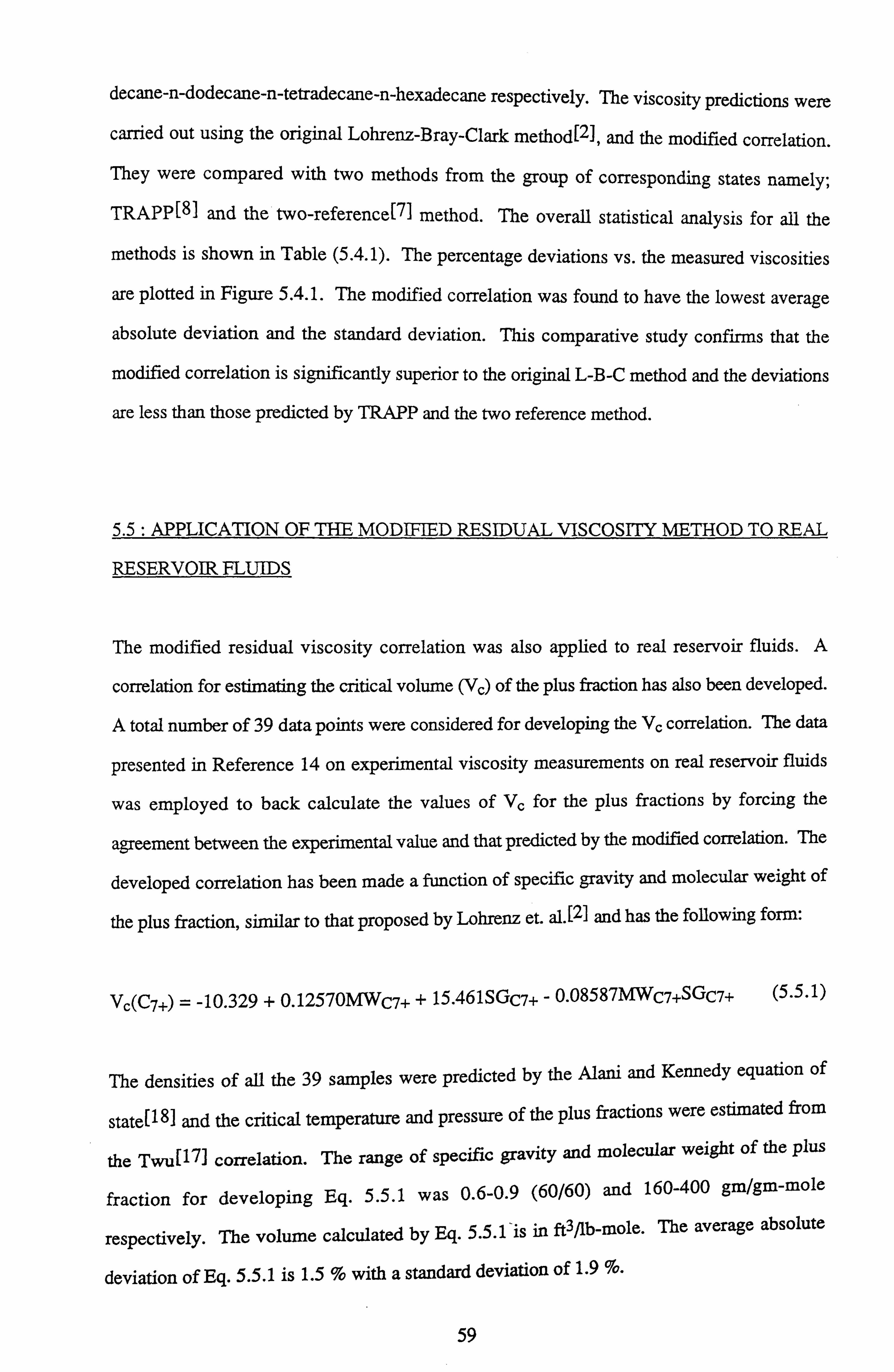
decane-n-dodecane-n-tetradecane-n-hexadecane respectively. The viscosity predictions were
carried out using the original Lohrenz-Bray-Clark method[21, and the modified correlation.
They were compared with two methods from the group of corresponding states namely;
TRAPPC81 and the two-reference[71 method. The overall statistical analysis for all the
methods is shown in Table (5.4.1). The percentage deviations vs. the measured viscosities
are plotted in Figure 5.4.1. The modified correlation was found to have the lowest average
absolute deviation and the standard deviation. This comparative study confirms that the
modified correlation is significantly superior to the original L-B-C method and the deviations
are less than those predicted by TRAPP and the two reference method.
5.5: APPLICATION OF THE MODIFIED RESIDUAL VISCOSITY METHOD TO REAL
RESERVOIR FLUIDS
The modified residual viscosity correlation was also applied to real reservoir fluids. A
correlation for estimating the critical volume (Vc) of the plus fraction has also been developed.
A total number of 39 data points were considered for developing the Vc correlation. The data
presented in Reference 14 on experimental viscosity measurements on real reservoir fluids
was employed to back calculate the values of VG for the plus fractions by forcing the
agreement between the experimental value and that predicted by the modified correlation. The
developed correlation has been made a function of specific gravity and molecular weight of
the plus fraction, similar to that proposed by Lohrenz et. al. {21 and has the following form:
Vc(C7+) = -10.329 + 0.1257OMWC7+ + 15.461SGC7+ - 0.08587MWC7+SGC7+ (5.5.1)
The densities of all the 39 samples were predicted by the Alani and Kennedy equation of
state[18} and the critical temperature and pressure of the plus fractions were estimated from
the Twu[171 correlation. The range of specific gravity and molecular weight of the plus
fraction for developing Eq. 5.5.1 was 0.6-0.9 (60/60) and 160-400 gm/gm-mole
respectively. The volume calculated by Eq. 5.5.1 'is in ft3/lb-mole. The average absolute
deviation of Eq. 5.5.1 is 1.5 % with a standard deviation of 1.9 %.
59

Table 5.4.1 - Statistical analysis for the modified residual viscosity correlation.
Synthetic Mixtures
Data Points Method STDEV % AAD % BIAS %
398 This work 10.8 8.2 -3.1
LBC 22.4 16.0 -8.8
TRAPP 24.5 17.3 -1.7
2 reference 16.0 11.2 -4.0
Table 5.5.1 - Statistical analysis for the modified residual viscosity correlation.
Real Reservoir Fluids
Data Points Method STDEV % AAD % BIAS %
106 This work
LBC
21.4
26.9
21.8
36.0
20.1
34.2
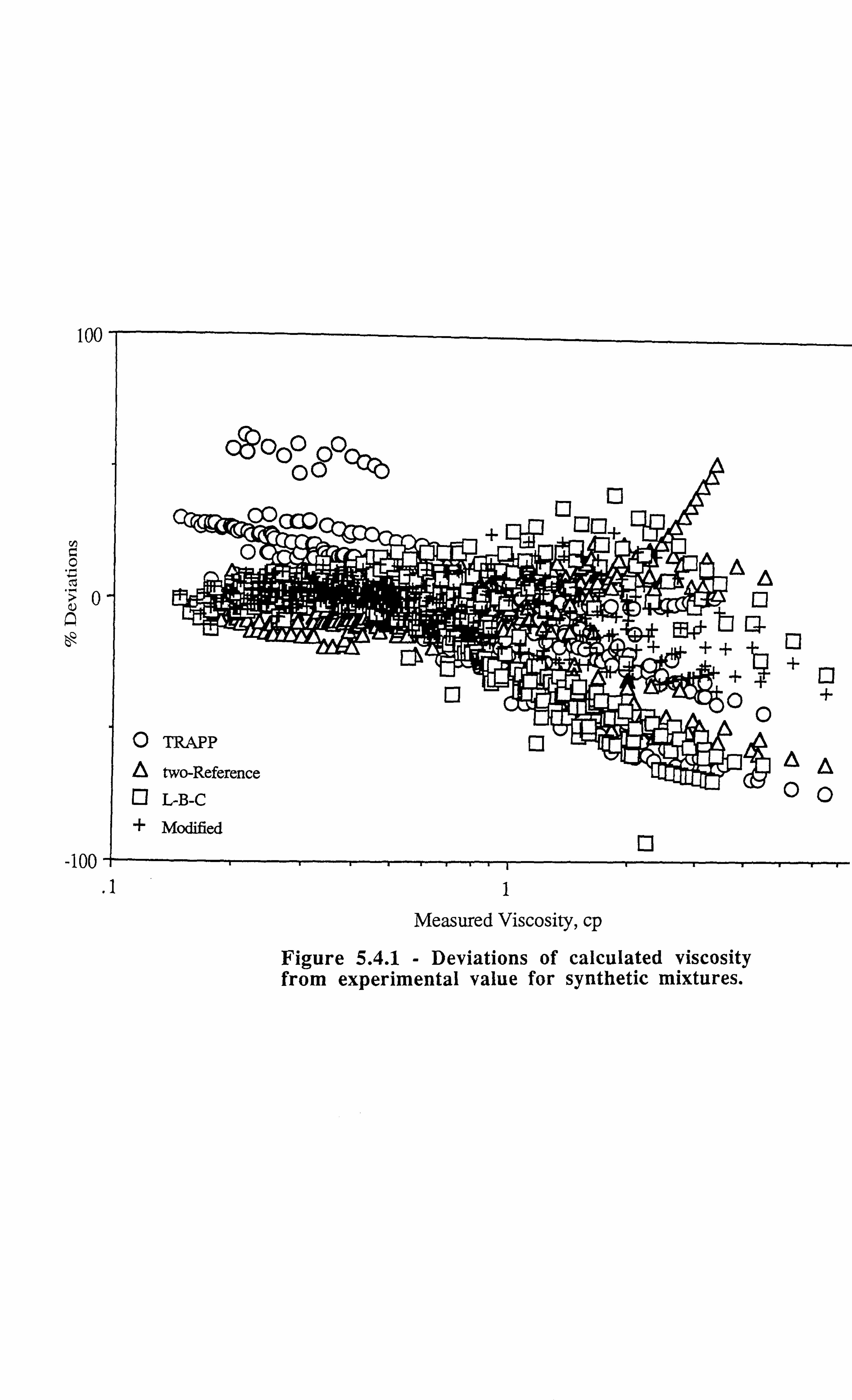
100,
4" Q
C)S)000 10 0 qýb
O TRAPP
two-Reference Q Lr-B-C ý" Modified
1-: 1 -100 , -
.11 Measured Viscosity, cp
kJM A
6-, & ý
+
A 0
+
A
0
Figure 5.4.1 - Deviations of calculated viscosity from experimental value for synthetic mixtures.
The modified residual viscosity correlation and the Lohrenz et. al. [2] method were
subsequently applied to a total number of 106 data points on real reservoir fluids[13,15]. The
above developed correlation for the critical volume of the plus fraction was utilised for the
modified correlation whereas the correlation developed by Lohrenz et. al. [2] was employed
for the L-B-C method. The critical temperature and pressure were estimated from the
Twu[17] correlation, and the fluid density at all conditions were estimated by the Alani and
Kennedy equation of state [ 18]. The liquid phase compositions for all the samples were
calculated by the in-house Vapour Liquid Equilibrium (VLE) model[20]. The statistical
analysis for the tested fluids is provided in Table (5.5.1). The modified residual viscosity
method again shows the lowest average absolute and standard deviation compared to the L-B-
C method.
References
1) Jossi, J. A., Stiel, L. I. and Thodos, G.: "The Viscosity of Pure Substances in
the Dense Gaseous and Liquid Phases", AIChEJ, Vol. 8, pp. 59 - 63, (1962).
2) Lohrenz, J., Bray, B. G. and Clark, C. R.: "Calculating Viscosities of
Reservoir Fluids from their Compositions", Journal of Petroleum Technology,
pp. 1171-1176, (Oct., 1964).
3) Oliveira, C. M. B. P. and Wakeham, W. A.: "The Viscosity of Five Liquid
Hydrocarbons at Pressures Up to 250 MPa", International J. of
Thermophysics, Vol. 13, No. 5, pp. 774-790, (1992).
4) Lee, A. L. and Ellington, R. T.: "Viscosity of n-Decane in the Liquid Phase",
Journal of Chem. Engg. Data, Vol. 10, No. 4, pp. 346-348, (1965).
5) Hogenboom, D. L., Webb, W. and Dixon, J. A.: "Viscosity of Several Liquid
Hydrocarbons as a Function of Temperature, Pressure an Free Volume", J.
Chem Phys., Vol. 46, No. 7, (April, 1967).
60
6) Cutler, W. G., McMickle, R. H., Webb, W. and Schiessler, R. W.: "Study of the Compression of Several High Molecular Weight Hydrocarbons", J. Chem
Phys., Vol. 29, No. 4, pp. 727-740, (October, 1958).
7) Aasberg-Petersen, K., Knudsen, K. and Fredenslund, A.: "Prediction of Viscosities of Hydrocarbon Mixtures", Fluid Phase Equilibria, Vol. 70, pp. 293-308, ( 1991 ).
8) Ely, J. F. and Hanley, H. J. M: "Prediction of the Viscosity and Thermal
Conductivity in Hydrocarbon Mixtures - Computer Program TRAPP",
Proceedings of the Sixtieth Annual Convention of Gas Processors
Association, pp. 20-29, (Mar., 1981).
9) Cooper, E. F. and Asfour, A. A.: "Densities and Kinematic Viscosities of
Some C6-C16 n-Alkane Binary Liquid Systems at 293.15 K", Journal of
Chem. Engg. Data, 36, pp. 285-288, (1991).
10) Cullick, A. S. and Mathis, M. L.: "Densities and Viscosities of Mixtures of
Carbon Dioxide and n-Decane from 310 to 403 K and 7 to 30 MPa", Journal
of Chem. Engg. Data, 29, pp. 393-396, (1984).
11) Dymond, J. H., Awan, M. A., Glen. and Isdale, J. D.: "Transport Properties of
Nonelectrolyte Liquid Mixtures. VIII. Viscosity Coefficients for Toluene and
for Three Mixtures of Toluene+Hexane from 25 to 100°C at Pressures up to
500 MPa", International Journal of Thermophysics, Vol. 12, No. 2, pp. 275-
287, (1991).
12) Ducoulombier, D., Zhou, H., Boned, C., Peyrelasse, J., Saint-Guirons, H.
and Xans, P.: "CONDENSED PHASES AND MACROMOLECULES,
Pressure (1-1000 bars) and Temperature (20-100°C) Dependence of the
Viscosity of Liquid Hydrocarbons", Journal of Physical Chemistry, 90, pp.
1692-1700, (1986).
13) Pedersen, et. al : "Properties of Oils and Natural Gases", (Contrib. Petrol.
Geol. & Eng., Vol. 5), Gulf Publishing Co., (1989).
14) Lawal, A. S. L.: "Improved Fluid Property Predictions for Reservoir
Compositional Simulation", PhD Dissertation, The University of Texas at
Austin, (1985).
61
15) Omar, M. I.: "Private Communication" (1991).
16) Knapstad, B., Skjolsvik, P. A. and Oye, H. A.: "Viscosity of n-Decane- Methane System in the Liquid Phase", Ber. Bunsenges. Phys. Chem., Vol.
94, pp. 1156-1165, (1990).
17) Twu, C. H: "An Internally Consistent Correlation for Predicting the Critical
Properties and Molecular Weights of Petroleum and Coal-Tar Liquids", Fluid
Phase Equilibria, Vol. 16, pp. 137-150, (1984).
18) Alan, G. H. and Kennedy, H. T.: "Volumes of Liquid Hydrocarbons at High
Temperatures and Pressures", Petroleum Transactions of AIME, Vol. 219, pp.
288-292, (1960).
19) Dandekar, A., Danesh, A., Tehrani, D. H. and Todd, A. C.: "A Modified
Residual Viscosity Method for Improved Prediction of Dense Phase
Viscosities", Presented at the 7th European Improved Oil Recovery (IOR)
Symposium in Moscow, Russia, October 27-29, (1993).
20) Xu, D.: "FPE, Predictions of Fluid Phase Equilibria", Department of
Petroleum Engineering, Heriot-Watt University, (1992).
62
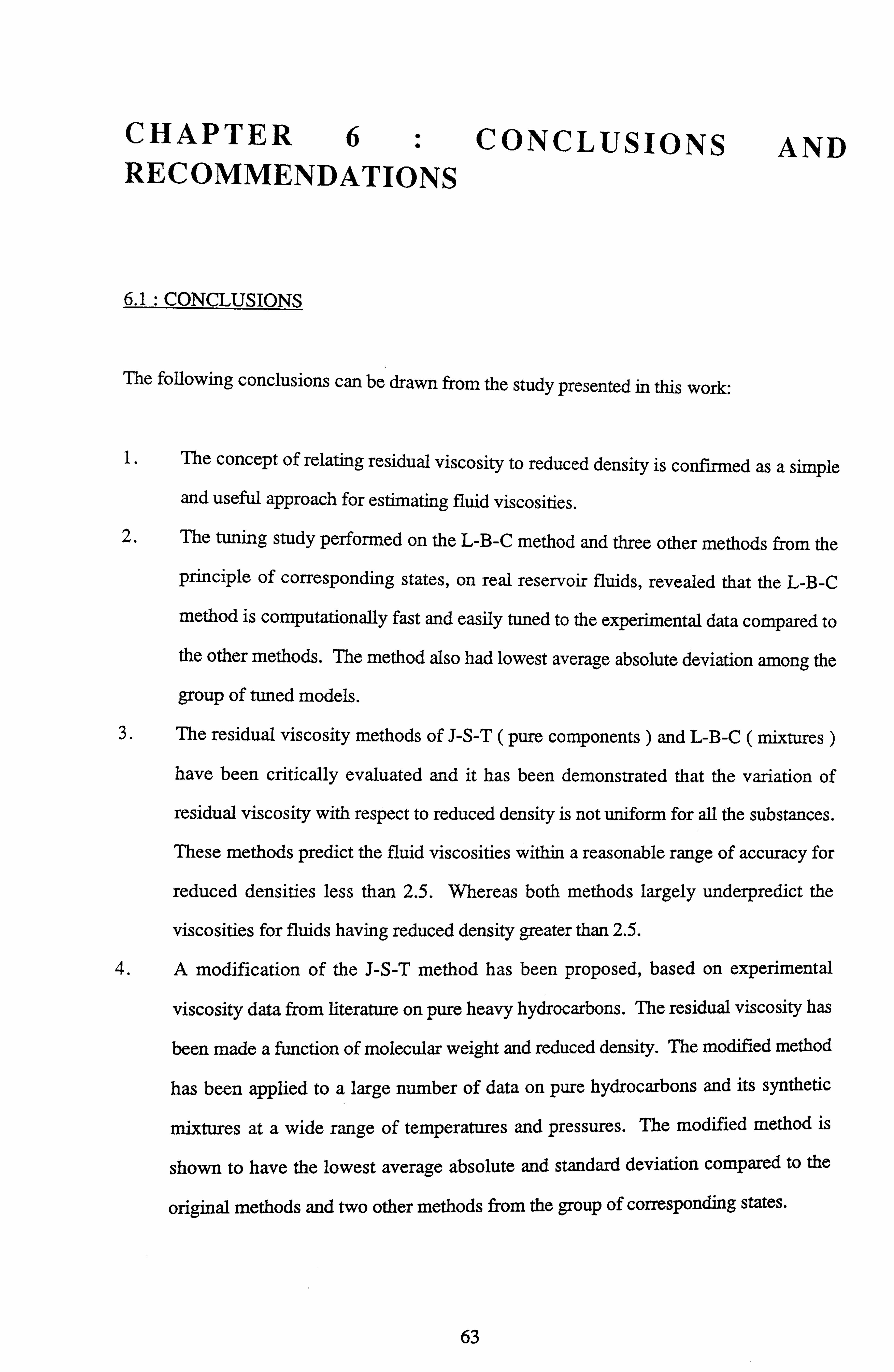
CHAPTER 6: CONCLUSIONS RECOMMENDATIONS
6.1: CONCLUSIONS
The following conclusions can be drawn from the study presented in this work:
AND
1. The concept of relating residual viscosity to reduced density is confined as a simple
and useful approach for estimating fluid viscosities.
2. The tuning study performed on the L-B-C method and three other methods from the
principle of corresponding states, on real reservoir fluids, revealed that the L-B-C
method is computationally fast and easily tuned to the experimental data compared to
the other methods. The method also had lowest average absolute deviation among the
group of tuned models.
3. The residual viscosity methods of J-S-T ( pure components) and L-B-C ( mixtures )
have been critically evaluated and it has been demonstrated that the variation of
residual viscosity with respect to reduced density is not uniform for all the substances.
These methods predict the fluid viscosities within a reasonable range of accuracy for
reduced densities less than 2.5. Whereas both methods largely underpredict the
viscosities for fluids having reduced density greater than 2.5.
4. A modification of the J-S-T method has been proposed, based on experimental
viscosity data from literature on pure heavy hydrocarbons. The residual viscosity has
been made a function of molecular weight and reduced density. The modified method
has been applied to a large number of data on pure hydrocarbons and its synthetic
mixtures at a wide range of temperatures and pressures. The modified method is
shown to have the lowest average absolute and standard deviation compared to the
original methods and two other methods from the group of corresponding states.
63
5. A correlation for estimating the critical volume of the plus fraction of a real reservoir
fluid for the modified correlation has been developed. The modified residual viscosity
correlation is also shown to be superior to the L-B-C method for real reservoir fluids.
6. All methods from the group of principle of corresponding states, (one reference or
two reference) methods and the TRAPP (Ely and Hanley) were found to be highly
inaccurate for dense fluid phase conditions. The methods were also found to be
unreliable at high pressures, the conditions at which the variation of fluid viscosity is
not uniform with respect to the reference component.
6.2: RECOMMENDATIONS
Following are the recommendations which could be made from the study:
1. If reliable and accurate density data is available, the residual viscosity method is highly
recommended for estimation of gas phase viscosities. However, in the absence of
density data, the principle of corresponding states (one reference) method is best
recommended.
2. The modified residual viscosity method is recommended when viscosity predictions
are required for dense phase fluid mixtures (pr > 2.5) provided the density data
supplied is of reasonable accuracy.
3. The extended principle of corresponding states (TRAPP) or the principle of
corresponding states method with two reference components is recommended for
hydrocarbon mixtures where the density data are scarce.
4. There exists a room for modification of the principle of corresponding states method
with two reference components. The method has been found to be unreliable for
fluids having molecular weights more than n-decane (the second reference
component). The prediction capability of the method can be significantly improved by
introduction of a third reference component heavier than n-decane.
64
5. The principle of corresponding states method with one reference component and the
residual viscosity method are best recommended for the purposes of tuning in a
compositional reservoir simulator.
6. A more accurate and reliable correlation for the critical volume (Vc) of the plus fraction
of a real reservoir fluid could further improve the accuracy of the modified residual
viscosity correlation for real reservoir fluids.
65