VISCOSITY SOLUTIONS METHODS FOR CONVERSEKAM THEORY

DIOGO A. GOMES, ADAM OBERMAN

Abstract. We review the connections between the viscosity so-lutions of Hamilton-Jacobi equation and KAM and Aubry-Mathertheories. We prove explicit a priori estimates for smooth viscos-ity solutions. These estimates yield necessary conditions (converseKAM theory) for Hamilton-Jacobi integrability of Hamiltonian sys-tems. These conditions are valid in any space dimension, and canbe implemented rigourously in a computer. We study the integra-bility of several classical examples, including the double pendulum.

1. Introduction

The classical procedure to integrate Hamiltonian systems, that is, to

find explicit solutions to the Hamiltonian dynamics

(1) x = −DpH(p, x) p = DxH(p, x),

is the Hamilton-Jacobi integrability method using generating functions

[AKN97]. A particularly important case is the one in which the Hamil-

tonian H(p, x) : R2n → R is smooth, strictly convex in p, that is,

D2ppH > γ > 0, and periodic in x, that is, H(p, x+ k) = H(p, x) for all

k ∈ Zn. The periodicity in x makes it natural to regard the Hamilton-

ian as a function in Tn × Rn → R, in which Tn is the n dimensional

torus.

This method requires a smooth periodic solution u(x, P ) of the Ham-

ilton-Jacobi equation:

(2) H(P +Dxu, x) = H(P ),

in which H(P ) is the unique value for which the equation admits a

periodic solution u. This solution is called a generating function since

it yields a change of coordinates X(p, x) and P (p, x), defined implicitly

by the equations

(3) p = P +Dxu, X = x+DPu.1

2 DIOGO A. GOMES, ADAM OBERMAN

By performing this change of coordinates, the Hamiltonian dynamics

is simplified to:

P = 0 X = −DPH(P ).

In other words, this means that for each P there is an invariant torus,

the graph p = P + Dxu(x, P ), in which the dynamics is simply a ro-

tation. However, the Hamilton-Jacobi method may fail in practice.

Indeed, (2) may not admit smooth solutions, or (3) may not define

a smooth change of coordinates. In particular, the Hamilton-Jacobi

method may be valid for certain initial conditions of (1) but not every-

where.

Given initial conditions for (1), it is important to determined whether

this integrability procedure can be carried out. In fact, in an integrable

system, sevral complex behaviours like Arnold diffusion, and chaotic

behaviour can be ruled out. The KAM theorem [AKN97] asserts that it

is possible to use the classical Hamilton-Jacobi method for most initial

conditions, provided that the Hamiltonian H has the special structure

H(p, x) = H0(p) + εH1(p, x),

that H0 satisfies non-resonance conditions, and ε is sufficiently small.

Then, the solution u of (2) can be written as a convergent power series

u = u0 + εu1 + ε2u2 + · · · .

There are variations of KAM theory that do not require such a special

structure. However, there are always some type of non-ressonance con-

ditions, as well as a restriction in the size of the perturbations [Lla02].

Using viscosity solutions [BCD97], [FS93], [Eva98], one can prove

that, in general, a weak form of integrability still holds [E99], [Fat97a],

[Fat97b], [Fat98a], [Fat98b], [CIPP98], [EG01a], [EG01b], [Gom01],

and [Gom02b]. Indeed, there exists always a number H(P ) and a peri-

odic viscosity solution u(x, P ) of (2) [LPV88]. Also, one can construct

an invariant set contained in the graph

(x,−DpH(P +Dxu, x)).

This graph contains the support of certain invariant measures - Aubry-

Mather measures [Mat89a], [Mat89b], [Mat91], [Mn92], [Mn96], which

are the natural generalizations of invariant tori. Unfortunately, not

every point is in the support of a Mather measure. Heuristically, one

can think of the phase space partitioned into several sets. One of

VISCOSITY SOLUTIONS METHODS FOR CONVERSE KAM THEORY 3

them is the union of the supports of all Mather measures. Another

one contains heteroclinic and homoclinic connections between different

components of Mather sets. Then, the remaining part of the phase

space contains elliptic periodic orbits and corresponding elliptic islands,

as well as areas in which the motion is irregular, possibly chaotic, as well

is this the region in which Arnold diffusion may occur. It is therefore

of interest to know whether the Mather sets are invariant tori, as in the

integrable case, or if there are gaps and therefore complex behaviour

may be present. The objective of this paper is to understand and give

an effective and rigorous numerical method to answer this question.

There have been several atempts in this direction since the original

paper by MacKay and Percival [MP85]. To cite just a few: [MMS89],

[Mac89], [Kna90], [Har99]. The main idea is that orbits in the Mather

set are absolute minimizers, and several consequences of this fact can

be explored to prove that a certain orbit lies outside the Mather set.

The approach in [MP85], as well as in [MMS89], [Mac89], [Kna90],

follows from the well known that the Mather set is a Lipschitz graph -

therefore if one can find an orbit that is not on a Lipschitz graph one

proves the existence of gaps in the Mather set. These methods seem

to work extremely well for one-dimensional maps, but do not extend

easily for multi-dimensional problems. In [Har99], the main idea is that

the orbits on the Mather set, being global minimizers, are also local

minimizers. Therefore, by computing second derivatives, one can show

that a certain orbit lies outside the Mather set. The main advantage

is that this method work for maps in any dimension.

Other approaches to prove non-integrability include, among others,

renormalization methods, anti-integrable limit, which are fundamen-

tally different from the ones considered in this paper (cite references).

Also a related work that uses variational methods to prove an analytic

counterexample to KAM theory is the paper by Bessi.

The methods that we study in this paper also explore the minimizing

character of the orbits in the Mather set. However, they are quite dif-

ferent from the previous ones. The main idea is to identify conditions

in which (2) does not admit a smooth solution, and therefore proving

the failure of the Hamilton-Jacobi integrability method. These condi-

tions consist in certain inequalities that can be checked numerically in

a very efficient way. The main advantage, however, is that this method

is valid in any dimension.

4 DIOGO A. GOMES, ADAM OBERMAN

The plan of the paper is as follows: in section 2 we review the neces-

sary background from Aubry-Mather theory and viscosity solutions. In

section 3 we prove explicit estimates for viscosity solutions. In section

4 we describe the converse KAM criteria. In section 6 we discuss the

numerical implementation, and finally the examples are considered in

section 7.

2. Aubry Mather measures and Viscosity Solutions

In this section we review background results from the theory of

Aubry-Mather measures and viscosity solutions, and in the following

section we will provide more detailed estimates and proofs.

Let L(x, v), the Lagrangian, be the Legendre transform of the Hamil-

tonian, H(p, x), defined by

L(x, v) = supp−v · p−H(p, x).

In Aubry-Mather theory [Mat89a], [Mat89b], [Mat91], [Mn92], [Mn96]

instead of looking for invariant tori, one looks for probability measures

µ on Tn × Rn that minimize the average action

(4)

∫L(x, v) + P · vdµ,

and satisfy a holonomy condition:∫vDxφdµ = 0,

for all φ(x) ∈ C1(Tn). The supports of these measures are called

the Aubry-Mather sets, and are the natural generalizations of invari-

ant tori. Recent results [E99], [Fat97a], [Fat97b], [Fat98a], [Fat98b],

[CIPP98], [EG01a], [EG01b], and [Gom01] show that viscosity solu-

tions of (2) encode the Aubry-Mather sets. In particular, we have∫L(x, v) + P · vdµ = −H(P ),

and the support of the Mather measure is a subset of the graph

(5) (x, v) = (x,−DpH(P +Dxu, x)),

for any viscosity solution of (2). Furthermore, the Mather set is invari-

ant under the flow generated by the Euler-Lagrange equations

(6)d

dtDvL(x, x)−DxL = 0,

VISCOSITY SOLUTIONS METHODS FOR CONVERSE KAM THEORY 5

which are equivalent by the Legendre transform p = P +DvL(x, x) to

(1).

In the Mather set, the asymptotics of the Hamiltonian dynamics are

controlled by viscosity solutions. Indeed, let (x, p) be any point in

Tn × Rn. Consider its flow by the Hamilton equations (1). If (x, p)

belongs to any Mather set then

x(T )

T→ Q,

as T →∞, for some vector Q ∈ Rn, with Q = −DPH(P ), for some P

if H is differentiable.

To find non-integrable regions, our strategy is the following: first we

prove rigorous estimates that either smooth solutions of (2) have to

satisfy. Then, numerically, one can verify whether these estimates are

satisfied or not, and therefore detect non-integrability.

3. Explicit estimates for viscosity solutions

In partial differential equations one frequently obtains estimates for

the solutions that depend on constants whose specific value is unim-

portant. However, for our purposes in this paper, we need explicit

estimates, and to understand the dependence of the viscosity solutions

with respect to parameters. Therefore , in this section we reprove some

known results, but taking care of tracking the constants with detail.

The main guiding principles are the following: we assume that we are

given a point (x, x), and we would like to investigate whether there is

a vector P , and a smooth solution u to (2) such that this point lies

in an invariant graph given by (5). The main difficulty with this ap-

proach is that P , u. Therefore our objective is to prove estimates for

P and u that only depend on known quantities. These estimates are:

bounds for second derivatives of u, uniform Lipschitz for u, bounds for

P in terms of the initial energy, and error estimates for the numerical

computation of H(P ).

In this section, and in the remaining part of the paper, we assume

that the Lagrangian has the form

L(x, x) = gij(x)xixj + hi(x)xi − V (x),

in which gij(x) is a positive definite metric, hi represents the magnetic

field and V (x) is the potential energy.

6 DIOGO A. GOMES, ADAM OBERMAN

First, we recall the well known fact that the energy is conserved by

the Euler-Lagrange equations, as well as the expression for the Hamil-

tonian. The proof of the next proposition can be found in any book on

classical mechanics, for instance [AKN97], or [Gol80].

Proposition 1. The energy

E =1

2gij(x)xixj + V (x)

is conserved by the Euler-Lagrange equations. The Hamiltonian corre-

sponding to L is given by

H =1

2gij(x)(pj − hj)(pi − hi) + V (x),

in which gij is the inverse of gij, that is gikgkj = δij. Furthermore

H(p, x) = E(x, x) for pj = gijxi + hj.

Remark. Note that the energy does not depend on the magnetic

field h. This is important because one of the our main examples is

L = x2

2+ Px+ V (x) and P may be unknown.

There are several important examples that fit this framework. For

instance, the one dimensional pendulum:

L =x2

2+ cos(2πx), H =

p2

2− cos(2πx),

the double pendulum

L(x1, x2, x1, x2) =

=2p2

1 + p22 + 2p1p2 cos(2π(x1 − x2))

2+ 2 cos(2πx1) + cos(2πx2),

whose corresponding Hamiltonian is

H(p1, p2, x1, x2) =

=p2

1 + 2p22 − 2p1p2 cos (2π(x1 − x2))

2[1 + sin2 (2π(x1 − x2))

] − 2 cos(2πx1)− cos(2πx2),

and a particle in an space-periodic magnetic field, for instance:

L =x2

1 + x22

2+ cosx1x2 − sin x2x1,

with

H =(p1 + sinx2)

2 + (p2 − cosx1)2

2.

VISCOSITY SOLUTIONS METHODS FOR CONVERSE KAM THEORY 7

To write our estimates as explicitly as possible, we assume the fol-

lowing bounds for the metric gij, the magnetic field hi and potential

V :

(1) gij(x) ≥ c0, gij(x) ≤ c1, |Dxgij(x)| ≤ c3, and |D2xxgij(x)| ≤ c4;

(2) |hi(x)| ≤ c5, |Dxhi(x)| ≤ c6, and |D2xxhi(x)| ≤ c7;

(3) 0 ≤ V (x) ≤ c8, |DxV | ≤ c9, |D2xxV | ≤ c10.

With these bounds we have that we can estimate the velocity x by

the energy

Proposition 2.

|x| ≤ (2E)1/2

c1/20

.

Proof. Since V ≥ 0 then

1

2c0|x|2 ≤

1

2gijxixj ≤ E.

�In the problems that we consider, the energy is a computable quan-

tity, since it only depends on the initial conditions. The previous result

implies that one can obtain uniform bounds on the velocity based sim-

ply on the initial conditions.

The viscosity solutions of (2) have an interpretation in terms of con-

trol theory. In fact, a function u is a viscosity solution of (2) if and

only if it satisfies the following fixed point identity:

(7) u(x) = inf

∫ t

0

L(x, x) + Px+H(P )dt+ u(x(t)),

in which the infimum is taken over Lipschitz trajectories x(·), with

initial condition x(0) = x. This control theory interpretation makes

possible to establish important properties for the viscosity solution such

as semiconcavity.

Theorem 1. Let u be a viscosity solution of (2), and assume that

x(t) is an optimal trajectory for (7) with initial energy E. Then u is

semiconcave, that is,

u(x+ y)− 2u(x) + u(x− y) ≤ C|y|2.

For |y| ≤ k1, the constant C is estimated by:

C ≤√c1

[c44

(2E

c0+k2

1

c1

)+ c7

(2E

c0+k2

1

c1

)1/2

+ c10 + 2

].

8 DIOGO A. GOMES, ADAM OBERMAN

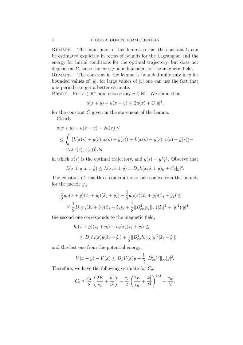
Remark. The main point of this lemma is that the constant C can

be estimated explicitly in terms of bounds for the Lagrangian and the

energy for initial conditions for the optimal trajectory, but does not

depend on P , since the energy is independent of the magnetic field.

Remark. The constant in the lemma is bounded uniformly in y for

bounded values of |y|, for large values of |y| one can use the fact that

u is periodic to get a better estimate.

Proof. Fix x ∈ Rn, and choose any y ∈ Rn. We claim that

u(x+ y) + u(x− y) ≤ 2u(x) + C|y|2,

for the constant C given in the statement of the lemma.

Clearly

u(x+ y) + u(x− y)− 2u(x) ≤

≤∫ t

0

[L(x(s) + y(s), x(s) + y(s)) + L(x(s) + y(s), x(s) + y(s))−

−2L(x(s), x(s))] ds,

in which x(s) is the optimal trajectory, and y(s) = y t−st

. Observe that

L(x± y, x± y) ≤ L(x, x± y)±DxL(x, x± y)y + C0|y|2.

The constant C0 has three contributions: one comes from the bounds

for the metric gij

1

2gij(x+ y)(xi + yi)(xj + yj)−

1

2gij(x)(xi + yi)(xj + yj) ≤

≤ 1

2Dxgij(xi + yi)(xj + yj)y +

1

8‖D2

xxgij‖∞(|xi|2 + |y|2)|y|2;

the second one corresponds to the magnetic field,

hi(x+ y)(xi + yi)− hi(x)(xi + yi) ≤

≤ Dxhi(x)y(xi + yi) +1

2‖D2

xxhi‖∞|y|2|xi + yi|;

and the last one from the potential energy:

V (x+ y)− V (x) ≤ DxV (x)y +1

2‖D2

xxV ‖∞|y|2.

Therefore, we have the following estimate for C0:

C0 ≤c48

(2E

c0+k1

t2

)+c72

(2E

c0+k2

1

t2

)1/2

+c10

2.

VISCOSITY SOLUTIONS METHODS FOR CONVERSE KAM THEORY 9

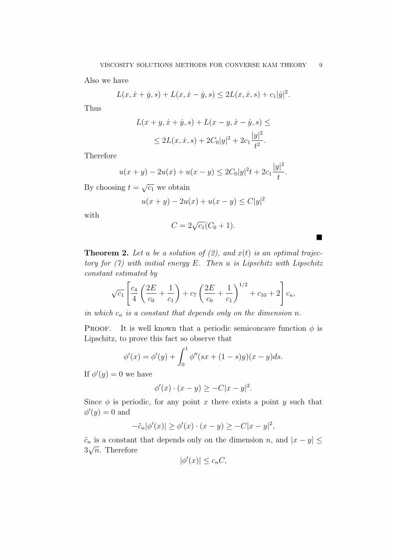
Also we have

L(x, x+ y, s) + L(x, x− y, s) ≤ 2L(x, x, s) + c1|y|2.

Thus

L(x+ y, x+ y, s) + L(x− y, x− y, s) ≤

≤ 2L(x, x, s) + 2C0|y|2 + 2c1|y|2

t2.

Therefore

u(x+ y)− 2u(x) + u(x− y) ≤ 2C0|y|2t+ 2c1|y|2

t.

By choosing t =√c1 we obtain

u(x+ y)− 2u(x) + u(x− y) ≤ C|y|2

with

C = 2√c1(C0 + 1).

�

Theorem 2. Let u be a solution of (2), and x(t) is an optimal trajec-

tory for (7) with initial energy E. Then u is Lipschitz with Lipschitz

constant estimated by

√c1

[c44

(2E

c0+

1

c1

)+ c7

(2E

c0+

1

c1

)1/2

+ c10 + 2

]cn,

in which cn is a constant that depends only on the dimension n.

Proof. It is well known that a periodic semiconcave function φ is

Lipschitz, to prove this fact so observe that

φ′(x) = φ′(y) +

∫ 1

0

φ′′(sx+ (1− s)y)(x− y)ds.

If φ′(y) = 0 we have

φ′(x) · (x− y) ≥ −C|x− y|2.

Since φ is periodic, for any point x there exists a point y such that

φ′(y) = 0 and

−cn|φ′(x)| ≥ φ′(x) · (x− y) ≥ −C|x− y|2,

cn is a constant that depends only on the dimension n, and |x − y| ≤3√n. Therefore

|φ′(x)| ≤ cnC,

10 DIOGO A. GOMES, ADAM OBERMAN

in which cn is a constant that depends only on the dimension n. �

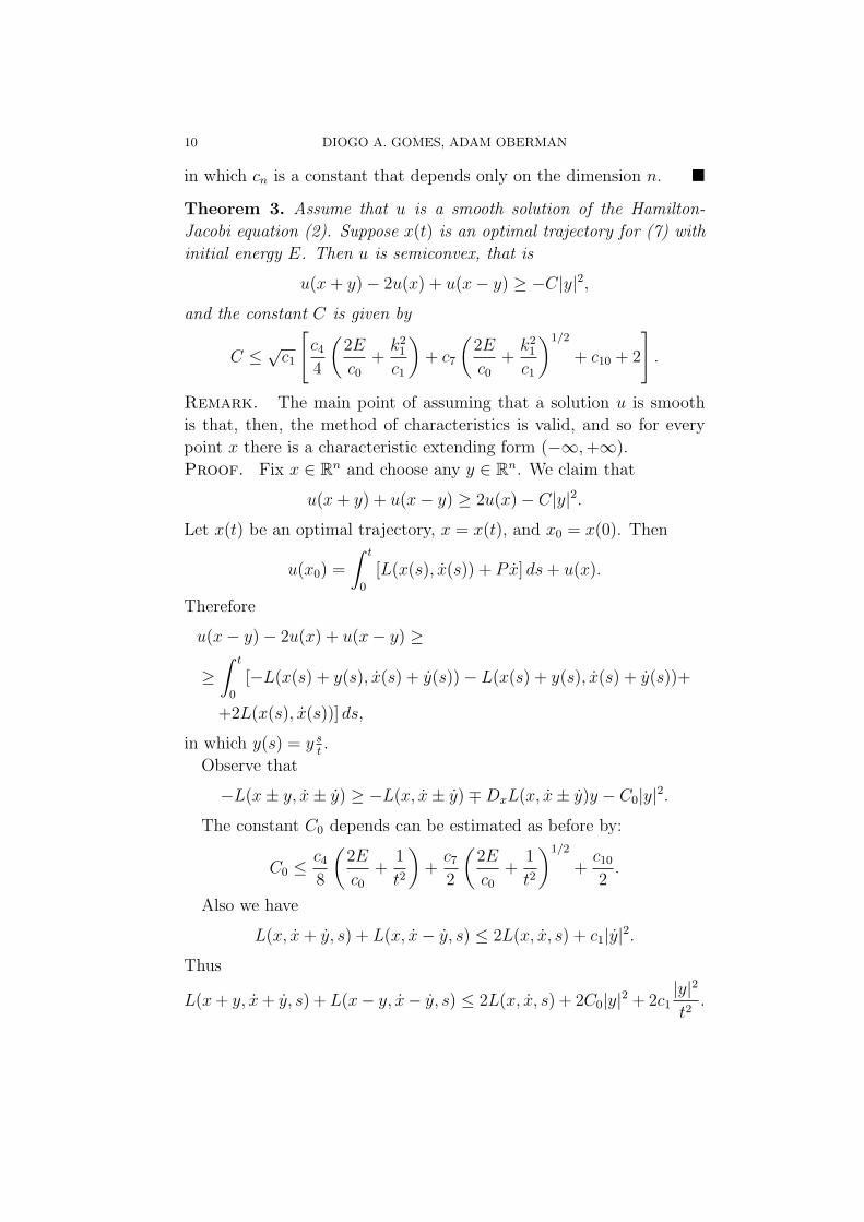
Theorem 3. Assume that u is a smooth solution of the Hamilton-

Jacobi equation (2). Suppose x(t) is an optimal trajectory for (7) with

initial energy E. Then u is semiconvex, that is

u(x+ y)− 2u(x) + u(x− y) ≥ −C|y|2,

and the constant C is given by

C ≤√c1

[c44

(2E

c0+k2

1

c1

)+ c7

(2E

c0+k2

1

c1

)1/2

+ c10 + 2

].

Remark. The main point of assuming that a solution u is smooth

is that, then, the method of characteristics is valid, and so for every

point x there is a characteristic extending form (−∞,+∞).

Proof. Fix x ∈ Rn and choose any y ∈ Rn. We claim that

u(x+ y) + u(x− y) ≥ 2u(x)− C|y|2.

Let x(t) be an optimal trajectory, x = x(t), and x0 = x(0). Then

u(x0) =

∫ t

0

[L(x(s), x(s)) + Px] ds+ u(x).

Therefore

u(x− y)− 2u(x) + u(x− y) ≥

≥∫ t

0

[−L(x(s) + y(s), x(s) + y(s))− L(x(s) + y(s), x(s) + y(s))+

+2L(x(s), x(s))] ds,

in which y(s) = y st.

Observe that

−L(x± y, x± y) ≥ −L(x, x± y)∓DxL(x, x± y)y − C0|y|2.

The constant C0 depends can be estimated as before by:

C0 ≤c48

(2E

c0+

1

t2

)+c72

(2E

c0+

1

t2

)1/2

+c102.

Also we have

L(x, x+ y, s) + L(x, x− y, s) ≤ 2L(x, x, s) + c1|y|2.

Thus

L(x+ y, x+ y, s) + L(x− y, x− y, s) ≤ 2L(x, x, s) + 2C0|y|2 + 2c1|y|2

t2.

VISCOSITY SOLUTIONS METHODS FOR CONVERSE KAM THEORY 11

Therefore

u(x+ y)− 2u(x) + u(x− y) ≥ −2C0|y|2t− 2c1|y|2

t.

By choosing t =√c1 we obtain

u(x+ y)− 2u(x) + u(x− y) ≥ −C|y|2

with

C = 2√c1(C0 + 1).

�Because of non-smoothness, it is difficult to solve (2) directly, and in

particular determining H(P ). In the integrable case, the value H(P )

agrees with the initial energy. However, if the initial conditions (x, x)

are not in the integrable region, then H is not defined. In fact, we have

the following inequality:

Proposition 3. Let (x, x) be an arbitrary point, and (x(t), x(t)) the

corresponding solution of (6). Then, for any P

H(P ) ≥ E(x, x) + limT→∞

1

T

∫ T

0

(p− P )x.

Remark. In the integrable case p− P = Dxu, and therefore the last

term vanishes.

Proof. We have

−H(P ) ≤ limT→∞

1

T

∫ T

0

L(x, x) + Px.

Since L(x, x) = −px− E(x, x) we conclude

−H(P ) ≤ −E(x, x) + limT→∞

1

T

∫ T

0

(P − p)x.

�It is therefore convenient to use a different formula to compute the

value ofH to explore this inequality. Given a value P , there are efficient

numerical methods to compute H(P ), and control the error [GO02].

These algorithms are based on the representation formula for H(P )

(8) H(P ) = infφ∈C1

per

supxH(P +Dxφ, x)

due to [CIPP98] (see also, for a more general setting, [LS02]).

12 DIOGO A. GOMES, ADAM OBERMAN

Let Th be a set of piecewise linear finite elements, and Hh(P ) be the

numerical approximation computed by:

Hh(P ) = infφ∈Th

esssupx

H(Dxφ, x).

Then the main error estimate is:

Theorem 4. For any convex Hamiltonian H(p, x) for which (2) has a

viscosity solution

H ≤ Hh(P ).

Furthermore, if (2) has a smooth viscosity solution then

Hh(P ) ≤ H(P ) + Ch,

and the constant depends only on bounds for the Hamiltonian, as well

as the energy, but not on P .

Proof. The first claim, that is,

H = infψ∈C1(Tn)

supxH(P +Dxψ, x) ≤ inf

φ∈Th

esssupx

H(P +Dxφ, x),

can be proved in the following way: to each φ ∈ Th we associate a

function

ψ = φ ∗ ηε ∈ C1(Tn).

Then the convexity of H implies

supxH(P +Dxψ, x) ≤ esssup

xH(P +Dxφ, x) +O(ε),

since

H(P +Dx(φ ∗ ηε)(x), x) ≤∫H(P +Dxφ(y), y)ηε(x− y)dy +O(ε).

Since ε is arbitrary, we get the desired inequality.

Before proving the second part we need a lemma:

Lemma 1. There exists a constant C such that

|P | ≤ H(P ) + C.

Proof. Let ω be an arbitrary vector such that |ω| = 1, and ω · k = 0

for k ∈ Zn implies k = 0, that is the flow x = ω is ergodic on torus.

Let x(t) = ωt. Then

H(P ) ≥ limt→∞

L(x, x) + Px = Pω +

∫Tn

L(x, ω)dx,

VISCOSITY SOLUTIONS METHODS FOR CONVERSE KAM THEORY 13

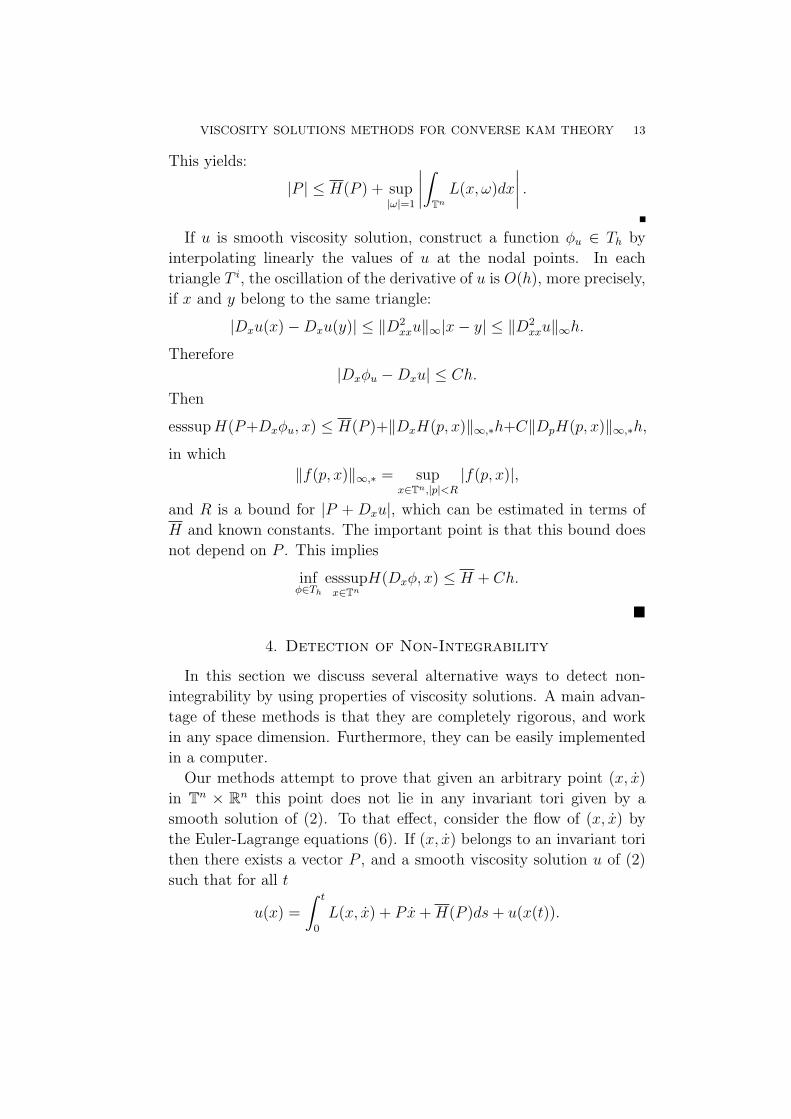
This yields:

|P | ≤ H(P ) + sup|ω|=1

∣∣∣∣∫Tn

L(x, ω)dx

∣∣∣∣ .If u is smooth viscosity solution, construct a function φu ∈ Th by

interpolating linearly the values of u at the nodal points. In each

triangle T i, the oscillation of the derivative of u is O(h), more precisely,

if x and y belong to the same triangle:

|Dxu(x)−Dxu(y)| ≤ ‖D2xxu‖∞|x− y| ≤ ‖D2

xxu‖∞h.

Therefore

|Dxφu −Dxu| ≤ Ch.

Then

esssupH(P+Dxφu, x) ≤ H(P )+‖DxH(p, x)‖∞,∗h+C‖DpH(p, x)‖∞,∗h,

in which

‖f(p, x)‖∞,∗ = supx∈Tn,|p|<R

|f(p, x)|,

and R is a bound for |P + Dxu|, which can be estimated in terms of

H and known constants. The important point is that this bound does

not depend on P . This implies

infφ∈Th

esssupx∈Tn

H(Dxφ, x) ≤ H + Ch.

�

4. Detection of Non-Integrability

In this section we discuss several alternative ways to detect non-

integrability by using properties of viscosity solutions. A main advan-

tage of these methods is that they are completely rigorous, and work

in any space dimension. Furthermore, they can be easily implemented

in a computer.

Our methods attempt to prove that given an arbitrary point (x, x)

in Tn × Rn this point does not lie in any invariant tori given by a

smooth solution of (2). To that effect, consider the flow of (x, x) by

the Euler-Lagrange equations (6). If (x, x) belongs to an invariant tori

then there exists a vector P , and a smooth viscosity solution u of (2)

such that for all t

u(x) =

∫ t

0

L(x, x) + Px+H(P )ds+ u(x(t)).

14 DIOGO A. GOMES, ADAM OBERMAN

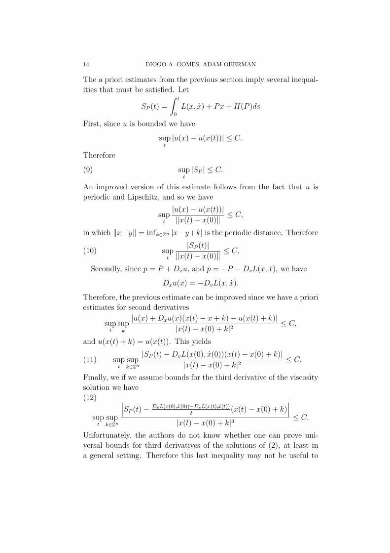
The a priori estimates from the previous section imply several inequal-

ities that must be satisfied. Let

SP (t) =

∫ t

0

L(x, x) + Px+H(P )ds

First, since u is bounded we have

supt|u(x)− u(x(t))| ≤ C.

Therefore

(9) supt|SP | ≤ C.

An improved version of this estimate follows from the fact that u is

periodic and Lipschitz, and so we have

supt

|u(x)− u(x(t))|‖x(t)− x(0)‖

≤ C,

in which ‖x−y‖ = infk∈Zn |x−y+k| is the periodic distance. Therefore

(10) supt

|SP (t)|‖x(t)− x(0)‖

≤ C,

Secondly, since p = P +Dxu, and p = −P −DvL(x, x), we have

Dxu(x) = −DvL(x, x).

Therefore, the previous estimate can be improved since we have a priori

estimates for second derivatives

supt

supk

|u(x) +Dxu(x)(x(t)− x+ k)− u(x(t) + k)||x(t)− x(0) + k|2

≤ C,

and u(x(t) + k) = u(x(t)). This yields

(11) supt

supk∈Zn

|SP (t)−DvL(x(0), x(0))(x(t)− x(0) + k)||x(t)− x(0) + k|2

≤ C.

Finally, we if we assume bounds for the third derivative of the viscosity

solution we have

(12)

supt

supk∈Zn

∣∣∣SP (t)− DvL(x(0),x(0))−DvL(x(t),x(t))2

(x(t)− x(0) + k)∣∣∣

|x(t)− x(0) + k|3≤ C.

Unfortunately, the authors do not know whether one can prove uni-

versal bounds for third derivatives of the solutions of (2), at least in

a general setting. Therefore this last inequality may not be useful to

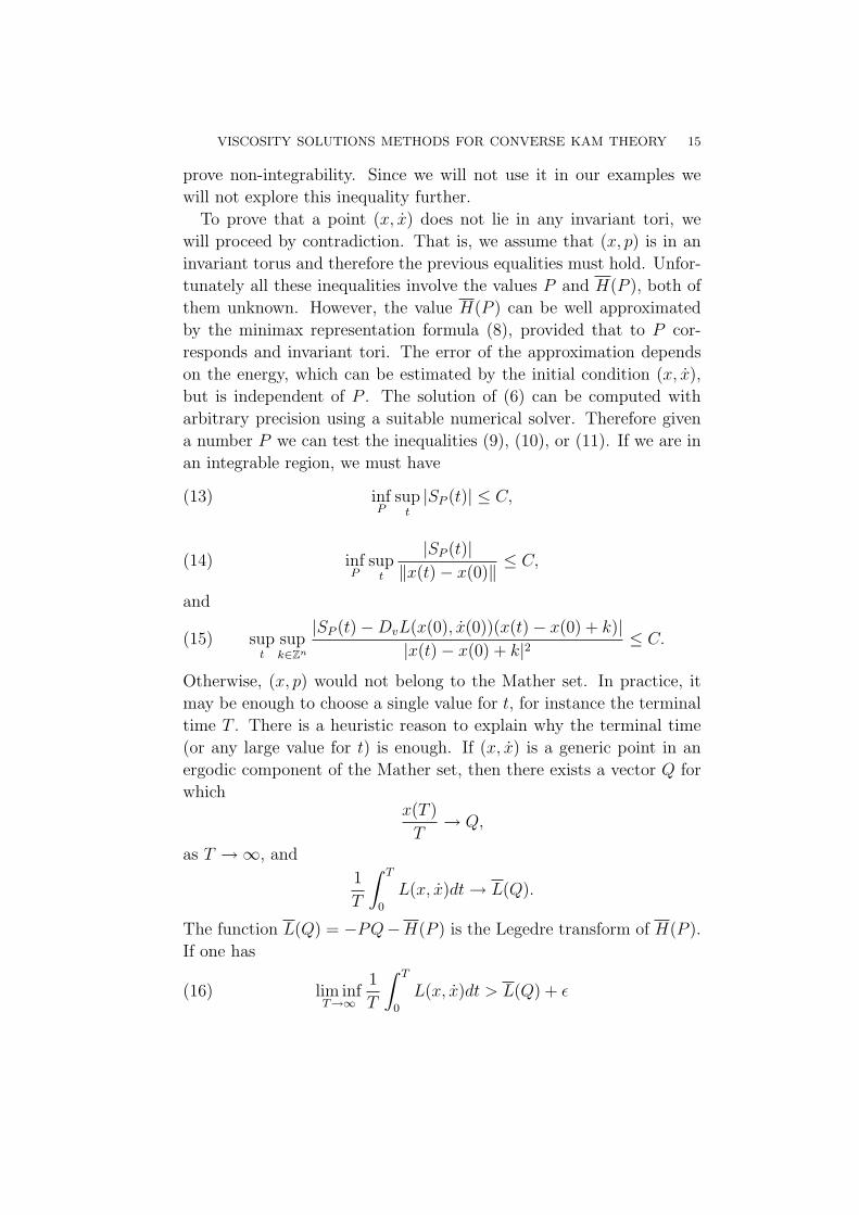
VISCOSITY SOLUTIONS METHODS FOR CONVERSE KAM THEORY 15

prove non-integrability. Since we will not use it in our examples we

will not explore this inequality further.

To prove that a point (x, x) does not lie in any invariant tori, we

will proceed by contradiction. That is, we assume that (x, p) is in an

invariant torus and therefore the previous equalities must hold. Unfor-

tunately all these inequalities involve the values P and H(P ), both of

them unknown. However, the value H(P ) can be well approximated

by the minimax representation formula (8), provided that to P cor-

responds and invariant tori. The error of the approximation depends

on the energy, which can be estimated by the initial condition (x, x),

but is independent of P . The solution of (6) can be computed with

arbitrary precision using a suitable numerical solver. Therefore given

a number P we can test the inequalities (9), (10), or (11). If we are in

an integrable region, we must have

(13) infP

supt|SP (t)| ≤ C,

(14) infP

supt

|SP (t)|‖x(t)− x(0)‖

≤ C,

and

(15) supt

supk∈Zn

|SP (t)−DvL(x(0), x(0))(x(t)− x(0) + k)||x(t)− x(0) + k|2

≤ C.

Otherwise, (x, p) would not belong to the Mather set. In practice, it

may be enough to choose a single value for t, for instance the terminal

time T . There is a heuristic reason to explain why the terminal time

(or any large value for t) is enough. If (x, x) is a generic point in an

ergodic component of the Mather set, then there exists a vector Q for

whichx(T )

T→ Q,

as T →∞, and

1

T

∫ T

0

L(x, x)dt→ L(Q).

The function L(Q) = −PQ−H(P ) is the Legedre transform of H(P ).

If one has

(16) lim infT→∞

1

T

∫ T

0

L(x, x)dt > L(Q) + ε

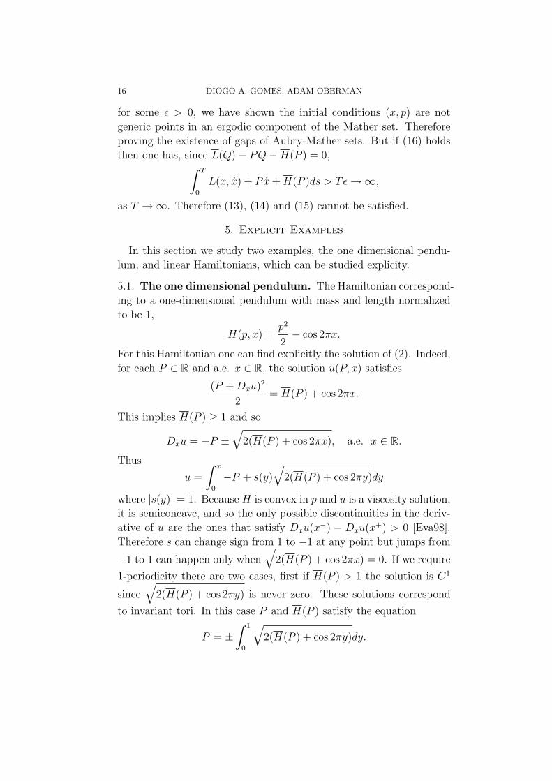
16 DIOGO A. GOMES, ADAM OBERMAN

for some ε > 0, we have shown the initial conditions (x, p) are not

generic points in an ergodic component of the Mather set. Therefore

proving the existence of gaps of Aubry-Mather sets. But if (16) holds

then one has, since L(Q)− PQ−H(P ) = 0,∫ T

0

L(x, x) + Px+H(P )ds > Tε→∞,

as T →∞. Therefore (13), (14) and (15) cannot be satisfied.

5. Explicit Examples

In this section we study two examples, the one dimensional pendu-

lum, and linear Hamiltonians, which can be studied explicity.

5.1. The one dimensional pendulum. The Hamiltonian correspond-

ing to a one-dimensional pendulum with mass and length normalized

to be 1,

H(p, x) =p2

2− cos 2πx.

For this Hamiltonian one can find explicitly the solution of (2). Indeed,

for each P ∈ R and a.e. x ∈ R, the solution u(P, x) satisfies

(P +Dxu)2

2= H(P ) + cos 2πx.

This implies H(P ) ≥ 1 and so

Dxu = −P ±√

2(H(P ) + cos 2πx), a.e. x ∈ R.

Thus

u =

∫ x

0

−P + s(y)

√2(H(P ) + cos 2πy)dy

where |s(y)| = 1. Because H is convex in p and u is a viscosity solution,

it is semiconcave, and so the only possible discontinuities in the deriv-

ative of u are the ones that satisfy Dxu(x−) − Dxu(x

+) > 0 [Eva98].

Therefore s can change sign from 1 to −1 at any point but jumps from

−1 to 1 can happen only when√

2(H(P ) + cos 2πx) = 0. If we require

1-periodicity there are two cases, first if H(P ) > 1 the solution is C1

since√

2(H(P ) + cos 2πy) is never zero. These solutions correspond

to invariant tori. In this case P and H(P ) satisfy the equation

P = ±∫ 1

0

√2(H(P ) + cos 2πy)dy.

VISCOSITY SOLUTIONS METHODS FOR CONVERSE KAM THEORY 17

It is easy to check that this equation has a solution H(P ) whenever

|P | ≥∫ 1

0

√2(1 + cos 2πy)dy,

that is

|P | > 4

π' 1.27324.

When this inequality fails, H(P ) = 1 and s(x) can have a discontinuity.

Indeed, s(x) jumps from −1 to 1 when x = 12

+ k, with k ∈ Z, and

there is a point x0 defined by the equation

−∫ 1

0

s(y)√

2(1 + cos 2πy)dy = P,

such that s(x) jumps from 1 to −1 at x0 + k, k ∈ Z.

Therefore, since for E < 1 there is no P and u(x) smooth so that

H(P +Dxu, x) = E,

these energy levels should be non-integrable (in the sense defined be-

fore, that is, the invariant sets are not Lagrangian graphs). In fact we

can detect this behaviour using our methods. We have

SP (T ) =

∫ T

0

L(x, x) + Pv +H(P ) =

=

∫ T

0

(P − p(t))x(t)−H(p(t), x(t)) +H(P ).

Since for E < 1 the trajectories are periodic we have∫ Tn

0

Px = 0,

for Tn a multiple of the period. We have x = −p(t). Thus∫ Tn

0

−p(t)v(t) ≥ 0.

Since H(P )−H(p, x) ≥ 1− E > 0, the integral∫ Tn

0

H(P )−H(p(t), x(t))dt

is unbounded.

18 DIOGO A. GOMES, ADAM OBERMAN

5.2. Linear Hamiltonians. It is well known that there may not exit

smooth solutions to the linear Hamilton-Jacobi equation

ω · (P +Dxu) + V (x) = H(P ),

with ω ∈ Rn. The Hamiltonian H(p, x) = ω · p + V (x) is convex in

p but not strictly convex, however as we will show, our methods still

work to detect non-integrability in some cases.

There is a necessary condition for the existence of solutions of the

Hamilton-Jacobi equation, which is∫ω · (P +Dxu) + V (x) =

∫H(P ),

that is

H(P ) = ω · P +H(0),

with H(0) =∫V (x), which we can assume to be zero.

The Lagrangian corresponding to the Hamiltonian is

L(v, x) =

{−V (x) if v = −ω+∞ otherwise.

The equation of the dynamics are

x = −ωp = −2πsin(2πx1).

Therefore the action SP (T ) is given by

SP (T ) =

∫ T

0

−V (x0 + ωt)dt

We consider three examples. The first one:

H(p, s) = (1,√

2) · p+ cos(2πx1),

that is, ω = (1,√

2). In this case, one can construct a smooth solution

to the Hamilton-Jacobi equation by using Fourier series. Therefore

SP (T ) =

∫ T

0

− cos(2πx1(0) + 2πt)dt,

which is bounded uniformly in T for any value of x1(0).

The second case is

(1, 1) ·Du+ cos(2πx1),

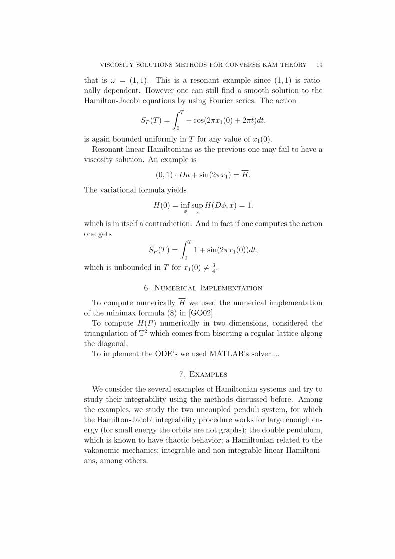
VISCOSITY SOLUTIONS METHODS FOR CONVERSE KAM THEORY 19

that is ω = (1, 1). This is a resonant example since (1, 1) is ratio-

nally dependent. However one can still find a smooth solution to the

Hamilton-Jacobi equations by using Fourier series. The action

SP (T ) =

∫ T

0

− cos(2πx1(0) + 2πt)dt,

is again bounded uniformly in T for any value of x1(0).

Resonant linear Hamiltonians as the previous one may fail to have a

viscosity solution. An example is

(0, 1) ·Du+ sin(2πx1) = H.

The variational formula yields

H(0) = infφ

supxH(Dφ, x) = 1.

which is in itself a contradiction. And in fact if one computes the action

one gets

SP (T ) =

∫ T

0

1 + sin(2πx1(0))dt,

which is unbounded in T for x1(0) 6= 34.

6. Numerical Implementation

To compute numerically H we used the numerical implementation

of the minimax formula (8) in [GO02].

To compute H(P ) numerically in two dimensions, considered the

triangulation of T2 which comes from bisecting a regular lattice algong

the diagonal.

To implement the ODE’s we used MATLAB’s solver....

7. Examples

We consider the several examples of Hamiltonian systems and try to

study their integrability using the methods discussed before. Among

the examples, we study the two uncoupled penduli system, for which

the Hamilton-Jacobi integrability procedure works for large enough en-

ergy (for small energy the orbits are not graphs); the double pendulum,

which is known to have chaotic behavior; a Hamiltonian related to the

vakonomic mechanics; integrable and non integrable linear Hamiltoni-

ans, among others.

20 DIOGO A. GOMES, ADAM OBERMAN

7.1. Uncoupled penduli. We consider the following Hamiltonian

H(px, py, x, y) =p2x + p2

y

2+ sin 2πx+ sin 2πy.

The corresponding Lagrangian is

L(vx, vy, x, y) =v2x + v2

y

2− sin 2πx− sin 2πy.

The equations of the dynamics are

px = 2π cos 2πx

py = 2π cos 2πx

x = −pxy = −py.

To plot the non integrable regions we choose an initial point (x, y)

and then vary the values of px and py. We only consider method one

and plot for large T the value

infPSP (T ).

We have the plots for (x, y) = (0, 0) and (x, y) = (34, 3

4).

7.2. Double pendulum. The Lagrangian for the double pendulum is

L(vx, vy, x, y) =ml22v2

x + v2y + 2vxvy cos(2π(x− y))

2+

+mgl(2 cos 2πx+ cos 2πy).

Setting m=l=g=1 we compute the Legendre transform, using the fact

that if

L =1

2vTMv + b

is a quadratic form, then the Legendre transform yields p = Mv, and

H =1

2pTM−1p− b.

This gives

px = 2vx + vy cos(2π(x− y)) py = vy + vx cos(2π(x− y))

and

H(px, py, x, y) =1

2

p2x − 2pxpy cos(2π(x− y)) + 2p2

y

2− cos2(2π(x− y))−

− 2 cos 2πx− cos 2πy.

VISCOSITY SOLUTIONS METHODS FOR CONVERSE KAM THEORY 21

The equations of the dynamics are

px =π−2(p2

x + 2p2y) cos(θ) + pxpy (5 + cos(2θ)) sin(θ)

(−2 + cos2(θ))2 +

+ 4π sin(2πx)

py =π2(p2

x + 2p2y) cos(θ)− pxpy (5 + cos(2θ)) sin(θ)

(−2 + cos2(θ))2 +

+ 2π sin(2πy)

x =− px − py cos(θ)

2− cos2(θ)

y =− 2py − px cos(θ)

2− cos2(θ),

in which θ = 2π(x− y).

We have the plots for (x, y) = (0, 0)

7.3. Vakonomic Hamiltonians. In this section we consider a class

of Hamiltonians which is convex but not strictly convex - and therefore

some of the previous estimates do not apply immediately.

As an example, consider

H(p, x) =|f1 ·Du|2

2+|f2 ·Du|2

2+ V (x, y)

in which the vector fields f1, f2 do not span R2 in every point but when

we consider the commutator [f1, f2] we have that f1, f2, [f1, f2] span R2

in every point. In this situation (2) has Holder continuous viscosity

solutions [EJ89], [Gom02a].

We chose V = 0, f1 = (0, 1), and f2 = (cos 2πx2, sin 2πx2). If

sin 2πx2 = 0 f2 = (0,±1) and so f1 and f2 are linearly dependent.

However

[f1, f2] = 2π(− sin 2πx2, cos 2πx2),

and so f1, f2, [f1, f2] always span R2. Therefore there is a Holder con-

tinuous viscosity solution.

In fact, this example can be reduced to a one-dimensional example.

The Hamilton-Jacobi equation is

cos2 2πx2

2(P1 + ux1)

2 +(1 + sin2 2πx2)

2(P2 + ux2)

2+

+ sin 2πx2 cos 2πx2(P1 + ux1)(P2 + ux2) = H(P1, P2).

22 DIOGO A. GOMES, ADAM OBERMAN

Since there is no explicit dependence in x1 there are solutions indepen-

dent of x1, given by the equation

cos2 2πx2

2P 2

1 +(1 + sin2 2πx2)

2(P2 + ux2)

2+

+ sin 2πx2 cos 2πx2P1(P2 + ux2) = H(P1, P2).

Since this equation is strictly convex in ux2 there is a Lipschitz solution.

To remove this degeneracy we considered the potential V (x1, x2) =

cos 2πx1 + sin 2π(x1 − x2), for which the previous reduction procedure

does not work.

The Lagrangian for this system is

L =1

2

(v2

1 − 2 cotan(2πx2)v1v2 + (−1 + 2 cosec2(2πx2))v22

)−

− cos 2πx1 − sin 2π(x1 − x2).

Note that the Lagragian has singularities which are a consequence of

H not being strictly convex.

The equations of the dynamics are

p1 =− 2π sin 2πx1 + 2π cos 2π(x1 − x2).

p2 =− cos(2πx2) sin(2πx2)p21 + sin(2πx2) cos(2πx2)p

22+

+ 2π cos2 2πx2p1p2 − 2π sin2 2πx2p1p2−− 2π cos 2π(x1 − x2)

x1 =− cos2(2πx2)p1 − sin(2πx2) cos(2πx2)p2

x2 =− (1 + sin2(2πx2))p2 − sin(2πx2) cos(2πx2)p1.

The Holder continuity of the solution u implies that the action

infP

supt|SP (t)| ≤ C,

and the quotient

infP

supt

|SP (t)|‖x(t)− x(0)‖α

≤ C,

if the trajectory x(t) lies on a torus.

We have the plots for (x, y) = (0, 0) ....

7.4. Time-periodic Hamiltonians. Another example is a periodic

time-dependent, one space dimension Hamilton-Jacobi equation:

−ut +H(Dxu, x, t) = H.

VISCOSITY SOLUTIONS METHODS FOR CONVERSE KAM THEORY 23

There exists a unique value H for which this problem admits space-

time periodic viscosity solutions [EG01b]. Moreover this solution is

Lipschitz.

Note also that P = (Pt, Px) but H(P ) is linear in Pt so we may as

well consider just the problem

infφ

sup(x,t)

−φt +H(Px +Dxφ, x, t) = H(Px).

For the forced pendulum, which is likely to be chaotic ...,

H(p, x) =p2

2+ cos 2πx+ sin 2πx sin 2πt.

The equations of motion are

p =− 2π sin(2πx) + 2π cos(2πx) sin(2πt)

x =− p.

The corresponding Lagrangian is

L(x, v, t) =

∫ T

0

v2

2− cos 2πx− sin 2πx sin 2πt.

8. Conclusions

References

[AKN97] V. I. Arnold, V. V. Kozlov, and A. I. Neishtadt. Mathematical aspects ofclassical and celestial mechanics. Springer-Verlag, Berlin, 1997. Trans-lated from the 1985 Russian original by A. Iacob, Reprint of the originalEnglish edition from the series Encyclopaedia of Mathematical Sciences[Dynamical systems. III, Encyclopaedia Math. Sci., 3, Springer, Berlin,1993; MR 95d:58043a].

[BCD97] M. Bardi and I. Capuzzo-Dolcetta. Optimal control and viscosity so-lutions of Hamilton-Jacobi-Bellman equations. Birkhauser Boston Inc.,Boston, MA, 1997. With appendices by Maurizio Falcone and PierpaoloSoravia.

[CIPP98] G. Contreras, R. Iturriaga, G. P. Paternain, and M. Paternain. La-grangian graphs, minimizing measures and Mane’s critical values. Geom.Funct. Anal., 8(5):788–809, 1998.

[E99] Weinan E. Aubry-Mather theory and periodic solutions of the forcedBurgers equation. Comm. Pure Appl. Math., 52(7):811–828, 1999.

[EG01a] L. C. Evans and D. Gomes. Effective Hamiltonians and averaging forHamiltonian dynamics. I. Arch. Ration. Mech. Anal., 157(1):1–33, 2001.

[EG01b] L. C. Evans and D. Gomes. Effective Hamiltonians and averaging forHamiltonian dynamics II. To appear in the Arch. Ration. Mech. Anal.,2001.

24 DIOGO A. GOMES, ADAM OBERMAN

[EJ89] L. C. Evans and M. R. James. The Hamilton-Jacobi-Bellman equa-tion for time-optimal control. SIAM J. Control Optim., 27(6):1477–1489,1989.

[Eva98] Lawrence C. Evans. Partial differential equations. American Mathemat-ical Society, Providence, RI, 1998.

[Fat97a] Albert Fathi. Solutions KAM faibles conjuguees et barrieres de Peierls.C. R. Acad. Sci. Paris Ser. I Math., 325(6):649–652, 1997.

[Fat97b] Albert Fathi. Theoreme KAM faible et theorie de Mather sur lessystemes lagrangiens. C. R. Acad. Sci. Paris Ser. I Math., 324(9):1043–1046, 1997.

[Fat98a] Albert Fathi. Orbite heteroclines et ensemble de Peierls. C. R. Acad.Sci. Paris Ser. I Math., 326:1213–1216, 1998.

[Fat98b] Albert Fathi. Sur la convergence du semi-groupe de Lax-Oleinik. C. R.Acad. Sci. Paris Ser. I Math., 327:267–270, 1998.

[FS93] Wendell H. Fleming and H. Mete Soner. Controlled Markov processesand viscosity solutions. Springer-Verlag, New York, 1993.

[GO02] D. Gomes and A. Oberman. Numerical computation of the effectiveHamiltonian. Preprint, 2002.

[Gol80] Herbert Goldstein. Classical mechanics. Addison-Wesley Publishing Co.,Reading, Mass., second edition, 1980. Addison-Wesley Series in Physics.

[Gom01] D. Gomes. Viscosity solutions of Hamilton-Jacobi equations,and asymptotics for Hamiltonian systems. J. Cal. of Var.,(http://dx.doi.org/10.1007/s005260100106), 2001.

[Gom02a] D. Gomes. Hamilton-Jacobi methods for Vakonomic Mechanics.Preprint, 2002.

[Gom02b] D. Gomes. Perturbation theory for Hamilton-Jacobi equations and sta-bility of Aubry-Mather sets. preprint, 2002.

[Har99] Alex Haro. Converse KAM theory for monotone positive symplectomor-phisms. Nonlinearity, 12(5):1299–1322, 1999.

[Kna90] Andreas Knauf. Closed orbits and converse KAM theory. Nonlinearity,3(3):961–973, 1990.

[Lla02] R. de la Llave. Introduction to KAM theory. 2002.[LPV88] P. L. Lions, G. Papanicolao, and S. R. S. Varadhan. Homogeneization

of Hamilton-Jacobi equations. Preliminary Version, 1988.[LS02] P. L. Lions and P. Souganidis. Correctors for the homogenization of

Hamilton-Jacobi equations in the stationary ergodic setting. Preprint,2002.

[Mac89] R. S. MacKay. Converse KAM theory. In Singular behavior and nonlineardynamics, Vol. 1 (Samos, 1988), pages 109–113. World Sci. Publishing,Teaneck, NJ, 1989.

[Mat89a] John N. Mather. Minimal action measures for positive-definite La-grangian systems. In IXth International Congress on MathematicalPhysics (Swansea, 1988), pages 466–468. Hilger, Bristol, 1989.

VISCOSITY SOLUTIONS METHODS FOR CONVERSE KAM THEORY 25

[Mat89b] John N. Mather. Minimal measures. Comment. Math. Helv., 64(3):375–394, 1989.

[Mat91] John N. Mather. Action minimizing invariant measures for positive def-inite Lagrangian systems. Math. Z., 207(2):169–207, 1991.

[MMS89] R. S. MacKay, J. D. Meiss, and J. Stark. Converse KAM theory forsymplectic twist maps. Nonlinearity, 2(4):555–570, 1989.

[Mn92] Ricardo Mane. On the minimizing measures of Lagrangian dynamicalsystems. Nonlinearity, 5(3):623–638, 1992.

[Mn96] Ricardo Mane. Generic properties and problems of minimizing measuresof Lagrangian systems. Nonlinearity, 9(2):273–310, 1996.

[MP85] R. S. MacKay and I. C. Percival. Converse KAM: theory and practice.Comm. Math. Phys., 98(4):469–512, 1985.