Homogeneous diffusion in ? with power-like nonlinear diffusivity
42
Homogeneous Diffusion in tt with Power-Like Nonlinear Diffusivity JUAN R. ESTEBAN & JUAN L. VAZQUEZ Communicated by HAIM BREZlS Abstract We study the nonnegative solutions of the initial-value problem ut ---- (u r ]Ux I p-I Ux)x, u(x, 0) E ZX(R), (1) where p > 0, r q- p > 0. The local velocity of propagation of the solutions is identified as V= --vx lv~l p-1 where v = cu ~ (with ~ ---- (r + p -- 1)/p and c = (r + p)/(r q- p -- 1)) is the nonlinear potential. Our main result is the a priori estimate 1 (Vx _-> (2p q- r) t which we use to establish: i) existence and uniqueness of a solution of (1), ii) regularity of the free boundaries that appear when r Jr p > l, and iii) asymptotic behavior of solutions and free boundaries for initial data with compact support. Introduction In this paper we are concerned with a nonlinear parabolic equation of the form ut-=(O(u, Ux)Ux) x, (xER, t>O), (0.1) where the diffusion coefficient D(u, ux) is given by D(u, ux) -= Cu r luxl p-' (0.2) for some constants C > 0 and r, p E R. Equations like (0.1) with coefficients as (0.2) arise in different physical situa- tions, some of which we will present below. To begin with, let us remark that for u ~ 0, (0.1), (0.2) is an equation of parabolic type which, at the points (x, t) where u(x, t)= 0 or Ux(X, t)-~ O,
-
Upload
independent -
Category
Documents
-
view
3 -
download
0
Transcript of Homogeneous diffusion in ? with power-like nonlinear diffusivity
Homogeneous Diffusion in tt with Power-Like Nonlinear Diffusivity
JUAN R . ESTEBAN & JUAN L . VAZQUEZ
Communicated by HAIM BREZlS
Abstract
We study the nonnegative solutions of the initial-value problem
ut ---- (u r ]Ux I p-I Ux)x, u(x, 0) E ZX(R), (1)
where p > 0, r q- p > 0. The local velocity of propagation of the solutions is identified as V = --vx lv~l p-1 where v = cu ~ (with ~ ---- (r + p - - 1)/p and c = (r + p)/(r q- p - - 1)) is the nonlinear potential. Our main result is the a priori estimate
1 (Vx _-> (2p q- r) t
which we use to establish: i) existence and uniqueness of a solution of (1), ii) regularity of the free boundaries that appear when r Jr p > l, and iii) asymptotic behavior of solutions and free boundaries for initial data with compact support.
Introduction
In this paper we are concerned with a nonlinear parabolic equation of the form
u t - = ( O ( u , Ux)Ux) x, ( x E R , t > O ) , (0.1)
where the diffusion coefficient D(u, ux) is given by
D(u, ux) -= Cu r luxl p - ' (0.2)
for some constants C > 0 and r, p E R. Equations like (0.1) with coefficients as (0.2) arise in different physical situa-
tions, some of which we will present below. To begin with, let us remark that for u ~ 0, (0.1), (0.2) is an equation of
parabolic type which, at the points (x, t) where u(x, t ) = 0 or Ux(X, t ) - ~ O,

40 J.R. ESTEBAN (~ J. L. VAZQUEZ
can be either degenerate or singular, according to the values of r and p. Thanks to the particular structure (0.2) of the diffusion coefficient we can write (0.1) in what is called doubly nonlinear form
8u 8 (8u m 8u" p-l~ 8--t" = 8--x ~ ~ ] (0.3)
r where m = 1 + - - and we have scaled out constant factors. Also we will assume
P that both exponents m and p are positive.
An important quantity in our study of equation (0.3) is the local veloeity o f propagation V(x, t), whose expression in terms of u can be obtained by writing the equation as a conservation law in the form
u, + (uV)x = O.
In this way we get
V = --vx Ivx ]P-', (0.4)
where the nonlinear potential v(x, t) is the following function of u
1 _ m p m - - - |
I v m p - - 1 u P if rap4= 1,
1 v = - - l o g u i f m p - ~ 1.
P
(0.5)
Equation (0.4) is usually referred to as a nonlinear Darcy law and appears in different physical settings. For instance, in the study of water infiltration through porous media, Darcy's linear relation
V = --K(O) grad 4> (0.6)
satisfactorily describes flow conditions provided velocities are small. Here V represents the seepage velocity of the water, 0 is the volumetric moisture content, K(O) is the hydraulic conductivity and ~ is the total potential, which can be ex- pressed as the sum of a hydrostatic potential ~o(0) and a gravitational potential z,
= ~v(0) -r z. (0.7)
However, (0.6) fails to describe the flow for large velocities. To get a more accurate description of the flow in this case, several nonlinear versions of (0.6) have been proposed. One of these versions is
V ~ = --K(O) grad (h (0.8)
where o~ ranges from 1 for laminar flow to 2 for completely turbulent flow, cf. [AhS], [Kr], [Vo] and their references. If it is assumed that infiltration takes place in a horizontal column of the medium, the continuity equation
80 8V 8-7 + T ; = 0 ,

Homogeneous Diffusion with Nonlinear Diffusivity 41
(0.7) and (0.8) give
e--? = ~x (n (oy 10~l ~- ' 0~)
with p : 1/~ and D ( 0 ) = K(O)w'(O). Choosing D ( 0 ) : DoO m ~ (cf. [M], [GP]) we obtain (0.3), u being the volumetric moisture content.
Another example where equation (0.3) appears is the one-dimensional turbu- lent flow of a gas in a porous medium, according to LF.IBENSON [L]. Here u stands for the density and the pressure is proportional to um-~; see also [EV]. Typical values o f p are again 1 for laminar (nonturbulent) flow and �89 for completely tur- bulent flow.
Notice that in the laminar case p = 1, we get
u, = (um) x, (0.9)
which is the porous medium equation if m > 1 ; cf. [M], [A1]. In this case, the pressure is given (up to a constant factor) by the potential v and the velocity follows the linear Darcy law
V : --Vx;
cf. (0.4). Equation (0.9) occurs in a variety of other settings. It describes, for instance, radiative heat transfer in ionized plasmas [RZ, Ch. 10] and crowd- avoiding population spreading, [GM]. If 0 < m < 1, (0.9) is usually known as the fast-diffusion equation, of. [AB], [BH], [HP]. When m = p : 1, (0.3) is the classical heat equation, c f [W].
Finally, the case m = 1, p :# 1 is of interest in Mechanics of non-newtonian fluids; ef. [MP]. See also [HV], where the propagation properties have been studied and its references.
This paper studies the nonnegative solutions of the Cauchy problem for (0.3). In the case of the porous medium equation a fairly complete theory has been developed in recent years; c f [A4], [AV]. Among the mathematical techniques used in overcoming the difficulties originated by the degenerate character of the equation, a key role is played by the a priori estimate
1 V~x >= (m + 1) t ' (0.10)
due to ARONSON & B~NILAN, lAB], and valid for all nonnegative solutions of (0.9) in Q = R • (0, oo).
In this work we obtain an estimate which plays the same role for the nonnega- tive solutions of the Cauchy problem for (0.3). With the above notations (0.4), (0.5) our crucial estimate has the form
1 V~ <~ p(m § I) t '
which can also be written as
1 (vx [vxlP-l)~ > p(m -~- 1) t" (0.ll)
42 J .R. ESTEBAN & J. L. VAZQUEZ
Observe that for p ---- 1 we obtain again (0.10). On the other hand the estimate is best possible since equality holds for a family of explicit solutions. In fact, these solutions are the asymptotic profiles to which all other solutions with compact sup- port will be shown to converge as t -+ ~ , and the exact constant 1/p(m + 1) is determinant in establishing the rates of convergence.
Using estimate (0.11) as the main tool, we construct a theory for the Cauchy problem for (0.3) with nonnegative, integrable initial data. In particular, we answer the following questions:
i) Existence, uniqueness and regularity of strong solutions; cf. Theorem 1 in Section 1.
ii) Existence and regularity of free boundaries; cf. Theorem 2 in Section 4.
iii) Asymptotic behaviour of solutions and free boundaries; cf. Theorem 3 in Section 5.
As for the mathematical difficulties involved, it should be remarked that in case p =[= 1 the equation is degenerate or singular even at points where u is posi- tive, whenever ux vanishes. One of the nice points of the theory of the porous me- dium equation, p ---- 1, is the fact that every positive solution is smooth. This is no longer true in the general setting so that, whenever we need to approximate with smooth solutions we are forced to modify the equation somehow. In particu- lar, a very delicate construction is needed to obtain the crucial estimate (0.1 l) with the best constant.
We end this introductory section with a comment on preceding works. One of the first mathematical contributions to the study of the initial-value problem for (0.3) is the paper [B], where BARENBLATT constructed a class of self-similar source-type solutions which have the property of finite propagation if mp ~ 1. These solutions will be extensively used in the sequel as a paradigm for the behavior of all nonnegative solutions with integrable initial data uo, especially when Uo has compact support.
A class of weak solutions with bounded velocity was constructed by KA- LASHNIKOV [K1] for mp ~ 1 and initial data whose velocity is bounded. The uniqueness question for this class of solutions remains open. The study of propaga- tion was continued in [K3].
In [EV] we constructed a class of unique strong solutions for the Cauchy problem with nonnegative and integrable initial data and showed that whenever mp ~ 1, the velocity is bounded for t ~ ~ ~ 0 with a bound depending on T and [[ Uo [[~. This result was then used to obtain H61der continuity of the solutions with an optimal exponent and also Lipschitz continuity of the free boundaries.
A number of authors have studied equations similar to (0.3) in one or several spatial variables; cf. e.g. [An], [AtB], [B61], [B~2], [K2], [PR], [R]. They are not directly related to our Cauchy problem. An interesting nonlinear diffusion equa- tion o f t h e f o r m ut = (O(u) cb(ux))~ with O(u)= u(l - - u ) and ~ ( s ) = s/(1 + s2), arising in a problem in hydrology, has been recently studied by VAN DUIJN & HIL- HORST [DH].

Homogeneous Diffusion with Nonlinear Diffusivity 43
1. The basic result
We are concerned with the one-dimensional initial-value problem
S t - - e x ~ O x l - ~ - x | ] in Q : R • co), (P)
u(x, O) : Uo(X) for x E R,
for m, p > 0 and nonnegative Uo E L~(R). Our first contribution to problem (P) consists in showing that a unique strong
solution of (P) exists and it obeys the crucial a priori estimate.
Theorem 1. Let m, p > O. For every Uo E Lx(R), Uo >= 0 a.e. there exists a unique u E C(Q), u >: 0 such that
a) uE C([O,~x~); La(R)) A L~(R• [r, oo)) for any r > O,
b) a.e. t > O, u m E WL~176
~u 0 [ ~ u ~ l ~ - ~ ~ c) -~, ~ \--~-x i-~x / /ELL((0, oo);L'(n)) a n d
eu ~ ( 0 u m e~m~,-,~ tg-'-}" : c2"-~ ~ -~--x I ] a.e. in Q,
and
d) u(x, O ) : Uo(X) a.e.
Moreover, i f v(x, t) is as in (0.5) then
l (v~ ' ' "jvxt'-')x>: p ( , n + l ) t" (I.1)
This theorem will be proved in Section 3 after estimate (1.1) has been derived in Section 2 for a family of smooth approximate problems.
The solutions satisfy moreover a series of other properties that we list next.
Corollary 1. a) We have
in D'(Q), and
U u, ~ (1.2)
p(m + 1) t
2 Iluol[~ []ut(" t)[la <~ p(m + 1) t" (1.3)
b) The total mass is conserved, i.e. for every t > 0
+ o o + o o
f u(x, t) dx = f uo(x) dx. - - o o - - o o
c) As I x l --* oo , we have (um)~ (x, t )-+ O uniformly on tE(r,T), 0 - < z < T < o o .
44 J.R. ESTEBAN • J. L. VAZQUEZ
d) I f Uo E L I (R) /5 L~(R) for some 1 <_ r <-- o0, then u(', t) C L~(R) I1 u(., t)lit < l[ no I!, for every t > O.
e) Moreover, for r ---- 1 we have the following contraction property:
f [u(x, t) -- u(x, t)]+ dx <= f [U(X, O) -- (t(x, 0)1+ dx, - - 0 o - - o 0
where u, ~ are an), two solutions of (P).
and
Existence and uniqueness of a strong solution was shown in [EV] for mp ~ 1, by using Nonlinear Semigroup Theory. In this paper we give a different and more direct proof which applies to all positive m and p; besides, (1.1)-(1.3) are new.
Estimates (1.1) and (1.2) are motivated by the knowledge of a class of explicit solutions to (P), called Barenblatt solutions; cf. [B]. This i~ a family ~(x, t; M) of selfsimilar solutions with a Dirac mass as initial data, ~(x, 0; M) = M O(x), (M > 0). They conserve the total mass
M = f ~ ( x , t ; M ) d x for t > 0 , (1.4) - - o o
and read as follows:
if m p > 1,
1 f P+.--!1 p . ( 1 . 5 ) -if(x, t; M) = t p(,.+1~ [ C _ k(rtl, p) [~'[ p ]+ rap--l;
if mp = 1,
l [ v + l I ( 1 . 6 )
~(x, t; M) = Ct vgl exp [--ko(p) ]~ rT] ;
if rap< I, (1.7)
1 [ ,+l]m " f f ( x , t ; M ) = t p(m+i) c+k,(m,p) l#l'~ ~-,,
where ~ = xt -lIp(m+1), k ( m , p ) = - - k ' ( m , p ) - - m p - - 1 ( 1
m(p %- 1) ,p (m + 1)1 > 0, ko(p) = pZ(l/(p %- 1)) (p+O/v and C = C(m,p, M) > 0 is computed from (1.4).
The Barenblatt solutions serve as a model (particularly in studying the asympto- tic behavior) for the nonnegative solutions of (P) with initial data of finite mass. They evidence two different kinds of behaviors:
i) if mp ~ 1, -if(x, t; M) is positive everywhere in Q,
ii) if m p > 1, -u(x, t ; M ) is compactly supported in x for every t > 0. Two curves x = • where
r(t) = c(m, p) (M "v-1 t) l/p(m+l) , (1.8)
usually called interfaces or)bee boundaries, separate the regions where ~ is positive, [ ~ > 0 ] - - - - - ( ( x , t ) : J x I < r ( t ) } and where ~ vanishes: [ ~ = 0 ] = { ( x , t ) : [ x I r(t)}.
Homogeneous Diffusion with Nonlinear Diffusivity 45
If mp ~ 1, these solutions have a maximal regularity, given by the Lipschitz continuity of the function
1
v(x, t; M) -- mp -if(x, t; M) m - 7 . m p - - I
The velocity V(x, t; M) of the Barenblatt solutions is given by
Therefore,
V(x, t; M) -- X
p(m q- 1) t for (x, t) E [-ff > 0].
is discontinuous at x = i r ( t ) . Moreover
p(m -k 1) t '
which shows that the constant I/p(m q- 1) obtained in (1.1) is sharp. This is the fact on which the study of the large-time behavior (Section 5) will be based.
We end this section by pointing out some consequences of Theorem 1. A simple computation on u(., t) for t > 0 shows that as a consequence of (IA) we have
Corollary 2. For x E R and t ~ 0,
u(x, t) <= C(m,p) Jlu0[['~ t -a,
with o~ : (p q- 1)/p(m q- 1) and fl = l i p ( m + 1).
In the same way, it follows that whenever m p > 1 the solutions have bounded velocity V(x, t) for any t ~ z- > 0 even if the initial data do not have this property.
Corollary 3. For every x E R and t ~ 0,
p4-1
I W(x,t)[---;---- FvAx, t)! p+l ~: - - p + l Ilv(., t)l!~
p p(m Jr 1) t" (1.9)
For another proof of these results see [EV]. In fact, the derivation of (1.9) by means of the Bernstein technique is the main object of that paper. H61der continuity of u is then obtained from (1.3) and (1.9).
The boundedness of the velocity implies the property of Finite Propagation of disturbances from rest, as exhibited by the Barenblatt solutions. Free boundaries appear separating the regions [u > 0] and [u = 0]. They are Lipschitz continuous curves, as it can be easily deduced from the boundedness of the velocity; c f [EV]. They are also monotone curves since u(xo, to) > 0 for some to > 0 implies U(Xo, t) > 0 for t _> to, thanks to (1.2). The properties of the free boundaries will be studied in detail in Section 4.
We remark that if mp ~ 1, the velocity is not necessarily bounded, as the Barenblatt solutions (1.6), (1.7) show. The Finite Propagation property does not hold in this case; on the contrary, u is positive everywhere in Q (see Proposition 3.4).
46 J.R. ESTEBAN & J.L. VAZQUEZ
2 . T h e c r u c i a l e s t i m a t e
To prove estimate (1.1) we will essentially differentiate equation (0.3) twice. Since the equation can be either degenerate or singular (according to the values of m and p) at the points where u = 0 or ux = 0, direct differentiation is not justi- fied, and we have to use an approximation process and estimate instead of the original velocity gradient, the one corresponding to the new problem.
We first avoid the level u = 0 in the usual way by considering smooth, initial data Uo such that 0 < ~ =< Uo(X) <= Mo holds for some constants 8, Mo. More- over we choose u~' to be Lipschitz continuous.
The problem at ux = 0 is more difficult. We circumvent it by replacing (0.3) by
~u ~ ( ~ ) --~- = ~x qS. u,-~-x , (2.1)
where #,(u, z) is a smooth approximation to the original nonlinearity # ( z ) = z [ziP-l, such that
<ee (.,z) __< c O < c = Oz
all d _ < u _ < M o ,
< + ~ (2.2)
and some constants c, C 8u"
then 6 = --
OV To this aim, we show that 0 = -- 0--~ satisfies a uniformly parabolic partial
differential equation of the form
and
0 t = A(x, t) 0,, x + B(x, t) 00 x + C(x, t) Ox
+ F(x, t) 02 + G(x, t) O, (2.5)
where the coefficients A, B, C, F, G are bounded. If moreover we can show that
F ~ p(m + 1) (2.6)
p(m + 1) t
G ~ 0, (2.7)
will be a subsolution for (2.5) and the estimate (2.4)
satisfies the estimate ~V 1
- - - - > ( 2 . 4 ) ~x = p(m + 1) t"
holds for fixed e > 0, ]z I ~ Mt
depending only on e, 8, Mo, M1. (The dependence of ~, not only on z = Ox
but also on u will be essential in some of our constructions.) One then obtains a smooth solution u --= u(x, t) of (2.1) with initial data
uo(x) as above. For this solution, we will prove that the corresponding velocity, defined as
' ( ~ ) V(x, t) ---- ----u ~ u , -~x ' (2.3)
Homogeneous Diffusion with Nonlinear Diffusivity 47
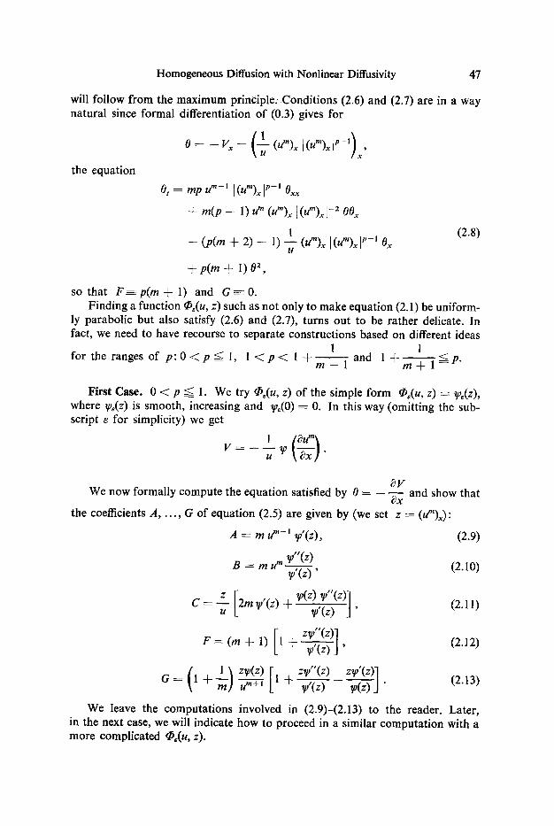
will follow from the maximum principle. Conditions (2.6) and (2.7) are in a way natural since formal differentiation of (0.3) gives for
the equation
0 t = mp lA m - I /(/gm)xlP-I Oxx
+ m(p -- 1) u 'n (u")x ](um)x1-2 O0 x
1 (2.8) + (p(m + 2) -- 1) - - (u")x I(u")x I ~-, 0x
U
+ p(m + 1) 0 2 ,
so that F = ~ p ( m + 1) and G ~ 0 . Finding a function q~,(u, z) such as not only to make equation (2.1) be uniform-
ly parabolic but also satisfy (2.6) and (2.7), turns out to be rather delicate. In fact, we need to have recourse to separate constructions based on different ideas
1 1 for the ranges of p : 0 < p = < 1, 1 < p < 1 + ~ and 1 +m+-------~ =< p"
First Case. 0 < p ~ 1. We try ~ ( u , z) of the simple form tP,(u, z) = ~,,(z), where ~p,(z) is smooth, increasing and ~(0) = 0. In this way (omitting the sub- script e for simplicity) we get
V = - - - - ~ o U
8V We now formally compute the equation satisfied by 0 = -- ~--~ and show that
the coefficients A, . . . , G of equation (2.5) are given by (we set z = (u")x) :
A = m u m-I ~o'(z), (2.9)
B = m u m v/'(z) v/(z) ' (2.1o)
z [ ,/,(z) "'(z) C = - [2m V,'(z) -~ ~ ] (2.11)
zr (2.12) F = ( m + l ) 1 + V,'(z)_]'
( [ (z, = 1 + ~ 1 + r'(z~ r(z) J" (2.13)
We leave the computations involved in (2.9)-(2.13) to the reader. Later, in the next case, we will indicate how to proceed in a similar computation with a more complicated ~,(u, z).
48 J .R. ESTEBAN ~; J. L. VAZQUEZ
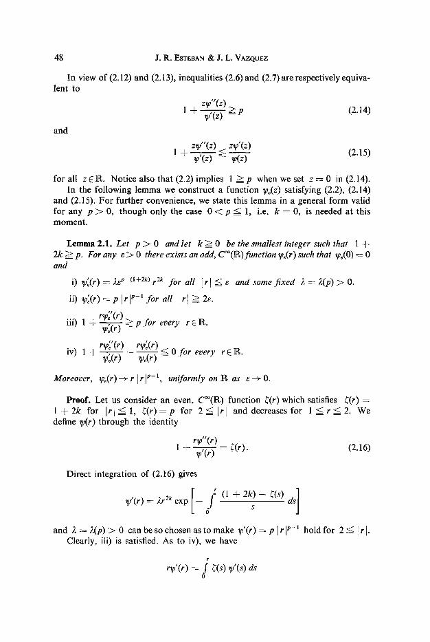
In view of (2.12) and (2.13), inequalities (2.6) and (2.7) are respectively equiva- lent to
z~p"(z) ~ P (2.14) 1 + ~p'(z'------~
and
z~."(z) ~ z~p'(z) (2.15) 1 + W'(z) - - ~o(z----5-
for all z E R . Notice also that (2.2) implies 1 ~ p when we set z = 0 in (2.14). In the following lemma we construct a function ~p~(z) satisfying (2.2), (2.14)
and (2.15). For further convenience, we state this lemma in a general form valid for any p > 0, though only the case 0 < p =< 1, i.e. k : 0, is needed at this moment.
Lemma 2.1. Let p ~ 0 and let k ~= 0 be the smallest integer such that 1 + 2k ~= p. For any e > 0 there exists an odd, C~176 function %(r) such that %(0) = 0 and
i) ~l)te(r) ~ - ~p--(l+2k) r2k for all ]r I ~ e
ii) ~o'~(r) : p [rlP-I for all [r[ ~ 2e.
r~p~'(r) ~ P for every r E R. iii) 1 + ~ :
r~p"(r) mp',(r) < 0 for every r E R. iv) 1 -~ ~p~(r) ~v,(r) =
and some fixed 2 : 2(p) > 0.
Moreover, %(r)-+r [riP-l, uniformly o n R as ~-+0.
Proof . Let us consider an even, C~(R) function r satisfies r : l + 2 k for I r i l l , r for 2 ~ l r l and decreases for l ~ r _ < 2 . We define ~p(r) through the identity
r~o"(r) 1 + - - - - ~(r). (2 .16)
~0'(r)
Direct integration of (2.16) gives
~P ' ( r )=2r2kexp[ - i o ( l + 2 k ) - - ~ ( S ) d s ] s
and 2 = 2(p) > 0 can be sochosen a s tomake ~p'(r) = p Irl p - ' hold for 2 ~ ]r I. Clearly, iii) is satisfied. As to iv), we have
r~p'(r) : f ~(s) W'(s) ds 0
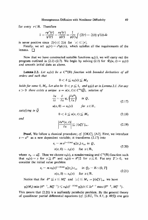
H o m o g e n e o u s Dif fus ion with Nonl inear Diffusivity 49
for every r E R. Therefore
r~v"(r) r~p'(r) 1 1 q- ~v,(r~- S ~v(r) = ~v(r) f (~(r) -- ~(s)) v/(s) as
is never positive since ( ( r ) ~ ~(s) for [ s ] ~ l r ] . Finally, we set ~0~(r) = eP~p(r/e), which satisfies all the requirements of the
lemma. [ ]
Now that we have constructed suitable functions ~p~(z), we will carry out the program outlined in (2.1)-(2.7). We begin by solving (2.1) for tb,(u, z) ---- ~o,(z) and smooth initial data as above.
Lemma 2.2. Let uo(x) be a C~176 with bounded derivatives of all orders and such that
0 < ~ ~ Uo(X) <= Mo
holds for some ~, Mo. Let also be 0 < p ~ 1, and ~o,(z) as in Lemma 2.1. For any
e > 0 there exists a unique u = u(x, t) E C~176 solution of
~u ~ [ ~u"~ ~--~ = ~-'~ ~P" l~ Ox ] in Q,
(2.17)
u(x, O) = Uo(X) for x E R ,
satisfying in O_ 0 < ~ ~ u(x, t) ~ Mo (2.18)
and ~um(x, t) <
= I[ (U~')' [1~- (2.19)
Proof. We follow a classical procedure; ef [ O K C ] , [A2]. First , we introduce v = u m as a new dependent variable; it transforms (2.17) into
v t : m v l-(I/m) ~3~(Vx) UXX in Q, (2.20)
v(x, O) = Vo(X) for x E R,
where Vo = u~'. Then we choose ~a(s), a nondecreasing and C~(R) function such that u ~ ( s ) = s for s ~ O m and ~n(s)=Om/2 for s ~ 0 . For any T > 0 , we consider the initial value problem
/)t : m ua(v) l --(I /m) ~/)~(Vx) Vx x in Qr : R • (0, T] (2.21)
v(x, O) = Vo(X) for x E R.
Notice that for a ' ~ s ~ M ~ and I z l = < M t =lJ(ua')'l]~ we have
w~(Mx) min (~m 1, M~,-1) < u~(s)l-(llm) ~o'(Z) =< 2e p-I max (hm-1, M~,-1).
This means that (2.21) is a uniformly parabolic problem. By the general theory of quasilinear partial differential equations (eft [LSU, Th. 8.1, p. 495]) one gets

50 J.R. ESTEBAN 8s J. L. VAZQUEZ
the existence of a unique solution v(x, t) of (2.21) which satisfies Iv(x, t) l :< M~'
o n QT, and
v E
for some t 3 E (0, 1). By the maximum principle,
0 ~ 0 m ~ v(x, t) ~ M~' on Qr,
and v satisfies (2.20) by the definition of un. The regularity v E C~ follows
by a standard bootstrap argument and the estimate Ivy(x, t) ] ~ M~ on Qr fol- lows from the maximum principle applied to the equation satisfied by z = v~, i.e.
Zt : ~X (m v(x, t)'-(l/m) ~)te(Z) Zx),
Finally, we define u = v z/m, which clearly satisfies all the conclusions of the lemma. [ ]
We can now establish the main estimate for the velocity defined in (2.3), which in the present case reads
1 ~cou"'[ V(x, t) -- u % ~-'~x ] " (2.22)
Lemma 2.3. Let Uo(X) and u(x, t) be as in Lemma 2.2 and V(x, t) as in (2.22). Then (2.4) holds in Q.
As explained above, the proof consists in applying the maximum principle to the equation satisfied by 0 ~- --Vx, i.e. equation (2.5) with coefficients given by (2.9)-(2.13). We will give in Appendix A a rigorous justification of this use of the maximum principle.
To continue, let us remark that using (2.17) and (2.22) we may write equation (0.3) in the form
co ~V 1 ut = ~x (uV) = --u "~x + mu --'-~ (um)x ~Pe((Xm)x)"
From this, (2.4) and zT)~(z)>: 0 for all z E R, we obtain the following
Corollary 2.4. Let Uo and u as above. Then in Q
6~U U - - > (2.23) ~ t = p(m + 1) t"
Therefore, the function t ~ u(x, t) t 1/p('+a) is nondecreasing in (0, oo) for every x E R .
Homogeneous Diffusion with Nonlinear Diffusivity 51
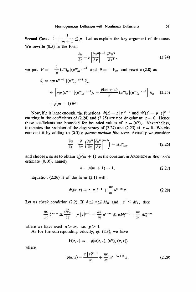
1 - - < p . Second Case. 1 + m + 1 :
We rewrite (0.3) in the form
Ou ~um~ -1 ~2um
x2' 1
we put V - - (um)z[(um)~] p-I and O : - - V ~ , U
Let us explain the key argument of this case.
(2.24)
and rewrite (2.8) as
0 t = m p u m - 1 I(u% t ~ Oxx
Imp(urn-1 ](Um)xf l)~ + +
+ p ( m + 1) 02 .
p ( m + 1) ] u (um)x I(Um)xl p- ' j O~ (2.25)
Now, i fp is large enough, the functions ~(z) = z Izl p-1 and q~'(z) = p Iz] p 1 entering in the coefficients of (2.24) and (2.25) are not singular at z = 0. Hence these coefficients are bounded for bounded values of z = (um)~. Nevertheless, it remains the problem of the degeneracy of (2.24) and (2.25) at z = 0. We cir- cumvent it by adding to (0.3) a porous -med ium- l i ke term. Actually we consider
On ~ (SU m ~Ump--I~ t3t - - 8x ~--~x -~x ] + e(td)xx (2.26)
and choose n so as to obtain 1/p(m + 1) as the constant in ARONSON & BI~NILAN'S estimate (0.10), namely
n = p ( m + 1 ) - 1. (2.27)
Equation (2.26) is of the form (2.1) with
n E ~e(U, z) : z I z l p - 1 . A f _ _ _ U n - m Z . (2.28)
m
Let us check condition (2.2). If ~ _< u <-- Mo and [z] ~ M~, then
ne ~ ne ne _ _ (~n--m < : p [ z f - l + _ _ un-m < p M f - l + _ _ M ~ - m m = 8z m = m
where we have used n > m , i.e. p > 1. As for the corresponding velocity, c f (2.3), we have
where
V(x , t ) : --r t) , (Um)x (X, t))
Z ]z[P--I r/E Un_(m+l) Z ~(u, z) - - -F - - �9 (2.29)
U m

52 J.R. ESTEBAN • J. L. VAZQUEZ
We next compute the equation satisfied by 0 ---- - -V x -= ekx.
4, = r162 + r
z = ur + ur ~ r + r
Z t = m(u m-l(wb)x)x
= (m + 1) zO + m u m O x + dpz x ,
and then
We have
(2.30)
(2.31)
~b t = mu~r + [ueku + (m + 1) z~bz + ~b] 0. (2.32)
Now we use (2.29) to work out the term within brackets, and obtain
u~b~ + (m + 1) zr + dp = p(m + 1) 4.
Hence
dpt = mumdpzOx -}- p(m + 1) ~bO,
and differentiation with respect to x gives finally
O, = mu~bzOxx
+ [m(umqb~)x + p(m + 1) ~b] 0 x
+ p(m + 1)02.
Surprisingly, conditions (2.6) and (2.7) are satisfied and equality holds. Now, if p > 4, all the steps performed in the first case can be repeated with the above choice of approximation, i.e. (2.26) and (2.28), and Lemmas 2.2 and 2.3 and Corollary 2.4 hold true.
This method would not work for lower p's because of the lack of sufficient regularity of the solutions. Nevertheless, the idea of the porous-medium perturba-
1 tion can be made to work in a slightly modified form for the range p >-- 1 +
Our approximate equation will now be m + 1"
~t - - ~x ~p~ ~ + e(U")xx. (2.33)
As in (2.27), n + 1 ---- p(m + 1). Therefore, q~,(u, z) is
n6 #,(u, z) : ~/,,(z) + - - d ' - " z (2.34)
m
and the velocity V = --4 is given by
~(u, z) ---- ~0~(z___~) + n___ee u~_(,,+l ) z. (2.35) u m
Observe that n - - ( m + 1)--> 0. To find the equation satisfied by 0 - - --Vx = 4~x we can use again (2.30)-(2.32). Differentiation of (2.32) with respect
Homogeneous Diffusion with Nonlinear Diffusivity 53
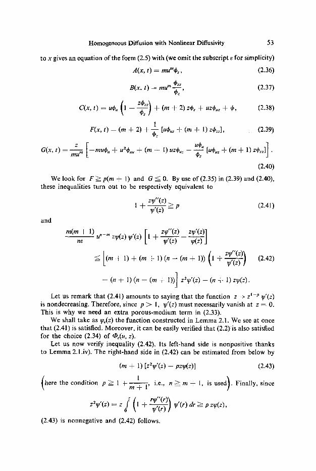
to x gives an equation of the form (2.5) with (we omit the subscript e for simplicity)
A(x, t) = m u ' % , (2.36)
B(x, t) = mu" ~ , (2.37)
C(x, t) = u4,, 1 r ] + (m + 2) Z4,z -r uZdOuz + 4', (2.38)
1 r(x, t) = (m + 2) + ~z [u4~,z + (m + 1) Z~zz], (2.39)
G(x, t) = ~Z [--murb,-{- u24,,, + (m 4- l) uz4,,z -- ~u~O" [u4,,z + ( m + l) zrbzz] ] .
(2.40)
We look for F >~ p(m + 1) and G =< 0. By use of (2.35) in (2.39) and (2.40), these inequalities turn out to be respectively equivalent to
zv?"(z) > P (2.41) 1 + v:(z----T =
and
[ re(rune + 1) u "-m zT~(z) ~o'(z) 1 + ~'(z) ~o(z) ]
~ (m-t- 1 ) + ( m + 1 ) ( n - - ( m + 1)) l - k - - ~ - ] (2.42)
- (n + 1) (n - (m + 1))] z2~/(z) - (n + 1) z~o(z).
Let us remark that (2.41) amounts to saying that the function z -+ z 1-p ~o'(z) is nondecreasing. Therefore, since p > I, ~o'(z) must necessarily vanish at z = 0. This is why we need an extra porous-medium term in (2.33).
We shall take as vA(z ) the function constructed in Lemma 2.1. We see at once that (2.41) is satisfied. Moreover, it can be easily verified that (2.2) is also satisfied for the choice (2.34) of ~,(u, z).
Let us now verify inequality (2.42). Its left-hand side is nonpositive thanks to Lemma 2.1.iv). The right-hand side in (2.42) can be estimated from below by
(m + 1) [z2~/(z) -- pzq,(z)] (2.43)
( 1 ) here the condition p=> 1 - S i n + 1' i.e., n > = m § 1, is used . Finally, since
+ r~"(r)~ z2~v'(z) ~ z J 1 ~o'(r) dr > o ~--~Tfl = I, z~o(z),
(2.43) is nonnegative and (2.42) follows.
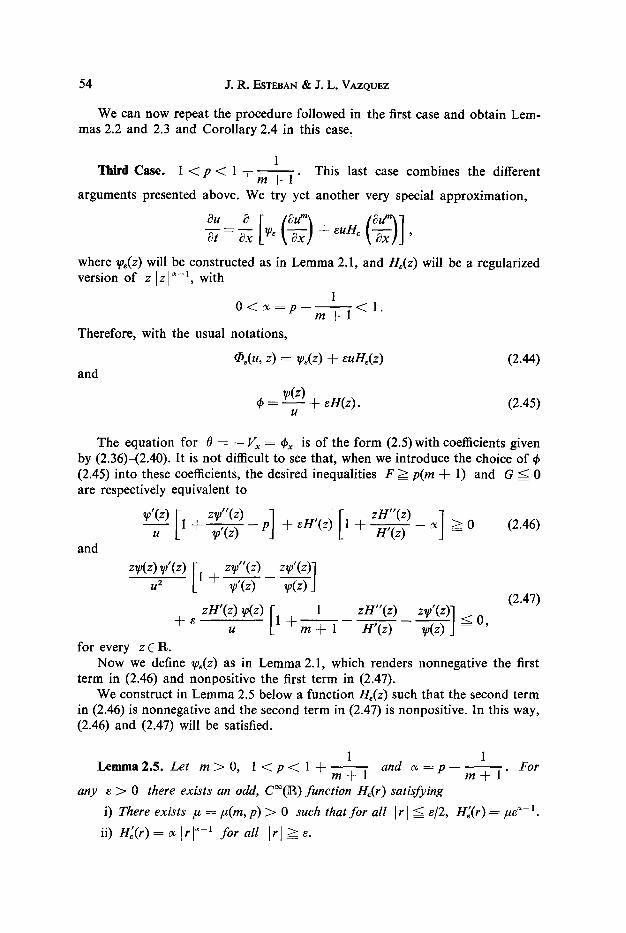
54 J .R . ESTEBAN 8s J. L. VAZQUEZ
We can now repeat the procedure followed in the first case and obtain Lem- mas 2.2 and 2.3 and Corollary 2.4 in this case.
1 Third Case. 1 < p < 1 -F m +'-----~" This last case combines the different
arguments presented above. We try yet another very special approximation,
St -- ~x ~o~ + euH, ,
where ~p,(z) will be constructed as in Lemma 2.1, and He(z) will be a regularized version of z [z[ ~-l, with
1 O < ~ = p - - < 1 .
m + l Therefore, with the usual notations,
Or(u, z) = ~o,(z) + euH,(z) (2.44) and
~o(z) r + el l (z) . (2.45)
U
The equation for 0 = -- Vx = q~x is of the form (2.5) with coefficients given by (2.36)-(2.40). It is not difficult to see that, when we introduce the choice of 4~ (2.45) into these coefficients, the desired inequalities F >= p(m + 1) and G < 0 are respectively equivalent to
~o'(z) I-~ p § 1 + I-I'(z) ~ > 0 (2.46) u v,,'(z) =
and
z~"(~) z~'(z)] z r ( z ) V/ (z ) 1 + - - u 2 ~o'(z) W(z) J
(2.47) 1 zH"(z ) zy)'(z)] + zH'(z) y)(z) I
u + ~ + H'(~) ~ J <= O, for every z E R.
Now we define ~p~(z) as in Lemma 2.1, which renders nonnegative the first term in (2.46) and nonpositive the first term in (2.47).
We construct in Lemma 2.5 below a function He(z) such that the second term in (2.46) is nonnegative and the second term in (2.47) is nonpositive. In this way, (2.46) and (2.47) will be satisfied.
1 1 L e m m a 2 . 5 . Let r e > O , l < p < 1 q - m + 1 and o~ -~ p m + 1 For
any e > 0 there exists an odd, C~176 function He(r) satisfying
i) There exists # ~- t~(m, p) > 0 such that for all [r I =< e/2, n ' ( r ) = / ~ e '~- ~.
ii) Hi(r) = or [r I ~-1 for all I r 1>~ e.

Homogeneous Diffusion with Nonlinear Diffusivity 55
rH" ( r ) iii) 1 + ..-777-7,, -> ~x for every r E R .
Hi(r) :
iv) I f ~p~(r) is as in Lemma 2.1, then for every r E R ,
1 rHi'(r) < rw'~(r) l + ~ + - -
m + 1 H' (r ) = ~o~(r)"
Moreover, eH~(r) -+ 0 uniformly on R as e -+ O.
Proof. Let us consider an even, Coo(R) function a(r) which satisfies aft) = 1 for i t [<_1/2 , a f t ) = o ~ for t r i a l and decreases if � 8 9 1.
As in Lemma 2.1, we define H(r) by means of
rH"(r ) 1 + H'(r----S - a(r),
and then set H,(r) = e~H(r/e). Let us prove iv) for ~p(r):
- - - - - - + a ( r ) - - ~ ( s ) ~ v ' ( s ) ds, m + 1 + a(r) ~v(r) ~v-~) o
where r is as in Lemma 2.1. This expression is never positive since ~(r) and aft)
have been chosen because 1 < p < 1 + so that ~ + a(r) ~ ~(s)
holds for all O--<s~<r. [ ]
Notice that the nondegeneracy condition (2.2) is clearly satisfied by ~,(u, z) as in (2.24) with the present choice of ~,,(z) and H,(z). With this construction, Lemmas 2.2 and 2.3 and Corollary 2.4 are also true and the proof of estimate (2.4) is complete for the whole range of m and p.
3. Existence and Uniqueness
We devote this Section to proving Theorem 1 and Corollary 1. The uniqueness statement in the theorem is an obvious consequence of the Ll-contraction property, part d) of Corollary 1, which we establish first.
Proposition 3.1. Let u(x, t) and t~(x, t) satisfy a), b) and c) o f Theorem 1. Then for every t >_ s >_ O
-boo -boo
f [u(x, t) - - fi(x, t)]+ dx <: f [u(x, s) - - ~(x, s)]+ dx. (3.1) - - o o - - O O
Proof. It is a rather standard argument. One subtracts the equations for u and t~, multiplies by ~(u m -- ~m), where r/(r) is a smooth approximation of the function sign+ (r) ( = 1 if r > O, = 0 if r ~ 0), integrates by parts with respect to
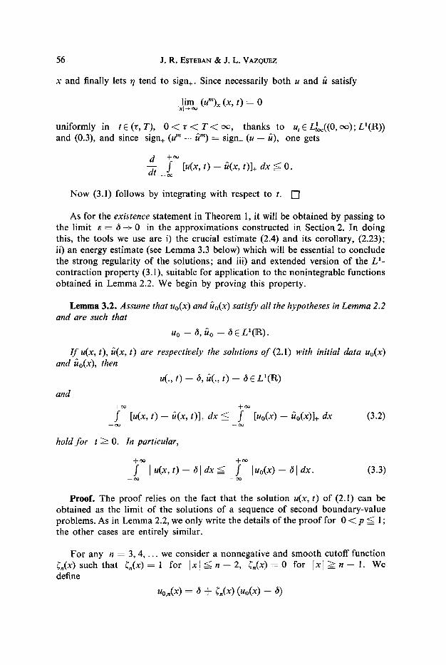
56 J: R. ESTEBAN 8l; J. L. VAZQUEZ
x and finally lets ~/ tend to sign+. Since necessarily bo th u and ~ satisfy
lim (Um)x (X, t) = 0 [ x l ~ O o
uniformly in t E (w, T), 0 < w < T < ~ , thanks to ut E L]oc((0, oo); LI (R)) and (0.3), and since sign+ (um - - {tin) = sign+ (u - - ~), one gets
d + o o
_ f ~ [u(x, t) - {t(x, t)l+ dx <= O. --d?
N o w (3.1) follows by integrat ing with respect to t. [ ]
As for the existence s ta tement in Theo rem 1, it will be obta ined by passing to the limit e = 8--~ 0 in the approx imat ions constructed in Section 2. In doing this, the tools we use are i) the crucial est imate (2.4) and its corollary, (2.23); ii) an energy est imate (see L e m m a 3.3 below) which will be essential to conclude the s t rong regulari ty o f the solut ions; and iii) and extended version o f the L 1- contract ion p roper ty (3.1), suitable for appl icat ion to the nonintegrable funct ions obta ined in L e m m a 2.2. We begin by proving this proper ty .
Lemma 3.2. Assume that Uo(X) and {to(X) satisfy all the hypotheses in Lemma 2.2 and are such that
Uo - - 8, {to - - 8 E L I ( R ) .
I f u(x, t), {t(x, t) are respectively the solutions of (2.1) with initial data Uo(X) and {to(X), then
u(., t) -- 8, {t(., t) -- 8 E LI(R)
and -t-oo q-eo
f [u(x, t) - - t~(x, t)]+ dx ~ f [Uo(X) -- {to(x)l+ dx (3.2) - o o - o o
hold for t >= O. In particular,
-~-oo q -oo
f I u(x, t) - 81 dx ~ f ]Uo(X) -- 81 dx. (3.3) - o o - o o
Proof . The p r o o f relies on the fact tha t the solution u(x, t) of (2.1) can be obta ined as the limit o f the solutions of a sequence of second boundary-va lue problems. As in L e m m a 2.2, we only write the details o f the p r o o f for 0 < p ~ 1 ; the other cases are entirely similar.
Fo r any n = 3, 4 . . . . we consider a nonnegat ive and smoo th cutoff funct ion ~n(x) such tha t (n(x) = 1 for Ix I ~ n - - 2, ~ ( x ) = 0 for I xl ~ n - 1. We define
uo,n(x) = 8 + Cn(x) (Uo(X) - 8)

Homogeneous Diffusion with Nonlinear Diffusivity 57
and Vo..(x) --- Uo~(X) m. For each n we consider the solution v.(x, t) of the second boundary-value problem
v,,,t = m vln -(l[m) ~Ote(Un,x) On,xx
Vn,x(• , t) = 0
As
in (--n, n)• T],
for 0 < t ~ T ,
v.(x, O) = Vo,.(x) for Ix I < n.
n---~e~, v .(x , t)---~ v(x, t) uniformly on compact subsets of Q, v(x, t) being the solution of (2.17). This assertion is shown in [LSU, Ch. V, w 8] for a sequence of first boundary-value problems. The same arguments apply for Neu- mann boundary conditions. See also [LSU, Ch. V, w 7].
We now set u,(x, t) = v~(x, t) l/m, which satisfies
u~,t = ~ W, ~-~-x] in (--n, n)• T],
~u7 ~x (• t) = o for 0 < t ~ T ,
and
u,(x, O) = Uo,,(x) for I x [ < , .
Therefore, for any fixed t we have
d f u ,(x , t) dx 0
dt -n
f [u.(x,t) - ~[ d x : f [Uo,.(x) -- O [ d x ~ Iluo - - OlE~(R). ~ n - - n
As n -+ cx~, Fatou's Lemma implies (3.3). The proof of (3.2) is obtained along the lines of Proposition 3.1. [ ]
We divide the actual existence proof into several steps. First step. Let Uo E LI(R) A L~(R) and be nonnegative. We also assume that
u~, 7 = min( l ,m} is Lipschitz continuous and Uo(X)> 0 for all x E R . For any e > 0 we consider an strictly positive averaging kernel 9,(x) ~ C ~
and define
Uo,,(x) = e + [ f 9 , (x - - y) uo(y) v dy] xle �9
As is easily verified, Uo,,(x) satisfies
0 < ~ <= Uo,~(x) <- ~ + I[ no II~
[(u~,,)' (x)l =< I[(u~)'ll~
Iluo,. - ~lh <= Iluo[ll,
and u0,, -- e ~ Uo in LI(R) and uniformly on R as e ~ 0.
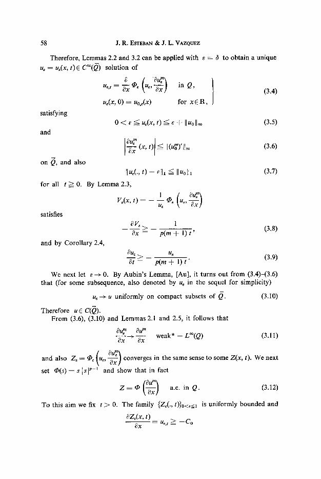
58 J.R. ESTEBAN & J. L. VAZQUEZ
Therefore, Lemmas 2.2 and 3.2 can be applied with e = 6 to obtain a unique
u, = u,(x, t)C C~176 solution of
in Q , (3.4)
for x E R ,
~,, = ~ ~ u~,-~-x/
u,(x, o) = uo:(x)
satisfying
and
on L), and also
for all
satisfies
0 ~. e ~ u,(x, t) ~ e -4- II Uo [Ioo
(x, t) ~ II (U'go)'lloo
l[u~(., t) - - t i l l =< Iluoh
t ~ o. By Lemma 2.3,
1 (.. V,(x, t) - - ~ u~ ~x/
and by Corollary 2.4,
(3.5)
(3.6)
(3.7)
t9 V~ > 1 (3.8) ~x ~ p(m -r l) t '
~u_._2 > u, (3.9) ~t = p(m -[- 1) t"
We next let e ~ 0. By Aubin's Lemma, [Au], it turns out from (3.4)-(3.6) that (for some subsequence, also denoted by u, in the sequel for simplicity)
u~ ~ u uniformly on compact subsets of Q- (3.10)
Therefore u C C(Q). From (3.6), (3.10) and Lemmas 2.1 and 2.5, it follows that
~ ~u ~ Ox ---~ --~-x weak* -- Loo(Q) (3.11)
~um] and also Z~ = ~ , u~, --~-x] converges in the same sense to some Z(x , t). We next
set ~(s) ---- s Isl ~ - ' and show that in fact
Z = ~ -~x a.e. in Q. (3.12)
To this aim we fix t > 0. The family {Z~(., t)}0<~_l is uniformly bounded and
oZ.(x, t) ~x - - u~.t >= --Co
Homogeneous Diffusion with Nonlinear Diffusivity 59
holds for some Co ~- Co(m, p, t, Uo) > 0, thanks to (3.5) and (3.9). Then, for any bounded interval I Q R, the total variation on I of Z,(x, t) is uniformly bounded. Therefore,
Z,(x, t) -+ Z(x, t) a.e. x E R . Since we also have
I i
uniformly on ~) (cf. Lemmas 2.1 and 2.5), we obtain
~ \--~x! ~ Z(x, t) a.e. x e R ;
(3.12) follows from this and (3.11) by Br~zis' Lemma; cf. [Br, p. 126]. On the other hand, (3.9) and (3.10) give
U
u, >~ p(m + 1) t (3.13)
in D'(Q). Actually, ut is a function as a consequence of the following energy esti- mate.
Lemma 3.3. Let be Uo, Uo., and u, as above. Then for every T > O, T +oo
lim~o o f -foo t l(u(*m+')12)t[2 dx dt ----< Cm I "0 m+lm+l" (3.14)
This type of estimate is due to BI~NILAN; cf. [B61], [B62]. The difficulty in our case consists in having to derive the estimate for the complicated approximate problems. We give a full proof of Lemma 3.3 in Appendix B. Since u is positive by (3.13), it follows that u t E L~oc(Q) and (0.3) is satisfied a.e. in Q.
To continue with the proof of Theorem 1, we show that for t > 0,
lim (u")x (x, t) = 0. (3.15) Ixl-+oo
We first remark tht u(., t)E LI(R) and
!lug t)lh < Iluoll~ (3.16)
by virtue of (3.7), (3.10) and Fatou's Lemma. Then (3.13) and (0.3) imply that
, / ~ ( x , t ) + p ( m + 1) t u(y, t ) dy
is nondecreasing in x. Therefore, the limits
lim ~ ( ~u~ ) x-~• ~o -~x (x, t)
must exist. Since u is bounded, both limits must be 0 and (3.15) is proved.
60 J . m . ESTEBAN & J. L. VAZQUEZ
We can now integrate (0.3) and get
+oo
f u,(x,t)dx<=O, - - o o
which together with (3.13), (3.16) yields
2 Ilu0111 Ilu,(., t)ll~ =< p(m q- 1) t"
In particular, we deduce:
i) u is a.e. differentiable from (0, cx~) into L~(R), so u E C((O, o0); L~(R)).
ii) urn(., t) E W~'~176 a.e. t > O, with
2 I!uox (., t)]P ~ p(m + 1) t"
We next show that
+oo
lim f ]u(x, t ) - - Uo(X)l dx = 0. (3.17) t-+0 --oo
Notice first that {u(., t)}t~0 is precompact in L~or since it is a bounded family in L~(R) on which translations are equicontinuous because
q - o o - } - c o
f l u (x+h, t ) - -u(x , t ) ]dx<= f l u o ( x q - h ) - u o ( x ) - - o o - - ~ o
dx.
(Use (3.2) to prove this, taking into account that u0,~ ~ u0 in LI(R).) Therefore, given any sequence t, ~ O, there is a subsequence tj such that u(., tj) ~ Uo in
Lloc(R) (recall that u E C(Q)). In fact this convergence takes place in LI(R) be- cause of (3.16). Since the limit is independent of the sequence, thus (3.17) is proved.
As a consequence of (3.17) and the flux condition (3.15) we obtain the property of conservation of the total mass:
q - c o -}-oo
f u(x, t) dx = f Uo(X) dx for all t > 0. (3.18) --~30 - -oO
We complete this step by displaying the main estimate for V. We recall that
I 1 V, -- Z,, and V = -- - - Z , (3.19)
U e U
where Z,, Z are as in (3.12). We know that Z~---~ Z a.e. and weakly in L~oc(Q). Moreover, since Uo is continuous and positive everywhere and u E C(Q), it follows from (3.13) that u is positive in Q and l/u, ~ 1/u uniformly on compact subsets of~9. Applying this to (3.19) we conclude that F~ ~ F a.e. and weakly in L~oc(Q). We may now pass to the limit in (3.8) and obtain (1.1). [ ]

Homogeneous Diffusion with Nonlinear Diffusivity 61
Second step. Let us assume that Uo E LI(R) A L~176 Uo ~ 0 a.e. and let be 7, P, as in the first step. We define
UoAX) = I f q,(x - y) uo(y) ~ dy] 11~.
As is easy to verify, 0 < Uo,,(x) <= Iluolloo, liuo,~lh =< Iluol[, and Uo,~-+ Uo in L~(P0 as e ~ 0. Moreover, for any e > 0, ug.~ is Lipschitz continuous.
Therefore, the results in the first step of the proof give the solution u,(x, t) of (0.3) corresponding to initial data u0,,. As e -+ 0, Theorem 1 is obtained with only small changes with respect to the proof of the first step. Thus the estimate
2 Iluolll [(u~n~ )x (x, t ) f ~ [lug,t(-, t)111 ~ p(m + 1) t (3.20)
must be used instead of (3.6). (3.20) implies H61der continuity also in t. To be precise: for every ~ > 0 , all t , t ' ~ z and x , x ' E R , we have
]u~(x, t) -- u~(x', t ') I <- C ( I x - x ' ? + It - t ' f ) ,
where 0~ = min {1, 1/m}, fl = o~/(o~ + 1) and C = C(m, p, 3, Uo) > 0 is inde- pendent of e. See [EV, Th. 2, b] for a proof. In particular, the convergence of the u~ takes place uniformly on compact subsets of Q.
On the other hand, the energy estimate (3.14) still holds in this step. If u is positive everywhere we easily conclude that ut E L~oc(Q). I f u is only nonnegative, the same conclusion can be reached from a result of B~NILAN, [B62, Lemma 4].
To prove (1.I) when mp ~ 1, we proceed as in the first step using the fact that u(x, t) is positive everywhere, (this is proved independently in Proposition 3.4 below). If mp > 1, we use the boundedness of the velocity (1.9) to pass to the limit. Now v~, v~,~ and V~ are bounded for t ~ T > 0 and V~,x ~: I/(p(m + 1) t). Arguing as in the proof of (3.12) we conclude that V~ ---> V a.e. and weakly in L~o~(Q), V being related to v by (0.4), (0.5), and V x <: 1/(p(m + 1) t). [ ]
Remark. There is no loss of generality in assuming that Uo is bounded. Indeed, from Corollary 2, any solution with initial data in LI(R) is bounded for any t > 0 with bound depending only on Iluolll. Therefore, if we suitably approximate Uo by UO,n E L~176 LI(B) all the above estimates will be independent of n for t ~ ~ > 0 and in the limit n -+ cx~ we will get a solution of (P).
We end this section by showing the following
Proposition 3.4. Let mp <= 1 and let Uo(X) and u(x, t) satisfy a)-d) in Theorem 1. Then
u(x, t) > 0 for all x E B and t > 0. (3.21)
Proof. If mp < 1, the operator
the homogeneity A(2u) = 2 mp A(u)
t u- A ( u ) - - x ,--ffx IT;/ z
(for all 2 > 0 ) of
62 J.R. F_,STEBAN & J. L. VAZQUEZ
implies ut <= u/((1 -- mp) t) a.e. in Q, by the results of B~NILAN • CRANDALL, [BC]. This leads to
u
O <= (1- - mP) t lax/ /
and the Strong Maximum Principle--as stated in [V3]--implies that either u > 0 or u ~ 0. Finally, mass conservation (3.18) gives no opportunity for u ~ 0 to occur.
If mp = 1, we cannot apply [BC], so we argue as follows. The mass conserva- tion and the continuity of u(x, t) imply that given ~" ~ 0 there exist ~ E 1%, 0 t o < r < T and M > 0 such that u ( ~ , t ) : > M holds for all t, to<~t<--71". By translation we may put ~ ---- 0 and to : 0, so that (3.21) reduces to proving the following
Lemma3.5. Let m p = 1 and Uo, u as above. I f u ( O , t ) ~ M > O for all O~t<- -T , then u(x ,T)>O for all xER .
Proof. We use the maximum principle and compare with a suitable positive subsolution. Let be 0 < p < 1 and Xo > 0 fixed. We set c = (1 -F Xo)/T and for x < ct define
w(x, t) = M exp [--2(ct -- x)-~],
where 0 ~ = p / ( 1 - - p ) , 2 = f l ( 1 - - p ) - ~ c -l/O-p) and ),---- lift satisfies V + V P = (1 -- p) -~ (1 + Xo) -(p+I)/O -p) T j/O-r).
It is easy to verify that
--E I / in $ 2 = ( O < x ~ c t , O < t < : T } .
Since also 0 < w ( 0 , t ) ~ w ( 0 , T ) < M ~ u ( 0 , t) and w(et, t ) = O ~ u ( c t , t) hold for 0 --< t --< T, we obtain w(x, t) _< u(x, t) on ~ . In particular 0 < W(Xo, T) <: U(Xo, T) holds.
I f p 2> 1, the same argument applies with
w(x, t ) : A ( e t - - x ) ~
for (x, t)E .Q, e = (1 + Xo)/T, 2 = M(1 q-Xo) -~ and o~> p such that
~x (1 p) l /p pT[(1 -]- Xo)/T] fv+I)/p. []
Remark. Notice that (3.21) can be deduced aposteriori from (1.1) by integrating it twice in x starting from a point Xo of maximum of u(., t).
As for the proof of Corollary 1, we have begun the section with a proof of part e). Parts a), b) and c) have been established in the course of proving existence,

Homogeneous Diffusion with Nonlinear Diffusivity 63
though we remark that they can be easily derived a posteriori. We are left 0nly with part d), i.e. that the map Uo -~- u(., t) is bounded in L'(P~) for all r E [1, cx~]. This can be proved in a standard way by multiplying (0.3) byj(um), where j E C 1 [0, e~) is a suitable increasing function, and then integrating by parts. We omit the easy details.
4. Regularity of the free boundary
In this Section we consider solutions u of (0.3) with mp > 1 and initial data that vanish in some interval, so that there is an interface or free boundary which separates the nonvoid subsets of Q, [u > 0] and [u --- 0]. Without loss of generality we assume that the initial data Uo satisfy
0 ----- ess sup (x E R: Uo(X) > O)
and consider only the right free boundary ((t), given by
r : sup {x E R: u(x, t) > 0} if t > 0,
and ~'(0) ---- 0. We study here the regularity of the free boundary r and of the solution near
~(t). In the porous-medium case, p ~ 1, this study has been performed by a number of authors, e.g. [A3], [Kn], [CF], [ACK], [ACV], IV2]. In this program a key role is played by the estimate vxx >~ --C/ t .
As we will show, the same program can be applied to the doubly nonlinear equation (0.3) using as a foundation the crucial estimate (1.1). Many of the argu- ments, in particular of [CF] and [ACK], will have counterparts in this general case. Though our equation can be either degenerate or singular at points where Ux = O, we will be able to exclude such points in a neighborhood of the moving part of the free boundary, which will be enough for our purposes.
We have already mentioned that ((t) is continuous in [0, e~), locally Lipschitz continuous in (0, oo) and nondecreasing. Since, for fixed t > 0, the function
X x - + p(m § 1) t V(x, t) is nondecreasing, the following limit exists:
Moreover, we have
lim V(x, t) : V(~(t), t ) . x-+ r
u (x , t ) > 0
Lemma 4.1. For every t > O, the right derivative D+~(t) ( = ~'(t) a.e.) exists and
D~((t) ~- V(((t) , t ) . (4.1)
This is proved in [Kn] for the porous medium equation (p = 1) and the same arguments apply for the doubly nonlinear case, provided (1.1) is known.
An important consequence of the main estimate (1.1) is
64 J.R. ESTEBAN ,~ J. L. VAZQUEZ
Lemma 4.2. The inequality
1 ~'(t) > ~ " ( t ) + ( 1 p ( m + l ) ' ) t =
is satisfied in the sense o f measures on (0, oo).
0 (4.2)
We remark that the free boundaries r(t), cf. (1.8) of the Barenblatt solutions, satisfy (4.2) with equality sign. (4.2) is proved in the case p ---- 1 in [CF] and [V1]. The same proof applies without major changes for p =~ 1.
1 Let fl : 1 > 0. The differential inequality (4.2) means that the
function p(m + 1) t
F(t) : f sa('(s) ds (4.3) 1
is convex in (0, oo). Therefore, it has side derivatives D+F(t) at every time t > 0 and D-F( t ) <= D+F(t). Writing (4.3) in the form
t
F(t) : ta((t) - - ((I) - - fl f sa- l ( ( s ) ds, 1
we conclude that D • ((t) exists for t > 0 and
D• : taD • ~(t)
for every t > 0. From this and the convexity of F(t) we get
O+((t) ~ O - ( ( t )
and also D • ~ (z/t) a O• (4.4)
for every t > z > 0. In particular, we have the following result for the waiting time:
t* = sup {t ~ O: ~(t) = 0}.
L e m m a 4.3. t* is finite (possibly zero) and ~(t) is strictly increasing on (t*, oo).
Examples of solutions with a positive waiting time are constructed in the case p ---- 1, c f [Kn], [ACK], and a precise characterization is given in [V2]. All of these results can be adapted without difficulty to the case p ~ 1.
The main result of this section is the following.
Theorem 2. The free boundary (( t) is a C 1 function in the interval (t*, ~ ) , v is a C ~ smooth function in a neighborhood o f x : (( t) , t > t*, restricted to x < ~(t), and
v(x, t) = v~(x -- ~(to), t -- to) + o(I x -- ~(to) [ -[- It -- to I) (4.5)
where 7 : ~'(to) and v~ is the constant-velocity front
Vr(X , t) : yllp[yt - - X]+.
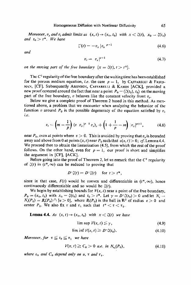
Homogeneous Diffusion with Nonlinear Diffusivity 65
Moreover, v x and vt admit limits as (x, t) -+ (Xo, to) with x < ((t), Xo - ~'(to) and t o > t * . We have
and
~'(t) = --vx I Vx i v - ' (4.6)
v, = Ivxl
on the moving part of the free boundary (x = ((t), t > t*}.
(4.7)
The C ~ regularity of the free boundary after the waiting time has been established for the porous medium equation, i.e. the case p = 1, by CAFFARELLI & FRIED- MAN, [CF]. Subsequently ARONSON, CAFFARELLI & KAMIN [ACK], provided a new proof centered around the fact that near a point Po = (((t0), to) on the moving part of the free boundary, v behaves like the constant velocity front v~.
Below we give a complete proof of Theorem 2 based in this method. As men- tioned above, a problem that we encounter when analyzing the behavior of the function v around Po is the possible degeneracy of the equation satisfied by v, i.e.
( 1 ) - - - m Ivxl (4 .8 ) v t : m - - (v ]vx[p-l vx)x + l + p
near Po, even at points where v > 0. This is avoided by proving that vx is bounded away and above from 0 at points (x, t) near Po such that v(x, t) > 0; cf. Lemma 4.4. We proceed then to obtain the linearization (4.5), from which the rest of the proof follows. On the other hand, even for p : 1, our proof is short and simplifies the argument in [CF], [ACK].
Before going into the proof of Theorem 2, let us remark that the C ~ regularity of ((t) in (t*, oo) can be reduced to proving that
D-~(t) : D§ for t > t*,
since in that case, F(t) would be convex and differentiable in (t*, oo), hence continuously differentiable and so would be ((t).
We begin by establishing bounds for V(x, t) near a point of the free boundary, Po = (Xo, to) with Xo = ((to) and to > t*. Let 7 = D+((to) > 0 and let N~ ---- N~(Po) = B~(Po) A [u > 0], where B~(Po) is the ball in R 2 of radius e > 0 and center Po. We also fix w and zt such that t * ~ w ~ w ~ .
Lemma 4.4. As (x, t) --> (Xo, to) with x ~ ((t) we have
lim sup V(x, t) ~ 7,
lira inf V(x, t) >= D-((to).
Moreover, for w ~ to <: wl we have
(4.9)
(4.10)
V(x, t) ~ Co > 0 a.e. in N~o(Po),
where eo and Co depend only on u, w and wl.
(4.11)
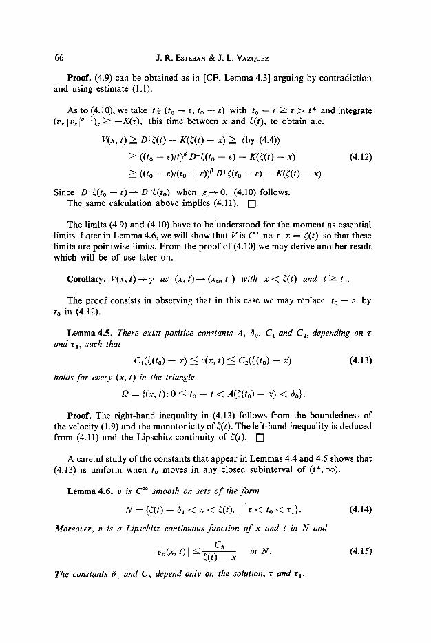
66 J.R. ESTEBAN ~; J. L. VAZQUEZ
Proof. (4.9) can be obtained as in [CF, Lemma 4.3] arguing by contradiction and using estimate (l.1).
As to (4.10), we take tC (to -- e, to q- e) with to -- e >_-- ~ > t* and integrate (v x [vxlP-l)x >= - -K(z ) , this time between x and ((t), to obtain a.e.
V(x, t) ~> D+((t) - - K( ( ( t ) - - x) ~= (by (4.4))
((to - - e)/t) ~ D+((to - - e) - - K ( ( ( t ) - - x) (4.12)
>= ((to - - e)/(to q- e)) ~ O+((to - - e) - - K( ( ( t ) - - x ) .
Since D+((to - - e ) -+ D-( ( to ) when e - + 0, (4.10) follows. The same calculation above implies (4.11). [ ]
The limits (4.9) and (4.10) have to be understood for the moment as essential limits. Later in Lemma 4.6, we will show that Vis C ~ near x ----- ((t) so that these limits are pointwise limits. From the proof of (4.10) we may derive another result which will be of use later on.
Corollary. V(x, t) -+ ~ as (x, t) -+ (Xo, to) with x < ~(t) and t >: to.
The proof consists in observing that in this case we may replace to -- e by to in (4.12).
Lemma 4.5. There exist positive Constants A, ~o, C1 and C2, depending on and ~ , such that
C~(~(to) - - x) ~ v(x, t) <: C2(~(to) -- x) (4.13)
holds f o r every (x, t) in the triangle
.Q : ((x, t): 0 <= to - - t < A(~(to) - - x) < t~o}.
Proof. The right-hand inequality in (4.13) follows from the boundedness of the velocity (1.9) and the monotonicity of ((t). The left-hand inequality is deduced from (4.11) and the Lipschitz-continuity of r [ ]
A careful study of the constants that appear in Lemmas 4.4 and 4.5 shows that (4.13) is uniform when to moves in any closed subinterval of ( t*,oo).
Lemma 4.6. v is Coo smooth on sets o f the f o rm
N : (~(t) - - 0 , < x < ~'(t), ~ < to < ~1}- (4.14)
Moreover, v is a Lipsehitz continuous function o f x and t in N and
C3 Ivtt(x, t) l =< r - x /n U. (4.15)
The constants ~1 and C3 depend only on the solution, ~ and 71.
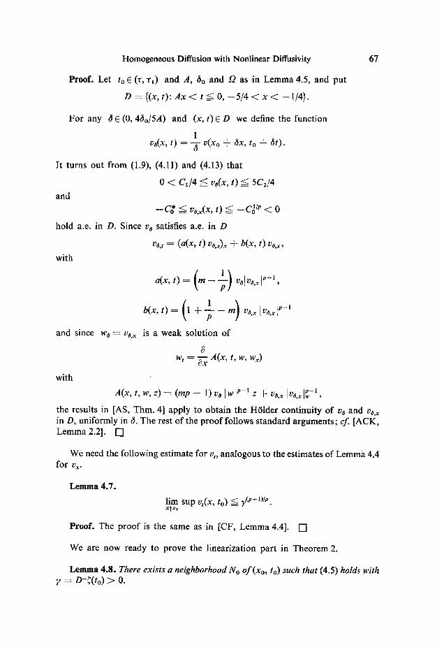
Homogeneous Diffusion with Nonlinear Diffusivity
Proof. Let to E (z, zl) and A, ~o and ~ as in Lemma 4.5, and put
O : ((x, t): A x < t ~ O, - - 5 / 4 < x < --1/4}.
For any ~ E (0, 4~o/5A) and (x, t) E D we define the function
i v~(x, t) = -T V(Xo + ~x, to + ~t).
It turns out from (1.9), (4.11) and (4.13) that
0 < C~/4 <: v~(x, t) <- 5C2/4
and
- -C~ <= V~,x(X , t) <= --C~/" < 0
hold a.e. in D. Since v~ satisfies a.e. in D
vo,t = (a(x, t) v~,~) x + b(x, t) Vo,x,
with
and since w6 : v,~,x
with
a(x t ) : (m-- v.,.xl '
) - - - - m V~,x [V~.xl " -~ b(x, t) = 1-ff P
is a weak solution of
wt : ~ A(x, t, w, Wx)
67
Lemma 4.7.
We need the following estimate for vt, analogous to the estimates of Lemma 4.4 for Vx.
lim sup v,(x, to) <: ?r X~Xo
Proof. The proof is the same as in [CF, Lemma 4.4]. [ ]
We are now ready to prove the linearization part in Theorem 2.
Lemma 4.8. There exists a neighborhood No o f (xo, to) such that (4.5) holds with 7 : D+~.(to) > O.
A(x, t, w, z) = (mp -- 1) v~ I w I " ' z + V~,x I v~,x I~w -1 ,
the results in [AS, Thin. 4] apply to obtain the H61dcr continuity of v~ and V~,x in D, uniformly in ~. The rest of the proof follows standard arguments; cf. [ACK, Lemma 2.2]. []
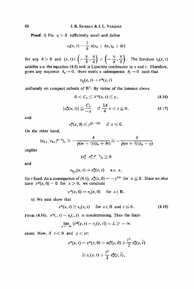
68 J .R. ESTEBAN • J. L. VAZQUEZ
Proof . i) Fix ~ /> 0 sufficiently small and define
I v~(x, t) : -~ V(Xo + 6X, to + 6t)
f ~ t $ > 0 and ( x ' t ) E ( ~ ~ - ) - 6 ' • ( ' 1 6 , 0 . ' q ) . The func t i~176
satisfies a.e. the equation (4.8) and is Lipschitz continuous in x and t. Therefore, given any sequence t$, ~ 0, there exists a subsequence t~j--> 0 such that
v~j(x, t)--> v*(x, t)
uniformly on compact subsets of a 2. By virtue of the lemmas above
0 < Co ~ V*(x, t) ~ 7, (4.16)
Ca 3A I v*(x, t) [ ~ if x ~ t ~ 0, (4.17)
=--X ~
and
On the other hand,
v*(x, O) <= 70'+l)/p if x =< 0.
implies
and
(V ,x ] V ,x lp-l)x 6
p(m + 1) (to + tSt) : p(m + 1) (t o -- ~])
v,j,x(X, t) -+ v*(x, t) a.e. x,
for t fixed. As a consequence of(4.1), v*(x, O) : --71/p for x ~ 0. Since we also have v*(x, 0 ) : 0 for x > 0, we conclude
v*(x, O) = v~(x, O) for x E R .
ii) We next show that
v*(x, t) >= vr(x, t) for x E 1% and t ~ 0. (4.18)
From (4.16), v*(., t) -- v~(., t) is nondecreasing. Thus the limit.
lim (v*(y, t) -- v~(y, t)) = L >= -- oo y ~ - - oo
exists. Now, if t ~ 0 and y ~ yt:
t a v*(y, t) = v*(y, O) + tv*t (y, O) + --f v*(y, 7)
t 2
__> v~(y, t) + T v*(y, 7),

Homogeneous Diffusion with Nonlinear Diffusivity 69
where t < T < 0 . As y - ~ o ~ , ( 4 . 1 7 ) y i e l d s L ~ 0 , Actually
v*(x , t) = vv(x, t)
which implies (4.18).
holds for every x E R and t ~ 0. This is proved with the Strong Maximum Principle when (x, t) is such that x =< yt. On the other hand, if (x, t) satisfies x > yt and v*(x, t) > 0, then necessarily v*(x , s) > 0 for all s ~ t. This leads
to a contradiction sincewe knowthat v * ( x , O ) ~ - O for x ~ 0 and v * I x , X } = 0 for x < 0 . \ y l
iii) Let us finally consider the case t > 0. Since D + ( ( t ) - + 9, as t ~v to, it follows (use also Lemma4.4) that v*(x , t ) > 0 if and only if x < 9,t, i.e. ~*(t) = 9,t is the free boundary for v*. Moreover, by the Corollary to Lemma 4.4, V~(x, t) ~ 9' if (x, t) ~ (0, 0) and x < ((t), hence V*(x , t) ---- y for x < yt. This means that v*(x, t ) = v f lx , t) for x E R and t > 0.
iv) Since the limit v* is unique, the whole family vn(x, t) converges to v* as 6 -+ 0. Formula (4.5) is a way of writing this limit with 9, = D+((to). [ ]
L e m m a 4 . 9 . D - ~ ( t o ) == y.
P r o o f . This is a simple consequence of the result of linearizing. Assume that D - ( ( t o ) < ~'. Then there exists a sequence e~ -~ 0 such that
~'(to - E . ) => ~-( to) - 7'1e, , > X o - 9,e,,
for some Yl "< V- Then for some ~n E (Xo - - 9,e., Xo - - ylen) we have, from Lemma 4.8,
v ~ ( ~ ' . , to - e . ) = (Y -- 7'I) e.
[V(Xo - - 9,1e., to - - ~.) - - V(Xo - - 7'e., to - - e,,)]
1 - - (9, - - Yl) e,, o(e,,) ~ 0 as n -~- o o .
On the other hand, the estimate (v x [I)xlP--I)x (X, to -- en)=> --K(z) implies
v ~ . , to - ~ . ) > v ( ~ ( t o - ~ . ) , to - ~ . ) - I C ( ~ ( t o - ~ . ) - ~ . )
--- o + ~ ( t o - ~ . ) - K ( ~ ( t o - ~ . ) - 2 . )
~ C o - O(~ ) ,
(where Co is the constant in (4.11)). We have arrived at a contradiction. [ ]
End o f P r o o f o f T h e o r e m 2 . W e have yet to establish the continuity of vx and vt up to the moving free boundary and formulae (4.6) and (4.7).
Firstly, the continuity of vx is a consequence of Lemmas 4.4 and 4.9. This also proves (4.6). As for v t, a bound from above is given by Lemma 4.7. The other
70 J .R. ESTEBAN • J. L. VAZQUEZ
bound is a consequence of the inequality
Vt = ( m - - - ~ ) v(,Vx]P-I Vx)x-~ [Vx] p+!
> I Vx I " + ' - K ( v ) v
which clearly implies
lim inf vt ~ y(v+o/,. [] (x , t ) -~ (xo , to )
x<~(t)
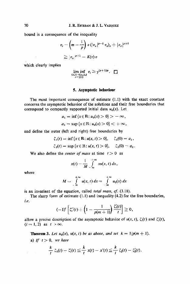
5. Asymptotic behaviour
The most important consequence of estimate (1.1) with the exact constant concerns the asymptotic behavior of the solutions and their free boundaries that correspond to compactly supported initial data Uo(X). Let
at = inf {x E R : Uo(X) > 0} > -- ~x~,
a2 = sup {x E B : Uo(X) > 0} < + cx~,
and define the outer (left and right) free boundaries by
~t(t) = inf {x E K: u(x, t) > 0}, ~t(0) = a l ,
r = sup {x 62 R: u(x, t) > 0}, ~2(0) = a2.
We also define the center of mass at time t > 0 as
1 +oo x(t) = "-~ f xu(x, t) dx,
- -oo
where + o o + ~ o
M = f u(x,t) d x = f Uo(X) dx - -oo - -oo
is an invariant of the equation, called total mass, cf. (3.18). The sharp form of estimate (1.1)and inequality (4.2)for the free boundaries,
i.e. 1 ~ ]
allow a precise description of the asymptotic behavior of u(x, t), ~i(t) and ~(t), ( i = 1,2) as t ~ c ~ .
Theorem 3. Let Uo(X), u(x, t) be as above, and set k = 1/p(m + 1).
a) I f t > O, we have
k k k ( t ( t ) ('l(t) < -'7" x(t) x'(t) < -T (2(t) (~(t). t - =

Homogeneous Diffusion with Nonlinear Diffusivity 71
b) There exists an asymptotic center o f mass, i.e. a point x~ E (a~, a2) such that
x( t ) ~ xoo and t Ix'(t) l ~ o,
as t -+ oo.
c) Let fi(x, t) = ~(x -- xoo, t; M ) be the Barenblatt solution centered at xoo with mass M. As t ~ oo, we have
i) (-- 1)" ((,(t) -- ~(t)) ~ 0,
ii) r ~ 1, t ](~(t) -- ~(t) l--~ 0,
iii) t ~ Iv(x, t) -- b(x, t) l ~ 0
1 ( I ) m uniformly on R , where oc = - - 1 i f 0 < p = ~x p (m + 1) i f l < p. p p(m + 1) < 1, and --
When p = 1--the porous medium equation--Theorem 3 was proved by VAZQUEZ in [Vl ], and much of the method of proof applies without major changes. Nevertheless, there is an interesting difference between the cases p = 1 and p =]= 1. Namely, in the latter case the center o f mass is not invariant in time for a large class of initial data. Assume in particular that Uo E L~(R) is compactly supported and that (u~)' I(u~)'l p-1 is a function of bounded variation on R. Then
+oo ~um p--I +co limt_+o _-~" -~x gum dx = .[" [P-' dx.
-fix --oo
This is easily deduced from
~u" t) p -fix(X, =< r[u,C, o/It = VAR [(Um)x ](Um)x p-llj
VAR [(u~o)' I(u~o)' [P-'].
In particular, if this last integral is not O, then x ' ( t ) =t= 0 at least for small t > O, since
1 f 1 fSu" ~-~-~-'dx. x ' ( t ) = " - ' ~ 3 xu t (x , t) dx = C X [
On the other hand, the center of mass is invariant if for instance Uo is sym- metric, i.e. uo(a + x ) - - - - -uo (a - x) for some a ER. Indeed, by symmetry x( t ) - - - -a for all t > 0 .
Proof of Theorem 3. Repeating the proof of Theorem A in [V1] we obtain the existence of x~ with al ~ x~ =< a 2 and c) of Theorem 3 holds.
In fact, x~ E (a~, a2). For if, say xoo = a2, then necessarily
~2(t) = ~2(t) = x ~ + r(t) for all t > 0.
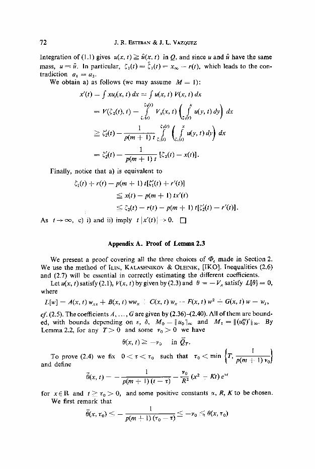
72 J. R. ESTEBAN & J. L. VAZQOEZ
Integra t ion of (1.1) gives u(x, t) ~= fi(x, t) in Q, and since u and fi have the same
mass, u ~ ft. In part icular, (~(t) = ~l(t) = xoo -- r(t), which leads to the con- tradict ion al = a2.
We obtain a) as follows (we may assume M = 1):
x'(t) = f xut(x, t) dx = f u(x, t) V(x, t) dx
= v ( G ( t ) , t) - f V~(x, t) ( u(y, t) dy dx r r
f u(y, t) dy dx => r -- p(m + 1) t cx r
1 = ~2(t) p(m -}- 1) t [r - - x(t)] .
Finally, notice tha t a) is equivalent to
r + r(t) - - p(m + 1) t[~'~(t) + r ' ( t ) ]
<: x( t ) -- p(m + 1) tx '( t)
<: (2(t) - - r(t) - - p(m + 1) t [~ ( t ) - - r ' ( t ) ] .
As t - + ~ , c) i) a n d i i ) imply t l x ' ( t ) [ - + 0 . [ ]
Appendix A. Proof of/ . ,emma 2.3
We present a p r o o f covering all the three choices of (b~ made in Section 2. We use the me thod of ILIN, KALASHNIKOV & OLEfNIK, [ IKO]. Inequali t ies (2.6) and (2.7) will be essential in correctly est imating the different coefficients.
Let u(x, t) satisfy (2.1), V(x, t) by given by (2.3) and 0 = - - Vx satisfy L[O] = O, where
L[w] = A(x, t) Wxx + B(x, t) ww x + C(x, t) Wx + F(x, t) w 2 q- 6 (x , t) w -- wt,
cf. (2.5). The coefficients A . . . . . G are given by (2.36)-(2.40). All o f them are bound- ed, with bounds depending on e, 8, Mo : lluo[Ioo and M1 : II(u'g0)'[Ioo. By L e m m a 2 . 2 , for any T > 0 and some t o > 0 we have
O(x, t) >: - - to in 0T-
To prove (2.4) we fix 0 < r < T o such tha t 7 o < m i n T , p ( m + t)~, and define
1 ~'o O(x, t) = -- p(m + 1) (t - - 7) R 2 (x2 + Kt) e at
for x C R and t ~ 7 0 > 0 , We first r emark tha t
0(x, 70) -<_ -
and some positive constants 0~, R, K to be chosen.
1 < --~o < O(x, ~o)
p(m + 1) (To - - 7) = =

Homogeneous Diffusion with Nonlinear Diffusivity 73
and
0(• t) < --%e~' < --% <= O(~k R, t).
Assume for a while that we have proved the following assertion:
There exist o~, K > O, which depend on m, p, To and the bounds o f the coefficients
A(x, t), B(x, t) and C(x, t), such that L[0] > 0 Jor every R > 0. (A.I)
Given (Xo, to) E Qr, we take 30, R such that (Xo, to) E (--R, R) • (30, T]. Then the maximum principle gives
-O(x, t) <= O(x, t) on [--R, R] x [30, T].
In particular,
1 ~o -- p(r~ + 1) (to -- z) R 2 (x2 + Kt~ eat~ ~ 0(Xo, to).
Since R does not depend on o~ and K, we obtain
1 - < O(xo, to )
p(m + 1) (to -- ~') ~-
by letting R-->oo. As r - + 0, we get
1 0(Xo, to).
p(m + 1) to
Since (Xo, to) is arbitrary, (2.4) holds. To complete the proof of the lemma, we have yet to show (A.1).
We compute L[0] and use (2.6), (2.7) to obtain
L[O'] ~ Sl q- S2 -k S3 + S,,,
where
1 [ F(x,t) ] $1 =p(rn + 1) (t -- ~.)2 Lp(m + 1 ) - 1 ,
~2 ( x2 § Kt) e z~t [2xB(x, t) + (x 2 § Kt) F(x, t)], S2 = --~
1 2Vo e~ t [xB(x, t) + (x 2 + Kt) F(x, t)], S3 = p(m + 1) (t - - ~:) R -'-~
~o e~ t [--2A(x, t) -- 2xC(x, t) + o~(x 2 + Kt) + K].
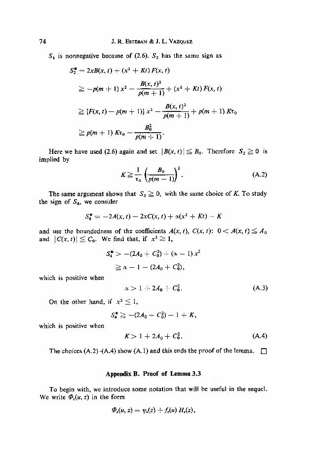
74 J.R. ESTEBAN • J. L. VAZQUEZ
$1 is nonnegative because of (2.6). $2 has the same sign as
S~ = 2xB(x, t) + (x 2 + Kt) F(x, t)
>--_ --p(m + 1) x 2 a(x, 0 2
p(m + 1) Jr (x 2 + Kt) F(x, t)
>~ IF(x, t) -- p(m + 1)1 x 2 B(x, t) z
p(m + I)
>= p(m + 1) K% Bo
p(m + I)"
+ p(m + 1) K'co
Here we have used (2.6) again and set [B(x, t)] <__ Bo. Therefore $2 ~ 0 is implied by
= ~ o p ( m ~ - l ) " (A.2)
The same argument shows that $3 ~ 0, with the same choice of K. To study the sign of S+, we consider
S* = --2A(x, t) -- 2xC(x, t) + o~(x 2 + Kt) + K
and use the boundedness of the coefficients A(x, t), C(x, t): 0 < A(x, t) <= Ao and [C(x, t) I < Co. We find that, if x 2 __> 1,
which is positive when
S~ > --(2Ao + Co 2) + (o~ -- 1) x 2
> ~ x - - 1 - - ( 2 A o + Co2),
c~> 1 + 2 A o + C 2. (A.3)
On the other hand, if x 2 ~ 1,
which is positive when
S* >~ --(2Ao + C 2) -- 1 + K,
K > I + 2 A o + C o 2. (A.4)
The choices (A.2)-(A.4) show (A.1) and this ends the proof of the lemma. [ ]
Appendix B. Proof of Lemma 3.3
To begin with, we introduce some notation that will be useful in the sequel. We write ~+(u, z) in the form
~+(u, z) : ~/,,(z) + f~(u) H~(z),
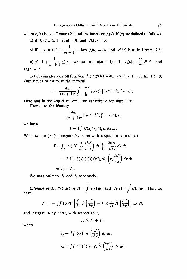
Homogeneous Diffusion with Nonlinear Diffusivity 75
where %(z) is as in Lemma 2.1 and the functions f,(u), H~(z) are defined as follows.
a) if 0 < p - - < _ l , f~(u)=O and H~(z)=O.
1 b) if 1 < p < 1 + m +-----1' then f~(u) = eu and H~(z) is as in Lemma 2.5.
~ m u~-m and c) if 1 + m + 1 ~ p ' we set n-----p(m+ 1 ) - - 1, f~(u) m
H~(z) ~- z.
Let us consider a cutoff function r E C~(R) with 0 ~ r ~ 1, and fix T > 0. Our aim is to estimate the integral
4m r +oo I (m + 1) 2 f -co f t~(x)2 ](u(m+O/2)t 12 dx dt.
Here and in the sequel we omit the subscript e for simplicity. Thanks to the identity
4m /,,(m+1)]25 2 ( l lm) t 14 t
(m + 1) ~ ! '" ,,L =
we have I = f f tr (u% u, dx dt.
We now use (2.1), integrate by parts with respect to x, and get
I = f f t~(x) 2 --~ -~x qbe u, -~x dx dt
-- 2 f f tr r (Um)t ~e (U, ~-~X ) dx dt
~ I1 +12 .
We next estimate 11 and 12 separately.
Estimate o f It. We set ~(z) = ~p(r) dr and [-I(z) = f H(r)dr. Then we have o o
11 = - f f tr 2 -[i ~ + f(u) --~ I-I ~ dx dt,
and integrating by parts, with respect to t,
I, ~ I3 + I , , where
h = f f r 2 ~ ~ ax at,
#) I, -- f f r 2 (tf(u)), h ~ dx at.
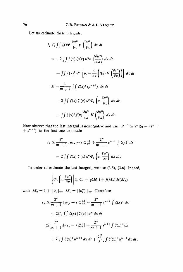
76 J . R . ESTEBAN & J. L. VAZQUEZ
Let us est imate these integrals:
I3 <= f f r 2 ~ v, t-~x ] dx at
( um) = - 2 f f r r um~j ~x dx dt
<_
- f f r ~ u" [ u , - ~
1 m q- 1 rrjj r m ,tu_+l), dx dt
- 2 f f r r umq~, (U, ~x ) dx dt
- f f r H ~ dx tit.
N o w observe tha t the last integral is nonnegat ive and use u m+l =< 2m[(u - - e) m§ + e " + l ] in the first one to obtain
/~_<-- 2 m 2 m
^llm+l @. /~m§ - - ellm+l m + 1 Iluo,, f ~(x) 2 dx
In order to est imate the last integral, we use (3.5), (3.6). Indeed,
( qb u, <= C~ -= ~p(Ml) + f(Mo) H(M~)
with Mo = 1 + Iluol[~, n ~ = II(~)'llo~. Therefore
2 m 2 m ^Hm§ ~ 8m+l
m + 1 Iluo,, - ~IFm§ ~ f r ~ dx
+ 2Ct f f g(x) I r l u m dx dt
2m 2 m < II Uo,~ o,m+l e,.+I = m + l - - ~iJm+l + ~ - - ~ ' f f r 2 dx
§ ~ f f r ~ e n+* dx dt + ~ f f r ~ u m-' dx tit,

Homogeneous Diffusion with Nonlinear Diffusivity 77
where 2 > 0 is arbitrary. Finally
m m+!
= m + l
§ (m -[- 1)~.Mg/[uolh
( 2m T) + ~ + 2 , ' + ' f r 2dx
+ f f r u ~-~ dx dr,
where we have used (3.7). We next estimate L . To this aim, we remark that (tf(u))t => 0 holds in all the
cases, because of (3.9). Then we put C2 = /~ (M1) and get
I , <= C2 f f r 2 (tf(u))t dx dt
= C 2 T f ((x)2f(u(x, T)) dx
= C~r [f $(x) ~ [f(u(x, T)) -- f(e)] dx + f ( e ) f r ~ dx].
In case b), we have .f(u) = eu and then
L <= eC2T [f r T) -- el dx + e f r 2 dx]
< eC~T [f (u(x, T) -- e) dx + s f r dx]
< ec2r[l[uo[h + e f r dx],
He from (3.7). In case c), we have f ( u ) = - - d '-m with n - - m ~ 1, and
m
I , <= nC2Te[(n -- m) M~ - ~ - l IIUo[ll + e"-m f ~-(X) 2 dx], m
where we have used (3.5) and (3.7). This completes the estimate o f /1 .
Estimate o f 12.
]/21 ~ 2Ct f f tr I r (~ ) , I dx dt
< �89 + 2mC~,ff tr 2 ~ - 1 dx dt.
We now put together the estimates of I~ and I2, and obtain
� 89 where
Is = 2mC21 f f r 2 d " -~ dx dt.
Let us now pass to the limit as e -+ O. We take ( , ( x ) = (o(eX), where (oEC~(R) , 0 ~ ( o ( X ) = < 1, (o(X)= 1 for [ x l ~ 1 and ( o ( X ) = 0 for ] x [ ~ 2 .

78 J . R . ESTEBAN • J. L. VAZQUEZ
We have
where
Then, if m ~ 1,
rtl
/3 < I1Uo,~ _ ilmq- 1 = - - e l l m + t m 4 - 1
4- (m 4- 1) 2(M~ n 4- e m) [luolh
4- 4 + 2 e m
4- 13,~
c? , z3, = T f f r dx dt.
CTC~M~ '-~ I3'~ ~ 2 e--~ O
as e - -+0. I f 0 < m < I, we use (3.5) and get
C T C 2 e m --~ 0 1 3 . ~
2
as e--~ O. Therefore, as e---~ O, we have
m ,, IIm+ 1 lim 13 < II"ollm+l -}- (m -21- 1) 2 HUoll~ HuOHl.
= r n 4 - 1
As for the integral /4, we have in all cases /4 ---- O(e). Is is similar to I3,6. Since 2 ~ 0 was arbitrary, we finally get
l i m I ~ Cm FJUolI,~_~. [] ~ -'~-0
[AhS]
[An]
[A1]
[A2]
[A3]
[A4]
R e f e r e n c e s
AHMED, N., t~ SUNADA, D. K. Nonlinear flows in porous media. J. Hydraulics Div. Proc. Amer. Soc. Civil Eng. 95 (1969), 1847-1857. ANTONCEV, S. N. On the localization of solutions of nonlinear degenerate elliptic and parabolic equations. Soviet Math. Dokl. 24 (1981), 420--424. ARONSON, D. G. Regularity properties of flows through porous media. SIAM J. Appl. Math. 17 (1969), 461-467. ARONSON, D. G. Regularity properties of flows through porous media: a counter- example. SIAM J. Appl. Math. 19 (1970), 299-307. ARONSON, O. G. Regularity properties of flows through porous media: the inter- face. Arch. Rational Mech. Anal. 37 (1970), 135-149. ARONSON, D. G. The porous medium equation, in Some Problems in Nonlinear Dtffusion (A. FASANO d~ M. PRIMICERIO, eds.). Lecture Notes in Math. 1224. Springer-Vedag, 1986.
Homogeneous Diffusion with Nonlinear Diffusivity 79
lAB] ARONSON, D. G., & B[NILAN, PH., Rdgularitd des solutions de I'dquation des milieux poreux dans R N. C. R. Acad. Sc. Paris 288 (1979), 103-105.
lACK] ARONSON, D. G., CAFFARELLI, L. A., & KAMtN, S., How an initially stationary interface begins to move in porous medium flow. SIAM J. Math. Anal. 14 (1983), 639-658.
[ACV] ARONSON, D. G., CAFFAm~LU, L. A., & VAZQUEZ, J. L., Interfaces with a corner point in one-dimensionalporous medium flow. Comm. Pure Appl. Math. 38 (1985), 375--404.
[AS] ARONSON, D. G., & SERRIN, J., Local behavior o f solutions o f quasilinear para- bolic differential equations. Arch. Rational Mech. Anal. 25 (1967), 81-123.
[AV] ARONSON, D. G., & VAZQUEZ, J. L., The porous medium equation, book in pre- paration for Pitman Monographs in Mathematics.
[AtB] ATKINSON, C., & BOUILLET, J., Some qualitative properties o f solutions o f a generalized diffusion equation. Math. Proc. Camb. Phil. Soc. 86 (1979), 495-510.
[Au] AUBIN, J. P., Un th~orbme de compacitd. C. R. Acad. Sc. Paris 256 (1963), 5042- 5044.
[B] BARENBLATT, G. I., On self-similar motions o f compressible fluids in porous media. Prikl. Mat. Mech. 16 (1952), 679-698. (Russian).
[B61] B~NILAN, PH., Sur un problbme dYvolution non monotone dans L2(12). Publ. Math. Fae. Sciences Besan~on, N. 2 (1976).
[B62] B~NILAN, PH., A strong regularity L p for solutions of the porous media equation, in Contributions to Nonlinear P.D.E. (C. BARDOS and others, eds.) Research Notes in Math. 89 (Pitman, 1983).
[BC] BENILAN, PH., & CRANDALL, M. G., Regularizing effects of homogeneous evo- lution equations, in Contributions to Analysis and Geometry, supplement to Amer. J. Math. (D. N. CLARK and others, eds.), Baltimore (1981), 23-39.
[BH] BERRYMAN, J. G., • HOLLAND, C. J., Stability o f the separable solution for fast diffusion. Arch. Rational Mech. Anal. 74 (1980), 379-388.
[Br] BR~zis, H., Monotonicity methods in Hilbert spaces and some applications to nonlinear partial differential equations, in Contributions to Nonlinear Functional Analysis. (E. ZARANTONELLO, ed.). Academic Press (1971), 101-156.
[CF] CAFFARELLI, L. A., & FRIEDMAN, A., Regularity o f the free boundary for the one- dimensional flow o f gas in a porous medium. Amer. J. Math. 101 (1979), 1193- 1218.
[DH] VAN DUIJN, H., & HILHORST, D., On a doubly nonlinear diffusion equation in hydrology. Nonlinear Anal. T.M. & A., 11 (1987), 305-333,
[EV] ESTEBAN, J. R., & VAZQUEZ, J. L., On the equation o f turbulent filtration in one-dimensionalporous media. Nonlinear Anal. T.M. & A. 10 (1986), 1303-1325.
[GP] GILDING, B. G., t~ PELETIER, L. A., The Cauchy problem for an equation in the theory o f infiltration. Arch. Rational Mech. Anal. 61 (1976), 127-140.
[GM] GURTIN, M. E., & MACCAMY, R. C., On the diffusion o f biological populations. Math. Biosc. 33 (1977), 35-49.
[HP] HERRERO, M.A., & PIERRE, M., The Cauchy problem for u t : A(u m) when 0 < m < 1. Trans. Amer. Math. Soc. 291 (1985), 145-158.
[HV] HERRERO, M. A., & VAZQUEZ, J. L., On the propagation properties o f a nonlinear degenerate parabolic equation. Comm. PDE 7 (1982), 1381-1402.
[IKO] ILIN, A. M., KALASHNXKOV, A. S., & OLEINIK, O. A., Second.order linear equa- tions o f parabolic type. Russian Math. Surveys 17 (1962), 1-143.
[K1] KALASHNIKOV, A. S., On a nonlinear equation appearing in the theory o f non- stationary filtration. Trud. Sem. I. G. Petrovsky 4 (1978), 137-146 (Russian).
[K2] KALASHNIKOV, A. S., On the Cauchy problem for second order degenerate parabolic
80 J .R. ESTEBAN ~, J. L. VAZQUEZ
equations with non power nonlinearities. Trud. Sem. I. G. Petrovsky 6 (1981), 83-96 (Russian).
[K3] KALASHNtKOV, A. S., On the propagation of perturbations in the first boundary- value problem for a doubly nonlinear degenerate parabolic equation. Trud. Sem. I. G. Petrovsky 8 (1982), 128-134 (Russian).
[Kn] KNERR, B. F., The porous medium equation in one dimension. Trans. Amer. Math. Soc. 234 (1977), 381-415.
[Kr] KRISrIANOVITCH, S. A., Motion of ground water which does not conform to Darcy's law. Prikl. Mat. Mech. 4 (1940), 33-52 (Russian).
[LSU] LADYZENSKAJA, O. A., SOLONNIKOV, V. A., & URALCEVA, N. N.,Linearand quasi- linear equations of parabolic type. Translations of Math. Monographs, A.M.S. 1968.
ILl LEIBENSON, L. S., General problem of the movement of a compressible fluid in a porous medium. Izv. Akad. Nauk SSSR, Geography and Geophysics 9 (1945), 7-10 (Russian).
[MP] MARTINSON, L. K., & PAVLOV, K. B., Unsteady shear flows of a conducting fluid with a theological power law. Magnit. Gidrodinamika 2 (1971), 50-58.
[M] MUSKAT, M., The flow of homogeneous fluids through porous media. McGraw Hill, 1937.
[PR] PAVLOV, K. B., & ROMANOV, A. S., IZariation of the region of localization of dis- turbances in nonlinear transport processes. Izv. Akad. Nauk SSSR, Mech. Zhidk. Gaza, 6 (1980), 57--62 (Russian).
[P] PELETIER, L. A., The porous media equation, in Applications of Nonlinear Ana- lysis in the Physical Sciences, (H. AMANN and others, eds.). Pitman, 1981.
[R] RAVlART, P. A., Sur la rdsolution de certaines dquations paraboliques non lin~aires. J. Funct. Anal. 5 (1970), 299-328.
[V1 ] VAZQUEZ, J. L., Asymptotic behavior and propagation properties of the one-dimen- sional flow of gas in a porous medium. Trans. Amer. Math. Soc. 277 (1983), 507-527.
[V2] VAZQUEZ, J. L., The interface of one-dimensional flows in porous media. Trans. Amer. Math. Soc. 285 (1984), 717-737.
[V3] VAZQUEZ, J. L., A strong maximum principle for some quasilinear elliptic equations. Appl. Math. Optim. 12 (1984), 191-202.
[Vo] VOLKER, R. E., Nonlinear flow in porous media by finite elements. J. Hydraulics Div. Proc. Amer. Soc. Civil Eng. 95 (1969), 2093-2114.
[W] WIDDER, D. V., The heat equation. Academic Press, 1975. [RZ] ZELDOVICH, YA. B., & RAIZER, YU. P., Physics of shock waves and high tempera-
ture hydrodynamic phenomena. Academic Press, 1966.
Departamento de Matemfiticas Universidad Aut6noma de Madrid
28049 Madrid, Spain
(Received December 23, 1987)