arX

iv:1

006.

0216

v1 [

cond

-mat

.sof

t] 1

Jun

201

0

Diffusivity and Weak clustering in a Quasi 2D Granular Gas

J. A. Perera-Burgos1,2,∗ G. Perez-Angel1,2, and Y. Nahmad-Molinari2

1Departamento de Fısica Aplicada, Centro de Investigacion y de Estudios Avanzados

del IPN, Unidad Merida, AP 73 “Cordemex”, 97310 Merida, Yuc. Mexico; and

2Instituto de Fısica “Manuel Sandoval Vallarta”,

Universidad Autonoma de San Luis Potosı,

Alvaro Obregon 64, San Luis Potosı, SLP, Mexico

(Dated: September 26, 2013)

Abstract

We present results from a detailed simulation of a quasi-2D dissipative granular gas, kept in a

non-condensed steady state via vertical shaking over a rough substrate. This gas shows a weak

power-law decay in the tails of its Pair Distribution Functions (PDF’s), indicating fractality and

therefore a tendency to form clusters over several size scales. This clustering depends monotonically

on the dissipation coefficient, and disappears when the sphere-sphere collisions are conservative.

Clustering is also sensitive to the packing fraction. This gas also displays the standard non-

equilibrium characteristics of similar systems, including non-Maxwellian velocity distributions. The

diffusion coefficients are calculated over all the conditions of the simulations, and it is found that

diluted gases are more diffusive for smaller restitution coefficients.

PACS numbers: 47.70.Nd, 83.10.Rs

∗Electronic address: jperera@mda.cinvestav.mx

1

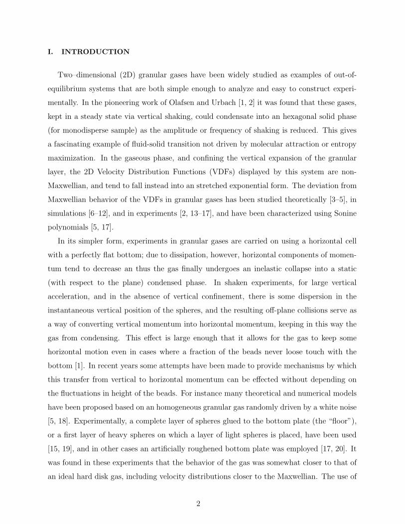
I. INTRODUCTION

Two–dimensional (2D) granular gases have been widely studied as examples of out-of-

equilibrium systems that are both simple enough to analyze and easy to construct experi-

mentally. In the pioneering work of Olafsen and Urbach [1, 2] it was found that these gases,

kept in a steady state via vertical shaking, could condensate into an hexagonal solid phase

(for monodisperse sample) as the amplitude or frequency of shaking is reduced. This gives

a fascinating example of fluid-solid transition not driven by molecular attraction or entropy

maximization. In the gaseous phase, and confining the vertical expansion of the granular

layer, the 2D Velocity Distribution Functions (VDFs) displayed by this system are non-

Maxwellian, and tend to fall instead into an stretched exponential form. The deviation from

Maxwellian behavior of the VDFs in granular gases has been studied theoretically [3–5], in

simulations [6–12], and in experiments [2, 13–17], and have been characterized using Sonine

polynomials [5, 17].

In its simpler form, experiments in granular gases are carried on using a horizontal cell

with a perfectly flat bottom; due to dissipation, however, horizontal components of momen-

tum tend to decrease an thus the gas finally undergoes an inelastic collapse into a static

(with respect to the plane) condensed phase. In shaken experiments, for large vertical

acceleration, and in the absence of vertical confinement, there is some dispersion in the

instantaneous vertical position of the spheres, and the resulting off-plane collisions serve as

a way of converting vertical momentum into horizontal momentum, keeping in this way the

gas from condensing. This effect is large enough that it allows for the gas to keep some

horizontal motion even in cases where a fraction of the beads never loose touch with the

bottom [1]. In recent years some attempts have been made to provide mechanisms by which

this transfer from vertical to horizontal momentum can be effected without depending on

the fluctuations in height of the beads. For instance many theoretical and numerical models

have been proposed based on an homogeneous granular gas randomly driven by a white noise

[5, 18]. Experimentally, a complete layer of spheres glued to the bottom plate (the “floor”),

or a first layer of heavy spheres on which a layer of light spheres is placed, have been used

[15, 19], and in other cases an artificially roughened bottom plate was employed [17, 20]. It

was found in these experiments that the behavior of the gas was somewhat closer to that of

an ideal hard disk gas, including velocity distributions closer to the Maxwellian. The use of

2

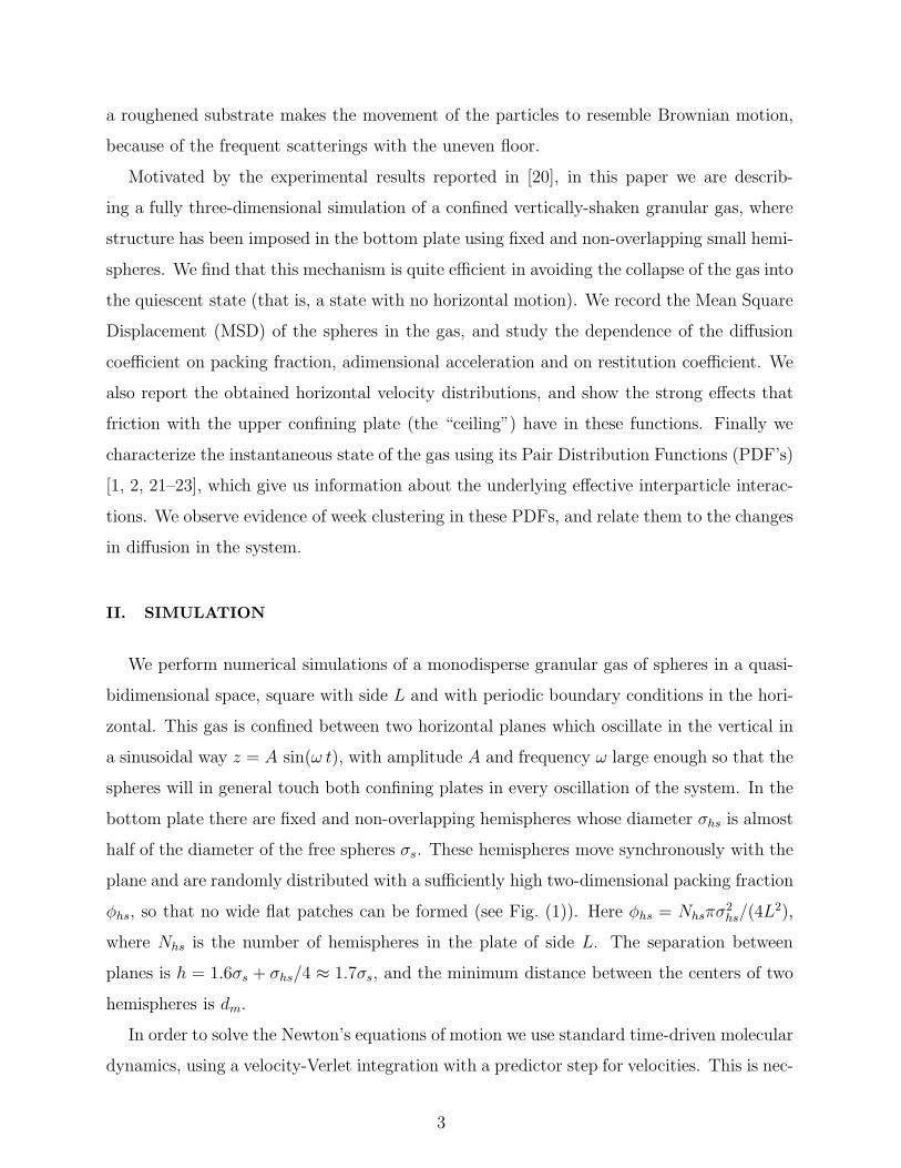
a roughened substrate makes the movement of the particles to resemble Brownian motion,

because of the frequent scatterings with the uneven floor.

Motivated by the experimental results reported in [20], in this paper we are describ-

ing a fully three-dimensional simulation of a confined vertically-shaken granular gas, where

structure has been imposed in the bottom plate using fixed and non-overlapping small hemi-

spheres. We find that this mechanism is quite efficient in avoiding the collapse of the gas into

the quiescent state (that is, a state with no horizontal motion). We record the Mean Square

Displacement (MSD) of the spheres in the gas, and study the dependence of the diffusion

coefficient on packing fraction, adimensional acceleration and on restitution coefficient. We

also report the obtained horizontal velocity distributions, and show the strong effects that

friction with the upper confining plate (the “ceiling”) have in these functions. Finally we

characterize the instantaneous state of the gas using its Pair Distribution Functions (PDF’s)

[1, 2, 21–23], which give us information about the underlying effective interparticle interac-

tions. We observe evidence of week clustering in these PDFs, and relate them to the changes

in diffusion in the system.

II. SIMULATION

We perform numerical simulations of a monodisperse granular gas of spheres in a quasi-

bidimensional space, square with side L and with periodic boundary conditions in the hori-

zontal. This gas is confined between two horizontal planes which oscillate in the vertical in

a sinusoidal way z = A sin(ω t), with amplitude A and frequency ω large enough so that the

spheres will in general touch both confining plates in every oscillation of the system. In the

bottom plate there are fixed and non-overlapping hemispheres whose diameter σhs is almost

half of the diameter of the free spheres σs. These hemispheres move synchronously with the

plane and are randomly distributed with a sufficiently high two-dimensional packing fraction

φhs, so that no wide flat patches can be formed (see Fig. (1)). Here φhs = Nhsπσ2hs/(4L

2),

where Nhs is the number of hemispheres in the plate of side L. The separation between

planes is h = 1.6σs + σhs/4 ≈ 1.7σs, and the minimum distance between the centers of two

hemispheres is dm.

In order to solve the Newton’s equations of motion we use standard time-driven molecular

dynamics, using a velocity-Verlet integration with a predictor step for velocities. This is nec-

3

essary in order to incorporate the dissipative part of the force, which is velocity-dependent.

The force between particles in contact is described by

Fij =

Fnij + Ft

ij when ξij > 0,

0 otherwise,(1)

where Fnij is a normal force which causes changes of the translational motion of the particles

and Ftij is a tangential force, originating in friction, which causes changes in both the trans-

lational and the rotational motion. The quantity ξij is the mutual overlap (compression) of

particles i and j and is defined by

ξij = max(0, σs − |ri − rj|) (2)

for interparticle collisions, by

ξij = max(0, (σs + σhs)/2− |ri −Rj|) (3)

for particle-scatterer collisions, and by

ξip = max(0, σs/2− dip) (4)

for sphere-plate collisions. Here ri denotes the center of the i-th grain, Ri the center of the

i-th scatterer, and dip is the normal distance from the center of the i-th grain to the surface

of the plate p.

Modeling a force that leads to inelastic collisions requires at least two terms: repulsion

and some type of dissipation. The existing models and their characteristics, as well as

comparisons among them, can be found in [24–29]. Here we have used for the normal force

the linear spring-dashpot model, in which the contact interaction is modeled by the damped

harmonic oscillator force

Fn = min{

0, −κnξ − γnξ}

, (5)

where γn is a damping constant and κn is related to the stiffness of a spring whose elongations

is ξ, the overlap between two grains (or a grain and a boundary plate). The advantage of

this model lays in its analytic solution, where the collision time is given by

tn = π

(

κn

meff

−(

γn2meff

)2)

−1/2

, (6)

4

and the restitution coefficient is

en = exp

(

− γn2meff

tn

)

. (7)

Here meff is the effective mass for the colliding pair. For the tangential force we consider

the Coulomb dynamical friction law Ftij = −µF n

ijvti,j , where vt

i,j is the unitary vector in the

direction of the relative tangential velocity between spheres i and j (or, by extension, between

a sphere and a scatterer or a sphere and a plate). The effect of gravity is incorporated into

the vertical acceleration.

For the actual simulations we have taken most parameters similar to those of the pre-

viously mentioned experiments [20], as performed with steel spheres. Therefore, we have

fixed the frequency of oscillation of the cell to f = 60 Hz, and have considered two ampli-

tudes of oscillation: A1 = 0.024 cm and A2 = 0.05 cm, for every packing fraction φ of free

spheres, getting in this way for the adimensional acceleration Γ ≡ (2πf)2A/g the values

Γ1 = 3.5 and Γ2 = 7.2. Here φ is defined as before by φ = Nσ2sπ/(4L

2). As parameters

for the normal force, Eq. (5), we use those extracted from Eqs. (6,7), and fix the collision

time to tn = 7.1x10−5 s, and use three values of the restitution coefficients en = 0.36, 0.66

and 1 for the sphere-sphere and sphere-hemisphere interactions (at each value of Γ and

for every packing fraction φ considered). The coefficient of restitution for sphere-substrate

interaction was fixed at 0.878, corresponding to an experimentally measured steel-acrylic

restitution coefficient [20], and the considered coefficient of dynamical friction µ was 0.25.

The time-step of the integration is always fixed to tn/100, and the simulation time is 40 s,

after a transient of 10 s. The diameter of the free spheres σs and of the hemispheres σhs have

been fixed to 0.44 cm and 0.2 cm, respectively, in all simulations. The minimal distance

between hemispheres is dm = 0.2 cm. Finally, the boundary plates have side L = 16 cm, and

the packing fractions used have been φ = 0.15, 0.20, 0.25, 0.30 and 0.35 for both Γ values

used. The resulting numbers of grains are Ns = 252, 336, 420, 504 and 588 respectively, and

the number of scatterers is Nhs = 4100. All the quantities reported here are the average

over 10 simulations, each with a different configuration of hemispheres and different initial

conditions.

5

III. NUMERICAL RESULT: DIFFUSION

We will start by presenting results for the diffusion in the quasi-2D granular gas. As

mentioned before, the interaction with the hemispheres provides horizontal momentum to

the particles, but also scatters their motion, making them to move on a pseudorandom way,

resembling in certain form a Brownian motion. It is clear that the interparticle collisions also

contribute to the scattering. In Fig. (2) we can see two trajectories for a single particle on

a complete simulation of 40 s, one for the case with en = 1 and another for en = 0.36. This

was done with a packing fraction φ = 0.15, and the trajectory includes the interactions with

the other particles and with the substrate. One must remember here that the restitution

coefficient for particle-plate collisions is always fixed, while that for particle-hemisphere

collisions is the same as the one for particle-particle collisions, and can be varied.

The MSDs measured fit very well the Einstein form

〈(r(t+ t0)− r(t0))2〉 = 4D t; (8)

this is not as trivially expected as it may seem, since some recent results point to a breakdown

of Einstein’s law for 2D granular gases [30]. This is related to a well-known anomaly for

self-diffusion in 2D, where the presence of hydrodynamical backflows gives origin to long

tails in the velocity autocorrelation function. These tails behave as t−1, giving in this way a

logarithmic divergence to the diffusion coefficient, accordingly to the Green-Kubo formula

[31, 32]. In our simulations we have not seen any evidence of non-Einstenian behavior; in

particular we have performed sets of longer runs (80 s) for three different sets of parameters,

and one set of runs for a bigger system (L = 16√2 = 22.63 cm), and in all cases the same

diffusive behavior was found, with the diffusion coefficient independent of the length of the

run or the system size. Looking at the difference between these results and those of [30], it

is clear that the presence of fixed (with respect to the plane) scatterers is the reason why

regular diffusion is restored.

In Fig. (3) we show the diffusion coefficient D versus the packing fraction for both values

of the adimensional acceleration. Here we can observe the following points: first, D increases

for low values of φ, and decrease for high values of φ. These results are in agreement with

those obtained by [33, 34], and are to be expected, since larger densities represent in general

more obstacles to the motion. Second, for small values of φ the diffusion coefficient increases

when we lower en, and this behavior is stronger for low Γ. As the concentration and Γ grow,

6

this behavior reverses, that is, for large φ there is a crossover were the diffusion grows

with en. Theoretical evidence for an inverse relationship between diffusion and restitution

coefficients has recently been found in [33], as shown in their Fig. (5). This is also noticeable

in our Fig. (2), where one can observe how the particle excursions are larger for lower en.

The increase in diffusion for smaller en is related to the appearance of density fluctuations

that become stronger as the dissipation increases. This weak clusterization becomes apparent

as a fall of the tails of the PDFs for large distances, as we will see later. Clusterization

ends up freeing some space in the system, allowing in this way faster diffusion. The same

phenomenon is well known in colloid-polymer mixtures, where the depletion forces induced

by the (small) polymers create strong density fluctuations in the colloidal phase, and increase

its diffusion [35, 36].

IV. GRANULAR TEMPERATURE AND VELOCITY DISTRIBUTION FUNC-

TIONS

In this section we perform a detailed analysis of the granular temperature Tg and of the

Velocity Distribution Functions (VDFs) P (v) obtained in the simulations. In Fig. (4) we

can observe the behavior of the in-plane Tg, defined as Tg = Tx + Ty = 〈v2x〉 + 〈v2y〉, as a

function of the packing fraction φ, for all values of Γ and en considered. The following points

deserve to be mentioned: first, for any given values of φ and en, Tg increases together with

Γ, as is intuitively expected, and experimentally observed [17]. Second, one can observe

that for given values of φ and Γ, Tg decreases together with en, also as expected. Third,

and more interesting, we find that for en = 1 the Tg grows slowly with φ, in agreement with

the experimental results obtained in [17]. In that experiment Tg grows monotonously until

reaching a maximum for some φmax ≈ 0.5, and then decays as φ keeps growing. We do not

find this later decay of Tg, probably because we are using values of φ below φmax.

The coincidence found for this particular value of en deserves some discussion: although

the authors of [17] do not report their working value of en, other references [1, 37] give

en ≈ 0.9 for the stainless steel spheres used there. As relates to the simulation, we remind

the reader that even when en = 1 there is some dissipation in our system, since this value of

the restitution coefficient is applied only for sphere-sphere and sphere-hemisphere collisions.

Contacts with the upper plate (and, even if infrequent, with the lower plate), are still

7

inelastic, with en = 0.878. Besides, the existence of a nonzero value of µ gives us some

energy losses via friction, for all collisions. One may therefore assume that there is, in our

simulation, some effective en a bit smaller than 1, and that the slow growth of the Tg for

diluted gases found in both experiment and simulation occurs for high values of en, not

necessarily en = 1. This should be stressed since, for values of en well bellow 1, Tg actually

decays very slowly as φ increases, at least for the range of φ considered here. We are not

aware of any experimental study of Tg for highly dissipative materials, and so there is no

verification of this curious behavior reversal for small restitution coefficients.

The VDFs for both components of the horizontal velocity have been obtained, for all

values of Γ, φ and en considered. In Fig. (5) we show a few of those curves, normalized

by their characteristic velocities vc =√

〈v2i 〉 =√Ti. In the same Figure we also show,

as a reference, a unitary Gaussian. The first remarkable fact is that for all values of φ,

when en = 0.66 and 1.0, with Γ = 3.5, and also for all values of en and Γ = 7.2, the

VDFs present a strong peak at the center of the distribution —that is, for low velocities—.

(Only some examples are shown, to avoid crowding the Figure.) These peaks can be also

found in Fig. (8) of [17], for small φ. In that reference, they are attributed to the fact

that at these packing fractions the effect of interparticle collisions is minimal, and so the

general distribution is dominated by the VDF corresponding to one isolated particle. The

simulations show that the main reason for the appearance of this peak is the friction of the

grains with the upper plate in the system. In particular, as can be easily visualized in a

1D system, rotational velocities acquired at the collisions with the floor act as a braking

factor upon contact with the ceiling, increasing in this way the concentration of particles

with low horizontal velocities. In Fig. (6) we show the normalized curves for the VDFs, for

the case φ = 0.20, Γ = 3.5, and en = 0.66 and 1.0, but taking the grain-ceiling value of µ

as 0.0 in one case and µ = 0.25 in the other. It is quite apparent from this Figure how,

when there is no friction with the ceiling, there are no low-velocity peaks. However, it can

be seen from the same Figure that the braking effect of the ceiling is not the only factor

involved in the non-Gaussian behavior of the VDFs; in particular, the line for en = 0.66

and µceiling = 0 shows very clear deviations from the Gaussian. Even stronger deviations

are found for en = 0.36 and µceiling = 0 (not shown in the Figure.) We would also like to

mention that these peaks diminish as the packing fraction of the systems grows, as observed

in [17].

8

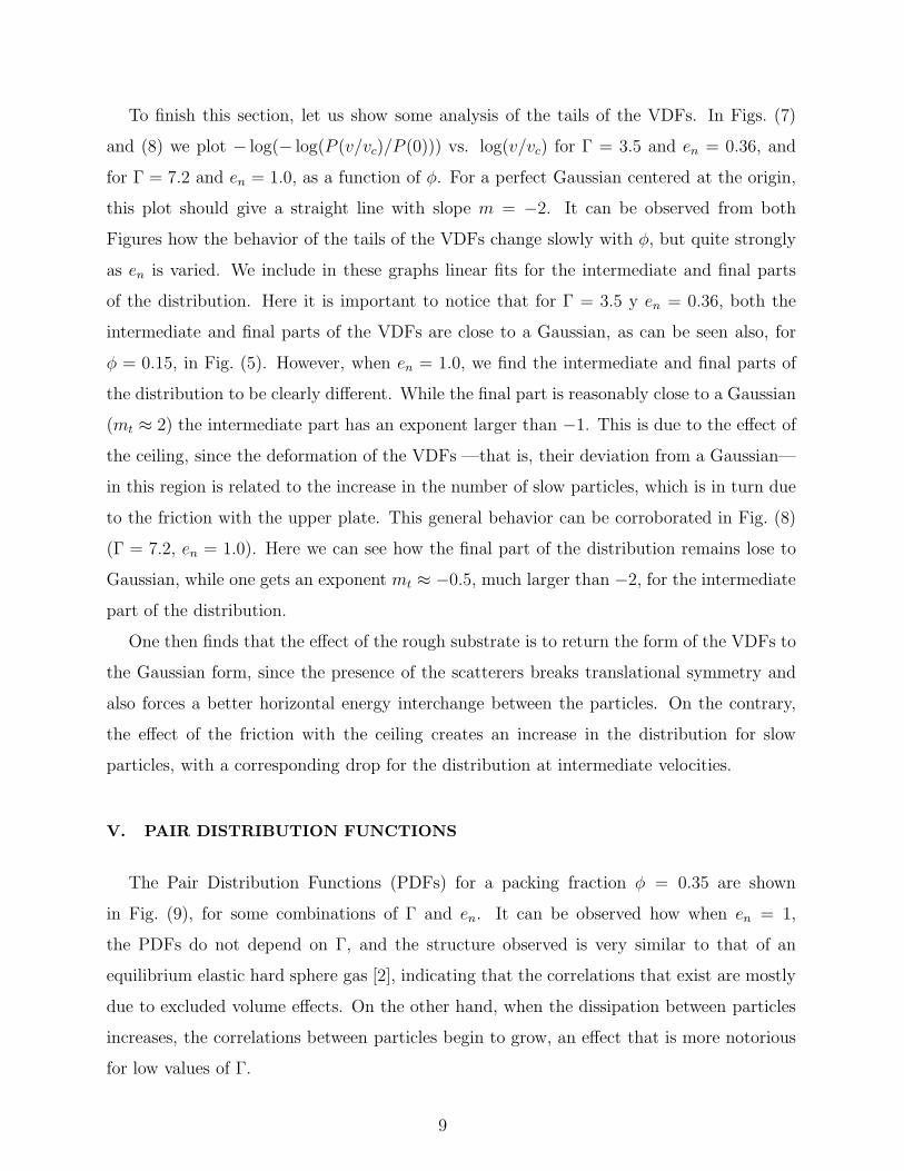
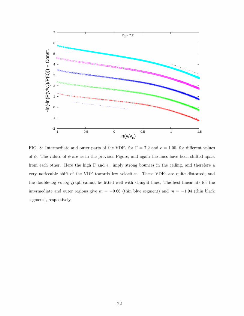
To finish this section, let us show some analysis of the tails of the VDFs. In Figs. (7)

and (8) we plot − log(− log(P (v/vc)/P (0))) vs. log(v/vc) for Γ = 3.5 and en = 0.36, and

for Γ = 7.2 and en = 1.0, as a function of φ. For a perfect Gaussian centered at the origin,

this plot should give a straight line with slope m = −2. It can be observed from both

Figures how the behavior of the tails of the VDFs change slowly with φ, but quite strongly

as en is varied. We include in these graphs linear fits for the intermediate and final parts

of the distribution. Here it is important to notice that for Γ = 3.5 y en = 0.36, both the

intermediate and final parts of the VDFs are close to a Gaussian, as can be seen also, for

φ = 0.15, in Fig. (5). However, when en = 1.0, we find the intermediate and final parts of

the distribution to be clearly different. While the final part is reasonably close to a Gaussian

(mt ≈ 2) the intermediate part has an exponent larger than −1. This is due to the effect of

the ceiling, since the deformation of the VDFs —that is, their deviation from a Gaussian—

in this region is related to the increase in the number of slow particles, which is in turn due

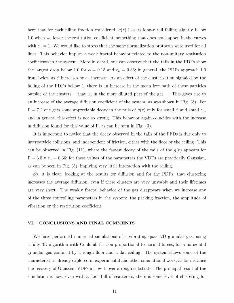
to the friction with the upper plate. This general behavior can be corroborated in Fig. (8)

(Γ = 7.2, en = 1.0). Here we can see how the final part of the distribution remains lose to

Gaussian, while one gets an exponent mt ≈ −0.5, much larger than −2, for the intermediate

part of the distribution.

One then finds that the effect of the rough substrate is to return the form of the VDFs to

the Gaussian form, since the presence of the scatterers breaks translational symmetry and

also forces a better horizontal energy interchange between the particles. On the contrary,

the effect of the friction with the ceiling creates an increase in the distribution for slow

particles, with a corresponding drop for the distribution at intermediate velocities.

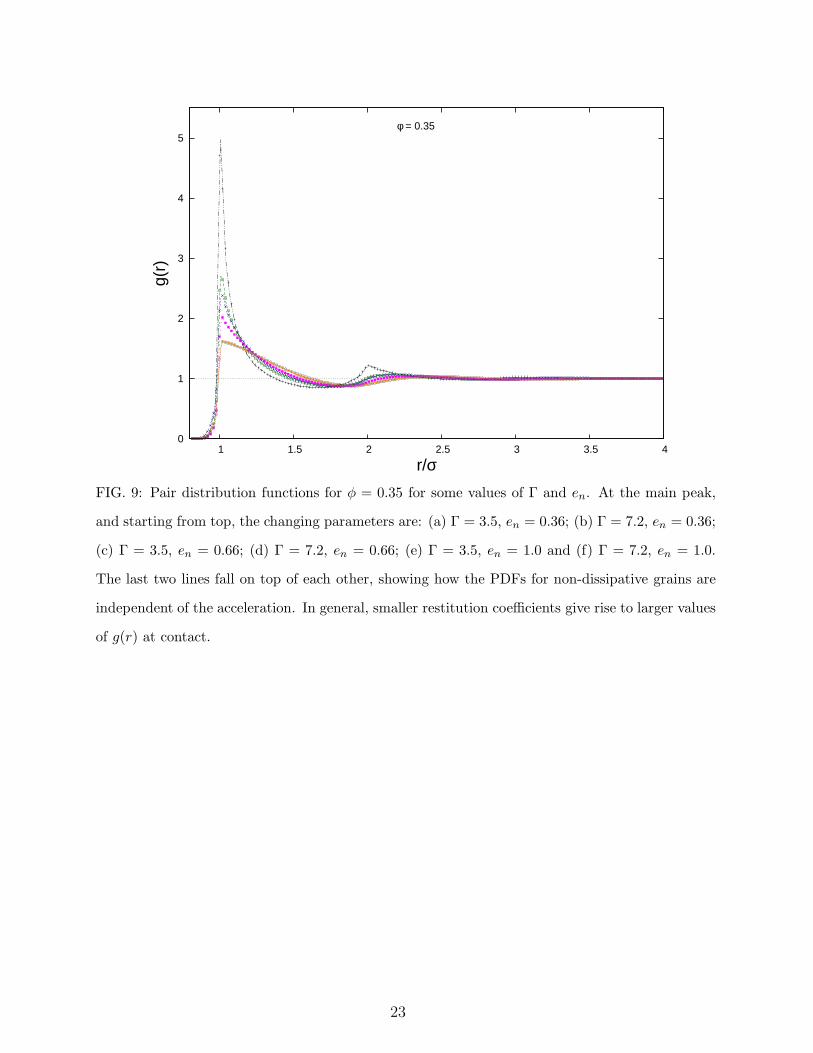
V. PAIR DISTRIBUTION FUNCTIONS

The Pair Distribution Functions (PDFs) for a packing fraction φ = 0.35 are shown

in Fig. (9), for some combinations of Γ and en. It can be observed how when en = 1,

the PDFs do not depend on Γ, and the structure observed is very similar to that of an

equilibrium elastic hard sphere gas [2], indicating that the correlations that exist are mostly

due to excluded volume effects. On the other hand, when the dissipation between particles

increases, the correlations between particles begin to grow, an effect that is more notorious

for low values of Γ.

9

The lines shown in the graph have two intriguing characteristics: first, we find a complete

absence of any structure at r/σ =√3 = 1.73, where a peak appears in the close-packed limit.

Neither there is a peak around r/σ =√2 = 1.41, which would signal some type of square

clustering. It is therefore clear that the rough floor eliminates completely the possibility of

formation of large crystalline clusters. Second, a very peculiar secondary peak develops, for

small driving and high dissipation (Γ = 3.5 and en = 0.36), at r/σ ≈ 2. The possible reason

we have identified for the origin of this peak is the formation, at this low values of driving

and restitution coefficient, of short-lived linear chains of grains (see Fig. (1) for an example).

These linear chains may be induced by some residual order in the substrate, an order that

in turn is due to the fact that it has to satisfy simultaneously a large density of scatterers

and the no-overlap condition. It will be therefore interesting to see the evolution of g(r)

in those experiments where an ordered substrate has been used [15, 19]; although it is also

clear from the graph that only for the smallest restitution coefficient used we get this peak.

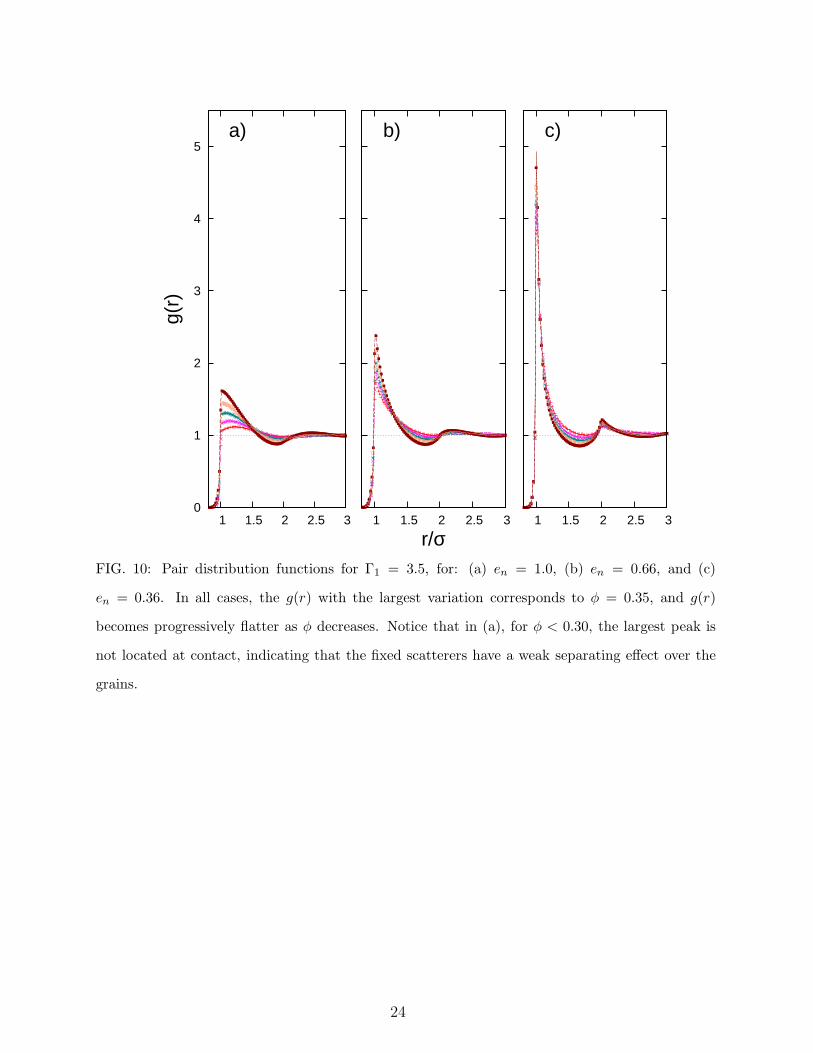
Fore a more comprehensive view of the evolution of g(r), in Fig. (10) we show the PDFs

for Γ = 3.5, as a function of en and φ. The very strong effect that en has in these curves is

the first thing to notice; for high dissipation the structure of the main peak in g(r) is almost

independent of φ, and little variation can be seen in the rest of the curve. The large value of

g(r) at the main peak signals a tendency to clustering. At the other extreme, the gas with

en = 1.0 shows much more sensitivity to φ. An unusual behavior can be seen for en = 1

and small φ: the largest value of g(r) no longer falls at contact, and instead, a soft “hill”

develops around r/σ ≈ 1.2–1.3. This is again an effect of the scatterers, that a this high

value of en intrude between the grains, and, for small packing factors, reduce the probability

of contact. Again, there is no signal of any peak at r/σ =√3, but we find instead that for

the most dissipative system, some peak at r/σ = 2 begins to form. Visual inspection of the

dynamics in this parameter sector shows in effect the presence of short-lived linear chains.

For Γ = 7.2 (not shown) the results found are analogous: there is an increase in the height

of the main peak of g(r) as en is lowered, although not as strong as for Γ = 3.5; and there

is absolutely no peak at r/σ =√3. As for the behavior around r/σ = 2, now only some

weak increase in g(r) can be detected. A remarkable result is the fact that for all φ used

the different g(r) obtained for en = 1 agree completely for both values of Γ.

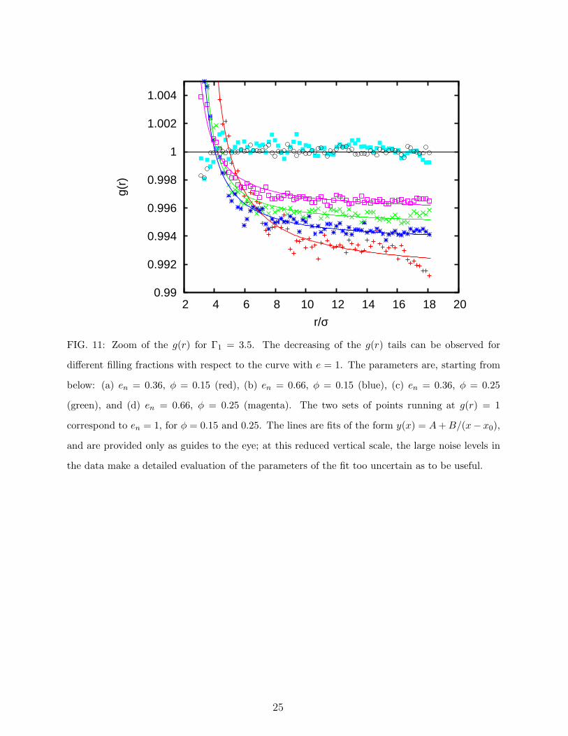
Finally, one of the most interesting points in the phenomenology of this granular gas is

shown in Fig. (11), which displays a close up to the PDFs for Γ = 3.5. It can be observed

10

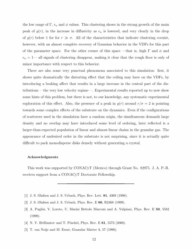
here that for each filling fraction considered, g(r) has its long-r tail falling slightly below

1.0 when we lower the restitution coefficient, something that does not happen in the curves

with en = 1. We would like to stress that the same normalization protocols were used for all

lines. This behavior implies a weak fractal behavior related to the non-unitary restitution

coefficients in the system. More in detail, one can observe that the tails in the PDFs show

the largest drop below 1.0 for φ = 0.15 and en = 0.36; in general, the PDFs approach 1.0

from below as φ increases or en increase. As an effect of the clusterization signaled by the

falling of the PDFs bellow 1, there is an increase in the mean free path of those particles

outside of the clusters —that is, in the more diluted part of the gas—. This gives rise to

an increase of the average diffusion coefficient of the system, as was shown in Fig. (3). For

Γ = 7.2 one gets some appreciable decay in the tails of g(r) only for small φ and small en,

and in general this effect is not so strong. This behavior again coincides with the increase

in diffusion found for this value of Γ, as can be seen in Fig. (3).

It is important to notice that the decay observed in the tails of the PFDs is due only to

interparticle collisions, and independent of friction, either with the floor or the ceiling. This

can be observed in Fig. (11), where the fastest decay of the tails of the g(r) appears for

Γ = 3.5 y en = 0.36; for these values of the parameters the VDFs are practically Gaussian,

as can be seen in Fig. (5), implying very little interaction with the ceiling.

So, it is clear, looking at the results for diffusion and for the PDFs, that clustering

increases the average diffusion, even if these clusters are very unstable and their lifetimes

are very short. The weakly fractal behavior of the gas disappears when we increase any

of the three controlling parameters in the system: the packing fraction, the amplitude of

vibration or the restitution coefficient.

VI. CONCLUSIONS AND FINAL COMMENTS

We have performed numerical simulations of a vibrating quasi 2D granular gas, using

a fully 3D algorithm with Coulomb friction proportional to normal forces, for a horizontal

granular gas confined by a rough floor and a flat ceiling. The system shows some of the

characteristics already explored in experimental and other simulational work, as for instance

the recovery of Gaussian VDFs at low Γ over a rough substrate. The principal result of the

simulation is how, even with a floor full of scatterers, there is some level of clustering for

11

the low range of Γ, en and φ values. This clustering shows in the strong growth of the main

peak of g(r), in the increase in diffusivity as en is lowered, and very clearly in the drop

of g(r) below 1 for for r ≫ σ. All of the characteristics that indicate clustering coexist,

however, with an almost complete recovery of Gaussian behavior in the VDFs for this part

of the parameter space. For the other corner of this space —that is, high Γ and φ and

en = 1— all signals of clustering disappear, making it clear that the rough floor is only of

minor importance with respect to this behavior.

There are also some very punctual phenomena associated to this simulation: first, it

shows quite dramatically the distorting effect that the ceiling may have on the VDFs, by

introducing a braking affect that results in a large increase in the central part of the dis-

tributions —the very low velocity regime—. Experimental results reported up to now show

some hints of this problem, but there is not, to our knowledge, any systematic experimental

exploration of this effect. Also, the presence of a peak in g(r) around r/σ = 2 is pointing

towards some complex effects of the substrate on the dynamics. Even if the configurations

of scatterers used in the simulation have a random origin, the simultaneous demands large

density and no overlap may have introduced some level of ordering, later reflected is a

larger-than-expected population of linear and almost-linear chains in the granular gas. The

appearance of undesired order in the substrate is not surprising, since it is actually quite

difficult to pack monodisperse disks densely without generating a crystal.

Acknowledgments

This work was supported by CONACyT (Mexico) through Grant No. 82975. J. A. P.-B.

receives support from a CONACyT Doctorate Fellowship.

[1] J. S. Olafsen and J. S. Urbach, Phys. Rev. Lett. 81, 4369 (1998).

[2] J. S. Olafsen and J. S. Urbach, Phys. Rev. E 60, R2468 (1999).

[3] A. Puglisi, V. Loreto, U. Marini Bettolo Marconi and A. Vulpiani, Phys. Rev. E 50, 5582

(1999).

[4] N. V. Brilliantov and T. Poschel, Phys. Rev. E 61, 5573 (2000).

[5] T. van Noije and M. Ernst, Granular Matter 1, 57 (1998).

12

[6] Y. H. Taguchi and H. Takayasu, Europhys. Lett. 30, 499 (1995).

[7] X. Nie, E. Ben-Naim and S. Y. Chen, Europhys. Lett. 51, 679 (2000).

[8] A. Barrat and E. Trizac, Phys. Rev. E 66, 051303 (2002).

[9] J. S. van Zon and F. C. MacKintosh, Phys. Rev. Lett. 93, 038001 (2004).

[10] J. S. van Zon and F. C. MacKintosh, Phys. Rev. E 72, 051301 (2005).

[11] D. J. Bray, M. R. Swift and P. J. King, Phys. Rev. E 75, 062301 (2007).

[12] A. Burdeau and P. Viot, Phys. Rev. E 79, 061306 (2009).

[13] W. Losert, D. G. W. Cooper, J. Delour, A. Kudrolli and J. P. Gollub, CHAOS 9, 682 (1999).

[14] A. Kudrolli and J. Henri, Phys. Rev. E 62, 1489 (2000).

[15] A. Prevost, D. A. Egolf and J. S. Urbach, Phys. Rev. Lett. 89, 084301 (2002).

[16] K. Kohlsted, A. Snezhko, M. V. Sapozhnikov, I. S. Aranson, J. S. Olafsen and E. Ben-Naim,

Phys. Rev. Lett. 95, 068001 (2005).

[17] P. M. Reis, R. A. Ingale and M. D. Shattuck, Phys. Rev. E 75, 051311 (2007).

[18] D. R. M. Williams and F. C. MacKintosh, Phys. Rev. E 54, R9 (1996).

[19] G. W. Baxter and J. S. Olafsen, Nature 425, 680 (2003).

[20] R. A. Bordallo-Favela, A. Ramırez-Saıto, C. A. Pacheco-Molina, J. A. Perera-Burgos, Y.

Nahmad-Molinari and G. Perez-Angel, Eur. Phys. J. E 28, 395 (2009).

[21] B. V. R. Tata, P. V. Rajamani, J. Chakrabarti, A. Nikolov and D. T. Wasan, Phys. Rev. Lett.

84, 3626 (2000).

[22] P. Eshuis, K. van der Weele, D. van der Meer and D. Lohse, Phys. Rev. Lett. 95, 258001

(2005).

[23] F. Pacheco-Vazquez, G. A. Caballero-Robledo and J. C. Ruiz-Suarez, Phys. Rev. Lett. 102,

170601 (2009).

[24] J. Schafer, S. Dippel and D. E. Wolf, J. Phys. I. France 6, 5 (1996).

[25] N. V. Brilliantov, F. Spahn, J.-M. Hertzsch and T. Poschel, Phys. Rev. E 53, 5382 (1996).

[26] A. Di Renzo and F. P. Di Maio, Chemical Engineering Science 59, 525 (2004).

[27] A. B. Stevens and C. M. Hrenya, Powder Technology 154, 99 (2005).

[28] H. Kruggel–Emden, E. Simsek, S. Rickelt, S. Wirtz and V. Scherer, Powder Technology 171,

157 (2007).

[29] T. Poschel and T. Schwager, Computational Granular Dynamics: Models and Algorithms

(Springer, 2004).

13

[30] C. Henrique, G. Batrouni and D. Bideau, in Granular Gases, edited by T. Poschel and S.

Luding, Lecture Notes in Physics vol. 564, p.140.

[31] B. J. Alder and T. E. Wainwright, Phys. Rev. A 1 18 (1970).

[32] P. J. Camp, Phys. Rev. E 71 031507 (2005).

[33] W. T. Kranz, M. Sperl and A. Zippelius, arXiv:1002.2150v1.

[34] A. R. Abate and D. J. Durian, Phys. Rev. E 74 031308 (2006).

[35] K. N. Pham et al., Science 296 104 (2002).

[36] R. Juarez-Maldonado and M. Medina-Noyola, Phys. Rev. E 77 051503 (2008).

[37] A. Kudrolli, M. Wolpert and J. P. Gollub Phys. Rev. lett. 78 1383 (1997).

14

FIG. 1: (a) Fraction of a snapshot (taken from above) of the granular gas, covering around 1/13 of

the actually simulated area. The hemispheres (scatterers) are shown as white circles, the moving

grains as yellow circles. Notice the presence of some short linear chains. (b) Schematic lateral view

of the simulated system, to scale.

15

0

2

4

6

8

10

12

14

16

0 2 4 6 8 10 12 14 16

y-po

sitio

n

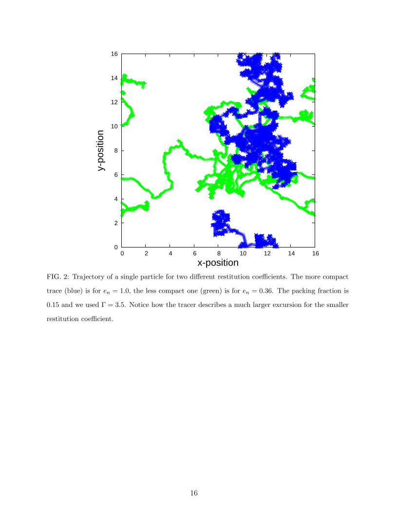
x-positionFIG. 2: Trajectory of a single particle for two different restitution coefficients. The more compact

trace (blue) is for en = 1.0, the less compact one (green) is for en = 0.36. The packing fraction is

0.15 and we used Γ = 3.5. Notice how the tracer describes a much larger excursion for the smaller

restitution coefficient.

16

0.4 0.5 0.6 0.7 0.8

0.15 0.2 0.25 0.3 0.35

D

φ

b)

0.5 0.6 0.7 0.8 0.9

1 1.1 1.2 1.3 1.4 1.5

D

a)

FIG. 3: Diffusion Coefficients vs Filling Fraction for: (a) Γ = 3.5, and (b) Γ = 7.2. The values of

en are, at the left and starting from top: en = 0.36 (red), en = 0.66 (green) and en = 1 (blue). For

the range of packing fractions covered, D always decreases with φ. The behavior with respect to

en is more complex: for small φ, D decays as en grows. For large φ there seems to be a crossover

where D starts growing with en.

17

150

200

250

300

0.15 0.2 0.25 0.3 0.35

Tg

φ

b)

50

100

150

200T

ga)

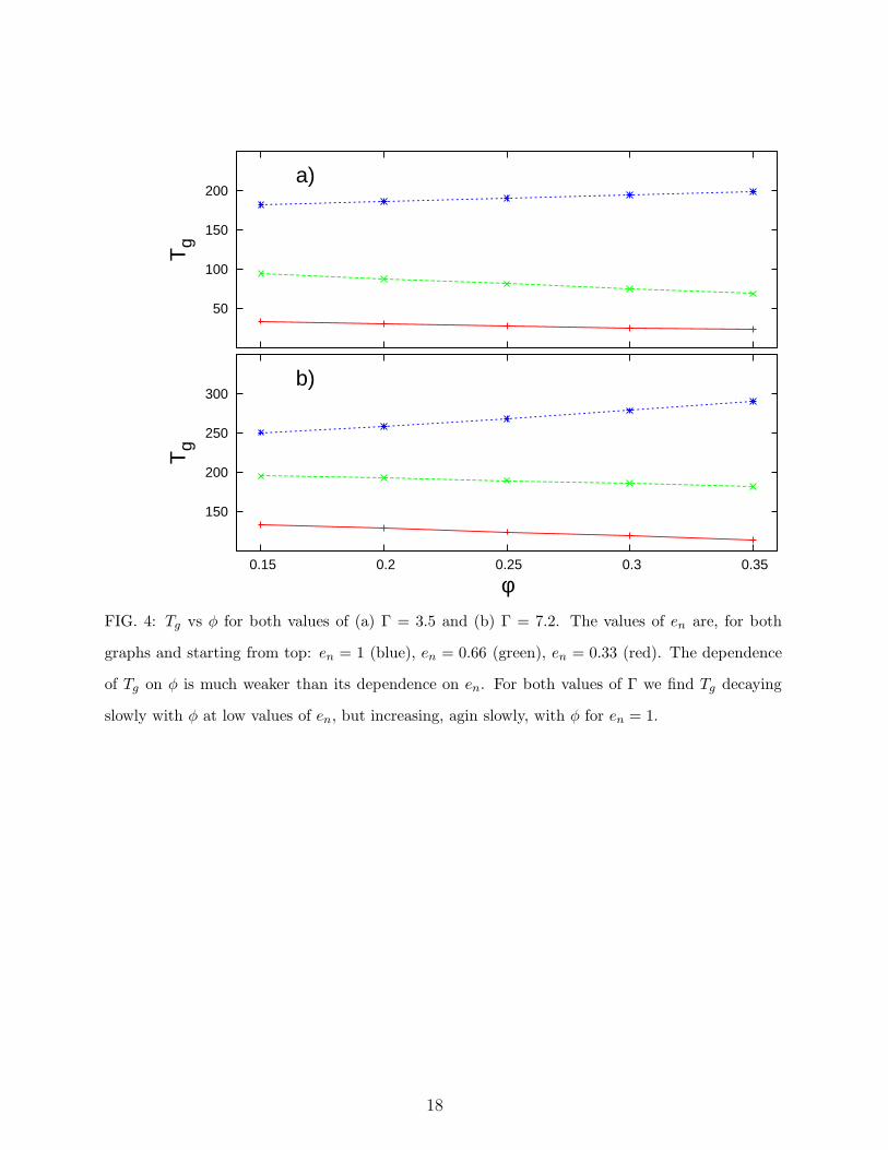
FIG. 4: Tg vs φ for both values of (a) Γ = 3.5 and (b) Γ = 7.2. The values of en are, for both

graphs and starting from top: en = 1 (blue), en = 0.66 (green), en = 0.33 (red). The dependence

of Tg on φ is much weaker than its dependence on en. For both values of Γ we find Tg decaying

slowly with φ at low values of en, but increasing, agin slowly, with φ for en = 1.

18

0.01

0.1

1

-3 -2 -1 0 1 2 3

P(v

/vc)

v/vc

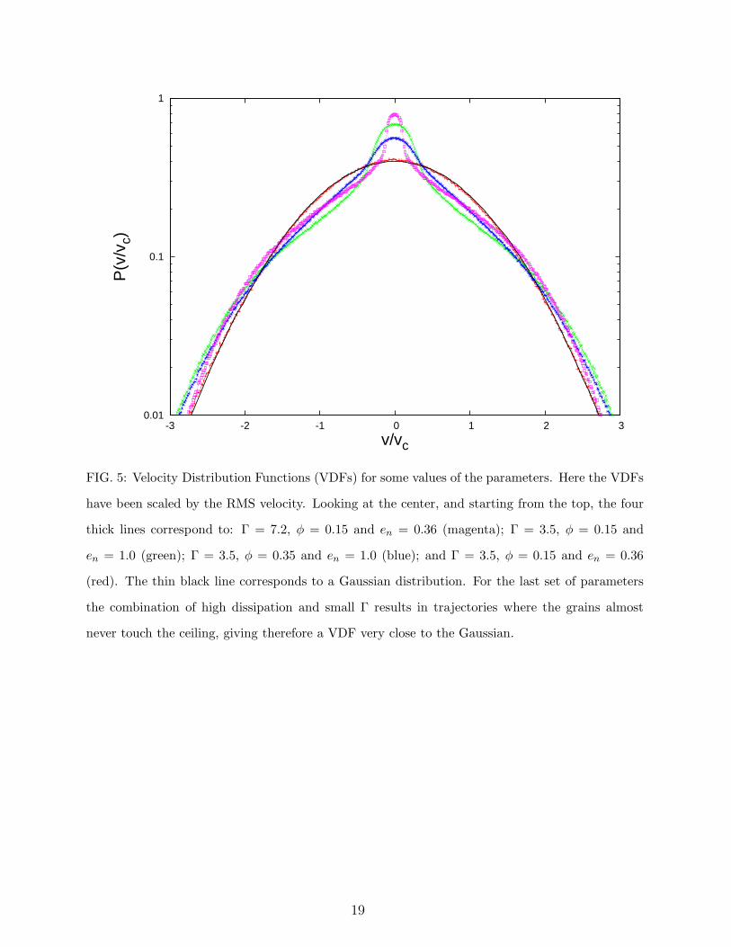
FIG. 5: Velocity Distribution Functions (VDFs) for some values of the parameters. Here the VDFs

have been scaled by the RMS velocity. Looking at the center, and starting from the top, the four

thick lines correspond to: Γ = 7.2, φ = 0.15 and en = 0.36 (magenta); Γ = 3.5, φ = 0.15 and

en = 1.0 (green); Γ = 3.5, φ = 0.35 and en = 1.0 (blue); and Γ = 3.5, φ = 0.15 and en = 0.36

(red). The thin black line corresponds to a Gaussian distribution. For the last set of parameters

the combination of high dissipation and small Γ results in trajectories where the grains almost

never touch the ceiling, giving therefore a VDF very close to the Gaussian.

19

0.001

0.01

0.1

1

-4 -3 -2 -1 0 1 2 3 4

P(v

/vc)

v/vc

φ = 0.20

FIG. 6: Some VDFs with and without friction with the ceiling. For all lines we have used here

Γ = 3.5 and φ = 0.2. Looking at the center, and starting from the top, the four thick lines

correspond to (a) en = 1.0 and µ = 0.25; (a) en = 0.66 and µ = 0.25; (a) en = 0.66 and µ = 0; and

(a) en = 1.0 and µ = 0. The thin black line is again a Gaussian distribution.

20

-2

-1

0

1

2

3

4

5

6

7

8

-1 -0.5 0 0.5 1 1.5

-ln(-

ln(P

(v/v

c)/P

(0))

) +

Con

st.

ln(v/vc)

Γ1 = 3.5

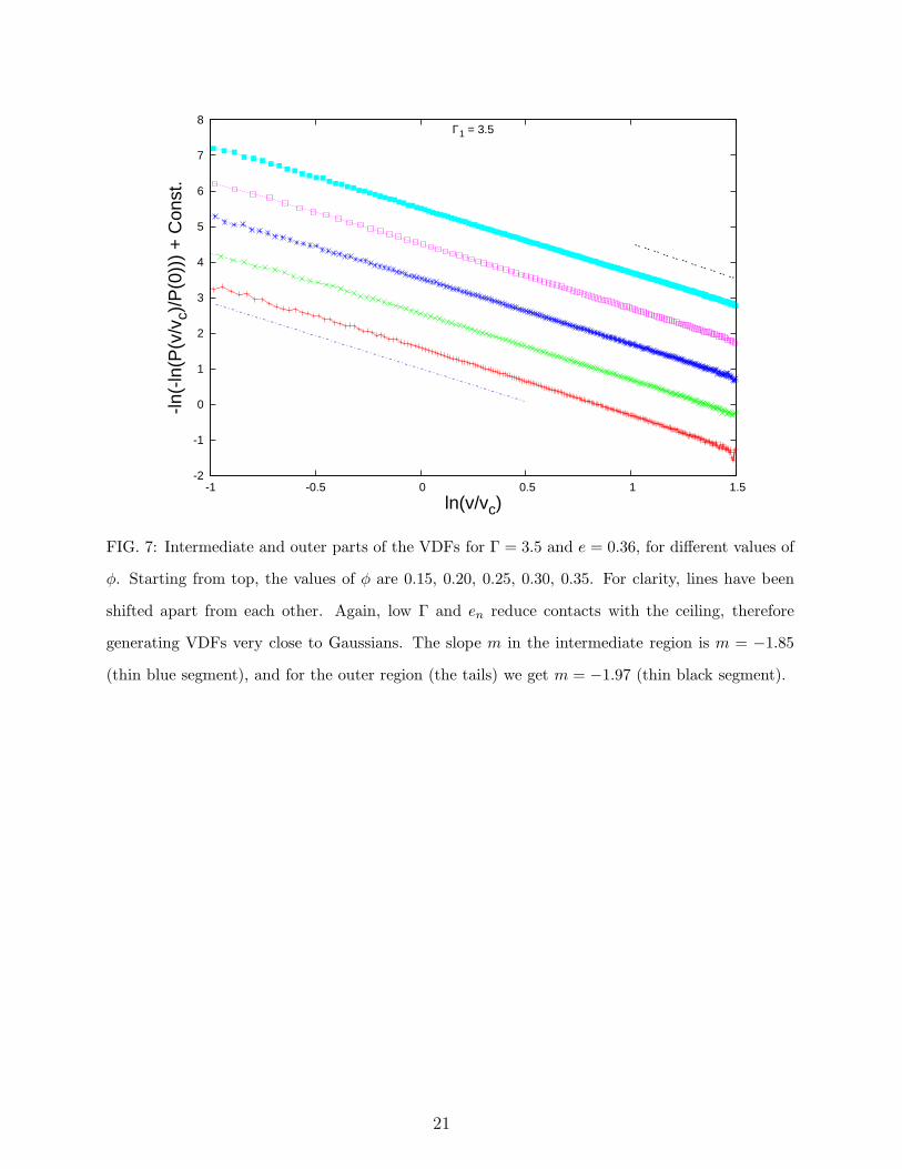
FIG. 7: Intermediate and outer parts of the VDFs for Γ = 3.5 and e = 0.36, for different values of

φ. Starting from top, the values of φ are 0.15, 0.20, 0.25, 0.30, 0.35. For clarity, lines have been

shifted apart from each other. Again, low Γ and en reduce contacts with the ceiling, therefore

generating VDFs very close to Gaussians. The slope m in the intermediate region is m = −1.85

(thin blue segment), and for the outer region (the tails) we get m = −1.97 (thin black segment).

21

-2

-1

0

1

2

3

4

5

6

7

-1 -0.5 0 0.5 1 1.5

-ln(-

ln(P

(v/v

c)/P

(0))

) +

Con

st.

ln(v/vc)

Γ2 = 7.2

FIG. 8: Intermediate and outer parts of the VDFs for Γ = 7.2 and e = 1.00, for different values

of φ. The values of φ are as in the previous Figure, and again the lines have been shifted apart

from each other. Here the high Γ and en imply strong bounces in the ceiling, and therefore a

very noticeable shift of the VDF towards low velocities. These VDFs are quite distorted, and

the double-log vs log graph cannot be fitted well with straight lines. The best linear fits for the

intermediate and outer regions give m = −0.66 (thin blue segment) and m = −1.94 (thin black

segment), respectively.

22

0

1

2

3

4

5

1 1.5 2 2.5 3 3.5 4

g(r)

r/σ

φ = 0.35

FIG. 9: Pair distribution functions for φ = 0.35 for some values of Γ and en. At the main peak,

and starting from top, the changing parameters are: (a) Γ = 3.5, en = 0.36; (b) Γ = 7.2, en = 0.36;

(c) Γ = 3.5, en = 0.66; (d) Γ = 7.2, en = 0.66; (e) Γ = 3.5, en = 1.0 and (f) Γ = 7.2, en = 1.0.

The last two lines fall on top of each other, showing how the PDFs for non-dissipative grains are

independent of the acceleration. In general, smaller restitution coefficients give rise to larger values

of g(r) at contact.

23

0

1

2

3

4

5

1 1.5 2 2.5 3

g(r)

a)

1 1.5 2 2.5 3

r/σ

b)

1 1.5 2 2.5 3

c)

FIG. 10: Pair distribution functions for Γ1 = 3.5, for: (a) en = 1.0, (b) en = 0.66, and (c)

en = 0.36. In all cases, the g(r) with the largest variation corresponds to φ = 0.35, and g(r)

becomes progressively flatter as φ decreases. Notice that in (a), for φ < 0.30, the largest peak is

not located at contact, indicating that the fixed scatterers have a weak separating effect over the

grains.

24

0.99

0.992

0.994

0.996

0.998

1

1.002

1.004

2 4 6 8 10 12 14 16 18 20

g(r)

r/σ

FIG. 11: Zoom of the g(r) for Γ1 = 3.5. The decreasing of the g(r) tails can be observed for

different filling fractions with respect to the curve with e = 1. The parameters are, starting from

below: (a) en = 0.36, φ = 0.15 (red), (b) en = 0.66, φ = 0.15 (blue), (c) en = 0.36, φ = 0.25

(green), and (d) en = 0.66, φ = 0.25 (magenta). The two sets of points running at g(r) = 1

correspond to en = 1, for φ = 0.15 and 0.25. The lines are fits of the form y(x) = A+B/(x− x0),

and are provided only as guides to the eye; at this reduced vertical scale, the large noise levels in

the data make a detailed evaluation of the parameters of the fit too uncertain as to be useful.

25