POF 2005 granular

Velocity profiles, stresses, and Bagnold scaling of sheared granularsystem in zero gravity

Oleh Barana� and Lou Kondicb�

Department of Mathematical Sciences and Center for Applied Mathematics and Statistics,New Jersey Institute of Technology, Newark, New Jersey 07102

�Received 28 July 2004; accepted 19 May 2005; published online 29 June 2005�

We report the results of three-dimensional event-driven simulations of sheared granular system in aCouette geometry. The simulations use realistic boundary conditions that may be expected inphysical experiments. For a range of boundary properties we report velocity and density profiles, aswell as forces on the boundaries. In particular, we find that the results for the velocity profilesthroughout the shearing cell depend strongly on the interaction of the system particles with thephysical boundaries. Even frictional boundaries can allow for significant slippage of the particles,therefore reducing the shear in the system. Next, we present stress distributions both for controlledvolume and for controlled stress configurations. We discuss the dependence of solid volume fractionon shear rate under the constant-pressure condition, and Bagnold scaling in volume-controlledsimulations. In addition, we study the influence of oscillatory driving of one of the domainboundaries on the system properties. © 2005 American Institute of Physics.�DOI: 10.1063/1.1951567�

I. INTRODUCTION

Sheared granular flows are important for both the betterunderstanding of the physics of granular matter and in manyindustrial applications �mixing, transport, etc.�. A significantprogress in the area of sheared granular systems has beenmade for the particular flows with simplified boundary con-ditions on the theoretical,1,2 numerical,3,4 and experimental5

levels. The simplifications used in these studies often involvesimplifying or ignoring the effect of physical boundaries �aswith periodic boundary conditions�, and assuming approxi-mately constant volume fraction throughout the system.

However, for applications it is important to understandthe effect of realistic boundaries on the sheared granularflow. There has been a number of studies that addressed thisproblem. Jenkins and Richman,6 for example, calculatedboundary conditions in a specific limit of plane flow of iden-tical, smooth, inelastic disks interacting with a bumpy wall.Louge, Jenkins, and Hopkins7 and later Louge8 tested thesetheoretical predictions for rapid sheared granular flows usingcomputer simulations. Related approaches to the question ofboundary conditions in continuum theories have been madeby Hui et al.9 and Gutt and Haff.10 Alam and Nott11 and Nottet al.12 theoretically studied the effect of boundaries on thestability of plane Couette flow of granular materials. In thiswork, we build upon these previous works and use discreteelement simulations to perform a systematic study of theeffect of realistic boundary conditions on sheared granularflow in a three-dimensional �3D� Couette cell under zerogravity.

The paper is organized as follows. Section II describes

the numerical approach and relevant parameters for our hardsphere �event-driven� simulations. In Sec. III we present theresults for bulk velocity and volume fraction profiles for avariety of boundary conditions. We also consider granularsystems which are, in addition to shear, subject to excitationsprovided by an oscillatory boundary. These oscillations areshown to lead to considerable modifications of velocity andvolume fraction profiles. In Sec. IV we discuss stresses onthe physical boundaries. In contrast to other works �mostnotably Ref. 8�, we do not analyze in detail how changes ofthe boundary conditions influence the system response, butinstead concentrate on the stress distributions for givenboundary conditions. We compare the normal and shear com-ponents of the stresses and discuss the factors determiningthe widths of the distributions and their average values, withparticular emphasis on the issues related to measuringstresses in granular system characterized by moderate to highvolume fractions.

All the results in Secs. III and IV are obtained for thesystems of directly controlled total volume. In Sec. V wepresent the stresses, velocities, and volume fraction profilesunder stress-controlled conditions. We then discuss the dif-ferences between these two configurations.

II. SIMULATION DETAILS

Numerical algorithm of our choice, event-driven algo-rithm for hard spheres, is described in detail in the papers byLubachevsky13 and Luding.14 In zero gravity all particles fol-low linear trajectories between the collisions. All collisionsbetween particles are instantaneous and binary. Consider twocolliding particles with diameters �1 and �2, masses m1 andm2, positions r1 and r2, linear and angular velocities v1, �1

and v2, �2. Then velocities after collision are

a�Present address: ExxonMobil Research and Engineering, 1545 Route 22East, Annandale, NJ 08801. Electronic mail: [email protected]

b�Author to whom correspondence should be addressed. Electronic mail:[email protected]

PHYSICS OF FLUIDS 17, 073304 �2005�

1070-6631/2005/17�7�/073304/15/$22.50 © 2005 American Institute of Physics17, 073304-1

Downloaded 05 Jul 2005 to 128.235.249.80. Redistribution subject to AIP license or copyright, see http://pof.aip.org/pof/copyright.jsp

http://dx.doi.org/10.1063/1.1951567

v1� = v1 −m2

m1 + m2�V, v2� = v2 +

m1

m1 + m2�V; �1�

�1� = �1 +m2

m1 + m2

�W

�1, �2� = �2 +

m1

m1 + m2

�W

�2; �2�

where

�V = �1 + e�vn + 27 �1 + ��vt, �W = 10

7 �1 + ��n � vt� .

�3�

Here n= �r1−r2� / �r1−r2� is the normal unit vector, vn and vt

are the normal and tangential components of the relative ve-locity vc=v1−v2−�� 1

2�1�1+ 12�2�2��n� of particles at the

contact point. Total linear and angular momentums are con-served during a collision; however, total translational androtational energies are lost.

Energy dissipation is controlled by three parameters:15

the coefficient of restitution e, coefficient of friction �, andcoefficient of tangential restitution �. The algorithm isadapted to include the particle’s interaction with physicalboundaries in the following way. The collisions with the topor bottom walls �also called horizontal walls� assume that awall is a particle of infinite radius and mass, and of linearvelocity equal to the wall’s velocity at the point of contact.Three dissipation parameters, ew, �w, and �w, characterizethese collisions. The sidewalls are the particles of infinitemass and radius and with the surface normal pointing hori-zontally toward the center of the cell. The properties of thesidewalls are characterized by a separate set of parameters,es, �s, and �s.

Experiments and theoretical studies show that the coef-ficient of restitution e noticeably depends on the impactvelocity.16,17 Therefore, we set this coefficient to be velocitydependent in the manner suggested in Ref. 18

e�vn� = �1 − Bvn3/4, vn � v0,

� , vn � v0.� �4�

Here vn is the component of relative velocity along the linejoining particle centers, B= �1−��v0

�−3/4�, v0=100�d / sec, and� is a restitution parameter.

Coefficient of tangential restitution �, defined as the ra-tio of the tangential components of the relative velocity afterand before collision, is given by14,18,19

� = �− 1 + 72��1 + e�vn/vt for sliding contacts,

�0 for rolling contacts.� �5�

Here � is the coefficient of friction, e is given by �4�, and �0

determines the transition between rolling and slidingcontacts.14,19

Table I summarizes our choice of dissipation parameters

for typical configurations. When different dissipation param-eters are used in the simulations, the results are always com-pared to the typical configuration.

Figure 1 shows the geometry of our 3D simulations ofpolydisperse inelastic frictional spheres in the Couette cell,with stationary sidewalls, rotated top wall, and the bottomwall that can move in the vertical direction. This featureallows us to, e.g., oscillate the bottom wall, similar to thelaboratory experiments.20 In addition, the moving bottomwall is used in stress-controlled simulations, where granularparticles determine the position of the bottom wall on theirown. More details can be found in Sec. V.

The particles are polydisperse with diameters randomlydistributed in the range �0.9,1.1� �d, where �d is the averagediameter of particles, which is used as a natural length scale.Our typical configuration consist of N=2000 particles, withfixed radii of inner cylinder and outer cylinder �Ri

=8�d ,Ro=12�d�. The height H of the cell is variable anddepends on the volume fraction , or on the average stress.For example, in the case of volume-controlled simulationswith 40% volume fraction, we have H� , t�= �4.22/+A sin�2ft��d. Here A and f are the amplitude scaled by�d, and the frequency in hertz of the bottom wall vibrations,if any. Typically we use A=1�d and f t=36.6 Hz, giving thedimensionless parameter �=A�2f�2 /g, which is above criti-cal for the onset of fluidization. Another system size brieflystudied is a wide configuration that has N=5000 particles ina Couette cell with radii of inner and outer cylinders Ri

=5�d and Ro=15�d, respectively. This configuration is usedto show 3D nature of the results.

The top wall can be covered with particles glued to its

TABLE I. Typical choice of dissipation parameters.

Particles �including glued� �=0.6 �=0.5 �0=0.35 Frictional inelastic particles

Top and bottom walls �w=0.1 �w=0.9 �0w=0.35 Very frictional and inelastic

Sidewalls �s=0.9 �s=0.1 �0s=0.35 Slightly frictional and inelastic

FIG. 1. Granular matter between two concentric stationary cylinders—sidewalls �not shown in the figure�. Top wall is rotating around the verticaly axes. Bottom wall can be vibrated in volume-controlled simulations, or itcan move as a result of applied stress in pressure-controlled simulations.

073304-2 O. Baran and L. Kondic Phys. Fluids 17, 073304 �2005�


surface, which have the same polydispersity, mean diameter,and material properties as the free particles. They are gluedinto the dimples on the surface so that each one protrudesinside the cell by the distance of half its diameter. For bothtypical and wide configurations, the number of glued par-ticles corresponds to 30% surface fraction, leading to con-figurations such that on average free particles cannot reachthe flat wall. The relevance of the distance between gluedparticles as a measure of surface roughness is discussed inRef. 6.

The initial conditions are prepared by first positioning Nparticles inside the container of the extended vertical dimen-sion with large initial spacing between the particles. Initially,particles and walls are set to be completely elastic and fric-tionless. The particles are assigned random velocities, andthe bottom is then moved up slowly until the desired volumefraction is reached. The resulting sample is then run for alonger time to eliminate compression waves �if any� createdby compression. The total momentum is then adjusted tozero, and finally the particles are set to be inelastic and fric-tional �see Table I�.

III. VELOCITY AND VOLUME FRACTION PROFILES

To measure angular velocity and volume fraction pro-files, ��y� and �y�, respectively, the volume of Couette cellis divided in Ns ring slices. Each slice is assigned a y binnumber iy =1, . . . ,Ns. In most cases, we set Ns=10. When thebottom wall is oscillated, we account for variable volume ofthe bottom slice or slices. In our measurements we average astudied quantity both over the volume of a y bin and over thetime interval tp, typically tp=0.5 sec. Within this time inter-val we measure the particle’s velocities and ’s every tp

leading to Np= tp / tp different distributions. It is convenientto express time in terms of Tw=1/ f t, giving tp=18.3Tw; weuse tp=Tw /10. All particles are binned in the corresponding

ring slices, and the average and the average velocity arecalculated as a function of y bin number. For wide configu-rations, in addition we measure as a function of the dis-tance to the inner cylinder, �r�.

A. Configurations with inelastic and frictionalsidewalls

Figure 2 shows the velocity profiles �top� and scaledtotal kinetic energy �bottom�. The latter is the kinetic energyper particle scaled by the energy of a particle of averagediameter and of average linear top wall velocity. All the mea-surements are done for the typical configuration systemswith 2000 particles and in zero gravity, but with four differ-ent boundary conditions: �a� and �b� without oscillating bot-tom wall; �c� and �d� with oscillations; �a� and �c� shearingwall with glued particles; �b� and �d� without glued particles.When oscillations are present, the position of the bottomwall is given by y=A sin�2ft�, with A= �d and f = f t

=36.6 Hz. In all four cases the shearing wall is rotating with�=10 rad/sec. This sets the linear shearing velocity rangebetween 80 �d / sec �close to inner cylinder� and 120 �d / sec�close to outer cylinder�. The effect of different shearing ve-locities is discussed later in this section.

Figure 2�a� shows that in the case of glued particles onthe top wall, and no oscillations, the system reaches a statecharacterized by a significant shear throughout the domain.By comparing 2�a� and 2�b�, we see that there is a strongeffect of glued particles on increasing shear. We emphasizethat the top wall without glued particles, Fig. 2�b�, does notlead to significant shear, although the wall itself is very fric-tional and inelastic. Also, we note that our simulations leadto asymmetric volume fraction distribution with significantdilation close to the shearing surface, in contrast to, e.g., Ref.7 which shows symmetric volume fraction profiles. The sym-metry in our system is broken due to the presence of �sta-

FIG. 2. Typical configurations results. Top panel: scaled velocity profiles �triangles� and volume fraction profiles �circles� in steady-state regime together withthe profiles in transient regimes �dashed lines�. Bottom panel: scaled energy plots. Insets in energy plots: kinetic energy plotted on a shorter time scale showingthe frequency of bottom wall oscillations. �a� and �b� Results without oscillating bottom wall; �c� and �d� with oscillations; �a� and �c� shearing wall with gluedparticles; �b� and �d� without glued particles. The dissipation parameters are as shown in Table I.

073304-3 Velocity profiles, stresses, and Bagnold scaling Phys. Fluids 17, 073304 �2005�


tionary� sidewalls, due to the glued particles being presentonly at the the top wall, and by other effects, such asvelocity-dependent restitution coefficient, see �4�.

Figures 2�c� and 2�d� show the results with oscillations,which account for a considerable slip velocity at the bottomwall. Similar to the case without oscillations, the presence ofglued particles greatly reduces the slip velocity at the topwall. We note that our results are in agreement with the onesderived using kinetic theory with simplified interactionmodel between the free particles and the walls,6,9 which pre-dict that slip velocity is inversely proportional to some mea-sure of roughness, and directly proportional to the local shearrate. The influence of roughness is clear from the resultsobtained with and without glued particles. By direct com-parison, we also verify that larger local shear rate in thesystem without oscillations, shown in Fig. 2�a�, results inlarger slip velocity.

Figure 2 also shows as a function of y. The steadystates, marked by the circles, show that ’s are not uniform,in contrast to volume fraction profiles typically obtained un-der the assumption of periodic boundary conditions. For eachof four cases we observe the maximum local 58% forsome intermediate y’s, with dilation effects close to thewalls. Oscillations, in particular, lead to very small ’s closeto the bottom wall. This is due to the fact that when thebottom wall moves downward, the adjacent granular layerdoes not follow it. This is also confirmed by computer visu-alization of the granular layer.

From energy plots, shown in the bottom panel of Fig. 2,we estimate the equilibrating time needed to reach steadystate for all four cases: te�a�=15 sec, te�b�=15 sec, te�c�=2 sec, and te�d�=6 sec. These times are shorter for the sys-tems with oscillating bottom wall due to increased collisionrate. Also, oscillations lead to modulation of the scaled en-ergy; this is shown in the insets in the energy plots. In addi-tion, in the systems with oscillations, the glued particles pro-vide an increase in collision rate and decrease inequilibration time.

Figure 3 shows the velocities and ’s for wide configu-ration, characterized by 5000 particles, and =40%, usingtypical values of all other parameters. The velocity profiles,shown in Fig. 3�a�, are qualitatively similar to the onesshown in Fig. 2, although velocities are slightly larger for

wide configuration, since the ratio of the areas of dissipativesidewalls to the area of shearing wall is smaller. The ’s �notshown� are very similar to those in Fig. 2.

Figure 3�b� shows �r�. We see that there is a significantdilation near the inner wall due to centrifugal effect, sincethe particles colliding with the top wall gain the momentumthat, on average, has a direction along the tangent line to thetrajectory at the contact point. On the other hand, the depen-dence of particle velocities on r �not shown� is rather weak.

B. Effect of dissipation parameters and shearingvelocity without oscillations

Here, as a basis, we use =40% typical configurationwithout oscillations and without glued particles �Fig. 2�b��,with one modification: to enhance shear, we assume com-pletely elastic sidewalls.

Figure 4�a� shows that there is a significant, qualitativedifference of the velocity profiles for the systems with elasticand smooth sidewalls compared to inelastic and rough side-walls shown in Fig. 2�b�. Effect of shearing is much strongerin the systems with elastic sidewalls, with almost linear ve-locity profile and large slippage at the bottom. We refer tothis shape of velocity profile as linear asymmetric, and notethat if we shear the same initial configuration by rotating thetop wall in one direction and bottom wall in the oppositeone, we obtain linear-symmetric velocity profile with equalslippage at the top and bottom.

Figure 4�a� shows that the velocity and volume fractionprofiles are very similar as �’s are varied over more than twoorders of magnitude. The energy plots similar to the onesshown in Fig. 2 show, however, that the time to reach thesteady state �equilibrating time�, te, does depend strongly on�. This effect is shown in more detail in Fig. 4�b�, whichshows that te is inversely proportional to �. Therefore, thesame amount of strain is needed to reach the steady state forall explored shearing velocities. We note that in our simula-tions we do not observe instabilities of layering type,11,12

possibly due to relatively small height of our computationaldomain.

In the next set of simulations we investigate the effect ofhorizontal walls properties in the same system. Out of threeparameters that characterize the horizontal walls��w ,�0w ,�w�, we vary one at a time and keep the othersfixed. We find that �w and �0w have relatively weak effect onthe velocity profiles. However, �w influences the flowstrongly. There exists a critical value �w

c , below which the

FIG. 3. Results for wide configurations: with glued particles and oscillations�filled triangles�; without glued particles and with oscillations �open tri-angles�; with glued particles and without oscillations �filled circles�; withoutglued particles and without oscillations �open circles�. �a� Velocity profilesin the y direction. �b� Volume fraction profiles in the radial direction.

FIG. 4. �a� Linear-asymmetric velocities and ’s for the case of elasticsidewalls, no glued particles, and no oscillations. �b� Equilibrating times te.



frictional force from the shearing wall cannot excite thegranular flow. For our configuration this value is �w

c �0.4.Understanding precisely the role of �w requires carefulanalysis, and we devote the rest of this section to this aspectof the problem.

Figure 5, which presents the results for �w in the interval�0.4, 0.9�, shows that the systems first reach a metastablestate of slow shearing �open symbols in Figs. 5�a� and 5�b��.This metastable state is characterized by negligibly smallslippage at the bottom wall and very large slippage at the top,as well as by high close to the bottom. As time progresses,the shear of the granular particles is increasing very slowly.However, after certain time tc, the system jumps into a stablestate of fast shearing with asymmetric-linear profile, alsoshown in Figs. 5�a� and 5�b�. We call this behavior delayeddynamics. This jump from metastable to stable state is illus-trated in Fig. 5�c�, which shows the scaled energy �kineticenergy per particle scaled by the energy of a particle of av-erage diameter and of average linear top wall velocity� forfour values of �w.

Figure 6�a� shows the crossover transition time tc, de-fined as the time when metastable state ends, i.e., when thegranular layer starts to pick up the energy fast. We find thattc��w−�w

c �−2, with critical friction parameter �wc =0.33.

Figure 6�b�, which shows scaled energy for �w=0.4, illus-trates the manner in which tc is obtained. The intersection ofthe tangent lines and the time axis gives tc, and the intersec-tion with the horizontal line at the level of the average scaledenergy in the steady state gives equilibrating time te. For allconsidered �w’s, te= te− tc is �18±4� sec. This result is

consistent with te obtained for the same �=10 rad/sec andvery frictional horizontal walls ��w=0.9�, see Fig. 4�b�. Forsuch a large �w, tc0, and te te.

Figure 7�a� illustrates the effect of � for the system indelayed dynamics regime for three different shearing veloci-ties, confirming that the transition times tc depend veryweakly on �. However, the te’s follow the inverse ruleshown in Fig. 4�b�. Therefore, te’s strongly depend on �,while being almost independent of �w.

To understand precisely the role which the horizontalwalls play in the mechanism of delayed dynamics, we nowconsider fixed coefficient of friction of the top wall�w�top�=0.45 and vary coefficient of friction of the bottomwall. The results, shown in Fig. 7�b�, clearly indicate that�w�bottom� does not have important effect on tc. However,smaller �w�bottom� leads to shorter te. We also note that forthese low �w�bottom� the energies are rising to the highervalues. This is an indication of higher overall velocities ofthe particles in the steady state due to higher slippage at thebottom wall for lower �w�bottom�.

An insight into the mechanism of the delayed dynamicscan be gained by considering also the time dependence of’s. Recall that Fig. 5�b� indicates formation of a high-density cluster in both metastable and stable states. Figure8�a� tracks the evolution of this cluster, by showing the po-sition of the center of mass of the particles, hc.m.

=�idi3yi /�idi

3, scaled by the cell height H, as a function oftime. This figure, discussed in more detail below, clearlyshows that there is a shift in hc.m. as system transitions frommetastable to stable state �viz. Fig. 5�c� for �w=0.45�.

Based on the results shown in Figs. 5–8, the mechanismof the delayed dynamics is as follows. The friction of the top

FIG. 5. Delayed dynamics regime. The shearing velocity in all cases is �=10 rad/sec. �a� and �b� show the typical velocity and volume fraction profiles inmetastable and stable states, using �w=0.45 at t=30 sec �metastable state� and t=150 sec �stable state�. �c� Scaled energy as a function of time for four valuesof �w.

FIG. 6. �a� Transition times tc vs wall friction: open circles are the simula-tion results, and the solid line is the best fit using inverse function t=a / ��−�c�2 with fitting parameters a=1.07 and �w

c =0.33. �b� An exampleof the close-up of “transition interval” for �w=0.4. The plot allows to de-termine the transition time tc and equilibrating time te, as discussed in thetext.

FIG. 7. Scaled energies in the transition interval for �a� �w=0.45 with threedifferent shearing velocities, �b� �w=0.45 for the top wall, variable �w forthe bottom wall, �=10 rad/sec.



wall controls the amount of the tangential momentum trans-ferred to the particles. Thus, the energy input is determinedby the top wall friction, as well as by the collision rate withthis wall. When the initial configuration is subjected to shear,the particles immediately dilate close to the top wall andform the cluster of high volume fraction close to the bottomwall, see Fig. 8, t�30 sec. If the friction of the top wall isweak enough, below some critical value �w

c , all the energy isquickly dissipated without inducing any shear. For higher�w, the energy transferred to the granular system starts toaccumulate slowly, until, at some critical time tc, the shear-ing between the dense cluster and the bottom wall is strongenough to dilate a region next to this wall and to push thecluster closer to the top wall, see Fig. 8. This process isaccelerated if �w�bottom� is smaller. As a result, the collisionrate with the top wall increases, and the energy from the topwall is rapidly transferred to the cluster, until the stable statecharacterized by linear asymmetric profile forms. Thus, thetime span of metastable state tc is determined mostly by thefriction of the top wall, and the time te is determined mostlyby the shearing velocity.

C. Effects of oscillations

To test the effect of the amplitude A and frequency f ofoscillations, it is more convenient to go back to the typicaldissipative sidewalls used in Sec. III A, since in the case ofsmooth sidewalls the slippage velocity at the bottom wall isapproaching �, making the analysis of the velocity profilesdifficult. So, as a base system we use the “oscillating bottomwall, no glued particles” configuration shown in Fig. 2�b�.

Figure 9 shows velocity and volume fraction profiles,where �a� f is fixed and A is varied and �b� A is fixed and fis varied. The characteristic feature of these results is high50% –60% in the middle of the cell, confined betweentwo layers of low close to the walls. Inside this band the

local shear rate is rather low, compared to the overall shearrate. In Fig. 9�a� we observe that the slippage at the bottomwall increases strongly with A. Also, as A increases, the peakof profile moves further away from the oscillating wall.Similarly, in Fig. 9�b� we see that an increase of the fre-quency of oscillations leads to an increase of velocitythroughout the system. However, ’s change very little withf .

Figure 10 shows how the properties of sidewalls influ-ence the velocities and ’s. Setting �s=0, �s=1 �Fig. 10,open triangles� makes almost all particles move with �. Set-ting �s=0.5, �s=0.6 �filled triangles� creates already enoughdissipation to almost completely resist the shearing force:Even oscillations cannot improve shearing when sidewallsare very frictional. The results for �s=0.1, �s=0.6 �opencircles� are almost identical to the results for the typical case,Fig. 2�b� �shown here with filled circles�. We conclude that�s plays the crucial role in defining velocity profiles, simi-larly as observed regarding �w in Sec. III B. The volumefraction profiles, on the other hand, very weakly depend onthe sidewall properties.

IV. NORMAL AND SHEAR STRESSES ON THEBOUNDARIES

Stresses in granular systems have been the focus ofmany studies, because of their importance in a number ofengineering designs. A significant part of these studies1,21,22

deals with the theoretical continuum models where stress isconsidered as a mean local quantity. Therefore, the validityof these models depends on the strength of stress fluctuationson the scale which defines “locality.” The knowledge ofstress distributions becomes crucial here. There are manyexperimental, numerical, and theoretical studies of stressfluctuations.23–26 Often, these studies deal with high volumefraction of static or slowly sheared granular systems. In thesesystems the distribution of stresses is characterized by anexponential decay for large stresses. It is speculated25 thatthe exponential tails in stress distributions are related to thepresence of force chains. However, recently, Longhi, Easwar,and Menon27 reported the experimental evidence of expo-nential tails in stress distributions in rapidly flowing granularmedium, i.e., in the systems where it was unlikely to findforce chains in the traditional “static” sense.

The results presented in this section concentrate on thestress distributions at the physical boundaries of rapidly

FIG. 8. Scaled center of mass vs time for the system with �w=0.45.

FIG. 9. Velocity �triangles� and volume fractions �circles� for �a� fixed fre-quency, f = f t=36.6 Hz, and different amplitudes of oscillations; �b� fixedamplitude, A= �d, and different f .

FIG. 10. Effect of sidewall properties on velocities �a� and ’s �b�: Typical�filled circles�, elastic-smooth �open triangles�, very frictional �filled tri-angles�, and elastic-frictional �open circles�.



sheared granular systems usually with =40%. In order tomake maximum connection with existing experimental re-sults and theories, we calculate the stresses similar to experi-ments, i.e., we introduce in our simulations stress sensors onthe boundaries. For low ’s and/or in rapid flow regime thesesensors can report zero stress during some measuring inter-vals, see, for example, Ref. 27. Therefore, the total distribu-tion of stresses must contain the distribution of nonzerostresses and a weighted delta function to account for zerostresses. In what follows we make a clear distinction be-tween nonzero and zero stresses and extend all relevant the-oretical arguments to account for the latter.

We present the stresses on the boundaries for the typicalconfigurations shown in Fig. 2. To calculate the stresses, wecover the respective boundaries with stress sensors, of thearea As=ds

2; typically, we set ds=1.09�d �larger sensors areconsidered later�. We use both square and sector shaped sen-sors without any difference in the results.

The instantaneous normal and tangential stresses on asensor are defined as

�n =�i

�pn�i�

As�t=

1

As�t

1

6�s�

i

di3�vy� − vy� , �6�

�t =�i

�pt�i�

As�t=

1

As�t

1

6�s�

i

di3�vt� − vt� . �7�

Here i counts all the collisions between the particles and thewalls in the sensor area during an averaging time interval �t;typically �t=Tw /10. �pn�i� and �pt�i� are the changes ofparticle’s normal and tangential momenta, �s is density of thesolid material, di is the diameter of a particle participating inthe collision i, and vectors v and v� are the velocities of thecolliding particle before and after a collision, respectively.Subscripts n and t refer to the normal and tangential compo-

nents. To obtain sufficient data for the stress probability dis-tribution function �PDF�, we measure instantaneous stresseson all sensors every �t for at least �T=1000�t, and showthe scaled PDFs of locally measured stresses, �n and �t, as afunction of �n / ��n or �t / ��t. The averages are defined as

��n,t� = �i

�p�n,t��i��Abase/�T, Abase = �Ro2 − Ri

2� .

�8�

In what follows, we concentrate mostly on the stress distri-butions and do not discuss in detail the relation betweenimposed boundary conditions and stresses; more resultsabout this aspect of the problem can be found in the paper byLouge.8

A. Normal stress distributions

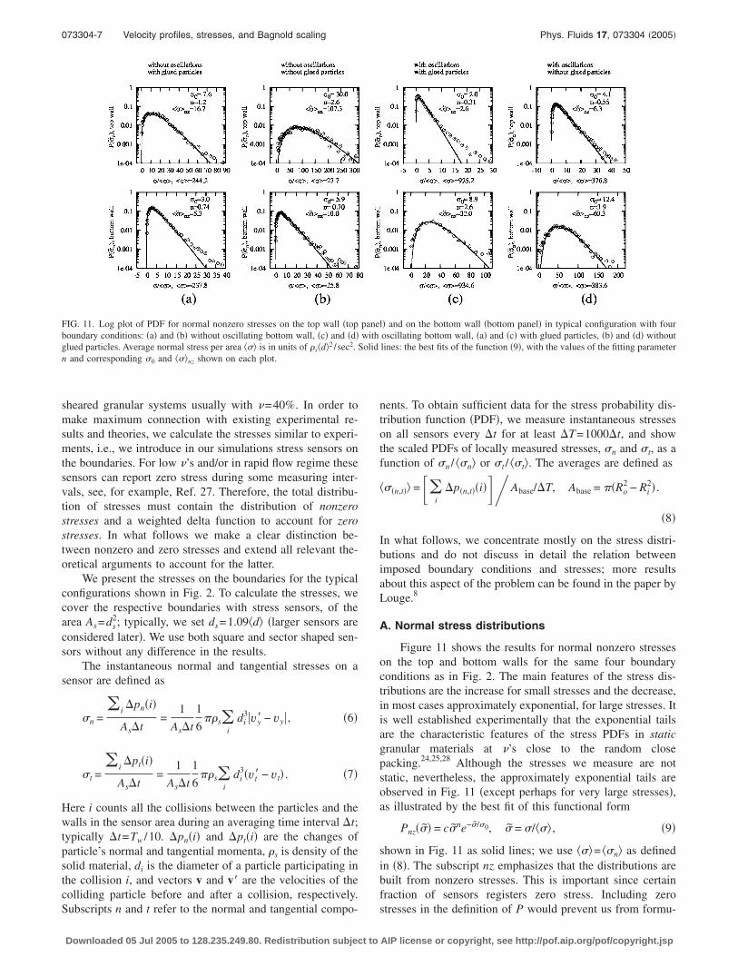
Figure 11 shows the results for normal nonzero stresseson the top and bottom walls for the same four boundaryconditions as in Fig. 2. The main features of the stress dis-tributions are the increase for small stresses and the decrease,in most cases approximately exponential, for large stresses. Itis well established experimentally that the exponential tailsare the characteristic features of the stress PDFs in staticgranular materials at ’s close to the random closepacking.24,25,28 Although the stresses we measure are notstatic, nevertheless, the approximately exponential tails areobserved in Fig. 11 �except perhaps for very large stresses�,as illustrated by the best fit of this functional form

Pnz��̃� = c�̃ne−�̃/�0, �̃ = �/�� , �9�

shown in Fig. 11 as solid lines; we use ��= ��n as definedin �8�. The subscript nz emphasizes that the distributions arebuilt from nonzero stresses. This is important since certainfraction of sensors registers zero stress. Including zerostresses in the definition of P would prevent us from formu-

FIG. 11. Log plot of PDF for normal nonzero stresses on the top wall �top panel� and on the bottom wall �bottom panel� in typical configuration with fourboundary conditions: �a� and �b� without oscillating bottom wall, �c� and �d� with oscillating bottom wall, �a� and �c� with glued particles, �b� and �d� withoutglued particles. Average normal stress per area �� is in units of �s�d2 / sec2. Solid lines: the best fits of the function �9�, with the values of the fitting parametern and corresponding �0 and ��nz shown on each plot.



lating the fitting function �9� and relate our results directly toexperiments and theory. We discuss the consequence of thisapproach in more details below.

The form �9� can be thought of as the generalization ofthe theoretical predictions for static stress distributions. �Theimportant assumptions of theoretical models of stress distri-butions are the maintained contact between particles that areclosely packed. These assumption are valid in both com-pletely static case and in the case of slow shearing at highdensity.� For example, the original q model,26,29 extendedlater by other authors,30,31 predicts the distribution �9� withn=Nc−1, where Nc is the number of force transmitting con-tacts between particles in adjacent layers. In 3D and fcc closepacking Nc=3, so n=2. Using different approach, Edwardsand Grinev32 predict the distribution �9� with n=1/2. n canalso depend on the number of contacts between sensor andparticles during averaging time, as will be shown in Sec.IV A 2. Therefore, it makes sense to think of n as a fittingparameter. Other parameters, c and �0, can be expressed interms of n and the average stress ��̃nz �measured directly insimulations� using the following expressions:

1 = �0

�

Pnz��̃�d�̃ = c��n + 1��0�1+n�� , �10�

��̃nz = �0

�

�̃Pnz��̃�d�̃ = �0�n + 1� . �11�

In Fig. 11 we show the fit of the functional form �9� withn as the only fitting parameter. Other parameters, calculatedusing �10� and �11�, and average quantities, obtained directlyfrom simulations, are also shown. These results show that theaverage stresses �� at the top and bottom walls are equalwithin the statistical error. However, the peak values and thewidths of distributions are different. In particular, for thesystems without oscillations the distributions are wider at thetop wall, while if oscillations are present, they are wider atthe bottom wall. Before discussing this result, we considerthe effects of volume fraction, collision rate, averaging, andcorrelations on the properties of the stress distributions.

1. The width of stress distributions

Let the width of a distribution be defined as the rootmean square of all measured stresses �including zerostresses� divided by the mean stress,

width =��2 − ��2

��=

��̃2 − ��̃2

��̃= ��̃2 − 1 �12�

�here we use ��̃=1, see below�. The distribution itself takesthe form of a linear combination of the distribution of non-zero stresses �9� and the delta function to account for zerostresses P��̃�=C1Pnz��̃�+ �1−C1� �0�. The constant C1 sig-nifies the fraction of nonzero stresses. Then, the mean andthe mean square of the stress are as follows:

��̃ = �0

�

�̃P��̃�d�̃ = C1��̃nz = 1, �13�

��̃2 = �0

�

�̃2P��̃�d�̃ = C1�02�n + 1��n + 2� . �14�

From the first equation we obtain C1=1/ ��̃nz and, using�11�, we arrive at the following expression for the width ofdistribution:

width = ��0�n + 2� − 1 = ��0 + ��̃nz − 1. �15�

Expression �15� reduces to ��0= �n+1�−1/2 if zero stressesare absent, i.e., when all sensors register at least one strikeper �t and ��̃nz= ��̃=1. Here, the width is determined byaveraging effects and correlations, as we discuss later. On theother hand, if zero stresses are present, there is a significantdependence of the width on the nonzero stress ��̃nz. In alimiting case ��̃nz�1, appropriate to systems shown in Fig.11, �15� reads

width =�� 1

1 + n+ 1��̃nz − 1 � ��̃nz, �16�

where we have used the fact that for ��̃nz�1 sensors do notregister more then one particle at a time, and for single par-ticle contacts n=const, as explained below. Equation �16� isconsistent with visual estimate of the widths in Fig. 11: Thelarger ��̃nz �shown in the right top area on each plot�, thewider is the distribution. Next we show that ��̃nz depends onthe collision rate, area of the sensors, and averaging time.

Let Nt=nsnT be the total number of stress measurements,obtained from all ns sensors during nT time intervals. Out ofNt stresses, Nnz�Nt are nonzero. The nonzero average stressdepends on the size of sensor As and averaging time �t,

��̃nz =��nz

��=

Nt

Nnz=

1

wAs�t, �17�

where w is the frequency of nonzero stress events per unitarea. For low-collision rate with the sensors, when not morethan one particle strikes As during �t, w signifies particle-wall collision rate per unit area.

Relations �16� and �17� allow us to explain the distribu-tions in Fig. 11. The sensor areas and averaging times arefixed, so it is the rate of nonzero events w which determinesthe average and the width. To first approximation w� closeto the respective boundary. From �y� in Fig. 2 we see that,without oscillations, is smaller at the top wall leading towider distributions. If oscillations are present, is smaller atthe bottom, so distributions are wider there.

2. Averaging effects

In this section we study one of the factors that can affectthe parameter n, i.e., the number of contacts N between theparticles and a sensor during the averaging time �t.

Let us define the parameter n0 that is characteristic forthe distribution of stresses due to single particle contacts,

PN��̃� = c�̃n0e−�̃/�0, N = 1. �18�

If more than one particle collide with the sensor of area As

during time �t �N�1�, then the stress distribution is differ-ent due to averaging effects. For instance, when two particles



strike the same sensor during �t, N=2, the probability ofregistering total stress F depends on the probability of one ofthem contributing the stress ��F and another one the stressF−�. Assuming both considered particles have independentdistributions �18�, the distribution of their collective stress Fis P2�F�=�0

FP��P�F−��d�. Using �18� and the integralidentity

�0

F

�r�F − ��qd� = F�r+q+1��r + 1��q + 1�/��r + q + 2�

�19�

valid for any positive real numbers r and q, and, in particu-lar, for r=q=n0, we arrive at the following distribution for

the stresses generated by double strikes P2�F̃�=c2F̃�2n0+1�e−F̃/�0, F̃=F / ��, where c2 is a normalization co-efficient. Applying the same argument to the case when Nparticles strike the sensor during �t we obtain the followingdistribution of stresses:

PN��̃� = c�̃�N�n0+1�−1�e−�̃/�0. �20�

The above calculation sets the relation between the param-eter n and the number N as n=N�n0+1�−1, see �9�. There-fore, if the particles are not correlated, we obtain that thedistributions of stresses generated by multiples collisions arecharacterized by higher power n. We will see below that thisresult is justified for the results shown in Fig. 11.

This conclusion may be used to explain the increasedvalues of n in Fig. 11�c�, bottom, and Fig. 11�d�, bottom.Here, the bottom wall is vibrated and most of the stress dataare collected during the phase when the bottom is rising up.This phase is characterized by increased compaction of par-ticles close to the sensors and an increased N. However, anincrease of N cannot be responsible for the large n’s on thetop wall shown in Fig. 11�b�, and, to a lesser extent, Fig.11�a�, top. In particular regarding Fig. 11�b�, we expect thatthe source of large n lies in the separately verified result thatthe typical normal components of the velocities of the par-ticles colliding with the top wall are large, leading to differ-ent stress distribution.

The results of Fig. 11 allow us to estimate the parametern0 defined earlier in this section as the value of n correspond-

ing to the distribution of stresses registered by the sensorswith N=1. Because n0�n �see �20��, the smallest found nprovides an upper bound on n0. The lowest values of n arefound in the distributions shown in Fig. 11: �a� bottom, �b�bottom, �c� top, and �d� top. For these cases n�1; therefore,n0�1. This result is very different from n0=2 in the qmodel: this should be no surprise because q model assumeshigh volume fraction and static configuration.

3. Correlations

The dependence of the normal stress distributions on thenumber of contacts per sensor can be described by �20� onlywhen the particles participating in contact with a sensor arenot correlated. However, there are certain regimes and con-ditions of granular flow when this assumption may not becorrect. For example, Miller, O’Hern, and Behringer23 stud-ied the response of the force distribution to the number N,controlled by the size of particles, and found that in densegranular flow the distribution widths were approximately in-dependent of N. This independence was attributed to thepresence of correlations due to force chains.

Here we present the systematic study of the effect ofsensor size �and, hence, the number N� on the bottom wallstress distributions for our typical configuration without os-cillations and with glued particles, Fig. 2�a�. This study al-lows us to confirm the validity of our predictions �15� and�20� in a more quantitative way and to check for possiblecorrelations.

Figure 12�a� shows the results for width �12� as a func-tion of As for fixed values of �t in the range betweenTw /100=0.0002 sec and 20Tw=0.5463 sec. This range in-cludes our typical value �t=Tw /10=0.0027 sec �open tri-angles� used to obtain the distributions in Fig. 11. To helpinterpretation of the results, we plot in Fig. 12�b� the value of��̃nz, in Fig. 12�c� the average number of contacts per sen-sor, and in Fig. 12�d� the widths of distributions versus theproduct of the averaging time and the sensor area.

This figure shows that if zero stresses are present, i.e.,��̃nz�1, the widths scale with the sensor area as As

−0.5,which is the scaling predicted by �16�. This result applies toall sensor sizes when �t=0.0002 sec, to the sensors of

FIG. 12. �a� The widths of force distributions as defined by �12� vs the sensor area As �in units of �d2� for various �t’s. �b� Average nonzero stress ��̃nz asa function of As �for �t�0.2731 ��̃nz=1�. �d� Average number of contacts per sensor as a function of As. �c� The widths vs �tAs. The solid lines havespecified slopes.



As�20�d2 when �t=0.0027 sec, and to the sensors of As

�2�d2 when �t=0.0273 sec, see Fig. 12�b�.When zero stresses are not present ��̃nz=1� the width

�15� reduces to

width = ��0 = �N�n0 + 1��−0.5. �21�

Here N�As is a number of contacts per sensor from �20� andabsence of correlations is assumed. This relation �21� is con-sistent with the As

−0.5 in Fig. 12�a� in the case �t=0.0027 sec and As�20�d2. However, when �t�0.0273 sec �for these large �t’s, the zero stresses are ab-sent for almost all considered sensors, see Fig. 12�b�� thewidths decrease as As is increased at a slower rate than pre-dicted by �21�. The slowest decrease, approximately As

−0.21,occurs for the sensor sizes 10�d2�As�100�d2, and for theaveraging times of 0.2731 sec.

We expect that the origin of this slower decrease is thepresence of correlations between the particles striking thesame sensor �which may include self-correlation, i.e., thesame particle colliding with the same sensor on multiple oc-casions during a given �t�. For example, the distribution ofstresses due to N completely correlated particles acting oneach sensor would have n=n0, leading to the widths indepen-dent of As. Therefore, the stronger are the correlations be-tween particles, the lower is the exponent in the width versusAs plot. In Fig. 12�a� we can see that stronger correlationeffects �i.e., slower decrease of the widths with an increaseof As� occur for longer �t and larger As. This is even moreevident when the width is plotted against the product As�t,see Fig. 12�d�: the slope changes gradually from −0.5 forsmall As�t to about −0.3 for large As�t. The collapse ofalmost all data on approximately single curve in Fig. 12�d�indicates the fact that the same averaging or correlation ef-fects result if either �t or As is increased by a same factor.Possible exception to this rule are very long �t’s, which wediscuss below.

We note that in Ref. 23 evidences were found of strongcorrelations, since they estimated experimentally the width�As

0 for �t=0.0005 sec and 5�d2�As�80�d2. However,the overall of their samples was considerably higher.Therefore, the spatial correlations can be explained if oneassumes the normal stress on the bottom wall is appliedthrough the network of force chains.33 In our case, where ’sare smaller, we expect that spatial correlations may arisefrom statistical fluctuations of the local . These fluctuationslead to occasional formation of denser structures of particles,stretched from the top to bottom wall: friction ensures thatthe lifetime of these formations is relatively long. As in thecase of force chains, the dense structures carry more stressthan the “free” particles in the “interstructure” space, thusintroducing spatial correlations. Unlike the force chains, thedense structures do not form dense force network. They mayform and disappear allowing for longer “structure-free” pe-riods. This concept is consistent with the fact that our corre-lations are weak and detected only when �t and As are largeenough to include such a structure event. In addition, theaverage number of contacts with sensors, see Fig. 12�c�, islarger than 10 in the regimes where �21� fails. This fact sug-

gests the possibility of frequent returning contacts of thesame particle with a sensor, which is a signature of a particlepressed to the sensor from above, as one would expect for aparticle that is member of a dense structure. The existence ofsimilar structures �named “transient force chains”� was alsosuggested in Ref. 27.

We note that the dependence of the width on As becomesstronger again in the case of very long �t’s, see the resultsfor �t=0.5463 sec in Fig. 12�a�. Simple estimate shows thatthis change in trend occurs when �t is so long that a particle,moving with a typical velocity, travels across a sensor in thetime that is shorter than �t, therefore decreasing this self-correlating effect.

B. Tangential stress distributions

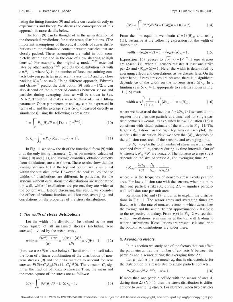
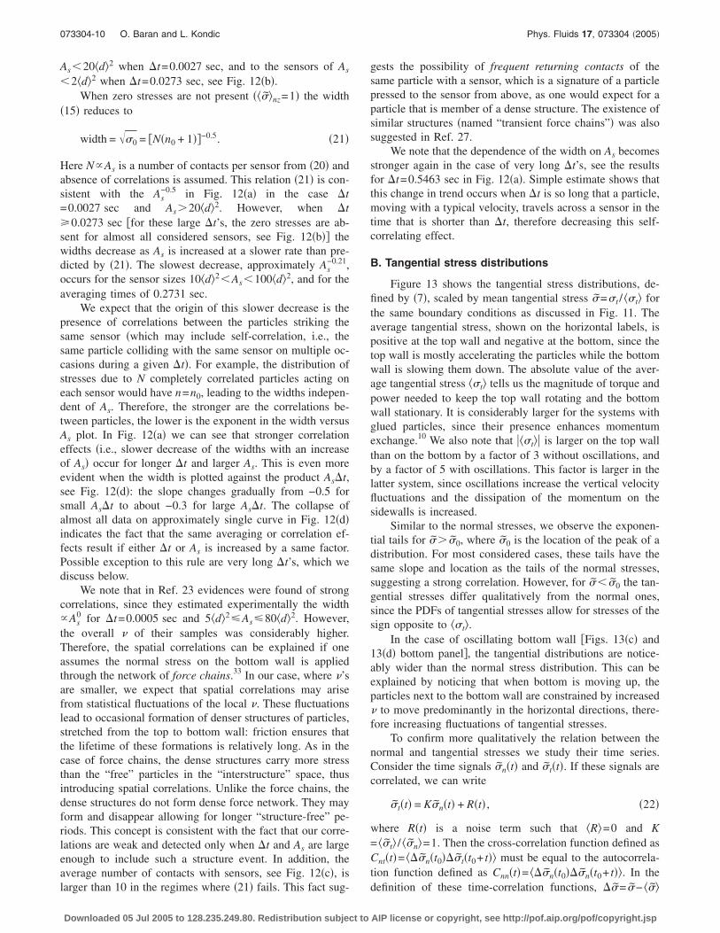
Figure 13 shows the tangential stress distributions, de-fined by �7�, scaled by mean tangential stress �̃=�t / ��t forthe same boundary conditions as discussed in Fig. 11. Theaverage tangential stress, shown on the horizontal labels, ispositive at the top wall and negative at the bottom, since thetop wall is mostly accelerating the particles while the bottomwall is slowing them down. The absolute value of the aver-age tangential stress ��t tells us the magnitude of torque andpower needed to keep the top wall rotating and the bottomwall stationary. It is considerably larger for the systems withglued particles, since their presence enhances momentumexchange.10 We also note that ��t� is larger on the top wallthan on the bottom by a factor of 3 without oscillations, andby a factor of 5 with oscillations. This factor is larger in thelatter system, since oscillations increase the vertical velocityfluctuations and the dissipation of the momentum on thesidewalls is increased.

Similar to the normal stresses, we observe the exponen-tial tails for �̃��̃0, where �̃0 is the location of the peak of adistribution. For most considered cases, these tails have thesame slope and location as the tails of the normal stresses,suggesting a strong correlation. However, for �̃��̃0 the tan-gential stresses differ qualitatively from the normal ones,since the PDFs of tangential stresses allow for stresses of thesign opposite to ��t.

In the case of oscillating bottom wall �Figs. 13�c� and13�d� bottom panel�, the tangential distributions are notice-ably wider than the normal stress distribution. This can beexplained by noticing that when bottom is moving up, theparticles next to the bottom wall are constrained by increased to move predominantly in the horizontal directions, there-fore increasing fluctuations of tangential stresses.

To confirm more qualitatively the relation between thenormal and tangential stresses we study their time series.Consider the time signals �̃n�t� and �̃t�t�. If these signals arecorrelated, we can write

�̃t�t� = K�̃n�t� + R�t� , �22�

where R�t� is a noise term such that �R=0 and K= ��̃t / ��̃n=1. Then the cross-correlation function defined asCnt�t�= ��̃n�t0��̃t�t0+ t� must be equal to the autocorrela-tion function defined as Cnn�t�= ��̃n�t0��̃n�t0+ t�. In thedefinition of these time-correlation functions, ��̃= �̃− ��̃



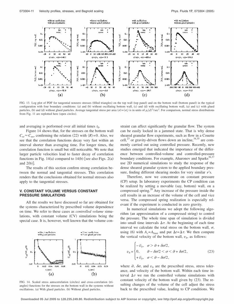
and averaging is performed over all initial times t0.Figure 14 shows that, for the stresses on the bottom wall

CntCnn, confirming the relation �22� with �R=0. Also, wesee that the correlation functions decay very fast within aninterval shorter than averaging time. For longer times, thecorrelation function is small but still noticeable. We note thatlarger particle velocities lead to faster decay of correlationfunctions in Fig. 14�a� compared to 14�b� �see also Figs. 2�a�and 2�b��.

The results of this section confirm strong correlation be-tween the normal and tangential stresses. This correlationrenders that the conclusions obtained for normal stresses alsoapply to the tangential stresses.

V. CONSTANT VOLUME VERSUS CONSTANTPRESSURE SIMULATIONS

All the results we have discussed so far are obtained forthe systems characterized by prescribed volume dependenceon time. We refer to these cases as controlled volume simu-lations, with constant volume �CV� simulations being thespecial case. It is, however, well known that the volume con-

straint can affect significantly the granular flow. The systemcan be easily locked in a jammed state. That is why densesheared granular flow experiments, such as flow in a Couettecell,23 or gravity-driven flows down an incline,34,35 are com-monly carried out using controlled pressure. Recently, newstudies emerged that indicated the importance of the differ-ence between controlled-volume and controlled-pressureboundary conditions. For example, Aharonov and Sparks36,37

use 2D numerical simulations to study the response of thedense sheared granular system to the applied boundary pres-sure, finding different shearing modes for very similar ’s.

Therefore, now we concentrate on constant pressure�CP� setup. In laboratory experiments the CP condition canbe realized by setting a movable �say, bottom� wall, on acompressed spring.20 Any increase of the pressure inside thecell results in an increase of the volume of the cell and viceversa. The compressed spring realization is especially rel-evant if the experiment is conducted in zero gravity.

In numerical simulations we adopt the following algo-rithm �an approximation of a compressed string� to controlthe pressure. The whole time span of simulation is dividedinto small time intervals ��. At the beginning of each timeinterval we calculate the total stress on the bottom wall, �,using �6� with As=Abase and put �t=��. We then computethe vertical velocity of the bottom wall, vb, as follows:

vb = �− v̄b, � � �̄ + �/2,

0, �̄ − �/2 � � � �̄ + �/2,

+ v̄b, � � �̄ − �/2,� �23�

where �̄, �, and vb are the prescribed stress, stress toler-ance, and velocity of the bottom wall. Within each time in-terval �� we run the controlled volume simulations withconstant velocity of the bottom wall given by �23�. The re-sulting changes of the volume of the cell adjust the stressback to the prescribed value, leading to CP conditions. We

FIG. 13. Log plot of PDF for tangential nonzero stresses �filled triangles� on the top wall �top panel� and on the bottom wall �bottom panel� in the typicalconfiguration with four boundary conditions: �a� and �b� without oscillating bottom wall, �c� and �d� with oscillating bottom wall, �a� and �c� with gluedparticles, �b� and �d� without glued particles. Average tangential stress per area ��= ��t is in units of �s�d2 / sec2. For comparison, normal stress distributionsfrom Fig. 11 are replotted here �open circles�.

FIG. 14. Scaled stress autocorrelation �circles� and cross-correlation �tri-angles� functions for the stresses on the bottom wall in the systems withoutoscillations. �a� With glued particles. �b� Without glued particles.



note that this model leads to vibration of the bottom wall insteady state, similarly to experiments.38

We consider the system without oscillations and withglued particles on the top wall �Fig. 2�a�� as a basis for allour CP simulations, and set the constant stress on the bottomwall being equal to the average stress ��n on this wall thatwe measured in CV simulations with �=10 rad/sec. Thechoice of the parameters used in the model �23� is

�̄ = 222�s�d2�sec−2�, � = 20�s�d2�sec−2� , �24�

�� = Tw/25, v̄b = �d/��/1000 = 0.915�d/sec. �25�

Figure 15�a� shows the PDF for the stresses on the com-plete bottom wall using the parameters �24� and �25� and�t=��. For comparison, the results of CV simulations forthe same As and �t are also shown. We see that the CPdistribution is wider compared to CV case. To understandthis difference it is useful to distinguish three sets of col-lected stress data in CP setting, each set resulting from one ofthree phases of the bottom wall motion: moving up, stayingput, and moving down �this separation of the stresses is pos-sible only because �t=��, i.e., during the averaging time thebottom wall does not change its velocity�. The resulting CPdistribution corresponds to the superposition of these threephases, leading to widening of the stress distribution in CPsetup, which can be estimated as follows. If �vy

�CV� is achange in the normal component of velocity of a particleinteracting with a stationary sensor and �vy

�CP� is a change inthe normal component of the velocity of the same particleinteracting with a sensor that has the velocity vb, then

�vy�CP�=�vy

�CV�+vb. If we have N particles of average diam-eter �d interacting with a sensor As during �t then, using thedefinition �6�,

�n�CP� = �n

�CV� + K1Nvb

As�t, �26�

where �n�CP� is a stress on a moving sensor, �n

�CV� is a stresson a stationary sensor, and K1=�s�d3 /6. Therefore, oneexpects that the distribution of �n

�CP� is 2K1Nvb / �As�t�wider than the distribution of �n

�CV�. This argument predictsthat �width�CP�−width�CV�� /width�CV��0.1–0.2, consistentlywith the results shown in Fig. 15�a� �in the estimate we useN=10, based on the results shown in Fig. 12�c��. We notethat the above argument applies only to the normal stresses,since this is the direction of vb.

In principle, both normal and tangential stresses can alsobe affected by the changes in and in the velocity profilesdue to the motion of the bottom wall, see Fig. 15�b�. Toestimate this effect, we note that it is characterized by theapproximate frequency of 1/ �2��=457 Hz and the ampli-tude of v̄b�� /2=0.0005�d. Despite high frequencies, the vi-brations of such a small amplitude are not expected to sig-nificantly modify stress distributions, as also illustrated byFig. 16.

Figure 16 shows stress PDFs on typical size sensors us-ing our typical averaging time �t=Tw /10. Compared to thestresses in CV simulations, Figs. 11�a� and 13�a�, we do notsee any significant differences. This is because �t��;therefore, during the averaging time the velocity of the bot-tom wall can change once or twice, resulting in “averagingout” the effect of the bottom wall motion. Therefore, weconclude that the model specified by �23�–�25� is effective inkeeping constant stress, while not modifying significantlystress distributions on the time scales of interest.

Bagnold scaling

In this section we investigate the effect of the shearingvelocity � on the stresses. The relation between average nor-mal stress and � under certain conditions takes the form ofBagnold scaling,39 where stresses increase with the square ofthe shear rate.3,21,34,38,40 This quadratic dependence is ob-served for the granular flows at high shearing rates or forlower ’s, i.e., in the systems where particles are not in-volved in multiple elastic deformations.41

FIG. 15. �a� Stress on the base PDF in CP case �circles� compared to CV�triangles�. Here �t=��=Tw /25 and As=Abase. �b� The position of the bot-tom wall �in units of �d� in the CP simulations. Zero corresponds to themean position of the wall. Inset: same data on finer time scale.

FIG. 16. Constant-pressure simulations: Stresses for the case without oscillations and with glued particles on the top wall. Size of sensors ds=1.09�d. �a� and�c� Sensors are on the top wall; �b� and �d� sensors are on the bottom wall; �a� and �b� normal stress PDF; �c� and �d� tangential stress PDF.



Figure 17�a� shows log-log plot of the mean normalstresses on the bottom wall versus � at CV setting for thesystem shown in Fig. 2�a�. For configurations of =40% and=50% these results confirm Bagnold scaling for the rangeof �’s between 1 rad/sec and 35 rad/sec. The data are fittedby the power function ��=a�b with a=0.015 and b=2.20±0.2 for =40% and a=0.201 and b=2.18±0.2 for=50%.

Figure 17�b� shows scaled velocity profiles for different�’s in CV simulations. The profiles are higher for fastershearing. The origin of this dependence may be related to theeffect of sidewalls on the sheared system. Indeed, when weshear the system with elastic and smooth sidewalls, see Fig.4, the profiles do not depend on �. Experimental studies42

also confirm the independence of velocity profiles on � ifboundary effects are significantly minimized. To explainthese results we consider the dependence of restitution pa-rameters on the particle’s velocity in particle-sidewall inter-actions. The normal coefficient of restitution �4� depends onthe normal velocity of colliding particle; however, this veloc-ity is not influenced significantly by �. On the other hand,the coefficient of tangential restitution, �, in the case of slid-ing contacts �5� depends stronger on �, since it involves theratio of normal to tangential velocity, and the latter scaleswith �. As it can be seen from �4�, lower ratio has the sameeffect on dissipative mechanics as lower coefficient of fric-tion, �. Therefore, in the case of higher shear rates, the effect

of sidewalls on the granular flow is reduced, explaining thevelocity profiles in Fig. 17�b�. Stresses shown in Fig. 17�c�are discussed below in the context of comparative study ofCV and CP.

In CP simulations we choose the fixed value of the stresson the bottom wall given by �24�. Figure 18�a� shows thevertical position of the bottom wall h as a function of timefor different � �h=0 corresponds to 40%�. As expected,we see that slower/faster shearing leads to smaller/largerstress, and to an adjustment of the wall position. The stabi-lized �long time� wall positions are used to calculate foreach �, shown in Fig. 18�b�. We note significant change in as � is modified: at high shearing �35 rad/sec� is about 1.6times smaller than at low shearing �1 rad/sec�.

Figure 19�a� shows the effect of � on the velocity pro-files. For small �’s, ��2.5 rad/sec, the shearing is strongerfor larger �. For intermediate �’s, 2.5 rad/sec��5 rad/sec the velocity profiles are almost the same, and for��5 rad/sec the shearing decreases with an increase of �.These results can be understood in terms of volume fractionas a determining factor. For the smallest � �solid line in Fig.19�a�� is about 53%; therefore, local jammed areas can beformed inside the sample reducing the overall mobility andshearing. These jammed areas can manifest themselves as“plateaus” in velocity profile. One such plateau can be seenin Fig. 19�a�, solid line, for 4�y�5. As decreases with anincrease of �, the sample gets more fluidized and the shear-

FIG. 17. CV simulations. �a� Stress as a function of � in log-log plot. Circles: =40%. Triangles: =50%. Solid lines are the best fits �see text�. The rest ofresults shown are calculated using =40%. �b� Velocity profiles; �c� stress PDF, bottom wall, �t=Tw /25. Measurements are taken over �T=5000�t=5.47 sec except for �=1 rad/sec, where �T=2 sec.

FIG. 18. Constant-pressure simulations. �a� Position of the bottom wall h �in units of �d� as a function of time for different shearing velocities; �b� as afunction of �.



ing improves. However, further increase of � and decreaseof makes the system more “compressible:” the dilationclose to the top wall is stronger, reducing the momentum fluxfrom the top wall to the bulk of the sample, resulting inweaker shearing. Therefore, the influence of � on a CP sys-tem is more complicated than in a CV case, where velocityprofiles are changing monotonously with �, see Fig. 17�b�.

The distributions of the normal stress on the bottom wallare shown in Fig. 17�c� for the CV and in Fig. 19�b� for theCP. In both cases, the widths of distributions increase with adecrease of �. The distributions differ in the following: inthe CP case �Fig. 19�b�� the distribution shows a double peakat low shearing, which is absent in the CV case. This doublepeak occurs, since at low �, is high, up to 52%. Thus thecollision rate between the particles and the moving bottomwall is higher, and hence larger momentum is transferred tothe granular system. If this momentum is large enough, wehave the situation in which the “restoring force” of the bot-tom wall brings the system in just one interval �� from theoverstressed state to understressed state or vice versa. There-fore, velocity of the wall, �23�, alternates between positiveand negative without taking zero value, resulting in twopeaks in stress distribution: one for overstressed state andanother one for understressed state.

VI. CONCLUSIONS

The presented studies concentrate on 3D event-drivensimulations in the Couette geometry with top rotating walland with physical boundary conditions in zero gravity. Thevelocity and volume fraction distributions are strongly de-pendent on various boundary conditions, such as top shear-ing wall properties, sidewall properties, presence of oscilla-tions of the bottom wall, or intensity of shearing. The overallvolume fraction of studied granular system is 40%; however,the shearing and vibrating walls impose the nonuniformity involume fraction distribution with the formation of high-dense band �cluster� where local volume fraction reaches upto 60%. The cluster can respond to shearing in differentways. For example, while very rough and inelastic top wall,but without glued particles, cannot induce any significantshearing when sidewalls are dissipating, it imposes a shearand high tangential velocities of all particles in the case ofsmooth and elastic sidewalls. Typically, inside the cluster the

shear rate is very small. However, the presence of the gluedparticles on the top wall considerably increases shear rateinside this cluster.

The presence of oscillations of the bottom wall seems tohave three effects: �1� The slippage velocity at the bottomincreases. �2� The dense cluster is located further away fromthe bottom wall compared to the systems without oscilla-tions. �3� Equilibrating times to reach a steady state areshorter in the systems with oscillations due to the increasedcollision rate.

The equilibrating dynamics involves attaining thesteady-state values of volume fractions and velocities. Thetime scales of these two equilibrating processes are different:in most cases, steady-state profile in volume fraction is at-tained very fast, while velocity profiles reach their finalshape much later. However, the volume fraction distributiontakes longer to reach a steady state when the rate of energyinput is low. This occurs in the systems without glued par-ticles and without oscillations. For example, in the so-called“delayed dynamics” regime, described in Sec. III B, the timeneeded for the cluster to accumulate enough energy to disat-tach from the bottom wall can be very long. However, oncethis happens, the velocity profile changes drastically. Moregenerally, these simulations show that the velocities and vol-ume fractions strongly depend on boundary conditions:simulations using, e.g., periodic boundary conditions maymiss a number of interesting effects presented in this work.

We have also analyzed stress and stress fluctuations onthe boundaries. We find that the distribution of normalstresses in a system of 40% volume fraction and rapid granu-lar flow can be described by the same functional form �9� asused for stress distribution in static dense system, i.e., withpower-law increase for small stresses and exponential de-crease for large ones. Considering this functional form as auseful guide, we predict the behavior of main characteristicsof stress distributions as a function of sensor area and aver-aging time. These predictions describe well the width of dis-tributions for small sensors and short �t’s. However, theyfail for large sensors and long averaging times, suggestingthe existence of additional correlations not accounted by ourfunctional form. The correlations may be related to the exis-tence of “denser structures” in the simulated systems.

We simulate constant pressure boundary condition anddiscuss the differences between the results in constant vol-ume and constant pressure settings. A key observation here isvery different response to an increase of shearing velocity inthe system with constant-pressure boundary condition com-pared to the systems with constant-volume boundary condi-tion. In the first case the shearing velocities are increasingbecause of the velocity dependence of the coefficients ofrestitution while in the second case they are initially increas-ing and then decreasing because of the changes of volumefraction with imposed shear.

ACKNOWLEDGMENTS

The authors acknowledge the support of NASA, GrantNo. NNC04GA98G, and thank Robert P. Behringer and

FIG. 19. CP simulations. �a� Velocity profiles; �b� stress PDF, bottom wall.These distributions are obtained from the stress data taken every �t=��=Tw /25 sec over �T=5000�t.



Karen E. Daniels of Duke University and Allen Wilkinson ofNASA Glenn for very useful discussions.

1J. T. Jenkins and S. B. Savage, “A theory for the rapid flow of identical,smooth, nearly elastic, spherical particles,” J. Fluid Mech. 130, 187�1983�.

2C. K. K. Lun, S. B. Savage, D. J. Jeffrey, and N. Chepurniy, “Kinetictheories for granular flow: Inelastic particles in Couette flow and slightlyinelastic particles in a general flowfield,” J. Fluid Mech. 140, 223 �1984�.

3C. S. Campbell and C. E. Brennen, “Computer simulation of granularshear flows,” J. Fluid Mech. 151, 167 �1985�.

4C. S. Campbell and A. Gong, “The stress tensor in a two-dimensionalgranular shear flow,” J. Fluid Mech. 164, 107 �1986�.

5L. Bocquet, W. Losert, D. Schalk, T. C. Lubensky, and J. P. Gollub,“Granular shear flow dynamics and forces: Experiment and continuumtheory,” Phys. Rev. E 65, 011307 �2002�.

6J. T. Jenkins and M. W. Richman, “Boundary conditions for plane flows ofsmooth, nearly elastic, circular disks,” J. Fluid Mech. 171, 53 �1986�.

7M. Y. Louge, J. T. Jenkins, and M. A. Hopkins, “Computer simulations ofrapid granular shear flows between parallel bumpy boundaries,” Phys.Fluids A 2, 1042 �1990�.

8M. Y. Louge, “Computer simulations of rapid granular flows of spheresinteracting with a flat, frictional boundary,” Phys. Fluids 6, 2253 �1994�.

9K. Hui, P. K. Haff, J. E. Ungar, and R. Jackson, “Boundary conditions forhigh-shear grain flows,” J. Fluid Mech. 145, 223 �1984�.

10G. M. Gutt and P. K. Haff, “Boundary conditions on continuum theories ofgranular flow,” Int. J. Multiphase Flow 17, 621 �1991�.

11M. Alam and P. R. Nott, “Stability of plane Couette flow of a granularmaterial,” J. Fluid Mech. 377, 99 �1998�.

12P. R. Nott, M. Alam, K. Agrawal, R. Jackson, and S. Sundaresan, “Theeffect of boundaries on the plane Couette flow of granular materials: Abifurcation analysis,” J. Fluid Mech. 397, 203 �1999�.

13B. D. Lubachevsky, “How to simulate billiards and similar systems,” J.Comput. Phys. 94, 255 �1991�.

14S. Luding, “Granular materials under vibration: Simulations of rotatingspheres,” Phys. Rev. E 52, 4442 �1995�.

15S. F. Foerster, M. Y. Louge, H. Chang, and K. Allia, “Measurements of thecollision properties of small spheres,” Phys. Fluids 6, 1108 �1994�.

16W. Goldsmith, Impact, The Theory and Physical Behavior of CollidingSolids �Arnold, London, 1964�.

17T. Schwager and T. Pöschel, “Coefficient of normal restitution of viscousparticles and cooling rate of granular gases,” Phys. Rev. E 57, 650 �1998�.

18C. Bizon, M. D. Shattuck, J. B. Swift, W. D. McCormick, and H. L.Swinney, “Patterns in 3D vertically oscillated granular layers: Simulationand experiment,” Phys. Rev. Lett. 80, 57 �1998�.

19O. R. Walton, in Particulate Two-Phase Flow, edited by M. C. Roco�Butterworth, Boston, 1993�, p. 884.

20K. E. Daniels and R. P. Behringer �private communications�.21S. B. Savage and D. J. Jeffrey, “The stress tensor in a granular flow at high

shear rates,” J. Fluid Mech. 110, 255 �1981�.22S. B. Savage, “Analyses of slow high-concentration flows of granular

materials,” J. Fluid Mech. 377, 1 �1998�.23B. Miller, C. O’Hern, and R. P. Behringer, “Stress fluctuations for conti-

nously sheared granular materials,” Phys. Rev. Lett. 77, 3110 �1996�.24C. Thornton, “Force transmission in granular media,” Kona 15, 81 �1997�.25F. Radjai, M. Jean, J. J. Moreau, and S. Roux, “Force distribution in dense

two-dimensional granular systems,” Phys. Rev. Lett. 77, 274 �1996�.26S. N. Coppersmith, C. Liu, S. Majumdar, O. Narayan, and T. A. Witten,

“Model for force fluctuations in bead packs,” Phys. Rev. E 53, 4673�1996�.

27E. Longhi, N. Easwar, and N. Menon, “Large force fluctuations in a flow-ing granular medium,” Phys. Rev. Lett. 89, 045501 �2002�.

28D. M. Mueth, H. M. Jaeger, and S. R. Nagel, “Force distribution in agranular medium,” Phys. Rev. E 57, 3164 �1998�.

29C. Liu, S. R. Nagel, D. A. Schecter, S. N. Coppersmith, S. Majumdar, O.Narayan, and T. A. Witten, “Force fluctuations in bead packs,” Science269, 513 �1995�.

30M. L. Nguyen and S. N. Coppersmith, “Properties of layer-by-layer vectorstochastic models of force fluctuations in granular materials,” Phys. Rev. E59, 5870 �1999�.

31J. E. S. Socolar, “Average stresses and force fluctuations in non-cohesivegranular materials,” Phys. Rev. E 57, 3204 �1998�.

32S. F. Edwards and D. V. Grinev, “Statistical mechanics of granular mate-rials: Stress propagation and distribution of contact forces,” GranularMatter 4, 147 �2003�.

33D. Howell and R. P. Behringer, “Fluctuations in a 2D granular Couetteexperiment: A critical transition,” Phys. Rev. Lett. 82, 5241 �1999�.

34L. E. Silbert, D. Ertas, G. S. Grest, T. C. Halsey, D. Levine, and S. J.Plimpton, “Granular flow down an inclined plane: Bagnold scaling andrheology,” Phys. Rev. E 64, 051302 �2001�.

35M. Y. Louge and S. C. Keast, “On dense granular flows down flat fric-tional inclines,” Phys. Fluids 13, 1213 �2001�.

36E. Aharonov and D. Sparks, “Shear profiles and localization in simulationsof granular materials,” Phys. Rev. E 65, 051302 �2002�.

37E. Aharonov and D. Sparks, “Rigidity phase transition in granular pack-ings,” Phys. Rev. E 60, 6890 �1999�.

38S. B. Savage and M. Sayed, “Stresses developed by dry cohesionlessgranular materials sheared in an annular shear cell,” J. Fluid Mech. 142,391 �1984�.

39R. A. Bagnold, “Experiments on a gravity-free dispersion of large solidspheres in a Newtonian fluid under shear,” Proc. R. Soc. London, Ser. A225, 49 �1954�.

40G. Bossis, Y. Grasselli, and O. Volkova, “Granular rheology in zero grav-ity,” J. Phys.: Condens. Matter 16, 3279 �2004�.

41C. S. Campbell, “Granular shear flows at the elastic limit,” J. Fluid Mech.465, 261 �2002�.

42W. Losert, L. Bocquet, T. C. Lubensky, and J. P. Gollub, “Particle dynam-ics in sheared granular matter,” Phys. Rev. Lett. 85, 1428 �2000�.



POF 2005 granular

Documents

Transcript of POF 2005 granular