On numerical simulation of granular flow
116
On numerical simulation of granular flow Sebastian Schmidt Vom Fachbereich Mathematik der Universit¨ at Kaiserslautern zur Verleihung des akademischen Grades Doktor der Naturwissenschaften (Doctor rerum naturalium, Dr. rer. nat.) genehmigte Dissertation. Gutachter: PD Dr. Oleg Iliev, Technische Universit¨ at Kaiserslautern & Fraunhofer ITWM Kaiserslautern Prof. Dr. G¨ unter B¨ arwolff, Technische Universit¨ at Berlin Datum der Disputation: 6. Juli 2009 D386
-
Upload
khangminh22 -
Category
Documents
-
view
3 -
download
0
Transcript of On numerical simulation of granular flow
On numerical simulation of granular flow
Sebastian Schmidt
Vom Fachbereich Mathematik der UniversitatKaiserslautern zur Verleihung des akademischen Grades
Doktor der Naturwissenschaften (Doctor rerum naturalium, Dr. rer. nat.)genehmigte Dissertation.
Gutachter:
PD Dr. Oleg Iliev,Technische Universitat Kaiserslautern & Fraunhofer ITWM Kaiserslautern
Prof. Dr. Gunter Barwolff,Technische Universitat Berlin
Datum der Disputation:
6. Juli 2009
D386


Fur meinen Opa
Herbert Schneider
Danksagungen
Ich mochte mich zuallererst bei Dr. Oleg Iliev und Dr. Arnulf Latz fur die intensive,diskussionsreiche und lehrreiche Begleitung und Betreuung wahrend der Entstehungdieser Arbeit bedanken.
Fur eine angenehme, freundschaftliche und vor allem vertrauensvolle Arbeit-sumgebung bedanke ich mich bei der Abteilung SMS des Fraunhofer ITWM im All-gemeinen und bei Dr. Konrad Steiner im Speziellen. Fur interessante Anregungenund Diskussionen mochte ich mich weiterhin bei Dr. Heiko Andra, Dr. GuntherBarwolff, Dr. Andreas Wiegmann und Dr. Aivars Zemitis bedanken. Bei Dr. Dar-iusz Niedziela bedanke ich mich fur die gute Zusammenarbeit.
Bei Zahra Lakdawala bedanke ich mich fur sehr angenehme Jahre im gemein-samen Buro und viele neue kulturelle Sichtweisen. Bei Tobias Zangmeister bedankeich mich fur viele gute Gesprache, Entspannungen von dieser Arbeit und am Endeihre gewissenhafte und qualvolle Korrekturlesung.
Ganz besonders mochte ich mich bei meinem Bruder, meinen Eltern und meinerGroßmutter fur ihre bedingungslose Unterstutzung bei jedem und auch diesem Vorhabenbedanken.
Die Mathematiker, die nur Mathematiker sind,denken also richtig, aber nur unter der Voraussetzung,dass man ihnen alle Dinge durch Definitionen und Prinzipien erklart;sonst sind sie beschrankt und unertraglich,denn sie denken nur dann richtig,wenn es um sehr klare Prinzipien geht.
Blaise Pascal (1623 - 1662)


Contents
Introduction 7
1 Models 131.1 The basic hydrodynamic model of fluid flow . . . . . . . . . . . . . . 14
1.1.1 The generalized Navier-Stokes Equations . . . . . . . . . . . . 141.1.2 Boundary conditions . . . . . . . . . . . . . . . . . . . . . . . 15
1.2 Kinetic theory of granular gases . . . . . . . . . . . . . . . . . . . . . 161.3 Modeling the dilute and dense flow of grains . . . . . . . . . . . . . . 17
1.3.1 Kinetic modeling . . . . . . . . . . . . . . . . . . . . . . . . . 181.3.2 An attempt to bridge kinetic and plastic models . . . . . . . . 211.3.3 Implemented model . . . . . . . . . . . . . . . . . . . . . . . . 23
2 Algorithms 292.1 Discussion on the type of numerical method . . . . . . . . . . . . . . 30
2.1.1 Arguments for an implicit, pressure based splitting . . . . . . 312.1.2 The need for a nonlinear method . . . . . . . . . . . . . . . . 322.1.3 The treatment of the temperature equation . . . . . . . . . . . 33
2.2 General space discretization . . . . . . . . . . . . . . . . . . . . . . . 332.2.1 Notation . . . . . . . . . . . . . . . . . . . . . . . . . . . . . . 332.2.2 Finite Volume space discretization . . . . . . . . . . . . . . . . 36
2.3 Introduction to fractional step methods . . . . . . . . . . . . . . . . . 402.3.1 The variants of fractional step methods . . . . . . . . . . . . . 402.3.2 Linear pressure correction algorithm . . . . . . . . . . . . . . 41
2.4 A nonlinear pressure based algorithm . . . . . . . . . . . . . . . . . . 432.4.1 Time discretization . . . . . . . . . . . . . . . . . . . . . . . . 432.4.2 Spatial discretization of the split system . . . . . . . . . . . . 462.4.3 Derivation of the nonlinear pressure equation . . . . . . . . . . 482.4.4 The Newton method and its variants . . . . . . . . . . . . . . 492.4.5 The nonlinear pressure algorithm . . . . . . . . . . . . . . . . 502.4.6 Detailed discretization . . . . . . . . . . . . . . . . . . . . . . 52
2.5 Initial and boundary conditions . . . . . . . . . . . . . . . . . . . . . 582.5.1 Approximation of boundary conditions . . . . . . . . . . . . . 592.5.2 Initial conditions for the granular flow model . . . . . . . . . . 61
3 Validation and numerical simulations 633.1 The granular shear flow experiment . . . . . . . . . . . . . . . . . . . 633.2 Validation of the granular flow model . . . . . . . . . . . . . . . . . . 64
3.2.1 Shear flow . . . . . . . . . . . . . . . . . . . . . . . . . . . . . 653.2.2 The angle of repose . . . . . . . . . . . . . . . . . . . . . . . . 663.2.3 Sliding down a rough inclined plane . . . . . . . . . . . . . . . 683.2.4 The stress tensor for granular flow . . . . . . . . . . . . . . . . 69
3.3 Validation of the algorithm . . . . . . . . . . . . . . . . . . . . . . . . 70

6 CONTENTS
3.3.1 Newtonian flow . . . . . . . . . . . . . . . . . . . . . . . . . . 713.3.2 Solutions for different grid resolutions . . . . . . . . . . . . . . 72
3.4 Numerical investigations . . . . . . . . . . . . . . . . . . . . . . . . . 733.4.1 Compressibility regimes . . . . . . . . . . . . . . . . . . . . . 743.4.2 Mass conservation . . . . . . . . . . . . . . . . . . . . . . . . . 753.4.3 Bifurcating solutions . . . . . . . . . . . . . . . . . . . . . . . 75
3.5 Simulation of industrial processes . . . . . . . . . . . . . . . . . . . . 763.5.1 Emptying of silos . . . . . . . . . . . . . . . . . . . . . . . . . 773.5.2 Compactification of granular media . . . . . . . . . . . . . . . 78
4 Software 814.1 Architecture and components . . . . . . . . . . . . . . . . . . . . . . 82
4.1.1 The framework components . . . . . . . . . . . . . . . . . . . 824.1.2 The implementations . . . . . . . . . . . . . . . . . . . . . . . 844.1.3 Discussion of the modular approach . . . . . . . . . . . . . . . 85
4.2 A generalized approach to discretization . . . . . . . . . . . . . . . . 874.2.1 Grid and volume data structure . . . . . . . . . . . . . . . . . 874.2.2 The discretization process . . . . . . . . . . . . . . . . . . . . 89
4.3 Parallel linear algebra . . . . . . . . . . . . . . . . . . . . . . . . . . 914.3.1 MPI data structures . . . . . . . . . . . . . . . . . . . . . . . 914.3.2 Assembly of the matrix . . . . . . . . . . . . . . . . . . . . . . 934.3.3 The nonlinear case . . . . . . . . . . . . . . . . . . . . . . . . 954.3.4 Discussion on the efficiency of the parallelization . . . . . . . . 95
4.4 Multiphase . . . . . . . . . . . . . . . . . . . . . . . . . . . . . . . . . 964.4.1 Multiphase through coupling terms . . . . . . . . . . . . . . . 974.4.2 Multiphase through a coupled system . . . . . . . . . . . . . . 98
5 Concluding remarks and outlook 99
A Appendix 103A.1 Collaps in kinetic models . . . . . . . . . . . . . . . . . . . . . . . . . 103A.2 Dynamic Coulomb friction . . . . . . . . . . . . . . . . . . . . . . . . 103
Notation 107
Bibliography 113

Introduction
Granular materials show a wonderfully diverse set of behaviors. Make a sand cas-tle, and the material appears solid. Push on the castle and it can fall down in anavalanche-like pattern. Sometimes the avalanche moves the bulk of the material,sometimes it is confined to a thin layer on the surface. Shake up crushed ice in amartini shaker, and it moves like a gas. Try to pour salt through an orifice, andit has a characteristic tendency to choke up and clog the orifice. Gas, liquid, solid,plastic flow, glassy behavior - a granular material can mimic them all. In addition,the properties of a granular material can depend upon its history. Tamped sand isdifferent from loose sand. But in many ways, a granular material is like an ordinaryfluid. Both types of material are composed of many small particles, and each has abulk behavior that hides the materials graininess. It is thus natural to ask whetherthe same equations, concepts, and theories that work for molecular material alsoapply to the granular form of matter.
Leo P. Kadanoff, “Built upon sand”1
About this work
The goal of this work is the simulation of granular flow. The definition of “gran-ular flow” is a nontrivial task in itself, see for example [Dar03]. We say that it iseither the flow of grains in a vacuum or in a fluid. A grain is an observable piece ofa certain material, for example stone when we mean the flow of sand.
Choosing a hydrodynamic view on granular flow, we treat the granular materialas a fluid. A hydrodynamic model has to be developed, that describes the processof flowing granular material. This is done through systems of partial differentialequations (PDEs) and algebraic relations. Solutions to these systems have to beobtained to understand the process. The equations are in most cases so difficult tosolve that an analytical solution is out of reach. So approximate solutions must beobtained.
Hence the next step is the choice or development of a numerical algorithm toobtain approximate solutions of the model. Common to every problem in numericalsimulation, these two steps do not lead to a result without implementation of thealgorithm. Hence the author attempts to present this work in the following frame, toparticipate in and contribute to the three areas Physics, Mathematics and Softwareimplementation and approach the simulation of granular flow in a combined andinterdisciplinary way.
This work is structured as follows. A continuum model for granular flow whichcovers the regime of fast dilute flow as well as slow dense flow up to vanishing veloc-ity is presented in Chapter 1. This model is strongly nonlinear in the dependenceof viscosity and other coefficients on the hydrodynamic variables and it is singular
1[Kad99]

8 INTRODUCTION
because some coefficients diverge towards the maximum packing fraction of grains.Hence the second difficulty, the challenging task of numerically obtaining approxi-mate solutions for this model is faced in Chapter 2. In Chapter 3 we attempt tovalidate both the model and the numerical algorithm through numerical experimentsand investigations and show their application to industrial problems. We finish withthe implementation of the simulation tools we have developed in Chapter 4.
Throughout the whole work, we focus on one experiment as our guideline. Thisis the shear flow experiment from [BLS+01]. It serves well to demonstrate thealgorithm, all boundary conditions involved and provides a setting for analyticalstudies in [BLS+01] to compare our results.
Review and state of the art
Modeling of granular flow: We attempt to model the flow of granular materialas a liquid. Due to the lack of a clear time and spatial scale separation and veryefficient mechanisms for energy dissipation in form of inelastic collisions (see [Kad99])this may seem overly brave. For mainly these reasons, a theory is still missing forthe description of granular flow on a macroscopic scale with the same accuracyas the Navier-Stokes Equations (NSE) for simple liquids. Still kinetic theory andhydrodynamic modeling are in many cases a valid approach to the simulation ofgranular flow, see [Duf01].
We have to trust the usual assumption that even for granular materials, thespatial variation of the hydrodynamic variables can be captured by terms linear inspatial derivatives. Then fortunately, for weakly inelastic granular media, kinetictheory provides a framework for deriving the correct hydrodynamic equations pre-sented in [BP03]. The kinetic theory with heuristic modifications is very useful formany simulations of granular flow in application problems at intermediate volumefractions as for example in the simulation of fluidized beds in [Gid94].
Kinetic theory assumes that grain collisions are binary which means that colli-sions always occur only between two particles at the same time and instantaneouswhich means that the particles separate immediately after the collision, see [BP03,Section 1.4, pg. 5]. It seems obvious at first sight that this assumption is invalidfor volume fractions close to the maximum packing. Therefore, the applicabilityof kinetic theory becomes questionable in this regime. Nevertheless, the literaturereports differently. In [MPB03], Meerson et al. show strikingly good agreement be-tween simulations at large volume fractions and hydrodynamic theory. The samehas been done by Boqcuet et al. in [BLS+01, BEL02] relying on experiments. Theseexperiments were carried out under shearing conditions which will become impor-tant later in this work. In that case they have shown that kinetic theory is able tomimic solid like behavior. It does so by exhibiting a solid like Coulomb stress as asolution of the hydrodynamic equations.

MOTIVATION, GOALS AND OVERVIEW 9
Numerics: We model granular flow by a time-dependent NSE-type system. Tocompute approximate solutions of the system we need to discretize it in space andtime. The former is achieved using a Finite Volume (FV) discretization. The latteris a novel pressure based nonlinear fractional step method (NFSM). In the linearcase, we call every method which decouples the solution of the NSE-type system intomultiple steps a linear fractional step method (LFSM). This may be misleading froma steady flow point of view because fractional step methods usually split the timestep. However, we are mainly concerned with the unsteady case where all thesemethods can be interpreted as splitting one full solution step into fractional steps.
The FV discretization seems to have been first introduced by Tikhonov andSamarskii in [TS61]. It partitions the domain into volumes over which the equationsare integrated. The resulting volume integrals are transformed to surface integralsalong the surface of the volume where possible. The approximation of these surfaceintegrals then yields the FV discretization. A collection of recent FV discretizationsand the state of the art mathematical theory of FV discretization schemes can befound in [EGH00].
The main concern of this work will be the time discretization of the NSE-typegranular flow model. Considering only implicit or semi-implicit methods which de-couple the NSE-type system, the first developments that lead to pressure based LFSMsgo back to the works of Chorin in [Cho68] and Patankar and Spalding in [PS72].Chorin has proposed a projection method for unsteady incompressible flow prob-lems which is basically a two-stage LFSM. Patankar and Spalding have introduced aFV implementation of these LFSMs in the SIMPLE method for steady incompressibleflow. The underlying idea of all the methods is the projection of a predicted velocityand pressure onto the space of divergence free velocity.
We see that pressure based methods were initially developed for incompressibleflow. The first extension of pressure based schemes for weakly compressible flowdates back to [HA68, HA71]. Much further work has been published on pressurebased LFSMs for the unsteady, compressible, non-isothermal NSE which are the basisfor our equation system. For an overview of methods see the book of Ferziger andPeric [FP96, Chapter 7] and for examples of recent methods see [vVW03] or [Chu03].
Mathematical frameworks have been used to systematically describe pressurebased methods. The Schur-Complement (SC) notation discussed by Turek in [Tur99]and operator splitting discussed in [GS98] should be mentioned here. These attemptto provide a way to compare the many variants of pressure based LFSMs.
Motivation, goals and overview
It becomes clear that the simulation of granular flow inherits two distinct dif-ficulties - the modeling and the numerical treatment. Regarding the first, there isstill no common agreement on the mathematical description for this type of flow.Regarding the second, numerical methods that are able to solve the presented model

10 INTRODUCTION
in both the dilute and the dense regime are rare.
Modeling of granular flow: We have stated above that in certain situationscurrent hydrodynamic models from kinetic theory show very good agreement withexperiments. Let us try to explain the reasons to be able to understand whereproblems will occur in other situations.
The mentioned experiments and simulations are carried out under shearing con-ditions. This is a situation of permanent input of energy through the movingwall that shears the material. Under these conditions, the existence of a dynamicCoulomb stress might explain why molecular dynamics (MD) simulations and ex-periments can be reproduced by hydrodynamic theory at all. For flowing granularmedia close to maximum packing fraction, collisional contacts of grains are replacedby frictional contacts. The proper theory of the stress in that case would be sometheory of static friction, for example the Coulomb friction theory. However, whenpermanent energy input prevents the granular system from arresting, the dynamicCoulomb friction of the hydrodynamic theory is able to mimic the true Coulombfriction.
The nature of these experiments hides a flaw in the kinetic models. This flawsurfaces only when a force is missing that would prevent the system from arresting.We will show in Section 1.3.2 that the above arguments will become invalid in thatcase. This motivates the extension of the available models.
We will show that kinetic theory alone is not able to reproduce the qualitativebehavior of typical arresting processes as for example the formation of heaps. InSection 1.3 we develop a model that is able to describe also arresting granular flow.Motivated by the work of Savage [Sav98], we present a hybrid model of kinetic theoryand a theory derived from soil mechanics. This theory overcomes the difficultiesobserved in kinetic theories and extends the applicability of hydrodynamic theoryto arresting granular flow.
Our model is a quite simplified version of the one presented by Savage. There isa good reason for that. The wealth of constitutive models is astonishing, see [Kol00]and a correct model has not been identified. It is necessary to obtain a constitutivemodel which can be calibrated and has as few parameters as possible. We presentsuch a model and show that we can produce the same results using our simplifiedmodel. We test the theory that we introduce by simulating heap formation withpredictable angle of repose, comparing simulations of flow down an inclined planeand reproducing core and mass flow in silos.
Numerics: The presented model is a strongly nonlinear and singular system ofPDEs and constitutive relations. To numerically obtain approximate solutions ofthis system we discretize it in space by using the FV method on a cell-centeredgrid of cuboids with collocated arrangement of the unknowns. The discretizationis derived from the integrated equations. Convective terms are discretized by afirst order upwind scheme and second order derivatives are discretized using centraldifferences.
The main focus of this work lies in the discretization of the system in time by a

MOTIVATION, GOALS AND OVERVIEW 11
pressure based NFSM. We start with a discussion on this numerical approach. Wewill especially point out our reasons for an implicit pressure based algorithm anddiscuss that the nature of the model strongly suggests the use of a nonlinear method.We then introduce the general notation and the operators for the space discretizationof certain PDE terms that we will use throughout this work. We proceed with anintroduction to LFSMs and the derivation of a linear pressure correction algorithm(LPCA) which will form the basis of the derivation of our NFSM.
Based on this derivation we introduce the splitting of the coupled granular flowsystem in a few easier to solve problems and derive a nonlinear pressure equation(NPE) from the split system. The first step will be the prediction of a velocity fieldfrom a linearized, fully implicit momentum equation using an old pressure field.Then we will present the derivation of a coupled system of a nonlinear pressureequation and a velocity correction equation as the correction step.
Finally we describe the nonlinear pressure algorithm (NPA) for solving the fulltime-dependent system. For the solution of the NPE we use a truncated Newtonmethod for systems of nonlinear equations. This method requires the evaluation ofthe Jacobian of the NPE. We obtain the Jacobian by finding the derivatives of theNPE and give a detailed discretization of both the NPE and the Jacobian.


Chapter 1
Models
This chapter provides all models and modeling aspects of the thesis. The models arederived on the basis of a hydrodynamic description of flows and are of Navier-StokesEquations (NSE)-type. For granular flow, this assumes that a continuum descriptionof particles is allowed which is discussed in [BP03, Section 1.3]. They argue thatparticles of granular gases are macroscopic bodies which allows for a continuumdescription of their interactions through a stress-strain relation.
Our aim is to arrive at a set of equations which models the flow of grains in bothdilute and dense regimes. The former is often called the regime of rapid granularflow and is extensively discussed in the literature, see [Duf01]. It seems to be agreedthat for this regime hydrodynamic models are able to reproduce many phenomenaof granular flow and the constitutive relations based on kinetic theory are valid.Outside this regime the topic becomes controversial. Clearly, a hydrodynamic modelwill not be able to reproduce mechanical interactions of single grains. However, wedo argue that hydrodynamic equations for granular flow are able to model the flowof dense bulk material as long as there is at least some movement.
The idea presented to arrive at such a model is a crossover of the constitutiverelations locally depending on the flow regime which depends on the volume fraction.The differential equations are the same throughout the regimes. Only the relationsfor viscosity, pressure, granular temperature etc. are continuously changed for thedense regime. This introduces a certain arbitrariness because it is not clear wheredilute flow ends and where dense flow begins. It must be asked at what volumefraction the flow is not dominated anymore by instantaneous collisions of grains butmainly by the sliding and rolling of grains on each other. We can not answer thisquestion, we have to treat the crossover volume concentration as a parameter whichmust be identified by comparison with experiments.
In Section 1.1 we shortly mention the commonly known system of generalized NSEfor the description of compressible non-isothermal fluid flow with varying viscosity.Then we proceed to Section 1.2 where we will provide a very brief introduction tothe kinetic theory of granular gases. This is followed by the derivation of a modelfor granular flow based on that theory in Section 1.3. Our final model extendsthe description of granular gases of [BP03]. In the regime above a certain volumefraction of grains where the assumptions of kinetic theory are not valid, we use amodeling approach from soil mechanics similar to the work of [Sav98].
Let 1 ≤ d ≤ 3 be the space dimension. Then as usual x ∈ Rd and t ∈ R denotethe space and time coordinates respectively. Let us denote velocity by u = u(x, t),pressure by p = p(x, t), density by ρ = ρ(x, t) and volume forces by f = f(x, t).We work in arbitrary domains Ω ⊂ Rd bounded by solid walls as well as inflow andoutflow boundaries denoted by ∂Ωsw, ∂Ωin and ∂Ωout respectively.

14 CHAPTER 1. MODELS
1.1 The basic hydrodynamic model of fluid flow
In the later sections of this chapter we will present a model for granular flow whichis based on the modeling of fluids. Therefore we give a short overview of the basicequations of fluid flow, the NSE. For detailed descriptions see [FP96] or [Wes01].
The NSE describe the motion of substances that can flow. This is based onseveral assumptions made on the fluid. The first is that the fluid is continuous. Itsignifies that it does not contain voids formed, for example, by bubbles of dissolvedgases. Also this means that it does not contain aggregates of any sort of particles.Another necessary assumption is that all the scalar and vector fields like velocity,pressure, density and temperature are differentiable. This would not be the case for,say, phase transitions.
Given that all these assumptions are valid for the fluids we consider, the equationsare derived from the basic principles of conservation of mass, momentum and energy.Usually this is done by considering a finite arbitrary volume called a control volumeover which these principles can be easily applied. This control volume is fixed intime and space with flow allowed to occur across the boundaries. The NSE thenfollow from the conservation laws and linear constitutive relations. For a detailedderivation of this form see [Fle91a, Sections 11.2.1-11.2.4].
1.1.1 The generalized Navier-Stokes Equations
Let us start with the model for instationary, compressible, viscous, isothermal flowdescribed by the system of NSE (1.1) for the unknowns u, p and ρ.
∂t(ρ) + div (ρu) = 0, (1.1a)
∂t(ρu) + div(ρu⊗ u)− div (σ) + grad(p)− f = 0, (1.1b)
where
σij := 2ηκij −2
3ηδij div (u) with κ :=
1
2
(∂ui
∂xj
+∂uj
∂xi
). (1.1c)
Assuming that we can write the momentum as the product of density and velocity,Equations (1.1a) and (1.1b) are the conservation of mass and momentum respec-tively. Equation (1.1c) denotes the general stress tensor and the general, sym-metrized rate of strain tensor. Volume forces are given in the right hand side fof Equation (1.1b). Furthermore, by δ we denote the Kronecker symbol. Thoughunusual for the standard NSE, we allow the viscosity to vary such that η = η(x, t)is our dynamic viscosity.
Due to the compressibility, the dependence of ρ on p, System (1.1) has to beextended by a relation between ρ and p which, for an ideal gas, reads
p = ρRT . (1.2)
Here T is a given constant temperature and R a constant dependent on the fluid.For non-isothermal flow, where T is not constant, a partial differential equation

1.1. THE BASIC HYDRODYNAMIC MODEL OF FLUID FLOW 15
(PDE) is necessary to describe the dynamic behavior of the internal energy of thesystem. We do not consider this topic further at this point as it is treated extensivelyfor Newtonian flow, for example in [Fle91a, Section 11.2.4]. It becomes an essentialpart of modeling for granular flow which we will discuss in the following section.
We have stated the NSE in their full complexity because we will need them asthe basis of our model for granular flow. However, for validation purposes and forreference in later parts of this work, let us retreat to a more simple case of fluid flow.If we assume the flow to be incompressible with constant density ρ, stationary andwith constant dynamic viscosity η then System (1.1) is reduced to
div (ρu) = 0, (1.3a)
div(ρu⊗ u)− div (σ) + grad(p)− f = 0, (1.3b)
where u and p are sought, ρ and f are given and σ is a much more simplified versionof the stress tensor
σ = ηκ, κij :=∂ui
∂xj
. (1.3c)
This models for example the stationary flow of water. Between System (1.1) andSystem (1.3) which will both be referred to in this work lie many orders of complexity.One of them is the model for instationary compressible Newtonian flow where thedensity is allowed to vary with pressure and the thermodynamic variables velocity,density and pressure are allowed to vary in time. We will develop our algorithm tosolve the most complex model based on ideas for that last mentioned model.
1.1.2 Boundary conditions
Let us remark on the complicated issue of boundary conditions on open boundaries(inflow, outflow) for NSE. Because the NSE are of mixed type they have propertiesof the parabolic variant of the Stokes system for creeping incompressible flow, see[Wes01, p. 32, Equations (1.15),(1.36)] and the Euler equations for compressibleconvective flow, see [Wes01, p. 32, Equations (1.76)-(1.78)]. Boundary conditionsfor the Stokes system are treated well and most extensively in [EG04, Chapter4]. Boundary conditions for the hyperbolic Euler equations are analyzed using themethod of characteristics, see [Wes01, Section 10.2, p. 402ff].
The study of well-posed boundary conditions for NSE-type systems relies initiallyon the work of Strikwerda in [Str76] on boundary conditions for the class of incom-pletely parabolic equations which the NSE belong to. This was followed by [GS78].In both works, the system of NSE is linearized and boundary conditions are chosensuch that the energy of the system which is the square of the solution in character-istic variables decays exponentially in time on the boundary. Then well-posednesscan be proven, see [OS78]. A different, completely nonlinear approach that does notrely on the framework of incompletely parabolic problems is followed in [Dut88].All these works provide theoretical boundary conditions, but implementation is notstraightforward from any of them.

16 CHAPTER 1. MODELS
Two works that give numbers of boundary conditions and forms that are im-plementable in a direct way are [HG97] and [SK03]. They state that for the 3-dimensional NSE (including an equation for internal energy) with subsonic inflowone must provide 5 boundary conditions on the inflow and 4 on the outflow. See[SK03, Table 1, Table 2]. One possible exact form of boundary conditions, thoughin characteristic variables is given in [HG97, Equations (19),(21)]. Based on theseinsights, we will provide in Section 1.3.3 the specific boundary conditions for thegranular flow model.
1.2 Kinetic theory of granular gases
Our approach to modeling granular flow in the upcoming Section 1.3 is largely basedon the kinetic theory of granular gases discussed in [BP03]. This introduction willbe based on that book.
Classic kinetic gas theory is derived on the basis of molecule collisions. It looks atthe microscopic properties of molecule interactions and from that derives a macro-scopic description. One of the main assumptions is that the collisions are elasticwhich means that the relative velocities of molecules before and after collision havethe same magnitude.
Because the collisions of particles or grains are inelastic, this basic assumption isnot valid and the concepts of kinetic gas theory have to be generalized to account forthe hence dissipative collisions. With these generalizations, granular gases may alsobe described by time-dependent fields of macroscopic variables such as pressure,density and temperature. For this one has to first investigate pairwise particlecollisions. Then statistical properties of ensembles of such particles have to bederived in ways very similar to molecular gases.
In [BP03, Chapter 1] the mechanics of particle collisions are investigated. Thestarting point is the investigation of the collision of particles on a line where acoefficient of restitution e smaller than 1 quantifies the change in relative velocitiesbefore and after a collision. If two those particles have a relative velocity u12 beforecollision, the relative velocity after collision u′12 is given by
u′12 = eu12, with e < 1. (1.4)
The coefficient of restitution (which in [BP03] is called ε) serves as the centralcharacteristics of a granular gas.
Through generalizations of the coefficient of restitution for collisions in space(see Figure 1.1, left) and further through few-particle systems, it is used to describethe cooling of granular gases due to dissipative collisions in [BP03, Chapter 5]. Themacroscopic granular temperature is introduced as the average kinetic energy of aresting system of grains
T :=1
3< u2 > (1.5)
just as the temperature in the theory of molecular gases. For moving granular

1.3. MODELING THE DILUTE AND DENSE FLOW OF GRAINS 17
Figure 1.1: Left: [BP03, Figure 6.2] showing the difference in collision behavior in space andtime for elastic (left) and inelastic (right) collisions. Right: [BP03, Figure 5.1] showing the collisioncylinder. Only particles located within the collisions cylinder collide with the gray particle. Fromthis the average energy loss through dissipative collisions is derived.
systems the granular temperature is the mean square velocity fluctuation of grains.From the energy loss of collisions in a collision cylinder as in the right side of Figure1.1 the evolution of granular temperature is derived. Finally, for the case of constantcoefficient of restitution it is shown in [BP03, Equation (8.12)] that the granulartemperature behaves as
∂T
∂t∝ −C(ρ)
√T · T. (1.6)
Above displayed is a simplified version of the relation presented in [BP03]. Theimportant note is that the cooling of granular temperature depends only on thetemperature and the density of the ensemble of grains. That latter dependency iscollected in C.
Following these derivations, the hydrodynamic equations for granular gases arederived from the Boltzmann Equation and stated in [BP03, Section 17.3]. Further-more, in the work of of [BLS+01] a much simpler form of the equations is validatedfor a shearing experiment. These two works form the basis for large parts of themodel we will derive in the following Section.
1.3 Modeling the dilute and dense flow of grains
We introduce a unified, hybrid, hydrodynamic model for granular flow. By uni-fied we mean that the model aims to be valid in regimes of both dilute and densegranular flow. It will be hybrid because it will in parts interpolate existing model-ing approaches between regimes. It will be a hydrodynamic approach because ourmodeling will results in a system of the type of System (1.1) assuming that we candescribe the ensemble of particles as a continuum. We account for the granularaspects with a regime dependent constitutive theory for inelastic particles.
A study of available results in the literature shows the manifested separation ofthe modeling of granular flow. Dilute granular flow is often modeled using kinetictheory as in [BP03]. Dense granular flow, if modeled at all on the basis of the NSE,is usually modeled with quasi-static approaches as in [GD99]. We model granular

18 CHAPTER 1. MODELS
flow in both regimes. We keep the same differential equations through all regimesand vary the constitutive relations locally and continuously depending on whetherwe are in the dilute or dense regime.
Our constitutive model will be non-Newtonian with the following characteristics.First, the dynamic viscosity η depends on time and space and will increase largelywith increasing volume fraction. Secondly we introduce an equation for granulartemperature T which will model the process of heating and cooling of the granularmaterial as in Section 1.2. And we introduce a relation between granular pressurep, granular density ρ and T .
We start with relations from the kinetic theory of granular gases in Section 1.3.1.We will show that these are not sufficient to describe arresting granular flow correctlyin the high density regime. Based on these insights, we will extend the kinetic modelby special relations for the dense regime in Section 1.3.2.
1.3.1 Kinetic modeling
A granular material differs from a simple fluid in many aspects. The most obviousis that energy is not conserved on the scale of grains. Contrary to gas dynamics,collisions between grains are inelastic, see Section 1.2 and (1.4). Parts of the kineticenergy of the grains before the collision is transferred to the molecules making upthe grain, hence slowing down the colliding grains. To capture this effect, we havedefined a granular temperature T in (1.5) which measures the fluctuating randommotion of the grains in (1.5) as in [BP03, Section 5.1]. We would like to stressagain that the dissipation of granular temperature is a crucial feature to the kineticmodeling of granular flow. It models the difference between molecular and granulargases. This is, a closed system containing a molecular gas remains in its initial stateof average motion where a granular gas tends towards the state of resting grainswith zero granular temperature.
The equation for granular temperature
The equation for the granular temperature is derived from the Boltzmann equationin the ensemble of constant volume in [BP03, p. 52ff]. Using standard techniquesfrom [LL78], the resulting equation needs to be transformed into the ensemble forconstant pressure, as this is valid in our situation, see [Lat06]. As mentioned be-fore, the dynamics of the granular temperature can be derived from the BoltzmannEquations, see [BP03, Chapter 5 and Chapter 17, Equation (17.32)].
ρ∂t(T ) + ρu grad(T ) =2
3(σ : κ− div q)− ρεT︸︷︷︸
Tdiss
, (1.7)
with the heat flux q and the energy loss rate ε.Equation (1.7) has the usual form of a heat transport equation as in [LL78] with
Tdiss added. The term Tdiss describes the dissipation of granular temperature dueto inelastic collisions on the basis of Equation (1.6). The left hand side describes

1.3. MODELING THE DILUTE AND DENSE FLOW OF GRAINS 19
the change of granular temperature due to free streaming. The right hand side de-scribes the effects of diffusive temperature transport, viscous heating and dissipationrespectively.
Constitutive equations from kinetic theory
System (1.1a),(1.1b),(1.7) consists of three equations with the unknowns ρ,u, p, Tand σ,q, ε. We obtain a closed model by providing constitutive relations for thesevariables. Small and intermediate densities are well described by the hydrodynamicequations derived by kinetic theory. Therefore, the derivation of hydrodynamicequations as well as expressions for the stress tensor σ and all transport coefficientsis possible. In [BP03] and [GD99], the hydrodynamic equations are derived usingChapman-Enskog theory. Hence, the stress tensor and the heat flux are in lowestorder linear in gradients of the hydrodynamic variables
σ = ηκ, q = −(λ grad (T )). (1.8)
Here λ denotes the heat conductivity and κ denotes the non-symmetrized strain ratetensor from (1.3c) given by
κij =∂ui
∂xj
. (1.9)
Let us explain the use of a non-symmetric stress tensor σ. A non-symmetric stresstensor violates the conservation of angular momentum of the macroscopic flow field.This is very hard to justify for simple liquids as the molecules making up the liquiddo not have additional macroscopic rotational degrees of freedom. For granularmedia however the situation is different. Macroscopic sources of rotation are causedby the microscopic dissipation of energy (1.4). This violation of macroscopic angularmomentum found in [Dah59], [Cam93] is used in the modeling of collisional granularflow in [MHN02]. The change of tangential velocity by grain collisions is discussedin [BP03, Section 3.4]. There it is shown that even for ideally smooth but inelasticspheres the coefficient of tangential restitution is less than 1. This means that in anirreversible process, the violation of the conservation of energy, caused by inelasticcollisions, energy is dissipated into sources of macroscopic rotation.
In this context, we derive the non-symmetrized stress tensor by defining a rota-tional viscosity ηR equal to the shear viscosity η. The definition of the stress tensoris then given as
σ =η
2
(κ + (κ)T
)+
ηR
2
(κ− (κ)T
),
which equals σ. Finally we want to point out that for the incompressible case, as-suming constant viscosity, the part (κ)T of the strain rate tensor does not contributeto the accelerating force at all. This is due to
∂η(κ)Tij
∂xj
= η∂uj
∂xixj
= η∂ div u
∂xj
= 0. (1.10)

20 CHAPTER 1. MODELS
In the dense regime we only have weakly compressible flow. In that case, Equation(1.10) suggests that our approximation of the stress tensor does not influence theresults too significantly. This form of the stress tensor can also be justified withnumerical experiments, see Section 3.2.4.
The expressions for the transport coefficients also follow from kinetic theory.They are derived in [GD99] and their form is quite involved. Fortunately Bocquetand others show in [BLS+01] and [BEL02] that a much simpler form of the equationscan produce quantitatively correct results for a shearing experiment. The necessarycriteria, to preserve the low and high density limits is fulfilled even for this simpleform. We will furthermore show in Chapter 3 that this more simple form togetherwith our extensions is applicable to various regimes of granular flow.
Hence we choose a similar form as in [BLS+01] for the transport coefficients andthe constitutive relation for pressure. We denote these expressions by the subscriptK because they are derived from kinetic theory. They read
pK = Tg(ρ)ρ (1.11a)
εK := ε0ρ2√
Tg(ρ) (1.11b)
λK := λ0
√Tg(ρ) (1.11c)
ηK := η0
√Tg(ρ), (1.11d)
where for the maximum packing density ρc,
g(ρ) :=
(1− ρ
ρc
)−1
. (1.12)
Here g is the value of the radial distribution function at contact for a given density.It models the tendency of grains to touch between low and high density and divergesat ρc. The constants ε0, λ0 and η0 are specified in Section 1.3.3. As we will see later,the introduced model is able to reproduce effects that make granular materials quitedifferent from fluids. One this the ability to form piles. This is due to a property ofthe model we call dynamic Coulomb friction.
Dynamic friction angle
One very interesting property of the model is that an internal friction angle isimplicitly contained in th solution of the model. It is shown in [BLS+01, Equation(35)] that for the high density limit, which is the only case where we would expectthe formation of piles
σx1x2 ∝ µ0p
where σx1x2 is the shear stress in x2-direction when shearing in x1-direction and µ0 issome factor which is given in detailed form in [BLS+01, Equation (35)]. This meansthat the shear force is expected to only depend on the pressure and in particular tobe independent of the shear rate κ as is usually found in solid friction.
This model is used successfully for rapid granular flow and also for intermediate

1.3. MODELING THE DILUTE AND DENSE FLOW OF GRAINS 21
densities. However, in the high density limit its validity becomes questionable. Wewill consider this in the following Section.
1.3.2 An attempt to bridge kinetic and plastic models
By the definition of the granular temperature from kinetic theory in (1.5), a restingbulk of grains has zero granular temperature. However, a bulk of grains rests becausethe gravity force is balanced by the repulsive part of the potential energy of themolecules constituting the grains. We will show in the next section that this ismissing in the kinetic model. That is the reasons why kinetic theory is not able toreproduce this static situation in a stable way. Consequently we need to simulate apotential energy. That will be done by introducing an athermal pressure togetherwith a constant nonzero granular temperature for bulk material based on criticalstate theory from soil mechanics.
Shortcomings of the kinetic model
The kinetic model is usually validated and produces good results in situations likeshear flow and gravity driven flow as in [BLS+01] and [DD99]. In both these situ-ations it is ensured that energy is continuosly put into the system. This happenseither via the application of a permanent torque in the shearing experiment or thepermanent transformation of potential energy into kinetic energy of the flow in thegravity driven flow. This guarantees that the granular temperature always staysnon-zero which in turn allows the purely thermal kinetic pressure pK from Equation(1.11a) to stabilize the system.
However, kinetic theory does not account for the strongly repulsive forces be-tween the grains, except for the radial distribution function at contact g from (1.12),which is the Enskog correction to pressure and transport coefficients. It models therepulsion of grains at a certain density. If for any reason, the temperature reachesthe zero limit faster than the density reaches the maximum packing limit then thepressure tends to zero and there is no force preventing the system from collapsing.This phenomenon called inelastic collapse is considered in [BP03, Section 4.1] forthe more simple case of a chain of particles. It is shown there that initial conditionsfor a chain of particles exist for which the energy of the relative motion is completelydissipated. In Appendix A.1 we will investigate this using Haff’s homogeneous cool-ing.
In addition to this instability, there are also indications in [DMB+03], that forhigh densities and small granular temperatures, the viscosity should not decreasewith decreasing temperature as in Equation (1.11). It should rather dramaticallyincrease. This discrepancy is due to neglecting collective phenomena caused by thestrong repulsion of the grains.

22 CHAPTER 1. MODELS
Hybrid constitutive model
The origin of the problems described in the previous section is the lack of any staticforce in the kinetic constitutive theory. Such a force would reflect the hard corerepulsion of the grains and is hence necessary. Macroscopically this force is felt asthe impossibility to compress a resting granular medium beyond a limit of densityor a resistance against external pressure. The dynamics in those situations is mostlyassociated with plastic deformations as described by soil mechanics. A first attemptto a model bridging kinetic and plastic regimes dates back to Savage [Sav98]. Wewill adopt a simplified model of [Sav98] which nevertheless captures the essentialfeatures and is capable of reproducing many known experimental results of granularflow from the dilute to the dense regime.
The main idea is to introduce a contribution pY to the pressure which is inde-pendent of the granular temperature. This contribution is acquired only above acertain cross over density ρco. In soil mechanics, one introduces a yield surface abovewhich quasi-static deformations occur. The pressure pY is related to the pressureon the yield surface as in [Sav98]. A discussion of the literature on the functionaldependency of the yield pressure on the density can also be found in [Sav98]. Theexact form is not known. Hence, for simplicity, it is acceptable to choose the sameform as for the kinetic pressure. The yield pressure pY is given by
pY = Θ(ρ− ρco) · T0 · (ρ− ρco)g(ρ), (1.13)
where Θ is the Heaviside step function. The constant T0 provides the non-vanishingathermal pressure which assures stability in the quasi-static regime. Then the totalpressure is the sum of both pressures
p = pK + pY . (1.14)
The transport coefficients η, ε and λ also have to be modified. They need to fulfillthe following requirements:
1. They must not vanish with vanishing temperature.
2. The viscosity η has to diverge with vanishing temperature. This is consistentwith glass transition which dense granular media is observed to resemble atT = 0, see [BLS+01].
3. The crossover from the kinetic regime to the yield regime must not modify theinternal friction angle. Otherwise stable piles would start to become instablewhen regimes are crossed.
We fulfill these requirements with the following relations for viscosity, energy dissi-

1.3. MODELING THE DILUTE AND DENSE FLOW OF GRAINS 23
pation rate and heat conductivity
η := ηK(1 +pY
pK
), (1.15a)
ε := εK(1 +pY
pK
), (1.15b)
λ := λK(1 +pY
pK
). (1.15c)
Point 1 is clearly fulfilled because by the definition of pY (1.13) the yield pressure isindependent of the temperature. For the third point, see Appendix A.2 for detailson the dynamic Coulomb friction and the friction angle for our hybrid model.
The analysis of the second point is a much more involved issue. For the case ofhomogeneous cooling we show in Appendix A.1 that for the purely kinetic relations(1.11) the temperature tends towards zero faster then the density reaches the limitρc and hence the kinetic pressure pK tends towards zero. In this case requirement 2above is fulfilled because pY (1.13) is finite.
However, it is not clear if the homogeneous cooling is always the case. As thedecay of temperature and the limit behavior of density is coupled within the fullmodel and in particular the equation of granular temperature (1.7), the full analysisof this issue is out of the scope of this work.
This closes the hybrid model for dilute and dense granular flow. The specificdetails that remain untouched will be discussed in Section 1.3.3 where we list thecomplete closed model together with implementational details.
1.3.3 Implemented model
The temperature Equation (1.7) from [BP03, Equation (17.32)] is derived in non-conservative form. This is consistent because the granular temperature is not aconserved quantity. However, for a Finite Volume (FV) discretization we want anequation for the unknown ρT rather than just T . Hence we use Equation (1.1a) tochange the term involving the time derivative and the convective term such that
ρ∂t(T ) + ρu grad(T )(1.1a)= ∂t(ρT ) + div(ρuT ).
We would like to comment on the issue of unphysical granular heating due to thedissipative term that we have found for our implemented model in numerical exper-iments. Let us consider the case of very dilute granular flow, for example when adomain is initially supposed to be empty of granular material which we simulate byproviding a very low initial volume fraction, compare for Section 2.5.2.
Kinetic theory in [BP03] yields that the dissipative term Tdiss in Equation (1.7)depends on density and the viscous heating term does not. This causes the granulartemperature to increase unphysically in regimes of very low density. The nature ofthis problem is not clear at all and it is not mentioned in the literature. The reasonfor this unphysical behavior might be the following. A realistic system of grains is

24 CHAPTER 1. MODELS
not closed with respect to the energy of the grains, even if the material is confinedwithin the domain. The collisions of grains with the wall are inelastic and hencekinetic energy of the molecules making up the grains is dissipated through the wallsof the confining domain. This effect is not taken into account in our modeling ofthe granular temperature boundary conditions.
As far as we this case of very dilute flow is just not considered. We thereforeleave the density out of the term as a regularization being aware how crude thisapproach is. In the regime where the kinetic model is validated, for example theshearflow we will introduce in Section 3.1, it does not make a big difference as 0.64 isclose enough to 1 and the density more or less acts only as a factor in the dissipationterm.
For the implementation all equations are scaled by the specific density of thegrains ρg such that the grain density in all equations is replaced by a dimensionlessvolume fraction c. This has an effect on the coefficients and their units. In Equation(1.1a), the scaling only changes ρ to c. In Equation (1.1b), the scaling dividesthe dynamic viscosity η by ρg. In the equation for granular temperature (1.7),the scaling affects η in the same way as in Equation (1.1b) as well as the heatconductivity λ. The constants λ0 and η0 given below are therefore divided by ρg. Forthe ease of notation we continue to denote volume fraction by ρ in this section. Weshould always keep in mind that for the implementation and hence every numericalexperiment the density is actually a volume fraction.
Let us introduce a few specific parameters of the model. First, in most cases ofthe application of the model the volume force f on the right hand side of equation(1.1b) is just the gravity which we will denote by g. This replaces in (1.1b) the termf by ρg.
Furthermore, the flow of granular media depends on the elasticity of the collisionsof grains. We introduce the coefficient of restitution e which is between 1 and 0for the elastic collisions with no dissipation of granular temperature and the fullyinelastic collisions respectively. Clearly, the dissipation of granular temperaturethrough grain collisions depends on e. We therefore introduce a dependency of thedissipation coefficient ε0 on e based on [GD99]
ε0 =8√
πDgrain
(1− e2
)(1 +
3
32c∗)
, c∗ =32 (1− e) (1− 2e2)
81− 17e + 30e2 (1− e),
where Dgrain is the grain diameter. This model assumes the particles to be hardspheres. The exact form of these very complicated relations is definitely a point ofuncertainty and one has to make a compromise between the exactness of the relationand the number of parameters that have to be fitted for very complicated relations.
Let us finally provide the values of some of the constants involved. The valuesof λ0, η0, ρc, ρco and T0 are
λ0 = 0.00034m2
s, η0 = 0.00023
m2
s, ρc = 0.64, ρco = 0.6, T0 = 0.5. (1.16)

1.3. MODELING THE DILUTE AND DENSE FLOW OF GRAINS 25
These values are again approximations, a vast amount of literature exists on formulasfor them. But let us also plainly state that for the modeling of granular flow, theuncertainties start at much earlier points and it is questionable whether even morecomplicated relations for variables like ε0 are reasonable. In our opinion the challengelies in keeping the number of parameters that enter the model at a reasonableamount, see [Kol00]. As we mentioned earlier, the parameter ρco has been introducedin this work and its specific value is not clear.
Furthermore, for the implementation, the equation of state for the density as afunction of pressure and temperature is needed
ρ(p, T ) =
ρc
pρcT + p , p ≤ pco
ρcp + ρcoT0
ρcT + p + ρcT0, p > pco
, with pco = ρ0Tg(ρco). (1.17)
To appreciate the complexity of the model and to summarize all the relations pre-viously derived we will provide the full system of equations used for the simulationof granular flow.
The full model of granular flow is
∂t(ρ) + div (ρu) = 0, (1.18a)
∂t(ρu) + div(ρu⊗ u)− div (σ) = ρg − grad(p), (1.18b)
∂t(ρT ) + div(ρuT ) =2
3(σ : κ− div q)− ρεT, (1.18c)
σ = ηκ, with κij =∂ui
∂xj
, (1.18d)
with the relations
g(ρ) =
(1− ρ
ρc
)−1
, (1.18e)
q = −(λ grad (T )), with
λ = λK(1 +pY
pK
), λK = λ0
√Tg(ρ), (1.18f)
p = pK + pY , where
pK = Tg(ρ)ρ, pY = Θ(ρ− ρco) · T0 · (ρ− ρco)g(ρ), (1.18g)
η = ηK(1 +pY
pK
), with ηK = η0
√Tg(ρ), (1.18h)
ε = εK(1 +pY
pK
), with εK = ε0ρ2√
Tg(ρ). (1.18i)
26 CHAPTER 1. MODELS
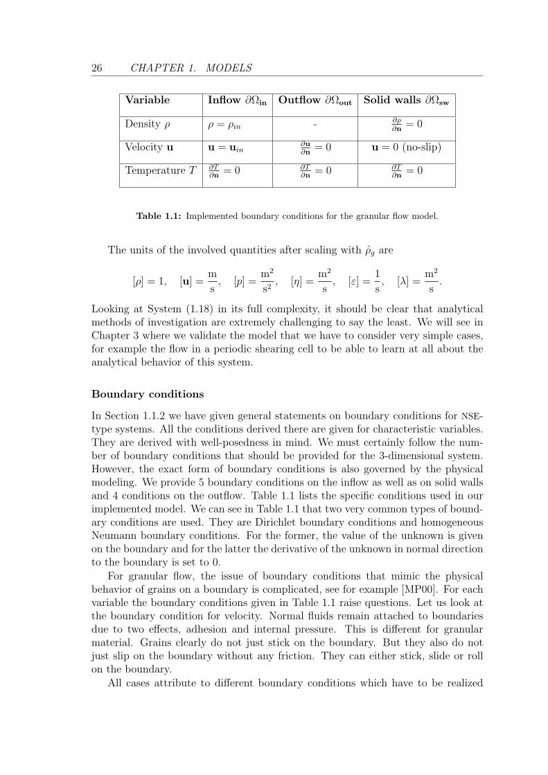
Variable Inflow ∂Ωin Outflow ∂Ωout Solid walls ∂Ωsw
Density ρ ρ = ρin - ∂ρ∂n
= 0
Velocity u u = uin∂u∂n
= 0 u = 0 (no-slip)
Temperature T ∂T∂n
= 0 ∂T∂n
= 0 ∂T∂n
= 0
Table 1.1: Implemented boundary conditions for the granular flow model.
The units of the involved quantities after scaling with ρg are
[ρ] = 1, [u] =m
s, [p] =
m2
s2, [η] =
m2
s, [ε] =
1
s, [λ] =
m2
s.
Looking at System (1.18) in its full complexity, it should be clear that analyticalmethods of investigation are extremely challenging to say the least. We will see inChapter 3 where we validate the model that we have to consider very simple cases,for example the flow in a periodic shearing cell to be able to learn at all about theanalytical behavior of this system.
Boundary conditions
In Section 1.1.2 we have given general statements on boundary conditions for NSE-type systems. All the conditions derived there are given for characteristic variables.They are derived with well-posedness in mind. We must certainly follow the num-ber of boundary conditions that should be provided for the 3-dimensional system.However, the exact form of boundary conditions is also governed by the physicalmodeling. We provide 5 boundary conditions on the inflow as well as on solid wallsand 4 conditions on the outflow. Table 1.1 lists the specific conditions used in ourimplemented model. We can see in Table 1.1 that two very common types of bound-ary conditions are used. They are Dirichlet boundary conditions and homogeneousNeumann boundary conditions. For the former, the value of the unknown is givenon the boundary and for the latter the derivative of the unknown in normal directionto the boundary is set to 0.
For granular flow, the issue of boundary conditions that mimic the physicalbehavior of grains on a boundary is complicated, see for example [MP00]. For eachvariable the boundary conditions given in Table 1.1 raise questions. Let us look atthe boundary condition for velocity. Normal fluids remain attached to boundariesdue to two effects, adhesion and internal pressure. This is different for granularmaterial. Grains clearly do not just stick on the boundary. But they also do notjust slip on the boundary without any friction. They can either stick, slide or rollon the boundary.
All cases attribute to different boundary conditions which have to be realized

1.3. MODELING THE DILUTE AND DENSE FLOW OF GRAINS 27
with a partial slip including friction. This however assumes that we can approximatethe boundary better than just with cuboids. The scope of this is large and we donot treat the issue in this work.
Regarding the density, we will see in the shear flow experiment 3.2.1 that the itbehaves differently near the boundary. So the assumption of the Neumann boundarycondition is quite brave. Also for granular temperature we are probably getting awaytoo easily by assuming a Neumann boundary condition. The temperature on wallsis usually lower than in the interior of the domain for granular material.


Chapter 2
Algorithms
The aim of this chapter is to derive, present and investigate a method for computingapproximate solutions of the granular flow model (1.18) from Section 1.3. It is apriory not clear how to approach the solution of such a system. It inhabits bothcompressible and nearly incompressible flow regimes. The constitutive relations arenonlinear and the density is a variable bounded by the maximum packing fraction ofgrains ρc. The flow is non-Newtonian meaning the viscosity depends on the pressureand the granular temperature.
We have to make a few general choices for the class of algorithms to consider. Ourmethod will be a nonlinear fractional step method (NFSM) meaning that advancingthe system in time is decoupled into substeps. We have already commented onthe history of these decoupling methods in the introduction Chapter. In Section2.1 we discuss these choices and argue why we think a nonlinear, implicit, pressurebased fractional step method seems a good choice. A nonlinear method seems tobe necessary because of the strongly nonlinear coupling of the constitutive relationsand the differential equations in (1.18). The method should be implicit to escapestrong time step restrictions posed by the high viscosity.
Before specific discussions on the algorithm we introduce a notation to describethe algorithms and specifically the discretizations in Section 2.2. We will introducethe notation for working on a collocated, cell-centered Finite Volume (FV) grid ofcuboids. Also we will describe FV discretizations for the general terms that appear inany Navier-Stokes Equations (NSE)-type system without giving the full discretizationof any system yet.
The development of our method will be preceded by Section 2.3 where we willgive an introduction to linear fractional step methods (LFSMs) exemplified by alinear pressure correction algorithm (LPCA). Our nonlinear algorithm will then bederived in a similar way as the methods in this section.
To our knowledge, a pressure based fractional step method with a nonlinearpressure equation has not been developed so far. In Section 2.4 we will derive thenonlinear pressure algorithm (NPA) which takes into account the nonlinear natureof our granular flow model. The algorithm introduces a novel nonlinear pressureequation (NPE) which is the nonlinear equivalent of the linear pressure correctionequation (LPCE) from Section 2.3.2.
Let us describe the steps towards a NPE in more detail. We first split up thecontinuous system into two steps which we call predictor and corrector. The pre-dictor is an implicit, linearized solution of intermediate velocity for an old pressurevalue. The corrector is a coupled system of two equations. We want to derive theNPE from the fully discretized system. Therefore we discretize the predictor andthe corrector in space. To derive the NPE from the discretized corrector, we make

30 CHAPTER 2. ALGORITHMS
use of ideas from the derivation of LFSMs and [GBHL06, Section 4.1] but keep thefull nonlinearities in the resulting system. Similar to the linear case, we use themass conservation equation to arrive at an equation for the update of pressure, theNPE. It comes out as the nonlinear analog to the elliptic operator in the LPCE andother terms. Also like in the linear case, this is accompanied by an equation forthe update of velocity. Unlike the linear case, the two equations remain coupledthrough a density upwind bias in the mass conservation. Hence, all novel aspectsof our algorithm, a NPE and coupled pressure update and velocity update are bothfound in the corrector.
All the above discussions result in the presentation of the NPA for solving thecomplete time-dependent system (1.18) in Section 2.4.5. As the NPA involves thesolution of the NPE, we need to solve a system of N nonlinear equations where N isthe number of volumes. We use a variant of the Newton method for that purpose.Therefore we devote one section to the introduction of Newton methods and thespecific method that we use. Following that, we write the NPE as a nonlinear equa-tion N (p) = 0 and provide its Jacobian J . Also we give the detailed discretizationsof both the nonlinear equation and the Jacobian.
Let us finally comment on Section 3.4 outside this chapter. For many aspectsof the problem, the combination of a very complex system of equations (1.18) to-gether with the partly nonlinear algorithm does not allow rigorous analysis. In theaforementioned Section 3.4 we provide a few numerical experiments which are aimedto support the derivation of the algorithm and investigate some of its properties incombination with the granular flow model.
2.1 Discussion on the type of numerical method
We are considering numerical solution methods or algorithms for the time-dependentNSE and ultimately our model for granular flow introduced in Section 1.3, System(1.18). Our aim is to solve that model for real processes of granular flow which inmost cases means long intervals of time.
Different ways exist to categorize the existing algorithms for NSE-type systems.We choose to say that there are methods which treat the system in a coupled wayand those that split up the process of obtaining a solution at a given time intosubsteps. The former usually discretize explicitly in time or treat at least most ofthe terms in an explicit fashion. This imposes problems as the viscosity (1.18h) inour granular flow model becomes very large for high volume fractions of grains.
In most cases the latter are implicit or semi-implicit methods that split one timestep using multiple substeps. For the case of so-called projection methods one of thesubsteps is the solution of a second order partial differential equation (PDE) for thepressure or a correction of the pressure. We develop such a pressure based fractionalstep method with a nonlinear pressure equation. Let us explain why.

2.1. DISCUSSION ON THE TYPE OF NUMERICAL METHOD 31
2.1.1 Arguments for an implicit, pressure based splitting
System (1.18) is of mixed type, as it is usual for NSE-type systems. This means itis neither always hyperbolic nor parabolic, rather it is of the class of incompletelyparabolic PDE, compare for [Str76] and Section 1.1.2. Therefore it is a difficult taskto solve the fully coupled system numerically where explicit schemes are usuallypreferred. For at least two reasons our System (1.18) is not suited for explicitsolvers:
Diffusive time step restriction: Explicit schemes are bounded to a time steprestriction of type τ < h2/η by stability considerations, where h is the scale ofthe space discretization. This stability condition can be derived in different waysbut is usually derived by von Neumann stability analysis. For further details see[Hir88, Section 8.3.1 Equation (8.3.18)] and for stability analysis using the matrixmethod see [Hir88, Section 10.3.1]. The condition is derived for the scalar heatdiffusion equation discretized with explicit Euler time discretization and centralfinite difference space discretization.
For our much more complex system this consideration still suggests that explicitschemes can pose problems as the viscosity η in (1.18h) may become arbitrarily largefor ρ → ρc. Therefore we assume that in certain regimes we would be bound by thisstability condition. Numerical experiments with explicit solvers show the relevanceof this problem.
Algebraic restrictions in granular flow: With an explicit scheme, it is diffi-cult to simultaneously fulfill the mass continuity (1.18a) and the constitutive rela-tion (1.18g). Especially close to maximum packing of the granular media, the timestep must become arbitrarily small to guarantee that one stays below the limit forρ. One way to overcome this, would be to restrict the density. This however causesundesired loss of mass. Mass conservation however is a crucial property to our al-gorithm. Certainly the splitting approach we argue for also introduces an error butwe consider the conservation of mass most critical.
Hence, we argue for an implicit scheme, where the common approach is to de-couple the system. In the case of LPCAs or more generally LFSMs, the system isdecoupled into the solution of the momentum conservation equation (1.1b) for ve-locity or momentum and an elliptic equation for the pressure, also sometimes calledthe pressure Poisson equation.
We follow this approach to derive an implicit pressure equation. Aside from thebenefit of solving equations of which we know the type instead of solving a systemof mixed type, our constitutive relations (1.18g) give another reason for making thepressure our unknown of choice.
Closely following the second argument above against an explicit scheme, let uslook at the equation of state for the density as a function of pressure and granulartemperature (1.17). We see that p may vary arbitrarily and nonetheless fulfills theconstitutive relation (1.17). The density however is bound to finite limits between

32 CHAPTER 2. ALGORITHMS
zero and the maximum packing fraction. This makes the pressure the logical choiceas an unknown for numerical computations and rules out density based fractionalstep methods.
2.1.2 The need for a nonlinear method
Many attempts of finding a stable LFSM for granular flow have preceded this work.Our numerical experiments failed to successfully apply a LFSM to the granular flowmodel (1.18) and we are not aware of any work which has solved a similarely complexmodel using an implicit LFSM. LPCAs that work in both weakly compressible andincompressible regimes have been addressed extensively, see for example [Chu03]and [vVW03]. However, suggested by numerical experiments we found that thenonlinearity of our equations, especially the dependence of density on pressure doesnot allow the straightforward use of any of those schemes.
Let us explain this in more detail. Pressure based algorithms, especially theLPCAs for compressible flow where density depends on pressure, yield a term
τ−1(ρ(pn+1)− ρn) (2.1)
Usually an equation for a correction to the pressure p′ := pn+1− pn is desired so theterm ρ(pn+1) needs to be approximated in some way, for example by
ρ(pn+1) ≈ ρn +∂ρ
∂pp′. (2.2)
In the case of a linear relation between density and pressure or simple nonlinearrelations this may work fine. In our nonlinear case and especially for boundeddensity this approximation is wrong and causes problems.
First, it yields a pressure which corresponds to a linearly approximated density.This is a bad approximation but with a sufficient number of iterations might becured. The more serious problem is that the density in (1.18) is bounded by themaximum packing volume fraction ρc by (1.12). We would have to make sure thatany extrapolation of the density for the new pressure stays within the limiting den-sity. We cure this problem by solving an equation for pressure, instead of pressurecorrection and taking into account the full nonlinearity of the problem. We willwrite the pressure equation with the full term (2.1) instead of approximating it. Inthis way the pressure equation inherits the density limit implicitly.
Furthermore we will introduce another type of nonlinearity in the NPE throughthe upwind discretization in the mass conservation equation. This is discussedshortly in [GBHL06]. We make use of some of the ideas therein, but modify themto the case of our NPE.
So we are using the full nonlinear dependence ρ(p) from (1.17). The carefulreader should recognize that by writing this, we have already simplified the relationand silently removed the dependence on the granular temperature. Let us discussthis in the next section.

2.2. GENERAL SPACE DISCRETIZATION 33
2.1.3 The treatment of the temperature equation
In the first chapter and especially in Section 1.3 we have stated that the granulartemperature is a key concept to a hydrodynamic model of granular flow. There is nosuch thing as isothermal granular flow. Hence in any model for granular flow, andspecifically in System (1.18) we are dealing with a non-isothermal set of equations.
In the linear case, a temperature dependence would be incorporated into a pres-sure equation by modifying (2.2) to ρ(pn+1) ≈ ρn+ ∂ρ
∂pp′+ ∂ρ
∂EE ′ where E is the energy
of the system and E ′ is some approximate energy difference. In our case we havediscussed in the previous section that we cannot approximate ρ(pn+1) in a linearway. So for the case of a NPE this would add the complete equation for granulartemperature to our last step in the algorithm, the corrector step in the derivationof the NPE in Section 2.4.3.
Another approach for the linear case that may be a hint also for granular tem-perature is that of [vVW03] of using the energy equation to construct a pressurecorrection equation. The energy equation for gases is a conservation equation. Theequation for granular temperature however is a dissipative equation and it is notclear whether the concept of [vVW03] is even applicable in this case.
Finally we decide to derive our NFSM and the NPE in an isothermal fashion.This means that while solving for the pressure, we consider a constant granulartemperature and only update it depending on density and pressure at the end ofeach time step. Certainly one may argue that the nonlinear dependence of pressureand density on temperature is not negligible. However, for the above reasons, theincorporation of the temperature equation into the pressure equation is out of reach.
2.2 General space discretization
Before continuing with the derivations of algorithms, we provide notations to de-scribe the space discretizations used in this work. The notations are generic withrespect to the dimension of the space. We first describe how the space is decom-posed into a set of finite volumes, and then describe how continuous functions andoperators are discretized on this grid. The grid is cell-centered which means that thediscrete values of the unknowns are located in the center of the volume. The grid iscollocated which means that the discrete values of all unknowns are are located atthe same point for each volume. In our approach of using cuboids (for the 3D case)the boundary is approximated very roughly by the grid. We will not consider theissue of geometrically approximating boundaries for FV methods. This is treated in[Wes01, Chapter 11].
2.2.1 Notation
Let d be the space dimension. The computational domain Ω is decomposed intofinite volumes of interval shape (d = 1), rectangular shape (d = 2), or cuboid shape

34 CHAPTER 2. ALGORITHMS
(d = 3). These volumes are indexed in the canonical way by a d-dimensional index
(i1, . . . , id) =: i ∈ Id ⊂ N0 × · · · × N0︸ ︷︷ ︸d−times
,
such that the index of a volume adjacent to the volume i in positive and negativeCartesian direction l is (i1, . . . , il + 1, . . . , id) and (i1, . . . , il − 1, . . . , id) respectively.For the purpose of a discrete formulation independent of the dimension and withoutrestriction to cuboid domains we prefer the use of a one-dimensional lexicographicalindex. We introduce the bijective function
πd : Id 7→ J ⊂ N0 (2.3)
mapping every d-dimensional index in Id to a one-dimensional index in J . Bothways of indexing will be used wherever they fit. Also, we omit the subscript d whereit does not create confusion. The computational domain is discretized into N := |J |finite volumes
V := Vπ(i)|i ∈ I. (2.4)
We assume that the set of volumes Vj, j = 1, . . . , N = V is a nonoverlappingdecomposition of Ω into subsets.
Let us now introduce the coordinates at the centers of the volumes, the centersof the faces and the centers of the neighbors of our volumes. The description of ourdiscretization is local. Whenever we omit the lexicographical index as a subscriptwe mean the current volume denoted by j. Let
[x1, . . . , xd] =: x = xi = x(i1,...,id) = xπ−1(j) ∈ Rd
be the coordinate of the node at the center of the volume Vj and in analog mannerlet
[h1, . . . , hd] =: h = hi = h(i1,...,id) = hπ−1(j) ∈ Rd (2.5)
be the lengths of the volume as in Figure 2.1. We introduce for a lexicographicalindex j the shifted indexes
j ± el := π(π−1(j)± el) for π−1(j)± el ∈ π−1(J), (2.6)
where el is the unit vector in the Cartesian direction l. Whenever it is convenientand does not create confusion we use a short form of the index ±el. By writing± we always mean both directions of one Cartesian direction l. This allows us toaccess neighbors in all Cartesian directions by a one-dimensional subscript. Eachvolume has 2d faces in the d Cartesian directions. Using the shifted indizes from(2.6) we denote a couple of faces in l-direction by F±el
and the set of all faces of avolume by Fj := F±el
|l = 1, . . . , d using the short form of the shifted index. Thenormals of the faces are denoted by
n± 12el.

2.2. GENERAL SPACE DISCRETIZATION 35
x− 12 e1
xih1
h2
Ω partitioned into Vj
F ∈ F (boundary face)
Vj ∈ V (interiour volume)
F+e2 ∈ F
V ∈ V (boundary volume)
Figure 2.1: Visualization of a volume Vj ∈ V, j ∈ J .
We define the set of all faces in Ω as a union
F :=⋃j∈J
Fj. (2.7)
To distinguish faces on the boundary and faces in the interior we introduce thesets
F := F ∈ F|F ∩ ∂Ω 6= ∅, (2.8a)
F := F \ F . (2.8b)
Similar to (2.8) we introduce the following sets for volumes that have faces onthe boundary and volumes in the interior.
V := Vj ∈ V|∃F ∈ Fj : F ∈ F, (2.9a)
V := V \ V . (2.9b)
using the one dimensional index j, the coordinates of the node centers and atthe face centers are denoted by
xj and xj± 12el
:= xj ±hl
2el
respectively. We will however use the short form omitting j whenever this is rea-sonable and it is clear that we are speaking about an arbitrary but fixed volume.The notation and the decomposition of the domain Ω into the set of volumes V arevisualized in Figure 2.1.
Note, at this point there is virtually no difference between a node at a boundaryface and a node at an interior face, but we will refer to this in more detail later inthis section and further in Section 2.5.1.
For an unknown q, being the pressure, a velocity component, etc. we introduce

36 CHAPTER 2. ALGORITHMS
the following notation for values at center nodes, the face centers and the neighborcenters as
qj := q(xj), qj± 12el
:= q(xj± 12el
) and qj±el:= q(xj±el
)
respectively. For example, the vector value of velocity at the center of the eastneighbor of the current volume j is denoted by u+e1 .
This should give us enough notation to describe the discretization in an elegantway. We will describe the discretization in an arbitrary volume j.
2.2.2 Finite Volume space discretization
We use a cell-centered grid with collocated arrangement of the unknowns where allunknowns have values at the same node in the center of the volume. In this sectionwe will not give the discretization of the complete equations (1.1) or (1.18). Thiswill be done in later sections. The aim here is to provide the discretization in formof operators which are each responsible for the discretization of a certain type ofPDE term.
These operators will then be used in later sections to write the discretization ofvarious equations and systems in an elegant way. For the FV method all differentialoperators are integrated over volumes and most of them are transformed to surfaceintegrals using the Gauss Theorem. For an introduction see [FP96, Section 4.1]. Thesurface of the volumes consists of the faces F from (2.8). So most of the differentialoperators in discrete form are written as discretization on faces. Since we store allunknowns at the volume centers, we introduce the interpolation between values atvolume centers and values on faces for a face Fj±el
∈ F of a volume with index j
qj± 12el≈ 1
0.5(hj)l + 0.5(hj±el)l
((hj±el)lqj + (hj)lqj±el
) . (2.10)
This is certainly a very simple form of interpolation and many different and moresophisticated ways exist. For details on the approximation of face center values forFV methods see [FP96, Section 4.4]. The coefficients of System (1.18), for examplethe viscosity η, vary strongly between regimes of dilute and dense granular materialbut they are continuous. Certainly in the discrete case the jump in values between avolume with a high density of grains and one with a very low density may look likea discontinuity. But then Therefore we assume that this linear interpolation (2.10)should suffice. In
Also this interpolation will always be used when a scalar or vector valued solu-tion of a certain FV discretized equation or system is needed on the face centers.Furthermore we will use another interpolation, the so-called upwinding introducedin [FP96, Section 4.4.1] for the discretization of certain operators.
Before we start with the space discretization let us make a remark on boundaryconditions. We will postpone the implementation of boundary conditions to Section2.5.1 because we want to give a general treatment for the linear discretization opera-
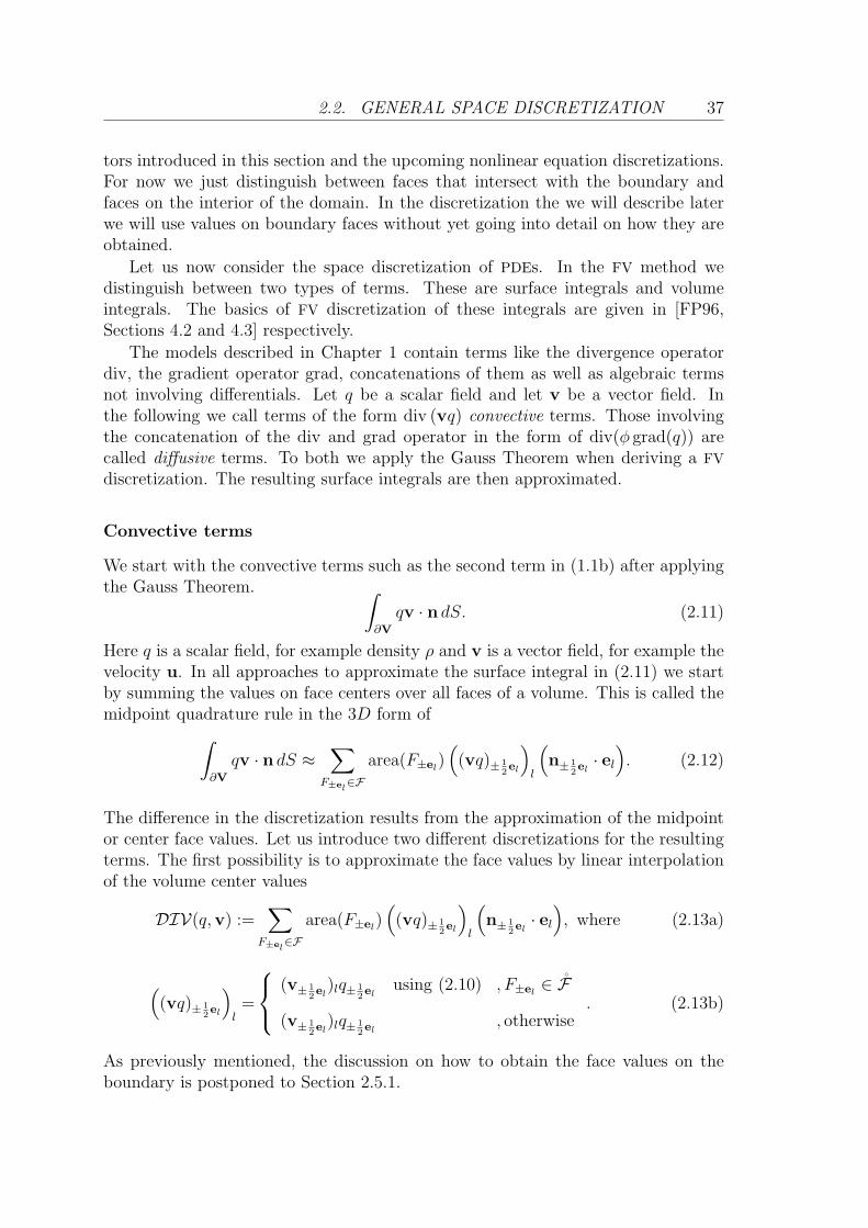
2.2. GENERAL SPACE DISCRETIZATION 37
tors introduced in this section and the upcoming nonlinear equation discretizations.For now we just distinguish between faces that intersect with the boundary andfaces on the interior of the domain. In the discretization the we will describe laterwe will use values on boundary faces without yet going into detail on how they areobtained.
Let us now consider the space discretization of PDEs. In the FV method wedistinguish between two types of terms. These are surface integrals and volumeintegrals. The basics of FV discretization of these integrals are given in [FP96,Sections 4.2 and 4.3] respectively.
The models described in Chapter 1 contain terms like the divergence operatordiv, the gradient operator grad, concatenations of them as well as algebraic termsnot involving differentials. Let q be a scalar field and let v be a vector field. Inthe following we call terms of the form div (vq) convective terms. Those involvingthe concatenation of the div and grad operator in the form of div(φ grad(q)) arecalled diffusive terms. To both we apply the Gauss Theorem when deriving a FVdiscretization. The resulting surface integrals are then approximated.
Convective terms
We start with the convective terms such as the second term in (1.1b) after applyingthe Gauss Theorem. ∫
∂V
qv · n dS. (2.11)
Here q is a scalar field, for example density ρ and v is a vector field, for example thevelocity u. In all approaches to approximate the surface integral in (2.11) we startby summing the values on face centers over all faces of a volume. This is called themidpoint quadrature rule in the 3D form of∫
∂V
qv · n dS ≈∑
F±el∈F
area(F±el)((vq)± 1
2el
)l
(n± 1
2el· el
). (2.12)
The difference in the discretization results from the approximation of the midpointor center face values. Let us introduce two different discretizations for the resultingterms. The first possibility is to approximate the face values by linear interpolationof the volume center values
DIV(q,v) :=∑
F±el∈F
area(F±el)((vq)± 1
2el
)l
(n± 1
2el· el
), where (2.13a)
((vq)± 1
2el
)l=
(v± 12el
)lq± 12el
using (2.10) , F±el∈ F
(v± 12el
)lq± 12el
, otherwise. (2.13b)
As previously mentioned, the discussion on how to obtain the face values on theboundary is postponed to Section 2.5.1.

38 CHAPTER 2. ALGORITHMS
Let us additionally introduce a first order upwind discretization. The function qon the faces is interpolated in direction of the flow depending on some velocity. Wewill remark on the reasons for such a discretization in detail later in the derivationof the algorithm 2.2 in Section 2.4. So let us introduce a function which upwinds aquantity q depending on a velocity u
UW (q,u, F±el) =
q ,u± 1
2el· n± 1
2el≥ 0
quw ,u± 12el· n± 1
2el
< 0, with (2.14a)
quw :=
q±el
, F±el∈ F
q± 12el
, otherwise, (2.14b)
where F±eldenotes any face of the couple of faces in l-direction on which the up-
winded quantity should be determined. The function UW maps to an upwindapproximation for face values with respect to the velocity u. This means that thevalue interpolated onto the face center depends on the flow direction at the facecenter . If the flow is in direction of the face with respect to the volume center,then the value of the volume center is used. If the flow is in the opposite directionthen the value of the neighboring volume center is used. The first order upwinddiscretization for terms of the form (2.11) is then given by
DIVUW (u)(q,v) :=∑
F±el∈F
area(F±el)(v± 1
2el
)lUW (q,u, F±el)(n± 1
2el· el
). (2.15)
For the case of discretizing a convective term we will always use u ≡ v. The reasonfor a notation that allows the upwinding by a different vector field than the actualconvecting velocity is the discretization of the System (1.18) in time which we willintroduce in the later Section 2.4.1. There we will work with the velocity field atdifferent values of time and will make full use of the notation introduced here.
Diffusive terms
The second major type of differential terms in any NSE-type system are diffusiveterms such as the third term in (1.1b) which, compared to the transport propertiesof convective terms model the viscous aspects of flow. They include some diffusivitycoefficient φ which may be the viscosity η from (1.18h). For such diffusive terms ofthe form ∫
∂V
φ grad (q) · n dS
we start with the same basic integration rule as in (2.12) except that our vector fieldis now a gradient of a scalar field. We introduce the discretization
D(q, φ) :=∑
F±el∈F
area(F±el)φ(x± 1
2el
)((grad q)± 1
2el
)l
(n± 1
2el· el
), with (2.16a)

2.2. GENERAL SPACE DISCRETIZATION 39
(grad q± 12el
)l ≈
1
(x±el)l−xl
(q±el− q) , F±el
∈ F1„
x± 12 el
«l
−xl
(q± 12el− q) , otherwise , (2.16b)
where φ will be the viscosity η as in (1.18h) or the thermal conductivity λ from(1.18f) which are both continuous functions.
In many applications of flow problems the diffusivity φ is not a function but aconstant and the discretization may look different in many standard FV references.This is because the flow in these cases is assumed to be Newtonian which is true formany standard fluids. The granular flow model (1.18) is a non-Newtonian modeland hence we need to be able to discretized diffusive terms with varying viscosity.
Other terms
Aside from those differential operators which can be transformed to surface integralsthere are those which have to be treated as volume integrals. A common exampleis the force f in the momentum equation (1.1b).
Another is the pressure gradient found in all NSE-like systems. Here we need toapproximate spatial gradients in a volume. We choose the approximation by differ-encing interpolated face center values across the volume and denote one componentof the spatial gradient by
∂q
∂xl
≈ GF(q)l :=1
hl
(q+ 12el− q− 1
2el
). (2.17)
The interpolation of the face center values is carried out as in (2.10). Then the gra-dient GF is the vector made up of the components GF l with l = 1, . . . , d. Generally,volumetric integrals are approximated by multiplying the volume with the value atthe volume center. With V := volume(V) we have∫
V
q dV ≈ V · q. (2.18)
The pressure gradient then will be approximated using (2.17) for q in (2.18).
Note that in the above discretizations we have omitted mixed derivatives as theyappear in (1.1c). Their treatment in an implicit discretization is quite straightfor-ward in the interior of the domain as in [Hir88, p191ff] but is challenging on theboundary.
In general our discretization operators are of low order. The upwind discretiza-tion (2.15) is crucial to stability, see [EGH00, Section 5.2.3], but restricts us inthe given form to a first order space discretization. Certainly FV discretizationsof higher order exist [Fle91b, Section 9.3.2] but only make sense combined with abetter approximation of the domain.
We have provided all the spatial discretization operators that will be needed forthe discretization of the equations in the following sections. As previously men-

40 CHAPTER 2. ALGORITHMS
tioned, we will first split up the continuous system into substeps in time, discretizethese subequations in space and then proceed with the derivation of a nonlinearpressure equation (NPE). This discretization in time will be a type of fractional stepmethods and hence we proceed with an introduction to these methods.
2.3 Introduction to fractional step methods
Although the focus of this work are NFSMs, the idea of LFSMs provides the basis forour development. We have mentioned before that we call all methods that split theadvancing of the system in time into multiple steps LFSMs. In the third paragraphon page 9 we have provided references to origins of these methods.Fractional stepmethods for the instationary NSE have first been mentioned by Kim and Moin in[KM85]. Let us give a short introduction on the terminology and relationship be-tween the different methods that split up the solution process. Then we will presenta LPCA which falls into the category of LFSMs. This serves as an introduction tothe development of our NPA.
2.3.1 The variants of fractional step methods
The pressure based NFSM NPA we will introduce is based on the very popular ’divideand conquer’ approach initially introduced for solving the incompressible NSEs. Thebasic idea is to split the numerical treatment of the different operators and unknownsin the equations thus solving the initially difficult problem in relatively easier sub-steps. This approach has different names under different modifications: operatorsplitting, fractional step method or projection method. The terms ’splitting scheme’and ’projection scheme’ partially overlap. It is generally accepted to use ’projectionscheme’ if the scheme is based on a Helmholtz decomposition of the velocity meaningit can be generated by a scalar potential and a vector potential. These schemesusually require that the pressure equation is solved after the convection-diffusionstep. Recently approaches are reported in the literature which bridge the differentalgorithm types and provide general formulations into which all the above methodscan be categorized. We specifically mention the very recent publication [NA07].They present a framework which theoretically allows the incorporation of nonlinearpressure equations at least for incompressible flow in [NA07, Equations (21)-(24)].
All the above mentioned schemes can also be considered ’splitting schemes’ sincethe convection-diffusion part is split from the imposition of the incompressibilityconstraint. For a detailed overview of the state of the art of the variants of theseschemes see [GS98, Min01, GMS06]. In the compressible case the idea remains butthe continuity equation adds a compressibility term to the pressure equation.
Another general concept to describe these algorithms is to write them in theform of fractional step methods from [FP96, Section 7.4.1]. We show how thismight be done by taking the simplest case, the explicit Euler time discretizationand schematically split the System (1.1) into a fractional step method. We consider

2.3. INTRODUCTION TO FRACTIONAL STEP METHODS 41
for the one dimensional case the following form.
ρn+1 = ρn + τ(CUW (ρu)) (2.19a)
un+1 = un + τ(CUW (ρuu) + D(u) + P ) (2.19b)
where CUW , D, P represent the convective, diffusive and pressure terms respectively.We omit the time indizes on these terms on purpose as they depend on the specificmethod used. This can now be split in many ways. One approach is the splittinginto
un+ 13 = un + τCUW (ρnunun+ 1
3 ) (2.20a)
un+ 23 = un+ 1
3 + τD(un+ 23 ) (2.20b)
un+1 = un+ 23 + τP. (2.20c)
In the third step (2.20c), P is the gradient of a quantity which obeys a Helmholtztype equation obtained by enforcing Equation (2.19a). Depending on the specificsof the splitting together with the way the split equations are enforced the methodhas different names, but the basic idea of LFSMs stays the same for all methods.
For the convergence analysis of splitting methods we we refer to [GRS07, Theo-rem 8.21] and the preceding text in [GRS07, Section 8.3.4].
2.3.2 Linear pressure correction algorithm
We will exemplify the concept of LFSMs by this short section on a LPCA for theSystem (1.1) on our collocated, cell-centered grid. This concept will later be usedfor the derivation of the NPA.
As in the previous section we will split up the solution of a full time step intosubsteps. The final step will be formulated as an elliptic equation for an unknowncorrection to a pressure computed in the previous time step. Therefore this specialLFSM is called pressure correction or Chorin projection method. The latter nameoriginates from the incompressible case where the values of old pressure and velocityare projected onto the divergence free space to satisfy the incompressibility conditiondiv (u) = 0.
So let us assume that
ρ = ρ(p), with ρn+1 = ρ(pn) +∂ρ
∂p(pn) · (pn+1 − pn), (2.21)
is a valid approximation of the compressibility condition and that the pressure pn
is known from the previous iteration, and η is constant. To obtain a first guess ofthe velocity in the current time step we solve the discretized integral form of the

42 CHAPTER 2. ALGORITHMS
momentum equation (1.1b) in componentwise form
V
τ
[(ρu)
n+ 12
l − (ρu)nl
]+DIVUW (un)((ρu)
n+ 12
l ,un)−D((ρn)−1(ρu)n+ 1
2l , η)
+ V GF l (pn) = 0 (2.22)
for (ρu)n+ 12 and l = 1, . . . , d where the convective term is linearized. Let us moreover
assume that all other changes in velocity are induced by the gradient of the pressurecorrection, then we reach the following condition for the corrected velocity andpressure
V
τ
[(ρu)n+1
l − (ρu)n+ 1
2l
]= −V GF l (p
n+1 − pn), l = 1, . . . , d ⇔
(ρu)n+1 = (ρu)n+ 12 − τ GF (p′) (2.23)
where p′ := pn+1 − pn. We apply the discrete divergence DIV(1, ·) to (2.23). Here1 is a vector where each entry is 1. Using DIV(1, ρu) = DIV(ρ,u), the discretizedEquation (1.1a)
V
τ
[ρn+1 − ρn
]+DIV (ρn+1,un+1) = 0
and (2.21), we transform (2.23) into the LPCE
− V
τ
[∂ρ
∂p(pn) · p′
]= DIV (ρn+ 1
2 ,un+ 12 )− τ DIV (1,GF (p′)) (2.24)
for the unknown p′. The relation ρ(p) may be the ideal gas law (1.2).
In the incompressible case of ∂ρ∂p
(pn) = 0 Equation (2.24) is elliptic, the last termon the right hand side is a discretization of the Laplace operator. Otherwise it is aHelmholtz-type equation. The term on the left side is there because we solve a com-pressible or weakly compressible system. Hence we have transformed the solution ofone time step for System (1.1) into two steps of solving the linearized velocity equa-tion (2.22) and the solution of a second order PDE (2.24) with a Laplace operator.We summarize the steps into the LPCA given in a schematic way in Algorithm 2.1.For the case of incompressible flow as modeled by (1.3) spurious oscillations in the
Algorithm 2.1: Linear pressure correction algorithm (one time step)
Solve linearized momentum prediction (2.22) for (ρu)n+ 12 with old pressure1
Solve pressure correction equation (2.24) for p′2
Correct momentum to (ρu)n+1 using (2.23)3
pn+1 = pn + p′4
ρn+1 = ρ(pn+1)5
pressure solution are known to occur for LPCAs on grids with collocated arrange-ment of the unknowns and our discretization of the pressure equation, see [Wes01,

2.4. A NONLINEAR PRESSURE BASED ALGORITHM 43
Chapter 6.3, p. 235ff.]. There it is shown that the discretization allows an oscillat-ing pressure solution completely independent of the velocity. Often this problem iscured by the so called Rhie-Chow approach introduced in [RC83] which introducesa certain velocity interpolation preventing these oscillations.
We have found these sometimes called checkerboard modes when using Algorithm2.1 for computing incompressible flow but we have chosen a different approach tocure the problem. Also for incompressible flow, Vabishchevich in [VPC96] andChuiko and Lapanik in [CL05] apply a regularization operator to the right handside of the pressure correction equation (2.24) to avoid pressure oscillations. Thisregularization operator is (∆ − ∆ext)p
n where the subscript means an extendedstencil. This, plainly speaking connects the discrete pressure and velocity solutionsand hence avoids spurious nodes.
However, because LPCAs are not the focus or this work and our upcoming dis-cretization of the NPE does not seem to allow these oscillations we will not go intofurther details on this issue.
2.4 A nonlinear pressure based algorithm
Based on the considerations in Section 2.1 we will use the space discretization oper-ators from Section 2.2 and the concept of LFSMs introduced in Section 2.3 to developa fractional step method with a NPE in this section. The method will be called NPAand its development is motivated by the need to solve System (1.18). However, thealgorithm is developed in general for NSE-type systems with nonlinear coefficientsor nonlinear constitutive relations.
We begin with splitting the continuous system in time into substeps which wewill call predictor and corrector. The corrector will then be discretized in space andfrom that we derive a NPE coupled to an equation for a corrected velocity. As theNPE is nonlinear we will shortly mention the variant of the Newton method whichwe use to solve the NPE before giving its detailed discretization and that of theJacobian.
2.4.1 Time discretization
Before we split up the time step into substeps, let us mention how partial timederivatives are treated. For discretization of such terms involving a partial timederivative, let q be any of the hydrodynamic quantities (density, one component ofvelocity or momentum or granular temperature) depending on time and space. Forthe partial time derivative of q, ∂tq, we use implicit Euler discretization
1
τn+1
(qn+1 − qn), (2.25)
where τn+1 denotes the difference between the (n+1)st and the nth moments in time.We further split one time step of τ into different fractional steps. The fractional

44 CHAPTER 2. ALGORITHMS
time steps will be denoted by superscripts of the form n+α, 0 < α < 1 as in Section2.3.
We have discussed in Section 2.1.3 that the temperature equation is treated de-coupled from the system. We will derive the substeps by assuming a known granulartemperature during one time step and solve the temperature equation (1.18c) at theend as a last substep.
The first fractional step will be the prediction of a velocity which we will denoteby α = 1
2. This step is very similar to the linear case for System (1.1), compare with
(2.22). There is a difference we would like to mention. We believe that instead ofa prediction of momentum we should predict velocity because of the characteristicsof System (1.18). We want to make the prediction step independent of strong andnonlinear dependence of density on pressure (1.17). This dependency has alreadybeen discussed in Section 2.1.1.
Prediction of an intermediate velocity
For the prediction of an intermediate velocity un+ 12 we solve a linearized version of
the velocity equation (1.18b)
ρnun+ 12 − ρnun
τ+ div (ρnun+ 1
2 ⊗ un)− div (η(pn)κ(un+ 12 )) + grad pn − ρngn+1 = 0.
(2.26)Because the gravity is a constant vector, we always write gn+1 regardless of thefractional step in which it is used. It is important to note that we use the densityfrom the old time step tn in the prediction of velocity. The reason for this is thatour final aim is the construction of a pressure equation. The dependence of p(ρ)in (1.18g) is highly nonlinear, which means for a small error in density predictiona large error in the initial guess for the pressure is possible, especially in the denseregime.
Similar to LPCA from Section 2.3.2, the prediction of velocity is necessary be-cause the convective and diffusive terms are not taken into account in the pressureequation. Only the change of velocity induced by the change in the pressure gradientis taken into account in the pressure equation.
There exist schemes that predict a density from the mass conservation equationto be used in the velocity prediction. Even though this is tempting we refrain fromthis practice again using the argument above that the dependence of density onpressure is very delicate and a small error in density corresponds to huge differencesin the pressure. Furthermore, by the construction of the pressure equation we willsee that the discrete version of (1.18a) will be satisfied exactly without a densityprediction.
A system for an updated pressure
To construct the corrector, a nonlinear operator for the pressure together with analgebraic correction for velocity will be derived. Ideally, the corrected velocity un+1

2.4. A NONLINEAR PRESSURE BASED ALGORITHM 45
should satisfy, amongst mass continuity the fully nonlinear and implicitly time-discrete version of the velocity equation (1.18b)
ρn+1un+1 − ρnun
τ+ div (ρn+1un+1 ⊗ un+1)− div (η(pn+1)κ(un+1))
+ grad pn+1 − ρn+1gn+1 = 0. (2.27)
So far we have obtained velocity and pressure fields which satisfy the predictionequation (2.26). To obtain the operator for the difference between the two fieldswe subtract (2.26) from (2.27). The splitting happens when we drop the differ-ence in velocity convection and diffusion. With this in mind, the subtraction givesequation (2.28a).
Speaking in the terms of Section 2.3.1 this effectively splits the solution methodinto a step for convection and diffusion using an old pressure field and, as we will seenext, an equation for an update of pressure. This assumes that the major changesin the velocity are caused by the gradient of pressure.
Furthermore, both the corrected velocity and the density should satisfy the time-discrete version of the mass balance (1.18a), which gives equation (2.28b). These tworequirements yield for the new pressure and velocity a coupled system of equations
ρn+1un+1 − ρnun+ 12
τ+ grad (pn+1 − pn)− (ρn+1 − ρn)gn+1 = 0, (2.28a)
ρn+1 − ρn
τ+ div (ρn+1un+1) = 0, (2.28b)
ρn+1 = ρ(pn+1). (2.28c)
So we have split up the solution of System (1.18) into a prediction step (2.26)with the convective and diffusive terms and a step of enforcing the correct pressureand velocity fields (2.28). This is as far as we will go for the system which is stillcontinuous in space. Hence the task preceding the derivation of a NPE will be thespace discretization.
But before, let us look at how much explicitness we have introduced through oursplitting. We do this by plugging our solution ρnun+ 1
2 of Equation (2.26) into Equa-tion (2.28). Hence we see that the combination of all fractional steps is effectivelythe solution of the system
ρ(pn+1)un+1 − ρnun
τ+ div (ρnun+ 1
2 ⊗ un)− div (η(pn)κ(un+ 12 )) =
− grad pn+1 + ρ(pn+1)gn+1, (2.29a)
ρ(pn+1)− ρn
τ+ div (ρ(pn+1)un+1) = 0 (2.29b)
We see that the mass conservation is fulfilled for final fields with superscript n + 1.However, the discretization of the velocity is only semi-implicit with respect toconvection and diffusion.

46 CHAPTER 2. ALGORITHMS
Above we have introduced for the continuous case the basic approach for derivinga fractional step method for solving System (1.18). But we have not yet reacheda satisfactory result. The System (2.28) is still difficult so solve in the given formand we have not yet derived a pressure equation. These steps towards the NPA willbe done for the discretized equations only and our NPE will be solely a discreteconcept. Therefore we will discretize the prediction step (2.26) and the coupledcorrection system (2.28) in space in the following section and then derive the NPE.
2.4.2 Spatial discretization of the split system
The equations involved in the split solution process are (2.26), (2.28) and an implic-itly discretized, linearized version of (1.18c). We give a FV discretization of theseequations using the space discretizations provided in Section 2.2. This will then beused to derive the NPE from the discrete equations.
So we first integrate the equations. For a control volume V fixed in time andspace, the integral of (2.26) is
∫V
[ρnu
n+ 12
l − ρnunl
τ+ div (ρnu
n+ 12
l un)− div (η(pn) grad(un+ 1
2l )) +
∂
∂xl
pn
− ρngnl
]dV = 0, (2.30)
for l = 1, . . . , d (d being the space dimension). Next we look at the integral form ofthe corrector (2.28). First we replace ρn+1 by (2.28c) in (2.28a) and (2.28b). Thenwe integrate both equations over the volume V which yields.∫
V
[ρ(pn+1)un+1 − ρnun+ 1
2
τ+ grad (pn+1 − pn)− (ρ(pn+1)− ρn)gn+1
]dV = 0,
(2.31a)∫V
[ρ(pn+1)− ρn
τ+ div (ρ(pn+1)un+1
]dV = 0.
(2.31b)
We apply the Gauss theorem to the terms involving a divergence operator. Thisresults in∫
V
[ρnu
n+ 12
l − ρnunl
τ+ ∂lp
n − ρngn+1l
]dV
+
∫∂V
[(ρnu
n+ 12
l un − η(pn) grad(un+ 1
2l )) · n
]dS = 0, (2.32)

2.4. A NONLINEAR PRESSURE BASED ALGORITHM 47
l = 1 . . . , d for the velocity prediction (2.30) and∫V
ρ(pn+1)− ρn
τdV +
∫∂V
(ρ(pn+1)un+1) · n dS = 0 (2.33)
for (2.31b).
Let us write these integrated equations in FV discretization. We make use ofthe discretization operators introduced for the various PDE terms in Section 2.2.Let ρ(p) be the pressure dependent density as in Equation (1.17). We describe thediscretization locally for any volume Vj and drop the index j in the following. Thediscrete version of the predictor Equation (2.32) is
V
τ
[ρnu
n+ 12
l − ρnunl
]+DIVUW (un)(ρ
nun+ 1
2l ,un)−D(u
n+ 12
l , η(pn))
+ V GF l (pn)− V ρngn
l = 0 (2.34)
for l = 1, . . . , d. The discrete versions of the equations for the corrector (2.31a)and (2.33) are
V
τ
[ρ(pn+1)un+1 − ρnun+ 1
2
]+ V GF (pn+1 − pn)− V (ρ(pn+1)− ρn)gn+1 = 0
(2.35a)
Vρ(pn+1)− ρn
τ+DIVUW (un+1)(ρ(pn+1),un+1) = 0.
(2.35b)
Note that we keep the full nonlinearities in the corrector in order to derive a NPE.The linearizations in the predictor serve the purpose of a low cost prediction.
Let us remark on the upwind discretization in Equation (2.35b). There aresimilar ideas introduced by Bijl, Wesseling and others for the linear case. They donot leave the pressure equation and velocity correction equation coupled but theydiscretize the mass conservation equation using a first order upwind scheme similarto (2.35b).
There seem to be two good reasons for this. First, Wesseling suggests in [vVW01,Section 4] that the application of what he calls a first order density upwind bias inthe mass conservation equation is necessary for stability in compressible flow. Thisapproach is introduced in [BW98, Section 3.2 and Equation (27)]. The second reasonis that pressure oscillations are avoided by this approach as explained in [GBHL06,Remark, pg. 11].
We will not give special attention to the discretization of the temperature equa-tion (1.18c) at this point because it is not used in the derivation of the NPE and itsdiscretization does not yield any further insights. Let us just remark that the con-vection and diffusion parts are discretized as the convection and diffusion in (2.34).The dissipation term Tdiss is implicitly treated as a volume term and the derivativesin the viscous heating term are explicitly discretized using (2.17).

48 CHAPTER 2. ALGORITHMS
2.4.3 Derivation of the nonlinear pressure equation
Our goal is to obtain a pressure operator with properties close to the Helmholtz op-erator for the LPCA from Section 2.3.2. In the linear case, this means applying thedivergence operator to a corrector equation and making use of the continuity equa-tion. We will follow a similar path by multiplying (2.35a) with [ρ(pn+1)V ]
−1. This
is permissible because by Equation (1.17) we know that ρ(p) > 0 at all times. Thegoal of this division by density is to be able to use the continuity equation (2.35b).This yields
1
τ
[un+1 − ρnρ(pn+1)−1un+ 1
2
]+ ρ(pn+1)−1 GF (pn+1 − pn)
− (1− ρ(pn+1)−1ρn)gn+1 = 0. (2.36)
Now we apply the upwind divergence operator DIVUW (un+1)(ρ(pn+1), ·) to equa-tion (2.36). In particular this yields a term
DIVUW (un+1)(ρ(pn+1),un+1)
which is replaced with V ρ(pn+1)−ρn
τusing (2.35b). We then define the operator
Lp := DIVUW (un+1)
(ρ(p), ρ(p)−1 GF(·)
), (2.37)
which should shorten the presentation significantly. We will apply this operator toboth pn+1 and pn. Also note that the unknown velocity un+1 is part of the operatorfor the upwinding interpolation. We choose this form for now. When we later givethe full algorithm we will introduce a form using an inner iteration between theunknown pressure pn+1 and the unknown velocity un+1.
Using this notation, applying the upwind divergence operator to Equation (2.36)results in the pressure equation
Lpn+1 − V
τ 2ρ(pn+1) = Lpn − V
τ 2ρ(pn)
+1
τDIVUW (un+1)
(ρ(pn+1), ρ(pn+1)−1ρnun+ 1
2
)(2.38)
+DIVUW (un+1)
(ρ(pn+1), (1− ρnρ(pn+1)−1)gn+1
).
It may seem strange to apply upwind divergence to a pressure gradient field or evento a gravity field, but looking closely at the definition of operator (2.15) we seethat only the values of ρ are affected by this upwinding. It could be described bydiscretizing the divergence of the pressure gradients multiplied with the upwindeddensity. Furthermore, this derivation is purely discrete. One should not attempt toassign a meaning other than purely mathematical transformations to this pressureequation. Equation (2.38) together with
un+1 =[ρ(pn+1)
]−1(ρnun+ 1
2 − τGF(pn+1 − pn) + τ(ρ(pn+1)− ρn
)gn+1
), (2.39)

2.4. A NONLINEAR PRESSURE BASED ALGORITHM 49
obtained from (2.36) solve the corrector exactly. We have gained two advantagesthat Equations (2.38), (2.39) have over the System (2.35). The first is that Equa-tion (2.38) with the operator L should have nice properties because it is the diver-gence of a gradient, though nonlinear. And secondly, with Equation (2.39) we havethe basis for an iterative procedure to compute pn+1 and un+1 only using scalarequations.
Before we come to this iterative procedure, let us note that we have arrived ata nonlinear equation for pressure, the NPE (2.38). In fact, in this discrete form,Equation (2.38) is a system of N scalar nonlinear equations where N is the numberof volumes into which the domain is decomposed as in (2.4) and as such may be quitelarge. A method is needed to solve this large system. We choose a variant of theNewton method for this purpose. Therefore, before we proceed with the completeNPA we will shortly remark on variants of the Newton method for large systems ofnonlinear equations.
2.4.4 The Newton method and its variants
The Newton method is originally a method for finding the roots of a nonlinear scalarfunction f : I → I where I is an interval I ⊂ R. Let f ′ be the derivative of f withrespect to x. Then, assuming that f ′(x) 6= 0 in the whole domain and with certainassumptions on the initial value x0, the sequence
xα+1 = xα − f(xα)
f ′(xα)(2.40)
converges towards a root of f . This idea can be extended to systems of nonlinearequations. For a detailed introduction to the Newton method and its variants see[QSS06, Chapter 6 and Section 7.1]. We give the equivalent of (2.40) for systems.Let N (q) be a system of N nonlinear functions for the discrete unknown q. Letfurther J be the Jacobian of N which contains the derivatives of all componentsof N with respect to all components of q and is a N × N matrix valued function.Then for a given q0 the Newton method can be written as
qα+1 = qα + δqα with δqα from J (qα)δqα = −N (qα). (2.41)
Hence we see that if written in this way, each iteration of the Newton methodinvolves the solution of a linear system. This is the point where the modern variantsof the Newton method differ. All methods where the linear system involved in everystep is not exactly solved are called quasi-Newton methods. The first type are themethods where Jacobian or its factorization for the linear solution method are notupdated in every step. The second are the so called inexact or truncated Newtonmethods which we will use for our problem.
Truncated Netwon Methods solve the linear system in every step by an iterativeprocedure but the maximum number of linear iterations is fixed. The idea is thatfar away from the nonlinear solution, there is no point in solving the linear system in

50 CHAPTER 2. ALGORITHMS
every step very precisely. The methods are then called according the linear iterativemethod. In our case, because the linear system will be solved by Krylov-subspacemethods we are using a Newton-Krylov method as described in [QSS06, Section7.1.2.2 pg. 290].
A robust implementation framework for using this class of truncated Newtonmethods for large nonlinear systems is provided by the PETSc, SNES software package[BGMS97]. We make use of their solvers and methods for the solution of our NPE.
Furthermore, in modern Newton methods a step control is usually applied. Bystep we mean the δqk. This is to ensure that the step does not leave the regionof quadratic convergence around the solution which exists for all these methods.Two methods are the most popular, the so call line search and the trust region stepcontrols. Both methods use the direction from the computed Newton step but limitthe length with which to go in that direction. The topic is very advanced and isout of the scope of this work. The book [QSS06] provides the basics very well. Fora complete coverage of all modern developments on Newton methods including thestep control we cite [Deu04, Chapters 2 and 3].
2.4.5 The nonlinear pressure algorithm
In the previous sections we have transformed System (2.35) into a system of theEquations (2.38) and (2.39). The two equations are still coupled through the up-winding velocity u. Therefore we will give in this section an algorithm for solvingthe latter two equations in an iterative procedure. First we will iterate in a nonlinearGauss-Seidel fashion through the two Equations (2.38) and (2.39). For this proce-dure we need to introduce an extra iteration index. Let us define another version ofthe pressure operator (2.37)
Ln+1,k+1 := DIVUW (un+1,k)
(ρ(pn+1,k),
[ρ(pn+1,k+1)
]−1 GF(·))
,
where the first superscript denotes the time step and the second denotes the it-erations between pressure equation and velocity correction equation. With thisdefinition we introduce Algorithm 2.2 which shows the details of the method. WithAlgorithm 2.2 we have arrived at the complete procedure for solving System (1.18).The description of the time discretization is fully given. We have written the spacediscretization in a very compact form which hides the details for the sake of pre-senting the time discretization, the NFSM NPA in an elegant way. We will follow upon this and write down the space discretization explicitly in the next Section.
As we have previously mentioned, we solve the NPE (2.38) by a variant of theNewton method, see Section 2.4.4. This method requires the evaluation of theJacobian of the NPE. Therefore, in the next Section we will not only provide thediscretization of the NPE but also find its derivative, the Jacobian and give thedetailed discretization of that.

2.4. A NONLINEAR PRESSURE BASED ALGORITHM 51
Algorithm 2.2: Nonlinear pressure algorithm (one time step)
Initialize: ρn+1,0 = ρn, pn+1,0 = pn1
Solve momentum prediction (2.34) for un+ 12,0
2
Set un+1,0 = un+ 12,0
3
repeat4
Solve pressure equation for pn+1,k+1 using the truncated Newton method5
Ln+1,k+1pn+1,k+1 =Ln+1,k+1pn +V
τ 2ρ(pn+1,k+1)− V
τ 2ρ(pn)
+1
τDIVUW (un+1,k)
(ρ(pn+1,k),
[ρ(pn+1,k+1)
]−1ρnun
)+DIVUW (un+1,k)
(ρ(pn+1,k), (1− ρn
[ρ(pn+1,k+1)
]−1)gn+1
)6
Correct velocity for un+1,k+1 (using (2.39))7
un+1,k+1 =[ρ(pn+1,k+1)
]−1 (ρnun − τ GF(pn+1,k+1 − pn) + τ(ρ(pn+1,k+1)− ρn)
)gn+1
Update old iteration values (p,u)n+1,k = (p,u)n+1,k+18
until ||pn+1,k+1 − pn+1,k|| < ε9
Solve temperature equation for T n+1(pn+1,un+1)10

52 CHAPTER 2. ALGORITHMS
2.4.6 Detailed discretization
We provide a description of the discretization of the full NPE (2.38) as a nonlinearfunction N (pn+1,k+1) of the unknown discrete pressure. As we have discussed inSection 2.4.4 we use a truncated Newton method with step control to solve the NPE.The iteration within the Newton method, which we have denoted by α in Section2.4.4 is the third nested iteration for which, out of notational convenience we do notgive an index within this Section. We keep in mind that in each Newton iterationfor the NPE the unknown is actually pn+1,k+1,α+1 and that the function N as wellas the Jacobian are evaluated at the given pressure field pn+1,k+1,α. Remember thatthe first iteration index n + 1 denotes the time step and the second k + 1 denotesthe iteration between (2.38) and (2.39). Because we want to solve a system as inEquation (2.41) we need to provide also the detailed form of the Jacobian J .
In fact, N is a system of N equations and J is a N ×N matrix valued functionwhere N is the number of finite volumes. For the ease of notation we replace thediscrete pressure pn+1,k+1,α by p for this section. The gravity term is included in theNPE and used in the simulations. But to further shorten the presentation we omit itin the description of the discretization it is just another volume term and does notyield any further insights.
The discretization will be provided for arbitrary domains independent of thedimension. Without giving the specific implementation of the boundary conditionsfrom Section 1.3.3 we will distinguish between faces that intersect with the boundaryand faces in the interior of the domain. This is possible because the discretizationof the function N is actually just a rule for an explicit evaluation of N (p) in everyNewton step, see (2.41). To apply the Newton method, we write the equation fromstep 5 of Algorithm 2.2 in the form
N n+1,k+1(p) = 0, N : RN 7→ RN ,
which again is a system of N nonlinear equations where each equation representsthe discretization of one volume Vj ∈ V .
The nonlinear function
The expression of N n+1,k+1 is very lengthy when written out fully. We try to givea description which does not omit any detail but we refrain from displaying theexpression in a single equation. We split up each equation of N n+1,k+1
j into five

2.4. A NONLINEAR PRESSURE BASED ALGORITHM 53
parts, N 1j to N 5j.
N n+1,k+1j (p) := +DIVUW (un+1,k)
(ρ(pn+1,k),
1
ρ(p)GF(p)
)︸ ︷︷ ︸
=:N1j
−DIVUW (un+1,k)
(ρ(pn+1,k),
1
ρ(p)GF(pn)
)︸ ︷︷ ︸
=:N2j
+V
τ 2ρ(p)︸ ︷︷ ︸
=:N3j
− V
τ 2ρ(pn)︸ ︷︷ ︸
=:N4j
+1
τDIVUW (un+1,k)
(ρ(pn+1,k),
1
ρ(p)ρnun
)︸ ︷︷ ︸
=:N5j
(2.42)
such that
N n+1,k+1j (p) = N 1j(p)−N 2j(p) +N 3j(p)−N 4j(p) +N 5j(p). (2.43)
Schematically comparing the NPE to a LPCE ∆p′ = div (ρu)n then the term N 5j
corresponds to the divergence of the old momentum. The term N 1j − N 2j corre-sponds to the Laplacian of p′ and the terms N 3j and N 4j appear because of thecompressibility and nonlinearity of the problem.
Before we continue with the spatial discretization let us refer to Section 2.2. Weuse the discretization operators from there. Actually, the NPE (2.38) is already givenin discretized form using these operators but certainly the schematic form and theabbreviation through the pressure operator L from (2.37) hide any details. This wasuseful to not distract from the derivation of the NPE.
For a detailed presentation of the space discretization, let Vj be any fixed volumein V , see (2.4). We first use the discretization operator (2.15). At the end ofSection 2.4.2 we have already remarked on the upwind discretization and the reasonsfor it. Because of the application of the upwind divergence operator to the fullEquation (2.36) this operator is contained in many terms and therefore we introducea factor D±el
D±el:= area(F±el
)UW (ρ(pn+1,k),un+1,k, F±el)(n± 1
2el· el) (2.44)

54 CHAPTER 2. ALGORITHMS
for using it in the sums over faces as in (2.12). We then write
N 1j(p) =∑Fj±el
l=1,...,d
Dj±el
(1
ρ(p)
)j± 1
2el
[GF(p)j± 1
2el
]l, (2.45a)
N 2j(p) =∑Fj±el
l=1,...,d
Dj±el
(1
ρ(p)
)j± 1
2el
[GF(pn)j± 1
2el
]l, (2.45b)
N 3j(p) =V
τ 2ρ(pj), (2.45c)
N 4j(p) =V
τ 2ρ(pn
j ), (2.45d)
N 5j(p) =∑Fj±el
l=1,...,d
Dj±el
(1
ρ(p)
)j± 1
2el
[(ρnun)j± 1
2el
]l. (2.45e)
where ρ(p) := ρ(p, T n) from (1.17).
Still some details are left for clarification in the above equations. These are theinverse pressure dependent density and the gradient of the unknown pressure onfaces in N 1,N 2 and N 5. Using the linear interpolation (2.10), the former is givenby
(1
ρ(p)
)j± 1
2el
=
(
112hl+
12(hj±el
)l
(12(hj±el
)lρ(pj) + 12hlρ(pj±el
)))−1
, Fj±el∈ F
1ρ(p
j± 12 el
), otherwise
,
(2.46)where ρ(pj± 1
2el
) is the boundary value at the face Fj±el. The latter, the gradient of
the unknown pressure on faces is a more involved issue. We need to approximatethe term [
GF(p)j± 12el
]l. (2.47)
To achieve a discretization which resembles the continuous case of applying diver-gence to the gradient we would need to use the same approximation for the gradientin both the momentum equation (2.34) and the pressure equation (2.38). The cor-rect expression for the gradient would then be the average of gradients of the volumecenters because the gradient in the momentum equation is computed in centers. Thiswould yield
12hl [GF(p)j±el
]l + 12(hj±el
)l [GF(p)j]l12hl + 1
2(hj±el
)l
.
This expression involves values of the pressure not only at neighboring volumes,but also at neighbors of neighbors. For a less complex discretization, we choose to

2.4. A NONLINEAR PRESSURE BASED ALGORITHM 55
approximate the pressure gradient in the pressure equation as
[GF(p)j± 1
2el
]l≈
pj±el
−pj
(xj±el)l−(xj)l
, Fj±el∈ F
pj± 1
2 el−pj
(xj± 1
2 el)l−(xj)l
, otherwise. (2.48)
We conclude that the nonlinear function N is given by (2.42) with (2.45) using(2.46) and (2.48). We have reached a stage where the discretization is given inenough detail to actually be implemented.
For using the Newton method we also need to provide a detailed discretizationof the Jacobian matrix valued function for N . This is done in the next Section.
The Jacobian
We will derive a Jacobian for the discrete system of equationsN given in the previousSection. We will take the continuous partial derivatives of N and evaluate theresulting matrix valued function at the discrete values of pressure. So we define theJacobian J as
Jjβ(p) :=∂N n+1,k+1
j
∂pn+1,k+1β
(p), (2.49)
Before we proceed with the details of (2.49), let us remark on the general topic ofcomputing Jacobians for Newton methods for large systems. We choose to find theanalytical derivatives of the discrete equations and compute the exact value of theJacobian J (p). For systems where this can be done with reasonable effort and whereanalytical derivatives exist for the discrete equations it is by far the most efficientmethod with regard to computation time. However, in any other case, there existother approaches to assemble a Jacobian for such a complicated discretization. Wewant to give two examples without going into too much detail.
Automatic differentiation: This is a very promising and quite recent approach.In this approach, the system of nonlinear functionsN is provided in a form where thedifferentials can be recognized by a certain library. This library then automaticallyfinds the derivative of the functions and provides the code to evaluate these deriva-tives. Once the derivatives are found, the approach is equivalent to our approach.The difference is that we have to program the derivatives after we have calculatedthem which is not necessary with automatic differentiation. Recent publications inthis area using the same library that we use for the Newton method are [HNS05]and [BH97].
Approximation by finite differences: This is the most obvious, straightfor-ward, easiest but also slowest approach. The idea is to form the Jacobian by
N (p + δp)−N p
δp

56 CHAPTER 2. ALGORITHMS
or any more sophisticated discretization approach.
If implemented successfully, the first approach would be very tempting. Therewould be no further need to look at Jacobians, only the nonlinear function needs tobe provided. The second approach is slow but very helpful for testing whether theNewton method is able to solve the nonlinear equation at all before having to derivea Jacobian.
Again, we choose to analytically determine J by forming the derivatives of Nwith respect to the unknown pressure p. This results in a very fast computation ofthe Jacobian.
The Jacobian has a band shape where only a few entries per line are nonzero.The exact form of a line of J depends on whether the volume associated with thatline is in the interior of the domain or has faces on the boundary. For ease of notationwe omit the superscript of N .
∂N0(p)∂p0
. . .
...
. . .∂Nj(p)
∂pj−e2. . .
∂Nj(p)
∂pj−e1
∂Nj(p)
∂pj
∂Nj(p)
∂pj−e1. . .
∂Nj(p)
∂pj−e2. . .
. . .∂Nj+1(p)
∂pj+1. . .
.... . . ∂NN (p)
∂pN
V0 ∈ V
...Vj ∈ VVj+1 ∈ V
...VN ∈ V
(2.50)
In (2.50) we see a possible configuration of the Jacobian. Because we are consideringarbitrary domains, it may happen that a line for a volume with faces on the boundaryis inbetween lines representing volumes in the interior. Each line contains an entry∂Nj
∂pjfor the center node of the respective volume and a certain number of entries for
neighboring nodes, depending on how many of the neighbors lie in the interior ofthe domain.
Let us derive N by the unknown pressure to find the specific form of J . Againwe split up N into N 1 to N 5 and take their derivatives separately. The part N 4does not depend on the unknown pressure and hence does not contribute to theJacobian. The simple term N 3 contributes only to the diagonal with the term
∂N 3j
∂pj
(p) =V
τ 2
∂ρ
∂p(pj). (2.51)
We have given ρ(p) for the granular flow model in (1.17). The derivative of thisrelation is
∂ρ
∂p(p)∣∣T=T n
=
ρ2
cTn
(p + ρcTn)2 , p ≤ pco
ρc(ρcTn + ρcT0 − ρcoT0)
(p + ρcTn + ρcT0)
2 , p > pco
. (2.52)

2.4. A NONLINEAR PRESSURE BASED ALGORITHM 57
Now let us look at the more complicated terms N 1,N 2 and N 5. Taking the deriva-tive of these three terms is very similar between them so we give the derivative ofall three together.
Let p ∈ pj∪pj±el, l = 1, . . . , d be either the unknown pressure in the volume
center or in the center of any of the neighbors. Using the prefactor D±elintroduced
in (2.44) the derivatives of (2.45a), (2.45b) and (2.45e) can be written as
∂N 1j
∂p(p) =
∑Fj±el
l=1,...,d
Dj±el
(∂
∂p
(1
ρ(p)
)j± 1
2el
[GF(p)j± 1
2el
]l+
(1
ρ(p)
)j± 1
2el
∂
∂p
[GF(p)j± 1
2el
]l
), (2.53)
∂N 2j
∂p(p) =
∑Fj±el
l=1,...,d
Dj±el
[GF(pn)j± 1
2el
]l
∂
∂p
(1
ρ(p)
)j± 1
2el
, (2.54)
∂N 5j
∂p(p) =
∑Fj±el
l=1,...,d
Dj±el
[(ρnun)j± 1
2el
]l
∂
∂p
(1
ρ(p)
)j± 1
2el
. (2.55)
The above is still a general form of the derivative. Some of the parts need specialattention if a face intersects with the boundary. Let us start with the derivative ofthe inverse pressure dependent wall density (2.46) which is essential to the derivatives(2.53)-(2.55). For the derivative with respect to the volume center and the neighborswe have
∂
∂pj
(1
ρ(p)
)j± 1
2el
=1
12hl + 1
2(hj±el
)l
(hj±el)l
∂ρ
∂p(pj)
(ρ(p)j± 1
2el
)2
(2.56a)
∂
∂pj±el
(1
ρ(p)
)j± 1
2el
=1
12hl + 1
2(hj±el
)l
(hl∂ρ
∂p(pj±el
)(ρ(p)j± 1
2el
)2
(2.56b)
respectively for Fj±el∈ F . Otherwise the derivatives are zero by (2.46). Using
(2.10) and (2.52) we then have fully derived the inverse pressure dependent walldensity.
The last terms left for clarification are the derivatives of the pressure gradientfaces that appear in (2.53). The derivative with respect to the volume center pressurepj is given by
∂
∂pj
[GF(p)j± 1
2el
]l=
−1
(xj±el)l − (xj)l
.

58 CHAPTER 2. ALGORITHMS
The derivatives with respect to the neighboring volume centers are given by
∂
∂pj±el
[GF(p)j± 1
2el
]l=
−1
(xj±el)l−(xj)l
, Fj±el∈ F
0, otherwise. (2.57)
Let us finally conclude how the Jacobian looks. The general shape of the matrixvalued function is given in (2.50). There we see that it has a band shape verysimilar to the discretization of a PDE where each line represents the discretizationof one finite volume. The difference for the Jacobian is that the columns containderivatives with respect to neighbor volumes instead of the coefficients with respectto neighbor volumes as in PDE discretization. The number of entries in each linedepends on how many faces of the volume for this line intersect with the boundary.
The major terms on the diagonal of the Jacobian are (2.51) and (2.53). Theyare the derivatives of the compressibility term and the pressure operator (2.37)respectively.
Certainly we have presented here only one possible way to discretizeN and henceto compute the Jacobian J . But as we are using a truncated Netwon Method wherethe linear system involving the Jacobian as in (2.41) is only solved approximatelyit is not critical to have an exact Jacobian. The reason why we find the derivativeanalytically is computation efficiency.
Furthermore we have not given a detailed treatment of the discretization ofboundary conditions. Even though in Equations (2.46),(2.48),(2.56) and (2.57) wehave distinguished between faces that intersect with the boundary and those in theinterior we have only made use of values on the faces. We postpone the question ofhow these values are obtained to Section 2.5.1.
2.5 Initial and boundary conditions
Up to this point we have given an overview of the theory of boundary conditions forNSE-type systems in Section 1.1.2 and we have mentioned the number and type ofcontinuous boundary conditions and the problems that exist for the granular flowmodel in Section 1.3.3 and especially in Table 1.1.
In the discretization of the NPE and its Jacobian in Section 2.4.6 we have distin-guished whether a discretization point is on a face that intersects with the boundaryor on an interior face in Equations (2.46),(2.48),(2.56) and (2.57). However, we havenot talked about how the values at boundary faces are approximated. The issue ofinitial conditions has been completely left out so far.
In this Section we will focus on how the boundary conditions enter the discretiza-tion and how initial conditions for the granular flow model (1.18) can be chosen.We are aware that we treat the issue of boundary and initial conditions in a verynarrow scope as this is not the focus of this work. Especially for granular flow, thetopic is vast and complicated as we have hinted in Section 1.3.3 and well deservestreatment in a work of its own.

2.5. INITIAL AND BOUNDARY CONDITIONS 59
2.5.1 Approximation of boundary conditions
We have already mentioned in Section 1.3.3 and particularly in Table 1.1 that weconsider two types of boundary conditions. Let us repeat them. The first areDirichlet conditions of the form
q = q on ∂Ω (2.58)
where q is any unknown density, pressure, velocity component etc. and q is a givenfunction on the boundary. The second are homogeneous Neumann boundary condi-tions where the derivative of an unknown on the boundary and in normal directionof the boundary is set to 0
∂q
∂n= 0 on ∂Ω. (2.59)
Here n is the normal on the boundary.
We distinguish between two cases of how these boundary conditions are imple-mented. The first case is the discretization of the NPE in Section 2.4.6. This iseffectively an explicit discretization because as we have mentioned in the first para-graph of Section 2.4.6 the function N is just evaluated at the given pressure fieldpn+1,k+1,α in every Newton step.
The second case are the linear implicit discretizations as for example the opera-tors DIV and D from (2.13) and (2.16) respectively. They are used for example inthe discretization (2.34) of the velocity prediction (2.26) but also in the discretizationof the temperature equation.
Let j be the index of a volume in V as in (2.9) and assume without loss ofgenerality and for ease of explanation within this Section that the face F+e1 ∈ Fj isin F from (2.7). Let us first consider the case of Dirichlet boundary conditions.
Dirichlet boundary conditions: There is no difference in their implementationbetween the NPE and the operators DIV and GF . So for any unknown q, let q bethe Dirichlet condition on the boundary. Then for the linear implicit discretizationoperators in (2.13b), (2.14b), (2.16b), (2.17) and for the discretization of the NPEin (2.44), (2.46), (2.48) we set
qj+ 12e1
= q(xj+ 12e1
). (2.60)
Note that for the NPE the unknown is always called p instead of the general q becausep is in that case the only unknown used in the discretization.
Homogeneous Neumann boundary conditions: They are treated differentlyfor the implicit linear operators and the NPE. In the discretization operator D fordiffusive terms in Equation (2.16) we set
(grad qj+ 12e1
)1 = 0

60 CHAPTER 2. ALGORITHMS
in (2.16b). In similar fashion for the pressure operator (2.37) of the NPE (2.38) weset [
GF(p)j+ 12e1
]1
= 0
in Equation (2.48).For the discrete divergence operator DIV in (2.13b), (2.14b), the operator GF
in (2.17) and the respective parts of the NPE discretization in (2.44), (2.46) we set
qj+ 12e1
= qj
to approximate the condition (2.59).A special case are periodic boundaries. We will show how the periodicity is
approximated in the discretization.
Periodic boundary conditions: Plainly speaking, the periodicity of a domainis realized by discretizing across the periodic boundary assuming the volume inthe opposite direction of the periodic boundary to be the direct neighbor. Thismeans that with respect to the discretization, a volume on the periodic boundary isdiscretized exactly like one on the interior with a different neighbor.
Let us exemplify this for the 1D case on the domain [0, 1] which we decomposeinto 5 volumes V1, . . . ,V5 of length h1 = 1
5each. If for example we look at the
incompressible case of Equation (2.24) we use the discretization operator D fromDefinition (2.16) as D(q,1) on an unknown q on this domain and assume the domainto be periodic, then the discretization in the volume V1 on the left periodic boundarylooks like
− 1
(x5 − x5+ 12e1
)1 + (x1− 12e1− x1)1
(q5 − q1) +1
(x2)1 − (x1)1
(q2 − q1). (2.61)
The notation seems a bit overly complicated for such a simple discretization but wewant to remain as close as possible to our general notation used for the definition ofD in (2.16). The difference between Equation (2.61) and (2.16) is in the denominatorof the first term in (2.61) where we determine the length between the periodicallyconnected volumes V1 and V5.
This discretization inhabits a problem. The resulting linear system to solveD(q,1) = 0 with the above periodic discretization is
1
5
−2 1 11 −2 1
1 −2 11 −2 1
1 1 −2
·
q1
q2
q3
q4
q5
= 0,
which has only rank 4 and is hence not invertible. This can be cured by fixing thevalue of the unknown at exactly one point of the periodic boundary. For examplefor the left boundary point, this removes the entry 1 at the upper right corner of

2.5. INITIAL AND BOUNDARY CONDITIONS 61
the matrix and hence it has rank 5.Here the 1D case looses its practicability because by setting one of the two
boundary points we loose periodicity. But in the 2D or 3D case this a successfulapproach which we use.
2.5.2 Initial conditions for the granular flow model
We have found during the development of the NPA 2.2 that the choice of initialconditions is crucial for the convergence and has a strong impact on the maximumpossible time step. As long as we are only dealing with an inflow into an emptydomain the issue is quite clear. We set the density variable to a very low value ofvolume fraction, say 1e−3, we provide a low granular temperature of the same orderwhich corresponds to very little movement of the few grains that are in the domainand use the relation (1.18g) to compute the corresponding pressure field. The initialstate is then fully determined.
The topic becomes much more complicated if we start with an initial bulk ofgranular material which fills the domain. We have such a case for example in theshearflow experiment in Section 3.1 and in the falling block of grains in Section 3.4.1.
Generally speaking, initial conditions should be chosen with a given pressureprofile and a given volume fraction as this determines the initial grain configura-tion. From these two fields a granular temperature should be computed again using(1.18g). In the case of simulations under the force of gravity, the best initial guesswe have for the pressure without solving the system is a hydrostatic pressure profilewhere the pressure balances out the gravity in direction of the filling height H asp = ρgHH. By filling height we mean the distance the grains have from the bottomin a pile.
But even with this condition remains the problem that we introduce a discretediscontinuity in the density and hence in the pressure and the temperature betweenthe region which is filled with grains and the region without grains. The value of ρas a volume fraction then changes from below 0.64 to 1e− 3 from one volume to thenext.
We have found that the algorithm NPA 2.2 together with our FV discretizationis able to handle at least the hydrostatic initial conditions or the initially emptydomain. It is however not clear how close to reality the time-dependent process iswhen we start, say the emptying of a Silo, with hydrostatic initial conditions. Weobserve that the granular material first compacts to a certain resting state beforeactual flow occurs. These problems are outside the scope of this thesis and shouldbe treated in a work of its own.


Chapter 3
Validation and numericalsimulations
In this chapter we present numerical experiments to validate, investigate and applyboth the granular flow model introduced in Section 1.3 and the nonlinear pressurealgorithm (NPA) introduced in Section 2.4. We start by presenting our main vali-dation experiment, the granular shear flow. This is the best studied granular flowexperiment and is approached analytically in [BLS+01]. It serves as a basis for vali-dating the model as well as the algorithm. Therefore we introduce the experiment inSection 3.1 and discuss its numerical setup in general. The results of the experimentwith respect to various validation aspects will be given in the subsequent sections.
In Section 3.2 we will show that the presented hybrid model for granular flowcan be solved with our numerical algorithm and is able to reproduce typical granularflow patterns. We will concentrate on the dense regime, since our model is equivalentto the often tested kinetic theory in dilute and intermediately dense flow. In Section3.3 we will investigate the NPA for both Newtonian and non-Newtonian flow.
Section 3.4 will show investigations of properties of the NPA in combination withthe granular flow model. This aims to support statements during the derivation ofthe algorithm and the model and should give some insights into the challenges posedby this combination and the properties of the NPA. Finally, in Section 3.5 we showthe applicability of our approach to two selected industrial problems.
3.1 The granular shear flow experiment
We simulate the shearing experiment from the experimental and analytical workof Bocquet et al. in [BLS+01]. In the experimental setup displayed in [BLS+01,Figure 1, pg. 4] the granular media is sheared in a Couette geometry. The grainsare agitated by the flow of air from the bottom. An inner cylinder rotates insidea resting outer cylinder. Inbetween the two cylinders the grains are constrained toa 12mm gap. In [BLS+01, Section 4] it is stated that the behavior of the innercylinder is very similar to the dynamics of a rough plate sliding across a granularlayer. Therefore we carry out the simulation with exactly this configuration usingperiodic boundaries in the shearing direction.
Our domain is a plate as in Figure 3.1 which is 1.8mm thick, 12mm wide and36mm long. The boundary conditions in x-direction are periodic to simulate thecylindrical layout in the experiment. The main difference between the experimentalsetup in [BLS+01, Figure 1, pg. 4] and our setup is the flow of air. As the flow ofair in [BLS+01] is perpendicular to the shearing profile, it does not contribute to

64 CHAPTER 3. VALIDATION AND NUMERICAL SIMULATIONS
Outer resting wall
Inner moving wall
Periodic wall
Heated walls
y
x
z
Periodic wall
Figure 3.1: Setup of the numerical shearing experiment.
the velocity profile induced by the shearing. However, the flow of air does agitatethe grains throughout the whole domain whereas our only source of agitation is theshearing velocity, the moving wall. Therfore in z-direction we put Dirichlet boundaryconditions for the granular temperature. This is an attempt to simulate constantagitation of the grains. We will see that this is successful only on the boundary andis not able to model the agitation caused by the airflow in the experiment throughoutthe whole domain. As no absolute values of temperature are given in [BLS+01] weset this agitation temperature as the mean value of the temperature between themoving and the resting wall from the measured results in [BLS+01, Figure 3, pg. 5].The top wall which corresponds to the outer cylinder in the experiment is a roughwall with no-slip boundary conditions. We set the velocity to be zero there.
The domain is discretized into 60× 40× 3 volumes. Trying to match the param-eters from [BLS+01] as closely as possible, the internal friction angle is 30 degreesand the grains have a diameter of 0.75mm. The bare grain density is 2550 kg
m3 . Theshearing velocity ushear in x-direction is 3.2mm
s.
3.2 Validation of the granular flow model
In this section we will try to validate the granular flow model with a few experiments.It is difficult to find real benchmark problems for granular flow because granularmaterial exists in very diverse flavors. As the modeling is not agreed upon, it isdifficult to define a benchmark. We therefore validate using various experiments.
We begin with the results of the shear flow experiment which has been introducedin Section 3.1. We continue with the angle of repose which is an indicator for theinternal friction angle, a material property. This property is studied in a Hele-Shaw-Cell which is a very thin cell between two plates simulating a 2D setup in a3D material. Then we consider a phenomenon of granular flow which also relatesto the internal friction angle. Granular material resists a force when put on aninclined plane. When increasing the angle of the plane the material suddenly startsto move. The dependency of the thickness of the resting layer on the inclination

3.2. VALIDATION OF THE GRANULAR FLOW MODEL 65
0 5 10 15
−1
−0.75
−0.5
−0.25
0
x2/D
grain
log 10
(T/T
max
)
Figure 3.2: Top row: Velocity and temperature profiles of the numerical shearing experiment.The velocity u1 is normalized by the shearing velocity ushear. The temperature is divided bythe maximum temperature and displayed on a logarithmic scale. Both values are displayed as afunction of distance from the shearing wall normalized by the grain diameter Dgrain. Bottom row:Figures [BLS+01, Figure 2, pg. 5] (left) and [BLS+01, Figure 3, pg. 5] (right).
angle is studied and compared to an experiment. We continue with an experimentof dense and dilute flow around a cylinder and investigate the behavior of the flow.The last subsection considers the aspect of mixed derivatives in the granular flowmodel.
3.2.1 Shear flow
Let us present the results of the numerical shearing experiment and compare them tothe experimental results from [BLS+01]. The velocity profile in Figure 3.2 matcheswith the one given in [BLS+01] which is the bottom left figure. There we matchclosest to the curve of solid triangles which is the experiment without airflow aswe a computing it. The temperature profile however does not match so well with[BLS+01, Figure 3, pg. 5]. We argue that this can be explained by the differencebetween the experiment and the numerical simulation and that the right graph inFigure 3.2 still makes sense for our setup.
We believe that the difference in the profile inbetween is caused solely by theinfluence of air blown through the whole domain in the experiment. Even though weapply an agitation source through Dirichlet boundary conditions for the granular

66 CHAPTER 3. VALIDATION AND NUMERICAL SIMULATIONS
temperature on the top and bottom walls, this is not sufficient to simulate theconstant agitation caused by the airflow throughout the whole domain. And asthere is no source of agitation other than the shearing wall, the fluctuation of thegrains should decrease similar to the velocity profile.
This is why our temperature profile seems reasonable for our setup. Close tothe wall, for a few layers of grains the temperature decreases very slowly as isthe case in [BLS+01]. Then it decreases quickly as the influence of the shearingdecreases. When we reach the point where no velocity is induced by the shearinganymore, then the grains also reach their minimum agitation which is measured bythe granular temperature. However, the amount of decrease in the temperature ismatched perfectly again. At the outer, resting wall the measured temperature is, onthe displayed logarithmic scale about −0.76 which is the same as in our simulation.
Let us further remark on the observation that we can find the same stability ofthe velocity profile as in [BLS+01, Figure 2, pg. 5]. There it can be observed that thevelocity profile remains almost unchanged for different shear velocities and differentair flow configurations. We can observe in our simulations that the velocity profilealso remains almost unchanged for temperature or periodic boundary conditions andfor different velocity boundary conditions on the shearing wall.
From an analytical viewpoint, the temperature is discussed in [BLS+01]. There,as usually for pure Couette flow, a solution with constant pressure is constructed.At constant pressure in [BLS+01, Equation (20)] an analytical expression for thegranular temperature is derived in [BLS+01, Equation (25)] which agrees with theexperimental results. This constant pressure solution fixes the temperature at themoving and the resting walls. In our numerical experiment the wall temperature isprescribed at a value which is not necessarily consistent with the constant pressuresolution because the absolute temperature values are not given in [BLS+01]. Inthis regard it is very interesting to observe the velocity profile does not seem to beinfluenced by our choice of wall temperature and hence not constant pressure.
The profile of the volume fraction is displayed in Figure 3.3. The authors of[BLS+01] do not give detailed graphs for volume fraction, but they do remark thatthe density close to the moving boundary is measured to be up to 40% below itslimiting value. They further state that the volume fraction increases rapidly withdistance from the sheared surface over several particle diameters. This correspondsto our observations in Figure 3.3.
3.2.2 The angle of repose
As discussed in Section 1.3.2 one of the most obviously observable properties thatmake granular media different from common fluids is the formation of piles. Eventhough the resulting angle of repose is not a material property, it is usually veryclose to the internal friction angle which quantifies the frictional interactions of thegrains. We show in Appendix A.2 that for our hybrid model analog to [BLS+01]this internal friction angle is given by tan Φ =
√ε0η0.
So we may a priori choose a desired internal friction angle which the solution of

3.2. VALIDATION OF THE GRANULAR FLOW MODEL 67
0 5 10 150
0.1
0.2
0.3
0.4
0.5
0.6
0.64
x2/D
grain
volu
me
frac
tion
Figure 3.3: Volume fraction profile of the shearing experiment displayed as a function of distancefrom the shearing wall normalized by the grain diameter Dgrain.
the granular flow equations (1.18) should obey. Though the internal friction anglemay differ by a few degrees from the measured angle of repose (which differs slightlythrough different experiments), the formula should still suggest a range of values tomatch the angle of repose found in our numerical experiments. We show that thisis the case.
Setup of the numerical experiment
To measure the angle of repose we simulate a Hele-Shaw-Cell experiment. A Hele-Shaw-cell is a very thin rectangular domain which is completely closed except for aninflow at the top. We use a two-dimensional grid with 94 x 82 volumes with volumewidth of 1.25e − 2m. The grid is uniform within the domain and is refined at theboundary to avoid that boundary effects obscure the results.
For initial conditions, we “fill” the domain with a volume fraction of sand of10−4. At the inflow we prescribe Dirichlet boundary conditions for the volumefraction (0.4) and the velocity in y direction (−0.5m
s). We should mention that
the whole process is simulated in one run of solving the time-dependent equationsdescribed above. This includes the free falling of grains out of the inlet as well asthe formation of the pile on the bottom.
Results
We run the simulation for three different internal friction angles of 51, 42 and 25degrees by adjusting the value of ε0. The measured angles of repose resulting fromthe simulations and displayed in Figure 3.4 come out as 48, 40 and 23 degrees. Thesevalues are within the commonly expected proximity to the internal friction angle.

68 CHAPTER 3. VALIDATION AND NUMERICAL SIMULATIONS
Figure 3.4: Inverse colour scale visualization of the volume fraction at the final stages of fillinga Hele-Shaw-Cell with granular media at angles, from left to right, of 48, 40 and 23 degrees.
3.2.3 Sliding down a rough inclined plane
Another aspect of granular flow is the transition from rest to flow depending on theforce acting. An extensively studied experiment is the sliding of layers of granularmedia on an inclined plane. Depending on inclination angle, the behavior of thegranular media is quite different. Below the angle of internal friction, the grainseither stay at rest or only a thin surface layer begins to slide. If the inclination isincreased through and above the internal friction angle, the thickness of the layer ofresting material decreases. In [BEL02], a kinetic model of granular flow is studiedwith regard to this aspect. A qualitative agreement to measurements is found there.Among many references, it cites [DD99] which gives experimental data which wewant to compare our simulations with.
Setup of the numerical experiment
Similar to the Hele-Shaw-Cell experiment in Section 3.2.2 we study the flow in athin cell, whose width is around 3 grain diameters of 1.75e − 4m. The height ofthe initial resting bulk of grains is 7e − 3m thick and rests on a 0.2m long plane.The resolution of the grid is 2e− 3m in x-direction and 5e− 4m in y-direction. Theinitial conditions of resting sand are achieved by performing a filling simulation atzero angle. Then the plane is inclined which initiates the transition from rest toflow. The thickness of the resting layer is determined by declaring all grain layerswith velocity less than 1e− 3m
sas resting. The inclination is actually achieved by a
rotated gravity vector. The angle of repose is 25 degrees.
Results
Figure (3.5) collects the results of our simulations as functions of critical thicknessagainst angle of inclination. The shape of the curve is in very good agreementwith the experimental findings in [DD99, Figure 1] even though we do not havequantitative agreement. This was expected as the reference does not give enoughdetails on the granular material used for the experiments and we are not able toadjust all parameters to mimic the material used. However, it can be seen that in ournumerical experiment the material immediately starts to move when the inclinationangle is above the angle of repose of 25 degrees. There is also a strong point in favor

3.2. VALIDATION OF THE GRANULAR FLOW MODEL 69
Figure 3.5: Plots of the thickness of the resting layer in number of grain layers against theinclination angle in degrees. Left: Figure 1 from [DD99] with experimental data from a slidingexperiment. Right: Simulations have been run for the angles marked with blue rectangles, thegraph is obtained by Matlab shape preserving interpolation.
of our hybrid model in contrast to the purely kinetic model. In agreement withexperiments the thickness of the resting layer approaches zero for angles significantlyabove the internal friction angle, where in [BEL02] the thickness seems to becomesmall but stays finite, see [BEL02, Figure 1]. The purely kinetic model proposedtherein seems not to be able to mimic the granular material correctly in that regimeswhereas ours does.
3.2.4 The stress tensor for granular flow
We want to follow up on the discussion of the form of the stress tensor σ (1.8) of themodel for granular flow introduced in 1.3. There we have argued that the specificsof granular media introduce a rotational viscosity and have ended up with a stresstensor that does not contain mixed derivatives like the general stress tensor (1.1c).
We want to strengthen our point by showing that the inclusion of mixed deriva-tives with κ as in (1.1c) leads to results which do not match experimental data. Asa general remark, we have found in numerous numerical experiments that mixedderivatives cause a much too large diffusion of momentum. When piles are formedit shows that the granular media appears to be much too fluid-like.
We quantify this effect on the example of the shear flow experiment from Section3.1. In the numerical experiments in Section 3.2.1 we have obtained velocity anddensity profiles which match the experimental profiles from [BLS+01]. We have car-ried out the same computation but including mixed derivatives using κ as in (1.1c).We compare the velocity and density profiles with and without mixed derivatives inFigure 3.6.

70 CHAPTER 3. VALIDATION AND NUMERICAL SIMULATIONS
0 5 10 15
0
0.5
1
x2/D
grain
u1/u
shea
rwith mixed derivativeswithout mixed derivatives
0 5 10 150
0.1
0.2
0.3
0.4
0.5
0.6
0.64
x2/D
grain
volu
me
frac
tion
with mixed derivativeswithout mixed derivatives
Figure 3.6: The plots show velocity (left) and density (right) profiles in the shear flow experimentfrom Section 3.2.1. The red line always shows the profile with mixed derivatives as in (1.1c). Theblack line shows the profiles with the stress tensor introduced in the granular flow model (1.18d).
In the plots it can be observed that the results are quite different with mixedderivatives and more importantly, they do not agree with the experiment anymore.This together with other numerical experiments on the formation of heaps suggeststhat (1.18d) is the correct approach to the modeling of the stress tensor for granularmaterials.
3.3 Validation of the algorithm
We will investigate the numerical properties of the NPA introduced in Section 2.4.All the numerical experiments in the previous Section 3.2 are computed using NPA.This shows that the algorithm is generally able to compute solutions the granularflow model (1.18) which agree with experimental data. However, it is not clear ifquantitative differences that occur at some points are due to the algorithm or aredifferences between the model and the real granular material used in the experiments.
We will first validate the NPA for the case of Newtonian flow in Section 3.3.1. Itis certainly necessary that the nonlinear algorithm includes the case of Newtonianflow. Then we will look at the algorithm in the case of the full nonlinear granularflow model (1.18).
Analytical solutions to the model (1.18) exist only for the case of shear flow andthere only in the high density limit. We have found agreement to our numericalresults in that case in Section 3.2.1. Therefore, for validation we will compute theshear flow example on a very fine mesh in Section 3.3.2 and compare the solutionson successively coarsened grids to that. These studies also show that the periodicboundary conditions which are implemented as described in Section 2.5.1 work wellfor the NPA.

3.3. VALIDATION OF THE ALGORITHM 71
Figure 3.7: Geometry from [TS96].
Figure 3.8: Computations with NPA. Snapshots of velocity (top) and pressure (bottom) after aquasi-static state has been reached
3.3.1 Newtonian flow
The NPA will be applied to the unsteady 2D benchmark from [TS96]. We run theunsteady test case “2D-2” from [TS96, Section 2.2 b)]. They consider the flowaround a cylinder with circular cross section. A parabolic inflow profile is appliedwith a maximum velocity of 1.5m
s. The kinematic viscosity is defined as η = 1.0e−
3m2
sand the fluid density is ρ = 1.0 kg
m3 . This results in a Reynolds number of100. At Reynolds numbers above 90 we usually expect some kind of unsteadyflow behind the cylinder in the form of a Karman vortex street. The benchmarkgeometry is displayed in Figure 3.7. A snapshot of the flow can be seen in Figure3.8. When applied to an incompressible, Newtonian flow problem the NPA shouldreduce to a linear problem. As expected, the number of Newton iterations to solvethe pressure equation is 1. We want to compare our computation to the ones in[TS96]. One of their benchmark quantities is the difference in pressure before andafter the cylinder. Because the flow is unsteady we have to take the time averageof the pressure values after the flow has been established. In Table 3.1 we givethe pressure drop averaged over 100 time steps. Our results are a bit outside theestimated interval for the “exact” pressure drop. This seems very understandableunder the given circumstances. It is stated in [TS96, Section 5] that the most

72 CHAPTER 3. VALIDATION AND NUMERICAL SIMULATIONS
Number of volumes Pressure differenceNPA 40600 2.4463[TS96] ≈ 15000− 300000 Estimated “exact” interval: 2.46− 2.50
Actual results: 2.4587− 2.5035
Table 3.1: Comparison of NPA results for the benchmark taking into account only FV solvers.
0 1 2 3 4 5 6
0
0.5
1
x2/D
grain
u1/u
shea
r
ReferenceFinestFineCoarseCoarsest
1 2 3 4
0.0150.15
1.5
2.5
x 10−4
Grid exponent α
Max
imum
err
or ||
u−
u r
ef|| in
f
Figure 3.9: Left: We compare the velocity profiles of the shear flow experiment on different grids.Right: The maximum error of the solutions for the different grids is plotted agains the grid size.On the x-axis we plot the exponent α of the factor 3α by which the reference grid is coarsened ineach direction.
accurate solvers are using FV with contour adapted grids. We do not have such anadaption. The cylinder in our case is approximated quite roughly by rectangularfinite volumes. Furthermore, the results for the pressure drop differ very stronglyacross the different solution methods. Actually only the solver [TS96, 7a] is withinthe bounds for all grid resolutions. In the light of all factors taken into account inthis benchmark our results seem very close.
3.3.2 Solutions for different grid resolutions
We investigate the solution of granular shear flow from Section 3.1 for succes-sively refined grids using the NPA introduced in Section 2.4. Even for the shearflow, analytical solutions are only available for limit cases. It is even usual forNavier-Stokes Equations (NSE)-type systems that no complete analytical solutionsare available for comparison to the numerical solutions. For simple partial differ-ential equations (PDEs) this problem is resolved by applying the PDE system toa given solution and computing the right hand side. Then solutions for the sys-tem with this right hand side are computed and compared to the initially providedanalytical solution.
For our very complicated system 1.18 this approach is not practicable. Theequations are highly nonlinear. We cannot judge how stable the relations behave

3.4. NUMERICAL INVESTIGATIONS 73
Grid Number of volumes ||u− uref ||inf ||u− uref||2/||u||2Reference 648× 405=262440 0 0Finest 216× 135=29160 1.540e− 6 5.578e− 4Fine 72× 45=3240 1.684e− 5 7.145e− 3Coarse 24× 15=360 1.553e− 4 8.244e− 2Coarsest 8× 5=40 2.567e− 4 5.365e− 1
Table 3.2: Errors of the computation on different grids with respect to the reference solution.
outside the physical realm of granular flow. So the task would be to find physicallyconsistent profiles of density, velocity, pressure and granular temperature whichsatisfy their dependencies given in 1.18 and stay within the existing limits, forexample 0.64 for the density and conservation of mass. Even if we would find suchprofiles, a right hand side would appear in the momentum equation which actsessentially as a volume force. Therefore we approach the problem by computing asolution which we use as our reference on a very fine grid.
The reference solution is computed on a grid with the resolution of 648 × 405volumes. The coarsest grid has 8× 5 volumes and is successively refined by a factorof three in each direction which means that a volume of any grid holds 9 volumesof the next finer grid. We use the factor 3 because of our cell-centered grid. Inthis way we are able to compare solutions on different grids directly by restrictionwithout interpolation because the centers of fine and coarse volumes coincide. InFigure 3.9 we show on the left how the solution approaches the reference solutionthrough refinement of the grid.
The error values for infinity-norm and 2-norm together with the data of thedifferent grids used is given in Table 3.2. Here we only compare the values ofvelocity, because we know from the experimental and analytical results in [BLS+01]that our computed reference velocity profile matches the data provided therein. Wedo not have any such data for the pressure.
The right picture in Figure 3.9 shows how the error is reduced by refining thegrid. With each refinement of increasing the number of volumes by a factor of 9we reduce the maximum error to the reference solution by roughly one order ofmagnitude. This is the case for all grids except from the coarsest to the coarse grid.There the error is reduced, but not by a whole order of magnitude.
3.4 Numerical investigations
In this section we will treat a few aspects of the algorithm development numerically.Most of the computations for the model (1.18) using the NPA 2.2 are carried outin Chapter 3. During the development of the NPA in Section 2.4 we have made afew statements about for example the conservation of mass and the compressibility.The numerical experiments here are meant to serve as supporting arguments for

74 CHAPTER 3. VALIDATION AND NUMERICAL SIMULATIONS
Figure 3.10: We visualize the process of the block of grains falling under the force of gravity.The transparent block is held on the top in the left figure, falls down in the two central figures andrest completely compressed on the bottom of the box in the right figure. The elevated plane showsthe compressibility of the center layer in z-direction and varies between 1e− 6 (blue and flat) and1e5 (red, elevated) during the stages of the process. The grain density is visualized by the color ofthe transparent block where the green color means loosely compressed grains at volume fraction0.4 and red means highly compressed grains marginally below a volume fraction of 0.64
these statements and show certain properties which cannot be treated analyticallybecause of the complexity of the model equations (1.18).
3.4.1 Compressibility regimes
At various stages in the development of the algorithm we have mentioned that themodel (1.18) inhabits both compressible and almost incompressible regimes. Thisis clear from a physical viewpoint. A very dilute set of grains can be compressedvery easily until it cannot be compressed at all anymore. To treat this analyticallyis very difficult because for the compressibility ∂ρ
∂pthere is always the dependency
of temperature, see (1.17). However, the temperature is part of the solution of thecomplete system (1.18) and therefore we can give the compressibility only for acertain solution.
So let us visualize the compressibility for a very simple numerical experiment.We choose the following setup. We hold a block of grains on the top half of a3D box. At t = 0 we remove instantaneously the plane holding the grains. Thecomputation is then started with gravity as the only acting force. Reality tells usthe block of grains should fall to the bottom, compress there and rest at a certainpacking fraction under the force of gravity. The different stages of the process areplotted in Figure 3.10
This shows that the compressibility varies strongly in both time and space be-tween values of around 1e5 and 1e − 6. Let us give a very rough sketch on Machnumbers. Of course, the speed of sound in solids or particle ensembles is a verydifficult issue, but let us for this consideration assume we are dealing with a simple
liquid. The speed of sound in liquids is defined as√
∂p∂ρ
. So for our compressibility
which is the inverse derivative ∂ρ∂p
the speed of sound ranges as low as around 3e−3ms.
For sand velocities of 1ms
which are not uncommon we have Mach numbers of atleast 100 which is highly compressible flow.

3.4. NUMERICAL INVESTIGATIONS 75
Figure 3.11: Mass integral of the falling grain block over time. The dashed lines plot an area of1 percent of mass deviation around the actual mass curve. Note that at some point the sand hitsthe bottom of the box where it starts to compress.
Our simulations suggests that our NPA 2.2 is able to handle these variations in astable way. For linear fractional step methods (LFSMs) and specifically linear pres-sure correction algorithms (LPCAs) this is approached in various ways, for examplein [BW98, vVW01] for highly compressible flows and [Chu03] for weakly compress-ible flows. It seems that in our case the use of a nonlinear pressure equation (NPE)makes these approaches unnecessary as we are not approximating the dependencyof density on pressure.
3.4.2 Mass conservation
We have shown in the previous section that for the example of a falling block ofsand, the compressibility varies strongly and that for granular flow we are in theregime of highly compressible flow with a large Mach number. With this in mind wewant to investigate another property of the algorithm which we have claimed duringits development. We have stated in Section 2.4.1 that the corrector of the NPA2.2 ensures the conservation of mass even for highly compressible flow. Thereforewe plot in Figure 3.11 the mass integral over the whole domain during the time-dependent solution process. The experiment suggests that the mass is conservedeven during the period of high compression of the grains. Also, in the period afterthe compression, when the pile of grains rests without further movement is stableand the amount of grains that initially filled the box remains constant.
3.4.3 Bifurcating solutions
For the granular shear flow experiment from Section 3.2.1 we have found a propertyof our granular flow model (1.18) which is very interesting to mention, even thoughits thorough or possibly even rigorous investigation is outside the scope of this work.There seems to exist more than one solution in the granular flow model (1.18) andhence bifurcations. We are not the first to mention this. In [BEL02] the model from[BLS+01] which our model is largely based on, is applied to the situation of the flow

76 CHAPTER 3. VALIDATION AND NUMERICAL SIMULATIONS
0.5 1 1.5 2 2.5 3 3.5 4
x 10−7
0.2
0.25
0.3
0.35
0.4
0.45
0.5
0.55
0.6
p,T
ρ a
s vo
lum
e fr
actio
nρ(p)ρ(T)
2.4 2.6 2.8 3 3.2 3.4 3.6 3.8
x 10−7
0.55
0.555
0.56
0.565
0.57
0.575
0.58
0.585
p
ρ a
s vo
lum
e fr
actio
n
ρ(p)
Figure 3.12: Left: Bifurcations in the solution for ρ(p, T ) in the shear flow experiment fromSection 3.1. Right: Zoom in on the bifurcation point of the ρ(p) graph.
on an inclined plane, compare also Section 3.2.3. The third paragraph in [BEL02,pg. 3] mentions the existence of multiple solutions above a certain volume fractionfor certain parameters where only one is mentioned to be dynamically stable.
The curves in Figure 3.12 show that multiple solutions of density depending ontemperature and pressure exist simultaneously at different points in space. Thetime-dependent simulation however starts with a bijective relation between den-sity, pressure and temperature (1.17). Hence, there must exist a point in time, abifurcation point, where a second solution branches off.
In Section 2.1.1 we have provided arguments in favor of an implicit or semi-implicit algorithm. Bifurcating solutions are an aspect which might be handledbetter by an explicit algorithm. For an explicit algorithm it is more likely that thetime marching stays on one of the branches once the bifurcation point is passed bythe way the solution is computed. Basically an explicit algorithm starts with thesolution of the previous time step and advances that solution with a very small timesteps. In an implicit algorithm, the previous solution is only the starting point of aniterative procedure, in our case a Newton method in line 5 of Algorithm 2.2. Henceany local solution maybe obtained from this iterative procedure, especially as thesolution branches have so little distance as in Figure 3.12.
3.5 Simulation of industrial processes
As the goal of work is not only the development of an algorithm and an imple-mentation for validation purposes but also the development of a software, the coderesulting code should be able to simulate granular flow on non-trivial domains. Alsoit should be easily extendable to solve new problems as they appear. In the Hele-Shaw-Cell experiment in Section 3.2.2 we have already shown that we are able tosimulate a process of granular flow by filling the Hele-Shaw-Cell with a pile of grains.
We want to show here two further examples of the applicability of the codeoutside pure validation purposes. The first in Section 3.5.1 is the process of emptyinga industry-size (2m high) 3D silo full of granular material. We carry out the complete

3.5. SIMULATION OF INDUSTRIAL PROCESSES 77
simulation starting from the full silo until all granular material has flown out. InSection 3.5.2 we extend our granular solver for a very interesting application ofsolid mechanics. In some industrial applications it is necessary to compact granularmaterial after it has been filled into a domain. We simulate this process by adding avolume force term to the momentum equation (1.18b) for certain volumes and henceapplying a force on the top of the bulk of granular material. We observe an increasein volume fraction of grains throughout the whole domain and we find that a staticpressure inside the bulk builds up which resists further compactification.
3.5.1 Emptying of silos
Simulation of granular media finds a wide range of applications in the field of han-dling of bulk goods. The vast majority of simulations in this area is carried outusing DEM methods, treating each grain as a separate particle. The downfall ofthis method is the amount of grains that would need to be simulated for a full silo.For a silo of industrial size, a realistic estimate is 109 to 1012 particles which isout of the reach of current computation equipment by many orders of magnitude.Certainly there may be effects that can only be simulated by accounting for singleparticle interactions, but those have to be restrained to much smaller scales. Withour method, we can simulate the complete process of emptying an industry-sizedsilo in days on standard non-parallel workstation hardware.
A basic qualitative phenomenon of silo flow is the distinction of core and massflow depending on the steepness of the silo cone. For flat silos, so called core flowoccurs where the grains flow towards the center of the silo and only in the centerflow towards the outlet occurs. For steep silos, the grains at every point in the siloflow downwards, no inverse cone in the center is observable and mass flow occurs.In industrial silos mass flow is desired to avoid resting of goods in certain areas ofthe silo. It is known from experiments with the silo geometries that we use, thatfor usual internal friction angles around 30 degrees a slope of 20 degrees will leadto mass flow, and at 60 degrees one should expect core flow. The slope is the anglebetween the hopper wall on the bottom of the silo and the y-axis.
We simulate the flow out of two different silos, one at 20 and one at 60 degrees.The shape of the silos can be seen in Figure 3.13. Both silos are discretized using88 × 487 volumes. As the flow is mainly in y-direction, downwards out the silos,the domains are refined in that direction. Both silos have a radius of 0.35m and aheight of 2m.
For numerical reasons, the domain does not end at the outflow as would besuggested by Figure 3.13. In fact, a channel with the radius of the silo is attachedto the bottom of the silo which at its end contains the actual outflow boundaryconditions. This has proven to be a much more stable outflow configuration. Thetop of the silo is also numerically treated as an outflow, it is an open boundary.
Another point which needs discussion are the initial conditions. We fill the wholesilo with a volume fraction of grains of 0.5. This is below the maximum packingfraction which, because of the gravitational force, causes the material to compress

78 CHAPTER 3. VALIDATION AND NUMERICAL SIMULATIONS
Figure 3.13: Plot of an intermediate stage in the process of emptying a silo with a 60 degreehopper (left) and a 20 degree hopper (right). We plot the magnitude of the mass flux where darkareas mean a large mass flux. The pictures are rotated for display convenience.
before it actually flows out.
Our results show exactly the expected behavior in Figure 3.13. The differencebetween mass flow and core flow can clearly be seen. In addition we observe in thesimulation that in the case of mass flow, the flux vectors are directed parallel to thedirection of gravity at every point in the silo where in the case of core flow the grainson the top slide into the middle of the silo and only from there slide downward.
3.5.2 Compactification of granular media
One of the industrial applications for the compactification of granular material isthe process of making sand cores for the casting industry, see [GKC96]. A sandcore is created by forming a mold from a sand mixture either by shooting or fillingsand in a form. In both cases the resulting sand might be compressed further by anexternally applied force.
We present an approach to the simulation of compacting granular material usingonly hydrodynamic equations. We show that a locally applied force extends intothe whole domain that is being compacted, and that distinct density and pressuredistributions arise. Furthermore, we will show that the compacted state is stable,i.e. the flow is compacted from one equilibrium reached through pure gravity forceto another equilibrium reached by applying the compactification force.
The flow of granular material is modeled by System (1.18). To apply the forcewe simulate a bar moving towards the sand filling which should compress the mate-rial. The movement of the bar of a certain density ρB is described by an ordinarydifferential equation (ODE). By χBg we denote those volumes where the bar touchesgrains that are above a certain volume fraction ccrit. The bar moves with an ini-tial velocity u0 and is slowed down by a viscosity ηB. The equation describing thismotion is:
ρB∂tu = ρBg − ηBuB −∑
∇pχBg. (3.1)
Equation (3.1) is a simple ODE which is solved by an implicit stepping algorithm.We write
ρBun+1
B − unB
τ= ρBg − ηBun+1
B −∑
∇pχBg, (3.2)

3.5. SIMULATION OF INDUSTRIAL PROCESSES 79
which gives
un+1B =
(1 +
τηB
ρB
)−1
(un+1B + τg − τ
ρB
∑∇pχBg). (3.3)
As mentioned before, the bar applies a force on the granular material. This ismodeled by a right hand side of equation (1.18b). The force the bar exerts on thegranular material is given by the acceleration of the bar multiplied with its mass.Hence the term
− ρB
(un+1
B − unB
τ+ g
)(3.4)
is added to the right hand side of equation (1.18b).The iteration between solutions for the granular system (1.18) and the bar move-
ment (3.2) is schematically given in Algorithm 3.1. The last step in Algorithm 3.1
Algorithm 3.1: Grain compactification
Solve a complete time step for the system (1.18) with right hand side (3.4)1
Compute the new bar velocity from (3.2) un+1B2
Move the bar by un+1B · τ to the new location xn+1
3
If the bar location is below the location of the volume face in moving4
direction, then set the bar onto the next layer of volumesSet the grain velocity of all volumes that have grain concentration above ccrit5
and coincide with the bar to the bar velocity
is carried out to ensure that all granular material moves at least with the velocityof the bar as there should be no grains where the bar has passed.
The density ρB of the bar is 6000 kgm3 , the viscosity ηB restraining the bar ac-
celeration is chosen as 36000 kgm3s
. To achieve non-accelerated movement of the bar(in absence of grain contact), we choose the initial velocity as u0 = g ρB
ηB. Above a
critical volume fraction we apply a force to the bar from the grains. The value ofthis critical volume fraction ccrit is 0.6.
The initial filling of the domain is achieved by simulating gravity driven compact-ification of grains until a steady state is reached. The initial density distribution isobtained by letting the granular material fall into the domain by the force of gravity.
Algorithm 3.1 is then applied to this initial configuration with the initial positionof the moving bar being significantly above the grains. The bar starts to move,collides with the grain piles, is slowed down and compacts the grains. The finalstage where the bar has come to a rest is shown in Figure 3.14
The compactification actually occurs, i.e. the grains rest at a higher volumefraction after compactification. We show this in Figure 3.15.

80 CHAPTER 3. VALIDATION AND NUMERICAL SIMULATIONS
Figure 3.14: Pseudocolor plots of distributions of density and pressure after compactification.On the left figure it can be observed that the top of the bulk has been flattend by the force applied.On the right one can see the pressure buildup which resists further compactification.
Figure 3.15: Histograms of density distribution before (left) and after (right) compactification.The horizontal axis holds the volume fraction and the vertical axis the number of volumes at thisrange of volume fraction. It can clearly be seen that the compactification process compacts thegranular material in those volumes that had low volume fraction before.

Chapter 4
Software
A goal of this work is that the implementation of the algorithms from Chapter 2goes in hand with the development of a software. By this we mean a code applicablebeyond the scope of the thesis. There is a wealth of available computer programsfor the simulation of fluid flow. In the following we call them computational fluiddynamics (CFD) codes. Our need to implement a completely new model and testdifferent constitutive relations is the first motivation for developing our own codeComplex Rheology Solvers (CoRheoS). The second motivation is the implementationof the novel nonlinear pressure algorithm (NPA) introduced in Section 2.4.5.
When solving partial differential equations (PDEs) for CFD, most codes start withimplementing a discrete version of the system to be solved. Usually, the discretiza-tion is done beforehand and implemented in the code. In CoRheoS this is done bythe code itself. We provide the software with the model in an abstract continuousform together with general rules how to discretize the parts involved. Any systemof PDEs is a collection of possibly coupled equations of which each in turn is a sumof terms involving differential or algebraic expressions. We call these terms parts.For each such part a rule of discretization is given such that the program can do thework of actually creating a discrete system from the model.
We describe an approach to separate the CFD process into modules. We introducea structure for programming which resembles the mathematical notation of equationsystems and algorithms closely. We show that parallelization of the linear algebraand building of a matrix of the discretized problem can be developed independentlyof a specific problem. We make use of both the linear and nonlinear iterative solversprovided by PETSc version 3.0, see [BBG+01, BGMS97]. Regarding the notation, wedepict diagrams in the UML format, see [SK98]. For code objects we use C++ notation.This includes denoting namespaces and class members by a double colon “::”. Forthe complete C++ language definition, see [Str97]. Our approach to describe objectoriented programming concepts using UML is quite common in computer science, see[Oes01].
The chapter is organized as follows. We first describe the modular approach thatCoRheoS follows in Section 4.1. After at least mentioning all components we will omitthe detailed description of the purely software-related ones such as visualization,input, output and framework design. We rather focus on modules that have aconnection to the thesis. These are our approach to the discretization process inSection 4.2 and the parallelization of linear algebra components in Section 4.3. Inthe last Section 4.4 we give details on the multiphase aspect of CoRheoS.

82 CHAPTER 4. SOFTWARE
Granular flow solver
Nonlinear equation solver
Parallel linear algebra solvers
Time marcher
Spatial discretizer
Geometry to grid converter
Output for visualization
User interface
.
.
.
Implementation template
Newtonian flow solver
CoRheoS framework
CoRheoS implementations
Implementation interface
Figure 4.1: Components making up CoRheoS. A clear separation is sought between frameworkcomponents common to all solvers on the left side and specific implementations on the right. Bothare connected only by an interface.
4.1 Architecture and components
The design of CoRheoS is modular. We aim at developing a basis for rheology solversrather than a single solver. Aside from a few specific demands, every flow solverneeds basic components. Linear algebra components are nearly always involvedin the solution process, even when the equations are nonlinear. Furthermore assoon as one is departing from academic computations the domain is always-nontrivial. Therefore a grid needs to be generated from geometry input of some form.Undoubtly visualizion of the complete solution or aspects of it is important, thereforewe need some way to output the results. All these components should only be codedonce and then reused for many solvers. This is our aim for CoRheoS. Therefore wesplit up the CFD process into modular steps. They are given in schematic view inFigure 4.1.
The main separation is between what we call framework on the left side in Figure4.1 and what we call implementation on the right. Following the well-acceptedprinciple of programming to an interface, not an implementation, this separationappears both in the design of CoRheoS and in the actual code. The frameworkcode is not touched by an implementation and all implementation code resides ina separate directory. Both connect only at compile time when the implementationcode, which is a specialization of the implementation template, is compiled togetherwith the framework code.
4.1.1 The framework components
We mention shortly the components common to all implementations. By commonwe mean that all implementations may use the framework components as they are,

4.1. ARCHITECTURE AND COMPONENTS 83
but also may customize them to specific needs if necessary. This is done through socalled hooks in the implementation template where an implementation may initializea framework component with its own parameters.
Spatial discretizer
The spatial discretization component provides two things. First a structure to forman abstract description of a discrete system, together with discretization basics likeinterpolation and discrete spatial derivatives. Secondly it provides a facility totransform the abstract discrete system into a set of coefficients for each finite volume.To achieve this, it makes use of either standard builtin discretization routines orroutines given in the specific flow solver implementation. These ideas are discussedin detail in Section 4.2.
Time Marcher
This component takes care of advancing the whole solution procedure in time, or,when solving steady problems it handles to pseudo time steps. It provides constanttime stepping and the abstract class corheos::TimeMarcher::TimeStepHandler
from which one may derive classes for different types of time stepping. Also itmanages the storage of old and new values with respect to the current time step.We will not give further details on this component.
Parallel linear algebra solvers
The linear algebra component provides a basis for all solvers using matrices. Itinteracts with the spatial discretization component such that the coefficient sets afterdiscretization are distributed among the number of parallel processes in a parallelmatrix. Then this linear system is solved using parallel linear algebra solvers fromPETSc. The solution is then collected from the various processes. Some of the ideasthat this component is based on are discussed in detail in Section 4.3.
Nonlinear equation solvers
For solving nonlinear equation systems in CoRheoS we make use of the PETSc SNES
library which provides Newton-like methods. It is not quite as straightforwardto parallelize the solution process of a nonlinear system of equations as it is forthe linear case. As of now CoRheoS provides only sequential solution methods fornonlinear systems. The idea however for parallelizing nonlinear solvers is clear.Two aspects have to be considered. The computation of the nonlinear function hasto be split into multiple processes and the solution procedure of the linear systeminvolving the Jacobian should use the parallelization approach that we will discussin Section 4.3. The nonlinear aspect of CoRheoS is discussed in Section 4.3.3.

84 CHAPTER 4. SOFTWARE
Input, output and user interface
These are the components on the bottom left of Figure 4.1. In CoRheoS, the gen-eration of a Finite Volume (FV) grid from various geometry input formats is out-sourced into the Geo2Grid library. This library makes of of the geometry data fromCoRheoGrid written by Dr. D. Niedziela at the Fraunhofer ITWM which is ableto transform arbitrary STL geometries to FV meshes. Within CoRheoS all its func-tionality can be accessed through the namespace geo2grid::. The visualizationcomponent makes use of VTK, an open-source visualization framework, see [SML03].It provides the abstract classes corheos::VTKReader and corheos::VTKWriter aswell as default implementations providing the reading and writing of CoRheoS resultsfor VTK unstructured grids. The standard user interface is console-based but is it-self only one of many possible implementations of the corheos::OutputFacility
abstract base class. These components are of large interest for the software devel-opment aspect of CoRheoS but go beyond the scope of this thesis. Hence we will notgive further details on them here.
4.1.2 The implementations
As mentioned before, implementations are separated from the framework throughthe implementation interface. This interface provides references to all CoRheoS frame-work components and binds the implementation to certain rules. Each implemen-tation is a specialization of the implementation template as shown in Figure 4.1.Assuming some unique string as <implementationName>, an implementation is de-clared by a configuration file called <implementationName>.config residing in theconfig folder of CoRheoS. A basic version of such a file looks like
CONFIG+=<implementationName><implementationName>
NAME=<implementationName>
DEFINES += PHASE COUNT=1DEFINES += PHASE SINGLE=0
IMPLEMENTATION ROOT = <implementationName>IMPLEMENTATIONS += <implementationName>/implementationIMPLEMENTATIONS += <implementationName>/framework
Listing 4.1: A very basic configuration file for an implementation.
There are certainly more options for the file but for the scope of this work the aboveis sufficient. This assumes a folder structure
CustomImplementations/<implementationName>/d e c l a r a t i o n s . cdm . xmlframework/implementation /
Listing 4.2: Directory structure of an implementation
within the CoRheoS folder. An implementation following the structure in Figure 4.1then consists of
1. The configuration file <implementationName>.config which mainly tells CoRheoSwhere to find the code of an implementation.

4.1. ARCHITECTURE AND COMPONENTS 85
2. A set of function and variable declarations specific to that implementation inthe form of a file called declarations.cdm.xml. This is essentially an XML
file, see [xml98]. At compile time, the functions and variables declared hereare converted to C++ code and merged with the framework code. This is doneby the cdm2c++ utility which is part of the CoRheoS framework.
3. A specialization of the implementation template in the framework subfolder.This is just a wrapper around the actual code mentioned below, but it imple-ments all the functions declared in the implementation template.
4. The code of the implementation itself which is used by the specialization ofthe implementation template in the implementation subfolder.
4.1.3 Discussion of the modular approach
As mentioned above, we separate the different parts of the CFD process. The un-derlying design principles are not new and are well known in software design. Incomputer science, these things we have incorporated into CoRheoS are called designpatterns. For a more detailed treatment of this topic we cite [GHJV95].
The idea in our design is to fulfill two goals simultaneously. The first is the sep-aration of framework and implementation code. This is fully achieved by the abovedesign. The second is to end up with a code that sacrifices as little performanceas necessary. That is the more difficult part. One possible approach to separatingframework and implementation would have been through inheritance. The frame-work would form base classes from which specific solver implementations inherit.However, the use of inheritance in components with many function calls can lead topoor performance.
This issue comes down to the ongoing discussion on performance in inclusionpolymorphism versus parametric polymorphism. An example of the former is theuse of inheritance, an example for the second is the use of templated classes or ourown approach of inserting specialization functions directly into components. Theperformance loss that can be caused by realizing the design patterns in [GHJV95] byinclusion polymorphism is discussed in [DLGD01]. They favor generic programmingwhich for us means parametric polymorphism or the use of templates or parameter-ized components as in our design of implementations above.
Even though from a software design point of view the discussion is quite straight-forward, our highly object oriented approach is not without controversy in the math-ematical community. We want to discuss the advantages and possible drawbacks ofthis approach. We start with what we think are strong points in favor of our ap-proach.
• The reuse of code is maximized. If, for example the linear solver routines aregeneral enough, they can be used by many kinds of solvers whether they aremeant to solve different kinds of PDE systems or other types of problems.

86 CHAPTER 4. SOFTWARE
• The cross dependencies of components on each other are minimized. To give afew examples, changing the discretization does not touch the linear algebra ifthat is not specifically desired. Adding or removing a term from the continuoussystem does not touch the discretization process. The parallelization does nottouch anything but the linear algebra. Changing the constitutive relationsdoes not touch the discretization.
• Development can be concentrated on the solver rather than wasting time onrewriting over and over again things like visualization, grid generation etc.
• All implementations benefit from improvements of framework components. Atthe same time, as the interface is assumed to be stable, none or little changeshave to be done on the implementation to achieve this.
• Implementations have to follow certain rules because they specialize the im-plementation template. Therefore they share a common look. A developerwho has written one solver is very likely to quickly be able to read the codefor another solver, written by someone else.
• Development can be specialized and easily distributed across many developers.An expert in linear solvers can improve that part of the framework withouthaving to know about PDEs. The developer of a PDE solver however will benefitfrom that expert work.
However there are drawbacks or things that might at first seem to be drawbacksespecially when writing code for mathematical or physical applications. They shallnot be omitted but discussed here.
• Layers of abstraction are necessary to realize the modularity of the software.These may have the effect of hiding connections in the code to inexperiencedviewers. The code can not be read in a sequential manner. The code isdistributed across many files and a deep hierarchy of directories. Functionalityof a class is distributed within a hierarchy of inheritances. Object instancesare managed by a central facility which requires advanced debugging methodsin following the path of execution of the code.
• Programming errors introduced in the framework effect all implementationsusing it. Therefore it has to be carefully balanced that implementations alwaysuse the newest version of the framework but do not sacrifice functionality bythat. The interface has to be kept stable and changes in the interface have tobe communicated.
It is our strong opinion that the advantages outweigh the drawbacks by far and withcareful software development they may not even be relevant. A highly efficient codewhich is only comprehendable by a few, or worse, only the author is useless. Alsoa code which is not extendable is useless. A compromise between efficiency andreusability must be established.

4.2. A GENERALIZED APPROACH TO DISCRETIZATION 87
Let us stress one more point. Certainly, our arguments do not hold when solversneed to be developed for very special purposes. It is clear that one can easily writea solver for specific cases, for example an elliptic problem with constant coefficients,which is both faster and more memory efficient than any possible CoRheoS solver.But in that case the specific code can hardly be extended, let alone reused fora more complex purpose. In that way, CoRheoS can be seen as a framework toeasily implement various solvers. Should a certain algorithm prove to be useful thenwriting a special purpose solver outside of CoRheoS may well result in a faster andmore memory efficient program.
4.2 A generalized approach to discretization
It is our strong opinion that Finite Volume (FV) discretization of linear or linearizedNavier-Stokes Equations (NSE)-type systems can be generalized on a code level. Ouraim is to provide a structure in which one can code equations as they appear onpaper in continuous form and hide the tedious coding of the actual discretizationon a lower level. In CoRheoS we realize this goal in the following way. First weassume that the grid on which discretization is performed is made up of volumesof which each volume knows how to discretize different terms for itself. We explainthis in detail in Section 4.2.1. In Section 4.2.2 we introduce a hierarchy of classesthat resemble the structure of a continuous PDE system as closely as possible. Bycreating instances of the therein provided classes one can assemble a system of PDEswhich already includes rules for discretizing each term. We then describe the processwhich creates a set of coefficients from those discretization rules. All the coefficientsof all volumes then make up the final matrix.
As a guideline through explaining the process, let us introduce an example. Wewant to sketch the steps from a continuous system of PDEs to the coefficient matrix.Assume we want to solve the following system of coupled PDEs. Using it purely forillustration purposes, let us assume a one-dimensional problem with a density ρ, amomentum m and α ∈ R.
∂t(ρ) + div (m) = 0, (4.1a)
∂t(m) + div(αm) = rhs. (4.1b)
We do not worry about boundary conditions or constitutive relations.
4.2.1 Grid and volume data structure
In our code we try to resemble the grid structure introduced in Section 2.2. The gridin CoRheoS is made up of volumes which in the code we call Control Volume (CV).Each volume has a certain number of faces (called walls in the code) dependingon the dimension. The class representing a grid corheos::Grid holds a pointerto the list of volumes corheos::Grid::computationCVs * as displayed in Figure4.2. Each volume holds geometric and numerical information. The geometric part

88 CHAPTER 4. SOFTWARE
Volume V1
Volume VN
Grid V CoefficientsValuesDiscretization functions
Numerical propertiesGeometrical properties
Coordinates
Neighbour pointersWall pointers
Lengths
Figure 4.2: The datastructure of the CoRheoS grid. The grid holds a pointer to a list of volumes(CVs). These volumes hold properties like coordinates, but also values of unknowns on the gridand discretization functions.
Figure 4.3: Simplified class diagram of a CoRheoS volume. In the actual code, there exist a fewlevels of inheritance. The most basic is the CV class declared in the geometry library from whichfinally the class corheos::DomainCV2 and corheos::BoundaryCV2 inherit. Displayed here is astripped version of corheos::BaseCV which is common to both domain and boundary volumes.A sample discretization function is given in the CV class.
consists of a pointer to a list of faces and a list of pointers to neighboring volumes aswell as coordinates and lengths. The numerical information consists of an array ofcoefficients and discretization functions. The involved classes and their relationshipsare displayed in Figure 4.3. Let us explain in detail what we mean by numericalinformation.
In general, the grid relies on the functionality of the individual volumes. Theidea is that when an operator is discretized on the grid, then the grid iterates overall its volumes and passes the work of discretization to each volume. This volumethen knows how to discretize itself depending on whether it is in the interior, on theboundary or possesses some other property. Hence, discretization rules are stored inthe volumes, as they may be volume dependent. When we say coefficients we meanthe factors that appear in discretization in front of the central node of a volumeand in front of the neighboring nodes. The discretization functions then fill thecoefficients of every volume.
Coming back to our example, a discretization function for the term ∂t(ρ) isgiven in Listing 4.3. It handles the implicit Euler time discretization of the ∂t(ρ)term in our example system (4.1). It discretizes the integrated equations whichis why the coefficients are multiplied by the volume. In a spatial discretizationinvolving neighbors one has to then put the respective coefficients to the variablescoeffs[EAST], coeffs[WEST] and so on.
Every discretization function follows the general form of the above. Furthermore,this is all the work necessary to program a discretization. Everything else, from

4.2. A GENERALIZED APPROACH TO DISCRETIZATION 89
Equation part
Unknown to be discretized
Discretization functionEquation for unknown q2
Parts discretizing q1
Parts discretizing q1 Parts discretizing q2
Parts discretizing q2
+
+ +
Part P 1q2,q2
Part P 2q2,q2
System for unknowns vector (q1, q2)
Equation for unknown q1
empty list
Part P 1q1,q1
Part P 1q1,q2
Figure 4.4: Scheme of discrete system in CoRheoS exemplified for our system (4.1). In general anysystem is a set of equations. Each equation is made up of sets of equation parts, one set for everyunknown of the system. Each equation part provides a rule (function pointer) for discretizing thatpart.
applying these rules to all the volumes of a grid to actually assembling a matrixfrom the values stored in the coeffs variable is done by the framework and will bedescribed in the following section.
1 void2 DomainCV2 : : d i s c r e t i z eT imeDer i va t i v e ( const Var iab le & var iab l e ,3 int component ,4 D i s c r e t i za t i onParamete r s ∗ parameters ) 5 c o e f f s [OWN]+=volume/ timeStep [PHASE SINGLE ] ;6 f r e eCo e f f+=−oldValues−>7 r e t r i e v e ( var i ab l e , component )∗ volume/ timeStep [PHASE SINGLE ] ;8
Listing 4.3: A sample discretization function for implicit Euler time discretization.
4.2.2 The discretization process
We aim to automate the process to compute solutions of a continuous system of PDEsas much as possible. For this we split up the process into steps. Also we introduce astandard structure to describe systems. In CoRheoS, every model is considered as asystem of equations. Each equation is made up of parts which in turn are made upof a variable and a rule of discretization of this part. Schematically, this is displayedin Figure 4.4. The figure shows the correspondence of the discrete system in CoRheoSto the continuous system, for example (4.1). In that case q1 is ρ, q2 is m and theparts in Figure 4.4 refer to the terms in (4.1). In addition to the schematic viewwe provide the actual class diagram for the classes making up the discrete systemstructure in CoRheoS in Figure 4.5. We start with a system of PDEs in continuousform. The following steps then make up the discretization process.
• We describe the system in the form of Figure 4.4 which for example can havetwo equations and two unknowns q1 and q2.

90 CHAPTER 4. SOFTWARE
Figure 4.5: Class diagram of a discrete system. In CoRheoS all equations or systems of equa-tions must be put in the form of corheos::DiscreteSystem. Each such instance must holdat least one corheos::DiscreteEquation. Each equation instance holds a list of instances ofcorheos::DiscreteEquationPart for each unknown. The discretization rules of all these partsthen form the discretization and finally a coefficient matrix.
• We apply Algorithm 4.1 which results in a matrix of the form∑
Pq1,q1
∑Pq1,q2∑
Pq2,q1
∑Pq2,q2
(4.2)
where the summation of parts means that in every row, the coefficients result-ing from every discretization function call are added.
Algorithm 4.1: Algorithm for discretizing a CoRheoS system: DISCRETIZER
Number of equations: Neq1
Number of unknowns: Nun2
Number of volumes: N3
Prepare matrix ∈ RNNeq×NNeq4
for i = 1, . . . Neq do5
for j = 1, . . . Nun do6
Number of parts discretizing unknown qj in equation i: Nparts7
for k = 1, . . . N do8
for p = 1, . . . , Nparts do9
Call discretization function of part P pqi,qj
in volume Vk10
Write coefficients from every volume to the respective matrix block11 ∑Pqi,qj
in (4.2)
We want to illustrate the process in actual CoRheoS code showing it for our example(4.1). To start, we need to formulate it in the discrete system classes. We assumethat we have declared the variables varDensity and varMomentum, have available aset of default discretization parameters and provided the general rules to discretize

4.3. PARALLEL LINEAR ALGEBRA 91
time derivatives, a divergence and volume terms. Then the definition of our systemin CoRheoS looks like the following.
/∗Bui ld ing equat ion f o r dens i ty ∗/DiscreteEquat ion eqnDensity ( varDensity , 2 ) ;eqnDensity . addPart (new DiscreteEquat ionPart ( d i s c r e t i z eT imeDer iva t i ve , parameters , varDensity ) , 0 ) ;eqnDensity . addPart (new DiscreteEquat ionPart ( d i s c r e t i z eD iv e r g enc e , parameters , varMomentum ) , 1 ) ;
/∗Bui ld ing equat ion f o r momentum∗/DiscreteEquat ion eqnMomentum(varMomentum , 2 ) ;eqnMomentum . addPart (new DiscreteEquat ionPart ( d i s c r e t i z eT imeDer iva t i ve , parameters , varMomentum ) , 1 ) ;parameters . p r e f a c t o r=alpha ;eqnMomentum . addPart (new DiscreteEquat ionPart ( d i s c r e t i z eD iv e r g enc e , parameters , varMomentum ) , 1 ) ;eqnMomentum . addPart (new DiscreteEquat ionPart ( d i s c r e t i z eRhs , parameters ,NULL) , 0 ) ;
/∗Combining the equat ions in to a system∗/DiscreteSystem system (2 , ”example” ) ;system . setEquat ion (0 , eqnDensity ) ;system . setEquat ion (1 , eqnMomentum ) ;
/∗Adding the newly created system to the CoRheoS systems ∗/d i s c r e t eSys t ems [ system . name]=system ;
Listing 4.4: Sample code for describing a system.
On a sidenote, the issues of boundary conditions and such are not relevant at thispoint. When the discretization functions of a volume are called, they know whetherthe calling volume is in the interior or on the boundary and then call the respectiveroutines. In a next step, both the corheos::Discretizer and corheos::Solver
need to be called on the system. The initialization of the linear system in thefollowing line 1 is actually done in the corheos::Initializer component wherethe lines following that are put into the corheos::TimeMarcher component.
1 globalVars−>r eg i s t e rL inea rSys t em (2 /∗number o f equat ions ∗/ , ” coupled ” ) ;2 DiscreteSystem system = algorithm−>getDiscreteSystem ( ”example” ) ;3 d i s c r e t i z e r−>d i s c r e t i z eSy s t em ( system , globalVars−>getLinearSystem ( ” coupled ” ) ) ;4 so lve r−>so lveDi sc re teSystem ( system , globalVars−>getLinearSystem ( ” coupled ” ) ) ;
Listing 4.5: Code for solving a discrete system.
Using Algorithm 4.1, the corheos::Discretizer creates the coefficients for eachvolume and then stores the coefficients in the respective matrix blocks of (4.2). Thismatrix is solved using PETSc.
4.3 Parallel linear algebra
The discretization process described in Section 4.2.2 is executed on the first of manypossible parallel processes. In line 3 of Listing 4.5, the function internally usesan instance of corheos:ParLinSysHandler to distribute the coefficients of eachblock onto the process in which the respective part of the parallel matrix resides.The parallelization makes use of PETSc which uses for internal operations MPI, see[MF97]. We use MPI within our C++ context for an efficient algorithm which reducescommunication cost across processes.
4.3.1 MPI data structures
MPI is a standard describing a set of subroutines that can be used to exchange databetween processes. A process is a running instance of a computer program. Plainlyspeaking, every process runs the same program with a unique process number (called

92 CHAPTER 4. SOFTWARE
rank) in its own area of memory. The MPI routines are then used to communicatedata between the multiple processes. The standard is designed to be independentof programming languages and is therefore very basic in the datatypes it supports.However, it provides routines to mimic the high-level datatypes that we use inCoRheoS.
For the parallel linear algebra component we want to distribute blocks of sparsematrices to various processes. As there is always an overhead involved in commu-nication between parallel processes we want to reduce the cost by sending a wholeblock at once. To achieve this, we have to define such a datatype that representsa matrix block in the code, retrieve its layout in the memory and then create therespective MPI datatype for communication.
We first define a class which holds one row of a sparse linear system, includingthe right hand side in Listing 4.6.
class LinSysRow public :int i n d i z e s [ Globa lVar iab le s : : nrMaxCoeffs ] ;double va lues [ Globa lVar iab le s : : nrMaxCoeffs ] ;double f r e eCo e f f ;LinSysRow ( )
for ( int i =0; i<Globa lVar iab le s : : nrMaxCoeffs ; i++) i n d i z e s [ i ]=−1;va lues [ i ]=0;
;
Listing 4.6: A sparse linear system row. The right hand side is stored in the variable freeCoeff.
In Listing 4.7 we show how to “trick” MPI into communicating instances of classes.The functionality of handling high level data structures such as classes is not builtinto MPI. Therefore we have to teach MPI how the class is laid out in the memory.Line 1 of Listing 4.7 announces that the memory of the new type will be dividedinto a field of integers, followed by a field of doubles and another field of doubles.In lines 6 to 11 we retrieve the memory locations of the integer and double arraysrelative to the starting address of linSysRows from line 4. Line 15 then defines anew MPI datatype which corresponds to our class LinSysRow from Listing 4.6.
1 MPI Datatype o ldtypes [3]=MPI INT ,MPI DOUBLE,MPI DOUBLE ;2 MPI Aint o f f s e t s [ 3 ] ;3 /∗Temporarely c r ea t e a dummy array o f LinSysRows to compute the memory o f f s e t s ∗/4 LinSysRow ∗ l inSysRows = new LinSysRow [ 2 ] ;5 /∗compute d i sp lacements ∗/6 MPI Address ( linSysRows ,& o f f s e t s [ 0 ] ) ;7 MPI Address ( l inSysRows [ 0 ] . values ,& o f f s e t s [ 1 ] ) ;8 MPI Address (&( linSysRows [ 0 ] . f r e eCo e f f ) ,& o f f s e t s [ 2 ] ) ;9 o f f s e t s [1]−= o f f s e t s [ 0 ] ;
10 o f f s e t s [2]−= o f f s e t s [ 0 ] ;11 o f f s e t s [ 0 ]=0 ;12 /∗ bu i ld the datatype ∗/13 int blockcounts [3]= nrNonzeroCoeffs , nrNonzeroCoeffs , 1 ;14 MPI Type struct (3 , blockcounts , o f f s e t s , o ldtypes ,&MPI linSysRow ) ;15 MPI Type commit(&MPI linSysRow ) ;16 /∗We have the o f f s e t s , so we don ’ t need the array anymore∗/17 delete [ ] l inSysRows ;
Listing 4.7: Creating an MPI datatype for sparse matrix blocks.
Because we may send arrays of any MPI datatype, we are now able to communicatematrix blocks across processes. As we will show in Section 4.3.4 this results in solittle overhead that for our problems we can call the method efficient and the overallmemory and computation time consumption of this approach can be neglected.

4.3. PARALLEL LINEAR ALGEBRA 93
4.3.2 Assembly of the matrix
The discretization process from Section 4.2.2 would result, in the serial case in amatrix containing as many blocks as there are equations times unknowns. It remainsto be explained how line 11 of Algorithm 4.1 is actually done in the parallel case.There we have to distinguish two different block structures of the matrix. The firstis given by the structure of the PDE system to be discretized. For our exampleabove, System (4.1) we have a 2× 2 block structure of the matrix because we havetwo unknowns and two equations which looks like (4.2).
But our matrix is also distributed among different processes and the numberof processes not necessarily coincides with the number of equations. Therefore weneed to distribute the coefficients into the parallel matrix by using our MPI datatypeintroduced in the previous section. Let us assume we have Neq equations, Nun
unknowns and we have Nproc number of processes. Then the left side of equation(4.3) shows the structure given by the discretization process and the right side showshow the matrix is distributed across the processes.
∑
Pq1,q1 . . .∑
Pq1,qNun
.... . .
...∑PqNeq ,q1 . . .
∑PqNeq ,qNun
Rows on process 1
...
...
Rows on process Nproc
(4.3)
Certainly in most cases the number of unknowns does not match with the number ofprocesses or at least that cannot be assumed. Therefore only parts of the coefficientsof the blocks for the first unknowns may go to the first process or, if we are using acoupled system with many unknowns on few processes the overlap may be the otherway around.
Using the MPI datatype defined in Listing 4.7 we proceed as follows. Assume thediscretization is done for one block
∑Pqi,qj
reaching line 11 of Algorithm 4.1. Thisblock is stored in the memory in the form of an array of the type linSysRow fromListing 4.6. We then need to determine what parts of that block goes to what partof the parallel matrix.
The code to do this is given in the following Listing 4.8. It is pseudocode short-ened to the relevant parts for the sake of a clear presentation. In the code A isthe matrix and f is the right hand side vector. In MPI terminology, each processis called rank and there is one master process which has the so called initializationrank. The discretization process described in the previous Section 4.2.2 is done onthe initialization rank. Therefore the coefficients reside in the memory in this rank.A parallel matrix will be assembled from these coefficients.
The function in Listing 4.8 has four parts. The first part is the initialization ofthe matrix part on the current rank. Then it sends out the relevant rows to the

94 CHAPTER 4. SOFTWARE
other ranks in the second block. The third block of code receives these rows onthe other ranks and fills the relevant parts of the matrix. The last block is therebecause parts of the matrix reside on the initialization rank. Even though it couldbe included in the first two, it would be inefficient to send memory from a processto itself. Therefore no MPI is involved in the last block.
1 void ParLinSysHandler : : d i s t r i b u t eC o e f f i c i e n t s ( int blockIdxEquation , int blockIdxUnknown ) 2 /∗Part 1 : Determine f i r s t and l a s t row o f matrix on t h i s rank . ∗/3 of f setRows = nrCVs∗blockIdxEquation ;4 of f setColumns = nrCVs∗blockIdxUnknown ;5 GetMatrixPartOnRank (A, s ta r t , end ) ;6 matrixBoundsStart [ rank ]=max( of fsetRows , s t a r t ) ;7 matrixBoundsEnd [ rank ]=min ( end , o f f setRows+nrCVs ) ;8 /∗Part 2 : Send out the c o e f f i c i e n t s to the other p r o c e s s e s ∗/9 i f ( rank i s i n i t i a l i z a t i o n rank ) )
10 for ( a l l other rankIdx in ( ranks without i n i t i a l i z a t i o n rank ) do) 11 nrRows = matrixBoundsEnd [ rankIdx ]−matrixBoundsStart [ rankIdx ] ;12 LinSysRow ∗ l inSysRows = new LinSysRow [ nrRows ] ;13 rowStart = matrixBoundsStart [ rankIdx ] ;14 rowEnd = matrixBoundsEnd [ rankIdx ] ;1516 for ( int i=rowStart ; i<rowEnd ; i++) 17 cvIdx = i−of f setRows ;18 domainCV=innerCVs [ cvIdx ] ;19 linSysRows [ i−rowStart ] . f r e eCo e f f=domainCV−>f r e eCo e f f ;20 domainCV−>ge tCoe f f s ( l inSysRows [ i−rowStart ] ) ;21 22 MPI Send ( linSysRows , nrRows , MPI linSysRow , rankIdx , . . . ) ;23 24 25 /∗Part 3 : Recieve the c o e f f i c i e n t s and f i l l the r e l evan t matrix par t s with them ∗/26 i f ( rank i s not i n i t i a l i z a t i o n rank ) 27 nrRows = matrixBoundsEnd [ rank]−matrixBoundsStart [ rank ] ;28 rowStart = matrixBoundsStart [ rank ] ;29 rowEnd = matrixBoundsEnd [ rank ] ;30 LinSysRow ∗ l inSysRows = new LinSysRow [ nrRows ] ;3132 MPI Recv ( linSysRows , nrRows , MPI linSysRow , globalVars−>r ank in i t , rank , . . . ) ;33 for ( int i=rowStart ; i<rowEnd ; i++) 34 rowIdx = i−rowStart ;35 A−>se tVa lues ( i , l inSysRows [ rowIdx ] )36 f−>addValue ( i , l inSysRows [ rowIdx ] . f r e eCo e f f ) ;3738 39 40 /∗Part 4 : F i l l the matrix with c o e f f i c i e n t s that go on the i n i t i a l i z a t i o n rank∗/41 i f ( rank i s i n i t i a l i z a t i o n rank ) 42 rowStart = matrixBoundsStart [ rank ] ;43 rowEnd = matrixBoundsEnd [ rank ] ;4445 for ( int i=rowStart ; i<rowEnd ; i++) 46 cvIdx = i−of f setRows ;47 domainCV=innerCVs [ cvIdx ] ;48 LinSysRow linSysRow ;49 linSysRow . f r e eCo e f f=domainCV−>f r e eCo e f f ;50 domainCV−>ge tCoe f f s ( linSysRow ) ;51 A−>se tVa lues ( i , linSysRow52 f−>addValue ( i , l inSysRows . f r e eCo e f f ) ;53 54 55
Listing 4.8: Pseudocode for distributing coefficients onto the parallel matrix.
This function is called in line 11 of Algorithm 4.1 for every list of parts belongingto one unknown in one equation. This function also serves well to illustrate howprogramming in MPI is done. Remember that the same code runs on all processeswith the only difference being that the values of rank are different and the memoryis separated between the processes. Therefore we check for the values of rank in thecode above and know that different processes execute different parts of the abovecode.

4.3. PARALLEL LINEAR ALGEBRA 95
4.3.3 The nonlinear case
The nonlinear case is treated separately, because we do not make use of a coefficientmatrix in that case. We rather need to build a Jacobian and a function N . Theparallelization of nonlinear equation solvers is a bit more tricky than in the linearcase. Firstly, the PETSc nonlinear library is much less matured than the linearcomponents. Therefore, there is no such thing as a standard parallel nonlinear solver.The parallelization has to be done manually, is in many aspects mere programmingwork and hence goes beyond the scope of the thesis.
The ideas however are clear. As we have seen in Section 2.4.5, the basic New-ton method relies on three mechanisms. These are the evaluation of the nonlin-ear function N at a know vector qn, the computation of a Jacobian matrix Jat the know vector qn and the efficient solution of a linear system of the formJ (qn)(qn+1 − qn) = N (qn). The latter looks analog the linear case for each Newtoniteration. However, the Jacobian may have to be computed at many points duringthe Newton method and therefore distribution of coefficients onto the processes maybecome an issue.
Therefore in the nonlinear case one has to develop a more sophisticated methodof parallelization where the nonlinear function should be decomposed onto multi-ple processes and the overlapping components must be communicated. This is achallenging topic in itself and will be postponed to future work.
4.3.4 Discussion on the efficiency of the parallelization
As mentioned before, our parallelization is only concerned with the linear algebracomponent. This, in a way is a very basic and naive parallelization. In any computerprogram one has to deal with two bottlenecks, the memory and the computationtime. Both can be eliminated with parallelization. Our approach does not eliminatethe memory bottleneck, we can only hope to reduce the overall computation time. Ifa problem is too large for the memory of one CPU then more sophisticated methodshave to be used, for example decomposition of the domain across processes.
The advantage of parallelizing only the linear algebra components is that thereis no difference between programming a serial or a parallel solver. Discretization iscarried out on the first process and the other processes are then only used for solvingthe resulting linear system in parallel. We have described in Section 4.3.2 how thisis done.
This clearly limits the cases where we can actually expect a speedup of oursolvers when using multiple processes. These are the cases where the solution ofa linear system takes up most of the computation time. In that case, however,we are measuring in large parts the scaling ability of PETSc. Figure 4.6 shows thecomputation times for the pressure correction equation summed over 10 time stepson 1 to 4 processes. Also in the graph are the times used for the discretizationprocess. Taking into account that the cumulative time for the whole NSE time step(the dashed line in Figure 4.6) is only a few percent above the time needed forthe solution of the pressure correction equation, we can see that the discretization

96 CHAPTER 4. SOFTWARE
1 2 3 40
50
100
150
200
250
300
Processes
Tim
e
1 2 3 40
50
100
150
200
Processes
Cum
ulat
ive
mem
ory
Figure 4.6: Left: The graph shows the CPU times (averaged over 5 identical runs) for 10 timesteps of the benchmark problem from Section 3.3.1. The times are for solving the pressure cor-rection equation (red markers) and for discretization (blue markers) The dashed line shows theoverall computation time. The solution times include collection the results from all processes andthe discretization times are for a complete run of Algorithm 4.1. Right: The graph shows theincrease in memory caused by the parallelization. We see that the memory overhead is marginal.
process can be neglected with respect to computation time. Hence we do not createcomputational overhead by the distribution of coefficients onto parallel processes.
4.4 Multiphase
One of the advanced features and a major advantage of the CoRheoS framework is thepossibility to combine existing singlephase solvers into a multiphase solver withoutchanging any of the existing singlephase code and by adding only very little extracode. When we talk about multiphase, we mean the interacting or non-interactingflow of more than one materials in the same domain. This can be grains emerged ina fluid phase where for each material a different fluid model is used and the couplinghappens through a term in the momentum equation. Or the flow of particles modeledas solid bodies that flow within a fluid phase and interact by volume forces on theparticle side and an averaged force term on the fluid side. Solvers for flow of differentmaterials can be made to interact very easily.
From now on when we use the term phase we mean an implementation of a flowsolver as in Figure 4.1. This feature does not have a restriction on the number ofphases but for the ease of presentation let us stick to two. As described in Section4.1.2 an implementation consists of a few declarations, source code in specifiedfolders and a configuration file.
Combining single phase solvers into a multiphase solver may best be explainedusing an example. Let us assume we have implemented an existing solver for afluid phase called phase1 and another for a fluid phase called phase2. So for bothphases we have a configuration file very similar to the one in Listing 4.1. Thesteps to make a twophase solver from these not connected solvers, we create a

4.4. MULTIPHASE 97
directory twophase/framework and put in the necessary files. The configuration filetwophase.config is given in Listing 4.9.
1 CONFIG+=twophase23 twophase 4 NAME=twophase5 DEFINES += PHASE COUNT=267 IMPLEMENTATION ROOT = twophase8 IMPLEMENTATIONS += twophase/ framework9 IMPLEMENTATIONS += twophase/ implementation
1011 DEFINES += PHASE PHASE1=012 IMPLEMENTATIONS += phase1/ implementation1314 DEFINES += PHASE PHASE2=115 IMPLEMENTATIONS += phase2/ implementation16
Listing 4.9: A very basic configuration file for combining single phases into a twophase code.
The work that remains towards a complete twophase code is the specializationof the implementation template. The easiest way to do this is to create a copy of theCustomImplementations/implementationTemplate into the twophase/frameworkfolder. Then the function timeStep() of the TimeMarcher component has to callboth the time step functions of the single phases and both phases are solved simul-taneously. This is the most basic way to solve two phases but it is also a very trivialcase. The phases are not yet coupled. Let us explain how this can be achieved.
4.4.1 Multiphase through coupling terms
The first very basic way to couple the two phases is to add terms to the systemsof both phases and solve the systems one after another. This might be sufficient inthe case of weak coupling of the phases. Explicit or implicit coupling terms are veryeasy to add to existing equations. We have seen in Listing 4.5 that a pointer to asystem that we define in CoRheoS can be retrieved at any point through the classcorheos::Algorithm. Listing 4.10 shows the necessary code to add an equationpart to an already existing system. Assume that for both phases we have createddiscrete system as as in Listing 4.4 but have named them according to the phasessystemPhase1 and systemPhase2.
1 DiscreteSystem ∗ systemPhase1=algorithm−>d i s c r e t eSys t ems [ ” system phase1 ” ] ;2 DiscreteEquat ion ∗ d i s c r e t eEquat i on=systemPhase1−>equat ions [ 1 ] ;34 D i s c r e t i za t i onParamete r s parameters = de f au l tD i s c r e t i z a t i onPa rame t e r s ;5 DiscreteEquat ionPart partCoupl ing ( phase1Discret i zeCoupl ing , parameters , varMomentum ) ;6 d i sc re teEquat ion−>addPart ( partCoupl ing ) ;
Listing 4.10: Adding coupling terms to existing systems. The code shows adding a part to thesystem of phase1. The procedure is analog for the second phase.
The function given in the newly created part can be any discretization functionas exemplified in Listing 4.3. Again no extra steps are necessary. After the termshave been added to the system, the code for each phase does not have to be changed,the discretization process will take into account the extra part automatically.
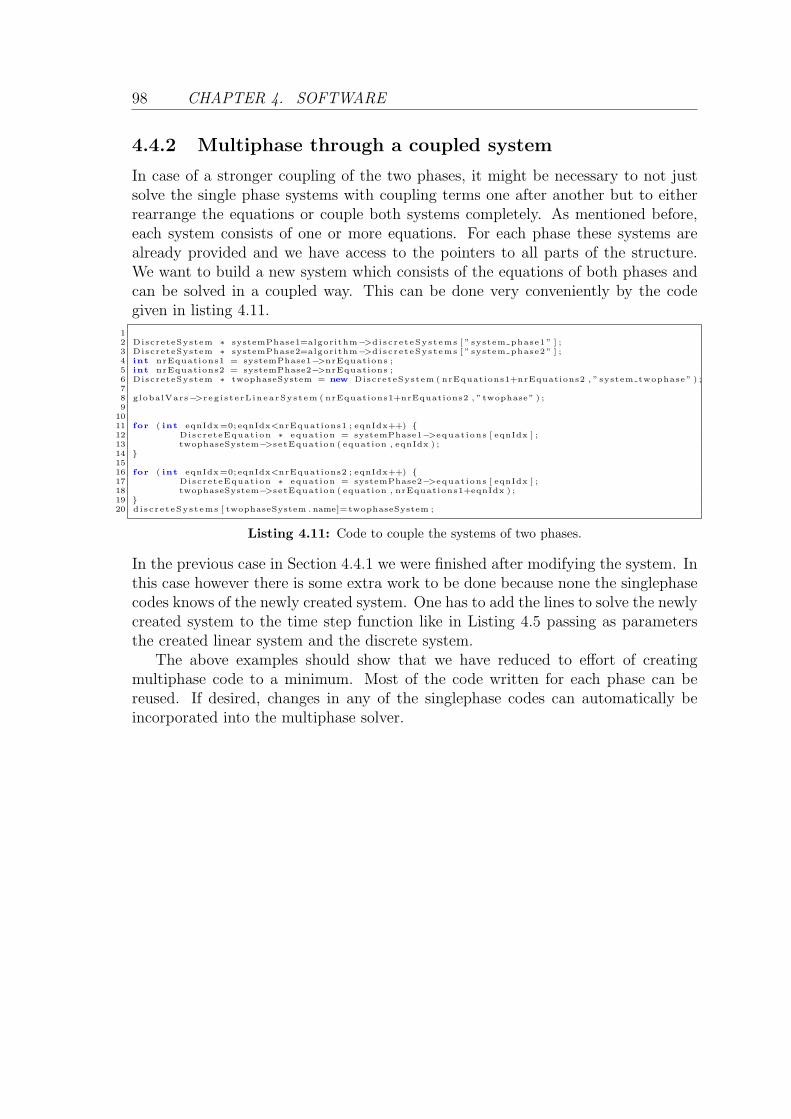
98 CHAPTER 4. SOFTWARE
4.4.2 Multiphase through a coupled system
In case of a stronger coupling of the two phases, it might be necessary to not justsolve the single phase systems with coupling terms one after another but to eitherrearrange the equations or couple both systems completely. As mentioned before,each system consists of one or more equations. For each phase these systems arealready provided and we have access to the pointers to all parts of the structure.We want to build a new system which consists of the equations of both phases andcan be solved in a coupled way. This can be done very conveniently by the codegiven in listing 4.11.
12 DiscreteSystem ∗ systemPhase1=algorithm−>d i s c r e t eSys t ems [ ” system phase1 ” ] ;3 DiscreteSystem ∗ systemPhase2=algorithm−>d i s c r e t eSys t ems [ ” system phase2 ” ] ;4 int nrEquations1 = systemPhase1−>nrEquations ;5 int nrEquations2 = systemPhase2−>nrEquations ;6 DiscreteSystem ∗ twophaseSystem = new DiscreteSystem ( nrEquations1+nrEquations2 , ” system twophase ” ) ;78 globalVars−>r eg i s t e rL inea rSys t em ( nrEquations1+nrEquations2 , ” twophase” ) ;9
1011 for ( int eqnIdx=0; eqnIdx<nrEquations1 ; eqnIdx++) 12 DiscreteEquat ion ∗ equat ion = systemPhase1−>equat ions [ eqnIdx ] ;13 twophaseSystem−>setEquat ion ( equation , eqnIdx ) ;14 1516 for ( int eqnIdx=0; eqnIdx<nrEquations2 ; eqnIdx++) 17 DiscreteEquat ion ∗ equat ion = systemPhase2−>equat ions [ eqnIdx ] ;18 twophaseSystem−>setEquat ion ( equation , nrEquations1+eqnIdx ) ;19 20 d i s c r e t eSys t ems [ twophaseSystem . name]=twophaseSystem ;
Listing 4.11: Code to couple the systems of two phases.
In the previous case in Section 4.4.1 we were finished after modifying the system. Inthis case however there is some extra work to be done because none the singlephasecodes knows of the newly created system. One has to add the lines to solve the newlycreated system to the time step function like in Listing 4.5 passing as parametersthe created linear system and the discrete system.
The above examples should show that we have reduced to effort of creatingmultiphase code to a minimum. Most of the code written for each phase can bereused. If desired, changes in any of the singlephase codes can automatically beincorporated into the multiphase solver.

Chapter 5
Concluding remarks and outlook
The field of simulation of granular flow is large. We have seen that it touches amultitude of advanced topics. In modeling, these are for example the kinetic theoryof granular gases and non-Newtonian fluid flow. Regarding the numerics we dealwith complex Navier-Stokes Equations (NSE)-type systems and nonlinear discretiza-tion approaches. Therefore an in-depth and complete coverage of the simulation ofgranular flow within such a work is not possible.
We have presented a specific approach to the simulation of granular flow. Wechoose to model granular flow as a fluid in as many regimes as possible. We have in-troduced a hybrid model for dilute and dense granular flow which has a significantlysimpler form than similar models introduced in the literature. Still, this modelingapproach results in a very complex NSE-type system with all imaginable complica-tions, varying viscosity, different regimes of very high and very low compressibilityand nonlinearities in the algebraic relations.
For the solution of this System of partial differential equations (PDEs) and al-gebraic relations (1.18) we have developed a novel pressure based fractional stepalgorithm with a nonlinear pressure equation. The fact that we have not reducedthe system and considered simplified versions but kept the full complexity of thesystem throughout this work is a contribution in itself.
To actually obtain approximate solutions of this model we have implementedthe model as well as the nonlinear pressure algorithm (NPA) into a software frame-work which we developed in this work. This framework provides a generalized andautomatic approach to discretization and automatic parallelization of the linear al-gebra components. Using this implementation we are able to compute solutions onarbitrary domains and visualize the results. The software however goes beyond thepurpose of showing the applicability of the model and the algorithm. It is a gen-eral software framework for implementing solution methods for the flow of complexfluids. Our granular flow is just an example and a proof of concept for the software.
Using the implementation we have provided numerical experiments towards thevalidation of both the model and the algorithm. For the study of properties ofthe model and the algorithm we have carried out further numerical investigations.Finally we have applied the implementation to two industrial problems to furthershowcase the capabilities of the developed approach to the simulation of granularflow.
In the first chapter and in the introductions to the other chapters we have alreadygiven thorough overviews in the respective aspects of the simulation of granular flow.In the following we shall rather focus on insights and problems we found on the way.
Regarding the hydrodynamic modeling of granular flow, we can say that it is insome aspects a quite heuristic task. As of now there is no single correct constitutive

100 CHAPTER 5. CONCLUDING REMARKS AND OUTLOOK
Figure 5.1: Instability in pile formation between β = 1.75 (first and second plot) compared toβ = 1 (third and fourth plot). The first and third plots display the volume fraction from low (dark)to high (light). The contour plots (second and fourth) display the boundary between volumes wherethe yield relations for the dense regime (1.15) are active and those in the kinetic regime (1.11).
model. That is not surprising because when we consider grains as hard spheresmany obvious observations that we make when we look at, say, grains of sand, areleft out. But not even all effects of few-particle systems with hard spheres can beincorporated without the equations becoming hopelessly complicated, see [BP03,pg. 34f]. Furthermore, minor specifics of the constitutive relations can have a majorimpact on the resulting solution. This is an important point in the modeling ofgranular flow and we want to emphasize it with an example.
During the development of the hybrid model we found a very interesting insta-bility shown in Figure 5.1. In [BLS+01, Equation (15)] the viscosity (1.18h) is givenwith an exponent β on g(ρ). The authors claim that a value β > 1 is necessary toobtain shear bands. When using our hybrid model this exponent is not necessaryand it even causes the displayed instability. It is rather symptomatic for this field ofmodeling that one can get lost in the misery of constitutive relations, to cite [Kol00].However, we believe that our model is as simple as possible with as few parametersas possible and, as we have shown, is still able to reproduce many effects of granularflow.
The modeling is followed by the task of computing solutions to the model. Wehave presented a pressure based fractional step method with a nonlinear pressureequation (NPE). We have explained why a linear method does not suffice in ourcase. After the decision for a NPE we followed the path laid out by linear fractionalstep methods (LFSMs). We ended up with two coupled equations for computing anew pressure and a new velocity in each time step. For reasons of stability we haveused an upwind biased density in the mass conservation equation. The NPE wassolved by a variant of the Newton method for systems of nonlinear equations. Thisresulted in a method which is able to solve the System (1.18). The method seemsto be mass conserving and generally seems to be able to handle the huge range ofcompressibility quite well without any of the modifications which are necessary inthe linear case, see Section 3.4.1. The rigorous analysis of these properties for thefull system is not part of this work but we support the statements made in Section3.4 at least numerically.
By using a NPE instead of a linear pressure correction equation (LPCE) we areable to obtain solutions of the very complicated granular flow model (1.18) but weintroduce new problems. One is the question of when the Newton method converges

101
for the NPE. It is well known that Newton methods only converge for starting valueswithin a certain interval around the solution and have quadratic convergence onlyif all intermediate iterations stay within this interval. Modern Newton methods asintroduced in Section 2.4.4 try to circumvent this restriction by very careful stepsize control but the issue of the initial value is still difficult.
This is especially the case for our way of solving the time-dependent problem.We use the value of the old pressure as an initial guess for the Newton method forthe NPE. It seems that in most cases we are close enough to the solution for thisapproach to work. However, for a surely robust method we would need to investigatea sophisticated time adaption where we restart the computation for the current timestep with a smaller τ if the iteration for the NPE has not converged.
This already brings us to the outlook of things that can and possibly shouldfollow this work. The whole issue around the Newton method certainly gives rise tomany possible directions of further research. We will not indulge into this further,as for this work we have been using a library for the actual solution of the NPE.For further research, it might well be necessary to investigate the optimal variant ofthe Newton method for our NPE from current publications and implement this fromscratch. But there are some other points which can be of further interest. They arelisted in the order of this work, first regarding the modeling, then the numerics andfinally the implementation.
Static Coulomb friction: We have mentioned in the last subsection of Section1.3.1 that the kinetic model has a property called dynamic Coulomb friction, inves-tigated in [BLS+01]. This allows the formation of heaps close to an internal frictionangle as we have shown for example in Section 3.2.2. We have extended the modelfor quasi-static situations and have kept the internal friction angle consistent asshown in Appendix A.2. Currently the angle of friction arises from the solution ofthe equations. In fully static situations, which are not part of this work, we havefound problems in our numerical experiments. We suppose that for a situation ofcomplete rest of the granular material, it is necessary to explicitely include a modelof real friction of grains.
Partial slip boundary conditions: As we have mentioned in Section 1.3.3 thecurrently used boundary conditions are not completely realistic. It is necessary tomodel the interaction of the grains with the boundary in a better way than justassuming them to stick or slide freely on the boundary. We need to prescribe afriction for grain movement tangential to the boundary. This however makes itnecessary to know exactly what direction is tangential to the boundary. Currentlywe approximate the boundary quite roughly by the cuboids.
Approximation of the boundary: There are different ways to find a betterapproximation of the boundary. Either at the point of grid generation for a certaindomain one can form volumes at the boundary which represent the shape of the

102 CHAPTER 5. CONCLUDING REMARKS AND OUTLOOK
boundary. Another method is to use the same volume mesh but take into accountthe shape of the boundary during discretization.
Investigation of the NPE: With the NPE we have introduced a novel equationfor computing an updated pressure value. In the linear case the elliptic equation,usually for a pressure correction is well studied. For the nonlinear case there existsthe property of so called monotone operators which is a generalization of ellipticity.
Parallelization: In Section 4.3 we have described a parallelization approach forour generalized approach to discretization. This parallelizes only the linear algebracomponents. With this approach we do not remove the bottleneck of memory, wecan only hope to speed up the computations. Some kind of domain decompositionshould be considered. However, this may introduce new complications for the NPE.We would need to find a way to parallelize the solution of this nonlinear equation.
All the above topics should provide good starting points for further research.Aside from these points we have presented in this work an interdisciplinary andin itself closed approach to the numerical simulation of granular flow. It is closedin that it provides all the steps necessary to simulate granular flow. Aside fromthe aforementioned contributions in the separate parts of the thesis, this is thepoint where we see the major contribution of this work. The topic of simulationof granular flow has been treated in an interdisciplinary way. The three pillars ofnumerical simulation, namely the modeling, the numerical algorithms for obtainingapproximate solutions of the model as well as the software implementation havebeen treated not separately but with respect to each other such that the final resultis a way to simulate the behavior of dense and dilute granular flow in arbitrarydomains.
”Who could ever calculate the path of a molecule? How do we know that thecreations of worlds are not determined by falling grains of sand?”
Victor Hugo from Les Miserables

Chapter A
Appendix
A.1 Collaps in kinetic models
In Section 1.3.2 we described the shortcoming of the kinetic model in static situationswithout continuing energy input. To understand how the state of zero temperatureand maximum packing fraction is reached we investigate Haff’s homogeneous coolingfor the temperature of the granular system described by Equations (1.7) and (1.11).Neglecting the gradients in the temperature and the velocities we obtain from (1.7)
∂T
∂t= −εT. (A.1)
For the final approach to a maximally packed state we can replace ε(ρ, T ) by εc inleading order with
εc := ε0ρ2c
√Tg(ρ) (A.2)
to obtain the equation∂T
∂t= −ε0ρ
2cgT 3/2. (A.3)
Equation (A.3) is solved by Haff’s law (see [BP03, p. 53, Equation (5.5)])
T (ρ, t) =T0(1− (ρ/ρc))
2
(1− (ρ/ρc) + A√
T0(t− t0))2, (A.4)
with A = ε0ρ2c . Using this expression for T in the kinetic pressure pK , compare
Equation (1.11a), we see that the pressure vanishes with the density approaching themaximum packing state ρ = ρc. In addition the system becomes thermodynamicallyunstable. This can be seen by calculating dpK/dρ, which is for large times given by
dpK
dρ=
1
A2(t− t0)2(1− 2
ρ
ρc
). (A.5)
In the asymptotic long time limit for ρ > ρc/2, the compressibility would becomenegative for the pure homogeneous cooling case. Similar regions of negative com-pressibility have been found in other kinetic models of granular gases, see [KM02].
A.2 Dynamic Coulomb friction
That grains form piles is easy to observe and makes granular media different fromcommon fluids. The angle at which the pile is formed, the angle of repose is not

104 APPENDIX A. APPENDIX
a material property, but it is usually very close to the internal friction angle. Thisinternal angle quantifies the frictional interaction of the grains.
Bocquet et al. have shown in [BLS+01], that solid like behavior is a solution ofthe purely kinetic model which is System (1.18) with ρco = ρc from (1.13) and (1.11)respectively. They derive that by solving with the kinetic expression for pressureand transport coefficients (1.11) for a shearing experiment at constant pressure, theshear stress σxy will be proportional to the normal stress component given by thepressure p independent of the shear rate
σxy = p tan Φ, (A.6)
where the tangent of the internal friction coefficient is approximately given by
tan Φ =√
ε0η0. (A.7)
We will now show, that we obtain the same relation with the choice of the hybridmodel (1.14) and (1.15).
For an ideal shearing experiment the coordinate system can be chosen such thatthe changes of the velocity are perpendicular to the direction of the velocity. If wechose the velocity u = (ux(y), 0, 0) the only non vanishing shear stress component isσxy = η ∂ux
∂y. Neglecting gradients in the granular temperature, Equation (1.7) gives
the balance of viscous heating and dissipation as
2η
3
(∂ux
∂y
)2
− ερT = 0. (A.8)
Equations (1.8) and (1.9) give the ratio of shear stress and pressure
σxy
p=
η
p
∂ux
∂y.
With Equation (A.8) this can be written as
σxy
p=
√32ηερT
p.
Using Equations (1.14) and (1.15) we obtain
σxy
p=
√32ηKεKρT
pK
. (A.9)
The angle of repose is relevant only for the high density limit, hence we replace ρby ρc in Equation (A.9). Using the expressions from (1.11) we get
σxy
p=
√3
2ρcη0ε0.

A.2. DYNAMIC COULOMB FRICTION 105
This shows that the yield pressure contribution does not affect the internal frictionangle. Arguing that we are only interested in a rough approximation of the angle, wesay that 3
2ρc is close enough to 1 to be neglected. Hence we arrive at the expressions
(A.6) and (A.7).The internal friction angle may differ by a few degrees from the measured angle
of repose, which differs slightly through different experiments. Nevertheless, theformula should still suggest a range of values to match the angle of repose found inour numerical experiments.


Notation
Acronyms
CFD computational fluid dynamics
CoRheoS Complex Rheology Solvers A software framework for implementing flowsolvers.
FV Finite Volume
LFSM linear fractional step method
LPCA linear pressure correction algorithm
LPCE linear pressure correction equation
MD molecular dynamics
NFSM nonlinear fractional step method
NPA nonlinear pressure algorithm An novel algorithm for pressure which involves anonlinear pressure equation.
NPE nonlinear pressure equation
NSE Navier-Stokes Equations
ODE ordinary differential equation
PDE partial differential equation
SC Schur-Complement
Mathematical notation
Vectors and vector valued functions are typeset in bold font, regardless of whetherthey are continuous or discrete. Components of vectors are scalar, hence they arenot bold as in
x and xi.
We use the following differential operators in this work. The divergence and gradientare denoted by the differential operators div and grad. The indices i and j willdenote rows and columns respectively. The divergence of a vector field F : Rd → Rd
is defined as
div (F ) := ∇ · F =∂
∂xj
(Fj).

108 NOTATION
For a tensor valued function T : Rd → R(d×d), T = Tij, the divergence operator isdefined as
div (T ) := ∇ · T =∂
∂xj
(Tij).
For a scalar valued function S : R → Rd, the gradient is defined as
grad (S) := ∇S =∂
∂xj
(S).
Symbols:
ρ - Density, introduced in System (1.1)
u,v - Velocities introduced in System (1.1)
p - Pressure introduced in System (1.1)
T - (Granular) temperature from Equation (1.7)
pK , pY - Kinetic and yield pressure of the granular flow model System (1.18)
σ - Stress tensor introduced in System (1.1)
σ - Stress tensor in the granular flow model System (1.18)
κ - Strain rate tensor introduced in System (1.1)
κ - Strain rate tensor in the granular flow model System (1.18)
q - Granular heat flux from Equations (1.7) and (1.8)
λ, λK - Granular heat conductivity from Equation (1.15c)
η, ηK - Granular viscosity from Equation (1.15a)
ε, εK - Granular energy loss rate from Equation (1.15b)
ρc - Limit density for random close packing of homogeneous spheres (1.12)
ρco - Crossover density between kinetic and yield regime, see Equation (1.13)
τ - Time step for time discretization (2.25)
π - Mapping between indizes of volumes, see Equation (2.3)
V , V , V - Volumes of the grid, interior and boundary, see Equation (2.4)
F , F , F - Faces of a volume, interior and boundary, see Equation (2.7)
h - Vector of lengths of finite volumes for space discretization, see Equation (2.5)
DIV - Discrete divergence, see Equation (2.13)
GF - Discrete gradient by faces, see Equation (2.17)
∝ - Denotes two proportional expressions
< · > - Averaging operator as in the definition of granular temperature (1.5)
v ⊗ u - Outer vector product uvT
σ : κ - Tensor contraction σijκij in Einstein notation

Bibliography
[BBG+01] S. Balay, K. Buschelman, W. D. Gropp, D. Kaushik, M. G. Knepley,L. C. McInnes, B. F. Smith, and H. Zhang, PETSc Web page, 2001,http://www.mcs.anl.gov/petsc.
[BEL02] L. Bocquet, J. Errami, and T. C. Lubensky, Hydrodynamic model for adynamical jammed-to-flowing transition in gravity driven granular media,Physical Review Letters 89 (2002), no. 18, 184301.
[BGMS97] S. Balay, W. D. Gropp, L. C. McInnes, and B. F. Smith, Modern softwaretools for scientific computing, ch. 8, Birkhauser Boston Inc., Cambridge, MA,USA, 1997.
[BH97] C. H. Bischof and P. D. Hovl, Using adifor and adic to provide a jacobianfor the snes component of petsc, Technical Memorandum ANL/MCS-TM-233,Mathematics and Computer Science Division, Argonne National Laboratory,1997.
[BLS+01] L. Bocquet, W. Losert, D. Schalk, T. C. Lubensky, and J. P. Gollub, Granularshear flow dynamics and forces: Experiment and continuum theory, PhysicalReview E 65 (2001), no. 1, 011307.
[BP03] N. V. Brilliantov and T. Poschel, Kinetic theory of granular gases, OxfordGraduate Texts, Oxford University Press, Berlin, April 2003.
[BW98] H. Bijl and P. Wesseling, A unified method for computing incompressible andcompressible flows in boundary-fitted coordinates, Journal of ComputationalPhysics 141 (1998), no. 2, 153–173.
[Cam93] C. S. Campbell, Boundary interactions for two-dimensional granular flows.part 1. flat boundaries, asymmetric stresses and couple stresses, Journal ofFluid Mechanics Digital Archive (1993), no. 247, 111–136.
[Cho68] A. J. Chorin, Numerical solution of navier-stokes equation, Mathematics ofComputation 22 (1968), 745–760.
[Chu03] A. Churbanov, A unified algorithm to predict compressible and incompressibleflows, Lecture Notes in Computer Science, vol. 2542/2003, pp. 412–419,Springer, Berlin, Heidelberg, 2003.
[CL05] M. Chuiko and A. Lapanik, Incompressible fluid flow computation in anarbitrary two-dimensional region on nonstaggered grid, Computational meth-ods in applied mathematics 5 (2005), no. 3, 242–258.
[Dah59] J. S. Dahler, Transport phenomena in a fluid composed of diatomic molecules,The Journal of Chemical Physics 30 (1959), no. 6, 1447–1475.
[Dar03] S. Dartevelle, Numerical and granulometric approaches to geophysical granularflows, Ph.D. thesis, Michigan Technological University, July 2003.

110 BIBLIOGRAPHY
[DD99] A. Daerr and S. Douady, Two types of avalanche behaviour in granular media,Nature 399 (1999), 241–243.
[Deu04] P. Deuflhard, Newton methods for nonlinear problems: Affine invariance andadaptive algorithms, Computational Mathematics, vol. 35, Springer, 2004.
[DLGD01] A. Duret-Lutz, T. Geraud, and A. Demaille, Design patterns for genericprogramming in c++, COOTS’01: Proceedings of the 6th conference onUSENIX Conference on Object-Oriented Technologies and Systems (Berke-ley, CA, USA), USENIX Association, 2001, pp. 14–14.
[DMB+03] G. D’Anna, P. Mayor, A. Barrat, V. Loreto, and F. Nori, Observing brownianmotion in vibration-fluidized granular matter, Nature 424 (2003), 909.
[Duf01] J. W. Dufty, Kinetic theory and hydrodynamics for rapid granular flow - aperspective, ArXiv Condensed Matter e-prints (2001).
[Dut88] P. Dutt, Stable boundary conditions and difference schemes for navier-stokesequations, SIAM Journal Numerical Analysis 25 (1988), no. 2, 245–267.
[EG04] A. Ern and J. L. Guermond, Theory and practice of finite elements, AppliedMathematical Sciences, vol. 159, Springer-Verlag, New York, 2004.
[EGH00] R. Eymard, T. Gallouet, and R. Herbin, Handbook of numerical analysis,vol. 7, ch. Finite volume methods, pp. 713–1020, Elsevier Science, 2000.
[Fle91a] C. A. J. Fletcher, Computational techniques for fluid dynamics, 2nd ed., vol. 2,Springer-Verlag, Berlin, Heidelberg, New York, 1991.
[Fle91b] , Computational techniques for fluid dynamics, 2nd ed., vol. 1,Springer-Verlag, Berlin, Heidelberg, New York, 1991.
[FP96] J. H. Ferziger and M. Peric, Computational methods for fluid dynamics,Springer, Berlin, Heidelberg, New York, 1996.
[GBHL06] L. Gastaldo, F. Babik, R. Herbin, and J.-C. Latche, An unconditionally stablepressure correction scheme for barotropic compressible navier-stokes equations,ECCOMAS CFD, 2006.
[GD99] V. Garzo and J. W. Dufty, Dense fluid transport for inelastic hard spheres,Physical Review E 59 (1999), no. 5, 5895–5911.
[GHJV95] E. Gamma, R. Helm, R. Johnson, and J. Vlissides, Design patterns - elementsof reusable object-oriented software, Addison-Wesley Publishing Co., Reading,Massachusetts, 1995.
[Gid94] D. Gidaspow, Multiphase flow and fluidization, contimnuum and kinetic theorydescription, Boston, Academic Press, 1934, 1994.
[GKC96] A. Gardziella, A. Kwasniok, and L. Cobos, Recent studies comparingcoremaking processes, Modern Casting 86 (1996), no. 3, 39–42.

BIBLIOGRAPHY 111
[GMS06] J. L. Guermond, P. D. Minev, and Jie Shen, An overview of projection methodsfor incompressible flows, Computer Methods in Applied Mechanics and Engi-neering 195 (2006), no. 44-47, 6011–6045.
[GRS07] C. Grossmann, H.-J. Roos, and M. Stynes, Numerical treatment of partialdifferential equations, Universitext, Springer, Berlin, Heidelberg, 2007.
[GS78] B. Gustafsson and A. Sundstrom, Incompletely parabolic problems in fluiddynamics, SIAM Journal of Applied Mathematics 35 (1978), no. 2.
[GS98] P. M. Gresho and R. L. Sani, Incompressible flow and the finite elementmethod. volume 1: Advection-diffusion and isothermal laminar flow, vol. 1,John Wiley and Sons, Inc, New York, NY (United States), December 1998.
[HA68] F. H. Harlow and A. A. Amsden, Numerical calculation of almostincompressible flow, Journal of Computational Physics 3 (1968), no. 1, 80–93.
[HA71] , A numerical fluid dynamics calculation method for all flow speeds,Journal of Computational Physics 8 (1971), no. 2, 197–213.
[HG97] J. S. Hesthaven and D. Gottlieb, A stable penalty method for the compressiblenavier-stokes equations. 1. open boundary conditions, SIAM Journal on Sci-entific Computing 18 (1997), no. 3, 658–685.
[Hir88] C. Hirsch, Numerical computation of internal and external flows, Wiley Seriesin Numerical Methods in Engineering, vol. 1, John Wiley & Sons, Chichester,New York, Brisbane, Toronto, Singapore, 1988.
[HNS05] P. Hovland, B. Norris, and B. Smith, Making automatic differentiation trulyautomatic: coupling petsc with adic, Future Generation Computer Systems21 (2005), no. 8, 1426–1438.
[Kad99] P. Kadanoff, Built upon sand: Theoretical ideas inspired by granular flows,Review of Modern Physics 71 (1999), no. 1, 435–444.
[KM85] J. Kim and P. Moin, Application of a fractional-step method to incompressiblenavier-stokes equations, Journal of Computational Physics 59 (1985), no. 2,308–323.
[KM02] E. Khain and B. Meerson, Symmetry-breaking instability in a prototypicaldriven granular gas, Physical Review E 66 (2002), no. 2, 021306.
[Kol00] D. Kolymbas, The misery of constitutive modelling, Constitutive Modelling ofGranular Materials, pp. 11–24, Springer, 2000.
[Lat06] A. Latz, Enthalpy equation: Temperature changes at constant pressure,ITWM Report, August 2006.
[LL78] L. D. Landau and E. M. Lifschitz, Hydrodynamic, Lehrbuch der theoretischenPhysik, vol. VI, Akademie-Verlag, Berlin, 1978 (ngerman).

112 BIBLIOGRAPHY
[MF97] MPI-Forum, Mpi-2: Extensions to the message-passing interface, Tech. report,University of Tennessee, Knoxville, Tennessee, 1997.
[MHN02] N. Mitarai, H. Hayakawa, and H. Nakanishi, Collisional granular flow as amicropolar fluid, Physical Review Letters 88 (2002), no. 17, 174301.
[Min01] P. D. Minev, A stabilized incremental projection scheme for the incompressiblenavier-stokes equations, International Journal for Numerical Methods in Fluids36 (2001), 441–464.
[MP00] M.M. Massoudi and T. X. Phuoc, The effect of slip boundary condition onthe flow of granular materials: a continuum approach, International Journalof Non-Linear Mechanics 35 (2000), 745–761.
[MPB03] B. Meerson, T. Poschel, and Y. Bromberg, Close-packed floating clusters:Granular hydrodynamics beyond the freezing point?, Physical Review Letters91 (2003), no. 2, 024301.
[NA07] M.-J. Ni and M. A. Abdou, A bridge between projection methods and simpletype methods for incompressible navier-stokes equations, International Journalfor Numerical Methods in Engineering 72 (2007), no. 12, 1490–1512.
[Oes01] B. Oestereich, Objektorientierte Softwareentwicklung - Analyse und Designmit der Unified Modeling Language, Oldenbourg, 2001.
[OS78] J. Oliger and A. Sundstrom, Theoretical and practical aspects of some initialboundary value problems in fluid dynamics, SIAM Journal of Applied Math-ematics 35 (1978), no. 3, 419–446.
[PS72] S. V. Patankar and D. B. Spalding, A calculation procedure for heat, massand momentum, International Journal of Heat and Mass Transfer 15 (1972),1787–1806.
[QSS06] A. Quarteroni, R. Sacco, and F. Saleri, Numerical mathematics (texts inapplied mathematics), Springer-Verlag New York, Inc., Secaucus, NJ, USA,2006.
[RC83] C. M. Rhie and W. L. Chow, Numerical study of the turbulent flow past anairfoil with trailing edge separation, AIAA Journal 21 (1983), 1525–1532.
[Sav98] S. B. Savage, Analyses of slow high-concentration flows of granular materials,Journal of Fluid Mechanics 377 (1998), 1–26.
[SK98] M. Schader and A. Korthaus, The unified modeling language, Physica-Verlag,Heidelberg, July 1998.
[SK03] J. C. Sutherland and C. A. Kennedy, Improved boundary conditions forviscous, reacting, compressible flow, Journal of Computational Physics 191(2003), 502–524.
[SML03] W. Schroeder, K. Martin, and B. Lorenson, The visualization toolkit, 3rdedition ed., Kitware, 2003.
BIBLIOGRAPHY 113
[Str76] J. C. Strikwerda, Initial boundary value problems for incompletely parabolicsystems, Ph.D. thesis, Stanford University, 1976.
[Str97] B. Stroustrup, The C++ programming language, 3rd edition ed., AddisonWesley Longman, Reading, Massachusetts, 1997.
[TS61] A. N. Thikonov and A. Samarskii, Homogeneous difference schemesa, ZhurnalVychislitelnoi Matematiki i Matematicheskoi Fiziki 1 (1961), 5–63.
[TS96] S. Turek and M. Schafer, Benchmark computations of laminar flow aroundcylinder, Notes on Numerical Fluid Mechanics, vol. 52, pp. 547–566, Vieweg,1996.
[Tur99] S. Turek, Efficient solvers for incompressible flow problems, Lecture Notes inComputational Science and Engineering, vol. 6, Springer, Heidelberg, 1999.
[VPC96] P. N. Vabishchevich, A. N. Pavlov, and A. G. Churbanov, Numerical methodsfor unsteady incompressible flows using primitive variables and nonstaggeredgrids, Matematicheskoe modelirovanie 8 (1996), no. 7, 81–108.
[vVW01] D. R. van der Heul, C. Vuik, and P. Wesseling, Stability analysis of segregatedsolution methods for compressible flow, Applied Numerical Mathematics 38(2001), 257–274.
[vVW03] , A conservative pressure-correction method for flow at all speeds, Com-puters & Fluids 32 (2003), no. 8, 1113–1132.
[Wes01] P. Wesseling, Principles of computational fluid dynamics, Springer Series incomputational mathematics, vol. 29, Springer, Berlin, Heidelberg, 2001.
[xml98] Extensible Markup Language (XML) 1.0, 1998,http://www.w3.org/TR/1998/REC-xml-19980210.


CURRICULUM VITAE
deutsch:
16.07.1981 geboren in Suhl
1988 – 1992 Besuch der Grundschule in Geschwenda
1992 – 1996 Besuch des Neideck Gymnasiums in Grafenroda
1996 – 1998 Besuch des Gymnasiums Goetheschule in Ilmenau
1998 – 1999 Besuch der Madawaska Higschool in Madawaska, ME, USA
1999 – 2000 Studium an der Northeastern University, Boston, MA, USA
2000 – 2005 Studium an der Technischen Universitat Ilmenau
September 2005 Abschluss des Studiums als Diplom-Mathematiker
seit Oktober 2005 Doktorand am Fraunhofer Institut furTechno- und Witschaftsmathematik in Kaiserslautern
english:
16.07.1981 born in Suhl, Germany
1988 – 1992 Elementary school, Geschwenda
1992 – 1996 Secondary school “Neideck Gymnasium Grafenroda”
1996 – 1998 Secondary school “Goetheschule Ilmenau”
1998 – 1999 Madawaska Higschool, Madawaska, ME, USA
1999 – 2000 Northeastern University, Boston, MA, USA
2000 – 2005 University, “Technische Universitat Ilmenau”
September 2005 Diploma as “Diplom-Mathematiker”
since Oktober 2005 PhD student at the “Fraunhofer Institut furTechno- und Witschaftsmathematik”, Kaiserslautern