A Numerical Simulation Framework for the Design, Managementand Optimization of CO2 Sequestration in Subsurface Formations

Investigators

Hamdi Tchelepi, Associate Professor of Energy Resources Engineering; LouDurlofsky, Professor of Energy Resources Engineering; and Khalid Aziz, Professor ofEnergy Resources Engineering.

Abstract

The objective is to develop a numerical simulation framework for modeling subsurfaceCO2 sequestration operations. We have made significant progress on severalinterrelated areas of investigation.

The vertical migration of CO2 plumes, which are immiscible with the surroundingbrine, was investigated using high-resolution simulation. The flux function forbuoyancy driven immiscible flow plays an important role in the resulting behavior.Plume stretching, wave interactions, overall migration distances and speeds arediscussed. This analysis is a prerequisite for the ongoing study of immiscible CO2

plume migration with capillary hysteresis.

The behavior of CO2 gravity currents in sloping aquifers in the presence of residualtrapping was investigated. Even though a simple mathematical model that accounts forresidual trapping in the wake of the gravity current was used, the analysis sheds lighton the long term fate of gravity currents of practical interest. Dependence of themaximum migration distance on initial plume size, aquifer slope, and viscosity ratio isdescribed. This study indicates that regional (gently dipping) aquifers of large extentcan be viable storage sites, and that the effectiveness of residual trapping increasesdramatically with slope.

Consistent with our objectives to develop a flexible and efficient numericalcomputational framework, we are investigating the development of high-order AIM(Adaptive Implicit Method) discretizations, in both space and time. High-orderapproximations were developed using the MOL (Method of Lines) framework as abase. These constructions are high-order (at least second order) in space and time,locally conservative, and unconditionally stable; however, these desirable propertiescome with a severe positivity restriction in the implicit regions, which limits the timestep size. Investigation of artificial-viscosity schemes to remedy these restrictions isongoing.

The multiscale finite-volume method was extended for compressible multiphase flow

in strongly heterogeneous domains. The accuracy of the formulation is demonstratedfor problems with high compressibility levels and strong permeability heterogeneity.This algebraic Operator Based Multiscale Method (OBMM) provides a flexibleframework for solving coupled problems of multiphase flow and transport and isapplicable to models with unstructured grid. Moreover, OBMM can be used to addmultiscale capabilities to standard flow simulators in a straight forward manner.

Development of a stochastic approach for modeling multiscale multi-physics problemsis ongoing. The framework is demonstrated for non-equilibrium capillary- pressureformulations. The description leads to a high dimensional transport equation, whereone of the dimensions is the saturation random variable. This equation is then solvedusing standard finite volumes. The flexibility of the framework in linking complexflow behaviors across scales is demonstrated using simple one-dimensional immiscibletwo-phase flow.

Finally, we describe our proposed flexible formulation for incorporating chemicalreactions in our general-purpose simulation framework. The extension will beperformed such that we take full advantage of the existing capabilities in GPRS,including, general-compositional, adaptive implicit, unstructured grid, advanced wells,and adjoint enabled. The objective is to be able to model the reactions associated withCO2 sequestration processes and their interactions with complex multi-componentmultiphase flow and transport for problems of practical interest.

Introduction

The overall objective of this project is to develop a numerical simulationframework for modeling CO2 sequestration operations in large-scale heterogeneousformations, such as deep saline aquifers and depleted oil and gas reservoirs. Thisframework is constructed based on in-depth understanding of the physics in theparameter space of interest for geologic sequestration of CO2, accurate andcomputationally efficient numerical algorithms for modeling flow and transportprocesses in large-scale porous formations, and a flexible extensible computationalframework for the design and optimization of CO2 projects during both the injectionand long term storage periods.

During the past year, we worked on several interrelated items: (1) detailedunderstanding of the physics associated with plume migration and gravity currents, (2)high-order AIM (adaptive implicit method) formulations, (3) multiscale finite-volumeformulation for compressible multiphase flow, and (4) development of a generalframework for modeling reactions in porous media flows. In this annual progressreport, we summarize the most recent developments, which are divided into sixsub-projects. These are: (1) vertical migration of CO2 plumes in porous media, (2)propagation of CO2 plumes in sloping aquifers with residual trapping, (3) constructionof high-order adaptive implicit methods, (4) algebraic multiscale formulation forcompressible multiphase flow, (5) stochastic framework for non-equilibrium models ofmultiphase flow in porous media, and (6) modeling CO2 mineralization reactions in ageneral-purpose flow simulator.

These projects deal with different aspects of the numerical framework we arebuilding. The first two projects are aimed at improved understanding of the physicalmechanisms that dictate the behavior of CO2 plumes in porous media. The third andfourth projects are concerned with the development of accurate and computationallyefficient numerical methods for modeling the complex behaviors associated withsubsurface CO2 sequestration. The fifth project relates to ongoing development of astochastic framework for modeling multiphase flow across multiple scales, accountingfor possibly having different equations that describe the physics at the different scales.A flexible and computationally efficient framework for modeling reactions associatedwith CO2 sequestration processes in natural porous media is the subject of the sixthproject.

In the first project, the evolution and vertical migration of a CO2 plume that isimmiscible with the resident brine is studied using very accurate numerical simulationsof two-phase flow. The relative permeability effects and the differences in density andviscosity between the CO2 and the brine can lead to highly complex nonlinearinteractions. In this progress report, we focus on the flux function and the behavior ofthe various saturation fronts in the mean flow. Issues related to spreading, waveinteractions, migration distances and speeds are discussed. This analysis serves as aprerequisite to the ongoing analysis of hysteresis effects and capillary trapping on CO2

plumes in the post-injection period.

In the second project, the long term fate of a CO2 gravity current that is initiallyponded against the boundary of a deep and slightly sloping aquifer is investigated. Asimple model is used to represent residual trapping in the wake of the gravity current.The migration distance of the gravity current, and its dependence on the plume sizeand aquifer slope are discussed.

The third project is on the construction of high-order approximations for theadaptive implicit method (AIM). Accurate simulation of the physics governingsubsurface CO2 sequestration requires solving coupled nonlinear conservationequations in highly heterogeneous domains. For such models, AIM allocates thecomputational resources when and where necessary. However, standard AIM isfirst-order in both space and time. Such a low-order treatment may be inadequate foraccurate modeling of buoyancy driven transport in the post-injection period. As aresult, we have been investigating high-order AIM schemes in both space and time.Our analysis has progressed quite significantly, and we summarize the effort in thisreport. However, several challenges remain, and we outline our plans for tacklingthem.

In the fourth project, we describe the extension of the multiscale finite-volumemethod for compressible multiphase flow in highly heterogenous formations. Thisoperator based multiscale method (OBMM) is a promising platform for includingadditional flow mechanisms (e.g., capillarity, buoyancy) as well as for solvingproblems on unstructured grids. We also report on the recent effort to develop anadaptive multiscale formulation for the nonlinear transport problem (saturationequations).

In collaboration with researchers at ETH, Zurich, we are further developing thestochastic framework for modeling multiphase flow and transport across scales. In thisreport, we describe the flexibility of this framework in dealing with non-equilibriummodels of the capillary pressure for immiscible two-phase flow.

Finally, in the sixth project we describe our recent effort to extend our numericalsimulation framework for coupled flow and transport processes to account for thechemical reactions that may be associated with subsurface CO2 sequestrationprocesses.

Next, we provide a description of the recent developments over the past year. Foreach of the six sub-projects, we place the activity in the larger context of the numericalframework we are building in this GCEP project, and we report our findings and theirsignificance. Moreover, for each project, we present our conclusions, remarks,ongoing activities, and proposed future plans.

Vertical migration of CO 2 plumes in porous media

Investigators

Hamdi Tchelepi, Associate Professor of Energy Resources Engineering; Amir Riaz,Research Associate

Introduction

The behavior of two-phase flow in porous media under conditions of unstabledensity stratification is an important and challenging problem applicable to manypractical settings of interest. Particularly, in the area of carbon dioxide storage indepleted reservoirs and saline aquifers, the dynamics of two-phase immiscible flowsthat are gravitationally unstable play a central role. The important issue in this regardis the understanding and prediction of the fate of CO2 over a time period of geologicalscale[1]. The success of CO2 sequestration operations in subsurface geologicalformations are linked with the ability of the storage site to sequester CO2 indefinitely.The main mechanisms of sequestration are, microscopic residual trapping, dissolutionof CO2 into brine, and chemical fixing of carbon in the rock[2]. Various time scales aswell as the nature of the storage site determine the relative importance of thesemechanisms.

The sequestration process can be broadly classified into three phases[3]. Namely,the injection phase where super-critical CO2 is injected into the storage site[4]. This isfollowed by the post injection period where CO2 rises as a buoyant plume. Residualtrapping and dissolution will be of importance in this stage. The final stage is thoughtto be governed by dissolution driven gravitationally unstable flows[5] as well aschemical reactions of CO2 with the porous rock.

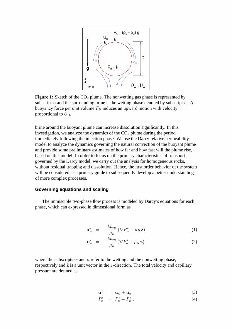
Figure 1 shows a sketch of a CO2 plume. The nonwetting gas phase is immersed inbrine, which is the wetting phase. A buoyancy force per unit volumeFB results inupward motion with velocity proportional toUB, inducing a downward flow of brinearound the plume. During the evolution of the CO2 plume in the post injection period,the processes of residual trapping and dissolution are expected to play the primaryrole. While in general, one can expect the CO2 plume, which is immiscible with thesurrounding brine, to rise due to buoyancy, the particular mechanisms of transport arethe subject of active research [6, 7, 8].

The main issues that need to be addressed are: (1) How far can the plume rise, (2)what is the velocity of rise and (3) how far does the plume spread during its ascent?The last issue is important from the point of view of dissolution, which occursimmediately when the gas comes into contact with unsaturated brine. However, sincethe amount of CO2 that can be dissolved in brine is small, a continuous supply of fresh

ρw , µw

ρn , µng

D

FB = (ρw - ρw) gUB

z

x

Figure 1: Sketch of the CO2 plume. The nonwetting gas phase is represented bysubscriptn and the surrounding brine is the wetting phase denoted by subscriptw. Abuoyancy force per unit volumeFB induces an upward motion with velocityproportional toUB.

brine around the buoyant plume can increase dissolution significantly. In thisinvestigation, we analyze the dynamics of the CO2 plume during the periodimmediately following the injection phase. We use the Darcy relative permeabilitymodel to analyze the dynamics governing the natural convection of the buoyant plumeand provide some preliminary estimates of how far and how fast will the plume rise,based on this model. In order to focus on the primary characteristics of transportgoverned by the Darcy model, we carry out the analysis for homogeneous rocks,without residual trapping and dissolution. Hence, the first order behavior of the systemwill be considered as a primary guide to subsequently develop a better understandingof more complex processes.

Governing equations and scaling

The immiscible two-phase flow process is modeled by Darcy’s equations for eachphase, which can expressed in dimensional form as

u∗w = −kkrw

µw

(∇P ∗w + ρ g z) (1)

u∗n = −kkrn

µn

(∇P ∗n + ρ g z) (2)

where the subscriptsw andn refer to the wetting and the nonwetting phase,respectively andz is a unit vector in thez-direction. The total velocity and capillarypressure are defined as

u∗T = uw + un (3)

P ∗c = P ∗

n − P ∗w . (4)

Equations 1 and 2, along with Eqs. 3 and 4, can be used to construct an expression forthe nonwetting phase velocity

u∗n =µw k

∗rn

µn k∗rw + µw k∗rn

u∗T

− kk∗rw k

∗rn

µn k∗rw + µw k∗rn

(dP ∗

c

dSw

∇Sn −∆ρ g z

)(5)

Similarly, the equation for the total velocity is

u∗T = − k

µw µn

(µn k∗rw + µw k

∗rn) ∇P ∗

n

+ kk∗rw

µw

(dP ∗

c

dSw

∇Sn −∆ρ g z

)(6)

where the density difference∆ρ = (ρw − ρn). Pressure is redefined to be

∇P ∗n = ∇P ∗

n + ρn g z . (7)

In order to make the above equations dimensionless we use the plume diameterD asthe length scale, as shown in Fig. 1 and the buoyancy velocityUB as the velocity scale,

UB = k∆ρ g/µw . (8)

Equations 5 and 6 in dimensionless form are

un = fn uT −krw krn

Caλ

dPc

dSw

∇Sn +krw krn

λM z (9)

uT = − λ

M∇Pn +

krw

M Ca

dPc

dSw

∇Sn − krw z , (10)

where

fn =M krn

λ(11)

λ = M krn + krw (12)

M =µw k

(1)rn

µn k(0)rw

. (13)

The end point values of relative permeability,k(0)rw andk(1)

rn , are used to scalerelative permeability functions and appear in the definition of the mobility ratioM .The relevant scalings for the nonwetting phase pressure and the capillary pressure are,

P ∗n = Pn

µn UB D

k, (14)

P ∗c = Pc γnw

√φ

k, (15)

whereγnw is the interfacial tension,φ is the porosity andk the permeability. Thecapillary number,Ca, is defined as

Ca =µn UB D√k φ γnw

. (16)

This capillary number can be interpreted as the macroscopic capillary number.Ca canalso be stated in terms of the microscopic capillary number,Cam,

Ca = CamD√k φ

. (17)

Equations governing the transport of the nonwetting phase and the incompressibilitycondition are,

∂Sn

∂t+∇ · un = 0 , (18)

∇ · uT = 0 , (19)

wheret is scaled withUB/D. The boundary conditions are

uT = 0 ; x = ±∞Sn = 0 ; x = ±∞ (20)

∇Pn = 0 ; x = ±∞ ,

which assume infinite vertical extent. The above equations are characterized by twomain nondimensional parameters, which are the time,t, and capillary number,Ca.These parameters can be expressed as

t∗ =µnDφ

k∆ρ gt , (21)

Ca =∆ ρ g D

√k√

φ γnw

. (22)

Note that the capillary number is independent of viscosity and can also be expressed interms of the Bond number as,

Bo =∆ ρ g d2

γnw

, (23)

Ca = Bo

/ √φ d2

D√k, (24)

whered is some characteristic pore length∼ O (10−5)m. Hence the capillary numberin this problem can be interpreted as representing the influence of the ratio of gravityto capillary effects relative to the ratio of the microscopic to macroscopic lengths.

Some particular values of density, viscosity and permeability relevant to the CO2

sequestration problem are

∆ρ = 103 kg/m3

µw = 1× 10−3 Pa-s

µn = 0.03× 10−3 Pa-s

γnw = 40× 10−3 N/m

φ = 0.3

k = 10−14 m2

D = 102 m

d = 10−5 m .

Based on these values,UB ∼ 10−6 m/s, and the dimensionless numbers are estimatedto be,

Bo ∼ 10−3 (25)

Cam ∼ 10−5 (26)

Ca ∼ 102 . (27)

The values of these dimensionless numbers may indicate a regime of pore scaleinstability[9], such that current macroscopic models may not be applicable. However,

Sn

flux

func

tion,

f n

0 0.2 0.4 0.6 0.80

0.1

0.2

0.3 M=1M=10M=1/10

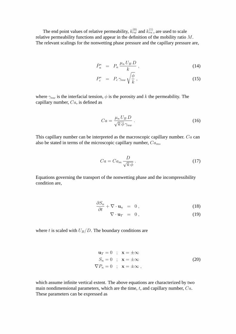
Figure 2: Flux function for zero injection velocity for different values of the mobilityratio. The flux function decays to zero at the maximum and minimum values ofsaturation. The vanishing gradient at intermediate saturations implies that thesaturations move in opposite directions, starting from the stagnation point.

this issue is unresolved and requires extensive investigation. For now, we will use thestandard two-phase Eqs. 5 and 6 in order to obtain preliminary estimates regarding theplume evolution.

One-dimensional solution

Before we solve the full 2-D problem, it is useful to look at the 1-D solutions ofEq. 18 to determine the influence of the viscosity ratio and capillary number for somesimple cases. Physically, the one-dimensional problem can be constructed as a layer ofa lighter nonwetting fluid, unbounded in the lateral extent, which is surrounded by theheavier wetting fluid. The wetting phase is not connected, hence the plume will notrise as a whole. This allows the analysis of the frontal displacements, only as afunction of relative permeability and the viscosity ratio. We will designate the topportion of this layer, where the heavier wetting fluid (Brine) is above the lighternonwetting fluid (CO2), as the front end. The lower part of the layer, where the heavierfluid is below the lighter fluid, will be referred to as the back end. We assume therelative permeability and capillary functions to be

krn =

(Sn − Snr

∆S

)2

, (28)

krw =

(1− Sn − Snr

∆S

)2

, (29)

dPc

dSw

= − 1

krn krw

, (30)

where∆S = 1− Snr − Swr, andSnr andSwr are the residual saturations for the

Sn

0 0.2 0.4 0.6 0.8-1

0

1

2

3

M=1M=10M=1/10

z

(a)

t-0

plume bottom

Sn

0 0.2 0.4 0.6 0.8-1

0

1

2

3

4

M=1, t=4M=10, t=2M=1/10, t=8

z

(b)

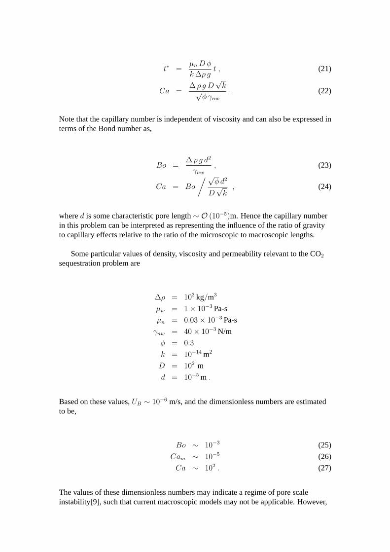
Figure 3: Saturation profiles for a 1-D plume forCa = 400. (a) t = 1, and (b) latetimes. The initial profile with a unit height is indicated by circular symbols in plot (a).The bottom of the plume is stationary while portions of the top end move upwards anddownwards according to Eq. 31.

nonwetting and the wetting fluids, respectively. Thez-direction component of Eq. 18with uT = 0 can be expressed as

∂Sn

∂t+

∂

∂z

(M

λkrw krn −

1

Caλ

∂Sn

∂z

)= 0 . (31)

Equation 31 is a weakly parabolic equation for largeCa. Similar to the purelyhyperbolic caseCa→∞, the solution develops along characteristics based on the fluxfunctionfnw = krw krn/λ. The flux function is plotted as a function of the nonwettingsaturation in Fig. 2 for various values of the mobility ratio. The plotted curves showthat thefnw curve goes through a maximum indicating a zero wave speed at thatsaturation. This leads to the development of two shocks with opposite speeds at thefront end. The upward moving shock spans saturations0 < Sn < ssu, while thedownward moving shock develops forssd < Sn < swi, wheressu andssd are the shocksaturations for the upward and downward moving shocks, respectively. The fluxfunction for theM = 10 case, that is when the plume is less viscous than the brine,shows the shock speeds are highest compared toM = 1 andM = 1/10 cases.

We use the physical capillary dispersion in the problem to obtain high accuracynumerical solutions that converge to the correct entropy solution in the limit ofvanishing dispersion. High accuracy numerical solutions are obtained with the4th

order accurate in time Runge-Kutta scheme and with6th order spatial accuracy throughWENO discretization[10]. The capillary dispersion term is solved with6th ordercentral, compact finite-difference scheme[11].

The solution of Eq. 31 is plotted in Fig. 3(a) for various values ofM . The initialcondition is a layer of CO2 of unit length positioned atz = 0 with Swi = 0.8 andSnr = 0, as shown with circular symbols in Fig. 3(a). In theM = 1 case, the shock

Sn

0 0.1 0.2 0.3

0

5

10

z

M=1M=10M=1/10

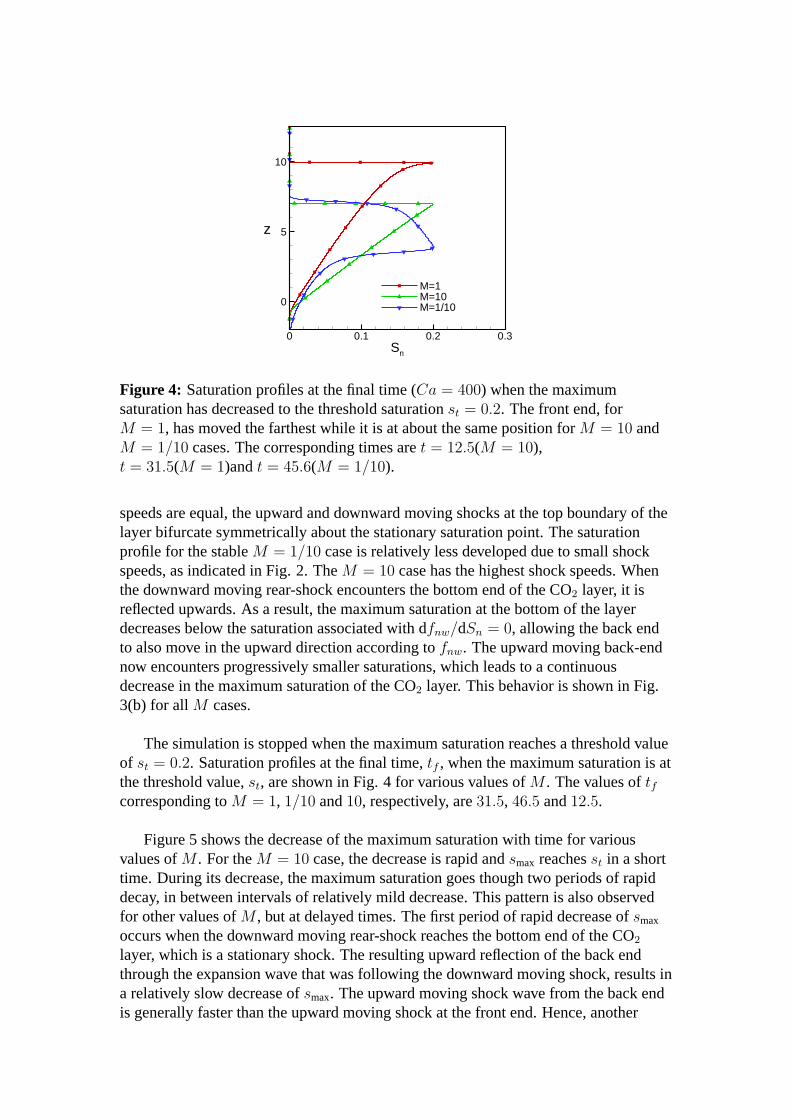
Figure 4: Saturation profiles at the final time (Ca = 400) when the maximumsaturation has decreased to the threshold saturationst = 0.2. The front end, forM = 1, has moved the farthest while it is at about the same position forM = 10 andM = 1/10 cases. The corresponding times aret = 12.5(M = 10),t = 31.5(M = 1)andt = 45.6(M = 1/10).

speeds are equal, the upward and downward moving shocks at the top boundary of thelayer bifurcate symmetrically about the stationary saturation point. The saturationprofile for the stableM = 1/10 case is relatively less developed due to small shockspeeds, as indicated in Fig. 2. TheM = 10 case has the highest shock speeds. Whenthe downward moving rear-shock encounters the bottom end of the CO2 layer, it isreflected upwards. As a result, the maximum saturation at the bottom of the layerdecreases below the saturation associated with dfnw/dSn = 0, allowing the back endto also move in the upward direction according tofnw. The upward moving back-endnow encounters progressively smaller saturations, which leads to a continuousdecrease in the maximum saturation of the CO2 layer. This behavior is shown in Fig.3(b) for allM cases.

The simulation is stopped when the maximum saturation reaches a threshold valueof st = 0.2. Saturation profiles at the final time,tf , when the maximum saturation is atthe threshold value,st, are shown in Fig. 4 for various values ofM . The values oftfcorresponding toM = 1, 1/10 and10, respectively, are31.5, 46.5 and12.5.

Figure 5 shows the decrease of the maximum saturation with time for variousvalues ofM . For theM = 10 case, the decrease is rapid andsmax reachesst in a shorttime. During its decrease, the maximum saturation goes though two periods of rapiddecay, in between intervals of relatively mild decrease. This pattern is also observedfor other values ofM , but at delayed times. The first period of rapid decrease ofsmax

occurs when the downward moving rear-shock reaches the bottom end of the CO2

layer, which is a stationary shock. The resulting upward reflection of the back endthrough the expansion wave that was following the downward moving shock, results ina relatively slow decrease ofsmax. The upward moving shock wave from the back endis generally faster than the upward moving shock at the front end. Hence, another

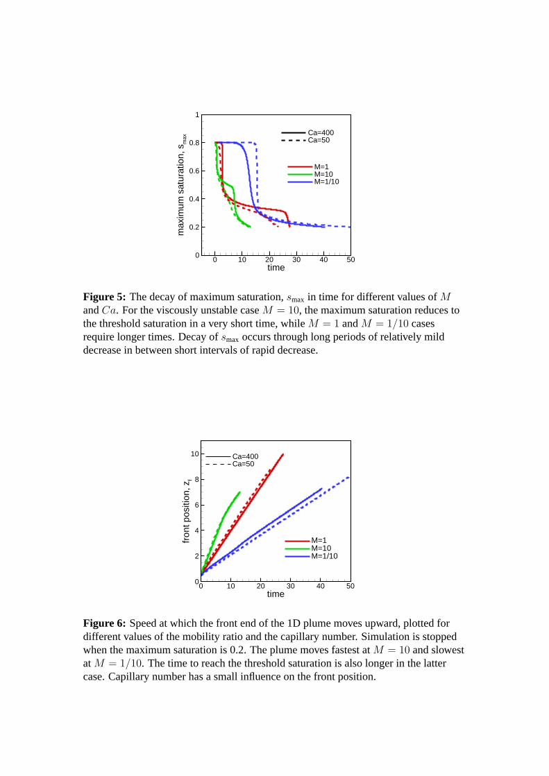
time

max

imum

satu

ratio

n,s m

ax

0 10 20 30 40 500

0.2

0.4

0.6

0.8

1

M=1M=10M=1/10

Ca=400Ca=50

Figure 5: The decay of maximum saturation,smax in time for different values ofMandCa. For the viscously unstable caseM = 10, the maximum saturation reduces tothe threshold saturation in a very short time, whileM = 1 andM = 1/10 casesrequire longer times. Decay ofsmax occurs through long periods of relatively milddecrease in between short intervals of rapid decrease.

time

fron

tpos

ition

,zf

0 10 20 30 40 500

2

4

6

8

10

M=1M=10M=1/10

Ca=400Ca=50

Figure 6: Speed at which the front end of the 1D plume moves upward, plotted fordifferent values of the mobility ratio and the capillary number. Simulation is stoppedwhen the maximum saturation is 0.2. The plume moves fastest atM = 10 and slowestatM = 1/10. The time to reach the threshold saturation is also longer in the lattercase. Capillary number has a small influence on the front position.

shock interaction occurs leading to a rapid decrease insmax. Small capillary numbersmask periods of sharp decay and give rise to an almost uniformly decreasing trend atall times, as shown in Fig. 5.

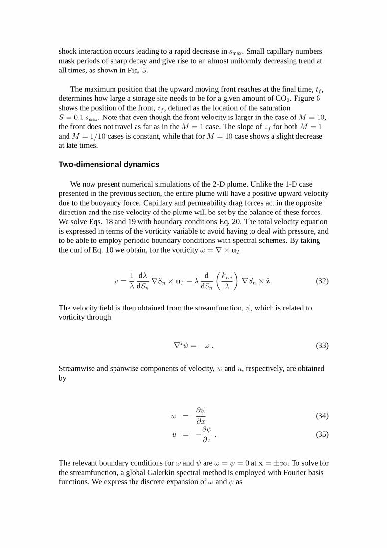
The maximum position that the upward moving front reaches at the final time,tf ,determines how large a storage site needs to be for a given amount of CO2. Figure 6shows the position of the front,zf , defined as the location of the saturationS = 0.1 smax. Note that even though the front velocity is larger in the case ofM = 10,the front does not travel as far as in theM = 1 case. The slope ofzf for bothM = 1andM = 1/10 cases is constant, while that forM = 10 case shows a slight decreaseat late times.

Two-dimensional dynamics

We now present numerical simulations of the 2-D plume. Unlike the 1-D casepresented in the previous section, the entire plume will have a positive upward velocitydue to the buoyancy force. Capillary and permeability drag forces act in the oppositedirection and the rise velocity of the plume will be set by the balance of these forces.We solve Eqs. 18 and 19 with boundary conditions Eq. 20. The total velocity equationis expressed in terms of the vorticity variable to avoid having to deal with pressure, andto be able to employ periodic boundary conditions with spectral schemes. By takingthe curl of Eq. 10 we obtain, for the vorticityω = ∇× uT

ω =1

λ

dλdSn

∇Sn × uT − λd

dSn

(krw

λ

)∇Sn × z . (32)

The velocity field is then obtained from the streamfunction,ψ, which is related tovorticity through

∇2ψ = −ω . (33)

Streamwise and spanwise components of velocity,w andu, respectively, are obtainedby

w =∂ψ

∂x(34)

u = −∂ψ∂z

. (35)

The relevant boundary conditions forω andψ areω = ψ = 0 atx = ±∞. To solve forthe streamfunction, a global Galerkin spectral method is employed with Fourier basisfunctions. We express the discrete expansion ofω andψ as

ωm,n =J∑0

K∑0

ωj,kexp

(i 2π j

m

MAz

+ i 2π kn

NAx

)(36)

ψm,n =J∑0

K∑0

ψj,kexp

(i 2π j

m

MAz

+ i 2π kn

NAx

)(37)

whereAz = H/D andAx = L/D are the normalized dimensions of the computationaldomain in thez andx-directions, respectively.N ,M are the number of grid points andJ ,K are the number of Fourier modes. Equation 33 can now be formulated in thespectral space. Sinceω andψ are real valued, only real parts of the eigenfunctionsωandψ are calculated,

ψj,k =ωj,k

(πj/Az)2 + (πk/Ax)2. (38)

After ψ is obtained from Eq. 38, it is transformed back into physical space to obtainwandu velocity components from Eqs. 34 and 35. The gradients in thez andx-directions are evaluated through6th order compact finite difference discretizationwith symmetric boundary conditions. The domain extentsAz = 10 andAx = 5 werefound to provide a good approximation to an infinite space.

The transport Eq. 18 is solved with4th order Runga-Kutta method. The spatialderivatives are evaluated with8th order accurate compact finite differencediscretization. The simulation is started with a circular plume of unit diameter centeredat (z = 0, x = 0). The initial plume is slightly diffused to avoid discontinuities insaturation values. Initial velocities are prescribed as(w = 0, u = 0) at t = 0. We use∼ 104 grid points to accurately resolve the steep gradients at the fronts.

Figure 7(left) shows the contour plots of saturation at an early time oft = 1 forM = 1 andCa = 200. The plume has progressed slightly from its initial positionleaving behind a wake of small saturation values. The location of the higher saturationvalues, indicated by regions with red color, has shifted towards the back end, similar tothe 1-D case discussed in the previous section. Due to the generation of spanwisevelocity in the 2-D case, the plume profile appears to bulge slightly in thex-coordinate. Figure 7(right) shows the plume profile at a later timet = 6. The plumehas traveled upwards about5 nondimensional units at this time. The shape of theplume has deviated significantly from the circular initial profile to attain a pointed tipfollowed by a broader tail. Velocity vectors plotted in Fig. 7 show that at early timesthe magnitude of the spanwise velocity is comparable to the streamwise component,which generates significant recirculation around the plume. At later time, Fig. 7(right)shows that the streamwise component is dominant and the spanwise velocity isconcentrated only at the tip of the plume. Hence, the ability of the plume to inducedownward motion in brine is significantly reduced at later times. As for the 1-D case,the simulation is stopped when the threshold saturationst = 0.2 is reached.

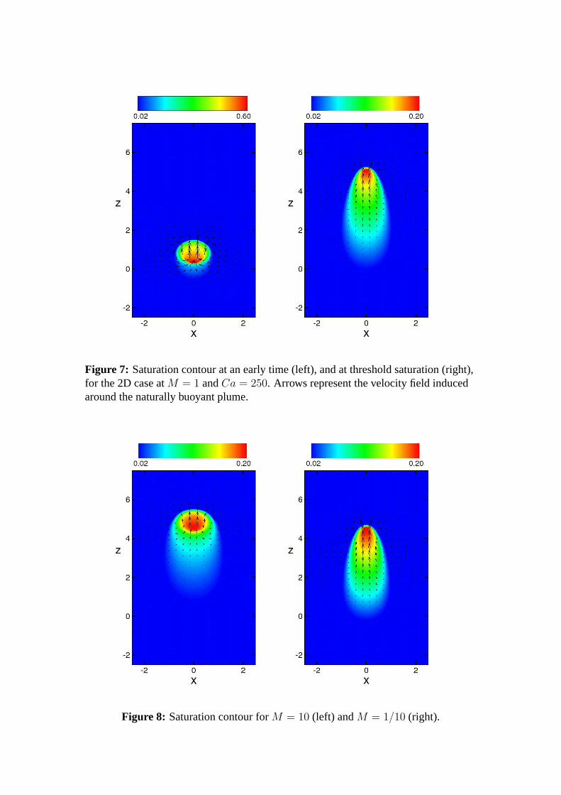
Figure 7: Saturation contour at an early time (left), and at threshold saturation (right),for the 2D case atM = 1 andCa = 250. Arrows represent the velocity field inducedaround the naturally buoyant plume.

Figure 8: Saturation contour forM = 10 (left) andM = 1/10 (right).

time

fron

tpos

ition

,zf

0 10 20 30 40 500

2

4

6

8

10

M=1M=10M=1/10

2D1D

Figure 9: The front positions obtained from 2-D simulations. The plume migrationdistance in the 2-D case is smaller than the 1-D case. Higher values of the slope ofzf

in the 2-D case indicate the contribution of buoyancy driven motion.

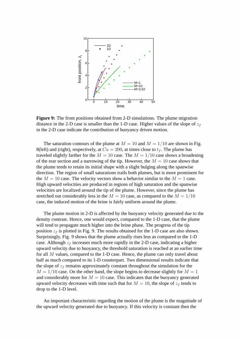
The saturation contours of the plume atM = 10 andM = 1/10 are shown in Fig.8(left) and (right), respectively, atCa = 200, at times close totf . The plume hastraveled slightly farther for theM = 10 case. TheM = 1/10 case shows a broadeningof the rear section and a narrowing of the tip. However, theM = 10 case shows thatthe plume tends to retain its initial shape with a slight bulging along the spanwisedirection. The region of small saturations trails both plumes, but is more prominent fortheM = 10 case. The velocity vectors show a behavior similar to theM = 1 case.High upward velocities are produced in regions of high saturation and the spanwisevelocities are localized around the tip of the plume. However, since the plume hasstretched out considerably less in theM = 10 case, as compared to theM = 1/10case, the induced motion of the brine is fairly uniform around the plume.

The plume motion in 2-D is affected by the buoyancy velocity generated due to thedensity contrast. Hence, one would expect, compared to the 1-D case, that the plumewill tend to propagate much higher into the brine phase. The progress of the tippositionzf is plotted in Fig. 9. The results obtained for the 1-D case are also shown.Surprisingly, Fig. 9 shows that the plume actually rises less as compared to the 1-Dcase. Althoughzf increases much more rapidly in the 2-D case, indicating a higherupward velocity due to buoyancy, the threshold saturation is reached at an earlier timefor all M values, compared to the 1-D case. Hence, the plume can only travel abouthalf as much compared to its 1-D counterpart. Two dimensional results indicate thatthe slope ofzf remains approximately constant throughout the simulation for theM = 1/10 case. On the other hand, the slope begins to decrease slightly forM = 1and considerably more forM = 10 case. This indicates that the buoyancy generatedupward velocity decreases with time such that forM = 10, the slope ofzf tends todrop to the 1-D level.

An important characteristic regarding the motion of the plume is the magnitude ofthe upward velocity generated due to buoyancy. If this velocity is constant then the

time

max

imum

velo

city

10-1 10010-2

10-1

100

0.5

M=1M=10M=1/10

wu

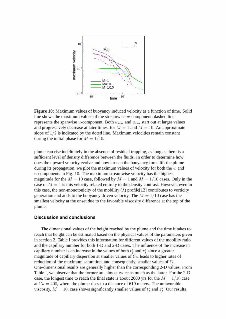
Figure 10: Maximum values of buoyancy induced velocity as a function of time. Solidline shows the maximum values of the streamwisew-component, dashed linerepresents the spanwiseu-component. Bothwmax andumax start out at larger valuesand progressively decrease at later times, forM = 1 andM = 10. An approximateslope of1/2 is indicated by the doted line. Maximum velocities remain constantduring the initial phase forM = 1/10.

plume can rise indefinitely in the absence of residual trapping, as long as there is asufficient level of density difference between the fluids. In order to determine howdoes the upward velocity evolve and how far can the buoyancy force lift the plumeduring its propagation, we plot the maximum values of velocity for both thew andu-components in Fig. 10. The maximum streamwise velocity has the highestmagnitude for theM = 10 case, followed byM = 1 andM = 1/10 cases. Only in thecase ofM = 1 is this velocity related entirely to the density contrast. However, even inthis case, the non-monotonicity of the mobility (λ) profile[12] contributes to vorticitygeneration and adds to the buoyancy driven velocity. TheM = 1/10 case has thesmallest velocity at the onset due to the favorable viscosity difference at the top of theplume.

Discussion and conclusions

The dimensional values of the height reached by the plume and the time it takes toreach that height can be estimated based on the physical values of the parameters givenin section 2. Table I provides this information for different values of the mobility ratioand the capillary number for both 1-D and 2-D cases. The influence of the increase incapillary number is an increase in the values of botht∗f andz∗f since a greatermagnitude of capillary dispersion at smaller values ofCa leads to higher rates ofreduction of the maximum saturation, and consequently, smaller values oft∗f .One-dimensional results are generally higher than the corresponding 2-D values. FromTable I, we observe that the former are almost twice as much as the latter. For the 2-Dcase, the longest time to reach the final state is about 2000 yrs for theM = 1/10 caseatCa = 400, where the plume rises to a distance of 610 meters. The unfavorableviscosity,M = 10, case shows significantly smaller values oft∗f andz∗f . Our results

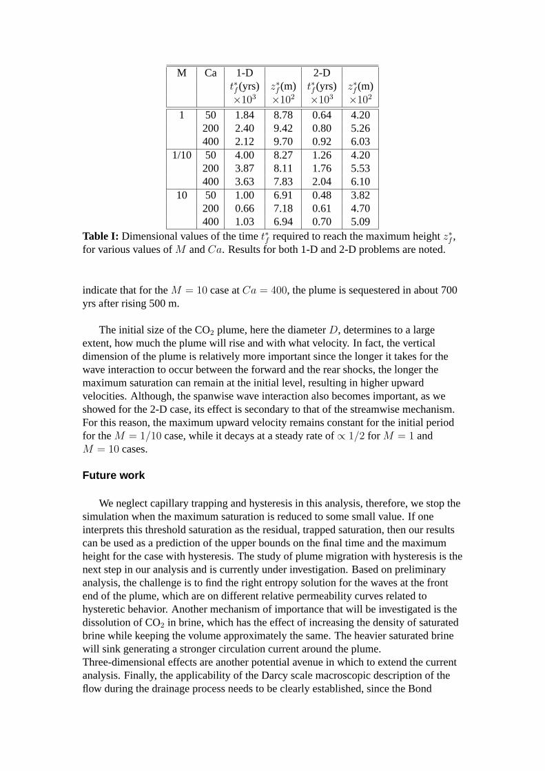
M Ca 1-D 2-Dt∗f (yrs) z∗f (m) t∗f (yrs) z∗f (m)×103 ×102 ×103 ×102

1 50 1.84 8.78 0.64 4.20200 2.40 9.42 0.80 5.26400 2.12 9.70 0.92 6.03

1/10 50 4.00 8.27 1.26 4.20200 3.87 8.11 1.76 5.53400 3.63 7.83 2.04 6.10

10 50 1.00 6.91 0.48 3.82200 0.66 7.18 0.61 4.70400 1.03 6.94 0.70 5.09

Table I: Dimensional values of the timet∗f required to reach the maximum heightz∗f ,for various values ofM andCa. Results for both 1-D and 2-D problems are noted.

indicate that for theM = 10 case atCa = 400, the plume is sequestered in about 700yrs after rising 500 m.

The initial size of the CO2 plume, here the diameterD, determines to a largeextent, how much the plume will rise and with what velocity. In fact, the verticaldimension of the plume is relatively more important since the longer it takes for thewave interaction to occur between the forward and the rear shocks, the longer themaximum saturation can remain at the initial level, resulting in higher upwardvelocities. Although, the spanwise wave interaction also becomes important, as weshowed for the 2-D case, its effect is secondary to that of the streamwise mechanism.For this reason, the maximum upward velocity remains constant for the initial periodfor theM = 1/10 case, while it decays at a steady rate of∝ 1/2 for M = 1 andM = 10 cases.

Future work

We neglect capillary trapping and hysteresis in this analysis, therefore, we stop thesimulation when the maximum saturation is reduced to some small value. If oneinterprets this threshold saturation as the residual, trapped saturation, then our resultscan be used as a prediction of the upper bounds on the final time and the maximumheight for the case with hysteresis. The study of plume migration with hysteresis is thenext step in our analysis and is currently under investigation. Based on preliminaryanalysis, the challenge is to find the right entropy solution for the waves at the frontend of the plume, which are on different relative permeability curves related tohysteretic behavior. Another mechanism of importance that will be investigated is thedissolution of CO2 in brine, which has the effect of increasing the density of saturatedbrine while keeping the volume approximately the same. The heavier saturated brinewill sink generating a stronger circulation current around the plume.Three-dimensional effects are another potential avenue in which to extend the currentanalysis. Finally, the applicability of the Darcy scale macroscopic description of theflow during the drainage process needs to be clearly established, since the Bond

numbers and the capillary numbers for the CO2 sequestration problem are very similarto the cases where microscopic instability is observed.

Propagation of CO2 plumes in sloping aquifers with residualtrapping

Investigators

Franklin M. Orr, Jr., Professor of Energy Resources Engineering; Hamdi Tchelepi,Associate Professor of Energy Resources Engineering; Marc Hesse, GraduateResearch Assistant.

Introduction

As long as the CO2 plume moves due to buoyancy, CO2 is trapped by capillary forcesin the wake of the plume, and it is left behind as trapped/residual saturation (Sgr).Residual CO2 is considered immobile on the reservoir timescale[13], and it is currentlyassumed that the residual CO2 will remain immobile over the timescale that isnecessary to dissolve it into the brine. It is therefore assumed that CO2 that has beentrapped as residual saturation cannot leak back into the atmosphere over the entirestorage period. Early numerical simulations of CO2 storage in saline aquifers[14, 15]did not show significant amounts of residual trapping, because the relativepermeability models did not account for hysteresis, and residual gas saturations wherecommonly set toSgr = 0.05. More recently it has been demonstrated that relativepermeability hysteresis can increase the trapped/residual CO2 saturation toSgr ≈ 0.4in strongly water-wet reservoirs[16]. Various numerical simulations have nowdemonstrated that residual trapping can immobilize significant amounts of CO2

relatively soon after the end of the injection period[16, 17, 18, 19, 20].

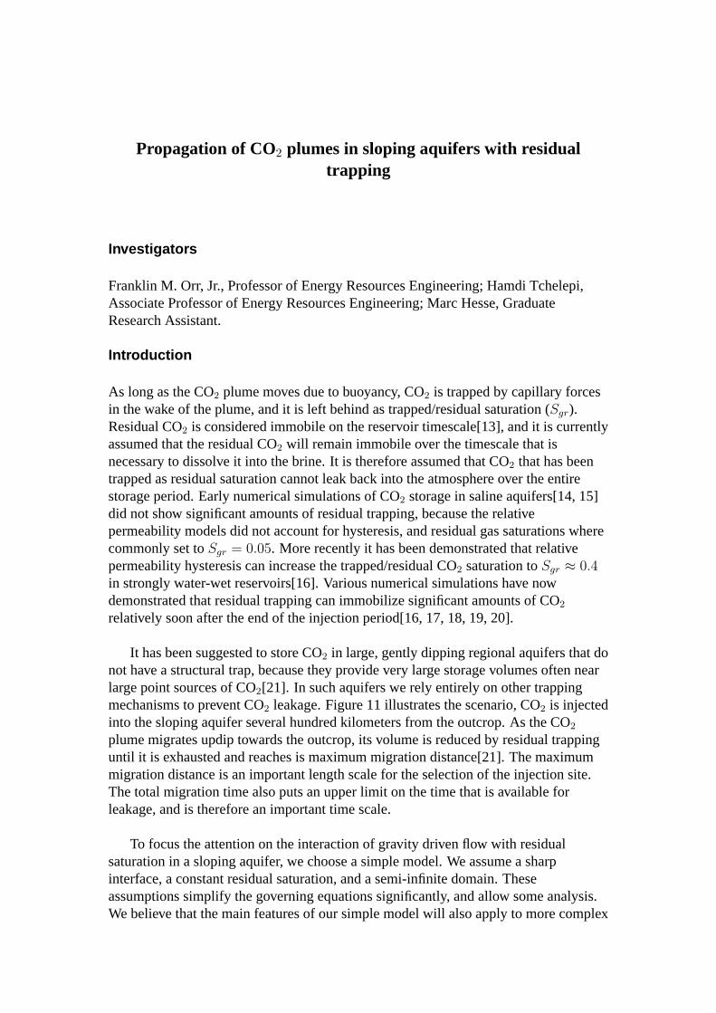
It has been suggested to store CO2 in large, gently dipping regional aquifers that donot have a structural trap, because they provide very large storage volumes often nearlarge point sources of CO2[21]. In such aquifers we rely entirely on other trappingmechanisms to prevent CO2 leakage. Figure 11 illustrates the scenario, CO2 is injectedinto the sloping aquifer several hundred kilometers from the outcrop. As the CO2

plume migrates updip towards the outcrop, its volume is reduced by residual trappinguntil it is exhausted and reaches is maximum migration distance[21]. The maximummigration distance is an important length scale for the selection of the injection site.The total migration time also puts an upper limit on the time that is available forleakage, and is therefore an important time scale.

To focus the attention on the interaction of gravity driven flow with residualsaturation in a sloping aquifer, we choose a simple model. We assume a sharpinterface, a constant residual saturation, and a semi-infinite domain. Theseassumptions simplify the governing equations significantly, and allow some analysis.We believe that the main features of our simple model will also apply to more complex

Figure 11: Migration of CO2 in a gently dipping regional aquifer.

real flows.

Derivation of the governing equation

We consider a finite volume of CO2 migrating along the top of a very deep porouslayer saturated with water. We assume that the height of the interface between thefluids is small compared to the thickness of the porous layer, so that the porous layercan be considered semi-infinite in the vertical direction. We assume that the two fluidsare immiscible, separated by a sharp interface, and that the saturations are constantwithin each fluid. During imbibition when CO2 is replaced by brine, a constanttrapped/residual gas saturationSgr is left behind. During drainage, a constantirreducible/connate water saturation is left behindSwc. The change of the volume ofCO2, ∆Vg, is given by

∆Vg = ∆x∆hφSg = ∆x∆hφ(1− Swc), (39)

whereh(x, t) is the height of the interface separating the fluids, measured down fromthe top of the reservoir.Sg is the saturation of CO2 in the plume which is given by theconnate saturation of brine (Sg = 1− Swr), andφ is the porosity of the medium, whichis assumed to be constant.

We assume the gravity current has a large aspect ratio so that the pressure ishydrostatic and flow is predominantly in the along slope direction. The pressure at thetop of the porous medium (z = 0) is

p(x, z = 0, t) = p0 − g(ρ+ ∆ρ) [x sin θ − h(x, t) cos θ]

− gρh(x, t) cos θ,

whereρ is the density of the gas, the density of the surrounding water isρ+ ∆ρ, andp0 is the pressure at the coordinate origin. The hydrostatic pressure at any point in the

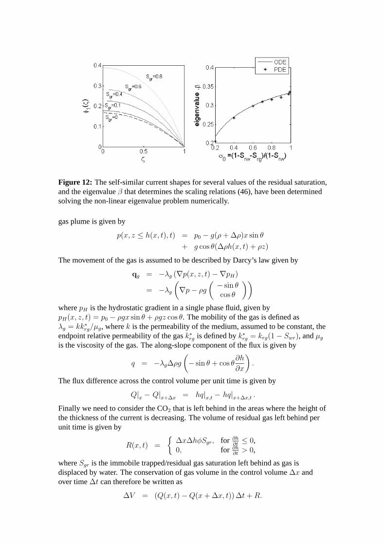
Figure 12: The self-similar current shapes for several values of the residual saturation,and the eigenvalueβ that determines the scaling relations (46), have been determinedsolving the non-linear eigenvalue problem numerically.

gas plume is given by

p(x, z ≤ h(x, t), t) = p0 − g(ρ+ ∆ρ)x sin θ

+ g cos θ(∆ρh(x, t) + ρz)

The movement of the gas is assumed to be described by Darcy’s law given by

qg = −λg (∇p(x, z, t)−∇pH)

= −λg

(∇p− ρg

(− sin θcos θ

))wherepH is the hydrostatic gradient in a single phase fluid, given bypH(x, z, t) = p0 − ρgx sin θ + ρgz cos θ. The mobility of the gas is defined asλg = kk∗rg/µg, wherek is the permeability of the medium, assumed to be constant, theendpoint relative permeability of the gask∗rg is defined byk∗rg = krg(1− Swr), andµg

is the viscosity of the gas. The along-slope component of the flux is given by

q = −λg∆ρg

(− sin θ + cos θ

∂h

∂x

).

The flux difference across the control volume per unit time is given by

Q|x − Q|x+∆x = hq|x,t − hq|x+∆x,t .

Finally we need to consider the CO2 that is left behind in the areas where the height ofthe thickness of the current is decreasing. The volume of residual gas left behind perunit time is given by

R(x, t) =

∆x∆hφSgr, for ∂h

∂t≤ 0,

0, for ∂h∂t> 0,

whereSgr is the immobile trapped/residual gas saturation left behind as gas isdisplaced by water. The conservation of gas volume in the control volume∆x andover time∆t can therefore be written as

∆V = (Q(x, t)−Q(x+ ∆x, t)) ∆t+R.

In the limit ∆x→ 0 and∆t→ 0 we obtain the following non-linear advectiondiffusion equation

∂h

∂t= κ(x, t)

∂

∂x

(h

(− sin θ + cos θ

∂h

∂x

)), (40)

with the discontinuous coefficient

κ(x, t) =

κ1 = kλg∆ρg

φ(1−Swc−Sgr), for ∂h

∂t≤ 0,

κ0 = kλg∆ρg

φ(1−Swc), for ∂h

∂t> 0.

(41)

The residual saturationsSwc andSgr are between 0 and 1, so thatSwr + Sgr ≤ 1, henceκ1 ≥ κ0. The nature of equation 40 becomes clearer if we expand the right hand sideto separate the advective and diffusive terms

∂h

∂t+ v[x, t, θ]

∂h

∂x= D[x, t, θ]

∂

∂x

(h∂h

∂x

). (42)

The advective velocity is given byv = κ[x, t] sin θ, and the diffusion coefficient isgiven byD = κ[x, t] cos θ. Note a diffusion coefficient has dimensions ofL2T−1Ω−1,whereΩ is the dimension of the dependent variable, in this case the dependent variableis h(x, t) which has dimensionL, therefore the diffusion coefficient has dimensions ofvelocity [D] = [v] = [κ] = LT−1.

For a horizontal surface (θ = 0), the equation becomes parabolic and is the onedimensional equivalent of the equation derived by Kochinaet al.[22] for the radialcase. In the limit of no residual trapping (Srg = 0) the equation reduces to the forminvestigated by Huppert and Woods[23]. For the numerical solution of Equation (42)we choose the following dimensionless variables

η = h/H0, χ = x/L0, σ = κ/κ1, τ = t/t∗,

with the time scalet∗ = L20(κ1H0 cos θ)−1, so that we obtain the equation

∂η

∂t= σ(χ, τ)

∂

∂χ

(η

(Pe+

∂η

∂χ

)),

where Pe= L0v/(H0D) = L0/H0 tan θ is a Peclet number. All numerical simulationsreported here had a rectangle function initial condition

h(χ, τ = 0) = u(χ+ 1/2)− u(χ− 1/2), (43)

whereu(χ) is the unit step function. The initial volume of the plume is unity, theinitial volume of mobile CO2 within the plume isV0 = Sg = 1− Swc. Thediscontinuous coefficientσ is now given by:

σ[χ, τ ] =

σ1 = 1, ∂η/∂τ ≤ 0;σ0 = 1−Swc−Sgr

1−Swc, ∂η/∂τ > 0.

(44)

All numerical simulations used a grid spacing of∆χ = 0.02, and the simulation wasterminated when the volume of mobile CO2 in the plume had decreased to a value ofVg = 10−3V0.

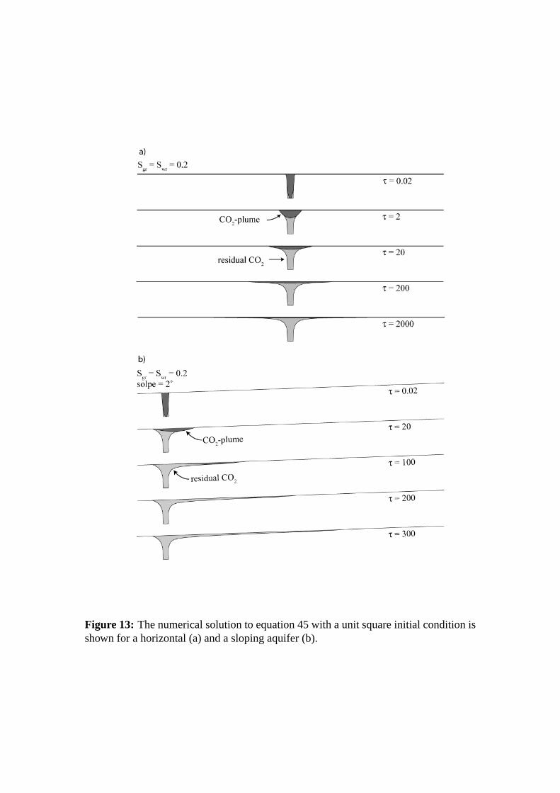
Figure 13: The numerical solution to equation 45 with a unit square initial condition isshown for a horizontal (a) and a sloping aquifer (b).

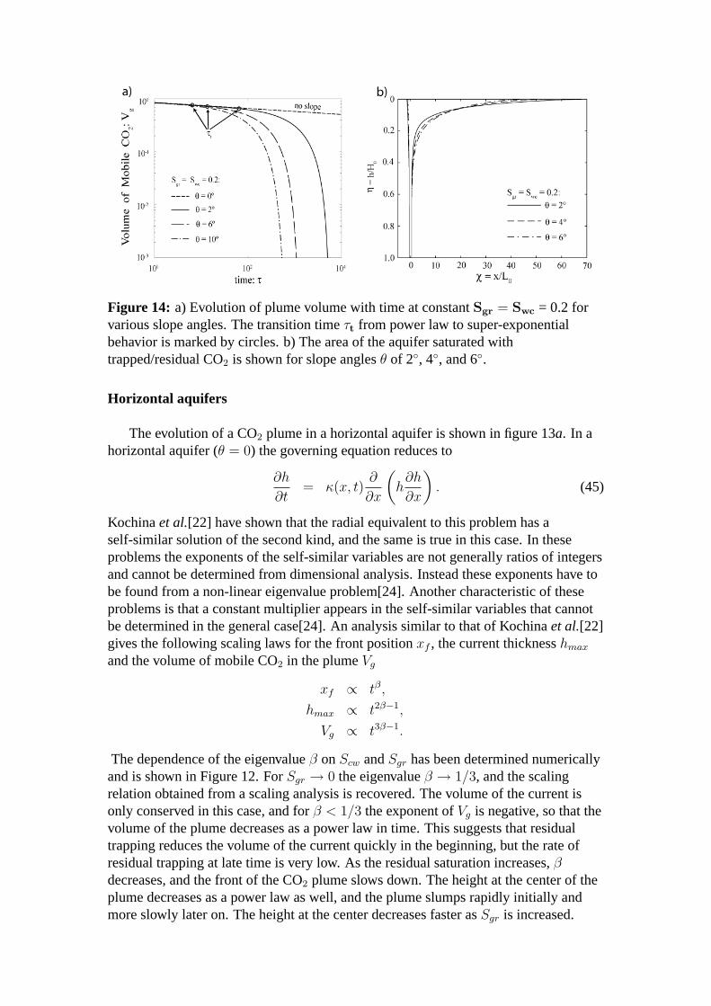
Figure 14: a) Evolution of plume volume with time at constantSgr = Swc = 0.2 forvarious slope angles. The transition timeτt from power law to super-exponentialbehavior is marked by circles. b) The area of the aquifer saturated withtrapped/residual CO2 is shown for slope anglesθ of 2, 4, and 6.

Horizontal aquifers

The evolution of a CO2 plume in a horizontal aquifer is shown in figure 13a. In ahorizontal aquifer (θ = 0) the governing equation reduces to

∂h

∂t= κ(x, t)

∂

∂x

(h∂h

∂x

). (45)

Kochinaet al.[22] have shown that the radial equivalent to this problem has aself-similar solution of the second kind, and the same is true in this case. In theseproblems the exponents of the self-similar variables are not generally ratios of integersand cannot be determined from dimensional analysis. Instead these exponents have tobe found from a non-linear eigenvalue problem[24]. Another characteristic of theseproblems is that a constant multiplier appears in the self-similar variables that cannotbe determined in the general case[24]. An analysis similar to that of Kochinaet al.[22]gives the following scaling laws for the front positionxf , the current thicknesshmax

and the volume of mobile CO2 in the plumeVg

xf ∝ tβ,

hmax ∝ t2β−1,

Vg ∝ t3β−1.

The dependence of the eigenvalueβ onScw andSgr has been determined numericallyand is shown in Figure 12. ForSgr → 0 the eigenvalueβ → 1/3, and the scalingrelation obtained from a scaling analysis is recovered. The volume of the current isonly conserved in this case, and forβ < 1/3 the exponent ofVg is negative, so that thevolume of the plume decreases as a power law in time. This suggests that residualtrapping reduces the volume of the current quickly in the beginning, but the rate ofresidual trapping at late time is very low. As the residual saturation increases,βdecreases, and the front of the CO2 plume slows down. The height at the center of theplume decreases as a power law as well, and the plume slumps rapidly initially andmore slowly later on. The height at the center decreases faster asSgr is increased.

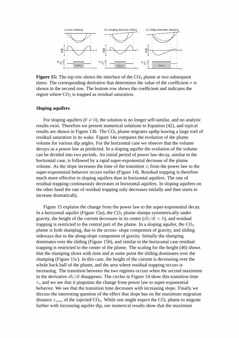
Figure 15: The top row shows the interface of the CO2 plume at two subsequenttimes. The corresponding derivative that determines the value of the coefficientσ isshown in the second row. The bottom row shows the coefficient and indicates theregion where CO2 is trapped as residual saturation.

Sloping aquifers

For sloping aquifers (θ 6= 0), the solution is no longer self-similar, and no analyticresults exist. Therefore we present numerical solutions to Equation (42), and typicalresults are shown in Figure 13b. The CO2 plume migrates updip leaving a large trail ofresidual saturation in its wake. Figure 14a compares the evolution of the plumevolume for various dip angles. For the horizontal case we observe that the volumedecays as a power law as predicted. In a sloping aquifer the evolution of the volumecan be divided into two periods. An initial period of power law decay, similar to thehorizontal case, is followed by a rapid super-exponential decrease of the plumevolume. As the slope increases the time of the transitionτt from the power law to thesuper-exponential behavior occurs earlier (Figure 14). Residual trapping is thereforemuch more effective in sloping aquifers than in horizontal aquifers. The rate ofresidual trapping continuously decreases in horizontal aquifers. In sloping aquifers onthe other hand the rate of residual trapping only decreases initially and then starts toincrease dramatically.

Figure 15 explains the change from the power law to the super-exponential decay.In a horizontal aquifer (Figure 15a), the CO2 plume slumps symmetrically undergravity, the height of the current decreases in its center (dh/dt < 0), and residualtrapping is restricted to the central part of the plume. In a sloping aquifer, the CO2

plume is both slumping, due to the across- slope component of gravity, and slidingsideways due to the along-slope component of gravity. Initially the slumpingdominates over the sliding (Figure 15b), and similar to the horizontal case residualtrapping is restricted to the center of the plume. The scaling for the height (46) showsthat the slumping slows with time and at some point the sliding dominates over theslumping (Figure 15c). In this case, the height of the current is decreasing over thewhole back half of the plume, and the area where residual trapping occurs isincreasing. The transition between the two regimes occurs when the second maximumin the derivativedh/dt disappears. The circles in Figure 14 show this transition timeτt, and we see that it pinpoints the change from power law to super-exponentialbehavior. We see that the transition time decreases with increasing slope. Finally wediscuss the interesting question of the effect that slope has on the maximum migrationdistancexmax of the injected CO2. While one might expect the CO2 plume to migratefarther with increasing aquifer dip, our numerical results show that the maximum

migration distance decreases with increasing slope. This surprising result becomesclear when we consider the following geometric argument (Figure 14b). The CO2

plume must be exhausted once the volume of trapped/residual saturation in the areaswept by the plume equals the initial volume of CO2. The total area of the aquiferAt

that needs to be swept by the CO2 plume isAt = (1− Swc)/SgrA0. As the slopeincreases, the CO2 plume migrates sideways (slides) faster and slumps more slowly,and it therefore has a greater vertical sweep. SinceAt is constant, increased verticalsweep leads to a shorter migration distance.

Implications for CO 2 storage in saline aquifers.

The results presented above suggest that residual trapping will be very effective insloping aquifers, even if the dip is very small. We will explore the length and timescales with an example calculation, using the same physical properties used above. Weassume a slope ofθ = 4, a connate brine saturationSwc = 0.1, a trapped/residual CO2saturation ofSgr = 0.2, an initial plume width at the end of injection ofL0 ≈ 1000m,and a plume height ofH0 ≈ 100m. In this case Pe= 0.699 andσ = 0.778. Numericalsolution of Equation (43) gives the following maximum migration distance:χmax ≈ 50. The dimensional maximum migration distance in this case isxmax = χmax ∗ L0 = 50 km updip of the injection site. This example suggests thatresidual trapping can contain the injected CO2 within reasonable distance of theinjection well. Therefore storage in gently sloping aquifers without a structural trapmay be possible if the injection site is selected to be far enough from the expectedleakage location.

Further work on sloping aquifers.

The results presented above on the interaction of aquifer slope and residualtrapping are preliminary, and we intend to expand them to cover the whole parameterspace in Pe[θ, L0/H0] andσ[Sgr, Swc]. Preliminary results suggest that simple scalinglaws for the dependence ofτt, τmax, andχmax on Pe andσ exist. And we will present afull discussion in our next report. An extension of this analysis to the radial case wouldallow more realistic estimates of the maximum migration distance, and would providea simple tool for the screening of potential storage sites.

Conclusions

Semi-analytic results for a plume spreading in a horizontal aquifer, show that thevolume of the mobile CO2 plume decays as a power law. Therefore, the efficiency ofresidual trapping in horizontal aquifers decreases with time. In sloping aquifers, aninitial power law decay is followed by super-exponential decrease of the mobile CO2

volume. This result suggests that residual trapping will be an effective way to reducethe volume of mobile CO2 in sloping aquifers. The increased vertical sweep in slopingaquifers also leads to a decrease in the maximum migration distance with increasingslope. Due to this enhanced residual trapping, sloping aquifers appear to be reasonabletargets for CO2 storage. Aquifers without a structural trap may be considered aspotential storage sites, if the injection site is sufficiently far away from the potentialleakage locations.

Construction of High-Order Adaptive Implicit Methodsfor Reservoir Simulation

Investigators

Hamdi Tchelepi, Associate Professor of Energy Resources Engineering; Romain deLoubens, Graduate Research Assistant; Amir Riaz, Research Associate.

Introduction

The success of the Adaptive Implicit Method (AIM) in reservoir simulation ismostly due to its increased efficiency compared to the traditional IMPES or FIMformulations (see [25], [26], [27], [28], [29] and [30]). The reduction of thecomputational cost comes from the mixed implicit-explicit treatment of the individualgrid block variables. However the standard AIM discretization of the massconservation equations is only first-order accurate in space and time. We aredeveloping high-order AIM approximations, for both space and time, in order toenhance the solution fidelity and improve the overall computational efficiency.

In the first section we present a numerical analysis of standard AIM. The first partof this analysis focuses on the consistency and convergence properties in the presenceof implicit-explicit boundaries. Then we study some important monotonicityproperties in the one-dimensional case. In the second section, we propose an AIMformulation based on highly accurate MOL schemes. Fully high-order AIM schemesare derived and then tested in 1D and 2D. Finally, we present an artificial viscositymethod to improve the monotonicity restriction in the implicit regions.

Numerical analysis of the standard AIM

Local inconsistency and convergence study

Consider one-dimensional flow of two immiscible phases in a porous medium.Under certain assumptions, this problem is described by the Buckley-Leverett equation

∂s

∂t+∂f(s)

∂x= 0 , (46)

where it is assumed for simplicity thatf ′(s) ≥ 0. The initial and boundary conditionsare given by

s(x, 0) = swc , s(0, t) = swi , (47)

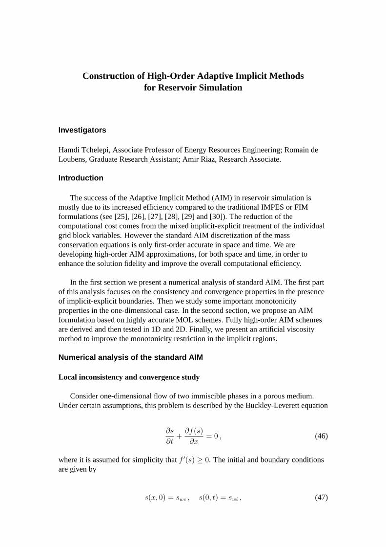
whereswc is the connate water saturation andswi the inlet saturation. In the following,we consider a uniform grid of sizem, with a unique implicit-explicit boundarybetween blocks (i− 1) and (i) (see figure 16). Here information propagates from leftto right so this configuration corresponds to an I→E boundary.

Figure 16: Schematic of an implicit-explicit (I-E) boundary

For this configuration, the standard AIM discretization reads:

0 =sn+1

j − snj

∆t+

1

∆x

[f(sn+1

j )− f(sn+1j−1 )

], j < i , (48)

0 =sn+1

j − snj

∆t+

1

∆x

[f(sn

j )− f(sn+1j−1 )

], j = i , (49)

0 =sn+1

j − snj

∆t+

1

∆x

[f(sn

j )− f(snj−1)

], j > i . (50)

Using Taylor series expansions we can show that the truncation error in the firstexplicit block (j = i) is given by

Eni = −∆t

∆x[f(s)t]

n+1i +O(∆x) +O(∆t) +O(∆t2/∆x) . (51)

The above equation indicates that the standard AIM scheme is inconsistent at thetransition from an implicit to an explicit region. Similarly, it is inconsistent at thetransition from an explicit to an implicit region. But by construction the standard AIMscheme is stable, so we do not expect the discretization errors at the various I-Eboundaries to be amplified with time. Nevertheless, convergence is not guaranteed apriori because the Lax equivalence theorem does not apply. Hence we need an erroranalysis to understand how these discretization errors propagate and to deduce theconvergence properties.

A linear error analysis shows that in the case of a fixed I-E boundary, the error afterNtime steps is given by

E (N) =N∑

k=1

MN−kS(k) . (52)

HereM is the standard AIM operator corresponding to the mesh size∆x = L/m andthe time step size∆t = Tf/N , while S(k) is a first-order source term due to the

inconsistency at the I-E boundary. The matrix vector products in (52) can be computedexactly, and we can prove that in the sense of the infinite norm, we obtain

lim∆x,∆t→0∆t<∆x

E (N) = 0 . (53)

This statement means that in this particular case the standard AIM scheme isconvergent, even though it is inconsistent at the I-E boundary. In fact, the convergenceproperties rely on the dissipative nature of the discretization. In practice, each I-Eboundary may create a “kink” in the solution profile. Those kinks are of order one, sothey are comparable to the numerical dispersion. But as we will see in the followingsubsections, in general the standard AIM still verifies strong monotonicity properties

Linear positivity and the maximum principle

In the linear case, the numerical approximation attn+1 is given by

s(n+1) = Ms(n) , (54)

whereM is the standard AIM operator. It is easy to show that this operator satisfiesM ≥ 0 (component-wise inequalities), which means that it is monotone. In particular,if s(n) ≥ 0, we have

s(n+1) = Ms(n) ≥ 0 . (55)

The above statement shows the linear positivity of the standard AIM scheme. In factthe monotonicity ofM implies that this scheme satisfies the maximum principle,which is an even stronger monotonicity property. Indeed, ifs(n) ≤ C1e(component-wise inequality withe = (1, . . . , 1)T ) for some arbitrary constantC1, then

s(n+1) = Ms(n) ≤ C1Me = C1e . (56)

Similarly if s(n) ≥ C2e, we obtains(n+1) ≥ C2e. Therefore, the standard AIMapproximation satisfies the maximum principle. However there is no guarantee that thestandard AIM scheme is oscillation-free. In fact, a scheme may satisfy the maximumprinciple and still produce localized overshoots or undershoots. Hence we propose toanalyze the total variation diminishing (TVD) property of the standard AIM scheme.

TVD property in the linear case

In the linear homogeneous case, for an I→E boundary (see figure 16), we have

(1 + λ)[sn+1i − sn+1

i−1 ] = λ[sn+1i−1 − sn+1

i−2 ] + [sni − sn

i−1] , i = 1, . . . , p , (57)

[sn+1p+1 − sn+1

p ] = (1− λ)[snp+1 − sn

p ] + λ[sn+1p − sn+1

p−1 ] + λ[sn+1p − sn

p ] , (58)

[sn+1p+2 − sn+1

p+1 ] = (1− λ)[snp+2 − sn

p+1] + λ[snp+1 − sn

p ]− λ[sn+1p − sn

p ] , (59)

[sn+1i − sn+1

i−1 ] = (1− λ)[sni − sn

i−1] + λ[sni−1 − sn

i−2] , i = p+ 3, . . . ,m , (60)

whereλ = ∆t∆x≤ 1. By manipulating these equations, we can show that

m∑i=1

|sn+1i − sn+1

i−1 | ≤m∑

i=1

|sni − sn

i−1| , (61)

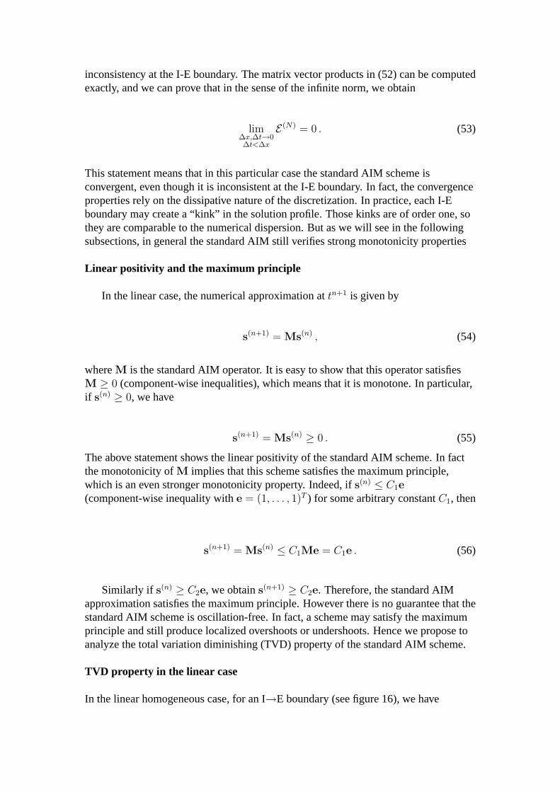
which means that the scheme is TVD, i.e.TV (sn+1) ≤ TV (sn) (see [31]). The sameresult is obtained in the case of an E→I boundary.

Figure 17 shows numerical results for the linear advection problem when the initialcondition is a jump discontinuity. The standard AIM solution (AIM-STD-UW1) canbe compared with the exact solution computed by the Method of Characteristics(MOC), and with the Forward Euler solution (FE-UW1). In the left plot, there is onlyone I→E boundary moving at a unit speed, thus following the jump discontinuity. Asexpected from the above results, the numerical solution remains monotonic. In theright plot, every other block is implicit, i.e. there is an I-E boundary at each cellinterface. Even in this situation, the TVD property is preserved.

Figure 17: Linear homogeneous case with a jump discontinuity

TVD property in the quasi-linear case

Here we consider the more general case wheref is a nonlinear function ofs, butfor simplicity we assume thatf ′ ≥ 0. As required, every explicit block satisfies theclassical CFL condition:

maxs∈[sn

i−1,sni ]|f ′(s)| ∆t

∆x≤ 1 . (62)

First we can show that the standard AIM discretization is always TVD across an E→Iboundary. The proof relies on the fact that the numerical speed of propagation in theexplicit region is greater than the physical speed, as implied by (62). Therefore themass accumulation over one time step in the first implicit block is limited by thepositive or negative mass difference with the upstream block.

In the case of an I→E boundary, the standard AIM is generally not TVD. However wecan show that the TVD property is maintained under the following restriction in thelast implicit block:

maxs∈[sn

p ,sn+1p ]

|f ′(s)| ∆t

∆x≤ 1 . (63)

This additional condition comes from the fact that the incoming flux for the firstexplicit block is calculated implicitly. But it cannot be verified a priori since the valueof sn+1

p is unknown.

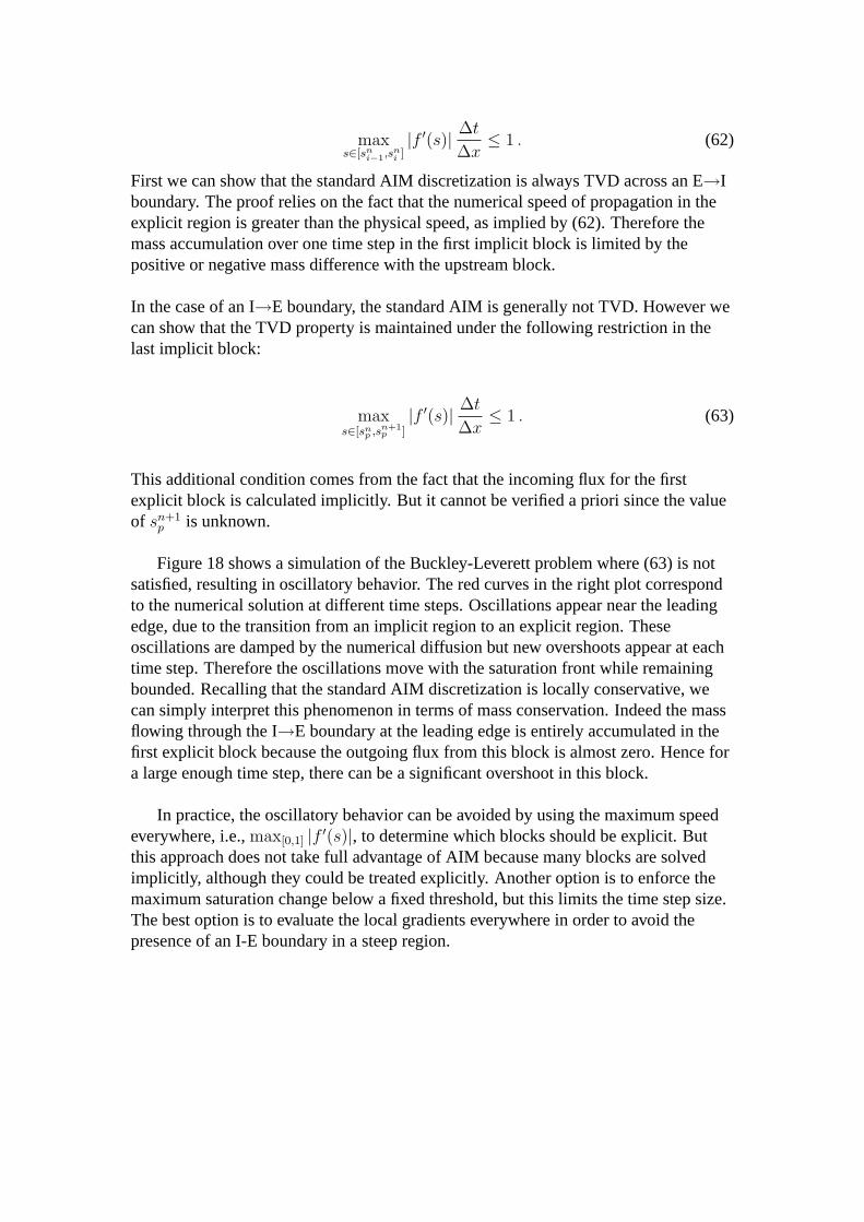
Figure 18 shows a simulation of the Buckley-Leverett problem where (63) is notsatisfied, resulting in oscillatory behavior. The red curves in the right plot correspondto the numerical solution at different time steps. Oscillations appear near the leadingedge, due to the transition from an implicit region to an explicit region. Theseoscillations are damped by the numerical diffusion but new overshoots appear at eachtime step. Therefore the oscillations move with the saturation front while remainingbounded. Recalling that the standard AIM discretization is locally conservative, wecan simply interpret this phenomenon in terms of mass conservation. Indeed the massflowing through the I→E boundary at the leading edge is entirely accumulated in thefirst explicit block because the outgoing flux from this block is almost zero. Hence fora large enough time step, there can be a significant overshoot in this block.

In practice, the oscillatory behavior can be avoided by using the maximum speedeverywhere, i.e.,max[0,1] |f ′(s)|, to determine which blocks should be explicit. Butthis approach does not take full advantage of AIM because many blocks are solvedimplicitly, although they could be treated explicitly. Another option is to enforce themaximum saturation change below a fixed threshold, but this limits the time step size.The best option is to evaluate the local gradients everywhere in order to avoid thepresence of an I-E boundary in a steep region.

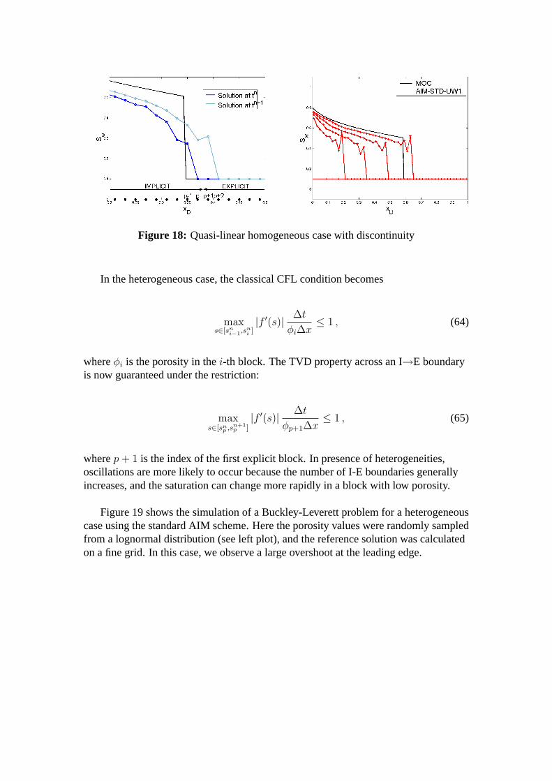
Figure 18: Quasi-linear homogeneous case with discontinuity

In the heterogeneous case, the classical CFL condition becomes

maxs∈[sn

i−1,sni ]|f ′(s)| ∆t

φi∆x≤ 1 , (64)

whereφi is the porosity in thei-th block. The TVD property across an I→E boundaryis now guaranteed under the restriction:

maxs∈[sn

p ,sn+1p ]

|f ′(s)| ∆t

φp+1∆x≤ 1 , (65)

wherep+ 1 is the index of the first explicit block. In presence of heterogeneities,oscillations are more likely to occur because the number of I-E boundaries generallyincreases, and the saturation can change more rapidly in a block with low porosity.

Figure 19 shows the simulation of a Buckley-Leverett problem for a heterogeneouscase using the standard AIM scheme. Here the porosity values were randomly sampledfrom a lognormal distribution (see left plot), and the reference solution was calculatedon a fine grid. In this case, we observe a large overshoot at the leading edge.

Figure 19: Quasi-linear heterogeneous case with discontinuity

Construction of high-order AIM

Requirements and methodology

Our objective is to construct a class of adaptive implicit methods that satisfies thefollowing requirements:

- High-order accuracy both in time and space.

- Unconditional stability in the implicit regions.

- Local mass conservation.

In the above list, there is no requirement regarding the monotonicity properties of themethod, but this point will be discussed further in this section.

To construct a high-order AIM discretization, we use the highly accurate numericalschemes formulated in the Method of Lines (MOL) framework (see [32] and [33]).The choice of the MOL approach is justified by many practical reasons (e.g.,multi-dimensional extensions, treatment of diffusive and reactive terms), and thenecessity to have a locally conservative scheme. High-order MOL schemes are derivedby combining a high-resolution spatial discretization with a highly accurate timeintegration method. As an initial step, a prototype program was written to test variouscombinations of space-time discretization schemes. Classical time integration methodsare listed below:

- Central and Trapezoidal rules with a Runge Kutta scheme (CRK2 and TRK2).

- Second-order Implicit Runge-Kutta scheme (IRK2).

- Third-order Diagonally Implicit Runge-Kutta scheme (DIRK3).

The common flux discretization strategies (see [34], [35], [36], [37], [38]) include:

- Second-order flux limiting scheme (FL2),

- Second-order central scheme (CS2),

- High-order ENO and WENO schemes (e.g. WENO2).

In a high-order AIM formulation, implicit and explicit time integration methods mustbe combined consistently. Otherwise, the inconsistencies at the various I/E boundarieswould lead to first-order errors. Thus, we propose using a high-order implicit methodas the framework for both implicit and explicit regions. The idea is to use a predictedvalue at the explicit nodes, whenever an implicit value is normally required.

AIM with high-order spatial accuracy

Given a high-order numerical fluxFi+ 12, we define the following AIM scheme:

sn+1i = sn

i − ∆t∆x

(F n∗

i+ 12

− F n∗i− 1

2

)F n∗

i+ 12

= Fi+ 12(sn∗), sn∗

i =

sn+1

i if ( i) implicitsn

i otherwise.

(66)

This scheme can be seen as an extension of the standard AIM because the timeintegration methods in the explicit and implicit regions correspond to Forward andBackward Euler. Alternatively, we propose the following AIM scheme:

sn+1i = sn

i − ∆t∆x

[F n+1

i+ 12

− F n+1i− 1

2

]F n+1

i+ 12

= Fi+ 12(sn+1) , sn+1

i =

sn+1

i if (i) implicits∗i otherwise.

(67)

Heres∗i is an explicit predictor ofsn+1i that is at least first-order accurate, e.g.

s∗i = sni −

∆t

∆x(F n

i+ 12− F n

i− 12) . (68)

The scheme (67) can be seen as an adaptive implicit version of the Backward Eulermethod in the sense that the fluxes are always evaluated at the new time level.

Figure 20 shows numerical solutions of a 1D Buckley-Leverett problem calculatedwith the AIM-STD-FL2 and AIM-BE-FL2 schemes, which correspond respectively to(66) and (67), whereFi+ 1

2is given by the second-order accurate flux limiting scheme.

Both methods give slightly more accurate results than the standard AIM scheme,AIM-STD-UW1. The gain in resolution is quite small because the time integration

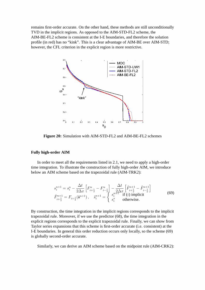
remains first-order accurate. On the other hand, these methods are still unconditionallyTVD in the implicit regions. As opposed to the AIM-STD-FL2 scheme, theAIM-BE-FL2 scheme is consistent at the I-E boundaries, and therefore the solutionprofile (in red) has no “kink”. This is a clear advantage of AIM-BE over AIM-STD;however, the CFL criterion in the explicit region is more restrictive.

Figure 20: Simulation with AIM-STD-FL2 and AIM-BE-FL2 schemes

Fully high-order AIM

In order to meet all the requirements listed in 2.1, we need to apply a high-ordertime integration. To illustrate the construction of fully high-order AIM, we introducebelow an AIM scheme based on the trapezoidal rule (AIM-TRK2):

sn+1i = sn

i −∆t

2∆x

[F n

i+ 12

− F ni− 1

2

]− ∆t

2∆x

[F n+1

i+ 12

− F n+1i− 1

2

]F n+1

i+ 12

= Fi+ 12(sn+1) , sn+1

i =

sn+1

i if ( i) implicits∗i otherwise.

(69)

By construction, the time integration in the implicit regions corresponds to the implicittrapezoidal rule. Moreover, if we use the predictor (68), the time integration in theexplicit regions corresponds to the explicit trapezoidal rule. Finally, we can show fromTaylor series expansions that this scheme is first-order accurate (i.e. consistent) at theI-E boundaries. In general this order reduction occurs only locally, so the scheme (69)is globally second-order accurate.

Similarly, we can derive an AIM scheme based on the midpoint rule (AIM-CRK2):

sn+1i = sn

i −∆t

∆x

[F

n+1/2

i+ 12

− Fn+1/2

i− 12

]F

n+1/2

i+ 12

= Fi+ 12(sn+1/2) , s

n+1/2i =

12(sn

i + sn+1i ) if ( i) implicit

12(sn

i + s∗i ) otherwise.

(70)

Applying the predictor (68), we can see that the time integration method in the explicitregions corresponds to the explicit midpoint rule. As a result, this scheme is alsoglobally second-order accurate.

The same approach can be used to derive higher order AIM schemes. Below wegive the general formulation of a third-order AIM scheme based on the DIRK3 methodwith γ = 1/2 +

√3/6 (AIM-DIRK3):

sn+1i = sn

i − ∆t2∆x

(F

(1)

i+ 12

− F(1)

i− 12

)− ∆t

2∆x

(F

(2)

i+ 12

− F(2)

i− 12

)s(1)i = sn

i − γ ∆t∆x

(F

(1)

i+ 12

− F(1)

i− 12

)s(2)i = sn

i − (1− 2γ) ∆t∆x

(F

(1)

i+ 12

− F(1)

i− 12

)− γ ∆t

∆x

(F

(2)

i+ 12

− F(2)

i− 12

) (71)

where

F(1)

i+ 12

= Fi+ 12(s(1)), s

(1)i =

s(1)i if ( i) implicit

s∗,(1)i otherwise,

(72)

and a similar definition holds forF (2)

i+ 12

. Here we need to apply a third-order numerical

flux, such as ENO3. In this case, the explicit predictorss∗,(1), s∗,(2) should correspondto the timest(1) = tn + γ∆t andt(2) = tn + (1− γ)∆t.

The high-order AIM schemes presented above require the following three-stepapproach:

1) Apply a predictor step in the explicit blocks,

2) Assemble and solve the system for the implicit blocks,

3) Update the solution in the explicit blocks.

In terms of computational cost, steps 1 and 3 are cheap, whereas step 2 is generallyexpensive because it requires solving a system of nonlinear equations. For this purposewe can apply the Newton-Raphson method. Note that there are mainly two factors thatexplain the additional computational cost of high-order AIM compared to standardAIM. First, the high-order time integration method may require solving several

systems of nonlinear equations in a given time step (e.g. in DIRK3), or solving a largersystem if the sub-steps of the time integration are coupled (e.g. in IRK2). Secondly,for each Newton step, the Jacobian has a larger band width than in the first-order case.Indeed, high-order spatial discretizations lead to larger numerical stencils, especiallyfor multi-dimensional problems.

Numerical tests in 1D and 2D

1D Buckley-Leverett problemFigure 21 shows two numerical solutions computedwith the second-order accurate AIM-CRK2-WENO2 scheme. The left plotcorresponds to CFL< 2, while the right plot was obtained for CFL> 2. In the firstcase, the numerical solution is very accurate even near the leading edge, and there isno kink at the I-E boundaries. However, for CFL> 2 we observe localized overshootsjust ahead of the saturation front. This result is expected, since the implicit trapezoidalrule is known to become oscillatory above this time step threshold.

Figure 21: AIM-TRK2-WENO2 solutions for CFL=1.5 (left), 2.5 (right)

2D miscible flow in a quarter-five spotFigure 22 shows a reference solution computedon a50× 50 grid using the forward Euler scheme. The left contour plot represents thepressure solution and the right contour plot the concentration profile calculated atTf = 2x106 s. For this simulation, the injection rate isqw = 10−3 m3/s, the length ofthe square isL = 100 m, the reservoir depthh = 1 m, the viscosityµ = 1 cp, theporosityφ = 0.3, and the permeability tensor is diagonal withkx = ky = 100 md. Thefinal time corresponds to 2/3 pore volumes injected.

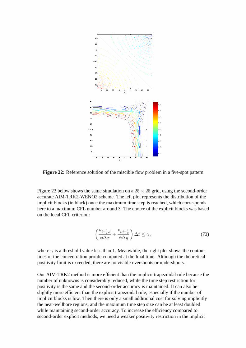
Figure 22: Reference solution of the miscible flow problem in a five-spot pattern

Figure 23 below shows the same simulation on a25× 25 grid, using the second-orderaccurate AIM-TRK2-WENO2 scheme. The left plot represents the distribution of theimplicit blocks (in black) once the maximum time step is reached, which correspondshere to a maximum CFL number around 3. The choice of the explicit blocks was basedon the local CFL criterion:

(ui+ 1

2,j

φ∆x+vi,j+ 1

2

φ∆y

)∆t ≤ γ , (73)

whereγ is a threshold value less than 1. Meanwhile, the right plot shows the contourlines of the concentration profile computed at the final time. Although the theoreticalpositivity limit is exceeded, there are no visible overshoots or undershoots.

Our AIM-TRK2 method is more efficient than the implicit trapezoidal rule because thenumber of unknowns is considerably reduced, while the time step restriction forpositivity is the same and the second-order accuracy is maintained. It can also beslightly more efficient than the explicit trapezoidal rule, especially if the number ofimplicit blocks is low. Then there is only a small additional cost for solving implicitlythe near-wellbore regions, and the maximum time step size can be at least doubledwhile maintaining second-order accuracy. To increase the efficiency compared tosecond-order explicit methods, we need a weaker positivity restriction in the implicit

regions. This can be achieved with other implicit methods such as IRK2 or DIRK3, oras shown later, by applying artificial viscosity.

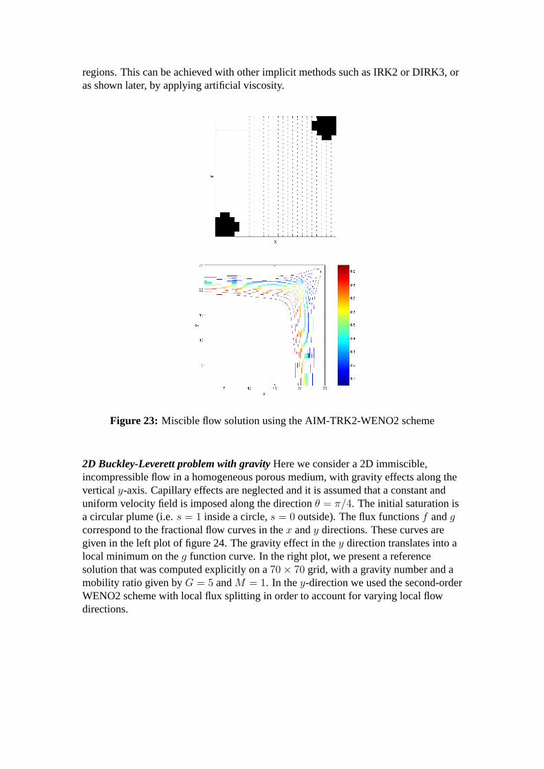
Figure 23: Miscible flow solution using the AIM-TRK2-WENO2 scheme

2D Buckley-Leverett problem with gravityHere we consider a 2D immiscible,incompressible flow in a homogeneous porous medium, with gravity effects along theverticaly-axis. Capillary effects are neglected and it is assumed that a constant anduniform velocity field is imposed along the directionθ = π/4. The initial saturation isa circular plume (i.e.s = 1 inside a circle,s = 0 outside). The flux functionsf andgcorrespond to the fractional flow curves in thex andy directions. These curves aregiven in the left plot of figure 24. The gravity effect in they direction translates into alocal minimum on theg function curve. In the right plot, we present a referencesolution that was computed explicitly on a70× 70 grid, with a gravity number and amobility ratio given byG = 5 andM = 1. In they-direction we used the second-orderWENO2 scheme with local flux splitting in order to account for varying local flowdirections.

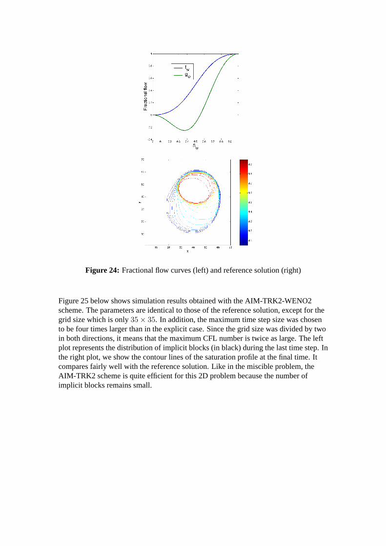
Figure 24: Fractional flow curves (left) and reference solution (right)

Figure 25 below shows simulation results obtained with the AIM-TRK2-WENO2scheme. The parameters are identical to those of the reference solution, except for thegrid size which is only35× 35. In addition, the maximum time step size was chosento be four times larger than in the explicit case. Since the grid size was divided by twoin both directions, it means that the maximum CFL number is twice as large. The leftplot represents the distribution of implicit blocks (in black) during the last time step. Inthe right plot, we show the contour lines of the saturation profile at the final time. Itcompares fairly well with the reference solution. Like in the miscible problem, theAIM-TRK2 scheme is quite efficient for this 2D problem because the number ofimplicit blocks remains small.

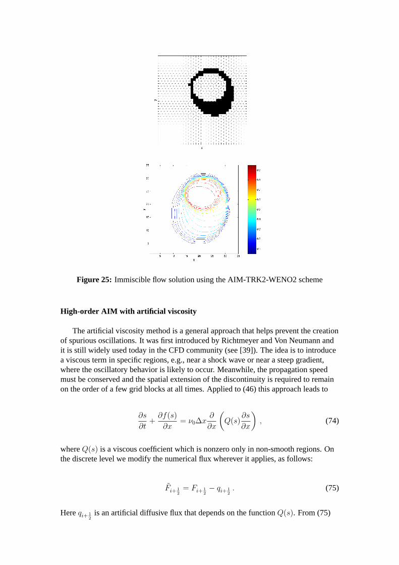
Figure 25: Immiscible flow solution using the AIM-TRK2-WENO2 scheme

High-order AIM with artificial viscosity

The artificial viscosity method is a general approach that helps prevent the creationof spurious oscillations. It was first introduced by Richtmeyer and Von Neumann andit is still widely used today in the CFD community (see [39]). The idea is to introducea viscous term in specific regions, e.g., near a shock wave or near a steep gradient,where the oscillatory behavior is likely to occur. Meanwhile, the propagation speedmust be conserved and the spatial extension of the discontinuity is required to remainon the order of a few grid blocks at all times. Applied to (46) this approach leads to

∂s

∂t+∂f(s)

∂x= ν0∆x

∂

∂x

(Q(s)

∂s

∂x

), (74)

whereQ(s) is a viscous coefficient which is nonzero only in non-smooth regions. Onthe discrete level we modify the numerical flux wherever it applies, as follows:

Fi+ 12

= Fi+ 12− qi+ 1

2. (75)

Hereqi+ 12

is an artificial diffusive flux that depends on the functionQ(s). From (75)

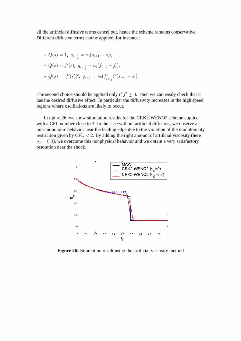
all the artificial diffusive terms cancel out, hence the scheme remains conservative.Different diffusive terms can be applied, for instance:

- Q(s) = 1, qi+ 12

= ν0(si+1 − si),

- Q(s) = f ′(s), qi+ 12

= ν0(fi+1 − fi),

- Q(s) = [f ′(s)]2, qi+ 12

= ν0(f′i+ 1

2

)2(si+1 − si).

The second choice should be applied only iff ′ ≥ 0. Then we can easily check that ithas the desired diffusive effect. In particular the diffusivity increases in the high speedregions where oscillations are likely to occur.

In figure 26, we show simulation results for the CRK2-WENO2 scheme appliedwith a CFL number close to 3. In the case without artificial diffusion, we observe anon-monotonic behavior near the leading edge due to the violation of the monotonicityrestriction given by CFL< 2. By adding the right amount of artificial viscosity (hereν0 = 0.4), we overcome this nonphysical behavior and we obtain a very satisfactoryresolution near the shock.

Figure 26: Simulation result using the artificial viscosity method

Remarks and Future Plans

Analysis of the standard AIM formulation revealed a local inconsistency at the I-Eboundaries. But the discretization errors are only of the order of the numericaldispersion. So in general we only observe small “kinks” in the solution profile.Moreover, we showed that the monotonicity properties of the solution are preserved,except in specific situations that can be avoided in practice.

Our construction of high-order AIM schemes relies on highly accurate MOLschemes. By using explicit predictors, the time integration in the explicit regions canbe based on the same time levels as in the implicit regions. Hence the consistency atthe I-E boundaries and the locally conservative form are maintained. Numericalexperiments comparing standard AIM with high-order AIM indicate a substantialreduction of the numerical dispersion. However, the high-order implicit timeintegration leads to a severe positivity restriction on the time step size. In fact,unconditionally positive methods can only be first-order accurate (see [40], [41]).Therefore, we propose to apply artificial viscosity in the implicit regions in order toremove the spurious oscillations at large CFL numbers. We also need to investigatefurther what optimal time integration method (with respect to positivity) should beemployed. Finally, the most robust approach for a wide range of practical applicationsconsists of applying the Backward-Euler method in the implicit regions and ahigh-order time integration method in the explicit regions. This will be validated usingexamples of practical interest.

Adaptive Operator Based Multiscale Method for CompressibleMultiphase Flow

Investigators

Hamdi Tchelepi, Associate Professor of Energy Resources Engineering; Hui Zhou,Graduate Research Assistant

Introduction

The accuracy of simulating flow and transport in natural formations depends on thequality and resolution of the reservoir description model. Formation properties, suchas porosity and permeability, typically vary over many scales. As a result, it is notunusual for a detailed geologic description to haveO(107)−O(108) gridblocks.However, this level of resolution is far beyond the computational capability of existingnumerical simulators. Thus, it is necessary to have an efficient and accuratecomputational method to study these highly detailed models.

The multiscale finite-volume approach is very promising due to its ability toresolve fine-scale information accurately without direct solution of the globalfine-scale equations. In order to describe flow and transport of CO2 in geologicformations, we need to be able to model compressible multiphase flow in large-scaleheterogeneous porous media. Existing multiscale methods ([42, 43, 44, 45, 46]),however, deal with the incompressible (elliptic) flow problem only. Here, we extendthe multiscale finite-volume method to compressible multiphase flow. The accuracy ofOperator Based Multiscale Method is demonstrated using several challenging cases,including highly compressible multiphase flow in a strongly heterogeneouspermeability field (SPE 10).

Background

Flow and transport in natural porous formations can be quite complex, and oftenreflect the intrinsic multiscale character of the geologic formation. This makes theproblem of modeling nonlinear flows in heterogeneous porous media a natural targetfor multiscale mathematical formulations and solution methods. For example, Hou andWu [43] proposed a multiscale finite-element method (MsFEM) that captures thefine-scale information by constructing special local basis functions. The methodproved to be quite accurate except that the reconstructed fine-scale velocity field wasnot locally conservative. Later, Chen and Hou proposed a locally conservative mixedfinite-element multiscale method. Another multiscale mixed finite-element method hasbeen presented by Arbogast[45] and Arbogast and Bryant [46], where numericalGreen functions are used to resolve the fine-scale information. The Green functions

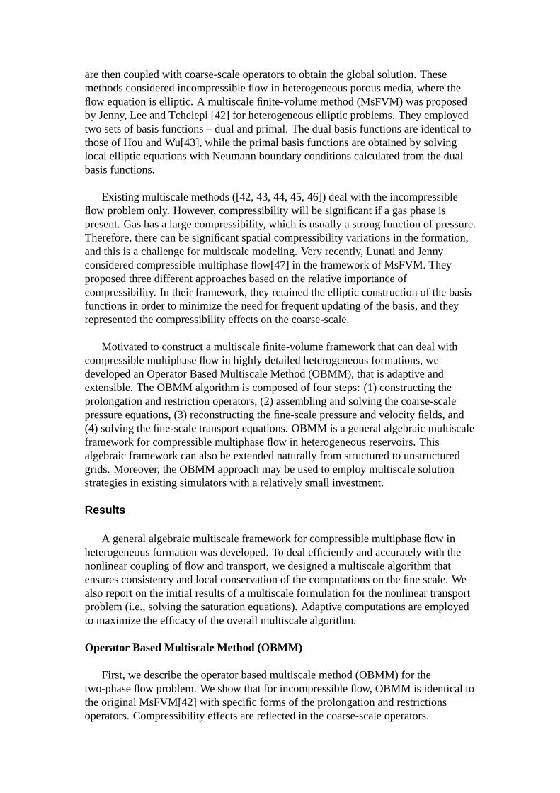
are then coupled with coarse-scale operators to obtain the global solution. Thesemethods considered incompressible flow in heterogeneous porous media, where theflow equation is elliptic. A multiscale finite-volume method (MsFVM) was proposedby Jenny, Lee and Tchelepi [42] for heterogeneous elliptic problems. They employedtwo sets of basis functions – dual and primal. The dual basis functions are identical tothose of Hou and Wu[43], while the primal basis functions are obtained by solvinglocal elliptic equations with Neumann boundary conditions calculated from the dualbasis functions.

Existing multiscale methods ([42, 43, 44, 45, 46]) deal with the incompressibleflow problem only. However, compressibility will be significant if a gas phase ispresent. Gas has a large compressibility, which is usually a strong function of pressure.Therefore, there can be significant spatial compressibility variations in the formation,and this is a challenge for multiscale modeling. Very recently, Lunati and Jennyconsidered compressible multiphase flow[47] in the framework of MsFVM. Theyproposed three different approaches based on the relative importance ofcompressibility. In their framework, they retained the elliptic construction of the basisfunctions in order to minimize the need for frequent updating of the basis, and theyrepresented the compressibility effects on the coarse-scale.

Motivated to construct a multiscale finite-volume framework that can deal withcompressible multiphase flow in highly detailed heterogeneous formations, wedeveloped an Operator Based Multiscale Method (OBMM), that is adaptive andextensible. The OBMM algorithm is composed of four steps: (1) constructing theprolongation and restriction operators, (2) assembling and solving the coarse-scalepressure equations, (3) reconstructing the fine-scale pressure and velocity fields, and(4) solving the fine-scale transport equations. OBMM is a general algebraic multiscaleframework for compressible multiphase flow in heterogeneous reservoirs. Thisalgebraic framework can also be extended naturally from structured to unstructuredgrids. Moreover, the OBMM approach may be used to employ multiscale solutionstrategies in existing simulators with a relatively small investment.

Results

A general algebraic multiscale framework for compressible multiphase flow inheterogeneous formation was developed. To deal efficiently and accurately with thenonlinear coupling of flow and transport, we designed a multiscale algorithm thatensures consistency and local conservation of the computations on the fine scale. Wealso report on the initial results of a multiscale formulation for the nonlinear transportproblem (i.e., solving the saturation equations). Adaptive computations are employedto maximize the efficacy of the overall multiscale algorithm.

Operator Based Multiscale Method (OBMM)

First, we describe the operator based multiscale method (OBMM) for thetwo-phase flow problem. We show that for incompressible flow, OBMM is identical tothe original MsFVM[42] with specific forms of the prolongation and restrictionsoperators. Compressibility effects are reflected in the coarse-scale operators.

Moreover, the basis functions and the reconstructed fine-scale fluxes also containcompressibility effects.

Governing Equations.We consider immiscible two-phase flow in porous media.Gravity and capillarity are neglected here. The governing equations are the massconservation equations of the two phases,

∂(φbl)

∂t+∇ · (blul) = ql,

ul = −λl∇p,

λl =kkrlblµ

,

(76)

wherel = 1, 2 denotes the two phases;bl is the inverse of the phase formation volumefactor, which is defined as the ratio of density at reservoir conditions to density atstandard conditions;ul is the phase volumetric flux at reservoir condition;ql is thesource term;λl is the phase mobility;krl is the phase relative permeability;φ andk arethe porosity and absolute permeability of porous medium.

Because multiscale methods are usually applied only to the flow problem (pressureequation), the flow and transport problems are treated differently. Thus, the flow andtransport equations are solved sequentially using either an IMPES (IMplicit PressureExplicit Saturation)[48], or a sequential implicit (SI) [49] method. Here we adopt thesequential implicit approach. The linearized discrete pressure equation can be obtainedfrom Eq.76 through simple algebraic manipulation. The semi-discrete equation foriterationν + 1 at time stepn+ 1 is

Cpν+1 − pν

∆t− αν

1∇ ·(bν1λ

ν1∇pν+1

)− αν

2∇ ·(bν2λ

ν2∇pν+1

)= Q, (77)

where,

αν1 =

1

bν1, αν

2 =1

bν2,

C =

(∂φ

∂p− φn(bn1S

n1

∂α1

∂p+ bn2S

n2

∂α2

∂p) +∆t

∂(α1q1 + α2q2)

∂p

)ν

,

Q = − φν

∆t+φn

∆t(αν

1bn1S

n1 + αν

2bn2S

n2 )− (α1q

ν1 + α2q

ν2 ).

(78)

Given a fine-scale problem, Eq.77 can be written in matrix form as

(Tf −Cf )pf = rf , (79)

whereTf is the fine-scale transmissibility matrix associated with the flow,Cf is thefine-scale compressibility matrix associated with accumulation,pf denotes thefine-scale pressure vector, andrf is the fine-scale right-hand-side vector.

The linearized discrete form of the transport equation for phase 1 is

φν+1bν+11 Sν+1

1 − φnbn1Sn1

∆t= ∇ ·

[bν+11 (f ν

1 +∂f1

∂S1

∣∣∣∣ν (Sν+11 − Sν

1 )

]uν+1

T

− q1,

(80)

wheref1 is the fractional flow of phase 1, anduT is the total velocity.

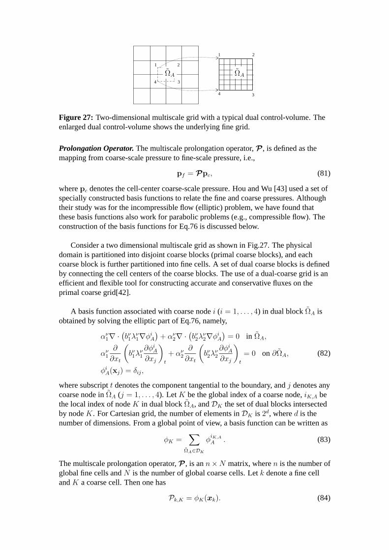
1 2

4 3

1 2

4 3

ΩA ΩA

Figure 27: Two-dimensional multiscale grid with a typical dual control-volume. Theenlarged dual control-volume shows the underlying fine grid.

Prolongation Operator.The multiscale prolongation operator,P , is defined as themapping from coarse-scale pressure to fine-scale pressure, i.e.,

pf = Ppc, (81)

wherepc denotes the cell-center coarse-scale pressure. Hou and Wu [43] used a set ofspecially constructed basis functions to relate the fine and coarse pressures. Althoughtheir study was for the incompressible flow (elliptic) problem, we have found thatthese basis functions also work for parabolic problems (e.g., compressible flow). Theconstruction of the basis functions for Eq.76 is discussed below.

Consider a two dimensional multiscale grid as shown in Fig.27. The physicaldomain is partitioned into disjoint coarse blocks (primal coarse blocks), and eachcoarse block is further partitioned into fine cells. A set of dual coarse blocks is definedby connecting the cell centers of the coarse blocks. The use of a dual-coarse grid is anefficient and flexible tool for constructing accurate and conservative fluxes on theprimal coarse grid[42].

A basis function associated with coarse nodei (i = 1, . . . , 4) in dual blockΩA isobtained by solving the elliptic part of Eq.76, namely,

αν1∇ ·

(bν1λ

ν1∇φi

A

)+ αν

2∇ ·(bν2λ

ν2∇φi

A

)= 0 in ΩA,

αν1

∂

∂xt

(bν1λ

ν1

∂φiA

∂xj

)t

+ αν2

∂

∂xt

(bν2λ

ν2

∂φiA

∂xj

)t

= 0 on ∂ΩA,

φiA(xj) = δij,

(82)

where subscriptt denotes the component tangential to the boundary, andj denotes anycoarse node inΩA (j = 1, . . . , 4). LetK be the global index of a coarse node,iK,A bethe local index of nodeK in dual blockΩA, andDK the set of dual blocks intersectedby nodeK. For Cartesian grid, the number of elements inDK is 2d, whered is thenumber of dimensions. From a global point of view, a basis function can be written as

φK =∑

ΩA∈DK

φiK,A

A . (83)

The multiscale prolongation operator,P , is ann×N matrix, wheren is the number ofglobal fine cells andN is the number of global coarse cells. Letk denote a fine cellandK a coarse cell. Then one has

Pk,K = φK(xk). (84)

Restriction Operator.Substitution of Eq.81 into Eq.79 leads to

(Tf −Cf )Ppc = rf . (85)

The significance of Eq.85 is that its unknowns are coarse-scale pressures. We need toapply a restriction operator,R, that provides a mapping from fine to coarse space. Sowe write

R(Tf −Cf )Ppc = Rrf , (86)

or,(Tc −Cc)pc = rc, (87)

whereTc,Cc, rc are the coarse-scale counterparts ofTf ,Cf , rf , and are defined as

Tc = RTfPCc = RCfPrc = Rrf .

(88)

Eq.87 is the coarse-scale equation we need to solve.

The restriction operator,R, maps the fine-scale discretization equations into thecoarse scale. The specific choice forR depends on the discretization scheme (e.g.,finite-element or finite-volume). We denote a fine-scale conservative equation byE. Afinite-volume formulation starts with∫

Ωk

E dV = 0 (∀ fine cellΩk, k = 1, . . . , n). (89)

A coarse-scale finite volume formulation requires∫ΩK

E dV = 0 (∀ coarse blockΩK , K = 1, . . . , N). (90)

Comparing Eq.89 and Eq.90, it is clear that Eq.90 can be obtained by summing Eq.89for all the fine cells inside a coarse blockK, i.e.,∫

ΩK

E dV =∑

Ωk∈ΩK

∫Ωk

E dV. (91)

The summation in Eq.91 can be represented as a restriction operator,R, as follows

RK,k =

1 if Ωk ⊂ ΩK

0 otherwise(K = 1, . . . , N ; k = 1, . . . , n). (92)

It is important to note that the restriction operator does not depend on the detaileddiscretization scheme (i.e., backward difference or central difference, etc.) and thus isgeneral for a given formulation. For a Galerkin-type finite element method, thecoarse-scale equation may be written as∫

ΩK

φME dV = 0 (K,M = 1, . . . , N), (93)

and one can show thatR takes the following form

R = PT . (94)

Zhou[50] provides a detailed treatment for finite-element based multiscaleformulations.

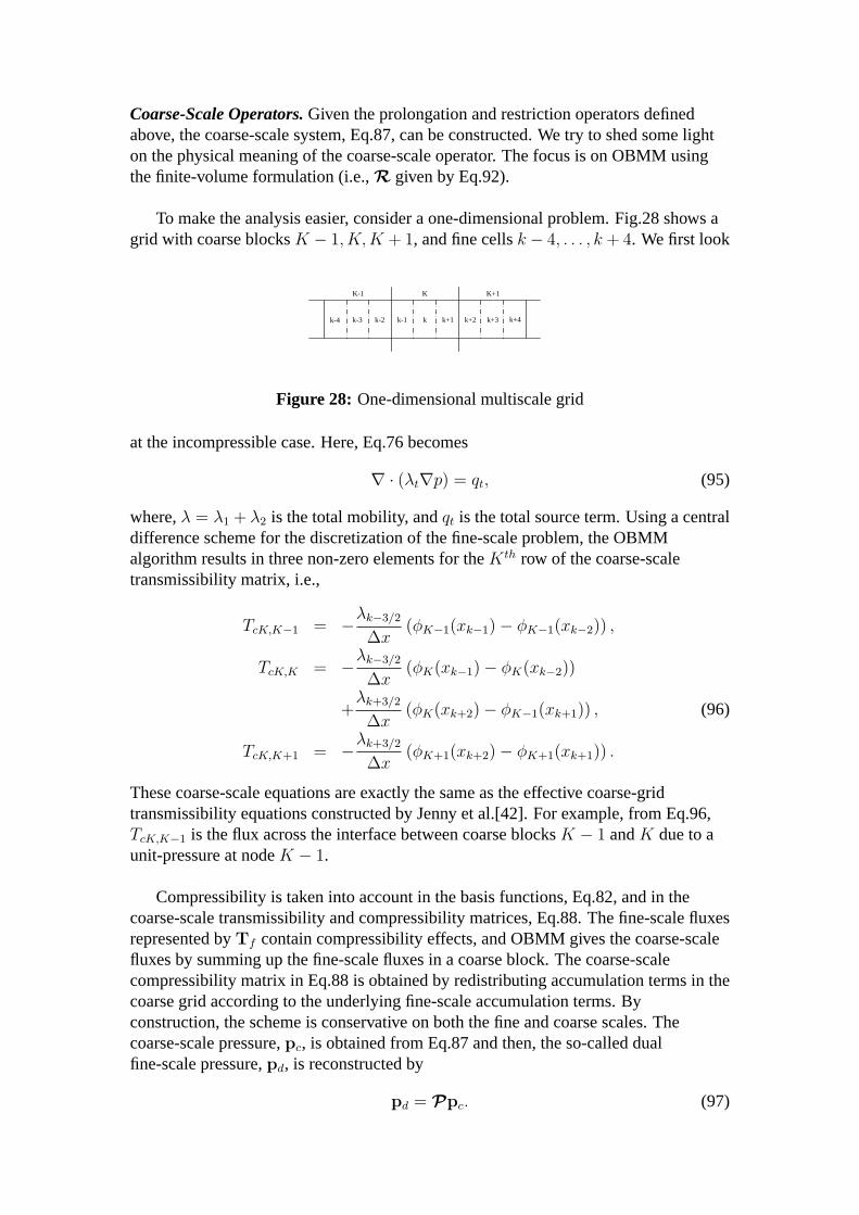
Coarse-Scale Operators.Given the prolongation and restriction operators definedabove, the coarse-scale system, Eq.87, can be constructed. We try to shed some lighton the physical meaning of the coarse-scale operator. The focus is on OBMM usingthe finite-volume formulation (i.e.,R given by Eq.92).

To make the analysis easier, consider a one-dimensional problem. Fig.28 shows agrid with coarse blocksK − 1, K,K + 1, and fine cellsk − 4, . . . , k + 4. We first look

K-1 K K+1

k-4 k-3 k-2 k-1 k k+1 k+2 k+3 k+4

Figure 28: One-dimensional multiscale grid

at the incompressible case. Here, Eq.76 becomes

∇ · (λt∇p) = qt, (95)

where,λ = λ1 + λ2 is the total mobility, andqt is the total source term. Using a centraldifference scheme for the discretization of the fine-scale problem, the OBMMalgorithm results in three non-zero elements for theKth row of the coarse-scaletransmissibility matrix, i.e.,

TcK,K−1 = −λk−3/2

∆x(φK−1(xk−1)− φK−1(xk−2)) ,

TcK,K = −λk−3/2

∆x(φK(xk−1)− φK(xk−2))

+λk+3/2

∆x(φK(xk+2)− φK−1(xk+1)) , (96)

TcK,K+1 = −λk+3/2

∆x(φK+1(xk+2)− φK+1(xk+1)) .

These coarse-scale equations are exactly the same as the effective coarse-gridtransmissibility equations constructed by Jenny et al.[42]. For example, from Eq.96,TcK,K−1 is the flux across the interface between coarse blocksK − 1 andK due to aunit-pressure at nodeK − 1.

Compressibility is taken into account in the basis functions, Eq.82, and in thecoarse-scale transmissibility and compressibility matrices, Eq.88. The fine-scale fluxesrepresented byTf contain compressibility effects, and OBMM gives the coarse-scalefluxes by summing up the fine-scale fluxes in a coarse block. The coarse-scalecompressibility matrix in Eq.88 is obtained by redistributing accumulation terms in thecoarse grid according to the underlying fine-scale accumulation terms. Byconstruction, the scheme is conservative on both the fine and coarse scales. Thecoarse-scale pressure,pc, is obtained from Eq.87 and then, the so-called dualfine-scale pressure,pd, is reconstructed by

pd = Ppc. (97)

Coupling Flow and Transport

For multiphase problems, the flow (pressure and total velocity) and transport(saturation) equations are solved in a sequential manner. After reconstruction of thefine-scale pressure field, we can then proceed to solve for saturation equations on thefine scale. Note that special care should be taken to ensure the conservation andconsistency of the coupled system.

Fine-scale Velocity.The fine-scale velocity,uT , calculated usingpd may bediscontinuous at the interfaces of the dual coarse blocks, since the basis functionsensure flux continuity only in the interior of each dual block. To obtain a conservativefine-scale velocity, we solve the fine-scale Eq.77 locally for each primal coarse blockwith flux boundary conditions, which are obtained frompd. The fine-scale pressurecomputed in this manner, which we denote aspv, is the primal fine-scale pressure.Then, the fine-scale velocity in the interior regions of primal coarse blocks iscalculated frompv, while the velocity on the boundary of the primal coarse block iscalculated frompd. The total velocity field obtained this way is locally conservative onthe fine and coarse scales.

Multiscale Algorithm for Compressible Multiphase Flow.Notice that Eq.77 isnonlinear, and thus we have to solve it iteratively. However, solving the pressuresystem is usually more expensive than solving the saturation equations. Thus, we havean outer loop, where we solve for the fine-scale pressure only once using OBMM andthen calculate the fine-scale primal pressure and total velocity. On the other hand, thesaturation equations are solved iteratively in an inner loop until convergence. Thepseudo code for one time step is listed in Fig.29, wheren denotes a time step andνdenotes an iteration step. Note that for the finite-volume OBMM, the restrictionoperator is constructed once as shown by Eq.92. Also note that when solving thesaturation equations in the inner loops, the total velocityuT is fixed.

Careful updating of the pressure dependent properties is an important part of theoverall scheme. We have two fine-scale pressure fields: dual and primal. Since theprimal pressure yields a conservative fine-scale velocity field, we calculate thepressure dependent properties based on the primal pressure. Also, to ensureconsistency and conservation, the properties in the pressure equation are completelyconsistent with those in the saturation equation.

Adaptive Multiscale Computation

The computational efficiency of multiscale methods mainly lies in that a large-scaleproblem is decomposed into small local problems. Thus, a lot of time is saved in thelinear solver step. Moreover, multiscale algorithms are well suited for parallelcomputation, since the local problems can be solved independently. Most importantly,multiscale methods are designed to be adaptive, and this is discussed below.

As described in the previous sections, basis functions are constructed by solving aseries of local problems in every dual coarse block. Actually, it is not necessary toupdate the basis functions in every block and for every iteration. It is obvious that if

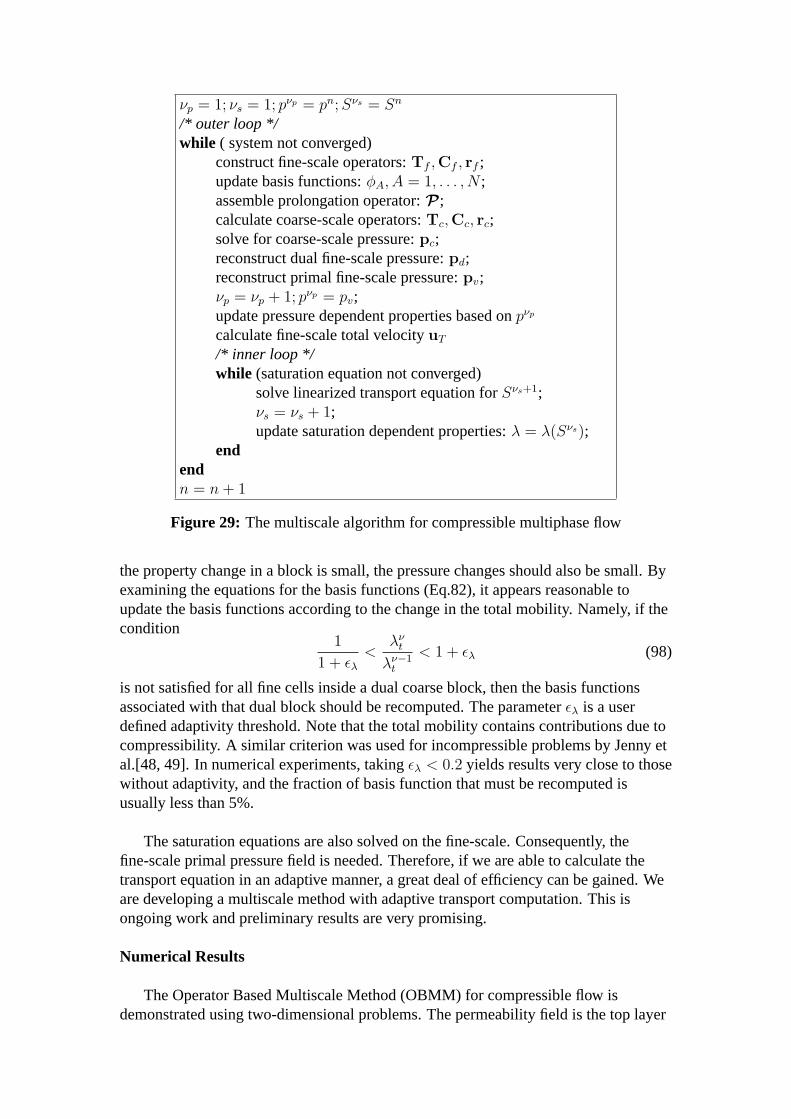
νp = 1; νs = 1; pνp = pn;Sνs = Sn

/* outer loop */while ( system not converged)

construct fine-scale operators:Tf ,Cf , rf ;update basis functions:φA, A = 1, . . . , N ;assemble prolongation operator:P ;calculate coarse-scale operators:Tc,Cc, rc;solve for coarse-scale pressure:pc;reconstruct dual fine-scale pressure:pd;reconstruct primal fine-scale pressure:pv;νp = νp + 1; pνp = pv;update pressure dependent properties based onpνp

calculate fine-scale total velocityuT

/* inner loop */while (saturation equation not converged)

solve linearized transport equation forSνs+1;νs = νs + 1;update saturation dependent properties:λ = λ(Sνs);

endendn = n+ 1

Figure 29: The multiscale algorithm for compressible multiphase flow

the property change in a block is small, the pressure changes should also be small. Byexamining the equations for the basis functions (Eq.82), it appears reasonable toupdate the basis functions according to the change in the total mobility. Namely, if thecondition

1

1 + ελ<

λνt

λν−1t

< 1 + ελ (98)

is not satisfied for all fine cells inside a dual coarse block, then the basis functionsassociated with that dual block should be recomputed. The parameterελ is a userdefined adaptivity threshold. Note that the total mobility contains contributions due tocompressibility. A similar criterion was used for incompressible problems by Jenny etal.[48, 49]. In numerical experiments, takingελ < 0.2 yields results very close to thosewithout adaptivity, and the fraction of basis function that must be recomputed isusually less than 5%.

The saturation equations are also solved on the fine-scale. Consequently, thefine-scale primal pressure field is needed. Therefore, if we are able to calculate thetransport equation in an adaptive manner, a great deal of efficiency can be gained. Weare developing a multiscale method with adaptive transport computation. This isongoing work and preliminary results are very promising.

Numerical Results

The Operator Based Multiscale Method (OBMM) for compressible flow isdemonstrated using two-dimensional problems. The permeability field is the top layer

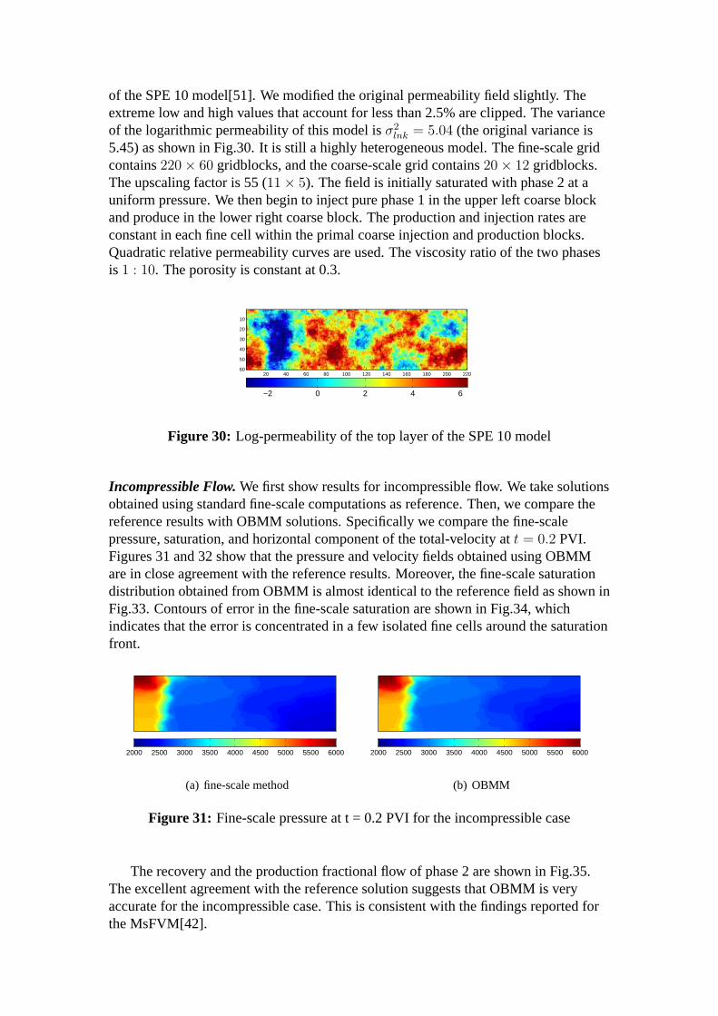
of the SPE 10 model[51]. We modified the original permeability field slightly. Theextreme low and high values that account for less than 2.5% are clipped. The varianceof the logarithmic permeability of this model isσ2

lnk = 5.04 (the original variance is5.45) as shown in Fig.30. It is still a highly heterogeneous model. The fine-scale gridcontains220× 60 gridblocks, and the coarse-scale grid contains20× 12 gridblocks.The upscaling factor is 55 (11× 5). The field is initially saturated with phase 2 at auniform pressure. We then begin to inject pure phase 1 in the upper left coarse blockand produce in the lower right coarse block. The production and injection rates areconstant in each fine cell within the primal coarse injection and production blocks.Quadratic relative permeability curves are used. The viscosity ratio of the two phasesis 1 : 10. The porosity is constant at 0.3.

20 40 60 80 100 120 140 160 180 200 220

10

20

30

40

50

60

−2 0 2 4 6

Figure 30: Log-permeability of the top layer of the SPE 10 model

Incompressible Flow.We first show results for incompressible flow. We take solutionsobtained using standard fine-scale computations as reference. Then, we compare thereference results with OBMM solutions. Specifically we compare the fine-scalepressure, saturation, and horizontal component of the total-velocity att = 0.2 PVI.Figures 31 and 32 show that the pressure and velocity fields obtained using OBMMare in close agreement with the reference results. Moreover, the fine-scale saturationdistribution obtained from OBMM is almost identical to the reference field as shown inFig.33. Contours of error in the fine-scale saturation are shown in Fig.34, whichindicates that the error is concentrated in a few isolated fine cells around the saturationfront.

2000 2500 3000 3500 4000 4500 5000 5500 6000

(a) fine-scale method

2000 2500 3000 3500 4000 4500 5000 5500 6000

(b) OBMM

Figure 31: Fine-scale pressure at t = 0.2 PVI for the incompressible case

The recovery and the production fractional flow of phase 2 are shown in Fig.35.The excellent agreement with the reference solution suggests that OBMM is veryaccurate for the incompressible case. This is consistent with the findings reported forthe MsFVM[42].

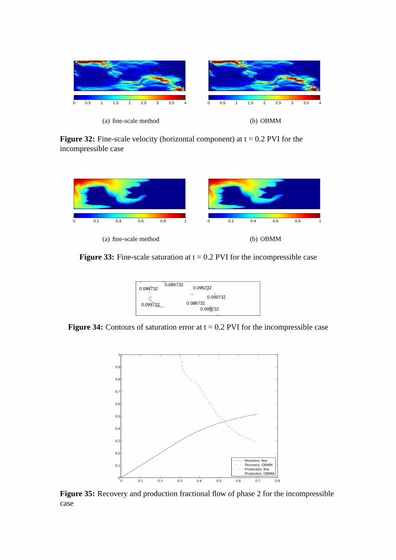
0 0.5 1 1.5 2 2.5 3 3.5 4

(a) fine-scale method

0 0.5 1 1.5 2 2.5 3 3.5 4

(b) OBMM

Figure 32: Fine-scale velocity (horizontal component) at t = 0.2 PVI for theincompressible case

0 0.2 0.4 0.6 0.8 1

(a) fine-scale method

0 0.2 0.4 0.6 0.8 1

(b) OBMM

Figure 33: Fine-scale saturation at t = 0.2 PVI for the incompressible case

0.0957320.095732

0.095732

0.0957320.095732 0.095732

0.095732

Figure 34: Contours of saturation error at t = 0.2 PVI for the incompressible case

0 0.1 0.2 0.3 0.4 0.5 0.6 0.7 0.80

0.1

0.2

0.3

0.4

0.5

0.6

0.7

0.8

0.9

1

Recovery: fineRecovery: OBMMProduction: fineProduction: OBMM

Figure 35: Recovery and production fractional flow of phase 2 for the incompressiblecase

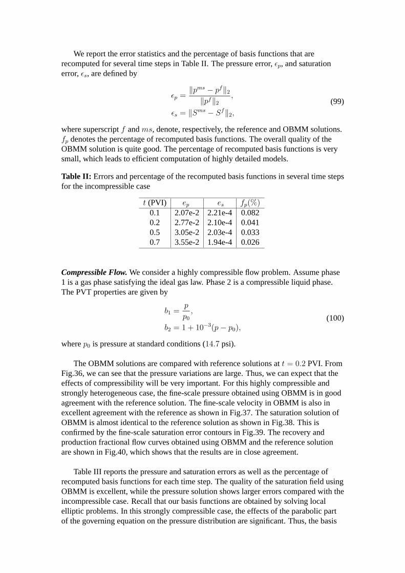
We report the error statistics and the percentage of basis functions that arerecomputed for several time steps in Table II. The pressure error,εp, and saturationerror,εs, are defined by

εp =‖pms − pf‖2

‖pf‖2

,

εs = ‖Sms − Sf‖2,

(99)

where superscriptf andms, denote, respectively, the reference and OBMM solutions.fp denotes the percentage of recomputed basis functions. The overall quality of theOBMM solution is quite good. The percentage of recomputed basis functions is verysmall, which leads to efficient computation of highly detailed models.

Table II: Errors and percentage of the recomputed basis functions in several time stepsfor the incompressible case

t (PVI) ep es fp(%)0.1 2.07e-2 2.21e-4 0.0820.2 2.77e-2 2.10e-4 0.0410.5 3.05e-2 2.03e-4 0.0330.7 3.55e-2 1.94e-4 0.026

Compressible Flow.We consider a highly compressible flow problem. Assume phase1 is a gas phase satisfying the ideal gas law. Phase 2 is a compressible liquid phase.The PVT properties are given by

b1 =p

p0

,

b2 = 1 + 10−3(p− p0),(100)

wherep0 is pressure at standard conditions (14.7 psi).

The OBMM solutions are compared with reference solutions att = 0.2 PVI. FromFig.36, we can see that the pressure variations are large. Thus, we can expect that theeffects of compressibility will be very important. For this highly compressible andstrongly heterogeneous case, the fine-scale pressure obtained using OBMM is in goodagreement with the reference solution. The fine-scale velocity in OBMM is also inexcellent agreement with the reference as shown in Fig.37. The saturation solution ofOBMM is almost identical to the reference solution as shown in Fig.38. This isconfirmed by the fine-scale saturation error contours in Fig.39. The recovery andproduction fractional flow curves obtained using OBMM and the reference solutionare shown in Fig.40, which shows that the results are in close agreement.

Table III reports the pressure and saturation errors as well as the percentage ofrecomputed basis functions for each time step. The quality of the saturation field usingOBMM is excellent, while the pressure solution shows larger errors compared with theincompressible case. Recall that our basis functions are obtained by solving localelliptic problems. In this strongly compressible case, the effects of the parabolic partof the governing equation on the pressure distribution are significant. Thus, the basis

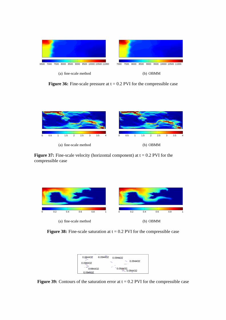
6500 7000 7500 8000 8500 9000 9500 10000 10500 11000

(a) fine-scale method

7000 7500 8000 8500 9000 9500 10000 10500 11000

(b) OBMM

Figure 36: Fine-scale pressure at t = 0.2 PVI for the compressible case

0 0.5 1 1.5 2 2.5 3 3.5 4

(a) fine-scale method

0 0.5 1 1.5 2 2.5 3 3.5 4

(b) OBMM

Figure 37: Fine-scale velocity (horizontal component) at t = 0.2 PVI for thecompressible case

0 0.2 0.4 0.6 0.8 1

(a) fine-scale method

0 0.2 0.4 0.6 0.8 1

(b) OBMM

Figure 38: Fine-scale saturation at t = 0.2 PVI for the compressible case

0.094432

0.0944320.094432

0.094432

0.094432

0.094432

0.094432

0.094432 0.094432

Figure 39: Contours of the saturation error at t = 0.2 PVI for the compressible case

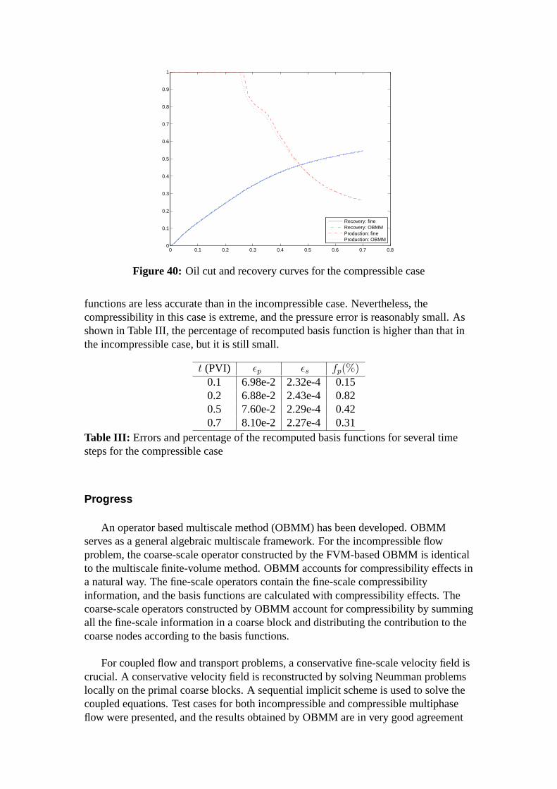
0 0.1 0.2 0.3 0.4 0.5 0.6 0.7 0.80

0.1

0.2

0.3

0.4

0.5

0.6

0.7

0.8

0.9

1

Recovery: fineRecovery: OBMMProduction: fineProduction: OBMM

Figure 40: Oil cut and recovery curves for the compressible case

functions are less accurate than in the incompressible case. Nevertheless, thecompressibility in this case is extreme, and the pressure error is reasonably small. Asshown in Table III, the percentage of recomputed basis function is higher than that inthe incompressible case, but it is still small.

t (PVI) εp εs fp(%)0.1 6.98e-2 2.32e-4 0.150.2 6.88e-2 2.43e-4 0.820.5 7.60e-2 2.29e-4 0.420.7 8.10e-2 2.27e-4 0.31

Table III: Errors and percentage of the recomputed basis functions for several timesteps for the compressible case

Progress

An operator based multiscale method (OBMM) has been developed. OBMMserves as a general algebraic multiscale framework. For the incompressible flowproblem, the coarse-scale operator constructed by the FVM-based OBMM is identicalto the multiscale finite-volume method. OBMM accounts for compressibility effects ina natural way. The fine-scale operators contain the fine-scale compressibilityinformation, and the basis functions are calculated with compressibility effects. Thecoarse-scale operators constructed by OBMM account for compressibility by summingall the fine-scale information in a coarse block and distributing the contribution to thecoarse nodes according to the basis functions.

For coupled flow and transport problems, a conservative fine-scale velocity field iscrucial. A conservative velocity field is reconstructed by solving Neumman problemslocally on the primal coarse blocks. A sequential implicit scheme is used to solve thecoupled equations. Test cases for both incompressible and compressible multiphaseflow were presented, and the results obtained by OBMM are in very good agreement

with reference solutions. The permeability field in the test cases is highlyheterogeneous. In the compressible flow case, the compressibility is high and thepressure variation is quite large. Such challenging features show that OBMM is areliable framework for solving highly compressible and strongly heterogeneousproblems.

The efficiency of OBMM relative to standard fine-scale methods lies in the factthat we do not solve a global fine-scale system. Constructing and solving thecoarse-scale equations takes a much smaller computational effort compared withsolving the global fine-scale system. Adaptive updating of the basis functions can leadto great efficiency gains. OBMM is readily extendible to more complicated physics.Moreover, it does not depend on explicit description of grid geometry and can bedirectly applied to unstructured models. OBMM is purely algebraic and makes full useof the fine-scale properties and equations. Thus, OBMM can be implemented inexisting reservoir simulators relatively easily.

Future Plans

To improve the efficiency of the multiscale method, we plan to continue theongoing work on developing a multiscale formulation for the transport problem(nonlinear saturation equation). The aim is to develop a fully adaptive multiscalemethod for the nonlinear coupling of multiphase flow and transport in highlyheterogeneous problems.

Stochastic Modeling of Non-equilibrium Multiphase Flow in PorousMedia

Investigators

Patrick Jenny, Associate Professor of Fluid Dynamics, ETH, Zurich; Hamdi Tchelepi,Associate Professor of Energy Resources Engineering; Manav Tyagi, GraduateResearch Assistant, ETH, Zurich.

Introduction

Several mechanisms have been proposed by whichCO2 can be trapped in therock-brine system, for example, hydrodynamic trapping [52], solution trapping [53],mineral trapping [54], and capillary trapping [55, 56]. The nonlinear multiphase flowprocesses involved may include nonequilibrium effects. The equilibrium conditioncorresponds to the case of standard Darcy’s law, where the phase mobility is a functionof the local saturation. In a nonequilibrium flow, the mobility can be different from theequilibrium mobility, and the difference may depend on, for example, how fast is theflow given the local balance of forces (capillary number) and whether the interface isuniform (viscosity ratio). In the past, several models have been proposed to treatnonequilibrium effects. One such model was proposed by Barenblatt [57], where therelative permeability and capillary pressure are not functions of the local saturationS ,but an effective saturationη, which is related toS by a linear relaxation equation

∂S

∂t=

1

τ(η − S). (101)

Hereτ is the relaxation time, which is zero when flow is in equilibrium. The flowapproaches the equilibrium condition with a time scale equal to this relaxation time,which in turn may depend on the flow conditions and fluid properties. There areseveral variations of Barenblatt’s model. For example, the case whenτ is a function ofsaturation has been considered by [58]. Here, we propose a stochastic framework formodeling nonequilibrium effects in multiphase flow in natural porous media. Unlikethe deterministic model, the effective saturation is assumed to be a random variable,whose probability density function (pdf) evolves in space and time. We consider ajoint-pdf of all the individual pdfs associated with each phase, and we derive anevolution equation for this joint-pdf in physical and (effective) saturation space. Theproblem is closed using a simple linear relaxation model, in which the effectivesaturation relaxes toward the actual saturation with a characteristic time scaleτ .

Stochastic Framework for Multiphase Flow in Porous Media

Consider the flow ofN -phases in a porous media. We defineSi as the probabilityto find a fluid volume of theith phase at location(x, t). With φ defined as the porosityof the medium, the following relation holds

N−1∑i=0

Si = φ . (102)

At a location(x, t), a fluid volume has velocity,ui, and mobility,λi. LetF i be theaverage mass flux of phasei at (x, t), then

F i =< ui >i ×Probability of finding a fluid volume of phasei (103)

or

F i =< ui >i Si, (104)

where< . >i denotes the conditional expectation with respect to phasei. Thus, theaverage phase velocity is given by the following expression

< ui >i=F i

Si. (105)

According to Darcy’s law, we have the following relationship between the averagemass flux of a phase and the pressure gradient

avergae phase flux= average phase mobility× pressure gradient, (106)

or

F i = − < λi >i ∇p. (107)

From Eq.( 105) and Eq.( 107) we propose the following rule for the phase velocity

ui = − λi

Si∇p. (108)

Note that this is only one of the possible solutions of Eq.( 105) and Eq.( 107). Byassuming incompressible flow, a poisson equation for the pressure can be derived

∇ · F = ∇ ·N−1∑i=0

F i = q. (109)

And it follows that

∇ · (−N−1∑i=0

< λi >i)∇p = q. (110)

Eq.( 108) can be recast to obtain the fractional flow formulation for the phasevelocity

ui =λi∑< λi >i

F

Si. (111)

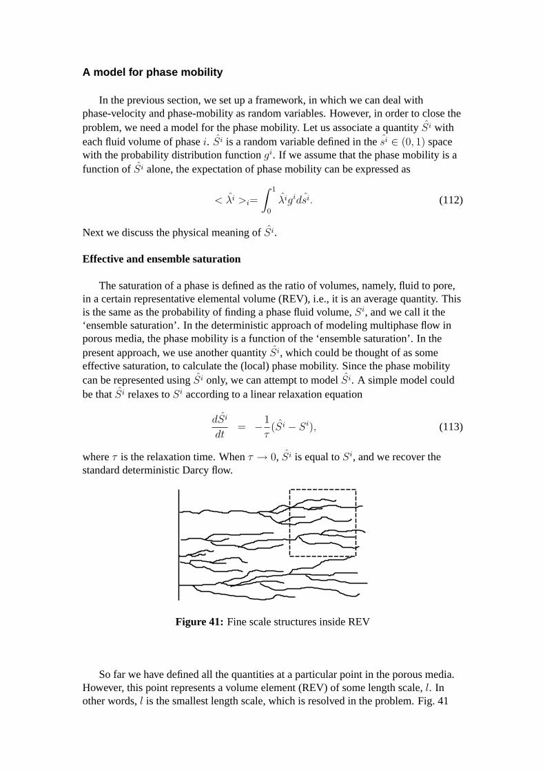
A model for phase mobility

In the previous section, we set up a framework, in which we can deal withphase-velocity and phase-mobility as random variables. However, in order to close theproblem, we need a model for the phase mobility. Let us associate a quantitySi witheach fluid volume of phasei. Si is a random variable defined in thesi ∈ (0, 1) spacewith the probability distribution functiongi. If we assume that the phase mobility is afunction ofSi alone, the expectation of phase mobility can be expressed as

< λi >i=

∫ 1

0

λigidsi. (112)

Next we discuss the physical meaning ofSi.

Effective and ensemble saturation

The saturation of a phase is defined as the ratio of volumes, namely, fluid to pore,in a certain representative elemental volume (REV), i.e., it is an average quantity. Thisis the same as the probability of finding a phase fluid volume,Si, and we call it the‘ensemble saturation’. In the deterministic approach of modeling multiphase flow inporous media, the phase mobility is a function of the ‘ensemble saturation’. In thepresent approach, we use another quantitySi, which could be thought of as someeffective saturation, to calculate the (local) phase mobility. Since the phase mobilitycan be represented usingSi only, we can attempt to modelSi. A simple model couldbe thatSi relaxes toSi according to a linear relaxation equation

dSi

dt= −1

τ(Si − Si), (113)

whereτ is the relaxation time. Whenτ → 0, Si is equal toSi, and we recover thestandard deterministic Darcy flow.

Figure 41: Fine scale structures inside REV

So far we have defined all the quantities at a particular point in the porous media.However, this point represents a volume element (REV) of some length scale,l. Inother words,l is the smallest length scale, which is resolved in the problem. Fig. 41

shows a possible flow scenario over this length where the invading phase fingersthrough the resident phase. In the deterministic approach, it is not possible to considerthe effect of such ”fine” scale structures on the large-scale flow behavior. However. ifwe assume that the system is ergodic over the lengthl, a fine scale fluid volume can betaken as a realization in our model. For example, we can associate the random variableSi to a finger to determine its dynamics.

Transport Equation for Joint Probability Density Function (JPDF)

We can combine the individual pdfs,gi, of Si into a single joint PDF ofS andA,whereS = Si whenA = i. We get

G(s, a) =∑

i

Sigiδ(a− i), (114)

and the following relation holds

∫G(s, a = i;x)ds = Si. (115)

The evolution ofG in x− s− a space, is governed by the following transportequation

∂G∂t

+∂

∂xj

⟨dXj

dt|s, a;x

⟩G

+∂

∂s

⟨dS

dt|s, a;x

⟩G

(116)

+∂

∂a

⟨dA

dt|s, a;x

⟩G

= 0. (117)

After substituting the conditional expectation expressions, we obtain

∂G∂t

+∂

∂xk

(∑i

uikδ(a− i)

)G

(118)

− ∂

∂s

1

τ

∑i

(si − Si)δ(a− i)G

= 0. (119)

Nonequilibrium capillary pressure effects

In this section, we use the stochastic framework to model nonequilibrium capillarypressure effects. We consider two-phase flowi = 0, 1 with the average phase pressuresp0 =< p0 >0 andp1 =< p1 >1. The capillary pressure is a random variable defined as

p1 − p0 = Pc = Pc(s0) (120)

For calculating the phase velocities, we use the average pressures

ui = −λi∇pi

Si, i = 0, 1. (121)

The expectation ofui will be

F i =< ui >= − < λi >i∇pi

Si, i = 0, 1, (122)

and the total mass flux is

F = F 0S0 + F 1S1 = − < λi >0 ∇p0− < λi >1 ∇p1 (123)

Taking the average of Eq.( 120)

< p1 >1 − < p0 >0= p1 − p0 =< Pc(s0) >0 (124)

Substituting forp1 in Eq.( 123)

F = − < λ0 >0 ∇p0− < λ1 >1 ∇p0− < λ1 >1 ∇ < Pc(s0) >0 (125)

From the above relation, we get an expression for∇p0

∇p0 =−F− < λ1 >1 ∇ < Pc(s0) >0

< λ0 >0 + < λ1 >1

, (126)

and for∇p1

∇p1 =−F+ < λ0 >0 ∇ < Pc(s0) >0

< λ0 >0 + < λ1 >1

. (127)

We can write the phase velocities in fractional flow form as follows

u0 =λ0F

S0(< λ0 >0 + < λ1 >1)+λ0 < λ1 >1 ∇ < Pc(s0) >0

S0(< λ0 >0 + < λ1 >1), (128)

and

u1 =λ1F

S1(< λ0 >0 + < λ1 >1)− λ1 < λ0 >0 ∇ < Pc(s0) >0

S1(< λ0 >0 + < λ1 >1). (129)

Numerical Results

The joint-pdf for transport derived in the previous section is solved using a FiniteVolume Method (FVM). Here we present some one-dimensional results for theclassical Buckley-Leverett problem. We also solve the problem using the stochasticparticle method (SPM) [59] and compare the results with FVM. In FVM, we use100× 100 grid to discretize Eq. 118. The mass flow rateF is 1ms−1. We assume thefollowing initial condition for the pdfs

g0 = δ(x)δ(s− Sin)

∆x+ (1− δ(x))

δ(s− Sout)

∆x, (130)

g1 = δ(x)δ(s− Sout)

∆x+ (1− δ(x))

δ(s− Sin)

∆x, (131)

whereSout is the initial saturation in the domain andSin is the saturation of injectedfluid atx = 0.

In order to show the effect of the relaxation parameter on the flow process, weconsider a test case in whichτ increases suddenly by a factor of 100 atx = 0.3.Fig. 42 shows the saturation profiles at different time intervals for the case whenSin = 0.95 andSout = 0.05. Fig. 43 shows the corresponding time evolution of thepdf. In order to check the validity of the code, we also solve the problem by SPM.Fig. 44 shows the comparison of the solutions obtained from SPM and FVM for twodifferent values ofτ . Next we varyτ . Fig. 45 depicts the saturation profiles fordifferent values ofτ with Sin = 0.95 andSout = 0.05. Fig. 46 depicts the saturationprofiles for different values ofτ with Sin = 0.8 andSout = 0.2. For the second case,we compare the mean and ensemble saturation in Fig. 47. It clear that for large valuesof τ the difference between the mean and ensemble saturations is significant.

Discussion and Conclusions

The main idea behind this work is to show how one can deal with the randomnessin a large scale flow quantity arising because of pore-scale fluctuations. Here weconsider the example of effective saturation (phase mobility) and derive a transportequation for the joint-pdf of the effective saturations associated with the phases. Thetransport equation can either be solved by a finite-volume method (FVM), or byconstructing an equivalent stochastic system with the same joint-pdf and thenperforming monte carlo simulation using the stochastic particle method (SPM) [59]. Ifthe dimensionality of the problem is up to four, then FVM is expected to be lessexpensive than SPM. However, for high-dimensional problems, numerical solutionsare feasible only with SPM. In our examples here, in addition to physical space oflocation and time, we have only one extra dimension representing the saturation space.As a result, the FVM method is quite efficient.

From the modeling viewpoint we showed how a simple relaxation model foreffective saturation can give rise to drastic change in the flow behavior. In this model,we have a parameter,τ which could be tuned such that the capillary pressure and

relative permeability relations as a function of saturation represent large-scaledynamics more accurately. In this framework, the relative probabilities and capillarypressure are no longer fixed functions of the ensemble saturations and depend uponhow far the flow is from equilibrium. Although the selection ofτ for a particular flowproblem is an open question, we hope that a detailed study of pore-scale flowdynamics, either by performing pore-network simulations, or by doing high-resolutionexperiments, may provide reasonable values forτ under various conditions. Thepresent framework can be easily extended for the modelingCO2 dissolution in brineand for accounting for chemical reactions. Similar to the effective saturation we canconsider a composition vector of the species associated with the each phase

φ = φ1, φ2..., φn

T(132)

Each species may undergo some chemical change according to the following equation

dφi

dt= Ri (133)

Consider a joint-pdfF(ψ1, ψ2..., ψn, a) of φ1, φ2..., φn, A in(ψ1 − ψ2...− ψn − a− x− t) space. Similar to Eq. 116, we can derive a transportequation forF .

∂F∂t

+∂

∂xj

⟨dXj

dt|s, a;x

⟩F

+∂

∂ψ1

⟨dφ1

dt|ψ, a;x

⟩F

(134)

+∂

∂ψ2

⟨dφ2

dt|ψ, a;x

⟩F

...+

∂

∂ψn

⟨dφn

dt|ψ, a;x

⟩F

(135)

+∂

∂a

⟨dA

dt|s, a;x

⟩F

= 0. (136)

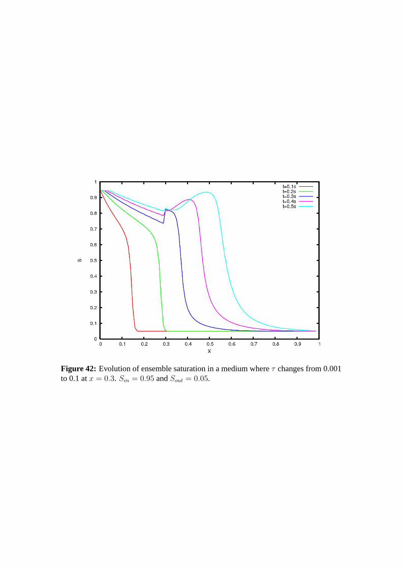
Figure 42: Evolution of ensemble saturation in a medium whereτ changes from 0.001to 0.1 atx = 0.3. Sin = 0.95 andSout = 0.05.

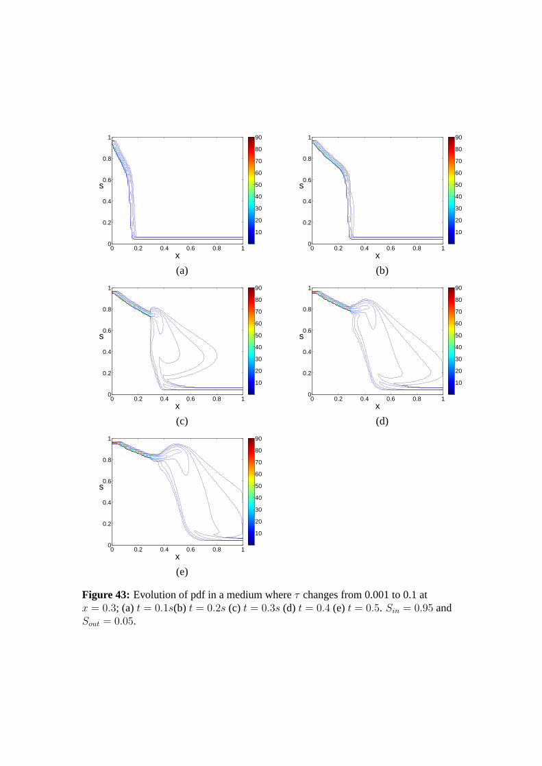
x

s

0 0.2 0.4 0.6 0.8 10

0.2

0.4

0.6

0.8

1

10

20

30

40

50

60

70

80

90

x

s

0 0.2 0.4 0.6 0.8 10

0.2

0.4

0.6

0.8

1

10

20

30

40

50

60

70

80

90

(a) (b)

x

s

0 0.2 0.4 0.6 0.8 10

0.2

0.4

0.6

0.8

1

10

20

30

40

50

60

70

80

90

x

s

0 0.2 0.4 0.6 0.8 10

0.2

0.4

0.6

0.8

1

10

20

30

40

50

60

70

80

90

(c) (d)

x

s

0 0.2 0.4 0.6 0.8 10

0.2

0.4

0.6

0.8

1

10

20

30

40

50

60

70

80

90

(e)

Figure 43: Evolution of pdf in a medium whereτ changes from 0.001 to 0.1 atx = 0.3; (a) t = 0.1s(b) t = 0.2s (c) t = 0.3s (d) t = 0.4 (e) t = 0.5. Sin = 0.95 andSout = 0.05.

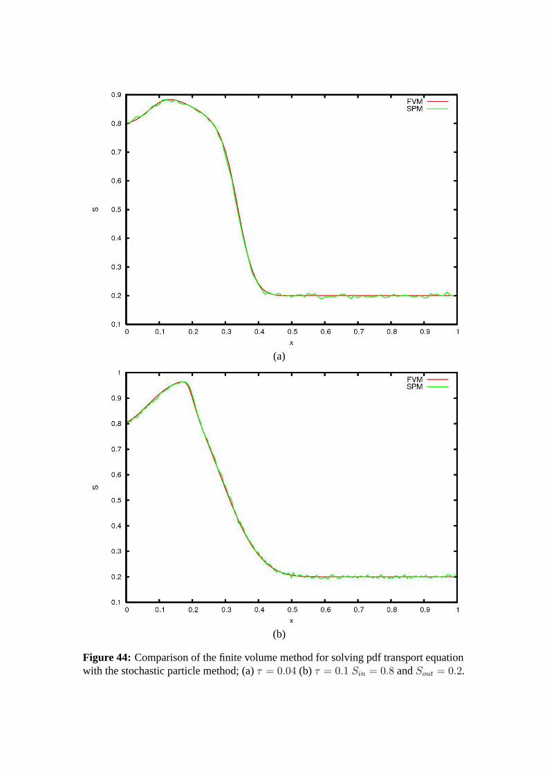
(a)

(b)

Figure 44: Comparison of the finite volume method for solving pdf transport equationwith the stochastic particle method; (a)τ = 0.04 (b) τ = 0.1 Sin = 0.8 andSout = 0.2.

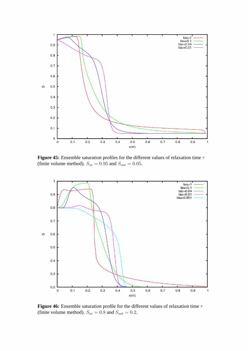
Figure 45: Ensemble saturation profiles for the different values of relaxation timeτ(finite volume method).Sin = 0.95 andSout = 0.05.

Figure 46: Ensemble saturation profile for the different values of relaxation timeτ(finite volume method).Sin = 0.8 andSout = 0.2.

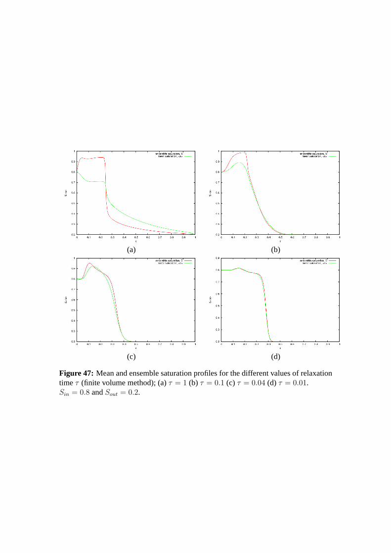
(a) (b)

(c) (d)

Figure 47: Mean and ensemble saturation profiles for the different values of relaxationtime τ (finite volume method); (a)τ = 1 (b) τ = 0.1 (c) τ = 0.04 (d) τ = 0.01.Sin = 0.8 andSout = 0.2.

Modeling CO2 Mineralization Reactions in a General Purpose FlowSimulator

Investigators

Lou Durlofsky, Professor of Energy Resources Engineering; Hamdi Tchelepi,Associate Professor of Energy Resources Engineering; Yaqing Fan, Graduate ResearchAssistant

Introduction

The design and monitoring of geological carbon storage operations require manykey capabilities, including advanced techniques for computational modeling. Becausean important long-term storage mechanism is the mineralization of the injected CO2

[60], it is essential that large-scale engineering models accurately represent thechemical interactions between liquids and minerals. The goal of this work is todevelop a robust, flexible and efficient capability for such modeling and to incorporateit into Stanford’s General Purpose Research Simulator (GPRS).

GPRS is our platform for research in the areas of general reservoir simulation andgeological storage of carbon dioxide. The simulator is object oriented, flexible andextensible, and has many advanced features (as described below) that render itparticularly well suited for both sets of applications. As discussed in last year’s annualreport to GCEP (and described in full detail in Fan’s MS thesis [61]), we recentlyincorporated several mechanisms (e.g., three-phase relative permeability hysteresis,dispersion) that are required for accurate modeling of CO2 sequestration into thissimulator. With the introduction of CO2 mineralization reactions, the simulator will beable to model all of the key currently known mechanisms for the long-term geologicalstorage of carbon dioxide.

Chemical reaction modeling within the context of CO2 sequestration has beenstudied by several research groups and incorporated into a number of simulators. It istherefore of interest to distinguish our work from these earlier efforts. CMG’s GEMsimulator is a coupled reactive-transport compositional simulator based on generalizedequations of state. Extensions were introduced to model the chemical reactions relatedto asphaltene precipitation and GHG sequestration. Specifically, Nghiemet al. [62]enhanced GEM to include mineral dissolution and precipitation kinetics.TOUGHREACT [63] is a reactive-transport simulator developed by LawrenceBerkeley National Laboratory. Interactions between gas, minerals, and liquid aremodeled. The software package NUFT [64], developed by Lawrence LivermoreNational Laboratory, has similar capabilities to TOUGHREACT. UTCHEM [65] is asimulator developed by The University of Texas at Austin which includes

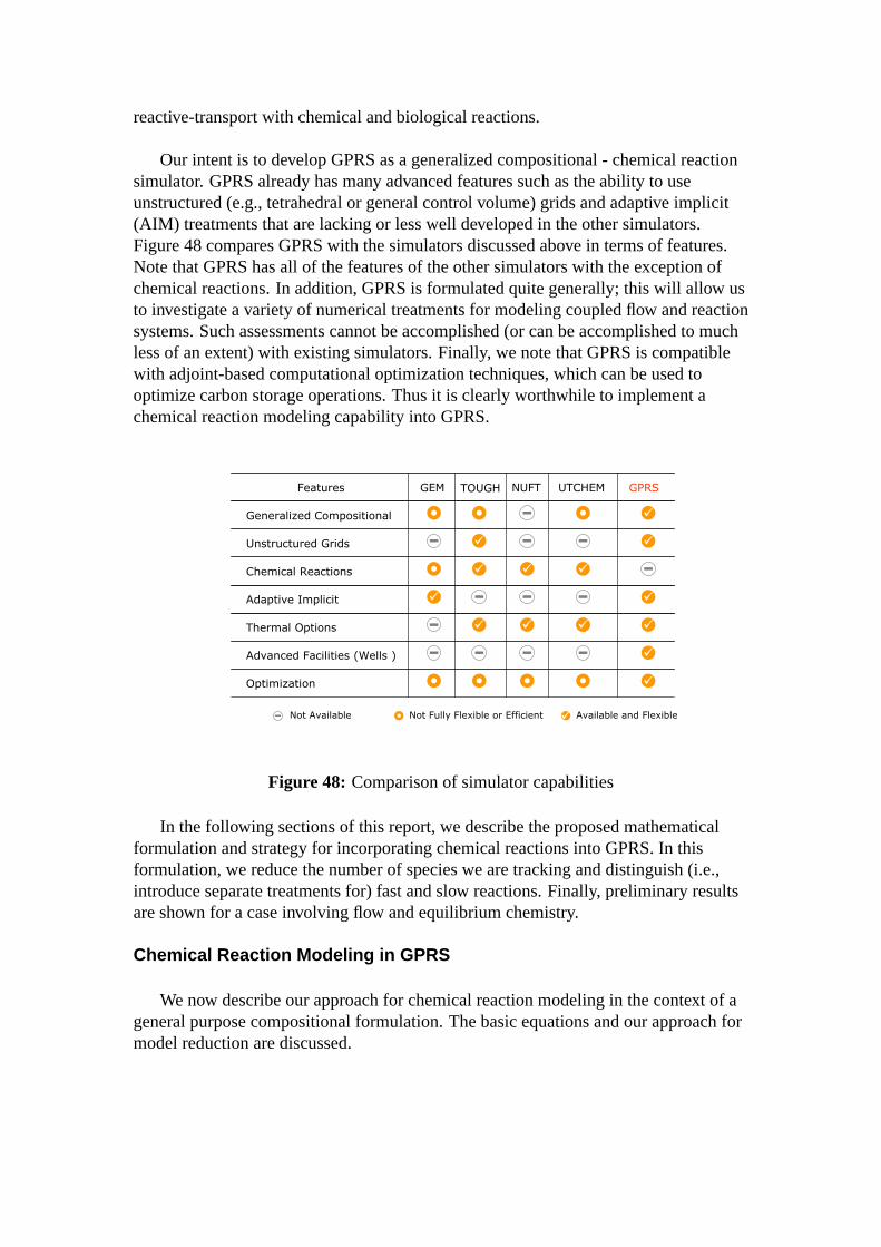
reactive-transport with chemical and biological reactions.

Our intent is to develop GPRS as a generalized compositional - chemical reactionsimulator. GPRS already has many advanced features such as the ability to useunstructured (e.g., tetrahedral or general control volume) grids and adaptive implicit(AIM) treatments that are lacking or less well developed in the other simulators.Figure 48 compares GPRS with the simulators discussed above in terms of features.Note that GPRS has all of the features of the other simulators with the exception ofchemical reactions. In addition, GPRS is formulated quite generally; this will allow usto investigate a variety of numerical treatments for modeling coupled flow and reactionsystems. Such assessments cannot be accomplished (or can be accomplished to muchless of an extent) with existing simulators. Finally, we note that GPRS is compatiblewith adjoint-based computational optimization techniques, which can be used tooptimize carbon storage operations. Thus it is clearly worthwhile to implement achemical reaction modeling capability into GPRS.

!"#

$% $ & '%(( % '%

$

Figure 48: Comparison of simulator capabilities

In the following sections of this report, we describe the proposed mathematicalformulation and strategy for incorporating chemical reactions into GPRS. In thisformulation, we reduce the number of species we are tracking and distinguish (i.e.,introduce separate treatments for) fast and slow reactions. Finally, preliminary resultsare shown for a case involving flow and equilibrium chemistry.

Chemical Reaction Modeling in GPRS

We now describe our approach for chemical reaction modeling in the context of ageneral purpose compositional formulation. The basic equations and our approach formodel reduction are discussed.

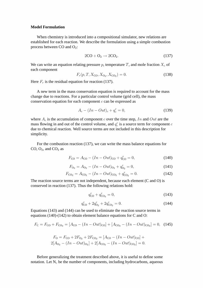
Model Formulation

When chemistry is introduced into a compositional simulator, new relations areestablished for each reaction. We describe the formulation using a simple combustionprocess between CO and O2:

2CO+ O2 → 2CO2. (137)

We can write an equation relating pressurep, temperatureT , and mole fractionXc ofeach component

Fr(p, T,XCO, XO2 , XCO2) = 0. (138)

HereFr is the residual equation for reaction (137).

A new term in the mass conservation equation is required to account for the masschange due to reactions. For a particular control volume (grid cell), the massconservation equation for each componentc can be expressed as

Ac − (In−Out)c + qrc = 0, (139)

whereAc is the accumulation of componentc over the time step,In andOut are themass flowing in and out of the control volume, andqr

c is a source term for componentcdue to chemical reaction. Well source terms are not included in this description forsimplicity.

For the combustion reaction (137), we can write the mass balance equations forCO, O2, and CO2 as

FCO = ACO− (In−Out)CO + qrCO = 0, (140)

FO2 = AO2 − (In−Out)O2 + qrO2

= 0, (141)

FCO2 = ACO2 − (In−Out)CO2 + qrCO2

= 0. (142)

The reaction source terms are not independent, because each element (C and O) isconserved in reaction (137). Thus the following relations hold:

qrCO + qr

CO2= 0, (143)

qrCO + 2qr

O2+ 2qr

CO2= 0. (144)

Equations (143) and (144) can be used to eliminate the reaction source terms inequations (140)-(142) to obtain element balance equations for C and O:

FC = FCO + FCO2 = [ACO− (In−Out)CO] + [ACO2 − (In−Out)CO2 ] = 0, (145)

FO = FCO + 2FO2 + 2FCO2 = [ACO− (In−Out)CO] +

2[AO2 − (In−Out)O2 ] + 2[ACO2 − (In−Out)CO2 ] = 0.

Before generalizing the treatment described above, it is useful to define somenotation. Let Nc be the number of components, including hydrocarbons, aqueous

species, and minerals. The number of elements is denoted by Ne. The number ofreactions is Nr, consisting of Neq reactions at equilibrium and Nneq nonequilibriumreactions controlled by reaction rates. It is always the case thatNr = Neq + Nneq.

In general, the Nc component mass balance equations can be transformed to Ne

element balance equations by linear combinations (as above) to eliminate reactionsource terms, as long as the reactions occur within the target block and within the timestep. This is often the case in subsurface reactive-transport problems and we will usethis assumption in the first phase of this work. We may eventually need to treatsituations in which reactions in a particular block depend strongly on effects insurrounding blocks, in which case our treatment will be extended.

After the linear transformation from component balance equations to elementequations, the computational cost will be reduced significantly compared to the casewhen all components are tracked. In fact, because the number of components can bevery large (due to complex reactions), it is usually not practical or desirable to solvefor all components simultaneously. The number of elements, by contrast, is usuallymuch smaller, particularly when we have a large number of components composed ofonly a few elements. Thus, tracking Ne elements is generally much more efficientcomputationally than tracking Nc components.

We can further reduce the number of governing equations and unknowns bytreating fast reactions and slow reactions separately. In general, chemical reactions canbe roughly divided into two groups: ‘sufficiently fast and reversible’ reactions, and‘slow or irreversible’ reactions. In the first group, the time scales for the reactions aresmall compared to the global time step, so these reactions can be assumed to reachequilibrium instantaneously. For example, the hydrolysis of calcium chloride issufficiently fast such that the equilibrium state is reached in each block at every timestep. For this reaction we have:

CaCl2 = Ca2+ + 2Cl−, (146)

Keq =aCa2+a

2Cl−

aCaCl2, (147)

wherea is activity of the component, which is related to mole fraction via the activitycoefficientγ

a = γcXc. (148)

Rearranging equation (147),

XCa2+ =KeqaCaCl2

γCa2+a2Cl−

. (149)

Equation (149) indicates that the mole fraction of Ca2+ can be expressed explicitly interms of other variables. Therefore,XCa2+ can be updated locally after each time steprather than being computed in the full set of governing equations.

We now consider the second type of reactions, so-called ‘rate-controlled’ reactions,which are generally not in equilibrium. The reaction in (150) is such a reaction, with atemperature-dependent ratekf

2CO+ O2

kf→ 2CO2, (150)

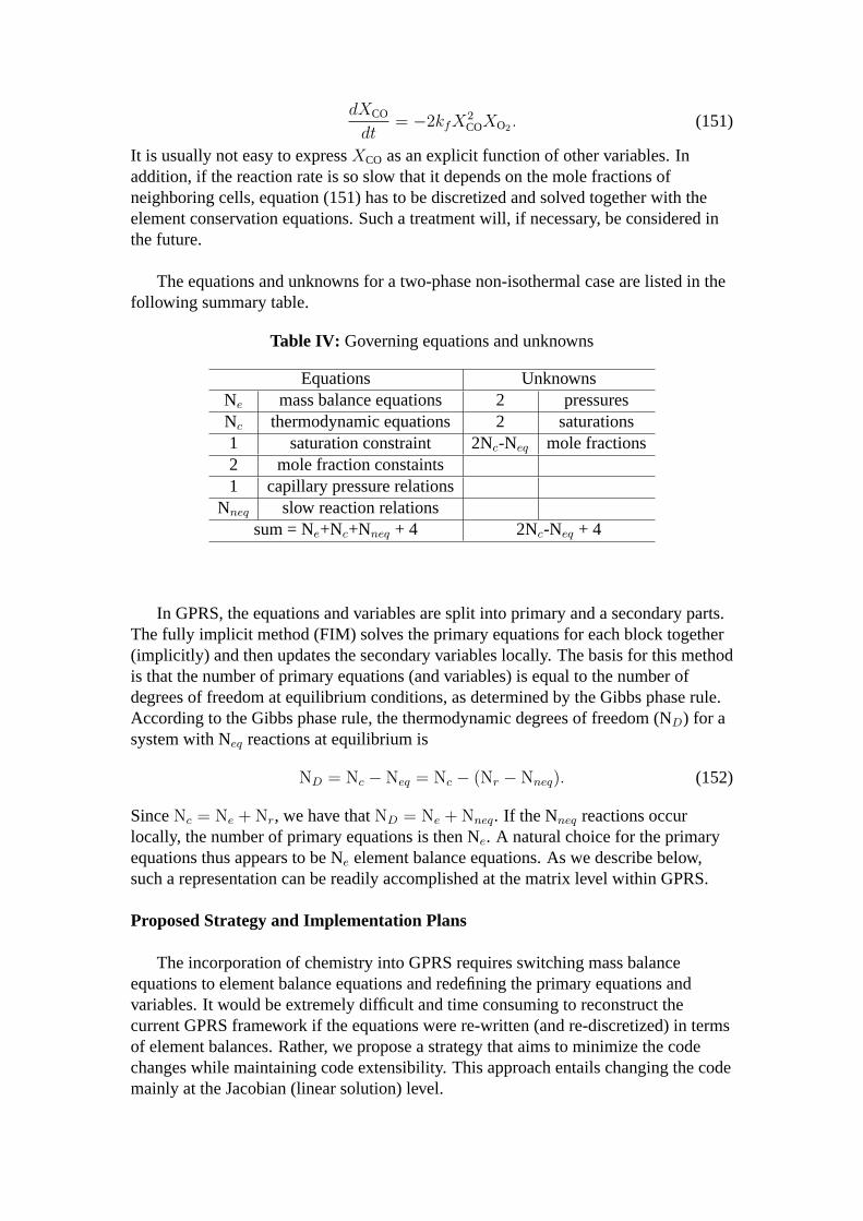
dXCO

dt= −2kfX

2COXO2 . (151)

It is usually not easy to expressXCO as an explicit function of other variables. Inaddition, if the reaction rate is so slow that it depends on the mole fractions ofneighboring cells, equation (151) has to be discretized and solved together with theelement conservation equations. Such a treatment will, if necessary, be considered inthe future.

The equations and unknowns for a two-phase non-isothermal case are listed in thefollowing summary table.

Table IV: Governing equations and unknowns

Equations UnknownsNe mass balance equations 2 pressuresNc thermodynamic equations 2 saturations1 saturation constraint 2Nc-Neq mole fractions2 mole fraction constaints1 capillary pressure relations

Nneq slow reaction relationssum = Ne+Nc+Nneq + 4 2Nc-Neq + 4

In GPRS, the equations and variables are split into primary and a secondary parts.The fully implicit method (FIM) solves the primary equations for each block together(implicitly) and then updates the secondary variables locally. The basis for this methodis that the number of primary equations (and variables) is equal to the number ofdegrees of freedom at equilibrium conditions, as determined by the Gibbs phase rule.According to the Gibbs phase rule, the thermodynamic degrees of freedom (ND) for asystem with Neq reactions at equilibrium is

ND = Nc − Neq = Nc − (Nr − Nneq). (152)

SinceNc = Ne + Nr, we have thatND = Ne + Nneq. If the Nneq reactions occurlocally, the number of primary equations is then Ne. A natural choice for the primaryequations thus appears to be Ne element balance equations. As we describe below,such a representation can be readily accomplished at the matrix level within GPRS.

Proposed Strategy and Implementation Plans

The incorporation of chemistry into GPRS requires switching mass balanceequations to element balance equations and redefining the primary equations andvariables. It would be extremely difficult and time consuming to reconstruct thecurrent GPRS framework if the equations were re-written (and re-discretized) in termsof element balances. Rather, we propose a strategy that aims to minimize the codechanges while maintaining code extensibility. This approach entails changing the codemainly at the Jacobian (linear solution) level.

Using this procedure, instead of rewriting the mass conservation equations in termsof element balances, we use the current mass balance equations to construct theJacobian matrix. Then, instead of forming the derivatives required for the elementbalance equations directly, these derivatives are obtained by performing lineartransformations on the Jacobian matrix. In GPRS, these transformations are performedafter all of the governing equations are discretized. The Jacobian matrix for thefacilities (i.e., wells) requires similar linear transformations. The process of reducingfrom the full equation set to the set of primary equations is very similar to reductionprocedures already performed in the current code.

Besides the manipulation of the Jacobian matrix, the local equilibrium calculationsalso need to be modified to account for chemical reactions. The equilibrium state nowmust satisfy both chemical and thermodynamic equilibrium relations. Two strategiescould be applied for this. In the first approach, the thermodynamic and chemicalequilibrium equations are calculated iteratively until the results for both converge. Inthe second approach, the two sets of equilibrium equations are solved together untilconvergence. The first approach is used in the initial implementation in GPRS (asshown in the case in the next section). The second approach will be explored soon inorder to determine which treatment is superior.

The implementation plan is divided into three stages. In the first stage, a localequilibrium module will be developed. The second stage entails transforming theJacobian matrix to calculate coupled reactive-transport equations. After these stagesare completed, GPRS will be able to solve chemical reaction problems in whichreactions are either at equilibrium or are rate-controlled. However, the chemicalreactions must not have significant dependency on surrounding blocks. In the thirdstage, we will investigate how to incorporate reactions that are affected by surroundingblocks.

Preliminary Results

A simple case involving CO2 injection into a carbonate reservoir is now presented.In the results presented here we consider only local chemical equilibrium reactions.

Model Description

The reservoir is modeled as a one-dimensional homogeneous carbonate reservoir,in which the reactive mineral is calcite (CaCO3). Initially, the reservoir is saturatedwith 100% water. Initial equilibrium is established between water, calcite, andelectrolytes in the water. A pure CO2 stream is injected at one end of the reservoir anda producer is introduced at the other end (as shown in Figure 49). The parametersdescribing the reservoir are listed in Table V.

A total of four equilibrium reactions are considered. The reactions and theirequilibrium constants are listed in Table VI. The species in these reactions aredistributed in the three phases. The gas phase contains CO2 and H2O, the solid phasecontains calcite only, and the aqueous phase contains CO2(aq), H2O and all ions. Inthe current calculation, neither ion adsorption nor ion change is included, and the ions

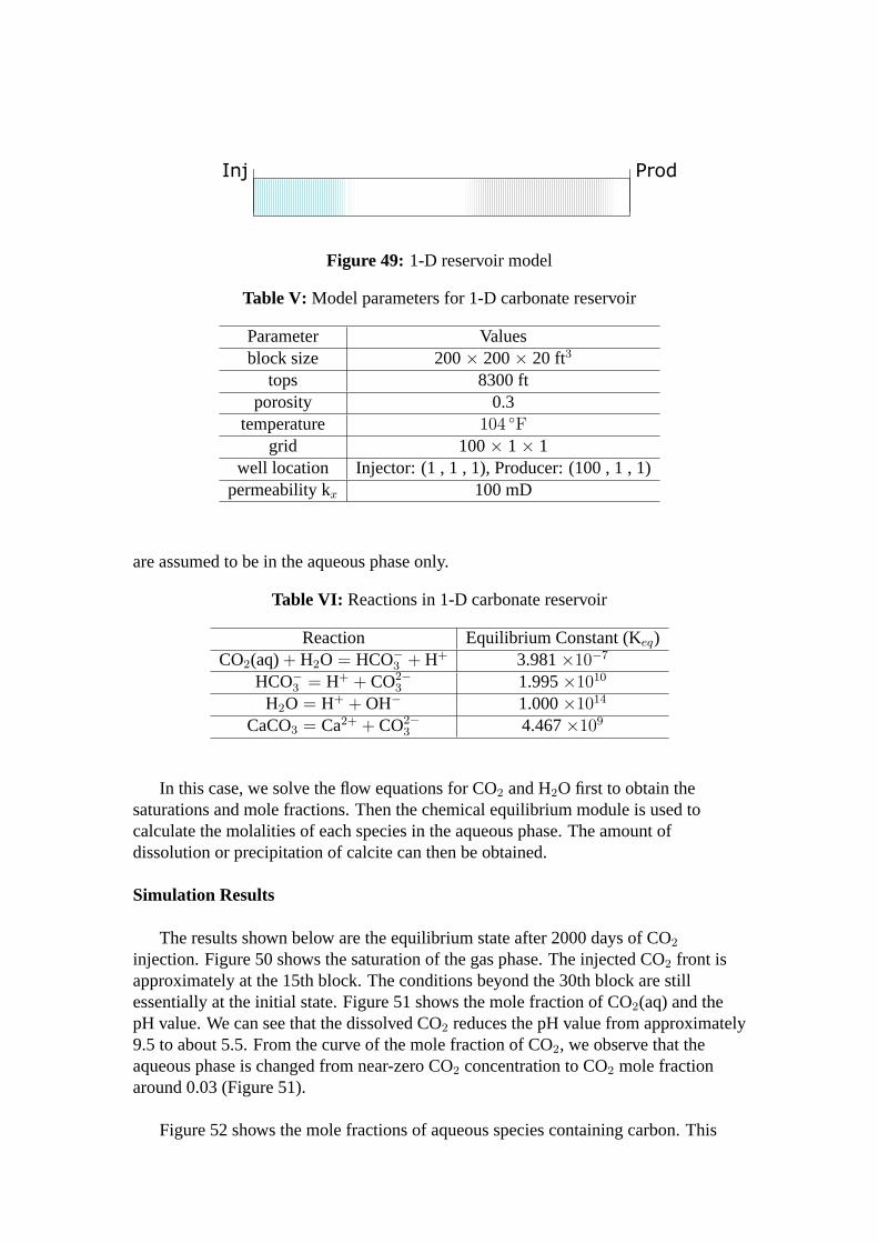
Figure 49: 1-D reservoir model

Table V: Model parameters for 1-D carbonate reservoir

Parameter Valuesblock size 200× 200× 20 ft3

tops 8300 ftporosity 0.3

temperature 104 Fgrid 100× 1× 1

well location Injector: (1 , 1 , 1), Producer: (100 , 1 , 1)permeability kx 100 mD

are assumed to be in the aqueous phase only.

Table VI: Reactions in 1-D carbonate reservoir

Reaction Equilibrium Constant (Keq)CO2(aq)+ H2O = HCO−

3 + H+ 3.981×10−7

HCO−3 = H+ + CO2−

3 1.995×1010

H2O = H+ + OH− 1.000×1014

CaCO3 = Ca2+ + CO2−3 4.467×109

In this case, we solve the flow equations for CO2 and H2O first to obtain thesaturations and mole fractions. Then the chemical equilibrium module is used tocalculate the molalities of each species in the aqueous phase. The amount ofdissolution or precipitation of calcite can then be obtained.

Simulation Results

The results shown below are the equilibrium state after 2000 days of CO2

injection. Figure 50 shows the saturation of the gas phase. The injected CO2 front isapproximately at the 15th block. The conditions beyond the 30th block are stillessentially at the initial state. Figure 51 shows the mole fraction of CO2(aq) and thepH value. We can see that the dissolved CO2 reduces the pH value from approximately9.5 to about 5.5. From the curve of the mole fraction of CO2, we observe that theaqueous phase is changed from near-zero CO2 concentration to CO2 mole fractionaround 0.03 (Figure 51).

Figure 52 shows the mole fractions of aqueous species containing carbon. This

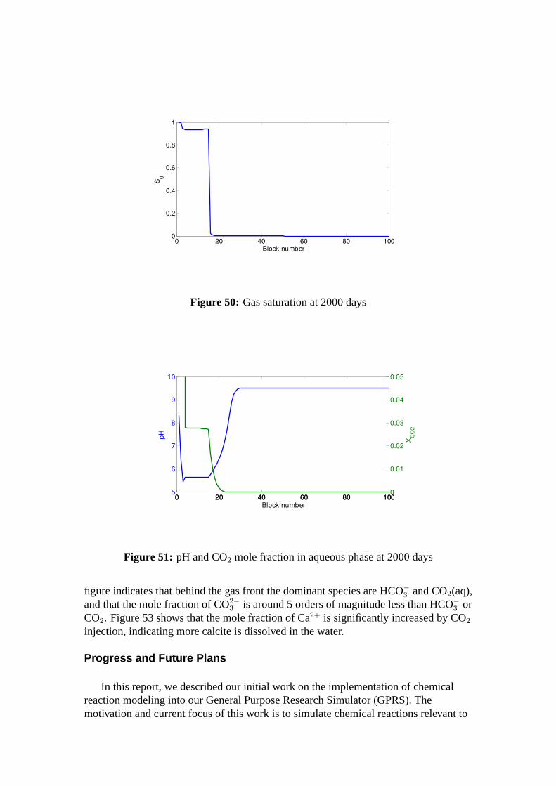
0 20 40 60 80 1000

0.2

0.4

0.6

0.8

1

Sg

Block number

Figure 50: Gas saturation at 2000 days

0 20 40 60 80 1005

6

7

8

9

10

pH

Block number0 20 40 60 80 100

0

0.01

0.02

0.03

0.04

0.05

XC

O2

Figure 51: pH and CO2 mole fraction in aqueous phase at 2000 days

figure indicates that behind the gas front the dominant species are HCO−3 and CO2(aq),

and that the mole fraction of CO2−3 is around 5 orders of magnitude less than HCO−3 or

CO2. Figure 53 shows that the mole fraction of Ca2+ is significantly increased by CO2injection, indicating more calcite is dissolved in the water.

Progress and Future Plans

In this report, we described our initial work on the implementation of chemicalreaction modeling into our General Purpose Research Simulator (GPRS). Themotivation and current focus of this work is to simulate chemical reactions relevant to

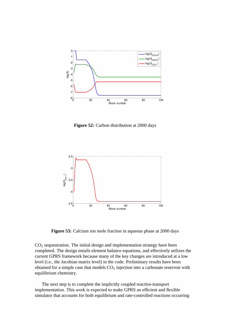
0 20 40 60 80 100-8

-7

-6

-5

-4

-3

-2

-1

0

Block number

log(

X)

log(XCO2,w)

log(XHCO3-)

log(XCO3--)

Figure 52: Carbon distribution at 2000 days

0 20 40 60 80 100-4.5

-4

-3.5

-3

-2.5

Block number

log(

X Ca+

+)

Figure 53: Calcium ion mole fraction in aqueous phase at 2000 days

CO2 sequestration. The initial design and implementation strategy have beencompleted. The design entails element balance equations, and effectively utilizes thecurrent GPRS framework because many of the key changes are introduced at a lowlevel (i.e., the Jacobian matrix level) in the code. Preliminary results have beenobtained for a simple case that models CO2 injection into a carbonate reservoir withequilibrium chemistry.

The next step is to complete the implicitly coupled reactive-transportimplementation. This work is expected to make GPRS an efficient and flexiblesimulator that accounts for both equilibrium and rate-controlled reactions occurring

locally. As GPRS contains a variety of numerical options for treating flow, we plan toexplore the use of various combinations of options for modeling flow and reaction. Weexpect this to provide an efficient and flexible overall capability for the modeling ofcarbon dioxide injection and geologic storage.

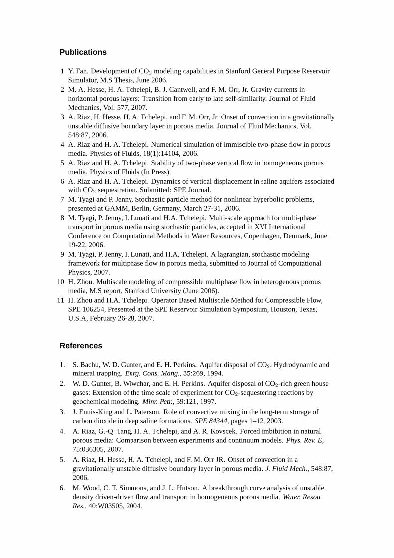
Publications

1 Y. Fan. Development of CO2 modeling capabilities in Stanford General Purpose ReservoirSimulator, M.S Thesis, June 2006.

2 M. A. Hesse, H. A. Tchelepi, B. J. Cantwell, and F. M. Orr, Jr. Gravity currents inhorizontal porous layers: Transition from early to late self-similarity. Journal of FluidMechanics, Vol. 577, 2007.

3 A. Riaz, H. Hesse, H. A. Tchelepi, and F. M. Orr, Jr. Onset of convection in a gravitationallyunstable diffusive boundary layer in porous media. Journal of Fluid Mechanics, Vol.548:87, 2006.

4 A. Riaz and H. A. Tchelepi. Numerical simulation of immiscible two-phase flow in porousmedia. Physics of Fluids, 18(1):14104, 2006.

5 A. Riaz and H. A. Tchelepi. Stability of two-phase vertical flow in homogeneous porousmedia. Physics of Fluids (In Press).

6 A. Riaz and H. A. Tchelepi. Dynamics of vertical displacement in saline aquifers associatedwith CO2 sequestration. Submitted: SPE Journal.

7 M. Tyagi and P. Jenny, Stochastic particle method for nonlinear hyperbolic problems,presented at GAMM, Berlin, Germany, March 27-31, 2006.

8 M. Tyagi, P. Jenny, I. Lunati and H.A. Tchelepi. Multi-scale approach for multi-phasetransport in porous media using stochastic particles, accepted in XVI InternationalConference on Computational Methods in Water Resources, Copenhagen, Denmark, June19-22, 2006.

9 M. Tyagi, P. Jenny, I. Lunati, and H.A. Tchelepi. A lagrangian, stochastic modelingframework for multiphase flow in porous media, submitted to Journal of ComputationalPhysics, 2007.

10 H. Zhou. Multiscale modeling of compressible multiphase flow in heterogenous porousmedia, M.S report, Stanford University (June 2006).

11 H. Zhou and H.A. Tchelepi. Operator Based Multiscale Method for Compressible Flow,SPE 106254, Presented at the SPE Reservoir Simulation Symposium, Houston, Texas,U.S.A, February 26-28, 2007.

References

1. S. Bachu, W. D. Gunter, and E. H. Perkins. Aquifer disposal of CO2. Hydrodynamic andmineral trapping.Enrg. Cons. Mang., 35:269, 1994.

2. W. D. Gunter, B. Wiwchar, and E. H. Perkins. Aquifer disposal of CO2-rich green housegases: Extension of the time scale of experiment for CO2-sequestering reactions bygeochemical modeling.Minr. Petr., 59:121, 1997.

3. J. Ennis-King and L. Paterson. Role of convective mixing in the long-term storage ofcarbon dioxide in deep saline formations.SPE 84344, pages 1–12, 2003.

4. A. Riaz, G.-Q. Tang, H. A. Tchelepi, and A. R. Kovscek. Forced imbibition in naturalporous media: Comparison between experiments and continuum models.Phys. Rev. E,75:036305, 2007.

5. A. Riaz, H. Hesse, H. A. Tchelepi, and F. M. Orr JR. Onset of convection in agravitationally unstable diffusive boundary layer in porous media.J. Fluid Mech., 548:87,2006.

6. M. Wood, C. T. Simmons, and J. L. Hutson. A breakthrough curve analysis of unstabledensity driven-driven flow and transport in homogeneous porous media.Water. Resou.Res., 40:W03505, 2004.

7. M. Stohr and A. Khalili. Dynamic regimes of buoyancy-affected two phase flow inunconsolidated porous media.Phy. Rev. E, 73:036301, 2006.

8. T. Tokunaga, K. Mogi, O. Matsubara, and H. Tosaka. Buoyancy and interfacial forceeffects on two-phase displacement patterns: An experimental study.AAPG Bul., 84:65,2000.

9. R. Lenormand, E. Touboul, and C. Zarcone. Numerical-models and experiments onimmiscible displacements in porous-media.J. Fluid. Mech., 189:165, 1988.

10. B. Cockburn, C. Johnson, C.-W. Shu, and E. Tadmor.Advanced numerical approximationof nonlinear hyperbolic equations.Lecture notes in mathametics. Springer, Berlin, 1998.

11. S. K. Lele. Compact finite differences with spectral-like resolution.J. Comput. Phys.,103:16, 1992.

12. A. Riaz and H. A. Tchelepi. Linear stability analysis of immiscible two-phase flow inporous media with capillary dispersion and density variation.Phys. Fluids, 16(12):4727,2004.

13. L. L. Lake. Enhanced Oil Recovery. Prentice-Hall, Inc., 1989.

14. T. Xu, J. A. Apps, and K. Pruess. Reactive geochemical transport simulation to studymineral trapping for co2 disposal in deep arenaceous formations.Journal of GeophysicalResearch, 108(doi:10.1029/2002JB001979,), 2003.

15. J. W. Johnson and J. J. Nitao. Reactive transport modeling of geologic CO2 sequestrationat Sleipner. In J. Gale and Y. Kaya, editors,Greenhouse Gas Control Technologies,volume 1, pages 327–333. Elsevier Science Ltd, 2003.

16. E. J. Spiteri, R. Juanes, M. J. Blunt, and F. M. Orr Jr. Relative permeability hysteresis:Trapping models and application to geological CO2 sequestration. InSPE AnnualTechnical Conference and Exhibition, number SPE 96448, Dallas , TX, 9-12 October 20052005.

17. A. Kumar, R. Ozah, M. Noh, G. A. Pope, S. Bryant, K. Sepehrnoori, and L. W. Lake.Reservoir simulation of CO2 storage in deep saline aquifers.SPE Journal, pages 336–348,September 2005.

18. R.C. Ozah, S. Lakshminarasimhan, G.A. Pope, K. Sepehrnoori, , and S.L. Bryant.Numerical simulation of the storage of pure co2 and co2-h2s gas mixtures in deep salineaquifers. InSPE Annual Technical Conference and Exhibition, number SPE 97255-MS,Dallas , TX, 9-12 October 2005 2005.

19. S. Mo and I. Akervoll. Modeling long-term CO2 storage in aquifer with a black-oilreservoir simulator. InSPE/EPA/DOE Exploration and Production EnvironmentalConference, number SPE 93951, Galveston, TX, 7-9 March 2005 2005.

20. S. Mo, P. Zweigel, E. Lindeberg, and I. Akervoll. Effect of geologic parameters on CO2

storage in deep saline aquifers. InSPE Eurospec/EAGE Annual Conference, number SPE93952, Madrid, Spain, 13-16 June 2005 2005.

21. J. Ennis-King and L. Paterson. Engineering aspects of geological sequestration of carbondioxide. InAsia Pacific Oil and Gas Conference and Exhibition, number SPE 77809,Melbourne, Australia, 8 - 10 October 2002 2002.

22. I. N. Kochina, N. N. Mikhailov, and M. V. Filinov. Groundwater mound damping.Int. J.Eng. Sci., 21:413–421, 1983.

23. H. E. Huppert and A. W. Woods. Gravity-driven flows in porous media.J. Fluid Mech.,292:55–69, 1995.

24. G. I. Barenblatt.Scaling, self-similarity, and intermediate asymptotics. CambridgeUniversity Press, 1996.

25. D.A. Collins J. Grabenstetter, Y.-K. Li and L.X. Nghiem. Stability-Based Switching

Criterion for Adaptive-Implicit Compositional Reservoir Simulation.SPE, (21225), 1991.

26. Jr. P.A. Forsyth and P.H. Sammon. Practical Considerations for Adaptive Implicit Methodsin Reservoir Simulation.Journal of Computational Physics, 62:265–281, 1986.

27. T.F. Russell. Stability Analysis and Switching Criteria for Adaptive Implicit MethodsBased on the CFL condition.SPE, (18416), 1989.

28. G.W. Thomas and D.H. Turnau. Reservoir Simulation Using an Adaptive Implicit Method.SPE, (10120), 1983.

29. G.W. Thomas and D.H. Turnau. The Mathematical Basis of the Adaptive Implicit Method.SPE, (25245), 1993.

30. L.C. Young and T.F. Russell. Implementation of an Adaptive Implicit Method.SPE,(25245), 1993.

31. E. Godlewski and P.A. Raviart.Numerical Approximation of Hyperbolic Systems ofConservation Laws. Springer Verlag, 1991.

32. W. Hundsdorfer and J.G. Verwer.Numerical Solution of Time-DependentAdvection-Diffusion-Reaction Equations. Springer, 2003.

33. Arieh Iserles.Numerical Analysis of Differential Equations. Cambridge University Press,1996.

34. B. Rubin and M.J. Blunt. High-Order Implicit Flux Limiting Schemes for Black-OilSimulation.SPE, (21222), 1991.

35. Alexander Kurganov and Eitan Tadmor. Non-oscillatory central differencing forhyperbolic consevation laws.Journal of Computational Physics, 87:408–463, 1990.

36. Bjorn Engquist, Stanley Osher, and Sukumar R. Chakravarthy. Uniformly High OrderAccurate Essentially Non-oscillatory Schemes.Journal of Computational Physics,71:231–303, 1987.

37. Chi-Wang Shu and Stanley Osher. Efficient implementation of essentially non-oscillatoryshock capturing schemes.Journal of Computational Physics, 83:32–78, 1989.

38. Guang-Shan Jiang and Chi-Wang Shu. Efficient Implementation of Weighted ENOSchemes.Journal of Computational Physics, 126:202–228, 1996.

39. Robert D. Richtmyer and K.W. Morton.Difference Methods for Initial Value Problems.Krieger, 1967.

40. Zoltan Horvath. On the positivity step size threshold of Runge-Kutta methods.AppliedNumerical Mathematics, 53:341–356, 2005.

41. Zoltan Horvath. Positivity of Runge-Kutta and diagonally split Runge-Kutta methods.Applied Numerical Mathematics, 28:309–326, 1998.

42. P. Jenny, S. H. Lee, and H. A. Tchelepi. Multiscale finite-volume method for ellipticproblems in subsurface flow simulation.Journal of Computational Physics, 187:47–67,2003.

43. T. Hou and X. H. Wu. A multiscale finite element method for elliptic problems incomposite matrials and porous meida.Journal of Computational Physics, 134:169–189,1997.

44. Z. Chen and T. Hou. A mixed finite element method for elliptic problems with rapidlyoscillating coefficients.Mathematic Computation, 72:541–576, 2003.

45. T. Arbogast. Implementation of a locally conservative numerical subgrid upscalingscheme for two-phase darcy flow.Computational Geosciences, 6:453–481, 2002.

46. T. Arbogast and S. L. Bryant. A two-scale numerical subgrid technique for waterfloodsimulations.SPE Journal, 7:446–457, 2002.

47. I. Lunati and P. Jenny. Multiscale finite-volume method for compressible multiphase flowin porous meida.Journal of Computational Physics, 216(2):616–636, 2005.

48. P. Jenny, S. H. Lee, and H. A. Tchelepi. Adaptive multiscale finite-volume method formultiphase flow and transportaion in porous media.Mulitscale Modeling and Simulation,3:50–64, 2004.

49. P. Jenny, S. H. Lee, and H. A. Tchelepi. Adaptive fully implicit multiscale finite-volumemethod for multiphase flow and transport in heterogeneous porous media.Journal ofComputational Physics, 217:627–641, 2006.

50. Hui Zhou. Operator based multiscale method for compressible flow. Master’s thesis,Stanford University, 2006.

51. M. A. Christie and M. J. Blunt. Tenth SPE comparative solution project: A comparision ofupscaling techniques.SPE Reservoir Eval. & Eng., 4:308–317, 2001.

52. S. Bachu, W.D. Gunther, and E.H. Perkins. Aquifer disposal of co2:hydrodynamic andmineral trapping.Energy Conversion and Management, 35:269–279, 1994.

53. K. Pruess and J. Garcia. Multiphase flow dynamics during co2 disposal into salineaquifiers.Environmental Geology, 42:282–295, 2002.

54. K. Pruess, T. Xu, and J. Apps J. Garcia. Numerical modeling of aquifier disposal of co2.SPE Journal, 8:49–60, 2003.

55. A. Kumar, R. Ozah, M. Noh, G.A. Pope, S. Bryant, K. Sepehrnoori, and L.W. Lake.Reservoir simulation of co2 storage in deep saline aquifers.SPE Journal, 10:336–348,2005.

56. R. Juanes, E.J. Spiteri, F.M. Orr Jr., and M.J. Blunt. Impact of relative permeabilityhysteresis on geological co2 storage.Water Resources Research, 42:W12418,doi:10.1029/2005WR004806, 2006.

57. G. I. Barenblatt, V. M. Entov, and V. M. Ryzhik.Theory of Fluid Flows Through NaturalRocks, volume 3 ofTheroy and Applications of Transport in Porous Media. KluwerAcademic Publishers, 1990.

58. D. Silin and T. Patzek. On barenblatt’s model of spontaneous countercurrent imbibition.Transport in Porous Media, 54:297–322, 2004.

59. M. Tyagi, P. Jenny, H.A. Tchelepi, and I. Lunati. A lagrangian, stochastic modelingframework for multiphase flow in porous media.submitted to Journal of ComputationalPhysics, 2007.

60. K. Pruess, T. Xu, J. Apps, and J. Garcia. Numerical modeling of aquifer disposal of CO2.SPE 66537 presented at the SPE/EPA/DOE Exploration and Production EnvironmentalConference held in San Antonio, Texas, 26-28 February, 2001.

61. Y. Fan. Development of CO2 sequestration modeling capabilities in Stanford GeneralPurpose Research Simulator.M.S. Thesis, June, 2006.

62. L.X. Nghiem, P. Sammon, J. Grabenstetter, and H. Ohkuma. Modeling CO2 storage inaquifers with a fully-coupled geochemical EOS compositional simulator.SPE 89474presented at the SPE/DOE Symposium on Improved Oil Recovery held in Tulsa,Oklahoma, 17-21 April, 2004.

63. T. Xu and K. Pruess. Coupled modeling of non-isothermal multiphase flow, solutetransport and reactive chemistry in porous and fractured media: 1. Model development andvalidation.Lawrence Berkeley National Laboratory Report LBNL-42050, Berkeley, CA,1998.

64. J.J. Nitao. Reference manual for the NUFT flow and transport code, version 2.0.UCRL-MA-130651, 1998.

65. UTCHEM-9.0: A three-dimensional chemical flood simulator.Reservoir EngineeringResearch Program Center for Petroleum and Geosystems Engineering TechnicalDocumentation, University of Texas at Austin, July, 2000.

ContactsKhalid Aziz: aziz@stanford.eduLouis J. Durlofsky: lou@stanford.eduYaqing Fan: yaqing@stanford.eduMarc Hesse: mhesse@pangea.stanford.eduPatrick Jenny: jenny@ifd.mavt.ethz.chRomain de Loubens: rloubens@stanford.eduFranklin M. Orr, Jr: fmorr@pangea.stanford.eduAmir Riaz: ariaz@stanford.eduHamdi Tchelepi: tchelepi@stanford.eduManav Tyagi: tyagi@ifd.mavt.ethz.chHui Zhou: huizhou@pangea.stanford.edu