Santa Clara UniversityScholar Commons

Mechanical Engineering School of Engineering

Fall 2008

Numerical simulation of thermo-elasticity,inelasticity and rupture inmembrane theoryMichael TaylorSanta Clara University, mjtaylor@scu.edu

Follow this and additional works at: http://scholarcommons.scu.edu/mech

Part of the Applied Mathematics Commons, and the Mechanical Engineering Commons

This Dissertation is brought to you for free and open access by the School of Engineering at Scholar Commons. It has been accepted for inclusion inMechanical Engineering by an authorized administrator of Scholar Commons. For more information, please contact rscroggin@scu.edu.

Recommended CitationTaylor, M. J. (2008). Numerical simulation of thermo -elasticity, inelasticity and rupture in membrane theory (Ph.D.). University ofCalifornia, Berkeley, United States -- California.

Numerical simulation of thermo-elasticity, inelasticity and rupture inmembrane theory

by

Michael James Taylor

B.A.(The Johns Hopkins University) 2003M.S. (University of California, Berkeley) 2005

A dissertation submitted in partial satisfaction of the

requirements for the degree of

Doctor of Philosophy

in

Engineering - Mechanical Engineering

in the

GRADUATE DIVISION

of the

UNIVERSITY OF CALIFORNIA, BERKELEY

Committee in charge:Professor David J. Steigmann, Chair

Professor Tarek I. ZohdiProfessor Francisco Armero

Fall 2008

The dissertation of Michael James Taylor is approved:

Chair Date

Date

Date

University of California, Berkeley

Fall 2008

Numerical simulation of thermo-elasticity, inelasticity and rupture in

membrane theory

Copyright 2008

by

Michael James Taylor

1

Abstract

Numerical simulation of thermo-elasticity, inelasticity and rupture in membrane

theory

by

Michael James Taylor

Doctor of Philosophy in Engineering - Mechanical Engineering

University of California, Berkeley

Professor David J. Steigmann, Chair

Two distinct two-dimensional theories for the modeling of thin elastic bodies are

developed. These are demonstrated through numerical simulation of various types of

membrane deformation.

The work includes a continuum thermomechanics-based theory for wrinkled thin

films. The theory takes into account single-layer sheets as well as composite membranes

made of multiple lamina. The resulting model is applied to the study of entropic elastic

elastomers as well as Mylar/aluminum composite films. The latter has direct application

in the area of solar sails. Several equilibrium deformations are illustrated numerically

by applying the theory of dynamic relaxation to a finite difference discretization based on

Green’s theorem.

In addition, a shell theory based on the peridynamic theory of Silling is developed.

2

Peridynamics is a reformulation of classical continuum theory particularly suited to the

modeling of damage and fracture. This theory is extended to include viscoelasticity and

viscoplasticity. Several dynamic simulations are presented using a mesh-free explicit code.

Professor David J. SteigmannDissertation Committee Chair

i

To my parents, James and Linda.

Thank you.

ii

Contents

List of Figures v

List of Tables ix

I Introduction 1

II Membrane Thermoelasticity 4

1 Introduction 5

2 Finite Thermoelasticity 7

3 Thermomechanical Weak Forms 123.1 Balance of Linear Momentum . . . . . . . . . . . . . . . . . . . . . . . . . . 133.2 Balance of Energy . . . . . . . . . . . . . . . . . . . . . . . . . . . . . . . . 14

4 Membrane Theory 154.1 Local Kinematic Constraints . . . . . . . . . . . . . . . . . . . . . . . . . . 24

5 Constitutive Theory 345.1 Entropic Elastic Materials . . . . . . . . . . . . . . . . . . . . . . . . . . . . 345.2 Hencky Materials . . . . . . . . . . . . . . . . . . . . . . . . . . . . . . . . . 395.3 Wrinkling . . . . . . . . . . . . . . . . . . . . . . . . . . . . . . . . . . . . . 40

5.3.1 Entropic Elastic Materials . . . . . . . . . . . . . . . . . . . . . . . . 435.3.2 Hencky Materials . . . . . . . . . . . . . . . . . . . . . . . . . . . . . 44

5.4 Bi-layer Membranes . . . . . . . . . . . . . . . . . . . . . . . . . . . . . . . 455.4.1 Two Hencky Layers . . . . . . . . . . . . . . . . . . . . . . . . . . . 48

6 Numerical Solution Scheme 516.1 Introduction . . . . . . . . . . . . . . . . . . . . . . . . . . . . . . . . . . . . 516.2 Nondimensionalization . . . . . . . . . . . . . . . . . . . . . . . . . . . . . . 52

iii

6.3 Spatial Discretization . . . . . . . . . . . . . . . . . . . . . . . . . . . . . . 536.4 Time Discretization . . . . . . . . . . . . . . . . . . . . . . . . . . . . . . . 626.5 Complete Algorithm . . . . . . . . . . . . . . . . . . . . . . . . . . . . . . . 63

7 Numerical Simulations 647.1 Material Properties . . . . . . . . . . . . . . . . . . . . . . . . . . . . . . . . 657.2 Additional Notes . . . . . . . . . . . . . . . . . . . . . . . . . . . . . . . . . 657.3 Effect of Membrane Composition on Natural Width . . . . . . . . . . . . . 667.4 Shear and Stretch of a Rectangular Sheet . . . . . . . . . . . . . . . . . . . 66

7.4.1 Vulcanized Rubber . . . . . . . . . . . . . . . . . . . . . . . . . . . . 687.4.2 Mylar/Aluminum Composite . . . . . . . . . . . . . . . . . . . . . . 71

7.5 Square Sheet Subjected to Uniform Pressure . . . . . . . . . . . . . . . . . . 737.5.1 Vulcanized Rubber . . . . . . . . . . . . . . . . . . . . . . . . . . . . 757.5.2 Mylar/Aluminum Composite . . . . . . . . . . . . . . . . . . . . . . 77

7.6 Axial Stretch of a Square Sheet with a Traction/Heat Flux Free Hole . . . . 797.6.1 Vulcanized Rubber . . . . . . . . . . . . . . . . . . . . . . . . . . . . 797.6.2 Mylar/Aluminum Composite . . . . . . . . . . . . . . . . . . . . . . 81

7.7 Square Sheet with Central Hole Displaced Transversely and Twisted . . . . 857.7.1 Vulcanized Rubber . . . . . . . . . . . . . . . . . . . . . . . . . . . . 887.7.2 Mylar/Aluminum Composite . . . . . . . . . . . . . . . . . . . . . . 90

7.8 Simple Shear of a Square Sheet with Fixed Circular Hub Subjected to Uni-form Pressure . . . . . . . . . . . . . . . . . . . . . . . . . . . . . . . . . . . 937.8.1 Vulcanized Rubber . . . . . . . . . . . . . . . . . . . . . . . . . . . . 937.8.2 Mylar/Aluminum Composite . . . . . . . . . . . . . . . . . . . . . . 96

III Peridynamic Analysis of Fracture, Viscoplasticity, and Viscoelas-ticity in Thin Bodies 100

8 Introduction 101

9 Peridynamic Theory 1039.1 Three Dimensional Theory . . . . . . . . . . . . . . . . . . . . . . . . . . . . 1039.2 Two Dimensional Theory for Thin Bodies . . . . . . . . . . . . . . . . . . . 106

10 Constitutive Modeling 11310.1 Damage . . . . . . . . . . . . . . . . . . . . . . . . . . . . . . . . . . . . . . 11310.2 Viscoelasticity . . . . . . . . . . . . . . . . . . . . . . . . . . . . . . . . . . . 11410.3 Viscoplasticity . . . . . . . . . . . . . . . . . . . . . . . . . . . . . . . . . . 115

11 Numerical Solution Scheme 11811.1 Membrane Model . . . . . . . . . . . . . . . . . . . . . . . . . . . . . . . . . 11811.2 Plate Model . . . . . . . . . . . . . . . . . . . . . . . . . . . . . . . . . . . . 12011.3 Choosing Bond Stiffness and Horizon Size . . . . . . . . . . . . . . . . . . . 121

iv

12 Numerical Simulations 12312.1 Tearing of a Rubber Sheet . . . . . . . . . . . . . . . . . . . . . . . . . . . . 12312.2 Axial Stretch of Viscoelastic Rubber Sheet with Edge Crack . . . . . . . . . 12412.3 Penetration of Viscoelastic Rubber Sheet . . . . . . . . . . . . . . . . . . . 12712.4 Viscoplasticity Examples . . . . . . . . . . . . . . . . . . . . . . . . . . . . . 13012.5 Axial Stretch of Viscoplastic Metallic Foil . . . . . . . . . . . . . . . . . . . 13612.6 Penetration of Viscoplastic Metallic Foil . . . . . . . . . . . . . . . . . . . . 13712.7 Axial Stretch of Viscoplastic Metallic Foil with Edge Crack . . . . . . . . . 14612.8 Axial Stretch of a Nonlinear Elastic Plate . . . . . . . . . . . . . . . . . . . 151

IV Summary and Discussion 154

Bibliography 157

v

List of Figures

4.1 Membrane in Reference Configuration . . . . . . . . . . . . . . . . . . . . . 174.2 Membrane in Deformed Configuration . . . . . . . . . . . . . . . . . . . . . 17

6.1 Finite-difference mesh based on Green’s theorem . . . . . . . . . . . . . . . 54

7.1 Natural Width for Different Membrane Compositions . . . . . . . . . . . . . 677.2 Max Principal Stretch in Shear/Stretch of Vulcanized Rubber at Room Tem-

perature . . . . . . . . . . . . . . . . . . . . . . . . . . . . . . . . . . . . . . 687.3 Wrinkling in Shear/Stretch of Vulcanized Rubber at Room Temperature . . 697.4 Max Principal Stretch in Shear/Stretch of Vulcanized Rubber with External

Heat Supply . . . . . . . . . . . . . . . . . . . . . . . . . . . . . . . . . . . . 707.5 Wrinkling in Shear/Stretch of Vulcanized Rubber with External Heat Supply 707.6 Temperature in Shear/Stretch of Vulcanized Rubber with External Heat Supply 717.7 Maximum Principal Stretch in Shear/Stretch of Composite Membrane at

Room Temperature . . . . . . . . . . . . . . . . . . . . . . . . . . . . . . . . 727.8 Wrinkling in Shear/Stretch of Composite Membrane at Room Temperature 727.9 Maximum Principal Stretch in Shear/Stretch of Composite Membrane with

External Heat Supply . . . . . . . . . . . . . . . . . . . . . . . . . . . . . . 737.10 Wrinkling in Shear/Stretch of Composite Membrane with External Heat Supply 747.11 Temperature in Shear/Stretch of Composite Membrane with External Heat

Supply . . . . . . . . . . . . . . . . . . . . . . . . . . . . . . . . . . . . . . . 747.12 Maximum Principal Stretch in Pressurized Vulcanized Rubber at Room Tem-

perature . . . . . . . . . . . . . . . . . . . . . . . . . . . . . . . . . . . . . . 757.13 Maximum Principal Stretch in Pressurized Vulcanized Rubber with External

Heat Supply . . . . . . . . . . . . . . . . . . . . . . . . . . . . . . . . . . . . 767.14 Temperature in Pressurized Vulcanized Rubber with External Heat Supply 767.15 Maximum Principal Stretch in Pressurized Composite at Room Temperature 777.16 Maximum Principal Stretch in Pressurized Composite with External Heat

Supply . . . . . . . . . . . . . . . . . . . . . . . . . . . . . . . . . . . . . . . 787.17 Temperature in Pressurized Composite with External Heat Supply . . . . . 787.18 Maximum Principal Stretch in Vulcanized Rubber under Axial Stretch at

Room Temperature . . . . . . . . . . . . . . . . . . . . . . . . . . . . . . . . 80

vi

7.19 Wrinkling in Vulcanized Rubber under Axial Stretch at Room Temperature 807.20 Wrinkling Close-Up in Vulcanized Rubber under Axial Stretch at Room Tem-

perature . . . . . . . . . . . . . . . . . . . . . . . . . . . . . . . . . . . . . . 817.21 Maximum Principal Stretch in Vulcanized Rubber under Axial Stretch with

Heat Supply . . . . . . . . . . . . . . . . . . . . . . . . . . . . . . . . . . . . 827.22 Wrinkling in Vulcanized Rubber under Axial Stretch with Heat Supply . . . 827.23 Wrinkling Close-Up in Vulcanized Rubber under Axial Stretch with Heat

Supply . . . . . . . . . . . . . . . . . . . . . . . . . . . . . . . . . . . . . . . 837.24 Temperature in Vulcanized Rubber under Axial Stretch with Heat Supply . 837.25 Maximum Principal Stretch in Composite under Axial Stretch at Room Tem-

perature . . . . . . . . . . . . . . . . . . . . . . . . . . . . . . . . . . . . . . 847.26 Wrinkling in Composite under Axial Stretch at Room Temperature . . . . . 847.27 Wrinkling Close-Up in Composite under Axial Stretch at Room Temperature 857.28 Maximum Principal Stretch in Composite under Axial Stretch with Heat

Supply . . . . . . . . . . . . . . . . . . . . . . . . . . . . . . . . . . . . . . . 867.29 Wrinkling in Composite under Axial Stretch with Heat Supply . . . . . . . 867.30 Wrinkling Close-Up in Composite under Axial Stretch with Heat Supply . . 877.31 Temperature in Composite under Axial Stretch with Heat Supply . . . . . . 877.32 Maximum Principal Stretch in Vulcanized Rubber with Displaced Central

Hub at Room Temperature . . . . . . . . . . . . . . . . . . . . . . . . . . . 887.33 Wrinkling in Vulcanized Rubber with Displaced Central Hub . . . . . . . . 897.34 Maximum Principal Stretch in Vulcanized Rubber with Displaced Central

Hub with External Heat Supply . . . . . . . . . . . . . . . . . . . . . . . . . 897.35 Temperature in Vulcanized Rubber with Displaced Central Hub with Exter-

nal Heat Supply . . . . . . . . . . . . . . . . . . . . . . . . . . . . . . . . . 907.36 Maximum Principal Stretch in Composite with Displaced Central Hub at

Room Temperature . . . . . . . . . . . . . . . . . . . . . . . . . . . . . . . . 917.37 Wrinkling in Composite with Displaced Central Hub . . . . . . . . . . . . . 917.38 Maximum Principal Stretch in Composite with Displaced Central Hub with

External Heat Supply . . . . . . . . . . . . . . . . . . . . . . . . . . . . . . 927.39 Temperature in Composite with Displaced Central Hub with External Heat

Supply . . . . . . . . . . . . . . . . . . . . . . . . . . . . . . . . . . . . . . . 927.40 Maximum Principal Stretch in Vulcanized Rubber in Pressurized Simple

Shear at Room Temperature . . . . . . . . . . . . . . . . . . . . . . . . . . 947.41 Wrinkling in Vulcanized Rubber in Pressurized Simple Shear at Room Tem-

perature . . . . . . . . . . . . . . . . . . . . . . . . . . . . . . . . . . . . . . 947.42 Maximum Principal Stretch in Vulcanized Rubber in Pressurized Simple

Shear with External Heat Supply . . . . . . . . . . . . . . . . . . . . . . . . 957.43 Wrinkling in Vulcanized Rubber in Pressurized Simple Shear with External

Heat Supply . . . . . . . . . . . . . . . . . . . . . . . . . . . . . . . . . . . . 957.44 Temperature in Vulcanized Rubber in Pressurized Simple Shear with Exter-

nal Heat Supply . . . . . . . . . . . . . . . . . . . . . . . . . . . . . . . . . 967.45 Maximum Principal Stretch in Composite in Pressurized Simple Shear at

Room Temperature . . . . . . . . . . . . . . . . . . . . . . . . . . . . . . . . 97

vii

7.46 Wrinkling in Composite in Pressurized Simple Shear at Room Temperature 977.47 Maximum Principal Stretch in Composite in Pressurized Simple Shear with

External Heat Supply . . . . . . . . . . . . . . . . . . . . . . . . . . . . . . 987.48 Wrinkling in Composite in Pressurized Simple Shear with External Heat Supply 987.49 Temperature in Composite in Pressurized Simple Shear with External Heat

Supply . . . . . . . . . . . . . . . . . . . . . . . . . . . . . . . . . . . . . . . 99

9.1 Reference Configuration in the Peridynamic Theory . . . . . . . . . . . . . 1049.2 Peridynamic Bond in the Current Configuration . . . . . . . . . . . . . . . 105

10.1 Illustration of Elastic-Plastic Peridynamic Bond in Sublayer Method . . . . 11610.2 Example Force vs. Extension Plot for Elastic-Plastic Peridynamic Bond in

Sublayer Method . . . . . . . . . . . . . . . . . . . . . . . . . . . . . . . . . 116

12.1 Tearing of Rubber Sheet, t = 0.005s . . . . . . . . . . . . . . . . . . . . . . 12412.2 Tearing of Rubber Sheet, t = 0.012s . . . . . . . . . . . . . . . . . . . . . . 12512.3 Tearing of Rubber Sheet, t = 0.019s . . . . . . . . . . . . . . . . . . . . . . 12512.4 Tearing of Rubber Sheet, t = 0.025s . . . . . . . . . . . . . . . . . . . . . . 12612.5 Tearing of Rubber Sheet, t = 0.039s . . . . . . . . . . . . . . . . . . . . . . 12612.6 Axial Stretch of Viscoelastic Rubber Sheet with Edge Crack, t = 0s . . . . 12712.7 Axial Stretch of Viscoelastic Rubber Sheet with Edge Crack, t = 0.025s . . 12812.8 Axial Stretch of Viscoelastic Rubber Sheet with Edge Crack, t = 0.052s . . 12812.9 Axial Stretch of Viscoelastic Rubber Sheet with Edge Crack, t = 0.063s . . 12912.10Axial Stretch of Viscoelastic Rubber Sheet with Edge Crack, t = 0.066s . . 12912.11Axial Stretch of Viscoelastic Rubber Sheet with Edge Crack, t = 0.067s . . 13012.12Penetration of Viscoelastic Rubber Sheet, t = 0s . . . . . . . . . . . . . . . 13112.13Penetration of Viscoelastic Rubber Sheet, t = 0.012s . . . . . . . . . . . . . 13112.14Penetration of Viscoelastic Rubber Sheet, t = 0.025s . . . . . . . . . . . . . 13212.15Penetration of Viscoelastic Rubber Sheet, t = 0.039s . . . . . . . . . . . . . 13212.16Penetration of Viscoelastic Rubber Sheet, t = 0.052s . . . . . . . . . . . . . 13312.17Penetration of Viscoelastic Rubber Sheet, t = 0.056s . . . . . . . . . . . . . 13312.18Penetration of Viscoelastic Rubber Sheet, t = 0.066s . . . . . . . . . . . . . 13412.19Penetration of Viscoelastic Rubber Sheet, t = 0.079s . . . . . . . . . . . . . 13412.20Penetration of Viscoelastic Rubber Sheet, t = 0.093s . . . . . . . . . . . . . 13512.21Penetration of Viscoelastic Rubber Sheet, t = 0.106s . . . . . . . . . . . . . 13512.22Bond Force vs. Extension in Metal Sheet Subjected to Central Impact . . . 13612.23Axial Stretch of Dynamic Plastic Metal Sheet. Color Shows % Bonds

Yielded. t = 0s. . . . . . . . . . . . . . . . . . . . . . . . . . . . . . . . . . . 13712.24Axial Stretch of Dynamic Plastic Metal Sheet. Color Shows % Bonds

Yielded. t = 0.009s. . . . . . . . . . . . . . . . . . . . . . . . . . . . . . . . 13812.25Axial Stretch of Dynamic Plastic Metal Sheet. Color Shows % Bonds

Yielded. t = 0.011s. . . . . . . . . . . . . . . . . . . . . . . . . . . . . . . . 13812.26Axial Stretch of Dynamic Plastic Metal Sheet. Color Shows % Bonds

Yielded. t = 0.016s. . . . . . . . . . . . . . . . . . . . . . . . . . . . . . . . 139

viii

12.27Axial Stretch of Dynamic Plastic Metal Sheet. Color Shows % BondsYielded. t = 0.023s. . . . . . . . . . . . . . . . . . . . . . . . . . . . . . . . 139

12.28Axial Stretch of Dynamic Plastic Metal Sheet. Color Shows % BondsYielded. t = 0.03s. . . . . . . . . . . . . . . . . . . . . . . . . . . . . . . . . 140

12.29Axial Stretch of Dynamic Plastic Metal Sheet. Color Shows % BondsYielded. t = 0.037s. . . . . . . . . . . . . . . . . . . . . . . . . . . . . . . . 140

12.30Axial Stretch of Dynamic Plastic Metal Sheet. Color Shows % BondsYielded. t = 0.047s. . . . . . . . . . . . . . . . . . . . . . . . . . . . . . . . 141

12.31Penetration of Viscoplastic Metallic Sheet, t = 0s. . . . . . . . . . . . . . . 14112.32Penetration of Viscoplastic Metallic Sheet, t = 0.021s. . . . . . . . . . . . . 14212.33Penetration of Viscoplastic Metallic Sheet, t = 0.0069s. . . . . . . . . . . . 14212.34Penetration of Viscoplastic Metallic Sheet, t = 0.01s. . . . . . . . . . . . . . 14312.35Penetration of Viscoplastic Metallic Sheet, t = 0.015s. . . . . . . . . . . . . 14312.36Penetration of Viscoplastic Metallic Sheet, t = 0.021s. . . . . . . . . . . . . 14412.37Penetration of Viscoplastic Metallic Sheet, t = 0.028s. . . . . . . . . . . . . 14412.38Penetration of Viscoplastic Metallic Sheet, t = 0.035s. . . . . . . . . . . . . 14512.39Penetration of Viscoplastic Metallic Sheet, t = 0.041s. . . . . . . . . . . . . 14512.40Penetration of Viscoplastic Metallic Sheet, t = 0.047s. . . . . . . . . . . . . 14612.41Axial Stretch of Viscoplastic Metallic foil with Edge Crack, t = 0s. . . . . . 14712.42Axial Stretch of Viscoplastic Metallic foil with Edge Crack, t = 0.0025s. . . 14712.43Axial Stretch of Viscoplastic Metallic foil with Edge Crack, t = 0.0041s. . . 14812.44Axial Stretch of Viscoplastic Metallic foil with Edge Crack, t = 0.0054s. . . 14812.45Axial Stretch of Viscoplastic Metallic foil with Edge Crack, t = 0.0077s. . . 14912.46Axial Stretch of Viscoplastic Metallic foil with Edge Crack, t = 0.011s. . . . 14912.47Axial Stretch of Viscoplastic Metallic foil with Edge Crack, t = 0.013s. . . . 15012.48Axial Stretch of Viscoplastic Metallic foil with Edge Crack, t = 0.016s. . . . 15012.49Axial Stretch of a Nonlinear Elastic Plate, t = 0s. . . . . . . . . . . . . . . 15112.50Axial Stretch of a Nonlinear Elastic Plate, t = 0.011s. . . . . . . . . . . . . 15212.51Axial Stretch of a Nonlinear Elastic Plate, t = 0.027s. . . . . . . . . . . . . 15212.52Axial Stretch of a Nonlinear Elastic Plate, t = 0.054s. . . . . . . . . . . . . 153

ix

List of Tables

7.1 Material Properties Used in Single-Layer Examples . . . . . . . . . . . . . . 657.2 Material Properties Used in Bi-Layer Examples . . . . . . . . . . . . . . . . 65

x

Acknowledgments

I owe a debt of gratitude to my advisor and mentor, Professor David Steigmann.

I consider working with someone with his kindness and mastery of mechanics to be a great

privilege. What I have learned from him extends well beyond what is contained within the

following pages.

Several other professors also deserve acknowledgment. Chief among those is Tarek

Zohdi. He played a big role in many of the key moments of my graduate career ranging from

my decision to come to Cal all the way to being a member of this dissertation committee.

Thanks to him and Professors G.I. Barenblatt, George Johnson and David Bogey for their

confidence in me to continue towards this goal. Many thanks to Professor Francisco Armero

for being on this committee and for offering helpful suggestions.

As a graduate student, you often receive a boost (or several) from the people in

the trenches with you. In that spirit, I’d like to thank David Powell. Over the years, we’ve

had probably hundreds of conversations ranging from finite elements to soap bubbles. Each

one helped me understand the subject, whatever it was, just a little bit more.

I had the pleasure of working with Scott McCormick, Pete Graham and Michael

Neufer for a summer in the Hesse Hall shop and in two semesters teaching the shock absorber

lab. These gentlemen do a terrific job supporting, maintaining, and improving student labs.

From day one they made me feel a part of their team. I am grateful for them letting a

theoretical fellow such as myself in on their fun.

On a more personal level, I’d like to offer big thanks to my parents. They always

were behind me one hundred percent and encouraged me to work hard and aim high. That

xi

I am here writing this is due, in large part, to their hard work as well. For that, I am

grateful.

Thanks muchly to Erin Haynes for her love, support, and encouragement. Grad-

uate school was much better with her beside me.

Finally, I’d like to acknowledge the financial support of the Department of Mechan-

ical Engineering through the Powley Fund for Ballistics Research, grants, and guaranteed

teaching positions.

1

Part I

Introduction

2

This work is concerned with the modeling and numerical analysis of thin films

and shells. Particularly, we are interested in deriving two-dimensional membrane and shell

theories that include thermoelasticity, viscoelasticity, viscoplasticity and fracture. The

models will be analyzed through numerical simulation of various equilibrium and dynamic

deformations. The theories are developed and explored in the next two parts.

In Part II, we derive a theory of membrane thermoelasticity based on the familiar

balance laws of continuum mechanics. The theory is developed for metallic and polymeric

films and composite laminates made of combinations of both. Wrinkling and slackening are

taken into account as well. A principal application of membrane thermoelasticity is to the

analysis of solar sails, which consist of laminated films and reflective coatings that transfer

the momentum of solar photons into thrust. Flexible polymer films with a number of

industrial applications are also formed from laminae having various chemical compositions.

The model is used to solve a number of equilibrium problems that demonstrate the effects

of heating and mechanical loading on the stress field and consequent wrinkling pattern.

In Part III, we develop a shell model based on the peridynamic theory of S.A.

Silling. The peridynamic theory was created as a reformulation of classical continuum

mechanics and is especially useful in the model of damage and fracture. In peridynamics,

the equation of motion is an integral equation as opposed to a differential equation. Thus,

discontinuities at crack surfaces do not propose difficulties as they do in classical mechanics.

This theory will be extended to encompass viscous effects (for certain rubber-like materials)

and yielding (for viscoplastic materials that exhibit work-hardening). We apply a mesh-free

numerical method to analyze the theory for several dynamic deformations of membranes.

3

In Part IV, we summarize the work and discuss the numerical results of Parts II

and III. This section concludes the dissertation.

4

Part II

Membrane Thermoelasticity

5

Chapter 1

Introduction

This part is concerned with the development of a theory for thermoelastic mem-

branes and numerical simulation of illustrative equilibrium deformations. In the second

chapter, we summarize some basic results in the theory of continuum finite thermoelastic-

ity. Weak forms based on the three-dimensional equations of thermoelastic equilibrium

are derived in chapter three. Chapter four develops the leading-order (membrane) theory

based on these weak forms.

In chapter five, we investigate the constitutive modelling of metallic materials,

polymers which exhibit thermal expansion and a special class of elastomers called entropic

elastic materials. Entropic elastic materials experience the Gough-Joule effect which causes

them to behave counter-intuitively in the presence of heat. A typical example of this type

of material is vulcanized natural rubber. In this chapter the theory is also modified to

incorporate wrinkling and the presence of multiple laminates. The particular application

of a laminated sheet to the design of solar sails is discussed.

6

The numerical method used, dynamic relaxation, is described in chapter six. In

dynamic relaxation, equilibria are considered to be long-time limits of damped dynamic

problem. We discretize the problem in space using finite difference approximations based

on Green’s theorem and in time using an explicit central differencing scheme. Chapter

seven demonstrates our numerical results, with particular focus on the effect of heat on

both stretch and wrinkling.

7

Chapter 2

Finite Thermoelasticity

We begin by laying down the basic results for a thermoelastic material in the

manner of Casey and Krishnaswamy [7]. The local equation for the balance of energy in

the referential form is:

ρκ ˙ =12S · C+ ρκr −DivQ, (2.1)

where S is the second Piola-Kirchoff Stress Tensor, E is the Lagrangian strain tensor, is

the internal energy per unit mass, r is the internal heat supply and Q is the referential heat

flux vector. Note, in addition, that the temperature in the deformed configuration is given

by θ and the referential temperature gradient is given by Dθ.

Let the constitutive equations for a thermoelastic material be given as

= ˜(F, θ) S = S(F, θ) Q = Q(F, θ,Dθ). (2.2)

By enforcing invariance under superposed rigid body motion to the above constitutive laws,

it can be shown that they must depend on the deformation gradient in the following way:

8

= ˆ(C, θ) S = S(C, θ) Q = Q(C, θ,Dθ), (2.3)

whereC = FTF is the Right Cauchy Green deformation tensor, and a superscript T denotes

tensor transpose.

Let us now subject our body B to a homothermal process (i.e., one for which Dθ

= 0 throughout the entire body for all time) between times t0 and t. The balance of energy

reduces to

ρκ ˙ =12S · C+ ρκr. (2.4)

From the first part of the Second Law of Thermodynamics, we know that the Clausius

integral,

C =

Z t

t0

r

θdt, (2.5)

is path independent in the strain-temperature space. This allows us to define the

entropy function, η(C, θ), in the following way:

η(C, θ) =r

θ, (2.6)

where we take η(0, θref ) = 0. We can then define the Helmholtz free energy function, ψ:

ψ(F, θ) = ψ(C, θ) = ˆ(C, θ)− θη(C, θ) (2.7)

From the energy balance equation (2.4) and the entropy definition (2.6), we deduce the

Gibbs equation:

9

ρκψ = 12S · C+ ρκηθ. (2.8)

Next, we substitute the free energy function (2.7) and deduce:

"ρκ

ÃSym

∂ψ

∂C

!− 1

2S

#· C+ ρκ

Ã∂ψ

∂θ+ η

!θ = 0 (2.9)

Because the coefficients of C and θ are rate independent, we can write the stress and entropy

functions in the familiar Gibbs relations form:

S = S(C, θ) = 2ρκ

ÃSym

∂ψ

∂C(C, θ)

!; η = η(C, θ) = −∂ψ

∂θ(C, θ) (2.10)

In addition, since all of the above terms are independent of the temperature gradient, Dθ,

the Gibbs relations are valid for all processes, not just homothermal ones.Using (2.7) and

(2.8), we can write (2.4) as,

ρκηθ = ρκr −DivQ, (2.11)

for a general thermoelastic process. Using the product rule,

DivQ =θDiv

µQ

θ

¶+Q·Dθ

θ, (2.12)

allows us to write (2.11) as,

ρκηθ = ρκr − θDiv

µQ

θ

¶−Q·Dθ

θ. (2.13)

10

We can express part two of the Second Law of Thermodynamics by means of the

Clausius-Duhem inequality:

ρκηθ ≥ ρκr −DivQ+Q·Dθ

θ. (2.14)

This, together with (2.11), allows us to deduce the heat conduction inequality:

−Q·Dθ ≥ 0 for all Dθ. (2.15)

We assume the material to be isotropic relative to the reference configuration in the sense

that:

ψ(C,θ) = ψ(RTCR,θ) and Q(C,θ,Dθ) = RQ(RTCR,θ,RTDθ) (2.16)

for all orthogonal R. The second restriction implies that a reversal of direction of the

temperature gradient induces a reversal in the direction of heat flux: Q(C,θ,−Dθ) =

−Q(C,θ,Dθ). This is compatible with (2.15).

Necessary and sufficient conditions for (2.16) are well known and may be expressed

in a variety of forms. For our present purposes it is enough to note that (2.16)1 is equivalent

to the requirement [20]

ψ(C,θ) = Ψ(λ1, λ2, λ3, θ), (2.17)

where the dependence on the first three arguments is completely symmetric and the λ0s are

the principal stretches, the positive square roots of the positive-definite tensor C. We then

have

S(C,θ) =X

λ−1i ∂W/∂λiui ⊗ ui, (2.18)

11

where

W (λ1, λ2, λ3, θ) = ρκΨ (2.19)

is the strain energy per unit volume of κ and ui are the right-handed orthonormal principal

vectors of C. Thus,

C =X

λ2iui ⊗ ui. (2.20)

The well-known formula [20]

F =X

λivi ⊗ ui, (2.21)

where vi are orthonormal and right handed, will also prove useful.

The general representation for functions Q satisfying (2.16)2 is [22], [18]:

Q(C,θ,Dθ) = KDθ, (2.22)

where

K =α0I+α1C+α2C2 (2.23)

in which the α0s may be arbitrary functions of the invariants

trC, trC∗, detC, θ, |Dθ| , Dθ ·CDθ, Dθ ·C2Dθ. (2.24)

12

Chapter 3

Thermomechanical Weak Forms

Our goal is to develop the three-dimensional weak forms of the equations of ther-

momechanical equilibrium. Weak forms are desirable since they involve thickness directly

(in the integration domain). Later, we will derive a leading-order (in thickness) theory

based on the weak forms to approximate membrane behavior.

In the absence of body force and internal heat supply, the equilibrium equations

are

Div P = 0 (3.1)

Div Q = 0 (3.2)

whereP is the first Piola-Kirchoff stress. This is related to the aforementioned second Piola-

Kirchoff stress by P = FS, where F = Dx is the deformation gradient, X is the position in

reference configuration κ, and x is the position in the current configuration R(t). Standard

13

boundary conditions for (3.1) would be to assign position x and Piola traction p = PN

on complementary parts of the boundary ∂κ with normal N. For (3.2), temperature θ

and heat flux h = Q ·N would be specified on (possibly different) complementary parts of

∂κ. Let us denote the part of the reference boundary on which position is specified by

∂κx and the part on which traction is specified by ∂κp. Likewise, we denote the portion of

the boundary on which temperature is specified by ∂κθ, and the part on which heat flux is

specified by ∂κq.

In the next two sections, we will develop the weak forms of equations (3.1) and

(3.2), respectively.

3.1 Balance of Linear Momentum

Let x(X, u) be a one parameter family of deformations with u = 0 corresponding

to equilibrium. We can express (3.1) as,

0 = x·Div P = Div(PT x)−P ·Grad x (3.3)

where an over-dot denotes a material time derivative with respect to parameter u evaluated

at u = 0, the superscript T denotes transpose and explicit use of the product rule has been

made. We can integrate (3.3) over an arbitrary sub-volume Π of κ and use the divergence

theorem to obtain,

ZΠ

P ·Gradx dV =

Z∂Π

PN · x dA. (3.4)

Note that x(X, u) = 0 on ∂κx and Gradx = F. Thus,

14

ZΠ

P · F dV =

Z∂Πp

p · xdA. (3.5)

This is the Principle of Virtual Work in the present context.

3.2 Balance of Energy

We proceed in a similar fashion by letting θ(X, u) be a one parameter family of

temperature fields. Again, u = 0 corresponds to equilibrium. If we take an inner product

of (3.2) with θ and use the product rule, we obtain,

0 = θ·Div Q = Div(θQ)−Q ·Grad θ (3.6)

Integrating (3.6) over arbitrary sub-volume Π of κ and using the divergence theorem we

have our second weak form:

ZΠ

Q ·Grad θ dV =

Z∂Π

θQ ·N dA. (3.7)

Since, θ(X, u) = 0 on ∂κθ, we can express this as,

ZΠ

Q ·Grad θ dV =

Z∂Πq

θh dA. (3.8)

For sufficiently smooth fields, (3.5) and (3.8) are equivalent to (3.1) and (3.2),

respectively.

15

Chapter 4

Membrane Theory

A thin film (membrane) is regarded as a body whose reference configuration κ

is a prismatic region generated by the parallel translation of a simply-connected plane Ω

with piecewise smooth boundary curve ∂Ω. We refer to Ω as the reference plane. Here, we

identify Ω with the mid-plane of the membrane. Note that other reference surfaces may

be considered when deriving approximate theories for thin bodies. The body itself occupies

the volume κ = Ω× (−h/2, h/2), where Ω = Ω∪ ∂Ω and h is the (uniform) thickness. Let l

be another length scale such as a typical span-wise dimension. We assume that .= h/l¿ 1

and proceed to generate a formal asymptotic expansion, in powers of , of the weak forms

of the equations. We regard l as a fixed scale and simplify the notation by setting l = 1.

We proceed in the manner of Taylor and Steigmann [32]. Solutions to three-

dimensional boundary-value problems in general depend parametrically on the scale

through the boundary conditions. We assume that all fields defined on the body admit

of uniformly valid regular asymptotic expansions in powers of the dimensionless thickness

16

. The leading-order terms in the weak forms of the equilibrium and energy equations are

obtained, and the local or strong forms of the equations for a thin membrane are deduced

from them via the fundamental lemma of the calculus of variations. This scheme extends

to thermoelasticity the well-known and highly successful asymptotic approach to shell the-

ory which has been advanced to its modern standard by Ciarlet and his school [10]. An

alternative approach based on the director theory of surfaces is described in [17].

First, we decompose the reference position into an in-plane component and an

out of plane component,

X(u, ζ) = u+ ζk, (4.1)

where u is the two-dimensional projection of X onto Ω, and k is a unit normal to Ω. Next,

let the deformed position of point X be x(u, ζ) = x(X(u, ζ)). To derive the form of the

deformation gradient, we write dx = FdX where dX = du+ dζk. Thus,

Fdu+Fkdζ = dx = ∇ux du+∂x

∂ζdζ (4.2)

Let the three dimensional identity tensor be decomposed in a similar fashion,

I = 1+ k⊗ k. (4.3)

Then, with FI = F,

∇ux = F1 = f (4.4)

∂x

∂ζ= Fk = d (4.5)

17

where d is called the director. Finally, this leads to the expression

F = f + d⊗ k. (4.6)

Figures (4.1) and (4.2) illustrate the reference and deformed configurations of the membrane.

Figure 4.1: Membrane in Reference Configuration

Figure 4.2: Membrane in Deformed Configuration

Now, we turn our attention to the weak form of the linear momentum balance

(3.5). In addition to applied tractions in plane, we will also consider traction on the lateral

18

surface. This will be of the form of a pressure—a force per unit deformed area. Let the top

and bottom lateral surfaces of the membrane in the deformed configuration be identified

with unit normals n+ and n−, respectively. Then the Cauchy traction due to the pressure

is

t = −pn−. (4.7)

Noting the relation between the Piola and Cauchy traction, pdA = tda, we write

p = −pJ2D−n−, (4.8)

where J2D = dadA . The weak form becomes,

ZΩ

Z /2

− /2P · F dζdA =

Z∂Ωp

Z /2

− /2p · x dζdS −

Z∂κ−

pJ2D−n− · x dA, (4.9)

where ∂κ− is the bottom lateral surface in the reference configuration. This equation

involves integrals of the form,

I(u; ) =

Z /2

− /2g(ζ,u) dζ. (4.10)

Expanding this in a Taylor series yields,

I(u; ) = I(u; 0) + I 0(u; 0) + o( ), (4.11)

where I(u; 0) = 0. To determine I 0(u; 0), we appeal to Liebniz’ Rule,

19

I 0(u; ) = g( /2)∂( /2)

∂− g(− /2)

∂(− /2)

∂(4.12)

Thus,

I 0(u; 0) = g(0) = g0 (4.13)

So,

I(u; ) = g0(ζ,u) + o( ) (4.14)

If = 0, i.e. there was no material, we would expect p = 0 in equilibrium. In other words,

p should vanish with . Thus we assume,

p = l p+ o( ), (4.15)

where p has units of force/volume. Recall that we set l = 1. Then, (4.9) becomes,

ZΩ

P0 · F0 dA+ o( ) =

Z∂Ωp

p0 · x0 dS + o( )−ZΩ

pJ2Dn · x0 dA+ o( ), (4.16)

Next, we divide by and let → 0 to get,

ZΩ

P0 · F0 dA =Z∂Ωp

p0 · x0 dS −ZΩ

pJ2Dn · x0 dA (4.17)

From (4.6),

ZΩ

P0 · (f0+d0 ⊗ k) dA =Z∂Ωp

p0 · x0 dS −ZΩ

pJ2Dn · x0 dA (4.18)

20

In the absence of constraints, this holds for all independent x0 and d0 with x0 = 0 on ∂Ωx.

Let x0 = 0 everywhere. Then,

ZΩ

P0 · d0 ⊗ k dA = 0 (4.19)

⇒ZΩ

P0k · d0 dA = 0, (4.20)

for any d0. Thus,

P0k = 0. (4.21)

This is the condition of plane stress. Note that this arose directly from the

equations and not from any a priori assumption about the stress state in the body. As a

result, (4.18) becomes,

ZΩ

P01 · f0 dA =Z∂Ωp

p0 · x0 dS −ZΩ

pJ2Dn · x0 dA. (4.22)

Next,

P01 · f0 = Div£(P01)

T x0¤− x0 ·Div(P01), (4.23)

and using the divergence theorem,

ZΩ

[Div(P01) + pJ2Dn] · x0 dA =Z∂Ωp

[(P01)ν − p0] · x0 dS, (4.24)

where ν is the in-plane unit normal to the boundary. To recover the strong forms of our

membrane approximation, we take x0 = 0 first on Π and then on ∂Ωp. Altogether,

21

Div(P01) + pJ2Dn= 0 (4.25)

(P01)ν = p0 on ∂Ωp (4.26)

P0k= 0. (4.27)

It is normally favorable to be able to assign a pressure on the membrane using the

traditional units of force/area; however, p has units of force/volume. To remedy this, we

multiply (4.25) through by the dimensional thickness h and introduce the two dimensional

stress, P2D0 = hP0, and pressure p∗ = hp. Thus, (4.25) becomes

Div(P2D0 1) + p∗J2Dn= 0 (4.28)

We can also express the temperature in the deformed configuration using the

same decomposition as was used for position: θ(u, ζ) = θ(Θ(u, ζ)). Following a procedure

analogous to finding F, we can express the temperature gradient as,

Grad θ = ∇uθ+βk, (4.29)

where β = ∂θ∂ζ . Next, we turn our attention to the weak form of the balance of energy (3.8).

In addition to heat supply through the edges, we also consider heat supplied through the

top at bottom surfaces ∂κ+ and ∂κ−, respectively. In this case (3.8) is

ZΩ

Z /2

− /2Q ·Grad θ dζdA =

Z∂Ωq

Z /2

− /2θh dζdS +

Z∂κ+

θ+h+ dA+

Z∂κ−

θ−h− dA. (4.30)

22

Next, we assume that both θ+ and θ− should approach θ0 (the mid-surface value)

as the thickness vanishes, in other words

θ+,− = θ0 ±2β0 + o( ). (4.31)

Similar to the treatment of lateral pressure, we assume that the lateral heat supplies, h+

and h−, should vanish as thickness vanishes. Thus,

h+,− = h+,− + o( ) (4.32)

After approximating the through-thickness integrals with a Taylor series and Liebniz rule,

the weak form becomes,

ZΩ

Q0·(Grad θ)0 dA+ o( ) =

Z∂Ωq

θ0h0 dS + o( ) + (4.33)

ZΩ

θ0(h+ − h−) dA+ o( ) +

2

2

ZΩ

β0(h+ + h−) dA+ o( ).

If we divide by and let → 0, we’re left with

ZΩ

Q0·(Grad θ)0 dA =

Z∂Ωq

θ0h0 dS −ZΩ

θ0R dA, (4.34)

where R = −(h+− h−) is the leading order heat influx to the membrane through the lateral

surface. Using (4.29),

23

ZΩ

Q0·(∇uθ0+β0k) dA =Z∂Ωq

θ0h0 dS −ZΩ

θ0R dA, (4.35)

where θ0 and β0 are independent. This allows us to let θ0 = 0 in (4.35), and thus,

ZΩ

Q0·β0k dA = 0 (4.36)

for any β0. Thus,

Q0·k = 0, (4.37)

i.e. there is no heat flux through the lateral surface. As a result, (4.35) becomes,

ZΩ

1Q0·∇uθ0 dA =Z∂Ωq

θ0h0 dS −ZΩ

θ0R dA (4.38)

Next,

1Q0·∇uθ0 = Div[1Q0θ0]−Div[1Q0]θ0 (4.39)

and using the divergence theorem, we have,

ZΩ

Div[1Q0]−Rθ0 dA =Z∂Ωq

1Q0 · ν − h0θ0 dS. (4.40)

Thus, the local forms are,

24

Div[1Q0]−R = 0 (4.41)

1Q0 · ν = h0 on ∂Ωq (4.42)

Q0·k = 0 (4.43)

4.1 Local Kinematic Constraints

Suppose we have a local deformation-temperature constraint of the form

C (F, θ) = 0. (4.44)

Then, F and θ must satisfy

CF · F+ Cθθ = 0. (4.45)

From objectivity requirements,

C (F, θ) = C (C, θ) (4.46)

Thus,

CC · C+ Cθθ = 0 (4.47)

In the presence of such a constraint, the Gibbs relations (2.10) are replaced by [7],

25

S(C, θ) = 2ρκ

ÃSym

∂ψ

∂C(C, θ)

!+ γCC (C, θ) ; (4.48)

η(C, θ) = −∂ψ∂θ(C, θ)− γCθ, (4.49)

where γ is a Lagrange multiplier. From (4.48), we can write

P = FS =ρκ∂ψ

∂F(F, θ) + µCF (F, θ) , (4.50)

where µ is a different Lagrange multiplier. A particular constraint of this type that interests

us is that of incompressibility under isothermal conditions. Considering material stability in

response to small perturbations of a thermostatic equilibrium [11] [26] shows that constraints

of type (4.44) with nonzero Cθ cause an instability. To avoid this problem, it is necessary to

either assume that the coefficient of thermal expansion is zero (thermal effects on volumetric

deformation are of second order or higher) or to assume an alternative constraint [26].

Dunwoody and Ogden [11] in their analysis of "almost constrained materials" showed that

the response of a compressible thermoelastic rubberlike material is consistent with that of

a material subject to the constraint detF =1 as the ratio of bulk to shear moduli becomes

large. They further showed that the entropy function for such a material can be uniquely

determined only if Cθ vanishes. In view of these results, we assume here that the considered

material remains incompressible even in the presence of thermal fluctuations. The same

assumption was adopted by Rajagopal and Huang [25] in an analysis of boundary-layer

effects in thermoelastic equilibrium problems and by Wegner [34] in the study of finite-

26

strain thermoelastic wave propagation. Thus,

C (F, θ) = detF−1 and CF = F∗. (4.51)

The only adjustment required is to the expression for the stress, which, using (2.18) now

reads

S =X

λ−1i (∂W/∂λi − λ−1i p)ui ⊗ ui, (4.52)

where p is a Lagrange multiplier associated with (4.51). The first Piola-Kirchoff stress is

given by

P =X(∂W/∂λi − λ−1i p)vi ⊗ ui. (4.53)

An implication of incompressibility is that detC = 1 and thus from (2.20),

λ21λ22λ23 = 1 (4.54)

Abeyaratne and Knowles [2] found, for a thermoelastic material not subject to internal

constraints, that necessary conditions for the dynamic stability of a state of uniform ther-

moelastic equilibrium characterized by F,θ consist of ψθθ < 0 and the Legendre-Hadamard

condition

a⊗ b · ψFF[a⊗ b] ≥ 0, (4.55)

where, for incompressible materials, a and b are subject to a · F∗b = 0 (see also [27]

and extensions to constrained materials in [26]). Technically, these are restrictions on

the considered equilibrium state, not on the function ψ. However, since the free-energy

function is determined entirely by equilibrium experiments, and stability is a salient feature

of physically relevant equilibria, it is natural, especially in view of its local character, to

27

adopt (4.55) as a restriction on the constitutive response. This view is accordingly adopted

here. In this work, we satisfy (4.55) by imposing the strong-ellipticity condition

a⊗ b ·ψFF[a⊗ b] > 0 for all a,b 6= 0,0. (4.56)

This condition is widely adopted as a constitutive inequality in works concerned with the

purely mechanical theory. Necessary and sufficient conditions in terms of the derivatives of

W with respect to the λi are given in [20].

In deriving the strong form for the balance of linear momentum in our membrane

approximation, we made explicit use of the fact that x0 and d0 were independent. However,

with a constraint on the deformation gradient, such as (4.51), this is no longer true. As a

result, a modified procedure is required, namely we will use the constraint to solve for the

director field. For orthonormal unit basis i, j,k, we can express the determinant of the

deformation gradient (evaluated at the midsurface) as,

det F0 = F0i×F0j · F0k. (4.57)

Taking k to be normal to Ω, we have F0k = d0 and

F0i×F0j = F∗0k = J2Dn, (4.58)

where F∗0 = (det F0)F−T0 is the cofactor of F0, J2D = da

dA is the local area dilation of Ω,

and n is the unit normal to the deformed midsurface, i.e. the unit normal to Tω(u). Thus,

for incompressibility, we require,

1 = J2Dn · d0. (4.59)

28

The general solution is,

d0 = J−12Dn+ v, any v ∈ Tω(u). (4.60)

The tensor f0 maps vectors on Ω onto vectors on Tω(u). Thus, equivalently, we write,

d0 = J−12Dn+ f0e, any e ∈ Ω. (4.61)

In light of (4.6), we conclude that F0 is determined by f0 and e regarded as independent

variables. Next, we define an energy G(f0, e, p, θ) such that,

G(f0, e, p, θ) = U(F0, p, θ0), (4.62)

where

U(F0, p, θ0) = ρκψ(F0, θ0)− pC (F0, θ0) . (4.63)

in accordance with the typical assumption that stress arising from kinematic constraints

contributes nothing to the work done by the material. In any parameterized process,

UF0 · F0+Upp+ Uθ0 θ0 = U = G = Gf0 · f0+Ge · e+Gpp+Gθ0 θ0, (4.64)

where, for C (F0, θ0) = det F0 − 1 = 0,

UF0 = ρκψF0 − pF∗0, Uθ0 = Gθ0 = ρκψθ0 and Up = Gp = detF0−1 = 0, (4.65)

Thus, from (4.50) with µ = −p,

29

P0 · F0 =UF0 · F0 = Gf0 · f0+Ge · e, (4.66)

Now, we return to (4.18), which becomes

ZΩ

(Gf0 · f0+Ge · e) dA =Z∂Ωp

p0 · x0dS −ZΩ

pJ2Dn · x0dA. (4.67)

Since, f0 and e are independent, we can set f0 = 0, i.e. x0 = 0. From (4.66), this implies

P0 · F0 = Ge · e, (4.68)

where, for this choice of f0,

F0 = (f0e)⊗ k. (4.69)

Thus,

Ge = fT0 (P0k). (4.70)

Using P = FS, we write

Ge = fT0 (F0S0k) = c0(S0k) + (k · S0k)c0e, (4.71)

where

c0 = fT0 f0 (4.72)

is the surface deformation tensor. It is related via (4.6) and (4.61) to the three-dimensional

30

deformation tensor C0 by

C0 = FT0F0= c0 + c0e⊗ k + k⊗ c0e + (J−22D + e · c0e)k⊗ k. (4.73)

From (4.67), the independence of x0 and e imply,

Ge = 0. (4.74)

We conclude from (4.71) that

(S0k) + (k · S0k)e = 0. (4.75)

A sufficient condition is,

S0k = 0 (4.76)

We will show that this condition is solved by taking e = 0 and p to be a certain

function determined by f0 and θ0. Taylor and Steigmann [32] demonstrate that this is

the only solution to (4.74) allowed by strong ellipticity. Thus, k is an eigenvector of S0

corresponding to a vanishing eigenvalue. Identifying this eigenvector with u3 (here and

henceforth eigenvalues and eigenvectors are associated with the deformation gradient F0 in

accordance with our notational scheme), it follows that u1,2 ∈ Ω and consistency between

(2.20) and (4.73) is achieved if and only if e = 0, yielding

C0 = c0+J−22Dk⊗ k with J2D = λ−13 = λ1λ2 and c0 =X

λ2αuα ⊗ uα. (4.77)

There is no transverse shear strain in the film. Further, from (2.21) and (4.59) we derive

d0 = λn, where λ = (λ1λ2)−1. (4.78)

31

Such an equation is typically imposed a priori as a kinematic constraint in alternative

treatments of plate and membrane theories [17]. Here it was derived from (4.74) together

with further restrictions associated with the isotropy of the material. For this reason it is

appropriate to conclude that (4.78) may not be an appropriate constraint for materials that

possess anisotropic bulk properties.

Combining (4.52) and (4.76) with u3= ±k furnishes

p = λ3∂W/∂λ3 (4.79)

and

S0 =X

λ−1α (∂W/∂λα − p/λα)uα ⊗ uα. (4.80)

Let

w(λ1, λ2, θ) =W (λ1, λ2, λ3, θ) with λ3 = (λ1λ2)−1. (4.81)

Then with (4.79) we have

∂w/∂λα = ∂W/∂λα − p/λα (4.82)

and (4.80) reduces to

S0 =X

λ−1α ∂w/∂λαuα ⊗ uα. (4.83)

To explore the remaining content of (4.67) we fix e and invoke (4.66) in the form

Gf · f0 = 12S0 · C0, (4.84)

where

C0 = c0 + k⊗ c0e+ c0e⊗ k+ [(J−22D)· + e · c0e]k⊗ k. (4.85)

32

In view of (4.76) we confine attention to stresses S0 of the form (4.83) and use (4.72) to

obtain

Gf · f0 = 12S0 · c0 = f0S0 · f0 . (4.86)

The left and right terms involve tensors of the same type as f0; namely, linear maps from

Ω to Tω(u). Hence,

Gf = f0S0 = P0, (4.87)

where we have used (4.53) and (4.83) to secure the second equality. Moreover, (2.21)

combines with (4.83) and (4.87) to give

f0 =X

λαvα ⊗ uα and Gf =X

∂w/∂λαvα ⊗ uα. (4.88)

Thus, we can write (4.67) in an analogous fashion to the compressible case,

ZΩ

[Div(Gf1) + pJ2Dn] · x0dA =Z∂Ωp

[(Gf1)ν − p0] · x0dS, (4.89)

which leads to the following strong forms,

Div(Gf1) + pJ2Dn = 0 (4.90)

(Gf1)ν = p0 on ∂Ωp (4.91)

Gfk= 0. (4.92)

To reduce (4.41), we use (4.73) to obtain

trC = trc+λ2, trC∗ = trc−1+λ−2, detC = λ2 det c, (4.93)

33

which may be regarded as functions of

trc, det c (4.94)

by virtue of the two-dimensional Cayley-Hamilton formula

c2 − (trc)c+ (det c)1 = 0. (4.95)

Combining (2.23), (4.73), (4.95) into (2.22) we obtain the leading-order heat flux

1Q = κ∇θ, (4.96)

where

κ = γ01+ γ1c (4.97)

in which γ0 and γ1 are constitutively-determined functions of the list (4.94) together with

θ, |∇θ| and ∇θ · c∇θ. (4.98)

34

Chapter 5

Constitutive Theory

5.1 Entropic Elastic Materials

Entropic elasticity is a phenomenon associated with rubber-like materials. A rub-

berlike material is defined as an amorphous elastomer above its glass transition temperature.

It is composed of a three dimensional network of molecule chains–commonly a carbon back-

bone with hydrogen sidegroups. Many of these chains are chemically cross-linked. A typical

example is vulcanized natural rubber. These materials are usually incompressible.

Due to the unique microstructure of these polymers, their thermoelastic response

is at times in opposition to the behavior exhibited by many common engineering materials,

e.g. metals. At low strains, a rubberlike material behaves as one would expect of any

Hookean solid. When it is heated, it is compelled to stretch, and when cooled it will shrink.

Subjected to higher strains, however, the material has just the opposite response. If it is

heated while stretched, the polymer will tend to shrink. And upon stretching, it cools. This

is commonly referred to as the Gough-Joule effect [33] [35].

35

The difference in behaviors at high and low strain can be explained by entropy.

When the chains are relaxed, they are in a high state of entropy: many configurations

are available for the chains to occupy, i.e. there is a lot of disorder in the microstructure.

As the chains are stretched, they straighten thereby decreasing the number of available

configurations and the overall state of disorder. In general, when a material’s temperature

is raised, its entropy increases. For a stretched rubberlike material, that implies that it

will tend to contract back to its higher order state. Likewise, when a rubberlike material is

cooled, its entropy increases and so it expands in response. At high strains, the effect of

entropy is more dominant. At low strains, however, internal energy is dominant. This leads

to competition between these two effects. It is the goal of entropic elasticity theory to take

this competition into account in the constitutive equations for free energy and stress.

Chadwick [8] introduced a phenomenological framework to describe these mate-

rials. The goal of this model is to unite microstructural influences with the continuum

approach to thermoelasticity. Chadwick and Creasy [9] modify the model to incorporate

a distinct energetic contribution to the deviatoric stress. It is this refined framework,

"modified entropic elasticity" that we shall use.

The dual contributions of internal energy and entropy effects makes the Helmholtz

energy equation (2.7) a natural starting place in deriving the appropriate strain-energy

function. Both the internal energy and the entropy are divisible into two parts: one that

is purely dependent on the deformation and one that is purely dependent on temperature.

= ˜(F, θ) = 1(F) + 2(θ) (5.1)

36

η = η(F, θ) = η1(F) + η2(θ) (5.2)

Substituting (5.1) and (5.2) into the Helmholtz equation (2.7), leads to

ψ = ψ(F, θ) = ψ1(F,θ) + ψ2(θ), (5.3)

where ψ2(θ) = 2(θ) + θη2(θ) and ψ1(F,θ) = 1(F) + θη1(F). We can express (5.3) equiva-

lently as,

ψ(F, θ) = ψ(F, θref )θ

θref− 1(F)

µθ

θref− 1¶+ ψ2(θ)− ψ2(θref )

θ

θref, (5.4)

where θref is an arbitrary reference temperature and ψ(F, θref ) = ψ1(F,θref ) + ψ2(θref ).

Assuming that the material is isotropic, we can introduce scalar response functions,

f(λi) =

µρκµ

¶³ψ(F, θref )− ψ(J

13 I, θref )

´(5.5)

l(λi) =

µρκγµ

¶³1(F)− 1(J

13 I)´

(5.6)

g(J) =³ρκκ

´ψ(J

13 I, θref ) (5.7)

h(J) =

µρκ

ακθref

¶1(J

13 I), (5.8)

37

where µ is the shear modulus, κ is the bulk modulus, and α and γ ∈ [0, 1) are empirical

constants. Notice that (5.5) and (5.6) are distortional in nature, while (5.7) and (5.8) are

dilatational in nature. These allow us to write the free energy (5.4) in the following way:

ψ(λi, θ) =µ

ρκ

½f(λi)

θ

θref− γl(λi)

µθ

θref− 1¶¾

+ (5.9)

κ

ρκ

½g(J)

θ

θref− αh(J)(θ − θref )

¾+ ψ2(θ)− ψ2(θref )

θ

θref.

Wegner [34] simplifies (5.9) by allowing the empirical form of the response function,

l(λi), to be equal to that of f(λi). Also in the incompressible case, there is no contribution

from g(J) and h(J). Taylor and Steigmann [32] express the strain-energy as,

W (λi, θ) = µf(λi)H(θ) +G(θ), (5.10)

where W (λi, θ) = ρκψ(λi, θ),

G(θ) = ψ2(θ)− ψ2(θref )θ

θref(5.11)

and

H(θ) = (1− γ)θ

θref+ γ. (5.12)

is strictly positive.

An example of a response function f(λi) would be the Mooney-Rivlin expression,

f(λ1, λ2, λ3) =1

2

£δ¡λ21 + λ22 + λ23 − 3

¢+ (1− δ)

¡λ−21 + λ−22 + λ−23 − 3

¢¤, (5.13)

38

where δ ∈ [0, 1] is a parameter. For δ = 1, this reduces to the well-known Neo-Hookean

function. The strong-ellipticity condition is satisfied by W if and only if it is satisfied by

f. That this is so has been shown in [19] for Mooney-Rivlin materials with the parameter

δ restricted as indicated and incorporating the neo-Hookean limit.

The adaptation of (5.10), (5.13) to membrane theory is obtained by using (4.81).

Thus,

w(λ1, λ2, θ) = µF (λ1, λ2)H(θ) +G(θ), (5.14)

where

F (λ1, λ2) = f(λ1, λ2, λ−11 λ−12 ). (5.15)

It follows that

∂w/∂λα(λ1, λ2, θ) = H(θ)∂w/∂λα(λ1, λ2, θref ). (5.16)

We remind the reader that we have suppressed the subscript 0 denoting the evaluation of

quantities of stretch and temperature change at the reference surface of the membrane.

Evidently ∂w/∂λα(1, 1, θ) = 0 for all θ. This means that variations in temperature are

achieved without stress in a cube of material that remains un-deformed as the temperature

is varied. In contrast, temperature variations without deformation would normally generate

stress in a material that exhibits thermal expansion [9]. Therefore, the equality of l(λi) and

f(λi) is consistent with our assumption that the material remains incompressible in the

presence of temperature fluctuations.

39

5.2 Hencky Materials

In addition to entropic elastic materials, we will also focus attention on isotropic

materials described by the Hencky formulation of the free-energy. In the presence of

thermal fluctuations, these materials behave in the "usual" sense. That is, when heated,

this material will tend to expand and, thus, has a coefficient of thermal expansion, α. The

Hencky energy is considered due to its versatility. It successfully models polymers over a

large range of strain [4], [5] and metallic materials at small strain. The free energy is given

by [4], [36], [6], [15]

WH(λ1, λ2, λ3,∆θ) =1

2λtr(H)2 + µH ·H− [(3λ+ 2µ)α∆θ] tr(H), (5.17)

where λ is the Lame parameter, µ is the shear modulus andH is the Hencky (or logarithmic)

strain,

H = lnU. (5.18)

The tensor U is the right stretch tensor obtained from the right polar decomposition of the

deformation gradient, U = RTF, where R is the rotation tensor. Because U is symmetric,

so is H, and thus it admits the spectral representation,

H =3X

i=1

hi ui ⊗ ui, (5.19)

where hi = lnλi, λi are the principal stretches and ui the principal vectors of U. Note

that tr(H) =3X

i=1

hi and H ·H =3X

i=1

h2i . Thus, we can write (5.17) as,

40

WH =1

2λ(h1 + h2 + h3)

2 + µ(h21 + h22 + h23)− (3λ+ 2µ)α∆θ (h1 + h2 + h3). (5.20)

This can be adapted to membrane theory by applying the plane stress condition

(4.21),

0 =∂WH

∂λ3=1

λ3

∂WH

∂h3, (5.21)

and solving for h3. This yields,

h3 = h3(h1, h2,∆θ) =−λ

λ+ 2µ(h1 + h2) +

µ3λ+ 2µ

λ+ 2µ

¶α∆θ. (5.22)

We remind the reader that we have suppressed the subscript 0 denoting the evaluation of

quantities of stretch and temperature change at the reference surface of the membrane.

Thus, for membranes,

wH(λ1, λ2, θ) =1

2λ(h1+h2+ h3)

2+µ(h21+h22+ h23)− (3λ+2µ)α∆θ (h1+h2+ h3) (5.23)

5.3 Wrinkling

It is well known that the Legendre-Hadamard inequality (4.55), which ensures

material stability in the sense of [2], is a necessary condition for minimizers of the potential

energy of deformation in isothermal boundary-value problems with self-adjoint data. This

coincidence is due to the fact that the temperature is involved in the inequality only as a

parameter. In membrane theory one may consider minimizers of the isothermal membrane

41

potential energy under suitable conditions of loading. The relevant Legendre-Hadamard

inequality is [23]

a⊗ b ·Gff [a⊗ b] ≥ 0, (5.24)

for all three-vectors a and for all two-vectors b ∈Ω0.

For isotropic materials, necessary and sufficient conditions are furnished by [23]

∂w/∂λα ≥ 0, ∂2w/∂λ2α ≥ 0, a ≥ 0 (5.25)

and

(∂2w/∂λ21∂2w/∂λ22)

1/2 − ∂2w/∂λ1∂λ2 ≥ b− a, (5.26)

(∂2w/∂λ21∂2w/∂λ22)

1/2 + ∂2w/∂λ1∂λ2 ≥ −b− a,

where

a = (λ1∂w/∂λ1 − λ2∂w/∂λ2)/(λ21 − λ22) and b = (λ2∂w/∂λ1 − λ1∂w/∂λ2)/(λ

21 − λ22).

(5.27)

For typical functions, including (5.14) and (5.23), the restrictions (5.25)1 on the

stresses are violated unless the stretches are suitably restricted. This implies that there

may be well-set boundary-value problems for which no energy-minimizing solution exists.

In such circumstances one may continue to use membrane theory provided that the original

strain-energy function is replaced by a relaxed strain energy [23] defined in the thermome-

chanical case by

42

wr(λ1, λ2, θ) = w(λ1, λ2, θ), if λ1 > ω(λ2, θ) and λ2 > ω(λ1, θ),

= w(λ1, θ), if λ1 > v(θ) and λ2 ≤ ω(λ1, θ),

= w(λ2, θ), if λ2 > v(θ) and λ1 ≤ ω(λ2, θ),

= 0, if 0 ≤ (λ1, λ2) ≤ v(θ), (5.28)

where ω(x, θ) is called the natural width in simple tension and

w(x, θ) = f(x, ω(x, θ), θ) = f(ω(x, θ), x, θ). (5.29)

The function v(θ) is the value of the axial stretch at which the uniaxial stress vanishes. The

relaxed energy is subject to all inequalities in (5.25) and (5.26) but automatically satisfies

the unilateral restrictions (5.25)1 on the stresses. Stretches belonging to the second, third

and fourth sub-domains of (5.28) are achieved by fine-scale wrinkling and do not engender

the compressive stresses that would violate the necessary conditions (5.25)1 if the original

strain-energy function were used [23]. Henceforth we use the relaxed energy wr(λ1, λ2, θ)

exclusively and drop the subscript r.

The natural width is the width that a unit square of material would assume if it

were subjected to a stretch x in the direction of a uniaxial stress. We seek expressions for

both ω(x, θ) and v(θ) for the two material types under study: entropic elastic materials and

Hencky materials.

43

5.3.1 Entropic Elastic Materials

For isotropic materials that are incompressible in bulk, the natural width in the

purely mechanical case is given by

ω(x) = x−1/2. (5.30)

We seek to determine that natural width for an entropic elastic material, (5.14), described

by taking F (λ1, λ2) to be (5.13) in Neo-Hooke form,

F (λ1, λ2) =1

2

¡λ21 + λ22 + λ−21 λ−22 − 3

¢. (5.31)

where, for convenience, we order the stretches such that λ1 > λ2. Taking ∂w/∂λ2 = 0, and

solving for λ2 yields,

λ2 = λ2(λ1) = λ−1/21 = ω(λ1, θ), (5.32)

where the strictly positive temperature dependent function (5.12) and shear modulus are

divided out. Thus, the natural width is exactly the same as that in the purely mechanical

case.

To determine the function v(θ), we consider states of uniaxial stress (∂w/∂λ1 6= 0,

∂w/∂λ2 = 0). Then, for F (λ1, λ2) in Neo-Hooke form,

∂w

∂λ1=1

2(2λ1 − 2λ−31 λ−22 )H(θ). (5.33)

Next, we evaluate the preceding at λ2 = ω(λ1) and consider the point where the stress

vanishes (i.e. where ∂w/∂λ1 = 0). This yields λ1 = v(θ), where

44

v(θ) = 1. (5.34)

This result (also the same as the purely mechanical case) is to be expected since a material

of this type does not experience thermal expansion.

5.3.2 Hencky Materials

To find the natural width for a Hencky material (5.23), we again order the stretches

such that λ1 > λ2. Taking ∂wH/∂λ2 = 0, and solving for λ2 yields,

ωH(λ1, θ) = ϑλ− λ2(λ+µ)

1 , (5.35)

where,

ϑ = exp

∙1

2

µ3λ+ 2µ

λ+ µ

¶α∆θ

¸(5.36)

We can easily relate the material parameters, λ and µ to the Poisson ratio, ν, and the

Young’s modulus, E through the following relations [31],

2µ =E

1 + ν, λ =

Eν

(1− 2ν)(1 + ν), ν =

λ

2(λ+ µ), E =

µ (3λ+ 2µ)

λ+ µ. (5.37)

Thus,

ωH(λ1, θ) = λ−ν1 exp [(1 + ν)α∆θ] . (5.38)

To determine the function v(θ), we again consider states of uniaxial stress (∂wH/∂λ1 6=

0, ∂wH/∂λ2 = 0). As we did for the entropic material, we evaluate ∂wH/∂λ1 at λ2 =

45

ω(λ1, θ). Next, we consider the point at which ∂wH/∂λ1 = 0 and solve for λ1 = v(θ),

where in this case,

v(θ) = exp (α∆θ) (5.39)

5.4 Bi-layer Membranes

In many engineering applications, multiple thin films are bonded together to form

a laminate sheet. Often, these thin films are made of different materials. One such example

would be a solar sail. The idea of solar sailing is to harness the momentum of solar photons

to propel a spacecraft [3]. Thus, a sail must have certain reflective properties, while also

withstanding the harshness of solar radiation. Typical designs involve coating a polymer

sheet (e.g. Mylar) with a thin film of aluminum [3]. We are interested in modeling how a

bi-layer membrane of this type deforms, using a Hencky material model for both layers.

To begin, we idealize the two layers as comprised of generally unequal-thickness

halves. We denote the top layer as occupying the region 0 < ζ ≤ a , the bottom layer

occupying (a− 1) ≤ ζ < 0, with ζ = 0 being the interface and where a is a parameter that

ranges from 0 to 1. When a = 1, the membrane is entirely the top layer, when a = 0, the

membrane is entirely the bottom layer. At the interface, we expect both x(u, ζ) and θ(u,

ζ) to be continuous. Thus, from (4.6) and (4.29), the jumps in the deformation gradient

and temperature gradient would be,

[F] = [d]⊗ k (5.40)

46

[Grad θ] = [β]k, (5.41)

where [·] = (·)+ − (·)−, i.e. the jump is equal to the difference in the value on the top (+)

and bottom (−). To see how this affects the stress, we revisit the left-hand side of (4.9) in

the bi-layer case,

ZΩ

Z a

(a−1)P · F dζdA =

ZΩ

Z a

0(P · F)+ dζdA+

ZΩ

Z 0

(a−1)(P · F)− dζdA. (5.42)

Next, we use a Taylor series,

Z a

0φdζ = a φ0 + (a )

2 φ00 + o( 2), (5.43)

to approximate the through-thickness integration. Thus, with (4.6), we have

Z a

(a−1)P · F dζ =

nahP+0 · (∇ux+ d⊗ k)

+0

i+ (1− a)

hP−0 · (∇ux+ d⊗ k)

−0

io+ o( ).

(5.44)

We can write P = PI = P1+Pk⊗ k, and so,

Z a

(a−1)P·F dζ = [aP+0 +(1− a)P−0 ]1·∇ux+ a P+0 k·d+0 +(1− a) P−0 k·d−0 +o( ). (5.45)

Proceeding as we did in the single layer case (for either compressible or incom-

pressible materials), we obtain the following Euler equations,

47

Div(P01) + pαn= 0 (5.46)

(P01)ν = p0 on ∂Ωp (5.47)

P±0 k= 0, (5.48)

where P0 = aP+0 + (1− a)P−0 .

Next, we seek an analogous expression for the referential heat flux. In the bi-layer

case, (4.30) becomes

ZΩ

Z a

(a−1)Q ·Grad θ dζdA =

ZΩ

Z a

0(Q ·Grad θ)+ dζdA+

ZΩ

Z 0

(a−1)(Q ·Grad θ)− dζdA.

(5.49)

Using (5.43) and (4.29),

Z a

(a−1)Q ·Grad θ dζ =

£aQ+0 · (∇uθ+βk)

+0 + (1− a)Q−0 · (∇uθ+βk)

−0

¤+ o( ). (5.50)

Writing the heat flux as, Q = IQ = 1Q+ (Q · k)k, we have,

Z a

(a−1)Q ·Grad θ dζ = 1[aQ+0 +(1− a)Q−0 ]·∇uθ+a (Q+0 ·k)β

+0 +(1− a) (Q−0 ·k)β

−0 +o( ).

(5.51)

Following the same procedure as in the single layer case, yields

48

Div[1Q0]−R = 0 (5.52)

1Q0 · ν = h0 on ∂Ωq (5.53)

Q±0 ·k = 0, (5.54)

where Q0 = aQ+0 + (1− a)Q−0 .

Finally, we need to consider the effect of multiple lamina on the natural width of

the film and on the function v(θ). In general, the strain energy for the total film will be

given by w(λ1, λ2, θ), where

w(λ1, λ2, θ) = aw+(λ1, λ2, θ) + (1− a)w−(λ1, λ2, θ). (5.55)

In particular, we will consider the case of a membrane made from two Hencky materials.

The results are summarized in the following section.

5.4.1 Two Hencky Layers

For two materials described by (5.23), the total membrane energy is,

wH(h1, h2, θ) = a

½1

2λ+(h1 + h2 + h+3 )

2 + µ+(h21 + h22 + (h+3 )2) (5.56)

−[(3λ+ + 2µ+)α+∆θ] (h1 + h2 + h+3 )ª

(5.57)

+(1− a)

½1

2λ−(h1 + h2 + h−3 )

2 + µ−(h21 + h22 + (h−3 )2) (5.58)

−[(3λ− + 2µ−)α−∆θ] (h1 + h2 + h−3 )ª

49

The natural width is found by taking ∂wH/∂λ2 = 0 and solving for λ2 (again with stretches

ordered such that λ1 > λ2). In this case, the natural width is given by,

λ2 = ωH(λ1, θ) = λ−ν1 exp(σ∆θ) = λ2(λ1, θ), (5.59)

where

ν =a³

Eν1−ν2

´++ (1− a)

³Eν1−ν2

´−a³

E1−ν2

´++ (1− a)

³E

1−ν2´− (5.60)

σ =a³

Eα1−ν

´++ (1− a)

³Eα1−ν

´−a³

E1−ν2

´++ (1− a)

³E

1−ν2´− . (5.61)

In the case that either a = 0 or a = 1, (5.59) reduces to a form identical to (5.38). The

quantity ν is the effective Poisson ration for the laminate.

Next, we consider states of uniaxial stress (∂wH/∂h1 6= 0, ∂wH/∂h2 = 0). The

laminate energy is,

wH(h1, θ) = wH(h1, h2(h1, θ), θ), (5.62)

where h2(h1, θ) = ln£λ2(λ1, θ)

¤and the associated tension is,

∂wH

∂h1=

∂wH

∂h1+

∂wH

∂h2

∂h2∂h1

=∂wH

∂h1. (5.63)

Thus,

∂wH

∂h1= E (h1 − α∆θ) , (5.64)

50

where

E = a( E1−ν2 )

+(1− ν+ν) + (1− a)( E1−ν2 )

−(1− ν−ν) (5.65)

is the effective Young’s modulus, and

Eα = a[ E+

1−ν+ (α+ − σ ν+

1+ν+ )] + (1− a)[ E−

1−ν− (α− − σ ν−

1+ν− )], (5.66)

wherein α is the effective thermal expansion coefficient. The tension vanishes at h1 =

h1(∆θ), where

h1(∆θ) = α∆θ. (5.67)

Thus, v(θ) = exp£h1(∆θ)

¤or simply,

v(θ) = exp (α∆θ) . (5.68)

51

Chapter 6

Numerical Solution Scheme

6.1 Introduction

From the discussion of wrinkling, we can see that the elastic moduli of the material

will vary discontinuously across the boundaries of the sub-domains of the relaxed strain

energy, wr. This causes difficulties when using stiffness based iterative methods (e.g. the

finite element method) to solve the equations of motion. Because of this, we will use the

method of dynamic relaxation to generate our numerical solutions. (Note: The method of

dynamic relaxation is not related to the idea of the relaxed strain-energy function). In this

method, equilibria are taken to be the long time limits of a damped dynamic problem. Our

equations of motion and energy then become,

div(P2D0 1) + p∗J2Dn = ρ1x(X, t) + c1ρ1x(X, t) = p (6.1)

52

div(1Q0)−R = −ρ2θ(X, t)− c2ρ2θ(X, t) = r, (6.2)

where ρ1 and ρ2 are "mass" parameters, and c1 and c2 are "damping" parameters. All

are positive constants. Over-dots represent material time derivatives. The advantage of

this method is that the parameters of mass, damping and the time need not correspond to

anything physical in the problem. This allows us to choose them in such a way so as to

enhance the rate of convergence and numerical stability. In Cartesian components, (6.1)

and (6.2) are

Piα,α + pJ2Dni = ρ1xi + c1ρ1xi = pi (6.3)

Qα,α −R = −ρ2θ − c2ρ2θ = r, (6.4)

where Greek indices range from one to two. Haseganu and Steigmann [12] previously ap-

plied this method to purely mechanical membrane deformations. We follow their approach

and extend it to the thermomechanical case.

6.2 Nondimensionalization

We wish to restate both (6.1) and (6.2) using dimensionless quantities and deriva-

tives. Recall that we have already introduced the nondimensionalized thickness, .= h/l, in

deriving the membrane approximation. We introduce the following dimensionless quantities

(in Cartesian components):

53

Xα =1

lXα; Piα =

1

hµPiα; p =

p∗

µ; φ =

θ

θref; (6.5)

xi =1

lxi; Qα =

l

kθrefQα; α = θrefα; R =

l2R

kθref, (6.6)

where µ is the three dimensional shear modulus and k is the thermal conductivity of the

material. We note that other moduli may be used instead of the shear modulus, e.g.

Young’s modulus. Thus, the equations of motion and energy can be expressed in the

following dimensionless form:

∂Piα∂Xα

+ pJ2Dni = ρ1∂2xi∂t21

+ c1ρ1∂xi∂t1

= pi (6.7)

∂Qα

∂Xα− R = ρ2

∂2φ

∂t22+ c2ρ2

∂φ

∂t2= r. (6.8)

Because the mass, damping and time parameters are user determined (and in our

simulations, non-physical), it is not important to know how their dimensional forms relate to

the dimensionless ones. In the following sections, we describe the numerical approximations

used in our simulations. To simplify notation, we will henceforth drop the use of bars to

denote dimensionless quantities.

6.3 Spatial Discretization

We distribute a mesh of nodes over the reference plane, Ω. Each node is labeled

with a pair of integer subscripts (i, j). The quadrilateral regions formed by the four nearest

neighbors of node (i, j) are called zones. Points on the sides of these quadrilaterals are

54

called zone-centered points (Figure (6.1)). They are labeled by half integer indices, e.g.

(i+1/2, j−1/2). Quantities associated with the nodal points include position, temperature

(and their time derivatives), and divergences of the stress and heat flux. Associated with

the zone-centered points are the stress, heat flux, deformation and temperature gradients

and the mass density.

Figure 6.1: Finite-difference mesh based on Green’s theorem

We base our approximations of these physical quantities on finite different approx-

imations of Green’s formula. For a piecewise smooth scalar function φ(X), Green’s theorem

is

ZZΨ

φ,α dA =

Z∂Ψ

φναds. (6.9)

where Ψ is an arbitrary (simply connected) region of the plane with piecewise smooth

55

boundary ∂Ψ, ν(s) is the normal to the boundary, and s is the arc length of the boundary.

Let the parametric equation of ∂Ψ be X(s). If we let k be the normal to the plane and

ν(s) be the (in-plane) normal to the boundary, then the unit tangent to ∂Ψ, t, is given by,

t = X0(s) = k× ν(s). (6.10)

Thus,

tds = dX(s) = (k× ν(s)) ds (6.11)

In Cartesians components,

dXβ = eβαναds, (6.12)

where eαβ is the two-dimensional unit alternator. This allows us to write (6.9) as,

ZZΨ

φ,α dA = eαβ

I∂Ψ

φdXβ, (6.13)

To approximate the divergence of the stress at time t = tn and node (i, j), we utilize

(6.13) by taking φ = P i,j,niα . The left hand side integral is approximated by multiplying Piα,α

at node (i, j) by the area of the zone around it (i.e. the area of the dashed contour in Figure

(6.1)). The integration on the right hand side is approximated by adding the contribution

of each of the four sides of the zone. For each side, the integrand is approximated to be

the value of the stress at the corresponding zone-centered point.

56

2Ai,j (Piα,α)i,j,n =

eαβ

hPi+1/2,j+1/2,niα

³Xi,j+1β −Xi+1,j

β

´+ P

i−1/2,j+1/2,niα

³Xi−1,jβ −Xi,j+1

β

´+P

i−1/2,j−1/2,niα

³Xi,j−1β −Xi−1,j

β

´− P

i+1/2,j−1/2,niα

³Xi,j−1β −Xi+1,j

β

´i(6.14)

An analogous procedure is used to approximate the divergence of the heat flux, this time

taking φ = Qi,j,nα , where Qα are the components of 1Q0.

2Ai,j (Qα,α)i,j,n =

eαβ

hQi+1/2,j+1/2,nα

³Xi,j+1β −Xi+1,j

β

´+Q

i−1/2,j+1/2,nα

³Xi−1,jβ −Xi,j+1

β

´+Q

i−1/2,j−1/2,nα

³Xi,j−1β −Xi−1,j

β

´−Q

i+1/2,j−1/2,nα

³Xi,j−1β −Xi+1,j

β

´i(6.15)

The quantity Ai,j is one half of the zone area and is given by,

Ai,j =1

4

h³Xi−1,j2 −Xi+1,j

2

´³Xi,j+11 −Xi,j−1

1

´−³Xi−1,j1 −Xi+1,j

1

´³Xi,j+12 −Xi,j−1

2

´i(6.16)

To approximate boundaries which are traction-free (or heat flux free), we would design the

mesh such that the boundary points were nodal points. The stresses (or heat fluxes) at

zone-centered points external to these boundaries would be set to zero.

In order to compute the divergences in (6.14) and (6.15) we need to compute the

values of stress and heat flux at the zone centered points. For the stress, this necessitates

computing the membrane deformation gradient, f0, at the zone-centered points. This is

accomplished by appealing again to (6.13) and taking φ = xi+1/2,j+1/2,ni . The left hand

side is approximated by multiplying the components of f0, Fiα, at the zone-centered point

(i+1/2, j+1/2) by the area, 2Ai+1/2,j+1/2, of region created its four nearest nodal neighbors

57

(the gray region in (6.1)). The integration on the right hand side is approximated by adding

the contribution of each of the four sides of this region. For each side, the integrand is

approximated to be the average value of the position at the end points.

³2Ai+1/2,j+1/2

´Fi+1/2,j+1/2,niα =

eαβ

h12

³xi,j+1,ni − xi+1,j+1,ni

´³Xi,j+1β −Xi+1,j+1

β

´+12

³xi+1,j+1,ni − xi+1,j,ni

´³Xi+1,j+1β −Xi+1,j

β

´+12

³xi+1,j,ni − xi,j,ni

´³Xi+1,jβ −Xi,j

β

´−12

³xi,j+1,ni − xi,j,ni

´³Xi,j+1β −Xi,j

β

´i(6.17)

where,

Ai+1/2,j+1/2 =1

2

³Xi,j+12 −Xi+1,j

2

´³Xi+1,j+11 −Xi,j

1

´− (6.18)

1

2

³Xi,j+11 −Xi+1,j

1

´³Xi+1,j+12 −Xi,j

2

´Several terms cancel yielding a simpler formula,

³2Ai+1/2,j+1/2

´Fi+1/2,j+1/2,niα =

eαβ

h³xi+1,j+1,ni − xi,j,ni

´³Xi,j+1β −Xi+1,j

β

´−³xi,j+1,ni − xi+1,j,ni

´³Xi+1,j+1β −Xi,j

β

´i (6.19)

Once we have computed f0, we compute the associated deformation tensor c0,

Ci+1/2,j+1/2,nαβ = (FiαFiβ)

i+1/2,j+1/2,n , (6.20)

where Cαβ are the components of c0. Let L,M be the eigenvectors of c0. Since c0 is

symmetric, L andM are orthogonal.

58

Thus, with reference to (4.3), we can express the two dimensional identity tensor

as

1 = L⊗ L+M⊗M, (6.21)

where L,M ∈ Ω. As a result, we can rewrite the deformation gradient as,

f0 = f01 = f0L⊗ L+ f0M⊗M. (6.22)

Now, we define two unit vectors l and m such that,

f0L = λl, f0M = µm, (6.23)

where l ∈Tω(x) is the deformed image of L, m ∈Tω(x) is the deformed image of M,and

λ(x) = (L · c0L)1/2 , µ(x) = (M · c0M)1/2 , (6.24)

are the associated principal stretches of c0. These are ordered such that λ(x) > µ(x).

Once the stretches are known, we need to compute the natural width and check whether

or not the membrane is wrinkled using (5.28). The ordering of the stretches implies that

the third branch of (5.28) will not be encountered. Using (4.88)2 with v1 = l, v2 = m,

u1 = L, and u2 =M, the stress can be written as,

Piα =

⎧⎪⎪⎪⎪⎪⎪⎨⎪⎪⎪⎪⎪⎪⎩wλliLα + wµmiMα;

w0liLα;

0;

µ > ω(λ, θ)

λ > v(θ), µ ≤ ω(λ, θ)

λ ≤ v(θ), µ ≤ v(θ)

(6.25)

59

The first branch corresponds to a wrinkle free tense state, the second branch corresponds

to a wrinkled state, while the third branch corresponds to a slack state. In general, the

stress will depend on the temperature measured at the zone-centered points. However,

temperature is computed at the nodes. Thus, to approximate zone-centered temperature,

we compute the average of the temperature values at the four nearest nodes.

In order to compute the zone-centered heat flux, we first need to compute the

zone-centered temperature gradient. This can approximated in similar fashion to the

deformation gradient.

³2Ai+1/2,j+1/2

´Dθi+1/2,j+1/2,nα =

eαβ

h³Xi,j+1β −Xi+1,j

β

´ ¡θi+1,j+1,n − θi,j,n

¢−³Xi+1,j+1β −Xi,j

β

´ ¡θi,j+1,n − θi+1,j,n

¢i (6.26)

The heat flux is computed according to (4.96). For simplicity, we use the classical Fourier

form κ = k1. In component form, the nondimensionalized equation is

Qi+1/2,j+1/2,nα = Dθi+1/2,j+1/2,nα (6.27)

We also need to account for both the external pressure and the external heat supply. The

pressure term is pJ2Dn, where p is prescribed. If e1 and e2 are orthonormal vectors

spanning Ω, then J2Dn = f0e1 × f0e2 and,

J2Dneαβ = f0eα × f0eβ = eijkFiαFjβek. (6.28)

Using eαβeαβ = 2, we have

60

J2Dn =1

2eijkeαβFiαFjβek. (6.29)

Consider,

Gkα =1

2eijkeαβxixj,β. (6.30)

Let Hk = Gkα,α, then

Hk =1

2eijkeαβFiαFjβ, (6.31)

and, thus,

Hk = J2Dnk, (6.32)

where nk = n · ek are the Cartesian components of the normal to the deformed surface. A

numerical approximation of J2Dn is needed at the nodes, but it depends on the deformation

gradient, which is computed at zone-centered points. Thus, at node (i, j), we cam take the

average of the Hk at the four nearest zone-centered points. In other words,

p(J2Dnk)i,j,n =

1

4p³H

i−1/2,j+1/2,nk +H

i+1/2,j+1/2,nk +H

i−1/2,j−1/2,nk +H

i+1/2,j−1/2,nk

´.

(6.33)

Alternatively, note,

Piα,α + pJ2Dni = (Piα + pGiα),α . (6.34)

61

Thus, using (6.30), we could instead compute Gi+1/2,j+1/2,niα , add it to P

i+1/2,j+1/2,niα , and

then take the divergence of this sum using (6.14).

The leading-order heat supplied per unit reference area is given by hR. Commonly,

heat supplied through the lateral surface is prescribed per unit deformed area. Let this

heat supply be called hR, where R = J−12DR. Then from (6.32),

R = kHkk R. (6.35)

We need an approximation of R at the nodes, but it too depends on the deformation

gradient. Again we use an average, as in (6.33),

Ri,j,n =1

4R³°°°Hi−1/2,j+1/2,n

k

°°°+ °°°Hi+1/2,j+1/2,nk

°°°+ °°°Hi−1/2,j−1/2,nk

°°°+ °°°Hi+1/2,j−1/2,nk

°°°´ .(6.36)

Next we discretize (6.7) and (6.8),

mi,j1 x

i,j,n + c1mi,j1 x

i,j,n = pi,j,n (6.37)

−mi,j2 φ

i,j,n − c2mi,j2 φ

i,j,n= ri,j,n, (6.38)

where

pi,j,n = Ai,jh(Piα,α)

i,j,n + p(J2Dnk)i,j,n

i(6.39)

ri,j,n = Ai,jh(Qα,α)

i,j,n −Ri,j,ni, (6.40)

and

62

mi,j1,2 = ρ1,2A

i,j . (6.41)

6.4 Time Discretization

Here we use the well known central difference approximation to discretize the

problem in time. We make use of the following approximations,

xn−1/2 =1

∆t

¡xn − xn−1

¢(6.42)

xn =1

∆t

³xn+1/2 − xn−1/2

´(6.43)

xn =1

2

³xn+1/2 + xn−1/2

´(6.44)

φn−1/2

=1

∆t

³φn − φ

n−1´(6.45)

φn=

1

∆t

³φn+1/2 − φ

n−1/2´(6.46)

φn=

1

2

³φn+1/2

+ φn−1/2´

(6.47)

where ∆t is the time step and the node labels have been omitted. Substitution into (6.37)

and (6.38) yields the explicit algorithm

¡∆t−1 + c1/2

¢mi,j1 x

i,j,n+1/2 =¡∆t−1 + c1/2

¢mi,j1 x

i,j,n−1/2 + pi,j,n (6.48)

xi,j,n+1 = xi,j,n +∆t³xi,j,n+1/2

´(6.49)

63

¡∆t−1 + c2/2

¢m

i,jφi,j,n+1/22 =

¡∆t−1 + c2/2

¢mi,j2 φ

i,j,n−1/2+ ri,j,n (6.50)

φi,j,n+1 = φi,j,n +∆t³φi,j,n+1/2

´. (6.51)

6.5 Complete Algorithm

The complete numerical solution procedure is as follows. First, we prescribe xi,j,0

and θi,j,0, and we set xi,j,0 = 0 and φi,j,0

= 0. Substituting the initial position and velocity

into (6.44) yields xi,j,1/2 = −xi,j,−1/2, and together with (6.48) yield

(2/∆t)mi,j1 x

i,j,1/2 = pi,j,0. (6.52)

Similarly, taking the initial temperature and temperature rate and plugging them into (6.47)

yields φi,j,1/2

= −φi,j,−1/2,and with (6.50) yield

(2/∆t)mi,j2 φ

i,j,1/2= ri,j,0. (6.53)

Both pi,j,0 and ri,j,0 are found from the initial data. For time step n > 0, equations (6.48)

through (6.51) are used to advance the solution in time.

We iterate until¡maxi,j

¯pi,j,n

¯+maxi,j

¯ri,j,n

¯¢< ε, where for our calculations,

ε = 1e− 6.

64

Chapter 7

Numerical Simulations

In this section, we use the method of dynamic relaxation to generate several il-

lustrative examples. We are interested in seeing how membrane composition and heat

supply affect quantities such as temperature, the magnitude of the principal stretches, and

wrinkling for a variety of deformations. As such, for each type of deformation, results are

obtained for single layer sheets made of vulcanized rubber (an entropic elastic material) and

for sheets made of Mylar bonded with a very thin layer of aluminum (Hencky materials). In

addition, simulations are run holding the membrane at room temperature (300K) and again

with a heat supply (for both membrane compositions). Thus, for each deformation type,

four simulations were run in total. In all cases, numerical experimentation was needed to

find appropriate values for the time-step size, mass, and damping terms, i.e. values which

yielded a stable, quickly decaying solution. As in [12], any apparent symmetries in the

examples were not assumed beforehand.

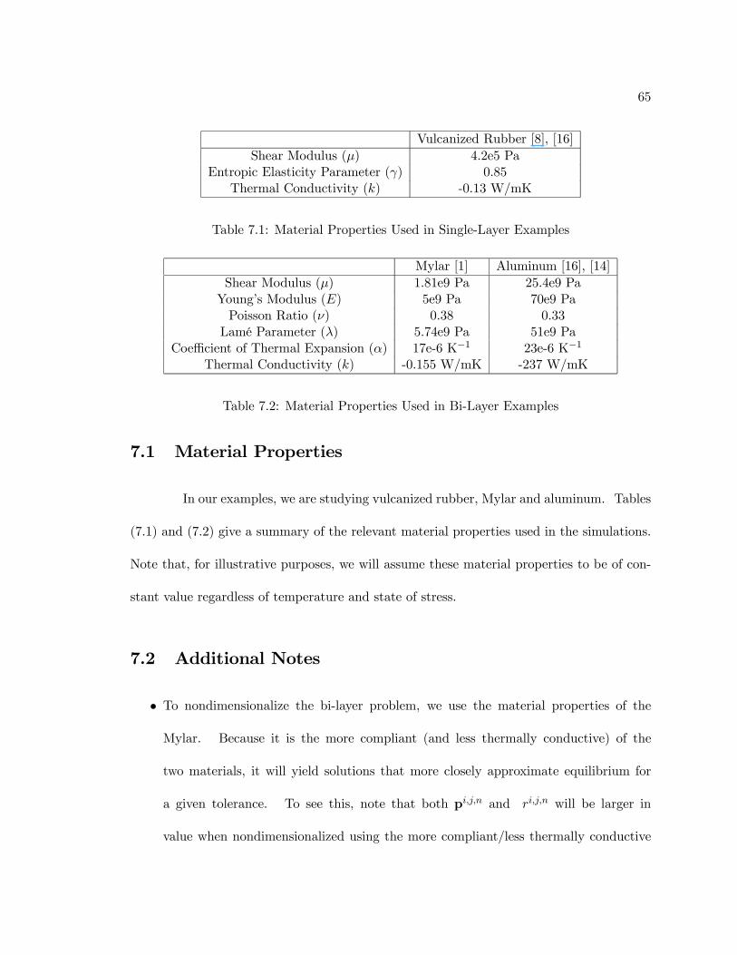
65

Vulcanized Rubber [8], [16]Shear Modulus (µ) 4.2e5 Pa

Entropic Elasticity Parameter (γ) 0.85Thermal Conductivity (k) -0.13 W/mK

Table 7.1: Material Properties Used in Single-Layer Examples

Mylar [1] Aluminum [16], [14]Shear Modulus (µ) 1.81e9 Pa 25.4e9 PaYoung’s Modulus (E) 5e9 Pa 70e9 PaPoisson Ratio (ν) 0.38 0.33Lamé Parameter (λ) 5.74e9 Pa 51e9 Pa

Coefficient of Thermal Expansion (α) 17e-6 K−1 23e-6 K−1

Thermal Conductivity (k) -0.155 W/mK -237 W/mK

Table 7.2: Material Properties Used in Bi-Layer Examples

7.1 Material Properties

In our examples, we are studying vulcanized rubber, Mylar and aluminum. Tables

(7.1) and (7.2) give a summary of the relevant material properties used in the simulations.

Note that, for illustrative purposes, we will assume these material properties to be of con-

stant value regardless of temperature and state of stress.

7.2 Additional Notes

• To nondimensionalize the bi-layer problem, we use the material properties of the

Mylar. Because it is the more compliant (and less thermally conductive) of the

two materials, it will yield solutions that more closely approximate equilibrium for

a given tolerance. To see this, note that both pi,j,n and ri,j,n will be larger in

value when nondimensionalized using the more compliant/less thermally conductive

66

material properties versus the stiffer material/more conductive properties.

• For all problems, a membrane of thickness of h = 1 µm was considered.

• Whenever a heat supply is specified, it is meant to refer to R introduced at equation

(6.35).

• In those figures showing the wrinkled regions of the membrane, the following coloring

scheme is used: white areas are wrinkled regions, gray areas are tense regions, and

black areas are slack regions.

7.3 Effect of Membrane Composition on Natural Width

For illustrative purposes, we consider a composite sheet where the aluminum layer

makes up 2% of the total thickness. This is consistent with typical solar sail constructions

[3]. Figure (7.1) shows how the natural width compares for different compositions for an

example ∆θ of 100K. As one would expect, the plot for the composite falls in between

those of the Mylar and the aluminum.

7.4 Shear and Stretch of a Rectangular Sheet

In this example, we take a 1 by 0.5 (dimensionless lengths) membrane and subject

it to a shearing and axial stretch deformation. The bottom boundary is held fixed while

the top boundary is displaced both horizontally and vertically. These boundaries are both

held at room temperature. The horizontal sides are both traction and heat flux free. This

type of deformation typically causes some amount of fine-scale wrinkling to occur. The

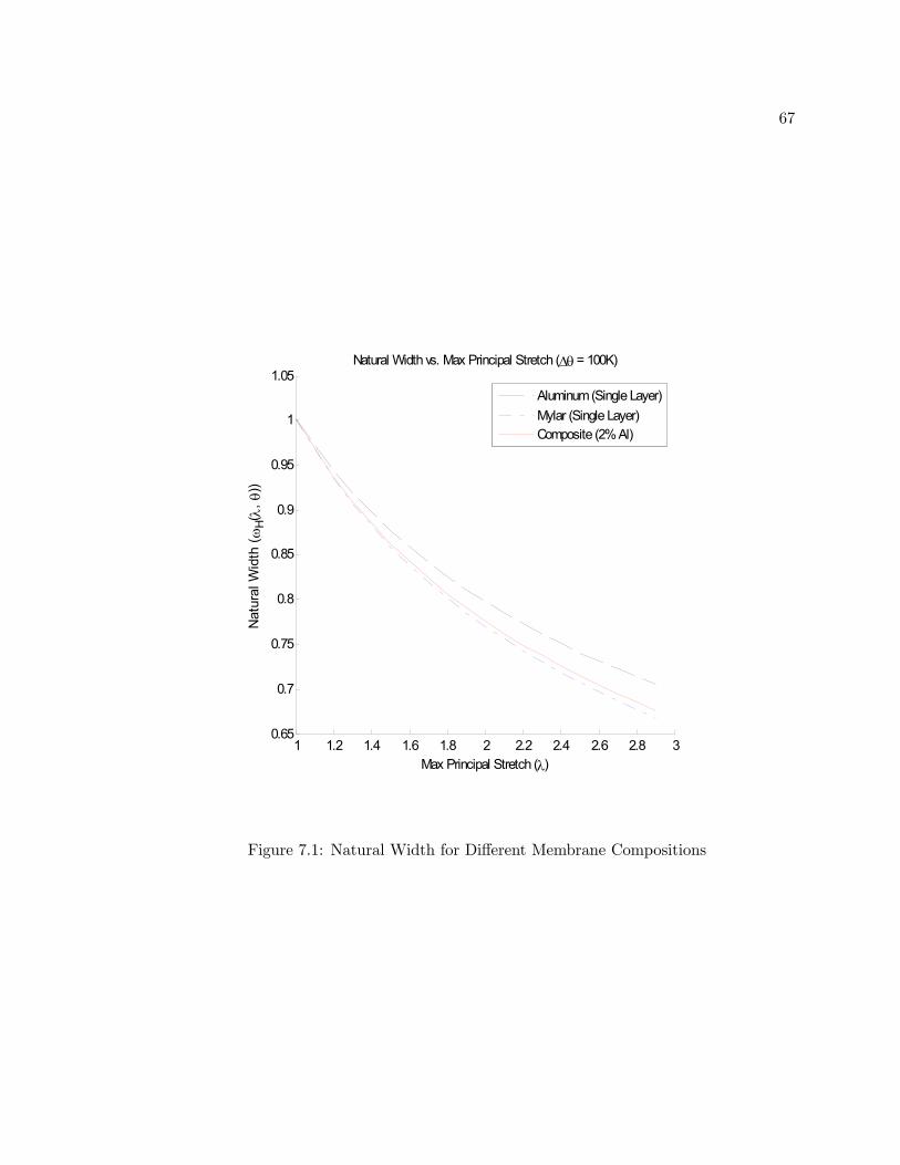
67

1 1.2 1.4 1.6 1.8 2 2.2 2.4 2.6 2.8 30.65

0.7

0.75

0.8

0.85

0.9

0.95

1

1.05

Max Principal Stretch (λ)

Nat

ural

Wid

th (ω

H(λ,

θ))

Natural Width vs. Max Principal Stretch (∆θ = 100K)

Aluminum (Single Layer)Mylar (Single Layer)Composite (2% Al)

Figure 7.1: Natural Width for Different Membrane Compositions

68

amount of wrinkling is very sensitive to both temperature fluctuations and material stiffness

and thus presents an easy way to see effects of each.

7.4.1 Vulcanized Rubber

First, we consider a membrane composed entirely of rubber and held at room

temperature. The top boundary is displaced 0.25 horizontally and 0.11 vertically. Figure

(7.2) shows the deformed configuration colored according to the value of the largest principal

stretch evaluated at the zone centered points. Figure (7.3) shows the wrinkling pattern.

Those areas colored gray denote areas of tension, while white areas correspond to wrinkled

regions.

0 0.2 0.4 0.6 0.8 1 1.20

0.2

0.4

0.6

0.8

1

1.2

Maximum Principal Stretch (Zone-Center)

1.1

1.2

1.3

1.4

1.5

1.6

1.7

1.8

1.9

2

Figure 7.2: Max Principal Stretch in Shear/Stretch of Vulcanized Rubber at RoomTemperature

Next, we apply a heat supply of R = 200 W/m3 (per deformed volume). Figure

(7.4) shows the stretches. Comparing this with Figure (7.2), we see that the membrane

69

0 0.2 0.4 0.6 0.8 1 1.20

0.2

0.4

0.6

0.8

1

1.2

Wrinkling

Figure 7.3: Wrinkling in Shear/Stretch of Vulcanized Rubber at Room Temperature

has tensed up very slightly. This is expected as it demonstrates the Gough-Joule effect

that is the hallmark of entropic elastic materials. The maximum principal stretch increases

from 1.867 to 1.899 with the addition of temperature. As we see in Figure (7.5), this

increase tension has also caused the region of wrinkling to become larger, specifically in

the area with the largest temperature change. The temperature distribution (estimated at

the zone-centered points) is shown in Figure (7.6). The zone-centered estimate is obtained

by averaging the temperatures at the four nearest nodes. Thus, the maximum nodal

temperature is higher than the highest zone estimate. In this example, the maximum

nodal temperature is 1.75 (about 524K).

70

0 0.2 0.4 0.6 0.8 1 1.20

0.2

0.4

0.6

0.8

1

1.2

Maximum Principal Stretch (Zone-Center)

1.1

1.2

1.3

1.4

1.5

1.6

1.7

1.8

1.9

2

Figure 7.4: Max Principal Stretch in Shear/Stretch of Vulcanized Rubber with ExternalHeat Supply

0 0.2 0.4 0.6 0.8 1 1.20

0.2

0.4

0.6

0.8

1

1.2

Wrinkling

Figure 7.5: Wrinkling in Shear/Stretch of Vulcanized Rubber with External Heat Supply

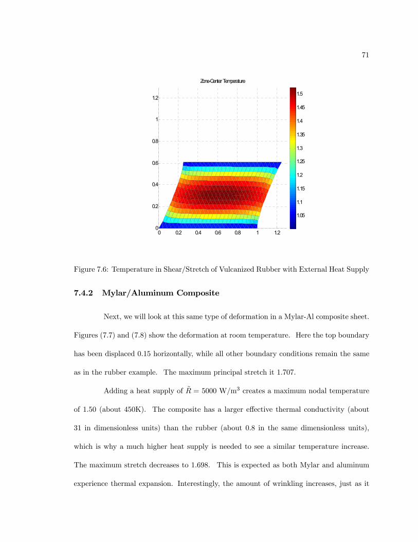
71

0 0.2 0.4 0.6 0.8 1 1.20

0.2

0.4

0.6

0.8

1

1.2

Zone-Center Temperature

1.05

1.1

1.15

1.2

1.25

1.3

1.35

1.4

1.45

1.5

Figure 7.6: Temperature in Shear/Stretch of Vulcanized Rubber with External Heat Supply

7.4.2 Mylar/Aluminum Composite

Next, we will look at this same type of deformation in a Mylar-Al composite sheet.

Figures (7.7) and (7.8) show the deformation at room temperature. Here the top boundary

has been displaced 0.15 horizontally, while all other boundary conditions remain the same

as in the rubber example. The maximum principal stretch it 1.707.

Adding a heat supply of R = 5000 W/m3 creates a maximum nodal temperature

of 1.50 (about 450K). The composite has a larger effective thermal conductivity (about

31 in dimensionless units) than the rubber (about 0.8 in the same dimensionless units),

which is why a much higher heat supply is needed to see a similar temperature increase.

The maximum stretch decreases to 1.698. This is expected as both Mylar and aluminum

experience thermal expansion. Interestingly, the amount of wrinkling increases, just as it

72

0 0.2 0.4 0.6 0.8 1 1.20

0.2

0.4

0.6

0.8

1

Maximum Principal Stretch (Zone-Center)

1.1

1.2

1.3

1.4

1.5

1.6

1.7

Figure 7.7: Maximum Principal Stretch in Shear/Stretch of Composite Membrane at RoomTemperature

0 0.2 0.4 0.6 0.8 1 1.20

0.2

0.4

0.6

0.8

1

Wrinkling

Figure 7.8: Wrinkling in Shear/Stretch of Composite Membrane at Room Temperature

73

0 0.2 0.4 0.6 0.8 1 1.20

0.2

0.4

0.6

0.8

1

Maximum Principal Stretch (Zone-Center)

1.1

1.2

1.3

1.4

1.5

1.6

1.7

Figure 7.9: Maximum Principal Stretch in Shear/Stretch of Composite Membrane withExternal Heat Supply

did in the rubber case. However, the rubber tenses up with added heat, whereas the

composite relaxes. This counter-intuitive result can be explained by recalling the forms of

the natural width for rubber and for Hencky materials. The natural width for an entropic

elastic material is independent of temperature. This is not so for a Hencky material, where

the natural width increases with temperature. Figures (7.9), (7.10) and (7.11) show the

deformation in this case.

7.5 Square Sheet Subjected to Uniform Pressure

Here, we consider a 1 by 1 square sheet and subject it to a uniform lateral pressure.

All four sides are fixed and held at room temperature. Although wrinkling is not a factor

in this example (as the membrane will be tense everywhere), it is interesting to see how

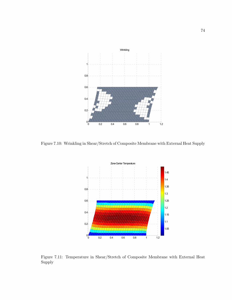
74

0 0.2 0.4 0.6 0.8 1 1.20

0.2

0.4

0.6

0.8

1

Wrinkling

Figure 7.10: Wrinkling in Shear/Stretch of Composite Membrane with External Heat Supply

0 0.2 0.4 0.6 0.8 1 1.20

0.2

0.4

0.6

0.8

1

Zone-Center Temperature

1.05

1.1

1.15

1.2

1.25

1.3

1.35

1.4

1.45

Figure 7.11: Temperature in Shear/Stretch of Composite Membrane with External HeatSupply

75

the maximum lateral deflection of the membrane is affected by temperature and membrane

composition.

7.5.1 Vulcanized Rubber

We subject the membrane to a pressure of 0.2 Pa. Figure (7.12) shows the de-

formed configuration for the case of no external heat supply. The maximum lateral deflec-

tion is 0.154 and the maximum principal stretch is 1.0827. When we heat the membrane up

with a heat supply of 200 W/m3 it reaches a maximum nodal temperature of 1.41 (424K).

This increased temperature causes the membrane to tense up, increasing its maximum prin-

cipal stretch to 1.0832 and decreasing it’s maximum lateral deflection to 0.152. Figures

(7.13) and (7.14) show the maximum principal stretches and temperature, respectively, in

the deformed configuration.

0

0.5

1 0

0.5

10

0.2

0.4

0.6

0.8

1

Maximum Principal Stretch (Zone-Center)

1.01

1.02

1.03

1.04

1.05

1.06

1.07

1.08

Figure 7.12: Maximum Principal Stretch in Pressurized Vulcanized Rubber at RoomTemperature

76

0

0.5

1 0

0.5

10

0.2

0.4

0.6

0.8

1

Maximum Principal Stretch (Zone-Center)

1.01

1.02

1.03

1.04

1.05

1.06

1.07

1.08

Figure 7.13: Maximum Principal Stretch in Pressurized Vulcanized Rubber with ExternalHeat Supply

0

0.5

1 0

0.5

10

0.2

0.4

0.6

0.8

1

Zone-Center Temperature

1.05

1.1

1.15

1.2

1.25

1.3

1.35

1.4

Figure 7.14: Temperature in Pressurized Vulcanized Rubber with External Heat Supply

77

0

0.5

1

0

0.5

10

0.2

0.4

0.6

0.8

1

Maximum Principal Stretch (Zone-Center)

1.005

1.01

1.015

1.02

1.025

1.03

1.035

1.04

1.045

1.05

1.055

Figure 7.15: Maximum Principal Stretch in Pressurized Composite at Room Temperature

7.5.2 Mylar/Aluminum Composite

We subject the composite membrane to a pressure of 500 Pa as it is stiffer than the

rubber. Figure (7.15) shows the maximum principal stretches for the room temperature

example. The maximum lateral deflection is 0.126, while the maximum principal stretch is

1.0556. When we heat the composite (heat supply of 10000 W/m3), the maximum nodal

temperature becomes 1.5376 (about 461K). As expected, the composite sheet relaxes with

the maximum principal stretch increasing slightly to 1.0557. This is accompanied by an

increase in maximum deflection to 0.129. Figures (7.16) and (7.17) show the deformation

with heat supplied.

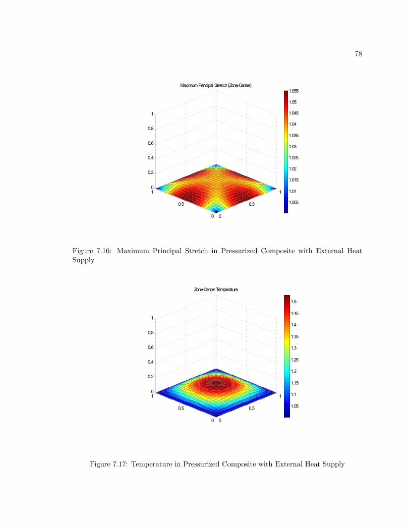
78

0

0.5

1

0

0.5

10

0.2

0.4

0.6

0.8

1

Maximum Principal Stretch (Zone-Center)

1.005

1.01

1.015

1.02

1.025

1.03

1.035

1.04

1.045

1.05

1.055

Figure 7.16: Maximum Principal Stretch in Pressurized Composite with External HeatSupply

0

0.5

1

0

0.5

10

0.2

0.4

0.6

0.8

1

Zone-Center Temperature

1.05

1.1

1.15

1.2

1.25

1.3

1.35

1.4

1.45

1.5

Figure 7.17: Temperature in Pressurized Composite with External Heat Supply

79

7.6 Axial Stretch of a Square Sheet with a Traction/Heat

Flux Free Hole

In this example, we consider a 2 x 2 square sheet with a central hole of radius 0.2

undergoing an axial stretch. The left and right edges are stretched a distance of 0.2 and

held at room temperature. The top and bottom sides, as well as the hole, are traction and

heat flux free. Wrinkling tends to occur in regions near the top and bottom boundary, as

well as in regions near the hole. Stress concentrations are generated on either side of the

hole as expected.

7.6.1 Vulcanized Rubber

Figure (7.18) shows plot of the maximum stretches in deformed configuration.

Overall, the largest stretch occurs near the hole and is 1.54. The wrinkling pattern is

shown in Figure (7.19). Areas colored gray indicate tense regions, black areas denote

slack (stretch free) regions, and wrinkled regions are white. Figure (7.20) shows a zoom-in

around the hole.

When heat up (heat supply of 200 W/m3), the membrane does experience an

increase in wrinkling near the hole. However, the maximum stretch decreases to 1.526.

Because the maximum stretch occurs at the areas of stress concentration around the hole,

the tendency for the membrane to tense up causes this area to relax slightly. Figure (7.21)

shows the maximum stretches. Figure (7.22) shows the wrinkling pattern with Figure

(7.23) showing a close up of the hole. The maximum temperature in the membrane is 1.65

(495K). The highest temperatures are concentrated in a vertical band in the center of the

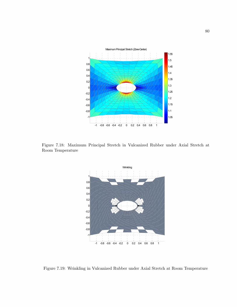
80

-1 -0.8 -0.6 -0.4 -0.2 0 0.2 0.4 0.6 0.8 1

-1

-0.8

-0.6

-0.4

-0.2

0

0.2

0.4

0.6

0.8

1

Maximum Principal Stretch (Zone-Center)

1.05

1.1

1.15

1.2

1.25

1.3

1.35

1.4

1.45

1.5

1.55

Figure 7.18: Maximum Principal Stretch in Vulcanized Rubber under Axial Stretch atRoom Temperature

-1 -0.8 -0.6 -0.4 -0.2 0 0.2 0.4 0.6 0.8 1

-1

-0.8

-0.6

-0.4

-0.2

0

0.2

0.4

0.6

0.8

1

Wrinkling

Figure 7.19: Wrinkling in Vulcanized Rubber under Axial Stretch at Room Temperature

81

-0.5 -0.4 -0.3 -0.2 -0.1 0 0.1 0.2 0.3 0.4 0.5

-0.5

-0.4

-0.3

-0.2

-0.1

0

0.1

0.2

0.3

0.4

0.5

Wrinkling

Figure 7.20: Wrinkling Close-Up in Vulcanized Rubber under Axial Stretch at RoomTemperature

membrane as shown in Figure (7.24) .

7.6.2 Mylar/Aluminum Composite

Under room temperature conditions, the composite membrane displays a similar

pattern of wrinkling compared to the rubber. However, there is slightly more wrinkling

around the hole than there was in either rubber example. The maximum stretch is also

a higher, 1.5918. Figure (7.25) shows the maximum principal stretches in the deformed

configuration. Figures (7.26) and (7.27) show the wrinkling pattern in the sheet.

Undergoing a heat supply of 10000 W/m3, the composite becomes more even more

wrinkled at hole. As in the rubber example, the maximum stretch decreases to 1.5861. As

in previous deformations, the composite doesn’t reach as high of a maximum temperature,

82

-1 -0.8 -0.6 -0.4 -0.2 0 0.2 0.4 0.6 0.8 1

-1

-0.8

-0.6

-0.4

-0.2

0

0.2

0.4

0.6

0.8

1

Maximum Principal Stretch (Zone-Center)

1.05

1.1

1.15

1.2

1.25

1.3

1.35

1.4

1.45

1.5

1.55

Figure 7.21: Maximum Principal Stretch in Vulcanized Rubber under Axial Stretch withHeat Supply

-1 -0.8 -0.6 -0.4 -0.2 0 0.2 0.4 0.6 0.8 1

-1

-0.8

-0.6

-0.4

-0.2

0

0.2

0.4

0.6

0.8

1

Wrinkling

Figure 7.22: Wrinkling in Vulcanized Rubber under Axial Stretch with Heat Supply

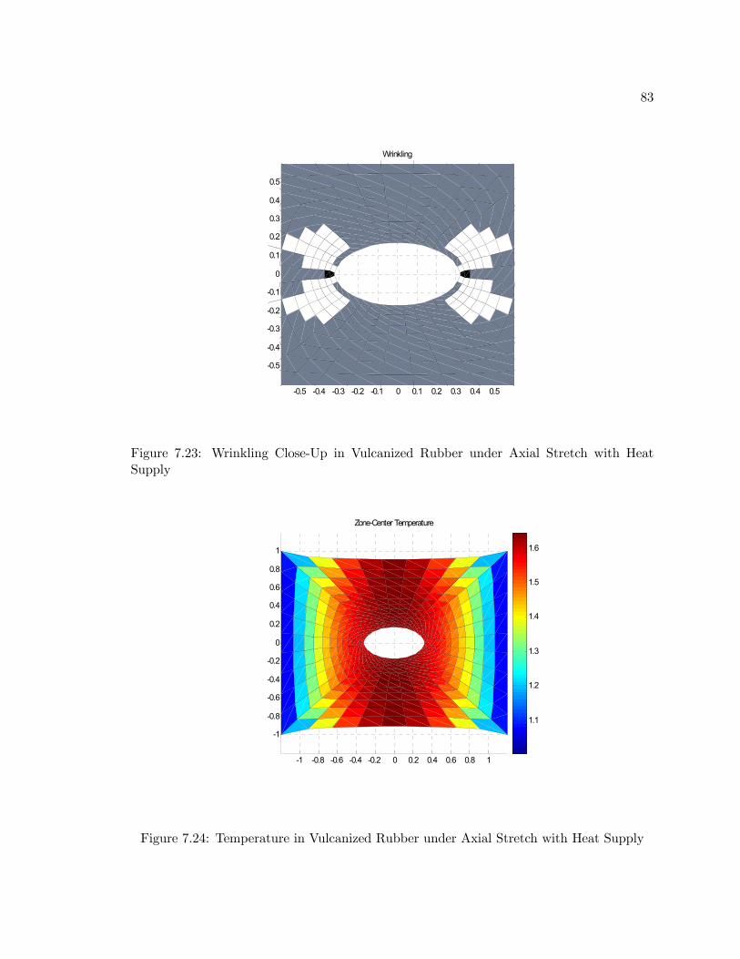
83

-0.5 -0.4 -0.3 -0.2 -0.1 0 0.1 0.2 0.3 0.4 0.5

-0.5

-0.4

-0.3

-0.2

-0.1

0

0.1

0.2

0.3

0.4

0.5

Wrinkling

Figure 7.23: Wrinkling Close-Up in Vulcanized Rubber under Axial Stretch with HeatSupply

-1 -0.8 -0.6 -0.4 -0.2 0 0.2 0.4 0.6 0.8 1

-1

-0.8

-0.6

-0.4

-0.2

0

0.2

0.4

0.6

0.8

1

Zone-Center Temperature

1.1

1.2

1.3

1.4

1.5

1.6

Figure 7.24: Temperature in Vulcanized Rubber under Axial Stretch with Heat Supply

84

-1 -0.8 -0.6 -0.4 -0.2 0 0.2 0.4 0.6 0.8 1

-1

-0.8

-0.6

-0.4

-0.2

0

0.2

0.4

0.6

0.8

1

Maximum Principal Stretch (Zone-Center)

1.05

1.1

1.15

1.2

1.25

1.3

1.35

1.4

1.45

1.5

1.55

Figure 7.25: Maximum Principal Stretch in Composite under Axial Stretch at RoomTemperature

-1 -0.8 -0.6 -0.4 -0.2 0 0.2 0.4 0.6 0.8 1

-1

-0.8

-0.6

-0.4

-0.2

0

0.2

0.4

0.6

0.8

1

Wrinkling

Figure 7.26: Wrinkling in Composite under Axial Stretch at Room Temperature

85

-0.5 -0.4 -0.3 -0.2 -0.1 0 0.1 0.2 0.3 0.4 0.5

-0.5

-0.4

-0.3

-0.2

-0.1

0

0.1

0.2

0.3

0.4

0.5

Wrinkling

Figure 7.27: Wrinkling Close-Up in Composite under Axial Stretch at Room Temperature

peaking here at 1.89 (566 K). Figure (7.28) shows the maximum principal stretches in the

deformed configuration. Figures (7.29) and (7.30) show the wrinkling pattern in the sheet.

Lastly, Figure (7.31) shows the temperature distribution.

7.7 Square Sheet with Central Hole Displaced Transversely

and Twisted

Again we take a 2 by 2 square sheet with a hole (hub) of radius 0.2. In this

example, we fix the outer boundaries and hold them at room temperature. We then

displace the central hub 0.5 out of plane and twist it by a certain number of degrees. The

hub is held at room temperature. Wrinkling tends to occur in the region surrounding the

hole. In all plots, the vertical axis is adjusted to show the deformation in better detail.

86

-1 -0.8 -0.6 -0.4 -0.2 0 0.2 0.4 0.6 0.8 1

-1

-0.8

-0.6

-0.4

-0.2

0

0.2

0.4

0.6

0.8

1

Maximum Principal Stretch (Zone-Center)

1.05

1.1

1.15

1.2

1.25

1.3

1.35

1.4

1.45

1.5

1.55

Figure 7.28: Maximum Principal Stretch in Composite under Axial Stretch with HeatSupply

-1 -0.8 -0.6 -0.4 -0.2 0 0.2 0.4 0.6 0.8 1

-1

-0.8

-0.6

-0.4

-0.2

0

0.2

0.4

0.6

0.8

1

Wrinkling

Figure 7.29: Wrinkling in Composite under Axial Stretch with Heat Supply

87

-0.5 -0.4 -0.3 -0.2 -0.1 0 0.1 0.2 0.3 0.4 0.5

-0.5

-0.4

-0.3

-0.2

-0.1

0

0.1

0.2

0.3

0.4

0.5

Wrinkling

Figure 7.30: Wrinkling Close-Up in Composite under Axial Stretch with Heat Supply

-1 -0.8 -0.6 -0.4 -0.2 0 0.2 0.4 0.6 0.8 1

-1

-0.8

-0.6

-0.4

-0.2

0

0.2

0.4

0.6

0.8

1

Zone-Center Temperature

1.1

1.2

1.3

1.4

1.5

1.6

1.7

1.8

Figure 7.31: Temperature in Composite under Axial Stretch with Heat Supply

88

7.7.1 Vulcanized Rubber

In this case, we twist the central hub 90 degrees. Figure (7.32) shows the maximum

stretches in the deformed configuration. The maximum stretch occurs around the hole and

is 2.54. When subjected to a 200 W/m3 heat supply, the membrane reaches a maximum

temperature of 1.17 (352K) and the maximum stretch increases to 2.565. Figure (7.34)

shows the maximum stretches and Figure (7.35) shows the temperature distribution in this

case. The amount of wrinkling doesn’t change. Figure (7.33) shows the areas of wrinkling.

Gray areas indicate regions of tension, while white areas indicate regions of wrinkling.

-1 -0.5 0 0.5 1-1 -0.5 0 0.5 10

0.1

0.2

0.3

0.4

0.5

0.6

0.7

0.8

0.9

1Maximum Principal Stretch (Zone-Center)

1.5

2

2.5

3

3.5

Figure 7.32: Maximum Principal Stretch in Vulcanized Rubber with Displaced Central Hubat Room Temperature

89

-1-0.5

00.5

1

-1-0.5

00.5

10

0.2

0.4

0.6

0.8

1

Wrinkling

Figure 7.33: Wrinkling in Vulcanized Rubber with Displaced Central Hub

-1 -0.5 0 0.5 1-1 -0.5 0 0.5 10

0.1

0.2

0.3

0.4

0.5

0.6

0.7

0.8

0.9

1Maximum Principal Stretch (Zone-Center)

1.5

2

2.5

3

3.5

Figure 7.34: Maximum Principal Stretch in Vulcanized Rubber with Displaced Central Hubwith External Heat Supply

90

-1 -0.5 0 0.5 1-1 -0.5 0 0.5 10

0.1

0.2

0.3

0.4

0.5

0.6

0.7

0.8

0.9

1Zone-Center Temperature

1.02

1.04

1.06

1.08

1.1

1.12

1.14

1.16

Figure 7.35: Temperature in Vulcanized Rubber with Displaced Central Hub with ExternalHeat Supply

7.7.2 Mylar/Aluminum Composite

For the composite, we twist the central hub through an angle of 45 degrees. Figures

(7.36) and (7.38) show the stretches in the room temperature case and the heat supply case

(20000 W/m3), respectively. In the room temperature case, the maximum stretch is 2.6687.

This decreases to 2.6322 with supplied heat. The maximum temperature is 1.42 (426 K).

The temperature distribution is shown in Figure (7.39). No change in the wrinkling occurs.

Figure (7.37) shows the wrinkling in the sheet. Again, white areas denote wrinkled regions

and gray areas denote tense regions.

91

-1 -0.5 0 0.5 10

0.1

0.2

0.3

0.4

0.5

0.6

0.7

0.8

0.9

1Maximum Principal Stretch (Zone-Center)

1.2

1.4

1.6

1.8

2

2.2

2.4

2.6

Figure 7.36: Maximum Principal Stretch in Composite with Displaced Central Hub at RoomTemperature

-1-0.5

00.5

1

-1-0.5

00.5

10

0.2

0.4

0.6

0.8

1

Wrinkling

Figure 7.37: Wrinkling in Composite with Displaced Central Hub

92

-1 -0.5 0 0.5 10

0.1

0.2

0.3

0.4

0.5

0.6

0.7

0.8

0.9

1Maximum Principal Stretch (Zone-Center)

1.2

1.4

1.6

1.8

2

2.2

2.4

2.6

Figure 7.38: Maximum Principal Stretch in Composite with Displaced Central Hub withExternal Heat Supply

-1 -0.5 0 0.5 10

0.1

0.2

0.3

0.4

0.5

0.6

0.7

0.8

0.9

1Zone-Center Temperature

1.05

1.1

1.15

1.2

1.25

1.3

1.35

1.4

Figure 7.39: Temperature in Composite with Displaced Central Hub with External HeatSupply

93

7.8 Simple Shear of a Square Sheet with Fixed Circular Hub

Subjected to Uniform Pressure

Now we take our 2 by 2 square with central hole and subject the outer boundary

to a simple shear deformation fixed at room temperature. The top and bottom sides are

each shifted a distance of 0.2. This is done while keeping the central hub fixed (and also at

room temperature). In addition, we subject the sheet to a lateral pressure. The vertical

axis on all of the following plots is adjusted to better see the deformation.

7.8.1 Vulcanized Rubber

Here, we subject the rubber membrane to pressure of 0.2 Pa. Figure (7.40) shows

the maximum principal stretches in the deformed configuration. The largest stretch, 1.347,

occurs near the hole. Wrinkling occurs at two of the corners as well as near the hole.

Figure (7.41) shows the wrinkling in a top down view of the sheet. White areas denote

regions of wrinkling, whereas gray colored regions are tense. When 200 W/m3 of heat is

supplied, the membrane tenses up in similar fashion to the other pressure example. The

maximum lateral deflection of the membrane decreases slightly from 0.201 to 0.200 and

the maximum stretch increases to 1.349. The wrinkling increases slightly near the hole.

The membrane reaches a maximum temperature of 1.15 (346K). Figures (7.42), (7.43) and

(7.44) the deformation.

94

-1-0.5

00.5

1

-1-0.5

00.5

1

0

0.2

0.4

0.6

0.8

1

Maximum Principal Stretch (Zone-Center)

1.05

1.1

1.15

1.2

1.25

1.3

Figure 7.40: Maximum Principal Stretch in Vulcanized Rubber in Pressurized Simple Shearat Room Temperature

-1 -0.8 -0.6 -0.4 -0.2 0 0.2 0.4 0.6 0.8 1

-1

-0.8

-0.6

-0.4

-0.2

0

0.2

0.4

0.6

0.8

1

Wrinkling

Figure 7.41: Wrinkling in Vulcanized Rubber in Pressurized Simple Shear at RoomTemperature

95

-1-0.5

00.5

1

-1-0.5

00.5

1

0

0.2

0.4

0.6

0.8

1

Maximum Principal Stretch (Zone-Center)

1.05

1.1

1.15

1.2

1.25

1.3

Figure 7.42: Maximum Principal Stretch in Vulcanized Rubber in Pressurized Simple Shearwith External Heat Supply

-1 -0.8 -0.6 -0.4 -0.2 0 0.2 0.4 0.6 0.8 1

-1

-0.8

-0.6

-0.4

-0.2

0

0.2

0.4

0.6

0.8

1

Wrinkling

Figure 7.43: Wrinkling in Vulcanized Rubber in Pressurized Simple Shear with ExternalHeat Supply

96

-1-0.5

00.5

1

-1-0.5

00.5

1

0

0.2

0.4

0.6

0.8

1

Zone-Center Temperature

1.02

1.04

1.06

1.08

1.1

1.12

1.14

Figure 7.44: Temperature in Vulcanized Rubber in Pressurized Simple Shear with ExternalHeat Supply

7.8.2 Mylar/Aluminum Composite

We subject the composite to a pressure of 500 Pa. Figure (7.45) shows the

stretches in the deformed configuration. The maximum stretch is 1.2796. Figure (7.46)

shows the wrinkling in the sheet. Again, white denotes wrinkled regions and gray colored

areas are tense. When heat up with a 20000 W/m3 heat supply, the stretch decreases to

1.2775. Figure (7.47) shows the stretches in the sheet. The maximum lateral deflection

increases from 0.17 to 0.172 with the added heat. There is also an increase in wrinkling as

shown in Figure (7.48). The maximum temperature is 1.4035 (421K). The temperature

distribution is shown in Figure (7.49).

97

-1-0.5

00.5

1

-1-0.5

00.5

1

0

0.2

0.4

0.6

0.8

1

1.2

Maximum Principal Stretch (Zone-Center)

1.05

1.1

1.15

1.2

1.25

Figure 7.45: Maximum Principal Stretch in Composite in Pressurized Simple Shear at RoomTemperature

-1 -0.8 -0.6 -0.4 -0.2 0 0.2 0.4 0.6 0.8 1

-1

-0.8

-0.6

-0.4

-0.2

0

0.2

0.4

0.6

0.8

1

Wrinkling

Figure 7.46: Wrinkling in Composite in Pressurized Simple Shear at Room Temperature

98

-1-0.5

00.5

1

-1-0.5

00.5

1

0

0.2

0.4

0.6

0.8

1

1.2

Maximum Principal Stretch (Zone-Center)

1.05

1.1

1.15

1.2

1.25

Figure 7.47: Maximum Principal Stretch in Composite in Pressurized Simple Shear withExternal Heat Supply

-1 -0.8 -0.6 -0.4 -0.2 0 0.2 0.4 0.6 0.8 1

-1

-0.8

-0.6

-0.4

-0.2

0

0.2

0.4

0.6

0.8

1

Wrinkling

Figure 7.48: Wrinkling in Composite in Pressurized Simple Shear with External Heat Supply

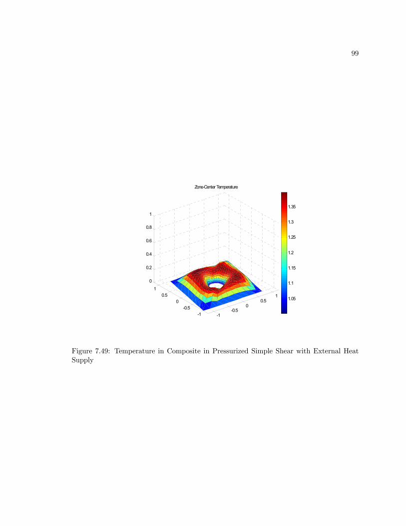
99

-1-0.5

00.5

1

-1-0.5

00.5

1

0

0.2

0.4

0.6

0.8

1

Zone-Center Temperature

1.05

1.1

1.15

1.2

1.25

1.3

1.35

Figure 7.49: Temperature in Composite in Pressurized Simple Shear with External HeatSupply

100

Part III

Peridynamic Analysis of Fracture,

Viscoplasticity, and Viscoelasticity

in Thin Bodies

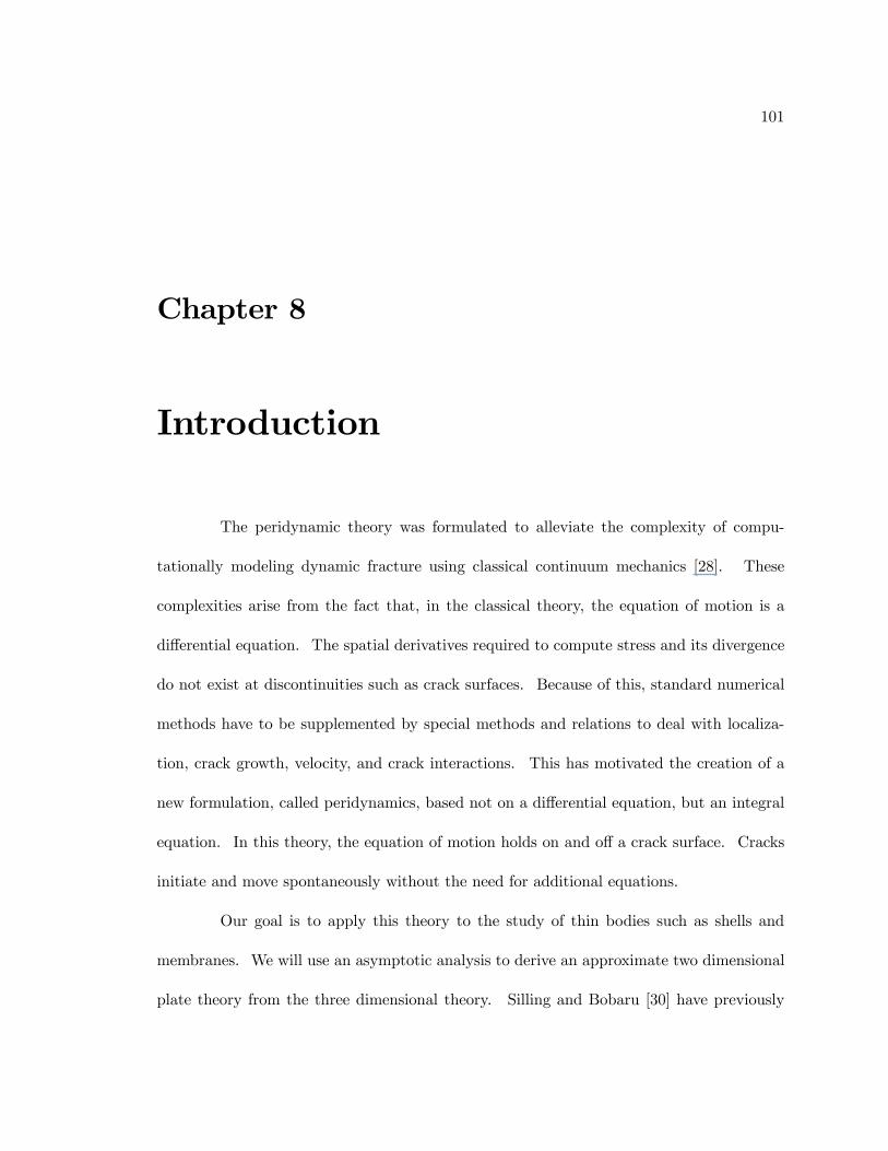
101

Chapter 8

Introduction

The peridynamic theory was formulated to alleviate the complexity of compu-

tationally modeling dynamic fracture using classical continuum mechanics [28]. These

complexities arise from the fact that, in the classical theory, the equation of motion is a

differential equation. The spatial derivatives required to compute stress and its divergence

do not exist at discontinuities such as crack surfaces. Because of this, standard numerical

methods have to be supplemented by special methods and relations to deal with localiza-

tion, crack growth, velocity, and crack interactions. This has motivated the creation of a

new formulation, called peridynamics, based not on a differential equation, but an integral

equation. In this theory, the equation of motion holds on and off a crack surface. Cracks

initiate and move spontaneously without the need for additional equations.

Our goal is to apply this theory to the study of thin bodies such as shells and

membranes. We will use an asymptotic analysis to derive an approximate two dimensional

plate theory from the three dimensional theory. Silling and Bobaru [30] have previously

102

applied the peridynamic theory to membranes and fabric. The equation of motion they use

for membranes will be shown to be the same as that in the leading order two-dimensional

theory we derive. We will also consider higher order bending effects present in thicker

bodies as well.

In peridynamic theory, forces arise from one dimensional particle interactions,

called bonds, at finite distances. The simplicity of these interactions allows us to consider

material behavior in a way that is less complicated than in three dimensional continuum

theory. Two such examples we consider are viscoelasticity and viscoplasticity.

Chapter nine summarizes the peridynamic theory for a general three dimensional

body. A two dimensional approximation of the three dimensional theory is derived for

thin bodies using an asymptotic analysis similar to that in Part I. Chapter ten discusses

the constitutive behavior of the particle interactions and how typical elastic models are

modified to incorporate damage, viscosity and plasticity. In chapter eleven, we describe

the numerical method used to solve the governing equations. The theory is illustrated

in chapter twelve through numerical simulations of both membranes and shells undergoing

in-plane and transverse deformations.

103

Chapter 9

Peridynamic Theory

9.1 Three Dimensional Theory

For a particle at X in the reference configuration of a body at time t, the equation

of motion in the peridynamic theory is

ρu (X, t) =

ZNX

f (η, ξ) dVX0 + b(X, t) (9.1)

where ρ is the mass density in the reference configuration, NX is a neighborhood of X, u is

the displacement field, b is a prescribed body force and f (η, ξ) is a pair-wise force function

representing the force (per unit volume squared) that a particle at X0 exerts on the particle

at X. The force function, f , typically depends on the deformation through the reference

distance between the two particles

ξ = X0 −X (9.2)

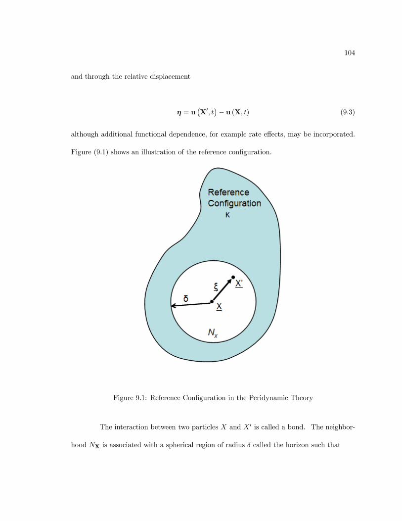
104

and through the relative displacement

η = u¡X0, t

¢− u (X, t) (9.3)

although additional functional dependence, for example rate effects, may be incorporated.

Figure (9.1) shows an illustration of the reference configuration.

Figure 9.1: Reference Configuration in the Peridynamic Theory

The interaction between two particles X and X 0 is called a bond. The neighbor-

hood NX is associated with a spherical region of radius δ called the horizon such that

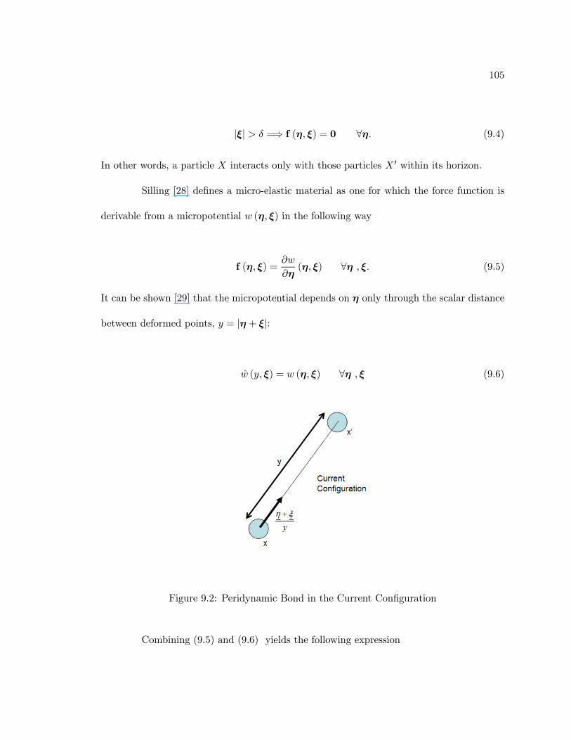
105

|ξ| > δ =⇒ f (η, ξ) = 0 ∀η. (9.4)

In other words, a particle X interacts only with those particles X 0 within its horizon.

Silling [28] defines a micro-elastic material as one for which the force function is

derivable from a micropotential w (η, ξ) in the following way

f (η, ξ) =∂w

∂η(η, ξ) ∀η , ξ. (9.5)

It can be shown [29] that the micropotential depends on η only through the scalar distance

between deformed points, y = |η + ξ|:

w (y, ξ) = w (η, ξ) ∀η , ξ (9.6)

Figure 9.2: Peridynamic Bond in the Current Configuration

Combining (9.5) and (9.6) yields the following expression

106

f (η, ξ) =η + ξ

yf(y, ξ) ∀η , ξ (9.7)

where

f(y, ξ) =∂w

∂y(y, ξ) (9.8)

is scalar valued and constitutively determined. Figure 9.2 shows a peridynamic bond in

the current configuration.

9.2 Two Dimensional Theory for Thin Bodies

Let the position of a particle be written as X = v + ζk where v = (I− k⊗ k)X

and ζ = k ·X. Similarly, let the position of another particle in the horizon of X be written

as X0 = v0 + ζ 0k. Using this decomposition, we can approximate the displacement near

X = v (ζ = 0) using a Taylor series,

u (X, t) = u0 (v, t) + ζa (v, t) +1

2ζ2b (v, t) +

1

6ζ3c (v, t) + o(ζ3), (9.9)

where

a (v, t) =∂u0 (v, t)

∂Xk =

∂u0 (v, t)

∂ζ(9.10)

b (v, t) =∂2u0 (v, t)

∂ζ2(9.11)

c (v, t) =∂3u0 (v, t)

∂ζ3, (9.12)

107

and the subscript 0 denotes that the quantity is evaluated at ζ = 0, i.e. the reference

surface. Then, the acceleration can be written as

u (X, t) = u0 + ζa+1

2ζ2b+

1

6ζ3c+ o(ζ3). (9.13)

We can also approximate the displacement near X0 = v0 (ζ 0 = 0) in a similar

fashion to (9.9) yielding

u¡X0, t

¢= u0

¡v0, t

¢+ ζ 0a0

¡v0, t

¢+1

2(ζ 0)2b0

¡v0, t

¢+1

6(ζ 0)3c0

¡v0, t

¢+ o(ζ 0)3. (9.14)

Thus, the relative displacement is approximately,

η = u0¡v0, t

¢− u0 (v, t) + ζ 0a0

¡v0, t

¢− ζa (v, t) +

1

2(ζ 0)2b0

¡v0, t

¢− 12ζ2b (v, t) + ... (9.15)

In addition,

ξ = v0 − v + (ζ 0 − ζ)k. (9.16)

In our previous derivation of membrane theory based on classical continuum me-

chanics, we used the midsurface of the body as the reference surface. When using the

midsurface, the next higher order terms come in at order thickness cubed, as the order

squared terms cancel out. Thus, here we will base our approximation about the lower

lateral surface of the body, that is the exterior surface with unit normal k. Let ε be

the membrane thickness and Ω denote the reference plane. Neglecting body force, (9.1)

becomes

108

ρ

µu0 + ζa+

1

2ζ2b+

1

6ζ3c+ o(ζ3)

¶=

ZΩ

εZ0

f (η, ξ) dζ 0dA0. (9.17)

We assume sufficient smoothness so that we may change the order of integration.

Next, we evaluate (9.17) at the reference surface (ζ = 0),

ρu0 (v, t) =

ZΩ

εZ0

f (η0, ξ0) dζ0dA0, (9.18)

where

η0 = u0¡v0, t

¢− u0 (v, t) + ζ 0a0

¡v0, t

¢+1

2(ζ 0)2b0

¡v0, t

¢− 12ζ2b (v, t) + ... (9.19)

and

ξ0 = v0 − v+ ζ 0k. (9.20)

Now, we evaluate (9.17) at the top surface (ζ = ε):

ρ

µu0 + εa+

1

2ε2b+

1

6ε3c+ o(ε3)

¶=

ZΩ

εZ0

f (ηε, ξε) dζ0dA0, (9.21)

where

ηε = η|ζ=ε = u0¡v0, t

¢−u0 (v, t)+ ζ 0a0

¡v0, t

¢− εa (v, t)+

1

2(ζ 0)2b0

¡v0, t

¢− 12ε2b (v, t)+ ...

(9.22)

and

109

ξε = ξ|ζ=ε = v0 − v + (ζ 0 − ε)k. (9.23)

Next, we subtract (9.18) from (9.21), yielding

ρ

µεa+

1

2ε2b+

1

6ε3c+ o(ε3)

¶=

ZΩ

εZ0

[f (ηε, ξε)− f (η0, ξ0)] dζ 0dA0. (9.24)

Consider,

I(ε) =

εZ0

G(ζ 0)dζ 0 = I(0) + εI 0(0) +1

2ε2I 00(0) + ..., (9.25)

where

I(0) = 0, I 0(ε) = G(ε), I 00(ε) = G0(ε), etc. (9.26)

Thus,

I(ε) = εG(0) +1

2ε2G0(0) + ... (9.27)

Let G(ζ 0) = f (η0, ξ0). Then,

G0(ζ 0) =

µ∂f

∂η0

¶∂η0∂ζ 0

+

µ∂f

∂ξ0

¶∂ξ0∂ζ 0

, (9.28)

where

∂η0∂ζ 0

= a0¡v0, t

¢+ ζ 0b0

¡v0, t

¢+ ... and

∂ξ0∂ζ 0

= k. (9.29)

Thus, G(0) = f (η00, ξ00) where,

110

η00 = η0|ζ0=0 = u0¡v0, t

¢− u0 (v, t) , (9.30)

and

ξ00 = ξ0|ζ0=0 = v0 − v. (9.31)

Also,

G0(0) =

µ∂f

∂η0

¶ζ0=0

a0¡v0, t

¢+

µ∂f

∂ξ0

¶ζ0=0

k, (9.32)

where,

µ∂f

∂η0

¶ζ0=0

=∂f

∂η(η00, ξ00) (9.33)µ

∂f

∂ξ0

¶ζ0=0

=∂f

∂ξ(η00, ξ00) . (9.34)

Then, (9.27) can be written as

I(ε) = εf (η00, ξ00) +1

2ε2½∙

∂f

∂η(η00, ξ00)

¸a0¡v0, t

¢+

∙∂f

∂ξ(η00, ξ00)

¸k

¾+ o(ε3). (9.35)

Thus, (9.18) becomes,

ρu0 (v, t) = ε

ZΩ

f (η00, ξ00) dA0 + (9.36)

1

2ε2ZΩ

½∙∂f

∂η(η00, ξ00)

¸a0¡v0, t

¢+

∙∂f

∂ξ(η00, ξ00)

¸k

¾dA0 + o(ε3).

111

Next, let G(ζ 0) = f (ηε, ξε) − f (η0, ξ0). Thus, G(0) = f (ηε0, ξε0) − f (η00, ξ00)

where,

ηε0 = u0¡v0, t

¢−u0 (v, t)−εa (v, t)−

1

2ε2b (v, t)+... = η00−εa (v, t)−

1

2ε2b (v, t)+... (9.37)

and

ξε0 = v0 − v − εk = ξ00 − εk (9.38)

Now, Taylor expanding f (ηε0, ξε0) about ζ = 0 yields

f (ηε0, ξε0) = f (η00, ξ00) +

∙∂f

∂η(η00, ξ00)

¸(ηε0 − η00) +

∙∂f

∂ξ(η00, ξ00)

¸(ξε0 − ξ00) + ...

(9.39)

Substituting (9.37) and (9.38) into (9.39) gives,

f (ηε0, ξε0) = f (η00, ξ00)− ε

∙∂f

∂η(η00, ξ00)

¸a− ε

∙∂f

∂ξ(η00, ξ00)

¸k+ o(ε2). (9.40)

Thus, (9.24) becomes

ρ

µεa+

1

2ε2b+

1

6ε3c+ o(ε3)

¶= −ε2

⎧⎨⎩ZΩ

∙∂f

∂η(η00, ξ00)

¸dA0

⎫⎬⎭a− (9.41)

ε2

⎧⎨⎩ZΩ

∙∂f

∂ξ(η00, ξ00)

¸dA0

⎫⎬⎭k+ o(ε3)

Silling’s stability criterion [28] is thatZΩ

h∂f∂η (η00, ξ00)

idA0 be positive definite. In the

case of statics this allows us to eliminate a. The result is uniformly valid (in ε) and, when

112

inserted into the o(ε2) term in (9.36), furnishes the bending term in static plate theory.

Retaining the leading order terms in (9.41) gives,

ρεa = −ε2⎧⎨⎩ZΩ

∙∂f

∂η(η00, ξ00)

¸dA0

⎫⎬⎭a− ε2

⎧⎨⎩ZΩ

∙∂f

∂ξ(η00, ξ00)

¸dA0

⎫⎬⎭k (9.42)

This, together with (9.36) yields a coupled system for u0 (v, t) ,a (v, t) . Note that the

horizon takes the form of a circular region on the reference surface instead of a sphere as

there are no bonds extending off of the membrane surface.

We regard membranes as those bodies with thickness sufficiently small so as to be

considered perfectly flexible, i.e. no bending effects. In this case, we keep only those terms

of order O(ε). Thus, the equation of motion (from (9.36)) is

ρu0 (v, t) = ε

ZΩ

f (η00, ξ00) dA0. (9.43)

This is identical to that proposed by Silling and Bobaru [30] for membranes.

113

Chapter 10

Constitutive Modeling

10.1 Damage

The bond stretch, λ, is defined as

λ(y, ξ) =y

|ξ| . (10.1)

The simplest way to include damage into the model is to assume that a bond can tolerate

stretching to a certain maximum, λ0, after which it will break completely and irreversibly.

We modify (9.8) to become

f(y, ξ,X,t) = f(y, ξ)µ(ξ,X,t) (10.2)

where the damage function, µ, is defined as

µ(ξ,X,t) =

½1, if λ(y, ξ) ≤ λ0 for all 0 ≤ t ≤ tf0, otherwise

(10.3)

114

Alternatively, bond breakage can be made to depend not on a critical stretch, but

on a critical force, f0. The damage function would then be,

µ(ξ,X,t) =

½1, if f(y, ξ) ≤ f0 for all 0 ≤ t ≤ tf0, otherwise

(10.4)

Thus, bonds break as a natural outcome of a deformation. Depending on the deformation,

enough bonds may break to form cracks which move through the body.

10.2 Viscoelasticity

We first consider isotropic materials which demonstrate nonlinearly elastic behav-

ior of which rubber is a typical example. Silling and Bobaru [30] propose a model for just

such a material,

w (y, ξ) = w (y, |ξ|) = c¡λ2 + λ−2 − 2

¢, 0 < |ξ| ≤ δ (10.5)

where c is a material constant. From (9.8), this yields

f(y, ξ) =2c

|ξ|¡λ+ λ−3

¢, 0 < |ξ| ≤ δ. (10.6)

This can easily be extended to those materials that exhibit viscous behavior by adding a

simple linear damping term,

f(y, ξ) =2c

|ξ|¡λ+ λ−3

¢+ νλ, 0 < |ξ| ≤ δ (10.7)

where ν is a material constant representing viscosity in a bond and λ is the time derivative

of the stretch found using (10.1).

115

10.3 Viscoplasticity

Next, we consider a material, such as steel, that under increasing load experi-

ences linearly elastic deformation followed by yielding and plastic deformation with work

hardening. Silling and Askari [29] propose the following simple linear model for bond force

f(y, ξ) =e (λ− 1) , 0 < |ξ| ≤ δ (10.8)

where e is the stiffness, a material constant. The one-dimensional nature of the bond force

function f(y, ξ) in the peridynamic theory allows plasticity to be dealt with much more easily

than classical three dimensional theories. Work hardening behavior can be approximated

by adapting the mechanical sub-layer method [13], [21], [24]. In this method, the bond

is comprised of n sub-elements of equal stiffness undergoing equal stretch, but yielding at

different forces. In this way, the force versus stretch curve for the bond is a piecewise

continuous assemblage of n linear segments with slope En. The total bond force is

f =nX

k=1

Wkfk (10.9)

where fk represents the force in the kth element (given by (10.8) for each element) and Wk

are weights given by [13]

Wk =Ek −Ek+1

e; E1 = e; En+1 = 0. (10.10)

To illustrate, Figure (10.1) shows a bond made of three sub-elements.

The stiffnesses Ek represent the slope of the kth line segment on the total bond

force versus extension curve (Figure (10.2)). For the first segment, the linearly elastic part

116

Figure 10.1: Illustration of Elastic-Plastic Peridynamic Bond in Sublayer Method

of the deformation, E1 = e.

Figure 10.2: Example Force vs. Extension Plot for Elastic-Plastic Peridynamic Bond inSublayer Method

Following (10.4), we can define a critical force on our curve at which the bond will

fracture. More complicated rate effects can be added to this plasticity model with little

difficulty. For example, we can accommodate the growing of the yield forces with increased

stretch rate by using the Cowper-Symonds relation

117

fdyk = fyk

⎛⎝1 +Ã λ

d

!1/p⎞⎠ (10.11)

where d and p are positive constants.

118

Chapter 11

Numerical Solution Scheme

Silling and Askari [29] present a mesh free numerical method to solve the full three

dimensional problem. We adapt this method to our two dimensional problem as follows.

11.1 Membrane Model

First, the membrane equation of motion (9.43) is cast in the dimensionless form

∂2

∂t2u0=ε

ZNX

f (η00, ξ00) dA0 + b0 (11.1)

with

u0 =u0L; ε =

ε

L; f =

L4

Ef ; dA0 =

dA0

L2; b =

L

Eb; t = t

sE

ρL2(11.2)

where L is a characteristic length scale of the body and E is the material’s Young’s modulus.

Next, the body is spatial discretized using a grid of nodes. Since there are no elements and

no geometrical connectivity to the grid, the method is considered mesh free. The equation

119

of motion (11.1) is discretized by replacing the integral with a finite sum. Dropping the

subscript 0, we have

∂2

∂t2uni =ε

Xp

f¡unp − uni ,Xp −Xi

¢Ap + bi (11.3)

where n represents the timestep. Ap is taken to be ∆x2 where ∆x is the node spacing. The

summation adds up the force contributions of all bonds, p, in a particular node’s horizon.

An explicit central difference method is used to integrate (11.3) in time. The

necessary equations are

um+1 = um + um+1/2h (11.4)

um =1

2

³um+1/2 + um−1/2

´(11.5)

um =1

h

³um+1/2 + um−1/2

´. (11.6)

When computing the deformation of a viscoplastic material, the following pro-

cedure is used to compute the bond force. For the kth sub-element at timestep m + 1,

compute an elastic predictor,

hfm+1k

itrial

= fmk + e¡λm+1 − λm

¢. (11.7)

Next, check the following four cases and proceed accordingly:

120

Ifhfm+1k

itrial

> fdyk then fm+1k = fdyk (11.8)

Ifhfm+1k

itrial

≤ fdyk then fm+1k =hfm+1k

itrial

(11.9)

Ifhfm+1k

itrial

< −fdyk then fm+1k = −fdyk (11.10)

Ifhfm+1k

itrial

≥ −fdyk then fm+1k =hfm+1k

itrial

(11.11)

11.2 Plate Model

For the plate, we need to solve two coupled equations, (9.36) and (9.42), for

u0 (v, t) ,a (v, t). First, we cast them into dimensionless forms:

∂2

∂t2u0 = ε

ZΩ

f (η00, ξ00) dA0 +

1

2ε2ZΩ

½∙∂f

∂η(η00, ξ00)

¸a0 +

∙∂f

∂ξ(η00, ξ00)

¸k

¾dA0

(11.12)

∂2

∂t2a = −ε

⎧⎨⎩ZΩ

∙∂f

∂η(η00, ξ00)

¸dA0

⎫⎬⎭ a− ε

⎧⎨⎩ZΩ

∙∂ f

∂ξ(η00, ξ00)

¸dA0

⎫⎬⎭k (11.13)

where, along with (11.2),

a = a,∂ f

∂η=

L5

E

∂f

∂η,∂ f

∂ξ=

L5

E

∂f

∂ξ. (11.14)

We proceed as we did with the membrane by spatial discretizing the bodies with nodes.

We replace the integrals in (11.12) and (11.13) with finite sums,

121

∂2

∂t2uni = ε

Xp

f¡unp − uni ,Xp −Xi

¢dAp + (11.15)

1

2ε2Xp

½∙∂f

∂η

¡unp − uni ,Xp −Xi

¢¸anp +

∙∂ f

∂ξ

¡unp − uni ,Xp −Xi

¢¸k

¾dAp

∂2

∂t2ani = −ε

(Xp

∙∂ f

∂η

¡unp − uni ,Xp −Xi

¢¸dAp

)ani − (11.16)

ε

(Xp

∙∂f

∂ξ

¡unp − uni ,Xp −Xi

¢¸dAp

)k

To integrate these equations in time, we again use the explicit scheme (11.4)

through (11.6). This is adequate for small bond stiffnesses (about 1e4 nondimensional-

ized). For larger bond stiffnesses (e.g. those used in the following membrane examples), an

explicit method is no longer appropriate as it produces an unstable solution. This makes

sense because the shell model has more "global" stiffness built in.

11.3 Choosing Bond Stiffness and Horizon Size

In classical continuum theory, materials are characterized by certain global prop-

erties, e.g. bulk modulus. In peridynamic theory, there is no concept of global properties.

The constitutive relationships happen at the bond level. A material is defined by both the

bond stiffness and the horizon size—two local quantities. Thus, an open question in this

theory is determining just what these quantities should be for a given material.

To determine a suitable bond stiffness, Silling and Askari [29] equate strain en-

ergies given by the classical theory and peridynamics for a isotropic extension of a large

122

homogeneous body for a particular material. In this way, they connect continuum elasticity

with peridynamics by deriving an equation that relates bond stiffness, horizon size and bulk

modulus.

A decision about horizon size can be informed by numerical considerations [29].

For small horizon sizes (with radius on the order of ∆x), cracks follow unnatural paths such

as along rows or columns of the mesh. We’ve also found that the stability of the solution can

be impacted as well, with small horizons (on the order of ∆x to 2∆x) sometimes requiring

smaller timesteps. Large horizon sizes (with radius on the order of 5 or more times ∆x) are

also unfavorable. Besides the longer computation time required, the solutions demonstrate

excessive wave dispersion taking on an appearance not unlike a fluid. Silling and Askari

[29] suggest a horizon size of 3∆x. We have found this to work well in our simulations.

123

Chapter 12

Numerical Simulations

The goal of this section is to provide several illustrative examples of the peridy-

namic theory applied to thin isotropic bodies. In particular, we investigate viscosity and

fracture in a rubber-like membrane and plasticity and fracture in a metal foil. These re-

sults are generated using a membrane specific code. Additionally, we give an example of a

nonlinearly elastic plate using a shell specific explicit code. The values of all quantities will

be given in dimensionless form, unless otherwise noted. The thickness for the membrane

examples is 1e-4 while the thickness for the plate example is 1e-2.

12.1 Tearing of a Rubber Sheet

In this example, we take a square 1 by 1 rubber membrane and fix a 0.06 inch

wide portion of three boundaries. A portion of the free boundary is pulled at a constant

velocity out of plane (0.67) and towards the interior of the sheet (0.134). Critical stretch

to failure is 1.1. The mesh spacing is 0.02, the timestep is 1e-3 and the horizon size is 0.06.

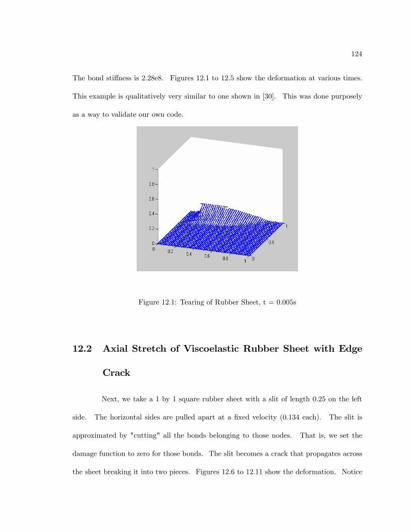
124

The bond stiffness is 2.28e8. Figures 12.1 to 12.5 show the deformation at various times.

This example is qualitatively very similar to one shown in [30]. This was done purposely

as a way to validate our own code.

Figure 12.1: Tearing of Rubber Sheet, t = 0.005s

12.2 Axial Stretch of Viscoelastic Rubber Sheet with Edge

Crack

Next, we take a 1 by 1 square rubber sheet with a slit of length 0.25 on the left

side. The horizontal sides are pulled apart at a fixed velocity (0.134 each). The slit is

approximated by "cutting" all the bonds belonging to those nodes. That is, we set the

damage function to zero for those bonds. The slit becomes a crack that propagates across

the sheet breaking it into two pieces. Figures 12.6 to 12.11 show the deformation. Notice

125

Figure 12.2: Tearing of Rubber Sheet, t = 0.012s

Figure 12.3: Tearing of Rubber Sheet, t = 0.019s

126

Figure 12.4: Tearing of Rubber Sheet, t = 0.025s

Figure 12.5: Tearing of Rubber Sheet, t = 0.039s

127

Figure 12.6: Axial Stretch of Viscoelastic Rubber Sheet with Edge Crack, t = 0s

how the viscosity of the sheet blunts the crack tip. Nodes that have broken completely free

of the sheet are not plotted. Critical stretch to failure is 3. The mesh spacing is 0.025, the

timestep is 1e-3 and the horizon size is 0.075. The bond stiffness is 9.34e7 and the viscosity

is 1e6.

12.3 Penetration of Viscoelastic Rubber Sheet

In this example, we subject a 1 by 1 viscous rubber sheet to a circular impact

at the center. The impact of a projectile is simulated by at first fixing the out of plane

velocity of the nodes in the impact region (in this example, the velocity is 0.268), while

allowing the in-plane motions of the nodes in this region to be free. If any of these nodes

move (slide) outside of this region (a radius of 0.15), all components of their position and

128

Figure 12.7: Axial Stretch of Viscoelastic Rubber Sheet with Edge Crack, t = 0.025s

Figure 12.8: Axial Stretch of Viscoelastic Rubber Sheet with Edge Crack, t = 0.052s

129

Figure 12.9: Axial Stretch of Viscoelastic Rubber Sheet with Edge Crack, t = 0.063s

Figure 12.10: Axial Stretch of Viscoelastic Rubber Sheet with Edge Crack, t = 0.066s

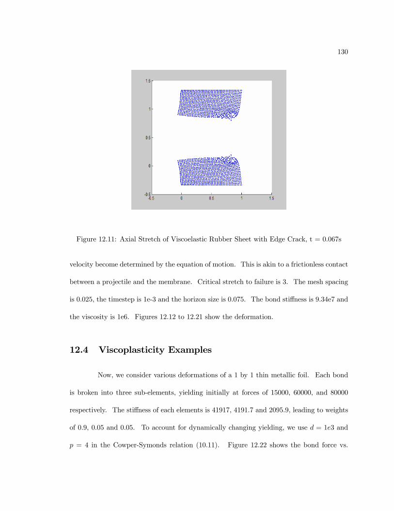
130

Figure 12.11: Axial Stretch of Viscoelastic Rubber Sheet with Edge Crack, t = 0.067s

velocity become determined by the equation of motion. This is akin to a frictionless contact

between a projectile and the membrane. Critical stretch to failure is 3. The mesh spacing

is 0.025, the timestep is 1e-3 and the horizon size is 0.075. The bond stiffness is 9.34e7 and

the viscosity is 1e6. Figures 12.12 to 12.21 show the deformation.

12.4 Viscoplasticity Examples

Now, we consider various deformations of a 1 by 1 thin metallic foil. Each bond

is broken into three sub-elements, yielding initially at forces of 15000, 60000, and 80000

respectively. The stiffness of each elements is 41917, 4191.7 and 2095.9, leading to weights

of 0.9, 0.05 and 0.05. To account for dynamically changing yielding, we use d = 1e3 and

p = 4 in the Cowper-Symonds relation (10.11). Figure 12.22 shows the bond force vs.

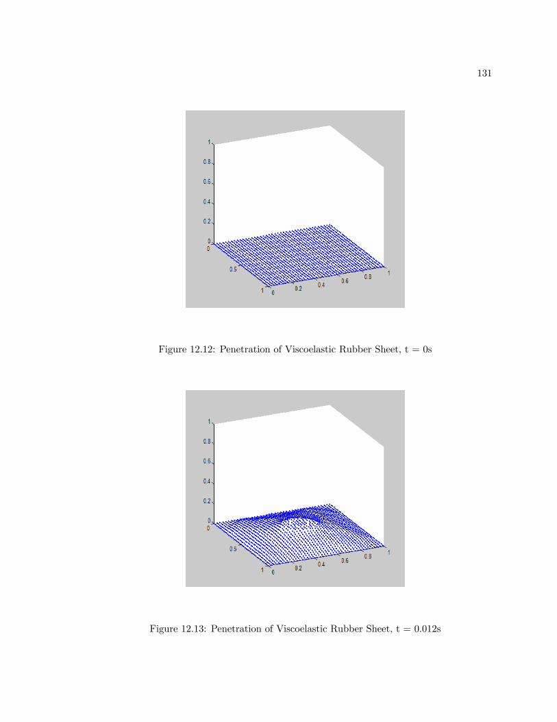
131

Figure 12.12: Penetration of Viscoelastic Rubber Sheet, t = 0s

Figure 12.13: Penetration of Viscoelastic Rubber Sheet, t = 0.012s

132

Figure 12.14: Penetration of Viscoelastic Rubber Sheet, t = 0.025s

Figure 12.15: Penetration of Viscoelastic Rubber Sheet, t = 0.039s

133

Figure 12.16: Penetration of Viscoelastic Rubber Sheet, t = 0.052s

Figure 12.17: Penetration of Viscoelastic Rubber Sheet, t = 0.056s

134

Figure 12.18: Penetration of Viscoelastic Rubber Sheet, t = 0.066s

Figure 12.19: Penetration of Viscoelastic Rubber Sheet, t = 0.079s

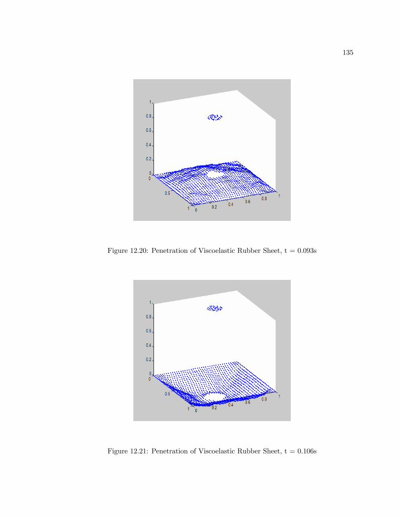
135

Figure 12.20: Penetration of Viscoelastic Rubber Sheet, t = 0.093s

Figure 12.21: Penetration of Viscoelastic Rubber Sheet, t = 0.106s

136

Figure 12.22: Bond Force vs. Extension in Metal Sheet Subjected to Central Impact

extension plot for the material. In those examples that include fracture, the critical force

is 2.017e4 as shown in the figure.

12.5 Axial Stretch of Viscoplastic Metallic Foil

In the first example, we subject the sheet to an axial stretch. The bottom bound-

ary is fixed, while the top boundary is pulled upwards with a fixed dimensionless velocity

of 0.0079. The vertical sides are free. While the membrane can, and does, experience

plastic deformation and work hardening, we do not allow bonds to break. Figures (12.23)

to (12.30) show the deformation. In each figure, the foil is colored based on the percentage

of bonds yielded. Blue denotes areas where it is still elastic and red areas denote where all

137

Figure 12.23: Axial Stretch of Dynamic Plastic Metal Sheet. Color Shows % Bonds Yielded.t = 0s.

bonds have yielded.

12.6 Penetration of Viscoplastic Metallic Foil

In this example, we take the sheer and subject it to a central penetration similar

to that in the viscoelasticity example above. The example combines the effects of plasticity,

work-hardening and fracture. Nodes in the impact region are given an out of plane velocity

of 0.0079. The mesh spacing is 0.025, the timestep is 1e-3 and the horizon size is 0.075.

Figures (12.31) to (12.40) show the deformation. Nodes are colored as follows: blue corre-

sponds to nodes where all bonds are intact and elastic, black corresponds to nodes where

some number of bonds have yielded, and red corresponds to nodes where some number of

bonds have broken (after initially yielding).

138

Figure 12.24: Axial Stretch of Dynamic Plastic Metal Sheet. Color Shows % Bonds Yielded.t = 0.009s.

Figure 12.25: Axial Stretch of Dynamic Plastic Metal Sheet. Color Shows % Bonds Yielded.t = 0.011s.

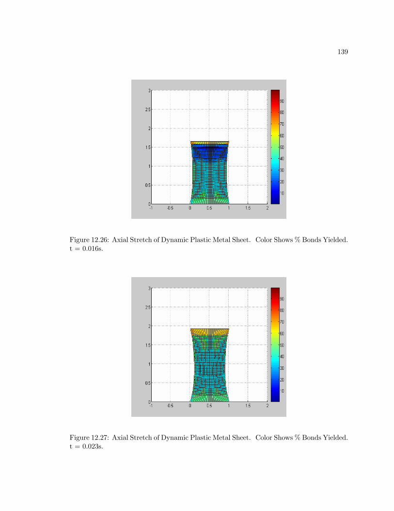
139

Figure 12.26: Axial Stretch of Dynamic Plastic Metal Sheet. Color Shows % Bonds Yielded.t = 0.016s.

Figure 12.27: Axial Stretch of Dynamic Plastic Metal Sheet. Color Shows % Bonds Yielded.t = 0.023s.

140

Figure 12.28: Axial Stretch of Dynamic Plastic Metal Sheet. Color Shows % Bonds Yielded.t = 0.03s.

Figure 12.29: Axial Stretch of Dynamic Plastic Metal Sheet. Color Shows % Bonds Yielded.t = 0.037s.

141

Figure 12.30: Axial Stretch of Dynamic Plastic Metal Sheet. Color Shows % Bonds Yielded.t = 0.047s.

Figure 12.31: Penetration of Viscoplastic Metallic Sheet, t = 0s.

142

Figure 12.32: Penetration of Viscoplastic Metallic Sheet, t = 0.021s.

Figure 12.33: Penetration of Viscoplastic Metallic Sheet, t = 0.0069s.

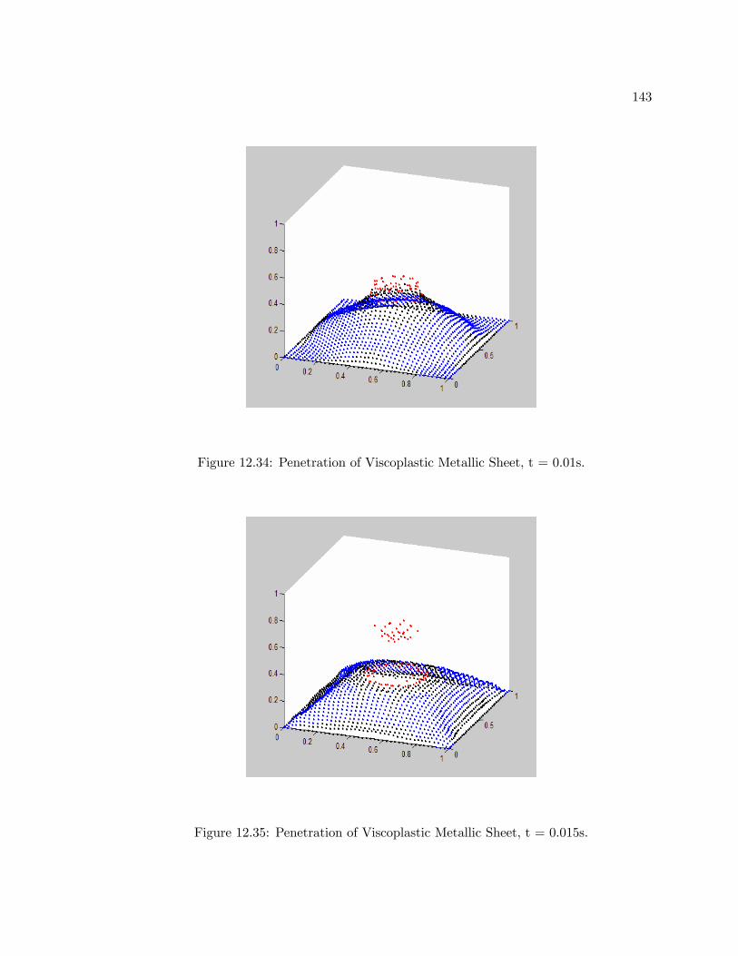
143

Figure 12.34: Penetration of Viscoplastic Metallic Sheet, t = 0.01s.

Figure 12.35: Penetration of Viscoplastic Metallic Sheet, t = 0.015s.

144

Figure 12.36: Penetration of Viscoplastic Metallic Sheet, t = 0.021s.

Figure 12.37: Penetration of Viscoplastic Metallic Sheet, t = 0.028s.

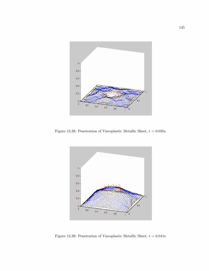
145

Figure 12.38: Penetration of Viscoplastic Metallic Sheet, t = 0.035s.

Figure 12.39: Penetration of Viscoplastic Metallic Sheet, t = 0.041s.

146

Figure 12.40: Penetration of Viscoplastic Metallic Sheet, t = 0.047s.

12.7 Axial Stretch of Viscoplastic Metallic Foil with Edge

Crack

Now we take a square sheet with an off-center horizontal edge slit of length 0.3

and subject it to an axial stretch. The horizontal edges are pulled apart with a velocity of

0.0079 (each). Like the similar viscoelastic example shown earlier, the crack will propagate

across the sheet. However, here, the sheet will plastically deform ahead of the crack. Thus,

the crack does not make it all the way across the sheet and it eventually breaks at the top

and bottom boundaries. Figures (12.41) through (12.48) show the deformation. Nodes

are colored as in the previous example.

147

Figure 12.41: Axial Stretch of Viscoplastic Metallic foil with Edge Crack, t = 0s.

Figure 12.42: Axial Stretch of Viscoplastic Metallic foil with Edge Crack, t = 0.0025s.

148

Figure 12.43: Axial Stretch of Viscoplastic Metallic foil with Edge Crack, t = 0.0041s.

Figure 12.44: Axial Stretch of Viscoplastic Metallic foil with Edge Crack, t = 0.0054s.

149

Figure 12.45: Axial Stretch of Viscoplastic Metallic foil with Edge Crack, t = 0.0077s.

Figure 12.46: Axial Stretch of Viscoplastic Metallic foil with Edge Crack, t = 0.011s.

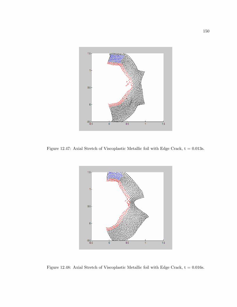
150

Figure 12.47: Axial Stretch of Viscoplastic Metallic foil with Edge Crack, t = 0.013s.

Figure 12.48: Axial Stretch of Viscoplastic Metallic foil with Edge Crack, t = 0.016s.

151

Figure 12.49: Axial Stretch of a Nonlinear Elastic Plate, t = 0s.

12.8 Axial Stretch of a Nonlinear Elastic Plate

In this example, we take a nonlinearly elastic plate and subject it to an axial

stretch. The top and bottom boundaries are pulled apart with a velocity of 0.268 (each

side). The bond force is given by (10.6) and the bond stiffness is 1e5. The mesh spacing is

0.025, the timestep is 1e-3 and the horizon size is 0.075. Figures (12.49) to (12.52) show the

deformation. In addition to the expected in-plane deformation, there is also a noticeable

out of plane deflection as well. Lighter colors denoted positive deflection, while darker

colors denote negative deflection. This is due to the fact that the two-dimensional theory

was derived using the bottom lateral surface as the reference surface. Had the midsurface

been chosen, this would not occur, however the resulting model would be more complicated.

The maximum out of plane deflection over the course of the simulation is 0.014.

152

Figure 12.50: Axial Stretch of a Nonlinear Elastic Plate, t = 0.011s.

Figure 12.51: Axial Stretch of a Nonlinear Elastic Plate, t = 0.027s.

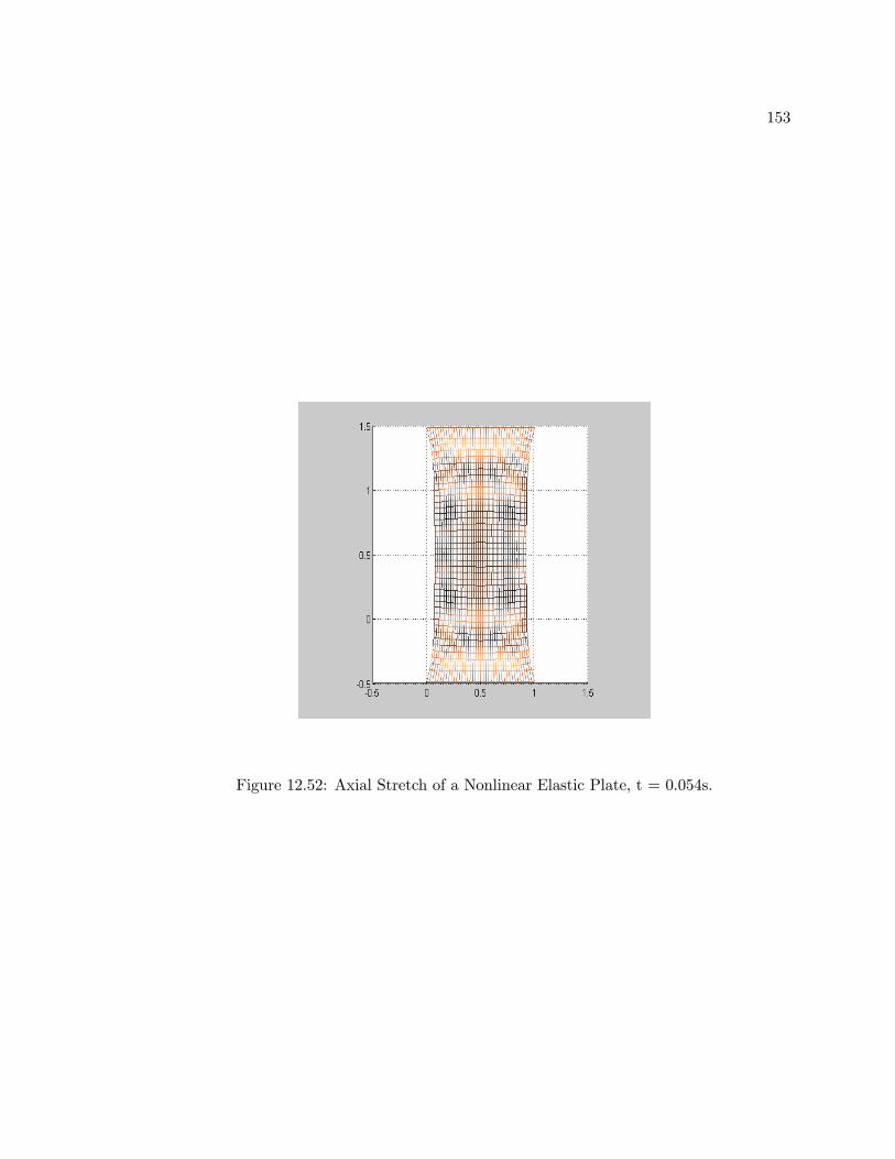
153

Figure 12.52: Axial Stretch of a Nonlinear Elastic Plate, t = 0.054s.

154

Part IV

Summary and Discussion

155

In the preceding sections, we developed two membrane theories based on asymp-

totic approaches and explored solutions to several deformations numerically . In Part II,

we derived a coupled thermomechanical theory for membranes based on continuum me-

chanics and thermodynamics. This model incorporates wrinkling by employing a relaxed

strain energy function. In addition, we incorporated the ability to model a composite sheet

made of two bonded layers. This allowed us to explore the effect of having each layer

made different materials. One application of such composites is solar sails. Solar sails

harness the momentum of solar photons to propel a spacecraft. They typically consist of

a polymer (e.g. Mylar) with a thin aluminum reflective coating. Materials such as Mylar

and aluminum are well characterized by using a Hencky free energy function. In addition

to these materials, we studied entropic elastic polymers (i.e. those which demonstrate the

Gough-Joule effect at high temperatures). Entropic elastomers tend to shrink upon heat-

ing in contrast to many familiar materials, such as those described by the Hencky material

model.

We applied the method of dynamic relaxation to solve the governing equations

numerically. In this method, equilibrium solutions are computed as long-time limits of

damped dynamic problems. Finite difference equations based on Green’s theorem were

derived to discretize the body spatially, while explicit central difference equations were

used to discretize the problem in time. Simulations were presented for entropic elastic

and dual-layer Mylar/aluminum composite membranes for a variety of deformations. As

expected, under increased temperature, a stretched entropic material tends to tense up,

while a Hencky material will expand. For both materials, this came with an increase in

156

the amount wrinkling.

In Part III, we developed a shell theory based on the peridynamic theory. Peridy-

namics is a theory of mechanics particularly suited to modeling fracture. In conventional

mechanics, cracks and fracture present a challenge. The balance of linear momentum re-

quires a certain level of continuity in the displacement field that does not exist at cracks.

Peridynamics reformulates mechanics such that the resulting equation of motion is not a

differential equation, but an integral equation. The theory is based around the idea that a

material point is connected to a certain neighborhood of points around it. These connec-

tions are called bonds, and it is the stretching of these bonds which lead to forces. Materials

are defined by the constitutive equations of their bonds and by the size of the neighbor-

hood (or horizon). The one-dimensional nature of the bonds, makes peridynamic theory

well suited to explore more complicated material responses. We presented a constitutive

model for viscoelastic materials as well as viscoplastic materials that exhibit work-hardening.

Work-hardening was incorporated by adapting the so-called sub-layer method.

To simulate these types of materials, we created two mesh-free explicit codes—one

to model membranes and the other to model shells (i.e., thin bodies with bending stiffness).

Dynamic deformations involving tearing of viscoelastic and viscoplastic membranes were

simulated. The added stiffness in the shell model makes simulating these type of bodies with

an explicit scheme a challenge. However, the code works well for shells with relatively low

bond stiffness and is a solid foundation for future refinements (such as the implementation

of an implicit scheme).

157

Bibliography

[1] “DuPont Teijin Films Mylar Data.” Retrieved on July 5, 2008 from:

http://usa.dupontteijinfilms.com/informationcenter/technicalinfo.aspx.

[2] Abeyaratne, R. and J.K. Knowles. “On the stability of thermoelastic materials,” J.

Elasticity , 53 :199—213 (1999).

[3] Albarado, T.L., et al. “Electron exposure measurements of candidate solar sail mate-

rials,” J. Sol. Energy Eng., 127 :125—130 (2005).

[4] Anand, L. “On H. Hencky’s approximate strain-energy function for modertate defor-

mations.,” ASME J. Appl. Mech., 46 :78—82 (1979).

[5] Anand, L. “Moderate deformations in extension-torsion of incompressible isotropic

elastic materials.,” J. Mech. Phys. Solids, 34 :293—304 (1986).

[6] Boley, B.A. and J.H. Weiner. Theory of Thermal Stresses. New York: Wiley, 1960.

[7] Casey, J. and S. Krishnaswamy. “A Characterization of Internally Constrained Ther-

moelastic Materials,” Math. and Mech. Solids, 3 :71—89 (1998).

158

[8] Chadwick, P. “Thermo-mechanics of Rubber-like Materials,” Phil. Trans. R. Soc. A,

1260 :371—403 (1974).

[9] Chadwick, P. and C.F.M. Creasy. “Modified Entropic Elasticity of Rubber-like Mate-

rials,” J. Mech. Phys. Solids, 32 (5):337—357 (1984).

[10] Ciarlet, P.G. Mathematical Elasticity, vol. III . North-Holland, 1988.

[11] Dunwoody, J. and R.W. Ogden. “On the thermodynamic stability of elastic heat-

conducting solids subject to a deformation-temperature constraint,” Math. Mech.

Solids., 7 :285—306 (2002).

[12] Haseganu, E. and D.J. Steigmann. “Analysis of partly wrinkled membranes by the

method of dynamic relaxation,” Computational Mechanics, 14 :596—614 (1994).

[13] Hunsaker Jr., B. et al. “On the use of two hardening rules of plasticity in incremental

and pseudo force analysis.,” Computational equations in viscoplasticity: Computational

and Engineering Aspects. AMD ASME , 20 :139—170 (1976).

[14] Incropera, F.P. and D.P. DeWitt. Fundamentals of Heat and Mass Transfer, 5th Ed..

Wiley, 2002.

[15] Johns, D.J. Thermal Stress Analysis . Pergamon Press, Oxford, 1965.

[16] Lai, W.M., et al. Introduction to Continuum Mechanics, 3rd Ed.. Butterworth-

Heinemann, 1990.

[17] Naghdi, P.M. “Theory of Shells and Plates,” S. Flugge (ed.), Handbuch der Physik ,

425—640 (1972).

159

[18] Noll, W. “Representations of Certain Isotropic Tensor Functions,” Archiv der Mathe-

matik , XXI :87—90 (1970).

[19] Ogden, R.W. “Waves in isotropic elastic materials of Hadamard, Green or harmonic

type,” J. Mech. Phys. Solids, 18 :149—163 (1970).

[20] Ogden, R.W. Non-linear Elastic Deformations. Dover, 1997.

[21] Pian, T.H.H. “Time-independent anisotropic plastic behavior by mechanical subele-

ment models,” Appl. Math. Mech., 5 (4):1425—1435 (1984).

[22] Pipken, A.C. and R.S. Rivlin. “The Formulation of Constitutive Equations in Contin-

uum Physics I,” Arch. Rational Mech. and Analysis, 4 (2):129—144 (1959).

[23] Pipkin, A.C. “The Relaxed Energy Density for Isotropic Elastic Membranes,” IMA J.

Appl. Math., 36 :85 (1986).

[24] Prager, W. and P.G. Hodge. Theory of Perfectly Plastic Solids. New York: Wiley,

1951.

[25] Rajagopal, K.R. and Y.N. Huang. “Finite circumferential shearing of nonlinear solids

in the context of thermoelasticity,” IMA J. Appl. Math, 53 :111—125 (1994).

[26] Rooney, F.J. and S.E. Bechtel. “Constraints, Constitutive Limits, and Instability in

Finite Thermoelasticity,” J. Elasticity , 74 :109—133 (2004).

[27] Silhavy, M. The Mechanics and Thermodynamics of Continuous Media. Berlin:

Springer, 1997.

160

[28] Silling, S.A. “Reformulation of elasticity theory for discontinuities and long-range

forces,” J. Mech. Phys. Solids, 48 :175—209 (2000).

[29] Silling, S.A. and E. Askari. “A meshfree method based on the peridynamic model of

solid mechanics,” Computers and Structures, 83 :1526—1535 (2005).

[30] Silling, S.A. and F. Bobaru. “Peridynamic modeling of membranes and fibres,” Int. J.

Non. Lin. Mech., 40 :395—409 (2005).

[31] Sokolnikoff, I.S. Mathematical Theory of Elasticity, 2nd Ed.. McGraw-Hill, 1956.

[32] Taylor, M. and D.J. Steigmann. “Entropic thermoelasticity of thin polymeric films,”

Acta Mechanica, 183 :1—22 (2006).

[33] Treloar, L.R.G. The Physics of Rubber Elasticity . Oxford: University Press, 1975.

[34] Wegner, J.L. “Some Aspects of Thermodynamic Effects in Finite Amplitude Wave

Propagation in Rubber-like solids,” Wave Motion, 39 :21—39 (2004).

[35] Weiner, J.H. Statistical Mechanics of Elasticity . New York: Dover, 2002.

[36] Xiao, H. and L.S. Chen. “Hencky’s elasticity model and linear stress-strain relations

in isotropic finite hyperelasticity,” Acta Mechanica, 157 :51—60 (2002).