An experimental and numerical approach to investigate the dynamic response of a four-flue chimney of...
150
-
Upload
independent -
Category
Documents
-
view
2 -
download
0
Transcript of An experimental and numerical approach to investigate the dynamic response of a four-flue chimney of...

Preface iii
Preface
This thesis was written during my time at the Institute for Machine Tools and Manufacturing (IWF) of the ETH Zurich.
Many people have contributed to this work and in this preface I would like to express my special gratitude to some of them.
First of all, I would like to thank Prof. Konrad Wegener, head of the IWF and supervisor of this thesis, for his support, trust and friendliness.
I am also grateful to Prof. Urs Meyer for being the temporary thesis supervision before Prof. Wegener has become head of the IWF and for being the co-supervisor of this thesis.
My sincere gratitude goes also to Prof. Walter Weingärtner, which has supported my studies in Switzerland.
Special gratitude I owe to Dr. Fredy Kuster. Dr. Kuster was my group leader at IWF and his patient explanations and strong trust in my capabilities have helped me during my entire journey.
I would like to thank all my colleagues and friends of the IWF for the experiences that I have shared with them. To some of these friends I would like to register my very special thanks: Guilherme Vargas, Eduardo Weingärtner, Angelo Boeira, Jérémie Monnin, Sergio Bossoni, Bernhard Bringmann, Michael Hadorn, Carl Wyen and Zoltan Sarosi.
Finally I would like to thank my wife, Maitê, and my parents for all the support during the years required to develop my thesis.
Fábio Wagner Pinto
May 2008

iv
To my family.

Contents v
Contents
Symbols and abbreviation ................................................................................... viii
Abstract ................................................................................................................. xi
Kurzfassung .......................................................................................................... xii
1. Introduction .................................................................................................. 1
2. State of the art .............................................................................................. 4
2.1 Single layer grinding tools .............................................................................. 4
2.1.1 Tool body ................................................................................................... 5
2.1.2 Superabrasive grains ................................................................................. 5
2.1.3 Electroplating bond system ........................................................................ 7
2.1.4 Brazing bonding system ............................................................................. 9
2.1.5 Coolants and their application methods ..................................................... 10
2.1.6 Conditioning methods for SLGT ................................................................. 12
2.2 Wear effects on SLGT .................................................................................... 12
2.3 Engineered grinding tools .............................................................................. 13
2.4 Modeling and simulation of the grinding process ........................................... 17
2.4.1 Molecular dynamics ................................................................................... 19
2.4.2 Description of kinematics ........................................................................... 19
2.4.3 Analytical description ................................................................................. 23
2.4.4 Finite element analysis .............................................................................. 24
2.4.5 Regression analysis ................................................................................... 25
2.4.6 Artificial neural networks ............................................................................ 26
2.4.7 Rule based models .................................................................................... 26
2.4.8 Modeling techniques suitable for EGT optimization ................................... 27
vi Contents
2.5 Resume .......................................................................................................... 28
3. Problem description and objectives ........................................................... 29
4. Production of braze bonded EGT ............................................................... 31
4.1 Description of placing system designed by Burkhard ..................................... 31
4.2 Alternative control method for the dispenser .................................................. 33
4.3 Description of the placing system ................................................................... 36
4.4 Resume .......................................................................................................... 42
5. Model concept .............................................................................................. 44
5.1 Tool model ..................................................................................................... 45
5.1.1 Body material deviations ............................................................................ 45
5.1.2 Effects of the brazing process .................................................................... 46
5.1.3 Grain pattern .............................................................................................. 47
5.1.4 Grain morphology ...................................................................................... 47
5.2 Kinematic process model ............................................................................... 50
5.3 Material removal model .................................................................................. 51
5.4 Simulation method for the cutting process ..................................................... 53
5.5 Grain wear model ........................................................................................... 54
5.6 Tangential grinding force model ..................................................................... 56
5.7 Further simulation outputs .............................................................................. 58
5.8 Resume .......................................................................................................... 59
6. Production and tests of tool samples ........................................................ 60
6.1 Tool design..................................................................................................... 60
6.2 Grinding tests ................................................................................................. 61
6.3 Results ........................................................................................................... 64
6.3.1 Roughness measurements ........................................................................ 64
6.3.2 Force measurements ................................................................................. 70
6.3.3 Microscopic characterization ...................................................................... 74
6.3.4 Further observations .................................................................................. 81
6.4 Conclusion of the experiments ....................................................................... 82
7. Numerical results ......................................................................................... 84
7.1 Kinematic-geometric process simulation ........................................................ 84
7.1.1 Evaluation of the grain size ........................................................................ 87
7.1.2 Evaluation of the grain sieving tolerances .................................................. 88
Contents vii
7.1.3 Evaluation of the grain morphologies ......................................................... 92
7.1.4 Evaluation of the effects of the braze process on the grain position .......... 95
7.1.5 Evaluation of the dressing techniques ....................................................... 95
7.1.6 Evaluation of the grain pattern parameters ................................................ 101
7.1.7 Evaluation of the tool unbalance ................................................................ 103
7.1.8 Evaluation of the ratio between tool and workpiece speeds ...................... 105
7.2 Wear model for kinematic-geometric cutting process simulation .................... 106
7.3 Simulation of conventional SLGT ................................................................... 114
7.4 Evaluation of the tangential grinding force ..................................................... 117
7.5 Conclusions.................................................................................................... 123
8. Conclusion and outlook .............................................................................. 126
8.1 Conclusions.................................................................................................... 126
8.2 Outlook ........................................................................................................... 128
8.2.1 Grains properties characterization ............................................................. 128
8.2.2 Placing technologies .................................................................................. 128
8.2.3 Braze bonding technology ......................................................................... 129
8.2.4 Single grain tests ....................................................................................... 129
8.2.5 Explore alternative application fields for EGT ............................................ 130
8.2.6 Analyze the coolant flow on the grinding gap ............................................. 130
Bibliography .......................................................................................................... 131

viii Symbols and abbreviations
Symbols and abbreviations
Abroken Area of the grain removed by wear
Agrain Cutting area of a grain
Alim Limit cutting area for the grain
Amax Cutting area at the position of maximal cutting depth
ae Interference between grinding tool and workpiece
AL Offset of the grain pattern
Ag Silver
ANN Artificial neural networks
b Cutting width on the cutting edge direction
bd Grinding tool width
bws Workpiece width
B Boron
b+, b- Limits of an uniform distribution
Cf Constant for the parameterization of the grain geometry
cBN Cubic boron nitride
Cu Copper
Cr Chromium
cgw Constant for the grinding wheel
cwp Constant for workpiece
Dedge Diameter of a region around the nominal cutting edge position where the cutting edge can be found
Deq Equivalent diameter
Dp Droplet diameter
Dpk Diameter correspondent to the precision while positioning the adhesive points over the tool body

Symbols and abbreviations ix
Dws Workpiece diameter
Dwz Grinding tool diameter
DCU Dispenser control unit
e1, e2, e3 Experimental exponents
EGT Engineered grinding tools
ES Expert system
Fc Cutting force in turning operations
Fnozzle Command frequency for the nozzle
FR’ Specific radial grinding force
FT’ Specific tangential grinding force
FEA Finite element analysis
h Cutting depth orthogonal to the cutting edge direction
hm Maximal cutting depth
I/O Input/Output
Kc1.1 Specific cutting force for a chip corss-section of 1mm2
KBS Knowledge based system
L Distance between grains
MD Molecular dynamics
N Nitrogen
NL Number of lines in one rotation
nrot Number of revolutions to layer the whole tool width
NWZ Tool rotation frequency
Ni Nickel
q Speed ratio between grinding wheel and workpiece speeds
Qw’ Specific material removal rate
Ra Arithmetical mean roughness
Radh Offset between the center of the adhesive point and the nominal position of the cutting edge
Rgrain Offset between the center of the adhesive point and the center of the grain projection
Redge Offset between the center of the grain projection and the position of the grain edge
RHTp Parameter of the Abbott-Firestone curve
Rsk Skewness
Rt Maximum distance between the highest peak and the lowest groove over a measuring distance “L”
Rz Ten-point mean roughness
x Symbols and abbreviations
RB Rule based models
Sb Tool width
SLGT Single layer grinding tools
Sn Tin
Ti Titanium
u Equivalent standard deviation for uniform distribution
vf Feed rate of the nozzle parallel to the rotational axis
vfr Radial feed rate of the grinding tool
vs Grinding speed
vw Workpiece speed
Vw’ Specific material removed [mm3/mm]
Zr Zirconium
α Angle of the grain pattern
∆x, ∆z, ∆z2 Parameters of the grain pattern
σ Standard deviation of a sample
σadh Standard deviation of the adhesive center point position
σ1 Equivalent standard deviation of the grain position on the adhesive point
σ2 Equivalent standard deviation of the cutting edge on the grain projection
Abstract xi
Abstract
Engineered Grinding Tools (EGT) are characterized by a predetermined and controlled arrangement of the abrasive grains. The distribution of the grains can be used to improve the performance of the grinding process by improving space for coolant supply and for chip removal. This is especially interesting for grinding operations with high specific material removal rates. A semi automatic method for the production of brazed bonded EGT is presented. The grain positioning precision of this method is analyzed. A numerical method was developed to analyze the effects of the grain pattern in the grinding process. This numerical method consists of a stochastically based tool model, a kinematic process model, a material removal model and a grain wear model. The tool model comprehends the relevant geometric properties of the abrasive layer, including the properties of the production technique for the grain pattern. The material removal model is based on the assumption of kinematic-geometrical cutting process. The wear model is based on a grain load limit and the grains’ load is assumed to be dependent on the cutting area. Once the cutting area of one grain exceeds the limit value, wear takes place. The grinding forces acting on the tool are simulated with an approximation of the Kienzle equation. Different tool samples were produced to validate the simulation results. A comparison with the conventional single-layer electroplated grinding tool is also presented.
Kurzfassung xii
Kurzfassung
Engineered Grinding Tools (EGT) sind Schleifwerkzeuge, welche durch eine definierte und kontrollierte Anordnung der Abrasivkörner charakterisiert sind. Mit der kontrollierten Anordnung kann der Spanraum vergrössert werden, was eine verbesserte Zugänglichkeit von Kühlschmierstoff, als auch einen verbesserte Abtransport der Späne gewährleistet. Ein grosser Spanraum ist von besonderem Interesse für Schleifanwendungen, in denen hohe spezifische Zeitspanvolumina gefordert werden. Im Rahmen dieser Arbeit wird eine Methode zur halbautomatischen Herstellung von gelöteten EGT vorgestellt. Die Platzierungsgenauigkeit wurde für dieses Verfahren analysiert. Es wurde ein numerisches Verfahren entwickelt, um den Einfluss des Platzierungsmusters auf den Schleifprozess auszuwerten. Dieses Verfahren beruht auf einem stochastischen Werkzeugmodell, einem kinematischen Prozessmodell, sowie Modellen für den Werkstoffabtrag und für den Kornverschleiss. Das Werkzeugmodell berücksichtigt die geometrischen Eigenschaften des Schleifbelags, inklusive der herstellspezifischen Platzierungsgenauigkeiten des Korns. Die Modellierung des Abtrags erfolgt auf der Grundlage kinematisch-geometrischer Schnittbedingungen. Dem Verschleissmodell liegt ein von der sich im Eingriff befindlichen Schneidfläche abhängiges Kornversagen zugrunde. Sobald die Schneidfläche eines Korns ein bestimmtes Mass überschreitet, verschleisst das entsprechende Korn. Die am Werkzeug wirkende Schnittkraft wird durch Näherung der Kienzle-Gleichung ermittelt. Mit verschiedenen Werkzeugmustern wurden die numerischen Ergebnisse experimentell verifiziert. Des Weiteren werden die EGT mit konventionellen galvanischen Schleifwerkzeugen verglichen.
Chapter 1 – Introduction 1
1. Introduction
The grinding process is usually connected to a finishing operation, placed at the end of the production line. As a finishing process, the tolerances on the workpiece dimensions are usually some microns and the grinding operation should generate the required surface roughness.
The constant demand for more efficient processes and the search for higher profitability on production lines have pushed the diversification of the grinding process. Nowadays, thanks to the development of grinding technologies, it is possible to apply grinding tools in high removal rate operations and substitute operations such as milling or turning.
The application of hard materials as diamonds and cubic boron nitrides (cBN) as abrasive particles material (the so-called superabrasives) is one of the most relevant developments towards the diversification of the grinding applications. Superabrasives have very high hardness and allow the application of very high grain loads and lower tool wear.
While the diamonds applied on grinding tools can be either synthetically produced or naturally obtained, cBN is obtained only by artificial synthesis processes. Diamond is the hardest material available, but the machining processes possible with this material are limited due to its affinity with ferrous materials. The cBN grains, on the other hand, have no reactivity with ferrous materials and have been largely applied on machining operations of steel alloys.
The purchase costs are the main disadvantage of the superabrasives in relation with conventional abrasive materials. Nowadays, the best price relation (per carat) between superabrasives and conventional abrasive material (corundum) is about 100:1. Comparing high and poor superabrasives qualities, the ratio is about 70:1. The high costs involved on the application of these materials have demanded their rational application: tools with superabrasives have the grains distributed on a thin layer on the active surface of the tool. This solution reduces the efforts required to acquire the grains and enables the economical application of these materials.
An interesting alternative for the application of superabrasives is to spread a single layer of grains and firmly bond them to the tool body. An electroplated layer is the usual method of bonding the grains on the body material (which must be metallic). An important aspect of the single layer grinding tools (SLGT) is the lower investment required to purchase them. However, to achieve the bonding forces required during the grinding process, the electroplated layer must cover a large
2 Chapter 1 – Introduction
amount of the grain height. This reduction of the grain protrusion reduces the volume available for chips and coolant during the process and may lead to material stuffing the tool surface.
The brazing technique is an alternative to the electroplated for single layer grinding tools. The brazed bond is generated with a chemical reaction between the grains, the tool body and the filler alloy. The successful bond depends on the coherent choice of the materials involved. The resulting abrasive layer presents, at once, high grain protrusion and high bonding forces, both desired Properties for the application of the grinding tool on rough grinding operations.
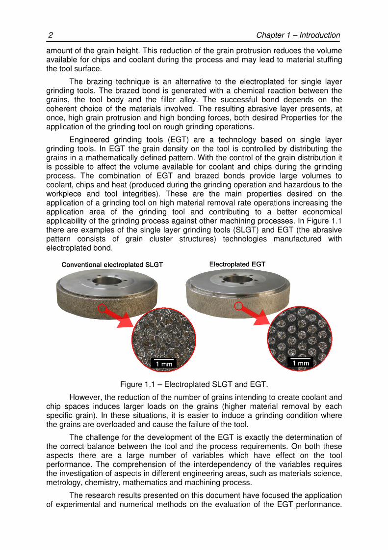
Engineered grinding tools (EGT) are a technology based on single layer grinding tools. In EGT the grain density on the tool is controlled by distributing the grains in a mathematically defined pattern. With the control of the grain distribution it is possible to affect the volume available for coolant and chips during the grinding process. The combination of EGT and brazed bonds provide large volumes to coolant, chips and heat (produced during the grinding operation and hazardous to the workpiece and tool integrities). These are the main properties desired on the application of a grinding tool on high material removal rate operations increasing the application area of the grinding tool and contributing to a better economical applicability of the grinding process against other machining processes. In Figure 1.1 there are examples of the single layer grinding tools (SLGT) and EGT (the abrasive pattern consists of grain cluster structures) technologies manufactured with electroplated bond.
Figure 1.1 – Electroplated SLGT and EGT.
However, the reduction of the number of grains intending to create coolant and chip spaces induces larger loads on the grains (higher material removal by each specific grain). In these situations, it is easier to induce a grinding condition where the grains are overloaded and cause the failure of the tool.
The challenge for the development of the EGT is exactly the determination of the correct balance between the tool and the process requirements. On both these aspects there are a large number of variables which have effect on the tool performance. The comprehension of the interdependency of the variables requires the investigation of aspects in different engineering areas, such as materials science, metrology, chemistry, mathematics and machining process.
The research results presented on this document have focused the application of experimental and numerical methods on the evaluation of the EGT performance.
Chapter 1 – Introduction 3
The experimental methods were applied to achieve a close look on the real performance of the tools, understanding the most relevant phenomena to be considered in the models. The numerical methods were applied to the analysis of the micro-cutting conditions and to understand the correlations of these with the macro-effects in the grinding process.
The structure of the work consists of an overview of the state of the art on the technologies applied on EGT (abrasives, bonding, placing and design techniques) which reveals the potential developments areas for the EGT. Brazed bonded tool are focused on the research. A new control technique for the production method of the tool is proposed and the grain positioning precision is discussed. Tool samples are produced and tested on external cylindrical plunge grinding operations. The results obtained with the tool samples will be applied to the validation of the numerical method, which comprehends the stochastic tool model, the material removal model and the description of the process kinematics for the grinding operation. The simulations are applied to investigate the effects of the geometrical properties of the tool on the grinding process and on the workpiece surface achieved.

4 Chapter 2 – State of the art
2. State of the art
The correct specification of single layer grinding tools depends on a series of process properties, such as workpiece material, material removal rate and of the abrasive grains applied. The following chapter elucidates the state of the art of these tools technologies, exploring the main tool properties, the methods of manufacturing and the state of the art of numerical methods for the optimization of tool design and performance.
2.1 Single layer grinding tools
The technology of single layer grinding tools (SLGT) has taken special profit from the development of the super-hard grain materials (superabrasives). On these tools there is just a single layer of abrasives available for the removal of the workpiece material. The grains must be firmly bonded to the tool body and must present high wear resistance (the main property of the superabrasives). Despite being about 100 times more expensive than the conventional abrasives (like corundum or aluminum oxide) it is possible to achieve economical advantages from the use of superabrasives due to the longer life of the tool (lower wear) and better precision achieved on the workpiece. For the optimal use of the superabrasives’ properties it is fundamental that the bond applied between tool body and the grains supports the high forces involved in the process. On a multi layer grinding tool this would imply a larger quantity of bond material, and so a consequent reduction of the chip space volume available for the chips [HOLZ88, MALK89, KÖNI96, WEBS04, MARI04, DING06, GHOS07].
SLGT have as their main field of application rough machining operations in the automotive and aerospace industries. Typical of these applications are the complex tool profiles, medium grain sizes and small tolerances on the finished part [KÖNI96, MARI04, WEBS04].
In the application of superabrasives for multi-layer tools it is usual for the cost of the abrasive grain to account for around 50% of the total costs of the tool. As on SLGT the grains are applied as a single layer, the reduction of the abrasive material enables economic advantage as the price of the tool is reduced [CAI03, WEBS04].
The application of SLGT has been found recently to have potential also in high precision applications. The low roughness values required are achieved with specific preparation techniques of the tool, changing the micro properties of the grains edges.
Chapter 2 – State of the art 5
In such applications SLGT take advantage of its better estimation of the position of the cutting edges (on a single layer) for the dressing process [RICK06].
The flexibility on the manufacturing profiled tools and the stability of the form are properties that makes the SLGT technology suitable for active dressing wheels. These tools are usually applied to dressing operations on ceramic bonded cBN grinding wheels, and on gear grinding wheels (worm grinding wheels or honing tools) [KLOC02].
The bond technique applied in the SLGT enables the use of higher rotational speed of the tool without the risk of tool failure (detaching of the abrasive layer due to the high centrifugal forces). Nevertheless, the tool body must be not only statically, but also dynamically balanced, and the machine structure must be designed to guarantee the safety of the machine operator [MALK89, KLOC02, MARI04].
The successful composition of a SLGT is the combination of a series of properties, such as a precisely manufactured body material, superabrasive grains and the correct bond material to the grains. In the next sections these different tool properties will be explored.
2.1.1 Tool body
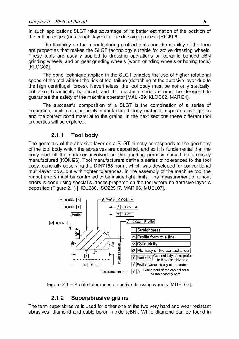
The geometry of the abrasive layer on a SLGT directly corresponds to the geometry of the tool body which the abrasives are deposited, and so it is fundamental that the body and all the surfaces involved on the grinding process should be precisely manufactured [KÖNI96]. Tool manufacturers define a series of tolerances to the tool body, generally observing the DIN7168 norm, which was developed for conventional multi-layer tools, but with tighter tolerances. In the assembly of the machine tool the runout errors must be controlled to be inside tight limits. The measurement of runout errors is done using special surfaces prepared on the tool where no abrasive layer is deposited (Figure 2.1) [HOLZ88, ISO22917, MARI06, MUEL07].
Figure 2.1 – Profile tolerances on active dressing wheels [MUEL07].
2.1.2 Superabrasive grains
The term superabrasive is used for either one of the two very hard and wear resistant abrasives: diamond and cubic boron nitride (cBN). While diamond can be found in
6 Chapter 2 – State of the art
nature or manufactured in controlled conditions, cBN is only achieved under specific synthesis conditions.
Diamond holds a unique place in the abrasives industry. Being the hardest known material, it is not only the natural choice for grinding the hardest and most difficult materials, but it is also the only material that can effectively be applied in truing and dressing operations of other abrasive wheels. Natural diamond grows predominantly in an octahedral form that provides several sharp points optimal for single point diamond tools. These properties are also preferred for dressing tools and form rolls [WILK91, KÖNI96, MARI04].
Synthetic diamonds may be monocrystalline or polycrystalline. Monocrystalline grains are utilized for particularly demanding applications. The easily recognizable cubic or cubic-octahedral shape reflects the typical crystallographic structure of diamond. Almost perfect crystals are obtained with a slow growth, low-density nucleation process, with limited metallic inclusion and little or poor interaction between various grains that are growing within the melt [WILK91].
Polycrystalline grains are highly friable and are produced by greatly accelerating the nucleation rate within the press, causing precipitation of diamond nuclei from the melt in a large number. Due to the crowding in the melt, the normal growth pattern is inhibited, so grains having undefined geometric shapes, which look like an agglomerate of smaller crystals, are obtained. These are very prone to fragmentation and partial break-up with dark spots within the grains that correspond to metallic inclusions [WILK91].
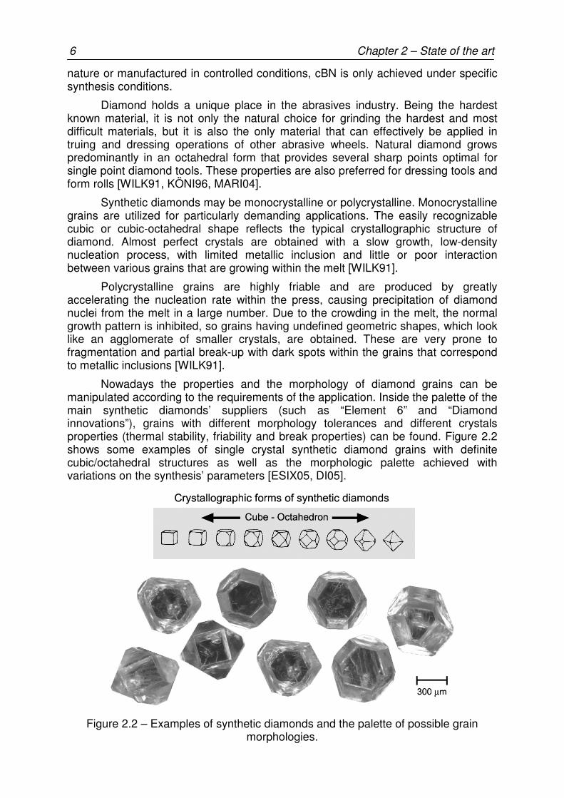
Nowadays the properties and the morphology of diamond grains can be manipulated according to the requirements of the application. Inside the palette of the main synthetic diamonds’ suppliers (such as “Element 6” and “Diamond innovations”), grains with different morphology tolerances and different crystals properties (thermal stability, friability and break properties) can be found. Figure 2.2 shows some examples of single crystal synthetic diamond grains with definite cubic/octahedral structures as well as the morphologic palette achieved with variations on the synthesis’ parameters [ESIX05, DI05].
Figure 2.2 – Examples of synthetic diamonds and the palette of possible grain morphologies.

Chapter 2 – State of the art 7
Invented in 1957 at the General Electrics research laboratory, cubic boron nitride (cBN) is an allotropic crystalline form of boron nitride which is the abrasive material which most closely approximates of diamond hardness (Knoop Scale). In cBN, each boron atom is connected to four nitrogen atoms, as each nitrogen atom is connected to four of boron, forming the typical tetrahedral structure of the crystals [WEBS04].
The use of cBN in grinding applications has become popular due to the hardness of the crystal, the thermal resistance (higher than that of diamond, allowing work at 1900°C) and the good chemical stability of cBN while machining ferrous alloys [MARI04].
Due to its asymmetric crystallographic structure (with Boron and Nitrogen atoms), cBN gains cannot achieve the same morphologic spectrum of the diamond grains and, for example, no cubic grain can be obtained. However, as happens with synthetic diamonds, the cBN properties and morphology can be strongly affected by the synthesis parameters applied. Figure 2.3 shows some examples of cBN grains and the basic morphological structures that can be achieved [BAIL95].
The spectrum of properties that can be achieved on the cBN grains has direct effect on the price of these hard particles. Superabrasive grains can be up to two orders of magnitude more expensive than conventional abrasives, and so their application is economized to a thin layer around the tool. Due to their higher grain resistance, the grains can be applied on higher removal rates if the bonding system of the grains will support the higher load as well [CAI03].
Figure 2.3 – Example of cBN grains and the possible grain morphologies.
2.1.3 Electroplating bond system
The electroplating process consists of the electrolytic deposition of a metal layer on a conducting substrate. Nickel is commonly applied to the formation of the bond on SLGT. In the electroplating process the metallic nickel is transferred from the anode to nickel ions by electrolysis. Those ions are going to be discharged on the cathode (the tool surface that is going to be layered) and form a coat of metallic nickel. Applied on abrasive tools, the coating process has three basic steps [INCO89]:
8 Chapter 2 – State of the art
• Creation of a nickel coat over the tool surfaces which are going to receive the abrasives.
• Deposition of the grains. The plating parameters applied on this stage are accountable for properties such as grain concentration, on the abrasive layer.
• Cover the grains up to a specific height, so that the bond force is guaranteed due to a sufficient mechanical support.
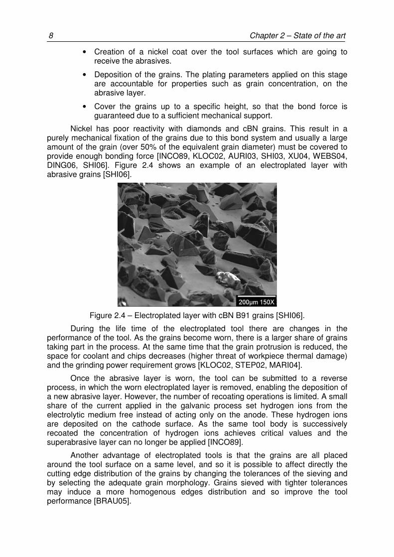
Nickel has poor reactivity with diamonds and cBN grains. This result in a purely mechanical fixation of the grains due to this bond system and usually a large amount of the grain (over 50% of the equivalent grain diameter) must be covered to provide enough bonding force [INCO89, KLOC02, AURI03, SHI03, XU04, WEBS04, DING06, SHI06]. Figure 2.4 shows an example of an electroplated layer with abrasive grains [SHI06].
Figure 2.4 – Electroplated layer with cBN B91 grains [SHI06].
During the life time of the electroplated tool there are changes in the performance of the tool. As the grains become worn, there is a larger share of grains taking part in the process. At the same time that the grain protrusion is reduced, the space for coolant and chips decreases (higher threat of workpiece thermal damage) and the grinding power requirement grows [KLOC02, STEP02, MARI04].
Once the abrasive layer is worn, the tool can be submitted to a reverse process, in which the worn electroplated layer is removed, enabling the deposition of a new abrasive layer. However, the number of recoating operations is limited. A small share of the current applied in the galvanic process set hydrogen ions from the electrolytic medium free instead of acting only on the anode. These hydrogen ions are deposited on the cathode surface. As the same tool body is successively recoated the concentration of hydrogen ions achieves critical values and the superabrasive layer can no longer be applied [INCO89].
Another advantage of electroplated tools is that the grains are all placed around the tool surface on a same level, and so it is possible to affect directly the cutting edge distribution of the grains by changing the tolerances of the sieving and by selecting the adequate grain morphology. Grains sieved with tighter tolerances may induce a more homogenous edges distribution and so improve the tool performance [BRAU05].

Chapter 2 – State of the art 9
The electroplating process has also some disadvantages when applied to abrasive layers for grinding tools. In profile tools the inhomogeneous distribution of the current density is often a problem. The resulting nickel coat thickness is proportional to the field strength, which is higher as the distance between the cathode and anode is shorter [INCO89]. This problem can be minimized, however, with finely controlled parameters, or with electrochemical material deposition.
Applied generally in grinding operations with high workpiece removal rates, each active grain in SLGT is exposed to very high specific forces [N/mm2]. Due to the mechanical bond characteristics of electroplated tools, “pull-outs” of grains from the nickel matrix are often found in these grinding operations. This is an evidence that the mechanical principle of bonding the grain to the tool may not fulfill all the process requirements. Space for coolant and chips are also necessitated in highly productive operations. Covering a large part of the grains to provide enough bond resistance reduces the volume available for chips and coolant [CHAT93, KHAL04, GHOS06].
2.1.4 Brazing bonding system
In contrast to the electroplating technique, on brazed bonded tools there is a chemical reaction between grains, filler alloy and tool body. The filler alloys are composed from two or more components, of which at least one of them has great chemical affinity with oxygen, carbon or nitrogen, the usual components of hard abrasive materials. However, the high affinity of the active metal atoms within the solder to the non-metallic elements in the hard materials causes a chemical reduction of atoms in abrasive particles, whereby atoms of the active metal in the binder are oxidized to different oxides, carbides or nitrides in a diffusion layer zone adjacent to the particles. This reduction–oxidation process takes place in the melted stage of the solder, during the soldering process, thus forming a very strong and tensile bond between the binder and the particles and/or their carrier, allowing the transmission of high stresses and shear forces through the binder to the carrier, without the separation of particles from the binder. The active elements react very sensitively with oxygen, and therefore the brazing process must be carried out in a high-vacuum atmosphere [CHAT93, BURK01].
The most common braze alloys are based on Ag-Cu, Cu-Sn or Ni-Cr. Generally, the main problem in preparing the brazed cBN grinding tools is not the bonding of filler alloy with the tool substrate, but joining cBN grains and filler alloy. The low surface tension of cBN grain crystals makes it unlikely that many molten metals satisfy the wetting condition for the reaction in the interfacial region. Titanium is usually added as active element on the brazing alloy and plays an important role in the chemical wetting property. Titanium mixture concentrates preferentially on the surface of the cBN grains to form a layer of needle-like Ti-N and Ti-B compounds by chemical metallurgic interaction between Ti, N and B at high temperature. In diamond grains the reaction is similar, but the components created are titanium-carbides [BURK02, HUAN04, KHAL04, GHOS06, DING06].
The brazing process requires high temperatures (usually over 900oC for cBN) to melt the brazing material and for the reactions of the active material with the ceramic grains. The correct choice of the materials involved is required to support the high thermal load applied. The thermal expansion of all the material involved must be chosen correctly. The inhomogeneous expansion of the tool body may lead to form deviations on tool after the brazing process. The difference between the thermal expansion coefficient of the abrasive, of the filler metal and of the tool body induces

10 Chapter 2 – State of the art
dangerous residual stresses on the joints, which may lead the tool to premature failure. The grains must also present high thermal stability, which guarantees that the grains do not lost their properties due to the exposure to high temperatures [CHAT93, BURK01, BACH04].
The typical bonding structure resulting from a successful brazing process is shown in Figure 2.5. The molten material around the grain has influence of the capillary of the geometries involved and of the reaction with the active element. The grain is well wetted and, at the same time, on contrary to what is normally found on galvanic tools, the bond is concentrated just around the grains and provides large coolant and chips spaces.
As with electroplated tools the brazed bond can be removed for the re-utilization of the tool body. Nevertheless, the brazed bond requires a chemical removal procedure as there are reactions with the tool body material and with the abrasive grains. Moreover, the brazing process generates a reaction layer on the tool surface which does not allow the recovery of the tool without re-machining the tool body (mainly due to the tight form tolerances of SLGT).
Figure 2.5 – Brazed cBN grain (ABN800 B251).
The main disadvantages of this bond technology are the high demands on the materials involved (grain and body), the expense of brazing installations (vacuum furnace), the risk of damaging the grain properties during the brazing process and the difficulties inherent in removing the worn abrasive layer.
Typical fields of application of brazed tools are in civil construction, stone machining and road maintenance.
2.1.5 Coolants and their application methods
The coolant has three main functions in the grinding process: cooling of the grinding process/machine/workpiece, lubrication of the grinding gap, and transport (heat and chips). According to the specification of the coolant medium one of these characteristics will be accentuated. Especially interesting for the grinding process is the application of oil-based coolants. With a prior lubrication function, these act directly avoiding the generation of heat due to the friction of the grains with the
Chapter 2 – State of the art 11
workpiece. Water-based coolants have larger capacity of transporting heat out of the grinding zone, but the disadvantage of presenting poor lubrication properties [KÖNI96, MARI04].
As environmental threats become more intensive on the limitation of the application of oil-based coolants, there is a steady move towards water-based fluids. Water-based emulsions concentrate contain a limited amount of basic oil (mostly mineral oils) and have higher cooling efficiency and washing-away capabilities. However, a serious disadvantage is the susceptibility to infection of the coolant with micro organisms, requiring high and constant maintenance costs. Being applied with cBN grains, the water steam generated reacts with the grains, accelerating the wear ratio of the tool [WEBS95, TAWA07].
SLGT characteristics such as no porosity, high grain protrusion and high thermal conductivity of abrasives and bond, require specific properties of the grinding coolant. As the tool has no porosity, the amount of coolant able to flow through the grinding gap is limited by the kinematic and geometric characteristics of the grinding process. To avoid large spindle power requirements for the acceleration of the coolant, it must be delivered at relatively high speeds (close to the grinding speed) and with tangential direction to the grinding speed on the grinding gap. The relationship between the volume required and the correct coolant speed are strongly affected by the coolant nozzle and are the key parameters to an optimal action of the coolant on the grinding operation [WEBS95, HRYN00, KLOC00, NINO04, RAME01].
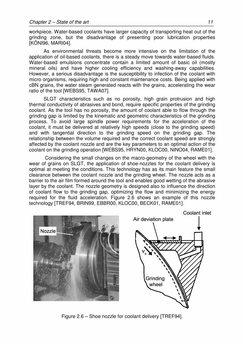
Considering the small changes on the macro-geometry of the wheel with the wear of grains on SLGT, the application of shoe-nozzles for the coolant delivery is optimal at meeting the conditions. This technology has as its main feature the small clearance between the coolant nozzle and the grinding wheel. The nozzle acts as a barrier to the air film formed around the tool and enables good wetting of the abrasive layer by the coolant. The nozzle geometry is designed also to influence the direction of coolant flow to the grinding gap, optimizing the flow and minimizing the energy required for the fluid acceleration. Figure 2.6 shows an example of this nozzle technology [TREF94, BRIN99, EBBR00, KLOC00, BECK01, RAME01].
Figure 2.6 – Shoe nozzle for coolant delivery [TREF94].
12 Chapter 2 – State of the art
2.1.6 Conditioning methods for SLGT
The main feature of the SLGT is the distribution of the grains on a single layer adjacent to the tool body. This is also the main limitation to the application of conventional conditioning processes. The only possible conditioning method is the modification of the micro-topography of the tool with the application of truing methods. The target is to act on the micro-geometry of the grains, modifying the distribution of the cutting edges of the grains on the tool by attacking the most protruded ones. The changes to the grinding edges are achieved mainly by three methods:
• Wearing the grains edges to create flat surfaces – effect achieved with the application of a dressing grinding wheel with an adequate speed ratio, so that the grains on the grinding tool suffer high wear and became flat.
• Micro-breaking of the grain edges – achieved either with another disc with specific speed ratio, or with a crushing tool (usually of hard metal).
• Removing the grains from the matrix – mostly achieved with a crushing tool, breaking away of the grains from the bond, the so called pull-outs (especially on galvanic tools).
Besides the conditioning tool applied, the results of the truing process are strongly affected by the properties of the grains applied on the tool. While single crystal grains have the tendency to form flat surfaces, polycrystalline grains have a higher tendency to present micro-breaks of the cutting edges.
The viability of the application of the different conditioning methods on the grinding tools must thoroughly be investigated. In all three variations presented, there is either a reduction of the grain protrusions or a reduction of the number of grains available on the tool, both undesired effects to a SLGT on a primary examination.
2.2 Wear effects on SLGT
The wear effects on SLGT can be divided in three phases: a rapid primary wear, a steady secondary wear and a more rapid tertiary wear. The grinding performance on the primary and on the tertiary stages is instable due to the high wear rates. On these stages there is a dominant effect of the break of grain particles or grain pull-outs. The secondary stage of the wear development is a stable section, where the attrition acts slowly but continuously on the geometry of the cutting edges of the grains, which become flats [CHEN02]. The changes on the wheel topography have direct effect on the workpiece roughness achieved. As the grains suffer progressive wear, there is an increase on the number of grains having an active participation at the grinding process, and the workpiece becomes smoother. Together with the increase of the amount of grains there is the increase of the flat area of the grain in contact with the workpiece, leading together not only to smoother workpieces, but also to the increase of the power required during the grinding process. The increase of the grinding power also acts on the higher thermal load applied on the workpiece during the process [KÖNI96, STEP02, SHI03, MARI04].
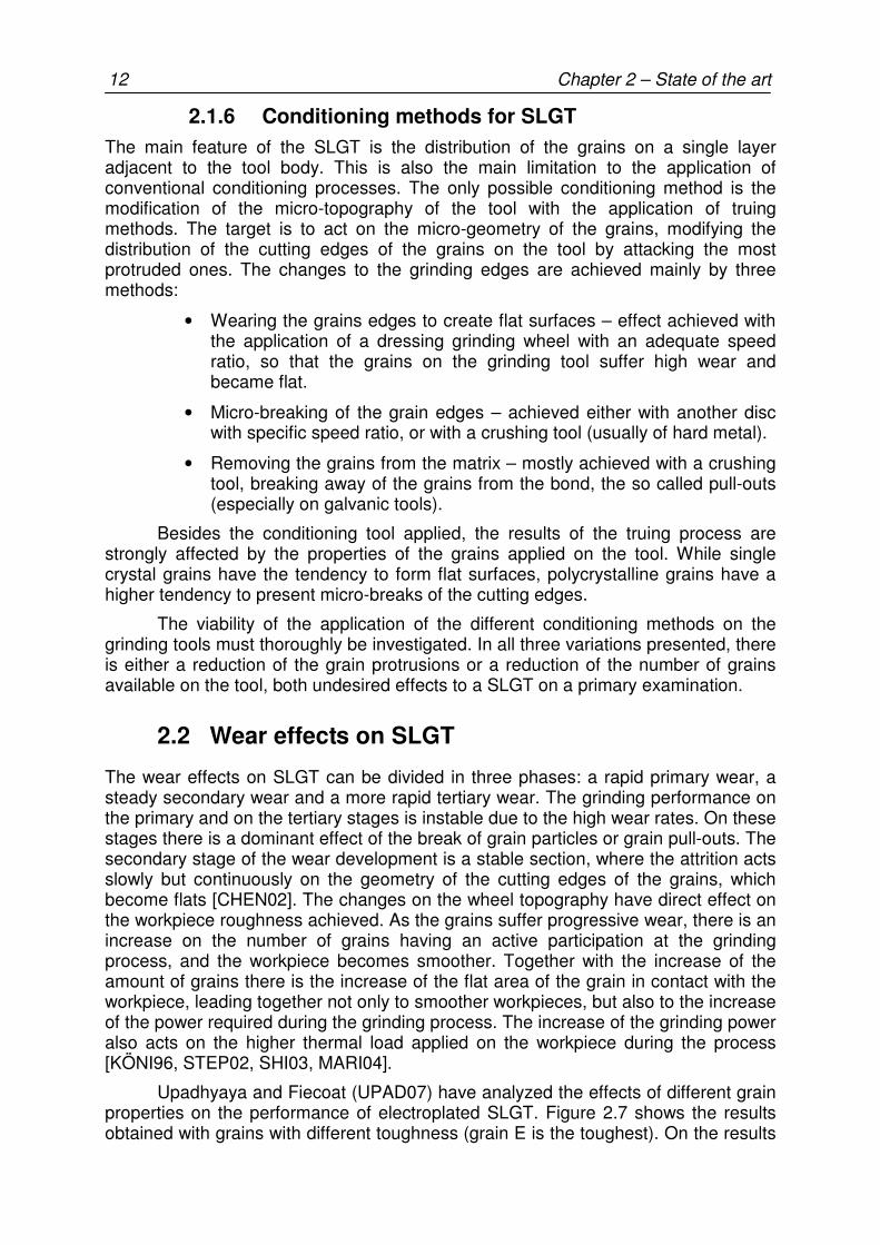
Upadhyaya and Fiecoat (UPAD07) have analyzed the effects of different grain properties on the performance of electroplated SLGT. Figure 2.7 shows the results obtained with grains with different toughness (grain E is the toughest). On the results
Chapter 2 – State of the art 13
it is clear to see the correlation between the effect of grinding power increase and workpiece roughness reduction.
Figure 2.7 – Workpiece roughness and grinding power correlation for different grain types [UPAD07].
As the continuous wear of the tool leads to a lower workpiece roughness, which is a desirable effect, it is important to control the relationship between the wear and the other process effects (such as grinding power, heat generation and grain protrusion reduction) to achieve successful application of this tool technology [SHI03, MARI04].
2.3 Engineered grinding tools
Engineered grinding tools (EGT) are a further development of the SLGT technology. The main feature of these tools is the arrangement of the abrasive grains under a mathematically defined pattern. Primarily EGT were designed with the aim to improve coolant and chip space on the grinding gap (features especially desired in grinding operations with high removal rates). Secondly, the reduced number and controlled position of the cutting edges enables a more deterministic approach of the grinding process, which may allow an easier and more precise evaluation of the cutting performance [CHAT93, SUNG99, BURK01, RICK06, GHOS06].
An important aspect in the development of EGT is that, in conventional SLGT, the grain size distribution and the kinematic characteristics of the grinding process (tool rotates much faster than the feed movement) do not allow 100% of the available grains on the tool to take an active role on the machining process. As a mater of fact, the usual share of gains active on a grinding tool does not exceed 30%. Reducing the amount of unnecessary grains generates the desired coolant/chip space and at the same time reduces the cost of the expensive superabrasive grains [SUNG99, BURK01, FU04].
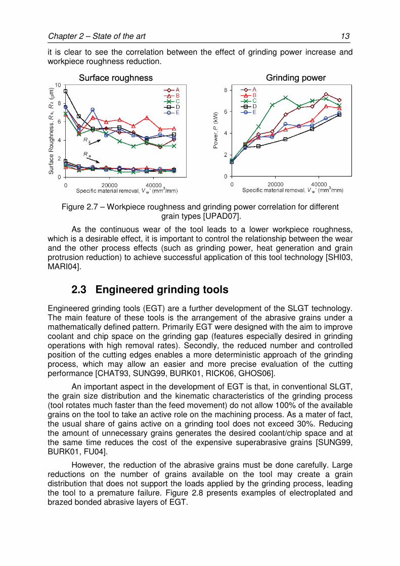
However, the reduction of the abrasive grains must be done carefully. Large reductions on the number of grains available on the tool may create a grain distribution that does not support the loads applied by the grinding process, leading the tool to a premature failure. Figure 2.8 presents examples of electroplated and brazed bonded abrasive layers of EGT.
14 Chapter 2 – State of the art
Figure 2.8 – Examples of abrasive layers on EGT.
Different to stochastic distributed SLGT, EGT require the application of a positioning technique for the grains. The development of production techniques is a key feature for achieving a competitive application of EGT in the market dominated today by the SLGT. There are several processes known to control density, distribution and separation of grains on a single layer matrix. Even with a large amount of patents registered, the principal ideas of these can be summarized as five major principles:
• Glass-particles or other grains with inferior strength or reduced size – the so-called distance providers intend to occupy the space of the abrasive grains. During the grinding process these less resistant particles are removed or broken-away from the bond structure and generate volume for chips and coolant.
• Hand placing methods – Applied mainly on the production of active dressing tools.
• Pattern machined on the tool surface – The tool body surface is machined to affect the protrusion of the grains.
• Templates created directly on the tool surface – A “mask” is deposed on the tool surface. The mask may be designed to affect the position of the grains or the allocation of coolant spaces on the abrasive layer.
• Automated determination of each grain position – The grains are either fixed directly on the tool surface (with an adhesive, for example) or they are placed on a template, which will be transferred to the tool surface.
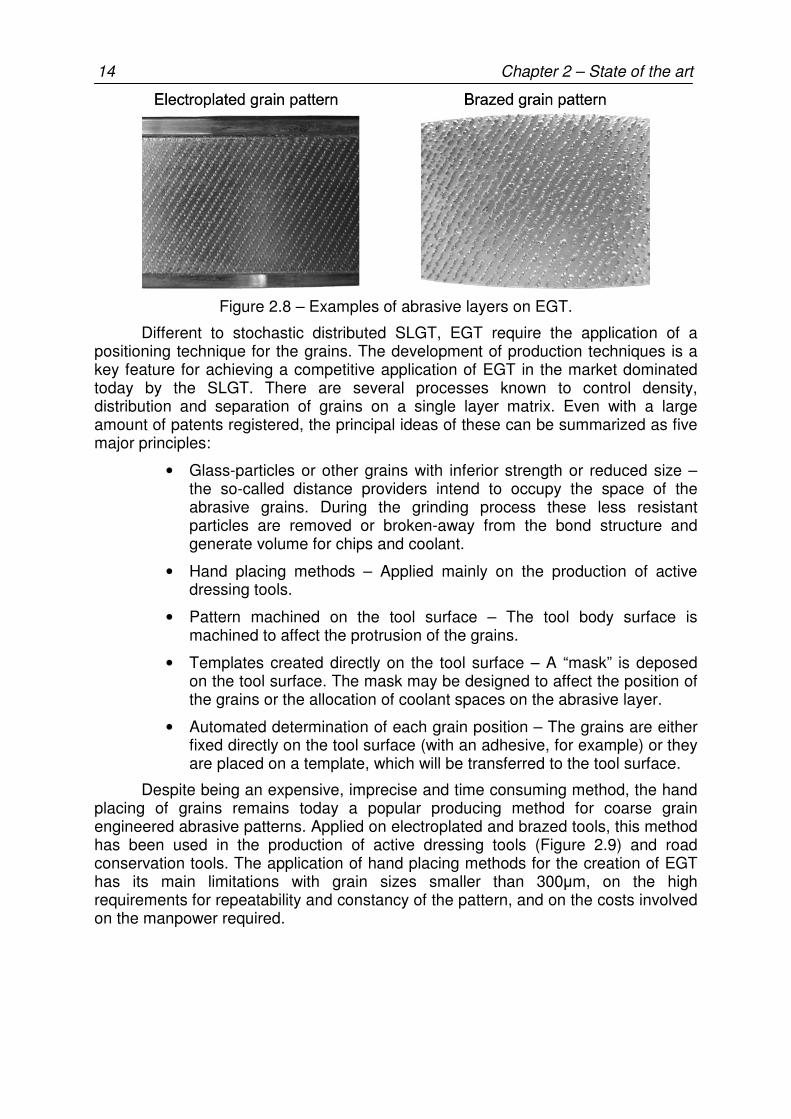
Despite being an expensive, imprecise and time consuming method, the hand placing of grains remains today a popular producing method for coarse grain engineered abrasive patterns. Applied on electroplated and brazed tools, this method has been used in the production of active dressing tools (Figure 2.9) and road conservation tools. The application of hand placing methods for the creation of EGT has its main limitations with grain sizes smaller than 300µm, on the high requirements for repeatability and constancy of the pattern, and on the costs involved on the manpower required.
Chapter 2 – State of the art 15
Figure 2.9 – Active dressing tool with hand placed grain pattern [KAIS06].
A detailed investigation of the techniques for manufacturing single layer, rigid abrasive tools revealed that the control of grain density, grain distribution and grain separation simultaneously and independently of the grain size and tool geometry in a simple and reliable way is only possible with automated systems to position the grains [BURK01].
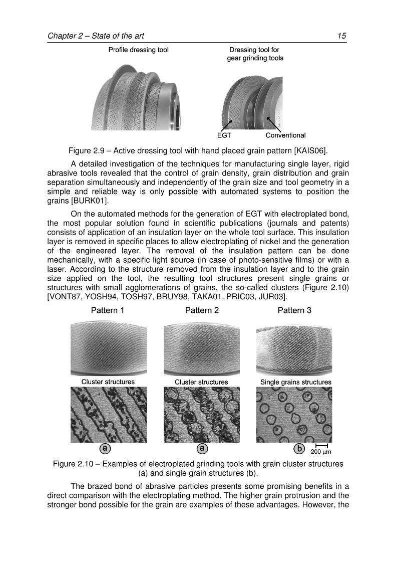
On the automated methods for the generation of EGT with electroplated bond, the most popular solution found in scientific publications (journals and patents) consists of application of an insulation layer on the whole tool surface. This insulation layer is removed in specific places to allow electroplating of nickel and the generation of the engineered layer. The removal of the insulation pattern can be done mechanically, with a specific light source (in case of photo-sensitive films) or with a laser. According to the structure removed from the insulation layer and to the grain size applied on the tool, the resulting tool structures present single grains or structures with small agglomerations of grains, the so-called clusters (Figure 2.10) [VONT87, YOSH94, TOSH97, BRUY98, TAKA01, PRIC03, JUR03].
Figure 2.10 – Examples of electroplated grinding tools with grain cluster structures (a) and single grain structures (b).
The brazed bond of abrasive particles presents some promising benefits in a direct comparison with the electroplating method. The higher grain protrusion and the stronger bond possible for the grain are examples of these advantages. However, the

16 Chapter 2 – State of the art
production of these tools is still mostly done by hand placing, and so the grain size is limited to coarse grains.
Automated methods developed for the production of brazed bonded EGT all present a similar concept: application of adhesive points on the tool surface and, on the sequence, spreading the abrasive grains over the pattern designed with the adhesive points, aiming to create a grain pattern with the position of the adhesive points. Among the publications found on the creation of this adhesive pattern, the method developed and patented by Burkhard at the ETH Zurich can be singled out due its high flexibility [BURK01]. The core of the system is a micro dispenser (Figure 2.11). The dispenser chosen by Burkhard is able to achieve adhesive droplets with diameter of 90 µm and so is able to place on an adhesive point a single grain with equivalent diameter of 125 µm [MICR07].
Figure 2.11 – Micro adhesive dispenser [MICR07].
The adhesive dispenser is commanded by a signal generator, and its operational range is between 100 and 2000 Hz. By coordinating the command signal for the dispenser with the movement of the nozzle over the tool surface, Burkhard developed a very flexible method for placing the adhesive points. An example of the nozzle assembly on a lathe structure (typical for layering an axial symmetric tool) is shown in Figure 2.12.
Figure 2.12 – Placing system developed by Burkhard [BURK01].
Chapter 2 – State of the art 17
The optimization of the EGT involves the analysis of a large amount of variables that have influence on the results of the grinding process. The optimization of the machining process with EGT can be done with two different methodologies: one focusing on the grinding operation and the other the grinding tool.
The methodology focusing the grinding operation has an important consideration of the economical aspects on the production of the EGT. On this methodology the grinding process (with parameters as grinding speed, feed-rates and active tool geometry) is designed based on a pre-established grain pattern. The economical advantage of this process comes from the easier logistics involved on the production of serial tools, instead of developing customized solutions for each grinding process.
In the approach that focuses on the grinding tool, the EGT is designed to support the loads applied by specific cutting conditions (parameters as the grinding speed, feed rate and workpiece hardness are fixed). This is the typical condition while evaluating the EGT performance in substitution for conventional grinding tools. The task on this method is to design the grain pattern to support the load applied by a specific process parameters, and to achieve the expected process results (such as workpiece roughness and tool-life).
The complex interaction between the tool and process variables makes pattern optimization a complex task. The analysis of the tool performance with samples may bring lots of information about the real tool properties, but cannot be applied alone to the optimization of the tool due to the high costs involved in the production of the samples. The application of numerical models and simulation methods is the most coherent alternative for the optimization of EGT. In a numerical model the single characteristics of the tool can be modeled and evaluated separately. However, the model, as it is defined, is an abstraction of the process, and this abstraction must be validated with samples to confirm if the tendencies revealed by the model can also be found under real conditions [TÖNS92].
2.4 Modeling and simulation of the grinding process
The relevance of coherent models and consequent simulations can be observed in the number of the publications dedicated to this topic in the last few decades (Figure 2.13). In the early 1980’s there was a clear growth of the number of publications considering models and simulation, following the trend in the development of computers. The models changed from being predominantly physical-analytic or physical-empiric to new concepts such as finite elements (FE), geometrical kinematic and molecular dynamics (MD) [BRIN06].

18 Chapter 2 – State of the art
Figure 2.13 – Literature search, 1970–2004 [BRIN06].
The complex phenomena involved and the investigation of different aspects of the grinding process have been accountable for the creation of different modeling techniques, each focusing on a specific application area (Figure 2.14).
Figure 2.14 – Overall application area of the different modeling techniques [BRIN06].
The next sections of this chapter will elucidate the application areas of these different modeling and simulation methods, presenting the state of the art of the numerical approach to grinding operations. Especially attention will be given to the methods which were applied on the simulation of the EGT performance. The presentation sequence of the different methods follows the same sequence presented on the Figure 2.14, starting from the MD method for the investigation of microscopic aspects of the grinding process.
Chapter 2 – State of the art 19
2.4.1 Molecular dynamics
Molecular Dynamics (MD) simulations using atomistic models have been attractive in order to gain a deeper understanding of microscopic material behavior and have been applied to study various materials properties and phenomena covering gases, liquids and solids. The more universal material representation in MD, considering microstructure, lattice constants and orientation, chemical elements and the atomic interactions, makes it possible to go beyond ideal, single crystalline structures or homogeneous material properties, and to describe poly-crystals, defect structures, pre-machine or otherwise constrained workpiece models and non-smooth surfaces [KOMA00, HAN04, KANG04, FANG05, BRIN06, GUO06].
Three-dimensional modeling is required for the correct material-specific anisotropic microstructure representation. The process simulation analysis allows calculation of the grain forces, temperature and stress distribution, as well as the resulting energy flow. Often the grinding process simulation was limited to the initial contacts and states of chip formation covering only a few nanometers machining length and a few nanoseconds of process time (mostly <15 ns). Two examples illustrate the limitations on the application of MD models: on a conventional grinding operation with grinding speed vs = 60m/s, the contact of a single grain with a workpiece takes around 100 ns; 100 million atoms correspond to an equilateral face centered cubic (fcc) structure and a side length of about 100 nm [KOMA00, BRIN06].
Regarding the computation, the challenge is not limited to maximizing the available computational power or allocated CPU time, but must also perform efficient data handling and analysis.
MD simulation has been applied on several fields to analyze the dynamic behaviors of particles. On machining applications MD modes have been applied on the description of the molecular movements during the cutting process, simulating not only the dynamic on the molecules of the workpiece during the cutting process, but also on the tool, being able also to estimate the wear effects on the tool molecules.
The state of the art in MD grinding, scratching, cutting or indentation does not consider fluids. Hence, its environment represents high vacuum without heat convection. The extension of the MD machining process models by molecular fluid dynamics provides an opportunity of realizing complete energy balance while machining [KOMA00, HAN04, KANG04, FANG05, BRIN06, GUO06].
2.4.2 Description of kinematics
Approximately 45 years have passed since the development of the first kinematic models for grinding processes. The basis of all these models is similar, with the description of the tool surface and of the process kinematic. However, there are significant differences in the methodology applied to the model description [BRIN06].
Interesting developments are the so-called “kinematic-geometric models”, where special attention is give to the description of the detailed three-dimensional tool topography. There are two principles to obtain the wheel micro-topography: using more or less directly scans of the topography of real grinding wheels, or synthetically generating the surface topography on the basis of statistical analyses of grinding wheel surfaces.

20 Chapter 2 – State of the art
The measurement of real wheel topography is a practical method to obtain the micro geometry of the abrasive layer for the simulations. As different tools profiles are saved on a PC, they can be compared with the kinematic model to evaluate the differences in the application. However, to obtain this wheel-topography library is an expensive and time consuming process. Much more interesting are general abrasive layers topography information, such as average and distribution of grain size, to the creation of virtual tools [STEF83, TÖNS92, INAS96, WARN98, KOSH03, HECK03, MARI04, BRIN06].
In both methods (with differences on the time consumption) it is possible to identify the grains’ cutting edges, and model each grain/workpiece contact. From this interaction it is possible to evaluate the local volume of workpiece removed by each grain as a function of the relative motion between the grinding wheel and the workpiece, and so it is possible to observe the grinding process in much deeper detail and in a more comprehensive way [STEF83, INAS96, WARN98, BRIN06].
Having evaluated the chip cross section, it is possible to apply analytical methods for the evaluation of the grinding forces and the temperature on the workpiece. Usual formulations for the grinding forces must consider, besides the chip-cross-section, the specific cutting energy for the workpiece material, the grinding speed and the friction coefficient. In most models, ideal micro cutting, or ideal material removal, is assumed, i.e. no plastic deformation is considered during the cut [STEF83, INAS96, WARN98, BRIN06].
The publications for the analysis of EGT have applied non deterministic variables for the elaboration of the tool model. The numerical method known as Monte Carlo can be loosely described as statistical simulation method, where statistical simulation is defined in general terms to be any method that utilizes sequences of random numbers to perform the simulation. This method is often applied to generate a stochastic behavior on specific geometrical characteristics, such as the grain size distribution and the orientation of the grain at the tool surface [AURI03, KOSH03, BRAU04, WIKI06].
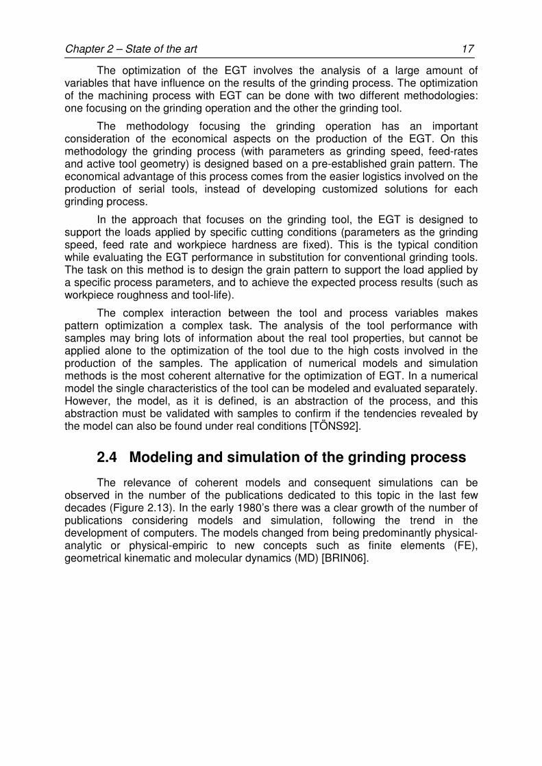
Some recent works on simulation of the tool performance were published by Koshy et al. [KOSH03] and Aurich et al. [AURI03, BRAU04, BRAU05], specially dedicated to the development of EGT. Koshy assumed the grains morphology as spheres with Gaussian distribution around an average grain size, and perfect cutting conditions of the workpiece. The main objectives of the simulation were to analyze the effects of geometric parameters of the tool (such as grain height distribution and grain pattern) on the roughness. Koshy’s results indicated that the roughness can be strongly affected by the distribution of the cutting edges and by the axial offset between adjacent rows of grains (Figure 2.15). The grain morphology, however, has only a small effect on the roughness and its relevance can be compared with the inherent process variability [KOSH03].
Chapter 2 – State of the art 21
Figure 2.15 – Effects of the grain pattern on roughness results by Koshy [KOSH03].
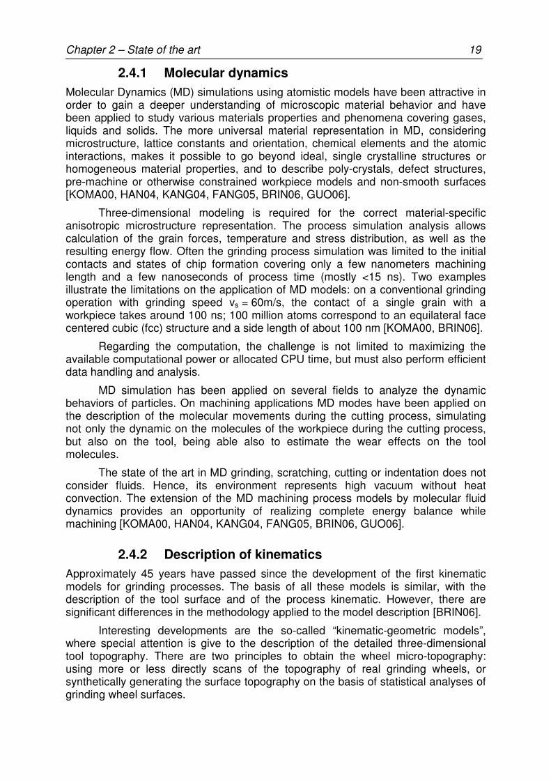
Aurich et al. have launched a series of publications in recent years concerning the development of kinematic simulation software for EGT [AURI03, BRAU04, BRAU05]. The main characteristics of the tool considered in the model were:
• Nominal grain pattern parameters.
• Grain morphology varied from cubic to octahedron and possible forms between, including different aspect ratios between the longest and the shortest grain axis.
• Imprecise positioning of the grains on the pattern.
• Tolerance of the sieving of the grains.
• Orientation of the grain in relation to the tool body.
After the analysis of these parameters a tool sample was designed with an optimal grain pattern, and it was manufactured by hand placing each grain in the tool body with an adhesive. The bond of the grain on the body was achieved by electroplating a nickel layer on the tool surface. Figure 2.16 shows a section of the tool sample that was manufactured. Tests of the tool showed good correlation with the expected roughness values, but the end of life of the tool was achieved earlier than expected. Errors in the grain pattern were deduced as reasons for tool failure.
22 Chapter 2 – State of the art
Figure 2.16 – EGT sample manufactured by Aurich et al. [AURI03].
The wear of the grinding tool has been considered with different methodologies on the numerical methods developed. Chen et. al [CHEN96a, CHEN96b, CHEN96c, CHEN98a, CHEN98b] have considered three different wear phenomena on the tool wear: attrition wear, fracture of the grains and fracture of the bond. The grain morphology presented was simplified to circular profiles with diameter equivalent to the grain size distribution chosen. The grains representations were modified according to the dressing parameters applied to generate the cutting edges. The generated grain profiles were then exposed to grain flattening caused by attrition wear and to fractures (parameterized according to the grain flats which are generated on the grain). Different radial wear stages of the grinding tool were simulated to evaluate the modifications on the micro geometries of the grains. Once generated the tool profile, the simulations are performed to evaluate the workpiece roughness and the grinding forces. The results have presented good correlation with the experiments performed.
Zhou and Xi [ZHOU02] have considered also simplified grain models where the grains morphology is approached by triangles. The height of the triangles follows a Gaussian distribution. The wear is modeled as modifications of the Gaussian distribution by truncating the distribution end (Figure 2.17). This modification of the Gaussian distribution represents the removal of abrasive grains on the tool, which is considered to be governing the overall wear phenomenon [ZHOU02].
Gunawardane and Yokouchi [GUNA04] described the wear phenomenon according to the theory of fracture of the brittle materials. The wheel wear of the grain breaking phenomenon mainly depends on the stress acting on a grain (σ) and the time duration (t) before breaking and were combined on two statistical variables: P(t), which is the probability that the grain does not break until time t; and µ(t), which is the probability density of breaking at time t.

Chapter 2 – State of the art 23
Figure 2.17 – Truncation of the Gaussian distribution applied by Zhou and Xi as grain wear model [ZHOU02].
Generally, the high level of detail allows results with high convergence to real grinding processes. Today, evaluating the grinding process using a complex and detailed kinematic model for a few milliseconds of grinding process time (some few revolutions of the tool) requires several hours of calculation time. Even so, the strong dependence of the abrasive processes on the cutting edge geometry of the single grains can only be considered approximately (as ideal cutting conditions are assumed). Therefore, absolute values of grinding forces or surface roughness cannot be calculated, but their trend can be identified [BRIN06].
2.4.3 Analytical description
The analytical approach is based on the development of predictive models that are derived from basic physical interrelationships. This technique is especially interesting when considering specific boundary conditions (such as temperature or pressure fields), and the formulation of their effects on the grinding process (for example, deformations or material damage due to high temperature exposure). The main advantages of this modeling technique are the simple identification of the main influences and the possibility of establishing a correlation with other machine and process characteristics [BRIN06, TÖNS92].
The evaluation of the grinding forces and energy are fundamental for the analysis of the deformations during the process and of the heat load generated on the grinding zone. The grinding power, which is the product of the grinding speed and tangential force, can be applied to the determination of the energy required for the chip formation. This energy is transformed almost completely into heat, which is going to be dissipated in the workpiece, coolant fluids, chips, tool and machine [TÖNS92].
Carslaw and Jaeger proposed an approach where the heat source during grinding operations is treated as a uniform heat flux which moves with constant velocity along the surface of a semi-infinite solid, under assumed quasi-steady-state heat transfer condition [CARS59]. This model is widely applied for prediction of the workpiece temperature and consequent material damages. The effects of the coolant are often estimated as a convection coefficient on the boundary of the workpiece. A key issue for accurate temperature prediction in grinding is the identification of heat

24 Chapter 2 – State of the art
allocation to the different thermal sinks in the grinding zone, i.e., workpiece, grinding wheel or abrasive grains, chips and coolant. Due to the complexity of the grinding process, the heat allocation is often determined by an experimental approach [RAME04]. Once obtained the real share of the heat which is directed to the workpiece, the basic model of Carslaw and Jaeger (with a flat heat source, with constant and equally distributed heat flux, moving parallel to the workpiece surface) has been modified to consider the tool and workpiece geometries, as well as inhomogeneous heat source along the contact zone of the tool and workpiece.
Another interesting approach is the evaluation of the useful coolant flow that can be applied on grinding. The analytical approach to this situation considers tool properties, like porosity and grain protrusion, and process parameters, such as rotating speeds and kinematic engagement, to evaluate the maximal quantity of coolant available in the grinding gap. From this point it is then possible to evaluate, for example, the maximal amount of energy (heat) that the coolant can transport away from the grinding gap or the pressure distribution on the grinding gap caused by the coolant compression. However, as in other analytical approaches, it is necessary to evaluate a series of empirical constants, such as convective heat transfer coefficients and tool porosity [CHON97, EBBR00, GE01, GVIN04].
Most of the models assume ideal cutting conditions of the workpiece (no plastic deformation). Also the wear of the tool, a time-dependent variable, remains often unconsidered, as it makes the model elaboration difficult due to the large number of influencing parameters.
2.4.4 Finite element analysis
The application of Finite Element Analysis (FEA) for simulation of grinding is focused on the evaluation of the influence of the process on the machine-tool/workpiece. There are two main evaluation methods adopted: the first is the analysis of specific boundary conditions (such as pressure fields or heat sources) on the process (machine deformations, workpiece temperature, etc.); the second approach is the estimation of the limiting conditions (such as maximum temperature on the interface or maximal pressure on the grinding gap) so that the machine/workpiece is not damaged (for example, material damages on the workpiece or excessive deformations) by the grinding parameters [MAMA03, BRIN06].
FEA can be separated into macro- and microscopic concepts. In most cases the macroscopic simulation is applied in order to calculate the effects of heat and mechanical surface pressure on the complete workpiece to evaluate temperature distribution or form deviations. The calculations are mainly based on thermo-mechanical and elasto-mechanical material characteristics. The plastic material properties and the chip formation are not considered [ZHOU97, WARN98, WARN99, MOUL01, MAMA03, GU04]. Typical outputs of these simulations are the deformations on the machine structure caused by forces generated during the machining process.
In contrast, microscopic simulation is limited to the analysis of the working zone. Thus, usually, a minor section of the workpiece and one contacted grain is simulated. Furthermore, current computer power is not sufficient to develop a comprehensive model of an entire grinding wheel in microscopic simulations or to consider the chip formation on macroscopic simulations. Nevertheless, the application of FEA has been useful to comprehend the relationship between the effects of alteration on the micro-cutting process characteristics on the macro effects
Chapter 2 – State of the art 25
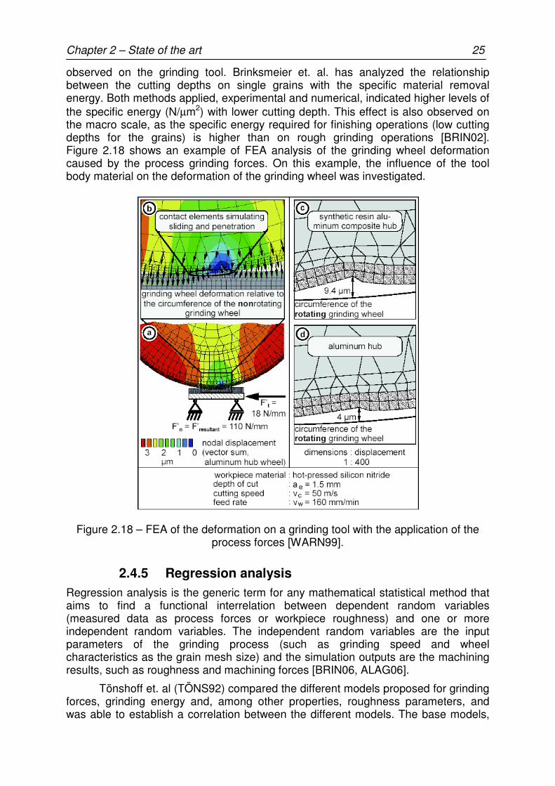
observed on the grinding tool. Brinksmeier et. al. has analyzed the relationship between the cutting depths on single grains with the specific material removal energy. Both methods applied, experimental and numerical, indicated higher levels of the specific energy (N/µm2) with lower cutting depth. This effect is also observed on the macro scale, as the specific energy required for finishing operations (low cutting depths for the grains) is higher than on rough grinding operations [BRIN02]. Figure 2.18 shows an example of FEA analysis of the grinding wheel deformation caused by the process grinding forces. On this example, the influence of the tool body material on the deformation of the grinding wheel was investigated.
Figure 2.18 – FEA of the deformation on a grinding tool with the application of the process forces [WARN99].
2.4.5 Regression analysis
Regression analysis is the generic term for any mathematical statistical method that aims to find a functional interrelation between dependent random variables (measured data as process forces or workpiece roughness) and one or more independent random variables. The independent random variables are the input parameters of the grinding process (such as grinding speed and wheel characteristics as the grain mesh size) and the simulation outputs are the machining results, such as roughness and machining forces [BRIN06, ALAG06].
Tönshoff et. al (TÖNS92) compared the different models proposed for grinding forces, grinding energy and, among other properties, roughness parameters, and was able to establish a correlation between the different models. The base models,
26 Chapter 2 – State of the art
such as that from equation 2.1, are dependent on empirical coefficients, which should be adjusted for the group of process parameters, such as machine, workpiece and grinding wheel.
e3eq
e2e
e1
gwwp'N .D.a
q1
..ccF
= (2.1)
cwp = constant for workpiece
cgw = constant for the grinding wheel
q = speed ratio
ae = working engagement [mm]
Deq = equivalent diameter of grinding wheel [mm]
e1, e2 & e3 = experimental exponents
The field of possible applications for models using regression analysis is vast and still expanding. The mathematical part of modeling is improved by using new and more complex functions obtaining a higher quality of calculation [TÖNS92].
2.4.6 Artificial neural networks
Artificial neural networks (ANN) models are distinguished by several properties that make them suitable for modeling complex, nonstationary processes that depend on many input parameters: first, analytical expressions are not required; second, information from different sensors and physical quantities can be processed and correlated; third, ANN can be efficiently combined with physical models to further improve the modeling performance [BRIN06, LIU06].
The most frequent application of ANN in grinding is the prediction of the grinding process output parameters based on the settable input parameters and/or time varying physical quantities measured during operation. For example, the modification of the workpiece diameter with the radial grinding wheel wear can be indirectly controlled if the grinding forces are monitored and relationship of the grinding wheel wear and the grinding forces is known. Another aspect is the evaluation of the suitable inputs so that the expected outputs can be achieved. [BRIN06].
The on-line evaluation of the process (including the possible tool life expected) is useful in the monitoring of the grinding process, as the signal from different sources (for example, force and acoustic emission sensor) can be simultaneously evaluated.
2.4.7 Rule based models
As the power of computers is increased and their costs decrease it is desired to transfer a high volume of low-level decisions making to machines, releasing human beings for low volume, high-level decision making. This is the base for the elaboration of Rule Based (RB) models [ROWE94, ZHAN04, NAND04].
Knowledge Based Systems (KBS) are a section of RB models dealing with systems for extending and/or requiring a knowledge base and performing a function that would normally require human intelligence and expertise. The related term ‘expert systems’ (ES) is normally used to refer to a highly domain-specific type of knowledge based system that gives advice and is used for a specialized purpose.
Chapter 2 – State of the art 27
The knowledge base contains the expert knowledge usually provided in the form of rules which are suitable for decision making. These rules consist of antecedents and conclusions, whereby antecedents can consist of multiple facts linked together with AND or OR conjunctions [ROWE94, ZHAN04, NAND04, BRIN06].
The formation of a reliable knowledge base is fundamental for the achievement of coherent results with ES. Often there are problems in the capture of the process information due to poor documentation and/or imprecise measurements.
An example on the application of the rule base models is the design of a grinding process (for example, as output, the choice of the dressing method for the grinding wheel) based on the results desired (such as workpiece roughness or roundness). Fundamental for the application of this process modeling technique is the formulation of correct rules for the model.
2.4.8 Modeling techniques suitable for EGT optimization
The actual state of the art in modeling and simulation of EGT has given high priority to the detailed description of the geometric characteristics of the tool. The grain pattern is the main feature of EGTs. The description of the pattern has not been done only considering the ideal grain pattern structure, but also the distortions brought by the placing method (deviations of the nominal position of the grains), the grain size (evaluation of the sieving tolerances) and the grain morphology (simple basic geometries such as octahedrons or cubes) [AURI03, BRAU04, BRAU05].
The cutting phenomena applicable to the EGT have been modeled exactly with the same method applied on other grinding tools technologies, and in almost all techniques the plastic deformations during the interaction of grains and workpiece have been ignored (only MD and some FEA have considered these phenomena) [AURI03, KOSH03, BRAU04, BRAU05].
Heat transfer phenomena have been mainly analyzed with the FEA modeling of the macro-structure of the tool. On the analysis performed with FEA, the micro-topography has not been considered in the models, and so the application of the influence of EGT on this aspect must be approximated by changes on empirical coefficients (for example, the convection coefficient between the tool and coolant).
The only modeling technique that considers the chip formation and its effects in the process are MD models. However, in the actual state of the art of MD models (modeling volume on the magnitude of 10-3 µm3), the simulation intervals for the cutting phenomena do not allow the evaluation of the effects of the chips on the grinding gap. The formation and presence has not been considered in the other modeling techniques.
The numerical simulation of the wear on grinding tools has been observed with different techniques. Nevertheless, there is a lack of simulation techniques for the first moments of the tool application on a grinding process. On these moments there are the most relevant changes on the tool topography due to the accelerated wear of overloaded grains. The grain geometry has been simplified to simple geometries, as circular and triangular profiles.
The applicability of the actual models for the optimization of the grinding process/tool has been limited by the long simulation time required. For example, the model proposed by Aurich et al. requires almost 50 hours for the evaluation of two revolutions of the tool (outer diameter of 400 mm and width of 25 mm).
28 Chapter 2 – State of the art
2.5 Resume
The development of EGT has required the development of different technologies. First, it is necessary to further develop the positioning method for grains to achieve higher flexibility. At the same time the precision in which the grain pattern is generated must be considered. According to the method chosen, there are different limitations that must be observed, such as economical viability and precision.
The placing methods are also strongly dependent on the bonding method that will be applied to the grain. Both electroplated and brazed tools reveal positive and negative aspects for application to EGT. While the technology involved with electroplated tools may require lower financial investment and easier application on metallic tool bodies, the brazed bond enables much higher grain protrusion and stronger bonding forces. With these aspects both bonding systems would be applicable on the EGT. However, the bond properties of an electroplated layer induce merely a mechanical bond between the grains and the tool body, and so a large covering of the grain is required to generate the required bonding force. On the brazed bond, the grains are exposed to high temperatures during the melting of the filler alloy (up to 1200oC), and there is the risk of damaging the grains. However, the abrasive layer generated presents, both, large grain protrusion and large bonding forces, as desired characteristics for rough grinding operation (large material removal rates).
The application of the grains in a single layer requires the application of highly expensive grains, as the successful application of the tool depends on the wear resistance of the abrasives. Special synthetic diamonds and cBN have been created to optimize the grains’ properties during grinding operations.
The injection of coolant/lubricant fluids in the grinding process can be optimized with the use of shoe-nozzles. In this nozzle technology the air barrier around the rotating tool is broken and the coolant reaches the surface of the grinding tool even with the application of low injection pressures. The amount and the injection pressure of coolant can be reduced without damaging the workpiece.
The application of numerical methods for the optimization of grinding operations has been growing in importance with the continuing improvement of the computing power and reduction in price of personal computers. Different modeling techniques have been developed to investigate specific characteristics of the process.
The most common aspects considered while modeling EGT are the micro-geometric characteristics of the tool (grain morphology and distribution on the tool) and the kinematics between the tool and the workpiece. Ideal kinematic cutting conditions are considered in these approaches, ignoring the possibility of micro-plastic deformations during the cutting process. Even with these simplifications, the geometric-kinematic approach has presented good agreement with the real tool performance during the experimental validations and is able to identify the trends in the development of the EGT. Nevertheless, these models are not able to predict the tool life. The evaluation of the cutting forces is still strongly dependent on empirical coefficients, and the simulation time required are much beyond those acceptable for a practical industrial application.
The lack of a practical design tool for analysis of the grain pattern in EGT is the main motivation for this work.
Chapter 3 – Problem description and objectives 29
3. Problem description and objectives
Electroplated and ceramic bonded grinding tools have been applied in high performance grinding applications, mainly in the automotive and aerospace industries, and set the actual performance expectation (mainly the production costs) to be achieved (or overtaken) by concurrent tool technologies. The successful application of the EGT on these industries depends on the attainment of the “boundary conditions” given by the input parameters (tool geometry, kinematic, machine-tool limits and workpiece material), by the expected outputs (roughness and form tolerances of the workpiece) and by the costs of the tool (life time and tool cost).
Even though promising some interesting benefits to the grinding process, the application of EGT in production lines has reached several barriers. The main one is the lack of understanding of the relationship between the grain pattern and its effects on the grinding process. The latest analysis methods published in scientific publications have applied experimental and numerical approaches to evaluate the effects of the defined grain arrangement. In the experimental approaches, the most interesting publications have considered the application of brazing technology on the bonding of the grains to the tool [BURK01, GHOS07]. The braze bonded technology generates tools with large grain protrusion (improving coolant flow and chip transport in the grinding gap) and strong bonding forces of the grains to the tool body (chemical bond between tool, filler alloy and abrasives). Brazing has been presented as a promising technology, but the requirements of high temperatures (often above 900oC) have imposed special requirements on the materials (abrasives and tool substrate) applied.
Numerical models have been preferentially developed based on the description of the tool’s geometry (macro and micro) and of the kinematics during the grinding operation. The tools have been described with different techniques: while Koshy et. al (KOSH03) have chosen a more abstract description of the grain morphology (approaching the grains to spheres), Braun and Aurich and their respective colleagues (AURI03, BRAU04, BRAU05) have described the grains morphology in details, and analyzed the effects of the grain morphology on the performance of the tool. In both strategies, the simulations have assumed ideal kinematic cutting conditions and the wear effects were neglected. It is known that a new SLGT will suffer relevant changes in its performance on the first workpieces to which it is applied. These changes are caused by modification of the tool micro-geometry, as the most protrusive grains are either heavily worn or pulled out of the abrasive layer. When optimal grinding parameters are applied, this unstable period with accelerated wear is short and the tool rapidly reaches a stable condition. When
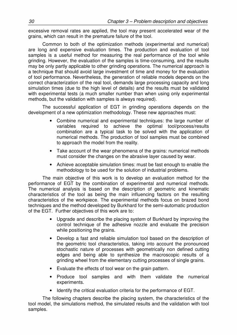
30 Chapter 3 – Problem description and objectives
excessive removal rates are applied, the tool may present accelerated wear of the grains, which can result in the premature failure of the tool.
Common to both of the optimization methods (experimental and numerical) are long and expensive evaluation times. The production and evaluation of tool samples is a useful method for measuring the real performance of the tool while grinding. However, the evaluation of the samples is time-consuming, and the results may be only partly applicable to other grinding operations. The numerical approach is a technique that should avoid large investment of time and money for the evaluation of tool performance. Nevertheless, the generation of reliable models depends on the correct characterization of the real tool, demands large processing capacity and long simulation times (due to the high level of details) and the results must be validated with experimental tests (a much smaller number than when using only experimental methods, but the validation with samples is always required).
The successful application of EGT in grinding operations depends on the development of a new optimization methodology. These new approaches must:
• Combine numerical and experimental techniques: the large number of variables required to achieve the optimal tool/process/results combination are a typical task to be solved with the application of numerical methods. The production of tool samples must be combined to approach the model from the reality.
• Take account of the wear phenomena of the grains: numerical methods must consider the changes on the abrasive layer caused by wear.
• Achieve acceptable simulation times: must be fast enough to enable the methodology to be used for the solution of industrial problems.
The main objective of this work is to develop an evaluation method for the performance of EGT by the combination of experimental and numerical methods. The numerical analysis is based on the description of geometric and kinematic characteristics of the tool as being the main influencing factors on the resulting characteristics of the workpiece. The experimental methods focus on brazed bond techniques and the method developed by Burkhard for the semi-automatic production of the EGT. Further objectives of this work are to:
• Upgrade and describe the placing system of Burkhard by improving the control technique of the adhesive nozzle and evaluate the precision while positioning the grains.
• Develop a fast and reliable simulation tool based on the description of the geometric tool characteristics, taking into account the pronounced stochastic nature of processes with geometrically non defined cutting edges and being able to synthesize the macroscopic results of a grinding wheel from the elementary cutting processes of single grains.
• Evaluate the effects of tool wear on the grain pattern.
• Produce tool samples and with them validate the numerical experiments.
• Identify the critical evaluation criteria for the performance of EGT.
The following chapters describe the placing system, the characteristics of the tool model, the simulations method, the simulated results and the validation with tool samples.

Chapter 4 – Production of braze bonded EGT 31
4. Production of braze bonded EGT
The concept presented by Burkhard is an ideal platform for the development of a semi automatic placing system for the grains on EGT [BURK01]. In the following sections the original system and an alternative to upgrade its capabilities and the analysis of the precision while positioning the grains are presented. Closing this chapter, the brazing technology applied in the production of the tool is presented.
4.1 Description of placing system designed by Burkhard
As shown in Chapter 2, the placing system developed by Burkhard is based on the application of a micro dispenser of adhesive as an indirect tool for the generation of grain patterns on the tool body. This concept opens possibilities to very different kinematics between the dispenser and the tool body. Nevertheless, the movements between nozzle and the tool body material have basically the same characteristics in any construction chosen, such as small clearance between the tool body and the nozzle and a low relative speed between the nozzle and the tool surface. For the characterization of the placing system the construction analyzed is based on the concept presented in Figure 2.12, where the rotation of the tool and the translation of the dispenser are synchronized. Figure 4.1 shows a schematic representation of the components of the placing system.
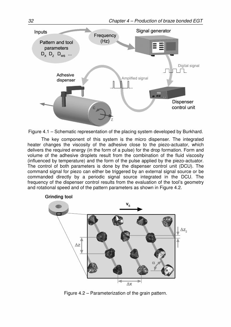
32 Chapter 4 – Production of braze bonded EGT
Figure 4.1 – Schematic representation of the placing system developed by Burkhard.
The key component of this system is the micro dispenser. The integrated heater changes the viscosity of the adhesive close to the piezo-actuator, which delivers the required energy (in the form of a pulse) for the drop formation. Form and volume of the adhesive droplets result from the combination of the fluid viscosity (influenced by temperature) and the form of the pulse applied by the piezo-actuator. The control of both parameters is done by the dispenser control unit (DCU). The command signal for piezo can either be triggered by an external signal source or be commanded directly by a periodic signal source integrated in the DCU. The frequency of the dispenser control results from the evaluation of the tool’s geometry and rotational speed and of the pattern parameters as shown in Figure 4.2.
Figure 4.2 – Parameterization of the grain pattern.

Chapter 4 – Production of braze bonded EGT 33
With the pattern parameterized, as presented in Figure 4.2, Burkhard calculated the control frequency for the adhesive dispenser according to the Equations shown below.
fvz =∆ (4.1)
∆⋅π
=alminno
WZL x
DintN (4.2)
L
WZN
Dx ⋅π=∆ (4.3)
( )α+π⋅∆= 2tanzA L (4.4)
WZLWZ
nozzle Nx
ADF ⋅
∆
+⋅π= (4.5)
vf = feed rate of the nozzle parallel to the rotational axis [mm/rot]
NL = number of lines in one rotation (must be an integer)
DWZ = Tool diameter [mm]
NWZ = Tool rotational frequency [Hz]
AL = Offset of the grain pattern [mm]
Fnozzle = Command frequency for the nozzle [Hz]
The frequency calculated with equation 4.5 is programmed into an external signal source, which is applied as the trigger signal to the DCU, synchronizing and modulating the command signal to the piezo-actuator on the dispenser. With this method Burkhard was able to achieve constant pattern parameters on cylindrical tools. However, when applied to profiled tools, the pattern suffered deviations as the tool diameter is not constant along the tool width. The pattern angle α (Figure 4.2) is fixed when evaluating equation 4.4, and the only patterns possible are lines (almost any angle, but with constant value along the tool width).
4.2 Alternative control method for the dispenser
The optimization of the EGT may require a more complex control method of the nozzle than that developed by Burkhard. The actual method applied on the control of the placing system reaches its limits in applications such as layering profiled tools or non-constant grain patterns along the tool geometry.
The largest flexibility (and resolution) possible in the placing system is achieved by generating a matrix with the position of each grain on the pattern. To generate this matrix, the position of the grains must be parameterized according to a reference system, as in the example shown in Figure 4.3 with the coordinate “z”.

34 Chapter 4 – Production of braze bonded EGT
Figure 4.3 – Parameterization of the grain pattern with the alternative control method.
Following the example where the placing system is applied to the layering of cylindrical tools with constant rotational speed of the tool and constant translation speed of the nozzle, it is possible to describe the position of each grain on the tool only with and cylindrical coordinate system, as shown in the following equations:
fbrot v/Sn = (4.6)
( )
∆
π−=φ
x*2
*)1n(i0 for ( ) [ ]π∈φ *2*n,0i rot0 (4.7)
f0 v**2
)i()i(z
π
φ= (4.8)
( ) ))i(z(fiA = (4.9)
( )iA)i()i( 0p +φ=φ (4.10)
nrot = Number of revolutions to layer the whole tool width
Sb = Tool width [mm]
φ0 (i) = angular position of each grain with α = π/2 (Figure 4.2) [rad]
A(i) = Offset on the grain position caused by the pattern [rad]
φp(i) = angular position of each grain on the pattern evaluated with f(z(i)) [rad]
Equation 4.10 describes a matrix with the information of the position of each grain on the tool surface. The variable φp is the angular position of the tool measured from a reference position (where z = 0 and φ0 = 0). With this parameterization it is possible, among other features, to describe the tool profile and to apply different grain densities and different grain patterns according to the coordinate system adopted (Figure 4.4). For the covering of axial symmetric but non cylindrical surfaces, it is possible to generate patterns as for cylindrical tools (with lines described by functions), but the distance ∆x between the lines is affected by the tool diameter. By

Chapter 4 – Production of braze bonded EGT 35
keeping the pattern parameter ∆x constant, the grain pattern cannot be described by a line. The grain pattern is than estimated by the following equation:
( ))i(D
x*2)1i(i
WZ00
∆+−φ=φ for ( ) [ ]π∈φ *2*n,0i rot0 (4.11)
DWZ(i) = Diameter of the tool Dwz(i)=f(z,φ0)
Figure 4.4 – Description of the tool profile, of the grain density and of the pattern function according to the coordinate system of the tool.
This mapping of the grains requires large modifications to the hardware applied in the placing system. The signal generator must be substituted by a computer, which correlates the position of the dispenser and the trigger signals for the DCU.
Far away from the assumptions of ideal constant translation and rotation speeds, the tool performs irregular movements along the trajectory of the dispenser. The variations of speed are the result of mechanical friction among the moving parts of the machine. They are unavoidable and this uncontrolled property brings undesired deviations in the grain pattern. The solution to this problem is a measuring system for the evaluation of the movements between nozzle and dispenser. An incremental rotational encoder was assembled on the machine to evaluate the rotation position and speed of the tool. The reference of the coordinate system (φp = 0, z = 0) is given by a switch (mechanically activated), adapted on the same device where the nozzle is fixed.
Equation 4.10 describes the position of each grain on the tool according to the variable φp. The computer, equipped with an I/O (Input/Output) interface, compares the position measured by the rotational encoder with the positions saved on φp, generating at the correct moment the trigger signal for the DCU. The encoder chosen has the resolution of 7E-5 radians (90,000 divisions per rotation) and its position is measured every 0.1 ms by the computer. These are not large requirements on the processing capacity of the computer applied in the dispenser control unit. For example, while layering a cylindrical tool with a diameter of 200 mm, width of 20 mm and with the main pattern parameters ∆x = 0.5 mm and ∆z = 0.5 mm (the other parameters do not have a direct effect on the number of grains on the tool), the matrix φp has about 51,000 points. This amount of data is processed, at typical

36 Chapter 4 – Production of braze bonded EGT
layering speeds, in about 8 minutes, representing no large requirement for the computer. Figure 4.5 shows a schematic representation of the placing system, with the information flow between the different elements.
Figure 4.5 – Schematic representation of the placing system with rotational encoder, reference switch and computer for system control.
4.3 Description of the placing system
The characterization of the grain placing system should evaluate not only the precision of the placing technique, but also reveal the optimal conditions for the operation of the nozzle.
The industrial application of brazed EGT is concentrated on grinding operations with high material removal rates. In this application, the design of the grain pattern must, above all, avoid the overload on the grains that induces the failure of the tool. The definition of this type of application also defines the materials to be used in the tool:
• cBN abrasives: Actually the most indicated abrasive to be applied in rough grinding operations, it is the second hardest material available. The poor affinity to carbon gives this material the ideal properties to machine iron-based alloys. Among the different cBN types available, the ABN800 series (Diamond Innovations) has the greatest thermal stability, showing no significant reduction of impact strength after heating to a temperature of 1100oC. The grain size chosen was B251, the size usually applied on rough grinding tools.
• Tool body: Austenitic steel X2CrNiMo 18-14-3. The choice of this material aims to minimize the geometry changes on the tool body material after the heating and cooling cycles of the brazing process.
• Filler alloy: Diabraze (73,8 Cu / 14,4 Sn / 10,2 Ti / 1,5 Zr). This filler material has titan and zirconium as active elements, to achieve good wetting conditions on the cBN grains. The brazing temperature is about 920oC. This filler is available as powder with different grain sizes.
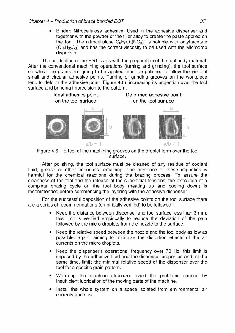
Chapter 4 – Production of braze bonded EGT 37
• Binder: Nitrocellulose adhesive. Used in the adhesive dispenser and together with the powder of the filler alloy to create the paste applied on the tool. The nitrocellulose C6H8O3(NO3)2 is soluble with octyl-acetate (C10H20O2) and has the correct viscosity to be used with the Microdrop dispenser.
The production of the EGT starts with the preparation of the tool body material. After the conventional machining operations (turning and grinding), the tool surface on which the grains are going to be applied must be polished to allow the yield of small and circular adhesive points. Turning or grinding grooves on the workpiece tend to deform the adhesive point (Figure 4.6), increasing its projection over the tool surface and bringing imprecision to the pattern.
Figure 4.6 – Effect of the machining grooves on the droplet form over the tool surface.
After polishing, the tool surface must be cleaned of any residue of coolant fluid, grease or other impurities remaining. The presence of these impurities is harmful for the chemical reactions during the brazing process. To assure the cleanness of the tool and the release of the superficial tensions, the execution of a complete brazing cycle on the tool body (heating up and cooling down) is recommended before commencing the layering with the adhesive dispenser.
For the successful deposition of the adhesive points on the tool surface there are a series of recommendations (empirically verified) to be followed:
• Keep the distance between dispenser and tool surface less than 3 mm: this limit is verified empirically to reduce the deviation of the path followed by the micro-droplets from the nozzle to the surface.
• Keep the relative speed between the nozzle and the tool body as low as possible: again, aiming to minimize the distortion effects of the air currents on the micro droplets.
• Keep the dispenser’s operational frequency over 70 Hz: this limit is imposed by the adhesive fluid and the dispenser properties and, at the same time, limits the minimal relative speed of the dispenser over the tool for a specific grain pattern.
• Warm-up the machine structure: avoid the problems caused by insufficient lubrication of the moving parts of the machine.
• Install the whole system on a space isolated from environmental air currents and dust.
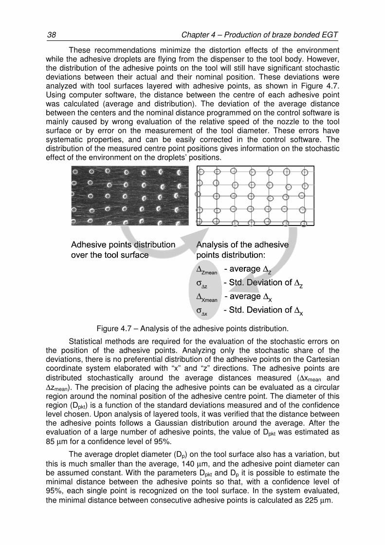
38 Chapter 4 – Production of braze bonded EGT
These recommendations minimize the distortion effects of the environment while the adhesive droplets are flying from the dispenser to the tool body. However, the distribution of the adhesive points on the tool will still have significant stochastic deviations between their actual and their nominal position. These deviations were analyzed with tool surfaces layered with adhesive points, as shown in Figure 4.7. Using computer software, the distance between the centre of each adhesive point was calculated (average and distribution). The deviation of the average distance between the centers and the nominal distance programmed on the control software is mainly caused by wrong evaluation of the relative speed of the nozzle to the tool surface or by error on the measurement of the tool diameter. These errors have systematic properties, and can be easily corrected in the control software. The distribution of the measured centre point positions gives information on the stochastic effect of the environment on the droplets’ positions.
Figure 4.7 – Analysis of the adhesive points distribution.
Statistical methods are required for the evaluation of the stochastic errors on the position of the adhesive points. Analyzing only the stochastic share of the deviations, there is no preferential distribution of the adhesive points on the Cartesian coordinate system elaborated with “x” and “z” directions. The adhesive points are distributed stochastically around the average distances measured (∆xmean and ∆zmean). The precision of placing the adhesive points can be evaluated as a circular region around the nominal position of the adhesive centre point. The diameter of this region (Dpkt) is a function of the standard deviations measured and of the confidence level chosen. Upon analysis of layered tools, it was verified that the distance between the adhesive points follows a Gaussian distribution around the average. After the evaluation of a large number of adhesive points, the value of Dpkt was estimated as 85 µm for a confidence level of 95%.
The average droplet diameter (Dp) on the tool surface also has a variation, but this is much smaller than the average, 140 µm, and the adhesive point diameter can be assumed constant. With the parameters Dpkt and Dp it is possible to estimate the minimal distance between the adhesive points so that, with a confidence level of 95%, each single point is recognized on the tool surface. In the system evaluated, the minimal distance between consecutive adhesive points is calculated as 225 µm.
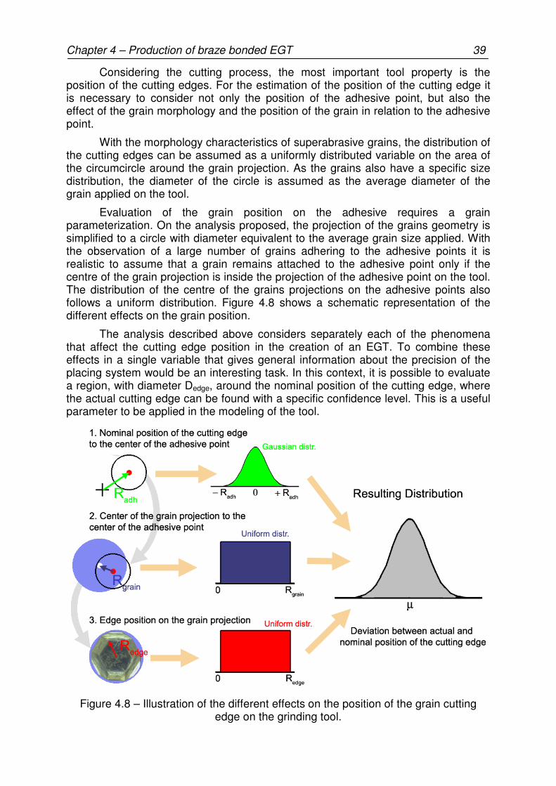
Chapter 4 – Production of braze bonded EGT 39
Considering the cutting process, the most important tool property is the position of the cutting edges. For the estimation of the position of the cutting edge it is necessary to consider not only the position of the adhesive point, but also the effect of the grain morphology and the position of the grain in relation to the adhesive point.
With the morphology characteristics of superabrasive grains, the distribution of the cutting edges can be assumed as a uniformly distributed variable on the area of the circumcircle around the grain projection. As the grains also have a specific size distribution, the diameter of the circle is assumed as the average diameter of the grain applied on the tool.
Evaluation of the grain position on the adhesive requires a grain parameterization. On the analysis proposed, the projection of the grains geometry is simplified to a circle with diameter equivalent to the average grain size applied. With the observation of a large number of grains adhering to the adhesive points it is realistic to assume that a grain remains attached to the adhesive point only if the centre of the grain projection is inside the projection of the adhesive point on the tool. The distribution of the centre of the grains projections on the adhesive points also follows a uniform distribution. Figure 4.8 shows a schematic representation of the different effects on the grain position.
The analysis described above considers separately each of the phenomena that affect the cutting edge position in the creation of an EGT. To combine these effects in a single variable that gives general information about the precision of the placing system would be an interesting task. In this context, it is possible to evaluate a region, with diameter Dedge, around the nominal position of the cutting edge, where the actual cutting edge can be found with a specific confidence level. This is a useful parameter to be applied in the modeling of the tool.
Figure 4.8 – Illustration of the different effects on the position of the grain cutting edge on the grinding tool.

40 Chapter 4 – Production of braze bonded EGT
For the evaluation of the region with diameter Dedge it is necessary to combine the effects of Gaussian and uniformly distributed variables. The standard deviation of the uniform distribution was approximated by a Gaussian distribution by equation 4.12, and the variable Dedge consequently can be evaluated by equation 4.13.
( )12
bb)x(u
2
i2 −+ +
= (4.12)
22
21
2adhedge 2D σ+σ+σ⋅= (4.13)
u = equivalent standard deviation for uniform distribution
b+ = upper limit of the uniform distribution
b- = lower limit of the uniform distribution
σadh = standard deviation of the adhesive centre point position
σ1 = equivalent standard deviation of the grain position on the adhesive point
σ2 = equivalent standard deviation of the cutting edge on the grain projection
On the evaluation proposed for the position of the cutting edge, the grain size has a large effect on the evaluation of diameter Dedge. Using as example cBN grains with size B251, the average droplet projection on the tool surface (Dp) of 140 µm and the error on the droplet positioning of 85 µm, the parameter Dedge is calculated as 187 µm.
The calculation of the region with diameter Dedge reveals that, even with the deterministic approach of the grain pattern design on EGT, the real position of the cutting edge is strongly affected by stochastic effects. The real weight of this tolerance on the design of EGT can only be evaluated with the application of numerical tools and with statistical analysis of the results.
After the tool surface is layered with the adhesive points, the grains are spread over the tool surface and, in an optimal condition, just one grain is placed per adhesive point. Among the different spreading methods tested, the best results were achieved with the application of a shaking reservoir with the grains under the tool, as shown in Figure 4.9.
Figure 4.9 – Technique for spreading the grains on the tool with adhesive points.

Chapter 4 – Production of braze bonded EGT 41
Further on the description of the grain pattern, there are two other effects that must be analyzed: the formation of grain clusters and the failure of occupation of specific adhesive points. Cluster formation is more common when smaller grain sizes are applied (especially grain sizes smaller than the equivalent droplet diameter on the tool surface). According to the grain size chosen, the cluster formation can have two or more grains on a single adhesive point. These agglomerations of grains have negative effects on the process. Due to the higher grain density, the bond between the grains tends to achieve a higher level, reducing the grain protrusion available. The higher bond level might difficult the coolant flow between the grains on the cluster and creates locally higher temperatures which may lead to a premature failure of the tool. Nevertheless, these damages have not been observed on the experiments. Figure 4.10 shows an example of cluster formation with cBN abrasive grain (ABN800 B251).
Figure 4.10 – Example of cluster formation on a grain pattern (ABN800 B251).
The other form of deviation in the grain pattern is adhesive points without any grain at all. This type of error has a more critical aspect than does cluster formation. The absence of one grain obliges another to assume its function in the removal of workpiece material, which may lead to an overloading of the grains and failure of the tool. However, as even on an EGT not all the grains take an active and fundamental part in the grinding process, the absence of some grains, even though extremely undesirable, may not lead the tool to failure.
Evaluating the application of cBN grains with size of B251 and the adhesive droplets characteristics, after the observation of a large number of EGT with grain pattern examples, the probability of cluster formation is calculated as 4.6% and the probability of missing grains from the pattern as 3.75%.
The nitrocellulose adhesive applied on the EGT requires specific conditions to cure. The tool layered with the grains must be heated up to temperatures of 180oC for a period of at least 15 minutes for the hardening of the adhesive. While the adhesive has not been hardened, the bond force of the grains is very low and the transport of the tool layered with the grains must be done carefully. After the adhesive has hardened the grains are relatively strongly bonded to the tool base material, not enough to support the grinding process forces, but sufficient to resist the application of the braze paste.

42 Chapter 4 – Production of braze bonded EGT
The brazing paste is applied with a brush onto the tool surface. The thickness of the braze paste layer is determined by the grain covering desired. This is usually a small amount of material and the quantity is difficult to control. The usual technique applied is to control the weight of the tool at specific areas, for example, every 10 cm2, covered with the brazing paste. When applying the paste on larger tools, where the precise control of the tool’s weight would be impracticable, it is also usual to control the weight of the braze paste reservoir and of the brush.
The braze paste applied for bonding cBN grains is achieved by mixing the same adhesive applied on the micro dispenser with the brazing powder, commercially know as Diabraze. This copper-based alloy has titanium and zirconium as active elements and a brazing temperature of 920oC. Due to the affinity of the active elements with oxygen, the brazing must be done under high vacuum atmosphere. The wetting of the cBN grains while the brazing process is achieved, as the Ti reacts with the boron-nitride, forms titanium-boron-nitrides (Ti2+xBN), which generate the tough and coherent bond between the matrix and the grains [ZIGE01].
The brazing process happens in a sequence of stages, where each one has a specific duration in time and also specific objectives. After the high vacuum is achieved, the first heating cycle starts with a ratio of 10oC per minute, up to 450oC. The adhesive polymer is decomposed at this temperature and builds a carbon rack, which will hold the grain its place. This temperature is maintained for between 10 and 20 minutes, followed by the next heat-up cycle. The heat-up ratio is kept constant at 10oC per minute, up to 780oC. This temperature is held for 20 to 30 minutes to equalize the temperature of the whole charge. The next step is heating up to the brazing temperature (950oC), and keeping this temperature for 10 minutes. On this stage the residues of the adhesive which held the grains position are completely dissolved on the meted filler alloys. The melted filler metal reacts, simultaneously, with the tool body material and with the grains. On this stage of the brazing process the grains position on the pattern is maintained by the capillary forces of the melted filler alloy. After this point the reaction between grains, brazing material and tool body is complete and the cooling process may start. The first cooling stage is done in vacuum, down to 500oC, followed by a second cooling stage down to room temperature in a free atmosphere.
4.4 Resume
This chapter has presented the modifications proposed to the placing method developed by Burkhard. The main goals were to achieve a better reproducibility and greater flexibility in the placing system. The new control technique is based on the acquisition of the tool rotational position with an encoder. This alternative has enabled the generation of much more flexible grain patterns on the tool and the account of the tool profile on the design of the grain pattern. Both features were not possible with the original placing system.
The generation of the brazed bond between grains, body material and filler metal depends on the coherent choice of materials for each of the components. These materials also have pronounced effects on the generation of the grain pattern. The evaluation of the placing method suggests a series of actions for the operation of the adhesive micro dispenser to achieve the best results when layering the tool body. Nevertheless, there is a quota of the deviations which cannot be controlled. These effects have been divided into three main groups: deviations of the adhesive point

Chapter 4 – Production of braze bonded EGT 43
size, deviations of the grain over the adhesive point and position of the cutting edge on the grain. These three effects can be analyzed individually and so allow, for example, the evaluation of the grain-placing tolerance with different grain sizes, without the production of new tool samples. This kind of evaluation is very useful, especially when working on optimization problems, such as the grain pattern on EGT.

44 Chapter 5 – Model concept
5. Model concept
The optimization of the grain pattern on EGT involves the analysis of a large amount of interdependent variables which can affect the grinding results. Numerical methods in this context can be used to find optimal application conditions. On modeling and simulating the tool it is possible to isolate tool properties which could not be separately analyzed well with the production and testing of samples.
The numerical analysis in this work focused mainly the geometrical properties of the tool in its performance. The analysis of the cutting performance is based on kinematic-geometric models. As described in Chapter 2, this method affords detailed descriptions of the tool geometric characteristics and of the kinematics between tool and workpiece to simulate the grinding operation. Figure 5.1 shows the information flow on the simulation of the tool performance.
Figure 5.1 – Interaction of the different modules on numerical analysis of EGT.
Chapter 5 – Model concept 45
In the next sections the methods used to obtain the models will be described and the simplifications required will be discussed.
5.1 Tool model
There are different methodologies applied when modeling grinding tools for geometric-kinematic simulations. Earlier models [KOSH03] applied strong simplifications of geometry in the description of the grains’ morphologies. The latest models published [AURI03, BRAU04, BRAU05], however, have demonstrated a greater concern about the detailed description of the cutting edges. This careful attention to the grains was possible due to the higher processing capacity of computers, allowing the evaluation of much more complex geometrical interactions.
The tool model considers the following characteristics on the tool design:
• The tool body material has smooth surface, with geometric deviations such as unbalancing of the profile according to the assumed tolerances.
• The pattern is described with the deviations obtained from the placing system (as shown in Chapter 4).
The grains geometry will be simplified to basic geometric shapes such as octahedrons and tetrahedrons (and the forms possible between these two basic geometries) and will follow the distributions in size and form according to samples evaluated and to the norm ISO 6106 [BAIL95, ISO6106].
There are two main methods to obtain the description of the wheel topography: scanning the real grinding wheel surface topography or synthetically generating the surface topography on the basis of statistical data of grinding wheel surfaces [BRIN06]. The most interesting method for the modeling of EGT involves a synthetic generation of the tool. Instead of controlling only the topography of a real grinding tool to create a database, the tool model is created with the Monte Carlo method, where the information of nondeterministic variables are applied to create the tool model. In the EGT there are a large amount of variables that can only be described with statistical tools (such as an average and the associated standard deviation). Examples of these variables are the size of each grain on the tool (with Gaussian distribution assumed by the sieving process) and the grain orientation on the tool surface (uniformly distributed).
The application of a stochastic tool model results that each tool model is unique. Models created with the same specifications must be treated as samples of a population, and the analysis of those samples requires the application of statistical tools and adequate confidence levels.
5.1.1 Body material deviations
Besides the obvious influences of the basic geometry information of the tool (such as tool profile, diameter and width), the positions of the cutting edges are affected by the deviations from the nominal geometry on the abrasive layer. Especially on SLGT, which cannot be dressed or trued for the correction of the profile, it is essential to consider the tolerances of the tool body on its performance. The tolerances modeled on the tool body material and on the tool assembly are summarized in Figure 5.2.

46 Chapter 5 – Model concept
Figure 5.2 – Modeled deviation of the tool body.
The tolerance values allowed in each of the geometry shown in Figure 5.2 are assumed by the tolerance intervals are based on the values given by ISO22917. On concentricity, perpendicularity, radial concentricity and axial concentricity, the angle on the tool circumference where the maximal deviation is found is assumed stochastically. Cylindricity and deviations on the profile form can be modeled as local errors on the tool surface or as complex form deviations, caused, for example, when machining the tool body.
5.1.2 Effects of the brazing process
The effects of the brazing process must be considered on the modeling of the tool. The first aspect to be modeled is the grain protrusion available after the brazing process. This information is relevant for the coolant and chip volume available on the tool. A second aspect is the shift of the grain position on the tool body. As the filler alloy melts during the brazing process, it slightly changes the position of the grains. The main effect considered in the model is the vertical position of the grain in relation to the tool surface. The evaluation of the shift on the vertical position was done with the observation of a large number of grains patterns before (the grains are fixed with the adhesive on the tool body) and after the brazing process. The best fit of the shift on the grains position was achieved with a Chi-distribution with two degrees of freedom (Figure 5.3). The mean of the distribution was evaluated on 12 µm, and the variance on 4 µm2.
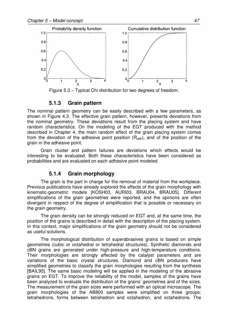
Chapter 5 – Model concept 47
Figure 5.3 – Typical Chi distribution for two degrees of freedom.
5.1.3 Grain pattern
The nominal pattern geometry can be easily described with a few parameters, as shown in Figure 4.3. The effective grain pattern, however, presents deviations from the nominal geometry. These deviations result from the placing system and have random characteristics. On the modeling of the EGT produced with the method described in Chapter 4, the main random effect of the grain placing system comes from the deviation of the adhesive point position (Radh), and of the position of the grain in the adhesive point.
Grain cluster and pattern failures are deviations which effects would be interesting to be evaluated. Both these characteristics have been considered as probabilities and are evaluated on each adhesive point modeled.
5.1.4 Grain morphology
The grain is the part in charge for the removal of material from the workpiece. Previous publications have already explored the effects of the grain morphology with kinematic-geometric models [KOSH03, AURI03, BRAU04, BRAU05]. Different simplifications of the grain geometries were reported, and the opinions are often divergent in respect of the degree of simplification that is possible or necessary on the grain geometry.
The grain density can be strongly reduced on EGT and, at the same time, the position of the grains is described in detail with the description of the placing system. In this context, major simplifications of the grain geometry should not be considered as useful solutions.
The morphological distribution of superabrasives grains is based on simple geometries (cubic or octahedral or tetrahedral structures). Synthetic diamonds and cBN grains are generated under high-pressure and high-temperature conditions. Their morphologies are strongly affected by the catalyst parameters and are variations of the basic crystal structures. Diamond and cBN producers have simplified geometries to classify the grain morphologies resulting from the synthesis [BAIL95]. The same basic modeling will be applied in the modeling of the abrasive grains on EGT. To improve the reliability of the model, samples of the grains have been analyzed to evaluate the distribution of the grains’ geometries and of the sizes. The measurement of the grain sizes were performed with an optical microscope. The grain morphologies of the AB800 samples were simplified on three groups: tetrahedrons, forms between tetrahedron and octahedron, and octahedrons. The

48 Chapter 5 – Model concept
probabilities of each of these groups were also obtained with the observation of samples. Figure 5.4 shows examples of the cBN grains modeled.
Figure 5.4 – Simplification from the superabrasive grains to the modeled geometries.
The generation of a virtual grain followed three basic steps:
• Determination of the grain morphology group: a random variable is applied to decide in which of the three basic morphology groups the grain will be generated;
• Determination of the grain size: the sieving tolerances applied can be flexibly chosen (for example, the sieving limits given by ISO6106). A random variable is applied for each grain to evaluate the characteristic grain size.
• Determination of the basic grain geometry: en each of the basic grain geometries modeled there is a basic geometry to fit the grain morphology in the grain size established. On tetrahedrons and octahedrons the grain sizes was parameterized with the edge length of the grain. For the morphology between the tetrahedron and octahedron, besides the grain edge, a second variable, which defines if the morphology is dominated by a tetrahedron (with characteristic value Cf = 0) or an octahedron (Cf = 1). The probability density function between the limits (0 and 1) is assumed as a uniformly distributed variable (Figure 5.5).
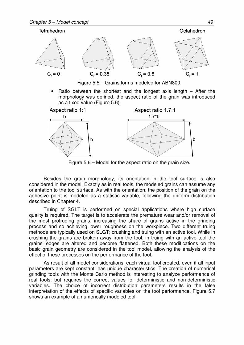
Chapter 5 – Model concept 49
Figure 5.5 – Grains forms modeled for ABN800.
• Ratio between the shortest and the longest axis length – After the morphology was defined, the aspect ratio of the grain was introduced as a fixed value (Figure 5.6).
Figure 5.6 – Model for the aspect ratio on the grain size.
Besides the grain morphology, its orientation in the tool surface is also considered in the model. Exactly as in real tools, the modeled grains can assume any orientation to the tool surface. As with the orientation, the position of the grain on the adhesive point is modeled as a statistic variable, following the uniform distribution described in Chapter 4.
Truing of SGLT is performed on special applications where high surface quality is required. The target is to accelerate the premature wear and/or removal of the most protruding grains, increasing the share of grains active in the grinding process and so achieving lower roughness on the workpiece. Two different truing methods are typically used on SLGT; crushing and truing with an active tool. While in crushing the grains are broken away from the tool, in truing with an active tool the grains’ edges are altered and become flattened. Both these modifications on the basic grain geometry are considered in the tool model, allowing the analysis of the effect of these processes on the performance of the tool.
As result of all model considerations, each virtual tool created, even if all input parameters are kept constant, has unique characteristics. The creation of numerical grinding tools with the Monte Carlo method is interesting to analyze performance of real tools, but requires the correct values for deterministic and non-deterministic variables. The choice of incorrect distribution parameters results in the false interpretation of the effects of specific variables on the tool performance. Figure 5.7 shows an example of a numerically modeled tool.
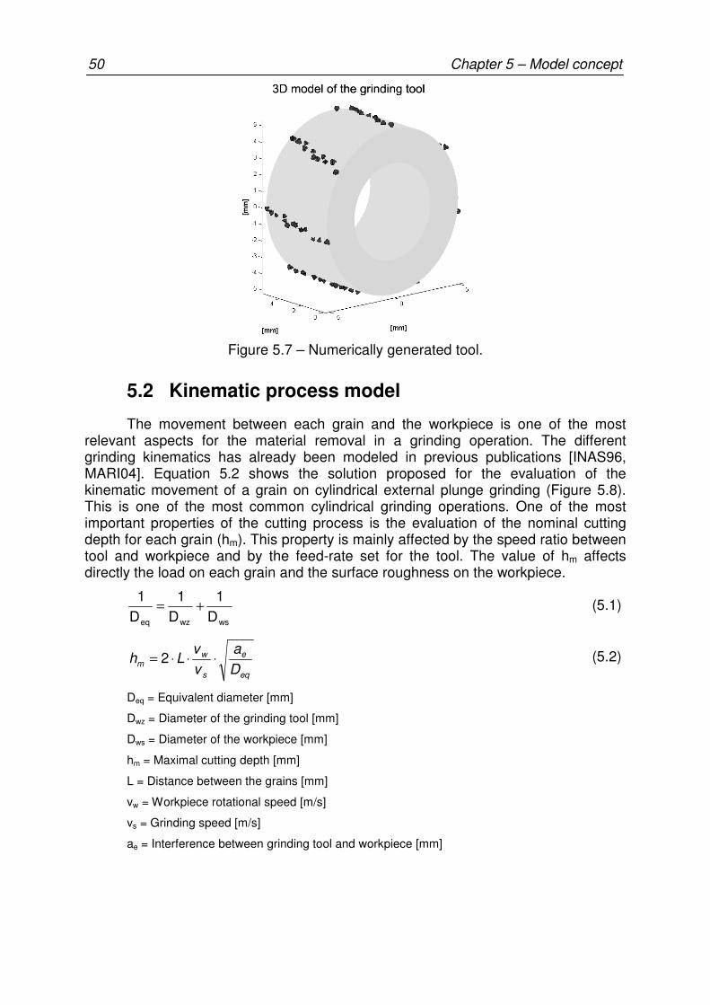
50 Chapter 5 – Model concept
Figure 5.7 – Numerically generated tool.
5.2 Kinematic process model
The movement between each grain and the workpiece is one of the most relevant aspects for the material removal in a grinding operation. The different grinding kinematics has already been modeled in previous publications [INAS96, MARI04]. Equation 5.2 shows the solution proposed for the evaluation of the kinematic movement of a grain on cylindrical external plunge grinding (Figure 5.8). This is one of the most common cylindrical grinding operations. One of the most important properties of the cutting process is the evaluation of the nominal cutting depth for each grain (hm). This property is mainly affected by the speed ratio between tool and workpiece and by the feed-rate set for the tool. The value of hm affects directly the load on each grain and the surface roughness on the workpiece.
wswzeq D
1
D
1
D
1+= (5.1)
eq
e
s
wm
D
a
v
vLh ⋅⋅⋅= 2 (5.2)
Deq = Equivalent diameter [mm]
Dwz = Diameter of the grinding tool [mm]
Dws = Diameter of the workpiece [mm]
hm = Maximal cutting depth [mm]
L = Distance between the grains [mm]
vw = Workpiece rotational speed [m/s]
vs = Grinding speed [m/s]
ae = Interference between grinding tool and workpiece [mm]
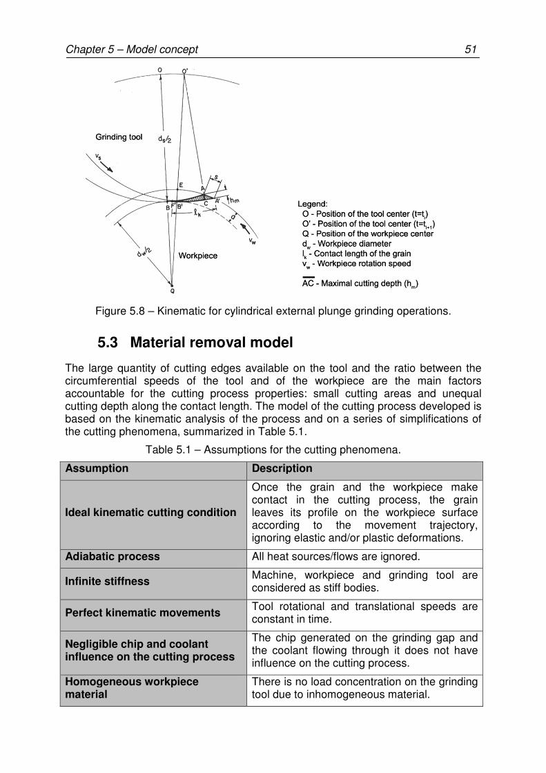
Chapter 5 – Model concept 51
Figure 5.8 – Kinematic for cylindrical external plunge grinding operations.
5.3 Material removal model
The large quantity of cutting edges available on the tool and the ratio between the circumferential speeds of the tool and of the workpiece are the main factors accountable for the cutting process properties: small cutting areas and unequal cutting depth along the contact length. The model of the cutting process developed is based on the kinematic analysis of the process and on a series of simplifications of the cutting phenomena, summarized in Table 5.1.
Table 5.1 – Assumptions for the cutting phenomena.
Assumption Description
Ideal kinematic cutting condition
Once the grain and the workpiece make contact in the cutting process, the grain leaves its profile on the workpiece surface according to the movement trajectory, ignoring elastic and/or plastic deformations.
Adiabatic process All heat sources/flows are ignored.
Infinite stiffness Machine, workpiece and grinding tool are considered as stiff bodies.
Perfect kinematic movements Tool rotational and translational speeds are constant in time.
Negligible chip and coolant influence on the cutting process
The chip generated on the grinding gap and the coolant flowing through it does not have influence on the cutting process.
Homogeneous workpiece material
There is no load concentration on the grinding tool due to inhomogeneous material.
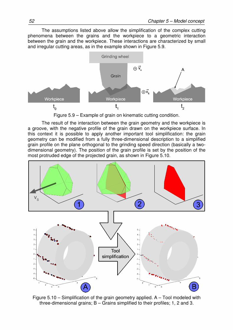
52 Chapter 5 – Model concept
The assumptions listed above allow the simplification of the complex cutting phenomena between the grains and the workpiece to a geometric interaction between the grain and the workpiece. These interactions are characterized by small and irregular cutting areas, as in the example shown in Figure 5.9.
Figure 5.9 – Example of grain on kinematic cutting condition.
The result of the interaction between the grain geometry and the workpiece is a groove, with the negative profile of the grain drawn on the workpiece surface. In this context it is possible to apply another important tool simplification: the grain geometry can be modified from a fully three-dimensional description to a simplified grain profile on the plane orthogonal to the grinding speed direction (basically a two- dimensional geometry). The position of the grain profile is set by the position of the most protruded edge of the projected grain, as shown in Figure 5.10.
Figure 5.10 – Simplification of the grain geometry applied. A – Tool modeled with three-dimensional grains; B – Grains simplified to their profiles; 1, 2 and 3.
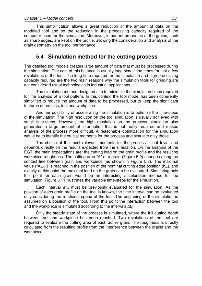
Chapter 5 – Model concept 53
This simplification allows a great reduction of the amount of data on the modeled tool and so the reduction in the processing capacity required of the computer used for the simulation. Moreover, important properties of the grains, such as sharp edges, are kept on the profile, allowing the consideration and analysis of the grain geometry on the tool performance.
5.4 Simulation method for the cutting process
The detailed tool models creates large amount of data that must be processed during the simulation. The cost of this balance is usually long simulation times for just a few revolutions of the tool. The long time required for the simulation and high processing capacity required are the two main reasons why the simulation tools for grinding are not considered usual technologies in industrial applications.
The simulation method designed aim to minimize the simulation times required for the analysis of a tool pattern. In this context the tool model has been coherently simplified to reduce the amount of data to be processed, but to keep the significant features of process, tool and workpiece.
Another possibility of accelerating the simulation is to optimize the time-steps of the simulation. The high resolution on the tool simulation is usually achieved with small time-steps. However, the high resolution on the process simulation also generates a large amount of information that is not really required and makes analysis of the process more difficult. A reasonable optimization for the simulation would be to identify the crucial moments for the process and simulate only these.
The choice of the most relevant moments for the process is not trivial and depends directly on the results expected from the simulation. On the analysis of the EGT, the main expectations are: the cutting load on the grain profile and the resulting workpiece roughness. The cutting area “A” of a grain (Figure 5.9) changes along the contact line between grain and workpiece (as shown in Figure 5.8). The maximal value (“Amax”) is reached in the position of the nominal cutting edge position (hm), and exactly at this point the maximal load on the grain can be evaluated. Simulating only this point for each grain would be an interesting acceleration method for the simulation. Figure 5.11 illustrates the variable time-steps for the simulation.
Each interval ∆t(i) must be previously evaluated for the simulation. As the position of each grain profile on the tool is known, the time interval can be evaluated only considering the rotational speed of the tool. The beginning of the simulation is assumed on a position of the tool. From this point the interaction between the tool and the workpiece is simulated according to the intervals ∆t(i).
Only the steady state of the process is simulated, where the full cutting depth between tool and workpiece has been reached. Two revolutions of the tool are required to evaluate the cutting area of each active grain. The roughness is directly calculated from the resulting profile from the interference between the grains and the workpiece.

54 Chapter 5 – Model concept
Figure 5.11 – Optimized time-step for the simulation.
5.5 Grain wear model
A failure criterion for the grains is also considered in the process model: once the cutting area “A” (Figure 5.9) exceeds a limit value (Alim), the geometry of the grain profile is altered. This change depends on the tool characteristics, such as grain break type and bond system properties. The changes in the grains geometry can be modeled in any reasonable way, which represents real failure modes, as, for example, pull-out, macro or micro-breaks (Figure 5.12).
Figure 5.12 – Examples of grain profile modification caused by the grain wear.
The failure model for each failure mode must reasonably represent the different failure mechanisms observed with different grain types under the load
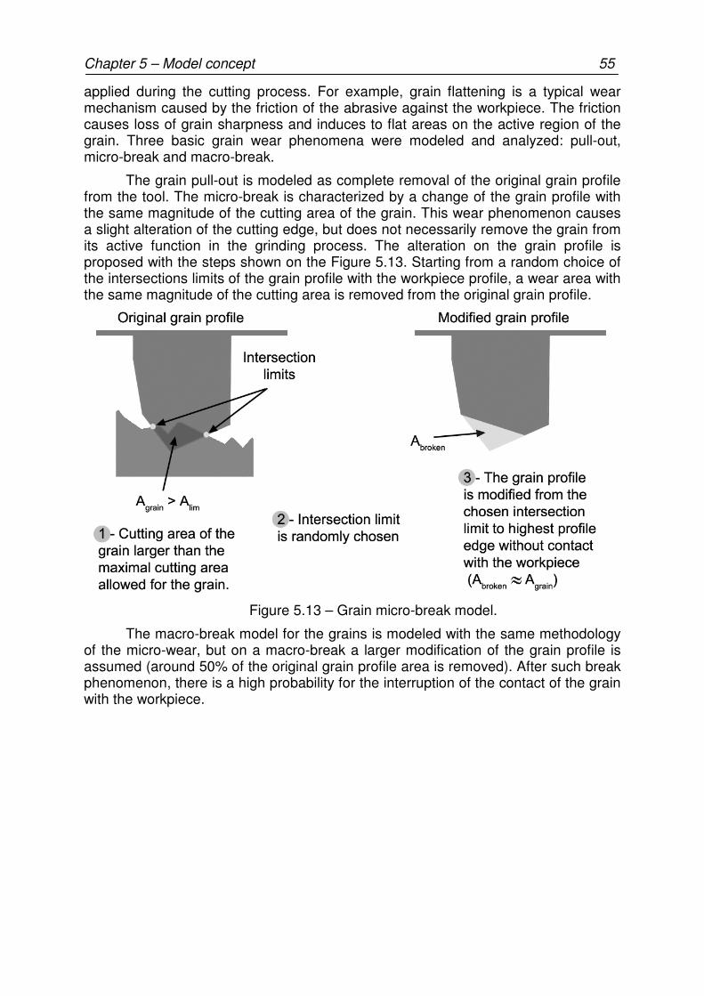
Chapter 5 – Model concept 55
applied during the cutting process. For example, grain flattening is a typical wear mechanism caused by the friction of the abrasive against the workpiece. The friction causes loss of grain sharpness and induces to flat areas on the active region of the grain. Three basic grain wear phenomena were modeled and analyzed: pull-out, micro-break and macro-break.
The grain pull-out is modeled as complete removal of the original grain profile from the tool. The micro-break is characterized by a change of the grain profile with the same magnitude of the cutting area of the grain. This wear phenomenon causes a slight alteration of the cutting edge, but does not necessarily remove the grain from its active function in the grinding process. The alteration on the grain profile is proposed with the steps shown on the Figure 5.13. Starting from a random choice of the intersections limits of the grain profile with the workpiece profile, a wear area with the same magnitude of the cutting area is removed from the original grain profile.
Figure 5.13 – Grain micro-break model.
The macro-break model for the grains is modeled with the same methodology of the micro-wear, but on a macro-break a larger modification of the grain profile is assumed (around 50% of the original grain profile area is removed). After such break phenomenon, there is a high probability for the interruption of the contact of the grain with the workpiece.

56 Chapter 5 – Model concept
Figure 5.14 – Grain macro-break model.
After the modification of the grain profile, a new series of two revolutions is simulated with the tool. This process is repeated up to the moment at which either no grain achieves a critical load level (tool has reached a stable condition), or one of the pre-defined failure criteria is reached (shown in Table 5.2).
Table 5.2 – Tool failure criteria.
Failure criteria Description
Contact between the tool body and the workpiece
Typical failure found on EGT. After a critical number of grains have broken on the tool, a specific region on the tool width has no more grains available for the grinding process, leading to direct contact between tool body and workpiece.
Roughness limits cannot be reached
The successive break of the grains can lead the abrasive layer on the tool to a steady state where the desired workpiece roughness can not be achieved with the grinding tool and process parameters applied.
5.6 Tangential grinding force model
The power required to perform the material removal on grinding operations can be evaluated by the product of the grinding speed and the tangential forces on the tool. As a typical application area for the EGT are grinding operations with high values of specific material removal rate (Qw’), the prediction of the cutting forces is an interesting result to evaluate the tool performance.
From the simulation of the tool it is possible to obtain the distribution of the active grains and their respective cutting areas. Kienzle has developed a series of equations to the correlation of the geometry and the force on the cutting process with determined cutting edge geometry. The equation 5.3 is the typical form of the Kienzle equation for predicting cutting forces in turning operations.

Chapter 5 – Model concept 57
)m1(1.1cc
chbkF -
⋅⋅= (5.3)
Fc = Cutting force [N]
kc1.1 = Specific cutting force for a section of 1 mm2 [N/mm2]
b = cutting width on the cutting edge direction [mm]
h = cutting depth orthogonal to the cutting edge direction [mm]
The Kienzle equations are typically applied to predict the cutting force and power for turning, milling and drilling operations. The constants “Kc1.1” and “mc” are experimentally obtained according to specific set of tool, workpiece and process characteristics.
The application of the Kienzle equation to the prediction of the cutting force in grinding operations requires some alterations in the formulation. The complex cutting geometries involved on the interaction of the abrasive grains and the workpiece during the grinding process difficult the recognition of a cutting depth or width. Figure 5.15 shows a typical example of the cutting area obtained with the simulation of the numerical tool.
Figure 5.15 – Typical cutting area on the application of the grain geometries on the cutting edges.
An alternative approach of the Kienzle equation is to parameterize the specific cutting force with the cutting area of the grain (equation 5.4). The resulting cutting force acting on the process at an instant “t” corresponds to the sum of the cutting forces acting on each of the active grains in contact with the workpiece (equation 5.5).
∑=
α
=
⋅=
n
1icic
icci
)t(F)t(F
)t(Ak)t(F
(5.4)
(5.5)
Fc(i,t)= Cutting force at the grain (i) in the instant (t) [N]
A(i,t) = Cutting area of the grain (i) in the instant (t) [mm2]
Fc(t) = Cutting force acting at the tool on the instant (t)
The whole simulation method is designed aiming the reduction of the processing capacity requirement for the simulation of the tool model. With this
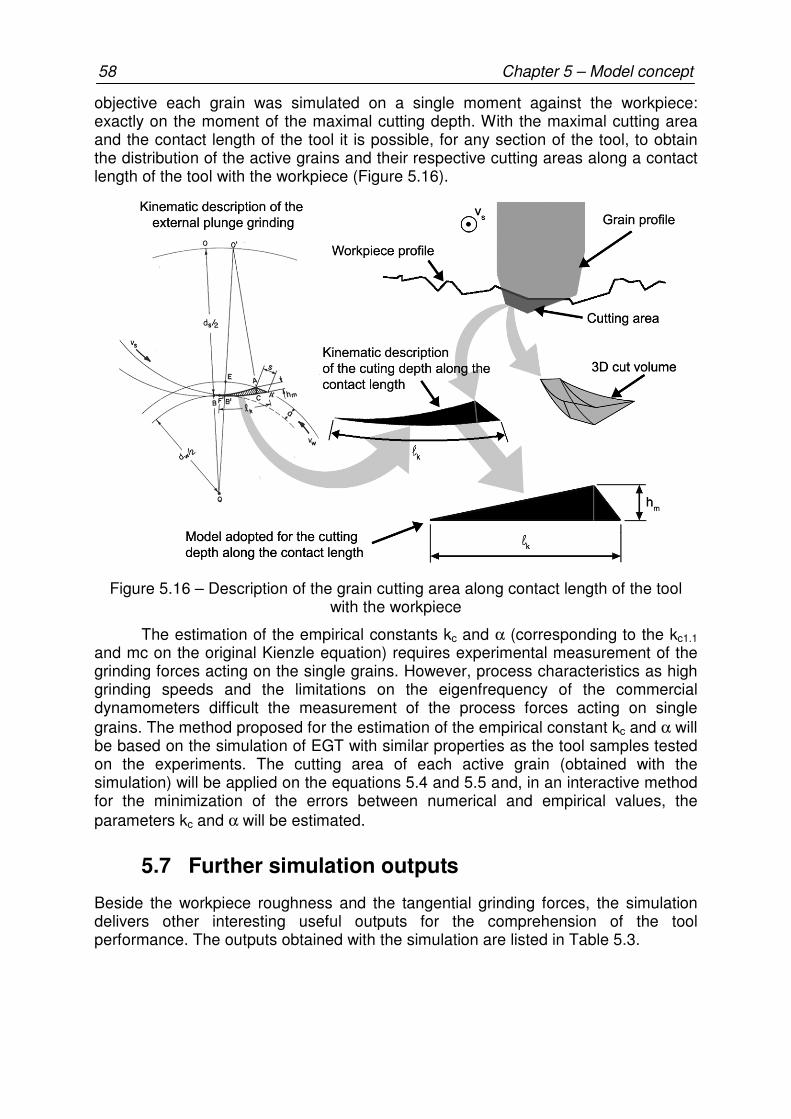
58 Chapter 5 – Model concept
objective each grain was simulated on a single moment against the workpiece: exactly on the moment of the maximal cutting depth. With the maximal cutting area and the contact length of the tool it is possible, for any section of the tool, to obtain the distribution of the active grains and their respective cutting areas along a contact length of the tool with the workpiece (Figure 5.16).
Figure 5.16 – Description of the grain cutting area along contact length of the tool with the workpiece
The estimation of the empirical constants kc and α (corresponding to the kc1.1 and mc on the original Kienzle equation) requires experimental measurement of the grinding forces acting on the single grains. However, process characteristics as high grinding speeds and the limitations on the eigenfrequency of the commercial dynamometers difficult the measurement of the process forces acting on single grains. The method proposed for the estimation of the empirical constant kc and α will be based on the simulation of EGT with similar properties as the tool samples tested on the experiments. The cutting area of each active grain (obtained with the simulation) will be applied on the equations 5.4 and 5.5 and, in an interactive method for the minimization of the errors between numerical and empirical values, the parameters kc and α will be estimated.
5.7 Further simulation outputs
Beside the workpiece roughness and the tangential grinding forces, the simulation delivers other interesting useful outputs for the comprehension of the tool performance. The outputs obtained with the simulation are listed in Table 5.3.
Chapter 5 – Model concept 59
Table 5.3 – Simulation outputs.
Output Description
Distribution of the edges of the grains
Once each point of the grain geometry and the position of the grain on the grinding tool are set, it is possible to determine the exact distribution of the cutting edges. The distribution can be presented as a density probability function or as an Abbott-Firestone curve. This is useful information for the evaluation of the grains in contact with the workpiece or for the specification of the truing parameters.
Distribution of the active cutting edges of the grains
This distribution is slightly different from the distribution of the cutting edges, as highest protruding edges are taking part in the cutting process.
Grain load distribution Statistical distribution of the cutting area (respectively the cutting force) of the active grains.
Region of the tool where the grains are heavily loaded
It is possible to identify the regions on the tool where the grains are potentially susceptible to failure.
With the analysis of the outputs it is possible to evaluate whether the combination of the designed grain pattern and kinematics chosen will result in a reliable process (workpiece roughness and grain load are below the specified limits).
5.8 Resume
The optimization of the grain pattern on EGT is designed with kinematic-geometrical simulation method. The macro- and micro-geometry of the tool are described in detail, aiming mainly to achieve a reliable representation of cutting edges. On the other hand, the simulation method is designed to achieve short simulation times and so enable the application of the numerical method on practicable optimization tasks. The simplification of the tool’s micro-geometry and the irregular time-steps for the simulation are the main simplifications assumed to reduce the simulation efforts.
The short evaluation times allows the evaluation of the wear phenomena on the grains. The wear models are designed as changes in the profile of the grains. Different grain wear mechanisms can be reproduced, such as grain macro and micro-break, pull-outs and grain flattening.
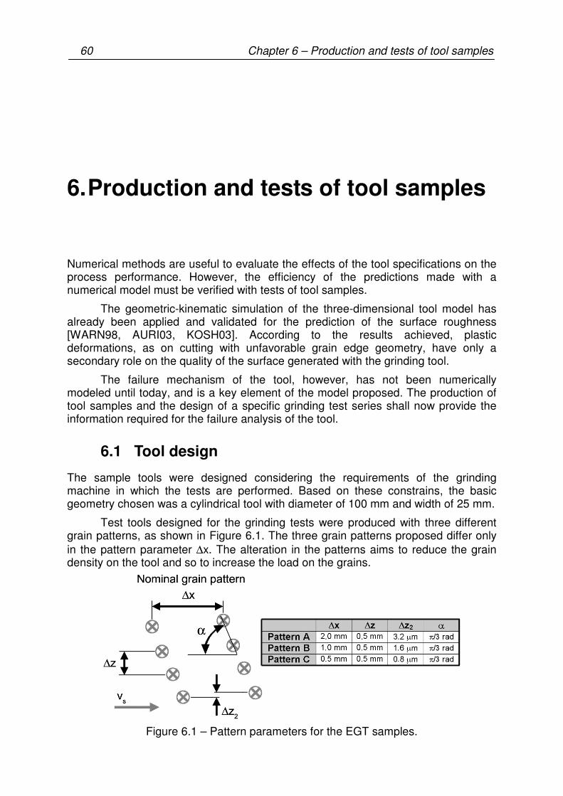
60 Chapter 6 – Production and tests of tool samples
6. Production and tests of tool samples
Numerical methods are useful to evaluate the effects of the tool specifications on the process performance. However, the efficiency of the predictions made with a numerical model must be verified with tests of tool samples.
The geometric-kinematic simulation of the three-dimensional tool model has already been applied and validated for the prediction of the surface roughness [WARN98, AURI03, KOSH03]. According to the results achieved, plastic deformations, as on cutting with unfavorable grain edge geometry, have only a secondary role on the quality of the surface generated with the grinding tool.
The failure mechanism of the tool, however, has not been numerically modeled until today, and is a key element of the model proposed. The production of tool samples and the design of a specific grinding test series shall now provide the information required for the failure analysis of the tool.
6.1 Tool design
The sample tools were designed considering the requirements of the grinding machine in which the tests are performed. Based on these constrains, the basic geometry chosen was a cylindrical tool with diameter of 100 mm and width of 25 mm.
Test tools designed for the grinding tests were produced with three different grain patterns, as shown in Figure 6.1. The three grain patterns proposed differ only in the pattern parameter ∆x. The alteration in the patterns aims to reduce the grain density on the tool and so to increase the load on the grains.
Figure 6.1 – Pattern parameters for the EGT samples.

Chapter 6 – Production and tests of tool samples 61
Grains of cBN were used for the sample tools, with the specification ABN800 B251. The choice of this grain quality was based on its high thermal stability (large thermal loads are applied on the tool during the brazing process). The B251 grain size was chosen to achieve large chip and coolant volume during rough grinding operations. The bond created with the brazing process (using the copper-based filler metal commercially known as “Diabrase”) resulted in an average thickness of the braze layer of 40% of the average grain size (between 80 – 100 µm).
Figure 6.2 shows sample sections of the three grain patterns produced. Note, on Pattern C (the one with the highest grain density among the patterns produced) the deviations caused by the brazing process have relevant effects on the final position of the grains. The undesired grain movement occurs during the brazing process, when large capillary forces are applied on the grains by the melted material.
Figure 6.2 – Samples of the grain patterns on the sample tools.
A statistical evaluation of the results obtained with the samples requires the evaluation of more tool samples. A total of four samples were manufactured for each grain pattern proposed.
Parallel to the tests with EGT brazed tools, a series of four conventional electroplated tools (stochastic grain layer) was also tested. The electroplated tools are layered with ABN300 grains. In comparison with the ABN800, applied on the brazed tools, the ABN300 have larger aspect ratio between the longest and the shortest grain axis and a different breakage property (generating new sharp edges when broken) [ESIX06]. ABN300 grains are the most popular cBN grain applied on electroplated tools. The comparison between the brazed and electroplated tools proposed provide the technological comparison between potentials and limitations of the actual state of art on electroplated tool technology with the new EGT.
6.2 Grinding tests
The tests to evaluate the performance of the EGT samples were performed on a universal circular grinder from the Studer company, model S31 (shown in Figure 6.3).
The EGT samples are assembled on a special tool holder (grinding quill). The quill was manufactured with a tolerance field h6 (SN EN 20286-2, ISO286), compatible with the tolerance field chosen on the grinding tool bore (H6). The tolerance for the discs assembly was specified as 5 µm. The control of the tolerances
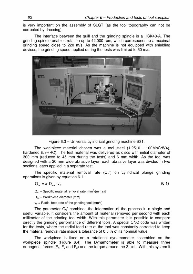
62 Chapter 6 – Production and tests of tool samples
is very important on the assembly of SLGT (as the tool topography can not be corrected by dressing).
The interface between the quill and the grinding spindle is a HSK40-A. The grinding spindle enables rotation up to 42,000 rpm, which corresponds to a maximal grinding speed close to 220 m/s. As the machine is not equipped with shielding devices, the grinding speed applied during the tests was limited to 60 m/s.
Figure 6.3 – Universal cylindrical grinding machine S31.
The workpiece material chosen was a tool steel (1.2510 - 100MnCrW4), hardened (59HRC). The test material was delivered as discs with initial diameter of 300 mm (reduced to 45 mm during the tests) and 6 mm width. As the tool was designed with a 20 mm wide abrasive layer, each abrasive layer was divided in two sections, each applied in a separate test.
The specific material removal rate (Qw’) on cylindrical plunge grinding operations is given by equation 6.1.
frwsw vD'Q ⋅⋅π= (6.1)
Qw’ = Specific material removal rate [mm3/(mm.s)]
Dws = Workpiece diameter [mm]
vfr = Radial feed rate of the grinding tool [mm/s]
The parameter Qw’ combines the information of the process in a single and useful variable. It considers the amount of material removed per second with each millimeter of the grinding tool width. With this parameter it is possible to compare directly the grinding performance of different tools. A special CNC code was written for the tests, where the radial feed rate of the tool was constantly corrected to keep the material removal rate inside a tolerance of 0.5 % of its nominal value.
The workpiece is fixed on a rotational dynamometer assembled on the workpiece spindle (Figure 6.4). The Dynamometer is able to measure three orthogonal forces (Fx, Fy and Fz) and the torque around the Z axis. With this system it
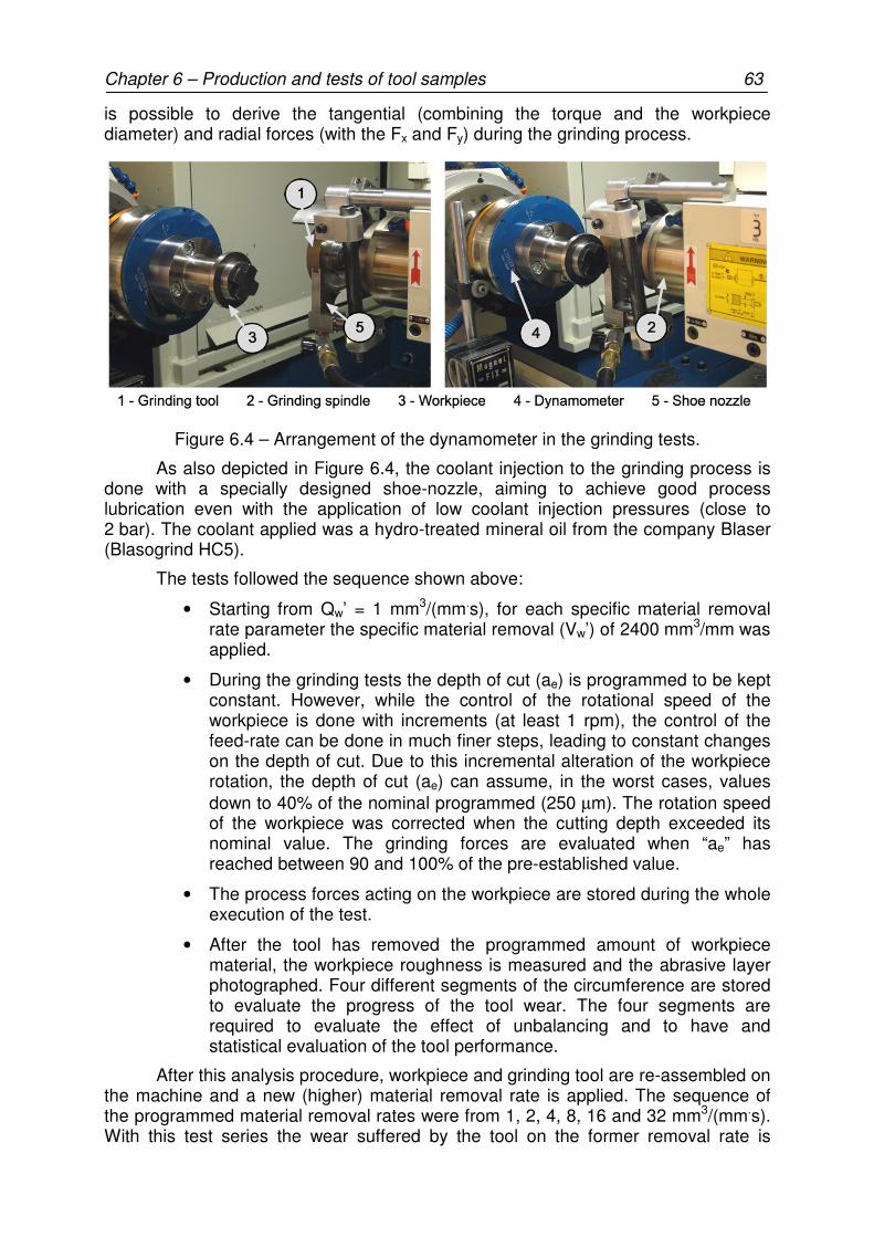
Chapter 6 – Production and tests of tool samples 63
is possible to derive the tangential (combining the torque and the workpiece diameter) and radial forces (with the Fx and Fy) during the grinding process.
Figure 6.4 – Arrangement of the dynamometer in the grinding tests.
As also depicted in Figure 6.4, the coolant injection to the grinding process is done with a specially designed shoe-nozzle, aiming to achieve good process lubrication even with the application of low coolant injection pressures (close to 2 bar). The coolant applied was a hydro-treated mineral oil from the company Blaser (Blasogrind HC5).
The tests followed the sequence shown above:
• Starting from Qw’ = 1 mm3/(mm.s), for each specific material removal rate parameter the specific material removal (Vw’) of 2400 mm3/mm was applied.
• During the grinding tests the depth of cut (ae) is programmed to be kept constant. However, while the control of the rotational speed of the workpiece is done with increments (at least 1 rpm), the control of the feed-rate can be done in much finer steps, leading to constant changes on the depth of cut. Due to this incremental alteration of the workpiece rotation, the depth of cut (ae) can assume, in the worst cases, values down to 40% of the nominal programmed (250 µm). The rotation speed of the workpiece was corrected when the cutting depth exceeded its nominal value. The grinding forces are evaluated when “ae” has reached between 90 and 100% of the pre-established value.
• The process forces acting on the workpiece are stored during the whole execution of the test.
• After the tool has removed the programmed amount of workpiece material, the workpiece roughness is measured and the abrasive layer photographed. Four different segments of the circumference are stored to evaluate the progress of the tool wear. The four segments are required to evaluate the effect of unbalancing and to have and statistical evaluation of the tool performance.
After this analysis procedure, workpiece and grinding tool are re-assembled on the machine and a new (higher) material removal rate is applied. The sequence of the programmed material removal rates were from 1, 2, 4, 8, 16 and 32 mm3/(mm.s). With this test series the wear suffered by the tool on the former removal rate is
64 Chapter 6 – Production and tests of tool samples
transferred to the next material removal rate. This test sequence limits the evaluation of the tool’s life, as the load on the grains is constantly changed.
The only interruption criteria for the test series was the failure of the tool. This may happen due to the overload on the grains, leading the EGT to have contact between the tool body and the workpiece, or due to excessive burns on the workpiece surface, which are especially to be expected on the high grain density observed on the electroplated tools.
6.3 Results
In the following sections the diverse measurements made with the EGT samples and with the electroplated tools are presented and discussed. Almost all tool patterns performed the whole test series successfully. The exceptions were two of the four tools designed with the pattern A (the lowest grain density tested), which failed on the application of the Qw’ = 32 mm3/(mm.s). In the last section of this chapter a relationship among the results collected will be presented.
6.3.1 Roughness measurements
The roughness profile of a grinded workpiece reveals valuable information about the profile of the tool applied on the machining operation. Changes on the cutting edges geometries have direct effect on the texture generated on the workpiece.
The arithmetical mean deviation parameter (Ra) is the most generally used roughness parameter. This parameter is easy to define and to measure, and gives a good general description of the height variations. The main limitations on the application of Ra are the absence of any wavelength information and the poor sensitivity to small and local changes in the profile [GADE02].
The following remarks can be made with the comparison of the Ra values measured in the different grain patterns and with the electroplated tools (shown in the Figure 6.5):
• The workpiece surface becomes smoother with the increment of Qw’: this effect is associated to the wear/break of the most protruding grains on the tool, increasing the number of grains active and reducing Ra.
• Higher grain densities tend to achieve smoother workpiece surfaces: this effect is mainly caused by the higher number of grains that have an effective participation in the grinding process.
• Electroplated tools have the most constant results and the lower roughness results: these effects are mainly caused by the higher grain density and by the wear property of the abrasives applied.
• The measurement uncertainty of the pattern A indicates higher variation of the results: this may be correlated to the lower share of grains available on the tool and to the higher sensitivity of Ra with the lower number of grains active on the tool. On the other hand, the electroplated tools have the lower measurement uncertainty and the lower Ra values. These results are associated to the higher grain density, where the wear effects have less representative effects on the resulting workpiece roughness.

Chapter 6 – Production and tests of tool samples 65
• The results achieved with patterns B and C are similar, indicating no significant difference in the number of active edges between these two tool designs.
Figure 6.5 – Ra measured with EGT and electroplated grinding tools.
The maximum height of the profile (Rt) is, contrary to Ra, very sensitive to the presence of isolated high peaks or deep valleys on the workpiece profile. On the tests performed, Rt and Ra showed similar behaviors (Figure 6.6). Remarkable are the lower values and measurement uncertainty with the electroplated tools for the values of Qw’ higher than 4 mm3/(mm.s). These results indicate that the tools have reached a stable wear progress, without rapid development of the wear at a specific region of the tool. On the other hand, the high uncertainties in the values of pattern A indicate instable wear development on the tools. On contrary to Ra, the difference between the patterns B and C can be better noticed, especially while observing the measurement uncertainties: tool with pattern B tend do have higher measurement
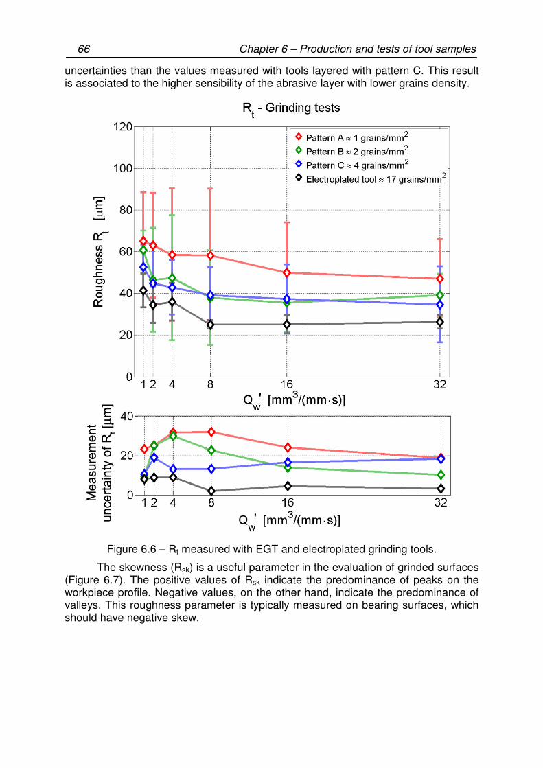
66 Chapter 6 – Production and tests of tool samples
uncertainties than the values measured with tools layered with pattern C. This result is associated to the higher sensibility of the abrasive layer with lower grains density.
Figure 6.6 – Rt measured with EGT and electroplated grinding tools.
The skewness (Rsk) is a useful parameter in the evaluation of grinded surfaces (Figure 6.7). The positive values of Rsk indicate the predominance of peaks on the workpiece profile. Negative values, on the other hand, indicate the predominance of valleys. This roughness parameter is typically measured on bearing surfaces, which should have negative skew.

Chapter 6 – Production and tests of tool samples 67
Figure 6.7 – Positive and negative skewness.
According to the properties of the abrasive layers, and with the progressive wear of the tool, it is possible to describe the expected workpiece skewness:
• New or unworn abrasive layers: a small number of largely protruded grains are accountable for the removal of material, inducing to negative skewness. This workpiece property should be observed on the lower material removal rates;
• Worn abrasive: the largely protruded grains are removed from the abrasive layer, creating a higher number of grains active and with a more homogeneous distribution of the cutting load. The workpiece skewness should be close to zero;
The results obtained have revealed the effects of the grains pattern on the workpiece skewness. The large grain density of the stochastic layered electroplated tools produced, in almost all situations, the tendency to negative skewness values. The large number of grains contributes to avoid the situations where the skewness achieved positive values. With the EGT, patterns B and C have presented similar average values, starting with negative values for the lower values of Qw’ and achieving values close to zero for Qw’ higher than 4 mm3/(mm.s). The tools with pattern C have higher measurement uncertainties than the tools with pattern B. This fact is associated to a more significant effect of the brazing process on the position of the grains on the pattern C than on the pattern B (the pattern C has a more irregular grain distribution due to the effects of the brazing process). The pattern A indicated in almost all situations the light tendency to achieve positive skewness. These results are associated to the lower grain density and to the largely spaced cutting edges on the axial direction of the tool. The larger distance between the cutting edges leads to workpiece surfaces with the predominance of peaks (regions where the material was not removed from the workpiece).
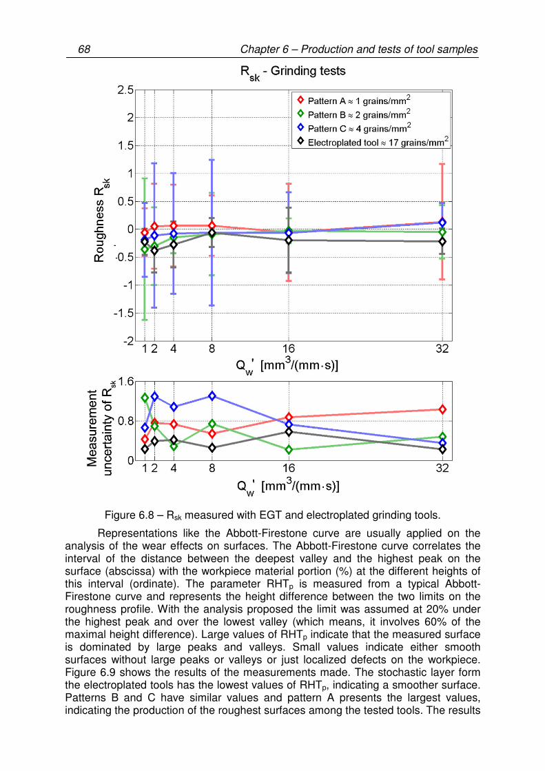
68 Chapter 6 – Production and tests of tool samples
Figure 6.8 – Rsk measured with EGT and electroplated grinding tools.
Representations like the Abbott-Firestone curve are usually applied on the analysis of the wear effects on surfaces. The Abbott-Firestone curve correlates the interval of the distance between the deepest valley and the highest peak on the surface (abscissa) with the workpiece material portion (%) at the different heights of this interval (ordinate). The parameter RHTp is measured from a typical Abbott-Firestone curve and represents the height difference between the two limits on the roughness profile. With the analysis proposed the limit was assumed at 20% under the highest peak and over the lowest valley (which means, it involves 60% of the maximal height difference). Large values of RHTp indicate that the measured surface is dominated by large peaks and valleys. Small values indicate either smooth surfaces without large peaks or valleys or just localized defects on the workpiece. Figure 6.9 shows the results of the measurements made. The stochastic layer form the electroplated tools has the lowest values of RHTp, indicating a smoother surface. Patterns B and C have similar values and pattern A presents the largest values, indicating the production of the roughest surfaces among the tested tools. The results
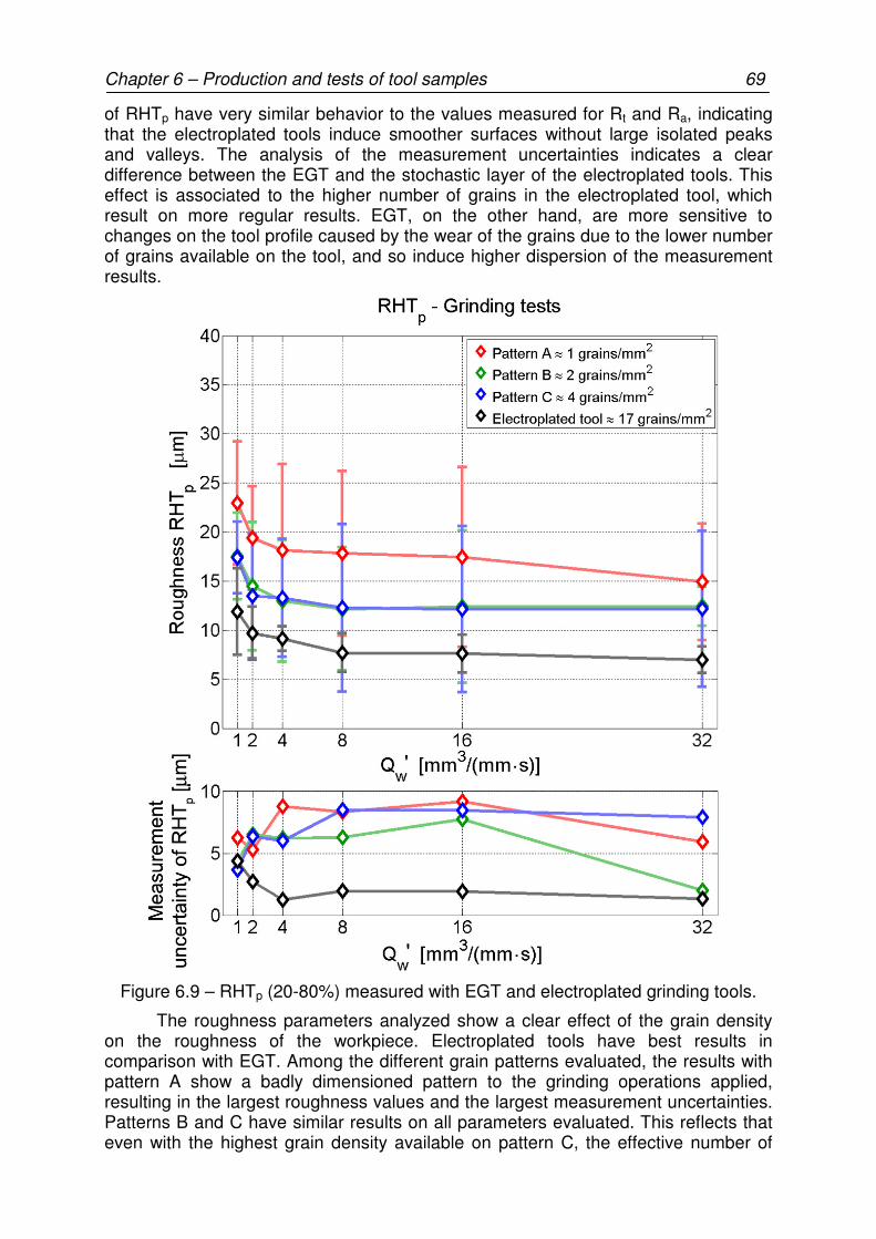
Chapter 6 – Production and tests of tool samples 69
of RHTp have very similar behavior to the values measured for Rt and Ra, indicating that the electroplated tools induce smoother surfaces without large isolated peaks and valleys. The analysis of the measurement uncertainties indicates a clear difference between the EGT and the stochastic layer of the electroplated tools. This effect is associated to the higher number of grains in the electroplated tool, which result on more regular results. EGT, on the other hand, are more sensitive to changes on the tool profile caused by the wear of the grains due to the lower number of grains available on the tool, and so induce higher dispersion of the measurement results.
Figure 6.9 – RHTp (20-80%) measured with EGT and electroplated grinding tools.
The roughness parameters analyzed show a clear effect of the grain density on the roughness of the workpiece. Electroplated tools have best results in comparison with EGT. Among the different grain patterns evaluated, the results with pattern A show a badly dimensioned pattern to the grinding operations applied, resulting in the largest roughness values and the largest measurement uncertainties. Patterns B and C have similar results on all parameters evaluated. This reflects that even with the highest grain density available on pattern C, the effective number of
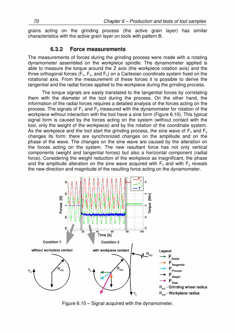
70 Chapter 6 – Production and tests of tool samples
grains acting on the grinding process (the active grain layer) has similar characteristics with the active grain layer on tools with pattern B.
6.3.2 Force measurements
The measurements of forces during the grinding process were made with a rotating dynamometer assembled on the workpiece spindle. The dynamometer applied is able to measure the torque around the Z axis (the workpiece rotation axis) and the three orthogonal forces (Fx, Fy, and Fz) on a Cartesian coordinate system fixed on the rotational axis. From the measurement of these forces it is possible to derive the tangential and the radial forces applied to the workpiece during the grinding process.
The torque signals are easily translated to the tangential forces by correlating them with the diameter of the tool during the process. On the other hand, the information of the radial forces requires a detailed analysis of the forces acting on the process. The signals of Fx and Fy measured with the dynamometer for rotation of the workpiece without interaction with the tool have a sine form (Figure 6.10). This typical signal form is caused by the forces acting on the system (without contact with the tool, only the weight of the workpiece) and by the rotation of the coordinate system. As the workpiece and the tool start the grinding process, the sine wave of Fx and Fy changes its form: there are synchronized changes on the amplitude and on the phase of the wave. The changes on the sine wave are caused by the alteration on the forces acting on the system. The new resultant force has not only vertical components (weight and tangential forces) but also a horizontal component (radial force). Considering the weight reduction of the workpiece as insignificant, the phase and the amplitude alteration on the sine wave acquired with Fx and with Fy reveals the new direction and magnitude of the resulting force acting on the dynamometer.
Figure 6.10 – Signal acquired with the dynamometer.
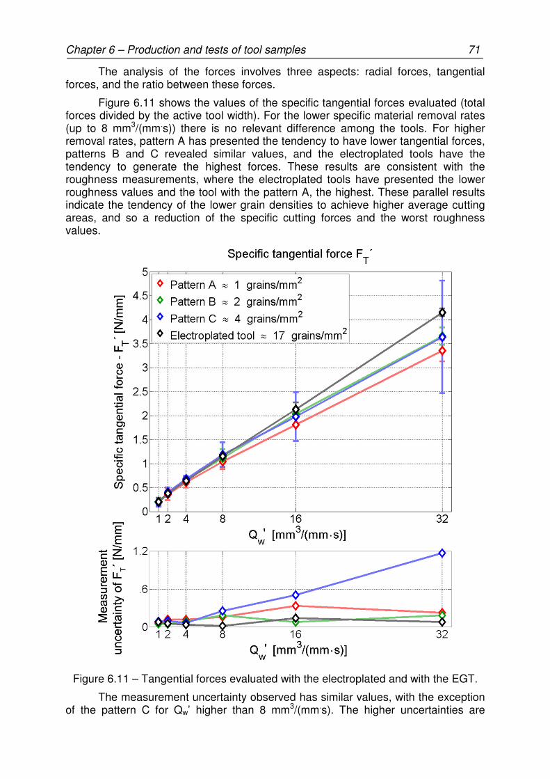
Chapter 6 – Production and tests of tool samples 71
The analysis of the forces involves three aspects: radial forces, tangential forces, and the ratio between these forces.
Figure 6.11 shows the values of the specific tangential forces evaluated (total forces divided by the active tool width). For the lower specific material removal rates (up to 8 mm3/(mm.s)) there is no relevant difference among the tools. For higher removal rates, pattern A has presented the tendency to have lower tangential forces, patterns B and C revealed similar values, and the electroplated tools have the tendency to generate the highest forces. These results are consistent with the roughness measurements, where the electroplated tools have presented the lower roughness values and the tool with the pattern A, the highest. These parallel results indicate the tendency of the lower grain densities to achieve higher average cutting areas, and so a reduction of the specific cutting forces and the worst roughness values.
Figure 6.11 – Tangential forces evaluated with the electroplated and with the EGT.
The measurement uncertainty observed has similar values, with the exception of the pattern C for Qw’ higher than 8 mm3/(mm.s). The higher uncertainties are

72 Chapter 6 – Production and tests of tool samples
related to a more instable process with the tools with pattern C. This fact is associated to the more relevant effects of the brazing process on the dense grain pattern, creating a more irregular and inconstant grain distribution, and so leading to higher fluctuations of the forces measured.
The evaluation of the radial forces provides interesting information about the tool wear. On this parameter, for specific material removal rates lower than 16 mm3/(mm.s) it is not possible to verify any relevant difference between the EGT and the electroplated tools (Figure 6.12). On the parameter Qw’ = 32 mm3/(mm.s), however, there is a significant change in the values of the radial forces for pattern A. The change in the radial forces indicates expressive alteration of the tool topography, increasing the surface of the tool in contact with the workpiece. With this parameter the failure of two of the four tools tested was verified. Nevertheless, the measurements of the tools which failed are not included into the statistic sample of the measurements. Patterns B and C, and the electroplated tools showed similar values to the radial forces.
Figure 6.12 – Radial forces evaluated with the electroplated and with the EGT.
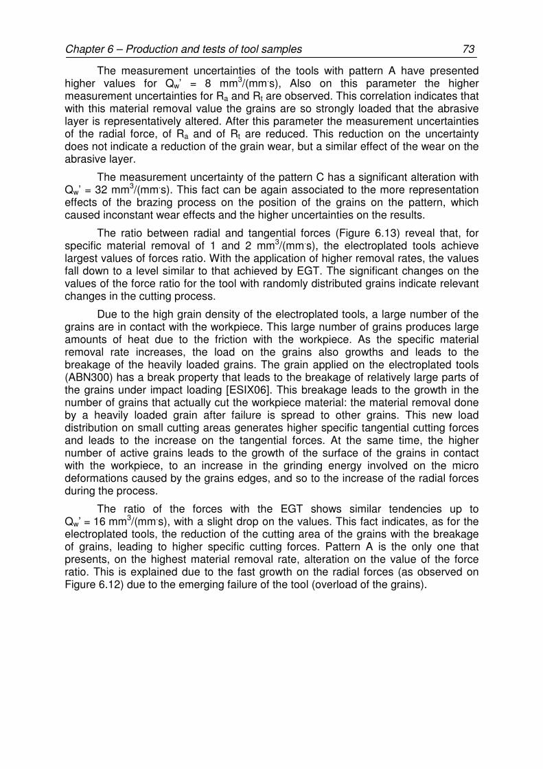
Chapter 6 – Production and tests of tool samples 73
The measurement uncertainties of the tools with pattern A have presented higher values for Qw’ = 8 mm3/(mm.s), Also on this parameter the higher measurement uncertainties for Ra and Rt are observed. This correlation indicates that with this material removal value the grains are so strongly loaded that the abrasive layer is representatively altered. After this parameter the measurement uncertainties of the radial force, of Ra and of Rt are reduced. This reduction on the uncertainty does not indicate a reduction of the grain wear, but a similar effect of the wear on the abrasive layer.
The measurement uncertainty of the pattern C has a significant alteration with Qw’ = 32 mm3/(mm.s). This fact can be again associated to the more representation effects of the brazing process on the position of the grains on the pattern, which caused inconstant wear effects and the higher uncertainties on the results.
The ratio between radial and tangential forces (Figure 6.13) reveal that, for specific material removal of 1 and 2 mm3/(mm.s), the electroplated tools achieve largest values of forces ratio. With the application of higher removal rates, the values fall down to a level similar to that achieved by EGT. The significant changes on the values of the force ratio for the tool with randomly distributed grains indicate relevant changes in the cutting process.
Due to the high grain density of the electroplated tools, a large number of the grains are in contact with the workpiece. This large number of grains produces large amounts of heat due to the friction with the workpiece. As the specific material removal rate increases, the load on the grains also growths and leads to the breakage of the heavily loaded grains. The grain applied on the electroplated tools (ABN300) has a break property that leads to the breakage of relatively large parts of the grains under impact loading [ESIX06]. This breakage leads to the growth in the number of grains that actually cut the workpiece material: the material removal done by a heavily loaded grain after failure is spread to other grains. This new load distribution on small cutting areas generates higher specific tangential cutting forces and leads to the increase on the tangential forces. At the same time, the higher number of active grains leads to the growth of the surface of the grains in contact with the workpiece, to an increase in the grinding energy involved on the micro deformations caused by the grains edges, and so to the increase of the radial forces during the process.
The ratio of the forces with the EGT shows similar tendencies up to Qw’ = 16 mm3/(mm.s), with a slight drop on the values. This fact indicates, as for the electroplated tools, the reduction of the cutting area of the grains with the breakage of grains, leading to higher specific cutting forces. Pattern A is the only one that presents, on the highest material removal rate, alteration on the value of the force ratio. This is explained due to the fast growth on the radial forces (as observed on Figure 6.12) due to the emerging failure of the tool (overload of the grains).
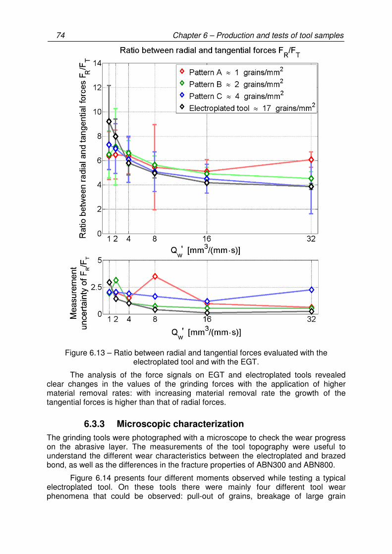
74 Chapter 6 – Production and tests of tool samples
Figure 6.13 – Ratio between radial and tangential forces evaluated with the electroplated tool and with the EGT.
The analysis of the force signals on EGT and electroplated tools revealed clear changes in the values of the grinding forces with the application of higher material removal rates: with increasing material removal rate the growth of the tangential forces is higher than that of radial forces.
6.3.3 Microscopic characterization
The grinding tools were photographed with a microscope to check the wear progress on the abrasive layer. The measurements of the tool topography were useful to understand the different wear characteristics between the electroplated and brazed bond, as well as the differences in the fracture properties of ABN300 and ABN800.
Figure 6.14 presents four different moments observed while testing a typical electroplated tool. On these tools there were mainly four different tool wear phenomena that could be observed: pull-out of grains, breakage of large grain
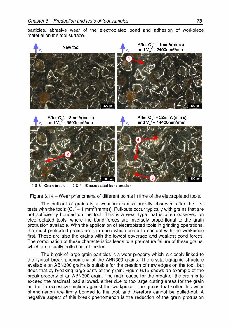
Chapter 6 – Production and tests of tool samples 75
particles, abrasive wear of the electroplated bond and adhesion of workpiece material on the tool surface.
Figure 6.14 – Wear phenomena of different points in time of the electroplated tools.
The pull-out of grains is a wear mechanism mostly observed after the first tests with the tools (Qw’ = 1 mm3/(mm.s)). Pull-outs occur typically with grains that are not sufficiently bonded on the tool. This is a wear type that is often observed on electroplated tools, where the bond forces are inversely proportional to the grain protrusion available. With the application of electroplated tools in grinding operations, the most protruded grains are the ones which come to contact with the workpiece first. These are also the grains with the lowest coverage and weakest bond forces. The combination of these characteristics leads to a premature failure of these grains, which are usually pulled out of the tool.
The break of large grain particles is a wear property which is closely linked to the typical break phenomena of the ABN300 grains. The crystallographic structure available on ABN300 grains is suitable for the creation of new edges on the tool, but does that by breaking large parts of the grain. Figure 6.15 shows an example of the break property of an ABN300 grain. The main cause for the break of the grain is to exceed the maximal load allowed, either due to too large cutting areas for the grain or due to excessive friction against the workpiece. The grains that suffer this wear phenomenon are firmly bonded to the tool, and therefore cannot be pulled-out. A negative aspect of this break phenomenon is the reduction of the grain protrusion
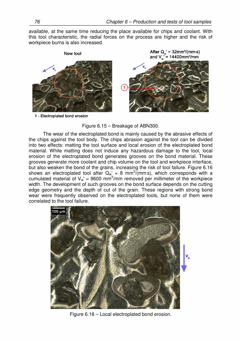
76 Chapter 6 – Production and tests of tool samples
available, at the same time reducing the place available for chips and coolant. With this tool characteristic, the radial forces on the process are higher and the risk of workpiece burns is also increased.
Figure 6.15 – Breakage of ABN300.
The wear of the electroplated bond is mainly caused by the abrasive effects of the chips against the tool body. The chips abrasion against the tool can be divided into two effects: matting the tool surface and local erosion of the electroplated bond material. While matting does not induce any hazardous damage to the tool, local erosion of the electroplated bond generates grooves on the bond material. These grooves generate more coolant and chip volume on the tool and workpiece interface, but also weaken the bond of the grains, increasing the risk of tool failure. Figure 6.16 shows an electroplated tool after Qw’ = 8 mm3/(mm.s), which corresponds with a cumulated material of Vw' = 9600 mm3/mm removed per millimeter of the workpiece width. The development of such grooves on the bond surface depends on the cutting edge geometry and the depth of cut of the grain. These regions with strong bond wear were frequently observed on the electroplated tools, but none of them were correlated to the tool failure.
Figure 6.16 – Local electroplated bond erosion.
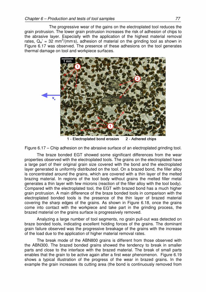
Chapter 6 – Production and tests of tool samples 77
The progressive wear of the gains on the electroplated tool reduces the grain protrusion. The lower grain protrusion increases the risk of adhesion of chips to the abrasive layer. Especially with the application of the highest material removal rates, Qw’ = 32 mm3/(mm.s), adhesion of material on the grinding tool as shown in Figure 6.17 was observed. The presence of these adhesions on the tool generates thermal damage on tool and workpiece surfaces.
Figure 6.17 – Chip adhesion on the abrasive surface of an electroplated grinding tool.
The braze bonded EGT showed some significant differences from the wear properties observed with the electroplated tools. The grains on the electroplated have a large part of their original grain size covered with the bond and the electroplated layer generated is uniformly distributed on the tool. On a brazed bond, the filler alloy is concentrated around the grains, which are covered with a thin layer of the melted brazing material. In regions of the tool body without grains the melted filler metal generates a thin layer with few microns (reaction of the filler alloy with the tool body). Compared with the electroplated tool, the EGT with brazed bond has a much higher grain protrusion. A main difference of the braze bonded tools in comparison with the electroplated bonded tools is the presence of the thin layer of brazed material covering the sharp edges of the grains. As shown in Figure 6.18, once the grains come into contact with the workpiece and take part in the grinding process, the brazed material on the grains surface is progressively removed.
Analyzing a large number of tool segments, no grain pull-out was detected on braze bonded tools, indicating excellent holding forces of the grains. The dominant grain failure observed was the progressive breakage of the grains with the increase of the load due to the application of higher material removal rates.
The break mode of the ABN800 grains is different from those observed with the ABN300. The brazed bonded grains showed the tendency to break in smaller parts and close to the interface with the brazed material. The break of small parts enables that the grain to be active again after a first wear phenomenon. Figure 6.19 shows a typical illustration of the progress of the wear in brazed grains. In the example the grain increases its cutting area (the bond is continuously removed from
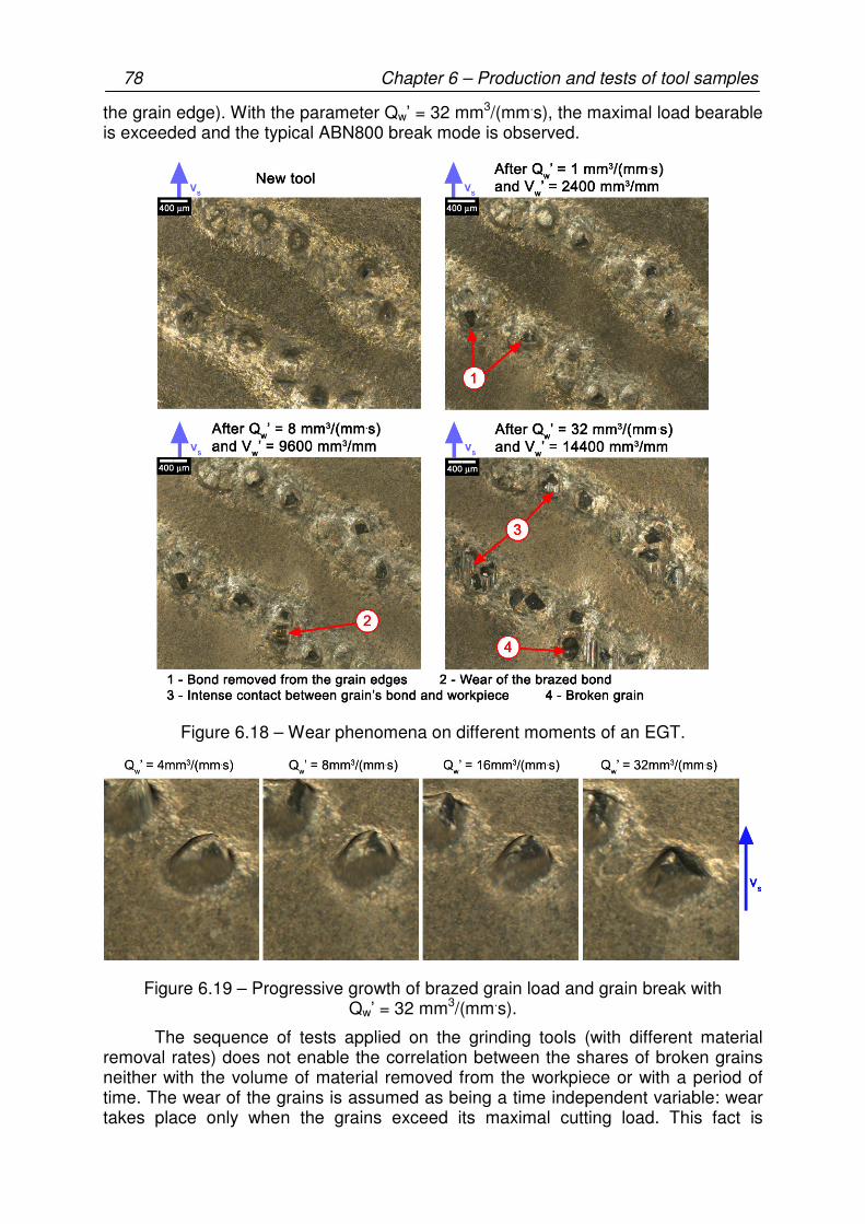
78 Chapter 6 – Production and tests of tool samples
the grain edge). With the parameter Qw’ = 32 mm3/(mm.s), the maximal load bearable is exceeded and the typical ABN800 break mode is observed.
Figure 6.18 – Wear phenomena on different moments of an EGT.
Figure 6.19 – Progressive growth of brazed grain load and grain break with Qw’ = 32 mm3/(mm.s).
The sequence of tests applied on the grinding tools (with different material removal rates) does not enable the correlation between the shares of broken grains neither with the volume of material removed from the workpiece or with a period of time. The wear of the grains is assumed as being a time independent variable: wear takes place only when the grains exceed its maximal cutting load. This fact is
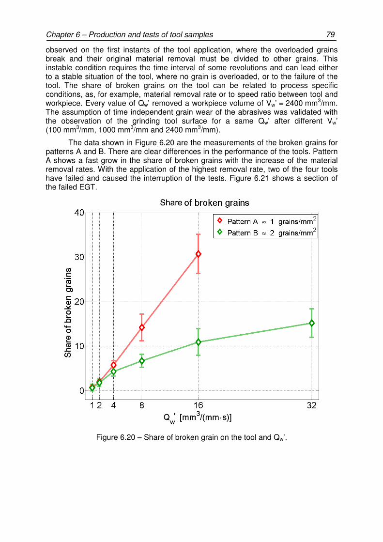
Chapter 6 – Production and tests of tool samples 79
observed on the first instants of the tool application, where the overloaded grains break and their original material removal must be divided to other grains. This instable condition requires the time interval of some revolutions and can lead either to a stable situation of the tool, where no grain is overloaded, or to the failure of the tool. The share of broken grains on the tool can be related to process specific conditions, as, for example, material removal rate or to speed ratio between tool and workpiece. Every value of Qw’ removed a workpiece volume of Vw’ = 2400 mm3/mm. The assumption of time independent grain wear of the abrasives was validated with the observation of the grinding tool surface for a same Qw’ after different Vw’ (100 mm3/mm, 1000 mm3/mm and 2400 mm3/mm).
The data shown in Figure 6.20 are the measurements of the broken grains for patterns A and B. There are clear differences in the performance of the tools. Pattern A shows a fast grow in the share of broken grains with the increase of the material removal rates. With the application of the highest removal rate, two of the four tools have failed and caused the interruption of the tests. Figure 6.21 shows a section of the failed EGT.
Figure 6.20 – Share of broken grain on the tool and Qw’.

80 Chapter 6 – Production and tests of tool samples
Figure 6.21 – Failed EGT.
The growth of the share of broken grains on the EGT with pattern B is slower than that observed on pattern A. This difference is explained by the higher share of grains available in pattern B, dividing the task of the material removal between a higher amount of gains. The evaluation of the critical load for the grains is a task that can hardly be explored only by experimental methods. Numerical methods, on the other hand, can reveal the relationship between the share of broken grains in the different patterns and the cutting parameters. The results of this analysis will be discussed in Chapter 7.
As observed on the electroplated tools, the chips have a strong abrasive action against the tool body on the EGT. Figure 6.22 shows a tool section where the progress of the abrasive wear of the chips against the tool can be observed. As observed on the electroplated tools, the erosive effect of the chips against the tool could not be pointed as a reason to the tool failure for the EGT. Especially with the brazed bond, the chemical reaction between the tool body, the filler metal and the grains guarantees high bonding forces, and the erosion of the bond material on the regions close to the grains does not create a risk of grain failure.
Figure 6.22 – Progressive wear of the brazed bond material in an EGT.
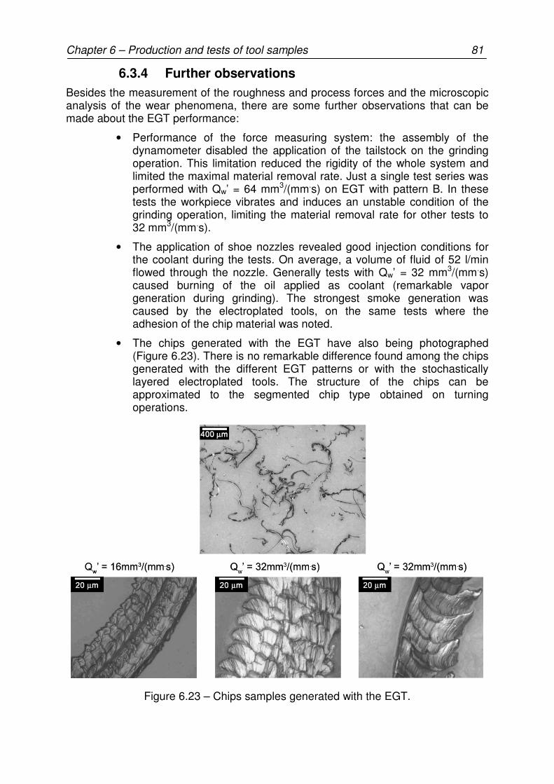
Chapter 6 – Production and tests of tool samples 81
6.3.4 Further observations
Besides the measurement of the roughness and process forces and the microscopic analysis of the wear phenomena, there are some further observations that can be made about the EGT performance:
• Performance of the force measuring system: the assembly of the dynamometer disabled the application of the tailstock on the grinding operation. This limitation reduced the rigidity of the whole system and limited the maximal material removal rate. Just a single test series was performed with Qw’ = 64 mm3/(mm.s) on EGT with pattern B. In these tests the workpiece vibrates and induces an unstable condition of the grinding operation, limiting the material removal rate for other tests to 32 mm3/(mm.s).
• The application of shoe nozzles revealed good injection conditions for the coolant during the tests. On average, a volume of fluid of 52 l/min flowed through the nozzle. Generally tests with Qw’ = 32 mm3/(mm.s) caused burning of the oil applied as coolant (remarkable vapor generation during grinding). The strongest smoke generation was caused by the electroplated tools, on the same tests where the adhesion of the chip material was noted.
• The chips generated with the EGT have also being photographed (Figure 6.23). There is no remarkable difference found among the chips generated with the different EGT patterns or with the stochastically layered electroplated tools. The structure of the chips can be approximated to the segmented chip type obtained on turning operations.
Figure 6.23 – Chips samples generated with the EGT.

82 Chapter 6 – Production and tests of tool samples
• The melting of the chips is a phenomenon observed often when too large specific grinding energies are applied or with inadequate coolant conditions of the process. The melting of the chips was not observed on none of the tool technologies tested (as the chips observed on the Figure 6.23, there is a predominance of sharp edges on the chips).
• In conventional grinding operations the chips produced are transported out of the machine structure with the coolant. During the grinding tests, the chips produced with the EGT tend to form agglomerates, which are not efficiently removed with the coolant from the machine. On numerous occasions the intervention of the machine operator was required to remove the chips from the blocked coolant filters in the machine outlets.
6.4 Conclusion of the experiments
The results of the experiments discussed in this chapter were useful to understand the tools’ performance during the grinding process. Analysis of roughness, of force measurements and of microscopic observation of the tools enables to draw the following conclusions:
• The wear of the grains has a large effect on the roughness achieved on the workpiece. With the progress of the share of grains broken, the number of grains acting on the grinding process grows and the machined workpiece becomes smoother.
• Electroplated tools exert higher tangential forces on the workpiece. These tools achieved also the smoothest workpiece surfaces. Both of these effects reflect the higher number of grains in contact with the workpiece on the electroplated tool compared to the EGT.
• The radial forces revealed similar progress for all tools tested up to the parameter of Qw’ = 16 mm3/(mm.s). On the next grinding parameter, Qw’ = 32 mm3/(mm.s), pattern A suffered an overload. The failure of the tool was associated with the continuous increase on the number of broken grains with the increase of Qw’.
• The ratio between normal and tangential forces revealed very unfavorable grinding conditions with the electroplated tool on the first two grinding conditions tested – Qw’ = 1 and 2 mm3/(mm.s). A small share of grains is accountable for the effective removal of the workpiece material, while a large number of grains act only generating friction with the workpiece. With higher values of Qw’ there is a significant alteration on the ratio between radial and cutting forces. This process alteration is associated to the wear (pull-out and break) of the ABN300 and lead to force behavior with similar values as those measured with the EGT.
• Both bonding technologies have shown strong abrasive erosion of the bond material due to the friction of the chips against the tool body. This effect may bring advantages, such as the increase of the volume available for coolant and chips in the grinding gap, but may also weaken the fixation of the grains (especially on the electroplated bond). Nevertheless, on none of the tools tested (brazed EGT or electroplated)
Chapter 6 – Production and tests of tool samples 83
this effect can be associated to the pull out-of grains or to the tool failure.
• ABN300 and ABN800 presented different wear properties. ABN300 tends to break in larger parts once it is overloaded and not be active again after it has been broken (the remaining grain is lower or on the same level of the bond). ABN800, on the other hand, tends to break in smaller parts and to be active again in the process.
• While electroplated bond allows the pull-out of grains from the bonding matrix, on none of the brazed EGT this phenomenon was observed, indicating the much better bonding properties achieved with the brazed bond.
• The reduction of the grain protrusion with the progressive wear of the electroplated tools causes the adhesion of chip to the grinding tool. This effect was not observed on any of the brazed EGT tested.
• On the last parameter tested, pattern A has a significant change on the value of the forces ratio. This effect is contrary to the tendency observed with the other EGT patterns and with the electroplated tools and indicates an eminent tool failure.
• On the series of tools tested, two of the four tools with pattern A have failed during the grinding tests. These tools failed due to the overload of the grains on the tool. A large share of broken grains was noticed on the tool (over 30% o the grains) with the analysis of the microscopic abrasive profile after the tests with Qw’ = 16 mm3/(mm.s). The strong reduction on the number of grains created regions along the width of the tool where just some few grains are accountable for the material removal. A further increase on Qw’ (to 32 mm3/(mm.s)) lead the grain pattern to an overloaded condition which resulted on the failure of the tools. These experimental results indicate the typical failure development on EGT. The correct interpretation of the results requires the application of numerical methods to evaluate the critical load which causes the break of the grains.
• Analysis of the share of broken grains revealed different behaviors for the different patterns. While pattern A had a constant and rapid increase of the share of grains broken with the higher specific material removal rates, the tools with patterns B and C have a slower rate of increase of grain breakage. The data available should be evaluated also with the numerical tool, aiming to understand the correlation between the maximal grains load with the values of Qw’ applied on the tool.
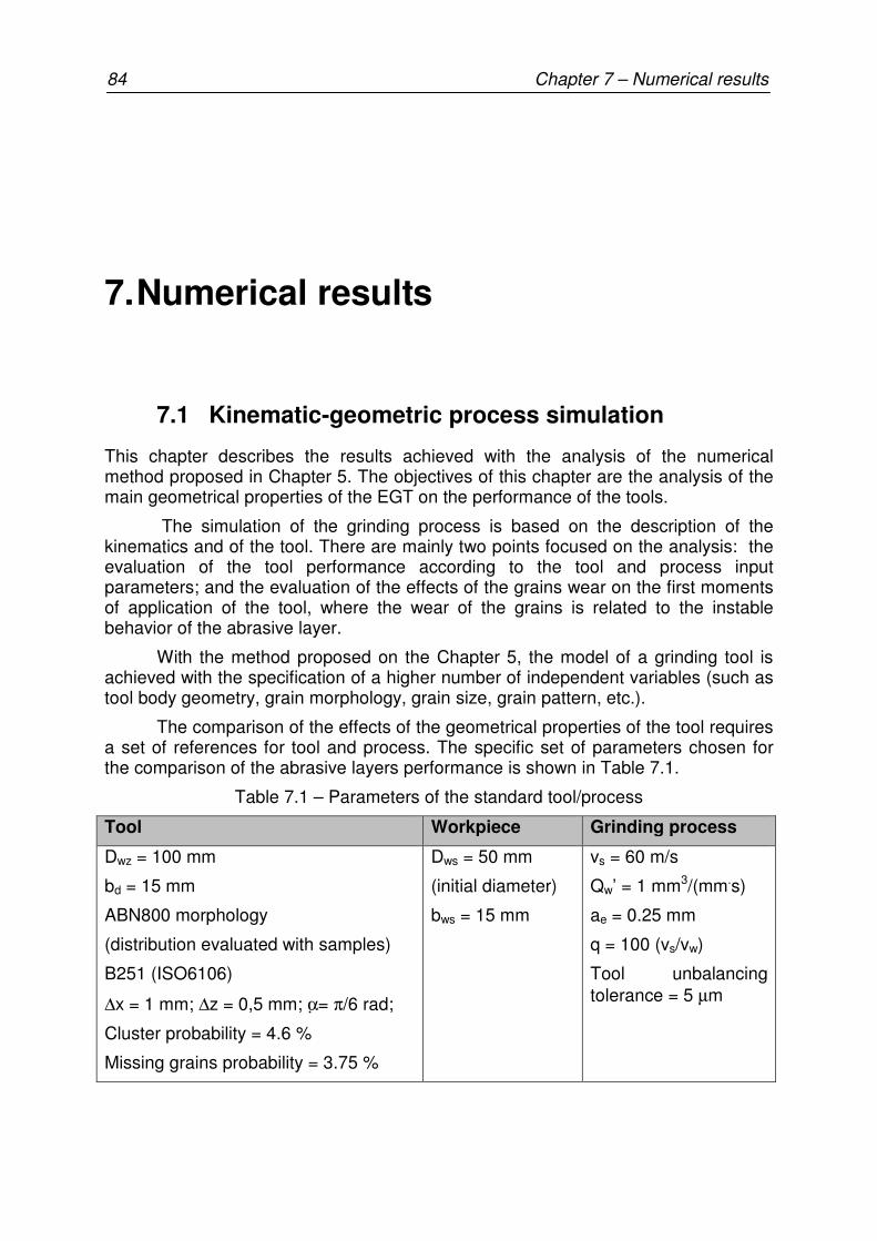
84 Chapter 7 – Numerical results
7. Numerical results
7.1 Kinematic-geometric process simulation
This chapter describes the results achieved with the analysis of the numerical method proposed in Chapter 5. The objectives of this chapter are the analysis of the main geometrical properties of the EGT on the performance of the tools.
The simulation of the grinding process is based on the description of the kinematics and of the tool. There are mainly two points focused on the analysis: the evaluation of the tool performance according to the tool and process input parameters; and the evaluation of the effects of the grains wear on the first moments of application of the tool, where the wear of the grains is related to the instable behavior of the abrasive layer.
With the method proposed on the Chapter 5, the model of a grinding tool is achieved with the specification of a higher number of independent variables (such as tool body geometry, grain morphology, grain size, grain pattern, etc.).
The comparison of the effects of the geometrical properties of the tool requires a set of references for tool and process. The specific set of parameters chosen for the comparison of the abrasive layers performance is shown in Table 7.1.
Table 7.1 – Parameters of the standard tool/process
Tool Workpiece Grinding process
Dwz = 100 mm
bd = 15 mm
ABN800 morphology
(distribution evaluated with samples)
B251 (ISO6106)
∆x = 1 mm; ∆z = 0,5 mm; α= π/6 rad;
Cluster probability = 4.6 %
Missing grains probability = 3.75 %
Dws = 50 mm
(initial diameter)
bws = 15 mm
vs = 60 m/s
Qw’ = 1 mm3/(mm.s)
ae = 0.25 mm
q = 100 (vs/vw)
Tool unbalancing tolerance = 5 µm
Chapter 7 – Numerical results 85
The morphology distribution of the ABN800 grains was obtained with the analysis of a large number of grain samples. The grains observed were classified in three groups (Table 2). In group 2, corresponding to the morphologies between tetrahedron and octahedron, the grains are uniformly distributed between the two geometric limits, as shown on chapter 5 (Figure 5.5).
Table 7.2 – ABN800 morphology
GROUP 1 Tetrahedron
GROUP 2 Between tetrahedron
and octahedron
GROUP 3 Octahedron
30 % 60 % 10 %
Measurements of samples revealed that the grain size distribution (equivalent to the circle which circumscribes the grain geometry) can be approached to a Gaussian distribution. For a confidence level of 95 % the grain size limits were coincident to the limits set by the norm ISO 6106.
The term protrusion will be often applied on this chapter for the evaluation of the simulation results. The protrusion of a grain corresponds to the position of the highest cutting edge of the grain, measured orthogonal to the tool body, without considering the presence of the bond material. The protrusion of each grain is an index of the distribution of the active cutting edges on the tool. During operation of the tool, the most protruded grains are the ones accountable for the material removal. Figure 7.1 shows two representations of the results achieved while numerically modeling a grinding tool with the parameters set on the Table 7.1: the Abbott-Firestone curve and the distribution of the amount edges according to the protrusion.
The distribution of the protrusions of the grains has a similar form observed on normal distributions. An interesting point is the evaluation of the average of the protrusion distribution has an offset from the average grain size expected: as shown in Figure 7.1, for ABN800 B251, the average grain size is 250 µm, but the distribution indicates an average height of the grain edges of 300 µm. This offset on the average is mainly caused by the morphology of the grains (stochastically oriented at the tool surface) and by the sieving tolerances while sieving the grains.
With the simulation of the cutting process, it is possible to evaluate the distribution of the grain edges that are active in the process. Figure 7.2 shows an example of results evaluated with the modeled tool on specific process conditions. Three characteristics are illustrated: the distribution of the grain edges available on the tool, the distribution of the edges of the active grains and the distribution of the intersections limits of the grains profile with the workpiece.

86 Chapter 7 – Numerical results
Figure 7.1 – Distribution of the highest cutting edge of the grains with a tool model designed with ABN800 B251.
Figure 7.2 – Distribution of the grain edges, of the intersection limits of the grain with the workpiece and of the edge of the active grains.
The relationship between the three distributions is a relevant factor in the evaluation of the tool performance. Even on EGTs, which have a much lower grain density than conventional electroplated grinding tools, the share of grains which participate of the grinding process is just a small proportion of the total number of grains available on the tool. These “active grains” are, as expected, the most protruded. The position of the intersections limits of the active grain profiles with the workpiece evidence the load on the grains and gives relevant information about the protrusion remaining on the tool. Figure 7.2 shows a typical relationship of these three distributions found on the EGT. The mean of the distribution of the intersection limits is slightly shifted to the left of the distribution of the active grain edges. This allocation of the distributions is typical for large cutting areas of the grains, where the limits of the intersections are shifted from the edge of the grains. With small cutting
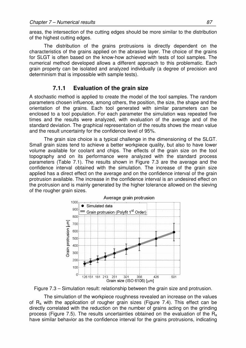
Chapter 7 – Numerical results 87
areas, the intersection of the cutting edges should be more similar to the distribution of the highest cutting edges.
The distribution of the grains protrusions is directly dependent on the characteristics of the grains applied on the abrasive layer. The choice of the grains for SLGT is often based on the know-how achieved with tests of tool samples. The numerical method developed allows a different approach to this problematic. Each grain property can be isolated and analyzed individually (a degree of precision and determinism that is impossible with sample tests).
7.1.1 Evaluation of the grain size
A stochastic method is applied to create the model of the tool samples. The random parameters chosen influence, among others, the position, the size, the shape and the orientation of the grains. Each tool generated with similar parameters can be enclosed to a tool population. For each parameter the simulation was repeated five times and the results were analyzed, with evaluation of the average and of the standard deviation. The graphical representation of the results shows the mean value and the result uncertainty for the confidence level of 95%.
The grain size choice is a typical challenge in the dimensioning of the SLGT. Small grain sizes tend to achieve a better workpiece quality, but also to have lower volume available for coolant and chips. The effects of the grain size on the tool topography and on its performance were analyzed with the standard process parameters (Table 7.1). The results shown in Figure 7.3 are the average and the confidence interval obtained with the simulation. The increase of the grain size applied has a direct effect on the average and on the confidence interval of the grain protrusion available. The increase in the confidence interval is an undesired effect on the protrusion and is mainly generated by the higher tolerance allowed on the sieving of the rougher grain sizes.
Figure 7.3 – Simulation result: relationship between the grain size and protrusion.
The simulation of the workpiece roughness revealed an increase on the values of Ra with the application of rougher grain sizes (Figure 7.4). This effect can be directly correlated with the reduction on the number of grains acting on the grinding process (Figure 7.5). The results uncertainties obtained on the evaluation of the Ra have similar behavior as the confidence interval for the grains protrusions, indicating
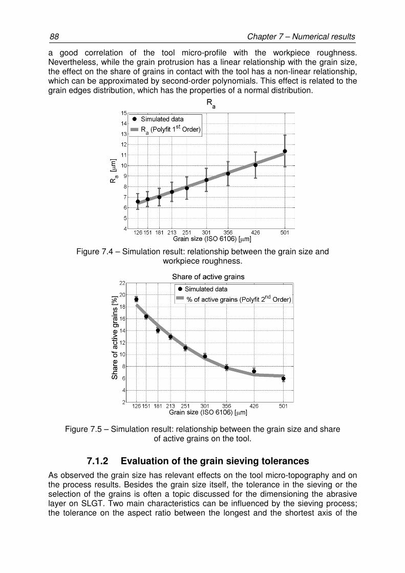
88 Chapter 7 – Numerical results
a good correlation of the tool micro-profile with the workpiece roughness. Nevertheless, while the grain protrusion has a linear relationship with the grain size, the effect on the share of grains in contact with the tool has a non-linear relationship, which can be approximated by second-order polynomials. This effect is related to the grain edges distribution, which has the properties of a normal distribution.
Figure 7.4 – Simulation result: relationship between the grain size and workpiece roughness.
Figure 7.5 – Simulation result: relationship between the grain size and share of active grains on the tool.
7.1.2 Evaluation of the grain sieving tolerances
As observed the grain size has relevant effects on the tool micro-topography and on the process results. Besides the grain size itself, the tolerance in the sieving or the selection of the grains is often a topic discussed for the dimensioning the abrasive layer on SLGT. Two main characteristics can be influenced by the sieving process; the tolerance on the aspect ratio between the longest and the shortest axis of the
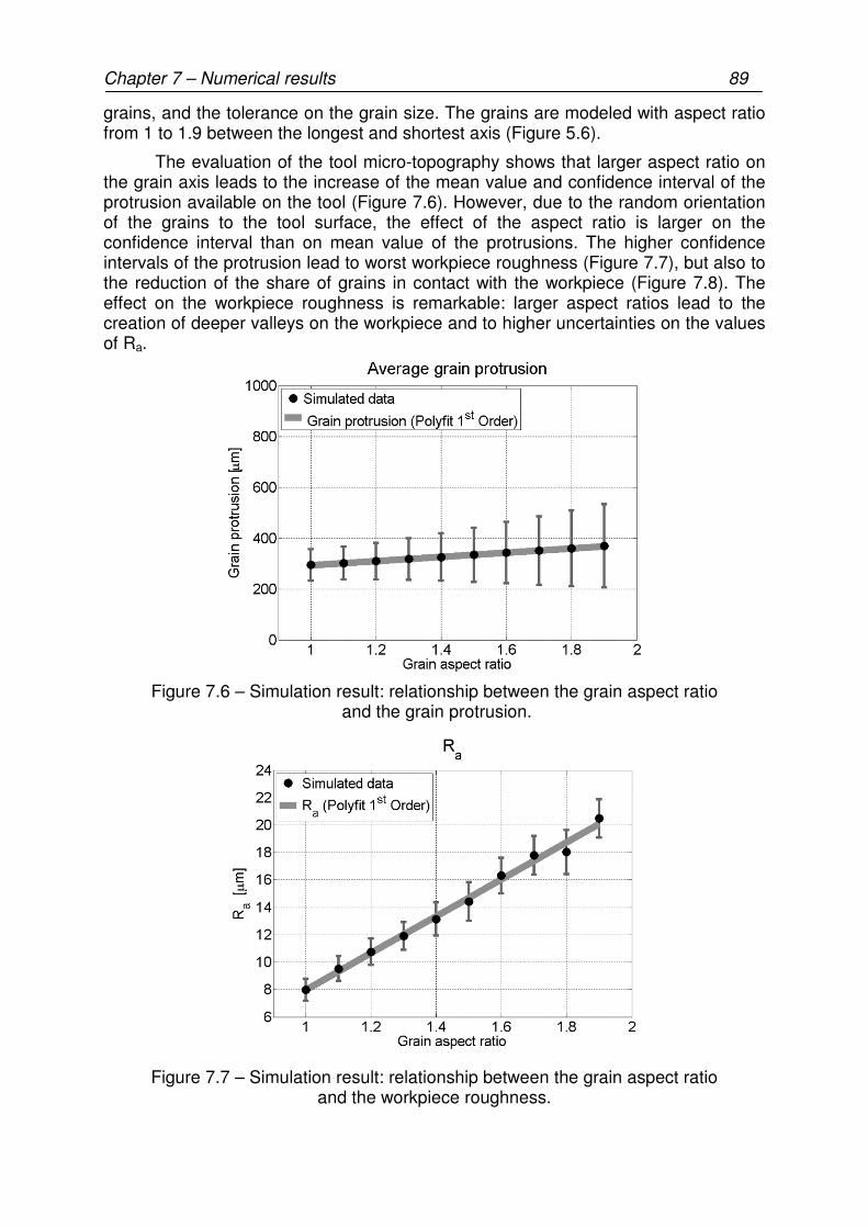
Chapter 7 – Numerical results 89
grains, and the tolerance on the grain size. The grains are modeled with aspect ratio from 1 to 1.9 between the longest and shortest axis (Figure 5.6).
The evaluation of the tool micro-topography shows that larger aspect ratio on the grain axis leads to the increase of the mean value and confidence interval of the protrusion available on the tool (Figure 7.6). However, due to the random orientation of the grains to the tool surface, the effect of the aspect ratio is larger on the confidence interval than on mean value of the protrusions. The higher confidence intervals of the protrusion lead to worst workpiece roughness (Figure 7.7), but also to the reduction of the share of grains in contact with the workpiece (Figure 7.8). The effect on the workpiece roughness is remarkable: larger aspect ratios lead to the creation of deeper valleys on the workpiece and to higher uncertainties on the values of Ra.
Figure 7.6 – Simulation result: relationship between the grain aspect ratio and the grain protrusion.
Figure 7.7 – Simulation result: relationship between the grain aspect ratio and the workpiece roughness.
90 Chapter 7 – Numerical results
Figure 7.8 – Simulation result: relationship between the grain aspect ratio and the share of active grains on the tool.
Contrariwise to the increase of the grain size, the larger aspect ratios have direct effects on the form of the cutting edges of the grains and have more representative effects in the workpiece roughness. Another method to alter the confidence interval of the protrusion with the grain properties would be to assume tighter limits to the sieving process. The ISO 6106 stipulates the sieving limits for each grain size. Considering the standard grain size for the simulation of B251, according to the ISO 6106, the sieving limits are 213 µm and 271 µm. Simulations were performed to investigate the effects of the reduction of this interval down to the impracticable value of 1µm (grain size between 250 µm and 251 µm). The decision to use fine-sieved grains (in extreme cases manually selected grains) is often made while trying to apply the grinding tool to achieve low surface roughness. As shown in the analysis done (Figure 7.9), there are slight changes in the average and in the confidence interval of the grains protrusions with fine sieved grains. These results reveal a dominant effect of the morphology and orientation of the grains on the tool surface over the sieving tolerance. As the grains are not orientated, but randomly placed on the tool surface, the position of the cutting edge is just slightly affected by fine-sieved grains.
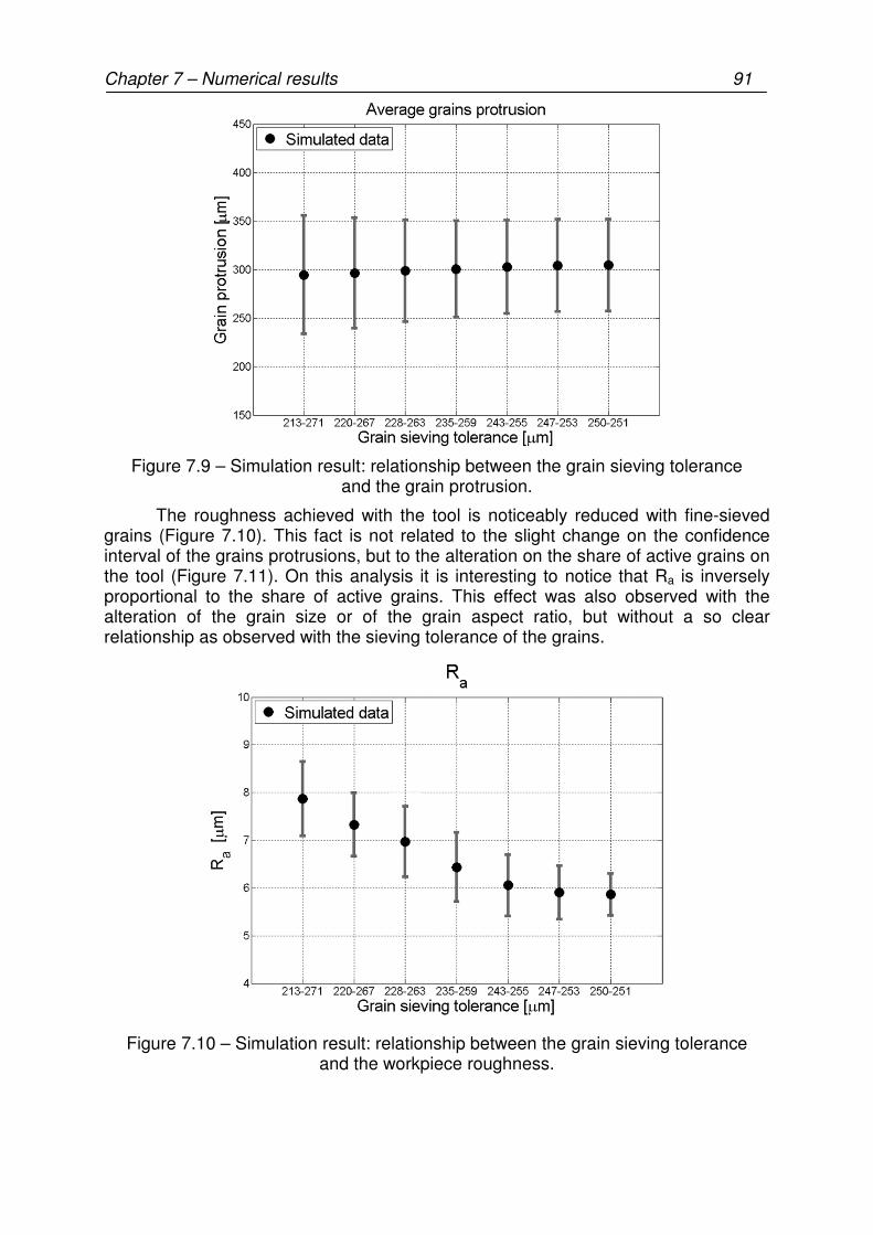
Chapter 7 – Numerical results 91
Figure 7.9 – Simulation result: relationship between the grain sieving tolerance and the grain protrusion.
The roughness achieved with the tool is noticeably reduced with fine-sieved grains (Figure 7.10). This fact is not related to the slight change on the confidence interval of the grains protrusions, but to the alteration on the share of active grains on the tool (Figure 7.11). On this analysis it is interesting to notice that Ra is inversely proportional to the share of active grains. This effect was also observed with the alteration of the grain size or of the grain aspect ratio, but without a so clear relationship as observed with the sieving tolerance of the grains.
Figure 7.10 – Simulation result: relationship between the grain sieving tolerance and the workpiece roughness.
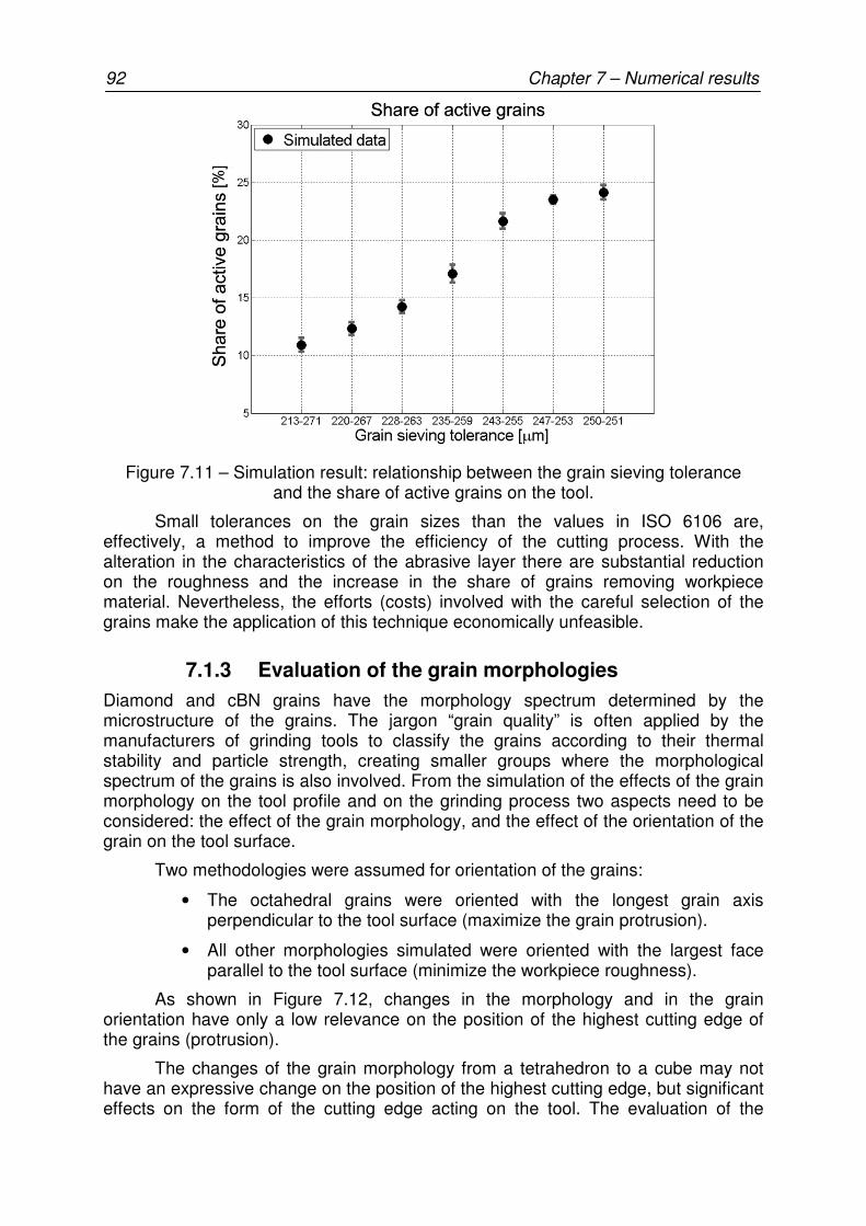
92 Chapter 7 – Numerical results
Figure 7.11 – Simulation result: relationship between the grain sieving tolerance and the share of active grains on the tool.
Small tolerances on the grain sizes than the values in ISO 6106 are, effectively, a method to improve the efficiency of the cutting process. With the alteration in the characteristics of the abrasive layer there are substantial reduction on the roughness and the increase in the share of grains removing workpiece material. Nevertheless, the efforts (costs) involved with the careful selection of the grains make the application of this technique economically unfeasible.
7.1.3 Evaluation of the grain morphologies
Diamond and cBN grains have the morphology spectrum determined by the microstructure of the grains. The jargon “grain quality” is often applied by the manufacturers of grinding tools to classify the grains according to their thermal stability and particle strength, creating smaller groups where the morphological spectrum of the grains is also involved. From the simulation of the effects of the grain morphology on the tool profile and on the grinding process two aspects need to be considered: the effect of the grain morphology, and the effect of the orientation of the grain on the tool surface.
Two methodologies were assumed for orientation of the grains:
• The octahedral grains were oriented with the longest grain axis perpendicular to the tool surface (maximize the grain protrusion).
• All other morphologies simulated were oriented with the largest face parallel to the tool surface (minimize the workpiece roughness).
As shown in Figure 7.12, changes in the morphology and in the grain orientation have only a low relevance on the position of the highest cutting edge of the grains (protrusion).
The changes of the grain morphology from a tetrahedron to a cube may not have an expressive change on the position of the highest cutting edge, but significant effects on the form of the cutting edge acting on the tool. The evaluation of the

Chapter 7 – Numerical results 93
workpiece roughness (Figure 7.13) and of the share of active grains on the tool (Figure 7.14) elucidates these changes in the tool profile.
Figure 7.12 – Simulation result: relationship between the grain morphology, its orientation and the grain protrusion.
Figure 7.13 – Simulation result: relationship between the grain morphology, its orientation and the workpiece roughness.

94 Chapter 7 – Numerical results
Figure 7.14 – Simulation result: relationship between the grain morphology, its orientation and the share of active grains on the tool.
The following conclusions can be drawn over the simulation results:
• “Blocky” grain morphology (shapes between cube and octahedron and between octahedron and tetrahedron) experience no significant alteration on the process results with the orientation of the grains.
• The effects of the grain orientation can be clearly noticed to the “cubic” grain morphology. In spite of having no change in the share of active grains on the tool, the changes in the cutting edges geometry enable the achievement of better surface qualities.
• The orientation of the “octahedral” grains maximizes and homogenizes the grain protrusion (smaller confidence interval), increasing the share of grains in contact with the workpiece. The alteration on the form of the cutting edge (sharper) should lead to worst workpiece roughness, but this effect is not noticed due to the higher share of grains cutting the workpiece.
• The orientation of the “tetrahedral” grains allows a much more homogeneous distribution of the cutting edges on the abrasive layer. The share of grains acting on the grinding process is almost duplicated. Nevertheless, the workpiece roughness is only insignificantly altered. The better distribution of grain edges allows an increase on the share of grains acting in the process, but the grains that have become active have only small cutting areas, so that they do not participate significantly in the grinding process and so do not contribute significantly to the amelioration of the workpiece roughness.
• The effects of the orientation on a complex grain distribution as observed with the ABN800 grains have negative impact on the process. The orientation of the largely different grain geometries has reduced the share of grains in contact with the workpiece (preferentially the octahedral grains have contact with the workpiece).
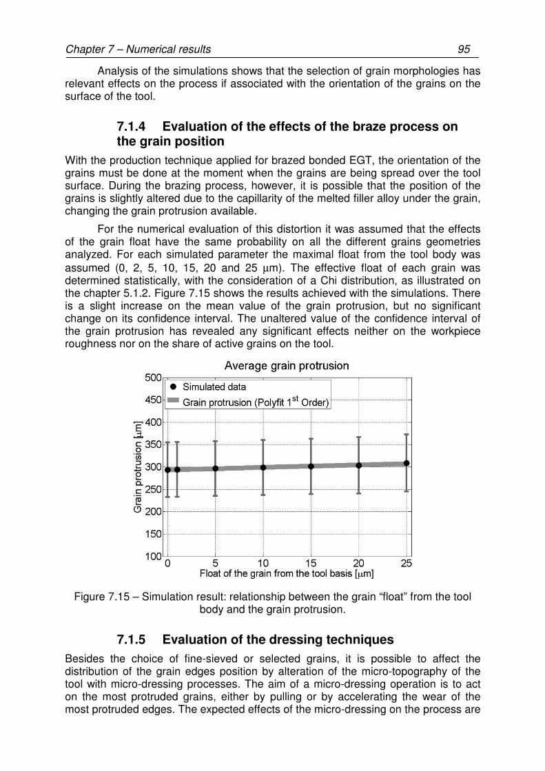
Chapter 7 – Numerical results 95
Analysis of the simulations shows that the selection of grain morphologies has relevant effects on the process if associated with the orientation of the grains on the surface of the tool.
7.1.4 Evaluation of the effects of the braze process on the grain position
With the production technique applied for brazed bonded EGT, the orientation of the grains must be done at the moment when the grains are being spread over the tool surface. During the brazing process, however, it is possible that the position of the grains is slightly altered due to the capillarity of the melted filler alloy under the grain, changing the grain protrusion available.
For the numerical evaluation of this distortion it was assumed that the effects of the grain float have the same probability on all the different grains geometries analyzed. For each simulated parameter the maximal float from the tool body was assumed (0, 2, 5, 10, 15, 20 and 25 µm). The effective float of each grain was determined statistically, with the consideration of a Chi distribution, as illustrated on the chapter 5.1.2. Figure 7.15 shows the results achieved with the simulations. There is a slight increase on the mean value of the grain protrusion, but no significant change on its confidence interval. The unaltered value of the confidence interval of the grain protrusion has revealed any significant effects neither on the workpiece roughness nor on the share of active grains on the tool.
Figure 7.15 – Simulation result: relationship between the grain “float” from the tool body and the grain protrusion.
7.1.5 Evaluation of the dressing techniques
Besides the choice of fine-sieved or selected grains, it is possible to affect the distribution of the grain edges position by alteration of the micro-topography of the tool with micro-dressing processes. The aim of a micro-dressing operation is to act on the most protruded grains, either by pulling or by accelerating the wear of the most protruded edges. The expected effects of the micro-dressing on the process are
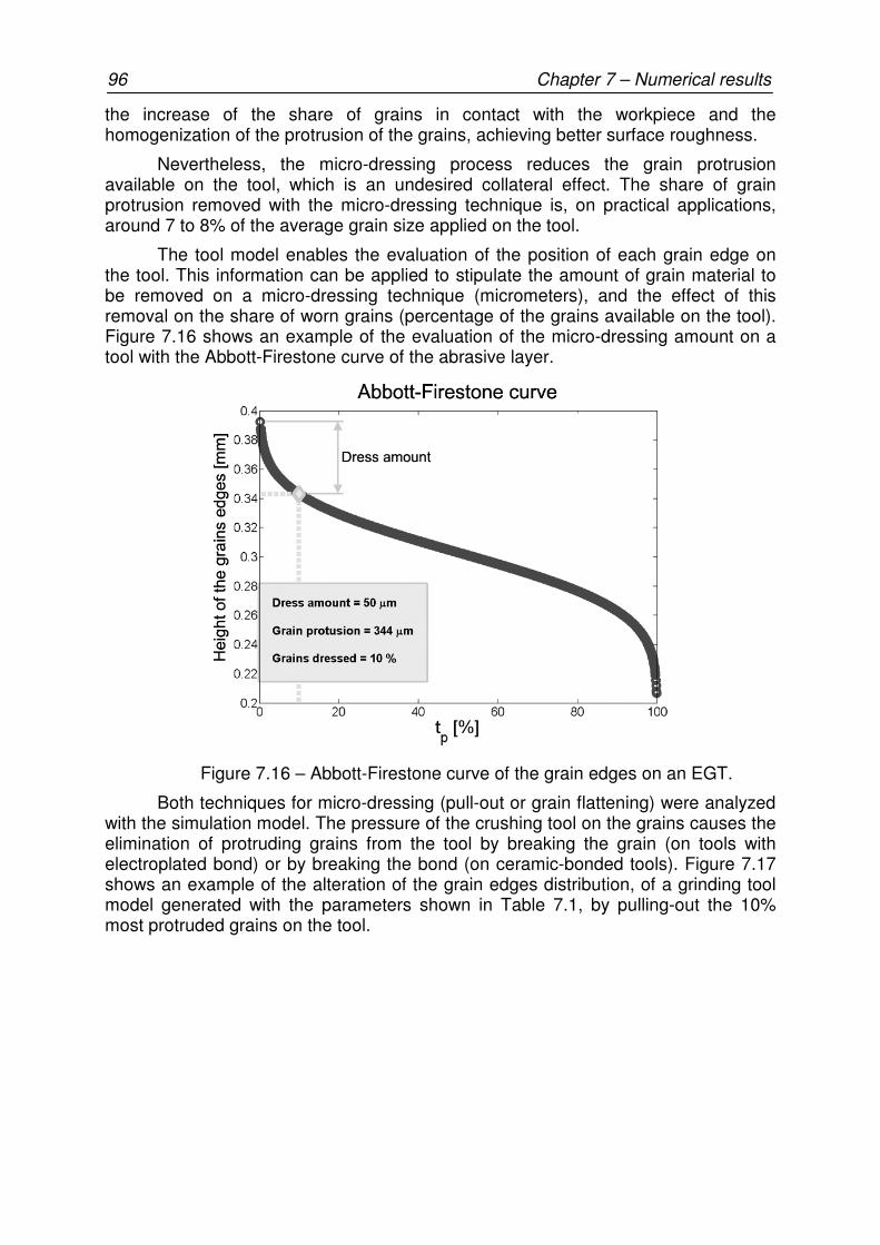
96 Chapter 7 – Numerical results
the increase of the share of grains in contact with the workpiece and the homogenization of the protrusion of the grains, achieving better surface roughness.
Nevertheless, the micro-dressing process reduces the grain protrusion available on the tool, which is an undesired collateral effect. The share of grain protrusion removed with the micro-dressing technique is, on practical applications, around 7 to 8% of the average grain size applied on the tool.
The tool model enables the evaluation of the position of each grain edge on the tool. This information can be applied to stipulate the amount of grain material to be removed on a micro-dressing technique (micrometers), and the effect of this removal on the share of worn grains (percentage of the grains available on the tool). Figure 7.16 shows an example of the evaluation of the micro-dressing amount on a tool with the Abbott-Firestone curve of the abrasive layer.
Figure 7.16 – Abbott-Firestone curve of the grain edges on an EGT.
Both techniques for micro-dressing (pull-out or grain flattening) were analyzed with the simulation model. The pressure of the crushing tool on the grains causes the elimination of protruding grains from the tool by breaking the grain (on tools with electroplated bond) or by breaking the bond (on ceramic-bonded tools). Figure 7.17 shows an example of the alteration of the grain edges distribution, of a grinding tool model generated with the parameters shown in Table 7.1, by pulling-out the 10% most protruded grains on the tool.

Chapter 7 – Numerical results 97
Figure 7.17 – Alteration of the grain edge distribution due to the pull-out of 10% of the most protruded grains.
The results of the simulations shown in Figure 7.18 reveal the less representative effect of the micro-dressing with the pull-out technique on the average than on the confidence interval of the grain protrusion.
Figure 7.18 – Simulation result: relationship between the amount of micro-dressed grains (pull-out) and the grain protrusion.
The results shown in Figure 7.19 and Figure 7.20 indicate different effects on the process. The values of Ra are more significantly altered with the pull-out of about 10% of the most protruded grains. Nevertheless, the share of active grains keeps growing up to micro-dressing amounts of 35% of the most protruded grains, where almost 18% of the grains are active on the grinding process. These results indicate that the growth in the number of grains active on the tool has more relevant effects
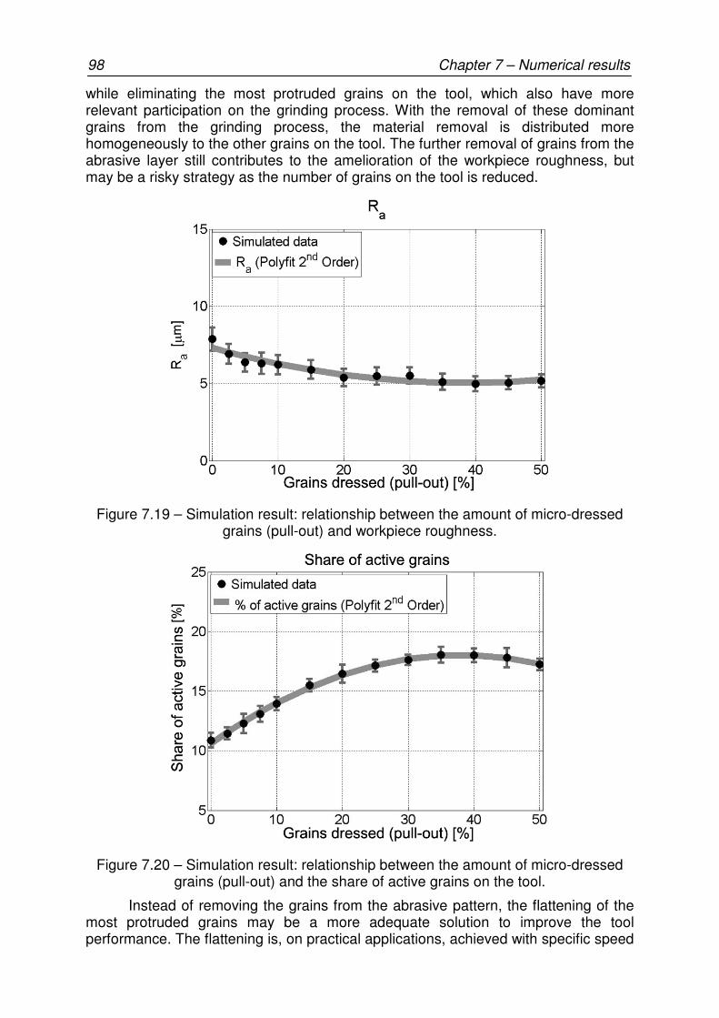
98 Chapter 7 – Numerical results
while eliminating the most protruded grains on the tool, which also have more relevant participation on the grinding process. With the removal of these dominant grains from the grinding process, the material removal is distributed more homogeneously to the other grains on the tool. The further removal of grains from the abrasive layer still contributes to the amelioration of the workpiece roughness, but may be a risky strategy as the number of grains on the tool is reduced.
Figure 7.19 – Simulation result: relationship between the amount of micro-dressed grains (pull-out) and workpiece roughness.
Figure 7.20 – Simulation result: relationship between the amount of micro-dressed grains (pull-out) and the share of active grains on the tool.
Instead of removing the grains from the abrasive pattern, the flattening of the most protruded grains may be a more adequate solution to improve the tool performance. The flattening is, on practical applications, achieved with specific speed
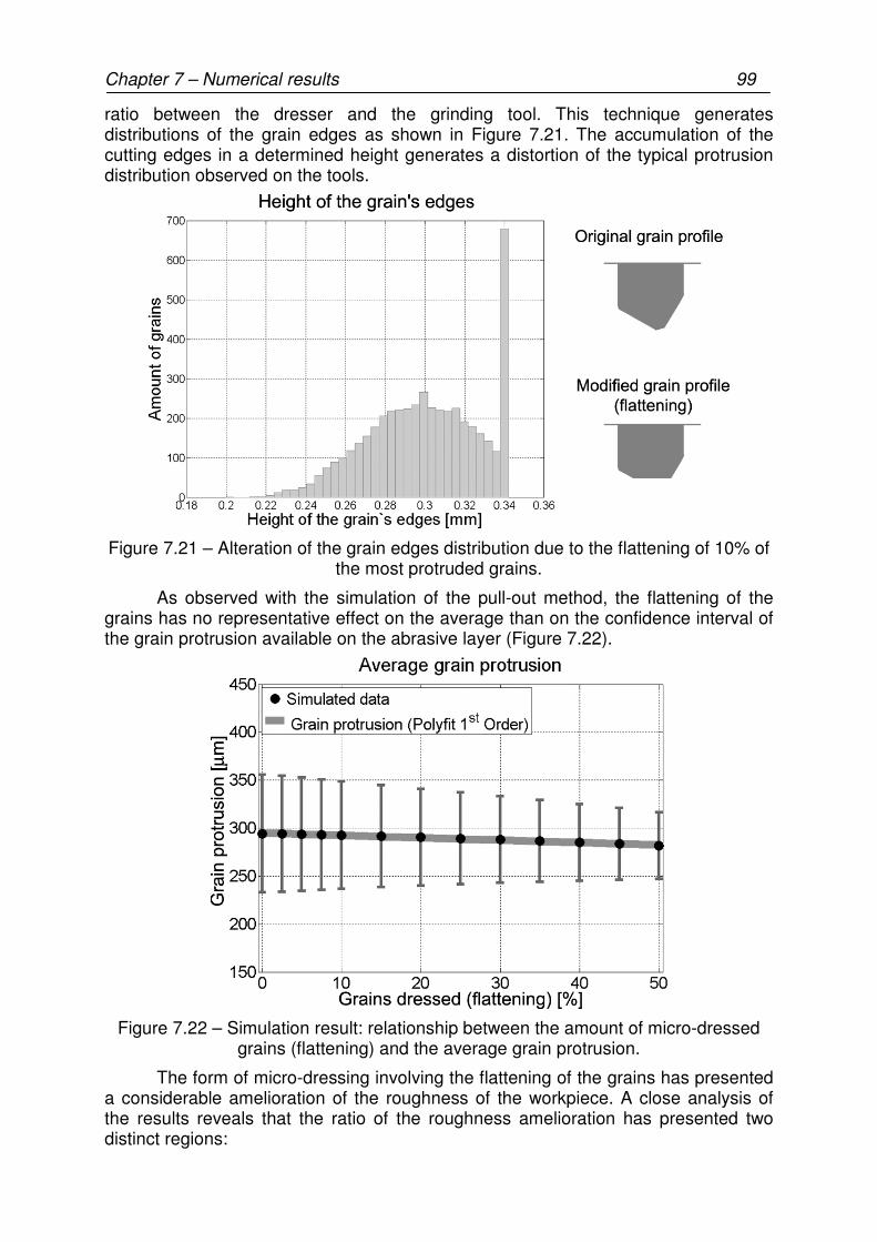
Chapter 7 – Numerical results 99
ratio between the dresser and the grinding tool. This technique generates distributions of the grain edges as shown in Figure 7.21. The accumulation of the cutting edges in a determined height generates a distortion of the typical protrusion distribution observed on the tools.
Figure 7.21 – Alteration of the grain edges distribution due to the flattening of 10% of the most protruded grains.
As observed with the simulation of the pull-out method, the flattening of the grains has no representative effect on the average than on the confidence interval of the grain protrusion available on the abrasive layer (Figure 7.22).
Figure 7.22 – Simulation result: relationship between the amount of micro-dressed grains (flattening) and the average grain protrusion.
The form of micro-dressing involving the flattening of the grains has presented a considerable amelioration of the roughness of the workpiece. A close analysis of the results reveals that the ratio of the roughness amelioration has presented two distinct regions:
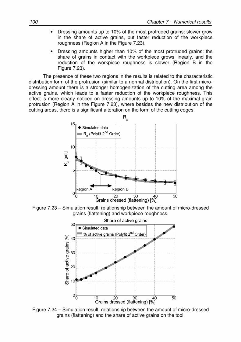
100 Chapter 7 – Numerical results
• Dressing amounts up to 10% of the most protruded grains: slower grow in the share of active grains, but faster reduction of the workpiece roughness (Region A in the Figure 7.23).
• Dressing amounts higher than 10% of the most protruded grains: the share of grains in contact with the workpiece grows linearly, and the reduction of the workpiece roughness is slower (Region B in the Figure 7.23).
The presence of these two regions in the results is related to the characteristic distribution form of the protrusion (similar to a normal distribution). On the first micro-dressing amount there is a stronger homogenization of the cutting area among the active grains, which leads to a faster reduction of the workpiece roughness. This effect is more clearly noticed on dressing amounts up to 10% of the maximal grain protrusion (Region A in the Figure 7.23), where besides the new distribution of the cutting areas, there is a significant alteration on the form of the cutting edges.
Figure 7.23 – Simulation result: relationship between the amount of micro-dressed grains (flattening) and workpiece roughness.
Figure 7.24 – Simulation result: relationship between the amount of micro-dressed grains (flattening) and the share of active grains on the tool.
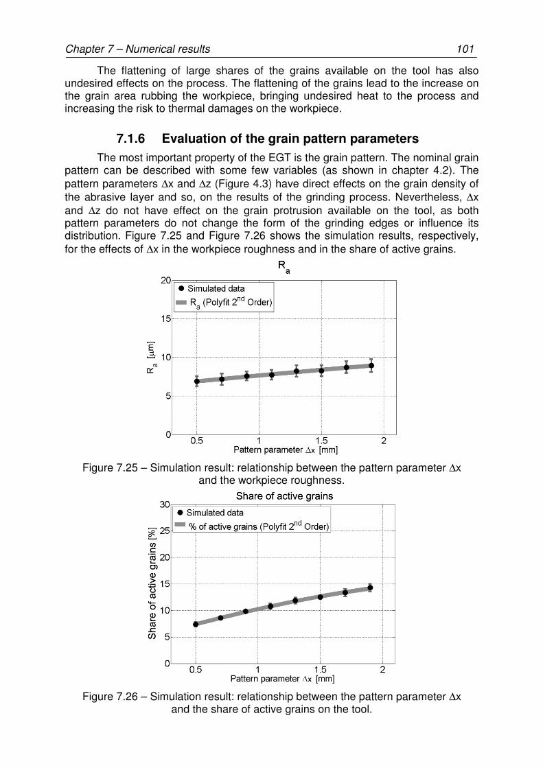
Chapter 7 – Numerical results 101
The flattening of large shares of the grains available on the tool has also undesired effects on the process. The flattening of the grains lead to the increase on the grain area rubbing the workpiece, bringing undesired heat to the process and increasing the risk to thermal damages on the workpiece.
7.1.6 Evaluation of the grain pattern parameters
The most important property of the EGT is the grain pattern. The nominal grain pattern can be described with some few variables (as shown in chapter 4.2). The pattern parameters ∆x and ∆z (Figure 4.3) have direct effects on the grain density of the abrasive layer and so, on the results of the grinding process. Nevertheless, ∆x and ∆z do not have effect on the grain protrusion available on the tool, as both pattern parameters do not change the form of the grinding edges or influence its distribution. Figure 7.25 and Figure 7.26 shows the simulation results, respectively, for the effects of ∆x in the workpiece roughness and in the share of active grains.
Figure 7.25 – Simulation result: relationship between the pattern parameter ∆x and the workpiece roughness.
Figure 7.26 – Simulation result: relationship between the pattern parameter ∆x and the share of active grains on the tool.
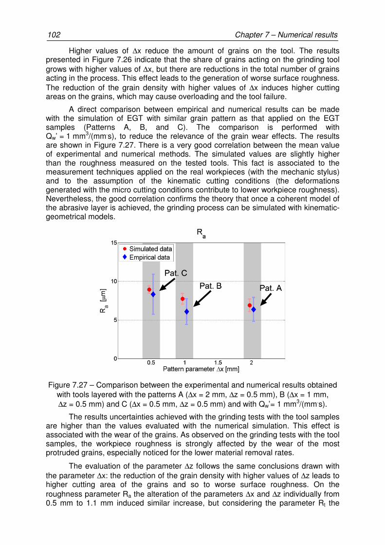
102 Chapter 7 – Numerical results
Higher values of ∆x reduce the amount of grains on the tool. The results presented in Figure 7.26 indicate that the share of grains acting on the grinding tool grows with higher values of ∆x, but there are reductions in the total number of grains acting in the process. This effect leads to the generation of worse surface roughness. The reduction of the grain density with higher values of ∆x induces higher cutting areas on the grains, which may cause overloading and the tool failure.
A direct comparison between empirical and numerical results can be made with the simulation of EGT with similar grain pattern as that applied on the EGT samples (Patterns A, B, and C). The comparison is performed with Qw’ = 1 mm3/(mm.s), to reduce the relevance of the grain wear effects. The results are shown in Figure 7.27. There is a very good correlation between the mean value of experimental and numerical methods. The simulated values are slightly higher than the roughness measured on the tested tools. This fact is associated to the measurement techniques applied on the real workpieces (with the mechanic stylus) and to the assumption of the kinematic cutting conditions (the deformations generated with the micro cutting conditions contribute to lower workpiece roughness). Nevertheless, the good correlation confirms the theory that once a coherent model of the abrasive layer is achieved, the grinding process can be simulated with kinematic-geometrical models.
Figure 7.27 – Comparison between the experimental and numerical results obtained with tools layered with the patterns A (∆x = 2 mm, ∆z = 0.5 mm), B (∆x = 1 mm, ∆z = 0.5 mm) and C (∆x = 0.5 mm, ∆z = 0.5 mm) and with Qw’= 1 mm3/(mm.s).
The results uncertainties achieved with the grinding tests with the tool samples are higher than the values evaluated with the numerical simulation. This effect is associated with the wear of the grains. As observed on the grinding tests with the tool samples, the workpiece roughness is strongly affected by the wear of the most protruded grains, especially noticed for the lower material removal rates.
The evaluation of the parameter ∆z follows the same conclusions drawn with the parameter ∆x: the reduction of the grain density with higher values of ∆z leads to higher cutting area of the grains and so to worse surface roughness. On the roughness parameter Ra the alteration of the parameters ∆x and ∆z individually from 0.5 mm to 1.1 mm induced similar increase, but considering the parameter Rt the
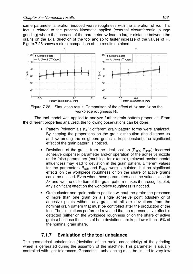
Chapter 7 – Numerical results 103
same parameter alteration induced worse roughness with the alteration of ∆z. This fact is related to the process kinematic applied (external circumferential plunge grinding) where the increase of the parameter ∆z lead to larger distance between the grains on the axial direction of the tool and so to faster increase of the values of Rt. Figure 7.28 shows a direct comparison of the results obtained.
Figure 7.28 – Simulation result: Comparison of the effect of ∆x and ∆z on the workpiece roughness Rt.
The tool model was applied to analyze further grain pattern properties. From the different properties analyzed, the following observations can be done:
• Pattern Polynomials (f(z)): different grain pattern forms were analyzed. By keeping the proportions on the grain distribution (the distance ∆x and ∆z among the neighbors grains is kept constant), no significant effect of the grain pattern is noticed.
• Deviations of the grains from the ideal position (Radh, Rgrain): incorrect adhesive dispenser parameter and/or operation of the adhesive nozzle under false parameters (enabling, for example, relevant environmental influences) may lead to deviation in the grain pattern. Different values for the parameters Radh and Rgrain were simulated, but no significant effects on the workpiece roughness or on the share of active grains could be noticed. Even when these parameters assume values close to ∆x and ∆z (the distortion of the grain pattern makes it unrecognizable), any significant effect on the workpiece roughness is noticed.
• Grain cluster and grain pattern position without the grain: the presence of more than one grain on a single adhesive point (cluster) or of adhesive points without any grains at all are deviations from the nominal grain pattern that must be controlled after the production of the tool. The simulations performed revealed that no representative effect is detected (either on the workpiece roughness or on the share of active grains) because the limits of both deviations are kept lower than 15% of the nominal grain share.
7.1.7 Evaluation of the tool unbalance
The geometrical unbalancing (deviation of the radial concentricity) of the grinding wheel is generated during the assembly of the machine. This parameter is usually controlled with tight tolerances. Geometrical unbalancing must be limited to very low
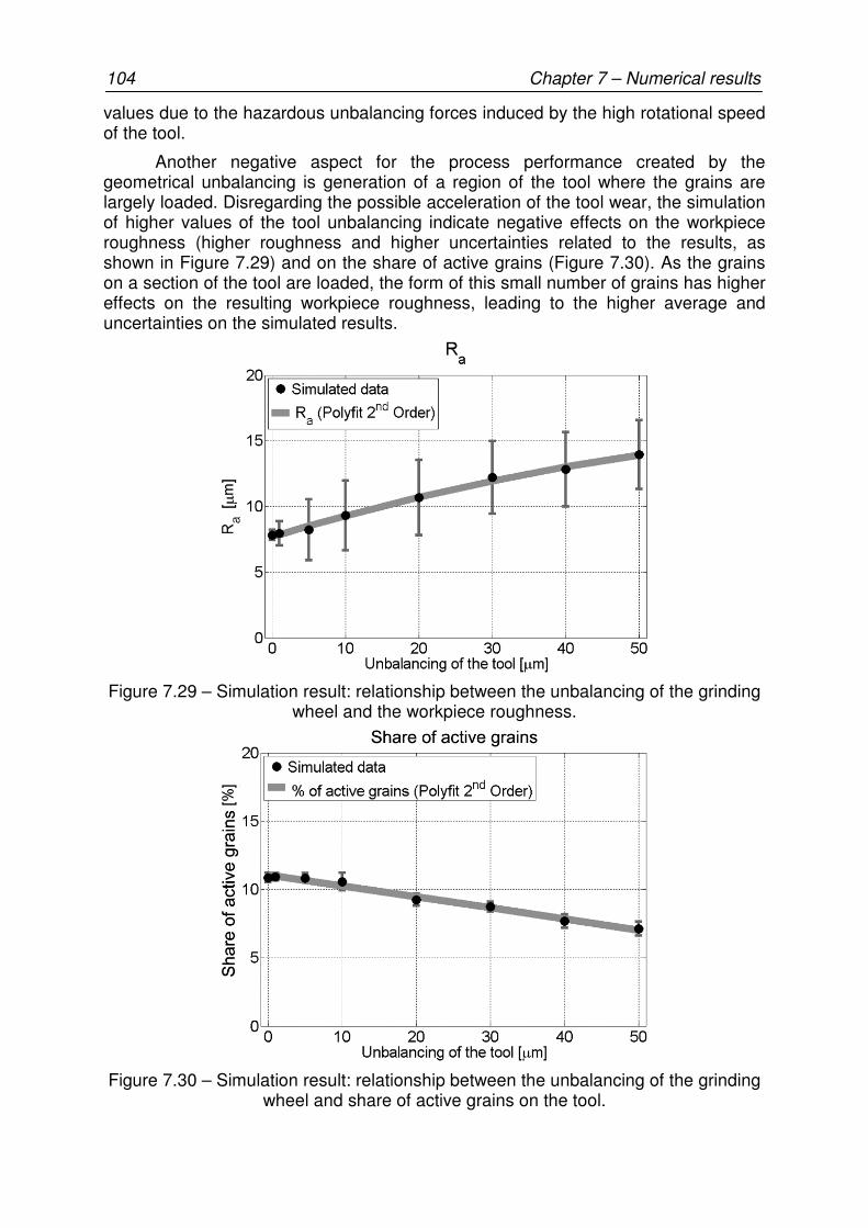
104 Chapter 7 – Numerical results
values due to the hazardous unbalancing forces induced by the high rotational speed of the tool.
Another negative aspect for the process performance created by the geometrical unbalancing is generation of a region of the tool where the grains are largely loaded. Disregarding the possible acceleration of the tool wear, the simulation of higher values of the tool unbalancing indicate negative effects on the workpiece roughness (higher roughness and higher uncertainties related to the results, as shown in Figure 7.29) and on the share of active grains (Figure 7.30). As the grains on a section of the tool are loaded, the form of this small number of grains has higher effects on the resulting workpiece roughness, leading to the higher average and uncertainties on the simulated results.
Figure 7.29 – Simulation result: relationship between the unbalancing of the grinding wheel and the workpiece roughness.
Figure 7.30 – Simulation result: relationship between the unbalancing of the grinding wheel and share of active grains on the tool.
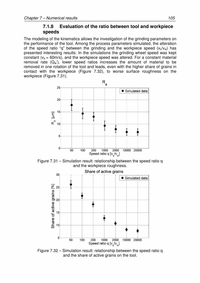
Chapter 7 – Numerical results 105
7.1.8 Evaluation of the ratio between tool and workpiece speeds
The modeling of the kinematics allows the investigation of the grinding parameters on the performance of the tool. Among the process parameters simulated, the alteration of the speed ratio “q” between the grinding and the workpiece speed (vs/vw) has presented interesting results. In the simulations the grinding wheel speed was kept constant (vs = 60m/s), and the workpiece speed was altered. For a constant material removal rate (Qw’), lower speed ratios increases the amount of material to be removed in one rotation of the tool and leads, even with the higher share of grains in contact with the workpiece (Figure 7.32), to worse surface roughness on the workpiece (Figure 7.31).
Figure 7.31 – Simulation result: relationship between the speed ratio q and the workpiece roughness.
Figure 7.32 – Simulation result: relationship between the speed ratio q and the share of active grains on the tool.
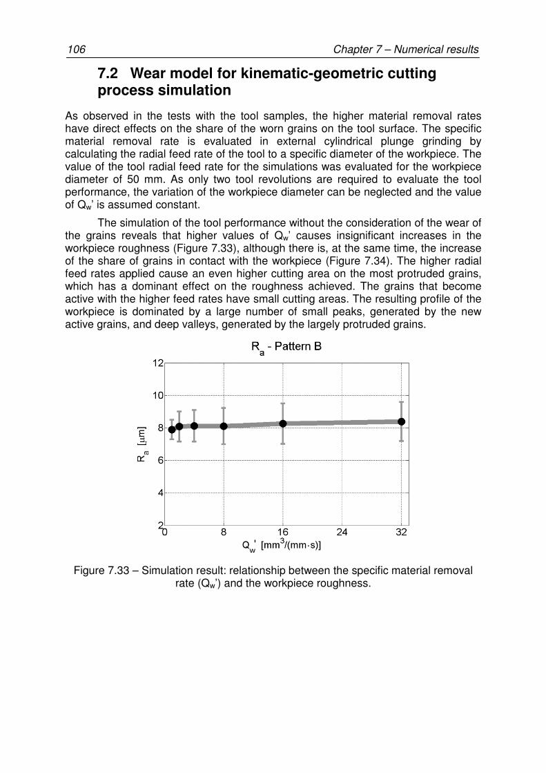
106 Chapter 7 – Numerical results
7.2 Wear model for kinematic-geometric cutting process simulation
As observed in the tests with the tool samples, the higher material removal rates have direct effects on the share of the worn grains on the tool surface. The specific material removal rate is evaluated in external cylindrical plunge grinding by calculating the radial feed rate of the tool to a specific diameter of the workpiece. The value of the tool radial feed rate for the simulations was evaluated for the workpiece diameter of 50 mm. As only two tool revolutions are required to evaluate the tool performance, the variation of the workpiece diameter can be neglected and the value of Qw’ is assumed constant.
The simulation of the tool performance without the consideration of the wear of the grains reveals that higher values of Qw’ causes insignificant increases in the workpiece roughness (Figure 7.33), although there is, at the same time, the increase of the share of grains in contact with the workpiece (Figure 7.34). The higher radial feed rates applied cause an even higher cutting area on the most protruded grains, which has a dominant effect on the roughness achieved. The grains that become active with the higher feed rates have small cutting areas. The resulting profile of the workpiece is dominated by a large number of small peaks, generated by the new active grains, and deep valleys, generated by the largely protruded grains.
Figure 7.33 – Simulation result: relationship between the specific material removal rate (Qw’) and the workpiece roughness.

Chapter 7 – Numerical results 107
Figure 7.34 – Simulation result: relationship between the specific material removal rate (Qw’) and the share of active grains on the tool.
There are representative differences between the empirical and the simulated data obtained while evaluating the influence of Qw’: while the tool samples have the reduction in the workpiece roughness with higher Qw’, the numerically simulated indicated almost unaltered results with the same alteration in Qw’.
Figure 7.35 – Comparison between the experimental and numerical workpiece roughness obtained with tools layered with the pattern B (∆x = 1 mm, ∆z = 0.5 mm)
without the consideration of the grain wear.
The results in Figure 7.35 indicate that the good correlation between empirical and numerical results is only valid for the lowest value of Qw’. With Qw’ = 1 mm3/(mm.s) just a small share of the grains is worn under this parameter (maximal 2%) and the effects of the grain wear are not sufficient to affect the average value of the measurements. However, even at this low material removal rate, there is a significant effect on the scattering of the results.
108 Chapter 7 – Numerical results
With higher values of Qw’ there is a larger discrepancy in the results. The higher Qw’ implies a higher load on the single grains and leads to a significant change on the abrasive layer topography. The worn abrasive layer has a direct effect on the workpiece roughness, which was not taken into account within the model, and leads to large differences between simulated and empirical data.
With the analysis of tool samples it is observed that the major mechanism of the tool wear is the breakage of small particles of the grains. This is a typical failure obtained when ABN800 grains are overloaded.
From the numerical model, it is possible to evaluate, for every active grain in the tool, its cutting area on a plane orthogonal to the grinding speed vector at the moment of the largest workpiece penetration. The wear model proposed assumes the failure of the grains as a function of the cutting area of the grains. Three breaking characteristics of the grains were modeled: pull-out, micro-break and macro-break.
With the models of wear established, the critical cutting area (Alim) is fitted to experimental data. For each grinding parameter, the value of the maximal cutting area of the grains was arbitrarily estimated and the performance of the tool was observed during the execution of the tool revolutions. During the simulation the cutting area of each grain is evaluated. If a grain exceeds the maximal cutting area, its geometry is altered with the methodology presented. This process is repeated up to the point where either no grain achieves the critical cutting area, or the abrasive layer achieves one of the pre-established failure criteria (Table 5.2). The value of the critical area is assumed correct when both parameters, workpiece roughness and share of broken grains, are coincident on both methods applied (empirical and numerical).
The progress of the simulated tool wear was documented with the methods shown in Figure 7.36 and Figure 7.37. Besides the distribution of the grain edges, of the active grains’ edges and of the intersections’ limits, the number of grains available along the entire tool circumference on different regions of the tool width was documented (Figure 7.36). During the simulation of a specific set of tool and process characteristics three distinct simulation results are possible:
• Alim is underestimated: the numerical tool reaches one of the failure criteria or the share of broken grains is higher than observed on the EGT samples. In simulations where the numerical tool fails, it is possible to identify the region of the grain pattern failure with the analysis of the share of grains available along the circumference on different positions of the tool width. At the failure region of the tool this share of grains is constantly reduced, down to the point where no grain is available and there is contact between the tool body material and the workpiece (typical failure by EGT, as observed in Figure 6.21).
• Alim is overestimated: no failure is observed in the tool, but the share of broken grains on the virtual tool is lower than observed on the tool samples. The roughness achieved with the tool sample is not necessarily different to that achieved with the numerical tool. The share of grains acting on the process is higher than that observed with the new tool, and there is clear alteration on the distribution of the cutting edges from the unworn tool.

Chapter 7 – Numerical results 109
• Alim is correctly estimated: the simulated tool presents similar results with the tests of the tool samples for the share of broken grains as well as for workpiece roughness obtained.
Figure 7.36 – Numerical analysis of the critical cutting area of the grains.
The numerical model also reveals the distribution of the cutting areas according to the critical cutting area assumed for the grains. On this analysis the changes in the cutting properties of the grains with the wear is clearly illustrated (Figure 7.37). The simulation of the tool without the grain wear reveals that the cutting areas are distributed on a large spectrum with a large number of grains with cutting area above the critical cutting value assumed. With the application of the grain wear model, two situations are possible: the tool achieves a stable condition (no grains with cutting area above the critical value), or the grain pattern fails before all grains achieve a cutting area lower than the limits specified.

110 Chapter 7 – Numerical results
Figure 7.37 – Characteristics of cutting area distributions on situation where the tool achieves the stable wear condition and where the tool fails.
The three wear models elaborated for the grain geometry presented different tendencies on the tool performance. The assumption of grain pull-out has not generated reasonable correlations between the share of broken grains and the workpiece roughness as observed on the EGT samples. Pull-outs where not observed on the EGT and led to more relevant changes on the abrasive layers than the changes observed on the tool samples. The macro-break of the grains led to a better correlation than that obtained with the grains pull-out. However, analysis of different grain patterns does not achieve good correlations.
The best correlation between numerical and experimental results was achieved with the assumption of the micro-break of the grains. This was the dominant wear effect observed in the experiments and led to a good correlation among the results obtained with the share of broken grains and the workpiece roughness for all the three grain patterns analyzed.
In the grinding tests, higher Qw’ caused not only higher radial feed rates of the grinding tool, but as the cutting depth (ae) was kept constant, the speed ratio between the grinding and workpiece speeds was also altered. In fact, for external cylindrical plunge grinding operations, the alteration of the speed ratios has a much more relevant influence on the undeformed chip thickness of the grains than a proportional alteration of the radial feed rate. Figure 7.38 shows the correlation of the share of broken grains with the speed ratios applied in the grinding process applied on the experiments.

Chapter 7 – Numerical results 111
Figure 7.38 – Correlation between the share of broken grains with the speed ratio between grinding and workpiece speeds (Patterns A, B and C).
Applying the numerical method to the determination of the critical cutting area and assuming the only wear model the micro-break of the grains’ edges, it is possible to achieve a correlation between the critical cutting area with the share of broken grains and the speed ratio q for all the tools tested on the experiments. The Figure 7.39 shows the results achieved for the correlation of the grains and the speed ratio q for the tool samples with pattern B. These results were applied on the model as a reference for the prediction of the workpiece roughness obtained with the patterns A and C. The results show in Figure 7.40 and Figure 7.41 have achieved good correlation between the numerical and empirical results.
Figure 7.39 – Correlation between the speed ratio q and the critical cutting area of the grains for tools with pattern B.
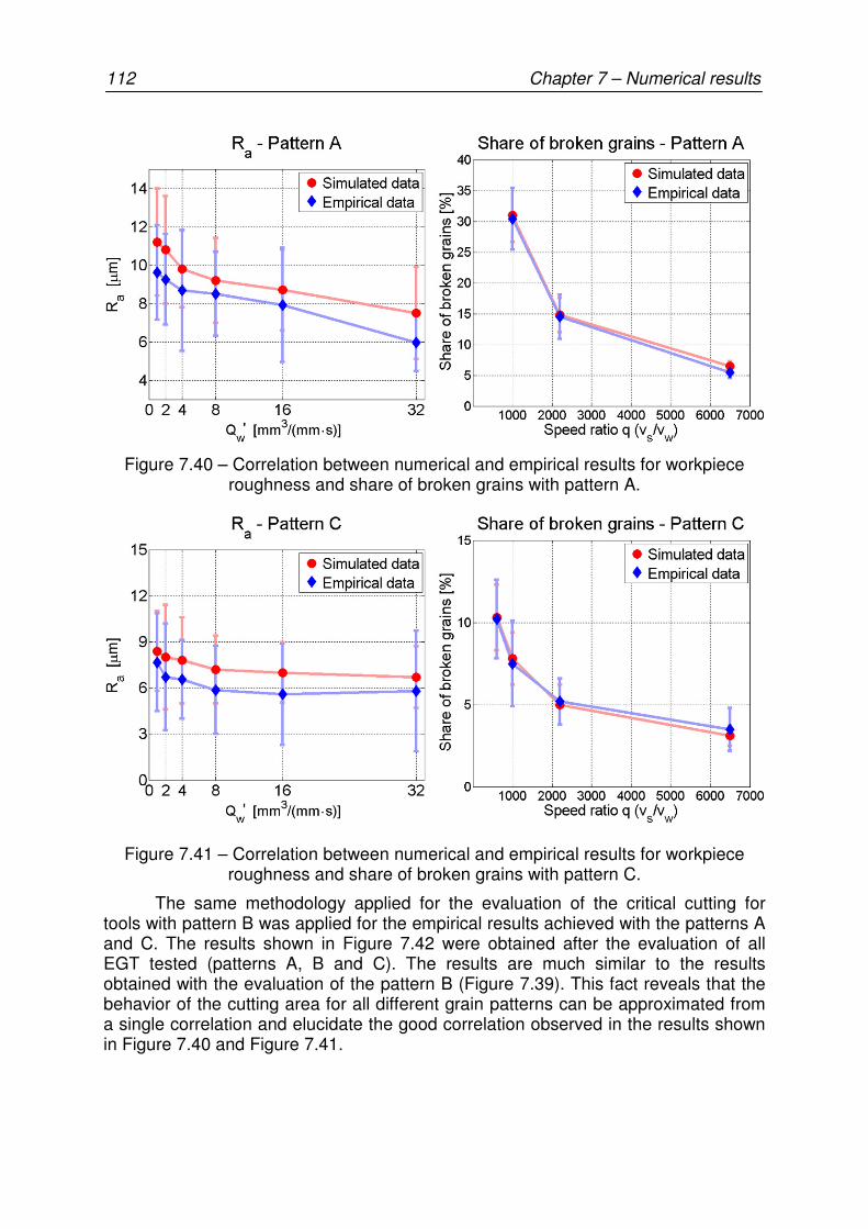
112 Chapter 7 – Numerical results
Figure 7.40 – Correlation between numerical and empirical results for workpiece roughness and share of broken grains with pattern A.
Figure 7.41 – Correlation between numerical and empirical results for workpiece roughness and share of broken grains with pattern C.
The same methodology applied for the evaluation of the critical cutting for tools with pattern B was applied for the empirical results achieved with the patterns A and C. The results shown in Figure 7.42 were obtained after the evaluation of all EGT tested (patterns A, B and C). The results are much similar to the results obtained with the evaluation of the pattern B (Figure 7.39). This fact reveals that the behavior of the cutting area for all different grain patterns can be approximated from a single correlation and elucidate the good correlation observed in the results shown in Figure 7.40 and Figure 7.41.
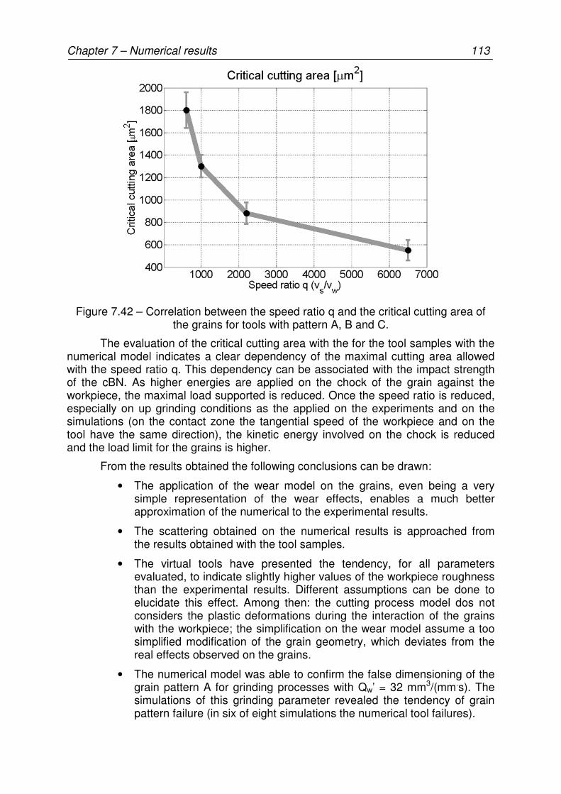
Chapter 7 – Numerical results 113
Figure 7.42 – Correlation between the speed ratio q and the critical cutting area of the grains for tools with pattern A, B and C.
The evaluation of the critical cutting area with the for the tool samples with the numerical model indicates a clear dependency of the maximal cutting area allowed with the speed ratio q. This dependency can be associated with the impact strength of the cBN. As higher energies are applied on the chock of the grain against the workpiece, the maximal load supported is reduced. Once the speed ratio is reduced, especially on up grinding conditions as the applied on the experiments and on the simulations (on the contact zone the tangential speed of the workpiece and on the tool have the same direction), the kinetic energy involved on the chock is reduced and the load limit for the grains is higher.
From the results obtained the following conclusions can be drawn:
• The application of the wear model on the grains, even being a very simple representation of the wear effects, enables a much better approximation of the numerical to the experimental results.
• The scattering obtained on the numerical results is approached from the results obtained with the tool samples.
• The virtual tools have presented the tendency, for all parameters evaluated, to indicate slightly higher values of the workpiece roughness than the experimental results. Different assumptions can be done to elucidate this effect. Among then: the cutting process model dos not considers the plastic deformations during the interaction of the grains with the workpiece; the simplification on the wear model assume a too simplified modification of the grain geometry, which deviates from the real effects observed on the grains.
• The numerical model was able to confirm the false dimensioning of the grain pattern A for grinding processes with Qw’ = 32 mm3/(mm.s). The simulations of this grinding parameter revealed the tendency of grain pattern failure (in six of eight simulations the numerical tool failures).
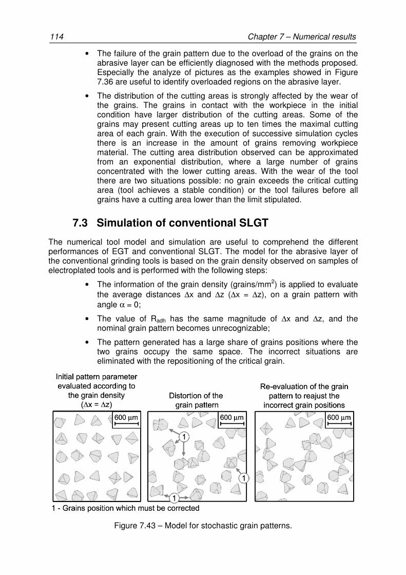
114 Chapter 7 – Numerical results
• The failure of the grain pattern due to the overload of the grains on the abrasive layer can be efficiently diagnosed with the methods proposed. Especially the analyze of pictures as the examples showed in Figure 7.36 are useful to identify overloaded regions on the abrasive layer.
• The distribution of the cutting areas is strongly affected by the wear of the grains. The grains in contact with the workpiece in the initial condition have larger distribution of the cutting areas. Some of the grains may present cutting areas up to ten times the maximal cutting area of each grain. With the execution of successive simulation cycles there is an increase in the amount of grains removing workpiece material. The cutting area distribution observed can be approximated from an exponential distribution, where a large number of grains concentrated with the lower cutting areas. With the wear of the tool there are two situations possible: no grain exceeds the critical cutting area (tool achieves a stable condition) or the tool failures before all grains have a cutting area lower than the limit stipulated.
7.3 Simulation of conventional SLGT
The numerical tool model and simulation are useful to comprehend the different performances of EGT and conventional SLGT. The model for the abrasive layer of the conventional grinding tools is based on the grain density observed on samples of electroplated tools and is performed with the following steps:
• The information of the grain density (grains/mm2) is applied to evaluate the average distances ∆x and ∆z (∆x = ∆z), on a grain pattern with angle α = 0;
• The value of Radh has the same magnitude of ∆x and ∆z, and the nominal grain pattern becomes unrecognizable;
• The pattern generated has a large share of grains positions where the two grains occupy the same space. The incorrect situations are eliminated with the repositioning of the critical grain.
Figure 7.43 – Model for stochastic grain patterns.
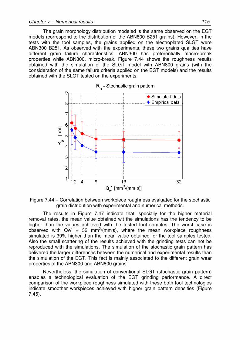
Chapter 7 – Numerical results 115
The grain morphology distribution modeled is the same observed on the EGT models (correspond to the distribution of the ABN800 B251 grains). However, in the tests with the tool samples, the grains applied on the electroplated SLGT were ABN300 B251. As observed with the experiments, these two grains qualities have different grain failure characteristics: ABN300 has preferentially macro-break properties while ABN800, micro-break. Figure 7.44 shows the roughness results obtained with the simulation of the SLGT model with ABN800 grains (with the consideration of the same failure criteria applied on the EGT models) and the results obtained with the SLGT tested on the experiments.
Figure 7.44 – Correlation between workpiece roughness evaluated for the stochastic grain distribution with experimental and numerical methods.
The results in Figure 7.47 indicate that, specially for the higher material removal rates, the mean value obtained wit the simulations has the tendency to be higher than the values achieved with the tested tool samples. The worst case is observed with Qw’ = 32 mm3/(mm.s), where the mean workpiece roughness simulated is 39% higher than the mean value obtained for the tool samples tested. Also the small scattering of the results achieved with the grinding tests can not be reproduced with the simulations. The simulation of the stochastic grain pattern has delivered the larger differences between the numerical and experimental results than the simulation of the EGT. This fact is mainly associated to the different grain wear properties of the ABN300 and ABN800 grains.
Nevertheless, the simulation of conventional SLGT (stochastic grain pattern) enables a technological evaluation of the EGT grinding performance. A direct comparison of the workpiece roughness simulated with these both tool technologies indicate smoother workpieces achieved with higher grain pattern densities (Figure 7.45).
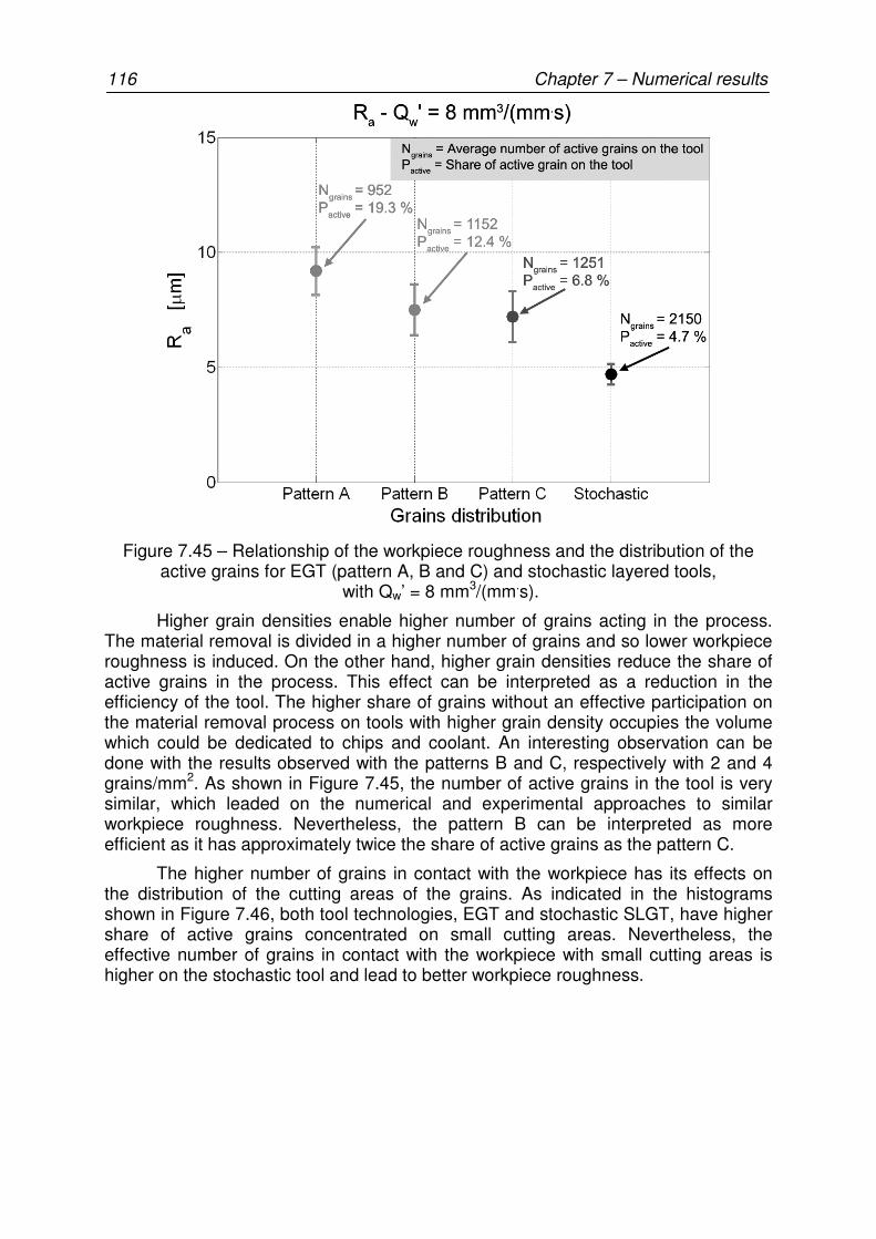
116 Chapter 7 – Numerical results
Figure 7.45 – Relationship of the workpiece roughness and the distribution of the active grains for EGT (pattern A, B and C) and stochastic layered tools,
with Qw’ = 8 mm3/(mm.s).
Higher grain densities enable higher number of grains acting in the process. The material removal is divided in a higher number of grains and so lower workpiece roughness is induced. On the other hand, higher grain densities reduce the share of active grains in the process. This effect can be interpreted as a reduction in the efficiency of the tool. The higher share of grains without an effective participation on the material removal process on tools with higher grain density occupies the volume which could be dedicated to chips and coolant. An interesting observation can be done with the results observed with the patterns B and C, respectively with 2 and 4 grains/mm2. As shown in Figure 7.45, the number of active grains in the tool is very similar, which leaded on the numerical and experimental approaches to similar workpiece roughness. Nevertheless, the pattern B can be interpreted as more efficient as it has approximately twice the share of active grains as the pattern C.
The higher number of grains in contact with the workpiece has its effects on the distribution of the cutting areas of the grains. As indicated in the histograms shown in Figure 7.46, both tool technologies, EGT and stochastic SLGT, have higher share of active grains concentrated on small cutting areas. Nevertheless, the effective number of grains in contact with the workpiece with small cutting areas is higher on the stochastic tool and lead to better workpiece roughness.

Chapter 7 – Numerical results 117
Figure 7.46 – Area distribution in the stochastic SLGT and an EGT with the pattern B.
7.4 Evaluation of the tangential grinding force
The position of the active grains and the cutting area on the maximal cutting depth of these grains is obtained with the numerical simulation. Figure 7.47 shows a typical example of a histogram of the grain area distribution on a simulated EGT. The cutting area has an exponential reduction on the number of grains with the increase of the cutting area. The dominant presence of the small cutting areas is mainly caused due the large number of active grains on the tool, which reduce the amount of material to be removed by each grain.
Figure 7.47 – Example of the cutting area distribution for an EGT at stable wear condition.
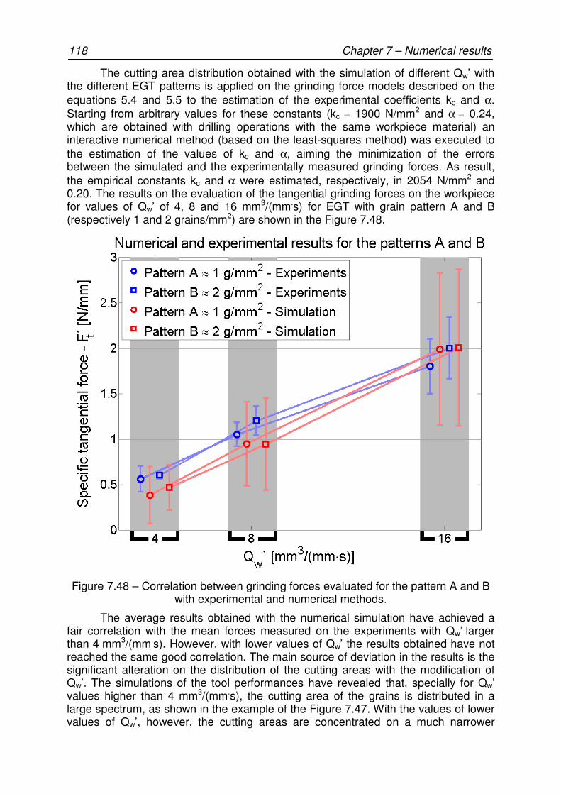
118 Chapter 7 – Numerical results
The cutting area distribution obtained with the simulation of different Qw’ with the different EGT patterns is applied on the grinding force models described on the equations 5.4 and 5.5 to the estimation of the experimental coefficients kc and α. Starting from arbitrary values for these constants (kc = 1900 N/mm2 and α = 0.24, which are obtained with drilling operations with the same workpiece material) an interactive numerical method (based on the least-squares method) was executed to the estimation of the values of kc and α, aiming the minimization of the errors between the simulated and the experimentally measured grinding forces. As result, the empirical constants kc and α were estimated, respectively, in 2054 N/mm2 and 0.20. The results on the evaluation of the tangential grinding forces on the workpiece for values of Qw’ of 4, 8 and 16 mm3/(mm.s) for EGT with grain pattern A and B (respectively 1 and 2 grains/mm2) are shown in the Figure 7.48.
Figure 7.48 – Correlation between grinding forces evaluated for the pattern A and B with experimental and numerical methods.
The average results obtained with the numerical simulation have achieved a fair correlation with the mean forces measured on the experiments with Qw’ larger than 4 mm3/(mm.s). However, with lower values of Qw’ the results obtained have not reached the same good correlation. The main source of deviation in the results is the significant alteration on the distribution of the cutting areas with the modification of Qw’. The simulations of the tool performances have revealed that, specially for Qw’ values higher than 4 mm3/(mm.s), the cutting area of the grains is distributed in a large spectrum, as shown in the example of the Figure 7.47. With the values of lower values of Qw’, however, the cutting areas are concentrated on a much narrower
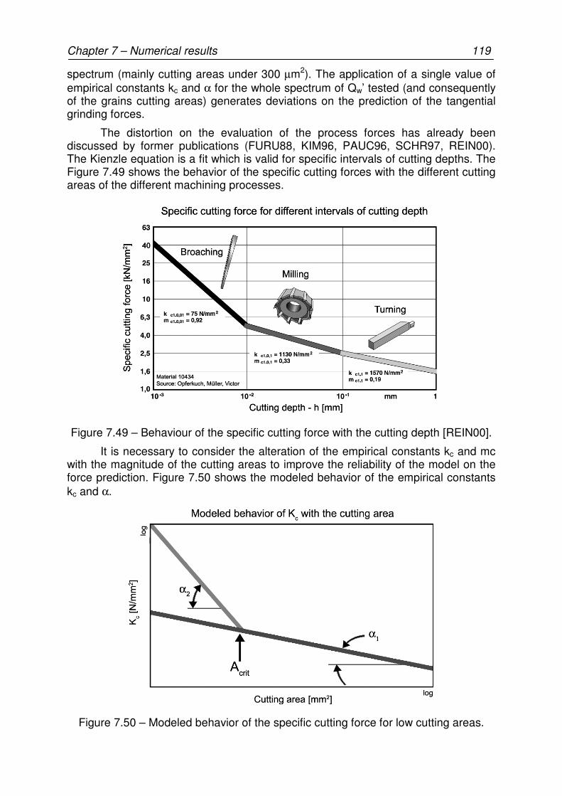
Chapter 7 – Numerical results 119
spectrum (mainly cutting areas under 300 µm2). The application of a single value of empirical constants kc and α for the whole spectrum of Qw’ tested (and consequently of the grains cutting areas) generates deviations on the prediction of the tangential grinding forces.
The distortion on the evaluation of the process forces has already been discussed by former publications (FURU88, KIM96, PAUC96, SCHR97, REIN00). The Kienzle equation is a fit which is valid for specific intervals of cutting depths. The Figure 7.49 shows the behavior of the specific cutting forces with the different cutting areas of the different machining processes.
Figure 7.49 – Behaviour of the specific cutting force with the cutting depth [REIN00].
It is necessary to consider the alteration of the empirical constants kc and mc with the magnitude of the cutting areas to improve the reliability of the model on the force prediction. Figure 7.50 shows the modeled behavior of the empirical constants kc and α.
Figure 7.50 – Modeled behavior of the specific cutting force for low cutting areas.
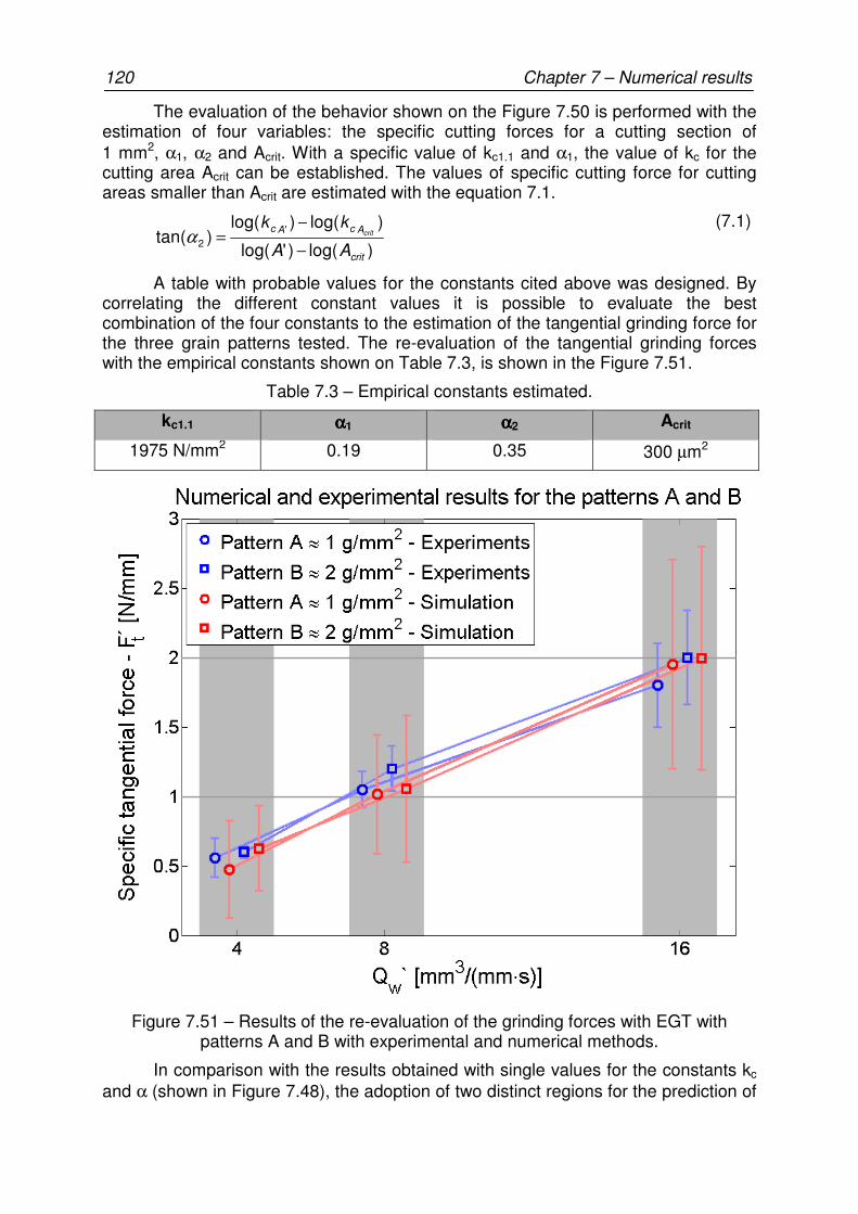
120 Chapter 7 – Numerical results
The evaluation of the behavior shown on the Figure 7.50 is performed with the estimation of four variables: the specific cutting forces for a cutting section of 1 mm2, α1, α2 and Acrit. With a specific value of kc1.1 and α1, the value of kc for the cutting area Acrit can be established. The values of specific cutting force for cutting areas smaller than Acrit are estimated with the equation 7.1.
)log()'log(
)log()log()tan( '
2crit
AcAc
AA
kkcrit
−
−=α
(7.1)
A table with probable values for the constants cited above was designed. By correlating the different constant values it is possible to evaluate the best combination of the four constants to the estimation of the tangential grinding force for the three grain patterns tested. The re-evaluation of the tangential grinding forces with the empirical constants shown on Table 7.3, is shown in the Figure 7.51.
Table 7.3 – Empirical constants estimated.
kc1.1 αααα1 αααα2 Acrit
1975 N/mm2 0.19 0.35 300 µm2
Figure 7.51 – Results of the re-evaluation of the grinding forces with EGT with patterns A and B with experimental and numerical methods.
In comparison with the results obtained with single values for the constants kc and α (shown in Figure 7.48), the adoption of two distinct regions for the prediction of

Chapter 7 – Numerical results 121
kc enables more precision in the prediction of the grinding forces, also for the lower values of Qw’, as shown in Figure 7.52.
Figure 7.52 – Results of the re-evaluation of the grinding forces with EGT with patterns A and B with Qw’ of 1 and 2 mm3/(mm.s).
The precise estimation of the behavior of the specific grinding forces with cutting area of the grains requires experimental methods for the estimation of the empirical coefficients kc and α. A reasonable technique for the evaluation of the specific cutting forces with the typical geometry of the abrasive grains would be the application of a sclerometer to the evaluation of the cutting force and measure the scratch geometry generated. The correlation of the cutting forces and the scratch geometry reveals the dependency of kc and α with the cutting area. Nevertheless, the kinematics applied on these single-grain-tests is much slower than the kinematic of the grinding process (translation speed of the grain is usually lower than 0,1 m/s). Among other operational difficulties, the limitation on the maximal speed of the tool on the scratching tests is limited by the eigenfrequency of the dynamometers commercially available for machining operations. The stiffness required for the measuring system requires large and heavy structures. This structural property of the measuring system reduces the eigenfrequency of the system (usually lower than 5 kHz) and limits the maximal sampling rate of the forces during the process. The eigenfrequency of the dynamometers requires the application of low-pass filter in the force signals, and so the maximal sampling rate of the measurement is limited. The comprehension of the cutting process with the typical abrasive geometry and with high process speeds will certainly be a topic explored on future technical publications.
Another relevant aspect which can be observed in the results shown in Figure 7.48 is the higher scattering of the forces in the simulation than in the experiments.
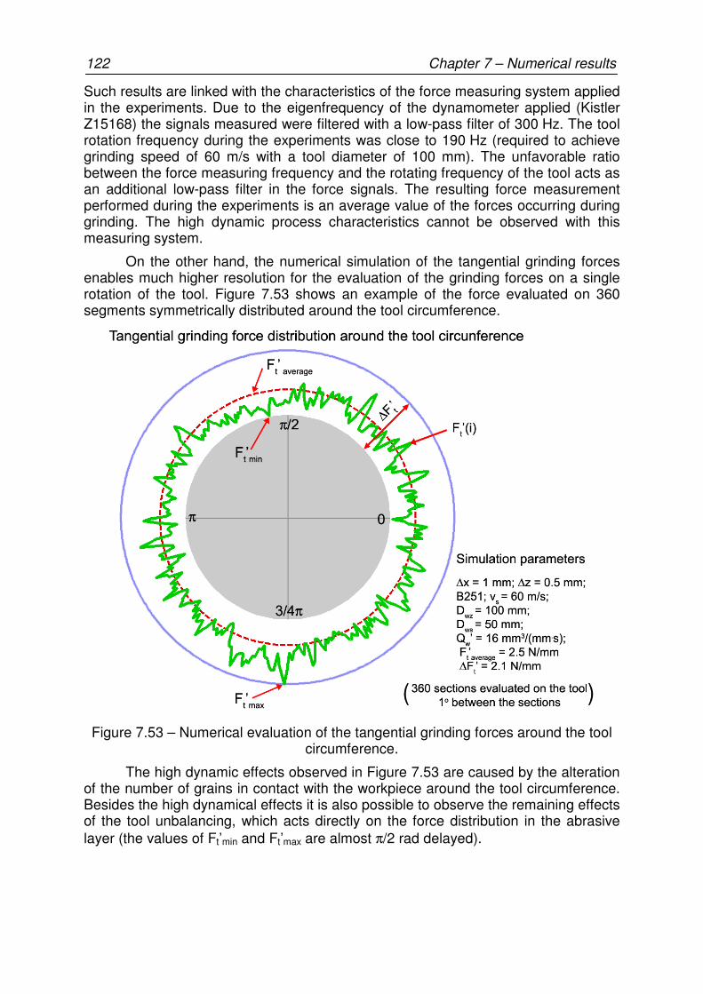
122 Chapter 7 – Numerical results
Such results are linked with the characteristics of the force measuring system applied in the experiments. Due to the eigenfrequency of the dynamometer applied (Kistler Z15168) the signals measured were filtered with a low-pass filter of 300 Hz. The tool rotation frequency during the experiments was close to 190 Hz (required to achieve grinding speed of 60 m/s with a tool diameter of 100 mm). The unfavorable ratio between the force measuring frequency and the rotating frequency of the tool acts as an additional low-pass filter in the force signals. The resulting force measurement performed during the experiments is an average value of the forces occurring during grinding. The high dynamic process characteristics cannot be observed with this measuring system.
On the other hand, the numerical simulation of the tangential grinding forces enables much higher resolution for the evaluation of the grinding forces on a single rotation of the tool. Figure 7.53 shows an example of the force evaluated on 360 segments symmetrically distributed around the tool circumference.
Figure 7.53 – Numerical evaluation of the tangential grinding forces around the tool circumference.
The high dynamic effects observed in Figure 7.53 are caused by the alteration of the number of grains in contact with the workpiece around the tool circumference. Besides the high dynamical effects it is also possible to observe the remaining effects of the tool unbalancing, which acts directly on the force distribution in the abrasive layer (the values of Ft’min and Ft’max are almost π/2 rad delayed).
Chapter 7 – Numerical results 123
7.5 Conclusions
The numerical methods applied aimed to increase the comprehension about the phenomena which are present in the grinding process. The geometric-kinematic simulation method was developed aiming at two main goals: to achieve reliable simulation times required; and develop a design tool for the grain pattern where the effects of the grain wear can be associated to the results on the tool performance, mainly to avoid the design of overloaded grain patterns.
The simplification assumed in the three-dimensional grain geometry of a grain projection on the orthogonal plane to the grinding speed and irregular time-steps for the simulation has generated a fast simulation method. As an example of the performance achieved, the time required for the generation of a tool model with 9,000 grains requires around three minutes.
Short simulation times enable not only the evaluation of a large amount of variables, but also the evaluation of the statistical distribution of the results achieved. Calculation of the grain wear also takes advantage of the short simulation times. The sequential modification of the tool profile with the grain wear requires the simulation of successive revolutions of the tool. On some of the situations evaluated (high material removal rates on the tool models with high grain density) up to 200 cycles were required to evaluate the effects of the grain wear.
The numerical method can be adapted to an optimization method with focus on the tool design. This optimization methodology involves a pre-defined set of process parameters and expected process results. The grain pattern is specially designed to fulfill the requirements of the process (for example, workpiece roughness) with the pre-defined process parameters. This analysis is typically applied while substituting the grinding tool on a process by an EGT. In an already existing process it may not be possible to modify the grinding parameters (for example, the former grinding tool already uses the maximal cutting speed allowed or the maximal power available on the machine), and so the tool must be designed with the pre-defined process characteristics. The main aspects evaluated with this approach are the geometric characteristics of the grain pattern to match the requirements of the process.
Another process optimization method is the evaluation of the “standard-tools” performance. The standard tools are tools that are not designed for a specific grinding operation, but with standardized grain patterns. The choice of the most suitable EGT for a process is based on the comparison of the performance required with the possibilities offered with the standard tools. This is an interesting option to facilitate the production of the EGT on large scales, where the tool supplier would be able to offer a tool palette.
On both methodologies proposed for the tool optimization, the dimensioning of the tool starts from the process requirement (such as workpiece roughness or minimal material removal rate) and limitations (such as grinding speed, tool diameter or process kinematics). It is important to realize that the characteristics expected of a grinding tool applied to the rough grinding of white cast iron (a usual application in the automotive industry) is different from the characteristics expected of the EGT applied to the dressing of gear grinding tools. In tools applied in high performance grinding operations, the usual target is the maximization of the removal rate of the workpiece material. In these situations it is interesting to provide large volumes of space for coolant and chips, but at the same time, larger Qw’ increases the load on
124 Chapter 7 – Numerical results
the grains and a dense pattern would be recommended. The numerical methods can play their part precisely in this context, providing the information required to optimize the tool and the process design.
The substitution of a conventional tool technology by an EGT must consider, besides the technological arguments, the economical aspects. Smaller amount of grains applied on the tool brings advantages with the reduction on the tool costs, especially with the valuable abrasives applied on SLGT (cBN and diamonds). Nevertheless, real economical advantage is achieved when a tool technology is able to demonstrate an overall positive balance in the costs. The application of the EGT as a reliable technology depends of the achievement of grinding conditions where the additional costs of production of the tool can be compensated by improved performance.
Another economical aspect of the application of the numerical analysis is the evaluation of the geometrical tolerances of the process. Parameters such as assembly tolerance, geometrical tolerance on the production of the tool body, sieving tolerance and morphology of the grains are examples of the geometrical effects that can be evaluated with the numerical tool. The correct tolerance field for each geometrical properties of the tool is another method to reduce the (unnecessary) production costs of EGT.
The simplifications of the numerical model for the grinding process imply the limitation of the results achieved with the numerical analysis. As such, the main limitations of the numerical model can be listed as follows:
• The time dependent effects of the grain wear are not considered. After a fast development of the grain wear due to the presence of overloaded grains, the wear of the grains assumes slower characteristics. This new progress of the grains wear is essential for the prediction of the tool-life.
• The workpiece roughness is evaluated on a single profile, orthogonal to the feed-rate direction of the tool. The amount of data required to obtain a three-dimensional representation of the workpiece would increase the time required for the simulation significantly.
• No deformation or burr formation is considered as the perfect kinematic cut conditions are assumed.
• The cutting material is considered homogeneous. The local alteration of the workpiece material hardness change the load on the grains and the cutting area cannot be applied as failure criterion for the grain.
• The grain structure is considered isotropic on the wear model. The anisotropy of the grains would implicate on a preferential crystallographic break direction on the grains.
• The influence of the coolant is ignored in the process model. The presence of coolant on the interface between the tool and the workpiece has direct influences on the cutting process (especially on the evaluation of the forces or on the prediction of the tool-life) which are not regarded.
• The cutting forces are predicted according to an approximation of the Kienzle equation. On the equation proposed the cutting force is proportional to the cutting area of the grain, and not to the cutting depth “h”. The results presented good correlation with some process

Chapter 7 – Numerical results 125
parameters. Nevertheless, a better correlation between the results and the experiments requires the evaluation of the empirical constants Kc and α for the typical grain geometries and cutting areas involved in the grinding cutting.
126 Chapter 8 – Conclusions and outlook
8. Conclusion and outlook
8.1 Conclusions
In the early stage of this work, the efforts were concentrated on the development of a new control method for the grain placing system developed by Burkhard. Better pattern visualization and higher flexibility were the main requirements. After the design of the grain pattern is complete the position of each grain on the tool is determined and is exported for the grain positioning system. As proposed by Burkhard, the position of the grains on the tool is determined by the position of adhesive points on the tool surface. The new control technique achieves greater flexibility with the correlation of the measured position of the adhesive dispenser with the pre-defined nominal position of the grains on the matrix.
After the new control method for the position of the grains on the tool was defined, the precision of the placing system was evaluated. For the grinding process, the most relevant point on the grain is its cutting edge. Three main effects are identified on the precision of positioning the grain edges on an EGT: deviations from the centre of the adhesive point, the position of the grain on the adhesive point and the position of the cutting edge on the grain. A statistical analysis was applied to define the radius of a region around the nominal position of the grain edge where, with a pre-defined confidence level, it is possible to find the position of the cutting edge.
For the evaluation of the tool performance a series of tool samples was produced with three different grain patterns. The performance of these three tool characteristics was compared with conventional electroplated tools with similar grain characteristics in cylindrical external plunge grinding operations. As general results, the brazed EGT resulted in worse workpiece roughness than that achieved with electroplated tools, and also lower cutting forces. The abrasive effect of the chips against the bond observed on the electroplated tools and, in a smaller proportion, on the brazed tools, was remarkable. During the experiments with tool samples, the wear of the grains was controlled with the observation of segments of the abrasive layer. This evaluation is relatively time consuming but has revealed differences in the break (or wear) characteristics observed between the grains applied on the electroplated tools (ABN300, which presented a macro-break characteristic) and on the brazed tools (ABN800, which presented a micro-break characteristic).
A better understanding of the cutting process was achieved with the development of the numerical model. This is based on the detailed description of the
Chapter 8 – Conclusions and outlook 127
tool’s geometrical characteristics, on the assumption of kinematic-geometric cutting process and on the description of the kinematics of the grinding process.
The numerical model of the cutting tool considered characteristics such as the grain morphology (modeled on the observation of samples of grains), the positioning precision of the grains (as characterized by the placing system) and the tolerances on the tool body (for example, the unbalancing created during the assembly). The three-dimensional description of a tool with 12,000 grains, for example, requires around 800,000 points for the determination of the position of the grain edges on a Cartesian coordinate system. On the assumption of kinematic-geometric cutting process, the workpiece profile is mainly determined by the projection of the grain geometry on the plane orthogonal to the grinding speed vector. With this cutting model, the simplification of the full 3-D representation of the grain to a 2.5-D model (projection of the grain on the plane orthogonal to the grinding speed) greatly reduces the amount of data required for the simulation. On the same example of the tool with 12,000 grains, a 2.5-D model reduces the amount of points to around 150,000.
The processing capacity required for the numerical model is also reduced with the non-uniform time steps. Instead of simulating the tool with a fixed time-step (usually smaller than 1 ms), the time simulation was performed according to the position of the 2.5-D grain profile, and only on the position of the maximal cutting depth of each grain. These assumptions enable the evaluation of a single workpiece profile during the process simulation and reduce the number of time-steps to the number of grains available on the tool.
The tests performed with the tool samples revealed significant effects of the grain wear during the grinding process on the workpiece profile. This fact indicates that the grain-wear model is indispensable for the correct analysis of the tool performance with numerical methods. The wear on the grains was modeled according to the characteristics observed on the tool samples tested (micro-break of the ABN800 grains). The occurrence of wear was parameterized according to the cutting area of the grains. With correct critical cutting area for the grains, the results obtained on the tool samples can be reproduced with good reliability by the numerical tool (the share of broken grains and the workpiece roughness correlate together).
The tool samples designed with the lowest grain density failed during the tests with Qw’= 32 mm3/(mm.s). This situation can be reproduced with the numerical tool. In the numerical tool it is possible to identify a region on the tool width where there is an accelerated reduction of the share of active grains and, in a failure situation, where the contact between the tool body and the workpiece occurs.
With the consideration of the grain failure (wear) criterion on the tool analysis it is possible to apply the numerical model as a design tool for the grain pattern. The effect of special boundary conditions for the tool specifications (diameter, for example) or for the machine parameters (maximal grinding speed, for example) can be added as limitations which must be considered in the process design.
The numerical tool also enables the evaluation of the relevant tolerances to be imposed during the tool body production (fit and profile tolerances, for example), on the choice of the abrasive grains (grain size, quality and morphology) and on the assembly of the tool in the machine (maximal radial and axial concentricity allowed). The correct design of the tolerance fields avoids unnecessary costs on the production of tool-body or on the acquisition of very fine sieved (and expensive) grains.
128 Chapter 8 – Conclusions and outlook
The suitability of the cutting force model for the prediction of the grinding forces requires the evaluation of the coherent empirical constants for the typical cutting conditions of the abrasive grains. Once the empirical constants are obtained, the numerical model can investigate the performance of the tool with a much higher time resolution than it is possible to achieve with a real measuring system. The dynamic behavior of the forces induced during the process can be evaluated (effects such as the excitation of machine vibrations).
8.2 Outlook
In the following sections there are some suggestions for further researches on grinding technologies. The topics are mainly related to the further development of the EGT. Nevertheless, the topics here proposed are in synergy with the overall development tendencies in the grinding process.
8.2.1 Grains properties characterization
• Break (wear) characterization: as attested in the development of the numerical method, the breaking property of the grain has a direct influence on the results obtained in the process. Nevertheless, the evaluation of the break characteristics required the production and the evaluation of tool samples, which is quite an expensive method. A fast and representative method for the estimation of the grain wear is required.
• Control of the sieving quality and characterization of the grain: this is required to achieve a reliable model of the grinding tool. The grain characterization applied in this work was performed with observation of a large amount of grains. This was again a time consuming task. An alternative method, maybe based on the pictorial analysis of grain samples, is required to accelerate the characterization of the abrasive grains.
• Evaluation of the anisotropy on the different grain structures: the model of the grain wear proposed assumed the isotropic property of the grain microstructure. The qualitative and quantitative investigation of the anisotropy of the different cBN and diamond grain qualities is interesting for the correlation of the grain load and break phenomena.
8.2.2 Placing technologies
• New placing system for grains larger than B46: the actual grain placing system has the minimal grain size applied on the EGT limited to B126 grains (average grain diameter of 126µm). This limitation is due to the size of the adhesive point generated by the micro dispenser on the placing system. Grain sizes smaller than B126 leads to the formation of grain clusters on each point. Especially for the application of grinding operations where low workpiece roughness is desired, smaller grains are interesting. The creation of single grain patterns with smaller grain sizes requires a new placing system.
Chapter 8 – Conclusions and outlook 129
• Regularization of the position of the highest grain edge: the numerical simulation of the different grain morphologies, grain sizes and grain aspect-ratio revealed the relevance of the grain edges distribution on the workpiece roughness achieved. Instead of achieving a better sieving process for the grains or choosing the grain morphology, it would be interesting to develop a method to place the grain edges at a more regular protrusion from the tool basis. The result of this grain allocation method would be the narrower distribution of the grain edges and the related benefits for the grinding process (lower workpiece roughness, higher share of grains in contact with the workpiece, more regularly distributed grain load).
8.2.3 Braze bonding technology
• Optimization of the filler metal application method: the filler metal is applied nowadays with different methods. On a general approach, all these methods are based on manual processes. The development of an automatic system for the application of the filler metal is required to accelerate the production and to assure better quality on the tools.
• Investigate the relationship between the bond material amount and the maximal load applied on the grain: Aiming the maximization of the coolant and chip volumes in the grinding gap, the amount of bond material should be kept in minimal values. Nevertheless, the reduction of the amount of bond material may weak the bond of the grains.
• Development of alternative filler metal alloys: the actual filler metal alloys require a large heat load during the brazing process (around 950oC for cBN and 600oC for diamonds with copper-based alloys). The large thermal load during the process requires a high thermal stability of the grains and the choice of special tool body materials. The development of brazing alloys that require lower brazing temperatures and achieve high bonding forces would enable the application of alternative grains and reduce the production costs of the brazed tools.
8.2.4 Single grain tests
• Development of a methodology for single grain tests: the main objective is to obtain the specific cutting forces on the cutting process with the typical cutting edge geometries, and to evaluate the wear effects which are not related to an overload of the grain. The combination of unfavorable grain geometries and low cutting areas generate large specific cutting forces for the process. Aiming to investigate the cutting process with the abrasive grain geometries, a series of pre-tests was performed applying a single grain brazed on a pin. The pin performed a series of scratches on the polished workpiece. During the creation of the scratches on the workpiece the forces were measured with a very sensitive force measuring system. After the execution of the scratches its geometry was mapped (either by mechanical or optical scanning) and the information of the scratch profile orthogonal to the cutting direction were correlated with the forces and with the geometry of the grains. The evaluation of the results was only partially successful as it
130 Chapter 8 – Conclusions and outlook
was very difficult to perform a coherent synchronization of the geometry with the force signals. The further analysis of the cutting process with the abrasive grain geometries requires mainly a deep analysis on the properties of the force measuring system to the application of high measuring frequencies and the development of a trigger signal to successful synchronization of the scratch and force signals.
8.2.5 Explore alternative application fields for EGT
• High precision grinding conditions: the benefits of the EGT may be found in applications not only with rough grinding conditions, but also in applications where high quality is required. As the position of each grain can be established on the tool, the tool can be designed to achieve very good workpiece quality due to better adequate grain edge distribution.
• Micro-dressing methods for EGT: as observed in the simulations of the grinding-tool performance, the crushing or the grain flattening have direct influence on the workpiece quality achieved. The achievement of the changes in tool micro-geometry is dependent on the dressing method. For example, as observed in conventional electroplated cBN tools, the occurrence of the grain flattening is related to the speed ratio applied between the dressing and grinding wheels. The investigations on this topic should provide a correlation between the dressing method and the modification achieved in the grinding wheel characteristics.
8.2.6 Analyze the coolant flow on the grinding gap
• Numerical methods: the reduction of the grain density on the abrasive layer due to the placing of the grains under a mathematically defined grain pattern on the EGT enables much larger coolant and chip volumes. Besides the larger volume there is also a growth on the volume of fluid flowing through the grinding gap and probably a faster flow of the coolant. All these effects should combine to improve lubrication and, more importantly, better cooling of the grinding process. Nevertheless, the reduction of the grain density may lead to fragile grain patterns, which are easily overloaded with the grinding process. The numerical analysis should be applied as a complement of the kinematic-geometric method, to achieve optimal conditions in the grain load distribution and in the coolant flow.
• Experimental methods: the numerical methods applied to solve the flow equation on the coolant flow (usually finite elements) require large abstraction of the geometries applied. The validation of these models requires the reproduction of the numerically simulated experiments on experimental environment. In this context there are different techniques that can be applied to the analysis of the coolant flow. One particularly interesting is the particle image velocimetry (PIV). This method consists of the application of a camera to capture the movement of the particles which are moving with the coolant flow, and so to evaluate the local speed vectors in the flow. The application of this technique to the visualization of the flow in a modeled grinding gap would enable the validation of the FE simulation.
Bibliography 131
Bibliography
[ALAG06] N. Alagumutthi, K. Palaniradja and V. Soundararajan. Optimization of grinding process through design of experiment (DOE) - A comparative study. Materials and Manufacturing Processes, 21:19-21, 2006.
[AURI03] J. C. Aurich, O. Braum and G. Warnecke. Development of a superabrasive grinding wheel with defined grains structure using kinematic simulation. Annals of the CIRP, 52/1:275-280, 2003.
[BACH04] F.-W. Bach, A. Deisser, K. Weinert and C. Peter. Development of an active brazed ceramic-cemented carbide compound drill. Advanced Engineering Materials, 6/3:153-157, 2004.
[BAIL95] M. W. Bailey and L. K. Hedges. Crystal morphology identification of Diamond and ABN. Industrial Diamond Rundschau, 1/1995:11-14, 1995.
[BECK01] T. Beck. Kühlschmierstoffeinsatz beim Schleifen mit cBN. Dissertation RWTH Aachen D82. Rheinisch-Westfälische Technische Hochschule Aachen, 2001.
[BRAU04] O. Braun, G. Warnecke and J. C. Aurich. Simulationsgestützte Entwicklung von CBN-Schleifscheiben mit definierter Kornanordnung. Industrial Diamond Rundschau, 38/1:26-32, 2004.
[BRAU05] O. Braun, G. Warnecke and J. C. Aurich. Simulation-based development of a superabrasive grinding wheel with defined grain structure. Journal of Society of Manufacturing Engineers, 33, 2005.
[BRUY98] D. Bruyr and N.-E. Elkandhici. Method to manufacture a grinding tool with galvanically bonded abrasive bodies. German Patent, DE19643113A1, 1998.
[BURK01] G. Burkhard. Spannen mit definiert angeordneten Hartstoffkörnern. Diss. ETH Zürich Nr. 14336. Eidgenössische Technische Hochschule Zürich, 2001.

132 Bibliography
[BURK02] G. Burkhard, F. Rehsteiner and B. Schumacher. High efficiency abrasive tool for honing. Annals of the CIRP, 51/1:271-274, 2002.
[BRIN99] E. Brinksmeier, C. Heinzel and M. Wittmann. Friction, cooling and lubrication in grinding. Annals of the CIRP, 48/2:581-597, 1999.
[BRIN02] E. Brinksmeier, F. Klocke, A. Giwerzen and D. Vucetic. Spanbildungsmechanismen beim Schleifen mit niedrigen Schnittgeschwindigkeiten. Industrial Diamond Rundschau, 4/2002:346-356, 2002.
[BRIN06] E. Brinksmeier, J. C. Aurich, E. Govekar, C. Heinzel, H-W- Hoffmeister, F. Klocke, J. Peters, D.J. Stephenson, E. Uhlmann, K. Weinert and M. Wittmann. Advances in modeling and simulation of grinding processes. Annals of the CIRP, 55/2:667-696, 2006.
[CAI03] R. Cai, W. B. Rowe and M. N. Morgan. The effect of porosity on the grinding performance of vitrified CBN wheels. Key engineering materials, 238-239:295-300, 2003.
[CARS59] H. S. Carslaw and J. C. Jaeger. Conduction of heat in solids, Oxford University Press, 1959.
[CHAT03] A. K. Chattopadhyay and H. E. Hintermann. On improved bonding of TiC-coated cBN grits on nickel-based-matrix. Annals of the CIRP, 42/1:413-416, 2003.
[CHEN96a] X. Chen and W. B. Rowe. Analysis and simulation of the grinding process. Part I: Generation of the grinding Wheel Surface. International Journal of Machine Tools and Manufacture, 36/8:871-882, 1996.
[CHEN96b] X. Chen and W. B. Rowe. Analysis and simulation of the grinding process. Part II: Mechanics of grinding. International Journal of Machine Tools and Manufacture, 36/8:883-896, 1996.
[CHEN96c] X. Chen and W. B. Rowe. Analysis and simulation of the grinding process. Part III: Comparison with experiment. International Journal of Machine Tools and Manufacture, 36/8:897-906, 1996.
[CHEN98a] X. Chen and W. B. Rowe, B. Mills and D. R. Allanson. Analysis and simulation of the grinding process. Part IV: Effects of wheel wear. International Journal of Machine Tools and Manufacture, 38/1-2:41-49, 1998.
[CHEN98b] X. Chen, D. R. Allanson and W. B. Rowe. Life cycle model of the grinding process. Computers in Industry, 36:5-11, 1998.
[CHEN02] X. Chen, W. B. Rowe and R. Cai. Precision grinding using CBN wheels. International Journal of Machine Tools and Manufacture, 42:585-593, 2002.
Bibliography 133
[CHON97] C. C. Chong. An application of lubrication theory to predict useful flow-rate of coolants on grinding porous media. Tribology International, 30/8:575-581, 1997.
[DI05] Diamond Innovations. (2005). MBG Diamantkörnung für anspruchvolle Schleifanwendungen. URL: <http://www.abrasivesnet.com/en/product/mbs/mbg/down/DI%20MBG%20German.pdf>, 2005.
[DING06] W. F. Ding, J. H. Xu, M. Shen, H. H. Su, Y. C. Fu and B. Xiao. Joining of CBN abrasive grains to medium carbon steel with Ag-Cu/Ti powder mixture as active brazing alloy. Materials Science and Engineering, 430:301-306, 2006.
[ESIX05] Element Six. (2001). Premadia. URL: <http://www.e6.com/e6/page.jsp?pageid=4002020>, 2005.
[ESIX06] Element Six. (2004). ABN: Cubic boron nitride abrasives. URL: <http://www.e6.com/e6/uploaded_files/335_en.pdf>, 2006.
[EBBR00] S. Ebbrell, N. H. Wooley, Y. D. Tridimas, D. R. Allanson, and W. B. Rowe. The effects of cutting fluid application methods on the grinding process. International Journal of Machine Tools and Manufacture, 40:209-223, 2000.
[FANG05] F. Z. Fang, H. Wu and Y. C. Liu. Modelling and experimental investigation on nanometric cutting of monocrystalline silicon. International Journal of Machine Tools & Manufacture, 45:1681-1686, 2005.
[FU04] Y. C. Fu, B. Xiao, J. H. Xu and H. J. Xu. Machining performance of monolayer brazed diamond tools. Key Engineering Materials, 259-260:73-77, 2004.
[FURU88] Y. Furukawa and N. Moronuki. Effect of material properties on ultra-precise cutting processes. Annals of the CIRP, 37/1:113-116, 1988.
[GADE02] E. S. Gadelmawla, M. M. Koura, T. M. A. Maksoud, I. M. Elewa and H. H. Soliman. Roughness parameters. Journal of Materials Processing Technology, 123/1:133-145, 2002.
[GE01] P. Q. Ge, J. G. Sun and Z. C. Liu. The application of the lubrication theory to surface grinding. Key engineering Materials. 202-203:89-92, 2001.
[GHOS06] A. Ghosh, A. K. Chattopadhyay. Experimental investigation on performance of touch-dressed single-layer brazed cBN wheels. International Journal of Machine Tools and Manufacture, 47/7-8:1206-1213, 2007.
134 Bibliography
[GVIN04] V. K. Gviniashvili, N. H. Wooley and W. B. Rowe. Useful coolant flow rate in grinding. International Journal of Machine Tools and Manufacture, 44/6:629-636, 2004.
[GU04] R. J. Gu, M. Shillor, G. C. Barber, T. Jen. Thermal analysis of the grinding process. Mathematical and Coputer Modelling, 49:901-1003, 2004.
[GUO06] X. G. Guo, D. M. Guo, R. K. Kang and Z. J. Jin. Molecular dynamics analyze on effects of abrasive size and cut depth on the monocrystal silicon grinding. Key Engineering Materials, 304-305:286-289, 2006.
[GUNA04] S. D. G. S. P. Gunawardane and H. Yokouchi. On the snagging operation: Part I: Modelling and simulation of wheel wear characteristics. Precision Engineering, 28/3:261-269, 2004.
[HAN04] X. S. Han, S. X. Wang and S. Y. Yu. Molecular dynamics simulation of nanometric grinding - the effect of crystal anisotropy on the quality of machined surface. Key Engineering Materials, 259-260:361-365, 2004.
[HECK03] R. L. Hecker and S. Y. Liang. Predictive modelling of surface roughness. International Journal of Machine Tool & Manufacture, 43:755-761, 2003.
[HOLZ88] R. Holz and J. Sauren. Schleifen mit diamant und cBN. Ernt Winter & Sohn (GmbH & Co.). Hamburg, Germany, 1988.
[HRYN00] P. Hryniewicz, A. Z. Szeri and S. Jahanmir. Coolant flow in surface grinding with non-porous wheels. International journal of Mechanical Science, 42:2347-2367, 2000.
[HUAN04] S.- F. Huang, H.- L. Tsai and S.- T. Lin. Effects of brazing route and brazing alloy on the interfacial structure between diamond and bonding matrix. Materials Chemistry and Physics, 84/2-3:251-258, 2004.
[INAS89] I. Inasaki, C. Chen, and Y. Jung. Surface, cylindrical and internal grinding of advanced ceramics. Grinding Fundamentals and Applications ASME. 39:201-211, 1989.
[INAS96] I. Inasaki. Grinding process simulation based on the wheel topography measurement. Annals of the CIRP, 45/1:347-350, 1996.
[INCO89] Inco. Taschenbuch der Vernicklung. Special Edition INCO Co., 1989.
[ISO286] ISO 286-2:1988 ISO system of limits and fits - Part 2: Tables of standard tolerance grades and limit deviations for holes and shafts. Geneva, Switzerland, 1988.
[ISO6106] ISO 6106:2005 Abrasive products - Checking the grit size of superabrasives. Geneva, Switzerland, 2005.
Bibliography 135
[ISO22917] ISO 22917:2005 Superabrasives - Limit deviations and run-out tolerances for grinding wheels with diamond or cubic boron nitride. Geneva, Switzerland, 2005.
[JURG03] V. D. Jurgen, Y. Falkenberg and D. Heinemann. Abrasive tools with precisely controlled abrasive array and method of fabrication. European Patent, EP1371451, 2003.
[KAIS06] Dr. Kaiser. Präzision durch Diamant URL: <http://www.drkaiser.de/>, 2006.
[KANG04] R. K. Kang, X. G. Guo, D. M. Guo and Z. J. Jin. A study of the molecular dynamics simulation in nanometric grinding. Key Engineering Materials, 257-258:33-38, 2004.
[KHAL04] F. H. Khalid, U. E. Klotz, E. -R. Elsener, B. Zigerlig and P.Gasser. On the interfacial nanostructure of brazed diamond grits. Scripta Materialia, 50:1139-1143, 2004.
[KHAL05] F. A. Khalid, U. E. Klotz, H. R. Elsener, B. Zigerlig and PH. R. Gasser. The role of binder content on microstructure and properties of a Cu-base active brazing filler metal for diamond and CBN. Advanced Engineering Materials, 7:375-379, 2005.
[KIM96] J. D. Kim, D.S. KIM. On the size effect of micro-cutting force in ultraprecision machining. International Journal of the Japan Society of Mechanical Engineers, 39-C:164-169, 1996.
[KLOC00] F. Klocke, A. Baus and T. Beck. Coolant Induced Forces in CBN high speed grinding with shoe nozzles. Annals of the CIRP, 49/1:241-244, 2000.
[KLOC02] F. Klocke and T. Merbecks. Charakterisierung von keramisch gebundenen cBN-Schleifscheiben - Teil 1. Industrial Diamond Rundschau, 3/2002:242-247, 2002.
[KÖNI96] W. König and F. Klocke. Fertigungstechnik Band 2; Schleifen, Honen, Läppen. VDI-Verlag, Düsseldorf, 1996.
[KOMA00] R. Komanduri, N. Chandrasekaran and L. M. Raff. M.D. simulation of nanometric cutting of single crystal aluminium – effect of crystal orientation and direction of cutting. Wear Magazine, 242:60-88, 2000.
[KOSH03] P. Koshy. A. Iwasaki and M. A. Elbestawi. Surface generation with engineered grinding wheels: insights from simulation. Annals of the CIRP, 52/1:271-274, 2003.
[LIU06] G. J. Liu, Y. D. Gong and W. S. Wang. Intelligent monitor and control system for grinding. Key Engineering Materials, 304-305:535-539, 2006.

136 Bibliography
[MALK89] S. Malkin. Grinding Technology. Theory and applications of machining with abrasives. Ellis Horwood Limited. Chichester, England, 1989.
[MAMA03] A. G. Mamalis, J. Kundrak, D. E. Manolakos, K.Gyani and A. Markopoulos. Thermal modeling of surface grinding using implicit finite element techniques. International Journal of Advanced Manufacturing Technologies, 21/22:929-934, 2003.
[MARI04] J. D. Marinescu, W. B. Rowe, B. Dimitrov and I. Inasaki. Tribology of abrasive machining processes. William Andrew Publishing. 2004.
[MICR07] Microdrop Technologies GmbH. URL: <http://www.microdrop.de/wDeutsch/products/md_series.shtml?navid=12>, 2007.
[MORG04] M. N. Morgan, W. B. Rowe and A. Batako. Energy limitations in HEDG and conventional grinding. Key engineering materials, 257-258:63-68, 2004.
[MOUL01] P. N. Moulik, H. T. Y. Yang and S. Chandrsekar. Simulation of thermal stresses due to grinding. International Journal of Mechanical Sciences, 43:831-851, 2001.
[MUEL07] G. Müller. CNC- und Profilrollen. Company brochure. Dr. Wilhelm Müller Diamantmetall. 2007.
[NAND04] A. K. Nandi and D. K. Pratihar. An expert system based on FBFN using a GA to predict surface finish in ultra-precision turning. Journal of Materials Processing Technology, 155-156:1150-1156, 2004.
[NINO04] S. Ninomiya, K. Suzuki, T. Uematsu, M. Iwai and K. Tanaka. Effect of a small gap nozzle facing to grinding wheel in slit grinding. Engineering Materials, 257-258:327-332, 2004.
[PAUC96] E. Paucksch. Zerspantechnik. Braunschweig. 1996.
[PRIC03] P. D. Prichard, K. H. Moh and D. C. Koskenmaki. Abrasive article with optimally oriented abrasive particles and method of making the same. United States Patent Application Publication, US2003/0009949, 2003.
[RAME01] K. Ramesh. S. H. Yeo, Z. W. Zhong, K. C. Sim. Coolant shoe development for high efficiency grinding. Journal of Materials Processing Technology, 114:240-245, 2001.
[RAME04] K. Ramesh, H. Huang and L. Yin. Analytical and experimental investigation of coolant velocity in high speed grinding. International Journal of Machine Tools and Manufacture, 44:1069-1076, 2004.
[REIN00] G. Reinhart and J. Milberg. Spannende Fertigungsverfahren – Grundlagen der Zerspannung. 2000.
Bibliography 137
[RICK06] K. Rickens, D. Grimme, O. Riemer and E. Brinksmeier, Engineered diamond wheels for precision ductile grinding. Production Engineering, XIII/2:71-76, 2006.
[ROWE94] W. B. Rowe, L. Yan, I. Inasaki and S. Malkin. Applications of Artificial Intelligence in Grinding. Annals of the CIRP, 43/2:521-531, 1994.
[SCHR97] R. B. Schroeter. Usinagem de ultraprecisão de elementos óptiocs transmissivos no espectro infravermelho. P.hD. Thesis. Universidade Federal de Santa Catarina – UFSC. 1997.
[SECO04] Seco. (2004). Seco Crownloc. Krone Wechseln statt nachschleifen. URL: <http://www.secotools.com/upload/europe/germany/produkte/pdf/Crownloc_Krone_wechseln.pdf>, 2004.
[SHI03] Z. Shi and S. Malkin. An investlgatlon of grlndlng wtth electroplated CBN wheels. Annals of the CIRP, 52/1:267-270, 2003.
[SHI06] Z. Shi and S. Malkin. Wear of electroplated CBN grinding wheels. Journal of Manufacturing Science and Engineering, 128:110-118, 2006.
[STEF83] K. Steffens and W. König. Closed loop simulation of grinding. Annals of the CIRP, 32/1:255-259, 1983.
[STEP02] D. J. Stephenson, T. Jin and J. Corbett. High efficiency deep grinding of a low alloy steel with plated CBN wheels. Annals of the CIRP, 51/1:241-244, 2002.
[SUNG99] C. M. Sung. Brazed diamond grid: a revolutionary design fro diamond saws. Diamond and related materials, 8:1540-1543, 1999.
[TAKA01] T. Takahashi, N. Shimomae and H. Hata. Electroplated grinding wheel and its production equipment. European Patent Application, EP1120196A2, 2001.
[TAWA07] T. Tawakoli, E. Westkämper, M. Rabiey and A. Rasifard. Influence of the type of coolant lubricant in grinding with CBN tools. International Journal of Machine Tools and Manufacture, 47:734-739, 2007.
[TOSH97] S. Toshihiko. Electroplated Diamond Cutter and its Manufacture. Japan Patent Application, JP9066468, 1997.
[TÖNS92] H.K. Tönshoff, J. Peters, I. Inasaki and T. Paul. Modeling and simulation of grinding processes. Annals of the CIRP, 41/2:677-688, 1992.
[TREF94] C. Treffert. Hochgeschwindigkeitsschleifen mit galvanisch gebundenen CBN-Schleifscheiben. Diss. RWTH Aachen. Rheinisch-Westfälische Technische Hochschule Aachen, 1994.
138 Bibliography
[UPAD07] R. P. Upadhyaya and J. H. Fiecoat. Factors affecting grinding performance with electroplated CBN wheels. Annals of the CIRP, 56/1:339-342, 2007.
[VONT87] J. H. Vontell and R. A. Pike. Method for depositing a layer of abrasive material on a substrate. United States Patent, US4680199, 1987.
[WARN98] G. Warnecke and U. Zitt. Kinematic simulation for analyzing and predicting high-performance grinding processes. Annals of the CIRP, 47/1:265-270, 1998.
[WARN99] G. Warnecke and C. Barth. Optimization of the dynamic behavior of grinding wheels for grinding of hard and brittle materials using the finite element method. Annals of the CIRP, 48/1:261-264, 1999.
[WEBS95] J. A. Webster, C. Cui and R. B. Mindek. Grinding fluid application system design. Annals of the CIRP, 44/1:333-338, 1995.
[WEBS04] J. Webster and M. Tricard. Innovation in abrasive products for precision grinding. Annals of the CIRP, 53/2:1-21, 2004.
[WIKI06] Wikipedia (2004). Monte-Carlo-Simulation. URL: <http://de.wikipedia.org/wiki/Monte-Carlo-Simulation>, 2006.
[WILK91] J. Wilks and E. Wilks. Properties and applications of diamond. Butterworth-Heinemann Ltd. Oxford, Great Britain, 1991.
[XU04] X. P. Xu, G. Q. Zhang and H. Huang. Face grinding of granite with brazed diamond grits. Key Engineering Materials, 259-260:26-32, 2004.
[YOSH94] K. Yoshihiro. Manufacture of abrasive grain electroplated tool. Japan Patent application, JP6015574, 1994.
[ZHAN04] G. Zhang, H. Hu and D. Ta. Ultrasonic detection of the metallurgical defects in the steel and its evaluation by neural network based on the wavelet transform noise suppression. Key Engineering Materials, 270-273:160-167, 2004.
[ZHOU97] Y. Zhou, P.D. Funkenbusch and D.J. Quesnel. Stress distribution at the abrasive-matrix interface during tool wear in bound abrasive grinding – a finite element analysis. Wear Magazine, 209:247-254, 1997.
[ZHOU02] X. Zhou and F. Xi. Modelling and predicting surface roughness of the grinding process. International Journal of Machine Tools and Manufacture, 42/8:969-977, 2002.
[ZIGE01] B. Zigerlig. Funktionen & Reaktionen Binder und Aktivlot. Private communications, 2001.