Iowa State UniversityDigital Repository @ Iowa State University

Graduate Theses and Dissertations Graduate College

2008

Numerical simulation of three dimensional vortex-dominated flowsAbrar Hasan MohammadIowa State University

Follow this and additional works at: http://lib.dr.iastate.edu/etd

Part of the Aerospace Engineering Commons

This Thesis is brought to you for free and open access by the Graduate College at Digital Repository @ Iowa State University. It has been accepted forinclusion in Graduate Theses and Dissertations by an authorized administrator of Digital Repository @ Iowa State University. For more information,please contact hinefuku@iastate.edu.

Recommended CitationMohammad, Abrar Hasan, "Numerical simulation of three dimensional vortex-dominated flows" (2008). Graduate Theses andDissertations. Paper 10981.

Numerical simulation of three dimensional vortex-dominated flows

by

Abrar Hasan Mohammad

A thesis submitted to the graduate faculty

in partial fulfillment of the requirements for the degree of

MASTER OF SCIENCE

Major: Aerospace Engineering

Program of Study Committee: Z. J. Wang, Major Professor

Tom I-P. Shih Richard H. Pletcher

Iowa State University

Ames, Iowa

2008

Copyright © Abrar Hasan Mohammad, 2008. All rights reserved.

ii

. TABLE OF CONTENTS

LIST OF FIGURES .................................................................................................................... iv LIST OF TABLES ...................................................................................................................... ix LIST OF SYMBOLS ....................................................................................................................x ACKNOWLEDGEMENTS ....................................................................................................... xi ABSTRACT ................................................................................................................................ xii CHAPTER 1 – INTRODUCTION ..............................................................................................1

1.1 Motivation .....................................................................................................................1 1.2 Thesis Outline ...............................................................................................................2

CHAPTER 2 – THE SPECTRAL DIFFERENCE METHOD .................................................3

2.1 Introduction ...................................................................................................................3 2.2 The Spectral Difference Method ...................................................................................3 2.3 Formulation of the Spectral Difference Method on Hexahedral Grids .........................5

2.3.1 Governing equation ........................................................................................5 2.3.2 Coordinate transformation .............................................................................7 2.3.3 Spatial discretization ......................................................................................9

CHAPTER 3 – LARGE EDDY SIMULATION OF FLOW OVER A CYLINDER ............13

3.1 Introduction .................................................................................................................13 3.2 Problem Definition and Computational Details ..........................................................15 3.3 Numerical Results and Discussion ..............................................................................18 3.4 Conclusions .................................................................................................................33

CHAPTER 4 – FLOW OVER A DELTA WING ....................................................................34

4.1 Introduction .................................................................................................................34 4.2 Problem Definition and Computational Details ..........................................................35 4.3 Numerical Results and Discussion ..............................................................................39 4.4 Conclusions and Future Work ....................................................................................49

CHAPTER 5 – TORNADO-TYPE WIND ENERGY SYSTEM ............................................51

5.1 Introduction .................................................................................................................51 5.2 System Description .....................................................................................................52 5.3 Experimental Investigations ........................................................................................52

iii

5.4 Problem Definition and Computational Details ..........................................................53 5.5 Mesh Details ...............................................................................................................55 5.6 Results and Discussion ...............................................................................................61 5.7 Conclusions and Future Work ....................................................................................79

BIBLIOGRAPHY .......................................................................................................................81

iv

LIST OF FIGURES

Figure 2-1 Transformation from a physical element to a standard element55 7

Figure 2-2 Distribution of solution points (circles) and flux points (squares) in a standard element for a 3rd order SD scheme55 9

Figure 3-1

The geometry of the flow over cylinder 16

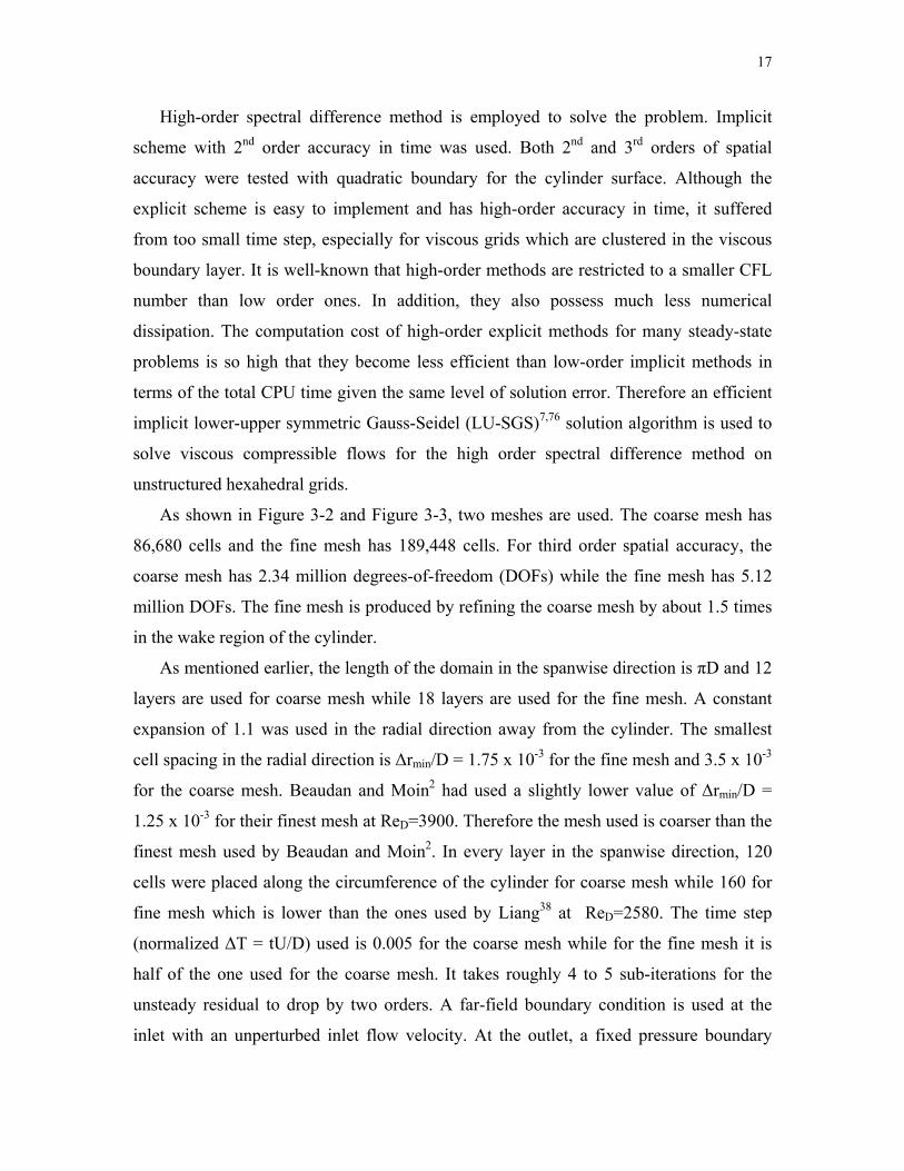
Figure 3-2

Coarse mesh in X-Y plane 18

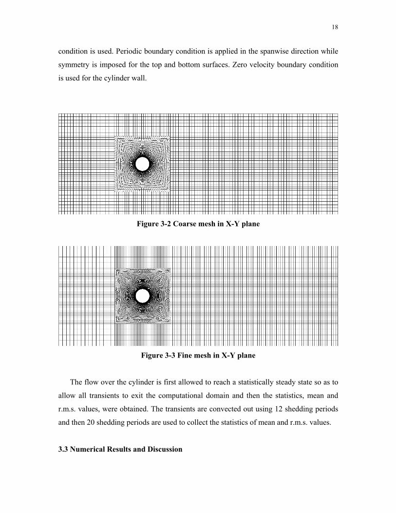
Figure 3-3

Fine mesh in X-Y plane 18

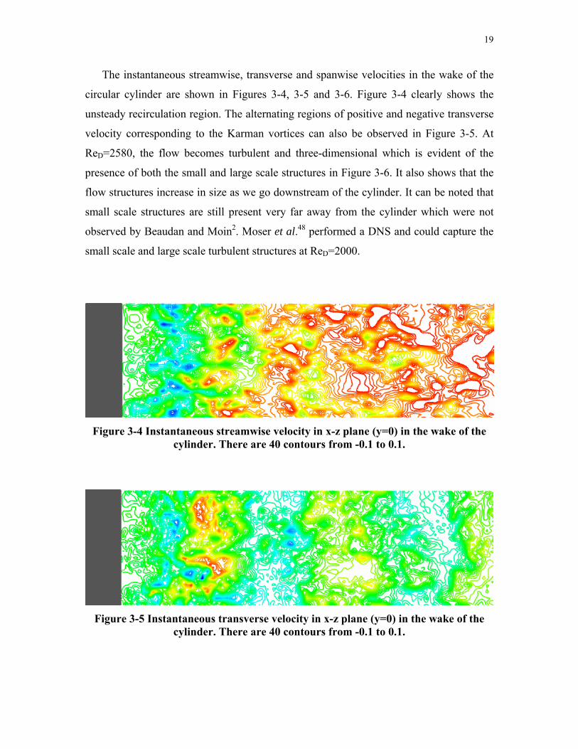
Figure 3-4 Instantaneous streamwise velocity in x-z plane (y=0) in the wake of the cylinder. There are 40 contours from -0.1 to 0.1 19

Figure 3-5

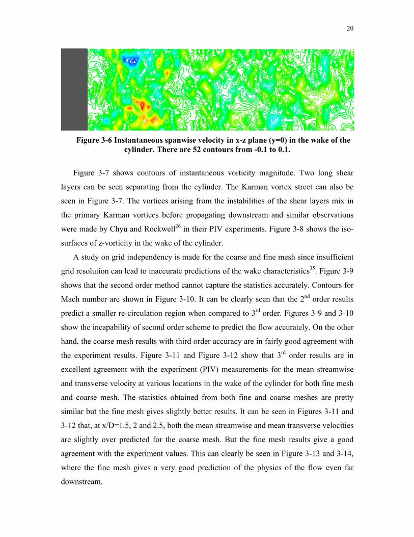
Instantaneous transverse velocity in x-z plane (y=0) in the wake of the cylinder. There are 40 contours from -0.1 to 0.1 19

Figure 3-6

Instantaneous spanwise velocity in x-z plane (y=0) in the wake of the cylinder. There are 52 contours from -0.1 to 0.1 20

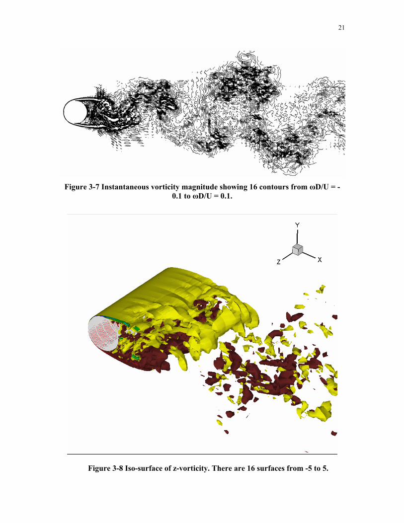
Figure 3-7 Instantaneous vorticity magnitude showing 16 contours from ωD/U = -0.1 to ωD/U = 0.1 21

Figure 3-8

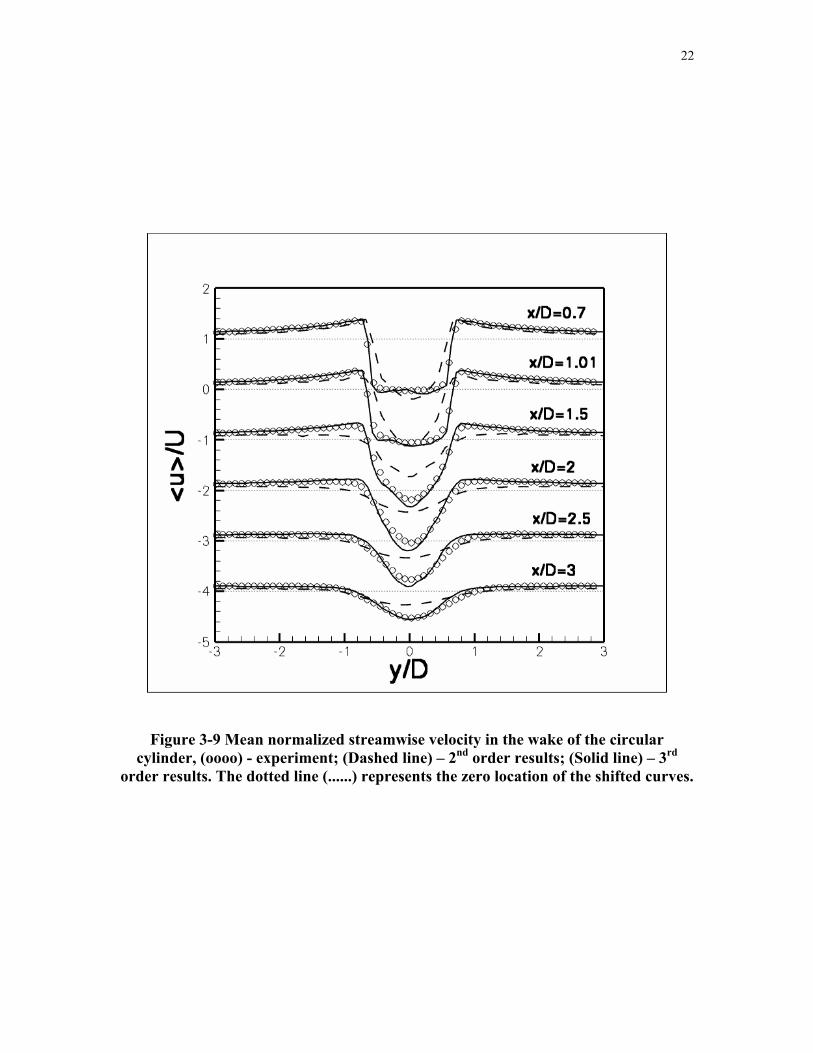
Iso-surface of z-vorticity. There are 16 surfaces from -5 to 5 21

Figure 3-9

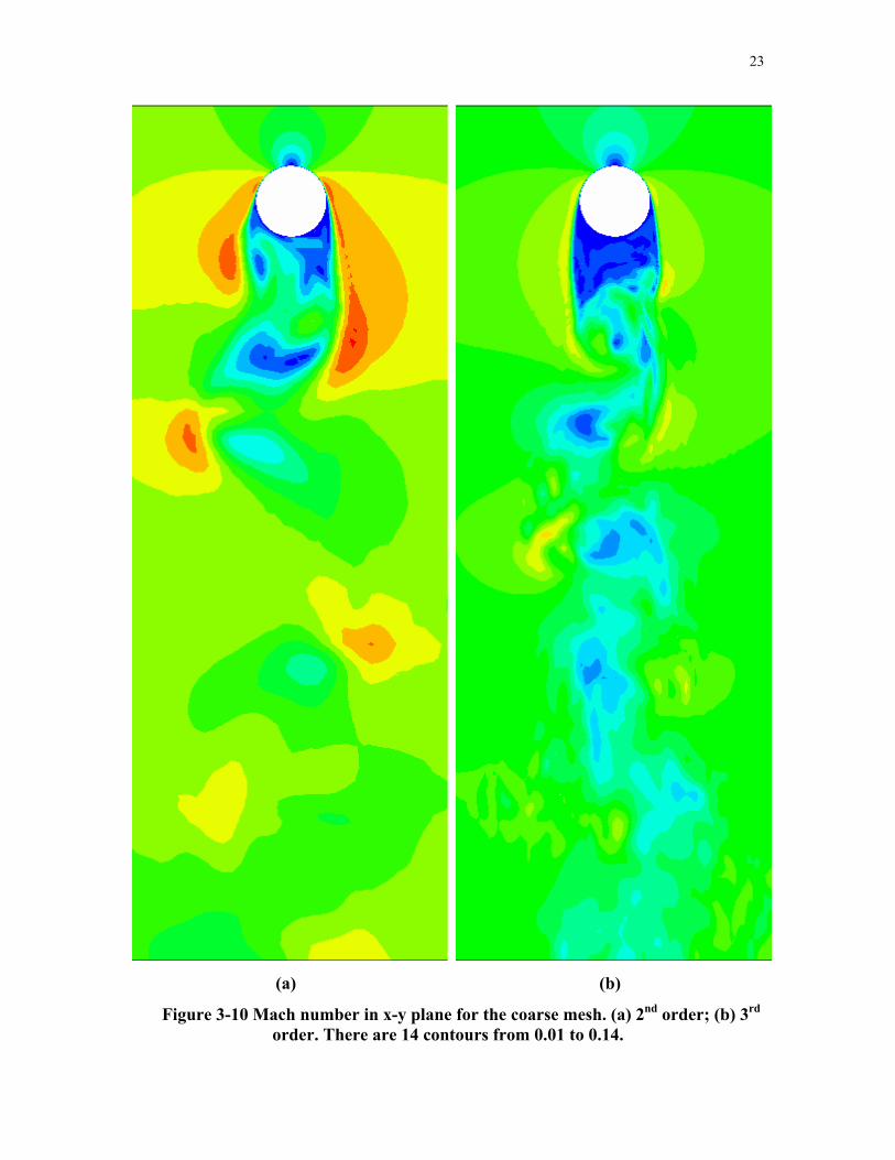
Mean normalized streamwise velocity in the wake of the circular cylinder, (oooo) - experiment; (Dashed line) – 2nd order results; (Solid line) – 3rd order results. The dotted line (......) represents the zero location of the shifted curves 22

Figure 3-10 Mach number in x-y plane for the coarse mesh. (a) 2nd order; (b) 3rd order. There are 14 contours from 0.01 to 0.14 23

Figure 3-11

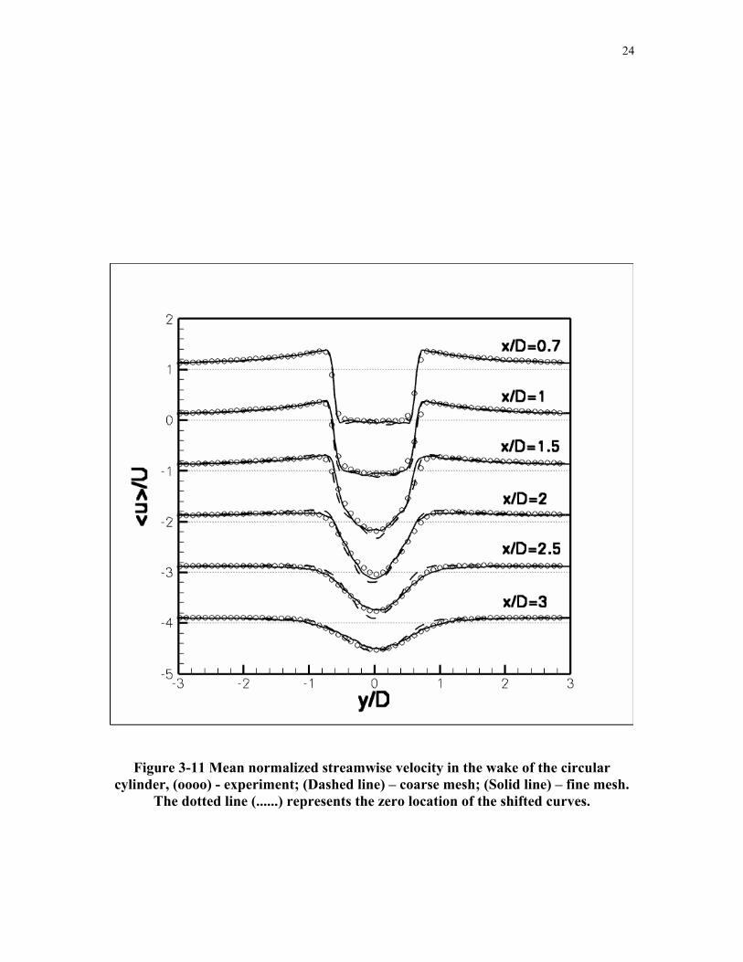
Mean normalized streamwise velocity in the wake of the circular cylinder, (oooo) - experiment; (Dashed line) – coarse mesh; (Solid line) – fine mesh. The dotted line (......) represents the zero location of the shifted curves 24

Figure 3-12

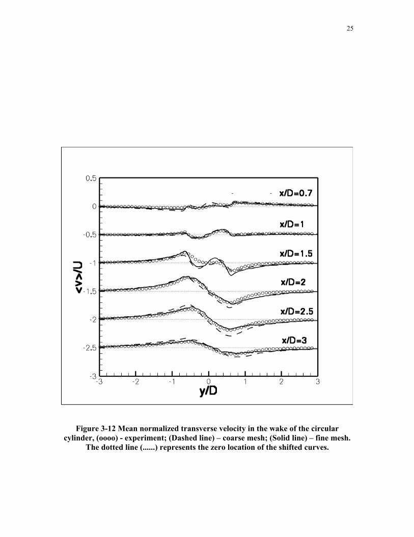
Mean normalized transverse velocity in the wake of the circular cylinder, (oooo) - experiment; (Dashed line) – coarse mesh; (Solid line) – fine mesh. The dotted line (......) represents the zero location of the shifted curves 25

v

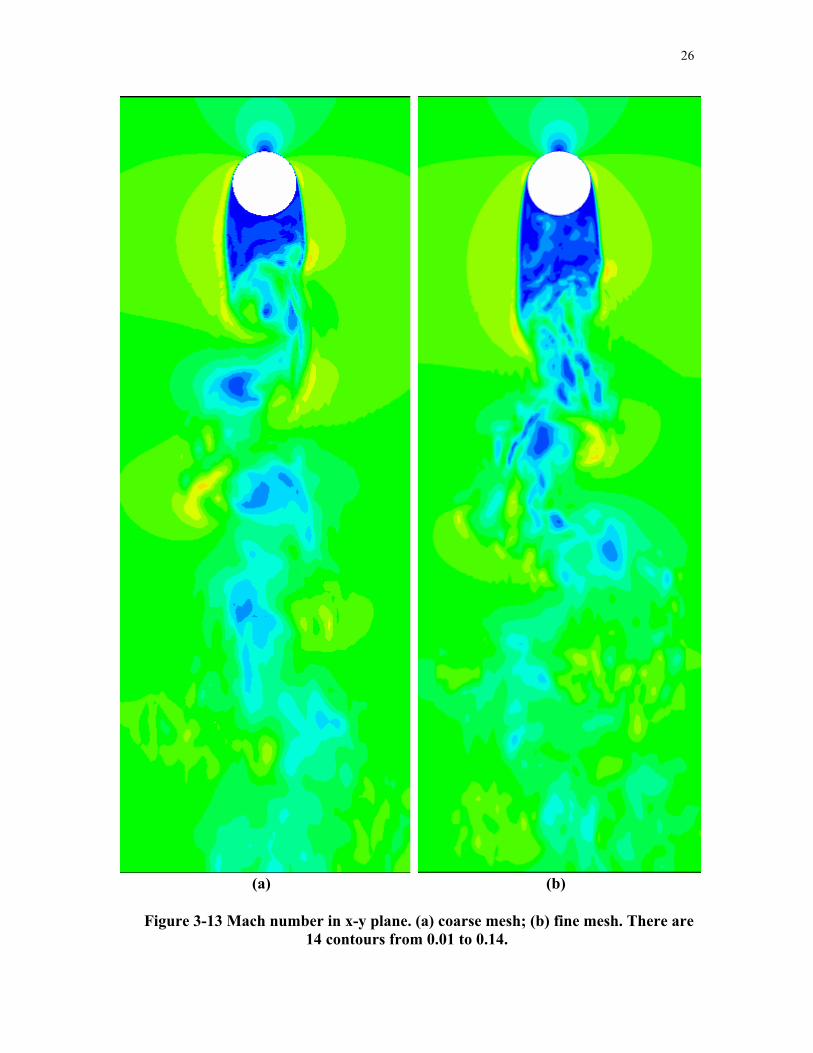
Figure 3-13 Mach number in x-y plane. (a) coarse mesh; (b) fine mesh. There are 14 contours from 0.01 to 0.14 26

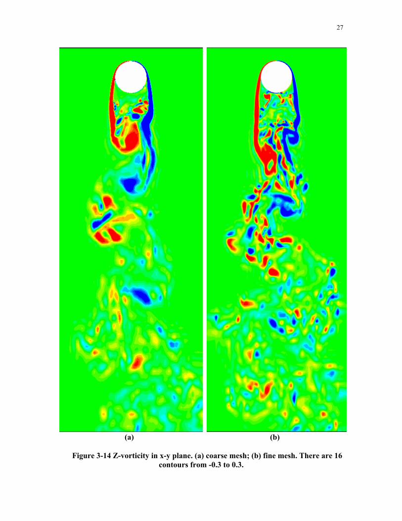
Figure 3-14 Z-vorticity in x-y plane. (a) coarse mesh; (b) fine mesh. There are 16 contours from -0.3 to 0.3 27

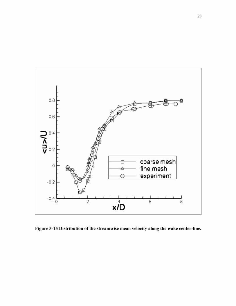
Figure 3-15 Distribution of the streamwise mean velocity along the wake center-line 28

Figure 3-16

Normalized <u'u'>/U2 in the wake of the circular cylinder, (oooo) - experiment; (Dashed line) – coarse mesh; (Solid line) – fine mesh. The dotted line (......) represents the zero location of the shifted curves 29

Figure 3-17

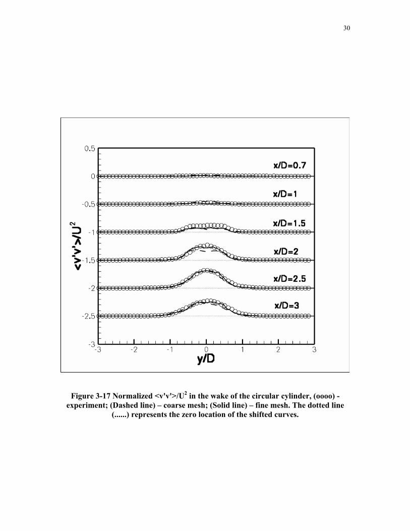
Normalized <v'v'>/U2 in the wake of the circular cylinder, (oooo) - experiment; (Dashed line) – coarse mesh; (Solid line) – fine mesh. The dotted line (......) represents the zero location of the shifted curves 30

Figure 3-18

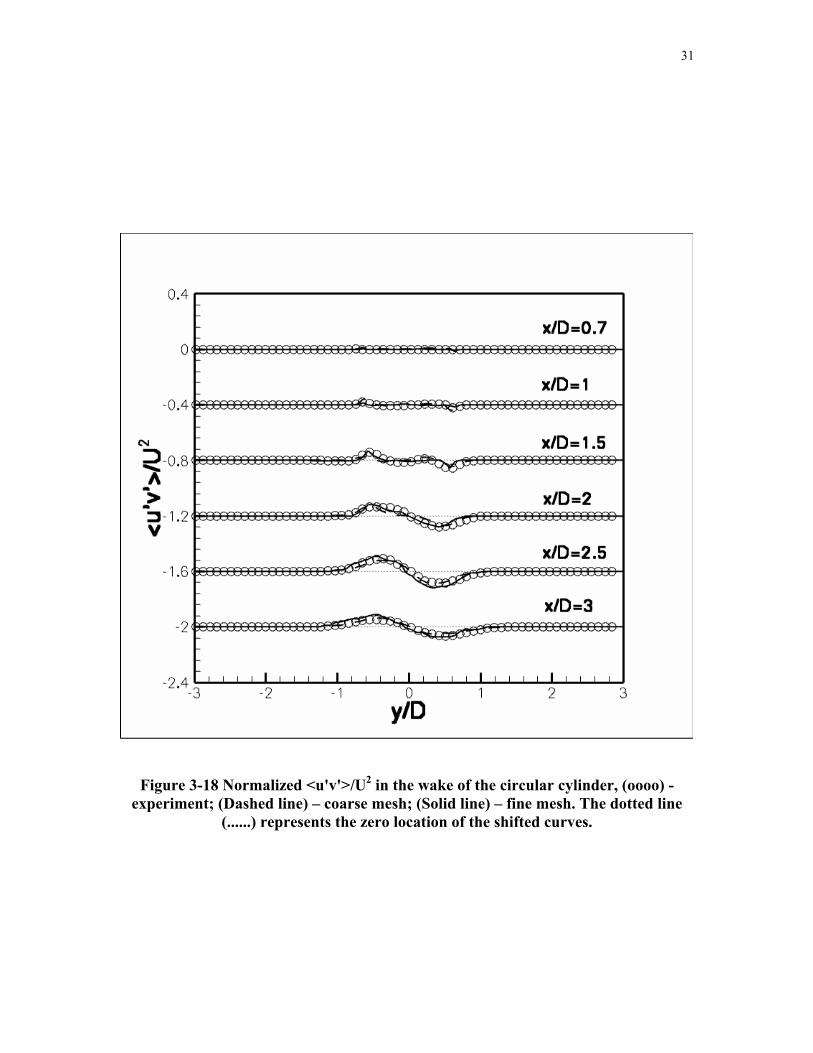
Normalized <u'v'>/U2 in the wake of the circular cylinder, (oooo) - experiment; (Dashed line) – coarse mesh; (Solid line) – fine mesh. The dotted line (......) represents the zero location of the shifted curves 31

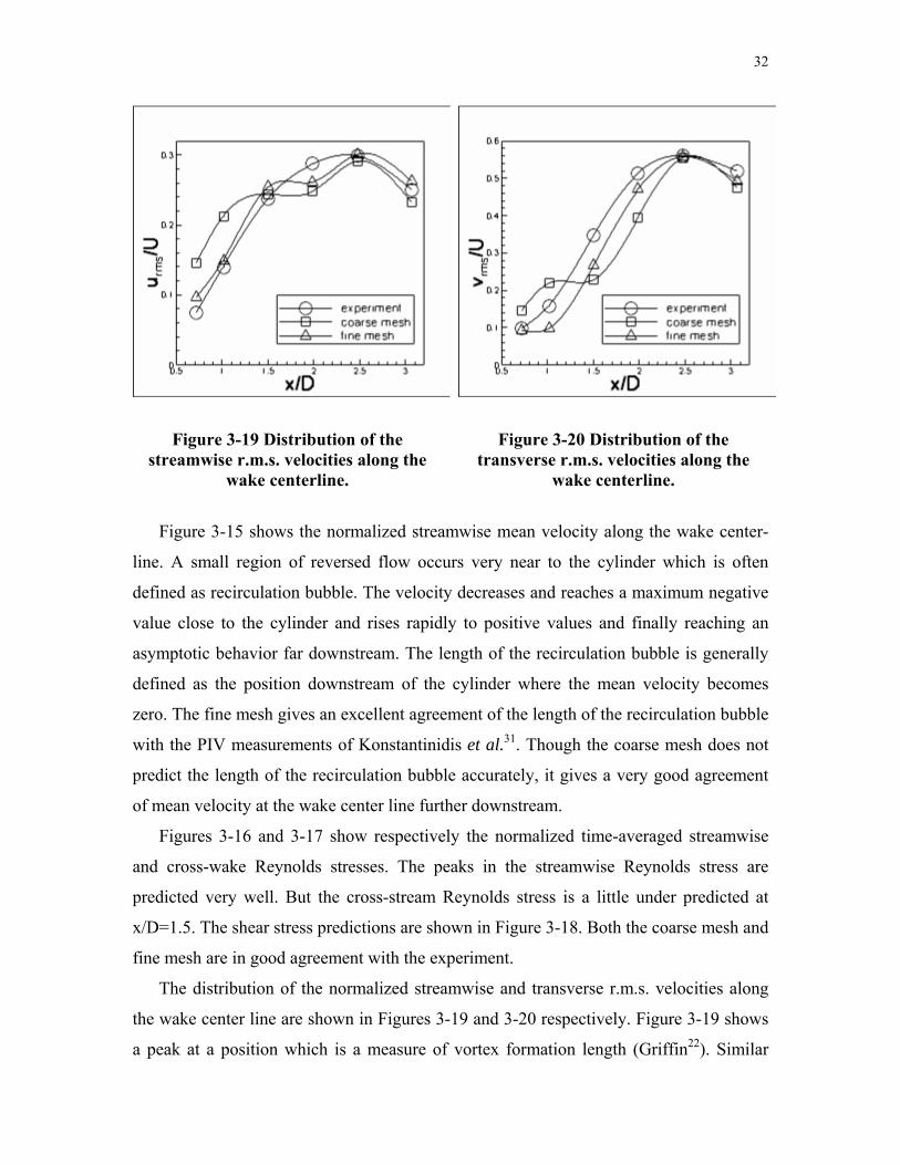
Figure 3-19 Distribution of the streamwise r.m.s. velocities along the wake centerline 32

Figure 3-20 Distribution of the transverse r.m.s. velocities along the wake centerline 32

Figure 4-1

Computational Delta Wing Geometry16 36

Figure 4-2

Grid structure of the cross-section of the delta wing 37

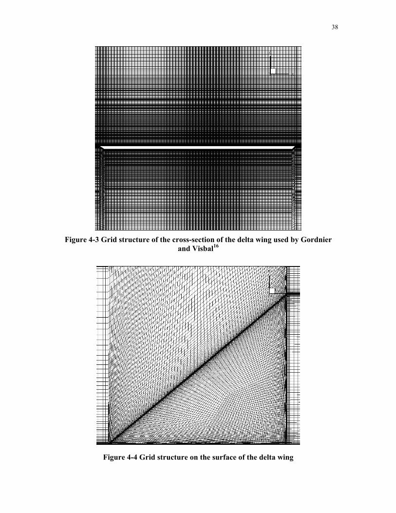
Figure 4-3 Grid structure of the cross-section of the delta wing used by Gordnier and Visbal16 38

Figure 4-4

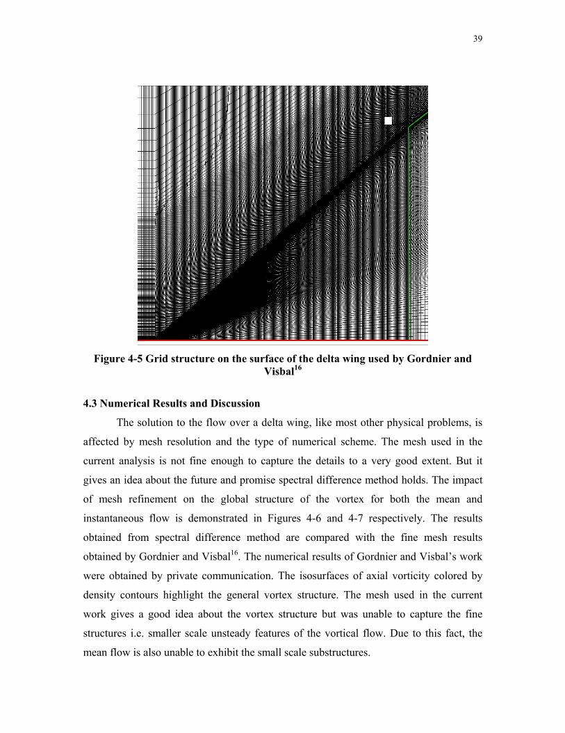
Grid structure on the surface of the delta wing 38

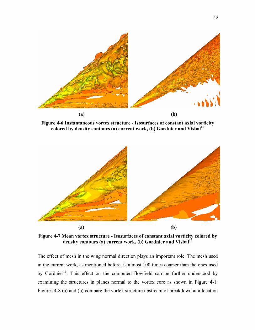
Figure 4-5 Grid structure on the surface of the delta wing used by Gordnier and Visbal16 39

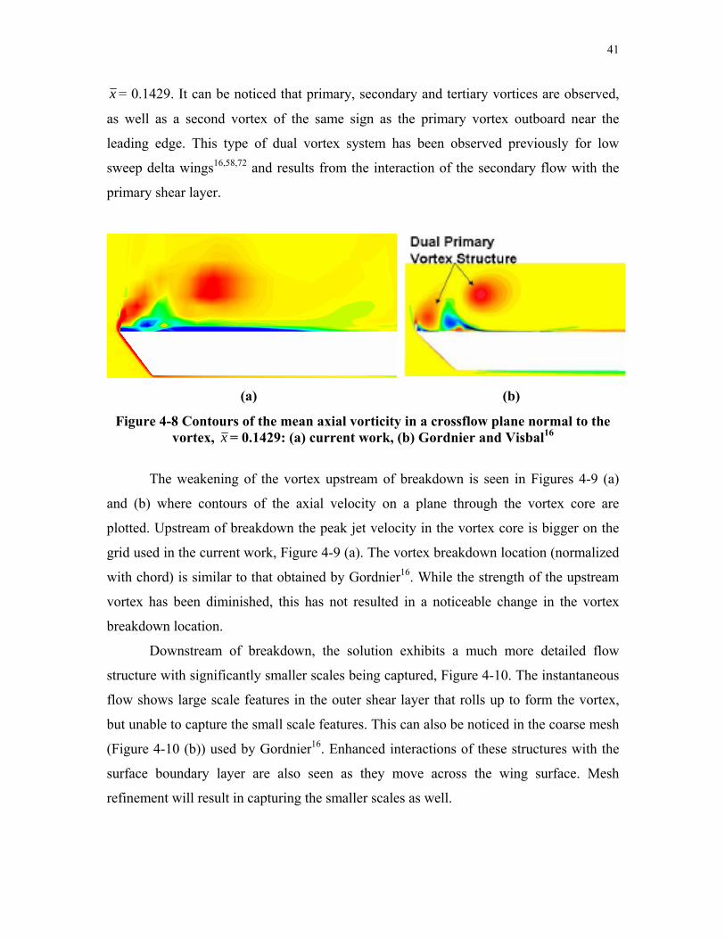
Figure 4-6

Instantaneous vortex structure - Isosurfaces of constant axial vorticity colored by density contours (a) current work, (b) Gordnier and Visbal16 40

vi

Figure 4-7

Mean vortex structure - Isosurfaces of constant axial vorticity colored by density contours (a) current work, (b) Gordnier and Visbal16 40

Figure 4-8

Contours of the mean axial vorticity in a crossflow plane normal to the vortex, x = 0.1429: (a) current work, (b) Gordnier and Visbal16 41

Figure 4-9 Contours of the mean axial velocity on a plane through the vortex core: (a) current work, (b) Gordnier and Visbal16 42

Figure 4-10

Contours of the instantaneous axial vorticity in a crossflow plane normal to the vortex, x = 0.85: (a) current work, (b) Gordnier and Visbal16 43

Figure 4-11

Comparison between the computation and PIV measurements on the crossflow plane x = 0.2: (a) current study, (b) Gordnier and Visbal16and (c) experiment, Re = 2 × 105 44

Figure 4-12 Computational mean velocity magnitude on a plane through the vortex core for the current work 45

Figure 4-13 Computational mean velocity magnitude on a plane through the vortex core by Gordnier and Visbal16 45

Figure 4-14 Experimental mean velocity magnitude on a plane through the vortex core 46

Figure 4-15 Mean axial velocity contours on a vertical plane through the vortex core: (a) current work, (b) Gordnier and Visbal16 46

Figure 4-16 Mean axial vorticity contours on a crossflow plane located at x =0.175: (a) current work, (b) Gordnier and Visbal16 47

Figure 4-17

Instantaneous axial vorticity contours on a crossflow plane normal to the vortex core at x =0.175: (a) current work, (b) Gordnier and Visbal16 48

Figure 4-18

Instantaneous spanwise vorticity on the wing surface 48

Figure 5-1

Large Tornado-Type Wind Energy System74 53

Figure 5-2

Defining the coordinate system for the tower bottom wall 54

vii

Figure 5-3

Three dimensional view of the computational model 56

Figure 5-4

Coarse mesh for Case 1 in x-y plane 58

Figure 5-5

Fine mesh for Case 1 in x-y plane 58

Figure 5-6

Finest mesh for Case 1 in x-y plane 59

Figure 5-7

Mesh used for simulations in FLUENT 59

Figure 5-8

Near-wall mesh resolution for coarse mesh 60

Figure 5-9

Near-wall mesh resolution for fine mesh 60

Figure 5-10

Near-wall mesh resolution for finest mesh 61

Figure 5-11 Coefficient of pressure Cp along the x-axis for different mesh sizes of case 1 62

Figure 5-12 Coefficient of pressure Cp along the y-axis for different mesh sizes of case 1 63

Figure 5-13 Coefficient of pressure Cp along the x-axis for different turbine heights 64

Figure 5-14 Coefficient of pressure Cp along the y-axis for different turbine heights 65

Figure 5-15 Coefficient of pressure Cp along the y-axis for different spiral diameters 66

Figure 5-16 Coefficient of pressure Cp along the y-axis for different spiral diameters 66

Figure 5-17

Pathlines of velocity inside the spiral 67

Figure 5-18

Pathlines of velocity in the wake of the turbine 67

Figure 5-19

Tangential velocity along x-axis inside the spiral 68

Figure 5-20

Tangential velocity along y-axis inside the spiral 68

Figure 5-21

Variation of minimum Cp along turbine height for case 1 69

Figure 5-22

Contours of tangential (swirl) velocity for case 1 69

viii

Figure 5-23 Coefficient of pressure Cp along the x-axis for different Wind Tunnel cross-sections 70

Figure 5-24 Coefficient of pressure Cp along the y-axis for different Wind Tunnel cross-sections 71

Figure 5-25

Coefficient of pressure Cp along x-axis for cases 1, 4 and 7 72

Figure 5-26

Coefficient of pressure Cp along y-axis for cases 1, 4 and 7 72

Figure 5-27 Comparison of coefficient of pressure Cp along x-axis for cases 1, 4 and 7 with experiment 73

Figure 5-28 Comparison of coefficient of pressure Cp along y-axis for cases 1, 4 and 7 with experiment 74

Figure 5-29 Contours of coefficient of pressure Cp for inviscid flow using FLUENT 75

Figure 5-30 Contours of coefficient of pressure Cp for viscous flow using FLUENT with RSM model 75

Figure 5-31 Contours of coefficient of pressure Cp for viscous flow using FLUENT with SA model 76

Figure 5-32 Contours of coefficient of pressure Cp for the finest mesh using MUSIC 76

Figure 5-33

Coefficient of pressure Cp distribution on the turbine wall 77

Figure 5-34

Contours of vorticity magnitude using FLUENT 78

Figure 5-35

Contours of pressure coefficient in the y-z plane 78

Figure 5-36

Contours of Mach number in the y-z plane 79

ix

LIST OF TABLES

Table 5-1

Mesh and solver details of all the different cases used 57

Table 5-2 Grid refinement and mesh details for case 1 57

x

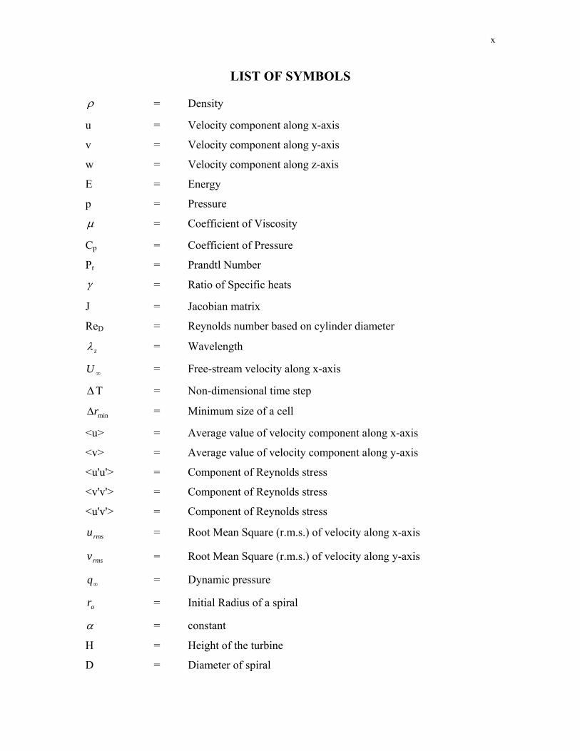
LIST OF SYMBOLS

ρ = Density

u = Velocity component along x-axis

v = Velocity component along y-axis

w = Velocity component along z-axis

E = Energy

p = Pressure

μ = Coefficient of Viscosity

Cp = Coefficient of Pressure

Pr = Prandtl Number

γ = Ratio of Specific heats

J = Jacobian matrix

ReD = Reynolds number based on cylinder diameter

zλ = Wavelength

∞U = Free-stream velocity along x-axis

ΔT = Non-dimensional time step

minrΔ = Minimum size of a cell

<u> = Average value of velocity component along x-axis

<v> = Average value of velocity component along y-axis

<u'u'> = Component of Reynolds stress

<v'v'> = Component of Reynolds stress

<u'v'> = Component of Reynolds stress

rmsu = Root Mean Square (r.m.s.) of velocity along x-axis

rmsv = Root Mean Square (r.m.s.) of velocity along y-axis

∞q = Dynamic pressure

or = Initial Radius of a spiral

α = constant

H = Height of the turbine

D = Diameter of spiral

xi

ACKNOWLEDGEMENTS

I wish to express my sincere gratitude to my supervisor Prof. Z. J. Wang of the Department of Aerospace Engineering at Iowa State University for his constant inspiration, guidance and personal attention while carrying out my master’s work. Prof Z. J. Wang helped me in making my work a success and gave me the opportunity to learn. I am indebted to him for extending all the necessary support during the course of the work. I would also like to give appreciative thanks to Dr. Chunlei Liang, Prof. Paul Durbin and Prof. Richard Pletcher for their suggestions for turbulent flow across bluff bodies. I would also like to thank Prof. Tom Shih for serving as my committee member. My heartfelt thanks are due to my fellow group members for their help and cooperation during my work. Last but not least, thanks to my parents and my friend Ayesha for their love and inspiration

xii

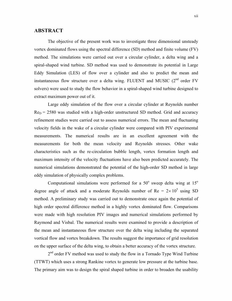
ABSTRACT

The objective of the present work was to investigate three dimensional unsteady

vortex dominated flows using the spectral difference (SD) method and finite volume (FV)

method. The simulations were carried out over a circular cylinder, a delta wing and a

spiral-shaped wind turbine. SD method was used to demonstrate its potential in Large

Eddy Simulation (LES) of flow over a cylinder and also to predict the mean and

instantaneous flow structure over a delta wing. FLUENT and MUSIC (2nd order FV

solvers) were used to study the flow behavior in a spiral-shaped wind turbine designed to

extract maximum power out of it.

Large eddy simulation of the flow over a circular cylinder at Reynolds number

ReD = 2580 was studied with a high-order unstructured SD method. Grid and accuracy

refinement studies were carried out to assess numerical errors. The mean and fluctuating

velocity fields in the wake of a circular cylinder were compared with PIV experimental

measurements. The numerical results are in an excellent agreement with the

measurements for both the mean velocity and Reynolds stresses. Other wake

characteristics such as the re-circulation bubble length, vortex formation length and

maximum intensity of the velocity fluctuations have also been predicted accurately. The

numerical simulations demonstrated the potential of the high-order SD method in large

eddy simulation of physically complex problems.

Computational simulations were performed for a 50o sweep delta wing at 15o

degree angle of attack and a moderate Reynolds number of Re = 2×105 using SD

method. A preliminary study was carried out to demonstrate once again the potential of

high order spectral difference method in a highly vortex dominated flow. Comparisons

were made with high resolution PIV images and numerical simulations performed by

Raymond and Visbal. The numerical results were examined to provide a description of

the mean and instantaneous flow structure over the delta wing including the separated

vortical flow and vortex breakdown. The results suggest the importance of grid resolution

on the upper surface of the delta wing, to obtain a better accuracy of the vortex structure.

2nd order FV method was used to study the flow in a Tornado Type Wind Turbine

(TTWT) which uses a strong Rankine vortex to generate low pressure at the turbine base.

The primary aim was to design the spiral shaped turbine in order to broaden the usability

xiii

of wind energy. Two solvers, FLUENT and MUSIC, both utilizing the 2nd order FV

method were used to perform the CFD analysis. Grid refinement study was carried out to

assess numerical errors. The effect of different parameters, like diameter of the spiral,

height of the turbine and blockage effect, on the vortex strength were studied. The

numerical results were compared with the experiment results. The distribution of pressure

was within 5-10% of experiment values but the values are not small enough to extract

high power out of the turbine.

1

Chapter 1 - Introduction

Lot of research on both low and high Reynolds number flows have been carried

out in the past. In the recent past, Computational Fluid Dynamics (CFD) is used in many

industry problems like thermal study of spent nuclear fuel casks, electronic cooling, rotor

blade flows, to name a few. The advent of high computational resources has allowed the

use of CFD to simulate many practical flow and thermal problems. Numerous numerical

schemes have been developed and based on the performance and accuracy; they are used

for problems of different nature. Tremendous amount of work has been carried out to

study vortex dominated flows – flows with the formation of a vortex or multiple vortices

which play an important role in the physics of the flow. After extensive research, more

accurate and reliable methods have been developed – one among them being high order

accurate algorithms for conservation laws. This led to the development of many methods

including the discontinuous Galerkin method9,10, the spectral volume (SV)41,66,68 and

spectral difference (SD)28,39,40,67 method and the k-exact finite volume1, 11 method.

Depending on the nature of the problem and accuracy level desired, a 2nd order finite

volume method or a high-order accurate method can be used.

1.1 Motivation

Innumerous studies have been carried out on Large Eddy Simulation of flow over

a circular cylinder. In the past, 2nd order finite volume method was used along with a

turbulence model like Smagorinsky, Dynamic Smagorinsky34,35,38 and many more. The

statistics obtained by Chunlei38 for an unperturbed inlet flow were not comparable at

most of the locations in the wake of the cylinder. This motivated the author to use a high

order method – spectral difference method – to obtain the flow statistics in the wake of a

cylinder at a sub-critical Reynolds number. Even though second order methods have

achieved success, there are several areas where their performance is unsatisfactory, e.g.,

for vortex-dominated flows including helicopter blade vortex interactions and flow over

high lift configurations. Higher order methods are more successful in handling these

flows. For example, high order compact methods have demonstrated much better results

than their lower order counterparts64. Not only are high order methods more accurate,

2

they also have the potential to reduce the CPU time required to obtain the solutions. This

again motivated the use of SD algorithm to predict the flow over a delta wing which has a

highly complex flowfield involving regions of laminar, transitional and turbulent flows

both on the surface of the wing and in the separated vortical flow. Most computations of

the delta wing flows in the past have employed lower-order (2nd order in space) numerical

schemes which require large number of grid points to capture with sufficient accuracy the

unsteady vortical flow features associated with a low sweep delta wing. A preliminary

study was carried out to study the flow over a delta wing.

Yen73-75 made lot of contributions in the past to study the characteristics of a

spiral shaped turbine. The idea was to develop a potential way to reduce the cost and

broaden the usability of wind energy. The system uses a large hollow tower of the shape

of a spiral to form an internal vortex. A commercial solver FLUENT12 and an in-house

solver MUSIC65 were used to study the physics of such a system. Most of the current

commercial CFD packages use the standard finite volume approach for discretizing the

Euler and the Navier-Stokes equations and are capable of simulating complex large scale

problems. In other words, the error decreases as O ( xΔ 2), with xΔ being the mesh size,

which is the case with the solvers used in the present study of tornado type wind turbine.

1.2 Thesis Outline

This thesis contains the work carried out in studying the Large Eddy Simulation

(LES) of flow over a cylinder, flow over a delta wing and physics of a tornado type wind

energy system. It is organized into different chapters – Chapter 2 gives a basic idea and

formulation of the spectral difference method, Chapter 3 includes the computational

details, geometry and numerical results for the flow over a cylinder, Chapter 4 discusses

about the computational details and preliminary results for the flow over a delta wing and

Chapter 5 talks about the tornado type wind energy system, solvers used and the results

obtained. Chapters 3, 4 and 5 also discuss about the possible future work.

3

Chapter 2 - The Spectral Difference Method 2.1 Introduction

Computational Fluid Dynamics (CFD) has been used in solving various flow

problems for more than three decades. The main area of concern has been the

performance of numerical methods in CFD tools with respect to both reliability and

accuracy. Extensive research efforts have led to the development of more accurate and

reliable methods. Various research projects have been carried out in the last decade to

develop and improve high order accurate algorithms for conservation laws. High-order

methods capable of handling unstructured grids are highly sought after in many practical

applications with complex geometries in LES, DNS of turbulence, computational aero-

acoustics, to name a few. Discontinuous galerkin method9,10 (DG), spectral volume

method41,66,68 (SV), and spectral difference method28,39,40,67 (SD) are a few high-order

schemes developed in the recent past. High-order methods are known not only for their

accuracy but also for their potential to reduce the CPU time required to obtain the

solutions. Most of the current calculations in computational aerodynamics, aero-acoustics

and CFD are performed using methods that are at most 2nd order accurate. Even though

second order methods have achieved successes, there exist several areas where their

performance is unsatisfactory, e.g., for vortex-dominated flows including helicopter blade

vortex interactions and flow over high lift configurations. Higher order methods are more

successful in handling these flows.

Methods like Finite Difference (FD) and Finite Volume (FV) normally employ

relatively low-order approximations in their formulations. But now we turn to spectral

methods which have the properties of very high accuracy and spectral (or exponential)

convergence5,21. In traditional spectral methods, the unknown variable is expressed as a

truncated series expansion in terms of some basis functions (trial functions) and solved

using the method weighted of residuals. The trial functions are infinitely differentiable

global functions, and the most frequently used ones are trigonometric functions or

Chebyshev and Legendre polynomials.

2.2 The Spectral Difference Method

4

The spectral difference (SD) method is a high-order, conservative, and efficient

numerical method developed for conservation laws on unstructured grids. It combines the

best features of structured and unstructured grid methods to attain computational

efficiency and geometric flexibility. It utilizes the concept of discontinuous and high-

order local representations to achieve conservation and high accuracy; and it is based on

the FD formulation for simplicity.

The SD method is a type of finite-difference method or nodal spectral method for

unstructured grids, in which inside each cell or element, there are structured nodal

unknown and flux distributions, in such a way that the local integral conservation is

satisfied. The conservative unknowns are defined at quadrature points. The unknowns are

updated using the differential form of the conservation law by approximating the flux

derivatives at those points. In order to obtain the flux derivatives, a polynomial

reconstruction of the fluxes is used from their values at certain flux points. To evaluate

the fluxes, the values of unknowns (and their gradients) at flux points are required. They

are obtained from a reconstruction of unknowns using their values at unknown points.

The reconstruction of fluxes is one order higher than that of unknowns.

In order to minimize the number of unknowns for a given accuracy, the unknowns

are normally placed at Gauss quadrature points, while the fluxes are placed at Gauss-

Lobatto quadrature points. By placing the unknowns and fluxes at the above quadrature

points, one can obtain the spectral convergence and accuracy5,30,33. However in a recent

study, Van den Abeele et al60 found that the SD method does not depend on where the

solution points are located, while the location of the flux points determines the method.

Therefore, the solution points can be chosen to maximize efficiency. It was also found

that the use of Chebyshev-Gauss-Lobatto points as the flux points results in a weak

instability by Van den Abeele et al60 and Huynh29. In the present study, the solution

points are chosen to be the Chebyshev-Gauss points.

There are two important features of the method dealing with the relation of

numerical solution in different cells. If the nodes are distributed in a geometrically similar

manner for all cells, the discretizations become universal. The other feature concerns the

fact that the flux at the surface points between two cells will in general be discontinuous.

In order to have local and global conservations, certain flux components must be

5

continuous. Therefore, the fluxes at those points are replaced with numerical fluxes. The

numerical fluxes serve to couple the solutions in two neighboring cells and provide the

necessary numerical dissipation to stabilize the numerical method.

The method is very simple to implement since it involves one-dimensional

operations only, and does not involve any surface or volume integrals. The basic idea is

presented next for the Navier-Stokes equations.

2.3 Formulation of the Spectral Difference Method on Hexahedral Grids

2.3.1 Governing equation

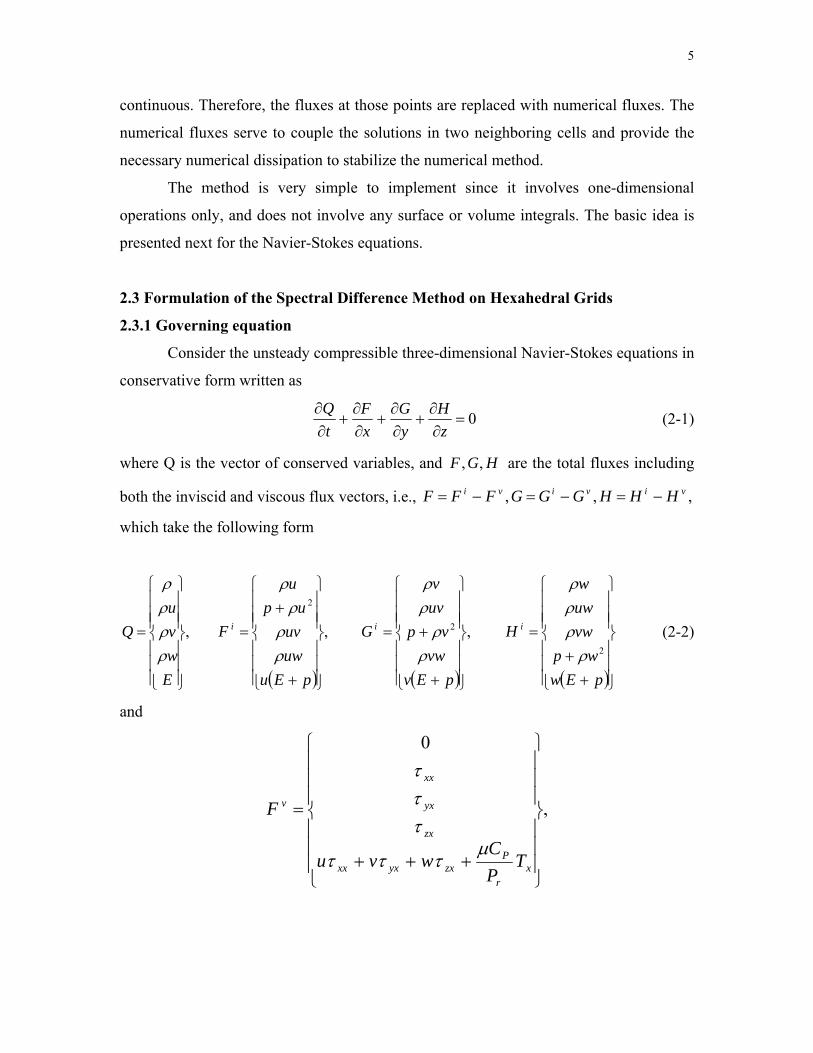
Consider the unsteady compressible three-dimensional Navier-Stokes equations in

conservative form written as

0=∂∂

+∂∂

+∂∂

+∂∂

zH

yG

xF

tQ

(2-1)

where Q is the vector of conserved variables, and are the total fluxes including

both the inviscid and viscous flux vectors, i.e.,

which take the following form

HGF ,,

,,, vivivi HHHGGGFFF −=−=−=

,

⎪⎪⎪

⎭

⎪⎪⎪

⎬

⎫

⎪⎪⎪

⎩

⎪⎪⎪

⎨

⎧

=

Ewvu

Qρρρρ

(2-2)

( )

,

2

⎪⎪⎪

⎭

⎪⎪⎪

⎬

⎫

⎪⎪⎪

⎩

⎪⎪⎪

⎨

⎧

+

+=

pEuuwuv

upu

F i

ρρρ

ρ

( )

,2

⎪⎪⎪

⎭

⎪⎪⎪

⎬

⎫

⎪⎪⎪

⎩

⎪⎪⎪

⎨

⎧

+

+=

pEvvw

vpuvv

G i

ρρ

ρρ

( )⎪⎪⎪

⎭

⎪⎪⎪

⎬

⎫

⎪⎪⎪

⎩

⎪⎪⎪

⎨

⎧

++

=

pEwwp

vwuww

H i

2ρρρρ

and

,

0

⎪⎪⎪

⎭

⎪⎪⎪

⎬

⎫

⎪⎪⎪

⎩

⎪⎪⎪

⎨

⎧

+++

=

xr

Pzxyxxx

zx

yx

xx

v

TPC

wvu

F

μτττ

τττ

6

,

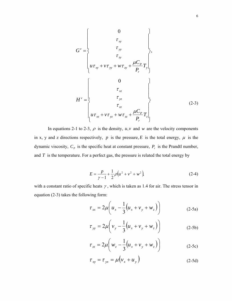
0

⎪⎪⎪

⎭

⎪⎪⎪

⎬

⎫

⎪⎪⎪

⎩

⎪⎪⎪

⎨

⎧

+++

=

yr

Pzyyyxy

zy

yy

xy

v

TPCwvu

G

μτττ

τττ

⎪⎪⎪

⎭

⎪⎪⎪

⎬

⎫

⎪⎪⎪

⎩

⎪⎪⎪

⎨

⎧

+++

=

zr

Pzzyzxz

zz

yz

xz

v

TPCwvu

H

μτττ

τττ0

(2-3)

In equations 2-1 to 2-3, ρ is the density, and are the velocity components

in x, y and z directions respectively, is the pressure, is the total energy,

vu, w

p E μ is the

dynamic viscosity, is the specific heat at constant pressure, is the Prandtl number,

and

PC rP

T is the temperature. For a perfect gas, the pressure is related the total energy by

( ),21

1222 wvupE +++

−= ργ

(2-4)

with a constant ratio of specific heats γ , which is taken as 1.4 for air. The stress tensor in

equation (2-3) takes the following form:

( )⎟⎠⎞

⎜⎝⎛ ++−= zyxxxx wvuu

312μτ (2-5a)

( )⎟⎠⎞

⎜⎝⎛ ++−= zyxyyy wvuv

312μτ (2-5b)

( )⎟⎠⎞

⎜⎝⎛ ++−= zyxzzz wvuw

312μτ (2-5c)

( )yxyxxy uv +== μττ (2-5d)

7

( )zyzyzy vw +== μττ (2-5e)

( )xzzxzx wu +== μττ (2-5f)

2.3.2 Coordinate transformation

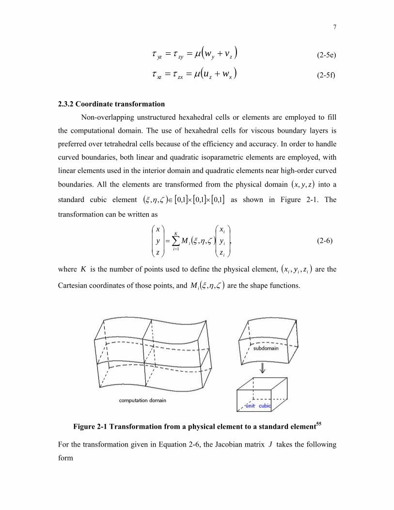
Non-overlapping unstructured hexahedral cells or elements are employed to fill

the computational domain. The use of hexahedral cells for viscous boundary layers is

preferred over tetrahedral cells because of the efficiency and accuracy. In order to handle

curved boundaries, both linear and quadratic isoparametric elements are employed, with

linear elements used in the interior domain and quadratic elements near high-order curved

boundaries. All the elements are transformed from the physical domain ( into a

standard cubic element ( ))zyx ,,

[ ] [ ] [ ]1,01,01,0,, ××∈ζηξ as shown in Figure 2-1. The

transformation can be written as

( ) ,,,1 ⎟

⎟⎟

⎠

⎞

⎜⎜⎜

⎝

⎛=

⎟⎟⎟

⎠

⎞

⎜⎜⎜

⎝

⎛

∑=

i

i

iK

ii

zyx

Mzyx

ζηξ (2-6)

where K is the number of points used to define the physical element, ( are the

Cartesian coordinates of those points, and

)iii zyx ,,

( )ζηξ ,,iM are the shape functions.

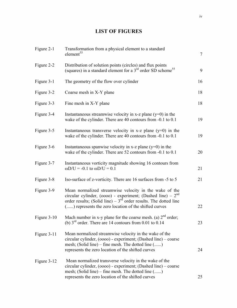
Figure 2-1 Transformation from a physical element to a standard element55

For the transformation given in Equation 2-6, the Jacobian matrix takes the following

form

J

8

( )( ) .

,,,,

⎥⎥⎥

⎦

⎤

⎢⎢⎢

⎣

⎡=

∂∂

=

ζηξ

ζηξ

ζηξ

ζηξzzzyyyxxx

zyxJ (2-7)

For a non-singular transformation, its inverse transformation must also exist, and the

Jacobian matrices are related to each other according to

( )( )

1

,,,, −=

⎥⎥⎥

⎦

⎤

⎢⎢⎢

⎣

⎡

=∂∂ J

zyxzyx

zyx

zyx

ζζζηηηξξξ

ζηξ. (2-8)

Therefore the metrics can be computed according to

( ) ( ) ( )J

yxyxJ

zxzxJ

zyzyzyx

ηζζηζηηζηζζη ξξξ−

=−

=−

= ,, (2-9a)

( ) ( ) ( )J

yxyxJ

zxzxJ

zyzyzyx

ζξξζξζζξζξξζ ηηη−

=−

=−

= ,, (2-9b)

( ) ( ) ( )J

yxyxJ

zxzxJ

zyzyzyx

ξηηξηξξηξηηξ ζζζ−

=−

=−

= ,, (2-9c)

The governing equations in the physical domain are then transformed into the

computational domain (standard element), and the transformed equations take the

following form

0~~~~=

∂∂

+∂∂

+∂∂

+∂∂

ζηξHGF

tQ (2-10)

where

QJQ ⋅=~

.~~~,~~~,~~~ vivivi HHHGGGFFF −=−=−=

9

⎥⎥⎥

⎦

⎤

⎢⎢⎢

⎣

⎡

⋅⎥⎥⎥

⎦

⎤

⎢⎢⎢

⎣

⎡

=⎥⎥⎥

⎦

⎤

⎢⎢⎢

⎣

⎡

i

i

i

zyx

zyx

zyx

i

i

i

HGF

JHGF

ζζζηηηξξξ

~~~

⎥⎥⎥

⎦

⎤

⎢⎢⎢

⎣

⎡

⋅⎥⎥⎥

⎦

⎤

⎢⎢⎢

⎣

⎡

=⎥⎥⎥

⎦

⎤

⎢⎢⎢

⎣

⎡

v

v

v

zyx

zyx

zyx

v

v

v

HGF

JHGF

ζζζηηηξξξ

~~~

Let ( )zyxJS ξξξξ ,,=r

, ( )zyxJS ηηηη ,,=r

and ( )zyxJS ζζζζ ,,=r

.

Then, finally ξSfF .~ r= , ηSfG .~ r

= , ζSfH .~ r= with ( )HGFf ,,=

r. In the implementation,

J is stored at the solution points, while ζηξ SSSrrr

,, are stored at flux points to minimize

memory usage.

2.3.3 Spatial discretization

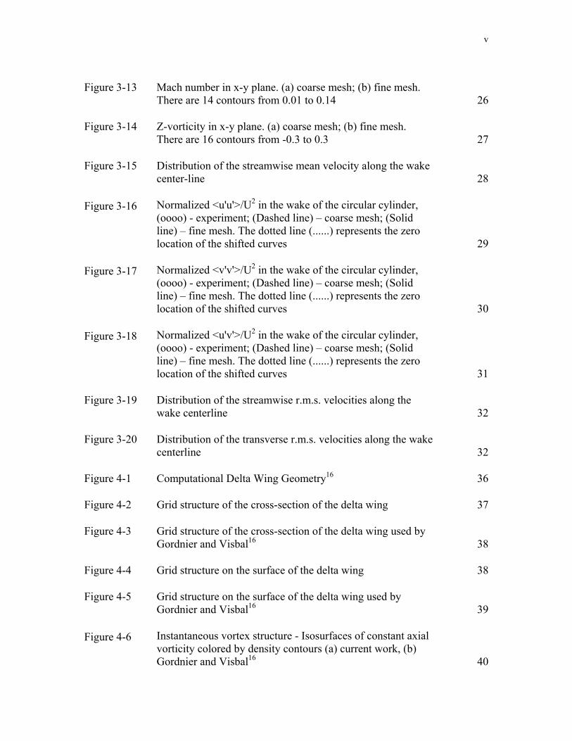
In a standard element, two sets of points are defined, namely the solution points

and the flux points, illustrated in Figure 2-2 for 2D. The solution unknowns or degrees-

of-freedom (DOFs) are the conserved variables at the solution points, while fluxes are

computed at the flux points in order to update the solution unknowns. In order to

construct a degree (N-1) polynomial in any direction, solutions at N points are required.

Figure 2-2 Distribution of solution points (circles) and flux points (squares) in a

standard element for a 3rd order SD scheme55

As mentioned earlier, Van den Abeele et al60 found that the SD method does not

depend on where the solution points are located, while the location of the flux points

determines the method. In the current work, the solution points are chosen to be the

Chebyshev-Gauss points defined by

10

NsN

sX s ,,2,1,2

12cos121

K=⎥⎦

⎤⎢⎣

⎡⎟⎠⎞

⎜⎝⎛ ⋅

−−= π . (2-11)

The flux points are selected to be the Legendre-Gauss-quadrature points plus the two end

points, 0 and 1, as suggested by Huynh29. Using the N solutions at the solution points, a

degree N-1 polynomial can be built using the following Lagrange basis defined as

∏≠=

⎟⎟⎠

⎞⎜⎜⎝

⎛−−

=N

iss si

si XX

XXXh,1

)( . (2-12)

Similarly, using the fluxes at the flux points, a degree N polynomial can be built

for the flux using a similar Lagrange basis defined as

1+N

∏≠= ++

++ ⎟⎟

⎠

⎞⎜⎜⎝

⎛−

−=

N

iss si

si XX

XXXl,0 2/12/1

2/12/1 )( . (2-13)

The reconstructed solution for the conserved variables in the standard element is just the

tensor products of the three one-dimensional polynomials, i.e.,

)()()(~

),,(1 1 1 ,,

,, ςηξςηξ kji

N

k

N

j

N

i kji

kji hhhJQ

Q ⋅⋅= ∑∑∑= = =

.

Similarly, the reconstructed flux polynomials take the following forms:

)()()(~),,(~2/1

1 1 0,,2/1 ςηξςηξ kji

N

k

N

j

N

ikji hhlFF ⋅⋅= +

= = =+∑∑∑ , (2-14a)

)()()(~),,(~2/1

1 0 1,2/1, ςηξςηξ kji

N

k

N

j

N

ikji hlhGG ⋅⋅= +

= = =+∑∑∑ , (2-14b)

)()()(~),,(~2/1

0 1 12/1,, ςηξςηξ +

= = =+ ⋅⋅= ∑∑∑ kji

N

k

N

j

N

ikji lhhHH . (2-14c)

The reconstructed fluxes are only element-wise continuous, but discontinuous across cell

interfaces. For the inviscid flux, a Riemann solver, such as the Rusanov or Roe flux, is

employed to compute a common flux at interfaces to ensure conservation and stability. In

summary, the algorithm to compute the inviscid flux derivatives consists of the following

steps:

1. Given the conserved variables at the solution points { }kjiQ ,,~ , compute the

conserved variables at the flux points

2. Compute the inviscid fluxes at the interior flux points using the solutions

computed at Step 1

11

3. Compute the inviscid flux at element interfaces using a Riemann solver, in terms

of the left and right conserved variables of the interface.

4. Compute the derivatives of the fluxes at all the solution points according to

∑=

++ ′⋅=⎟⎟⎠

⎞⎜⎜⎝

⎛

∂∂ N

rirkjr

kji

lFF0

2/1,,2/1,,

)(~~ξ

ξ, (2-15a)

∑=

++ ′⋅=⎟⎟⎠

⎞⎜⎜⎝

⎛

∂∂ N

rjrkri

kji

lGG0

2/1,2/1,

,,

)(~~η

η, (2-15b)

∑=

++ ′⋅=⎟⎟⎠

⎞⎜⎜⎝

⎛

∂∂ N

rkrrji

kji

lHH0

2/12/1,,

,,

)(~~ς

ς. (2-15c)

The viscous flux is a function of both the conserved variables and their gradients, e.g.,

. Therefore the key is how to compute the solution gradients

at the flux points. The following steps are taken to compute the viscous fluxes:

),(~~,,2/1,,2/1,,2/1 kjikji

vv QQFFkji ++ ∇=

+

1. Same as Step 1 for the inviscid flux computations;

2. When computing the derivatives, the solution Q at the cell interface is not

uniquely defined. The solution at the interface is simply the average of the left

and right solutions, . 2/)(ˆRL QQQ +=

3. Compute the gradients of the solution at the solution points using the solutions at

the flux points. Then the gradients are interpolated from the solution points to the

flux points using the same Lagrangian interpolation approach given in.

4. Compute the viscous flux at the flux points using the solutions and their gradients

at the flux points. Again at cell interfaces, the gradients have two values, one from

the left and one from the right. The gradients used in the viscous fluxes at the cell

interface are simply the averaged ones, i.e., . )2/)(,2/)((~~RLRL

vv QQQQFF ∇+∇+=

Once all fluxes are computed at the flux points, the flux polynomials are built according

to Equation 2-14, and the derivatives of the fluxes are then evaluated at each solution

point to update the DOFs, i.e.,

kji

HGFtQ

,,

~~~~

⎟⎟⎠

⎞⎜⎜⎝

⎛∂∂

+∂∂

+∂∂

−=∂∂

ζηξ (2-16)

12

More details of the SD method can be found in References 55 and 56.

The potential of spectral difference method in vortex-dominated flows is

demonstrated in the case of flow over a circular cylinder and flow over a delta wing,

discussed in chapters 3 and 4 to follow.

13

Chapter 3 – Large Eddy Simulation of Flow over a

Cylinder

3.1 Introduction

The flow around bluff bodies is very complex and can involve regions of laminar,

transitional and turbulent flows, unsteady separation and reattachment, and the formation

of coherent structures, particularly in the wake region of the flow. The understanding of

bluff body vortex shedding is of great practical importance and the uniform flow over a

circular cylinder is a classical example of bluff body flow. The configuration is quite

simple but the flow is characterized by a very complex wake at Reynolds number

ReD=2580 examined in the current work. The importance of using high order methods to

study the numerical and physical aspect of unsteady wake flow involving separation,

recirculation, unsteady vortex shedding and large complex flow structures at a sub-

critical Reynolds number is shown. The near wake structure behind a bluff body plays an

important role in the overall vortex formation and shedding processes and determines the

magnitude of mean and fluctuating forces exerted on the body. Direct numerical

simulations (DNS) of the Navier-Stokes equations, in which all eddy scales have to be

captured, is almost impossible for problems with moderately high Reynolds number

because of the huge computational requirements in resolving all turbulence scales. Hence

a less expensive and accurate method is required. In Reynolds averaged Navier-Stokes

(RANS) approach, all eddies are averaged over to give equations for variables

representing the mean flow. But RANS has proved to be generally inadequate in

predicting the effects of turbulent separating and reattaching flows, because the large

eddies responsible for the primary transport are geometry dependent. For any turbulent

flow, the largest scale is of the order of the domain size and the small scales are related to

the dissipative eddies where the viscous effects become predominant. Large eddy

simulation (LES) is a method where the three-dimensional and unsteady motion of the

large eddies is computed explicitly and the non-linear interactions with the smaller

eddies, which are assumed to be isotropic and universal, are modeled. LES is an active

14

area of research and the numerical simulation of complex flows is essential in the

development of the method as a tool to predict flows of engineering interest.

In the current work, implicit LES computations were performed without any sub-grid

scale model in order to investigate the effectiveness of the spectral difference method.

These simulations were deliberately not called direct numerical simulations because they

did not comply with the resolution requirements of DNS. Turbulent flow past a circular

cylinder has been the subject of a large number of experimental and numerical

investigations54,70. In recent years a good understanding of the physics of flow at low

Reynolds number of below a few hundred, has been obtained. But at higher Reynolds

number, still subcritical though, considerably less is known. A comprehensive review of

the flow characteristics for a wide range of Reynolds numbers was studied by

Williamson69. In addition, a number of simulations at various Reynolds numbers, mostly

LES, have been carried out6,59. The cylinder flow at Reynolds number ReD=3900 has

become a common test case for LES primarily because of the availability of the

experimental results of Lourenco and Shih36 and Ong and Wallace51. The calculations

were performed on structured2,4,35,45 and unstructured meshes15,26,42. Beaudan and Moin2,

Mittal and Moin45, Kravchenko and Moin34 were among the first to perform LES studies

at ReD=3900. Motivated by the direct simulation results of Rai and Moin52, Beaudan and

Moin2 used high-order upwind-biased schemes for the numerical simulations of the

compressible Navier–Stokes equations. The profiles of mean velocity and Reynolds

stresses obtained in these simulations were in reasonable agreement with the

experimental data. However, inside the recirculation region, the streamwise velocity

profiles differed in shape from those observed in the experiment36. These differences

were attributed to the experimental errors as manifested in the large asymmetry of the

experimental data2. A new experiment at the same Reynolds number was carried out by

Ong and Wallace51 and provided the mean flow data at several locations in the near wake

of the cylinder downstream of the recirculation region. Even though fair agreement

between the simulations of Beaudan and Moin2 and the experiment was observed in the

mean velocity profiles, turbulence intensities at several downstream locations did not

match the experimental data. Also the Reynolds stresses were not predicted correctly

when compared to experimental data. Similar problems were observed with Mittal and

15

Moin's work35,45. In the two mentioned simulations, they showed a shape of the

streamwise velocity profile inside the recirculation region different from that observed in

the experiment of Laurenco and Shih36. A new experiment at the same Reynolds number

was carried out by Ong and Wallace51 and provided the mean flow data at several

locations in the near wake of the cylinder downstream of the recirculation region. Even

though fair agreement between the simulations of Beaudan and Moin2 and the experiment

was observed in the mean velocity profiles, turbulence intensities at several downstream

locations did not match the experimental data. Several other researchers have examined a

variety of aspects that affect the quality of LES solutions at ReD=3900. The numerical

and modeling aspects which influence the quality of LES solutions were studied by

Breuer3. He had also carried out LES computations without any sub-grid scale model.

DNS of the cylinder flow at ReD=3900 was performed by Ma et al.42. The mean

velocity profiles and the power spectra are in good agreement with the experimental data

in the near wake as well as far downstream. In particular, the velocity profiles agree well

with those from the experiments in the vicinity of the cylinder. Compared with LES35, the

pressure coefficient in DNS is a little lower, while the recirculation bubble length is

larger. Franke and Frank13 found out that this is an effect of the averaging time in

computing statistics. In DNS42 the statistics is accumulated over 600 convective time

units (D/U), while in LES35 the statistics is accumulated over 35 convective time units.

The numerical issues raised in the previous large eddy simulations prompted us to

attempt simulations of the flow over a circular cylinder using a high order method.

Second-order simulations for unperturbed inlet flow conditions at ReD=2580 were

performed by Liang38. The length of the recirculation bubble was under predicted

probably due to under-resolution. The primary motivation for using a high order method

is to accurately study the wake flow at Reynolds number ReD=2580. The numerical

results obtained were compared with the PIV experiment performed by Konstantinidis et

al.31.

3.2 Problem Definition and Computational Details

The simulation was performed to match the geometry of the experiment performed by

Konstantinidis et al31. The experiments were performed using the PIV technique in a

16

stainless steel water tunnel with a cross-section of 72mm x 72mm. The origin and size of

the computational domain are shown in Figure 3-1. The x-axis is along the streamwise

flow direction and the z-axis is along the cylinder axis i.e. the spanwise direction. The

cylinder has a non-dimensional unit diameter. The upstream velocity is fixed at U=0.1

m/s and is assumed to be uniform across the inlet. The Reynolds number based on the

cylinder diameter and upstream velocity is 2580.

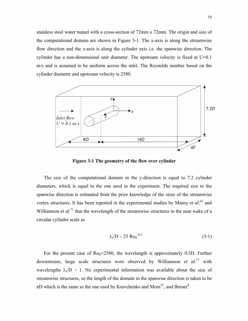
Figure 3-1 The geometry of the flow over cylinder

The size of the computational domain in the y-direction is equal to 7.2 cylinder

diameters, which is equal to the one used in the experiment. The required size in the

spanwise direction is estimated from the prior knowledge of the sizes of the streamwise

vortex structures. It has been reported in the experimental studies by Mansy et al.43 and

Williamson et al.71 that the wavelength of the streamwise structures in the near wake of a

circular cylinder scale as

λz/D ~ 25 ReD-0.5 (3-1)

For the present case of ReD=2580, the wavelength is approximately 0.5D. Further

downstream, large scale structures were observed by Williamson et al.71 with

wavelengths λz/D ~ 1. No experimental information was available about the size of

streamwise structures, so the length of the domain in the spanwise direction is taken to be

πD which is the same as the one used by Kravchenko and Moin35, and Breuer4.

17

High-order spectral difference method is employed to solve the problem. Implicit

scheme with 2nd order accuracy in time was used. Both 2nd and 3rd orders of spatial

accuracy were tested with quadratic boundary for the cylinder surface. Although the

explicit scheme is easy to implement and has high-order accuracy in time, it suffered

from too small time step, especially for viscous grids which are clustered in the viscous

boundary layer. It is well-known that high-order methods are restricted to a smaller CFL

number than low order ones. In addition, they also possess much less numerical

dissipation. The computation cost of high-order explicit methods for many steady-state

problems is so high that they become less efficient than low-order implicit methods in

terms of the total CPU time given the same level of solution error. Therefore an efficient

implicit lower-upper symmetric Gauss-Seidel (LU-SGS)7,76 solution algorithm is used to

solve viscous compressible flows for the high order spectral difference method on

unstructured hexahedral grids.

As shown in Figure 3-2 and Figure 3-3, two meshes are used. The coarse mesh has

86,680 cells and the fine mesh has 189,448 cells. For third order spatial accuracy, the

coarse mesh has 2.34 million degrees-of-freedom (DOFs) while the fine mesh has 5.12

million DOFs. The fine mesh is produced by refining the coarse mesh by about 1.5 times

in the wake region of the cylinder.

As mentioned earlier, the length of the domain in the spanwise direction is πD and 12

layers are used for coarse mesh while 18 layers are used for the fine mesh. A constant

expansion of 1.1 was used in the radial direction away from the cylinder. The smallest

cell spacing in the radial direction is Δrmin/D = 1.75 x 10-3 for the fine mesh and 3.5 x 10-3

for the coarse mesh. Beaudan and Moin2 had used a slightly lower value of Δrmin/D =

1.25 x 10-3 for their finest mesh at ReD=3900. Therefore the mesh used is coarser than the

finest mesh used by Beaudan and Moin2. In every layer in the spanwise direction, 120

cells were placed along the circumference of the cylinder for coarse mesh while 160 for

fine mesh which is lower than the ones used by Liang38 at ReD=2580. The time step

(normalized ΔT = tU/D) used is 0.005 for the coarse mesh while for the fine mesh it is

half of the one used for the coarse mesh. It takes roughly 4 to 5 sub-iterations for the

unsteady residual to drop by two orders. A far-field boundary condition is used at the

inlet with an unperturbed inlet flow velocity. At the outlet, a fixed pressure boundary

18

condition is used. Periodic boundary condition is applied in the spanwise direction while

symmetry is imposed for the top and bottom surfaces. Zero velocity boundary condition

is used for the cylinder wall.

Figure 3-2 Coarse mesh in X-Y plane

Figure 3-3 Fine mesh in X-Y plane

The flow over the cylinder is first allowed to reach a statistically steady state so as to

allow all transients to exit the computational domain and then the statistics, mean and

r.m.s. values, were obtained. The transients are convected out using 12 shedding periods

and then 20 shedding periods are used to collect the statistics of mean and r.m.s. values.

3.3 Numerical Results and Discussion

19

The instantaneous streamwise, transverse and spanwise velocities in the wake of the

circular cylinder are shown in Figures 3-4, 3-5 and 3-6. Figure 3-4 clearly shows the

unsteady recirculation region. The alternating regions of positive and negative transverse

velocity corresponding to the Karman vortices can also be observed in Figure 3-5. At

ReD=2580, the flow becomes turbulent and three-dimensional which is evident of the

presence of both the small and large scale structures in Figure 3-6. It also shows that the

flow structures increase in size as we go downstream of the cylinder. It can be noted that

small scale structures are still present very far away from the cylinder which were not

observed by Beaudan and Moin2. Moser et al.48 performed a DNS and could capture the

small scale and large scale turbulent structures at ReD=2000.

Figure 3-4 Instantaneous streamwise velocity in x-z plane (y=0) in the wake of the

cylinder. There are 40 contours from -0.1 to 0.1.

Figure 3-5 Instantaneous transverse velocity in x-z plane (y=0) in the wake of the

cylinder. There are 40 contours from -0.1 to 0.1.

20

Figure 3-6 Instantaneous spanwise velocity in x-z plane (y=0) in the wake of the

cylinder. There are 52 contours from -0.1 to 0.1.

Figure 3-7 shows contours of instantaneous vorticity magnitude. Two long shear

layers can be seen separating from the cylinder. The Karman vortex street can also be

seen in Figure 3-7. The vortices arising from the instabilities of the shear layers mix in

the primary Karman vortices before propagating downstream and similar observations

were made by Chyu and Rockwell26 in their PIV experiments. Figure 3-8 shows the iso-

surfaces of z-vorticity in the wake of the cylinder.

A study on grid independency is made for the coarse and fine mesh since insufficient

grid resolution can lead to inaccurate predictions of the wake characteristics35. Figure 3-9

shows that the second order method cannot capture the statistics accurately. Contours for

Mach number are shown in Figure 3-10. It can be clearly seen that the 2nd order results

predict a smaller re-circulation region when compared to 3rd order. Figures 3-9 and 3-10

show the incapability of second order scheme to predict the flow accurately. On the other

hand, the coarse mesh results with third order accuracy are in fairly good agreement with

the experiment results. Figure 3-11 and Figure 3-12 show that 3rd order results are in

excellent agreement with the experiment (PIV) measurements for the mean streamwise

and transverse velocity at various locations in the wake of the cylinder for both fine mesh

and coarse mesh. The statistics obtained from both fine and coarse meshes are pretty

similar but the fine mesh gives slightly better results. It can be seen in Figures 3-11 and

3-12 that, at x/D=1.5, 2 and 2.5, both the mean streamwise and mean transverse velocities

are slightly over predicted for the coarse mesh. But the fine mesh results give a good

agreement with the experiment values. This can clearly be seen in Figure 3-13 and 3-14,

where the fine mesh gives a very good prediction of the physics of the flow even far

downstream.

21

Figure 3-7 Instantaneous vorticity magnitude showing 16 contours from ωD/U = -

0.1 to ωD/U = 0.1.

Figure 3-8 Iso-surface of z-vorticity. There are 16 surfaces from -5 to 5.

22

Figure 3-9 Mean normalized streamwise velocity in the wake of the circular cylinder, (oooo) - experiment; (Dashed line) – 2nd order results; (Solid line) – 3rd

order results. The dotted line (......) represents the zero location of the shifted curves.

23

(a) (b)

Figure 3-10 Mach number in x-y plane for the coarse mesh. (a) 2nd order; (b) 3rd order. There are 14 contours from 0.01 to 0.14.

24

Figure 3-11 Mean normalized streamwise velocity in the wake of the circular cylinder, (oooo) - experiment; (Dashed line) – coarse mesh; (Solid line) – fine mesh.

The dotted line (......) represents the zero location of the shifted curves.

25

Figure 3-12 Mean normalized transverse velocity in the wake of the circular cylinder, (oooo) - experiment; (Dashed line) – coarse mesh; (Solid line) – fine mesh.

The dotted line (......) represents the zero location of the shifted curves.

26

(a) (b)

Figure 3-13 Mach number in x-y plane. (a) coarse mesh; (b) fine mesh. There are 14 contours from 0.01 to 0.14.

27

(a) (b)

Figure 3-14 Z-vorticity in x-y plane. (a) coarse mesh; (b) fine mesh. There are 16 contours from -0.3 to 0.3.

28

Figure 3-15 Distribution of the streamwise mean velocity along the wake center-line.

29

Figure 3-16 Normalized <u'u'>/U2 in the wake of the circular cylinder, (oooo) - experiment; (Dashed line) – coarse mesh; (Solid line) – fine mesh. The dotted line

(......) represents the zero location of the shifted curves.

30

Figure 3-17 Normalized <v'v'>/U2 in the wake of the circular cylinder, (oooo) - experiment; (Dashed line) – coarse mesh; (Solid line) – fine mesh. The dotted line

(......) represents the zero location of the shifted curves.

31

Figure 3-18 Normalized <u'v'>/U2 in the wake of the circular cylinder, (oooo) - experiment; (Dashed line) – coarse mesh; (Solid line) – fine mesh. The dotted line

(......) represents the zero location of the shifted curves.

32

Figure 3-19 Distribution of the

streamwise r.m.s. velocities along the wake centerline.

Figure 3-20 Distribution of the

transverse r.m.s. velocities along the wake centerline.

Figure 3-15 shows the normalized streamwise mean velocity along the wake center-

line. A small region of reversed flow occurs very near to the cylinder which is often

defined as recirculation bubble. The velocity decreases and reaches a maximum negative

value close to the cylinder and rises rapidly to positive values and finally reaching an

asymptotic behavior far downstream. The length of the recirculation bubble is generally

defined as the position downstream of the cylinder where the mean velocity becomes

zero. The fine mesh gives an excellent agreement of the length of the recirculation bubble

with the PIV measurements of Konstantinidis et al.31. Though the coarse mesh does not

predict the length of the recirculation bubble accurately, it gives a very good agreement

of mean velocity at the wake center line further downstream.

Figures 3-16 and 3-17 show respectively the normalized time-averaged streamwise

and cross-wake Reynolds stresses. The peaks in the streamwise Reynolds stress are

predicted very well. But the cross-stream Reynolds stress is a little under predicted at

x/D=1.5. The shear stress predictions are shown in Figure 3-18. Both the coarse mesh and

fine mesh are in good agreement with the experiment.

The distribution of the normalized streamwise and transverse r.m.s. velocities along

the wake center line are shown in Figures 3-19 and 3-20 respectively. Figure 3-19 shows

a peak at a position which is a measure of vortex formation length (Griffin22). Similar

33

peak is observed in the case of transverse r.m.s. velocity distribution along the wake

center line. It can be noted from Figures 3-19 and 3-20 that the magnitude of the

transverse fluctuations is roughly two times that of the streamwise fluctuations at almost

every position due to the way that vortices are formed, typical of bluff body wakes. The

maximum r.m.s. fluctuations along the wake center line for the fine mesh is in good

agreement with the experiment results. The maximum streamwise r.m.s. velocity

(u'/U)max for the coarse mesh is slightly less than the experiment results. The maximum

values were over predicted by Konstantinidis et al.32. The results agree very well with the

ones published by Noberg49 at a slightly higher Reynolds number ReD=3000.

3.4 Conclusions

An unperturbed inlet flow past a circular cylinder at a Reynolds number of ReD=2580

was simulated using the spectral difference method. The predictions for the mean

velocities and Reynolds stresses agree well with the experiment results obtained by

Konstanidis et al.31. The second order results are inaccurate but higher order (=3) of

spatial accuracy gives excellent results. The length of the recirculation bubble and vortex

formation length were very well predicted. The effect of mesh refinement was also

studied by considering both coarse and fine meshes. Higher order results on a finer mesh

showed the best agreement with experimental data. The wake characteristics were very

well captured with the third order SD method, demonstrating its effectiveness and

potential in handling bluff body problems and vortex dominated flows.

34

Chapter 4 – Flow over a Delta Wing 4.1 Introduction

Modern fighter aircraft and proposed unmanned combat air vehicle (UCAV) and

macro air vehicles (MAV) incorporate wings of moderate sweep of about 40 to 60

degrees. The complex flows over these types of maneuvering, unmanned aircraft may

involve massive separation whose simulation places numerous demands on a

computational method. The flow fields are unsteady and three dimensional. The flow can

involve regions of laminar, transitional and turbulent flows both on the surface of the

wing and in the separated vortical flow. Significantly less research has been undertaken

for these higher aspect ratio delta wing configurations. The aerodynamic issues

associated with lower sweep angles may be even more complicated than those already

encountered for slender delta wing flowfields. Several recent papers25,44,50 have presented

experimental investigations of the flow field structure over moderately swept wings. The

current work performed explores the complex unsteady vortical flow field that develops

over a 50 degree sweep flat plate delta wing through highly accurate numerical

simulations. Most computations of the delta wing flows have employed lower-order (2nd

order in space) numerical schemes. It requires large number of grid points to capture with

sufficient accuracy the unsteady vortical flow features associated with a low sweep delta

wing using these lower-order schemes. Therefore, to simulate the flow accurately,

spectral difference method has been employed.

Morton et al.46,47 and Görtz20 have recently investigated the Detached Eddy

Simulation (DES) approach to predict the unsteady vortical flow fields over delta wings.

DES employs a RANS turbulence model (Spallart-Allmaras) to represent the assumed

turbulent wall boundary layer. The model then smoothly switches to an LES-like model

(Smagorinsky) in the separated region to represent the separated flow. In the present

work, spectral difference method is employed. Once again, no subgrid scale model is

used.

In recent years a concerted effort has been made both experimentally50,57,58,72 and

computationally16 to understand the distinctive characteristics of low sweep delta wing

flows. These investigations have primarily been performed at low Reynolds numbers

35

(<40,000). Reviews by Gursul23 and Gursul, Gordnier and Visbal24 provide good

summaries of this body of work. Interest in higher Reynolds numbers exists due to the

operation of UCAVs and small air vehicles in moderate Reynolds number ranges (1x105

< Re < 1x106). In the previous chapter, SD method showed good promise in capturing the

flow physics for the flow around a cylinder. Hence it is used in the present work to study

the flow over a low sweep delta wing. In the present work, computations are performed

for a 50o sweep delta wing at Reynolds number Re = 2x105. It is a preliminary study and

more computational analysis needs to be carried out. Experimental measurements have

also been made at the specified Reynolds number and are compared with the computed

flow field. The results are also compared with the ones obtained by Gordnier and

Visbal16. They used an implicit LES modeling technique which was developed based on

the Pade differentiation and low-pass spatial filtering procedures.

4.2 Problem Definition and Computational Details

Computations are carried out on a low-sweep delta wing (Λ = 50o). The model

has a chord length c = 310mm and a thickness t = 5mm, giving a thickness-to-chord ratio

t/c = 1.6%. The model has 45-deg beveled sharp leading edges, and a square trailing

edge. Numerical simulations were carried out at a wing incidence of and at a

Reynolds number of 2x10

o15=α5 ( νcU ∞=Re , where U∞ is the free-stream velocity and ν is

the fluid kinematic viscosity).

Figure 4-1 shows the equivalent delta wing geometry used in the computations.

The present computations are carried out for one half of the delta wing assuming flow

symmetry about its axis to reduce computational requirements. The computational

domain is a rectangular cross-section of 3m x 6m. The boundaries are located far from

the delta wing. The x-axis is along the line of symmetry of the delta wing. The z-axis is

perpendicular to the plane of the delta wing. The upstream velocity is fixed at U∞ = 68

m/s with an angle of incidence of . The size of the computational domain in the y-

direction is equal to approximately 10 times the chord length c of the delta wing. As

mentioned earlier, the boundaries are very far from the body i.e. the domain size is 29c in

the x-direction and 20c in the z-direction.

o15=α

36

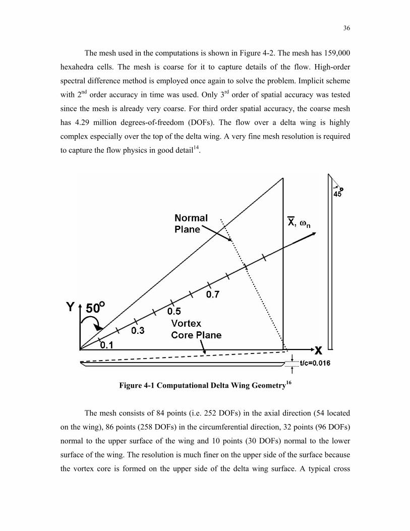
The mesh used in the computations is shown in Figure 4-2. The mesh has 159,000

hexahedra cells. The mesh is coarse for it to capture details of the flow. High-order

spectral difference method is employed once again to solve the problem. Implicit scheme

with 2nd order accuracy in time was used. Only 3rd order of spatial accuracy was tested

since the mesh is already very coarse. For third order spatial accuracy, the coarse mesh

has 4.29 million degrees-of-freedom (DOFs). The flow over a delta wing is highly

complex especially over the top of the delta wing. A very fine mesh resolution is required

to capture the flow physics in good detail14.

Figure 4-1 Computational Delta Wing Geometry16

The mesh consists of 84 points (i.e. 252 DOFs) in the axial direction (54 located

on the wing), 86 points (258 DOFs) in the circumferential direction, 32 points (96 DOFs)

normal to the upper surface of the wing and 10 points (30 DOFs) normal to the lower

surface of the wing. The resolution is much finer on the upper side of the surface because

the vortex core is formed on the upper side of the delta wing surface. A typical cross

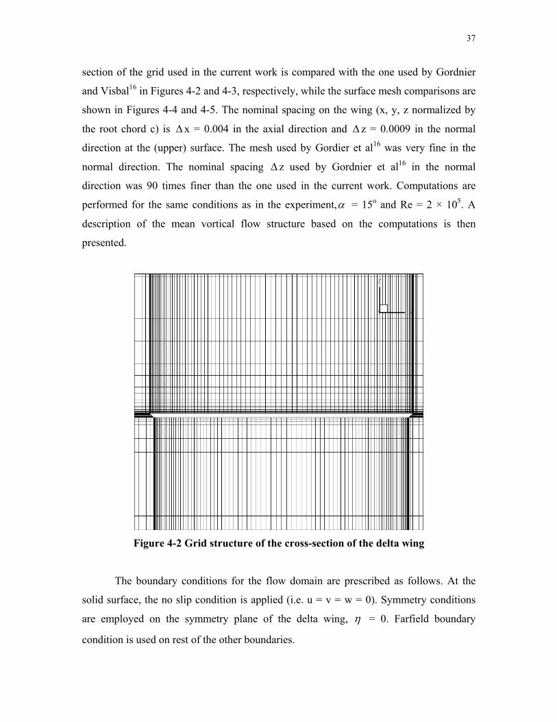
37

section of the grid used in the current work is compared with the one used by Gordnier

and Visbal16 in Figures 4-2 and 4-3, respectively, while the surface mesh comparisons are

shown in Figures 4-4 and 4-5. The nominal spacing on the wing (x, y, z normalized by

the root chord c) is x = 0.004 in the axial direction and Δ Δ z = 0.0009 in the normal

direction at the (upper) surface. The mesh used by Gordier et al16 was very fine in the

normal direction. The nominal spacing Δz used by Gordnier et al16 in the normal

direction was 90 times finer than the one used in the current work. Computations are

performed for the same conditions as in the experiment,α = 15o and Re = 2 × 105. A

description of the mean vortical flow structure based on the computations is then

presented.

Figure 4-2 Grid structure of the cross-section of the delta wing

The boundary conditions for the flow domain are prescribed as follows. At the

solid surface, the no slip condition is applied (i.e. u = v = w = 0). Symmetry conditions

are employed on the symmetry plane of the delta wing, η = 0. Farfield boundary

condition is used on rest of the other boundaries.

38

Figure 4-3 Grid structure of the cross-section of the delta wing used by Gordnier

and Visbal16

Figure 4-4 Grid structure on the surface of the delta wing

39

Figure 4-5 Grid structure on the surface of the delta wing used by Gordnier and

Visbal16

4.3 Numerical Results and Discussion

The solution to the flow over a delta wing, like most other physical problems, is

affected by mesh resolution and the type of numerical scheme. The mesh used in the

current analysis is not fine enough to capture the details to a very good extent. But it

gives an idea about the future and promise spectral difference method holds. The impact

of mesh refinement on the global structure of the vortex for both the mean and

instantaneous flow is demonstrated in Figures 4-6 and 4-7 respectively. The results

obtained from spectral difference method are compared with the fine mesh results

obtained by Gordnier and Visbal16. The numerical results of Gordnier and Visbal’s work

were obtained by private communication. The isosurfaces of axial vorticity colored by

density contours highlight the general vortex structure. The mesh used in the current

work gives a good idea about the vortex structure but was unable to capture the fine

structures i.e. smaller scale unsteady features of the vortical flow. Due to this fact, the

mean flow is also unable to exhibit the small scale substructures.

40

(a) (b)

Figure 4-6 Instantaneous vortex structure - Isosurfaces of constant axial vorticity colored by density contours (a) current work, (b) Gordnier and Visbal16

(a) (b)

Figure 4-7 Mean vortex structure - Isosurfaces of constant axial vorticity colored by density contours (a) current work, (b) Gordnier and Visbal16

The effect of mesh in the wing normal direction plays an important role. The mesh used

in the current work, as mentioned before, is almost 100 times coarser than the ones used

by Gordnier16. This effect on the computed flowfield can be further understood by

examining the structures in planes normal to the vortex core as shown in Figure 4-1.

Figures 4-8 (a) and (b) compare the vortex structure upstream of breakdown at a location

41

x = 0.1429. It can be noticed that primary, secondary and tertiary vortices are observed,

as well as a second vortex of the same sign as the primary vortex outboard near the

leading edge. This type of dual vortex system has been observed previously for low

sweep delta wings16,58,72 and results from the interaction of the secondary flow with the

primary shear layer.

(a) (b)

Figure 4-8 Contours of the mean axial vorticity in a crossflow plane normal to the vortex, x = 0.1429: (a) current work, (b) Gordnier and Visbal16

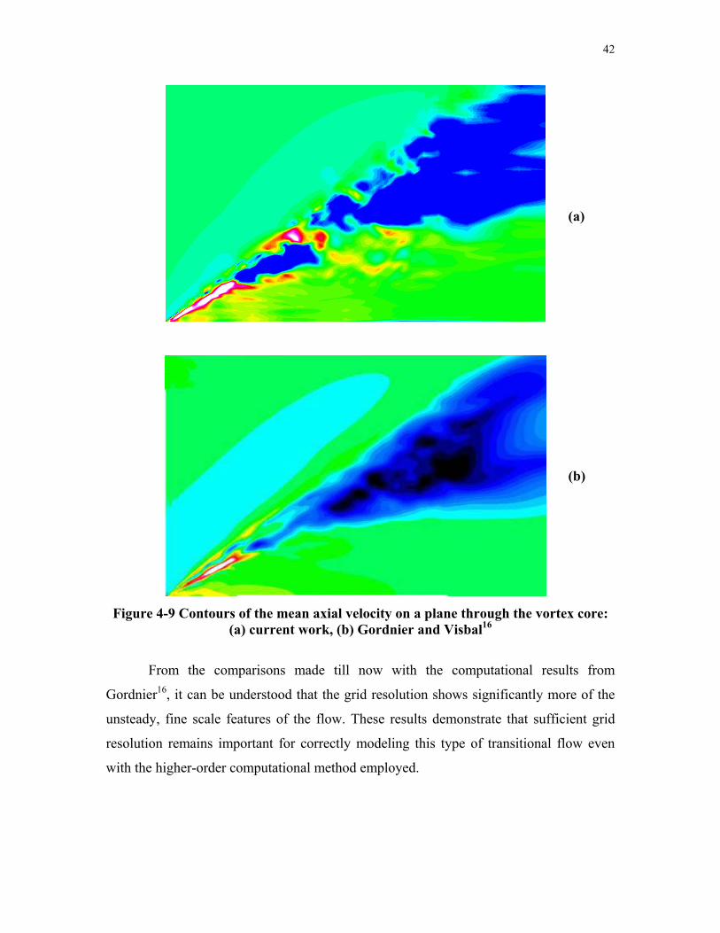
The weakening of the vortex upstream of breakdown is seen in Figures 4-9 (a)

and (b) where contours of the axial velocity on a plane through the vortex core are

plotted. Upstream of breakdown the peak jet velocity in the vortex core is bigger on the

grid used in the current work, Figure 4-9 (a). The vortex breakdown location (normalized

with chord) is similar to that obtained by Gordnier16. While the strength of the upstream

vortex has been diminished, this has not resulted in a noticeable change in the vortex

breakdown location.

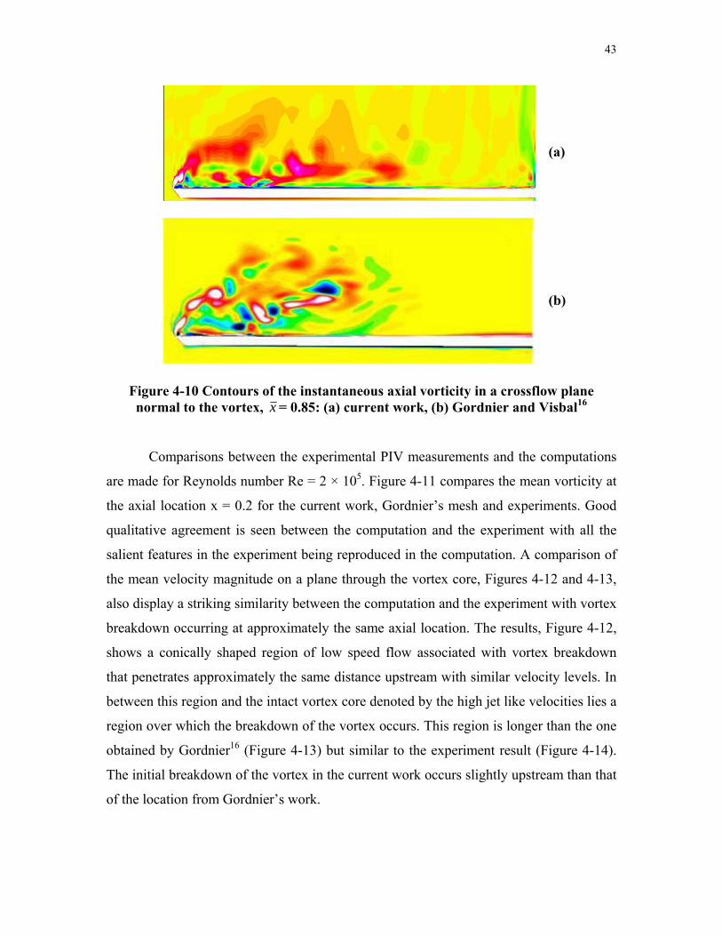
Downstream of breakdown, the solution exhibits a much more detailed flow

structure with significantly smaller scales being captured, Figure 4-10. The instantaneous

flow shows large scale features in the outer shear layer that rolls up to form the vortex,

but unable to capture the small scale features. This can also be noticed in the coarse mesh

(Figure 4-10 (b)) used by Gordnier16. Enhanced interactions of these structures with the

surface boundary layer are also seen as they move across the wing surface. Mesh

refinement will result in capturing the smaller scales as well.

42

(a)

(b)

Figure 4-9 Contours of the mean axial velocity on a plane through the vortex core: (a) current work, (b) Gordnier and Visbal16

From the comparisons made till now with the computational results from

Gordnier16, it can be understood that the grid resolution shows significantly more of the

unsteady, fine scale features of the flow. These results demonstrate that sufficient grid

resolution remains important for correctly modeling this type of transitional flow even

with the higher-order computational method employed.

43

(a)

(b)

Figure 4-10 Contours of the instantaneous axial vorticity in a crossflow plane normal to the vortex, x = 0.85: (a) current work, (b) Gordnier and Visbal16

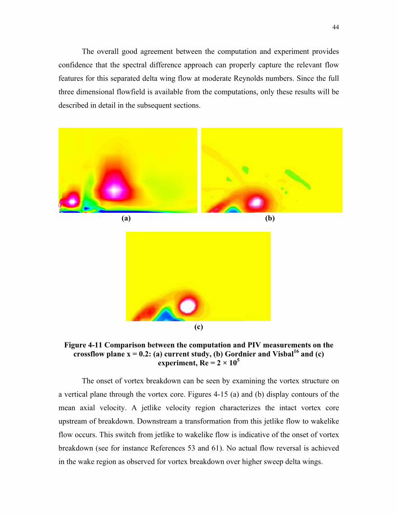
Comparisons between the experimental PIV measurements and the computations

are made for Reynolds number Re = 2 × 105. Figure 4-11 compares the mean vorticity at

the axial location x = 0.2 for the current work, Gordnier’s mesh and experiments. Good

qualitative agreement is seen between the computation and the experiment with all the

salient features in the experiment being reproduced in the computation. A comparison of

the mean velocity magnitude on a plane through the vortex core, Figures 4-12 and 4-13,

also display a striking similarity between the computation and the experiment with vortex

breakdown occurring at approximately the same axial location. The results, Figure 4-12,

shows a conically shaped region of low speed flow associated with vortex breakdown

that penetrates approximately the same distance upstream with similar velocity levels. In

between this region and the intact vortex core denoted by the high jet like velocities lies a

region over which the breakdown of the vortex occurs. This region is longer than the one

obtained by Gordnier16 (Figure 4-13) but similar to the experiment result (Figure 4-14).

The initial breakdown of the vortex in the current work occurs slightly upstream than that

of the location from Gordnier’s work.

44

The overall good agreement between the computation and experiment provides

confidence that the spectral difference approach can properly capture the relevant flow

features for this separated delta wing flow at moderate Reynolds numbers. Since the full

three dimensional flowfield is available from the computations, only these results will be

described in detail in the subsequent sections.

(a) (b)

(c)

Figure 4-11 Comparison between the computation and PIV measurements on the

crossflow plane x = 0.2: (a) current study, (b) Gordnier and Visbal16 and (c) experiment, Re = 2 × 105

The onset of vortex breakdown can be seen by examining the vortex structure on

a vertical plane through the vortex core. Figures 4-15 (a) and (b) display contours of the

mean axial velocity. A jetlike velocity region characterizes the intact vortex core

upstream of breakdown. Downstream a transformation from this jetlike flow to wakelike

flow occurs. This switch from jetlike to wakelike flow is indicative of the onset of vortex

breakdown (see for instance References 53 and 61). No actual flow reversal is achieved

in the wake region as observed for vortex breakdown over higher sweep delta wings.

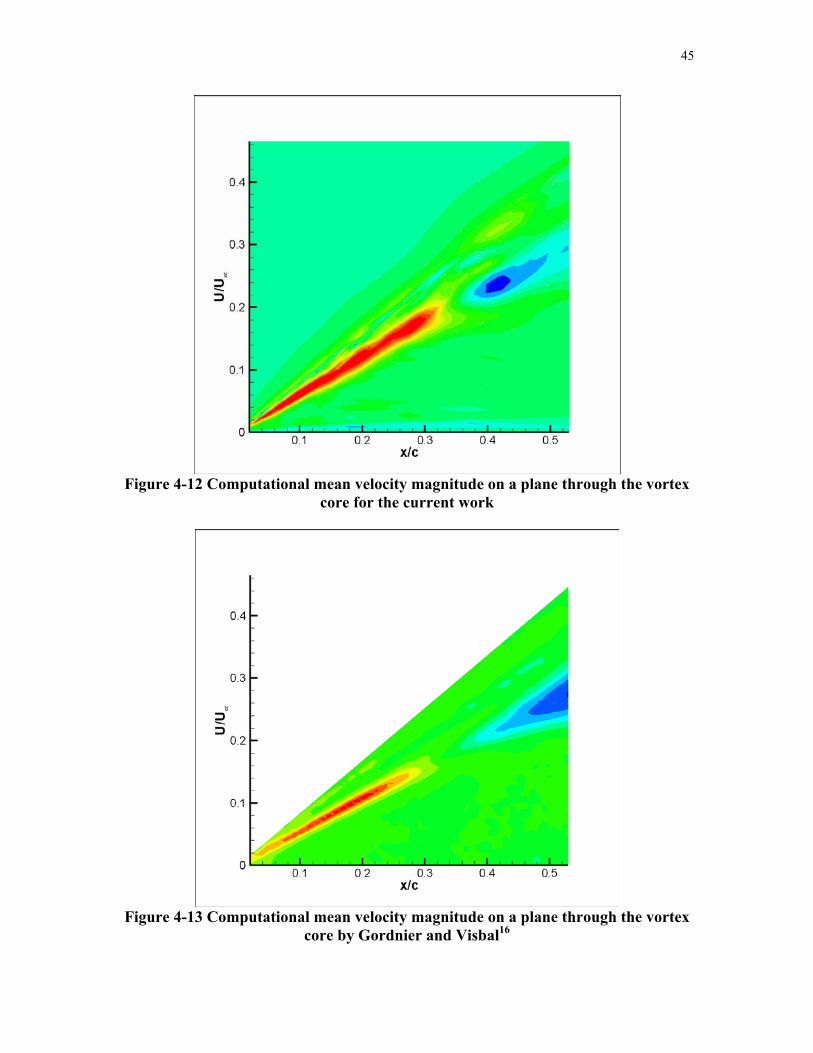
45

Figure 4-12 Computational mean velocity magnitude on a plane through the vortex

core for the current work

Figure 4-13 Computational mean velocity magnitude on a plane through the vortex

core by Gordnier and Visbal16

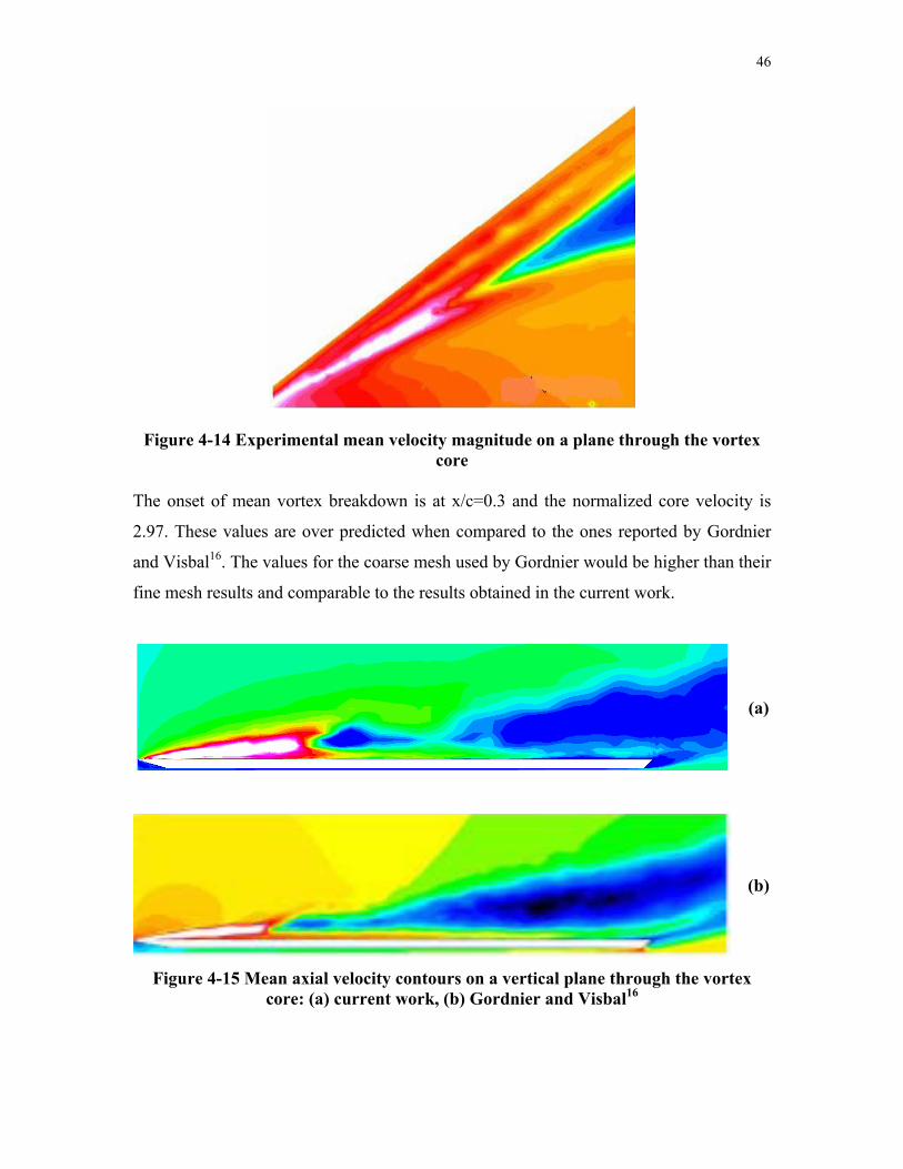
46

Figure 4-14 Experimental mean velocity magnitude on a plane through the vortex core

The onset of mean vortex breakdown is at x/c=0.3 and the normalized core velocity is

2.97. These values are over predicted when compared to the ones reported by Gordnier

and Visbal16. The values for the coarse mesh used by Gordnier would be higher than their

fine mesh results and comparable to the results obtained in the current work.

(a)

(b)

Figure 4-15 Mean axial velocity contours on a vertical plane through the vortex core: (a) current work, (b) Gordnier and Visbal16

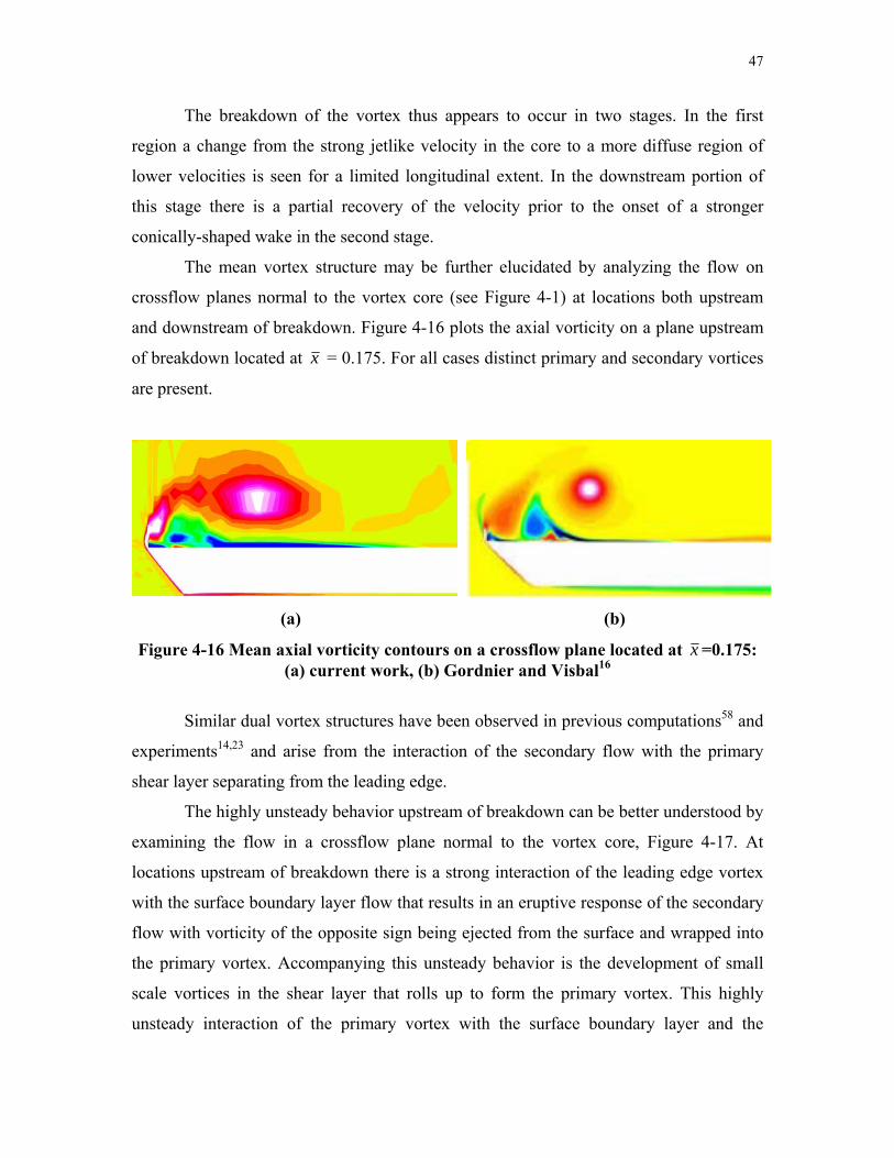
47

The breakdown of the vortex thus appears to occur in two stages. In the first

region a change from the strong jetlike velocity in the core to a more diffuse region of

lower velocities is seen for a limited longitudinal extent. In the downstream portion of

this stage there is a partial recovery of the velocity prior to the onset of a stronger

conically-shaped wake in the second stage.

The mean vortex structure may be further elucidated by analyzing the flow on

crossflow planes normal to the vortex core (see Figure 4-1) at locations both upstream

and downstream of breakdown. Figure 4-16 plots the axial vorticity on a plane upstream

of breakdown located at x = 0.175. For all cases distinct primary and secondary vortices

are present.

(a) (b)

Figure 4-16 Mean axial vorticity contours on a crossflow plane located at x =0.175: (a) current work, (b) Gordnier and Visbal16

Similar dual vortex structures have been observed in previous computations58 and

experiments14,23 and arise from the interaction of the secondary flow with the primary

shear layer separating from the leading edge.

The highly unsteady behavior upstream of breakdown can be better understood by

examining the flow in a crossflow plane normal to the vortex core, Figure 4-17. At

locations upstream of breakdown there is a strong interaction of the leading edge vortex

with the surface boundary layer flow that results in an eruptive response of the secondary

flow with vorticity of the opposite sign being ejected from the surface and wrapped into

the primary vortex. Accompanying this unsteady behavior is the development of small

scale vortices in the shear layer that rolls up to form the primary vortex. This highly

unsteady interaction of the primary vortex with the surface boundary layer and the

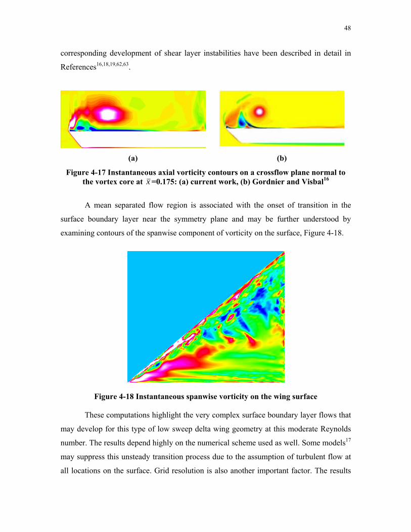
48

corresponding development of shear layer instabilities have been described in detail in

References16,18,19,62,63.

(a) (b)

Figure 4-17 Instantaneous axial vorticity contours on a crossflow plane normal to the vortex core at x =0.175: (a) current work, (b) Gordnier and Visbal16

A mean separated flow region is associated with the onset of transition in the

surface boundary layer near the symmetry plane and may be further understood by

examining contours of the spanwise component of vorticity on the surface, Figure 4-18.

Figure 4-18 Instantaneous spanwise vorticity on the wing surface

These computations highlight the very complex surface boundary layer flows that

may develop for this type of low sweep delta wing geometry at this moderate Reynolds

number. The results depend highly on the numerical scheme used as well. Some models17

may suppress this unsteady transition process due to the assumption of turbulent flow at

all locations on the surface. Grid resolution is also another important factor. The results

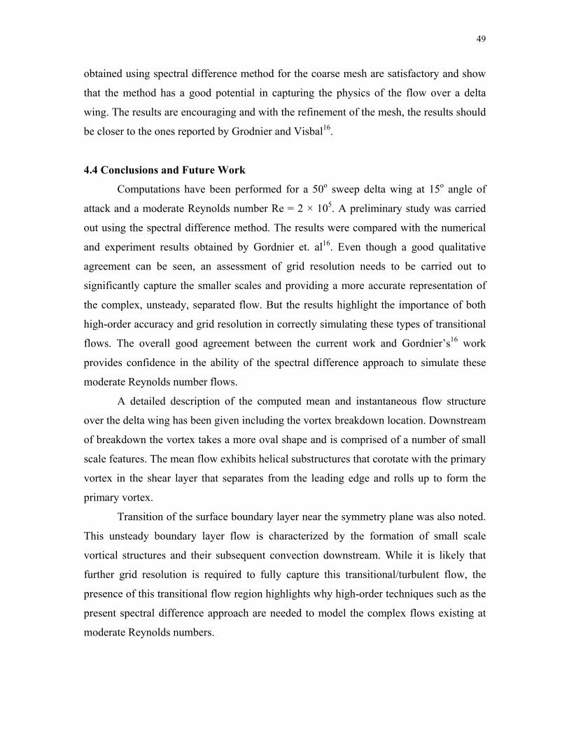
49

obtained using spectral difference method for the coarse mesh are satisfactory and show

that the method has a good potential in capturing the physics of the flow over a delta

wing. The results are encouraging and with the refinement of the mesh, the results should

be closer to the ones reported by Grodnier and Visbal16.

4.4 Conclusions and Future Work

Computations have been performed for a 50o sweep delta wing at 15o angle of

attack and a moderate Reynolds number Re = 2 × 105. A preliminary study was carried

out using the spectral difference method. The results were compared with the numerical

and experiment results obtained by Gordnier et. al16. Even though a good qualitative

agreement can be seen, an assessment of grid resolution needs to be carried out to

significantly capture the smaller scales and providing a more accurate representation of

the complex, unsteady, separated flow. But the results highlight the importance of both

high-order accuracy and grid resolution in correctly simulating these types of transitional

flows. The overall good agreement between the current work and Gordnier’s16 work

provides confidence in the ability of the spectral difference approach to simulate these

moderate Reynolds number flows.

A detailed description of the computed mean and instantaneous flow structure

over the delta wing has been given including the vortex breakdown location. Downstream

of breakdown the vortex takes a more oval shape and is comprised of a number of small

scale features. The mean flow exhibits helical substructures that corotate with the primary

vortex in the shear layer that separates from the leading edge and rolls up to form the

primary vortex.

Transition of the surface boundary layer near the symmetry plane was also noted.

This unsteady boundary layer flow is characterized by the formation of small scale

vortical structures and their subsequent convection downstream. While it is likely that

further grid resolution is required to fully capture this transitional/turbulent flow, the

presence of this transitional flow region highlights why high-order techniques such as the

present spectral difference approach are needed to model the complex flows existing at

moderate Reynolds numbers.

50

The present work provides enough confidence about the performance of spectral

difference method in predicting the flow features over a delta wing. But a lot of work still

needs to be carried out i.e. like grid refinement to capture the small scale features more

accurately. The author also suggests the study of flow over the delta wing with increasing

Reynolds number and also at different angles of attack.

51

Chapter 5 – Tornado Type Wind Energy System 5.1 Introduction

The Tornado-Type Wind Energy System73-75 is one of several and innovative

concepts being investigated as potential ways to reduce the cost and broaden the usability

of wind energy. This system (Figure 5-1) uses a large hollow tower to form an internal

vortex, and the low pressure at the core of the tower provides an effective and low

pressure exhaust reservoir for the turbine, which accepts air inlet supply. The tower

serves as a stationary and omni-directional collector and concentrator capable of

collecting immense amounts of wind energy and concentrating the collected energy into a

high power density turbine. This system provides the unique advantages of a small,

compact, vertical-axis, enclosed, and high efficiency turbine. This wind energy system

promises a structurally rugged and stable design for both on-land and offshore

installations. Based on this design, large and low-cost multi-megawatt wind energy

systems may be developed and constructed for the utilities, and small and economically

competitive systems may be provided for individual farms and homes.

Analytical investigations of several designs are being carried out. It will however

be sometime before all the flow processes involved will be known well enough to yield

highly accurate analytical predictions of performance. A variety of models have been

designed and CFD analysis has been carried out. Experiments were carried out in the low

speed wind tunnel at Iowa State University on some of the models. The prospect for the

Tornado-Type Wind Energy System looks encouraging.

Computational and experimental investigations on the Tornado-Type Wind

Energy System (Figure 5-1) have been carried out. A general description of the system is

presented below:

There are several major difficulties that have to be overcome by an innovative

wind energy concept in order to develop a low-cost, rugged, and practical wind energy

power plant capable of producing large amounts of power e.g., 10 to 100 MW. The

principal difficulty is caused by the basic fact that the energy density of wind is very low.

With usual system efficiency or a power coefficient of 30%, a collecting surface of

around of around 200m in diameter is needed for a wind energy power plant to collect

52

sufficient amounts of wind energy for producing 10 MW with a 30 mph wind speed. This

diameter is increased to 600m if the wind energy power plant is to produce 100 MW.

5.2 System Description

In the Tornado-Type Wind Energy System, a stationary collector is used for

collecting immense amount of wind energy, and then concentrates and converts the wind

energy into mechanical energy using a compact vertical-axis turbine which is located

near the ground. Briefly, as seen in Figure 5-1, wind energy is collected by a stationary

and omni-directional collector comprised of a stationary tower. Incoming wind into the

tower forms a vortex. The low-pressure core of the vortex is situated directly above the

vertical axis turbine so as to reduce the back pressure of the turbine. The underside of the

turbine is connected to the atmosphere through an omni-directional bottom inlet. A well

designed bottom inlet may raise the pressure within the bottom inlet to the ambient

stagnation pressure, higher than the ambient atmospheric pressure.

It is well known that the core of a strong vortex can have a very low pressure.

Hence, the vortex and the bottom inlet can maintain a very large pressure difference

across the turbine. For example, for a 30 mph (14 m/s) wind, the dynamic pressure

2

21

∞∞ = Vq ρ of the wind amounts to only 1/930 of the standard atmospheric pressure.

Hence, if the vortex core pressure is at 5% below the atmospheric then a pressure

difference of more than can be maintained across the turbine. In contrast, less than

one can be maintained by the wind across a conventional propeller-type wind turbine.

Hence, a Tornado-Type Wind Energy System can produce a much larger pressure

difference across, and a much higher power density from the turbine.

∞q45

∞q

5.3 Experimental Investigations

All the experiments were carried out at the Iowa State University. Detailed static

pressure measurements have been made in two wind tunnels of sizes 8ft wide by 6ft high

section and 3ft high by 2.5ft wide at various wind speeds. Two different sizes of the

models were tested out in the wind tunnels. The computational results are compared with

the results obtained from the wind-tunnel experiments.

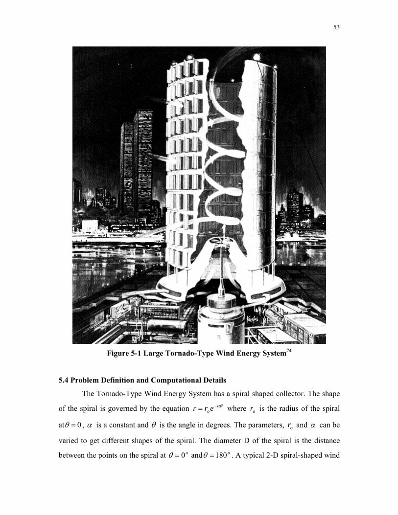
53

Figure 5-1 Large Tornado-Type Wind Energy System74

5.4 Problem Definition and Computational Details

The Tornado-Type Wind Energy System has a spiral shaped collector. The shape

of the spiral is governed by the equation where is the radius of the spiral

at

αθ−= err o or

0=θ , α is a constant and θ is the angle in degrees. The parameters, and or α can be

varied to get different shapes of the spiral. The diameter D of the spiral is the distance

between the points on the spiral at and . A typical 2-D spiral-shaped wind o0=θ o180=θ

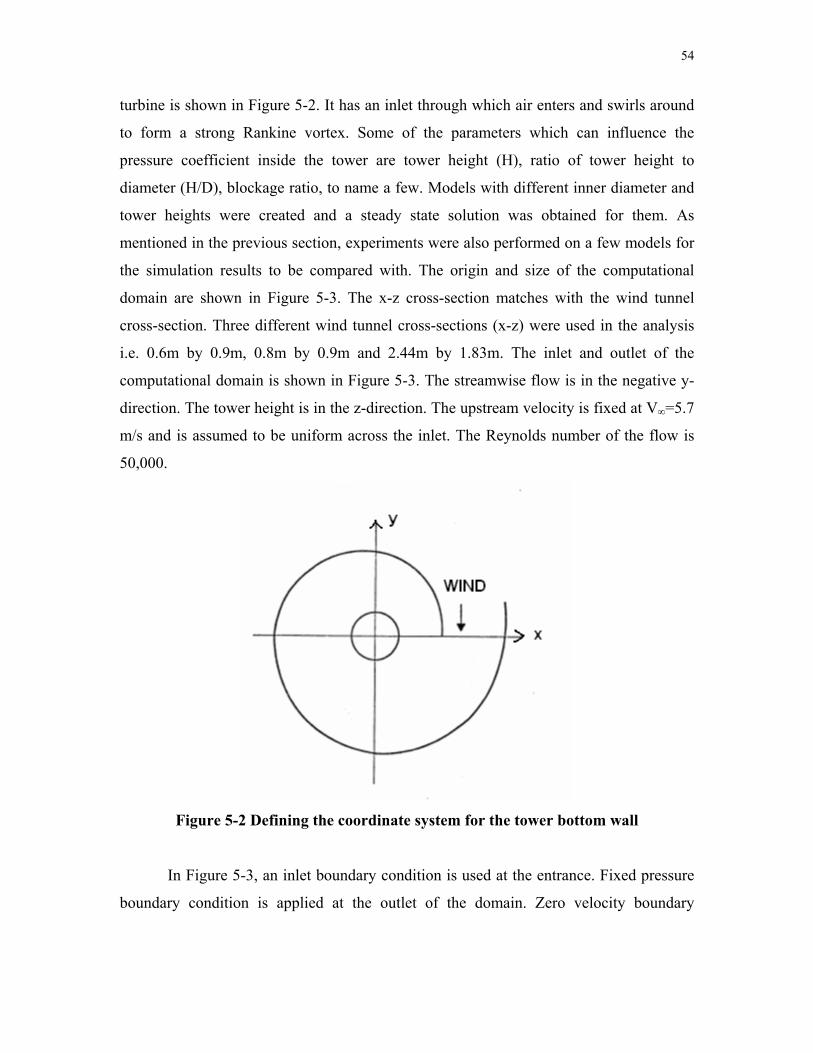
54

turbine is shown in Figure 5-2. It has an inlet through which air enters and swirls around

to form a strong Rankine vortex. Some of the parameters which can influence the

pressure coefficient inside the tower are tower height (H), ratio of tower height to

diameter (H/D), blockage ratio, to name a few. Models with different inner diameter and

tower heights were created and a steady state solution was obtained for them. As

mentioned in the previous section, experiments were also performed on a few models for

the simulation results to be compared with. The origin and size of the computational

domain are shown in Figure 5-3. The x-z cross-section matches with the wind tunnel

cross-section. Three different wind tunnel cross-sections (x-z) were used in the analysis

i.e. 0.6m by 0.9m, 0.8m by 0.9m and 2.44m by 1.83m. The inlet and outlet of the

computational domain is shown in Figure 5-3. The streamwise flow is in the negative y-

direction. The tower height is in the z-direction. The upstream velocity is fixed at V∞=5.7

m/s and is assumed to be uniform across the inlet. The Reynolds number of the flow is

50,000.

Figure 5-2 Defining the coordinate system for the tower bottom wall

In Figure 5-3, an inlet boundary condition is used at the entrance. Fixed pressure

boundary condition is applied at the outlet of the domain. Zero velocity boundary

55

condition is used for the turbine tower wall, while symmetry is imposed on the other

surfaces.

Numerical simulations were carried out to seek a steady state solution for different shapes

of the spiral. The aim was to obtain practical design parameters which lead to minimum

pressure at the tower bottom. A 2nd order finite volume code MUSIC65 capable of

handling arbitrary meshes for compressible fluid flow was used to carry out the

numerical simulations. Roe flux difference splitting scheme is used in the convective flux

discretization. A commercial solver FLUENT12 was also used to solve the problem and

make comparisons with the results obtained from MUSIC and experiments. Mostly,

MUSIC was used to carry out the numerical simulations. A second order scheme in space

with a block LU-SGS time scheme for time integration was used. No turbulence model

was used with MUSIC. Though, for some of the simulations, a limiter was used. Some of

the numerical simulations were carried out using FLUENT with a SIMPLE pressure-

based discretization. A 2nd order steady implicit scheme with two different turbulent

models Reynolds Stress Models (RSM) and Spallart-Almaras (SA) were used in

FLUENT.

5.5 Mesh Details

One of the challenging aspects of this problem was to create a mesh with

reasonable resolution to capture the vortex and to avoid its dissipation due to coarseness

of the mesh. The mesh and geometry details for all the cases are given in Table 5-1. For

case 1, grid refinement study was carried out to assess numerical errors if any. Three

meshes with different resolution were created – coarse, fine and finest. The coarse mesh

has 1.9 million cells, fine mesh has 3.6 million cells and the finest mesh has 5.1 million

cells. The mesh details for different resolution are shown in Table 5-2. Since a strong

vortex is formed at the center of the spiral, the mesh resolution in the radial direction is

increased from the coarse mesh to the finest mesh. The resolution in the z-direction i.e.

along the tower height was increased tremendously from the coarse mesh to the finest

mesh. Case 1 forms the basic setup of the problem. Variations have been made to this

model to study the other cases. Various simulations carried out to study the effect of H/D

ratio, tower height H and the size of the wind tunnel on the pressure coefficient Cp and

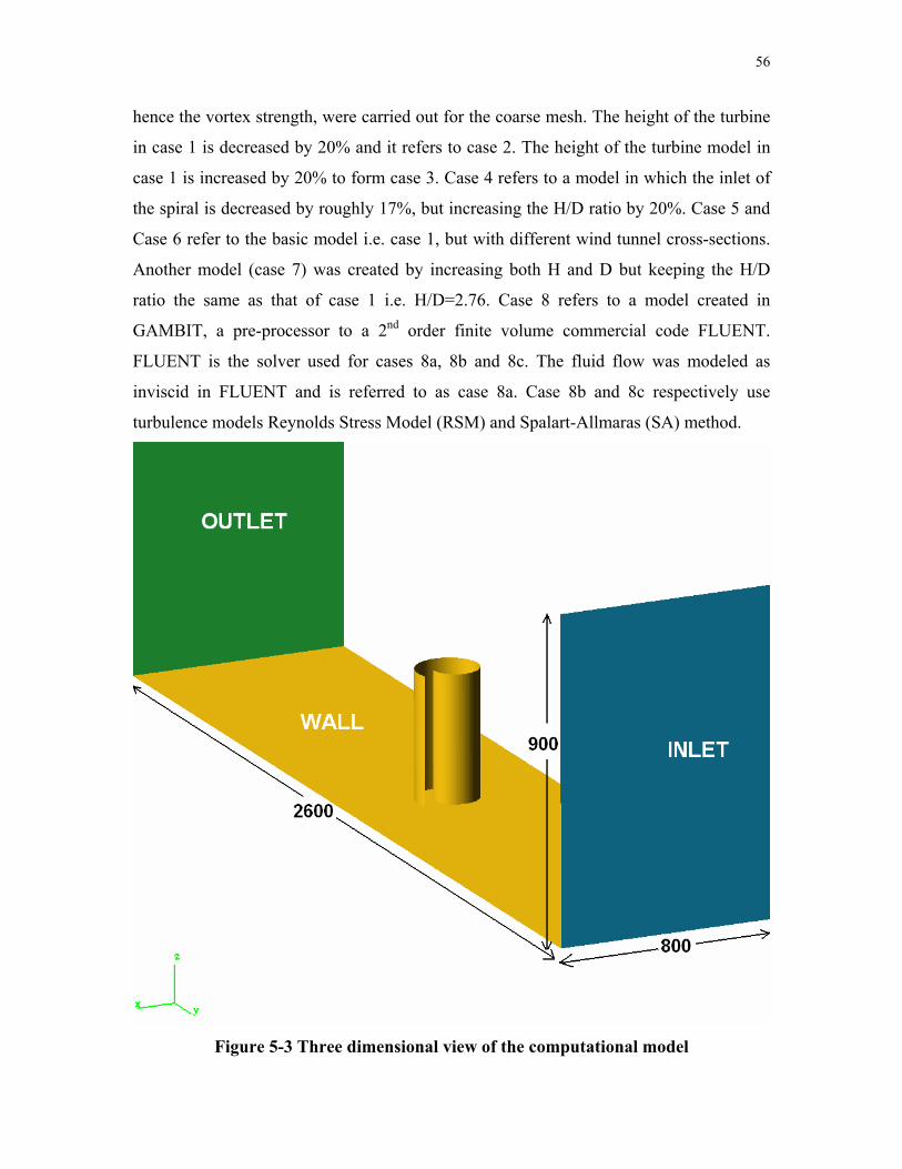
56

hence the vortex strength, were carried out for the coarse mesh. The height of the turbine

in case 1 is decreased by 20% and it refers to case 2. The height of the turbine model in

case 1 is increased by 20% to form case 3. Case 4 refers to a model in which the inlet of

the spiral is decreased by roughly 17%, but increasing the H/D ratio by 20%. Case 5 and

Case 6 refer to the basic model i.e. case 1, but with different wind tunnel cross-sections.

Another model (case 7) was created by increasing both H and D but keeping the H/D

ratio the same as that of case 1 i.e. H/D=2.76. Case 8 refers to a model created in

GAMBIT, a pre-processor to a 2nd order finite volume commercial code FLUENT.

FLUENT is the solver used for cases 8a, 8b and 8c. The fluid flow was modeled as

inviscid in FLUENT and is referred to as case 8a. Case 8b and 8c respectively use

turbulence models Reynolds Stress Model (RSM) and Spalart-Allmaras (SA) method.

Figure 5-3 Three dimensional view of the computational model

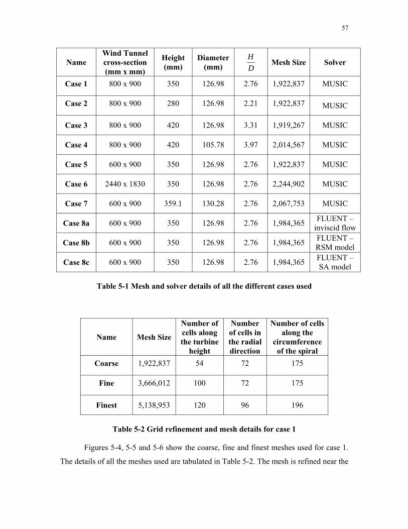
57

Name Wind Tunnel cross-section (mm x mm)

Height (mm)

Diameter (mm) D

H Mesh Size Solver

Case 1 800 x 900 350 126.98 2.76 1,922,837 MUSIC

Case 2 800 x 900 280 126.98 2.21 1,922,837 MUSIC

Case 3 800 x 900 420 126.98 3.31 1,919,267 MUSIC

Case 4 800 x 900 420 105.78 3.97 2,014,567 MUSIC

Case 5 600 x 900 350 126.98 2.76 1,922,837 MUSIC

Case 6 2440 x 1830 350 126.98 2.76 2,244,902 MUSIC

Case 7 600 x 900 359.1 130.28 2.76 2,067,753 MUSIC

Case 8a 600 x 900 350 126.98 2.76 1,984,365 FLUENT – inviscid flow

Case 8b 600 x 900 350 126.98 2.76 1,984,365 FLUENT – RSM model

Case 8c 600 x 900 350 126.98 2.76 1,984,365 FLUENT – SA model

Table 5-1 Mesh and solver details of all the different cases used

Name Mesh Size

Number of cells along the turbine

height

Number of cells in the radial direction

Number of cells along the

circumference of the spiral

Coarse 1,922,837 54 72 175

Fine 3,666,012 100 72 175

Finest 5,138,953 120 96 196

Table 5-2 Grid refinement and mesh details for case 1

Figures 5-4, 5-5 and 5-6 show the coarse, fine and finest meshes used for case 1.

The details of all the meshes used are tabulated in Table 5-2. The mesh is refined near the

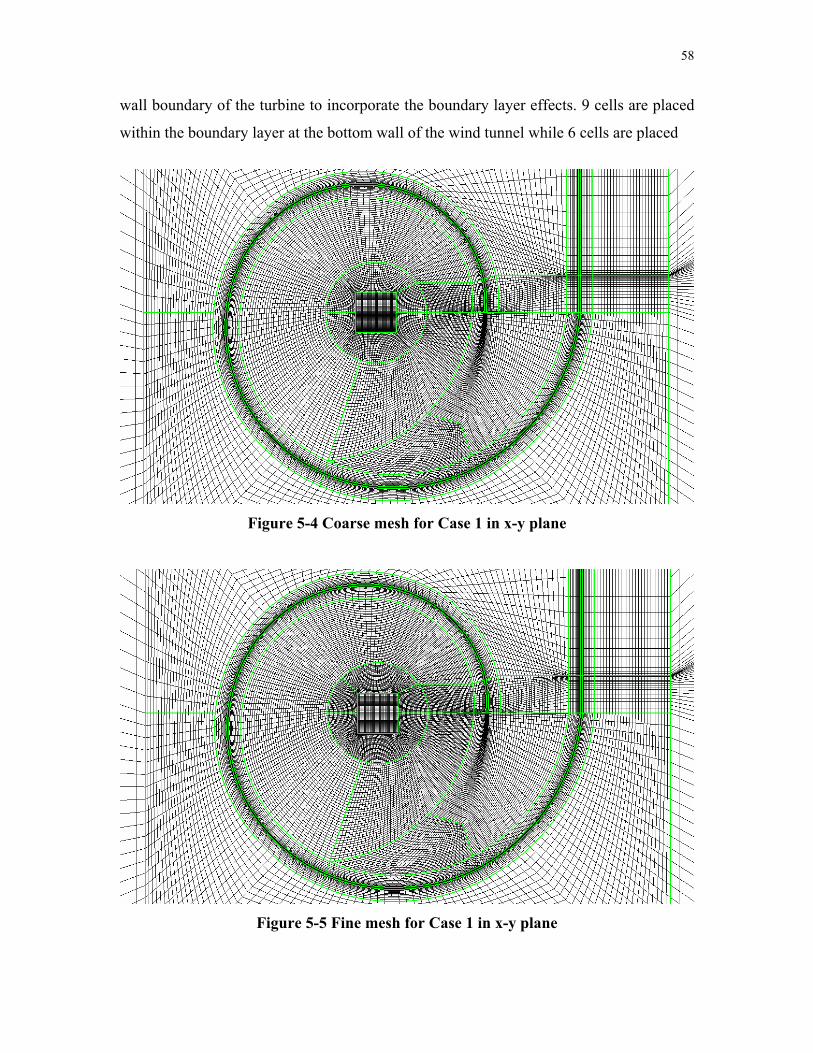
58

wall boundary of the turbine to incorporate the boundary layer effects. 9 cells are placed

within the boundary layer at the bottom wall of the wind tunnel while 6 cells are placed

Figure 5-4 Coarse mesh for Case 1 in x-y plane

Figure 5-5 Fine mesh for Case 1 in x-y plane

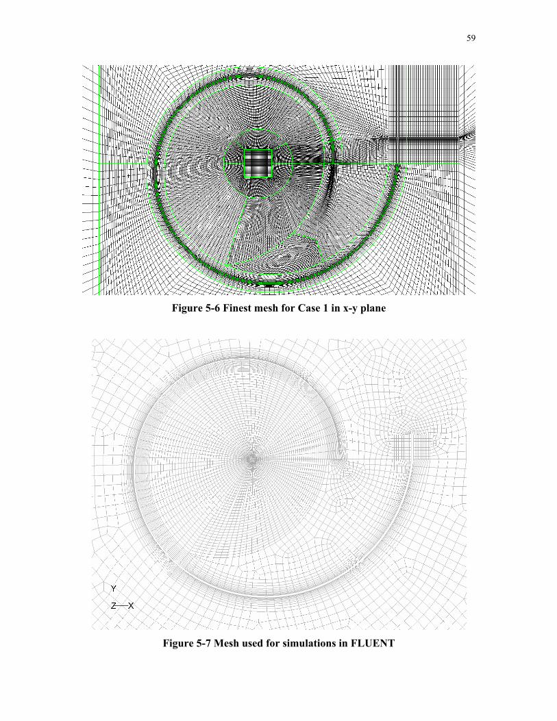
59

Figure 5-6 Finest mesh for Case 1 in x-y plane

Figure 5-7 Mesh used for simulations in FLUENT

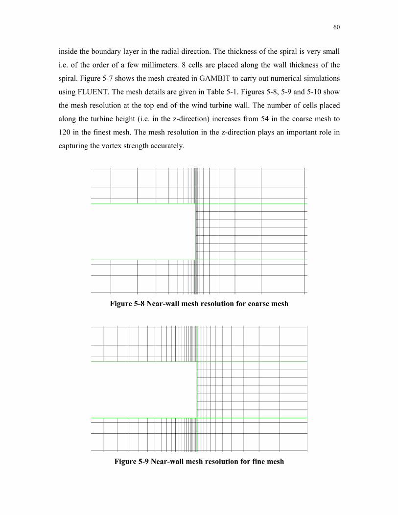
60

inside the boundary layer in the radial direction. The thickness of the spiral is very small

i.e. of the order of a few millimeters. 8 cells are placed along the wall thickness of the

spiral. Figure 5-7 shows the mesh created in GAMBIT to carry out numerical simulations

using FLUENT. The mesh details are given in Table 5-1. Figures 5-8, 5-9 and 5-10 show

the mesh resolution at the top end of the wind turbine wall. The number of cells placed

along the turbine height (i.e. in the z-direction) increases from 54 in the coarse mesh to

120 in the finest mesh. The mesh resolution in the z-direction plays an important role in

capturing the vortex strength accurately.

Figure 5-8 Near-wall mesh resolution for coarse mesh

Figure 5-9 Near-wall mesh resolution for fine mesh

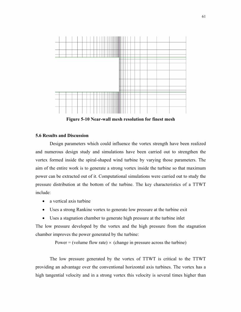
61

Figure 5-10 Near-wall mesh resolution for finest mesh

5.6 Results and Discussion

Design parameters which could influence the vortex strength have been realized

and numerous design study and simulations have been carried out to strengthen the

vortex formed inside the spiral-shaped wind turbine by varying those parameters. The

aim of the entire work is to generate a strong vortex inside the turbine so that maximum

power can be extracted out of it. Computational simulations were carried out to study the

pressure distribution at the bottom of the turbine. The key characteristics of a TTWT

include:

• a vertical axis turbine

• Uses a strong Rankine vortex to generate low pressure at the turbine exit

• Uses a stagnation chamber to generate high pressure at the turbine inlet

The low pressure developed by the vortex and the high pressure from the stagnation

chamber improves the power generated by the turbine:

Power = (volume flow rate) × (change in pressure across the turbine)

The low pressure generated by the vortex of TTWT is critical to the TTWT

providing an advantage over the conventional horizontal axis turbines. The vortex has a

high tangential velocity and in a strong vortex this velocity is several times higher than

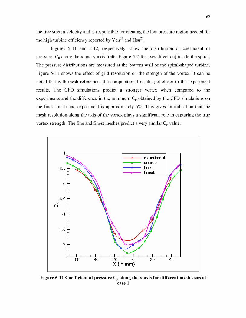
62

the free stream velocity and is responsible for creating the low pressure region needed for

the high turbine efficiency reported by Yen73 and Hsu27.

Figures 5-11 and 5-12, respectively, show the distribution of coefficient of

pressure, Cp along the x and y axis (refer Figure 5-2 for axes direction) inside the spiral.

The pressure distributions are measured at the bottom wall of the spiral-shaped turbine.

Figure 5-11 shows the effect of grid resolution on the strength of the vortex. It can be

noted that with mesh refinement the computational results get closer to the experiment

results. The CFD simulations predict a stronger vortex when compared to the

experiments and the difference in the minimum Cp obtained by the CFD simulations on

the finest mesh and experiment is approximately 5%. This gives an indication that the

mesh resolution along the axis of the vortex plays a significant role in capturing the true

vortex strength. The fine and finest meshes predict a very similar Cp value.

Figure 5-11 Coefficient of pressure Cp along the x-axis for different mesh sizes of

case 1

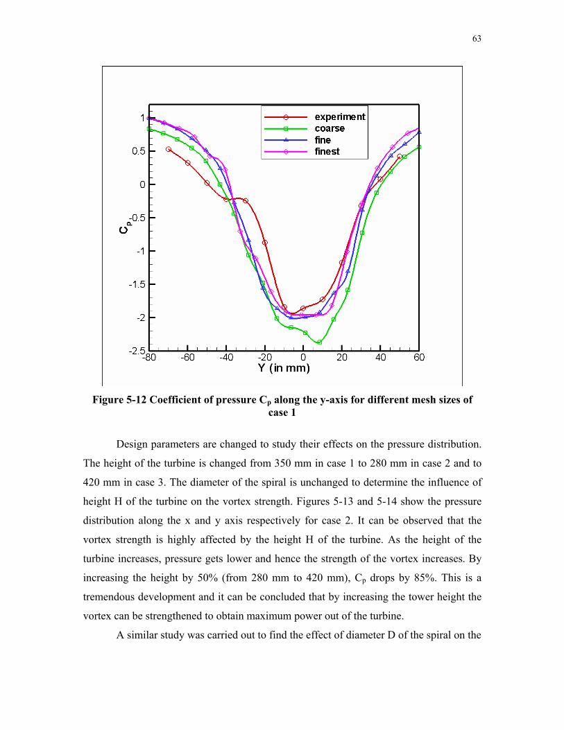
63

Figure 5-12 Coefficient of pressure Cp along the y-axis for different mesh sizes of

case 1

Design parameters are changed to study their effects on the pressure distribution.

The height of the turbine is changed from 350 mm in case 1 to 280 mm in case 2 and to

420 mm in case 3. The diameter of the spiral is unchanged to determine the influence of

height H of the turbine on the vortex strength. Figures 5-13 and 5-14 show the pressure

distribution along the x and y axis respectively for case 2. It can be observed that the

vortex strength is highly affected by the height H of the turbine. As the height of the

turbine increases, pressure gets lower and hence the strength of the vortex increases. By

increasing the height by 50% (from 280 mm to 420 mm), Cp drops by 85%. This is a

tremendous development and it can be concluded that by increasing the tower height the

vortex can be strengthened to obtain maximum power out of the turbine.

A similar study was carried out to find the effect of diameter D of the spiral on the

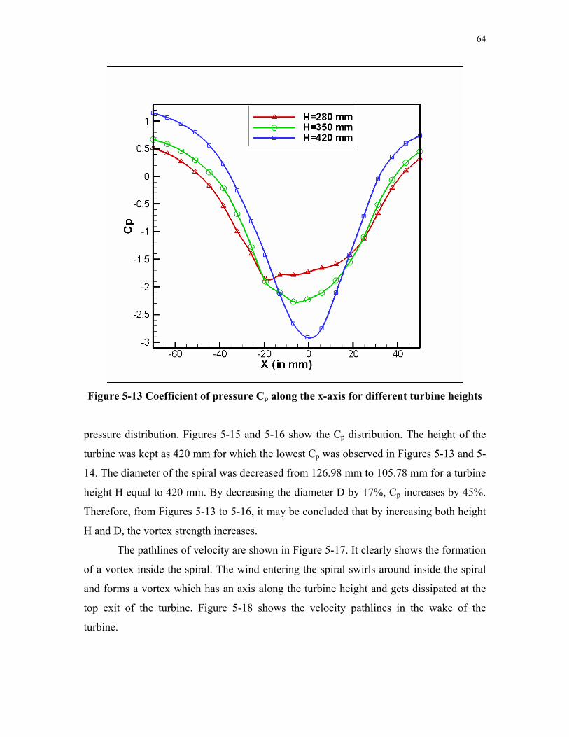
64

Figure 5-13 Coefficient of pressure Cp along the x-axis for different turbine heights

pressure distribution. Figures 5-15 and 5-16 show the Cp distribution. The height of the

turbine was kept as 420 mm for which the lowest Cp was observed in Figures 5-13 and 5-

14. The diameter of the spiral was decreased from 126.98 mm to 105.78 mm for a turbine

height H equal to 420 mm. By decreasing the diameter D by 17%, Cp increases by 45%.

Therefore, from Figures 5-13 to 5-16, it may be concluded that by increasing both height

H and D, the vortex strength increases.

The pathlines of velocity are shown in Figure 5-17. It clearly shows the formation

of a vortex inside the spiral. The wind entering the spiral swirls around inside the spiral

and forms a vortex which has an axis along the turbine height and gets dissipated at the

top exit of the turbine. Figure 5-18 shows the velocity pathlines in the wake of the

turbine.

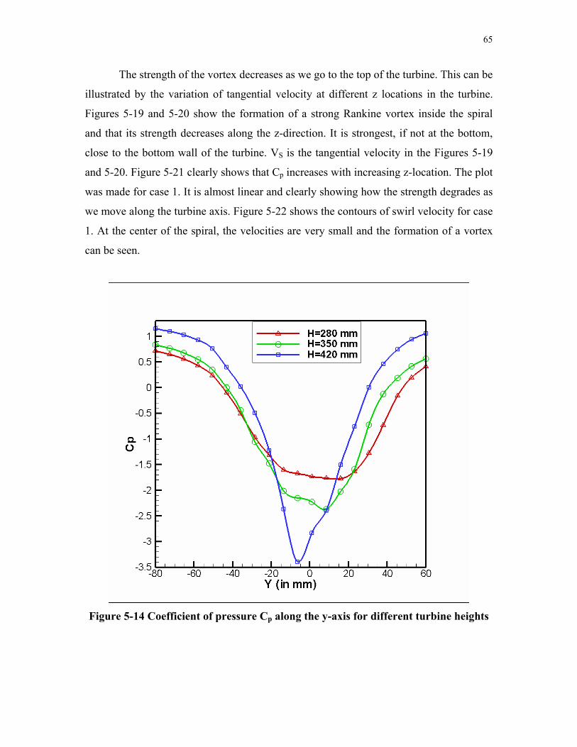
65

The strength of the vortex decreases as we go to the top of the turbine. This can be

illustrated by the variation of tangential velocity at different z locations in the turbine.

Figures 5-19 and 5-20 show the formation of a strong Rankine vortex inside the spiral

and that its strength decreases along the z-direction. It is strongest, if not at the bottom,

close to the bottom wall of the turbine. VS is the tangential velocity in the Figures 5-19

and 5-20. Figure 5-21 clearly shows that Cp increases with increasing z-location. The plot

was made for case 1. It is almost linear and clearly showing how the strength degrades as

we move along the turbine axis. Figure 5-22 shows the contours of swirl velocity for case

1. At the center of the spiral, the velocities are very small and the formation of a vortex

can be seen.

Figure 5-14 Coefficient of pressure Cp along the y-axis for different turbine heights

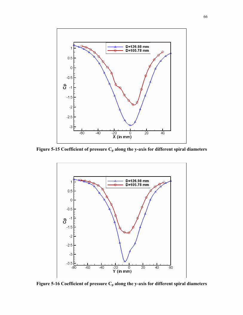
66

Figure 5-15 Coefficient of pressure Cp along the y-axis for different spiral diameters

Figure 5-16 Coefficient of pressure Cp along the y-axis for different spiral diameters

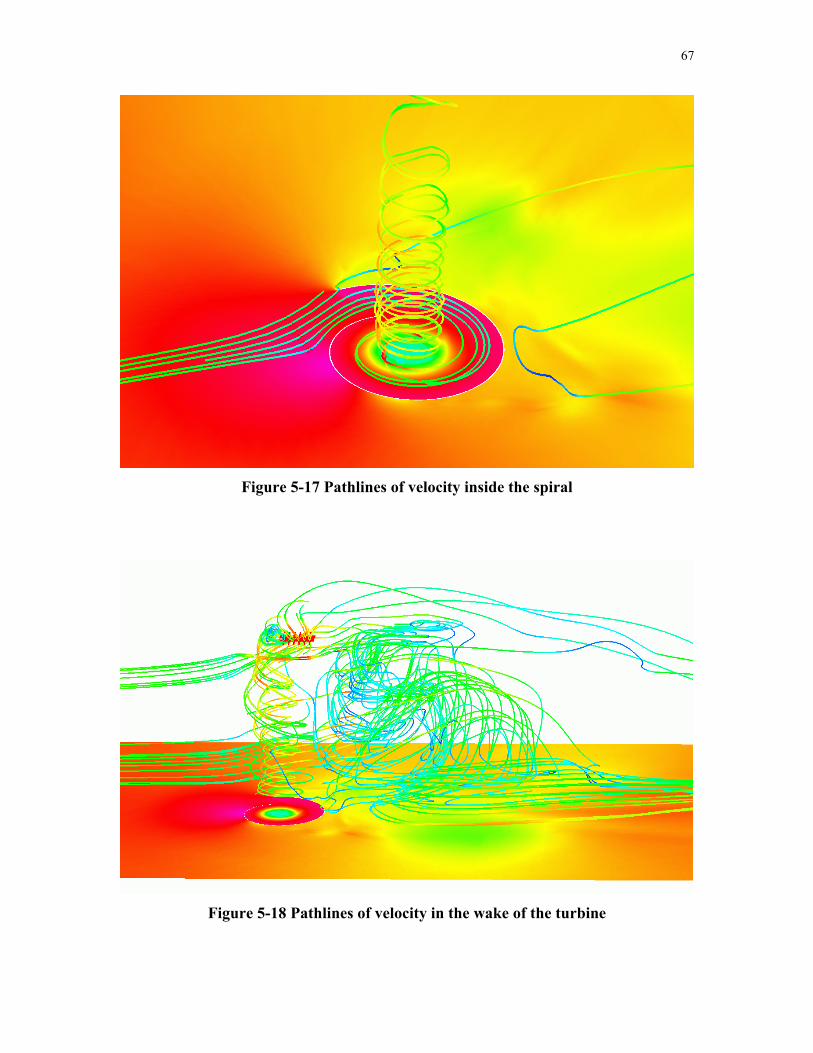
67

Figure 5-17 Pathlines of velocity inside the spiral

Figure 5-18 Pathlines of velocity in the wake of the turbine

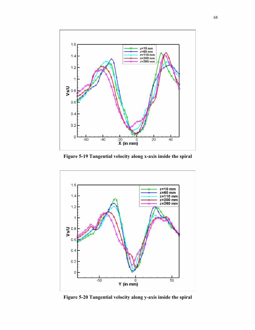
68

Figure 5-19 Tangential velocity along x-axis inside the spiral

Figure 5-20 Tangential velocity along y-axis inside the spiral

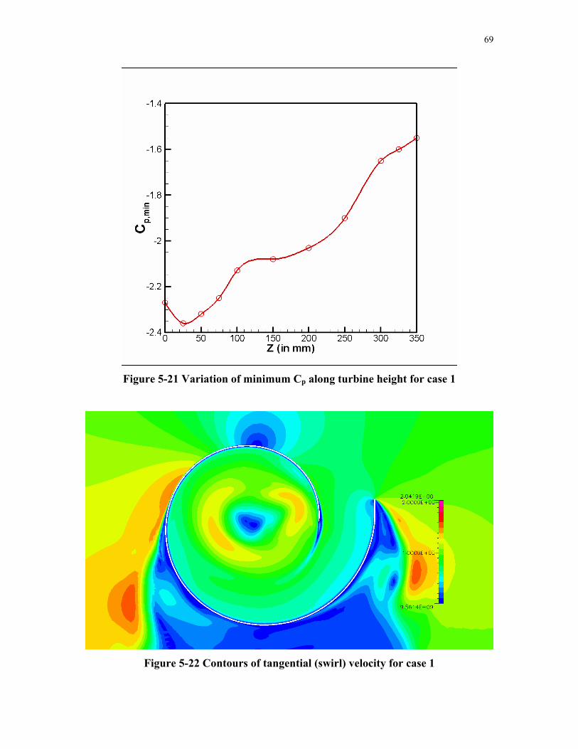
69

Figure 5-21 Variation of minimum Cp along turbine height for case 1

Figure 5-22 Contours of tangential (swirl) velocity for case 1

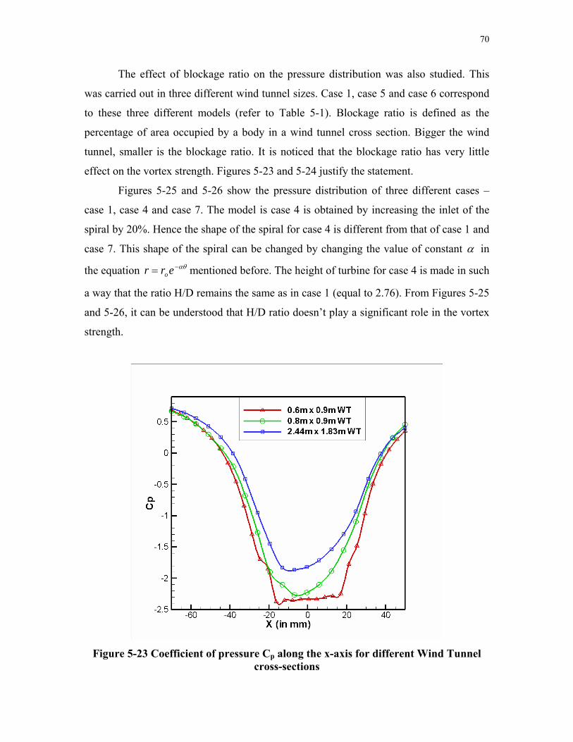
70

The effect of blockage ratio on the pressure distribution was also studied. This

was carried out in three different wind tunnel sizes. Case 1, case 5 and case 6 correspond

to these three different models (refer to Table 5-1). Blockage ratio is defined as the

percentage of area occupied by a body in a wind tunnel cross section. Bigger the wind

tunnel, smaller is the blockage ratio. It is noticed that the blockage ratio has very little

effect on the vortex strength. Figures 5-23 and 5-24 justify the statement.

Figures 5-25 and 5-26 show the pressure distribution of three different cases –

case 1, case 4 and case 7. The model is case 4 is obtained by increasing the inlet of the

spiral by 20%. Hence the shape of the spiral for case 4 is different from that of case 1 and

case 7. This shape of the spiral can be changed by changing the value of constant α in

the equation mentioned before. The height of turbine for case 4 is made in such

a way that the ratio H/D remains the same as in case 1 (equal to 2.76). From Figures 5-25

and 5-26, it can be understood that H/D ratio doesn’t play a significant role in the vortex

strength.

αθ−= err o

Figure 5-23 Coefficient of pressure Cp along the x-axis for different Wind Tunnel

cross-sections

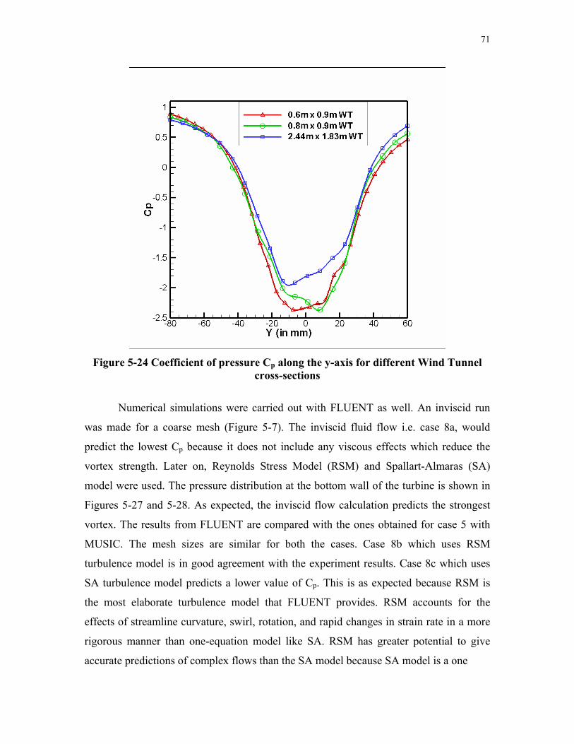
71

Figure 5-24 Coefficient of pressure Cp along the y-axis for different Wind Tunnel

cross-sections

Numerical simulations were carried out with FLUENT as well. An inviscid run

was made for a coarse mesh (Figure 5-7). The inviscid fluid flow i.e. case 8a, would

predict the lowest Cp because it does not include any viscous effects which reduce the

vortex strength. Later on, Reynolds Stress Model (RSM) and Spallart-Almaras (SA)

model were used. The pressure distribution at the bottom wall of the turbine is shown in

Figures 5-27 and 5-28. As expected, the inviscid flow calculation predicts the strongest

vortex. The results from FLUENT are compared with the ones obtained for case 5 with

MUSIC. The mesh sizes are similar for both the cases. Case 8b which uses RSM

turbulence model is in good agreement with the experiment results. Case 8c which uses

SA turbulence model predicts a lower value of Cp. This is as expected because RSM is

the most elaborate turbulence model that FLUENT provides. RSM accounts for the

effects of streamline curvature, swirl, rotation, and rapid changes in strain rate in a more

rigorous manner than one-equation model like SA. RSM has greater potential to give

accurate predictions of complex flows than the SA model because SA model is a one

72

Figure 5-25 Coefficient of pressure Cp along x-axis for cases 1, 4 and 7

Figure 5-26 Coefficient of pressure Cp along y-axis for cases 1, 4 and 7

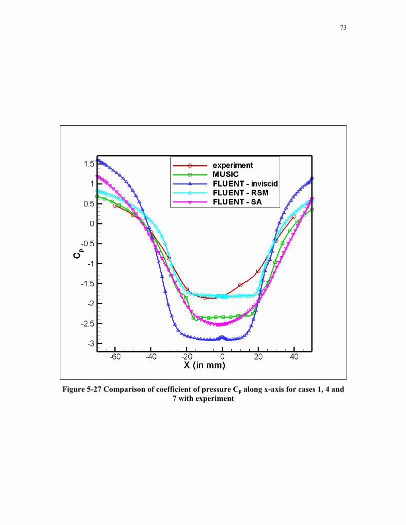
73

Figure 5-27 Comparison of coefficient of pressure Cp along x-axis for cases 1, 4 and

7 with experiment

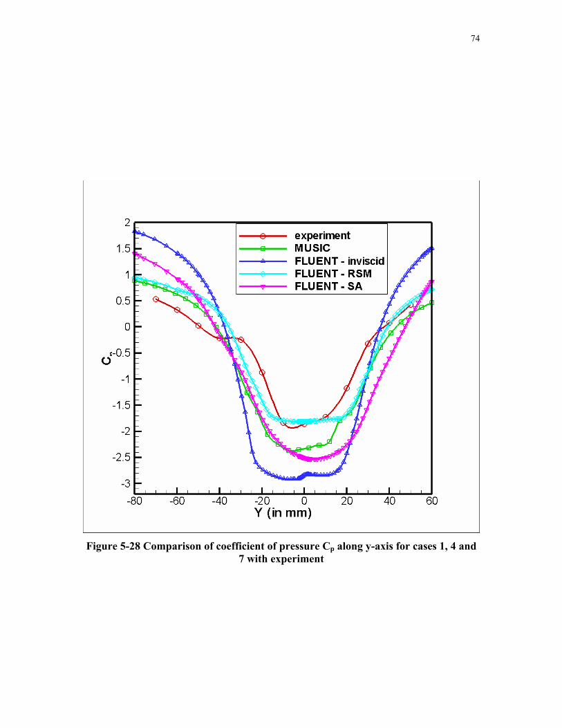
74

Figure 5-28 Comparison of coefficient of pressure Cp along y-axis for cases 1, 4 and

7 with experiment

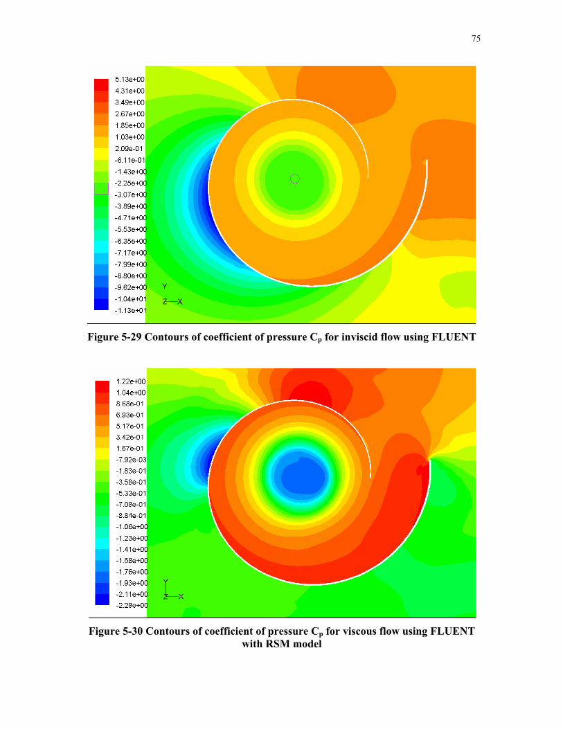
75

Figure 5-29 Contours of coefficient of pressure Cp for inviscid flow using FLUENT

Figure 5-30 Contours of coefficient of pressure Cp for viscous flow using FLUENT

with RSM model

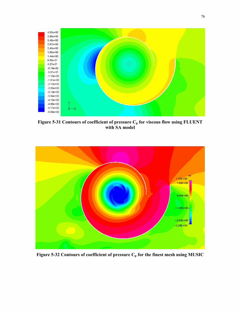
76

Figure 5-31 Contours of coefficient of pressure Cp for viscous flow using FLUENT

with SA model

Figure 5-32 Contours of coefficient of pressure Cp for the finest mesh using MUSIC

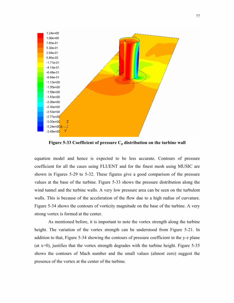
77

Figure 5-33 Coefficient of pressure Cp distribution on the turbine wall

equation model and hence is expected to be less accurate. Contours of pressure

coefficient for all the cases using FLUENT and for the finest mesh using MUSIC are

shown in Figures 5-29 to 5-32. These figures give a good comparison of the pressure

values at the base of the turbine. Figure 5-33 shows the pressure distribution along the

wind tunnel and the turbine walls. A very low pressure area can be seen on the turbulent

walls. This is because of the acceleration of the flow due to a high radius of curvature.

Figure 5-34 shows the contours of vorticity magnitude on the base of the turbine. A very

strong vortex is formed at the center.

As mentioned before, it is important to note the vortex strength along the turbine

height. The variation of the vortex strength can be understood from Figure 5-21. In

addition to that, Figure 5-34 showing the contours of pressure coefficient in the y-z plane

(at x=0), justifies that the vortex strength degrades with the turbine height. Figure 5-35

shows the contours of Mach number and the small values (almost zero) suggest the

presence of the vortex at the center of the turbine.

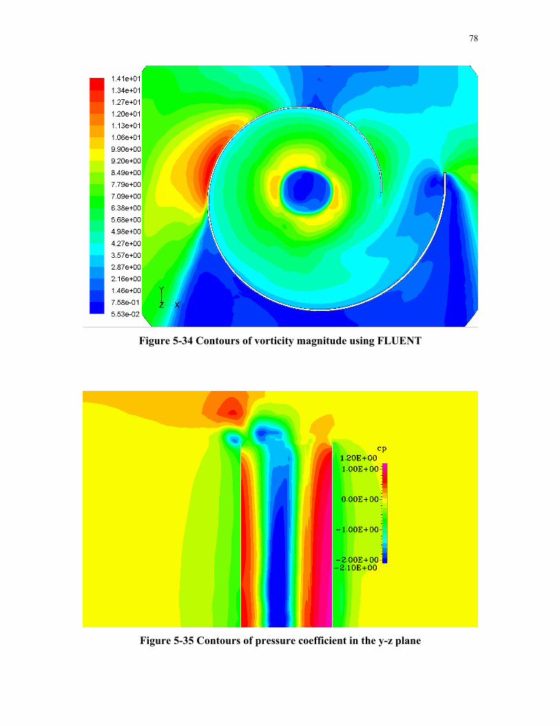
78

Figure 5-34 Contours of vorticity magnitude using FLUENT

Figure 5-35 Contours of pressure coefficient in the y-z plane

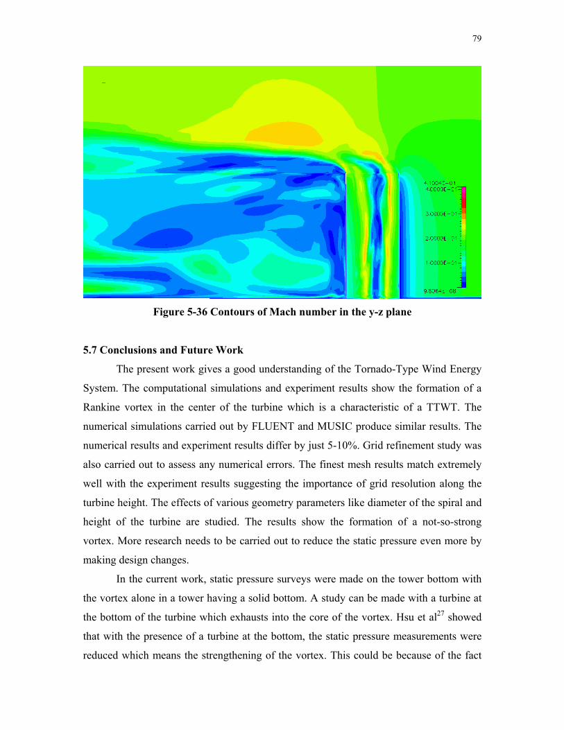
79

Figure 5-36 Contours of Mach number in the y-z plane

5.7 Conclusions and Future Work

The present work gives a good understanding of the Tornado-Type Wind Energy

System. The computational simulations and experiment results show the formation of a

Rankine vortex in the center of the turbine which is a characteristic of a TTWT. The

numerical simulations carried out by FLUENT and MUSIC produce similar results. The

numerical results and experiment results differ by just 5-10%. Grid refinement study was

also carried out to assess any numerical errors. The finest mesh results match extremely

well with the experiment results suggesting the importance of grid resolution along the

turbine height. The effects of various geometry parameters like diameter of the spiral and

height of the turbine are studied. The results show the formation of a not-so-strong

vortex. More research needs to be carried out to reduce the static pressure even more by

making design changes.

In the current work, static pressure surveys were made on the tower bottom with

the vortex alone in a tower having a solid bottom. A study can be made with a turbine at

the bottom of the turbine which exhausts into the core of the vortex. Hsu et al27 showed

that with the presence of a turbine at the bottom, the static pressure measurements were

reduced which means the strengthening of the vortex. This could be because of the fact

80

that with the solid bottom, the vortex is bounded. This is a well proven fact37 that a vortex

can be strengthened by injecting a flow into its core if the flow is in the forward direction

of the vortex axial velocity. In this way, there is a possibility that the vortex is

strengthened when the turbine is installed to the exhaust into the core of the vortex.

81

Bibliography 1. T. J. Barth, and P. O. Frederickson, “High-order solution of the Euler equations on

unstructured grids using quadratic reconstruction”, AIAA Paper No. 90-0013, 1990.

2. P. Beaudan, and P. Moin, “Numerical experiments on the flow past a circular

cylinder at a subcritical Reynolds number”, Technical report TF-62,

Thermosciences Division, Department of Mechanical Engineering, Stanford

University, 1994.

3. Michael Breuer, “Large eddy simulation of the subcritical flow past a circular

cylinder: numerical and modeling aspects”, International Journal for Numerical

Methods in Fluids, Vol. 28, 1998, pp. 1281-1302.

4. Michael Breuer, “Numerical and modeling influences on large eddy simulations for

the flow past a circular cylinder”, International Journal of Heat and Fluid Flow,

Vol. 19, 1998, pp. 512-521.

5. C. Canuto, M. Y. Hussaini, A. Quarteroni, and T. A. Zang, “Spectral Methods in

Fluid Dynamics”, Springer-Verlag, New York, 1987.

6. P. Catalano, M. Wang, G. Laccarino, and P. Moin, “Numerical simulation of the

flow around a circular cylinder at high Reynolds numbers”, International Journal of

Heat and Fluid Flow, Vol. 24, 2003, pp. 463-469.

7. R.F. Chen, and Z.J. Wang, “Fast, Block Lower-Upper Symmetric Gauss-Seidel

Scheme for Arbitrary Grids”, AIAA Journal, 2000, Vol. 38, no. 12, pp. 2238-2245.

8. C. K. Chyu, and D. Rockwell, “Near wake structure of an oscillating cylinder:

Effect of controlled shear layer vortices”, Journal of Fluid Mechanics, Vol. 322,

1996, pp. 21-49.

9. B. Cockburn, and C. W. Shu, “The Runge-Kutta discontinuous Galerkin method for

conservation laws V: multidimensional systems”, Journal of Computational

Physics, Vol. 141, 1998, pp. 199-224.

10. B. Cockburn, and C. W. Shu, “TVB Runge-Kutta local projection discontinuous

Galerkin finite element method for conservation laws II: General framework”,

Math. Comput., Vol. 52, 1989, pp. 411.

82

11. M. Delanaye, and Y. Liu, “Quadratic reconstruction .finite volume schemes on 3D

arbitrary unstructured polyhedral grids”, AIAA Paper No. 99-3259-CP, 1999.

12. FLUENT Computational Fluid Dynamics Software, Version 6.3.26 (Fluent, Inc.,

Centerra Resource Park, 10 Cavendish Court, Lebanon, NH 03766).

13. J. Franke, and W. Frank, “Large eddy simulation of the flow past a circular cylinder

at ReD=3900”, Journal of Wind Engineering and Industrial Aerodynamics, Vol. 90,

2002, pp. 1191-1206.

14. Jacob A. Freeman, “Computational Fluid Dynamics Investigation of Vortex

Breakdown for a Delta Wing at High Angle of Attack”, Thesis submitted to the

Department of the Air Force Air University, Air Force Institute of Technology,

Ohio, 2003.

15. J. Frohlich, W. Rodi, P. Kessler, J. P. Bertoglio, and D. Laurence, “Large eddy

simulation of flow around circular cylinder on structured and unstructured grids”,

In: E. H. Hirshel, editor. Notes on numerical fluid mechanics, Vol. 66, 1998, pp.

319- 338.

16. R. E. Gordnier and M. R. Visbal, “Compact Difference Scheme Applied to

Simulation of Low-Sweep Delta Wing Flow”, AIAA Journal, Vol. 43, No. 8, 2005,

pp. 1744–1752.

17. R. E. Gordnier and M. R. Visbal, “High-Order Simulation of Low Sweep Delta

Wing Flows Using ILES and Hybrid RANS/ILES Models,” AIAA-2006-504,

January 2006.

18. R. E. Gordnier and M. R. Visbal, “Instabilities in the Shear Layer of Delta Wings,”

AIAA-95-2281, June 1995.

19. R. E. Gordnier and M. R. Visbal, “Unsteady Vortex Structure over a Delta Wing,”

Journal of Aircraft, Vol. 31, No. 1, Jan.-Feb. 1994, pp. 243–248.

20. S. Görtz, “Detached-Eddy Simulations of a Full-Span Delta Wing at High

Incidence”, AIAA-2003-4216, June 2003.

21. D. Gottlieb, and S. A. Orszag, “Numerical Analysis of Spectral Methods: Theory

and Applications”, Society for Industrial and Applied Mathematics, Philadelphia,

1977.

83

22. O. M. Griffin, “A note on bluff body vortex formation”, Journal of Fluid

Mechanics, Vol. 284, 1995, pp. 217-224.

23. I. Gursul, “Review of Unsteady Vortex Flows over Slender Delta Wings”, Journal

of Aircraft, Vol. 42, No. 2, 2005, pp. 299–319.

24. I. Gursul, R. E. Gordnier, and M. Visbal, “Unsteady Aerodynamics of Nonslender

Delta Wings”, Progress in Aerospace Sciences, Vol. 41, No. 7, 2005, pp. 515–557.

25. I. Gursul, G. Taylor, and C. L. Wooding, “Vortex Flows over Fixed-Wing Micro

Air Vehicles”, AIAA Paper 2002-0698, Jan. 2002.

26. R. P. Hasen, and L. N. Long, “Large eddy simulation of a circular cylinder on

unstructured grids”, AIAA Paper 2002-0982.

27. C. T. Hsu, G. Mellor, and J. T. Yen, “Some Flow Analysis of a Tornado-Type Wind

Turbine”, ASME Winter Annual Meeting, December 1978.

28. P. G. Huang, Z. J. Wang, and Y. Liu, “An Implicit space-time Spectral Difference

method for discontinuity capturing using adaptive polynomials”, AIAA-2005-5255.

29. H.T. Huynh, “A Flux Reconstruction Approach to High-Order Schemes Including

Discontinuous Galerkin Methods,” AIAA-2007-4079.

30. G. E. Karniadakis, and S. J. Sherwin, “Spectral/hp Element Methods for CFD”,

Oxford University Press, 1999.

31. E. Konstantinidis, S. Balabani, and M. Yianneskis “Conditional averaging of PIV

plane wake data using a cross-correlation approach”, Experiments in Fluids, Vol.

39, 2005, pp. 38-47.

32. E. Konstantinidis, S. Balabani, and M. Yianneskis, “The effect of flow

perturbations on the near wake characteristics of a circular cylinder”, Journal of

Fluids and Structures, Vol. 18, 2003, pp. 367-386.

33. D. A. Kopriva, “A conservative staggered-grid Chebyshev multidomain method for

compressible flows”, Journal of Computational Physics, Vol. 125, 1996, pp. 244-

261.

34. A. G. Kravchenko, and P. Moin, “B-spline methods and zonal grids for numerical

simulations of turbulent flows”, Technical report TF-73, Department of Mechanical

Engineering, Stanford University, USA, 1998.

84

35. A. G. Kravchenko, and P. Moin, “Numerical studies of flow over a circular cylinder

at ReD=3900”, Physics of Fluids, Vol. 12, 2000, pp. 403-417.

36. M. Laurenco, and C. Shih, “Characteristics of the plane turbulent near wake of a

circular cylinder, a particle image velocimetry study”, Private communication by

Beaudan and Moin, 1993.

37. W. S. Lewellen, “A Review of Confined Vortex Flows”, NASA CR-1772, 1971.

38. C. Liang, and G. Papadakis, “Large eddy simulation of pulsating flow over a

circular cylinder at subcritical Reynolds number”, Computers and Fluids, Vol. 36, n

2, February 2007, pp. 299-312.

39. Y. Liu, M. Vinokur, and Z. J. Wang, “Discontinuous Spectral Difference Method

for Conservation laws on unstructured grids”, In proceedings of the 3rd

International Conference in CFD, Toronto, Canada, July 2004.

40. Y. Liu, M. Vinokur, and Z. J. Wang, “Multi-dimensional Spectral Difference

method for unstructured grids”, AIAA-2005-0320.

41. Y. Liu, M. Vinokur, and Z. J. Wang, “Spectral (Finite) Volume Method for

Conservation Laws on Unstructured Grids V: Extension to Three-Dimensional

Systems”, Journal of Computational Physics, Vol. 212, 2006, pp. 454-472.

42. X. Ma, G. S. Karamanos, and G. E. Karniadakis, “Dynamics and low

dimensionality of a turbulent near wake”, Journal of Fluid Mechanics, Vol. 410,

2000, pp. 29-65.

43. H. Mansy, P. M. Yang, and D. R. Williams, “Quantitative measurements of three-

dimensional structures in the wake of a circular cylinder”, J. of fluid mechanics,

Vol. 270, 1994, pp. 227.

44. J. J. Miau, K. T. Kuo, W. H. Liu, S. J. Hsieh, J. H. Chou, and C. K. Lin, “Flow

Developments above 50-Deg Sweep Delta Wings with Different Leading-Edge

Profiles”, Journal of Aircraft, Vol. 32, No. 4, 1995, pp. 787-794.

45. R. Mittal, and P. Moin, “Suitability of upwind-biased finite-difference schemes for

large-eddy simulation of turbulent flow”, AIAA Journal, Vol. 35, 1997, pp. 1415-8.

46. S. A. Morton, “High Reynolds Number DES Simulations of Vortex Breakdown

over a 70m Degree Delta Wing”, AIAA-2003-4217, June 2003.

85

47. S. A. Morton, J. Forsythe, A. Mitchell and D. Hajek, “DES and RANS Simulations

of Delta Wing Vortical Flows”, AIAA-2002-0587, January 2002.

48. R. D. Moser, M. M. Rogers, and D. W. Ewing, “Self-similarity of time evolving

plane wakes”, Journal of Fluid Mechanics, Vol. 367, 1998, pp. 255-289.

49. C. Noberg, “Interaction of free stream turbulence and vortex shedding for a single

tube in cross-flow”, Journal of Wind Engineering and Industrial Aerodynamics,

Vol. 23, 1986, pp. 501-514.

50. M. V. Ol, and M. Gharib, “Leading-Edge Vortex Structure of Nonslender Delta

Wings at Low Reynolds Number”, AIAA Journal, Vol. 41, No.1, 2003, pp. 16-26.

51. L. Ong, and J. Wallace, “The velocity field of the turbulent very near wake of a

circular cylinder”, Exp. Fluids, Vol. 20, 1996, pp. 441-453.

52. M. M. Rai, and P. Moin, “Direct numerical simulation of transition and turbulence

in a spatially evolving boundary layer”, Journal of Computational Physics, Vol.

109, 1993, pp. 169.

53. D. Rockwell, “Three-Dimensional Flow Structure on Delta Wings at High Angle-

of-Attack: Experimental Concepts and Issues,” AIAA-93-0550, January 1993.

54. T. Sarpkaya, “A critical review of the intrinsic nature of vortex-induced vibrations”,

Journal of Fluids and Structures, Vol. 19, 2004, pp. 389-447.

55. Y. Sun, Z. J. Wang and Y. Liu, “Efficient Implicit Non-linear LU-SGS Approach

for Compressible Flow Computation Using High-Order Spectral Difference

Method”, Communications in Computational Physics, Vol. 5, No. 2-4, pp. 760-778,

2009.

56. Y. Sun, Z. J. Wang and Y. Liu, “High-Order Multidomain Spectral Difference

Method for the Navier-Stokes Equations on Unstructured Hexahedral Grids”,

Communications in Computational Physics, Vol. 2, No. 2, pp. 310-333, 2007.

57. G. S. Taylor and I. Gursul, “Unsteady Vortex Flows and Buffeting of a Low Sweep

Delta Wing”, AIAA-2004-1066, January 2004.

58. G. S. Taylor, T. Schnorbus, and I. Gursul, “An Investigation of Vortex Flows over

Low Sweep Delta Wings”, AIAA-2003-4021, June 2003.

59. A. Travin, M. Shur, M. Strelets, and P. Spalart, “Detached-eddy simulations past a

circular cylinder”, Flow, Turbulence and Combustion, Vol. 63, 1999, pp. 293-313.

86

60. K. Van den Abeele, C. Lacor and Z.J. Wang, "On the stability and accuracy of the

spectral difference method,” Journal of Scientific Computing, in press.

61. M. R. Visbal, “Computed Unsteady Structure of Spiral Vortex Breakdown on Delta

Wings,” AIAA-96-2074, June 1996.

62. M. R. Visbal and R. E. Gordnier, “Origin of Computed Unsteadiness in the Shear

Layer of Delta Wings,” Journal of Aircraft, Vol. 32, No. 5, 1995, pp. 1146–1148.

63. M. R. Visbal, and R. E. Gordnier, “On the Structure of the Shear Layer Emanating

form a Swept Leading Edge at Angle of Attack,” AIAA-2003-4016, June 2003.

64. Z. J. Wang, “Spectral volume and difference methods for unstructured grids”, VKI

lecture series, 2005.

65. Z. J. Wang, and R.F. Chen, “Anisotropic Solution Adaptive Viscous Cartesian Grid

Method for Turbulence Flow Simulation”, AIAA Journal, Vol. 40, No. 10, Oct.

2002.

66. Z. J. Wang, and Y. Liu, “Spectral (Finite) Volume Method for Conservation Laws

on Unstructured Grids III: Extension to One-Dimensional Systems”, Journal of

Scientific Computing, Vol. 20, No. 1, 2004, pp. 137-157.

67. Z. J. Wang, and Y. Liu, “The Spectral Difference method for the 2D Euler

equations on unstructured grids”, AIAA-2005-5112.

68. Z. J. Wang, L. Zhang, and Y. Liu, “Spectral (Finite) Volume method for

conservation laws on unstructured grids IV: extension to two-dimensional systems”,

Journal of Computational Physics, Vol. 194, 2004, pp. 716-741.

69. C. H. K. Williamson, “Vortex dynamics in the cylinder wake”, Annual Review of

Fluid Mechanics, Vol. 28, 1996, pp. 477-539.

70. C. H. K. Williamson, and R. Govardhan, “Vortex Induced Vibrations”, Annual

Review of Fluid Mechanics, Vol. 36, 2004, pp. 413-455.

71. C. H. K. Williamson, J. Wu, and J. Sheridan, “Scaling of Streamwise Vortices in

Wakes”, Physics of Fluids, Vol. 7, 1995, pp. 2307.

72. B. Yaniktepe and D. Rockwell, “Flow Structure on a Delta Wing of Low Sweep

Angle”, AIAA Journal, Vol. 42, No. 3, 2004, pp. 513–523.

87

73. J. T. Yen, “Summary of Recent Progress on Tornado-Type Wind Energy Systems”,

Third Wind Energy Workshop, ed. J. B. F. Scientific Corp., Washington D. C.,

September 1977, pp. 808-818.

74. J. T. Yen, “Tornado-Type Wind Energy System”, Proceedings, Intersociety Energy

Conversion Engineering Conference, September 1975, pp. 987-994.

75. J. T. Yen, “Tornado-Type Wind Energy System, Basic Considerations”, ASME

Paper 76-WA-Ener-2, 1976.

76. S. Yoon and A. Jameson A, “Lower-upper symmetric-Gauss-Seidel method for the

Euler and Navier-Stokes equations”, AIAA Journal, 1988, Vol. 26, pp. 1025-1026.