Suppressing vacuum fluctuations with vortex excitations

J. F. de Medeiros Neto,1, ∗ Rudnei O. Ramos,2, † Carlos Rafael M. Santos,1, ‡

Rodrigo F. Ozela,1, § Gabriel C. Magalhaes,1, ¶ and Van Sergio Alves1, ∗∗

1Faculdade de Fısica, Universidade Federal do Para, 66075-110, Belem, PA, Brazil2Departamento de Fısica Teorica, Universidade do Estado do Rio de Janeiro, 20550-013, Rio de Janeiro, RJ, Brazil

The Casimir force for a planar gauge model is studied considering perfect conducting and perfectmagnetically permeable boundaries. By using an effective model describing planar vortex exci-tations, we determine the effect these can have on the Casimir force between parallel lines. Anappropriate mapping is considered for the system under study, where the effective model for planarvortices reduces to a simpler one, where generic boundary conditions can be most easily applied andthe Casimir force be derived in a most straightforward way. It is shown that vortex excitations canbe an efficient suppressor of vacuum fluctuations, in particular for the case of perfect conductingboundary conditions, leading to smaller magnitudes for the Casimir force than in the absence ofquantum vortex excitations. Some possible applications for these results are discussed.

PACS numbers: 03.70.+k, 11.10.Ef, 11.15.Yc

I. INTRODUCTION

There has been considerable interest in studying the validity of Newton’s gravitational law at sub-millimeter scalesand well below that (for a recent review see, e.g., Ref. [1]). There is a possibility that with these experimentsdeviations from the standard power-law behavior could be found, thus, possibly probing phenomena like modifiedgravity scenarios predicted by string theory, or by physics beyond the standard model of particle physics. Forexample, compactified extra spatial dimensions in string theory could lead to a modification of the quadratic power-law according to the number of extra dimensions, while physics beyond the standard model of particle physics canproduce Yukawa-type corrections for the gravitational force (for a comprehensive review, see also, e.g., Ref. [2] andreferences therein).

Laboratory experiments measuring gravity related forces at extremely small scales pose some extraordinary chal-lenges. One of these challenges of probing forces at such very small scales is to distinguish gravitation-like interactionsfrom those that can come from quantum phenomena, most notably the Casimir force effect [3], which can potentiallydominate gravity effects by several orders of magnitude at micrometer and below distances. In fact, the fast recentdevelopments on laboratory experiments measuring the Casimir force [4, 5] have also helped to put some strongconstraints on the level of possible corrections to gravity [6]. On the other hand, it is also highly desirable to deviseways of either isolating the Casimir effect or to suppress it up to the level of precision in those experiments. Recently,graphene [7] has been proposed for such purpose due to its extraordinary absorption properties, which could effectivelyfunction as a shield for quantum vacuum fluctuations. It is also important to look for other types of materials thatcan be as versatile in terms of been easily produced and also with tunable properties under laboratory conditions.One such possibility could be, for example, the use of superconducting films.

It is known that superconducting films can have magnetic vortex excitations. Most of the properties of these systemscan be described in terms of planar gauge systems. We recall that planar gauge field theories, in particular Chern-Simons (CS) type of models, have long been recognized as important for understanding several physical phenomenathat can be well approximated as planar ones, like high-temperature superconductors and the fractional quantumHall effect, just to cite a few examples (see e.g. Ref. [8] and references therein). The Casimir force in the presenceof condensed vortices in a plane was studied in Ref. [9] from the point of view of the particle-vortex duality, wherean effective description of vortex excitations was made in terms of a Maxwell-Proca-Chern-Simons (MPCS) model.It has been shown in that work that vortex excitations in these planar gauge systems have the ability of suppressing

∗Electronic address: jfmn@ufpa.br†Electronic address: rudnei@uerj.br‡Electronic address: carlos.santos@icen.ufpa.br§Electronic address: ozelarf@gmail.com¶Electronic address: gconduru@ufpa.br∗∗Electronic address: vansergi@ufpa.br

2

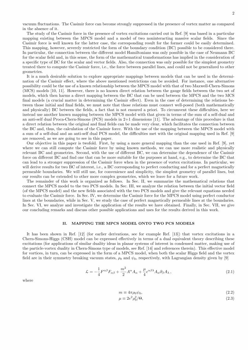
vacuum fluctuations. The Casimir force can become strongly suppressed in the presence of vortex matter as comparedin the absence of it.

The study of the Casimir force in the presence of vortex excitations carried out in Ref. [9] was based in a particularmapping existing between the MPCS model and a model of two noninteracting massive scalar fields. Since theCasimir force is well known for the latter case, the corresponding result for the former could be easily determined.This mapping, however, severely restricted the form of the boundary condition (BC) possible to be considered there.In particular, the connection between the different model Hamiltonians was only possible in the case of Neumann BCfor the scalar field and, in this sense, the form of the mathematical transformations has implied in the consideration ofa specific type of BC for the scalar and vector fields. Also, the connection was only possible for the simplest geometrytreated there to compute the Casimir force, i.e., the force between parallel lines, and could not be generalized to othergeometries.

It is a much desirable solution to explore appropriate mappings between models that can be used in the determi-nation of the Casimir effect, where the above mentioned restrictions can be avoided. For instance, one alternativepossibility could be the use of a known relationship between the MPCS model with that of two Maxwell-Chern-Simons(MCS) models [10, 11]. However, there is no known direct relation between the gauge fields between the two set ofmodels, which then harms a direct mapping between the BC that can be used between the MPCS and the two MCSfinal models (a crucial matter in determining the Casimir effect). Even in the case of determining the relations be-tween those initial and final fields, we must note that those relations must connect well-posed (both mathematicallyand physically) BC between the fields, a fact that is not ensured a priori. To circumvent these difficulties, here weinstead use another known mapping between the MPCS model with that given in terms of the sum of a self-dual andan anti-self dual Proca-Chern-Simons (PCS) models in 2+1 dimensions [11]. The advantage of this procedure is thata direct relation between the original and final fields can be made very clear, which facilitates the connection betweenthe BC and, thus, the calculation of the Casimir force. With the use of the mapping between the MPCS model witha sum of a self-dual and an anti-self dual PCS model, the difficulties met with the original mapping used in Ref. [9]are removed, as we are going to see in this paper.

Our objective in this paper is twofold. First, by using a more general mapping than the one used in Ref. [9], yetwhere we can still compute the Casimir force by using known methods, we can use more realistic and physicallyrelevant BC and geometries. Second, with the use of different BC, we can determine the dependence of the Casimirforce on different BC and find one that can be more suitable for the purposes at hand, e.g., to determine the BC thatcan lead to a stronger suppression of the Casimir force when in the presence of vortex excitations. In particular, wewill derive results for two BC of interest, i.e., a BC corresponding to perfect conducting and for a perfect magneticallypermeable boundaries. We will still use, for convenience and simplicity, the simplest geometry of parallel lines, butour results can be extended to other more complex geometries, which we leave for a future work.

The remainder of this work is organized as follows. In Sec. II, we summarize the mathematical relations thatconnect the MPCS model to the two PCS models. In Sec. III, we analyze the relation between the initial vector field(of the MPCS model) and the new fields associated with the two PCS models and give the relevant equations neededto evaluate the Casimir force. In Sec. IV, we determine the Casimir force for the MPCS model using perfect conductorlines at the boundaries, while in Sec. V, we study the case of perfect magnetically permeable lines at the boundaries.In Sec. VI, we analyze and investigate the application of the results we have obtained. Finally, in Sec. VII, we giveour concluding remarks and discuss other possible applications and uses for the results derived in this work.

II. MAPPING THE MPCS MODEL ONTO TWO PCS MODELS

It has been shown in Ref. [12] (for earlier derivations, see for example Ref. [13]) that vortex excitations in aChern-Simons-Higgs (CSH) model can be expressed effectively in terms of a dual equivalent theory describing theseexcitations (for applications of similar duality ideas in planar systems of interest in condensed matter, making use ofthe particle-vortex duality in Chern-Simons type of models, see Ref. [14] and references therein). This effective modelfor vortices, in turn, can be expressed in the form of a MPCS model, when both the scalar Higgs field and the vortexfield are in their symmetry breaking vacuum states, ρ0 and ψ0, respectively, with Lagrangian density given by [9]

L = −1

4FαβFαβ +

m2

2AαAα +

µ

4εαβλAα∂βAλ , (2.1)

where

m ≡ 4πρ0ψ0, (2.2)

µ ≡ 2e2ρ20/Θ, (2.3)

3

and Θ is the Chern-Simons parameter of the original CSH model from where Eq. (2.1) is derived.We could start directly from Eq. (2.1) and use standard methods (based on the vacuum expectation values for the

space-space and time-time components of the energy-momentum tensor (like, e.g., those discussed in Ref. [15]) tocompute the Casimir force for the MPCS model. This procedure leads, however, to a hard to solve system of partialdifferential equations (PDE). It turns out that it is much simpler to try to express the original model (2.1) in terms ofan equivalent one, which can be easier to treat mathematically. In particular, we want to have a well defined mappingbetween the fields in each model, such as to unequivocally establish their behaviors at the physical boundaries ofthe system. Such mapping must imply in a direct correspondence between the BC considered for the MPCS and itsequivalent model, resulting in a one-to-one mapping between the Casimir forces for the models involved. As we haveexplained in the Introduction, in this work we will follow the proposal of Refs. [10, 11], where the MPCS of Eq. (2.1)is mapped in a doublet consisting of the sum of a self-dual and an anti self-dual PCS models in 2+1 dimensions. Oneof the advantages of this procedure is that a direct relation between the original and final fields can be made veryclear, which facilitates the connection between the BC. Besides, it also allows the use of different BC and, eventually,also generalize to different geometries, as opposite to the case treated originally in Ref. [9].

Following in particular Ref. [11], we consider a doublet consisting of an anti self-dual and a self-dual PCS model,represented, respectively, by the Lagrangian densities,

L+ =1

2εµνβf

µ∂νfβ +m+

2fµf

µ, (2.4)

and

L− = −1

2εµνβg

µ∂νgβ +m−2gµg

µ, (2.5)

where fµ and gµ are two independent vector fields. By making use of a soldering field Wµ with no dynamics, it is asimple exercise to obtain, from the combination of L+ and L−, a final Lagrangian density that does not depend onWµ. For example, we can define an intermediate Lagrangian density given by

L = L−(g) + L+(f)−Wµ

[Jµ−(g) + Jµ+(f)

]+

1

2(m+ +m−)WµW

µ, (2.6)

where Jµ± are defined by

Jµ+(f) ≡ m+fµ + εµαβ∂αfβ , (2.7)

Jµ−(g) ≡ m−gµ − εµαβ∂αgβ . (2.8)

In the generating functional associated with (2.6), Wµ plays the role of an auxiliary field, which can be eliminatedby a direct integration (another way to see the auxiliary role of Wµ is by the use of its equation of motion). Theresulting final Lagrangian density can then be written as

L = −1

4FµνF

µν +(m− −m+)

2εµνβA

µ∂νAβ +1

2m+m−AµA

µ, (2.9)

where Aµ is a new vector field, related to fµ and gµ by

Aµ ≡1√

m+ +m−(fµ − gµ) , (2.10)

and m+ and m− are related to the original mass parameters µ and m of Eq. (2.1) by

m− −m+ = µ/2 , (2.11)

m+m− = m2 , (2.12)

or, equivalently,

4

m± = ∓µ4

+

õ2

16+m2 . (2.13)

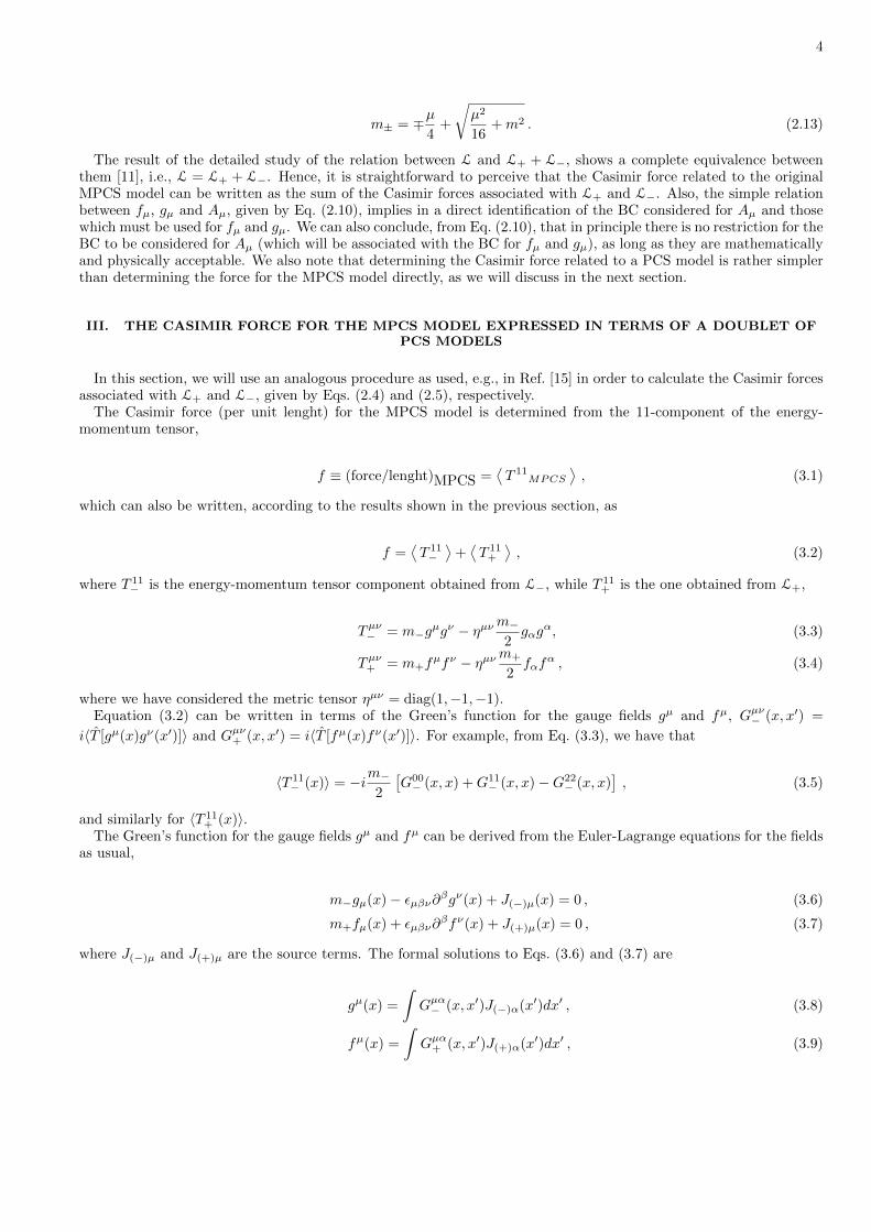
The result of the detailed study of the relation between L and L+ + L−, shows a complete equivalence betweenthem [11], i.e., L = L+ + L−. Hence, it is straightforward to perceive that the Casimir force related to the originalMPCS model can be written as the sum of the Casimir forces associated with L+ and L−. Also, the simple relationbetween fµ, gµ and Aµ, given by Eq. (2.10), implies in a direct identification of the BC considered for Aµ and thosewhich must be used for fµ and gµ. We can also conclude, from Eq. (2.10), that in principle there is no restriction for theBC to be considered for Aµ (which will be associated with the BC for fµ and gµ), as long as they are mathematicallyand physically acceptable. We also note that determining the Casimir force related to a PCS model is rather simplerthan determining the force for the MPCS model directly, as we will discuss in the next section.

III. THE CASIMIR FORCE FOR THE MPCS MODEL EXPRESSED IN TERMS OF A DOUBLET OFPCS MODELS

In this section, we will use an analogous procedure as used, e.g., in Ref. [15] in order to calculate the Casimir forcesassociated with L+ and L−, given by Eqs. (2.4) and (2.5), respectively.

The Casimir force (per unit lenght) for the MPCS model is determined from the 11-component of the energy-momentum tensor,

f ≡ (force/lenght)MPCS =⟨T 11

MPCS

⟩, (3.1)

which can also be written, according to the results shown in the previous section, as

f =⟨T 11−⟩

+⟨T 11+

⟩, (3.2)

where T 11− is the energy-momentum tensor component obtained from L−, while T 11

+ is the one obtained from L+,

Tµν− = m−gµgν − ηµνm−

2gαg

α, (3.3)

Tµν+ = m+fµfν − ηµνm+

2fαf

α , (3.4)

where we have considered the metric tensor ηµν = diag(1,−1,−1).Equation (3.2) can be written in terms of the Green’s function for the gauge fields gµ and fµ, Gµν− (x, x′) =

i〈T [gµ(x)gν(x′)]〉 and Gµν+ (x, x′) = i〈T [fµ(x)fν(x′)]〉. For example, from Eq. (3.3), we have that

〈T 11− (x)〉 = −im−

2

[G00− (x, x) +G11

− (x, x)−G22− (x, x)

], (3.5)

and similarly for 〈T 11+ (x)〉.

The Green’s function for the gauge fields gµ and fµ can be derived from the Euler-Lagrange equations for the fieldsas usual,

m−gµ(x)− εµβν∂βgν(x) + J(−)µ(x) = 0 , (3.6)

m+fµ(x) + εµβν∂βfν(x) + J(+)µ(x) = 0 , (3.7)

where J(−)µ and J(+)µ are the source terms. The formal solutions to Eqs. (3.6) and (3.7) are

gµ(x) =

∫Gµα− (x, x′)J(−)α(x′)dx′ , (3.8)

fµ(x) =

∫Gµα+ (x, x′)J(+)α(x′)dx′ , (3.9)

5

and

m−Gµα− − εµβν∂βGνα− + δ(x− x′)ηµα = 0 , (3.10)

m+Gµα+ + εµβν∂

βGνα+ + δ(x− x′)ηµα = 0 . (3.11)

Note that unlike the calculations followed in Refs. [15, 16], where the Green’s functions for the field’s dual, e.g.,gµ ≡ εµνγ∂

νgγ , were used, here we work directly in terms of the Green’s functions for the fields themselves. Thisfact is directly related to the form of the Proca term, m−gµg

µ/2 (and its analogous for fµ), which cannot be directlyrewritten in terms of the field’s dual tensor. This is also the case when we try to calculate the Casimir force forthe MPCS model directly: The Proca term m2AµA

µ/2 implies that we need to work with the Green’s functions forAµ itself (and not for its dual). As a consequence, the system of second-order differential equations that we need tosolve, in order to find the Casimir force for the MPCS model (if we decide to treat the MPCS model directly, without“transforming” it to a doublet of PCS models beforehand as we are proceeding here) are more difficult than theones that we have in the case of the MCS model [15, 16]. The transformations taken here simplifies the calculationssignificantly, since the system of equations with which we have to deal with is relativelly easier to solve, given byEqs. (3.10) and (3.11).

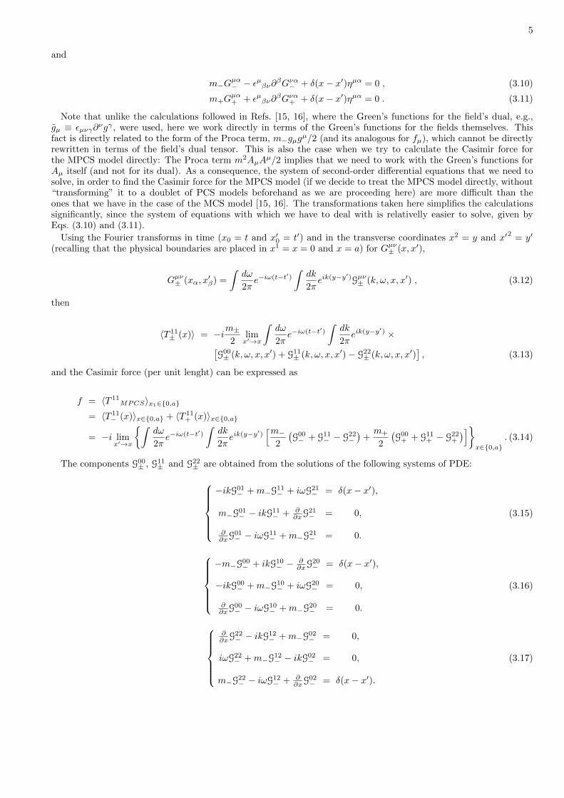
Using the Fourier transforms in time (x0 = t and x′0 = t′) and in the transverse coordinates x2 = y and x′2

= y′

(recalling that the physical boundaries are placed in x1 = x = 0 and x = a) for Gµν± (x, x′),

Gµν± (xα, x′β) =

∫dω

2πe−iω(t−t

′)

∫dk

2πeik(y−y

′)Gµν± (k, ω, x, x′) , (3.12)

then

〈T 11± (x)〉 = −im±

2limx′→x

∫dω

2πe−iω(t−t

′)

∫dk

2πeik(y−y

′) ×[G00± (k, ω, x, x′) + G11

± (k, ω, x, x′)− G22± (k, ω, x, x′)

], (3.13)

and the Casimir force (per unit lenght) can be expressed as

f = 〈T 11MPCS〉x1∈{0,a}

= 〈T 11− (x)〉x∈{0,a} + 〈T 11

+ (x)〉x∈{0,a}

= −i limx′→x

{∫dω

2πe−iω(t−t

′)

∫dk

2πeik(y−y

′)[m−

2

(G00− + G11

− − G22−)

+m+

2

(G00+ + G11

+ − G22+

)]}x∈{0,a}

. (3.14)

The components G00± , G11

± and G22± are obtained from the solutions of the following systems of PDE:

−ikG01

− +m−G11− + iωG21

− = δ(x− x′),

m−G01− − ikG11

− + ∂∂xG

21− = 0,

∂∂xG

01− − iωG11

− +m−G21− = 0.

(3.15)

−m−G00

− + ikG10− − ∂

∂xG20− = δ(x− x′),

−ikG00− +m−G

10− + iωG20

− = 0,

∂∂xG

00− − iωG10

− +m−G20− = 0.

(3.16)

∂∂xG

22− − ikG12

− +m−G02− = 0,

iωG22− +m−G

12− − ikG02

− = 0,

m−G22− − iωG12

− + ∂∂xG

02− = δ(x− x′).

(3.17)

6

ikG01

+ +m+G11+ − iωG21

+ = δ(x− x′),

m+G01+ + ikG11

+ − ∂∂xG

21+ = 0,

− ∂∂xG

01+ + iωG11

+ +m+G21+ = 0,

(3.18)

−m+G

00+ − ikG10

+ + ∂∂xG

20+ = δ(x− x′),

ikG00+ +m+G

10+ − iωG20

+ = 0,

− ∂∂xG

00+ + iωG10

+ +m+G20+ = 0,

(3.19)

− ∂∂xG

22+ + ikG12

+ +m+G02+ = 0,

−iωG22+ +m+G

12+ + ikG02

+ = 0,

m+G22+ + iωG12

+ − ∂∂xG

02+ = δ(x− x′).

(3.20)

The above equations are explicitly solved in the following sections for specific BC.

IV. THE CASIMIR FORCE FOR PERFECT CONDUCTOR BOUNDARIES

We now describe the mapping between the original BC that can be imposed on the original vector field Aµ of theMPCS model with the ones imposed on the fields fµ and gµ. The Casimir effect follows from Eq. (3.2). We will firstconsider perfect conductors at the boundaries, which can be represented mathematically by F1 = 0, where

Fµ ≡ εµνγ∂νAγ , (4.1)

is the dual of Aµ. This is a BC that could not be treated for instance in Ref. [9], due to the specific form of themathematical transformations used in that work, which were based on scalar degrees of freedom.

In our case, the BC F1 = 0 will imply (due to Eq. (4.1)) in ∂2A0 = ∂0A2. Noting that fµ and gµ are independentfrom each other, and using Eq. (2.10), we then see that the BC is satisfied if we have, at the boundaries,

{∂2f0 = ∂0f2,∂2g0 = ∂0g2.

(4.2)

By representing fµ and gµ in terms of their Green functions, Gµν± (x, x′), and using Eq. (3.12), we see that the BCs(4.2) are observed if we have

[limx′→x

G0ν± (k, ω;x, x′)

]x∈{0,a}

=[

limx′→x

G2ν± (k, ω;x, x′)

]x∈{0,a}

= 0. (4.3)

Equation (4.3) can now be used as BC for solving the system of equations written in the previous section and to findthe components of Gµν± necessary to obtain the Casimir effect from Eq. (3.14). Note also that we only need to obtainG11± , since the contributions from G00

± and G22± give no contribution to the Casimir effect because of the present BC.

In the following, we will use the standard method of continuity, and also consider a notation similar to the one usedin Ref. [15] for convenience. Thus, we define

κ±2 = ω2 − k2 −m±2, (4.4)

ss± = sin(κ± x<) sin[κ±(x> − a)], (4.5)

cc± = cos(κ± x<) cos[κ±(x> − a)], (4.6)

7

sc± =

sin(κ± x) cos[κ±(x′ − a)], if x < x′,

cos(κ± x′) sin[κ±(x− a)], if x > x′,

(4.7)

cs± =

cos(κ± x) sin[κ±(x′ − a)], if x < x′,

sin(κ± x′) cos[κ±(x− a)], if x > x′,

(4.8)

where x> (x<) is the greater (smaller) value in the set {x, x′}.To obtain G11

± , it is useful to first use Eqs. (3.15) to write it in terms of G01− (to which the BC are directly imposed).

Thus, for example for G11− , we obtain:

G11− (x, x′) =

1

m−2 − ω2

[i (km− + ω∂x)G01

− (x, x′) +m−δ(x− x′)], (4.9)

and

(∂

∂x2+ κ2−

)G01− (x, x′) = i

(ω

m−

∂

∂x− k)δ(x− x′) , (4.10)

where G01− (x, x′) satisfy the BC given by Eq. (4.3). Hence, from the use of the discontinuity method Eq. (4.10) can

be solved, and we obtain

G01− (x, x′) =

i

sin(aκ−)

(k

κ−ss− +

ω

m−sc−

). (4.11)

By substituting Eq. (4.11) in Eq. (4.9), it follows that

G11− (x, x′) =

ω2κ2−cc− + k2m−2ss− + kωκ−m−(cs− + sc−)

(ω2 −m−2)m−κ− sin(a κ−), (4.12)

where we have dropped a delta-function (which gives no contribution, since x 6= x′).For G11

+ a very analogous procedure follows. We have that

G11+ (x, x′) =

1

m+2 − ω2

[i (ω∂x − km+)G01

+ (x, x′) +m+δ(x− x′)], (4.13)

(∂2x + κ2+

)G01+ (x, x′) = i

(ω

m+∂x + k

)δ(x− x′) , (4.14)

G01+ (x, x′) =

i

sin(aκ+)

(k

κ+ss+ −

ω

m+sc+

), (4.15)

which then leads to the result

G11+ (x, x′) =

ω κ+ km+(cs+ + sc+)− ω2κ2+ cc+ − k2m+2 ss+

(ω2 −m+2)m+ κ+ sin(a κ+)

. (4.16)

Inserting the expressions for Gνν± in Eq. (3.14), we can write

f =⟨T 11− (x = 0)

⟩+⟨T 11+ (x = 0)

⟩, (4.17)

8

where

⟨T 11± (x = 0)

⟩=i

2

∫dω

2π

∫dk

2π

ω2κ±(ω2 −m±2)

cot(κ±a). (4.18)

The integrals appearing in Eq. (4.18) can be evaluated in an analogous fashion as in Refs. [15, 16]: First, we makea complex rotation ω → iζ, where ζ is real (this is possible since there are no poles in the first and in the thirdquadrants). The effect of this rotation is to turn κ± (= (ω2− k2−m±2)1/2) into a purely complex variable, and thenwe can redefined it as κ± = iλ±, where λ± is a real variable. Then, using the relation

cot(κ±a) = −i[1 +

2

exp(2λ± a)− 1

], (4.19)

we can rewrite Eq. (4.18) as an integral defined entirely in the real plane (ζ, k),

⟨T 11± (x = 0)

⟩= −

∫dζ

2π

∫dk

2π

ζ2λ±(m±2 + ζ2) [exp(2λ± a)− 1]

. (4.20)

We can rewrite Eq. (4.20) in terms of polar coordinates (r, φ), defined by

ζ = r cosφ, (4.21)

k = r sinφ . (4.22)

Using Eqs. (4.21) and (4.22) in Eq. (4.20) and performing the integration over φ, we obtain,

⟨T 11± (x = 0)

⟩=

1

2π

∫ ∞0

drr(m± −

√m±2 + r2

)exp

(2a√m±2 + r2

)− 1

= − 1

2π

∫ ∞m±

dλ(λ−m±)λ

exp(2λ a)− 1, (4.23)

where to obtain the last expression on the right-hand side in Eq. (4.23) we have made the change of integrationvariables, λ2 = r2 +m2.

From Eq. (4.23), the Casimir force (4.17), for the case of perfect conducting (PC) boundaries becomes,

fPC = − 1

16πa3

∫ ∞2am+

dxx(x− 2am+)

exp(x)− 1− 1

16πa3

∫ ∞2am−

dxx(x− 2am−)

exp(x)− 1. (4.24)

V. THE CASIMIR FORCE FOR PERFECT MAGNETICALLY PERMEABLE BOUNDARIES

Following an analogous derivation as outlined in the previous section, we now derive the Casimir force for the caseof perfect magnetically permeable (MP) lines at the boundaries. The same mapping is still valid and also the systemof PDE, Eqs. (3.15)-(3.20). Perfect magnetically permeable lines at the boundaries is represented by the BC F0 = 0.Instead of Eq. (4.2), we now have the following conditions on the derivatives of the gauge fields f and g,

{∂2f1 = ∂1f2,∂2g1 = ∂1g2.

(5.1)

Since the functions Gµν± depend on x, the BC given in Eq. (5.1) does not imply in G2ν

± = 0. Hence, in this case wewill not have a direct analogous result such as Eq. (4.3). Instead, we can represent the present case as

[limx′→x

G1ν± (k, ω;x, x′)

]x∈{0,a}

=[

limx′→x

∂xG2ν± (k, ω;x, x′)

]x∈{0,a}

= 0. (5.2)

9

Note from the above BC that G11± does not contribute to the Casimir force and we only need to obtain G00

± and G22± .

Using an analogous procedure as applied in the previous section, we first find a relation between G00± and G10

± , whichthe BC is imposed directly. For example, for G00

+ , we can write (dropping terms that give contributions that areindependent on a):

G00+ (x, x′) =

i

k2 − ω2

[k

m

(ω2 − k2

)G10+ + ω

∂

∂xG10+ (x, x′) +

k

m

∂

∂x2G10+ (x, x′) +m+δ(x− x′)

], (5.3)

and

(∂

∂x2+ κ2−

)G10+ (x, x′) = i

(ω

m+

∂

∂x− k)δ(x− x′) , (5.4)

which then gives

G10+ (x, x′) = − i

sin(aκ+)

(k

κ+ss+ +

ω

m+sc+

). (5.5)

Hence,

G00+ (x, x′) =

1

(k2 − ω2) sin(aκ+)

[ω2κ+m+

cc+ + ωk (cs+ + sc+) +k2m+

κ+ss+

]. (5.6)

The procedure to find G00− is completely analogous, and we find

G00− (x, x′) =

1

(k2 − ω2) sin(aκ−)

[−ω

2κ−m−

cc− + ωk (cs− + sc−)− k2m−κ−

ss−

]. (5.7)

For G22± , we can find, for x < x′ (we will consider the boundary x = 0 and hence x < x′):

G22± (x, x′) = ∓

k2 +m2±

κ±m±cos(xκ±) cos(x′κ±) cot(aκ±) . (5.8)

Using the above expressions for G00± and G22

± in Eq. (3.14), we obtain

⟨T 11± (x = 0)

⟩= − 1

4π

∫ ∞m±

dλ2λ2 +m±

2

exp(2λ a)− 1, (5.9)

and the Casimir force for the case of perfect MP boundaries becomes

fMP = − 1

16πa3

∫ ∞2am+

dxx2 + 2(am+)2

exp(x)− 1− 1

16πa3

∫ ∞2am−

dxx2 + 2(am−)2

exp(x)− 1. (5.10)

VI. COMPARISON AND APPLICATION OF THE CASIMIR FORCE UNDER DIFFERENTBOUNDARY CONDITIONS

As shown in the previous section, the Casimir force depends on the boundary conditions considered. Next, wecompare the different results obtained for the Casimir force.

Note that Eqs. (4.24) and (5.10) for the Casimir force in the cases of PC and MP Bcs, respectively, are both of theform of a second Debye function [17],

∫ ∞y

dxxn

ex − 1=

∞∑k=1

e−ky(yn

k+ n

yn−1

k2+ n(n− 1)

yn−2

k3+ . . .+

n!

kn+1

), (6.1)

10

indicating that the Casimir force for both cases decays exponentially with am±.Specific limits for am±, like for small or large values, can be easily derived using directly the expressions (4.24) and

(5.10), or from (6.1). These results can also be readily expressed in terms of the Proca and Chern-Simons masses, mand µ, respectively, using Eq. (2.13), or also from Eqs. (2.2) and (2.3), relating these masses to the original parametersof the effective vortex Lagrangian density model.

By expressing m± in terms of the the original parameters of the particle-vortex dual Lagrangian density model,i.e., in terms of the vacuum expectation values for the Higgs field, ρ0, for the vortex field, ψ0, and the CS parameterΘ, we have that

m± =e2ρ202Θ

√1 +

(8π

Θψ0

e2ρ0

)2

∓ 1

. (6.2)

It was shown in Ref. [12] that vortices are energetically favored to condense for values of the CS parame-ter below a critical value Θc ≈ (e2/π) ln 6 ' 0.57e2. For Θ < Θc, the vortex condensate can be written as

ψ20 ≈ (e2ρ20/Θ)

√6− exp(πΘ/e2). The condensed vortex phase can be interpreted as being equivalent to the Shub-

nikov phase for type-II superconductors in the presence of a magnetic field [18], with a Ginzburg-Landau parameter

κ ≡ eρ0/Θ > 1/√

2. In the analysis that follows, we will remain within parameter values satisfying these conditions.

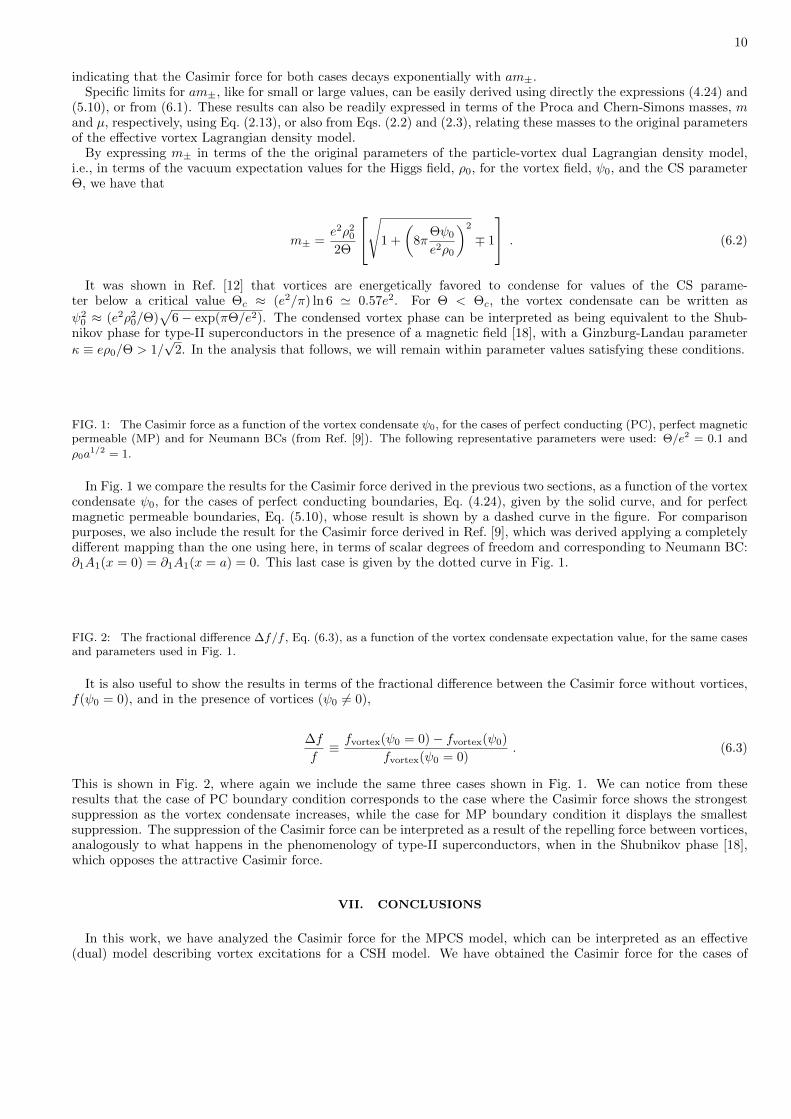
FIG. 1: The Casimir force as a function of the vortex condensate ψ0, for the cases of perfect conducting (PC), perfect magneticpermeable (MP) and for Neumann BCs (from Ref. [9]). The following representative parameters were used: Θ/e2 = 0.1 and

ρ0a1/2 = 1.

In Fig. 1 we compare the results for the Casimir force derived in the previous two sections, as a function of the vortexcondensate ψ0, for the cases of perfect conducting boundaries, Eq. (4.24), given by the solid curve, and for perfectmagnetic permeable boundaries, Eq. (5.10), whose result is shown by a dashed curve in the figure. For comparisonpurposes, we also include the result for the Casimir force derived in Ref. [9], which was derived applying a completelydifferent mapping than the one using here, in terms of scalar degrees of freedom and corresponding to Neumann BC:∂1A1(x = 0) = ∂1A1(x = a) = 0. This last case is given by the dotted curve in Fig. 1.

FIG. 2: The fractional difference ∆f/f , Eq. (6.3), as a function of the vortex condensate expectation value, for the same casesand parameters used in Fig. 1.

It is also useful to show the results in terms of the fractional difference between the Casimir force without vortices,f(ψ0 = 0), and in the presence of vortices (ψ0 6= 0),

∆f

f≡ fvortex(ψ0 = 0)− fvortex(ψ0)

fvortex(ψ0 = 0). (6.3)

This is shown in Fig. 2, where again we include the same three cases shown in Fig. 1. We can notice from theseresults that the case of PC boundary condition corresponds to the case where the Casimir force shows the strongestsuppression as the vortex condensate increases, while the case for MP boundary condition it displays the smallestsuppression. The suppression of the Casimir force can be interpreted as a result of the repelling force between vortices,analogously to what happens in the phenomenology of type-II superconductors, when in the Shubnikov phase [18],which opposes the attractive Casimir force.

VII. CONCLUSIONS

In this work, we have analyzed the Casimir force for the MPCS model, which can be interpreted as an effective(dual) model describing vortex excitations for a CSH model. We have obtained the Casimir force for the cases of

11

perfect conductor and perfect magnetically permeable BC. This has been possible by mapping the MPCS model ina doublet consisting of a self-dual and an anti self-dual PCS models. Other mappings associated with the MPCSmodel are known. For example, another possibility could be in terms of two MCS models, or also in terms of a twononinteracting massive scalar fields. However, in the former case there is no straightforward relation between thefields and, thus on the mapping of the BC for the fields in each model, while in the latter case the form of the relationbetween the fields restricts too much the BC that are possible to use (which is true for mappings between gauge andscalar fields in general [9, 19]).

We have studied the Casimir force obtained by the use of the two types of BC we have considered and we haveshown that the perfect conductor case is the one that leads to the most expressive suppression. Even though it canbe argued that the model we have studied here, which can be associated with the vacuum state of a system of vortexexcitations in a plane, is mostly of theoretical interest and might be far from describing real physical systems ofinterest, our results are, however, indicative of a behavior that can manifest in these systems. As such, our resultsmight be of relevance for the next generation of experiments involving the Casimir effect [20], or those involving, forexample, vortex-based superconducting detectors [21, 22]. Usually, such systems involve nanometer scales, in whichthe Casimir force turns out to be relevant, and possibly also altering the microscopic parameters of detectors [23].Our results can also be of relevance when devising materials based on superconducting films to work as possiblesuppressors of the Casimir force, such as in those laboratory experiments that require performing extremely carefulforce measurements near surfaces. This might be the case of the searches for possible deviations of Newtonian gravity.Our results also highlight the importance of considering various types of BC when computing the Casimir effect, inparticular for those BC that we have considered and that can be associated with different physical situations.

The study performed here for the MPCS model also has its own merits, independent of its connection to a vortexmodel. The MPCS model constitutes of massive gauge particles, with mass terms that have both topological andnon-topological origins. Also, the Maxwell-Proca and the MCS models can be seen as particular cases of the MPCSmodel. So, we expect that a better comprehension of the roles of the mass terms (topological and non-topological)in the Casimir force of the MPCS model might eventually provide arguments in favor of one or the other, whenusing these models with the objective of understanding some of the properties of real planar systems with massiveexcitations. This also includes, of course, deriving the Casimir force under different BC, as we have studied in thiswork.

Acknowledgments

R.O.R. is partially supported by Conselho Nacional de Desenvolvimento Cientıfico e Tecnologico (CNPq-Brazil)and by Fundacao de Amparo a Pesquisa do Estado do Rio de Janeiro (FAPERJ). V. S. A. is partially supported byCoordenacao de Aperfeicoamento de Pessoal de Nıvel Superior (CAPES-Brazil). J.F.M.N. thanks J.A. Helayel Neto,S. Perez and D. T. Alves for very fruitful commentaries.

[1] C. M. Will, Living Rev. Rel. 17, 4 (2014).[2] E. G. Adelberger, B. R. Heckel and A. E. Nelson, Ann. Rev. Nucl. Part. Sci. 53, 77 (2003).[3] H. B. G. Casimir, Indag. Math. 10, 261 (1948) [Kon. Ned. Akad. Wetensch. Proc. 51, 793 (1948)] [Front. Phys. 65, 342

(1987)] [Kon. Ned. Akad. Wetensch. Proc. 100N3-4, 61 (1997)].[4] M. Bordag, G. L. Klimchitskaya, U. Mohideen and V. M. Mostepanenko, Advances in the Casimir Effect (Oxford University

Press, Oxford, 2009).[5] G. L. Klimchitskaya, U. Mohideen and V. M. Mostepanenko, Rev. Mod. Phys. 81, 1827 (2009).[6] V. B. Bezerra, G. L. Klimchitskaya, V. M. Mostepanenko and C. Romero, Phys. Rev. D 81, 055003 (2010).[7] S. Ribeiro and S. Scheel, Phys. Rev. A 88, 042519 (2013); Erratum: Phys. Rev. A 89, 039904(E) (2014).[8] X.-L. Qi and S.-C. Zhang, Rev. Mod. Phys. 83, 1057 (2011); Y. H. Chen, F. Wilczek, E. Witten and B. I. Halperin, Int.

J. Mod. Phys. B 3, 1001 (1989).[9] J. F. de Medeiros Neto, R. O. Ramos and C. R. M. Santos, Phys. Rev. D 86, 125034 (2012).

[10] R. Banerjee and C. Wotzasek, Nucl. Phys. B 527, 402 (1998); R. Banerjee and S. Kumar, Phys. Rev. D 60, 085005 (1999).[11] R. Banerjee and S. Kumar, Phys. Rev. D 63, 125008 (2001).[12] R. O. Ramos and J. F. Medeiros Neto, Phys. Lett. B 666, 496 (2008).[13] X. G. Wen and A. Zee, Phys. Rev. Lett. 62, 1937 (1989).[14] C. P. Burgess and B. P. Dolan, Phys. Rev. B 63, 155309 (2001).[15] K. A. Milton and Y. J. Ng, Phys. Rev. D 42 (1990) 2875.[16] D. T. Alves, E. R. Granhen, J. F. Medeiros Neto and S. Perez, Phys. Lett. A 374, 2113 (2010).

12

[17] M. Abramowitz and I. A. Stegun, (Eds.), Handbook of Mathematical Functions with Formulas, Graphs, and MathematicalTables, (9th printing, New York, Dover, 1972).

[18] M. Tinkham, Introduction to Superconductivity, (McGraw- Hill, New York, 1996).[19] J. F. de Medeiros Neto, R. F. Ozela, R. O. Correa Junior and R. O. Ramos, in press Braz. J. Phys. (2014).[20] A. Allocca, G. Bimonte, D. Born, E. Calloni, G. Esposito, U. Huebner, E. Il’ichev and L. Rosa et al., J. Supercond. Nov.

Mag. 25, 2557 (2012).[21] A. M. Kadin, M. Leung, A. D. Smith, J. M. Murduck, Appl. Phys. Lett. 57, 2487 (1990).[22] A. D. Semenov, et. al., Supercond. Sci. Technol. 20, 919 (2007); A. D. Semenov, et. al., Physica C 468, 627 (2008).[23] D. Brandt, G. W. Fraser, D. J. Raine and C. Binns, J. of Low Temp. Phys. 151, 25 (2008).