arX

iv:n

ucl-

th/9

5020

42v1

23

Feb

1995

Scissors Modes and Spin Excitations in LightNuclei including ∆N=2 excitations:

Behaviour of 8Be and 10Be

M. S. Fayache, S. Shelly Sharma* and L. Zamick

Department of Physics and Astronomy, Rutgers University, Piscataway, NJ

08855

*Departamento de Fisica, Universidade Estadual de Londrina, Londrina, Parana,

86051-970, Brazil

Abstract

Shell model calculations are performed for magnetic dipole excita-

tions in 8Be and 10Be in which all valence configurations plus 2hω ex-

citations are allowed (large space). We study both the orbital and spin

excitations. The results are compared with the ‘valence space only’

calculations (small space). The cumulative energy weighted sums are

calculated and compared for the J = 0+ T=0 to J = 1+ T=1 exci-

tations in 8Be and for J = 0+ T=1 to both J = 1+ T=1 and J=1+

T=2 excitations in 10Be. We find for the J = 0+ T=1 to J = 1+

T=1 isovector spin transitions in 10Be that the summed strength in

the large space is less than in the small space. We find that the high

energy energy-weighted isovector orbital strength is smaller than the

low energy strength for transitions in which the isospin is changed,

but for J = 0+ T=1 to J = 1+ T=1 in 10Be the high energy strength

is larger. We find that the low lying orbital strength in 10Be is anoma-

lously small, when an attempt is made to correlate it with the B(E2)

strength to the lowest 2+ states. On the other hand a sum rule of

Zheng and Zamick which concerns the total B(E2) strength is rea-

sonably satisfied in both 8Be and 10Be. The Wigner supermultiplet

scheme is a useful guide in analyzing shell model results. In 10Be and

with a Q · Q interaction the T = 1 and T = 2 scissors modes are

degenerate, with the latter carrying 53 of the T = 1 strength.

2

1 The Experimental Situation

From our perspective, much experimental information is lacking in the

nuclei 8Be and 10Be. For example, no J = 1+ states have been identified in10Be. The B(E2) from the 2+

1 state of 8Be to the J = 0+ ground state is not

known -this is understandable because of the large decay width to two alpha

particles.

The following states and their properties are of interest to us:

(a) 8Be

The J = 2+1 state has an excitation energy of 3.04MeV . The J = 4+

1 state

is at 11.4 MeV . This is consistent with an J(J +1) spectrum of a rotational

band, but it should be recalled that any spin-independent interaction gives

an J(J + 1) spectrum in the p shell. The J = 1+1 T = 1 state, which we

discussed extensively in a previous publication [1] is at 17.64 MeV and the

J = 1+1 T = 0 state is at 18.15 MeV .

The B(M1) from the 17.64 MeV state to the ground state has a strength

of 0.15 W.u. or B(M1) = 0.27µN2. The B(M1) of this state to the 2+

1 state

is 0.12 W.u. or B(M1) = 0.21µN2 [2]. Of course B(M1) ↑=3B(M1) ↓

(b) 10Be

The J = 2+1 state is at 3.368 MeV and the J = 2+

2 state at 5.960 MeV .

We recall that with a spin independent interaction the 2+1 and 2+

2 would be

degenerate. The experimental spectrum looks more vibrational. However,

the values of B(E2) from the J = 0+ ground state to the 2+1 state is very

strong: B(E2) = 52 e2fm4. Raman et. al. deduce from this a deformation

parameter β = 1.13 [3]. As mentioned above, there are no J = 1+ states

mentioned in the compilation of Ajzenberg-Selove [2]. Also the J = 4+ state

has not been found.

3

2 The Interactions

We have chosen two types of interactions to do the calculations. First we

use a short range ‘simplified realistic’ (x, y) interaction previously used by

Zheng and Zamick [4], and then we use a long-range quadrupole-quadrupole

interaction. By choosing these two extremes, we make sure that the results

we obtain are not too dependent on the specifics of the model.

In more detail, the(x, y) Hamiltonian is:

H =∑

Ti +∑

i<j

V (ij)

where

V = Vc + xVso + yVt

with c ≡central, s.o. ≡spin-orbit, and t ≡tensor.

For (x, y)=(1,1) the matrix elements of this interaction are close to those

of realistic G matrices such as Bonn A. We can study the effects the spin-orbit

and tensor interactions by varying x and y.

Note that we do not add any single-particle energies to the above Hamil-

tonian. Rather, we let the single-particle energies be implicitly generated by

H . Hence, if we set x=0 i.e. turn off the two-body spin-orbit interaction,

we will also be turning off the one-body spin-orbit splitting coming from this

interaction.

As a counterpoint, we repeat all the calculations with the Q ·Q Hamilto-

nian

HQ =∑

i

p2i

2m+

1

2mω2r2

i − χ∑

i<j

Q ·Q

Note that we have added the term 12mω2r2 which is not present for the (x, y)

interaction. The reason for this is that Q · Q cannot generate any single-

particle potential energy splitting whereas the (x, y) interaction can.

4

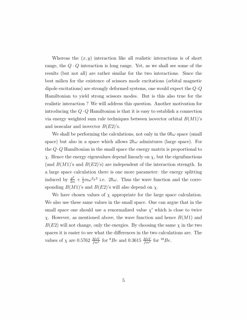
Whereas the (x, y) interaction like all realistic interactions is of short

range, the Q · Q interaction is long range. Yet, as we shall see some of the

results (but not all) are rather similar for the two interactions. Since the

best milieu for the existence of scissors mode excitations (orbital magnetic

dipole excitations) are strongly deformed systems, one would expect the Q·Q

Hamiltonian to yield strong scissors modes. But is this also true for the

realistic interaction ? We will address this question. Another motivation for

introducing the Q ·Q Hamiltonian is that it is easy to establish a connection

via energy weighted sum rule techniques between isovector orbital B(M1)’s

and isoscalar and isovector B(E2)’s.

We shall be performing the calculations, not only in the 0hω space (small

space) but also in a space which allows 2hω admixtures (large space). For

the Q ·Q Hamiltonian in the small space the energy matrix is proportional to

χ. Hence the energy eigenvalues depend linearly on χ, but the eigenfunctions

(and B(M1)’s and B(E2)’s) are independent of the interaction strength. In

a large space calculation there is one more parameter: the energy splitting

induced by p2

2m+ 1

2mω2r2 i.e. 2hω. Thus the wave function and the corre-

sponding B(M1)’s and B(E2)’s will also depend on χ.

We have chosen values of χ appropriate for the large space calculation.

We also use these same values in the small space. One can argue that in the

small space one should use a renormalized value χ′ which is close to twice

χ. However, as mentioned above, the wave function and hence B(M1) and

B(E2) will not change, only the energies. By choosing the same χ in the two

spaces it is easier to see what the differences in the two calculations are. The

values of χ are 0.5762 MeVfm4 for 8Be and 0.3615 MeV

fm4 for 10Be.

5

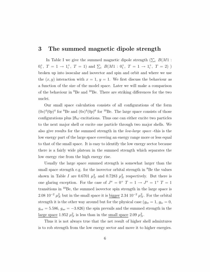
3 The summed magnetic dipole strength

In Table I we give the summed magnetic dipole strength (∑

i B(M1 :

0+1 , T = 1 → 1+

i , T = 1) and∑

i B(M1 : 0+1 , T = 1 → 1+

i , T = 2) )

broken up into isoscalar and isovector and spin and orbit and where we use

the (x, y) interaction with x = 1, y = 1. We first discuss the behaviour as

a function of the size of the model space. Later we will make a comparison

of the behaviour in 8Be and 10Be. There are striking differences for the two

nuclei.

Our small space calculation consists of all configurations of the form

(0s)4(0p)4 for 8Be and (0s)4(0p)6 for 10Be. The large space consists of those

configurations plus 2hω excitations. Thus one can either excite two particles

to the next major shell or excite one particle through two major shells. We

also give results for the summed strength in the low-large space -this is the

low energy part of the large space covering an energy range more or less equal

to that of the small space. It is easy to identify the low energy sector because

there is a fairly wide plateau in the summed strength which separates the

low energy rise from the high energy rise.

Usually the large space summed strength is somewhat larger than the

small space strength e.g. for the isovector orbital strength in 8Be the values

shown in Table I are 0.6701 µ2N and 0.7283 µ2

N respectively. But there is

one glaring exception. For the case of Jπ = 0+ T = 1 → Jπ = 1+ T = 1

transitions in 10Be, the summed isovector spin strength in the large space is

2.08 10−2 µ2N but in the small space it is bigger 2.34 10−2 µ2

N . For the orbital

strength it is the other way around but for the physical case (glπ = 1, glν = 0,

gsπ = 5.586, gsν = −3.826) the spin prevails and the summed strength in the

large space 1.952 µ2N is less than in the small space 2.09 µ2

N .

Thus it is not always true that the net result of higher shell admixtures

is to rob strength from the low energy sector and move it to higher energies.

6

In some cases the total strength gets depleted.

We next compare the low energy sum in the large space with the small

space sum. In all cases the latter is larger than the low energy sum, thus

indicating that there is a quenching of the low energy part due to higher

shell admixtures. The hindrance factor [(low large)/small] is 0.88 for the

isovector orbital in 8Be, 0.73 for the isovector spin in 8Be, 0.77 for the total

M1 in 10Be etc.

Note that the totalM1’s for 10Be are somewhat larger than for 8Be. How-

ever there is a dramatic drop in the orbital strength in 10Be relative to that

in 8Be. The large space summed orbital strength for 8Be is 0.73 µ2N whereas

for 10Be (to J = 1+ T = 1 and T = 2) the value is (0.196 + 0.183)=0.38

µ2N . In the low energy sector the 8Be value is 0.59 µ2

N whereas for 10Be it is

0.10 + 0.13 = 0.23 µ2N , less than half the value for 8Be.

From the systematics of orbital transitions in heavy nuclei one concludes

that the proper milieu for isovector orbital transitions is strongly deformed

nuclei. Can one conclude that 10Be is not strongly deformed? The answer,

by examining the tables of Raman et. al. [3] is no! There is a strong E2

connecting the 0+1 and 2+

1 states in 10Be. From this the authors conclude

that the deformation parameter β is about 1.13 -quite enormous. Of course8Be might have an even stronger E2 transition -there is no data on this in

the Raman paper [3], probably because of the rapid decay of the 2+1 state

into two alpha particles.

4 The cumulative energy weighted strength

for orbital transitions in 8Be and 10Be

In this section we present results and figures for the cumulative energy

weighted sum of magnetic dipole strength.

7

We are motivated in so doing by various energy-weighted sum rules that

have been developed e.g. by Zheng and Zamick [5], Heyde and de Coster

[6], Moya de Guerra and Zamick [7], Nojarov [8], Hamamoto and Nazarewicz

[9] and Fayache and Zamick [1]. We will focus in particular on the orbital

strength for which the operator is ( ~Lπ − ~Lν)/2. In a previous publication

we presented results for the (x, y) interaction with x=1, y=1 for 8Be [1]. In

this work the quadrupole-quadrupole interaction results are compared with

the (x, y) interaction results, and furthermore we extend the calculation to10Be. In the latter nucleus one does not have N = Z and this leads to big

differences.

Whereas in 8Be there is only one isospin channel for isovector transitions

J = 0+1 T = 0 → J = 1+ T = 1, in 10Be there are two: J = 0+

1 T = 1 →

J = 1+ T = 1 and J = 0+1 T = 1 → J = 1+ T = 2. The low lying J = 1+

T = 1 states in 10Be are expected to have much smaller excitation energies

than the J = 1+ T = 1 states in 8Be. This makes it easier to look for such

states experimentally.

In Table II we present the results for the summed energy weighted strengths

for the (x, y) interaction. As a crude orientation it should be noted that sim-

ple models e.g. the Nilsson model used by de Guerra and Zamick [7] and a

model by Nojarov [8] would have the ‘large’ result be twice the ‘low large’

result. On the other hand Hamamoto and Nazarewicz [9] have argued that

the ‘large’ result should be much more than twice the ‘low large’ result. The

actual ratios for the (x, y) and Q ·Q interactions for this calculation (all 0hω

configurations plus 2hω excitations) are

8

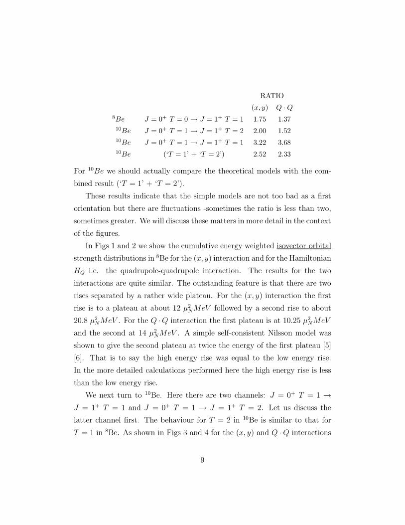
RATIO

(x, y) Q · Q

8Be J = 0+ T = 0 → J = 1+ T = 1 1.75 1.3710Be J = 0+ T = 1 → J = 1+ T = 2 2.00 1.52

10Be J = 0+ T = 1 → J = 1+ T = 1 3.22 3.68

10Be (‘T = 1’ + ‘T = 2’) 2.52 2.33

For 10Be we should actually compare the theoretical models with the com-

bined result (‘T = 1’ + ‘T = 2’).

These results indicate that the simple models are not too bad as a first

orientation but there are fluctuations -sometimes the ratio is less than two,

sometimes greater. We will discuss these matters in more detail in the context

of the figures.

In Figs 1 and 2 we show the cumulative energy weighted isovector orbital

strength distributions in 8Be for the (x, y) interaction and for the Hamiltonian

HQ i.e. the quadrupole-quadrupole interaction. The results for the two

interactions are quite similar. The outstanding feature is that there are two

rises separated by a rather wide plateau. For the (x, y) interaction the first

rise is to a plateau at about 12 µ2NMeV followed by a second rise to about

20.8 µ2NMeV . For the Q ·Q interaction the first plateau is at 10.25 µ2

NMeV

and the second at 14 µ2NMeV . A simple self-consistent Nilsson model was

shown to give the second plateau at twice the energy of the first plateau [5]

[6]. That is to say the high energy rise was equal to the low energy rise.

In the more detailed calculations performed here the high energy rise is less

than the low energy rise.

We next turn to 10Be. Here there are two channels: J = 0+ T = 1 →

J = 1+ T = 1 and J = 0+ T = 1 → J = 1+ T = 2. Let us discuss the

latter channel first. The behaviour for T = 2 in 10Be is similar to that for

T = 1 in 8Be. As shown in Figs 3 and 4 for the (x, y) and Q ·Q interactions

9

respectively, there are two rises separated by a plateau and here the second

rise is about twice the first rise for the (x, y) interaction. For the Q · Q

interaction (with χ = 0.3615) the low energy rise is to 1.7 µ2NMeV and the

next rise is to 2.6 µ2NMeV -only 1.5 to one.

There is a big difference in the cumulative energy weighted distributions,

shown in Figs 5 and 6, for the J = 0+ T = 1 → J = 1+ T = 1 channel. For

the (x, y) interaction the first plateau (at about 2.5 µ2NMeV ) is not very flat,

but the most outstanding feature in the curve is that the high energy rise

is much larger than the low energy rise. The energy weighted sum reaches

up to about 8 µ2NMeV . Thus the high energy rise is over three time the low

energy rise. For the Q ·Q interaction, the first plateau is better defined -it is

located at 1 µ2NMeV and the cumulative sum extends to about 3.8 µ2

NMeV .

5 The Zheng-Zamick Sum Rule

Energy weighted sum rules for magnetic dipole transitions, be they spin

or orbital, are highly model dependent. An energy weighted sum rule for

isovector orbital magnetic dipole transitions for the quadrupole-quadrupole

interaction Q·Q was developed by Zheng and Zamick [5]. This was motivated

by the work of the Darmstadt group [10] [11] showing a linear relationship

between summed orbital B(M1) strength and the square of the deformation

parameter i.e. δ2.

The result was

∑

n

(En−E0)B(M1)o =9χ

16π

∑

i

[B(E2, 01 → 2i)isoscalar −B(E2, 01 → 2i)isovector]

(EWSR)

where B(M1)o is the value for the isovector orbital M1 operator (glπ =

0.5 glν = −0.5 gsπ = 0 gsν = 0) and the operator for the E2 transitions

10

is∑

protons epr2Y2 +

∑

neutrons enr2Y2 with ep = 1, en = 1 for the isoscalar

transition, and ep = 1, en = −1 for the isovector transition.

Let us now describe in detail how this sum rule works. The sum rule

should work for single-shell as well mixed-shell space.

We first consider the case of 8Be. We have the following values in a

large space calculation for the HQ interaction corresponding to orbital M1

excitations from the J = 0+ T = 0 ground state to all 1+ T = 1 states:

1. Energy weighted isovector orbital M1 strength: 14.040 µ2NMeV

2. The isoscalar summed strength B(E2; 1, 1): 237.46 e2fm4

3. The isovector summed strength B(E2; 1,−1): 89.611 e2fm4

4. The right hand side ( 9χ

16π= 0.1032): 15.25 µ2

NMeV .

We don’t get exact agreement (14.04 µ2NMeV vs. 15.25 µ2

NMeV ) but it

is reasonably close. One possible reason for the disagreement is that spurious

states have been removed and/or that only 2hω excitations to the ∆N = 2

shell are taken into account [6] [10].

There have been other approaches, especially in the context of the Inter-

acting Boson Model [6] which relate the energy weighted orbital magnetic

sum to the B(E2) of the lowest 2+ state. As a matter of curiosity we shall

examine in our calculation what happens if we take only the lowest 2+ state

in the right hand side of the sum rule (EWSR).

For the 2+1 state in 8Be we obtain (in our large space calculation)B(E2; 1, 1) =

196.76 and B(E2; 1,−1) = 0 (because the 2+1 state has T = 0). The right

hand side becomes 20.30 µ2NMeV . We get a larger answer using the lowest

2+ state than we do if we use all 2+ states in the 0hω and 2hω space. The

reason for this is that when the lowest 2+ state is excluded, the isovector

B(E2) is larger than the isoscalar B(E2).

11

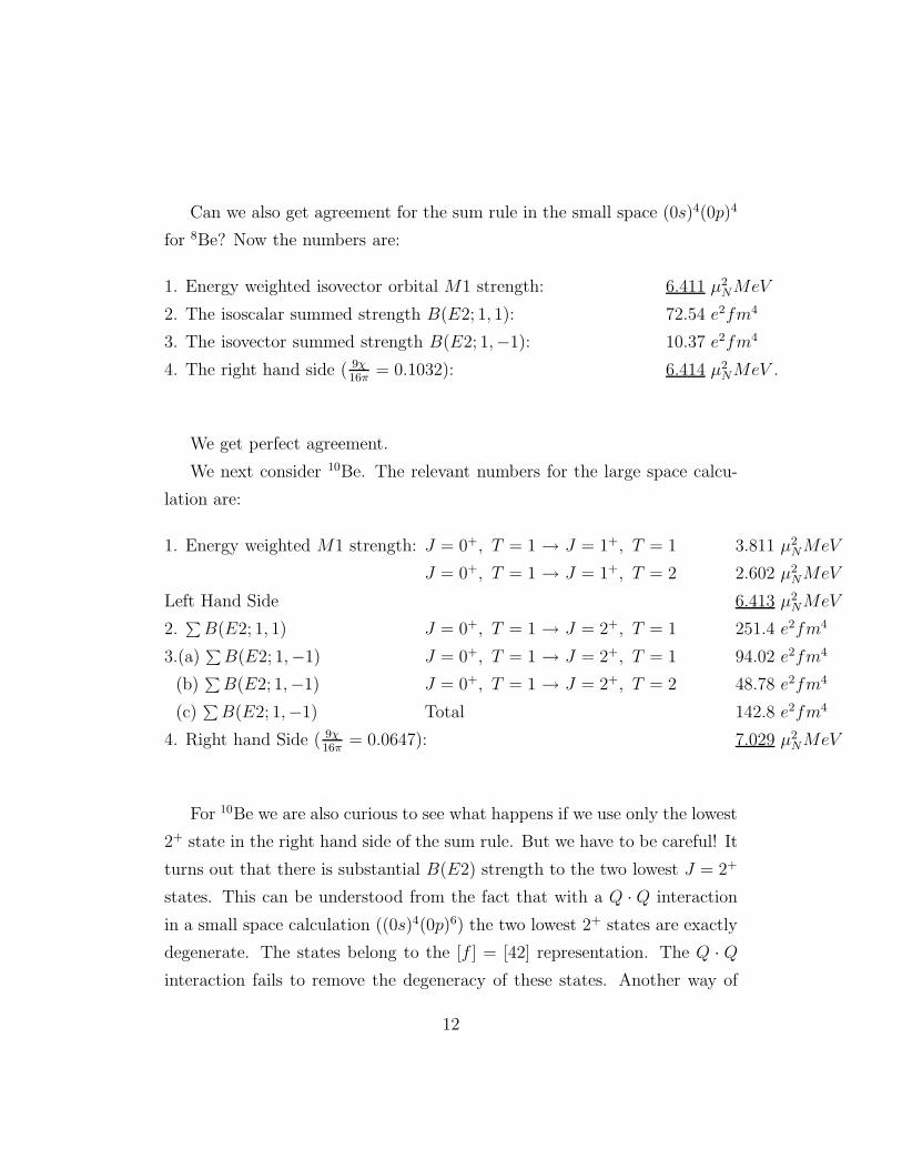
Can we also get agreement for the sum rule in the small space (0s)4(0p)4

for 8Be? Now the numbers are:

1. Energy weighted isovector orbital M1 strength: 6.411 µ2NMeV

2. The isoscalar summed strength B(E2; 1, 1): 72.54 e2fm4

3. The isovector summed strength B(E2; 1,−1): 10.37 e2fm4

4. The right hand side ( 9χ

16π= 0.1032): 6.414 µ2

NMeV .

We get perfect agreement.

We next consider 10Be. The relevant numbers for the large space calcu-

lation are:

1. Energy weighted M1 strength: J = 0+, T = 1 → J = 1+, T = 1 3.811 µ2NMeV

J = 0+, T = 1 → J = 1+, T = 2 2.602 µ2NMeV

Left Hand Side 6.413 µ2NMeV

2.∑

B(E2; 1, 1) J = 0+, T = 1 → J = 2+, T = 1 251.4 e2fm4

3.(a)∑

B(E2; 1,−1) J = 0+, T = 1 → J = 2+, T = 1 94.02 e2fm4

(b)∑

B(E2; 1,−1) J = 0+, T = 1 → J = 2+, T = 2 48.78 e2fm4

(c)∑

B(E2; 1,−1) Total 142.8 e2fm4

4. Right hand Side ( 9χ

16π= 0.0647): 7.029 µ2

NMeV

For 10Be we are also curious to see what happens if we use only the lowest

2+ state in the right hand side of the sum rule. But we have to be careful! It

turns out that there is substantial B(E2) strength to the two lowest J = 2+

states. This can be understood from the fact that with a Q · Q interaction

in a small space calculation ((0s)4(0p)6) the two lowest 2+ states are exactly

degenerate. The states belong to the [f ] = [42] representation. The Q · Q

interaction fails to remove the degeneracy of these states. Another way of

12

stating this is that the (λµ) values for both states are (22), and the allowed

values of the K quantum number in the Nilsson scheme are K = µ, µ − 2,

etc. Thus the 2+ states have K = 0 and K = 2.

When we go to the large space calculation with aQ·Q interaction, limiting

the excitations to 2hω, the degeneracy is removed but the states are still fairly

close together. The calculated values are:

E2(1, 1) E2(1,−1)

2+1 E = 2.08 MeV 64.94 12.32

2+2 E = 2.92 MeV 93.38 10.11

Thus, using the calculated values of B(E2) for the lowest two 2+ T = 1

states in 10Be, we get for the right hand side of the sum rule a value of 8.80

µ2NMeV . Again, as in the case of 8Be, this is larger than the value 7.03

µ2NMeV that is obtained by using all 2+ T = 1 and all 2+ T = 2 states.

The corresponding numbers in small space for 10Be are:

1. Energy weighted M1 strength: J = 0+, T = 1 → J = 1+, T = 1 0.7597 µ2NMeV

J = 0+, T = 1 → J = 1+, T = 2 1.266 µ2NMeV

Left Hand Side 2.026 µ2NMeV

2.∑

B(E2; 1, 1) J = 0+, T = 1 → J = 2+, T = 1 68.31 e2fm4

3.(a)∑

B(E2; 1,−1) J = 0+, T = 1 → J = 2+, T = 1 33.80 e2fm4

(b)∑

B(E2; 1,−1) J = 0+, T = 1 → J = 2+, T = 2 3.203 e2fm4

(c)∑

B(E2; 1,−1) Total 37.003 e2fm4

4. Right hand Side ( 9χ

16π= 0.0647): 2.026 µ2

NMeV

13

6 A discussion of the calculated B(E2) values

Although the main thrust of this work is on B(M1) values, we have

established a connection with B(E2) for the orbital case. It is therefore ap-

propriate to discuss the calculated B(E2) values -comparing the behaviours

in 8Be and 10Be, and comparing the different interactions that have been

used (see tables III and IV .)

In making the comparison between 8Be and 10Be we should lump together

the B(E2)’s of the first two 2+ states in 10Be because with the interactions

used here -especially Q · Q- these states are nearly degenerate. (However,

experimentally the states are well separated E2+

1= 3.368 MeV and E2+

2=

5.958 MeV ). When this is done we find that the B(E2) values in the two

nuclei are comparable.

For the (x, y) interaction, the calculated (large space) value of B(E2) to

the lowest two 2+ states in 10Be is 22.90 e2fm4, whereas it is 25.97 e2fm4

to the lowest 2+ state in 8Be. With the Q · Q interaction the two values

are respectively 46.40 and 49.16 e2fm4. One big difference between the

two interactions is the ratio of large to small space values for corresponding

B(E2) values. In 8Be the ratio of the large sum to the small sum is 1.98 for

the (x, y) interaction whereas it is much larger 3.28 for the Q ·Q interaction.

There is much more core polarization with the Q · Q interaction than with

the (x, y) interaction.

There have been many discussions concerning the correlation of summed

orbital M1 strength and the B(E2) from the J = 0+ ground state to the

first 2+ state. The latter is an indication of the nuclear deformation. We

have noted that the calculated values of B(E2) are about the same in 8Be

and 10Be. Thus we would expect the orbital M1 strengths in the two nuclei

to be about the same.

There is a certain ‘vagueness’ in what is meant by ‘strength’. It is clear

14

that the experiments thus far sample only low energy strengths up to about

6 MeV in heavy deformed nuclei [10] [11]. Also some of the theories involve

summed strength per se and others involve the energy weighted strength.

Rather than enter into deep philosophical discussions about what is meant

by strength, we will give a variety of ratios of strength10Be8Be in Table V . We

see that all the ratios, be they non-energy weighted or energy weighted, be

they in small spaces or in large spaces, are substantially less than one. In

forming the ratios, we added for the numerator (10Be) the J = 0+ T = 1 to

J = 1+ T = 1 and J = 0+ T = 1 to J = 1+ T = 2 strengths.

7 A comparison of the J = 1+ → 0

+1 and J = 1

+

→ 2+1 Magnetic Dipole Transitions

Let us assume that the 0+1 and 2+

1 states are members of a K = 0

rotational band and that the 1+ states have K = 1. We can then use the

rotational formula of Bohr and Mottelson (Eq. 4-92) in their book [12] (K1 =

0, K2 = 1) (We use the notation

J1 J2 J

M1 M2 M

for a Clebsch-Gordan

coefficient):

〈K2I2||M(λ)||K1 = 0I1〉 =√

2(2I1 + 1)

I1 λ I2

0 K2 K2

〈K2|M(λ, ν = K2)|K1 = 0〉

From this we can easily deduce

r =B(M1)J=1+,K=1→J=2+,K=0

B(M1)J=1+,K=1→J=0+,K=0

=1

2

Note, however, that the experimental ratio for 8Be from the J = 1+ T = 1

state at 17.64 MeV (see section 1) is 0.120.15

= 0.8. Bohr and Mottelson later

discuss corrections to the above simple formula.

15

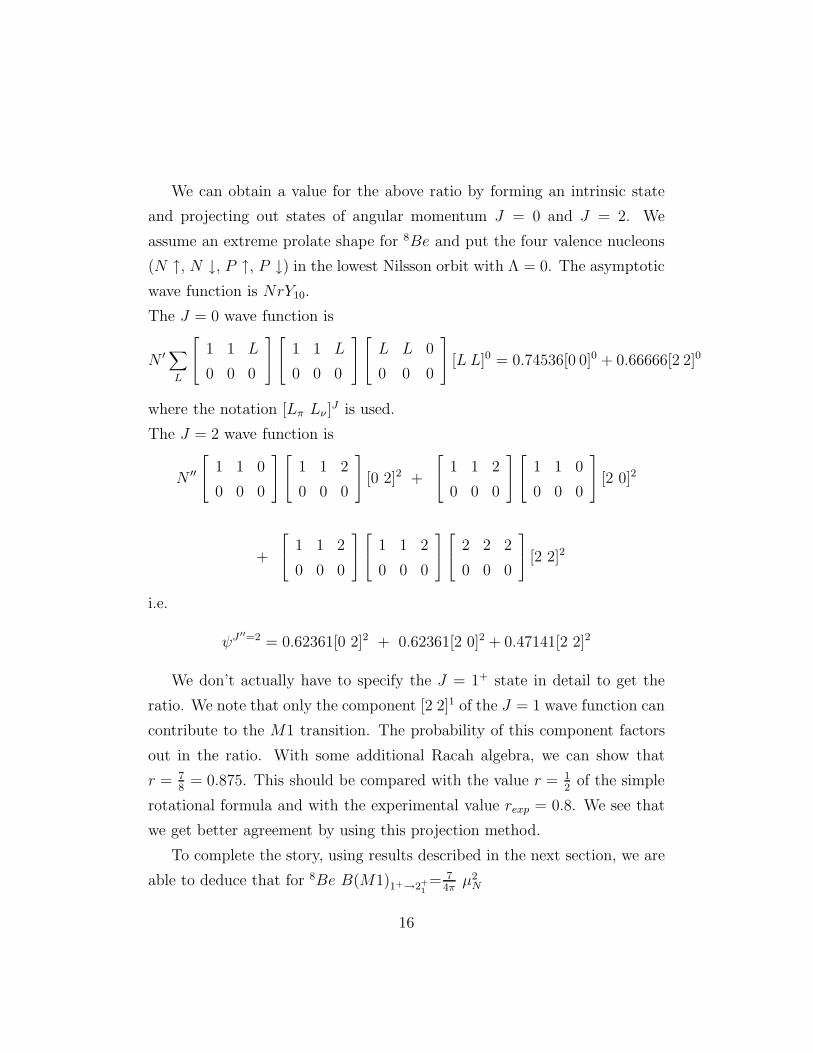
We can obtain a value for the above ratio by forming an intrinsic state

and projecting out states of angular momentum J = 0 and J = 2. We

assume an extreme prolate shape for 8Be and put the four valence nucleons

(N ↑, N ↓, P ↑, P ↓) in the lowest Nilsson orbit with Λ = 0. The asymptotic

wave function is NrY10.

The J = 0 wave function is

N ′∑

L

1 1 L

0 0 0

1 1 L

0 0 0

L L 0

0 0 0

[L L]0 = 0.74536[0 0]0 + 0.66666[2 2]0

where the notation [Lπ Lν ]J is used.

The J = 2 wave function is

N ′′

1 1 0

0 0 0

1 1 2

0 0 0

[0 2]2 +

1 1 2

0 0 0

1 1 0

0 0 0

[2 0]2

+

1 1 2

0 0 0

1 1 2

0 0 0

2 2 2

0 0 0

[2 2]2

i.e.

ψJ ′′=2 = 0.62361[0 2]2 + 0.62361[2 0]2 + 0.47141[2 2]2

We don’t actually have to specify the J = 1+ state in detail to get the

ratio. We note that only the component [2 2]1 of the J = 1 wave function can

contribute to the M1 transition. The probability of this component factors

out in the ratio. With some additional Racah algebra, we can show that

r = 78

= 0.875. This should be compared with the value r = 12

of the simple

rotational formula and with the experimental value rexp = 0.8. We see that

we get better agreement by using this projection method.

To complete the story, using results described in the next section, we are

able to deduce that for 8Be B(M1)1+→2+

1= 7

4πµ2

N

16

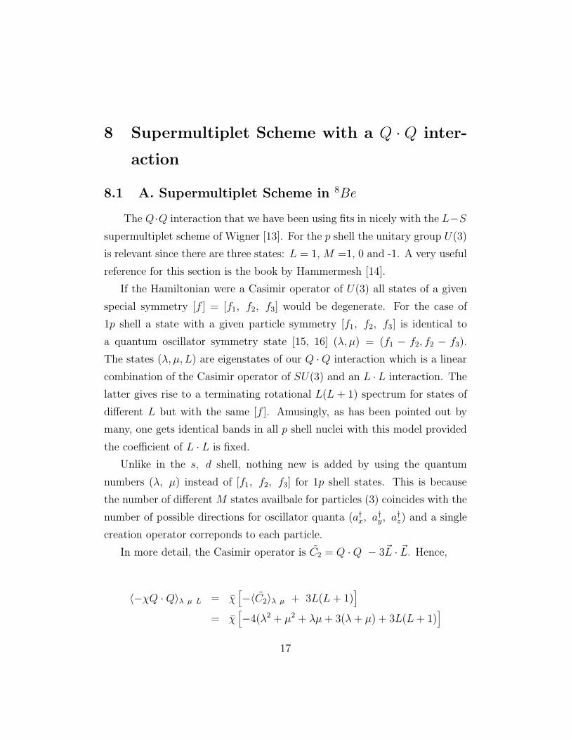
8 Supermultiplet Scheme with a Q · Q inter-

action

8.1 A. Supermultiplet Scheme in 8Be

The Q·Q interaction that we have been using fits in nicely with the L−S

supermultiplet scheme of Wigner [13]. For the p shell the unitary group U(3)

is relevant since there are three states: L = 1, M =1, 0 and -1. A very useful

reference for this section is the book by Hammermesh [14].

If the Hamiltonian were a Casimir operator of U(3) all states of a given

special symmetry [f ] = [f1, f2, f3] would be degenerate. For the case of

1p shell a state with a given particle symmetry [f1, f2, f3] is identical to

a quantum oscillator symmetry state [15, 16] (λ, µ) = (f1 − f2, f2 − f3).

The states (λ, µ, L) are eigenstates of our Q ·Q interaction which is a linear

combination of the Casimir operator of SU(3) and an L ·L interaction. The

latter gives rise to a terminating rotational L(L + 1) spectrum for states of

different L but with the same [f ]. Amusingly, as has been pointed out by

many, one gets identical bands in all p shell nuclei with this model provided

the coefficient of L · L is fixed.

Unlike in the s, d shell, nothing new is added by using the quantum

numbers (λ, µ) instead of [f1, f2, f3] for 1p shell states. This is because

the number of different M states availbale for particles (3) coincides with the

number of possible directions for oscillator quanta (a†x, a†y, a

†z) and a single

creation operator correponds to each particle.

In more detail, the Casimir operator is C2 = Q ·Q − 3~L · ~L. Hence,

〈−χQ ·Q〉λ µ L = χ[

−〈C2〉λ µ + 3L(L+ 1)]

= χ[

−4(λ2 + µ2 + λµ+ 3(λ+ µ) + 3L(L+ 1)]

17

where χ = χ 5b4

32πwith b the harmonic oscillator length parameter (b2 = h

mω).

The magnetic dipole modes in the L S T representation are:

L = 1 S = 0 T = 0 L = 0 S = 1 T = 1 (isovector spin mode)

L = 1 S = 0 T = 1 (scissors mode) L = 1 S = 1 T = 0

L = 0 S = 1 T = 0 L = 1 S = 1 T = 1

With the Q · Q interaction that we have chosen, transitions from the

L = 0 S = 0 ground state in 8Be to all of these modes except one will

vanish. The only surviving mode is the L = 1 S = 0 T = 1 scissors mode.

Let us give briefly the energies and some properties of the states in 8Be

(χ = 0.1865):

(a) [f]=[4,0] (λ, µ)=(4,0) Ground State Band

L S T Eχ

E∗(MeV )

0 0 0 −112 0

2 0 0 −94 3.36

4 0 0 −52 11.19

(b) [f]=[3,1] (λ, µ)=(2,1) -contains the scissors mode (L = 1, S = 0,

T = 1).

Note that the (S, T ) combinations (0,1), (1,0) and (1,1) are allowed.

L Eχ

E∗(MeV )

1 −58 10.07

2 −46 12.31

3 −28 15.67

18

(c) [f]=[2,2] (λ, µ)=(0,2) The (S, T ) combinations (0,0), (0,2), (2,0) and

(1,1) are allowed.

L Eχ

E∗(MeV )

0 −40 13.43

2 −22 16.78

(d) [f]=[2,1,1] (λ, µ)=(1,0) The (S, T ) combinations (0,1), (1,0), (1,1),

(1,2) and (2,1) are allowed.

L Eχ

E∗(MeV )

1 −10 19.02

Note that this supermultiplet also has a state with the quantum numbers

of the scissors mode L = 1 S = 0 T = 1.

Some further comments are in order. The scissors mode state in 156Gd,

as a single band state originally discovered in electron scattering [17], was

found when finer resolution (γ, γ′) experiments were performed to consist of

many states [18, 19]. This was a beautiful example of intermediate structure.

The supermultiplet scheme here affords a concrete example of the origin of

the intermediate structure. Our scissors mode state at an energy of −58 χ is

degenerate with an L = 1 S = 1 T = 1 state. If we introduce spin-dependent

interactions the two states will admix and the degeneracy will be removed.

We will get intermediate structure.

8.2 B. Supermultiplet Scheme in 10Be

We now give the energies and some properties of the states in 10Be

(χ = 0.1286): (a) [f]=[4,2] (λ, µ)=(2,2) (includes ground state).

19

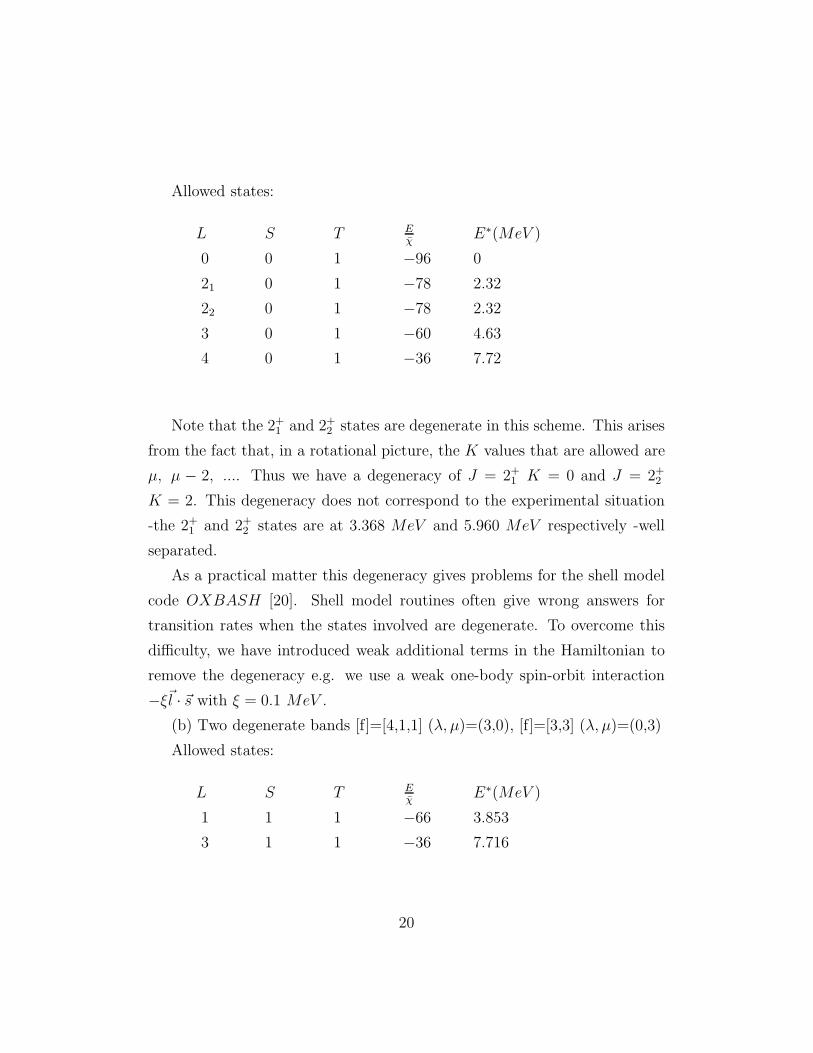
Allowed states:

L S T Eχ

E∗(MeV )

0 0 1 −96 0

21 0 1 −78 2.32

22 0 1 −78 2.32

3 0 1 −60 4.63

4 0 1 −36 7.72

Note that the 2+1 and 2+

2 states are degenerate in this scheme. This arises

from the fact that, in a rotational picture, the K values that are allowed are

µ, µ − 2, .... Thus we have a degeneracy of J = 2+1 K = 0 and J = 2+

2

K = 2. This degeneracy does not correspond to the experimental situation

-the 2+1 and 2+

2 states are at 3.368 MeV and 5.960 MeV respectively -well

separated.

As a practical matter this degeneracy gives problems for the shell model

code OXBASH [20]. Shell model routines often give wrong answers for

transition rates when the states involved are degenerate. To overcome this

difficulty, we have introduced weak additional terms in the Hamiltonian to

remove the degeneracy e.g. we use a weak one-body spin-orbit interaction

−ξ~l · ~s with ξ = 0.1 MeV .

(b) Two degenerate bands [f]=[4,1,1] (λ, µ)=(3,0), [f]=[3,3] (λ, µ)=(0,3)

Allowed states:

L S T Eχ

E∗(MeV )

1 1 1 −66 3.853

3 1 1 −36 7.716

20

We get the low-lying 1+ states (one from [4,1,1] and one from [3,3]). Note

however that we have L = 1, S = 1, hence the states cannot be excited by

either the orbital operator or the spin operator.

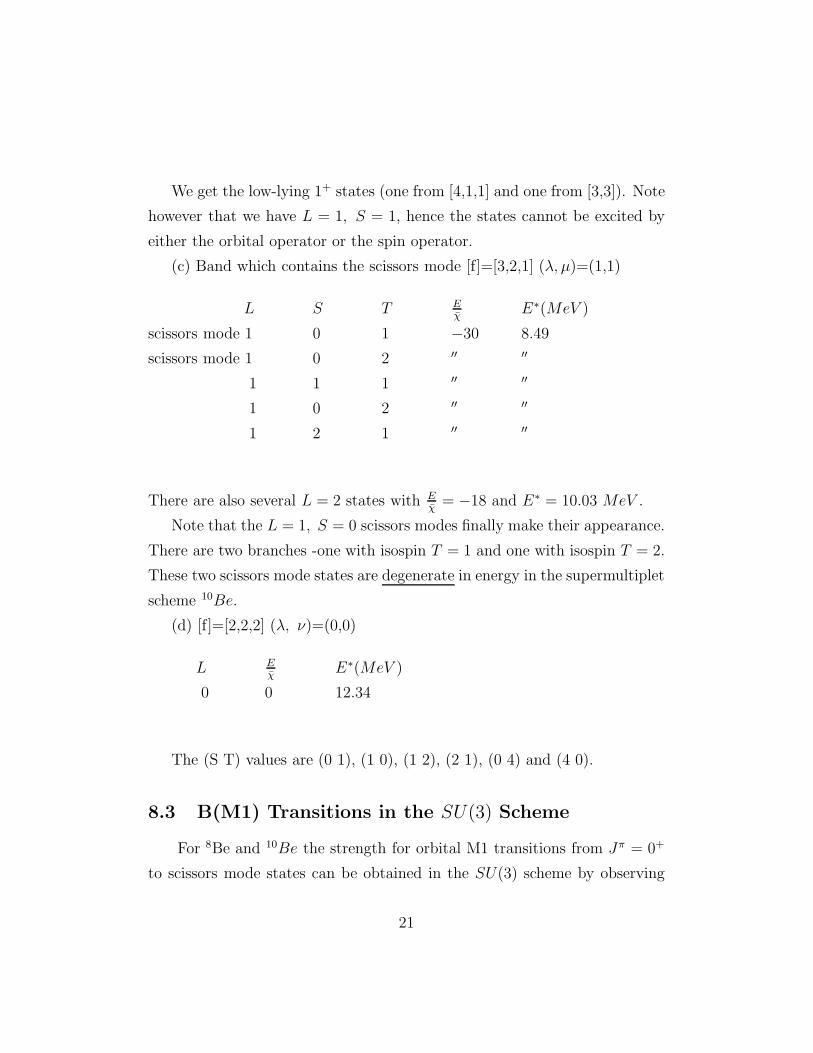
(c) Band which contains the scissors mode [f]=[3,2,1] (λ, µ)=(1,1)

L S T Eχ

E∗(MeV )

scissors mode 1 0 1 −30 8.49

scissors mode 1 0 2 ′′ ′′

1 1 1 ′′ ′′

1 0 2 ′′ ′′

1 2 1 ′′ ′′

There are also several L = 2 states with Eχ

= −18 and E∗ = 10.03 MeV .

Note that the L = 1, S = 0 scissors modes finally make their appearance.

There are two branches -one with isospin T = 1 and one with isospin T = 2.

These two scissors mode states are degenerate in energy in the supermultiplet

scheme 10Be.

(d) [f]=[2,2,2] (λ, ν)=(0,0)

L Eχ

E∗(MeV )

0 0 12.34

The (S T) values are (0 1), (1 0), (1 2), (2 1), (0 4) and (4 0).

8.3 B(M1) Transitions in the SU(3) Scheme

For 8Be and 10Be the strength for orbital M1 transitions from Jπ = 0+

to scissors mode states can be obtained in the SU(3) scheme by observing

21

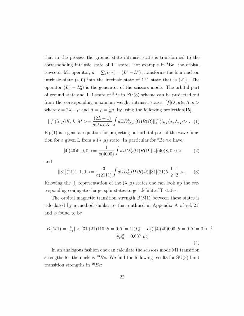
that in the process the ground state intrinsic state is transformed to the

corresponding intrinsic state of 1+ state. For example in 8Be, the orbital

isovector M1 operator, µ =∑

i li τiz = (Lπ −Lν) ,transforms the four nucleon

intrinsic state (4, 0) into the intrinsic state of 1+1 state that is (21). The

operator (Lπ0 − Lν

0) is the generator of the scissors mode. The orbital part

of ground state and 1+1 state of 8Be in SU(3) scheme can be projected out

from the corresponding maximum weight intrinsic states |[f ](λ, µ)ǫ,Λ, ρ >

where ǫ = 2λ+ µ and Λ = ρ = 12µ, by using the following projection[15],

|[f ](λ, µ)K,L,M >=(2L+ 1)

a(λµLK)

∫

dΩDLM,K(Ω)R(Ω)|[f ](λ, µ)ǫ,Λ, ρ > . (1)

Eq.(1) is a general equation for projecting out orbital part of the wave func-

tion for a given L from a (λ, µ) state. In particular for 8Be we have,

|[4](40)0, 0, 0 >=1

a(4000)

∫

dΩD000(Ω)R(Ω)|[4](40)8, 0, 0 > (2)

and

|[31](21)1, 1, 0 >=3

a(2111)

∫

dΩD101(Ω)R(Ω)|[31](21)5,

1

2,1

2> . (3)

Knowing the [f] representation of the (λ, µ) states one can look up the cor-

responding conjugate charge spin states to get definite JT states.

The orbital magnetic transition strength B(M1) between these states is

calculated by a method similar to that outlined in Appendix A of ref.[21]

and is found to be

B(M1) = 916π

| < [31](21)110, S = 0, T = 1|(Lπ0 − Lν

0)|[4](40)000, S = 0, T = 0 > |2

= 2πµ2

n = 0.637 µ2n

(4)

In an analogous fashion one can calculate the scissors mode M1 transition

strengths for the nucleus 10Be. We find the following results for SU(3) limit

transition strengths in 10Be:

22

B(M1)(0+1 → 1+1) =9

32πµ2

n = 0.0895µ2n

B(M1)(0+1 → 1+2) =15

32πµ2

n = 0.1492µ2n.

8.4 Realistic Spin-Orbit Interaction and Restoration

of SU(3) Symmetry

As pointed out before, an important role of spin dependent part of in-

teraction is to remove the degeneracies present in the SU(3) limit by mixing

up the same final angular momentum states arising due to a given intrinsic

state as well as from different intrinsic states. In a realistic interaction, the

relative strengths of spin dependent and spin independent part of interaction

determine whether the wavefunctions are close to SU(3) scheme or a (j-j)

coupling scheme is a better description of the system.

To understand further the part played by spin independent part of the full

realistic interaction in the restoration of SU(3) symmetry, we consider a small

space calculation with the full spin-orbit part of the (x, y) interaction plus a

variable Q.Q interaction. Figure.(7) is a plot of isovector orbital, spin and

total strength for M1 transitions from J = 0+1 T = 0 → J = 1+T = 1 states

versus t, the parameter multiplying the full Q.Q interaction matrix elements

for 8Be. For the spin part we use the operator 9.412∑

σtz i.e. we include the

large isovector factor. In 8Be, with increasing t the orbital isovector strength

is seen to approach the SU(3) limit value of 0.637µ2n. The contribution of

isovector spin transition, on the other hand to total B(M1) decreases as t

becomes large. This is because the SU(4) limit is being approached and in

this limit the spin contribution vanishes.

In Fig.(7) with only spin-orbit part of realistic interaction in play, the cal-

culated M1 transition strength for 0+0 to 1+1 transitions has a large spin flip

23

contribution and is found tobe as large as 9.7 µ2n. In a small space calculation

with full realistic interaction(x, y)(Table I), a total B(M1) value of 1.0547µ2n

is obtained with an isovector orbital transition strength of 0.67µ2n and an

isovector spin contribution of 0.38µ2n. Of course to get the physical B(M1)

we add the spin and orbital amplitudes and square. The spin B(M1) is a

factor of 25 lower here than the t = 0 value in Fig 7. It still has some effect

because of the factor 9.412. We may note that the orbital transition strength

arising due to full realistic interaction is very close to the SU(3) limit indi-

cating that the realistic interaction favors a restoration of SU(3) symmetry.

The large space realistic interaction calculation inspite of the correlations

induced by shell mixings results in a B(M1) value 1.2866µ2n and isovector

orbital transition strength of 0.728µ2n indicating that the wavefunctions are

still very close to SU(3) wave functions.

In 10Be the situation is more interesting due to splitting of scissors mode

strength into two degenerate states in SU(3) limit. Figures (8) and (9) show

the orbital and spin part respectively of M1 transition strength for transitions

from ground state to J = 1+T = 1 states, J = 1+T = 2 states and all J = 1+

states. For ground state to J = 1+T = 1 transitions the orbital B(M1) is seen

to dip to a minimum for t = 0.3 before it starts increasing so as to approach

its SU(3) limit. An opposite trend is observed in the corresponding spin

strength that shows some increase, reaches a maximum and then tends to

the SU(4) limit of zero. The characteristic behaviour at t = 0.3 is possibly

a manifestation of a shape change at small deformation before the system

stabilizes by acquiring a permanent deformation. The M1 transition sums

for ground state to J = 1+T = 2 states, show a behaviour similar to that

observed for ground state to J = 1+T = 1 transitions in 8Be.

24

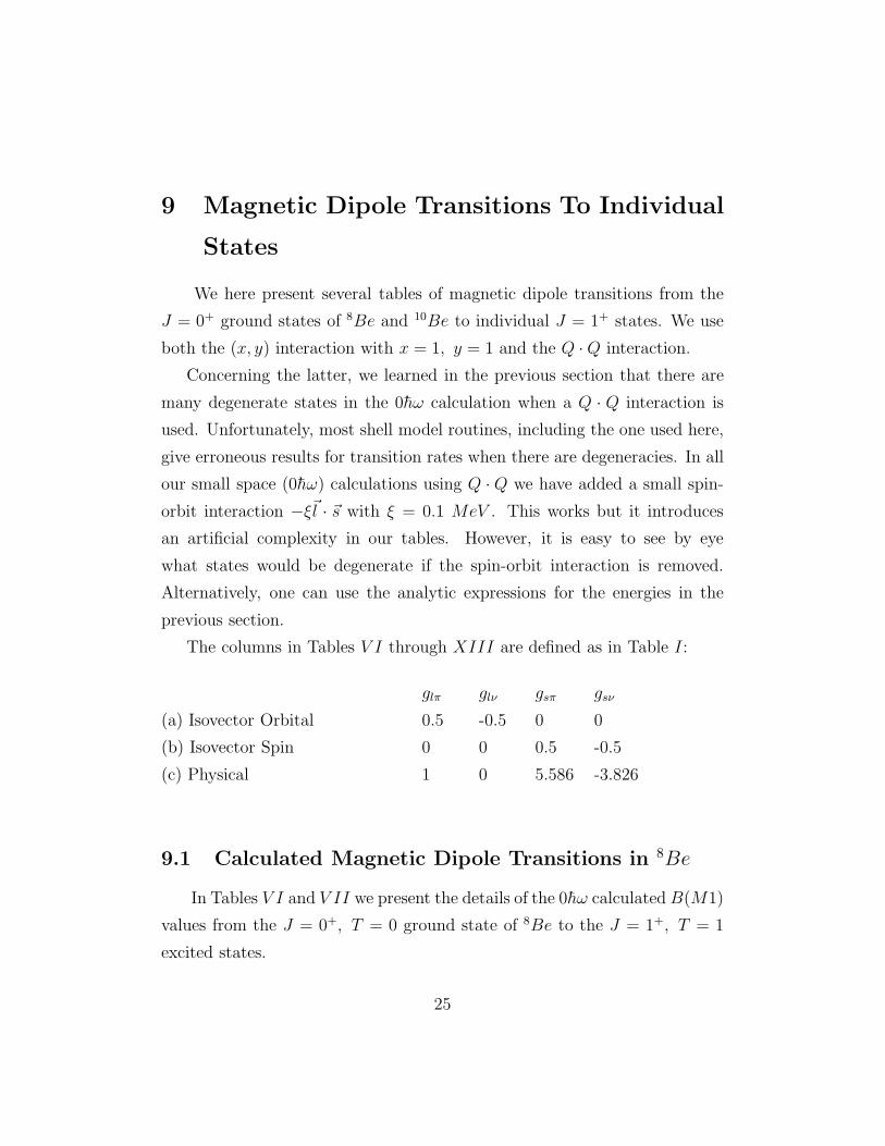
9 Magnetic Dipole Transitions To Individual

States

We here present several tables of magnetic dipole transitions from the

J = 0+ ground states of 8Be and 10Be to individual J = 1+ states. We use

both the (x, y) interaction with x = 1, y = 1 and the Q ·Q interaction.

Concerning the latter, we learned in the previous section that there are

many degenerate states in the 0hω calculation when a Q · Q interaction is

used. Unfortunately, most shell model routines, including the one used here,

give erroneous results for transition rates when there are degeneracies. In all

our small space (0hω) calculations using Q · Q we have added a small spin-

orbit interaction −ξ~l · ~s with ξ = 0.1 MeV . This works but it introduces

an artificial complexity in our tables. However, it is easy to see by eye

what states would be degenerate if the spin-orbit interaction is removed.

Alternatively, one can use the analytic expressions for the energies in the

previous section.

The columns in Tables V I through XIII are defined as in Table I:

glπ glν gsπ gsν

(a) Isovector Orbital 0.5 -0.5 0 0

(b) Isovector Spin 0 0 0.5 -0.5

(c) Physical 1 0 5.586 -3.826

9.1 Calculated Magnetic Dipole Transitions in 8Be

In Tables V I and V II we present the details of the 0hω calculated B(M1)

values from the J = 0+, T = 0 ground state of 8Be to the J = 1+, T = 1

excited states.

25

For the realistic (x, y) interaction, the isovector orbital strength is con-

centrated in three states at 13.7, 16.6 and 18.0 MeV . The sum of the orbital

strengths is∑

B(M1) ↑= 0.67 µ2N . This is in fair agreement with the ex-

perimental value B(M1) ↑= 0.81 µ2N (which is actually deduced from the

downward γ decay of the 17.64 MeV J = 1+, T = 1 state to the ground

state). However, in the experiment all the strength is concentrated in one

state whereas in our calculation we have considerable fragmentation. On

the other hand, if we look at the physical transitions, there is much more

concentration in one state at 13.73 MeV with B(M1) ↑= 0.72 µ2N . We will

discuss this more soon.

With the Q ·Q interaction, all the orbital strength is concentrated in the

(2-fold degenerate) state at 10.1 MeV with a summed strength B(M1) ↑=

0.64 µ2N , very similar to that of the (x, y) interaction. The energy is too

low compared with experiment, but we must remember that we did not

renormalize the strength χ to allow for ∆N = 2 admixtures. Note that the

isovector spin transitions are zero with the Q ·Q interaction. This is because

we are at the SU(4) limit since Q ·Q is a spin-independent interaction.

Note that with the Q ·Q interaction the summed orbital strength is 2πµ2

N ,

confirming the expressions that were derived in the previous section. Coming

back to the (x, y) interaction, we see that here also the isovector spin tran-

sitions are very weak. But note that for the 13.73 MeV state whereas the

orbital value of B(M1) ↑ is 0.2569 µ2N and the spin value is 0.0013 µ2

N , the

physical value is 0.7155 µ2N . The reason is that the spin and orbit amplitudes

add coherently and that the spin amplitude is multiplied by the factor 9.412.

For other states there is destructive interference between spin and orbit.

For example, for the 16.64 MeV state, the value of B(M1) ↑ is 0.234 µ2N for

the orbital case but only 0.065 µ2N for the physical case.

26

9.2 Calculated Magnetic Dipole Transitions in 10Be

In Tables V III and IX we present the details of the 0hω calculated

B(M1) values from the J = 0+ T = 1 ground state of 10Be to the J =

1+ T = 1 and to J = 1+ T = 2 excited states. We caution the reader that

whereas for 8Be we presented the results in units of µ2N (Tables V I and V II),

for 10Be we use 10−2 µ2N as the unit. The reason for this is that the orbital

transitions to individual states in 10Be are considerably smaller than those

in 8Be.

Let us look at the Q · Q interaction (Table IX) first. There are several

outstanding features which are explained in the previous section on L S

coupling and supermultiplet symmetry.

The first two J = 1+ T = 1 states are degenerate at E∗ = 3.86 MeV .

They carry no spin or orbital strength from the from the ground state. The

[f] symmetries are [4 1 1] and [3 3]. They have additional quantum numbers

L = 1 S = 1 T = 1. Since the isovector orbital operator ( ~Lπ- ~Lν) cannot

change both L and S from zero to one, the orbital B(M1) vanishes. A

similar argument holds for the isovector spin operator. These lowest two

states are therefore not scissors mode states.

Then we have a four fold set of degenerate states with [3 2 1] symmetry

at about 8.5 MeV excitation which does include the L = 1 S = 0 T = 1

scissors mode. We note that for 10Be, the T = 1 scissors mode is degenerate

with the T = 2 scissors mode also at 8.5 MeV excitation. This again is a

prediction of the supermultiplet theory.

The summed isovector orbital strength is 932π

µ2N from J = 0+ T = 1 to

the J = 1+ T = 1 states, and it is 1532π

µ2N to the J = 1+ T = 2 states. We

have in effect a (2T + 1) rule:

(2T + 1)T=2

(2T + 1)T=1=

5

3

27

This coincides with the ratio of T = 2 to T = 1 strength.

Recalling that the 8Be strength was 2πµ2

N , we see that the ratio of total

strength10Be8Be

is 38.

We now come back to Table V III which shows the same calculational

results with the ‘realistic’ (x, y) interaction. There are several similarities but

also some differences with the Q·Q results. Just as with the Q·Q interaction,

the orbital transitions to the lowest two J = 1+ T = 1 states at 6.14 and 7.68

MeV are very weak 0.16 and 0.17 × (10−2µ2N) respectively. However, the

spin transitions, which with Q ·Q were also zero, are now sufficiently strong

so as to have a visible effect. For example, the physical B(M1) ↑ to the 7.68

MeV state is calculated to be 1.85 µ2N . This is certainly measurable.

As with the Q · Q interaction, the scissors mode states with the (x, y)

interaction are at a much higher energy than the lowest two 1+ states 19

MeV . Also, the J = 1+ T = 1 and T = 2 excitations are roughly in the

same energy range -the Q ·Q interaction has them degenerate. The ratio of

T = 2 to T = 1 orbital strength is about the same for the (x, y) interaction

as for Q ·Q 1.44 vs. 53.

One major difference is that the energy scale is larger for the (x, y) inter-

action than for Q ·Q. The lowest and higher energies in Table V III are 6.14

MeV and 30.96 MeV whereas in Table IX they are 3.85 MeV and 12.35

MeV .

In Tables X and XI we present results of large space calculations for8Be to be compared with the corresponding small space Tables VI and VII.

Likewise in Tables XII and XIII we present the large space results for 10Be

to be compared with tables VIII and IX. We do not show all the states here,

only the low energy sector. The excitation energies are in general larger in

the large space calculations. The major changes occur when one has nearly

degenerate levels sharing some strength. For example, the lowest two 1+

28

states in the large space calculations, which are at 7.38 MeV and 9.62 MeV

have almost equal M1 strengths 0.64 µ2N and 0.79 µ2

N . In the small space,

the lowest state has only 0.011 µ2N and the second one 1.8 µ2

N .

A sensible attitude is to assume that neither calculation is accurate enough

to give the detailed distribution of strength between the two states -only the

summed strength for the two states should be compared with experiment.

With the Q ·Q interaction in the large space, the degeneracy encountered

in the small space calculation is removed. In part, this is due to the fact

that we do not include the single-particle terms∑

i=j Q(i) ·Q(j). These will

induce a single-particle splitting between 1s and 0d in the N = 2 shell. But

since degeneracies give us trouble in our shell model diagonalizations, we are

happy to leave the calculation as is.

WithQ·Q the scissors mode strength in 8Be gets pushed up from the small

space value of 10.1 MeV to the large space value of 15.5 MeV . For 10Be the

corresponding numbers are 8.5 MeV and 11.3 MeV for the J = 1+, T = 1

states and essentially the same for J = 1+, T = 2 states. That is, the near

degeneracy of the T = 1 and T = 2 scissors modes in 10Be is maintained in

the large space calculation.

Lastly, we reiterate the fact that the shell model calculations here yield

not only colective magnetic states but also show intermediate structure. That

this structure is a natural occurence is shown by the supermultiplet model,

where for a given [f ]L=1 there are several S and T values possible. It is of

course very difficult to get the details of the intermediate structure to come

out right, but it is good to be able to explain the origin of this structure.

29

10 Additional Comments and Closing Remarks

We can gain further insight into the nature of 8Be and 10Be by evaluating

the quadrupole moments of the J = 2+ states. A small space calculation gives

the following values:

Q ·Q − 0.1~l · ~s (x, y) interaction8Be J = 2+, T = 0 Q = −8.02 e fm2 Q = −7.86 e fm2

10Be J = 2+1 , T = 1 Q = −2.52 e fm2 Q = −7.68 e fm2

10Be J = 2+2 , T = 1 Q = +2.06 e fm2 Q = +6.91 e fm2

In the rotational model the quadrupole moment of the 2+ of aK = 0 band

is −27Q0 where Q0 is the intrinsic quadrupole moment. Thus a negative Q

corresponds to a prolate shape and a positive Q to an oblate shape. From

the above, 8Be acts as a normal deformed nucleus of the prolate shape.

It has been pointed out by Harvey that in the SU(3) scheme, whenever

µ is less than or equal to λ the nucleus becomes oblate [15]. For the ground

state band in 8Be λ is bigger than µ but for 10Be λ and µ are equal. The

situation with 10Be is somewhat confusing. With the Q·Q interaction, which

one might think would favor deformation, the quadrupole moment of the 2+1

state drops to -2.52 e fm2. Recall that for a perfect vibrator, the value of Q

is zero, so it would appear that 10Be is headed in that direction. However

with the realistic interaction, which contains a large spin-orbit interaction

that one might think would oppose deformation, the quadrupole moment of10Be becomes more negative -almost the same as that of 8Be. Note also

that the calculated values of Q for the 2+1 and 2+

2 states are nearly equal but

opposite to both interactions.

We have learned many interesting things by considering scissors modes in

light nuclei. First of all there is evidence for their existence. This evidence

30

comes strangely from a nucleus whose ground state is unstable -8Be. We learn

of the existence from the inverse process i.e. γ decay from the J = 1+, T = 1

state at 17.64 MeV to the ground state [2]. The decay to the 2+1 state,

presumably a member of a K = 0 rotational band, is also observed and this

suggests that theoretical studies (and experimental ones as well whenever

possible) should be made not only between between J = 1+ K = 1 and

J = 0+ K = 0 states but also between J = 1+ K = 1 and J = 2+ K = 0

states. This will make the picture of scissors modes more complete. In this

work we considered but one example and showed that the ratio of J = 1+

decay rate to J = 2+ vs J = 0+ deviates from the simple rotational formula

result of 0.5. Further studies along these lines are being planned.

To make the picture even more complete, one can also study the decay

of J = 1+ K = 1 to J = 2+ K = 2. We were almost forced into such a

study by the fact that in the SU(3) scheme there is a two-fold degeneracy of

the lowest J = 2+ states in 10Be [14, 16]. Presumably, these two states are

admixtures of 2+ K = 0 and 2+ K = 2.

The shell model approach used here [20] enables us to study fragmen-

tation or intermediate structure. We find for example that with an elec-

tromagnetic probe there are, besides the strong scissors mode states, some

almost ‘invisible’ states. These have separately substantial orbital contribu-

tions and substantial spin contributions to the magnetic dipole excitations

but the physical B(M1) is very small because of the destructive interference

of the spin and orbital amplitudes. For example, as seen in Table X, in 8Be

we calculate that the low lying orbital strength is shared almost equally be-

tween two states (at 18.0 MeV and 20.8 MeV ) -the strengths being 0.22

µ2N and 0.30 µ2

N respectively. However, the physical B(M1)’s are 0.62 µ2N

and 0.12 µ2N . Thus one can miss considerable orbital strength into these

‘invisible’ sttaes if one uses only an electromagnetic probe.

31

Another thing we learn is that although spin excitations are strongly

suppressed they cannot be ignored. In the SU(4) limit, the spin matrix

elements vanish and there is a clear tendency in our calculations in that

direction. However, since the isovector spin operator is multiplied by a factor

of 9.412, the spin and orbital contributions tend to be on the same footing.

In the example of the above paragraph in the decay of the (calculated)

18.0MeV state, the orbitalB(M1) is only 0.22 µ2N but the physical one which

induces the spin contribution is 0.62 µ2N . In 10Be the first two J = 1+ states

are calculated to be excited mainly by the spin operator and the B(M1)’s

should be substantial 0.5 µ2N . Yet in the U(3) − SU(4) limit, these lowest

two states [f]=[4,1,1] and [3,3] should not be excited at all either by the spin

or by the orbital operators.

We have found the Wigner supermultiplet scheme [13] combined with the

SU(3) scheme [15, 16] a very useful guide to the more complicated shell model

calculations that we have performed. There is the added simplicity in the p

shell that there is a one-to-one correpondence between a given [f] symmetry

and the (λ, µ) symmetries. Many interesting properties about scissors modes

can be literally read off the pages of the book by Hammermesh [14]. For

example, there is the fact that the T = 1 and T = 2 scissors mode states

in 10Be are degenerate in energy. This is an exact result with the Q · Q

interaction in a p shell calculation. Results very close to this are obtained

with a realistic interaction, but we frankly didn’t notice this until we made

an SU(3) analysis. Also the non-obvious fact that the lowest two 1+ states

in 10Be are not scissors mode states is made clear by such an analysis.

Also the fact that scissors mode states everywhere, including 156Gd, have

intermediate structure [18, 19] is made clear by the supermultiplet scheme.

For a given L = 1 state there are often several S, T combinations which are

degenerate. The removal of the degeneracy and the mixing of these states e.g.

32

by a spin-orbit interaction leads to fragmentation and intermediate structure.

By extending the shell model calculations to ‘large space’ i.e. by including

2hω excitations, we were able to calculate the cumulative energy weighted

strength distribution for isovector orbital excitations. The results which are

shown in several figures are characterized by a low energy rise followed by a

second plateau. The shapes of the distributions were similar for the two con-

trasting interactions used here -the ‘realistic’ short range interaction and the

schematic quadrupole-quadrupole interaction. The results were compared

witht the simple Nilsson model [7, 8] which predicts that the energy-weighted

sum at high energy (beyond the first plateau) should equal the low energy

rise i.e. the ratio totallow energy

should be 2:1. The actual calculated ratios witht

the (x, y) interaction are 1.75 for 8Be and 2.52 for 10Be. The correspond-

ing numbers for the Q · Q interaction were 1.37 and 2.33. We see that the

Nilsson model is not bad as a first orientation but there are fluctuations.

The fact that the above ratios are larger for the (x, y) interaction than for

the Q ·Q interaction may support the idea of Hamamoto and Nazarewicz [9]

that the symmetry energy will cause the ratio to increase. Our calculations

however do not support their claim that the high energy part of the energy

weighted orbital strength should always be much larger than the low energy

part -certainly not for a ‘normal’ rotational nucleus like 8Be. For 10Be the

ratio is however somewhat larger than the Nilsson model prediction.

Whether this is due to the atypical properties of 10Be mentioned in the

text or is a harbinger of what will happen for most other nuclei remains to be

seen. From an experimental point of view, it would be helpful to have more

data on 10Be. Not only have no J = 1+ states been identified but neither

has the J = 4+1 state been seen. The location of this state might help us

decide whether 10Be is rotational or vibrational.

33

At any rate, we should examine a larger range of nuclei and look into more

detail about the symmetry energy in order to be able to make more definitive

statements about the systematics of the cumulative energy weighted distri-

butions. We note that the Zheng-Zamick sum rule [5] is able to handle the

divergent behaviour between 8Be and 10Be. This sum rule involves the dif-

ference between isoscalar and isovector summed B(E2) strength, whereas

corresponding expressions by Heyde and de Coster [6] based on the I.B.A.

model [22, 23] as well as empirical analyses [10] involve only B(E2) to the

lowest 2+ states. Even here more sharpening up is in order.

Our initial reason for studying lighter nuclei is that they would give us

insight into the behaviour of heavier nuclei, and we could carry out more

complete calculations in the low A region. But then we found many results

which made light nuclei studies fascinating for their own sake. One rather

broad lesson we have learned in the light nucleus study is that there can

be considerable change in going from one nucleus to the next, and perhaps

in heavier nuclei too much effort has been made to make the nuclei fit into

a smooth pattern. For example, we find that whereas in 8Be the lowest

1+ state is dominantly a scissors mode state, in 10Be the lowest 1+ states

are not scissors mode states at all -they can only be reached by the spin

operator. We should perhaps be looking for more variety of behaviour in

heavier nuclei. Lastly the supermultiplet scheme which we found extremely

useful was originally thought to be of interest only in light nuclei where the

spin-orbit interaction is small relative to the residual interaction. However, it

is now being realized that even in heavy nuclei -especially for superdeformed

states this scheme may once again be very relevant. This would make our

light nuclear studies all the more important.

34

Acknowledgement

This work was supported by the Department of Energy Grant No. DE-

FG05-86ER-40299. S.S. Sharma would like to thank the Department of

Physics at Rutgers University for its hospitality and to acknowledge financial

support from CNPq, Brazil. We thank E. Moya de Guerra for familiarizing

us with her work in collaboration with J. Retamosa, J.M. Udias and A. Poves.

We thank I. Hamamoto for her interest. We also thank N. Sharma for useful

comments about matrix diagonalization.

35

Table I. Summed Magnetic Dipole Strengths (in µ2N ).

The (x, y) interaction (x = 1, y = 1)

Space Isovector Orbital(d) Isovector Spin(e) Isoscalar Orbital(f) Physical(g)

8Be J = 0+1 T = 0 → J = 1+ T = 1

Small(a) 0.6701 0.00427 1.0547

Large(b) 0.7283 0.00622 1.2866

Low Large(c) 0.5890 0.00322 0.8999

10Be J = 0+1 T = 1 → J = 1+ T = 1

Small 0.1112 0.0234 0.0245 2.0930

Large 0.1963 0.0208 0.0270 1.9517

Low Large 0.1002 0.0187 0.0200 1.6070

10Be J = 0+1 T = 1 → J = 1+ T = 2

Small 0.1508 0.00105 0.0597

Large 0.1830 0.00222 0.2276

Low Large 0.1339 0.000928 0.0754

The Q · Q interaction

8Be J = 0+1 T = 0 → J = 1+ T = 1

Small 0.6364 0.0000 0.6364

Large 0.7408 0.0005 0.7858

Low Large 0.6593 0.0002 0.6775

10Be J = 0+1 T = 1 → J = 1+ T = 1

Small 0.0895 0.0001 0.0986

Large 0.1788 0.0004 0.2044

Low Large 0.0922 0.0000 0.0881

10Be J = 0+1 T = 1 → J = 1+ T = 2

Small 0.1492 0.0000 0.1486

Large 0.1744 0.0002 0.1950

Low Large 0.1513 0.0000 0.1617

36

Table I Captions

(a) Small Space (0s)4(0p)6

(b) Large Space (0s)4(0p)6 + all 2hω excitations

(c) Low energy part of Large Space (up to the first plateau)

(d) glπ = 0.5 glν = −0.5 gsπ = 0 gsν = 0

(e) glπ = 0 glν = 0 gsπ = 0.5 gsν = −0.5

(f) glπ = 0.5 glν = 0.5 gsπ = 0 gsν = 0. The value for isoscalar spin is the same

as for isoscalar orbital in the case of 10Be J = 0+, T = 1 → J = 1+, T = 1.

For ∆T = 1 the isoscalar case gives zero.

(g) glπ = 1 glν = 0 gsπ = 5.586 gsν = −3.826

37

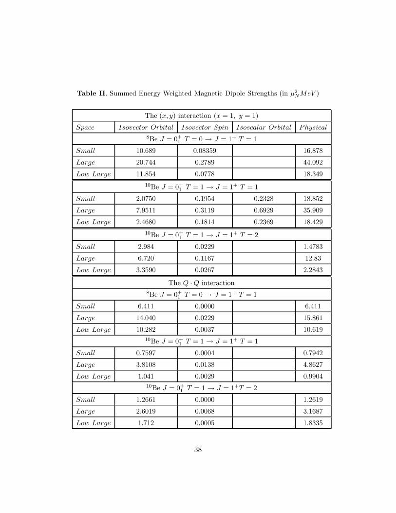
Table II. Summed Energy Weighted Magnetic Dipole Strengths (in µ2NMeV )

The (x, y) interaction (x = 1, y = 1)

Space Isovector Orbital Isovector Spin Isoscalar Orbital Physical

8Be J = 0+1 T = 0 → J = 1+ T = 1

Small 10.689 0.08359 16.878

Large 20.744 0.2789 44.092

Low Large 11.854 0.0778 18.349

10Be J = 0+1 T = 1 → J = 1+ T = 1

Small 2.0750 0.1954 0.2328 18.852

Large 7.9511 0.3119 0.6929 35.909

Low Large 2.4680 0.1814 0.2369 18.429

10Be J = 0+1 T = 1 → J = 1+ T = 2

Small 2.984 0.0229 1.4783

Large 6.720 0.1167 12.83

Low Large 3.3590 0.0267 2.2843

The Q · Q interaction

8Be J = 0+1 T = 0 → J = 1+ T = 1

Small 6.411 0.0000 6.411

Large 14.040 0.0229 15.861

Low Large 10.282 0.0037 10.619

10Be J = 0+1 T = 1 → J = 1+ T = 1

Small 0.7597 0.0004 0.7942

Large 3.8108 0.0138 4.8627

Low Large 1.041 0.0029 0.9904

10Be J = 0+1 T = 1 → J = 1+T = 2

Small 1.2661 0.0000 1.2619

Large 2.6019 0.0068 3.1687

Low Large 1.712 0.0005 1.8335

38

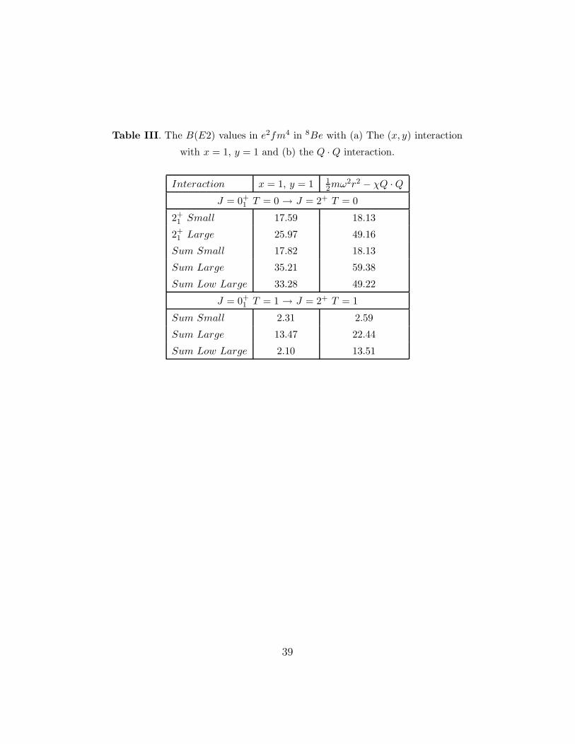
Table III. The B(E2) values in e2fm4 in 8Be with (a) The (x, y) interaction

with x = 1, y = 1 and (b) the Q · Q interaction.

Interaction x = 1, y = 1 12mω2r2 − χQ · Q

J = 0+1 T = 0 → J = 2+ T = 0

2+1 Small 17.59 18.13

2+1 Large 25.97 49.16

Sum Small 17.82 18.13

Sum Large 35.21 59.38

Sum Low Large 33.28 49.22

J = 0+1 T = 1 → J = 2+ T = 1

Sum Small 2.31 2.59

Sum Large 13.47 22.44

Sum Low Large 2.10 13.51

39

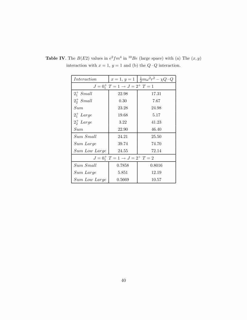
Table IV. The B(E2) values in e2fm4 in 10Be (large space) with (a) The (x, y)

interaction with x = 1, y = 1 and (b) the Q · Q interaction.

Interaction x = 1, y = 1 12mω2r2 − χQ · Q

J = 0+1 T = 1 → J = 2+ T = 1

2+1 Small 22.98 17.31

2+2 Small 0.30 7.67

Sum 23.28 24.98

2+1 Large 19.68 5.17

2+2 Large 3.22 41.23

Sum 22.90 46.40

Sum Small 24.21 25.50

Sum Large 39.74 74.70

Sum Low Large 24.55 72.14

J = 0+1 T = 1 → J = 2+ T = 2

Sum Small 0.7858 0.8016

Sum Large 5.851 12.19

Sum Low Large 0.5669 10.57

40

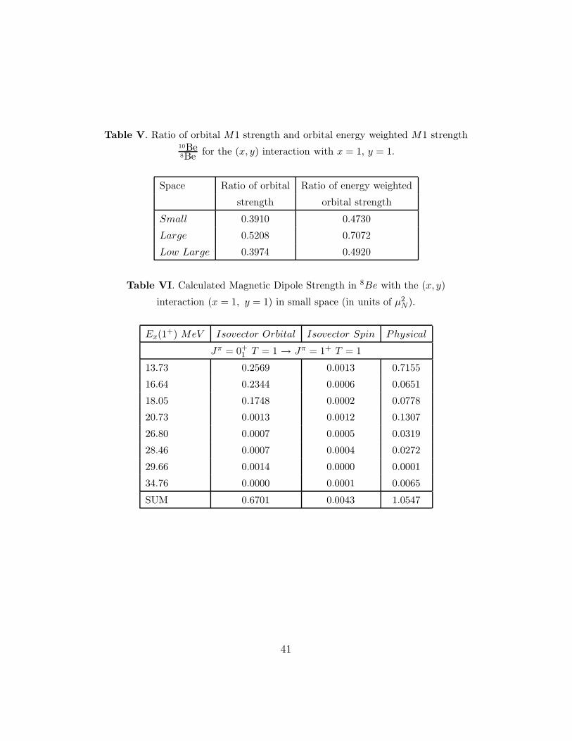
Table V. Ratio of orbital M1 strength and orbital energy weighted M1 strength10Be8Be for the (x, y) interaction with x = 1, y = 1.

Space Ratio of orbital Ratio of energy weighted

strength orbital strength

Small 0.3910 0.4730

Large 0.5208 0.7072

Low Large 0.3974 0.4920

Table VI. Calculated Magnetic Dipole Strength in 8Be with the (x, y)

interaction (x = 1, y = 1) in small space (in units of µ2N ).

Ex(1+) MeV Isovector Orbital Isovector Spin Physical

Jπ = 0+1 T = 1 → Jπ = 1+ T = 1

13.73 0.2569 0.0013 0.7155

16.64 0.2344 0.0006 0.0651

18.05 0.1748 0.0002 0.0778

20.73 0.0013 0.0012 0.1307

26.80 0.0007 0.0005 0.0319

28.46 0.0007 0.0004 0.0272

29.66 0.0014 0.0000 0.0001

34.76 0.0000 0.0001 0.0065

SUM 0.6701 0.0043 1.0547

41

Table VII. Calculated Magnetic Dipole Strength in 8Be with the Hamiltonian

H = p2

2m+ 1

2mω2r2 − χQ · Q with χ = 0.5762 in small space (µ2N ).

Ex(1+) MeV Isovector Orbital Isovector Spin Physical

Jπ = 0+1 T = 1 → Jπ = 1+ T = 1

10.06 0.4599 0.0000 0.4851

10.11 0.1765 0.0000 0.1524

12.33 0.0000 0.0000 0.0001

13.43 0.0000 0.0000 0.0000

16.84 0.0000 0.0000 0.0000

18.97 0.0000 0.0000 0.0000

19.05 0.0000 0.0000 0.0000

19.11 0.0000 0.0000 0.0000

SUM 0.6364a 0.0000 0.6376

(a) The summed isovector orbital strength is 2π

µ2N .

42

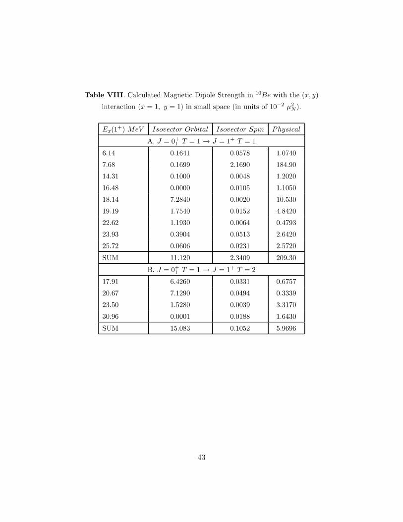
Table VIII. Calculated Magnetic Dipole Strength in 10Be with the (x, y)

interaction (x = 1, y = 1) in small space (in units of 10−2 µ2N ).

Ex(1+) MeV Isovector Orbital Isovector Spin Physical

A. J = 0+1 T = 1 → J = 1+ T = 1

6.14 0.1641 0.0578 1.0740

7.68 0.1699 2.1690 184.90

14.31 0.1000 0.0048 1.2020

16.48 0.0000 0.0105 1.1050

18.14 7.2840 0.0020 10.530

19.19 1.7540 0.0152 4.8420

22.62 1.1930 0.0064 0.4793

23.93 0.3904 0.0513 2.6420

25.72 0.0606 0.0231 2.5720

SUM 11.120 2.3409 209.30

B. J = 0+1 T = 1 → J = 1+ T = 2

17.91 6.4260 0.0331 0.6757

20.67 7.1290 0.0494 0.3339

23.50 1.5280 0.0039 3.3170

30.96 0.0001 0.0188 1.6430

SUM 15.083 0.1052 5.9696

43

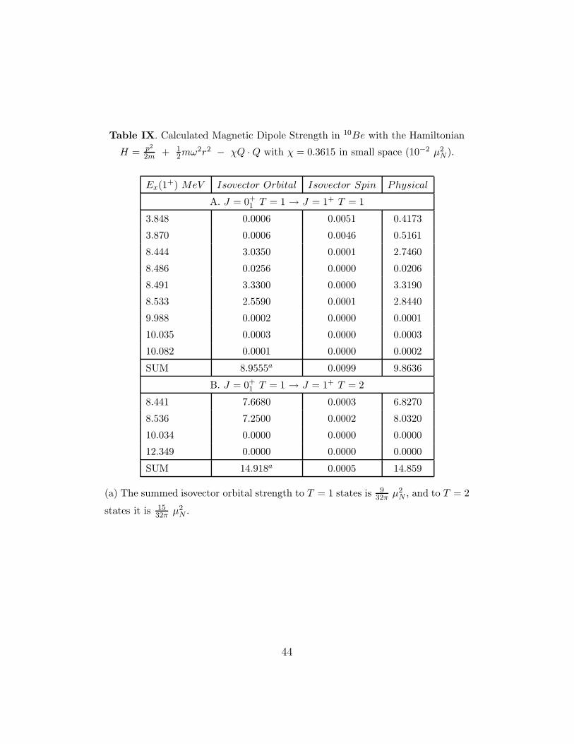
Table IX. Calculated Magnetic Dipole Strength in 10Be with the Hamiltonian

H = p2

2m+ 1

2mω2r2 − χQ · Q with χ = 0.3615 in small space (10−2 µ2N ).

Ex(1+) MeV Isovector Orbital Isovector Spin Physical

A. J = 0+1 T = 1 → J = 1+ T = 1

3.848 0.0006 0.0051 0.4173

3.870 0.0006 0.0046 0.5161

8.444 3.0350 0.0001 2.7460

8.486 0.0256 0.0000 0.0206

8.491 3.3300 0.0000 3.3190

8.533 2.5590 0.0001 2.8440

9.988 0.0002 0.0000 0.0001

10.035 0.0003 0.0000 0.0003

10.082 0.0001 0.0000 0.0002

SUM 8.9555a 0.0099 9.8636

B. J = 0+1 T = 1 → J = 1+ T = 2

8.441 7.6680 0.0003 6.8270

8.536 7.2500 0.0002 8.0320

10.034 0.0000 0.0000 0.0000

12.349 0.0000 0.0000 0.0000

SUM 14.918a 0.0005 14.859

(a) The summed isovector orbital strength to T = 1 states is 932π

µ2N , and to T = 2

states it is 1532π

µ2N .

44

Table X. Calculated Magnetic Dipole Strength in 8Be with the (x, y) interaction

(x = 1, y = 1) in large space(a) (in units of µ2N ).

Ex(1+) MeV Isovector Orbital Isovector Spin Physical

J = 0+1 T = 0 → J = 1+ T = 1

17.96 0.2208 0.0011 0.6160

20.80 0.2970 0.0004 0.1213

22.89 0.0670 0.0001 0.0213

27.04 0.0000 0.0010 0.0935

33.51 0.0007 0.0002 0.0081

34.57 0.0000 0.0003 0.0250

35.73 0.0007 0.0000 0.0000

40.22 0.0001 0.0000 0.0036

46.07 0.0003 0.0000 0.0110

46.41 0.0000 0.0000 0.0000

48.46 0.0060 0.0001 0.0001

49.61 0.0019 0.0000 0.0023

49.92 0.0012 0.0000 0.0004

50.32 0.0004 0.0000 0.0036

SUM 0.5986 0.0033 0.9063

(a) Large Space: all 0hω configurations plus 2hω excitations.

45

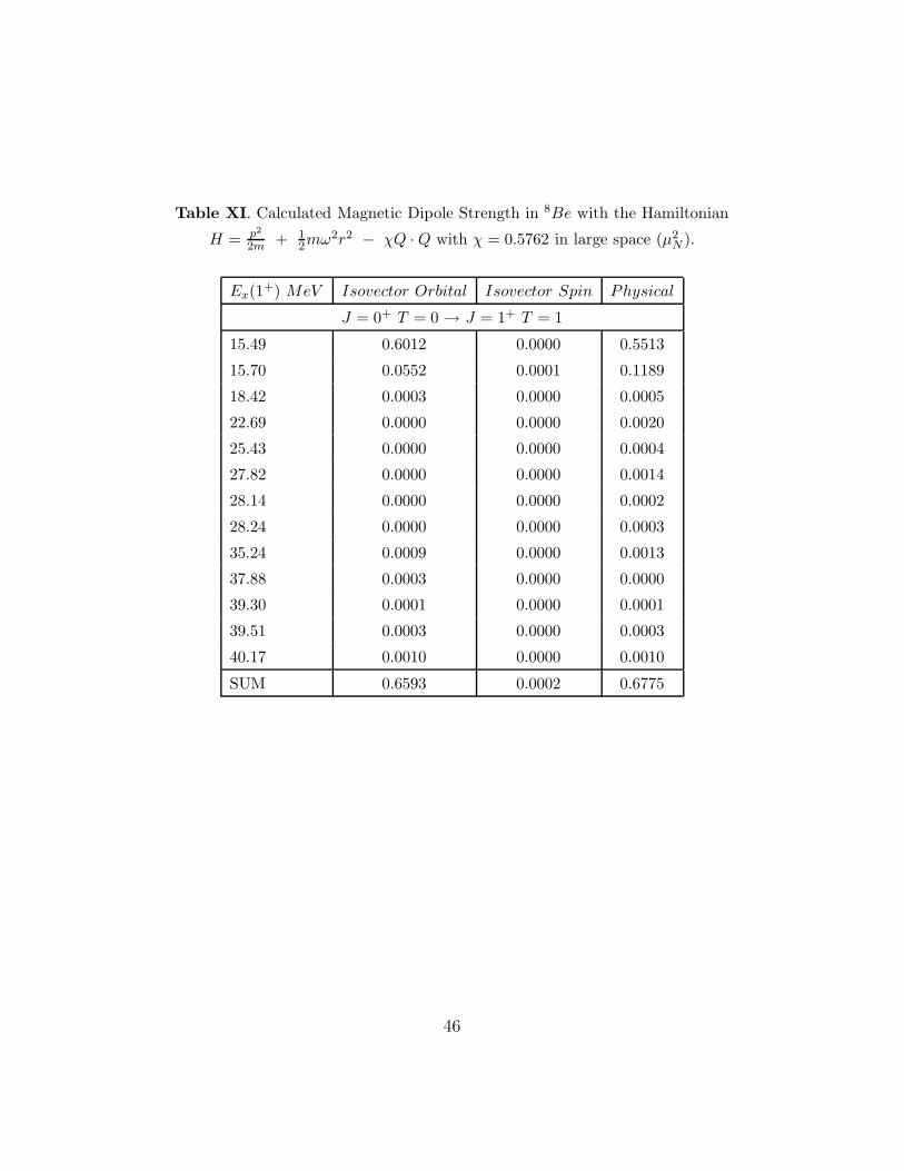
Table XI. Calculated Magnetic Dipole Strength in 8Be with the Hamiltonian

H = p2

2m+ 1

2mω2r2 − χQ · Q with χ = 0.5762 in large space (µ2N ).

Ex(1+) MeV Isovector Orbital Isovector Spin Physical

J = 0+ T = 0 → J = 1+ T = 1

15.49 0.6012 0.0000 0.5513

15.70 0.0552 0.0001 0.1189

18.42 0.0003 0.0000 0.0005

22.69 0.0000 0.0000 0.0020

25.43 0.0000 0.0000 0.0004

27.82 0.0000 0.0000 0.0014

28.14 0.0000 0.0000 0.0002

28.24 0.0000 0.0000 0.0003

35.24 0.0009 0.0000 0.0013

37.88 0.0003 0.0000 0.0000

39.30 0.0001 0.0000 0.0001

39.51 0.0003 0.0000 0.0003

40.17 0.0010 0.0000 0.0010

SUM 0.6593 0.0002 0.6775

46

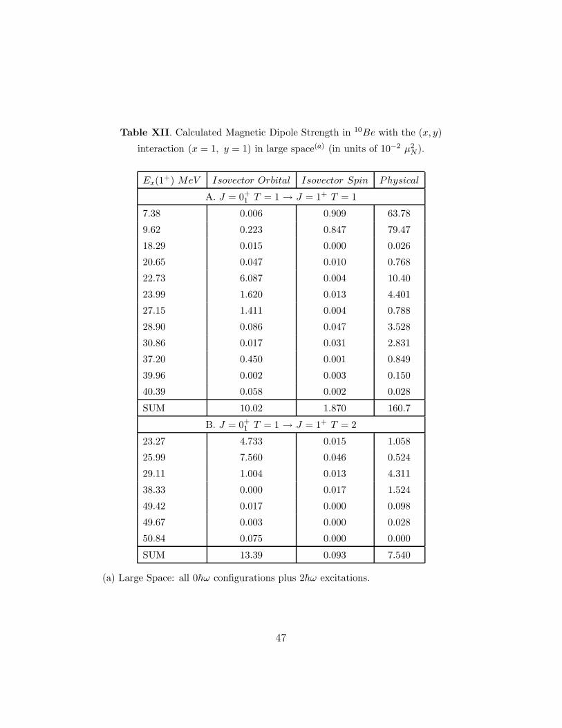
Table XII. Calculated Magnetic Dipole Strength in 10Be with the (x, y)

interaction (x = 1, y = 1) in large space(a) (in units of 10−2 µ2N ).

Ex(1+) MeV Isovector Orbital Isovector Spin Physical

A. J = 0+1 T = 1 → J = 1+ T = 1

7.38 0.006 0.909 63.78

9.62 0.223 0.847 79.47

18.29 0.015 0.000 0.026

20.65 0.047 0.010 0.768

22.73 6.087 0.004 10.40

23.99 1.620 0.013 4.401

27.15 1.411 0.004 0.788

28.90 0.086 0.047 3.528

30.86 0.017 0.031 2.831

37.20 0.450 0.001 0.849

39.96 0.002 0.003 0.150

40.39 0.058 0.002 0.028

SUM 10.02 1.870 160.7

B. J = 0+1 T = 1 → J = 1+ T = 2

23.27 4.733 0.015 1.058

25.99 7.560 0.046 0.524

29.11 1.004 0.013 4.311

38.33 0.000 0.017 1.524

49.42 0.017 0.000 0.098

49.67 0.003 0.000 0.028

50.84 0.075 0.000 0.000

SUM 13.39 0.093 7.540

(a) Large Space: all 0hω configurations plus 2hω excitations.

47

Table XIII. Calculated Magnetic Dipole Strength in 10Be with the Hamiltonian

H = p2

2m+ 1

2mω2r2 − χQ · Q with χ = 0.3615 in large space (10−2 µ2N ).

Ex(1+) MeV Isovector Orbital Isovector Spin Physical

A. J = 0+1 T = 1 → J = 1+ T = 1

3.60 0.002 0.000 0.019

6.45 0.005 0.001 0.058

11.19 2.548 0.000 2.393

11.31 1.685 0.000 2.229

11.32 4.563 0.001 3.382

11.35 0.395 0.001 0.702

12.92 0.019 0.000 0.019

12.98 0.004 0.000 0.003

13.02 0.002 0.000 0.003

22.69 0.011 0.001 0.154

23.12 0.019 0.000 0.001

25.42 1.579 0.000 1.220

25.94 0.043 0.003 0.497

26.51 0.090 0.000 0.012

26.65 0.004 0.000 0.005

SUM 10.97 0.007 10.70

B. J = 0+1 T = 1 → J = 1+ T = 2

11.31 13.82 0.001 15.79

11.34 1.301 0.003 0.348

12.98 0.000 0.000 0.002

16.76 0.000 0.000 0.007

26.58 0.002 0.000 0.001

26.67 0.002 0.000 0.010

28.25 0.001 0.000 0.003

SUM 15.13 0.004 16.16

48

Figure Captions

Figure (1): The cumulative sum of the energy-weighted isovector orbital

B(M1) strength for the 0+1 , 0 → 1+, 1 transitions in 8Be with the realistic

interaction (x = 1, y = 1).

Figure (2): Same as Figure 1 but with the Q ·Q interaction.

Figure (3): The cumulative sum of the energy-weighted isovector orbital

B(M1) strength for the 0+1 , 1 → 1+, 2 transitions in 10Be with the realistic

interaction (x = 1, y = 1).

Figure (4): Same as Figure 3 but with the Q ·Q interaction.

Figure (5): The cumulative sum of the energy-weighted isovector orbital

B(M1) strength for the 0+1 , 1 → 1+, 1 transitions in 10Be with the realistic

interaction (x = 1, y = 1).

Figure (6): Same as Figure 5 but with the Q ·Q interaction.

Figure (7):∑

B(M1)(J = 0+1 T = 0 → J = 1+T = 1 states) versus t

for 8Be. The solid line, dashed line and dot-dash line are the total, spin and

orbital parts of∑

B(M1) .

Figure (8): The orbital part of∑

B(M1) versus t for 10Be. The solid

line, dashed line and dot-dash line are the total,∑

B(M1)(J = 0+1 T = 1 →

J = 1+T = 1 states) and∑

B(M1)(J = 0+1 T = 1 → J = 1+T = 2 states)

respectively.

Figure (9): Same as in Fig.(8) for spin part of∑

B(M1).

49

References

[1] M.S. Fayache and L.Zamick, Physics Letters B 338, (1994)421.

[2] F. Ajzenberg-Selove, Nucl. Phys. A 490, (1988)1-225

[3] S. Raman, C.H. Malarkey, W.T. Milner, C.W. Nesta, J.R. and P.H. Stelson,

ATOMIC DATA AND NUCLEAR DATA TABLES, 36, (1987)1-96

[4] D.C. Zheng and L. Zamick, Ann. of Phys. 206, (1991)106.

[5] L. Zamick and D.C. Zheng, Phys. Rev. C 44, (1991)2522; C bf 46, (1992)2106.

[6] K. Heyde and C. de Coster, Phys. Rev. C 44, (1991)R2262.

[7] E. Moya de Guerra and L. Zamick, Phys. Rev. C 47, (1993)2604.

[8] R. Nojarov, Nuclear Physics A 571, (1994)93.

[9] I. Hamamoto and W. Nazarewicz, Phys. Lett 297 B, (1992)25.

[10] W. Ziegler, C. Rangacharyulu, A. Richter and C. Spieler, Phys. Rev. Lett.

65, (1990)2515.

[11] A. Richter, Nuclear Physics A 507, (1990)99

[12] A. Bohr and B. Mottelson, Nuclear Structure, Vol. II (Benjamin, New York,

1975)

[13] E.P. Wigner, Physical Review 51,(1937)107

[14] M. Hammermesh, Group Theory and its Applications to Physical Problems,

Addison-Wesley, Reading MA 1962.

[15] M. Harvey, Advances in Nuclear Physics Vol. I, edited by Michel Baranger

and Erich Vogt, Plenum press, 67(1968)

[16] J.P Elliot, Proc. Royal Soc. A 245: (1958) 128 and 562.

50

[17] D. Bohle, A. Richter, W. Steffen, A.E.L. Dieprink, N. Lo Iudice, F. Palumbo

and O. Scholten, Phys. Lett. 137 B, (1984)27.

[18] U.E.P. Berg et. al., Phys. Lett. B 149(1984)59

[19] D. Bohle et. al., Nucl. Phys. A 458(1986)205

[20] B. A. Brown, A. Etchegoyen and W. D. M. Rae, The computer code OXBASH,

MSU-NSCL report number 524(1992).

[21] J. Retamosa, J. M. Udias, A. Poves and E. Moya de Guerra, Nucl. Phys.

A511221(1990)

[22] F. Iachello, Nuclear Physics A 358, (1981)890

[23] A.E.L. Dieprink, Prog. in Part. and Nucl. Phys. 9,(1983)121

51