Useful Constants and Conversion Factors

Quoted to a useful number of significant figures.

Speed of light in vacuum Electron charge magnitude Planck's constant

Boltzmann's constant

Avogadro's number Coulomb's law constant

Electron rest mass Proton rest mass Neutron rest mass Atomic mass unit (C 12 = 12)

c = 2.998 x 108 m/sec e = 1.602 x 1 0 = 19 coul h = 6.626 x 10 -34 joule-sec h = h/27c = 1.055 x 10 -34 joule-sec

= 0.6582 x 10 -15 eV-sec k = 1.381 x 10 -23 joule/°K

= 8.617 x 10 -5 eV/°K No = 6.023 x 1023/mole 1 /47rE0 = 8.988 x 109 nt -m2/coul2

me = 9.109 x 10 -31 kg = 0.5110 MeV/c2 mp = 1.672 x 10 -27 kg = 938.3 MeV/c2

m„ = 1.675 x 10 -Z7 kg = 939.6 MeV/c 2 u = 1.661 x 10-27 kg = 931.5 MeV/c 2

Bohr magneton Nuclear magneton Bohr radius Bohr energy

Electron Compton wavelength Fine-structure constant kT at room temperature

ub = eh/2me = 9.27 x 10 -24 amp-m2 (or joule/tesla) µn = eh/2m, = 5.05 x 10 -27 amp-m2 (or joule/tesla) ao = 47c€0h2/mee2 = 5.29 x 10 -11 m = 0.529 A E 1 = — mee4/(4rcE0)22h2 = —2.17 x 10 -18

joule = —13.6 eV Ac = h/m ec = 2.43 x 10 -12 m = 0.0243 A a = e2 /4nE 0hc = 7.30 x 10 -3 1/137 k300°K = 0.0258 eV ^ 1/40 eV

1eV= 1.602 x 10 -19 joule 1 A=10 -10 m

i joule = 6.242 x 10 18 eV 1F=10 -15 m l barn (bn)= 10-28m2

QUANTUM PHYSICS

Assisted by

yid O CaIgweal Univer^^#y^qf^#^rni^ ^^ arbara

United'•°Stalês C^^t^^ ^,;^^ Odemy

The figure on the cover is frori ; èction „ 9-4, where it is used to show the tendency for two identical spin 1/2 particles (such as electrons) to avoid each other if their

spins are essentially parallel. This tendency, or its inverse for the antiparallel case,

is one of the recurring themes in quantum physics explanations of the properties of

atoms, molecules, solids, nuclei, and particles.

QUANTUM PHYSICS of Atoms, Molecules, Solids,

Nuclei, and Particles

Second Edition

ROBERT EISBERG University of California, Santa Barbara

JOHN WILEY & SONS New York Chichester Brisbane Toronto Singapore

Copyright © 1974, 1985, by John Wiley & Sons, Inc.

All rights reserved. Published simultaneously in Canada.

Reproduction or translation of any part of this work beyond that permitted by Sections 107 and 108 of the 1976 United States Copyright Act without the permission of the copyright owner is unlawful. Requests for permission or further information should be addressed to the Permissions Department, John Wiley & Sons.

Library of Congress Cataloging in Publication Data:

Eisberg, Robert Martin. Quantum physics of atoms, molecules, solids, nuclei, and particles.

Includes index. 1. Quantum theory. I. Resnick, Robert, 1923—

II. Title, QC174.12.E34 1985 530.1'2 84-10444 ISBN 0-471-87373-X

Printed in the United States of America

Printed and bound by the Hamilton Printing Company.

30 29 28 27 26 25 24 23

PREFACE TO THE SECOND EDITION

The many developments that have occurred in the physics of quantum systems since the publication of the first edition of this book—particularly in the field of elementary particles—have made apparent the need for a second edition. In preparing it, we solicited suggestions from the instructors that we knew to be using the book in their courses (and also from some that we knew were not, in order to determine their objections to the book). The wide acceptance of the first edition made it possible for us to obtain a broad sampling of thought concerning ways to make the second edition more useful. We were not able to act on all the suggestions that were re-ceived, because some were in conflict with others or were impossible to carry out for technical reasons. But we certainly did respond to the general consensus of these suggestions.

Many users of the first edition felt that new topics, typically more sophisticated aspects of quantum mechanics such as perturbation theory, should be added to the book. Yet others said that the level of the first edition was well suited to the course they teach and that it should not be changed. We decided to try to satisfy both groups by adding material to the new edition in the form of new appendices, but to do it in such a way as to maintain the decoupling of the appendices and the text that characterized the original edition. The more advanced appendices are well inte-grated in the text but it is a one-way, not two-way, integration. A student reading one of these appendices will find numerous references to places in the text where the development is motivated and where its results are used. On the other hand, a student who does not read the appendix because he is in a lower level course will not be frustrated by many references in the text to material contained in an appendix he does not use. Instead, he will find only one or two brief parenthetical statements in the text advising him of the existence of an optional appendix that has a bearing on the subject dealt with in the text.

The appendices in the second edition that are new or are significantly changed are: Appendix A, The Special Theory of Relativity (a number of worked-out examples added and an important calculation simplified); Appendix D, Fourier Integral De-scription of a Wave Group (new); Appendix G, Numerical Solution of the Time-Independent Schroedinger Equation for a Square Well Potential (completely rewritten to include a universal program in BASIC for solving second-order differential equa-tions on microcomputers); Appendix J, Time-Independent Perturbation Theory (new); Appendix K, Time-Dependent Perturbation Theory (new); Appendix L, The Born Approximation (new); Appendix N, Series Solutions of the Angular and Radial Equations for a One-Electron Atom (new); Appendix Q, Crystallography (new); Appendix R, Gauge Invariance in Classical and Quantum Mechanical Electromag-netism (new). Problem sets have been added to the ends of many of the appendices, both old and new. In particular, Appendix A now contains a brief but comprehensive set of problems for use by instructors who begin their "modern physics" course with a treatment of relativity.

v

PR

EF

AC

E T

O T

HE

SE

CO

ND

ED

ITIO

N A large number of small changes and additions have been made to the text to

improve and update it. There are also several quite substantial pieces of new mate-rial, including: the new Section 13-8 on electron-positron annihilation in solids; the additions to Section 16-6 on the Mössbauer effect; the extensive modernization of the last half of the introduction to elementary particles in Chapter 17; and the en-tirely new Chapter 18 treating the developments that have occurred in particle phy-sics since the first edition was written.

We were very fortunate to have secured the services of Professor David Caldwell of the University of California, Santa Barbara, to write the new material in Chapters 17 and 18, as well as Appendix R. Only a person who has been totally immersed in research in particle physics could have done what had to be done to produce a brief but understandable treatment of what has happened in that field in recent years. Furthermore, since Caldwell is a colleague of the senior author, it was easy to have the interaction required to be sure that this new material was closely integrated into the earlier parts of the book, both in style and in content. Prepublication reviews have made it clear that Caldwell's material is a very strong addition to the book.

Professor Richard Christman, of the U.S. Coast Guard Academy, wrote the new material in Section 13-8, Section 16-6, and Appendix Q, receiving significant input from the authors. We are very pleased with the results.

The answers to selected problems, found in Appendix S, were prepared by Profes-sor Edward Derringh, of the Wentworth Institute of Technology. He also edited the new additions to the problem sets and prepared a manual giving detailed solutions to most of the problems. The solutions manual is available to instructors from the publisher.

It is a pleasure to express our deep appreciation to the people mentioned above. We also thank Frank T. Avignone, III, University of South Carolina; Edward Cecil, Colorado School of Mines; L. Edward Millet, California State University, Chico; and James T. Tough, The Ohio State University, for their very useful prepublication reviews.

The following people offered suggestions or comments which helped in the develop-ment of the second edition: Alan H. Barrett, Massachusetts Institute of Technology; Richard H. Behrman, Swarthmore College; George F. Bertsch, Michigan State Uni-versity; Richard N. Boyd, The Ohio State University; Philip A. Casabella, Rensselaer Polytechnic Institute; C. Dewey Cooper, University of Georgia; James E. Draper, University of California at Davis; Arnold Engler, Carnegie-Mellon University; A. T. Fromhold, Jr., Auburn University; Ross Garrett, University of Auckland; Russell Hobbie, University of Minnesota; Bei-Lok Hu, University of Maryland; Hillard Hun-tington, Rensselaer Polytechnic Institute; Mario Iona, University of Denver; Ronald G. Johnson, Trent University; A. L. Laskar, Clemson University; Charles W. Leming, Henderson State University; Luc Leplae, University of Wisconsin-Milwaukee; Ralph D. Meeker, Illinois Benedictine College; Roger N. Metz, Colby College; Ichiro Miya-gawa, University of Alabama; J. A. Moore, Brock University; John J. O'Dwyer, State University of New York at Oswego; Douglas M. Potter, Rutgers State University; Russell A. Schaffer, Lehigh University; John W. Watson, Kent State University; and Robert White, University of Auckland. We appreciate their contribution.

Santa Barbara, California

Robert Eisberg Troy, New York

Robert Resnick

PREFACE TO THE FIRST EDITION

The basic purpose of this book is to present clear and valid treatments of the prop-erties of almost all of the important quantum systems from the point of view of elementary quantum mechanics. Only as much quantum mechanics is developed as is required to accomplish the purpose. Thus we have chosen to emphasize the applica-tions of the theory more than the theory itself. In so doing we hope that the book will be well adapted to the attitudes of contemporary students in a terminal course on the phenomena of quantum physics. As students obtain an insight into the tre-mendous explanatory power of quantum mechanics, they should be motivated to learn more about the theory. Hence we hope that the book will be equally well adapted to a course that is to be followed by a more advanced course in formal quantum mechanics.

The book is intended primarily to be used in a one year course for students who have been through substantial treatments of elementary differential and integral cal-culus and of calculus level elementary classical physics. But it can also be used in shorter courses. Chapters 1 through 4 introduce the various phenomena of early quantum physics and develop the essential ideas of the old quantum theory. These chapters can be gone through fairly rapidly, particularly for students who have had some prior exposure to quantum physics. The basic core of quantum mechanics, and its application to one- and two-electron atoms, is contained in Chapters 5 through 8 and the first four sections of Chapter 9. This core can be covered well in appre-ciably less than half a year. Thus the instructor can construct a variety of shorter courses by adding to the core material from the chapters covering the essentially independent topics: multielectron atoms and molecules, quantum statistics and solids, nuclei and particles.

Instructors who require a similar but more extensive and higher level treatment of quantum mechanics, and who can accept a much more restricted coverage of the applications of the theory, may want to use Fundamentals of Modern Physics by Robert Eisberg (John Wiley & Sons, 1961), instead of this book. For instructors requir-ing a more comprehensive treatment of special relativity than is given in Appendix A, but similar in level and pedagogic style to this book, we recommend using in addition Introduction to Special Relativity by Robert Resnick (John Wiley & Sons, 1968).

Successive preliminary editions of this book were developed by us through a pro-cedure involving intensive classroom testing in our home institutions and four other schools. Robert Eisberg then completed the writing by significantly revising and extending the last preliminary edition. He is consequently the senior author of this book. Robert Resnick has taken the lead in developing and revising the last prelimi-nary edition so as to prepare the manuscript for a modern physics counterpart at a somewhat lower level. He will consequently be that book's senior author.

The pedagogic features of the book, some of which are not usually found in books at this level, were proven in the classroom testing to be very suçcessful. These fea-tures are: detailed outlines at the beginning of each chapter, numerous worked out

vii

PR

EF

AC

E T

O T

HE

FIR

ST

ED

ITIO

N

examples in each chapter, optional sections in the chapters and optional appendices, summary sections and tables, sets of questions at the end of each chapter, and long and varied sets of thoroughly tested problems at the end of each chapter, with subsets of answers at the end of the book. The writing is careful and expansive. Hence we believe that the book is well suited to self-learning and to self-paced courses.

We have employed the MKS (or SI) system of units, but not slavishly so. Where general practice in a particular field involves the use of alternative units, they are used here.

It is a pleasure to express our appreciation to Drs. Harriet Forster, Russell Hobbie, Stuart Meyer, Gerhard Salinger, and Paul Yergin for constructive reviews, to Dr. David Swedlow for assistance with the evaluation and solutions of the problems, to Dr. Benjamin Chi for assistance with the figures, to Mr. Donald Deneck for editorial and other assistance, and to Mrs. Cassie Young and Mrs. Carolyn Clemente for typing and other secretarial services.

Santa Barbara, California

Robert Eisberg Troy, New York

Robert Resnick

CONTENTS

1 THERMAL RADIATION AND PLANCK'S POSTULATE 1

1-1 Introduction 2 1-2 Thermal Radiation 2 1-3 Classical Theory of Cavity Radiation 6 1-4 Planck's Theory of Cavity Radiation 13 1-5 The Use of Planck's Radiation Law in Thermometry 19 1-6 Planck's Postulate and Its Implications 20 1-7 A Bit of Quantum History 21

2 PHOTONS—PARTICLELIKE PROPERTIES OF RADIATION 26

2-1 Introduction 27 2-2 The Photoelectric Effect 27 2-3 Einstein's Quantum Theory of the Photoelectric Effect 29 2-4 The Compton Effect 34 2-5 The Dual Nature of Electromagnetic Radiation 40 2-6 Photons and X-Ray Production 40 2-7 Pair Production and Pair Annihilation 43 2-8 Cross Sections for Photon Absorption and Scattering 48

3 DE BROGLIE'S POSTULATE—WAVELIKE PROPERTIES OF PARTICLES 55

3-1 Matter Waves 56 3-2 The Wave-Particle Duality 62 3-3 The Uncertainty Principle 65 3-4 Properties of Matter Waves 69 3-5 Some Consequences of the Uncertainty Principle 77 3-6 The Philosophy of Quantum Theory 79

4 BOHR'S MODEL OF THE ATOM 85

4-1 Thomson's Model 86 4-2 Rutherford's Model 90 4-3 The Stability of the Nuclear Atom 95 4-4 Atomic Spectra 96 4-5 Bohr's Postulates 98 4-6 Bohr's Model 100 4-7 Correction for Finite Nuclear Mass 105 4-8 Atomic Energy States 107 4-9 Interpretation of the Quantization Rules 110 4-10 Sommerfeld's Model 114 4-11 The Correspondence Principle 117 4-12 A Critique of the Old Quantum Theory 118

ix

CO

NT

EN

TS

5 SCHROEDINGER'S THEORY OF QUANTUM MECHANICS 124

5-1 Introduction 125 5-2 Plausibility Argument Leading to Schroedinger's Equation 128 5-3 Born's Interpretation of Wave Functions 134 5-4 Expectation Values 141 5-5 The Time-Independent Schroedinger Equation 150 5-6 Required Properties of Eigenfunctions 155 5-7 Energy Quantization in the Schroedinger Theory 157 5-8 Summary 165

6 SOLUTIONS OF TIME-INDEPENDENT SCHROEDINGER EQUATIONS 176

6-1 Introduction 177 6-2 The Zero Potential 178 6-3 The Step Potential (Energy Less Than Step Height) 184 6-4 The Step Potential (Energy Greater Than Step Height) 193 6-5 The Barrier Potential 199 6-6 Examples of Barrier Penetration by Particles 205 6-7 The Square Well Potential 209 6-8 The Infinite Square Well Potential 214 6-9 The Simple Harmonic Oscillator Potential 221 6-10 Summary 225

7 ONE-ELECTRON ATOMS 232

7-1 Introduction 233 7-2 Development of the Schroedinger Equation 234 7-3 Separation of the Time-Independent Equation 235 7-4 Solution of the Equations 237 7-5 Eigenvalues, Quantum Numbers, and Degeneracy 239 7-6 Eigenfunctions 242 7-7 Probability Densities 244 7-8 Orbital Angular Momentum 254 7-9 Eigenvalue Equations 259

8 MAGNETIC DIPOLE MOMENTS, SPIN, AND TRANSITION RATES 266

8-1 Introduction 267 8-2 Orbital Magnetic Dipole Moments 267 8-3 The Stern-Gerlach Experiment and Electron Spin 272 8-4 The Spin-Orbit Interaction 278 8-5 Total Angular Momentum 281 8-6 Spin-Orbit Interaction Energy and the Hydrogen Energy Levels 284 8-7 Transition Rates and Selection Rules 288 8-8 A Comparison of the Modern and Old Quantum Theories 295

9 MULTIELECTRON ATOMS—GROUND STATES AND X-RAY EXCITATIONS 300

9-1 Introduction 301 9-2 Identical Particles 302 9-3 The Exclusion Principle 308 9-4 Exchange Forces and the Helium Atom 310 9-5 The Hartree Theory 319

x 9-6 Results of the Hartree Theory 322 9-7 Ground States of Multielectron Atoms and the Periodic Table 331 9-8 X-Ray Line Spectra 337

S1

N3

lNO

0

10 MULTIELECTRON ATOMS—OPTICAL EXCITATIONS 347

10-1 Introduction 348 10-2 Alkali Atoms 349 10-3 Atoms with Several Optically Active Electrons 352 10-4 LS Coupling 356 10-5 Energy Levels of the Carbon Atom 361 10-6 The Zeeman Effect 364 10-7 Summary 370

11 QUANTUM STATISTICS 375

11-1 Introduction 376 11-2 Indistinguishability and Quantum Statistics 377 11-3 The Quantum Distribution Functions 380 11-4 Comparison of the Distribution Functions 384 11-5 The Specific Heat of a Crystalline Solid 388 11-6 The Boltzmann Distributions as an Approximation to Quantum

Distributions 391 11-7 The Laser 392 11-8 The Photon Gas 398 11-9 The Phonon Gas 399 11-10 Bose Condensation and Liquid Helium 399 11-11 The Free Electron Gas 404 11-12 Contact Potential and Thermionic Emission 407 11-13 Classical and Quantum Descriptions of the State of a System 409

12 MOLECULES 415

12-1 Introduction 416 12-2 Ionic Bonds 416 12-3 Covalent Bonds 418 12-4 Molecular Spectra 422 12-5 Rotational Spectra 423 12-6 Vibration-Rotation Spectra 426 12-7 Electronic Spectra 429 12-8 The Raman Effect 432 12-9 Determination of Nuclear Spin and Symmetry Character 434

13 SOLIDS—CONDUCTORS AND SEMICONDUCTORS 442

13-1 Introduction 443 13-2 Types of Solids 443 13-3 Band Theory of Solids 445 13-4 Electrical Conduction in Metals 450 13-5 The Quantum Free-Electron Model 452 13-6 The Motion of Electrons in a Periodic Lattice 456 13-7 Effective Mass 460 13-8 Electron-Positron Annihilation in Solids 464 13-9 Semiconductors 467 13-10 Semiconductor Devices 472

CO

NT

EN

TS

14 SOLIDS—SUPERCONDUCTORS AND MAGNETIC PROPERTIES 483

14-1 Superconductivity 484 14-2 Magnetic Properties of Solids 492 14-3 Paramagnetism 493 14-4 Ferromagnetism 497 14-5 Antiferromagnetism and Ferrimagnetism 503

15 NUCLEAR MODELS 508

15-1 Introduction 509 15-2 A Survey of Some Nuclear Properties 510 15-3 Nuclear Sizes and Densities 515 15-4 Nuclear Masses and Abundances 519 15-5 The Liquid Drop Model 526 15-6 Magic Numbers 530 15-7 The Fermi Gas Model 531 15-8 The Shell Model 534 15-9 Predictions of the Shell Model 540 15-10 The Collective Model 545 15-11 Summary 549

16 NUCLEAR DECAY AND NUCLEAR REACTIONS 554

16-1 Introduction 555 16-2 Alpha Decay 555 16-3 Beta Decay 562 16-4 The Beta-Decay Interaction 572 16-5 Gamma Decay 578 16-6 The Mössbauer Effect 584 16-7 Nuclear Reactions 588 16-8 Excited States of Nuclei 598 16-9 Fission and Reactors 602 16-10 Fusion and the Origin of the Elements 607

17 INTRODUCTION TO ELEMENTARY PARTICLES 617

17-1 Introduction 618 17-2 Nucleon Forces 618 17-3 Isospin 631 17-4 Pions 634 17-5 Leptons 641 17-6 Strangeness 643 17-7 Families of Elementary Particles 649 17-8 Observed Interactions and Conservation Laws 653

18 MORE ELEMENTARY PARTICLES 666

18-1 Introduction 667 18-2 Evidence for Partons 667 18-3 Unitary Symmetry and Quarks 673 18-4 Extensions of SU(3)—More Quarks 678 18-5 Color and the Color Interaction 683 18-6 Introduction to Gauge Theories 688 18-7 Quantum Chromodynamics 691 18-8 Electroweak Theory 699 18-9 Grand Unification and the Fundamental Interactions 706

Appendix A The Special Theory of Relativity Appendix B Radiation from an Accelerated Charge Appendix C The Boltzmann Distribution Appendix D Fourier Integral Description of a Wave Group Appendix E Rutherford Scattering Trajectories Appendix F Complex Quantities Appendix G Numerical Solution of the Time-Independent Schroedinger

Equation for a Square Well Potential Appendix H Analytical Solution of the Time-Independent Schroedinger

Equation for a Square Well Potential Appendix I Series Solution of the Time-Independent Schroedinger

Equation for a Simple Harmonic Oscillator Potential Appendix J Time-Independent Perturbation Theory Appendix K Time-Dependent Perturbation Theory Appendix L The Born Approximation Appendix M The Laplacian and Angular Momentum Operators in

Spherical Polar Coordinates Appendix N Series Solutions of the Angular and Radial Equations for

a One-Electron Atom Appendix O The Thomas Precession Appendix P The Exclusion Principle in LS Coupling Appendix Q Crystallography Appendix R Gauge Invariance in Classical and Quantum Mechanical

Electromagnetism Appendix S Answers to Selected Problems Index

S1

N3L

NOJ

QUANTUM PHYSICS

1 THERMAL RADIATION

AND PLANCK'S POSTULATE

1-1 INTRODUCTION

old quantum theory; relation of quantum physics to classical physics; role of Planck's constant

1 -2 THERMAL RADIATION

properties of thermal radiation; blackbodies; spectral radiancy; distribution functions; radiancy; Stefan's law; Stefan-Boltzmann constant; Wien's law; cavity radiation; energy density; Kirchhoff's law

1 -3 CLASSICAL THEORY OF CAVITY RADIATION

electromagnetic waves in a cavity; standing waves; count of allowed frequencies; equipartition of energy; Boltzmann's constant; Rayleigh-Jeans spectrum

1 -4 PLANCK'S THEORY OF CAVITY RADIATION

Boltzmann distribution; discrete energies; violation of equipartition; Planck's constant; Planck's spectrum

1 -5 THE USE OF PLANCK'S RADIATION LAW IN THERMOMETRY

- optical pyrometers; universal 3°K radiation and the big bang

1 -6 PLANCK'S POSTULATE AND ITS IMPLICATIONS

general statement of postulate; quantized energies; quantum states; quantum numbers; macroscopic pendulum

1 -7 A BIT OF QUANTUM HISTORY

Planck's initial work; attempts to reconcile quantization with classical physics

QUESTIONS

PROBLEMS

2

2

6

13

19

20

21

22

23

1

N T

HE

RM

AL R

AD

IAT

ION

AN

D P

LA

NC

K'S

PO

ST

ULA

TE

Q

s U

1-1 INTRODUCTION

At a meeting of the German Physical Society on Dec. 14, 1900, Max Planck read his paper, "On the Theory of the Energy Distribution Law of the Normal Spectrum." This paper, which first attracted little attention, was the start of a revolution in phys-ics. The date of its presentation is considered to be the birthday of quantum physics, although it was not until a quarter of a century later that modern quantum mechan-ics, the basis of our present understanding, was developed by Schroedinger and others. Many paths converged on this understanding, each showing another aspect of the breakdown of classical physics. In this and the following three chapters we shall examine the major milestones, of what is now called the old quantum theory, that led to modern quantum mechanics. The experimental phenomena which we shall discuss in connection with the old quantum theory span all the disciplines of classical physics: mechanics, thermodynamics, statistical mechanics, and electromagnetism. Their repeated contradiction of classical laws, and the resolution of these conflicts on the basis of quantum ideas, will show us the need for quantum mechanics. And our study of the old quantum theory will allow us to more easily obtain a deeper under-standing of quantum mechanics when we begin to consider it in the fifth chapter.

As is true of relativity (which is treated briefly in Appendix A), quantum physics represents a generalization of classical physics that includes the classical laws as spe-cial cases. Just as relativity extends the range of application of physical laws to the region of high velocities, so quantum physics extends that range to the region of small dimensions. And just as a universal constant of fundamental significance, the velocity of light c, characterizes relativity, so a universal constant of fundamental significance, now called Planck's constant h, characterizes quantum physics. It was while trying to explain the observed properties of thermal radiation that Planck introduced this con-stant in his 1900 paper. Let us now begin to examine thermal radiation ourselves. We shall be led thereby to Planck's constant and the extremely significant related quantum concept of the discreteness of energy. We shall also find that thermal radia-tion has considerable importance and contemporary relevance in its own right. For instance, the phenomenon has recently helped astrophysicists decide among compet-ing theories of the origin of the universe. Another example is given by the rapidly developing technology of solar heating, which depends on the thermal radiation received by the earth from the sun.

1-2 THERMAL RADIATION

The radiation emitted by a body as a result of its temperature is called thermal

radiation. All bodies emit such radiation to their surroundings and absorb such radia-tion from them. If a body is at first hotter than its surroundings, it will cool off be-cause its rate of emitting energy exceeds its rate of absorbing energy. When thermal euilibxium_is reached the rates of emission and absorption are equal.

Matter in a condensed state (i.e., solid or liquid) emits a continuous spectrum of radiation. The details of the spectrum are almost independent of the particular mate-rial of which a body is composed, but they depend strongly on the temperature. At ordinary temperatures most bodies are visible to us not by their emitted light but by the light they reflect. If no light shines on them we cannot see them. At very high temperatures, however, bodies are self-luminous. We can see them glow in a darkened room; but even at temperatures as high as several thousand degrees Kelvin well over 90% of the emitted thermal radiation is invisible to us, being in the infrared part of the electromagnetic spectrum. Therefore, self-luminous bodies are quite hot.

Consider, for example, heating an iron poker to higher and higher temperatures in a fire, periodically withdrawing the poker from the fire long enough to observe its properties. When the poker is still at a relatively low temperature it radiates heat, but it is not visibly hot. With increasing temperature the amount of radiation that the

N

N01

1b'Ia

`dE

I 1`d

Wa

3H

1

poker emits increases very rapidly and visible effects are noted. The poker assumes a dull red color, then a bright red color, and, at very high temperatures, an intense blue-white color. That is, with increasing temperature the body emits more thermal radiation and the frequency of the most intense radiation becomes higher.

The relation between the temperature of a body and the frequency spectrum of the emitted radiation is used in a device called an optical pyrometer. This is essentially a rudimentary spectrometer that allows the operator to estimate the temperature of a hot body, such as a star, by observing the color, or frequency composition, of the thermal radiation that it emits. There is a continuous spectrum of radiation emitted, the eye seeing chiefly the color corresponding to the most intense emission in the visible region. Familiar examples of objects which emit visible radiation include hot coals, lamp filaments, and the sun.

Generally speaking, the detailed form of the spectrum of the thermal radiation emitted by a hot body depends somewhat upon the composition of the body. How-ever, experiment shows that there is one class of hot bodies that emits thermal spectra of a universal character. These are called blackbodies, that is, bodies that have sur-faces which absorb all the thermal radiation incident upon them. The name is ap-propriate because such bodies do not reflect light and appear black when their tem-peratures are low enough that they are not self-luminous. One example of a (nearly) blackbody would be any object coated with a diffuse layer of black pigment, such as lamp black or bismuth black. Another, quite different, example will be described shôrtly._ Independent of the details of their composition, it is found that all black-bodies at the same temperature emit thermal radiation with the same spectrum. This general fact can be understood on the basis of classical arguments involving thermo-dynamic equilibrium. The specific form of the spectrum, however, cannot be obtained from thermodynamic arguments alone. The universal properties of the radiation emitted by blackbodies make them of particular theoretical interest and physicists sought to explain the specific features of their spectrum.

The spectral distribution of blackbody radiation is specified by the quantity R T(v), called the spectral radiancy, which is defined so that R T (v) dv is equal to the energy emitted per unit time in radiation of frequency in the interval y to y + dv from a unit area of the surface at absolute temperature T. The earliest accurate measurements of this quantity were made by Lummer and Pringsheim in 1899. They used an instru-ment essentially similar to the prism spectrometers used in measuring optical spectra, except that special materials were required for the lenses, prisms, etc., so that they would be transparent to the relatively low frequency thermal radiation. The experi-mentally observed dependence of R T(v) on y and T is shown in Figure 1-1.

Distribution functions, of which spectral radiancy is an example, are very common in physics. For example, the Maxwellian speed distribution function (which looks rather like one of the curves in Figure 1-1) tells us how the molecules in a gas at a fixed pressure and temperature are distributed according to their speed. Another distribution function that the student has probably already seen is the one (which has the form of a decreasing exponential) specifying the times of decay of radioactive nuclei in a sample containing nuclei of a given species, and he has certainly seen a distribution function for the grades received on a physics exam.

The spectral radiancy distribution function of Figure 1-1 for a blackbody of a given area and a particular temperature, say 1000°K, shows us that: (1) there is very little power radiated in a frequency interval of fixed size dv if that interval is at a frequency v which is very small compared to 10 14 Hz. The power is zero for v equal to zero. (2) The power radiated in the interval dv increases rapidly as v increases from very small values. (3) It maximizes for a value of v ^z 1.1 x 10 14 Hz. That is, the radiated power is most intense at that frequency. (4) Above ^, 1.1 x 10 14 Hz the radiated power drops slowly but continuously as v increases. It is zero again when v approaches infinitely large values.

The two distribution functions for the higher values of temperature, 1500°K and 2000°K, displayed in the figure show us that (5) the frequency at which the radiated power is most

2000° K

1500°K

1000°K

0 1 2 v(10 14 Hz)

3

TH

ER

MA

L R

AD

IAT

ION

AN

D P

LAN

CK'S

PO

STU

LAT

E 3

Figure 1 -1 The spectral radiancy of a blackbody radiator as a function of the frequency of radiation, shown for temperatures of the radiator of 1000 ° K, 1500° K, and 2000 ° K. Note that the frequency at which the maximum radiancy occurs (dashed line) increases linearly with increasing temperature, and that the total power emitted per square meter of the radiator (area under curve) increases very rapidly with temperature.

intense increases with increasing temperature. Inspection will verify that this frequency in-creases linearly with temperature. (6) The total power radiated in all frequencies increases with increasing temperature, and it does so more rapidly than linearly. The total power radiated at a particular temperature is given simply by the area under the curve for that temperature,

f ô R T (v) dv, since R T (v) dv is the power radiated in the frequency interval from v to v + dv.

The integral of the spectral radiancy R T(v) over all y— is the total energy emitted per unit time per unit area from a blackbody at temperature T. It is called the radiancy RT. That is

co

RT = J R T (v) dv (1-1)

o

As we have seen in the preceding discussion of Figure 1-1, RT increases rapidly with increasing temperature. In fact, this result is called Stefan's law, and it was first stated in 1879 in the form of an empirical equation

RT = aT4 (1-2) where

a = 5.67 x 10 -S W/m2 -°K4 is called the Stefan-Boltzmann constant. Figure 1-1 also shows us that the spectrum shifts toward higher frequencies as T increases. This result is called Wien's displace-

ment law Vmax G T (1-3a)

where vmax is the frequency v at which R T (v) has its maximum value for a partic-ular T. As T increases, Vmax is displaced toward higher frequencies. All these results are in agreement with the familiar experiences discussed earlier, namely that the amount of thermal radiation emitted increases rapidly (the poker radiates much more heat energy at higher temperatures), and the principal frequency of the radiation becomes higher (the poker changes color from dull red to blue-white), with increasing temperature.

Figure 1-2 A cavity in a body connected by a small hole to the outside. Radiation incident on the hole is completely absorbed after successive reflections on the inner surface of the cavity. The hole absorbs like a blackbody. In the reverse process, in which radiation leaving the hole is built up of contributions emitted from the inner surface, the hole emits like a blackbody.

Another example of a blackbody, which we shall see to be particularly important, can be found by considering an object containing a cavity which is connected to the outside by a small hole, as in Figure 1-2. Radiation incident upon the hole from the outside enters the cavity and is reflected back and forth by the walls of the cavity, eventually being absorbed on these walls. If the area of the hole is very small compared to the area of the inner surface of the cavity, a negligible amount of the incident radiation will be reflected back through the hole. Essentially all the radia-tion incident upon the hole is absorbed; therefore, the hole must have the properties of the surface of a blackbody. Most blackbodies used in laboratory experiments are constructed along these lines.

Now assume that the walls of the cavity are uniformly heated to a temperature T. Then the walls will emit thermal radiation which will fill the cavity. The small fraction of this radiation incident from the inside upon the hole will pass through the hole. Thus the hole will act as an emitter of thermal radiation. Since the hole must have the properties of the surface of a blackbody, the radiation emitted by the hole must have a blackbody spectrum; but since the hole is merely sampling the thermal radiation present inside the cavity, it is clear that the radiation in the cavity must also have a blackbody spectrum. In fact, it will have a blackbody spectrum characteristic of the temperature T on the walls, since this is the only temperature defined for the system. The spectrum emitted by the hole in the cavity is specified in terms of the energy flux R T(v). It is more useful, however, to specify the spectrum of radiation inside the cavity, called cavity radiation, in terms of an energy density, p T (v), which is defined as the energy contained in a unit volume of the cavity at temperature T in the frequency interval y to y + dv. It is evident that these quantities are proportional to one another; that is

PT(v) cc R T (v) (1 -4)

Hence, the radiation inside a cavity whose walls are at temperature T has the same character as the radiation emitted by the surface of a blackbody at temper-ature T. It is convenient experimentally to produce a blackbody spectrum by means of a cavity in a heated body with a hole to the outside, and it is convenient in theo-retical work to study blackbody radiation by analyzing the cavity radiation because it is possible to apply very general arguments to predict the properties of cavity radiation.

Example 1-1. (a) Since Av = c, the constant velocity of light, Wien's displacement law (1-3a)

can also be put in the form 2max T = const (1-3b)

where Amax is the wavelength at which the spectral radiancy has its maximum value for a

particular temperature T. The experimentally determined value of Wien's constant is 2.898 x

10 -3 m-°K. If we assume that stellar surfaces behave like blackbodies we can get a good

estimate of their temperature by measuring Amax. For the sun Amax = 5100 A, whereas for the

North Star Amax = 3500 A. Find the surface temperature of these stars. (One angstrom = 1A =10 -10 m.)

NO

Ilt/

Iab

'a 1

`dW

a3H

1

co TH

ER

MA

L R

AD

IAT

ION

AN

D P

LA

NC

K'S

PO

ST

UL

AT

E

► For the sun, T = 2.898 x 10 -3 m-°K/5100 x 10 -1° m = 5700°K. For the North Star, T = 2.898 x 10 -3 m-°K/3500 x 10 -1° m = 8300°K.

At 5700°K the sun's surface is near the temperature at which the greatest part of its radia-tion lies within the visible region of the spectrum. This suggests that over the ages of human evolution our eyes have adapted to the sun to become most sensitive to those wavelengths which it radiates most intensely. •

(b) Using Stefan's law, (1-2), and the temperatures just obtained, determine the power ra-diated from 1 cm 2 of stellar surface. ■For the sun

RT = (TT' = 5.67 x 10-8

W/m2-°K4 x (5700°K)4 = 5.90 x 107 W/m 2 ^ 6000 W/cm2

For the North Star RT = 6T4 = 5.67 x 10 -8 W/m2 K. x (8300°K)4

= 2.71 x 108 W/m 2 ^ 27,000 W/cm 2

Example 1 -2. Assume we have two small opaque bodies a large distance from one another supported by fine threads in a large evacuated enclosure whose walls are opaque and kept at a constant temperature. In such a case the bodies and walls can exchange energy only by means of radiation. Let e represent the rate of emission of radiant energy by a body and let a repre-sent the rate of absorption of radiant energy by a body. Show that at equilibrium

Q. ei = e2= 1 t a i a2

(1-5)

O This relation, (1-5), is known as Kirchhoff's law for radiation. ■The equilibrium state is one of constant temperature throughout the enclosed system, and in that state the emission rate necessarily equals the absorption rate for each body. Hence

e l = a l and e2 = a2 Therefore

e1 =1—e2 al a2

If one body, say body 2, is a blackbody, then a 2 > a l because a blackbody is a better ab-sorber than a non-blackbody. Hence, it follows from (1-5) that e 2 > e 1 . The observed fact that good absorbers are also good emitters is thus predicted by Kirchhoff's law. 4

1-3 CLASSICAL THEORY OF CAVITY RADIATION

Shortly after the turn of the present century, Rayleigh, and also Jeans, made a calcu-lation of the energy density of cavity (or blackbody) radiation that points up a serious conflict between classical physics and experimental results. This calculation is similar to calculations that arise in considering many other phenomena (e.g., specific heats of solids) to be treated later. We present the details here, but as an aid in guiding us through the calculations we first outline their general procedure.

Consider a cavity with metallic walls heated uniformly to temperature T. The walls emit electromagnetic radiation in the thermal range of frequencies. We know that this happens, basically, because of the accelerated motions of the electrons in the metallic walls that arise from thermal agitation (see Appendix B). However, it is not necessary to study the behavior of the electrons in the walls of the cavity in detail. Instead, attention is focused on the behavior of the electromagnetic waves in the in-terior of the cavity. Rayleigh and Jeans proceeded as follows. First, classical electro-magnetic theory is used to show that the radiation inside the cavity must exist in the form of standing waves with nodes at the metallic surfaces. By using geometrical arguments, a count is made of the number of such standing waves in the frequency interval v to v + dv, in order to determine how the number depends on v. Then a

result of classical kinetic theory is used to calculate the average total energy of these waves when the system is in thermal equilibrium. The average total energy depends, in the classical theory, only on the temperature T. The number of standing waves in the frequency interval times the average energy of the waves, divided by the volume of the cavity, gives the average energy content per unit volume in the frequency in-terval y to y + dv. This is the required quantity, the energy density p T (v). Let us now do it ourselves.

We assume for simplicity that the metallic-walled cavity filled with electromagnetic radiation is in the form of a cube of edge length a, as shown in Figure 1-3. Then the radiation reflecting back and forth between the walls can be analyzed into three components along the three mutually perpendicular directions defined by the edges of the cavity. Since the opposing walls are parallel to each other, the three compo-nents of the radiation do not mix, and we may treat them separately. Consider first the x component and the metallic wall at x = O. All the radiation of this component which is incident upon the wall is reflected by it, and the incident and reflected waves combine to form a standing wave. Now, since electromagnetic radiation is a trans-verse vibration with the electric field vector E perpendicular to the propagation direc-tion, and since the propagation direction for this component is perpendicular to the wall in question, its electric field vector E is parallel to the wall. A metallic wall cannot, however, support an electric field parallel to the surface, since charges can always flow in such a way as to neutralize the electric field. Therefore, E for this component must always be zero at the wall. That is, the standing wave associated with the x-component of the radiation must have a node (zero amplitude) at x = O. The standing wave must also have a node at x = a because there can be no parallel electric field in the corresponding wall. Furthermore, similar conditions apply to the other two components; the standing wave associated with the y component must have nodes at y = 0 and y = a, and the standing wave associated with the z component must have nodes at z = 0 and z = a. These conditions put a limitation on the possible wavelengths, and therefore on the possible frequencies, of the electromagnetic radia-tion in the cavity.

Figure 1 -3 A metallic walled cubical cavity filled with electromagnetic radiation, showing three noninterfering components of that radiation bouncing back and forth between the walls and forming standing waves with nodes at each wall.

NO

ilt/I

Q`d

l:l A

lU1

`dO

JO A

aO

9H

l 1`d

OIS

Sb'

10

co T

HE

RM

AL R

AD

IAT

ION

AN

D P

LA

NC

K'S

PO

ST

ULA

TE

Now we shall consider the question of counting the number of standing waves

with nodes on the surfaces of the cavity, whose wavelengths lie in the interval 2 to 2 + d2 corresponding to the frequency interval v to v + dv. To focus attention on the ideas involved in the calculation, we shall first treat the x component alone; that is, we shall consider the simplified, but artificial, case of a "one-dimensional cavity" of length a. After we have worked through this case, we shall see that the procedure for generalizing to a real three-dimensional cavity is obvious.

The electric field for one-dimensional electromagnetic standing waves can be de-scribed mathematically by the function

E(x,t) = E0 sin (2irx/2) sin (2irvt) (1-6) where 2 is the wavelength of the wave, v is its frequency, and E 0 is its maximum amplitude. The first two quantities are related by the equation

v = c/2 (1-7)

where c is the propagation velocity of electromagnetic waves. Equation (1-6) repre-sents a wave whose amplitude has the sinusoidal space variation sin (2irx/A) and which is oscillating in time sinusoidally with frequency v like a simple harmonic oscillator. Since the , amplitude is obviously zero, at all times t, for positions satisfying the relation

2x/A = 0, 1, 2, 3, ... (1-8)

the wave has fixed nodes; that is, it is a standing wave. In order to satisfy the re-quirement that the waves have nodes at both ends of the one-dimensional cavity, we choose the origin of the x axis to be at one end of the cavity (x = 0) and then require that at the other end (x = a)

2x//1, = n forx = a (1-9) where

n = 1,2,3,4,... This condition determines a set of allowed values of the wavelength A. For these

allowed values, the amplitude patterns of the standing waves have the appearance shown in Figure 1-4. These patterns may be recognized as the standing wave patterns for vibrations of a string fixed at both ends, a real physical system which also satisfies (1-6). In our case the patterns represent electromagnetic standing waves.

It is convenient to continue the discussion in terms of the allowed frequencies instead of the allowed wavelengths. These frequencies are v = c/ A, where 2a/1 = n. That is

v = cn/2a n = 1, 2, 3, 4, ... (1-10)

We can represent these allowed values of frequency in terms of a diagram consisting of an axis on which we plot a point at every integral value of n. On such a diagram, the value of the allowed frequency v corresponding to a particular value of n is, by (1-10), equal to c/2a times the distance d from the origin to the appropriate point, or the distance d is 2a/c times the frequency v. These relations are shown in Figure 1-5. Such a diagram is useful in calculating the number of allowed values in frequency

n =1

Figure 1 -4 The amplitude patterns of standing waves in a one-dimensional cavity with walls at x = 0 and x = a, for the first three values of the index n.

fly

^ d=(2a/c) (v+dv)

d=(2a/c) v

0 1 2 3 4••• n

Figure 1 -5 The allowed values of the index n, which determines the allowed values of the frequency, in a one-dimensional cavity of length a.

range v to v + dv, which we call N(v) dv. To evaluate this quantity we simply count the number of points on the n axis which fall between two limits which are con-structed so as to correspond to the frequencies v and v + dv, respectively. Since the points are distributed uniformly along the n axis, it is apparent that the number of points falling between the two limits will be proportional to dv but will not depend on v. In fact, it is easy to see that N(v) dv = (2a/c) dv. However, we must multiply this by an additional factor of 2 since, for each of the allowed frequencies, there are actually two independent waves corresponding to the two possible states of polariza-tion of electromagnetic waves. Thus we have

N(v)dv = 4a dv (1-11)

This completes the calculation of the number of allowed standing waves for the arti-ficial case of a one-dimensional cavity.

The above calculation makes apparent the procedures for extending the calcula-tion to the real case of a three-dimensional cavity. This extension is indicated in Figure 1-6. Here the set of points uniformly distributed at integral values along a single n axis is replaced by a uniform three-dimensional array of points whose three coordinates occur at integral valuès along each of three mutually perpendicular n

axes. Each point of the array corresponds to a particular allowed three-dimensional

nx

Figure 1-6 The allowed frequencies in a three-dimensional cavity in the form of a cube of edge length a are determined by three indices nx , ny, nZ , which can each assume only integral values. For clarity, only a few of the very many points corresponding to sets of

these indices are shown.

NO

IlV

Iab

'I:I A

lln`d

0 AO

AaOO

Hl i `

dOIS

St/

1O

CD T

TH

ER

MA

L R

AD

IAT

ION

AN

D P

LA

NC

K'S

PO

ST

UL

AT

E

standing wave. The integral values of nx , ny , and nz specified by each point give the number of nodes of the x, y, and z components, respectively, of the three-dimensional wave. The procedure is equivalent to analyzing a three-dimensional wave (i.e., one propagated in an arbitrary direction) into three one-dimensional component waves. Here the number of allowed frequencies in the frequency interval v to v + dv is equal to the number of points contained between shells of radii corresponding to fre-quencies v and v + dv, respectively. This will be proportional to the volume contained between these two shells, since the points are uniformly distributed. Thus it is ap-parent that N(v) dv will be proportional to v 2 dv, the first factor, v 2, being proportional to the area of the shells and the second factor, dv, being the distance between them. In the following example we shall work out the details and find

N(v) dv = 87c3V v 2 dv (1-12)

where V = a3 , the volume of the cavity.

Example 1 -3. Derive (1-12), which gives the number of allowed electromagnetic standing waves in each frequency interval for the case of a three-dimensional cavity in the form of a metallic-walled cube of edge length a. No-Consider radiation of wavelength 2 and frequency y = c/2, propagating in the direction de- fined by the three angles a, f, y, as shown in Figure 1-7. The radiation must be a standing wave since all three of its components are standing waves. We have indicated the locations

ci of some of the fixed nodes of this standing wave by a set of planes perpendicular to the propa-

Û gation direction a, 13, y. The distance between these nodal planes of the radiation is just .A/2, where 2 is its wavelength. We have also indicated the locations at the three axes of the nodes of the three components. The distances between these nodes are

2x/2 = 2/2cos a Ay/2 = 2/2cos fl (1-13) .1z/2 = i/2cos y

Let us write expressions for the magnitudes at the three axes of the electric fields of the three components. They are

E(x,t) = E0x sin (2irx/Ax) sin (27rvt)

E(y,t) = Eon, sin (27ry/2 y) sin (27rvt)

E(z,t) = E0 sin (271z1 A z) sin (2irvt)

z

Xx/2 > c Xx/2

Figure 1 -7 The nodal planes of a standing wave propagating in a certain direction in a cubical cavity.

The expression for the x component represents a wave with a maximum amplitude E ox, with a space variation sin (2nx/1 ), and which is oscillating with frequency v. As sin (27 -cx/1x) is zero for 2x/1x = 0, 1, 2, 3, ... , the wave is a standing wave of wavelength 2x because it has fixed nodes separated by the distance Ax = 1x/2. The expressions for the y and z components repre-sent standing waves of maximum amplitudes E0 and Eoz and wavelengths A y and A Z , but all three component standing waves oscillate with the frequency y of the radiation. Note that these expressions automatically satisfy the requirement that the x component have a node at x = 0, the y component have a node at y = 0, and the z component have a node at z = 0. To make them also satisfy the requirement that the x component have a node at x = a, the y com-ponent have a node at y = a, and the z component have a node at z = a, set

2x/Ax = nx for x = a

2y/23,= ny for y = a

2z/A Z = nZ for z = a

where nx = 1, 2, 3, ... ; ny = 1, 2, 3, ... ; nZ = 1, 2, 3, .... Using (1-13), these conditions become

(2a/2) cos a = nx (2a/A) cos /3 = ny (2a/A) cos y = nZ Squaring both sides of these equations and adding, we obtain

(2a/2) 2 (cos 2 a + cos 2 f3 + cos2 y) = nx2 + ny + nZ but the angles a, 13, y have the property

cos 2 a + cos 2 /3 + cos 2 y = 1

Thus 2a/A = V nx ny + nz

where nx, ny , take on all possible integral values. This equation describes the limitation on

the possible wavelengths of the electromagnetic radiation contained in the cavity.

We again continue the discussion in terms of the allowed frequencies instead of the allowed

wavelengths. They are

v — C

, =2a vn x +nÿ + 2 (1-14a)

Now we shall count the number of allowed frequencies in a given frequency interval by constructing a uniform cubic lattice in one oct ant of a rectangular coordinate system in such a way that the three coordinates of each point of the lattice are equal to a possible set of the three integers n x , ny , nZ (see Figure 1-6). By construction, each lattice point corresponds to an allowed frequency. Furthermore, N(v)dv, the number of allowed frequencies between y and

v + dv, is equal to N(r) dr, the number of points contained between concentric shells of radii r and r + dr, where

r = ^nx + nÿ +nz From (1-14a), this is

r 2a = v (1-14b) c

Since N(r) dr is equal to the volume enclosed by the shells times the density of lattice points, and since, by construction, the density is one, N(r) dr is simply

2 N(r) dr = 8 4zcr2 dr =

rcr2 dr (1-15)

Setting this equal to N(v)dv, and evaluating r2 dr from (1-14b), we have 3

N(v) dv = 2 C2a^

v2 dv

This completes the calculation except that we must multiply these results by a factor of 2 because, for each of the allowed frequencies we have enumerated, there are actually two inde-pendent waves corresponding to the two possible states of polarization of electromagnetic ra-diation. Thus we have derived (1-12). It can be shown that N(v) is independent of the assumed shape of the cavity and depends only on its volume. •

^

CD ^

CLA

SS

ICA

L T

HE

OR

Y O

F C

AV

ITY

RA

DIA

TI O

N

TH

ER

MA

L R

AD

IAT

ION

AN

D P

LA

NC

K'S

PO

ST

ULA

TE

Note that there is a very significant difference between the results obtained for the

case of a real three-dimensional cavity and the results we obtained earlier for the artificial case of a one-dimensional cavity. The factor of y 2 found in (1-12), but not in (1-11), will be seen to play a fundamental role in the arguments that follow. This factor arises, basically, because we live in a three-dimensional world—the power of y being one less than the dimensionality. Although Planck, in ultimately resolving the serious discrepancies between classical theory and experiment, had to question certain points which had been considered to be obviously true, neither he nor others working on the problem questioned (1-12). It was, and remains, generally agreed that (1-12) is valid.

We now have a count of the number of standing waves. The next step in the Ray-leigh-Jeans classical theory of blackbody radiation is the evaluation of the average total energy contained in each standing wave of frequency v. According to classical physics, the energy of some particular wave can have any value from zero to infinity, the actual value being proportional to the square of the magnitude of its amplitude constant E 0 . However, for a system containing a large number of physical entities of the same kind which are in thermal equilibrium with each other at temperature T, classical physics makes a very definite prediction about the average values of the energies of the entities. This applies to our case since the multitude of standing waves, which constitute the thermal radiation inside the cavity, are entities of the same kind which are in thermal equilibrium with each other at the temperature T of the walls of the cavity. Thermal equilibrium is ensured by the fact that the walls of any real cavity will always absorb and reradiate, in different frequencies and directions, a small amount of the radiation incident upon them and, therefore, the different standing waves can gradually exchange energy as required to maintain equilibrium.

The prediction comes from classical kinetic theory, and it is called the law of equi-partition of energy. This law states that for a system of gas molecules in thermal-equilibrium at temperature T, the average kinetic energy of a molecule per degree of freedom is kT/2, where k = 1.38 x 10 -23 joule/°K is called Boltzmann's constant. The law actually applies to any classical system containing, in equilibrium, a large number of entities of the same kind For the case at hand the entities are standing waves which have one degree of freedom, their electric field amplitudes. Therefore, on the average their kinetic energies all have the same value, k T/2. However, each sinusoi-dally oscillating standing wave has a total energy which is twice its average kinetic energy. This is a common property of physical systems which have a single degree of freedom that execute simple harmonic oscillations in time; familiar cases are a pendulum or a coil spring. Thus each standing wave in the cavity has, according to the classical equipartition law, an average total energy

= kT (1-16) The most important point to note is that the average total energy g is predicted to have the same value for all standing waves in the cavity, independent of their frequencies._

The energy per unit volume in the frequency interval y to y + dv of the blackbody spectrum of a cavity at temperature T is just the product of the average energy per standing wave times the number of standing waves in the frequency interval, divided by the volume of the cavity. From (1-15) and (1-16) we therefore finally obtain/the result

8nv 2kT p T (v) dv =

c3 dv (1-17)

This the Rayleigh-Jeans formula for blackbody radiation. In. Figure 1-8 we compare the predictions of this equation with-experimental data.

The discrepancy is apparent. In the limit of low frequencies, the classical spectrum approaches the experimental results, but, as the frequency becomes large, the theo-retical prediction goes to infinity! Experiment shows that the energy density always

I "Classical / theory !

I — I —

/ I / I /

I I I 1 2 3 4

v (10 14 Hz)

Figure 1-8 The Rayleigh-Jeans prediction (dashed line) compared with the experimental results (solid line) for the energy density of a blackbody cavity, showing the serious dis-crepancy called the ultraviolet catastrophe.

remains finite, as it obviously must, and, in fact, that the energy density goes to zero at very high frequencies. The grossly unrealistic behavior of the prediction of classical theory at high frequencies is known in physics a,s the "ultraviolet catastrophe." This term is suggestive of the importance of the failure of the theory.

1 -4 PLANCK'S THEORY OF CAVITY RADIATION

In trying to resolve the discrepancy between theory and experiment, Planck was led to consider the possibility of a violation of the law of equipartition of energy on which the theory was based. From Figure 1-8 it is clear that the law gives satisfactory results for small frequencies. Thus we can assume

v , o kT (1-18)

that is, the average total energy approaches kT as the frequency approaches zero. The discrepancy at high frequencies could be eliminated if there is, for some reason, a cutoff, so that

I v.^ - 0 (1-19)

that is, if the average total energy approaches zero as the frequency approaches in-finity In other words, Planck realized that, in the circumstances that prevail for the case of blackbody radiation, the average energy of the standing waves is a function of frequency 1(v) having the properties indicated by (1-18) and (1-19). This is in contrast to the law of equipartition of energy which assigns to the average energy I a value independent of frequency.

Let us look at the origin of the equipartition law. It arises, basically, from a more comprehensive result of classical statistical mechanics called the Boltzmann distribu-tion. (Arguments leading to the Boltzmann distribution are given in Appendix C for students not already familiar with it.) Here we shall use a special form of the Boltzmann distribution

e - g/kT P(e)

kT (1-20)

in which p(e)de is the probability of finding a given entity of a system with energy

in the interval between g and g + de, when the number of energy states for the

entity in that interval is independent of e. The system is supposed to contain a large

NO

Il`d

Ia`d

Ii A

llA

t/J JO

AbO

3H

1 S

>IJM

did

TH

ER

MA

L R

AD

IAT

ION

AN

D P

LAN

CK'S

PO

STU

LATE

number of entities of the same kind in thermal equilibrium at temperature T, and k represents Boltzmann's constant. The energies of the entities in the system we are

considering, a set of simple harmonic oscillating standing waves in thermal equilib-rium in a blackbody cavity, are governed by (1-20).

The Boltzmann distribution function is intimately related to Maxwell's distribution func-tion for the energy of a molecule in a system of molecules in thermal equilibrium. In fact,

the exponential in the Boltzmann distribution is responsible for the exponential factor in the

Maxwell distribution. The factor of g1/2 that some students may know is also present in the

Maxwell distribution results from the circumstance that the number of energy states for a

molecule in the interval C to C + de is not independent of C but instead increases in proportion to 6.112.

The Boltzmann dist ribution function provides complete information about the energies of the entities in our system, including, of course, the average value g of the energies. The latter quantity can be obtained from P(C) by using (1-20) to evaluate the integrals in the ratio

0 )

(1-21)

o

The integrand in the numerator is the energy, C, weighted by the probability that the

entity will be found with this energy. By integrating over all possible energies, the

average value of the energy is obtained. The denominator is the probability of finding

the entity with any energy and so should have the value one; it does. The integral in

the numerator can be evaluated, and the result is just the law of equipartition of

energy = kT (1-22)

Instead of actually carrying through the evaluation here, it will be better, for the

purpose of arguments to follow, to look at the graphical presentation of P(C) and I shown in the top half of Figure 1-9. There P(C) is plotted as a function of C. Its .

maximum value, 1/kT, occurs at C = 0, and the value of P(C) decreases smoothly with increasing C to approach zero as C —* oo. That is, the result that would most

probably be found in a measurement of C is zero. But the average I of the results that would be found in a number of measurements of C is greater than zero, as is shown on the abscissa of the top figure, since many measurements of C will lead to values greater than zero. The bottom half of Figure 1-9 indicates the evaluation of I from P(C).

Planck's great contribution came when he realized that he could obtain the re-quired cutoff, indicated in (1-19), if he modified the calculation leading from P(4') to

by treating the energy C as if it were a discrete variable instead of as the continuous variable that it definitely is from the point of view of classical physics. Quantitatively, this can be done by rewriting (1-21) in terms of a sum instead of an integral. We

shall soon see that this is not too hard to do, but it will be much more instructive

for us to study the graphical presentation in Figure 1-10 first.

Planck assumed that the energy C could take on only certain discrete values, rather

than any value, and that the discrete values of the energy were uniformly distributed;

that is, he took

. ('

^ J p(e)de .. U

f eP(e) de g = °

C = 0, AC, 2AC, 3AC, 4AC, ... (1-23) as the set of allowed values of the energy. Here AC is the uniform interval between

kT

kT

Figure 1-9 Top: A plot of the Boltzmann probability distribution P(C) = e -e'kT /kT. The aver-age value of the energy 6' for this distribution is A T = kT, which is the classical law of equipartition of energy. To calculate this value of er, we integrate CP(C) from zero to infinity. This is just the quantity that is being averaged, C, multiplied by the relative prob-ability P(C) that the value of C will be found in a measurement of the energy. Bottom: A plot of CP(C). The area under this curve gives the value of e.

successive allowed values of the energy. The top part of Figure 1-10 illustrates an evaluation of e from P(C), for a case in which AC « kT. In this case the result obtained is e ^ kT. That is, a value essentially equal to the classical result is obtained here since the discreteness AC is very small compared to the energy range kT in which P()) changes by a significant amount; it makes no essential difference in this case whether C is continuous or discrete. The middle part of Figure 1-10 illustrates the case in which AC kT. Here we find I < kT, because most of the entities have energy C = 0 since P(C) has a rather small value at the first allowed nonzero value M so C = 0 dominates the calculation of the average value of 4' and a smaller result is obtained. The effect of the discreteness is seen most clearly, however, in the lower part of Figure 1-10, which illustrates a case in which AC » kT. In this case the prob-ability of finding an entity with any of the allowed energy values greater than zero is negligible, since P(C) is extremely small for all these values, and the result obtained is l « kT.

Recapitulating, Planck discovered that he could obtain I kT when the difference in adjacent energies M is small, and I ^ 0 when AC is large. Since he needed to obtain the first result for small values of the frequency y, and the second result for large values of v, he clearly needed to make AC an increasing function of v. Numerical work showed him that he could take the simplest possible relation between AC and y having this property. That is, he assumed these quantities to be proportional

AC cc v (1-24) Written as an equation instead of a proportionality, this is

AC = by (1-25) where h is the proportionality constant.

Further numerical work allowed Planck to determine the value of the constant h by finding the value which produced the best fit of his theory with the experimental

PL

AN

CK

'S T

HE

OR

Y OF

CA

VIT

Y R

AD

IAT

ION

g

.::_.4an:: ?>^^

CO T

o

Area = ^ mom:.

TH

ER

MA

L R

AD

IAT

ION

AN

D P

LA

NC

K'S

PO

ST

UL

AT

E

1

1

1

kT â 6. ---,-

Figure 1-10 Top: If the energy e is not a continuous variable but is instead restricted to discrete values 0, M, 2A4 , 3& , ... , as indicated by the ticks on theee axis of the figure, the

integral used to calculate the average value I must be replaced by a summation. The average value is thus a sum of areas of rectangles, each of width M, and with heights

given by the allowed values of é times P(s) at the beginning of each interval. In this figure M « kT, and the allowed energies being closely spaced the area of all the rectangles

differs but little from the area under the smooth curve. Thus the average value g is nearly equal to kT, the value found in Figure 1-9. Middle: A6 kT, and g has a smaller value than it has in the case of the top figure. Bottom: tg» kT, and g is further reduced. In all three figures the rectangles show the contribution to the total area of eP(e) for each allowed energy. The rectangle for e = 0 of course is always of zero height. This will make a large

effect on the total area if the widths of the rectangles are large.

data. The value he obtained was very close to the currently accepted value

h = 6.63 x 10 -34 joule-sec

This very famous constant is now called Planck's constant. The formula Planck obtained for I by evaluating the summation analogous to

the integral in (1-21), and that we shall obtain in Example 1-4, is

1(v) = envIkTV — 1

(1-26)

Since e"vikr —* 1 + hv/kT for hv/kT -* 0, we see that e(v) -* kT in this limit as predicted by (1-18). In the limit by/kT —> oo , e

n°IkT 0 , and I(v) 0, in agreement with the prediction of (1-19).

The formula which he then immediately obtained for the energy density in the blackbody spectrum, using his result for I(v) rather than the classical value 1 = kT,

00 E nae na

g= =kTn=^ E e

— na

n=0

nhv e - nhv/kT

n =o kT

E _ e - nhv/kT

n =0 kT

hv where a =

k T

1.75

0.25

2 4 X (104 A)

0

is 2 PT(v)dv = gc3 ehv/ hv —

dv (1 -27)

This is Planck's blackbody spectrum. Figure 1-11 shows a comparison of this result of Planck's theory (expressed in terms of wavelength) with experimental results for a

temperature T = 1595°K. The experimental results are in complete agreement with

Planck's formula at all temperatures. We should remember that Planck did not alter the Boltzmann distribution. "All"

he did was to treat the energy of the electromagnetic standing waves, oscillating

sinusoidally in time, as a discrete instead of a continuous quantity.

Example 1-4. Derive Planck's expression for the average energy I and also his blackbody

spectrum. ► The quantity I is evaluated from the ratio of sums

e-- n =0

oo

E P(e) n=0

analogous to the ratio of integrals in (1-21). Sums must be used because with Planck's postulate the energy becomes a discrete variable that takes on only the values e = 0, hv, 2hv, 3hv, ... .

That is, e = nhv where n = 0, 1, 2, 3, .... Evaluating the Boltzmann distribution P(s)= e eikT/kT, we have

co

NO

IlVIa

Va

JIl

IAV

J 3O

.lt

:IO3H

1 S

NO

NV

id

This, in turn, can be evaluated most easily by noting that

d °° °° d —a — S' e —nœ — E a — e-na

n=0 da w E e

- n. n=0

d —a — ln E e

-na = n — v

da n=0 co

L e —na

n0

CO

E nae- na

— n=0 co

L e- na

n= 0

Figure 1-11 Planck's energy density prediction (solid line) compared to the experimental

results (circles) for the energy density of a blackbody. The data were reported by Coblentz

in 1916 and apply to a temperature of 1595 ° K. The author remarked in his paper that after

drawing the spectral energy curves resulting from his measurements, "owing to eye fatigue

it was impossible for months thereafter to give attention to the reduction of the data." The

data, when finally reduced, led to a value for Planck's constant of 6.57 x 10 -34 joule-sec.

THE

RM

AL

RA

DIA

TIO

N A

ND

PLA

NC

K'S

PO

STU

LATE

CO T

so that d d

= kT( -a — ln E e - "")= -hv ln ^ e'\\ da n=0 da n= 0

Now co

E e n"= 1 + e - œ+e - 2a +e 3a + . ..

n=0 = 1+X+X2 +X 3 + • where X = e - "

(1- X) - 1 = 1+ X +X2 +X3 + ••

= -hv —d a ln(1- e - ") -i

(1 - e ") i ( 1 )( 1 - e-")-2e-"

hve - " hv hv

1 - e -" e" - 1 eh`'/kT — 1

We have derived (1-26) for the average energy of an electromagnetic standing wave of fre- quency v. Multiplying this by (1-12), the number N(v) dv of waves having this frequency derived

in Example 1-3, we immediately obtain the Planck blackbody spectrum, (1-27). • d.. Ç Example 1 -5. It is convenient in analyzing experimental results, as in Figure 1-11, to

O express the Planck blackbody spectrum in terms of wavelength 2 rather than frequency v. Ob- tain p T (2), the wavelength form of Planck's spectrum, from p T (v), the frequency form of the spectrum. The quantity p T (2) is defined from the equality p T (2) d2 = - pT (v) dv. The minus sign indicates that, though p T (.1) and p T (v) are both positive, and dv have opposite signs. (An

increase in frequency gives rise to a corresponding decrease in wavelength.)

■ From the relation v = c/). we have dv = - (c/22 ) d1, or dv/d.l = -(02), so that

dv c PT(2) = -PT(i') dA = Pr(v) .2

but

so

0

3

0.5 1.0

15

X (104 A)

Figure 1 -12 Planck's energy density of blackbody radiation at various temperatures as a

function of wavelength. Note that the wavelength at which the curve is a maximum de-creases as the temperature increases.

c)

in

A}:

1131

NO

WIA

3H1 N

I Md

1 N

OI1

`dlO

b'id

S, N

ON

did

d0

3S

f1 3

H1

If now we set v = c/ A in (1-27) for p T (v) we obtain

PT(' )d2 =

87thc d^ (1-28) /15 ehcRicT _ 1

In Figure 1-12 we show p T (1) versus 2 for several different temperatures. The trend from "red heat" to "white heat" to "blue heat" radiation with rising temperatures becomes clear as the distribution of radiant energy with wavelength is studied for increasing temperatures. 4

Stefan's law, (1-2), and Wien's displacement law, (1-3), can be derived from the

Planck formula. By fitting them to the experimental results we can determine values

of the constants h and k. Stefan's law is obtained by integrating Planck's law over

the entire spectrum of wavelengths. The radiancy is found to be proportional to the

fourth power of the temperature, the proportionality constant 2ir 5 k4/15c2h 3 being identified with a-, Stefan's constant, which has the experimentally determined value

5.67 x 10- 8 W/m2-°K4. Wien's displacement law is obtained by setting dp(2)/d l = O. We find 2max T = 0.2014hc/k and identify the right-hand side of the equation with Wien's experimentally determined constant 2.898 x 10' 3 m-°K. Using these two measured values and assuming a value for the speed of light c, we can calculate the values of h and k. Indeed, this was done by Planck, his values agreeing very well with

those obtained subsequently by other methods.

1-5 THE USE OF PLANCK'S RADIATION LAW IN THERMOMETRY

The radiation emitted from a hot body can be used to measure its temperature. If total radiation is used, then, from the Stefan-Boltzmann law, we know that the energies emitted by two sources are in the ratio of the fourth power of the temperature. However, it is difficult to measure total radiation from most sources so that we measure instead the radiancy over a finite wavelength band. Here we use the Planck radiation law which gives the radiancy as a function of temperature and wavelength. For monochromatic radiation of wavelength 2 the ratio of the spectral intensities emitted by sources at T2 °K and T 1 °K is given from Planck's law as

ehci.lkT1 — 1

ehci lTz — 1 If T1 is taken as a standard reference temperature, then T2 can be determined relative to the standard from this expression by measuring the ratio experimentally. This procedure is used in the International Practical Temperature Scale, where the normal melting point of gold is taken as the standard fixed point, 1068°C. That is, the primary standard optical pyrometer is arranged to compare the spectral radiancy from a blackbody at an unknown temperature T > 1068°C with a blackbody at the gold point. Procedures must be adopted, and the theory developed, to allow for the practical circumstances that most sources are not blackbodies and that a finite spectral band is used instead of monochromatic radiation.

Most optical pyrometers use the eye as a detector and call for a large spectral bandwidth so that there will be enough energy for the eye to see. The simplest and most accurate type of instrument used above the gold point is the disappearing filament optical pyrometer (see Fig-ure 1-13). The source whose temperature is to be measured is imaged on the filament of the

Objective

Pyrometer

Microscope lens

lamp

Source of • radiation

Figure 1 -13 Schematic diagram of an optical pyrometer.

O T

HE

RM

AL

RA

DIA

TIO

N A

ND

PLA

NC

K'S

PO

ST

ULA

TE

r

pyrometer lamp, and the current in the lamp is varied until the filament seems to disappear into the background of the source image. Careful calibration and precision potentiometers insure accurate measurement of temperature.

A particularly interesting example in the general category of thermometry using blackbody radiation was discovered by Dicke, Penzias, and Wilson in the 1950s. Using a radio telescope operating in the several millimeter to several centimeter wavelength range, they found that a blackbody spectrum of electromagnetic radiation, with a characteristic temperature of about 3°K, is impinging on the earth with equal intensity from all directions. The uniformity in direction indicates that the radiation fills the universe uniformly. Astrophysicists consider these measurements as strong evidence in favor of the so-called big-bang theory, in which the universe was in the form of a very dense, and hot, fireball of particles and radiation around 10 1° years ago. Due to subsequent expansion and the resulting Doppler shift, the temperature of the radiation would be expected to drop by now to something like the observed value of 3°K.

1-6 PLANCK'S POSTULATE AND ITS IMPLICATIONS

Planck's contribution can be stated as a postulate, as follows: Any physical entity with one degree of freedom whose "coordinate" is a sinusoidal

function of time (i.e., executes simple harmonic oscillations) can possess only total energies 6' which satisfy the relation

e = nhv n=0, 1,2,3,.,.. where v is the frequency of the oscillation, and h is a universal constant.

The word coordinate is used in its general sense to mean any quantity which describes the instantaneous condition of the enity. Examples are the length of a coil spring, the angular position of a pendulum bob, and the amplitude of a wave. All these examples happen also to be sinusoidal functions of time.

An energy-level diagram, as shown in Figure 1-14, provides a convenient way of illustrating the behavior of an entity governed by this postulate, and it is also useful in contrasting this behavior with what would be expected on the basis of classical physics. In such a diagram we indicate each of the possible energy states of the entity (

with a horizontal line. The distance from the line to the zero energy line is propor-tional to the total energy to which it corresponds. Since the entity may have any energy from zero to infinity according to classical physics, the classical energy-level diagram consists of a continuum of lines extending from zero up. However, the entity executing simple harmonic oscillations can have only one of the discrete total energies e = 0, hv, 2hv, 3hv ... if it obeys Planck's postulate. This is indicated by the discrete set of lines in its energy-level diagram. The energy of the entity obeying Planck's postulate is said to be quantized, the allowed energy states are called quantum states, and the integer n is called the quantum number.

It may have occurred to the student that there are physical systems whose behavior seems to be obviously in disagreement with Planck's postulate. For instance, an ordi-

i t

e= 5hv e= 4hv

— 3hv e— 2hv

— hv e- 0

Classical

e— 0 Planck

Figure 1-14 Left: The allowed energies in a classical system, oscillating sinusoidally with frequency y, are continuously distributed. Right: The allowed energies according to Planck's postulate are discretely distributed since they can only assume the values nhv. We say that the energy is quantized, n being the quantum number of an allowed quantum state.

nary pendulum executes simple harmonic oscillations, and yet this system certainly appears to be capable of possessing a continuous range of energies. Before we accept this argument, however, we should make some simple numerical calculations con-cerning such a system.

Example 1-6. A pendulum consisting of a 0.01 kg mass is suspended from a string 0.1 m in length. Let the amplitude of its oscillation be such that the string in its extreme positions makes an angle of 0.1 rad with the vertical. The energy of the pendulum decreases due, for instance, to frictional effects. Is the energy decrease observed to be continuous or dis-continuous? ► The oscillation frequency of the pendulum is

1 g 1 9.8 m/sec 2 / V 2x l 27-c 0.1 m

= 1.6 sec

The energy of the pendulum is its maximum potential energy mgh = mgl(1 — cos 9) = 0.01 kg x 9.8 m/sec t x 0.1 m x (1 — cos 0.1)

= 5 x 10 - 5 joule The energy of the pendulum is quantized so that changes in energy take place in discontinuous jumps of magnitude AE = hv, but

AE = hv = 6.63 x 10 -34 joule-sec x 1.6/sec = 10 -33 joule whereas E = 5 x 10 -5 joule. Therefore, LE/E = 2 x 10-29. Hence, to measure the discrete-ness in the energy decrease we need to measure the energy to better than two parts in 10 29 . It is apparent that even the most sensitive experimental equipment is totally incapable of this energy resolution. •

We conclude that experiments involving an ordinary pendulum cannot determine whether Planck's postulate is valid or not. The same is true of experiments on all other macroscopic mechanical systems. The smallness of h makes the graininess in the energy too fine to be distinguished from an energy continuum. Indeed, h might as well be zero for classical systems and, in fact, one way to reduce quantum formulas to their classical limits would be to let h —* 0 in these formulas. Only where we con-sider systems in which v is so large and/or e is so small that AS = hv is of the order of 8 are we in a position to test Planck's postulate. One example is, of course, the high-frequency standing waves in blackbody radiation. Many other examples will be considered in following chapters.

1-7 A BIT OF QUANTUM HISTORY

In its original form, Planck's postulate was not so far reaching as it is in the form we have given. Planck's initial work was done by treating, in detail, the behavior of the electrons in the walls of the blackbody and their coupling to the electromagnetic radiation within the cavity. This coupling leads to the same factor v 2 we obtained in (1-12) from the more general arguments due to Rayleigh and Jeans. Through this coupling, Planck related the energy in a particular frequency component of the blackbody radiation to the energy of an electron in the wall oscil-lating sinusoidally at the same frequency, and he postulated only that the energy of the oscillating particle is quantized. It was not until later that Planck accepted the idea that the oscillating electromagnetic waves were themselves quantized, and the postulate was broadened to include any entity whose single coordinate oscillates sinusoidally.

At first Planck was unsure whether his introduction of the constant h was only a mathemat-ical device or a matter of deep physical significance. In a letter to R. W. Wood, Planck called his limited postulate "an act of desperation." "I knew," he wrote, "that the problem (of the equilibrium of matter and radiation) is of fundamental significance for physics; I knew the formula that reproduces the energy distribution in the normal spectrum; a theoretical interpre-tation had to be found at any cost, no matter how high." For more than a decade Planck tried to fit the quantum idea into classical theory. With each attempt he appeared to retreat

.lb1

O1S

IH 1/1

f11N

`d(lO

AO

118 `

d

N T

HE

RM

AL

RA

DIA

TI O

N A

ND

PLA

NC

K'S

PO

ST

ULA

TE

from his original boldness, but always he generated new ideas and techniques that quantum theory later adopted. What appears to have finally convinced him of the correctness and deep significance of his quantum hypothesis was its support of the definiteness of the statistical concept of entropy and the third law of thermodynamics.

It was during this period of doubt that Planck was editor of the German research journal Annalen der Physik. In 1905 he received Einstein's first relativity paper and stoutly defended Einstein's work. Thereafter he became one of young Einstein's patrons in scientific circles, but he resisted for some time the very ideas on the quantum theory of radiation advanced by Einstein that subsequently confirmed and extended Planck's own work. Einstein, whose deep insight into electromagnetism and statistical mechanics was perhaps unequalled by anyone at the time, saw as a result of Planck's work the need for a sweeping change in classical statistics and electromagnetism. He advanced predictions and interpretations of many physical phe-nomena which were later strikingly confirmed by experiment. In the next chapter we turn to one of these phenomena and follow another road on the way to quantum mechanics.

QUESTIONS

1. Does a blackbody always appear black? Explain the term blackbody. 2. Pockets formed by coals in a coal fire seem brighter than the coals themselves. Is the tem-

perature in such pockets appreciably higher than the surface temperature of an exposed glowing coal?

3. If we look into a cavity whose walls are kept at a constant temperature no details of the interior are visible. Explain.

4. The relation RT = 6T4 is exact for blackbodies and holds for all temperatures. Why is this relation not used as the basis of a definition of temperature at, for instance, 100°C?

5. A piece of metal glows with a bright red color at 1100°K. At this temperature, however, a piece of quartz does not glow at all. Explain. (Hint: Quartz is transparent to visible light.)

6. Make a list of distribution functions commonly used in the social sciences (e.g., distribu-tion of families with respect to income). In each case, state whether the variable whose distribution is described is discrete or continuous.

7. In (1-4) relating spectral radiancy and energy density, what dimensions would a propor-tionality constant need to have?

8. What is the origin of the ultraviolet catastrophe? 9. The law of equipartition of energy requires that the specific heat of gases be independent

of the temperature, in disagreement with experiment. Here we have seen that it leads to the Rayleigh-Jeans radiation law, also in disagreement with experiment. How can you relate these two failures of the equipartition law?

10. Compare the definitions and dimensions of spectral radiancy R T(v), radiancy RT, and energy density p T(v).

11. Why is optical pyrometry commonly used above the gold point and not below it? What objects typically have their temperatures measured in this way?

12. Are there quantized quantities in classical physics? Is energy quantized in classical physics?

13. Does it make sense to speak of charge quantization in physics? How is this different from energy quantization?

14. Elementary particles seem to have a discrete set of rest masses. Can this be regarded as quantization of mass?

15. In many classical systems the allowed frequencies are quantized. Name some of the sys-tems. Is energy quantized there too?

16. Show that Planck's constant has the dimensions of angular momentum. Does this neces-sarily suggest that angular momentum is a quantized quantity?

17. For quantum effects to be everyday phenomena in our lives, what would be the minimum order of magnitude of h?

ca

sw31

8oa

d

18. What, if anything, does the 3°K universal blackbody radiation tell us about the tempera-ture of outer space?

19. Does Planck's theory suggest quantized atomic energy states?

20. Discuss the remarkable fact that discreteness in energy was first found in analyzing a con-tinuous spectrum emitted by interacting atoms in a solid, rather than in analyzing a dis-crete spectrum such as is emitted by an isolated atom in a gas.

PROBLEMS

1. At what wavelength does a cavity at 6000°K radiate most per unit wavelength? 2. Show that the proportionality constant in (1-4) is 4/c. That is, show that the relation

between spectral radiancy R T(v) and energy density p T(v) is R T(v) dv = (c/4)p T(v) dv.

3. Consider two cavities of arbitrary shape and material, each at the same temperature T, connected by a narrow tube in which can be placed color filters (assumed ideal) which will allow only radiation of a specified frequency y to pass through. (a) Suppose at a cer-tain frequency v', p T (v') dv for cavity 1 was greater than pr(v') dv for cavity 2. A color filter which passes only the frequency y' is placed in the connecting tube. Discuss what will happen in terms of energy flow. (b) What will happen to their respective temperatures? (c) Show that this would violate the second law of thermodynamics; hence prove that all blackbodies at the same temperature must emit thermal radiation with the same spectrum independent of the details of their composition.

4. A cavity radiator at 6000°K has a hole 10.0 mm in diameter drilled in its wall. Find the power radiated through the hole in the range 5500-5510 A. (Hint: See Problem2.)

5. (a) Assuming the surface temperature of the sun to be 5700°K, use Stefan's law, (1-2), to determine the rest mass lost per second to radiation by the sun. Take the sun's diameter to be 1.4 x 109 m. (b) What fraction of the sun's rest mass is lost each year from elec-tromagnetic radiation? Take the sun's rest mass to be 2.0 x 10 3° kg.

6. In a thermonuclear explosion the temperature in the fireball is momentarily 10 7 °K. Find the wavelength at which the radiation emitted is a maximum.

7. At a given temperature, Amax = 6500 A for a blackbody cavity. What will Amax be if the temperature of the cavity walls is increased so that the rate of emission of spectral radia-tion is doubled?

8. At what wavelength does the human body emit its maximum temperature radiation? List assumptions you make in arriving at an answer.

9. Assuming that Amax is in the near infrared for red heat and in the near ultraviolet for blue heat, approximately what temperature in Wien's displacement law corresponds to red heat? To blue heat?

10. The average rate of solar radiation incident per unit area on the earth is 0.485 cal/cm 2-min (or 338 W/m2). (a) Explain the consistency of this number with the solar constant

(the solar energy falling per unit time at normal incidence on a unit area) whose value is 1.94 cal/cm 2 -min (or 1353 W/m 2). (b) Consider the earth to be a blackbody radiating energy into space at this same rate. What surface temperature would the earth have under these circumstances?

11. Attached to the roof of a house are three solar panels, each 1 m x 2 m. Assume the equiv-alent of 4 hrs of normally incident sunlight each day, and that all the incident light is absorbed and converted to heat. How many gallons of water can be heated from 40°C to 120°C each day?

12. Show that the Rayleigh-Jeans radiation law, (1-17), is not consistent with the Wien dis-placement law vmax cc T, (1-3a), or AmaxT = const, (1-3b).

13. We obtain vmax in the blackbody spectrum by setting dp T(v)/dv = 0 and Amax by setting dp T(2)/dA = 0. Why is it not possible to get from A max T = const to vmax = const x T simply by using Amax = C/Vmax? That is, why is it wrong to assume that vmaxAmax = c, where c is the speed of light?

14. Consider the following numbers: 2, 3, 3, 4, 1, 2, 2, 1, 0 representing the number of hits garnered by each member of the Baltimore Orioles in a recent outing. (a) Calculate

N T

HE

RM

AL

RA

DIA

TIO

N A

ND

PLA

NC

K'S

PO

ST

ULA

TE

directly the average number of hits per man. (b) Let x be a variable signifying the number of hits obtained by a man, and let f(x) be the number of times the number x appears. Show that the average number of hits per man can be written as

4 xf(x)

o = 4

o f(x)

(c) Let p(x) be the probability of the number x being attained. Show that x is given by 4

= E xp(x) o

15. Consider the function

f(x)= 10(10 —x)2

f(x) = 0

(a) From

— co

find the average value of x. (b) Suppose the variable x were discrete rather than contin-uous. Assume Ax = 1 so that x takes on only integral values 0, 1, 2, ... , 10. Compute x and compare to the result of part (a). (Hint: It may be easier to compute the appropriate sum directly rather than working with general summation formulas.) (c) Compute z for Ax = 5, i.e. x = 0, 5, 10. Compare to the result of part (a). (d) Draw analogies between the results obtained in this problem and the discussion of Section 1-4. Be sure you understand the roles played by g, M, and P(s).

16. Using the relations P(s) = e-67k T/kT and f â P(g) dg = 1, evaluate the integral of (1-21) to deduce (1-22), 1 = kT.

17. Use the relation R T(v) dv = (c/4)p T(v) dv between spectral radiancy and energy density, together with Planck's radiation law, to derive Stefan's law. That is, show that

co ( 27 h v 3 dv

J 2 by/kT

0 where o = 27z 5 k4/15c 2h3 .

OD 3 ̂4

Hint: q dq — eq —1 15

0

18. Derive the Wien displacement law, AmaxT = 0.2014 he/k, by solving the equation dp(A)/dA = 0. (Hint: Set he/AkT = x and show that the equation quoted leads to e - x + x/5 = 1. Then show that x = 4.965 is the solution.)

19. To verify experimentally that the 3°K universal background radiation accurately fits a blackbody spectrum, it is decided to measure R T(A) from a wavelength below /1,max where its value is 0.2RT(Amax) to a wavelength above Amax where its value is again 0.2RT(2max). Over what range of wavelength must the measurements be made?

20. Show that, at the wavelength Amax, where p T(2) has its maximum

PT(2max) = 1707t(kT)5/(hc)4

0 < x < 10

all other x

RT = c e —

= QT4 1

IV ^

SW3

-180

1:1d

21. Use the result of the preceding problem to find the two wavelengths at which p T ()) has a value one-half the value at Amax. Give answers in terms of Amax.

22. A tungsten sphere 2.30 cm in diameter is heated to 2000°C. At this temperature tungsten

radiates only about 30% of the energy radiated by a blackbody of the same size and tem-perature. (a) Calculate the temperature of a perfectly black spherical body of the same

size that radiates at the same rate as the tungsten sphere. (b) Calculate the diameter of

a perfectly black spherical body at the same temperature as the tungsten sphere that

radiates at the same rate.

23. (a) Show that about 25% of the radiant energy in a cavity is contained within wave-lengths zero and Amax; i.e., show that

(Hint: he/)maxkT = 4.965; hence Wien's approximation is fairly accurate in evaluating the

integral in the numerator above.) (b) By what percent does Wien's approximation used

over the entire wavelength range overestimate or underestimate the integrated energy

density? 24. Find the temperature of a cavity having a radiant energy density at 2000 A that is 3.82

times the energy density at 4000 A.

2 PHOTONS

PARTIC LELIKE PROPERTIES

OF RADIATION

2-1 INTRODUCTION

27

interaction of radiation with matter

2-2 THE PHOTOELECTRIC EFFECT 27

stopping potential; cutoff frequency; absence of time lag

2-3 EINSTEIN'S QUANTUM THEORY OF THE PHOTOELECTRIC EFFECT 29

photons; photon energy quantization; work function; re-evaluation of Planck's constant; electromagnetic spectrum; momentum conservation

2-4 THE COMPTON EFFECT

34

Compton shift; derivation of Compton's equation; Compton wavelength; Rayleigh scattering; competition between Rayleigh and Compton scattering

2-5 THE DUAL NATURE OF ELECTROMAGNETIC RADIATION

40

diffraction; split personality of electromagnetic radiation; contemporary attitude of physicists

2-6 PHOTONS AND X-RAY PRODUCTION

40

production of x rays; bremsstrahlung; relation of bremsstrahlung to photo-electric effect

2-7 PAIR PRODUCTION AND PAIR ANNIHILATION

43

positrons; production of electron-positron pairs; pair annihilation; positro-nium; Dirac theory of positrons

2-8 CROSS SECTIONS FOR PHOTON ABSORPTION AND SCATTERING

48

definition of cross section; energy dependence of scattering, photoelectric, pair production, and total cross sections; exponential attenuation; atten-uation coefficients and lengths

QUESTIONS

51

PROBLEMS

52

26

Quartz window

14^

Incident light

2-1 INTRODUCTION

In this chapter we shall examine processes in which radiation interacts with matter.

Three processes (the photoelectric effect, the Compton effect, and pair production)

involve the scattering or absorption of radiation in matter. Two processes (brems-strahlung and pair annihilation) involve the production of radiation. In each case

we shall obtain experimental evidence that radiation is particlelike in its interaction

with matter, as distinguished from the wavelike nature of radiation when it propa-gates. In the following chapter we shall study a generalization of this result, due to

de Broglie, which leads directly into quantum mechanics. Some of the material of

these two chapters may be a review of topics the student has already come across

in studying elementary physics.

2-2 THE PHOTOELECTRIC EFFECT

It was in 1886 and 1887 that Heinrich Hertz performed the experiments that first

confirmed the existence of electromagnetic waves and Maxwell's electromagnetic

theory of light propagation. It is one of those fascinating and paradoxical facts in

the history of science that in the course of his experiments Hertz noted the effect

that Einstein later used to contradict other aspects of the classical electromagnetic

theory. Hertz discovered that an electric discharge between two electrodes occurs

more readily when ultraviolet light falls on one of the electrodes. Lenard, following

up some experiments of Hallwachs, showed soon after that the ultraviolet light

facilitates the discharge by causing electrons to be emitted from the cathode surface.

The ejection of electrons from a surface by the action of light is called the photo-electric effect. It is the phenomenon underlying the operation of the solar cells being

developed to convert thermal energy received from the sun directly into electrical

energy. Figure 2-1 shows an apparatus used to study the photoelectric effect. A glass

envelope encloses the apparatus in an evacuated space. Monochromatic light, in-cident through a quartz window, falls on the metal plate A and liberates electrons,

Figure 2-1 An apparatus used to study the photoelectric effect. The potential difference

V can be varied continuously in magnitude, and also reversed in sign by the switching

arrangement. If the same metal is used to make plate A and cup B then the potential difference between them equals the value of V measured with a voltmeter between the points indicated in the figure. But if this is not the case then the measured value of V must be corrected by adding to it the contact potential acting between the two metals in order to obtain the quantity of interest—the potential difference between A and B. The phenom-enon of contact potential is explained in Chapter 11.

103dd3 O

Ild1O

313O

lOH

d 3

H1

— 0 +

Applied potencial

yo difference V

CO N

PH

OT

ON

S- P

AR

TIC

LE

LIK

E P

RO

PE

RT

IES

OF

RA

DIA

TIO

N

Figure 2-2 Graphs of current i as a function of potential difference V from data taken with the apparatus of Figure 2-1. The applied potential dif-ference V is called positive when the cup B in Figure 2-1 is positive with respect to the photo-electric surface A. In curve b the incident light intensity has been reduced to one-half that of curve a. The stopping potential Vo is independent of light intensity, but the saturation currents l a and ib are directly proportional to it.

called photoelectrons. The electrons can be detected as a current if they are attracted to the metal cup B by means of a potential difference V applied between A and B. The sensitive ammeter G serves to measure this photoelectric current.

Curve a of Figure 2-2 is a plot of the photoelectric current, in an apparatus like that of Figure 2-1, as a function of the potential difference V. If V is made large enough, the photoelectric current reaches a certain limiting (saturation) value at which all photoelectrons ejected from A are collected by cup B.

If V is reversed in sign, the photoelectric current does not immediately drop to zero, which suggests that the electrons are emitted from A with kinetic energy. Some will reach cup B in spite of the fact that the electric field opposes their motion. How-ever, if this reversed potential difference is made large enough, a value Vo called the stopping potential is reached at which the photoelectric current does drop to zero. This potential difference V0 , multiplied by electron charge, measures the kinetic energy Kmax of the fastest ejected photoelectron. That is

Kmax = eVo (2-1) The quantity Kmax turns out experimentally to be independent of the intensity of the light, as is shown by curve b in Figure 2-2 in which the light intensity has been reduced to one-half the value used in obtaining curve a.

Figure 2-3 shows the stopping potential Vo as a function of the frequency of the light incident on sodium. Note that there is a definite cutoff frequency v o , below which no photoelectric effect occurs. These data were taken in 1914 by Millikan whose painstaking work on the photoelectric effect won him the Nobel prize in 1923. Because the photoelectric effect for visible or near-visible light is largely a surface phenomenon, it is necessary in the experiments to avoid oxide films, grease, or other surface contaminants.

There are three major features of the photoelectric effect that cannot be explained in terms of the classical wave theory of light:

1. Wave theory requires that the oscillating electric vector E of the light wave increase in amplitude as the intensity of the light beam is increased. Since the force applied to the electron is eE, this suggests that the kinetic energy of the photo-

4 8

12 Frequency (10 14/sec)

Figure 2-3 The stopping potential at various frequencies for sodium. The points show Millikan's data, except that the correction mentioned in the caption to Figure 2-1 has been recalculated using a recent measure-ment of the contact potential. The cutoff fre-quency vo is 5.6 x 10 14 Hz.

electrons should also increase as the light beam is made more intense. However, Figure 2-2 shows that Kmax, which equals eV0 , is independent of the light intensity. This has been tested over a range of intensities of 10'.

2. According to the wave theory the photoelectric effect should occur for any fre-quency of the light, provided only that the light is intense enough to give the energy needed to eject the photoelectrons. However, Figure 2-3 shows that there exists, for each surface, a characteristic cutoff frequency v 0 . For frequencies less than v0 , the photoelectric effect does not occur, no matter how intense the illumination.

3. If the energy acquired by a photoelectron is absorbed from the wave incident on the metal plate, the "effective target area" for an electron in the metal is limited, and probably not much more than that of a circle having about an atomic diameter. In the classical theory the light energy is uniformly distributed over the wave front. Thus, if the light is feeble enough, there should be a measurable time lag, which we shall estimate in Example 2-1, between the time when light starts to impinge on the surface and the ejection of the photoelectron. During this interval the electron should be absorbing energy from the beam until it has accumulated enough to escape. However, no detectable time lag has ever been measured. This disagreement is partic-ularly striking when the photoelectric substance is a gas; under these circumstances collective absorption mechanisms can be ruled out and the energy of the emitted photoelectron must certainly be soaked out of the light beam by a single atom or molecule.

Example 2-1. A potassium plate is placed 1 m from a feeble light source whose power is 1 W = 1 joule/sec. Assume that an ejected photoelectron may collect its energy from a circular area of the plate whose radius r is, say, one atomic radius: r ^ 1 x 10 -10 m. The energy re-quired to remove an electron through the potassium surface is about 2.1 eV = 3.4 x 10 -19 joule. (One electron volt = 1 eV = 1.60 x 10 -19 joule is the energy gained by an electron, of charge 1.60 x 10 -19 coul, in falling through a potential drop of 1 V.) How long would it take for such a target to absorb this much energy from the light source? Assume the light energy to be spread uniformly over the wave front. •The target area is 7cr 2 = it x 10 -20 m2 . The area of a 1 m sphere centered on the source is 4741 m)2 = 47c m 2. Thus if the source radiates uniformly in all directions (i.e., if the energy is uniformly distributed over spherical wave fronts spreading out from the source, in agreement with classical theory) the rate R at which energy falls on the target is given by

7c x 10 -20 m2 R = 1 joule/sec x

47t m2 = 2.5 x 10 -21 joule/sec

Assuming that all this power is absorbed, we may calculate the time required for the electron to acquire enough energy to escape; we find

3.4 x 10 -19 joule 102 t = = 1.4 x 10 sec ^ 2 min

2.5 x 10 -21 joule/sec

Of course, we could modify the preceding picture to reduce the calculated time by assuming a larger effective target area. The most favorable assumption, that energy is transferred by a resonance process from light wave to electron, leads to a target area of /1 2 , where /1, is the wave-length of the light, but we would still obtain a finite time lag which is well within our ability to measure experimentally. (For ultraviolet light of ) = 100 A, for example, t ^ 10 -2 sec.) However, no time lag has been detected under any circumstances, the early experiments setting an upper limit of 10 -9 sec on any such possible delay! •

2-3 EINSTEIN'S QUANTUM THEORY OF THE PHOTOELECTRIC EFFECT

In 1905 Einstein called into question the classical theory of light, proposed a new theory, and cited the photoelectric effect as one application that could test which theory was correct. This was many years before Millikan's work, but Einstein was in-fluenced by Lenard's experiment. As we have mentioned, Planck originally restricted

EIN

ST

EIN

'S Q

UA

NT

UM

TH

EO

RY

OF

TH

E P

HO

TO

ELE

CT

RIC

EF

FE

CT

0 CO

PH

OT

ON

S- P

AR

TIC

LE

LIK

E P

RO

PE

RT

IES

OF

RA

DIA

TIO

N

his concept of energy quantization to the radiating electron in the walls of a black-body cavity. Planck believed that electromagnetic energy, once radiated, spreads through space like water waves spread through water. Einstein proposed instead that radiant energy is quantized into concentrated bundles which later came to be called photons.

Einstein argued that the well-known optical experiments on interference and dif-fraction of electromagnetic radiation had been performed only in situations involving very large numbers of photons. These experiments yield results which are averages of the behaviors of the individual photons. The presence of the photons is not apparent in them any more than the presence of individual droplets of water is apparent in a fine spray from a garden hose, if the number of droplets is very high. Of course the interference and diffraction experiments definitely show that photons do not travel from where they are emitted to where they are absorbed in the simple ways that classical particles, like water droplets, do. They travel like classical waves, in the sense that calculations based on the way such waves propagate (and in particular the way two component waves reinforce or nullify each other depending on their relative phases) correctly explain measurements of the average way photons travel.

Einstein focused his attention not on the familiar wavelike way radiation propa-gates, but on what he first realized is the particlelike way it is emitted and absorbed. He reasoned that Planck's requirement that the energy content of the electromagnetic waves of frequency v in a radiant source (e.g., an ultraviolet light source in a photo-electric experiment) can only be 0, or hv, or 2hv, ... , or nhv,... implies that in the process of going from energy state nhv to energy state (n — 1)hv the source would emit a discrete burst of electromagnetic energy of energy content hv.

Einstein assumed that such a bundle of energy is initially localized in a small volume of space, and that it remains localized as it moves away from the source with velocity c. He assumed that the energy content E of the bundle, or photon, is related to its fre-quency v by the equation

E = hv (2-2) He also assumed that in the photoelectric process one photon is completely absorbed by one electron in the photocathode.

When the electron is emitted from the surface of the metal, its kinetic energy will be

K = by — w (2-3) where hv is the energy of the absorbed incident photon and w is the work required to remove the electron from the metal. This work is needed to overcome the attrac-tive fields of the atoms in the surface and losses of kinetic energy due to internal collisions of the electron. Some electrons are bound more tightly than others; some lose energy in collisions on the way out. In the case of loosest binding and no in-ternal losses, the photoelectron will emerge with the maximum kinetic energy, Kmax. Hence

Kmax = hv — wo (2-4) where wo , a characteristic energy of the metal called the work function, is the mini-mum energy needed by an electron to pass through the metal surface and escape the attractive forces that normally bind the electron to the metal.

Consider now how Einstein's photon hypothesis meets the three objections raised against the wave theory interpretation of the photoelectric effect. As for objection 1 (the lack of dependence of Kmax on the intensity of illumination), there is complete agreement of the photon theory with experiment. Doubling the light intensity merely doubles the number of photons and thus doubles the photoelectric current; it does not change the energy hv of the individual photons or the nature of the individual photoelectric process described by (2-3).

Objection 2 (the existence of a cutoff frequency) is removed at once by (2-4). If K. equals zero we have

hvo = wo (2-5)

which asserts that a photon of frequency v o has just enough energy to eject the photo-electrons and none extra to appear as kinetic energy. If the frequency is reduced below vo , the individual photons, no matter how many of them there are (that is, no matter how intense the illumination), will not have enough energy individually to eject photoelectrons.

Objection 3 (the absence of a time lag) is eliminated in the photon theory because the required energy is supplied in concentrated bundles. It is not spread uniformly over a large area, as we assumed in Example 2-1, which is based on the assumption that the classical wave theory is true. If there is any illumination at all incident on the cathode, then there will be at least one photon that hits it; this photon will be immediately absorbed, by some atom, leading to the immediate emission of a photoelectron.

Let us rewrite Einstein's photoelectric equation, (2-4), by substituting e Vo for K. from (2-1). This yields

hv w o Vo =---

e e

Thus Einstein's theory predicts a linear relationship between the stopping potential Vo and the frequency v, in complete agreement with experimental results as shown in Figure 2-3. The slope of the experimental curve in the figure should be hie or, using data from the figure

h 2.1V-0.1V = 4.0 x 10 -15 V-sec

e 11.0 x 10 14/sec — 6.0 x 10 14/sec

We can find h by multiplying this ratio by the electronic charge e. Thus h = 4.0 x 10 -15 V-sec x 1.6 x 10 -19 coul = 6.4 x 10 -34 joule-sec. From a much more careful analysis of these and other data, including data taken with lithium surfaces, Millikan found the value h = 6.57 x 10 -34 joule-sec, with an accuracy of about 0.5%. This early measurement was in good agreement with the value of h derived from Planck's radiation formula. The numerical agreement in two determinations of h, using com-pletely different phenomena and theories, is striking A modern value of h, deduced from diverse experiments, is

h = 6.6262 x 10 -34 joule-sec To quote Millikan: "The photoelectric effect ... furnishes a proof which is quite independent

of the facts of blackbody radiation of the correctness of the fundamental assumption of the quantum theory, namely, the assumption of a discontinuous or explosive emission of the en-ergy absorbed by the electronic constituents of atoms from ... waves. It materializes, so to speak, the quantity h discovered by Planck through the study of blackbody radiation and gives us a confidence inspired by no other type of phenomenon that the primary physical concep-tion underlying Planck's work corresponds to reality."

Example 2-2. Deduce the work function for sodium from Figure 2-3. ► The intersection of the straight line in Figure 2-3 with the horizontal axis is the cutoff frequency, v o = 5.6 x 1014/sec. Substituting this into (2-5) gives us

wo = hvo = 6.63 x 10 -34 joule-sec x 5.6 x 10 14/sec l eV

= 3.7 x 10 -19 joule x 19 1.60 x 10 joule

= 2.3 eV The same value is obtained from Figure 2-3 as the magnitude of the intercept of the extended line with the vertical axis.

EIN

ST

EIN

'S Q

UA

NT

UM

TH

EO

RY

OF

TH

E P

HO

TO

ELE

CT

RIC

EF

FE

CT

N M For most conducting metals the value of the work function is of the order of a few electron

volts. It is the same as the work function for thermionic emission from these metals. • P

HO

TON

S-P

AR

TIC

LELI

KE

PR

OP

ER

TIE

S O

F R

AD

IATI

ON

Example 2-3. At what rate per unit area do photons strike the metal plate in Example 2-1? Assume that the light is monochromatic, of wavelength 5890 A (yellow light). ► The rate per unit area at which energy falls on a metal plate 1 m from a 1-W light source (see Example 2-1) is

1 joule/sec 2 2 R =

= 8.0 x 10 joule/m 2-sec 44741 m) 2

= 5.0 x 10 17 eV/m2-sec

Each photon has an energy of

E=hv=he 6.63 x 10 -34 joule-sec x 3.00 x 10 8 m/sec — =

5.89 x 10 -7 m = 3.4 x 10 -19 joule = 2.1 eV

Thus the rate R at which photons strike a ùnit area of the plate is

1 2 1 photon 17 photon R = 5.0 x 10 eV/m2-sec x = 2.4 x 10

2.1 eV m2-sec

The photoelectric effect is just able to occur because the photon energy just equals the 2.1 eV work function for the potassium surface (see Example 2-1). Note that if the wavelength is slightly increased (that is, if v is slightly decreased) the photoelectric effect will not occur, no matter how large the rate R might be.

This example suggests that the intensity of light I can be regarded as the product of N, the number of photons per unit area per unit time, and hv, the energy of a single photon. We see that even at the relatively low intensity here (^ 10 -1 W/m2) the number N is extremely large (^ 10 17 photons/m 2-sec) so that the energy of any one photon is very small. This accounts for the extreme fineness of the granularity of radiation and suggests why ordinarily it is difficult to detect at all. It is analogous to detecting the atomic structure of bulk matter which for most purposes can be regarded as continuous, the discreteness being revealed only under special circumstances. •

In 1921 Einstein received the Nobel Prize for predicting theoretically the law of the photo-electric effect. Before Millikan's complete experimental validation of this law in 1914, Einstein was recommended to membership in the Prussian Academy of Sciences by Planck and others. Their early negative attitude toward the photon hypothesis is revealed in their signed affidavit,

praising Einstein, in which they wrote: "Summing up, we may say that there is hardly one among the great problems, in which modern physics is so rich, to which Einstein has not made an important contribution. That he may have sometimes missed the target in his speculations, as, for example, in his hypothesis of light quanta (photons), cannot really be held too much against him, for it is not possible to introduce fundamentally new ideas, even in the most exact sciences, without occasionally taking a risk."

Today the photon hypothesis is used throughout the electromagnetic spectrum, not only in the light region (see Figure 2-4). A microwave cavity, for example, can be said to contain-photons. At )L = 10 cm, a typical microwave wavelength, the photon energy can be computed as above to be 1.20 x 10 -5 eV. This energy is much too low to eject photoelectrons from metal surfaces. For x rays, or for energetic y rays such as are emitted from radioactive nuclei, the photon energy may be 10 6 eV or higher. Such photons can eject electrons bound deep in heavy atoms by energies of the order of 10 5 eV. The photons in the visible region of the electromagnetic spectrum are not energetic enough to do this, the photoelectrons which they eject being the so-called conduction electrons which are bound to the metal by energies of only a few electron volts.

Energy per photon(eV)

cosmic rays

— 107 —

- 106 - .y rays

— 105 - x ray

— 104 -

- 103 -

2 — 10 _ Ultraviolet —

—

10 — Visible _

I light — 1—

—

—

10 0 — Infrared

- 10

2 -

-3 10

_ —

— 10 4 EHF

- Radar bands.

—

10-5

-

SHF

10-6 UHF — I TV

I TV

—

10-7 HF VHF

— FM TV

—

10-8— HF

MF Standard

I broadcast- radio 10

-9 - LF

— 10-10 — VLF

—

10-11-- —

-

10-12 -

- T Power

Frequency (Hz)

10 22

1021

10 2°

10 19

1018

1017

1016

1015

1014

1013

1012

1011

1010

109

10 8

107

106

105

10 4

103

1 02

10

W G)

10

3dd

3 O

I81

03

13

O1

OH

d 3H

1 JO

Aa

O3

H1

Wf1

1N`d

f1O

S N

I31S

NI3

Wavelength (m)

10-13

10-12

10-11

10-10

10-9

10-8

10-7

-6 10

-5 10

10-4

1

10

10 2

103

104

1 0 5

106

10 7

Figure 2 -4 The electromagnetic spectrum, showing wavelength, frequency, and energy per photon on a logarithmic scale.

Notice that the photons are absorbed in the photoelectric process. This requires the electrons to be bound to atoms, or solids, for a truly free electron cannot absorb a photon and conserve both total relativistic energy and momentum in the process. We must have a bound electron, therefore, the binding forces serving to transmit momentum to the atom or solid. Due to the large mass of an atom, or solid, com-pared to the electron, the system can absorb a large amount of momentum without acquiring a significant amount of energy. Our photoelectric energy equation remains valid, the effect being possible only because there is a heavy recoiling particle in ad-dition to an ejected electron. The photoelectric effect is one important way in which photons, of energy up to and including x-ray energies, are absorbed by matter. At higher energies other photon absorption processes, soon to be discussed, become more important.

PH

OTO

NS

- PA

RT

ICL

EL

IKE

PR

OP

ER

TIE

S O

F R

AD

IAT

ION

Finally, it should be emphasized here that in the Einstein picture a photon of fre-

quency v has exactly the energy hv; it does not have energies that are integral multiples of hv. Of course, there can be n photons of frequency v so that the energy at that fre-quency can be nhv. In treating blackbody cavity radiation in the Einstein picture, we deal with a "photon gas," because the radiant energy is localized in space in bundles rather than extended through space in standing waves. Years after the Planck deduc-tion of the cavity radiation formula, Bose and Einstein derived the same formula on the basis of a photon gas.

2-4 THE COMPTON EFFECT

The corpuscular (particlelike) nature of radiation received dramatic confirmation in 1923 from the experiments of Compton. He allowed a beam of x rays of sharply defined wavelength 2 to fall on a graphite target, as shown in Figure 2-5. For various angles of scattering, he measured the intensity of the scattered x rays as a function of their wavelength. Figure 2-6 shows his experimental results. We see that, although the incident beam consists essentially of a single wavelength 2, the scattered x rays have intensity peaks at two wavelengths; one of them is the same as the incident wavelength, the other, A', being larger by an amount A2. This so-called Compton shift AA _ A' — 2 varies with the angle at which the scattered x rays are observed.

The presence of scattered wavelength 2' cannot be understood if the incident x radiation is regarded as a classical electromagnetic wave. In the classical model the oscillating electric field vector in the incident wave of frequency v acts on the free electrons in the scattering target and sets them oscillating at that same frequency. These oscillating electrons, like charges surging back and forth in a small radio trans-mitting antenna, radiate electromagnetic waves that again have this same frequency v. Hence, in the classical picture the scattered wave should have the same frequency v and the same wavelength 2 as the incident wave.

Compton (and independently Debye) interpreted his experimental results by pos-tulating that the incoming x-ray beam was not a wave of frequency v but a collec-tion of photons, each of energy E = hv, and that these photons collided with free electrons in the scattering target as in a collision between billiard balls. In this view, the "recoil" photons emerging from the target make up the scattered radiation. Since the incident photon transfers some of its energy to the electron with which it col-lides, the scattered photon must have a lower energy E'; it must therefore have a

x-ray source

Lead collimating Detector

slits

Figure 2-5 Compton's experimental arrangement. Monochromatic x rays of wavelength /I. fall on a graphite scatterer. The distribution of intensity with wavelength is measured for x rays scattered at any scattering angle O. The scattered wavelengths are measured by observing Bragg reflections from a crystal (see Figure 3-3). Their intensities are mea-sured by a detector such as an ionization chamber.

Primary B = 0°

B =45°

B = 90°

•

= 135°

° ^ (A) —^

o

i

0

0 0.700 0.750

CT

(J) CD ^

N

lO3

dd3 N

Old

WO

O 3

H1

Figure 2-6 Compton's experimental results. The solid

vertical line on the left corresponds to the wavelength A,

that on the right to A'. Results are shown for four differ-ent angles of scattering 0. Note that the Compton shift, AA = — A, for 0 = 90°, agrees well with the theoretical

prediction h/m oc = 0.0243 A.

lower frequency y' = E'lh, which implies a longer wavelength 2' = c/v'. This point of view accounts qualitatively for the wavelength shift, 02 = A' — 2. Notice that in the interaction the x rays are regarded as particles, not as waves, and that, as distin-guished from their behavior in the photoelectric process, the x-ray photons are scat-tered rather than absorbed. Let us now analyze a single photon-electron collision

quantitatively. For x radiation of frequency v, the energy of a photon in the incident beam is

E= hv

Taking the idea of a photon as a localized bundle of energy quite literally, we shall

consider it to be a particle of energy E and momentum p. Such a particle must, however, have certain quite specialized properties. Consider the equation (see Appen-dix A) giving the total relativistic energy of a particle in terms of its rest mass m o and its velocity y

E = moc2/,I 1 — v2/c2

Since the velocity of a photon equals c, and since its energy content E = by is finite, it is apparent that the rest mass of a photon must be zero. Thus a photon can be

considered to be a particle of zero rest mass, and of total relativisitic energy E which is entirely kinetic. The momentum of a photon can be evaluated from the general re-lation between the total relativistic energy E, momentum p, and rest mass m o . This is

E2 = c 2p2 + (m0 c 2) 2

(2-6) For a photon the second term on the right is zero, and we have

p = E/c = by/c (2-7)

PH

OT

ON

S-

PA

RT

ICL

EL

IKE

PR

OP

ER

TIE

S O

F R

AD

IAT

ION

or

p = h/.1, (2-8)

where A. = c/v is the wavelength of the electromagnetic radiation that the photon

comprises. It is quite interesting to note that Maxwell's classical wave theory of

electromagnetic radiation also leads to an equation p = E/c, with p representing the momentum content per unit volume of radiation and E representing its energy

content per unit volume. Now the frequency y of the scattered radiation was observed to be independent of

the material in the foil. This implies that the scattering does not involve entire atoms.

Compton assumed that the scattering was due to collisions between the photon and

an individual electron in the target. He also assumed that the electrons participating

in this scattering process are free and initially stationary. Some a priori justification of these assumptions can be found from considering the fact that the energy of an

x-ray photon is several orders of magnitude greater than the energy of an ultraviolet

photon, and from our discussion of the photoelectric effect it is apparent that the

energy of an ultraviolet photon is comparable to the minimum energy with which

an electron is bound in a metal. Consider, then, a collision between a photon and a free stationary electron, as in

Figure 2-7. In the diagram on the left, a photon of total relativistic energy E 0 and momentum po is incident on a stationary electron of rest mass energy m oc 2 . In the diagram on the right, the photon is scattered at an angle B and moves off with total

N relativistic energy E 1 and momentum p i , while the electron recoils at an angle 9 ci with kinetic energy K and momentum p. Compton applied the conservation of

momentum and total relativistic energy to this collision problem. Relativistic equa-tions were used since the photon always moves at relativistic velocities, and the recoiling electron does too under most circumstances.

Momentum conservation requires

po= pi cos O+p cos 9 and

p l sin 0=p sin 9p Squaring these equations, we obtain

(po — pi cos 0) 2 =p2 cos 2 (p

and pi sin2 B = p2 sin2 cp

Photon E0,P0

V ^ X

Electron K,p

Before After

Figure 2-7 Compton's interpretation. A photon of wavelength 2 is incident on a free

electron at rest. On collision, the photon is scattered at an angle B with increased wave-length 2', while the electron moves o ff at angle 'p.

Adding, we find

pô + pi — 2popi cos 0 = p2 Conservation of total relativistic energy requires

E0 + moc2 = E1 + K + moc2

(2-9)

Thus Eo —E 1 =K

According to (2-7), this is

c(po — Pi) = K

Writing K + moc2 for E in (2-6), that equation becomes (K + moc 2)2 = c2p2 + (moc 2)2

which simplifies to K 2 + 2Kmoc2 = c 2p2

or K2/c2 + 2Kmo = p2

Evaluating p2 from (2-9) and K from (2-10), we have

(Po — p1) 2 + 2moc(po — Pi) = pô + pi — 2PoPi cos 0 which reduces to

moc(po — Pi) = pop1(1 — cos 0)

or 1 1 1

— (1 — cos 0) Pi Po moc

(2-10)

10

3d

d3 N

Old

W0

0 3

H1

Multiplying through by h, and applying (2-8), we obtain the Compton equation

AA= 21 — io=Ac( 1— cos 0) (2-11) where

2c = h/moc = 2.43 x 10 -12 m = 0.0243 A (2-12)

is the so-called Compton wavelength. Notice that A),, the Compton shift, depends only on the scattering angle 0, and not

on the initial wavelength A. Equation (2-11) predicts the experimentally observed Compton shifts of Figure 2-6 to within the experimental limits of accuracy. In (2-11) we see that Ail varies from zero (for 0 = 0, corresponding to a "grazing" collision with the incident photon being scarcely deflected) to 2h/m oc = 0.049 A (for 0 = 180°, corresponding to a "head-on" collision, the incident photon being reversed in direc-tion). Figure 2-8 is a plot of A). versus 0.

Subsequent experiments (by Compton, Simon, Wilson, Bothe, Geiger, and Blass) detected the recoil electron in the process, showed that it appeared simultaneously with the scattered x ray, and confirmed quantitatively the predicted electron energy and direction of scattering.

The presence of the peak in Figure 2-6 for which the photon wavelength does not change on scattering must still be explained. We have assumed heretofore that the electron with which the photon collides is free. Even though the electron is initially bound, this assumption is justifiable if the kinetic energy acquired by the electron in the collision is much larger than its binding energy. If the electron is particularly strongly bound to an atom in the target, however, or if the incident photon energy is very small, there is some chance that the electron will not be ejected from the atom. In this case, the collision can be regarded as taking place between the photon and the whole atom. The ionic core, to which the electron is bound in the scattering

2h m^c

PH

OT

ON

S-

PA

RT

I CL

EL

IKE

PR

OP

ER

TI E

S O

F R

AD

IAT

ION

CO M

L

7r/2

9 Figure 2-8 Compton's result AA _ (him oc)(1 — cos 9).

target, recoils as a whole during the collision. Then the mass M of the atom is the

characteristic mass for the process, and it must be substituted in the Compton shift

equations for the electron mass m o. Since M » m o (M ^ 22,000m0 for carbon, for instance), the Compton shift for collisions with tightly bound electrons is seen, from

(2-11) and (2-12), to be immeasurably small (one millionth of an angstrom for carbon),

so that the scattered photon is essentially unmodified in wavelength. To summarize,

some photons are scattered from electrons which are freed by the collision; these pho-tons are modified in wavelength. Other photons are scattered from electrons which

remain bound during the collision; these photons are not modified in wavelength.

The process that scatters photons without changing their wavelength is called

Rayleigh scattering, after the physicist who developed a classical theory of the

scattering of electromagnetic radiation by atoms around the year 1900. He considered

a beam of electromagnetic waves whose oscillating electric field interacts with the

charges of the atomic electrons in the target. This interaction produces forces on

the electrons which cause oscillating accelerations. As a result of the accelerations,

the electrons will radiate electromagnetic waves of the same frequency, and in phase

with, the incident waves. (See Appendix B.) Thus the atomic electrons absorb energy from the incident beam of x rays and scatter it in all directions, without modifying

the wavelength. Although this classical explanation of Rayleigh scattering is different

from the quantum explanation presented in the preceding paragraph, both explain

the same feature observed in the measurements. Thus Rayleigh scattering is a case

where classical and quantum results merge. It is interesting to ask in what region of the electromagnetic spectrum Rayleigh

scattering will be the dominant process, and in what region Compton scattering will

dominate. If the incident radiation is in the visible, microwave, or radio part of the

spectrum, then % is extremely large compared to the Compton shift A2, independent

of whether an electron or an atomic mass is used in evaluating the Compton wave-length of (2-12). Thus the scattered radiation in this region of the spectrum will in

all circumstances have a wavelength which is the same as the wavelength of the

incident radiation within experimental accuracy. So, as 2 —> co the quantum results

merge with the classical results, and Rayleigh scattering dominates. Moving into the

x-ray region of the spectrum, Compton scattering starts to become important, partic-ularly for scattering targets of low atomic number where the atomic electrons are

not very tightly bound, and the wavelength shift in scattering from an electron which

^

W CO

Ci) CD o N

10

3d

d3

NO

ldW

OO

3H

1

is freed in the process becomes easily measurable. In the y-ray region where I -4 0, the photon energy becomes so large, that an electron is always freed in a collision, and Compton scattering dominates.

It is in the short wavelength region that the classical results fail to explain the scattering of radiation, just as in the ultraviolet catastrophe of classical physics where predictions concerning the radiation in a cavity diverged radically from experimental results at short wavelengths. These circumstances are due to the size of Planck's con-stant h. At long wavelengths the frequency y is small, and since h is also small the granularity in electromagnetic energy, hv, is so small as to be virtually indistin-guishable from the continuum of classical physics. But at sufficiently short wave-lengths, where y is large enough, hv is no longer small enough to be negligible and quantum effects abound.

Example 2-4. Consider an x-ray beam, with = 1.00 A, and also a y-ray beam from a Cs 137

sample, with A = 1.88 x 10 -2 A. If the radiation scattered from free electrons is viewed at 90° to the incident beam: (a) What is the Compton wavelength shift in each case? (b) What kinetic energy is given to a recoiling electron in each case? (c) What percentage of the incident photon energy is lost in the collision in each case? ► (a) The Compton shift, with 0 = 90°, is

h 6.63 x 10 -34 joule-sec AA = (1 - cos 0) = x (1 - cos 90°) 31

moc 9.11 x 10 kg x 3.00 x 108 m/sec

= 2.43 x 10 -12 m = 0.0243 A

This result is independent of the incident wavelength, the same for the y rays as the x rays. (b) Equation (2-10) can be written as

he/.l = he/l' + K

Then, since 2' = 2 + AA., we have

hc/A = hc/(2 + AA) + K

so that K = he A),/2O. + AA). For the x-ray beam, with 2 = 1.00 A, we have

6.63 x 10 -34 joule-sec x 3.00 x 10 8 m/sec x 2.43 x 10 -12 m 1 K =

= 4.73 x 10 joule 1.00 x 10 lo m x (1.00 + 0.024) x 10 lo m

= 295 eV = 0.295 keV

For the y-ray beam, with 2 = 1.88 x 10 -2 A, we have

6.63 x 10 -34 joule-sec x 3.00 x 108 m/sec x 2.43 x 10 -12 m l4 K =

= 5.98 x 10 joule 1.88 x 10 la m x (0.0188 + 0.0243) x 10 -1° m

= 378 keV.

(c) The incident x-ray photon energy is he 6.63 x 10 -34 joule-sec x 3.00 x 108 m/sec 1 s

E=hv=-_ =1.99=10 joule 2 1.00 x 10 -1Ô m

= 12.4 keV The energy lost by the photon equals that gained by the electron, or 0.295 keV, so the percentage loss in energy is

x 100% = 2.4% 12.4 keV

The incident y-ray photon energy is he 6.63 x 10 -34 joule-sec x 3.00 x 10 8 m/sec

E = hv = = 1.88x10 -i2 m

= 660 keV

0.295 keV

= 1.06 x 10 -13 joule

PH

OT

ON

S- P

AR

TIC

LE

LIK

E P

RO

PE

RT

IES

OF

RA

DIA

TIO

N

N

^

^

o

The energy lost by the photon equals that gained by the electron, or 378 keV, so that the

percentage loss in energy is 378 keV 660 keV x 100% = 57%

Hence, the more energetic photons (which have small wavelengths) experience a larger percent loss in energy in Compton scattering. This corresponds to the fact that the photons of smaller wavelengths experience a larger percent increase in wavelength on being scattered. This be-comes clear from the expression for fractional loss in energy, given simply by

K hcA2/2(2 + Ail) A2 hc/.l A + 4^

From this it can be shown that at 2 = 5500 A, corresponding to visible photons, the per- centage loss (for 0 = 90°) is less than one-thousandth of 1%, whereas at 2 = 1.25 x 10 -2 A, corresponding to 1 MeV y-ray photons, the percentage loss (for 8 = 90°) is 67%. 1

2-5 THE DUAL NATURE OF ELECTROMAGNETIC RADIATION

In his paper, "A Quantum Theory of the Scattering of X-rays by Light Elements,"

Compton wrote: "The present theory depends essentially upon the assumption that

each electron which is effective in the scattering scatters a complete quantum

(photon). It involves also the hypothesis that the quanta of radiation are received

from definite directions and are scattered in definite directions. The experimental

support of the theory indicates very convincingly that a radiation quantum carries

with it directed momentum as well as energy."

The need for a photon, or localized particle, interpretation of processes dealing

with the interaction between radiation and matter is clear, but at the same time we

need a wave theory of radiation to understand interference and diffraction phenom-ena. The idea that radiation is neither purely a wave phenomenon nor merely a

stream of particles must therefore be taken seriously. Whatever radiation is, it be-haves wavelike under some circumstances and particlelike under other circumstances.

Indeed, the situation is revealed most forcefully in Compton's experimental work

where (a) a crystal spectrometer is used to measure x-ray wavelengths, the measure-ment being interpreted by a wave theory of diffraction and (b) the scattering affects

the wavelength in a way that can be understood only by treating the x rays as

particles. It is in the very expressions E = by and p = h/2 that the wave attributes

(v and A,) and the particle attributes (E and p) are combined. Although many physicists felt at first very uncomfortable when contemplating the

"split personality" of electromagnetic radiation, the broader point of view provided

by the development of quantum mechanics has caused the contemporary attitude to

be quite different. The duality evident in the wave-particle nature of radiation is no

longer considered at all unusual because it is now known to be a general charac-teristic of all physical entities. We shall see that electrons and protons, for example,

have exactly the same dual nature as photons. We shall also see that it is possible

to reconcile the existence of the wave aspects with the existence of the particle

aspects, for any of these entities, with the aid of quantum mechanics.

2-6 PHOTONS AND X-RAY PRODUCTION

X rays, so named by their discoverer Roentgen because their nature was then un-known, are radiations in the electromagnetic spectrum of wavelength less than about

1.0 A. They show the typical transverse wave behavior of polarization, interference,

and diffraction that is found in light and all other electromagnetic radiation. X rays

are produced in the target of an x-ray tube, illustrated in Figure 2-9, when a beam

of energetic electrons, accelerated through a potential difference of thousands of volts,

NO

IlJ

flaO

bld

At/

H-X

aN

t/ S

NO

lOH

d

Figure 2-9 An x-ray tube. Electrons are emitted thermally from the heated cathode C and are accelerated toward the anode target A by the applied potential V. X rays are emitted from the target when electrons are stopped by striking it.

is stopped upon striking the target. According to classical physics (see Appendix B), the deceleration of the electrons, brought to rest in the target material, results in the emission of a continuous spectrum of electromagnetic radiation.

Figure 2-10 shows, for four different values of the incident electron energy, how the x rays emerging from a tungsten target are distributed in wavelength. (In addition to the continuous x-ray spectrum shown in the figure, x-ray lines characteristic of the target material are emitted. We shall discuss the lines in Chapter 9.) The most notable feature of these smooth curves is that, for a given electron energy, there exists a well-defined minimum wavelength Amin; for 40 keV electrons, for instance, Amin is 0.311 A. Although the shape of the continuous x-ray distribution spectrum depends slightly on the choice of target material as well as on the electron accel-erating potential V, the value of Amin depends only on V, being the same for all target materials. Classical electromagnetic theory cannot account for this fact, there being no reason why waves whose wavelength is less than a certain critical value should not emerge from the target.

A ready explanation appears, however, if we regard the x rays as photons. Figure 2-11 shows the elementary process that, on the photon view, is responsible for the continuous x-ray spectrum of Figure 2-10. An electron of initial kinetic energy K is

10

Rela

tive

inte

nsity

Il 20 keV

0.2 0.4 0.6 0.8 10 a Wavelength (A)

Figure 2-10 The continuous x-ray spectrum emitted from a tungsten target for four differ-ent values of eV, the incident electron energy.

N P

HO

TO

NS

-P

AR

TIC

LELI

KE

PR

OP

ER

TIE

S O

F R

AD

IAT

ION

^

• Target nucleus

i

Bremsstrahlung photon

K

Electron

Figure 2-11 The bremsstrahlung process responsible for the production of x rays in the continuous spectrum.

decelerated during an encounter with a heavy target nucleus, the energy it loses

appearing in the form of radiation as an x-ray photon. The electron interacts with

the charged nucleus via the Coulomb field, transferring momentum to the nucleus.

The accompanying deceleration of the electron leads to photon emission. The target

nucleus is so massive that the energy it acquires during the collision can safely be

neglected. If K' is the kinetic energy of the electron after the encounter, then the

energy of the photon is by=K — K'

and the photon wavelength follows from

he/A = K — K' (2-13) Electrons in the incident beam can lose different amounts of energy in such en-

counters and typically a single electron will be brought to rest only after many

encounters. The x rays thus produced by many electrons make up the continuous

spectrum of Figure 2-10 and are very many discrete photons whose wavelengths vary

from Amin to A — co, corresponding to the different energy losses in the individual encounters. The shortest wavelength photon would be emitted when an electron loses all its kinetic energy in one deceleration process; here K' = 0 so that K = he/Amin. Since K equals eV, the energy acquired by the electron in being accelerated through the potential difference V applied to the x-ray tube, we have

eV = he/ Amin or

Amin = he/eV (2-14) Thus the minimum wavelength cutoff represents the complete conversion of the electron's kinetic energy to x radiation. Equation (2-14) shows clearly that if h 0 then Amin 0, which is the prediction of classical theory. This shows that the very

existence of a minimum wavelength is a quantum phenomenon.

The continuous x radiation of Figure 2-10 is often called bremsstrahlung, from the German brems (= braking, i.e., decelerating) + strahlung (= radiation). The brems-strahlung process occurs not only in x-ray tubes but wherever fast electrons collide

with matter, as in cosmic rays, in the van Allen radiation belts which surround

the earth, and in the stopping of electrons emerging from accelerators or radioactive

nuclei. The bremsstrahlung process can be considered as an inverse photoelectric

effect: in the photoelectric effect, a photon is absorbed, its energy and momentum

going to an electron and a recoiling nucleus; in the bremsstrahlung process, a photon

is created, its energy and momentum coming from a colliding electron and nucleus.

We deal with the creation of photons in the bremsstrahlung process, rather than

with their absorption or scattering by matter.

^

^

^

Example 2-5. Determine Planck's constant h from the fact that the minimum x-ray wavelength

produced by 40.0 keV electrons is 3.11 x 10 -11 m.

■ From (2-14), we have h

C (D n 1.60 x 10 -19 coul x 4.00 x 104 V x 3.11 x 10 -11 m iv

3.00 x 108 m/sec

= 6.64 x 10 34 joule-sec This agrees well with the value of h deduced from the photoelectric effect and the Compton effect.

Measurement of V, Amin, and c provides one of the most accurate methods for evaluating the ratio h/e. Bearden, Johnson, and Watts at the Johns Hopkins University found in 1951, using this procedure, h/e = 1.37028 x 10 -15 joule-sec/coul. This ratio is combined with many other measured combinations of physical constants, the assembly of data being analyzed by elaborate statistical methods to find the "best" value for the various physical constants. The best values change (but usually only within the a priori estimates of accuracy) and become in-creasingly precise as new experimental data and higher precision methods are used.

2-7 PAIR PRODUCTION AND PAIR ANNIHILATION

In addition to the photoelectric and Compton effects there is another process whereby photons lose their energy in interactions with matter, namely the process of pair production. Pair production is also an excellent example of the conversion of radiant energy into rest mass energy as well as into kinetic energy. In this process, illustrated schematically in Figure 2-12, a high energy photon loses all of its energy hv in an encounter with a nucleus, creating an electron and a positron (the pair) and endowing them with kinetic energies. A positron is a particle which is identical in all of its prop-erties with an electron, except that the sign of its charge (and of its magnetic moment) is opposite to that of an electron; a positron is a positively charged electron. In pair production the energy taken by the recoil of the nucleus is negligible because it is so massive, and thus the balance of total relativistic energy in the process is simply

hv = E_ + E+ = (moc2 + K _ ) + (m oc2 + K+) = K_ + K+ + 2m0c 2 (2-15)

In this expression E _ and E + are the total relativistic energies, and K _ and K + are the kinetic energies of the electron and positron, respectively. Both particles have the same rest mass energy m oc 2 . The positron is produced with a slightly larger kinetic energy than the electron because the Coulomb interaction of the pair with the posi-tively charged nucleus leads to an acceleration of the positron and a deceleration of the electron.

In analyzing this process here we ignore the details of the interaction itself, con-sidering only the situation before and after the interaction. Our guiding principles are the conservation of total relativistic energy, conservation of momentum, and con-servation of charge. From these conservation laws, it is not difficult to show that a photon cannot simply disappear in empty space, creating a pair as it vanishes. The

PA

IR P

RO

DU

CT

I ON

AN

D P

AIR

AN

NIH

ILA

TIO

N

hp

Nucleus

e

K_ Figure 2-12 The pair production process.

PHO

TO

NS

-PA

RT

ICLE

LIK

E P

RO

PE

RT

IES

OF

RA

DIA

TIO

N presence of the massive nucleus (which can absorb momentum without appreciably

affecting the energy balance) is necessary to allow both energy and momentum to

be conserved in the process. Charge is automatically conserved, the photon having

no charge and the created pair of particles having no net charge. From (2-15) we see

that the minimum, or threshold, energy needed by a photon to create a pair is 2m 0c2 or 1.02 MeV (1 MeV = 10 6 eV), which is a wavelength of 0.012 A. If the wavelength is shorter than this, corresponding to an energy greater than the threshold value, the

photon endows the pair with kinetic energy as well as rest mass energy. The pair

production phenomenon is a high-energy one, the photons being in the very short

x-ray or y-ray regions of the electromagnetic spectrum (see Figure 2-4), where their

energies by are equal to or greater than 2m oc2. As we shall see in the next section,

experimental results demonstrate that the absorption of photons in interaction with

matter occurs principally by the photoelectric process at low energies, by the Comp-ton effect at medium energies, and by pair production at high energies.

Electron-positron pairs are produced in nature by cosmic-ray photons and in the

laboratory by bremsstrahlung photons from particle accelerators. Other particle

pairs, such as proton and antiproton, can be produced as well if the initiating photon

has sufficient energy. Because the electron and positron have the smallest rest mass

of known particles, the threshold energy of their production is the smallest. Experi-ment verifies the quantum picture of the pair production process. There is no satis-factory explanation whatever of this phenomenon in classical theory.

Example 2-6. Analysis of a bubble chamber photograph (as in Figure 2-13) reveals the cre-ation of an electron-positron pair as photons pass through matter. The electron and positron

tracks have opposite curvatures in the uniform magnetic field B of 0.20 weber/m 2, their radii r each being 2.5 x 10 -2 m. What was the energy and the wavelength of the pair producing

photon? •The momentum p of the electron is given by

p = eBr = 1.6 x 10 - 19 cowl x 2.0 x 10 -1 weber/m 2 x 2.5 x 10 -2 m

= 8.0 x 10 -22 kg-m/sec Its total relativistic energy E_ is given by

E2 = c2p2 + (moc2)2 Since moc 2 = 0.51 MeV, and pc = 8.0 x 10 -22 kg-m/sec x 3.0 x 10 8 m/sec = 2.4 x 10 -13

joule = 1.5 MeV, we have E2 = (1.5 MeV) 2 + (0.51 MeV) 2 and E_ = 1.6 MeV. The positron's total relativistic energy had the same value since its track had the same

radius, so the energy of the photon was

hv=E_+E + = 3.2 MeV

The photon's wavelength follows from E =hv=hc/ d%

or he 6.6 x 10 -34 joule-sec x 3.0 x 108 m/sec 13 ^,_—_ — 3.9 x 10 m= 0.0039 A t E 3.2 x 10 6 eV x 1.6 x 10 -19 joule/eV

Closely related to pair production is the inverse process called pair annihilation.

An electron and a positron, which are essentially at rest near one another, unite and are annihilated. Matter disappears and in its place we get radiant energy. Since the initial momentum of the system is zero and momentum must be conserved in the process, we cannot have only one photon created because a single photon cannot have zero momentum. The most probable process is the creation of two photons moving with equal momenta in opposite directions. Less probable, but possible, is the creation of three photons.

In the two-photon process illustrated by Figure 2-14, momentum conservation

gives 0 = p i + p2 or p i = —p2 so that the photon momenta are oppositely directed

PAIR PRODUCTION AND PAIR ANNI

HILATION

Figure 2-13 Electron pair production, as seen in a bubble chamber. The electron and positron tracks are the two spirals meeting at the point where the production took place in the liquid filling of the chamber. The student can determine which of the two spirals belongs to the positron by knowing that the long tracks are primarily positively charged deuterons which are incident from the left. (Courtesy of C. R. Sun, State University of New York at Albany)

but equal in magnitude. Hence, p l = p2 or hv 1/c = hv 2/c and y 1 = y2 = v. Total rel-ativistic energy conservation then requires that m oc2 + moc 2 = hv + hv, the positron and electron having no initial kinetic energy and the photon energies being the same. Hence, hv = moc2 = 0.51 MeV, corresponding to a photon wavelength of 0.024 A. If the initial pair had some kinetic energy then the photon energy would exceed 0.51 MeV and its wavelength could be less than 0.024 A.

Positrons are created in the pair production process. On passing through matter a positron loses energy in successive collisions until it combines with an electron to form a bound system called positronium. The positronium "atom' is short lived, decaying into photons within about 10 -10 sec of its formation. The electron and positron presumably move about their common center of mass in a kind of death dance before mutual annihilation.

Example 2-7. (a) Assume that Figure 2-14 represents the annihilation process in a reference frame S, the electron-positron pair being at rest there and the two annihilation photons mov-ing along the x axis. Find the wavelength 2 of these photons in terms of m0 , the rest mass of an electron or positron.

• • +e —e Before

Figure 2-14

P2 Pi

"P2 hv1

After

Pair annihilation producing two photons.

tO P

HO

TONS

-P

AR

TIC

LELI

KE

PR

OP

ER

TIE

S O

F R

AD

IATI

ON

c +v —v

•We saw that p 1 = p2 and hv 1 = hv 2 . Each photon has the same energy, the same frequency, and the same wavelength. We can drop the subscripts then and from the relation by = moc 2 and p = E/c we obtain

p=E/c=hv/c=moc 2/c=moc

p = so that

.1 = hip =h/mo c

Hence, in the rest frame of the positronium atom each photon has the same wavelength, 2 = h/m oc. •

(b) Now consider the same annihilation event to be observed in frame S', moving relative to S with a velocity v to the left. What wavelength does this (moving) observer record for the annihilation photons? ► Here, the pair has initial total relativistic energy 2mc 2 , where m is relativistic mass, rather than merely the rest mass energy 2m 0c 2, so that conservation of energy in the annihilation process gives us

2mc = plc + p'2c

Also, the pair now moves with velocity v along the positive x' axis so that its initial momentum is 2mv, rather than zero as before. Conservation of momentum now gives us

2mv =p'1 — p'2

the photons moving in opposite directions also the x' axis. Let us combine these two expres- sions. We multiply the second by c and add it to the first, obtaining, since m = m o/N/1 — v 2/c 2

pi =m(c+ v)— m o(c + v) —mcc

v 2/c 2

But p'1 = h/21, so that

h_ h c—v c—v p'1 moc c+v c+ v

In a similar manner, by subtracting the second equation from the first, we obtain h — h /c+v — c+ v

212 'Vf

P2 moc c — v c— v

The photons do not have the same wavelength, but they are Doppler shifted from the wave-length 2 they had in the rest frame of the source (the positronium atom). If an observer is situated on the x' axis so that the source moves toward him, he will receive photon 1, having a frequency higher than the "rest" frequency. If an observer is situated on the x' axis so that the source moves away from him, he will receive photon 2, having a frequency lower than the rest frequency. This Example is actually a derivation of the longitudinal Doppler shift formula of relativity theory. •

The first experimental evidence for the pair production process, and the existence of posi-trons, was obtained in 1933 by Anderson during an investigation of the cosmic radiation. This radiation consists of a flux of very high energy photons and charged particles incident upon the earth from extra-terrestrial sources. Anderson was using a cloud chamber containing a thin lead plate, with the entire apparatus in a magnetic field. Upon exposing this apparatus to the cosmic radiation, it was found that very infrequently a pair of charged particles was ejected from some point in the lead plate. These events were assumed to be the result of the interaction of a photon in the lead because no charged particle was seen to strike the point of ejection, whereas a photon, being uncharged, could strike the point of ejection without being seen. The two charged particles ejected in these events were bent in opposite directions by the magnetic field. Therefore their charges were of opposite sign. From other considerations it could be shown that the magnitudes of these charges were equal to one electronic charge and that the masses of the particles were approximately equal to one electronic mass.

But we also have the relation

The discovery of the pair production process explained the origin of a discrepancy between

the then current theory of x-ray attenuation and the measured attenuation coefficients of sev-eral materials for 2.6 MeV x rays (y rays obtained from a radioactive source). As the theory

originally did not include pair production, the predicted attenuation was too small; with the

inclusion of the pair production process, good agreement is now obtained between experiment

and theory. However, the real importance of Anderson's discovery was in the beautiful con-firmation which it provided for Dirac's relativistic quantum mechanical theory of the electron.

The Dirac theory leads to the prediction that the allowed values of total relativistic energy

E for a free electron are E = ± Vc2p2 + (moc2)2

where mo is the electron rest mass. These are simply the solutions for E of (2-6), but the solu-tion with the minus sign corresponds to a negative total relativistic energy—a concept as

foreign to relativistic mechanics as a negative total energy is to classical mechanics. Instead

of just throwing away the negative part on the grounds that it is not physically realistic, Dirac

pursued the consequences of the entire equation. In doing this he was led to some very inter-esting conclusions. Consider Figure 2-15, which is an energy-level diagram representing (2-17).

If the indicated continuum of negative energy levels exists, all free electrons of positive energy

should be able to make transitions into these levels, accompanied by the emission of photons of the appropriate energies. This obviously disagrees with experiment because free electrons

are not generally observed to emit spontaneously photons of energy hv > 2m0c2 . However, Dirac pointed out that this difficulty can be removed by assuming that all the negative energy

levels are normally filled at all points in space. According to this assumption, a vacuum consists of a sea of electrons in negative energy levels. This does not disagree with experiment. For

instance, the negative charge could not be detected, as it is assumed to be uniformly distributed

and therefore exerts no force on a charged body. Similar considerations will demonstrate that

all the "usual" properties of a sea of negative energy electrons are such that its presence would

not be apparent in any of the usual experiments. However, Dirac's theory of the vacuum is

not completely vacuous because it predicts certain new properties which can be tested by

experiment. The energy-level diagram for a free electron suggests the possibility of exciting an electron

in a negative energy level by the absorption of a photon. Since all the negative energy levels

are assumed to be fully occupied, the electron must be excited to one of the unoccupied posi-tive energy levels. The minimum photon energy required for this process is obviously hv =

2moc 2, and the process results in the production of an electron in a positive energy level plus

a hole in a negative energy level. We can demonstrate that a hole in a negative electron energy

level has all the mechanical and electrical properties of a positron of positive energy. For in-stance, there is a positive charge +e associated with the absence of an electron of negative

charge — e. Consequently, this is the pair production process observed experimentally by

Anderson three years after its theoretical prediction by Dirac.

^

Higher + levels, corresponding to p> 0

+moc2

0—

—mo c2

Lowest + level, corresponding to p = 0

Highest — level, corresponding to p = 0

Lower — levels, corresponding to p > 0

(2-17)

PAIR PRODUCTION AND PAIR ANNIHILATION

Figure 2 -15 The energy levels of a free electron according to Dirac.

co P

HO

TON

S-P

AR

TIC

LELI

KE

PR

OP

ER

TIE

S O

F R

AD

IAT

ION

N

Q

o

2-8 CROSS SECTIONS FOR PHOTON ABSORPTION AND SCATTERING

Consider a parallel beam of photons passing through a slab of matter, as in Figure 2-16. The photons can interact with the atoms in the slab by four different processes: photoelectric, pair production, Rayleigh, and Compton. The first two absorb photons completely, while the last two only scatter them, but all the processes remove photons from the parallel beam. The question of what the chances of these processes happen-ing are, in a given set of circumstances, is one of considerable theoretical and practical significance. For instance, it is very important to a medical physicist designing the shielding for an x-ray machine, or a nuclear engineer designing the shielding for a reactor. The answer to the question is expressed in terms of quantities called cross sections. We first meet cross sections here in connection with photons, but we shall encounter them again in other connections elsewhere in this book.

The probability that a photon of a given energy will be, for example, absorbed by the photoelectric process in passing an atom of the slab is specified by the value of the photoelectric cross section 6pE . This measure of the likelihood of the photoelectric process occurring is defined so that the number NpE of photoelectric absorptions occurring is

NpE = apEIn (2-18) when a beam containing I photons is incident on a slab containing n atoms per unit area. It is assumed here that the slab is thin enough that the probability of a given photon being absorbed in passing through the slab is much smaller than one.

The definition of (2-18), which is a prototype of the definitions of all cross sections, is sufficiently important to warrant careful physical interpretation. First note that the number NpE of absorptions should certainly increase in proportion to the number I of photons incident on the slab. Furthermore, it the slab is thin in the sense specified previously the atoms in the slab will not appreciably "shadow" each other, as far as the incident photons are concerned. Then the number NpE of absorptions should also increase in proportion to the number n of target atoms per unit area of the slab. Thus we should have

NpE Cc In

If we write this proportionality as an equality, calling the proportionality constant 6pE , we obtain the defining equation for that cross section. Thus we see that the cross section, which has a value depending on both the energy of the photon and the type of atom, measures how effective such atoms are in absorbing those photons by the photoelectric effect. Since the quantities NpE and I in (2-18) are dimensionless, while n has the dimensions of (area) -1 , it is clear that 6p E must have the dimensions of (area). Thus it is reasonable to use the name cross section for 613E. It is often given

Figure 2-16 A beam of photons passing through a slab.

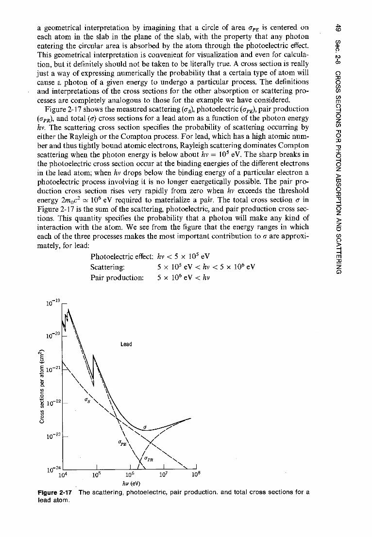
10-19

Lead

^\\ o / \ ^

^PE\\

\\u^

\ % N.\

\ 6pR

NN

108

a geometrical interpretation by imagining that a circle of area 6pE is centered on each atom in the slab in the plane of the slab, with the property that any photon

entering the circular area is absorbed by the atom through the photoelectric effect.

This geometrical interpretation is convenient for visualization and even for calcula-tion, but it definitely should not be taken to be literally true. A cross section is really

just a way of expressing numerically the probability that a certain type of atom will

cause a photon of a given energy to undergo a particular process. The definitions

and interpretations of the cross sections for the other absorption or scattering pro-cesses are completely analogous to those for the example we have considered.

Figure 2-17 shows the measured scattering (as), photoelectric (ape), pair production (6pR), and total (a) cross sections for a lead atom as a function of the photon energy

hv. The scattering cross section specifies the probability of scattering occurring by

either the Rayleigh or the Compton process. For lead, which has a high atomic num-ber and thus tightly bound atomic electrons, Rayleigh scattering dominates Compton

scattering when the photon energy is below about hv = 105 eV. The sharp breaks in the photoelectric cross section occur at the binding energies of the different electrons

in the lead atom; when hv drops below the binding energy of a particular electron a

photoelectric process involving it is no longer energetically possible. The pair pro-duction cross section rises very rapidly from zero when hv exceeds the threshold

energy 2moc2 ^ 106 eV required to materialize a pair. The total cross section a in

Figure 2-17 is the sum of the scattering, photoelectric, and pair production cross sec-tions. This quantity specifies the probability that a photon will make any kind of

interaction with the atom. We see from the figure that the energy ranges in which

each of the three processes makes the most important contribution to a are approxi-mately, for lead:

Photoelectric effect: hv < 5 x 105 eV Scattering: 5 x 10 5 eV < hv < 5 x 10 6 eV Pair production: 5 x 106 eV < by

CR

OS

S S

EC

TIO

NS

FO

R P

HO

TO

N A

BS

OR

PT

ION

AN

D S

CA

TT

ER

ING

Figure 2-17 The scattering, photoelectric, pair production, and total cross sections for a

lead atom.

0 LO

PH

OT

ONS

-P

AR

TIC

LELI

KE

PR

OP

ER

TIE

S O

F R

AD

IAT

ION

Because these processes have probabilities with different dependences on atomic number, the energy ranges in which they dominate are quite different for atoms of low atomic number. The energy ranges are approximately, for aluminum:

Photoelectric effect: hv < 5 x 104 eV Scattering: 5 x 104 eV < hv < 1 x 10' eV Pair production: 1 x 10' eV < hv

E$ample 2-8. Evaluate, in terms of the total cross section a, the attenuation of a parallel beam of x rays in passing through a thick slab of matter. ■ Referring to Figure 2-16, I(0) photons are in the beam as it is incident on the front face of the slab of thickness t, which contains p atoms per cm 3 . Assume, for simplicity, that the area of the slab is 1 cm 2 . Because of scattering and absorption processes, the parallel beam contains a smaller number I(x) of photons after penetrating x cm into the slab. Consider a thin lamina of the slab, of width dx located at x. The number of atoms per cm 2 in the lamina is p times its volume dx, or p dx. The number of beam photons that will be scattered or absorbed in the lamina is specified by the total cross section a, in a definition analogous to (2-18). It is 6I(x)p dx. Thus the number of beam photons emerging from the lamina, I(x + dx), which equals the number incident minus the number removed, is

I(x + dx) = 1(x) — aI(x)pdx

or

dI(x) - I(x + dx) — I(x) = —6I(x)pdx

We find 1(t), the number of beam photons emerging from the rear face of the slab, by solving for dI(x)/I(x) and then integrating over x

dI(x)

I(x) —apdx

t t

fJI(1(x) x)=-6pdx

0 0

In I(x)]ô = —ap t

In 1(0)

= apt

I(t) = e - apt

I(0)

I(t) = I(0)e - °pt (2-19)

The intensity of the beam, as measured by the number I of photons it contains, decreases exponentially as the thickness t of the slab increases. The quantity 6p, which is called the at-tenuation coefficient, has the dimensions (cm i ) and is the reciprocal of the thickness of slab required to attenuate the beam intensity by a factor of e. This thickness is called the attenua-tion length A. That is

A = 1/6p (2-20) Of course, the attenuation coefficient has the same dependence on photon energy as the total cross section. Figure 2-18 shows measured attenuation coefficients of lead, tin, and aluminum for photons of relatively high energy. •

This section summarizes many of the practical aspects of the electromagnetic radia-tion emission and absorption phenomena we have studied in the present chapter. But the fundamental aspects of these phenomena are better summarized by saying that they show electromagnetic radiation to be quantized into particles of energy called photons. It should also be emphasized that the phenomena of interference and diffraction show photons do not travel through a system from where they are emitted to where they are absorbed in the simple way that classical particles do. Instead, photons act as if they were guided by classical waves because photons travel through

2.0

1.8

1.6

1.4

I 1.2

; 1.0

g ^ 0.8

b 0.6

0.4

0.2

Pb

10 8 10 9 Figure 2-18 The attenuation coefficients for several atoms and a range of photon energies.

10 7

hv (eV)

a system such as a diffraction apparatus in a way that is best described by the way

that classical waves would propagate through the apparatus.

QUESTIONS

1. In the photoelectric experiments, the current (number of electrons emitted per unit time)

is proportional to the intensity of light. Can this result alone be used to distinguish

between the classical and quantum theories?

2. In Figure 2-2 why does the photoelectric current not rise vertically to its maximum

(saturation) value when the applied potential difference is slightly more positive than

V0? 3. Why is it that even for incident radiation that is monochromatic, photoelectrons are

emitted with a spread of velocities?

4. The existence of a cutoff frequency in the photoelectric effect is often regarded as the

most potent objection to a wave theory. Explain. 5. Why are photoelectric measurements very sensitive to the nature of the photoelectric

surface? 6. Do the results of photoelectric experiments invalidate Young's interference experiment?

7. Can you use the device of letting h -* 0 to obtain classical results from quantum results

in the case of the photoelectric effect? Explain.

8. Assume that the emission of photons from a source of radiation is random in direction.

Would you expect the intensity (or energy density) to vary inversely as the square of the

distance from the source in the photon theory as it does in the wave theory?

9. Does a photon of energy E have mass? If so, evaluate it. 10. Why, in Compton scattering, would you expect A/I to be independent of the materials

of which the scatterer is composed?

11. Would you expect to observe the Compton effect more readily with scattering targets

composed of atoms with high atomic number or those composed of atoms with low atomic number? Explain.

12. Do you observe a Compton effect with visible light? Why?

13. Would you expect a definite minimum wavelength in the emitted radiation for a given

value of the energy of an electron incident on the target of an x-ray tube from the

classical electromagnetic theory of the process?

14. Does a television tube emit x rays? Explain.

15. What effect(s) does decreasing the voltage across an x-ray tube have on the resulting

x-ray spectrum?

SN

OIl

S3

f lO

PH

OTO

NS

- PA

RT

ICLE

LIK

E P

RO

PE

RT

IES

OF

RA

DIA

TIO

N

16. Discuss the bremsstrahlung process as the inverse of the Compton process. Of the photo-electric process.

17. Describe several methods that can be used to determine experimentally the value of Planck's constant h.

18. From what factors would you expect to judge whether a photon will lose its energy in interactions with matter by the photoelectric process, the Compton process, or the pair production process?

19. Can you think of experimental evidence contradicting the idea that vacuum is a sea of electrons in negative energy states?

20. Can electron-positron annihilation occur with the creation of one photon if a nearby nucleus is available for recoil momentum?

21. Explain how pair annihilation with the creation of three photons is possible. Is it possible in principle to create even more than three photons in a single annihilation process?

22. What would be the inverse of the process in which two photons are created in electron-positron annihilation? Can it occur? Is it likely to occur?

23. What is wrong with taking the geometrical interpretation of a cross section as literally true?

PROBLEMS

1. (a) The energy required to remove an electron from sodium is 2.3 eV. Does sodium show a photoelectric effect for yellow light, with 1 = 5890 A? (b) What is the cutoff wave-length for photoelectric emission from sodium?

2. Light of a wavelength 2000 A falls on an aluminum surface. In aluminum 4.2 eV are required to remove an electron. What is the kinetic energy of (a) the fastest and (b) the slowest emitted photoelectrons? (c) What is the stopping potential? (d) What is the cutoff wavelength for aluminum? (e) If the intensity of the incident light is 2.0 W/m 2, what is the average number of photons per unit time per unit area that strike the surface?

3. The work function for a clean lithium surface is 2.3 eV. Make a rough plot of the stopping potential Vo versus the frequency of the incident light for such a surface, indi-cating its important features.

4. The stopping potential for photoelectrons emitted from a surface illuminated by light of wavelength 2 = 4910 A is 0.71 V. When the incident wavelength is changed the stopping potential is found to be 1.43 V. What is the new wavelength?

5. In a photoelectric experiment in which monochromatic light and a sodium photocathode are used, we find a stopping potential of 1.85 V for 2 = 3000 A and of 0.82 V for 2 _ 4000 A. From these data determine (a) a value for Planck's constant, (b) the work func-tion of sodium in electron volts, and (c) the threshold wavelength for sodium.

6. Consider light shining on a photographic plate. The light will be recorded if it dissociates an AgBr molecule in the plate. The minimum energy to dissociate this molecule is of the order of 10 -19 joule. Evaluate the cutoff wavelength greater than which light will not be recorded.

7. The relativistic expression for kinetic energy should be used for the electron in the photoelectric effect when v/c > 0.1, if errors greater than about 1% are to be avoided. For photoelectrons ejected from an aluminum surface (w o = 4.2 eV) what is the smallest wavelength of an incident photon for which the classical expression may be used?

8. X rays with 2 = 0.71 A eject photoelectrons from a gold foil. The electrons form circular paths of radius r in a region of magnetic induction B. Experiment shows that rB = 1.88 x 10 -4 tesla-m. Find (a) the maximum kinetic energy of the photoelectrons and (b) the work done in removing the electron from the gold foil.

9. (a) Show that a free electron cannot absorb a photon and conserve both energy and momentum in the process. Hence, the photoelectric process requires a bound electron. (b) In the Compton effect, however, the electron can be free. Explain.

G)

sw31

aoa

d

10. Under ideal conditions the normal human eye will record a visual sensation at 5500 A if as few as 100 photons are absorbed per second. What power level does this correspond

to? 11. An ultraviolet lightbulb, emitting at 4000 A, and an infrared lightbulb, emitting at 7000 A,

each are rated at 40 W. (a) Which bulb radiates photons at the greater rate, and (b) how

many more photons does it produce each second over the other bulb?

12. Solar radiation falls on the earth at a rate of 1.94 cal/cm 2 -min on a surface normal to the incoming rays. Assuming an average wavelength of 5500 A, how many photons per cm2 -min is this?

13. What are the frequency, wavelength, and momentum of a photon whose energy equals

the rest mass energy of an electron?

14. In the photon picture of radiation, show that if beams of radiation of two different

wavelengths are to have the same intensity (or energy density) then the numbers of the

photons per unit cross-sectional area per sec in the beams are in the same ratio as the

wavelengths. 15. Derive the relation

cotg =(1 + m c 2J

tanrp o

between the direction of motion of the scattered photon and the recoil electron in the

Compton effect.

16. Derive a relation between the kinetic energy K of the recoil electron and the energy E of the incident photon in the Compton effect. One form of the relation is

^2hv^ 2 0 s in — K _ 1110C

2 2 E

1+ (

2hv 1 sin 0

moc2 2

(Hint: See Example 2-4.)

17. Photons of wavelength 0.024 A are incident on free electrons. (a) Find the wavelength of a photon which is scattered 30° from the incident direction and the kinetic energy imparted to the recoil electron. (b) Do the same if the scattering angle is 120°. (Hint: See Example 2-4.)

18. An x-ray photon of initial energy 1.0 x 10 5 eV traveling in the +x direction is incident on a free electron at rest. The photon is scattered at right angles into the + y direction. Find the components of momentum of the recoiling electron.

19. (a) Show that AE/E, the fractional change in photon energy in the Compton effect, equals (hv'/m oc 2)(1 — cos 0). (b) Plot AE/E versus 0 and interpret the curve physically.

20. What fractional increase in wavelength leads to a 75% loss of photon energy in a Comp-ton collision?

21. Through what angle must a 0.20 MeV photon be scattered by a free electron so that it loses 10% of its energy?

22. What is the maximum possible kinetic energy of a recoiling Compton electron in terms of the incident photon energy by and the electron's rest energy m oc 2?

23. Determine the maximum wavelength shift in the Compton scattering of photons from protons.

24. (a) Show that the short wavelength cutoff in the x-ray continuous spectrum is given by Amin = 12.4 A/V, where V is applied voltage in kilovolts. (b) If the voltage across an x-ray tube is 186 kV what is Amin?

25. (a) What is the minimum voltage across an x-ray tube that will produce an x ray having the Compton wavelength? A wavelength of 1 A? (b) What is the minimum voltage needed

Lc) P

HO

TO

NS

-P

AR

TIC

LELI

KE P

RO

PE

RT

IES

OF

RA

DIA

TIO

N across an x-ray tube if the subsequent bremsstrahlung radiation is to be capable of pair production?

26. A 20 KeV electron emits two bremsstrahlung photons as it is being brought to rest in two successive decelerations. The wavelength of the second photon is 1.30 A longer than the wavelength of the first. (a) What was the energy of the electron after the first decelera-tion, and (b) what are the wavelengths of the photons?

27. A y ray creates an electron-positron pair. Show directly that, without the presence of a third body to take up some of the momentum, energy and momentum cannot both be conserved. (Hint: Set the energies equal and show that this leads to unequal momenta before and after the interaction.)

28. A y ray can produce an electron-positron pair in the neighborhood of an electron at rest as well as a nucleus. Show that in this case the threshold energy is 4m 0c 2 . (Hint: Do not ignore the recoil of the original electron, but assume that all three particles move off together.)

29. A particular pair is produced such that the positron is at rest and the electron has a kinetic energy of 1.0 MeV moving in the direction of flight of the pair-producing photon. (a) Neglecting the energy transferred to the nucleus of the nearby atom, find the energy of the incident photon. (b) What percentage of the photon's momentum is transferred to the nucleus?

30. Assume that an electron-positron pair is formed by a photon having the threshold en-ergy for the process. (a) Calculate the momentum transferred to the nucleus in the process. (b) Assume the nucleus to be that of a lead atom and compute the kinetic energy of the recoil nucleus. Are we justified in neglecting this energy compared to the threshold energy assumed above?

31. An electron-positron pair at rest annihilate, creating two photons. At what speed must an observer move along the line of the photons in order that the wavelength of one photon be twice that of the other?

32. Show that the results of Example 2-8, expressed in terms of p and t, are valid independent of the assumed area of the slab.

33. Show that the attenuation length A is just equal to the average distance a photon will travel before being scattered or absorbed.

34. Use the data of Figure 2-17 to calculate the thickness of a lead slab which will attenuate a beam of 10 keV x rays by a factor of 100.

3 DE BROGLIE'S POSTULATE

WAVELIKE PROPERTIES OF PARTICLES

3-1 MATTER WAVES

de Broglie's postulate; de Broglie wavelength; Davisson -Germer experiment; Thomson experiment; diffraction of helium atoms and neutrons

3-2 THE WAVE-PARTICLE DUALITY

complementarity principle; Einstein's interpretation of duality for radiation; Born's interpretation of duality for matter; wave functions; superposition principle

3-3 THE UNCERTAINTY PRINCIPLE

statement of principle; interpretation; Bohr's explanation of its physical origin

3-4 PROPERTIES OF MATTER WAVES

wave and group velocities; equality of particle velocity and group velocity; spread of reciprocal wavelengths and frequencies in a wave group; deriva-tion of uncertainty principle from de Broglie postulate; width of a quantum state

3-5 SOME CONSEQUENCES OF THE UNCERTAINTY PRINCIPLE 77

relation to complementarity; limitations imposed on quantum mechanics

3-6 THE PHILOSOPHY OF QUANTUM THEORY 79

Copenhagen interpretation of Bohr and Heisenberg; points of view of Einstein and de Broglie

QUESTIONS

80

PROBLEMS

81

56

62

65

69

55

Co D

E B

RO

GLI

E'S

PO

ST

ULA

TE

3-1 MATTER WAVES

Maurice de Broglie was a French experimental physicist who, from the outset, had supported Compton's view of the particle nature of radiation. His experiments and discussions impressed his brother Louis so much with the philosophic problems of physics at the time that Louis changed his career from history to physics. In his doctoral thesis, presented in 1924 to the Faculty of Science at the University of Paris, Louis de Broglie proposed the existence of matter waves. The thoroughness and originality of his thesis was recognized at once but, because of the apparent lack of experimental evidence, de Broglie's ideas were not considered to have any physical reality. It was Albert Einstein who recognized their importance and validity and in turn called them to the attention of other physicists. Five years later de Broglie won the Nobel Prize in physics, his ideas having been dramatically confirmed by experiment.

The hypothesis of de Broglie was that the dual, that is wave-particle, behavior of radiation applies equally well to matter. Just as a photon has a light wave associated with it that governs its motion, so a material particle (e.g., an electron) has an asso-ciated matter wave that governs its motion. Since the universe is composed entirely of matter and radiation, de Broglie's suggestion is essentially a statement about a grand symmetry of nature. Indeed, he proposed that the wave aspects of matter are related to its particle aspects in exactly the same quantitative way that is the case for radiation. According to de Broglie, for matter and for radiation alike the total energy E of an entity is related to the frequency y of the wave associated with its motion by the equation

E = by (3-la) and the momentum p of the entity is related to the wavelength 2 of the associated wave by the equation

p = h/2 (3-1b)

Here the particle concepts, energy E and momentum p, are connected through Planck's constant h to the wave concepts, frequency y and wavelength A. Equation (3-1b), in the following form, is called the de Broglie relation

2 = h/p (3-2) It predicts the de Broglie wavelength 2 of a matter wave associated with the motion of a material particle having a momentum p.

Example 3 -1. (a) What is the de Broglie wavelength of a baseball moving at a speed v = 10 m/sec? • Assume in = 1.0 kg. From (3-2)

h h 6.6 x 10 -34 joule-sec gs 2s A= - _—_ = 6.6 x 10 - m=6.6 x 10 A p my 1.0 kg x 10 m/sec

(b) What is the de Broglie wavelength of an electron whose kinetic energy is 100 eV? • Here

h h 6.6 x 10 -34 joule-sec

P V2 mK (2 x 9.1 x 10 -31 kg x 100 eV x 1.6 x 10 -19 joule/eV) 1 / 2

6.6 x 10 -34 joule-sec 10 = 1.2 x 10 m = 1.2 A 5.4 x 10 -24 kg-m/sec

The wave nature of light propagation is not revealed by experiments in geometrical optics, for the important dimensions of the apparatus used there are very large compared to the wavelength of light. If a represents a characteristic dimension of an optical apparatus (e.g., the width of a lens, mirror, or slit) and 2 is the wavelength of the light passing through the apparatus, we are in the domain of geometrical optics

when 2/a -+ 0. The reason is that the diffraction effects in any apparatus are always confined to angles of about 9 = 2/a, so diffraction effects are completely negligible when 1/a -i 0. Note that geometrical optics involves ray propagation, which is similar to the trajectory motion of classical particles.

However, when the characteristic dimension a of an optical apparatus becomes comparable to, or smaller than, the wavelength 2 of the light going through it, we are in the domain of physical optics. In this case, where 2/a $ 1, the diffraction angle 0 = 2/a is large enough that diffraction effects are easily observed and the wave nature of light propagation becomes apparent. To observe wavelike aspects in the motion of matter, therefore, we need systems with apertures or obstacles of suitably small dimensions. The finest scale systems of apertures available to experimentalists at the time of de Broglie made use of the spacing between adjacent planes of atoms in a solid, where a 1 A. (Now systems are available involving nuclear dimensions of ^ 10 -4 A.) Considering the de Broglie wavelengths evaluated in Example 3-1, we see that we cannot expect to detect any evidence of wavelike motion for a baseball, where 2/a 10 -25 for a ^ 1 A; but for a material particle of very much smaller mass than a baseball, the momentum p is reduced, and the de Broglie wavelength A = h/p is increased sufficiently for diffraction effects to be observable. Using apparatus with characteristic dimensions a = 1 A, wavelike aspects in the motion of the 2 = 1.2 A electron of Example 3-1 should be very apparent.

Elsasser pointed out, in 1926, that the wave nature of matter might be tested in the same way that the wave nature of x rays was first tested, namely by allowing a beam of electrons of appropriate energy to fall on a crystalline solid. The atoms of the crystal serve as a three-dimensional array of diffracting centers for the electron wave, and so they should strongly scatter electrons in certain characteristic directions, just as for x-ray diffraction. This idea was confirmed in experiments by Davisson and Germer in the United States and by Thomson in Scotland.

Figure 3-1 shows schematically the apparatus of Davisson and Germer. Electrons from a heated filament are accelerated through a potential difference V and emerge from the "electron gun" G with kinetic energy eV. This electron beam falls at normal incidence on a single crystal of nickel at C. The detector D is set at a particular angle 9 and readings of the intensity of the scattered beam are taken at various values of the accelerating potential V. Figure 3-2, for example, shows that a strong scattered electron beam is detected at 9 = 50° for V = 54 V. The existence of this peak in the

F

S v .

T

C

Figure 3-1 The apparatus of Davisson and Germer. Electrons from filament F are accelerated by a variable potential difference V. After scattering from crystal C they are collected by detector D.

S3A

VM

h13

11`d

W

35 40 45 50 Kinetic energy (eV) B

Figure 3 -2 Left: The collector current in detector D of Figure 3-1 as a function of the kinetic energy of the incident electrons, showing a diffraction maximum. The angle 0 in Figure 3-1 is adjusted to 50 ° . If an appreciably smaller or larger value is used, the dif-fraction maximum disappears. Right: The current as a function of detector angle for the fixed value of electron kinetic energy 54 eV.

electron scattering pattern demonstrates qualitatively the validity of de Broglie's pos- tulate because it can only be explained as a constructive interference of waves scattered by the periodic arrangement of the atoms into planes of the crystal. The phenomenon is precisely analogous to the well-known "Bragg reflections" which occur in the scattering of x rays from the atomic planes of a crystal. It cannot be understood on the basis of classical particle motion, but only on the basis of wave motion. Classical particles cannot exhibit interference, but waves can! The interference involved here is not between waves associated with one electron and waves associated with another. Instead, it is an interference between different parts of the wave associated with a single electron that have been scattered from various regions of the crystal. This can be demonstrated by using an electron beam of such low intensity that the elec-trons go through the apparatus one at a time, and by showing that the pattern of the scattered electrons remains the same.

Figure 3-3 shows the origin of a Bragg reflection, obeying the Bragg relation derived in the caption to that figure

n2.= 2 d sin ce (3-3) For the conditions of Figure 3-3 the effective interplanar spacing d can be shown by x-ray scattering from the same crystal to be 0.91 A. Since B = 50°, it follows that cp = 90° — 50°/2 = 65°. The wavelength calculated from (3-3), assuming n = 1, is

A= 2 d sin cp= 2 x 0.91 A x sin 65° = 1.65 A The de Broglie wavelength for 54 eV electrons, calculated from (3-2), is

= h/p = 6.6 x 10' 34 j oule-sec/4.0 x 10 - 24 kg-m/sec = 1.65 A This impressive agreement gives quantitative confirmation of de Broglie's relation between A, p, and h.

The breadth of the observed peak in Figure 3-2 is easily understood, also, for low-energy electrons cannot penetrate deeply into the crystal, so that only a small number of atomic planes contribute to the diffracted wave. Hence, the diffraction maximum is not sharp. Indeed, all the experimental results were in excellent qualita-tive and quantitative agreement with the de Broglie prediction, and they provided convincing evidence that material particles move according to the laws of wave motion.

In 1927, G. P. Thomson showed the diffraction of electron beams passing through thin films and independently confirmed the de Broglie relation 2 = h/p in detail. Whereas the Davisson-Germer experiment is like Laue's in x-ray diffraction (reflec-tion from the regular array of atomic planes in a large single crystal), Thomson's experiment is similar to the Debye-Hull-Scherrer method of powder diffraction of x rays (transmission through an aggregrate of very small crystals oriented at random).

DE

BR

OG

LIE'S

PO

ST

ULA

TE

Figure 3-3 Top: The strong diffracted beam at 9 = 50° and V = 54 V arises from wavelike scattering from the family of atomic planes shown, which have a sep-aration distance d = 0.91 A. The Bragg an-gle is cp = 65° . For simplicity, refraction of the scattered wave as it leaves the crystal surface is not indicated. Bottom: Deriva-tion of the Bragg relation, showing only two atomic planes and two rays of the in-cident and scattered beams. If an integral number of wavelengths n t just fit into the distance 21 from incident to scattered wave fronts measured along the lower ray, then the contributions along the two rays to the scattered wave front will be in phase and a diffraction maximum will be obtained at the angle go. Since lid = cos(90° — (p) = sin cp, we have 21= 2d sin cp, and so we obtain the Bragg relation nil = 2d sin cp. The "first order" diffraction maxi-mum (n = 1) is usually most intense.

S3

Ad

M 1:1

311

`dW

Thomson used higher-energy electrons, which are much more penetrating, so that many hundred atomic planes contribute to the diffracted wave. The resulting dif-fraction pattern has a sharp structure. In Figure 3-4 we show, for comparison, an x-ray diffraction pattern and an electron diffraction pattern from polycrystalline substances (substances in which a large number of microscopic crystals are oriented at random).

It is of interest that J. J. Thomson, who in 1897 discovered the electron (which he charac-terized as a particle with a definite charge-to-mass ratio) and was awarded the Nobel Prize in 1906, was the father of G. P. Thomson, who in 1927 experimentally discovered electron diffraction and was awarded the Nobel Prize (with Davisson) in 1937. Max Jammer writes of this, "One may feel inclined to say that Thomson, the father, was awarded the Nobel Prize for having shown that the electron is a particle, and Thomson, the son, for having shown that the electron is a wave."

Not only electrons but all material objects, charged or uncharged, show wavelike characteristics in their motion under the conditions of physical optics. For example, Estermann, Stern, and Frisch performed quantitative experiments on the diffraction of molecular beams of hydrogen and atomic beams of helium from a lithium fluoride crystal; and Fermi, Marshall, and Zinn showed interference and diffraction phenom-ena for slow neutrons. In Figure 3-5 we show a neutron diffraction pattern for a sodium chloride crystal. Even an interferometer operating with electron beams has been constructed. The existence of matter waves is well established.

It is instructive to note that we had to go to relatively long de Broglie wavelengths to find experimental evidence for the wave nature of matter. For both large and small

0 CO

DE

BR

OG

LIE

'S P

OS

TU

LAT

E

Photographic plate

Incident beam

of x rays or electrons

Crystalline film

Figure 3-4 Top: The experimental arrangement for Debye-Scherrer di ffraction of x rays or electrons by a polycrystalline material. Bottom left: Debye-Scherrer pattern of x-ray diffraction by zirconium oxide crystals. Bottom right: Debye-Scherrer pattern of electron diffraction by gold crystals.

wavelengths, both matter and radiation have both particle and wave aspects. The particle aspects are emphasized when their emission or absorption is studied, and the wave aspects are emphasized when their behavior in moving through a system is studied. But the wave aspects of their motion become more difficult to observe as their wavelengths become shorter. Once again we see the central role played by Planck's constant h. If h were zero then in A = h/p we would obtain A = 0 in all cir-cumstances. All material particles would then always have a wavelength smaller than any characteristic dimension, and diffraction effects could never be observed. Although the value of h is definitely not zero, it is small. It is the smallness of h that obscures the existence of matter waves in the macroscopic world, for we must have very small momenta to obtain measurable wavelengths. For ordinary macroscopic particles the mass is so large that the momentum is always sufficiently large to make the de Broglie wavelength small enough to be beyond the range of experimental detection, and classical mechanics reigns supreme. In the microscopic world the masses of material particles are so small that their momenta are small even when their velocities are quite high. Thus their de Broglie wavelengths are large enough to be comparable to characteristic dimensions of systems of interest, such as atoms, and the wavelike properties are experimentally observable in their motion. But we should not forget that in their interaction, for instance when they are detected, their particle-like properties dominate even when their wavelengths are large.

Example 3-2. In the experiments with helium atoms referred to earlier, a beam of atoms of nearly uniform speed of 1.635 x 10 5 cm/sec was obtained by allowing helium gas to escape

a) 1

S3A

b'M

1:i3

11

`dW

Figure 3-5 Top: Laue pattern of x-ray diffraction by a single sodium choride crystal. Bottom: Laue pattern of diffraction of neutrons from a nuclear reactor by a single sodium

choride crystal.

N ^

DE

BR

OG

LIE'S

PO

ST

ULA

TE

through a small hole in its enclosing vessel into an evacuated chamber and then through

narrow slits in parallel rotating circular disks of small separation (a mechanical velocity selec-tor). A strongly diffracted beam of helium atoms was observed to emerge from the lithium

fluoride crystal surface upon which the atoms were incident. The diffracted beam was detected

with a highly sensitive pressure gage. The usual crystal diffraction analysis of the experimental

results indicated a wavelength of 0.600 x 10 -8 cm. How does this agree with the calculated

de Broglie wavelength? The mass of a helium atom is

M 4.00 g/mole m = = = 6.65 x 10 -27 kg

No 6.02 x 1023 atom/mole

According to the de Broglie equation the wavelength then is

h h 6.63 x 10 -34 joule-sec ci p my 6.65 x 10 -27 kg x 1.635 x 10 3 m/sec L U

This result, 1.5% greater than the value measured by crystal diffraction, is well within the limits of error of the experiment. 4

Experiments like the one considered in Example 3-2 are very difficult since the intensities obtainable in atomic beams are quite low. Neutron diffraction experiments, using crystals of known lattice spacing, give confirmation of the existence of matter waves and precise con-firmation of de Broglie's equation. The precision is due to the fact that the supply of neutrons from nuclear reactors is copious. Indeed, neutron diffraction is now an important method of studying crystal structure. Certain crystals, such as hydrogenous organic ones, are particularly well suited to neutron diffraction analysis, since neutrons are strongly scattered by hydrogen atoms whereas x rays are very weakly scattered by them. X rays interact chiefly with electrons in the atom, and electrons interact with the nuclear charge of the atom as well as the atomic electrons by electromagnetic forces, so that their interaction with hydrogen atoms is weak because the charge is small. Neutrons interact principally with the nucleus of the atom by nuclear forces, however, and the interaction is strong.

3-2 THE WAVE-PARTICLE DUALITY

In classical physics energy is transported either by waves or by particles. Classical

physicists observed water waves carrying energy over the water surface or bullets

transferring energy from gun to target. From such experiences they built a wave

model for certain macroscopic phenomena and a particle model for other macro-scopic phenomena, and they quite naturally extended these models into visually less

accessible regions. Thus they explained sound propagation in terms of a wave model

and pressures of gases in terms of a particle model (kinetic theory). Their successes

conditioned them to expect that all entities are either particles or waves. Indeed, these

successes extended into the early twentieth century with applications of Maxwell's

wave theory to radiation and the discovery of elementary particles of matter, such

as the neutron and positron.

Hence, classical physicists were quite unprepared to find that to understand radia-tion they needed to invoke a particle model in some situations, as in the Compton

effect, and a wave model in other situations, as in the diffraction of x rays. Perhaps

more striking is the fact that this same wave-particle duality applies to matter as well

as to radiation. The charge-to-mass ratio of the electron and its ionization trail in

matter (a sequence of localized collisions) suggest a particle model, but electron

diffraction suggests a wave model. Physicists now know that they are compelled to

use both models for the same entity. It is very important to note, however, that in

any given measurement only one model applies—both models are not used under the same circumstances. When the entity is detected by some kind of interaction, it acts

= 0.609 x 10 -10 m

= 0.609 x 10 -8 cm

like a particle in the sense that it is localized; when it is moving it acts like a wave in the sense that interference phenomena are observed, and, of course, a wave is ex-tended, not localized.

Neils Bohr summarized the situation in his principle of complementarity. The wave and particle models are complementary; if a measurement proves the wave character of radiation or matter, then it is impossible to prove the particle character in the same measurement, and conversely. Which model we use is determined by the nature of the measurement. Furthermore, our understanding of radiation, or of matter, is incomplete unless we take into account measurements which reveal the wave aspects and also those that reveal the particle aspects. Hence, radiation and matter are not simply waves nor simply particles. A more general and, to the classical mind, a more complicated model is needed to describe their behavior, even though in extreme situations a simple wave model or a simple particle model may apply.

The link between wave model and particle model is provided by a probability interpretation of the wave-particle duality. In the case of radiation it was Einstein who united the wave and particle theories; subsequently Max Born applied a similar argument to unite wave and particle theories of matter.

In the wave picture the intensity of radiation, I, is proportional to 6' 2 , where 6' 2 is the average value over one cycle of the square of the electric field strength of the wave. (I is the average value of the so-called Poynting vector and we use the symbol g instead of E for electric field to avoid confusion with the total energy E.) In the photon, or particle, picture the intensity of radiation is written as I = Nhv where N

is the average number of photons per unit time crossing unit area perpendicular to the direction of propagation. It was Einstein who suggested that g2, which in electro-magnetic theory is proportional to the radiant energy in a unit volume, could be interpreted as a measure of the average number of photons per unit volume.

Recall that Einstein introduced a granularity to radiation, abandoning the con-tinuum interpretation of Maxwell. This leads to a statistical view of intensity. In this view, a point source of radiation emits photons randomly in all directions. The aver-age number of photons crossing a unit area will decrease with increasing distance from source to area. This is due to the fact that the photons spread over a sphere of larger area the farther they are from the source. Since the area of a sphere is pro-portional to the square of its radius, we obtain, on the average, an inverse square law of intensity just as in the wave picture. In the wave picture we imagine that spherical waves spread out from the source, the intensity dropping inversely as the square of the distance from the source. Here, these waves, whose strength can be measured by g2, can be regarded as guiding waves for the photons; the waves themselves have no energy—there are only photons—but they are a construct whose intensity mea-sures the average number of photons per unit volume.

We use the word "average" because the emission processes are statistical in nature. We do not specify exactly how many photons cross unit area in unit time, only their average number; the exact number can fluctuate in time and space, just as in kinetic theory of gases there are fluctuations about an average value from many quantities. We can say quite definitely, however, that the probability of having a photon cross unit area 3 m from the source is exactly one-ninth the probability that a photon will cross unit area 1 m from the source. In the formula I = Nhv, therefore, N is an aver-age value and is a measure of the probability of finding a photon crossing unit area in unit time. If we equate the wave expression to the particle expression we have

I = (1/poc)& 2 = hvN

so that e2 is proportional to N. Einstein's interpretation of e2 as a probability mea- sure of photon density then becomes clear. We expect that, as in kinetic theory, fluc- tuations about an average will become more noticeable at low intensities than at

l.11

-1`dfla

310

I1.8

dd

-3A

`dM

3H

1

CD D

E B

RO

GLI

E'S

PO

ST

ULA

TE

M

high intensities, so that the granular quantum phenomena contradict the continuum classical view more dramatically there.

In analogy to Einstein's view of radiation, Max Born proposed a similar uniting of the wave-particle duality for matter. This came several years after Schroedinger developed his generalization of de Broglie's postulate, called quantum mechanics. We shall examine Schroedinger's theory quantitatively in later chapters. Here we wish merely to use Born's idea in a qualitative way to set the stage conceptually for the subsequent detailed analysis.

Let us associate more than just a wavelength and frequency with matter waves. We do this by introducing a function representing the de Broglie wave, called the wave function 'P. For particles moving in the x direction with a precise value of linear momentum and energy, for example, the wave function can be written as a simple sinusoidal function of amplitude A, such as

This is analogous to

&(x,t) = A sin 27t ( — vt) (3-4b)

for the electric field of a sinusoidal electromagnetic wave of wavelength 2, and fre-quency y, moving in the positive x direction. The quantity 'F 2 will play a role for matter waves analogous to that played by )2 for waves of radiation. That quantity, the average of the square of the wave function of matter waves, is a measure of the probability of finding a particle in unit volume at a given place and time. Just as g is a function of space and time, so is W; and, as we shall see later, just as g satisfies a wave equation, so does 'P (Schroedinger's equation). The quantity g is a (radiation) wave associated with a photon, and 'P is a (matter) wave associated with a material particle.

As Born says: "According to this view, the whole course of events is determined by the laws of probability; to a state in space there corresponds a definite probability, which is given by the de Broglie wave associated with the state. A mechanical pro-cess is therefore accompanied by a wave process, the guiding wave, described by Schroedinger's equation, the significance of which is that it gives the probability of a definite course of the mechanical process. If, for example, the amplitude of the guiding wave is zero at a certain point in space, this means that the probability of finding the electron at this point is vanishingly small."

Just as in the Einstein view of radiation we do not specify the exact location of a photon at a given time, but specify instead by g2 the probability of finding a photon at a certain location at a given time, so here in Born's view we do not specify the exact location of a particle at a given time, but specify instead by 'P 2 the probability of finding a particle at a certain location at a given time. Just as we are accustomed to adding wave functions (g 1 + g2 = g) for two superposed electromagnetic waves whose resultant intensity is given by g2, so we shall add wave functions for two superposed matter waves (Y' 1 + W2 = 'P) whose resultant intensity is given by 'P2 . That is, a principle of superposition applies to matter as well as to radiation. This is in accordance with the striking experimental fact that matter exhibits interference and diffraction properties, a fact that simply cannot be understood on the basis of ideas in classical mechanics. Because waves can be superposed either constructively (in phase) or destructively (out of phase), two waves can combine either to yield a resultant wave of large intensity or to cancel, but two classical particles of matter cannot combine in such a way as to cancel.

The student might accept the logic of this fusion of wave and particle concepts but nevertheless ask whether a probabilistic or statistical interpretation is necessary.

ci.

v 'Y(x,t) = A sin 27c (j,x — vt (3-4a)

It was Heisenberg and Bohr who, in 1927, first showed how essential the concept of probability is to the union of wave and particle descriptions of matter and radiation. We investigate these matters in succeeding sections.

3-3 THE UNCERTAINTY PRINCIPLE

The use of probability considerations is not foreign to classical physics. Classical sta-tistical mechanics makes use of probability theory, for example. However, in classi-cal physics the basic laws (such as Newton's laws) are deterministic, and statistical analysis is simply a practical device for treating very complicated systems. According to Heisenberg and Bohr, however, the probabilistic view is the fundamental one in quantum physics and determinism must be discarded. Let us see how this conclusion is reached.

In classical mechanics the equations of motion of a system with given forces can be solved to give us the position and momentum of a particle at all values of the time. All we need to know are the precise position and momentum of the particle at some value of the time t = 0 (the initial conditions) and the future motion is deter-mined exactly. This mechanics has been used with great success in the macroscopic world, for example in astronomy, to predict the subsequent motions of objects in terms of their initial motions. Note, however, that in the process of making obser-vations the observer interacts with the system. An example from contemporary as-tronomy is the precise measurement of the position of the moon by bouncing radar from it. The motion of the moon is disturbed by the measurement, but due to the very large mass of the moon the disturbance can be ignored. On a somewhat smaller scale, as in a very well-designed macroscopic experiment on earth, such disturbances are also usually small, or at least controllable, and they can be taken into account accurately ahead of time by suitable calculations. Hence, it was naturally assumed by classical physicists that in the realm of microscopic systems the position and mo-mentum of an object, such as a electron, could be determined precisely by observa-tions in a similar way. Heisenberg and Bohr questioned this assumption.

The situation is somewhat similar to that existing at the birth of relativity theory. Physicists spoke of length intervals and time intervals, i.e., space and time, without asking critically how one actually measures them. For example, they spoke of the simultaneity of two separated events without even asking how one would physically go about establishing simultaneity. In fact, Einstein showed that simultaneity was not an absolute concept at all, as had been assumed previously, but that two sepa-rated events that are simultaneous to one observer occur at different times to another observer moving with respect to the first. Simultaneity is a relative concept Similarly then, we must ask ourselves how we actually measure position and momentum.

Can we determine by actual experiment at the same instant both the position and momentum of matter or radiation? The answer given by quantum theory is: not more accurately than is allowed by the Heisenberg uncertainty principle. There are two parts to this principle, also called the indeterminacy principle. The first has to do with the simultaneous measurement of position and momentum. It states that experi-ment cannot simultaneously determine the exact value of a component of momentum, px say, of a particle and also the exact value of its corresponding coordinate, x. Instead, our precision of measurement is inherently limited by the measurement process itself such that

ApxAx >_ h/2 (3-5) where the momentum px is known to within an uncertainty of Apx and the position x at the same time to within an uncertainty Ax. Here h (read h-bar) is a shorthand symbol for h/2n, where h is Planck's constant. That is

h - h/2n

31d

I ON

Iad

Jl1N

I`d11

i130

Nf1

3H

1

DE

BR

OG

LIE

'S P

OS

TU

LAT

E

There are corresponding relations for other components of momentum, namely Ap yAy > h/2 and Ap,Az > h/2, and for angular momentum as well. It is important to realize that this principle has nothing to do with improvements in instrumentation leading to better simultaneous determinations of px and x. Rather the principle says that even with ideal instruments we can never in principle do better than Ap xAx > h/2. Note also that the product of uncertainties is involved, so that, for example, the more we modify an experiment to improve our measure of px , the more we give up ability to determine x accurately. If px is known exactly we know nothing at all about x (i.e., if Ap x = 0, Ax = co). Hence, the restriction is not on the accuracy to which x or px can be measured, but on the product Ap xAx in a simultaneous measure-ment of both.

The second part of the uncertainty principle has to do with the measurement of the energy E and the time t required for the measurements, as for example, the time interval At during which a photon of energy spread AE is emitted from an atom. In this case

AEAt > h/2 (3-6)

where AE is the uncertainty in our knowledge of the energy E of a system and At the time interval characteristic of the rate of change in the system.

Heisenberg's relations will be shown later to follow from the de Broglie postulate plus simple properties common to all waves. Because the de Broglie postulate is verified by the experiments we have already discussed, it is fair to say that the un-certainty principle is grounded in experiment. We shall also consider soon the con-sistency of the principle with other experiments. Notice first, however, that it is Planck's constant h that again distinguishes the quantum results from the classical ones. If h, or h, in (3-5) and (3-6) were zero, there would be no basic limitation on our measurement at all, which is the classical view. Again it is the smallness of h that takes the principle out of the range of our ordinary experiences. This is analogous to the smallness of the ratio v/c in macroscopic situations taking relativity out of the range of ordinary experience. In principle, therefore, classical physics is of limited validity and in the microscopic domain it will lead to contradictions with experi-mental results. For if we cannot determine x and p simultaneously, then we cannot specify the initial conditions of motion exactly; therefore, we cannot precisely deter-mine the future behavior of a system. Instead of making deterministic predictions, we can only state the possible results of an observation, giving the relative proba-bilities of their occurrence. Indeed, since the act of observing a system disturbs it in a manner that is not completely predictable, the observation changes the previous motion of the system to a new state of motion which cannot be completely known.

Let us now illustrate the physical origin of the uncertainty principle. With the in-sight thereby gained we shall better appreciate a more formal proof given in the fol-lowing section. First, we use a thought experiment due to Bohr to verify (3-5). Let us say that we wish to measure as accurately as possible the position of a "point" par-ticle, like an electron. For greatest precision we use a microscope to view the electron, as in Figure 3-6. To see the electron we must illuminate it, for it is actually the light photon scattered by the electron that the observer sees. At this stage, even before any calculations are made, we can see the uncertainty principle emerge. The very act of observing the electron disturbs it. The moment we illuminate the electron, it recoils because of the Compton effect, in a way that we shall soon find cannot be completely determined. If we don't illuminate the electron, however, we don't see (detect) it. Hence the uncertainty principle refers to the measuring process itself, and it expresses the fact that there is always an undetermined interaction between observer and ob-served; there is nothing we can do to avoid the interaction or to allow for it ahead of time. In the case at hand we can try to reduce the disturbance to the electron as much as possible by using a very weak source of light. The very weakest we can get

31

dIJ

NIa

d A

lNI`

d11:1

30N

f1 3H

1 E-

C 'o

eS

rn

Eyepiece 4.0bserver

Objective lens

Electron

Light source

x-component of scattered photon

momentum, (h/X) sin B

I

16 /

\ I ^ Scattered photon momentum

Region available to photons

entering lens x

x-component of recoil electron momentum, (h/X) sin B

Photon of momentum h/X incident

Ax

Figure 3-6 Bohr's microscope thought experiment. Top: The apparatus. Middle: The scattering of an illuminating photon by the electron. Bottom: The diffraction pattern image of the electron seen by the observer.

is to assume that we can see the electron if only one scattered photon enters the ob-jective lens of the microscope. The magnitude of the momentum of the photon is

p = h/A. But the photon may have been scattered anywhere within the angular range 20' subtended by the objective lens at the electron. This is why the interaction cannot

be allowed for. Hence, we find that the x component of the momentum of the photon

can vary from + p sin 0' to — p sin 0' and is uncertain after the scattering by an

amount

Apx = 2p sin 0' = (2h/2) sin 0'

Conservation of momentum then requires that the electron receive a recoil momen-tum in the x direction that is equal in magnitude to the x momentum change in the

photon and, therefore, the x momentum of the electron is uncertain by this same

amount. Notice that to reduce Ap x we can use light of longer wavelength, or use a microscope with an objective lens subtending a smaller angle.

What about the location along x of the electron? Recall that a microscope's image

of a point object is not a point, but a diffraction pattern; the image of the electron

DE

BR

OG

LIE

'S P

OS

TU

LAT

E

is "fuzzy." The resolving power of a microscope determines the ultimate accuracy to which the electron can be located. If we take the width of the central diffraction maximum as a measure of the uncertainty in x, a well-known expression for the resolving power of a microscope gives

Ax = 2/sin 9'

(Note that, since sin 0 ^ 0, this is an example of the general relation a ^ 2/0 between the characteristic dimension in a diffraction apparatus, the wavelength of the dif-fracted waves, and the diffraction angle.) The one scattered photon at our disposal must have originated then somewhere within this range from the axis of the micro-scope, so the uncertainty in the electron's location is Ax. (We cannot be sure exactly where any one photon originates even though in a large number of repetitions of the experiment the photons forming the total image will produce the diffraction pat-tern shown in the figure.) Notice that to reduce Ax we can use light of shorter wave-length, or a microscope with an objective lens subtending a larger angle.

If now we take the product of the uncertainties we find

Ap xAx = I 2h

sin e'^ (sin B') — 2h (3-7)

in reasonable agreement with the ultimate limit h/2 set by the uncertainty principle. We cannot simultaneously make Apx and Ax as small as we wish, for the procedure that makes one small makes the other large. For instance, if we use light of short wavelength (e.g., y rays) to reduce Ax by obtaining better resolution, we increase the Compton recoil and increase Ap x, and conversely. Indeed, the wavelength 2 and the angle B' subtended by the objective lens do not even appear in the result. In practice an experiment might do much worse than (3-7) suggests, for that result represents the very ideal possible. We arrive at it, however, from genuinely measurable physical phenomena, namely the Compton effect and the resolving power of a lens.

There really should be no mystery in the student's mind about our result. It is a direct result of quantization of radiation. We had to have at least one photon illu-minating the electron, or else no illumination at all; and even one photon carries a momentum of magnitude p = h/.1. It is this single scattered photon that provides the necessary interaction between the microscope and the electron. This interaction dis-turbs the particle in a way that cannot be exactly predicted or controlled. As a result, the coordinates and momentum of the particle cannot be completely known after the measurement. If classical physics were valid, then since radiation is regarded there as continuous rather than granular, we could reduce the illumination to arbitrarily small levels and deliver arbitrarily small momentum while using arbitrarily small wavelengths for "perfect" resolution. In principle there would be no simultaneous lower limit to resolution or momentum recoil and there would be no uncertainty principle. But we cannot do this; the single photon is indivisible. Again we see, from ApxAx >_ h/2, that Planck's constant is a measure of the minimum uncontrollable disturbance that distinguishes quantum physics from classical physics.

Now let us consider (3-6) relating energy and time uncertainties. For the case of a free particle we can obtain (3-6) from (3-5), which relates position and momen-tum, as follows. Consider an electron moving along the x axis whose energy we can write as E = p!/2m. If px is uncertain by Apr, then the uncertainty in E is given by AE = (pxlm)Ap x = vxAp x . Here vx can be interpreted as the recoil velocity along x of the electron which is illuminated with light in a position measurement. If the time interval required for the measurement is At, then the uncertainty in its x position is Ax = vxAt. Combining At = Ax/vx and AE = vxAp x , we obtain AEAt = Ap xAx. But ApxAx >_ h/2. Hence

AEA t > h/2

Ax > 47rOp — 4rc x 2.7 x 10 -32 kg-m/sec =2 x 10 -3 m=0.2cm

h6.6 x 10 - 34 joule-sec

Example 3-3. The speed of a bullet (m = 50 g) and the speed of an electron (m = 9.1 x 10 -28 g) are measured to be the same, namely 300 m/sec, with an uncertainty of 0.01%. With what fundamental accuracy could we have located the position of each, if the position is measured simultaneously with the speed in the same experiment? •For the electron

p = my = 9.1 x 10 -31 kg x 300 m/sec = 2.7 x 10 -28 kg-m/sec

S3A

b'M

1:1

311`

dW 3

0 5

311

1:13

dO

ad

and

so that Op = mOv = 0.0001 x 2.7 x 10 -28 kg-m/sec = 2.7 x 10 -32 kg-m/sec

For the bullet

and

so that

p = my = 0.05 kg x 300 m/sec = 15 kg-m/sec

Ap = 0.0001 x 15 kg-m/sec = 1.5 x 10 -3 kg-m/sec

^x h _ 6.6 x 10 -34 joule-sec = 3 x 10 -32 m

4nAp 47r x 1.5 x 10 -3 kg-m/sec Hence, for macroscopic objects such as bullets the uncertainty principle sets no practical limit to our measuring procedure, Ax in this example being about 10 -17 times the diameter of a nucleus; but, for microscopic objects such as electrons, there are practical limits, Ax in this example being about 10' times the diameter of an atom. 1

3-4 PROPERTIES OF MATTER WAVES

In this section we shall derive the uncertainty principle relations by combining the de Broglie-Einstein relations, p = h/2 and E = hv, with simple mathematical prop-erties that are universal to all waves. We begin a development of these properties by calling attention to an apparent paradox.

The velocity of propagation w of a wave with wavelength and frequency 2 and y is given by the familiar relation, which we shall verify later

w 2v (3-8)

Let us evaluate w for a de Broglie wave associated with a particle of momentum p . and total energy E. We obtain

hE E w=2v=--=—

ph p

Now assume the particle is moving at nonrelativistic velocity y in a region of zero

potential energy. (The validity of our conclusions will not be limited by these assump-tions.) Evaluating p and E in terms of y and the mass m of the particle, we find

E mv 2/2 y w =

p = my

= 2 (3-9)

This result seems disturbing because it appears that the matter wave would not be

able to keep up with the particle whose motion it controls. However, there is really

no difficulty, as the following argument shows.

Imagine that a particle is moving along the x axis under the in fluence of no force because its potential energy has the constant value zero. Moving along that axis is

also its associated matter wave. Assume, for the sake of this thought experiment, that

we have distributed along the axis a set of (hypothetical) instruments which are capable

of measuring the amplitude of the matter wave. At some time, say t = 0, we record

^

^ D

E B

RO

GL

IE'S

PO

ST

ULA

TE

4'(x, t)

t =0

Figure 3 -7 A de Broglie wave for a particle.

the readings of these instruments. The results of the experiment can be presented as a plot of the instantaneous values of the wave, which we designate by the symbol `If(x,t), as a function of x at a fixed time t = O. It is not necessary to know much about matter waves at present to realize that the plot must look qualitatively like the one shown in Figure 3-7. The amplitude of the matter wave must be modulated in such a way that its value is nonzero only over some finite region of space in the vicinity of the particle. This is necessary because the matter wave must somehow be asso-ciated in space with the particle whose motion it controls. The matter wave is in the form of a group of waves and, as time passes, the group surely must move along the x axis with the same velocity as the particle.

The student may recall, from his study of classical wave motion, that for such a moving group of waves it is necessary to distinguish between the velocity g of the group and the quite different velocity w of the individual oscillations of the waves. This is encouraging, but of course we must prove that g is equal to the velocity of the particle. To do this, we develop a relation between g and the quantities v and 2 comparable to the relation of (3-8) between w and these two quantities.

We start by considering the simplest type of wave motion, a sinusoidal wave of frequency v and wavelength 2, which is of constant unit amplitude from — co to

+ co, but which is moving with uniform velocity in the direction of increasing x. Such a wave can be represented mathematically by the function

x T(x,t) = sin 2n — vt) (3-10a)

or, in a more convenient form 'P(x,t) = sin 2n(Kx — vt) where K - 1/ (3-10b)

That this does represent the wave just described can be seen from the following

considerations: 1. Holding x fixed at any value, we see that the function oscillates in time

sinusoidally with frequency v and amplitude one. 2. Holding t fixed, we see that the function has a sinusoidal dependence on x, with

wavelength 2 or reciprocal wavelength K. 3. The zeros of the function, which correspond to the nodes of the wave it rep-

resents, are found at positions x„ for which 2n(Kx„ — vt) = 1rn n = 0, +1, + 2, .. .

Or

n v x = +— t

„ 2K K

Thus these nodes, and in fact all points on the wave, are moving in the direction of

increasing x with velocity w = dx„/dt

which is equal to W = V/K

Note that this is identical with (3-8) since K = 1/ A. Next we discuss the case in which the amplitude of the waves is modulated to

form a group. We can obtain mathematically one group of waves moving in the

direction of increasing x, similar to the group of matter waves pictured in Figure

3-7, by adding together an infinitely large number of waves of the form of (3-10b),

each with infinitesimally differing frequencies v and reciprocal wavelengths K. (We shall soon explain how this happens.) The mathematical techniques become a little

involved, however, and for our purposes it will suffice to consider what happens

when we add together only two such waves. Thus we take

'P(x,t) = P 1(x,t) + W 2(x,t) (3-11) where

'Y 1(x,t) = sin 27r[Kx — vt]

and 'P2(x,t) = sin 27r[(K + dK)x — (v + dv)t]

Now sin A + sin B = 2 cos [(A — B)/2] sin [(A + B)/2]

Applying this to the case at hand, we have

CdK dv [(2K + dK) (2v + dv) W(x,t) = 2 cos 27r 2 x — 2 t sin 2^rL 2 x 2 t

Since dv « 2v and dK « 2K, this is

k(x,t) = 2 cos 27r (-e

x — —dv

t I sin 2ir(Kx — vt) (3-12)

A plot of 'V(x,t) as a function of x for a fixed value of t. = 0 is shown in Figure 3-8. The second term of'F(x,t) is a wave of the same form as (3-10b), but this wave is modulated by the first term so that the oscillations of 'P(x,t) fall within an en-velope of periodically varying amplitude. Two waves of slightly different frequency and reciprocal wavelength alternately interfere and reinforce in such a way as to produce a succession of groups. These groups, and the individual waves which they contain, are both moving in the direction of increasing x. The velocity w of the individual waves can be evaluated by considering the second term of 1(x,t), and the velocity g of the groups can be evaluated from the first term. Proceeding as in consideration 3, we find again

V W = —

K (3-13a)

S3A

dM

a3

11b'

W JO

S3I

1a

3dO

ad

w t =0

etc. \ etc. > x

^

i

^g 1

dtc

Figure 3-8 The sum of two sinusoidal waves of slightly different frequencies and recip-rocal wavelengths K.

N ti

DE

BR

OG

LIE

'S P

OS

TULA

TE

and also the new result

dv/2 _ dv = g

dK/2 dK (3-13b)

It can be shown that, for an infinitely large number of waves that combine to form one moving group, the dependence of the wave velocity w, and the group velocity g, on v, K, and dv/dK is exactly the same as for the simple case we have considered. Equations (3-13a) and (3-13b) have general validity.

Finally we are in a position to calculate the group velocity g of the group of matter waves associated with the moving particle. From the Einstein and de Broglie rela-tions, we have

CM

Q„ SO

L U

v = E/h and K = VA= p/h

dv = dE/h and dK = dp/h

Thus the group velocity is g = dv/dK = dE/dp

Setting z

E = 2 an d p = my

we obtain

dE_ my dv _

dp mdv — v

which gives us the satisfying result that g=v

The velocity of the group of matter waves is just equal to the velocity of the particle whose motion they govern, and de Broglie's postulate is internally consistent. The same conclusion is obtained when relativistic expressions for E and p are used in evaluating dE/dp.

Now we shall derive the uncertainty relations by combining the de Broglie-Einstein relations, p = h/2 and E = hv, with properties of groups of waves. First consider a simple limiting case. Let 2 be the wavelength of a de Broglie wave associated with a particle. We can picture a definite (monochromatic) wavelength in terms of a single sinusoidal wave extending over all values of x, i.e., an infinitely long unmodulated wave like

= A sin 2ir(Kx — vt) or

= A cos 27r(Kx — vt)

If the wavelength has the definite value 2 there is no uncertainty AA and the associated particle momentum p = h/2 is also definite so Ap x = O. In such a wave the amplitude has the constant value A everywhere; it is the same over the entire infinite range of x. Therefore, the probability of finding the particle, which Born tells us is to be related to the amplitude of the wave, is not concentrated in a particular range of x. In other words, the location of the particle is completely unknown. The particle can be any-where, so that Ax = c . Analogous statements are that since E = hv, and since the frequency is definite, then AE = O. But to be sure that the amplitude of the wave is perfectly constant in time we must observe the wave for an infinite time, so that At = co. For this simple case we satisfy Ap xAx > h/2, and AEAt > h/2, in the limits Ap x = O, Ax = co, and AE = O, At = co.

In order to have a wave whose amplitude varies with x or t, we must superpose several monochromatic waves of different wavelengths or frequencies. For two such waves superposed we obtain the familiar phenomenon of beats, as we have seen earlier in this section, with the amplitude being modulated in a regular way through-out space or time. If we wish to construct a wave having a finite extent in space (a single group with a definite beginning and end), then we must superpose sinusoidal waves having a continuous spectrum of wavelengths with a range A2. The amplitude of such a group will be zero everywhere outside a region of extent Ax.

To help visualize this, consider first a case in which we superpose a finite number of sinusoidal waves of slightly different wavelengths ), or reciprocal wavelengths K. Figure 3-9 shows seven component sinusoidal waves 111K = A, cos 2n(Kx — vt), at time t = O. Their reciprocal wavelengths K = 1/). take on integral values from K = 9 to K = 15. The amplitude of each is given by A K , with Al2 = 1 , A13 = A11 = 1/2, A 14 = A 10 = 1/3, and A15 = A9 = 1/4, as shown in the figure. All the waves are in phase at x = 0 where they are centered (this is why cosines are used), but they get out of phase with one another proceeding in either direction from that point. As a result, their sum 'P = T9 + • • • +'Y15 oscillates with maximum amplitude at x = 0, but its oscillations die out with increasing or decreasing x as the phase relations of the component waves get scrambled. The superposition thus contains a group whose extent in space Ax has a value that can be read from the figure to be slightly larger than 1/12, if we adopt the usual convention and measure from maximum amplitude to half-maximum amplitude. With an analogous convention, the range of reciprocal wavelengths used to compose the group, AK, has a value of 1. Note that the approxi-mate value of the product AxAK equals 1/12. Indicated on the right edge of the figure is the presence of an auxiliary group, of the same shape as the central group. Auxiliary groups are formed at uniformly spaced intervals along the positive and negative x axis. They occur because, with only a finite number of component waves, there are points on the axis separated from x = 0 by a distance which is exactly some different integral number of wavelengths for each component. At these points the components are in phase again, and so the group is repeated. If the number of com-ponent waves spanning a fixed range AK of reciprocal wavelengths is doubled, the width of the central group will be essentially unchanged but the distances separating it from the auxiliary groups will be doubled.

If we combine an infinitely large number of sinusoidal component waves, each with infinitesimally different reciprocal wavelength drawn from the same range K = 9 to 15, we obtain a central group quite similar to the one shown in Figure 3-9, but the auxiliary groups will not be present. The reason is that in such a case there is no length of the x axis into which an exactly integral number of wavelengths fits for every one of the infinite number of components. The components are all in phase at and near x = 0, and so they combine constructively to form the group. Proceeding away from this point, in either direction, the component waves begin to get out of phase with each other because their wavelengths or reciprocal wavelengths differ. Beyond certain points the phases of the infinite number of components become com-pletely random, and so the component waves sum up to zero. Furthermore, they never again get back into phase. Thus the components form one group of restricted length Ax. It is clear that the larger the range of reciprocal wavelengths AK from which the components are drawn, the smaller the length Ax of the group; the reason is simply that if the wavelengths cover a bigger span the phases will become random in a shorter distance. In fact, Ax is just inversely proportional to AK. The exact value of the proportionality constant depends on the relative amplitudes of the component waves, as does the exact shape of the group that they form.

The mathematics used in carrying out the procedure just described involves the so-called Fourier integral. Appendix D applies the Fourier integral to a simple case,

S3A

VM

1:131

1VW

d0 S

3111

:13d

Oad

LAAAAAAÀAAAAAAAA Y 1 VVVYYT 11► YY 1 VVY

DE

BR

OG

LIE'S

PO

ST

ULA

TE

4'12W 10

11

12

qY9

K =

A A A A ^ V V V V VV V V V V V

4'13 13

4'14 14

4'15 LA • • • • • n • • • • • • • • • • • • • • V V V V V V V V V V V V V V V V V V V V V V 15

1 —6 —5 —4 —3 — - 1 2 3 4 5 6 7 s (units of 1/12) --?-

8 9 10 11 12

V

Figure 3-9 Showing, at t = 0, the superposition of seven cosine waves "K = A K cos 2zc(Kx — vt) with uniformly spaced reciprocal wavelengths drawn from the range K = 9 to K = 15. Their amplitudes A K maximize at the value Al2 = 1 for the wave whose K lies in the center of the range, and they decrease symmetrically through the values 1/2, 1/3, and 1/4 for the other waves as their K approach the ends of the range. The sum

= EK 111 K of these waves consists of a group centered on x = 0, plus repeating groups of the same shape periodically spaced along the x axis in both directions from x = O. With Ax defined as the maximum amplitude to half-maximum amplitude width of tP, and AK defined as the range of reciprocal wavelengths of the components of `P from maximum amplitude to half-maximum amplitude, we have Ax 1/12, AK 1, and AXAK ^ 1/12.

obtaining numerical results that are similar to the results we obtained from the con-struction in Figure 3-9. Furthermore, the Fourier integral can be used to prove the following relation

AxAK >— 1/47r (3-14) This relation states that the optimum job that can be done in composing a group of

(half-width at half-maximum amplitude) length Ax from components with reciprocal wavelengths covering a (half-width at half-maximum amplitude) range of AK yields Ax = 1/4nAK, or AxAK = 1/4n. Generally a somewhat larger value of this product is obtained.

A group of waves traveling through space of limited extent passes any given point of observation in a limited time. If At is the duration of the group, or pulse, of waves then it necessarily must be composed from component sinusoidals whose frequencies span a range Av, where

AtAv >_ 1/4n (3-15)

Thus the frequency of the group is spread over the range Av if its duration covers the range At, just as its reciprocal wavelength is uncertain to within AK if its width is Ax. Equation (3-15) is also obtained from a Fourier integral. It and (3-14) are different ex-pressions of the same property; but the frequency-time relation, or at least some of its implications, may be more familiar to the student, as the following example shows.

Example 3-4. The signal from a television station contains pulses of full-width At — 10 - 6 sec. Explain why it is not feasible to transmit television in the AM broadcasting band. •The full-width range of frequencies in the signal is, from (3-15), Av -. 1/10 -6 sec = 106 sec - = 106 Hz. Thus the entire broadcast band (v -= 0.5 x 10 6 Hz to v ^ 1.5 x 10 6 Hz) would be able to accommodate only a single television "channel." There would also be serious difficulties in building transmitters and receivers with such a very large fractional bandpass. At the frequencies used in television transmission (v ^ 10 8 Hz) many channels fit into a rea-sonable portion of the spectrum, and the bandpass requirements are nominal. •

Equations (3-14) and (3-15) are universal properties of all waves. If we apply them to matter waves by combining them with the de Broglie-Einstein relations, we im-mediately obtain the Heisenberg uncertainty relations. That is, if in

AxAK = AxA(1/A) >_ 1/4it we set p = h/2 or 1/A = p/h, we obtain

AxA(p/h) _ (1/h)AxAp > 1/4n or

ApAx >_ h/2 (3-16) And if in

AtAv > 1/4n we set E = hv or v = E/h, we obtain

AtA(E/h) = (1/h)AtAE > 1/4n or

AEAt >_ h/2 (3-17) These results agree with our original statements of the relations in (3-5) and (3-6).

To summarize, we have seen that physical measurement necessarily involves inter-action between the observer and the system being observed. Matter and radiation are the entities available to us for such measurements. The relations p = h/A and E = hv apply to matter and to radiation, being the expression of the wave-particle duality. When we combine these relations with the properties universal to all waves we obtain the uncertainty relations. Hence, the uncertainty principle is a necessary consequence of this duality, that is, of the de Broglie-Einstein relations, and the uncertainty principle itself is the basis for the Heisenberg-Bohr contention that probability is fundamental to quantum physics.

Example 3 -5. An atom can radiate at any time after it is excited. It is found that in a typical case the average excited atom has a life-time of about 10 -8 sec. That is, during this period it emits a photon and is deexcited.

S3

AV

M 1

:131

1b'W

3O

S311

1:13d

Od

d

DE

BR

OG

LIE

'S P

OS

TU

LAT

E

(a) What is the minimum uncertainty Av in the frequency of the photon? ► From (3-15) we have

AVAt >_ 1/4n

or

Av >_ 1/4xAt With At = 10 -8 sec we obtain Av > 8 x 10 6 sec -1 .

(b) Most photons from sodium atoms are in two spectral lines at about A = 5890 A. What is the fractional width of either line, Av/v? • For 2 = 5890 A, we obtain v = c//1, = 3 x 10 1° cm-sec -1/5890 x 10 -8 cm = 5.1 x 10 14

sec-1 . Hence Av/v = 8 x 10 6 sec -1/5.1 x 10 14 sec -1 = 1.6 x 10 -8or about two parts in 100 million.

This is the so-called natural width of the spectral line. The line is much broader in practice because of the Doppler broadening and pressure broadening due to the motions and collisions of atoms in the source. •

(c) Calculate the uncertainty AE in the energy of the excited state of the atom. • The energy of the excited state is not precisely measurable because only a finite time is available to make the measurement. That is, the atom does not stay in an excited state for an indefinite time but decays to its lowest energy state, emitting a photon in the process. The spread in energy of the photon equals the spread in energy of the excited state of the atom in accordance with the energy conservation principle. From (3-17), with At equal to the mean life-time of the excited state, we have

AE > h/4n — h _ 6.63 x 10 -34 joule-sec At 47tAt 4ir x 10 -8 sec

4.14 x 10 -15 eV-sec 4n x 10 -8 sec

This agrees, of course, with the value obtained from part (a) by multiplying the uncertainty in photon frequency Av by h to obtain AE = hAy.

The energy spread of an excited state is usually called the width of the state. • (d) From the previous results determine, to within an accuracy AE, the energy E of the

excited state of a sodium atom, relative to its lowest energy state, that emits a photon whose wavelength is centered at 5890 A. ► We have Av/v = hAv/hv = AE/E. Hence, E = AE/(Av/v) = 3.3 x 10 -8 eV/1.6 x 10 -8 = 2.1 eV, in which we have used the results of the calculations in parts (b) and (c). •

Example 3-6. A measurement is made on the y coordinate of an electron, which is a member of a broad parallel beam moving in the x direction, by introducing into the beam a slit of narrow width Ay. Show that as a result an uncertainty Ap y is introduced in the y component of momentum of the electron, such that Ap yAy > h/2, as required by the uncertainty principle. Do this by considering the diffraction of the wave associated with the electron. • In propagating through the apparatus shown in Figure 3-10, the wave will be diffracted by the slit. The angle 0 to the first minimum of the "single-slit" diffraction pattern sketched in the figure is given by sin 0 = 2/Ay. (This is another example of the general relation 0 ^ Ala between diffraction angle, wavelength, and characteristic dimension of a diffraction apparatus.) Since the propagation of the wave governs the motion of the associated particle, the diffraction pattern also gives the relative probabilities for the electron to arrive at different locations on the photographic plate. Thus the electron passing through the slit will be deflected through an angle which lies anywhere within a range from about —0 to + 0. Even though its y mo-mentum was known with great precision to be zero before passing through the slit (because very little was then known about its y position), after passing the slit where the measurement of its y position was made its y momentum can be anywhere within a range from about —p y to +py , where sin 0 = py /p. So the y momentum of the electron is made uncertain by the y position measurement due to diffraction of the electron wave. The uncertainty is

Ap y ^ py = p sin 0 = p2/Ay Using the de Broglie relation p = h/a, to connect the momentum of the particle with the wave-

3.3 x 10 -8 eV

y

Slit Photographic plate

Figure 3-10 Measurement of the y coordinate of an electron in a broad parallel beam, by

requiring it to pass through a slit. The intensity pattern of the diffracted electron wave is

indicated by using the line representing the photographic plate as an axis for a plot of the

pattern.

length of the wave, we obtain or 4py = h/Ay

Apydy = h

Our result agrees with the limit set by the uncertainty principle. Diffraction, which refers to

waves, and the uncertainty principle, which refers to particles, provide alternative but equiv- alent ways of treating this and all similar problems. •

Note that in Example 3-6 the wave associated with a single electron is regarded as being diffracted. The probability that the electron hits some point on the photo-graphic plate is determined by the intensity of the electron wave. If only one elec-tron goes through the apparatus it can hit anywhere except at the zero intensity

locations of the diffraction pattern, and it will most likely hit somewhere near the

principal maximum. If many electrons go through the apparatus each of their waves

is diffracted independently in the same way and their points of arrival on the photo-graphic plate are distributed according to the same pattern. The fact that diffrac-tion phenomena involve interference between different parts of a wave belonging

to a single particle, and not interference between waves belonging to different par-ticles, was first shown experimentally by G. I. Taylor for the case of photons and

light waves. Using light of such low intensity that the photons were known to be

going through a diffraction apparatus one at a time, he obtained, after a very long

exposure, a diffraction pattern. Then turning the intensity up to normal levels where

many photons were in the apparatus at any time, he obtained the same diffraction

pattern. Essentially the same experiment has subsequently been performed for elec-trons and other material particles.

3-5 SOME CONSEQUENCES OF THE UNCERTAINTY PRINCIPLE

The uncertainty principle allows us to understand why it is possible for radiation,

and matter, to have a dual (wave-particle) nature. If we try experimentally to deter-mine whether radiation is a wave or a particle, for example, we find that an experi-ment which forces radiation to reveal its wave character strongly suppresses its

Incident electron

beam

^

f

SO

ME

CO

NS

EQ

UE

NC

ES

OF T

HE

UN

CE

RT

AIN

TY

PR

INC

IPL

E

DE

BR

OG

LIE

'S P

OS

TU

LA

TE

particle character. If we modify the experiment to bring out the particle character, its wave character is suppressed. We can never bring the wave and the particle view face to face in the same experimental situation. Radiation, and also matter, are like coins that can be made to display either face at will but not both simultaneously. This, of course, is the essence of Bohr's principle of complementarity; the ideas of wave and of particle complement rather than contradict one another.

Consider Young's two-slit interference experiment with light. On the wave picture the original wave front is split into two coherent wave fronts by the slits, and these overlapping wave fronts produce the interference fringes on the screen that are so characteristic of wave phenomena. Suppose now that we replace the screen by a photoelectric surface. Measurements of where the photoelectrons are ejected from the surface yield a pattern corresponding to the double-slit intensity pattern, so the wavelike aspects of the radiation seem to be present. But if the energy and time distributions of the ejected photoelectrons are measured, we obtain evidence which shows that the radiation consists of photons, so the particlelike aspects will seem to be present. If we then think of radiation as photons whose motion is governed by the wave propagation properties of certain associated (de Broglie) waves, we are faced with another apparent paradox. Each photon must pass through either one slit or the other; if this is the case, how can its motion beyond the slits be in-fluenced by the interaction of its associated waves with a slit through which it did not pass?

The fallacy in the paradox lies in the statement that each photon must pass through either one slit or the other. How can we actually determine experimentally whether a photon detected at the screen has gone through the upper or the lower of the two slits? To do this we would have to set up a detector at each slit, but the detector that interacts with the photon at a slit throws it out of the path that it would otherwise follow. We can show from the uncertainty principle that a detector with enough space resolution to determine through which slit the photon passes disturbs its momentum so much that the double-slit interference pattern is destroyed. In other words, if we do prove that each photon actually passes through one slit or the other, we shall no longer obtain the interference pattern. If we wish to observe the interference pattern, we must refrain from disturbing the photons and not try to observe them as particles along their paths to the screen. We can observe either the wave or the particle behavior of radiation; but the uncertainty principle prevents us from observing both together, and so this dual behavior is not really self-contra-dictory. The same is true of the wave-particle behavior of matter.

The uncertainty principle also makes it clear that the mechanics of quantum systems must necessarily be expressed in terms of probabilities. In classical mechan-ics, if at any instant we know exactly the position and momentum of each particle in an isolated system, then we can predict the exact behavior of the particles of the system for all future time. In quantum mechanics, however, the uncertainty principle shows us that it is impossible to do this for systems involving small dis-tances and momenta because it is impossible to know, with the required accuracy, the instantaneous positions and momenta of the particles. As a result, we shall be able to make predictions only of the probable behavior of these particles.

Example 3-7 Consider a microscopic particle moving freely along the x axis. Assume that at the instant t = 0 the position of the particle is measured and is uncertain by the amount Axo . Calculate the uncertainty in the measured position of the particle at some later time t. •The uncertainty in the momentum of the particle at t = 0 is at least

Apx = h/2Ax 0 Therefore, the velocity of the particle at that instant is uncertain by at least

Avx = Apxl in = h/2rnAxo

^

CO and the distance x travelled by the particle in the time t cannot be known more accurately than within

Ax = tAvx = ht/2mAx o If by a measurement at t = 0 we have localized the particle within the range Ax o , then in a measurement of its position at time t the particle could be found anywhere within a range at least as large as Ax.

Note that Ax is inversely proportional to Ax o , so that the more carefully we localize the

particle at the initial instant, the less we shall know about its final position. Also, the un-certainty Ax increases linearly with time t. This corresponds to a spreading out, as time goes on, of the group of waves associated with the motion of the particle. •

3-6 THE PHILOSOPHY OF QUANTUM THEORY

Although there is agreement by all physicists that quantum theory works in the sense that it predicts results that are in excellent agreement with experiment, there is a growing con-troversy over its philosophic foundation. Neils Bohr has been the principal architect of the present interpretation, known as the Copenhagen interpretation, of quantum mechanics. His approach is supported by the vast majority of theoretical physicists today. Nevertheless, a sizable body of physicists, not all in agreement with one another, questions the Copenhagen interpretation. The principal critic of this interpretation was Albert Einstein. The Einstein-Bohr debates are a fascinating part of the history of physics. Bohr felt that he had met every challenge that Einstein invented by way of thought experiments intended to refute the uncertainty principle. Einstein finally conceded the logical consistency of the theory and its agreement with the experimental facts, but he remained unconvinced to the end that it repre-sented the ultimate physical reality. "God does not play dice with the universe," he said, referring to the abandonment of strict causality and individual events by quantum theory in favor of a fundamentally statistical interpretation.

Heisenberg has stated the commonly accepted view succinctly: "We have not assumed that the quantum theory, as opposed to the classical theory, is essentially a statistical theory, in the sense that only statistical conclusions can be drawn from exact data .... In the formula-tion of the causal law, namely, `If we know the present exactly, we can predict the future,' it is not the conclusion, but rather the premise which is false. We cannot know, as a matter of principle, the present in all its details."

Among the critics of the Bohr-Heisenberg view of a fundamental indeterminacy in physics is Louis de Broglie. In a foreward to a book by David Bohm, a young colleague of Einstein's whose attempts at a new theory revived interest in reexamining the philosophic basis of quantum theory, de Broglie writes: "We can reasonably accept that the attitude adopted for nearly 30 years by theoretical quantum physicists is, at least in appearance, the exact counter-part of information which experiment has given us of the atomic world. At the level now reached by research in microphysics it is certain that the methods of measurement do not allow us to determine simultaneously all the magnitudes which would be necessary to obtain a picture of the classical type of corpuscles (this can be deduced from Heisenberg's uncertainty principle), and that the perturbations introduced by the measurement, which are impossible to eliminate, prevent us in general from predicting precisely the result which it will produce and allow only statistical predictions. The construction of purely probabilistic formulae that all theoreticians use today was thus completely justified. However, the majority of them, often under the influence of preconceived ideas derived from positivist doctrine, have thought that they could go further and assert that the uncertain and incomplete character of the knowledge that experiment at its present stage gives us about what really happens in microphysics is the result of a real indeterminacy of the physical states and of their evolution. Such an extra-polation does not appear in any way to be justified. It is possible that looking into the future to a deeper level of physical reality we will be able to interpret the laws of probability and quantum physics as being the statistical results of the development of completely deter-mined values of variables which are at present hidden from us. It may be that the powerful means we are beginning to use to break up the structure of the nucleus and to make new particles appear will give us one day a direct knowledge which we do not now have at this deeper level. To try to stop all attempts to pass beyond the present viewpoint of quantum

A1:1O

3H1

INf1

1NH

f10 d

O .I

Hd

OS

O1I

Hd

3H

1

0 CO

DE

BR

OG

LIE

'S P

OS

TU

LAT

E

physics could be very dangerous for the progress of science and would furthermore be contrary to the lessons we may learn from the history of science. This teaches us, in effect, that the actual state of our knowledge is always provisional and that there must be, beyond what is actually known, immense new regions to discover." (From Causality and Chance in Modern

Physics by David Bohm, © 1957 D. Bohm; reprinted by permission of D. Van Nostrand Co.) The student should notice here the acceptance of the correctness of quantum mechanics at

the atomic and nuclear level. The search for a deeper level, where quantum mechanics might be superseded, is motivated much more by objection to its philosophic indeterminism than by other considerations. According to Einstein, "The belief in an external world independent of the perceiving subject is the basis of all natural science." Quantum mechanics, however, regards the interactions of object and observer as the ultimate reality. It uses the language of physical relations and processes rather than that of physical qualities and properties. It rejects as meaningless and useless the notion that behind the universe of our perception there lies a

co hidden objective world ruled by causality; instead it confines itself to the description of the relations among perceptions. Nevertheless, there is a reluctance by many to give up attrib- co

Û uting objective properties to elementary particles, say, and dealing instead with our subjective knowledge of them, and this motivates their search for a new theory. According to de Broglie, such a search is in the interest of science. Whether it will lead to a new theory that in some currently unexplored realm contradicts quantum theory and also alters its philosophic founda-tions, no one knows.

QUESTIONS

1. Why is the wave nature of matter not more apparent to us in our daily observations?

2. Does the de Broglie wavelength apply only to "elementary particles" such as an electron or neutron, or does it apply as well to compound systems of matter having internal structure? Give examples.

3. If, in the de Broglie formula, we let m --> oo, do we get the classical result for macroscopic particles?

4. Can the de Broglie wavelength of a particle be smaller than a linear dimension of the particle? Larger? Is there necessarily any relation between such quantities?

5. Is the frequency of a de Broglie wave given by E/h? Is the velocity given by Ay? Is the velocity equal to c? Explain.

6. Can we measure the frequency v for de Broglie waves? If so, how?

7. How can electron diffraction be used to study properties of the surface of a solid? 8. How do we account for regularly reflected beams in diffraction experiments with elec-

trons and atoms? 9. Does the Bragg formula have to be modified for electrons to account for the refraction

of electron waves at the crystal surface? 10. Do electron diffraction experiments give different information about crystals than can be

obtained from x-ray diffraction experiments? From neutron diffraction experiments? Discuss.

11. Could crystallographic studies be carried out with protons? With neutrons? 12. Discuss the analogy: physical optics is to geometrical optics as wave mechanics is to

classical mechanics. 13. Is an electron a particle? Is it a wave? Explain. 14. Does the de Broglie wavelength associated with a particle depend on the motion of the

reference frame of the observer? What effect does this have on the wave-particle duality? 15. Give examples of how the process of measurement disturbs the system being measured. 16. Show the relation between the uncontrollable nature of the Compton recoil in Bohr's

y-ray microscope experiment and the fact that there are four unknowns and only three conservation equations in the Compton effect.

17. The uncertainty principle is sometimes stated in terms of angular quantities as AL 4 Arp > h/2 where AL 4, is the uncertainty in a component of angular momentum and Acp is the uncertainty in the corresponding angular position. In some quantum mechanical systems the angular momentum is measured to have a definite (quantized) magnitude. Does this contradict this statement of the uncertainty principle?

18. Argue from the Heisenberg uncertainty principle that the lowest energy of an oscillator cannot be zero.

19. Discuss similarities and differences between a matter wave and an electromagnetic wave.

20. Explain qualitatively the results of Example 3-7 that the uncertainty in position of a particle increases the more accurately we localize the particle initially and that the uncertainty increases with time.

21. Does the fact that interference occurs between various parts of the wave associated with a single particle (as in the G. I. Taylor experiments) simplify or complicate quantum physics?

22. Games of chance contain events which are ruled by statistics. Do such games violate the strict determination of individual events? Do they violate cause and effect?

23. According to operational philosophy, if we cannot prescribe a feasible operation for determining a physical quantity, the quantity should be given up as having no physical reality. What are the merits and drawbacks of this point of view in your opinion?

24. Bohm and de Broglie suggest that there may be hidden variables at a level deeper than quantum theory which are strictly determined. Draw an analogy to the relation between statistical mechanics and Newton's law of motion.

25. In your opinion is there an objective physical reality independent of our subjective sense impressions? How is this question answered by defenders of the Copenhagen interpreta-tion? By critics of the Copenhagen interpretation?

26. Are our concepts limited in principle by our everyday experiences or is this only our conceptual starting point? How is this question related to a resolution of the wave-particle duality?

PROBLEMS

1. A bullet of mass 40 g travels at 1000 m/sec. (a) What wavelength can we associate with it? (b) Why does the wave nature of the bullet not reveal itself through diffraction effects?

2. The wavelength of the yellow spectral emission of sodium is 5890 A. At what kinetic energy would an electron have the same de Broglie wavelength?

3. An electron and a photon each have a wavelength of 2.0 A. What are their (a) momenta and (b) total energies? (c) Compare the kinetic energies of the electron and the photon.

4. A nonrelativistic particle is moving three times as fast as an electron. The ratio of their de Broglie wavelengths, particle to electron, is 1.813 x 10 - 4 . Identify the particle.

5. A thermal neutron has a kinetic energy (3/2)k T where T is room temperature, 300°K. Such neutrons are in thermal equilibrium with normal surroundings. (a) What is the energy in electron volts of a thermal neutron? (b) What is its de Broglie wavelength?

6. A particle moving with kinetic energy equal to its rest energy has a de Broglie wavelength of 1.7898 x 10 - 6 A. If the kinetic energy doubles, what is the new de Broglie wavelength?

7. (a) Show that the de Broglie wavelength of a particle, of charge e, rest mass m o , moving at relativistic speeds is given as a function of the accelerating potential V as

1/2

= h

(1 + eV / - /2moe V ` 2moc2l

(b) Show how this agrees with 2 = h/p in the nonrelativistic limit

SW3180ad

N CO 8. Show that for a relativistic particle of rest energy E 0 , the de Broglie wavelength in A

is given by D

E B

RO

GLI

E'S

PO

ST

UL

AT

E

1.24 x 10 -2 (1 — /32)1/2

A = where /3 = v/c. E0(MeV) /3

9. Determine at what energy, in electron volts, the nonrelativistic expression for the de Broglie wavelength will be in error by 1% for (a) an electron and (b) a neutron. (Hint: See Problem 7.)

10. (a) Show that for a nonrelativistic particle, a small change in speed leads to a change in de Broglie wavelength given from

AA, Av

Ao vo (b) Derive an analogous formula for a relativistic particle.

11. The 50-GeV (i.e., 50 x 10 9 eV) electron accelerator at Stanford University provides an electron beam of very short wavelength, suitable for probing the fine details of nuclear structure by scattering experiments. What is this wavelength and how does it compare to the size of an average nucleus? (Hint: At these energies it is simpler to use the extreme relativistic relationship between momentum and energy, namely p = E/c. This is the same relationship used for photons, and it is justified whenever the kinetic energy of a particle is very much greater than its rest energy m o c 2 , as in this case.)

12. Make a plot of de Broglie wavelength against kinetic energy for (a) electrons and (b) pro-tons. Restrict the range of energy values to those in which classical mechanics applies reasonably well. A convenient criterion is that the maximum kinetic energy on each plot be only about, say, 5% of the rest energy m oc 2 for the particular particle.

13. In the experiment of Davisson and Germer, (a) show that the second- and third-order diffracted beams, corresponding to the strong first maximum of Figure 3-2, cannot occur and (b) find the angle at which the first-order diffracted beam would occur if the ac-celerating potential were changed from 54 to 60 V? (c) What accelerating potential is needed to produce a second-order diffracted beam at 50°?

14. Consider a crystal with the atoms arranged in a cubic array, each atom a distance 0.91 A from its nearest neighbor. Examine the conditions for Bragg reflection from atomic planes connecting diagonally placed atoms. (a) Find the longest wavelength electrons that can produce a first-order maximum. (b) If 300 eV electrons are used, at what angle from the crystal normal must they be incident to produce a first-order maximum?

15. What is the wavelength of a hydrogen atom moving with a velocity corresponding to the mean kinetic energy for thermal equilibrium at 20°C?

16. The principal planar spacing in a potassium chloride crystal is 3.14 A. Compare the angle for first-order Bragg reflection from these planes of electrons of kinetic energy 40 keV to that of 40 keV photons.

17. Electrons incident on a crystal suffer refraction due to an attractive potential of about 15 V that crystals present to electrons (due to the ions in the crystal lattice). If the angle of incidence of an electron beam is 45° and the electrons have an incident energy of 100 eV, what is the angle of refraction?

18. What accelerating voltage would be required for electrons in an electron microscope to obtain the same ultimate resolving power as that which could be obtained from a "y-ray microscope" using 0.2 MeV y rays?

19. The highest achievable resolving power of a microscope is limited only by the wavelength used; that is, the smallest detail that can be separated is about equal to the wavelength. Suppose we wish to "see" inside an atom. Assuming the atom to have a diameter of 1.0 A, this means that we wish to resolve detail of separation about 0.1 A. (a) If an electron microscope is used, what minimum energy of electrons is needed? (b) If a photon micro-scope is used, what energy of photons is needed? In what region of the electromagnetic spectrum are these photons? (c) Which microscope seems more practical for this purpose? Explain.

o0

sw31eoad

20. Show that for a free particle the uncertainty relation can also be written as A1Ax >_ 2/4n

where Ax is the uncertainty in location of the wave and A2 the simultaneous uncertainty in wavelength.

21. If A2/2 = 10 -7 for a photon, what is the simultaneous value of Ax for (a) 2 = 5.00 x 10 -4 A (y ray)? (b) 2 = 5.00 A (x ray)? (e) 2 = 5000 A (light)?

22. In a repetition of Thomson's experiment for measuring elm for the electron, a beam of 104 eV electrons is collimated by passage through a slit of width 0.50 mm. Why is the beamlike character of the emergent electrons not destroyed by diffraction of the electron wave at this slit?

23. A 1 MeV electron leaves a track in a cloud chamber. The track is a series of water droplets each about 10 -5 m in diameter. Show, from the ratio of the uncertainty in transverse momentum to the momentum of the electron, that the electron path should not notice-ably differ from a straight line.

24. Show that if the uncertainty in the location of a particle is about equal to its de Broglie wavelength, then the uncertainty in its velocity is about equal to one tenth its velocity.

25. (a) Show that the smallest possible uncertainty in the position of an electron whose speed is given by fi = v/c is

Ax min h (1 — /32)112

Ac / 1 _ fl 2 min 47Lm0c 47r

where 2c is the Compton wavelength h/m 0 c. (b) What is the meaning of this equation for fi = 0? For /3 = 1?

26. A microscope using photons is employed to locate an electron in an atom to within a distance of 0.2 A. What is the uncertainty in the velocity of the electron located in this way?

27. The velocity of a positron is measured to be: vx = (4.00 ± 0.18) x 10 5 m/sec, vy = (0.34 + 0.12) x 10 5 m/sec, vZ = (1.41 ± 0.08) x 10 5 m/sec. Within what minimum volume was the positron located at the moment the measurement was carried out?

28. (a) Consider an electron whose position is somewhere in an atom of diameter 1 A. What is the uncertainty in the electron's momentum? Is this consistent with the binding energy of electrons in atoms? (b) Imagine an electron to be somewhere in a nucleus of diameter 10 -12 cm. What is the uncertainty in the electron's momentum? Is this consistent with the binding energy of nuclear constituents? (c) Consider now a neutron, or a proton, to be in such a nucleus. What is the uncertainty in the neutron's, or proton's, momentum? Is this consistent with the binding energy of nuclear constituents?

29. The lifetime of an excited state of a nucleus is usually about 10 -12 sec. What is the un-certainty in energy of the y-ray photon emitted?

30. An atom in an excited state has a lifetime of 1.2 x 10 -8 sec; in a second excited state the lifetime is 2.3 x 10 8 sec. What is the uncertainty in energy for the photon emitted when an electron makes a transition between these two levels?

31: Use relativistic expressions for total energy and momentum to verify that the group velocity g of a matter wave equals the velocity v of the associated particle.

32. The energy of a linear harmonic oscillator is E = p/2m + Cx2/2. (a) Show, using the uncertainty relation, that this can be written as

h2 Cx2 E= +

327c2mx2 2

(b) Then show that the minimum energy of the oscillator is by/2 where 1 C

v =— 27z

is the oscillatory frequency. (Hint: This result depends on the AxAp x product achieving its limiting value h/2. Find E in terms of Ax or Apx as in part (a), then minimize E with

co D

E B

RO

GLI

E'S

PO

ST

ULA

TE

respect to Ax or Ap x in part (b). Note that classically the minimum energy would be zero.)

33. A TV tube manufacturer is attempting to improve the picture resolution, while keeping costs down, by designing an electron gun that produces an electron beam which will make the smallest possible spot on the face of the tube, using only an electron emitting cathode followed by a system of two well-spaced apertures. (a) Show that there is an optimum diameter for the second aperture. (b) Using reasonable TV , tube parameters, estimate the minimum possible spot size.

34. A boy on top of a ladder of height H is dropping marbles of mass m to the floor and trying to hit a crack in the floor. To aim, he is using equipment of the highest possible precision. (a) Show that the marbles will miss the crack by an average distance of the order of (h/m) 1/2(H/g)1"4, where g is the acceleration due to gravity. (b) Using reasonable values of H and m, evaluate this distance.

35. Show that in order to be able to determine through which slit of a double-slit system each photon passes without destroying the double-slit diffraction pattern, the condition AyAp y « h/2 must be satisfied. Since this condition violates the uncertainty principle, it cannot be met.

86

90

95

96

98

100

105

107

110

114

4 BOHR'S MODEL OF

THE ATOM

4-1 THOMSON'S MODEL

properties of model; a particles; multiple scattering; Geiger-Marsden experi-ment; failure of model

4-2 RUTHERFORD'S MODEL

nuclei; cc-particle trajectories; impact parameter and distance of closest ap-proach; Rutherford's calculation; comparison with Geiger-Marsden experi-ment; nuclear radii; definition of differential cross section; solid angle; Ru-therford scattering cross section

4-3 THE STABILITY OF THE NUCLEAR ATOM

radiation by an accelerated classical charged body

4-4 ATOMIC SPECTRA

line spectra; hydrogen series; Balmer formula; Rydberg constant; alkali series; absorption spectra

4-5 BOHR'S POSTULATES

statement of postulates; orbital angular momentum quantization; appraisal

4-6 BOHR'S MODEL

Bohr's calculation; orbit radii; one-electron atom energy quantization; com-parison with Balmer formula; singly ionized helium

4-7 CORRECTION FOR FINITE NUCLEAR MASS

reduced mass; Rydberg constant evaluation; positronium; deuterium; mu-onic atom

4-8 ATOMIC ENERGY STATES

Franck-Hertz experiment; ionization energy; continuum states

4-9 INTERPRETATION OF THE QUANTIZATION RULES

Wilson- Sommerfeld quantization rules; phase space and phase diagrams; simple harmonic oscillator; one-electron atom and de Broglie's interpreta-tion; particle in one-dimensional box

4-10 SOMMERFELD'S MODEL

quantization of elliptical orbits; principal and azimuthal quantum numbers; degeneracy; effect of relativity; hydrogen fine structure; fine-structure con-stant; selection rules

85

BO

HR

'S M

OD

EL

OF

TH

E A

TO

M

4-11 THE CORRESPONDENCE PRINCIPLE

117

statement of principle; justification; charged simple harmonic oscillator; hydrogen atom

4-12 A CRITIQUE OF THE OLD QUANTUM THEORY

118

recapitulation; failures of the old quantum theory; search for a replacement

QUESTIONS

119

PROBLEMS

120

4-1 THOMSON'S MODEL

By 1910 experimental evidence had been accumulated which showed that atoms contain electrons (e.g., scattering of x rays by atoms, photoelectric effect, etc.). These experiments also provided an estimate of Z, the number of electrons in an atom. They found it to be roughly equal to A/2, where A is the chemical atomic weight of the atom in question. Since atoms are normally neutral, they must also contain positive charge equal in magnitude to the negative charge carried by their normal complement of electrons. Thus a neutral atom has a negative charge — Ze, where — e is the electron charge, and also a positive charge of the same magnitude. That the mass of an electron is very small compared to the mass of even the lightest atom implies that most of the mass of the atom must be associated with the positive charge.

These considerations naturally led to the question of the distribution of the positive and negative charges within the atom. J. J. Thomson proposed a tentative description, or model, of an atom according to which the negatively charged electrons were located within a continuous distribution of positive charge. The positive charge dis-tribution was assumed to be spherical in shape with a radius of the known order of magnitude of the radius of an atom, 10 -20 m. (This value can be obtained from the density of a typical solid, its atomic weight, and Avogadro's number.) Owing to their mutual repulsion, the electrons would be uniformly distributed through the sphere of positive charge. Figure 4-1 illustrates this "plum pudding" model of the atom. In an atom in its lowest possible energy state, the electrons would be fixed at their equilibrium positions. In excited atoms (e.g., atoms in a material at high temperature), the electrons would vibrate about their equilibrium positions. Since classical electromagnetic theory predicts that an accelerated charged body, such as a vibrating electron, emits electromagnetic radiation, it was possible to understand qualitatively the emission of such radiation by excited atoms on the basis of Thom-son's model. Quantitative agreement with experimentally observed spectra was lack-ing, however.

Example 4-1. (a) Assume that there is one electron of charge —e inside a spherical region of uniform positive charge density p (a Thomson hydrogen atom). Show that its motion, if it has kinetic energy, can be simple harmonic oscillation about the center of the sphere.

Figure 4-1 Thomson's model of the atom—a sphere of positive charge embedded with electrons.

1 2.3 x 102 nt/m i s 1 = 2.5 x 10 sec

m 27c 9.11 x 10 -31 kg J

•Let the electron be displaced to a distance a from the center, with a less than the radius of the sphere. From Gauss's law, we know that we can calculate the force on it by using

Coulomb's law 1 (4 3 e _ pea _

F 4zcE O 3

Ira p a2 3E0

where (4/3)7ca 3 p is the net positive charge in a sphere of radius a. Hence, we can write F =

— ka, where the constant k = pe/3E0 . If the electron at a is freed with no initial velocity, this

force will produce simple harmonic motion along a diameter of the sphere since it is always

directed towards the center and has a strength which is proportional to the displacement

from the center. • (b) Let the total positive charge have the magnitude of one electron charge (so that the

atom has no net charge), and let it be distributed over a sphere of radius r' = 1.0 x 10 -10 m. Find the force constant k and the frequency of the motion of the electron.

► We have e

p= 4 ^^, 3

3

so that

3 9.0 x 109 nt-m2/coul 2 x (1.6 x 10 -19 coul)2

102 — 2.3 x 10 nt/m (1.0 x 10 -10 m)3

The frequency of the simple harmonic motion is then

pe e e e 2 k=

3E 0 4 /3 3E0 47cE 0r' 3 — 7cr

13

aO1A

1 S

AO

SW

OH

l

Since (in analogy to radiation emitted by electrons oscillating in an antenna) the radiation emitted by the atom will have this same frequency, it will correspond to a wavelength

c 3.0 x 10 8 m/sec v 2.5x1015/sec —

1.2x10 m=1200 A

in the far ultraviolet portion of the electromagnetic spectrum. It is easy to show that an electron moving in a stable circular orbit of any radius inside the Thomson atom revolves at this same frequency, and so it would radiate at this frequency also.

Of course, a different assumed radius of the sphere of positive charge would give a different frequency. But the fact that a Thomson hydrogen atom has only one characteristic emission frequency conflicts with the very large number of different frequencies observed in the spectrum of hydrogen. •

Conclusive proof of the inadequacy of Thomson's model was obtained in 1911 by Ernest Rutherford, a former student of Thomson's, from the analysis of experiments on the scattering of a particles by atoms. Rutherford's analysis showed that, instead of being spread throughout the atom, the positive charge is concentrated in a very small region, or nucleus, at the center of the atom. This was one of the most im-portant developments in atomic physics and was the foundation of the subject of nuclear physics.

Rutherford had already been awarded the Nobel Prize in 1908 for his "investigations in

regard to the decay of elements and ... the chemistry of radioactive substances." He was a

talented, hard-working physicist with enormous drive and self-confidence. In a letter written

later in life, the then Lord Rutherford wrote, "I've just been reading some of my early papers

and, you know, when I'd finished, I said to myself, `Rutherford, my boy, you used to be a

damned clever fellow. — Though pleased at winning a Nobel Prize he was not happy that it

was a chemistry prize, rather than one in physics. (Any research in the elements was then

a-particle trajectory

BO

HR

'S M

OD

EL

OF

TH

E A

TO

M

Diaphragm

a-particle source Thin foil

Figure 4-2 Arrangement of an a-particle scattering experiment. The region traversed by the a particles is evacuated.

considers mistry.) In his speech accepting the prize he noted that he had observed many transformations 'n his work with radioactivity but never had seen one as rapid as his own, from physicist to chemist.

Rutherford already knew a particles to be doubly ionized helium atoms (i.e., He atoms with two electrons removed), emitted spontaneously from several radioactive materials at high speed. In Figure 4-2 we show a typical arrangement that he and his colleagues used to study the scattering of a particles on passing through thin foils of various substances. The radioactive source emits a particles which are collimated into a narrow parallel beam by a pair of diaphragms. The parallel beam is incident upon a foil of some substance, usually a metal. The foil is so thin that the particles pass completely through with only a small decrease in speed. In traversing the foil, how-ever, each a particle experiences many small deflections due to the Coulomb force acting between its charge and the positive and negative charges of the atoms of the foil. Since the deflection of an a particle in passing through a single atom depends on the details of its trajectory through the atom, the net deflection in passing through the entire foil will be different for different a particles in the beam. As a result, the beam emerges from the foil not as a parallel beam but as a divergent beam. A quanti-tative measure of its divergence is found by measuring the number of a particles scattered into each angular range O to O + d0. The a particle detector consisted of a layer of the crystalline compound ZnS and a microscope. The crystal ZnS has the useful property of producing a small flash of light when struck by an cc particle. If observed with a microscope, the flash due to the incidence of a single cc particle can be distinguished. In the experiment an observer counts the number of light flashes produced per unit time as a function of the angular position of the detector.

Let .N' represent the number of atoms that deflect an cc particle in its passage through the foil. If B represents the angle of deflection in passing through one atom, as in Figure 4-3, and O is the net deflection in passing through all the atoms in its

Figure 4-3 An a particle passing through a Thomson model atom. The angle B specifies the deflection of the cc particle.

CO ^ trajectory through the foil, then statistical theory shows that

(0 2) 1/2 = Vs- (02 ) 1/2 (4-1)

Here (0 2) 112 is the root mean square net deflection, or scattering, angle and (92)1/2 is the root mean square scattering angle in a deflection from a single atom. The factor J.At comes from the randomness of the deflection; if all deflections were in the same direction, clearly we would obtain X instead of /.N' . More generally, statistical theory gives the following angular distribution of the scattered a particles

— N(0) d0 = OO e

- e2 /e2 d0 (4-2)

where N(0) de is the number of a's scattered within the angular range O to O + dO, and I is the number of a's passing through the foil.

Because electrons have a very small mass compared to the a particle, they can in any case produce only small a-particle deflections; and because the positive charge is distributed over all the volume of the r' 10' 10 m radius Thomson atom it cannot provide a Coulomb repulsion intense enough to produce a large deflection of the a particle. Indeed, using Thomson's model we find that the deflection caused by one atom is 0 < 10 -4 rad. This result and (4-1) and (4-2) comprise the a-particle scattering predictions of the Thomson model of the atom. Rutherford and his group tested these predictions.

Example 4-2. (a) In a typical experiment (Geiger and Marsden, 1909), a particles were

scattered by a gold foil 10 -6 m thick. The average scattering angle was found to be (02)1/2

1° ^ 2 x 10 -2 rad. Calculate (02)1/2.

■ The number of atoms traversed by the a particle is approximately equal to the thickness

of the foil divided by the diameter of the atom. Hence

✓V ^ 10-6 m/10-tom= 104 The average deflection angle in traversing a single atom then, from (4-1), is

2 (82)1/2 =

(02)1/2 2 x1010 ,,, 2 x 10 -4 rad

not in disagreement with the Thomson atom estimate 0 < 10 -4 rad. 4 (b) More than 99% of the a particles were scattered at angles less than 3°. The measure-

ments, using 1° for (02)1/2, were in agreement with (4-2) for NOD) de for angles Co in this

range; but the angular distribution of the small number of particles scattered at larger angles

was in marked disagreement with (4-2). It was found, for example, that the fraction of a's

scattered at angles greater than 90°, N(O > 90°)/I, was about 10 -4. What does (4-2) predict? ► We have

180°

N(0) de N(0 > 90°) _ 90e

—

e —(90) 2 = 10-3500 I I

a strikingly different result than the experiment value of 10 -4. In general the number of scattered a particles was observed to be very much larger than

the predicted number for all scattering angles greater than a few degrees. •

The existence of a small, but nonzero probability for scattering at large angles

could not be explained at all in terms of Thomson's model of the atom, which

basically involves small angle scattering from many atoms. To scientists accustomed to thinking in terms of this model it came as a great surprise that some a particles

were deflected through very large angles, up to 180°. In Rutherford's words: "It was

quite the most incredible event that ever happened to me in my life. It was as

incredible as if you fired a 15-inch shell at a piece of tissue paper and it came

back and hit you."

13a01

A1 S

NO

SW

OH

l

0 rn

BO

HR

'S M

OD

EL

OF

TH

E A

TO

M

Experiments using foils of various thicknesses showed that the number of large angle scatterings was proportional to ✓V' , the number of atoms traversed by the a particle. This is just the dependence on .N 1 that would arise if there were a small probability that an a particle could be scattered through a large angle in traversing a single atom. That cannot happen in Thomson's model of the atom, and this led Rutherford in 1911 to propose a new model.

4-2 RUTHERFORD'S MODEL

In Rutherford's model of the structure of the atom, all the positive charge of the atom, and consequently essentially all its mass, are assumed to be concentrated in a small region in the center called the nucleus. If the dimensions of the nucleus are small enough, an a particle passing very near it can be scattered by a strong Coulomb repulsion through a large angle in the traversal of a single atom. If, instead of using r' = 10' 1 ° m for the radius of the positive charge distribution of the Thomson atom, which leads to a maximum deflection angle 0 10 -4 rad, we ask what the radius r' of a nucleus should be to obtain 0 ^ 1 rad, say, we find r' = 10' 14 m. This, as we shall see, turns out to be a good estimate of the radius of the atomic nucleus.

Rutherford made a detailed calculation of the angular distribution to be expected for the scattering of a particles from atoms of the type proposed in his model. The calculation was concerned only with scattering at angles greater than several degrees. Hence, scattering due to atomic electrons can be ignored. The scattering is then due to the repulsive Coulomb force acting between the positively charged a particle and the positively charged nucleus. Furthermore, the calculation considered only the scattering from heavy atoms, to permit the assumption that the mass of the nucleus is so large compared to that of the a particle that the nucleus does not recoil ap-preciably (remains fixed in space) during the scattering process. It was also assumed that the a particle does not actually penetrate the nuclear region, so that the particle and the nucleus (both assumed to be spherical) act like point charges as far as the Coulomb force is concerned. We shall see later that all these assumptions are quite valid except for the scattering of a particles from the lighter nuclei, and we can correct for the finite nuclear mass in such cases. The calculation, finally, uses non-relativistic mechanics, since v/c 1/20.

Figure 4-4 illustrates the scattering of an a particle, of charge + ze and mass M, in passing near a nucleus of charge + Ze. The nucleus is fixed at the origin of the coordinate system. When the particle is very far from the nucleus, the Coulomb force on it is negligible so that the particle approaches the nucleus along a straight line with constant speed v. After the scattering, the particle will move off finally along a straight line again with constant speed y'. The position of the particle relative to the nucleus is specified by the radial coordinate r and the polar angle (p, with the latter measured from an axis drawn parallel to the initial trajectory line. The per-pendicular distance from that axis to the line of initial motion is called the impact parameter, specified by b. The scattering angle 9 is just the angle between the axis and a line drawn through the origin parallel to the line of final motion; the perpendi-cular distance between these two lines is b'.

Example 4-3. Show that y = v' and b = b'. •The force acting on the particle, being a Coulomb force, is always in the radial direction. Hence, the angular momentum of the particle about the origin has a constant value, L. Specifically then, the initial angular momentum is equal to the final angular momentum, or

Mvb = Mv'b' = L Of course, the kinetic energy of the particle does not remain constant during the scattering, but the initial kinetic energy must be equal to the final kinetic energy since the nucleus is

^

Ze

Figure 4 -4 The hyperbolic Rutherford trajectory, showing the polar coordinates r, 9 and the parameters b, D. These two parameters completely determine the trajectory, in particu-lar the scattering angle 8 and the distance of closest approach R. The nuclear point charge Ze lies at a focus of the branch of the hyperbola.

assumed to remain stationary. Thus

2 Mv2 = 1 Mv'2 2 2

Therefore, y = y' and so from the previous equation b = b', as drawn in Figure 4-4. t

By a straightforward calculation of classical mechanics, using the repulsive Cou-lomb force (1/4rr€ 0)(zZe2/r2), we can obtain the following equation for the trajectory

of the a particle (see Appendix E for a derivation)

1 b sin 9+ 2b2 (cos ç — 1) (4-3)

D 47tE0 Mv2/2 (4-4)

It is a convenient parameter equal to the distance of closest approach to the nucleus in a head-on collision (b = 0), since D is the distance at which the potential energy (1/4it€ 0)(zZe 2/D) is equal to the initial kinetic energy Mv 2/2 (simply equate the two and solve for D). At this point the particle would come to a stop and then reverse its direction of motion. The scattering angle 0 follows from (4-3) by finding the value of cp as r — co and setting 0 = m — gyp. In this way we find

cot = (4-5)

Example 4-4. Evaluate R, the distance of closest approach of the particle to the center of the

nucleus (the origin in Figure 4-4). ■ The radial coordinate r will equal R when the polar angle is rp = (7c — 9)/2. Evaluating (4-3) for this angle, we get

R = 1 sin (7r 2

9 I + 2b2 I cos (7 2 B) 1^

the equation of a hyperbola in polar coordinates. Here D is a constant, defined by 1 zZe 2

N w B

OH

R'S

MO

DE

L O

F T

HE

AT

OM

D

R= 2 1+

Now, from (4-5) we can put D B

b= D

C^— B ^ 2 cot = 2 2 tan 2

and, after some manipulation, obtain

(71c

— B cos 2

or

R = D

[1 + sin (1(9/2)1 (4-6)

This result can be checked physically. Note that as 0 —> 7E, corresponding to b = 0 or a head-on collision, R —* D, the distance of closest approach. Also, as B -* 0, corresponding to no deflection at all, both b and R go to infinity, as would be expected. 4

From (4-5) we see that, in the scattering of an a particle by a single nucleus, if

the impact parameter is in the range b to b + db then the scattering angle is in the

range 8 to 0 + dB, where the relation between b and 9 is given by the equation. This is illustrated in Figure 4-5. The problem of calculating the number N(0) dO

of a particles scattered into the angular range O to O + dO in traversing , the entire foil is therefore equivalent to the problem of calculating the number which are in-cident, with impact parameter from b to b + db, upon the nuclei in the foil. As we show in the following example, the result is

( )

C

1 1 2 / zZe2 ^ 2 I pt2it sin Co dO ( ) M N N O O

= 47c€O/f 2Mv2 sin' (0/2) -7 where I is the number of a particles incident on a foil of thickness t cm containing p nuclei per cubic centimeter.

Example 4-5. Verify (4-7). ■ Consider a segment of the foil with a cross-sectional area of 1 cm 2, as shown in Figure 4-6. A ring, of inner radius b and outer radius b + db, is drawn around an incident axis passing

through each nucleus, the area of each ring being 2irb db. The number of such rings in this segment of the foil is pt. The probability that an a particle will pass through one of these rings, P(b) db, is equal to the total area obscured by the rings, as seen by the incident a particles, divided by the total area of the segment. We assume the foil to be thin enough that

we can ignore overlapping of rings from different nuclei. The process involves single scattering and the probability for appreciable scattering by more than one nucleus is very low. Hence

P(b) db = pt2icb db

+ze +ze

•

+Ze

Figure 4 -5 The relation between the impact parameter b and the scattering angle B. As b increases (less close nuclear approach) the angle B decreases (smaller scattering angle). The a particles with impact parameters between b and b + db are scattered into the angular range between 0 and 0 + dB.

Incident a particles

13aO

1A1 s

aao

Aa3

Hl

na

Figure 4-6 A beam of a particles incident on a foil of 1 cm 2 area and thickness t cm. The rings, which are purely geometrical constructs and not anything physical, are centered on nuclei. Actually there are enormously many more rings than shown and the rings are very much smaller than shown.

but b = (D/2) cot (0/2) so that

and

b db

Thus

db = D d0/2 2 sine (0/2)

D2 sin 0 d0

8 sin3 (0/2) 16 sin4 (0/2) D2 cos (0/2) d0

P(b) db = — 8 ptD2 sin 0 sin4 (0/2)

But —P(b)db is equal to the probability that the incident particles will be scattered into the angular range 0 to 0 + d0. The minus sign arises from the fact that a decrease in b, i.e., —db, corresponds to an increase in 0, i.e., +d0. Using our earlier notation O for the scattering angle in passing through the entire foil, this is

N(0) dO 2 sin O d0 — I — P(b) db =

8 ptD

sin4 (0/2) Finally, with D = (1/4it€ 0)zZe 2/(Mv2/2), we obtain (4-7). •

If we compare the Rutherford atom result, (4-7), to the Thomson atom result, (4-2), we see that although the angular factor decreases rapidly with increasing angle in both, the decrease is very much less rapid for Rutherford's prediction. Large angle scattering is very much more probable in single scattering from a nuclear atom than in multiple small angle scattering from a plum pudding atom. Detailed experimental tests of (4-7) were performed within a few months of its derivation by Geiger and Marsden, with the following results:

1. The angular dependence was tested, using foils of Ag and Au, over the angular range 5° to 150°. Although N(0) dO varies by a factor of about 10 5 over this range, the experimental data remained proportional to the theoretical angular distribution to within a few percent.

2. The quantity N(0) dO was found indeed to be proportional to the thickness t of the foil for a range of about 10 in thickness for all the elements investigated.

3. Equation (4-7) predicts that the number of scattered a's will be inversely pro-portional to the square of their kinetic energy, Mv 2/2. This was tested by using a particles from several different radioactive sources and the predicted energy depen-dence was confirmed experimentally over an available energy variation of about a factor of 3.

4. Finally, the equation predicts N(0) dO to be proportional to (Ze) 2, the square of the nuclear charge. At the time Z was not known for the various atoms. Assuming

BO

HR'S

MO

DE

L O

F T

HE

AT

OM

(4-7) to be valid, the experiment was used to determine Z and it was found that Z was equal to the chemical atomic number of the target atoms. This implied that the first atom, H, in the periodic table contains one electron, the second atom, He, contains two electrons, the third atom, Li, contains three, etc., since Z is also the number of electrons in the neutral atom. This result was soon independently con-firmed by x-ray techniques that will be discussed in Chapter 9.

Rutherford, his model now confirmed, was able to put limits on the size of the nucleus. The distance of closest approach, D, is the smallest value that R takes on, which is R at O = 180°. Hence

1 zZe 2 R1800 = D = 4n€0 Mv 2/2

The nucleus radius must be no larger than D because the results are based on the assumption that the force acting on the a particle is always strictly a Coulomb force between two point charges. This assumption would not be true if the particle pene-trated the nuclear region at its distance of closest approach. The previous equation shows that R1800 decreases as Z decreases. The question arises: How much can R1800

decrease before R1800 is less than the nuclear radius? Departures from the predicted Rutherford scattering were actually observed from the very light (low Z) nuclei. Part of this was due to a violation, for the very light nuclei, of the assumption that the nuclear mass is large compared to the alpha particle mass; however, deviations re-mained even after the finite nuclear mass was taken into account in the theory. This suggests that penetration of the nucleus occurs in these cases thereby altering the predicted scattering. Hence, the nuclear radius can be defined as the value of R at the limiting scattering angle, or limiting incident energy, at which deviations from Rutherford scattering set in. In Figure 4-7, for example, we show data from Ruther-ford's group for the scattering of a particles, of various energies, at a fixed large angle from an Al foil. The ordinate is the ratio of the observed number of scattered particles to the number predicted by the Rutherford theory (corrected for the finite nuclear mass). The abscissa is the distance of closest approach calculated from (4-6). These data imply that the radius of the Al nucleus is about 10 -14 m = 10 F. (The unit of distance used in nuclear physics is the fermi, which equals 10' 15 m. Note that 1 F = 10' 5 A, where A, the angstrom, is the unit used in atomic physics.)

The Rutherford scattering formula, (4-7), is usually expressed in terms of a differ-ential cross section da/dQ. This quantity is defined so that the number dN of a particles scattered into a solid angle dS2 at scattering angle Co is

dN =

do- In dS2 (4-8)

Aluminum

x

d

â o .--.

X 7C-

0 '

0 0.6 0.8 1.0 1.2 1.4 1.6 1.8

R (10 -14 m)

Figure 4-7 Sorte data obtained in the scattering of a particles from a radioactive source by aluminium. The abscissa is the distance of closest approach to the nuclear center.

TH

E S

TA

BIL

ITY

OF

TH

E N

UC

LE

AR

AT

OM

Incident beam of I particles

n nuclei per cm 2 of target

dN particles emitted into

solid angle du

Figure 4-8 Illustrating the definition of the differential cross section doidS2. If the target is thin enough for an incident particle to have negligible chance of interacting with more than

one nucleus while passing through the target, then dN = (doIdfl)In dS2

if I a particles are incident on a target foil containing n nuclei per square centimeter. The definition is analogous to the definition of a cross section 6 in (2-18)

N = 6In

It is illustrated in Figure 4-8. The solid angle AI, which is essentially a two-dimensional angular range, is measured numerically by the area which the angular range includes on a sphere of unit radius centered where the scatterings occur. For Rutherford scattering, which is symmetric about the axis of the incident beam, we are interested in the solid angle (K2 corresponding to all events in which the scattering angle lies in the range dO at O. As is shown in the figure

dS2 = 27c sin O dO Using this in (4-7), writing N(0) dO in that equation as dN, and also writing the term pt appearing there as n, we immediately obtain

C 1 ^2 zZe2 ^ 2 1 dN =

4ic0 2Mv2 sin4 (0/2) In df2

Comparison with the definition of (4-8) then shows that the Rutherford scattering differential cross section is

d6 ( 1 ) 2 (zZe 2 12 1 dS2 47r€0 J 2Mv2 J sin4

4-3 THE STABILITY OF THE NUCLEAR ATOM

The detailed experimental verification of the predictions of Rutherford's nuclear

model of the atom left little room for doubt concerning the validity of the model.

At the center of the atom is a nucleus whose mass is approximately that of the entire

atom and whose charge is equal to the atomic number Z times e; around this nucleus there exist Z electrons, neutralizing the atom as a whole. But serious ques-tions emerge about the stability of such an atom. If we assume, for example, that the

electrons in the atom are stationary, there exists no stable arrangement of the elec-trons which would prevent the electrons from falling into the nucleus under the

influence of its Coulomb attraction. We cannot allow the atom to collapse (back to

a nuclear-sized plum pudding) because then its radius would be of the order of a

du = area/r 2 = 27r sin Ode

(0/2) /2) (4-9)

co ^

BO

HR

'S M

OD

EL

OF

TH

E A

TO

M

Slit

nuclear radius, which is four orders of magnitude smaller than diverse experiments

show the radius of the' atom to be. At first glance it seems that we can simply allow the electrons to circulate about

the nucleus in orbits similar to the orbits of the planets circulating about the sun.

Such a system can be stable mechanically, as is the solar system. A serious difficulty

arises, however, in trying to carry over this idea from the planetary system to

the atomic system. The problem is that the charged electrons would be constantly

accelerating in their motion around the nucleus and, according to classical electro-magnetic theory, all accelerating charged bodies radiate energy in the form of elec-tromagnetic radiation (see Appendix B). The energy would be emitted at the expense

of the mechanical energy of the electron, and the electron would spiral into the

nucleus. Again we have an atom which would rapidly collapse to nuclear dimensions.

(For an atom of diameter 10' ° m the time of collapse can be computed to be 10 -12 sec!) Furthermore, the continuous spectrum of the radiation that would be

emitted in this process is not in agreement with the discrete spectrum which is known to be emitted by atoms.

This difficult problem of the stability of atoms actually led to a simple model of atomic structure. A key feature of this very successful model, proposed by Niels Bohr in 1913, was the prediction of the spectrum of radiation emitted by certain atoms. Hence, it is appropriate at this point to describe some of the principal features of such spectra.

4-4 ATOMIC SPECTRA

A typical apparatus used in the measurement of atomic spectra is indicated in Figure 4-9. The source consists of an electric discharge passing through a region containing a monatomic gas. Owing to collisions with electrons, and with each other, some of the atoms in the discharge are put into a state in which their total energy is greater than it is in a normal atom. In returning to their normal energy state, the atoms give up their excess energy by emitting electromagnetic radiation. The radiation is colli-mated by the slit and then it passes through a prism (or diffraction grating for better resolution) where it is broken up into its wavelength spectrum which is re-corded on the photographic plate.

The nature of the observed spectra is indicated on the photographic plate. In con-trast to the continuous spectrum of electromagnetic radiation emitted, for instance, from the surface of solids at high temperature, the electromagnetic radiation emitted

Photographic plate

Figure 4 -9 Schematic of an apparatus used to measure atomic spectra.

m ^

`d1:1

103d

S 0I

1/4O

1d

1717

'OaS

g

co

A (R) ° co co

Ln N T.

�C7

▪

^

CO

cr ; CO CO

m Lri

C^7

by free atoms is concentrated at a number of discrete wavelengths. Each of these wave-length components is called a line because of the line (image of the slit) which it pro-duces on the photographic plate. Investigation of the spectra emitted from different kinds of atoms shows that each kind of atoms has its own characteristic spectrum, i.e., a characteristic set of wavelengths at which the lines of the spectrum are found. This feature is of greatest practical importance because it makes spectroscopy a very useful addition to the usual techniques of chemical analysis. Chiefly for this reason

much effort was devoted to the accurate measurement of atomic spectra, and, in fact, much effort was needed because the spectra consist of many hundreds of lines and in general are very complicated.

However, the spectrum of hydrogen is relatively simple. This is perhaps not sur-prising since hydrogen, which contains just one electron, is itself the simplest atom. Most of the universe consists of isolated hydrogen atoms so that the hydrogen spec-trum is of considerable practical interest. There are historical and theoretical reasons as well for studying it, as will become apparent later. Figure 4-10 shows that part of the atomic hydrogen spectrum which falls approximately within the wavlength range of visible light. We see that the spacing, in wavelengths, between adjacent lines of the spectrum continuously decreases with decreasing wavelength of the lines, so that the series of lines converges to the so-called series limit at 3645.6 A. The short wavelength lines, including the series limit, are hard to observe experimentally because of their close spacing and because they are in the ultraviolet.

The obvious regularity of the H spectrum tempted several people to look for an empirical formula which would represent the wavelength of the lines. Such a formula was discovered in 1885 by Balmer. He found that the simple equation

2 = 3646

n2n 4

(in A units)

where n = 3 for H OE , n = 4 for HR , n = 5 for H y , etc., was able to predict the wave-length of the first nine lines of the series, which were all that were known at the time, to better than one part in 1000. This discovery initiated a search for similar empirical formulas that would apply to series of lines which can sometimes be identified in the complicated distribution of lines that constitute the spectra of other elements. Most of this work was done around 1890 by Rydberg, who found it convenient to deal with the reciprocal of the wavelength of the lines, instead of their wavelength. In terms of reciprocal wavelength K the Balmer formula can be written

K = 1/11, = RH(1/2 2 — 1/n2) n = 3, 4, 5, ... (4-10)

where RH is the so-called Rydberg constant for hydrogen. From recent spectroscopic

Designation of line

H^ H^ Hy Hs HE HI, Hx

Near ultraviolet Color Red Blue Violet

Figure 4-10 A photograph of the visible part of the hydrogen spectrum. (Spectrum from W. Finkelnburg, Structure of Matter, Springer-Verlag, Heidelberg, 1964.)

Table 4-1 The Hydrogen Series

Names Wavelength Ranges Formulas B

OH

R'S

MO

DE

L O

F T

HE

AT

OM

C 1 1^ K=RH

1 2 - n

z

C1 11

K = RH 22 n2

^ 1 11 K RH 3

2 n2

(42l l)

K-RH — nz

^ l 11 K = RH 5 2 n2

n= 2,3,4,...

n=3,4,5,...

n=4,5,6,...

n= 5,6,7,...

n= 6,7,8,...

Lyman Ultraviolet

Balmer Near ultraviolet and visible

Paschen Infrared

Brackett Infrared

Pfund Infrared

data, its value is known to be RH = 10967757.6 ± 1.2 m -1

This indicates the accuracy possible in spectroscopic measurements. Formulas of this type were found for a number of series. For instance, we now

know of the existence of five series of lines in the hydrogen spectrum, as shown in Table 4-1.

For alkali element atoms (Li, Na, K, . . .) the series formulas are of the same general structure. That is

1 1 1 ) K= =R (m — a)z (n—b)2

(4-11

where R is the Rydberg constant for the particular element, a and b are constants for the particular series, m is an integer which is fixed for the particular series, and n is a variable integer. To within about 0.05% the Rydberg constant has the same value for all elements, although it does show a very slight systematic increase with increasing atomic weight.

We have been discussing the emission spectrum of an atom. A closely related prop-erty is the absorption spectrum. This may be measured with apparatus similar to that shown in Figure 4-9 except that a source emitting a continuous spectrum is used and a glass-walled cell, containing the monatomic gas to be investigated, is inserted somewhere between the source and the prism. After exposure and development, the photographic plate is found to be darkened everywhere except for a number of un-exposed lines. These lines represent a set of discrete wavelength components which were missing from the otherwise continuous spectrum incident upon the prism, and which must have been absorbed by the atoms in the gas cell. It is observed that for every line in the absorption spectrum of an element there is a corresponding (same wavelength) line in its emission spectrum; however, the reverse is not true. Only certain emission lines show up in the absorption spectrum. For hydrogen gas, nor-mally only lines corresponding to the Lyman series appear in the absorption spec-trum; but, when the gas is at very high temperatures, e.g., at the surface of a star, lines corresponding to the Balmer series are found.

4-5 BOHR'S POSTULATES

All these features of atomic spectra, and many more which we have not discussed,

must be explained by any successful model of atomic structure. Furthermore, the very

great precision of spectroscopic measurements imposes severe requirements on the

accuracy with which such a model must be able to predict the quantitative features of the spectra.

Nevertheless, in 1913 Niels Bohr developed a model which was in accurate quanti-tative agreement with certain of the spectroscopic data (e.g., the hydrogen spectrum). It had the additional attraction that the mathematics involved was very easy to understand. Although the student has probably seen something of Bohr's model in studying elementary physics, or chemistry, we shall consider it in detail here in order to obtain various results that we shall want to make comparisons with elsewhere in this book, and also in order to take a careful look at the rather confusing postulates on which the model is based. These postulates are:

1. An electron in an atom moves in a circular orbit about the nucleus under the in-fluence of the Coulomb attraction between the electron and the nucleus, obeying the laws of classical mechanics.

2. Instead of the infinity of orbits which would be possible in classical mechanics, it is only possible for an electron to move in an orbit for which its orbital angular momen-tum L is an integral multiple of h, Planck's constant divided by 2n.

3. Despite the fact that it is constantly accelerating, an electron moving in such an allowed orbit does not radiate electromagnetic energy. Thus, its total energy E remains constant.

4. Electromagnetic radiation is emitted if an electron, initially moving in an orbit of total energy E i, discontinuously changes its motion so that it moves in an orbit of total energy E f . The frequency of the emitted radiation v is equal to the quantity (E 1 — E f ) divided by Planck's constant h.

The first postulate bases Bohr's model on the existence of the atomic nucleus. The second postulate introduces quantization. Note the difference, however, between Bohr's quantization of the orbital angular momentum of an atomic electron moving under the influence of an inverse square (Coulomb) force

L = nh n = 1, 2, 3, ... (4-12)

and Planck's quantization of the energy of a particle, such as an electron, executing simple harmonic motion under the influence of a harmonic restoring force : E = nhv, n = 0, 1, 2, .... We shall see in the next section that the quantization of the orbital angular momentum of the atomic electron does lead to the quantization of its total energy, but with an energy quantization equation which is different from Planck's equation. The third postulate removes the problem of the stability of an electron moving in a circular orbit, due to the emission of the electromagnetic radiation required of the electron by classical theory, by simply postulating that this particular feature of the classical theory is not valid for the case of an atomic electron. The pos-tulate was based on the fact that atoms are observed by experiment to be stable—even though this is not predicted by the classical theory. The fourth postulate

Ei — E f v = h (4-13)

is really just Einstein's postulate that the frequency of a photon of electromagnetic radiation is equal to the energy carried by the photon divided by Planck's constant.

These postulates do a thorough job of mixing classical and nonclassical physics. The electron moving in a circular orbit is assumed to obey classical mechanics, and yet the nonclassical idea of quantization of orbital angular momentum is included. The electron is assumed to obey one feature of classical electromagnetic theory (Coulomb's law), and yet not to obey another feature (emission of radiation by an accelerated charged body). However, we should not be surprised if the laws of classical physics, which are based on our experience with macroscopic systems, are not completely valid when dealing with microscopic systems such as the atom.

S31

V1I

IlS

Od

8,1:1

H0

9

0 0

BO

HR

'S M

OD

EL

OF

TH

E A

TO

M

4-6 BOHR'S MODEL

The justification of Bohr's postulates, or of any set of postulates, can be found only by comparing the predictions that can be derived from the postulates with the results of experiment. In this section we derive some of these predictions and compare them with the data of Section 4-4.

Consider an atom consisting of a nucleus of charge + Ze and mass M, and a single electron of charge —e and mass m. For a neutral hydrogen atom Z = 1, for a singly ionized helium atom Z = 2, for a doubly ionized lithium atom Z = 3, etc. We assume that the electron revolves in a circular orbit about the nucleus. Initially we suppose the mass of the electron to be completely negligible compared to the mass of the nucleus, and consequently assume that the nucleus remains fixed in space. The con-dition of mechanical stability of the electron is

1 Ze2 y2

=m— 4rrE O r2 r

where y is the speed of the electron in its orbit, and r is the radius of the orbit. The left side of this equation is the Coulomb force acting on the electron, and the right side is ma, where a is the centripetal acceleration keeping the electron in its circular orbit. Now, the orbital angular momentum of the electron, L = mvr, must be a constant, because the force acting on the electron is entirely in the radial direction. Applying the quantization condition, (4-12), to L, we have

mvr = nh n = 1, 2, 3, ... (4-15) Solving for y and substituting into (4-14), we obtain

2 2 h2 Ze 2 = 47nE0mv2r = 47rEOmr

n = 4rr€ O n

mr mr so

and

n2h2 r = 4nEO 2

mZe

nh 1 Ze 2 v =—=

mr 47rE0 nh

n = 1, 2, 3, . . . (4-16)

n = 1, 2, 3, . . . (4-17)

The application of the angular momentum quantization condition has restricted the possible circular orbits to those of radii givèn by (4-16). Note that these radii are proportional to the square of the quantum number n. If we evaluate the radius of the smallest orbit (n = 1) for a hydrogen atom (Z = 1) by inserting the known values of h, m, and e, we obtain r = 5.3 x 10 -11 m ^ 0.5 A. We shall show later that the electron has its minimum total energy when in the orbit corresponding to n = 1. Consequently we may interpret the radius of this orbit as a measure of the radius of a hydrogen atom in its normal state. It is in good agreement with the estimate, mentioned previously, that the order of magnitude of an atomic radius is 1 A. Hence, Bohr's postulates predict a reasonable size for the atom. Evaluating the orbital velocity of an electron in the smallest orbit of a hydrogen atom from (4-17), we find y = 2.2 x 106 m/sec. It is apparent from the equation that this is the largest velocity possible for a hydrogen atom electron. The fact that this velocity is less than 1% of the velocity of light is the justification for using classical mechanics instead of relativistic mechanics in the Bohr model. On the other hand, (4-17) shows that for large values of Z the electron velocity becomes relativistic; the model could not be applied in such cases. That equation also makes it apparent why Bohr could not allow the quantum number n ever to assume the value n = 0, as it may in Planck's quantization equation.

(4-14)

Next we calculate the total energy of an atomic electron moving in one of the allowed orbits. Let us define the potential energy to be zero when the electron is

infinitely distant from the nucleus. Then the potential energy V at any finite distance r can be obtained by integrating the work that would be done by the Coulomb force acting from r to oo. Thus

CO

2 Ze Ze 2

V = — 471E0r2 dr — 47tEOr

r

The potential energy is negative because the Coulomb force is attractive; it takes work to move the electron from r to infinity against this force. The kinetic energy of the electron, K, can be evaluated, with the aid of (4-14), to be

1 2 Ze e K =—mv =

2 4ic€02r The total energy of the electron, E, is then

Ze 2 E=K+V= — = —K

4t€02r Using (4-16) for r in the preceding equation, we have

2 4 E = _ mZ e 1 n = 1, 2, 3, ... (4-18)

(47.(e0)22h2 n2

We see that the quantization of the orbital angular momentum of the electron leads to a quantization of its total energy.

The information contained in (4-18) is presented as an energy-level diagram in Figure 4-11. The energy of each level, as evaluated from (4-18), is shown on the left, in terms of joules and electron volts, and the quantum number of the level is shown on the right. The diagram is so constructed that the distance from any level to the level of zero energy is proportional to the energy of that level. Note that the lowest (most negative) allowed value of total energy occurs for the smallest quantum number n = 1. As n increases, the total energy of the quantum state becomes less negative, with E approaching zero as n approaches infinity. Since the state of lowest total energy is, of course, the most stable state for the electron, we see that the normal state of the electron in a one-electron atom is the state for which n = 1.

E n 0

—1.36 x 10-19

joule 4 = - 0.85 eV

- 2.41 x10-19

joule 3 _ -1.51 eV

- 5.42 x 10 -19 joule 2 = - 3.39 eV

- 21.7 x10 -19 joule 1 = -13.6 eV

Figure 4-11 An energy-level diagram for the hydrogen atom.

00

ô J

Ci) CD ^

^

13Q

01A1

S,1

:IÎHO

8

N 0

BO

HR'S

MO

DE

L O

F T

HE

AT

OM

Example 4-6. Calculate the binding energy of the hydrogen atom (the energy binding the electron to the nucleus) from (4-18).

The binding energy is numerically equal to the energy of the lowest state in Figure 4-11, corresponding to n = 1 in (4-18). This yields, with Z = 1

1 me 4 E _

47rE O) 2h2 _ (9.0 x 10 9 nt-m 2/coul 2) 2 x 9.11 x 10 -31 kg x (1.60 x 10 -19 coul)4

2 x (1.05 x 10 -34 joule-sec) 2 = —2.17 x 10 -18 joule= —13.6 eV

which agrees very well with the experimentally observed binding energy for hydrogen. t

Next we calculate the frequency y of the electromagnetic radiation emitted when

the electron makes a transition from the quantum state n i to the quantum state n f , that is, when an electron initially moving in an orbit characterized by the quantum

number ni discontinuously changes its motion so that it moves in an orbit charac-terized by quantum number n f . Using Bohr's fourth postulate (4-13), and (4-18), we

have

v — Ei —

Ef — + 1 2 mZ2 e4 1

h \47c€ O 4r7h3 of ni

In terms of the reciprocal wavelength K = = v/c, this is

or

1 2 me4 K __ 47rE0 47rh3c Z

2

(1 1

2 2

nf ni

^ 1 1) K=R„Z2

nf n? 1 2 me 4

where R 47rE0 47rh3c

(4-19)

and where ni and n f are integers. The essential predictions of the Bohr model are contained in (4-18) and (4-19). Let

us first discuss the emission of electromagnetic radiation by a one-electron Bohr atom in terms of these equations.

1. The normal state of the atom will be the state in which the electron has the lowest energy, i.e., the state n = 1. This is called the ground state. (Ground state means fundamental state, the term originating from the German word grund, meaning fundamental.)

2. In an electric discharge, or in some other process, the atom receives energy due to collisions, etc. This means that the electron must make a transition to a state of higher energy, or excited state, in which n > 1.

3. Obeying the common tendency of all physical systems, the atom will emit its excess energy and return to the ground state. This is accomplished by a series of transitions in which the electron drops to excited states of successively lower energy, finally reaching the ground state. In each transition electromagnetic radiation is emitted with a wavelength which depends on the energy lost by the electron, i.e., on the initial and final quantum numbers. In a typical case, the electron might be excited into state n = 7 and drop successively through the states n = 4 and n = 2 to the ground state n = 1. Three lines of the atomic spectrum are emitted with reciprocal wavelengths given by (4-19) for ni = 7 and n f = 4, ni = 4 and n f = 2, and n i = 2 and of =1.

4. In the very large number of excitation and deexcitation processes which take place during a measurement of an atomic spectrum, all possible transitions occur and the complete spectrum is emitted. The reciprocal wavelengths, or wavelengths, of the set of lines which constitute the spectrum are given by (4-19), where we allow

nl and of to take on all possible integral values subject only to the restriction that n• > nf .

For hydrogen (Z = 1) let us consider the subset of spectral lines which arises from transitions in which of = 2. According to (4-19) the reciprocal wavelengths of these lines are given by

K= R oe (1/nf — 1 /n?) nf = 2 and ni > nf or

K= R.,(1/2 2 -1/n2) n=3,4,5,6,...

This is identical with the series formula for the Balmer series of the hydrogen spec-trum (4-10), if R oe is equal to RH. According to the Bohr Model

1 2 me4 R o = (47TE ° ) 47ti 3 c

Although the numerical values of some of the quantities entering into this equation were not very accurately known at the time, Bohr evaluated R oe in terms of these quantities and found that the resulting value was in quite good agreement with the experimental value of RH. In the next section we shall make a detailed comparison, using recent data, between the experimental value of RH and Bohr's prediction, and we shall show that the two agree almost perfectly.

According to the Bohr model, each of the five known series of the hydrogen spec-trum arises from a subset of transitions in which the electron goes to a certain final quantum state n f . For the Lyman series n f = 1; for the Balmer n f = 2; for the Paschen n f = 3; for the Brackett n f = 4; and for the Pfund n f = 5. The first three of these series are conveniently illustrated in terms of the energy-level diagram of Figure 4-12. The transition giving rise to a particular line of a series is indicated in this diagram by an arrow going from the initial quantum state ni to the final quantum state nf . Only the arrows corresponding to the first few lines of each series and to the series limit are shown. Since the distance between any two energy levels in such a diagram is proportional to the difference between the energy of the two levels, and since (4-13) states that the frequency y (or reciprocal wavelength) is proportional to the energy difference, the length of any arrow is proportional to the frequency (or reciprocal wavelength) for the corresponding spectral line.

The wavelengths of the lines of all these series are fitted very accurately by (4-19) by using the appropriate value of n f . This was a great triumph for Bohr's model. The success of the model was particularly impressive because the Lyman, Brackett, and Pfund series had nbt been discovered at the time the model was developed by Bohr. The existence of these series was predicted, and the series were soon found experimentally by the persons after whom they are named.

The model worked equally well when applied to the case of one-electron atoms with Z = 2, i.e., singly ionized helium atoms He + . Such atoms can be produced by passing a particularly violent electric discharge (a spark) through normal helium gas. They make their presence apparent by emitting a simpler spectrum than that emitted by normal helium atoms. In fact, the atomic spectrum of He + is exactly the same as the hydrogen spectrum except that the reciprocal wavelengths of all the lines are almost exactly four times as great. This is explained very easily, in terms of the Bohr model, by setting Z 2 = 4 in (4-19).

The properties of the absorption spectrum of one-electron atoms are also easy to understand in terms of the Bohr model. Since the atomic electron must have a total energy exactly equal to the energy of one of the allowed energy states, the atom can only absorb discrete amounts of energy from the incident electromagnetic radiation. This fact leads to the idea that we consider the incident radiation to be a beam of photons, and that only those photons can be absorbed whose frequency is given by

13Q

OW

S aH

OB

o

BO

HR'S

MO

DE

L O

F T

HE

AT

OM

n

4 3

2

1

E (eV) 0

0.85 —1.51

3.39

13.6

I I 1000

r 1300

I 2000 3000 5000

I I o 10,000 20,000 X (A)

I 3000 2400 1700 I

1000 500 200 v (10 12 Hz)

Figure 4 -12 Top: The energy-level diagram for hydrogen with the quantum number n for each level and some of the transitions that appear in the spectrum. An infinite number of levels is crowded in between the levels marked n = 4 and n = GO. Bottom: The corresponding spectral lines for the three series indicated. Within each series the spectral lines follow a regular pattern, approaching the series limit at the shortwave end of the se-ries. As drawn here, neither the wavelength nor frequency scale is linear, being chosen as they are merely for clarity of illustration. A linear wavelength scale would more nearly represent the actual appearance of the photographic plate obtained from a spectroscope. The Brackett and Pfund series, which are not shown, lie in the far infared part of the spectrum.

E = hv, where E is one of the discrete amounts of energy which can be absorbed by the atom. The process of absorbing electromagnetic radiation is then just the inverse of the normal emission process, and the lines of the absorption spectrum will have exactly the same wavelengths as the lines of the emission spectrum. Normally the atom is always initially in the ground state n = 1, so that only absorption processes from n = 1 to n > 1 can occur. Thus, only the absorption lines which correspond (for hydrogen) to the Lyman series will normally be observed. However, if the gas con-taining the absorbing atoms is at a very high temperature, then, owing to collisions, some of the atoms will initially be in the first excited state n = 2, and absorption lines corresponding to the Balmer series will be observed.

Example 4-7. Estimate the temperature of a gas containing hydrogen atoms at which the Balmer series lines will be observed in the absorption spectrum. ■ The Boltzmann probability distribution (see Appendix C) shows that the ratio of the num-

ber n2 of atoms in the first excited state to the number n 1 of atoms in the ground state, in a large sample in thermal equilibrium at temperature T, is

n2 e -E2/kT

n1 a -Ei/kT

where k is Boltzmann's constant, k = 1.38 x 10 -23 joule/°K = 8.62 x 10 -5 eV/°K. For hydrogen atoms the energies of these two states are given in the energy-level diagram of Fig-

ure 4-11: E 1 = —13.6 eV, E2 = — 3.39 eV. Hence

n2 = e -(- 3.39+13.6) eV/(8.62 x 10 -5 eV /°K)T =

e - 1.18 x 10 5 °K/T

n 1

Therefore, a significant fraction of the hydrogen atoms will initially be in the first excited state only when T is not too much smaller than 10 5 °K; and only when they absorb from that state can they produce absorption lines of the Balmer series.

The situation is complicated by the fact that the n = co level is not far above the n = 2 level. This proximity makes the probability that hydrogen atoms will initially be ionized increase with increasing temperature about as rapidly as the probability that the atoms will initially be in their first excited state. But no absorption lines at all can be produced by initially ionized hydrogen atoms. Detailed calculations predict that the maximum amount of Balmer absorp-tion should be observed when the temperature is about 10 4 °K.

Balmer absorption lines are actually observed in the hydrogen gas of some stellar atmo-spheres. This gives us a way of estimating the temperature of the surface of a star. •

4-7 CORRECTION FOR FINITE NUCLEAR MASS

In the previous section we assumed the mass of the atomic nucleus to be infinitely large compared to the mass of the atomic electron, so that the nucleus remains fixed in space. This is a good approximation even for hydrogen, which contains the lightest nucleus, since the mass of that nucleus is about 2000 times larger than the electron mass. However, the spectroscopic data are so very accurate that before we make a detailed numerical comparison of these data with the Bohr model we must take into account the fact that the nuclear mass is actually finite. In such a case the electron and the nucleus move about their common center of mass. However, it is not difficult to show that in such a planetarylike system the electron moves relative to the nucleus as though the nucleus were fixed and the mass m of the electron were slightly reduced to the value µ, the reduced mass of the system. The equations of motion of the system are the same as those we have considered if we simply substitute µ for m, where

mM m+M

is less than m by a factor 1/(1 + m/M). Here M is the mass of the nucleus. To handle this situation Bohr modified his second postulate to require that the

total orbital angular momentum of the atom, L, is an integral multiple of Planck's con-

stant divided by 221. This is achieved by generalizing (4-15) to µvr = nh n = 1, 2, 3, ... (4-21)

Using instead of m in this equation takes into account the angular momentum of the nucleus as well as that of the electron. Making similar modifications to the rest of Bohr's derivation for the case of finite nuclear mass, we find that many of the equations are identical with those derived before, except that the electron mass m is replaced by the reduced mass µ. In particular, the formula for the reciprocal wave-lengths of the spectral lines becomes

l K=RMZ2(4 — n I where R M -m MM R o = m R (4-22)

\\ .r j The quantity R M is the Rydberg constant for a nucleus of mass M. As M/m --+ co , it is apparent that R M —+ R., the Rydberg constant for an infinitely heavy nucleus which appears in (4-19). In general, the Rydberg constant R M is less than R oe by the factor 1/(1 + m/M). For the most extreme case of hydrogen, M/m = 1836 and R M is less than R oe by about one part in 2000.

If we evaluate RH from (4-22), using the currently accepted values of the quantities m, M, e, c, and h, we find RH = 10968100 m7 1 . Comparing this with the experimen-tal value of RH given in Section 4-4, we see that the Bohr model, corrected for finite nuclear mass, agrees with the spectroscopic data to within three parts in 100,000!

(4-20)

0 01

CO

RR

EC

TIO

N F

OR

FI N

ITE

NU

CL

EA

R M

AS

S

^

0 ^

BO

HR

'S M

OD

EL O

F T

HE

AT

OM

Example 4-8. In Chapter 2 we spoke of the positronium "atom," consisting of a positron and

an electron revolving about their common center of mass, which lies halfway between them.

(a) If such a system were a normal atom, how would its emission spectrum compare to that

of the hydrogen atom? ■ In this case the "nuclear" mass M is that of the positron, which equals m, the mass of the

electron. Hence, the reduced mass (4-20) is

mM m2 m = m+M 2m 2

The corresponding Rydberg constant R M is, according to (4-22)

m R a, R, R m+m c° 2

The energy states of the positronium atom then would be given by

R MhcZ 2 R cc hcZ 2

Epositronium = n 2 2n2

ro and the reciprocal wavelengths of the emitted spectral lines by L

1 v R ao 2 ^ 1 - 1 1 h= _ = Z

â c 2 of n i

The frequencies of the emitted lines would then be half, and the wavelengths double, that of a hydrogen atom (with infinitely heavy nucleus), Z being equal to one for positronium and for hydrogen. •

(b) What would be the electron-positron separator, D, in the ground state orbit of positronium?

• In (4-16) we merely replace m by p = m/2 and we find

471E Dn 2 h 2 47iE^n 2 h 2

Dpositronium — pZe2

2 mZe2

2rhydrogen

Hence, for any quantum state n the distance of the electron from the "nucleus" is twice as great in the positronium atom as in the hydrogen atom (with infinitely heavy nucleus). 4

Example 4-9. A muonic atom contains a nucleus of charge Ze and a negative muon, p - , moving about it. The p - is an elementary particle with charge —e and a mass that is 2197 times as large as an electron mass.

(a) Calculate the muon-nucleus separation, D, of the first Bohr orbit of a muonic atom with Z = 1.

• The reduced mass of the system, with m u _ = 207m, and M = 1836m e , is, from (4-20)

207m, x 1836me = 186me

207m, + 1836me

Then, from (4-16), with n = 1, Z = 1, and m = 186me , we obtain 2

Di 86m e2 186 x 5.3 x 10 -11 m = 2.8 x 10 -13 m = 2.8 x 10 -3 A

Therefore the it - is much closer to the nuclear (proton) surface than is the electron in a hydro- gen atom. It is this feature which makes such muonic atoms interesting, information about

nuclear properties being revealed from their study. • (b) Calculate the binding energy of a muonic atom with Z = 1.

► From (4-18), with Z = 1, n = 1, and m = p = 186m e , we have 4

E = —186 met

= —186 x 13.6 eV = —2530 eV (47r€0)22h2

—

as the ground state energy. Hence, the binding energy is 2530 eV. • (c) What is the wavelength of the first line in the Lyman series for such an atom?

10.-From (4-22), with Z = 1, we have

^ 1 11

K = RM nz — nz /I

f t

For the first Lyman line, n i = 2 and nî = 1. In this case, RM = (µ/m e)R c = 186R„,. Hence

K= = 186R 03 (1-4)=139.5R^

With R oe, = 109737 cm -1 we obtain 2 6.5 A

so that the Lyman lines lie in the x-ray part of the spectrum. X-ray techniques are necessary, therefore, to study the spectrum of muonic atoms. •

Example 4-10. Ordinary hydrogen contains about one part in 6000 of deuterium, or heavy hydrogen. This is a hydrogen atom whose nucleus contains a proton and a neutron. How does the doubled nuclear mass affect the atomic spectrum?

■ The spectrum would be identical if it were not for the correction for finite nuclear mass. For a normal hydrogen atom

RH _ R ^

µZ - //

R oo - 109737 ï -1 = 109678 cm -1

I 1 + M

^ (1 + 1836)

For an atom of heavy hydrogen, or deuterium

RD _ R µi = R 1 =

109737 1 -1 = 109707 cm -1

C1 + M ) (1 + 2 x 1836) Hence, RD is a bit larger than RH, so that the spectral lines of the deuterium atom are shifted to slightly shorter wavelengths compared to hydrogen.

Indeed, deuterium was discovered in 1932 by H. C. Urey following the observation of these shifted spectral lines. By increasing the concentration of the heavy isotope above its normal value in a hydrogen discharge tube, we now can enhance the intensity of the deuterium lines which, ordinarily, are difficult to detect. We then readily observe pairs of hydrogen lines; the shorter wavelength members of the pair correspond exactly to those predicted from RD

earlier. The resolution needed is easily obtained, the HOE-line pair being separated by about 1.8 A, for example, several thousand times greater than the minimum resolvable separation.

•

4-8 ATOMIC ENERGY STATES

The Bohr model predicts that the total energy of an atomic electron is quantized. For

example, (4-18) gives the allowed energy values for the electron in a one-electron

atom. Although we have not attempted to derive similar expressions for the electrons

in a multielectron atom, it is clear that according to the model the total energy of

each of the electrons will also be quantized and, consequently, that the same must be

true of the atom's total energy content. The Planck theory of blackbody radiation

had also predicted that in the process of emission and absorption of radiation, the

atoms in the cavity wall behaved as though they had quantized energy states. Hence,

according to the old quantum theory every atom can have only certain discretely

separated energy states. Direct confirmation that the internal energy states of an atom are quantized came

from a simple experiment performed by Franck and Hertz in 1914. The type of

apparatus used by these investigators is indicated in Figure 4-13. Electrons are emit-ted thermally at low energy from the heated cathode C. They are accelerated to the anode A by a potential V applied between the two electrodes. Some of the elec-trons pass through holes in A and travel to plate P, providing their kinetic energy upon leaving A is enough to overcome a small retarding potential V,. applied between P and A. The entire tube is filled at a low pressure with a gas or vapor of the

atoms to be investigated. The experiment involves measuring the electron current

S31

b'1

S A

01:1

3■3 JI

WO

l`d

co 0 T

BO

HR

'S M

OD

EL

OF

TH

E A

TO

M

1 T

Heater

Gas or vapor of atoms being investigated

A P

o +

—C

Figure 4-13 Schematic of the apparatus used by Franck and Hertz to prove that atomic

energy states are quantized.

reaching P (indicated by the current I flowing through the meter) as a function of the accelerating voltage V.

The first experiment was performed with the tube containing Hg vapor. The nature of the results are indicated in Figure 4-14. At low accelerating voltage, the current I is observed to increase with increasing voltage V. When V reaches 4.9 V, the current abruptly drops. This was interpreted as indicating that some interaction between the electrons and the Hg atoms suddenly begins when the electrons attain a kinetic energy of 4.9 eV. Apparently a significant fraction of the electrons of this energy excite the Hg atoms and in so doing entirely lose their kinetic energy. If V is only slightly more than 4.9 V, the excitation process must occur just in front of the anode A, and after the process the electrons cannot gain enough kinetic energy in falling toward A to overcome the retarding potential Vr, and reach plate P. At somewhat larger V, the electrons can gain enough kinetic energy after the excitation process to over-come Vr, and reach P. The sharpness of the break in the curve indicates that elec-trons of energy less than 4.9 eV are not able to transfer their energy to an Hg atom. This interpretation is consistent with the existence of discrete energy states for the Hg atom. Assuming the first excited state of Hg to be 4.9 eV higher in energy than the ground state, an Hg atom would simply not be able to accept energy from the bombarding electrons unless these electrons had at least 4.9 eV.

300 ^

E co

E 200

a^

100

5

10

15 Volts

Figure 4-14 The voltage dependence of the current measured in the Franck-Hertz

experiment.

vr

Continuum

E=0

t=-1

0.4

eV

Now, if the separation between the ground state and the first excited state is ac-tually 4.9 eV, there should be a line in the Hg emission spectrum corresponding to the atom's loss of 4.9 eV in undergoing a transition from the first excited state to the ground state. Franck and Hertz found that when the energy of the bombarding electrons is less than 4.9 eV no spectral lines at all are emitted from the Hg vapor in the tube, and when the energy is not more than a few electron volts greater than this value only a single line is seen in the spectrum. This line is of wavelength 2536 A, which corresponds exactly to a photon energy of 4.9 eV.

The Franck-Hertz experiment provided striking evidence for the quantization of the energy of atoms. It also provided a method for the direct measurement of the energy differences between the quantum states of an atom—the answers appear on the dial of a voltmeter! When the curve of I versus V is extended to higher volt-ages, additional breaks are found. Some are due to electrons exciting the first ex-cited state of the atoms on several separate occasions in their trip from C to A; but some are due to excitation of the higher excited states and, from the position of these breaks, the energy differences between the higher excited states and the ground state can be directly measured.

Another experimental method of determining the separations between the energy states of an atom is to measure its atomic spectrum and then empirically to construct a set of energy states which would lead to such a spectrum. In practice this is often quite difficult to do since the set of lines constituting the spectrum, as well as the set of energy states, is often very complicated; however, in common with all spectro-scopic techniques, it is a very accurate method. In all cases in which determinations of the separations between the energy states of a certain atom have been made, using both this technique and the Franck-Hertz technique, the results have been found to be in excellent agreement.

In order to illustrate the preceding discussion, we show in Figure 4-15 a con-siderably simplified representation of the energy states of Hg in terms of an energy-level diagram. The separations between the ground state and the first and second excited states are known, from the Franck-Hertz experiment, to be 4.9 eV and 6.7 eV. These numbers can be confirmed, and in fact determined with much higher accuracy, by measuring the wavelengths of the two spectral lines corresponding to transitions of an electron in the Hg atom from these two states to the ground state. The energy

_ —10.4 eV, of the ground state relative to a state of zero total energy, is not determined by the Franck-Hertz experiment. However, it can be found by measuring the wavelength of the line corresponding to a transition of an atomic electron from

S31

`d1

S A

01:1

3N

3 01

1A10

1`d

2nd excited state

1st excited state

Ground state

Figure 4-15 A considerably simplified energy-level diagram for mercury. Lying above the highest discrete energy level at E = 0 is a continuum of levels.

BO

HR

'S M

OD

ELS

OF

TH

E A

TO

M

° a state of zero total energy to the ground state. This is the series limit of the series terminating on the ground state. The energy ( can also be measured by measuring the energy which must be supplied to an Hg atom in order to send one of its electrons from the ground state to a state of zero total energy. Since an electron of zero total energy is no longer bound to the atom, 6' is the energy required to ionize the atom and is therefore called the ionization energy.

Lying above the highest discrete state at E = 0 are the energy states of the system consisting of an unbound electron plus an ionized Hg atom. The total energy of an unbound electron (a free electron with E > 0) is not quantized. Thus any energy E > 0 is possible for the electron, and the energy states form a continuum. The electron can be excited from its ground state to a continuum state if the Hg atom receives an en-ergy greater than 10.4 eV. Conversely, it is possible for an ionized Hg atom to capture a free electron into one of the quantized energy states of the neutral atom. In this process, radiation of frequency greater than the series limit corresponding to that state will be emitted. The exact value of the frequency depends on the initial energy E of the free electron. Since E can have any value, the spectrum of Hg should have a continuum extending beyond every series limit in the direction of increasing fre-quency. This can actually be seen experimentally, although with some difficulty. These comments concerning the continuum of energy states for E > 0, and its consequences, have been made in reference to the Hg atom, but they are equally true for all atoms.

4-9 INTERPRETATION OF THE QUANTIZATION RULES

The success of the Bohr model, as measured by its agreement with experiment, was certainly very striking; but it only accentuated the mysterious nature of the postulates on which the model was based. One of the biggest mysteries was the question of the relation between Bohr's quantization of the angular momentum of an electron mov-ing in a circular orbit and Planck's quantization of the total energy of an entity, such as an electron, executing simple harmonic motion. In 1916 some light was shed upon this by Wilson and Sommerfeld, who enunciated a set of rules for the quan-tization of any physical system for which the coordinates are periodic functions of time. These rules included both the Planck and the Bohr quantization as special cases. They were also of considerable use in broadening the range of applicability of the quantum theory. These rules can be stated as follows:

For any physical system in which the coordinates are periodic functions of time, there exists a quantum condition for each coordinate. These quantum conditions are

pq dq = nqh (4-23)

where q is one of the coordinates, p q is the momentum associated with that coordinate, nq is a quantum number which takes on integral values, and means that the integration is taken over one period of the coordinate q.

The meaning of these rules can best be illustrated in terms of some specific ex-amples. Consider a one-dimensional simple harmonic oscillator. Its total energy can be written, in terms of position and momentum, as

E=K+V= + 2m k22

or

p2 x2 _ 2mE 2E/k 1

The quantization integral px dx is most easily evaluated, for the relation between px and x that is imposed by this equation, if we consider a geometric interpretation. The relation between px and x is the equation of an ellipse. Any instantaneous state of motion of the oscillator is represented by some point in a plot of this equation on a two-dimensional space having coordinates px and x. We call such a space (the p-q plane) phase space, and the plot is a phase diagram of the linear oscillator, shown in Figure 4-16. During one cycle of oscillation the point representing the position and momentum of the particle travels once around the ellipse. The semiaxes a and b of the ellipse pX/b 2 + x2/a2 = 1 are seen, by comparison with our equation, to be

b = 1/2mE and a = J2E/k

Now the area of an ellipse is nab. Furthermore, the value of the integral px dx is just equal to that area. (To see this note that the integral over a complete oscillation equals an integral in which the representative point travels from x = —a to x = + a over the upper half of the ellipse plus an integral in which the point travels back to x = —a over the lower half. In the first integral both px and dx are positive and its value equals the area enclosed between the upper half and the x axis; in the second both px and dx are negative so the value of the integral is positive and equals the area enclosed between the lower half of the ellipse and the x axis.) Thus we obtain

px dx = nab

In our case

px dx = 2nE Vk/m

Px

Figure 4-16 Top: A phase space diagram of the motion of the representative point for a linear simple harmonic oscillator. Bottom: The allowed energy states of the oscillator are represented by ellipses whose areas in phase space are given by nh. The space between adjacent ellipses (for example the shaded area) has an area h.

INT

ER

PR

ET

AT

ION

OF

TH

E Q

UA

NT

IZA

TIO

N R

ULE

S

BO

HR

'S M

OD

EL

OF

TH

E A

TO

M

but Oc/m = 27ry

where v is the frequency of the oscillation, so that

px dx = E/v

If we now use (4-23), the Wilson- Sommerfeld quantization rule, we have ^

px dx= E/v =nxh-nh

or E = nhv

which is identical with Planck's quantization law.

Note that the allowed states of oscillation are represented by a series of ellipses in phase

space, the area enclosed between successive ellipses always being h (see Figure 4-16). Again we find that the classical situation corresponds to h —* 0, all values of E and hence all ellipses being allowed if that were true. The quantity 4 px dx is sometimes called a phase integral; in classical physics it is the integral of the dynamical quantity called the action over one oscilla-tion of the motion. Hence, the Planck energy quantization is equivalent to the quantization of action.

We can also deduce the Bohr quantization of angular momentum from the Wilson-Sommerfeld rule, (4-23). An electron moving in a circular orbit of radius r has an angular momentum, mer = L, which is constant. The angular coordinate is 8, which is a periodic function of the time. That is, B versus t is a saw-tooth function, increas-ing linearly from zero to 27r rad in one period and repeating this pattern in each succeeding period. The quantization rule

n

pq dq = nqh

becomes, in this case

LdB=nh

and 2n

^ L dB= L d9 = 27rL

o

27rL = nh

L = nh/27r - nh

which is identical with Bohr's quantization law.

A more physical interpretation of the Bohr quantization rule was given in 1924 by

de Broglie. The Bohr quantization of angular momentum can be written as in (4-15)

as mvr = pr = nh/27r n = 1, 2, 3, .. .

where p is the linear momentum of an electron in an allowed orbit of radius r. If we

substitute into this equation the expression for p in terms of the corresponding de

^

so that

or

Broglie wavelength

the Bohr equation becomes

or

p=h/.l

hr/A = nh/2R

2irr = n2 n = 1, 2, 3, ... (4-24) Thus the allowed orbits are those in which the circumference of the orbit can contain exactly an integral number of de Broglie wavelengths.

Imagine the electron to be moving in a circular orbit at constant speed, with the associated wave following the electron. The wave, of wavelength A, is then wrapped repeatedly around the circular orbit. The resultant wave that is produced will have zero intensity at any point unless the wave at each traversal is exactly in phase at that point with the wave in other traversals. If the waves in each traversal are exactly in phase, they join on perfectly in orbits that accommodate integral numbers of de Broglie wavelengths, as illustrated in Figure 4-17. But the condition that this happens is just the condition that (4-24) be satisfied. If this equation were violated, then in a large number of traversals the waves would interfere with each other in such a way that their average intensity would be zero. Since the average intensity of the waves, `Pa, is supposed to be a measure of where the particle is located, we interpret this as meaning that an electron cannot be found in such an orbit.

This wave picture gives no suggestion of progressive motion. Rather, it suggests standing waves, as in a stretched string of a given length. In a stretched string only certain wavelengths, or frequencies of vibration, are permitted. Once such modes are excited, the vibration goes on indefinitely if there is no damping. To get standing waves, however, we need oppositely directed traveling waves of equal amplitude. For the atom this requirement is presumably satisfied by the fact that the electron can traverse an orbit in either direction and still have the magnitude of angular momen-tum required by Bohr. The de Broglie standing wave interpretation, illustrated in Figure 4-17, therefore provides a satisfying basis for Bohr's quantization rule and, for this case, of the more general Wilson-Sommerfeld rule.

There is another example of a system in which the origin of the Wilson-Sommerfeld quantization rule can be understood in terms of the requirement that the de Broglie

Figure 4-17 Illustrating standing de Broglie waves set up in the first three Bohr orbits. The locations of the nodes can, of course, be found anywhere on each orbit provided that their spacings are as shown.

S3

ifla

NO

Ilt/Z

I1N

b'f10

3H

1 dO

NO

Ilb

'13ad

a31

NI

BO

HR

'S M

OD

EL

OF

TH

E A

TO

M

waves associated with a particle undergoing periodic motion form a set of standing waves. Consider a particle which moves freely along the x axis from x = — a/2 to x = + a/2, but which does not penetrate into the regions outside these limits. This system can be thought of as representing approximately the motion of a conduction electron in a one-dimensional piece of metal that extends from — a/2 to + a/2. The particle bounces back and forth between the ends of the region with momentum px

that changes sign at each bounce, but maintains a constant magnitude p. So the Wilson-Sommerfeld equation reads

= p2a = nh

or

n h = 2a (4-25) p

But hip is just the de Broglie wavelength A of the particle, so we have nA = 2a

Thus an integral number of de Broglie wavelengths just fits into the distance covered by the particle in one traversal of the region, and this allows the waves associated with successive traversals to be in phase and so set up a standing wave.

We shall see in the following chapters that the properties of standing waves are equally important in the quantization conditions of Schroedinger's quantum me-chanics. And the time-independent features of the standing wave associated with an electron in the ground state of an atom will make it possible to understand in a simple way the fundamental question of why the electron does not emit electromag-netic radiation and spiral into the nucleus.

4-10 SOMMERFELD'S MODEL

One of the important applications of the Wilson-Sommerfeld quantization rules is to the case of a hydrogen atom in which it was assumed that the electron could move in elliptical orbits. This was done by Sommerfeld in an attempt to explain the fine struc-ture of the hydrogen spectrum. The fine structure is a splitting of the spectral lines, into several distinct components, which is found in all atomic spectra. It can be ob-served only by using equipment of very high resolution since the separation, in terms of reciprocal wavelength, between adjacent components of a single spectral line is of the order of 10 -4 times the separation between adjacent lines. According to the Bohr model, this must mean that what we had thought was a 'single energy state of the hydrogen atom actually consists of several states which are very close together in energy.

Sommerfeld first evaluated the size and shape of the allowed elliptical orbits, as well as the total energy of an electron moving in such an orbit, using the formulas of classical mechanics. Describing the motion in terms of the polar coordinates r and 0,

he applied the two quantum conditions

^ L d9 = neh

^pr dr=n,h

The first condition yields the same restriction on the orbital angular momentum L = not/ = 1, 2, 3, . . .

that it does for the circular orbit theory. The second condition (which was not appli- cable in the limiting case of purely circular orbits) leads to the following relation

^ p x dx =

Figure 4-18 Some elliptical Bohr-Som-merfeld orbits. The nucleus is located at the common focus of the ellipses, indi-cated by the dot.

between L and a/b, the ratio of the semimajor axis to the semiminor axis of the ellipse L(a/b — 1) = n th nr = 0, 1, 2, 3, .. .

By applying the condition of mechanical stability analogous to (4-14), a third equa-tion is obtained. From these equations Sommerfeld evaluated the semimajor and semiminor axes a and b, which give the size and shape of the elliptical orbits, and also the total energy E of an electron in such an orbit. The results are

4nE O n2 h2

(4-26b)

1 2 µZ2e4 E _ — (4-26c)

4rtE0 2n2 h2

where it is the reduced mass of the electron, and where the quantum number n is defined by

n - ne +nr Since no = 1, 2, 3, ... and nr = 0, 1, 2, 3, ... , n can take on the values

n= 1,2,3,4,... For a given value of n, no can assume only the values

no = 1, 2,3,...,n The integer n is called the principal quantum number, and no is called the azimuthal quantum number.

Equation (4-26b) shows that the shape of the orbit (the ratio of the semimajor to the semiminor axes) is determined by the ratio of no to n. For no = n the orbits are circles of radius a. Note that the equation giving a in terms of n is identical with (4-16), the equation giving the radius of the circular Bohr orbits. (Remember that (4-16) will have m replaced by p if proper account is taken of the finite nuclear mass.) Figure 4-18 shows, to scale, the possible orbit§ corresponding to the first three values of the principal quantum number. Corresponding to each value of the principal quantum number n there are n different allowed orbits. One of these, the circular orbit, is just the orbit described by the original Bohr model. The others are elliptical. But despite the very different paths followed by an electron moving in the different possible orbits for a given n, (4-26c) tells us that the total energy of the electron is the same. The total energy of the electron depends only on n. The several orbits characterized by a common value of n are said to be degenerate. The energies of different states of motion "degenerate" to the same total energy.

ng = 2

a = µZe e no

b=a — n

(4-26a)

130

OW

S,0

13

d/J

3W

WO

S

CD B

OH

R'S

MO

DE

L O

F T

HE

AT

OM

This degeneracy in the total energy of an electron, following the orbits of very dif-

ferent shape but common n, is the result of a very delicate balance between potential

and kinetic energy, which is characteristic of treating the inverse square Coulomb

force by the methods of classical mechanics. Exactly the same phenomenon is found

in planetary or satellite motion, which is governed by the inverse square gravitational

force. For instance, a satellite may be launched into any one of a whole family of

elliptical orbits, all of which correspond to the same total energy and have the same

semimajor axis. Of course there is effectively no quantization of the orbit parameters

in these macroscopic cases, but as far as degeneracy is concerned they are completely

analogous to the case of a hydrogen atom.

Sommerfeld "removed the degeneracy" in the hydrogen atom by next treating the

problem relativistically. In the discussion following (4-17) we showed that, for an

electron in a hydrogen atom, v/c 10 -2 or less. Thus we would expect the relativistic

corrections to the total energy, due to the relativistic variation of the electron mass

whit% will be of the order of (v/c) 2, to be only of the order of 10 -4; however, this is just the order of magnitude of the splitting in the energy states of hydrogen that would

be needed to explain the fine structure of the hydrogen spectrum. The actual size of

the correction depends on the average velocity of the electron which, in turn, depends

on the ellipticity of the orbit. After a calculation which is much too tedious to re-produce here, Sommerfeld showed that the total energy of an electron in an orbit

characterized by the quantum numbers n and no is equal to

µZ2 e4 L2 2 a2Z2 1 — 3 / J

( ) E (4ir€0) 2n n 4n h 1+ ne

4-27a

The quantity a is a pure number called the fine structure constant. Its value is a

a =4 E c = 7.297 x 10-3

^ 137 (4-27b) 0

In Figure 4-19 we represent the first few energy states of the hydrogen atom in

terms of an energy-level diagram. The separation between the several levels with a

common value of n has been greatly exaggerated for the sake of clarity. Arrows in-dicate transitions between the various energy states which produce the lines of the

atomic spectrum. Lines corresponding to the transitions represented by the solid

arrows are observed in the hydrogen spectrum. The wavelengths of these lines are

in very good agreement with the predictions derived from (4-27a).

However, the lines corresponding to the transitions represented by dashed arrows

in Figure 4-19 are not found in the spectrum. The transitions concerned do not take

place. Inspection of the figure will demonstrate that transitions only occur if

nei — no f = ± 1 (4-28)

n=4 n=3, ne =3 —3, ne =2

n= 3, ne =1 .^n = 2, n8 =2

n= 2, ne =1

n = 1, no = 1 Figure 4-19 The fine-structure splitting of some energy levels of the hydrogen atom. The splitting is greatly exaggerated. Transitions which produce observed lines of the hydrogen

spectrum are indicated by solid arrows.

-

r r TV

r

This is called a selection rule. It selects from all the transitions those that actually OMIT.

4-11 THE CORRESPONDENCE PRINCIPLE

A justification of selection rules could sometimes be found with the aid of an auxiliary postulate known as the correspondence principle. This principle, enunciated by Bohr in 1923, consists of two parts:

1. The predictions of the quantum theory for the behavior of any physical system must correspond to the prediction of classical physics in the limit in which the quantum numbers specifying the state of the system become very large.

2. A selection rule holds true over the entire range of the quantum number concerned. Thus any selection rules which are necessary to obtain the required correspondence in the classical limit (large n) also apply in the quantum limit (small n).

Concerning the first part, it is obvious that the quantum theory must correspond to the classical theory in the limit in which the system behaves classically. The only question is: Where is the classical limit? Bohr's assumption is that the classical limit is always to be found in the limit of large quantum numbers. In making this assump-tion he was guided by certain evidence available at the time. For instance, the classical Rayleigh-Jeans theory of the blackbody spectrum agrees with experiment in the limit of small v. Since Planck's quantum theory agrees with experiment everywhere, we see that correspondence between the quantum and classical theories is found, in this case, in the limit of small v. But it is easy to see that as y becomes small the average value n, of the quantum number specifying the energy state of blackbody electro-magnetic waves of frequency y, will become large. (Since g = nhv, we have = nhv. But as y -+ 0, I -* kT, so in this limit nhv = kT, which is a constant. Thus n —+ co as

0 in the classical limit Note also that if we fix y in the relation nhv = kT = const, and take h -i 0 as we frequently have in considering the classical limit, we again find n —+ co in that limit.) The second part of the correspondence principle was purely an assumption, but certainly a reasonable one.

Let us illustrate the correspondence principle by applying it to a simple harmonic oscillator, such as a pendulum oscillating at frequency v. One prediction of quantum theory for this system is that the allowed energy states are given by E = nhv. In the discussion in Chapter 1, we saw that, in the limit of large n, this prediction is not in disagreement with what we actually know about the energy states of a classical pen-dulum. In this case of a simple harmonic oscillator, the quantum and classical theories do correspond for n —> co insofar as the energy states are concerned. Next assume that the pendulum bob carries an electric charge, so that we can compare the predic-tions of the two theories concerning the emission and absorption of electromagnetic radiation by such a system. Classically the system would emit radiation due to the accelerated motion of the charge, and the frequency of the emitted radiation would be exactly v. According to the quantum physics, radiation is emitted as a result of the system making a transition from quantum state ni to quantum state n f . The energy emitted in such a transition is equal to Ei — E f = (ni — n f )hv. This energy is carried away by a photon of frequency (Ei — E f )/h = (ni — n f )v. Thus, in order to obtain correspondence between the classical and quantum predictions of the fre-quency of the emitted radiation, we must require that the selection rule n i — n f = 1 be valid in the classical limit of large n. A similar argument concerning the absorption of radiation by the charged pendulum shows that in the classical limit there is also the possibility of a transition in which ni — n f = —1. The validity of these selection rules in the quantum limit of small n can be tested by investigating the spectrum of radiation emitted by a vibrating diatomic molecule. The vibrational energy states for such a system are just those of a simple harmonic oscillator, since the force which

31dIO

NId

d 3

0N

3G

NO

dS3

ba

O0 3

H1

CO T

BO

HR

'S M

OD

EL

OF

TH

E A

TO

M

Table 4-2 The Correspondence Principle for Hydrogen

n v0 y % Difference

5 5.26x10 13 7.38 x 10 13 29 10 6.57 x 10 12 7.72 x 10 12 14

100 6.578 x 10 9 6.677 x 109 1.5 1,000 6.5779 x 106 6.5878 x 10 6 0.15

10,000 6.5779 x 10 3 6.5789 x 10 3 0.015

leads to the equilibrium separation of the two atoms has the same form as a harmonic restoring force. From the vibrational spectrum it can be determined that the selection rule ni — n f = ± 1 actually is in operation in the limit of small quantum numbers, in agreement with the second part of the correspondence principle.

A number of other selection rules were discovered empirically in the analysis of atomic and molecular spectra. Sometimes, but not always, it was possible to under-stand these selection rules in terms of a correspondence principle argument.

Example 4-11. Apply the correspondence principle to hydrogen atom radiation in the classical limit •The frequency of revolution v o of an electron in a Bohr orbit follows from (4-16) and (4-17)

and is given by v 1 2 me4 2

v0 2rcr = (471€ 0) 4Tih 3 n 3 According to classical physics the frequency of the light emitted in such a case is equal to

v0 , the frequency of revolution. Quantum physics predicts that the frequency v of the emitted light is, from (4-19)

C 1 1u=—=

CK=47CE0

)2 me4 ri 47ch 3 n f n?]

But, if this is to agree with v o , we must have ni — o f = 1 as a selection rule for large quantum numbers. To see this, take ni — n f = 1 and obtain

v = ( 1 2 me4 1 1 1 —

4111 0) 42Th 3 [(n — 1)2 ] — \ )

2 me4 [ 2n 1

where ni = n and n f = n — 1. Then as n —* co the expression in the square brackets above approaches 2/n 3 so that v -* v0 as n —> co.

In Table 4-2 we illustrate the correspondence for large n. 4

It is instructive to note that although both parts of the correspondence principle lead to agreement with experiment for the simple harmonic oscillator, only the first part agrees with experiment in the hydrogen atom considered in the preceding ex-ample. For experiment shows that the selection rule n i — n f = 1, which was necessary to satisfy the first part of the principle for large n, does not apply to the hydrogen atom for small n. Transitions are observed to occur between states of low n, in which the quantum numbers differ in value by more than one. This illustrates the fact that the old quantum theory cannot always be made to agree with experiment, however it is patched up.

4-12 A CRITIQUE OF THE OLD QUANTUM THEORY

In the past four chapters we have discussed some of the developments which led to modern quantum mechanics. These developments are now referred to as the old quantum theory. In many respects this theory was very successful, even more so than may be apparent to the student because we have not mentioned a number of success-

n2 471E0 47ih3 (n — 1) 2n2

ful applications of the old quantum theory to phenomena, such as the heat capacity of solids at low temperature, which were inexplicable in terms of the classical theo-ries. However, the old quantum theory certainly was not free of criticism. To com-plete our discussion of this theory we must indicate some of its undesirable aspects:

1. The theory only tells us how to treat systems which are periodic, by using the Wilson-Sommerfeld quantization rules, but there are many systems of physical in-terest which are not periodic. And the number of periodic systems for which a physical basis of these rules can be found in the de Broglie relation is very small.

2. Although the theory does tell us how to calculate the energies of the allowed states of certain systems, and the frequency of the photons emitted or absorbed when a system makes a transition between allowed states, it does not tell us how to calculate the rate at which such transitions take place. For example, it does not tell us how to calculate the intensities of spectral lines. And we have seen that the theory cannot always tell us even which transitions actually are observed to occur and which are not.

3. When applied to atoms, the theory is really only successful for one-electron atoms. The alkali elements (Li, Na, K, Rb, Cs) can be treated approximately, but only because they are in many respects similar to a one-electron atom. The theory fails badly even when applied to the neutral He atom, which contains only two electrons.

4. Finally we might mention the subjective criticism that the entire theory seems somehow to lack coherence—to be intellectually unsatisfying.

That some of these objections are really of a very fundamental nature was realized by everyone concerned, and much effort was expended in attempts to develop a quantum theory which would be free of these and other objections. The effort was well rewarded. In 1925 Erwin Schroedinger developed his theory of quantum me-chanics. Although it is a generalization of the de Broglie postulate, the Schroedinger theory is in some respects very different from the old quantum theory. For instance, the picture of atomic structure provided by quantum mechanics is the antithesis of the picture, used in the old quantum theory, of electrons moving in well-defined orbits. Nevertheless, the old quantum theory is still frequently employed as a first approximation to the more accurate description of quantum phenomena provided by quantum mechanics. The reasons are that the old quantum theory is often capable of giving numerically correct results with mathematical procedures which are con-siderably less complicated than those used in quantum mechanics, and that the old quantum theory is often helpful in visualizing processes which are difficult to visualize in terms of the rather abstract language of quantum mechanics.

QUESTIONS

1. In a collision between an a particle and an electron, what general considerations limit the momentum transfer? Does the fact that the force is Coulombic play any role in this respect?

2. How does the Thomson atom differ from a random distribution of protons and electrons in a spherical region?

3. List objections to the Thomson model of the atom. 4. Why do we specify that the foil be thin in experiments intended to check the Rutherford

scattering formula? 5. The scattering of a particles at very small angles disagrees with the Rutherford formula

for such angles. Explain. 6. How does the deduction of (4-3), which gives the trajectory of a particle moving under

the influence of a repulsive inverse square Coulomb force, differ from the deduction of

srvo

ils3

no

0 N T

BO

HR

'S M

OD

EL O

F T

HE

AT

OM

the trajectory of a planet moving under the influence of the gravitational field of the sun?

7. Could a differential scattering cross section, defined as in (4-8), be used to describe very small angle a-particle scattering?

8. Did Bohr postulate the quantization of energy? What did he postulate? 9. For the Bohr hydrogen atom orbits, the potential energy is negative and greater in

magnitude than the kinetic energy. What does this imply? 10. If only lines in the absorption spectrum of hydrogen need to be calculated, how would

you modify (4-19) to obtain them? 11. On emitting a photon, the hydrogen atom recoils to conserve momentum. Explain the

fact that the energy of the emitted photon is less than the energy difference between the energy levels involved in the emission process.

12. Can a hydrogen atom absorb a photon whose energy exceeds its binding energy, 13.6 eV? 13. Is it possible to get a continuous emission spectrum from hydrogen? 14. What minimum energy must a photon have to initiate the photoelectric effect in hydrogen

gas? (Careful!) 15. Would you expect to observe all the lines of atomic hydrogen if such a gas were excited

by electrons of energy 13.6 eV? Explain. 16. Assume that electron-positron annihilation takes place from the ground state of posi-

tronium. How, if at all, does this alter the y-ray energies of the two-photon decay calculated in Chapter 2 by ignoring the bound system?

17. Is the ionization energy of deuterium different from that of hydrogen? Explain. 18. Why is the structure of the Franck-Hertz current versus voltage curve, Figure 4-14, not

sharp? 19. Is the peak in Figure 4-14 just below 10 eV due to two consecutive excitations of the

first excited state of mercury or to one excitation of the second excited state? 20. What examples of degeneracy in classical physics, other than planetary motion, can you

think of? 21. The fine-structure constant a is dimensionless and relates e, h, and c, three of the fun-

damental constants of physics. Is any other combination of these constants dimension-less (other than powers of the same combination, of course)?

22. How can the correspondence principle be applied to the phase diagram of a linear oscillator, Figure 4-16?

23. According to classical mechanics, an electron moving in an atom should be able to do so with any angular momentum whatever. According to Bohr's theory of the hydrogen atom, however, the angular momentum is quantized to L = nh/2m. Can the correspon-dence principle reconcile these two statements?

PROBLEMS

1. Show, for a Thomson atom, that an electron moving in a stable circular orbit rotates with the same frequency at which it would oscillate in an oscillation through the center along a diameter.

2. What radius must the Thomson model of a one-electron atom have if it is to radiate a spectral line of wavelength 2 = 6000 A? Comment on your results.

3. Assume that the density of positive charge in any Thomson atom is the same as for the hydrogen atom. Find the radius R of a Thomson atom of atomic number Z in terms of the radius RH of the hydrogen atom.

4. (a) Ana particle of initial velocity y collides with a free electron at rest. Show that, as-suming the mass of the a particle to be about 7400 electronic masses, the maximum de-flection of the a particle is about 10 -4 rad. (b) Show that the maximum deflection of an a particle that interacts with the positive charge of a Thomson atom of radius 1.0 A is

also about 10 -4 rad. Hence, argue that 8 < 10 -4 rad for the scattering of ana particle by a Thomson atom.

5. Derive (4-5) relating the distance of closest approach and the impact parameter to the scattering angle.

6. A 5.30 MeV a particle is scattered through 60° in passing through a thin gold foil. Calcu-late (a) the distance of closest approach, D, for a head-on collison and (b) the impact parameter, b, corresponding to the 60° scattering.

7. What is the distance of closest approach of a 5.30 MeV a particle to a copper nucleus in a head-on collision?

8. Show that the number of a particles scattered by an angle O or greater in Rutherford scattering is

Cz z z

4 É /

rcIpt(Mv2)

cot e (0/2) o \\

9. The fraction of 6.0 MeV protons scattered by a thin gold foil, of density 19.3 g/cm 3, from the incident beam into a region where scattering angles exceed 60° is equal to 2.0 x 10 -5 . Calculate the thickness of the gold foil, using results of the previous problem.

10. A beam of a-particles, of kinetic energy 5.30 MeV and intensity 10 4 particle/sec, is in-cident normally on a gold foil of density 19.3 g/cm 3, atomic weight 197, and thickness 1.0 x 10 -5 cm. An a particle counter of area 1.0 cm 2 is placed at a distance 10 cm from the foil. If Co is the angle between the incident beam and a line from the center of the foil to the center of the counter, use the Rutherford scattering differential cross section, (4-9), to find the number of counts per hour for Co = 10° and for Co = 45°. The atomic number of gold is 79.

11. In the previous problem, a copper foil of density 8.9 g/cm 3 , atomic weight 63.6 and thick-ness 1.0 x 10 -5 cm is used instead of gold. When Co = 10° we get 820 counts per hour. Find the atomic number of copper.

12. Prove that Planck's constant has the dimensions of angular momentum.

13. The angular momentum of the electron in a hydrogen-like atom is 7.382 x 10 -34 joule-sec. What is the quantum number of the level occupied by the electron?

14. Compare the gravitational attraction of an electron and proton in the ground state of a hydrogen atom to the Coulomb attraction. Are we justified in ignoring the gravitational force?

15. Show that the frequency of revolution of the electron in the Bohr model hydrogen atom is given by y = 2IEI /hn where E is the total energy of the electron.

16. Show that for all Bohr orbits the ratio of the magnetic dipole moment of the electronic orbit to its orbital angular momentum has the same value.

17. (a) Show that in the ground state of the hydrogen atom the speed of the electron can be written as y = ac where cc is the fine-structure constant. (b) From the value of a what can you conclude about the neglect of relativistic effects in the Bohr calculations?

18. Calculate the speed of the proton in a ground state hydrogen atom. 19. What is the energy, momentum, and wavelength of a photon that is emitted by a hydrogen

atom making a direct transition from an excited state with n = 10 to the ground state? Find the recoil speed of the hydrogen atom in this process.

20. (a) Using Bohr's formula, calculate the three longest wavelengths in the Balmer series. (b) Between what wavelength limits does the Balmer series lie?

21. Calculate the shortest wavelength of the Lyman series lines in hydrogen. Of the Paschen series. Of the Pfund series. In what region of the electromagnetic spectrum does each lie?

22. (a) Using Balmer's generalized formula, show that a hydrogen series identified by the in-teger m of the lowest level occupies a frequency interval range given by

Ay = cR H/(m + 1)2 .

(b) What is the ratio of the range of the Lyman series to that of the Pfund series?

sw318oad

N N

BOHR

'S MO

DEL

OF THE AT

OM

â _ U

23. In the ground state of the hydrogen atom, according to Bohr's model, what are (a) the quantum number, (b) the orbit radius, (c) the angular momentum, (d) the linear momen-tum, (e) the angular velocity, (f) the linear speed, (g) the force on the electron, (h) the ac-celeration of the electron, (i) the kinetic energy, (j) the potential energy, and (k) the total energy? How do the quantities (b) and (k) vary with the quantum number?

24. How much energy is required to remove an electron from a hydrogen atom in a state with n = 8?

25. A photon ionizes a hydrogen atom from the ground state. The liberated electron re-combines with a proton into the first excited state, emitting a 466 A photon. What are (a) the energy of the free electron and (b) the energy of the original photon?

26. A hydrogen atom is excited from a state with n = 1 to one with n = 4. (a) Calculate the energy that must be absorbed by the atom. (b) Calculate and display on an energy-level diagram the different photon energies that may be emitted if the atom returns to its n = 1 state. (c) Calculate the recoil speed of the hydrogen atom, assumed initially at rest, if it makes the transition from n = 4 to n = 1 in a single quantum jump.

27. A hydrogen atom in a state having a binding energy (this is the energy required to remove an electron) of 0.85 eV makes a transition to a state with an excitation energy (this is the difference in energy between the state and the ground state) of 10.2 eV. (a) Find the energy of the emitted photon. (b) Show this transition on an energy-level diagram for hydrogen, labeling the appropriate quantum numbers.

28. Show on an energy-level diagram for hydrogen the quantum numbers corresponding to a transition in which the wavelength of the emitted photon is 1216 A.

29. (a) Show that when the recoil kinetic energy of the atom, p 2/2M, is taken into account the frequency of a photon emitted in a transition between two atomic levels of energy difference AE is reduced by a factor which is approximately (1 — AE/2Mc 2). (Hint: The recoil momentum is p = hv/c.) (b) Compare the wavelength of the light emitted from a hydrogen atom in the 3 -* 1 transition when the recoil is taken into account to the wave-length without accounting for recoil.

30. What is the wavelength of the most energetic photon that can be emitted from a muonic atom with Z = 1?

31. A hydrogen atom in the ground state absorbs a 20.0 eV photon. What is the speed of the liberated electron?

32. Apply Bohr's model to singly ionized helium, that is, to a helium atom with one electron removed. What relationships exist between this spectrum and the hydrogen spectrum?

33. Using Bohr's model, calculate the energy required to remove the electron from singly ionized helium.

34. An electron traveling at 1.2 x 10' m/sec combines with an alpha particle to form a singly ionized helium atom. If the electron combined directly into the ground level, find the wavelength of the single photon emitted.

35. A 3.00 eV electron is captured by a bare nucleus of helium. If a 2400 A photon is emitted, into what level was the electron captured?

36. In a Franck-Hertz type of experiment atomic hydrogen is bombarded with electrons, and excitation potentials are found at 10.21 V and 12.10 V. (a) Explain the observation that three different lines of spectral emission accompany these excitations. (Hint: Draw an energy-level diagram.) (b) Now assume that the energy differences can be expressed as hv and find the three allowed values of v. (c) Assume that y is the frequency of the emitted radiation and determine the wavelengths of the observed spectral lines.

37. Assume, in the Franck-Hertz experiment, that the electromagnetic energy emitted by an Hg atom, in giving up the energy absorbed from 4.9 eV electrons, equals hv, where y is the frequency corresponding to the 2536 A mercury resonance line. Calculate the value of h according to the Franck-Hertz experiment and compare with Planck's value.

38. Radiation from a helium ion He + is nearly equal in wavelength to the H OE line (the first line of the Balmer series). (a) Between what states (values of n) does the transition in the

N W

sw31

8oa

d

helium ion occur? (b) Is the wavelength greater or smaller than that of the H a line? (c) Compute the wavelength difference.

39. In stars the Pickering series is found in the He + spectrum. It is emitted when the electron in He jumps from higher levels into the level with n = 4. (a) State the exact formula for the wavelength of lines belonging to this series. (b) In what region of the spectrum is the series? (c) Find the wavelength of the series limit (d) Find the ionization potential, if He +

is in the ground state, in electron volts. 40. Assuming that an amount of hydrogen of mass number three (tritium) sufficient for

spectroscopic examination can be put into a tube containing ordinary hydrogen, deter-mine the separation from the normal hydrogen line of the first line of the Balmer series that should be observed. Express the result as a difference in wavelength.

41. A gas discharge tube contains H 1 , H2, He 3 , He4, Lib, and Li z ions and atoms (the super-script is the atomic mass), with the last four ionized so as to have only one electron. (a) As the potential across the tube is raised from zero, which spectral line should appear first? (b) Give, in order of increasing frequency, the origin of the lines corresponding to the first line of the Lyman series of H 1 .

42. Consider a body rotating freely about a fixed axis. Apply the Wilson-Sommerfeld quan-tization rules, and show that the possible values of the total energy are predicted to be

E = h2 n2/2I n=0,1,2,3,... where I is its rotational inertia, or moment of inertia, about the axis of rotation.

43. Assume the angular momentum of the earth of mass 6.0 x 10 24 kg due to its motion around the sun at radius 1.5 x 10 11 m to be quantized according to Bohr's relation L = nh/2n. What is the value of the quantum number n? Could such quantization be detected?

5 SCHROEDINGER'S

THEORY OF QUANTUM MECHANICS

5-1 INTRODUCTION

125

role of Schroedinger theory; limitations of de Broglie postulate; need for differential wave equation

5-2 PLAUSIBILITY ARGUMENT LEADING TO SCHROEDINGER'S EQUATION 128

required consistency with de Broglie postulate and classical energy equa-tion; required linearity; assumed sinusoidal solution for free particle; failure of real solution; success of complex solution; postulated generality; relation to Dirac theory; simple harmonic oscillator wave function

5-3 BORN'S INTERPRETATION OF WAVE FUNCTIONS

134

complex character of wave functions; wave functions as computational de-vices; probability density; Born's postulate; quantum and classical simple harmonic oscillator probability densities; normalization; statistical predic-tions of quantum mechanics

5-4 EXPECTATION VALUES

141

repeated measurements and position expectation value; simple harmonic oscillator position expectation value; momentum expectation value; differ-ential operators; operator equations; variable-operator associations; general prescription for expectation values; particle in a box

5-5 THE TIME-INDEPENDENT SCHROEDINGER EQUATION

150

separation of variables; time dependence of wave functions; discussion of time-independent equation; eigenfunctions; plausibility argument for time-independent equation

5-6 REQUIRED PROPERTIES OF EIGENFUNCTIONS

155

finiteness, single valuedness, and continuity of acceptable solutions and their first derivatives; justification

5-7 ENERGY QUANTIZATION IN THE SCHROEDINGER THEORY

157

geometrical properties of differential equation solutions; curvature; diffi-culty with finiteness of time-independent Schroedinger equation solutions; discrete total energies for bound solutions; continuum for unbound solu-tions; qualitative forms of simple harmonic oscillator eigenfunctions

124

5-8 SUMMARY

eigenvalues, eigenfunctions, wave functions, quantum numbers, and quan-tum states; general solution to Schroedinger equation; static or oscillating probability densities and radiation emission by atoms

QUESTIONS

165

168

PROBLEMS

169

5-1 INTRODUCTION

We have presented experimental evidence which shows conclusively that the particles of microscopic systems move according to the laws of some form of wave motion, and not according to the Newtonian laws of motion obeyed by the particles of macroscopic systems. Thus a microscopic particle acts as if certain aspects of its behavior are governed by the behavior of an associated de Broglie wave, or wave function. The experiments considered dealt only with simple cases (such as free particles, or simple harmonic oscillators, etc.) that can be analyzed with simple procedures (involving direct applications of the de Broglie postulate, Planck's pos-tulate, etc.). But we certainly want to be able to treat the more complicated cases that occur in nature because they are interesting and important. To be able to do this we must have a more general procedure that can be used to treat the behavior of the particles of any microscopic system. Schroedinger's theory of quantum mechan-ics provides us with such a procedure.

The theory specifies the laws of wave motion that the particles of any micro-scopic system obey. This is done by specifying, for each system, the equation that controls the behavior of the wave function, and also by specifying the connection between the behavior of the wave function and the behavior of the particle. The theory is an extension of the de Broglie postulate. Furthermore, there is a close relation between it and Newton's theory of the motion of particles in macroscopic systems. Schroedinger's theory is a generalization that includes Newton's theory as a special case (in the macroscopic limit), much as Einstein's theory of relativity is a generalization that includes Newton's theory as a special case (in the low velocity limit).

We shall develop the essential points of the Schroedinger theory and use them to treat a number of important microscopic systems. For instance, we shall use the theory to obtain a detailed understanding of the properties of atoms. These prop-erties form the basis of much of chemistry and solid state physics, and they are closely related to the properties of nuclei.

After we have applied Schroedinger's theory to a number of cases, the student should find that he is beginning to develop an intuition concerning the behavior of quantum mechanical systems, just as he has developed an intuitive feeling for classical systems from his study of Newton's theory and its applications to a number of cases. Actually, a better comparison can be made between the Schroedinger theory and Maxwell's theory of electromagnetism. The reason for this is that electromagnetic waves behave in a manner which is very analogous to the behavior of the wave functions of the Schroedinger theory. We shall use this analogy, when appropriate, to show how quantum mechanical results are related to results that are familiar from the study of electromagnetism, or of other forms of classical wave motion. We shall also discuss many experiments which directly confirm the quantum mechanical re-sults that we obtain, just as we have discussed many experiments which set the stage for the theory. But the student will have to exercise a little patience because there

NO

IlJ

fl4O

alN

I

SC

HR

OE

DIN

GE

R'S

TH

EO

RY

OF

QU

AN

TU

M M

EC

HA

NIC

S

is much to be done in developing the theory, and in working out its consequences, before we can make many comparisons between these consequences and experiment.

Now, we have seen that de Broglie's postulate provides a fundamental step in the development of Schroedinger's general theory of the behavior of microscopic parti-cles. However, it is only a step. The postulate says the motion of a microscopic particle is governed by the propagation of an associated wave, but the postulate does not tell us how the wave propagates. The postulate does predict successfully the wavelength of the wave inferred from measurements of the diffraction pattern observed in the motion of the particle, but only in cases in which the wavelength is essentially constant. Furthermore, we must have a quantitative relation between the properties of the particle and the properties of the wave function that describes the wave. That is, we must know exactly how the wave governs the particle.

In this chapter we shall first study the equation, developed by Erwin Schroedinger in 1925, which tells us the behavior of any wave function of interest. Then we shall study the relation, developed by Max Born in the following year, which connects the behavior of the wave function to the behavior of the associated particle. Detailed solutions of the Schroedinger equation are deferred to the following chapters, but in this chapter we shall look at its solutions in a general way, and we shall see how they lead very naturally to the quantization of energy and other important phenomena.

We can appreciate some of the problems concerning the applicability of the de Broglie postulate, and also get some clues about what will have to be done to remove the problems, by considering again the case of a free particle. In this case we have been successful in doing much with the postulate. When, in Chapter 3, it was necessary to have a mathematical expression for a wave function, we used a simple sinusoidal traveling wave, such as

T(x,t) = sin 2n (—x

— vt)

(5-1)

or else a wave function formed by adding several simple sinusoidals. The form in (5-1) was obtained essentially by guessing, with the guess being based on the fact that a free particle has a linear momentum p of constant magnitude, since it is not acted on by a force, and therefore it has an associated de Broglie wavelength 2 = h/p of constant magnitude. Equation (5-1) is just the familiar form for a sinusoidal traveling wave of constant wavelength A. It also has a constant frequency y, which we evaluated from the Einstein relation y = E/h, where E is the total energy of the associated particle.

In Chapter 4 we were able to extend the use of a wave function like (5-1) to the case of a particle moving in a circular Bohr orbit by imagining such a sinusoidal wrapped around the orbit. But this was possible only because in a circular orbit the magnitude p of the linear momentum remains constant so that 2 = h/p, the de Broglie wavelength, is also constant, even though the particle is acted on by a force.

We shall not be able to make such simple extensions to treat cases where the linear momentum of the particle is of changing magnitude, and, of course, these cases are typical of what happens when a particle is acted on by a force. The point is that the de Broglie postulate, 2 = h/p, says the wavelength 2 will change if p changes; but a wavelength is not even well defined if it changes very rapidly. We illustrate this with the nonsinusoidal wave shown in Figure 5-1. For this wave it is difficult to define even a variable wavelength since the separation between adjacent maxima is not equal to the separation between adjacent minima. To put the point another way, if the linear momentum of a particle is not of constant magnitude because the particle is acted on by a force, functions which are more complicated than the sinusoidal of (5-1) are required to describe the associated wave. We shall need help to find these more complicated wave functions.

W(x, t) N ^

Fixed t

x

NO

IlJfIQ

OalN

I

Figure 5-1 A non-sinusoidal wave. Inspection will show that the separation between an adjacent pair of maxima differs from that between the closest adjacent pair of minima.

Therefore it is difficult to define a wavelength even for a single oscillation.

The Schroedinger equation will provide the required assistance. This is the equation

that tells us the form of the wave function `P(x,t), if we tell it about the force acting

on the associated particle by specifying the potential energy corresponding to the

force. In other words, the wave function is a solution to the Schroedinger equation

for that potential energy. The most common type of equation which has a function

for a solution is a differential equation. In fact, the Schroedinger equation is a differ-ential equation. That is, the equation is a relation between its solution `P(x,t) and

certain derivatives of `Y(x,t) with respect to the independent space and time variables

x and t. As there is more than one independent variable, these must be partial

derivatives, such as 3'P(x,t) a P(x,t) a2W(x,t) ô2T(x,t)

ax or at or axe or ate (5-2)

Example 5-1. Evaluate the partial derivatives listed above of the sinusoidal function, (5-1).

► A partial derivative is a derivative of a function of several independent variables, which is

evaluated by allowing one of the variables to vary, while holding all the others temporarily

fixed. This is indicated by using a symbol such as ô"(x,t)/ôx instead of the usual symbol for

the ordinary derivative d`II(x,t)/dx. The symbol means, for instance

ÔW(x,t) [dtP(xt)]

(5-3)

7x dx evaluated by treating t as a constant

or ô`11(x,t)[d(xt) ]

_

at dt evaluated by treating x as a constant

Before applying this procedure on the sinusoidal function of (5-1), it is convenient to rewrite

it in terms of the quantities k = 2701 and co = 27rv. We obtain

`I'(x,t) = sin 27x C — vt) = sin (kx — cot)

The partial differentiations then yield

ô'(x,t)_ ô sin (kx — cot) =k cos (kx — cot)

ex ex

02111(x,t) ô cos (kx — wt)

ôx2 k

ax = k2 sin (kx — cot)

ô`F(x,t) ô sin (kx — wt)

at at = w cos (kx — wt)

ô2 (x,t) ô cos (kx - wt) — w — w2 sin (kx — wt 2 ( )

(5-5)

SC

HR

OE

DIN

GE

R'S

TH

EO

RY

OF

QU

AN

TU

M M

EC

HA

NIC

S

since t can be treated as a constant in the first two differentiations, whereas x can be treated as a constant in the last two. These results will prove to be useful shortly. 4

The Schroedinger equation is a partial differential equation. We shall, in due course, study solutions of this equation, and we shall see that it is generally quite easy to decompose it into a set of ordinary differential equations (i.e., differential equations involving only ordinary derivatives). These ordinary differential equations will then be handled by the application of straightforward techniques. In all this work we shall assume no previous knowledge about differential equations of any type on the part of the student. We shall assume only that he knows how to differentiate and integrate. Of course, the student very probably has had some experience with ordinary differential equations in connection with his study of classical me-chanics. He has probably even had a little experience with partial differential equations because the Schroedinger equation is a member of the class of partial differential equations called wave equations, which arise in many fields of classical as well as quantum physics. Examples from the former field are the wave equation for vibrations in a stretched string and the wave equation for electromagnetic radiation. We shall see that the quantum me-chanical wave equation has many properties in common with the classical wave equation, and also that it has some very interesting differences.

5-2 PLAUSIBILTY ARGUMENT LEADING TO SCHROEDINGER'S EQUATION

Now the first problem at hand is not how to solve a certain differential equation; instead, the problem is how to find the equation. That is, we are in the position of Newton when he was looking for the differential equation

dp 2 F dt m dt2

(5-6)

which is the basic equation of classical mechanics, or of Maxwell, when he was looking for the differential equations such as

0Ex OEy OEz p (5-7)

ex + ey +

ôz = E0 5-7

that form the basis of classical electromagnetism. The wave equation for a stretched string can be derived from Newton's law, and

the electromagnetic wave equation can be derived from Maxwell's equations; but we cannot expect to be able to derive the quantum mechanical wave equation from any of the equations of classical physics. However, we can expect to receive some help from the de Broglie-Einstein postulates

= h/p and y = E/h (5 - 8)

which connect the wavelength 2 of the wave function with the linear momentum p of the associated particle, and also connect the frequency y of the wave function with the total energy E of the particle, for the case of a particle with essentially con-stant p and E. That is, the quantum mechanical wave equation we seek must be consistent with these postulates, and we shall use this required consistency in our search. Equations (5-8), plus others that we shall have reason to accept, will be woven into an argument that is designed to make the quantum mechanical wave equation seem very plausible, but it must be emphasized that this plausibility argu-ment will not constitute a derivation. In the final analysis, the quantum mechanical wave equation will be obtained by a postulate, whose justification is not that it has been deduced entirely from information already known experimentally, but that it correctly predicts results which can be verified experimentally.

We begin our plausibility argument by listing four reasonable assumptions con-cerning the properties of the desired quantum mechanical wave equation:

1. It must be consistent with the de Broglie-Einstein postulates, (5-8) = h/p and v=E/h

2. It must be consistent with the equation

E=p2/2m+V

relating the total energy E of a particle of mass m to its kinetic energy p 2/2m and its potential energy V.

3. It must be linear in `P(x,t). That is, if 'P 1 (x,t) and 'P 2(x,t) are two different solutions to the equation for a given potential energy V (we shall see that partial differential equations have many solutions), then any arbitrary linear combination of these solutions,'P(x,t) = c 1 1P 1 (x,t) + c 2'P2(x,t), is also a solution. This combination is said to be linear since it involves the first (linear) power of 'P 1(x,t) and 'I' 2(x,t); it is said to be arbitrary since the constants c 1 and c2 can have any (arbitrary) values. This linearity requirement ensures that we shall be able to add together wave functions to produce the constructive and destructive interferences that are so characteristic of waves. Interference phenomena are commonplace for electromagnetic waves; all the diffraction patterns of physical optics are understood in terms of the addition of electromagnetic waves. But the Davisson-Germer experiment, and others, show that diffraction patterns are also found in the motion of electrons, and other particles. Therefore, their wave functions also exhibit interferences, and so they should be capable of being added.

4. The potential energy V is generally a function of x, and possibly even t. How-ever, there is an important special case where

V(x,t) = V0 (5-10)

This is just the case of the free particle since the force acting on the particle is given by

F = - ôV(x,t)/âx

which yields F = 0 if Vo is a constant. In this case Newton's law of motion tells us that the linear momentum p of the particle will be constant, and we also know that its total energy E will be constant. We have here the situation of a free particle with constant values of A = hl p and y = E/h, discussed in Chapter 3. We therefore assume that, in this case, the desired differential equation will have sinusoidal traveling wave solutions of constant wavelength and frequency, similar to the sinusoidal wave func-tion, (5-1), considered in that chapter.

Using the de Broglie-Einstein relations of assumption 1 to write the energy equa-tion of assumption 2 in terms of A and y, we obtain

h2/2m2 2 +

Before proceeding, it is convenient to introduce the quantities

k = 2n/A and w = 2nv (5-11)

As in Example 5-1, they are useful because they keep variables out of denominators and because they "absorb" a factor of 2n that would otherwise appear every time we write a sinusoidal wave function. The quantity k is called the wave number; the quantity w is called the angular frequency. Introducing them, we obtain

h2 k2/2m + V(x,t) = hw (5-12)

where h - h/2n

is Planck's constant divided by 2n. To satisfy assumptions 1 and 2, the wave equa-tion we seek must be consistent with (5-12).

PLA

US

I BIL

ITY

AR

GU

ME

NT

LE

AD

ING

TO

SC

HR

OE

DIN

GE

R'S

EQ

UA

TIO

N

V(x,t) = hv

SC

HR

OE

DIN

GE

R'S

TH

EO

RY

OF

QU

AN

TU

M M

EC

HA

NIC

S

In order to satisfy the linearity assumption 3, it is necessary that every term in the differential equation be linear in 'P(x,t), i.e., be proportional to the first power of W(x,t). Note that any derivative of W(x,t) has this property. For instance, if we con-sider the change in the magnitude of 02 'P(x,t)/ax e that results if we change the mag-nitude of 'P(x,t), say by a factor of c, we see that the derivative increases by the same factor and thus is proportional to the first power of the function. This is true since

02 [c'(x,t)] a211(x,t) =c

ax 2 ax2

where c is any constant. In order that the differential equation itself be linear in 'P(x,t), it cannot contain any term which is independent of 'P(x,t), i.e., which is pro-portional to [LP(x,t)] ° , or which is proportional to ['P(x,t)]2 or any higher power. After obtaining the equation, we shall demonstrate explicitly that it is linear in W(x,t), and in the process the validity of these statements will become apparent.

Now let us use the assumption 4, which concerns the form of the free particle solution. As suggested by that assumption, we shall first try to write an equation containing the sinusoidal wave function, (5-1), and/or derivatives of that wave func-tion. We have already evaluated some of the derivatives in Examples 5-1. Inspecting these, we see that the effect of taking the second space derivative is to introduce a factor of — k 2 , and the effect of taking the first time derivative is to introduce a factor of —w. Since the differential equation we seek must be consistent with (5-12), which contains a factor of k 2 in one term and a factor of w in another, these facts suggest that the differential equation should contain a second space derivative of P(x,t) and a first time derivative of 'P(x,t). But there must also be a term containing a factor of V(x,t) because it is present in (5-12). In order to ensure linearity, this term must con-tain a factor of 'P(x,t). Putting all these ideas together, we try the following form for the differential equation

a a21-1-1(x,t)

+ V(x t)W(x,t) = l3 a`P(x,t) (5-13) ax2 at

The constants cc and 13 have values which remain to be determined. They are used to provide flexibility which, we might guess, will be needed in fitting (5-13) to the various requirements it must satisfy.

The form of (5-13) seems reasonable in general, but will it work in detail? To find out we consider the case of a constant potential, V(x,t) = V° , and evaluate 'P(x,t) and its derivatives from (5-1) and (5-5). We obtain immediately

— a sin (kx — wt)k 2 + sin (kx — wt)V ° = — /3 cos (kx — wt)w (5-14)

Even though the constants a and fi are at our disposal, we cannot make this agree with (5-12), and thus satisfy assumptions 1 and 2, except for special combinations of the independent variables x and t for which sin (kx — wt) = cos (kx — wt). It is true that we could obtain agreement if a and fi were not constants, but we reject this possibility in favor of the very much simpler one presented next.

The difficulty at hand arises because differentiation changes cosines into sines, and vice versa. This fact suggests that we try using for the free particle wave function not the single sinusoidal of (5-1), but instead the combination

(x,t) = cos (kx — wt) + y sin (kx — wt) (5-15)

where y is a constant, of as yet undetermined value, which is introduced for the pur-pose of providing additional flexibility. We hope to find the proper mixture of a cosine and a sine that will remove the difficulty. Evaluating the required derivatives, we find

3W(x,t) ex = — k sin (kx — cot) + ky cos (kx — cot)

i 2 (

x,t ) = —k 2 cos (kx — cot) — k ey sin (kx — cot) (5 - 16)

8x 2

ô'P(x,t) et = co sin (kx — cot) — coy cos (kx — cot)

Then we try again; substituting (5-15) and (5-16) into the same assumed form, (5-13), for the differential equation, and setting V(x,t) = Vo , we obtain

—ak 2 cos (kx — cot) — ak 2y sin (kx — cot) + Vo cos (kx — cot) + V oy sin (kx — cot)

= /3co sin (kx — cot) — f3coy cos (kx — cot)

or [ — ak 2 + Vo + f3coy] cos (kx — cot) + [ — ak 2y + Voy — /3co] sin (kx — cot) = 0

In order that the last equality hold for all possible combinations of the independent variables x and t, it is necessary that the coefficients of both the cosine and the sine be zero. Thus we obtain

—ak2 +Vo = — 13Yw and

— ak2 + Vo = /co/Y (5-18) Now we have a problem that is easily handled; there are three algebraic equations that we must satisfy, (5-12), (5-17), and (5-18), but we have three free constants a, f, and y, at our disposal.

Subtracting (5-18) from (5-17), we find

0 = — /3Yw — f3w/Y or

y = — 1 /Y

y 2 = — 1 or

y=± /-1-+i (5-19) where i is the imaginary number (see Appendix F). Substituting this result into (5-17) we find

—ak2 + Vo = + i f3co

This can be compared directly with (5-12) h2 k2/2m + Vo = Pico

to yield

and

or

a = —h2/2m

+if3 = h

(5-20)

(3 = + iii (5-21) There are two possible choices of the sign in (5-19). It turns out to be of no significant consequence which choice is made, and therefore we follow conventional usage and choose the plus sign. Then (5-21) yields f3 = + ih and, with (5-20), we finally can evaluate all the constants in the assumed form of the differential equation. Thus

(5-17)

so that

PLA

US

IBILIT

Y A

RG

UM

EN

T LE

AD

ING

TO

SC

HR

OE

DIN

GE

R'S E

QU

ATIO

N

N CO ^

SC

HR

OE

DIN

GE

R'S

TH

EO

RY

OF

QU

AN

TU

M M

EC

HA

NIC

S

(5-13) becomes

—

h 2 02(x't) + V(x,t)T(x,t) = ih

atP(x,t) (5-22)

2m ôx2 et This differential equation satisfies all four of our assumptions concerning the quantum

mechanical wave equation. It should be emphasized that we have been led to (5-22) by treating a special case:

the case of a free particle where V(x,t) = V0 , a constant. At this point it seems plau-sible to argue that the quantum mechanical wave equation might be expected to

have the same form as (5-22) in the general case where the potential energy V(x,t)

does actually vary as a function of x and/or t (i.e., where the force is not zero); but we

cannot prove this to be true. We can, however, postulate it to be true. We do this, and therefore take (5-22) as the quantum mechanical wave equation whose solutions

W(x,t) give us the wave function which is to be associated with the motion of a par-ticle of mass m under the influence of forces which are described by the potential

energy function V(x,t). The validity of the postulate must be judged by comparing

its implications with experiment, and we shall make many such comparisons later. Equation (5-22) was first obtained in 1926 by Erwin Schroedinger, and it is therefore

called the Schroedinger equation. Schroedinger was led to his equation by an argument different from ours (and more

esoteric). We shall see the essential ideas of his argument in Section 5-4. However,

he was as strongly influenced by the de Broglie postulate in his work as we have been

in ours. This can be seen in the following quotation, in which the physicist Debye ci describes the circumstances surrounding Schroedinger's development of his equation. L

"Then de Broglie published his paper. At that time Schroedinger was my successor at the

University in Zurich, and I was at the Technical University, which is a Federal Institute, and

we had a colloquium together. We were talking about de Broglie's theory and agreed that we

did not understand it, and that we should really think about his formulations and what they

mean. So I called Schroedinger to give us a colloquium. And the preparation of that really got

him started. There were only a few months between his talk and his publications."

It should be pointed out that we cannot expect the Schroedinger equation to be valid when applied to particles moving at relativistic velocities. This is the case be-cause the equation has been designed to be consistent with (5-9), the classical energy equation, which is incorrect for velocities comparable to the velocity of light. In 1928 Dirac developed a relativistic theory of quantum mechanics utilizing essentially the same postulates as the Schroedinger theory, except that (5-9) was replaced by its relativistic analogue

E = Jc2p2 + (moc2)2 + V The Dirac theory reduces to the Schroedinger theory, of course, in the low-velocity limit Because of the serious complications introduced by the square root in the relativistic energy equation, a quantitative treatment of the Dirac theory would not be appropriate in this book. However, some of the more interesting features of the Dirac theory will be described qualitatively in the following chapters on occasions when relativistic quantum phenomena must be discussed; and one feature, pair pro-duction, has already been described. Fortunately, most of the interesting quantum phenomena can be studied in cases which are nonrelativistic.

Example 5 -2. Verify that the Schroedinger equation is linear in the wave function `F(x,t);

i.e., that it is consistent with the linearity assumption 3. ■ We must show that, if ' 1 (x,t) and `h 2(x,t) are two solutions to (5-22) for a particular V(x,t),

then

tY(x,t) = c i tI' i (x,t) + c2Y`2(x,t)

is also a solution to that equation, where c l and c2 are constants of arbitrary value. Trans- posing

(5-22), we have for the Schroedinger equation

h2 2

— 2 + V— ii â = 0 cp

m a

Now we check the validity of the linear combination by substituting it into this equation it is iv supposed to satisfy. We obtain 1

(

- Zm Cl as l +

C2 ^ 2)

+ V(ClTl + C2'I'2) — ihI \cl

aâ l + C2 aâ 2) = 0

which can be rewritten as

clL-2

z z r z z l as l

+V`Y1— iii aatl]+czL2

a z V`Yzi% sz J =0

If the linear combination actually is a solution to the Schroedinger equation then the last equality should be satisfied. It is, for all values of c l and c 2 , because the Schroedinger equation says each bracket equals zero since T 1 and `I' 2 are solutions to that equation for the same V.

A little thought should convince the student that this essential result would not be obtained if the Schroedinger equation contained any terms which are not proportional to the first power of '(x,t). •

In following chapters we shall solve in a methodical way Schroedinger's equation for a number of important systems, and we shall obtain thereby the wave functions that describe the systems. But in this chapter we must use some of these wave func-tions in order to illustrate various properties of the Schroedinger theory. These wave functions will be "pulled out of the hat," as required. However, we shall give the student confidence in their validity by verifying that each is a solution to the Schroe-dinger equation, for the system it is supposed to describe, by the simple procedure of substituting it into that equation. In Example 5-3 we do this for a wave function which is particularly useful for illustrative purposes.

Example 5-3. The wave function `I'(x,t) for the lowest energy state of a simple harmonic oscil-lator, consisting of a particle of mass m acted on by a linear restoring force of force constant

C, can be expressed as `Y(x,t) = Ae Cm/2h)x2 e -(i/2)./C/mt

where the real constant A can have any value. Verify that this expression is a solution to the

Schroedinger equation for the appropriate potential. (The time-dependent term is a complex

exponential; see Appendix F.) ► The expression applies to the case in which the equilibrium point of the oscillator (the point

at which the classical particle would rest if it were not oscillating) is at the origin of the x

axis (x = 0). In this case the time-independent potential energy is

V(x,t) = V(x) = Cx2/2

as can be verified by noting that the corresponding force, F = — dV(x)/dx = — Cx, is a linear restoring force of force constant C. The Schroedinger equation for this potential is

2 82ty —

2 +

2x 2'I'= ih atp

To check the validity of the solution quoted, we evaluate its derivatives. We find

PLA

US

I BILIT

Y A

RG

UM

EN

T LE

AD

ING

TO

SC

HR

OE

DIN

GE

R'S E

QU

AT

ION

and

= - 2 at

C m

4'

a2^

atp _ — V2̂ m

2xT — ,/cm

xTh

_ — VCm ^` —

-\/Cm x ^ — \/Cm x^i'^ — -,./Cm Cm

+ ^m x2T ax2

SC

HR

OE

DIN

GE

R'S

TH

EO

RY

OF

QU

AN

TU

M M

EC

HA

NIC

S

Substituting into the Schroedinger equation yields / Z h22rnhm 2 ^m x2T+ Z x2^= ih( - 2^ m `h

or h ff C C Z C 2 h

2^Im w- 2 x ^+ 2 x T = 2

Since the last equality is obviously satisfied, the solution must be valid. The general solution to the simple harmonic oscillator Schroedinger equation is treated in

the following chapter. •

5-3 BORN'S INTERPRETATION OF WAVE FUNCTIONS

A very interesting and important property of wave functions can be seen by eval-uating y = i in (5-15), which specifies the form of the free particle wave function. We

obtain tP(x,t) = cos (kx — wt) + i sin (kx — wt) (5-23)

The wave function is complex. That is, it contains the imaginary number i. Recall that this behavior was forced upon us. We first tried to find a way of satisfying our four

assumptions concerning the Schroedinger equation by using a purely real free particle

wave function, (5-1), and we found that there was no reasonable way of doing this.

Only when we allowed the free particle wave function to have an imaginary part, by

using the free particle wave function of (5-15) in which y turned out to be equal to i, did we succeed. In this process, we also ended up with an i in the Schroedinger equation, (5-22). If the student looks carefully at our plausibility argument, it will

become apparent that the equation contains an i because it relates a first time deriva-tive to a second space derivative. This is due, in turn, to the fact that the Schroedinger

equation is based on the energy equation which relates the first power of total energy

to the second power of momentum. The presence of an i in the Schroedinger equation implies that in the general case (for any potential energy function) the wave functions

which are its solutions will be complex. We shall shortly see that this is true.

Since a wave function of quantum mechanics is complex, it specifies simultaneously

two real functions, its real part and its imaginary part (see Appendix F). This is in contrast to a "wave function" of classical mechanics. For instance, a wave in a string

can be specified by one real function which gives the displacement of various ele-ments of the string at various times. This classical wave function is not complex

because the classical wave equation does not contain an i since it relates a second time derivative to a second space derivative.

The fact that wave functions are complex functions should not be considered a

weak point of the quantum mechanical theory. Actually, it is a desirable feature

because it makes it immediately apparent that we should not attempt to give to wave

functions a physical existence in the same sense that water waves have a physical

existence. The reason is that a complex quantity cannot be measured by any actual

physical instrument. The "real" world (using the term in its nonmathematical sense)

is the world of "real" quantities (using the term in its mathematical sense).

Therefore, we should not try to answer, or even pose the question: Exactly what is

waving, and what is it waving in? The student will remember that consideration of

just such questions concerning the nature of electromagnetic waves led the nine-teenth century physicists to the fallacious concept of the ether. As the wave func-tions are complex, there is no temptation to make the same mistake again. Instead,

it is apparent from the outset that the wave functions are computational devices which have a significance only in the context of the Schroedinger theory of which they are

a part. These comments should not be taken to imply that the wave functions have

C —4' m

no physical interest. We shall see in this and the next sections that a wave function actually contains all the information which the uncertainty principle allows us to know about the associated particle.

The basic connection between the properties of the wave function W(x,t) and the behavior of the associated particle is expressed in terms of the probability density P(x,t). This quantity specifies the probability, per unit length of the x axis, of finding the particle near the coordinate x at time t. According to a postulate, first stated in 1926 by Max Born, the relation between the probability density and the wave func-tion is

P(x,t) = q*(x,t)T(x,t) (5-24) where the symbol T*(x,t) represents the complex conjugate of 'P(x,t) (see Appendix F). For emphasis, and clarification, we shall restate Born's postulate as follows:

If, at the instant t, a measurement is made to locate the particle associated with the wave function T(x,t), then the probability P(x,t) dx that the particle will be found at a coordinate between x and x + dx is equal to q*(x,t)T(x,t) dx.

Justification of the postulate can be found in the following considerations. Since the motion of a particle is connected with the propagation of an associated wave function (the de Broglie condition), these two entities must be associated in space. That is, the particle must be at some location where the waves have an appreciable amplitude. Therefore P(x,t) must have an appreciable value where Y'(x,t) has an appreciable value. We attempt to illustrate schematically the situation in Figure 5-2. If the situation were otherwise, there would be serious difficulties with the theory. For instance, if the particle were separated in space from the wave, relativistic problems would arise because of the time required to transmit information between the two entities that are required to follow each other. Since the measurable quantity prob-ability density P(x,t) is real and non-negative, whereas the wave function T(x,t) is complex, it is obviously not possible to equate P(x,t) to `P(x,t). However, since LP*(x,t)T(x,t) is always real and non-negative, Born was not inconsistent in equating it to P(x,t).

Example 5 -4. Prove that 'P*(x,t)`P(x,t) is necessarily real, and either positive or zero. Any complex function, such as P(x,t), can always be written

`P(x,t) = R(x,t) + iI(x,t) (5-25a)

where R(x,t) and I(x,t) are both real functions that are called, respectively, its real and imaginary parts. The complex conjugate of T(x,t) is defined as

`l'*(x,t) = R(x,t) — iI(x,t) (5-25b) Multiplying the two together, we obtain

'P*q = (R — iI)(R + iI)

or, since i2 = — 1

'Y*'P =R2 — i 21 2 = R 2 +12

BO

RN

'S IN

TE

RP

RE

TA

TIO

N O

F W

AV

E F

UN

CT

I ON

S

Figure 5-2 A very schematic picture of a wave function and its associated particle. The particle must be at some location where the wave function has an appreciable amplitude.

SC

HR

OE

DIN

GE

R'S

TH

EO

RY

OF

QU

AN

TU

M M

EC

HA

NIC

S

Thus 111 *(x,t)1(x,t) = [R(x,t)] 2 + [I(x,t)] 2 (5-26)

That is, it equals the sum of the squares of two real functions. Thus `P*(x,t)`P(x,t) must be real, and either positive or zero. •

Of course, there are other possible functions that can be generated from `P(x,t) that are real. An example is the absolute value, or modulus, I'P(x,t)I. However, all these other possibilities can be ruled out by arguments, too lengthy to reproduce here, which show that they would lead to an unphysical behavior for P(x,t).

It is worthwhile for us to consider again an analogy between electromagnetism and quantum mechanics, discussed in Section 3-2. The connection between the density of photons in a field of electromagnetic radiation and the square of the elec-tric field vector is analogous to the connection between the probability density and the wave function multiplied by its complex conjugate. Consider, for instance, that the electric field vector is a solution to the electromagnetic wave equation, while the wave function is a solution to the quantum mechanical wave equation. Both quanti-ties specify the amplitudes of waves, although the electric vector is real whereas the wave function is complex. Therefore, the square of the amplitude of the waves, e2, gives the intensity of the waves in the electromagnetic case, while it is necessary to take the amplitude times its complex conjugate, `P*F, to obtain a real intensity in the quantum mechanical case. In the electromagnetic case the intensity of the waves is proportional to their energy density. Since each photon in the electromagnetic field carries energy hv, the energy density is, in turn, proportional to the density of photons. For one dimension, this is the probability per unit length of finding a photon. In the quantum mechanical case the intensity of the waves gives directly the probability density which is, in one dimension, the probability per unit length of finding a particle.

Example 5-5. Evaluate the probability density for the simple harmonic oscillator lowest energy state wave function quoted in Example 5-3. ■ The wave function is

`'(x,t) = Ae-( ✓cm/2!)x2e-012),/C/mt

The probability density is therefore (see Appendix F for the evaluation of `P*) P = ̀ P*tiP = Ae -(

✓cm12*)x2 e +(i/2),/C/m tAe -(,/Cm/2h)x 2e -(i12)„/C/mt

Or P = A2e -(1h)x 2

Note that the probability density is independent of time, even though the wave function depends on time. We shall see later that this is true in any case in which the particle associated with the wave function is in a single energy state. The probability density P predicted by quantum mechanics is plotted as a function of x by the solid curve in the upper part of Figure 5-3. The probability that a measurement of the location of the oscillating particle will find it in an element of the x axis between x and x + dx is equal to P dx.

Since P has a maximum at x = 0, the equilibrium point of the oscillator, quantum mechanics predicts that the particle is most likely found in an element dx located at the equilibrium point. Proceeding in either direction from that location, the chances of finding it in an element of the same length dx decrease rather rapidly, but there are no well-defined limits beyond which the probability of finding the particle in an element of the x axis is precisely zero. In the following example we shall find that these predictions are very different from what would be expected for the oscillating particle according to classical mechanics. •

Example 5-6. Evaluate the predictions of classical mechanics for the probability density of the simple harmonic oscillator of Example 5-5, and compare them with the quantum mechanical predictions found in that example.

■ In classical mechanics the oscillating particle has a definite momentum p, and therefore a definite velocity y, at every value of its displacement x from the equilibrium point. The

2 or

P(x) B

OR

N'S

INT

ER

PR

ET

AT

ION

OF

WA

VE

FU

NC

TIO

NS

— 2E/C U -4 2E/C Figure 5-3 Quantum mechanical (top) and classical (bottom) probability densities for a particle in the lowest energy state of a simple harmonic oscillator. The quantum mechan-ical probability density peaks near the equilibrium point and extends beyond the sharp limits of motion predicted by classical physics. The classical probability density is in-versely proportional to the classical velocity and is greatest at the endpoints of the motion, where the velocity vanishes.

probability of finding it in an element of the x axis of fixed length is proportional to the amount of time it spends in the element, and this is inversely proportional to its velocity when it passes through the element. That is

B 2 P =—

v

where B2 is some constant. We obtain an expression for v in terms of x most simply by considering the energy equation

mv2 Cx2 E= K+V= + 2 2

where E, K, and V are total, kinetic, and potential energies, and where the latter has been evaluated in terms of x and the oscillator force constant C from an equation justified in Example 5-3. We have then

MV Cx2 =E

2

v =

CO co

SCHROEDINGER'S

THE

ORY

OF Q

UANTUM MECHANICS

So

P=

B 2

This expression for the classical probability density P is plotted as the curve in the lower

part of Figure 5-3. It has a minimum value at the equilibrium point x = 0, and it rises rapidly

near the limits of the oscillation. The limits occur at values of x where the particle has no

kinetic energy so the potential energy equals its total energy

Cx2 E_

or 2

2E C

Of course, the classical probability density drops abruptly to zero outside these limits of the

particle's motion, as indicated by the straight lines in the figure. Simply put, the probability of

finding the oscillating classical particle in an element of the x axis of a given length is smallest

near the equilibrium point, where it spends the least time, and it rises rapidly near the limits

of its motion, where it lingers. The value of the constant B 2 in the expression for the classical probability density can be

determined by imposing the requirement that the total probability of finding the particle

somewhere must equal one. The total probability is just the integral over all x of P so the ^n expression ci Go +,/2E/C L U

can be used to evaluate B 2 . We shall not bother to carry out this so-called normalization procedure for the classical probability density, although it is not difficult to do after expressing

E in terms of C; but we shall carry out such a procedure in Example 5-7 to determine the value

of the corresponding constant A 2 that occurs in the quantum mechanical probability density.

Figure 5-3 shows that the classical prediction for the probability density is very different

from the quantum mechanical prediction. According to classical mechanics, measurements of

the location of the particle in the simple harmonic oscillator will always find it within two

well-defined limits, and they will usually find it near one or the other of these limits According

to quantum mechanics, when the simple harmonic oscillator is in the lowest energy state

measurements will usually find the particle to be near the equilibrium point, but there are no

well-defined limits beyond which the particle will never be found.

When the oscillator is in its lowest energy state we are very far from the range of validity of

classical physics. Thus we expect that, of the two predictions, the one made by quantum

mechanics is correct. As we shall see in Chapter 12, this can be confirmed by measuring

properties of diatomic molecules that depend on the interatomic spacing, since in low-energy

states the two atoms in such a molecule feel the linear restoring force characteristic of simple

harmonic motion. Of course, the trouble with the classical calculation is that it neglects the

uncertainty principle in associating a definite value of the velocity, or momentum, of the

particle with a definite value of its position. In Example 5-12 we shall make a comparison be-tween the classical and quantum mechanical predictions of the probability density function

for a particle in a high-energy state of a simple harmonic oscillator, where the range of validity

of classical physics is approached because the uncertainty principle is of no consequence. There

we shall find the predictions of the two theories to be very similar, as would be expected from

the correspondence principle. •

In Example 5-5 we saw one of the predictions of quantum mechanics concerning the behavior of a particle in a simple harmonic oscillator. The prediction is typical of

x= +

- 00

(' 2 J dx Pdx=

B

^

=1

,/2E/c NIE — Cx 2/2

the type of information that the theory can provide. It cannot tell us that a particle in a given energy state will be found in a precise location at a certain time, but only the relative probabilities that the particle will be found in various locations at that time. The predictions of quantum mechanics are statistical.

The uncertainty principle provides the fundamental reason why quantum mechan-ics expresses itself in probabilities, and not in certainties. For instance, consider in-vestigating a harmonic oscillator in some typical energy state. In order to really know that the system is in a particular state, we must make a measurement of its energy. The measurement necessarily disturbs the system in a way that cannot be completely determined, so it is not surprising that we cannot predict with certainty where the particle will be found when we make a position measurement. In classical mechanics, even though the energy of the system is microscopic, we can make the energy mea-surement, plus any other measurements, without disturbing the system. So classical mechanics says we can predict precisely where the particle will be found in a subse-quent measurement, if we wish. But, when applied to a microscopic system, classical mechanics is wrong. Not only is it impossible to predict from classical mechanics precisely where a particle in a microscopic system will be in a subsequent measure-ment, it is, as we found in Example 5-6, impossible even to predict accurately from that theory the relative probabilities of finding the particle in various locations. Quantum mechanics does allow us to make accurate predictions about these relative probabilities because it takes into account quantitatively the fundamental fact of life of the microscopic world—the uncertainty principle.

Born has expressed the situation as follows:

"We describe the instantaneous state of the system by a quantity W, which satisfies a differ-ential equation, and therefore changes with time in a way which is completely determined by its form at a time t = 0, so that its behavior is rigorously causal. Since, however, physical significance is confined to the quantity `If*`If, and to other similarly constructed quadratic expressions, which only partially define W, it follows that, even when the physically determin-able quantities are completely known at time t = 0, the initial value of the `Y-function is necessarily not completely definable. This view of the matter is equivalent to the assertion that events happen indeed in a strictly causal way, but that we do not know the initial state exactly. In this sense the law of causation is therefore empty; physics is in the nature of the case indeterminate, and therefore the affair of statistics."

The first point that Born makes, about the space dependence of `P at some initial time being sufficient to completely determine its space dependence at any subsequent time, is a consequence of the fact that W satisfies the Schroedinger equation which contains only a first time derivative.

His second point, about not being able to completely define the space dependence of the wave function at the initial time, can be seen by inspecting (5-25a) and (5-26). These show that if we know a probability density from an initial set of measurements on a system, we still cannot determine uniquely an initial wave function to associate with the system. All we can determine is the sum of the squares of the real and imag-inary parts of the wave function.

We can summarize the ideas of the last few paragraphs by saying that the behavior of a given wave function of a system is predictable in the sense that the Schroedinger equation for the corresponding potential energy will determine exactly its form at some later time in terms of its form at some initial time; but its initial form cannot be specified completely by an initial set of measurements and its final form predicts only the relative probabilities of the results of the final set of measurements. Again quoting Born: "The motion of particles conforms to the laws of probability, but the probability itself is propagated in accordance with the law of causality."

BO

RN

'S IN

TE

RP

RE

TA

TIO

N O

F W

AV

E FU

NC

TIO

NS

O

T S

CH

RO

ED

ING

ER

'S T

HE

OR

Y O

F Q

UA

NT

UM

ME

CH

AN

ICS

Example 5-7. Normalize the wave function of Example 5-3, by determining the value of the

arbitrary constant A in that wave function for which the total probability of finding the as-sociated particle somewhere on the x axis equals one.

•The total probability of finding the particle somewhere on the entire range of the x axis is necessarily equal to one if the particle exists. This total probability can be obtained mathe-matically by integrating the probability density function P over all x. Doing this, and setting the result equal to one, we have

GO ^

CO

f Pdx = J `F

*`Fdx = A2 f e -(✓cm /h)xz dx = 1

Co- -^ Co-

Since the integrand e -('/ n/h)x 2

depends on x 2, it is an even function of x. That is, its value for a certain x equals its value for —x, as can be seen in Figure 5-4. Thus the contribution to the total value of the integral obtained in the range — co to 0 equals the contribution obtained

in the range 0 to + co, and we have 00 oo

A 2 e(Nfcm/h)x2 dx = 2A2 e c✓cm/h)x2 dx = 1

The definite integral can be evaluated by consulting appropriate tables, and yields

00

( )1/2 r e —( cm/h)x2 dx — 7Ch J 2(Cm)1 /4

o

Then we find immediately that the required value of A is

A =(Cm) 1 /8

0) 1 /4

With this value of A, the wave function becomes

=(Cm) 118

1P(x,t) — e-Wcm/2$0x2 e_(i12)✓c/mt • (nh) 1 /4 The procedure gone through in Example 5-7 is called normalization of a wave func-

tion, and the wave function quoted at the end of the example is said to be normalized. Before the procedure is carried out, the amplitude of a wave function is arbitrary because the linearity of the Schroedinger equation allows a wave function to be mul-tiplied by a constant of arbitrary magnitude and still remain a solution to the equa-tion. Normalizing has the effect of fixing the amplitude by fixing the value of the multiplicative constant, such as A in Example 5-7. It is not always necessary to really carry through the calculation that leads to the value of the amplitude constant be-cause useful results can often be obtained in terms of relative probabilities that are in-dependent of the actual values of the amplitudes. But it should always be remembered that

f P dx = J 1JJ*tJi dx _1

Co- Co-

(5-27)

x — x1

Figure 5-4 A plot of the even function a -( imx.2 Since the function depends on x 2 , its value for any particular x 1 equals its value for —x1.

S3

tl-I

b'A

NO

I1b'

10

3d

X3

since these integrals give the total probability of finding somewhere the particle de- scribed by the wave function, and the probability must equal one if there is a particle.

5-4 EXPECTATION VALUES

In the previous section we saw that the wave function contains information about ° the behavior of the associated particle in that it specifies the probability density for the particle. In this section we shall see how to extract from the wave function a wide variety of additional information concerning the particle. That is, we shall learn how to obtain from the wave function detailed numerical information not only about the position of the particle but also about its momentum, energy, and all other quantities that characterize its behavior. For instance, we shall find out how to give quantitative evaluations of the terms Ax and Ap in the uncertainty principle. Wave functions are useful because they contain so much information about the behavior of the associated particle.

Consider a particle and its associated wave function `P(x,t). In a measurement of the position of the particle in the system described by the wave function, there would be a finite probability of finding it at any x coordinate in the interval x to x + dx, as long as the wave function is nonzero in that interval. In general, the wave function is nonzero over an extended range of the x axis. Thus we are generally not able to state that the x coordinate of the particle has a certain definite value. However, it is possible to specify some sort of average position of the particle in the following way. Let us imagine making a measurement of the position of the particle at the instant t. The probability of finding it between x and x + dx is, according to Born's postulate, (5-24)

P(x,t) dx = `Il*(x,t)gI(x,t) dx

Imagine performing this measurement a number of times on identical systems de-scribed by the same wave function P(x,t), always at the same value of t, and recording the observed values of x at which we find the particle. An example would be a set of measurements of the x coordinates of particles in the lowest energy states of identical simple harmonic oscillators. In three dimensions, an example would be a set of mea-surements of the positions of electrons in hydrogen atoms, with all the atoms in their lowest energy states. We can use the average of the observed values to characterize the position at time t of a particle associated with the wave function 'Y(x,t). This average value we call the expectation value of the x coordinate of the particle at the instant t. It is easy to see that the expectation value of x, which is written x, will be given by

fx =

xP(x,t) dx

The reason is that the integrand in this expression is just the value of the x coordinate weighted by the probability of observing that value. Therefore, we obtain upon inte-grating the average of the observed values. Using Born's postulate to evaluate the probability density in terms of the wave function, we obtain

x = r^

J T*(x,t)xlY(x,t) dx (5-28)

- ao

The terms of the integrand are written in the order shown to preserve symmetry with a notation which will be developed later.

SC

HR

OE

DIN

GE

R'S

TH

EO

RY

OF

QU

AN

TU

M M

EC

HA

NIC

S

Figure 5-5 A plot of the odd function xe -(.i6" )x2 . The value of the function for any par-ticular x 1 equals the negative of its value for —x 1 .

Some students may find these equations more familiar if they are written in the form

I xP(x,t) dx J ^*(x,t)xT(x,t) dx

- ^ =

J P(x,t) dx J 'P *(x,t) 111(x,t) dx

but these are actually equivalent to the forms we use since (5-27) shows that the denominators

à equal one. co ^j Example 5-8. Determine x for a particle in the lowest energy state of a simple harmonic oscil-

lator, using the wave function and probability density considered in the preceding examples.

► We can see immediately from Figures 5-3 and 5-4 that x = O. The reason is that x is the

average value of x, with the average computed using a weighting factor 'P*'P which is symmet-rical about x = 0; for every chance of observing a certain positive value of x there is an exactly

compensating chance of observing a negative value of x of the same magnitude. The behavior

of the particle in the oscillator is symmetrical about its equilibrium point at x = 0, so = O.

More formally, we have

= ̀If*x111 dx

- ^

where the factor 111 * 111 in the integrand is plotted in Figures 5-3 and 5-4. Now this factor is

an even function of x, and the remaining factor in the integrand is x itself, which is an odd

function of x. So the entire integrand is an odd function of x. That is, its value at a particular x is exactly equal to the negative of its value at — x, as illustrated in Figure 5-5. From this it follows that the integral yields zero since for every contribution to its total value obtained from an element of the x axis at some x there is a compensating contribution of the opposite sign from the corresponding element at — x.

From arguments using a coordinate system in which the origin of the x axis is chosen at the equilibrium point of the oscillator, we have concluded that z lies at the equilibrium point, as indicated in Figure 5-6a; but this conclusion is true, independent of the choice of the origin. That is, if the equilibrium point of the oscillator is located to the right of the origin, 1-11 *`11 is still centered on the equilibrium point so is still located at that point, as indicated in Figure 5-6b. The reason is that the behavior of the oscillator is still symmetrical about its equilibrium point. If the oscillator is distorted by making the restoring force stronger in one direction than in the other, this symmetry is destroyed. (It will no longer be a simple harmonic oscillator.) Then'11* 1I' will lose its symmetry, and will be displaced from the equilibrium point. Examples are shown in Figures 5-6c and 5-6d. •

It is apparent that an expression of the same form as (5-28) would be appro-priate for the evaluation of the expectation value of any function of x. That is

x

x

x

(a)

S3

fl1t/n N

01

1b'1

03

dX

3

(b)

(c)

x (d)

Figure 5-6 (a) The probability density for the ground state of a harmonic oscillator whose

equilibrium point (marked with a triangle) lies at the origin. The expectation value x (marked with an arrow) also lies at the origin. (b) The oscillator is displaced along the x axis, but the expectation value x remains coincident with the equilibrium point. (c) The

restoring force is made weaker for positive displacements than for negative displacements,

destroying the symmetry of the oscillator. The particle now would more likely be found to the right of the equilibrium point than to left, so the expectation value z now lies to the

right of that point. But the equilibrium point is still the location where the particle would most likely be found because it is still where the probablity density maximizes. (d) As the restoring force is made even more asymmetric, x is further displaced to the right. In all figures the short vertical marks on the x axis indicate the limits of the classical oscil-lation for the appropriate potential, or restoring force, and total energy.

co

x2 = I T*(x,t)x 2111(x,t) dx - ^

and CO

f(x) = *(x ,t) f (x)41(x,t) dx

- cc

where f (x) is any function of x. Even for a function which may explicitly depend on

the time, such as a potential energy V(x,t), we may still write co

V(x,t) = J

TI*(x ,t)V( x,t)V( x ,t) dx (5-29)

because all measurements made to evaluate V(x,t) are made at the same value of t, and so the preceding arguments would still hold.

The coordinate x and the potential energy V(x,t) are two examples of the dynamical quantities which can be used to characterize the behavior of the particle. Examples of other dynamical quantities are the momentum p and the total energy E. The expec-tation value of these quantities is always given by the same type of expression. For

SC

HR

OE

DIN

GE

R'S

TH

EO

RY

OF

QU

AN

TU

M M

EC

HA

NIC

S

example, the expectation value of the momentum is given by

(

Go

'

= J tI'*(x,t)plY(x,t) dx

CO

However, in order to evaluate the integral in (5-30), the integrand `P*(x,t)pP(x,t)

must be expressed as a function of the variables x and t. In classical mechanics, p can always be written as a function of the variables x and/or t. For instance, for a particle moving in a time-independent potential, p can be written as a function of x alone since

its momentum is precisely known at every point on its path (after the problem has

been solved). A moment's consideration of the behavior of a classical simple harmonic

oscillator will verify this. But in quantum mechanics the uncertainty principle tells

us that it is not possible to write p as a function of x, because p and x cannot be simultaneously known with complete precision. Nor is it possible to write p as a func-tion of t. We must find some other way of expressing the integrand of (5-30) in terms

of x and t. A clue can be found by considering the free particle wave function, (5-23), which is

T(x,t) = cos (kx — cot) + i sin (kx — cot)

Differentiating with respect to x, we have

= —k sin (kx — wt) + ik cos (kx — cot)

ax = ik[cos (kx — cot) + i sin (kx — cot)]

Since k = p/h, this is ô tP(x,t) i ^ = 'B(x,t)

which can be written

p[`I`(x,t)] = — ih ôx [`P(x,t)]

This indicates that there is an association between the dynamical quantity p and the differential operator — ih(ô/ôx). That is, the effect of multiplying the function ti (x,t)

by p is the same as the effect of operating on it with the differential operator — ih(ô/ôx) (that is, of taking —iii times the partial derivative of the function with respect to x).

A similar association can be found between the dynamical quantity E and the dif-ferential operator ih(a/at) by differentiating the free particle wave function ¶(x,t) with respect to t. We obtain

OT(x,t) at = + w sin (kx — wt) — ico cos (kx — wt)

= — ico[cos (kx — cot) + i sin (kx — cot)]

Since w = E/h, this can be written

E[`I`(x,t)] = ih [`I`(x,t)]

Are these relations restricted to the case of free particle wave functions? No! Consider (5-9), which relates the total energy E to the momentum p and the potential energy V(x,t)

(5-30)

p + V(x,t) = E 2m

Let us replace the dynamical quantities p and E by their associated differential op-erators. Then we have

^ o,

2 2m ^

ax + V(x,t) = ih at

Since (— ih) 2 = — h2 , and (a/ax) 2 = (a/ax)(a/ax) = a2/0xe, we obtain h2 2

— 22 + V(x,t)=ih^ (5-31)

This is an operator equation. It has significance when applied to any wave function

'P(x,t), in tlié sense that identical results are obtained after performing on the wave

function the operations indicated on either side of the equal sign. That is, (5-31)

implies h2 02 (x't) + V(x,t)^(x ,t) = i^1

01P(x,t) 2m ax2 at

where'P(x,t) is any wave function. Of course, this is just the Schroedinger equation.

Therefore, we conclude that postulating the associations

p 4—)— ih x

and E H ih t̂

(5-32)

is equivalent to postulating the Schroedinger equation. The validity of these associa-tions is unrestricted.

The procedure used in the last paragraph is essentially the one originally followed by Schroedinger in obtaining his equation. It provides us with a powerful method for obtaining the quantum mechanical wave equation for more complicated cases than the one-particle, one-dimensional case we treat in this chapter. We shall use it later to treat the systems we ultimately must deal with.

Now let us use the first of the operator associations to obtain an integrable ex-pression for the expectation value of the momentum. We take (5-30), which is

p = J YJ*(x,t)pT(x,t) dx

and replace the p in the integrand by — ih(a/ax). We obtain CO

p = f 111 *(x,t)( — ih x l'P(x,t)dx J j -

or CO

p = — ih 'Y a^(x,t)

*(x,t) ax

dx

— oo

(5-33)

We thus obtain an expression which can be integrated immediately if we know 'P(x,t).

At this point we can see the reason for the ordering of the terms in the integrands of (5-30)

and (5-33). It would not be possible to have

p= —ih

'I`*(x,t)tP(x,t) 8x

-dx

S3(

IiH

A N

OIl

`d1O

3d

X3 V

-5 '3

3S

- CO

CO

T S

CH

RO

ED

ING

ER

'S T

HE

OR

Y O

F Q

UA

NT

UM

ME

CH

AN

ICS

since this is meaningless. Nor would it be possible to have

= —ih J ax [T * (x,t) 111(x,t)] dx

= — ih [P * (x,t)P(x,t)] `°

because the right-hand side of the last equation always equals zero. This is true because, in any

realistic situation, the particle would never be found at either x = + co or x = — co, and there-fore the probability density vanishes at both these limits It should also be mentioned that using the expression

CO

= —ih J P(x,t) âW*(x,t)

dx a

is equivalent to using the minus sign in (5-19), and it adds nothing new to the theory.

The ordering of terms is of no consequence in integrands that occur in expressions for the

expectation values of quantities that are functions of position and/or time, such as (5-28) and

(5-29), because no derivatives are involved. Nevertheless, it is conventional to use the same

ordering as is required in the expressions for the expectation value of the momentum.

Using the second of the operator associations of (5-32), we can evaluate the expec-tation value of the total energy E of a particle in a state described by the wave func-tion qi(x,t), as follows

- 00

But note that we can also use the energy equation, (5-9), to write E in terms of p and V(x,t), and then employ the first of the operator associations of (5-32) to convert p into an operator, obtaining

CO

E = J 'P*(x, t) ^ 2m x̂2 + V(x,t) LY(x,t) dx

In fact, the expectation value of any dynamical quantity can be evaluated by using only the first of the operator associations of (5-32). That is, if f (x,p,t) is any dynamical quantity which is a function of x, p, and possibly t, useful in describing the state of motion of the particle associated with the wave function T(x,t), then its expectation value f(x,p,t) is given by

CO

f (x,p,t) = J

`P * (x,t)ffop (x, — ih ax , t)^(x,t) dx

- 00

(5-34)

where the operator fop(x, — ih ô/ax,t) is obtained from the function f(x,p,t) by everywhere

replacing p by — ih 0/0x.

We have found that the wave function 'P(x,t) contains more information than just

the probability density P(x,t) _ `P*(x,t)`P(x,t). The wave function also contains,

through (5-34), the expectation value of the coordinate x, the potential energy V, the momentum p, the total energy E, and, in general, the expectation value of any

dynamical quantity f(x,p,t). In fact, the wave function contains all the information that the uncertainty principle will allow us to learn about the associated particle.

Example 5-9. Consider a particle of mass m which can move freely along the x axis anywhere from x = — a/2 to x = + a/2, but which is strictly prohibited from being found outside this region. The particle bounces back and forth between the walls at x = +a/2 of a (one-dimensional) box. The walls are assumed to be completely impenetrable, no matter how energetic is the particle. Of course, this assumption is an idealization, but it is a very useful one. We shall study this problem in the following chapter, and we shall find that the wave function for the lowest energy state of the particle is

A cos x e `E`/ —a/2 < x < +a/2

`F(x,t) = a

0 x < —a/2 or x >_ + a/2

where A is an arbitrary real constant, and E is the total energy of the particle. This wave func-tion is another one which is convenient for us to use in this chapter for illustrative purposes. Justify its use here by verifying that it is a solution to the Schroedinger equation in the region — a/2 < x < + a/2, and determine the value of E for this lowest energy state. ■ If there are no forces acting on the particle in the region in question, the potential energy function must be constant in the region. As potential energies are always undefined to within an additive constant, we can take the value of the potential energy to be zero in the region. Then the Schroedinger equation in the region reads

2 a2 q,

=ih ât —a/2<x<+a/2

We verify the wave function by substituting its derivatives into the equation. With

TCx - iEr/^i `I'=A cos — e a

we obtain 7L ^x

- iEt/fi — A sin — e

âx a a

^ ^

= —( it)2

A cos ^ e iEt/i; _ —^â22 l

and

Substitution yields

or

OT iE A cos ^x e- iEt/fl =— iE

at h a h

h2 n2 _ — i

iE

+ 2m a2 ̂i ^

h2n2

E =2ma2

Thus we have determined the required value of E corresponding to the wave function we are

dealing with, and have also verified that the wave function is a solution of the Schroedinger

equation. Figure 5-7 illustrates the wave function by a plot of its space dependence. Note that the

interior (inside the box) values of Y'(x,t) join onto the exterior (outside the box) values of zero

at the boundaries of the region at x = — a/2 and x = + a/2 (walls of the box) because the

T=ELI' 2ma2

This is satisfied identically, providing E has the value x2h2

S3

MIt

ln N

OIl

t/1

03

dX

3

00

T

Fixed t

x

Figure 5-7 The x dependence of a wave function for the lowest energy state of a particle

strictly confined to a region of length a, but moving freely therein. Everywhere outside the

region the value of the wave function is zero.

cosine function goes to zero when x approaches ± a/2. The exterior values of T(x,t) are zero,

of course, because the wave function describes a particle which is strictly prohibited from being

found outside the region. •

Example 5-10. Use the "particle-in-a-box" wave function treated in Example 5-9 to evaluate

the expectation values of x, p, x 2, and p 2 for the particle associated with the wave function.

► To evaluate x , we must evaluate

= ̀F*x`P dx

-

^

Ci_ t U

Using the wave function of Example +a

x=

5-9, this is /2

Ex + iEr/^i TEX A cos — e xA cos— e

a a iEt/^ dx

—a/2

+a/2

A2 2 ^x

= A x cos — dx a

—a/2

where the integration has been restricted to the region from — a/2 to + a/2 since `I'(x,t) is zero

outside this region. Now note that the integrand is a product of cos 2 (nx/a), which is an even function of x, times x itself, which is an odd function of x. The integrand is therefore an odd

function of x. From this conclusion it follows that

+a/2

(^ 2 ^x J x cos — dx = 0

a —a/2

because the integral of an integrand which is an odd function of the variable of integration is

zero if the integration is taken over a range which is centered about its origin (see Example5-8).

Thus we obtain

x=0 A moment's thought should make it clear why measurements of the location of the particle

which moves freely between — a/2 and + a/2 would be expected to average cut to zero.

To evaluate p, we evaluate CO

p = f J q' *( — ir~i) atit

ex dx

-

Using the given 1(x,t), and its x derivative which has been calculated in Example 5-9, we ob-tain

+(a'/2

p= — ifi J A cos —TCX( a) —

7r A sin nx e — iEt/n dx

a a — a/2

SC

HR

OE

DIN

GE

R'S

TH

EO

RY

OF

QU

AN

TU

M M

EC

HA

NIC

S

—a/2 a/2

or +a/2

TEX p= iii -a

a A 2 I COS —

ax sin —

adx

J — a/2

Again, the integrand is, in total, an odd function of the variable of integration since it is the product of an even function cos (xx/a) times an odd function sin (xx/a). Thus we obtain

p=0 because the integral is taken over a range centered on the origin, and consequently it yields zero. Physically, the expectation value of the momentum of the particle is zero because, if the particle is confined to the region from —a/2 to + a/2 and moving with total energy E, it must be bouncing back and forth between the ends of the region and constantly reversing the sign (i.e., the direction) of its momentum. That is, the magnitude of its momentum must be such that p2/2m = E but, since it is equally probable that the sign of the momentum will be either posi-tive or negative, measurements of this quantity will average out to zero.

In evaluating x 2, we must evaluate the integral co +a/2

X2 = ̀F*x2p dx =

A cos — e+ ZEt/lx2A cos

nx e-`Et/1 dx a a

— co —a/2

+a/2

= A2 J a/2

X2 cos

TCX dx

a

This will not yield zero because the integrand is an even function of x. For the same reason we may, as in Example 5-7, immediately simplify the integral to obtain

+a

a

/2

X 2 = 2A2

J x2 cos2 -x dx

a 0

If we multiply and divide by (a/x) 3 , this can be written

(a)

3+ir/2( )2

x2=2A2 J

cost ^a d ^

0

The integral can now be evaluated by consulting appropriate tables. We find

2 2 a3 7E2

X2 = A 47r2 (

6 1^

In order to fully determine x 2, we must also know the value of the constant A that deter-mines the amplitude of the wave function. As in Example 5-7, we can find the proper value by demanding that the wave function be normalized. That is, we adjust A so that the total prob-ability of finding the particle somewhere is equal to one. The condition gives

co +a/2 +

(

,t/2

f tp*`Y dx = A 2 J cost -7cx

dx = 2A2 a J cos2 7x d(-1") = 1 J a E a a

- Co —a/2 0

Integrating, we obtain

2A2a=1

n4

or

A=

Thus we have _ 3 2

a2

x2 = 2 a ^

1 = a (

-7r2 1) = 0.033a2

a 47c 2 ( 6 } 2n2 6

S3fllb

'n N

OIl

`d103dX

3

o ^

SC

HR

OE

DIN

GE

R'S

TH

EO

RY

OF

QU

AN

TU

M M

EC

HA

NIC

S

The quantity x 2 is not zero, even though z = 0, because any measurement of x 2 must neces-sarily yield a positive result. This quantity, or its square root /x 2 (the root-mean-square position of statistical theory), can be taken as a measure of the flu ctuations about the average, z = 0, that would be observed in determinations of the position of the particle. The latter quantity has the value

,\/x 2 =0.18a The fluctuations arise because the particle is not always found at the same location, but instead at various locations, since the particle can be found wherever 'I'*' has an appreciable value. (In this case where î = 0, the quantity •,/x 2 is a measure of the fluctuations. In a case where

z 0 0, the quantity Jx2 — x 2 is a measure of the fluctuations. Analogous comments apply to the momentum p.) _

Finally, let us evaluate p2 from the expression 00 co

2 2 P =

f T*(—ifi)2 a

âx2 dx = —h2 J 'I'* a dx

J âx 2

- -^

Using the value of 0 2T/ôx 2 calculated in Example 5-9, we have

00

p2 = h2

a

2̂ dx

J -co

Of course the integral equals one since it is just the probability of finding the particle some- where. If we were interested only in evaluating p 2, we would not find it necessary to actually carry through the normalization procedure to evaluate A since we can make this statement and immediately conclude that

The square root of this quantity (the root-mean-square momentum)

hn JP — a

is a measure of the fluctuations about the average, p = 0, that would be observed in determina- tions of the momentum of the particle. The fluctuations arise, as discussed above, because the particle can sometimes be found with momentum p = + \/2mE and sometimes with momentum p = — /2mE . If we evaluate

2m7c 2h2 xh 2ma 2 = a

from Example 5-9, we note that ../p2 is just equal to the magnitude of p. If we define Jx2 and N/p2 as the uncertainties Ax and Ap in the position and momentum

of the particle in the energy state we have been dealing with, we obtain

nh AxAp = V

a

/x2 J 2 = 0 . 18a a

= 0.57h

This is certainly consistent with the lower limit h/2 set by the uncertainty principle. Note that

this is the first time we have been able to become really quantitative when referring to the

uncertainty principle. Expectation values calculated from wave functions make it possible to

give quantitative definitions to the uncertainties. •

5-5 THE TIME-INDEPENDENT SCHROEDINGER EQUATION

The usefulness of wave functions more than justifies the work that is required to

obtain them. This is done by solving Schroedinger's equation, (5-22)

h2 02 (x't) + V(x,t)'ll(x,t) = iii

F(x,t) 2m ôx2 ôt

2

()2

a

using the potential energy function V(x,t) that properly describes the forces acting on the particle of interest. We shall now take the first step in solving this partial differ-ential equation. As we promised, we shall carefully develop the required mathemat-ical procedures, assuming no previous knowledge of differential equations on the part of the student.

The standard technique for solving partial differential equations consists of search-ing for solutions in the form of products of functions, each of which contains only a single one of the independent variables that are involved in the equation. The tech-nique, called the separation of variables, is used because it immediately reduces the partial differential equation to a set of ordinary differential equations. As we shall see, this is a significant simplification. Here we are dealing with a partial differential equa-tion involving a single space variable x plus the time variable t. Thus the technique consists in searching for solutions in which the wave function ¶(x,t) can be written as the product

'P(x,t) = 11i(x)(p(t) (5-35)

where the first term on the right side is a function of x alone and the second term is a function of t alone. We shall assume the existence of solutions of this form, sub-stitute these solutions into the Schroedinger equation that they are supposed to sat-isfy, and see what happens. If our assumed form is invalid we shall, of course, soon find out. However, we shall actually find that solutions of the assumed form do exist, provided that the potential energy does not depend explicitly on the time t so that the function can be written as V(x). Since in quantum mechanics, as in classical mechan-ics, almost all systems have potential energies of this form, the condition is not a very serious restriction.

Separation of variables will lead to the conclusion that the function i(i(x), which specifies the space dependence of the wave function 'Y(x,t) = >/i(x)(p(t), is a solution to the differential equation

2m dx2 + V(x)ifi(x) = Et/i(x)

called the time - independent Schroedinger equation. Note that this equation is simpler than the Schroedinger equation for the same potential energy because it involves only one independent variable, x, and it is therefore an ordinary differential equation in-stead of a partial differential equation. The technique will give us even more informa-tion about the function çp(t) specifying the time dependence of the wave function. In fact, it will show that cp(t) satisfies a simple ordinary differential equation that can be solved immediately to yield the simple expression

(p(t) = e iEt/t,

where E is the total energy of the particle in the system. Separation of variables is such a useful technique that we shall employ it on a number of occasions in the remainder of this book. Let us now carry through the details of its application to the Schroedinger equation.

Substituting the assumed form of the solution, 'F(x,t) = tli(x)çp(t), into the Schroe-dinger equation, and also restricting ourselves to time-independent potential energies that can be written as V(x), we obtain

h2 02 0(x)w(t) + V(x)0(x)(P(t) = ih atfr(x)(P(t) 2m ax 2 at

Now

h2 d2 11 /(x)

TH

E T

IME

-IND

EP

EN

DE

NT

SC

HR

OE

DIN

GE

R E

QU

AT

ION

021k(x)çP(t) _ a2 ' (x) et/i(x) ax2 (Pt) ax2 = (jc' (t) dx2

SC

HR

OE

DIN

GE

R'S

TH

EO

RY

OF

QU

AN

TU

M M

EC

HA

NI C

S

the notation ô 20(x)/âx 2 being redundant with d20(x)/dx 2 since i/r(x) is a function of x alone. Similarly

00(x)w(t) _ ^( ) a^(t) tG( ) d^(t) at

x ôt

x dt

Therefore, we have

2m cp(t) d dz(x) — + V(x) (x)ço(t) = iht/r(x) d o(t) dt

Dividing both sides of this equation by I(x)(p(t), we obtain 1 h2 d2 (x) + V(x)11/(x)1=iii 1 4(0

^i (x) 2m dx 2 rp(t) dt (5-36)

Note that the right side of (5-36) does not depend on x, while the left side does not

depend on t. Consequently, their common value cannot depend on either x or t. In other words, the common value must be a constant, which we shall call G. The result of this consideration is that (5-36) leads to two separate equations. One equation is

obtained by setting the left side equal to the common value

h2 z

0(x) 2m dd 2x) + V(x)^Jr(x)] = G (5-37)

The other equation is obtained by setting the right side equal to the common value

1 d(p(t) = (5-38) ih

9(t) dt G

The constant G is called the separation constant, for the same reason that this tech- nique for solving partial differential equations is called the separation of variables.

In retrospect, we see that the effect of employing the technique has been to convert

the single partial differential equation, involving two independent variables x and t, into a pair of ordinary differential equations, one involving x alone and the other

involving t alone. These equations are coupled in the sense that they both contain the

same separation constant G, but this type of coupling does not lead to any difficulty in

obtaining solutions to the equations. We shall find that the time equation, (5-38), has

a very simple solution. Furthermore, when we demand that this solution agree with

the de Broglie-Einstein postulate, we shall see that the value of the separation con-stant G becomes determined Substituting this value of G into the space equation, (5-37), we then have an ordinary differential equation, whose solutions can be ob-tained by employing one of the several standard techniques that have been developed

for solving such equations. What we have done, in effect, is to reduce the problem

from that of solving the partial differential space-time Schroedinger equation, (5-22),

to that of solving the ordinary differential space equation. The product of the solution

of that equation and the solution of the time equation is the desired solution of the

Schroedinger equation.

We can see that the product form 1P(x,t) = >/i(x)cp(t), which we assumed for the

wave function, is justified because we shall be able to carry out the procedure just

outlined. We can also see that we cannot carry through the separation of (5-36), into

the pair of equations that follow from it, if the potential energy function depends on

both x and t, as stated earlier. The reason is that we cannot then separate terms so

that one side of the equation does not depend on x while the other side does not

depend on t. The time equation, (5-38), is a simple first-order ordinary differential equation for

(p as a function of t. There are several general techniques available for finding the

solutions to such equations. All these techniques have a common feature; they involve

assuming a general form for the solution, substituting this form into the differential

equation and, from the resulting equation, determining the specific form required for

the solution. After studying these techniques, it is often possible to develop enough

intuition to be able to guess the specific form of the solution in the first instance, at

least for fairly simple differential equations. This is a time saving and perfectly

legitimate procedure, providing the guess is verified by substituting it into the differ-ential equation and showing that the equation is satisfied, and this is the procedure

that will usually be employed in this book. Consider (5-38) which, upon transposition, can be written as

dcp(t) = iG

dt ^ yo(t) (5-39)

This differential equation tells us that the function yp(t), which is its solution, has the property that its first derivative is proportional to the function itself. Anyone with much experience in differentiating would not have difficulty in guessing that 9(t) must be an exponential function. Therefore, let us assume that the solution to the differ-ential equation is of the form

9(t) = eŒt

where a is a constant that will be determined shortly. We verify this assumed solution by differentiating it, to obtain

dcp(t) = ace Œt = ayp(t) dt

which we then substitute into (5-39). This yields

agq(t) = — i

^P(t)

If we set iG

=— h

the assumed solution obviously satisfies the equation. Therefore

9(t) = e - ictIh (5-40) is a solution to (5-38) or (5-39).

The solution 9(t) is written in (5-40) as a complex exponential, but it can be written as

cp(t) = e-iGtth = cost — i sin

t (5-41a)

or

94) = cos 2n —G

t — i sin 27r G t (`• b)

We see that 9(t) is an oscillatory function of time of frequency v = G/h. But, according to the de Broglie-Einstein postulates of (5-8), the frequency must also be given by v = E/h, where E is the total energy of the particle associated with the wave function corresponding to 00. The reason is, of course, that 9(t) is the function that specifies the time dependence of the wave function. Comparing these expressions, we see that the separation constant must be equal to the total energy of the particle. That is

G = E (5-42) Using this value of G in the space equation, (5-37), that we obtained from the

separation of variables, we have h 2 d2 /i(x) 2m dx2

+ V(x)1//(x) = Et/i(x) (5-43)

TH

E T

IME

-IND

EP

EN

DE

NT

SC

HR

OE

DIN

GE

R E

QU

AT

ION

^

T S

CH

RO

ED

ING

ER

'S T

HE

OR

Y O

F Q

UA

NT

UM

ME

CH

AN

ICS

Using this value of G in the solution (5-40) to the time equation, so that we complete

the specification of p(t), the product form of the wave function becomes

Lp(x,t) = 0(x)e - 'Et/' (5-44)

where E is the total energy of the particle.

Equation (5-43) is called the time-independent Schroedinger equation, because the

time variable t does not enter the equation. Its time-independent solutions t/i(x) deter-mine, through (5-44), the space dependence of the solutions Y(x,t) to the Schroedinger

equation. For the one-dimensional cases that we have been treating in this chapter,

the time-independent Schroedinger equation can involve only one independent vari-able x, and it must, therefore, be an ordinary differential equation. However, if there

are more space dimensions, the time-independent Schroedinger equation will involve

more independent variables and will therefore be a partial differential equation. (It

can usually be reduced to a set of ordinary differential equations, in such cases, by

applying the technique of separation of variables.) In all cases the time-independent Schroedinger equation does not contain the

imaginary number i, and its solutions 0(x) are therefore not necessarily complex

functions. (That is, 0(x) need not be complex, but it can be if convenience dictates.)

This equation, and its solutions, are essentially identical to the time-independent

differential equation for classical wave motion, and its solutions.

The functions qi(x) are called eigenfunctions. The first part, eigen, is the German word for characteristic. We shall subsequently get a better idea of why characteristic

is appropriate terminology. Here it will suffice to say that its use is conventional.

It is also conventional not to translate it into English, perhaps in honor of the

dominant role played by German speaking physicists in the development of quantum

mechanics. The student is cautioned to keep clearly in mind the difference between the eigen-

functions 0(x) and the wave functions 'P(x,t), and also the difference between the

time-independent Schroedinger equation and the Schroedinger equation itself. Wave

functions will always be represented by a capital letter Y'; eigenfunctions will always

be represented by a lower case letter 0.

Example 5 -11. Develop a plausibility argument, similar to the one given in Section 5-2, which

leads directly to the time-independent Schroedinger equation.

• We assume the equation must be consistent with the classical energy equation

P2 + V = E 2m

and also with the de Broglie postulate

These two relations combine to yield

or

h p = -, = hk

h 2 k2 +V =E

2m

k 2 =Lm (E—V)

Then we assume that the space dependence of the wave function for a free particle is given

by the sinusoidal

0(x)(x) = sin 27rx=

sin kx

The wave number k is constant since the potential energy V is constant for the case of a free particle, and since the total energy is constant also. Differentiating 4i(x) twice with respect

to its only independent variable, we obtain d>G(x)

= k cos kx dx

d d Zx) _ — k 2 sin kx = — k2 ^fi(x)

since k is a constant. Now we substitute for k 2 the value found above, and obtain d^ zx) = —

h 2 (E — V) (x)

or h2

d2/p(x) + tj/(x) = EtP(x) 2m dxZ

This is the time-independent Schroedinger equation, but we have obtained it from an argument specific to the case of a free particle where V is a constant. If, as in Section 5-2, we postulate that the equation is valid even in the general case where V = V(x), we obtain the time-inde-pendent Schroedinger equation for a particle acted on by a force.

We have followed a much longer route in the text to obtain the same equation, but we have, of course, learned much along the way that is not contained in the time-independent Schroe-dinger equation. For instance, we know about the time dependence of the wave function 1I'(x,t) = >/i(x)e - `E", which is responsible for its necessarily complex character and the many

consequences resulting therefrom. •

5-6 REQUIRED PROPERTIES OF EIGENFUNCTIONS

In the following section we shall consider, in a very general way, the problem of

finding solutions to the time-independent Schroedinger equation. These consider-ations will show that energy quantization appears quite naturally in the Schroedinger

theory. We shall see that this extremely significant property results from the fact that

acceptable solutions to the time-independent Schroedinger equation can be found

only for certain values of the total energy E. To be an acceptable solution, an eigenfunction t/i(x) and its derivative dt/i(x)/dx are

required to have the following properties:

iii(x) must be finite. dtli(x)/dx must be finite.

4i(x) must be single valued. dt/i(x)/dx must be single valued.

>/i(x) must be continuous. d>/i(x)/dx must be continuous.

These requirements are imposed in order to ensure that the eigenfunction be a mathe-matically "well-behaved" function so that measurable quantities which can be eval-uated from the eigenfunction will also be well-behaved. Figure 5-8 illustrates the

meaning of these properties by plotting functions which are not finite, not single

valued, or not continuous, at the point x o . If i/i(x) or dijr(x)/dx were not finite, or not single valued, then the same would be true

for'(x,t) = e - `Et/h tfr(x) or ô`I'(x,t)/ôx = e - iEt//i d f (x)/dx. Since the general formula for

calculating expectation values of position or momentum, etc., (5-34), contains T(x,t)

and alP(x,t)/ax, we see that in any of these cases we might not obtain finite and definite values when we evaluate measurable quantities. This would be completely unacceptable because measurable quantities, like the expectation value of position x, or of momen-tum p, do not behave in unreasonable ways. (In very rare circumstances, which we shall not encounter, 0(x) may actually go to infinity at a point, providing it does so slowly enough to keep finite the integral of ,*(x)t/i(x) over a region containing that point.)

In order that dk(x)/dx be finite, it is necessary that t/r(x) be continuous. The reason is that any function always has an infinite first derivative wherever it has a discon-

RE

QU

IRE

D P

RO

PE

RT

IES

OF

EI GE

NF

UN

CTIO

NS

Not single valued

SC

HR

OE

DIN

GE

R'S

TH

EO

RY

OF

QU

AN

TU

M M

EC

HA

NIC

S

0

f(x)

0

f(x)

xo

f(x)

Not continuous

0

Figure 5 -8 Illustrating functions which are not finite, x

not single valued, or not continuous at a point x o . xo

tinuity. The necessity for di/i(x)/dx to be continuous can be demonstrated by con-sidering the time-independent Schroedinger equation, which we write as

d2 i/r(x) = 2m [V(x) —

E3 ox)

dx2 h2

For finite V(x), E, and t/i(x), we see that d 2 i/i(x)/dx 2 must be finite. This in turn, demands that we require d0(x)/dx to be continuous because any function that has a discontinuity in the first derivative will have an infinite second derivative at the same point. (Note that there are discontinuities in the first derivative of the eigenfunction for the particle in a box, considered in Example 5-9. They occur at the walls of the box, and they arise from the fact that the system is an idealization in which the walls are assumed to be completely impenetrable, no matter how high the energy of the particle. That is, the potential energy is assumed to become infinite at the walls. This is discussed at length in the next chapter.)

The importance of these requirements on the properties of acceptable solutions to the time-independent Schroedinger equation cannot be overemphasized. Differential equations have a wide variety of possible solutions. It is only when we select from all-the possible solutions those that conform to these requirements that we obtain energy quantization, or other equally significant properties of the Schroedinger

X xo

X

theory that will be treated in the following chapter. The requirements of finiteness and continuity will be used immediately; single valuedness will not be used until later, but it is of equal importance.

5-7 ENERGY QUANTIZATION IN THE SCHROEDINGER THEORY

It is educational to study the problem of obtaining acceptable solutions to the time-independent Schroedinger equation with qualitative arguments that concern the cur-vatures and slopes of curves obtained by plotting the solution. As we shall see, these arguments are both very general and very simple. They can teach us about many important properties of the time-independent Schroedinger equation, while avoiding any involved mathematics. In fact, the point of view that we shall use in this section is very useful for making a preliminary investigation of the properties of almost any differential equation, and it also provides an intuitive understanding of the behavior of such equations.

We shall obtain only qualitative conclusions from these arguments, but they will be quite valuable. A number of quantitative solutions to the time-independent Schroe-dinger equation for various potentials will be found in the following chapters. We shall obtain those solutions from standard analytical techniques for solving differen-tial equations. A quantitative solution to the time-independent Schroedinger equa-tion will also be found in Appendix G. That solution is obtained by using a numerical technique that is based on the same ideas used in the qualitative arguments of this section, and so the student may wish to read that appendix after reading this section.

We begin our arguments by writing the time-independent Schroedinger equation as a*

dx 2 = [V(x) — E] t/ (5-45)

The properties of this differential equation depend, among other things, upon the form of the potential energy function V(x). This is as it should be since V(x) deter-mines the force acting on the particle whose behavior is supposed to be described by the solutions to the differential equation. We consequently cannot say much about the properties of the differential equation until we say something about V(x), so we shall do this first.

In Figure 5-9 we specify the form of V(x) that we shall use in our arguments by plotting V versus its independent variable x. The form has been chosen so that it

X Equilibrium Dissociation separation separation

Figure 5-9 The potential energy V(x) for an atom that can be bound to a similar atom to form a diatomic molecule, plotted as a function of the separation between the centers of the two atoms.

EN

ER

GY

QU

AN

TIZ

AT

ION

IN T

HE

SC

HR

OE

DIN

GE

R T

HE

OR

Y

SC

HR

OE

DIN

GE

R'S

TH

EO

RY

OF

QU

AN

TU

M M

EC

HA

NIC

S

contains features which will allow us to illustrate several interesting points, but the form also has physical significance. It represents the potential energy for an atom that can be bound to a similar atom and form a diatomic molecule. In this case the x coordinate represents the separation between the centers of the two atoms. The minimum in V(x) occurs at the equilibrium separation, and at the minimum the force acting on the atom is F = — dV(x)/dx = 0. As the separation decreases from the equi-librium value a repulsive force develops in the direction of increasing separation, and it becomes larger as the atoms get closer. As the separation increases from the equi-librium value an attractive force develops in the direction of decreasing separation. But if the separation exceeds the disassociation separation indicated in Figure 5-9, the force drops to zero since the molecule is broken and the atoms no longer interact.

With our choice of V(x) the time-independent Schroedinger equation, (5-45), begins to assume a specific form. Since this differential equation contains the total energy E in a crucial location, however, we must also choose its value in order that the equation have properties which are specific enough to make them easy to discuss. The value that we choose is indicated in Figure 5-10 by the horizontal line: energy = E = const. This figure also replots the curve: energy = V(x). We choose the total energy E in such a way that the molecule is bound (classically the separation distance x between the atoms must be between the values x' and x" shown in the figure), but the exact value of E that we choose is, at this stage, arbitrary. We shall not have to say any-thing about the combination of parameters 2m/h 2, appearing in the differential equa-tion, other than that it has a positive value.

Our argument will consider the differential equation, (5-45), as a prescription which determines the value of the second derivative d 2 1///dx 2 of the solution, at a certain x, in terms of the values of (2m/h 2)[V(x) — E] and of the solution i/i itself, at that x. This will allow us to study important properties of the equation in terms of the general shape of the curve traced by a plot of ÿr versus x. Thus we shall obtain a geometrical interpretation of the differential equation.

We shall be particularly concerned with the sign of d 2 tP/dx 2 because it is a property of second derivatives that a curve, of the dependent variable plotted versus the inde-pendent variable, is concave upwards wherever the second derivative is positive and concave downwards wherever the second derivative is negative. Students not already familiar with this property should inspect Figure 5-11, which shows a case in which the slope of the curve of versus x is negative for small x, becomes less negative with increasing x, goes through zero, and then becomes positive as x continues to

V(x)

E

0 x' x"

Figure 5-10 The potential energy V(x) used in qualitative arguments concerning the solutions to the time-independent Schroedinger equation, and the total energy E chosen for these arguments.

X

0

Figure 5-11 A curve which is concave upwards. The value of the first derivative of the function plotted by the curve increases with increasing x, so the second derivative is positive.

increase. The slope, which is equal to dpi/dx, always increases in numerical value with increasing x. Therefore the rate of change of slope, which is equal to d2Ji/dx 2, is always positive. The curve in this figure is said to be concave upwards. Figure 5-12 shows a case in which the curve is said to be concave downwards Similar consider-ations prove that in this case d 2 1/r/dx 2 is always negative.

Now note that in Figure 5-10 there are two intersections of the line energy = E and the curve energy = V(x). These intersections occur at x = x' and x = x", which divide the x axis into three regions: x < x', x' < x < x", and x > x". In the first and third regions the quantity [V(x) — E] is positive since the value of V(x) is everywhere greater than the value of E in these regions. In the second region [V(x) — E] is negative. Inspection of (5-45) then shows that the sign of d2 t/J/dx2 is the same as the sign of in the first and third regions, and it is opposite to the sign of i/i in the second region, since the sign of 2m/h 2 is positive. This means that in the first and third regions the curve of i/r versus x will be concave upwards if the value of /i itself is positive, and it will be concave downwards if the value of Li is negative. In the second region the curve will be concave downwards if ifi is positive, and it will be concave upwards if t/r is negative. The various possibilities are shown in Figure 5-13. We have now laid the groundwork for our geometrical interpretation of the time-independent Schroedinger equation.

For a given form of the potential energy V(x), the differential equation enforces a relation between d 2 Ji/dx 2 and Ii that determines the general behavior of >/i. If we also specify the value of çi and its first derivative ch/i/dx at some value of the inde-pendent variable x, then the particular behavior of the dependent va riable ti is deter-mined for all values of x. The situation is completely analogous to situations found

0

Figure 5-12 A curve which is concave downwards. The value of the first derivative of the function decreases with increasing x, so the second derivative is negative.

x

x

A1: IO

3H

1 8

3ON

Ia3O

1:1H

OS

3H

1 N

I NO

I1t/Z

I1N

b'f1

O A

JH3

N3

0 x" x

x'

Region 1 Region 2 Region 3

[V(x)—E1> 0 [V(x)—El< 0 [V(x) — E] > 0

SC

HR

OE

DIN

GE

R'S

TH

EO

RY

OF

QU

AN

TU

M M

EC

HA

NIC

S

Figure 5-13 Illustrating the relation between the sign of >/i and the sign of d 2>/i/dx2 in the regions defined by the sign of [V(x) — E]. The relation can be summarized by

stating that /i is concave away from the x axis wherever [V(x) — E] > 0, and concave toward the x axis wherever [V(x) — E] < O.

in classical mechanics. Consider the differential equation for a classical simple har-monic oscillator

d2x_ Cx dt2 m

This is just Newton's law of motion, a = F/m, with a linear restoring force of force constant C. In this case x is the dependent variable, and the independent variable is t, but otherwise the analogy is complete. The differential equation enforces a relation between x and its second derivative, which determines the general behavior of x as a function of t. And if we also specify the value of x and its first derivative dx/dt at some value of t (the initial conditions of the motion), then the particular behavior of x is determined for all values of t.

Thus it should be possible to use the time-independent Schroedinger equation, for the V(x) and E we have chosen, to determine the behavior of i/i for all x in terms of assumed values of tfr and dpi/dx for some particular x. Quantitative calculations that do this are found in the next chapters and, particularly, in Appendix G. Here we shall obtain qualitative results from arguments based upon the features of the differential equation just developed. The arguments will be presented as "thought calculations," in the same spirit as the thought experiments of Einstein or Bohr.

On curve 1 of Figure 5-14 we indicate qualitatively the results of a thought calcula-tion, which started with assumed values of >/i and di/r/dx at a convenient point x o in the second region, and then traced out the behavior of ÿr in the direction of increasing x. Since we took the initial value of >/i to be positive in the region x' < x < x", we found the curve describing 1,G initially to be concave downwards. It remained concave downwards until it passed into the third region, x > x", where [V(x) — E] changes sign. Although the slope of the curve was negative at x = x", it soon became zero, and then positive. Then tit started to increase in value, and matters rapidly went from bad to worse. The reason is that the differential equation shows that the rate of change of slope, i.e., d2 i/i/dx 2, is proportional to the distance from the curve to the axis, i.e., >/r. This first calculation produced a iÿ that goes to infinity as x becomes large. We found (part of) a solution to the differential equation, but it was not an acceptable solution because an acceptable eigenfunction remains finite.

Curve 2 of Figure 5-14 indicates the results of another attempt made to find an acceptable solution. There was no point in changing the assumed initial value of ik

0 CO

Figure 5-14 Three attempts at finding an acceptable solution to a time-independent Schroedinger equation for an assumed value of the total energy E. The first two (1,2) failed because the solution became infinite at large x. The third (3) gave the solution with acceptable behavior at large x, but failed because the solution became infinite at small x (dashed curve).

as this would only expand or contract the vertical scale of the curve because of the linearity of the differential equation. What was done was to change the assumed initial value of dtÿ/dx. The attempt was not successful because tk became negative in the region where [V(x) — E] is positive. The curve became concave downwards and went to negative infinity.

The difficulty in obtaining an acceptable eigenfunction should now be apparent. It should also be apparent that, by making exactly the right choice for the initial value of dtÿ/dx, it is possible to find a tk whose acceptable behavior with increasing x is as indicated by curve 3 of Figure 5-14. For this tk the curve is concave upwards in the third region because it remains above the x axis. Nevertheless, the curve does not turn up because it gets closer and closer to the axis with increasing x, and the closer it gets the less concave upwards it becomes. That is, d2zfr/dx 2 approaches zero as

approaches zero because the differential equation says these two quantities are proportional.

In Figure 5-14 we also indicate with a dashed curve the results of extending the tk of curve 3 in the direction of decreasing x. From the preceding discussion we must expect that, in general, tk will go to either positive or negative infinity when extended to decreasing x. This cannot be prevented by adjusting the initial choice of dtÿ/dx, as that would disturb the acceptable behavior for large x. Nor can the infinite value of 1i at small x be prevented by joining two different tk functions with different slopes at x = x o. This is ruled out by the requirement that for an acceptable eigenfunction dtk/dx is everywhere continuous. For a similar reason we cannot try a discontinuity in i/i itself. We are forced to conclude that, for the particular value of the total energy E that was initially chosen, there is no acceptable solution to the time-independent Schroedinger equation. The relation between vi and its second derivative d21/î/dx 2 , imposed by the differential equation for the given V(x) and that E, is such that tÿ will approach ± co at either large x or small x (or both). The solution to the equa-tion is unstable, in the sense that it has a pronounced tendency to go to infinity in regions where E < V.

By repeating this procedure for many different choices of the energy E, however, it will eventually be possible to find a value E 1 for which the time-independent Schroe-dinger equation has an acceptable solution tk 1 . In fact, there will, in general, be a num-ber of allowed values of total energy, E 1 , E2, E3, ... for which the time-independent Schroedinger equation has acceptable solutions tÿ1, lÿ2, 03, .... In Figure 5-15 we indicate the form of the first three acceptable solutions. The behavior of tÿ 1 for both small and large x is the same as the behavior of the function shown in curve 3 of

EN

ER

GY

QU

AN

TI Z

AT

ION

IN T

HE

SC

HR

OE

DIN

GE

R T

HE

OR

Y

SC

HR

OE

DIN

GE

R'S

TH

EO

RY

OF

QU

AN

TUM

ME

CH

AN

I CS

1

0

—1

Figure 5-15 The form of the acceptable eigenfunctions corresponding to the three lowest allowed energy states for a potential with a minimum. At x = x o all three eigenfunctions have the same value, but ÿr3 has the largest curvature because it corresponds to the highest energy of the three. The solutions are for the potential in Figure 5-10, and they are not accurately left-right symmetric because the potential is not symmetric about its minimum.

Figure 5-14 for large x. For x < x o, the behavior of 02 is at first similar to the behav-ior of `V 1, but, since its second derivative is relatively larger in magnitude, 0 2 crosses the axis at some value of x less than x o but greater than x'. When this happens, the sign of the second derivative reverses and the function becomes concave upwards. At x = x' the second derivative reverses again and, for x < x', the function gradually approaches the x axis.

From Figure 5-15 we can see that the allowed energy E2 is larger than the allowed energy E 1•. Consider the point x o where both t/ i i and 02 have the same value. It is apparent from the figure that at this point the rate of change of the slope for the latter exceeds the same quantity for the former, i.e.

d2 iP2 d20 1 dx 2 > dx2

Using this in the time-independent Schroedinger equation, (5-45), we find that

1 17(x) — E21 > 1V(x) — E1 1 Consulting Figure 5-10, it is clear that if this is true at x o then

E2 > E 1

since E > V(x) at x o . From a similar argument we can show that E3 > E2. It is also apparent that the energy differences E2 — E1, E3 — E2, etc., are not infinitesimals since, for example, the difference in the first inequality above is not an infinitesimal. Thus the allowed values of energy are well separated and form a discrete set of ener-gies. For a particle moving under the influence of a time-independent potential V(x), acceptable solutions to the time-independent Schroedinger equation exist only if the energy of the particle is quantized, that is, restricted to a discrete set of energies E1, E2, E3, ... .

This statement is true as long as the relation between the potential energy V(x) and the total energy E is similar to that shown in Figure 5-10, in the sense that there are two values of the coordinate, x' and x", with [V(x) — E] positive for all x < x' and also positive for all x > x". But for a potential of the type illustrated in Figure 5-9, that is, a potential which has a finite limiting value V as x becomes very large, there is generally room only for a finite number of discrete allowed energy values which satisfy the relation E < V. This is illustrated in Figure 5-16. For E > V, the situation changes. Now the molecule is unbound (classically the separation distance x between the atoms could be any value larger than x'). As far as the time-independent

x

0 x

Figure 5-16 Illustrating discretely separated allowed energies E„ lying below the limiting value VI of a potential V(x), and the continuum of E„ lying above. Since En+1

— En decreases as V(x) approaches V I , if the approach is gradual enough there can be an infinite number of En < VI . But generally there are only a finite number.

Schroedinger equation is concerned, there are now only two regions of the x axis: x < x' and x > x'. In the second region [V(x) — E] will be negative for all values of x, no matter how large. But, when [V(x) — E] is negative, t/i is concave downwards if its value is positive, and concave upwards if its value is negative. It always tends to return to the axis and is, therefore, an oscillatory function. Consequently, there will be no problem of i/i(x) going to infinity for large values of x. Since we can always make I'(x) gradually approach the axis for small values of x by a proper initial choice of dpi/dx, we shall be able to find an acceptable eigenfunction for any value of E > V. Thus the allowed energy values for El are continuously distributed, and are said to form a continuum. It is evident that if the potential V(x) is restricted in value for small values of x, or for both large and small values of x, then the allowed energies will form a continuum for all energies greater than the lowest V.

The conclusion of our arguments can be stated concisely as follows: When the relation between the total energy of a particle and its potential energy is

such that classically the particle would be bound to a limited region of space because the potential energy would exceed the total energy outside the region, then Schroedinger theory predicts that the total energy is quantized. When that relation is such that the particle is not bound to a limited region, then the theory predicts the total energy can have any value.

Since in classical mechanics a particle bound to a limited region would move periodically between the limits of the region, the Wilson-Sommerfeld rules of the old quantum theory would also predict a quantization of the particle's energy in such circumstances; but these quantization rules were a postulate of the old quantum theory, which had a justification in the de Broglie relation only for certain special cases. In his first paper on quantum mechanics, Schroedinger wrote:

"The essential point is the fact that the mysterious `requirement of integralness' no longer enters 'into the quantization rules but has been traced, so to speak, a step further back having been shown to result from the finiteness and single-valuedness of a certain space function (an eigenfunction)."

Example 5 -12. Use the arguments developed in this section to draw qualitative conclusions concerning the form of the eigenfunction for one of the higher energy states of a simple har-monic oscillator. Then compare the corresponding probability density function with what would be predicted for a classical simple harmonic oscillator of the same energy.

EN

ER

GY

QU

AN

TIZ

AT

I ON

IN T

HE

SC

HR

OE

DIN

GE

R T

HE

OR

Y

SC

HR

OE

DIN

GE

R'S

TH

EO

RY

OF

QU

AN

TU

M M

EC

HA

NIC

S

Figure 5-17 The potential energy V(x) and one of the higher allowed values of the total energy E for a simple harmonic oscillator.

► The potential V(x) for a simple harmonic oscillator (see Example 5-3) is plotted by the curve in Figure 5-17. In the same figure one of the higher allowed values of the total energy E is plotted by a horizontal line. According to the time-independent Schroedinger equation, (5-45)

d2111 = dx2 m[

V(x) — EN/

the eigenfunction ' will be an oscillatory function throughout the region where [V(x) — E] is negative since d2 /i/dx 2 will be negative (concave downward) if 0 is positive in that region, while d20/dx 2 will be positive (concave upwards) if 0 is negative in that region. However, 0 will oscillate less rapidly near the ends of the region than it does near the center since the magnitude of d 20/dx2, which determines the rapidity of oscillation of 0, is proportional to the magnitude of [V(x) — E], and the difference between V(x) and E becomes smaller as the ends of the region are approached. Therefore, the separation between the nodes of the oscillatory function increases near the ends of the region, in the manner indicated in Figure 5-18. The figure shows the amplitude of the oscillations in >fi increasing as the ends of the region are approached. The reason is that 0 must become larger in magnitude where it "bends over," if [V(x) — E] becomes smaller in magnitude, in order that d20/dx 2 , which is proportional to their product, continue to have a large enough magnitude to make it bend. Note that Figure 5-18 indicates 0 gradually approaches the axis outside the region where [V(x) — E] is negative, as is required for an acceptable bound state eigenfunction. Also note that as rfi crosses the points where [V(x) — E] changes sign, it has no curvature because both that quantity and d20/dx2 are zero at these points.

x"

Figure 5 -18 The eigenfunction for the thirteenth allowed energy of the simple harmonic oscillator. The classical limits of motion are indicated by x' and x".

> x

Aa

`dw

wns

n

^

^

A

A

4 J u

1 ^

J V ^

1

^ J L

P (x)

0 x"

Figure 5-19 The solid curve is the probability density function for the thirteenth allowed

energy of the simple harmonic oscillator. The dashed curve is the classical probability density function for simple harmonic motion with the same energy, and it follows closely the average value of the fluctuating quantum mechanical function. Compare with these functions for the first allowed energy shown in Figure 5-3.

The probability density function is essentially the square of fi, and is indicated in Figure 5-19 by a solid curve. The dashed curve in the same figure indicates the probability density that would be expected in classical mechanics for a particle executing simple harmonic os-cillations in the same potential with the same total energy. As we discussed at length in Example 5-6, the classical probability density becomes relatively large near the ends of the region where [V(x) — E] is negative since the particle moves most slowly near the ends. The figure actually shows the classical and quantum mechanical probability densities for a state of only moderately large energy E (actually E 13 ), but it makes quite apparent the nature of the correspondence between the probability densities found in the classical limit of very large values of E(En as n —' oo). In this limit the quantum mechanical probability density fluctuates within such small distances that only its average behavior, which agrees with the classical pre-diction, can be detected experimentally. Also, in the classical limit the quantum mechanical probability density does not penetrate a measurable distance outside the region where [V(x) — E] is negative because the penetration distance is comparable to the distance in which it fluctuates. This agrees with the sharp cutoff predicted by the classical probability density. For an idealized simple harmonic oscillator, V(x) remains proportional to x 2 even for very large values of x 2, and so all the allowed energies are discretely separated. 4

5-8 SUMMARY

A particular quantum mechanical system is described by a particular potential energy

function. We have found that if the potential is time-independent, i.e., can be written

V(x), the Schroedinger equation for the potential leads immediately to the corre-sponding time-independent Schroedinger equation. We have also found that accept-able solutions to the time-independent Schroedinger equation exist only for certain

values of the energy, which we list in order of increasing energy as

E1, E2,E3,..., En , . .

These energies are called the eigenvalues of the potential V(x); a particular potential has a particular set of eigenvalues. The eigenvalues early in the list may be discretely

separated in energy. However, unless the potential increases without limit for both

SC

HR

OE

DIN

GE

R'S

TH

EO

RY

OF

QU

AN

TU

M M

EC

HA

NIC

S

1.0

-C o

very large and very small values of x, the eigenvalues become continuously distributed

in energy beyond a certain energy. Corresponding to each eigenvalue is an eigenfunction

i (x), Y' 2(x), Y' 3(x), ... , Y' n (x), .. •

which is a solution to the time-independent Schroedinger equation for the potential V(x).

For each eigenvalue there is also a corresponding wave function

1(x,t),'P2(x,t),'3(x,t), ... ,T , i(x,t), .. .

From (5-44) we know that//''these wave ,u/ functions are

1V 1 (x)e-iEl t/h, Y2 2 (x)e

-iE2t/ft, t 3 (x)e-

iE3t/h, ... ,^ I,n(x)e-iE,,t/h .. •

Each wave function is a solution to the Schroedinger equation for the potential V(x).

The index n, which takes on successive integral values, and which is employed to

designate a particular eigenvalue and its corresponding eigenfunction and wave

function, is called the quantum number. If the system is described by the wave function LPn (x,t), it is said to be in the quantum state n.

Each of the wave functions iP n (x,t) is a particular solution to the Schroedinger equation for the potential V(x). Since that equation is linear in the wave function, we expect that any linear combination of these functions will also be a solution. This was verified in Example 5-2 for the case of a linear combination of two wave functions, but the proof can clearly be extended to show that an arbitrary linear combination of all wave functions which are solutions to the Schroedinger equation for a particular potential V(x), i.e.

kP(x,t) = c1 1P1(x,t) + c2 tP2(x,t) + • • • + cn WPn(x,t) + • • • (5-46) is also a solution to that Schroedinger equation. In fact, this expression gives the most general form of the solution to the Schroedinger equation for a potential V(x). Its generality can be appreciated by noting that it is a function which is composed of a very large number of different functions combined in proportions governed by the adjustable constants cn .

It should be noted that the time-independent Schroedinger equation is also a linear equa-tion but, in contrast to the Schroedinger equation, it contains explicitly the total energy E.

Therefore, an arbitrary linear combination of different solutions will satisfy the equation only if they all correspond to the same value of E. We shall see in the next chapter that there are two different solutions to the time-independent Schroedinger equation that do correspond to the same value of E because the equation involves a second derivative. We shall also see that both solutions are not always acceptable, even for an allowed value of E.

Example 5 -13. When a particle is in a state such that a measurement of its total energy can lead only to a single result, the eigenvalue E,

/it is described by the wave function

= ^(x)e-iEt/hi

An example (whose three-dimensionality makes no difference here) would be an electron in

the ground state of a hydrogen atom. In this case, the probability density function * _ 1 * (x)e + iEt/ii (x)e - iEt/ 1

— * (x)t, (x)

does not depend on time, as we have seen before. Consider a particle in a state such that a measurement of its total energy could lead to either of two results, the eigenvalue E 1 or the eigenvalue E2. Then the wave function describing the particle is

= eltkl(x)e-iEttm

+ c202(x)e- iE2t/h

An example would be an electron that is in the process of making a transition from an excited

state to the ground state of the atom. Show that in this case the probability density function is

an oscillatory function of time, and calculate the oscillation frequency.

■ We have for the probability density /I'' '//,,

T*41 = [c1 / (x)e+iEitrn + c / iE

(x)e+2t/i][c1Y'1(x)e- iEit/3r +

c2Y'2(x)e -

iE2t/fir]

Multiplying the two terms in brackets, we obtain four terms

* = ciclt/4(x)I1(x) + cic2Ji(x)k 1/2(x) + cic1 i(x)01(x)e

i(E2 -Ei)t/fi (5-47)

+ cic2/4(x)/2(x)e-i(E2-Ei)t/*

The time dependences cancel in the first two, but not in the last two. These two terms contain

complex exponentials that oscillate in time at frequency v. By rewriting the complex expo-nentials as in (5-41a) and (5-41b), we see immediately that

E22^h 1

E2

h

E1 V (5-48)

t

Some very interesting comments can be made about the results of Example 5-13. Consider an electron in the ground state of a hydrogen atom. Since the electron could be found at any location where the probability density has an appreciable value, the charge it carries would not be confined to a particular location. Thus, when speaking of average properties of the electron in the atom, it is appropriate to speak of its charge distribution, which is proportional to its probability density. Since the probability density is independent of time in the ground state, the charge dist ribution is also. But even in classical electromagnetism a static distribution of charge does not emit radiation. We see that quantum mechanics provides a way of resolving the paradox of old quantum theory concerning the stability, against the emission of radiation, of atoms in their ground states.

Atoms that are excited do emit radiation, and they eventually return to their ground states. Consider an electron in the process of making a transition from an ex-cited state to the ground state of a hydrogen atom. Its probability density, and there-fore the associated charge distribution, are oscillating in time at the frequency given by (5-48)

E2 - E1

h

where E2 is the energy of the excited state and E 1 is the energy of the ground state. Ac-cording to classical electromagnetism, this charge distribution would be expected to emit radiation at the same frequency; but this is also precisely the frequency of the photon that Bohr and Einstein say should be emitted, since the energy carried by the photon is E2 - E 1 . Of course this cannot happen for an electron in the ground state of the atom because there is no state of lower energy for the ground state to mix with and produce an oscillatory probability density or charge distribution.

In addition to predicting correctly the frequencies of the photons emitted in atomic transitions, quantum mechanics also predicts correctly the probabilities per second that the transitions will take place. We shall obtain these predictions in Chapter 8 by a simple extension of the calculation of Example 5-13. It will be seen there that the perplexing selection rules of old quantum theory follow as an immediate consequence of these predictions.

Schroedinger stressed the fact that his theory provides a physical picture of the process of emission of radiation by excited atoms that is very much more appealing than that provided by the Bohr theory. In discussing the advantages of his theory, he wrote: "It is hardly necessary to point out how much more gratifying it would be to conceive of a quantum transition as an energy change from one vibrational mode to another than to regard it as a jumping of electrons."

v=

Al:I`

dww

ns

SC

HR

OE

DIN

GE

R'S

TH

EO

RY

OF

QU

AN

TU

M M

EC

HA

NIC

S

QUESTIONS 1. Why are there difficulties in applying the de Broglie postulate, A = h/p, to a particle whose

linear momentum is of changing magnitude? 2. How does the de Broglie postulate enter into the Schroedinger theory? 3. Is the experimental evidence that the de Broglie-Einstein relation, y = E/h, applies to

wave functions for material particles as firm as the evidence that it applies to electro-magnetic waves and photons? Is the evidence that it applies to wave functions as firm as the evidence that A = h/p applies to wave functions?

4. What would be the effect on the Schroedinger theory of changing the definition of total energy in the relation y = E/h by adding the constant rest mass energy of the particle?

5. Why is the Schroedinger equation not valid for relativistic particles? 6. Did Newton derive his laws of motion, or did he obtain them from plausibility argu-

ments? 7. Give a reason why the Schroedinger equation is written in terms of the potential energy,

and not in terms of the force. 8. Why is it so important for the Schrodinger equation to be linear in the wave function? 9. The mass m of a particle appears explicitly in Schroedinger's equation, but its charge e

does not, even though both may effect its motion. Why? 10. The wave equations of classical physics contain a second space derivative and a second

time derivative. The Schroedinger equation contains a second space derivative and a first time derivative. Use these facts to explain why the solutions to the classical wave equa-tions can be real functions, while the solutions to the Schroedinger equation must be com-plex functions.

11. Why does the Schroedinger equation contain a first time derivative? 12. Explain why it is not possible to measure the value of a complex quantity. 13. In electromagnetism we compute the intensity of a wave by taking the square of its am-

plitude. Why do we not do exactly the same thing with quantum mechanical waves? 14. Consider a water wave traveling across the surface of the ocean. If no one were observing

the wave, or even thinking about it, would you say that the wave exists? Would you auto-matically give the same answer for a quantum mechanical wave? If not, why not?

15. What is the basic connection between the properties of a wave function and the behavior of the associated particle?

16. Why does the probability density function have to be everywhere real, non-negative, and of finite and definite value?

17. Explain in words what is meant by normalization of a wave function. 18. If the normalization condition is not applied, why can a wave function be multiplied by

any constant factor and still remain a solution to the Schroedinger equation? 19. Why does Schroedinger quantum mechanics provide only statistical information? In your

opinion, does this reflect a failing of the theory, or a property of nature? 20. Since the wave function describing the behavior of a particle satisfies a differential equa-

tion, its evolution in time is perfectly predictable. How does this fact fit in with the un-certainty principle?

21. State in words the meaning of the expectation value of x. 22. Why is it necessary to use a differential operator in calculating the expectation value of

p? 23. Are there other examples in science, engineering, or mathematics in which differential

operators are related to physical quantities? 24. Do you think it is legitimate to say that we have solved a differential equation by guessing

the form of the solution and then verifying the guess by substitution? 25. Explain briefly the meaning of a well-behaved eigenfunction in the context of Schroedin-

ger quantum mechanics.

26. Why must an eigenfunction be well behaved in order to be acceptable in the Schroedinger theory?

27. Explain in two or three sentences how the quantization of energy is related to the well-behaved character of acceptable eigenfunctions.

28. Why is i/i necessarily an oscillatory function if V(x) < E?

29. Why does tfi tend to go to infinity if V(x) > E?

30. Is it ever possible for an allowed value of the total energy E of a system to be less than the minimum value of its potential energy V(x)? Give a qualitative argument, along the lines of the arguments in Section 5-7, to justify your answer.

31. We have seen several examples of the general result that the lowest allowed value of the total energy E, for a particle bound in a potential V(x), lies above the minimum value of V(x). Use the uncertainty principle in a qualitative argument to explain why this must be so.

32. If a particle is not bound in a potential, its total energy is not quantized. Does this mean the potential has no effect on the behavior of the particle? What effect would you expect it to have?

PROBLEMS

1. If the wave functions `F 1 (x,t), P 2(x,t), and T 3(x,t) are three solutions to the Schroedinger equation for a particular potential V(x,t), show that the arbitrary linear combination I(x,t) = c 1 P 1(x,t) + c 2T2(x,t) + c 3 'P 3(x,t) is also a solution to that equation.

2. At a certain instant of time, the dependence of a wave function on position is as shown in Figure 5-20. (a) If a measurement that could locate the associated particle in an element dx of the x axis were made at that instant, where would it most likely be found? (b) Where would it least likely be found? (c) Are the chances better that it would be found at any positive value of x, or are they better that it would be found at any negative value of x? (d) Make a rough sketch of the potential V(x) which gives rise to the wave function. (e)To which allowed energy does the wave function correspond?

3. (a) Determine the frequency v of the time-dependent part of the wave function, quoted in Example 5-3, for the lowest energy state of a simple harmonic oscillator. (b) Use this value of v, and the de Broglie-Einstein relation E = hv, to evaluate the total energy E of the oscillator. (c) Use this value of E to show that the limits of the classical motion of the oscillator, found in Example 5-6, can be written as x =

4. By evaluating the classical normalization integral in Example 5-6, determine the value of the constant B 2 which satisfies the requirement that the total probability of finding the particle in the classical oscillator somewhere between its limits of motion must equal one.

5. Use the results of Examples 5-5, 5-6, and 5-7 to evaluate the probability of finding a particle, in the lowest energy state of a quantum mechanical simple harmonic oscillator,

± h 112/(Cm)

1 14•

sw37

eoad

Figure 5-20 The space dependence of a wave function considered in Problem 2, evaluated at a certain instant of time.

0 ti

SC

HR

OE

DIN

GE

R'S

TH

EO

RY

OF

QU

AN

TU

M M

EC

HA

NIC

S

within the limits of the classical motion. (Hint: (i) The classical limits of motion are ex-pressed in a convenient form in the statement of Problem 3c. (ii) The definite integral that will be obtained can be expressed as a normal probability integral, or an error func-tion. It can then be evaluated immediately by consulting mathematical handbooks which tabulate these quantities. Or, the integral can easily be evaluated by expanding the ex-ponential as an inifinite series before integrating, and then integrating the first few terms in the series. Alternatively, the definite integral can be evaluated by plotting the integrand on graph paper, and counting squares to find the area enclosed between the integrand, the axis, and the limits )

6. At sufficiently low temperature, an atom of a vibrating diatomic molecule is a simple harmonic oscillator in its lowest energy state because it is bound to the other atom by a linear restoring force. (The restoring force is linear, at least approximately, because the molecular vibrations are very small.) The force constant C for a typical molecule has a value of about C 10 3 nt/m. The mass of the atom is about m 10 -26 kg. (a) Use these numbers to evaluate the limits of the classical motion from the formula quoted in Problem 3c. (b) Compare the distance between these limits to the dimensions of a typical diatomic molecule, and comment on what this comparison implies concerning the be-havior of such a molecule at very low temperatures.

7. Use the particle in a box wave function verified in Example 5-9, with the value of A deter-mined in Example 5-10, to calculate the probability that the particle associated with the wave function would be found in a measurement within a distance of a/3 from the right-hand end of the box of length a. The particle is in its lowest energy state. (b) Compare with the probability that would be predicted classically from a very simple calculation related to the one in Example 5-6.

8. Use the results of Example 5-9 to estimate the total energy of a neutron of mass about 10 -27 kg which is assumed to move freely through a nucleus of linear dimensions of about 10 -14 m, but which is strictly confined to the nucleus. Express the estimate in MeV. It will be close to the actual energy of a neutron in the lowest energy state of a typical nucleus.

9. (a) Following the procedure of Example 5-9, verify that the wave function

`h( x t = A sin tax e - `Earn

- a/2 < x < + a/2 ,)

0 x < —a12 or x > + a/2

is a solution to the Schroedinger equation in the region — a/2 < x < +a12 for a particle which moves freely through the region but which is strictly confined to it. (b) Also deter-mine the value of the total energy E of the particle in this first excited state of the system, and compare with the total energy of the ground state found in Example 5-9. (c) Plot the space dependence of this wave function. Compare with the ground state wave function of Figure 5-7, and give a qualitative argument relating the difference in the two wave functions to the difference in the total energies of the two states.

10. (a) Normalize the wave function of Problem 9, by adjusting the value of the multiplicative constant A so that the total probability of finding the associated particle somewhere in the region of length a equals one. (b) Compare with the value of A obtained in Example 5-10 by normalizing the ground state wave function. Discuss the comparison.

11. Calculate the expectation value of x, and the expectation value of x 2, for the particle associated with the wave function of Problem 10.

12. Calculate the expectation value of p, and the expectation value of p2 , for the particle associated with the wave function of Problem 10.

13. (a) Use quantities calculated in the preceding two problems to calculate the product of the uncertainties in position and momentum of the particle in the first excited state of the system being considered. (b) Compare with the uncertainty product when the particle is in the lowest energy state of the system, obtained in Example 5-10. Explain why the un-certainty products differ.

^ 14. (a) Calculate the expectation values of the kinetic energy and the potential energy for a

particle in the lowest energy state of a simple harmonic oscillator, using the wave function

of Example 5-7. (b) Compare with the time-averaged kinetic and potential energies for a

classical simple harmonic oscillator of the same total energy.

15. In calculating the expectation value of the product of position times momentum, an am-biguity arises because it is not apparent which of the two expressions

SW

378

0ad

xp = J `I^*x ^ —i^i x̂ )`Fdx

-

px =

should be used. (In the first expression xW.) (a) Show that neither is acceptable that xp should be real since it is

f^xp= T*

J -00

x

measurable.

CO

T*\

— i^i ^ x`Pdx

ô/ôx operates on W; in because both violate

(b) Then show that

— iii ax ^ +—i% ax Ix

the second it operates on the obvious requirement

the expression

T dx 2

- ^

is acceptable because it does satisfy this requirement. (Hint: (i) A quantity is real if it equals its own complex conjugate. (ii) Try integrating by parts. (iii) In any realistic case the wave function will always vanish at x = + oo.)

16. Show by direct substitution into the Schroedinger equation that the wave function tiP(x,t) = 1/i(x)e

satisfies that equation if the eigenfunction 0(x) satisfies the time-independent Schroe-dinger equation for a potential V(x).

17. (a) Write the classical wave equation for a string of density per unit length which varies with x. (b) Then separate it into two ordinary differential equations, and show that the equation in x is very analogous to the time-independent Schroedinger equation.

18. By using an extension of the procedure leading to (5-31), obtain the Schroedinger equa-tion for a particle of mass m moving in three dimensions (described by rectangular coor-dinates x, y, z).

19. (a) Separate the Schroedinger equation of Problem 18, for a time-independent potential, into a time-independent Schroedinger equation and an equation for the time dependence of the wave function. (b) Compare to the corresponding one-dimensional equations, (5-37) and (5-38), and explain the similarities and the differences.

20. (a) Separate the time-independent Schroedinger equation of Problem 19 into three time-independent Schroedinger equations, one in each of the coordinates. (b) Compare them with (5-37). (c) Explain clearly what must be assumed about the form of the potential energy in order to make the separation possible, and what the physical significance of this assumption is. (d) Give an example of a system that would have such a potential.

21. Starting with the relativisitic expression for the energy, formulate a Schroedinger equa-tion for photons, and solve it by separation of variables, assuming V = O.

22. Consider a particle moving under the in fluence of the potential V(x) = Clxl, where C is a constant, which is illustrated in Figure 5-21. (a) Use qualitative 'arguments, very similar to those of Example 5-12, to make a sketch of the first eigenfunction and of the tenth eigenfunction for the system. (b) Sketch both of the corresponding probability density functions. (c) Then use the classical mechanics to calculate, in the manner of Example 5-6, the probability density functions predicted by that theory. (d) Plot the classical proba-bility density functions with the quantum mechanical probability density functions, and discuss briefly their comparison.

V(x) S

CH

RO

ED

ING

ER

'S T

HE

OR

Y O

F Q

UA

NT

UM

ME

CH

AN

ICS

Figure 5-21 A potential function considered in Problem 22.

23. Consider a particle moving in the potential V(x) plotted in Figure 5-22. For the following ranges of the total energy E, state whether there are any allowed values of E and if so, whether they are discretely separated or continuously distributed. (a) E < V0 , (b) V0 < E< V1 , (c) V1 < E < V2 , (d) V2 < E < V3 , (e) V3 < E.

V(x)

V3 00

co -( V2

Vo

x 0

Figure 5-22 A potential function considered in Problem 23.

24. Consider a particle moving in the potential V(x) illustrated in Figure 5-23, that has a rectangular region of depth Vo , and width a, in which the particle can be bound. These parameters are related to the mass m of the particle in such a way that the lowest allowed energy E 1 is found at an energy about V0/4 above the "bottom." Use qualitative argu-ments to sketch the approximate shape of the corresponding eigenfunction t/i 1 (x).

V(x)

Vo

E1

+a/2 Figure 5-23 A potential function considered in Problem 24. — a/2

0

25. Suppose the bottom of the potential function of Problem 24 is changed by adding a bump in the center of height about V0/10 and width a/4. That is, suppose the potential now

looks like the illustration of Figure 5-24. Consider qualitatively what will happen to the curvature of the eigenfunction in the region of the bump, and how this will, in turn, a ffect the problem of obtaining an acceptable behavior of the eigenfunction in the region out- side the binding region. From these considerations predict, qualitatively, what the bump will do to the value of the lowest allowed energy E 1 .

SW

319

O9

d

kI: I a /4 .I

Figure 5-24 A rectangular bump added to the z bottom of the potential of Figure 5-23; for Problem

25.

26. Because the bump in Problem 25 is small, a good approximation to the lowest allowed energy of the particle in the presence of the bump can be obtained by taking it as the sum of the energy in the absence of the bump plus the expectation value of the extra potential energy represented by the bump, taking the `P corresponding to no bump to calculate the expectation value. Using this point of view, predict whether a bump of the same "size," but located at the edge of the bottom as in Figure 5-25, would have a larger, smaller, or equal effect on the lowest allowed energy of the particle, compared to the effect of a centered bump. (Hint: Make a rough sketch of the product of P*'P and the potential energy function that describes the centered bump. Then consider qualitatively the effect of moving the bump to the edge on the integral of this product.)

27. By substitution into the time-independent Schroedinger equation for the potential illus-trated in Figure 5-23, show that in the region to the right of the binding region the eigenfunction has the mathematical form

i/i(x) = Ae-W2m(Vo - E)/fi)x x > + a/2

28. Using the probability density corresponding to the eigenfunction of Problem 27, write an expression to estimate the distance D outside the binding region of the potential within which there would be an appreciable probability of finding the particle. (Hint: Take D to extend to the point at which `Y*`Y is smaller than its value at the edge of the binding region by a factor of e - 1 . This e - 1 criterion is similar to one often used in the study of electrical circuits.)

29. The potential illustrated in Figure 5-23 gives a good description of the forces acting on an electron moving through a block of metal. The energy difference V o — E, for the highest energy electron, is the work function for the metal. Typically, V o — E ^ 5 eV. (a) Use this value to estimate the distance D of Problem 28. (b) Comment on the results of the estimate.

x Figure 5-25 The same rectangular bump as in Figure 5-24, but moved to the edge of the potential; for Problem 26.

vo/lo

a/4

x 0

V(x)

x

V(x)

0

Figure 5-26 An eigenfunction (top curve) and three possible forms (bottom curves) of the potential energy function considered in Problem 30.

x

SC

HR

OE

DIN

GE

R'S

TH

EO

RE

Y O

F Q

UA

NT

UM

ME

CH

AN

ICS

30. Consider the eigenfunction illustrated in the top part of Figure 5-26. (a) Which of the three potentials illustrated in the bottom part of the figure could lead to such an eigen-function? Give qualitative arguments to justify your answer. (b) The eigenfunction shown is not the one corresponding to the lowest allowed energy for the potential. Sketch the form of the eigenfunction which does correspond to the lowest allowed energy E 1 . (c) Indicate on another sketch the range of energies where you would expect discretely separated allowed energy states, and the range of energies where you would expect the allowed energies to be continuously distributed. (d) Sketch the form of the eigenfunction which corresponds to the second allowed energy E2. (e) To which energy level does the eigen-function presented in Figure 5-26 correspond?

31. Estimate the lowest energy level for a one-dimensional infinite square well of width a containing a cosine bump. That is, the potential V is

V = Vo cos (xx/a) — a/2 < x < + a/2 V = infinity x < —a/2 or x > + a/2

where Vo « n22/2ma2 . 32. Using the first two normalized wave functions `P 1 (x,t) and'F 2(x,t) for a particle moving

freely in a region of length a, but strictly confined to that region, construct the linear combination

'P(x,t) = c1'P1(x,t) + c2'V2(x,t) Then derive a relation involving the adjustable constants c 1 and c2 which, when satisfied, will ensure that `I (x ,t) is also normalized. The normalized'P 1 (x,t) and'P 2(x,t) are obtained in Example 5-10 and Problem 10.

33. (a) Using the normalized "mixed" wave function of Problem 32, calculate the expectation value of the total energy E of the particle in terms of the energies E 1 and E2 of the two states and of the values c 1 and c2 of the mixing parameters. (b) Interpret carefully the meaning of your result.

cn

SW

318O

bd

34. If the particle described by the wave function of Problem 32 is a proton moving in a nucleus, it will give rise to a charge distribution which oscillates in time at the same frequency as the oscillations of its probability density. (a) Evaluate this frequency for values of E 1 and E2 corresponding to a proton mass of 10 - 27 kg and a nuclear dimension of 10 -14 m. (b) Also evaluate the frequency and energy of the photon that would be emitted by this oscillating charge distribution as the proton drops from the excited state to the ground state. (c) In what region of the electromagnetic spectrum is such a photon?

6 SOLUTIONS OF

TIME-INDEPENDENT SCHROEDINGER

EQUATIONS

6-1 INTRODUCTION

roles of nonbinding and binding potentials

6-2 THE ZERO POTENTIAL

classical motion in potential; general solution of equation; interpretation of sinusoidal traveling wave eigenfunctions and wave functions; box nor-malization; group traveling waves; Newton's law from Schroedinger's equa-tion

6-3 THE STEP POTENTIAL (ENERGY LESS THAN STEP HEIGHT)

classical motion; general eigenfunction for region under step; finiteness; continuity conditions at step; reflection coefficient; penetration under step; classical limit; penetration distances for dust particle and conduction electron

6-4 THE STEP POTENTIAL (ENERGY GREATER THAN STEP HEIGHT)

classical motion; absence of reflected wave in region over step; continuity conditions; reflection and transmission coefficients; classical limit; reflec-tion of neutron entering nucleus

6-5 THE BARRIER POTENTIAL

classical motions; procedure for solution; barrier penetration probability density and transmission coefficient; tunneling; transmission coefficient for passage over barrier; electron-atom scattering, Ramsauer's effect and size resonances; comparison of barrier and step; frustrated total internal reflec-tion and barrier penetration

6-6 EXAMPLES OF BARRIER PENETRATION BY PARTICLES

a particle-nucleus potential; a emission; Gamow-Condon-Gurney a-decay theory; ammonia molecule inversion and atomic clocks; tunnel diodes

6-7 THE SQUARE WELL POTENTIAL

classical motion; systems approximated by potential; procedure for solu-tion; eigenvalues and eigenfunctions; classical limit; infinite square well limit

177

178

184

193

199

205

209

176

6-8 THE INFINITE SQUARE WELL POTENTIAL 214

systems approximated by potential; solution; eigenvalues; zero-point energy and relation to uncertainty principle; eigenfunctions; direct app lication of de Broglie relation; electron bound in nucleus; parity of eigenfunctions; classical limit

6-9 THE SIMPLE HARMONIC OSCILLATOR POTENTIAL

221

small vibrations; classical motion; procedure for solution; eigenvalues and zero-point energy; eigenfunctions and parity

6-10 SUMMARY

225

tabulated properties of potentials studied

QUESTIONS

226

PROBLEMS

228

6-1 INTRODUCTION

In this chapter we shall obtain many interesting predictions concerning quantum mechanical phenomena. We shall also discuss some of the experiments confirming the predictions, and some of the important practical applications of the phenomena. The predictions will be obtained by solving the time-independent Schroedinger equa-tion for different forms of the potential energy function V(x), to find the eigen-functions, eigenvalues, and wave functions, and then using the procedures developed in the previous chapter to interpret the physical significance of these quantities.

Our approach will be very systematic. We shall start by treating the simplest possible form of the potential, namely V(x) = O. Then we shall gradually add com-plexity to the potential. With each new potential treated, the student will obtain new insight into quantum mechanics and into the behavior of microscopic systems. In this process the student should begin to develop an intuition for quantum mechanics, just as he has developed an intuition for classical mechanics by repeated use of that theory.

The potentials considered in the first sections of this chapter are not able to bind a particle because there is no region in which they have a depression. Although dis-crete quantization of energy will not be found for these potentials, other fundamental phenomena will be found. In addition to the fact that they naturally fit in at the be-ginning of our systematic approach, another reason for treating nonbinding poten-tials first is that it emphasizes their importance. Probably half of the work currently being done in quantum mechanics concerns unbound particles.

It is true, however, that most of the applications of quantum mechanics that were made initially concerned bound particles. Most aspects of the structure of atoms, molecules, and solids are examples of bound particle problems, as are many aspects of nuclear structure. Since these are the topics we shall concentrate on in the following chapters . of this book, some students (or instructors) may prefer to go directly to Section 6-7, which is the first to treat binding potentials, or to Section 6-8, which treats an important special case. Those sections are sufficiently self-contained to make such short cuts feasible without too much difficulty.

Throughout this chapter we deal only with time-independent potentials, since only for such potentials does the time-independent Schroedinger equation have signifi-cance. We further restrict ourselves to a single dimension because this simplifies the

NO

I10

f1Q

OH

lNI

SO

LUTI

ONS

OF

TIM

E-I

ND

EP

EN

DE

NT

SC

HR

OE

DIN

GE

R E

QU

AT

ION

S

mathematics while still allowing us to demonstrate most of the interesting quantum

phenomena. Obvious exceptions are phenomena involving angular momentum, since

this quantity has no meaning in one dimension. Because angular momentum plays a

dominant role in atomic structure, the following chapter begins by extending our

development of quantum mechanics to three dimensions.

6-2 THE ZERO POTENTIAL

The simplest time-independent Schroedinger equation is the one for the case: V(x) _ const. A particle moving under the influence of such a potential is a free particle since the force acting on it is F = —dV(x)/dx = O. As this is true regardless of the value of the constant, we do not lose generality by choosing the arbitrary additive constant,

that always arises in the definition of a potential energy, in such a way as to obtain

V(x) = 0 (6-1) We know that in classical mechanics a free particle may be either at rest or moving

with constant momentum p. In either case its total energy E is a constant.

To find the behavior predicted by quantum mechanics for a free particle, we solve

the time-independent Schroedinger equation, (5-43), setting V(x) = O. With this form

for the potential, the equation is h2 d2 tŸ(x) = Et11(x) (6-2) 2m dx 2

The solutions are the eigenfunctions lfr(x), and the wave functions '(x,t) according

to (5-44) are 1P(x,t) = a(x)e

-iEtm (6-3) The eigenvalues E are equal to the total energy of the particle. From the qualitative

discussion of Section 5-7, we know that an acceptable solution of the time-inde-pendent Schroedinger equation for this nonbinding potential should exist for any value of E > O.

Of course, we already know a form of the free particle wave function from our

plausibility argument leading to the Schroedinger equation. That wave function,

(5-23), is 'P(x,t) = cos (kx — wt) + i sin (kx — cot)

Rewriting it as a complex exponential, we have 'Y(x,t) = e i(kx - wt) (6-4a)

The wave number k and angular frequency w are

p ^2mE E k = = h

and w = (6-4b)

We break the exponential into the product of two factors

W(x,t) = e ikxe - hot = e ikxe- iEtm

Then we compare with the general form of the wave function quoted in (6-3)

P(x,t) = lf/(x)e - iEt/i^

This comparison makes it apparent that l

0(x)

eikx where k = V2 ^ E

(6-5)

That is, the complex exponential of (6-5) gives the form of a free particle eigenfunction corresponding to the eigenvalue E.

More specifically, it is a traveling wave free particle eigenfunction because the corresponding wave function, `P(x,t) = ei(kx-wt), represents a traveling wave. This can

x

Rea

l par

t of tY

(x, t)

--

q1

*(x,

t)

qi (

x,

t) ^

be seen, for example, from the fact that the nodes of the real part of the oscillatory wave function are located at positions where kx — wt = (n + 1/2)7r, with n =0, + 1, ± 2, .... The reason is that the real part of `Y(x,t), which is cos (kx — wt), has the value zero wherever kx — wt = (n + 1/2)71. Thus the nodes occur wherever x = (n + 1/2)7r/k + wt/k and, since these values of x increase with increasing t, the nodes travel in the direction of increasing x. The conclusion is illustrated in the top part of Figure 6-1 which shows plots of the real part of'P(x,t) at successively later times. For this wave function, the probability density P*(x,t)T(x,t), illustrated in the bottom of Figure 6-1, conveys no sense of motion.

Intuition suggests that, for the same value of E, there should also be a wave func-tion representing a wave traveling in the direction of decreasing x. The preceding argument indicates that this wave function would be written with the sign of kx reversed, that is

k(x,t) = e rg kx—wt) (6-6)

The corresponding eigenfunction would be

0(x) = e - ikx where k = m

E (6-7)

It is easy to see that this eigenfunction is also a solution to the time-independent Schroedinger equation for V(x) = 0. In fact, any arbitrary linear combination of the

Figure 6-1 Top: The real part, cos (kx — cot), of a complex exponential traveling wave function, AV = eqNX--0 , for a free particle. With increasing time the nodes move in the di- rection of increasing x. Bottom: For this wave funotion a sense of motion is not conveyed by plotting the probability density = e-/(kx- ,,,t)egk`_cot) = 1 since it is constant for all t (and all x). Of course, we cannot plot itself, as it is complex.

1dI1

N310

d 0

1: 13

Z 3

H1

o w T

(6-8)

SO

LUT

ION

S O

F T

IME

- IN

DE

PE

ND

EN

T S

CH

RO

ED

ING

ER

EQ

UA

TIO

NS

two eigenfunctions of (6-5) and (6-7), for the same value of the total energy E, is also a solution to the equation. To prove these statements, we take the linear combination

J2mE ll/(x) = Ae ikx + Be - ikx where k = h

in which A and B are arbitrary constants, and substitute it into the time-independent Schroedinger equation, (6-2). Since d

x(x) = i2k2Aeikx + i2k2Be-ikx = — k2 (x) =

2m E i(x) 2 =

subs titution into the equation yields h2

2mE iŸ(x) = Etli(x) 2m Since this is obviously satisfied, the linear combination is a valid solution to the time-independent Schroedinger equation.

The most general form of the solution to an ordinary (i.e., not partial) differential equation

involving a second derivative contains two arbitrary constants. The reason is that obtaining

the solution from such an equation basically amounts to performing two successive integra-tions to remove the secônd derivative, and each step yields a constant of integration. Examples

familiar to the student are found in general solutions of Newton's equation of motion, which

involve two arbitrary constants such as initial position and velocity. Since the linear combina-tion of (6-8) is a solution containing two arbitrary constants to (6-2), it is its general solution. The general solution is useful because it allows us to describe any possible eigenfunction as-sociated with the eigenvalue E. For instance, if we set B = 0, we obtain an eigenfunction for a wave traveling in the direction of increasing x. If we set A = 0, the wave is traveling in the direction of decreasing x. If we set IAI = IBI, there are two oppositely directed traveling

waves that combine to form a standing wave. Standing wave eigenfunctions will be used in

Section 6-3.

Let us consider now the question of giving physical interpretation to the free par-ticle eigenfunctions and wave functions. Take first the case of a wave traveling in

the direction of increasing x. The eigenfunction and wave function for this case are

i/i(x) = Aeikx and 'P(x,t) = Aei(kx-mi) (6-9)

An obvious guess is that the particle whose motion is described by these functions is also traveling in the direction of increasing x. To verify this, let us calculate the expectation value of the momentum, p, for the particle. According to the general ex-pectation value formula, (5-34)

p = J LY*poP`F dx

-^

where the operator for momentum is a

pop = — ih ax

Now, for the wave function in question, we have

pops` = — iii x Aei(kx-wr) = —ih(ik)Aei(kx-') = + ikt' = + ,\/2mE `F

so

J= + P*V2mETdx = +2mE x J

-^

The integral on the right is the probability density integrated over the entire range of the x axis. This is just the probability that the particle will be found somewhere, which must equal one. Therefore, we obtain

p = + J2mE This is exactly the momentum that we would expect for a particle moving in the direction of increasing x with total energy E in a region of zero potential energy.

For the case of a wave traveling in the direction of decreasing x, the eigenfunction and wave function are

ÿi(x) = Be' and P(x,t) = kx— wt) (6-10)

When we operate on `I' with pap, the sign reversal of the kx term in the former leads to a sign reversal in the result. This, in turn, leads to a momentum expectation value of

= — V2mE

Therefore, we interpret the eigenfunction, and wave function, as describing the mo- tion of a particle which is moving in the direction of decreasing x with negative momentum of the magnitude that would be expected in consideration of its energy.

The eigenfunctions and wave functions just considered represent the idealized sit-uations of a particle moving, in one direction or the other, in a beam of infinite length. Its x coordinate is completely unknown because the amplitudes of the waves are the same in all regions of the x axis. That is, the probability densities, for instance

,p ty = A *e-i(kx-wo Ae i(kx-00 = A*A

are constants independent of x. Thus the particle is equally likely to be found any-where, and the uncertainty in its position is Ax = co. The uncertainty principle states that in these situations we may know the value of the momentum p of the particle with complete precision, since

ApAx > h/2

can be satisfied for an uncertainty in its momentum of Ap = 0, if Ax = co. Perfectly precise values of p are also indicated by the de Broglie relation, p = hk, because these wave functions contain only a single value of the wave number k. Since there is an infinite amount of time available to measure the energy of a particle traveling through a beam of infinite length, the energy-time uncertainty principle AEA t >— h/2 allows its energy to be known with complete precision. This agrees with the presence of a single value of the angular frequency w in these wave functions, because the de Broglie-Einstein relation E = hw shows this means a single value of the energy E.

A physical example approximating the idealized situation represented by these wave functions would be a proton moving in a highly monoenergetic beam emerging from a cyclotron. Such beams are used to study the scattering of protons by targets of nuclei inserted in the beam. From the point of view of the target nucleus, and in terms of distances of the order of its nuclear radius r', the x position of a proton in the beam may be for all practical purposes completely unknown. That is Ax » r'. Thus the free particle wave functions of (6-9) and (6-10) can give a good approxima-tion to the description of the beam proton in the region of interest near the nucleus where the scattering takes place. In other words, near a nucleus the wave function of (6-9)

'Y = Ae i(kx - wt)

can be used to describe a proton in a cyclotron beam directed towards increasing x, providing the beam is extremely long compared to the dimensions of the nucleus—a condition which is always satisfied in practice since nuclei are extremely small. The wave function describes a particle moving with momentum precisely p = hk and

1d

I1N

31

0d

Oa3Z

3H

1

N CO

SO

LUTI

ON

S O

F T

IME

-IN

DE

PE

ND

EN

T S

CH

RO

ED

ING

ER

EQ

UA

TIO

NS

total energy precisely E = hw, where these quantities are related by the equation p = \/2mE appropriate to a particle of mass m moving in a region of zero potential energy.

There is a difficulty concerning the normalization of the wave functions of (6-9) and (6-10). In order to have, for instance

J qi*qi dx = J A *A dx = A*A J dx = 1 00 - 00 - Co

the amplitude A must be zero as f °° dx has an infinite value. The difficulty arises from the unrealistic statement made by the wave function that the particle can be found with equal probability anywhere in a beam of infinite length. This is never really true since real beams are always of finite length. The proton beam is limited on one end by the cyclotron and on the other end by a laboratory wall. Although the uncertainty Ax in location of a proton is very much larger than a nuclear radius r', it is not larger than the distance L from the cyclotron to the wall. That is, even though Ax » r' , it is also true that Ax < L. This suggests that normal-ization can be obtained by setting `If = 0 outside of the range —L/2 < x < + L/2, or else by restricting x to be within that range. In either way we obtain a more realistic description of the actual physical situation, and we can also normalize the wave function with a nonvanishing amplitude A. The procedure is called box normalization. Despite the fact that the value of A obtained depends on the length L of the box, it always turns out that the final result of calcu-lation of a measurable quantity is independent of the actual value of L used. Furthermore, we shall see that it is usually not necessary to carry through box normalization in detail because quantities of physical interest can be expressed as ratios in which the value of A cancels.

The situation is quite analogous to ones commonly encountered in classical physics. For instance, in solving a problem of electrostatics, a straight charged wire of infinite length is often used to approximate one of finite length in a system where "end effects" are not impor-tant. This idealization very much simplifies the geometry of the problem, but it leads to the difficulty that an infinite amount of energy is required to charge the infinitely long wire, unless its charge density is zero. It is usually possible, however, to get around this difficulty simply by expressing the quantities that arise in the problem in terms of ratios.

It is possible to obtain a much more realistic sense of motion than is seen in either part of Figure 6-1 by using a large number of wave functions of the form of (6-9) to generate a group of traveling waves. Figure 6-2 shows the probability density 11191 for a particularly simple group, its motion in the direction of increasing x, and the ever increasing width of the group. At any instant the location of the group can be well characterized by the expectation value z , calculated from the probability density. The constant velocity of the group, dz/dt, equals the constant velocity of the free particle, y = p/m = N/2mE/m = /2E/m, in agreement with the conclusions of Chapter 3. The spreading of the group is a characteristic property of waves that is intimately related to the uncertainty principle, as discussed in that chapter. Of course the behavior of the group wave function is easier to interpret than the behavior of a purely sinusoidal wave function, such as that of (6-9), because the corresponding probability density is closer to the description of particle motion we are familiar with from classical mechanics. However the mathematics required to describe the group, and treat its behavior analytically, is much more complicated. The reason is that a group must necessarily involve a distribution of wave numbers k, and therefore a distribution of energies E = h2k 2/2m. In order to compose even as simple a group as the one shown in the figure, a very large number of sinusoidal waves, with very small differences in wave numbers or energies, must be summed in the manner described in Chapter 3. These mathematical complications far outweigh any advantages involved in the ease of interpretation. Consequently, groups are rarely used in practical quan-

1HI1

N3

10

d 0

1: 13Z

3H

1

o ̂x

x

t = to + At

>x x

t = to + 2At

x Figure 6-2 The probability density 'Y*li for a group traveling wave function of a free

particle. With increasing time the group moves in the direction of increasing x, and also spreads.

turn mechanical calculations, and most such calculations are performed with wave functions involving a single wave number and energy.

Our consideration of the motion of the group in Figure 6-2 leads us to discuss briefly a related case of great interest. If, instead of having the constant value zero, the potential function V(x) changes so slowly that its value is almost constant over a distance of the order of the de Broglie wavelength of the particle, the group wave function will still propagate in a manner similar to that illustrated in the figure, but the velocity of the group will now also change slowly. Calculations, starting from the Schroedinger equation, lead to an expression relating the change in the velocity, dx/dt, of the group to the change in the potential, V(x). The expression is

ddz d V(x) dt (dt l dx m

or

dV(x) d 2z dx F(x)

dt2 m m

where the bars denote expectation values and F(x) is the force corresponding to the potential V(x). It is unfortunate that the calculations are too complicated to repro-duce here. They are very significant because they show that the acceleration of the average location of the particle associated with the group wave function equals the average force acting on the particle, divided by its mass. That is, Schroedinger's equation leads to the result that Newton's law of motion is obeyed, on the average, by a particle of a microscopic system. The fluctuations from its average behavior reflect the uncertainty principle, and they are very important in the microscopic limit. But these fluctuations become negligible in the macroscopic limit where the uncertainty principle is of no consequence, and it is no longer necessary to speak of averages in talking about locations in that limit Also, in the macroscopic limit any realistic potential changes by only a small amount in a distance as short as a de Broglie wavelength. So it is also not necessary, in that limit, to speak of averages when discussing potentials. Thus, in the macroscopic limit we can ignore the bars

CO T

SO

LUT

ION

S O

F T

IME

-IN

DE

PE

ND

EN

T S

CH

RO

ED

ING

ER

EQ

UA

TIO

NS

representing expectation values, or averages, in the equations just displayed. We then conclude that Newton's law of motion can be derived from the Schroedinger equation, in the classical limit of macroscopic systems. Newton's law of motion is a special case of Schroedinger's equation.

6-3 THE STEP POTENTIAL (ENERGY LESS THAN STEP HEIGHT)

In the next sections we shall study solutions to the time-independent Schroedinger equation for a particle whose potential energy can be represented by a function V(x) which has a different constant value in each of several adjacent ranges of the x axis. These potentials change in value abruptly in going from one range to the adjacent range. Of course potentials which change abruptly (i.e., are discontinuous functions of x) do not really exist in nature. Nevertheless, these idealized potentials are used frequently in quantum mechanics to approximate real situations because, being con-stant in each range, they are easy to treat mathematically. The results we obtain for these potentials will allow us to illustrate a number of characteristic quantum me-chanical phenomena.

An analogy, that is surely familiar to the student, is found in the procedure used in studying electromagnetism. This involves treating many idealized systems like the infinite wire, the capacitor without edges, etc. These systems are studied because they are relatively easy to handle, because they are excellent approximations to real ones, and because real systems are usually complicated to treat mathematically since they have complicated geometries. The idealized potentials we treat in this chapter are used in the same way and with the same justification.

The simplest case is the step potential, illustrated in Figure 6-3. If we choose the origin of the x axis to be at the step, and the arbitrary additive constant that always occurs in the definition of a potential energy so that the potential energy of the par-ticle is zero when it is to the left of the step, V(x) can be written

V(x) 0 ° x < 0 (6-11)

where V0 is a constant. We may think of V(x) as an approximate representation of the potential energy function for a charged particle moving along the axis of a system of two electrodes, separated by a very narrow gap, which are held at different voltages. The upper half of Figure 6-4 illustrates this system, and the lower half illustrates the corresponding potential energy function. As the gap decreases, the potential function approaches the idealization illustrated in Figure 6-3. In Example 6-2 we shall see that the potential energy for an electron moving near the surface of a metal is very much like a step potential since it rapidly increases at the surface from an essentially con-stant interior value to a higher constant exterior value.

Assume that a particle of mass m and total energy E is in the region x < 0, and that it is moving toward the point x = 0 at which the step potential V(x) abruptly changes its value. According to classical mechanics, the particle will move freely in that region until it reaches x = 0, where it is subjected to an impulsive force F = — dV(x)/dx acting in the direction of decreasing x. The idealized potential, (6-11), yields an im-pulsive force of infinite magnitude acting only at the point x = O. However, as it acts on the particle only for an infinitesimal time, the quantity $ F dt (the impulse), which determines the change in its momentum, is finite. In fact, the momentum change is not affected by the idealization.

The motion of the particle subsequent to experiencing the force at x = 0 depends, in classical mechanics, on the relation between E and V0 . This is also true in quantum mechanics. In the present section we treat the case where E < Vo , i.e., where the total energy is less than the height of the potential step as illustrated in Figure 6-5. (The

r* - Ĵ♦

V(x)

V(x) = V0

V(x) = 0 X

Figure 6-3 A step potential.

V(x) — V(x)

Figure 6-4 Illustrating a physical system with a potential energy function that can be approximated by a step potential. A charged particle moves along the axis of two cylindrical

electrodes held at different voltages. Its potential energy is constant when it is inside either

electrode, but it changes very rapidly when passing from one to the other.

case where E > Vo is treated in the following section.) Since the total energy E is a constant, classical mechanics says that the particle cannot enter the region x > O. The reason is that in that region

2 E= Zm +V(x)<V(x)

or

p2 < 0 2m

Thus the kinetic energy p 2/2m would be negative in the region x > 0, which would lead to an imaginary value for the linear momentum p in the region. Neither is al-lowed, or even makes physical sense, in classical mechanics. According to classical mechanics, the impulsive force will change the momentum of the particle in such a way that it will exactly reverse its motion, traveling off in the direction of decreasing x with momentum in the direction opposite to its initial momentum. The magnitude of the momentum p will be the same before and after the reversal since the total en-ergy E = p2/2m is constant.

V(x)

V(x) = V0

E

TH

E S

TE

P P

OT

EN

TIA

L (E

NE

RG

Y LE

SS

TH

AN

ST

EP

HE

IGH

T)

V(x) = 0

Figure 6-5 The relation between total and potential energies for a particle incident upon a potential step with total energy less than

the height of the step. 0

SO

LUT

ION

S O

F T

IME

-IN

DE

PE

ND

EN

T S

CH

RO

ED

ING

ER

EQ

UA

TIO

NS

To determine the motion of the particle according to quantum mechanics, we must

find the wave function which is a solution, for the total energy E < Vo , to the Schroedinger equation for the step potential of (6-11). Since this potential is inde-pendent of time, the actual problem is to solve the time-independent Schroedinger equation. From our qualitative discussion of the previous chapter, we know that an acceptable solution should exist for any value of E > 0, since the potential cannot bind the particle to a limited range of the x axis.

For the step potential, the x axis breaks up into two regions. In the region where x < 0 (left of the step), we have V(x) = 0, so the eigenfunction that will tell us about the behavior of the particle is a solution to the simple time-independent Schroedinger equation

h 2 d20(x) = Eifr(x) 2m dx2

x < 0 (6-12)

In the region where x > 0 (right of the step), we have V(x) = V o , and the eigenfunction is a solution to a time-independent Schroedinger equation which is almost as simple

h2 d20(x) +V00(x)=Et/i(x) x>0 (6-13) 2m dx 2

The two equations are solved separately. Then an eigenfunction valid for the entire range of x is constructed by joining the two solutions together at x = 0 in such a way as to satisfy the requirements, of Section 5-6, that the eigenfunction and its first derivative are everywhere finite, single valued, and continuous.

Consider the differential equation valid for the region in which V(x) = 0, (6-12). Since this is precisely the time-independent Schroedinger equation for a free particle, we take for its general solution the traveling wave eigenfunction of (6-8). We write that eigenfunction as

ox) = Aezklx x/2mE

Be -iklx where k 1 = h

x < 0 (6-14)

Next consider the differential equation valid for the region in which V(x) = V 0 , (6-13). From the qualitative considerations of Section 5-7, we do not expect an oscil-latory function, such as in (6-14), to be a solution since the total energy E is less than the potential energy Vo in the region of interest. In fact, those considerations tell us that the solution will be a function which "gradually approaches the x axis." The sim-plest function with this property is the decreasing real exponential, which can be written

`Y(x) =

e -kzx x > 0 (6-15) Let us find out if this is a solution and, if so, also find the required value of k 2 , by substituting it into (6-13), which it is supposed to satisfy. We first evaluate

d20(x) k2) 2e -k2x = kzi(x)

Then the substitution yields h2 2m 14(x) + V0 0(x) (x) = E i (x)

This satisfies the equation, and therefore verifies the solution, providing

k2 = \/2m(l o — E)

E < V0 (6-16)

The solution we have just verified is not a general solution to the time-independent Schroedinger equation, (6-13). The reason is that the equation contains a second

dx2 — (

derivative, so the general solution must contain two arbitrary constants. However,

if we can find a solution to the equation for the same value of E, which is different in form from the one we have just found, we can make an arbitrary linear combina-tion of these two so-called particular solutions. The linear combination will also be a

solution and, since it will contain two arbitrary constants, it will be a general solution.

A clue to the form of another particular solution is found by noting that k 2 enters as a square in the equation preceding (6-16). Therefore, its sign is immaterial, and

the increasing exponential

0(x) = e +k2x where k2 = N/2m(Vo — E)

x > 0 (6-17)

should also be a solution to the time-independent Schroedinger equation that we are dealing with. It is equally easy to verify this, by substitution into the equation. But let us instead verify that the arbitrary combination of the two particular solutions

ti(x) = Cek2x + De - k2x where k2 = V2m(Vo — E) x > 0 (6-18)

and where C and D are arbitrary constants, is a solution to (6-13). We calculate

d 2 J(x) _ z k2x 2 k2x _ z 2m V E) dx2 — Ck

2e + D(— k2) e — kz^(x) _ ( 2 ) tk(x)

and substitute the result into the equation. We obtain

h2 — 2 2 (Vo — E)/(x) + VoV(x) = Et/i(x)

Since this is obviously satisfied, we have verified that (6-18) is a solution. Since it contains two arbitrary constants, it is the general solution to the time-independent Schroedinger equation for the region of the step potential where V(x) = V0 , with E < Vo . Although the increasing exponential part will not actually be used in the present section, it will be used in a subsequent section.

The arbitrary constants A, B, C, and D of (6-14) and (6-18) must be so chosen that the total eigenfunction satisfies the requirements concerning finiteness, single val-uedness, and continuity, of 0(x) and d0(x)/dx. Consider first the behavior of ti(x) as x —> + co. In this region of the x axis the general form of 0(x) is given by (6-18). Inspection shows that it will generally increase without limit as x —+ + co, because of the presence of the first term, Cek2 x. In order to prevent this, and keep iii(x) finite,

we must set the arbitrary coefficient C of the first term equal to zero. Thus we find

C = 0 (6-19) Single valuedness is satisfied automatically by these functions. To study their con-tinuity, we consider the point x = 0. At this point the two forms of 0(x), given by (6-14) and (6-18), must join in such a way that i/i(x) and dk(x)/dx are continuous. Continuity of 0(x) is obtained by satisfying the relation

D(e -k2x) = A(e`k 'x) + B(e- `k, x)

x0 x=o x=0 which comes from equating the two forms at x = 0. This relation yields

D=A+B (6-20) Continuity of the derivative of the two forms

dtP(x) = — k 2 De k2 x x > 0 dx

and

dr/r(x) = ik Ae`k 'x — ik Be ^k,x dx

i i x <0

TH

E S

TE

P P

OT

EN

TIA

L (E

NE

RG

Y L

ES

S T

HA

N S

TE

P H

EIG

HT

)

SO

LUT

ION

S O

F T

IME

- IN

DE

PE

ND

EN

T S

CH

RO

ED

ING

ER

EQ

UA

TIO

NS

is obtained by equating these derivatives at x = 0. Thus we set

—k 2D(e -k2x)x0 — ik 1 A(e ik1 x)x=0 — ik1B(e iktx)x=0

This yields

Adding (6-20) and (6-21) gives

Subtracting gives

^ \ 2 k / B = — 1 --

l

We have now determined A, B, and C in terms of D. Thus the eigenfunction for the step potential, and for the energy E < V0 , is

tŸ(x) =-2

(1 + ik2/kl)eiklx + D

(1 — ik2/k 1)e'lx x < 0 (6-24)

De -k2 x x>- 0 The one remaining arbitrary constant, D, determines the amplitude of the eigen-

function, but it is not involved in any of its more important characteristics. The

presence of this constant reflects the fact that the time-independent Schroedinger

equation is linear in ifr(x), and so solutions of any amplitude are allowed by the

equation. We shall see that useful results can usually be obtained without bothering

to carry through the normalization procedure that would specify D. The reason is that the measurable quantities that we shall obtain as predictions of the theory con-tain D in both the numerator and the denominator of a ratio, and so it cancels out.

The wave function corresponding to the eigenfunction is

A eikix e - iEt/h + Be iklx e iEt/h = Ae i(k ix-Et/h) + Bei(-klx-Et/h) x < O W(x,t) =

De - k2x e - iEt/h x > 0 (6-25)

Consider the region x < 0. The first term in the wave function for this region is a trav-eling wave propagating in the direction of increasing x. This term describes a particle

moving in the direction of increasing x. The second term in the wave function for x <

0 is a traveling wave propagating in the direction of decreasing x, and it describes

a particle moving in that direction. This information, plus the classical predictions

described earlier, suggests that we should associate the first term with the incidence

of the particle on the potential step and the second term with the reflection of the

particle from the step. Let us use this association to calculate the probability that

the incident particle is reflected, which we call the reflection coefficient R. Obviously, R depends on the ratio B/A, which specifies the amplitude of the reflected part of the

wave function relative to the amplitude of the incident part. But in quantum mechan-ics probabilities depend on intensities, such as B*B and A*A, not on amplitudes. Thus, we must evaluate R from the formula

B*B =

A* (6-26)

That is, the reflection coefficient is equal to the ratio of the intensity of the part of

the wave that describes the reflected particle to the intensity of the part that describes

the incident particle. We obtain

R — B*B — (1 — ik2 /kl) *( 1 — ik2/kl) A*A (1 + ik 2/k i)*(1 + ik2/ki)

k2 D =A—B ^

^\ 2/ k

A = — 1+ i

(6-21)

(6-22)

(6-23)

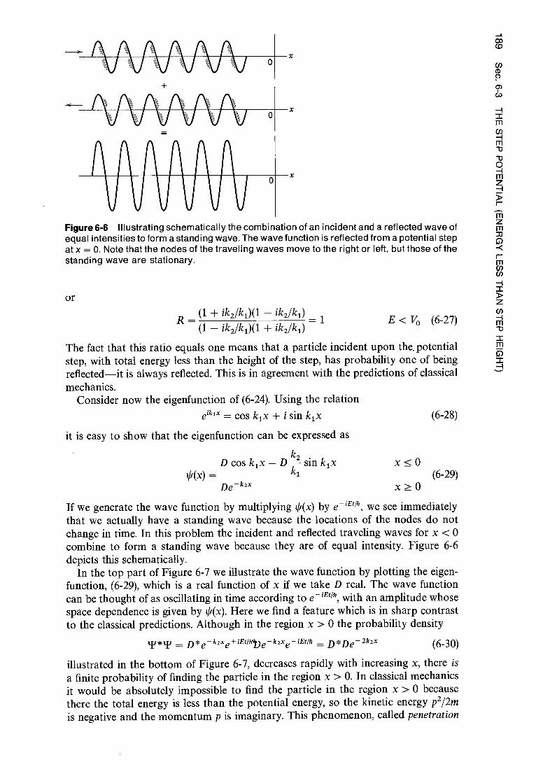
x

y7

4\ A^ A^ À

\

o

^

TH

E S

TE

P P

OT

EN

TIA

L (E

NE

RG

Y LE

SS

TH

AN

ST

EP

HE

IGH

T)

Figure 6-6 Illustrating schematically the combination of an incident and a reflected wave of

equal intensities to form a standing wave. The wave function is reflected from a potential step at x = O. Note that the nodes of the traveling waves move to the right or left, but those of the standing wave are stationary.

or

R — (1 + ik 2/k i )(1 — ik2/ki) _ 1

E < Vo (6-27) (1 — ik2/ki)( 1 + ik2/ki)

The fact that this ratio equals one means that a particle incident upon the. potential step, with total energy less than the height of the step, has probability one of being reflected—it is always reflected. This is in agreement with the predictions of classical mechanics.

Consider now the eigenfunction of (6-24). Using the relation

eiktx = cos k ix + i sin kix (6-28)

it is easy to show that the eigenfunction can be expressed as

D cos k lx—Dk2 sin k ix x<0 t//(x) = k1 (6-29)

De-k2x x>- 0

If we generate the wave function by multiplying /i(x) by a - `E:m, we see immediately that we actually have a standing wave because the locations of the nodes do not change in time. In this problem the incident and reflected traveling waves for x < 0 combine to form a standing wave because they are of equal intensity. Figure 6-6 depicts this schematically.

In the top part of Figure 6-7 we illustrate the wave function by plotting the eigen-function, (6-29), which is a real function of x if we take D real. The wave function can be thought of as oscillating in time according to e - iEt/J, with an amplitude whose space dependence is given by 0(x). Here we find a feature which is in sharp contrast to the classical predictions. Although in the region x > 0 the probability density

^*^ ^ = D* e k 2 x e +iEt^ e -k2x e -iEtlh = D*De 2k2x (6-30)

illustrated in the bottom of Figure 6-7, decreases rapidly with increasing x, there is a finite probability of finding the particle in the region x > 0. In classical mechanics

it would be absolutely impossible to find the particle in the region x > 0 because

there the total energy is less than the potential energy, so the kinetic energy p 2/2m is negative and the momentum p is imaginary. This phenomenon, called penetration

e

J J J

1 A

^

r

J V f

1

kY *(x, t) kJ, (x, t) All t

0

Figure 6-7 Top: The eigenfunction iii(x) for a particle incident upon a potential step at x= 0, with total energy less than the height of the step. Note the penetration of the eigenfunc-tion into the classically excluded region x > O. Bottom: The probability density T*`I` = i/i*0 = 2 corresponding to this eigenfunction. The spacing between the peaks of 02 is twice as

Y close as the spacing between the peaks of Li.

of the classically excluded region, is one of the more striking predictions of quantum mechanics.

We shall discuss later certain experiments which confirm this prediction, but here we should like to make several points about it. One is that penetration does not mean that the particle is stored in the classically excluded region. Indeed, we have seen that the incident particle is definitely reflected from the step.

Another point is that penetration of the excluded region, which obeys (6-30), is not in conflict with the experiments of classical mechanics. It is apparent from the equa-tion that the probability of finding the particle with a coordinate x > 0 is only appreciable in a region starting at x = 0 and extending in a penetration distance Ax, which equals 1/k 2 . The reason is that e - 2kzx goes very rapidly to zero when x is very much larger than 1/k 2 . Since k 2 = V2m(Vo — E)/h, we have

h

J2m(Vo — E)

In the classical limit, the product of m and (V0 — E) is so large, compared to h 2 , that Ax is immeasurably small.

Example 6 -1. Estimate the penetration distance Ax for a very small dust particle, of radius

r = 10 -6 m and density p = 104 kg/m 3 , moving at the very low velocity y = 10 -2 m/sec, if the particle impinges on a potential step of height equal to twice its kinetic energy in the region

to the left of the step. •The mass of the particle is

m= 4 nr3p^_ 4x 10 - 18 m 3 x 104 kg/m 3 =4x 10 -14 kg

SO

LUT

ION

S O

F T

IME

-IN

DE

PE

ND

EN

T S

CH

RO

ED

I NG

ER

EQ

UA

TIO

NS

x

Ox =

Its kinetic energy before hitting the step is

2 mv 2 2 x 4 x 10 -14 kg x 10 -4 m2/sec 2 = 2 x 10 -18 joule

and this is also the value of (V0 — E). The penetration distance is h 10 -34 joule-sec

Ax = V2m(V o — E) J2 x 4 x 10 -14 kg x 2 x 10 -18 joule

2 x 10 -19 m

Of course, this is many orders of magnitude smaller than could be detected in any possible measurement. For the more massive particles and higher energies typically considered in classical mechanics, Ax is even smaller. •

Furthermore, we should like to point out that the uncertainty principle shows the wavelike properties exhibited by an entity in penetrating the classically excluded re-gion are really not in conflict with its particlelike properties. Consider an experiment capable of proving that the particle is located somewhere in the region x > O. Since the probability density for x > 0 is appreciable only in a range of length Ax, the experiment amounts to localizing the particle within that range. In doing this, the experiment necessarily leads to an uncertainty Ap in the momentum, which must be at least as large as

h AP

^ ^ V/2m(Vo — E)

Consequently, the energy of the particle is uncertain by an amount

AE ^ (0)a Vo — E

and it is no longer possible to say that the total energy E of the particle is definitely less than the potential energy Vo . This removes the conflict alluded to.

Penetration of the classically excluded region can lead to measurable consequences. We shall see this later for a potential that steps up to a height V o > E, but remains up only for a distance not much larger than the penetration distance Ax, and then steps down. In fact, the phenomenon has significant practical consequences. One ex-ample, which we shall refer to soon, is the tunnel diode used in modern electronics.

Example 6 -2. A conduction electron moves through a block of Cu at total energy E under the influence of a potential which, to a good approximation, has a constant value of zero in the interior of the block and abruptly steps up to the constant value Vo > E outside the block. The interior value of the potential is essentially constant, at a value that can be taken as zero, since a conduction electron inside the metal feels little net Coulomb force exerted by the approxi-mately uniform charge distributions that surround it. The potential increases very rapidly at the surface of the metal, to its exterior value V 0 , because there the electron feels a strong force exerted by the nonuniform charge distributions present in that region. This force tends to attract the electron back into the metal and is, of course, what causes the conduction electron to be bound to the metal. Because the electron is bound, V0 must be greater than its total energy E. The exterior value of the potential is constant, if the metal has no total charge, since outside the metal the electron would feel no force at all. The mass of the electron is m = 9 x 10 -31 kg. Measurements of the energy required to permanently remove it from the block, i.e., measurements of the work function, show that Vo — E = 4 eV. From these data estimate the distance Ax that the electron can penetrate into the classically excluded region outside the block. ■ In the mks system

1.6 x 10 -19 joule . Vo — E = 4eV x

1eV ^ 6 x 10 joule

TH

E S

TE

P P

OT

EN

TIA

L (E

NE

RG

Y L

ES

S T

HA

N S

TE

P H

EIG

HT

)

N c) r

SO

LUTI

ON

S O

F T

IME

- IN

DE

PE

ND

EN

T S

CH

RO

ED

ING

ER

EQ

UA

TIO

NS

So

h

J2m(Vo — E)

10 - 34joule-sec

N/2x9x 10 -31 kg x 6 x 10 -19 joule 10 -le m

The penetration distance is of the order of atomic dimensions. Therefore, the effect can be of consequence in atomic systems. We shall find soon that, in certain circumstances, the effect is very important indeed. •

Let us finally make the point that penetration of the classically excluded region is nonclassical in the sense that an entity that does it is not behaving like a classical par-ticle. But it is behaving like a classical wave since, as we shall see later, the phenom-enon has been known to occur with light waves since the time of Newton. Penetration of the classically excluded region by material particles is just another manifestation of the wavelike nature of material particles.

Figure 6-8 shows the probability density for a wave function in the form of a group, for the problem of a particle incident in the direction of increasing x upon a potential step with an average value of the total energy less than the step height. The wave func-tion can be obtained by summing, over the total energy E, a very large number of wave functions of the form we have obtained in (6-25). It can also be obtained by a direct numerical solution of the Schroedinger equation. Either way involves a large amount of work on a high-speed computer, as can be guessed from the complications

t =0 t =5At t = 60t

^

t = 7At t = 90t t = 110t

t = 12At t = 140t t = 20At

A .

Figure 6 -8 A potential step, and the probability density `1" for a group wave function

describing a particle incident on the step with total energy less than the step height. As time

evolves, the group moves up to the step, penetrates slightly into the classically excluded region, and then is completely reflected from the step. The complications of the mathe-matical treatment using a group are indicated by the complications of its structure during

reflection.

Ax =

indicated in the figure. The results of the calculations certainly convey a realistic sense of the particle motion; but note that these results show, again, that the particle associ-ated with the wave function is reflected from the step with probability one, and that there is some penetration of the classically excluded region. The fact that we have been able to learn these basic results from simple calculations, involving only the wave function of (6-25) which contains a single value of E, is an example of the fact that it is generally not necessary in quantum mechanics to use wave functions in the form of groups. Of course, we must be willing to learn how to interpret the simple wave functions.

6-4 THE STEP POTENTIAL (ENERGY GREATER THAN STEP HEIGHT)

In this section we consider the motion of a particle under the influence of a step potential, (6-11), when its total energy E is greater than the height Vo of the step. That is, we take E > Vo , as illustrated in Figure 6-9.

In classical mechanics, a particle of total energy E traveling in the region x < 0, in the direction of increasing x, will suffer an impulsive retarding force F = — dV(x)/dx at the point x = O. But the impulse will only slow the particle, and it will enter the region x > 0, continuing its motion in the direction of increasing x. Its total energy E remains constant; its momentum in the region x < 0 is p i , where pi/2m = E; its momentum in the region x > 0 is p2 , where p/2m = E — Vo .

We shall see that the predictions of quantum mechanics are not so simple. If E is not too much larger than V0 , the theory predicts that the particle has an appreciable chance of being reflected at the step back into the region x < 0, even though it has enough energy to pass over the step into the region x > O.

One example of this is found in the case of an electron in the cathode of a photo-electric cell, which has received energy from absorbing a photon, and which is trying to escape the surface of the metallic cathode. If its energy is not much higher than the height of the step in the potential that it feels at the surface of the metal, it may be reflected back and not succeed in escaping. This leads to a significant reduction in the efficiency of photocells for light of frequencies not far above the cutoff frequency.

A more important example of reflection occurring when a particle tries to pass over a potential step is found in the motion of a neutron in a nucleus. To a good approxi-mation, the potential acting on the neutron near the nuclear surface is a step poten-tial. The potential rises very rapidly at the nuclear surface because a nucleus tends to bind a neutron. If the neutron has received energy, in one way or another, and is trying to escape the nucleus, it will probably be reflected back into the nucleus at the surface if its energy is only a little greater than the step height. This has the effect of inhibiting the emission of lower energy neutrons from nuclei, and thereby consider-ably increases the stability of nuclei in low-lying excited states. The effect is a mani-festation of the wavelike properties of neutrons that is very significant in the processes taking place in nuclear reactions, as we shall see near the end of this book.

V(x)

E

V(x) = Vo 1

TH

E S

TE

P P

OT

EN

TIA

L (E

NE

RG

Y G

RE

AT

ER

TH

AN

ST

EP

HE

IGH

T)

V(x) = 0

Figure 6-9 The relation between total and potential energies for a particle incident up-on a potential step with total energy greater than the height of the step. 0

SO

LUT

ION

S O

F T

IME

-IN

DE

PE

ND

EN

T S

CH

RO

ED

ING

ER

EQ

UA

TI O

NS

In quantum mechanics, the motion of the particle under the influence of the step

potential is described by the wave function

^(x,t) = (x)e Ufa,

where the eigenfunction ÿr(x) satisfies the time-independent Schroedinger equation for the potential. This equation has different forms in the regions to the left and right of the potential step, namely

and

h2 d2 tŸ(x) = EVI(x) 2m dx 2

h 2 d2t//(x) _ (E — Vo)(P(x) 2m dx 2

x < 0 (6-31)

x > 0 (6-32)

The eigenfunction ti/(x) also satisfies the conditions requiring finiteness, single valued- ness, and continuity, for it and its derivative, particularly at the joining point x = 0.

Equation (6-31) describes the motion of a free particle of momentum p i . Its general solution is

ifi(x) = Ae iklx + Be -iklx x < 0 (6-33) where

k i =h h

Equation (6-32) describes the motion of a free particle of momentum p 2 . Its general solution is

cc) ci where

Û V2m(E— Vo) pz k 2 =h h

The wave function specified by these two forms consists of traveling waves of de Broglie wavelength ;L i = h/p i = 2i/k i in the region x < 0, and of longer de Broglie

wavelength /1 2 = h/p 2 = 27r/k 2 in the region x > O. Note that the functions we deal with here already satisfy the requirements of finiteness and single valuedness; but we must explicitly consider their continuity, and we shall do so shortly.

A particle initially in the region x < 0, and moving towards x = 0 would, in classical mechanics, have probability one of passing the point x = 0 and entering the region x > O. This is not true in quantum mechanics. Because of the wavelike prop-erties of the particle, there is a certain probability that the particle will be reflected at the point x = 0, where there is a discontinuous change in the de Broglie wave-length. Thus we need to take both terms of the general solution of (6-33) to describe the incident and reflected traveling waves in the region x < 0. We do not, however, need to take the second term of the general solution of (6-34). This term describes a wave traveling in the direction of decreasing x in the region x > O. Since the particle is incident in the direction of increasing x, such a wave could arise only from a reflection at some point with a large positive x coordinate (well beyond the discontinuity at x = 0). As there is nothing out there to cause a reflection, we know that there is only a transmitted traveling wave in the region x > 0, and so we take the arbitrary constant D to have the value

D = 0 (6-35)

The arbitrary constants A, B, and C must be chosen to make fi(x) and dtr(x)/dx continuous at x = O. The first requirement, that the values of Ji(x) expressed by (6-33)

V2mE Pi

If/ (x) = Ce`kzx + De ikzx x > 0 (6-34)

E > Yo

^ cn S

ec. 6

-4 T

HE

ST

EP

PO

TE

NT

IAL

(EN

ER

GY

GR

EA

TE

R T

HA

N S

TE

P H

EIG

HT

) and (6-34) be the same at x = 0, is satisfied if

A(e iki x )x-0

+ B(e -ikix)x= 0 - C(e ik2x)x =0

or A + B = C (6-36)

The second requirement, that the values of the derivatives of the two expressions for

tji(x) be the same at x = 0, is satisfied if

ik A(eikix) — ik B(e-ik2x)

= ik C(e ik2x) 1 x=0 1 x0 2 x=o

or k l (A—B)=k 2 C

From the last two numbered equations, we find

B k l + k2 A and C= k

+ik A i 2 i 2

Thus the eigenfunction is

Aeikix + A kl - k2 e iklx x Ç 0

kl + k2

A 2k1 eikzx x > 0 kl + k2

As before, it will not be necessary to evaluate the arbitrary constant A that determines the amplitude of the eigenfunction.

It is clear that an eigenfunction satisfying the two continuity conditions could not have been

found if we had initially set the coefficient B of the reflected wave equal to zero. We would then

have had only two arbitrary constants to satisfy the two continuity conditions, and we would

not have had one left over to play the role, demanded by the linearity of the time-independent

Schroedinger equation, of an arbitrary constant that determines the amplitude of the eigen-function.

By analogy with our interpretation of the eigenfunction of (6-24), we recognize that

the first term in the expression of (6-39) valid for x < 0 (left of the discontinuity)

represents the incident traveling wave; the second term in the expression valid for

x < 0 represents the reflected traveling wave; and the expression valid for x > 0 (right

of the discontinuity) represents the transmitted traveling wave.

Figure 6-10 illustrates the probability density `F*(x,t)T(x,t) = *(x) /,(x) for the

wave function T(x,t) corresponding to the eigenfunction t/i(x) of (6-39) (in the repre-sentative case k l = 2k2). We do not plot either the eigenfunction or wave function, as

both are complex. In the region x > 0 the wave function is a pure traveling wave (of

amplitude 4A/3 in this case) traveling to the right, and so the probability density is

'Y * (x, t) W (x, t) All t

^ (16/9) AM

(4/9) AM

(6-37)

(6-38)

(6-39)

r

x 0

Figure 6-10 The probability density 'I' *P for the eigenfunction of (6-39), when k l = 2k2 .

SO

LUT

ION

S O

F T

IME

-IN

DE

PE

ND

EN

T S

CH

RO

ED

ING

ER

EQ

UA

TIO

NS

constant as in the bottom part of Figure 6-1. In the region x < 0 the wave function is a combination of the incident traveling wave (of amplitude A) moving to the right, and a reflected traveling wave (of amplitude A/3) moving to the left. As the ampli-tude of the reflected wave is necessarily smaller than that of the incident wave, the two cannot combine to yield a pure standing wave. Their sum `Y(x,t) in that region is, instead, something between a standing wave and a traveling wave. This is seen in the behavior of `I'*(x,t) 11'(x,t) for x < 0, which looks like something between the pure standing wave probability density of Figure 6-7 and the pure traveling wave proba-bility density of Figure 6-1 in that it oscillates but has minimum values greater than zero.

The ratio of the intensity of the reflected wave to the intensity of the incident wave gives the probability that the particle will be reflected by the potential step back into the region x < 0. This probability is the reflection coefficient R. That is

R _ B*B _ k 1 — k2l

* (k1 — k 2 k 1 — k 2 2 E > V A*A \k1 + k2) \k1 + k2) k 1 + k2) ° (6-40)

We see from this result that R < 1 when E > Vo , i.e., when the total energy of the particle is greater than the height of the potential step. This is in contrast to the value R = 1 when E < V° , that we obtained from the result of Section 6-3. Of course, the thing that is surprising about the present result is not that R < 1, but that R > 0. It is surprising because a classical particle would definitely not be reflected if it had enough energy to pass the potential discontinuity. On the other hand, at a corre-sponding discontinuity a classical wave would be reflected, as we shall discuss shortly.

Also of interest is the transmission coefficient T, which specifies the probability that the particle will be transmitted past the potential step from the region x < 0 into the region x > 0. The evaluation of T is slightly more complicated than the evaluation of R because the velocity of the particle is different in the two regions. According to accepted convention, transmission and reflection coefficients are actually defined in terms of the ratios of probability fluxes. A probability flux is the probability per second that a particle will be found crossing some reference point traveling in a particular direction. The incident probability flux is the probability per second of finding a par-ticle crossing a point at x < 0 in the direction of increasing x; the reflected proba-bility flux is the probability per second of finding a particle crossing a point at x < 0 in the direction of decreasing x; and the transmitted probability flux is the probability per second of finding a particle crossing a point at x > 0 in the direction of increasing x. Since the probability per second that a particle will cross a given point is pro-portional to the distance it travels per second, the probability flux is proportional not only to the intensity of the appropriate wave but also to the appropriate velocity of the particle. (A more detailed discussion of this point is given in connection with Figure L-2 in Appendix L.) Thus, according to the strict definition, the reflection co-efficient R is

R_ v 1 B B — B B (6-41)

v1A*A A*A

where v 1 is the velocity of the particle in the region x < 0. Since the velocities cancel, what remains is identical to the formula we have used previously for R. For T, the velocities do not cancel, and we have

v2 C*C _ v2 ( 2k1 )2 _

T v1 A*A v l I\k l + k2 )

v2 is the velocity of the particle in the region x > 0. Now

pi hk1 p2 hk2

v 1 =—= and v2 =—_ m m m m

So the above expression gives

T _ k 2 (2k1 ) 2 4ki k 2

k2)2 = k2)2 E > Vo (6-42) cn k 1 (k1 + k2) (k1 + k2) cD

It is easy to show by evaluating R and T from (6-40) and (6-42) that o>

R + T = 1 (6-43) This useful relation is the motivation for defining the reflection and transmission co-efficients in terms of probability fluxes.

The probability flux incident upon the potential step is split into a transmitted flux and a reflected flux. But (6-43) says their sum equals the incident flux; i.e., the proba-bility that the particle is either transmitted or reflected is one. The particle does not vanish at the step; nor does the particle itself split at the step. In any particular trial the particle will go one way or the other. For a large number of trials, the average probability of going in the direction of decreasing x is measured by R, and the aver-age probability of going in the direction of increasing x is measured by T.

Note that R and T are both unchanged in value if k 1 and k2 are exchanged in (6-40) and (6-42). A moment's consideration should convince the student that this means the same values of R and T would be obtained if the particle were incident upon the potential step in the direction of decreasing x from the region x > 0. The wave func-tion describing the motion of the particle, and consequently the probability flux, is partially reflected simply because there is a discontinuous change in V(x), and not because V(x) becomes larger in the direction of the incidence of the particle. The be-havior of R and T when k 1 and k2 are exchanged involves a characteristic property of all waves that, in optics, is sometimes called the reciprocity property. When light passes perpendicularly through a sharp interface between media with different indices of refraction, a fraction of the light is reflected because of the abrupt change in its wavelength, and the same fraction is reflected independent of whether it is incident from one side of the interface or from the other. Exactly the same thing happens when a microscopic particle experiences an abrupt change in its de Broglie wavelength. In fact, the equations governing the two phenomena are identical in form. We see, once again, that a microscopic particle moves in a wavelike manner.

In Figure 6-11 the reflection and transmission coefficients are plotted as functions of the convenient ratio E/Vo . By evaluating k 1 and k2 in (6-40) and (6-42), we find that these expressions for the reflection and transmission coefficients can be written in terms of the ratio as

R=1 —T— 1 — — Vo/E 2 E

— > 1 (6-44) — 1 + 1Vo/ E) Vo

^

0.5 1.0 1.5 2.0 E/V0

Figure 6-11 The reflection and transmission coe ff icients R and T for a particle incident upon a potential step. The abscissa E/Vo is the ratio of the total energy of the particle to the increase in its potential energy at the step. The case k 1 = 2k2 , illustrated in Figure 6-10, corresponds to E/Vo = 1.33.

TH

E S

TE

P P

OT

EN

TIA

L (E

NE

RG

Y G

RE

AT

ER

TH

AN

ST

EP

HE

IGH

T)

CO

rn

S

OLU

TIO

NS

OF

TIM

E-I

ND

EP

EN

DE

NT

SC

HR

OE

DIN

GE

R E

QU

ATI

ON

S The figure also plots the results

R =1—T=1 V <1 o

obtained in (6-27) of the preceding section for a step potential when E/Vo < 1. As an example, for E/Vo = 1.33 the transmission coefficient has the value T = 0.88.

This E/Vo ratio corresponds to the case k 2 = k 1/2 whose probability density pattern is illustrated in Figure 6-10. Note from that figure that the probability of finding the particle in a given length of the x axis, which is long enough to average over the quantum mechanical fluctuations in the probability density, is nearly twice as large to the right of the potential step as it is to the left of the step. From a classical point of view, which is appropriate to discussing an average over quantum mechan-ical fluctuations, it can be said that the reasons for this are: (a) the probability that the particle will pass the step and proceed into the region to its right is almost equal to one, and (b) the particle's velocity is halved when it enters the region to the right of the step since k = p/h = mv/h and k2 = k 1 /2, so it spends twice as much time in any given length of the axis in that region.

From Figure 6-11 we see that the energy of the particle must be appreciably higher than the height of the potential step before the probability of reflection becomes negligible. However, the case in which E becomes very large is not necessarily the case of the classical limit for which we know there will be no reflection at all. The point is that (6-44) says R depends only on the ratio E/Vo , so that it will keep the same value if Vo increases as rapidly as E. This seems paradoxical until we realize that, in the limit of large energies, our basic assumption that the change in the value of the step potential V(x) is perfectly sharp can no longer be even an approximation to a real physical situation. If the potential function changes only very gradually with x, then the de Broglie wavelength will change only very gradually. In this case the reflection will be negligible because the change in wavelength is gradual, and reflec-tion arises from an abrupt change in the wavelength. Specifically, if the fractional change in V(x) is very small when x changes by one de Broglie wavelength, then the reflection coefficient will be very small. This gives rise to the classical limit since in that limit the de Broglie wavelength is so short that any physically realistic po-tential V(x) changes only by a negligible fraction in one wavelength.

For particles in atomic or nuclear systems, the de Broglie wavelength can be long relative to the distance in which the potential experienced by the particle changes value significantly. Then the step potential is a very good approximation. For these microscopic particles, the probability of reflection can be large.

Example 6-3. When a neutron enters a nucleus, it experiences a potential energy which drops at the nuclear surface very rapidly from a constant external value V = 0 to a constant internal value of about V = — 50MeV. The decrease in the potential is what makes it possible for a neutron to be bound in a nucleus. Consider a neutron incident upon a nucleus with an external kinetic energy K = 5 MeV, which is typical for a neutron that has just been emitted from a nuclear fission. Estimate the probability that the neutron will be reflected at the nuclear surface, thereby failing to enter and have its chance at inducing another nuclear fission. ■ For an estimate, we may take the neutron-nucleus potential to be a one-dimensional step potential, as illustrated in Figure 6-12. Because of the reciprocity property of the reflection coefficient, we may evaluate it from (6-44), using V o = 50 MeV and E = 55 MeV for reasons that can be seen by inspection of the figure. We have

R

= (

1 — /1- 50/55) 2 , 0.29 1 + — 50/55

This estimate gives a correct impression of the great importance of the reflection phenomenon when low-energy neutrons collide with nuclei. But the numerical value we have obtained for the reflection coefficient is not very accurate since the actual neutron-nucleus potential does not

x

1bI1

N3

10d

}:11aab'8

3H

1 9

- 9 '0

9S

> ^

11

E =

55

MeV

Figure 6-12 A neutron of external kinetic energy K incident upon a decreasing potential

step of depth Vo , which approximates the potential it feels upon entering a nucleus. Its total energy, measured from the bottom of the step potential, is E.

drop quite as rapidly at the nuclear surface, in comparison to the de Broglie wavelength,

as a step potential.

6-5 THE BARRIER POTENTIAL

In this section we consider a barrier potential, illustrated in Figure 6-13. The potential can be written as follows

Vo 0<x<a V(x) = (6 -45)

0 x<Oorx> a According to classical mechanics, a particle of total energy E in the region x < 0, which is incident upon the barrier in the direction of increasing x, will have proba-bility one of being reflected if E < Vo , and probability one of being transmitted into the region x > a if E > Vo .

Neither of these statements describes accurately the quantum mechanical results. If E is not much larger than Vo , the theory predicts that there will be some reflection, except for certain values of E. If E is not much smaller than V0, quantum mechanics predicts that there is a certain probability that the particle will be transmitted through the barrier into the region x > a.

In "tunneling" through a barrier whose height exceeds its total energy, a material particle is behaving purely like a wave. But in the region beyond the barrier it can be detected as a localized particle, without introducing a significant uncertainty in the knowledge of its energy. Thus penetration of a classically excluded region of limited width by a particle can be observed, in the sense that the particle can be observed to be a particle, of total energy less than the potential energy in the excluded region, both before and after it penetrates the region. We shall discuss some consequences of this fascinating effect in the present section, as well as some consequences of the reflection of particles attempting to pass over a barrier. The following section is devoted completely to examples of tunneling through barriers, and considers three of particular importance: (1) the emission of a particles from radioactive r^ lei through the potential barrier they experience in the vicinity of the nuclei, (2) the inversion of the ammonia molecule which provides a frequency standard for atomic clocks, and (3) the tunnel diode used as a switching unit in fast electronic circuits.

V(x)

Vo

0 a

Figure 6-13 A barrier potential.

0 0 N

SO

LUT

ION

S O

F T

IME

-IN

DE

PE

ND

EN

T S

CH

RO

ED

ING

ER

EQ

UA

TIO

NS

For the barrier potential of (6-45), we know from the qualitative arguments of the

last chapter that acceptable solutions to the time-independent Schroedinger equation

should exist for all values of the total energy E > O. We also know that the equa-tion breaks up into three separate equations for the three regions: x < 0 (left of the

barrier), 0 < x < a (within the barrier), and x > a (right of the barrier). In the regions

to the left and to the right of the barrier the equations are those for a free particle

of total energy E. Their general solutions are 0(x) = Ae` k,x + Be - `k'x x < 0

(6-46)

where ^2mE

k1_ h

In the region within the barrier, the form of the equation, and of its general solution,

depends on whether E < Vo or E > Vo . Both of these cases have been treated in the

previous sections. In the first case, E < Vo , the general solution is 0(x) = Fe-k " + GekIIx 0 < x < a (6-47)

where J2m(V0 —E)

h

In the second case, E > Vo , it is 0(x) = Fe` k'nx + Ge - ck1IIx

where -\I2m(E — Vo)

kII, =

h

Note that (6-47) involves real exponentials, whereas (6-46) and (6-48) involve complex exponentials.

Since we are considering the case of a particle incident on the barrier from the

left, in the region to the right of the barrier there can be only a transmitted wave

as there is nothing in that region to produce a reflection. Thus we can set

D= 0 In the present situation, however, we cannot set G = 0 in (6-47) since the value of x is limited in the barrier region, 0 < x < a, so 0(x) for E < Vo cannot become infinitely large even if the increasing exponential is present. Nor can we set G = 0 in (6-48) since /i(x) for E > Vo will have a reflected component in the barrier region that arises from the potential discontinuity at x = a.

We consider first the case in which the energy of the particle is less than the height of the barrier, i.e., the case: E < Vo In matching ,P(x) and di/i(x)/dx at the points x = 0 and x = a, four equations in the arbitrary constants A, B, C, F, and G will be obtained. These equations can be used to evaluate B, C, F, and G in terms of A. The value of A determines the amplitude of the eigenfunction, and it can be left arbitrary. The form of the probability density corresponding to the eigenfunction obtained is indicated in Figure 6-14 for a typical situation. In the region x > a the wave function is a pure traveling wave and so the

probability density is constant, as for x > 0 in Figure 6-10. In the region x < 0 the

wave function is principally a standing wave but has a small traveling wave com-ponent because the reflected traveling wave has an amplitude less than that of the

tlf (x) = Ce k̀Ix + De X > a

k11 = E < Vo

0 < x < a (6-48)

E > Vo

^Y * (x, (x, t) All t

x

v1C*C T — — (ekna — e — k'Ia)2

1 + —1 — sinh2 k„a

1 + -1

v1A* A 16E 1—E

Vo Vo 4E(1

E 1

Vo Vo/J

_

1d

I1N

310d

1:131

aaV

8 3H

1

0

Figure 6-14 The probability density function 'PT for a typical barrier penetration situation.

incident wave. So the probability density in that region oscillates but has minimum values somewhat greater than zero, as for x < 0 in Figure 6-10. In the region 0 < x < a the wave function has components of both types, but it is principally a standing wave of exponentially decreasing amplitude, and this behavior can be seen in the behavior of the probability density in the region.

The most interesting result of the calculation is the ratio T, of the probability flux transmitted through the barrier into the region x > a, to the probability flux incident upon the barrier. This transmission coefficient is found to be

6-49 ( )

where

kola = J2mJ'a2 (

1— V E < Vo

0

If the exponents are very large, this formula reduces to

T — 16 Vo ( 1 Vo le zkIIa kIla » 1 (6-50)

as can be verified with ease. When (6-50) is a good approximation, T is extremely small.

These equations make a prediction which is, from the point of view of classical mechanics, very remarkable. They say that a particle of mass m and total energy E,

incident on a potential barrier of height Vo > E and finite thickness a, actually has a certain probability T of penetrating the barrier and appearing on the other side. This phenomenon is called barrier penetration, and the particle is said to tunnel through the barrier. Of course, T is vanishingly small in the classical limit because in that limit the quantity 2m Voa2/h 2, which is a measure of the opacity of the barrier, is ex-tremely large.

We shall discuss barrier penetration in detail shortly, but let us first finish de-scribing the calculations by considering the case in which the energy of the particle is greater than the height of the barrier, i.e., the case: E> Vo In this case the eigenfunction is oscillatory in all three regions, but of longer wave-length in the barrier region, 0 < x < a. Evaluation of the constants B, C, F, and G

by application of the continuity conditions at x = 0 and x = a, leads to the following formula for the transmission coefficient

T — v1C*C = 1 — (eikIlIa — e tkIIIa)z 1

— 1 + sinz kiria -1 6-51 * (6-51)

v 1 A A 16

Vo (Vo-1^ Vo (Vo-1 1

N O N

SO

LUT

ION

S O

F T

IME

-IN

DE

PE

ND

EN

T S

CH

RO

ED

ING

ER

EQ

UA

TIO

NS

2mV°a2 ^ E krna =

h 2 Vo

where

1 ) E > V0

Example 6 -4. An electron is incident upon a rectangular barrier of height V 0 = 10 eV and thickness a = 1.8 x 10 -10 m. This rectangular barrier is an idealization of the barrier en-countered by an electron that is scattering from a negatively ionized gas atom in the "plasma" of a gas discharge tube. The actual barrier is not rectangular, of course, but it is about the height and thickness quoted. Evaluate the transmission coefficient T and the reflection coeffi-cient R, as a function of the total energy E of the electron. • From Example 6-2 we can see that if E is a reasonable fraction of V0 the penetration length Ax will be comparable to the barrier thickness a. Thus we can expect appreciable transmission through the barrier. To determine exactly how much, we use the numbers given to evaluate the combination of parameters

2mV0a2 2 x 9 x 10 -31 kg x 10 eV x 1.6 x 10 -19 joule/eV x (1.8) 2 x 10 -20 m2 _ ^ 9 h2 10 -68 joule2 -sec 2

which enters (6-49). From this we can plot T, and also R = 1 — T, versus E/V0 , in the range 0 < E/VO < 1. The plot is shown in Figure 6-15. We see that T is very small when E/V O « 1. But, when E/VO is only somewhat smaller than one, so that E is nearly as large as V0 , T is not at all negligible. For instance, when E is half as large as V0 so that E/VO = 0.5, the transmis-sion coefficient has the appreciable value T ^ 0.05. It is apparent that electrons can penetrate this barrier with relative ease.

For E/VO > 1, we evaluate T, and R = 1 — T, from (6-51), using the same combination of parameters as before. The results are also shown in Figure 6-15. For E/V O > 1, the transmission coefficient T is in general somewhat less than one, owing to reflection at the discontinuities in the potential. However, from (6-51) it can be seen that T = 1 whenever krna = m, 2n, 3n, .... This is simply the condition that the length of the barrier region, a, is equal to an integral or half-integral number of de Broglie wavelengths )m = 2n/k,,, in that region. For this particular barrier, electrons of energy E 21 eV, 53 eV, etc., satisfy the condition k üja = 2n, etc., and so pass into the region x > a without any reflection. The effect is a result of destructive inter-ference between reflections at x = 0 and x = a. It is closely related to the Ramsauer effect observed in the scattering of low-energy electrons by noble gas atoms, in which electrons of certain energies in the range of a few electron volts pass through these atoms as if they were not there, and so have transmission coefficients equal to one.- Essentially the same effect is seen in scattering of neutrons, with energies of a few MeV, from all nuclei. The nuclear effect, called size resonance, will be discussed later in the book. •

T

J

0 1

5

1 0 E/V0

Figure 6-15 The reflection and transmission coefficients R and T for a particle incident upon a potential barrier of height VO and thickness a, such that 2mV 0a 2/h 2 = 9. The abscis- sa E/V O is the ratio of the total energy of the particle to the height of the potential barrier.

1 .0

0 R

We can bring together the results of the last three sections by comparing the plot of the energy dependence of the reflection coefficient R for a barrier potential, in Fig-ure 6-15, with the plot of the same thing for a step potential, in Figure 6-11. The com-parison shows that for both potentials R —* 1 as E/Vo 0, and R —> 0 as E/Vo —> oo, with the decrease in R occurring around E/Vo = 1. But for the barrier potential the reflection coefficient approaches one gradually, at small energies, since the finite thick-ness of the classically excluded region allows some transmission. Also, the barrier potential reflection coefficient oscillates, at large energies, because of interferences in the reflections from its two discontinuities. As the step potential can be considered to be a limiting case of a barrier of very great width, we can see from our comparison the behavior of the barrier potential reflection coefficient in this limit.

Now we shall discuss in some detail the origins of these results. They all involve phenomena which arise from the wavelike behavior of the motion of microscopic particles, and each phenomenon is also observed in other types of wave motion. As we remarked in Chapter 5, the time-independent differential equation governing classical wave motion is of the same form as the time-independent Schroedinger equation. For instance, electromagnetic radiation of frequency y propagating through a medium with index of refraction it obeys the equation

d 2 0(x)

(27-cv

, h2 0(x) = 0 (6-52)

where the function tfr(x) specifies the magnitude of the electric or magnetic field. When we compare this with the time-independent Schroedinger equation, written in the form

d d (x) + hm [E — V(x)]r/i(x) = 0

we see that they are identical if the index of refraction in the former is connected with the potential energy function in the latter by the relation

,u(x) = 2TCv 2 [E — V(x)] (6-53)

Thus the behavior of an optical system with index of refraction µ(x) should be iden-tical to the behavior of a mechanical system with potential energy V(x), providing the two functions are related as in (6-53). Indeed, there are optical phenomena which are exactly analogous to each of the quantum mechanical phenomena that arise in considering the motion of an unbound particle. An optical phenomenon, completely analogous to the total transmission of particles over barriers of length equal to an integral or half-integral number of wavelengths, is used in the coating of lenses to obtain very high light transmissions and in thin film optical filters.

An optical analogue to the penetration of barriers by particles is found in the imag-inary indices of refraction that arise in total internal reflection. Consider a ray of light incident upon a glass-to-air interface at an angle greater than the critical angle O . The resulting behavior of the light ray is called total internal reflection, and it is illustrated in the top of Figure 6-16. A detailed treatment of the process in terms of electromagnetic theory shows that the index of refraction, measured along the line ABC, is real in the region AB but imaginary in the region BC. Note that an imaginary µ(x) is suggested by (6-53) for a region analogous to one in which E < V(x). Further-more, electromagnetic theory shows that there are electromagnetic vibrations in the region BC of exactly the same form as the decreasing exponential standing wave of (6-29) for the region where E < V(x). The flux of energy (the Poynting vector) is zero in this electromagnetic standing wave, just as the flux of probability is zero in the quantum mechanical standing wave, so the light ray is totally reflected. However, if a second block of glass is placed near enough to the first block to be in the region in

1`dI

1N31

0d 1=I

3IH

EIb

B 3

H1

Figure 6-16 Top: Illustrating total internal reflection of a light ray. The angle of in-cidence is greater than the critical angle. Bottom: Illustrating frustrated total internal reflection. Some of the light ray is trans-mitted through the air gap if the gap is suf-ficiently narrow.

SO

LUT

ION

S O

F T

IME

- IN

DE

PE

ND

EN

T S

CH

RO

ED

ING

ER

EQ

UA

TIO

NS

A C

Figure 6-17 The total internal reflection of water waves. A long vibrating plunger on the left produces a set of waves in a region of shallow water, the waves being illuminated so as to make their crests easily visible. The waves are totally internally reflected at the diagonal boundary of a region where the layer of water abruptly becomes deeper, this reflection occurring because the velocity of water waves depends on the depth of the water. Note that the intensity of the waves decreases rapidly when they try to penetrate into the region of deeper water, but there is some penetration of that region. (Courtesy Film Studio, Education Development Center)

Figure 6-18 Frustrated total internal reflection of water waves. When the region of deeper water becomes a sufficiently narrow gap, the waves that have penetrated into the deeper water are picked up and transmitted into a second region of shallow water. (Courtesy Film Studio, Education Development Center)

which the electromagnetic vibrations are still appreciable, these vibrations are picked up and propagate through the second block. Furthermore, the electromagnetic vibra-tions in the air gap now carry a flux of energy through to the second block. This phenomenon, called frustrated total internal reflection, is illustrated in the bottom of Figure 6-16. Essentially the same thing happens in the quantum mechanical case when the region in which E < V(x) is reduced from infinite thickness (step potential) to finite thickness (barrier potential). The transmission of light through an air gap, at an angle of incidence greater than the critical angle, was first observed by Newton around 1700. The equation relating the intensity of the transmitted beam to the thickness of the air gap, and other parameters, is identical in form to (6-49), and it has been verified experimentally.

It is particularly easy to observe frustrated total internal reflection of electromag-netic waves, using the microwave region of the spectrum and two blocks of paraffin separated by an air gap. Furthermore, careful inspection of the "ripple tank" photo-graphs in Figures 6-17 and 6-18 will show that the phenomenon can even be observed with water waves. Frustrated total internal reflection, or its quantum mechanical equivalent barrier penetration, arises from properties common to all forms of classical or quantum mechanical wave motion.

6-6 EXAMPLES OF BARRIER PENETRATION BY PARTICLES

There are a number of interesting, and important, examples of barrier penetration by micro-scopic particles. A widespread, but not widely recognized, example occurs in aluminum house-hold wiring. The usual way for an electrician to join two wires is to twist them together. Often there is a layer of aluminum oxide between the two wires, and this material is quite an effective

S3

10

Il1:1

b'd A

8 N

OIlH

1:113

N3d

b3I1

:11: 1

t18

dO

S31

dW

bX

3

CO 0 N

SO

LU

TIO

NS

OF

TIM

E- I

ND

EP

EN

DE

NT

SC

HR

OE

DIN

GE

R E

QU

AT

ION

S

Kinetic energy at large r

E

U 238

r' r "= 3.Ox

10 -14 m r

insulator. Fortunately, the layer is extremely thin so the electrons flowing through the wire are able to tunnel through the layer by barrier penetration.

Historically, the first application of the quantum mechanical theory of barrier penetration by particles was to explain a long standing paradox concerning the emission of a particles in the decay of radioactive nuclei. As a typical example, consider the U238 nucleus. The potential energy V(r) of an a particle at a distance r from the center of the nucleus had been investigated around 1910 by Rutherford, and others, who performed scattering experiments. Using as a probe the 8.8 MeV a particles emitted from the radioactive nuclei of Po212, it was observed that their probability of scattering at various angles from U238 nuclei agreed with the pre-dictions of Rutherford's scattering formula (see Chapter 4). The student will recall that the formula was based on the assumption that the interaction between the a particle and the nucleus strictly followed the Coulomb law repulsion that would be expected to operate be-tween the two positively charged spherical objects. Thus Rutherford was able to conclude that, for the U238 nucleus, the potential function V(r) felt by a neighboring a particle followed Coulomb's law, V(r) = 2Ze 2/4neor, where 2e is the a-particle charge and Ze is the nuclear charge—at least for distances greater than r" = 3 x 10 -14 m where V(r') = 8.8 MeV, the probe a-particle energy. It was also known by scattering a particles from nuclei of light atoms that V(r) eventually departs from a 1/r law when r < r', the nuclear radius, although the exact value of r' was not known for the nuclei of heavy atoms at that time. Furthermore, since a particles are occasionally emitted by U238 nuclei, it was assumed that they exist inside such nuclei, to which they are normally bound by the potential V(r). From these arguments it was concluded that the form of V(r) in the region r < r" must be qualitatively as depicted in Figure 6-19. This conclusion has been verified by modern experiments involving the scattering of a particles produced by cyclotrons at energies high enough to allow the investigation of the potential over the entire range of r.

The paradox was connected with the fact that it was also known that the kinetic energy of a particles emitted in radioactive decay by U238 was 4.2 MeV. The kinetic energy was, of course, measured at a very large distance from the nucleus where V(r) = 0 and the kinetic energy equals the total energy E. This value of the constant total energy of the decay a particles emitted by U238 is also shown in Figure 6-19. From the point of view of classical mechanics, the situation was certainly paradoxical. An a particle of total energy E is initially in the region r < r'. This region is separated from the rest of space by a potential barrier of a height which was known to be at least twice E. Yet it was observed that on occasion the a particle pene-trates the barrier and moves off to large values of r.

Figure 6-19 The potential energy V acting on an a particle at a distance r from the center of a U

238 nucleus, and the total energy E of an a particle emitted from that radioactive nucleus. The solid part of the potential 'curve was known from scattering measurements to follow Coulomb's law into the distance of closest approach r" of an 8.8 MeV a particle. The dashed part of the curve shows that the potential was assumed to continue to follow Cou-lomb's law into the nuclear radius r', where it must drop very rapidly to form a binding region. A 4.2 MeV a particle emitted from the radioactive nucleus must penetrate the poten-tial barrier from the nuclear radius r' to the point at distance r" from the center where its potential energy V becomes less than its total energy E.

To put it another way, according to classical mechanics an a particle emitted from a region where the potential energy function has the form shown in Figure 6-19 must, necessarily, have a much higher kinetic energy than was actually observed when it is far from the region. The reason is simply that in classical mechanics the total energy must be greater than the maximum value of the potential energy, if the particle is to escape the barrier. Consider the following analogy. You are walking beneath the span of a tall bridge, not looking up. Suddenly a brick hits you on the head, but gently, with a light tap. There is no place for the brick to come from, other than the bridge, but a brick falling from such a height would have developed enough kinetic energy to kill you!

In 1928 Gamow, Condon, and Gurney treated a-particle emission as a quantum mechanical barrier penetration problem. They assumed that V(r) = 2Ze 2/47re0r for r > r', where 2e is the a-particle charge and Ze is the charge of the nucleus remaining after the a particle is emitted. They also assumed that V(r) < E for r < r', as shown in Figure 6-19. Equation (6-50) was used to evaluate the transmission coefficient T since the exponent kna, which determines T, has a value large compared to one. In fact, the exponent is so large that the exponential completely dominates the behavior of T, and it was sufficient to take

T ^ e - 2krna = e - 2✓(2m1h2)(Vo— E)n

This expression was derived for a rectangular barrier of height V0 and width a, but when the expression is valid it can be applied to the barrier V(r) by considering it to be a set of adjacent rectangular barriers of height V(r z) and very small width Ar e . This reasoning leads, in the limit, to the expression

T e - 2fr, ✓(2m1*2)[V(r)—E]dr (6-55)

where the integration is taken from the nuclear radius r', where V(r) rises above E, to the ra-dius r"', where V(r) drops below E. The use of (6-54), which was derived for a one-dimensional case, in (6-55) that concerns a three-dimensional problem, was justified because the a particles are almost always emitted with zero angular momentum. That is, they move out along essen-tially linear paths emanating from the nuclear center, obeying equations which are essentially one-dimensional.

The quantity T gives the probability that in one trial an a particle will penetrate the barrier. The number of trials per second could be estimated to be

v

N 2r' (6-56)

if it were assumed that an a particle is bouncing back and forth with velocity y inside the nucleus of diameter 2r'. Then the probability per second that the nucleus will decay by emitting an a particle, called the decay rate R, would be

R v e -2fr; " .^/(2m/h 2)(2Ze 2/4, eor—E)d r

— 2r ' (6-57)

Today we know that (6-56) is not a very accurate estimate, but this function, or its more correct form, varies so slowly compared to the rapid variation in the exponential that the result expressed by (6-57) is an accurate estimate.

In applying (6-57) to a particular radioactive nucleus, Gamow, Condon, and Gurney took all the quantities in the expression as known, except y and r' (r"' can be evaluated from Z and E). Assuming y to be comparable to the velocity of the a particle after emission (i.e., mv 2/2 = E), the decay rate R is then a function only of the nuclear radius r'. Using r' = 9 x 10 -15 m, which was certainly in line with the values obtained from Rutherford's analysis of a-particle scattering from light nuclei, they obtained values of R which were in good agreement with those measured experimentally, although the decay rate varies over â tremendously large range. As an example, for U238 , the decay rate is R = 5 x 10 -18 sec -1 . An example at the other extreme is Po212, for which R = 2 x 106 sec- 1 . This variation in R is due primarily to the variation, from one radioactive nucleus to the next, of the energy E of the emitted a particles. The height of the barrier and the nuclear radius do not change significantly for nuclei in the limited range of the periodic table in which a-emitting nuclei are found. A com-parison between experiment and theory is shown in Figure 6-20. The successful application

(6-54)

EX

AM

PL

ES

OF

BA

RR

IER

PE

NE

TR

AT

ION

BY

PA

RT

ICLE

S

CO o N

SO

LUT

IONS

OF

TIM

E-I

ND

EP

EN

DE

NT

SC

HR

OE

DIN

GE

R E

QU

AT

ION

S

CD ô co L U

Po21

^ u 238

E9

8

x

10 5

10°

r. 10-5

U ^ N

tz4 10-10

10-15

1 0-20 0 3 0.4 0.5

E-1/2

(MeV -1/2 )

Figure 6-20 The probability per second R that a radioactive nucleus will emit an a particle of energy E. The points are experimental measurements and the solid curve is the prediction of

(6-57), a result of barrier penetration theory.

Figure 6-21 A schematic illustration of the NH 3 mole-cule. The light spheres represent the three H atoms arranged in a plane. The dark spheres represent two equivalent equilibrium positions of the single N atom.

V(x)

1 E Ab. Es M ̂

1111111111111111111WE4 5

^I ^ 3

^^^- E1 0

Figure 6-22 The potential energy of the N atom in the NH 3 molecule, as a function of its distance from the plane containing the three H atoms, which lies at x = 0. In its lower energy states, the total energy of the molecule lies below the top of the barrier separating the two

minima, as indicated by the eigenvalues of the potential shown in the figure.

x < —a12 or x > + a/2

—a/2 < x < + a/2 (6-58)

of Schroedinger quantum mechanics to the a-particle emission paradox provided one of its earliest, and most convincing, verifications.

Barrier penetration of atoms takes place in the periodic inversion of the ammonia molecule, NH 3 . Figure 6-21 illustrates schematically the structure of this molecule. It consists of three H atoms arranged in a plane, and equidistant from the N atom. There are two completely equiv-alent equilibrium positions for the N atom, one on either side of the plane containing the H atoms. Figure 6-22 indicates the potential energy acting on the N atom, as a function of its distance x from that plane. The potential function V(x) has two minima, corresponding to the two equilibrium positions, which are symmetrically disposed about a low maximum located at x = 0. This maximum, which constitutes a barrier separating the two binding regions, arises from the repulsive Coulomb forces that act on the N atom if it penetrates the plane of the H atoms. The forces are strong enough that in classical mechanics the N atom is not able to cross the barrier, if the molecule is in one of its low-lying energy states; that is, the lower allowed energies of this binding potential are below the top of the barrier, as indicated in the figure. But penetration of the classically excluded region allows the N atom to tunnel through the barrier. If it is initially on one side, it will tunnel through and eventually appear on the other side. Then it will do it again in the opposite direction. The position of the N atom with respect to the plane containing the H atoms actually oscillates slowly back and forth across the plane. (Since the molecule's center of mass remains fixed in an inertial reference frame, in such a reference frame the H atoms must always move in the direction opposite to the direction of motion of the N atom. And since the H atoms have relatively small mass, their motion must be relatively large.) The oscillation frequency is v = 2.3786 x 10 10 Hz, when the mole-cule is in its ground state. This frequency is much lower than those found in molecular vibra-tions not involving barrier penetration, or in other atomic or molecular phenomena. Due to the resulting technical simplifications, the frequency was used as a standard in the first atomic clocks which measure time with maximum precision.

A recent, and very useful, example of barrier penetration of electrons is found in the tunnel diode. This is a semiconductor device, like a transistor, which is used in fast electronic circuits since its high frequency response is much better than that of any transistor. The operation of a tunnel diode will be explained in Chapter 13, in the context of a discussion of semicon-ductors. So here we shall say only that the device employs controllable barrier penetration to switch currents on or off so rapidly that it can be used to make an oscillator that can operate at frequencies about 10 i1 Hz.

6-7 THE SQUARE WELL POTENTIAL

In the preceding sections we have treated the motion of particles in potentials which are not capable of binding them to limited regions of space. Although a number of interesting quantum phenomena showed up, energy quantization did not. Of course we know, from the qualitative discussion of the last chapter, that energy quantization can be expected only for potentials which are capable of binding a particle. In this section we shall discuss one of the simplest potentials having this property, the square well potential.

The potential can be written

V(x) = Ôo

The illustration in Figure 6-23 indicates the origin of its name. If the particle has total energy E < V0 , then in classical mechanics it can be only in the region — a/2 < x < + a/2 (within the well). The particle is bound to that region and bounces back and forth between the ends of the region with momentum of constant magnitude but alternating direction. Furthermore, any value E > 0 of the total energy is possible. But in quantum mechanics only certain discretely separated values of the total energy are possible.

The square well potential is often used in quantum mechanics to represent a situa-tion in which a particle moves in a restricted region of space under the influence of

1VI1

N3

10

d 1

13

M 3

b`d

11O

S 3

Hl

— a/2 0 +a/2

Figure 6-23 A square well potential.

V(x) O ^

N

SO

LUTI

ON

S O

F T

IME

- IN

DE

PE

ND

EN

T S

CH

RO

ED

ING

ER

EQ

UA

TIO

NS

x

forces which hold it in that region. Although this simplified potential loses some details of the motion, it retains the essential feature of binding the particle by forces of a certain strength to a region of a certain size. From the discussion in Example 6-2 it is apparent that it is a good approximation to represent the potential acting on a conduction electron in a block of metal by a square well. The depth of the square well is around 10 eV, and its width equals the width of the block. Figure 6-24 indicates, from a point of view different from that used in Example 6-2, how something like a square well can be obtained by superimposing the potentials produced by the closely spaced positive ions in the metal. In Example 6-3, we indicated that the motion of a neutron in a nucleus can be approximated by assuming that the particle is in a square well potential with a depth of about 50 MeV. The linear dimensions of the potential

CD equal the nuclear diameter, which is about 10 -14 m. c We begin our treatment by considering, qualitatively, the form of the eigenfunc- co o tions which are solutions to the time-independent Schroedinger equation for the square

well potential of (6-58). As in the preceding sections, the problem decomposes itself into three regions: x < — a/2 (left of the well), — a/2 < x < + a/2 (within the well),

One ion

Ix

Three ions in line

Many closely spaced ions in line

(AAMMAAAAAMAA

Figure 6-24 A qualitative indication of how an approximation to a square well potential

results from superimposing the potentials acting on a conduction electron in a metal. The

potentials are due to the closely spaced positive ions in the metal.

and x > + a/2 (right of the well). The so-called general solution to the equation for the region within the well is

NI2mE tli(x) = Ae ikIx + Be - ikix where k I = —a12 < x < +a/2 (6-59)

The first term describes waves traveling in the direction of increasing x, and the second term describes waves traveling in the direction of decreasing x. (This solution was derived in Section 6-2. If the student has not studied that section, he can easily show that it is a solution to the time-independent Schroedinger equation, for any values of the arbitrary constants A and B, by substituting it into (6-2).)

Now, the classical description of the particle bouncing back and forth within the well suggests that the eigenfunction in that region should correspond to an equal mixture of waves traveling in both directions. The two oppositely directed traveling waves of equal amplitude will combine to form a standing wave. We can obtain such behavior by setting the arbitrary constants equal to one another, so that A = B. This yields

w (x) = B(eikIx +

which we write as / e ikix + e -ikIx

iP(x)=B 2

where B' is a new arbitrary constant defined by the relation B' = 2B. But this com-bination of complex exponentials gives us simply

ifi(x) = B' cos kIx where k 1 = E

(6-60) h

This eigenfunction describes a standing wave since inspection of the associated wave function `I'(x,t) = fi(x)e - jEtm shows that it has nodes in the fixed locations where cos kIx = 0.

We can also obtain a standing wave by setting — A = B. This gives

I (x) = A(eikix _

which we write as

IŸ(x) = A' 2i where A' is a new arbitrary constant defined by A' = 2iA. But this is just

111(x) = A' sin kIx where kI = V2 E (6-61)

Since both (6-60) and (6-61) specify solutions to the time-independent Schroedinger equation for the same value of E, and since that differential equation is linear in 0(x), their sum

111(x) = A' sin kIx + B' cos k ix where kI = ,/2mE

— a/2 < x < + a/2 (6-62)

is also a solution, as can be verified by direct substitution. In fact, this is a general solution to the differential equation for the region within the well because it contains' two arbitrary constants—it is just as general as the solution (6-59). Mathemati-cally, the two are completely equivalent. However, (6-62) is more convenient to use in problems involving the motion of bound particles. Physically, (6-62) can be thought of as describing a situation in which a particle is moving in such a way that the magnitude of its momentum is known to be precisely p = hk1 = -,,/2mE, but the direc-tion of the momentum could either be in the direction of increasing or decreasing x.

e - ikIx)

e ik Ix — e -ikIx

1b'I

1N31

0d 1

13M

31:

1b'f1

OS

3H1

N

CT N

SO

LUT

ION

S O

F T

IME

-IN

DE

PE

ND

EN

T S

CH

RO

ED

ING

ER

EQ

UA

TIO

NS

vo

E3

E2

E1

+a/20 0 —a/2

Now consider the solutions to the time-independent Schroedinger equation in the

two regions outside the potential well: x < — a/2 and x > + a/2. In these regions the general solutions have the forms

> fi (x) = CekI'x + De - kiix where k11 = ^2m( l^° — E) x < — a/2 (6-63)

and

0(x) = Fekiix + Ge- kiix where k11 = 1/2m(o — E)

x > +a/2 (6-64)

The two forms of 0(x) describe standing waves in the region outside the well, since in the associated wave function 'P(x,t) = 4/i(x)e - `Et /k the x and t dependences occur as separate factors. These standing waves have no nodes, but they will be joined onto the standing waves inside the well which do have nodes. (The general solutions were derived in Section 6-3. Their validity, for any values of the arbitrary constants C, D, F, and G, can easily be verified by students who skipped that section by substitution in (6-13).)

Eigenfunctions valid for all x can be constructed by joining the forms assumed, in each of the three regions of x, by the general solutions to the time-independent Schroedinger equation. These three forms involve six arbitrary constants: A', B', C, D, F, and G. Now since an acceptable eigenfunction must everywhere remain finite, we can immediately see that we must set D = 0 and F = O. If this were not done the second exponential in (6-63) would make 4i(x) -4 co as x —* — oo, and the first expo-nential in (6-64) would make 4i(x) —* co as x —* + oo. Four more equations involving the remaining arbitrary constants can be obtained by demanding that 0(x) and

dt/i(x)/dx be continuous at the two boundaries between the regions, x = — a/2 and x = + a/2, as is required for acceptable eigenfunctions. (They are already single

valued.) But we cannot allow all four of the remaining arbitrary constants to be

specified by these four equations. One of them must remain unspecified so that the

amplitude of the eigenfunction can be arbitrary. Arbitrary amplitude is required

because the differential equation is linear in the eigenfunction i/i(x). Thus there seems

to be a discrepancy between the number of equations to be satisfied and the number

of constants that can be adjusted. But it is resolved by treating the total energy E as an additional constant that can be adjusted, as needed. We shall find that this pro-cedure works, but only for certain values of E. That is, there will emerge a certain set of possible values of the total energy E, and so the energy will be quantized to a

set of eigenvalues. Only for these values of the total energy does the Schroedinger

equation have acceptable solutions. It is not difficult to carry through this procedure, as we shall see shortly in treating

a special case. But the general case leads to a solution involving a complicated tran-scendental equation (an equation in which the unknown is contained in the argument

Figure 6-25 A square well potential and its three bound eigenvalues. Not shown is a con-tinuum of eigenvalues of energy E > Vo.

fV

W

1V

I1N

31

0d 1

13M

31:1

df1

0S

3IH

1

cc e — R2m( Vo — Ei)/A]x

Î I x —a/2 0 +a/2

Figure 6-27 The first eigenfunction for a square well with walls of moderate height.

+ a/2 —a/2 0

x

Ii/2

x

x

Figure 6-26 The three bound eigenfunctions for the square well of Figure 6-25.

of a function such as a sinusoidal), which precludes expressing the solution mathemat-ically in a concise way. Therefore, we relegate the details of the general solution to Appendix H, and here continue for a while with our qualitative discussion.

Figures 6-25 and 6-26 show, respectively, the eigenvalues and eigenfunctions for the three bound states of a particle in a particular square well potential. Not shown are a continuum of eigenvalues which extend from the top of the well on up, since any value of total energy E that is greater than the height of the potential walls V o is allowed. Also not shown are the continuum eigenfunctions. Focusing attention first on the region of x within the well, we note that the curvature of the sinusoidal part of the eigenfunction increases as the energy of the corresponding eigenvalue increases. As a consequence, the higher the energy of the eigenvalue the more numerous are the oscillations of the corresponding eigenfunction and the higher is its wave number. These results reflect the fact that the wave number k I, in the solution of (6-62) for the region inside the well, is proportional to E 1 /2 .The square well potential depicted in the figure does not have a fourth bound eigenvalue because the associated value of k I , and therefore of E 1 J 2 , would be too large to satisfy the binding condition E < Vo .

Now consider the parts of the eigenfunctions that extend into the regions outside the well. In classical mechanics a particle could never be found in these regions since its kinetic energy is p2/2m = E — V(x), which is negative where E < V(x). Note that the eigenfunctions go to zero in these classically excluded regions more rapidly the lower the energy of the corresponding eigenvalue. This agrees with the fact that the exponential parameter kII , in the solutions of (6-63) and (6-64) for the region outside the well, is proportional to (V0 — E) 1 / 2 . It also agrees with the idea that the more serious the violation of the classical restriction, that the total energy E must be at least as large as the potential energy V(x), the more reluctant the eigenfunctions are to penetrate the classically excluded regions.

It is instructive to consider the effect on the eigenfunctions of letting the walls of the square well become very high, i.e., letting Vo —> co. Shown in Figure 6-27 is the first

413

SO

LUT

ION

S O

F T

IME

- IN

DE

PE

ND

EN

T S

CH

RO

ED

ING

ER

EQ

UA

TIO

NS

ap à

6-8 THE INFINITE SQUARE WELL POTENTIAL

>/i,i (x) = 0 x < —a/2 or x >_ + a/2 (6-65) This condition for infinite square well eigenfunctions can only be satisfied by violating at x = + a/2 the requirement of Section 5-6 that the derivative dhi„ (x)/dx of an eigen-function be continuous everywhere. But if the student will review the argument which was presented to justify the requirement, he will find that the derivative must be continuous only when the potential is finite.

eigenfunction for a square well potential. As Vo cc, E 1 will increase, but it will do so very slowly compared to the increase in Vo. This is true because E 1 is determined essentially by the requirement that approximately half an oscillation of the eigen-function must fit into the length of the well. Therefore, the exponential parameter k1I = \/2m(Vo — E)/h, which determines the behavior of the eigenfunction in the regions outside of the well, will become very large as Vo becomes very large, and the eigenfunction will go to zero very rapidly outside the well. In the limit, 0 1 (x) must be zero for all x < — a/2 and for all x > + a/2. For a square well with infinitely high walls, 0 1 (x) has the form shown in Figure 6-28. It is apparent that this argument holds for all the eigenfunctions of such a potential. That is, for all values of n, in an infinite square well potential

—a/2 0 +a/2

Figure 6-28 The first eigenfunction of a square well with walls of infinite height.

The infinite square well potential is written as

V(x) = oo x < — a/2 or x > + a/2 (6-66

0 —a/2 < x < + a/2 ) and is illustrated in Figure 6-29. It has the feature that it will bind a particle with any finite total energy E > O. In classical mechanics, any of these energies are possible, but in quantum mechanics only certain discrete eigenvalues E„ are allowed.

We shall see that it is very easy to find simple and concise expressions for the eigenvalues and eigenfunctions of this potential because the transcendental equation that arises in the solution of its time-independent Schroedinger equation happens to have simple solutions. For values of the quantum number n which are not too large, these eigenvalues and eigenfunctions can often be used to approximate the corre-sponding (same n) eigenvalues and eigenfunctions of a square well potential with

V(x)

—a/2 0 +a/2 x Figure 6-29 An infinite square well potential.

_N Ui

Td

I1N

310

d 112M

31:1

1/2f1bS

31

INId

NI 3

H1

8-9 '0

8S

large but finite Vo . For instance, we mentioned before that it is a very good approxi-mation to take the potential for a conduction electron in a block of metal to be a finite square well. In Example 6-2 we showed that for the typical metal Cu the eigen-functions penetrate into the classically excluded regions exterior to the well by a distance of about 10' 1 ° m. This distance is so small compared to the width of the square well, which is the width of the Cu block, that for many purposes it is an equally good approximation to use the corresponding eigenfunctions and eigenvalues for an infinite square well, and we shall do so later. We shall also use infinite square well potentials to discuss the quantum mechanical properties of a system of gas molecules, and other particles, which are strictly confined within a box of certain dimensions. A particle moving under the influence of an infinite square well potential is often called a particle in a box.

In the region within the well the general solution to the time-independent Schroe-dinger equation for the infinite square well potential can be written as the standing wave of (6-62), which we simplify, by dropping the primes, into the form

tii (x) = A sin kx + B cos kx where k = E —a12 < x < + a/2 (6-67)

(Students who have skipped the preceding sections can see that this i/r(x) represents a standing wave by noting that the associated wave function'Y(x,t) = t/r(x)e -L" has fixed nodes. They can verify that the i/i(x) is actually a solution to the applicable time-independent Schroedinger equation by substituting it into (6-2).) According to the condition of (6-65), tJi(x) has the value zero in the regions outside the well. Of course, this must be true so that the probability density will be zero in these regions, since the particle is strictly confined within the well by its infinitely high potential walls. In particular, at the boundaries of the well

i/r(x) = 0 x = + a/2 (6-68) That is, the standing wave has nodes at the walls of the box.

Now we develop relations which are satisfied by the arbitrary constants A and B, and by the parameter k. Applying the boundary conditions of (6-68) at x = + a/2, we obtain

At x = — a/2, (6-68) yields

A sin Za + B cos 2a

= 0 (6-69)

A sin —2

a + B cos (—

2a)=0

or

—Asin 2aa + Bcos

2 = 0

Addition of the last two numbered equations gives

2B coska 2

=0

Subtraction gives

(6-70)

(6-71)

2A sin 2

a = 0 (6-72)

Both (6-71) and (6-72) must be satisfied. When this is done, t/i(x) and dt/r(x)/dx will be everywhere finite and single valued, and i/i(x) will be everywhere continuous. As discussed at the end of the preceding section, d>li(x)/dx will be discontinuous at x = + a/2.

11rn (x) = A n sin kn x where k n = a

n = 2, 4, 6, . . . (6-80) nn

co S

OLU

TIO

NS

OF

TIM

E- I

ND

EP

EN

DE

NT

SC

HR

OE

DIN

GE

R E

QU

AT

ION

S

There is no value of the parameter k for which both cos (ka/2) and sin (ka/2) are simultaneously zero. And we certainly do not want to satisfy the two equations by setting both A and B equal to zero, for then ÿr(x) = 0 everywhere and the eigen-function would be of no interest because the associated particle would not be in the box! However, we can satisfy these equations either by choosing k so that cos (ka/2) is zero and also setting A equal to zero, or by choosing k so that sin (ka/2) is zero and also setting B equal to zero. That is, we take either

A = 0 and cos Za

= 0 (6-73)

or

B = 0 and sin ka

= 0

(6-74)

Thus there are two classes of solutions. For the first class

/i(x) = B cos kx where cos Za

= 0

(6-75)

For the second class

111(x) = A sin kx where s in Za

= 0 (6-76)

The conditions on the wave number k, expressed in (6-75) and (6-76), are in the form of transcendental equations since the unknown, k, occurs in the arguments of the sinusoidals; but these transcendental equations happen to be so simple that their solutions can be written in concise form immediately. The allowed values of k for the first class, (6-75), are

ka it 3m 5n

2 2' 2 2 , since cos (n/2) = cos (3n/2) = cos (5n/2) = • • • = O. It is convenient to express this as

k = nrc

n a n = 1, 3, 5, . . . (6-77)

The allowed values of k for the second class, (6-76), are ka 2 = it, 2n,3n,...

since sin it = sin 2g = sin 3rc = = O. This can also be expressed as

k = nail n a n = 2, 4, 6, . . . (6-78)

Knowing the allowed values of k, we can then obtain the solutions to the time-inde-pendent Schroedinger equation for the infinite square well from (6-75) and (6-76). We find

i/rn(x) = B n cos knx where kn = nn .(x) = 1, 3, 5, ... (6-79) a

and

The solution corresponding to n = 0 is /10 (x) = A sin 0 = 0; it is ruled out because it does not describe a particle in a box. The quantum number n has been used to label the different solutions of the transcendental equations, and the corresponding eigen-

functions. If it is necessary to apply the normalization condition, the constants A" and B", which specify the amplitudes of the eigenfunctions, will thereby be determined (see Example 5-10); but it is not usually necessary to do this.

The quantum number n is also used to label the corresponding eigenvalues. Using the relation k = /2mE/h of (6-67), and the expression k" = nt/a in (6-79) and (6-80) for the allowed values of k, we find

h2 k2 7c2 h2 n2 E" = "= 2 n=1,2,3,4,5,... (6-81)

2m 2ma Thus we conclude that only certain values of the total energy E are allowed. The total energy of the particle in the box is quantized.

The quantitative treatment of the finite square well, discussed in the preceding section and carried out in Appendix H, is essentially the same as what we have just gone through. But the penetration of the eigenfunction into the regions outside the well, which varies with the energy of the associated eigenvalue, leads to more complicated transcendental equations for k that must_be solved graphically or numerically.

Figure 6-30 illustrates the infinite square well potential and its first few eigenvalues specified by (6-81). Of course, all the eigenvalues are discretely separated for an in-finite square well potential since the particle is bound for any finite eigenvalue. Note that the pattern formed by the first three eigenvalues of the infinite square well is quite similar to that formed by the three bound eigenvalues of the finite square well shown in Figure 6-25. In this regard, the infinite square well results provide an ap-proximation to the finite square well results. However, in detail each potential energy function V(x) has its own characteristic set of bound eigenvalues En .

Of particular interest is the energy of the first eigenvalue. For the infinite square well it is

n2h2 E1 =

2ma2 (6-82)

This is called the zero-point energy. It is the lowest possible total energy the particle can have if it is bound by the infinite square well potential to the region — a/2 < x < +a/2. The particle cannot have zero total energy. The phenomenon is basically a result of the uncertainty principle. To see this, consider the fact that if the particle is bound by the potential, then we know its x coordinate to within an uncertainty of about Ax ^ a. Consequently, the uncertainty in its x momentum must be at least Ap h/2Ax ^ h/2a. The uncertainty principle cannot allow the particle to be bound by the

V(x)

Figure 6-30 The first few eigenvalues of an — a/2 0 +a /2 -- infinite square well potential.

1`d

I1N

31

0d

TO

M 3

ad

f 1O

S 3

1IN

IdN

I 3

H1

_Nw

SO

LU

TIO

NS

OF

TIM

E-I

ND

EP

EN

DE

NT

SC

HR

OE

DIN

GE

R E

QU

AT

ION

S

potential with zero total energy since that would mean the uncertainty in the momen-tum would be zero. For the particular case of eigenvalue E 1 , the magnitude of the momentum is pi ^ -\12mE 1 = ih/a. Since the particle is in a state of motion described by a standing wave eigenfunction, it can be moving in either direction and the actual value of the momentum is uncertain by an amount which is about ap ^ 2p 1 ^ 2nh/a. The uncertainty product AxAp ^ a2rh/a ^ 27th is roughly in agreement with the lower limit h/2 set by the uncertainty principle. (Compare with the accurate calcula-tion of Example 5-10.)

We conclude that there must be a zero-point energy because there must be a zero-point motion. This is in sharp contrast to the idea, of classical physics, that all motion ceases when a system has its minimum energy content at the temperature of absolute zero. The zero-point energy is responsible for several interesting quantum phenomena that are seen in the behavior of matter at very low temperatures. A striking example is the fact that helium will not solidify even at the lowest attainable temperature ( 0.001°K), unless a very high pressure is applied.

The first few eigenfunctions of the infinite square well potential are shown in Figure 6-31. Note that the number of half wavelengths of each eigenfunction is equal to its quantum number n, and that therefore the number of nodes is n + 1. By comparing these eigenfunctions with the corresponding eigenfunctions of the finite square well shown in Figure 6-26, the student can see again how the results obtained for the simple potential can be used to approximate those of the more complicated potential (most accurately for eigenfunctions of lowest n value).

Students familiar with stringed musical instruments may notice that the eigenfunc-tions for a particle strictly confined between two points at the ends of the box look like the functions describing the possible shapes assumed by a vibrating string fixed at two points at the ends of the string. The reason is that both systems obey time-independent differential equations of analogous form, and they satisfy analogous conditions at the two points. Here is yet another example of the relation between quantum mechanics and classical wave motion. Musically inclined students may also notice that the frequencies, v„ = En/h, of the time-dependent factor in the wave func-tions for the confined particle satisfy the relation v„ cc n 2 (since En = r 2 h2 n 2/2ma 2), whereas the frequencies of the vibrating string satisfy the "harmonic progression" vn cc n. This difference arises because the two systems obey time-dependent differ-ential equations which are not at all analogous.

Example 6-5. Derive the infinite square well energy quantization law, (6-81), directly from the de Broglie relation p = h/I, by fitting an integral number of half de Broglie wavelengths 1/2 into the width a of the well. ► It is clear from Figure 6-31 that the infinite square well eigenfunctions satisfy the following relation between the de Broglie wavelengths and the length of the well

n 2 =a n= 1,2,3,...

11/3(x)

x

x

Figure 6-31 The first few eigenfunctions of in- —a/2 0 +a/2 x

finite square well potential.

That is, an integral number of half-wavelengths fits into the well. This means

2a n= 1,2,3,...

n

So according to de Broglie, the corresponding values of the momentum of the particle are

h hn _ _ P 2a

n= 1,2,3,...

As the potential energy of the particle is zero within the well, its total energy equals its kinetic energy. Thus

p 2 h2n2 7r2h2n2

E_—= 2m 2m4a2 2ma2

in agreement with (6-81). This trivial calculation can be used only for the simplest case of a bound particle—the case of an infinite square well potential. It cannot be applied to find the eigenvalues or eigenfunctions of a more complicated potential such as a finite square well. (See also the discussion, in connection with (4-25), of the application of the Wilson-Sommerfeld quantization rule to the infinite square well.) •

Example 6-6. Before the discovery of the neutron, it was thought that a nucleus of atomic number Z and atomic weight A was composed of A protons and (A — Z) electrons, but there was a serious problem concerning the magnitude of the zero-point energy for a particle as light as an electron confined to a region as small as a nucleus. Estimate the zero-point energy E. ■ Setting the electron mass m equal to 10 -3° kg and the width of the well equal to 10 - 14 m (a typical nuclear dimension), from (6-82) we obtain

_ rc 2 h2 10 x 10 -68 joule 2-sec 2 10-9 E

2m 10

a2 — 2 x -30 kg x 10 -28 m 2 — 2 joule

10 -9 joule x 1 eV 109 eV

2 1.6 x 10 -19 joule

= 10 3 MeV

For estimating the zero-point energy, we are certainly justified in treating the electron as if it were confined to an infinite square well. We are also justified in ignoring the three-dimensional character of the actual system. But we would not be justified in quoting the value of E just obtained because it is extremely large compared to the electron rest mass energy m o c 2 0.5 MeV. A relativistically valid analogue of (6-82) must be used in this particular problem.

The required formula can be obtained from the technique used in Example 6-5. Both of the equations A = 2a/n and p = h/ A. retain their validity in the extreme relativistic range. So, if we replace E = p 2/2m by E = cp (the energy-momentum relation E 2 = c 2p2 + môc 4 in the limit E » mo c 2 ), we immediately obtain for n = 1

ch chn 2rch— E = cp = A = 2a = a

3 x 3 x 10 8 m/sec x 10 -34 joule-sec leV — 108 eV = 102 MeV

10 -14 m 1.6 x 10 -19 joule

An electron could be found in a nucleus with this zero-point energy, if the magnitude of the depth of the binding potential were greater than the magnitude of the zero-point energy. There is a binding potential acting on the electron due to the Coulomb attraction of the positive charge of the nucleus, but the magnitude of the potential is not great enough. We may esti-mate this magnitude by setting r = 10-14 m, and Q 1 = Ae, Q2 = — e, where e is the magni-tude of the electron charge, in the Coulomb potential formula. We obtain, for a typical value of A = 100

Q1Q2 A e 2 10 2 x (1.6 x 10 -19 coul) 2 1 eV x

47rE0r 47rE0r —

10 -10 cou1 2/nt-m 2 x 10 -14 m 1.6 x 10 -19 joule

— —10 v eV = —10 MeV

This is ten times smaller than the required binding energy. So an electron could not be bound in a nucleus because of the zero-point energy required by the uncertainty principle.

n = 1, 2,3,...

Sec

. 6-8

TH

E IN

FINIT

E S

QU

AR

E W

ELL P

OT

EN

TIA

L

0 N

N

SO

LUT

I ON

S O

F T

IME

-IN

DE

PE

ND

EN

T S

CH

RO

ED

ING

ER

EQ

UA

TIO

NS

In 1932 Chadwick, motivated by a suggestion of Rutherford, discovered the neutron. We

now know that a nucleus is composed of Z protons and (A — Z) neutrons. Because neutrons are heavy particles, like protons, their zero-point energy in a nucleus is relatively low so they

can be bound without difficulty. Indeed, we shall see in Chapter 15 that some of the most

important properties of nuclei can be explained in terms of the quantum states of neutrons, and

protons, moving in a (finite) square well potential. •

Figure 6-31 makes quite apparent the essential difference between the two classes

of standing wave eigenfunctions specified by (6-79) and (6-80). The eigenfunctions of

the first class, 0 1(x), 0 3(x), 0 5 (x), ... , are even functions of x; that is

— x) = + li(x) (6-83)

In quantum mechanics, these functions are said to be of even parity. The eigenfunc-tions of the second class, 0 2(x), 04(x), 0 6(x), ... , are odd functions of x; that is

0( — x) = — 0(x) (6-84) and are said to be of odd parity.

The eigenfunctions have a definite parity, either even or odd, because we have cho-sen the origin of the x axis so that the symmetrical square well potential V(x) is an even function of x. Note that if we redefine the origin of the x axis in Figure 6-31 to be at, say, the point x = — a/2, the eigenfunctions will no longer have a definite parity.

These results are obtained for the square well potential, and for any other symmet-rical potential, since measurable quantities describing the motion of a particle in bound states of such potentials must also be symmetrical about the point of symmetry of the potential. If the origin of the x axis is chosen to be at that symmetry point, then the function describing the measurable quantity must be an even function. As an example, this is true for the probability density function P(x,t), for both even and odd parity eigenfunctions, since

P(—x,t) = 0*(-x)0(-x) = [+0*(x)][±0(x)] = 0*(x)0(x) = P(x,t) (6-85)

This is not true for the wave function itself in the case of an odd parity eigenfunction; such a wave function is an odd function of x, but this is not a contradiction because the wave function itself is not measurable. Eigenfunctions for unbound states of poten-tials that are even functions of x do not necessarily have definite parities since they do not necessarily describe symmetrical motions of the particle.

In one dimension, the fact that standing wave eigenfunctions have definite parities, if V(— x) = V(x), is of importance largely because it simplifies certain calculations. In three dimensions, the property has a deeper significance that will be seen first in Chapter 8 in connection with the emission of radiation by an atom making a transi-tion from an excited state to its ground state.

The probability density functions, corresponding to the first few eigenfunctions of the infinite square well, are plotted in Figure 6-32. Also illustrated in the figure is the probability density that would be predicted by classical mechanics for a bound particle bouncing back and forth between — a/2 and + a/2. Since the classical particle

I3 1 33

iŸ2 * lŸ2

X

1P1*;Ÿi Figure 6 -32 The first few probability density func- -^ tions for an infinite square well potential. The dashed

— a/2 0 +a/2 x

curves are the predictions of classical mechanics.

x

would spend an equal amount of time in any element of the x axis in that region, it would be equally likely found in any such element. The quantum mechanical proba-bility density oscillates more and more as n increases. In the limit that n approaches infinity, that is for eigenvalues of very high energy, the oscillations are so compressed that no experiment could possibly have the resolution to observe anything other than the average behavior of the probability density predicted by quantum mechanics. Furthermore, the fractional separation of the eigenvalues approaches zero as n ap-proaches infinity, so in that limit their discreteness cannot be resolved. Thus we see that the quantum mechanical predictions approach the predictions of classical me-chanics in the large quantum number, or high-energy, limit. This is what would be expected from the correspondence principle of the old quantum theory.

6-9 THE SIMPLE HARMONIC OSCILLATOR POTENTIAL

We have discussed several potentials which are discontinuous functions of position with constant values in adjacent regions. Now we turn to the more realistic cases of potentials which are continuous functions of position. It turns out that there are only a limited number of such potentials for which it is possible to obtain solutions to the Schroedinger equation by analytical techniques. But, fortunately, these potentials include some of the most important cases, such as the Coulomb potential, V(r) cc discussed in the following chapter, and the simple harmonic oscillator potential, V(x) cc x 2, discussed in this section. (In this connection, we should remind the student that solutions to the Schroedinger equations for potentials of any form can always be obtained by the numerical techniques developed in Appendix G.)

The simple harmonic oscillator is of tremendous importance in physics, and all fields based on physics, because it is the prototype for any system involving oscilla-tions. For instance, it is used in the study of: the vibration of atoms in diatomic molecules, the acoustic and thermal properties of solids which arise from atomic vi-brations, magnetic properties of solids that involve vibrations in the orientation of nuclei, and the electrodynamics of quantum systems in which electromagnetic waves are vibrating. Generally speaking, the simple harmonic oscillator can be used to de-scribe almost any system in which an entity is executing small vibrations about a point of stable equilibrium.

At a position of stable equilibrium, the potential function V(x) must have a mini-mum. Since any realistic potential function is continuous, the function in the region near its minimum can almost always be well approximated by a parabola, as illus-trated in Figure 6-33. But for small vibrations the only thing that counts is what V(x) does near its minimum. If we choose the origins of the x axis and the energy axis to be at the minimum, we can write the equation for this parabolic potential function as

V(x) = 2 x2 (6-86)

V(x)

Figure 6-33 Illustrating the fact that any continuous potential with a minimum (solid curve) can be ap- proximated near the minimum very well by a para-

x bolic potential (dashed curve). o

TH

E S

IMP

LE

HA

RM

ON

IC O

SC

ILL

AT

OR

PO

TE

NT

IAL

N N N

SO

LUTI

ONS

OF

TIM

E-I

ND

EP

EN

DE

NT

SC

HR

OE

DIN

GE

R E

QU

AT

ION

S

0 Figure 6-34 The simple harmonic oscillator po-tential.

where C is a constant. Such a potential is illustrated in Figure 6-34. A particle moving under its influence experiences a linear (or Hooke's law) restoring force F(x) = —dV(x)/dx = — Cx, with C being the force constant.

Classical mechanics predicts that a particle under the influence of the linear res-toring force exerted by the potential of (6-86), which is displaced by an amount x o

from the equilibrium position and then released, will oscillate in simple harmonic motion about the equilibrium position with frequency

(6-87)

where m is its mass. According to that theory, the total energy E of the particle is proportional to x6, and can have any value since x o is arbitrary.

Quantum mechanics predicts that the total energy E can assume only a discrete set of values because the particle is bound by the potential to a region of finite extent. Even in the old quantum theory this was known. The student will recall that Planck's postulate predicts that the energy of a particle executing simple harmonic oscillations can assume only one of the values

E„ = nhv n = 0, 1, 2, 3, ... (6-88) What are the allowed energy values predicted by Schroedinger quantum mechanics for this very important potential? To find out, the time-independent Schroedinger equation for the simple harmonic oscillator potential must be solved.

The mathematics used in the analytical solution to the equation is not difficult to follow, and it is quite interesting; but since the solution is very lengthy it has been placed in Appendix I. Other than verifying by substitution a typical eigenfunction and eigenvalue obtained from the solution, here we shall concentrate on describing the results of the solution and discussing their physical significance.

It is found that the eigenvalues for the simple harmonic oscillator potential are given by the formula

E,1 _ (n + 1/2)hv n = 0, 1, 2, 3, ... (6-89) where y is the classical oscillation frequency of the particle in the potential. All the eigenvalues are discrete since the particle is bound for any of them. The potential, and the eigenvalues, are shown in Figure 6-35.

If we compare the Schroedinger results with the Planck postulate, we see that in quantum mechanics all the eigenvalues are shifted up by an amount by/2. As a con-sequence, the minimum possible total energy for a particle bound to the potential

C

m

V( x)

Figure 6-35 The first few eigenvalues of the sim-ple harmonic oscillator potential. Note that the classically allowed regions (between the intersec-tions of V(x) and En) expand with increasing values of En .

is E0 = hv/2. This is the zero-point energy for the potential, the existence of which is required by the uncertainty principle. Therefore, Planck's postulated energy quanti-zation of the simple harmonic oscillator, in the form described in Chapter 1, was actually in error by the additive constant hv/2. (In fairness to Planck, it should be pointed out that in 1914 he published a speculation, based upon entropy considera-tions, which reads very much like Schroedinger's conclusion concerning hv/2.) This constant cancels out in most applications of Planck's postulate because they involve only differences between two energy values. As an example, consider the electromag-netic radiation emitted by the vibrating charge distribution of a diatomic molecule whose interatomic spacing is executing simple harmonic oscillations. Since the fre-quencies of the emitted photons depend only on the differences in the allowed energies of the molecule, the additive constant has no effect on the frequencies of the photons.

But there are observable quantities that show Planck's original postulate is in error because it does not contain the zero-point energy. The most important example is also connected with the emission of radiation by a vibrating molecule, or atom. When we study this subject in a subsequent chapter, we shall see that the rate of emission of the photons would not agree with experiment unless simple harmonic oscillators have zero-point energies. In fact, we shall find the only reason why the molecule emits any radiation is that its vibrations have been stimulated by a surrounding electromag-netic field whose field strengths are executing simple harmonic oscillations because of the zero-point energy of the field.

In addition to providing completely correct eigenvalues, quantum mechanics also provides the eigenfunctions for the simple harmonic oscillator. The eigenfunctions 4k,,, corresponding to the first few eigenvalues En , are listed in Table 6-1 and plotted

Table 6-1 Some Eigenfunctions fi(u) for the Simple Harmonic Oscillator Potential, where u is Related to the Coordinate x by the Equation u = [(Cm) 1/4

/ht/2 ]x

1V

IlN

3lO

d 1=

IOlV

-11I

0 SO

OIN

OW

}Jb

H 3

1d

WIS

3H

1

Quantum Number Eigenfunctions

qio = Aoe u2/2

= Alue u2/2

Y' 2 = A 2(1 — 2u2)e-u2/2

I 21 Y' 3= A3(31l — 2u3)e u 2

= A4(3 — 12u 2 + 4144)e -u2/2

= AA5(15/4 — 20u 3 + 4u5)e-u2 /2

0 1 2 3 4 5

x

x

SO

LUT

I ON

S O

F T

IME

-IN

DE

PE

ND

EN

T S

CH

RO

ED

ING

ER

EQ

UA

TIO

NS

x

Figure 6-36 The first few eigenfunctions of the simple harmonic oscillator potential. The vertical ticks on the x axes indicate the limits of classical motion shown in Figure 6-35.

in Figure 6-36. The eigenfunctions are expressed in terms of the dimensionless vari-able u = [(Cm)114/h 112]x, which differs from x only by a proportionality constant that

depends on the properties of the oscillator. For all values of x, the eigenfunction is

given by the product of an exponential, whose exponent is proportional to — x 2 , times a simple polynomial of order x". The polynomial is responsible for the oscillatory

behavior of tli,, in the classically allowed region where E" < V(x). The number of oscil-lations increases with increasing n because there are n values of x for which a poly-nomial of the order x" has the value zero. These values of x are the locations of the

nodes of ,//". The classically allowed regions lie within the vertical marks shown in

Figure 6-36. These regions become wider with increasing n because of the shape of the simple harmonic oscillator potential V(x), as can be seen by inspecting Figure 6-35

which also indicates the classically allowed regions for each E. Outside these regions, the eigenfunctions decrease very rapidly because their behavior is dominated by the

decreasing exponential. Since the reiation V(— x) = V(x) is satisfied by the potential, we expect that its eigenfunctions should have definite parities. Inspection of Table 6-1

shows this is true, and that the parity is even for even n and odd for odd n. Thus the eigenfunction for the lowest allowed energy is of even parity, as in the case of a square

well potential. The multiplicative constants A" determine the amplitudes of the eigen-functions. If necessary, the normalization procedure can be used to fix their values,

as in Example 5-7; but this is usually not necessary. The simple harmonic oscillator eigenfunctions contain a wealth of information

about the behavior of the system. Some of this information was extracted in Chapter

5. For instance, Figures 5-3 and 5-18 gave accurate representations of the proba-bility density functions for the n = 0 and n = 12 quantum states of the oscillator. In

Chapter 8 we shall show how the eigenfunctions can be used to calculate the rate

of emission of radiation by a charged simple harmonic oscillator, and derive the

n. — of = ± 1 selection rule that had to be introduced in the old quantum theory by

arguments based on the rather unreliable correspondence principle.

Example 6 -7. Because the simple harmonic oscillator eigenfunctions for small n have fairly simple mathematical forms, it is not too difficult to verify by direct substitution that they

satisfy the time-independent Schroedinger equation, for the potential of (6-86), and for the

eigenvalues of (6-89). Make such a verification for n = 1. (For n = 0 the wave function was verified by direct substitution in the Schroedinger equation in Example 5-3.)

•The time-independent Schroedinger equation is

_ h 2 d2 `" C 2 + x 2m dx2

2 ^i = Eli

N N CJ1

^ CD C)

rn

O

Aad

ww

ns

To verify that the eigenvalue 3 3 h (Cl 1/2 3

h (C 1/2

E1= 2 hv= 22rc1m/ 2

and the eigenfunction (Cm)1/4

where u = h112 x

satisfy the equation, we evaluate the derivatives

di/i l du d0(Cm) 114 __ -u2/2 u2/2 dx dx du h1/2 [A le - u2/2 A l u(—u)e ]

1/4 _ ( hm) 2 A l e-u2/2[1 — u 2] and

d2 i/i 1 du d do l (Cm)114 t d (Cm)1/4 A

le u2/2 1 — u2]

dx du dx hl/ 2 du h 112 1 ̂ ̂

h A 1 {—ue - u212 [1 — u2] + e - u212 [ -2u]}

(Cm) 1 / 2

{u 2 - 3 }Y' 1 = (^ ̂ 1/2 1 (C ^ l/2 x 2 3101 Substitution of d 2>li l /dx 2 and E 1 into the equation they are supposed to satisfy yields

h2 (Cm)1/2 h

2m h

{(Gm)/ 2 h

x2 — 3 } ^1+2rŸ1= 2 m ^1

Since inspection shows this is satisfied, the verification is completed. • 6-10 SUMMARY

In Table 6-2 we summarize some of the properties of the systems studied in this chap-ter. The table gives an abbreviated name for each idealized system, and an example

of a physical system whose potential and total energies are approximated by the ide-alization. It also gives sketches of the forms of the potential and total energies, and

corresponding probability density functions, for each system. If the particle is not

bound, it is incident from the left. We have chosen one significant feature of each

system to list in the table, but there are many other significant features that we have

discussed, which are not listed. In fact, in this chapter we have obtained most of

the important predictions of quantum mechanics for systems involving one particle

moving in a one-dimensional potential. In the following chapters we shall obtain pre-dictions from the theory for systems involving three dimensions and several particles.

A powerful approximation procedure which extends the techniques used in the

later sections of this chapter to solve the time-independent Schroedinger equation

for bound particles is given in Appendix J. Appendix K modifies the procedure of Appendix J so that it can be applied directly to Schroedinger equations in cases where

time-independent equations cannot be obtained from them by separating variables.

And Appendix L uses the results of Appendix K to develop a procedure for extending

to three dimensions the treatment of unbound particles given in the earlier sections

of this chapter. A student willing to read out of context a few short passages from

following chapters will find it quite feasible to study these appendices at this point.

But many may prefer to wait until all material prerequisite to the appendices and,

more importantly, the motivation to study them, has been developed. For such it is

recommended that Appendices J and K be read after Chapter 10 and Appendix L

after Chapter 15.

0 1 = Alue u2 /2

(Cm) 1 / 2

h

(Cm) 1 / 2

h

A l ue - u212 {u 2 — 3}

* ^Y ,

a

No reflection at certain

qi * qi energies

x a

Energy quantization

Approximation to finite square well

x

x

Zero-point energy

E

Results used for other systems

Penetration of excluded

x region

Partial reflec-tion at potential discontinuity

Tunneling

0

E

V (x)

E

J V (x) 0 a

Table 6 -2. A Summary of the Systems Studied in Chapter 6 S

OLU

TIO

NS

OF

TIM

E-I

ND

EP

EN

DE

NT

SC

HR

OE

DIN

GE

R E

QU

ATI

ON

S

Name of System

Zero potential

Step potential (energy below top)

Step potential (energy above top)

Barrier potential (energy below top)

Barrier potential (energy above top)

Finite square well potential

Infinite square well potential

Simple harmonic oscillator potential

Physical Example

Proton in beam from cyclotron

Conduction electron near surface of metal

Neutron trying to escape nucleus

a particle trying to escape Coloumb barrier

Electron scat-tering from negatively ionized atom

Neutron bound in nucleus

Molecule strictly confined to box

Atom of vibrating diatomic molecule

Potential and

Probability

Significant Total Energies

Density

Feature

QUESTIONS

1. Can there be solutions with E < 0 to the time-independent Schroedinger equation for the zero potential?

2. Why is it never possible in classical mechanics to have E < V(x)? Why is it possible in quantum mechanics, providing there is some region in which E > V(x)?

3. Explain why the general solution to a one-dimensional time-independent Schroedinger equation contains two different functions, while the general solution to the corresponding Schroedinger equation contains many different functions.

4. Consider a particle in a long beam of very accurately known momentum. Does a wave function in the form of a group provide a more or a less realistic description of the particle

than a single complex exponential wavefunction like (6-9)?

5. Under what circumstances is a discontinuous potential function a reasonable approxi-mation to an actual system?

6. If a potential function has a discontinuity at a certain point, do its eigenfunctions have discontinuities at that point? If not, why not?

7. By combining oppositely directed traveling waves of equal amplitudes, we obtain a stand-ing wave. What kind of a wave do we get if the amplitudes are not equal?

8. Just what is a probability flux, and why is it useful?

9. How can it be that a probability flux is split at a potential discontinuity, although the associated particle is not split?

10. Is there an analogy between the splitting of a probability flux that characterizes the behav-ior of an unbound particle in a one-dimensional system, and the alternative paths that can be followed by an unbound particle moving in two dimensions through a diffraction apparatus? Why?

11. Exactly what is meant by the statement that the reflection coefficient is one for a particle incident on a potential step with total energy less than the step height? What is meant by the statement that the reflection coefficient is less than one if the total energy is greater than the step height? Can the reflection coefficient ever be greater than one?

12. Since a real exponential is a nonoscillatory function, why is a complex exponential an oscillatory function?

13. What do you think causes the rapid oscillations in the group wave function of Figure 6-8 as it reflects from the potential step?

14. What is the fallacy in the following statement? "Since a particle cannot be detected while tunneling through a barrier, it is senseless to say that the process actually happens."

15. A particle is incident on a potential barrier, with total energy less than the barrier height, and it is reflected. Does the reflection involve only the potential discontinuity facing its direction of incidence? If the other discontinuity were removed, so that the barrier were changed into a step, is the reflection coefficient changed?

16. In the sun, two nuclei of low mass in violent thermal motion can collide by penetrating the Coulomb barrier which separates them. The mass of the single nucleus formed is less than the sum of the masses of the two nuclei, so energy is liberated. This fusion process is responsible for the heat output of the sun. What would be the consequences to life on earth if it could not happen because barriers were impenetrable?

17. Are there any measurable consequences of the penetration of a classically excluded region which is of infinite length? Consider a bound particle in a finite square well potential.

18. Show from a qualitative argument that a one-dimensional finite square well potential always has one bound eigenvalue, no matter how shallow the binding region. What would the eigenfunction look like if the binding region were very shallow?

19. Why do finite square wells have only a finite number of bound eigenvalues? What are the characteristics of the unbound eigenvalues?

20. What would a standing wave eigenfunction for an unbound eigenvalue of a finite square well look like?

21. Why do the lowest eigenvalues and eigenfunctions of an infinite square well provide the best approximation to the corresponding eigenvalues and eigenfunctions of a finite square well?

22. In the n = 3 state, the probability density function for a particle in a box is zero at two positions between the walls of the box. How then can the particle ever move across these positions?

23. Explain in simplest terms the relation between the zero-point energy and the uncertainty principle.

24. Would you expect the zero-point energy to have much effect on the heat capacity of matter at very low temperatures? Justify your answer.

25. If the eigenfunctions of a potential have definite parities, the one of lowest energy always has even parity. Explain why.

N

N

SN

OIl

S3

flb

SO

LUT

ION

S O

F T

IME

-IN

DE

PE

ND

EN

T S

CH

RO

ED

ING

ER

EQ

UA

TIO

NS

26. Are there analogies in classical physics to the quantum mechanical concept of parity? 27. Are there unbound states for a simple harmonic oscillator potential? How many bound

states are there? How realistic is the potential? 28. Explain all aspects of the behavior of all the probability densities of Table 6-2; in partic-

ular explain the probability density for the barrier potential with energy above the top. 29. What are the other significant features of the systems of Table 6-2? 30. Considering separately each system treated in this chapter, state which of its properties

agree, and disagree, with classical mechanics in the microscopic limit. Which agree, and disagree, with classical wave motion in that limit? Make the same classifications for the properties of the systems in the macroscopic limit.

31. The eigenvalues in Figure 6-35 are equally spaced, but the lowest eigenvalues in Figure 6-22 come in closely spaced pairs. By considering the effect of a large bump in a potential well on the eigenvalues for symmetric versus antisymmetric eigenfunctions, explain the tendency for the eigenvalues to come in pairs in Figure 6-22.

PROBLEMS

1. Show that the step potential eigenfunction, for E < V° , can be converted in form from the sum of two traveling waves, as in (6-24), to a standing wave, as in (6-29).

2. Repeat the step potential calculation of Section 6-4, but with the particle initially in the region x > 0 where V(x) = V° , and traveling in the direction of decreasing x towards the point x = 0 where the potential steps down to its value V(x) = 0 in the region x < 0. Show that the transmission and reflection coefficients are the same as those obtained in Section 6-4.

`° one, for the case of a step potential with E > Vo . ci. 3. Prove (6-43) stating that the sum of the reflection and transmission coefficients equals

4. Prove (6-44) which expresses the reflection and transmission coefficients in terms of the v ratio E/Vo .

5. Consider a particle tunneling through a rectangular potential barrier. Write the general solutions presented in Section 6-5, which give the form of l in the different regions of the potential. (a) Then find four relations between the five arbitrary constants by matching and d>y/dx at the boundaries between these regions. (b) Use these relations to evaluate the transmission coefficient T, thereby verifying (6-49). (Hint: First eliminate F and G, leaving relations between A, B, and C. Then eliminate B.)

6. Show that the expression of (6-49), for the transmission coefficient in tunneling through a rectangular potential barrier, reduces to the form quotéd in (6-50) if the exponents are very large.

7. Consider a particle passing over a rectangular potential barrier. Write the general solu-tions, presented in Section 6-5, which give the form of >/i in the different regions of the potential. (a) Then find four relations between the five arbitrary constants by matching and dpi/dx at the boundaries between these regions. (b) Use these relations to evaluate the transmission coefficient T, thereby verifying (6-51). (Hint: Note that the four relations become exactly the same as those found in the first part of Problem 5, if k 1I is replaced by îk111 . Make this substitution in (6-49) to obtain directly (6-51).)

8. (a) Evaluate the transmission coefficient for an electron of total energy 2 eV incident upon a rectangular potential barrier of height 4 eV and thickness 10 -1° m, using (6-49) and then using (6-50). Repeat the evaluation for a barrier thickness of (b) 9 x 10 -9 m and (c) 10 -9 m.

9. A proton and a deuteron (a particle with the same charge as a proton, but twice the mass) attempt to penetrate a rectangular potential barrier of height 10 MeV and thickness 10 -14 m. Both particles have total energies of 3 MeV. (a) Use qualitative arguments to predict which particle has the highest probability of succeeding. (b) Evaluate quantita-tively the probability of success for both particles.

N co

sw3-

1801

:1d

10. A fusion reaction important in solar energy production (see Question 16) involves capture of a proton by a carbon nucleus, which has six times the charge of a proton and a radius of r' ^ 2 x 10 -15 m. (a) Estimate the Coulomb potential V experienced by the proton if it is at the nuclear surface. (b) The proton is incident upon the nucleus because of its thermal motion. Its total energy cannot realistically be assumed to be much higher than 10 kT, where k is Boltzmann's constant (see Chapter 1) and where T is the internal temperature of the sun of about 10' °K. Estimate this total energy, and compare it with the height of the Coulomb barrier. (c) Calculate the probability that the proton can penetrate a rectangular barrier potential of height V extending from r' to 2r', the point at which the Coulomb barrier potential drops to V/2. (d) Is the penetration through the actual Coulomb barrier potential greater or less than through the rectangular barrier po-tential of part (c)?

11. Verify by substitution that the standing wave general solution, (6-62), satisfies the time-independent Schroedinger equation, (6-2), for the finite square well potential in the region inside the well.

12. Verify by substitution that the exponential general solutions, (6-63) and (6-64), satisfy the time-independent Schroedinger equation (6-13) for the finite square well potential in the regions outside the well.

13. (a) From qualitative arguments, make a sketch of the form of a typical unbound standing wave eigenfunction for a finite square well potential. (b) Is the amplitude of the oscillation the same in all regions? (c) What does the behavior of the amplitude predict about the probabilities of finding the particle in a unit length of the x axis in various regions? (d) Does the prediction agree with what would be expected from classical mechanics?

14. Use the qualitative arguments of Problem 13 to develop a condition on the total energy of the particle, in an unbound state of a finite square well potential, which makes the probability of finding it in a unit length of the x axis the same inside the well as outside the well. (Hint: What counts is the relation between the de Broglie wavelength inside the well and the width of the well.)

15. (a) Make a quantitative calculation of the transmission coefficient for an unbound particle moving over a finite square well potential. (Hint: Use a trick similar to the one indicated in Problem 7.) (b) Find a condition on the total energy of the particle which makes the transmission coefficient equal to one. (c) Compare with the condition found in Problem 14, and explain why they are the same. (d) Give an example of an optical analogue to this system.

16. (à) Consider a one-dimensional square well potential of finite depth V ° and width a. What combination of these parameters determines the "strength" of the well—i.e., the number of energy levels the well is capable of binding? In the limit that the strength of the well becomes small, will the number of bound levels become 1 or 0? Give convincing justifica-tion for your answers.

17. An atom of the noble gas krypton exerts an attractive potential on an unbound electron, which has a very abrupt onset. Because of this it is a reasonable approximation to describe the potential as an attractive square well, of radius equal to the 4 x 10 -1° m radius of the atom. Experiments show that an electron of kinetic energy 0.7 eV, in regions outside the atom, can travel through the atom with essentially no reflection. The phenom-enon is called the Ramsauer effect. Use this information in the conditions of Problem 14 or 15 to determine the depth of the square well potential. (Hint: One de Broglie wave-length just fits into the width of the well. Why not one-half a de Broglie wavelength?)

18. A particle of total energy 9V0 is incident from the — x axis on a potential given by

8V° x <0

V= 0 0 <x< a

5V0 x>a

Find the probability that the particle will be transmitted on through to the positive side of the x axis, x > a.

SO

LU

TIO

NS

OF

TIM

E- I

ND

EP

EN

DE

NT

SC

HR

OE

DIN

GE

R E

QU

AT

ION

S -a/2

+a/2

Figure 6 -37 Two eigenfunctions considered in Problem -a/2

+a/2 20.

19. Verify by substitution that the standing wave general solution, (6-67), satisfies the time-independent Schroedinger equation, (6-2), for the infinite square well potential in the region inside the well.

20. Two possible eigenfunctions for a particle moving freely in a region of length a, but strictly confined to that region, are shown in Figure 6-37. When the particle is in the state corresponding to the eigenfunction O h its total energy is 4 eV. (a) What is its total energy in the state corresponding to gi ll? (b) What is the lowest possible total energy for the particle in this system?

21. (a) Estimate the zero-point energy for a neutron in a nucleus, by treating it as if it were in an infinite square well of width equal to a nuclear diameter of 10 -14 m. (b) Compare your answer with the electron zero-point energy of Example 6-6.

22. (a) Solve the classical wave equation governing the vibrations of a stretched string, for a string fixed at both its ends. Thereby show that the functions describing the possible shapes assumed by the string are essentially the same as the eigenfunctions for an infinite square well potential. (b) Also show that the possible frequencies of vibration of the string are essentially different from the frequencies of the wave functions for the potential.

23. (a) For a particle in a box, show that the fractional difference in the energy between adjacent eigenvalues is

AE„ 2n+1 E„ n2

(b) Use this formula to discuss the classical limit of the system. 24. Apply the normalization condition to show that the value of the multiplicative constant

for the n = 3 eigenfunction of the infinite square well potential, (6-79), is B3 = V21a.

25. Use the eigenfunction of Problem 24 to calculate the following expectation values, and comment on each result: (a) z, (b) p, (c) x2 , (d) p2 .

26. (a) Use the results of Problem 25 to evaluate the product of the uncertainty in position times the uncertainty in momentum, for a particle in the n = 3 state of an infinite square well potential. (b) Compare with the results of Example 5-10 and Problem 13 of Chapter 5, and comment on the relative size of the uncertainty products for the n = 1, n = 2, and n = 3 states. (c) Find the limits of Ax and Ap as n approaches infinity.

27. Form the product of the eigenfunction for the n = 1 state of an infinite square well potential times the eigenfunction for the n = 3 state of that potential. Then integrate it over all x, and show that the result is equal to zero. In other words, prove that

GO

l (x)>/i 3 (x) dx = 0

- GO

(Hint: Use the relation: cos u cos y = [cos (u + y) + cos (u — v)]/2.) Students who have worked Problem 36 of Chapter 5 have already proved that the integral over all x of the n = 1 eigenfunction times the n = 2 eigenfunction also equals zero. It can be proved that the integral over all x of any two different eigenfunctions of the potential equals zero. Furthermore, this is true for any two different eigenfunctions of any other potential. (If the eigenfunctions are complex, the complex conjugate of one is taken in the integrand.) This property is called orthogonality.

28. Apply the results of Problem 20 of Chapter 5 to the case of a particle in a three-dimensional box. That is, solve the time-independent Schroedinger equation for a particle

moving in a three-dimensional potential that is zero inside a cubical region of edge length a, and becomes infinitely large outside that region. Determine the eigenvalues and eigen-functions for the system.

29. Airline passengers frequently observe the wingtips of their planes oscillating up and down with periods of the order of 1 sec and amplitudes of about 0.1 m. (a) Prove that this is definitely not due to the zero-point motion of the wings by comparing the zero-point energy with the energy obtained from the quoted values plus an estimated mass for the wings. (b) Calculate the order of magnitude of the quantum number n of the observed oscillation.

30. The restoring force constant C for the vibrations of the interatomic spacing of a typical diatomic molecule is about 10 3 joules/m2 . Use this value to estimate the zero-point energy of the molecular vibrations. The mass of the molecule is 4.1 x 10 -26 kg.

31. (a) Estimate the difference in energy between the ground state and first excited state of the vibrating molecule considered in Problem 30. (b) From this estimate determine the energy of the photon emitted by the vibrations in the charge distribution when the system makes a transition between the first excited state and the ground state. (c) Determine also the frequency of the photon, and compare it with the classical oscillation frequency of the system. (d) In what range of the electromagnetic spectrum is it?

32. A pendulum, consisting of a weight of 1 kg at the end of a light 1 m rod, is oscillating with an amplitude of 0.1 m. Evaluate the following quantities: (a) frequency of oscillation, (b) energy of oscillation, (c) approximate value of quantum number for oscillation, (d) separation in energy between adjacent allowed energies, (e) separation in distance between adjacent bumps in the probability density function near the equilibrium point.

33. Devise a simple argument verifying that the exponent in the decreasing exponential, which governs the behavior of simple harmonic oscillator eigenfunctions in the classically excluded region, is proportional to x 2 . (Hint: Take the finite square well eigenfunctions of (6-63) and (6-64), and treat the quantity (V0 — E) as if it increased with increasing x in proportion to x2 .)

34. Verify the eigenfunction and eigenvalue for the n = 2 state of a simple harmonic oscillator by direct substitution into the time-independent Schroedinger equation, as in Example 6-7.

sw31

eo

ad

7 ONE-ELECTRON ATOMS

7-1 INTRODUCTION 233

importance of one -electron atom; reduced mass

7-2 DEVELOPMENT OF THE SCHROEDINGER EQUATION 234

three -dimensional Schroedinger equation; time -independent equation

7-3 SEPARATION OF THE TIME-INDEPENDENT EQUATION

235

spherical polar coordinates; equations in r, B, and (P

7-4 SOLUTION OF THE EQUATIONS

237

solution of cp equation; single valuedness and quantum number nh; pro-cedure for solution of 8 equation and quantum number l; procedure for solution of r equation and quantum number n

7-5 EIGENVALUES, QUANTUM NUMBERS, AND DEGENERACY

239

eigenvalues; comparison with other binding potentials; conditions satis-fied by quantum numbers; degeneracy of eigenfunctions; comparison with classical degeneracy

7-6 EIGENFUNCTIONS

242

comparison of Bohr and Schroedinger treatments; verification of typical eigenfunction and eigenvalue

7-7 PROBABILITY DENSITIES

244

radial probability density; shells; comparison with Bohr atom; uncertainty principle argument for ground state radius; l dependence of probability density near nucleus; angular dependence of probability density; nodal surfaces; significance of z axis; interpretation of angular dependence in terms of orbital angular momentum

7-8 ORBITAL ANGULAR MOMENTUM

254

role in quantum physics; classical definition; associated operators; expec-tation values of z component and magnitude; geometrical description of behavior

7-9 EIGENVALUE EQUATIONS

259

expectation values of a fluctuating quantity; absence of fluctuations in z component and magnitude of orbital angular momentum; general eigen-value equations; Hamiltonian operator

QUESTIONS

262

PROBLEMS

263

232

7-1 INTRODUCTION

In this chapter we begin our quantum mechanical study of atoms by treating the simplest case, the one-electron atom. This is also the most important case. For in-stance, the one-electron atom hydrogen is of historical importance because it was the first system which Schroedinger treated with his theory of quantum mechanics. We shall see that the eigenvalues which the theory predicts for the hydrogen atom agree with those predicted by the Bohr model and observed by experiment. This provided the first verification of the Schroedinger theory.

There is much more to the Schroedinger theory of the one-electron atom than its prediction of the eigenvalues, because it also predicts the eigenfunctions. Using the eigenfunctions, we shall learn about the following properties of the atom: (1) the prob-ability density functions, which give us detailed pictures of the structure of the atom that do not violate the uncertainty principle as do the precise orbits of the Bohr model, (2) the orbital angular momenta of the atom, which were incorrectly pre-dicted by the Bohr model, (3) the electron spin and other effects of relativity on the atom, which were also incorrectly predicted by the Bohr model, and (4) the rates at which the atom makes transitions from its excited states to its ground state—measurable quantities that were not predictable at all by the Bohr model.

Above and beyond its historical and intrinsic importance, the Schroedinger theory of the one-electron atom is of great practical importance because it forms the founda-tion of the quantum mechanical treatment of all multielectron atoms, as well as of molecules and nuclei. In later chapters this will become very apparent.

The one-electron atom is the simplest bound system that occurs in nature. But it is more complicated than the systems we have dealt with in the preceding chapters because it contains two particles, and because it is three dimensional. The system consists of a positively charged nucleus and a negatively charged electron, moving under the influence of their mutual Coulomb attraction and bound together by that attraction. The three-dimensional character of the system allows it to have angular momentum. We shall see that interesting new quantum mechanical phenomena arise as a consequence. Quantum mechanical phenomena involving angular momentum could not arise in our earlier considerations, which dealt only with one-dimensional systems.

The three-dimensional character of the atom causes difficulty because it compli-cates the mathematical procedures that must be used in its treatment. However, the procedures are straightforward extensions of the simpler ones we have used on one-dimensional systems, so no conceptual problems should arise. We shall avoid prac-tical problems by relegating to appendices the solution of the more difficult equations, as well as other details of interest to some but not all students. We shall present in this chapter enough of the mathematics to make it apparent how it is related to that used in the preceding chapters. But here we shall emphasize the physical considerations underlying the mathematics, the results which it yields, and the inter-pretation of the results.

The fact that the one-electron atom contains two particles causes no difficulty at all, if use is made of the reduced mass technique. This technique, discussed in Section 4-7, models the actual atom by an atom in which the nucleus is infinitely massive and the electron has the reduced mass u given by

_ (mMM)m

(7-1)

where m is the true mass of the electron and M is the true mass of the nucleus. The reduced mass electron moves about the infinitely massive nucleus with the same electron-nucleus separation as in the actual atom. Since the infinitely massive nucleus

N Co)

W

NO

Il`J

f1O

Ob

1N

l

^

Actual system

ON

E-E

LEC

TR

ON

AT

OM

S

Figure 7-1 Left: In an actual one-electron atom, an electron of mass m and nucleus of mass M move about their fixed center of mass. Right: In the equivalent model atom, a particle of reduced mass moves about a stationary nucleus of infinite mass.

must be completely stationary, it is necessary to treat only the motion of the reduced

mass electron in the model atom, and the problem is therefore simplified from one

involving a pair of moving particles to one involving only a single moving particle. In classical mechanics, the motion of the reduced mass electron about the sta-

tionary nucleus in the model atom exactly duplicates the motion of the electron

relative to the nucleus in the actual atom. Furthermore, the total energy of the model

atom, which is just the total energy of its reduced mass electron, equals the total

energy of the actual atom in a frame of reference in which its center of mass is at

rest. The student may have seen a proof of these results of classical mechanics in

connection with the motion of a planet about the sun, or some other system involving

the motion of two particles. It is not difficult to prove that the same results are

obtained in quantum mechanics, but we shall not bother to do so here. Figure 7-1

indicates the behavior of the electron and the nucleus in the actual atom and in the

model atom. In both cases the center of mass of the atom is at rest.

7-2 DEVELOPMENT OF THE SCHROEDINGER EQUATION

We consider, therefore, an electron of reduced mass which is moving under the

influence of the Coulomb potential z

V = V(x,y,z) = — Ze

(7-2) 47r€0 .\/x 2 + y2 + z2

where x, y, z are the rectangular coordinates of the electron of charge —e relative to the nucleus, which is fixed at the origin. The square root in the denominator is just the electron-nucleus separation distance r. The nuclear charge is +Ze (Z = 1 for neutral hydrogen, Z = 2 for singly ionized helium, etc.).

As a first step, we must develop the Schroedinger equation for this three-dimen-sional system. We do this by using the procedure indicated in Section 5-4. We first write the classical expression for the total energy E of the system

2µ (px2 + p;, + pz) + V(x,y,z) = E (7-3)

The quantities px , py,, pZ are the x, y, z components of the linear momentum of the electron. Thus the first term on the left is the kinetic energy of the system, while the second term is its potential energy. Now we replace the dynamical quantities px, p,,, pZ, and E by their associated differential operators, using an obvious three-dimensional extension of the scheme in (5-32). This gives us the operator equation

Z2 2 a2 a

µ ax 2 + ây2 + az2

+ V(x,y,z) = ih at (7-4)

Operating with each term on the wave function ^' w Cn

`P _ W(x,y,z,t) (7-5) w

we obtain the Schroedinger equation for the system a) V

—

h2 ra2w(x,Y,z,t) a2'`(x,Y,z,t) a2P(x,.y,z,t) G' 2µ L axe + 0)72 + aza + V(x,y,z) (x,Y,z,t)

= ih aP(x,Y,z , t) (7-6) at

It is often convenient to write this as

— 2

z

- V2' + VT = ih OT (7-7)

where we use the symbol 32 a2 a 2

O2=ax2+ a Y2 + az2

(7-8)

which is called the Laplacian operator, or "del squared," in rectangular coordinates. Many of the properties of the three-dimensional Schroedinger equation, and of

the wave functions which are its solutions, can be obtained by obvious extensions of the properties developed in the preceding chapters. For instance, it is easy to show by the technique of separation of variables, used in Section 5-5, that since the poten-tial function V(x,y,z) does not depend on time there are solutions to the Schroedinger equation which have the form

'(x,Y,z,t) = j(x,Y,z)e-IEtm (7-9)

where the eigenfunction ,/i(x,y,z) is a solution to the time-independent Schroedinger equation

h2 — 2 V2 i (x,Y,z) + V (x,Y,z) (x,Y,z) = Eiji(x,y,z) (7-10)

fz

Note that in three dimensions this equation is a partial differential equation because it contains three independent variables, the space coordinates x, y, z.

7-3 SEPARATION OF THE TIME- INDEPENDENT EQUATION

The time-independent Schroedinger equation for the Coulomb potential can be solved by making repeated applications of the technique of separation of variables to split the partial differential equation into a set of three ordinary differential equations, each involving only one coordinate, and then using standard procedures to solve these equations. However, separation of variables cannot be carried out when rectan-gular coordinates are employed because the Coulomb potential energy is a function V(x,y,z) = —Ze 2/47r€O\/x 2 + y 2 + z2 of all three of these coordinates. Separation of variables will not work in rectangular coordinates because the potential itself cannot be split into terms, each of which involves only one such coordinate.

The difficulty is removed by changing to spherical polar coordinates. These are the coordinates r, O, cp, illustrated in Figure 7-2. The length of the straight line connecting the electron with the origin (the nucleus) is r, and 9 and 9 are the polar and azimuthal angles specifying the orientation of that line. Now the distance between the electron and the nucleus is just r. So in spherical polar coordinates the Coulomb potential can be expressed as a function of a single coordinate r = /x2 + y2 + z2 , as follows

z

V = V(r) _ — Ze (7-11) 47rEOr

OF

TH

E T

IME

-IND

EP

EN

DE

NT

EQ

UA

TIO

N

^

N O

NE

-ELE

CT

RO

N A

TO

MS

^

d.

o

—

2iC v 2 11 (r,0,9) + V(r)til(r,e,9) = Etfr(r,e,rP)

h2 (7-12)

z

Figure 7-2 The spherical coordinates r, B, 9 of x a point P, and its rectangular coordinates x, y, z.

Because of this great simplification in the form of the potential, it then becomes pos-sible to carry out the separation of variables on the time-independent Schroedinger

equation, as we shall soon see. The space derivatives in the time-independent Schroedinger equation also change

form when the coordinates are changed from rectangular to spherical. A straight-forward, but tedious, application of the rules of differential calculus shows that the

time-independent Schroedinger equation can be written as

where

V' = 1 ô r2 +

1 sin e a

+ 1 ôz

(7-13) r2 ôr

Or r2 sin e ôe ôe r2 sin2 B 09 2

is the Laplacian operator in the spherical polar coordinates r, B, gyp. For the details of the coordinate transformation leading to (7-12) and (7-13), the student should consult

Appendix M. A comparison of the forms of the Laplacian operator in rectangular

and spherical polar coordinates, (7-8) and (7-13), shows that we have simplified the

expression of the potential energy function at the expense of considerably compli-cating the expression of the Laplacian operator in the time-independent Schroedinger

equation that must be solved.

Nevertheless, the change of coordinates is worthwhile because it will allow us to

find solutions to the time-independent Schroedinger equation of the form

r(r,9,9) = R(r)0(8)c(9) (7-14) That is, we shall show that there are solutions iJr(r,9,9) to (7-12) that split into prod-ucts of three functions, R(r), 0(9), and b((p), each of which depends on only one of

the coordinates. The advantage lies in the fact that these three functions can be found

by solving ordinary differential equations. We show this by substituting the product

form, t11(r,9,9) = R(r)0(e)cF(9), into the time-independent Schroedinger equation ob-tained by evaluating the Laplacian operator in (7-12) from (7-13). This yields

h2 l a 2 ôROa. 1 ô sin axon 1

+ 1 ô2 Rool

2 Lr2 ôr \r ôr / + r2 sin e ae 9 ôe J r2 sin2 8 ô 2 J + V(r)ROl) = EROO

Carrying outthe partial differentiations, we have h2 roe, d / 2 dR'\ R1 d d® \ RO d211 2,u L r2 dr

r dr + r2 sin 9 de

sin e de ) + r2 sin2 8 d92

+ V(r)R0430 = EROS

N w S

ec. 7-4 S

OL

UT

ION

OF

TH

E E

QU

AT

ION

S

In this equation we have written the partial derivative ôR/ôr as the total deriva-tive dR/dr since the two are equivalent because R is a function of r alone. The same comment applies to the other derivatives. If we now multiply through by — 2µr 2 sin2 0/RO Ih 2, and transpose, we obtain

1 d2 1 _ sin2 0 d r

— sin 0 d sin 0

d(i)2µ r2 sin2 0[E — V(r)]

d92 R dr r 2 dR dr O d0 ( d0 h2

As the left side of this equation does not depend on r or 0, whereas the right side

does not depend on gyp, their common value cannot depend on any of these variables.

The common value must therefore be a constant, which we shall find it convenient to

designate as — mi . . Thus we obtain two equations by setting each side equal to this

constant d2 (1) d92

= - mÎ ̂

and N 2

1 _ 2 _ —R

—dr r d } O sin 0 d0 (

sin 0 de — h2 r2 [E — V(r)] = sin2 0

By transposing, we can rewrite the second equation as 1 d m 2 1 d (

dd())dr Cr2 dR 2r2

dr + h2 [E — V(r)] = sin2 0 O sin 0 d0

(sin 0 d0

Since we have` here an equation whose left side does not depend on one of the vari-ables and whose right side does not depend on the other, we conclude again that both sides must equal a constant. It is convenient to designate this constant as 1(1 + 1). Thus we obtain, by setting each side equal to 1(1 + 1), two more equations

1 d (sin 0

dO + m` O = 1(1 + 1)0 (7-16)

sin 0 d0 d0 sin2 0

and

N2 (r2

dR l + 2 [E — V(r)]R =1(1+ 1) R (7-17)

dr

We see that the assumed product form of the solution, ÿr(r,0,9) = R(r)0(0)0(9), is valid because it works! We also see that the problem has been reduced to that of solving the ordinary differential equations, (7-15), (7-16), and (7-17), for (l )(T), 0(0), and R(r).

In solving these equations, we shall find that the equation for D(T) has acceptable solutions only for certain values of m l . Using these values of m 1 in the equation for 0(0), it turns out that this equation has acceptable solutions only for certain values of 1. With these values of 1 in the equation for R(r), this equation is found to have acceptable solutions only for certain values of the total energy E; that is, the energy of the atom is quantized.

7-4 SOLUTION OF THE EQUATIONS

Consider (7-15) for F((p). By differentiation and substitution, the student may easily verify that it has a particular solution

(DM = e tmw

(The discussion following Example 7-5 explains why this particular solution is used.) Here we must, for the first time, explicitly consider the requirement of Section 5-6 that the eigenfunctions be single valued. This demands that the function OM be single valued, and the demand must be considered explicitly because the azimuthal angles 9 = 0 and 9 = 27c are actually the same angle. Thus, we must require that

(7-15)

ON

E-E

LEC

TR

ON

AT

OM

S

O(cp) has the same value at cp = 0 as it does at cp = 2n, that is EI)(0) _ 0(2g)

Evaluating the exponential in the particular solution 1(cp), we obtain eimt0 = eiml2n

or 1 = cos m 127r + i sin m 12ir

The requirement is satisfied only if the absolute value of m 1 has one of the values

Imll = 0, 1, 2, 3, ... (7-18) In other words, m 1 can be only a positive or negative integer. Thus the set of functions

Q which are acceptable solutions to (7-15) are

Û (1)m,(ço) = e irn o (7-19) where m 1 has one of the integral values specified by (7-18). The quantum number m 1 is used as a subscript to identify the specific form of an acceptable solution.

In solving (7-16) for the functions O(0), the procedure is similar to that used in

Appendix I to obtain analytical solutions of the time-independent Schroedinger equa-tion for the simple harmonic oscillator potential. Interested students are referred to

Appendix N, which goes through this quite lengthy procedure. Here we shall only

quote the results. It is found that solutions to (7-16) which are acceptable (remain finite) are obtained only if the constant 1 is equal to one of the integers

= I m1l , I mil + 1, l mll + 2, 'mil + 3, . . . (7-20) The acceptable solutions can be written

Oimi(0) = sin^m^^OFi (cos 0) (7-21) The Filmil (cos 0) are polynomials in cos 0, which have forms that depend on the value

of the quantum number 1 and on the absolute value of the quantum number m i . Thus it is necessary to use both of these quantum numbers to identify the functions Oimi (0) that are acceptable solutions to the equation. Examples of these functions will be

presented in Section 7-6.

The procedure used in the solution of (7-17) for the functions R(r), which is also similar to that used for the simple harmonic oscillator potential, is also carried out

in Appendix N. It is found that there are bound-state solutions which are acceptable (remain finite) only if the constant E (the total energy) has one of the values En , where

uZ 2e4 En =

(47rc0)22h2n2 (7-22)

In this expression the quantum number n is one of the integers

n=1+1,1+2, 1 +3,... (7-23) The acceptable solutions are most conveniently written as

i Rni(r) = e

Zr/nao Zr Gn1

Zr (7-24)

ao cto )

where the parameter ao is 4gEO h2

ao = ue2 (7-25)

The Gni(Zr/ao) are polynomials in Zr/ao , with different forms for different values of n and 1. Thus both of these quantum numbers are required to identify the different functions Rn1 (r) that are acceptable solutions to the equation. But the allowed values En of the total energy carry only the quantum number n as a label since they depend only on the value of that quantum number. Examples of the functions Rni(r) will be presented in Section 7-6.

0 —0.85 —1.51

—3.39

7-5 EIGENVALUES, QUANTUM NUMBERS, AND DEGENERACY

One of the important results of the Schroedinger theory of the one-electron atom is the prediction of (7-22) for the allowed values of total energy of the bound states of the atom. Comparing this prediction for the eigenvalues

itZ 2e4 13.6 eV En _

(4irc0)22h2n2 - n2

with the predictions of the Bohr model (see (4-18)), we find that identical allowed en-ergies are predicted by these treatments. Both predictions are in excellent agreement with experiment. Schroedinger's derivation of (7-22) provided the first convincing verification of his theory of quantum mechanics. Figure 7-3 illustrates the Coulomb potential V(r) for the one-electron atom, and its eigenvalues En .

What is the relation between the Coulomb potential and its eigenvalues, and the potentials studied in Chapter 6 and their eigenvalues? One obvious difference is that the quantum mechanical calculations leading to the eigenvalues of the Coulomb potential are appreciably more complicated. But the Coulomb potential is an exact description of a real three-dimensional system. The potentials previously treated are approximate descriptions of idealized one-dimensional systems, which are designed to simplify the calculations. Part of the complication for the Coulomb potential is also due to its spherical symmetry, which forces the use of spherical polar coordinates instead of rectangular coordinates.

The similarities are much more fundamental than the differences. For the Coulomb potential, as for any other binding potential, the allowed total energies of a particle bound to the potential are discretely quantized. Figure 7-4 makes a comparison be-tween the allowed energies for a Coulomb potential and for several one-dimensional binding potentials. In this figure the Coulomb potential is represented on a crosscut along a diameter through the one-electron atom. Note that all the binding potentials have a zero-point energy. That is, in all cases the lowest allowed value of total energy lies above the minimum value of the potential energy. Associated with its zero-point energy, the one-electron atom has a zero-point motion like other systems described by binding potentials. In the following section we shall see that this phenomenon can give us a basic explanation of the stability of the ground state of the atom.

Figure 7-3 The Coulomb potential V(r) and its eigenvalues En . For large values of n the eigenvalues become very closely spaced in energy since E„ approaches zero as n approaches infinity. Note that the intersection of V(r) and En , which defines the location of one end of the classically allowed region, moves out as n increases. Not shown in this figure is the continuum of eigenvalues at positive energies corresponding to unbound states.

A0

`d1: 1

3N3

03

a 4

N`d

̀Sb

381 A

1f1

N W

f11M

df10 ̀S

311-

1tlA

N30

13

0 N

ON

E- E

LEC

TR

ON

AT

OM

S

+ 03

Simple harmonic oscillator

Coulomb

Figure 7-4 A comparison between the allowed energies of several binding potentials. The three-dimensional Coulomb potential is shown in a cross-sectional view along a diameter; the other potentials are one-dimensional.

Although the eigenvalues of the one-electron atom depend on only the quantum number n, the eigenfunctions depend on all three quantum numbers n, 1, m 1 since they are products of the three functions &t(), (1) i„,,(e), and (I),„,((p). The fact that three quantum numbers arise is a consequence of the fact that the time-independent Schroedinger equation contains three independent variables, one for each space coor- dinate. Gathering together the conditions which the quantum numbers satisfy, we have

lmil =0,1,2,3,...

l=lmil, lmil +1,lmil+ 2,lmil+ 3,... (7-26) n=1+1,1+2, 1 +3,...

These conditions are more conveniently expressed as n = 1,2,3,... 1= 0, 1,2,...,n-1 (7-27)

m 1 = —1, —1+1, ... , 0, ..., +1-1,1

Example 7-1. Show that the conditions of (7-27) are equivalent to those of (7-26). 10. According to (7-26) the minimum value of 1 is equal to Imi l , and the miminum value of Imil is O. Thus the minimum value of / is 0 and the minimum value of n, which is equal to 1 + 1, is 0 + 1 = 1. Since n increases by integers without limit, the possible values of n are n = 1, 2, 3, .... For a given n, the maximum value of l is the one satisfying the relation n = 1 + 1, that is, 1 = n — 1. Consequently the possible values of 1 are 1= 0, 1, 2, ... , n — 1. Finally, for a given 1, the largest value which l mi l can assume is l m i l = 1. Thus the maximum value of mi is +1 and the minimum value is —1, and it can assume only the values mi = —1, —1 + 1, , 0, , +1 — 1, +1. •

Because of its role in specifying the total energy of the atom, n is sometimes called the principal quantum number. Because the azimuthal, or orbital, angular momentum of the atom depends on 1, as we shall soon see, 1 is sometimes called the azimuthal quantum number. We shall also see that if the atom is in an external magnetic field there is a dependence of its energy on m i . Consequently, m 1 is sometimes called the magnetic quantum number.

The conditions of (7-27) make it apparent that for a given value of n there are generally several different possible values of 1 and m i . Since the form of the eigen-functions depends on all three quantum numbers, it is apparent that there will be situations in which two or more completely different eigenfunctions correspond to exactly the same eigenvalue E. As the eigenfunctions describe the behavior of the atom, we see that it has states with completely different behavior that nevertheless have the same total energy. In physics the word used to characterize this phenomenon is degeneracy, and eigenfunctions corresponding to the same eigenvalue are said to be degenerate. There is little relation to the common usage of the word; degenerate eigenfunctions are not at all reprehensible!

Finite square well

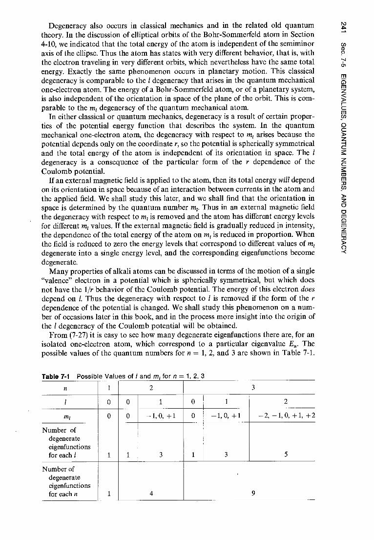
N

^

Degeneracy also occurs in classical mechanics and in the related old quantum

theory. In the discussion of elliptical orbits of the Bohr-Sommerfeld atom in Section

4-10, we indicated that the total energy of the atom is independent of the semiminor

axis of the ellipse. Thus the atom has states with very different behavior, that is, with

the electron traveling in very different orbits, which nevertheless have the same total

energy. Exactly the same phenomenon occurs in planetary motion. This classical degeneracy is comparable to the 1 degeneracy that arises in the quantum mechanical

one-electron atom. The energy of a Bohr-Sommerfeld atom, or of a planetary system,

is also independent of the orientation in space of the plane of the orbit. This is com-parable to the m i degeneracy of the quantum mechanical atom.

In either classical or quantum mechanics, degeneracy is a result of certain proper-ties of the potential energy function that describes the system. In the quantum

mechanical one-electron atom, the degeneracy with respect to m r arises because the potential depends only on the coordinate r, so the potential is spherically symmetrical and the total energy of the atom is independent of its orientation in space. The /

degeneracy is a consequence of the particular form of the r dependence of the Coulomb potential.

If an external magnetic field is applied to the atom, then its total energy will depend on its orientation in space because of an interaction between currents in the atom and

the applied field. We shall study this later, and we shall find that the orientation in

space is determined by the quantum number m 1. Thus in an external magnetic field the degeneracy with respect to m I is removed and the atom has different energy levels

for different m 1 values. If the external magnetic field is gradually reduced in intensity,

the dependence of the total energy of the atom on m l is reduced in proportion. When

the field is reduced to zero the energy levels that correspond to different values of m 1 degenerate into a single energy level, and the corresponding eigenfunctions become

degenerate. Many properties of alkali atoms can be discussed in terms of the motion of a single

"valence" electron in a potential which is spherically symmetrical, but which does

not have the 1/r behavior of the Coulomb potential. The energy of this electron does depend on 1. Thus the degeneracy with respect to 1 is removed if the form of the r dependence of the potential is changed. We shall study this phenomenon on a num-ber of occasions later in this book, and in the process more insight into the origin of

the / degeneracy of the Coulomb potential will be obtained.

From (7-27) it is easy to see how many degenerate eigenfunctions there are, for an

isolated one-electron atom, which correspond to a particular eigenvalue E. The possible values of the quantum numbers for n = 1, 2, and 3 are shown in Table 7-1.

Table 7-1 Possible Values of I and m1 for n = 1, 2, 3

n 1 2 3

l 0 0 1 0 1 2

m 1 0 0 —1,0, +1 0 —1,0, +1 —2, —1,0, +1, +2

Number of degenerate eigenfunctions for each l 1 1 3 1 3 5

Number of degenerate eigenfunctions for each n 1 4 9

EIG

EN

VA

LU

ES

, QU

AN

TU

M N

UM

BE

RS

, AN

D D

EG

EN

ER

AC

Y

ON

E- E

LEC

TR

ON

AT

OM

S

Inspection of this table makes it apparent that:

1. For each value of n, there are n possible values of 1. 2. For each value of 1, there are (21 + 1) possible values of m 1 . 3. For each value of n, there are a total of n 2 degenerate eigenfunctions.

7-6 EIGENFUNCTIONS

The mathematical techniques used in quantum mechanics to obtain (7-22) for the

eigenvalues of the one-electron atom are, admittedly, quite complicated compared to

those used in the Bohr model to obtain the same equation. Putting aside questions

concerning the logical consistency of the postulates of the Bohr model, it is still rea-sonable to question whether all the extra work involved in the quantum mechanical

treatment of the one-electron atom is justified by the results obtained. The answer

is, overwhelmingly, yes! We can now find out much more about the one-electron

atom than we possibly could from the Bohr model, because we have the eigenfunctions as well as the eigenvalues. The eigenfunctions contain a wealth of additional infor-mation about the properties of the atom. The remainder of this chapter, and the

following chapter, will be devoted largely to studying the eigenfunctions and ex-tracting this information from them.

We know that the eigenfunctions are formed by taking the product

Y'nlm:(r,e,(P) = R./(00/.,(19)(1).,(0

We also know, from (7-19), (7-21), and (7-24) that for any bound state

'mt(W) = eimiro

0im,(0) = sinlm'l 0 (polynomial in cos 0) and

Rn1(r) = e- (constant)r/n r1 (polynomial in r)

All the eigenfunctions have basically the same mathematical structure, except that

with increasing values of n and 1 the polynomials in r and cos 0 become increasingly more complicated. Table 7-2 lists the one-electron atom eigenfunctions for the first

three values of n. They are expressed in terms of the parameter

4^rEO^i2 ao= 2 =0.529 x 10 -to m = 0.529 A

which is the radius (or, from Section 4-7, the electron-nucleus separation) of the smallest orbit of a Bohr hydrogen atom. The multiplicative constant in front of each eigenfunction has been adjusted so that it is normalized. In other words, the integral over all space of the corresponding probability density functions equals one, so that in each quantum state there is probability one of finding the atomic electron somewhere.

Example 7-2. Verify that the eigenfunction 0211, and the associated eigenvalue E2, satisfy the time-independent Schroedinger equation, (7-12), for the one-electron atom with Z = 1. • Since the differential equation is linear in 0, for the purposes of this verification we can ignore completely the multiplicative constant 1/8n 11242, and write the eigenfunction as

tif = re-'12a0 sin Oe`co

This is the simplest case with a nontrivial dependence on all three coordinates. Nevertheless, the verification of this case should give the student some confidence in the validity of all the eigenfunctions quoted in Table 7-2.

Before beginning, let us introduce the convenient notation

>Ji = f(r,cp) sin 0 = f sin 0

N w

Table 7-2 Some Eigenfunctions for the One-Electron Atom

Quantum Numbers . n

1 m1 Eigenfunctions

Zr/2a°

2 1 0 ,I, _^ (Z )3/2 Zr

e Zr/2ao cos B Y'210 —

4 2^ ao ao

'/^ 1 2 1 ±1 4'21±1= 8 r

^3/2

o a

f Z e -Zr/2ao sin ee + "° o ^1 ,^ \a /

'I, 13/2 2 2 3 0 0 4'300 =

1

CZ `

C27 — 18

Zr + 2 Z 2 ) e zn/ 3 a0

V ao ao

3 1 0 ifr310 = — Vi

3/2 (6 — e 3aocos 0

81^ (ao) \ ao/ ao

3 1 +111/ 31 ± 1 — C Z)3/2 (

6_ aoj Zr Zr -Zr/3 ao i9±`

— /f81 rc

ao 13/2 ao

3 2 0 ̂3032,o0 = 1 (Z)

Z222 e - Zr/3ao(3 cos2 0 — 1) 81 ^/67c `aoj ao

3 2 +1 032±1 = (z \3/2 Z 2

2 e -

Zr/3a0 sin B cos O e ± `9

81 ^ ao ao

'I, 1 ( z y/2 Z2r2 2 + 3 2 ±2 Y'32±2 = ( 2 e

Zr/3ao sin2 e -2i(p

162 jc \a• ao

and

= 9(00)Ye-r/2a0 = gre- r/2ao

This notation will be useful in evaluating the derivatives that enter in (7-12), which is

h2 2 V 2^ — r 01- (r ar ) + r2 sin B

sin e a 2p [

e ) + r2 sin2 0 42+ V Elk

First we calculate

NI a =ae(f sin e) = f cos e

30

sin 9 0

= f sin e cos 0

73--6 f s in 0ae

= f(cos2 e — sin2 6)

1 a a ►^

= f (cos2 e— sin2 e

B (

r 2 sin 0 aB (sin ae ) r2 \ sin e

Next we calculate 2

_ (020 = — tif = —f sin 0

a2, 1, f

r2 sin 2 e r2 sin e

3/2 -Zr/a° 1 0 0 1

^ 100 = ^

(z

ao ) e

2 0 0 ^zoo 1

(z)3/2

0 \ ao / = 2 -- e

4 ̂ 2^

1

SN

OIlO

Nfl3

N3

013

ON

E-E

LEC

TR

ON

AT

OM

S

Adding these two results, we obtain 1

a (sin B a

+ 1 a2tfr f (cost B — sin2 8 — 1)

r2 sin B a4 a8 r2 sin 2 8 a92 r2 sin 8

2f sin 2 B 2f sin 6 21/i r2 sin B r2 r2

Then we calculate

e - r/2ao — e - r/2ao a =

% r

Or g I\ 2a0 3

r2 a^ = _ rz e - r/2ao _ r e -r/tap ar g ( 2a0

2 2 2 a (r2 a^) = g 2re r/2a0 _ r e r/zao _ 3r e r/2ao + r e -r/2a0

Or ( Or ( 2a0 2a0 4a2 o 2 2

= 2gre- r/ zao

( 1 —

8a2) = 2 (1 — a

0 +

8a 2) 4 0 0 0

1 a (r2atk) = 2 r (z — 1 1 2)0 r2 Or Or rao + 8ao

Substituting this term, and the term coming from the B and cp derivatives, into the differential equation that is supposed to be satisfied, we obtain

2µ [2 (r ra + 8a2) r ] + V l/i = Eli/

0 0 or

h 2

µao (1 1

r 8a0) + V = E

E = E2 8(471E0)2h2

e2 V=

4zzE0r

47tE Oh2 ao = 2

µe

So we have

Since inspection demonstrates that this equation is satisfied identically, we have completed the

verification. •

7-7 PROBABILITY DENSITIES

We begin to extract information from the one-electron atom eigenfunctions by

studying the forms of the corresponding probability density functions

w*tp* e iEnt/ri a — iE„t/ 'I,* ** * — P nlm t — 4' nlmi'Pnlmi = RO nl lm r ^ m l R nOI lmi mi

As these are functions of three coordinates, we cannot directly plot them in two

dimensions. Nevertheless, we can study their three-dimensional behavior by con-sidering separately their dependence on each coordinate. We treat first the r depen-dence in terms of the radial probability density P(r), defined so that P(r) dr is the

Now

Also

and

,ue4

h2 µe2 (1 µe2 e2 /ie4

µ 47tE0h 2 r 8(47CE 0)h 2 47te0r 8(47CE 0) 2h 2

0 15

15 20

0.02

0.01

0.02

0.01

15 0 0.5

n=3,1=0

0.5

0.4

0.3

0.2

0.1

0

0.2

0.1

0 0.2

0.1

probability of finding the electron at any location with radial coordinate between r and r + dr. By integrating the probability density `F*`h which is a probability g g p Y Y ̂ p YPer unit volume, over the volume enclosed between spheres of radii r and r + dr, it is m easy to show that P

P„l(r) dr = R,*,i(r)R„1(r)4itr2 dr (7-28) The factor of 4nzr 2 is present on the right side because the volume enclosed between

the spheres is given by that factor. The use of the quantum numbers n and l as labels

to specify the form of a particular radial probability density function is obviously ap-propriate, but the form of these functions does not depend on the quantum number

mi . Figure 7-5 plots several P„l (r), using dimensionless quantities for each axis.

0.1

10 15 20 25 r

ao/Z

Figure 7 -5 The radial probability density for the electron in a one-electron atom for n = 1, 2, 3 and the values of / shown. The triangle on each abscissa indicates the value of

r„i as given by (7-29). For n = 2 the plots are redrawn with abscissa and ordinate scales expanded by a factor of 10 to show the behavior of P„I (r) near the origin. Note that in the three cases for which 1 = /max = n — 1 the maximum of Pn1 (r) occurs at rBohr = n 2a o/Z, which is indicated by the location of the dashed line.

S3

I1IS

N3

0 A

lI1

I8H

8O

ad

co

N O

NE

-EL

EC

TR

ON

AT

OM

S

Inspection of the figure shows that the radial probability densities, for each set of the pertinent quantum numbers, have appreciable values only in reasonably restricted ranges of the radial coordinate. Thus, when the atom is in one of its quantum states, specified by a particular set of its quantum numbers, there is a high probability that the radial coordinate of the electron will be found within a reasonably restricted range. The electron would quite probably be found within a certain so-called shell contained within two concentric spheres centered on the nucleus. A study of the figure will demonstrate that the characteristic radii of these shells is determined pri-marily by the quantum number n, although there is a small 1 dependence.

This property can be seen in a more quantitative way by using the expectation value of the radial coordinate of the electron to characterize the radius of the shell. An obvious extension of the arguments of Section 5-4 to three dimensions shows that

c the expectation value is given by the expression o

rn1 = J rPn,(r) dr

o

If the integral is evaluated, this yields

rn1 = nZ o { 1 + 2 C1 l(l n2 1)1l

(7-29)

rBohr =

which gives the radii of the circular orbits of a Bohr atom (more precisely, it gives the electron-nucleus separation; see Section 4-7.) Quantum mechanics shows that the radii of the shells are of approximately the same size as the radii of the circular Bohr orbits. These radii increase rapidly with increasing n. The basic reason is that the total energy E„ of the atom becomes more positive with increasing n, so the region of the coordinate r for which E„ is greater than V(r) expands with increasing n, as can be seen in Figure 7-3. That is, the shells expand with increasing n because the classically allowed regions expand.

Example 7-3. (a) Calculate the location at which the radial probability density is a maximum for the ground state of the hydrogen atom. (b) Next calculate the expectation value for the radial coordinate in this state. (c) Then interpret these results in terms of the results of measure-ments of the location of the electron in the atom. •(a) The radial probability density for the n = 1, 1 = 0 ground state is

P1 o(r)

We take R 10(r) from the r-dependent factor of the first eigenfunction listed in Table 7-2, with Z = 1, and obtain

P1o(r) = e-r/aOe -r/a°r2 = e- 2r/aor2

We have ignored normalization (i.e., for simplicity taken the multiplicative constant equal to one) since it has no effect on what we are about to do. This is to find the maximum in P 1 0(r) by evaluating its derivative with respect to r and setting the result equal to zero. That is

dP10(r) = — 2 e - 2r/ao1. 2 + e 2r/ao2r dr a0

- 2r/a ° = — r e 2r=0

00

The values of rn1 are indicated in Figure 7-5 with small triangles. It is apparent that rn1 depends primarily on n, since the l dependence is suppressed by the factor of 1/2 and the factor of 1/n 2 in (7-29).

An interesting comparison can be made between (7-29) and (4-16) n 2 a0

= Rio(r)R1o(r)47cr2

ao

The solution to the equation we have obtained is r

--=0 ac,

or r = ao

This is the location of the maximum in the radial probability density. (b) To calculate the expectation value of the radial coordinate r, we evaluate (7-29), with

n = 1, l = 0, and Z = 1. We obtain rio = ao {1 + (1/2)[1]} = 1.5a 0

(c)We have found that the expectation value of r is somewhat larger than the value of r at which the radial probability density is a maximum. The reason is that the radial probability density is asymmetrical about its maximum in such a way that there is a small, but not negli-gible, probability of finding fairly large values of r in measurements of the location of the elec-tron in the atom. So, although the most likely location of the electron is at r = ac, (i.e., at the ground state Bohr electron-nucleus separation, the average value obtained in measure-ments of the location is r = 1.5a0 . All these features can be seen by inspecting the top curve of Figure 7-5. •

Example 7 -4. In its ground state, the size of the hydrogen atom can be taken to be the radius of the n = 1 shell for Z = 1, which is essentially ac, = 4xe0h 2/pee 0.5 A. Show that this fun-damental atomic dimension can be obtained directly from consideration of the uncertainty . principle. ► The form of the potential function 2

—e

4nEor

tends to cause the atom to collapse since the smaller the distance from the electron to the nucleus the more negative is the potential energy. This tendency is opposed by the effect of the uncertainty principle, as follows.

If the electron is located within a region of size R, then any component of its linear momen-tum must have an uncertainty of approximately

Ap= R

This uncertainty reflects the fact that the linear momentum of magnitude p can be in any direction, so the components can have values ranging from —p to +p. Thus the uncertainty in any component of the linear momentum also satisfies approximately the relation

Op=p Therefore, the electron must have a kinetic energy approximately equal to

p2 (»)2 h2

2p 2p 2pR 2

We see that the kinetic energy becomes more positive with decreasing R, which opposes the effect of the potential energy to cause collapse.

If the size of the atom is R, its potential energy is approximately e2

2pR 2 4ne0R

Obeying the common tendency of all physical systems to be as stable as possible, the atom will adjust its size so as to minimize its total energy. The existence of an optimum size can be seen qualitatively by inspecting Figure 7-6, which plots K, V, and E as functions of R. (Note that R is not the radial coordinate; it is the size of the atom, which we are treating as a variable in order to determine its optimum value.) We can find the most energetically favorable size quantitatively by differentiating E with respect to R, and setting the derivative equal to zero.

V(r) =

V =4itEOR

Then the total energy of the atom is approximately h2 e2

E=K+V=

S3I

1IS

N3

a A

1I1I

8`d

8 O1:i

d

Energy O

NE

-ELE

CT

RO

N A

TO

MS

E=K+V

0

R

C=11■■=01.1111

Figure 7-6 The qualitative behavior of the kinetic energy K, potential energy V and total energy E of a hydrogen atom, as functions of the size R of the atom. For small R, K increases more rapidly than V decreases because K oc 1/R 2 while V cc —1/R. For large R, K becomes negligible compared to V. As a result, E has a minimum at a certain value of R (indicated by the mark on the R axis), and at this size the atom is most stable.

That is

dE 2h 2 e2 dR 2µR 3 + 47r€0R 2

Solving this equation for R, we find 47rE0h2

R = µe2 = a()

the size which gives minimum total energy, and therefore the most stable atom. The uncertainty principle governs the minimum size of the atom because it governs its

minimum energy. This is the zero-point energy of the ground state, which has a size that arises from its zero-point motion. These simple ideas provide a very satisfactory answer to the question of the stability of the ground state of the atom. And this is particularly so if we also consider the discussion following Example 5-13, which shows that in its ground state the atom does not radiate.

Figure 7-5 shows that the details of the structure of the radial probability density functions do depend on the value of the quantum number 1. For a given n, the func-tion has a single strong maximum when l takes on its largest possible value; but additional weaker maxima develop inside the strong one when 1 takes on smaller values. Generally, these weaker maxima are not so important. However, there is a related property that can be very important. Inspection of the figure, particularly the expanded plots for n = 2, 1 = 0, and n = 2, 1 = 1, will demonstrate that the radial probability density functions have appreciable values near the origin at r = 0 only for 1 = 0. This means that only for l = 0 will there be an appreciable probability of finding the electron near the nucleus.

Another way of seeing this property is to consider the probability density, 1P*+ = elk, itself. Inspection of the eigenfunctions listed in Table 7-2 will show that for values of r which are small compared to ao/Z, where the exponential term is slowly

= 0

co N

S3I

1IS

N3

0 J

IlI1

I8b

r80

ad

varying, the radial dependence of all the eigenfunctions has the behavior

fi cc r' r —> 0 (7-30) This behavior can easily be verified by direct substitution into (7-17), the equation

that determines the radial dependence of the tp. As a consequence, the radial depen-dence of the probability densities for small r is

cc r21 r 0 (7-31)

From this it follows that the value of elk in a small volume near r = 0 is relatively large only for 1 = 0, and decreases very rapidly with increasing 1. The reason is that r° »r2 » r4 »..., for r-0.

We see that there is some probability that the electron will be near the nucleus if

= 0, but very much less probability that this will happen if 1 = 1, and even less if 1 = 2, etc. This can have important effects in certain circumstances because the poten-tial energy of the atom becomes very large in magnitude if the electron is near the

nucleus. We shall see later that this is particularly true for the case of multielectron

atoms, which have essentially the same property. In fact the r1 behavior of the eigen-functions for small r is of predominant importance in the structure of multielectron atoms. We shall also see later that the r1 behavior is due physically to the angular momentum of the atom, which depends on 1.

Now let us proceed to the study of the angular dependence of the probability den-sity functions

4^nimt 1 nlmt — Rn Rn1OÎmtOtmtalmtalmt

From (7-19) we have

Ont# ) `mt (9) = e -imw etmi0 = 1

Thus the probability density does not depend on the coordinate çp. The three-dimensional behavior of >/iimttbnlmt is therefore completely specified by the product of the quantity R 1(r)R n,(r) = Pn,(r)/4itr2 and the quantity 0i t (0)01mt(0), which plays the role of a directionally dependent modulation factor.

The form of the factor 01 t (0)01mt (0) is conveniently presented in terms of polar

diagrams, of which one is shown in Figure 7-7. The origin of the diagram is at the

point r = 0 (the nucleus), and the z axis is taken along the direction from which the

angle 0 is measured. The distance from the origin to the curve, measured at the angle

0, is equal to the value of 0i t (0)01mt (0) for that angle. Such a diagram can also be thought of as representing the complete directional dependence of 1ÿflan, Y' nlmt by visualizing the three-dimensional surface obtained by rotating the diagram about the z axis through the 360° range of the angle cp. The distance, measured in the direction specified by the angles 0 and gyp, from the origin to a point on the surface, is equal to 0i t (0)01mt (0)(1)m t (Çp)'Fmt(cp) for those values of 0 and cp.

Figure 7-7 A polar diagram of the factor which determines the directional dependence of the one-electron atom probability density.

0 ^

N O

NE

-ELE

CT

RO

N A

TO

MS

z

1=3 , m1 =±1

z

1 =3 , m1 = ±2

z z

1 =3, m i = ±3

z

1=1,m1= ±1 1=2,m1=±2

1 = 3,m1 =0 Figure 7-8 Polar diagrams of the directional dependence of the one-electron atom prob-ability densities for / = 3; m 1 = 0, ±1, ±2, ±3.

In Figure 7-8 we illustrate an example of the dependence of the form of Oi ,(9)O 1m,(9) on the quantum number m l , by a set of polar diagrams for l = 3, and the seven possible

values of m 1 for this value of 1, i.e., for m 1 = — 3, — 2, —1, 0, 1, 2, 3. Note the way in which the region of concentration of O*,,,(9)O 1m,(9), and therefore Otnitfrnlmi, shifts from the z axis to the plane perpendicular to the z axis as the absolute value of m 1 increases. Some features of the dependence of O1 1 (9)O1m,(9) on the quantum number / are indicated in

Figure 7-9 in terms of a set of polar diagrams for m 1 = ± l and l = 0, 1, 2, 3, 4. In the case n = 1, 1 = m1 = 0, which is the ground state of the atom, 1/i n m14'nlm, depends on neither 0 nor cp and the probability density is spherically symmetrical. For the other

states, the concentration of probability density in the plane perpendicular to the z axis, when m 1 = ± 1, becomes more and more pronounced with increasing 1. Figure 7-10 is an

attempt to overcome the limitations of the two-dimensional printed page using shading

to represent the three-dimensional appearance of the probability density functions for

various states of the one-electron atom.

The probability density functions displayed in these figures generally have a set of

spherical and conical surfaces, defined by certain values of r and 0, on which they equal

1=3,m1=1- 3 1=4,m1=±4

Figure 7-9 Polar diagrams of the directional dependence of the one-electron probability

densities for 1 = 0, 1, 2, 3, 4; m 1 = ±1.

CI) CD C)

.44

S3I

1ISN

3a A

111

18t1

8O

ad

n = 1,1=m1 = 0

i

n=3, 1= 2, m 1 =0

Figure 7-10 An artist's conception of the three-dimensional appearance of several one-electron atom probability density functions. For each of the drawings a line represents the z axis. If all the probability densities for a given n and 1 are combined, the result is spherically symmetrical.

ON

E-E

LEC

TR

ON

AT

OM

S

zero. These nodal surfaces are analogous to the nodal points at which the probability density for a particle bound in a one-dimensional potential equals zero (see, for example, Figure 6-32). They are a consequence of the fact that the wave functions for a bound particle must be standing waves with fixed nodes.

However, if a collection of hydrogen atoms has been completely isolated from its environment, it is not possible to then make measurements on the locations of the electron in each atom, knowing that they are all in a quantum state with a particular set of quantum numbers n, 1, m l , and thereby locate the nodal surfaces for that state. If it could be done it would certainly be remarkable, because it would allow the deter-mination of the direction of the z axis. And this would amount to finding for each atom a preferred direction in a space which should be spherically symmetrical, because the Coulomb potential of the atom V = — Ze 2/4rrE0 r is spherically symmetrical. In fact, it cannot be done because it is generally not possible to observe any of the probability density patterns of Figure 7-10 in actual measurements on free atoms (i.e., atoms in the complete absence of external magnetic or electric fields). The only excep-tion is the spherically symmetrical state for n = 1, 1 = m1 = 0. The reason is that, with the exception of the state just mentioned, every state is degenerate with several other states of the same n value. Because the energies of atoms in degenerate states are identical, it is not possible experimentally to separate them from each other with tech-niques that leave the probability density unchanged. Thus, all that can be measured is the average probability density of the atoms for the entire set of states which are degenerate with each other. It turns out that the probability density functions, when averaged together in this manner, always yield a spherically symmetrical function.

Example 7-5. Evaluate the average of the probability density functions for the set of degener-ate states corresponding to the energy E2.

■ We have 1 ''//, ' II,, ' rr,, I I' 'I 4 [1''2001''200 + Y' 21-1121-1 + 4'210`1'210 + 5' 2114'211]

Z)

3 1 = 128 ( J

e-zr/a° C(2

—

ao I + (

ao/ 2 (2 sine 0 + 2 sine 8 + cos 2 O

Zr 2

3 L ' 2 2

128 1 (a0 a e -zr/aO

L \2 r^ + r/ J (7-32)

0 \a 0

This spherically symmetrical distribution would be the result of a sequence of measurements on

the locations of the electrons in one-electron atoms of total energy E2. Of course, it cannot be used to detelmine the direction of the z axis, and so there is no contradiction with the fact that this

direction was initially chosen in a completely arbitrary way.

` •ote that even for each subset of states including all possible values of m 1 for a given n and 1 (a "subshell") the sum of the probability densities is spherically symmetrical. That is ,

2oo^20o is

spherically symmetrical, and also t f/2 1 -1 11121 -1 + 1V 210 210 +114114/211 is spherically symmetrical. This important property is illustrated in Figure 7-10. It will be used later in argu- ments concerning multielectron atoms, and nuclei. •

On the other hand,, consider a situation in which the orientation of the z axis is not arbitrary because there is a preferred direction defined, for instance, by an external

magnetic or electric field applied in that direction to the collection of hydrogen atoms.

In such a field the quantum states are not degenerate, as we shall see later, and

measurements of the probability density of atoms in a particular state can be per-formed. In fact, such measurements can be used to determine the direction of the

external field.

To help the student understand the ideas just discussed, let us restate them as follows:

1. If the behavior of an alom is governed by a potential which has spherical symmetry, like

the Coulomb potential which depends only on the distance from the electron to the nucleus,

none of the properties of the atom should single out any particular direction in space because all directions are equivalent.

2. If the atom is placed in an external electric or magnetic field, the spherical symmetry is destroyed and the direction defined by the external field becomes unique.

3. When one direction is unique, we choose one axis of our coordinate system to be in that preferred direction because it simplifies the description of the physical situation. We can choose other directions, but this unnecessarily complicates the mathematical description. (In electro-magnetism, as an example, when treating a cylindrical wire it is very advantageous to take one axis of the coordinate system along the axis of the cylinder.)

4. By convention, we call the preferred axis the z axis. (The convention probably comes from cylindrical coordinates, in which the axis about which the angular coordinate varies is called the z axis.) But we could have called the preferred axis the x or y axis, just as well.

5. Even if there is no preferred direction, because no external field is applied to the atom, we still must choose some arbitrary direction in space for the z axis of our coorindate system. But in this case the z axis is not unique physically; it is merely a mathematical construct. Therefore, its choice should have no measurable consequences.

We should also point out that a uniform applied field can serve to define for the atom only a single preferred direction. As we have indicated, such a field will generally remove part of the degeneracy of the eigenfunctions, and probability densities that depend on the angle B can be measured. But the probability densities remain independent of the angle 9, since 1i*i/i cc (1)„*,(0)I;,ü (cp) = e - amt9e`mt ° = 1 for every eigenfunction. That is, the probability densities retain their axial rotation symmetry about the direction of the applied field, as certainly must be the case.

A nonuniform applied field can serve to define additional preferred directions. It is not surprising that such fields can destroy the axial rotation symmetry of the probability density of an atom under their influence. Although we have not allowed for this possibility in our development, because we shall not need to, it is easy to do if necessary by taking particular solutions to (7-15) in the form (1),„,,((p) = cos mi cp or im,(cp) = sin m 1 cp, instead of in the form we have taken. With no applied field, or with uniform applied field, the eigenfunction associated with cos m 1 cp is degenerate with the eigenfunction associated with sin m ice, so measurement of the probability density will always yield a co-independent combination cc cos t mice + sine mice = 1, just as with the eigenfunctions that we use. In the nonuniform applied field the degeneracy can be removed, however, and probability densities that do not have axial rotation symmetry can be observed. The solutions 1 mt(cp) = cos mice and t mi((p) = sin m ice are fre-quently used in chemistry since one atom in a molecule is acted on by a highly nonuniform field produced by the other atoms.

In the next section we shall show that the quantum numbers 1 and m 1 are related to the magnitude L of the orbital angular momentum of the electron, and to its z com-ponent LZ, by the relations

L= N/l(l+ 1)h L Z = mi ff

We mention this now because it is an important clue to the interpretation of the dependence of t/J n nitfr„ mi on 1 and m 1 . Consider the case m 1 = 1. Then LZ = lh, which is almost equal to L = \/l(l + 1)h. In this case the angular momentum vector must point nearly in the direction of the z axis. For a Bohr atom this would mean that the orbit of the electron would lie nearly in the plane perpendicular to the z axis, as illus-trated in Figure 7-11. With increasing values of 1, the value of lh approaches the value of /l(l + 1)h, so that L Z approaches L. This means the angle between the angular momentum vector and the z axis decreases. In terms of the Bohr picture, this demands that the orbit lie more nearly in the plane perpendicular to the z axis. An inspection of the polar diagrams of Figure 7-9 will demonstrate the correspondence between these features of i/rnlmtJniml and the picture of a Bohr orbit. For m 1 = 0 we have LZ = 0, and the angular momentum vector must be perpendicular to the z axis. In a Bohr atom this would mean that the plane of the orbit contained the z axis. Some

S3I

1IS

N34 A

lIiIB

t/B

Oad

z O

NE

-ELE

CTR

ON

AT

OM

S

Figure 7-11 A Bohr orbit lying in a plane nearly perpendicular to the z axis.

indication of this behavior can be seen in the polar diagram for l = 3, ml = 0 of Figure 7-8.

Although there are many points at which the quantum mechanical theory of the one-electron atom corresponds quite closely to the Bohr model, there are certain striking differences. In both treatments the ground state corresponds to the quantum number n = 1, and it has the same value of total energy. But in the Bohr model the orbital angular momentum for this state is L = nh = h, whereas in quantum mech-anics it is L = 111(/ + 1)h = 0, since l = 0 when n = 1. There is an overwhelming amount of evidence, from measurements of atomic spectra and elsewhere, that shows the quantum mechanical prediction for zero orbital angular momentum in the ground state to be the correct one. This prediction is also in agreement with one obtained by using the techniques we developed earlier to calculate the expectation values of the total kinetic energy of the electron in the ground state and of the kinetic energy associated only with radial motion. The two values are found to be equal, implying that the motion is entirely radial in that state. If the Bohr model were modified in a way that would allow for zero angular momentum states, the orbit for such a state would be a radial oscillation in which the electron passes directly through the nucleus, and the oscillation could take place along any direction in space. This would corre-spond, in a sense, to a spherically symmetrical probability density or charge dis-tribution, similar to that which is predicted by quantum mechanics and is observed experimentally. Nevertheless, it is difficult to visualize the motion of an electron in the ground state of the quantum mechanical atom. That is, it is difficult to make an analogy to a classical picture, such as the Bohr picture. But this situation is not unique; it is equally difficult to visualize the motion of an electron traveling through a two-slit diffraction apparatus.

7-8 ORBITAL ANGULAR MOMENTUM

We shall now proceed to justify the relations

LZ = mlh

(7-33) L= V1(/ +1)h

(7-34) between the quantum numbers m l and 1, and the z component L Z and magnitude L of the angular momentum of an electron in its "orbital" motion about the center of an atom. The justification will take a little effort, but it will be well worth it. We have just seen that these relations are very useful in interpreting the angular dependence of the probability density functions for a one-electron atom. As we continue our study of quantum physics, we shall see that the angular momentum relations are extremely im-portant in the study of all atoms (and nuclei). The basic reason is that in most circum-

stances the z component and magnitude of the angular momenta of the particles in microscopic systems remain constant. From a classical point of view, this happens because in most systems the particles move in spherically symmetrical potentials that cannot exert torques on them. We shall find that, of all the quantities that can be used to describe atoms (and nuclei), angular momentum and total energy are about the only ones that do remain constant. A consequence is that most experiments on such systems involve measuring angular momentum and total energy. Therefore, quantum mechanics must be able to make predictions about angular momentum, as well as total energy. Another parallel between these two is that both are quantized. In other words, the relations of (7-33) and (7-34), stating that L z and L have the precise values m r h and Jl(l + 1)h, are quantization relations just like the energy quantization rela-tion stating that the total energy E of a one-electron atom has the precise values

—uZ2 e4/(4n€0 ) 22h2 n2 . Angular momentum quantization is certainly as important as

energy quantization. The only reason that it has not appeared before in our treatment

of Schroedinger quantum mechanics is that the treatment was restricted to one-dimensional systems. Of course, angular momentum is the dynamical quantity that

sets real three-dimensional systems apart from one-dimensional idealizations in

which it has no meaning. The angular momentum of a particle, relative to the origin of a certain coordinate

system, is the vector quantity L defined by the equation L = r x p (7-35a)

where r is the position vector of the particle relative to the origin, and p is the linear momentum vector for the particle. By evaluating the components in rectangular co-ordinates of the vector, or cross, product, it is easy to show that the three rectangular

components of L are Lx = Ypz — zp y Ly = zpx — xp z (7-35b)

Lz = xpy — Ypx

where x, y, z are the components of r, and px , py , pz are the components of p.

In order to study the dynamical quantity angular momentum in quantum mech-anics, we construct the associated operators. This is done by replacing px , py , pz by their quantum mechanical equivalents — ih a/ax, — ih 0/0y, — ih 0/3z, according to an obvious three-dimensional extension of (5-32). Thus the operators for the three

components of angular momentum are

Lxop = — ih\Y az — z a Y

a Lyop = — ih (zal

ôx — x-

0) (7-36)

Lzop = — ih(x —88y— y ax )

Because we must use spherical polar coordinates, these expressions must be trans-formed into these coordinates. Appendix M shows how this can be done. The results are

L xop = ih sin (p 6 + cot B cos çP ^

\ ^P /

Lyop = ih — c os cp â + cot 8 sin (p ^ ) C ^

L = — i^t ô^p

(7-37)

W(1

1N

3W

OW

EI`d

T1

JNV

1d

11

81:1 0

CO ^ N

We shall also be interested in the square of the magnitude of the angular momentum vector L, which is

ON

E- E

LEC

TR

ON

AT

OM

S

L2 =LX + Ly + Lz As is indicated in Appendix M, in spherical polar coordinates the associated operator is

o __ 2 r 1 a C

l 1 a2

L°p —

sin 0 a0 sin 0

a a0 + sine 0 09 2,

The first step in deriving the angular momentum quantization equations involves using the operators to calculate the expectation values of the z component of L, and of the square of its magnitude, for an electron in the n, 1, m 1 quantum state of a one-electron atom. According to the three-dimensional extension of the prescription of (5-34), the expectation value L z is

L z = J T*Lzop lii dZ

Here dr stands for the three-dimensional volume element r 2 sin 0 dr dO dçp, and f stands for the three definite integrals f ô Pig'. ô'. The same shorthand notation will be used in the remainder of this chapter, and in the following chapters. Continuing our calculation of L z, by expressing the wave function as a product of the eigenfunction and the exponential time factor we obtain

or

Lz =

J etE,,f/NY'n Lmt L zop e

-

iEnt/^tY'nlmt dZ

Lz = jZm i L;opVmnim i dz (7 -39)

Similarly, the expectation value of L 2 is

L2 =

^/^ * ,/, Y^nlmtLop

o2 Y'nlmt dZ (7-40 (7-40)

To evaluate the integrals in the two numbered equations above, we must first evaluate

' Lzop^nlmt and Lop2 J^ Iinlm i . Example 7-6. Evaluate Lz opi nlm t , where Lzop = —itza/ap, and where Cam , is a one-electron atom eigenfunction. to-We have

a L ^/ = Ih Y'nlmt

zop nlmt 09

Since

we obtain knlmt = R nl(r)eImtleAmt(9)

a^nlmt r d^m t (9)1 l^2

09 = Rnl^r)^Im t ^B) L — I^l Ll9

(7-38)

ci.

v r^

JJ

ir Zit

=J T*Lzpp YJr 2 sin 0 dr dO dkp

0 0 0

The quantity r2 sin 0 dr d0 dçp is the element of volume in spherical polar coordinates,

and the integrations are taken over the complete ranges of all three coordinates.

Because it will simplify the notation, without causing confusion, we shall write this

expression as

According to (7-19)

SO

omt((P) = en"' N ^ v

dOmi(T) = lYnietm^^ = lml 0m t (40)

dyp

Thus

i^i. a anlm [ = R (I')O (B) [ — Illlm ^ ( ^ ni ~Imt I m t ^)^

= mlhRnl(r)OIm t (e)0m t ((p) and we obtain the answer

Lzop ^Ÿnlm t — mlhOnlmt

^

Although we do not have a concise expression for the functions O lmt (9), which must be differentiated to evaluate L p!r/nlmt, we know that these functions satisfy the differ-ential equation (7-16). Using this fact, it is not difficult to show that

Loptfrnlmt = 1(1 + 1)1221T nlmt (7-42)

Using (7-41) from Example 7-6 in (7-39), which is

Lz = J Y'nlmtLzoPY^nlm t dx

it is trivial to evaluate Lz . We have

Lz = mlh Y^nimt^nlmt dz

But we know that this integral has the value one because it is equal to the probability

density integrated over all space, i.e., the probability of finding the electron some-where. Thus we obtain

In a similar fashion we use (7-42) in (7

L2 =

to obtain

LZ = 1(1 + _ L Z = 1(1 +

Lz = -40),

^*

1)h2J

1)h2

nlmtLop^Y

m lh which is

2 , 1, nlm t da

*

,, Y^nlmt`l'J/,, nlmt da

(7-43)

(7-44)

Let us compare the results of our expectation value calculations, (7-43) and (7-44),

with the quantization relations we are trying to verify, that can be written

Lz = mitt (7-45) L2 = l(1 + (7-46)

The former are certainly consistent with the latter, but they are not proofs of the lat-ter. The quantization relations make stronger statements about the values of L z and L2 . These relations say that any measurement of the angular momentum of an elec-tron in the n, 1, m 1 state of the atom will always yield Lz = m lh and L 2 = 1(1 + 1)h2

(7-41)

1A1I 1

1N

3W

OW

ad

TnJN

d 1

b`1

181:

10

—NI2(2 + 1)

ON

E-E

LEC

TR

ON

AT

OM

S

since, in that state, these quantities have precisely the values quoted. But the expecta- tion value relations say only that the values quoted will be obtained on the average,

that is, when the results of a large number of measurements of L Z and L2 are averaged. To complete the proof of the quantization relations is a matter of continuing along

the line we have been following. For example, by calculating the expectation value

of some power of L Z, say the square Lz, it is found that LZ = (m 1h) 2 . This immedi-ately leads to the conclusion that not only must L Z equal mh on the average, i.e., L Z m 1h, but that LZ must equal mh always, i.e., L Z = m 1h. The point is that if L Z fluctuated about its average m 1h it would not be possible to obtain LZ = (m 1h)2 because when averaging a power of L Z higher than the first more weight is given to fluctuations above the average than to fluctuations below the average. In order to proceed with

our interpretation of the angular momentum of one-electron atoms, we defer the de-tails of this proof to the following section. There we shall also obtain the interesting

conclusion that Lx and L y , the x and y components of the orbital angular momentum,

do not obey quantization relations. The fact that Cam, does not describe a state with a definite x and y component of

orbital angular momentum, because these quantities are not quantized, is mysterious

from the point of view of classical mechanics. According to the angular momentum

conservation law of classical mechanics, the orbital angular momentum vector of an

electron moving under the influence of a spherically symmetrical potential V(r) of a one-electron atom in free space would be completely fixed in direction and magni-tude, and all three components of the vector would have definite values. The reason

is that there would be no torques acting on the electron. The fact that this result is

not obtained in the quantum mechanical theory is a consequence of the fact that there

is an uncertainty principle relation which states that no two components of an angu-lar momentum can be known simultaneously with complete precision. Because the z component of orbital angular momentum has the precise value m 1h, the relation re-quires that the values of the x and y components be indefinite But one thing can be

said about the values of these components: Upon evaluating Lx and L y, their average values, it is found that both equal zero. So although the particular value of L x that would be obtained in any particular measurement cannot be predicted, it can be pre-dicted that the average value that would be obtained in a set of measurements of L x is zero. And similarly for L y .

Many of the properties of the orbital angular momentum can be conveniently

represented by a vector model. Consider the set of states having a common value of the

quantum number 1. For each of these states the length of the orbital angular momen-tum vector, in units of h, is L/% = x/1(1 + 1). In the same units, the z component of this vector is L Z/h = m 1 . The z component can assume any integral value from L Z/1i = — Ito L i/h = +1, depending on the value of m 1 . The case of l = 2 is illustrated in Fig-ure 7-12. The figure depicts the angular momentum vectors for each of the five states

-0̂ ► Figure 7-12 Representing the angular momentum vectors (measured in units of h) for the possible states with I = 2. In each state the vector is equally

C 1

- likely to be found anywhere on a cone symmetrical i _____ about the z axis. It has a definite magnitude and z

-2 component but does not have a definite x or y component.

corresponding to the five possible values of m 1 for this value of 1. In any one of these states the angular momentum vector is equally likely to be found anywhere on a cone symmetrical about the z axis, and therefore has a definite z component as well as a definite magnitude. The vector does not have a definite x or y component, but the value of either of these quantities is as likely to be positive as it is to be negative. The actual orientation in space of the angular momentum vector is known with the great-est precision for the states with m 1 = + 1. But even for these states there is some un-certainty since the vector can be anywhere on a cone of half-angle cos' [lWl(l + 1)]. In the classical limit 1 — co, and this angle becomes vanishingly small. Thus, in the

classical limit the angular momentum vector for the states m 1 = + l is constrained to lie almost along the z axis and is therefore essentially fixed in space. This agrees with the behavior predicted by the classical theory, i.e., with the classical orbital angular

momentum conservation law. The quantum number m1 determines the space orientation of the orbital angu-

lar momentum vector of the one-electron atom. Therefore, in a sense it determines

the orientation in space of the atom itself. As the spherically symmetrical Coulomb

potential implies that there is no preferred direction in the space in which the atom

is situated, we can understand why the theory predicts that the total energy of the

atom does not depend on m 1 , which determines this orientation. Thus we can

understand why the eigenfunctions are degenerate with respect to the quantum num-ber ml . The energy of the atom simply does not depend on its orientation in empty

space.

7-9 EIGENVALUE EQUATIONS

Here we shall complete the derivation, started in the previous section, of the orbital angular

momentum quantization conditions. Then we shall generalize the results of the derivation to

point out an interesting feature of Schroedinger's theory of quantum mechanics.

To study the quantization of the orbital angular momentum, we focus attention first on its

z component, L2 . Now, if the z component quantization condition of (7-45) is valid, then any

measurement of L Z will always yield the same precise value specified by that quantization

condition LZ = m1 hi (7-47)

Furthermore, measurements of some higher power of L 2 , say the square LZ , will always yield the same value LZ = (m 1 h) 2 . As a consequence, the expectation value of the square of L Z will be just LZ = (m lh)2 . Note that, since we also have L Z = m 1h, this means

Lz = LZz (7-48)

That is, the expectation value of the square of L Z equals the square of the expectation value

of L2 , if the quantization condition of (7-47) is valid. On the other hand, if (7-47) is not valid then measurements of L Z can lead to various values,

subject, however, to the constraint that the values average out to yield mlhi because we have proven in (7-43) that L Z = m 1h in any case. If the measured values of L Z fluctuate about the average value m 1h, then the expectation value of the square of L Z will no longer equal the square of m itt.. The reason is that when averaging a higher power of L2 , like its square LZ , we give much more weight to the cases in which L Z is larger than LZ , and much less weight to the equally numerous cases in which L Z is smaller than L. In this situation Lz (mlh) 2 , so L?L 2 .

An example is shown in Table 7-3, which applies the ideas just discussed to calculating the square of the average, and the average of the squares, of the ages of a group of children whose individual ages are 1, 2, and 3 years. Inspection of the table shows that when the ages are first squared, and then averaged, a larger result is obtained than when the ages are first averaged, and then squared. This will be true in any case in which a power of the ages higher than the first is averaged, and in which the ages fluctuate. But if all the children in the group have ages precisely equal to each other, and therefore to the average age, then it makes no difference in

N 01 ^

SN

OI.L

df10

3 3

fTI`

dnN

30I3

0 m N

ON

E-E

LEC

TR

ON

AT

OM

S

Table 7-3 The Square of the Average, and the Average of the Squares, of a Set of Fluctuating Numbers

A= 1,2,3

A -

1+2+3 - 6

- 2 3 3

A2 = 4

A2 = 1,4,9

2 -1+4+9 - 14

- 4.67 3 3

^

Q AA- N/A 2 —A 2 =,/4.67-4=,/0.67=0.82 ^ r U

which order the operations are carried out and the average of the squares equals the square

of the averages. An example of that situation is shown in Table 7-4. _

For another illustration of these ideas, consider the quantity Ax = Jx2 — z 2. As men-tioned in Example 5-10, this quantity is used as a measure of the fluctuations that would be observed in measurements of the x coordinate of a particle. If there were no fluctuations, then x2 = X2 . But the uncertainty principle demands that there be fluctuations in x (which are larger the smaller the fluctuations in the linear momentum p). As a result x 2 > x2, and the difference between x 2 and z2 increases as the fluctuations in x increase so ,Jx2 — x 2 is a measure of these fluctuations. _

Now, it is easy to prove the validity of the relation expressed by (7-48), LZ = Lz2 , and therefore also the validity of the quantization condition L z = m idi of (7-47). To do this we twice use (7-41), Lzo r4'nimi = mih1nimi, to calculate L. According to the three-dimensional exten-sion of the prescription for calculating expectation values, we have

LZ = J `I' *LZoP lif di

This immediately gives

z Lz = Vnimi Lzop I nimt d^

The dynamical quantity LZ is the product of two factors of the form L z LZ =Lz •Lz

According to the expectation value prescription, the operator L oP obtained from that dyna- mical quantity is thus the product of two operators of the form Lzpp . Therefore

L o4'n pim i = Lzop Lzopt1''

nim,

Table 7-4 The Square of the Average, and the Average of the Squares, of a Set of Nonfluctuating Numbers

A = 2, 2, 2 ^ - 2 +2+2 — 6 =2

3 3 A 2

= 4 A 2 =4,4,4

A-

2- 4+4+4

= 12

- 4 3 3

AA — A 2 = —4=0

In other words, L opt/ nim, means that operates twice on i/inimi. But according to (7-41) —L

Lz op l nim, = mlhY nlmi

co Thus each operation of Lz.p on Otani, yields the same function Y'nim,, multiplied by a constant factor mih. Therefore, the result of two operations is simply to multiply `i'nlm, by two factors of m ih. That is

//,` cb

Lz opinim i = (mlh) 2 Y'nim,

Knowing this, we immediately obtain

''//,, Lz = J 4'n m,(mih) 2V'nim t dZ

= (mih)2 J

'Zm1'fl1m1 dT

= (mlh)2

= L 2

where we have made use of the fact that the integral over all space of tiromiOnim, equals one because of the normalization condition. Since we have verified (7-48), we have completed our verification of the quantization condition Lz = mih. The proof of the validity of the quantiza-tion condition L 2 = 1(1 + 1)h2 is carried through in a completely parallel manner.

Note that these proofs depend on (7-41) and (7-42), Lzoptitnim, = mlh n lm i and 4,20„1 ,n, = 1(1 + 1)h2llinimi. The equations state the surprising facts that the result of operating on the one-electron atom eigenfunction Y'nimi with the differential operator Lzop is simply to multiply that eigenfunction by the constant mih, while the result of operating on it with the differential

operator Lop is simply to multiply it by the constant 1(1 + 1)h2 . These results are certainly not typical of what happens when a differential operator operates on a function. For instance, if

we operate on a function, say f(x) = x2 , with the differential operator d/dx, we obtain a very different function f'(x) = 2x. As another example, it is not difficult to show that the results of

operating on cam , with the operators Lxop or Lyop is to produce new functions of r, 8, 9 in which these variables enter quite differently from the way they enter in the function Y'nim,• That is

Lxop`Nnim, # (const)ilin/m,

Lyop^nimt (const)ilinim i

The ideas that we have developed, in the process of verifying the angular momentum quantization conditions, can be extended to provide a deeper insight into the theory of Schroedinger quantum mechanics. They can also be used to lead into the more sophisticated theories, such as Heisenberg's matrix mechanics. We must leave these matters for more ad-vanced books. Here we shall say only that the properties associated with (7-41) and (7-42) are perfectly general. That is, whenever the dynamical quantity f has the precise value F in the quantum state described by the function ifi, then that function satisfies the relation

fop ll/ = Flk (7-51)

where fop is the operator corresponding to f. We shall also show that the time-independent Schroedinger equation can be written in the

form of (7-51). To do this, consider the time-independent Schroedinger equation in rectangular

coordinates h2 020 a20.

a2,k1 2µ ax2 + ay2 + az2 + Vi/r = Etli

Rewrite it as

C 2,u ^a 2 + ^ 2 + 2̂J

+Vl i^=Ei%i

By comparing (7-3) with (7-4), we see that the square bracket is just the operator eop for the total energy. Thus we have

eop ifi = Elfr

SN

OI1

`df 1

O3 3

MId

AN

300

(7-49) (7-50)

N CO N

ON

E-E

LEC

TR

ON

AT

OM

S

Here E is one of the precise allowed values of the total energy of the system described by the potential V. The system is also described by the total energy operator eop .

The general relation of (7-51) is called an eigenvalue equation, i' is said to be an eigenfunction of the operator fop , and F is said to be the corresponding eigenvalue. This is the same termin-ology as is used in the particular case of the eigenvalue equation for the total energy operator that is, in the case of the time-independent Schroedinger equation. The total energy operator eop is sometimes called the Hamiltonian.

These considerations lead to the important conclusion that, since (7-49) and (7-50) show I'nlmz is not an eigenfunction of the operators Lx0 or Lyop , the corresponding dynamical quantities Lx and Ly do not have precise values in the one-electron atom. That is, L x and Ly

do not obey quantization conditions.

QUESTIONS

U 1. If a hydrogen atom were not at rest, but moving freely through space, how would the quantum mechanical description of the atom be modified?

2. Since it is well known that the Coulomb potential has a much simpler form in spherical polar coordinates, why did we begin our treatment of the one-electron atom in rectan-gular coordinates?

3. In what important equations of classical physics does the Laplacian operator enter? 4. Would the results of the calculations be affected if we took different forms for the separa-

tion constants that arise in the splitting of the time-independent Schroedinger equation, for the one-electron atom, into three ordinary differential equations?

5. Why must I'((p) be single valued? How does this lead to the restriction that ml must be an integer?

6. What would happen if we took e - `m` 0 as the particular solution to the D((p) equation? What about cos m i ce or sin m i ce?

7. Why do three quantum numbers arise in the treatment of the (spinless) one-electron atom? 8. Can you say what the functions O(0) and 1(cp) would be like if V were a function of r,

but not proportional to — 1/r? (This is the case for the valence electron of an alkali atom.)

9. Just what is degeneracy? 10. What is the relation between the size of a Bohr atom and the size of a Schroedinger atom? 11. What is the fundamental reason why the size of the hydrogen atom in its ground state

has the value it does? 12. For a one-electron atom in free space, what would be the mathematical consequences of

changing the choice of direction of the z axis? The physical consequences? What if the atom is in an external electric or magnetic field?

13. Why does a uniform electric or magnetic field define only one unique direction in space? 14. How do the predictions of the Bohr and Schroedinger treatments of the hydrogen atom

(ignoring spin and other relativistic effects) compare with regard to the location of the electron, its total energy, and its orbital angular momentum?

15. Devise an explanation for the obvious relation between the last two terms of the Lapla-cian operator, in spherical polar coordinates, and the operator for the square of the magnitude of the orbital angular momentum.

16. Using the connection between L and 1, explain physically why >(i*0 is very small near r = 0, unless 1 = 0.

17. Exactly why do we say that for a hydrogen atom in free space the orbital angular momen-tum vector can be located with equal probability anywhere on a cone symmetrical about the z axis?

18. Is every eigenfunction of angular momentum magnitude necessarily also an eigenfunction of total energy? Is the reciprocal statement true?

19. Are examples of eigenvalue equations found in classical physics? If so, what are they?

PROBLEMS N ^

W

1. Using the technique of separation of variables, show that there are solutions to the

three-dimensional Schroedinger equation for a time-independent potential, which can be

written P(x,y,z,t) = Y' (x,y,z)e -

iEtm

where l/i(x,y,z) is a solution to the time-independent Schroedinger equation.

2. Verify that D(cp) = eim") is the solution to the equation for (Kcp), (7-15). 3. Hydrogen, deuterium, and singly ionized helium are all examples of one-electron atoms.

The deuterium nucleus has the same charge as the hydrogen nucleus, and almost exactly twice the mass. The helium nucleus has twice the charge of the hydrogen nucleus, and almost exactly four times the mass. Make an accurate prediction of the ratios of the ground state energies of these atoms. (Hint: Remember the variation in the reduced mass.)

4. (a) Evaluate, in electron volts, the energies of the three levels of the hydrogen atom in the states for n = 1, 2, 3. (b) Then calculate the frequencies in hertz, and the wavelengths in angstroms, of all the photons that can be emitted by the atom in transitions between these levels. (c) In what range of the electromagnetic spectrum are these photons?

5. Verify by substitution that the ground state eigenfunction Iiloo, and the ground state eigenvalue E 1 , satisfy the time-independent Schroedinger equation for the hydrogen atom.

6. (a) Extend Example 7-4 to obtain from the uncertainty principle a prediction of the total energy of the ground state of the hydrogen atom. (b) Compare with the energy predicted by (7-22).

7. (a) Calculate the location at which the radial probability density is a maximum for the n = 2, 1 = 1 state of the hydrogen atom. (b) Then calculate the expectation value of the radial coordinate in this state. (c) Explain the physical significance of the difference in the answers to (a) and (b). (Hint: See Figure 7-5.)

8. (a) Calculate the expectation value V for the potential energy in the ground state of the hydrogen atom. (b) Show that in the ground state E = V/2, where E is the total energy. (c) Use the relation E = K + V to calculate the expectation value K of the kinetic energy in the ground state, and show that K = — V/2. These relations are obtained for any state of motion of any quantum mechanical (or classical) system with a potential in the form V(r) cc — 1/r. They are sometimes called the virial theorem.

9. (a) Calculate the expectation value V of the potential energy in the n = 2, 1 = 1 state of the hydrogen atom. (b) Do the same for the n = 2, 1 = 0 state. (c) Discuss the results of

(a) and (b), in connection with the virial theorem of Problem 8, and explain how they

bear on the origin of the 1 degeneracy. 10. By substituting into the equation for R(r), (7-17), the form R(r) cc r1, show that it is a

solution for r —* O. (Hint: Ignore terms that become negligible relative to others as r -> O.)

11. Consider the probability of finding the electron in the hydrogen atom somewhere inside

a cone of semiangle 23.5° of the +z axis ("arctic polar region"). (a) If the electron were

equally likely to be found anywhere in space, what would be the probability of finding

the electron in the arctic polar region? (b) Suppose the atom is in the state n = 2, 1 = 1, m1 = 0; recalculate the probability of finding the electron in the arctic polar region.

12. (a) Sketch a polar diagram of the directional dependence of the one-electron atom proba-bility density for 1 = 2, m 1 = O. (b) At what angle 6 does the angular probability density

have its minimum value ? (c) Where does the angular probability density have a value

one-fourth its maximum value? 13. Consider the hydrogen atom eigenfunction 0432. What are (a) the total energy in eV;

(b) the expectation value of the radial coordinate in A; (c) the total angular momentum;

(d) the z component of the angular momentum; (e) the uncertainty in the angular momen-tum; (f) the uncertainty in the z component of the angular momentum?

14. Show that the sum of hydrogen atom probability densities for the n = 3 quantum states,

analogous to the sum in Example 7-5, is spherically symmetrical.

sw31

8oad

15. Show that I(q) = cos m 19, and 41)(9) = sin m 19, are particular solutions to the equation

for 0(p), (7-15). CD N

ON

E- E

LEC

TR

ON

AT

OM

S 16. (a) Evaluate 4,0 ,, 11/2 -1 for the hydrogen atom. (b) Why does the result indicate that

Y' 21 _ 1 is not an eigenfunction of Lx. p ? 17. Prove that Lôpl//nlm, = 1(1 + 1)h2111n1mz. (Hint: Use the differential equation satisfied by

01mi(0), (7-16).) 18. We know that 1/i = elkx is an eigenfunction of the total energy operator eop for the one-

dimensional problem of the zero potential. (a) Show that it is also an eigenfunction of the linear momentum operator pop , and determine the associated momentum eigenvalue. (b) Repeat for rÿ = e - 1kx . (c) Interpret what the results of (a) and (b) mean concerning

measurements of the linear momentum. (d) We also know that lit = cos kx and t = sin kx are eigenfunctions of the zero potential e ap . Are they eigenfunctions of pop? (e) Interpret the results of (d).

19. All four of the functions e`m'u, e - am^ 9', cos mo, and sin m1q are particular solutions to the equation for 0(9), (7-15) (see Problem 15). (a) Find which are also eigenfunctions of

the operator for the z component of angular momentum LZop . (b) Interpret your results.

20. A particle of mass ti is fixed at one end of a rigid rod of negligible mass and length R. The other end of the rod rotates in the x-y plane about a bearing located at the origin, whose axis is in the z direction. This two-dimensional "rigid rotator" is illustrated in Figure 7-13. (a) Write an expression for the total energy of the system in terms of its

angular momentum L. (Hint: Set the constant potential energy equal to zero, and then

express the kinetic energy in terms of L.) (b) By introducing the appropriate operators

into the energy equation, convert it into the Schroedinger equation

h2 a2`P(cp,t) = ih

a1P(p,t) 21 09 2 at

where I = µR 2 is the rotational inertia, or moment of inertia, and 'P(9,t) is the wave function written in terms of the angular coordinate 9 and the time t. (Hint: Since the angular momentum is entirely in the z direction, L = LZ and the corresponding operator is LZ0 =

21. By applying the technique of separation of variables, split the rigid rotator Schroedinger

equation of Problem 20 to obtain: (a) the time-independent Schroedinger equation

h2 d20(9)

Figure 7-13 The rigid rotator moving in the x-y plane considered in Problem 20.

2I d^2 = E^(q )

and (b) the equation for the time dependence of the wave function

dT(t) _ iE

dt h T(t)

In these equations E = the separation constant, and ch(9)T(t) = 111(9,t), the wave function.

22. (a) Solve the equation for the time dependence of the wave function obtained in Prob-lem 21. (b) Then show that the separation constant E is the total energy.

23. Show that a particular solution to the time-independent Schroedinger equation for the

rigid rotator of Problem 21 is IM = e`m° where m = J2IE/h. 24. (a) Apply the condition of single valuedness to the particular solution of Problem 23.

(b) Then show that the allowed values of the total energy E for the two-dimensional quantum mechanical rigid rotator are

h2m2

E 2I Im^= 0,1,2,3,...

(c) Compare the results of quantum mechanics with those of the old quantum theory obtained in Problem 42 of Chapter 4. (d) Explain why the two-dimensional quantum mechanical rigid rotator has no zero-point energy. Also explain why it is not a completely realistic model for a microscopic system.

25. Normalize the functions OM = e`mc found in Problem 24. 26. (a) Calculate the expectation value of the angular momentum, L, for a two-dimensional

rigid rotator in a typical quantum state, using the eigenfunctions found in Problem 25.

(b) Then calculate L 2 and L2, and interpret what your results have to say about the

values of L that would be obtained in a series of measurements on the system.

sw31eoad

8 MAGNETIC DIPOLE

MOMENTS, SPIN, AND TRANSITION

RATES

8-1 INTRODUCTION

267

relation between magnetic dipole moment and angular momentum; justifi-cation of using partly classical procedures

8-2 ORBITAL MAGNETIC DIPOLE MOMENTS

267

magnetic dipole moment and angular momentum of orbiting electron; Bohr magneton; orbital g factor; Larmor precession; magnetic dipole in uniform magnetic field; effects of nonuniform magnetic field

8-3 THE STERN -GERLACH EXPERIMENT AND ELECTRON SPIN

272

apparatus; space quantization; qualitative agreement, and quantitative dis-agreement, with Schroedinger predictions; Phipps-Taylor experiment; spin; quantum numbers s and ms; spin angular momentum, magnetic dipole moment and g factor; Zeeman effect; spin and fine structure; nonclassical character of spin; Dirac's relativistic theory

8-4 THE SPIN-ORBIT INTERACTION 278

internal magnetic field in one-electron atom; spin-magnetic dipole moment orientational energy; Thomas precession; spin-orbit interaction energy

8-5 TOTAL ANGULAR MOMENTUM

281

coupling between orbital and spin angular momenta; behavior of total angular momentum; conditions satisfied by quantum numbers j and mi

8-6 SPIN-ORBIT INTERACTION ENERGY AND THE HYDROGEN ENERGY 284 LEVELS

convenient expression for spin-orbit interaction energy; application to hy-drogen atom; other relativistic effects; fine-structure constant; comparison of Dirac, Sommerfeld, and Bohr results; Lamb shift; hyperfine structure

8-7 TRANSITION RATES AND SELECTION RULES

288

one-electron atom selection rules; failure of old quantum theory to explain transition rates; relation between transition rates and selection rules; oscil-lating electric dipole moment in a mixed quantum state; radiation by an oscillating electric dipole; evaluation of transition rate; electric dipole matrix element; quantum electrodynamics picture of stimulated and spontaneous emission; relation of selection rules to matrix elements; evaluation of ml

266

N rn

^

Cu C)

selection rule; selection rules and physical, or mathematical, symmetries; l

dependence of parity of eigenfunctions for spherically symmetrical poten-tials; selection rule violations; metastable states

8-8 A COMPARISON OF THE MODERN AND OLD QUANTUM THEORIES 295 CO

superiorities of the modern theories N

QUESTIONS

296

PROBLEMS

297

8-1 INTRODUCTION

In this chapter we continue our study of the one-electron atom. First we shall discuss

experiments which measure the orbital angular momentum L of an atomic electron.

These experiments do not actually measure L directly. Instead they measure a related

quantity µl , the orbital magnetic dipole moment, by measuring its interaction with

a magnetic field applied to the atom. We shall develop the relation between p i and L that forms the basis of the measurements. We shall also remind the student of some

of the properties of the interaction between a magnetic dipole and a magnetic field

used in the measurements, and in others frequently carried out in atomic, solid state,

and nuclear physics. When considering the results of measurements of atomic magnetic dipole moments,

we shall discover the very important fact that electrons have an intrinsic angular

momentum called spin, and an associated spin magnetic dipole moment. The effect

that electron spin has on the energy levels of a one-electron atom will then be ex-plored. Finally, we shall develop a procedure for calculating the rate at which excited

one-electron atoms make transitions to lower-lying states by emitting the photons

that form their line spectrum. Our treatments in this chapter will employ a combination of simple electromag-

netic theory, partly classical physics such as the Bohr model, and quantum mechanics.

Completely quantum mechanical treatments will not be presented because they re-quire a more advanced knowledge of electromagnetic theory than has been assumed

in this book. This procedure is justified by the fact that the results agree with those

of completely quantum mechanical treatments. Of course, the justification is available

to us only because someone has taken the trouble to work out the completely quan-tum mechanical treatments.

8-2 ORBITAL MAGNETIC DIPOLE MOMENTS

Consider an electron of mass in and charge — e moving with velocity of magnitude y in a circular Bohr orbit of radius r, as illustrated in Figure 8-1. (Since it is conventional

to use for magnetic dipole moment, here we do not use it for the reduced electron

mass. No confusion will arise because the inherent accuracy of the experiments, and

calculations, generally does not warrant making a distinction between the reduced

électron mass and the electron mass m.) The charge circulating in a loop constitutes

a current of magnitude e ev = =

T 2nr

where T is the orbital period of the electron whose charge has magnitude e. In elemen- tary electromagnetic theory, it is shown that such a current loop produces a magnetic

OR

BIT

AL M

AG

NE

TIC

DIP

OL

E M

OM

ENTS

(8-1)

MA

GN

ET

IC D

IPO

LE M

OM

EN

TS

, S

PIN

, AN

D T

RA

NS

ITIO

N R

AT

ES

Figure 8-1 The orbital angular momentum L and the orbital magnetic dipole moment µ1 of an electron —e moving in a Bohr orbit. The magnetic field B produced by the circulating charge is indicated by the curved lines. The fictitious magnetic dipole that would produce an identical field far from the loop is indicated by its poles N, S.

field which is the same at large distances from the loop as that of a magnetic dipole located at the center of the loop and oriented perpendicular to its plane. For a current i in a loop of area A, the magnitude of the orbital magnetic dipole moment 1.11 of the equivalent dipole is

= iA (8-2) and the direction of the magnetic dipole moment is perpendicular to the plane of the orbit, in the sense indicated in Figure 8-1. The figure shows the magnetic field pro-duced by the current loop. It also indicates the two fictitious poles of a dipole that would produce a magnetic field which becomes identical to the actual field far from the loop. The quantity µ1 specifies the strength of this magnetic dipole; it equals the product of the poles' strength times their separation. Because the electron has a neg-ative charge, its magnetic dipole moment µ1 is antiparallel to its orbital angular mo-mentum L, whose magnitude is given by

L = mvr (8-3) and whose direction is illustrated in Figure 8-1.

Evaluating i from (8-1), and A for a circular Bohr orbit, (8-2) yields ev _ evr

µi = iA = 2rcr 7.0.2 2

Dividing by (8-3), we obtain µ1 _ _ evr e L 2mvr 2m

(8-5)

We see that the ratio of the magnitude µ1 of the orbital magnetic dipole moment to the magnitude L of the orbital angular momentum for the electron is a combination of universal constants. It is usual to write this ratio as

µ1 __ AltaL h (8-6)

(8-4)

where eh

=0.927 x 10 -23 amp-m 2 lb= 2m

and

g1 = 1 (8-8) The quantity µb forms a natural unit for the measurement of atomic magnetic dipole moments, and is called the Bohr magneton. The quantity gi is called the orbital g factor. It is introduced, even though it appears here to be redundant, to preserve symmetry with equations we shall develop later in treating cases involving g factors which are not equal to one. In terms of these quantities, we may rewrite (8-5) as a vector equation specifying both the magnitude of µ1 and its orientation relative to L.

That is

glub =— h

L (8-9)

The ratio of 1u1 to L does not depend on the size of the orbit or on the orbital frequency. By making a calculation similar to the one above for an elliptical orbit, it can be shown that gi/L is independent of the shape of the orbit. That this ratio is completely independent of the details of the orbit suggests its value might not depend on the details of the mechanical theory used to evaluate it, and this is actually the case. Upon evaluation of µi quantum mechanically (which cannot be done here because the electromagnetic theory required is too sophisticated), and dividing by the quantum mechanical expression L = .Jl(l + 1)h, the ratio of 121 to L is found to have the same value that we have obtained. Granting this, the student will accept that the correct quantum mechanical expressions for the magnitude and z component of the orbital magnetic dipole moment are

and

gh b L = 9^ b µi = ^l(l + 1)h = glµb^l(l + 1) (8-10)

µi z = —

g^ b L Z = 9^ b mlh = — giµbmi (8 - 11)

The minus sign in the last equation reflects the fact that the vector µi is antiparallel to the vector L.

Now we shall remind the student of the behavior of a magnetic dipole of moment u1 when it is placed in an applied magnetic field B. In elementary electromagnetic theory it is shown that the dipole will experience a torque

= gi x B (8-12) tending to align the dipole with the field, and that, associated with this torque, there is a potential energy of orientation

AE = —µi • B (8-13)

Example 8-1. Assume that a magnetic dipole, whose moment has magnitude µ i is aligned parallel to an external magnetic field, whose strength has magnitude B. Take µi = 1 Bohr magneton (typical of the magnetic dipole moment of an atom), and B = 1 tesla (typical of the field produced by a fairly powerful electromagnet). Calculate the energy required to turn the

magnetic dipole so that it is aligned antiparallel to the field.

► According to (8-13), the orientational potential energy when the dipole is parallel to the field

is —µ 1B, and it is +fi1B when the dipole is antiparallel to the field. So the energy that must be supplied to turn the dipole is

2µ 1B =•2 x 0.927 x 10 - 23 amp- m2 x 1 joule/amp-m 2

= 1.85 x 10 -23 joule = 1.16 x 10 -4 eV

(8-7)

S1N

3W

OW

31O

dI4

0I1

3N

Jt/

W 1

b1

I91=1

O

o ti

//c/

L

MA

GN

ET

IC D

IPO

LE M

OM

EN

TS

, S

PIN

, AN

D T

RA

NS

ITIO

N R

AT

ES

Although this energy is very small, even by atomic standards, the dipole cannot turn unless it

is supplied the energy. Conversely, if the dipole is originally aligned antiparallel to the field, it

cannot turn to align itself parallel to the field unless it can get rid of the same amount of

elegy •

If there is no way for a system, consisting of a magnetic dipole moment µ l in a magnetic field B, to dissipate energy the orientational potential energy AE of the

system must remain constant. In these circumstances, µ/ cannot align itself with B. Instead t1 will precess around B in such a way that the angle between these two

vectors remains constant, and that the magnitudes of both vectors remain constant.

The precessional motion is a consequence of the fact that, according to (8-9) and

(8-12), the torque acting on the dipole is always perpendicular to its angular momen-tum, in complete analogy to the case of a spinning top. The precession, and its ex-planation, are illustrated in Figure 8-2. It is easy to show (see the figure caption) that

the magnitude of the angular frequency of precession of pi about B is given by

= gittb B (8-14)

This equation also indicates that the sense of the precession is in the direction of B. The phenomenon is known as the Larmor precession, and to is called the Larmor frequency.

;/ Equation (8-14) is obtained from a classical treatment. But a quantum mechanical treat-ment leads to the same result, in the sense that the expectation values of the components per-pendicular to the magnetic field of a quantum mechanical magnetic dipole moment change

cyclically in time in the same way as do the actual components perpendicular to the magnetic

field of a classical magnetic dipole moment. To simplify the discussion in subsequent sections,

we shall frequently speak of the precession of a quantum mechanical magnetic dipole moment

\ / \

/ \ / \^ Figure 8-2 A torque ti= µl x B= — (gbub/h) L x B

/ arises as the atom's magnetic dipole moment p i inter- ____i____. \

L sin 81 ------... \ acts with the applied field B. This torque gives rise to a change dL in the angular momentum during time

dt, according to a form of Newton's law, dL/dt = T. The change dL causes L to precess through an angle

/ wdt, where w is the precessional angular velocity. / From the diagram, we see that dL = (L sin 0)w dt,

or Lw sin 8 = dL/dt = z = (g bub/h)LB sin B. So w =

\^,— _ _ -- gbubBlh, as in (8-14).

Figure 8-3 In a region where an applied field B is converging, an electron moves in a Bohr orbit with velocity y, the field exerting force F on the electron. Because the electron charge is negative, F cc —v x B. Regardless of the position of the electron in the orbit, this force has a component that is radially outward and a component in the direction towards which B becomes more intense. Averaged over the orbit, the radial component cancels, and the average force is in the latter direction (upward).

Figure 8-4 Illustrating the forces FN and Fs acting on the poles of a fictitious magnetic dipole, equivalent to the circulating electron of Figure 8-3, located in a region where the applied field B is converging. Since FN is greater in magnitude than Fs , the net force on the dipole is in the direction in which B becomes more intense. This situation may be familiar to the student in the case in which the fields and dipole moment are electric instead of magnetic.

in a magnetic field, although to be strictly correct we should speak of the cyclic change in the expectation values of its perpendicular components.

If the applied magnetic field is uniform in space, there will be no net translational force acting on the magnetic dipole (although there is certainly a torque). But if the field is nonuniform, there will be such a translational force (in addition to the torque). What really happens is illustrated in Figure 8-3. This figure shows that an electron moving with velocity y through a circular orbit, in a region in which the B field is converging, feels a force proportional to — v x B that always has a component in the direction in which the field becomes more intense. The effect can also be seen via the analogy between a fictitious magnetic dipole in a nonuniform magnetic field, and an electric dipole in a nonuniform electric field, as illustrated in Figure 8-4. Using this analogy, it is easy to show that the average force acting on the magnetic dipole is

FZ = Oz lu (8-15)

where z is the coordinate axis in the direction of increase of the field strength, and ôB Z/ôz is the rate at which it increases. We conclude that a magnetic dipole in a non-uniform magnetic field experiences a torque, which will cause precession, and a force, which will cause displacement.

S1N

3W

OW

310dI4

0I1

3NJV

W 1

V11

81: 1

0

N ^

N M

AG

NE

TIC

DIP

OLE

MO

ME

NT

S,

SP

IN, A

ND

TR

AN

SIT

ION

RA

TE

S

Figure 8-5 The Stern-Gerlach apparatus. The field between the two magnet pole pieces

is indicated by the field lines drawn at the near end of the magnet. The field intensity

increases most rapidly in the positive z direction (upward).

8-3 THE STERN-GERLACH EXPERIMENT AND ELECTRON SPIN

In 1922 Stern and Gerlach measured the possible values of the magnetic dipole

moment for silver atoms by sending a beam of these atoms through a nonuniform

magnetic field. A drawing of their apparatus is shown in Figure 8-5. A beam of neutral

atoms is formed by evaporating silver from an oven. The beam is collimated by a

diaphragm, and it enters a magnet. The cross-sectional view of the magnet shows that

it produces a field that increases in intensity in the z direction defined in the figure, which is also the direction of the magnetic field itself in the region of the beam. As the

atoms are neutral overall, the only net force acting on them is the force F of (8-15), which is proportional to µ z .. Since the force acting on each atom of the beam is pro-portional to its value of pl. , each atom is deflected in passing through the magnetic

field by an amount which is proportional to pl=. Thus the beam is analyzed into components according to the various values of pi.. The deflected atoms strike a

metallic plate, upon which they condense and leave a visible trace.

If the orbital magnetic moment vector of the atom has a magnitude µi, then in classical physics the z component µis of this quantity can have any value from — µi to +µi . The reason is that classically the atom can have any orientation relative to the

z axis, and so this will also be true of its orbital angular momentum and its magnetic dipole moment. The predictions of quantum mechanics, as summarized by (8-11), are

that µii can have only the discretely quantized values

µi s = — giµbmi (8-16a) where m 1 is one of the integers

mi =- 1, -1+1,...,0,...,+1 - 1,+ 1 (8-16b)

Thus the classical prediction is that the deflected beam would be spread into a con-tinuous band, corresponding to a continuous distribution of values of pi= from one atom to the next. The quantum mechanical prediction is that the deflected beam would be split into several discrete components. Furthermore, quantum mechanics predicts that this should happen for all orientations of the analyzing magnet. That is, the magnet is essentially acting as a measuring device which investigates the quanti-zation of the component of the magnetic dipole moment along a z axis, which it defines as the direction in which its field increases in intensity most rapidly. Since,

according to quantum mechanics, A. should be quantized for any choice of the z direction because LZ is quantized for any choice of that direction, the same results

should be obtained for all positions of the analyzing magnet.

TH

E S

TE

RN

-GE

RL

AC

H E

XP

ER

IME

NT

AN

D E

LEC

TR

ON

SP

IN

Figure 8-6 The deflection pattern recorded on the detecting plate in a Stern-Gerlach measure-ment of the z component of the magnetic dipole moment of silver atoms. Maximum deflection oc-curs at the center of the beam because the atoms there pass through the region of maximum field gradient, ôB Z/8z. The observed pattern consists of two discrete components due to space quantiza-tion. According to the classical prediction a con-tinuous band would be expected.

Stern and Gerlach found that the beam of silver atoms is split into two discrete components, one component being bent in the positive z direction and the other bent in the negative z direction. Figure 8-6 shows the type of pattern observed on the detecting plate. They also found that these results were obtained independent of the choice of the z direction. The experiment was repeated using several other species of atoms, and in each case investigated it was found that the deflected beam is split into two, or more, discrete components. The results are, qualitatively, very direct experi-mental proof of the quantization of the z component of the magnetic dipole moments of atoms and, therefore, of their angular momenta. In other words, the experiments showed that the orientation in space of atoms is quantized. The phenomenon is called space quantization.

But the results of the Stern-Gerlach experiment are not quantitatively in agreement with (8-16a) and (8-16b), the equations summarizing the predictions of the theory we have developed. According to these equations, the number of possible values of j is equal to the number of possible values of m l, which is 21 + 1. Since l is an integer, this is always an odd number. Also for any value of l one of the possible values of m 1 is zero. Thus the fact that the beam of silver atoms is split into only two components, both of which are deflected, indicates either that something is wrong with the Schroedinger theory of the atom, or that the theory is incomplete.

The theory is not wrong (we shall see later that atoms do have orbital angular momenta and magnetic dipole moments with the predicted properties); but, as it stands, the Schroedinger theory of the atom is incomplete. This is shown most clearly by an experiment performed in 1927 by Phipps and Taylor, who used the Stern-Gerlach technique on a beam of hydrogen atoms. The experiment is particularly significant because the atoms contain a single electron, so the theory we have de-veloped makes unambiguous predictions. Since the atoms in the beam are in their ground state because of the relatively low temperature of the oven, the theory predicts that the quantum number / has the value l = 0. Then there is only one possible value of m1 , namely mi = 0, and we expect that the beam will be unaffected by the magnetic field since pi. will be equal to zero. However, Phipps and Taylor found that the beam is split into two symmetrically deflected components. Thus there is certainly some magnetic dipole moment in the atom which we have not hitherto considered.

One possibility is a magnetic dipole moment associated with motion of charges in the nucleus. The magnitude of such a magnetic dipole moment would be of the order of ehl2M, where M is the mass of a proton. But the magnetic dipole moment mea-sured experimentally from the size of the splitting is of the order of Lb = ehl2m, where m is the mass of an electron, which is about 2000 times larger. Therefore, the nucleus cannot be responsible for the observed magnetic dipole moment. Its source must be the electron.

This leads us to some reasonable assumptions, which are also supported by other evidence to be discussed shortly. We assume that an electron has an intrinsic (built-in) magnetic dipole moment µs , due to the fact that it has an intrinsic angular momentum S called its spin. From a classical point of view, we can think, at least crudely, of the

Observed

Classically predicted

MA

GN

ET

IC D

IPO

LE

MO

ME

NTS

, S

PIN

, A

ND

TR

AN

SIT

ION

RA

TE

S

electron producing the external magnetic field of a magnetic dipole because of the curent loops associated with its spinning charge. We also assume that the magnitude S and the z component S. of the spin angular momentum are related to two quantum numbers, s and ms, by quantization relations which are identical to those for orbital angular momentum. That is

S = Vs(s + 1)h S Z = msh

(Note that Sx and S,, are not quantized, as is also the case for L x and L,,.) We further assume that the relation between the spin magnetic dipole moment and the spin angu-lar momentum is of the same form as the relation for the orbital case. That is

9sµb s (8-19)

11s.= —gsitbms (8-20)

The quantity gs is called the spin g factor. From the experimental observation that the beam of hydrogen atoms is split into

two symmetrically deflected components, it is apparent that ,us= can assume just two values, which are equal in magnitude but opposite in sign. If we make the final as-sumption that the possible values of m s differ by one and range from —s to +s, as is true of the quantum numbers m 1 and 1 for orbital angular momentum, then we can conclude that the two possible values of m s are

ms = —1/2, + 1/2 (8-21)

co and that s has the single value ci s = 1/2 (8-22) s O

By measuring the splitting of the beam of hydrogen atoms, it is possible to evaluate the net force FZ they feel while traversing the magnetic field. From analogy to (8-15), and from (8-20), this is F = — (ôBZ/az)p hgsms . Since ub is known and ôBZ/ôz can be measured, the experiments determine the value of the quantity gsms . Within their accuracy, it was found that gsms = ± 1. Since we have concluded that m, = + 1/2, this implies

9s = 2 (8-23) These conclusions are confirmed by many different experiments. For instance, in

the Zeeman effect a uniform external magnetic field is applied to a collection of atoms, and measurements are made of the potential energies of orientation in the field of the magnetic dipole moments of the atoms. As we shall discuss in detail in Chapter 10, this is done by measuring the splitting of the spectral line emitted when the atoms decay from some higher energy level to their ground state energy level. The splitting of the line occurs because the levels themselves are split according to the different values assumed by the orientational potential energy of the atoms. A simple example is the Zeeman effect for hydrogen atoms. In their ground state these atoms have no orbital angular momentum, and therefore no orbital magnetic dipole moments. But the measurements show that their ground state energy level is split by the applied magnetic field into two components, symmetrically disposed about the energy of the ground state in the absence of a field. This splitting reflects the two possible values of the orientational potential energy

AE= — 'is •B= —p s.B

= gsubmsB

= ± gsLbB/2

(8-17) (8-18)

^

^

^ w

TH

E S

TE

RN

-GE

RLA

CH

EX

PE

RIM

EN

T A

ND

ELE

CT

RO

N S

PIN

where the z axis is taken in the direction of the applied field. The fact that the level is symmetrically split into two components confirms the conclusion that m s = ± 1/2, and the measured magnitude of the splitting confirms the conclusion that gs = 2.

Recent spectroscopic measurements of Lamb, using a technique of extreme accu-racy, actually have shown that gs = 2.00232. However in almost all situations it is quite adequate to say simply that the spin g factor for an electron is twice as large as its orbital g factor; i.e., that the spin magnetic dipole moment is twice as large, compared to the spin angular momentum, as the orbital magnetic dipole moment is compared to the orbital angular momentum. On the other hand, µs and S are anti-parallel, just like µ i and L, because the relative orientation of either pair of vectors depends only on the fact that the electron has a negative charge.

Example 8-2. A beam of hydrogen atoms, emitted from an oven running at a temperature

T = 400°K, is sent through a Stern-Gerlach magnet of length X =1 m. The atoms experience a magnetic field with a gradient of 10 tesla/m. Calculate the transverse deflection of a typical atom in each component of the beam, due to the force exerted on its spin magnetic dipole moment, at the point where the beam leaves the magnet. •At this temperature, the atoms are in their ground state and have no orbital angular mo-mentum or orbital magnetic dipole moment. They typically have kinetic energy 2kT, where k is Boltzmann's constant. (The kinetic theory shows that while the atoms in the oven typically have kinetic energy (3/2)k T, the atoms emitted in the beam typically have kinetic energy 2kT. The reason is that the more energetic atoms hit the walls of the oven more frequently and thus have a higher probability of impinging on the hole in the wall through which the beam is emitted.) From (8-15) and (8-20), they experience a transverse force

aBz F2_az libgsms

Since gsms = +1, this is

FZ=±aaZ µb

The typical longitudinal velocity v x of an atom of mass M in traveling through the magnet

can be evaluated by setting

2 Mvz =2kT

4kT

M Thus the time t the atom experiences the transverse force in traveling through the magnet of

length X is

X X

t = —= —X

vx l4kT Vj M

Because of the force they have a transverse acceleration a2 = FZ /M, and so suffer a transverse

deflection 1 2

2 Z

1 FZX2M Z=a t 2M 4kT

- 8kT — + 10 tesla/m x 0.927 x 10 -23 amp-m2 x 1 m 2

— 8 x 1.38 x 10 -23 joule/°K x 400°K +2.1x10-3 m

So

vx =

M 4kT

aa z µbX 2 _ +

MA

GN

ET

IC D

IPO

LE M

OM

EN

TS,

SP

IN, A

ND

TR

AN

SIT

ION

RA

TE

S

The separation of the two components is about half a centimeter, which is quite easy to observe. 4

The idea of electron spin was introduced some time before the work of Phipps and Taylor. In the final sentence of a research paper on the scattering of x rays by atoms, published in 1921, Compton had written, "May I then conclude that the electron itself, spinning like a tiny gyroscope, is probably the ultimate magnetic particle." This was really more of a speculation than a conclusion, and Compton apparently never followed it further.

Credit for the introduction of electron spin is generally given to Goudsmit and Uhlenbeck. In 1925, as graduate students, they were trying to understand why certain lines of the optical spectra of hydrogen and the alkali atoms are composed of a closely spaced pair of lines. This is the fine structure, which had been treated by Sommerfeld in terms of the Bohr model as due to a splitting of the atomic energy levels because of a small (about one part in 10 4) contribution to the total energy resulting from the relativistic variation of electron mass with velocity (see Section 4-10). The results of Sommerfeld were in good numerical agreement with the observed fine structure of hydrogen. But the situation was not so satisfactory for the alkalis. In these atoms the electron responsible for the optical spectrum would be expected( to move in a Bohr-like orbit of large radius at low velocity, so the relativistic variation of mass would be expected to be small. However, the fine structure splitting was observed to be very much larger than in hydrogen. Consequently, doubt arose concerning the validity of Sommerfeld's explanation of the origin of fine structure. In considering other possibilities, Goudsmit and Uhlenbeck proposed that an electron has an in-trinsic angular momentum and magnetic dipole moment, whose z components are specified by a fourth quantum number m s, which can assume either of two values, —1/2 and + 1/2. The splitting of the atomic energy levels could then be understood as due to a potential energy of orientation of the magnetic dipole moment of the electron in the magnetic field that is present in the atom because it contains moving charged particles. The energy of orientation would be either positive or negative depending on the sign of m s , i.e., depending on whether the spin is "up" or "down" relative to the direction of the internal magnetic field of the atom. (This should not be confused with the previously mentioned Zeeman effect, which involves the splitting of energy levels of an atom due to the orientational pptential energy of its magnetic dipole moment in an external magnetic field applied to the atom.) Uhlenbeck has described the circumstances as follows:

"Goudsmit and myself hit upon this idea by studying a paper of Pauli, in which the famous exclusion principle (to be treated in Chapter 9) was formulated and in which, for the first time, four quantum numbers were ascribed to the electron. This was done rather formally; no concrete picture was connected with it. To us this was a mystery. We were so conversant with the proposition that every quantum number corresponds to a degree of freedom (an inde-pendent coordinate), and on the other hand with the idea of a point electron, which obviously had three degrees of freedom only, that we could not place the fourth quantum number. We could understand it only if the electron was assumed to be a small sphere that could rotate... .

Somewhat later we found in a paper of Abraham, to which Ehrenfest drew our attention, that for a rotating sphere with surface charge the necessary factor two in the magnetic moment (gs = 2) could be understood classically. This encouraged us, but our enthusiasm was considerably reduced when we saw that the rotational velocity at the surface of the electron had to be many times the velocity of light! I remember that most of these thoughts came to us on an afternoon at the end of September 1925. We were excited, but we had not the slightest intention of publishing anything. It seemed so speculative and bold, that something ought to be wrong with it, especially since Bohr, Heisenberg, and Pauli, our great authorities, had never proposed anything of the kind. But of course we told Ehrenfest. He was impressed at once, mainly, I feel, because of the visual character of our hypothesis, which was very much

in his line. He called our attention to several points, e.g., to the fact that in 1921 A. H. Compton already had suggested the idea of a spinning electron as a possible explanation of the natural unit of magnetism, and finally said that it was either highly important or nonsense, and that we should write a short note for Naturwissenschaften (a physics research journal) and give it to him. He ended with the words `and then we will ask Lorentz.' This was done. Lorentz received us with his well known great kindness, and he was very much interested, although, I feel, somewhat skeptical too. He promised to ,think it over. And in fact, already next week he gave us a manuscript, written in his beautiful handwriting, containing long calculations on the electromagnetic properties of rotating electrons. We could not fully understand it, but it was quite clear that the picture of the rotating electron, if taken seriously, would give rise to serious difficulties. For one thing, the magnetic energy would be so large that by the equivalence of mass and energy the electron would have a larger mass than the proton, or, if one sticks to the known mass, the electron would be bigger than the whole atom! In any case, it seemed to be nonsense. Goudsmit and myself both felt that it might be better for the present not to publish anything; but when we said this to Ehrenfest, he answered: `I have already sent your letter in long ago; you are both young enough to allow yourselves some foolishness!' " (from The Conceptual Development of Quantum Mechanics by Max Jammer, McGraw-Hill, 1966)

The most recent experimental evidence indicates that the electron is a point par-ticle, and certainly not "bigger than the whole atom." One set of experiments studies the scattering of electrons by electrons at very high kinetic energies. If these objects had appreciable extent in space, in collisions which were so close that they overlap, the force acting between them would be modified just as in the close col-lision of an a particle and a nucleus. It was found that the electrons always act like two point objects, with charge —e and magnetic dipole moment µ s, even in the closest collisions investigated. Thus electrons have an extent less than this collision distance, which is about 10 -16 m. In comparison to the dimensions of an atom (10 -10 m), or even the dimensions of a nucleus (10 -14 m), electrons have negligible dimensions.

Although the electron seems to be a point particle, four quantum numbers are required to specify its quantum states. The first three arise because three independent coordinates are required to describe its location in three-dimensional space. The fourth arises because it is also necessary to describe the orientation in space of its spin, which can be either "up" or "down" relative to some z axis. For a classical point particle, there is room only for the first three quantum numbers. But the electron is not a classical particle.

Schroedinger quantum mechanics is completely compatible with the existence of electron spin; but it does not predict it, so spin must be introduced as a separate postulate. The reason for this is that the theory is an approximation which ignores relativistic effects. The student will recall that the theory is based on the nonrelativ-istic energy equation, E = p2/2m + V. The student may also recall reading in Chapter 5 brief mention of the fact that Dirac developed a relativistic theory of quantum mechanics in 1929. Using the same postulates as the Schroedinger theory, but re-placing the energy equation by its relativistic form E = (c2p2 + môc4)1/2 + V, Dirac showed that an electron must have an intrinsic s = 1/2 angular momentum, an in-trinsic magnetic dipole moment with a g factor of 2, and all the other properties we have stated previously. This was a great triumph for relativity theory; it put electron spin on a firm theoretical foundation and showed that electron spin is intimately con-nected with relativity. A quantitative treatment of the Dirac theory would, unfortu-nately, be beyond the level of this book, but we shall from time to time describe qualitatively its results.

Another aspect of the nonclassical character of spin can be seen by noting that the quantum number s, which specifies the magnitude of the spin angular momentum S, has the fixed value 1/2. Therefore, we cannot take S to the classical limit by letting

TH

E S

TE

RN

-GE

RLA

CH

EX

PE

RIM

EN

T A

ND

ELE

CT

RO

N S

PIN

MA

GN

ET

IC D

IPO

LE

MO

ME

NT

S, S

PIN

, A

ND

TR

AN

SIT

ION

RA

TE

S

s --> cc, as we did in Section 7-8 for the magnitude of the orbital angular momentum L by letting its quantum number 1—> co. An equivalent statement is that in the classical limit the magnitude of S is completely negligible because h is so small, so spin is essentially nonclassical. This being the case, it is sometimes more harmful than helpful to think of spin in terms of a classical model like a small spinning sphere; but it must be admitted that it is difficult to avoid thinking in such terms.

8-4 THE SPIN -ORBIT INTERACTION

Although spin itself is subtle, there is nothing subtle about many of the effects it produces. Perhaps the most important is that it doubles the number of electrons which the "exclusion principle" allows to populate the quantum states of multi-electron atoms. When we study this effect in Chapter 10, we shall see that the ground states of atoms would be very much altered if electrons did not have spin. This would have profound consequences on the periodic properties of atoms, and therefore on all of chemistry and solid state physics.

In the present section we shall study the interaction between an electron's spin magnetic dipole moment and the internal magnetic field of a one-electron atom. Since the internal magnetic field is related to the electron's orbital angular momentum, this is called the spin-orbit interaction. It is a relatively weak interaction which is respon-sible, in part, for the fine structure of the excited states of one-electron atoms.

The spin-orbit interaction also occurs in multielectron atoms, but in such atoms it is reasonably strong because the internal magnetic fields are very strong. Further-more, an effect completely analogous to the spin-orbit interaction occurs in nuclei. The nuclear spin-orbit interaction is so strong that it governs the periodic properties of nuclei.

The origin of the internal magnetic field experienced by an electron moving in a one-electron atom is easy to understand if we consider the motion of the nucleus from the point of view of the electron. In a frame of reference fixed on the electron, the charged nucleus moves around the electron and the electron is, in effect, located inside a current loop which produces the magnetic field. The argument is illustrated qualitatively in Figure 8-7. To make the argument quantitative, we note that the charged nucleus moving with velocity — y constitutes a current element j, where

j = — Zev

According to Ampere's law, this produces a magnetic field B which, at the position of the electron, is

B — ,ua jxr _ Ze,u o v xr 4n r3 47L r3

Figure 8-7 Left: An electron moves in a circular Bohr orbit, the motion as seen by the nucleus. Right: The same motion, but as seen by the electron. From the point of view of the electron, the nucleus moves around it. The magnetic field B experienced by the electron is in the direction out of the page at the electron's location.

It is convenient to express this in terms of the electric field E acting on the electron. According to Coulomb's law

E— Ze r 47CEp r3

From the last two equations, we have B = — Eoµ ov x E

or

B = — Z v xE c

(8-24)

since c = 1/1/€0 µo . The quantity B is the magnetic field strength experienced by the electron when it is moving with velocity v relative to the nucleus, and therefore through the electric field of strength E which the nucleus exerts on it. Equation (8-24) is actually of very general validity, and it can be derived from relativistic considera-tions.

The electron and its spin magnetic dipole moment can assume different orienta-tions in the internal magnetic field of the atom, and its potential energy is different for each of these orientations. If we evaluate the orientational potential energy of the magnetic dipole moment in this magnetic field, from an equation analogous to (8-13), we have

AE= —µ 5 •B

Using (8-19), this can be written in terms of the electron's spin angular momen-tum S as

AE= 9b S• B h

But this energy has been evaluated in a frame of reference in which the electron is at rest, whereas we are interested in the energy as measured in the normal frame of reference in which the nucleus is at rest. Because of an effect of the relativistic trans-formation of velocities, called the Thomas precession, the transformation back to the nuclear rest frame results in a reduction of the orientational potential energy by a factor of 2. Thus, the spin-orbit interaction energy is

AE = 2 g h S• B (8-25)

The transformation leading to the factor of 2 is interesting, but rather complicated, so we shall not carry it out here. (It is carried out in Appendix O.)

We shall find it convenient to express (8-25) in terms of S • L, the scalar, or dot, product of the spin and orbital angular momentum vectors. To this end, we use, in (8-24), the relation

—eE=F

between the electric field E and the force F acting on the electron of charge — e. We also use the relation

dV(r) r _

F dr r

between the force and the potential. (The term r/r is a unit vector in the radial direc-tion which gives F its proper direction.) With these relations, (8-24) becomes

1 1 dV(r)

B=— vxr 2 ec r dr

NO

I18

d1:1

31N

I 11

8b

10-N

IdS

3H

1

0 ^ N

MA

GN

ET

IC D

IPO

LE

MO

ME

NT

S,

SP

IN, A

ND

TR

AN

SIT

ION

RA

TE

S

^

^.

^

L U

So

and

Multiplying and dividing by the electron mass m allows us to write this in terms of the orbital angular momentum, L = r x my = — my x r, as

B = 1 1 dV(r) L (8-26)

emc 2 r dr

Note that the strength of the magnetic field B, experienced by the electron because it is moving about the nucleus with orbital angular momentum L, is proportional to the magnitude of L, and also that the magnetic field vector is in the same direction as the angular momentum vector. With this result, we can express the spin-orbit interaction energy, (8-25), as

DE = gslµb 1 dV(r) S • L

2emc 2 ^i r dr

Evaluating gs and Jib , we obtain 4E = 1 1 dV(r)

S • L (8-27) 2m 2c 2 r dr

This equation was first derived in 1926 by Thomas, using as we have a combination of the Bohr model, Schroedinger quantum mechanics, and relativistic kinematics. However, it is in complete agreement with the results of the relativistic quantum mechanics of Dirac. It is important in the theory of multielectron atoms as well as of one-electron atoms. Furthermore, a similar equation is central to the understand-ing of the theory of the structure of nuclei, as we shall see later in the book.

Example 8-3. Estimate the magnitude of the orientational potential energy AE for the n = 2, l = 1 state of the hydrogen atom, to check whether it is of the same order of magnitude as the observed fine-structure splitting of the corresponding energy level. (There is no spin-orbit en-ergy in the n = 1 state, since for n = 1 the only possible value for lis l = 0, which means L = 0.) ► The potential is

e2 V(r) = r 1

47rE0

dV(r) e2 2 r dr 47rE0

2

^E= e 1 S•L

47rE02m2 c2 r3

The magnitude of S • L is approximately h2 since each of these angular momentum vectors has a magnitude of approximately h. The expectation value of 1/r 3 for the n = 2 state is approximately 1/(3a 0 ) 3 . Thus

e2 1 m3e6 2 me8

IAEI . 47rE02m 2c2 3 3 (471E0)3 h6 54 x (47rE0) 4c2h4

(9 x 109 nt-m2/coul2 )4 x 9 x 10 -31 kg x (1.6 x 10 -19 coul)8 54 x (3 x 10 8 m/sec) 2 x (1.1 x 10 -34 joule-sec)4

—10-23 jou1e-10 -4 eV

Since S • L can be either positive or negative, depending on the relative orientation of the two vectors, the energy level is split by roughly 2 x 10 -4 eV.

Comparing this with the energy of the n = 2, 1 = 1 level of hydrogen, E 2 = — 3.4 eV, we see that the ratio of the predicted energy splitting to the energy itself, IAE/EI, is about one part in 104. This is in reasonable agreement with the splitting required to explain the fine structure of the lines of the hydrogen spectrum associated with this level, as discussed in Section 4-10, and therefore it provides some confirmation of the theory we have developed. A more detailed comparison of the theory with experiment will be made shortly. t

Example 8-4. Estimate the magnitude of the magnetic field B acting on the spin magnetic dipole moment of the electron in Example 8-3. 10- From an equation analogous to (8-13), we have AE = —µ S • B. So

14E1 — µsB

where

µs µb — 10 -23 amp-m2 Therefore

10 -23 joule B~ 10 23 am m2 - 1tesla

p-

This is about equal to the field produced by an electromagnet operating at the limit at which its iron core saturates. We see that the electron's spin magnetic dipole moment feels a strong magnetic field because it is moving at a high velocity through the strong electric field surround-ing the nucleus.

8-5 TOTAL ANGULAR MOMENTUM

If there were no spin-orbit interaction, the orbital and spin angular momenta L and S of an atomic electron would be independent of each other. That is, when an atom without spin-orbit interaction is in free space there would be no torques acting on either L or S, so both of these vectors are equally likely to be found anywhere on cones surrounding the z axis—with the orientation of one vector unrelated to the orientation of the other. (The vector S is found with equal likelihood anywhere on such a cone, just as is true of the vector L, because S x = Sy = 0, just as L x = Ly = O.) The vectors do, however, have the fixed magnitudes and z components L, L5 , S, S. These fixed values are the ones specified by the quantum numbers 1, m 1 , s, m 5 .

However, there is a spin-orbit interaction. That is, a strong internal magnetic field is acting on the atomic electron, the orientation of which is determined by L, and produces a torque on its spin magnetic dipole moment, the orientation of which is determined by S. As in the case of the Larmor precession of Section 8-2, the torque will not change the magnitude of S. Nor will the reaction torque acting on L change its magnitude. But the torque does enforce a coupling between L and S which makes them undergo a precessional motion with the orientation of each dependent on the orientation of the other. They precess around their sum, instead of lying in cones symmetrical about the z axis. Since these vectors are not constrained to be found in cones that have z-axis symmetry, their z components, L Z and S Z , do not have fixed values when there is a spin-orbit interaction.

The situation is illustrated in Figure 8-8, which shows L and S precessing due to the spin-orbit interaction coupling. Their motion is involved, but not as involved as it might be because they must move in such a way that their sum, the total angular momentum J, has a simple behavior. That is, if the atom is in free space so that no external torques act on it, its total angular momentum

J = L + S (8-28)

maintains a fixed magnitude J and a fixed z component J. The vectors L and S pre-cess around their sum J, and their components in the direction of J remain fixed so that its magnitude J is fixed. Also, J has a fixed component JZ since it can be found with equal probability anywhere on a cone symmetrical about the z axis. As we con-tinue our studies of atoms, we shall find the total angular momentum to be quite useful because of the simple behavior of its magnitude and z component. This is particularly so in the case of multielectron atoms, where the many orbital and spin angular momenta, that compose the total angular momentum, have very complicated behaviors.

Wf1

1N31

/1O

W td

bif1

JNb' 1

d1

01

co N

MA

GN

ET

IC D

IPO

LE

MO

ME

NT

S,

SP

IN, A

ND

TR

AN

SIT

ION

RA

TE

S

Figure 8-8 The angular momentum vectors L, S, and J for a typical case of a state with 1 = 2, j = 5/2, m; = 3/2. The vectors L and S precess uniformly about their sum J, and J can be found anywhere on the cone symmetrical about the z axis.

By using techniques closely related to those we used in Section 7-8 to study the properties of the orbital angular momentum, it can be shown that the magnitude and z component of the total angular momentum J are specified by two quantum numbers j and m;, according to the usual quantization conditions

J = Vj(j + 1)h (8-29) and

JZ = mitt (8-30) The possible values of the quantum number mi are, as would be expected

m; = —j, —j + 1, ... , +j — 1, +j (8-31) We may determine the possible values of the quantum number j by taking the z

component of (8-28), which defines J. This gives JZ =L2 +SZ

Now, in the absence of the spin-orbit interaction, L Z and SZ would satisfy the quantiza-tion conditions LZ = m1h and S Z = m2h. And in such a situation it would still be pos-sible to define J = L + S, and its z component would still satisfy the quantization condition JZ = m;h. So if there were no spin-orbit interaction we could write

m .h = mlh + msh

or m; = m l +ms

Since the maximum possible value of m 1 is 1, and the maximum possible value of m s is s = 1/2, the maximum possible value of m; is

(mi)max = l + 1/2 (8-32) Even though there actually is a spin-orbit interaction, (8-32) is valid. The reason is that angular momentum conservation prevents any interaction internal to the iso-lated atom from changing the z component of its total angular momentum. Hence the spin-orbit interaction cannot change the restriction on that quantity imposed by (8-32).

According to (8-31), the maximum possible value of m ; is also the maximum pos-sible value of j. In common with the other angular momentum quantum numbers, the possible values of j differ by integers. Therefore these values must be members of the decreasing series

j=l+ 1/2, 1— 1/2, l- 3/2, 1- 5/2,. ..

STIL +S S

ILI + ISI

LII LI / LI / L+S L I L L + S ^L + S ILI — lSII

Figure 8-9 Vector diagrams which show that for any two vectors L and S the magnitude IL + SI of their sum is always at least as large as the magnitude of the difference in their

magnitudes, IILI — S. The case for which ILI > ISI is shown; the student can show in his

own diagram that the conclusion is unaltered if ILI < ISI.

To determine where the series terminates, we may use the vector inequality IL + Si >_ IILI — IS

whose validity the student may easily demonstrate by inspecting Figure 8-9. Writing L + S as J, we have from the above inequality

or

IJI >- II LI - I SII

\/j(/ + 1)h 10(/ + 1)h — Vs(s + 1)hl

From this it can be shown with no difficulty that since s = 1/2 there are generally two members of the series which satisfy the inequality. These are

j = l + 1/2, 1 — 1/2 (8-33a)

It is even more apparent that if 1 = 0 there is only one possible value of j, namely

j = 1/2 if l = 0 (8-33b)

The content of the equations stating the possible values of the quantum numbers mi and j can be represented in terms of the rules of vector addition, by constructing

a set of vectors whose lengths are proportional to the values of the quantum numbers

1, s, and j. This is illustrated in the following example.

Example 8-5. Enumerate the possible values of the quantum numbers j and mi, for states in which 1 = 2 and, of course, s = 1/2. •According to (8-33a), the two possible values of j are 5/2 and 3/2. According to (8-31), for j = 5/2 the possible values of m 1 are — 5/2, — 3/2, —1/2, 1/2, 3/2, 5/2. The same equation states that for j = 3/2 the possible values of mi are — 3/2, —1/2, 1/2, 3/2. Vector diagrams for this case are shown in Figure 8-10. Inspection should make their interpretation obvious. •

Vector diagrams of the type shown in Figure 8-10 represent only the rules for adding the quantum numbers l and s to obtain the possible values of the quantum numbers j and mi. If the relation between the magnitude of an angular momentum vector, such as L, and its associated quantum number were L = 1h, instead of L =

V1(1 + 1)h, these diagrams would also represent the addition of the angular momenta L and S to obtain the angular momentum J and its z component J. Since this re-lation is approximately valid, such diagrams are sometimes used in discussions of atomic structure as a simplified description of the addition of the angular momentum vectors themselves. The description is another form of the vector model. The descrip-tion is useful, but it must be remembered that it is only approximate. An accurate description of the behavior of the angular momenta would have an appearance similar to that previously shown in Figure 8-8, which illustrates the angular momen-tum vectors for the case 1 = 2, j = 5/2, m; = 3/2.

S

Wfl1

NO

WO

W E

IVif

lJN

V 1

V1

01

co N

MA

GN

ETI

C D

I PO

LE

MO

ME

NTS

, S

PIN

, AN

D T

RA

NS

ITIO

N R

AT

ES

Figure 8-10 Vector diagrams representing the rules for adding the quantum numbers / = 2 and s = 1/2 to obtain the possible values for the quantum numbers j and m i . Left: The maximum possible value of j is obtained when a vector of magnitude / is added to a parallel vector of magnitude s, yielding j = / + s = 2 + 1/2 = 5/2. The maximum possible z component of this vector gives the maximum possible value of the quantum number mi , and the minimum possible z component gives the minimum possible value of mi . The inter-mediate values of mi differ by integers. Thus the possible values are mi = —5/2, —3/2, —1/2, 1/2, 3/2, 5/2. Right: A vector of magnitude I = 2 is added to an antiparallel vector of mag-nitude s = 1/2 to yield a vector of magnitude j =I — s = 2 — 1/2 = 3/2, which represents the minimum possible value of the quantum number j. The possible z components of the vector of magnitude j =°3/2, which differ in value by integers, correspond to the possible values m• = —3/2, —1/2, 1/2, 3/2. There are no values of j intermediate between 5/2 and 3/2 since its possible values also may differ only by integers. Note that these diagrams do not accurately represent the addition of the angular momenta associated with the quantum numbers.

8-6 SPIN-ORBIT INTERACTION ENERGY AND THE HYDROGEN ENERGY LEVELS

In the first part of this section we shall obtain an expression for the spin-orbit inter-action energy in terms of the potential function V(r) and the quantum numbers 1, s, and j. In the second part we shall explain how the expression is used to predict the detailed structure of the energy levels of the hydrogen atoms. The expression for the spin-orbit interaction energy will also enter, on several occasions, into our subse-quent discussion of multielectron atoms, and it will enter into our discussion of nuclei, since they have very strong spin-orbit interactions.

According to (8-27), the spin-orbit interaction energy is 1 1 dV(r)

AE = 2tn2 c 2 r dr

S • L

To express this in terms of 1, s, and j, we first write J=L+S

Taking the dot product of this equality times itself, and employing the fact that L•S=S•L,we have

So

or

J•J=L•L+S•S+2S•L

S•L=(J•J—L•L—S•S) /2

S•L= (J2 —L2 —S2)l2 (8-34)

5/2 z

CV

3/2

1/2

—1/2

—3/2

—5/2

In a quantum state associated with the quantum numbers 1, s, and j, each term on the w right has a fixed value, and S • L has the fixed value

S • L =

h2 [ j(j + 1) — 1(1 + 1) — s(s + 1)] 0

CO

Thus h2 dVr( )

AE = 4 2c2 [1(1 + 1 ) 1(1 + 1)— s(s + 1)] r dr

It should be evident that the spin-orbit energy for the state is the expectation value of this quantity. (See Appendix J for a detailed justification.) That is, the energy arising from the spin-orbit interaction is

h 2 AE 4m2c2 [j(j + 1) — 1(1 + 1) — s( s + 1)]

1 dV(r) (8-35)

where the expectation value (1/r) dV(r)/dr is calculated using the potential function V(r) for the system and the probability density (actually the radial probability density 4irr2RZR i1) for the state of interest. As was indicated earlier, (8-35) gives a conve-nient expression of an important result.

Now we consider the energy levels of the hydrogen atom. In Section 7-5 we ob-tained the predictions of quantum mechanics for the energy levels of a hydrogen atom in which the spin-orbit interaction is not considered, and found that they are simply the predictions of the Bohr model. In Example 8-3 we estimated the change in the energy of a typical one of these levels due to the presence of the spin-orbit interaction. We found that the energy is shifted up by about one part in 10 4 if L is approximately parallel to S (if j = 1 + 1/2), and that it is shifted down about that amount if L is approximately antiparallel to S (if j = 1— 1/2). We also saw that there is obviously no spin-orbit energy shift if L = 0 (if j = 1/2).

To obtain quantitative predictions of the hydrogen atom spin-orbit interaction energy-level shifts from the general expression of (8-35), the potential function is equated to the Coulomb potential V(r) = — e 2/47rE Or, and then the expectation value (1/r) dV(r)ldr is calculated using the hydrogen atom eigenfunctions. However, before these predictions can be compared with experiments, other effects, of comparable im-portance in the hydrogen atom, must be taken into account. In discussing Sommer-feld's relativistic modification of the Bohr model in Section 4-10, we estimated that the shift in a typical hydrogen atom energy level, due to the relativistic dependence of mass on velocity, is about one part in 10 4. So this relativistic effect produces energy shifts in the hydrogen atom comparable to those produced by the spin-orbit inter-action, which is really also a relativistic effect but a different one. A complete treat-ment of all the effects of relativity on the energy levels of the hydrogen atom can be given only in terms of the Dirac theory. But results which are almost (i.e., except for 1 = 0. states) complete can be obtained from the Schroedinger theory by adding to the simple hydrogen energy-level formula both the expectation value of the correc-tion to the energy due to the spin-orbit interaction and the expectation value of the correction to the energy due to the dependence of mass on velocity. We shall not do this for two reasons: (1) it would get us into some fairly lengthy calculations, and (2) relativistic effects, other than the spin-orbit interaction, are significant only for hydrogen and a few more atoms of very small atomic number Z. For typical atoms of medium and large values of Z, and the levels involved in their optical spectra, the energy associated with these relativistic effects remains of the order of 10 -4 times the energy of a level. But we shall see later that the spin-orbit interaction energy increases very rapidly with increasing Z. The spin-orbit interaction is the only effect we have considered that is generally important in a typical atom, and we have al-ready said enough about it here. Therefore, we do no more than present the results

SP

IN-O

RB

IT IN

TE

RA

CT

ION

EN

ER

GY

AN

D T

HE

HY

DR

OG

EN

EN

ER

GY

LEV

ELS

Bohr

n= 3

n = 2

0

-5

MA

GN

ET

IC D

IPO

LE

MO

ME

NT

S,

SPI

N, A

ND

TR

AN

SIT

ION

RA

TE

S

of Dirac's completely relativistic treatment of the hydrogen atom energy levels, which

predicts that the energies are

(4^r€O 22h2n2 [1 + n2 (j +1 1/2 4n)] (8-36)

In this equation µ stands for the reduced electron mass, u = mM/(m + M), and a is the fine-structure constant, a = e2/47rEahc ^ 1/137.

If the student will compare these results of the Dirac theory with the results of

the Sommerfeld model expressed in (4-27a) and (4-27b), he will see that they are es-sentially the same. (Both j + 1/2 and no are integers ranging from 1 to n.) Since the

Sommerfeld model is based on the Bohr model, it is only a very rough approxima-tion to physical reality. In contrast, the Dirac theory represents an extremely refined

expression of our understanding of physical reality. That these two theories lead to

essentially the same results for the hydrogen atom is a coincidence that caused much

confusion in the 1920s, when the modern quantum theories were being developed. The coincidence occurs because the errors made by the Sommerfeld model, in ig-noring the spin-orbit interaction and in using classical mechanics to evaluate the

average energy shift due to the relativistic dependence of mass on velocity, happen

to cancel for the case of the hydrogen atom.

The energy levels of the hydrogen atom, as predicted by Bohr, Sommerfeld, and

Dirac are shown in Figure 8-11. In order to make visible the energy-level splittings,

Sommerfeld Dirac

no= 3 j= 5/2.l = 2 ng =2 j = 3/2, l = 1,2 ng = 1 j= 1/2,1=0,1

ng =2 j= 3/2,1=1

ng =1 j = 1/2,1=0,1

n=1

-15

j-1/2,1=0

Figure 8-11 The energy levels of the hydrogen atom for n = 1, 2, 3 according to Bohr, Sommerfeld, and Dirac. The displacements of the Sommerfeld and Dirac levels from those given by Bohr have been exaggerated by a factor of (1/a) 2 ti (137) 2 1.88 x 104.

SP

IN-O

RB

IT IN

TE

RA

CT

ION

EN

ER

GY

AN

D T

HE

HY

DR

OG

EN

EN

ER

GY

LEV

ELS

called the fine structure, the shifts of the Sommerfeld and Dirac energy levels from those given by Bohr have been exaggerated by a factor of (137) 2 = 1.88 x 104. Thus the diagrams would be completely to scale if the value of the fine-structure constant

a were 1 instead of ^ 1/137. Not shown on the Dirac energy-level diagram are the

values of the quantum number mi, which specify the orientation in space of the atom,

since its energy is independent of the orientation if there are no external fields. There

is a similar space orientation quantum number in the Sommerfeld model, whose

M

I I r,A,A1 1K=

SS

To amplifier

H2 ---^ D O

M

Metastable state

l=0 n=2, j= 1/21 4.4x10 eV l-1

10.2 eV

n=1, j = 1/2 1= 0

Ground state

Figure 8-12 The apparatus of Lamb and Retherford. Molecular hydrogen (H 2) entering oven O is largely dissociated into atomic hydrogen which leaves the oven, passing through slits S, S. The arrangement K, A is essentially a vacuum diode, electrons being emitted from heated cathode K and accelerated toward anode A. As the hydrogen passes through this region, some atoms collide with the electrons and are excited into the n = 2, 1 = 0 state described in the text. This state is called a metastable state because decay from it to the ground state (n = 1, I = 0) is highly inhibited by the A/ selection rule and because all other

states lie above it except the n = 2, I = 1, j = 1/2 state which, according to the Dirac theory,

has exactly the same energy as the metastable state. The experiment showed, however

that the / = 1 state was in fact about 4.4 µeV below the metastable state. These levels are

shown below the apparatus. The metastable atoms pass out of the collision region K, A and are detected by detector

D. Any mechanism which causes these atoms to undergo a transition to the / = 1 state (transitions to the ground state are forbidden) will result in a decreased signal from D, which is sensitive only to metastable atoms. Such transitions can be induced by passing

the atoms through a region where there is an alternating electric field whose frequency

y is such that by — 4.4 µeV, or y 1060 MHz. Such an alternating field is provided by a waveguide W,W, through whose walls the beam is passed.

To measure exactly the energy difference (Lamb shift) between the metastable (/ = 0) and

1= 1 states (both n = 2, j = 1/2), we could in principle merely vary the frequency y, searching for a value that maximized transitions from the former to the la tter state, thereby minimizing the signal from D. In practice, the frequency is not easily adjusted and the levels themselves are adjusted instead by a known amount by means of a magnet M,M, this shifting being due to the Zeeman e ffect.

MA

GN

ET

IC D

IPO

LE

MO

ME

NTS

, S

PIN

, AN

D T

RA

NS

ITIO

N R

AT

ES

values are not shown on the Sommerfeld energy levels, since the quantum number is of no consequence unless an external field is applied to the atom. Also not shown are the energy levels of hydrogen measured by optical spectroscopy. They are in very good agreement with the levels of both Sommerfeld and Dirac.

The only difference between the results of these two treatments is that Dirac, but not Sommerfeld, predicts that for most levels there is a degeneracy (in addition to the trivial degeneracy with respect to space orientation just mentioned) because the energy depends on the quantum numbers n and j but not on the quantum number 1. Since there are generally two values of l corresponding to the same value of j, the Dirac theory predicts that most levels are really double. This prediction was verified experimentally in 1947 by Lamb, who showed that for n = 2 and j = 1/2 there are two levels, which actually do not quite coincide. The 1 = 0 level lies above the / = 1 level by about one-tenth the separation between that level and the n = 2, j = 3/2, l = 1 level. The experiments involved measuring the frequency of photons absorbed in transitions between the two levels, using the apparatus shown in Figure 8-12. The energy separation between these levels is so small that the frequency is in the micro-wave radio range. Since measurements of radio frequencies can be made very accu-rately, it is possible to obtain the energy separation to five significant figures. These very accurate measurements of the so-called Lamb shift can be explained with preci-sion in terms of the theory of quantum electrodynamics, as can the slight departure of the spin g factor from 2 mentioned in Section 8-3. We cannot develop this quite so-phisticated theory here, but we shall discuss it in the following section in connection with radiation by excited atoms, and in Chapter 17 in connection with the properties of the elementary particles.

Even with its exaggerated scale, Figure 8-11 cannot show the hyperfine splitting of co the energy levels, which in hydrogen is due to an interaction between the internal

magnetic field produced by the motion of the electron and a spin magnetic dipole moment of the nucleus. As nuclear magnetic dipole moments are smaller than elec-tronic magnetic dipole moments by —10', the hyperfine splitting is smaller than the spin-orbit splitting by the same factor. Nevertheless, we shall see later that this effect can be understood quantitatively in terms of Schroedinger quantum mechanics, and that it can be used to measure nuclear spins and magnetic moments. In fact, every aspect of the behavior of a hydrogen atom can be explained in detail by the theories of quantum physics!

8-7 TRANSITION RATES AND SELECTION RULES

If hydrogen atoms are excited to their higher energy levels, e.g., in collisions with energetic electrons in a gas discharge tube, the atoms will in due course spontaneously make transitions to successively lower energy levels. In each transition between a pair of levels, a photon is emitted of frequency equal to the difference in their energies divided by Planck's constant. The discrete frequencies emitted in all the transitions that take place constitute the "lines" of the spectrum, but measurements show that not all conceivable transitions do take place. Photons are observed only with fre-quencies corresponding to transitions between energy levels whose quantum numbers satisfy the selection rules:

Al = +1 (8-37) Aj = 0, ± 1 (8-38)

That is, transitions take place only between levels whose 1 quantum numbers differ by one and whose j quantum numbers differ by zero or one. Measurements of the spectra of other one-electron atoms show that these selection rules apply to transi-tions in all such atoms.

As discussed in Section 4-11, some of the selection rules could be given some justifi-cation in the old quantum theory by using the correspondence principle to invoke certain restrictions that apply in the classical limit; but the predictions of this tech-nique were not reliable. Furthermore, the old quantum theory had nothing at all to say about atomic transition rates. A transition rate is the probability per second that an atom in a certain energy level will make a transition to some other energy level. It is easy to measure a transition rate by measuring the probability per second of detecting a photon of the corresponding frequency, since this is proportional to the intensity of the corresponding spectral line. So it should certainly be possible to cal-culate a transition rate from atomic theory. An impressive feature of the Schroedinger quantum mechanics is that this can be done with no difficulty, using the atomic eigenfunctions. Of course all the selection rules can be obtained from transition rate calculations, since a selection rule just specifies which transitions have rates so small that they are not normally observed.

We have already used elementary quantum mechanics, in Example 5-13 and the discussion following, to develop much of the physical picture that the theory provides for the emission of photons by excited atoms. According to that example, if the wave function describing an atom is the wave function associated with a single quantum state, then the probability density function for the atom will be constant in time. But if the wave function is a mixture of the wave functions associated with two quantum states, corresponding to the two energy levels E2 and E 1 , then the probability density contains terms which oscillate in time at frequency y = (E2 — E 1 )/h. Since the atomic electron can be found at any location where the probability density has an appre-ciable value, the charge it carries is not confined to a particular location. In effect, the atom has a charge distribution which is proportional to its probability density. Thus when the atom is in a mixture of two quantum states its charge distribution oscillates at precisely the frequency of the photon emitted in the transition between the states. This is true since the photon carries away the excess energy E2 — E1, and so has frequency y = (E 2 — E 1)/h.

The simplest aspect of the atom's charge distribution that can be oscillating is the electric dipole moment. This is the product of the electron charge and the expectation value of its displacement vector from the essentially fixed massive nucleus. The elec-tric dipole moment is a measure of the separation of the center of the electron charge distribution from the nuclear center of the atom. Even in classical physics, a charge distribution that is constant in time will not emit electromagnetic radiation, while a charge distribution with an oscillating electric dipole moment emits radiation of fre-quency equal to the oscillation frequency. In fact, an oscillating electric dipole is the most efficient radiator.

We can actually use the classical formula for the rate of emission of energy by an oscillating electric dipole to obtain the important factors in thé formula for atomic transition rates. In Appendix B it is shown that the dipole radiates electromagnetic energy at the average rate R, where

47z 3 v4

R = 3EOC3 p2 (8-39)

with p the amplitude of its oscillating electric dipole moment and y the frequency of oscillation. Since the energy is carried off by photons whose energies are of magni-tude hv, the rate of emission of photons, R, is

R 4ir3 v 3 R=—= 2 (8-40) 3E0hc3

p ( ) This probability per second that a photon is emitted is just equal to the probability per second that the atom has undergone the transition. Thus R is also the atomic transition rate.

S31

f11: i

NO

I10

31

3S

aN

d S

31

H1: 1

NO

IlIS

NH

al

0 w N

MA

GN

ETIC

DIP

OLE

MO

ME

NT

S, S

PIN

, AN

D T

RA

NS

ITI O

N R

AT

ES

Relative to an origin at the essentially fixed nucleus, the electric dipole moment p of the one-electron atom is defined as

p = —er (8-41)

where —e is the charge of the electron and r is its position vector from the nucleus

at the origin. To obtain an expression for the amplitude of the oscillating electric

dipole moment of the atom when it is in a mixture of two states, we calculate the

expectation value of p, using the mixed state probability density obtained in Ex- ample 5-13

I, 'I, ,/, ,/^ /, I, ,/, ,I' = Crc1W14'1 + *21/402 + c!cit 2 '4'1e i(E2 -E1)t/^i + crc2`Vtu'2e-i(EZ- E1)tm

There is no way, from the present argument, for us to determine precisely what values

of the adjustable constants c 1 and e2 should be used to specify how much of the two quantum states are mixed together. But the results we seek are independent of their

values, as will be seen shortly, so for simplicity we set them both equal to 1. Then

we have w*ip = Vf(Ÿf + oc o + * i// fe i(E; — Ef)t/fi + ,l, D ie —i(EL—E1)11

where we have replaced the labels 2 and 1 by i and f, for initial and final. As this probability density is not normalized, when we use it to evaluate the expectation value of p we obtain only a proportionality, but this will suffice. That is, we have

p cc J' T1*(_ er)11 dT cc -Veil-P dz

or

p cc I kIkf terich + J tuirertuJ1d + ei(E;- Ef)t/he I tfrterll/f dti + e - i(E , -Ef)t/# J * ertui d Z where we have sandwiched the term er between the other terms of the integrands to conform with accepted notation, and where the integrals are three-dimensional. Now the first two integrals on the right are not associated with an oscillating p; in fact both integrals yield zero. The last two integrals are each multiplied by complex expo-nentials with a time dependence that oscillates at the frequency y = (1/27r)(Ei — E f )/h = (E1 — E f )/h. These two terms describe oscillations in the electric dipole moment ex-pectation value, of amplitude which is measured by the magnitude of the integral in either term. Thus we find that the amplitude of the oscillating electric dipole moment is proportional to the quantity pfi , where

r pfi -

J ^/i fer^A i ch (8-42)

This quantity is called the matrix element of the electric dipole moment taken between

the initial and final states. Note that its value depends on the behavior of the atom

in both the initial state, through th, and in the final state, through tPfc. This is reason-able because the radiating atom is in a mixture of the two states. Setting the p in (8-40) proportional to pfi , we obtain

3 2

R oc v pfi

EphC 3

where R is the transition rate. We have obtained the factors v 3 and pf i, as well as the constants Eohc 3 , in the ex-

pression for the transition rate by a partly classical argument. A much more sophisti-cated argument which uses only Schroedinger quantum mechanics (and is based on

the last equation derived in Appendix K) leads to the same result, except that the

numerical proportionality constant is determined. The result is

167t 3 v 3p fi R = (8-43)

3€0hc3

Emitted

O photon

The same equation can be derived in an even more rigorous manner from the theory of quantum electrodynamics, which provides an exact treatment of the quan-tization properties of electromagnetic fields. Although the results are not different, quantum electrodynamics gives a more complete picture of the emission of photons by excited atoms. In particular, it explains how the radiating atom gets into the mixed state. This happens through a kind of resonance interaction between vibrations of the appropriate frequency, in a surrounding field of electromagnetic radiation, and an atom in the initial state. The interaction induces the charge oscillations of that frequency, which are characteristic of the mixed state, and then the atom emits elec-tromagnetic radiation of the same frequency. The process is indicated schematically in Figure 8-13.

The emission of photons by atoms, under the influence of the photons that com-prise an electromagnetic field applied to the atom, is a phenomenon called stimulated emission. Atoms also emit photons when an electromagnetic field is not applied, in a phenomenon called spontaneous emission. Quantum electrodynamics shows that spontaneous emission takes place because there is always some electromagnetic field present in the vicinity of an atom, even if a field is not applied! The reason is that the electromagnetic field has an energy content which is discretely quantized because the energy, at any particular frequency, is given by the number of photons of that frequency. Like any other system with discretely quantized energy, the electromag-netic field has a zero -point energy. The quantum electrodynamics shows that there will always be some electromagnetic field vibrations present, of whatever frequency is required to induce the charge oscillations that cause the atom to radiate "spon-taneously." We can see that spontaneous and stimulated emission are qualitatively similar. In spontaneous emission, the electromagnetic field surrounding the atom is in its zero-point energy state. In stimulated emission an additional field is applied so that the electromagnetic field surrounding the atom is in a higher energy state. Then more intense field vibrations of the required frequency are present, and there is more chance that the atom will be stimulated to radiate.

From this argument, it is apparent that the transition rate for stimulated emission is proportional to the intensity of the applied electromagnetic field. For intense fields it becomes very large and the atom radiates very efficiently. This has important prac-tical consequences in the laser, a device to produce extremely bright beams of coher-ent light that will be discussed in Chapter 11. In that chapter we shall go more deeply into the relation between stimulated and spontaneous emission, but here we shall consider only spontaneous emission.

The transition rate for spontaneous emission, evaluated in (8-43), is independent of whether or not an external field is applied. It depends only on the proporties of the atomic eigenfunctions. Since the eigenfunctions are known, the electric dipole moment matrix elements between various pairs of levels can be obtained by calcu-lating the value of the associated integral (8-42). Then the rates for transitions be-tween these levels can be calculated from (8-43).

Inducing photon

TR

AN

SIT

ION

RA

TE

S A

ND

SE

LE

CT

ION

RU

LE

S

Before During After

Figure 8-13 A schematic illustration of the emission of a photon by an atom. Electromag-netic radiation impinging on the atom induces dipole charge oscillations in the atom. Then the atom emits electromagnetic radiation.

N ^

N

MA

GN

ET

IC D

IPO

LE

MO

ME

NT

S,

SP

IN, A

ND

TR

AN

SIT

ION

RA

TE

S

It is found that the agreement between the predictions and the measurements is quite good, even though the transition rates vary appreciably from one case to the next. For the transition of the hydrogen atom from its first excited state to its ground state, the transition rate has the value R ti 108 sec'. This means that in about 10 -8

sec the probability that the transition has occurred is about equal to one. It is said that the first excited state has a lifetime t = 1/R ^ 10 -8 sec. Although the 1,3 depen-dence in (8-43) leads to a range of values of R, the value just quoted is typical of the orders of magnitude encountered in atomic transition rates—except that the transition rates between certain pairs of levels are essentially zero. These are the transitions for which the spectral lines are observed to be absent, or extremely weak. The transition rates are predicted to be zero in these cases because the integral in the electric dipole matrix element yields zero. Thus the selection rules are a set of con-ditions on the quantum numbers of the eigenfunctions of the initial and final energy

levels, such that the electric dipole matrix elements are zero when calculated with a pair of eigenfunctions whose quantum numbers violate these conditions.

Example 8-6. When a hydrogen atom is placed in a very strong external magnetic field,

the spin-orbit interaction coupling of its orbital angular momentum L to its spin angular mo-mentum S is overwhelmed, and both vectors precess independently about the direction of the

external field with constant z components LZ = m ih and SZ = msh. That is, mi and m, are good quantum numbers under these circumstances. Spectrum measurements made on such atoms

show the existence of a selection rule Am / = 0, ± 1. Obtain this section rule by evaluating

the appropriate electric dipole matrix element.

► Written in full, the matrix element is

J (

n

'

2'

7r

J J 1f (r,B,9)erilr i(r,B,cp)r 2 sin B dr dB dip

0 0 0 The triple integral factors into the product of three single integrals. The one that is interesting, because it leads to the selection rule, is

2n

I = ^

(131 f(p)r(1)i(9) dcp

0 This is a vector quantity, which has components

27r

I x = J 4131 (9)x0i(9) dcP

0 2

r

^

1-y = J

(1)4/(0.0)i(rp)d9

0 2

r

n

Iz = J of(ozali((p)d9 0

If we use the relations x =r sin 0 cos cp

y= r sin 0 sin (p

z=r cos B

which can be verified by inspecting Figure 7-2, and also evaluate ci(cp) and f((p) from (7-19), we obtain

2'n

fIx = r sin B J cos (pe i(m`; - nilf»dip

o

2'n

Iy = r sin B sin (pe` (mti - "f»4p i

o 27c

I= r cos 9 e i(mli - mif )^ d(p Jz

o Any table of definite integrals will show that the integral in Iz equals zero, unless

m l , — m i f = 0 or Ami = 0 The integral in Ix can be rewritten, to yield

2a

Ix = 1 r sin B Cei(m mi t i - f -1)^0 + e i(m ti -m if +1)ip] d(p 2

o

This definite integral equals zero, unless

— mif = ± 1 or Am i = +1 The same result is obtained from the integral in Iy . Therefore, unless Am i = 0, or ± 1, there will be no components of I that are not zero. Since this will also be true of the electric dipole matrix element, we have obtained the selection rule. •

Physically, the selection rules arise because of symmetry properties of the oscillat-ing charge distribution of the atom. The atom cannot radiate like an electric dipole unless the electric dipole moment of its electron charge distribution is oscillating. A classical analogy is found in a very short antenna, which is center-fed from high frequency sources of alternating current, as illustrated in Figure 8-14. If the leads to the antenna are fed out of phase, so that charge flows into one end at the same time it flows out of the other, the antenna will radiate relatively efficiently. But if

TR

AN

SIT

ION

RA

TE

S A

ND

SE

LEC

TION

RU

LES

To ground

To ground

Figure 8-14 Upper diagrams: Center-fed antennas driven out of phase. Lower diagrams: Driven in phase. Left diagrams: The charge distributions are shown at some initial time.

Right diagrams: At half a period later. The antenna driven in phase will emit very little

radiation if its length is short compared to a wavelength, and if the distance to the ground

plane is long compared to a wavelength.

rn N

MA

GN

ETI

C D

IPO

LE

MO

ME

NT

S,

SP

IN, A

ND

TR

AN

SIT

ION

RA

TE

S

the leads are fed in phase, so that charge flows into or out of both ends in unison,

the antenna will hardly radiate at all. Mathematically, it is the symmetry properties of the eigenfunctions in the matrix

element that are responsible for the selection rules. Some idea of this can be obtained

in an easy way by considering the parities of the eigenfunctions. In Section 6-8 we

defined the parity of a one-dimensional eigenfunction as the quantity which describes

the behavior of the eigenfunction when the sign of the coordinate is changed. The

definition can be extended immediately to three dimensions. That is, eigenfunctions

satisfying the relation t/i(—x,—y, —z) = +ÿr(x,y,z) (8-44)

are said to be of even parity, and eigenfunctions satisfying the relation

li( — x, — y, — z) = — 11J(x, y,z) (8-45)

are said to be of odd parity. All eigenfunctions that are bound-state solutions to

time-independent Schroedinger equations for a potential that can be written as V(r), like the Coulomb potential, have definite parities, either even or odd. The reason

is that the probability densities ietP will then have the same value at the point (— x,

—y,—z) that they have at the point (x,y,z), which is a requirement of the fact that

the potential has the same value at these points.

An example is found in the one-electron atom eigenfunctions of Table 7-2. To see

this, inspect Figure 8-15, which shows that when the signs of the rectangular co-ordinates are changed in the parity operation the behavior of the spherical polar coodinates is

r^ r, 9—*rc — B, cp —+ir + (p (8-46) By carrying out these changes on several of the eigenfunctions, it is easy to demon-strate that

4inlmt(r, 7L — 9,rc + cp) = (— 1) 1 /I 1m l(r,e,Çp) (8-47) The parity is determined by (-1) i; it is even if the orbital angular momentum quantum-number 1 is even, and odd if l is odd. This is true for all eigenfunctions, bound or unbound, of any spherically symmetrical potential V(r), since the only significant assumption that is used to obtain (8-47) is that V can be written as V(r).

Now consider the matrix element of the electric dipole moment

Pfi = fvJf*ervJ dr

The parity of er is odd since the vector r changes into its negative when the signs of

the rectangular coordinates are changed. Therefore, if the initial and final eigenfunc-tions `Y i and Of are of the same parity, both even or both odd, the entire integrand

will be of odd parity. If this is the case the integral will yield zero because the con-

z

B

z

x

Figure 8-15 Illustrating the parity operation.

tribution from any volume element will be cancelled by the contribution from the diametrically opposite volume element. Then the transition rate will also be zero. Therefore, the parity of the final eigenfunction must differ from the parity of the initial eigenfunction in an electric dipole transition. Since the parities are determined by (-1)', we can understand why transitions for A/ = 0, or ± 2, are not allowed, in agreement with the Al = ± 1 selection rule of (8-37). The reason is that in such transi-tions the parities of the initial and final eigenfunctions would be the same.

Quantum electrodynamics shows, and experiments verify, that a photon carries angular momentum as well as linear momentum. In particular, the theory shows that the angular momentum carried by a photon emitted in an electric dipole transition is, in units of h, equal to 1. From this point of view, the total angular momentum quantum number selection rule Aj = 0, ± 1 of (8-38) represents the requirements of angular momentum conservation, which is fundamentally a symmetry property, by restricting electric dipole transitions to pairs of states where the change in the total angular momentum of the atom can be compensated for by the angular momentum carried by the photon it emits. (When Aj = 0 angular momentum conservation is satisfied by a change in the orientation in space of the total angular momentum vector of the atom at the time the photon is emitted.) This point of view also makes it apparent that Al = ± 3 electric dipole transitions cannot occur because they would lead to too large a change in the total angular momentum, even though they would be all right as far as parity is concerned.

It should be mentioned that selection rules do not absolutely prohibit transitions that violate them, but only make such transitions very unlikely. If a transition cannot take place by the normal means of emission of radiation from an oscillating electric dipole moment, there is a very small probability (typically reduced by a factor of about 10 -4) that it will take place by emission of radiation from an oscillating magnetic dipole moment. This may occur through oscillations in orientation of elec-tron spin angular momentum and magnetic dipole moment. Transitions can also take place with very small probabilities (typically reduced by approximately a factor of 10 -6) by emission of radiation from an oscillating electric quadrupole moment. This involves oscillations in the electron charge distribution of the atom between an elongated ellipsoid and a flattened ellipsoid.

If an atom is excited to a state from which it can return to its ground state only by one of these highly inhibited transitions, it may remain in the excited state for an appreciable fraction of a second, instead of the lifetime of 10 -8 sec corresponding to the typical transition rate of 10 8 sec -1 . The excited state is said to be metastable, and the delayed emission of a photon is a form of phosphorescence. In practice, phos-phorescence of atoms is rarely observed because the metastable state is deexcited, without the emission of a photon, when the atom collides with the wall of its container and gives up its excess energy directly to the atoms of the wall. A process completely analogous to phosphorescence is commonly observed in nuclei, however.

8-8 A COMPARISON OF THE MODERN AND OLD QUANTUM THEORIES

We shall very briefly summarize the last chapters by making a comparison between the modern quantum theories (Schroedinger, Dirac, and quantum electrodynamics) and the old quantum theories (Bohr and Sommerfeld).

One of the most striking aspects of the modern quantum theories is the way they lead progressively to more and more accurate treatments of the hydrogen atom. The Schroedinger theory without electron spin accounts for the energy levels of the atom that are observed in spectroscopic measurements of moderate resolution. Measure-ments of high resolution reveal the fine-structure splitting of the energy levels. They

A C

OM

PA

RIS

ON

OF

TH

E M

OD

ER

N A

ND

OLD

QU

AN

TU

M T

HE

OR

IES

MA

GN

ET

IC D

IPO

LE

MO

ME

NT

S,

SP

IN, A

ND

TR

AN

SIT

ION

RA

TE

S

can be explained almost completely by adding to the Schroedinger theory corrections for the electron spin-orbit interaction and for the relativistic dependence of mass on velocity. They can be explained completely by the Dirac theory. Spectroscopic measurements of very high resolution show the Lamb shift, which can be understood in terms of quantum electrodynamics. Extremely high-resolution measurements show the hyperfine splittings, which can be accounted for in the Schroedinger theory by an interaction involving the nuclear spin. Another great success of the modern quan-tum theories is their ability to give very satisfactory treatments of the transition rates and selection rules observed in the measurements of the spectra emitted by hydrogen atoms, and all other one-electron and multielectron atoms.

The record of the old quantum theory is spotty. The Bohr model leads to correct values for the energies of the unsplit hydrogen atom levels. Sommerfeld's relativistic modification of the model agrees with the fine-structure splittings in hydrogen, but the agreement is accidental. The relativistic modification cannot account for the Lamb shift, nor for hyperfine splittings. Furthermore, it disagrees by orders of magni-tude with the fine-structure splittings seen in typical multielectron atoms. In fact, the Bohr model itself fails completely to explain many of the most obvious features of the energy levels of multielectron atoms; it is already in serious trouble with the helium atom that contains only two electrons. The old quantum theory is unreliable in explaining selection rules, and incapable of explaining transition rates.

A particularly helpful feature of the Schroedinger theory is that almost all of the work done in applying it to one-electron atoms carries over directly when it is applied to multielectron atoms. And the theory is certainly accurate enough to explain every important feature of multielectron atoms. Furthermore, it is not very much more complicated to apply Schroedinger quantum mechanics to such atoms than it is to apply it to one-electron atoms. As we shall see in the next two chapters, part of the reason that this is true is that most of the electrons in a multielectron atom group together with other electrons to form symmetrical and inert shells in which they do not have to be treated individually. Only the few electrons in the atom which are not in such shells require detailed treatment.

QUESTIONS

1. Why, in discussing Figures 8-1 and 8-4, do we speak of fictitious magnetic poles? 2. Why does the torque acting on a magnetic dipole in a magnetic field cause the dipole to

precess about the field, instead of lining up with the field? 3. It is not possible to do a Stern-Gerlach experiment on a free electron to measure its spin

magnetic dipole moment; it is only possible if the electron is in a neutral atom. Explain why. (Hint: There is a superficial answer, which has a superficial rebuttal. A complete answer involves the uncertainty principle.)

4. Exactly why do we conclude that the spin quantum numbers are half-integral? 5. Is it fair to criticize Schroedinger quantum mechanics for not predicting electron spin? 6. Are there conceptual difficulties with the idea of a point electron? 7. Is the electron the "ultimate magnetic particle"? S. Explain in simple terms why an electron in a hydrogen atom experiences a magnetic field.

Does it experience a field in all quantum states? 9. Just what is the spin-orbit interaction? How does it lead to the observed fine-structure

splitting of the spectral lines of the hydrogen atom? 10. When the spin-orbit interaction is taken into account, it is sometimes said that m1 and ms

are no longer "good quantum numbers." Explain why this terminology is appropriate. What are the good quantum numbers for the one-electron atom when the spin-orbit interaction is taken into account?

11. What are good quantum numbers for a one-electron atom in an external magnetic field which, compared to the internal field, is very weak? Extremely strong?

12. Why is the spin-orbit interaction particularly sensitive to the form of the potential V(r) for small r? How can this be used to study experimentally the potentials of multielectron atoms?

13. What is the justification of performing vector additions, as in Figure 8-10, with vectors whose lengths are proportional to the quantum numbers specifying the angular momenta, instead of with the angular momentum vectors themselves?

14. Describe briefly all the features of the hydrogen atom energy-level diagram in Figure 8-11, and explain the origin of these features. What features are not shown?

15. Can there be electromagnetic radiation emitted from an oscillating electric monopole (i.e., emitted from a charge of oscillating magnitude at a fixed location)?

16. There are similarities between the emission of electromagnetic radiation by a system of oscillating charges, and the emission of gravitational radiation by a system of oscillating masses, but dipole gravitational radiation cannot be emitted. Why?

17. What experimental evidence do you know of that is in contradiction to the presence of zero-point energy vibrations of the electromagnetic field? In support of its presence?

18. What is the relation between spontaneous and stimulated emission?

19. Explain in physical terms the origin of the selection rules.

20. Do all atoms pf a certain species take the same time to make a transition between a certain pair of levels?

PROBLEMS

1. Evaluate the magnetic field produced by a circular current loop at a point on the axis of symmetry far from the loop. Then evaluate the magnetic field produced at the same point by a dipole formed from two separated magnetic monopoles located at the center of the loop and lying along the axis of symmetry. Show that the fields are the same if the current in the loop and its area are related to the magnetic moment of the dipole by (8-2). Can you see how to extend the argument to show that the fields will be the same at all points far from the loop or dipole, and independent of the shape of the loop?

2. (a) Evaluate the ratio of the orbital magnetic dipole moment to the orbital angular momentum, it i/L, for an electron moving in an elliptical orbit of the Bohr-Sommerfeld atom discussed in Section 4-10. (Hint: The area swept out by the radius vector of length r, when the angular coordinate increases by the increment dB, is dA = r2 d9/2. Use L = mr2 dB/dt to evaluate dB in terms of the time increment dt, and then make the trivial in-tegration.) (b) Compare the results with those of (8-5) for a circular orbit.

3. The field of an electromagnet is given by B = 0.02 + 0.0115z2, with B in tesla and z = distance in cm from the north pole of the magnet. A magnetic dipole whose moment has magnitude 1.34 x 10 -23 amp-m2 is located 8.00 cm from the north pole, the dipole moment vector at 40° to the local magnetic field direction. What are (a) the torque on the dipole, (b) the force on the dipole, and (c) the energy released if the magnetic dipole is turned parallel to the field?

4. A beam of hydrogen atoms in their ground state is sent through a Stern-Gerlach magnet, which splits it into two components according to the two spin orientations. One com-ponent is stopped by a diaphragm at the end of the magnet, and the other continues into a second Stern-Gerlach magnet which is coaxial with the beam leaving the first magnet, but is rotated relative to the first magnet about their approximately common axes through an angle a. There is a second diaphragm fixed on the end of the second magnet which also allows only one component to pass. Describe qualitatively how the intensity of the beam passing the second diaphragm depends on a.

5. Determine the field gradient of a 50 cm long Stern-Gerlach magnet that would produce a 1 mm separation at the end of the magnet between the two components of a beam of

sw37

8oad

AErei

= 8Yn 3 C2

p4 E2 + V2 -2EV

2mc 2

MA

GN

ET

IC D

IPO

LE

MO

ME

NT

S,

SP

IN, A

ND

TR

AN

SIT

ION

RA

TE

S

silver atoms emitted with typical kinetic energy from a 960°C oven. The magnetic dipole

moment of silver is due to a single 1 = 0 electron, just as for hydrogen.

6. If a hydrogen atom is placed in a magnetic field which is very strong compared to its

internal field, its orbital and spin magnetic dipole moments precess independently about

the external field, and its energy depends on the quantum numbers m l and ms which specify their components along the external field direction. (a) Evaluate the splitting of

the energy levels according to the values of m l and ms. (b) Draw the pattern of split levels

originating from the n = 2 level, enumerating the quantum numbers of each component of the pattern. (c) Calculate the strength of the external magnetic field that would produce

an energy difference between the most widely separated n = 2 levels which equals the dif-ference between the energies of the n = 1 and n = 2 levels in the absence of the field.

7. Use the procedure of Example 8-3 to estimate the spin-orbit interaction energy in the

n = 2, 1= 1 state of a muonic atom, defined in Example 4-9.

8. Prove that the only possible values of the quantum number j from the series j = l + 1/2, l — 1/2, 1— 3/2, ... , that satisfy the inequality ,\,/j (j + 1) > IVl(l + 1) — Js(s + 1) 1 with s= 1/2, are j=l+1/2, 1- 1/2,if 1 0, or j = 1/2, if 1 = 0.

9. (a) Enumerate the possible values of j and mj, for the states in which 1 = 1, and, of course, s = 1/2. (b) Draw the corresponding "vector model" figures. (c) Draw a figure illustrating

the angular momentum vectors for a typical state. (d) Show also the spin and orbital

magnetic dipole moment vectors, and their sum the total magnetic dipole moment vector.

(e) Is the total magnetic dipole moment vector antiparallel to the total angular momentum

vector? 10. Consider the states in which l = 4 and s = 1/2. For the state with the largest possible j

and largest possible m j , calculate (a) the angle between L and S, (b) the angle between µi

and µs , and (c) the angle between J and the +z axis. 11. Enumerate the possible values of j and mj for states in which / = 3 and s = 1/2. 12. The relativistic shift in the energy levels of a hydrogen atom due to the relativistic

dependence of mass on velocity can be determined by using the atomic eigenfunctions to

calculate the expectation value AErei of the quantity AErei = Erei — Ecias, the difference between the relativistic and classical expressions for the total energy E. Show that for p not too large

so that e4 , ^,^ 1

AErei = — 2mc2 (4itE0)22mc2 lJnljm) Y2 "nljm^ dz

Ene 2 ç 1

47LE mC 2 J Inljm, r Cairn; dz

0

13. (a) Draw the hydrogen energy-level diagram for all states through n = 2 as in the right-hand part of Figure 8-11, but with the splitting according to l also shown. (b) With arrows connecting pairs of levels, show all the transitions that are allowed by the selection rules.

14. Verify that the parities of the one-electron atom eigenfunctions r 3007 0310 , 032o, and t//322 are determined by (-1) 1 .

15. (a) Use parity considerations to prove that the first two integrals of the display equation

preceding (8-42) both yield zero. (b) Interpret what this means about the existence of

atomic electric dipole moments which are static in time.

16. By a straightforward evaluation of the electric dipole matrix elements for the eigen-functions of Table 7-2, show that the selection rule Al = ± 1 of (8-37) is valid for the n = 2 —* n = 1 transitions of the hydrogen atom.

17. Consider the electric dipole moment matrix elements for a charged one-dimensional

simple harmonic oscillator making the transitions ni = 3, n f = 0; ni = 2, n f = 0; ni = 1, n1 = 0. Use the eigenfunctions of Table 6-1 to show that the matrix elements which are

not zero agree with the selection rule An = ± 1, discussed in Section 4-11. (Hint: Use parity considerations whenever you can.)

18. (a) Calculate the rate for spontaneous transitions between the n = 1 and n = 0 states of a simple harmonic oscillator, carrying charge e. Take the mass of the oscillator to be equal to the mass of an atom of some typical ionic molecule, and the restoring force constant C to be 10 3 joules/m2 , which is typical for such a molecule. (Hint: Normalized eigenfunctions must be used.) (b) From the transition rate, estimate the average time re-quired to complete the transition. This is the lifetime of the n = 1 vibrational state of the molecule.

19. Consider enough of the electric dipole moment matrix elements for a charged particle in an infinite square well potential, using the eigenfunctions of Section 6-8, to see if there is a selection rule for this system and, if so, to determine what it is.

20. Find the selection rule for a rigid rotator carrying charge — e. Use the eigenfunctions in 0 found in Problem 23 of Chapter 7. (Note: the selection rule to be found is Am = +1 not Am = 0, ± 1.)

21. Use the result of Problem 8-20 to find the ratio R i2/Rol of the rates of transition from states 2 to 1 and 1 to 0.

SW

318

01:I

d

9 MULTIELECTRON

ATOMS-GROUND STATES AND X-RAY

EXCITATIONS

9-1 INTRODUCTION

procedure to be used in analyzing a complicated system by a series of not too complicated steps

9-2 IDENTICAL PARTICLES

relation to multielectron atoms; distinguishability of identical particles in classical physics; indistinguishability in quantum physics; time-independent Schroedinger equation for two noninteracting identical particles; necessity of, and difficulty with, labeling particles; eigenfunctions whose probability densities are unchanged in relabeling; symmetric and antisymmetric eigen-functions for two identical independent particles in box; orthogonality

9-3 THE EXCLUSION PRINCIPLE

weak and strong statements of principle; Slater determinants; fermions and bosons; relation between spin and symmetry

9-4 EXCHANGE FORCES AND THE HELIUM ATOM

separation of space and spin eigenfunctions for two noninteracting elec-trons; general form of symmetric and antisymmetric space eigenfunctions; specific forms of singlet antisymmetric spin eigenfunction and of triplet symmetric spin eigenfunctions; total spin; quantum numbers s' and ms; geometrical interpretation of singlet and triplet spin states; correlation be-tween spin and space coordinates; exchange forces; low-lying excited states of helium; helium ground state and Pauli's discovery of exclusion principle

9-5 THE HARTREE THEORY

necessity of treating atomic electrons as moving independently in net po-tential; self-consistent determination of net atomic potenti al; Hartree's procedure; Fock's calculation

9-6 RESULTS OF THE HARTREE THEORY

multielectron atom eigenfunction angular dependence; radial and total radial probability densities; argon atom results; shells; effective Z; shielding; shell radii and energies described by using effective Z in one-electron atom equations; l dependence of electron energies; its physical origin; subshells

302

308

310

319

322

300

W o

9-7 GROUND STATES OF MULTIELECTRON ATOMS AND THE PERIODIC 331 TABLE

significance of periodic table; energy ordering of outer filled subshells; spec-troscopic notation; electron configuration; exclusion principle construction of periodic table; exceptional configurations; origin of properties of noble gases, alkalis, halogens, transition elements, lanthanides, and actinides; ion-ization energy; electron affinity

9-8 X-RAY LINE SPECTRA

337

x-ray tubes; production of line spectra; holes; x-ray energy levels; x-ray notation; selection rules; effective Z estimates of x-ray wavelengths and their relation to Moseley's experiment and interpretation; determination of atomic number; x-ray absorption and absorption edges

QUESTIONS

343

PROBLEMS

344

9-1 INTRODUCTION

In this chapter we shall use Schroedinger's quantum mechanics to study multi-electron atoms from helium to uranium. First we shall discuss in a general way the interesting properties of quantum mechanical systems containing several identical particles, such as electrons. This will lead us to the so-called exclusion principle, which is of dominant importance in determining the structure of multielectron atoms. Then we shall consider multielectron atoms in their ground states, and the systematic description of these atoms provided by the periodic table of the elements. We shall see that quantum mechanics gives a complete explanation of the periodic table, which is the basis of inorganic chemistry and much of organic chemistry and solid state physics. Finally, we shall consider the high-energy excited states of multielectron atoms that are involved in the emission of x rays by these atoms.

A multielectron atom of atomic number Z contains a nucleus of charge + Ze surrounded by Z electrons each of charge —e. Every electron moves under the in-fluence of an attractive Coulomb interaction exerted by the nucleus and the repulsive Coulomb interactions exerted by all the other Z — 1 electrons, as well as certain weaker interactions involving the angular momenta. The quantum mechanical treat-ment of this complicated system is easier than might be supposed. One reason is that the various interactions experienced by an atomic electron are of different strengths, so it is possible to deal with them one or two at a time in order of decreasing strength. In the first step, which we consider in this chapter, an approximate description which takes into account only the strongest interactions is developed. In subsequent steps, which we consider in the next chapter, the description is made more and more exact by successively taking into account the weaker interactions. We shall find that with this procedure it is not difficult to obtain a qualitative understanding of the behavior of multielectron atoms.

Quantitative information about multielectron atoms can be obtained from this approximation procedure, but the required calculations must be carried out on large computers. Of course, we shall not be able to reproduce such calculations. However, in this chapter and the next we shall describe the calculations and their results. We shall also compare the results with the properties of multielectron atoms observed

NO

IlO

fID

Oa

lNI

2

1

• 1.

2

2

• 2

1

•

MU

LTIE

LEC

TR

ON

AT

OM

S-G

RO

UN

D S

TA

TE

S A

ND

X-R

AY

EX

CIT

AT

ION

S

by experiment. Our description will be based, in major part, on the theory of the one-electron atom developed in the preceding chapters.

9-2 IDENTICAL PARTICLES

Before studying multielectron atoms, we must discuss an important topic of quantum mechanics that does not enter into the theory of one-electron atoms. This concerns the question of how to give an accurate quantum mechanical description of a system containing two or more identical particles, such as electrons. Discussing this question will lead us to quantum mechanical phenomena that have absolutely no classical analogues. In fact, the discussion will bring out some of the most striking differences between classical and quantum mechanics.

The nature of the question can best be illustrated by a specific example. Consider a box containing two electrons. These two identical particles move around in the box, bouncing from the walls and occasionally scattering from each other. In a classical description of this system, the electrons travel in sharply defined trajectories so that constant observation of the system allows us to distinguish between the two electrons, even though they are identical particles. For instance, in classical physics we can follow the development of the system, without disturbing it, by taking motion pictures of the system. If on a certain frame of the film we label the image of one of the electrons 1, and label the image of the other electron 2, we can follow the motion of the electrons through subsequent frames and always be able to say which electron is 1 and which electron is 2. The procedure is indicated in Figure 9-1. Of course, we cannot label the electrons themselves any more than we can paint one red and the other green. Electrons are identical particles—any electron is exactly the same as any other electron. Nevertheless, in classical physics identical particles can be distin-guished from each other by procedures which do not otherwise affect their behavior, and so it is possible to assign labels to the particles.

In quantum mechanics this cannot be done because the uncertainty principle does not allow us to observe constantly the motion of the electrons without changing their

Figure 9-1 Top: A sequence of ten frames from a motion picture of two electrons moving in a box, according to classical physics. If labels were assigned to their images in the first frame, there would be no ambiguity in assigning the same labels to their images in any subsequent frame, although it may be necessary to use high magnification and "slow motion." Bottom: An enlarged superposition of all ten frames, showing the trajectories of the electrons.

behavior. As we have seen in Section 3-3, the photons which we must use to illuminate

the scene for the motion picture camera interact with the electrons in a significant

and unpredictable manner. The behavior of the electrons is seriously affected by any

attempt to distinguish them. An equivalent, but more formal, statement is that in quantum mechanics the finite

extent of the wave functions associated with each electron may lead to an overlapping

of these wave functions that makes it difficult to tell which wave function was asso-ciated with which electron. A good example is provided by the helium atom. The

wave functions of the two electrons overlap highly in all quantum states, and so the

electrons cannot be distinguished. There is also an overlap of the wave functions

associated with the electron and the proton of a hydrogen atom. But this does not

lead to any problems in distinguishing one particle from the other because an elec-tron and a proton are not identical—they can be distinguished by the differences in

their mass, charge, etc. We see that there is a fundamental distinction between the classical and quantum

mechanical description of a system containing identical particles. An accurate quan-tum mechanical treatment of these systems must be formulated in such a way that

the indistinguishability of identical particles is explicitly taken into account. That

is, measurable results obtained from accurate quantum mechanical calculations should

not depend on the assignment of labels to identical particles. This property leads to important effects which have no classical analogies because indistinguishability itself

is purely quantum mechanical. Since it is the eigenfunctions that carry the burden of describing quantum mechan-

ical systems, we must look for a way of writing them so that they contain a mathe-matical expression of the qualitative ideas developed above. We continue consider-ing two identical particles (e.g., two electrons, or two protons, or two a particles, or

two helium atoms) in a box. To simplify the argument, we assume that we can

neglect the interactions between the particles. Then they will bounce between the

walls of the box, but they will not scatter from each other. Despite this simplification,

the results of the following discussion are of quite general validity.

The time-independent Schroedinger equation for our system of two noninteracting

particles in three dimensions can be written

h2 aZY' T + aZW T + a2 Y' T hZ a2 Y' T + aZ^T 2m ^ ax; ay; ôzi ^ 2m

(.020T+

ôx2 ôy2 ôz2 T4 T + V ' =EdT

(9-1)

where m = the mass of either particle

x1, y 1 , z 1 = the coordinates of particle 1

x2, y2 , z2 = the coordinates of particle 2

This equation can be obtained immediately by writing the classical expression for the total energy of the system, replacing the dynamical quantities by their associated quantum mechanical operators to obtain the Schroedinger equation, and then sepa-rating out the time dependence. Since the procedure is a simple extension of that used to obtain the time-independent Schroedinger equation for one particle in three dimensions, (7-10), and since the validity of (9-1) is quite obvious anyway, we shall not include the details here. It is more important to point out that (9-1) does use labels, which specify the identity of the two particles as 1 and 2. The language of mathematics forces us to use such labels because there would otherwise be hopeless confusion between the symbols; we challenge the student to devise a way to write an unambiguous equation, analogous to (9-1), without employing particle labels. In

S3

10

I11:

Ib'd

1d

JIlN

3a

I

co M

ULT

IEL

EC

TR

ON

AT

OM

S- G

RO

UN

D S

TA

TE

S A

ND

X- R

AY

EX

CIT

AT

ION

S

using (9-1), we clearly stand a chance of violating the quantum mechanical require-ments of indistinguishability. We shall see later that this does happen, but that it is

possible to arrange things in such a way as to remove the difficulty. We shall do this

by finding certain linear combinations of labeled eigenfunctions which lead to mea-surable predictions that are independent of the assignment of the labels.

In the time-independent Schroedinger equation, (9-1)

,z 2) = the eigenfunction for the total system

VT(x l , . . . ,z 2) = the potential energy for the total system ET = the total energy for the total system

Since we have assumed that there is no interaction between the two particles, the particles move independently. The potential energy of the total system is then simply the sum of the potential energies of each particle in its interaction with the walls of the box. Each potential energy will depend only on the coordinates of one particle and, since the particles are identical, the two potential energy functions are the same. Thus

VT(xl, . • . ,z2) = V(xl,y1,z1) + V(x2,y2,z2) (9-2)

It is easy to show, by applying the technique of separation of variables, that for the

potential of (9-2), there are solutions to (9-1) of the form

t1T(x1, ... ,z2) = 0(x1,y1,z1)0(x2,y2,z2) (9-3) where 0(x 1 ,y 1 ,z 1) and iJi(x2iy2 ,z2) satisfy identical one-particle time-independent Schroedinger equations. Note that the total eigenfunction is written as a product of the two eigenfunctions describing the independently moving particles.

Each of the eigenfunctions describing one of the particles requires three quantum numbers to specify the mathematical form of its dependence on its three space co-ordinates. In addition, each requires one more quantum number to specify the orien-tation of the spin of the particle. We shall shorten the notation by using a single symbol, such as a, or /3, or y, etc., to designate a particular set of the four quantum numbers required to specify the space and spin quantum state of one of the particles. Thus a, for example, stands for a certain set of values of the four quantum numbers. Then a particular eigenfunction for particle 1 would be written

4a(x1,y1,Z1)

We further shorten the notation by writing this as

tka( 1 ) This eigenfunction contains the information that particle 1 is in the space and spin

quantum state described by a. Numerically, it is the function of the form specified by

>lia , evaluated at the coordinates of particle 1. An eigenfunction indicating that par-ticle 2 is in the space and spin quantum state /3 would be written

Vja(2) The total eigenfunction 1 T(x l , ... ,z2) for the case in which particle 1 is in the state a,

and particle 2 is in the state 16, is

OT(xi, • • • ,z2) =' ( 1 ) a(2) (9-4) An eigenfunction indicating that particle 1 is in the state J6, and particle 2 is in the

state a, has the quantum number symbols interchanged '

T(x1, ... ,Z 2) = i ( 1 )Y'Œ(2) (9-5) Now let us see whether measurable quantities, evaluated from these total eigen-

functions, depend on the assignment of the particle labels. The simplest measurable

is the probability density function. For the eigenfunction of (9-4), it is

^T OT = 0a( 1 )Y^/3(2)YIa( 1)0p(2) (9-6)

and for the eigenfunction of(9-5), it is ,/^

i TkT = i^(1)^a(2)Y'#( 1)0a(2)

(9-7)

Since the two identical particles are indistinguishable, we should be able to exchange their labels without changing a measurable quantity such as the probability density. As an example, we carry out this operation on (9-6), obtaining

4( 1)02)ia( 1 )(frQ(2) 1-*2' ia(2)14( 1 )ia(2)1kQ( 1 ) 2 1

where the arrows mean that the expression on the left changes into the expression on

the right when 1 changes into 2 and 2 changes into 1. But it is apparent that the

relabeled probability density function is not equal to the original probability density

function. For instance, the first term in the relabeled function (expression on the

right) is 1//« evaluated at the coordinates x 2 , y 2 , z 2 , while the first term in the original function (expression on the left) is tfrâ evaluated at the coordinates x i , y i , z i . Thus a relabeling of the particles actually does change the probability density function

calculated from the eigenfunction of (9-4). The same is true for the eigenfunction of

(9-5). Therefore, we must conclude that these are not acceptable eigenfunctions for

the accurate description of a system containing two identical particles. The suspicion

which we expressed after writing the time-independent Schroedinger equation, (9-1),

has been justified. It is, however, possible to construct an eigenfunction which satisfies the time-

independent Schroedinger equation, and yet has the acceptable property that its

probability density function is not changed by a relabeling of the particles. In fact,

there are two ways of doing this. Consider the following two linear combinations of

the eigenfunctions of (9-4) and (9-5)

= r [0a(1)0 (3(2) + 0 13( 1)0a(2)] (9-8)

and

1/1,4 = [ia( 1 *,q(2) — IPp( 1 )0a(2)] (9-9)

The first is called the symmetric total eigenfunction, and the second the antisymmetric total eigenfunction (for reasons that will become apparent soon). Now the total

energy of a system containing a particle in a quantum state a and another particle

in a quantum state /3 will not depend on which particle is in which state, if the

particles are identical. Thus both i/i T = t/r a(1)I/ (2) and 0 2. = t/rp(1)I/ç(2) are solutions to the time-independent Schroedinger equation, (9-1), corresponding to the same value of the total energy ET. Because that equation is linear in I/ T, it follows im-mediately that the linear combinations Os and OA, of the two forms of I//T, are also solutions. Since they correspond to the same value of ET, they are degenerate solu-tions—that is i/is and Il' A are different eigenfunctions corresponding to precisely the same eigenvalue. The phenomenon is called exchange degeneracy since the difference between the degenerate eigenfunctions has to do with exchange of the particle labels. The factor of 1/V2 ensures that O s and tfr A will be normalized if tJI T = IPa(1)0p(2) and t/I T = i/I (1)tfi a(2) are normalized.

It is easy to evaluate the probability density functions for his and 111 A, and then show that in both cases their values are not changed by an exchange of the particle labels. We shall obtain this result by investigating the effect of an exchange of the particle labels on the eigenfunctions themselves. Carrying out the operation, we have

frs = 1

(1)^ a ^^a(2) + 0^( 1 )^a(2)] > 1 [^a(2)^^( 1) + ^R(2)^a( 1)] = ^s (9-10) 1-^2 ^ 2-^1 V2

S31

0I1

1:IV

d 1

`dJI

lN3

4I

a/2 a/2

f ^ 2 ^a)2 Ccos2

^x l sin

2 2^cx2 + sin2 2

7cx1 cos

2 Ex2 `V +

dx ldx2 = a a a a

m 0 M

and M

ULT

IELE

CT

RO

N A

TO

MS

-GR

OU

ND

ST

AT

ES

AN

D X

- RA

Y E

XC

ITA

TIO

NS

= [0.( 1 )0/3(2) /tl2) - ^/il 1)^a12)^ —>^ [0a(2)0Jill ) - ^fi(2)Y^ a(l)] = — ^A ^Y' 1 2 ^ 1/` 2 -^1 V `

(9-11) We see that the symmetric total eigenfunction Os is unchanged by an exchange of the particle labels, and that the antisymmetric total eigenfunction 0A is multiplied by minus one by an exchange of the particle labels. (These properties give rise to their

names.) We then have for the probability densities

1s0s 1-+22 V'sY's (9-12) 2-∎ 1

and

4' A4'A 1^2 ( 1) 2 Y'AVIA — Y'VJA 2 -

Hence, for both the symmetric and antisymmetric total eigenfunctions, the proba-bility density functions are not changed by an exchange of the particle labels. The change in sign of the antisymmetric eigenfunction under an exchange of the particle labels is, of course, not objectionable since an eigenfunction itself is not measurable.

It can be shown that any measurable quantity that can be obtained from the sym-metric, or antisymmetric, total eigenfunctions is not affected by an exchange of the particle labels. Thus these two eigenfunctions provide an accurate description of a system containing two identical particles. Although the labels 1 and 2 do appear in the expressions for Os and OA, this labeling does not violate the requirements of indis-tinguishability because the value of any measurable quantity obtained from the eigen-functions is independent of the assignment of the labels.

Example 9-1. Two identical particles move independently in a one-dimensional box of

length a, one being in the ground state of the infinite square well potential describing the box

and the other being in the first excited state of that potential. For simplicity, assume that the

particles have no spin, so that the total eigenfunctions for the system are just space eigen-functions. (a) Evaluate the symmetric and antisymmetric total eigenfunctions of (9-8) and

(9-9), and verify that the factor 1/J' in these equations does properly normalize them.

•Using the general forms of (6-79) and (6-80) for the eigenfunctions for one particle in an

infinite square well potential, and also using the normalization constant evaluated in Example

5-10, we find that the normalized space eigenfunction of the particle in the ground state is

-\12/a cos (nx /a) and the normalized space eigenfunction for the particle in the first excited

state is \/2/a sin (2rcx/a). Thus writing the symmetric and antisymmetric space eigenfunctions

for the two particle system as 0 + and 0_, we have from (9-8) and (9-9)

1 2 r xx 1 2x2 2x 1 xx21 1/i + = - cos sin + sin cos N a a a a a

1 2 r xx 1 2nx 1 1 tfr - = cos sin

2xx2 xx2 sin cos J

^ a a a a a

when both x 1 and x2 lie within the range -a/2 to a/2. When either x 1 or x2 lie outside that range both 0 + and >(i - are zero since the one particle eigenfunctions have zero value there.

The normalization integral for 0 + is

(9-13)

-a/2 -a/2

xx1 2xx2 2x1 cos

xx2 + cos sin sin —71

a

xi

a a 2xx 1 xx2 xxl 2xx2

+ sin cos cos sin dx 1 dx 2 a a a a

- a

f

/2 a

(r/'2

WO

- = 2

cos2 ^a

1 dx1 J 2 a

sin2 27cax2 dx2

_-a/2 -a/2 n

a/2 a/2

2+ J - sin2 2"1 dx l J - cos ^x2

dx2 ^'

a a a a

-a/2 -a/2

a/2 a/2

1 2 xx l 27cx 1 2 2itx2 rcx 2 + J

-a sin dx l - sin cos d

a a a a a ax2

- a/2 - a/2

a/2 a/2

(' 2 2rcx 1 Tcxl 2 xx2 2rcx 2 + J -sin cos dx l cos sin dx 2 a a a a a a

- a/2 -a/2 -

Now each of the first two terms in the bracket yields one since in each both integrals are

just the normalization integrals for the normalized one-particle eigenfunctions J2/a cos (xx/a) and \/2/a sin (27cx/a). Furthermore, each of the last two terms in the bracket yields zero since

both are the product of two integrals of the form, and value

a/2

xx 27cx cos — sin dx = 0

a a -a/2

The value can be verified in any table of definite integrals. Thus the normalization integral

for 0+ yields (1/2)[1 + 1], where the 1/2 came from squaring the factor 1/,J in (9-8). So we

find that that factor does properly normalize 0 + by making its normalization integral equal

one. We can also immediately show that the same conclusion is obtained for >Ji-.

Inspection of a table of definite integrals will further show that the integral from -a/2 to

a/2 of any two different sinusoidal eigenfunctions for a particle in an infinite square well

potential has the value zero. In fact, it can be proven from general considerations that the

integral over all x of any two different eigenfunctions of any particular potential has the value

zero. This property is called orthogonality. Because of the orthogonality of one-particle eigen-functions, only 2 of the 2 2 terms in the normalization integral for any symmetric or anti-symmetric two-particle eigenfunction have nonzero values; and because of the normalization

of one-particle eigenfunctions, those two values are both equal to 1. Therefore, the factor

1/V2 in (9-8) and (9-9) ensures that these total eigenfunctions are normalized in all cases. 4 (b) Write expressions for the expectation value of the separation distance D between the

particles for the case in which the space eigenfunction for the two-particle system is sym-metric, and for the case in which it is antisymmetric. Then show that in neither of these

cases is this expectation value affected by an exchange of the particle labels.

•The separation distance D is the absolute value of the difference in their x coordinates.

That is, D =1x2 - x11 = 1x1 - x2 1. The expectation value D is, for the case of 0 + co co a/2 a/2

-oo -oo -a/2 -a/2

a/2 a/

f2

[cos2

- ^

1x2 - x11 ^al sin2 27Câ 2 + sin 27Câ 1 cos

MC

-a/2 -a/2

+ 2 cos nxl

sin 27rx2

sin 2nx1

cos rcx2]

dx l dx 2 a a a a

Similarly, for the case of i/i - a//2 a/2

r

D =

2

J J 1x2 - x11 Lcos2 ma l sin 27Lâ 2 +sin2 2 a 1

n coscos a 2

-a/2 -a/2

- 2 cos nxl

sin 27Ex2

sin 2 cos dx2 I dx 1 dx 2 a a a a

s319

ila

d

J J /4D/j ± dx 1 dx2 = J J DO+dx l dx2

MU

LTIE

LEC

TR

ON

AT

OM

S- G

RO

UN

D S

TA

TES

AN

D X

- RA

Y E

XC

ITA

TIO

NS

Some work would be required to evaluate the integrals fôr these two cases. But we can see

immediately that in both the values are not affected by exchanging the particle labels. The reason is that in both integrals neither the factor ix2 — x i I nor the third term in the square brackets are changed and, although the first term in the square bracket changes into the second term, the second term changes into the first term.

We can also see that the value of D obtained with the symmetric space eigenfunction is different from the value obtained with the antisymmetric space eigenfunction, because of the difference of the sign of the third term in the square bracket. In other words, the average separation between the particles in a state in which the space eigenfunction is symmetric is different from what it is in a state in which the space eigenfunction is antisymmetric. In Section 9-4 we shall give further interpretation to these results, and we shall see that they have very interesting consequences. •

9-3 THE EXCLUSION PRINCIPLE

As a result of an analysis of data concerning the energy levels of atoms, which we shall study soon, in 1925 Pauli was led to his famous exclusion principle (weaker condition):

In a multielectron atom there can never be more than one electron in the same quantum state. He then established from the analysis of other experimental data that the exclusion principle represents a property of electrons and not, specifically, of atoms. The ex-clusion principle operates in any system containing electrons.

Now consider the antisymmetric total eigenfunction of (9-9), for a case in which both particles are in the same space and spin quantum state a. It is

Y'A = [ ►fra( 1»a(2) — Œ( 1 )u(2)] = 0 (9-14)

The eigenfunction is identically equal to zero. Hence, if two particles are described by the antisymmetric total eigenfunction, they cannot both be in a state with the same space and spin quantum numbers. The eigenfunctions we have been dealing with were obtained under the assumption that there are two identical particles, and that the interactions between them can be neglected. If there are more than two identical particles and/or if their interactions must be taken into account, the total eigenfunc-tions have different forms, as we shall see in Examples 9-2 and 9-3. But they can still be used to make linear combinations of definite symmetry, either symmetric or anti-symmetric, and the antisymmetric linear combinations still have values identically equal to zero if any two particles are in the same quantum state. In other words, all antisymmetric total eigenfunctions have properties which conform to the require-ments of the exclusion principle. So we conclude there is an alternative expression of the exclusion principle (stronger condition):

A system containing several electrons must be described by an antisymmetric total eigenfunction.

The condition specified by the second statement of the exclusion principle is stronger than the condition specified by the first statement, because it satisfies that condition, and it also satisfies the requirements of indistinguishability which demand total eigenfunctions of a definite symmetry. The stronger condition must be used in quantum mechanical calculations that aim for complete accuracy, but the weaker condition, which is much easier to apply, is often used in approximate calculations. In Section 9-5 we shall discuss the use of these conditions in the treatment of multi-electron atoms, and we shall compare the results obtained from the stronger one with those obtained from the weaker.

In discovering the exclusion principle, Pauli found the answer to a long-standing problem concerning the structure of multielectron atoms. He has written:

"The question as to why all electrons for an atom in its ground state were not bound in the

innermost shell had already been emphasized by Bohr as a fundamental problem in his

earlier works.... However, no convincing explanation of this phenomenon could be given on

the basis of classical mechanics. It made a strong impression on me that Bohr at that time

and in later discussions was looking for a general explanation."

Pauli's explanation of the problem was certainly general. All the electrons cannot be bound

in the same quantum state represented by the innermost shell of the atom because the system

must be described by antisymmetric total eigenfunctions, which vanish if even two electrons

are in the same quantum state. To emphasize just how fundamental the problem is, we jump

a little ahead of our development to state that if all the electrons in an atom were in the

innermost shell, then the atom would be essentially like a noble gas. The atom would be inert, and it would not combine with other atoms to form molecules. If electrons did not obey the

exclusion principle this would be true of all atoms. Then the entire universe would be radically

different. For instance, with no molecules there would be no life!

Example 9-2. Determine the form of the normalized antisymmetric total eigenfunction for a

system of three particles, in which the interactions between the particles can be ignored.

► This is easy to do if it is noted that the two-particle antisymmetric total eigenfunction

= 1 [C( 1 )tiip(2) — tfrp( 1 )t/a(2)]

can also be written as a so-called Slater determinant

1 OA =

2!

iGa( 1 ) ipa(2)

op(1) op(2)

where 2! = 2 x 1 = 2. The identity of these two expressions can be verified by expanding the determinant. In determinantal form, the extension to three particles is obvious

1 Jia( 1 ) Ÿp( 1 )

OP)

^/a(2) Op(2) tfr y(2)

/ia(3) 0p(3) OP)

111 = 3!

where 3! = 3 x 2 x 1 = 6. Expansion of this determinant yields

^iA =

[ 0,( 1)(Pp(2)1/ y(3) + tip( 1)0 y(2) i,(3) 3!

+ ifr y( 1)0a(2)1ip(3) — O y( 1 )Iip(2)Iia(3) — tfrp( 1 )0a(2)IÎi y(3) — tfra( 1 )ti y(2)0p(3)]

Each term of this linear combination is a solution, for the same total energy, to the time-independent Schroedinger equation for a potential energy function in which the variables can

be grouped into a sum of terms that each depend on the coordinates of only one particle, as in

(9-2). Therefore, the linear combination is also a solution. By exchanging the appropriate

particle labels, as we did in (9-11) for a system of two particles, it is easy to verify that it is

antisymmetric with respect to the exchange of any pair of labels. It also has the property of

being identically equal to zero if any two particles are in the same space and spin quantum

state. This can be seen most easily from the determinant itself, since it is a well known

property of determinants that they vanish if any two rows are identical. It is not difficult to

follow the procedures of Example 9-1 and to show that W A is normalized if i/i a(1)0 p(2)1/i y(3), and similar terms, are normalized. •

As is the case for electrons, the symmetry character of other kinds of particles is a

question settled by experiment. It is found that systems of protons, or of neutrons, or

of certain other particles, must also be described by antisymmetric total eigenfunc-tions. On the other hand, it is found that systems of photons, helium atoms, and certain other particles, must be described by symmetric total eigenfunctions. There

are important phenomena associated with the symmetry character of the symmetric

particles. The most spectacular example is the "superfluid" behavior of liquid helium

31d

ION

iad

NO

ISM

OX

3 3

H1

O r

MU

LTIE

LEC

TR

ON

AT

OM

S- G

RO

UN

D S

TA

TE

S A

ND

X-R

AY

EX

CIT

AT

I ON

S

Table 9-1 The Symmetry Character of Various Particles

Particle Symmetry Generic Name Spin (s)

Electron Antisymmetric Fermion 1/2 Positron Antisymmetric Fermion 1/2 Proton Antisymmetric Fermion 1/2 Neutron Antisymmetric Fermion 1/2 Muon Antisymmetric Fermion 1/2

a particle Symmetric Boson 0 He atom (ground state) Symmetric Boson 0 rc meson Symmetric Boson 0 Photon Symmetric Boson 1 Deuteron Symmetric Boson 1

at temperatures near absolute zero. This, and other examples, will be discussed in

Chapter 11, which treats the general properties of systems containing a large number

of symmetric, or antisymmetric, particles.

Table 9-1 lists several kinds of particles, their symmetry character, and also the

value of the quantum number s that specifies the magnitude of their spin angular

momentum. Also indicated are the two names, fermion and boson, sometimes used to distinguish the two classes of particles according to their symmetry character. It is

very interesting to note that there must be some connection between the symmetry

character of a particle and its spin. The point is that all the antisymmetric particles

have half-integral spin just as the electron has, while all the symmetric particles have

zero or integral spin. This connection has been studied by Pauli, and others, using

very sophisticated forms of quantum mechanics. Some understanding of its origin

has been obtained, but at the level of this book it is appropriate to say that the

symmetry character of a particle should be considered as a basic property, like mass,

charge, and spin, which is determined by experiment. An exception to this statement

is that the symmetry of a well-bound composite particle, like a helium atom, can be

predicted immediately from the symmetries of its constituents. (If the composite

particle has an even number of antisymmetric constituents, it is symmetric.)

Example 9 -3. Determine the form of the normalized symmetric total eigenfunction for a

system of three particles, in which the interactions between the particles can be ignored.

► In analogy to the relation between (9-8) and (9-9), the required eigenfunction can be

obtained immediately by writing the linear combination found in Example 9-2 with all the

signs positive. That is 1

s = ̂̂a( 1)1M2)0 y(3) + 0/3(1)0 y(2)0a(3) 3!

+ 0y(1)0a(2)Pp(3) + iky( 1 )0/3(2)Y/a( 3)

+ Y'/3( 1)J/a(2)Ii (3) + 0a( 1 )0 7(2)0p(3)] It is immediately apparent that this linear combination is symmetric with respect to the

exchange of any two particle labels. The normalization can be verified by the procedure used

in Example 9-1. •

9-4 EXCHANGE FORCES AND THE HELIUM ATOM

We turn now to a property of indistinguishable particles which is, to say the least,

very strange. Consider a pair of electrons in a system in which we can ignore any

explicit interactions (like the Coulomb interaction) between the two particles. Ac-

cording to (9-9), the total eigenfunction for the system can be written

^A = 12 [0.( 1)1M2) — ^R( 1)tka(2)] z

This antisymmetric total eigenfunction depends on both the space variables and the

spin variables of the two electrons since the symbols oc, /3, y, ... specify sets of three space quantum numbers plus one spin quantum number. For the present discussion

we rewrite it in such a way that the space and spin variables occur in separate factors,

i.e. (total eigenfunction) = (space eigenfunction) x (spin eigenfunction)

We also make both factors have a definite symmetry with respect to exchange of the

particle labels. Antisymmetry of the total eigenfunction can then be obtained by

multiplying a symmetric space eigenfunction times an antisymmetric spin eigenfunc-tion, or by multiplying an antisymmetric space eigenfunction times a symmetric spin

eigenfunction. The normalized symmetric and antisymmetric space eigenfunctions have the forms

we used in Example 9-1 symmetric space 1 eigenfunction: [fra( 1 )0b(2) + tfrb( 1»a(2)]

antisymmetric space 1 eigenfunction: [1fra(1)042) — O b(1)0a(2)]

where IIi a(1)1/i b(2) and tJi b(1)1/42) are normalized. Each symbol from the series a, b, c, ... represents a particular set of the three space quantum numbers only (in contrast

to the a, /3, y , ... , which represent sets of three space and one spin quantum number).

Of course these forms are very general, there being a wide variety of different Oa and 4/b for different systems.

The forms of the symmetric and antisymmetric spin eigenfunctions are quite an-other matter. The reason is that the spin variable is not continuous like a space vari-able, but instead is discrete. For instance, the spin of a single electron can have only two discrete orientations relative to any z axis since its z component is either + 1/2 or —1/2, in units of h. Continuous functions, such as those displayed in the one-electron atom space eigenfunctions of Table 7-2, therefore cannot be used for spin eigenfunctions. For the case of two noninteracting electrons, each of which has two possible spin orientations, there are only four possible spin states for the system, and therefore only four possible spin eigenfunctions. Because there are so few we can dis-play their specific forms. If these four spin eigenfunctions for the system are written so as to have definite symmetries, then one will be antisymmetric and the other three symmetric. Matrices are frequently employed to write mathematical expressions for the spin eigenfunctions, but here we shall write them in terms of combinations of the symbols + 1/2 and —1/2 because their interpretations will be more obvious.

The only possible antisymmetric spin eigenfunction for two noninteracting elec- t trons is antisymmetric spin 1

eigenfunction: N/1-2[(+ 1/2, — 1/2) — (-1/2, + 1/2)] (singlet) (9-17)

This is a linear combination of a symbol (+ 1/2, — 1/2) that specifies a state where the z components of the spins have values, in units of h, of + 1/2 for electron 1 and —1/2 for electron 2, minus a symbol (-1/2, + 1/2) that specifies a state where the z

components are —1/2 for electron 1 and + 1/2 for electron 2. Due to the minus sign between the symbols, the linear combination is antisymmetric in an exchange of the

(9-15)

(9-16) WOld

INf1

I13H

3H

1 a

Nb'

S3

0171

O3 3

0N

b'H

JX

3

N T

MU

LTIE

LEC

TR

ON

AT

OM

S- G

RO

UN

D S

TA

TE

S A

ND

X- R

AY

EX

CIT

AT

ION

S

labels of the two electrons since such an exchange would convert the first symbol to (-1/2, +1/2) and the second symbol to (+ 1/2, — 1/2), thereby changing the overall sign of the linear combination. We shall not need to further manipulate these symbols and their linear combinations, and we shall only use them to describe spin states. So it will not be necessary for us to further specify their mathematical (i.e., matrix) properties.

There are three possible symmetric spin eigenfunctions (+ 1/2, + 1/2)

symmetric spin 1 eigenfunctions: [(+ 1/2, — 1/2) + (-1/2, + 1/2) (triplet) (9-18)

(— 1/2, —1/2) Their symmetry is obvious since for each an exchange of labels results in no change in the eigenfunction. These three describe the so-called triplet states, and the anti-symmetric eigenfunction describes the so-called singlet state. All four of these spin eigenfunctions are normalized.

A physical interpretation of the singlet and triplet states can be obtained by eval-uating, for each state, the magnitude S' and z component Sz of the total spin angular momentum S'. This vector is

S'= S1+S2 (9-19) the sum of the spin angular momenta of the two electrons. As is true for all angular momenta in quantum mechanics, S' and Sz are quantized according to the relations

S' = /s'(s'+ 1)h Sz = msh

z

(9-20)

Triplet Singlet

Figure 9-2 Vector diagrams representing the rules for adding the quantum numbers s i = 1/2 and s 2 = 1/2 to obtain the possible values for the quantum numbers s' and ms. Left: The maximum possible value of s' is obtained when a vector of magnitude s i is added to a parallel vector of magnitude s2 , yielding s' = s i + s2 = 1/2 + 1/2 = 1. The maximum possible z component of this vector gives the maximum possible value of the quantum number ms, and the minimum possible z component gives the minimum possible value of ms. The intermediate values of ms (only one in this case) differ by integers. Thus the possible values are m's = +1, 0, —1. Right: A vector of magnitude s i = 1/2 is added to an antiparallel vector of magnitude s 2 = 1/2 to yield a vector of magnitude s' = s 1 — s 2 = 1/2 — 1/2 = O. A vector whose length is zero must have z component zero as well, so the only possible value for ms is zero. The term triplet refers to the state s' = 1 where three possible values of ms arise; the term singlet refers to the state s' = 0 where only one possible value of m' arises.

The quantum numbers satisfy the relations m's ' ms = — —s, . , +s s'= 0,1

The relations between the quantum numbers, obtained when S' and Sz are evaluated, can be represented and explained by the rules of vector addition used in Section 8-5. Figure 9-2 shows two vectors of length s = 1/2 added to form a vector of length s' = 0 or 1, which can have, in the latter case, z components of + 1, 0, —1. As we have warned the student before, these vector addition diagrams must be interpreted cautiously since the vectors are not really angular momenta. But they do convey correctly the impression that in the three triplet states, which correspond to s' = 1, ms = + 1; s' = 1, m' = 0; s' = 1, ms = —1, the electron spins are essentially parallel. In the singlet state, s' = 0, ms = 0, the electron spins are essentially antiparallel. Figure 9-3 attempts to show the angular momenta; but as it cannot truly represent the linear combinations in (9-17) and (9-18) it oversimplifies somewhat.

Now we shall employ these ideas to explain a fundamental property of a system containing two electrons. If the spins of the two electrons are "parallel" and the spin

S;'4.1 7 . Fes,

(9-21)

EX

CH

AN

GE

FO

RC

ES

AN

D T

HE

HE

LIU

M A

TO

M

Triplet state

Singlet state

0

Figure 9-3 Triplet state: Two spin angular momentum vectors of magnitudes S 1 = S2 = V(1/2)(1/2 + 1)h. Either can be found with equal likelyhood anywhere on a cone symmetrical about the vertical z axis. But their orientations are correlated so that if one is found to be pointing in a particular direction the other will be found to be pointing in the same general direction. If their z components are both positive, S 1-- = S2= = + (1/2)h, or both negative,

S1. = Sts = — (1/2)h, their sum is a total spin vector of magnitude S' = x/1(1 + 1)h and pos-itive z component, S' = + 1h, or negative z component, Sz = — 1h. If the spin vectors have z components of opposite sign, but point in the same general direction, the total spin vector has a zero z component, Sz = 0, but still has magnitude S' = V1(1 + 1)h, because it will be found lying in the plane perpendicular to the z axis. These possibilities are the three which can occur in the triplet state. Singlet state: If the two spin vectors have z components of opposite sign and point in essentially opposite directions the total spin vector has zero z component, Sz = 0, because it has zero magnitude, S' = O. This is the singlet state. In a certain sense, the two spin vectors are out of phase in this state. In the same sense, the two vectors are in phase in the Sz = 0 triplet state. These phases are related to the minus and plus signs occurring between the terms in the linear com-binations of the total spin eigenfunctions of (9-17) and (9-18).

MU

LTIE

LEC

TR

ON

AT

OM

S-G

RO

UN

D S

TA

TES

AN

D X

-RA

Y E

XC

ITA

TIO

NS

M eigenfunction is one of the symmetric triplets of (9-18), the space eigenfunction must

be antisymmetric as in (9-16), in order to have the total eigenfunction antisymmetric.

Let us consider such a situation for a case in which the space variables of the two

electrons happen to have almost the same values. Then >ya(1) 0a(2) since the left-hand side is evaluated at the coordinates of electron 1, which are almost equal to

the coordinates of electron 2 where the right-hand side is evaluated. For the same

reason, /J b(1) ^ 'ii b(2). As a consequence ^^ (( ^^//,,

tka(1)Y1b(2) ilj ( 1)Y'a(2) In this case the value of the antisymmetric space eigenfunction is

r [4^a( 1 )4 (2) — Y'b( 1 )1Pa12)] r [00)0a(2) — Wb( 1 )0a(2)] = 0

The result is that the probability density will be very small when the triplet state

electrons have similar coordinates, i.e., when they are close together. Since there is

little chance of finding them close together, the triplet state electrons act as if they repel each other. This has nothing to do with a Coulomb repulsion because we as-sumed at the very beginning of our treatment that there is no explicit interaction

between the electrons. Instead, it has to do with the properties of antisymmetric space

eigenfunctions. Symmetric space eigenfunctions have inverse properties. If the space eigenfunction

for the two electrons is symmetric, and they happen to have almost the same coordi-nates, then that eigenfunction is

2 [ G( 1)4'b(2) + b(1)0a(2)] ti [(1»a(2) + Ob( 1)0a(2)] = ' " Ob( 1 )t//a(2) y Y2

since we shall again have ' a(1) ^ tia(2) and lib(1) th(2). Thus the probability den-sity will have the value 20b (1) // (2) /' b(1)i/i a(2) when the two electrons with a symmetric

space eigenfunction are close together. This is twice the average value over all space

of the probability density for the symmetric space eigenfunction (because i/i b(1)1/i a(2) is normalized so the integral of 0b (1) L' (2)z/i b(1)0a(2) over all space equals one, as

does the integral over all space of the symmetric space eigenfunction probability den-sity). So there is a particularly large chance of finding the two noninteracting electrons

close together if their space eigenfunction is symmetric. Thus, if the spins of the two

electrons are "antiparallel" and the spin eigenfunction is the antisymmetric singlet,

as in (9-17), the space eigenfunction must be symmetric, as in (9-15), and the singlet state electrons act as if they attract each other since there is a large chance of finding

them close together.

Figure 9-4 illustrates the symmetries of surfaces representing the x 1 and x2 dependences of a typical antisymmetric, or symmetric, space eigenfunction for a one-dimensional system con-taining two identical noninteracting particles. The particular simple case shown is for one

particle being in the ground state of an infinite square well potential of width a, for which the eigenfunction has the form of one-half of a cosine wave, and the other particle being in the

first excited state of that potential, for which the eigenfunction has the form of one full sine

wave. The top surface represents a situation in which the particle whose coordinate is written

x 1 is in the ground state (note the half cosine in the x 1 direction), and the particle whose coordi-nate is x 2 is in the first excited state (note the full sine in the x 2 direction). Since identical par-ticles are indistinguishable, it is equally possible that the system is in a situation in which the

particle with coordinate x 1 is in the first excited state and the particle with coordinate x 2 is in the ground state. This situation is described by the second surface from the top. In quantum

mechanics, both situations are allowed for by taking the eigenfunction for the system to be a linear combination of equal parts of the eigenfunctions describing either of them. This can be

done either by adding or subtracting. In subtracting, we obtain the antisymmetric space eigen-function for the system, which is illustrated by the third surface; in adding, we obtain the sym-

WO

l`d

Wf1

113H

3H

1 d

Nb'

S3

01:1

O3 3

0N

dH

JX

3 X].

xi

X2

Figure 9 -4 Depicting the antisymmetric and symmetric space eigenfunctions of Example

9-1, 0_ and tp + for a system of two noninteracting identical particles in a one-dimensional

infinite square well potential of width a when one particle is in the ground state with

eigenfunction J2/a cos (irx/a) and the other is in the first excited state with eigenfunction

V2/a sin (27rx/a). Top: The first term of Ji_ is shown by constructing the surface whose

distance above or below the x i , x2 plane is the positive or negative value of (2/a) cos (irx i la) sin (2irx2/a). Upper middle: The surface describing the second term of t4 _ , i.e.,

(2/a) sin (27rx i /a) cos (lrx2/a). Lower middle: 1/J2- times the first term minus the second term, which shows the geometry of tp _ itself. It is apparent that the value of 0_ is zero along the line x i = x2 , and it is small everywhere near that line. Thus the probability density I*_0 _ is very small wherever x i ^^ x 2 , and so the probability is very small that this condition will be achieved. Bottom: 1// times the sum of the term (2/a) cos (nxi /a) sin (21rx2/a) and the term (2/a) sin (21rx i /a) cos (lrx 2/a), showing the symmetric space eigenfunction 0 + for the system. This eigenfunction has its maximum magnitudes along the line x 1 = x2 . The prob-ability density 0+0 + therefore has its largest magnitudes if the two particles are in the

same location in their one-dimensional well, and so we conclude that there is a large

chance of finding them close together.

^

r

MU

LTIE

LEC

TR

ON

AT

OM

S- G

RO

UN

D S

TA

TE

S A

ND

X- R

AY

EX

CIT

AT

ION

S

metric space eigenfunction for the system, illustrated by the bottom surface. The point of

particular interest here is that the antisymmetric space eigenfunction is zero along the line

x 1 = x2 corresponding to the two particles being in the same location, while the symmetric

space eigenfunction has its maximum magnitudes along the line. Thus the probability density

telfr will be very small for the antisymmetric case, and very large for the symmetric case, when

evaluated for coordinates of the two particles which are nearly the same.

In classical mechanics a roughly analogous situation could arise in a system containing two

identical particles, if no effort were made to distinguish them by measurement, in that the

probability function describing the system would be a linear combination of equal parts (one

for particle 1 being in a lower energy state and particle 2 in a higher energy state and the

other for particle 1 being in the higher state and particle 2 being in the lower state). But the

single possible result for this situation has no analogy to the two distinctly different quantum

results, because in quantum mechanics we deal with eigenfunctions that can exhibit interfer-ences since they can be of either sign (or even complex), and then we calculate probabilities

from them, whereas in classical mechanics we deal directly with probabilities which are nec-essarily positive and so cannot interfere.

If the student visualizes similar figures, he will be able to see why the same striking difference

between the antisymmetric and symmetric space eigenfunctions is found when the particles

are in any two different states of the infinite square well potential, or any other one-, two-, or

three-dimensional potential. For a system containing more than two identical particles, these

conclusions are also obtained for space eigenfunctions which are antisymmetric, or symmetric,

with respect to the exchange of any two particle labels, since the geometry of the terms in the

eigenfunctions that involve the two labels can be analyzed in the same way as for a system

containing only two particles.

The triplet and singlet cases for a system of two electrons is illustrated schematic-ally in Figure 9-5. The requirement that an accurate description of the system must use a total eigenfunction which is antisymmetric in an exchange of their labels leads to a coupling between their spin and space variables. They act as if they move under the influence of a force whose sign depends on the relative orientation of their spins. This is called an exchange force. It is a purely quantum mechanical effect and has no classical analogy.

Exchange forces do not arise between two electrons which are always constrained to remain far apart. An example is the electrons in two hydrogen atoms which are well separated from each other. In fact, none of the requirements of indistinguish-ability need be taken into account for a pair of identical particles which are so widely separated that their wave functions do not overlap. The reason is simply that these particles can be distinguished from each other by appropriate measurements.

Exchange forces do arise between two electrons in the same atom, or two neutrons or protons in the same nucleus. We shall show this by considering the low-lying en-ergy levels of the helium atom.

Example 9-4. The simplest, but least accurate, treatment of the helium atom involves ig-noring the Coulomb interaction between its two electrons, and taking the total energy of the

atom to be the sum of the one-electron atom energies of each electron moving about the Z = 2 nucleus. Use this treatment to predict the energies of the ground and first excited states of the

atom.

Triplet

Singlet

Figure 9 -5 A schematic illustration of the tendency for electrons in a triplet spin state to be relatively far apart, and the tendency for electrons in a singlet spin state to be relatively close

together.

•From (7-22) for the one-electron atom eigenvalues, we have ttZ 2 e4 ttZ 2e4

E _ (4ir€0) 22h2ni (4i€0)22h2n2 m 4x 13.6 eV 4x 13.6 eV

2 2

n l n 2

where we have set Z = 2. In the ground state, the quantum numbers n 1 and n2 are both equal to 1, and we obtain

E= —(4+4) x 13.6 eV= —109 eV In the first excited state, one of these quantum numbers equals 1, and the other equals 2. For this we obtain

E= —(4+1)x 13.6 eV= —68 eV The energies predicted are shown on the left side of the energy-level diagram of Figure 9-6. The right side of that figure shows the energies of the first few levels of helium obtained from measurements of the optical spectrum emitted by that atom. The predictions are quite inac-curate because the Coulomb interaction between the two electrons in the atom is really not negligible compared to the Coulomb interactions between each electron and the nucleus, as was assumed in this simple treatment, and also because the treatment ignores exchange forces. •

Figure 9-7 indicates the origin of the first few energy levels of the helium atom. The left side of the figure shows the energies of the levels that would be found, as in Example 9-4, if there were no Coulomb interaction between its electrons. If this were the case, the total energy would be just the sum of the one-electron atom energies of each electron moving about the Z = 2 nucleus in states described by the one-electron atom eigenfunctions with the quantum numbers indicated. The center of the figure shows, in part, the effect of the Coulomb interaction between the electrons. Since this interaction energy is positive because both electron charges have the same sign, the levels are raised. Furthermore, the upper level is split into two. The reason is that the two electrons are somewhat more widely separated on the average when one has n = 1, l = 0, and the other has n = 2, l = 0, than when one has n = 1, / = 0 and the

Figure 9-6 Left: Helium energy levels predicted by a treat-ment in which the electron-electron interaction is ignored. Right: The ground state and first four excited states of helium, as determined from the observed spectrum.

EX

CH

AN

GE

FO

RC

ES AN

D T

HE

HE

LIUM

AT

OM

CO T

MU

LTIE

LEC

TR

ON

AT

OM

S- G

RO

UN

D S

TA

TE

S A

ND

X-R

AY

EX

CIT

AT

ION

S

—50 —

( n =1,1=0; n=2,l=Singlet __ Triplet

%' - Singlet

% / /

7 `n=1,1=0;n=2,1=0 Triplet

-n=1;n=2

n= 1,l=0;n= 1,1=0 i i

-‹—Singlet

—90

—100

—110 - n= 1;n=1

Figure 9-7 The low-lying energy levels of helium. Left: The levels that would be found if there were no Coulomb interaction between its electrons. Center: The levels that would be found if there were a Coulomb interaction but no exchange force. Right: The levels that would be found if there were a Coulomb interaction and an exchange force. These levels are in excellent agreement with the experimentally observed levels shown on the right in Figure 9-6.

other has n = 2, l = 1. This can be seen by inspecting the one-electron atom radial probability densities of Figure 7-5. As the energy associated with the Coulomb inter-action between the electrons is inversely proportional to their separation, the energy of the atom is raised less for the first set of quantum numbers, and the degeneracy with respect to the l quantum number (found in one-electron atoms) is removed by this interaction. The right side of Figure 9-7 shows the effect of the exchange force. In the triplet states the electrons tend to keep apart, and in the singlet state they tend to keep together. Therefore, the Coulomb interaction between them is relatively less effective in raising the energy of the atom in the triplet states, and relatively more effective in the singlet state. Part of the m s degeneracy (of one-electron atoms) is also removed by the Coulomb interaction between the electrons, and the levels are further split into singlet state and triplet state levels. These are the energy levels that are ob-served from measurements of the spectrum of the helium atom. Quantitative results in good agreement with the measurements can be obtained from quantum mechanics by adding to the energies obtained in Example 9-4 the expectation values of the energies due to the Coulomb repulsion between the two electrons. Antisymmetric total eigenfunctions, composed of one-electron atom eigenfunctions for Z = 2, are used to calculate the expectation values.

It is particularly interesting to note from Figure 9-7 that there is no triplet level corresponding to the singlet level in the ground state of helium. It is absent because the antisymmetric space eigenfunction, which must be used to multiply the symmetric triplet spin eigenfunction, has the form

C4' a( 1 )C,(2) — Y'a( 1) 1//a(2)] = 0

—60

— —70

>. 'ao

—80

Surface of atom

Electronic repulsive forces

4r { RR

r Nuclear `attractive

force

The value is identically equal to zero in the ground state since the space quantum numbers for both electrons have the same values, n = 1, 1 = 0, ml = O. In agreement with the exclusion principle, only the singlet level is found in the ground state since the spin quantum numbers of the two electrons must be different, i.e., the two elec-trons must have "antiparallel" spins. Historically the argument was made in the op-posite order. The experimental fact that the helium spectrum shows this triplet level to be absent provided the primary evidence that led Pauli to the discovery of the ex-clusion principle.

9-5 THE HARTREE THEORY

We begin here the quantum mechanical study of multielectron atoms that will occupy us for the remainder of this chapter, and the next chapter. Compared to simplified one-dimensional systems, or even to the one-electron atom, multielectron atoms are quite complicated. But it is possible to treat them in a reasonable way by using a succession of approximations. Only the most important interactions experienced by the atomic electrons are treated in the first approximation, and then the treatment is made more exact in succeeding approximations that take into account the less im-portant interactions. In this way the treatment is broken into a series of steps, none of which is too difficult. The results obtained will certainly justify the effort expended because we shall have a detailed understanding of the atoms that are the constituents of everything in the universe. Furthermore, the procedures used are worth studying for their own sake because they are typical of those used in solving the real problems of professional science and engineering, in contrast to the artificial problems of much textbook science and engineering.

In the first approximation used in treating a multielectron atom of atomic number Z, we must consider the Coulomb interaction between each of its Z electrons of charge — e and its nucleus of charge + Ze. Due to the magnitude of the nuclear charge, this is the strongest single interaction felt by each electron. But even in the first approximation we must also consider the Coulomb interactions between each elec-tron and all the other electrons in the atom. These interactions are individually weaker than the interaction between each electron and the nucleus, but, as we saw for the case of the helium atom in Example 9-4, they are certainly not negligible. Further-more, in a typical multielectron atom there are so many interactions between an electron and all the other electrons that their net effect is very strong except if the electron is quite near the nucleus. This is illustrated in Figure 9-8.

Figure 9 -8 Left: The strong attractive force exerted by the nucleus on an electron near the surface of an atom, and the weak repulsive forces exerted by the other electrons. The net effect of the repulsive forces is important because they tend to reinforce each other. Right: The very strong attractive force exerted by the nucleus on an electron near the center of an atom, and the weak repulsive forces exerted by the other electrons. Here the repulsive forces tend to cancel each other.

A1:1

O3

H1

33

1:ila

dH

3E

11

0 N M

MU

LTIE

LEC

TR

ON

AT

OM

S- G

RO

UN

D S

TA

TE

S A

ND

X-R

AY

EX

CIT

AT

ION

S

On the other hand, the first approximation must not be so complicated that the Schroedinger equation to which it leads is unsolvable. In practice, this requirement means that in the first approximation the atomic electrons must be treated as moving independently so that the motion of one electron does not depend on the motion of the others. Then the time-independent Schroedinger equation for the system can be separated into a set of equations, one for each electron, which can be solved without too much difficulty since each involves the coordinates of a single electron only. Note that this is how the solutions, (9-3), were obtained to the time-independent Schroe-dinger equation, (9-1), for two particles moving independently in a box.

The requirements of the last two paragraphs are in conflict—the Coulomb inter-actions between the electrons must be considered, but the electrons must be treated as moving independently. A compromise between the requirements is obtained by assuming each electron to move independently in a spherically symmetrical net po-tential V(r), where r is the radial coordinate of the electron with respect to the nu-cleus. The net potential is the sum of the spherically symmetrical attractive Coulomb potential due to the nucleus and a spherically symmetrical repulsive potential which represents the average effect of the repulsive Coulomb interactions between a typical electron and its Z — 1 colleagues. It can be seen from Figure 9-8 that very near the center of the atom the behavior of the net potential acting on an electron should be essentially like that of the Coulomb potential due to the nuclear charge + Ze. The reason is that in this region the interactions of the electron with the other electrons tend to cancel. It can also be seen from the figure that very far from the center the behavior of the net potential should be essentially like that of the Coulomb potential due to a net charge + e, which represents the nuclear charge + Ze shielded by the charge —(Z — 1)e of the other electrons.

The procedure of introducing a net potential is one that is encountered in the study of many fields of physics. For instance, in Chapter 15 we shall find that a net poten-tial is the basis of the "shell model" which provides a relatively simple, but very use-ful, description of the behavior of neutrons and protons in a nucleus.

It might seem that there is no way to find the net potential of an atom at inter-mediate distances from its center. The problem is that it obviously depends on the details of the charge distribution of the atomic electrons, and this is not known until solutions have been obtained to the Schroedinger equation that contains the net potential. But it can be taken care of by demanding that the net potential be self-consistent. That is, if we calculate the electron charge distribution from the correct net potential, and then evaluate the net potential from the charge distribution, we demand that the potential with which we end up must be the same as the potential with which we started. As we shall see, this condition of self-consistency is enough to determine the correct net potential.

Most of the work in this field has been done by Douglas Hartree and collaborators, starting in 1928 and continuing to this day. It involves solving the time-independent Schroedinger equation for a system of Z electrons moving independently in the atom. This equation is analogous to the equation for two electrons moving independently in a box, (9-1), in that the total potential of the atom can be written as the sum of a set of Z identical net potentials V(r), each depending on the radial coordinate r of one electron only. Consequently, the equation can be separated into a set of Z time-independent Schroedinger equations, all of which are of the same form, and each of which describes one electron moving independently in its net potential. A typical time-independent Schroedinger equation for one electron is

h2 — -

m \72 11/(r,0,9) + V(r)tk(r,8",o) = EtP(r,e,9) (9-22)

Ze e 4TcE Or

e2 V(r) _

Here r, B, qP are the spherical polar coordinates of the typical electron; V2 is the Laplacian operator in these coordinates, of (7-13); E is the total energy of the electron; V(r) is its net potential; and /i(r,B,cp) is the eigenfunction of the electron. The total energy of the atom is the sum of Z of these total energies. The total eigenfunction for the atom is composed of products of Z of these eigenfunctions that describe the independently moving electrons.

Initially, the exact form of the net potential V(r) experienced by the typical electron is not known, but it can be found by going through a self-consistent treatment com-prised of the following steps:

1. A first guess at the form of V(r) is obtained by taking

r 0 (9-23)

r oo 4nEor

and by taking any reasonable interpolation for intermediate values of r. This guess is based on the idea, mentioned previously, that an electron very near the nucleus feels the full Coulomb attraction of its charge + Ze, while an electron very far from the nucleus feels a net charge of +e because the nuclear charge is shielded by the charge — (Z — 1)e of the other electrons surrounding the nucleus.

2. The time-independent Schroedinger equation for a typical electron, (9-22), is solved for the net potential V(r) obtained in the previous step. This is not easy to do because the radial part of the equation must be solved by numerical integration, as in Appendix G, since V(r) is a complicated function. The eigenfunctions for a typical electron, found in this step, are: ilr a(r,80), ty a(r,d,cp), t1 y(r,0,9), .... They are listed in order of increasing energy of the corresponding eigenvalues: Ea, E,2 , Ey , .... Each of the symbols, a, /3, y, ... , stands for a complete set of three space and one spin quan-tum numbers for the electron.

3. To obtain the ground state of the atom, the quantum states of its electrons are filled in such a way as to minimize the total energy and yet satisfy the weaker con-dition of the exclusion principle. That is, the states are filled in order of increasing energy, with one electron in each state, as illustrated schematically in Figure 9-9. Then the eigenfunction for the first electron will be i/i «(r l ,O ,9 l ), the eigenfunction for the second will be IIR(r2i02 ,rp2), and so forth through the Z eigenfunctions corre-sponding to the Z lowest eigenvalues, obtained in the previous step.

4. The electron charge distributions of the atom are then evaluated from the eigen-functions specified in the previous step. This is done by taking the charge distribu-tion for each electron as the product of its charge — e times its probability density

Figure 9-9 A schematic energy-level diagram illustrating the effect of the exclusion principle in limiting the population of each quantum state of an atom with six electrons. Note that the total energy of the atom would be much more negative if the exclusion principle did not operate. The diagram does not indicate that many quantum states are actually degenerate, nor are the spacings between the levels meant to be realistic.

Ey

ES

E a

•

A1:1O

3H

1 3

31:1

11:Id

H 3

H1

MU

LTIE

LEC

TR

ON

AT

OM

S-

GR

OU

ND

ST

AT

ES

AN

D X

-RA

Y E

XC

ITA

TIO

NS

function *i. The justification is that *0 determines the probability that the charge would be found in various locations in the atom. The charge distributions of Z — 1 representative electrons are added to the nuclear charge distribution, a point charge + Ze at the origin, to determine the total charge distribution of the atom as seen by a typical electron.

5. Gauss's law of electrostatics is used to calculate the electric field produced by the total charge distribution obtained in the previous step. The integral of this electric field is then evaluated to obtain a more accurate estimate of the net potential V(r) experienced by a typical electron. The new V(r) that is found generally differs from the estimate made in step 1.

6. If it is appreciably different, the entire procedure is repeated, starting at step 2 and using the new V(r). After several cycles (2 -4 3 -4 4 -4 5 —> 2 —* 3 -* 4 --> 5 —> • • • ) the V(r) obtained at the end of a cycle is essentially the same as that used in the be-ginning. Then this V(r) is the self-consistent net potential, and the eigenfunctions calculated from this potential describe the electrons in the ground state of the multi-electron atom.

In the Hartree procedure, the weaker condition of the exclusion principle is satis-fied by the requirement of step 3 that only one electron populates each quantum state. But the stronger condition is not satisfied since antisymmetric total eigenfunc-tions are not used. The reason is that an antisymmetric eigenfunction would involve a linear combination of Z! = Z(Z — 1)(Z — 2) • • • 1 terms, which is an extremely large number for all atoms except those of very small Z. The procedure is difficult enough as is, and the use of antisymmetric eigenfunctions would make it very much more difficult. Anyway, the main effect of using antisymmetric total eigenfunctions would be to decrease the separation between certain pairs of electrons, and increase it be-tween others. This leaves the average electron charge distribution of the atom essen-tially unchanged. Since the average electron charge distribution is the important quantity in the approximation treated by Hartree, the use of eigenfunctions which are not of a definite symmetry does not introduce a significant error. This has been verified by Fock. He made calculations using antisymmetric total eigenfunctions for a restricted selection of atoms, and he compared his results with those obtained by Hartree. When we discuss in the next chapter the excited states of atoms, however, it will be necessary for us to take into account the fact that antisymmetric total eigen-functions must be used to give a completely accurate description of a system of elec-trons. Fock's calculations, and the ones we shall consider in the next chapter, are feasible because, for reasons we shall see, it is really only necessary to antisymmetrize the part of the total eigenfunction describing the behavior of a limited number of electrons in a "partially filled subshell."

It is an interesting bit of history to recall that one of the first large digital com-puters was employed to perform Hartree calculations. It used relays as switching elements, instead of the transistors of modern computers. But even with modern computers the calculations are so time consuming that results for a wide variety of atoms were obtained only in the 1960s by Herman and Skillman. These results pro-vide a very satisfactory explanation of the essential features of all multielectron atoms in their ground states. As we shall find, the explanation is not unduly complicated.

9-6 RESULTS OF THE HARTREE THEORY

The eigenfunctions that are found in the Hartree theory, for the electron in the spheri- cally symmetrical net potential of a multielectron atom, are closely related to the eigenfunctions discussed in Chapter 7 for the electron in a one-electron atom. In fact,

the Hartree eigenfunctions can be written(( ( (

nlmimslr 8^^) = RnI(r)®Imi( 0)^mi\(P)(ms) (9-24) The eigenfunctions are labeled by the same set of quantum numbers n, 1, ml , ms , as are used for the one-electron atom eigenfunctions, and these quantum numbers are

related to each other just as before. The spin eigenfunction, which we indicate sche-matically as (ms), is exactly the same as for a one-electron atom. Furthermore, the

functions describing the angular dependence, O lmi (0) and O mi (ç ), are also exactly the

same. The reason is that the time-independent Schroedinger equation for an electron

in a spherically symmetrical net potential, (9-22), is of exactly the same form as the

time-independent Schroedinger equation for an electron in the spherically symmetri-cal Coulomb potential, (7-12), as far as 0 and cp are concerned. Therefore, (9-22) leads

directly to (7-15) and (7-16), whose solutions are O 1mi (0) and (1) mi (9). Consequently, all the discussion of Chapter 7 concerning the 0 and cp dependence of the eigenfunctions

for an electron in a one-electron atom applies directly to the 0 and cp dependence of

the eigenfunctions for an electron in a multielectron atom. As an example, (7-32) shows that the sum of the probability densities for the one-

electron atom eigenfunctions with n = 2, l = 1, and all possible values of m l , is spheri-cally symmetrical. This statement is certainly also true for n = 2, l = 0, and it can be shown to be true for any given n and 1. From the previous discussion, we conclude

that the same statement applies to the eigenfunctions for a multielectron atom. Now,

when a multielectron atom is in its ground state, the lowest energy quantum states

of its electrons are completely filled. This means that for almost all values of n and

/ there are electrons in states with all possible values of m I . Since the sum of the prob-ability densities for these electrons is spherically symmetrical, their total charge dis-tribution is also. At most, only a few electrons in the highest energy states, that is

states where all possible values of m I might not be filled, can contribute to any asym-metries in the charge distribution. In step 4 of the Hartree procedure the charge dis-tribution used is taken to be completely spherically symmetrical; i.e., it is the best fit

of a spherically symmetrical distribution to the distribution actually obtained.

The r dependence of the eigenfunctions for an electron in a multielectron atom is not

the same as for an electron in a one-electron atom. The reason is that the net potential V(r), which enters the differential equation that determines the functions R„I(r), does not have the same r dependence as the Coulomb potential. Typical examples of the

radial behavior of the multielectron atom eigenfunctions are shown in Figure 9-10.

In this figure we plot the results of a Hartree calculation for the argon atom, Z = 18, in terms of the quantities 2(21 + 1)4nr2Ri(r) = 2(2l + 1)P„I(r). Here P„I(r) is the ra-dial probability density of (7-28), which specifies the probability of finding an electron,

with quantum numbers n and 1, in a location with a radial coordinate near r. Since there are (21 + 1) possible values of m I for each 1, and since for each of these there are 2 possible values of ms, the quantity 2(2/ + 1)P„I(r) is the radial probability den-sity for the quantum states with quantum numbers n and 1, times the total number of electrons which the exclusion principle allows to populate those states. In the

ground state of argon, two electrons populate the states for n = 1, l = 0; two for n = 2, l = 0; six for n = 2, l = 1; two for n = 3, l = 0; and six for n = 3, 1 = 1. These are the states which are filled in the ground state of the atom because, as we shall

see later, they have the lowest energy.

Figure 9-11 shows the total radial probability density P(r) for the argon atom. This is the sum, over the n and / values populated in the atom, of the radial probability

density for each state times the number of electrons it contains. That is, P(r) gives the probability of finding some electron with radial coordinate in the region of r.

Figure 9-11 also shows the radial dependence of the net potential V(r) in which each electron of the argon atom is moving, as obtained from Hartree calculations

A1:1

O3

H1

3

H1.

3O

Sli

f1S

3a

N co

MU

LTIE

LEC

TR

ON

AT

OM

S-

GR

OU

ND

ST

AT

ES

AN

D X

-RA

Y E

XC

ITA

TIO

NS

20

18 = 1,1=0

Argon

=2,1=0

n= 3,1=1 /^^--^ \ . .

% n= 3, 1=0 ^^^ -.....„.

•... .........

( ....1 ......... ....:^---I-- --I

0.5 1.0 1.5 2.0 2.5 3.0 3.5 4.0 r/ao

Figure 9-10 The Hartree theory radial probability densities for the filled quantum states

of the argon atom, plotted as functions of r/a o , the radial coordinate in units of the hydrogen atom first Bohr orbit radius a o . For each n the probability density is largely concentrated in a restricted range of rla o , called a shell. Note that the characteristic

radius of the outermost shell (n = 3) has an rla 0 , value only a little larger than 1.0, while the characteristic radius of the innermost shell (n = 1) has an r/ao value much smaller than 1.0. That is, the outermost shell of argon is only a little larger in radius than a o , which is the radius of the single shell in hydrogen. The innermost shell of argon is of much smaller radius than the hydrogen shell.

1.0 1.5 2.0 2.5 3.0 3.5 4.0 r/a o

Figure 9-11 The total radial probability density P(r) of the argon atom, and the quantity Z(r) that specifies its net potential.

Argon

for that atom. The net potential is not displayed directly, but indirectly in terms of a convenient quantity Z(r). The relation between the two is given by the equation

2 V(r) = Z(r)e

(9-25) 47rEOr

Note that the figure shows Z(r) -* Z as r —* 0, and Z(r) -. 1 as r —+ co, in agreement with the ideas discussed in connection with (9-23).

By inspecting the plots of Pnl(r) in Figure 9-10, we see that, for all the electrons in states with common values of the quantum number n, the probability densities are large only in essentially the same range of r. All these electrons are said to be in the same shell—terminology we have used before in connection with one-electron atoms. Furthermore, the range of r in which the probability densities are large (the "thickness" of each shell) is restricted enough that Z(r) has a reasonably well-defined value in that range.

These circumstances form the basis of a crude, but useful, approximate description of the results of the Hartree theory, in which all the electrons in the shell labeled by n of a multielectron atom are considered to be moving in a Coulomb potential

Vn(r) = Zne2 (9-26)

Example 9-5. Determine the values of Zn for the argon atom, and then use these values to estimate the total energy of the electrons in the three shells populated in the ground state of the atom. ► Inspecting Figure 9-11 to estimate the average values of r characteristic of the populated shells, obtaining the values of Z(r) for these r from the same figure, and setting the Z n equal to these values of Z(r), we find that for the argon atom with Z = 18

Z 1 16 and Z2 = 8 and Z3 = 3 As indicated earlier, we may use the one-electron atom energy formula, (7-22), with Z = Zn

liZ2 e4 __ Zn 2 E (4ite0)22h2n2 — (n) x 13.6 eV

to obtain an estimate to the electron energies yielded by the Hartree theory calculations. Doing this, we obtain

z E1 ^ —(161 x

13.6 eV = —3500 eV

I/\ J E2 ^ —I )

2 x 13.6 eV = —220 eV

E 3 . — (3)2x 13.6 eV=

These energies agree within somethinglike 20% with the Hartree results. • In Example 9-5 we found that for the argon atom, with Z = 18, the effective Z of

the innermost shell (n = 1) is Z 1 ^ 16. Hartree calculations show that in all multi-electron atoms Z 1 has a value of about Z 1 ^ Z — 2. The reason is that for all atoms a sphere surrounding the nucleus, of radius equal to the average radial coordinate of an

4irE Or

where Zn is a constant equal to Z(r) evaluated at the average value of r for the shell (the "radius" of the shell.) In the crude approximation of (9-26), the one-electron atom equations specifying the total energy, and other quantities of interest, can be used if we replace Z by Zn . The quantity Zn is sometimes called the effective Z for the shell. This approximation is useful because it allows us to discuss many results of the Hartree theory in terms of some very simple equations with easily understandable properties, although the Hartree theory actually uses purely numerical procedures and so leads to results which must be expressed in cumbersome tables or graphs.

w ^

RE

SU

LTS

OF

TH

E H

AR

TR

EE

TH

EO

RY

^

N M

MU

LTIE

LEC

TR

ON

AT

OM

S-G

RO

UN

D S

TA

TE

S A

ND

X-R

AY

EX

CIT

AT

ION

S

electron in the n = 1 shell, contains a negative charge of about — 2e, due to the charge distributions of all the other electrons. According to Gauss's law of electro-statics, this spherically symmetrical distribution of negative charge shields the n = 1 electron from part of the nuclear charge + Ze, effectively reducing it to about + Ze — 2e = +(Z — 2)e. Thus the n = 1 electron experiences an effective Z of about Z 1 = Z 2.

We also found in Example 9-5 that for the outermost shell of the argon atom (n = 3 for that atom), the effective Z has the small value Z,, ^ 3. This is because an

electron in the outermost shell is almost completely shielded from the nuclear charge by the intervening charge distributions of all the other electrons. The result is com-parable to what is found in all Hartree calculations. But with increasing Z the value of Z„ obtained from the calculations for the outermost shell slowly increases; i.e., it increases about as slowly as the increase in n itself. The reason it increases is that the shielding of the nuclear charge by the electrons in the intervening shells is not perfect. To an accuracy consistent with the crude approximation we are considering, we may

describe these results by saying that in all multielectron atoms Z„ has a value of about Z„ ^ n, if n specifies the outermost shell populated in the atom.

We shall now use the facts stated in the last two paragraphs to describe and explain a number of important results of the Hartree theory:

1. In multielectron atoms the inner shells of small n are of very small radii because for these shells there is little shielding, and the electrons feel the full Coulomb attrac-tion of the highly charged nucleus. In fact, the Hartree theory predicts that the radius of the n = 1 shell is smaller than that of the n = 1 shell of hydrogen by approximately a factor of 1/(Z — 2). (This prediction is not too accurate for atoms of very large Z

because of relativistic effects, not taken into account in the Hartree theory, which become important because inner shell electrons in large Z atoms have energies com-parable to their rest mass energies mc 2 ^ 5 x 105 eV.) The prediction can be under-stood in our crude description of the Hartee theory results by setting Z = Z 1 Z — 2 and n = 1 in the one-electron atom equation for the radial coordinate ex-pectation value, (7-29)

_ n2ao Y ^' z

yielding

rhydrogen rhydrogen

Z 1 Z- 2

2. The electrons in the inner shells are in a region of large negative potential en-ergy, so their total energies are correspondingly large and negative. The results of the

Hartree theory predict that the magnitude of the total energy of an electron in the n = 1 shell is more negative than that of an electron in the n = 1 shell of hydrogen by approximately a factor of (Z — 2)2 . (Relativistic effects limit the accuracy for high Z.) This can be understood by setting Z = Z 1 ^ Z — 2 and n = 1 in the one-electron atom energy equation, (7-22)

itZ 2e4 E=

(47cE 0)2 2h2 n2

yielding E ^—' Z1Eh y drogen (Z — 2) 2Ehydrogen

3. Electrons in the outer shells of large n are almost completely shielded from the

nucleus, and so they feel an attraction to it not so different from that felt by an elec-tron to the singly charged nucleus of a hydrogen atom. The radius of the outermost

shell can be obtained from our crude description by setting Z = Z„ ^ n in the one-

r

^

^

RE

SU

LTS

OF

TH

E H

AR

TR

EE

TH

EO

RY

electron atom radial expectation value equation, yielding co

n2ao n 2 ao r ^ ' nao cn

Z„ n CD If we check the predictions of this equation with the actual Hartree results for the

argon atom shown in Figure 9-10, we see that the equation overestimates by a factor

of 2. About the same factor of 2 overestimate is found in a similar comparison with

Hartree results for elements of the highest atomic number. The effective Z description of the Hartree results is crude, but still useful, because it correctly describes the fact

that the radius of the outermost populated shell increases only very slowly with increas-ing atomic number. The Hartree results themselves show that this radius is only about three times larger for elements of the highest atomic number than it is for hydrogen.

Since the radius of the outermost populated shell is essentially the size of the atom,

the previous statements apply directly to the sizes of various atoms. Nevertheless, it

is a common misconception to think that atoms of high atomic number are very

much larger than atoms of low atomic number. Measurements made on atoms, mole-cules, and solids show this is not true. The Hartree theory explains that it is not true,

basically because, as the nuclear charge Z increases in going from one atom to the

next, the inner atomic shells rapidly contract. 4. We can also see, from our crude description of the Hartree theory results, that

the theory predicts that the total energy of an electron in the outermost populated shell of any atom is comparable to that of an electron in the ground state of hydrogen.

If we set Z = Z„ in the one-electron atom energy equation to obtain

tizn e4 E

(47rE0)22h2n2 (9-27)

and in this set Z n ^ n, we obtain a predicted energy which is approximately equal to the ground state hydrogen energy. The basic reason for this is the shielding of the

outer shell electron from the full nuclear charge by the charges of the intervening

inner shell electrons. 5. Finally, we can use (9-27) to describe crudely the dependence, for a given atom,

of the total energy of an electron on its quantum number n. Due both to the Zn in the numerator and the n 2 in the denominator, E becomes less negative with increasing n in going through the shells of a given atom. The total energy of an electron in a given multielectron atom becomes less negative very rapidly with increasing n for small n, but much less rapidly for large n. The behavior for large n reflects the fact that the

energy cannot become positive since the electron is bound. This prediction of the

Hartree theory, and all the others just mentioned, are verified by experiment.

We close our discussion of the results of the Hartree theory by describing its

predictions for the total energies of the atomic electrons more accurately than can be done on the basis of the crude description we have been using. In a one-electron atom, all the quantum states corresponding to a certain shell have exactly the same total energy, if the very small energy associated with the spin-orbit interaction is ignored. That is, all states in a shell of a particular n are degenerate since the total energy depends only on n. But in a multielectron atom this is not the case. As men-tioned in Section 7-5, the fact that the total energy of a one-electron atom does not depend on 1 is a consequence of the fact that its potential is Coulombic, i.e., exactly proportional to — 1/r. In a multielectron atom the electrons are moving in a net po-tential V(r) which is definitely not proportional to — 1/r, and so the total energy of these electrons depends on l as well as on n. (Since we are here ignoring the spin-orbit and certain other weak interactions, the total energy of the electrons does not depend on the quantum number m s which determines the space orientation of the spin, nor

on the quantum number m 1 which determines the space orientation of the "orbit")

MU

LTIE

LEC

TR

ON

AT

OM

S- G

RO

UN

D S

TA

TES

AN

D X

-RA

Y E

XC

ITA

TIO

NS

rn â

O

The results of the Hartree theory show that the total energy of an atomic electron is actually somewhat more negative than would be predicted from (9-27), the energy equation obtained from our crude description of the theory. The difference is largest for 1= 0, and it diminishes progressively with increasing 1. Thus in the Hartree approximation we write the energy of an electron in a multielectron atom as Ent , to indicate that it depends on both n and 1.

The explanation for the 1 dependence concerns the behavior of the electron prob-ability density telP, in the region of small r near the nucleus of the multielectron atom. According to (7-31)

te tP cc 1. 21 r—> 0

This was demonstrated for one-electron atom eigenfunctions, but it is equally true for multielectron atom eigenfunctions. The reason can be seen by inspecting (7-17), which is the differential equation for the function R governing the radial behavior of the eigenfunctions. Note that as r —* 0 the term [1(1 + 1)/r2]R completely dominates the other term (2,u/h 2)[E — V(r)]R since the factor 1/r 2 makes it increase so rapidly with decreasing r for small r. Consequently, for small r the exact form of V(r) is unimportant as long as it increases in magnitude less rapidly than 1/r 2. In all atoms the eigenfunctions have a radial dependence proportional to r' for small r, and therefore the probability density is proportional to r21 for small r. So if we consider, as an example, two electrons in the same shell n of a multielectron atom, one with l = 0 and the other with 1 = 1, there is much more chance of finding the 1 = 0 electron in the region of small r than of finding the 1 = 1 electron in that region. This is true since r° » r2 for small r. Similarly, the chance of finding an 1 = 1 electron is much larger than the chance of finding an 1 = 2 electron of the same n at small r since there r2 » r4, etc. This property can be seen by carefully inspecting Figure 9-10.

Before using the property to explain the dependence of Ent on 1, we indicate its physical origin by going through a semiclassical argument involving Figure 9-12. An electron with quantum number 1 has an orbital angular momentum of fixed magni-tude L = N/l(1 + 1)h. But L = rp 1 , where p l is the magnitude of its component of linear momentum perpendicular to its radial coordinate vector whose length is r. If the electron moves into a region where r becomes small, then p1 must become large. Since the kinetic energy K of the electron contains a term proportional to pi, it becomes more positive with decreasing r in proportion to 1/r 2, for small r. But for small r the net potential approaches the Coulomb potential of an unshielded nuclear charge, so the potential energy V of the electron becomes more negative with decreasing r in proportion to 1/r. Since K cc + 1/r2 and V cc —1/r for small r, its kinetic energy in-creases more rapidly than its potential energy decreases, as r —* 0. Thus the electron avoids that region because there it cannot maintain a constant value of its total en-ergy E = K + V, as is required by energy conservation. However, the tendency to avoid the region of small r is not present for 1 = 0 since then L = 0. So there is much more chance of finding an 1 = 0 electron at small r than of finding an / = 1 electron in that region. Since the tendency to avoid small r is more pronounced with increas-ing 1, there is much more chance of finding an / = 1 electron than an / = 2 electron at small r, etc.

Now we can understand the / dependence of Ent . The crude description of the re-sults of the Hartree theory underestimates how negative the total energy of an atomic electron is because it assumes essentially that the electron stays within its shell. In fact, there is a small probability that the electron will be found inside its shell in the region of small r near the nucleus. When the electron is in this region it has penetrated the intervening charge distributions of the other electrons, and it feels nearly the full unshielded nuclear charge. Then it has a very much more negative potential energy than it has when it is in its shell. The electron will also occasionally be found out-

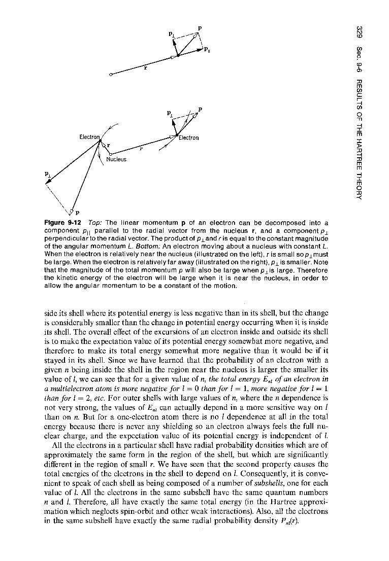
Al:I

O31

- 11 3

H1 3

O S

lif1

Sa

1

p

r

Figure 9-12 Top: The linear momentum p of an electron can be decomposed into a component p 11 parallel to the radial vector from the nucleus r, and a component p1 perpendicular to the radial vector. The product of p l and r is equal to the constant magnitude of the angular momentum L. Bottom: An electron moving about a nucleus with constant L. When the electron is relatively near the nucleus (illustrated on the left), r is small sop lmust be large. When the electron is relatively far away (illustrated on the right), p1 is smaller. Note that the magnitude of the total momentum p will also be large when ps is large. Therefore the kinetic energy of the electron will be large when it is near the nucleus, in order to allow the angular momentum to be a constant of the motion.

side its shell where its potential energy is less negative than in its shell, but the change is considerably smaller than the change in potential energy occurring when it is inside its shell. The overall effect of the excursions of an electron inside and outside its shell is to make the expectation value of its potential energy somewhat more negative, and therefore to make its total energy somewhat more negative than it would be if it stayed in its shell. Since we have learned that the probability of an electron with a given n being inside the shell in the region near the nucleus is larger the smaller its value of 1, we can see that for a given value of n, the total energy En, of an electron in a multielectron atom is more negative for 1 = 0 than for 1 = 1, more negative for 1 = 1 than for 1 = 2, etc. For outer shells with large values of n, where the n dependence is not very strong, the values of Ent can actually depend in a more sensitive way on 1 than on n. But for a one-electron atom there is no 1 dependence at all in the total energy because there is never any shielding so an electron always feels the full nu-clear charge, and the expectation value of its potential energy is independent of 1.

All the electrons in a particular shell have radial probability densities which are of approximately the same form in the region of the shell, but which are significantly different in the region of small r. We have seen that the second property causes the total energies of the electrons in the shell to depend on 1. Consequently, it is conve-nient to speak of each shell as being composed of a number of subshells, one for each value of 1. All the electrons in the same subshell have the same quantum numbers n and 1. Therefore, all have exactly the same total energy (in the Hartree approxi-mation which neglects spin-orbit and other weak interactions). Also, all the electrons in the same subshell have exactly the same radial probability density Pnl(r).

1

Is H

3 4 2s Li Be

11 12

3s Na Mg

19 20 4s K Ca 3d

37 38

5s Rb Sr 4d

55 56 6s Cs Ba 5d

87 88 7s Fr Ra 6d

s l s 2

21 Sc

22 Ti

23

V

24

Cr

4s 1 3d 5

25

Mn

26

Fe

27

Co

28

Ni

29 Cu

4s 1 3d 10

30

Zn

39

Y

40

Zr

41

Nb

5s1 4d 4

42

Mo

43

Tc

44

Ru

5s 14d 7

45

Rh

5s 1 4d 8

46

Pd

5s04410

47

Ag

5s1 4d 10

48

Cd

Lantha- sicles

72 Hf

73 Ta

74 W

57 La

75 Re

76 Os

77 Ir

78 Pt

6s 1 5d 9

79 Au

6s 1 5d 10

80 Hg

89 Ac

Actinides

d 1

d 2

d 3

d 4

d 5

d 6

d 7

d 8

d 9 d 10

5 B

6 C

7 N

8 0

9 F

10 Ne

13

Al

14

Si

15

P

16

S 17

CI 18

A

31

Ga

32

Ge

33

As

34

Se

35

Br

36

Kr

49

In

50

Sn

51

Sb

52

, Te

53

I

54

Xe

81 Ti

82 Pb

83 Bi

84 Po

85 At

86 Rn

P1

P2

p3 p4 p5 p6

2

He

2p

3p

4p

5p

6p

7p

Chap. 9 MULTIELECTRON ATOMS—GROUND STATES AND X-RAY EXCITATIONS 330

4f Lanthanides

58 59 60 61 62 63 64 65 66 67 68 69 70 71

Ce Pr Nd Pm Sm Eu Gd Tb Dy Ho Er Tm Yb Lu

5do4f2 5d04f3 5do4f 4 5do4f5 5d o4f 6 5d04f7 5d14f7 5d0419 5d04f10 5da4fu 5do4f 12 5d04/13 5do4f14 5d 141 14

5f

Actinides

90 91 92 93 94 95 96 97 98 99 100 101 102 103

Th Pa U Np Pu Am Cm Bk Cf Es Fm Md No Lw

6d 2 5f 9 6d 1 5f 2 6d 1 5f3 6d 1 5f 4 6d 1 5f- 5 6d15f6 6d15f7 6d15f8 6d05f10 6d05f11 6do5f1z 6d° 5113 6d05(14 6d15f14

f14 f 1 f 2 f 3 f4 f 5 6

f 7 f8 f9 f10 fll [12 f13

Figure 9-13 The periodic table of the elements, showing the electron configuration for each element.

9-7 GROUND STATES OF MULTIELECTRON ATOMS AND THE PERIODIC TABLE

Most of the properties of the chemical elements are periodic functions of the atomic number Z that specifies the number of electrons in an atom of the element. It was first emphasized by Mendeleev in 1869 that these periodicities can be made most apparent by constructing a periodic table of the elements. A modern version of his table is presented in Figure 9-13. Each element is represented in the table by its chemical symbol, and also by its atomic number. Elements with similar chemical and physical properties are in the same column. For instance, all elements in the first column are alkalis and have a valence of plus one; all elements in the last column are noble gases and have a valence of zero. The discovery of the periodic table was a great breakthrough of chemistry. Its interpretation was an equally significant devel-opment of physics.

We assume that the student has some familarity with the periodic properties of the elements from his study of elementary chemistry. For this reason, we do not need to stress their importance to chemistry. Our task here is to interpret these properties in terms of the Hartree theory of multielectron atoms. That is, in this section we shall present the quantum mechanical interpretation of the basis of inorganic chemistry, plus that of much organic chemistry and solid state physics.

The interpretation of the periodic table is based on information about the ordering according to energy of the outer filled subshells of multielectron atoms. The required information can be obtained from the results of the Hartree calculations, described in the last section, which yield the ordering according to energy of the outer filled sub-shells as is shown in Table 9-2. The first column identifies the subshell by the quantum numbers n and 1.

The second column of Table 9-2 identifies the subshells by giving the spectroscopic notation for n and 1. This notation is commonly used in discussing the spectra and

Table 9-2 The Energy Ordering of the Outer Filled Subshells

Quantum Numbers n, 1

Designation of Subshell

Capacity of Subshell 2(21 + 1)

6, 2 6d 10 5, 3 5f 14 7, 0 7s 2 6, 1 6p 6 5, 2 5d 10 4, 3 4f 14 6, 0 6s 2 5, 1 5p 6 4, 2 4d 10 5,0 5s 2 4, 1 4p 6 3, 2 3d 10 4, 0 4s 2 3,1 3p 6 3, 0 3s 2 2, 1 2p 6 2, 0 2s 2 1,0 is 2

i Increasing energy

(less negative)

— Lowest energy (most negative)

GR

OU

ND

ST

AT

ES

OF

MU

LTIE

LEC

TR

ON

AT

OM

S A

ND

TH

E P

ER

I OD

IC T

AB

LE

MU

LT

IEL

EC

TR

ON

AT

OMS

-G

RO

UN

D S

TA

TE

S A

ND

X- R

AY

EX

CIT

AT

ION

S

Table 9-3 The Spectroscopic Notation for 1

l 0 1 2 3 4 5 6

Spectroscopic notation s p d fg h i

energy levels of atoms. The number gives the value of n, and the letter gives the value of l according to the scheme shown in Table 9-3. In this scheme the l = 0 state is called an s state; the l = 1 state is called a p state; etc.

The third column of Table 9-2 is equal to 2(21 + 1). As mentioned in the last section, that quantity is the number of possible combinations of m l and mS, for the value of l characteristic of the subshell. Thus the third column gives the maximum number of electrons that can occupy different states in the same subshell without violating the exclusion principle.

In our discussion of the last section we found that the Hartree theory predicts that the energy of the subshell becomes more negative with decreasing values of n and with decreasing values of l. We see this immediately in Table 9-2. The i s subshell, which is the only subshell in the n = 1 shell, has the lowest energy. The two subshells of the n = 2 shell are both of higher energy and, of these, the 2s subshell is of lower energy than the 2p subshell. In the n = 3 shell the subshells 3s, 3p, 3d are also ordered in energy according to the predictions of the Hartree theory. However, the energy of the 4s subshell is actually lower than the energy of the 3d subshell because, for reasons described in the last section, the l dependence of the energy Ent of the subshells can be more important than the n dependence for outer subshells with large values of n. Continuing up the list, we see that the ordering of the outer subshells always satisfy the following rule:

For a given n, the outer subshell with the lowest l has the lowest energy. For a given 1, the outer subshell with the lowest n has the lowest energy. Near the top of the list, the l dependence of Ent becomes so much stronger than the n dependence that the energy of the 7s subshell is lower than the energy of the 5f subshell.

It should be noted that Table 9-2 does not necessarily give the energy ordering of all subshells in any particular atom, but only the energy ordering of the subshells which happen to be the outer subshells for that atom. For instance, the energy of the 4s subshell is lower than that of the 3d subshell for K atoms and the next few atoms of the periodic table. But for atoms further up in the periodic table the 3d sub-shell is of lower energy than the 4s subshell because for these atoms they are inner subshells and the n dependence of Ent is so strong that it dominates the l dependence. Additional information of this type is presented in Figure 9-14.

Now the characteristics of an atom depend on the behavior of its electrons. The behavior of an electron is specified by the set of four quantum numbers which specify its quantum state. However, in the approximation represented by the Hartree theory only the quantum numbers n and l are important. Therefore, in this approximation an atom can be characterized by specifying the n and 1 quantum numbers of all the electrons. This specification of the subshells occupied by the various electrons is called the configuration of the atom. The ordering according to energy of the outer filled subshells being known, it is trivial to determine the configuration of any atom in its ground state. In the ground state the electrons must fill all the subshells in such a way as to minimize the total energy of the atom and yet not exceed the capacity 2(2l + 1) of any subshell. The subshells will fill in order of increasing energy, as listed in Table 9-2.

Consider first the H atom. The single electron occupies the i s subshell, with its spin either "up" or "down". For the He atom both electrons are in the is subshell, one

5d 5 5s p

3d \^ 4p 4d

4s • 4s

^° 3p

w ^ 3d 3p 3s 3s

2p

2s

is • is

I I I - I I I I I I 0 20 40 60 80

Z

Figure 9-14 A schematic representation of the energy ordering of all the subshells in an

atom, as a function of its atomic number Z. Each curve begins at the Z for which the subshell begins to be occupied. Only subshells occupied in atoms through mercury are shown, so all

curves stop at Z = 80. The ordering of the outer filled subshel Is in various atoms is found on

the left side of the diagram. The ordering of all filled subshells in mercury is found on the right

side of the diagram. The energy scale is non-linear and, furthermore, varies with Z.

with spin "up" and the other with spin "down". The configuration of H is written 1 H: ls 1

The configuration of He is written 2He: 1s 2

The superscript on the subshell designation specifies the number of electrons which it contains; the superscript on the chemical symbol specifies the Z values for the atom. In the 'Li atom one of the electrons must be in the 2s subshell because the capacity of the is subshell is only 2. The configuration of this atom is

3 L1: is22s 1 The 4Be atom completes the 2s subshell and has the configuration

4Be: 1s2 2s2 In the six elements from 5 B to 10Ne the additional electrons fill the 2p subshell. The configurations of 5 B and 10Ne are

5 B: 1s22s22p 1

10Ne : 1s22s22p6

Note that the periodic table of the elements presented in Figure 9-13 is divided vertically into a series of blocks with each row labeled by the subshell which, accord-ing to Table 9-2, the elements of the row are filling. Knowing this, it is easy to write the configuration of any atom, with a procedure that will become more apparent in Example 9-6. But there are certain atoms for which the last few electrons are observed.

4p

2p 2s

318

`d1

OId

OIa

3d

3H

1 a

Md

SW

O1d

NO

1:11

0313

I11

f101

3O

S31b'1

S d

Nf1

O1:1

9

MU

LT

I E

LE

CT

RO

N A

TO

MS

-G

RO

UN

D S

TA

TE

S A

ND

X-R

AY

EX

CIT

AT

ION

S

to be in different subshells than would be predicted by this scheme. The configura-tions for these atoms are indicated in the periodic table by the entries below their chemical symbol.

Example 9-6. Write the configurations for the ground states of 19K, 23V, 24Cr, 43Tc, 44Ru, 46Pd 57 La, 58Ce, and 59Pr. ■ From the absence of any entry below 19 K in the periodic table of Figure 9-13, we con-clude that there is nothing exceptional about its configuration. The configuration is then obtained by inspecting the periodic table and listing in order the lowest energy subshells, and their populations, for the 19 electrons of the atom. It is

19 K: 1s22s2 2p6 3s2 3p64s 1

The first 18 electrons completely fill the subshells of lowest energy, and the last electron partly fills the 4s subshell. Adding four more electrons to obtain 23V completes the filling of the 4s subshell and puts three electrons in the 3d subshell, which is the one of next highest energy. The configuration is

23V: is22s2 2p6 3s2 3p64s2 3d3

The entry 4s 1 3d 5 for 24Cr in Figure 9-13 means that the configuration of this atom does not end with the symbols 4s 2 3d4, as would be expected, but instead is

24Cr: 1s 22s 22p6 3s 2 3p64s 1 3d 5

The reason for this behavior will be explained later. Inspection shows that the configurations of the other atoms of interest are

43Tc: is2 2s2 2p6 3s2 3p64s2 3d 1°4p6 5s 24d 5 44Ru: 1s2 2s22p6 3s2 3p64s2 3d 104p6 5s 14d7 46Pd: 1s2 2s 2 2p 6 3s2 3p64s2 3d 1°4p64d' o

57La: 1s22s22p6 3s2 3p64s23d 104p6 5s24d' ° 5p6 6s 2 5d 1 58Ce: 1s2 2s 2 2p6 3s 2 3p 64s2 3d 1°4p6 5s24d' ° 5p66s24f2

59Pr: 1s2 2s 2 2p6 3s 2 3p64s 2 3d 1°4p6 5s24d' ° 5p66s24f3

We see from Example 9-6 that in certain cases the actual configurations observed for the elements do not strictly adhere to the predictions of Table 9-2. For instance, this table says that the energy of the 3d subshell is greater than the energy of the 4s subshell when these subshells are filling Yet in Z4Cr, and also in "Cu, one of the electrons that could be in the 4s subshell is actually in the 3d subshell. Similar situa-tions are observed to occur for the 5s and 4d subshells. In 43Tc the 5s subshell is filled in the normal manner. But in 45 Rh there is only one electron in the 5s subshell; in 46 Pd both electrons have left the 5s subshell and moved to the 4d subshell. The 78 13t and 79Au configurations show that the same kind of thing can happen for the 6s and 5d subshells. From these circumstances we conclude that the energy separa-tions between the 4s and 3d, the 5s and 4d, and the 6s and 5d subshells must be so small while they are being filled that, although generally the ordering of these sub-shells is as shown in Table 9-2, in certain cases the ordering can actually be reversed. This can be seen in Figure 9-14. Configurations which disagree with Table 9-2 are also observed in 57La and in the lanthanides (Z = 58 to 71), more commonly called the rare earths. Table 9-2 predicts that after the completion of the 6s subshell the 4f subshell should fill, but in two of the rare earths there is one 5d electron. A similar situation occurs in the group of elements following 89Ac, which are called the ac-tinides (Z = 90 to 103). From the same argument we used previously, we interpret these observations to mean that the energy differences between the 5d and 4f sub-shells, and between the 6d and 5f subshells, are very small while these subshells are being filled.

On the other hand, certain predictions of Table 9-2 are always obeyed. Since none of the configurations is exceptional for elements in the first two and last six columns

of the periodic table, we conclude that every p subshell is always of higher energy than the preceding s or d subshell while these subshells are being filled, and that in these circumstances every s subshell is always of higher energy than the preceding p subshell. Therefore there must be large energy differences between the subshells con-cerned while they are being filled. In fact, the energy differences between every s subshell and the preceding p subshell are particularly large as can be seen in Figure 9-14, and it is easy to understand why. Since for a given n the energy of a subshell becomes higher with increasing 1, an s subshell is always the first subshell to be occupied in a new shell. Consequently, when an electron is added to a configuration with a completed p subshell and goes into the subshell of next highest energy, which according to Table 9-2 is always an s subshell, the electron will be the first one in a new shell. Compared to the electrons in the preceding subshell, its average radial coordinate will be considerably larger, its average potential energy will be consid-erably less negative, and its total energy will be considerably higher—much higher than for the usual increase in total energy in going from one subshell to the next.

The fact that there is a particularly large energy difference between every s subshell and the preceding p subshell has some important consequences. Consider atoms of the elements 10Ne,' 8 A, 36 Kr, 54Xe , and 86 Rn, in which a p subshell is just completed. Because of the very large difference between the energy of an electron in the p subshell and the energy it would have if it were in the s subshell, the first excited state of these atoms is unusually far above the ground state. As a result, these atoms are particularly difficult to excite. In their ground state, Gauss's law shows they produce no electric field external to the atom since they consist of sets of completely filled subshells, and so they have spherically symmetrical charge distributions with zero net charge because they are neutral overall. Furthermore, these atoms produce no external magnetic fields in their ground state since, as we shall see later, the total angular momenta of electrons in completely filled subshells couple to zero, and this coupling yields zero total magnetic dipole moment. Because of the absence of external fields (at least on a time-averaged basis), it is very difficult for these atoms to interact with other atoms to produce chemical compounds. They also have very low boiling and freezing points because they have little tendency to condense into liquids or solid form. These are the noble gas elements.

The atom 'He is also a noble gas because for it the first unfilled subshell is an s subshell (even though it does not contain a filled p subshell) so it has an unusually high first excited state, and because in its ground state the atom consists of com-pletely filled subshells and so produces no external fields. That 'He is a noble gas is indicated by its being listed in the last column of the periodic table instead of the second column. An element such as 20Ca is not a noble gas, even though it consists of completely filled subshells, because in its first excited state an electron goes to a 3d subshell. So the excited state is not far above the ground state and very little energy is required to make the atom produce an external field which will allow it to interact with other atoms.

Another aspect of the particular inertness of the noble gases can be obtained by plotting, for the various elements, the measured values of the magnitude of the total energy of an electron in the highest-energy filled subshell. This is equal to the energy required to remove the electron from the atom, which is the ionization energy of the atom. Figure 9-15 shows such a plot. We see that the ionization energy oscillates about an average value which is essentially independent of Z, in agreement with our conclusion of the previous section that the total energy of electrons in the outer shells is roughly the same throughout the periodic table. The oscillations are quite pro-nounced, however, and it is apparent that the total energy of an electron in the highest-energy filled subshell of a noble gas is considerably more negative than aver-age. These electrons are very tightly bound, and the atoms are very difficult to ionize.

GR

OU

ND

ST

AT

ES

OF

MU

LTIE

LEC

TR

ON

AT

OM

S A

ND

TH

E P

ER

I OD

IC T

AB

LE

^

C^) CO

MU

LTIE

LEC

TR

ON

AT

OM

S-

GR

OU

ND

ST

AT

ES

AN

D X

- RA

Y E

XC

ITA

TIO

NS

25

f 20

—*He Ne •

S A ^ 15 — • • Kr

• • • Xe Ç H • • • • Rn

Ç 10 —• • • • • • •

° . • 'r%' . ..:•; «

ô 5 ^ • • • • f .• •^ •^^ • i U — Li Na K

• • •

Rb Cs

I I i I i I I I I I I I I I I I I I I I 0

10 20 30 40 50 60 70 80 90 100 Z

Figure 9-15 The measured ionization energies of the elements.

We also see that the ionization energy is particularly small for the elements 3 Li, 11Na, 19K, 37Rb, 55Cs, and 87Fr. These are the alkalis. They contain a single weakly bound electron in an s subshell. Alkali elements are very active chemically because it is energetically favorable for them to get rid of the weakly bound electron and revert to the more stable arrangement obtained with completely filled subshells. These elements are said to have one valence electron, and a valence of plus one.

At the other extreme are the halogens, 9F, 17 C1, 35Br, 53 I, and 85At, which have one less electron than is required to fill their p subshell. These elements have a high electron affinity; i.e., they are very prone to capture an electron. They have a valence of minus one. In 1962 it was discovered that in special circumstances noble gases could be made to combine with the halogen 9F to form stable molecules. Before that time it was believed that the noble gases were completely inert. These molecules can be formed only because 9F has such a high electron affinity that it can remove one of the very tightly bound electrons from the filled outer subshells of the noble gases.

For the first three rows of the periodic table, the properties of the elements, such as valence and ionization energy, change uniformly from the alkali element with which the row begins to the noble gas with which it ends. In the fourth row of the periodic table this situation is no longer always true. The elements 21 Sc through 28Ni, which are called the first transition group, have quite similar chemical properties and almost the same ionization energies. These elements occur during the filling of the 3d subshell. The radius of this subshell is considerably less than that of the 4s subshell, which is completely filled for all the first transition group except "Cr. The filled 4s subshell tends to shield the 3d electrons from external influences, and so the chemical properties of these elements are all quite similar, independent of exactly how many 3d electrons they contain. The point is that the chemical properties of the elements depend on the electrons in the outer subshells of their atoms, since these are the electrons responsible for producing the electric and magnetic fields that inter-act with electrons in other atoms. The chemical properties of 29Cu are somewhat dif-ferent from those of the first transition group because it has only a single 4s electron in the outermost subshell. To a lesser extent this is also true for 'Cr. The element 30Zn consists of a set of completely filled subshells and so is somewhat more inert,

as can be seen from its ionization energy Similar transition groups occur in the filling of the 4d and 5d subshells.

An extreme example of the same situation is found in the rare earths 58Ce through 71 Lu. These are the elements in which the 4f subshell is filling. This subshell lies deep within the 6s subshell, which is completely filled in all the rare earths. The 4f electrons are so well shielded from the external environment that the chemical properties of these elements are almost identical. The same thing happens in the actinides, 90Th

through 1o3Lw. In this group the 5f subshell is filling inside the filled 7s subshell. Some of the most exciting work in contemporary chemistry is the study of the ac-tinides of highest atomic number, which have only recently been discovered.

It is appropriate to close our discussion by emphasizing the importance of the exclusion principle. If it were not obeyed, all the electrons in a multielectron atom would be in the is subshell because this is the subshell of lowest energy. If this were the case, all atoms would have spherically symmetrical charge distributions of very small radii that would produce no external electric fields, and furthermore they would also have very high first excited states. Then all atoms would be much like noble gases, and therefore there would be no molecules. In fact, the entire universe would be completely different if electrons did not obey the exclusion principle!

Example 9-7. Make an order of magnitude estimate of the ionization energy of 92U, if the exclusion principle did not operate so that all of its electrons were in its n = 1 shell. For this purpose assume that the typical electron feels the nuclear charge shielded by the charge of half the other electrons in the shell. Compare the results of the estimate with the actual value of the ionization energy shown in Figure 9-15. •An estimate of the total energy of a typical electron can be obtained from the one-electron atom energy formula

uZ2e4 _ Z2 E

(47zE O) 22h n2 — n2 x 13.6 eV

If we set n = 1 and use an effective Z with the value Z 1 = Z/2 = 92/2 = 46, the absolute value of the result is the ionization energy. So we obtain

1E1 = (46) 2 x 13.6 eV 3 x 104 eV

From Figure 9-15 we find that the actual ionization energy is

IEI = 4 eV

Without the exclusion principle the ionization energy of 92U would be something like four orders of magnitude larger than it actually is.

9-8 X-RAY LINE SPECTRA

In an x-ray tube such as the one shown in Figure 2-9, electrons are emitted from a heated cathode, accelerated in a beam to kinetic energies of the order of 10 4 eV by a voltage applied between the cathode and anode, and then strike the anode. While traveling through the atoms of the anode, a beam electron occasionally passes near an electron in an inner subshell. By means of the Coulomb interaction between the energetic beam electron and the atomic electron, the latter can be given enough energy to remove it from its very negative energy level and eject it from the atom. This leaves the atom in a highly excited state because one of its electrons that had a very negative energy is missing. The atom will eventually return to its ground state by emitting a set of high energy, and therefore high-frequency, photons which are members of its x-ray line spectrum. (The interaction between a beam electron and an outer subshell atomic electron leading to low-energy excited states, and the produc-tion of the optical spectrum, is discussed in the next chapter.) The total spectrum of x radiation emitted by an x-ray tube consists of the discrete line spectrum, super-imposed on a continuum, as is illustrated for a typical case in Figure 9-16. The continuum is due to the bremsstrahlung processes occurring when the beam electrons suffer accelerations in scattering from the nuclei of the atoms in the anode. As we saw in Section 2-6, the shape of the bremsstrahlung continuum depends mainly on the energy of the electron beam. But the shape of the x-ray line spectrum is characteristic of the particular atoms composing the anode.

t/1:I

103d

S 3

NI1

l.b

'a-X

I I

0.5 1.0 1.5 0

Wavelength (Â)

MU

LTI E

LEC

TR

ON

AT

OM

S-G

RO

UN

D S

TA

TE

S A

ND

X-R

AY

EX

CIT

AT

ION

S

Figure 9-16 A typical x-ray spectrum. The lines are characteristic of the atoms of the x- ray tube anode (tungsten for the case illustrated). The continuum arises from bremsstrahlung by electrons accelerated in scattering from the nuclei of these atoms.

X-ray line spectra are of practical interest because they are significant features of x rays, which have so many useful applications in technology and science. These spectra are of theoretical interest because they provide information about the energies of electrons in the inner subshells of atoms. We shall see that this information is in good agreement with the predictions of the Hartree theory.

As an example of the production of an x-ray line spectrum, assume that an electron is initially removed from the is subshell of an atom in the anode of the tube. In the first step of the deexcitation process an electron from one of the subshells of less negative energy drops into the hole in the is subshell; for instance, a 2p electron could drop into the hole. This would leave a hole in the 2p subshell, but the excitation energy of the atom would be considerably reduced. Energy is conserved by the emis-sion of a photon of energy equal to the decrease in the excitation energy of the atom, that is, the difference between the energies associated with an electron missing from the is and 2p subshells. Typically there would be several subsequent steps in the de-excitation process. For instance, the hole in the 2p subshell could be filled by a 3d electron, leaving a hole in the 3d subshell which is then filled by a 4p electron, etc. The net effect of each step is that a hole jumps to a subshell of less negative energy. When the hole works its way to the subshell of the atom of least negative energy, which is usually the outermost shell, it is filled by the electron initially ejected from the is subshell or, more typically, by some other electron in the anode. The atom is then neutral again, and in its ground state.

The energy levels of an atom which are involved in the emission of its x-ray line spectrum are most conveniently represented in terms of an energy-level diagram that is rather different from the standard type with which we have become familiar. Figure 9-17 shows such a diagram for the 92U atom, including all its x-ray energy levels through n = 4. Because of the wide range of energies involved, it is conventional to use a logarithmic energy scale. Because it simplifies the discussion, it is also con-ventional to define the total energy of the atom to be zero when the atom is in its ground state. Since the energy scale is logarithmic, the zero energy level representing the ground state cannot be displayed on the diagram, but this does no harm. The most important difference between an x-ray energy-level diagram and a standard energy-level diagram is that the x-ray diagram gives the energy of the atom when one electron of the indicated quantum numbers n, 1,1 is missing. That is, the diagram describes the energy levels of the hole, with quantum numbers n, 1, j, that jumps from one subshell to the next when the atom emits its x-ray line spectrum. As a hole re-

105

104

P23 a) C W

103

10 2

K series

V

V

^(

v

n l j

1 0 1/2

2 0 1/2 2 1 1/2 2 1 3/2 3 0 1/2 3 1 1/2 3 1 3/2 3 2 3/2 3 2 5/2

4 0 1/2 4 1 1/2 4 1 3/2 4 2 3/2 4 2 5/2 4 3 5/2 4 3 7/2

i

v V

V

v

M series

lLI f-LII `^LIII

/MI wMII ^MIII

MV ks*NI

NII NIII

Niv Nv

NvI

NvII

-c---K1

b1:I

103dS

3N11

AbL

l-X

f

L series

^

Figure 9-17 The higher energy x-ray levels for the uranium atom and the transitions between these levels allowed by the selection rules.

presents the absence of an electron of negative energy, the energy associated with a

hole is positive. So the energies of all the levels of an x-ray diagram are positive.

The energy levels in Figure 9-17 are also identified by a notation commonly used

in discussing x-ray spectra. In this notation the value of the quantum number n is

specified by capital letters, according to the scheme shown in Table 9-4. That is, an

n = 1 level is called a K level, an n = 2 level is called an L level, etc. Similarly, the n = 1 shell is called the K shell, etc. Roman numeral subscripts are used to label levels

of the same n, according to decreasing energy. That is, in order of decreasing energy

the three L levels are called L I , L11 , and Linn.

If the energy of an atom with an electron of quantum numbers n, 1, j is particularly negative, the energy of an atom with a hole of the same quantum numbers is par-ticularly positive since more energy must be given to the atom to remove the electron. In other words, the lack of a large negative energy is equivalent to the presence of a large positive energy. Keeping this inversion in mind, we see from Figure 9-17, which was obtained from an analysis of the measured x-ray line spectrum of 92U, that the n, 1, j dependences of the x-ray energy levels are as would be expected from the Hartree theory. The energies of these levels increase with decreasing values of n and of 1, in agreement with an inversion of the rule describing the theoretical predictions that was stated in the preceding section. The x-ray energy level for j = 1 + 1/2 has lower energy, and the level for the other possibility, j = 1 — 1/2, has higher energy. This is the expected inversion of the splitting of the energy levels according to j, discussed in connection with one-electron atoms in Section 8-6. In the L shell (n = 2) of 92U this splitting is more than 2000 eV, and it is larger than the dependence on 1. So it is hardly appropriate to call the j dependence of x-ray energy levels "fine-structure splitting." The strong j dependence, which is characteristic of the inner shells of all atoms except those of very low Z, is partly due to the increase in the magnitude of the spin-orbit interaction because of the high value of the term (1/r)dV(r)/dr in (8-35). It also involves the other relativistic effects that become very large for the high ve-locity electrons that populate the inner shells of these atoms.

Table 9-4 The Spectroscopic Notation for n

n 1 2 3 4 5

Spectroscopic notation K L M N O

0

M M

ULT

IELE

CT

RO

N A

TO

MS

-G

RO

UN

D S

TA

TE

S A

ND

X-R

AY

EX

CIT

AT

ION

S

As we have indicated, it is convenient to think of the production of the x-ray line spectra in terms of the creation of a hole in one of its higher-energy levels, and the subsequent jumping of the hole through its lower-energy levels. With each jump, an x-ray photon is emitted that carries off the excess energy. The frequency y of the photon bears the usual relation to the energy E which it carries, E = hv. But not all transitions occur. There is the following set of selection rules for the change in quantum numbers of the hole:

Al = + 1

Aj = 0, ±1

These are the same as the selection rules of (8-37) and (8-38), for an electron in a one-electron atom, and they have the same explanation as presented in Section 8-7. The x-ray energy-level diagram for 92U, of Figure 9-17, shows the transitions that obey these selection rules. The totality of x rays which are emitted .in such transitions (plus a few which are observed to be emitted very infrequently in violation of the selection rules) constitute the x-ray line spectrum of the atom. All transitions from the K shell produce lines of the so-called K series, with K a corresponding to a transi-tion to the L shell, K R to the M shell, etc. All transitions from the L shell produce lines of the L series, and so forth.

Example 9-8. Estimate the minimum accelerating voltage required for an x-ray tube with a 26 Fe anode to emit a K a line of its spectrum. Also estimate the wavelength of a Ka photon. ■ We can use the crude description of the results of the Hartree theory to estimate the excitation energy of a 26Fe atom with a hole in its K shell. Equation (9-27) tells us that this energy is

l-cZ e4 Zn E K ~ + (47LE0)22h2n2

13.6 n2 eV

13.6(Z — 2) 2 eV = 13.6 x (24)2 eV

+7.8x103 eV

where we have set n = 1 and Z n = Z1 = Z — 2. A beam electron bombarding an atom in the anode must have this much energy to produce the hole. The voltage V required to accelerate the beam electron to this energy is just

V^ 7.8 x 10 3 V

After the atom emits a K a photon, the hole is in its L shell. Then its energy is

EL + 13.6 nz

eV 13.6 (26 —

4

10)2 eV ^ + 8.7 x 10 2 eV

where we have set n = 2 and, following the results of Example 9-5, set Zn = Z2 = Z — 10. The photon carries away energy

hv = EK — EL

But since the value of EL is only about 10% of the value of EK, and since the crude approxi- mation we have used to obtain EK is generally not accurate to 10%, we might as well take

hv EK

The wavelength , of the photon is related to its frequency y and its velocity c by the expression

1 v hv

c hc

so

1 EK ke4

Z — 2 2 ,

hc ti

(47CE0)24iwh3 ( )

The term multiplying (Z — 2) 2 is Rydberg's constant, R M , defined in (4-22). Therefore

1 R M (Z — 2) 2 ^ 1.1 x 10' x (24) 2 m -1 = 6.3 x 109 m -1

(9-28)

(9-29)

(9-30)

co ^

b1:1

103d

S 3N

11 A

b'a

-X 8-

6 '0

aS

and

^1.6x10 -10 m=1.6 A This wavelength is about the size of a typical molecule, or the spacing of atoms or molecules in a crystal. Thus the Ka x rays from 26Fe can be used in diffraction experiments to study the structure of molecules or crystals.

A striking feature of x-ray line spectra is that the frequencies and wavelengths of the lines vary smoothly from element to element. There are none of the abrupt changes from one element to the next which occur in atomic spectra in the optical frequency range. The reason is that the characteristics of x-ray spectra depend on the binding energies of the electrons in the inner shells. With increasing atomic number Z, these binding energies simply increase uniformly, owing to the higher nuclear charge, and they are not affected by the periodic changes in the number of electrons in the outer shells of the atom that affect the optical spectra. The regularity of x-ray spectra was first observed by Moseley. In 1913 he made a survey of x-ray spectra and obtained data for a number of elements on the wavelengths of the Ka line. (There are really two closely spaced Ka lines, as can be seen from Figure 9-17, but it was difficult for Moseley to resolve this structure.) The measured wavelengths could be fitted within experimental accuracy by the empirical formula

1 C(Z — a)2 (9-31)

where C is a constant with a value approximately equal to the Rydberg constant RM , and a is a constant with a value of about 1 or 2. This formula, and some of the data,

are plotted in Figure 9-18. Moseley interpreted the empirical formula on the basis of the Bohr model, which

had been proposed just before he made his measurements. He performed a calculation essentially the same as our calculation in Example 9-8 to obtain (9-30), which agrees well enough with (9-31), but he took the basic energy equation, (9-27), from the Bohr model instead of the Hartree theory. That is, he adapted the Bohr energy equation into (9-27) by replacing Z by Zn , as a way of describing the shielding of the nuclear charge by electron charges in a multielectron atom. His arguments concerning shield-ing were similar to ours of Section 9-6, except that he thought the electrons travel in well-defined Bohr orbits and concluded that Z 1 ^ Z — 1 instead of Z 1 ^ Z — 2.

Moseley's work, carried out when he was a graduate student, was an important step in the development of quantum physics. His simple and successful application of the Bohr model to x-ray line spectra provided one of its earliest confirmations. By using the empirical formula to determine Z, he established unambiguously the

a 5 10 15 20 25 30 35 40

z Figure 9 -18 Points representing Moseley's data, and a curve representing his empirical

formula. The curve is a straight line since the square root of the reciprocal of the wave

lengths of the x-ray lines is plotted versus the atomic number of the atoms producing the

lines.

N

M M

ULT

IELE

CT

RO

N A

TO

MS

- GR

OU

ND

ST

AT

ES

AN

D X

- RA

Y E

XC

ITA

TIO

NS

1 0 -1

^

O

correlation between the nuclear charge of an atom and its ordering in the periodic

table of the elements. For instance, he found that the atomic number of 'Co is one

less than that of 28Ni, even though its atomic weight is greater. He also showed that

there were gaps in the periodic table, as it was then known, at Z = 43, 61, 72, and 75. Elements of these atomic numbers have subsequently been discovered. Moseley's

contributions were brought to a halt by service in World War I, from which he did

not return.

Example 9-9. Measured values of the probability that a 82Pb atom will absorb by the photoelectric effect an x-ray photon from an incident beam of photons, are displayed in

Figure 9-19 by plotting the absorption cross section as a function of the energy hv of the photon. The prominent discontinuity just below 10 5 eV is called the K absorption edge. Show that it occurs at an energy for which the incident photon can just produce a hole in the K shell of 82Pb. Then explain the origin of the discontinuities a little above 10 4 eV. ► According to (9-27), the energy required to produce a hole in the K shell of 82Pb is approximately

Zz EK ^ + 13.6 Z eV ^ 13.6(Z — 2) 2 eV = 13.6 x (80) 2 eV = 8.7 x 104 eV

n This agrees within a few percent with the measured energy of the K absorption edge. A photon whose energy is slightly above this edge can be absorbed by the photoelectric effect on any electron of the atom. But a photon of energy slightly below the K absorption edge does not have enough energy to eject a K shell electron, so for it the photoelectric effect cannot occur on a K shell electron. Thus the photoelectric absorption cross section drops abruptly at the K absorption edge.

At energies a little above 10 4 eV there are three L absorption edges. These occur at the energies required to produce holes in the L shell of the atom. There are three because "fine structure", due to spin-orbit and other relativistic effects, splits the L level into three levels, L1, L11, L111, as can be seen in Figure 9-17. •

10 4 10 5 Photon energy hv (eV)

Figure 9-19 The probability that a lead atom will absorb an x-ray photon by the photo-electric effect, as a function of the energy of the photon. The probability is expressed in terms of the absorption cross section.

106

QUESTIONS

1. Why is there difficulty in distinguishing the two electrons in a helium atom from each other, but not the two electrons in separated hydrogen atoms? What about a diatomic hydrogen molecule?

2. Explain, without reference to the time-independent Schroedinger equation, why the pro-duct form of the eigenfunction of (9-3) immediately implies that the two particles it describes move independently.

3. Can you write a time-independent Schroedinger equation for two identical particles, without using particle labels?

4. Are particle labels themselves objectionable, in working with quantum mechanical sys-tems containing identical particles? If not, explain precisely what care must be exercised in using them.

5. Since the value of an antisymmetric total eigenfunction changes when its particle labels are exchanged, why can such eigenfunctions be used to give an accurate description of a system of electrons?

6. Does the exchange degeneracy increase the number of degenerate states in an atom containing two electrons? Ex4plain.

7. Do you think the sign of the charge of an elementary particle, like an electron or proton, is a more, or less, fundamental property than the "sign" of its symmetry?

8. Would atoms be affected more by reversing the signs of the charges of all their con-stituent particles, or by reversing all their symmetries?

9. Exactly what is meant by the statement that the spin variable is not continuous?

10. Would it be possible to measure effects of the exchange force acting between two electrons if there were no Coulomb interaction between them to produce an interaction energy of magnitude dependent on the sign of the exchange force?

11. Why would it be much more difficult to solve the time-independent Schroedinger equation for a system of interacting particles than for a system of independently moving particles?

12. Describe the steps in a cycle of the self-consistent Hartree treatment of a multielectron atom. Why is the estimate of the net potential V(r) obtained at the end of a cycle more accurate than the estimate used at the beginning?

13. Why is the angular dependence of multielectron atom eigenfunctions the same as for one-electron atom eigenfunctions? Why is the radial dependence different, except near the origin where it is the same?

14. Just what is the justification for using one-electron atom equations with an effective Z to discuss multielectron atoms?

15. What are the consequences of the fact that the sizes of all atoms are about the same? What are the reasons for this fact?

16. Devise a purely mechanical system in which a classical particle would exhibit the ten-dency, illustrated in Figure 9-12, to avoid the point about which it rotates.

17. Explain all aspects of the Z dependence of the subshell energies, plotted in Figure 9-14.

18. Why is it particularly difficult to separate mixtures of the rare earth elements by chemical techniques?

19. How can we be sure that if there were no molecules there would be no life?

20. What property of x rays makes them so useful in seeing otherwise invisible internal structures?

21. Give an example in the classical world where the concept of a hole might be used in a way comparable to the way it is used in discussing x-ray line spectra.

22. What argument might Moseley have used to conclude that the effective Z for the K shell is Z 1 Z — 1? Can Gauss's law of electrostatics be applied to evaluate the shielding produced by electrons moving in Bohr orbits?

CO

4= , w

SN

OIlS

3f1O

MU

LTIE

LEC

TR

ON

AT

OM

S- G

RO

UN

D S

TA

TE

S A

ND

X- R

AY

EX

CIT

AT

ION

S

23. What features of the periodic table of Figure 9-13 would Mendeleev fail to recognize? 24. Do the properties of the electrons in multielectron atoms provide any explanation of why

the element of highest atomic number found in nature is 92U? 25. In your opinion, what is the most important consequence of the exclusion principle?

PROBLEMS

1. By going through the procedure indicated in the text, develop the time-independent Schroedinger equation for two noninteracting identical particles in a box, (9-1).

2. By applying the technique of separation of variables, show that, for a potential of the additive form of (9-2), there are solutions to the two-particle time-independent Schroe-dinger equation, (9-1), in the product form of (9-3).

3. Exchange the particle labels in the two probability density functions, obtained from the symmetric and antisymmetric eigenfunctions of (9-8) and (9-9), and show that neither is affected by the exchange.

4. Verify that the expanded form of the three-particle eigenfunction of Example 9-2 is antisymmetric with respect to an exchange of the labels of two particles.

5. Verify that the expanded form of the three-particle eigenfunction of Example 9-2 is identically equal to zero if two particles are in the same space and spin quantum state.

6. Verify that the 1/ J3! normalization factor quoted in Example 9-2 is correct. 7. Verify that the expanded form of the three-particle eigenfunction of Example 9-3 is

symmetric with respect to an exchange of the labels of two particles. 8. An a particle contains two protons and two neutrons. Show that if each of its con-

stituents is antisymmetric then it must be symmetric, as stated in Table 9-1. (Hint: Consider a pair of a particles, and the effect of exchanging the labels of all the con-stituents in one with those of all the constituents in the other.)

9. Write an expression for the expectation value of the energy associated with the Coulomb interaction between the two electrons of a helium atom in its ground state. Use a space eigenfunction for the system composed of products of one-electron atom eigenfunctions, each of which describes an electron moving independently about the Z = 2 nucleus. Do not bother to evaluate the expectation value integral, but instead comment on its relation to the energy levels shown in Figure 9-7.

10. Prove that any two different nondegenerate bound eigenfunctions i/i i (x) and tk i(x) that are solutions to the time-independent Schroedinger equation for the same potential V(x) obey the orthogonality relation

J t//7(x)0 i (x) dx = 0

i j

(Hint: (i) Write the equations to which t/i i and tk i are solutions, and then take the complex conjugate of the second one to obtain the equation satisfied by 4. (ii) Multiply the equation in ti i by tJ'7, the equation in ti* by tpi, and then subtract. (iii) Integrate, using a relation such as 0i* d2 i/dx 2 — tfrid2 e/dx 2 = (d/dx)(07 dii/dx — tfüdI'7/dx).) The proof can be extended to include degenerate eigenfunctions, and also unbound eigen-functions that are properly normalized. Can you see how to do this?

11. (a) By going through the procedure indicated in Section 9-5, develop the time-independent Schroedinger equation for a system of Z electrons of an atom moving independently in a set of identical net potentials V(r). (b) Then separate it into a set of Z identical time-independent Schroedinger equations, one for each electron. (c) Verify that the form of a typical one is as stated in (9-22). (d) Compare this form with the time-independent Schroedinger equation for a one-electron atom, (7-12).

12. (a) Show that there are N! terms in the linear combination for an antisymmetric total eigenfunction describing a system of N independent electrons. (Hint: Consider Example 9-2, and use the mathematical technique of induction.) (b) Evaluate the number of such

terms for the case of the argon atom with Z = 18. (Hint: Use a mathematical table to evaluate N!, or use Stirling's formula, found in most mathematical references, to approxi-mate it.) (c) State briefly the connection between the results of (b) and the procedure used by Hartree to treat the argon atom.

13. (a) Use information from Figure 9-11 to make a sketch, on semilog paper, of the net potential V(r) for the argon atom. Be sure to determine several values for r/a p between 0 and 0.25, as this information will be used in Problem 18. (b) Also show the energy levels E 1 and E2, using estimates from Example 9-5, and the energy level E3, using measured data from Figure 9-15.

14. (a) Find the value of Z 1 for the helium atom which, when used in the energy equation, (9-27), leads to agreement with the ground state energy shown in Figure 9-6. (b) Com-pare Z 1 with Z. (c) Is Z 1 meaningful for an atom with as few electrons as helium? Explain briefly.

15. From Figure 9-6 estimate the average distance between the two electrons in a helium atom (a) in the ground state and (b) in the first excited state. Neglect the exchange energy.

16. (a) Use the Z, z for the argon atom obtained in Example 9-5 in the one-electron atom equation for the radial coordinate expectation value, to estimate the radii of the n = 1, 2, and 3 shells of the atom. (b) Compare the results with Figure 9-10.

17. Develop a mathematical argument for the tendency, illustrated in Figure 9-12, of an atomic electron with angular momentum L to avoid the point about which it rotates. Treat the electron semiclassically by assuming that it moves around an orbit in a fixed plane passing through the nucleus. (a) Show that its total energy can be written

2L2 2

E 2m + [ V(r) + 2mr2 ] 2m +

V (r)

where p H is its component of linear momentum parallel to its radial coordinate vector of length r. (b) Explain why this indicates that its radial motion is as it would be in a one-dimensional system with potential V'(r). (c) Then show that V'(r) becomes repulsive for small r because of the dominant behavior of the term L 2/2mr2, sometimes called the centrifugal potential.

18. (a) Sketch the potentials V'(r) for the argon atom with 1 = 0 and 1 = 1, defined in Problem 17, by adding the corresponding centrifugal potentials to the V(r) obtained in Problem 13. (b) Also sketch the energy level E2. (c) Show the classical limits of motion, within which E2 > V'(r). (d) Compare these limits with the radial probability densities of Figure 9-10, for n = 2, l = 0, and n = 2, l = 1.

19. Write the configurations for the ground states of 28Ni,

20. Write the configurations for the ground states of all the lanthanides, making as much use as possible of ditto marks.

21. Recent work in nuclear physics has led to the prediction that nuclei of atomic number Z = 110 might be sufficiently stable to allow some of the element Z = 110 to have survived from the time the elements were created. (a) Predict a likely configuration for this element. (b) Make a prediction of the chemical properties of the element. (c) Where would be a likely place to start searching for traces of it?

22. (a) From information contained in Figures 9-6 and 9-15, determine the energy required to remove the remaining electron from the ground state of a singly ionized helium atom. (b) Compare this energy with the energy predicted by the quantum mechanics of one-electron atoms.

23. (a) Draw a schematic representation of a standard energy-level diagram for the 22Tî atom, showing the states populated by electrons for a case in which one electron is missing from the K shell. The diagram should be comparable to the one in Figure 9-9 in that it should not attempt to give the energies of the levels to an accurate scale, and no distinction should be made between L I , L11 , and L111 levels, etc. (d) Do the same for a case in which one electron is missing from the L shell. (c) Draw a schematic representation of an x-ray energy-level diagram showing the energies of the atom when a hole is in the

29Cu, 30Zn, 31Ga.

sw31

eoad

MU

LT

IEL

EC

TR

ON

AT

OM

S- G

RO

UN

D S

TA

TE

S A

ND

X- R

AY

EX

CIT

AT

ION

S

K or L shells. (d) Compare the utility of the standard and x-ray energy-level diagrams for cases in which a hole is in an inner shell. (e) Also make such a comparison for cases in which a hole is in an outer shell.

24. The wavelengths of the lines of the K series of 74W are (ignoring fine structure): for K a, = 0.210 A; for K R , 2= 0.184 A; for K y, 2 = 0.179 A. The wavelength corresponding to

the K absorption edge is A= 0.178 A. Use this information to construct an x-ray energy-level diagram for 74W.

25. (a) Make a rough estimate of the minimum accelerating voltage required for an x-ray tube with a 26Fe anode to emit a La line of its spectrum. (Hint: As in Example 9-5, Z2 ^ Z — 10.) (b) Also estimate the wavelength of the L a photon.

26. (a) Use Moseley's data of Figure 9-18 to determine the values of the constants C and a in his empirical formula, (9-31). (b) Compare these values with those of (9-30), which was derived from the results of the Hartree theory.

27. It is suspected that the cobalt is very poorly mixed with the iron in a block of alloy. To see regions of high cobalt concentration, an x-ray is taken of the block. (a) Predict the energies of the K absorption edges of its constituents. (b) Then determine an x-ray photon energy that would give good contrast. That is, determine an energy of the photon for which the probability of absorption by a cobalt atom would be very different from the probability of absorption by an iron atom.

28. The Lyman-alpha lifetime in hydrogen is about 10 -8 sec. From this, find the lifetime for the Ka x-ray transition in lead. (Hint: For the inner electrons in lead the vvavefunctions are hydrogenic with appropriate effective Z; lifetime = 1/R; see (8-43).)

10 MULTIELECTRON

ATOMS-OPTICAL EXCITATIONS

10-1 INTRODUCTION

interactions experienced by atomic electrons; production of optical excita-tions

10-2 ALKALI ATOMS

optically active electron; hydrogen, lithium, and sodium energy levels; Hartree interpretation; fine structure; selection rules

10-3 ATOMS WITH SEVERAL OPTICALLY ACTIVE ELECTRONS

limitations of Hartree approximation; residual Coulomb and spin-orbit interactions; tendency for spins to couple together; tendency for orbital angular momenta to couple together; opposing tendency for each spin to couple to its orbital angular momentum; LS coupling; total spin angular momentum and quantum number s'; total orbital angular momentum and quantum number l'; total angular momentum and quantum number j'; JJ coupling

10-4 LS COUPLING

geometrical representation; quantum number m i; conditions satisfied by s', l', and j'; energy levels in typical LS coupling configuration; spectroscopic notation; multiplets; Landé interval rule; test for LS coupling; experimental assignment of quantum numbers

10-5 ENERGY LEVELS OF THE CARBON ATOM

treated as example of preceding discussion; hyperfine splitting; exclusion principle in LS coupling; properties of filled subshells; selection rules

10-6 THE ZEEMAN EFFECT '

normal and anomalous effects; qualitative discussion; derivation of Landé g factor; selection rules; electron spin resonance; experimental assignment of quantum numbers; Paschen-Bach effect; selection rules

10-7 SUMMARY

tabulated properties of interactions experienced by atomic electron in less than half-filled subshells; more than half-filled subshells

QUESTIONS

PROBLEMS

348

349

352

356

361

364

370

371

372

347

co M

M

ULT

I ELE

CT

RO

N A

TO

MS

-O

PT

ICA

L E

XC

ITA

TIO

NS

10-1 INTRODUCTION

A description of the behavior of electrons in multielectron atoms involves a succes-sion of increasingly accurate approximations. In the first step only the strongest inter-actions felt by the atomic electrons are considered. This is the Hartree approximation, discussed in the preceding chapter, in which each electron is treated as if it were moving independently in a spherically symmetrical net potential that describes the average of its Coulomb interactions with the nucleus and the other electrons. In the next steps the description is made more and more accurate by taking into account successively the weaker interactions which the electrons feel. In a typical multielectron atom these weaker interactions include two that involve departures of the actual Coulomb interactions experienced by an atomic electron from the average described by the net potential. One of these leads to couplings between the orbital angular momenta of the electrons, and the other leads to couplings between the spin angular momenta of the electrons through an interesting effect of the exchange force. A third weaker interaction involves the internal magnetic fields of the atom, and leads to couplings between the spin and orbital angular momenta. A fourth weaker interac-tion is present if the atom is placed in an external magnetic field, as in the so-called Zeeman effect. In this chapter we discuss qualitatively the steps in this succession of approximations, and we use the discussion to describe the behavior of the atomic electrons. That is, we shall consider the four weaker interactions experienced by these electrons, and we shall see that they provide a very satisfactory explanation of the important properties of the ground states and low-energy excited states of all atoms.

An atom is raised from its ground state to one of its low-energy excited states when an electron in one of its outer subshells is given a small amount of energy. As an example, this can happen when an atom collides with another atom in a gas discharge tube. The Coulomb field of the incident atom can act on an electron in an outer subshell of the struck atom and give it a few electron volts of excitation energy. In the deexcitation process, the atom that has received energy goes from the state initially excited to its ground state by emitting a set of low-energy photons whose frequencies constitute its optical line spectrum. The initial excitation is therefore called an optical excitation. Note the contrast between an optical excitation, which involves giving a small amount of energy to an electron in an outer subshell, and an x-ray excitation, which involves giving a large amount of energy to an electron in an inner subshell.

The low-energy excited states of atoms that enter into the production of optical line spectra are certainly worth studying. One reason is that a study of these excited states of atoms leads to an extremely complete description of their ground states. Another reason is that the general ideas behind the successive approximation procedure used in the study are similar to those behind the procedures used throughout science and engineering to break down a complicated problem into a sequence of not too com-plicated steps. The details of the procedure are of particular interest to students who will continue in physics beyond the level of this book because they are closely related to those used in the theory of molecules, nuclei, and elementary particles. (Such stu-dents should read Appendix J, which provides a theoretical foundation for the pro-cedure.) Furthermore, optical line spectra are themselves of great practical interest because they are valuable experimental tools in many fields. Certainly the best ex-ample is astronomy. Much of what is known about the stars has come from measure-ments- and analysis of optical line spectra. The pattern of lines observed in emission spectra is used to identify the composition of stars; the intensity of lines observed in absorption spectra is used to measure the temperatures of stellar surfaces; the Doppler shift of the spectral lines is used to measure the velocities of stars; and the Zeeman effect is used to measure the magnetic fields produced by stars.

1 H 3 Li 11 Na r--\ 6 _ ...._—_-5 6p 6d —67- 6d 6f

5 5s

5p 5d 5f — — — 6s 6p 5d 5f

4 4p 4d 4f 5p 4d 4f

4s 5s

3 73 3d 4p

3d

3s 4s

3p

2 2p

10-2 ALKALI ATOMS

We begin our study of the optical excitations of multielectron atoms with the simplest m case, alkali atoms. In their ground states, these atoms contain a set of completely filled P

subshells, the highest energy one being a p subshell, plus a single additional electron in the next s subshell. As discussed in Section 9-7, the energy of the electrons in a filled p subshell is quite a bit more negative than the energy of an electron in the next s subshell. Consequently, the p subshell electrons are not excited in any of the low-energy processes which lead to the production of the optical spectra. In essence, an alkali atom consists of an inert noble gas core plus a single electron moving in an external subshell. The analysis of the optical line spectrum of an alkali atom in terms of its excited states is fairly simple since the excited states can be described completely by describing the single so-called optically active electron, and the core of filled sub-shells can be ignored. The total energy of the core does not change, so the total energy of the atom is a constant plus the total energy of the optically active electron. It is convenient in discussing the excited states of an alkali atom to define the zero of total energy in such a way that the total energy of the atom is equal to that of the optically active electron. Using this definition, we present in Figure 10-1 diagrams showing the energies of the ground state and the first few excited states of the alkali atoms 3 Li and "Na, obtained from an analysis of the optical line spectra of these elements, and also the energy levels of 1 H for n = 2, 3, 4, 5, and 6. Each energy level is labeled by the quantum numbers n and / of the optically active electron, i.e., by its configuration. These diagrams do not show fine-structure splittings, which will be discussed shortly.

SW

OlV

I1

`d>1

7d

0

—1

—2

—4

—5

3s

2s

—6

Figure 10-1 Some of the energy levels of hydrogen, lithium, and sodium atoms.

MU

LT

IEL

EC

TR

ON

AT

OM

S- O

PT

ICA

L E

XC

ITA

TIO

NS

The Hartree theory works particularly well as a first step in calculating the energy

levels of the optically active electron of an alkali element because the net potential V(r), due to the nucleus plus the electrons of the core, actually is spherically symmetri-cal as assumed in the theory. The energies predicted by the theory are in excellent agreement with those shown in Figure 10-1. Furthermore, the theory makes it easy to understand the structure of these energy-level diagrams and their relation to the dia-gram for 'H. The dependence of the energy of the optically active electron on its quantum numbers n and l is just as we have described in the previous chapter. For a given n, the energy is most negative for the smallest value of l because the electron spénds more time near the center of the atom, where it feels the full nuclear charge. In the ground state of the 'Li atom, the optically active electron is in the 2s subshell and its energy is about 2 eV more negative than an n = 2 electron in a 1H atom. In the first excited state, the optically active electron is in the 2p subshell and its energy is only about 0.2 eV more negative than an n = 2 electron in 'H. For "Na the / dependence makes the 4s level more negative than the 3d level. However, for the large radii subshells with large values of n, the l dependence becomes less important, and the energy levels of the optically active electron become very close to the energy levels of an electron in a 1 H atom. The reason is that the shielding of the nuclear charge +Ze by the charge —(Z — 1)e of the electrons in the core of the alkali atom becomes practically complete for an electron in a subshell of radius large compared to the radius of the core, so the electron experiences essentially the same Coulomb potential due to a single charge + e as an electron in a 'H atom.

The lines of the optical spectra emitted by alkali elements show a fine-structure splitting which indicates that all energy levels are double, except those for 1 = 0. This is due to a spin-orbit interaction acting on the optically active electron, i.e., due to the coupling between the magnetic dipole moment of the electron and the internal magnetic field it feels because it moves through the electric field of the atom. Other relativistic effects, which are just as important as the spin-orbit interaction in the case of a one-electron atom, are generally quite negligible for the optically active electrons in all multielectron atoms. We can see this by using the Bohr model result of (4-17)

Ze e v

= 47rEO nh

to estimate the average velocity y of an optically active electron, providing we replace Z by Zn . As Zn/n is about equal to one for the optically active electrons of all atoms, the equation shows that the average value of v/c is about equal to its value in the ground state of the 1H atom; that is v/c ^ 10 -2. The associated relativistic effects for optically active electrons thus are of the same order of magnitude throughout the periodic table. In contrast, we shall see below that the spin-orbit interaction increases in magnitude rapidly in going from 1H to elements further up the periodic table, and so it dominates the other relativistic effects.

The splitting of the energy levels of an alkali element due to the spin-orbit inter-action acting on the optically active electron can be understood by considering the interaction energy, (8-35)

h2 1 dV(r) _ AE 4m2c2 [j(j + 1) — l(l + 1) — s(s + 1)] r dr

The arguments leading to this equation apply as well to the optically active electron in an alkali atom as to the electron of a one-electron atom, providing that V(r) is equated to the Hartree net potential and the expectation value of (1/r)dV(r)/dr is calculated using the probability density obtained from the Hartree eigenfunctions. As is true for a one-electron atom, when the spin-orbit interaction is included the eigenfunctions describing the optically active electron of an alkali atom are labeled

SW

OltJ Il`

d>Ilb

'

l = 0

s =1/2

1 — 1 /2, 1 + 1/2 J _ 1/2

(10-1)

l^ 0 (10-2)

by the quantum numbers n, 1, j, mi . These quantum numbers obey the same rules as before. Specifically

mi = -j,-j+1,..., +j- 1, +j (10-3) For 1 = 0, (8-35) shows that the spin-orbit interaction energy is AE = 0. For other

values of 1, it shows that AE assumes two different values, one positive and the other

negative, according to whether j = 1 + 1/2 or j = 1— 1/2. Except for 1 = 0, each energy level is thus split into two components, one of slightly higher energy for the

spin and orbital angular momenta "parallel," and one of slightly lower energy for

these angular momenta "antiparallel." The energy difference is the work required to

turn the electron magnetic dipole moment from one orientation to the other in the

internal magnetic field of the atom. The magnitude of the energy splitting is pro-portional to the expectation value of (1/r)dV (r)/dr, which determines the strength

of the magnetic field. Since both 1/r and the derivative of the net potential V(r) become large for small r, the expectation value is dependent primarily on the behavior

of V(r) near r = 0. According to (9-25) for the net potential V(r) of the Hartree theory, the larger the

value of Z the more rapidly V(r) becomes negative as r becomes small. Thus the

magnitude of dV(r)/dr increases with increasing Z, near r = 0. Consequently (1/r) dV(r)/dr, and also the spin-orbit splitting, should increase in magnitude with in-creasing Z. This behavior can be found in the experimental data of Table 10-1, which lists the observed splittings of the energy levels of an electron excited to the first p sub-shell of various alkali atoms.

The spectral lines of an alkali atom are emitted in transitions between energy levels

whose quantum numbers satisfy the selection rules:

Al = +1 (10-4)

Aj = 0, + 1 (10-5) These selection rules for the transitions of the single optically active electron of an

alkali atom are the same as those for the electron of a one-electron atom, and they

have the same explanation. Of course, the frequencies of the spectral lines are the

energy differences of the levels involved in the transition, divided by Planck's

constant. If an alkali atom is not placed in an external magnetic field, only one of the weaker

interactions, mentioned in Section 10-1, acts on the optically active electron. This is

the spin-orbit interaction that arises from the presence of the internal magnetic field

of the atom. There are no weaker interactions arising from departures of the actual

Coulomb interactions experienced by the optically active electron from the average

described by the spherically symmetrical net potential V(r). The reason is that the potential experienced by the optically active electron really is spherically symmetrical

since all the other electrons in the alkali atom are in the spherically symmetrical core.

We shall soon see that this simplification does not hold for a typical atom.

Table 10-1 Spin-Orbit Splittings in a Number of Alkali Atoms

Element 3 Li ''Na 19K 37 Rb 55 Cs

Subshell 2p 3p 4p 5p 6p

Spin-orbit splitting (eV)

0.42 x 10 -4 21 x 10 -4 72 x 10 -4 295 x 10 -4 687 x 10 -4

MU

LTIE

LEC

TR

ON

AT

OM

S-O

PT

ICA

L E

XC

ITA

TIO

NS

Example 10-1. The yellow light of sodium vapor lamps frequently employed in highway illumination is a spectral line arising from the 3p to 3s transitions in 11 Na. (a) Evaluate the wavelength of this line by using information contained in Figure 10-1. (b) The line is split by the spin-orbit interaction. Evaluate the separation in wavelength of its two components from information contained in Table 10-1. (c) Also comment on the application of the selection rules to the transitions involved in emission of the two components of the line. ► (a) Careful inspection of Figure 10-1 shows that the energy difference between the 3p and 3s levels of 11 Na is

E3p —E3 s ^—'(-3.0 eV) —(-5.1 eV) =2.1 eV

The photons emitted in transitions between these levels carry away energy hv = E 3 — E3s, and have frequency y and wavelength 2, where

c he 6.6 x 10 -34 joule-sec x 3.0 x 108 m/sec v

hv 2.1 eV x 1.6 x 10 -19 joule/eV

The value obtained directly from accurate measurements is 2 = 5893 A. (b) According to Table 10-1, the spin-orbit interaction splits the 3p level by an energy

dE = 2.1 x 10 -3 eV. Since

2= cv -1

it follows that

s d^ =

dl _ — cv 2 dv

and that the magnitude of the separation in wavelength of the two components of the spectral ° line is

c hch dv he dE

U v 2dv =

(hv)2 (hv) 2

6.6 x 10 -34 joule-sec x 3 x 10 8 m/sec x 2.1 x 10 -3 eV x 1.6 x 10 -19 joule/eV (2.1 eV x 1.6 x 10 -19 joule/eV) 2

=5.7x10 -10 m=5.7 A (c) The 3p level of higher energy corresponds to j = l + 1/2 = 1 + 1/2 = 3/2, and the 3p

level of lower energy corresponds to j = 1 — 1/2 = 1 — 1/2 = 1/2. The 3s level is not split since 1 = 0, and j = 1/2 only. For transitions from the higher 3p level to the 3s level, 4l = —1 and 4j = —1; for transitions from the lower 3p level to the 3s level, 4l = —1 and 4j = 0. So both of these transitions are allowed by the selection rules of (10-4) and (10-5). 4

10-3 ATOMS WITH SEVERAL OPTICALLY ACTIVE ELECTRONS

We turn now to the more typical case of an atom containing a core of completely

filled subshells surrounding the nucleus, plus several electrons in a partially filled

outer subshell. Since any of these electrons can participate in the excitations leading

to the emission of the optical spectrum of the atom, all the electrons in the partially

filled subshell are optically active. The excited states of such an atom are treated by

first using the Hartree approximation, which accounts for the stronger interactions

felt by its optically active electrons, and by then including the effects of other inter-actions which are weaker but still important.

It should be emphasized that we shall consider here, and in the remainder of the

chapter, only atoms in which the outer subshell is less than half filled. If the subshell is more than half filled, the optical excitations of the atom are discussed in terms

of the behavior of holes—not electrons—as in our discussion of x-ray line spectra.

Since a hole is the absence of a negative charge, it is equivalent to the presence of a

positive charge. Because of this sign reversal, certain effects that we shall deal with

have a sign reversal in atoms with outer subshells that are more than half filled.

In the Hartree approximation, the energy of each independently moving optically

active electron is determined by its quantum numbers n and 1. The dependence of its

energy E„ 1 on these two quantum numbers is similar to that of a single optically active electron in an alkali atom with the same core, since its net potential is not very different from the net potential due to the core alone. The total energy of the atom is the constant total energy of the core, plus the sum of the total energies of the optically active electrons. Consequently, the energy of the atom is determined completely in the Hartree approximation by the configuration of the optically active electrons, which specifies the n and 1 quantum numbers of each of these electrons. Since there are 2l + 1 possible values of m 1 for every 1, and since there are also 2 possible values of ms , every configuration has a number of different quantum states of the same energy. Thus, in the Hartree approximation there are a number of de-generate energy levels associated with each configuration. Many of these degeneracies are removed when weaker interactions, ignored in the Hartree approximation, are finally taken into account. This is just what happens when the spin-orbit interaction is applied to alkali atoms, removing some of the degeneracies of its energy levels.

The weaker interactions experienced by optically active electrons must be included in a treatment of the low-energy excited states of typical atoms. They can be thought of as corrections for effects ignored in the Hartree approximation. The two most important corrections are for:

1. The residual Coulomb interaction, an electric interaction that compensates for the fact that the Hartree net potential V(r) acting on each optically active electron describes only the average effect of the Coulomb interactions between that electron and all the other optically active electrons.

2. The spin-orbit interaction, a magnetic interaction that couples the spin angular momentum of each optically active electron with its own orbital angular momentum.

There are also relativistic corrections, corrections for interactions between the spin of one optically active electron and another because of magnetic interactions between the associated magnetic moments, etc.; but these are all very small and can usually be ignored.

We are by now quite familiar with the spin-orbit interaction since it is found in studying the optical excitations of one-electron atoms and alkali atoms. The residual Coulomb interaction is something new (except for our brief discussion of the 'He atom in Section 9-4) since it is found only in studying the optical excitations of atoms with two or more optically active electrons. In such atoms the Coulomb interactions felt by an optically active electron include those due to the presence of the other optically active electrons in the same subshell. Since the charge distribution of the other optically active electrons is not spherically symmetrical because the subshell is only partly filled, the effect of their Coulomb interactions is not spherically sym-metrical. Therefore, the spherically symmetrical net Hartree potential V(r) cannot accurately describe the actual Coulomb interactions felt by an optically active elec-tron, but only the best spherically symmetrical average of these interactions. For accuracy, we must consider the departures from this average of the actual Coulomb interactions. We must also take into account the requirement that an eigenfunction describing accurately the optically active electrons be antisymmetric in an exchange of the labels of any two of them, since this requirement alters their charge distribution.

A quantitative treatment can be given by adding, to the energies obtained from the Hartree theory, the expectation values of the energies of the residual Coulomb and spin-orbit interactions. This is rather like the treatment of the 1 H atom energy levels described in Section 8-6, but in the present case antisymmetric eigenfunctions must be used for the optically active electrons. Since there are, at most, only a few optically active electrons, these antisymmetric eigenfunctions are not too complicated to be handled by a large computer. Of course, we cannot present the quantitative treatment here; we present instead a qualitative discussion of the excited states of typical atoms.

SN

O1:

11

03

13

3/1

IlO

b A

llb

011d

O lb

>=13n

3S 1

-111

M S

WOlb

^n M

MU

LTIE

LEC

TR

ON

AT

OM

S-O

PT

ICA

L E

XC

ITA

TI O

NS

L'

We have laid the groundwork for a qualitative discussion of one aspect of the residual Coulomb interaction in Section 9-4. The student will recall that the require-ment that the total eigenfunction describing two electrons be antisymmetric, in an exchange of their labels, introduces a connection between the relative orientation of the spins of the electrons and their relative space coordinates (the exchange force). The average distance between the two electrons is larger in the triplet states where the spins are "parallel" than it is in the singlet state where they are "antiparallel". Consequently, the positive Coulomb repulsion energy acting between the two elec-trons is smaller in the triplet states, for which the magnitude of the total spin has the constant value of S' = ./1(1 + 1) h, than it is in the singlet state, for which it has the constant value S' = 0. We have seen an example of this in our consideration of the low-energy excited states of the 'Ile atom at the end of Section 9-4. In that atom the spin angular momenta of the two optically active electrons couple together so as to yield a total spin angular momentum with either the constant magnitude S' = V1(1 + 1)h or the constant magnitude S' = 0, while maintaining constant magni-tudes for their individual spin angular momenta. Due to the connection between the spin orientation and space coordinates, and also to what we now call the residual Coulomb interaction, the energy of the atom is lowest for the state in which S' is largest and the electrons are furthest apart. It is found in analyses of the experi-mentally observed spectra, and it is also found in the quantitative theoretical treat-

o ment, that essentially the same effect is important in all atoms with two or more optically active electrons. That is, for such atoms the residual Coulomb interaction

•c produces a tendency for the spin angular momenta of the optically active electrons to couple in such a way that the magnitude of the total spin angular momentum S' is constant, and the energy is usually lowest for the state in which S' is largest.

It is easy to see that another aspect of the residual Coulomb interaction is to produce a tendency for the orbital angular momenta of the optically active electrons to couple in such a way that the magnitude of the total orbital angular momentum L' is con- stant. This happens simply because in most quantum states the charge distributions of the electrons are not spherically symmetrical, and so they exert torques on each other. Since the space orientation of the charge distribution of an electron is related to the space orientation of its orbital angular momentum vector, there are torques acting between the angular momentum vectors. The torques do not tend to change the magnitude of the individual orbital angular momentum vectors, but only tend to make them precess about the total orbital angular momentum vector in such a way that its magnitude L' remains constant.

The question then arises: Which of the possible values of L' corresponds to the state of lowest energy? There are opposing tendencies, but the basis of the one which usually dominates can be understood even from classical physics by considering two electrons in a Bohr atom, as illustrated in Figure 10-2. Because of the Coulomb

Figure 10-2 Two optically active electrons mov-ing in the same Bohr orbit tend to remain at op-posite ends of a diameter so as to minimize their Coulomb repulsion. As a result, their orbital angu-lar momenta tend to couple in such a way as to yield a maximum total orbital angular momentum.

AT

OM

S W

ITH

SE

VE

RA

L OP

TIC

ALLY

AC

TIV

E E

LEC

TRO

NS

repulsion between the electrons, the most stable arrangement is obtained when the electrons stay at the opposite ends of a diameter. In this state of lowest energy, the electrons rotate together with individual orbital angular momentum vectors parallel, and therefore with the magnitude L' of the total angular momentum vector a max-imum. This conclusion is confirmed by an analysis of the spectra produced by atoms with several optically active electrons. That is, for such atoms the residual Coulomb interaction produces a tendency for the orbital angular momenta of the optically active electrons to couple in such a way that the magnitude of the total orbital angular momen- tum L' is constant, and the energy is usually lowest for the state in which L' is largest.

In constrast to the tendencies produced by the residual Coulomb interaction, the spin-orbit interaction produces a tendency for the spin angular momentum of each optically active electron to couple with its own orbital angular momentum, in such a way as to leave the magnitudes of these vectors constant, while they precess about their resultant total angular momentum vector that is of constant magnitude J. We are familiar with this tendency in one-electron atoms and in alkali atoms. We know that it is due to torques arising from the interaction of the magnetic dipole moment con-nected with the spin angular momentum and the magnetic field connected with the orbital angular momentum. We also know that the energy is lowest for the state in which J is smallest (for a less than half-filled subshell).

The residual Coulomb and spin-orbit interactions tend to produce effects which are in opposition to each other. But for atoms of small and intermediate Z the effects of the residual Coulomb interaction are much larger than the effects of the spin-orbit interaction. Except for atoms of large Z, the residual Coulomb interaction is treated first, since it is the most important, and the spin-orbit interaction is temporarily ignored. Then the individual spin angular momenta S i of the optically active electrons are considered to couple to form a total spin angular momentum S', where

S'=S 1 + S2+•••+Si+••• (10-6) and where S' has a constant magnitude satisfying the quantization condition

S' = s'(s' + l)h (10-7) Also, the individual orbital angular momenta L i of the optically active electrons are considered to couple to form a total orbital angular momentum L', where

L'=L 1 + L2+•••+ Li +••• (10-8)

and where L' has a constant magnitude satisfying the quantization condition L' = + 1)h (10-9)

These vectors couple in such a way that all their magnitudes S i and Li also remain constant. Because of the residual Coulomb interaction, the energy of the atom de-pends on S' and L', so quantum states of the same configuration, but associated with different values of S' and L', no longer have the same energy. The state with the maximum possible values of S' and L' usually has the minimum energy.

Having taken the dominant residual Coulomb interaction into account, the weaker spin-orbit interaction is then included. This is done by considering a spin-orbit inter-action between the angular momentum vectors S' and L'. The interaction couples these two vectors in such a way that the magnitude J' of the total angular momentum

J'=L'+S' (10-10) is constant, and S' and L' remain constant. The magnitude of J' is also quantized according to the usual condition

J' = ^J(J' + 1) h (10-11)

As a result of the spin-orbit interaction, the energy of the atom depends also on J'. The state with the minimum possible value of J' has the minimum energy. The pro-

cedure described in the last two paragraphs is commonly named LS coupling. But

MU

LTIE

LEC

TR

ON

AT

OM

S- O

PT

ICA

L E

XC

ITA

TIO

NS

sometimes it is named Russell-Saunders coupling after the two astronomers who first used it in studying atomic spectra emitted by stars. The procedure is valid except for atoms of large Z.

The student should be warned that the common name frequently causes confusion because it seems to imply that the coupling between the L and S vectors is the most important. In fact, just the opposite is true. In LS coupling the coupling of the in-dividual L vectors to form the total L vector, and also the coupling of the individual S vectors to form the total S vector, are the most important because they have the largest effect on the energy. The coupling of the total L vector to the total S vector is less important because it has a smaller effect on the total energy.

If Z is large, the spin-orbit interaction is too strong (see Table 10-1) to justify ignoring it even temporarily. This complicates the situation because both the residual Coulomb and the spin-orbit interactions must then be treated simultaneously. For atoms of the largest Z, the spin-orbit interaction begins to dominate the residual Coulomb interaction, and the treatment simplifies because a sequential procedure again becomes possible. This procedure, called JJ coupling, involves first treating the relatively strong coupling of the spin and orbital angular momenta of each optically active electron of the large Z atom, to form its total angular mo-mentum, and then treating the relatively weak coupling of these angular momenta to form the total angular momentum for all the electrons. Since most atoms are either good or fair ex-amples of LS coupling, it is the only procedure we shall consider in this chapter. In Chapter 15, we shall consider JJ coupling in connection with the behavior of protons and neutrons in nuclei, since in all nuclei these particles move under the influence of a very strong spin-orbit interaction.

10-4 LS COUPLING

Figure 10-3 illustrates the way the various angular momentum vectors combine in LS coupling in the state which is normally the one of minimum energy for two optically active electrons with quantum numbers l l = 1, s 1 = 1/2, and 12 = 2, s2 = 1/2. The spin angular momenta S i and S2 precess about their sum S', and S' has its maximum possible magnitude (corresponding to s' = 1). The precession is rapid because their coupling is relatively strong. The orbital angular momenta L 1 and L2 precess rapidly about their sum L' because their coupling is also relatively strong, and L' also has its

s

Figure 10-3 The coupling of various angular momentum vectors in a typical LS coupling state of minimum energy. Left: The orbital angular momenta L 1 and L2 of the two electrons precess rapidly about their vector sum L'. Similarly, their spins S 1 and S2 precess rapidly about their sum S'. Right: The total orbital angular momentum L' and the total spin angular momentum S' precess slowly about their sum J', the total angular momentum. Finally, J' can be found anywhere on a cone symmetrical about the z axis.

s2 = 1/24NA s sl = 1/2 s2 = 1/2 =1/2 T ̂̂

s' =1 s' =0

12 = 2

11=1t

l '=3 l '=2

1' li = 12=2

l' = 1

l '=2 j' j 1'=3

maximum possible magnitude (corresponding to l' = 3). In addition, there is a slow precession of S' and L' about their sum J', with J' having its minimum possible magnitude (corresponding to j' = 2). This precession is slow because the coupling between S' and L' is relatively weak. Finally, J' can be found anywhere on a cone symmetrical about the z axis, with its component Jz along that axis a constant given by the quantization condition

Jz= m'J^i

where m; = —j',—j' + 1,...,+j'-1,+j' (10-13)

Figure 10-3 is drawn for m' = j'. The quantization of the magnitude of the total angular momentum J', and of its z component Jz, is a necessary requirement of the absence of external torques acting on the atom.

Figure 10-3 shows only one of the quantum states that can be formed in LS coupling by two optically active electrons with quantum numbers ll = 1, s 1 = 1/2,

and l2 = 2, s2 = 1/2. In fact, there are twelve different sets of states, with different quantum numbers s', l', j', that can be formed by these two electrons; and each of these twelve sets contains states of 2j' + 1 different possible values of m ; . The rule specifying the possible values of m i is expressed by (10-13). The rules specifying the possible values of s', l', j' are conveniently expressed with reference to vector addition diagrams employing vectors whose lengths are proportional to the quantum numbers, just as we have done in Section 8-5. For the two electrons in question, these diagrams have the form indicated in Figure 10-4. The student may verify that the possible values of s', l', j' shown in the vector diagrams agree with those obtained from the

(10-12)

JN

Ild

noJ S

7

s ' = 1

1 s ' = 1

s ' = 1

/ '=3

^

l' = 1 '=3

^

l'=2

=2

j' =4 j' =3 j' =2 j' =3 j' =2 j' =1 j' = 2 j' =1 j' =0

s ° =1,1'=3 s' =1,1'=2 s' =1,1'=1

l' =1Itj'

s' = 0, 1'=3, j' =3 s' = 0, 1'=2, j' =2 s' = 0, 1'=1, j' =1

Figure 10-4 Vector addition diagrams for the quantum numbers I L = 1, s 1 = 1/2; / 2 = 2,

s2 = 1/2.

s3 = 1/2 s2 = 1/2 sl = 1/2

13 = 4

12 = 2

11 _1

equations

52 = 1/2 sl = 1/2

12 = 2

MU

LTIE

LEC

TR

ON

ATO

MS

-OP

TIC

AL

EX

CIT

AT

ION

S

s' = 3/2

1 '=7

53 = 1/2 s' = 1/2

/3 = 4 Figure 10-5 Vector addition diagrams for the maximum and minimum values of s' and l' in a configuration of three opt-ically active electrons with / = 1, / 2 = 2, / 3 = 4.

s' = Is l - s 2 1, Isl - s 2 I + 1, . . . , s l + s2, l'=111 -12 1,11 1 -121+ 1,...,1 1 + 1 2 (10-14) j' = is' - l'I , is' -1'1+1,...,s'+l'

Since s 1 = s2 = 1/2, the first equation gives s' =0,1

This is the same as (9-21). The other two equations can be proved by the same type of vector inequality arguments we used to prove (8-33). Obvious generalizations of the vector diagrams can be used to find the possible quantum numbers for cases with more than two optically active electrons.

Example 10 -2. Find the possible values of s', l', and j' for a configuration with three optically active electrons of quantum numbers l l = 1, 12 = 2, and 1 3 = 4. ► With the aid of the constructions shown in Figure 10-5, we conclude that the minimum value of s' is 1/2 and that the maximum value of s' is 3/2. Therefore, the possible values are s' = 1/2, 3/2. The constructions also show that the minimum value of l' is 1, and that the maximum value of J' is 7. So the possible values are 1' = 1, 2, 3, 4, 5, 6, 7. The possible values of j' are then j' = 1/2, 3/2, 5/2, 7/2, 9/2, 11/2, 13/2, 15/2, 17/2. Not indicated in Figure 10-5, or in Figure 10-4, are the 2j' + 1 possible values of m for each value of j'. In the absence of external fields, the energy of the atom does not depend on mp •

Figure 10-6 illustrates the splitting of the single degenerate level of a particular con-figuration of an atom with two optically active electrons, due to the residual Coulomb and spin-orbit interactions. The configuration is 3d 1 4p 1 , or in abbreviated form 3d4p, which involves the same quantum numbers, l l = 1, s l = 1/2; 12 = 2, s2 = 1/2, con-sidered in Figures 10-3 and 10-4. Also illustrated in the figure is the notation used by spectroscopists to label the quantum numbers of the levels. For instance, the lowest energy level is identified by the symbol 3d4p 3F2 . The first part of the symbol gives the configuration. The second part gives the values of s', 1', j'. The letter specifies the value of l' according to the scheme of Table 9-3 (except that it is conventional to use capitals); that is, F means l' = 3. The subscript gives the value of j'; that is, j' = 2. The superscript is equal to 2s' + 1 (and, if s' < l', is also equal to the number of components into which the levels are split by the spin-orbit interaction); that is, 2s' + 1 = 3 so s' = 1. The second part of the symbol is read "triplet F 2."

l' = 1 j' = 1 1

s' ^ l _2 j -2 1D = 0

/ l' =3 j' = 3 ^

% ... , 1F3

/ / j' - 2,1,0

/ l ' = 1 _ ^^^sP 2

3d4p / i ̂s=-^_ .r 3P1

-~\ i j ' = 3, 2,1 \---3p0\\ i/ l' _ 2 ^ -_%+,3D \ s' = 1 Gi _ ̂ __ E- gD \ 3

^3D1 ■\■ j ' = 4, 3, 2

^■ l' = 3 __ ^^^

,3F4

` ̂̂ ..E-3F3

..‘"•-?F2

Figure 10-6 The splitting of the energy levels in a typical LS coupling configuration.

We cannot present explicit equations from which the energies of all the levels in Figure 10-6 can be evaluated, but we can write an equation which gives the j' depen-dence of the spin-orbit interaction energy. This dependence splits the levels for s' = 1, and a given l', into triplets of levels. We consider again (8-35) for the spin-orbit inter-action energy, writing it as

AE= K[j'(j'+1)—l'(l'+1)—s'(s'+1)] (10-15)

This equation predicts the expectation value of the interaction energy of the total spin and orbital angular momentum vectors S' and L', providing LS coupling is valid so that these vectors are meaningful. The quantity K is not simply proportional to a term like (1/r) dV(r)ldr, as might be expected from earlier applications of (8-35), because the potential is more complicated in the present situation. However, K does have the same value for all the energy levels of a so-called multiplet; i.e., for all the energy levels of a configuration with common values of s' and 1'. Therefore, we can calculate from (10-15) the separation in energy between the adjacent levels of a multi-plet. If the quantum number associated with the level of lower energy is j', the quan-tum number associated with the level of higher energy is j' + 1, and the separation e in the energy of the two levels is

e=K[(j' +1)(j'+2)— l'(l' +1)— s'(s' +1)]

K[j'(j' +1)— l'(l' +1)— s'(s' +1)]

=K[(j ' + 1)(j'+2)—j ' (j ' + 1 )] This yields the simple result

e = 2K(j' + 1) (10-16)

Thus we see that the separation f in the energy of adjacent levels of a multiplet is proportional to the total angular momentum quantum number of the level of higher energy. This prediction of (10-16) is called the Landé interval rule. It is widely used in atomic physics, as we shall see in Examples 10-3 and 10-4. Essentially the same rule is used in molecular and nuclear physics.

Example 10 -3. In the 3d3d configuration of the 20Ca atom there is a multiplet (in this case a triplet) of levels: 3P0 , 3 P 1 , 3P2 . The lowest energy level is observed to be 3P0 , the next is 3 P 1 , and the highest is 3P2 . The measured separation g in energy between the 3 P 1 and 3P0 levels is 16.7 x 10 -4 eV, and g between the 3P and 3P 1 levels is measured to be 33.3 x 10 -4 eV. Compare these values of e with the predictions of the Landé interval rule, (10-16). ► The theory does not predict an accurate value for the K in (10-16), but it does predict that K has the same value for all the levels of a multiplet. So we can obtain an accurate prediction for the ratio of the two values of g. For the lowest energy level j' = 0; for the next j' = 1; and

JNIld

f100 S

7

0 co M

UL

TIE

LE

CT

RO

N A

TO

MS

-O

PT

ICA

L E

XC

ITA

TIO

NS

Table 10-2 Fine-Structure Splittings in the Calcium Atom

Configuration Levels Separation Levels Separation

Ratio

Exp. Theo.

3d3d 31) 1, 3 P0 16.7 x 10 -4eV 3P2 , 3P 1 33.3 x 10 -4eV 1.99 2/1 4s4p 3 P1 , 3 P0 64.9 x 10 -4eV 3P2 , 3P1 131.2 x 10 -4eV 2.02 2/1 4s3d 3 D 2 , 3 D 1 16.9 x 10 -4eV 3D3, 3 1)2

26.9 x 10 -4eV 1.59 3/2

3d4p 3 D2, 3 D1 33.1 x 10 -4eV 3 D3, 3 13 2 49.6 x 10 -4eV 1.50 3/2

for the highest j' = 2. Thus the Landé interval rule predicts

g(3P2, 3P1) _ 2K(j' + 11)i , =1 2

6'(3P 1 , 3P0) 2K(j' + 1)̂ , =0 1 The ratio of the measured values of e is

e(3P2, 3P1) 33.3 x 10 -4 eV

613/3 1, 3P0)3P0) 16.7 x 10 -4 eV = 1.99

This excellent agreement between the experimentally measured and theoretically predicted

ratios of ' provides evidence for LS coupling in the 20Ca atom. In other words, the Landé

interval rule can be used as a test for the presence of LS coupling. •

The first row in Table 10-2 summarizes the successful Landé interval rule test for

the presence of LS coupling, carried out in Example 10-3, for a triplet in one of the

configurations of the 20Ca atom. The other rows show the equally successful results

of the same test applied to triplets in other configurations of that atom. All together,

these tests provide convincing evidence for the presence of LS coupling in the 20Ca atom. When the same tests are applied to multiplets in various configurations of other

atoms with more than one optically active electron, they show that LS coupling is present in all such atoms of small and intermediate Z.

Example 10-4. Measurements made on the line spectrum emitted by a certain atom of

intermediate Z show that the separations between adjacent energy levels of increasing energy,

in a particular multiplet, are approximately in the ratio 3 to 5. Use the Landé interval rule to

assign the quantum numbers s', l', j' to these levels. This example gives some insight into the procedure used by the experimental spectroscopist in analyzing his measurements.

► The experimental information is indicated in the energy-level diagram of Figure 10-7. If the

separation between the lowest energy pair of levels is ', then the separation between the higher

energy pair is approximately (5/3)e. Although the values of j' for the levels are not initially

known, it is known that the possible values differ by one, and that the lowest energy level is

obtained for the lowest j'. So if that quantum number has the value j' for the lowest level, it has the values j' + 1 and j' + 2 for the successively higher levels.

Now the Landé interval rule says that the separation between adjacent levels is proportional

to the j' value of the upper level. So the separation between the lower pair of levels should be

= 2K(j'+1)

and the separation between the higher pair of levels should be

(5/3)6' = 2K(j' + 2) Dividing the first equation by the second, to eliminate the unknown K, we obtain

3^ 2K(j' + 1) 5^ 2K(j' + 2)

Figure 10-7 Illustrating the assignment of quan-tum numbers in a multiplet from the observed level separations.

j' +2

j' + 1

j'

which gives

or

and

+ 5=3j' + 6

2j'=1

j' = 1/2

Thus the j' values of the levels are, in order of increasing energy, j' = 1/2, 3/2, 5/2. To determine the values of s' and 1' for the multiplet, we use the third of equations (10-14)

j' = Is ' —l'I, Is'

—l ' I +l ,..., s ' + l'

Since the minimum value of j' is 1/2 and the maximum is 5/2, we have

Is — l'I = 1/2

and s'+l' = 5/2

To handle the absolute value, we consider two cases. In the first case s' > l', and these two equations are

and

Adding gives

Subtracting gives

s' — l' =1/2

s' + l' = 5/2

2s' = 6/2 or s' = 3/2

2l'=4/2 or l'=1

In the second case s' < l', and the equations we must solve are — (s' — 1') = 1/2

and s' +l' =5/2

Adding gives 2l' = 6/2 or l' = 3/2

But this is not possible, as the total orbital angular momentum quantum number l' cannot have a half-integral value. Therefore, the first case, s' > l', is the correct one, and we conclude that s' = 3/2 and l' = 1.

The spectroscopist carries out this procedure on all the multiplets of a particular configura-tion, the levels being grouped into configurations by the similarity of their energies. Having thereby obtained the l' values for the multiplets of the configuration, the 1 quantum numbers of the configuration are identified by using the second of (10-14) (or by using an obvious ex-tension of the equation if he knows that there are more than two optically active electrons because some of the s' values are larger than 1). Identification of the n quantum numbers associated with the various 1 quantum numbers is not difficult, if the n quantum numbers of the ground state configuration are known, by making use of the fact that the energy of the subshells with common values of 1 increases monotonically with increasing n. The identifica-tion of the n quantum numbers of the ground state configuration of the atoms is based on the same fact.

10-5 ENERGY LEVELS OF THE CARBON ATOM

As yet another example of LS coupling, we consider in this section the energy-level diagram of the 6C atom, shown in Figure 10-8. The ground state of this atom has the configuration 1s22s22p2 , so that there are two p electrons which are optically active. The zero of the energy scale in the diagram is defined such that the magnitude of the total energy of the atom in its ground state is equal to the energy required to

WO

lt/

NO

Bab

'O 2

H1 3

O S

13

/01

A01

:13N

3

0 ^ .-i ̂ ,-. m m m ,-a .-i

1 1 1 1 1 1 1 1 I I

—1 — 2p5s— — _ — — — — —

—2 2p4s 2p4p — —

—3 2p3p

—4 2p3s

—5 ^

T Gp —6 ai W —7

—8

—9

—10 2172

—11

—12

N CO ^

MU

LTI E

LEC

TR

ON

AT

OM

S-O

PT

ICA

L E

XC

ITA

TIO

NS

ti N m

^^ A ^^ .-^ m m m

2p4d — —

2p3d — —

Figure 10-8 Some energy levels of the carbon atom.

singly ionize the atom. Consequently, the diagram is directly comparable with en-ergy-level diagrams for alkali atoms and 1 H, in which the zero of energy is defined

in the same way. The energy levels are labeled by the configuration of the two opti-cally active electrons, and by the spectroscopic symbol specifying s', l', j'.

Consider first the average energy of the levels of the various configurations. In the

configuration of lowest energy, 2p 2, both electrons remain in the same subshell that

they occupy in the ground state of the atom. In other configurations, one electron

remains in that subshell and one is in a subshell of higher energy. Note that the

average energies of the configurations depend on the n and 1 quantum numbers of the electron in the higher energy subshell in essentially the same way as if this electron

were the single optically active electron in an alkali atom.

In the 2p2 configuration, the one of lowest average energy, the 3P0 1,2 states are of lower energy than the 1S0 and 1 D 2 states because they correspond to a larger value

of s', and the 1 D2 states are of lower energy than the 1S0 state because they corre-spond to a larger value of 1'. Note that the s' dependence is stronger than the l' depen-dence. It is almost always found that the energy associated with the residual Coulomb interaction coupling of the spin angular momenta is somewhat larger than the energy associated with the residual Coulomb interaction coupling of the orbital angular momenta. Of the three closely spaced energy levels for the 3P0 , 1 , 2 states that would be resolved on a larger diagram, the one for the 3P0 state is of lowest energy because it corresponds to the smallest value of j'. Thus the ground state of the atom is the state 2p 2 3P0 . That is, in the ground state of carbon there are two electrons in the partially filled third subshell (the 2p subshell), which are coupled so that they have one unit of total spin angular momentum, one unit of total orbital angular momen-tum, and zero total angular momentum. The study of the low-energy excited states of atoms leads to an extremely complete description of their ground states!

In the 2p3s configuration of 6 C the level corresponding to maximum s' is lowest in energy, just as in the 2p 2 configuration. Deviations from this rule, and from the

rule that the maximum l' gives the lowest energy, are seen in the configurations of higher average energy, but in 6C there are no deviations from the rule that the mini-mum j' gives the minimum energy.

Not shown in Figure 10-8 are a few energy levels of the configuration 2s2p 3, which are not usually excited. Also not shown is the spin-orbit splitting of the energy levels, since it is much too small to be seen on the scale of the diagram.

Although not present in 6C, in many atoms there is a hyperfine splitting of the energy levels. It is smaller than the spin-orbit splitting by about three orders of magnitude. Hyperfine splitting is due to either or both of the following: (1) the inter-action between an intrinsic magnetic dipole moment of the nucleus and a magnetic field produced by the atomic electrons, and/or (2) the interaction between a nonspherically symmetrical nuclear charge distribution and a nonspherically symmetrical electric field produced by the atomic electrons. These effects are of interest principally because they can provide very useful information about the nucleus, and they will be dis-cussed in Chapter 15. ` 1f

Note the absence in the 6 C energy-level diagram, of Figure 10-8, of levels for the 1 P, and 3S1 states in the 2p 2 configuration. This is an effect of the exclusion principle. In all other configurations of the diagram the exclusion principle is automatically satisfied by the fact that the n quantum numbers of the optically active electrons dif-fer. But in the 2p 2 configuration both the n and 1 quantum numbers are the same, so the exclusion principle puts restrictions on the possible values of the remaining quantum numbers. In the Hartree approximation these are sets of the quantum numbers m 1 , m s , one set for each of the independent optically active electrons having common values of the quantum numbers n and 1. In this approximation the restric-tions of the exclusion principle are simply that no two electrons can have the same set of all four quantum numbers. In LS coupling, where the m 1 and ms are not useful and the quantum numbers l', s', j', mi are used instead to specify the way the optically active electrons are interacting, the restrictions of the exclusion principle are more complicated. For the general situation the arguments used to work out the LS coupling exclusion principle restrictions are very involved, and even in simpler special situations they are somewhat involved. (Interested students will find a sample of these arguments, and a complete statement of their conclusions, in Appendix P.) Here we shall only mention two of the conclusions obtained from the arguments. One is that the absence of the 1 P, and 3 S 1 states in a 2p2 configuration, and of other states in other configurations in which the electrons have the same n and 1 quantum numbers, can be understood on the basis of the exclusion principle. Another conclusion is that when there are as many electrons having the same n and 1 quantum numbers as is allowed by the exclusion principle, then the only state that occurs is 'S o . This restric-tion can be expressed by saying that when a subshell is completely filled, the only allowed state is one in which the total spin angular momentum, total orbital angular momentum, and total angular momentum are all zero. A consequence of the fact that there are no total angular momenta in a completely filled subshell is that it has no net magnetic dipole moment. Therefore, only the few electrons in an atom that are not in filled subshells are involved in its interaction with external magnetic fields—an important simplification.

This particular restriction of the exclusion principle applied to LS coupling is exactly what would be expected from the exclusion principle applied to the Hartree approximation. To see that this is so, assume that the electrons in a completely filled subshell are not interacting at all with each other. Then the behavior of each can be described by values of the quantum numbers m, and ms. Since the subshell is filled, electrons would be found with all possible combinations of m 1 and m,, but since all the electrons have the same n and 1, each combination of m 1 and m, would occur only once. The result is that for each electron having a certain

WO

lb' N

O9ab

'O 3

1-1

1 3

O S

i3A

31 A

01:1

3N3

co co M

ULT

IELE

CT

RO

N A

TOM

S-O

PTI

CA

L E

XC

ITA

TIO

NS

positive z component of orbital angular momentum (because it has a certain positive m 1), there would be an electron having the corresponding negative z component (because it has the corresponding negative m 1). Thus the total orbital angular momentum of the electrons in the filled subshell would sum up to zero. The same would be true for their total spin angular momentum. Therefore, their total angular momentum would also have to be zero.

The optical line spectrum of the 6C atom, or of any other LS coupling atom, can be constructed from its energy-level diagram by evaluating the energy and frequency of photons emitted in all possible transitions that do not violate the following LS-coupling selection rules:

1. Transitions can occur only between configurations which differ in the n and 1 quantum numbers of a single electron. This means that two or more electrons cannot simultaneously make transitions between subshells.

2. Transitions can occur only between configurations in which the change in the 1 quantum number of that electron satisfies the same restriction that applies to one-electron atoms, (8-37)

Al =+1 3. Transitions can occur only between states in these configurations for which the

changes in the s', l', j' quantum numbers satisfy the restrictions As' =0 Ai' =0, +1 (10-17) Aj' =0, + 1 (but not j' =0to j' =0)

The first of (10-17) prohibits transitions between singlet (s' = 0) and triplet (s' = 1) states, and vice versa. Nevertheless, transitions are observed between the 2p 21 D2

states and the 2p2 3P0,1,2 states of 6C. The reason is that all excitations of that atom to singlet states eventually lead to the population of its 2p 2 'D 2 states, since Figure 10-8 shows them to be the lowest energy singlet states. When they are highly pop-ulated, the total number of transitions per second to the 2p 2 3P01,2 states becomes appreciable, even though the probability is very small that any single atom will make this transition since it violates the As' = 0 selection rule. Physically, this rule says that if the coupling of the electron spins changes in an atomic transition, the atom cannot emit radiation of the type produced by oscillating electric dipole moments. If the spin coupling does change, radiation is emitted, but at a very low rate. The radiation is produced inefficiently by oscillating spin magnetic dipole moments, as-sociated with the change in the spin coupling. The last two selection rules of (10-17) are similar to those of (8-37) and (8-38).

10-6 THE ZEEMAN EFFECT

In 1896 it was observed by Zeeman that, when an atom is placed in an external magnetic field, and then excited, the spectral lines it emits in the deexcitation process are split into several components. Examples of the Zeeman effect are illustrated in Figure 10-9. For fields less than several tenths of 1 tesla, the splitting is proportional to the strength of the field. The Zeeman splitting in such fields is smaller than the fine-structure splitting, which is proportional to the strength of the more intense internal fields of the atom. Clearly, the Zeeman effect indicates that the energy levels of the atom are split into several components in the presence of an external magnetic field. In certain special cases, which were called "normal," these energy-level splittings could be understood in terms of a classical theory developed by Lorentz. But in general cases, which were called "anomalous," even a qualitative explanation of the observed splittings could not be given until the development of quantum mechanics and the introduction of electron spin.

t■ No field

Weak field

Transitions between any singlet states in atom with even number of optically active electrons.

Transitions between doublet first excited state and doublet ground state in the sodium atom.

2I.1/2 to 251/2 2P312 to 251/2

INN TTT

Normal Anomalous

Figure 10-9 Representations of photographic plates showing the splitting of several spectral lines in the normal and anomalous Zeeman e ffect. The arrows show the splittings predicted by a classical theory of Lorentz.

In terms of the modern theory, both the normal and the anomalous Zeeman splittings are easy to understand. Except when it is in an 1S0 state, an atom will have a total magnetic dipole moment, µ, due to the orbital and spin magnetic dipole moments, µ i and µs , of its optically active electrons. (The other electrons are in com-pletely filled subshells which have no net magnetic dipole moments.) When this magnetic dipole moment of the atom is in the external magnetic field B it will have the usual potential energy of orientation

AE= —µ• B (10-18) Each of the atom's energy levels will be split into several discrete components corre-sponding to the various values of'AE associated with the different quantized orienta-tions of µ relative to the direction of B. In other words, because it has a magnetic dipole moment the energy of the atom depends upon which of the possible orienta-tions it assumes in the external magnetic field.

To see qualitatively what is behind the distinction between normal and anomalous splittings, we evaluate µ by using (8-9) and (8-19) to obtain p i and its for each optically active electron in terms of its orbital and spin angular momenta, and then summing over all these electrons. That is, we take

giµbL gllUb L2 h l _ h

— . . .

gsµbS

gslib S h 1_ h 2

_...

h [(L1 + L2 + ...)+2(S1 +S2+ ...)]

We have inserted the values g 1 = 1 and gs = 2 for the orbital and spin g factors that determine the ratios of the magnetic dipole moments to the angular momenta. Now, if the atom obeys LS coupling, the individual orbital angular momenta couple to give the total orbital angular momentum L', and the individual spin angular momenta couple to give the total spin angùlar momentum S'. Then the expression for the total magnetic dipole moment of the atom immediately simplifies to

µ = —b [L' + 2S'] (10-19)

We see that the total magnetic dipole moment of the atom is not antiparallel to its total angular momentum

µ= 1

03

JJ3

Nb

'W3

3Z

3H

1

J' = L' + S' (10-20)

MU

LT

IEL

EC

TR

ON

AT

OMS

-O

PT

ICA

L E

XC

ITA

TIO

NS

The basic reason is that the orbital and spin g factor have different values. The result is that the behavior of pi is quite complicated because its orientation is not simply related to the orientation of J'. But if S' = 0, i.e., if the spin angular momenta of the optically active electrons couple to zero, then µ is antiparallel to J', and the behavior of µ, and thus the term µ • B that produces the energy level splittings, is simpler. In fact, in this case where the nonclassical phenomenon of spin is effectively not involved, the behavior of µ • B can be explained satisfactorily by the old theory of Lorentz. This is the case of normal Zeeman splitting. In the general case, S' 0 and the theory of Lorentz fails. This is the case of anomalous Zeeman splitting. The terminology was introduced long before quantum theory provided a complete understanding of all aspects of the Zeeman splittings and, from the modern point of view, it is not very appropriate because there is really nothing anomalous about any of the splittings. It is interesting to note that the anomalous splittings could have been used at a very early date to show that spin exists and to show that the spin g factor differs from the orbital g factor.

Now we shall evaluate quantitatively the Zeeman splittings for typical energy levels of LS coupling atoms by applying what we have learned about the behavior of the various angular momentum vectors in such atoms. From (10-20) we see that L', S', and J' always lie in a common plane. But that plane precesses about J' because of the Larmor precession of S' in the internal atomic magnetic field associated with L' (i.e., because of the spin-orbit interaction). Equation (8-14) shows that this precessional frequency is proportional to the strength of the internal magnetic field of the atom. From (10-19) we see that It also lies in the precessing plane, and is typically not anti-parallel to J'. So µ must also precess about J' with a precessional frequency pro-portional to the internal magnetic field of the atom. If an external magnetic field B is applied to the atom, there will in addition be a tendency for µ to precess about the direction of this field, with a precessional frequency proportional to its strength. If the external field is weak compared to the atomic field, the precession of µ about B will be slow compared to its precession about J'. Then the motion of it is something like that illustrated in Figure 10-10. Even in the case of a relatively weak external field the motion of It is complicated, but not too complicated to prevent the evaluation of the orientational potential energy AE.

In Example 8-4 we saw that the strength of an internal magnetic field acting on an optically active electron is typically of the order of 1 tesla. So we assume that the external magnetic field B is weak compared to 1 tesla. To evaluate the potential energy AE of the orientation of µ in the field B, we must evaluate — p • B = — µBB, where µB is the component of it along the direction of B. Since It precesses much more rapidly about J' than about B, we may evaluate µB by first finding pi., which is the average component of µ in the direction of J'. We do this by multiplying µ by the cosine of the angle between µ and J'. Then we find µB by multiplying ,u,, by the cosine of the angle between J' and B. That is

µ •J' _ µ b (L'+2S')•(L'+S') uJ —

µ µJ' h J'

and

J' • B Jz- µb (L' + 2S') • (L' + S')Jz

JIB = µa J, B = ux J, _ h J,z

where we have chosen the z axis to be in the direction of B. Evaluating the dot prod-uct gives

J ' µB = —

14 12 (L '

+2S'2 + 3L ' •S') J2

z

OD rn ^

103333 N

`dW

33Z

3H

l

B

Figure 10-10 Left: The total orbital angular momentum L' and total spin S' couple together to form the total angular momentum J' of a typical atom. The total orbital magnetic dipole moment µ I- and total spin magnetic dipole moment µs , similarly couple together to form the total magnetic dipole moment µ. Since the proportionality constant connecting L' and

µ^. is only half the magnitude of the constant connecting S' and pe , the total dipole moment will not be exactly antiparallel to J'. And since L' and S' precess rapidly about J', µi , and

µs . precess rapidly as well, causing µ to precess about — J' at the same rate. Thus the component of µ perpendicular to — J' averages to zero, and the component parallel to — J' remains a constant of magnitude pr . Right: In a weak applied magnetic field B, a torque is exerted which causes the direction — J', on which µ has the constant average component /ix , to precess about the direction of —B. So the average magnitude of this component on the direction of the field has the magnitude Its indicated in the figure.

Writing (8-34) with primes, we have 3L'•S' = 3(J' 2 —L'2 — S'2)/2

So ,

µB= —

[L,2+.2S'2+3(J

J,2,2—L'2—S^2)l2^

__ µb (3J'2 + S'2 — L'2) h 2J'2

Then, according to (10-18) AE = —pi • B = —,u BB

the orientational potential energy is

AE — ptbB (3J'2 + S'2 — L'2)

J' h 2J'2 Z (10-21)

Jz

2p3/2

(g = 4/3)

2P1 /2

(g = 2/3)

MU

LTIE

LEC

TR

ON

AT

OMS

-O

PTI

CA

L E

XC

ITA

TIO

NS

In the state specified by the quantum numbers s', l', j', m; the dynamical quantities

Si2, L' 2 , J'2, Jz have the precise values s'(s' + 1)h2 , l'(l' + 1)h2 , j'(j' + l)h 2, m h, respec-tively. Using these values in (10-21) we obtain an expression for the Zeeman effect energy splitting that is most conveniently written as

AE = µbBgm ; (10-22) where

g=1+f(7 +1)+s'(s'+1)—l'(l'+ 1) (10-23) 2f(f + 1 )

The quantity g is called the Landé g factor. Note that its value is g = 1 = g1 , when s' = 0 so j' = 1'. Its value is g = 2 = g3 , when l' = 0 so j' = s'. These are just the values that would be expected since if s' = 0 the angular momentum is purely orbital, and if l' = 0 it is purely spin. Thus the Landé g factor is a kind of variable g factor that determines the ratio of the total magnetic dipole moment to the total angular mo-mentum in states where that angular momentum is partly spin and partly orbital. From (10-22) we see that in an external field of strength B each energy level will split into 2j' + 1 components, one for each value of m i'. We also see that the magnitude of the splitting will be different for levels with different Landé g factors.

Example 10-5. Evaluate the Landé g factor for the 3 P 1 level in the 2p3s configuration of the 6C atom, and use the result to predict the splitting of the level when the atom is in an external

° magnetic field of 0.1 tesla. ► For the 3P 1 state s' = 1' = j' = 1. So

Û 1(1 +1)+1(l+1)-1(1+1) — 2 3 g— 1 +

1(1 2x1(1+1) 1+ 2x2 2

For j' = 1 the possible values of m; are -1, 0, 1, so the level is split into three components, one with the same energy and the others displaced in energy by

DE = µ bBgm; = ±µbag = +9.3 x 10 -24 amp m 2 x 10 1 tesla x 1.5

= ±1.4 x 10 -24 joule

= +8.7 x 10 -6 eV 44

Figure 10-11 shows, to scale, the splittings of the 25112 ground state energy level and the 2P112 and 2P312 lowest-excited-state energy levels of the 11Na atom, when it is placed in a weak external magnetic field. Note that the external magnetic field re-

+3/2 +1/2

1/2 3/2

+1/2 -1/2

+1/2

1/2

A V

2 v v V V V

s1/2 C V V V V V !e —91

No external

Weak external magnetic field

magnetic field

Figure 10-11 The Zeeman splittings of the 2P1/2 , 3/2 first excited state levels of sodium, and of its 2S 1/2 ground state level. The transitions allowed by the selection rules are shown. Compare the resulting spectral lines with those shown in Figure 10-9.

m;

+1/2 2 ' 1/2

1/2

moves the last vestige of degeneracy of the levels, since the energy depends on The figure also shows the transitions allowed by the selection rule for

Am; = 0, + 1 (but not m; = 0 to m; = 0 if Aj' = 0) (10-24) This selection rule is very closely related to the one we derived in Example 8-6. Even with its restrictions on the allowed transitions, the Zeeman effect splits each spectral line emitted by the atom into a pattern that generally contains a number of com-ponents. The student should compare the allowed transitions, indicated by arrows in Figure 10-11, with the anomalous pattern of lines emitted by "Na in these tran-sitions, shown in Figure 10-9.

All spectral lines arising from transitions between singlet states are split into a simple pattern of two components symmetrically disposed about a third component that has the same frequency as the single zero-field line, as can be seen in the normal pattern of lines shown in Figure 10-9. The reason is that s' = 0 for singlet states, so all the g factors have the same value g = 1. It is easy to show that this leads to spectral lines with only three components, by constructing a diagram similar to Figure 10-11.

Example 10-6. The most easily interpreted evidence for the splitting of atomic energy levels in an external magnetic field is electron spin resonance. If 11 Na atoms in their ground state are placed in a region containing electromagnetic radiation of frequency y, and a magnetic field of strength B is applied to the region, electromagnetic energy will be strongly absorbed when the photons have energy hv which just equals the Zeeman splitting of the two components of the ground state energy level. The reason is that these photons are able to induce transitions be-tween the components, indicated in Figure 10-12, in which they are absorbed. In a typical experiment y = 1.0 x 101° Hz. Determine the value of B at which the frequency defined by the Zeeman splitting is in resonance with this microwave frequency. ► The ground state of 11 Na is a 2S112 state, for which g = 2 and = ± 1/2. So (10-22) pre- dicts that the displacement in energy of the components of the ground state level in an external field B will be

AE = ubB9m; = ubB2(± 1/2) = ± µbB Equating hv to the separation in energy between these two components, we have

hv = 2µbB

So hv 6.6 x 10 -34 joule-sec x 1.0 x 10 1 °/sec

B = — = 0.35 tesla 2µb 2 x 9.3 x 10 - 24 amp-m2

This effect is widely used by chemists to measure the magnetic fields experienced by an optically active electron in an atom that is part of a molecule. The electromagnetic radiation is supplied by a microwave oscillator, and the power drawn from the oscillator is monitored while its frequency is varied until the resonance condition is observed. •

The Zeeman effect is very useful in experimental spectroscopy. By analyzing the Zeeman splittings of the spectral lines of an atom, the spectroscopist determines the Zeeman splittings of the energy levels of the atom. These can conclusively confirm the assignment of the quantum number j' of each level, because 2j' + 1 is equal to the number of components into which the level is split. Furthermore, the magnitude of the splitting between any two components gives the value of pbBg and, /Lb and B being known, this gives the value of g for the energy level. Since the value of g depends on s', l' , j' if the atom obeys LS coupling, it can be used to confirm the assignment of s' and 1'. The initial assignment of values to these three quantum numbers usually

Figure 10-12 Illustrating the transition observed in electron spin resonance involving the ground state en-ergy levels of sodium, split by an external magnetic field.

103dd3 N

b'W

33

Z 9

H1

o ^ co

MU

LTIE

LE

CT

RO

N A

TO

MS

-OP

TIC

AL

EX

CIT

AT

I ON

S

comes from application of the Landé internal rule to measured separations of the

levels of a multiplet, as in Example 10-4. An external magnetic field B, which is weak compared to the internal atomic mag-

netic fields that couple S' and L' to form J', cannot disturb this coupling and only causes a relatively slow precession of J' about the direction of B. However, if B is stronger than the atomic magnetic field, it overpowers the field and destroys the

coupling of S' to L'. In this case S' and L' precess independently about the direction

of B. This is the case of the Paschen-Bach effect, which is observed for external fields

somewhat larger than 1 tesla. If the atom obeys LS coupling, its total magnetic dipole moment is still given by (10-19)

= — [L' + 2S']

since neither the coupling of the individual spin angular momenta to form S' nor the

coupling of the individual orbital momenta to form L' are destroyed by such an ex-ternal field. But in this case ,uB is simply

= — (LZ + 2SZ)

where we have chosen the z axis in the direction of B. Then

AE= — µ• B= — N,BB=B(LZ+ 2Sz)

and we obtain immediately AE = ,ubB(m'l + 2ms) (10-25)

The quantum numbers mi and ms are useful for an atom in an external magnetic field somewhat stronger than the internal magnetic field, because LZ and Sz have definite values in these circumstances. It is observed that the selection rules for the two quan-tum numbers are:

ams = 0 (10-26) Am; = 0, + 1 (10-27)

The first selection rule says that the total spin angular momentum, and magnetic dipole moment, do not change orientation in an atomic transition. Since such transi-tions involve the emission of electric dipole radiation, whereas a magnetic dipole moment of changing orientation would lead to the emission of magnetic dipole radia-tion, the origin of the selection rule is obvious. The second selection rule was derived in Example 8-6. All the spectral lines are split by the Paschen-Bach effect into three components, just as in the normal Zeeman effect.

10-7 SUMMARY

This chapter is summarized in Table 10-3, which lists, in order of decreasing impor-tance in determining the energy, all of the significant interactions experienced by the optically active electrons in a typical multielectron atom placed in a weak external magnetic field. By typical, we mean an atom with a less than half-filled outer subshell, whose atomic number Z is low enough that it obeys LS coupling. If Z is very high, the atom obeys JJ coupling and the most important weaker interaction is the spin-orbit interaction. If the external magnetic field is stronger than the internal magnetic field, the interaction it produces is called the Paschen-Bach interaction, and it is more important than the spin-orbit interaction in LS coupling. External electric fields have effects similar to, but more complicated than, external magnetic fields.

If the optically active electrons are in a more than half-filled subshell the sign of the spin-orbit interaction is reversed because the atom acts as if it had positively

Hartree

Residual Coulomb; spin coupling

Residual Coulomb; orbital coupling

Spin-orbit

Zeeman

a set of n, 1

l '

j ,

W "NJ Table 10-3 Interactions in a Typical (LS Coupling; Less Than Half-Filled Subshell) Atom

Placed in a Weak External Magnetic Field

Name

SN

OIlS

3fl

O

Importance in Determining

Energy Nature of Interaction

Quantum Numbers

Determining Energy

Energy Lowest For

Dominant interaction

Most important weaker inter-action

Slightly less important

Appreciably less important

Least important

Electric; average potential

Electric; departures from average potential

Electric; departures from average potential

Magnetic; internal field

Magnetic; m^ external field

Minimum n Minimum 1

Maximum s'

Maximum 1'

Minimum j'

Most negative m^

charged holes instead of negatively charged electrons, which reverses the relative orientation of the magnetic dipole moment and angular momentum vectors. This re-

sults in the energy level with maximum instead of minimum j' lying lowest. But for such atoms maximum s' and maximum l' still give the lowest energy level because the sign of the residual Coulomb interaction is unchanged; it is repulsive between positive holes just as it is between negative electrons.

QUESTIONS

1. Give an example of a system studied in science or engineering, other than a multielectron

atom, which is best treated by a succession of increasingly accurate approximations.

2. Why are astronomers so dependent on information obtained from optical spectra?

3. Why is it not possible to give a small amount of energy to an electron in an inner subshell

of an atom? What happens if a large amount of energy is given to an electron in an outer

subshell?

4. Where in the Hartree approximation is the assumption made that the net potential is

spherically symmetrical? 5. Explain, in simple terms, why the spin-orbit interaction becomes stronger with increasing

Z. 6. Do atoms of high Z generally have more optically active electrons than atoms of low Z?

7. Chemists usually speak of valence electrons. What is the corresponding term usually

employed by physicists? S. In studying the residual Coulomb interaction, eigenfunctions are used which are anti-

symmetric with respect to exchange of the labels of pairs of optically active electrons.

What is the justification for not using eigenfunctions which are antisymmetric with respect

to the exchange of labels for any pair of electrons in the atom?

9. Does the coupling of the spin angular momentum of one optically active electron in a

typical atom to the spin angular momentum of another optically active electron involve a

magnetic interaction between their spin magnetic dipole moments? If not, explain why

not, and also explain in simple terms what the coupling is due to.

MU

LTIE

LE

CT

RO

N A

TO

MS

-OP

TI C

AL

EX

CIT

AT

I ON

S

10. Explain the physical origin of the coupling between the orbital angular momenta of the optically active electrons in a typical atom.

11. Why is there a classical explanation for the coupling of orbital angular momenta of optically active electrons, but not for the coupling of their spin angular momenta?

12. In a multiplet with s' > 1', into how many components are the levels split by the spin-orbit interaction? Consider the multiplet discussed in Example 10-4.

13. What is the difference between LS coupling and JJ coupling?

14. What is the relation between the quantum states allowed by the LS coupling exclusion principle for a subshell with one hole (i.e., completely filled except for one electron) and the quantum states allowed for a subshell with one electron? Would there be a simple relation between the optical excitations of a halogen atom and the optical excitations of an alkali atom?

15. What would the exclusion principle be like for JJ coupling?

16. Is it possible for a Landé g factor to have a value smaller than 1? Larger than 2?

17. What would be the effect of placing an atom in an external magnetic field of strength very much larger than the strength of the internal magnetic field?

18. Is it possible to completely remove the degeneracy of atomic energy levels without using an external magnetic field?

PROBLEMS

1. (a) Calculate the wavelength of the 2p to 2s transition in 3 Li. (b) Find the wavelength dif-ference of the two components into which the line is split by the spin-orbit interaction.

2. Show that the spin-orbit energy splitting of an alkali atom is given by _ h2 1 dV _ DE

4m2c2(2l+1) r dr

except for 1 = 0, in which case the splitting is zero.

3. (a) Construct an energy-level diagram for "Na, similar to Figure 10-1, showing all levels lower in energy than the 5s level. (b) Devise a way of indicating the spin-orbit splitting of the levels. (Hint: See Figure 10-8.) (c) Indicate which transitions between these levels are allowed by the selection rules.

4. (a) Predict the values of s', 1', j', in the state of maximum energy of two optically active electrons with the quantum numbers l l = 1, s l = 1/2; 1 2 = 2, s 2 = 1/2. (b) Make a sketch, similar to Figure 10-3, which shows the motion of the angular momentum vectors in this state.

5. Find the possible values of s', l', j' for a configuration with two optically active electrons with quantum numbers 1 1 = 2, s 1 = 1/2; l 2 = 3, s 2 = 1/2. Specify which j' go with each l' and s' combination.

6. (a) Write down the quantum numbers for the states described in spectroscopic notation as 2S312, 3 D2, and 5 P3. (b) Determine if any of these states are impossible, and if so explain why.

7. Make a sketch, similar to Figure 10-6, which illustrates the LS coupling splittings of the energy levels of a 4s3d configuration. Use the Landé interval rule to predict the ratios of the fine-structure splittings of each multiplet, so that they can be drawn to scale. Label the levels with spectroscopic notation.

8. For an atomic state with quantum numbers l' = 2, s' = 1, j' = 3, find the angle between the total magnetic moment and the direction antiparallel to the total angular momentum. There is no external field present.

9. (a) Use the periodic table of Figure 9-13 to determine the ground state configurations for the atoms 12Mg, 13A1, and 14Si. (b) Then predict the LS coupling quantum numbers for the ground state of each atom. Express your result in spectroscopic notation.

10. Use the procedure of Example 10-3 to verify the theoretical prediction of Table 10-2 for

the Landé interval rule test for the presence of LS coupling in the 4s3d configuration of the 20Ca atom.

11. In an atom which obeys LS coupling, the separations between adjacent energy levels of increasing energy in the five levels of a particular multiplet are in the ratios 1:2:3:4. Use the procedure of Example 10-4 to assign the quantum numbers s', 1', j' to these levels.

12. Consider a completely filled d subshell, i.e., one containing the ten electrons allowed by the exclusion principle. Ignore the interactions between the electrons, so that the Hartree approximation quantum numbers n, 1, m 1 , mS can be used to describe each electron. (a) Show that there is only one possible quantum state for the system that satisfies the exclusion principle. (b) Show that in this state the z components of the total spin angular momentum, the total orbital angular momentum, and the total angular momentum, are all zero. (c) Give an argument showing that these conclusions imply that the magnitudes of the total spin angular momentum, the total orbital angular momentum, and the total angular momentum, are also all zero. (Hint: If an angular momentum vector is not of zero magnitude, but has zero z component in one quantum state, then there are other quantum states in which it has a nonzero z component.) (d) Now consider the interactions between the electrons that are actually present. Can they change the conclusion about the total angular momentum of the subshell? What about the total spin angular momentum and total orbital angular momentum?

13. (a) Make a rough sketch of the 6C energy levels in the 2p 2 and 2p3s configurations, using information from Figure 10-8. Indicate the fine-structure splittings of the levels by exaggerating their magnitude. (b) Show all the transitions allowed by the LS coupling selection rules.

14. (a) Find a state with s', 1', j' quantum numbers for which the value of the Landé g factor lies outside the range g = 1 to g = 2. (b) Make a sketch, similar to Figure 10-10, which illustrates the angular momentum and magnetic dipole moment vectors for this state.

15. Consider the 2p3s configuration of the 6 C atom, in which the ordering of the energy levels according to s', 1', j', and the relative strengths of the dependences of the energy on these quantum numbers, are what is normal for LS coupling. Draw a schematic energy-level diagram for this configuration, like Figure 10-6. Use the same (exaggerated) scale for the fine-structure splitting, given by the Landé interval rule, for all the levels within a given multiplet. (b) Label each level with the spectroscopic notation.

16. On the energy-level diagram of Problem 15, draw to the same (highly exaggerated) scale the Zeeman effect splitting, given by the Landé g factor, for each level under the influence of a weak external magnetic field.

17. (a) Count the total number of components obtained in Problem 16, i.e., the total number of different quantum states in the configuration. (b) Show that this equals the degeneracy of the configuration in the Hartree approximation, i.e., the product of degeneracy factors 2(21 + 1) for each of the two optically active electrons in the configuration.

18. Derive an expression for the Zeeman effect splitting of the levels of a singlet. (Hint: Start at the beginning, and take s' = 0 so that a simple expression is obtained for the total magnetic dipole moment.)

19. Give a classical explanation of the normal Zeeman effect based on Faraday's law applied to electrons revolving in circular orbits of constant radius. Show that the correct fre-quency interval between the three components can be obtained.

20. (a) Construct a diagram, similar to Figure 10-11, which shows transitions allowed by the selection rules between the singlet states 2p3s 1 P 1 and 2p2 1 D 2 of the 6C atom. (b) Verify that the normal Zeeman pattern of three spectral lines will be produced in these transi-tions. (c) Evaluate the differences in wavelength of these three spectral lines when the atom is in an external field of 0.1 tesla. (Hint: Use a formula for the difference in wave-length derived in Example 10-1). (d) Evaluate the wavelength of the single line obtained when there is no external field, using information from Figure 10-8.

21. (a) Redraw the energy levels of Figure 10-11, for a case in which the strength of the ex-ternal magnetic field is increased to the point where the splitting is described by the Paschen-Bach effect. (Hint: Here j' is no longer a useful quantum number.) (b) Redraw the

sw319oad

MU

LTIE

LEC

TR

ON

ATO

MS

-OP

TIC

AL

EX

CIT

AT

ION

S

transitions allowed by the ms and in; selection rules, as in Figure 10-11, and show that they then produce spectral lines which are split into only three components.

22. (a) Use the information contained in Figure 10-8 to estimate the magnitude of the energy associated with the coupling of the two spin angular momenta to form the total spin angular momentum, and with the coupling of the two orbital angular momenta to form the total orbital angular momentum, in the 2p 2 configuration of the 6 C atom. (b) Then estimate the strength of an external field which will produce an energy of orientation with the magnetic dipole moment of each optically active electron larger than the energy esti-mated in (a). In such a field the couplings of the angular momenta of the optically active electrons are completely destroyed. (c) Is such a field available in the laboratory?

11 QUANTUM STATISTICS

11-1 INTRODUCTION

376

utility of statistical considerations; Boltzmann distribution

11 -2 INDISTINGUISHABILITY AND QUANTUM STATISTICS

377

inapplicability of Boltzmann distribution to quantum systems; review of indistinguishability; restatement of fermion inhibition factor; derivation of boson enhancement factor

11 -3 THE QUANTUM DISTRIBUTION FUNCTIONS

380

thermal equilibrium; detailed balancing; Bose distribution derived by com-bining detailed balancing, Boltzmann distribution, and boson enhancement factor; Fermi distribution derived by same technique using fermion inhibi-tion factor

11 -4 COMPARISON OF THE DISTRIBUTION FUNCTIONS

384

normalization constants; Fermi energy; qualitative interpretation of low-temperature behavior of Fermi distribution, merging of classical and quan-tum distributions at high energies; classical distribution intermediate to quantum distributions at low energies; tabulated comparison of distribu-tions

11 -5 THE SPECIFIC HEAT OF A CRYSTALLINE SOLID

388

Dulong and Petit law; Einstein's treatment; Debye's treatment; elastic vibra-tion modes; applicability of Boltzmann distribution; Debye temperature; Debye formula

11-6 THE BOLTZMANN DISTRIBUTION AS AN APPROXIMATION TO

391

QUANTUM DISTRIBUTIONS

Boltzmann factor; applicability to gas molecules; nuclear magnetic reso-nance

11-7 THE LASER 392

relation between spontaneous emission, stimulated absorption, and stim-ulated emission; derivation of Einstein A and B coefficients; prediction of emission to absorption ratio; population inversion by optical pumping; co-herence; energy levels of a ruby laser; design of laser; lasers as examples of boson enhancement factor

11 -8 THE PHOTON GAS 398

Bose distribution for photons; derivation of Planck's spectrum

11 -9 THE PHONON GAS 399

qualitative discussion of phonons

375

m 11-10 BOSE CONDENSATION AND LIQUID HELIUM 399 Q

UA

NT

UM

ST

AT

IST

ICS

Bose distribution normalization factor evaluated by particle-in-box state

count; average particle energy for ideal boson gas; degeneracy effect; degen-eracy term related to ratio of interparticle distance to de Broglie wavelength;

Bose condensation; degeneracy term estimate for helium; properties of liq-uid helium; explanation by boson enhancement factor

11 -11 THE FREE ELECTRON GAS 404

average particle energy for ideal fermion gas; electron gas; conduction elec-tron energy distribution; specific heat of conduction electrons

11 -12 CONTACT POTENTIAL AND THERMIONIC EMISSION 407

observed properties and Fermi distribution explanation; work functions and

11-13 CLASSICAL AND QUANTUM DESCRIPTIONS OF THE STATE OF A 409 SYSTEM

phase space; quantum limitations on minimum volume of phase space cell;

relation to entropy

QUESTIONS 410

PROBLEMS 411

1

11-1 INTRODUCTION

As the number of constituents of a physical system increases, a detailed description of the behavior of the system becomes more complex. Thus as we proceed in our studies from one-electron atoms to multielectron atoms, and then to molecules, and finally to solids, we anticipate increasing complexity and difficulty in treating in detail these systems. For a familiar example, consider what would be involved in trying to describe the motion of one molecule of a gas in a system containing a liter of that gas under standard conditions (containing ^ 10 22 molecules). Fortunately, it is generally unnecessary to have such detailed information to determine the most important properties of the system—that is, to determine the measurable properties, like the pressure and temperature of a gas. Furthermore, the very complexity of a system containing a large number of constituents is often responsible for many of the simple properties that we observe, as we now explain.

If we apply the general principles of mechanics (such as the conservation laws) to a system of many particles, we can ignore the detailed motion or interaction of each particle and deduce simple properties of the behavior of the system from statistical considerations alone. In fact, even an elementary statistical approach enables us to describe and explain a wide range of physical phenomena and gives us a good deal of insight into the behavior of real physical systems. The reason is that there is a rela-tionship between the observed properties and the probable behavior of the system, if the system contains enough particles for statistical considerations to be valid. Con-sider, for instance, an isolated system containing a large number of classical particles in thermal equilibrium with each other at temperature T. To achieve, and maintain, this equilibrium, the particles must be able to exchange energy with each other. In the exchanges, the energy of any one of the particles will fluctuate, sometimes having a larger value and sometimes a smaller value than the average value of the energy

c^ c Fermi energies U

of a particle in the system. However, the classical theory of statistical mechanics demands that the energies successively assumed by the particle, or the energies of the various particles of the system at some particular time, be determined by a definite probability distribution function, called the Boltzmann distribution, which has a form that depends on the temperature T. Knowing the probabilities that the particles of the system will occupy the various energy states, we can then predict a variety of important properties of the entire system by using these occupation probabilities to calculate averages over the system of the corresponding properties of the particles when they are in those states.

A more specific example that the student has likely encountered earlier in his studies of physics is the relation between the properties of a classical gas and the Maxwell distribution of speeds of the molecules of the gas. The Maxwell distribution is a consequence of the Boltzmann distribution. It is described by a distribution function N(v), where N(v) dv gives the probability that a molecule has a speed in the interval between y and y + dv. From it we can calculate quantities such as the average speed (which is related to the momentum carried by the molecules), the average squared speed (which is related to the energy they carry), etc., and from these average quantities we calculate observable properties such as the pressure (which is related to the momentum) and temperature (which is related to the energy), etc.

Statistical treatments are also applicable as an approximation in systems that con-tain only moderately large numbers of particles. For instance, we shall in Chapter 15 apply a statistical treatment to a nucleus (containing ^ 10 2 nucleons) in the so-called Fermi gas model of nuclei. But that treatment will not use the Boltzmann distribu-tion, since it is not valid for quantum particles like those found in a nucleus.

In this chapter we seek distribution functions that are valid for quantum particles. We shall find that there are two: the Bose distribution, which applies to particles that must be described by eigenfunctions which are symmetric with respect to an exchange of any two particle labels (like a particles or photons); and the Fermi distribution, which applies to particles that must be described by eigenfunctions which are anti-symmetric in such an exchange of labels (like electrons, protons, and neutrons).

First we shall review the procedures of classical statistical mechanics, developed in Appendix C and used in Chapter 1, that lead to the Boltzmann distribution. Then we shall see how quantum considerations force significant changes in the classical procedures. Next we shall derive the quantum distribution functions in simple equi-librium arguments that start from the Boltzmann distribution. Then we shall obtain useful insights by comparing all the distribution functions with one another. Finally we shall give a variety of examples of the application of each of them, and compare their predictions with experiment. In this process we shall examine many important phenomena, such as superfluidity, electronic and lattice specific heats of solids, and light amplification by stimulated emission of radiation (the laser).

11 -2 INDISTINGUISHABILITY AND QUANTUM STATISTICS

The Boltzmann distribution predicts the probable number of particles in each of their energy states for a classical system containing many identical particles in thermal equilibrium at a certain temperature. It is a fundamental result of classical physics, not quantum physics. Nevertheless, it is frequently used in discussing quantum phys-ics, as we have seen before and shall see again. For these reasons, in this book we have included two quite different arguments that each lead to the Boltzmann dis-tribution, but we have put these arguments in Appendix C. The student would be well advised to read, or reread, that appendix now.

Our first argument in Appendix C involves counting the number of distinguishable ways the identical entities of a system in thermal equilibrium can divide between

SO

IIS

IIV

IS IN

f11N

Hf1

O O

Md

AlI1

18

bH

SIf1

JN

IlS

ION

I

QU

AN

TU

M S

TA

TIS

TIC

S

them the fixed total energy of the system. The Boltzmann distribution follows from assuming that all possible divisions occur with the same probability. In this proce-dure, an energy division is counted as distinguishable from some other division if it differs from that division only by a rearrangement of identical entities between dif-ferent energy states. That is, identical entities are treated as if they are distinguishable in such rearrangements. In the second argument leading to the Boltzmann distribu-tion, we assume that the presence of one entity in some particular energy state in no way inhibits or enhances the chance that another identical entity will be in that state and, again, that all possible divisions of the system's energy occur with the same probability.

These assumptions are perfectly acceptable in classical physics. In quantum physics the assumption that all possible divisions occur with the same probability remains acceptable; but the other assumptions do not. As we saw in Section 9-2, if there is appreciable overlapping of the wave functions of two identical particles in a system, very important nonclassical effects arise from the indistinguishability of identical par-ticles (i.e., identical entities). One is that measurable results cannot depend on the assignment of labels to identical particles. So the classical definition of distinguishable divisions of the energy of a system is in error because if there is no unambiguous way to label the identical particles of the system there is no way to distinguish between two divisions which differ only by rearranging them, even in rearrangements between different quantum states (i.e., energy states). Another effect of the indistinguishability of quantum particles is that the presence of one in a particular quantum state very definitely influences the chance that another identical particle will be in that state. We have seen that if two identical particles are described by an antisymmetric total eigenfunction, that is, if they are particles like electrons which obey the exclusion principle, then the presence of one in some quantum state totally inhibits the other from being in that state. We shall see soon that if the two identical particles are de-scribed by a symmetric total eigenfunction, that is, if they are like a particles in that they do not obey the exclusion principle, then the presence of one in some quantum state considerably enhances the chance that the other will be in the same state.

Of course, if a system contains identical quantum particles, but the circumstances are such that there is negligible overlap of the wave functions of any two, the particles actually can be distinguished experimentally. In these circumstances the effects of in-distinguishability become negligible, as we mentioned before in Sections 9-2 and 9-4, and the assumptions underlying the Boltzmann distribution become valid. An ex-ample of such a system is, again, a gas. In the range of density normally encountered in the laboratory, the wave functions of the molecules, which are certainly identical quantum particles, do not overlap appreciably, and so the Boltzmann distribution can be accurately applied to predict the properties of the system.

In quantum statistics, particles which are described by antisymmetric eigenfunc-tions are called fermions, and particles which are described by symmetric eigenfunc-tions are called bosons. That is, the eigenfunction for a system of several identical fermions changes sign if the labels of any two of them are exchanged, while the eigen-function for a system of several identical bosons does not change sign in such a label exchange. A partial list of fermions and bosons is found in Table 9-1. These names honor two physicists, Fermi and Bose, who were prominent in the development of quantum statistics.

The fact that one fermion prevents another identical fermion from joining it in the same quantum state, i.e., the exclusion principle, and certain of its extremely impor-tant consequences, is something we are familiar with from our study of multielectron atoms. This can be described, somewhat formally, by saying that if there are already n fermions in a quantum state the probability of one more joining them is smaller by an inhibition factor of (1 — n) than it would be if there were no quantum mechanical in- distinguishability requirements. If n = 0, the factor has the value (1 — 0) = 1, and so

there is no inhibition of the probability for the first fermion entering the state. But for n = 1, the factor has the value (1 — 1) = 0, and so a second fermion is strictly inhibited from entering the same state. Note that the factor automatically limits the number n of fermions in any particular quantum state to the values n = 0 or n = 1, in agreement with the exclusion principle. The use of the plural in the preceding italicized statement may therefore seem somewhat inappropriate; it is used to make the statement analogous to one concerning bosons that will follow, and because otherwise the argument immediately below the statement would be circular.

We have not had occasion to show that the presence of one boson in a quantum state enhances the probability of a second identical boson being found in that state, because we have done little with bosons since developing the quantum mechanics of indistinguishable particles. Let us show this now.

Consider the symmetric eigenfunction for a system of two identical bosons, (9-8)

W S = G CIYa( 1» (2) + tfrp(1)0a(2)]

Recall that Ifr a(1) means the particle labeled 1 is in the quantum state a, Op) means particle 2 is in state /3, etc., and that although particle labels are actually used, mea-surable quantities like the probability density /s 4' s have values which are indepen-dent of the assignment of labels to particles. Recall also that 4's is normalized, by the normalization factor 1/N7i, if we assume that Ii a(1) Ip(2) and tip(1)ili a(2) are normalized. Now we place both bosons in the same state, say the state 13, by setting a = fi. Then the eigenfunction is

Os = 1 [0p( 1 )0p(2) + 0p( 1 )0p(2il

= 2 0p( 1)0p(2) = V G tt/ p( 1 )tŸp(2)

and the probability density is

0s* iks = 24( 1) a(2)0p( 1 )0p(2)

What would the eigenfunction and probability density for this two identical par-ticle system be like if we had not taken into account the quantum mechanical re-quirements of indistinguishability of identical particles? The eigenfunction would be in the form given by (9-4) or (9-5), since we obtained those directly from the Schroe-dinger equation before applying indistinguishability requirements. Let us take (9-4)

= 0a(1)00) This eigenfunction /i is normalized since we have assumed that C(1)tji p(2) is normal-ized. For the case at hand, where a = 13, we have

= 0p( 1 )0p(2) and the normalized probability density is

0*0 = 01)4(2)0p( 1)0p(2) (11-2)

It is fair to compare the probability densities of (11-1) and (11-2), since both are properly normalized. Doing so, we see that the probability 0'P/i s of having two bosons in the same quantum state has twice the value of the probability elk of this situation occurring if the system is described by an eigenfunction that does not satisfy the quantum mechanical requirements of indistinguishability. We can express this by saying that the probability of having two bosons in the same state is twice what it would be for classical particles. Thus the presence of one boson in a particular quan-tum state doubles the chance that the second boson will be in that state, compared to the case of classical particles where there is no particular correlation between the energy states occupied by the particles.

IND

IST

ING

UI S

HA

BIL

ITY

AN

D Q

UA

NT

UM

ST

AT

ISTIC

S

QU

AN

TU

M S

TA

TI S

TIC

S

Example 11 -1. Compare the probability for three bosons to be in a particular quantum state with the probability for three classical particles to be in the same state. ► Inspection of the symmetric eigenfunction for a three boson system, found in Example 9-3, shows that it contains 3! = 3 x 2 x 1 = 6 terms like 1li a(1)0p(2)0 1,(3), and that the normaliza-tion constant is 1/ 3!. After setting a = f = y to put all the bosons in the same state, the prob-ability density contains (3!) 2 equal terms, but it is multiplied by the square of the normalization constant, (1/r3!) 2 . So the probability is larger by a factor of (3!) 2/3! than it would be if there were three identical classical particles in the state. The probability for the boson case conse-quently is larger by a factor of 3!. •

The results of Example 11-1 can obviously be extended to the case of n identical bosons in the same quantum state, and show that the probability of this occurring is larger by a factor of n! = n(n — 1)(n — 2) 1, compared to the probability that it would occur in the case of n identical classical particles. These results can be looked at from a most useful point of view by answering the following question. If there are already n bosons in a particular final quantum state of a system in which bosons are making transitions from various initial to various final states, what is the probability that one more boson will make a transition to that particular final state?

Let P 1 represent the probability that the first boson is added to the originally emp-ty state of particular interest. If the enhancement effect we are discussing did not exist, the probability that there be n bosons in that state would be just the nth power of P 1

since the probabilities of adding successive bosons would all be the same, and since the additions would take place independently and independent probabilities are multiplicative. That is

Pn = (P1 )n

But the actual probability that there are n bosons in the state is enhanced to the value pnoson = n!Pn = n! (pi )n

The actual probability that there are n + 1 bosons in the state is

Pn+in = (n + 1)! Pn + 1 Since (n + 1)! = (n + 1)n!, and since Pn+1 = (P1)n+l = (P1)nP1 = PnP1 , we have

Pn+in — (n + 1)n!PnP1 or

Pn+in = (1 + n)Pi Pnoson (11-3) Now pnoson is the probability that there actually are n bosons in the state. So the answer to the question posed, "If there are already n bosons in a particular final quantum state ... ?," is (1 + n)P 1 . But P 1 is the probability of adding any one of the bosons if there were no enhancement. So we conclude that, if there are already n bosons in a quantum state, the probability of one more joining them is larger by an enhancement factor of (1 + n) than it would be if there were no quantum mechanical indistinguishability requirements.

11 -3 THE QUANTUM DISTRIBUTION FUNCTIONS

The most frequently used procedure for obtaining distribution functions that are consistent with the requirements of the indistinguishability of quantum particles in-volves modifying the first argument of Appendix C so as to satisfy these require-ments, and then extending the calculations to the case of a large number of particles and energy states. Here we shall use a much simpler procedure that is in the spirit of the second argument of Appendix C.

As a preliminary, consider a system of identical classical particles in thermal equi-librium. The particles exchange energy, but they act independently in that one does not influence the specific behavior of another. Focus attention on two particular

R 1 , 2

R2 e e -> 1

1/kT

e -G`2/kT (11-8)

energy states of these particles and S2 , and let the average numbers of particles occupying them be n 1 and n2 . Also let the average rate at which a particle of the system that is in state 1 makes a transition to state 2 be R 1 , 2 , and the rate at which a particle that is in state 2 makes a transition to state 1 be R21. Both R1,2 and R2,1 are rates per particle, i.e., probabilities per second per particle. So the total rate at which particles of the system will be making 1 -* 2 transitions is n 1 R1, 2, since n 1 is the number of particles that have an opportunity to do so and R1,2 is the probability per second that each will take the opportunity. The total rate at which

particles in the system will make 2 1 transitions is n2R2-.1

If these total transition rates are equal, that is if

niRl —r2 = n2 R2 „. 1

and if the same is true of "forward" and "backward" total transition rates between

all pairs of particle energy states, then the average population of each of these states

will obviously remain constant in time. But constant average state populations is the condition that characterizes thermal equilibrium. Equation (11-4) is a condition

which ensures that the equilibrium we assume in all of our arguments is maintained. In principle, equilibrium can also be maintained by balancing interlocking sets of

transition cycles, each involving several energy states, without balancing individual

pairs of total transition rates as in (11-4); but there is no evidence that this situation

arises in practice. To put the matter another way, (11-4) can be taken as a postulate,

called detailed balancing, whose justification is found in the fact that it leads to results

which agree with experiment.

Note that (11-4) implies

n2 R1—>2

Now in thermal equilibrium the average, or probable, number n 1 of particles in our classical system that will be found in state 1 is given by the Boltzmann distribution, derived in Appendix C, evaluated at the state energy e 1 . So

n1 = n(e1) = Ae - 1 IkT (11-6) and similarly for n 2 . Thus the population ratio has the value

n1 e -g1IkT

n = e ^°z/kT (11-7) 2

Hence, (11-5) and (11-7) show that the transition rates per particle must be in the ratio

(11-4)

(11-5)

TH

E Q

UA

NT

UM

DIS

TR

IBU

TION

FU

NC

TIO

NS

for classical particles. Now we shall apply the thermal equilibrium condition of (11-4) to a system of

bosons. We write it as

n i l 2= n Rboson (11-9) 1 1->2 2 2-^1

where n 1 and n2 are the average boson populations of two quantum states of interest,

and R i_s°2 and RZ21 are the transition rates per boson between these states. These

rates can be expressed in terms of the rates for the case of classical particles simply

by multiplying the classical rates by the (1 + n) enhancement factor derived at the

end of Section 11-2. That is, since there are on the average n 2 bosons in quantum state 2 when the 1 -> 2 transition takes place, the actual probability per second per particle,

Rb°ÿ2, is larger by a factor of (1 + n 2) than the value R 1 , 2 , the rate a classical par-ticle that does not satisfy the indistinguishability requirements would have. As n

ranges from ^ 0 (for a state which almost never contains a boson) to larger and larger

values (for a state which contains more and more bosons), the enhancement factor

QU

AN

TU

M S

TA

TIS

TIC

S

ranges from ^ 1 (almost no enhancement) to ever larger values (ever larger enhance-ment). To summarize, we have

Rb°y2 = (1 + n2)R1-.2 01-10)

and, similarly R'302,7 = (1 + n 1 )R2 . 1 (11-11)

Combining (11-9), (11-10), and (11-11), we obtain n 1 (1 + n2 )R 1 - 2 = n2 (1 + n1)R2.1

or

n 1 (1 + n 2 ) R2..1 e'1IkT

n2 (1 + n i ) R1_,2 = e- S2IkT (11-12)

ci cis where we have used (11-8) to evaluate the ratio of the classical transition rates per particle in terms of the Boltzmann distribution. Equation (11-12) can be expressed as

n 1 egl/kT = n2 ee2/kT

1+ n 1 1+n2 (11-13)

The left side of this equality does not involve properties of state 2, and the right side does not involve properties of state 1. So the common value of both sides cannot involve properties particular to either state, but only a property common to both. It obviously does, as the common equilibrium temperature T is found on both sides. Thus we conclude that both sides of (11-13) are equal to some function of T, which is most conveniently written as e - ", where a = a(T). Equating the left side to the common value, we have

n 1 eti/kT = e -a

or 1 + n 1

ni = e - (a +g1IkT)

1 + n i

so ni = 1 n e

- (a +e1lkT) + e -(a+e1IkT)

or n 1 [1 — e - (a+SilkT)] = e — (a +eilkT)

Thus e -(OE+e1lkT) _ 1

n l = 1 — e- (Œ+e1IkT) e"ee 1IkT — 1

If we use the right side of (11-13), we obtain a completely similar result for the

dependence of n 2 on e2 . In fact, this result is obtained for the average, or probable,

number of bosons occupying a quantum state of any energy S. So we have

n(S) _ 1

e"e^I kT — 1

This is the Bose distribution, which specifies the probable number of bosons, of a sys-tem in equilibrium at temperature T, that will be in a quantum state of energy 6.

The same sort of argument can be applied to an equilibrium system of fermions. For these particles we write the thermal equilibrium condition, (11-4), as

nRfe1->,mi2 2" = n Rfe2->1rmi" (11-15) Here Rie , 2i°n is the rate per fermion for transitions between quantum states 1 and 2,

R? li°n is the same for 2 —* 1 transitions, and n 1 and n2 are the average fermion

TH

E Q

UA

NT

UM

DIS

TR

IBU

TION

FU

NC

TIO

NS

populations of these states. Because of the exclusion principle, the instantaneous

populations of either state can be only zero or one. The populations fluctuate in time,

due to the statistical nature of the processes that maintain thermal equilibrium, and

they have average values given by n 1 and n2 . The fermion transition rates can be expressed in terms of the rates for classical particles simply by multiplying the classi-cal rates by the (1 — n) inhibition factor discussed in the middle of Section 11-2. With

n being interpreted as the average population of a quantum state, (1 — n) is the aver-age value of the inhibition factor, and this is just what is needed here. As n ranges

from ^ 0 (for a state which almost never contains a fermion) to ^ 1 (for a state which almost always contains a fermion), the inhibition factor ranges from ^ 1 (almost no inhibition) to ^ 0 (almost complete inhibition), in agreement with the exclusion principle. Thus we have

Rfe`m'o° = (1 — n R ( 2) 1,2

and Rz i'°° = (1 — n 1 )R2 _ 1 (11-17)

where R1_,2 and R2_,1 are the rates for a classical particle that does not satisfy the

indistinguishability requirements leading to the exclusion principle for fermions. Combining (11-15), (11-16), and (11-17), we obtain

n 1 (1 — n2)R1-, 2 = n2 (1 — nl)R2-->1

or

n1( 1 — n 2) R 2 _ 1 e g1/kT

n2 (1 — n 1 ) R 1 _, 2 e

gz/kT (11-18)

where we have used (11-8) to evaluate the ratio of the classical transition rates per particle in terms of the Boltzmann probabilities. Equation (11-18) can be expressed as

n 1 egtlkT = n2 egZ1kT

1— n 1 1—n2 (11-19)

By the same reasoning that we used previously, we see that both sides of this equation are equal to some function of T, which we again write as e - a, where a = a(T). Equating the left side to the common value, we have

n 1 eei/kT = e -a

or

1 — n 1

n l = e (a+el/kT)

1 — n 1 so

Or

Thus

n 1 = 1 — n e - (a+g,/kT) + e- («+g,/kT)

n l ^1 + e (a +ei/kT)^ =

e - (a +g1/kT)

n 1 =1 + e-(a +eS/kT)

1

We write this as

eaegi/kT + 1

1 n(s) = eaeglkT 1 (11-20)

where we again drop the subscript 1 because the same results are obtained for all

quantum states. This is the Fermi distribution which gives the average, or probable,

w co

QU

AN

TU

M S

TA

TIS

TIC

S

ic }kT

T(°K) a Itz

l .0

C.)

1000 —2.84 5000 —0.42

10000 0.62

number of fermions, of a system in equilibrium at temperature T, to be found in a quantum state of energy e.

11 -4 COMPARISON OF THE DISTRIBUTION FUNCTIONS

Consider first the Boltzmann distribution of (11-6) n(s) = Ae -elkT

If we set the multiplicative constant A equal to e - a, the Boltzmann distribution is 1

d. 1 U nBose( ) = eaeelkT — 1 (11-22)

and (11-20) tells us that the Fermi distribution is ( 1

nFermi(e) = eaeeIkT

1 (11-23)

In these relations, k is Boltzmann's constant and T is the equilbrium temperature of the system. The parameter a, for a given temperature and system, is specified by the total number of particles it contains. For instance, at the end of Appendix C we eval-uated A = e' for a special form of the Boltzmann distribution that applies to a sys-tem of simple harmonic oscillators where we defined nBoltz(e) to be a measure of the probability of finding a particular one of them in a state at energy e. The result was A = 1/k T. If there we defined nBoltZ(e) in terms of the probability of finding any one of the oscillators in the state, or the probable number in the state, we would obviously have found A = ✓r/kT, where Jr is the total number of oscillators in the system. This is essentially the way we define nBoltz(e) here, since it gives the probable number of classical particles in the state of energy e. In other words, A is a normalization constant whose value for a given T is specified by the total number of particles in the system described by the Boltzmann distribution. So the same is true for the parameter

e (eV)

Figure 11 -1 The Boltzmann distribution function versus energy for three different values of T and a. This function is a pure exponential, falling by a factor of 1/e with each increase kT in energy. The energy kT is shown for each temperature at the top of the figure. The figure is drawn for a system of particles with the same density as that used in Figure 11-3. Choosing the density fixes a for any temperature T.

nBoltz(U`) = eaee/kT

From (11-14), we know that the Bose distribution is

SN

OIlJ

Nfld

NO

Ilf1

8I1:I

1SIa

3H

1 JO

NO

SIa

`dd1

A10

0

kT

IC

6' (eV)

Figure 11 -2 The Bose distribution function versus energy for three different values of T, all with a = O. At energies large compared to kT this function approaches the exponential form of the Boltzmann distribution, but at energies small compared to kT it exceeds the Boltzmann values, tending to infinity as the energy goes to zero. The energy kT for each temperature is shown at the top of the figure.

cc appearing in that distribution. It is also true that the cc appearing in the Bose distri-bution for a given T is specified by the total number of Bosons in the system, and that the distribution gives the probable number of bosons in the state of energy ?. The corresponding statements apply as well for the Fermi distribution.

In Figure 11-1 we plot the Boltzmann distribution function versus energy for three different values of T and a. Note that this distribution is a pure exponential which falls by a factor of 1/e for each increase of kT in the energy (, as we discussed at some length in Chapter 1.

In Figure 11-2 we plot the Bose distribution function versus energy for three dif-ferent values of T. We choose cc = 0 in each case, so that e" = 1, a case applicable to the photon gas to be discussed later. Notice that at energies small compared to kT the number of particles per quantum state is greater for the Bose distribution than for the Boltzmann distribution. This is a result of the presence of the —1 term in the denominator of the Bose distribution law. At energies large compared to kT, however, the distribution approaches the exponential form characteristic of the Boltzmann distribution, for in this range the exponential factor in (11-22) overwhelms the term —1. This is the region in which the average number of particles per quantum state is much less than one.

In Figure 11-3 we plot the Fermi distribution function versus energy for four dif-ferent values of T and cc. Because the exclusion principle applies here we cannot have more than one particle per quantum state. This accounts for the distinctly different shape of the curves at low energies compared to the other two distributions in which there was no restriction against multiple occupancy of states. If we define the Fermi energy as 4 = -xkT, so that cc = — gF/kT, we can write (11-23) conveniently as

1

nFermi(‘) = e(g-gF)/kT + 1 (11-24)

This facilitates interpretation of the distribution function. For example, for states with e « eF the exponential term in the above equation is essentially zero at low tempera-tures and nFermi = 1. These states contain one fermion. For states with e » e,, the exponential dominates the denominator at low temperatures and the Fermi dis-tribution approaches the Boltzmann distribution. Note that in this region the average

QU

AN

TU

M S

TA

TIS

TIC

S

0.5

1.0

1.5

kT

a

H b f I d

a T (OK)

a 0 — b 1000 —3.15 c 5000 —1.51 d 10000 —0.69

J l 3

Figure 11-3 The Fermi distribution function versus energy for four different values of T and a. The exclusion principle sets the limit of one particle per quantum state. The Fermi energy "F is shown for each curve at the bottom of the figure, and the energy kT is shown at the top. The drop, occurring in a region of width about kT centered on eF , becomes more gradual as the temperature increases. At high temperatures and energies, the function approaches the Boltzmann distribution function. The figure is drawn for a material with electron density similar to that of potassium, whose Fermi energy is about 2.1 eV. Choosing the density fixes the Fermi energy and, for any given T, fixes a as well.

number of particles per quantum state is much less than one. At '. _ 4, the average number of particles per quantum state is exactly one-half because of the way °F is defined.

When T = 0, the Fermi distribution gives Fermi = 1 for all states with energies below 4 and nFermi = 0 for all states with energies above SF. Thus at T = 0 the lowest energy states are filled, starting from the bottom and putting one fermion in each successively higher state, until the last fermion in the system goes into the highest energy filled state at eF . This obviously minimizes the total energy content of the system, as would be expected at absolute zero temperature. Note from Figure 11-3 that for T « SF/k, SF is at nearly the same energy as it is for T = 0. For these relatively low temperatures, the thermal energy of the system has gone into pro-moting fermions from states of energy somewhat below the zero-temperature 4 energy to states somewhat above that energy. The population changes are restricted to a region of width about equal to kT, since kT is a measure of the thermal energy content per particle of the system. The depopulation below the zero-temperature 4 energy is quite symmetrical to the population above that energy for very small temperatures, and so (i F, which is always the energy where nFermi = 0.5, hardly changes energy. For increasing temperatures, °F begins to shift downward in energy as this symmetry begins to be lost.

Certain general features of the three distribution functions should be cited. At high energies (6 » kT) where the probable number of particles per quantum state for the classical distribution is much less than one, the quantum distributions merge with the classical distribution. That is, nFermi

ti nBoltz ^ nose, if nBoltz « 1. At low energies

(6 « kT) where this number is comparable to or larger than one, the quantum dis-tributions fall on opposite sides of the classical distribution. That is, nFermi < nBoitz <

nose, if nBoltz $ 1. These features are most easily seen in Figure 11-4, which plots the three distribution functions against the energy ratio 6/kT for the same value of a. These features are just what would be expected from our considerations of Section 11-2. When n5o11z « 1 the effects of the indistinguishability of two identical particles

1 g (eV)

3 g/kT

Figure 11-4 The Boltzmann, Bose, and Fermi distribution functions plotted versus e/kT for two different values of a, —0.1 and —1.0. It should be noted that the dashed curves, if moved to the left (-0.1) — (-1.0) = 0.9 units, would coincide exactly with the solid curves. This observation may provide some further insight into the physical interpretation of a.

will have very little chance to manifest themselves because there is very little chance anyway that two particles will be in the same quantum state. So we expect the quan-tum distributions to join with the classical distribution for n Boitz « 1. When the clas-sical distribution predicts an appreciable probability of there being more than one particle per quantum state, i.e., when nBo,t, $ 1, then this probability will be inhibited for fermions and enhanced for bosons, and we expect the quantum distributions to diverge from the classical distribution in the manner indicated in Figure 11-4. Table 11-1 summarizes the most important attributes of the three distribution functions.

Table 11-1 Comparison of the Three Distribution Functions

Boltzmann Bose Fermi

Basic Applies to dis- Applies to indis- Applies to indis- characteristic tinguishable tinguishable tinguishable

particles particles not obeying the exclusion principle

particles obeying the exclusion principle

Example of system Distinguishable Bosons—identical Fermions—identical particles, or particles of zero particles of odd approximation to quantum distri-butions at e » kT

or integral spin half integral spin

Eigenfunctions of No symmetry Symmetric under Antisymmetric under particles requirements exchange of particle

labels exchange of particle labels

1 1 Distribution

function Ae —glkT

e"eg/kT — 1 e(g — gF)lkT + 1

Behavior of distri-bution function

Exponential For e » kT, expo-nential

For e » kT, expo- nential where

versus e/kT For e « kT, lies above Boltzmann

g » gF If eF » kT, decreases abruptly near f F

Specific problems Gases at essentially Photon gas (cavity Electron gas applied to in this any temperature; radiation); phonon (electronic specific chapter modes of vibration gas (heat capacity); heat, contact poten-

in an isothermal enclosure

liquid helium tial, thermionic emission)

CO

MP

AR

ISO

N O

F T

HE

DIS

TR

I BU

TION

FU

NC

TIO

NS

QU

AN

TU

M S

TA

TIS

TIC

S

U

11-5 THE SPECIFIC HEAT OF A CRYSTALLINE SOLID

In this section we present the first of several examples of applications of the Boltzmann distribution to quantum systems. The specific heat of a solid was found in the early (room temperature) experiments of Dulong and Petit to be very similar for all materials, about 6 cal/mole-°K. That is, the amount of heat energy required per molecule to raise the temperature of a solid by a given amount seemed to be about the same regardless of the chemical element of which it is composed. At the time this result could be understood on the basis of the following classical statistical ideas. There are Avogadro's number, N o , atoms in a mole. Each atom is regarded as exe-cuting simple harmonic oscillations about its lattice site in three dimensions, so one mole of the solid has 3N 0 degrees of freedom. Each degree of freedom is assigned an average total energy kT, according to the classical law of equipartition of energy, so that

E = 3No kT = 3RT

where R is the universal gas constant. Then, the heat capacity at constant volume is

c„= dT = 3R = 6 cal/mole-°K

This is called the law of Dulong and Petit. Later experiments showed conclusively, however, that as we lower the temperature

the molar heat capacities vary. In fact, the specific heats of all solids tend to zero as the temperature decreases, and near absolute zero the specific heat varies as T 3 . It was Einstein who saw that the kT factor, from classical equipartition, had to be replaced by a factor that takes into account the energy quantization of a simple harmonic oscillator much as Planck had done in the cavity radiation problem. He represented a solid body as a collection of 3N 0 simple harmonic oscillators of the same fundamental frequency and replaced kT with the result by/(e hvIkT — 1) of (1-26), which was obtained by combining Planck's energy quantization and the Boltzmann distribution. He thus found

3N o hv by/kT (11-25 ) E = ehvIkT 1 = 3RT ehv/kT _ 1

From this he calculated the specific heat as c, = dE/dT and found qualitative agree-ment with experiment at reasonably low temperatures. Although all substances do have curves of c„ versus T of the same form, we must choose a different character-istic frequency y for each substance to match the experimental results. Furthermore, at very low temperatures the Einstein formula does not contain the T 3 temperature dependence required by experiment.

Peter Debye, in a general and simple way, found the theoretical approach that successfully yields the exact experimental results. Earlier treatments dealt with the individual atoms in a solid as if they vibrated independently of one another. Actually, of course, the atoms are strongly coupled together. Rather than N o atoms vibrating in three dimensions independently at the same frequency, we should deal with a system of 3N 0 coupled vibrations. Such a dynamical problem would not only be difficult to handle directly but, because the atoms do interact strongly, we could not use the statistics of noninteracting particles. Debye pointed out, however, that a superposition of elastic modes of longitudinal vibration of the solid as a whole—each mode independent of the others like the independent modes of two coupled pendulums—gives the same individual atom motions as the actual coupling. The temperature vibrations of the atoms of a solid are equivalent to a large combination of standing elastic waves of a great range of frequencies. The atomic vibrations of a crystal lattice appear as macroscopic elastic vibrations of the whole crystal. The prob-

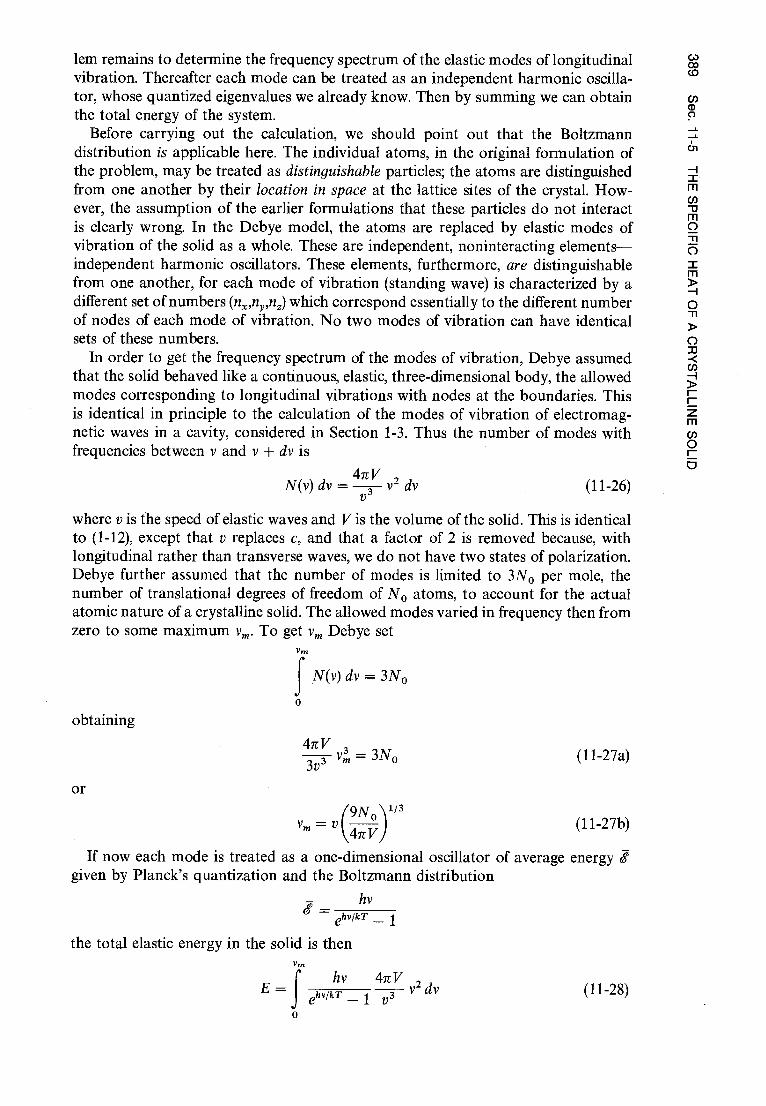
lem remains to determine the frequency spectrum of the elastic modes of longitudinal vibration. Thereafter each mode can be treated as an independent harmonic oscilla-tor, whose quantized eigenvalues we already know. Then by summing we can obtain the total energy of the system.

Before carrying out the calculation, we should point out that the Boltzmann distribution is applicable here. The individual atoms, in the original formulation of the problem, may be treated as distinguishable particles; the atoms are distinguished from one another by their location in space at the lattice sites of the crystal. How-ever, the assumption of the earlier formulations that these particles do not interact is clearly wrong. In the Debye model, the atoms are replaced by elastic modes of vibration of the solid as a whole. These are independent, noninteracting elements—independent harmonic oscillators. These elements, furthermore, are distinguishable from one another, for each mode of vibration (standing wave) is characterized by a different set of numbers (nx ,ny ,nz) which correspond essentially to the different number of nodes of each mode of vibration. No two modes of vibration can have identical sets of these numbers.

In order to get the frequency spectrum of the modes of vibration, Debye assumed that the solid behaved like a continuous, elastic, three-dimensional body, the allowed modes corresponding to longitudinal vibrations with nodes at the boundaries. This is identical in principle to the calculation of the modes of vibration of electromag-netic waves in a cavity, considered in Section 1-3. Thus the number of modes with frequencies between v and v + dv is

N(v)dv=47rV

v2 dv v

where y is the speed of elastic waves and V is the volume of the solid. This is identical to (1-12), except that y replaces c, and that a factor of 2 is removed because, with longitudinal rather than transverse waves, we do not have two states of polarization. Debye further assumed that the number of modes is limited to 3N 0 per mole, the number of translational degrees of freedom of N o atoms, to account for the actual atomic nature of a crystalline solid. The allowed modes varied in frequency then from zero to some maximum v m. To get vm Debye set

Vm

f N(v) dv = 3N o

o

obtaining

or 3v3 v,r, = 3No (11-27a)

(9N0

/ 1/3vm v

47r V (11-27b)

If now each mode is treated as a one-dimensional oscillator of average energy c given by Planck's quantization and the Boltzmann distribution

hv ehv/kT _ 1

the total elastic energy in the solid is then Vm

(11-26)

THE

SP

EC

IFIC

HE

AT

OF

A C

RY

ST

ALLIN

E S

OLID

hv 47r 2 E ehv/k T _ 1

y3 v dv

_

0 (11-28)

QU

AN

TU

M S

TA

TIS

TIC

S

This expression can be put in a more compact form if we change to a dimensionless

variable of integration x = hv/kT so that xm = hv m/kT. Then v„, xm

E — 4rcV f hv 3 dv — 4itV (kT\4 h f x 3 dx

v3 ehv/kT — 1 y 3 h ) ex — 1

o o

and, after substituting 47V/v 3 = 9No/vp3, and consolidating symbols, we obtain x„

3 E=3RT x3

ex d 1

m o

which is Debye's formula. Because x is a dimensionless quantity, hv m/k has the dimensions of a temperature.

It is often called the Debye characteristic temperature, O, of the substance involved. Hence, with x m = Co/T, (11-29) becomes

©/T T4 r x3

E = 9R 03 ex —1 dx (11-30)

0

and Debye's formula for the specific heat of a solid is O/T

3 3 H

cv = d7 = 9R 4 0 ex — 1 dx —

O e°/T - 1 (11-31)

0

Debye's theory involves a parameter O which, because of its connection to the elastic properties of the solid, can be determined independently of specific heat measure-ments, as we shall see in Example 11-2. Using these independently determined values in the theory, we obtain the excellent agreement with experimental measurements of specific heat illustrated in Figure 11-5. In particular, the theory agrees with the ob-served T 3 law at very low temperatures.

Example 11 -2. (a) Show how O can be obtained directly from the elastic properties of a solid. IN-Because 0 = hvm/k we must find vm first. From (11-27b), v m = v(9N0/4'tV) 1 /3 so we have 0 = (hv/k)(9N 0 /4n(V) 1 / 3 . All quantities are measurable experimentally so that 0 can be found from measurements of V (the molar volume) and y (the speed of elastic waves).

Actually, since both longitudinal (compressional) and transverse (shear) waves can be trans-mitted by the solid, and since their speeds are different, we replace y by a more general ex-

I I

xv-x.tIr+-x^ax

5

+ Al o Ca F2 A Cu V KCI _ O Pb

CI

❑ Zn •

I I I I I I I I 1 I I I I

0.2 0.4 0.6 0.8 1.0 1.2 1.4 1.6 1.8 2.0 2.2 2.4 2.6 2 8 T/0

Figure 11-5 The measured specific heat at constant volume, as a function of temperature, for several materials. Horizontal line I represents the Dulong-Petit law, and curve II repre-sents the predictions of the Debye theory.

(11-29)

pression. In particular, if y 1 represents the speed of longitudinal waves and v t the speed of CO transverse waves in the solid, we require 3N 0 = (4mmV/3vl )vm + (4mV/3vr )2vm instead of (11-27a), where allowance is now made for the two polarization states of transverse waves, as cn well. Then we use in (11-27b)

1 (1 2l - v3 { v3 + vt3 J

/ t/ From the measurements of y 1 and vt , v is computed. Some calculated results for O and v m are:

Iron O = 465°K vm = 9.7 x 10 12 sec -1 Aluminum O = 395°K vm = 8.3 x 10 12 sec -1 Silver O = 210°K vm = 4.4 x 10 12 sec -1 •

(b) Show that as T —* 0, c„ —> const x T 3 in Debye's (11-31). ► We have

C T/3

(^ x 3

0 1 c„= 9R 4 J ex

- 1 dx Te° l T - 1 o

As T decreases, O/T becomes very large. Indeed, as T —> 0, 0/T —> oo, and the last term goes to zero. Hence co

T\ 3 (' x3 c„ —>9R4

^ I

J ex — 1 dx

/

which, because f ô x 3 /(ex — 1) dx = 714/15, yields 12m4 R __

the required T 3 law for very low temperatures. (c) Show how O can be obtained from specific heat measurements.

■If T = 0, then from (11-31) we have 1

(' 3 c„ = 9R 4 J exx 1 dx e 1 1 = 2.856R = 5.67 cal/mole -°K

0

so that the Debye temperature O can be defined as that temperature at which c „ = 2.856R. For comparison with part (a), the values so obtained are 455°K for iron, 420°K for aluminum, and 215°K for silver. •

It is remarkable that so simple a model as Debye's yields such excellent results. The true frequency spectrum of the modes of vibration should depend on the actual lattice structure of the crystalline solid and may differ from the results of Debye's continuum model. Such differences as have been found between experiment and Debye's predic-tions can indeed be accounted for by expected differences between the actual spec-trum and Debye's so that the experimental facts of the specific heats of solids seem to be completely understood. Here we have considered the contributions to the specific heat of a solid from the lattice vibrations alone. In Section 11-11 we shall consider the contribution made by free electrons to the specific heat of a solid conductor.

11-6 THE BOLTZMANN DISTRIBUTION AS AN APPROXIMATION TO

QUANTUM DISTRIBUTIONS

We have seen that, where the average number of particles per quantum state is much less than one, the quantum distributions merge with the classical distribution. Par-ticularly useful in this region is the Boltzmann factor

nBoltz( 62)

nBottz('1)

T 3 cU 5 03 T

O/T

•

TH

E B

OLT

ZM

AN

N D

IST

RIB

UT

ION

AS

AN

AP

PR

OX

IMA

TIO

N T

O Q

UA

NT

UM

DIS

TR

IBU

TIO

NS

= e -ce2-6.1)/kT (11-32)

N rn M

QU

AN

TU

M S

TA

TIS

TIC

S

giving the relative number of particles per quantum state at two different energies g2 and Si , for a system in equilibrium at temperature T. We have already made use of this approximation in Example 4-7. It can be applied in all quantum systems at energies more than several kT above the ground state—the states are sparsely occu-pied so that nBoltz is very much less than one. For example, when we consider thermal collisions of atoms in a gas in equilibrium at temperature T the excited states of the atoms are normally sparsely populated. Hence we can obtain the relative equilibrium populations of the various excited states as a function of temperature by using the Boltzmann factor. Since the intensities of the spectral lines depend on these popula-tions, we can then predict the variation of spectral intensities with temperature. More often the procedure is reversed; that is, starting with the known relative intensities we can determine the temperature of the source, such as the star considered in Ex-

c co ample 4-7. The same idea is applicable to molecular spectra, as we shall see in Chap- Ç ter 12.

The Maxwell distribution of speeds of gas molecules moving freely inside a box is validly deduced from the Boltzmann distribution because nBoltz for all the free particle states is very small under the conditions usually existing in nature for ordinary gases.

Example 11-3. The technique of nuclear magnetic resonance is used to obtain information about internal magnetic fields in solids. It is more sensitive than chemical techniques, for ex-ample, in identifying magnetic impurities in a crystal. Principally, however, it enables us to use the nucleus as a probe to get information about solids, much as radioactive tracers are used in biological systems. For nuclei of nonzero spin the degeneracy of the energy levels with respect to the orientation of the nuclear spin is lifted by the magnetic field. (This is analogous to the Zeeman effect.) A resonance absorption of electromagnetic power occurs when photons bombarding the solid have the proper energy to excite transitions between these levels. The strength of the absorption depends upon the difference in population of the levels involved. To illustrate the sensitivity of the technique, use the Boltzmann factor to compute the differ-ence between the populations n 1 and n 2 of two levels at room temperature, if the resonant absorption is detected at a frequency of 10 MHz. • The Boltzmann factor is

nBoltz(e2) = e -(e2 - oikr = n2

nBoltZ(g1) n1

We have T = 300°K, 62 - = hv, and v = 10 7 sec -1 . Hence

n2 = e -hv/kT n 1

= e - 6.6 x 10 - 34 joule-sec x 10 7 sec -1 /1.4 x 10 - 23 joule-°K- 1 x 300°K

= e -1.6 x 10 -6 . 1 - 1.6 x 10 -6 Therefore

1 —n2

= 1.6 x 10 -6 n l

or

= 1.6 x 10 -6 n 1

So a difference in populations of less than two parts in a million is detectable, a result which reveals the high sensitivity of the NMR technique. The Boltzmann factor is applicable here since the population is spread over several close levels, so both n 1 and n2 are small. •

11-7 THE LASER

We saw in the previous section that the relative number of particles per quantum state at two different energies for a system in thermal equilibrium at temperature T is given, in certain circumstances, by the Boltzmann factor, e - V 2-"Ikr . We use this result

n l — n2

now to explain the behavior of a very important device called a laser, an acronym for "light amplification by stimulated emission of radiation." A maser is the correspond-ing system operating in the microwave region of the electromagnetic spectrum.

Consider transitions between two energy states of an atom in the presence of an electromagnetic field. In Figure 11-6 we illustrate schematically the three transition processes, namely, spontaneous emission, stimulated absorption, and stimulated emis-sion. In the spontaneous emission process, the atom is initially in the upper state of energy g2 and decays to the lower state of energy f1 by the emission of a photon of frequency y = (e2 — 6'1)/h. (The mean lifetime of an atom in most excited states is about 10 - 8 sec. But some decays may be much slower, the excited states then being called metastable; the mean lifetime in such cases may be as long as 10 s sec.) In the stimulated absorption process, an incident photon of frequency y, from an electro-magnetic field applied to the atom, stimulates the atom to make a transition from the lower to the higher energy state, the photon being absorbed by the atom. In the stimulated emission process, an incident photon of frequency y stimulates the atom to make a transition from the higher to the lower energy state; the atom is left in this lower state at the emergence of two photons of the same frequency, the incident one and the emitted one.

The processes of stimulated absorption and emission of electromagnetic energy in quantized systems can be regarded as analogous to the stimulated absorption or emission of mechanical energy in classical resonating systems upon which a periodic mechanical force of the same frequency as the natural frequency of the system is im-pressed. In such a mechanical system, energy can be put in or taken out depending on the relative phases of motion of the system and the impressed force. The spon-taneous emission process, however, is a strictly quantum effect. As discussed in Section 8-7, quantum electrodynamics shows that there are fluctuations in the electro-magnetic field. Because of the zero-point energy of the electromagnetic field, these fluctuations occur even when classically there is no field. It is these fluctuations that induce the so-called spontaneous emission of radiation from atoms in excited states. In all three processes, then, we deal with the interaction of radiation with the atom.

We wish to show now how these processes are related quantitatively. Let the spec-tral energy density of the electromagnetic radiation applied to the atoms be p(v). Con-sider that there are n 1 atoms in energy state g1 and n2 in state g2 , where g2 > g1.

Before After

Spontaneous emission

(a)

e2

Stimulated -r\-/A-R-,-)

absorption

^i

(b)

e2 o

Stimulated emission rtJVl

e i (c)

Figure 11 -6 Illustrating (a) the spontaneous emission process, (b) the stimulated absorp- tion process, and (c) the stimulated emission process, for two energy states of an atom.

4:13S

V1 3

H1

QU

AN

TU

M S

TA

TIS

TI C

S

The probability per atom per unit time, or transition rate per atom, that an atom in state 1 will undergo a transition to state 2 (stimulated absorption) clearly will be proportional to the energy density p(v) of the applied radiation at frequency y = (e2 — S1)/h. In Section 8-7 we argued that the transition rate for stimulated emis-sion is also proportional to p(v). But as we explained in Section 8-7, the transition rate for spontaneous emission does not contain p(v) because that process does not involve the applied electromagnetic field.

The transition rates also depend on the detailed properties of the atomic states 1 and 2 through the electric dipole moment matrix element of (8-42). Hence, the probability per unit time for a transition from state 1 to state 2 can be written as

R1-.2 = B 12p(v) (11-33)

in which B12 is a coefficient that includes the dependence on properties of the states 1 and 2. The total probability per unit time that an atom in state 2 will undergo a transition to state 1 is the sum of two terms, the probability per unit time A21 of spon-taneous emission and the probability per unit time B21 p(v) of stimulated emission. Again, A21 and B21 are coefficients whose values depend on the properties of states 1 and 2, through the appropriate matrix elements. Hence

R2->1 = A21 + B21p(v) (11-34)

Note again that spontaneous emission occurs at a rate independent of p(v), whereas stimulated emission occurs at a rate proportional to p(v).

If now we consider that the n 1 atoms in state 1 and the n 2 atoms in state 2 of the system are in thermal equilibrium at temperature T with the radiation field of energy density p(v), then the total absorption rate for the system n 1 R and the total emis-sion rate n 2R2 _ 1 must be equal, as in (11-4). That is

n 1 R 1 _, 2 = n2 R2 _, 1 (11-35) Thus we have

n1B12p(v) = n 2 [A21 + B21p(v)]

If we solve this equation for p(v) we obtain

A21

p(v) _ B21 (11-36) n1 B12

1 n2 B21

We now assume we can use the Boltzmann factor, (11-32), with by = 6'2 — e1 , to obtain

_ = Q(^z-^i)lkT = ehv/kT

n2 so that (11-36) becomes

A21

p(v) = B21 (11-37)

B12 ehvIkT — 1

B21

This equation, giving the spectral energy density of radiation of frequency y that is in

thermal equilibrium at temperature T with atoms of energies e1 and 6 2 , must be consistent with Planck's blackbody spectrum, (1-27)

87chv 3 1 1 PT(v) = e3 (ehvIkT — 1

n 1

Hence, we conclude that

B12 = 1 B21

(11-38)

and A2 1 87LhV 3

B21 C 3

These results were first obtained by Einstein in 1917, and therefore the coefficients are called the Einstein A and B coefficients. Note that the argument does not give us values of the coefficients, but only their ratios. However, if we compute the sponta-neous emission coefficient A 21 from quantum mechanics, using the techniques of Section 8-7, we then can obtain the other coefficients from these formulas.

There is much of physical interest here. For one thing, we find from (11-38) that the coefficients of stimulated emission and stimulated absorption are equal. For another, we see from (11-39) that the ratio of the spontaneous emission coefficient to the stimulated emission coefficient varies with frequency as y 3 . This means, for example, that the bigger the energy difference between the two states, the much more likely is spontaneous emission compared to stimulated emission. Equation (8-43) shows that the y 3 is present in this ratio because A2 1 itself is proportional to y 3 . Still another result is that we can obtain the ratio of the probability A21 of spontaneous emission to the probability B 21 p(v) of stimulated emission, namely

B2 1 p(v)

This shows that, for atoms in thermal equilibrium with the radiation, spontaneous emission is far more probable than stimulated emission if by » kT. Since this condi-tion applies to electronic transitions in both atoms and molecules, stimulated emis-sion can be ignored in such transitions. Stimulated emission can become significant, however, if hv ^ kT, and it may be dominant if hv « kT, a condition that applies at room temperature to atomic transitions in the microwave region of the spectrum where y is relatively small.

We are now in a position to understand the concept behind lasers and masers. In general, the ratio of the emission rate to the absorption rate can be written as n2R2_1/ n 1 R 1 _ 2 or

rate of emission n2A21 + n2B21p(v)

rate of absorption r n1B12p(v)

= C 1 A21 n2 (11-41)

Bz1p(v) n1

If we have energy states such that e 2 — « kT, or hv « kT, then (11-40) shows that we can ignore the second term in the parenthesis as very much smaller than one, and obtain

rate of emission n2 - (11-42) rate of absorption n 1

This result is general in the sense that we have not assumed an equilibrium situation. In situations of thermal equilibrium, where the Boltzmann factor applies, we expect n2 < n 1 . But in nonequilibrium situations any ratio is possible in principle. If now we have a means of inverting the normal population of states so that n 2 > n 1 , then the emission would exceed the absorption rate. This means that the applied radiation of frequency v = (e2 — 6 1)/h will be amplified in intensity by the interaction process, more such radiation emerging than entering. Of course, such a process will reduce the population of the upper state until equilibrium is reestablished. In order to sustain

(11-39)

A21 = ehv/kT - 1 (11-40)

a3

Sh

c 3

H1

QU

AN

TU

M S

TA

TIS

TIC

S

the process, therefore, we must use some method to maintain the population inversion of the states. Devices that do this are called lasers or masers, depending upon the portion of the electromagnetic spectrum in which they operate. Energy must be injected into the system, most commonly by a method described later called optical pumping, and the output is an intense, coherent, monochromatic beam of radiation, as we now explain.

In the ordinary atomic light sources there is a random relationship between the phases of the photons emitted by different atoms so that the resulting radiation is incoherent. The reason is that there is no correlation in the times that the atoms make their transitions. In laser light sources, on the other hand, atoms radiate in phase with the inducing radiation because their charge oscillations are in phase with that radiation. Since in a laser the inducing radiation is a coherent parallel beam formed by reflection between the ends of a resonant cell, the emitted photons are all in phase and act coherently. The resulting intensity, which is the square of the constructively combined amplitudes, is correspondingly high. The states between which transitions are made are an upper metastable state, whose relatively long lifetime allows it to be highly populated, and the lower ground state of infinitely long lifetime. From the uncertainty relation AEAt ^ h, with At equal to the long lifetime of the upper state, we conclude that the energy uncertainty in the energy difference of the states is small and the emitted transition frequency is sharp, giving a highly monochromatic beam. In practical devices the beam is also unidirectional, the coherence property making it possible to obtain essentially perfect collimation, or focusing. This further enhances the concentration of energy density. Some indication of the concentration of energy in a laser beam is given by the fact that a laser with less power than a typical light bulb can burn a hole in a metal plate.

In the solid state laser that operates with a ruby crystal, some Al atoms in the Al 2O 3 molecules are replaced by Cr atoms. These "impurity" chromium atoms ac-count for the laser action. In Figure 11-7 we show a simplified version of the appro-priate energy-level scheme of chromium. (The uppermost level is really a multiplet.) The level of energy e1 is the ground state and the level of energy e3 is the unstable upper state with a short lifetime (^ 10 -8 sec), the energy difference e3 — f1 corre-sponding to a wavelength of about 5500 A. Level e2 is an intermediate excited state which is metastable, its lifetime against spontaneous decay being about 3 x 10 -3 sec. If the chromium atoms are in thermal equilibrium, the population numbers of the states are such that n 3 < n2 < n 1 . By pumping in radiation of wavelength 5500 A, however, we stimulate absorption of incoming photons by Cr atoms in the ground state, thereby raising the population number of energy state e3 and depleting energy state e1 of occupants. Spontaneous emission, bringing atoms from state 3 to state 2, then enhances the occupancy of state 2, which is relatively long-lived. The result of this optical pumping is to decrease n 1 and increase n 2 , so that n 2 > n 1 and popula-tion inversion exists. Now, when an atom does make a transition from state 2 to state 1, the emitted photon of wavelength 6943 A will stimulate further transitions. Stimu-lated emission will dominate stimulated absorption (because n 2 > n 1 ) and the output of photons of wavelength 6943 A is much enhanced. We obtain an intensified co-herent monochromatic beam.

In practice, the ruby laser is a cylindrical rod with parallel, optically flat reflecting ends, one of which is only partly reflecting as shown in Figure 11-7. The emitted photons that do not travel along the axis escape through the sides before they are able to cause much stimulated emission. But those photons that move exactly in the direction of the axis are reflected several times, and they are capable of stimulating emission repeatedly. Thus the number of photons is built up rapidly, those escaping from the partially reflecting end giving a unidirectional beam of great intensity and sharply defined wavelength.

a3

sd

13

Hl

Pumping radiation 4vvv).-

5500 Â

-`^"* Stimulated emission,

6943 Â

Ground state

Partly transparent

mirror

External beam

Short-lived state

'Spontaneous decay

Metastable state 6'2

Coiled lamp

( Mirror

+ iwa -

Figure 11 -7 Top: The relevant energy levels of chromium atoms in a ruby laser. State 3 is very broad (large AE) because it is short lived (small At). State 2 is very sharp (small AE) because it is long lived (large At). Optical pumping raises the atom from ground state 1 to excited state 3, the latter's breadth facilitating the process. Then spontaneous decay occurs to state 2, the energy released usually going into mechanical energy in the ruby crystal rather than into photon radiation. Finally, state 2 decays to the ground state, either through spontaneous emission or through stimulated emission due to photons from other such transitions. Since state 2 is very sharply defined and the ground state is infinitely sharply defined, this radiation will be very monochromatic. Bottom: A schematic of the ruby laser, showing the optical pumping lamp, the escape of photons not moving axially, sug-gesting the buildup of repeatedly reflected axially moving photons which stimulate further emission, and indicating the escape of a fraction of the axial photons through the partially reflecting mirror at one end.

Note that this is reminiscent of the conclusion of Section 11-2 that n bosons already in a quantum state will enhance the probability of one more joining them by a factor of (1 + n). The conclusion is applicable to the photons in the quantum states of the cylindrical rod, since photons are bosons. It is possible to develop the basic theory of the laser by applying the Bose distribution to the quantum states of the photons, instead of by applying the Boltzmann distribution to the quantum states of the atoms as we have done here. But the treatments are very closely related (as they should be since they lead to the same results) because the energy density p(v) of (11-34) is proportional to the number n of photons in a state at energy by so that equation is very similar to the enhancement equations, (11-10) or (11-11), that we used in deriving the Bose distribution. Furthermore, (11-35) is identical to the thermal equilibrium condition of (11-4) that was also used in the Bose distribution derivation.

Generally speaking, a laser is a device in which a material is prepared so that the higher of two energy levels is more highly populated than the lower energy level, the material being enclosed in an appropriate resonator of sharp response. The system produces coherent radiation at those frequencies common to the resonator and the difference in energy of the levels. There is now a wide variety of lasers—gas lasers, liquid lasers, and solid state lasers—covering various regions of the electromagnetic spectrum. The intense coherent nature of the radiation they provide has led to in-creasing application of lasers in fields such as radio astronomy, microwave spectros-copy, photography, biophysics, and communications.

QU

AN

TU

M S

TA

TIS

TIC

S

11-8 THE PHOTON GAS

We begin in this section to study applications of the Bose distribution. The first will be a derivation of Planck's blackbody cavity radiation spectrum, in which the pho-tons in thermal equilibrium at temperature T with the walls of the cavity are treated as a gas that is governed by the Bose distribution. According to (11-22), that distribu-tion is

n(s) = eaeg/kT — 1

The discussion following (11-22) indicated that the value of the parameter a is speci-fied by the total number of particles the system governed by the distribution contains. But for the case at hand the total number of particles in the system is not constant. A photon can be completely absorbed when it strikes a wall of the cavity, or the hot wall may at some other time emit a new photon. Thus for a system of photons the distribution cannot contain the term e". That is, the Bose distribution for photons (or other bosons that can be created or destroyed within the system) must have the form

n(s) _ kT (11-43) e -1 — 1

The number of particles in the system has indeed specified the value of a; because that number varies it is necessary that a = 0 so that e = 1. Confirmation of the validity of this argument will be obtained soon.

Let N(s) represent the number of quantum states per unit energy interval at energy i—called the density of states—for photons in the cavity. Then N(e) de is the number of quantum states for photons in the cavity within the energy interval 6' to e + de. Since n(s) is the probable number of photons per quantum state, the product n(g)N(g) dg gives the number of photons in the energy interval. However, mode for radiation confined to a cavity has already been evaluated by geometrical argu-ments in Example 1-3, except that the language used there is different from that which we are currently using; there we spoke of the radiation as waves and here we speak of it as particles (photons). We found there that

N(v) dv = 8 3V v 2 dv C

where V is the volume of the cavity and y is the frequency of a wave contained in the cavity. Using the familiar relation g = hv to evaluate the energy of the associated photon, here we find, after multiplying and dividing the term v 2 dv by h 3, that

8rcV e2 dP

8Tcv 2 hv p T (v)dv =

c 3 ehv/kT — 1 dv (11-45)

Equation (11-45) is identical to (1-27), obtained in Chapter 1 and verified there by comparison with experiment. Note that this agreement confirms the validity of the Bose distribution for photons, (11-43). In the Planck derivation the radiation is a set of waves confined to the cavity. Each of these standing waves is a mode of vibration

1

mode = c3 h3 (11-44)

Taking the product of this expression times n(s), multiplying by the energy b carried by each photon, and then dividing by the volume V of the cavity, we have

en(e)N(é) de _ 87c S3 de PT(g) e 3 h3(ee/kT _ 1)

where PT(e) de is the energy per unit volume in the energy interval e to g + de. Planck's spectrum follows at once by using the relation e = hv to convert from S to v. Thus

1 n(e) = eae^lkT —

(11-46)

that is distinguishable from all the others, just as for the lattice vibration modes in

the Debye model, so it is valid to apply the Boltzmann distribution to them. In the

present derivation the cavity radiation is a set of indistinguishable particles—photons

to which the Bose distribution must be applied.

11 -9 THE PHONON GAS

We were able to use the wave-particle duality for electromagnetic radiation to derive

the thermally excited distribution of radiation in a cavity either on a wave picture

or a particle picture. Similarly, the thermally excited distribution of elastic vibrations

in a solid can be deduced by applying a wave-particle duality for acoustic radiation.

Just as photons are the quanta of electromagnetic radiation, so phonons are the quanta of acoustic radiation. Just as photons are emitted and absorbed by vibrations

of the atoms in a cavity wall, so phonons are emitted and absorbed by vibrating atoms

at the lattice points in the solid. The sources of each type of radiation are quantized

so that the energy gain or loss is discrete; the discrete energy transferred through

the system has an energy hv, where y is the frequency of the acoustic vibration for

phonons and of the electromagnetic vibration for photons. Just as the number of

photons is not fixed or conserved, so the number of phonons is not fixed or conserved.

The Bose distribution with a = 0, i.e., (11-43), applies to phonon and to photon. There

are differences, of course, between the photons and phonons. For example, the photon

propagates through vacuum whereas the phonon propagates through a crystal lattice.

This leads to different energy-momentum relations, a matter we return to in a sub-sequent chapter.

It should be clear that the Debye specific heat formula can be deduced on the

phonon picture from the Bose distribution in a way analogous to the photon deduc-tion of the Planck spectrum formula using the Bose distribution. That is, the wave-particle duality for acoustic radiation is used just as before we used the wave-particle

duality for electromagnetic radiation. The phonon calculation will not be reproduced

here because it is completely analogous to the photon calculation and leads to no

new results. The solid contains a gas of phonons just as the cavity contained a gas of

photons.

11 -10 BOSE CONDENSATION AND LIQUID HELIUM

Here we sketch an application of the Bose distribution to an ideal gas in order to

compare quantum and classical gas behavior. As a practical application we shall then

consider the remarkable properties of liquid helium.

The general form of the Bose distribution is

BO

SE C

ON

DE

NS

ATIO

N A

ND

LIQU

ID H

ELIU

M

To apply this to bosons whose total number X in a system remains fixed, like helium

atoms, we must first determine the parameter a. This is done by setting

cc

✓V = J n(g)N(e) de

o

where me) dg is the number of quantum states of the system in an energy interval

e to e + de, and n(s) is the number of bosons per quantum state, so that the integral

is just the total number X'. Using (11-46), we. have oo

N(S) de = eaeglkT 1

(11-47) 0

0 0

QU

AN

TU

M S

TA

TIS

TIC

S

To proceed we must determine for an ideal gas the number of states in the energy interval e to f + de, which is the product of the density of states N(s) and the size de of the energy interval. Consider the gas particles to be in a cubical box of side a. The potential energy for a particle in such a three-dimensional box is that of a three-dimensional infinite square well. The Schroedinger equation for a one-dimensional in-finite square well was solved in Section 6-8, giving allowed energies en = (h2/8ma 2)n 2 . By a simple extension of the calculation we find the allowed energies f for a three-dimensional well to be

h2

e 8ma2 (nx ± ny + nz) (11-48)

in which the quantum numbers nx , n nZ are positive integers. The number of states in an energy interval can be obtained by plotting, in a space formed by axes n x, ni,, nZ , the allowed states (which are points where n x , n nZ take on positive integral values) and counting them. We have done this, in a different context, for the calculation of Example 1-3. There we defined r = jnx + ny + fZ, and we found in (1-15) that the number of states for r lying between r and r + dr is

nr2 dr N(r) dr = 2

The same is true here. We convert this into the desired form, N(e)de, by using (11-48) to write

2 h e = r2

8ma2

and then taking this equation, and its differential, to evaluate rcr2 dr =

4TE h2

8ma2 ) -3/2 g1/2 de = 4ha3 (2m3)1/26,1I2 de

So the number of states for e lying between g and e + de is

me) de = 4h3 (2m3)1/26e1/2 de (11-49)

where V = a3 , the volume of the box. If now we combine this result with (11-47) and carry out the integration we obtain

(27cm hT)3/2 V e-Π1 + 23/2 e -a + 3 3/2 e -2a + .. .

To simplify the appearance of this equation, let e - a = A so that we can write (27rmkT3 312 V

A 1+23 2 A+332 A 2 + (11-50)

For large mass m and high temperature T, A must be very small since X is fixed. In these circumstances, terms beyond the first power in A can be dropped. But lt.rge m and high T should be the classical region. Indeed, we find that the first term gives the classical Boltzmann result

.J1( _ (27cmkT)312V A

h3

or 3

A = (2nrmkT) 312 V = e' (11-51)

Note that A = e' a is proportional to X, as in the Boltzmann result for a system of classical oscillators discussed after (11-23). Also note that here we conclude that since

Now, if A >_ d we expect wave effects to be important. This requires h

kT) 1 /2—) 1/3

V > —

(3m

is fixed a must be very large (as A is very small), in contrast to our conclusion that a is zero for a system of bosons in which .N' varies.

If we now compute the total energy E of the ideal gas from

E = J en(e)N(e) dS

we obtain 3/2

E _ (2^ h

3 V 2 kT A(1 + 25/2 A + 3 5/2 Az + •) (11-52)

Once again the classical result follows for very small values of A. Neglecting terms beyond the first power in A, and using (11-51), we have E = (3/2).iVkT. This corre-sponds to an average energy per particle EIS' equal to (3/2)k T, which is the classical equipartition of energy result for three-dimensional translational motion. The general

Bose result for the average energy per particle, obtained by dividing (11-52) by (11-50),

is, including terms up to A 2 3

E = = 2 kT [1 — 2 5 / 2 V(2 mkT)3/z] (11-53)

The term beyond 1 in the bracketed expression of (11-53) represents the deviation

of the Bose gas from the classical gas. This is sometimes called the degeneracy effect. (This degeneracy effect, or gas degeneration, is not related to the degeneracy that

describes different quantum states having the same energy.) Equation (11-53), which

neglects higher order terms, pertains to the case of weak degeneracy. Note that the

degeneracy term is negative so that the average particle energy is less for a Bose gas

than for a classical gas. This corresponds to previous results in which we found a

greater probability of two particles to an energy state for the Bose distribution than

for the Boltzmann distribution, the lower energy states being relatively fuller in the

Bose gas than in the classical gas) as a consequence. Physically, this manifests itself,

for example, as a lower gas pressure (lower average momentum) at the same tempera-ture for a Bose gas than for a classical gas.

Example 11 -4. Whenever the mean interparticle distance is comparable to or smaller than the de Broglie wavelength assigned to particles on the basis of their temperature, we should expect to observe wave effects, that is quantum effects, in the system of particles. Show that this criterion leads to the requirement that the degeneracy term .4Vh 3/V(2xmkT) 3/2 not be negligible compared to 1 if deviations from classical behavior are to be detected. ■ The de Broglie wavelength of a particle is A = h/p. In a gas in equilibrium at temperature T the mean kinetic energy is (3/2)kT so that p = -.%/2mK = J3mkT. Hence

h (3mkT) 1 /2

If the volume of gas is V and there are ✓V atoms of gas, the volume per particle V/.A 1 can be set equal to d 3 , where d is the mean interatomic separation. Hence

( V

)

1/3 d

Wf 1

113H

a111

01

1 a

Nd

NO

Ilb

'SN

3a

N00

3909

or, cubing each side h3 V

(3mkT)312 >

N O

QU

AN

TU

M S

TA

TI S

TIC

S

which is the same as

.A h 3

V(3mkT )312

Hence, ✓Vh 3/V(27rmkT) 312 should exceed about 1/3 and so the term beyond 1 in the bracketed part of (11-53) should exceed about 1/16 to meet our criterion. •

Under what circumstances might we detect the degeneracy effect experimentally? The degeneracy term is negligible in practice for most gases, having a value of about 10 -5 , so that the Boltzmann distribution applies almost universally to them. Note that the degeneracy term, .IVh 3/V(27rmkT) 3 " 2 , becomes more important the smaller the mass m, the lower the temperature T, and the higher the density .AVIV. The smallest mass gases obeying the Bose distribution (zero or integral spin angular mo-mentum) are H2 and He. If we prepare such a gas to be at high density and low tem-perature we bring it near its condensation point. For this reason, and another to be mentioned shortly, the degeneracy effect is sometimes called the Bose condensation. For H2 the degeneracy term at its normal condensation point is less than 1/100, whereas for He near its normal condensation point (4.2°K) the degeneracy term is about 1/7. Hence, we should get observable effects more easily for helium. The theory would be approximate in this case, for at such high densities the behavior is like a real gas of interacting particles rather than an ideal gas of noninteracting particles. Indeed, in the liquid, or condensed phase, we observe the most striking nonclassical effects in the behavior of helium. Let us now describe these effects.

Ordinary helium gas is composed almost wholly of neutral atoms of the isotope He4. The spin angular momentum of such an atom is zero so that the Bose distribu-tion must be used to treat the behavior of this gas. At normal atmospheric pressure helium gas condenses to a liquid at 4.18°K. It remains as a liquid, i.e., it does not freeze into a solid, down to the absolute zero of temperature if it is cooled at a pres-sure equal to its own vapor pressure. (To obtain solid helium it is necessary to pres-surize the liquid, about 26 atm of pressure being needed near absolute zero.) If, by pumping off the vapor, the temperature of liquid helium is reduced to 2.18°K, a dramatic change in its properties is observed. The temperature 2.18°K is called the A point because the shape of the graph of specific heat versus temperature resembles the letter A with the anomaly at 2.18°K. Liquid helium is called He I when it is above this temperature and He II when below. He I is essentially a classical fluid, its be-havior not being unusual, but He II contains a superfluid component which causes it to show spectacular large scale quantum effects, including the following:

1. As the temperature of liquid helium is lowered by evaporation and the vapor is pumped away, the liquid boils in the usual manner. But as the A point is reached and passed the boiling suddenly stops throughout the liquid. Though evaporation continues, and the temperature and vapor pressure fall, the liquid is completely calm (see Figure 11-8). This is explained by the fact that heat can be conducted out of the liquid with practically no resistance, since the heat conductivity is measured to in-crease by a factor of about one million below the A point.

2. We can determine the viscosity of liquid helium by measuring its rate of flow through a fine capillary tube. At the A point, the measured value of the viscosity drops by a factor of about one million.

3. Most unusual and spectacular is the ability of liquid helium, below the A point, to creep as a thin film along the walls of its container, as shown in Figure 11-9. The speed of this ordered mass motion may be 30 cm or more per second. The effect in-volves helium first adsorbing on the entire surface of the cold container to form a thin film. The film then acts like a siphon through which the liquid flows with almost no viscosity.

>1

BO

SE

CO

ND

EN

SA

TIO

N A

ND

LI QU

ID H

ELIU

M

Figure 11-8 The 2 paint transition in liquid helium. As liquid helium is cooled from its normal boiling point at 4.2°K by evaporation, with the use of a vacuum pump, it boils normally with small bubbles. As it undergoes the phase transition from He Ito He II at the 1 point, 2.18 ° K, it suddenly and briefly boils up violently (see top and middle pictures), and equally suddenly stops boiling altogether (see bottom picture). Below this transition point liquid helium cannot boil, even when pumping, evaporation, and cooling continue. (Cour-tesy of A. Leitner, Rensselaer Polytechnic Institute)

QU

AN

TU

M S

TA

TIS

TIC

S

o (a) (b) ..........:

Figure 11-9 The creeping motion of a film of liquid He 4 below the transition temperature demonstrates the superfluidity of He II. The film behavior, suggestive of liquid flow through a siphon, is shown schematically for liquid levels in the container (a) below and (b) above the level of the liquid helium reservoir. In (c) is a photograph of a glass vessel partially filled with liquid He II and suspended by threads above the surface of the same liquid seen at the bottom of the picture. He II creeps up along the inside wall, over the rim, and down along the outside wall as a thin film, collecting as a drop on the bottom. When this drop falls another will form, and so on, until the vessel is empty. (Courtesy of A. Leitner, Rensselaer Polytechnic Institute)

K. Mendelssohn has written of the film flow as follows:

"If the beaker is withdrawn from the bath, the level will drop until it has reached the level of the bath. If the beaker is pulled out completely, the level will still drop, and one can see little drops of helium forming at the bottom of the beaker and falling back into the bath. This is the sort of thing that makes one look twice and rub his eyes and wonder whether it is quite true. I remember well the night when we first observed this film transfer. It was well after dinner, and we looked around the building and finally found two nuclear physicists still at work. When they, too, saw the drops, we were happier."

All of the properties of He II indicate that it has a very high degree of order. For instance, the almost complete absence of viscosity means that, when flowing, He II does not develop the small scale turbulences that cause the frictional energy loss re-sponsible for the viscosity of ordinary fluids. The order is imposed by the (1 + n) enhancement factor that we often find when studying the low-energy behavior of a system of bosons. When the temperature becomes low enough to allow it, all the he-lium atoms in a system tend to condense into the same lowest' energy quantum state. This is the Bose condensation. The superfluid component, whose concentration rap-idly approaches 100% as the temperature decreases below the point, is comprised of those atoms which are in that quantum state. To the extent that all the atoms do get into the same microscopic state, it becomes the state of the entire macroscopic system and the system can only behave in a completely ordered way in which the action of any atom "is correlated _with the action of all the others. This tendency is extremely pronounced because the factor (1 + n) has an extremely large value if n is anything like the total number of atoms in a beaker of liquid helium.

11 -11 THE FREE ELECTRON GAS

In this and the following section we apply the Fermi distribution to quantum systems. In a manner analogous to that used for a boson gas, we could deduce the behavior

of an ideal gas of fermions. To the same degree of approximation we would find, for example, that the average energy per particle is

3 E =

X = 2 kT[1 + 25/2 V(2mk T)3/2] (11-54)

which is the Fermi result corresponding to the Bose result of (11-53). The degeneracy term here (second term in brackets) is positive so that the average particle energy is greater for a Fermi gas than for a classical gas. This corresponds to a lower probability

SV

J N

O171

1031

3 33

b13

31H

1

(strictly zero) of finding two particles in the same quantum state for the Fermi dis-tribution than for the Boltzmann distribution, the lower energy states being relatively fuller in the classical gas than in the Fermi gas as a result. Physically, this manifests itself as a higher gas pressure (higher average momentum), at the same temperature,

for a Fermi gas than for a classical gas. Notice again how the Bose and Fermi results

fall on opposite sides of the classical result.

It is natural to ask for an example of a Fermi gas whose degeneracy effect we can

detect. In Chapter 15 we shall find an example in the neutrons, and the protons, con-fined to a nucleus. Helium gas containing only the isotope He 3 also obeys the Fermi distribution, as do all particles with odd half-integral spin angular momentum, and it remains a gas without condensing to a low enough temperature that the degeneracy term of (11-54) is detectable. This isotope is rare and more difficult to get in large quantities, but the behavior of He 3 atoms has been shown to be markedly different from that of He 4 atoms in ways predicted by the different distribution functions ap-plicable to them. For example, the vapor pressure of liquid He 3 at a given tempera-ture is much higher than that of liquid He 4. Indeed, this is the basis for a practical method of cooling to 0.02°K.

It would be quite easy to detect the effect of the degeneracy term for fermions, however, if we could obtain a gas of electrons. The degeneracy term can be written as nh 3/(27rmkT) 3 / 2, in which n = X/V is the number density of the particles. Notice that a small mass in and a high density n can increase the importance of this term, as well as a low temperature T. Because the electronic mass is several thousand times smaller than that of atoms, the degeneracy effect for electrons should actually be de-tectable even at high temperatures. For electrons in a metal the number density n of conduction electrons is also very high, so that conduction electrons in a metal show quantum degeneracy effects. The question remains whether we can regard such elec-trons, even approximately, as a gas of free electrons, i.e., an ideal gas.

In a crystalline solid most of the atomic electrons are bound to the nuclei at the lattice points, but if it is a metallic conductor electrons from outer subshells of the atoms are relatively free to move through the solid. These are the conduction electrons. Because their mutual repulsion is cancelled, on the average, by the attractions of the atomic cores, we may regard the conduction electrons as approximately free particles and can treat them to good approximation as an ideal electron gas (see Figure 6-24). Indeed, we can regard the interior of the solid as a region of approximately constant potential for these electrons with the metal boundaries acting as high potential walls. The electron then behaves as a particle in a box whose quantum states we already know (see Section 6-8).

To get the number N(S)de of states in an energy interval f to e + de we simply count the number of standing waves, each representing a definite state of the motion, in that energy interval. We have made this calculation before for an ideal gas in a box, with results described in (11-49). The results here are the same, after taking into account the two possible spin orientations for an electron having a given space eigen-function. That is

8rc V(2m 3) 1 /2 N(e) dg = h3 e1/2

de

(11-55)

Multiplying by n('), the probable number of electrons per quantum state, we obtain

8^ V ( yn 3 ) 1/2 1/2 de n(e)N(e) de =

F ec^ ^F)l + 1 ̂F = — akT (11-56)

This is the electron gas energy distribution of conduction electrons in a metal. If now we assume that the temperature is very low (strictly speaking, T = 0), we

know that all the quantum states up to the Fermi energy 'F are occupied and that

o o

QU

AN

TU

M S

TA

TIS

TIC

S

none of the higher states are occupied. In that case the total number of free electrons

equals the total number of distinct states up to energy eF , and we have a way of cal-culating the Fermi energy. That is

eF F

Jr. = f N(e) de = 8nV(2m3)1/2 X1'2 d^ = 16m V3hm3)"2 n/2

J 0

or

h2 (

3 , 2/3

I (11-57)

F 8m\ ITV/

For temperatures such that kT « eF this result is an excellent approximation. For ordinary metals we need temperatures of the order of several thousand degrees before

the approximation breaks down.

Example 11 -5. Consider silver in the metallic state, with one free (conduction) electron per atom.

(a) Calculate the Fermi energy from (11-57). •The density of silver is 10.5 g/cm 3 and its atomic weight is 108. Hence

.N 6.02 x 1023 atom/mole x 10.5 g/cm 3 n =

_

V 108 mole x 1 free electron/atom

g/ = 5.9 x 1022 free electron/cm 3 = 5.9 x 1028/m 3

Therefore h2 C3n\2/3 _ (6.6 x 10 -34 joule-sec) 2

(

3 x 5.9 x 10 -2$/m3\2/3 F 8m 71 8 x 9.1 x 10 -31 kg ^ fI

=8.8 x 10 -19 joule =5.5eV (b) Calculate the degeneracy term for the conduction electrons in metallic silver at 300°K.

► We have 5.9 x 1028/m3 x (6.6 x 10 -34 joule-sec) 3

(2irmkT) 3/ 2 (27c x 9.1 x 10 -31 kg x 1.38 x 10 -23 joule/°K x 300°K) 312 4700

so that the second term in the brackets of (11-54) has the value 1 nh3

25/2 (21CmkT)3 /2 820

Hence, the degeneracy term is extremely large and completely overwhelms the leading (clas-sical) term of (11-54). The electron gas is said to be a completely degenerate Fermi gas; that

is, it behaves as if T ^ 0°K with the electrons in the configuration of lowest energy. Such a

gas shows quantum behavior (i.e., is nonclassical) up to the highest attainable metallic tem-perature, the electron gas in silver remaining almost completely degenerate until the tempera-ture is of the order of 10 5 °K. At those temperatures and higher the degeneracy term becomes

small compared to one.

We can now understand a result that classical physics was unable to explain, name-ly the experimental observation that the conduction electrons do not contribute to

the specific heat of metals at ordinary temperatures. According to the classical view

the free electrons take part in the thermal motion in a metal, each free electron having

a mean energy (3/2)k T. Therefore, the specific heat for a metal should be not simply

3R, due to the vibrations of the atoms at the lattice sites, but it should be (3 + 3/2)R

instead, in which the (3/2)R term is the contribution per mole of the electron gas. The origin of this term is seen by noting that if E = (3/2)k TN 0 = (3/2)R T, then c„ =

dE/dT = (3/2)R, where N o is Avogadro's number. According to the Fermi model of an electron gas, the electrons do not exhibit this classical behavior until the tempera-ture reaches about 10 5 °K. That is, there is no equipartition of energy between elec-

nh3

trons and lattice contributions, the electron gas in this sense not being anywhere near thermal equilibrium with the atoms of the metal confining it. As the temperature is raised, the Fermi distribution of electrons among available energy levels is affected only slightly at the high-energy end (see Figure 11-3) so that the average electron energy is hardly changed at all. This means that at ordinary temperatures the electron gas does not contribute to the specific heat of the metal in an appreciable way. That is, E (3/2)kTN 0 , but instead it is approximately independent of temperature, so that c„ = O. Hence, the Fermi distribution is in accord with experimental facts con-cerning electrons at ordinary temperatures.

At ordinary temperatures, and even at temperatures high enough to make the cv = 3R law of Dulong and Petit a good approximation to the specific heat contri-bution of the lattice vibrations of a solid, the electronic specific heat term is too small relative to the atomic specific heat term to be detected. At temperatures near absolute zero, where the atomic specific heat is very small, the electronic contribution will exceed the atomic contribution. It is in the region of a few degrees Kelvin that the electronic specific heat dependence is observed experimentally, again in agreement with the Fermi distribution predictions.

11-12 CONTACT POTENTIAL AND THERMIONIC EMISSION

Up to now we have treated the electron in a metal as a particle in a box, that is we have implicitly assumed the electron does not escape the metal, the potential box having very high walls. We know, however, that electrons can escape from metals, as in the photoelectric effect, thermionic emission, etc., so that we should modify the potential function somewhat. Inside the metal the potential function is approximately constant, and near the metal boundary it increases rapidly to reach its higher constant value outside the metal. If we take the zero of potential energy to correspond to the electron being far outside the metal, then we can let — Y o represent the depth of the resulting potential energy well illustrated in Figure 11-10.

We can determine Yo from photoelectric experiments, specifically from the fact that there is a cutoff frequency v o below which photons cannot eject electrons from the metal (see Section 2-2). This suggests that the most energetic electrons in the metal are an energy interval hv 0 below the top of the potential well. The fact that the photo-electric current rises rapidly as the photon energy rises above the threshold value suggests an abrupt rise in the number of electrons with decreasing kinetic energy

NO

ISS

IIN3

OIN

OIW

1d3H

1 ❑

NV

1`d

I1N

3lO

d l

Ob'

1NO

0

A

wp Empty energy levels

Filled energy levels

o

Vacuum Metal Vacuum

Figure 11-10 The average potential energy for a conduction electron in a metal. The potential is a well of depth V o that rises rapidly near the metal boundaries to zero. The energy levels increase in density in proportion to f 112 , and are filled up to the Fermi energy 4. The work function is wo , and Vo = wo + 4.

CO 0

QU

AN

TU

M S

TA

TIS

TIC

S

inside the metal. This corresponds to the features of the Fermi distribution, the most energetic electrons having kinetic energy and many electrons having nearby smaller kinetic energies. Therefore, we can retain the energy distribution of quantum states that we found for the particle in a box. (See Section 6-8 for a discussion of the similarity in energy levels of an infinite and a finite square well potential.) At T = 0 all states are filled up to an energy 6F above the bottom of the well, this high-est state having a total energy — hv 0 . That is, — V0 + gaF = — hvo . Recall now that hv0 = w0, the work function of the metal, so that — V0 + eF = — w0 or

V0 = w0 (11-58) For silver the work function is 4.7 eV and is 5.5 eV, so that V0 is 10.2 eV. For most metals V0 lies between 5 and 15 eV, as can be seen in Table 11-2. Of course, at ordinary temperatures the Fermi distribution does not give a sharp cutoff at eF but is spread out continuously over a narrow energy region near eF. In a region of the order of kT on each side of the Fermi energy, i.e., in a transition region of width 2kT, the number of particles per quantum state goes from a value near one to a value near zero. In the limit when T —* 0 this transition region becomes infinitesimally narrow.

With this model for the behavior of electrons in a metal we can explain the contact potential difference of two metals and understand the thermionic emission process. First, consider the thermionic emission process, which is of great practical importance because it is responsible for the emission of electrons from the heated filament of a vacuum tube. At high temperatures (i.e., for large values of kT) the distribution of electrons among available energy states in a metal extends to energies well above 4. At sufficiently high temperature some electrons may acquire a kinetic energy greater than V0 (i.e., greater than 6aF + w0) and thereby escape from the metal. We can calculate the thermoelectric current density emitted from a metal surface as a function of temperature from the Fermi distribution and from the Boltzmann distri-bution. The calculation involves determining how many electrons will arrive at the metal surface moving in the required direction and with enough kinetic energy to escape. The two distributions give a different temperature dependence for the current density, and experiment rules in favor of the Fermi distribution for electrons.

As for the contact potential difference between metals, consider two metals A and B which at first are not in contact, as is indicated schematically in the left part of Figure 11-11. Outside the metals the potential energy of an electron is zero. Inside the metals the Fermi level of metal A is WA below zero and the Fermi level of metal B is wB below zero. Let w B > WA so that the Fermi level of metal A is higher than that of B. Now let the metals be connected electrically, as illustrated in the right part of Figure 11-11. Then the most energetic electrons in metal A will flow into metal B, filling the energy levels in B just above its Fermi energy and depleting the upper levels in A. The process continues until equilibrium is reached; that is, until the high-est filled levels in A and B are at the same energy, because the total energy of the

Table 11 -2 Work Function and Fermi Level Energy for Some Metals

Metal w0 (eV) (eV)

Ag 4.7 5.5 Au 4.8 5.5 Ca 3.2 4.7 Cu 4.1 7.1 K 2.1 2.1 Li 2.3 4.7 Na 2.3 3.1

CLA

SS

ICA

L A

ND

QU

AN

TU

M D

ES

CR

IPT

ION

S O

F T

HE

ST

AT

E O

F A

SY

ST

EM

V= 0

Metal A Space Metal B Metal A Space Metal B Figure 11 -11 Left: Showing the potential energy for an electron in two separated metals A and B with different work functions. Right: The metals are now connected electrically by a wire, becoming oppositely charged and exhibiting a contact potential difference.

system is minimized when this situation is achieved. The result is that metal A be-comes positively charged in the process and metal B becomes negatively charged. Consequently there is a potential difference of (w $ — w A )/e between the metals when they are connected electrically, a result in essential agreement with experimental values.

11-13 CLASSICAL AND QUANTUM DESCRIPTIONS OF THE STATE OF A SYSTEM

We saw in Section 4-9 an example of how the instantaneous state of the motion of a classical particle can be represented by a point in phase space. For the one-dimensional motion con-sidered there, the phase space was a two-dimensional space whose abscissa was the position x and whose ordinate was the momentum px . For a three-dimensional motion, phase space is a six-dimensional space of coordinates x, y, z, p x , py , pz . As the particle moves, the point rep-resenting it in phase space traces out a path, the path being an ellipse in our earlier example of a one-dimensional harmonic oscillator. If we had a large number of such oscillators we would have a large number of representative points in phase space corresponding to the instan-taneous distribution of oscillators. For most systems of interest we can write the total energy of each member as E = K + V = (px + py + p!)/2m + V(x,y,z) so that the location of a point (x,y,z,p x ,py ,pz) in phase space gives the total energy of that member of the system which the point represents. The distribution of points gives the distribution in energy of all members of the system.

Thus, in classical statistics we can characterize the energy distribution of a system by giving the number of points in each small volume of phase space, say AxAyAzAp xApyApz. We call such a small volume element a cell in phase space, and points in that cell have total energy between E and E + dE, corresponding to momentum values between px and px + Ap r, etc., and position values between x and x + Ax, etc. The cell is chosen to be small enough that the average total energy of its representative points differs little from the energy of any one of them; it is chosen large enough so that there are many points in a cell, thereby permitting the application of statistical ideas. Hence, the size of a cell is somewhat arbitrary and indefinite, but once it is chosen the cell is characterized by an average total energy and a population number. The cell then is the classical statistical analogue to the quantum state of quantum statistics. In Figure 11-12 we illustrate the situation for a one-dimensional system.

In quantum mechanics we must modify the preceding picture because of the uncertainty principle. For one thing we cannot describe the trajectory of a particle by giving the path of a representative point in two-dimensional phase space because we cannot simultaneously know the exact values of x and px for the particle. The best we can do is locate the representative point at any time between x and x + Ax and px and px + Apr where AxApx ^ h, so that in-stead of a representative point tracing out a line we have a small area tracing out a ribbonlike

QU

AN

TU

M S

TA

TI S

TIC

S

0

•

•

LiPx

<

o Px

x Figure 11-12 Phase space and representative points for a one-dimensional system.

path in two-dimensional phase space. More important, however, is the fact that there is a def-inite smallest size to any cell in the quantum description. A cell in which AxAp x is less than h is meaningless, such a specification being more precise than allowed by the uncertainty prin-ciple. For the general six-dimensional phase space, therefore, the smallest cell has a "volume" of P.

It is therefore possible in the quantum description to remove the arbitrariness and indef-initeness of the volume element in phase space. Because the size of the cell obviously affects the counting of distinguishable divisions of the total energy of the system, there is a certain indefiniteness in the results of classical statistics. For example, the entropy of a system can be written as S = k In P where P is the number of distinguishable divisions of its energy content (i.e., P is a measure of the probability that it has the particular energy). However, the classical entropy has an arbitrary constant in it basically because of the indefiniteness of the cell size. The quantum value is exact, because of the definiteness of the cell size, and it gives an absolute entropy constant in agreement with experiment and the laws of thermodynamics Indeed, it was this result, and not the results concerning the cavity radiation, that convinced Max Planck of the correctness of his ideas concerning energy quantization and the constant h. And it is this smallest size of a cell in phase space in quantum statistics that is the origin of the factor h3 displayed in many of the equations in this chapter.

From considerations discussed here we can also understand the applicability of the classical Boltzmann distribution to so many quantum problems. If there is no definite smallest size to a cell in phase space then we can always get a situation in which there is not more than one particle per state. But this is just the high temperature case wherein classical and quantum statistics agree. The classical distribution function is valid in this case, regardless of the indis-tinguishability of particles. Of course, the real quantum world does set a limit to the smallness of a cell so that the classical distribution will not apply when the number of particles per cell is more than one.

QUESTIONS

1. Exactly what do the inhibition and enhancement factors describe? What are their origins 2. Can you devise a cycle of transitions between three states which would maintain an

equilibrium in the populations of these states, with transitions that violate detailed bal-ancing? Does it seem reasonable to extend this to a system with many states?

3. What is the basic reason why the quantum distributions merge with the classical distri-bution at energies much larger than kT?

4. Explain why the behavior of the Boltzmann distribution is intermediate to that of the Bose and Fermi distributions.

5. Give examples of systems to which the Boltzmann distribution is applicable in principle. As a good approximation.

6. What factors determine the value of a for the thrée distributions?

7. Interpret physically the Fermi energy eF .

8. Thermal expansion is related to the anharmonic nature of the vibrations of atoms in a solid. Would the Debye model be appropriate to studying thermal expansion of solids?

9. In Debye's model of a solid, the maximum frequency v m corresponds to a minimum wavelength. Because of the discrete nature of a solid this minimum wavelength corre-sponds to a vibration in which adjacent atoms move 180° out of phase with one another; that is, the interatomic spacing is half a wavelength. Is this plausible? Explain.

10. Interpret the Debye characteristic temperature O physically.

11. In our analysis of emission and absorption processes of an atom in an electromagnetic field we neglected recoil effects. How does this affect our results? Are we justified in ignoring recoils?

12. What are the dimensions of the Einstein A and B coefficients?

13. It is said that a laser is not a source of energy but a converter of energy. Explain.

14. We have ignored the possible degeneracy of the states involved in laser action. How would you take this into account? What effect does it have?

15. Make a step-by-step comparison of the deduction of the Planck radiation law on the basis of the Maxwell distribution and the Bose distribution.

16. List similarities and differences between phonons and photons.

17. At low densities and high temperatures the Bose gas behaves like a classical ideal gas. Make this result plausible physically.

18. In writing about experiments on the scattering of a particles in helium Rutherford said, "On account of the impossibility of distinguishing between the scattered alpha particles and the projected He nuclei, the results are subject to a certain ambiguity." Explain how an awareness of quantum statistics could have removed the ambiguity. What determines whether a gas obeys Bose or Fermi distributions?

19. How can the ordered state of the He II explain its lack of resistance to heat conduction?

20. What examples of a Fermi gas are there other than an electron gas and a gas of He 3 atoms?

21. In the ideal gas equations we use the rest mass of particles. Should we ever use the relativistic mass instead? Consider the effect of temperature and the nature of the particle.

22. Give a plausibility argument for the relation, (11-57), between the Fermi energy eF and the density of free electrons in a metal.

23. In the Fermi distribution we obtain the result that at the Fermi energy gF the average number of particles per quantum state is exactly one-half. This is definitely not the same as saying that 50% of the particles are at energies above the Fermi energy and 50% below. Explain.

24. Justify the assumption that conduction electrons behave approximately as a system of free noninteracting particles.

25. Is there a connection between Vo , the depth of the potential well for conduction electrons in a metal, and electron diffraction experiments of the Davisson-Germer type? Can we determine V0 from such experiments?

26. Explain physically the effect of letting h 0 in expressions for the density of states, such as (11-49). Explain physically the effect of letting h -4.0 in equations involving the quantum degeneracy term, such as (11-53).

PROBLEMS

1. The equilibrium state is one of maximum entropy S in thermodynamics and one of maximum probability P in statistics. Assuming then that S is a function of P, show that we should expect S = k In P, where k is a universal constant. This relation is sometimes called the Boltzmann postulate. (Hint: Consider the effect on S and P of combining two systems.)

sw31

aoad

N T ^

QU

AN

TU

M S

TA

TIS

TIC

S

2. The Maxwell distribution can be developed by looking at elastic collisions between two particles. If initially these particles have energies f1 and g2, and finally g3 and e4 , then

+ = -a)+(e2 +5)

If all possible states are equally probable, the number of collisions per second P is proportional to the number of particles in each initial state, i.e.

P1,2 = CP(g1)P(e2)

where Red is the probability of a state being occupied, and C is a constant. Similarly P3 , 4 = CP(^3)P(e4). In equilibrium, for each collision (1,2) -+ (3,4) there must be a collision (3,4) (1,2). Thus P1,2 = P3 , 4. (a) Show that P(g1) = e-gilkT solves this equa- tion. (b) Use similar reasoning to derive the Fermi distribution. Here, however, the initial states must be filled and the final states must be empty, and the number of collisions becomes

P1,2 = CP(GP(e2)[1 - P(e3)][1 - P(4)] Then show that the equation P1,2 = P3,4 can be solved by

[

1 - P(6L) -

Cep IkT P(^`) J

which yields (11-23). 3. (a) Show that at T = 0, in the Fermi distribution, n(s) = 1 for all energy states in which

<'F and n(s) = 0 for all energy states in which e > eF . (b) Show that n(s) = 1/2 for g = gF.

4. Consider the Fermi distribution of (11-24), n(s) = l/[ev-g'F>1kT + 1]. (a) Show that n(s) = 1 - n(24 - g); that is, with é - SF = S, show that n(e, + (5) = 1 - n(gF - (5). This proves that the distribution has a symmetry about n(4) = 1/2. (b) Find n(s) for b = g - eF = kT, or 2kT, or 4kT, or 10k T. Make a rough sketch of n(s) versus e for any T > 0. (c) What percent error is made by approximating the Fermi distribution by the Boltzmann distribution when 8/kT = 1, 2, 4, 10?

5. (a) At what energy is the Bose distribution function (for a = 0) equal to one for a temperature of 7000°K? (b) What is the temperature of the Bose function (for a = 0) with a value of 0.500 at this same energy?

6. For the Fermi distribution function (a) show that gF

J n(e) de = kT [in (1 + eg'F/kT)/2]

o

(b) Show that this reduces to ‘F for T = 0. (c) Show that gF

J n(g) de = J n(g) dg + k T(ln 2)

o o

7. (a) From (11-25), show that the Einstein model of a solid gives the specific heat as

(b) Show that c,,-* 0 as T -* 0 but that at low T, c„ increases as a -hv/kT rather than as the required T 3 law.

8. Show that the Debye specific heat result, (11-31), reduces to the classical law of Dulong

and Petit at high temperatures. (Hint: First expand both exponentials and retain only first

order terms. Justify.) 9. Imagine a cavity at temperature T. Show that c,,, the specific heat of the enclosed radia-

tion, is given by (32n 5 kV/15)(kT/hc) 3 . Explain why c„ does not have an upper limit in this case whereas it does for solids.

10. In some temperature region graphite can be considered a two-dimensional Debye solid,

but there are still 3N 0 modes per mole. (a) Show that N(v) dv = (2nA/v 2)v dv where A is

ehv/kT by \ 2l

= 3R [(ehvIkT - 1)2 (kT

^

w

sw31

soad

2 .Vk

^

kT

the area of the sample. (b) Find an expression for v m and Co for graphite. (c) Show that at low temperatures the heat capacity is proportional to T 2 .

11. .N' distinguishable atoms are distributed over two energy levels e1 = 0 and g 2 = ^.

(a) Show that the energy of the system is given by

✓t we -e/kT

1 + e - g1kT

(b) Show that c„ is given by

E_

e -g/kT

cv = (1 + e-g1kT)2

(This is the Schottky specific heat and is observed for paramagnetic solids at low tempera-tures. The energy levels correspond to the magnetic moments being aligned parallel or

antiparallel to the magnetic field.) (c) Sketch the heat capacity as a function of tem-perature, being careful to have the correct temperature dependence at high and low

temperatures. 12. The variation of density p with altitude y of the gaseous atmosphere of the earth can be

written as p = poe-9(P°1P°)y, where po and Po are sea level density and pressure, provided the temperature is assumed to be uniform. (a) From the ideal gas laws show that this can be put into the form p = poe - mgy/kT (b) Show that this has the form of the Boltzmann distribution.

13. (a) By combining n(s) of (11-21) and N(e) of (11-49) for an ideal gas of classical particles,

with

A =e- "= Nh a

show that (27cmkT ) 312 V

n(6)N(6)dg _ (kT)312n112 g 1 1 2 e g/kT de

is the energy distribution of particles in an ideal gas. (b) Show that Maxwell's speed

distribution of molecules in a gas, which has the form n(v) dv = Cv2e-mv212kT dv, where C is a constant, follows directly from this.

14. Assume that the thermal neutrons emerging from a nuclear reactor have an energy

distribution corresponding to a classical ideal gas at a temperature of 300°K. Calculate

the density of neutrons in a beam of flux 10 13/m2-sec. (Hint: Consider the average

velocity, and justify its use.)

15. In a certain nucleus the magnetic moment is 1.4 x 10 -26 joule-m 2/weber. Calculate the fractional difference in population of the nuclear Zeeman levels in a magnetic field of

1 weber/m 2 , (a) at room temperature and (b) at 4°K.

16. Electron spin resonance is much like nuclear magnetic resonance except that electronic

transitions are excited between atomic Zeeman levels. These experiments are done at

microwave frequencies. If the electromagnetic wave has a frequency of 32 KMHz (K band)

calculate the fractional difference in population between two atomic Zeeman levels (a) at

room temperature and (b) at 4°K.

17. (a) Determine the order of magnitude of the fraction of hydrogen atoms in a state with

principle quantum number n = 2 to those in state n = 1 in a gas at 300°K. (b) Take into

account the degeneracy of the states corresponding to quantum numbers n = 1 and 2 of

atomic hydrogen and determine at what temperature approximately one atom in a

hundred is in a state with n = 2.

18. Consider the relation n i/n2 = e(g2-"MT , the Boltzmann factor for nondegenerate states for systems in equilibrium, where e2 > g1. (a) Show that n 2 = 0 at T = 0. (b) Show that n 1 = n2 at T = o0 or T = - oo. (c) Show that n 2 > n 1 at finite negative temperature T. (d) Show that n 1 - 0 as T -> -0. (e) Hence, explain the statements, "Negative absolute temperatures are not colder than absolute zero but hotter than infinite temperature," and

QU

AN

TU

M S

TA

TIS

TIC

S

"One approaches negative temperatures through infinity, not through zero." (f) Can you suggest a change in temperature scale that would avoid temperatures that are negative in this sense?

19. Determine approximately the ratio of the probability of spontaneous emission to the probability of stimulated emission at room temperature in (a) the x-ray region of the electromagnetic spectrum, (b) the visible region, (c) the microwave region.

20. An atom has two energy levels with a transition wavelength of 5800 A. At room tempera-ture 4 x 1020 atoms are in the lower state. (a) How many occupy the upper state, under conditions of thermal equilibrium? (b) Suppose instead that 7 x 10 2° atoms are pumped into the upper state, with 4 x 10 20 in the lower state. How much energy in joules could be released in a single pulse?

21. The energy levels in a two-level atom are separated by 2.00 eV. There are 3 x 10 18 atoms in the upper level and 1.7 x 10 18 atoms in the ground level. The coefficient of stimulated emission is 3.2 x 10 5 m3/W-sec 3, and the spectral radiancy is 4 W/m 2-Hz. Calculate the stimulated emission rate.

22. If B 10 = 2.7 x 10 19 m3/W-sec 3 for a particular atom, find the life-time of the 1 to 0 transition at (a) 5500 A (visible) and (b) 550 A (ultraviolet)?

23. Combine (11-49) and (11-47) to obtain (11-50), as follows. Let .x = g/kT and obtain CO

2n V(2mkT) 3 / 2 Î x1 /2 dx h3 J e" +x _ 1

0

Then, with a positive, use the relation (e" + — 1) -1 = e- " - x(1 — e - " -x) -1 = e- "(e -x + a-- —2x + ) to obtain (11-50).

24. Obtain (11-52) as follows. Let x = g/kT and show that op

2rckTV(2mkT)312 (' x312 dx 3 V(27umkT) 312 / 1 1 E = h 3 e"+x_ 1 = 2 k T h3 e' 1+25/2 e-"

+•••

25. Show that the quantum degeneracy in a Fermi gas occurs if kT « eF . (Hint: See Example 11-4 and use (11-57).)

26. Show from the Fermi distribution that in a metal at T = 0°K the average energy of an electron is 34F/5.

27. Using 23 as the atomic weight and 9.7 x 10 2 kg/m 3 as the density of metallic sodium, compute the Fermi energy on the assumption that each sodium atom gives one electron to the conduction band. (Hint: See Example 11-5.)

28. Using 197 as the atomic weight and 19.3 x 10 3 kg/m 3 as the density of gold, compute the depth of the potential well for free electrons in gold. The work function is 4.8 eV and there is one free electron per atom.

29. In a one-dimensional system the number of energy states per unit energy is (l/h) \/2m/e, where 1 is the length of the sample and m is the mass of the electron. There are ../If electrons in the sample and each state can be occupied by two electrons. (a) Determine the Fermi energy at 0°K. (b) Find the average energy per electron at 0°K.

30. Show that about one conduction electron in a thousand in metallic silver has an energy greater than the Fermi energy at room temperature.

12 MOLECULES

12-1 INTRODUCTION

416

relevance of molecular physics

12-2 IONIC BONDS

416

electromagnetic origin of molecular binding; energy budget in ionic binding of sodium chloride; polar molecules; nondirectionality of ionic bonds; likely candidates for ionic binding

12-3 COVALENT BONDS

418

role of hydrogen molecular ion; preferred eigenfunction symmetry for ion; energy budget in ion; energy budget in hydrogen molecule; paired electron sharing in covalent bond; saturation; directionality of covalent bonds; ho-mopolar molecules

12-4 MOLECULAR SPECTRA

422

comparison to atomic spectra; decomposition of level structure and spectra into electronic, vibrational, and rotational

12-5 ROTATIONAL SPECTRA

423

quantization of rotational energy; quantum number r; selection rule; spectra

12-6 VIBRATION -ROTATION SPECTRA

426

quantization of vibrational energy, quantum number y; selection rule; vi- bration-rotation bands; isotope effects; vibrational and rotational constants

12-7 ELECTRONIC SPECTRA

429

band spectra; Franck -Condon principle

12-8 THE RAMAN EFFECT

432

description; role of intermediate state; relation to Rayleigh scattering; use in study of molecules with identical nuclei

12-9 DETERMINATION OF NUCLEAR SPIN AND SYMMETRY CHARACTER 434

symmetries of vibrational, rotational, and nuclear spin factors of molecular eigenfunction; nuclear spin quantum number i, ortho and para molecules; alternation of intensities; missing lines; application to several nuclei

QUESTIONS

438

PROBLEMS

438

415

MO

LEC

ULE

S

12-1 INTRODUCTION

The subject matter of the previous chapters is considered to be common to all of quantum physics. The concepts and techniques we have developed in these chapters for the purpose of studying atoms prove to be necessary, or at least useful, in studying most of the areas to which quantum physics is applied. But from atoms the applica-tions of quantum physics branch into two well-defined, and fairly well-separated, channels. One of these leads to the systems larger than atoms; i.e., it goes from atoms to molecules and then to solids. The other channel leads from atoms to the smaller systems; i.e., to nuclei and then to their constituents, the elementary particles. In the next three chapters we shall follow the first channel, and in the last four chapters of this book we shall explore the second.

We know that two or more atoms can combine to form a stable molecule. Here we seek a description of the interatomic forces which bind atoms into molecules, and also an understanding of the nature of energy levels and spectra of molecules. Since a very large number of atoms may join together to make a solid, in much the same way as a few do to form a molecule, the phenomenon of molecular binding is very relevant to the properties of solids. The motivation for studying molecular spectra, in addition to its intrinsic interest, is found in practical considerations. For example, a new but rapidly expanding field of science is molecular astronomy, which involves the measurement of molecular spectra originating in interstellar, or intergalactic, matter, for the purpose of determining its composition and condition. And as we shall see, measurements of molecular spectra have for a long time provided the pri-mary source of information about important properties of the nuclei contained in the molecule.

12-2 IONIC BONDS

From one point of view a molecule is a stable arrangement of a group of nuclei and electrons. The exact arrangement is determined by electromagnetic forces and the laws of quantum mechanics. This concept of a molecule is a natural extension of the concept of an atom. Another view regards a molecule as a stable structure formed by the association of two or more atoms. In this view the atoms retain their identity whereas in the first-mentioned view they do not. Of course, both views are useful and there are situations wherein each is directly applicable. In general, however, the struc-ture and properties of molecules are best described by a combination of both views. When a molecule is formed from two atoms, the inner shell electrons of each atom remain tightly bound to the original nucleus and are barely disturbed at all. The outermost loosely bound electrons, known as the valence electrons, are influenced by all the particles (ions + electrons) of the system. Their wave functions are significantly modified when the atoms are brought together. Indeed, it is this very interaction that leads to binding, i.e., to a lower total energy, when the nuclei or ions are close to-gether. This interaction, called the interatomic force, is of electromagnetic origin. Hence, we see that valence electrons play the central role in molecular binding.

There are two principal types of molecular binding, the ionic bond and the covalent bond. The NaCl molecule is an example of ionic binding and the H2 molecule an example of covalent binding. Consider the formation of a NaCl molecule from an atom of Na and an atom of Cl which are far apart initially. Figure 9-15 shows that to remove the outermost 3s electron from Na and form the Na + ion requires an ionization energy of 5.1 eV. The atomic binding in the alkali Na is relatively weak because its filled inner subshells are effective in shielding the valence electron elec-trically from the nucleus so that it moves in a weakened field at an outlying position. If now we attach this electron to the halogen Cl atom it will complete a previously

SdN

OB

ON

O!

Na+ + e + CI

5.1 eV Na 3.8 eV CI ionization electron

energy affinity

Na+ + Cl' (for R=œ)

Na + CI

3.6 eV

unfilled 3p shell in Cl to form a Cl ion. The halogen has a relatively high electron affinity; that is, the closed shell ion is more stable than the neutral atom, its energy being lower by 3.8 eV. Hence, at the cost of 1.3 eV of energy (5.1 eV — 3.8 eV), we have formed two distinct separate ions, Na + and Cl ; but these ions exert attractive Coulomb forces on one another, and the energy of attraction is greater than 1.3 eV. Now, since the mutual Coulomb potential energy of the ions is negative, the potential energy of the combined system initially decreases as the separation of the ions is steadily reduced. As the ions are brought still closer together the electron charge dis-tributions begin to overlap. This has two effects, each of which increases the potential energy: (1) the nuclei are not as well shielded from one another as before and they begin to repel one another and (2) at small internuclear separation we effectively have a single system to which the exclusion principle applies, and some electrons must be in higher energy states than before to avoid violating this principle. The po-tential energy curve therefore yields a repulsive force at small interatomic separations and an attractive force at large separations. There is a separation at which this energy is a minimum, the energy being 4.9 eV lower at this proximity than for distantly sep-arated ions. Hence, compared to two neutral atoms, Na + Cl, the combined system NaCl is lower in energy by 3.6 eV (that is, E = 1.3 eV — 4.9 eV = — 3.6 eV) so that a bound state is energetically favored, as illustrated in Figure 12-1. The equilibrium nuclear separation in NaC1 is 2.4 A.

Example 12-1. Evaluate approximately the depth of the minimum in Figure 12-1 by assuming that at the 2.4 A equilibrium nuclear separation R of NaCl the Na + and Cl ions have spherically symmetrical charge distributions that do not yet overlap. ■ With this assumption, Gauss's law of electrostatics allows us to evaluate the Coulomb bind-ing energy of the unit charge ions from the simple expression

1 e 2 V =

-4.9

Figure 12-1 The energy for the neutral atoms Na and Cl, and for the ions Na + and CI - , as functions of the internuclear separation R. The ionic combination lower__ energy at small separation, while the neutral atom combination has lower energy at large se-paration. Thus, as the two neutral atoms are brought together, they go over to ionic form when their separation becomes less than a certain value.

4nE O R

1.6 x 10 -19 joule

9.0 x 109 nt-m 2/cou1 2 x (1.6 x 10 -19 coul) 2 V —

= —9.7 x 10 -19 joule x

2.4 x 10 -10 m

l eV

MO

LEC

ULE

S

where R = 2.4 A. We obtain

= —6.0 eV If the student extrapolates slightly the 1/R behavior in Figure 12-1 to R = 2.4 A, he will see that the results of this evaluation are consistent with its assumptions. •

NaC1 is a molecule held together by ionic binding. Because the region of positive charge (Na t ) and the region of negative charge (C1 - ) are separated, there is a per-manent electric dipole moment. An ionic molecule is thus said to be a polar molecule. Ionic binding is also called heteropolar binding. Ionic bonds are not directional, for each ion has a closed shell configuration which is spherically symmetrical. Ionic bonds can be formed with more than one valence electron, as in the case of the MgC12 molecule, when the molecular state is energetically lower than the state of separated atoms. The number of ionic bonds that an atom can form depends on the shell structure of the atom, i.e., on the ionization potentials for successively removing electrons. It will be energetically favorable to form ionic bonds only for those (few) outer subshell electrons that have ionization potentials in certain ranges. Compounds of elements from the first column, and the second from last column, of the periodic table (the alkali halides, such as KC1, LiBr, etc.) are ionic, as are many of those from the second column and the third from last column (the alkaline-earth oxides, sulfides, etc.).

12-3 COVALENT BONDS

Let us consider now the formation of the H2 molecule. If in the case of H2 we were to calculate the energy required to form positive and negative hydrogen ions by moving an electron from one hydrogen atom to the other, and then added to this the energy of the Coulomb interaction of the ions, we would find that there is no distance of separation at which the total energy is negative. That is, ionic bonding does not result in a bound H2 molecule. The fact that H2 is bound is explained quan-tum mechanically by the behavior of the electronic eigenfunction describing the charge distribution of the system, as two hydrogen atoms approach one another. As we shall see soon, the resulting charge distribution does lead to electrostatic attrac-tion, but it is a charge distribution that can be interpreted as a sharing of electrons by both atoms. The binding is called covalent.

We can best understand the covalent bond by treating first the simpler case of H2 , the hydrogen molecular ion. In this case we have two nuclei each exerting a Coulomb repulsion on the other, and both exerting a Coulomb attraction on the single electron. Since the electron motion is very rapid compared to the nuclear mo-tions, the procedure is to assume that the nuclei are at rest a distance R apart, with the single electron moving in their Coulomb fields, and then determine the electron energy from the Schroedinger equation. We next treat R as a variable and consider both the electron energy, and the internuclear Coulomb repulsion energy, as a func-tion of the internuclear separation. The total energy of the system is the sum of these two energies, and the system will be bound if the total energy exhibits a minimum at some value of internuclear separation.

The top of Figure 12-2 indicates the potential energy in which the electron moves by plotting its value along an x axis passing through the two nuclei, for an inter-nuclear separation R = 1.1 A. The potential energy is symmetrical with respect to a plane perpendicular to the line connecting the two nuclei and passing through its

—6 —5-4-3 —2 —1 0 1 2 3 4 5 6

Odd R = 1.1Â Even

—4 —3 ® 1 2 3 4 —1

—2

3

x (Â)

x (A)

N

W

S4N

O9

1N

31

`dA

O0

Figure 12-2 Top: The potential function, and the two lowest energy levels, for an electron in a H2 molecule with internuclear separation R = 1.1 A. The potential function is evaluated along the line passing through the two nuclei. Bottom: The even and odd eigerunctions corresponding to the two energy levels, evaluated along the internuclear line. Néar each nucleus, both eigenfunctions have magnitudes that are decreasing exponentials of-the distance from the nucleus, as in the ground state of the hydrogen atom.

middle, since the potential is just the sum of a Coulomb potential centered on one end of that line and an equal Coulomb potential centered on the other end. Because the motion of the electron in a bound state of this potential will have the same sym-metry, the electron's bound state probability densities etfr will have equal values at two points on either side of the plane and equidistant from it. But this requires each of its eigenfunctions 0 to have either precisely the same value at the two points, or else to have at one point a value precisely the negative of its value at the other point. That is, the eigenfunctions must be either even or odd with respect to reflection in the plane. The situation is shown schematically in the bottom of Figure 12-2 by plot-ting the lowest energy even and odd normalized eigenfunctions along a line passing through the two nuclei. The important idea is that the odd eigenfunction must nec-essarily have zero value at the center of this line since it obeys the equation t, ( — x) _ — (x), which would otherwise be internally inconsistent at the center where x = O. But the even eigenfunction is not so constrained, and thus it has an appreciable value at x = O.

Because an electron with probability density vf*/i for the odd eigenfunction must avoid the center of the molecule, to a certain extent it avoids the central region. And since the integral over all space of 0*0 equals one, if that quantity is relatively small in the region between the nuclei, it must be relatively large in the regions outside the nuclei. These outside regions are where the potential is least binding, however, so such an electron is relatively loosely bound. The odd eigenfunction could be more tightly concentrated in the regions near the nuclei, while still being zero at the center, but only if its curvature were higher. Since higher curvature requires higher kinetic energy, this would not decrease the total energy of the electron. An electron whose behavior is described by the probability density for the even eigenfunction has a rel-atively high probability of being found in the region where the potential is most

0 N M

OLE

CU

LES

1 2 3 4 5 6 7 I; I I I I I I

h0 CI)

W

Even

binding—that is, in the region from near one nucleus, through the center of the mol-ecule, to near the other nucleus. Thus such an electron is relatively tightly bound. The two lowest energy levels for an electron in the potential are shown in Figure 12-2. We can now understand why the lowest of these is for the quantum state in which the eigenfunction is even.

Figure 12-3 shows the sum of the electron energy and the internuclear. Coulomb repulsion energy for the two lowest energy states of the H2 molecule, as a function of the internuclear separation distance R. For very large R, the electron will bind to one nucleus or the other in the lowest energy state of an H atom, and the repulsion energy will be negligible, so the energy of the system will have the familiar value —13.6 eV. For the quantum state with the even eigenfunction, the energy of the sys-tem at first decreases with decreasing R. The reason is that the binding energy exerted on the electron already near one nucleus becomes negative more rapidly, as the other nucleus moves into proximity, than the repulsion energy between the two nuclei be-comes positive. (The electron in the even eigenfunction state at moderate internuclear separation tends to be between the nuclei, so its distance to either nucleus is smaller than the distance separating the nuclei.) As the internuclear separation continues to decrease, the energy of the system passes through a minimum and then begins to increase rapidly. This happens because the electron binding energy when the nuclei overlap can become no more negative than — (2) 2 x 13.6 eV = — 54.4 eV, the ground state energy of a singly ionized helium atom, whereas the internuclear repulsion energy increases without limit as the internuclear separation decreases. For the even eigenfunction case the molecule is stably bound by a rudimentary covalent bond. At equilibrium it has R 1.1 A, which is where the energy as a function of R has a minimum that is about 2.7 eV deep. The measured binding energy, i.e., the energy required to dissociate HZ into H and H + , is in good agreement with this value. Be-cause of the significantly weaker binding of the electron in the odd eigenfunction state, the corresponding total molecular energy curve does not have a minimum at any value of R. Thus the molecule will not bind if the eigenfunction of the electron is odd since its energy always decreases as the nuclear separation increases.

If we now add a second electron to H2 to form H2, the energy of the system is decreased further, the two additional attractive forces acting between this electron and the nuclei more than counteracting the electron-electron repulsion. For H2 the binding energy is about 4.7 eV, and the equilibrium internuclear separation is about 0.7 A. So H2 is more compact, and more tightly bound, than HI. The second electron in H2 goes into a quantum state whose eigenfunction has the same space properties

Figure 12-3 The total energy of the HZ molecule for the two lowest electron energy levels, as a function of the internuclear separation. The molecule binds only in the state where the electron eigenfunction is even.

IF o

—4.7

as the eigenfunction for the first electron. That is, in the lowest energy state of H2

both electrons are in a state with the same space eigenfunction, and that eigenfunction is even with respect to reflection in the plane halfway between the two nuclei. So for both the probability density shows some concentration in the region between the two nuclei. Of course the exclusion principle demands that the two electrons have different spin eigenfunctions; thus they have spins with opposite z components. Using the more precise terms of Section 9-3, the eigenfunction describing the system of two indistinguishable electrons is a product of a symmetric space eigenfunction and the antisymmetric (i.e., singlet) spin eigenfunction . In that section we found that the two electrons may be relatively close together when the system is described by such an eigenfunction. Of course this is consistent with the idea that both have a reasonable chance of being located near the point halfway between the nuclei.

Because of the complete space overlap of the wave functions of the indistinguish-able electrons in H2, it is definitely not possible to associate a particular electron with a particular atom of the molecule. Instead, the two electrons, which are responsible for the bond that holds the atoms together as a molecule, are shared by the molecule, or shared by the bond itself. This is the idea of the shared pair of electrons, with "anti-parallel" spins, that form a covalent bond. Note that if the two electrons had essentially parallel spins they could not both be in the region between the two nuclei. Then they could not both be where they optimize the attraction exerted on them by both nuclei. If we imagined trying to form H2 by bringing two separated H atoms together, it would make a decisive difference whether the electrons' spins were "parallel" or "anti-parallel." In Figure 12-4 we show the prediction of quantum mechanics for the total energy of the system as a function of internuclear separation in the two possibilities; binding is obtained only for "antiparallel" spins. The calculations that produced the curves in Figure 12-4 take into account the electron-electron repulsion. This has a quantitative effect in reducing the binding, but it does not make a qualitative change in the description we have presented of the origin of the covalent bond.

No more than two electrons can form one covalent bond. We say an electron from one atom pairs up with an electron of "antiparallel" spin from another atom. If an atom has several electrons in an uncompleted outer subshell, i.e., if it has several va-lence electrons, each may try to form a covalent bond with a valence electron in a nearby atom. However, if there are two valence electrons with "antiparallel" spins in one atom, an additional valence electron from another atom will not succeed in forming a bond with either of them since they are already paired with each other.

"Parallel" spins and antisymmetric

space eigenfunction

SO

NO

S 1

N3

1V

AO

0

> R (A)

"Antiparallel" spins and symmetric space

eigenfunction

Figure 12-4 The total energy of the H2 molecule for "parallel" and "antiparallel" elec-tron spins, as a function of the internuclear separation. The molecule binds only in the state where the electron spins are "antiparallel".

N N

MO

LEC

ULE

S

That is, if the spin of the additional electron is "antiparallel" to the spin of one of these electrons, it is "parallel" to the spin of the other. Since the exclusion principle acts in the molecule in such a way as to prevent two electrons with "parallel" spins from having the same space eigenfunction, the additional electron may not occupy the same energetically favorable molecular region as the electrons of the preexisting pair. Therefore the valence electrons of an atom that are effective in forming cova-lent bonds are those which the action of the exclusion principle in the atom has not already forced into pairs with "antiparallel" spins. For instance, in the Hartree theory all of the three 2p electrons in N can have "parallel" spins because there are three possible values of the quantum number m 1 for 1 = 1, so none of them are forced to pair in that atom. (In the residual Coulomb interaction theory the three electrons do have "parallel" spins in the ground state of the LS coupling atom N.) The result is that the molecule N2 has three covalent bonds. But O has a fourth electron in the 2p subshell, and the exclusion principle forces it to have its spin "antiparallel" to the spin of one of the other three. So there are only two unpaired valence electrons in 0, and the molecule 0 2 has only two covalent bonds. In general, the number of un-paired valence electrons equals the number of electrons in the subshell up to the point where it is half filled, and it equals the number of vacancies, or holes, in the subshell beyond that point.

As in ionic binding, the forces saturate in covalent binding. That is, a given atom strongly interacts with only a limited number of other atoms. Saturation is due to the limited number of electrons or vacancies in the outermost occupied subshell of the atom. As distinguished from the ionic bond, the covalent bond is directional. The directional property is not present in H2 since the probability density of the valence electron in each separated H atom is spherically symmetrical, so the only defined direction in the H2 molecule is the one connecting the two nuclei, and the covalent bond acts along that direction, whatever it may be. In a more typical case the prob-ability density of a valence electron has its own directional dependence and certain preferred directions for forming covalent bonds. The directional properties of cova-lent bonds are manifested in the structural properties of covalently bonded molecules, and so form the basis of organic chemistry. The charge distribution of the paired electrons in a covalent bond has a symmetry about the center of the molecule, as we discussed in the case of H2, so there is no permanent electric dipole moment asso-ciated with the covalent bond. The bond is therefore sometimes called homopolar. Because the binding in molecules other than those containing two identical nuclei may be partly ionic, even though principally covalent, only molecules such as 02 or N2 are strictly homopolar.

12-4 MOLECULAR SPECTRA

Molecules can remain bound in excited states as well as in the ground state. The emission and absorption spectra of molecules are due to transitions between allowed energy states. The energy-level scheme is relatively complicated and differs in many respects from the atomic case. For one thing, we can no longer classify states accord-ing to the electronic orbital angular momentum. Because the force on an electron is not a central force (in a diatomic molecule, e.g., there are two separated nuclear at-tracting centers), the magnitude of its orbital angular momentum L is not conserved. In the words of Section 7-9, the energy eigenfunctions are not eignfunctions of the operator L op . However, in a diatomic molecule the total charge distribution is sym-metrical about an axis connecting the nuclei, say the z axis, so that the component of angular momentum about this axis, L Z , is conserved. We find then that the mole-cular energy eigenfunctions are eigenfunctions of LZ0 and that L Z has allowed values which are integral multiples of h, in analogy to the values m 1h of atomic states.

Another difference between the molecular and atomic cases is that we could neglect the nuclear motion in an atom, or else we could take it into account easily by using the reduced electron mass. Of course, in a molecule, as well as in an atom, we do not need to consider the translational motion because that motion, being free particle motion, is not quantized. However, the nuclei in a molecule can move relative to one another. In a diatomic molecule, for example, the nuclei can vibrate about the equilibrium separation, and in addition the whole system can rotate about its center of mass. The energy in each of these motions, vibrational and rotational, is quantized so that we expect many more energy levels in a molecule than in an atom. Indeed, these motions interact or couple with one another and an exact analysis would have to take this into account.

Of course, the solution of the Schroedinger equation for any but the simplest molecules is very difficult. However, empirical results of molecular spectroscopy show that we can consider the energy of a molecule to be made up of three p rincipal parts—electronic, vibrational, and rotational. The molecular energy levels fall into widely separated groups, each group being said to correspond to a different electronic state of the molecule. For a given electronic state the levels again fall into groups separated by nearly equal energy intervals; these are said to correspond to successive states of vibration of the nuclei. Within a vibrational state is a fine structure of levels ascribed to different states of rotation of the molecules. This level structure (which will be dis-cussed later in connection with Figure 12-9) suggests that we can obtain an approx-imate solution to the Schroedinger equation by separating it into three equations, one describing the motion of the electrons, one the vibration of the nuclei, and one the rotation of the nuclei. In the next approximation we can take into account the coupling between the electronic and the nuclear motions, such as that between the electronic angular momentum and the rotation of the molecule, and the coupling between the nuclear vibrational and rotational motions.

The spectrum emitted by a molecule can be divided into three spectral ranges corresponding to the different types of transitions between molecular quantum states. In the far infrared we observe the rotation spectra, corresponding to radiation emitted in transitions between rotational states of a molecule having an electric dipole mo-ment. In the near infrared we observe the vibration-rotation spectra, corresponding to radiation emitted in vibrational transitions of molecules having electric dipole moments, within which there are changes in rotational states as well. In the visible and ultraviolet part of the spectrum we observe electronic spectra, corresponding to radiation emitted in electronic transitions. The electronic vibrations undergo many cycles in the time required for the nuclear configuration to change (this being the physical reason that permits us to separate the eigenfunction into an electronic and nuclear factor to begin with), so that the electronic spectra have a fine structure determined by the rotational and vibrational state of the nuclei during electronic transitions.

In the succeeding sections we shall examine the motion and spectra of diatomic molecules and from this extract valuable information about their properties.

12-5 ROTATIONAL SPECTRA

The rotational motion of a diatomic molecule can be visualized as the rotation of a rigid body about its center of mass, illustrated in Figure 12-5. The center of mass lies on the axis connecting the nuclei, and the angular momentum associated with the rotation is a vector passing through the center of mass on the axis of rotation per-pendicular to the internuclear axis. Rotation about the internuclear axis itself is negligible. The rotational inertia, or moment of inertia, about the axis of rotation due to the nuclei is I = µRô where R 0 is the (equilibrium) separation of the nuclei and

`d1:1

103

dS

1HN

OI1

tf1O

E1

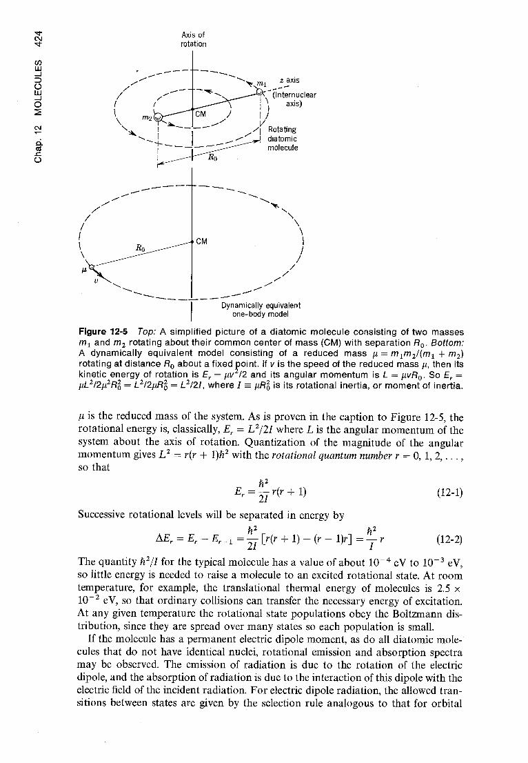
"t- m1 z axis

- (Internuclear

H axis)

/

ri Rotating • diatomic

molecule

^

^

Dynamically equivalent one-body model

MO

LEC

ULE

S

Axis of rotation

Figure 12-5 Top: A simp ified picture of a diatomic molecule consisting of two masses m 1 and m 2 rotating about their common center of mass (CM) with separation R o . Bottom: A dynamically equivalent model consisting of a reduced mass µ = m 1 m 2 /(m 1 + m2 ) rotating at distance R o about a fixed point. If v is the speed of the reduced mass µ, then its kinetic energy of rotation is Er = µv /2 and its angular momentum is L = µvR o . So Er = µL 2 /21.12R1 = L 2/20> = L2/2I, where 1 - µR1 is its rotational inertia, or moment of inertia.

µ is the reduced mass of the system. As is proven in the caption to Figure 12-5, the

rotational energy is, classically, Er = L 2/21 where L is the angular momentum of the

system about the axis of rotation. Quantization of the magnitude of the angular

momentum gives L2 = r(r + 1)h 2 with the rotational quantum number r = 0, 1, 2, ... , so that

h2

Er = 21 r(r + 1)

Successive rotational levels will be separated in energy by

DEr = Er — Er_ 1 = 2I [r(r + 1) — (r — 1)r] = h2

(12-1)

(12-2)

The quantity b 2/I for the typical molecule has a value of about 10 -4 eV to 10 -3 eV, so little energy is needed to raise a molecule to an excited rotational state. At room

temperature, for example, the translational thermal energy of molecules is 2.5 x

10 -2 eV, so that ordinary collisions can transfer the necessary energy of excitation.

At any given temperature the rotational state populations obey the Boltzmann dis-tribution, since they are spread over many states so each population is small.

If the molecule has a permanent electric dipole moment, as do all diatomic mole-cules that do not have identical nuclei, rotational emission and absorption spectra

may be observed. The emission of radiation is due to the rotation of the electric

dipole, and the absorption of radiation is due to the interaction of this dipole with the

electric field of the incident radiation. For electric dipole radiation, the allowed tran-sitions between states are given by the selection rule analogous to that for orbital

2 3 2

ri = 1 rf _0 4

5 3

4

6 5 4 3 . 1 1 2 3 4 , 4 1 ^

100 7

angular momentum in atomic transitions, namely Ar = ± 1. The spectral wavelengths N A follow from (12-2), and v,

AE, = by Q m C, That is : . N

h 2 =

he I

6 r A

or 1 h A 27rIc r (12-3)

in which r is the quantum number of the upper rotational state. With Ar = ± 1, the separation between spectral lines (in terms of reciprocal wavelength) then is A(1/2) = h/27tIc, a constant. This is illustrated in Figure 12-6. Measurement of the separation gives the value of I, the rotational inertia of the molecule, and from this we can esti-mate the value of the equilibrium internuclear separation R o . In the case of HCI, for

r-5

0

b'1:1

103

dS

1b

'N01

1b'1

O1:

1

v

80 — 8 • 8 HCI

°- 9 9 E. 60 ô to to ¢ 40 11

J J

20 -12 12

104° 103° 102° 101° 100° 99° Grating setting

Figure 12-6 Top: Schematic energy-level diagram for the rotational energy states of a diatomic molecule, and the corresponding frequency emission spectrum for allowed

transitions. Bottom: The rotational absorption spectrum for gaseous HCI, giving the percent absorption versus a measure of the reciprocal wavelength.

co N M

OLE

CU

LES

example, we find h/27cic = 2079.4 m -1 , which gives I = 2.66 x 10 -47 kg-m2 ; from the known masses of H and Cl we then obtain R o = 1.27 x 10 -10 m as a measure of the separation of the atoms in the molecule. Pure rotational spectra fall in the extreme infrared or the microwave regions, the corresponding wavelengths A being about 1 mm to 1 cm. An example is shown in Figure 12-6. Diatomic molecules with identical nuclei, like 02 , having no permanent electric dipole moment, do not exhibit pure rotational spectra.

N Example 12 -2. (a) Find the ratio of nr , the number of molecules in rotational level r, to n0 ,

Q- the number in the r = 0 level, in a sample in equilibrium at temperature T. es _j ► From the Boltzmann factor we have

nr _ '17r e - (Er-E0)/kT

no Jr0 in which the "Cs are the degeneracy factors, or number of degenerate quantum states for each energy level. For energy E,. there are 2r + 1 states, corresponding to the number of possible values of the z component quantum number m r associated with each value of r. Hence, ✓Vr, = 2r + 1 and x0 = 1, so that

nr - (Er - E0)lkT • no

(b) Show that the population of rotational energy levels first increases with r and then decreases as r continues to increase. •From (12-1) we have E,. = (h 2/2I)r(r + 1) and E 0 = 0, so that

nr = no (2r + 1)e -(h212IkT) r(r + 1)

Now as r increases the factor 2r + 1 increases whereas the exponential factor decreases. For large r the exponential term dominates so that at first n r increases with r, but soon the ex-ponential suppresses the increase and n,. decreases for larger r. For example, for HBr at room temperature nr is a maximum at r = 3 with n 3/n0 ^ 4, whereas by r = 9 we have n9/n0 1/2.

• (c) Relate these populations to the intensities of the rotational lines.

► Consider the absorption spectrum. The probability that a particular frequency will be absorbed is proportional to the number of molecules in the initial rotational energy level. Hence the intensity variation of the absorption lines (Ar = + 1) are proportional to the pop-ulations of the initial rotational energy levels (see Figure 12-6). The student should construct a similar argument for the emission spectrum. •

12-6 VIBRATION-ROTATION SPECTRA

The nuclei do not maintain a fixed separation, of course, as we assumed previously, so that the molecule is not like a rotating rigid body except in approximation. Indeed, the rotational inertia I changes from the value assumed previously when the molecule rotates because of the stretching of the internuclear distance. Also the nuclei vibrate about some equilibrium separation and this vibrational motion is quantized. Let us now consider the vibrational motion.

For a given electronic configuration, we have a potential energy curve whose minimum is at an equilibrium separation R 0 . Near R 0 the curve is nearly a parabola so that small oscillations are simple harmonic. According to (6-89) the energy of such oscillations is quantized to satisfy

Ev = (y + 1/2)hv 0 (12-4) with the vibrational quantum number y = 0, 1, 2, 3, ... , and where the classical vibra-tion frequency is v 0 = (1/27r) /C/µ. Note that the energy levels here are equally spaced and that there is a zero-point energy (1/2)hv 0 . The separation hvo equals 0.04 eV for NaC1 and, because the dissociation energy is about 1 eV, there are approximately 20 vibrational levels in the potential well. Actually as the energy rises the potential

1 N

^

`d1:1

10

3dS

NO

I1`d

1O1J

-NO

Ilb

'Id8

IA

energy curve becomes anharmonic so that the levels are not equally separated but get somewhat closer to one another. The rotational levels are spaced much closer still, as we saw earlier, there being about 40 rotational levels of NaC1, and about 50 of HC1, between each pair of vibrational levels.

Example 12-3. (a) Given that the equivalent force constant C of a vibrating HC1 molecule is about 470 nt/m, estimate the energy difference between the lowest and the first vibrational state of HC1. ► We have for HC1

and C = 470 nt/m

and also

= 1 _ 1

mH 6.02 x 1023 g 6.02 x 1026 kg

From (12-4) we have that AE = hv o , where vo = (1/211) /C/µ. Hence, using these data, we get the energy difference to be hv o = (h/27r),/C/µ = 0.59 x 10 -19 joule = 0.37 eV. •

(b) Given that the rotational inertia of HC1 has the value I = 2.66 x 10 -47 kg-m 2, estimate the energy difference between the lowest and first excited rotational state of HC1.

► Since Er = (h 2/2I)r(r + 1), the lowest rotational state has an energy E 0 = 0 and the first excited rotational state has an energy E 1 = (h2/21)2 = h2/I. The required energy difference then is AE = h 2/I. Hence

h2 _ (6.63 x 10 -34 joule-sec)2 22 3 — 4.2 x 10 joule = 2.6 x 10 eV I (2x) 2 x 2.66 x 10 - 47 kg-m 2

Thus the energy difference between the two lowest vibrational levels is greater by a factor 142 (i.e., 0.37/2.6 x 10 -3) than that between the two lowest rotational levels in HC1. •

(c) At room temperature, collisions of HC1 molecules in a gas can transfer sufficient kinetic energy to internal energy to excite many rotational states.. At what temperature would the

number of molecules in the first excited vibrational state be equal to 1/e (about 37%) of the number in the ground vibrational state? ■ We have

n1 - -47.1 e -(E1 -Eo)/kT

no At0 where the subscripts refer to y = 1 or y = 0. The vibrational states are not degenerate so that

= 1 = .iro . Also (E 1 — E0) = hvo so that n1

= e-nvo/kT

no and if kT = hv o

n 1 = noe 1

Hence

T = 4300°K k 1.38 x 10 -23 joule/°K

is the temperature at which the number of HC1 molecules in the first excited vibrational state is about 37% of the number in the ground state. Clearly the number of HC1 molecules in the

v = 1 state at room temperature is negligible compared to the number in the ground state. •

If the molecule, like HC1 or NaC1, has a permanent electric dipole moment at the

equilibrium internuclear separation, it will exhibit vibrational emission and absorp-tion spectra due to the oscillations in the electric dipole moment arising from oscilla-tions in the nuclear separation. The selection rule for electric dipole transitions is

Av = + 1 so that AE U ^ hvo . The resulting spectral lines lie in the infrared, between

8000 A and 50,000 A for most molecules. Diatomic molecules with identical nuclei

= 35 36 YnH

hv o 0.59 x 10 -19 joule

co N

MO

LE

CU

LE

S

5 4

v -^

Abs

orp t

ion --

IvN

^

6

HCI

do not have vibrational spectra because they have no electric dipole moment at any

nuclear separation. In a vibrational transition the molecule may also change its rota-tional state so that vibrational changes really result in a combined vibration-rotation

spectrum. The vibrational transition determines the wavelength region of the spec-trum and the rotational transitions determine the separation of the lines. The spec-trum consists of a band of lines, as in Figure 12-7.

Among the interesting results that can be obtained from analysis of vibrational

states and spectra are the relative abundance of nuclear isotopes. The frequency of

vibration, vo = (1/2ic)JC/,u, depends on the masses of the atoms in the molecule

through the reduced mass u. If in a sample of HCI molecules, for example, the isotopes

C1 35 and C1 37 are each present, then the vibrational frequencies and resulting energy

levels will be slightly different for the two types of molecule (see Figure 12-7). Their

spectral lines, consequently, will be shifted with respect to one another, and from a

measurement of spectral intensities we can obtain the relative abundance of the

isotopes Cl" and Cl".

r'- 5

4

3 = 1

2 1 0

Ar= +1 Or =0 Or= — 1-->

5 r" —

4 N./

3 =0

2 v

1 V V 0

3000 2900 2800

2700 Reciprocal wavelength (cm -1 )

Figure 12-7 Top: Energy-level diagram for vibrational and rotational states of a diatomic

molecule, showing allowed transitions and the formation of a band of equally spaced

lines, as indicated in the spectrum below. Note that all Ar = 0 transitions would yield photons of the same frequency v o , but being forbidden, that line is missing in the spectrum.

Bottom: A recorder trace of the vibration-rotation absorption spectrum in HCI. Again note

that the central transition is missing. The slightly different frequencies at each absorption

line are due to the presence of two isotopes of chlorine.

b 'a1

03

dS

OIN

Oa1O

313

0

Figure 12-8 The energy for H2, HD, and D2 is the same function of the internuclear se-paration R. But the ground state vibrational energy S differs for each molecule.

In a somewhat related way we obtain experimental evidence for the finite zero-point energy of an oscillator. Consider the molecules H2, HD, and D2 in which D stands for a deuterium atom. Because the electric forces are identical in all cases we

obtain for all the same potential energy curve V(R), illustrated in Figure 12-8. The

energy required to dissociate the molecule is Ed = V0 — b. If the ground state energy 8 were zero, then the dissociation energies would be the same, Ed = Vo , for each type of molecule. Quantum theory gives a finite zero-point energy, namely b = (1/2)hv o . However, because the reduced mass ,u enters the formula for v o , a has a different value for each type of molecule so that their dissociation energies should differ. In fact, with

/1D2 = 2µH2 and PHD = (4/3),uH2

we can predict the difference, and we find that the observed dissociation energies differ exactly as predicted, thereby verifying the existence of a zero-point energy in agree-ment with the requirements of the uncertainty principle.

In Table 12-1 we list the rotational and vibrational constants of some diatomic molecules.

12-7 ELECTRONIC SPECTRA

The rotational and vibrational states in molecules are due to the motion of the nuclei. There can be also electronic excited states, of course. For each of the electronic states, corresponding to different electron configurations, there is a different dependence of the molecule's energy on its internuclear separation. Because the atoms are more loosely bound in the excited states, the curves representing the molecule's potential energy as a function of nuclear separation become shallower and broader, and the

Table 12-1 Rotational and Vibrational Constants of Some Diatomic Molecules

Molecule Ro(A) vo (cm -1 ) ^2 ^2 21 (eV) Molecule Ro(Â) vo (cm - i) —

2/ (eV)

H2 O.74 4395 7.56 x 10 -3 LiH 1.60 1406 9.27 x 10 -4 HD 0.74 3817 5.69 x 10 - 3 HC13 5 1.27 2990 1.32 x 10 -3

D2 0.74 3118 3.79 x 10 -3 NaC1 35 2.51 380 2.36 x 10 -5 Li2 2.67 351 8.39 x 10 -5 KC1 35 2.79 280 1.43 x 10 -5 N2 1.09 2360 2.48 x 10 -4 KBr79 2.94 231 9.1 x 10 -6 02 1.21 1580 1.78 x 10 -4 HBr79 1.41 2650 1.06 x 10 -3

MO

LEC

ULE

S

N

d

L U

Rotational levels Er"

0 M

Vibrational levels E,"

11

10

9 8

7

6

5

One electronic

state

j

0

Figure 12 -9 Illustrating electronic states. Each vibrational level has its

R —

the molecular energy versus internuclear separation curves for two electronic state has its own set of vibrational levels, and each own set of rotational levels.

equilibrium separation R 0 increases, with increasing electronic excitation, as illus-trated in Figure 12-9. The energy separation between different electronic states is from 1 to 10 eV, so that transitions between electronic states give radiation in the visible or ultraviolet portion of the electromagnetic spectrum.

To each electronic state Ee there are many bound vibrational states of energy E0 , and to each vibrational state there are many bound rotational states of energy Er. Neglecting interactions between these modes, we can write the total energy as E _ Ee + Ev + Er . The energies of all three modes may change in an electronic transition so that in general we can write

4E = AEe + (E', — Fe') + (E'r — Er) (12-5) The initial (primed) and final (double-primed) vibrational and rotational states differ in their binding so that the equilibrium spacing, the rotational inertia, and the fun-damental vibrational frequency change. A great many transitions are possible and they produce a complex spectrum of lines, which appear in a series of bands as il-lustrated in Figure 12-10. Hence the term band spectra.

The term 4Ee is the energy difference of the minima of the two electronic states. The vibrational term is Ev — Ez = (y' + 1/2)hvO — (v" + 1/2)hv' (; and the rotational term is Er — Er = (h2/21')r'(r + 1) — (h2/2l")r"(r" + 1). For a given electronic tran-sition the spectrum consists of bands, where each band corresponds to given values

N

C2 Swan bands

6191 A 5636 A 5165 A 4737 A 4383 A N

O O O

O O

O

IIIIII II III III IIII

r'- 11

0 //

tJa

10

3dS

OIN

O1=1

1031

3

Ill III IIIIIII IIIIIIiii HI ill In N .-I M N" N .--I O O

I I I ' I I I 1 1 I CO 1fl <t n CO 1f1 O O O .-I

CN (Red) 4606 A 4216 A 3883 A 3590 A

'CN (Violet)

Figure 12-10 Top: Energy-level diagram and transitions leading to the formation of an electronic band. Unlike Figure 12-7, the band spectrum indicated folds back on itself, giving

rise to a band head at the right end of the spectrum. Again note that the transition of frequency vo is missing. Bottom: Bands of the CN and C2 molecules in a carbon arc in air. (From Herzberg, Spectra of Diatomic Molecules, 1950. D. Van Nostrand Co., Inc., New York)

1 ^

V V V

r J

y

^ r

3 1y V

7 r I r

5 Ir Y r

5

y 1

3 r

i

2 1 0 U 123 3 2 1 ° 012

1^ 0

r' = 10 r" = 11

9 10

1 0

9

8

7

6

5

4 3 2

r" = 1

1

N M

MO

LEC

ULE

S

of v' and y" and all possible values of r' and r". The selection rules determine the possible combination of values of y', y", and r', r". The rotational selection rule here is Ar = 0, ± 1 for electric dipole radiation. This rule is broader than for pure rotation in that Ar = 0 is now allowed. The reason is that the change in the electronic config-uration accompanying the rotational change eliminates the parity considerations which earlier excluded Ar = 0 (see Section 8-7). The vibrational selection rule for electric dipole radiation is Av = ± 1 for a simple harmonic oscillator. If, however, the potential deviates from the simple harmonic,_ i.e., if it is anharmonic, then Av = 2, 3, ... , etc., are also allowed. These vibrational rules apply only if the electronic state does not change and they apply to pure vibration-rotation bands. If there is a change in electronic state then the selection rules are determined from the so-called Franck-Condon principle, which we explain next.

We have seen that there is little interaction between the electronic motion and the nuclear motion in a molecule. Furthermore, the characteristic time for an electronic transition is At ^ 10' 16 sec, whereas for a nuclear vibration the time has the much longer value At ^ 10 -13 sec. As a result the internuclear distance stays about the same during an electronic transition, and a vertical line (a line of constant R) in Figure 12-9 accurately represents such a transition. If the upper state corresponds to y' = 0, then the probability distribution function for the oscillator is large only near the equi-librium separation, and an electronic transition to the lower state leaves the molecule at about the point P on the potential curve in that figure. This corresponds to y" = 7 for the lower state. Notice that classically the nuclei have small kinetic energy in each case, because y' = 0 initially, and because P corresponds to the end point of the vib-rational motion for y" = 7. This meets the requirement that the relative nuclear velocity be about the same in both states at the time of a transition in order that the nuclear motion be able to adjust quickly to the new electronic conditions. Transitions are most favorable under these conditions. Quantum mechanically we get the same result because in the ground state of an oscillator, as in y' = 0, the maximum ampli-tude of the eigenfunction occurs at the center of the motion, whereas for the upper states, such as in y" = 7, the eigenfunction has maximum amplitude near the ends of the oscillation. Since the integral in the electric dipole matrix element, (8-42), that determines the relative intensities, or selection rules, involves a product of the eigen-functions of the upper and lower states, the intensities will be large only where both these eigenfunctions have significant space overlap. In general, the most favored transitions are those which, from a classical point of view, can occur with the inter-nuclear distance for both initial and final states the same and the nuclei at end points of their oscillations. Examples in Figure 12-9 are shown by vertical lines from v' = 5 to y" = 2 or y" = 11. These rules were deduced by Franck from classical considera-tions and put on a firm quantum mechanical basis by Condon.

If the excited electronic state is not bound, the molecule dissociates. Because such unbound states have a continuum of possible energies, the corresponding spectrum gives a continuous band. The appearance of a continuum in the absorption spectrum of a molecule is therefore experimental evidence for photochemical dissociation.

12-8 THE RAMAN EFFECT

An interesting effect which gives much information about molecular quantum states was dis-covered experimentally in 1928 by Raman. This is the scattering of light by molecules with a frequency change. The student may be familiar with other light scattering processes. In ordi-nary Rayleigh scattering by molecules, the scattered frequency is the same as the incident frequency. In the fluorescence process, the frequency of the incident light coincides with an absorption frequency of the scattering gas molecules; this is a resonance phenomenon in which the molecule is raised to an excited state and, after a short lifetime there, reemits light at a

W w

10

33

33

N`d

Wb

Id 3

H1

8-Z

1-

'00S

^

A

v—^

r- 4

3

2

1 0

different frequency. In the Raman effect, the scattered frequency is different from the incident

frequency, and the incident frequency is not related to a characteristic frequency of the scat-tering molecule.

If the incident radiation is intense and monochromatic with a frequency y, it is found that the light scattered at right angles to the incident direction contains not only radiation of frequency

y (Rayleigh scattering), but also weaker radiation of frequency y + v' (Raman scattering). The scattered spectrum therefore has weak Raman lines on each side of the Rayleigh line. If we

change the incident frequency, we again find weak lines on each side of the Rayleigh line in

the scattered spectrum with the same frequency difference as before. The frequency difference V between the incident and scattered light in the Raman effect is characteristic of transitions

in the scattering molecule. During the scattering process the molecule may have its state

changed from one allowed energy to another. To conserve energy in the process the scattered

photon must then have an energy different from the incident photon by an amount equal but

opposite to the molecular energy change.

Consider a scattering molecule in a rotational state r. In the ordinary rotational spectrum,

lines will be found corresponding to transitions with Ar = + 1. In the scattered Raman spec-trum, however, we find frequency shifts from the incident frequency that correspond to rota-tional transitions in the scattering molecule with Ar = ± 2. Hence, transitions that are not

allowed in the ordinary emission or absorption spectrum are allowed in the Raman process.

A quantum mechanical analysis of the Raman process leads to the conclusion that a Raman

transition between states a and f can occur only if there is a state y such that ordinary transi-tions are allowed between a and y and /3 and y. It is as though we get from a to 13 by going through y. In this case, if a has quantum number r then y has r + 1. An ordinary transition

from y to /3, however, requires another change Ar = + 1, so that the total change in r from a

to 16 is Ar = 0, ± 2. The Ar = 0 selection rule gives Rayleigh scattering, and the Ar = +2 selec-tion rule gives Raman scattering. Hence in the scattered spectrum we have lines on each side

of the incident line which are spaced about twice as far apart in frequency as the lines in the

ordinary rotational spectrum. This is shown schematically in Figure 12-11.

There is a Raman effect with vibrational states as well. In the process of scattering a photon

of frequency y a molecule may change its vibrational state. Because Ay = + 1, the final vibra-tional level of the molecule may be one just above or just below the initial level. Therefore

the Raman scattering frequency will be y + y', where the frequency change y' is a characteristic

vibrational frequency of the molecule. At ordinary temperature, however, most molecules are

in the ground vibrational state, y = 0, so that the molecule absorbs energy in changing to

state y = 1. Hence, only the lower frequency line y — y' appears in the Raman spectrum. How-ever, the higher frequency line y + v' may be observed if the y = 1 level is sufficiently populated

so that enough transitions from y = 1 to y = 0 occur to give detectable intensities. This is more

likely the lower the energy of the y = 1 state and the higher the temperature of the scattering

gas. As an example of the utility of Raman scattering, consider molecules with two identical

nuclei, such as 0 2 and N2. We cannot directly observe rotational spectra or vibration-rotation

spectra for such molecules because they have no electric dipole moment. We can, however,

obtain a spectrum corresponding to vibration and rotation of such molecules in the Raman

Figure 12-11 Schematic diagram showing the origin of rotational Raman lines on each side of the Rayleigh scattering line.

MO

LEC

ULE

S

scattering. It is as though the incident radiation polarizes the molecule, thereby inducing an electric dipole moment; this permits absorption and emission of radiation corresponding to rotational and vibrational motions of the molecule. Of course, in an electronic transition in 02 or N2 the fine structure of the,spectrum reveals the vibrational and rotational structure, but such a spectrum lies in the ultraviolet and the fine structure is very difficult to resolve. Historically, Rasetti used the Raman spectrum to make the first determination of the rotational inertia, or moment of inertia, of the N2 molecule.

12-9 DETERMINATION OF NUCLEAR SPIN AND s SYMMETRY CHARACTER o

We have ignored the weaker interactions that enter in the detailed structure of molec-ular spectra, such as the effect of nuclear spin on the energy states of a molecule. But we cannot ignore a very important effect that nuclear spin has on the spectrum of a molecule even when the spin interaction itself is negligible. For a diatomic molecule with identical nuclei, the states that can be occupied and the transitions that are allowed are restricted by symmetry requirements. If the nuclear spins are integral (0,1,2, ...) then the complete eigenfunction of the molecule must be symmetric with respect to exchange of the labels of the two identical boson nuclei. If the nuclear spins are half-integral (1/2,3/2, ...) then this eigenfunction must be antisymmetric in an exchange of the labels of the two nuclei because they are identical fermions.

If we neglect the small interactions between the modes associated with the elec-tronic, vibrational, rotational, and nuclear spin behavior of the molecule, we can write the molecular eigenfunction as a product of four factors. Since it is usually the case, we henceforth assume the electronic factor is symmetric in an exchange of the labels of the two nuclei because it is even in a reflection in the plane half way between them (as in H 2). The vibrational factor is always symmetric since it can be written

tfry = (Mkt — x 2 1) where x 1 and x2 are the coordinates of the nuclei labeled 1 and 2, measured along their center to center line. That is, the independent variable in the vibrational eigen-function is the magnitude of the distance between the two identical nuclei. Since this does not change when the nuclear labels are exchanged, 0, itself does not change and so is symmetric with respect to the exchange. Thus the symmetry of the molecular eigenfunction is governed by the symmetry of the product of its rotational factor and its nuclear spin factor.

The question of what happens to the sign of the rotational factor Cr when we ex-change the labels of the identical nuclei is intimately related to the question of what happens to the sign when we change the signs of all the coordinates, providing we are wise enough to choose the origin of coordinates at the center of the molecule (i.e., at its center of mass, halfway between the nuclei). With this choice, the parity ques-tioning operation of (8-44) (x -* — x,y —* — y,z — z) obviously accomplishes the same thing as the symmetry questioning operation (1 —> 2,2 —> 1), and the symmetry of Or becomes the same as its parity. Furthermore, we can immediately apply the interpretation of (8-47) to determine the parity of fir, if we change from the orbital angular momentum quantum number l used there to the rotational quantum num-ber r used here, and conclude that the parity of 1// r is even if r is even and the parity of >Jir is odd if r is odd. The justification is that if the rotational angular momentum of the molecule is quantized then there can be no external torques acting on it, so the potential energy function describing the external environment (if any) in which the molecular rotation takes place must be spherically symmetrical about our origin of coordinates; this is the only requirement for the validity of (8-47). Putting it all together, we see that the rotational eigenfunction C. is symmetric if r is even, and antisymmetric if r is odd.

Now let us consider a situation in which the nuclear spin angular momentum quan-tum number i has one of the values i = 1/2, 3/2, 5/2, .... Then the complete molecular eigenfunction must be antisymmetric in a nuclear label exchange. There are two ways this can come about: (1) either the nuclear spin eigenfunction is antisymmetric and the rotational eigenfunction is symmetric, or (2) the nuclear spin eigenfunction is symmetric and the rotational eigenfunction is antisymmetric. Both possibilities will occur, but not in the same molecule. The reasons are: (1) the symmetry of the nuclear spin eigenfunction factor is determined by the relative orientation of the two nuclear spins (e.g., for i = 1/2, the symmetric case corresponds to the two spins being essen-tially parallel while the antisymmetric case corresponds to them being essentially antiparallel, exactly as for two electrons with spin quantum number s = 1/2), and (2) the interaction between the nuclear spins is very small so that if the spins have a particular relative orientation, they will maintain it for a very long time (as long as years).

Practically, it is as though there are two distinctly different species of molecules. The species with symmetric nuclear spin eigenfunctions is called ortho and the species with antisymmetric nuclear spin eigenfunctions is called para as, for example, ortho-hydrogen and parahydrogen. The same terminology is used in the same way, whether i is half-integral or integral. But if i is half-integral, the ortho species has only anti-symmetric rotational eigenfunctions and the para species only symmetric rotational eigenfunctions, as we have been considering; while if i is integral, the symmetry of the complete molecular eigenfunction is reversed so the ortho species has only sym-metric rotational eigenfunctions and the para species has only antisymmetric rota-tional eigenfunctions. These relations are summarized in the rotational energy-level diagrams of Figure 12-12. The pair on the left is for molecules whose nuclei have half-integral spin. For the ortho species of such molecules only odd-r rotational states can be populated because the rotational eigenfunction must be antisymmetric, and it is only for odd r. In the para species only the symmetric rotational states can be populated, and these are the ones for even r. The relations are reversed for mole-cules with integral spin nuclei, as is indicated in the pair of energy-level diagrams on the right side of Figure 12-12. The dots in the figure show the energy levels that can be populated, and the arrows show the possible transitions between these levels.

DE

TE

RM

INA

TIO

N O

F N

UC

LE

AR

SP

IN A

ND

SY

MM

ET

RY

CH

AR

AC

TE

R

Ortho Para (symmetric (antisymmetric

spin spin eigenfunction) eigenfunction)

Ortho Para (symmetric (antisymmetric

spin spin eigenfunction) eigenfunction)

Half-integral nuclear spin Integral nuclear spin

Figure 12-12 Illustrating the relation between the rotational and spin states that can -be populated in molecules having symmetric electronic factors with identical half-integral, and integral, spin nuclei. The dots indicate the possible states and the arrows indicate transitions between these states.

co co M

OLE

CU

LES

Since molecules with two identical nuclei have no electric dipole moments, we

cannot directly observe the rotational spectra emitted in such transitions; but we can indirectly observe transitions between rotational states in Raman scattering, or in band spectra, as explained in earlier sections.

Measurements of the number of transitions made by the para species of such molecules, relative to the number of transitions made by the ortho species, constitute a quite frequently used procedure for determining the value of the spin quantum number i of the nuclei forming the molecules. These numbers are in proportion to the relative amounts of the two species present in the sample and, at ordinary tem-peratures where many rotational states are excited, the relative amounts are in pro-portion to the numbers of nuclear spin states for the two species. We shall show in Example 12-6 that the ratio of the number of antisymmetric spin states, Xpara, to the number of symmetric spin states, . Northo, is

para _ l (12-6) 'Kortho l + 1

The 'number of transitions should be in this ratio, so that we get an alternation of intensities in the Raman spectra or band spectra, of diatomic molecules with identical nuclei. This can be seen in the photograph of the N2 rotational Raman spectrum, shown in Figure 12-13, for which the intensities of alternate lines are measured to be quite accurately in the ratio 1/2. Even more dramatic is the spectrum of C2, for which the ratio is 0/1 because alternate lines are completely missing! We do not show that spectrum because the drama is not apparent until a careful comparison between the measured and predicted frequencies of the lines demonstrates that half are absent.

Example 12-4. Determine the values of the nuclear spin quantum number i for the nuclei in N2 and C2, by using the measured intensity ratios 1/2 and 0/1 in (12-6). ► Since the possible values of i are restricted to i = 0, 1/2, 1, 3/2, 2, ... , inspection immediately demonstrates that the solution to

1 i

2 i +1 is i = 1. This is the spin of the N nucleus (i.e., of its overwhelmingly abundant isotope N14)

For

Figure 12 -13 Alternating intensities in a rotational Raman spectrum of N2, excited by the Hg line 2536.5 A.

the solution is obviously i = O. This is the spin of the C nucleus (actually, of its most abundant isotope C 12, since the other isotopes, C 13 and C 14, are so rare that the abundant one com- pletely dominates the spectrum). •

The reason for the complete absence of half of the transitions involving rotational levels of molecules having symmetric electronic factors and two identical i = 0 nuclei is simply that i = 0 means the nuclei are bosons that have no spin, so the molecular eigenfunction is necessarily symmetric and has no spin factor in it. Therefore its rotational factor must always be symmetric, which requires that the molecule only be in even-r rotational levels. Proof that these symmetry considerations are very real indeed comes from that fact that if in C2 the nuclei are not identical (e.g., if we have C 12 — C13), then half the transitions are not missing. This experimental fact actually led to the discovery of the isotope C 13

As we have said, the procedure of Example 12-4 has been widely applied. It was used in the first determination of the spin i = 1/2 of the proton, from the measured intensity ratio of 1/3 in the spectrum of H2. The measurements are difficult to make only when i becomes very large.

The determination of the symmetry character of the identical nuclei in molecules like N2 is a matter of keeping track of which lines of the spectrum are the more intense. Example 12-5. In N2 it is observed that transitions involving even-r rotational states yield the most intense lines. Determine the symmetry character of the nuclei in that molecule. ► Since (12-6) shows that the highest population is for nuclear spin states that are symmetric (ortho), and since even-r rotational states are also symmetric, the symmetric nuclear spin states are associated with the symmetric rotational states. Therefore the N 14 nucleus must be a boson. •

Symmetry character determinations made in this manner on a number of nuclei provided some of the earliest evidence for the correlation, seen in Table 9-1, between symmetry character and spin. Furthermore, we shall see in Chapter 15 how the fact that the particular nucleus N 14 is an i = 1 boson was used at an early date to show that nuclei must contain protons and neutrons, instead of protons and electrons. Example 12-6. Show that the ratio of the number of antisymmetric spin states to the number of symmetric spin states is i/(i + 1), in agreement with (12-6). •The number of possible individual states of spin for a particle of a given spin quantum number i is equal to the number of possible values of its z component quantum number m i . Since, as usual, the values of m i differ by integers and range from — i to + i, this number is the familiar (2i + 1). So the total number of possible independent combinations of spin states for two identical particles of spin i is (2i + 1)(2i + 1) = (2i + 1)2 . In (2i + 1) of these states both particles will have the same m i, and so are in identical spin states. For these the spin eigen-function of the two particle system is symmetric with respect to particle label exchange (like the top and bottom members of (9-18) in the case of i = 1/2). Of the (2i + 1) 2 — (2i + 1) = 2i(2î + 1) remaining states, half will be symmetric and half will be antisymmetric in such an exchange, since half will involve the sums of products of individual spin eigenfunctions and the other half will involve the differences of the same products (like the center member of (9-18), and (9-17), in the case of i = 1/2). So the total number of symmetric eigenfunctions is

Xsymmetric ortho = (2i + 1) + (1/2)2i(2i + 1) = (i + 1)(2i + 1) and the total number of antisymmetric eigenfunctions is

'AV'antisymmetric = para = (1/2)2i(2i + 1) = 1(2l + 1)

The ratio of the number of eigenfunctions, or spin states, is

Afpara _ l

cirortho l + 1 in agreement with (12-6). •

DE

TER

MIN

AT

ION

OF N

UC

LEA

R S

PIN

AN

D S

YM

ME

TR

Y C

HA

RA

CT

ER

MO

LEC

ULE

S

QUESTIONS

1. Discuss the statement that the interatomic force law must be attractive to permit con-densed phases and must be repulsive to avoid zero volume.

2. Would you expect H3 to exist in a bound state? He t? Explain.

3. Of the so-called inert gases, which might most easily form molecules with other elements? Explain.

4. How would you explain the existence of bound states of XeF 4, in view of the absence of valence electrons in a Xe atom?

5. Do the even, or odd, H2 eigenfunctions have even, or odd, parity?

6. Explain why only two electrons can form a covalent bond.

7. Would you predict ionic binding or covalent binding in H 2 O? In NH3? In CH4? Does experiment decide the issue or can you rule out one or the other types of binding independently?

8. From the fact that CO 2 does not have a permanent electric dipole moment, what can you conclude about the binding and the arrangements of the atoms in the molecule?

9. Of the molecules H2 , D2, and HD, 'which has the greatest binding energy? The least?

10. What does it mean to say that a molecule is in an excited state? 11. Explain how the existence of a finite zero-point vibrational energy is related to the un-

certainty principle. 12. The fundamental vibrational energy for HC1 is about ten times that for NaCl. Con-

sidering the factors determining this quantity, make this plausible.

13. What effect, if any, does the increasing angular momentum of higher rotational states of a diatomic molecule have on the vibrational energy of the molecule?

14. What effect does the change in internuclear separation in a diatomic molecule due to its vibration (the binding energy curve is asymmetric) have on the rotational energy levels of the molecule?

15. The asymmetry in the binding energy curve accounts for thermal expansion of solids. How can information from molecular spectra be used to determine the shape of this curve?

16. Explain why the separation between vibrational levels is somewhat smaller in an excited electronic state than in the ground electronic state (see Figure 12-9). Explain the same effect for rotational states.

17. If Raman rotational lines arise from an induced electric dipole moment how can we explain that the selection rule is Ar = ± 2 rather than Ar = ± 1?

18. Since it is known to take a very long time for the para and ortho species of a molecule to convert themselves into each other, the interaction between the two nuclear spins in a molecule must be very small. Why would you expect this to be the case?

19. What changes must be made in the result developed in Section 12-9 if the electronic factor of the molecular eigenfunction is antisymmetric in an exchange of the labels of the two nuclei?

PROBLEMS

1. From the following data, find the energy required to dissociate a KC1 molecule into a K atom and a Cl atom. The first ionization potential of K is 4.34 eV; the electron affinity of Cl is 3.82 eV; the equilibrium separation of KC1 is 2.79 A. (Hint: Show that the mutual potential energy of K + and Cl is —(14.40/R) eV if R is given in Angstroms).

2. The first ionization potential for K is 4.3 eV; the ion Br - is lower in energy by 3.5 eV than the neutral bromine atom. Compute the largest separation of K + and Br ions that gives a bound KBr molecule.

3. For a system which executes simple harmonic motion about a position of stable equi-librium, the force, F, is given by

w CO

SI/1

31

80

8d

(02 v

F=— 2( )RO(R —R0)

where V is the potential energy and R — R o is the deviation from equilibrium. Show that the zero-point vibration of a molecule is given by

( 2 /

1172

2 hv o = ^

47cu 1/2\aR2 R 0

4. The potential energy V of NaC1 can be described empirically by

e2 V = + Ae -RIp

4Te0R

where R is the internuclear separation. The equilibrium separation of the nuclei R o is 2.4 A and the dissociation energy is 3.6 eV. (a) Calculate A and p/R o , neglecting zero-point vibrations. (b) Sketch V and each of the terms in V on one graph. (c) Give the physical significance of A and p.

5. (a) Show that the ratio of the number of molecules in rotational level r to the number in the r = 0 level, in a sample at thermal equilibrium, is a maximum for the level

specified by r = (kTI/lî2)1"2 — 1/2

(b) For HC1, what is the most populated level at 600°K?

6. Taking the rotational inertia of H2 from Table 12-1, find the temperature at which the average translational kinetic energy of an H2 molecule equals the energy between the ground rotational state and first excited rotational state. What can you conclude about

the occupation of rotational excited states in H2 at room temperature?

7. Determine b, the zero-point vibrational energy, for a NaCl molecule, given that its

fundamental vibrational frequency is 1.14 x 10 13 vib/sec. 8. (a) Show that, if Ed is the dissociation energy of a molecule, the fraction of the molecules

that dissociate at a temperature T is e - Ed/kT. (b) It is found (from electron diffraction studies) that as T increases, the internuclear separation increases. Explain what effect this

has on the potential energy curve and on the result of part (a).

9. For NaC1, the separation of two vibrational levels is about 4 x 10 -2 eV. Using Table 12-1, and noting that the rotational levels are not equally spaced, show that there are

about 40 rotational levels between a pair of vibrational levels. 10. The potential energies of two diatomic molecules of the same reduced mass are shown

in Figure 12-14. From the graph determine which molecule has the larger (a) inter-nuclear distance, (b) rotational inertia (moment of inertia), (c) separation between

V

Figure 12-14 Potential energy curves considered in Problem 10.

MO

LEC

ULE

S

rotational energy levels of the same r and y, (d) binding energy, (e) zero-point energy (Hint: See Problem 3), (f) separation between low-lying vibrational states.

11. (a) What fraction of HC1 molecules at 1000°K will be found in the first excited vibrational state? (Hint: Use the Boltzmann factor.) (b) Find the ratio of HCI molecules in the first excited rotational state to those in the first excited vibrational state at 1000°K. (Hint: Remember the degeneracy factors.)

12. (a) Derive an expression giving the ratio of the energy of a transition from the lowest to the first excited vibrational level to the energy of a transition from the lowest to the first excited rotational level for a diatomic molecule. (b) What is this ratio for NaCl? For H 2? (Hint: See Example 12-3.)

13. (a) Show that the relative frequency shift of a spectral line in a rotational band arising from a mixture of two isotopic diatomic molecules is given by Av/v = — Aµ/µ, where u

is the reduced mass of the molecule. (b) What is this ratio for a mixture of HC1 35 and HC1 37?

14. Show that the ratio R of the total number of molecules in all excited vibrational states to the number in the ground vibrational state is

R = (e

provided that the levels are assumed to be equally spaced. 15. What is the amplitude of vibration of HCl in the first excited vibrational state? 16. (a) Use data from Example 12-3 to predict the reciprocal wavelength of the zero-point

vibration of HC1 given in Table 12-1. (b) What must be the force constant to give exact agreement?

17. From the value 2940.8 cm -1 for the reciprocal wavelength equivalent to the fundamental vibration of a molecule C1 2 , each of whose atoms has an atomic weight 35, determine the corresponding reciprocal wavelength for C1 2 in which one atom has atomic weight 35 and the other 37. What is the separation of spectral lines, in reciprocal wavelengths, due to this isotope effect?

18. (a) Specify the resolution, A2/2, of a spectrometer which can just resolve the rotational spectra of Na 23 C135 and Na23C1 37 assuming R 0 to be the same for both molecules. (b) Would this spectrometer also resolve the vibrational spectra of the two molecules, as-suming the force constants are the same?

19. Calculate the difference in dissociation energies of H2 and D2 from the value 4395.2 cm -1 for the reciprocal wavelength equivalent to the fundamental vibration of an H2 molecule.

20. The zero-point vibrational energy for H2 is 0.265 eV. Compare the vibrational energy levels of H2, D2, and HD numerically for the low-lying states.

21. From the fact that the lowest electronic excited state in 0 2 and N2 molecules is over 3 eV above the ground state, explain why air is transparent in the visible.

22. In the vibrational Raman spectrum of HF are adjacent Raman lines of wavelength 2670 A and 3430 A. (a) What is the fundamental vibrational frequency of the molecule? (b) What is the equivalent force constant for HF?

23. A ruby laser (2 = 6943 A) is used to excite the Raman spectrum of N2. (a) What are the wavelengths of the lines which result from the lowest energy allowed transitions in the pure rotational spectrum of N 2? (b) What is the ratio of the intensities of the lines of part (a) at room temperature? (c) What are the wavelengths of the lines which result from the allowed transitions to and from the ground state vibrational level? (d) What is the ratio of the intensities of the lines of part (c) at room temperature? (e) How do the answers to parts (a) and (c) change if the laser is used to excite the Raman spectrum of diatomic molecules with nonidentical nuclei having the same rotational inertia and force constant as N 2?

24. The energy-level diagram for the rotational levels in each of the two lowest vibrational states of the electronic ground state is given in Figure 12-15 for a diatomic molecule. Find the energies of the transitions that give rise to the allowed spectral lines in the infrared and Raman spectra, (a) for molecules containing two identical i = 0 nuclei,

hva/kT _ 1)-1

r' — 3

2

1 o

= 3 r"

8x 10 -4 eVi

2 x 10 -1 eV

U' = 1

2

1 a"=0 0

1 x 10 -3 eVJ

Figure 12 -15 Energy levels considered in Problems 24, 25, and 26.

(b) for molecules containing two identical i = 1/2 nuclei, and (c) for molecules containing two nonidentical nuclei.

25. Calculate the relative intensities at room temperature for the lines found in parts (a) and (b) of Problem 24.

26. Using the information in Figure 12-15, (a) calculate the rotational inertia, or moment of inertia, of the molecule in each vibrational level, and (b) calculate the zero-point energy,

27. (a) How many rotational degrees of freedom do you expect in a polyatomic molecule? Translational degrees? If the molecule has N atoms (N > 2) there should be 3N — 6 vibrational degrees of freedom, i.e., independent modes of vibration. Explain. (b) How many vibrational degrees of freedom are there in an H 2 O molecule? A CH4 molecule?

28. Consider the relative intensities of the spectra of H2 and D2 to determine which Raman rotation spectrum will yield lines alternating in intensity and having a relative intensity of 1/2.

29. Band spectrum measurements of diatomic molecules containing C1 35 nuclei yield an alternating intensity ratio of 3/5. What is the spin of the C1 35 nucleus?

sw3

1so

ad

13 SOLIDS

CONDUCTORS AND SEMICONDUCTORS

13-1 INTRODUCTION

443

subjects included in solid state physics

13-2 TYPES OF SOLIDS

443

crystal lattices; qualitative characteristics of molecular, ionic, covalent, and metallic solids

13-3 BAND THEORY OF SOLIDS

445

exchange degeneracy in a lattice of identical atoms; comparison to hydrogen molecule; formation of energy bands; allowed and forbidden bands; over-lapping bands; occupation of bands; unit cells; insulators; conductors; elec-tron momenta in insulators and conductors; valence and conduction bands; semiconductors

13-4 ELECTRICAL CONDUCTION IN METALS

450

electron-lattice imperfection collisions; classical expressions for resistivity, conductivity, and mobility; Hall effect; Hall coefficient; hole conduction

13-5 THE QUANTUM FREE -ELECTRON MODEL

452

free-electron energy dist ribution and density of states; estimate of Fermi energy and relative number of conduction electrons for metal; evaluation of energy width of band; density of states for band in two-dimensional metal

13-6 THE MOTION OF ELECTRONS IN A PERIODIC LATTICE

456

Bloch eigenfunctions; Kronig-Penney model; Bragg reflection; relation of Kronig-Penney results to Bragg conditions; eigenfunction symmetry and origin of band gaps; Brillouin zones

13-7 EFFECTIVE MASS 460

properties of wave groups recapitulated; equation of motion of electron in lattice under applied electric field; interpretation of effective mass; effective mass in various regions of a Brillouin zone; relation to Bragg reflection; comparison of level densities by means of effective mass; use of effective mass in classical expressions for conductivity and resistivity; lattice imper-fections and resistivity; effective mass of holes

13-8 ELECTRON -POSITRON ANNIHILATION IN SOLIDS

464

energy-momentum conservation; correlation measurements; electron mo-mentum distributions; defects; lifetime measurements; positronium

442

13-9 SEMICONDUCTORS 467

energy gaps in silicon and germanium; temperature dependence of con-ductivity; intrinsic and extrinsic conductivity; photoconductivity; donor im-purities and n-type semiconductors; estimate of donor electron binding energy; acceptor impurities and p-type semiconductors; Fermi energy in an intrinsic semiconductor; temperature dependence of Fermi energy in im-purity semiconductors

13-10 SEMICONDUCTOR DEVICES 472

p-n junctions; thermal current; recombination current; application of re-verse or forward bias; rectifier action; advantages over vacuum tube recti-fier; junction transistors; operation explained in terms of junctions; power amplifier action; tunnel diodes; negative resistance characteristic and fast response time

QUESTIONS 477

PROBLEMS 478

13-1 INTRODUCTION

Solid state physics is a vast area of quantum physics in which we are concerned with understanding the mechanical, thermal, electrical, magnetic, and optical properties of solid matter. Some aspects have been discussed in earlier chapters, such as the lattice and electronic contributions to the specific heats of solids, radiation from a black-body, thermionic emission, and contact potentials. Here we shall focus on the origin of the forces that hold atoms together in a solid and on the allowed energy levels of the electrons in the solid. This will lead us to the band theory of solids. That theory will then be applied to phenomena of much practical and theoretical interest, in-cluding semiconductors and semiconductor devices. Many electrical, thermal, and optical properties of solids will thereby become more clearly understood. In the next chapter we extend the theory to the phenomenon of superconductivity and consider magnetic properties of solids as well.

13-2 TYPES OF SOLIDS

In the gaseous state the average distance between molecules is large compared to the size of a molecule, so the molecules may be regarded as isolated from one another. Many substances, however, are in the solid state at ordinary temperatures and pressures. In that state molecules (or atoms) can no longer be regarded as isolated. Their separation is comparable to the molecular size, and the strength of the forces holding them together is of the same order of magnitude as the forces binding the atoms into a molecule. Hence, the properties of a molecule are altered by the presence of neighboring molecules. Characteristic of crystalline solids is the regular arrange-ment of atoms, a recurrent or periodic pattern called a crystal lattice. The solid can be regarded as a large molecule, the forces between atoms being due to interaction between atomic electrons, and the structure of the solid being determined as that arrangement of nuclei and electrons which yields a quantum mechanically stable system. Although the number of atoms involved is very large, they are arranged in a regular pattern. In noncrystalline solids, such as concrete and plastic, the perfectly regular pattern does not hold over long distances, but there is an orderly pattern in the neighborhood of any one atom. We shall discuss only crystalline solids in this

Sa

l-lO

S J

O S

3d

Al

SO

LID

S- C

ON

DU

CT

OR

S A

ND

SE

MIC

ON

DU

CT

OR

S

book. Such solids are classified according to the predominant type of binding, the principal types being molecular, ionic, covalent, and metallic.

Molecular solids consist of molecules which are so stable that they retain much of their individuality when brought in close proximity. The electrons in the molecule are all paired so that atoms in different molecules cannot form covalent bonds with one another. The intermolecular binding force is the weak van der Waals attraction that is present between such molecules in the gaseous phase. The physical mechanism involved in the van der Waals attraction is an interaction between electric dipoles. Because of the fluctuating quantum mechanical behavior of the electrons in a mole- cule, all molecules have a fluctuating electric dipole moment, even though for many of them symmetry considerations require that it fluctuate about an average value of zero. At a time when a molecule has a certain instantaneous electric dipole moment, the external electric field that it produces will induce in the charge distribution of a nearby molecule a dipole moment. By drawing rudimentary sketches of the charges and field in various cases, the student can immediately convince himself that the force exerted between the inducing and the induced electric dipole is always attractive. The interaction energy is proportional to the mean square of the inducing electric dipole moment. The resulting attraction is weak, the binding energies being of the order of 10 -2 eV and the force varying with the inverse seventh power of the intermolecular separation. In the solid, successive molecules have electric dipole moments which alternate in orientation so as to produce successive attractions. Many organic com-

ci.

pounds, inert gases, and ordinary gases such as oxygen, nitrogen, and hydrogen form molecular solids in the solid state. Because the binding is weak, solidification takes place only at very low temperatures where the disruptive effects of thermal agitation are very small. (The melting point of solid hydrogen is 14°K, for example.) The weak binding makes molecular solids easy to deform and compress, and the absence of free electrons makes them very poor conductors of heat or electricity.

Ionic solids, such as sodium chloride, consist of a close regular three-dimensional array of alternating positive and negative ions having a lower energy than the sepa-rated ions. The structure is stable because the binding energy due to the net elec-trostatic attraction exceeds the energy spent in transferring electrons to create the isolated ions from neutral atoms, just as for ionic binding in molecules. Ionic binding in solids is not directional because spherically symmetrical closed shell ions are in-volved. Hence the ions are arranged like close-packed spheres. The actual crystal geometry depends on which arrangement minimizes the energy, and this in turn depends principally on the relative sizes of the ions involved. Because there are no free electrons to carry energy or charge from one part of the solid to another, such solids are poor conductors of heat or electricity. Because ctf the strong electrostatic forces between the ions, ionic solids are usually hard and have high melting points. Lattice vibrations can be excited by energies corresponding to radiation in the far infrared, so that ionic solids show strong optical absorption properties in that region. But optical absorption by excitation of electrons requires energies in the ultraviolet, so that ionic crystals are transparent to visible radiation.

Covalent solids contain atoms that are bound by shared valence electrons, as in covalent binding of molecules. The bonds are directional and determine the geo-metrical arrangement of atoms in the crystal structure. The rigidity of their electronic structure makes covalent solids hard and difficult to deform, and it accounts for their high melting points. Because there are no free electrons, covalent solids are not good heat or electrical conductors. Sometimes, as for silicon and germanium, they are semiconductors. At room temperature some covalent solids, such as diamond, are transparent; the energy required to excite their electronic states exceeds that of photons in the visible region of the spectrum so that such photons are not absorbed. But most covalent solids absorb in the visible and are therefore opaque.

Metallic solids exhibit a binding that can be thought of as a limiting case of covalent binding in which electrons are shared by all the ions in the crystal. When a crystal is formed of atoms having a few weakly bound electrons in the outermost subshells, electrons can be freed from the individual atoms by the energy released in binding. These electrons move in the combined potential of all the positive ions and are shared by all the atoms in the crystal. We speak of an electron gas interspersed between the positive ions and exerting attractive forces on each ion that exceed the repulsive forces of other ions, hence the binding. The atoms have vacancies in their outermost electron subshell, and there are not enough valence electrons per atom to form tight covalent bonds. The electrons are shared by all the atoms and are free to wander through the crystal from atom to atom, there being many unoccupied elec-tronic states. In this sense they behave like a gas, an "electron gas." A metallic solid is a regular lattice of spherically symmetrical positive ions, arranged like close-packed spheres, through which the electrons move. Metallic solids are obviously excellent conductors of electricity, or heat, the electrons easily absorbing energy from incident radiation, or lattice vibrations, and moving under the in fluence of an applied electric field, or thermal gradient. Because radiation in the visible portion of the electromag-netic spectrum is easily absorbed, such solids are opaque. All the alkalies form metal-lic solids.

The type of binding that a particular solid has is determined experimentally by studies of x-ray diffraction, dielectric properties, optical emissions, and so forth. There are some solids whose binding must be interpreted as a mixture of the principal types we have described. In addition, not all solids have the ideal structure implied by the discussion so far. Indeed, the so-called lattice imperfections, or deviations from ideal crystal structure, lead to many properties of solids which have practical consequences.

13-3 BAND THEORY OF SOLIDS

To understand the effect of putting a great many atoms close together in a solid, consider first two atoms only that are initially far apart. All of the energy levels of this two-atom system have a twofold exchange degeneracy. That is, for the combined system the space part of the eigenfunction for the electrons can contain either a combination of the individual atom space eigenfunctions which is symmetric in an exchange of pairs of electron labels, or which is antisymmetric in such a label ex-change. (The total eigenfunction of the system of electrons is, of course, antisym-metric, since the symmetric space eigenfunction is associated with an antisymmetric spin eigenfunction, and vice versa.) When the atoms are widely separated, the two different types of eigenfunctions lead to the same energy, and so each of the energy levels is said to have a twofold exchange degeneracy. But when the atoms are brought together, the exchange degeneracy is removed. Because the electron charge density in the important region between the atoms depends on whether the space eigenfunction is symmetric or antisymmetric, when the atoms are close enough together that the wave functions of the individual atoms overlap, the energy of the system depends on the symmetry of the space eigenfunction. Hence, a given energy level of the system is split into two distinct energy levels as overlap commences, and the splitting in-creases as the separation of the atoms decreases. Of course a famous example of this phenomenon is found in the ground state energy level of the system containing two hydrogen atoms, as we saw in Section 12-3. Figure 12-4 shows this splitting for the ground state level only, but each of the higher levels of the system splits in the same way, and for the same reason, as the atoms are brought together.

If we had started with three isolated atoms, we would have had a threefold ex-change degeneracy of the energy levels. When the atoms are brought together in a

Sa

I10

S 3O

A1:

1O

3H

1 a

Md

B E

-El 3

aS

SO

LID

S- C

ON

DU

CT

OR

S A

ND

SE

MIC

ON

DU

CT

OR

S

R

Figure 13-1 Schematic drawing of the splitting of an energy level in a system of six atoms, as a function of the separation distance R between adjacent atoms. The space eigenfunction of the level at the top of the band is antisymmetric with respect to two-at-a-time label exchange, and the one at the bottom is symmetric with respect to such an exchange. The total eigenfunction is antisymmetric for all the levels in the band. But the space eigenfunction for the intermediate levels is neither symmetric nor antisymmetric. Instead, the space eigenfunction of each of these levels has what might be called a mixed symmetry, there being a different mixed symmetry for each intermediate level. The net result is a gradual transition of the electron charge distribution from one that leads to a minimum energy to

t one that leads to a maximum energy in going from the bottom to the top of the band. The O reason why only two levels in a band can have a space eigenfunction with a well defined

symmetry (that is, either symmetric or antisymmetric) is that the label exchanges are carried out two at a time.

uniform linear lattice, each of the levels splits into three distinct levels. Figure 13-1 illustrates this schematically for a typical energy level of a system of six atoms. The splitting commences when the center-to-center atomic separation R becomes small enough for the atoms to begin overlapping. As R decreases from this value there is a decrease in the energy of the levels for which the symmetry of the space eigenfunction leads to a favorable electron charge distribution (i.e., which puts electron charge where the ions exert the strongest binding), and an increase in the energy of the levels associated with space eigenfunctions whose symmetry leads to an unfavorable charge distribution. The more favorable, or unfavorable, the charge distribution is, the greater is the decrease, or increase, in the energy. So the levels are spread, by the quantum mechanical requirements of indistinguishability, about an average energy equal to the energy the system would have at a given R if there were no such re-quirements. Note that this average energy begins to increase rapidly for sufficiently small R. This is due to the Coulomb repulsion that the ions exert on each other.

As we go to a system containing N atoms of a given species, each level of one of these atoms leads to an N-fold degenerate level of the system when the atoms are well separated. With decreasing separation, each of these splits into a set of N levels. The spread in energy between the lowest and highest level of a particular set depends on the separation distance R, since R specifies the amount of overlap that causes the splitting. But it does not depend significantly on the number of atoms in the system if the same separation distance is maintained. Thus, as more and more atoms are added to the system each set of split levels contains more and more levels spread over about the same energy range at a particular R. At the values of R found in a solid, a few angstroms, the energy spread is of the order of a few electron volts (see Figure 12-4). If we then consider that a solid contains something like 10 23 atoms per mole, we see that the levels of each set in a solid are so extremely closely spaced in energy that they form a practically continuous energy band.

SaI1

OS

JO A

1`IO

3H

1 a

Nb'

8

Figure 13-2 Top: Energy-level scheme for two isolated atoms. Middle: Energy-level scheme for the same two atoms in a diatomic molecule. Bottom: Energy-level scheme for four of the same atoms in a rudimentary one-dimensional crystal. Note that the lowest lying levels are not split appreciably because the atomic eigenfunctions for these levels do not overlap significantly.

The process we have just described is indicated in Figure 13-2. We see from this figure that the lower-lying energy levels are spread less than those that lie higher. The reason is that the electrons in lower levels are electrons in inner subshells of the atoms, which are not significantly influenced by the presence of nearby atoms. These elec-trons are localized on particular atoms, even when R is small, because the potential barriers between the atoms are for them relatively high and wide. The valence elec-trons, on the other hand, are not localized at all for small R, but they become part of the whole system. The overlapping of their wave functions results in a spreading of their energy levels. It should be pointed out that the is level of an individual atom becomes a band of N levels, as does the 2s level, if we count in such a way that each of these can accommodate two electrons of opposite spin. But the 2p level is triply degenerate in the space quantum number m 1 in the isolated atom, since m 1 can assume any of the values —1, 0, + 1. Thus the 2p level in the atom leads to 3N levels in the solid. As we shall discuss soon, these can be thought of as forming three bands of N levels, whose energy ranges may or may not coincide.

In Figure 13-3 we show the band formation for the higher levels of sodium, whose ground state atomic configuration is 1s 22s2 2p6 3s 1 . Several general features of allowed bands (the continuous bands of energy levels for electrons) and forbidden bands (the regions where there are no electron energy levels) are illustrated in this figure. Allowed bands corresponding to inner subshells, such as 2p in sodium, are extremely narrow until the interatomic spacing becomes smaller than the value actually found in the crystal. As we go through the outer occupied subshells and into the unoccupied subshells of the atom in its ground state, however, the bands become progressively wider at a given interatomic separation. The reason is, again, that the greater the energy of the electrons the larger the regions in which they can move and the more they are affected by nearby ions. As the energy increases, therefore, the successive allowed bands widen and overlap each other in energy.

Direct experimental verification of energy bands comes from observations of x-ray spectra in solids. For example, the 3s 2p transition in sodium gives the L series x-ray lines. A very sharp line spectrum is observed for gaseous sodium in which the 3s and 2p levels are narrow.

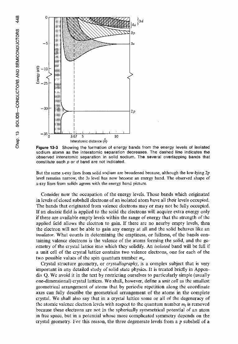
Cha

p. 1

3 S

OL

IDS

—C

ON

DU

CT

OR

S A

ND

SE

MIC

ON

DU

CT

OR

S

3

Figure 13-3 Showing the formation of energy bands from the energy levels of isolated sodium atoms as the interatomic separation decreases. The dashed line indicates the observed interatomic separation in solid sodium. The several overlapping bands that constitute each p or d band are not indicated.

But the same x-ray lines from solid sodium are broadened because, although the low-lying 2p level remains narrow, the 3s level has now become an energy band. The observed shape of x-ray lines from solids agrees with the energy band picture.

Consider now the occupation of the energy levels. Those bands which originated in levels of closed subshell electrons of an isolated atom have all their levels occupied. The bands that originated from valence electrons may or may not be fully occupied. If an electric field is applied to the solid the electrons will acquire extra energy only if there are available empty levels within the range of energy that the strength of the applied field allows the electron to gain. If there are no nearby empty levels, then the electron will not be able to gain any energy at all and the solid behaves like an insulator. What counts in determining the emptiness, or fullness, of the bands con-taining valence electrons is the valence of the atoms forming the solid, and the ge-ometry of the crystal lattice into which they solidify. An isolated band will be full if a unit cell of the crystal lattice contains two valence electrons, one for each of the two possible values of the spin quantum number m s .

Crystal structure geometry, or crystallography, is a complex subject that is very important in any detailed study of solid state physics. It is treated briefly in Appen-dix Q. We avoid it in the text by restricting ourselves to particularly simple (usually one-dimensional) crystal lattices. We shall, however, define a unit cell as the smallest geometrical arrangement of atoms that by periodic repetition along the coordinate axes can fully describe the geometrical arrangement of the atoms in the complete crystal. We shall also say that in a crystal lattice some or all of the degeneracy of the atomic valence electron levels with respect to the quantum number m 1 is removed because these electrons are not in the spherically symmetrical potential of an atom in free space, but in a potential whose more complicated symmetry depends on the crystal geometry. For this reason, the three degenerate levels from a p subshell of a

single atom lead to three bands of N levels, each capable of holding two electrons of opposite spin, in a crystal containing N of these atoms. These bands may be com-pletely nonoverlapping, partly overlapping, or completely overlapping in energy, de-pending on the crystal geometry. The term isolated band, used in expressing the condition for a full band, refers to a case in which these bands do not overlap each other or bands from other subshells. Then if there are two valence electrons per unit cell, each of the N levels in the lowest lying band will have its full complement of two electrons. Note that the quantity determining occupation is the number of va-lence electrons per unit cell, and not per atom. In a uniform one-dimensional lattice of identical atoms, such as we considered in the argument from which we concluded that a band contains N levels, if the crystal contains N atoms, a unit cell contains one atom and there is no distinction to be made. When that argument is extended to three-dimensional crystals containing atoms of different species, it is found that the conclusion remains the same, providing. N is the number of unit cells in the crystal. Thus if there are two valence electrons per unit cell there will be two in each of the levels of the band, and the band will be fully occupied.

The problem in predicting whether or not a solid is an insulator is that the question of band overlap is all important, and this depends on details of the geometry of the crystal structure (and of the geometry of the atomic eigenfunctions). If what, as far as valence is concerned, might have been a completely filled band actually overlaps what might have been a completely empty band, then there will be two partly filled bands. The result is that a solid that might have been an insulator will actually be a conductor. But it is at least possible to say that a solid can certainly not be an insu-lator unless one of its unit cells contains an even number of valence electrons, because an odd valence electron can never be in a filled band. Most covalent solids like dia-mond, or ionic solids like sodium chloride, are insulators; they all have an even num-ber of valence electrons per unit cell. In diamond each carbon atom has four valence electrons, and there are two atoms in each unit cell. The eight valence electrons per unit cell fully occupy the 4N levels of four bands, one originating from the 2s sub-shell of the atom and three originating from the three 2p subshells. These bands over-lap each other, but they are well separated from empty higher energy bands. Sodium chloride contains one sodium ion and one chlorine ion per unit cell, and the valence band consists of a set of completely filled bands that overlap each other but do not overlap unfilled bands. Alkali-earth atoms like beryllium are divalent and form crys-tals with an even number of valence electrons per unit cell, but these solids are metals, not insulators, because overlapping bands make slightly higher unfilled levels ener-getically available to the electrons.

In solids formed from the monovalent alkali atoms like sodium, the band con-taining the valence electrons cannot be filled, and so the solid behaves like a conduc-tor. Only half of the levels of the isolated 3s allowed band of sodium are filled because a sodium atom has a single electron in the 3s level, whereas the exclusion principle allows such a level to accommodate two electrons. Hence electrons in the solid can easily acquire a small amount of additional energy. Thus any applied electric field will be effective in giving electrons energy, and the solid will be a conductor. As we mentioned in the previous paragraph, conductors are also found in cases where bands containing valence electrons overlap.

It is worthwhile putting the distinction between conductors and insulators into momentum, instead of energy, language. Without an applied electric field there are as many electrons in the solid with momentum vectors in one direction as there are with momentum vectors in the opposite direction, since there is no net current. When an electric field is applied, this equilib-rium can be upset causing a current to flow, if some of the electrons can go into quantum states with changed momentum vectors. This is quite possible for electrons in a partially filled band, but it cannot be done by electrons in a completely filled band.

SU

RO

S 3

O A

1:1O

3H1

aNV

B

0 ^

SO

LID

S- C

ON

DU

CT

OR

S A

ND

SE

MIC

ON

DU

CT

OR

S

p

1 ne2/1 mv

(13-1b)

At temperatures above absolute zero it is, of course, possible for some electrons to gain enough thermal energy to jump over the energy gap of a forbidden band of energy into a higher allowed band, thereby creating vacancies in the lower allowed band and making a new allowed band available. We speak of the nearly filled band as a valence band and the nearly empty band as a conduction band. The probability of this happening increases with temperature, and it depends strongly on the width of the forbidden band. Substances in which the width of the energy gap is small are called semiconductors. An example is silicon, a covalent solid with a diamondlike structure, but with a forbidden band only about 1 eV wide. It becomes reasonably conducting at room temperature though at low temperatures it is an insulator. On the other hand the gap between the filled and empty allowed bands in diamond is about 7 eV. Thus diamond is an insulator even at relatively high temperatures.

13-4 ELECTRICAL CONDUCTION IN METALS

Some useful results concerning conduction electrons in metals can be obtained from classical ideas. In the absence of an applied electric field, the directions in which these electrons move are random. The reason is that the electrons frequently collide with imperfections in the crystal lattice of the metal, which arise from thermal motion of the ions about their equilibrium positions in the lattice or from the presence of im-purity ions in the lattice. In colliding with these imperfections, the electrons suffer changes in speed and direction, and this makes their motion random. As in the case of molecular collisions in a classical gas, we can describe the frequency of electron-lattice imperfection collisions by a mean free path 2, where 2 is the average distance that an electron travels between collisions. When an electric field is applied to a metal, the electrons modify their random motion in such a way that, on the average, they drift slowly in the direction opposite to that of the field, because their charge is negative, with a drift speed v d . This drift speed is very much less than the effective instantaneous speed v of the random motion. In copper vd is of the order of 10 -2 cm/sec, whereas v is of the order of 10 8 cm/sec.

The drift speed can be calculated in terms of the applied electric field E and of v and 2. When a field is applied to an electron in the metal, it will experience a force

of magnitude eE which will give it an acceleration of magnitude a given by a = eE/m. Consider now an electron that has just collided with a lattice imperfection. In general, the collision will momentarily destroy the tendency to drift and the electron will move in a truly random direction after the collision. Just before its next collision the electron will have changed its velocity, on the average, by a2/v where 2/v is the mean time between collisions. We call this the drift speed v d , so that

a2 eE2 V = — _ v mv

If n is the number of conduction electrons per unit volume and j is the current den-sity, we have v d = j/ne = eE2/mv. Combining this with the definition of resistivity, p = E/j, gives us

my

P ne2 (13-1a)

Equation (13-1a) can be taken as a statement that metals obey Ohm's law, for the

quantities v and 2 that determine the resistivity p do not depend on the applied elec-tric field, which is the criterion that the law is obeyed.

Often we deal with the conductivity

This can be put in a more useful form by defining a measurable quantity, the mobility µ, of magnitude given by the ratio of the drift speed to the applied electric field, i.e.

vd e^ D

E my (13-1c)

Then since o- = ne 2A/mv, we have µ = a/ne or a = neµ (13-2)

If we have conduction by positive carriers as well as negative carriers, the conductivity is given by

a = ngnµn + pq u in which µn and µp are the mobilities of negative and positive carriers, qn and qP are their charges, and n and p are the numbers of these carriers per unit volume. If con-duction is by negative charge carriers the charge q of the carrier is negative, whereas q is positive if conduction is by positive carriers. Since the sign of y also depends on the sign of q, each term in the expression for a is always positive.

The sign of the charge carrier of electric current in a metal can be determined from

measurements of the Hall effect. That is, when a current carrying conducting sheet is placed perpendicular to a magnetic field, an electric field is set up perpendicular both to the magnetic field and the flow of current. By measuring the potential dif-ference between the two surfaces of the conductor, it is possible to deduce the sign and value of the quantity 1/nq, called the Hall coefficient. Here n is the number of charge carriers per unit volume and q is the charge of the carrier. The electric field arises from an accumulation of charge carriers on one surface due to the v d x B force exerted on them when they move with velocity v d through the magnetic field B.

In some metals, as zinc and beryllium for example, the Hall effect indicates net positive charge carriers. This is interpreted as being due to transitions of electrons from the filled valence band to the conduction band leaving holes (unoccupied energy levels) in the valence band. Such holes correspond to the absence of an electron and behave much like positive charges. As these vacancies are filled by electrons, moving under the influence of an electric field, the holes move in a direction opposite to the electrons just as though positive charge carriers were moving in the field direction. In the case of metals with an s2 atomic configuration, such as zinc and beryllium, the mobility of the s-band holes is much greater than that of the p-band electrons. Since the sign of the Hall coefficient depends on which type of carrier has the higher mobility, the Hall coefficient is positive for these metals.

In Table 13-1 we list the Hall coefficients of some metals and also the number of free electrons per atom. The latter is computed from the value of the Hall coefficient, 1/nq, and the density of the metal. For the alkalis and other monovalent metals, Hall measurements agree with one conduction electron per atom. Of course, the free-electron model on which the simple Hall effect analysis is based is not expected to be valid for all metals.

Table 13-1 Observed Hall Coeff icient and Calculated Number of Free Electrons per Atom.

Metal 1/nq

(10 -10 m 3 /coul) No./atom Metal 1/nq

(10 -10 m 3/coul) No./atom

Na —2.5 0.99 Be +2.4 —2.2 K —4.2 1.1 Zn +0.33 —2.9 Cu — 0.55 1.3 Cd +0.60 —2.5 Ag —0.84 1.3 As +40 —0.04 Al —0.30 3.5 Sb —20 0.09 Li —1.70 1.0 Bi —5000 0.0005

SiV

13

W N

I NO

I1O

f1aN

OO

1V

OI U

10

313

i

^ { H kT —..—.—.—.\

SO

LIDS

-C

ON

DU

CT

OR

S A

ND

SE

MIC

ON

DU

CT

OR

S

i^

eF 0

n (e) N(e) Unfilled levels

Filled levels

1

I .`

n(g) N(s) Unfilled levels

Filled levels

N ^ N (e) N (e)

Figure 13-4 Left: The distribution with energy of conduction electrons in an unfilled band of width emax in a solid at T = 0, according to the free electron model. Right: The same at a higher temperature.

13-5 THE QUANTUM FREE-ELECTRON MODEL

Let us now recall our application in Section 11-11 of quantum theory and the Fermi

distribution to conduction electrons in a metal. There we saw that the potential in

which the electron moves can be approximated by a rectangular potential well. This

constant potential smooths out the actual periodic variation due to the ion cores and

includes the average effect of all the remaining electrons. It is equivalent to treating

the electrons as an ideal gas of fermions inside the solid. This approximation, which

greatly simplifies quantum mechanical calculations, turns out to be surprisingly good

in determining many of the observed properties of solids, as we saw in Section 11-12

when we used it in describing phenomena such as contact potential and electronic

specific heats. In connection with our present discussion we can use the result, (11-56),

for the distribution with energy of free conduction electrons in a metal, namely

8zc V (

m 3) 1 /2 1/2 de

n(g)N(g) dg = e(' eF)' + 1

(13-3)

where n(g)N(g) dg is the number of electrons with energy from e to e + de in a metal at temperature T. The justification is that the distribution of energy states in a band is nearly the same as that for free electrons if the Fermi energy is not close

to the top of the band. This condition applies to the alkali metals, for example, and

accounts for the success that the free-electron model has in describing their electrical

properties. On the left side of Figure 13-4 we show the prediction of (13-3) for the absolute

zero temperature energy distribution of electrons in a partly filled band, with energy

being measured from the lowest energy in the band. The maximum energy allowed in

the band is fi and ^ F < max) as shown in that figure. At a temperature greater than zero, the uppermost electrons are excited to occupy nearby available higher states, and the distribution function takes the form shown on the right side of Figure 13-4. The number of quantum states in an energy interval e to e + de is the factor

^ w S

ec. 1

3 -5 T

HE

QU

AN

TU

M F

RE

E-E

LEC

TRO

N M

OD

EL

N(e)de of (13-3), namely 87tV(2m 3) 112

N(g) de = h3 e 112 dg (13-4)

In Figure 13-4 N(s) is shown by a dashed curve and, for unit volume, is the density of states. The dash-dot curve is n(s), the Fermi distribution for the number of elec-trons per state. The solid curve gives the product n(e)N(e), the energy distribution of electrons, or number of electrons per unit energy interval.

Example 13-1. The Fermi energy, gF, for lithium is 4.72 eV at T = 0. Calculate the number of conduction electrons per unit volume in lithium. ► From (11-57) we have

= for kT « ‘F (13-5)

so that the number of free electrons per unit volume is _ N _ 8m\3/2

3 /2 n V —\h2l

^F 3TE

in which m is the mass of the electron. Then, with eF = 4.72 eV, we have

8 x 9.11 x 10- 31 kg 3/2 (4.72 x 1.60 x 10 -19 joule) 3/ 2 n=

V (6.63 x 10 -34 joule-sec) 2 3

= 4.64 x 1028/m 3 = 4.64 x 1022/cm 3

as the number of conduction electrons per unit volume in lithium. This corresponds exactly to one free electron per lithium atom, since the number of lithium

atoms per unit volume, in solid lithium of density 0.534 g/cm 3 , is

0.534 g x 1 mole x 6.02 x 1023 atom = 4.64 x 10 22 atom/cm 3 • cm3 6.94 g mole

Example 13-2. Make an estimate of the relative number of conduction electrons in a metal which are thermally excited to higher energy states. • Figure 13-4 shows that most of the excited electrons are in a range AS above the Fermi energy en F , where M ^ 2kT. Assuming that kT « gF, the number A.N' of excited electrons can be calculated from

N(eF)n(eFmM ti N(gF)( 1/2)2kT ^ N(SF)kT

Equation (13-5) shows that, for kT « gF

= 3

C 3/2 g3/2 F

and (13-4) shows that

aV 1/2

N(eF)= 2

eF

Hence O.N' N(gF)kT ✓V N'

1 ^ C h^)3 /2 gFl2kT

7TV 8m 3/z Ch2

3 kT ^

603/2/2 3

_ J 2 .6aF

kT

gF

h2 (^

3N 2/3

8m ^ V

SO

LIDS

-C

ON

DU

CT

OR

S A

ND

SE

MIC

ON

DU

CT

OR

S

The fraction of conduction electrons that is thermally excited is small. At room temperature kT ^ 0.025 eV and typically eF ^ 4 eV, so that Ai/.4(^ 1/160. The absolute number of excited conduction electrons is large, however, because .iV itself is so large.

Now we shall use the free-electron model to evaluate the width in energy of a band for the simple case of a one-dimensional metal. The eigenfunctions for an electron in the deep square well, representing the smoothed out attraction of the ion cores distributed uniformly along the x axis plus the average repulsion of the remaining electrons, are essentially sinusoidal standing waves like

i/i cc cos 2Ex

= cos kx and tk cc sin 2Ex

= sin kx (13-6)

where 2 is the wavelength and k = 2E/2 is the wave number. The eigenfunctions have nodes at each end of the well since their values go to zero outside the well. These boundary conditions lead immediately to the requirement that n2/2 = L, where L is the length of the well. Each value of the integer n = 1, 2, 3, ... , corresponds to a different eigenfunction, or energy level if we allow two electrons of opposite spin per level. Since for free electrons the energy is e = p 2/2m = h2/2m22 = h2n2/8mL 2, the minimum value of n corresponds to the level of essentially zero energy at the bottom of the band, and the maximum value of n corresponds to the level of maximum en-ergy at the top, the width of the band being approximately equal to that maximum energy. If there are N ions each separated by distance a in the one-dimensional metal of length L, then N = L/a. As we have explained before, the number of levels in the band is just equal to N, so the maximum value of n will also be equal to N. Thus the maximum energy, or energy width of the band in our one-dimensional metal, is

h2N2 h2L 2 max = 8mL2 8mL2a2

or h2n2

max = 2ma2 (13-7)

This result, which depends on a but is independent of N, confirms the statement made earlier that the width of a band depends on the separation of the ions and not on the number of ions in the lattice.

The free-electron model gives very good results for many metals. It is especially good for the alkali metals where the overlap of bands (as in Figure 13-3 for sodium) is so complete that the density of states N(e) behaves like the curves of Figure 13-4. The ei/2 dependence of N(e) on e is not correct, however, in the case of an isolated band. Although the actual shape of the curve of density of states depends on the posi-tion of the band and the structure of the lattice, its shape is roughly symmetric, as shown in the upper part of Figure 13-5, in that it decreases to zero at the top of the band.

To understand how this comes about, we consider a one-dimensional crystal which is so long that we first ignore the boundary conditions at its end. Then the most con-venient eigenfunctions for a free electron are sinusoidal traveling waves like

cc eikx and ti cc e- ikx (13-8) where the forms with positive, or negative, exponents describe an electron moving in the positive, or negative, direction of the x axis. It is even more convenient to take only the form 1i cc e`k x, and let k be either positive or negative. Now we write the energy e of a free electron in terms of its wave number k = p/h, where p is its momen-tum. That is

_ p2 h2 k2 e _ 2m 2m (13-9)

Unfilled levels

N(e)

0

N(6°)

0

Figure 13-5 Top: A qualitative representation of the density of states as a function of energy in an unfilled isolated band. Bottom: The same for the case of two barely overlapping bands.

This relation is plotted in Figure 13-6, over a range of k including both positive and negative values. A positive value of k corresponds to an electron moving in the posi-tive x direction, and a negative k corresponds to motion in the opposite direction. The energy depends on k 2 , so the curve is symmetrical about k = 0. It can be seen immediately by comparing (13-7) and (13-9) that

k < + n/a (13-10) That is, the values of k corresponding to the maximum value of g found in the band are — n/a and +n/a, and the value of k corresponding to the mimimum value g = 0 is the value k = 0 in the middle of this range. Since k cc 11,10c n and n = 1, 2, 3, .. o , the values of k allowed by the boundary conditions are evenly spread throughout this range. Each of them is associated with a different quantum state for the electron.

k — 7r/a 0 + it/a

Figure 13-6 The energy of a free electron plotted as a function of its wave number k. The points indicate schematically the uniformly spaced allowed values of k. For the first band of the crystal they fall within the range —2t/a < k < +n/a, where a is the ion separation of the one-dimensional lattice in which the electron moves freely.

134O

W N

Oa

10

31

3-3

31: 1

3 W

fllN

dfl

O 3H

1

CO ^

SO

LID

S-C

ON

DU

CT

OR

S A

ND

SE

MIC

ON

DU

CT

OR

S

Figure 13-7 Illustrating the uniformly distrib-uted allowed values of the x and y component wave numbers for a free electron in the first band of a two-dimensional square lattice with

ion separation a.

Next consider a two-dimensional metal with ions spaced by the same distance a in both the x and y directions. In a band the allowed values of both the x and y

component wave numbers, k x and ky , are uniformly distributed over ranges extending from — rz/a to + rz/a, as shown in Figure 13-7. Each pair of kx and ky values defines a point that specifies a quantum state for a free electron of the metal; these points are uniformly distributed within the square. A circle surrounding the origin of radius k, where k 2 = kx + kÿ, passes through all states having the same energy since in two dimensions (13-9) reads

^_ h2(kz + ky) h2k2

The number of states dN, for values of k ranging from k to k + dk, is equal to the number of points contained within the area limited by k and k + dk. As the points are uniformly distributed, this number will be proportional to the area. The figure shows that as long as k < rc/a, dN increases with increasing k; specifically dN = 2rtk dk. When k begins to exceed rz/a, further increase in k causes dN to decrease. Thus dN/dk = N(k), the number of states per unit range of wave number, increases from zero for small k, reaches a maximum, and then decreases back to zero when k reaches the largest allowed value for the band of our two-dimensional metal.

The same general behavior is found when these results are converted from N(k) to N(s), the number of states per unit energy. In a real three-dimensional metal it is also true. That is, the density of states N(6) increases from zero for small e (the bottom of the band), reaches a maximum, and then decreases back to zero at the largest allowed value (max found in the band (the top of the band). The detailed

behavior of N(s) depends on the geometrical details of the arrangements of ions in

the crystalline metal, as does the exact value of emax• But the general behavior is

always about as we have indicated, and the approximate value of émax is given by (13-7) if a is interpreted as the characteristic ion spacing in the crystal.

13-6 THE MOTION OF ELECTRONS IN A PERIODIC LATTICE

The free-electron model that we have used ignores the effects of electrons interacting

with the crystal lattice. Let us begin to consider this by making some general remarks

about the effect of the periodic variation in the potential. For one thing, the lattice

periodicity has the effect that the wave functions for an infinitely long lattice are no

longer sinusoidal traveling waves of constant amplitude, but they exhibit the lattice

periodicity in their amplitudes. In addition, electrons may be scattered by the lattice.

Just as an electromagnetic wave suffers a Bragg "reflection" when the Bragg condi-tion is satisfied, so also when the de Broglie wavelength of the electron corresponds

to a periodicity in the spacing of the ions the electron interacts particularly strongly

2m 2m

b= a — l

Kronig-Penney model potential <— l

^E a

with the lattice. We shall see that these modifications result, among other things, in changing the resistance of the crystal to the conduction of electricity.

Our approach in finding the allowed energies of electrons in solids has been to consider the effect of forming a solid as the individual constituent atoms are brought together. If, instead, we had begun by modelling the periodic potential seen by an electron in the crystal lattice by a succession of rectangular wells and barriers, and had then solved the Schroedinger equation for such a potential, we would have found sinusoidal wave solutions in certain energy ranges (the allowed bands) and real de-caying exponential wave solutions in the other energy ranges (the forbidden bands). This approach permits detailed quantitative calculations, but we present it here only qualitatively.

Although the electrons tend to smooth out the variations in the potential due to the ions, the potential is not constant but varies in a periodic way. The actual shape of the potential determines the exact solution to the Schroedinger equation for an electron in a crystal lattice, but the most important feature of the potential is its peri-odicity. The effect of periodicity is to change the free particle traveling wave eigen-function in such a way that instead of constant amplitude it has a varying amplitude which changes with the period of the lattice. If the space periodicity of the lattice is a, then, according to Bloch, the eigenfunctions for a one-dimensional system do not have the free particle traveling wave form i/i(x) = Ae ikx of (13-8), but instead they have the form

41/(x) = uk(x)e ikx (13-11a)

where the periodicity of the lattice requires that uk(x) = uk(x + a) = uk(x + na) (13-11b)

n being an integer. Hence, the effect of the periodicity is to modulate periodically the free-electron solution amplitude. The wave function is

'P(x,t) = uk(x)e i(kx (13-12)

where the second (exponential) factor describes a wave of wavelength )L = 2rc/k that travels toward + x if k > 0 and toward — x if k < 0, and the first factor uk(x) describes the modulation. The function u k(x) resembles the eigenfunction for an isolated atom. Its exact form depends on the particular potential assumed and the value of k. A very good approximation to V(x) for a crystal is an array of rectangular potential wells and barriers having the lattice periodicity, as in Figure 13-8. Each well represents an approximation of the potential produced by one ion. This is the Kronig-Penney model which is, of course, easier to treat mathematically than the real case, but which retains all of its important features. Let us now examine the model in more detail.

For wells that are deep and widely spaced, the electron of not too high energy is practically bound within one of the wells, so that the lower energy eigenvalues are those of a single well. For wells that are closer together the eigenfunctions can pene-trate the potential barriers more easily. This results in the spreading of a previously

- n•n• Actual potential

THE

MO

TI O

N O

F E

LEC

TR

ON

S IN

A P

ER

IOD

IC LA

TT

ICE

Figure 13-8 Illustrating how the potential for an electron moving in a periodic lattice can be

approximated by the Kronig-Penney model of an array of rectangular potential wells and

barriers.

co ^

Vo

0.51

0.23

0

Single potential well Periodic array of wells

SO

LID

S-C

ON

DU

CT

OR

S A

ND

SE

MIC

ON

DU

CT

OR

S

0.058

Figure 13-9 Left: Allowed energies for an electron in a single potential well. Right: Allowed energies in an array of periodically spaced wells and barriers. The levels shown are for a

well strength given by 2mV 0/2 /h 2 = (11) 2 , and a barrier thickness b = //16. Note the appearance of forbidden bands even for energies g greater than Vo .

single energy level into a band of energy levels. As the separation of the wells is re-duced the band becomes wider. Indeed, in the limit of zero barrier thickness we

obtain an infinitely wide single well in which all energies are allowed, i.e., we obtain

the free-electron model. In Figure 13-9 we compare the allowed energies of a single

well with those of the Kronig-Penney model of an array of wells and barriers. Notice

that each allowed band corresponds to a discrete level of the single well, and that

forbidden bands appear even for energies 6 greater than the well depth v o . The band widths can be made to approach the level width as a increases (the width of the indi-vidual wells, 1, remaining fixed) and to approach a continuum as a decreases.

In solving the Schroedinger equation for the Kronig-Penney model, we must sat-isfy the conditions on the continuity of and dpi/dx, just as we had to do for the single rectangular well. This restricts the validity of the Bloch solution, (13-1 la) and (13-11b), to certain ranges of energy and gives the allowed bands. For energy values in the forbidden bands, the eigenfunctions are rapidly damped by a real decaying exponential factor. The expression e(k) for the allowed energies in terms of the wave number k of the electron is more complicated than that for the free electron, but the gaps or discontinuities in energy occur at values of k given simply by

k=±â,±2a,±3a ,... (13-13)

in which a is the space periodicity of the lattice. In Figure 13-10 we plot the func-tion e(k). At values of k equal to the values specified in (13-13) we get energy gaps, whereas for values of k not near those values the energies are much like that of a free electron shown by the dashed curve in the figure. The origin of the allowed and for-bidden bands is apparent from the figure. Each allowed band corresponds to solu-tions to the Schroedinger equation in which the wave number k has positive values in a range of width n/a, and also negative values in a range of the same width. Note

Vo

1.0

I^ %

^

a

Brillouin 6 I 5 zone number

37r 27r 71-

a a a a

3 I 2 I 1

a 2 a a

2

a

3 J 4 I 5 0

4

Energy bands

•

2.0

a

6

W

C!D

THE

MO

TION

OF

ELE

CT

RO

NS

IN A

PE

RIO

DIC

LA

TT

ICE

Figure 13-10 Allowed energies in a one-dimensional lattice of periodicity a, as a function of the wave number k. The dashed curve gives the free electron model result, for comparison. The allowed and forbidden energy bands that result are shown on the right.

that this agrees with a conclusion obtained from a very different point of view in the last section, and expressed in (13-10).

From the present point of view, the gaps between the top of an allowed band and the bottom of the next one up can be understood as a result of Bragg reflection of the traveling wave describing an electron propagating down the lattice. If a wave travel-ing to the right is incident on a set of barriers representing the regions between the ions of the lattice, spaced by the uniform distance a, it will be partly reflected by each of these barriers. Generally, the reflected waves traveling to the left will not be exactly in phase with each other, and so they will not combine constructively to produce a net reflected wave of large amplitude. But they will be in phase if the wavelength 2 of the incident and reflected waves is related to the spacing a by the one-dimensional version of (3-3), the Bragg condition

2a = 2, 22, 32, ... (13-14) Here 2a is the extra distance traveled in reflections from successive barriers, so if it equals an integral number of wavelengths 2 the reflected waves will all be precisely in phase and there will be a net reflected wave whose amplitude equals the amplitude of the incident wave. Since 2 = 2n/k, the Bragg condition is 2a = 2n/k, 2(2n/k), 3(27c/k), ... , or k = + rc/a, +27c/a, + 37c/a, ... , where we have inserted + signs to account for the fact that the incident wave could as well be moving to the left (to — x) as moving to the right (to +x). Comparing with (13-13), we see that the values of k

at which the gaps in the function f(k) occur are just those values of the wave number for which the wavelength 2 satisfies the Bragg condition for constructive reflection.

The gaps themselves arise because there are two distinctly different ways for the amplitude of the reflected wave to equal the amp litude of the incident wave, at each critical value of k where these amplitudes are equal. Consider, for instance, a unit amplitude incident wave moving to the right along the x axis with k = rc/a. The traveling wave eigenfunction describing this is eikx = eirzxia. The reflected wave, which also has unit amplitude for this value of k, is e - ikx = e 'xIa. The total eigenfunction

cn CD

is obtained by adding these two or, equally well, by subtracting them. The first possi-bility gives

o co .4r

SO

LID

S- C

ON

DU

CT

OR

S A

ND

SE

MIC

ON

DU

CT

OR

S

0'1°' + e - i(^c^a)x oc cos a.

xr = ei(

(13-15)

and the second gives

ÿr = e`ocia)x — e -i(n/a)x oc sin —7r

x (13-16) a

In both, the reflected wave has the same amplitude as the incident wave, and so it

combines with it to form a standing wave; but the two cases differ very significantly

in regard to the locations of the nodes of the standing wave, and therefore in the

locations of the maxima and minima of the probability density tJr*tfr. In the case where

t/r oc cos mx/a, the probability density will maximize at x = 0, as well as at x = + a, ±2a, +3a, ... , while for t(i cc sin 7rx/a the probability density will be zero at all

these points. If they are the locations of the barriers between ions, the electron de-scribed by IA will feel a larger repulsion, and therefore have a higher energy, in the

cosine case than in the sine case. If these points are the locations of the ions, the

situation will be reversed. But the basic conclusion—that there are two different

energies e corresponding to the same value of the wave number k when k is any one of the values given by (13-13)—is independent of how the origin of the x axis is

defined. Looking again at the function &(k) plotted in Figure 13-10, we see the two different

values of e at each of the critical values of k where Bragg reflection will occur. We also see how this circumstance causes the e(k) curve to have an S-shaped deviation

from the parabolic curve for a free electron in each region between the critical values

of k. The range of k values between — 7r/a and + n/a defines what is called the first

Brillouin zone; those k values between — 27c/a and — 7c/a and between + 7r/a and + 2n/a define the second Brillouin zone, etc., as is indicated below the k axis of the figure.

13-7 EFFECTIVE MASS

When discussing the behavior of an electron in a periodic lattice under the applica-tion of an external electric field, it is very convenient to introduce the concept of the

effective electron mass. This is done by using a relation developed in Section 3-4 to

describe the motion of the electron in terms of a group of traveling waves. According to (3-13b), the velocity g of such a group equals the derivative of the frequencies y of its component sinusoidal traveling waves with respect to their reciprocal wavelengths

K. That is dv = do)

= g dK dk

where v is converted to the angular frequency w, and K to the wave number k, by multiplying and dividing dv/dic by 2n. To remind the student of the meaning of this

relation, we shall apply it to the simple case of a free electron, whose energy is

p2 h2k2

e = 2m 2m =

no)

The last equality depends on the Einstein-de Broglie relation e = by = hcw. Evalua-ting dw/dk from this expression, we have

dc^ h2k hk p my g =—= ------=v dk 2m m m m

(13-17)

We obtain the correct result that the group velocity g equals the velocity y of the electron whose motion is represented by the group. Of course this result is of general validity.

Now we consider an electron in a one-dimensional lattice, whose wave number dependence of energy has the form 6' (k) that we have been discussing. To this system an external electric field E is applied. In time dt the electron of charge q moves distance dx, and the work done by the external field is the applied force qE multiplied by dx. Since this equals the magnitude of the change de in the energy of the electron, we have, using (13-17)

de = qE dx = qE d^

dt = qEv dt = qEg dt

But we also have, from e = ho)

de= haw =hdkdk=hgdk

Comparison then shows that qE dt = h dk

or

h dt = qE

If we take the time derivative of do) 1 de

g dk h dk

we obtain dg _ 1 d2e _ 1 d2e _ 1 deg dk dt h dt dk h dk dt h dk 2 dt

or, using (13-18) dg 1 d2e dt h2 dk2 qE

Employing (13-17) again, this can be written dv qE

dt m*

where 1 1 d2e

m* h 2 dk2

(13-18)

The quantity 1/m* is the reciprocal of the effective mass of the electron in the crystal lattice.

The electron we are studying moves under the in fluence of internal forces, exerted on it by the ions of the lattice, and an external force, exerted on it by the applied electric field E. If we wish, we can use (13-19a) to discuss its motion in terms of the external force alone since that equation is in the form of Newton's law of motion, acceleration equals external force divided by mass. Of course the effects of the internal forces are actually contained in the equation. They appear, however, only in the reciprocal effective mass 1/m*, which can have values quite different from the recip-rocal of the true electron mass, 1/m.

The properties of the lattice determine 1/m* because, as we saw in the preceding section, they determine the form of the function e(k) and so also the derivative

SS

W]

3/1

I10

33

33

1/m*<0

SO

LID

S-C

ON

DU

CT

ORS

AN

D S

EM

ICO

ND

UC

TO

RS

e%vo

1/m*^—'1/m

—7r/a 0 + rr/a k

Figure 13 -11 Illustrating the reciprocal effective mass at various locations in the first and second Brillouin zones of a one-dimensional lattice. The points on the k axis indicate the uniformly distributed allowed values of k.

d2 6(k)/dk 2 appearing in (13-19b). Figure 13-11 shows the first, and part of the sec-ond, Brillouin zones of a one-dimensional crystal. The solid curve is e(k) and the

co parabolic dashed curve is the free electron relation 6' = h20/2m. Near the center of c the first zone, where k h2k2 2m 1 m* = 026 dk 2 h2 02212,0h2 = 1 m. So in bc this region the lattice has very little effect on the electron, because its reciprocal

effective mass is almost the same as its reciprocal true mass, and it responds to the applied electric field as if it were an essentially free electron. The curvature of the function g(k) changes significantly from the curvature of the parabola in proceeding in either direction from the center of the zone, which makes dramatic changes in the reciprocal of the effective mass of the electron and so in its response to the applied field. Since d2 6/dk 2 goes through zero, and then becomes negative and of large mag-nitude as k approaches either boundary of the first zone, 1/m* does the same. Thus in the upper part of the energy range of the band corresponding to the first zone the electron in the lattice responds to the applied electric field very differently from the way it would if it were a free electron. Where 1/m* is zero a given applied force qE causes no acceleration of the electron, and where 1/m* is negative the force causes an acceleration in the opposite direction to that which would be experienced by a free electron. (This has nothing to do with the sign of the electron charge which, to avoid confusion, we have written as q instead of — e.) At the bottom of the energy band for the second Brillouin zone, 1/m* is positive but appreciably larger than 1/m for a free electron, so the applied force produces a relatively large acceleration of the electron in the lattice.

The response of an electron in a crystal to an applied electric field can be under-stood in terms of the way the electron wave is reflected by the potential barriers located between each pair of ions. At the bottom of the first energy band where the magnitude of the wave number has the value IkI 0 there is practically no reflection since the Bragg condition IkI = rc/a is far from being satisfied. When the field is applied the force it produces will increase the electron's momentum, and the work it does will increase the electron's energy, just as in the case of a free electron. Higher up in the band, where IkI is closer to the critical Bragg value n/a, reflection starts to become appreciable. In this region the work done on the electron will still increase its energy, but this increases the amount of reflection, and reflection corresponds to reversing the sign of its momentum. At the point where 1/m* = 0, the gain in positive momentum due to the applied field acting directly on the electron is exactly com-pensated for by the gain in negative momentum due to the enhanced reflection of

SS

dW

3n

I1033d3

the electron by the lattice ions. Thus here the net change in electron velocity is zero, and from the point of view of its response to the applied field the electron effec-tively has infinite mass, or zero reciprocal mass. (Momentum is, of course, given to the lattice by the overall effect of applying the field, but not to the electron.) At the top of the band the reciprocal effective mass is large and negative because the en-hanced reflection resulting from the closer approach to the Bragg condition of perfect reflection is much more significant in changing the electron momentum than the direct action of the applied field. The situation is reversed at the bottom of the next higher band, and so the reciprocal effective mass is large and positive there.

Effective mass is also used in a somewhat different way to compare, for various bands, the curvature of the function e(k) in the concave upward approximately para-bolic regions found except near the tops of bands. If the zero of k is taken to be at the boundary of the second zone, and the zero of e is taken at the bottom of the corresponding band, then f(k) for the part of the second zone shown in Figure 13-11 can be written as

h2k 2 e(k) . 2m* (13-20)

If the curvature of g(k) is high, so that e increases rapidly with increasing k, then 1/m* in this expression is large. Since the allowed values of k are uniformly distributed along the k axis of Figure 13-11, the density of the corresponding energy levels along the e axis will be low if Z increases rapidly with increasing k. So the reciprocal mass can also be used to compare level densities of bands, in the regions where they obey (13-20). If the level density is relatively low, 1/m* is relatively large; if the level density is relatively high, 1/m* is relatively small.

The concept of effective mass is useful in a variety of ways. For instance, the classi-cal theory of the behavior of charge carriers under the in fluence of an applied electric field is summarized by (13-1b), which predicts that the electrical conductivity a of the material containing the carriers is proportional to the reciprocal of their masses. We can easily modify this to take into account the quantum behavior of charge carrying electrons in a crystal lattice by replacing the reciprocal true mass with the reciprocal effective mass, obtaining

a cc 1*

(13-21) m

Consider iron. The valence electrons in this metal partly fill its 3d bands, which are overlapping and narrow since 3d is an inner subshell in the transition element iron so the splitting of the atomic 3d level into the 3d bands is not very pronounced. Because the bands are narrow, the level density is high. Therefore the reciprocal effective mass is small for the electrons involved in electrical conduction in iron, the value of 1/m* being about 0.1/m. As a consequence, the metal is not a particularly good conductor. Copper, on the other hand, is a good electrical conductor. The reason is that for copper the 3d bands are filled, and the conduction electrons are 4s electrons which are in a very broad band (it overlaps the 3d bands) that has a low-level density and a high reciprocal effective mass (1/m* is roughly equal to 1/m). The 4s band is broad because this is an outer subshell of the atom and so the splitting in the crystal of the 4s atomic level is large. The result is that the conductivity of copper is an order of magnitude higher than the conductivity of iron.

It should be pointed out that using the reciprocal effective mass in (13-21) amounts to ac-counting for the influence of a perfect crystal lattice on the accelerated motion of an electron in an applied electric field. As was discussed in Section 13-4, accelerated motion takes place between collisions of the electron with the imperfections that are actually found in the lattice of a real material, due to thermal motion of the ions or to impurity ions. These collisions

SO

LIDS

-C

ON

DU

CT

OR

S A

ND

SE

MI C

ON

DU

CT

OR

S

tend to randomize the electron motion, and they cause the over-all electron motion to be a drift with velocity proportional to the strength of the applied field, in contrast to an ever increasing velocity with acceleration proportional to the strength of the field. If there were no lattice imperfections, after a fixed field was applied the electron current would increase in time until it reached such large values that it was limited by practical considerations having nothing to do with either the strength of the field or the properties of the material. In such circumstances the material could be said to have zero resistance (or at least it could be said not to obey Ohm's law). So the presence of nonzero resistance, or noninfinite conductivity, is due to the presence of lattice imperfections. This can be seen in the fact that the resistance of a metal increases with increasing temperature and with increasing impurity concentration. Neverthe-less, the value of 1/m*, which has to do with the properties of a perfect lattice, influences the value of the resistivity or conductivity because it influences the average velocity gain between randomizing collisions with imperfections, and this determines the drift velocity.

In situations where all the levels of an isolated band are filled except for those near the very top, it is convenient to think in terms of holes representing the absence of electrons in an otherwise completely filled band. Since the absence of a negatively charged electron is equivalent to the presence of a positive charge, holes behave as if they are positively charged. Futhermore, since the effective mass is negative for the levels near the top of a band, holes, describing the absence of negative effective mass, behave as if they have positive effective mass. We shall have more to say about them, after we have explained briefly one of the most useful procedures for determining experimentally the behavior of electrons in solids.

13-8 ELECTRON-POSITRON ANNIHILATION IN SOLIDS

The interaction of positrons with electrons provides a technique used, with great success, to measure the momenta of electrons in solids. The positron was introduced in Section 2-7. These particles have the same mass and the same magnitude of charge as electrons but positrons are positively charged. In that section the process of pair production, in which a photon disappears and is replaced by an electron-positron pair, was described. Of interest for the measurement of electron momentum, however, is the reverse process, pair annihilation, in which an electron and a positron disappear and are replaced by photons.

In the usual experiment, high energy positrons, from radioactive sources, are directed toward a sample. Once inside, they quickly lose energy, via scattering and electronic excitation, to the particles of the material. They generally reach their lowest quantum state in about 10 -12 sec or less, after penetrating into the sample a distance on the order of 10 -4 m Annihilation takes place well inside the material and, at annihilation, the momentum of the positron is nearly zero. The most likely result of the annihilation event is the appearance of two photons, trav-eling in nearly opposite directions, each with energy nearly equal to the electron rest mass energy (511 keV).

Slight deviations of the photon momenta from the same straight line can be used to obtain information about the electron momentum distribution in the sample. The geometry is illus-trated in Figure 13-12, which shows an electron incident on a positron at rest and the emission directions of the resulting photons. For the analysis which follows, the direction of one of the photons is taken as the z axis and the x axis is taken to be in the plane of the photons. Experimentally the z axis is determined by the position of one of the photon detectors.

Total relativistic energy is conserved in the annihilation process, so 2m0c 2 = cp1 + cp2

where m o is the rest mass of the electron (or positron), p i is the magnitude of the momentum of one photon, and p2 is the magnitude of the momentum of the other photon. The kinetic and potential energies of the electron are small compared to its rest mass energy m oc2 and are neglected. Momentum is also conserved during annihilation, so

p cos cp= p i — p 2 cos 0 and

p sin cp= p2 sin B

x

P2

z Pi

Figure 13-12 Top: An electron incident on a positron at rest. Bottom: The momenta of the resulting photons.

where p is the magnitude of the electron momentum and the angles 9 and 0 are defined in the figure. The momentum equations are solved for p i and p2 and the results are substituted into the energy equation to yield

2moc = p (cos 9 sin 0 + sin 9 cos 0 + sin 9)/sin 0 For all electrons in solids p « m o c and 0 is extremely small, usually around 10 -3 radians. So sin 0 can be approximated by 0, in radians, and cos 0 can be approximated by 1. The first term in the parentheses is small compared to the other two and is neglected. When the last equation is solved for 0, using these approximations, the result is

0_ p sin 9

mo c

The angle 0 is measured in what is called an angular correlation experiment and the result is used to calculate the x component of the electron momentum, p sin q). The difference in the photon energies is given by AE = cp l — cp 2 = cp cos 9 and, if this quantity is measured, the result can be used to calculate the z component of the electron momentum, p cos 9. This is rarely done, however, since much finer resolution can be obtained for angular measurements than for energy measurements.

Example 13 -3. Position annihilation takes place in a free electron gas with the same concen-tration (number per unit volume) as the conduction electrons in lithium. Find the largest corre-lation angle 0, defined in Figure 13-12. ■ Consideration of the figure will make it apparent that 0 has the largest value when the annihilated electron has the largest possible momentum magnitude and one of the photons is emitted in a direction perpendicular to the electron momentum. Electrons with an energy equal to the Fermi energy 4 have the largest momentum magnitude. This is the Fermi momentum pF, where 4 = pF/2mo . Since the Fermi energy depends only on concentration, according

to (11-57), and since the Fermi energy for lithium is 4.72 eV, we have

pF = ^12moeF = (2 x 9.11 x 10 -31 kg x 4.72 eV x 1.60 x 10 -19 joule/eV) 1 / 2 or pF = 1.17 x 10 -24 kg-m/sec. The maximum angle is

_ 1.17 x 10 -24 kg-m/sec O _F — pF/moc 9.11 x 10 -31 kg x 3.00 x 10 8 m/sec

or O F = 4.29 x 10 -3 rad. •

Sa

I10

S N

I NO

LLV

1IH

INN

V N

O1

ilIS

Od

-NO

bla

313

CD CD

SO

LIDS

-C

ON

DU

CT

OR

S A

ND

SE

MIC

ON

DU

CTO

RS

o (10 -3 rad) 5 10 15

Figure 13-13 Number of two photon annihilation events as a function of correlation angle B for a typical metal. The small angle portion is due to annihilation by conduction electrons while the large angle portion is due to annihilation by core electrons.

For a metal, a typical graph of the number of two-photon events as a function of the cor-relation angle 8 is like that shown in Figure 13-13. The curve is proportional to the number of electrons in the sample with x component of momentum equal to p sin (p. The central part of the curve is due to annihilation of conduction electrons. For an electron gas, this has a parabolic shape and the shape is not much different for conduction electrons in metals and semiconductors. By taking measurements with the sample in various orientations relative to the z direction, it is possible to construct the momentum distribution of the electrons. If the central portion of the curve is extrapolated, the correlation angle for annihilation of an electron whose energy equals the Fermi energy can be found and, from this, its Fermi momentum can be calculated.

The wings of the curve, which generally have a Gaussian shape, are due to annihilation of electrons in atomic cores, which have higher momenta. The situation here is more complicated than for conduction electrons because the positron is repelled by the positively charged atomic core and may acquire a high momentum itself before annihilation. The curve reflects the mo-menta of both electrons and positrons.

In most molecular solids, including a great many organic materials, in amorphous materials, and perhaps in ionic solids, some positrons become bound to electrons and form hydrogen-like "atoms," called positronium. There are two states of interest: a singlet state with the spins of the particles essentially antiparallel and a triplet state with the spins essentially parallel. Annihilation from the singlet state produces two photons, and the lifetime of positronium, in this state, is short—on the order of 10 -1° sec. In contrast, two-photon annihilation from the triplet state violates conservation of angular momentum and, instead, three photons are usually produced. The lifetime of triplet positronium is about 10 - 7 sec in free space. Detection of both prompt and delayed photons, in different events, is a signal that positronium has been formed. An external magnetic field is sometimes used to change the spin orientations, and the change in the relative yield of prompt and delayed photons provides further verification of positronium formation. Positronium does not form in materials, such as metals, in which electron concen-trations are high and the positron suffers many collisions during its lifetime.

In solids, the triplet state lifetime shortens to around 10 -9 sec, not as short as the singlet state lifetime but longer than the free-space triplet state lifetime. This decrease occurs because the positron, while still bound to an electron, is annihilated by another electron, outside the positronium "atom." The lifetime is dependent on the electron concentration at the site of the positronium and so a lifetime measurement provides information about the concentration. Positronium is generally trapped in large open spaces between molecules of the material, and the positron samples the electron concentration of such a region. Both the number of such regions and the electron concentration in them undergo changes when the material changes phase, and positronium lifetime measurements are used to study phase transitions in amor-phous substances, such as glasses, and in organic crystals.

Sa

Ol0

na

NO

aIW

3S

13-9 SEMICONDUCTORS

Semiconductors are of much interest because their behavior is the basis for many practical electronic devices, such as transistors. Also, they are excellent illustrations of the ideas discussed in previous sections. Semiconductors are covalent solids that may be regarded as "insulators" because the valence band is completely full and the conduction band is completely empty at the absolute zero of temperature, but they have an energy gap between the valence and conduction bands of no more than about 2 eV. For silicon the energy gap is 1.14 eV and for germanium the gap is 0.67 eV. Although the value of the Fermi distribution function governing the relative popula-tion of an energy state in the conduction band to an energy state in the valence band is small, since kT 0.025 eV at room temperature, the number of available states in the conduction band is high. Hence the thermal excitation from the valence band into the conduction band occurs for a significant number of electrons, this number being the product of the number of electrons per quantum state and the number of quantum states per energy interval. Furthermore, the conductivity of a semicon-ductor increases rapidly with rising temperature, the number of excited electrons in silicon, for example, increasing by a factor of about one billion with a doubling of temperature from 300°K to 600°K. Since the valence band is filled at low temperature, with the four valence electrons of silicon or germanium forming covalent bonds, each electronic excitation into the conduction band leaves a hole in the valence band. These holes, acting as positive charge carriers, also contribute to the conductivity. In Figure 13-14 we illustrate the semiconductor band scheme.

The conductivity of the semiconductors arising from thermal excitation is called intrinsic conductivity. There are other ways to enhance the conductivity, such as by photoexcitation. The energy gap in semiconductors is equivalent to the energy of photons in the red or infrared portion of the electromagnetic spectrum so that semi-conductors are photoconductive. This contribution to the conductivity increases with the intensity of the light and will drop to zero when the light source is turned off and the normal thermal equilibrium distribution of electrons is restored. Still another way to increase the conductivity is by adding impurities to the semiconductor. That is, we replace some atoms of the semiconductor with atoms of another element, having about the same size but a different valence. The resulting conductivity, whose origin we explain presently, is called extrinsic conductivity, and the procedure is called doping.

If a small quantity of arsenic is added to molten germanium, the arsenic impurities will crystallize with the germanium into its diamondlike structure. `Arsenic has five electrons per atom in the valence band and germanium has four electrons per atom in the valence band. Hence, four of the arsenic electrons are used for covalent binding and the fifth electron is nearly free. It cannot go into the filled valence band and is very weakly bound in an "orbit" of very large radius around the singly charged arsenic ion. The arsenic ion Coulomb attraction is largely shielded by polarization of the intervening germanium atoms; that is, the field of the ion is weakened by the dielectric nature of the germanium crystal. Because this fifth electron has such a small binding energy to the arsenic, it can be ionized, and go into the conduction band at a much

Conduction band

Energy gap

Valence band

Figure 13-14 The band scheme of a semicon-ductor in which the energy gap between the ini-tially full valence band and the initially empty conduction band is small. Thermal excitation raises some electrons over the gap into the con-duction band, leaving holes in the valence band.

SO

LIDS

-C

ON

DU

CT

OR

S A

ND

SE

MIC

ON

DU

CT

OR

S

lower temperature than would be needed for electrons in the valence band. Hence,

this excess electron will occupy some one of a set of discrete energy levels just below

the conduction band at a low temperature, but it can very easily be thermally excited

into that band. At ordinary temperatures all of these excess electrons go into the con-duction band. The electrical conductivity can be controlled by the amount of arsenic

used as an impurity. A significant effect is obtained with as little as one impurity atom

per million semiconductor atoms. An impurity that contributes electrons is called a

donor impurity and the resultant semiconductor is called an n- type (negative) semi-conductor because it has an excess of free electrons.

Example 13 -4. Make a rough estimate of the binding energy of the donor electron of ar-senic in a germanium crystal, taking the dielectric constant of the crystal to have the value K = 16, and the effective mass of the electron to have the value m* = 0.2 m.

► The donor electron moves in the field of the arsenic ion, As +, and it behaves like the electron

in the ground state of a hydrogenlike atom. The chief difference is that this electron moves in

a polarizable lattice rather than in vacuum. Because the potential energy of the ion-electron

system is now —e 2/K47rE O r, the corresponding hydrogenlike energy levels are given by re-placing 4nE0 by K47re0 in the hydrogen energy-level formula, (4-18), and also by replacing the electron mass m found there by the effective mass m* to take into account the fact that the electron is actually in a crystal lattice. Since the electron is near a lower band edge where d2 e/dk 2 is large, m* is small; various evidence indicates the value is m* ^ 0.2m. So we have

ci E 1 C 1 2 m

* e4 L U

where K = 16, m* = 0.2m, and n = 1. Since for K = 1 and m* = m the energy E has the value —13.6 eV, it is easy to show that

E —0.01 eV

Hence, according to our estimate, the energy required to ionize the arsenic donor electron in a germanium crystal to the bottom of the conduction band is about 0.01 eV. The value obtained directly from measurements of the photon energy required to ionize, or indirectly from measurements of the temperature dependence of the conductivity, is 0.0127 eV. See Table 13-2 for measured values in other cases.

Note that the radius of the Bohr-like orbit of the donor electron is Km/m* - 80 times that of the ground state hydrogen atom, as can be seen by inspecting (4-16). So the electron moves in an orbit that contains a large number of germanium atoms. This justifies the use, in our previous estimate, of the dielectric constant, which is a macroscopic rather than a microscopic quantity that characterizes the germanium crystal when it is regarded as a continuum. t

If a small quantity of gallium is added to germanium, the situation will be different

from that just discussed. Gallium has three electrons per atom in the valence band, so

that it has a deficiency of one electron per atom in forming the covalent bonds. The

Table 13-2 Donor and Acceptor Ionization Energies

In Germanium In Silicon

Impurity ^ — donor (eV)

Arsenic 0.0127 0.049 Antimony 0.0096 0.039

Impurity eacceptor — é, (eV)

Gallium 0.0108 0.065 Indium 0.0112 0.16

K 2 47rE^ 2h 2 n2

Conduction band

T( Donor

Li6b= 0.013 eV impurity 6, = 0.67 eV

levels g

Valence band

(As in Ge) (Ga in Ge)

Figure 13-15 Left: Schematic energy-level diagram of a germanium crystal containing donor impurity atoms. Right: Containing acceptor impurity atoms.

result is a hole, which can drift through the crystal, behaving like a positive charge and mass as successive electrons fill one hole and create another. From an energy point of view, this impurity introduces vacant discrete levels slightly above the top of the valence band. Valence electrons are then easily excited into these impurity levels, which can accept them, leaving holes in the valence band. The energy separa-tion between the acceptor levels and the top of the valence band is small for the same reasons that give a small separation between the donor levels and the bottom of the conduction band: a high dielectric constant and a small effective mass. An impurity that is deficient in electrons is called an acceptor impurity and the resultant semi-conductor is called a p- type (positive) semiconductor.

Whether the conductivity of a semiconductor is p-type or n-type can be determined by the Hall effect. In Figure 13-15 we show schematically the energy-level diagram corresponding to each type. The localized energy levels of impurity atoms are not broadened into bands because these atoms are many lattice spacings apart and in-teract with each other very weakly. In Table 13-2 we list the energy of the levels in-troduced into germanium and silicon crystals by small amounts of common impurities. For donor impurities the energy from donor levels to the energy 6', at the bottom of the conduction band is given, whereas for acceptor impurities the energy from the top of the valence band 4, to the acceptor levels is given. Note that these energies are comparable to kT = 0.025 eV at room temperature. Therefore, we can expect to have plenty of thermal ionization at room temperature.

In an intrinsic semiconductor the number of vacant states in the valence band is equal to the number of occupied states in the conduction band, so that the Fermi energy is located somewhere in the gap between the bands. If the densities of states in the two bands are symmetrical then the Fermi energy will be in the middle of the gap. The Fermi energy, as the student will recall, is defined as the energy for which the average number of electrons that would occupy a quantum state there is 0.5, where we treat electron spin in such a way that the maximum occupancy is 1.0.

Example 13 -5 Consider a forbidden band of width g9 that separates a valence band and a symmetrical empty conduction band in an intrinsic semiconductor. Show that the Fermi energy lies at the center of the forbidden band, i.e., that = 6 /2 if g = 0 is taken to be the upper edge of the valence band. •The proof can be followed by inspecting Figure 13-16. At the top of the figure we plot N(e) the number of quantum states per unit energy interval for the upper part of the valence band and the lower part of the conduction band. The figure tentatively places the Fermi energy eF in the center of the gap of width g9 between the two bands. The density of states N(8) is drawn so that its descending behavior moving towards the top of the valence band is symmetrical to its ascending behavior moving away from the bottom of the conduction band. This is in qualitative agreement with the general behavior of N(e) throughout an entire isolated band (see, for example, Figure 13-5).

saol

onaN

OO

I W3s

o S

OLI

DS

-C

ON

DU

CT

OR

S A

ND

SE

MIC

ON

DU

CT

OR

S

ti n (e)

6°r

N(e)

c Figure 13-16 The number of electrons as a function of energy in the valence and conduc-

as tion bands of an insulator or semiconductor with a forbidden band width ey , as a product 0 of the density of states N (e) and the Fermi distribution n(s).

In the middle of Figure 13-16, we show the Fermi distribution n(s), which is the probable number of electrons per state. For clarity, it is constructed for an operating temperature where kT (°g . It is also constructed for eF in the center of the forbidden band.

The solid curve in the bottom of Figure 13-16 shows the product n(e)N(e), which gives the number of electrons per unit energy in various states at the temperature just mentioned. The dashed curve shows the same thing for a temperature of absolute zero. At T = 0, the valence states are completely filled and the conduction states are completely empty, so the dashed curve in the valence region is just N(s), while it is the e axis in the conduction region. The area A between the dashed and solid curves is proportional to the number of valence states that electrons leave when the temperature is raised; that is, it is a measure of the number of holes created. The area B between the solid and dashed curves is proportional to the number of electrons that are promoted to states in the conduction band at the operating temperature.

In an intrinsic semiconductor it is necessary that area A equal area B, since the density of holes in the valence band equals the density of electrons in the conduction band. It is apparent that this condition is satisfied by Figure 13-16, because we have constructed it with eF in the center of the forbidden band. A moment's consideration will show the student that it would not be satisfied for a different choice of e F, due to the symmetry of n(s) about gF, and to the (approximate) symmetry of N(s) about the center of the gap between the two allowed bands.

Example 13-6. Make an estimate of the relative number of electrons in the conduction band of an insulator or semiconductor at temperature T. ► Figure 13-16 also shows an exaggerated picture of the energy distribution of electrons as a product of the density of states mg)' and the Fermi distribution n(s) appropriate in the valence, forbidden, and the conduction bands of an insulator. If, in the Fermi distribution n(s), we have e - eF » kT, then

1 1 e(6. - e.HAT +1 — e(g - gF)IkT

so that in such an energy range the Fermi distribution varies with energy like the Boltzmann distribution. We know from Example 13-5 that e - gF = e9/2 at the bottom of the con- duction band in an insulator, if we measure e from the top of the valence band. So the

n(e) _

condition t - » kT is met since é9 » kT for an insulator. Thus we can take

( ) 1 - s /2kT n = e s12kT = 2

as the number of electrons per state in the conduction band of an insulator. The Fermi distribution falls in value by an order of magnitude in an energy range of about

M = 2kT so that we get a good estimate. of AS', the number of conduction electrons, by evaluating those in the range 2kT above the bottom of the conduction band. Since AS . = n(g)N(g) M we must now evaluate N(s), the density of states. Because N(6) starts at zero at the bottom of the conduction band, a good average value over the range M = 2kT is obtained by evaluating N(s) at e = kT. Hence

As- = n(6)N(e) M =g9/2kT(kT)2kT

Let us use here the results .iV' = (2/3)gFN(gF) of Example 13-2 for a metal as an estimate of the total number of electrons, .iY. We also note from (13-4) that N(kT)/N(4) = (kT/ ) 1/2, so we have

0s- e-g9/2kT N(kT)2kT _ 3e_es/2kT (kT)(kT)1/z

^ N (213)4N(4) \ eF

or (kT)3/2

e —G°9/2kT

This is the relative number of conduction electrons for an insulator. This fraction is much smaller than the corresponding result kT/gr. of Example 13-2 for a

metal, partly because the density of states N(s) is smaller near the bottom of the conduction band in an insulator than at the Fermi energy in a metal, but principally because of the occu-pation factor e - e912kT . Let us take g9 = 6 eV as the gap in a typical insulator so that at room temperature this factor is e g912kT =

e-1 50 = 10 -65 . Not only is the fraction AX/.4( insig-

nificant, but the absolute number of conduction electrons is also negligible for an insulator. If,

however, g9 = 1 eV, as for a semiconductor, then although e gy/2kT = e-25 = 10 -1 1 gives a very small fraction, the number of conduction electrons is no longer insignificant. •

In an impurity semiconductor containing donors, the Fermi energy lies above the middle of the forbidden band because there are more electrons in the conduction band than there are holes in the valence band. In an impurity semiconductor con-taining acceptors the Fermi energy is below the middle of the forbidden band because there are fewer electrons in the conduction band than there are holes in the valence band. It is instructive to consider the combined effect of temperature and impurities on the Fermi energy. Let us begin at a temperature of absolute zero in an n-type semiconductor. The donor levels are all occupied but there are no electrons in the conduction band. The Fermi energy then must lie between the donor levels and the bottom of the conduction band, because the number of electrons per state n(s) is one up to and including the donor levels and zero in the conduction band. Now, as the temperature is increased electrons are raised from donor levels to the conduction band. At that temperature at which half the donor states are empty, the Fermi energy corresponds to the donor-level energy. With a further increase in temperature, elec-trons in the valence band are excited and the Fermi energy drops more. When the number of electrons from the valence band is a very large fraction of those in the conduction band, the semiconductor acts as though it were intrinsic and the Fermi energy drops to nearly the center of the gap. If we had started with a p-type semi-conductor we would find in a similar manner that, as the temperature is raised, the Fermi energy moves from between the top of the valence band and the acceptor levels, at absolute zero, to the center of the gap at high temperatures. At low tem-peratures, where kT « Ç9 , conduction is due mostly to the impurities because there is little excitation of valence electrons. At high temperatures the impurity levels have been used up, that is, they have either donated or accepted electrons, so that the

S1:1

O10

n4N

O0

IW3S

Valence band

p region I Junction End of I region

rod

^ Valence band::

n region End of

rod

SO

LID

S- C

ON

DU

CT

OR

S A

ND

SE

MIC

ON

DU

CTO

RS Conduction

band Donor levels

4g/2 High

concentration T

Valence Acceptor

o / band

idiV/A levels

n type p type

Figure 13-17 Left: The Fermi energy as a function of temperature for n-type semicon-ductors of two different impurity concentrations. Right: For p-type semiconductors of twb different impurity concentrations.

semiconductor acts as though it were intrinsic. In Figure 13-17 we plot the Fermi

energy as a function of temperature for impurity semiconductors.

13-10 SEMICONDUCTOR DEVICES

We shall illustrate the use of impurity semiconductors in electronics by discussing

briefly the operation of three semiconductor devices, the rectifier, the transistor, and

the tunnel diode. A rectifier is formed by having acceptor impurities (p-type) in one region of a crystal

and donor impurities (n-type) in another region. The boundary between these regions

is called a p-n junction. Figure 13-18 shows the energy band structure of an unbiased

p-n junction at room temperature. The boundaries of the bands must be warped in

going from the p-region through the junction to the n-region because the Fermi en-ergy is close to the top of the valence band in the p-region and close to the bottom

Electron energy

Unbiased electron current

Reverse biased current

Forward biased current

Thermal Recombination

—^ Thermal Recombination

Thermal Recombination

61, =

Valence

/kW/JIIWffl band

T

concentration

High concentration

Low 4/2

Low oncentration

Figure 13-18 Electron energy-level diagram for an unbiased p-n junction.

of the conduction band in the n-region, yet the Fermi energy must have the same value everywhere. The reason is that if the Fermi energy were not the same in both regions the energy of the system would not be minimized. It could be reduced by electrons in one region flowing to unoccupied states of lower energy in the other re-gion, and so the system would not be in equilibrium. Actually, considerable electron flow did take place in establishing equilibrium when the p-region was initially put into contact with the n-region. This led to an accumulation of electrons on the p-side of the junction, and a deficiency of electrons, or accumulation of holes, on the n-side of the junction. Thus the junction region has similarities to a plane parallel condenser with a negative charge on the p-side and a positive charge on the n-side, as shown in the figure. If an electron is moved through the electric field produced within this dipole layer, its energy will increase in going from the n-side to the p-side. This is reflected in the way the energy levels at the top of the valence band, and at the bottom of the conduction band, are displaced upward in going through the junction region.

Even after equilibrium is established there is still a flow of electrons back and forth through the junction. For one thing, from time to time thermal excitation causes an electron to jump up to the conduction band of the p-region (leaving yet another hole in its valence band). The electron can move freely to the junction region, and then be accelerated by the potential hill it sees there into the n-region, constituting part of what is called the thermal current. Also, an electron in the conduction band of the n-region with energy slightly below the bottom of the conduction band in the p-region can gain a little extra energy in a fluctuation and be able to move into the p-region. There it may recombine with one of the many holes in the p-region. That electron is part of the so-called recombination current. There must be such a current because in equilibrium the thermal current must be balanced so that there is no net current across the junction.

Now consider an external voltage source applied across the ends of the device, with negative voltage applied to the p-region and positive voltage applied to the n-region. This will increase the energy of all the electrons in the p-region, and decrease the energy of all of those in the n-region, thereby increasing the height of the potential hill between the two regions. Since the junction region was already depleted of charge carriers, its resistance is relatively high and most of the voltage drop due to the ap-plied voltage appears across the junction. As the amount of thermal current depends on the temperature and the width of the gap between the valence and conduction bands, neither of which are changed by applying the voltage, the thermal current will not change. The recombination current will be decreased by a large factor, however, because the potential hill is higher so now only the very many fewer electrons farther out in the exponentially decreasing tail of the Fermi distribution in the n-region con-duction band have a chance to move into the p-region conduction band. The net effect will be a small flow of electrons in the direction from the p- to the n-regions, due to the unbalanced thermal current. This flow of electron current is, of course, in the direction that the applied voltage would be expected to produce. It is the small reverse bias current indicated by the arrows at the bottom of Figure 13-18.

The junction rectifier is given a forward bias by applying a positive voltage to the p-region and a negative voltage to the n-region. This decreases the height of the electron energy hill between the two regions. Again, there is no appreciable effect on the thermal current, but the recombination current is increased by a large factor. All of a sudden, the very many more electrons that are closer to eF in the Fermi dis-tribution of the n-region have enough energy to pass through the junction into the p-region conduction band, because the bottom of that conduction band has moved down in energy. These electrons do not instantaneously respond to the application of a forward bias, but instead they diffuse into the p-region in much the same way that the molecules of a gas would diffuse into a region of lower density that suddenly

ô

S3

01

A3

0 a

OlO

f10

NO

0IW

3S

SO

LID

S-

CO

ND

UC

TO

RS

AN

D S

EM

ICO

ND

UC

TO

RS

became accessible to them. The net electron current in a forward biased rectifier flows in the direction of the recombination electron current, as indicated at the bottom of Figure 13-18. The junction is a rectifier because the magnitude of the forward bias current is much larger than the magnitude of the reverse bias current, for a given magnitude of bias voltage. The reason is that the reverse bias current is limited by the small value of the thermal current, whereas the forward bias current becomes very large as the height of the electron hill is made small by increasing the forward bias. Resistance to current flow in reverse bias is typically greater than resistance in for-ward bias by four or five orders of magnitude. Note that our explanation has been phrased in terms of electron flow. It could as well have been in terms of hole flow; both processes occur, and they result in the same rectifying properties of the junction.

A semiconductor rectifier has many advantages over a diode vacuum tube rectifier, including longer life and much smaller size. Like the diode, the p-n junction is a non-Ohmic element, the current-voltage relation being nonlinear, as shown in Figure 13-19. Unlike a vacuum tube, however, there is no need for a power-consuming fila-ment in the semiconductor device so that its efficiency is greater.

A transistor can be regarded as a combination of two semiconductor rectifying junctions, such as a p-n-p or n-p-n combination. In Figure 13-20 we display a cir-cuit that exhibits transistor behavior. The n-p-n-regions are called emitter, base, and collector, respectively. The emitter-base connection is biased in the forward direction, so that the resistance to current flow is small in this part of the circuit. The base-collector connection is biased in the reverse direction, so that ordinarily there is higher resistance to current flow in that part of the circuit. However, when a voltage is applied in the emitter circuit so that a current is established there, the electrons arriving in the base region (which is very thin and of lower conductivity than the emitter) are attracted by the potential difference between the base and the collector. Hence, there will be a current in the collector circuit. (Because the emitter has a higher conductivity than the base, most of the current across the emitter-base junction is carried by electrons moving from the emitter to the base, instead of holes moving from the base to the emitter.)

The basic idea of transistor action is that a current in the emitter circuit controls a current in the collector circuit. More than 90% of the current through the emitter passes through the collector, so that the currents are of similar magnitudes. But the voltage across the base-collector connection can be very much greater than that across the emitter-base connection, because the former is reverse biased, so the power output in the collector circuit can be very much larger than the power input in the

Circuit symbol:

Silicon rectifier type 1N256

—500 —250

—0.002

Figure 13 -19 Left: A circuit in which the voltage across a p-n junction can be varied. The voltage is taken as positive when the p-side is at higher potential. Right: Current through the junction as a function of the applied voltage. Note that very different scales are used for the forward- and reverse-biased portions of the curve.

0 Base

Circuit symbol:

Emitter

p-.

I^ (mA)

IE = 5 mA

4 4 mA

A—Collector 3 mA

® 2— 2mA

1 mA

I I 1 I I I {0 mA 1

r — 1 0 1 2 3 VcB (volts)

Silicon n-p-n transistor — 2 — type 2N3646

Sec

. 13 -1

0 SE

MIC

ON

DU

CTO

R D

EV

ICE

S

Figure 13-20 Left: A circuit in which an n-p-n transistor acts as a power amplifier. Electrons

flow in the direction shown by the arrow, from emitter to collector. Right: Characteristic curves for a transistor acting as a power amplifier.

emitter circuit. Hence, the transistor acts as a power amplifier. Characteristic current

versus voltage curves are shown in Figure 13-20. Other circuit connections make

transistors useful as current amplification or voltage amplification devices, as well.

A tunnel diode is a semiconductor device that makes use of the phenomenon of

potential barrier penetration discussed in Section 6-5. It is like a p-n junction made

from semiconductors with very high impurity concentration. Figure 13-21a plots the

electron energy across an unbiased junction. The bands are similar to those shown in

Figure 13-18, except that (1) with a higher impurity concentration the junction is

narrower since a smaller length of semiconductor contains enough charge carriers to

produce the required dipole layer across the junction, and (2) the donor and acceptor

levels, in the n-type and p-type material, are no longer sharp but become broad bands

which overlap the valence and conduction bands, since the donors, and also the ac-ceptors, are so closely spaced that they interact. The Fermi energy thus moves up

into the conduction band on the n-side and down into the valence band on the p-side.

Because the junction is narrow ( 10' 8 m), electrons can pass through the forbid-den band at the junction by a process that is in every respect the same as barrier penetration. For instance, the eigenfunction describing an electron tunneling through the forbidden band has the same exponential form as the eigenfunction for an elec-tron tunneling through a barrier. At equilibrium, as shown in Figure 13-21a, the rate of electron tunneling through the barrier is the same in both directions.

If now a small external voltage is applied across the ends of the rod with forward bias, electron tunneling from the n-side to the p-side is increased because there are empty allowed energy states in the p-side valence band, whereas electron tunneling in the other direction is decreased. Hence, there is a net current flow through the junction as shown in Figure 13-21b. As the applied voltage continues to be increased, the net current begins to decrease because the number of empty states available for electron tunneling decreases. In Figure 13-21c the net current is reduced almost to zero because electrons in the n-type material find no allowed energy states into which to flow. With still higher applied voltage the electron current becomes that charac-teristic of a normal p-n junction. That is, electrons flow through the junction, without tunneling, into allowed energy states in the conduction band of the p-type material. This happens because the difference in the energies of the bands decreases, making it possible for electrons to diffuse through the junction into the conduction band of the p-region. This process is indicated in Figure 13-21d.

Figure 13-22 shows the current-voltage curve characteristic of a typical tunnel diode. The letters labeling points on the curve correspond to the four applied vol-tages of the previous figure. In the region between points b and c, the slope of the

p type n type S

OLI

DS

-CO

ND

UC

TO

RS

AN

D S

EM

ICO

ND

UC

TO

RS

(b)

(d) (c)

End of rod

1.2

Germanium tunnel diode type 1N2940A

1.0

0.8

E 0.6 ti

0.4

0.2

0.5

Figure 13-21 Electron energy-level diagrams for the n-type, junction, and p-type regions of a tunnel diode. In (a) the diode is unbiased. In (b) a small voltage is applied between the ends of the device, with the p-type end positive. In (c) and (d) the voltage is increased progressively. The arrows indicate the flow of electrons across the junction between the two regions.

V (volts)

Figure 13-22 The current flowing through a tunnel diode as a function of the applied potential difference. The points labeled by letters correspond to the four applied voltages of Figure 13-19. Note that the resistance of the diode is negative for applied voltages between b and c. The dashed line indicates the characteristic current were no tunneling to take place—namely that for an ordinary germanium junction rectifier.

^

^

SN

OIlS

3f1

0

curve, dI/dV, is negative and the tunnel diode has a negative resistance, the current decreasing with increasing applied voltage. This feature makes it particularly useful

in the switching circuits of computers.

The greatest advantage of the tunnel diode is its very fast response time when

operating in the region a to c. The current flow in other kinds of semiconductor

diodes and transistors always depends on the diffusion process. Since the rate of diffu-sion can change only as fast as the charge carrier distribution can be changed, these

devices have relatively slow response (slower than vacuum tubes) and it is difficult

to use them at high frequencies. But the rate of tunneling can change as fast as the

energy bands can be changed by the applied voltage, and this is a much less serious

limitation. Tunnel diodes have been used as oscillators at frequencies above 10 11 Hz, and in switching circuits that operate in times less than 10 -9 sec.

QUESTIONS

1. In the text the solid state is contrasted with the gaseous state in terms of atomic (or

molecular) interactions. How would you characterize the liquid state in this regard?

2. Explain the statement that the exclusion principle prevents solids from collapsing to zero

volume. 3. Is there an analogy between the splitting of an energy level as two atoms are brought

together to form a molecule and the splitting of the resonant frequencies as two resonant

electrical circuits are coupled? Why?

4. It is often said that a crystal is one giant molecule. Explain. Can we regard a diatomic

molecule as a small solid? 5. Why does metallic binding usually occur with atoms having a small number of valence

electrons? 6. Why is it, considering the very similar electronic structures, that lithium is a metal where-

as hydrogen is a molecular solid? 7. Explain why metallic binding leads to a close-packed arrangement of atoms; i.e., explain

why the lowest energy in metallic binding corresponds to the greatest number density of

atoms. 8. Why are metallic solids mostly opaque, covalent solids sometimes opaque, and ionic

solids hardly ever opaque to visible radiation? 9. Of the four types of binding in solids discussed in the text, which one (or ones) is most

likely to produce an insulator? A conductor? A semiconductor?

10. Justify the statement that (13-1a) meets the criterion that a material obeys Ohm's law.

11. What mechanisms account for the ordinary electrical resistivity of metals? Which are

temperature dependent? 12. How do electrons contribute to thermal conductivity? Are they better than lattice vibra-

tions as carriers of heat energy?

13. Explain why the electrical conductivity of materials varies over a factor of 10 24 whereas the thermal conductivity of materials only varies over a factor of about 10 8 .

14. Explain why we regard the sequential filling of holes by electrons as equivalent to a posi-tive current. Could this process be regarded instead as an electron current?

15. How is the result of Example 13-2, concerning the fraction of conduction electrons that

is thermally excited, related to the specific heats of metals at high temperatures?

16. Example 13-2 implies that only AiVI ✓V of the free electrons take part in the conduction

of electricity, whereas certain other experiments, such as the Hall effect, indicate that all

.iV electrons take part. Explain.

17. Explain why a negative effective mass does not lead to a violation of Newton's law of

motion. 18. What techniques, other than electron-positron annihilation, might be useful in measuring

the momenta of electrons in solids?

AAAAAA (d)

(c)

(b)

Figure 13-23 Charge densities for valence elec-1 1 1 1 trons in four solids considered in Problem 1.

SO

LIDS

-C

ON

DU

CT

OR

S A

ND

SE

MIC

ON

DU

CT

OR

S

19. How is the optical transparency of a semiconductor related to the energy gap of the forbidden band?

20. What elements other than arsenic and antimony can be used as an impurity with ger-manium to form an n-type semiconductor? What elements other than gallium and indium can be used to form a p-type semiconductor?

21. Could the conductivity of a semiconductor be affected by electron bombardment? By bombardment by other particles?

22. What effect does an applied electric field have on an insulator?

23. Experimentally the addition of impurities to metals increases their resistivity, but the ad-dition of impurities to semiconductors decreases their resistivity. Explain. Many insulators, however, are not very pure. Why do impurities not affect the resistivity of insulators?

24. Name the properties of solids that are little affected by the presence of small concentra-tions of chemical impurities. Name the properties of solids that are greatly affected by the presence of small concentrations of chemical impurities.

25. Give an argument, similar to that given in the text for an n-type semiconductor, ex-plaining the variation of gF with Tin a p-type semiconductor.

26. Explain why the curves of Fermi energy as a function of temperature differ for different impurity concentrations, as shown in Figure 13-17.

27. Explain why the junction transition region is narrower in a semiconductor diode when the doping is heavy than it is when the doping is light.

Q 28. Rephrase the discussion of the operation of a p-n rectifying junction in terms of hole flow.

U PROBLEMS

1. In Figure 13-23 we illustrate schematically four charge density distributions for valence electrons as functions of the location of atoms, ions, or molecules (shown as dots at the bottom). For each distribution (a), (b), (c), (d), state to which type of binding in solids it most closely corresponds.

2. Each element of the row of the periodic table from lithium through neon has a solid form (some at very low temperatures). Solids can also be formed by certain compounds of two elements of this row. For all of these solids, describe the binding and state whether the solid is a metal, a semiconductor, or an insulator.

3. Describe the binding of solids formed by single elements of the column of the periodic table from carbon through lead, and state whether the solid is a metal, a semiconductor, or an insulator.

4. Determine the type of binding in each of the solids described here. (a) Reflects light in the

visible; electrical resistivity increases with temperature; melting point below 1000°C. (b) Reflects light in the visible; electrical resistivity decreases with increasing temperature; melting point above 1000°C. (c) Transmits light in the visible; conducts electricity only at high temperatures. (d) Transmits light in the visible; does not conduct electricity at any temperature. (e) Transmits light in the visible; very low melting point.

5. The field E produced at a point r by an electric dipole p is given by

1 ° ( p r•p / E

47rE r3 - 3 r5 r

where the dipole is located at the origin of coordinates. (a) A molecule with an electric dipole moment p will induce an electric dipole moment p' in a nearby molecule, where p' = aE, a being the polarizability of the nearby molecule. Show that the mutual potential energy of the interacting dipoles is

a 2 V=- p'• E= (1+3cos 2 0)p

(47CE °) 2 r6

where B is the angle between r and p. (b) Show the force is attractive and varies as r-7 .

6. Find the order of magnitude of the electric field needed in ionic solids to free electrons from the filled shells of ions. (Hint: Consider the binding energy of an electron and the approximate dimensions of an ion.)

7. Find the region of the electromagnetic spectrum at which crystals of Si, Ge, CdS, KC1, and Cu become opaque. The band gap energies fq are Si = 1.14 eV; Ge = 0.67 eV; CdS = 2.42 eV; KC1 = 7.6 eV; Cu = 0 eV.

8. (a) Using classical physics show that the resistivity of a metal near room temperature is proportional to the 3/2 power of the absolute temperature, in disagreement with the linear temperature dependence experimentally observed. (Hint: Show that v cc T1I2 and

cc T -1 .) (b) How does the application of the ideas of quantum mechanics and quantum statistics yield the proper temperature dependence of the resistivity?

9. Compare the values of (a) the drift velocity, (b) the thermal velocity, and (c) the velocity corresponding to the Fermi energy, or Fermi velocity, for electrons in copper at room temperature. (Hint: Use Table 11-2. A current of 5 amp can easily be carried in a copper wire 0.1 cm in diameter.)

10. Show that, according to the free-electron model, the resistance R of a length L of wire is given by

R = mL/nAe 2 T

where A is the cross-sectional area of the wire and T is the mean time between collisions. 11. An aluminum wire has a resistance of 0.01 ohm, a diameter of 0.83 mm; the mean colli-

sion time is 2.0 x 10- 12 sec. (a) If the effective electron mass is 0.97m, find the length of the wire. (b) Find the mean free path for an electron having the Fermi energy. Use data from Table 13-1.

12. Calculate the number of electrons per atom of aluminum that conduct electricity from the value, -0.3 x 10 -i° m3/coul, of the Hall coefficient. The density of aluminum is 2.7 x 103 kg/m 3. What does the result suggest about the band structure of aluminum?

13. (a) Show that the Hall coefficient for a semiconductor in which there is conduction by both holes and electrons is given by (pµp - nµ„)/e(p ji + nµ„)2 . (b) If in a certain semiconductor there is no Hall effect, what fraction of the current is carried by holes?

14. Copper is a monovalent metal with a density of 8 g/cm 3 and an atomic weight of 64. (a) Calculate the Fermi energy in electron volts at 0°K. (b) Estimate the width of the conduction band.

15. (a) Calculate the Fermi energy of an alloy of 10% zinc (which is divalent) in copper as-suming that the alloy has the same atomic spacing and structure as Cu. (b) How does the width of the conduction band of the alloy compare to that of copper? The assumption used in (a) is not strictly accurate.

16. Make an estimate of the width of a conduction band in a metal whose internuclear spacing has the typical value 3.5 x 10 -1° m.

SW3180ad

o co S

OLI

DS

-C

ON

DU

CT

OR

S A

ND

SE

MIC

ON

DU

CT

OR

S

17. The Fermi temperature is defined by TF = gF/k. (a) Using Table 11-2, calculate the Fermi temperature for sodium. (b) What does this tell us about the applicability of classical considerations to metals near room temperature? (c) What does this tell us about the density of conduction electrons in a metal at room temperature?

18. The Fermi energy of lithium is 4.72 eV. (a) Calculate the Fermi velocity. (b) Calculate the de Broglie wavelength of an electron moving at the Fermi velocity and compare it to the interatomic spacing.

19. The Fermi energy for lithium is 4.72 eV at T = 0°K. Find the density of states at 3.0 eV. 20. Calculate an approximate ratio of the electronic specific heat to the lattice specific heat of

lithium at room temperature. (Hint: Use the results of Example 13-2, and justify this use.)

21. (a) Show that the effect of a lattice periodicity a on periodic potentials having Bloch function solutions is to modulate the free-electron solution so that >ji(x + a) = 1/i(x)eika.

(b) Show that e ika = —1 at the Brillouin zone boundaries. Comment on the meaning of this result.

22. For a three-dimensional free electron gas confined to a cube, the allowed values of the momentum are distributed uniformly in momentum space. Assume that for each v alue of the momentum with magnitude less than the Fermi momentum p F (the momentum cor-responding to the Fermi energy) there are two electrons which have that momentum and that there are no electrons with momentum greater than pF. Show that the number of electrons that have a given x component px of momentum is proportional to 1 — (px/pF)2 .

This result explains the parabolic shape of the angular correlation curves for positron annihilation in metals.

Û 23. (a) For sodium use the concentration of conduction electrons to estimate the Fermi energy, the Fermi momentum, and the maximum correlation angle OF for photons from positron annihilation events involving conduction electrons. Sodium has a cubic unit cell with edge a = 4.22 A and there are two atoms per cube. (b) Repeat the calculations for potassium. Potassium has the same crystalline structure as sodium but the cube edge is 5.22 A. (c) In positron annihilation experiments, which of these two metals produces the greater fraction of photon pairs with correlation angle greater than 9F?

24. At what temperature will the number of conduction electrons increase by a factor of 20 over the number at room temperature for germanium? The gap energy is 0.67 eV.

25. (a) Show that the number of electrons per unit volume in the conduction band of an intrinsic semiconductor is given by ,ir° e -(‘` -") IkT where X° = 2(22rmkT) 3 / 2/h 3 , and where 6, is the conduction band-edge energy. (b) Show that the number of holes per unit volume in the valence band of an intrinsic semiconductor is given .N„e -VF-gOlkT,

where ✓V„ = 2(27rmkT) 3 /2/h 3 , and where ell is the valence band-edge energy. 26. Use the expression for the number of electrons in the conduction band, and the number of

holes in the valence band, given in Problem 25, and charge neutrality to find the position of the Fermi energy in an intrinsic semiconductor.

27. (a) Show that the product of the number of holes in the valence band and the number of electrons in the conduction band depends only on temperature and the gap energy. (b) Show that the conductivity a of an intrinsic semiconductor can be used to measure the gap energy by calculating ln a.

28. Write exact expressions for .iY and Xâ, the concentration of ionized and neutral donors respectively, in a semiconductor doped to a concentration of .Nd.

29. (a) The position of the Fermi energy in a doped semiconductor can be found from the condition of charge neutrality: X, + .iV = Afp + ✓V â , where A 7 is the number of electrons in the conduction band, is the number of ionized acceptors, Xi, is the number of holes in the valence band and 4â is the number of ionized donors. Assuming .N = 0 and ✓V„ » .Np show that charge neutrality leads to an equation quadratic in e gF/kT which has the solution

eeF/kT = — 1+ 1 + 4 -*d eV`—ed)IkT

.11(c

2e - gdlkT

where ec is the conduction band-edge energy, and ed is the donor-level energy. (b) This equation is soluble in two limits. One is

4 ^d e(g'- ea)IkT « 1

This means ./rd small or T large. Use a binomial expansion of the square root to show that ✓V„ = Afd and gF = ^^ + kT ln Gird/Arc). This is the exhaustion region. All the donors are ionized but no electrons are excited from the valence band. (c) In the other limit

4 d̂ e_ 1 » 1 ✓v^

Also .Nd is large and T is small. Show that

,/Îrn = ^JVic e-(g,-ga)I2kT

and

` +ed

+ kT ln ✓rd 2 2 .Arc

This is the extrinsic region. Here the donors are being ionized.

30. Draw an energy-level diagram like that of Figure 13-18 for an n-p-n junction transistor and describe the power amplifier action of the transistor in terms of the figure.

31. The current which flows in a p-n junction is proportional to the number of electrons in the conduction band. (a) For an unbiased p-n junction, show that the current from the p-region to the n-region is proportional to e - (eg - 5F)/kT and this current is equal to the current from the n-region to the p-region so that no net current flows. (b) When a bias

potential V is applied show that the net charge flow per unit area of junction is pro-portional to

e — (eg — SF•)IkT( eeV/kT _ 1)

where eV is positive for forward bias and negative for reverse bias. 32. A p-n junction is a double layer of opposite charges separated by a small distance and has

the properties of a capacitance. The resistivity of a semiconductor can be controlled by doping. Thus the elements in the transistor circuit of Figure 13-24a can be manufactured

SW

318

0a

d

00

G (a)

o

P •N Nara Er

(b)

Figure 13-24 An integrated circuit considered in Problem 32.

SO

LIDS

-CO

ND

UC

TO

RS

AN

D S

EM

ICO

ND

UC

TO

RS

on a p-n-p semiconductor with appropriate layers etched away as shown in Figure 13-24b. This is an integrated circuit. Label the appropriate parts of Figure 13-24b with the corresponding numbers and letters of Figure 13-24a.

33. A tunnel diode junction is approximated by a rectangular barrier 100 A thick and 3.3 eV high. If 1.00 x 10 25 electrons strike the barrier each second with kinetic energy 3.1 eV, and the effective electron mass is 0.30m, what current passes the junction?

14

SOLIDS SUPERCONDUCTORS

AND MAGNETIC PROPERTIES

14-1 SUPERCONDUCTIVITY

484

review of independent electron motion theories of conductivity; tempera-ture dependence of conductivity; resistanceless current in superconductors; critical temperature; Meissner effects and their relation to resistanceless current; critical field; isotope effect evidence for importance of lattice vi-brations; attractive electron-electron interactions by means of phonon ex-change; conditions for formation of Cooper pairs; ordered pair motion under applied electric field; pair binding energy; origin of energy gap; gap width and relation to critical temperature; estimate of size and density of pairs; applications of superconductivity; Type II superconductors; flux quantization

14-2 MAGNETIC PROPERTIES OF SOLIDS

492

relations between magnetic induction, magnetization, magnetic field strength, and magnetic susceptibility; diamagnetism and Lenz's law; com-parison of diamagnetic, paramagnetic, and ferromagnetic susceptibilities

14-3 PARAMAGNETISM 493

role of independent permanent magnetic dipole moments; calculated sus-ceptibility of system of atoms with two spin orientations; Curie's law as an approximation; comparison with experiment; paramagnetic susceptibility in metals

14-4 FERROMAGNETISM 497

Curie temperature; failure of classical dipole-dipole interaction explana-tion; role of exchange interactions; structure of 3d bands in transition elements; partial bands; origin of ferromagnetism; domains; hysteresis; per-manent magnetism

14-5 ANTIFERROMAGNETISM AND FERRIMAGNETISM

503

properties; role of exchange interactions

QUESTIONS

503

PROBLEMS

504

483

SO

LID

S- S

UP

ER

CO

ND

UC

TO

RS

AN

D M

AG

NE

TIC

PR

OP

ER

TIE

S

14-1 SUPERCONDUCTIVITY

Shortly after the discovery of the electron it was recognized that the high electrical and thermal conductivities of metals could be attributed to the motion of electrons in the metal. Classical theories of metallic conduction treated these electrons as a gas of independent particles within the metals colliding with lattice imperfections. Using methods of the classical kinetic theory, many experimental facts of electrical and thermal conductivity could be explained. With the advent of quantum mechanics, it became possible to take into account the wave nature of electrons and the exclusion principle. A number of phenomena not previously explainable then became clear. For example, the need to use the Fermi distribution for free electrons led to an under-standing of the electronic contribution to the specific heats of solids. The further application of wave ideas led to quantization of energy levels and the band theory of solids, which accounted for the wide range in conductivities observed in normal solids. The free-electron model approximation averaged out variations in the inter-actions of electrons with one another and with the lattice ions, and it could account for resistance to electron flow under normal conditions. A major failure of this independent particle model, however, is its inability to explain superconductivity. To understand that phenomenon requires taking into account the collective behavior of electrons and ions, or the so-called many-body effects, in solids. Let us now examine superconductivity.

Many factors contribute to the electrical resistivity of a solid, as we have seen. Electrons are scattered by the deviations from a perfect lattice due to structural defects or impurities in a crystal. In addition, there are vibrations of the lattice ions in normal modes that constitute something like sound waves traveling through the solid; we refer to such waves as phonons. The higher the temperature is, the more phonons there are present in the lattice. When phonons are present, there is an elec-tron-phonon interaction which scatters conduction electrons and causes further re-sistance. Hence, the electrical resistance of a solid should decrease as the temperature decreases, but we expect a residual resistance even near absolute zero due to the crystal imperfections. It therefore seems remarkable that the electrical resistance of some solids disappears completely at sufficiently low temperatures.

In 1911, Kammerlingh-Onnes found that the electrical resistance of solid mercury drops to an immeasurably small value when cooled below a certain temperature, called the critical temperature Tc . Mercury goes from a normal state to a supercon-ducting state as the temperature drops below T, = 4.2°K. Many other elements, and many compounds and alloys, have since been found to be superconductors with critical temperatures as high as 23°K. But not all materials superconduct. Figure 14-1 shows the resistivity at very low temperatures for a superconductor, tin, and a non-superconductor, silver. In a superconductor, currents can be set up which persist for years with no detectable decay.

In 1933, Meissner and Oschenfeld found that as a superconducting substance is cooled below its critical temperature in the presence of an applied magnetic field, it expels all magnetic flux from its interior. If the field is applied after the substance has been cooled below its critical temperature, the magnetic flux is excluded from the superconductor. Hence, a superconductor acts like a perfect diamagnet. Both Meissner effects are illustrated in Figure 14-2. According to Lenz's law, when the magnetic flux through a circuit is changing, an induced current is established in such a direction as to oppose the change in flux. In a diamagnetic atom, the orbital elec-trons adjust their rotational motion to produce a net magnetic moment opposite to the externally applied magnetic field. We can say analogously that an external mag-netic field does not penetrate the interior of a superconducting substance because in a superconductor the conduction electrons, whose motion is as unimpeded as in an

20 w ^

Tin

Silver

I I I I I I I I I

0 10 20

T (° K)

Figure 14-1 A plot of resistivity p versus temperature T, showing the drop to zero at the critical temperature T, for a super-conductor, and the finite resistivity of a normal metal at

absolute zero.

atom, adjust their motion to produce a counteracting magnetic field. The entire super-conductor behaves like a single diamagnetic atom in this respect. Hence, the two prin-cipal characteristics of superconductors, namely the exclusion of magnetic flux and

the absence of resistance to current flow, are related to one another. It is necessary

to have a persisting (resistanceless) current to maintain the flux exclusion when the

external field is on.

Figure 14-3 shows a photograph of superconducting levitation. If a small permanent magnet

is placed over a perfectly conducting surface, it will float there. If the magnet is placed on a

surface which thereafter is made superconducting (by lowering its temperature), it will rise and

float. A repulsive force large enough to overcome the weight of the magnet exists between the

magnet and the diamagnetic superconductor, because the superconducting body excludes the

magnetic lines of flux associated with the magnet. Serious engineering studies have indicated

the feasibility of using this phenomenon to provide very smooth support for high-speed pas-senger trains.

It is found that if the external field is increased beyond a certain value, called the critical field H„ the metal ceases to be superconducting and becomes normal. The value of this critical field for a given material depends on the temperature, as shown for the case of lead in Figure 14-4. As the external magnetic field increases, therefore, the critical temperature is lowered until when H > H,(0°K) there is no supercon-ductivity for that material at any temperature. We can understand this as follows. Suppose that at some temperature below T, we turn on a magnetic field; the super-conductor will act to exclude this field (the Meissner effect). The energy decrease of the magnetic field appears as increased energy of the electrons that make up the superconducting current. As the strength of the external magnetic field is increased, the energy acquired by the superconductor also increases. At the critical value of the field, H„ the energy of the superconducting state becomes higher than the energy of the normal state, so that the material becomes normal.

-NŒ=t- =tiff -

H#0,T>T° H#0,T<Tc H=O,T<TT H#O,T<TT

Figure 14-2 Left: A schematic illustration of expulsion. Right: The exclusion of magnetic flux in a superconductor. Both are called Meissner effects.

AlIn

Il0

f14

NO

0b13

df1

S

SO

LIDS

-S

UP

ER

CO

ND

UC

TO

RS

AN

D M

AG

NET

IC P

RO

PE

RT

IES

Figure 14-3 A permanent magnet floating over a superconducting surface.

Evidence that the lattice vibrations play an important role in the phenomenon of

r superconductivity came in 1950 when experiment revealed that the critical temper- c ature of crystals made from different isotopes of the same element depends on the

isotopic mass. The dependence, given by

M' 12 TC = const (14-1) in which M is the average isotopic mass of the solid, is called the isotope effect. This relation shows that the critical temperature would go to zero (hence, no supercon-ductivity) in the absence of lattice vibrations (when M co). The importance of

lattice vibrations suggests that an electron-phonon interaction is responsible for

superconductivity. We can no longer ignore those very interactions which were ne-glected in the independent particle model of a solid—the electron-phonon and also

the electron-electron interactions if we hope to get a theoretical explanation of

4 6 T^ T (° K)

Figure 14-4 The variation with temperature of the critical field He for lead. Note that He is zero when the temperature T equals the critical temperature Tc.

superconductivity. In 1957, Bardeen, Cooper, and Schrieffer proposed a detailed microscopic theory, now known as the BCS theory, in which these interactions are included. The predictions of the BCS theory are in excellent agreement with experi-mental results. Let us now consider a qualitative picture of it.

An electron in a solid passing by adjacent ions in the lattice can act on these ions with a set of Coulomb attractions which gives each of them momentum that causes them to move slightly together. Because of the elastic properties of the lattice, this region of increased positive charge density will then propagate as a wave, which carries momentum, through the lattice. The electron has emitted a phonon! The mo-mentum the phonon carries is supplied by the electron, whose momentum changed when the phonon was emitted. If a second electron subsequently passes by the moving region of increased positive charge density, it will experience an attractive Coulomb interaction, and thereby it can absorb all the momentum the moving region carries. That is, the second electron can absorb the phonon, thereby absorbing the momentum supplied by the first electron. The net effect is that the two electrons have exchanged some momentum with each other, and thus they have interacted with each other. Although the interaction was a two-step one, involving a phonon as an inter-mediary, it certainly was an interaction between the two electrons. Furthermore, it was an attractive interaction, since the electron involved in each of the steps partici-pated in an attractive Coulomb interaction. The BCS theory shows that in certain conditions the attraction between two electrons due to a succession of phonon ex-changes can exceed slightly the repulsion which they exert directly on each other because of the (shielded) Coulomb interaction of their like charges. Then the elec-trons will be weakly bound together, and form a so-called Cooper pair. We shall see that Cooper pairs are responsible for superconductivity.

The conditions for their formation, in numbers large enough to allow supercon-ductivity, are (1) that the temperature be low enough to make the number of random thermal phonons present in the lattice small (they would inhibit the ordered processes involved in superconductivity); (2) that the interaction between an electron and a phonon be strong (so that a substance which has a relatively low resistance at room temperature, because its conduction electrons interact weakly with thermal lattice vibrations, will not be a possible superconductor at low temperature); (3) that the number of electrons in states lying just below the Fermi energy be large (these are the electrons which are energetically able to form Cooper pairs); (4) that the two electrons have "antiparallel" spins (then their space eigenfunction will be symmetric in a label exchange, which means that they will be close enough together to form a pair); and (5) that, in the absence of an externally applied electric field, the two electrons of a pair have linear momenta of equal magnitude but opposite direction (as will be explained next, this facilitates the participation of the maximum number of electrons in pair formation).

Because Cooper pairs are weakly bound, they are constantly breaking up and then reforming, usually with different partners. Also, because they are weakly bound they are large. (In Example 14-2 we shall estimate the typical separation of two electrons in a pair to be of the order of 10 ¢ A.) Thus, within the region occupied by the electrons of a pair, there are very many other electrons that would also like to participate in the pairing process. The system will be most tightly bound, and therefore most stable, if they can do so. The system achieves this by having the total linear momentum of each pair equal to zero, in the absence of an applied electric field. The discussion of the formation of a pair shows that the total momentum of any pair is a constant, since the net result of exchanging a phonon between the two electrons is to preserve the total momentum of the pair. If all the pairs have the same constant total momentum, then there will be no inhibition to the unavoidable process of old pairs breaking up and new pairs reforming, because any pair can be converted to any other pair by

^

^

All

nllO

naN

O01

:13d

ns

co co S

OLI

DS

-S

UP

ER

CO

ND

UC

TO

RS

AN

D M

AG

NE

TIC

PR

OP

ER

TIE

S

phonon exchange, and so the maximum number of pairs will be present. This con-clusion is plausible from the qualitative argument we have given. It is put on a com-pletely firm foundation by the quantitative calculations of the BCS theory, which show that the wave functions describing pair formation are in phase, and thus add constructively and lead to a large total probability for pair formation, when the pairs all have the same total momentum. In the absence of an applied electric field, sym-metry considerations obviously demand that the common value of the pair total mo-mentum be zero. So we see why the two electrons of each pair have linear momenta of equal magnitude, but opposite direction, in such circumstances. We also see that the ground state of the system is very highly ordered, in that all the pairs in the lattice are doing exactly the same thing as far as the motion of their centers of mass is concerned. This order extends through the lattice, and not just through the region occupied by a pair, because the pairs are relatively large and there are many of them so there is multiple overlapping. The order propagates through adjacent overlapping regions.

When an external electric field is applied, the pairs, which behave rather like parti-cles with two electron charges, move through the lattice under the influence of the field. But they do it in such a way as to continue to maintain the order, because that will maintain their number at a maximum. Thus they carry current by moving through the lattice with all of their centers of mass having exactly the same momentum. The motion of each pair is locked into the motion of all the rest, and so none of them can be involved in the random scatterings from lattice imperfections that cause low-temperature electrical resistance. This is why the system is a superconductor.

It is tempting to think of a Cooper pair as acting like a boson, since it contains two fermions. If this could be done, superconductivity would be simply another example of Bose condensa-tion, as in the superfluidity of liquid helium. That is, it would be the completely correlated motion of a set of bosons all in the same quantum state due to the effect of the (1 + n) boson enhancement factor discussed in Chapter 11. Theories which preceded the BCS theory tried unsuccessfully to use this approach. The reason why it is not valid is that the individual electrons in each pair are weakly bound to the pair, which also means the pair is large. As a consequence, the eigenfunction for the system of overlapping pairs must take into account the exchange of labels of one electron from one pair and one electron from another pair, as well as the exchange of labels of one complete pair and another complete pair. In the latter exchange the system eigenfunction will not change sign because two fermion labels are being exchanged, but in the former the eigenfunction does change sign since only one fermion label is being exchanged. So Cooper pairs are neither purely bosonlike (no sign change), nor purely fermion-like (sign change) with respect to all eigenfunction label exchanges that must be considered. In a system of tightly bound helium atoms, the only type of label exchange that must be considered is an exchange of the label of one atom with the label of another. Such an exchange actually involves an even number of fermion label exchanges (each atom contains two elec-trons, two protons, and two neutrons), so the eigenfunction does not change sign and the atoms of the system act like bosons.

According to the BCS theory, the binding energy of a Cooper pair at absolute zero is about 3kTT . As the temperature rises, the binding energy is reduced, and goes to zero when the temperature equals the critical temperature T c . Above T„ a Cooper pair is not bound.

With a binding electron-electron interaction at absolute zero, it is energetically advantageous for two electrons, each in single-particle states just below the Fermi energy, 4, to promote themselves to vacant states just above where they can interact in such a way as to form a Cooper pair. The energy required to put the elec-trons into the higher single-particle states is more than compensated for by the energy

made available by the binding of the Cooper pair they form. Thus the zero tempera-ture Fermi distribution of a superconductor is unstable, in the sense that electrons in states within a range of the order of kT, below the Fermi energy will leave those states and enter states within a similar range above the Fermi energy, where they will form pairs. The result is that the T = 0 distribution of occupied states of a superconductor looks something like a T = TT Fermi distribution for a normal conductor. The reason why the electrons must be above `f to be able to freely form pairs is that a large number of unoccupied states are found only above 4, and unoccupied states must be available for the two electrons of a pair to enter after they change their momenta by one emitting and the other absorbing a phonon.

Although there is an almost continuous distribution of single particle states avail-able to each electron in a superconductor at T = 0, the distribution of states available to the system is anything but continuous. As far as the system is concerned, there is its superconducting ground state, then an energy gap of width eig in which there are no states at all, and above the gap a set of states which are nonsuperconducting. The gap width eg equals the binding energy of a Cooper pair. The gap arises because if one electron of the system in a single particle state in the region of width — kT, sur-rounding 6'F absorbs energy from some source, so that it makes a transition from that state to another single particle state only infinitesimally different in energy, then the pair of which it had been a member will be broken and the binding energy of the pair will be lost to the system. Thus the source must be able to supply an energy equal to a pair binding energy before an electron near gF can make a transition to the energetically nearest state. (Even more energy must be supplied to excite an elec-tron well below eF, despite the fact that it is not in a pair, since all the nearby states are already occupied.) Therefore the minimum energy that can be accepted by the ground state system, which is the width of its energy gap, is the binding energy of a Cooper pair. The states which begin at the top of the gap are not superconducting since in them the system has enough energy for pairs to be broken.

The width of the gap at T = 0 is (' g ^ 3kT,. But it narrows as the temperature rises, and it becomes of zero width at T = TT where the pairs are no longer bound. At temperatures below TT the superconducting ground state corresponds to a large scale quantum state in which the motions of all the electrons and ions are highly correlated. It takes the gap energy Çg to excite the system to the next higher state, which is not superconducting, and this is more energy than the thermal energy avail-able to the system. For instance, at T = 0.1T, the value of the gap energy is still about eg = 3kT„ while the thermal energy is about kT = 0.1kTc .

For most superconductors near T = 0 the energy needed to bridge the gap corre-sponds to photons in the very far infared, or microwave, portion of the electromag-netic spectrum. The existence and width of the gap is established experimentally by the abrupt change in absorption of far infared or microwave radiation when the photon energy by drops below the gap energy.

Example 14-1. The critical temperature of mercury is 4.2°K. (a)What is the energy gap in electron volts at T = 0?

•As stated earlier, the Cooper pair binding energy, or gap energy, is eg 3kT °

So eig 3 x 1.4 x 10 -23 joule/°K x 4.2°K = 1.8 x 10 -22 joule

1.1x10 -3 eV • (b)Calculate the wavelength of a photon whose energy is just sufficient to break up Cooper

pairs in mercury at T = 0. In what region of the electromagnetic spectrum are such photons found?

AlInIl

Of1

0NO

01:1

3df1

S

0 rn

SO

LID

S-S

UP

ER

CO

ND

UC

TO

RS

AN

D M

AG

NE

TIC

PR

OP

ER

TIE

S

• The energy is he = hv =

So the wavelength is he 6.6 x 10 -34 joule-sec x 3 x 10 8 m/sec 3

^,_ =1.1x 10 - m (©g 1.8 x 10 -22 joule

These photons are in the very short wavelength part of the microwave region. • (c) Does the metal look like a superconductor to electromagnetic waves having wavelengths

shorter than that found in part (b)? Explain. • No, since the energy content of shorter wavelength photons is sufficiently high to break up

the Cooper pairs, or excite the conduction electrons through the energy gap into the non-superconducting states above the gap. •

Example 14 -2. (a) Estimate the size of a Cooper pair of binding energy gg . • The wave function of a Cooper pair is made up of waves, describing its two component electrons, with wave numbers drawn from a range Ak corresponding to an energy range Al — Sg . The energy range is centered on SF, and the wave number range is centered on the corresponding kF . Since the energy of one of the electrons is

2 h2k2

2m* 2m* we have

M = h22k Ak

2m*

and M _ h2 k Ak2m* 2Ak Ak

^ m *h2 k 2 k ti

k

Setting g = SF, k = kF , and Ai = gg , we have Ak gg

kF 1F As 1g/1F — 10 -4 in a typical case, we obtain

Ak 10 -4kF Since we saw in Chapter 13 that at the top of a band k = ic/a, if the zeros of k and I are taken at the bottom of the band as we do here, we can set kF 1/a. We also know that the lattice spacing is a — 1 A. Thus we find that

Ak ^ lA

is the range of wave numbers contained in the wave function for a Cooper pair. A very general property of waves ((3-14), which leads to the uncertainty principle) then immediately tells us that the extent in space of the wave function is

Ax ^ `^ Ak 104 A

This is the size of a typical Cooper pair. (b) Estimate the density of Cooper pairs in a superconductor.

► Example 13-1 shows that the density of conduction electrons in a metal is n 102 2/cm 3 . The fraction that will form Cooper pairs in a superconductor is of the order of Ak/k F —10 -4. So

nCooper pairs `v 10 18/ cm 3

Note that the volume of one pair is —(10 4 A) 3 = (10 -4 cm) 3 = 10 -12 cm 3 . So each such

volume contains —10 6 overlapping pairs! •

The width of the forbidden gap, and the density of quantum states, in a super-conductor can be determined from the current-voltage characteristic of a tunnel

P ^ _

10 4

junction. In such junctions a thin oxide layer ( 10- 9 m thick) separates a normal and a superconducting metal. Electrons tunnel through the barrier, which the non-conducting oxide layer represents, with the aid of an applied voltage. In 1962, Josephson predicted that if the metals on both sides of the junction are supercon-ducting, a current can flow when no voltage is supplied. If a small voltage (' a few millivolts) is applied, an alternating current of frequency in the microwave range results. These effects can be used to detect extremely small voltage differences and to measure with enormous precision the ratio e/h used in determination of the fun-damental physical constants. Other superconducting effects predicted by Josephson permit a number of quantum properties to be seen in a very simple way, particularly the quantization of magnetic flux, discussed below.

There are many important applications of superconductivity. An obvious applica-tion is to superconducting electromagnets, whose fields arise from resistanceless cur-rents flowing through the magnet windings, for use in electric motors and generators. A difficulty is that magnetic fields tend to be induced in the wires of the windings, which tends to destroy their superconductivity. But progress is being made in finding what are called Type II superconductors, which have Cooper pairs whose dimensions are small enough to allow a magnetic field to thread its way through the length of a wire in a set of localized channels. These channels lose their superconductivity, but the channels in between them do not. Several niobium-titanium alloys have been found which are Type II superconductors, and they also have the convenience of relatively high critical temperatures (T, ^ 20°K).

The absence of power dissipation in superconducting elements makes possible many electronic applications in which space requirements and transmission time re-quirements are limited, as in computers. Because superconductors are diamagnetic, they can be used to shield out unwanted magnetic flux. This can be put to use in shaping the magnetic lens system of an electron microscope, for example, to eliminate stray field lines and to greatly improve the practical resolving power of the instru-ment thereby.

Apart from such technological applications of superconductivity, of which a great many more can be cited, there is an increasing application of the theoretical ideas to other fields of physics. For example, these ideas have been applied to analyzing nuclear structure, with much success in accounting for otherwise unexplained experi-mental facts. In the next chapter we shall see similarities between the collective model of the nucleus and the BCS collective model of superconductivity. Some of the methods of superconductivity theory are being applied to the elementary particles of high-energy physics, as well, so that the theory suggests a unity underlying the various areas of quantum physics.

The Meissner effect can be stated in another way, namely, that it is possible to induce currents in a specimen in a time-invariant magnetic field simply by lowering the temperature. Such a statement contradicts Maxwell's equation E • dl = —d(1:1 B /dt (or V x E = — aB/at) and shows that the Meissner effect is not a classical effect but a quantum effect revealing itself on a macroscopic scale. This has been confirmed by experiments on a superconducting ring. If such a ring in a normal state is placed in a uniform magnetic field, and then cooled to the superconducting state, electric currents are established that flow in opposite directions on the inner and outer surfaces of the ring, as in the upper part of Figure 14-5. This excludes the field from the interior of the ring but does not affect the field inside the hole of the ring. When the external field is removed, the outside surface current disappears but the inside surface current persists. We say that the superconducting ring has trapped the original magnetic field in the hole, as in the lower part of Figure 14-5. When the magnetic flux trapped in the ring is mea-sured as a function of the strength of the applied magnetic field, it is found that the flux is quantized, i.e., it increases in discrete steps. The system acts very much like a macroscopic Bohr atom in which one eigenfunction describes the correlated motion of the entire set of

AlIA

IlO

naN

O0a

3dnS

N ^

SO

LID

S- S

UP

ER

CO

ND

UC

TOR

S A

ND

MA

GN

ET

IC P

RO

PE

RT

IES

Figure 14-5 Top: A ring of superconducting material is cooled below the critical temper-ature in the presence of a uniform magnetic field. Currents are established as shown on the inner and outer surfaces of the ring, thereby excluding the field from the superconduc-ting material comprising the ring. Bottom: The external field is removed. The outside sur-face current disappears, and the inside surface current persists. The result is that magnetic

flux is trapped in the hole enclosed by the ring.

Cooper pairs traveling around the ring. Flux quantization arises because the eigenfunction

must be single valued. The quantum of flux is 2ific/q, where q is the charge carried by one pair. The measurements confirm the BCS prediction that q = 2e.

14-2 MAGNETIC PROPERTIES OF SOLIDS

Materials may have intrinsic magnetic dipole moments, or they may have magnetic

dipole moments induced in them by an applied external magnetic field of induction.

In the presence of a magnetic field of induction, the elementary magnetic dipoles,

whether permanent or induced, will act to set up a field of induction of their own that

will modify the original field. The student will recall that magnetic dipole moments, which can be regarded as microscopic currents (e.g., in atoms), are a source of mag-netic induction B just as are macroscopic currents (e.g., in magnet windings). In fact,

we can write B = ,uoH + µoM (14-2)

in which M, called the magnetization, is the volume density of magnetic dipole mo-ment, and H, called the magnetic field strength, is associated with macroscopic cur-rents only. The magnetic vector H, which can be written as H = (B — µoM)/µ o , plays a role in magnetism that is analogous to the role of D in electricity, since D, the electric displacement, originates only with free charges, not polarization charges. The

magnetic vector M, which can be written as µ/V, the magnetic dipole moment per

unit volume, has the same dimensions as H. For certain magnetic materials, it is found empirically that the magnetization M

is proportional to H. Hence, we can write M = xH (14-3)

in which the dimensionless quantity x is called the magnetic susceptibility. The prin-

cipal problem in studying the magnetic properties of such materials is to determine o.)

x for them and to find how it depends, if at all, on the temperature T and the value co of H. The magnetization M can be put in terms of x and B as

M = xB (14-4) w

uo( 1 + x) From this expression we can see that if the susceptibility x is small compared to one, then M ^ xB/,u o and the contribution made to B by the magnetic moments, that is poM in (14-2), is small. This applies in fact to magnetic materials which are dia-magnetic or paramagnetic.

Diamagnetism is negative magnetic susceptibility, and paramagnetism is positive susceptibility. In diamagnetic materials the magnetization is opposite in direction to the field of induction, so that x is negative in (14-4). The value of B is smaller in the region of the diamagnetic material than it would be if the material were absent. The origin of diamagnetism is Lenz's law: the magnetic dipole moment arising from cur-rents induced by an applied field opposes that field. A perfect diamagnet, such as a superconductor, excludes all flux from its interior so that B = 0 and x = —1 for such materials. For nonsuperconducting diamagnets, however, the magnitude of x is generally less than 10 -5 . In a vacuum, there is, of course, no magnetization and x = O. All substances exhibit diamagnetism, but the induced magnetic dipole moment responsible for it is masked in most substances by the existence of a permanent magnetic dipole moment. In such substances, called paramagnetic, the permanent magnetic dipole moments of the atoms tend to line up in the direction of the applied field. Here the magnetization M is in the direction of B and the magnetic suscepti-bility x is positive. For typical paramagnetic materials, x ^ 10 -4. In the presence of a strong field of induction diamagnetic substances are weakly repelled and para-magnetic substances are weakly attracted by the field, corresponding to the fact that x is relatively small for both types of substance though of opposite sign.

A third, and most important, type of magnetic material is ferromagnetic. Ferra-magnetism is the presence of a spontaneous magnetization in materials even in the absence of an externally applied field of induction. The only ferromagnetic elements are iron, cobalt, nickel, gadolinium, and dysprosium, but there are many compounds and alloys of these and other elements that are ferromagnetic. Ferromagnetic sub-stances are strongly attracted even by relatively weak fields, their magnetization being very large. Ferromagnetic susceptibilities are as large as 10 5 . There is a connection between ferromagnetism and paramagnetism, only those crystals whose atoms or molecules are individually paramagnetic being capable of exhibiting the kind of co-operative behavior that leads to ferromagnetism. In the succeeding sections we ex-amine paramagnetism and ferromagnetism in greater detail, and we discuss their relationship to one another and to diamagnetism.

14-3 PARAMAGNETISM

In a paramagnetic material the atoms contain permanent magnetic dipole moments. These moments are associated with the intrinsic electron spin and the orbital motion of the electrons. (Nuclear magnetic dipole moments are three orders of magnitude smaller than the electronic magnetic dipole moments, and so they can be neglected for our purposes here.) An externally applied field of induction B will tend to align these dipole moments parallel to the field. Because the energy is lower when the mag-netic dipole moment is parallel to the field than when it is antiparallel, the parallel alignment is preferred. The result is an induced field that adds to the applied field so that the susceptibility is positive. In comparison, diamagnetic effects are negligible. The tendency of magnetic dipole moments to line up in the field direction is opposed

■S

II3N

JH

Wt/

atld

rn S

OL

IDS

- SU

PE

RC

ON

DU

CT

ORS

AN

D M

AG

NE

TIC

PR

OP

ER

TIE

S

by the thermal motion which tends to make the directions of the magnetic dipoles random. Hence the susceptibility is temperature dependent, and its value is deter-mined by the relative strength of the thermal energy kT and the magnetic interaction energy —p. • B. We expect the susceptibility to decrease with increasing temperature and, indeed, Curie found at low fields and not too low temperatures that

C x T

where C is a positive constant characteristic of the particular paramagnetic material.

This is called the Curie law. In atoms with filled subshells, the spin magnetic dipole moments, and separately

the orbital magnetic dipole moments, cancel in pairs. Only unfilled subshells can have unpaired electrons, so that we expect paramagnetism only in materials containing atoms whose electronic subshells are partly filled. In such materials the orientation in space of the total magnetic dipole moments can change without changing the elec-tronic configurations of the constituent atoms. The inert gases, and many ions, have closed subshell configurations, so that they do not exhibit paramagnetism and are excellent for diamagnetic studies. Likewise in materials in which the pairing of spins is required, such as in covalent crystals and many ionic crystals, the magnetic dipole moments cannot change direction and such materials are also diamagnetic. The basic requirement for paramagnetism in solids is that the individual magnetic dipole mo-ments have some degree of isolation. The atoms must act independently, for if the wave functions overlap significantly the operation of the quantum mechanical re-quirements concerning indistinguishable particles will tend to pair up the magnetic dipole moments. Many of the transition elements, and all of the rare earths, form paramagnetic solids. In these cases we have unfilled inner subshells, and the required isolation of the individual moments results from the shielding of these inner subshells by the filled outer subshells of the atoms.

Let us now calculate the paramagnetic susceptibility for the simplest kind of system, that is one containing separated atoms, in each of which the electronic orbital angular momentum is zero and there is an unpaired electron of spin angular momentum with two possible space orientations. We imagine unpaired electrons placed in a magnetic field B, and we neglect the interactions between such electrons. Let n represent the number of unpaired magnetic dipole moments per unit volume. If n _ represents the volume density of moments that are parallel to the field and sn + represents the same for moments that are antiparallel, then n_ + n + = n. For a parallel alignment of the magnetic dipole moment it the magnetic potential energy is —12B, and for an antiparallel alignment the energy is µB. Then, from the Boltzmann distribution, we have for the number in each energy state n_ = cne"B/kT and n + _ cne - uB/kT , in which c is some constant of proportionality. The resultant magnetiza-tion, i.e., the magnetic dipole moment per unit volume, is

M = ,ll(n_ — n +) = µcn(euB/kT _ e-AB/kT)

It is convenient to consider the average net moment, defined as µ = M/n and given by

M µcn(e^`B/kT - e - µB/kT ) = =

^ n (n_ + n +)

cn(eµB/kT _ e - µB/kT )

- cn(eµB/kT + e-uB/kT) or

eµB/kT - e - µB/kT

µ - µ eµB/kT + e- µB/kT (14-5)

1.0

0.75

^ 0.50

0.25

0

Since under ordinary circumstances µB « kT, we can expand the exponentials and obtain

CD ^

( 1 + µB/kT) — (1 — icB/kT) µ 2B

(1 + yB/kT)+(1 —12B/kT) kT

The paramagnetic susceptibility then is given by

M nµ nu 2B ,uonu2 H H kTH kT

where we have used (14-4), for small x, to write B y oH. Hence, we obtain an approximation to the Cu rie result x = C/T, in which C = µon,u2/k and the suscepti-bility varies inversely with the temperature. Note (14-5) shows that if the applied field

B is removed we have µ = 0, and there is no net magnetization. The alignment of the elementary dipoles depends on the presence of the field and, in its absence, the

thermal motion randomizes the dipole directions so that the net magnetization is

zero. In the top of Figure 14-6 we plot the magnetization, M = nµ from (14-5), as a

function of the applied field B for different temperatures. For small values of B, M is essentially a straight line whose slope is greater the lower the temperature. As B is increased the magnetization approaches the value nµ asymptotically. This is the saturation condition, in which all the unpaired magnetic dipole moments it are aligned with the applied field B. The strength of the field required for saturation increases with the temperature.

In the bottom of Figure 14-6 we plot the ratio M/Mmax, where Mmax is the satura-tion magnetization, versus B/T for a paramagnetic salt. The curve is predicted by the

exact theoretical calculation, (14-5), which agrees very well with the experimental

I 1 1 1 – Curie's s

= law

I I ^

^

I I – –

–

>^

• 1.30°K – ° • 2.00 K –

X 3.00°K – • 4.21°K =

—Theory – –

I I II ri ll 1 il l I I 1 1 – 0 10 20

BIT (10 3gauss/°K)

Figure 14-6 Top: A plot of magnetization M versus the magnetic induction B in a para-magnetic substance for two temperatures T 1 and T2 = 3T1 . Bottom: A plot of MIMmax versus

BIT for the paramagnetic salt potassium chromium sulfate.

(14-6)

30

40

WS

II3N

J`d

Wb'

ad

d

SO

LIDS

-S

UP

ER

CO

ND

UC

TORS

AN

D M

AG

NE

TIC

PR

OP

ER

TIE

S points. The Curie law prediction, (14-6), is seen to be a good approximation at small

values of B/T.

Example 14 -3. (a) A magnetic field of induction achievable with an iron core eletromagnet is 1.0 tesla. Compare the magnetic interaction energy of an electron spin magnetic dipole moment with this field to the thermal energy at room temperature. ► We have for spin magnetic dipole moment

eh = µb = = 9.3 x 10 - 24 joules/tesla

2m and for the magnetic interaction energy

,uB = 9.3 x 10 -24 joule/tesla x 1.0 tesla = 9.3 x 10 -24 joule = 5.8 x 10 -5 eV

At room temperature, T = 300°K, the thermal energy is kT = 8.6 x 10 -5 eV/°K x 300°K = 2.6 x 10 -2 eV

so that µB 5.8 x 10 -5 eV 3 = 2.2 x 10 -

kT 2.6 x 10 -2 eV

Hence, the assumption jiB « kT is quite valid at ordinary temperatures and fields, ,uB being about 0.2% of kT in this example. In practice, the saturation region of Figure 14-6 is reached by going to lower temperatures rather than to higher fields.

(b) For this case estimate the paramagnetic susceptibility in a solid material having n = 2.0 x 1028 moments/m 3 , a typical value for substances with one unpaired electron per atom. ■ From (14-6) we have, when tiB « kT

2

1.38 x 10 -23 joule/°K x 300°K = 5.2 x 10 -

The result is an estimate because the theory used is approximate, neglecting, as it does, inter- actions between the electrons. Most paramagnetic substances have measured values somewhat

smaller than this result. •

It is found that the Curie relation deduced above does not apply to metals, al-though it does apply to nonmetallic paramagnetic materials. Indeed, in metals the paramagnetic susceptibility is much smaller and virtually independent of tempera-ture. We have a situation here somewhat like the one in Section 11-11 where we sought an understanding of the electronic contribution to the specific heats of metals. In the analysis leading to (14-6), we used the classical Boltzmann distribution. That was valid because the electrons were associated with different atoms and they could be distinguished by their location, but in metals we must use the Fermi distribution because the electrons behave there as a Fermi gas of indistinguishable particles. When we do so we get a smaller susceptibility than before, and one that is independent of temperature, as we now explain.

In Figure 14-7a we plot the energy distribution of electrons in a metal, the energy states that correspond to spin magnetic dipole moments aligned antiparallel to the field being plotted above the energy axis and those that correspond to moments aligned parallel being plotted below the axis. Here we imagine the field B to be (nearly) zero. When B is increased, at first all the electron energies shift, the energy rising by ,uB for antiparallel moments and dropping by µB for parallel moments, as shown in Figure 14-7b. Some electrons will subsequently make transitions from the

higher energy antiparallel states to the lower energy parallel states, leading to the equilibrium situation of minimum total energy shown in Figure 14-7c. We have seen in Example 14-3 that µB = 10 -4 eV at B = 1.0 tesla, which is a very small energy

^ l2onk rx =kT ci

Û _ 47.c x 10 -7 tesla-m/amp x 2.0 x 1028/m 3 x (9.3 x 10 - 24 joule/tesla) 2

n (&)N(e) n (4)N(e) n (1;)N(&)

(a) (b) (c)

Figure 14-7 The distribution of electrons with energy in a metal; the electrons occupy states indicated by the shaded areas. States with spin magnetic dipole moments antiparallel to the applied field are plotted above the energy axis, and states with moments parallel to the field are plotted below. (a)-The applied field is essentially zero. (b) The situation immediately after the field is increased to value B. (c) The equilibrium situation in applied field B. In these diagrams the magnetic interaction energy )uB is greatly exaggerated relative to the Fermi energy eF .

shift compared to the Fermi energy, eF ^ 1 eV. Hence, the number of electrons with parallel moments is only slightly larger than those with antiparallel moments, the randomizing thermal effect dominating, so that the susceptibility should have a small value. Furthermore the situation would not be expected to be sensitive to reasonable temperature changes so the susceptibility should be practically independent of tem-perature, as is observed experimentally for metals.

14-4 FERROMAGNETISM

Ferromagnetism is a spontaneous magnetization of small regions of a material that exists even in the absence of an external field of induction. Let us summarize the principal known features of ferromagnetism. First, the spontaneous magnetization in ferromagnetic materials varies with the temperature. The magnetization is a maxi-mum at T = 0°K and drops to zero at a temperature T c, called the ferromagnetic Curie temperature, as is illustrated in Figure 14-8. Secondly, at temperatures higher than Tc the materials become paramagnetic and have a magnetic susceptibility that is given by the relation x = C/(T — T e). This is a modification of the Curie relation for paramagnetic materials, in which x is not defined for temperature below Tc where the material has a permanent magnetization. Thirdly, a ferromagnetic material is not magnetized in the same direction throughout its volume but has many smaller regions of uniform magnetization direction, called domains, that may be randomly oriented with respect to each other. Finally, the only ferromagnetic elements are iron, cobalt, nickel, gadolinium, and dysprosium There is a quantum theory of ferro-magnetism that can explain all these observed properties. But before going into it, we show in the following example that a simple classical explanation, which obvi-ously suggests itself, is not sufficient.

M,.

WS1

13N

Ob'

WO

H1:1

3J

nµ

0 Tc c

Figure 14-8 The spontaneous magnetization M, versus temperature T in a ferromagnetic material. Tc is the ferromagnetic Curie temperature.

SO

LID

S-S

UP

ER

CO

ND

UC

TO

RS

AN

D M

AG

NE

TIC

PR

OP

ER

TIE

S

Example 14-4. The field of induction produced by a magnetic dipole of moment along a line parallel to its axis is given by B = µ0µ/2xx 3 , where x is the distance from the dipole. Calculate the interaction energy of two iron atoms, with parallel and collinear magnetic dipole moments of magnitude µ = 2.2 Bohr magnetons, separated by the interatomic spacing in iron, 3 A. Then evaluate the temperature at which the magnetic interaction energy equals the thermal energy, to show that this classical dipole-dipole interaction will not explain ferro-magnetism in iron.

The interaction energy, when one dipole aligns itself in the field produced by the other dipole, is negative (binding) and of magnitude

E — µoµ2_ 4n x 10 - ' tesla-m/amp x (2.2 x 9.3 x 10 -24 joule/tesla) 2 2itx 3 22t x (3 x 10 -10 m) 3

= 3.1 x 10 -24 joule

Equating this energy to the thermal energy kT, and solving for T, we find

E 3.1 x 10 -24 joule k 1.38 x 10 -23 joule/°K

The temperature is very low because the dipole-dipole interaction energy is very small. At room temperature, thermal energy is three orders of magnitude larger, and the randomizing tendency of thermal agitation would completely destroy the tendency for the dipole-dipole interaction to align the individual magnetic dipole moments and produce a large total mag-netization. Such alignment is, however, actually found in iron at room temperature because it is ferromagnetic at that temperature. So we conclude that the explanation of ferro-magnetism cannot be the very weak classical dipole-dipole interaction. •

To illustrate the quantum theory of ferromagnetism consider iron, cobalt, or nickel, all of which are transition elements that have partially filled 3d inner subshells. The quantum numbers m 1 and m s for the 3d electrons in an atom of a ferromagnet con-taining such atoms will have those values that minimize the energy of the ferro-magnetic system, consistent with the requirements of the exclusion principle. If the z component orbital angular momentum quantum numbers m 1 of two 3d electrons have the same values, for example, the z component spin angular momentum quan-tum numbers m s must have opposite values. If the m 1 values are different, the m s

values can be the same, which means that the spins can be essentially parallel. Now the g factor, which specifies the ratio of the total magnetic dipole moment to the total angular momentum, has a value for ferromagnetic materials near the value g = 2 that corresponds to electron spin (see Section 10-6, particularly (10-23)). This indicates that the magnetization is due to "parallel" spin rather than orbital mag-netic dipole moments. Thus the electrons in the 3d subshell of an atom of iron align themselves so that the spins are essentially parallel. The reason is that it reduces the energy of the atom. That is, two 3d electrons stay farther apart on the average if their spins are "parallel" than if their spins are "antiparallel," and if they are farther apart their mutual Coulomb repulsion energy is reduced. This is just the tendency (see Section 10-4) for the spins in an unfilled subshell to all couple "parallel" and maximize the total spin, to the extent allowed by the exclusion principle, because this minimizes the residual Coulomb energy. Thus a single atom of iron is paramagnetic, because it has a permanent spin magnetic dipole moment, basically because of the interaction between the spin coordinates and space coordinates imposed by the quantum mechanical requirements concerning the exchange of labels of indistin-guishable particles. For this reason the spin coupling is sometimes said to be due to the strong exchange interaction operating within the atom.

Now consider a crystal lattice of iron atoms. There is also a strong exchange interaction between adjacent atoms of the lattice because the electrons in the atoms are indistinguishable and the atoms are close enough to each other that indistin-guishability makes a difference. This exchange interaction will also lead to a coupling

of spins, i.e., the total spins of adjacent atoms, but it is more complicated than the exchange interaction within a single atom because the geometry of the system of atoms is more complicated than the geometry of a single atom. The results of the exchange interaction can be that the lowest energy of the system occurs when the spins of adjacent pairs of atoms are "parallel," or that it occurs when they are "antiparallel." In the first case the system will be ferromagnetic; in the second it will be antiferromagnetic.

We can understand ferromagnetism by considering the five overlapping 3d energy bands of a crystal composed of one of the transition element atoms. The totality of these bands, which we shall here call the 3d band, can hold ten electrons per atom. When full, the band has five electrons with spin "up" and five with spin "down," per atom. The band is narrow because the 3d subshell is an inner subshell, as we discussed in Section 13-7. In the ferromagnetic atoms, however, the 3d band is only partially filled. In iron, for example, there are six 3d electrons per atom. If we at first assumed that three of these electrons have spin with one orientation and three have spin with the other orientation, the electrons occupying the lowest energy available states in each of two partial bands of opposite spin, we could not be sure that this is the state of lowest energy for the system because the exchange interaction of the lattice will shift the partial bands of opposite spin with respect to each other. The partial band of one spin, i.e., the collection of energy levels in which all the electrons have one spin orientation, will be lowered in energy by the exchange interaction and the partial band of the other spin will be raised in energy by the interaction. We could have five electrons per atom in one partial band, and the sixth in the partial band of the opposite spin, if the total energy of the system is lowered more by the exchange inter-action than it is raised by the higher energy resulting from the asymmetrical popula-tion of electron energy levels between the two partial bands. That is, competing with the desire of all electrons to go into the partial band of lowest energy is the fact that, if they do, some will be forced by the exclusion principle to go into the higher energy levels of that partial band. We shall soon present a figure that illustrates, and further explains, this competition.

Calculations show that for a few elements one partial band will indeed be filled and the other will not, so that a large spontaneous magnetization will exist in them. When the interaction between spins is calculated as a function of the ratio of one-half the internuclear separation to the radius of the 3d subshell in transition elements, it is found that parallel spin alignment is favored if this ratio exceeds 1.5. Typical values of the ratio are Mn, 1.47; Fe, 1.63; Co, 1.82; Ni, 1.98; so that iron, cobalt, and nickel are expected to be ferromagnetic and manganese not to be. In fact manganese crystals are not ferromagnetic. The theory is further confirmed by the fact that certain com-pounds (such as the Heusler alloys) which contain manganese atoms that are farther apart are ferromagnetic.

In Figure 14-9 we plot the energy difference between magnetized and unmagnetized configurations versus the ratio of half the internuclear separation to the 3d radius. As the separation between atoms is increased from the value giving the maximum, the 3d wave functions overlap less and less and the indistinguishability requirements soon cease to apply; hence, the exchange interaction reduces the energy less and less. If in a crystal lattice the valence electron subshell radii are small compared to the inter-nuclear spacing, as in the rare earth elements, we expect the material to be paramag-netic because the individual spin magnetic dipole moments are isolated from one another. As the separation between atoms is decreased from the value which yields the maximum, the energy bands widen and the excess energy associated with the asymmetrical population in the magnetized state increases more than the exchange interaction reduces the energy. Indeed, we approach the situation in diatomic mole-cules wherein "antiparallel" spins give the lowest energy since the electrons spend

WS1

13N

Od

W0

lia33

SO

LIDS

-S

UP

ER

CO

ND

UC

TO

RS

AN

D M

AG

NE

TIC

PR

OP

ER

TIE

S

Ni

1.4 1.6 1.8 2.0 2.2 n R

2r3d

Figure 14-9 The variation of the energy difference between unmagnetized and magnetized configurations with the ratio of the internuclear separation to the diameter of the 3d subshell, for some transition elements.

most of their time between nuclei. In elements with valence electrons in outer unfilled subshells, the subshell radius is large enough, compared to internuclear separation, that we expect all these electrons to form pairs having "antiparallel" spins. Then there will be no spin magnetic dipole moment and the material will be diamagnetic. Fig-ure 14-10 illustrates schematically the population of two partial bands of opposite spin, for internuclear separation smaller than, equal to, and larger than the range of values that leads to ferromagnetism.

We see that the ferromagnetic situation is a delicate one in which the valence sub-shell radius is large enough to permit sufficient space overlap to allow the require-ments of indistinguishability to apply, but at the same time small enough to prevent the width of the valence band from becoming too large. In those cases in which the magnetized state is favored, the energy difference between magnetized and unmag-netized states is of the order of a tenth of an electron volt per atom. This situation makes it clear, therefore, that the spontaneous magnetization is temperature de-pendent and that additional thermal energy made available by an increase in temperature can eliminate the conditions favoring the spin alignment responsible for ferromagnetism. At T = 0°K all the spin alignment permissible exists, but as the temperature is raised successively more of the "parallel" alignments are made random by thermal motion. Just below the Curie temperature, Tc, the alignment breaks up rapidly (see Figure 14-8), and it is entirely gone above Tc . For iron the Curie temperature is 1043°K, for cobalt it is 1400°K, and for nickel 631°K.

The origin of domains remains to be explained. Ferromagnetic materials are not observed to be magnetized unless they have been put in an external magnetic field previously. It is said that, although spontaneous magnetization exists, the magnetiza-tion in one small region, or domain, of a ferromagnetic material can be oriented in a direction different from that in another domain, so that the macroscopic resultant magnetization can be zero. Domains arise in the first place because the energy of a large crystal is not a minimum when it is uniformly magnetized. The particular size and shape of a domain is determined by a process that minimizes the total of three different types of energy involved. There is first the magnetic field energy. If, for example, the entire solid specimen formed a single domain there would be a large external field and a large magnetic energy associated with the field. The external magnetic field can be greatly reduced, thereby decreasing the energy in it, by dividing the specimen into domains whose magnetizations tend to cancel one another as in

Ferromagnetic Larger spacing spacing

Smaller spacing

Figure 14 -10 Illustrating schematically the valence band structure for three different internuclear spacings of a system of atoms which are, individually, paramagnetic. With decreasing spacing, the wavefunctions of electrons in valence subshells of adjacent atoms overlap, and exchange effects set in. They cause the valence level to split into a band and, from the point of view of the band being decomposed into two partial bands of oppositely aligned spins, they also cause the partial bands to be displaced with respect to each other. The possibility of ferromagnetism arises because, in a favorable case such as is illustrated, with decreasing spacing the displacement at first increases about as rapidly as the band width increases. This relation is not maintained into very small spacings because the band width increases more and more rapidly with decreasing spacing (see Figure 13-3). At all spacings, the levels of the two partial bands will be occupied in such a way that the Fermi energies are equal, since this minimizes the total energy of the system. For the situation described by the central figure, the number of valence electrons in the total band is sufficient to completely fill all levels of the lower partial spin band, but only the lower levels of the upper partial spin band. The system is then ferromagnetic since most of the valence electron spins are aligned in the same direction. In the figure on the right this does not happen because the energies associated with both exchange effects are small compared to kT. It does not happen in the figure on the left because the band width is large compared to the partial band displacements. Thus ferromagnetism requires not only that there be a range of valence subshell overlap where the two exchange effects have a particular relation, but also that the internuclear spacing to valence subshell diameter ratio be such as to make the overlap in the actual system be in that range.

Figure 14-11. However, the domain boundaries, or walls, are sites of highly localized and nonuniform magnetic fields of considerable intensity, and a second type of energy is required to create them. The third energy is the difference in energy between a situation where the specimen is magnetized in one direction relative to the axis of the crystal and a situation in which it is magnetized in another direction.

In an unmagnetized piece of iron the individual domains, within which the mag-netic dipole moments are aligned, are oriented at random. As we magnetize the iron by placing it in an external magnetic field, two effects take place. One is a growth in size of the domains that are favorably oriented with respect to the field at the expense of those that are not, as shown in Figure 14-12. Another is a rotation of the direction of magnetization within a domain toward the direction of the applied field. The well-known hysterisis effect, in which the magnetization of ferromagnetic materials does not return to zero as we first apply an external field and then remove it, is due to the fact that the domain boundaries do not move completely back to their original positions when the external field is removed. The motion of these boundary walls is not reversible and is affected by crystal imperfections such as impurities and strains. The material is left magnetized even though there is no externally applied field, a condition called permanent magnetism.

WS

I13N

rJb'

WO

1:1a

3d

N O ^

SO

LID

S-S

UP

ER

CO

ND

UC

TO

RS

AN

D M

AG

NE

TIC

PR

OP

ER

TIE

S

%u ^H H= 0

U n magnetized Preferential domain growth Sudden domain rotation

Saturation

\ ^ \

\

Figure 14-11 Ferromagnetic domains. Top left: In a single crystal the magnetization vectors

must lie along equivalent axes of the crystal. This crystal has no net magnetization, although

each domain is magnetized. Top right: In a polycrystalline substance the crystal axes are randomly oriented, so that the magnetization vectors are randomly oriented. Bottom: Domain patterns for a single crystal of iron containing 3.8% silicon. The white lines show the

boundaries between the domains. (Courtesy H. J. Williams, Bell Telephone Laboratories)

0.01 mm

Figure 14-12 Top: The growth of domains in a single crystal in an externally applied magnetic field H, showing schematically preferential domain growth, domain rotation, and

saturation. Bottom: An external magnetic field, directed to the right, is imposed on a spec-imen. The magnetization in each domain is shown by white arrows. The domain boundary moves down across a region in which there is a crystal imperfection as the preferentially oriented domain grows. (Courtesy H. J. Williams, Bell Telephone Laboratories)

Ferromagnetism

Antiferromagnetism

o, o CA)

SN

OIl

S3f1

0

J ✓ J ^/ J

(a)

✓ ✓ ✓ J J J

(b)

J ✓ ^

$ $ $ Ferrimagnetism

✓ J ✓ J

(c)

Figure 14-13 Showing how elementary magnetic dipole moments are oriented by the interatomic exchange interaction in (a) ferromagnetism, (b) antiferromagnetism, and (c) ferrimagnetism.

14-5 ANTIFERROMAGNETISM AND FERRIMAGNETISM

Two other types of magnetism, closely related to ferromagnetism, are antiferro-magnetism and ferrimagnetism. In antiferromagnetic materials, of which Mn0 2 is an illustration, the exchange interaction forces adjacent atoms to have "antiparallel"

spin orientations, as in Figure 14-13b. In Mn0 2 , for example, the negative oxygen

ion has on each side a positive manganese ion; the magnetic dipole moments of the

positive ions are aligned essentially antiparallel because each is paired with one of

the oppositely oriented electron spins of the oxygen ion in the lowest energy con-figuration of the system. Hence such materials show very little gross external mag-netism. If they are heated sufficiently the materials become paramagnetic, the

exchange interaction ceasing to act. In ferrimagnetic substances two different kinds of magnetic ions are present; in nickel ferrite the two ions are Ni + + and Fe+ + + The exchange interaction locks the ions into a pattern like that of Figure 14-13c. The same

antiferromagnetic exchange interaction exists, which aligns the magnetic dipole mo-ments "antiparallel," but since ions with two different magnitudes of magnetic dipole

moment are present, the net magnetization is not zero. The external magnetic effects

are intermediate between ferromagnetism and antiferromagnetism, and here too the

exchange interaction disappears if the material is heated above a certain characteristic

temperature. The ferrites are crystals having small electrical conductivity compared

to ferromagnetic materials, and they are useful in high-frequency situations because of

the absence of significant eddy current losses.

QUESTIONS

1. Why do superconducting currents flow on the surface of a superconductor?

2. Why is the electric field zero inside a superconductor?

3. Does perfect conductivity require that the interior magnetic field of a body be zero? What

does it require of the interior magnetic field?

4. How would you measure the critical field of a superconductor as a function of tempera-ture?

5. The critical external magnetic field at absolute zero varies with the material as M-1/2.

Explain. 6. Can you say whether lead or aluminum has the higher superconducting critical tempera-

ture from the fact that at room temperature the electrical conductivity of aluminum is

much larger than that of lead?

0 ^

SO

LID

S- S

UP

ER

CO

ND

UC

TO

RS

AN

D M

AG

NE

TIC

PR

OP

ER

TIE

S

7. A superconducting film can be used as a high sensitivity bolometer (an instrument for

measurement of heat radiation). Explain.

8. To what extent can the two electrons in a Cooper pair be thought of as moving as if they

were bound to opposite ends of a spring? What property of the system constitutes the

spring? 9. Exactly what is the distinction between the energy states of an electron in a supercon-

ductor and the energy states of the superconductor itself?

10. Are there analogies between superconductivity and superfluidity?

11. Superconductors whose Cooper pairs are small enough to allow the existence of magnetic

field carrying channels also have relatively high critical temperatures. What is the reason

for this very convenient behavior of Type II superconductors?

12. Discuss the use of a paramagnet as a thermometer. In what temperature range would it

be useful?

13. The magnetization induced in a diamagnetic sphere by an external magnetic field does not

vary with the temperature, in sharp contrast to the situation in paramagnetism. Make this

plausible. 14. Does the orbital motion of an electron contribute to paramagnetic behavior of the atom

or only the intrinsic spin of an electron? 15. The paramagnetic susceptibility of the rare earth elements is generally greater than that

of the transition elements. Take into account the electronic shell structure and explain

why. 16. Is the neglect of the nuclear spin magnetic dipole moment justifiable in our discussion of

paramagnetism? Explain. 17. From the fact that most organic molecules have magnetic dipole moments of less than a

few Bohr magnetons, show that life processes cannot be affected by laboratory magnetic

a fields. ro t 0 18. Why do the ferromagnetic elements come from the middle of the group of transition

elements or from the middle of the rare earth elements rather than the ends of the respective

groups? 19. Copper has a filled inner 3d electronic subshell and one 4s valence electron. Explain why

you would not expect it to be ferromagnetic. 20. Why is susceptibility not defined for temperatures below the Curie temperature in ferro-

magnetic materials? 21. Are the electronic configurations of gadolinium and dysprosium consistent with the fact

that they are ferromagnetic elements? Explain.

22. Why can the exchange interaction have a significant effect on a narrow band with a high

density of states (as the 3d band in the transition elements) although the interaction

energy is small? 23. A nail is placed at rest on a smooth table top near a strong magnet. It is released and

attracted to the magnet. What is the source of the kinetic energy the nail has just before

it strikes the magnet? 24. Why, for permanent magnets, do we use materials composed of small crystals and having

large imperfections? Also why, for transformer magnets, do we use materials composed

of large crystals having few imperfections?

PROBLEMS

1. Estimate the size of a Cooper pair in mercury by equating the binding energy at 0°K to

the electrostatic repulsion energy between the two electrons.

2. (a) Show, from Maxwell's equations, that resistivity p = 0 (a perfect conductor) implies that B = const inside the material. (b) Show, from Maxwell's equations, that B = 0 inside a material (a superconductor) implies that the resistivity of the material is p = O.

eF

SW

378O

1:id

Figure 14-14 The energy as a function of positive

k wave number for a superconductor; for Problem 5.

3. Show from Lenz's law that the Meissner effect implies perfect conductivity, but that per-fect conductivity does not imply the Meissner effect.

4. The critical field of tin at 2°K is 0.02 weber/m 2 . Draw a graph of the magnetization at 2°K of a long thin sample of tin as a function of applied field.

.5. Part of the e versus k diagram for electrons in a superconductor is shown in Figure 14-14. (a) Draw a curve of the density of electrons as a function of e for a superconductor at T = 0°K. (b) Draw a graph of the energy necessary to place holes in the supercon-ducting state and electrons in the normal state. This is a graph of (e - eF) versus k;

is at the center of the gap for a superconductor. The notion that only electrons are in the normal state and only holes in the superconducting state is not accurate.

6. When two metals are separated by a very thin insulator, electrons from one metal can tunnel through the insulator to the other metal. Electrons flow until the Fermi levels of the two metals are equal. When a battery is connected between the two metals, as shown in Figure 14-15, the Fermi levels are displaced and a current flows if there are filled electron levels in one metal opposite empty levels in the other metal. Draw current voltage characteristics for the following junctions. (a) Normal metal-normal metal. (b) Normal metal-superconductor. (c) Superconductor-superconductor. (Hint: The Fermi energy of a superconductor lies at the center of the energy gap.)

7. Use Faraday's law of induction to show that a hole in a superconductor will trap mag-netic flux, i.e., dB/dt = 0 in the hole. Remember that the electric field E = 0 in any circuit through the superconductor which encloses the hole, and also that the Meissner effect does not apply to the hole.

8. Estimate the magnitude of the isotope effect for superconducting materials. Take the critical temperature for naturally occurring vanadium (99.76% V 51 , with mass 50.9440u; 0.24% V 50, with mass 49.9472u) to be 5.300°K precisely. What is the critical temperature for pure V50?

9. Derive (14-4) for the magnetization, using (14-2) and (14-3).

111 11 AA/U` Figure 14-15 Metals separated by a thin insulator; for Problem 6.

co 0 ^

SO

LIDS

-S

UP

ER

CO

ND

UC

TO

RS

AN

D M

AG

NE

TIC

PR

OP

ER

TIE

S

10. Show from (14-2) and (14-3) that x = —1 for a superconductor. Is this result consistent

with (14-4)? 11. (a) Calculate the magnetization of 1 mole of oxygen at standard temperature and pressure

in the earth's magnetic field. The susceptibility of oxygen is 2.1 x 10 -6 and the earth's field is 5 x 10 - 5 tesla. (b) What is the saturation magnetization of 1 mole of oxygen? Its

magnetic dipole moment is 2.8 Bohr magnetons.

12. (a) Find the value of ,uB/kT for a paramagnetic material with a magnetization one-half

the saturated value. (b) Use this result to find the magnetic dipole moment per molecule

of potassium chromium sulphate. 13. Calculate the temperature of the sample of Example 14-3 when the magnetic field is re-

duced isentropically from 1 tesla at 1°K to 0.01 tesla, assuming Curie's law. (An isentropic

process is one in which the populations of the states do not change. Hence the magne-tization must remain constant.) This process is called adiabatic demagnetization and is useful in low-temperature physics.

14. What is the magnetization of the two-level system, discussed in connection with (14-5),

when 1 uB » kT?

15. From Figure 14-7 it can be argued that the magnetization due to conduction electrons

should be proportional to the number of electrons within µB of the Fermi energy. (a)

Show that this leads to the susceptibility being given approximately by

3.AV µ0µb = x 2k TF

where AT is the number of conduction electrons, y o is the permeability constant, jb is the Bohr magneton, and TF is the Fermi temperature. (b) Evaluate x for copper.

16. (a) Show that the specific heat at constant field CH for the two-level system, discussed in connection with (14-5), is given by

Cg = (e2µB1kT + 1) 2

where ✓Y is the number of atoms in the system. This is the Schottky specific heat. (Hint: Take the energy of the dipoles aligned parallel to the field to be zero.) (b) What is the temperature dependence of cH at high and low temperatures? (c) Sketch cH as a function of T. Estimate (do not calculate) where CH will be a maximum.

17. A ferromagnet can be considered to be similar to a paramagnet except that there is an

internal molecular field Hw tending to spontaneously align the elementary dipoles. (a) The material will become spontaneously magnetized when the energy of interaction between the dipole and the molecular field is equal to kTc . Calculate the value of Hw for iron where the magnetic moment is 2.2 Bohr magnetons and Tc is 1000°K. (b) What is the magnetization of a 1 cm 3 sample of iron which has a single domain? (Density = 7.9 g/cm 3 ; atomic weight = 56). (c) What is the energy in the field?

18. The molecular field of Problem 17 can be taken as proportional to the magnetization of the sample so that Hw = 2M. (a) Show that this leads to a susceptibility given by

C X = T — T c

where Tc = CA. (b) Calculate the value of for iron. 19. A simple model for an antiferromagnet is a lattice of two kinds of paramagnetic ions such

that the nearest neighbors of A atoms are B atoms. If the antiferromagnetic interactions are between nearest neighbors only, the magnetization of the sample above the Curie point can be written as

TM A = C'(H — 2MB)

and TM B = C'(H — AMA)

,/rk 2f lB 2 e2µB/kT

( kT^

cn 0

s■3

1aoad

Here C' is the Curie constant for one sublattice only. The effective field in sublattice A is H — AMB, and positive A corresponds to antiferromagnetic interactions between A and B atoms. Show that this leads to a susceptibility above Tc given by

C x

— T+Tc

where C = 2C' and Tc = CA.

20. Sketch curves of x -1 versus T for T > Tc for (a) a paramagnet, (b) a ferromagnet, and (c) an antiferromagnet, and discuss the meaning of the intercept on the T axis.

15 NUCLEAR MODELS

15-1 INTRODUCTION

role of models; comparison of nuclear and atomic energy scales

15-2 A SURVEY OF SOME NUCLEAR PROPERTIES

previously considered and newly introduced information concerning nu-clear masses, charges, radii, magnetic dipole moments, spin, symmetry, and electric quadrupole moments; nuclear forces and their strong, attractive, short range, charge independent character; neutrons as nuclear constituents

15-3 NUCLEAR SIZES AND DENSITIES

electron scattering measurements of nuclear charge distributions; charge density; half-value radii; surface thickness; similar value of interior mass density for all nuclei

15-4 NUCLEAR MASSES AND ABUNDANCES

mass spectrometry; mass unit; isotopes; energy balance in reactions; Q value relations; results of mass determinations; mass deficiency; binding energy per nucleon and its roughly constant value for nearly all nuclei; saturation; fission; fusion; relation between stable N and Z values; tendency for even N and even Z

15-5 THE LIQUID DROP MODEL

relation of universal values of interior mass density and binding energy per nucleon to properties of liquid drop; classical arguments for volume, surface, and Coulomb terms of mass formula; introduction of asymmetry and pair-ing terms; parameters; use of formula to predict neutron binding energies;

. Brueckner theory determination of volume term parameter

15-6 MAGIC NUMBERS 530

experimental evidence; analogy to atomic physics; apparent difficulties in considering independent particle motion

15-7 THE FERMI GAS MODEL

531

net nuclear potentials; exclusion principle production of independent parti-cle motion; estimate of Fermi energy; origin of asymmetry term in mass formula

15-8 THE SHELL MODEL 534

relation to Hartree theory; eigenfunctions; radial node quantum number n; ordering of energy levels according to n and l; centrifugal potentials; exclusion principle construction of nuclei; failure to explain higher magic numbers; introduction of strong, inverted, spin-orbit interaction

15-9 PREDICTIONS OF THE SHELL MODEL

540

spins at or near magic numbers; JJ coupling; attractive residual interaction; antiparallel pairing tendency; origin of pairing term in mass formula; spins

509

510

515

519

526

508

cn o 0

C/) CD C)

^ ^ 1

NO

IlJ

fla

Oa

lNl

and parities for nuclei of odd A, or of even A with N and Z even; nuclei of even A with N and Z odd; difficulties with magnetic dipole moments

15-10 THE COLLECTIVE MODEL

deformable net nuclear potentials describing collective motions; satisfactory prediction of magnetic dipole moments; shell model difficulties with electric quadrupole moments and satisfactory collective model predictions

15-11 SUMMARY

tabulated features of nuclear models

QUESTIONS

PROBLEMS

15-1 INTRODUCTION

In the past chapters our considerations have taken us from atoms to the larger systems, molecules and solids, of which atoms are constituents. Now we reverse our direction and consider the smaller systems, nuclei, which are constituents of atoms.

There is a pronounced difference between the theoretical study of atoms, or systems of atoms, and the theoretical study of nuclei. Long before the theory explaining the properties of atoms was being developed, the basic nature of the electromagnetic forces acting on individual electrons in atoms was known in complete detail. But during most of the period when the understanding of the properties of nuclei was being developed, very little was known about the details of the nuclear forces acting on the protons and neutrons in nuclei. Although a fairly complete knowledge of nuclear forces has recently become available, they turn out to be complicated enough that it has not yet been possible to use this knowledge to construct a comprehensive theory of nuclei. That is, we cannot explain all of the properties of nuclei in terms of the properties of the nuclear forces acting between their protons and neutrons. However, there are a number of models, or rudimentary theories of restricted validity. Each of these can explain a certain limited range of nuclear properties, using argu-ments that do not involve all the details of the nuclear forces. Even though progress is being made on the development of a comprehensive theory, an introductory study of nuclei is still largely the study of the various nuclear models. In this chapter we treat the most important models and use them to describe and explain the properties of nuclei in their ground states. In Chapter 16 we use these models to study nuclei in their excited states, and to study naturally occurring transitions between nuclear states (nuclear decay, including radioactivity) and artificially produced transitions (nuclear reactions, including fission and fusion). The detailed properties of nuclear forces are treated in Chapter 17, where we consider the elementary particles which are constituents of nuclei.

A pronounced difference between the experimental study of atoms and the experi-mental study of nuclei arises from the difference between their characteristic energies. The energy characteristic of nuclei is of the order of 1 MeV. For instance, we saw in Chapter 6 that the attractive nuclear potential exerted on a neutron when it is in a nucleus is a few MeV deep, and that the height of the repulsive Coulomb barrier sep-arating two positively charged nuclei is also a few MeV. We shall soon see that the same order of magnitude characterizes the binding energy of a proton or neutron to a typical nucleus, and the separation in energy between its ground state and first excited state. The energy characteristic of atoms is of the order of 1 eV. Because this is so

545

549

550

551

O N

UC

LE

AR

MO

DE

LS

10

5 --Ga

0.1

0.05

0.02 -

- \ 2 –

1.0 -

a> \

0.5 — \ n3 - \ ^ \

^ Mo ¢ 0.2 —

La

Bi

Pb = n

001 I I I

60 80 100 120 140 160 180 200 220

Mass number A

Figure 15-1 The relative abundance of the elements. Note strong fluctuations superposed

on a general decreasing trend with increasing A, the mass number.

low (not much higher than room temperature thermal energy kT ^ 0.025 eV) atoms are easily excited, and they have little difficulty in combining to form molecules and

solids. For nuclei, very special circumstances are required to produced excitation

because of their very high characteristic energy. Weisskopf has described the situation

well:

"In our immediate environment atomic nuclei exist only in their ground state; they affect

the world in which we live only by their charge and mass and not by their intricate dynamic

properties. In fact, all the interesting nuclear phenomena ... come into play only under

conditions which we have created ourselves in accelerating machines. It is to some extent a

man-made world. It is not completely man made, however. The centers of all stars are regions of the universe

where nuclear reactions go on, and thus where nuclear dynamics plays an essential role in the

course of nature. Hence the nuclear phenomena are the basis of our energy supply on earth, in

reactors as well as in the sun. But nuclear physics is even more important for the world in

which we live from the point of view of the history of the universe. The composition of matter

as we see it today is the product of nuclear reactions which have taken place a long time ago

in the stars or in star explosions, where conditions prevailed which we simulate in a very micro-scopic way within our accelerating machines. Hence the material basis of the world in which

we live is a product of the laws of nuclear physics. I cannot better illustrate the interconnection

of all facts of nature, the tightly woven net of the laws of physics, than by pointing to the chart

of abundances of elements in our part of the universe (see Figure 15-1). Each maximum and

minimum in the curve of abundances corresponds to some trait of nuclear dynamics, here a

closed shell, there a strong neutron cross section, or a low binding energy. If the 7.65 MeV

resonance in carbon did not exist, then, according to Hoyle and Salpeter, practically no car-bon would have been formed and we would probably not have evolved to contemplate these

problems. Whenever we probe nature—be it by studying the structure of nuclei, or by learning

about macromolecules, or about elementary particles, or about the structure of solids we

always get some essential part of this great universe." (From "Problems of Nuclear Structure," by Victor Weisskopf, Physics Today 14: 7, 1961.)

15-2 A SURVEY OF SOME NUCLEAR PROPERTIES

We begin our study of nuclei by quickly reviewing what we have already learned

about them in the process of studying atoms and molecules, and by adding some new

information that is also obtained largely from atoms and molecules. The items of new

information are considered here only briefly; each will be discussed in more detail later:

1. We have learned (Chapter 4) that the mass of a nucleus is only slightly less than the mass of an atom containing that nucleus. Thus the nuclear mass is approximately equal to the integer A times the mass of a hydrogen atom, or approximately equal to A times the mass of a proton, the nucleus of a hydrogen atom. The integer A, called the mass number, is the one closest to the atomic weight of the atom containing the nucleus in question. We have also learned (Chapters 4 and 9) that the charge of a nucleus is exactly equal to the atomic number Z of the corresponding atom, times the negative of the charge of an electron, or exactly Z times the charge of a proton. The atomic number gives the location of an atom in the periodic table of the elements. That table (Chapter 9) shows that A is roughly equal to 2Z, except for the proton for which Z = A = 1.

2. Analysis of a-particle scattering from nuclei of low A (Chapter 4) indicated that the radii of such nuclei are somewhat less than 10 F, where the radius is defined as the distance from the center of the nucleus at which the potential acting on the a particle first deviates from a Coulomb potential. Analysis of the rate of emission of a particles by radioactive nuclei of high A (Chapter 6) indicated that the radii of these nuclei, defined in the same way, are ^ 9 F. The symbol F represents the unit of length, called the fermi, used in nuclear physics. Its value is

1 F = 1 x 10 -15 m (15-1)

Note that this length, characteristic of nuclei, is five orders of magnitude smaller than the length 1 A characteristic of atoms since 1 A = 1 x 10 -1 ° m.

3. Both the a-particle scattering and the a-particle emission analyses showed that there is a nuclear force, which is attractive, acting between the particle and the nucleus, in addition to the repulsive Coulomb force acting between the two. They indicated that the nuclear force is of very short range, i.e., that it extends only for a distance appreciably less than 10 F. The analyses also indicated that the nuclear force is strong, compared to the Coulomb force, since it dominates the latter, which is repulsive, to produce an overall attraction on the a particle when it is very close to the nucleus. Modern experiments involving the scattering of protons from protons show that the range of the nuclear force is 2 F, and that the magnitude of the negative energy associated with the attractive force is larger than their Coulomb energy, when the two protons are separated by that distance, by roughly a factor of 10 2 . Furthermore, ex-periments involving the scattering of protons from neutrons indicate that the nuclear force is charge independent. That is, the nuclear force between protons and neutrons is the same as between protons and protons, or between neutrons and neutrons (except for exclusion principle effects that apply in the latter two cases only). Although the scattering experiments which provide direct experimental proof of the charge independence of nuclear forces are fairly recent, an educated guess was made at an early stage that the nuclear force would have this simplifying property. We shall consider the scattering experiments in Chapter 17, and certain other evidence for charge independence later in this chapter and in Chapter 16. Until then we too shall make the assumption that the nuclear force is charge independent. Finally, it should be mentioned that the nuclear force is extremely strong compared to the gravitational force. The magnitude of the energy associated with the nuclear force acting between two protons separated by less than 2 F is larger than their gravitational energy by a factor of about 10 40

4. It has been mentioned (Chapters 8 and 10) that nuclei have magnetic dipole moments. They arise from the intrinsic magnetic dipole moments of the protons and neutrons in the nuclei, and from the currents circulating in the nuclei due to the mo-tion of the protons. Nuclear magnetic dipole moments are studied by using optical

A SURVEY OF SOME NUCLEAR P

ROPERTIE

S

N T

NU

CL

EA

R M

OD

EL

S

spectroscopic equipment of extremely high resolution to measure the hyperfine split-

ting of atomic energy levels, which results from the interaction of the dipole moments with the magnetic field produced by the atomic electrons. The value of the interaction energy AE depends on the orientation of the nuclear magnetic dipole moment in the internal magnetic field, and is given by the equation

AE = C[f(f + 1) — i(i + 1) — j(j + 1)] (15-2)

where j, i, and f are quantum numbers specifying the magnitudes of the atom's total electronic angular momentum, total nuclear angular momentum, and grand total angular momentum, respectively. This equation is completely analogous to (10-15),

r which describes the atomic spin-orbit interaction energy. The constant C is propor- tional to the magnitude of the nuclear magnetic dipole moment ,u. Measurements of

Û AE, and therefore of C, show that for all nuclei it is of the order of the nuclear magneton µ,,. This quantity is

eh µn = 2M = 0.505 x 10 -26 amp-m2 ^ 10 -3/4 (15-3)

where M is the proton mass and µb is the Bohr magneton. Measurements of hyperfine splitting also show that the sign of the nuclear magnetic dipole moment (giving the re-lative orientation of the magnetic dipole moment vector and the angular momentum vector of the nucleus) is positive (parallel) in some cases and negative (antiparallel) in others. Nuclei with both A and Z even have µn = 0.

5. The total nuclear angular momentum quantum number i, usually called the nuclear spin, can be obtained simply by counting the number of energy levels of a hyperfine splitting multiplet. If the multiplet is associated with a value of j larger than i, then f can assume 2i + 1 different values so there will be 2i + 1 different energy levels. It is found that i is an integer for nuclei of even A, with i = 0 if Z is also even, and that i is a half-integer for nuclei of odd A. The magnitude I of the total nuclear angular momentum is given in terms of i by the usual relation I = Ji(i + 1) h. The total angular momentum of a nucleus arises from the intrinsic spin angular momenta of its protons and neutrons and also from the orbital angular momenta due to the motion of these particles within the nucleus. It should be emphasized that in nuclear physics the word spin frequently refers to the total angular momentum of a nucleus, in contrast to atomic physics where the word refers to the intrinsic spin angular mo-mentum only. When there is possibility of confusion, we shall henceforth use the ter-minology intrinsic spin angular momentum, and we shall continue to use the symbol s, when referring to that part of the angular momentum of a single particle that has nothing to do with orbital angular momentum (e.g., the intrinsic spin angular mo-menta of both protons and electrons are given by s = 1/2).

6. Closely related to the spin of a nucleus is the symmetry character of the eigen-function for a system containing two or more nuclei of the same species (Chapter 9). This is studied by analyzing the spectra of diatomic molecules containing two identi-cal nuclei (Chapter 12). It is found that nuclei with integral spin quantum number i

(nuclei of even A) are of the symmetric type, i.e., they are bosons, while nuclei with half-integral i (nuclei of odd A) are of the antisymmetric type, i.e., they are fermions. Such molecular spectra also provide independent measurements of i, which confirm values obtained from hyperfine splitting.

7. As we have already indicated, nuclei are composed of protons and neutrons. The neutron is an uncharged particle of nearly the same mass as the proton, and pre-cisely the same intrinsic spin angular momentum and symmetry character (s = 1/2, antisymmetric). A nucleus with mass number A and atomic number Z contains A nucleons, a word used for both protons and neutrons, of which Z are protons and A — Z are neutrons. This rule obviously leads to a mass and charge in agreement with item 1.

Before the discovery of the neutron, it was thought that a nucleus of mass number A and atomic number Z contains A protons and A — Z electrons. This rule also leads to a mass and charge in agreement with item 1, but we have seen that the zero-point m energy is unrealistically high if a particle as light as an electron is confined in a region P as small as a nucleus (Chapter 6). Furthermore, the spin and symmetry character of w nuclei composed of protons and neutrons are, in all cases, in agreement with the mea-surements

described in items 5 and 6. For nuclei in which A is even and Z is odd, the spin and symmetry character disagree with the measurements if nuclei are com-posed of protons and electrons.

Example 15-1. The mass number and atomic number of the nucleus of the most prevalent variety of nitrogen are: A = 14, Z = 7. Its measured nuclear spin and symmetry character are: i = 1, symmetric. (See Examples 12-4 and 12-5.) Show that the spin and symmetry character disagree with the assumption that nuclei contain A protons and A — Z electrons. Also show that the spin and symmetry character are in agreement with the assumption that nuclei contain A nucleons, of which Z are protons and A — Z are neutrons. ► If the nucleus contains 14 protons and 7 electrons, it contains an odd number, 14 + 7 = 21, of the particles that all have half-integral intrinsic spin angular momentum quantum numbers. (They all have s = 1/2.) The rules for combining angular momentum quantum numbers presented in Section 8-5 make it apparent that, whether or not these particles have orbital angular momenta, each of their tot al angular momentum quantum numbers will be half-integral since orbital angular momentum quantum numbers are always integral. Furthermore, it is apparent that a nucleus containing an odd number of particles, each with half-integral total angular momentum quantum number, can only have a half-integral total angular momentum quantum number. In other words, its nuclear spin will be half-integral, in dis-agreement with the measurements.

It is also apparent from the discussion of Section 9-3 that the symmetry character of a nucleus containing an odd number of antisymmetric particles must be antisymmetric. The reason is that an exchange of labels of two such nuclei amounts to an odd number of exchanges of labels of antisymmetric particles. This multiplies the total eigenfunction of the system by an odd power of minus one, which equals minus one, so that the total eigenfunction is anti-symmetric. Again we see that the nitrogen nucleus cannot contain 14 protons and 7 electrons, giving it an odd total number of particles, since the measurements show that it is a nucleus of the symmetric type.

If the nucleus contains 7 protons and 7 neutrons, the total number of particles is 7 + 7 = 14, an even number. Since neutrons have the same intrinsic spin angular momentum and symmetry character as protons (or electrons), we see that the nucleus will be symmetric because in an exchange of labels of two nuclei the total eigenfunction will be multiplied by an even power of minus one, and an even power of minus one equals plus one. Its nuclear spin will be integral since an even number of particles of half-integral intrinsic spin angular momentum quantum numbers must have an integral total angular momentum quantum number. Both of these predictions are in agreement with the measurements. •

Some years before its discovery, Rutherford suggested the existence of a particle having the properties of what we now call the neutron. A number of people tried to devise experiments to detect it. But this was difficult because, being uncharged, the neutron does not easily ionize atoms when it passes through matter, and most devices for detecting particles depend on ionization. In 1932 Chadwick succeeded in detecting neutrons emitted from beryllium nuclei when they are bombarded with cc particles obtained from a radioactive source. He used a Geiger counter behind a layer of paraffin. The neutrons collide with protons in the paraffin, and they transfer an appreciable fraction of their kinetic energy to the protons. The protons then penetrate the Geiger counter, where they are counted with high efficiency since they are charged and therefore produce much ionization. The experimental arrangement is indicated in Figure 15-2.

8. Many nuclei are not precisely spherical in shape, but instead they are in the shape of an ellipsoid. The earliest evidence for this came from accurate measurements

S3

111:

13d

Oad

1:It/3

10

f1N

3W

OS

3O

A3

naf l

S ̀d

NU

CLE

AR

MO

DE

LS

a source

Paraffin wax film

n

Geiger counter

Beryllium foil

Figure 15 -2 A schematic depiction of the experimental arrangement used by Chadwick in the discovery of the neutron.

of the hyperfine splitting of the energy levels of atoms of these nuclei. If the hyperfine splitting were due entirely to the energy of orientation of the nuclear magnetic dipole moment in the internal magnetic field of the atom as assumed in (15-2), the analogy with (10-15) for the spin-orbit interaction would require that the pattern formed by the split atomic energy levels obey an interval rule like Landé's (10-16). But deviations from such an interval rule are seen in the hyperfine splitting of many atoms. The deviations indicate that in these atoms the hyperfine splitting is partly due to an elec-tric interaction between an ellipsoidal distribution of the nuclear charge and the atomic electric field. That is, in these atoms the energy depends on the orientation of the ellipsoidal nuclear charge distribution in the internal electric field of the atom, as well as on the orientation of the nuclear magnetic dipole moment in the internal magnetic field of the atom.

The observed departure of the nuclear charge distribution from spherical symmetry is specified by the nuclear electric quadrupole moment q. As is illustrated in Figure 15-3, for q > 0 the ellipsoidal charge distribution is elongated in the direction of its symmetry axis, with the elongation increasing as q becomes more positive. For q < 0 the ellipsoidal charge distribution is flattened in the direction of its symmetry axis, with the flattening increasing as q becomes more negative. A more precise definition of q will be given in Section 15-10.

For nuclei with spin i >_ 1, the hyperfine splitting measurements show that there are cases with electric quadrupole moment q > 0, as well as cases with q < 0. But for nuclei with i = 0 or i = 1/2, these measurements always yield q = 0; that is, no departures from spherical shape are observed for such nuclei in these measurements. It is easy to see why nuclei appear to have a spherical shape if they have zero nuclear spin. If they have no nuclear spin they do not have any particular orientation in space, as there is no total angular momentum vector that must maintain a fixed component in some direction. The nuclei must then have all possible orientations in space. So even though they are actually nonspherical, we cannot see this in the hyperfine split-ting measurements because, averaged over a sample containing many nuclei, the nuclei would appear to be spherical. But we can see their true shape in measurements involving nuclear reactions. As will be discussed in the following chapter, they show that certain nuclei with nuclear spin i = 0 do have quadrupole moments.

q>

Figure 15 -3 Left: A prolate (football-shaped) charge distribution gives rise to a positive quadrupole moment q. Right: An oblate (fat pumpkin-shaped) charge distri-bution gives rise to a negative quadrupole moment. Both ellipsoids are symmetrical about the axis through

q< 0 their center.

Nuclei must also be observed to be spherical in hyperfine splitting measurements if they have nuclear spin i = 1/2. The reason is that for i = 1/2 there are only two possible orientations of the nuclear shapes relative to the direction defined by any electric field which is applied to the nuclei. Since both give the same energy of inter-action between this field and the electric quadrupole moments, on the average the energy splitting is zero, and so no evidence of quadrupole moments can be observed in these measurements.

The largest values of q are found for nuclei in the region of the rare earth elements. In the most extreme case the largest dimension of the ellipsoidal charge distribution is along the direction of the symmetry axis, and it exceeds the smallest dimension by about 30%. But for typical nuclei with i > 1, the difference in the largest and smallest dimensions of the ellipsoid is only a few percent. So for most purposes it is a good approximation to assume that typical nuclei are spherical, particularly since more than half of all the nuclei have i = 0, and so they appear in most circumstances to be precisely spherical.

15-3 NUCLEAR SIZES AND DENSITIES

We begin our detailed discussion of nuclei by considering the results of measurements of their sizes. The most straightforward and accurate measurements involve scatter-ing of electrons, of several hundred MeV kinetic energy, from thin targets containing atoms whose nuclei are to be investigated. As nuclear forces do not act on an electron, its scattering is due to its Coulomb interaction with the nuclear charge distribution. An electron scattered through an appreciable angle has had a single close encounter with a nucleus, just as in oc-particle scattering from nuclei (see Section 4-2). Therefore, measurements of electron scattering should be able to provide information about the nuclear charge distribution, such as its size. The charge distribution is, of course, only the distribution of protons in the nucleus, but there is much additional evidence indicating that the neutrons have approximately the same distribution as the protons.

The method can be thought of as the use of an "electron microscope" to "look at" the charge distribution. What is actually seen is not the charge distribution itself, but a diffraction pattern which it produces in scattering the electron wave function. Qualitatively, we know that the separation in angle between adjacent minima of the diffraction pattern, 0, will obey the usual diffraction relation (see Chapter 3 and, in particular, Appendix L)

S311

ISN

3a d

Nb'

S3

ZIS

13b'

3-1

0f1

N

(15-4)

where 2 is the electron de Broglie wavelength, and r' is the radius of the charge dis-tribution. Thus a measurement of 0 gives immediately an estimate of r', since 2 can be calculated from the known kinetic energy.

Example 15-2. Electrons of kinetic energy K = 500 MeV are scattered from a target of nuclei, of charge distribution radius r', into a diffraction pattern that has minima with an average separation of 0 ^ 30°. Estimate r'. •First we must evaluate the de Broglie wavelength 2 from the electron momentum p. Since the total energy E of the electrons is very high compared to their rest mass energy m oc2 = 0.51 MeV, we may use expressions that are valid in the extreme relativistic limit

E K p = —= —

c c

500 MeV 1 joule l a x = 2.7 x 10 kg-m/sec 3 x 10 8 m/sec 6.2 x 10 12 MeV

NU

CLE

AR

MO

DE

LS

g Scatteri cha m be

Target

Concrete shielding

Beam stopper

Deflecting magnet

Figure 15-4 An apparatus used to study the scattering of high-energy electrons from a target of nuclei. Only the end of the electron linear accelerator is shown. It is actually a very long evacuated tube in which radio frequency fields accelerate the electrons to the required energy.

Then the de Broglie relation gives

_ h

p 6.6 x 10 -34 joule-sec _ 24 x 10

-15 m 2.7 x 10 -19 kg-m/sec

Converting 0 to radians, and invoking (15-4), we find

r' 0 2.4 x 10 -15 m = 4.5 x 10 -15 m= 4.5F

0.53 rad

for an estimate of the charge distribution radius. •

An accurate determination of the nuclear charge distribution can be obtained if the shape of the electron diffraction pattern is analyzed quantitatively. This involves adding up the portions of the electron wave function scattered from each region of the nucleus, in proportion to an assumed charge density in that region, and taking into account the phase differences that produce the constructive or destructive inter-ference at different scattering angles which constitutes the diffraction pattern. The assumed charge distribution is varied until the best fit to the measured diffraction pattern is obtained. It is found that the fit is very sensitive to the details of the charge distribution, so that it can be well determined even if the diffraction pattern contains only one minimum. The analysis is related to the one-dimensional Schroedinger scat-tering calculations of Chapter 6. But it is much more complicated because it is three dimensional and because it is relativistic, so the Dirac version of quantum mechanics must be used. Thus we can only quote results.

Figure 15-4 indicates the experimental apparatus used by Hofstadter, and collabor-ators, to measure the scattering of high-energy electrons from various nuclei. The electrons are produced in a linear accelerator, part of which is shown. It operates something like a very large-scale version of the electron guns used in electron micro-scopes, or television tubes. The electrons are scattered from a thin target foil, whose atoms contain the nuclei of interest, located at the center of the evacuated scattering

30° 40° 50° 60° B

70° 80° 90°

Figure 15-5 A measure of the number of electrons scattered from 6C as a function of the scattering angle for 420 MeV incident electrons. The differential scattering cross section du/di-2 is the measure used. It is eval-uated in terms of the area unit commonly employed in nuclear physics, called the barn; 1 bn = 10- 24 cm-2. The curve is the fit to the data points obtained from the scattering anal-ysis described in the text.

S3I

1IS

N3a

aN

d S

3Z

IS a

d3

10f

1N

chamber. Scattered electrons are detected by the spectrometer, which determines their kinetic energy by bending them in its magnetic field. Only the elastically scattered electrons are counted, that is, those whose kinetic energy is the same as the electrons of the incident beam, less the small amount of kinetic energy of the recoiling nuclei. This requirement ensures that the nuclei remain undisturbed, so that their ground state charge distribution will be obtained.

Figure 15-5 shows results obtained in the scattering of 420 MeV electrons from the small mass number nucleus 6C. The ordinate is the differential scattering cross section da/dS2, a quantity defined in (4-8) which is proportional to the number of electrons scattered at each angle. The points with accuracy estimates are the data, and the solid curve is the best fit to the data obtained from the analysis. The radial distribution of nuclear charge density p(r), which produces this fit, is shown by the curve labeled 6C in Figure 15-6.

For a given electron energy, the diffraction patterns measured for nuclei of larger mass number A develop additional minima, which become more closely spaced as A increases. Equation (15-4) indicates this means the radius of the charge distribution increases with increasing A. The quantitative results are shown by the curves in Fig-ure 15-6, which represent the charge densities p(r) obtained for a number of nuclei. All of these charge densities can be described fairly accurately by the empirical equation

P(r) = P(0) (15 -5) 1 + e(r - a)/6

where the parameters a and b have the values

a = 1.07A1 " 3 x 10 -15 m = 1.07A 1 " 3 F

(15-6) b = 0.55 x 10 -15 m=0.55F

(15-7)

We draw the following conclusions from Figure 15-6 and (15-5) through (15-7): 1. The charge density of nuclei, which is essentially the distribution of protons in

the nuclei, is constant in the nuclear interior and falls fairly rapidly to zero at the nuclear surface.

r (F)

Figure 15-6 The charge densities of a number of nuclei. The charge density labeled 6C produced the fit to the scattering data shown in Figure 15-5. The half-value radius para-meter a, surface thickness 2h, and interior charge density p(0), are shown for 6 C.

2. The radius at which the density has one-half its interior value, a, increases slowly with increasing number of nucleons in the nucleus, A. Specifically, the radius a is pro-portional to A 1 t 3

3. The thickness of the nuclear surface is given approximately by the quantity 2b, since most of the drop in the value of the factor 1/[1 + ear - a)11, from its interior value of one to its exterior value of zero, occurs when r charges from a — b to a + b. This surface thickness 2b has approximately the same value for all nuclei.

4. The interior value of the charge density, p(0), decreases slowly with increasing A. 5. If we assume that the distribution of protons in nuclei is approximately the

same as the distribution of neutrons (there is good evidence for this assumption), then the charge density p(r), which gives the density of protons in the nucleus, is the same as the mass density p M(r), which gives the density of all nucleons in the nucleus, except for a factor proportional to Z/A, the ratio of the number of protons to the total number of nucleons in the nucleus. That is

p(r) cc  pm(r) (15-8)

Then the decrease of p(0) with increasing A is explained entirely by the decrease in Z/A with increasing A. (The periodic table shows that Z/A ^ 1/2 for A 40, while Z/A ^ 1/2.5 for A ^ 240.) This indicates that the interior value of the mass density, pM(0), is approximately the same for all nuclei.

Example 15 -3. Evaluate approximately the interior mass density of a nucleus. ► Approximate results can be obtained most easily by noting that the ratio of the density of a nucleus to the density of a solid, containing atoms with that nucleus, is

density of nucleus volume of nucleus -1 [(radius of nucleus)31- 1

density of solid matter a

volume of atom C radius of atom

For all nuclei

. 10 s radius of nucleus

radius of atom

For instance, the radius of the outer shell of the 6C atom is a little less than 2 A = 2 x 10 -1 ° m, while the half-value radius of its nuclear charge or mass distribution is a little more than 2 F =

2 x 10 -15 m. Thus we obtain

density of solid matter

Since the density of solid matter is of the order of 10 3 kg/m 3 , we find that the density of a nucleus has the extremely high value

density of nucleus — 10 18 kg/m 3 The densities of nuclei are some 15 orders of magnitude larger than the densities encountered

in the macroscopic world. It is, therefore, not surprising that other properties of nuclei can differ remarkably from the properties of macroscopic objects. •

15-4 NUCLEAR MASSES AND ABUNDANCES

Very precise measurements of nuclear masses provide information about some of the most basic nuclear properties. Now the masses of atoms of a particular Z, but pos-sibly a mixture of A, can be obtained to several significant figures by chemical tech-niques and a knowledge of Avogadro's number. Since the mass of a nucleus differs from the mass of the corresponding atom by a known amount, these techniques pro-vide fairly accurate determinations of nuclear masses. But for the extremely accurate determinations needed in the study of nuclei, we must use the physical techniques of mass spectrometry or energy balance in nuclear reactions. Both give information about the masses of atoms of a particular Z and A. From these masses, the masses of the corresponding nuclei can be evaluated by subtracting Z times the electron mass. The mass equivalent of the electron binding energies is small enough to be ignored.

An example of one of the many types of mass spectrometers is the Bainbridge de-sign, illustrated in Figure 15-7. The source produces singly ionized atoms with charge + e, mass M, and a distribution of velocities. These atoms travel through an evacu-ated region of crossed electric and magnetic fields which act as a velocity filter, pass-ing only those with velocity y satisfying the equation

eE = Bev

Figure 15-7 An apparatus used to measure atomic masses. Magnetic pole pieces above and below the plane of the paper provide a uniform magnetic field into the paper through-out the region enclosed by the dashed line. The entire apparatus shown is contained in a vacuum chamber.

density of nucleus N 101 s

S3JN

VdN

f18V

aN

V S

3S

SV

W 1:1

V31

0f1

N

0 N ^

NU

CLE

AR

MO

DE

LS

The terms on the left and right are the magnitudes of the opposing electric and mag-netic forces. Atoms of velocity y = E/B enter a region of uniform magnetic field, are bent into a semicircle of radius R, and fall on a photographic plate where they pro-duce an image. The distance from the diaphragm S2 to the image is 2R, where R satis-fies the equation

Bev = Rv 2

The term on the right is the mass times the centripetal acceleration. Solving for M, we obtain

RBe _ RB 2e M =

(15-9) v E

The singly ionized atomic mass can be determined from absolute measurements of the quantities on the right side of (15-9). But in practice use is made of various hydro-carbon molecules to calibrate the apparatus over a wide range of masses, in terms of the standard mass of carbon. The main reason that carbon is used as a standard, or unit, of mass is that many different hydrocarbons are readily available. In fact, the ion source usually produces some ionized hydrocarbons automatically, since hydro-carbons in the form of vacuum pump oil are present in the apparatus. The mass of the neutral atom can be obtained from that of the singly ionized atom by adding one electron mass.

With the mass spectrometry technique, extremely accurate measurements can be made. As an example, consider the nucleus 20Ca40 . (The superscript before the chem-ical symbol gives the value of Z; the superscript after the symbol gives the value of A.) The mass of atom with this nucleus is quoted as

M2oCa 4o The symbol u represents one mass unit; it is defined in terms of the prevalent species of carbon in such a way that

M6C i2 - 12.0000000u (15-10) A number of other examples of atomic masses are found in Table 15-1.

Using the first mass spectrometer, Thomson discovered the existence of isotopes in 1911. When the ion source contained a mixture of noble gases, he found an image on the photographic plate with mass corresponding to A = 20, and an associated

Table 15-1 Atomic Masses and Binding Energies

Z A

Binding Energy in MeV

Mass in u Total (SE)

Per Nucleon (AE/A)

on 1

1H1

1H2

1H3

2He3

2He4

4Be9

6Cr2

8016

29 CU63

5osn 12o

74W 184

92U238

0 1 1 1 2 2 4 6 8

29 50 74 92

1 1 2 3 3 4 9

12 16 63

120 184 238

1.0086654 (±4) 1.0078252 (± 1) 2.0141022 (+1) 3.0160500 (+10) 3.0160299 (+2) 4.0026033 (±4) 9.0121858 (±9)

12.0000000 (+0)

15.994915 (±1)

62.929594 (+6)

119.9021 (±1)

183.9510 (±4)

238.05076 (±8)

2.22 8.47 7.72

28.3 58.0 92.2

127.5 552

1020 1476 1803

1.11 2.83 2.57 7.07 6.45 7.68 7.97 8.75 8.50 8.02 7.58

= 39.962589 ± 0.000004u

weaker image corresponding to A = 22. A number of tests proved these were both due to a noble gas, and this could only be Ne, with chemical atomic weight of 20.18. He interpreted these results to mean that there are two chemically indistinguishable species of Ne atoms, called isotopes, one with A = 20 and relative abundance of about 91%, and one with A = 22 and relative abundance of about 9%. They are chemically indistinguishable since they have exactly the same structure of atomic electrons because their nuclei have the same charge and therefore the same Z, but they are physically distinguishable since they have different masses because their nuclei have different A. The nuclei of the Ne isotopes are: lo Ne 2o , loNe21 , loNe22; the second occurs with relative abundance of about 0.3%, and it could not be detected by Thompson's apparatus. All three of these nuclei contain 10 protons; however, the first contains 10 neutrons, the second contains 11 neutrons, and the third contains 12 neutrons.

Modern mass spectrometers, using detectors which are very sensitive and have a linear response, provide accurate determinations of the relative abundance of the various isotopes. As an example, the abundances of the normally occurring mixture of 8 0 isotopes are

8 O i6 = 99.759% 80 17 = 0.037% 80 18 = 0.204%

Another technique of accurate mass determination, which provides a supplement and check for the technique of mass spectrometry, is the study of energy balance in nuclear reactions. Consider the nuclear reaction

2 He4 + 7 N 14 _÷ 8017 + 1H1

A bombarding particle 2He4 (an a particle) interacts with a target nucleus 7N 14 to produce a residual nucleus 80 17 and a product particle 'H' (a proton). This was the first artificially produced nuclear reaction, discovered in 1919 by Rutherford who used 7.7 MeV a particles from a radioactive source. Now x particles of a variety of energies obtained, perhaps, from an electrostatic generator would be used to investigate this typical reaction. As is discussed in Appendix A, mass and kinetic energy are not separately conserved in nuclear reactions. Instead, there is conservation of total rela-tivistic energy, E = K + mc 2 , where K is kinetic energy and m is used here for rest mass. For the general case, illustrated in Figure 15-8, a bombarding particle a inter-acts with a target nucleus A to produce a residual nucleus B and a product particle b; that is

a+A-413+b (15-12) In this case the conservation of total relativistic energy in the laboratory frame of reference reads

(K a + mac') + mA c2 = (KB + mBc 2) + (Kb + mbc2) (15-13)

a

A

Before

After Figure 15-8 A nuclear reaction wherein a bombard-ing particle a is incident on a target nucleus A. After the reaction takes place, the product particle b is emitted at the angle 0, and the residual nucleus B recoils in such a way that momentum is conserved.

NU

CL

EA

R M

AS

SE

S A

ND

AB

UN

DA

NC

ES

NU

CLE

AR

MO

DE

LS

Note that KA = 0 since A is stationary in the laboratory frame. Because there can be an exchange of energy between kinetic energy and rest mass energy, it is possible for the final kinetic energy KB + Kb to be greater, or less, than the initial kinetic energy K a . The difference is called the Q value of the reaction. That is

Q= K B +Kb — Ka (15-14) From (15-13), this can also be written

Q= (Ma +mA — mB — mb)c 2 (15-15) We see that a measurement of the Q value of a reaction gives information about

the rest masses of the entities involved in the reaction. The Q value can be measured by measuring Ka, Kb, and K B . However, the latter quantity is usually difficult to measure. The difficulty can be avoided by using a relation that comes from the con-servation of momentum to eliminate K B from (15-14), This is easy to do in the limit

K a/mace « 1 K b/m bc2 « 1 KB/mBC 2 « 1 where the classical expressions such as K a = maya/2 and pa = maya can be used. The result is that in this classical limit

Q = Kb(1 + mb/ — Ka (l — ma —

2 (KaKbmamb) 112 cos 0 (15-16) MB MB

where 0 is the angle of emission of the product particle, defined in Figure 15-8. This result is of sufficient accuracy for the analysis of nuclear reactions at the energies which have been used in most experiments.

In (15-15), the masses refer to the rest masses of the nuclei A and B, and to the rest masses of the completely ionized nuclear particles a and b. However, to the accuracy of the approximation in which the mass equivalent of the electron binding energy is ignored, this equation can also be considered to read

Q = (Ma + MA — MB — Mb)c 2 (15-17) where the large M refer to the masses of the neutral atoms. The second form is obtained from the first by adding (Za + ZA )mc 2 to the first two terms and subtracting (Z B + Z b)mc 2 from the last two, where mc 2 is the rest mass energy of an electron. This procedure is valid since the relation

Za + ZA =ZB+Zb (15-18) must be true in any nuclear reaction in order to have conservation of charge.

Example 15-4. In Rutherford's reaction, (15-11), bombarding 2 He4 particles (a particles) of kinetic energy Ka = 7.70 MeV interact with 7N14 target nuclei to produce 8017 residual nuclei and 1 H 1 product particles (protons). The protons emitted at 90° to the beam of bom-barding a particles are found to have kinetic energy Kb= 4.44 MeV. (a) Determine the Q value of the reaction. (b) Then use it to determine the atomic mass of 80 17 in terms of the other three atomic masses involved in the reaction. ► (a) Since the emission angle is 8 = 90°, (15-16) for the Q value simplifies to

Q= Kb 1-I mb

— K a (1 — 111a MB MB

With sufficient accuracy, we can take mb/m B , the ratio of the product particle and residual nucleus masses, as 1/17; we can also take m a/mB , the ratio of the bombarding particle and residual nucleus masses, as 4/17. So

Q = Kb(1 + 1/17) — Ka(1 — 4/17) = 1.06Kb — 0.765Ka = 1.06 x 4.44 MeV — 0.765 x 7.70 MeV = —1.18 MeV

(b) The atomic masses involved in the reaction are related to the Q value divided by c 2 , which is

Q 1.18 MeV

c2 C 2

Attractive potential

To express this in mass units, we use the relation N uc2 = 931.5 MeV

w

which comes from evaluating the rest mass energy of a particle of rest mass lu. We obtain cp Q 1 2 1

c2 = .18 c 2

x 931.5 MeV —0.00127u

According to (15-17), the atomic mass of 80 17 can be expressed in terms of the other atomic masses, and Q/c2 , as follows

M8 0 17 = M2He4 + M7N i4 — M1 H1 — = M2 He4 + M7N i4 — M1 H 1 + 0.00127u

Thus the atomic mass of 8 0 17 can be determined from the measured Q value, if the other atomic masses are accurately known. •

The analysis of energy balance in a large number of reactions has provided results which accurately check the results obtained by mass spectrometry. Furthermore, the agreement between these two methods provides the most accurate confirmation of the relativistic theory of mass and energy, upon which the energy balance is based. Table 15-1 lists a few of the many atomic masses that have been measured by these methods, as well as the mass of the neutron. Now let us begin to extract information about the nuclei from the precise measurements of their masses.

Example 15 -5. Use the data of Table 15-1 to compare the mass of the 2He4 atom with the mass of its constituent parts. ► The mass of the 2 He4 atom is

M2He4 = 4.0026033u The mass of its constituent parts is the mass of two 1 H 1 atoms plus the mass of two neutrons; that is

2M1 H 2 + 2M08 1 = 2 x 1.0078252u + 2 x 1.0086654u = 4.0329812u

Both M2He 4 and 2M2H i + 2M08 1 contain two electron rest masses. But the former is smaller than the latter by the amount

AM = 4.0329812u — 4.0026033u = 0.0303779u We shall see immediately that this result is a manifestation of the binding energy of the 2He4

nucleus. •

For any atom, a calculation as in Example 15-5 will show that its mass is less than the mass of its constituent parts by an amount AM called the mass deficiency. The origin lies in the nucleus, and in the equivalence between energy and mass. For instance, consider any one of the four nucleons in the 2He4 nucleus. Since the nucleon is stably bound to the nucleus, it must be moving in some sort of an attractive po-tential representing the net attraction of the other three nucleons. Furthermore, to be bound it must have a negative energy E < O. The situation is depicted in Figure 15-9. The energy required to remove the nucleon from the nucleus, leaving it a free nucleon

Figure 15 -9 A schematic representation of the potential and total energies of a nucleon in a helium nucleus. The potential extends beyond the nuclear mass distribution by about the range of the nuclear force, and then it rapidly goes to zero.

S3

ON

t/a

Nf1

8t/ a

N`d

S3

SS

dW 1

:1br

319

f1N

N 67

NU

CLE

AR

MO

DE

LS

of negligible kinetic energy at r -* co, is IEI. Conversely, if such a free nucleon comes

in from r -4 co and combines with the other nucleons to form the nucleus, its energy

must decrease by the amount IEI. The excess energy could be carried off by the

emission of electromagnetic radiation., The same situation holds for the other nu-cleons in the nucleus. Thus we see that when a dispersed system of free nucleons

combines to form a nucleus, the total energy of the system must decrease by an

amount AE, the binding energy of the nucleus. The decrease AE in the total energy

of the system must, according to relativity theory, be accompanied by a decrease

AM in its mass, where Lo AMc 2 = AE (15-19) T

For 2He4, the mass deficiency is AM = 0.0303779u. Therefore its binding energy is as Û AE = AMc 2 = 28.3 MeV, where we have used the convenient relation from Example

15-4 lu x c2 = 931.5 MeV (15-20)

This value of AE is listed in the next to last column of Table 15-1. The last column of the table lists AE/A, called the average binding energy per nucleon, which is the binding energy of the nucleus divided by the number of nucleons it contains. For 2He4, the value of AE/A is 28.3 MeV/4 = 7.07 MeV.

One of the most important features of a nucleus is its average binding energy per nucleon. The quantity is plotted as a function of A in Figure 15-10. The points are the data obtained from the measured masses in the manner just described. Note that AE/A at first rises rapidly with increasing A, but very soon AE/A is roughly constant at a value

8 MeV (15-21) If each nucleon in a nucleus exerted the same attraction on all the other nucleons,

the binding energy per nucleon would continue to increase as more and more nu-cleons were added to the nucleus; that is, AE/A would be proportional to A. The extremely important fact that AE/A is not proportional to A is due, in part, to the short range of nuclear forces. A complete explanation of the saturation of nuclear forces, which is responsible for the fact that AE/A has approximately the same value throughout most of the periodic table, will be given in Chapter 17. This saturation

9—

01 6

8 C.

He4 7 ■ • B11

e Be 9 B R)

6— • Li 7

âi 5 ••Li6 ^

Gj 4

3— • He 3

2

1 H 2

I I I I I I I I I I I I 0

20 40 60 80 100 120 140 160 180 200 220 240 A

Figure 15-10 The average binding energy per nucleon for stable nuclei. The smooth curve

is obtained from the semiempirical mass formula developed in Section 15-5.

100

90

80

70

60

50

40

30

20

10

has a certain analogy to the saturation of molecular forces in covalent bonding, but

the origins of the two saturation phenomena have no relation to each other, as we

shall see in that chapter. Inspection of Figure 15-10 shows that AE/A actually maximizes at about 8.7 MeV

for A ^ 60, and then decreases slowly to about 7.6 MeV for A ^ 240. We shall find that the decrease is due to Coulomb repulsions between protons in the nucleus. One

consequence is the phenomenon of nuclear fission, in which a large A nucleus, such as 92U238 , splits into two intermediate A nuclei because the two intermediate A nuclei are more stable than the large A nucleus.

Example 15 -6. Use Figure 15-10 to estimate the difference between the binding energy of a

92U238 nucleus and the sum of the binding energies of the two nuclei produced if it fissions

symmetrically. ► The figure shows that the average binding energy per nucleon for a nucleus of mass number

around A = 238 is 7.6 MeV. So the binding energy of the nucleus present before the fission

is 238 x 7.6 MeV 1810 MeV. The figure also shows that the average binding energy per

nucleon for a nucleus of mass number around A = 238/2 = 119 is ^ 8.5 MeV. So each of the two nuclei present after the symmetrical fission has a binding energy of ^ 119 x 8.5 MeV 1010 MeV. The sum of their binding energies is ^ 2020 MeV. This sum is larger than the initial binding energy 1810 MeV by about 210 MeV. Thus the final state (after the nucleus fissions) is

more stable than the initial state (before the nucleus fissions), because the total binding energy

is higher in the final state. When the total binding energy increases by about 210 MeV in the fission, energy in this amount is liberated. Most of it goes into the kinetic energy of the two

nuclei produced in the fission. In a nuclear reactor this kinetic energy is degraded into thermal

energy, which is the source of the power produced by the reactor. • In nuclear fusion two or more nuclei of very small A combine to form a larger

nucleus that has a higher average binding energy per nucleon because its value of A is nearer the value A 60 , at which AE/A maximizes. It might seem that only a few nuclei near A = 60 would be stable. This is not true because there are other factors, to be discussed later, which inhibit fission and fusion.

We conclude this section by considering the distribution of Z and A values of the stable nuclei, which is additional information obtained from the mass spectrometer measurements. The data are plotted in Figure 15-11. Each stable nucleus is indicated

-Jr

_^ .

• J .

lb%

.

■ ■

■■ ..

as ■■ ■■ ■

. •• oil

• • .

■ • • . •

e .

•

1 . ■

la

10 20 30 40 50 60 70 80 90 100 110 120 130 140 N = (A — Z)

Figure 15-11 The distribution of stable nuclei.

S3

ON

baN

f18

`d a

Md

S3S

Sb

'W 1

:1b3

10

f1N

^

N ^

NU

CLE

AR

MO

DE

LS

Table 15-2 The Distribution of Stable Nuclei

Number of A N Z Stable Nuclei

Even Even 166 Odd Odd 8 Even Odd 57 Odd Even 53

with a square whose abscissa is the neutron number N = A — Z, the number of neu-trons in the nucleus, and whose ordinate is the atomic number Z, the number of protons in the nucleus. Note that for small Z there is a tendency for stable nuclei to have Z = N. We shall see that this is due to the fact that nuclear forces operate symmetrically on neutrons and protons because nuclear forces are charge indepen-dent, as mentioned in Section 15-2. For large Z, stable nuclei tend to have Z < N.

This is another effect of the Coulomb repulsions between protons, which produce a positive energy proportional to Z 2 . The effect discriminates energetically against the presence of protons in nuclei of large Z, but it is not important in nuclei of small Z

where the Z = N tendency dominates. There is a tendency for stable nuclei to have even Z and also even N. This can

be seen from the data of Table 15-2, which lists the number of stable nuclei of various types. We shall find that this tendency is present because two nucleons of the same species can form a closely spaced pair in which they interact particularly strongly, and thereby make a particularly large contribution to the nuclear binding energy.

15-5 THE LIQUID DROP MODEL

We shall now employ the liquid drop model of the nucleus, and information obtained from the data concerning the distribution of Z and A values for stable nuclei, to obtain a formula for the masses of these nuclei. This formula will then be used in a variety of ways throughout our treatment of nuclei. The liquid drop model is based on two properties that we have found are common to all nuclei, except those of very small A, (1) their interior mass densities are approximately the same and (2) their total binding energies are approximately proportional to their masses since AE/A ^ const. Both of these properties can be compared with analogous ones concerning macro-scopic drops of some incompressible liquid. For such classical liquid drops of various sizes (1) their interior densities are the same and (2) their heats of v porization are proportional to their masses. The second comparison is meaningful since the heat of vaporization is the energy required to disperse the drop into its constituent mole-cules, and so it is comparable to the binding energy of the nucleus. The mass formula will be developed by using the model to suggest other analogies between a nucleus and a classical liquid drop, but it will also be necessary to include terms in the formula that describe certain nuclear properties whose origins are nonclassical.

The liquid drop model approximates the nucleus as a sphere with a uniform inte-rior density, that abruptly drops to zero at its surface. The radius is proportional to A 113 ; the surface area is proportional to A 213 ; and the volume is proportional to A. Since the mass is also proportional to A, which is the number of nucleons in the nucleus, this gives the result that density = mass/volume cc A/A = const, in agree-ment with the electron scattering measurements.

The mass formula consists of a sum of six terms

Even

Odd

Mz,A = .fo(Z,A) + fl(Z,A) + f2(Z,A) + f3(Z,A) + f4(Z,A) + f5(Z,A) (15-22)

where Mz, A represents the mass of an atom whose nucleus is specified by Z and A. N; The first term is the mass of the constituent parts of the atom

f0(Z,A) = 1.007825Z + 1.008665(A — Z) (15-23) m

The coefficient of Z is the mass of the 'IV atom in mass units, and the coefficient ̂,

of (A — Z) is the mass of the neutron, °n', in the same units. The remaining terms C131 correct for the mass equivalents of various effects contributing to the total nuclear binding energy.

Of most importance is the volume term

fi(Z,A) = —a,A (15-24)

This accounts for a binding energy proportional to the nuclear mass, or volume. The term describes the tendency to have the binding energy per nucleon a constant. Such a term would be present for a classical liquid drop. Because it is negative, it reduces the mass, and therefore increases the binding energy.

Next is the surface term

f2(Z,A) = +a2A 213 (15-25) It is a correction proportional to the surface area of the nucleus. Since the term is

positive, it increases the mass and consequently reduces the binding energy. In a clas-sical drop of liquid, this term would represent the effect of the surface tension energy. It would arise from the fact that a molecule at the surface of the drop feels attractive forces only from one side, so its binding energy is less than the binding energy of a molecule in the interior which feels attractive forces from all sides. Therefore, simply setting the total binding energy proportional to the volume of the drop overestimates the binding energy of the surface molecules, and a correction proportional to the number of such molecules, or to the surface area, must be made to reduce the binding energy. The same thing happens in a nucleus.

The Coulomb term is

/ Z2 f3(Z,A) = +a3 A113 (15-26)

It accounts for the positive Coulomb Ipnergy of the charged nucleus, which is assumed

to have a uniform charge distribution of radius proportional to A" 3 . This effect of the Coulomb repulsions between the protons increases the mass and reduces the binding

energy. A similar -term would be present for a charged drop of a classical liquid.

The next term brings in a property specific to nuclei. It is the asymmetry term

(Z — A/2) 2 f4(Z,A) _ + a4

A (15-27)

which accounts for the observed tendency to have Z = N. Note that it is zero for Z = N = (A — Z), or 2Z = A, but is otherwise positive and increases with increasing

departures from that condition. That is, the greater the departure from Z = N, the larger the mass or the smaller the binding energy. The form used in (15-27) is about

the simplest one having these properties, but there is also some theoretical justifica-tion, involving the charge independence of nuclear forces, that will be indicated later.

The tendency of nuclei to have even Z and even N is accounted for by the pairing term

= —f(A) if Z even, A — Z = N even

f5(Z,A) = 0 if Z even, A — Z = N odd or Z odd, A — Z = N even

= +f(A) if Z odd, A — Z = N odd

(15-28)

13a0

1 A1

dO

bla

al f

10

1i 3

Hl

NU

CLE

AR

MO

DE

LS

It decreases the mass if both Z and N are even, and increases it if both Z and N are odd. Thus it maximizes the binding energy if both Z and N are even. A qualitative explanation of the origin of this term will be given later; it involves the quantum mechanical properties of indistinguishability of identical particles. But the exact form of the function f(A) is usually determined by fitting the data. For a simple power law, the best fit is obtained with

^ 1 Q

+ a3Z2A -1/3 + a4(Z — A/2)2A 1 + 0 a5A- 1/2 (in u) (15-30) U

This is called the semiempirical mass formula because the parameters al through a5 are obtained by empirically fitting the measured masses. A formula of this type was

first developed by Weizsacker in 1935. Determinations of the parameters have since

been made on several occasions. One set providing good results is

a l = 0.01691 a2 = 0.01911 a3 = 0.000763 (in u) (15-31)

a4 = 0.10175 a5 = 0.012

Using these parameters, the formula yields excellent agreement with the average

trend of the measured masses of all the stable nuclei except those of very small A. A comparison is shown in Figure 15-10, in which the smooth curve is AE/A evaluated from the sum of the volume, surface, Coulomb, and asymmetry terms. Figure 15-12

shows these terms individually. The semiempirical mass formula is of great practical

utility because it is a simple formula that predicts with considerable accuracy the

masses, and therefore the binding energies, of some 200 stable nuclei, and many more

unstable nuclei. As we shall see in the following example, predictions of nuclear binding energies can lead immediately to predictions of other quantities of interest.

Surface term

Coulomb term

f(A) = a 5 A -112

Gathering together (15-22) through (15-29), we have

MZ,A = 1.007825Z + 1.008665(A — Z) — a l A + a2 A 2I 3

(15-29)

+1

Volume term

Asymmetry term

Net binding energy per

nucleon

I I I i i i I l i i l t i i i l

50 100 150 200 250

Mass number A

Figure 15-12 Illustrating how the volume, surface, Coulomb, and asymmetry terms of the semiempirical mass formula combine to yield the average binding energy per nucleon.

134O

W d

OaO

diflb

11 3

H1

Example 15-7. Use the semiempirical mass formula to predict the binding energy made avail-able if a 92U235 nucleus captures a neutron. This is the energy which induces fission of the 92U236 nucleus that is formed in the capture.

•The binding energy is

En = {[M92,235 + M0,1] — [M92,236]}c 2

The term in the first square bracket is the mass of a 92U235 atom plus the mass of a neutron, which are the constituents of the 92U236 atom whose mass appears in the second square brac-ket. Since the neutron mass, M 0 , 1 , is precisely 1.008665u, the first two terms from the semi-empirical mass formula, (15-30), cancel out in the expression for En . Then we obtain

2/3 (92) 2 (92 — 235/2) 2 ] En = —a i (235) + a2(235)213 + a,

+ a4 235 J (92)2 (92 — 236/2)2 2

— [—ai (236) + a2 (236) 213 + a3 (2 6) 13 + a4 236 (236)1/2

cz

= {

ai — a2 [(236)213 — (235) 2/3 ] + a3 (92) 2 r 1 1

L (235) 1/3 (236) 1/3]

— a4 [(26.0) 2 (25.5)2 1 + a5 ^ c2

236 235 J (236) 1 / 2

{0.0169 — 0.0191 x 0.11 + 0.00076 x 1.9 — 0.1018 x 0.097 + 0.012 x 0.065}c 2 _ {0.0169 — 0.0021 + 0.0014 — 0.0099 + 0.0008}c 2 = {0.0071u}c2 = 6.6 MeV

where we have used (15-20) to convert to MeV.

If the neutron has negligible kinetic energy before it is captured, the 92U236 nucleus is formed in a state of excitation energy equal to En . As we shall discuss at length in the next chapter, the excitation energy often sets the nucleus into a vibration in which it oscillates

between being elongated (having a positive quadrupole moment) and being flattened (having

a negative quadrupole moment). This vibration cannot take place without the excitation

energy since the surface term of the semiempirical mass formula inhibits departures of the

nucleus from the approximately spherical shape it has in its ground state. When the nucleus

has a maximum elongation, the effect of the Coulomb term can cause it to fission.

Of great importance in nuclear reactor technology is the fact that En for neutron capture by a 92U238 nucleus is about 1.5 MeV smaller than the value just calculated for capture by

92U235 The terms in the preceding expressions have almost the same values, except that the

contribution of the pairing term (the last term) is negative instead of positive. Since all 92U nuclei require an excitation of about 6 MeV to overcome the surface term inhibition,

will fission only if the neutron it captures brings in more than about 1 MeV of kinetic energy,

in addition to its binding energy. We shall see that this means 92U238 is not very useful in the "chain reaction" that takes place in reactors. •

The liquid drop model is the oldest, and most classical, nuclear model. At the time the semiempirical mass formula was first developed, mass data was available, but

not much else was known about nuclei. The parameters were purely empirical, and

there was not even a qualitative understanding of the asymmetry and pairing terms.

Nevertheless, the formula was significant because it described fairly accurately the

masses of hundreds of nuclei in terms of only five parameters. At present we do have

an insight into the origin of the two terms mentioned. And the most important

parameter, the al of the volume term, is no longer purely empirical. Nuclear theory has been developed to the point that it predicts the value of a l , reasonably well, in terms of the detailed properties of nuclear forces. The nuclear theory, which is largely

the work of Brueckner, is very similar to the Hartree theory of the atom in the sense

that it involves self-consistent calculations for a system of fermions, but the calcula-tions are even more complicated because of the complicated nature of nuclear forces.

We shall make no attempt to describe them.

92U238

o C'M u7

NU

CLE

AR

MO

DE

LS

15-6 MAGIC NUMBERS

The liquid drop model gives a good account of the average behavior of nuclei in regard to mass, or binding energy. Since binding energy is a direct measure of sta-bility—the higher the binding energy of a nucleus the more stable it is—the liquid drop model describes well the average behavior of nuclei in regard to their stability. However, nuclei with certain values of Z and/or N show significant departures from this average behavior by being unusually stable. These values of Z and/or N are the magic numbers

Z and/or N = 2, 8, 20, 28, 50, 82, 126 (15-32) The situation is analogous to the unusual stability of the electron shells of noble gas atoms containing Z = 2, 10, 18, 36, 54, 86 electrons. But in the nuclear case the in-dications are not as pronounced as in the atomic case, and it is necessary to consider several of them to demonstrate the "magic" character of the numbers quoted in (15-32). The two most convincing are:

1. Nuclei prefer having magic Z and/or N. This can be seen by inspecting Figure 15-11. To quote just two examples, there are six stable isotopes for Z = 20, whereas the average number of stable isotopes in that region is about two. For Z = 50 there are ten stable isotopes, whereas the average number in that region of the periodic table is about four. All plausible explanations of how nuclei were originally formed relate this type of abundance to stability; i.e., the more stable a particular type of nucleus is, the more numerous are its stable isotopes.

2. Figure 15-10 shows that the average binding energy per nucleon is significantly higher for nuclei that have Z and/or N equal to 2 or 8 than it is for neighboring nuclei. The outstanding example is Z He4, for which Z = N = 2. The effect is even more pronounced if a measure of stability more sensitive than AE/A is considered. This is En , or Ep, the minimum energy required to separate a neutron, or proton, from the nucleus; it is usually called the binding energy of the "last" neutron, or proton. As an example, for 'He' the value of En is 20.6 MeV (i.e., this much energy is required to produce the reaction 2He4 2He3 + ° n ' ). The value of Ep for 2He4 is 19.8 MeV. These are abnormally high. Figure 15-13 is a plot of the difference between the value of En measured for a number of nuclei, and the value predicted by the semiempirical mass formula. Except for the effect of the pairing term, the predicted value is a smooth function that decreases slowly from around 8 MeV for intermediate values of N to around 6 MeV for large values of N (as we saw in Example 15-7 where we predicted En for 92U236). The unusual stability of nuclei with N = 28, 50, 82, 126 is shown by the exceptionally large energy required to remove their last neutron.

There are a number of other somewhat less convincing pieces of evidence for the magic numbers, such as the fact that for most of the known spontaneous neutron

S +3 — +2 — •• •

—1— •

—2 — SF W -3

20 28 40 50 60 80 82 100 120 126 140 N

Figure 15-13 The difference between the binding energy of the last neutron and the pre-diction of the semiempirical mass formula, as a function of the number of neutrons in the nucleus. These data provide clear, evidence for the magic numbers 28, 50, 82, and 126, for neutrons. Similar evidence shows that 20, 28, 50, and 82 are also magic numbers for protons. But there is no concrete evidence, pro or con, concerning 126 for protons since nuclei with such large Z values have not yet been detected.

emitters, like 8017, 36 Kr 87 , and 54Xe 137 , N equals a magic number plus one. This implies an unusually small affinity for the extra neutron.

The analogy between nuclear and atomic magic numbers prompted many people to look for an explanation of the nuclear phenomenon that was similar to the ex-planation of the atomic phenomenon. The student will recall that the key point in that explanation is the formation of closed shells by the electrons moving indepen-dently in the atomic potential. However, when the nuclear magic numbers were first being discussed seriously, around 1948, it seemed very difficult to understand how nucleons could move independently in a nucleus. The reason was that the liquid drop model had been dominant for a number of years, and it seemed basic to this model that a nucleon in a nucleus (of density — 10 1s kg/m 3 !) would constantly interact with its neighbors through the strong nuclear force. If so, the nucleon would be repeatedly scattered in traveling through the nucleus, and it would follow an erratic path, re-sembling Brownian motion much more than the motion of an electron moving in-dependently through its orbit in an atom.

15-7 THE FERMI GAS MODEL

Weisskopf first pointed out that there is a simple explanation of how nucleons can move independently through a nucleus in its ground state. The explanation is based on the Fermi gas model of the nucleus. This model is essentially the same as the free-electron gas model of the conduction electrons in a metal, considered in Section 11-11. It assumes that each nucleon of the nucleus moves in an attractive net potential, that represents the average effect of its interactions with other nucleons in the nucleus. The net potential has a constant depth inside the nucleus since the distribution of nucleons is constant in this region; outside the nucleus it goes to zero within a dis-tance equal to the range of nuclear forces. Thus the net potential is approximately like a three-dimensional finite square well of radius a little larger than the nuclear radius, and of depth that will be determined in Example 15-8. In the ground state of the nucleus, its nucleons, which are all fermions of intrinsic spin s = 1/2, occupy the energy levels of the net potential in such a way as to minimize the total energy without violating the exclusion principle.

Figure 15-14 indicates the quantum states filled by the neutrons in the ground state of a nucleus. Since protons are distinguishable from neutrons, the exclusion principle operates independently on the two types of nucleons, and we must imagine a separate and independent diagram representing the quantum states filled by the protons. It is immediately apparent from these diagrams why the exclusion principle prevents almost all the nucleons from scattering from each other when the nucleus is in its ground state. The point is that almost all the states which are energetically accessible are already completely filled, and so there can be essentially no collisions except those in which two nucleons of the same type exchange quantum states. The net effect of such an exchange of two indistinguishable particles is, however, the same as if there had been no collision at all. Of course, if there is a set of partly filled degenerate states at the Fermi energy, the few nucleons in these states can collide with each other, but only a small fraction of the total number of nucleons can be in such states. Thus we see why almost all of the nucleons that compose a nucleus can move freely within the nucleus if it is in its ground state.

Example 15 -8. Evaluate the Fermi energy of a typical nucleus, and use the results to deter-mine the depth of the net nuclear potential. •The Fermi energy, SF, is the energy indicated in Figure 15-14 of the nucleon in the highest filled level of the system, measured from the bottom of the potential well. It is related to the

13

40

1 /1 S

b'J

IW

a3

3 3

Hl L

-51 '0

9S

NU

CL

EA

R M

OD

ELS

Figure 15-14 A schematic representation of the energy levels filled by the neutrons in the ground state of a nucle-us. The lowest levels are filled, according to the limitations of the exclusion principle, up to the Fermi energy S F .

nucleon mass M, and nucleon density p, by (11-57), which we write here as 2h2 3 )2/3

gF 2M \n P

(15-33)

(This expression can be obtained directly from the equation for the energies of the levels of a three-dimensional square well simply by filling its lowest levels up to the Fermi energy.)

Let us consider the Fermi gas of neutrons in a uniform spherical nucleus of radius r' = aA1 / 3

For a typical nucleus, the number of neutrons is N 0.60A

Thus N

P'=4 na 3A

3

0.60A 0.45 P=

and the Fermi energy is n2h2 (0.26)

F 2Ma2

Using a radius constant a ^ 1.1F consistent with the electron scattering measurements as summarized by (15-6), and evaluating the other parameters, we obtain

cfF ^ 43 MeV

The relations between the depth of the potential Vo , the Fermi energy 4, and the binding energy of the last neutron En , are shown in Figure 15-15. As mentioned in the previous section, E„ is approximately equal to 7 MeV for a typical nucleus. Thus for this nucleus the

aA 1/3

gives

1.33na 3 A na3

(15-34)

T 0 E„

Vo T 110 0) C w 66F

r Figure 15-15 Illustrating the relation between the depth Vo of a nuclear square well potential of radius r' = aA 1 " 3 , the Fermi energy enF, and the binding energy E„ of the last neutron.

cn Co) CA)

l3a

01

/ 1 S

VO

I1A1

1:133 3

H1 L-

51-

39S

depth of the net nuclear potential acting on its neutrons is

Vo= gF+ E„^ 43 MeV + 7 MeV = 50 MeV A very similar result is obtained for the net nuclear potential for protons. (Of course pro- tons also feel a net Coulomb potential exerted by the charges of other protons in the nucleus.) •

There is evidence from a number of studies of the behavior of nucleons of various energies that the depth of the net nuclear potential, Vo , is not a constant, but instead it decreases slowly, and approximately linearly, as the energy of the nucleon increases. This causes no difficulty because its effect on the dynamics of nucleon motion in the net potential can be completely described by introducing an effective nucleon mass, in much the same way as we did in Section 13-7 when treating the independent particle motion of a conduction electron in the net poten-tial for a crystal lattice. That is, it is possible to continue treating V o as a constant with the value we have obtained in Example 15-8, if the actual nucleon mass M is replaced by an effective nucleon mass M*. Furthermore, because the actual change in, Vo is slow, M* is not very different from M, and so for most considerations involving nucleons of not too high energy it is permissible to take M* = M, i.e., to completely ignore the fact that Vo is not quite a constant.

There is also a dependence of the depth of the net nuclear potential V o seen by a proton, or by a neutron, on the difference between the number Z of protons and number N of neu-trons that the nucleus contains. This is described by adding to Vo a term A Vo cc ± (N — Z)lA, with the plus sign used for the potential seen by a proton and the minus sign used for the potential seen by a neutron. The dependence is a result of the exclusion principle, which restricts the interactions between two protons, or two neutrons, to certain quantum states, but puts no restrictions on the interactions between a proton and a neutron. Consequently, the attractive interaction between two nucleons in a nucleus is stronger between a proton and a neutron than between two protons or between two neutrons. Thus the net nuclear potential acting on a proton is deeper than that acting on a neutron if the nucleus contains more neutrons than protons in proportion to the fractional neutron excess, and vice versa if there is a proton excess. This dependence plays an important role in the effect described by the asymmetry term of the semiempirical mass formula, as we shall indicate. In most other consid-erations it is not so important and can be ignored.

The tendency for nuclei to have Z = N also has a simple explanation in the Fermi gas model. Consider a nucleus of very small Z, for which the Coulomb force acting between protons can be ignored in comparison to the stronger nuclear force. In this nucleus there are two independent Fermi gases, the neutrons and the protons. Both move in net nuclear potentials which, in this approximation, are the same—basically because the nuclear force acting between neutrons is the same as the nuclear force acting between protons since the nuclear force is charge independent. As is indicated in Figure 15-16, the energy levels of the two systems must then also be the same in this approximation. For a given value of A, the total energy of the nucleus is obvi-ously minimized if the levels are filled with Z = N, because nucleons would occupy

Figure 15-16 A schematic representation of independent Fermi gases of neutrons and protons in the minimum energy state of a nucleus of very small Z, which is indi-cated by a square well with rounded edges. Neutrons Protons

co ^

NU

CLE

AR

MO

DE

LS

levels of energy higher than necessary if this condition were violated. A nucleus can adjust its N and Z values while maintaining a fixed value of A = N + Z by using the beta decay process (discussed in Chapter 16) to convert neutrons to protons, or vice versa. When the argument is made quantitative, it leads to the mathematical expression, (15-27), used in the asymmetry term of the semiempirical mass formula. The reason why the factor 1/A appears in the term is that the levels of a three-dimensional potential well are more closely spaced the larger the value of A. So with increasing A there is a scaling down of the energy penalty, associated with violating the N = Z condition, that is described by the factor (Z — A/2) 2 .

The effect of the term AVo cc ±(N — Z)/A in the depth of the net nuclear potential, ex-plained previously, also contributes significantly to the presence of the asymmetry term in the

U semiempirical mass formula, and its consequences. Consider a typical nucleus containing N neutrons and Z protons, with N > Z. The contribution of the AK, term to the total binding

energy from the Z protons is canceled by its contribution from the first Z neutrons. But there is an uncanceled contribution from the remaining (N — Z) neutrons which decreases the total binding energy, or increases the nuclear mass, in proportion to (N — Z) 2/A cc (Z — A/2) 2/A.

15-8 THE SHELL MODEL

The Fermi gas model establishes the validity of treating the motion of the bound

nucleons in a nucleus in terms of the independent motion of each nucleon in a net

nuclear potential. The next step is obviously to solve the Schroedinger equation for

that potential, and to obtain a detailed description of the behavior of the nucleons.

This procedure is employed in the shell model of the nucleus. The shell model plays a role in nuclear physics comparable to that played by the Hartree theory in atomic

physics. But the shell model is cruder since the exact form of the net atomic potential

is internally determined by the self-consistent atomic theory, while the exact form of

the net nuclear potential must be inserted into the nuclear model. Of course, some

general information about the net nuclear potential is available from the Fermi gas

model. The procedure of the shell model involves first finding the neutron and proton

energy levels for an assumed form of the net potential of a particular nucleus. That

is, if each nucleon is treated as moving independently in a net nuclear potential V(r),

the nucleon has allowed energy levels which are determined by the form of V(r), and which are found by solving the Schroedinger equation for that potential. The only

forms for the net potential considered are spherically symmetrical functions, V(r), where r is the distance from a nucleon to the center of the nucleus; other forms

would greatly increase the difficulty of solving the Schroedinger equation. Just as in

the Hartree theory of atoms, it is found that the energy of a nucleon energy level of the

net nuclear potential V(r) depends on quantum numbers n and 1, which specify the radial and angular behavior of a nucleon in the level. The quantum number 1 is just the same as the one we encounter throughout atomic physics when dealing with any

spherically symmetrical potential like V(r). The quantum number n used in nuclear physics is related to, but not the same as, the quantum number of atomic physics

that is symbolized by the same letter. Because of the approximate square well form

of the net potential V(r) which arises in nuclear physics, it is more convenient in that

field to use what is called the radial node quantum number n. Figure 15-17 contains schematic illustrations of some of the energy levels, and

associated eigenfunctions, of the bound states of a three-dimensional square well

V(r). On the left, the n dependence of the energies of the levels is indicated for a well

which is wide and deep enough to bind a ls, 2s, and 3s state. The radial behaviors of the corresponding eigenfunctions iji(r,9, p) = R(r)0(9)t(q) are indicated by plot-

Figure 15 -17 Left: Illustrating qualitatively the product rR of the radial coordinate r and the radial dependence R of the eigenfunction V/ for states, of the indicated three-dimensional square well, with I = 0 and n = 1, 2, 3. Each is shown by using its energy level as an r axis. Since the radial probability density is P = 4nr2 R*R = 4n(rR) 2 , if the student visualizes the squares of the functions depicted he can make comparisons with the radial probability densities for states of a one-electron atom Coulomb potential, or a multielectron atom Hartree net potential, by looking also at Figures 7-5 or 9-10. In so doing, he should keep in mind that the quantum number n is used differently in atomic physics. The fact that the radial node quantum number n of nuclear physics just specifies the number of nodes of rR within the well is made apparent by this figure. Right: The same for states with n = 1 and I = 0, 1, 2. The way that what might be called a centrifugal effect tends to prevent a nucleon from approaching r = 0 as the orbital angular momentum quantum number I becomes larger than 0 is seen in this figure.

ting for each rR(r), whose square is proportional to the radial probability density, using the appropriate energy level as an r axis. The notation is means n = 1 and l = 0, as usual. Note that for fixed 1, the energy increases with increasing n. The reason is that rR(r) for n = 1 contains essentially one-half of an oscillation within the well region, rR(r) for n = 2 contains two half oscillations, and rR(r) for n = 3 contains three half oscillations. So the eigenfunctions kfr for higher n necessarily have higher curvature, and higher curvature requires higher kinetic or total energy. Note also that the number of nodes within the well of the radial dependence of r times each eigenfunction is just equal to n, as its name implies.

There are bound states in the well of Figure 15-17 for values of 1 other than 1 = 0. On the right side of that figure the 1 dependence, for fixed n, of the energies of the levels, and r times the radial behavior of the corresponding eigenfunctions, are indi-cated by showing them for the ls, 1p, and ld states. Since all of these have n = 1, all the rR(r) have only one radial node. Nevertheless, the radial behavior of the eigenfunction i/r changes with changing 1 because of the property expressed by (7-32)

i/roc R(r)ocr` r —> 0 and discussed at length in Chapters 7 and 9. This is the familiar tendency of a particle in states of any spherically symmetrical potential, for which orbital angular momen-tum is constant so that 1 is a good quantum number, to avoid the origin more .and more as 1 gets larger. Thus, with increasing 1 the one-half of an oscillation in the various rR(r) for n = 1 is contained within a smaller and smaller region of the r axis. So the eigenfunctions i/i have higher curvature, and the corresponding energy levels are found higher in the well.

The results concerning three-dimensional square wells that are of most conse-quence are that the energies of bound levels increase with increasing n, for a given 1, and that they also increase with increasing 1, for given n. The student should further observe that when using the radial node quantum number n of nuclear physics there is no restriction on the largest possible value of l for a given n.

There is such a restriction in atomic physics because the quantum number n used there, called the principal quantum number, is just equal to the sum of the radial node quantum number and the orbital angular momentum quantum number. That is

nprincipal = nradial + 1

13

a0

1A1 1

131-

IS 31

-11

NU

CLE

AR

MO

DE

LS

Since the minimum value of nradial is 1, the largest possible value of 1 for a given nprincipai is

(nprincipai — 1). The reason why nprincipal is used in atomic physics is that when V(r) is an attractive Coulomb potential, V(r) cc — 1/r, the way the energy of a level increases with in-creasing nradial happens to be precisely the same as the way it increases with increasing 1. Thus the energy of the levels of a Coulomb potential does not depend on both nradiai and 1, but only on their sum nprincipal. This gives yet another insight into the origin of the degeneracy of the energy levels of the hydrogen atom.

Additional insight into the properties of the quantity rR can be obtained by considering the radial part of the time-independent Schroedinger equation for a spherically symmetrical po-tential V(r), which is (7-17). Inspection will show that we can immediately put it in the form

^n h2 d2 (rR) [1(1( + 1)h2 ll

2µ dr2 +

2µr2 + V(r)J (rR) = E(rR) cs

This is seen to be equivalent to the Schroedinger equation in the function rR for motion in one dimension, r, except that the term 1(1 + 1)h2 /2121.2 = L2 /2 µr 2 is added to the potential V(r). This term is often called the centrifugal potential, for reasons which can be seen by considering

the energy conservation equation for a classical particle of mass µ moving under the influence of a potential V(r). As a particle will move in a plane containing the origin, it can be described

by the coordinates r, 0, and the equation is 2 2

E =

1 µ (dry + 1 (r µ de

I + V(r)

Also the orbital angular momentum of the particle is a constant

= 2 d8

L — µr dt

so the energy equation can be written 2 2

E=1

2 µ (dt) + L2 r2 + V(r)i

µ This is seen to be the energy conservation equation for classical motion in one dimension, if r is the one-dimensional coordinate, with the term L 2/2µr 2 added to the potential V(r). This positive term acts like a repulsive potential, tending to keep the particle away from the origin.

The higher the value of L, the stronger is the effect, in agreement with our usual conclusion.

Note also that for 1 = 0 the differential equation for rR is mathematically identical to the one-dimensional time-independent Schroedinger equation for fr. This is why the plots of rR in Figure 15-17 for ls, 2s, and 3s states look so much like the plots of ip for a one-dimensional square well potential in that they are both sinusoidal within the well and decreasing exponen-tial outside. They are not identical, however, because rR necessarily has the value zero in all states at the point r = O.

Having found the nucleon energy levels in the assumed square-well-like form of the

net nuclear potential V(r), the next step of the shell model is to "construct" the nucleus

by filling them, in order of increasing energy, with the N neutrons and Z protons that the nucleus contains. The exclusion principle limits the occupancy of each level to 2(2l + 1) neutrons, or protons. This occupancy corresponds to the 2 possible values

of the quantum number m s, which specifies the orientation of the intrinsic spin

angular momentum of a nucleon, and the (2l + 1) possible values of the quantum

number ml , which specifies the orientation of the orbital angular momentum of the

nucleon. These two z component angular momentum quantum numbers are the same as in the Hartree theory of atoms. And the procedure for constructing a nucleus by

filling its nucleon energy levels is just the same as that used in the Hartree theory to

construct an atom by filling its electron energy levels, except that in a nucleus there

are particles of two distinguishable species—the neutrons and the protons—to which

the exclusion principle applies independently. Originally, it was hoped that a partic-ular form for the potentials V(r) of the various nuclei could be found in which the

ordering and spacing of the nucleon energy levels would be such that an unusually

tightly bound level, containing an appropriate number of neutrons or protons, would completely fill in those nuclei having values of N or Z equal to the magic numbers—just as the filling of unusually tightly bound electron energy levels leads to the noble gas atoms for Z equal to the atomic magic numbers. Many different detailed forms for the radial dependence of the nuclear potential were tried (including one aptly called the "wine bottle potential," a square well with a bump centered in the bottom, like the profile of a wine bottle bottom, which suppresses somewhat the 1 dependence of the energy). It was found that there is no form for V(r) which leads even to the ordering of the nucleon energy levels required to explain the magic numbers.

The mystery of the magic numbers was solved in 1949 by Mayer, and indepen-dently by Jensen, who introduced the idea of a nuclear spin-orbit interaction. They proposed that each nucleon in a nucleus feels, in addition to the net nuclear potential, a strong inverted spin-orbit interaction proportional to S • L, the dot product of its spin and orbital angular momentum vectors. Strong means that the interaction energy is much (about 20 times) larger than would be predicted by using the atomic spin-orbit formula, (8-35), equating V(r) to the net nuclear potential and m to the nucleon mass. Inverted means that the energy of the nucleon is decreased when S • L is positive, and increased when it is negative. Thus the sign of the interaction is opposite to the sign of the magnetic spin-orbit interaction experienced by an electron in an atom; that is, the interaction energy is negative when the total angular momentum of the nucleon J = S + L has its maximum possible magnitude (i.e., when S and L are as parallel as possible, and S • L is positive). However, as the magnitude of the spin-orbit interaction is proportional to S • L just as it is for an atomic electron, the magnitude of the spin-orbit splitting of the nucleon energy levels will be approximately proportional to the value of the quantum number 1, just as it is for the electron energy levels. Although there are similarities between the atomic and nuclear spin-orbit interactions, their differences make it clear that the latter is not magnetic in origin. Instead, it is an attribute of the nuclear force whose origin will be explained in Chapter 17.

The left-hand part of Figure 15-18 shows the ordering and approximate spacing of the energy levels which nucleons are filling in nuclei with potentials V(r) in the form of square wells with rounded edges, like the potential shown in Figure 15-16. As the levels are filled, in proceeding up the periodic table, the depth of the potentials is held constant while their radii increase in proportion to the cube root of the number of nucleons they contain in the filled levels. The same general features seen in the left part of Figure 15-18 are found in all spherically symmetrical potentials that have a form bearing any resemblance to an attractive square well. Of course, the details of the ordering and spacing of the nucleon energy levels depends on the details of the competition between the n dependence and the 1 dependence of the energy, and this depends on the details of the radial behavior of the nuclear potential; but any reason-able nuclear potential gives essentially the same ordering of the levels according to n and 1 as that for square wells with rounded edges, and it also gives gaps between the levels in essentially the same places. Since, as we saw in Example 15-8, the net nuclear potential is related to the nuclear mass density, square wells with rounded edges are most certainly the correct forms for the potential as they reflect the constant inte-rior values, and fairly gradual changes at the nuclear surface, of the mass densities. But as we have already said, and will see specifically in Example 15-9, the ordering and spacing of the energy levels for these potentials, shown in the left-hand part of Figure 15-18, does not lead to the observed magic numbers if there is no spin-orbit interaction.

The right-hand part of Figure 15-18 shows how the nucleon energy levels are split by the nuclear spin-orbit interaction. In the presence of the spin-orbit interaction, m 1 and ms are no longer useful quantum numbers because the z components of the orbital and intrinsic spin angular momenta of a nucleon are no longer constants when

13aO

W -1

13H

S H

.I.

3

NU

CL

EA

R M

OD

ELS

u•D

4s —

\ ^

^

\—

f

+

1 G

+ v 184 168

^

^ U Ea)

184 1./15/2 3d312 4

2 164 4 J y , 1 , 2 — 3d = _----^ 2g7/2 — 8 162

154 ^- ^ ^ 11 11/2 12 2g —

< ̂ 3d5; 2 — 6 142 ^-----__^—

/ 136 2g9/2 10

li - ^

14 126 126 1/ 13(2 — 2 112 31)1/2

— 3p 110 106

—

-^!— 2j5/2 4

31)3/2 — 6 2f

21712 100 8 92 lh 9/2 — 10

—lh

82 82 11111/2 — 12

3s —' 2 70

2d —

3s 1/2 68 2d3/2 — 4

64 2d 572 — 6

58 „-

g I 12 8

1g ^ \

10 50 50 4,9 /2 2

— 2p C ^ 2p112

6 40

38 1r512 32

— 1f < 2p3/2 — 4

28 28 117/2 8

2s 1d312 — 4 20 20

^--'— 16 — — ld —^^_

25 1/2 2

14 1 d512 — 6

— 2 8 8 ^ 1p112 4

lp _ 6 lp3/2

— is 2 2 15 1/2 2

Without With S• L S•L

Figure 15-18 Left: The order of filling, as the occupancy and well radius increase, of the

levels of rounded edge square wells with no spin-orbit interaction. Right: The levels that arise when a strong inverted S • L interaction is added. The column marked (2j + 1) shows the number of like nucleons that may occupy the corresponding level without violating the exclusion principle. The column marked E (2j + 1) gives for each level the cumulative

number of nucleons that lie in all levels up through that level. Significant energy gaps lie

above each of the levels marked with a magic number in the last column.

these angular momenta are coupled by the interaction. Thus n, 1, j, mi must be used to label the split energy levels. The quantum number j specifies the magnitude of the total angular momentum, J, of a nucleon, which is the sum of its spin and orbital angular momenta; and m; is the quantum number specifying the z component of its total angular momentum, J. As a result of the spin-orbit interaction, the energies of the levels depend on j as well as on n and 1, with the larger j (corresponding to the larger value of J, or S • L) yielding the smaller energy since the sign of the nuclear spin-orbit interaction is inverted. According to the exclusion principle, each of these levels has a capacity of (2j + 1), which is equal to the number of possible values of

m; . This is shown in the first column on the right in the figure. The second column

shows the total capacity of the levels up to and including the level in question. The third column shows the same thing for each level which lies unusually far below the next higher level. Since these are the levels which will be unusually tightly bound, we see that the shell model with strong inverted spin-orbit interaction predicts pre-cisely the magic numbers of (15-32).

Figure 15-18 is so frequently used by nuclear physicists that many of them have it memo-rized. An easier procedure is to construct it by using the acrostic

spuds if pug dish of pig which means: (eat) potatoes if the pork is bad. Deletion of all vowels, except the last, yields

spdsfpgdshfpig

This is the ordering of 1 for all the unsplit levels, through those leading to the magic number 126. The values of n are assigned easily since the first s level is ls, the second is 2s, etc. The remainder of the figure is constructed by applying an inverted spin-orbit splitting, proportional to 1.

It should also be pointed out that Figure 15-18 is not an energy-level diagram for any particular nucleus; instead it gives the order in which the nuclear levels appear below the Fermi energy as the radius of the nuclear potential increases in proportion to A 113 . That is, it gives the order in which the highest energy levels of the various nuclei fill. It also gives an indication of the relative magnitudes of the separation between adjacent levels as they are filling So it is analogous to the diagram that could be constructed for atoms by using only the left side of Figure 9-14.

Finally, we should mention that there is some recent experimental and theoretical evidence showing that there may be small but important changes from Figure 15-18 in the filling order of the highest levels in the case of protons. We shall discuss this in Section 16-2.

Example 15-9. Use Figure 15-18 to predict the first four magic numbers for nuclei with potentials in the form of square wells with rounded edges (a) under the assumption that there is no spin-orbit interaction, and (b) under the assumption that there is a strong inverted spin-orbit interaction. •(a) If there is no spin-orbit interaction then the nucleon energy levels are simply those shown on the left-hand part of the figure. Recalling that the capacity of each level is 2(21 + 1), and that s, p, d, f, g, ... mean l = 0, 1, 2, 3, 4, ... , we see that the first few levels, and their capacities, are, in order of increasing energy: ls, capacity 2; 1p, capacity 6; ld, capacity 10; 2s, capacity 2; 1f, capacity 14; 2p, capacity 6; 1g, capacity 18. The first magic number will be the number of nucleons required to fill the first level, i.e., 2. The next magic number will be the number required to fill the first two levels, i.e., 2 + 6 = 8. If the third and fourth levels are very close in energy, as indicated in the figure, the next magic number will be the number of nucleons required to fill the first four levels, i.e., 2 + 6 + 10 + 2 = 20. So far these magic numbers are in agreement with the observed magic numbers: 2, 8, 20, 28, 50, 82, 126. But the next magic number predicted in the absence of spin-orbit interaction will be the total number of nucleons required to fill the first five levels, or the first six levels, depending on whether or not the fifth and sixth levels are considered to be very close in energy. The two possibilities are,

2 + 6 + 10 + 2 + 14 = 34, or 2 + 6 + 10 + 2 + 14 + 6 = 40. Both disagree with the observed magic number 28. Similar numerology will make it apparent that the higher predicted magic numbers also disagree with those that are observed, and that there is no way to remove the discrepancy by rearranging the spacing, or even the ordering, of the nucleon energy levels in the absence of spin-orbit interaction.

(b) If there is a strong inverted spin-orbit interaction, then the nucleon levels are split into the filling pattern shown on the right-hand part of Figure 15-18. The figure also shows the capacity (2j + 1) of each level, as well as the sum E(2j + 1) of its capacity and the capacity of all the lower energy levels, as explained in the text. The spin-orbit interaction splitting does not change the first three predicted magic numbers, 2, 8, 20, as is clear from the figure, so the agreement with observation is maintained. But agreement is also obtained with the higher magic numbers. For instance, the spin-orbit interaction splits the 1f level into the 1f 712, whose energy is depressed, and the 1 f 5/2, whose energy is elevated. Since the capacity of the 1 f 7/2

13

aO

W 1

13H

S 3

H1 8-

9L '

099

0

^

NU

CLE

AR

MO

DE

LS

level is (2j + 1) = 2 x 7/2 + 1 = 8, the magic number after 20 is predicted to be 20 + 8 = 28, in agreement with the observation. The observed magic number 50 is obtained because the 1992 level, with a capacity of 2 x 9/2 + 1 = 10, is depressed in energy and so comes close to the 2p level. Since the total number of nucleons filling the levels up to and including the 2p is 40, as we saw earlier, the total number filling the levels up to and including the 1g 912 is 40 + 10 = 50. Inspection of Figure 15-18 makes the origin of the remaining magic numbers apparent. Note that the fact that the spin-orbit splitting increases in magnitude, with increas-ing 1, plays an important role in achieving agreement with the observations. •

15-9 PREDICTIONS OF THE SHELL MODEL

The shell model can do much more than predict the magic numbers, and all their

consequences. For instance, it can also predict the total angular momentum of the

ground states of almost all the nuclei. Consider nuclei for which both N and Z are magic, such as 8016, 20Ca40, and

82 Pb208 . According to the model, they will contain

only completely filled subshells of neutrons and protons, and the exclusion principle

therefore requires that, for both the neutron and proton systems, the intrinsic spin

and orbital angular momentum vectors of all the nucleons couple together (add up)

to yield zero total angular momentum. (The formal proof of this obvious requirement

is essentially the same as that given in Appendix P.) This agrees with the measure-ments, discussed in Section 15-2, which show that for these nuclei the total angular

momentum quantum number, called the nuclear spin, is i = O. For nuclei which con-tain a magic number of nucleons of one type, and a magic number plus, or minus,

one of nucleons of the other type, the exclusion principle demands that the total angu-lar momentum of the nucleus be the total angular momentum of the extra nucleon,

or (compare Appendix P) of the hole. For such nuclei the nuclear spin i should equal the total angular momentum quantum number j of the extra nucleon, or hole.

Example 15-10. Use Figure 15-18, and the exclusion principle argument just stated, to

predict the ground state spins of the following nuclei: (a) 7N15 (b) 80 17 (c) 19K39 (d) 82pb207

and (e) ■ (a) Figure 15-18 predicts that 7N15 is doubly magic except for a proton hole in the 1 p1/2 subshell. So it should have a spin i equal to the value j = 1/2 for that subshell. This prediction agrees with measurement. It will also be obtained from a somewhat different point of view in

Example 15-11. (b)The figure predicts that 8 0 17 is doubly magic except for an extra neutron in the 1d572

subshell. So it should have i = j = 5/2, in agreement with measurement. (c)19K 39 is predicted to be doubly magic except for a proton hole in the 1d 3/2 subshell, so

it should have i = j = 3/2. It does. (d)According to Figure 15-18, 82Pb207 is doubly magic except for a neutron hole in the

11 13/2 subshell. So the exclusion principle predicts that it should have a spin i = j = 13/2. How-ever, the measured spin is i = 1/2. This is not a failure of the exclusion principle, but instead

is a failure of Figure 15-18, as we shall explain shortly.

(e)The figure predicts that 83 Bi 209 is doubly magic except for an extra proton in the 1h 9î2 subshell. So its spin should be i = j = 9/2. This agrees with measurement. •

Now consider nuclei for which N and/or Z are not near magic numbers. These nuclei contain subshells with several nucleons, or holes, and the problem of how the intrinsic spin and orbital angular momenta of these nucleons couple is much the same problem as that studied in Chapter 10 in connection with the behavior of electrons in atoms. But there are important differences between atoms and nuclei in this regard. One is that most atoms obey what is called LS coupling, while essentially all nuclei obey what is called JJ coupling. The difference in the angular momentum coupling schemes obeyed by atoms and nuclei has to do with the fact that the spin-orbit inter-action is relatively weak in atoms, and quite strong in nuclei (see Section 10-3). Thus in nuclei the spin-orbit interaction dominates the coupling. That is, in JJ coupling, the

83Bi209

intrinsic spin angular momentum of a nucleon couples strongly with its own orbital angular momentum to form the total angular momentum for that nucleon. This hap-pens for each nucleon. Finally, the several total angular momenta that have been formed couple together less strongly to form the total angular momentum for the nucleus. Another difference between the angular momentum couplings in atoms and nuclei is that the final coupling which forms the total angular momentum of the nucleus is particularly simple. This is apparent from the fact that all nuclei with even N and even Z are found to have a total angular momentum given by i = 0, as stated in Section 15 -2. An explanation is that, whenever there is an even number of nu-cleons of a given species in a subshell, the total angular momenta of each of these nucleons couple together to yield a total angular momentum for the nucleus, which is zero. This is true, but the coupling is even simpler. There is much evidence indi-cating that the total angular momenta of the protons in a subshell couple together in pairs, with the total angular momentum of each pair of protons equal to zero, and that the same thing happens for pairs of neutrons in a subshell.

Some of the evidence for the pairing tendency has been presented before in discuss-ing the abundance of stable nuclei, and the semiempirical mass formula. It arises from a pairing interaction. This is a residual nuclear interaction, i.e., a part of the total nuclear interaction experienced by the nucleons that is not described by the spherically symmetrical net potential V(r) of the shell model, or by the spin-orbit interaction. Although not described by these attributes of the shell model, the pairing interaction can be predicted from them. The net potential V(r) represents the inter-actions experienced by a nucleon on the average. The pairing interaction represents a departure from the average interaction described by V(r), that arises when the nucleon is particularly close to another nucleon with which it can have an individual inter-action. It involves the collision of nucleons in degenerate states of a partly filled subshell, mentioned in Section 15-7. A pair of nucleons having the same values of j but opposite values of m (e.g., j = 5/2, m; = 5/2; j = 5/2, m; = — 5/2) collide with each other in such an interaction, and after the collision enter previously empty states that have different but still opposite values of m; (e.g., j = 5/2, m; = 3/2; j = 5/2, m; = — 3/2). It is clear that angular momentum is conserved in such collisions, and that the collisions are not inhibited by the exclusion principle. The energy of the system is reduced because, when colliding, the nucleons are particularly close together, and the exclusion principle does not prevent them from exerting on each other the strongly attractive short range nuclear force.

Because the nuclear force exerted between two nucleons is strong and short range, the departures from the average described by the pairing interaction are pronounced. Thus the pairing interaction is fairly strong, although it is less strong than the spin-orbit interaction. It is short range, just like the nuclear force leading to the fluctuation it represents. It is attractive because that force is attractive. A similar interaction re-sulting from a departure from the average, called the residual Coulomb interaction, arises in the treatment of atoms, as we have seen in Section 10 -3. In atoms, the repul-sive residual Coulomb interaction between the electrons in a subshell tends to make them form parallel couplings of their angular momenta. In nuclei the tendency is for antiparallel couplings because the residual nuclear interaction between the nucleons is attractive. The reason can be understood by carrying through arguments similar to those used for the atomic couplings (see Section 10-3), in the case of an attractive residual interaction. Briefly, these arguments show that since two nucleons of the same species are described by an antisymmetric total eigenfunction, on the average they are closer to each other if their spin angular momenta are essentially antiparallel. Also they are closer on the average if their orbital angular momenta are essentially anti-parallel, because then they move in opposite directions around the same "orbit" and so frequently pass by each other. Thus they form a closely spaced pair if their total

PR

ED

ICTIO

NS

OF

TH

E S

HE

LL M

OD

EL

N

^

NU

CL

EA

R M

OD

EL

S

angular momentum vectors are essentially antiparallel. When they form such a closely

spaced pair with zero total angular momentum, the attractive nuclear force acting

between them makes a larger contribution to the binding energy of the nucleus, and

so makes the nucleus more stable. Hence the tendency to form a pair, and maintain

essentially antiparallel total angular momentum vectors throughout their sequence

of collisions with each other. These collisions change the orientation of their orbit,

but they always move in opposite directions through whatever orbit they happen to

be in. The energy decrease, arising from the coupling of a pair of nucleons of the same

type, or pairing energy, gives rise to the preference for nuclei to have even Z and

even N, and to the pairing term of the semiempirical mass formula. It is also

responsible for the occasional failure of Figure 15-18 to predict correctly the ground

state nuclear spins. For the case of 82 PbZ07 , considered in Example 15-10, the nuclear

spin is 1/2 because it is energetically favorable for a neutron from the 3p1/2 subshell to pair with the odd neutron in the 111 3/2 subshell, leaving a hole in the 3p1/2 subshell. The reason is that the pairing energy is larger the larger the 1 values of the compo-nents of the pair, because with increasing 1 the nucleons move in a more classical way (i.e., more like particles confined to orbits in a plane), and this increases the overlap of their wave functions (i.e., they get closer together). Since the two subshells have very nearly the same energy, the pairing effect dominates.

If a subshell contains an even number of nucleons, their total angular momenta should couple together in pairs to yield zero total angular momentum. If one more nucleon is added, it should be difficult for it to disturb the pairs that were already there, because the pairing interaction is fairly strong. Thus the total angular momen-tum of the whole subshell should be due entirely to the odd nucleon. Therefore, the entire angular momentum of an odd-A nucleus should be due to the total angular momen-tum of the single odd nucleon in the highest energy occupied subshell, and the nuclear spin i should be equal to the value of the quantum number j for that subshell. With only one or two exceptions, this rule allows the observed values of i for all odd-A nuclei to be explained in terms of Figure 15-18. It is, however, necessary to allow for occasional interchanges of the filling order of some closely spaced levels because of the pairing effect discussed in the preceding paragraph.

For odd-A nuclei, the shell model is also quite successful in predicting the parities of the nuclear eigenfunctions, i.e., whether they are even or odd functions of their space variables (see (8-44) and (8-45)). Because the nucleons in the shell model are, basically, moving independently, a nuclear eigenfunction can be written as a product of the eigenfunctions for each of its nucleons just as in the Hartree theory of atoms. We shall see in Example 15-11 that the parity of the nuclear eigenfunction is just the parity of the eigenfunction for the odd nucleon. Because (8-47) shows that the parity of that eigenfunction is determined by (-1)`, we find that if the odd nucleon is in a subshell in which l is even, the nuclear parity is even; if 1 is odd, the parity is odd. In the next chapter we shall find that the nuclear parity is extremely important in determining the types of transitions that occur in certain kinds of radioactivity and nuclear reactions because there are selection rules that involve parity.

It should be apparent that the shell model predicts that for even-A nuclei, with N and Z even, the nuclear spin is i = 0 and the nuclear parity is even. This agrees with experiment. For even-A nuclei, with N and Z odd, the value of j and the parity of the eigenfunctions are predicted for each of the two odd nucleons. From this the nuclear parity can be obtained immediately, but it is only possible to set limits on the nuclear spin and to say that it must have an integral value. However, there are only a few odd-N, odd-Z nuclei. The arguments of the last two paragraphs can also be extended to provide information about the spins and parities of low-lying excited

states of nuclei. As we shall see later, this information is dependable only if the N and/or Z values lie near the magic numbers.

Example /1

,5-11. Predict the ground state nuclear spin and parity for the following nuclei:

/ (a) 8016 , (b) 80 17 (e) 80 18 (d) 7N15 (e) 7N14.

• (a) The 8 0 16 nucleus has even N and even Z, and it is also doubly magic since both N and Z equal 8. It has two neutrons in the is 1/2 subshell which couple together in a pair to yield zero total angular momentum. Both of these neutrons are described by even parity eigenfunctions, since l = 0, so their part of the product eigenfunction for the nucleus is even. There are four neutrons in the 1p 3/2 subshell, that couple into two pairs, both of which have zero total angular momentum. All four of these neutrons are described by odd parity eigen-functions since 1 = 1, but the product of four odd functions is an even function, so their part of the product eigenfunction for the nucleus is also even. There are two neutrons in the 1p 1/2

subshell, which form a pair of zero total angular momentum. They contribute two odd eigenfunctions to the product eigenfunction for the nucleus, so their part of the product eigenfunction is also even. Exactly the same remarks apply to the protons. The net result is that the nuclear spin is zero, and the nuclear parity is even.

(b) 80 17 is an odd-N, even-Z nucleus. Its neutrons and protons are doing the same things as the neutrons and protons in 8016, except that it has a single extra unpaired neutron in a 1d5/2 subshell. This gives the nucleus a spin of i = 5/2. The parity of the eigenfunction for the unpaired neutron is even since l = 2, so the nuclear parity is even.

(c)80 18 is an even-N, even-Z nucleus. The predicted spin and parity are i = 0, and even. The reasons are that there are two neutrons in the 1d5î2 subshell, which form a pair of zero total angular momentum, and which both have even parity eigenfunctions.

(d)7N 15 is an even-N, odd-Z nucleus. Its neutrons and protons behave as in 8016, except that it has only one unpaired proton in the 1p 1i2 subshell. This odd proton gives the nucleus a spin of i = 1/2. Since the eigenfunction for the proton is odd because 1 = 1, the nuclear parity is odd. Note that we predicted the nuclear spin, from a somewhat different point of view, in Example 15-10.

(e)7N14 is an odd-N, odd-Z nucleus. It has an unpaired proton in the 1p 1/2 subshell, and also an unpaired neutron in the 1p 1/2 subshell. Both have a total angular momentum quantum number of j = 1/2. We cannot say precisely what the nuclear spin should be without knowing how these two different particles couple their angular momenta. But we can say that there are only two possibilites for the nuclear spins, i = 0, or i = 1. Experiments show that i = 1 is the correct value. We can predict unambiguously that the nuclear parity will be even, since the unpaired proton and the unpaired neutron both contribute an odd eigenfunction to the product eigenfunction for the nucleus, and the product of two odd functions is an even function. This prediction is born out by the experiments, as are all the predictions made in the earlier parts of this example. •

The shell model is not so successful in predicting the magnetic dipole moments of nuclei. It says that the magnetic dipole moment of an odd-A nucleus (i.e., even N and odd Z, or odd N and even Z) should be due entirely to that of the single odd (unpaired) nucleon. The reason is that the magnetic dipole moments of the other nucleons would be expected to cancel out in pairs, if their total angular momenta do the same. The experimental data are illustrated in the two parts of Figure 15-19, for even-N, odd-Z nuclei and for odd-N, even-Z nuclei. The data are obtained in the manner indicated in Section 15-2. Also shown in the figure are the so-called Schmidt lines, which represent the predictions of the shell model for cases in which the spin and orbital angular momenta of the odd nucleon are either essentially parallel or essentially antiparallel, that is for the two possible cases j = 1 + 1/2 or j = 1 — 1/2. The data show only a barely recognizable tendency to follow qualitatively the predictions of the shell model.

The failure in the model is due to its assumption that the nuclear magnetic dipole moment is due entirely to the single odd nucleon. It is not true that all the other nucleons are always paired off with total angular momenta and magnetic dipole

13

0O1

A1 1

13H

S 3H

1 3

0 S

NO

IlO

Ia3

}:1d

K39

NU

CLE

AR

MO

DE

LS

0 -•/Rh lo3

1

6

5

Ga

- F19 C11881—CU 63

- Na23 -Br81 T1205 Br 79 69

- \T1203 AS75 =- Tb 159

• P31 C135

H 3 --s

• H

Aglo7 37 Er"'

/A8 109 Kla

l ^

1 Bu-s-- 71

Odd-Z Upper Schmidt line

j= t+1/2

Y9 AU19i

N 15

• Li 7 Rb87

• V51

SC45 • • CO 59

Bi 209 •

Nb93 • Tc9 ■

In = - •

In 113

• pr 141

Re 187— ,—Re 1s5 EU 151-;_S b121

AI27• M n 55

1 127 •

• Eu 153

R b85'

/1-U 175

La139 LCS137 135- ^1129

CS 133^^ Sb 123

Ta1s1 •

1091

N r 193

Lower Schmidt line j= l-1/2

1/2 3/2 5/2 Nuclear spin

7/2 9/2

+1.0

+ 1.5

+0.5

- Upper Schmidt line* j=l- 1/2

S35 • ^ Ba 137

C 13 189 •-Ba 135 •Zn67

• Pt 195 oS j—Xe131

:,Pb2o7 S33—:—Cr 53

Ybi7i Hg199

Odd--N

- 1.5

• w 183

P^39 $e77 29

•/Cd 111

Y Cd113

^Xe 131

\"--Te 123 -

Xe 129 Te 125

Sn119 Sn Sn117

• Fe57 • Ni 61

zal • Pd 105

S149

; Er 16as

M

•Hg

Ybll3 • 47 la7 '—Nd

g2J _ 9—Ti Sm—

•_

• U

235 Mo95

M o9^:^Z r 91 N d 143 ;—Se79 Ti 49- •

• Zr 91 • Be9

• Caa3

Ge73

Kr83 • Srs-7- :

Zr 91

• 017 nl•

- Lower Schmidt line • He3 j= 1+1/2

I I I I I 1/2 3/2 5/2

7/2 9/2 Nuclear spin

Figure 15-19 Top: Measured magnetic dipole moments of even-N, odd-Z nuclei and the shell model predictions. The upper line is the prediction if the spin and orbital angular

momenta of the odd proton are assumed to be essentially parallel, and the lower line is the prediction if they are assumed to be essentially antiparallel. Bottom: The same for odd N, even Z. Here, the lower line is for the "parallel" assumption and the upper line is for the

"antiparallel" assumption.

- 2.0

2.5

12

00W

3/1

110311

00 3

H1

moments that strictly cancel. The assumption is good enough to lead to the predic-tion of correct magnitude for the total angular momentum of the nucleus, since this quantity is quantized. If occasionally the pairs have a nonzero total angular mo-mentum, then at that time the odd nucleon must have exactly the right total angular momentum to compensate and keep the magnitude of the total angular momentum of the nucleus constant. This kind of compensation cannot also take place for the magnetic dipole moments since the g factors, which relate the magnitudes of the mag-netic dipole moments to the magnitudes of the angular momenta, change as the angu-lar momentum couplings change (see Section 10-6). And since the nuclear magnetic dipole moment does not have a quantized magnitude, there is nothing to enforce such a compensation.

15-10 THE COLLECTIVE MODEL

The shell model is based upon the idea that the constituent parts of a nucleus move independently. The liquid drop model implies just the opposite, since in a drop of incompressible liquid the motion of any constituent part is correlated with the motion of all the neighboring parts. The conflict between these ideas emphasizes that a model provides a description of only a limited set of phenomena, without regard to the exis-tence of contrary models used for the description of other sets. A theory, such as relativity or quantum theory, provides a description of a very large set of phenomena. At the border lines between its own set of phenomena and other sets of phenomena, a theory fuses without conflict into the theories used for the description of the other sets.

As nuclear physics evolves, attempts are made to remove conflicts between various models and unify them into more comprehensive models. The most successful and most important example is the collective model of the nucleus, which combines certain features of the shell and liquid drop models. It is partly the work of Aage Bohr, whose father developed the Bohr model of the atom. The collective model assumes that the nucleons in unfilled subshells of a nucleus move independently in a net nuclear potential produced by the core of filled subshells, as in the shell model. However, the net potential due to the core is not the static spherically symmetrical potential V(r) used in the shell model; instead it is a potential capable of undergoing deformations in shape. These deformations represent the correlated, or collective, motion of the nucleons in the core of the nucleus that are associated with the liquid drop model.

As in the shell model, the nucleons fill the energy levels of the potential, which are split by the same spin-orbit interaction and lead to the same magic numbers, and nuclear spin and parity predictions. Consider a nucleus with one more than a magic number of nucleons. Inspection of the shell model energy levels of Figure 15-18 will show that the extra nucleon will have a relatively large orbital angular momentum. Classically, it will move in an orbit of relatively large radius, near the surface of the core of completely filled subshells. Because of the attractive nuclear interaction be-tween the extra nucleon and the nucleons in the core, the core is distorted. Bulges circulate around the surface of the core, following the motion of the extra nucleon. The effect is very much like the tides at the surface of the earth, which follow the motion of the moon, and arise from the attractive gravitational interaction. If there are two extra nucleons of the same species, classically they will move in opposite directions around the surface of the core in orbits that are essentially in the same plane. The reason is that their pairing interaction produces "antiparallel" coupling of their angular momenta. This increases the distortion of the core. Physically, the distortion of the core affects the motion of the extra nucleons. Mathematically, this is handled by distorting the net potential in which these nucleons move. One result is

co ^

NU

CLE

AR

MO

DE

LS

a considerable complication of the necessary task of solving the Schroedinger equa-tion for the potential. Another result is a considerable extension of the set of phenom-ena that can be described accurately by the model.

For instance, in the collective model, part of the total angular momentum of the nucleus is carried in the form of orbital angular momentum by the "tidal waves" circulating around the surface of the core. A moving deformation, partly composed of protons, constitutes a current that produces a magnetic dipole moment propor-tional to its angular momentum. This is also true in the case of the single moving nucleon that the shell model says is totally responsible for the nuclear magnetic dipole moment, but the proportionality constants differ. The moving deformation produces less magnetic dipole moment than a moving proton, and more than a moving neu-tron, relative to the angular momentum it carries. These changes are exactly what is required to remove the discrepancies between the measured nuclear magnetic dipole moments and the shell model predictions, shown by the Schmidt lines in Figure 15-19.

The student may notice an analogy between the behavior of two electrons always moving

in opposite directions with antiparallel spins in a Cooper pair of a superconductor, and two

neutrons or two protons always moving in opposite directions in an unfilled subshell of a

nucleus with spins that, because of the nuclear pairing interaction, are also antiparallel. An-other analogy is that in both cases the behavior of a pair of interacting particles influences,

and is influenced by, the behavior of the other particles in the system, which move collectively.

Analogies are also found between the mathematical procedures used in BCS superconductivity

calculations and in nuclear collective model calculations.

A nuclear property which can be explained quite well in terms of the collective

model is the electric quadrupole moment q. The hyperfine splitting measurements yielding q were briefly explained in Section 15-2, and there it was also stated that

q is a measure of the departure from spherical symmetry of the nuclear charge distribu-tion, as observed in measurements such as hyperfine splitting which are sensitive to

the average of this departure over a sample containing many nuclei. The exact defini-tion of the electric quadrupole moment is

R = J p[3z2 (x2 + y2 + z2)] dz (15-35)

where p is the average nuclear charge density in units of proton charges, and where

the three-dimensional integral is taken over the nuclear volume with di the volume element. Note that q is equal to Z, the number of protons in the nucleus, multiplied by the average over p of the difference between three times the square of the z coor-dinate and the sum of the squares of all the coordinates. That is

q = Z[3z2 — (x 2 + y2 + z2)] (15 - 36) It is clear then that q = 0 if the average nuclear charge density p is spherically symmetrical, since in that case x 2 = y2 = z 2 . If p is not spherically symmetrical, it must at least have symmetry about the axis of the cone on which the total angular

momenta of the nuclei are found. In typical cases the average charge density is an

ellipsoid with such a symmetry axis. For (15-35) and (15-36), the symmetry axis is

taken as the z axis. The second of these equations shows immediately that q > 0 if p is elongated in the z direction so that z 2 > x 2 = y2 , and that q < 0 if p is flattened in the z direction so that z 2 < x2 = y2 .

The measured values of the average nuclear electric quadrupole moment q are shown in Figure 15-20. Some features of the data shown in the figure can be under-stood qualitatively in terms of the shell model. For example, that model predicts

q < 0 for an even-N, odd-Z nucleus with Z equal to a magic number plus one. The reason is that the nucleus contains only completely filled proton subshells, which

1 I I

1 Er167

0.30

0.20

0.25

B10

Lu 176

175

1340W

3A

11

03

11

00

3H

1

0.15

0.10 Eu 153 • 50

0.05

H

N 1• K 8

La 139

Ho165

n lls

'Cd

n 113

n 115 } r

Euli91 I I

Mn 55

Co5° 23

Br 79- Bra'

As75 Rb85 41 i

: Ga 69 Kr83 K3-

^•I Ga67 Z n67

535 11 ^ Ga71 Rb87

181 Am241 • Yb73 Ta Am243: • • Hf

Re187 H f 177 1

Gd 155

• Gd 157

• Qs189

- B11 AI27

1 Be9A Na

I r 193

‘• Hg 201

- 0.05

• 0 17

— T 8

1 Cu 65

CI 37 S33 C U 63 Ge73

CI 35 N b93

^ t 20 28

• Fr 141

C5133 B1209

129

127 Ac 227

125

1 ^

82 126

131

Sb121

• Sb 123 - 0.10 I I I I I 1 I I I I I 1 I 1

0 20 40 60 80 100 120 140 Number of odd nucleans

Figure 15-20 The nuclear electric quadrupole moment, q, about the symmetry axis, divided by Zr' 2 , for odd-A nuclei. The distance r' is the average from the center of the ellipsoidal distribution, of charge +Ze, to the surface. The quantity 1 + q/Zr' 2 is approxi-mately equal to the ratio of the distances from the center to the surface measured parallel

to, and perpendicular to, the symmetry axis.

have a spherically symmetrical charge distribution, plus one odd proton moving in an "orbit" near a plane perpendicular to its symmetry axis. Thus the charge distri-bution is flattened in the direction of the symmetry axis. For an even-N, odd-Z nucleus with Z one less than a magic number, the shell model correctly predicts q > 0 since this nucleus would contain one proton hole (the absence of charge) moving in a similar orbit. These shell model arguments are illustrated in Figure 15-21. They make plausible the observations (1) that q is positive for an even-N, odd-Z nucleus if Z is in a range just below a magic number, (2) that q is zero if Z is at the magic number, and (3) that q is negative if Z is in a range just above the magic number.

NU

CLE

AR

MO

DE

LS

Z z

Figure 15-21 Left: Illustrating schematically an odd proton in a nucleus with Z equal to one more than a magic number. To a fair approximation the proton moves in an orbit of

radius equal to the nuclear radius. Averaged over time, its charge distribution looks like

a ring. The same is true at any time of the charge distribution averaged over a sample

containing many such nuclei. The total charge distribution contains an excess of charge, relative to a spherical distribution, in a plane perpendicular to the symmetry axis (the z axis). Thus the nucleus has a negative quadrupole moment. Right: Illustrating a proton hole in a nucleus with Z equal to one less than a magic number. The hole leads, on the average, to a ring containing a deficiency in charge in a plane perpendicular to the sym-metry axis. The electric quadrupole moment is positive because the charge distribution has an excess of charge, relative to a spherical distribution, in the direction of the sym-metry axis (the z axis).

However, the shell model is not capable of yielding correct quantitative results for

electric quadrupole moments. Its predictions for the magnitude of q are generally low, and for some nuclei between magic numbers they are lower than the observed

magnitude by more than a factor of 10.

Example 15 -12. Estimate the shell model prediction for the average electric quadrupole

moment q of the nucleus 51Sb123, and compare with the measured value shown in Figure

15-20. ■ According to the shell model, the charge distribution of this nucleus is due to a spherically

symmetrical core of completely filled proton subshells, plus a single odd proton in a 1g 712 subshell. Since the orbital angular momentum of this proton is high (1 = 4), to a fair ap-proximation it can be thought of as moving in a Bohr-like orbit of radius about equal to the

nuclear radius r'. (Recall we found in Section 7-8 that orbital motion approaches the classical

limit as 1 becomes large.) Thus an average of the nuclear charge distribution looks some-thing like that shown on the left of Figure 15-21. The spherical core makes no contribution

to the nuclear electric quadrupole moment q. So, if we take the symmetry axis perpendicular

to the orbit as the z axis, we have

q = Jp[3z2 (x2 + y2 + z2)] dr

where p is approximately the charge density for a uniformly charged ring, of radius r', in a

plane perpendicular to z. This p is zero except where x 2 + y2 = r' 2 and z = 0. Thus

q _,-., f — r' 2 Jp dr

The integral of p yields one since the ring contains the charge of one proton and p is measured in units of proton charges. Therefore, the result we obtain for an estimate of the shell model predictions of q for 51Sb123 is

q^ —r'2

Figure 15-20 shows that the measured value of q for this nucleus is such that

Zq 2 ^ -0.09

or q ^ 0.09Zr' 2 —0.09 x 51r' 2 —5r' 2

The magnitude of the shell model prediction is too low, compared to the measurements, by about a factor of 5. t

Another prediction of the shell model is that the value of the electric quadrupole moment for odd-A nuclei depends significantly on whether they have odd N, even Z or even N, odd Z. The reason is simply that the odd nucleons are uncharged neutrons in the first case and charged protons in the second case. But Figure 15-20 shows that the value of q for odd-A nuclei depends on only the number of odd nucleons, independent of whether or not the odd nucleons are charged.

The collective model explains all the features of the measured electric quadrupole moments that are incorrectly predicted by the shell model. It leads to large enough values of q because the core can be deformed so that the charges of many protons contribute to the total electric quadrupole moment. For nuclei between the magic numbers the core deformations become quite large, and therefore the electric quad-rupole moments also become quite large. As the deformations can be due to extra nucleons of either species, the collective model explains why the observed values of q do not depend significantly on whether the odd nucleons are neutrons or protons.

In addition to the collective rotations of the nuclear core that we have been con-sidering, there are also collective vibrations. Certainly the most spectacular example is nuclear fission. This will be discussed in the next chapter.

15-11 SUMMARY

Table 15-3 briefly summarizes this chapter by listing the nuclear models we have treated, and some of their most significant features. We have seen that each model can provide satisfactory explanations of certain properties of nuclei in their ground states (but no single model can explain all the properties). In the next chapter we shall find that these models can provide explanations of the properties of nuclear decay and nuclear reactions. In that chapter we shall also come across another important nuclear model, not listed in Table 15-3. This is the optical model, which

Table 15-3 Nuclear Models and the Ground State Properties of Nuclei

Name Assumptions Theory Used Properties Predicted

Liquid drop Nuclei have similar Classical (asymmetry Accurate average model mass densities, and and pairing terms masses and binding

binding energies introduced with no energies through nearly proportional to masses—like charged liquid drops

justification) semiempirical mass formula

Fermi gas Nucleons move Quantum statistics Depth of net model independently in of Fermi gas of nuclear potential

net nuclear potential nucleons Asymmetry term Shell model Nucleons move Schroedinger Magic numbers

independently in net equation solved for Nuclear spins nuclear potential, with strong inverted spin-orbit coupling

net nuclear potential Nuclear parities Pairing term

Collective Net nuclear potential Schroedinger equation Magnetic dipole model undergoes deforma- solved for non- moments

tions spherical net nuclear potential

Electric quadrupole moments

Aab

'ww

ns

NU

CLE

AR

MO

DE

LS

is a generalization of the shell model that describes the behavior of an unbound nucleon moving through a nucleus.

QUESTIONS

1. Was there a stage in the development of atomic physics in which models played a role comparable to that now played by models in nuclear physics? Are models used now in atomic physics?

2. In those regions of the universe where thermal energy is kT ' 10 6 eV, are atomic processes more apparent than nuclear processes? What about those regions where kT -r 10 -6 eV?

Ç 3. All nuclei have an electric monopole moment (which measures their total charge). Some O nuclei have an electric quadrupole moment (which measures the departure from a

spherical shape of their charge distribution). No nuclei have an electric dipole moment (which would measure the departure of the center of their charge distribution from the center of their mass distribution). Why would we not expect electric dipole moments for nuclei?

4. Nuclei have magnetic dipole moments. Why do they not have magnetic monopole mo-ments? What about magnetic quadrupole moments?

5. If an electron of kinetic energy 100 keV passed through a typical atom it could be scattered through a fairly large angle in a close collision with an atomic electron. If its kinetic energy is 100 MeV it could be scattered through a fairly large angle only in a close collision with the nucleus. Why?

6. Why is the mass unit not defined in terms of the mass of the hydrogen atom? (Hint: Use Table 15-1 to make a quick estimate of the mass of 92U238 if the mass of 1 H 1 is 1.000000u.)

7. Since atomic and molecular reactions also involve binding energies, why did the nineteenth century chemists not observe mass deficiencies and thereby discover relativity theory?

8. Many textbook problems in mechanics consider zero Q-value collisions between idealized classical particles. Is the Q value exactly zero in collisions between real classical particles (like real billiard balls)? What is the sign of the Q value?

9. Why are the most stable nuclei found in the region near A ^ 60? Why do not all nuclei have A 60?

10. The semiempirical mass formula contains five parameters, and it predicts quite accurately more than 500 masses. How does its ratio of predictions to parameters compare with other empirical formulas of physics or engineering?

11. Why does the pairing term make a negative contribution to the energy liberated when a neutron is captured by 92U238, and a positive contribution in the case of 92U235?

What are the practical consequences of this situation? 12. Why are the atomic magic numbers not the same as the nuclear magic numbers? 13. Explain why there can be no collisions between a typical nucleon and another in a nucleus

in its ground state. If a high-energy nucleon, say from a cyclotron beam, enters a nucleus in its ground state, can it collide with a nucleon in the nucleus?

14. What fundamental law of physics is most responsible for the existence of nuclear magic numbers?

15. Is there a relation between the l dependence of the spin-orbit splitting of nuclear levels and the Landé interval rule for the spin-orbit splitting of atomic energy levels?

16. Why do most nuclei obey JJ coupling, whereas most atoms obey LS coupling? 17. Use the argument associated with Figure 9-4 to explain why there is a tendency for the

intrinsic spin angular momenta of a pair of identical nucleons to be essentially antiparallel in order to minimize their average separation. Then modify the argument illustrated in Figure 10-2 to explain why the average separation of the pair is minimized if their orbital

angular momenta are also essentially antiparallel. Do these arguments explain why the pairing interaction tends to make the total angular momenta of the pair essentially antiparallel?

18. If one factor in a nuclear eigenfunction consists of a product of an even number of eigen-functions for nucleons in a particular subshell, why is the parity of the factor even, independent of whether the parities of the nucleon eigenfunctions are all even or all odd? How does this lead to the rule for predicting the parities of odd-A nuclear eigenfunctions?

19. How can the magnetic dipole moment data of Figure 15-19 be used to identify the orbital angular momentum quantum number 1, of many nuclei, in terms of the measured value of their total angular momentum quantum number j?

20. If the tidal waves circulating around the nuclear core in the collective model were entirely composed of protons, instead of being composed partly of protons and partly of neutrons, what would be the effect on the magnetic dipole moments predicted by the model?

21. What is the simplest distribution of point charges that has an electric quadrupole moment?

22. Is a positive electric point charge surrounded by a concentric circular ring of negative charge, of total magnitude equal to that of the point charge, an electric monopole, dipole, quadrupole, or something else?

23. Why are there no magic numbers that are odd? 24. Why is the nuclear shell model called a model, while the comparable atomic Hartree

theory is called a theory? Generally speaking, how does a model differ from a theory?

PROBLEMS

1. The analysis of the optical spectrum of an atom shows that there are four energy levels in a certain hyperfine splitting multiplet. The analysis also shows that the value of the total electronic angular momentum quantum number for that multiplet is j = 2. Deter-mine the value of the nuclear angular momentum quantum number, or nuclear spin i, for the nucleus of the atom.

2. The nuclear spin and symmetry character of the boron nucleus with Z = 5 and A = 10 are: i = 3, symmetric. (a) Show that the mass, charge, nuclear spin, and symmetry character agree with the assumption that nuclei contain Z protons and A — Z neutrons. (b) Which of these four properties disagree with the assumption that nuclei contain A protons and A — Z electrons?

3. (a) Evaluate, in MeV, the energy of gravitational attraction for two spherically sym-metrical protons with a center-to-center separation of 2 F. (b) Do the same for the energy of Coulomb repulsion at that separation. (c) Compare your results with the energy of nuclear attraction, which is about —10 MeV at that separation.

4. Electrons of kinetic energy 1000 MeV are scattered from a target containing 79Au nuclei. (a) Use data from Figure 15-6 to find the radius at which the nuclear charge density is half its interior value. (b) Then use this radius to predict the approximate separation in angle between adjacent minima of the diffraction pattern that is observed in the scattering.

5. Use the empirical equation representing the measured nuclear charge densities, (15-5), and the parameter b quoted in (15-7), to determine the distance in which the nuclear charge densities fall from 90% to 10% of their internal values.

6. Show that for 6C 12 the nuclear density given by (15-5) is one-half the central density at a radius differing from the parameter a by 0.0126 F approximately.

7. A mass spectrometer selects ions moving at 4.8 x 10 5 m/sec; the magnetic field is 0.22 tesla. A sample of triply ionized oxygen atoms is analyzed. How far apart are the images produced by 8016 and 80 18 ions on the photographic plate?

8. Estimate the pressure in a mass spectrometer with an ion path radius of about 10 cm by setting the mean free path equal to the length of the trajectory.

sw31eoad

N ^

^

NU

CL

EA

R M

OD

ELS

9. Derive (15-16), which relates the Q value of a nuclear reaction to the dynamical quantities

involved in the reaction. (Hint: Write equations for the conservation of the components of linear momentum in the directions parallel to and perpendicular to the direction of the incident particle. Then eliminate from these the angle between the direction of the residual nucleus and the direction of the incident particle.)

10. (a) Use (15-16) to calculate the energy of protons emitted in the direction of incidence of the 7.70 MeV a particles in the Rutherford reaction of (15-11). The Q value of the reaction is —1.18 MeV. (b) Compare your results with Example 15-4.

11. How much energy in MeV would have to be supplied to a nucleus of 24Cr52 in order to split it into two identical fragments? The atomic mass of 24Cr 52 is 51.94051u, and that of 12Mg26 is 25.98260u.

12. Since the reaction 1 H2 + 1 H 3 —+ 2 He4 + 0n 1 has a high positive Q value, it is frequently Û used to obtain high-energy neutrons, 0n 1 , from a low-energy electrostatic generator

accelerating a beam of deuterons, 1 H 2, into a target of tritons, 1 H 3 . (a) Use information presented in Table 15-1 to calculate the Q value for the reaction. (b) Use (15-16) to calculate the energy of the neutrons emitted from the reaction in the same direction as the incident beam of deuterons, if the energy of the deuterons is 0.500 MeV.

13. Use the masses quoted in Table 15-1 to verify that the binding energy per nucleon of 6C12 has the value quoted in that table.

14. (a) Use information presented in Table 15-1 to evaluate, in MeV, the energy released in the fusion of two 1 H 2 nuclei to form a 2 He4 nucleus. (b) Also evaluate, in MeV, the height of the Coulomb repulsion barrier which must be overcome before there is an appreciable probability that the two nuclei can get close enough together for fusion to take place. Treat the 1 H2 nuclei as uniformly charged spheres of radius 1.5 F, and evaluate the energy of Coulomb repulsion when they are just touching.

15. (a) The Coulomb energy of a uniformly charged sphere of radius r', i.e., the energy required to assemble the charge, is

5 47EO r'

Take r' = 1.1A 1 " 3 F, which is consistent with the electron scattering measurements, and show that V then assumes the form of the Coulomb term of the semiempirical mass formula. (b) Evaluate, in mass units, the coefficient of Z 2/A 1 / 3 in the expression obtained for V, and compare with the empirical value of the coefficient a 3 given in (15-31).

16. The nuclei 5 B 11 and 6011 are said to be a pair of mirror nuclei because they have the same number of nucleons, and the number of protons in one equals the number of neutrons in the other. If nuclear forces are charge independent, their total binding energies should differ only in that the Coulomb energy is higher in 6C 11 . The atomic mass of 5B " is 11.009305u, and the atomic mass of 6C11 is 11.011432u. (a) Evaluate the difference in their total binding energies. (b) Assuming both nuclei to be uniformly charged spheres of the same radius r', and using the expression for the Coulomb energy given in Problem 15, find the value of r' that leads to a difference in Coulomb energy that agrees with the difference in binding energy. (c) Compare this charge distribution radius with the radial dependence of the charge density for the similar nucleus

17. (a) Evaluate the terms of the semiempirical mass formula for 26 Fe 56 . (b) Convert them to their equivalents in MeV, divide by A, and then compare them with Figure 15-12. (c) Use the terms to predict the atomic mass. (d) Evaluate the average binding energy per nucleon, and compare with Figure 15-10.

18. According to the a-particle model of the nucleus, 6C 12 consists of three a particles, i.e., 2 He4 nuclei, and 8016 consists of four a particles. (a) Use Table 15-1 to evaluate the difference between the total binding energy of 6 C 12 and the total binding energies of three a particles. (b) Evaluate the difference between the total binding energy of 80 16 and the total binding energies of four a particles. (c) Draw schematic diagrams of 6C 12 and

8016

3 Z2e2 V=

6C12 shown in Figure 15-6.

according to the a-particle model, and use them to show that there can be three "bonds" connecting the a particles in 6C 12, while there can be six bonds connecting the a particles

in 8016 . The exact nature of a bond was not specified in the model, but it was thought that they were somehow analogous to bonds in molecules. (d) Use the results of parts (a) and (b) to show that the total binding energies of 6C12 and 8016 could be accounted for by saying that every possible bond contributes a binding energy of a little over 2 MeV. The a-particle model is not highly regarded because little more can be done with it than has been done in this problem.

19. Use the acrostic explained in Section 15-8 to construct the diagram giving the ordering and approximate spacing of the energy levels which the nucleons are filling in the shell model. After you have finished, compare with Figure 15-18.

20. Use the exclusion principle argument of Example 15-10 to predict from the shell model diagram of Figure 15-18 the nuclear spins of:

21. (a) Use the existence of the pairing interaction to predict from the shell model diagram of Figure 15-18 the nuclear spins and parities of 6011 , 20Ca44 2sNi61 32Ge73 . Briefly justify each prediction. (b) The observed spins and parities are: (3/2, odd), (0, even), (3/2, odd), (9/2, even). Give an explanation of any discrepancies you find.

22. (a) Predict from the shell model diagram of Figure 15-18 the possible values of the nuclear spins, and also predict the parities, of the following odd-N, odd-Z nuclei: 231/50 (b) The observed spins and parities are: (3, even), (4, odd), (6, even). Does there seem to be any preferential tendency in the coupling of the angular momenta of the odd neutron and odd proton?

23. Use the shell model to predict for the ground state of 80 17 (a) the spin; (b) parity; (c) sign of the magnetic dipole moment; (d) sign of the electric quadrupole moment.

24. The measured nuclear spin of 23V51 is 7/2. Since this is an even-N, odd-Z nucleus, the nuclear spin is due to the odd proton that has a total angular momentum quantum num-ber j = 7/2. Since there are two possible relations between j and the orbital angular momentum quantum number 1 for that proton, namely j = 1— 1/2 and j = / + 1/2, the value of l could be either 3 or 4. (a) Use the measured value of the magnetic dipole moment and its relation to the Schmidt lines, shown in Figure 15-19, to predict the most likely value of 1. (b) Use the shell model diagram of Figure 15-18 to predict the value of 1, and compare with (a).

25. (a) Use the measured electric quadrupole moment of 73Ta 181 , presented in Figure 15-20, to evaluate approximately the ratio of the distances from the center to the surface of its ellipsoidal charge distribution, measured parallel to and perpendicular to its symmetry axis. (b) Use the electron scattering charge distribution radius a, from (15-6), to evaluate approximately the average of these distances. (c) From the answers to (a) and (b) evaluate approximately these distances, which are the semimajor and semiminor axes of the ellipsoidal charge distribution. (d) Make a sketch, to scale, of the charge distribution.

26. A solid right circular cylinder of radius R and length L has uniform charge density p. Find its electric quadrupole moment, indicating for what ratios L/R it will be positive,

negative, or zero.

20Ca40 20Ca39 20Ca41

5B10 19K40 , ,

sw3

18o

ad

16 NUCLEAR DECAY AND NUCLEAR REACTIONS

16-1 INTRODUCTION

information provided by decay and reactions

16-2 ALPHA DECAY

relation between decay and reactions; radioactivity; parent and daughter nuclei; decay energy and nuclear models; barrier penetration; decay rate; exponential decay; lifetime; half-life; equilibrium in series decay; radioactive series; spontaneous fission; superheavy elements

16-3 BETA DECAY

presence in radioactive series; decay energetics for electron emission and capture, and positron emission; energy sharing; neutrinos; momentum spectra; matrix elements; fl-decay interaction and coupling constant; Kurie plot; decay rate; FT value; selection rules; forbidden decays

16-4 THE BETA-DECAY INTERACTION

coupling constant evaluation; comparison of strength to other interactions; range; Reines-Cowan experiment; Wu experiment; parity nonconservation; helicity

16-5 GAMMA DECAY 578

experimental techniques; comparison to atomic radiation; electric and magnetic radiation; multipolarity; shell model transition rates; selection rules and their origin; internal conversion; lifetimes and widths

16-6 THE MOSSBAUER EFFECT

584

resonant absorption; phonons; Doppler shift; applications to uncertainty principle, solids, and relativity

16-7 NUCLEAR REACTIONS

588

conservation laws and their application; processes occurring in reactions; Coulomb and nuclear potential scattering; optical model; size resonances and single-particle states; direct interactions; compound nucleus reactions; compound nucleus resonances and many particle states; Breit-Wigner formula

16-8 EXCITED STATES OF NUCLEI

598

general survey; low-lying shell model states; rotational states; vibrational states; states of mirror nuclei

16-9 FISSION AND REACTORS

602

chain reactions; bombs and reactors; fission energetics; spontaneous and induced fission; fission neutrons; moderators; control rods; breeder reactors

555

555

562

572

554

16-10 FUSION AND THE ORIGIN OF THE ELEMENTS

607

thermal fusion; fusion reactors; big-bang processes; stellar formation; proton-proton cycle; carbon cycle; formation of elements

QUESTIONS 611

PROBLEMS 613

.lt/

O3

a d

Hdl

`d

16-1 INTRODUCTION

In the preceding chapter we used the properties of the ground states of stable nuclei to introduce the most important nuclear models. In this chapter we use these models to consider the decay of unstable nuclei, and also to consider nuclear reactions in-volving both stable and unstable nuclei. Our considerations will concern excited states of nuclei, as well as their ground states.

Nuclear decay divides itself into three categories. One is a decay—the spontaneous emission of an a particle from a nucleus of large atomic number. We shall see that this process, or the closely related process of spontaneous fission, is responsible for setting an upper limit on the atomic numbers of the chemical elements occurring in nature. A second type of nuclear decay is fi decay—the spontaneous emission or absorption of an electron or positron by a nucleus. It is particularly interesting because it will tell us much about the fi-decay interaction, which is one of the funda-mental interactions, or forces, of nature. A third type of nuclear decay is y decay—the spontaneous emission of high-energy photons when a nucleus makes transitions from an excited state to its ground state. We shall find that y decay gives detailed infor-mation about the excited states of nuclei that can be used to improve the nuclear models. We shall also find that y decay is used in the Mössbauer effect to make extremely high-resolution energy measurements in many different fields of physics.

Nuclear reactions will provide us with additional information about excited states of nuclei, since the residual nucleus in a reaction is typically formed in an excited state. Among the nuclear reactions that we shall consider are those that occur in the nuclear fission reactors that are now used as inexpensive sources of energy. We shall also consider the reactions that may some day be used to produce energy on earth by nuclear fusion and that have been used for a long time by stars to produce the energy, and the chemical elements, of which nature is composed.

16-2 ALPHA DECAY

Nuclear decay occurs, sooner or later, whenever a nucleus containing a certain num-ber of nucleons is put in an energy state which is not the lowest possible one for a system with that number of nucleons. Invariably, the nucleus is put into the unstable state as a consequence of a nuclear reaction. But in some cases the nuclear reaction responsible for producing the unstable nucleus took place recently in a man-made particle accelerator, while in other cases it took place in natural events that happened billions of years ago when our part of the universe was formed. Unstable nuclei that originate from the natural events are often called radioactive; the processes that occur in their decay are often called radioactive decay, or radioactivity. One of the reasons why radioactive decay is interesting is that it provides clues about the origin of the universe.

A process that is particularly important in radioactive decay is a decay, occurring commonly in nuclei with atomic number greater than Z = 82. It involves the decay

NU

CLE

AR

DE

CA

Y A

ND

NU

CLE

AR

RE

AC

TIO

NS

of an unstable parent nucleus into its daughter nucleus by the emission of an a particle, the nucleus 2He4. The process takes place spontaneously because it is energetically favored, the mass of the parent nucleus being greater than the mass of the daughter nucleus plus the mass of the a particle. The reduction in nuclear mass in the decay is primarily due to a reduction in the Coulomb energy of the nucleus when its charge Ze is reduced by the charge 2e carried away by the a particle. The energy made available in the decay is the energy equivalent of the mass difference. This decay energy is carried away by the a particle as kinetic energy. Ignoring the mass equiva-lents of atomic electron binding energies, the cc-decay energy E can be written in terms of the atomic masses of the parent nucleus, Mz , A, of the daughter nucleus, Mz _ 2,A- 4, and of the a particle, M 2 ,4, as

E = [Mz,A — (Mz- 2,A-4 + M2,4)]C2 (16-1) Figure 16-1 displays the decay energies E for parent nuclei in the a-emitting range

of Z, or A. The data are obtained from direct measurements of the kinetic energy of the a particles by bending them in a magnetic field, and/or by using (16-1) with the measured masses. The dashed line represents the general trend for the parent nuclei to become increasingly unstable to a decay as A gets further away from the value A ^ 60, where the average binding energy per nucleon, AE/A, maximizes. It also represents the predictions of the liquid drop model. Superimposed on the general

ci. trend is a peak, roughly 4 MeV high, occurring at the parent nucleus 84Po212 . The

Ç peak is explained by the shell model as due to the particular stability of the associated daughter nucleus, 82Pb208 . Since the daughter has magic Z = 82 and magic N = 126, it is about 4 MeV more tightly bound than typical nuclei in this region of A. (Figure 15-13 shows that about 2 MeV of extra binding energy is found at each magic num-

Th232 U 238

4 I I I I I 200 210 220 230 240 250 260

A

Figure 16-1 Alpha-decay energies for nuclei in the a-emitting region. The dashed curve represents the general trend predicted by the semiempirical mass formula.

ber.) Note that the a-decay energies range from 8.9 MeV for 84Po212 to 4.1 MeV for aoTh232

The moderately energetic particles emitted in a decay of radioactive nuclei were put to very good use by Rutherford, and others, in the scattering experiments that led to the discovery of nuclei (see Chapter 4). Similar use continued to be made of a particles from radioactive sources in investigating nuclear structure, until the invention of cyclotrons by Lawrence in the late 1930s. Cyclotrons, and other types of particle accelerators, produce particles of higher energy which can be used in more precise measurements because they have shorter de Broglie wavelength. Accelerators also produce more intense beams of particles than can be obtained from radioactive sources, and this makes the measurements easier to carry out.

Example 16-1. Ana particle is emitted by the parent nucleus 84Po212. Estimate the Coulomb potential it feels at the nuclear surface, and then make an approximate plot of the sum of the Coulomb and nuclear potentials acting on the a particle in various locations. •If we approximate the daughter nucleus and the a particle as uniformly charged spheres,

the Coulomb repulsion potential energy when they are just touching will be 2Ze2

Vo = + 41cEOr'

where + 2e is the a-particle charge, + Ze is the daughter nucleus charge, and r' is the sum of the radii of the a-particle and daughter nucleus uniform charge distributions. We can estimate these radii by using the charge density half value radii a of the actual charge distributions found in the electron scattering measurements, and quoted in (15-6)

a = 1.07A 113 F

We obtain for the sum of the radii r'= (41 /3 + 208 1 / 3)1.07 F

= 8.0 F

So 2 x 82 x (1.6 x 10 -19 coul) 2

Vo — — is =4.8 x 10 12 joule 1.1 x 10 10 coul2 /nt-m z x 8.0 x 10 -15 m

= 30 MeV

Figure 16-2 indicates the total (Coulomb plus nuclear) potential acting on the a particle. As it approaches the nucleus, it feels the repulsive Coulomb potential increasing in inverse proportion to the distance between the centers of the a particle and nucleus, and reaching the value of Vo when this distance equals r'. Inside the surface it feels a rapid onset of the strong attractive nuclear potential, which soon dominates. (The onset is, of course, not quite as rapid as shown in the figure.) Also indicated is the 84Po212 a-decay energy E = 8.9 MeV, which is

30

I I I I 0 r' 10 20 30 40

Center-to-center separation (F)

Figure 16-2 An approximate representation of the Coulomb plus nuclear potential V acting on an cc particle emitted from a 84Po212 nucleus, and the total energy E of the cc particle.

Ab'

O3

a d

Hd

ib'

N(t) t

I dN =—R dt= —Rt

N N(0) 0

co ^

cr) the energy of the emitted cc particle. Note that it is much less than 170 , the height of the Coulomb barrier. •

NU

CLE

AR

DE

CA

Y A

ND

NU

CLE

AR

RE

AC

TIO

NS

Since every decay energy shown in Figure 16-1 is far less than the height of the Coulomb barriers, which is 30 MeV for all a decays, the cc particle tends to be trapped by the barrier in every decay. It can escape only by the quantum mechanical process of barrier penetration. We have previously gone through a detailed treatment of this process, so here we shall only remind the student of the results, but he would be well advised to look again at Section 6-6. At least he should inspect Figure 6-20, which plots the probability per second that a nucleus will emit an a particle, called the decay rate R, versus the decay energy E. The figure shows that the decay rate decreases extremely rapidly as the decay energy decreases and the cc particle tunnels more deeply through the Coulomb barrier.

Now consider a system containing many nuclei of the same species at some initial time. The nuclei cc decay (or, equally well, fl or y decay) at the decay rate R. We shall calculate the number of undecayed nuclei present at some subsequent time. If there are N undecayed nuclei at time t, then the number decaying in the following time interval dt can be written dN. Since R is the probability that a particular nucleus will decay in 1 sec, R dt is the probability that it will decay during the time interval, and NR dt is the probability that any one of the nuclei will decay in that interval. Thus the average number of decaying nuclei is

where the minus sign accounts for the fact that dN is intrinsically negative since N decreases. Rearranging the terms, and integrating, we obtain

dN = —Rdt

^ r ^. s dN = —NRdt (16-2) U

ln N(t) — ln N(0) = ln N(t)

N(0) = —Rt

or

N(t) = e _ Rt N(0)

so

N(t) = N(0)e -Rt (16-3) In this expression N(0) is the number of undecayed nuclei at the initial time 0, and

N(t) the number of undecayed nuclei at the subsequent time t. Since the calculation involves probabilities, its results are correct only on the average, but fluctuations

from the average are very small in the typical case in which the number of nuclei in-volved is very large. Figure 16-3 is a plot of (1p-3), which is called the exponential

decay law. Also indicated in Figure 16-3 is the lifetime T characteristic of the decay. This is the

average time a nucleus survives before it decays. It is obvious from their definitions that T is inversely proportional to the decay rate R. In fact, it is easy to show from a simple integration of the decay law that

T = R

(16-4)

Using this relation in (16-3), we conclude that in one lifetime the number of un- decayed nuclei decreases by a factor of e, as indicated in the figure. Further indicated

JlV

J3O

VH

d1

V

Figure 16-3 The exponential decay law for N(t), the number of nuclei surviving at time t. Also shown are the lifetime T and half-life T112. Note that N(t) is expressed in units of the original number of nuclei N(0), while time is expressed in units of the lifetime T.

is the half- life T 112 , which is the time required for the number of undecayed nuclei to decrease by a factor of 2. The relation between the two times is obtained directly from the decay law

T112 = (In 2)T = 0.693T (16-5) In a more typical system, there are several related radioactive nuclei decaying

successively into each other by a decay (and/or other decay processes). For instance, 92U234 a decays into 90Th230, which a decays into 88 Ra226 , etc. Thus a system ini-tially filled with 92U234 will eventually contain a mixture of all these nuclei. Differen-tial equations governing the general behavior of such a family can be written down easily, and they can be solved with not much more difficulty in certain cases. In the most important case, the significant features of the solution can be discerned from the following qualitative argument. Consider a family of decays in which the parent has by far the smallest decay rate, or longest lifetime. The situation is indicated sche-matically in Figure 16-4. On a time scale comparable with the parent lifetime, the population of the parents decreases exponentially. But on the much shorter time scale comparable to the daughter lifetimes, the population of the parents remains essen-tially constant, and so the total number decaying per second into the first daughters seems contant. Since the first daughters decay rapidly after they are formed, their population is governed by the constant resupply from decay of the parents. Thus the population of the first daughters remains constant. The same is true for the second daughters, since they are being formed at a constant rate from the decay of the con-stant population of the first daughters. In fact, the populations of all the daughters will remain constant as long as we consider times short compared to the parent life-time so that the population of the parents remains essentially constant. (If we consider longer times all that happens is that the population of the parents, and of all the daughters, decreases exponentially at the same rate following the slow decay of the parents.) Thus, on the shorter time scale, we have an equilibrium condition, which requires that the following relation be satisfied

NOR0 = N 1 R 1 = N2R2 = • • • (16-6)

Figure 16 -4 A schematic representation of a family of successive decays.

0

^

NU

CL

EA

R D

EC

AY

AN

D N

UC

LE

AR

RE

AC

TIO

NS

For instance, the left side of the first equality is the total number of parents decaying

per second to form first daughters, while the right side is the total number of first

daughters decaying per second. If the total rate of formation of first daughters did not

equal their total rate of decay, their population would not remain constant. Equation

16-6 describes the most important case of a family of decays. It is sometimes used to

determine the values of the R, or T, from measurements of the N, and one known R. We can now understand how a-decaying nuclei with very short lifetimes can be

found in nature. For example, 84Po212 , with T — 10 -6 sec, can be extracted from naturally occurring minerals that presumably have been in existence for billions of

years. The reason is simply that the short lifetime a emitters are in equilibrium in

decay families with long lifetime parents, called radioactive series. There are three such series that occur naturally: the 4n series whose parent is 90Th232 with T = 2.01 x 10 10 yr, the 4n + 2 series whose parent is 92U238 with T = 6.52 x 10 9 yr, and the 4n + 3 series whose parent is 92U235 with T = 1.02 x 10 9 yr. The names charac-terize the A values for the members of the series. For instance, the parent of the

4n + 3 series has A equal to four times an integer plus three, where the integer is 58.

Since each a decay reduces A by four (and the other decay processes do not change

A), all the daughters of this series will also have A equal to four times some smaller integer plus three.

There is evidently also room for a 4n + 1 series. Actually there is such a series,

whose parent is 93Np237 with lifetime T = 3.25 x 106 yr. The series can be produced artificially by using a nuclear reaction to make the parent, but it is not found in nature

since the lifetime of the parent is very short compared to the age of the earth, which

is estimated from geological and cosmological evidence to be —10 10 yr (see Example 16-2). Consequently any parent nuclei initially present have decayed away.

In this connection note that Figure 16-1 shows the decay energies of the parents of

the three naturally occurring series are particularly low. If they were less than 1 MeV

higher their decay rates would be so much higher, and their lifetimes so much shorter

than — 10 1 ° yr, the age of the earth, that the naturally occurring elements would stop

at Z = 82 instead of Z = 92. The same figure indicates why the presently known naturally occurring elements do stop at Z = 92. It is because the a-decay energies for

nuclei with Z > 92 are large enough to lead to lifetimes short compared to the age

of the earth. Finally, an extrapolation of Figure 16-1 to Z < 82 shows that the corre-sponding elements are apparently stable to a decay because their decay energies are

so small that the lifetimes are immeasurably long.

Students frequently wonder why nuclei of large Z spontaneously emit a particles, ZHe4, but do not spontaneously emit any of the particles 2He3 , 1 H2, or 1H 1 , even though emitting any of these particles reduces the Coulomb energy of the nucleus.

The reason is simply that for the particles other than 2He4 the binding energy per nucleon, AE/A, is much smaller than it is for a typical nucleus. Thus their emission

is not energetically favorable. The emission of a 6C12 particle from a nucleus of large Z would be energetically favorable because it has a high AE/A and also reduces con-siderably the Coulomb energy of the nucleus. And the emission of a particle of even

larger Z would be even more so because of the increased reduction of the Coulomb

energy. Such a process is called spontaneous fission. For naturally occurring nuclei of

the highest Z values, i.e., for Z in the range just below 92, the decay rate for spon-taneous fission is very much smaller than the decay rate for emitting an a particle

because of the very much reduced probability of a more massive particle penetrating

a higher Coulomb barrier. As Z becomes larger than about 100, the decay rate for

spontaneous fission becomes comparable to, and eventually larger than, the decay

rate for a-particle emission. The reason is that with increasing Z the decay energy for spontaneous fission increases more rapidly than the decay energy for a-particle

emission, so the spontaneous fission Coulomb barrier becomes relatively easier to

penetrate.

There is an as yet unverified prediction that the nucleus of the element with Z = 110 and A = 294 might have a lifetime as long as ti 108 yr. If so, a little of it could possibly still be

present on the earth if enough of it were formed 10 1° yr ago. The prediction follows from

the prediction that the proton magic number after Z = 82 is Z = 114, not Z = 126 as indicated in Figure 15-18 of the shell model. Of course the prediction of that figure that N = 126 is a neutron magic number is abundantly verified by experiment, and it is also believed that

N = 184 is a neutron magic number as predicted by the figure. But there is no experimental

evidence concerning Z values much beyond 100 since the corresponding nuclei have not been discovered yet, so Z = 126 is not actually known to be magic. The difference between the recent

shell model predictions for the higher proton and neutron magic numbers arises because for

protons there is, in addition to the nuclear potential, a repulsive Coulomb potential that be-comes large for nuclei of large Z. It tends to raise all the proton levels, but more so for levels

of small l whose probability densities extend deeper into the nuclear center where the Coulomb

potential is stronger. The result is to raise the 2f and 3p levels relative to the li level, making the 1/13/2 level lie just above the 2f712 level, and creating a proton magic number at Z = 100 + 14 = 114. Thus the nucleus with Z = 114, and N = 184, is believed to be doubly magic. That nucleus also lies near, but not on, the curve of maximum stability obtained from an

extrapolation of the semiempirical mass formula of the liquid drop model. In othe words,

Z = 114 and N = 184, or Z = 114 and A = 298, is expected to be doubly magic and also to have almost the most stable value of Z for that value of A. Collective model calculations

indicate that the best compromise between the requirements for stability of the shell and liquid

drop models is obtained by removing four protons to reduce the Coulomb energy, which is

extremely important for nuclei of such large Z. Thus these calculations predict maximum

stability at Z = 110 and A = 294. They also predict a lifetime of ' 10 8 yr against decay by a-particle emission or spontaneous fission into two smaller nuclei. The fission process is

actually the most likely decay because it is more effective in reducing the Coulomb energy.

So Z = 110 and A = 294 is predicted to be "an island of stability in a sea of spontaneous

fission."

Example 16-2. In the mixture of isotopes normally found on the earth at the present time,

92U238 has an abundance of 99.3% and 92U235 has an abundance of 0.7%. The measured lifetimes of these radioactive isotopes are 6.52 x 10 9 yr and 1.02 x 109 yr, respectively. By assuming that they were equally abundant when the uranium in the earth was originally

formed, estimate how much time has elapsed since the time of formation. (That is assume

pairing effects in the initial formation ratios are small compared to lifetime effects in the pre-sent abundance ratios.) ► If the number of 92U238 nuclei originally formed is N, the number present now is

N238 = Ne—xt = Ne-t/T = Ne- 1/6.52

where t is the elapsed time in units of 10 9 yr. Since the number of 92U235 nuclei originally formed is, by assumption, also N, the number now present is

N235 = Ne t/1.02

The present abundance of 92U235 is

7 X lO_3 =

N235 _ N235 Ne

N235 + N238

ti

N238 Ne - 06.52

t/1.02

= e - (01.02-06.52) =

e - 0 . 827t

So

e0.827t 1

= 143 7 x 10 -3

0.827t ^ ln (143) = 4.96 4.96

t =6.0

^ 0.827

That is, the elapsed time is

^ rn

A`d

J34 d

Hd1V

t 6.0 x 109 y

N Co lf)

NU

CL

EA

R D

EC

AY

AN

D N

UC

LE

AR

RE

AC

TIO

NS

92

90

88

86

84

82

80

78

L U

The estimate obtained from this simple argument is in reasonable agreement with the estimates of the age of the earth, or of the solar system, obtained from more sophisticated geological and cosmological arguments. 4

16-3 BETA DECAY

A more complete description of the processes occurring in the 4n radioactive series

is plotted in Figure 16-5. In addition to a decay, there is also [3 decay. For the radioactive series, 16 decay involves a nucleus Z, A emitting a negatively charged electron and being transformed into the nucleus Z + 1, A. There are also two other types of f3 decay that will be considered shortly.

It is instructive to superimpose Figure 16-5 on Figure 15-11, the plot of the Z and N values of the stable nuclei. The result, shown in Figure 16-6, makes it clear

that the radioactive series uses /3 decay to keep as good a match as possible between the average slope of the path traced out by its decay and the average slope of the

"curve of stability." Another way of saying this is that the a-decay energy of a nucleus

is relatively small if the nucleus it would a decay into is too far from the curve of

stability. But in just these circumstances the fl-decay energy is relatively large. As

the decay rates for both processes increase rapidly with increasing decay energy, the

co nucleus in question will 10 decay because that process has a larger decay energy, and Q so a much larger decay rate. In some cases, the decay rates for the two competing

processes are comparable, both processes occur, and the series branches (see 84Po216

and 83 Bi212 in the 4n series). In the first part of this section we shall study the energetics of f3 decay. Then we

shall study the dependence of the decay rate on the decay energy. There we shall see that the decay rate also depends strongly on the spins and parities of the nuclear states involved in the decay. This dependence on spin and parity makes the fl-decay process a very useful tool in the investigation of nuclei.

To discuss the energetics of f3 decay, we plot atomic masses MZ, A, in the region of the curve of stability, as a function of Z for fixed A. Figure 16-7 shows typical results for odd A, and Figure 16-8 shows results typical for even A. Except near magic numbers, all the results are well described by the semiempirical mass formula. For odd A, the values of MZ,A are found to lie on a parabola. For even A, there are

90 Th228 90 Th 232

‘11'

89 Ac228\' d'

88

à 88 Ra 228 86 Em 22o

85 216 Ajt^

^

84Po

212 ill `

^̂ \^° â4 Po216

s2 Pb 2os 1̂ °\ °^^ $ ^pb

212

81 T1 208 83 Bi 212

124 126 128 130

132 134 136 138 140 142

144 N

Figure 16-5 The decay processes occurring in -the 4n series.

Ad0

3O

d138

4n series

MMEMMEMM _AM MITIMMEMEMIN MUM Curve of stability—, j MIMI= MUM TATE INEMMO MIMI EMI MIIMMm MIIMME OEM IMMAIMME =NMI m MUM MIME r.

/(Z,A)=+f(A) odd Z

Even A (A = 102)

f5 (Z, A) = — f (A) even Z

42 44 46 Z

100

90

80

70

60

50

40

30

20

10

0 10 20 30 40 50 60 70 80 90 100 110 120 130 140 150 N=(A—Z)

Figure 16-6 Illustrating why fi decay occurs in the 4n and other radioactive series.

I ^

I I

I I I I Figure 16-7 The masses of atoms with a given

52 54 56 Z

58 odd value of A. The value A = 135 is chosen for this example.

Figure 16-8 The masses of atoms with a given even value of A. The value A=102 is chosen for this example.

NUCLEAR DECAY AND NUCLEAR REACTI

ONS

to r

two parabolas corresponding to the two possible signs of the pairing term, (15-28); the upper one is for odd Z, odd N, and the lower one is for even Z, even N. These curves are really cross cuts through the curve of stability, showing its structure. They specify how the masses increase when the Z values depart from their most stable values for a given A. Note that for an odd value of A, there is generally only one most stable value of Z. (Rarely there are two values straddling the bottom of the parabola that happen to lead to almost the same mass.) For a given even A, there are generally two stable values of Z (but occasionally there are three).

Nuclei whose Z values are not the most stable, in consideration of their A values, can change Z to attain stability by three different fl-decay processes. One is the process of electron emission that occurs in the radioactive series. In this process, a negatively charged electron is emitted by the nucleus, so Z increases by one, N de-creases by one, and A remains fixed. The other processes are electron capture and positron emission. In the former the nucleus captures a negatively charged atomic electron, and in the latter it emits a positively charged positron. In both, Z decreases by one, N increases by one, and A remains fixed.

Electron emission takes place if the mass mz ,A of the initial nucleus exceeds the mass mz+1,A of the final nucleus plus one electron rest mass m. The mass excess times c2 equals the energy E made available in the decay. That is, the decay energy is

E = [mz,A — (mz+ 1,A + m)]c 2 (16-7a) à s This energy must be positive for the decay to occur. We can write it in terms of atomic O masses by adding and subtracting Z electron rest masses, to yield

E = [mz , A + Zm — (mz+1,A + Zm + m)]c 2

Neglecting the binding energies of atomic electrons, we obtain the simple result that the decay energy in electron emission is

E = [Mz,A — Mz+1,A]c2 (16-7b)

We see that electron emission occurs when the initial atomic mass exceeds the final atomic mass because the mass of the electron added to the atom is compensated for by the mass of the electron emitted by the nucleus.

Electron capture takes place if the mass mz , A of the initial nucleus plus one electron rest mass m exceeds the mass mz_ 1 ,A of the final nucleus. The energy made available in the decay is

E = [(mz , A + m) — mz-1,A1 c 2 = [mz,A — (mz-1,A — m)]c 2 (16-8a) or

E = [mz , A + Zm — (mz- 1,A + Zm — m)]c 2

In terms of atomic masses, the decay energy in electron capture is

E = [Mz,A — Mz-1,A]c2 (16-8b)

When the energy is positive, electron capture occurs. This simple result is obtained because the mass of the electron taken from the atom in the capture is compensated for by the mass of the electron captured by the nucleus.

Positron emission requires that the mass mz A of the initial nucleus exceed the mass mz _ 1,A of the final nucleus plus one positron rest mass, which also equals m. The energy made available in the decay is

E = [mz,A — (mz- i,A + m)]c2 (16-9a) or

E = [mz , A +Zm—(m z _ 1-,A+Zm — m) - 2m]c 2

In terms of atomic masses, this expression says that the decay energy in positron emis-sion is

E = [Mz,A — Mz-1,A — 2m]c2 (16-9b)

O Electron

Z + 1, A

Final state

In positron emission the atom must emit one electron since its nucleus emits one positron and has, therefore, one less positive charge. Thus there cannot be the com-pensation of electron masses found in the other fl-decay processes. The result is that in order to have the decay energy in positron emission positive, which is a necessary condition for the process to occur, the initial atomic mass must exceed the final atomic mass by more than two electron rest masses, 2m = 0.00110u.

We conclude that if Mz ,A > Mz+1 , A then electron emission can occur. If Mz ,A > Mz _ 1 ,A then electron capture can occur. But positron emission can occur only if MZ,A > MZ-1,A + 2m; and in this case electron capture can also occur. Thus there is a range in which the difference in atomic masses is such that electron capture is possible while positron emission is energetically forbidden. In practice, atomic mass differences frequently fall in this range and so there are relatively few positron emit-ters in nature. In all these processes the decay energy E varies from case to case from a small fraction of 1 MeV to more than 10 MeV, and typically it is somewhat less than 1 MeV.

Example 16-3. The only known nuclei with A = 7 are 3 Li 7 , whose atomic mass is M3 7 = 7.01600u, and 4Be7 , whose atomic mass is M4 , 7 = 7.01693u. Which of these nuclei is stable to fi decay? What process is employed in the f decay of the unstable nucleus to the stable nucleus? ► Since the atomic mass of 3 Li 7 is the lowest, it is the nucleus which is fi stable.

As far as charge conservation is concerned, the fl-unstable 4Be 7 could decay into the stable nucleus either by capturing an atomic electron or by emitting a positron. But as far as energy conservation is concerned, only electron capture is possible since the difference in the atomic masses, M4, 7 - M3 , 7 = 7.01693u — 7.01600u = 0.00093u, is less than two electron masses, 2m = 0.00110u. Thus electron capture is the process employed in the fi decay of 4Be 7 into 3Li7 . 4

Now let us consider the very interesting question of what happens to the decay energy in fl-decay processes. Take the most common one, electron emission. A nu-cleus Z, A, which we assume to be stationary in the initial state, emits an electron and recoils, as indicated in Figure 16-9. If there are just two particles in the final state, there can be only one linear momentum conserving way in which the available energy, which is the decay energy E, can be shared. In fact, since nuclei are so massive their recoil velocities are extremely low and they carry practically no kinetic energy. Thus the electron should carry away almost all of the decay energy E in the form of kinetic energy. But measurements made at an early stage in the study of radioactivity, using bending magnets, showed that the electrons are emitted with a spectrum of kinetic energies K e, as indicated in Figure 16-10.

For many years, the fact that electrons are emitted in fi decay with a spectrum of energies was very mysterious and very disturbing. Electrons emitted at the end point Ké aX of the spectrum carry away all the decay energy E, since Ké 8X was observed to equal E within experimental accuracy. That is

KQ aX = E (16-10) But typical electrons carry away much less than the energy E which, the measured mass differences show, must be released in the process. It would appear that some of

Ad

O3a

b1

38

O Z, A

Initial state

Figure 16-9 The electron emission process, assuming (incorrectly, as we shall see) that only two particles comprise the final state.

9 co co

rn 8 o 7

°—'

•

6 a ) ^ 0 5 �

^ 4 E 0 a^̂ 3

fi• 2 a ) 1

0 01 0.2 03 04 0.5 06 0.7 08 09 10 11 121.3 Kinetic energy of electrons, Ke (MeV)

Figure 16-10 The spectrum of electrons emitted in the fi decay of 83 Bi 210 .

this energy has vanished! Several attempts were made to detect the missing energy, for instance by placing the fl-decaying material inside a calorimeter with very thick lead walls, but they were fruitless. The situation was grave enough that some physi- cists were beginning to seriously consider abandoning the law of conservation of rela-

c tivistic energy, when Pauli proposed a less repugnant alternative. ccs Û In 1931 Pauli postulated that a particle, now called the antineutrino v, is also emit-

ted in the electron emission process, but it is not normally detected because its inter-action with matter is extremely weak. He also postulated that the antineutrino has (1) zero charge, (2) intrinsic spin s = 1/2, and (3) zero rest mass. The first property permits charge conservation to be maintained in electron emission. The second property allows angular momentum to be conserved. Consider the nucleus Z, A emitting an electron to become the nucleus Z + 1, A and assume, for example, that A is even. Then the nuclear spin i is an integer for both the initial and final nuclei. If only the electron with intrinsic spin s = 1/2 were emitted, it would be impossible to conserve angular momentum, because the sum of a half-integral angular momentum (the elec-tron) and an integral angular momentum (the final nucleus) can only be half-integral. If an antineutrino with s = 1/2 is also emitted, the difficulty is removed. The third property was postulated to agree with measurements showing that the end point K ' of the electron spectrum equals the decay energy E, to the accuracy of the measurements. When an electron happens to be emitted at the end point, it carries away all the decay energy and none is left for rest mass energy of the antineutrino. In positron emission and electron capture, the particle that is emitted, but very difficult to detect, is called the neutrino v. It has the same zero charge, spin 1/2, and zero rest mass as the antineutrino.

The relation between neutrinos and antineutrinos is explained by Dirac's relativistic quan-tum mechanics. This theory shows that every particle with intrinsic spin s = 1/2 has its anti-particle. A familiar, and closely related, example is the electron and its antiparticle called the

positron. (Unrelated examples are the proton and antiproton, and neutron and antineutron.)

The theory also shows that when a particle is produced a related antiparticle must be produced.

The familiar example is, again, the electron and positron, which are produced in pairs. This

is also found in the three 13-decay processes. In electron emission a particle (electron) is pro-duced with an antiparticle (antineutrino), while in positron emission a particle (neutrino) is

produced with an antiparticle (positron). Electron capture fits into this scheme since in the

Dirac theory the destruction of an electron is identical to the creation of a positron.

Figure 16-11 schematically illustrates electron and positron emission in terms of Dirac

energy-level diagrams for the related particles, electrons and neutrinos. We saw in the discus-sion of Figure 2-15 that in pair production the energy of an absorbed photon makes possible

NU

CL

EA

R D

EC

AY

AN

D N

UC

LE

AR

RE

AC

TIO

NS

fri\

•

End point Kemax

Ad

03

0 d

13

8

Electron emission

2 mc 2

0 Pair

production

Electron Neutrino Positron emission

Figure 16-11 Electron and neutrino Dirac energy-level diagrams illustrating pair pro-duction, electron emission, and positron emission.

the transition of an electron of rest mass m from one of the all pervading sea of filled electron

levels that extend downward from — mc 2 to one of the empty levels that extend upward from

+ mc2 . The result is an electron in a positive energy level, and a hole in a negative energy

level, which is a positron. Such a transition could be represented by a vertical arrow connecting

the lower and upper electron levels. In a similar way, an electron emission transition can be

represented by a diagonal arrow connecting a filled neutrino level with an empty electron level,

as shown in Figure 16-11. The energy made available by the difference in the nuclear masses

converts a neutrino from the neutrino sea into an electron, leaving a hole in a neutrino level,

which is an antineutrino. The diagonal arrow connecting a filled electron level with an empty

neutrino level represents positron emission since the result is a hole in an electron level, or

positron, and a neutrino. Note that there is no gap separating the filled and empty neutrino

levels because neutrinos are postulated to have zero rest mass. Also note that the minimum

energy that the nuclear mass difference must provide to make either fl-decay process possible

is one electron rest mass energy, mc 2, in agreement with (16-7a) and (16-9a). There is an obvious distinction between a particle and its antiparticle if they are charged,

because their charges are of opposite sign. The distinction is more subtle if the particle and

antiparticle are neutral, like the neutrino and antineutrino. Nevertheless, there really is a dis-tinction. Recent evidence that we shall discuss soon shows the component of intrinsic spin

angular momentum along the direction of motion is always — h/2 for a neutrino and always

+ h/2 for an antineutrino.

The problem concerning the emission of electrons with a spectrum of energies is re-solved by the postulate that an antineutrino is also emitted in the fl decay, since then the decay energy E can be shared between the electron kinetic energy K e and the antineutrino kinetic energy K. That is

K e + Kv = E (16-11) where we neglect the nuclear recoil energy. As there are very many ways in which this

energy division can be made, the values of K e form a spectrum. Detailed agreement

with the measured forms of the f3-decay spectra can be obtained if the argument is

made quantitative. This involves the use of statistical procedures, similar to but some-what more complicated than those used in Chapters 1 and 11, to determine the num-ber of energy divisions in each range of K e . (See also Appendix K.)

The results are most conveniently expressed, and explained, in terms of the momen-tum spectrum R(p e), which is the rate of emission of electrons with linear momentum

Pe per unit time and per unit momentum. It is found that

[(E — Ke) 2p ( N r é 1 R(pe) L 27L3^1'c3 ]

M*M (16-12)

NU

CL

EA

R D

EC

AY

AN

D N

UC

LE

AR

RE

AC

TIO

NS

where M is the fl-decay matrix element

M = J

In (16-12) the term (E — K e) 2 = Kv is proportional to pÿ , the square of the anti-neutrino linear momentum. So the rate R is proportional to the product of two factors, each of which is the square of the momentum of one of the particles emitted in the f3 decay. These p2 factors are just measures of the number of quantum states per unit momentum interval into which the antineutrino, or electron, can be emitted in the decay. Both can be obtained by a trivial modification of the argument in Example 1-3. If the allowed wavelength 2 in Figure 1-7 is taken to be the de Broglie wavelength of a particle in a box, then (1-15) can immediately be converted from the form N(r) cc r2 to the form N(p) cc p 2 since the quantity r in that equation is inversely proportional to 2 and, according to de Broglie, 2 is inversely proportional to the particle's momentum p. Thus we see that N(p), the number of allowed states per unit momentum interval for an antineutrino or electron of momentum p, which is confined to a box, is proportional to p2 . The box is a mathematical one that is used to nor-malize the free particle eigenfunctions representing the emitted antineutrino, or elec-tron, as discussed in Section 6-2.

In other words, if a particle is confined to a box (of arbitrarily large dimensions) so that its eigenfunction can be normalized, it is no longer strictly a free particle and thus has a discrete (albeit arbitrarily closely spaced) set of quantum states available to it. The number of these states per unit momentum is proportional to the square of its momentum. If we then make the usual statistical assumption that all possible divisions of energy, or momentum, occur with the same probability, the rate for a f3 decay with a particular division will be proportional to the total number of states for that division, which is the number of states for one particle times the number of states for the other. Thus the rate R will be proportional to the momentum density of states factor for the antineutrino times the momentum density of states factor for the electron. So we see how the shape of the electron momentum spectrum is gov-erned by the bracketed terms of (16-12). Crudely speaking, the spectrum is symmet-rical about a maximum at the momentum which represents equal momentum sharing between the electron and antineutrino. The reason is that if one of these particles takes more momentum in the decay, the other must take less, and this will decrease the value of the product of the two density of state factors.

The term M*M in (16-12) governs the magnitude of the momentum spectrum, and therefore the overall rate of emission of electrons in the 13 decay. Equation (16-13) shows that M depends on the value of a quantity f3, which will be identified in the following paragraphs. It also depends on the eigenfunction i/i t of the /3-decaying nucleus in its initial state (before the decay) and on the complex conjugate of the eigenfunction Of of the nucleus in its final state (after the decay). We shall see that the f3-decay matrix element M is really a measure of how easy it is for the nucleus to change from the initial to the final state.

Equations (16-12) and (16-13) are analogous to (8-42) and (8-43), which we derived for the rate of emission of photons in the decay of an excited state of an atom. In particular, the /3-decay matrix element is analogous to the electric dipole moment matrix element

(16-13)

J t/i fertli i dz

that enters in the theory of the "photon decay" of atoms. The /3-decay matrix element is a volume integral of the quantity f3, taken between the eigenfunction of the nucleus in its initial state and the complex conjugate of the eigenfunction of the nucleus in its

AdO

34 b

138

final state. So M is something like an average of the quantity /3, evaluated while the nucleus is in the process of decaying and is in a mixture of the two states. Thus fi plays a role in governing the rate of 13 decay much like the role played by the electric dipole moment, er, in governing the rate of photon decay by atoms.

Equations (16-12) and (16-13) were first obtained by Fermi, under the simplifying assumption that the Coulomb interaction between the nuclei and the emitted elec-trons could be neglected. He also assumed that fi is a universal constant, called the fl-decay coupling constant. Then the /3-decay matrix element M immediately reduces to

M=fi J fi ii i ch= f3M'

(16-14)

where M' is the so-called nuclear matrix element

M' = f

(16-15)

Fermi's theory of electron emission from nuclei is closely related to the theory of photon emission from atoms. Perhaps the biggest difference is that Fermi's theory is complicated by the fact that two particles are emitted and share the available energy. Certainly the biggest similarity is that in both theories none of the particles emitted are considered to have prior existences—they are created at the time of emission.

It should be emphasized that /3 decay is not a consequence of the nuclear force, or interaction. Instead, f3 decay is a consequence of an interaction that we have not previously encountered in our study of quantum physics—the fl-decay interaction. This is one of the four interactions of nature. The other three are the nuclear, elec-tromagnetic, and gravitational interactions. In the next section we shall study the prop-erties of the fl-decay interaction, and we shall find that it is set apart from the other interactions observed in nature by the very different magnitude of its strength, which is governed by the value of the f3-decay coupling constant /3. We shall als6 find that the f3-decay interaction has properties concerning parity which are strikingly different from the other interactions.

The function R(p e), of (16-12), is the momentum spectrum of the emitted electrons. It also applies to positron emission. The equation predicts that a plot of [R(p e)/pe] 112 versus (E — K e), or simply versus K Q7 should yield a straight line. Figure 16-12 shows such a Kurie plot for the simplest of all electron emission processes

on 1 , 1H1 + e + v (16-16) the decay of a free neutron ont into a proton 1 H 1 plus an electron e and an anti- neutrino P. The neutron decays because [M0,1 — Ml,1]c 2 = +0.78 MeV, and the

0.1 0.2 0.3 0.4 0.5 0.6 0.7 0.8 0.9 1.0 Ke (MeV)

Figure 16-12 A Kurie plot for the /3 decay of the neutron.

o ti ^

NU

CLE

AR

DE

CA

Y A

ND

NU

CL

EA

R R

EA

CT

ION

S

I I I I I 1 l I U I I I I I

lifetime T of the decay is about 1000 sec. (A neutron in a stable nucleus does not f

decay into a proton because it is prevented from so doing by the nuclear interaction,

which is much stronger than the fl-decay interaction.) The comparison in Figure

16-12 is typical of the good agreement obtained between the theory and experiment

for the /3 decay of nuclei of low Z. Small downward deviations of the experimental

data at low energies are sometimes seen, but they usually represent experimental

problems with self-absorption of low-energy electrons in the source of f3-decaying

material. For nuclei of high Z, there are real deviations between the predictions of the Fermi

theory and experiment. They are due to the neglect of the Coulomb interaction

between the final nucleus and the emitted electron, or positron. This interaction

decelerates the electrons, or accelerates the positrons. Its effect is to enhance the

low-energy or momentum end of the electron spectra, or to deplete that end of the

positron spectra. By integrating the momentum spectrum of (16-12) over all electron momenta up

to the maximum momentum ',Tax, an expression is obtained for the total rate of emis-sion of electrons. Since this is just the decay rate R, according to (16-4) its reciprocal is the lifetime T. The results are

3 R =

T 273h7 (3 2M'*M'F (16-17)

where F is a function of the maximum momentum pe aX, or of the corresponding

maximum kinetic energy which is the end point energy Ké aX In Figure 16-13, F is plotted as a function of Ké aX. Note that F increases fairly rapidly with increasing

Ké ax. Corrections made to the theory to account for the effect of the Coulomb inter-action on the emitted electron change the values of F. For small Z the change in F is negligible. But for Z = 100, and Ké ax = 1 MeV, F is increased by about a factor of

100 for electron emission, or decreased by about a factor of 10 for positron emission.

We see from (16-17) that the lifetime T of a fl-decaying nucleus decreases fairly

rapidly with increasing end point energy KT", or decay energy E = Ke aX, because of the increase in the value of F with increasing energy. For naturally occurring

f3-decaying nuclei, T ranges from —1 sec for E around several MeV, to —10 8 sec for E around several hundredths of an MeV.

We also see from (16-17) that the quantity

2rc 3 h 7 1 1 ^sc4 o2.

0.02 0.04 01 02 04 0.6 1 End point energy KT ax (MeV)

Figure 16-13 A base-10 logarithmic plot of the function F versus the end point energy Ké aX of the /3 decay of nuclei of very small Z. The decay rate is proportional to F. Thus as F increases with increasing end point energy, the decay rate increases and the lifetime

decreases.

FT (16-18)

6 5 4 3 2

1 „a 0 a 1

2 3 4 5

—6 0.01 2 4 6 10

depends on a collection of universal constants, and on the value of the nuclear matrix element

M' = J ^z ±1,A ►^z,A dz (16-19)

This expression for the nuclear matrix element is just (16-15), with the subscripts on the initial and final eigenfunctions rewritten to indicate that the theory applies to both electron and positron emission. The quantity FT is sometimes called the comparative lifetime. It can be used to compare /3 decays of different decay energy, and rank them according to the lifetimes they would have if they all had the same decay energy. That is, multiplying T by F removes the energy dependence, and so produces a quan-tity whose value depends only on a collection of universal constants and on the value of the nuclear matrix element. Since the matrix element contains the eigenfunctions for the nuclear states involved in a f decay, it is apparent that the FT value for the decay can provide information about those nuclear states.

Example 16 -4. One of the simplest /3 decays is 1 H 3 -> 2 He3 + e+ v

The measured values of the decay energy and half-life are E = 0.0186 MeV and T1/2 = 12.3 yr. Calculate the value of FT. ► Since Z is very small, we can evaluate F from Figure 16-13, using K' = E = 0.0186 MeV. We find

log F -5.7 or

F^ 2.1x10 -6 Converting T1/2 in years to the lifetime T in seconds gives

T1^2 12.3 yr x 365 day/yr x 24 hr/day x 60 min/hr x 60 sec/min s T = 0.693 0.693

5.6 x 10 sec

so

FT 2.1 x 10 -6 x 5.6 x 108 sec = 1.2 x 10 3 sec This is one of the smallest FT values observed. In other words the /3 decay is inherently fast because its lifetime T is small, in consideration of the value of F dictated by the value of the decay energy E. In Example 16-5 we shall see that this fact has some important theoretical consequences.

It also has some important practical consequences. Uncontrolled testing of hydrogen bombs in the 1950s produced large amounts of 1H3 (also called tritium) in the atmosphere. Since the /3 decay of this radioactive isotope is inherently fast, most of it has by now decayed into the harmless stable isotope 2He3. 4

Since (16-18) shows that the FT value is inversely proportional to the value of

M'*M', the nuclear matrix element times its complex conjugate, we see that FT is a minimum when M'*M' is a maximum. This happens when the initial nuclear eigen- function >/iz ,A is identical to the final nuclear eigenfunction z±1,A, because then the normalization condition for eigenfunctions requires that (16-19) yield M' = 1. If the eigenfunctions are not identical, M'*M' < 1, and it becomes smaller as the eigen-functions become less similar. In fact, M', and therefore M'*M', is exactly zero if Wz,A and tfrz ± 1,A are so dissimilar as to correspond to different values of nuclear spin

i, or opposite nuclear parities. These two properties immediately give the Fermi selection rules:

Ab

O3a d

13

8

Ai = 0 The nuclear parity must not change

If either is violated the /i decay will not take place, according to the Fermi theory.

The first restriction reflects the fact that no allowance is made in the theory for the

(16-20)

NU

CLE

AR

DE

CA

Y A

ND

NU

CLE

AR

RE

AC

TIO

NS

emitted particles to carry angular momentum, so the conservation law demands there be no change in the nuclear angular momentum. The second restriction arises because the integrand will be of odd parity if the eigenfunctions have opposite parity, and then the contribution to the integral from the point x, y, z will be canceled by the contribution from the point — x, — y, — z. (Recall the arguments at the end of Section 8-7.)

A theory developed later by Gamow and Teller takes into account the spins of the emitted particles, and it shows that the first Fermi selection rule is too restrictive. The Fermi theory restriction arises from the circumstance that the matrix element in (16-13) does not involve spins. In the Gamow-Teller theory the corresponding matrix element contains the spin of the neutron that is being converted into a proton, and the spin of the neutrino that is being converted into an electron, in the /3 decay. If the two particles emitted in the decay have their s = 1/2 intrinsic spins essentially parallel, Ai = ± 1 is also allowed. Thus we have the Gamow-Teller selection rules:

Ai = 0, + 1 (but not i. = 0 if = 0) (16-21)

The nuclear parity must not change

The reason why Ai = 0 is allowed by the Gamow-Teller rules is that it is possible for the two particles to be emitted with essentially parallel spins in a Gamow-Teller decay, thereby carrying away one unit of angular momentum, with the nucleus changing the orientation in space, but not the magnitude, of its spin. But this is not possible if the nuclear spin is zero, as is indicated by the qualification in parentheses. In a Fermi decay the particle spins are "antiparallel," and the nuclear spin may be zero.

Even if Ai is larger than one, fi decay still can occur in such a way that angular momentum is still conserved, since the particles can be emitted with orbital angular momentum. But the decay rates for these forbidden processes are much smaller than for the allowed processes that satisfy the Fermi or Gamow-Teller selection rules. The decay rate decreases by something like a factor of 10' for each unit of orbital angular momentum carried away by the particles. These inhibition factors result from the low probabilities of emitting a particle with orbital angular momentum of one or more h units from a system of radius as small as that characteristic of a nucleus, if the particle has linear momentum as small as that characteristic of fi decay.

For many nuclear physicists /3 decay is a favorite field of investigation because it provides valuable information about the nuclei involved in the decay. A measurement of the end point KT", or of the atomic masses to determine the decay energy E, is used to obtain the value of F from a curve like Figure 16-13, if Z is small. If Z is not small, the value of F is obtained from tables that are available of F versus Ké

ax and Z. Next, FT is calculated from the measured value of the half-life, or

lifetime, as in Example 16-4. Then (16-18) is used to evaluate the nuclear matrix element M'. The order of magnitude of M' is often enough to give information about the spins and parities of the nuclear states participating in the decay, and more accurate values of M' can give details about the eigenfunctions of these states, through (16-19). Of course, it is first necessary to know the value of the fi-decay coupling constant /3. This quantity is evaluated experimentally from fi decays involving certain very simple nuclear states, for which M' is already known from other considerations to be discussed next.

16-4 THE BETA-DECAY INTERACTION

The fi-decay interaction is the least familiar of the four interactions (nuclear, electro- magnetic, /3 decay, gravitational) that govern the operation of everything in the universe. In this section we shall explore some of its properties. We begin by using

^

GJ

Se

c. 1

6 -4 T

HE

BE

TA

-DE

CA

Y IN

TE

RA

CT

ION

2 He

Neutrons Protons

/32 2^3^a' 1 FTm5c4 M'* M'

1 H 3

Neutrons Protons

Figure 16-14 Shell model descriptions of the ground states of the pair of nuclei 1H3

and 2 He 3 .

the iH3 to 2He 3 /3 decay, considered in Example 16-4, to determine the value of the fl-decay coupling constant, f3, which specifies the strength of the interaction.

Since we found in Example 16-4 that the FT value for the i decay 'H 3 -+ 2He3 + e + v is particularly small, the inverse proportionality between FT and M'*M', of (16-18), tells us that the nuclear matrix element M' is particularly large for this decay. In fact, there is reason to believe that it assumes the maximum value allowed by the normalization condition, M' = 1. Figure 16-14 gives the shell model description of the ground states of the two nuclei, which are the states involved in the f3 decay. Since the nucleons are in the 1s 1/2 subshell, which has j = 1/2 and even parity, according to the shell model both ground states should have nuclear spin i = 1/2 and even parity. These predictions are confirmed by independent measurements of the spins and parities. Thus the f3 decay between these states is certainly allowed by the Fermi selection rules. But the shell model makes the even stronger prediction that M' = 1, almost exactly, in this decay. Since all the nucleons are in the same subshell, the eigenfunctions for the two nuclei can differ only if the Coulomb, or nuclear, inter-actions between the nucleons differ. The Coulomb interactions do differ for the two nuclei, but they are negligible compared to the strong nuclear interactions. And there is much other evidence that the nuclear interactions are the same because they are charge independent and so make no distinction between neutrons and protons. Thus the two eigenfunctions should be essentially identical and, if the eigenfunctions are properly normalized, the integral will yield

M' = J ,3i , 3 dr = J 4,301,3 ch = 1

Knowing the value of M', we can then use the measured FT value to evaluate f3, the

f3-decay coupling constant. It should be emphasized that the conclusion that M' =1

depends on the particular symmetry found between the behavior of the neutrons and

protons in the two nuclei involved in the decay. In the first nucleus there are a pair

of nucleons of one species and an unpaired nucleon of the other species in the same

subshell—in the second nucleus exactly the same is true, although the species of the

nucleons are reversed.

Example 16-5. Use the FT value for the f3 decay of Example 16-4, plus the conclusion that

M' = 1 for that decay, to evaluate the f3-decay coupling constant, fi. •Equation (16-18) gives

So we have

2 N 271 3(1.05 x 10 -34 joule-sec) 7 1 a 1.2 x 103 sec x (0.91 x 10 -30 kg) 5 x (3.0 x 108 m/sec)4 1

ti ^

NU

CL

EA

R D

EC

AY

AN

D N

UC

LEA

R R

EA

CT

ION

S

or )6 2 — 1.4 x 10 -123 joule 2 -m 6

Thus

/3 ^ 3.7 x 10 -62 joule-m 3 •

There are several other pairs of nuclei whose ground states have shell model descriptions with the same kind of symmetry between neutrons and protons as in Figure 16-14. An example of such a pair is 3 Li 7 and 4Be 7. One member of each pair f decays into the other, with a nuclear matrix element M' that must certainly be

almost precisely equal to 1. The measured FT values of these decays lead, through

calculations like the one in Example 16-5, to values of /3 which are in good agreement

with the value obtained there. Thus we conclude that the /3-decay coupling constant

has the very small value /3 — 10 -62 joule-m 3 (16-22)

If we divide /3 by the volume of a typical nucleus, — (10 -14 m)3 10 -42 m 3 , we obtain 10 -62 joule-m 3/10 -42 m 3 = 10 -20 joule ^ 10 - ' MeV. We can then make a comparison of this characteristic energy to the energy of the order of 1 MeV that characterizes the nuclear interaction. As it is the square of the /3-decay coupling con-stant that enters into measurable quantities, such as the FT value, it is appropriate to say that the f-decay interaction is weaker than the nuclear interaction by a factor of 10 -14

Since the nuclear interaction is only about two orders of magnitude stronger

than the electromagnetic interaction (see Section 15-2), the /3-decay interaction is

also very much weaker than the electromagnetic interaction. On the other hand, the

gravitational interaction is weaker than the nuclear interaction by about 40 orders

of magnitude (see also Section 15-2), so the f-decay interaction is stronger than the

gravitational interaction by about 26 orders of magnitude. Thus there are extremely

pronounced differences in strength between the /3-decay interaction and the other

interactions observed in nature. These matters will be discussed at more length in the

following chapters where it will be seen, for instance, that the gravitational interaction

is the most obvious one in the everyday world, despite the fact that it is inherently

the weakest by far, because it has a long range and always has the same sign.

The range of an interaction is a characteristic as important as its strength. The

gravitational interaction has a long range since the gravitational interaction energy

between two massive objects decreases quite slowly as their separation r increases (in proportion to 1/r). The electromagnetic interaction also has a long range since

the interaction energy between two charged objects has the same slow dependence

on their separation. The nuclear interaction has a short range because the interaction

energy cuts off abruptly when two nucleons are separated by more than about 2 F.

The /3-decay interaction has an extremely short range. Some evidence for this is found

from the following considerations. The form for the f-decay matrix element M used

in the Fermi theory, (16-14)

M=fI(PfC d^

is obtained from the assumption that the extension in space of the /3-decay inter-action is very small compared to the dimensions of the nucleus. Without this assump-tion, the integrand in M would not be'I /I , but 41/ ii averaged over a volume of

dimensions equal to the range of the interaction. If this were the case, M would be

affected in such a way as to change the predictions of the theory for the shape of the

momentum spectra of the electrons emitted in the f decay. But the observed momen-tum spectra are in good agreement with the theoretical predictions as they stand.

Thus the assumption of a very short range /3-decay interaction, which the predictions stand upon, is probably correct. Additional evidence supporting this conclusion will be presented in the following chapters.

The very small value of /3 is responsible for the fact that neutrinos and antineu-trinos interact so weakly with matter that they are very difficult to detect. Calcula-tions show that when they are produced in /3 decay following nuclear reactions in the center of the sun, they can travel all the way to the surface with little chance of being absorbed. This has an effect on the production of solar energy. The fi-decay interaction of electrons and positrons is equally weak, but since these particles also interact with matter through the electromagnetic interaction they are easy to detect.

Despite the obvious difficulties due to the extreme weakness of their interaction with matter, antineutrinos were detected in 1953 by Reines and Cowan. They used the reaction

1H1 —> On' +é

where the symbol é stands for a positron. This is the inverse of the reaction 1 H ' +v

which is the alternative form of neutron decay, (16-16) on 1H1 + e +V

(Note that the two forms of neutron decay indicate the equivalence of the destruc-tion of an antiparticle, the positron, and the creation of the associated particle, the electron. In the Dirac theory the processes are identical.) The Reines-Cowan reac-tion took place in the hydrogen of a very large hydrogenous scintillation counter (a modern version of Rutherford's ZnS counter, using photocells instead of eyes to de-tect the light flashes). The counter was exposed to the enormous flux of antineutrinos emitted from the fission induced /3 decays in a nuclear reactor, and the positrons were detected by the scintillations they produced in the same counter. Elaborate methods were required to minimize background scintillation. This was necessary because only about one reaction per minute was obtained, despite the intense flux of antineutrinos and the huge size of the target, due to the weakness of the /3-decay interaction.

Now we shall briefly discuss two other experiments, performed in the 1950s, that tell us about a unique property of the /3-decay interaction. Wu, and collaborators, studied the decay

27Co°° — 28Ni6° + e + v by measuring the direction of emission of the electrons relative to the orientation of the magnetic dipole moments of the 'Co" nuclei. The magnetic dipole moments were aligned by using a very strong external magnetic field, and a very low tempera-ture to minimize thermal disorder. Figure 16-15 is a schematic drawing of the experi-ment, showing a typical nucleus and a typical emitted electron. To make the drawing closer to physical reality, a current loop of positive charge is used to indicate the ori-entation of the magnetic dipole moment. Wu found that the electrons are not emitted symmetrically with respect to the plane of the current loop. Instead, there is a pre-ferred direction of emission that is related to the circulation of the current loop in the same way as the direction of advance of a left-hand screw is related to its rotation. The figure also shows the experiment, as seen when looking in a mirror. The preferred direction of emission appears to be the same, but the circulation of the current loop appears to have reversed. As viewed in the mirror, the results of the experiment are described by saying the relation between the direction of the typical electron and the circulation of the current loop is like that of a right-hand screw. Thus a description of this /3 decay (and others) is not the same as a description of the mirror image. This

NO

IlO

t/a

31

N I .l

`dO

34-`

d139 3

1-1

1

NU

CLE

AR

DE

CA

Y A

ND

NU

CLE

AR

RE

AC

TIO

NS

Preferred direction of electron emission

Circulation of positive charges in current loop

Normal view

Figure 16-15 A schematic drawing of the experiment which proved that parity is not conserved in fi decay. Also shown is a mirror image of the experiment.

seems to be a property unique to the I6-decay interaction, among all the observed interactions of nature (nuclear, electromagnetic, i3 decay, and gravitational). For in-stance, charges circulating around a macroscopic current loop emit photons by the electromagnetic interaction, because the charges are accelerating. But the photons are emitted symmetrically with respect to the plane of the loop, so the mirror descrip-tion of this process cannot differ from the normal description. Since the operation of taking a mirror image is related to the parity operation in the manner illustrated in Figure 16-16, it is said that 16 decay is not invariant to the parity operation, or that parity is not conserved in fi decay (but it is in the electromagnetic interaction).

z

P x1(— x, —y, —z)

Before parity operation

After parity operation

Figure 16-16 The parity operation (x,y,z) —* (—x,—y,—z). In this figure the operation is carried out by reversing the direction of each of the coordinate axes, keeping the location of the representative point P fixed (compare with Figure 8-15). Before the operation we have a set of right-hand axes, i.e., a right-hand screw, rotated in the sense that would carry the x axis into the y axis, would advance the screw in the direction of the z axis. After the parity operation they become a set of left-hand axes. This change can also be obtained by the operation of taking a mirror image, which converts right-hand axes into left-hand axes. So the mirror image operation is related to (but not identical to) the parity operation.

Direction of spin angular momentum

Direction of advance and of

linear momentum

Direction of advance and of

linear momentum

Direction of spin angular

Right-hand screw momentum Left-hand screw

(antineutrino) (neutrino)

Figure 16-17 The helicities of a right-hand screw and a left-hand screw.

Measurements of Goldhaber, and collaborators, have shown that the so-called helicity of the antineutrino is responsible for the results of the Wu experiment. The method is a little too complicated to explain here. But they found that in the normal view of nature the spin angular momentum of an antineutrino is, within the accuracy of their measurements, always essentially parallel to the direction of its linear momen-tum. It is said that the antineutrino has the helicity of a right-hand screw, depicted in Figure 16-17. They also found that the neutrino has the helicity of a left-hand screw; i.e., within experimental accuracy its spin angular momentum is always essentially antiparallel to its linear momentum in the normal view. Now the fj decay studied by Wu is between an i = 5, even parity, ground state of 27Co60, and an i = 4, even parity, excited state of 28Nî60 . So it is a Gamow-Teller allowed transition in which angular momentum conservation requires the antineutrino and electron to be emitted with their spin angular momentum vectors essentially parallel to that of 'Co", or to a vector representing its magnetic dipole moment. Furthermore, in such a transi-tion the antineutrino and electron tend to be emitted with linear momentum vectors in opposite directions. Figure 16-18 shows how these relations between the vectors, plus the parallel relation between the spin and linear momentum vectors of the anti-neutrino demanded by its helicity, cause the typical electron to be emitted in the direction described. As viewed in a mirror, the helicity of the antineutrino changes, just as the helicity of a real screw changes, and this leads to the change in the mirror image description of the Wu experiment.

It should be noted that there is no violation of parity conservation by the nuclei in the 27

C0 60 to 28Nî6° decay. Both nuclear states involved are of even parity so there is no nuclear parity change, in agreement with the Gamow-Teller selection rules.

It should also be noted that it is not possible for an antineutrino, or neutrino, to have a definite helicity in the normal view of nature unless its rest mass is zero. If it had a nonzero rest mass, it would travel with velocity less than c, and we could always find a moving frame of reference in which its linear momentum would be reversed in direction. As its spin would be unchanged by such a transformation, its helicity would be reversed. But the Goldhaber experi-ment shows that antineutrinos and neutrinos do have definite helicities, and this would not be possible if their helicities depended on the motion of the reference frame from which they are viewed. So we can conclude that their rest masses are zero, within the accuracy of the ex-periment. Direct measurements of the rest masses of these particles confirm this conclusion.

NO

IlJt/

b3

1N

I A

`d03

0- b

'13

8 3

H1

Figure 16-18 The ,8 decay of aligned 27 Co60 . The vectors give the directions only of p and I, Sv and py , and Se and Pe , which are the nuclear magnetic dipole mo-ment and spin, the antineutrino spin and linear momen-tum, and the electron spin and linear momentum. Parity is not conserved because S, and pv are always essen-tially parallel. /4 I S Pv Se Pe

4

S 3 d

bA N w 2

1

0

NUCLEAR DECAY AND NUCLEAR REACTIONS

16-5 GAMMA DECAY

There are y rays emitted from many of the nuclei of the radioactive series. These are photons of electromagnetic radiation that carry away the excess energy when nuclei make y-decay transitions from excited states to lower energy states. As the energy differences in nuclear excited states range upwards from — 10' 3 MeV, y rays have energies greater than — 10' 3 MeV (see Figure 2-4). Most typically, y decay will arise when a preceding fi decay has produced some of the daughter nuclei in states of several MeV excitation, because the fl-decay selection rules prevent the decay from obeying the tendency, imposed by the energy dependence, for transitions to go over-whelmingly to the ground state. An example is shown in the "Cl" decay scheme of Figure 16-19. There are also many other ways to produce nuclei in excited states, which subsequently y decay. For instance, states of excitation energy around 7 or 8 MeV are produced when this much binding energy is liberated by the capture of a low-energy neutron in a nucleus.

The most accurate technique for measuring the energy of y rays is to study their diffraction from a crystal lattice of known lattice spacing. This is exactly the technique of x-ray diffraction, but since y rays have somewhat higher energies than x rays, their wavelengths are somewhat shorter, and this forces the use of diffraction apparatus of inconveniently large dimensions in order to measure accurately the small diffraction angles. The most widely used technique for measuring y-ray energies involves letting the photons transfer their energies to electrons by one of the processes described in Chapter 2, namely, the Compton effect, the photoelectric effect, or pair production. The energies of the electrons are measured by using a NaI scintillation counter, or a semiconductor counter, which has a response proportional to the energy a charged particle deposits in it. The measured energy spectrum of y rays emitted in transitions

(3, odd)

(2, even)

(0, even) 18A38

Figure 16 -19 The decay scheme of 17 C1 38 . The half-life, spin, and parity of the ground state of this f-unstable nucleus are shown as well as the energy of the state relative to the ground state of 18A38. Also shown are the energies, spins, and parities of the ground and first two excited states of 18A38, and the relative probabilities that the /3 decay goes to each of these states. When the excited states are populated, they y decay to the ground state. The /3 decay to the (3, odd) state is allowed by the Gamow-Teller selection rules, while the other /3 decays are both forbidden by these and the Fermi selection rules. They nevertheless occur with appreciable probabilities because of the way the rates for all decays, allowed and forbidden, increase rapidly as the decay energy increases.

between the excited states of a nucleus is used to determine the energies of these states just like the spectrum of photons emitted from an atom is used to determine the energies of atomic states. Of course, this provides very valuable information about the nucleus.

Another valuable source of information is the y-decay transition rate R of each excited state. In some cases R can be measured directly. In other cases it can be obtained indirectly by measuring the lifetime T of the state. If the state makes only a single transition to a lower energy state, (16-4) tells us T = 1/R (after correction is made for the "internal conversion" process to be discussed at the end of this section). When T > 10 -10 sec, it can be determined by electronically timing the average delay between the excitation of a state and its decay. When T is shorter than this figure, in some cases it can be determined by using the Mössbauer effect (discussed in the next section) to determine the energy spread, or "width," of the state, and then employing the energy-time uncertainty principle. With these different techniques, transition rates have been observed ranging from R — 10 -8 sec - 1 to R 10 18 sec".

The energies of the excited states of nuclei will be considered in a subsequent section. Here we shall consider their transition rates for y decay. As we shall use the ideas developed in treating optical transitions of atoms in Section 8-7, the student certainly should review that material before proceeding.

For an atom, only electric dipole radiation is important. This is the radiation pro-duced by oscillations in its electric dipole moment. In principle, radiation can be emitted by a more complicated behavior of the atomic electrons, such as an oscilla-tion of the magnetic dipole moment or of the electric quadrupole moment. In practice, for an atom such radiation can be ignored because the transition rate is very much smaller than for electric dipole radiation. Electromagnetic considerations show that the transition rate for magnetic dipole radiation should be smaller than for electric dipole radiation by a factor of the order of (v/c) 2 — (10 -2)2 = 10 -4, where y is the typical velocity of the electrons and c is the velocity of light. Geometrical consider-ations show that the transition rate for electric quadrupole radiation should be small-er than for electric dipole radiation by a factor of the order of (r'/2) 2 — (10 -10 m/ 10 -7 m)2 = 10 -6 , where r' and 2 are typical values of the atomic radius and the wave-length of the radiation. If the selection rules prevent an atom from emitting electric dipole radiation, it is almost always deexcited by hitting some other atom long before it can emit magnetic dipole or electric quadrupole radiation.

For a nucleus the same factors suppress the transition rates for magnetic dipole and electric quadrupole radiation, but their values are not so small: (v/c) 2 — (10-1)2 = 10 -2; (r'/2)2 — (10 -14 m/10 -12 m)2 = 10 -4. Furthermore, the Coulomb barrier keeps nuclei from getting close enough to deexcite each other. So if the selection rules prevent a nucleus with several MeV of excitation from emitting electric dipole radia-tion, it must wait until it can decay by emitting some other electromagnetic radiation (or by the related process of internal conversion).

The transition rates for various types of electromagnetic radiation can be calcu-lated by extensions of the procedure developed in Section 8-7. Since the calculations are very sensitive to the detailed behavior of the nucleons in the states involved in the decays, and since the nuclear models only provide approximate descriptions of this behavior, the results can only be expected to give rough ideas of general trends. Table 16-1 shows transition rates obtained by Weisskopf from calculations, based on the shell model, for a nucleus of radius r' = 7 F. The integer L labels the multipolarity of both the electric and magnetic transitions; it is 1 for dipole, 2 for quadrupole, 3 for octupole, etc. Note that for 1 MeV y rays, predicted rates for magnetic transitions are smaller than for electric transitions, of the same L, by about 10 -2 — (v/c) 2 . At that typical energy, predicted rates for both types of transitions decrease by about 10 -4 —(r'/2) 2 , for each unit increase of L. Also note that the dipole transition rates have

Ada

a `d

ww

dJ

NUCLEAR DECAY AND NUCLEAR REACTIONS

co Table 16-1 Shell Model 7-Decay Transition Rates in sec -1 for a Nucleus of Radius r' = 7 F

Transition L 10 MeV y-Ray Energy

1 MeV 0.1 MeV

Elec. dipole 1 2 x 10 18 2 x 1015 2 x 1012

Mag. dipole 1 2 x 10 16 2 x 10 13 2 x 101° Elec. quadrupole 2 1 x 10 16 1 x 10 11 1 x 106 Mag. quadrupole 2 1 x 10 14 1 x 109 1 x 104 Elec. octupole 3 1 x 10 13 1 x 106 1 x 10 -1 Mag. octupole 3 1 x 10 11 1 x 104 1 X 10 -3 Elec. sixteenpole 4 1 x 10 1° 1 x 10 1 1 x 10 -8 Mag. sixteenpole 4 1 x 108 1 x 10 -1 1 x 10 -10

approximately an E 3 cc y3 dependence on the energy or frequency of the emitted y ray. We have seen this y 3 dependence before in the electric dipole transition rates for atoms, (8-43). Since (r'/2)2 cc y 2 cc E2 , the quadrupole transition rates depend approximately on E5 and the octupole transition rates depend approximately on E7 .

The calculations also show that the y-decay selection rules are: For electric transitions

The nuclear parity must change if L is odd, (16-23) and it must not change if L is even.

For magnetic transitions

—i f l < L<ii +if (but not i i = 0 to if = 0) The nuclear parity must change if L is even, (16-24) and it must not change if L is odd

In these expressions, ii is the nuclear spin of the initial state and if is the nuclear spin of the final state of the decaying nucleus. The decay will, of course, always proceed by the allowed transition having the largest transition rate. Because of the strong L dependence of the transition rate, it follows that the dominant transition will have L = — if I. If this value of L is odd, it will be an electric transition when the initial and final states are of the opposite parity, and a magnetic transition when these states are of the same parity. If this value of L is even, it will be an electric transition when these states are of the same parity, and a magnetic transition when they are of the opposite parity.

Example 16-6. Use the information in the decay scheme of Figure 16-19 to determine the types of radiation emitted by 18A38 in the y decays between its three lowest energy states. •In the decay between the states of i = 3, odd parity, and i = 2, even parity, we have

— if l = 1 = L. Since this value is odd, and since the nuclear parity changes, the radiation is electric dipole.

In the decay between the states of i = 2, even parity, and i = 0, even parity, we have — if l = 2 = L. Since this value is even, and since the nuclear parity does not change, the

radiation is electric quadrupole. •

By running the arguments of Example 16-6 in the reverse direction, information about the spins and parities of the nuclear states can be obtained if the types of radia-tion emitted in transitions between the states are known. The types of radiation can be identified from approximate measurements of the transition rates (or from mea-surements, described later, of internal conversion). Since the transition rates are very sensitive to the behavior of the nucleons in the nucleus, their accurate measurement provides information that is currently being used to improve the nuclear models.

cc.

j lii — if l<L<ii + if (but not i i = 0 to if = 0)

The parts of the selection rules relating L to the nuclear spins arise from the re-quirement that angular momentum be conserved in y decay. The student can verify this with ease, if he will accept a result obtained from quantum electrodynamics: a y

ray emitted in a transition, of multipolarity L, carries L units of angular momentum. (Since it is not possible for a system of particles to have an oscillating electric mono-pole moment, or to have any magnetic monopole moment at all, it immediately follows from this result that there is no way to produce an L = 0 y ray, or an L = 0 photon in any region of the electromagnetic spectrum Thus we see why all photons must carry at least one unit of angular momentum.)

The parts of the selection rules relating L to the nuclear parities arise from sym-metry properties of the matrix elements for the transitions. In Example 8-6, we saw that the electric dipole matrix element can be broken into components, the first of which is

M oc J frf*x f/i dz (16-25)

The factor x enters because it is proportional to the x component of the electric dipole

moment. Calculations show that the first component of the electric quadrupole ma-trix element is

M cc J Ix2 ,dt (16-26)

The factor x2 is proportional to one of the components of the electric quadrupole

moment. (There are generally more than three since a quadrupole generally must be

described in terms of a tensor.) For the magnetic dipole matrix element, the first com-ponent turns out to be

M cc J /i*LfJ dr

where Lx is the x component of orbital angular momentum. This factor enters because it is proportional to the x component of the magnetic dipole moment (if we assume, for simplicity, that it is purely orbital). Since

dz dy Lx = (r x P)x=ypZ— zpy =m(yvz— zvy) = m(y

dt — z

dt the magnetic dipole matrix element component can also be written

M cc ^f (Y dt — z dt) i di (16-27)

At the end of Section 8-7 we proved that the integral in (16-25) yields zero unless / i and Of have opposite parities. We leave it to the student to prove from similar arguments that the integrals in (16-26) and (16-27) yield zero unless ii i and Of have the same parities. These results are precisely the parity selection rules for the three transitions we have taken as examples.

In many y decays, several groups of monoenergetic electrons are emitted along with the y rays. (If there is a preceding 16 decay these groups will be superimposed on the continuous fl-decay spectrum.) The energies 6' of these electrons are found to

be related to the decay energy E by the equation

e _ E — W (16-28) where W for the most prominent group equals the binding energy of a K shell elec-tron of the y-decaying atom, and W for the other groups equals the binding energies

of electrons in the L, M, etc., shells. The process involved is called internal conversion. It consists of a direct transfer of energy through the electromagnetic interaction be-tween a nucleus in an excited state and one of the electrons of its atom. The nucleus

Ad

a3

a ̀ d

ww

t/O

N CO

NUCLEAR DECAY AND NUCLEAR REACTIONS

decays to a lower state, without ever producing a y ray. But the decay is still electro-magnetic, depending on an interaction between the electron and the longitudinal components of the electric field produced by the oscillating multipole moment of the nucleus. The transverse components are responsible for y decay (see Appendix B).

Figure 16-20 shows calculated values of the K shell internal conversion coefficient, aK , for the "Zr atom. This is the ratio of the probability that a K electron will be emitted, in a decay of its nucleus, to the probability that a y ray will be emitted. The calculations should be very accurate because factors involving not too well known nuclear properties cancel out of the ratio. Since the chances for internal conversion increase rapidly as the value at the nucleus of the bound electron eigenfunction in-creases, aK rapidly becomes larger as the Coulomb attraction becomes larger with increasing Z. For the same reason, at a given Z and E, the quantity aK is usually larger than the quantity ocL . Furthermore, at a given Z and E, the quantity aK/aL depends strongly on the L value of the y-ray transition, and on whether it is electric or magnetic. Accurate measurements of aK/aL , which are relatively easy to make, therefore provide a good method of identifying the type of transition, and of deter-mining thereby the relative spins and parities of the nuclear states involved.

Internal conversion does not compete with y-ray emission in the sense that one process inhibits the other. The processes are independent alternatives, so the total rate R 1 for transitions between the initial and final nuclear states is the sum

Ç R, = R + Rte (16-29)

where R and R IS are the transition rates for y emission and for internal conversion. This can be written as

R 1 =R+atR=R(l+at)

where at = aK + aL + am + • • • is the total internal conversion coefficient. If the ini-tial state can decay only to a single final state, as is usually true for longer lifetime decays, then from (16-4)

R, R(1 + at)

The experimental values of the lifetime T can thus be used to obtain the transition rate R, since at can be accurately calculated.

10 2 —

e 101 —

II

bi 1

•

0° U

ô1Ô-1 _

U O aÀ̀i 10-2 - › O

c 10-3 _

ar .,-.

t; 10-4 - _c

10-5 01

Figure 16-20 K-shell internal conversion coefficients for 40Zr. The solid curves are for electric transitions and the broken curves are for magnetic transitions. The numbers refer to the multipolarity L.

0.2 0.4 1 2 4 Nuclear transition energy (MeV)

1 1 T = = (16-30)

18

16

Te123

°Ag 110

Te127 Te125

Tc97° . P{197

Te 129 91 Hg 197 Xe 131

Nb c99 ° ° '^ Xe 129 133 Ba133

$n 117 Te131 ô Ba135 199

Nb95 ^195 Hg Y87

K ^n 115

%•' • Zn69 Mn52

In113 $r87 . °YBa137

I I I I I

20 50 100 200 500 Energy (keV) ^

Figure 16-21 Lifetimes for a group of magnetic sixteenpole y-decay transitions. The base-10 logarithm of the product of the lifetime T (in sec) and the sixth power of the nuclear

radius r' (in F) is plotted as a function of the energy of the y ray (in keV). The points are experimental and the straight line is the prediction of the shell model.

Figure 16-21 is a comparison of the transition rates so obtained, and the predic-tions of the shell model calculations, for a group of transitions that have been identi-fied as magnetic sixteenpole (L = 4, parity change). The agreement is fair. Inspection of the shell model diagram of Figure 15-18 will demonstrate that all such transitions are between states quite near those filled at the magic numbers. So this is where the calculations should be at their best. For other transitions shell model predictions are in poor agreement with measurement. But collective model predictions can be used in these cases to obtain good agreement since the collective model can describe quite accurately the complicated oscillations in the charge, or current, distributions that are responsible for the emission of electric, or magnetic, radiation.

The lifetime of an excited state is frequently expressed in terms of its width. Ac-cording to the energy-time uncertainty principle, if an average nucleus survives in an excited state only for the lifetime T of the state, then its energy in the state can be specified only within an energy range F, satisfying approximately the relation

F = T (16-31)

Excited states are, therefore, not perfectly sharp. Instead, they are spread over an

energy range of width F. A detailed treatment shows that (16-31) is actually satisfied

exactly, providing F is the full width at half-maximum of the energy profile of the

state indicated in Figure 16-22.

Let us estimate the width of a typical y-decaying state of lifetime T 10 -10 sec. We find

h 10 -15 eV-sec

r= - = 10 5 eV ^

T 10 -10 sec

Figure 16-22 The width F of an excited state. A mathe-matical expression for the shape shown in this figure is given in (16-32). Energy

14

^ 12 o

1 0

8

6

4

1b

030 b

'WW

`dJ

NU

CL

EA

R D

EC

AY

AN

D N

UC

LE

AR

RE

AC

TIO

NS

In comparison to the typical energy E = 1 MeV of such a state, I' is extremely small. In fact, the minute value of the ratio

F' 10-5 eV _ 10 _ 11 E

ti

106 eV explains why we have hitherto neglected the widths of the lower energy states that

are excited in radioactive decay. When we consider the higher energy states excited

in nuclear reactions, we shall see that some of them have widths that are too large

to be neglected.

16-6 THE MeISSBAUER EFFECT

In 1958 a graduate student named Mössbauer made a discovery that allows the extremely small width to energy ratio of low-lying excited states to be used in many different applications as an energy spectrometer of extremely good resolution. The basic idea of the Mössbauer effect is illustrated in Figure 16-23. A source nucleus in an excited state makes a transition to its ground state, emitting a y ray. The y ray is subsequently caught by an unexcited absorber nucleus of the same species, which ends up in the same excited state. The potentialities as an energy spectrometer become clear when it is realized that changes in the source energy, the absorber energy, or the energy of the y ray in flight, will destroy the "resonant" absorption—even if the energy change is only a few parts in 10 11 ! For some years physicists had been attempting to utilize these potentialities, but with little success. The problem had to do with recoil of the nuclei upon emission and absorption of the y ray, as we see in the following example.

Example 16-7. Mdssbauer's original resonant absorption experiments used y rays emitted in transitions from the 0.129 MeV first excited state to the ground state of 771r 191 . (a) Con-sider the recoil of the nucleus, assumed to be free, when it emits the y ray, and determine the downward shift in the energy of the y ray that results from the energy taken by the nuclear recoil. (b) Then compare this energy shift to the width of the first excited state of 771r 191 which has a measured lifetime of T = 1.4 x 10 -1° sec. ■ (a) Since the total linear momentum of the decaying nucleus is zero before emitting the y ray, the magnitude of the nuclear recoil momentum p„ after the emission must equal the magnitude of the momentum p y carried by the emitted y ray. As the nuclear mass M is high, its recoil velocity is low, so we may use the classical expression

p„ = V2MK

to relate p„ to the kinetic energy of nuclear recoil K. The y-ray momentum py is related to its energy E by the relativistic expression

E Py =

Thus we have

= ^/2MK Py = —c =P„ —

or

E2 C2

= 2MK

E2

K =2Mc2

Figure 16-23 Resonant absorption, the basis of the

y Decay

y Excitation

Z, A Z, A M&ssbauer effect.

^

rn ^

103d

33 1

:13f

1`dB

SS

OW

31-1

1

Since the sum of the y-ray energy E and the nuclear recoil energy K must equal the energy available in the y decay, i.e., the 0.129 MeV energy of the first excited state of the decaying

nucleus, we see that E is less than the energy of the first excited state by an amount K. This is the downward shift AE in the energy of the y ray due to nuclear recoil. That is

E2

2Mc2 Because M is so large, AE is very small compared to E, and we may evaluate it approximately

by setting E = 0.129 MeV. Using the relation 931 MeV = uc2 to express the nuclear rest mass energy Mc 2 in MeV, we have

(0.129)2 MeV2 $ AE

_ 2 x 191 x 931 MeV

—4.7 x 10 MeV

= —4.7 x 10 -2 eV The same result could be obtained by considering the y ray to be emitted from a moving source, the recoiling nucleus, and using the longitudinal Doppler shift formula of Example

2-7 to evaluate the downward shift in its frequency, or energy.

(b) If the lifetime of the first excited state of 77Ir191 is T = 1.4 x 10 -10 sec, its width is

h 6.6 x 10 -16 eV-sec t= = 4.7x10 -6 eV

T 1.4 x 10 -10 sec Clearly, the y ray emitted by the decay from the first excited state of the 771r191 source nucleus cannot excite a 77Ir 191 absorber nucleus from its ground state to its first excited state. The nuclear recoil shift of the y ray is larger by a factor of 10 4 than the width of the state it is supposed to excite. So the y ray is thrown completely out of resonance, and the resonant absorption is destroyed. (If there actually were an absorption, there would be two sources of the total recoil shift, one due to recoil of the emitting nucleus and the other due to recoil of the absorbing nucleus. This is because to be absorbed by a free nucleus, the y ray must have an energy that is greater than the energy difference of the nuclear states by the amount AE = + K. There would also be two sources of the total width of the resonance, one due to the width of the state emitting the y ray and the other due to the width of the state absorbing it.) 4

If the emitter nucleus is bound in a solid, the solid recoils as a whole: the momentum of the solid is equal in magnitude and opposite in direction to the momentum of the emitted photon. Because the mass of the solid is so large, the kinetic energy of recoil is extremely small and can be neglected. An estimate of the recoil energy can be obtained by substituting a mass of a few grams into the equation for AE developed in the preceding example for a single nucleus.

That the recoil energy is so small does not necessarily mean that the photon energy is the same as the energy difference of the excited and ground states of the nucleus. The emitting nucleus interacts with atoms of the solid and participates in the lattice vibrations. As explained in Section 11-9, lattice vibrational energy is quantized in units of hv p , called phonons. Here h is Planck's constant and vp is the frequency of vibration. Upon emission of a photon, a phonon may also be emitted or absorbed and, in these cases, the photon energy is greater than or less than the energy difference of the nuclear states by hv p .

It is of prime importance that some photon emission events occur without the emission or absorption of a phonon. This is the Mössbauer effect. A typical emission spectrum might look like that shown in Figure 16-24(a). There is a distribution of photon energies, on the order of a few tenths of an electron volt wide, because, in different events, phonons with different energies are created. This is called the phonon wing. The zero phonon or Mössbauer peak is sharp. These are the events for which no phonons are created and the photon energy is the same as the energy difference of the nuclear states. The peak does have width, given by h/T, where T is the lifetime of the excited state, but it cannot be seen on the scale of the drawing. There is also a small number of events for which a phonon is absorbed and the photon energy is greater than the energy difference of the nuclear states.

A typical absorption spectrum is shown in Figure 16-24(b). Again there is a sharp peak at the energy corresponding to the nuclear transition energy and at higher energy there is a phonon wing. For photon energies in this range, a phonon is created during the absorption

AE= — K=

NU

CL

EA

R D

EC

AY

AN

D N

UC

LE

AR

RE

AC

TIO

NS

(a) (b)

Figure 16 -24 (a) Emission spectrum and (b) absorption spectrum for a nucleus bound in a solid. The quantity E is the photon energy and E0 is the energy difference of the nuclear states.

process and the photon must have a correspondingly higher energy to be absorbed. Note that the emission and absorption spectra overlap only for the Mössbauer events and for a few events involving low energy phonons. Without this overlap the photons emitted would not be absorbed and the absorber levels could not be used as a photon detector.

The fraction of events which occur without phonon emission or absorption depends on the temperature. At high temperatures there are fewer such events and the Mössbauer peak becomes indistinguishable from the phonon wing. Most Mössbauer experiments are performed at the temperature of liquid helium.

The Mössbauer peak can be scanned by placing the emitter and absorber in different solids and moving them relative to each other. Since the relative velocity y is much less than the velocity of light c, the photon energy in the reference frame in which the absorber is at rest is given by

E = 4(1 + -v

a result which follows from the Doppler shift of the photon frequency (see Example 2-7). Here E0 is the energy in the frame in which the emitter is at rest and the relative velocity is positive if the absorber and emitter are moving toward each other. This is equivalent to shifting the emission spectrum shown in Figure 16-24(a) to the right by AE = E0 v/c. Photons which pass through without being absorbed are counted and the fraction absorbed is displayed as a function of the relative velocity. Relative motion is usually obtained by mechanically driving the emitter toward and away from the absorber with a variable velocity. The motion is re-peated many times to obtain a large number of counts.

A typical result is shown in Figure 16-25. The central 'region is due to the overlap of the Doppler shifted Mössbauer emission peak and the Mdssbauer absorption peak. The tails of the curve show some emission and absorption in the phonon wings. More of the phonon wings can be seen if higher relative velocities are used but, for most applications, it is the Mössbauer peak itself which is important. Note that the peak occurs for y = 0, indicating that the nuclear states in the emitter and absorber have the same energy difference. Its full width at half max-imum is about 10 x 10 -6 eV. This agrees well with the expectation that it should be twice the width F of the two nuclear states involved, since their measured lifetimes of T = 1.4 x 10 -1° sec yield F = 4.7 x 10 -6 eV. The agreement also verifies (16-31), used to calculate F from T, and therefore verifies the energy-time uncertainty principle!

Example 16-8. For 77 Ir 191 what range of emitter speeds must be used to scan the Mössbauer peak? ► At the half intensity points AE is the sum of the emission and absorption widths or 2 x 4.7 x 10 -6 eV = 9.4 x 10 -6 eV. The emitter speed is given by v/c = AE/E ° = 9.4 x 10 -6 eV/ 0.129 x 106 eV = 7.3 x 10 -11 or y = 0.022 m/sec. So the velocity must range from — 0.022 m/sec to +0.022 m/sec, as can be seen in Figure 16-25. 1

Most applications of the Mössbauer effect deal with situations for which the emitter and absorber are in different environments, so that the emission and absorption peaks do not occur

Nu

mbe

r o

f p

hoto

ns

1.2

0 . 8

0 .4

-0.04 0 0.04 0.08 0.012 Source speed (m/sec)

I I I I I 1 I I 1 -30 -20 -10 0 10 20 30 40 50

Doppler shift (10 -6 eV)

Figure 16-25 The Mössbauer effect in 771r191 at 88°K. Note the extremely low source speeds and extremely small resulting Doppler shifts which are sufficient to eliminate the resonant absorption.

at precisely the same energy. The relative velocity required to obtain maximum absorption is measured and the results used to study the environment of the emitter or absorber.

For example, the position of the peak on the Mössbauer curve depends on the electronic configuration around the emitter and absorber nuclei. Wave functions for electrons in s sub-shells do not vanish at the nucleus and there is a probability that such an electron is inside the nucleus, where it interacts strongly with the protons and changes the nuclear energy levels. The shift in energy is proportional to p(r 2)av , where p is the electron probability density at the nucleus and (r 2)a, is the mean square radius of the proton distribution. Both the excited and ground states are shifted and if the proton distribution radii are different, the energy of the Mössbauer peak is changed by Apl(ri)av - (r(2,)avl• Here the subscript 0 refers to the ground state, the subscript 1 refers to the excited state, and the quantity A is a constant of proportionality. Furthermore the emitter and absorber can be placed in different host solids for which the electron probability density is different. Then the Mössbauer peaks for emission and absorption differ by

AE = A(Pe - Pa)I(rl)av - (r0)avl where Pe refers to the emitter and p a to the absorber.

To match the Mössbauer absorption peak the frequency of the photon must be Doppler shifted and the peak of the Mössbauer curve occurs for relative velocity y = cAE/E o , not for y = O. A measurement of the relative velocity which tunes the system to maximum absorption can be used to investigate either pe - Pa or (ri)av - (rô)av, provided the other quantity is known. The first quantity is of interest to solid state physicists and chemists who want informa-tion about the electron distribution in a solid while the second is of interest to nuclear physicists who want to know if the proton distribution changes when a nucleus is excited. The change in the position of the Mössbauer peak is known as the chemical (or sometimes isomer) shift.

By placing the emitter in various solids and measuring the chemical shift for each situation, it is possible to obtain information about the charge state of an ion and about changes in the electron distribution brought about by changes in bonding. Even if it is chiefly the distribution of electrons in p and d subshells which change, as in covalent or partially covalent bonds, these influence the s subshell electron distribution and the chemical shift.

Mössbauer experiments are also used to study the internal magnetic fields of solids. For this purpose, one of the most widely used nuclei is 26Fe 57 . Unstable 27 Co 57 nuclei, implanted in the sample, decay by means of electron capture to the first excited state of 26Fe57 and many of the iron nuclei decay to the ground state by y emission. The two 26Fe 57 states of interest are separated in energy by 14.4 keV and the width of the excited state is on the order of 10 -9 eV. The nuclear ground state has spin io = 1/2 and the first excited state has spin i 1 = 3/2. In magnetic field B a nuclear Zeeman effect occurs, with the result that the ground state splits

103333 a

3f1

`d8S

SQ

W 3H

1

NU

CL

EA

R D

EC

AY

AN

D N

UC

LE

AR

RE

AC

TIO

NS

into 2 levels and the excited state splits into 4 levels. The splitting is proportional to It • B, where µ is the magnetic dipole moment of the nucleus. The magnetic dipole moment may be different for the ground and excited states. Since Am i = + 2 transitions are very slow, y rays with 6 different values of energy are produced, in different events. For splitting to occur it is necessary that the magnetic field remain constant over periods which are longer than the precession period of the magnetic dipole moment and it is usual to place the absorber in a host for which the internal field fluctuates rapidly. The absorber then has a single narrow Mössbauer absorption peak, which is used to scan the 6 peaks of the emission spectrum.

Both the local magnetic field at the site of the nucleus and the ratio of the magnetic dipole moments of the excited and ground states can be calculated from the positions of the Mössbauer peaks. The Mössbauer effect is particularly useful for the study of the magnetic field in ferromagnetic materials. For example, the transition to a paramagnetic state can be investigated. The effect is also used to study the environment of iron atoms in biological materials.

Splitting of nuclear levels also occurs if the nucleus has an electric quadrupole moment and is situated in a spatially varying electric field. Then measurements of the Mössbauer peak separation can be used to obtain information about the electric field gradient at the nucleus. This information, in turn, provides knowledge of the distribution of charge around the nucleus. Mössbauer studies have been used to determine the number of bonds formed by atoms in solids, for example.

One important use of the Mössbauer effect has been to verify the prediction of relativity theory that the frequency of electromagnetic radiation is dependent on the strength of the gravitational field. Suppose the emitter is a distance d above the absorber in a uniform gravita-tional field. When it is in the ground state, the mass of the nucleus is in = Eo/c 2. Compared to the absorber it has an additional potential energy mgd = Eogd/c 2 , where g is the accelera-tion due to gravity. Similarly, when it is in the excited state the nucleus has an additional potential energy Elgd/c 2 . The energy 'difference of the emitter states is now

E1 ( 1 + gd) — Eo ( 1 + d) = AE( 1 + 9d I c c c

where AE is the energy difference of the absorber states (or of the emitter states in the absence of a gravitational field). The photon energy is now

by = hvol n 1 + gd)

where hv o is the energy of a photon which will cause a transition in the absorber. The photon energy is greater than the energy of the absorption peak and the absorber must move away from the emitter for absorption to occur. If the emitter is below the absorber, the energy of the photon is less and the absorber must move toward the emitter. The experiments were first carried out by Pound and Rebka, around 1960, and excellent agreement with theory was obtained. Mössbauer was awarded a Nobel prize in 1961.

16-7 NUCLEAR REACTIONS

We turn now from nuclear decay to nuclear reactions. One important reason why nuclear reactions are studied is that they provide information about the excited states of nuclei which supplements that provided by the study of nuclear decay. Other important reasons will become apparent when we discuss nuclear fission and fusion in subsequent sections. And, of course, the energy balance in nuclear reactions is studied with real justification because it tells about the masses of the participants in the reactions.

In our treatment in Section 15-4 of the energy balance in nuclear reactions we have already considered the application of the total relativistic energy, linear momen-tum, and charge conservation laws to the initial and final states of a reaction. By way of summary, we shall list these conservation laws and also others that apply to any reaction, and then use them in an example. In any nuclear reaction the following quantities must be conserved: (1) total relativistic energy, (2) linear momentum, (3)

SN

OIlJd

31:1

bd

37O

f1N

angular momentum, (4) charge, (5) parity, and (6) the number of nucleons. In all the reactions we discussed before the number of nucleons was conserved, i.e., the total number of nucleons present before the reaction equals the total number present after. It is found that this is true of any nuclear reaction. We did not consider the conser- vation of angular momentum or parity at all in Section 15-4 because these quantities do not affect the energy balance. But they do affect the rates, or cross sections, for the reactions, as we shall indicate later. It is clear that angular momentum must be conserved in a nuclear reaction. Parity is conserved because the interaction involved in a nuclear reaction is the strong parity conserving nuclear interaction, not the weak parity nonconserving fl-decay interaction.

Example 16-9. When 50.0 MeV protons in the external beam of a cyclotron strike a beryllium target, it is found that copious numbers of high-energy neutrons are emitted from the target. The highest energy neutrons are emitted in the same direction as the incident protons, and their energy is 48.1 MeV. In order to increase the number of neutrons produced, so that they can be more easily used in other experiments, it is decided to put the beryllium target inside the cyclotron where it will be bombarded by the much more intense internal beam. In this configuration neutrons produced at 30° to the direction of the bombarding protons will have a clear path out past the external parts of the cyclotron. (a) Use the conservation laws to find the residual nucleus in the reaction in which a proton 'Hi is the bombarding particle, a neutron 0n 1 is the product particle, and 4Be9 is the target nucleus. (b) Then apply the con-servation laws to predict the maximum energy neutrons produced at 30° to the direction of the 50.0 MeV bombarding protons. ► (a) The reaction is

1H1 + 4Be9 — ZXA + on i

where ZX A represents the unknown residual nucleus. Conservation of charge requires that the sum of the Z values on the left side of the reaction formula equal the sum of the Z values on the right side. That is

1+4= Z +0 or

Z= 5 Conservation of the number of nucleons requires that the sum of the A values on the left side equal the sum of the A values on the right side. Therefore

1+9=A+1 or

A= 9 Thus we have identified the residual nucleus as 5 B 9, and the reaction is

'Hi + 4Be9 -+ 5B9 + on i

(b) To calculate the energies of neutrons emitted at various angles, we use the conservation of total relativistic energy and linear momentum, combined in the form of the Q-value formula of (15-16)

Q = Kb C1 + mB/

— Ka Cl — ma

— B (KaK bmamb) 1 I2 cos 0

where Ka and ma are the kinetic energy and mass of the proton, Kb and m b are the kinetic energy and mass of the neutron, m B is the mass of 5B9, and 9 is the angle of emission of the neutron relative to the direction of the proton. Since we are always dealing with the maximum energy neutrons emitted, the Q value always pertains to a situation in which the residual nucleus is in its ground state.

First we determine the Q value by setting Ka = 50.0, Kb = 48.1, and 0 = 0, where we use MeV for the unit of energy. Since to a very good approximation m a/m B = mb/mB = 1/9, we have

Q = 48.1 x 9 —

50.0x9-2 150.0x48.1x9x9

= 53.4 — 44.4 — 10.9 = —1.9

NU

CL

EA

R D

EC

AY

AN

D N

UC

LE

AR

RE

AC

TIO

NS

or

Q = —1.9 MeV

Note that Q is just equal to Kb — Ka . But this is only true when m a = mb , 0 = 0, and IQ! is small compared to K a .

Knowing the Q value, we find Kb when 0 = 30° by again using (15-16). We have, since cos 30° = 0.866

—1.9 = Kb x 9— 50.0 x 9— 9 1/50 .0 x 0.866 1/K b

We write this as 1.11(1/K b ) 2 — 1.36 1/Kb — 42.5 = 0

to make it easier to apply the standard solution of a quadratic equation in the unknown 1/K b . This gives

1.36 ± 1/(1.36) 2 +4 x 1.11 x 42.5 _ 1.36 ± 13.79 ^Kb 2 x 1.11 2.22

The equation is not a quadratic in Kb, and has only one valid solution. We may easily show that it is obtained for the plus sign. Using that sign, we find

1/Kb = 6.82

or Kb= 46.5

Thus the maximum neutron energy produced at 30° is Kb = 46.5 MeV

The subject of nuclear reactions is a vast one because there are so many different

types of reactions. Any stable nuclear particle can be the bombarding particle; any

stable nucleus can be the target nucleus; and a wide variety of particles can be emitted

from the reaction as product particles. The residual nucleus can be either stable or

radioactive. Typically it will be stable if the reaction does not change the Z-to-A

ratio of the residual nucleus very much from the stable Z-to-A ratio that the target

nucleus has. An example of a reaction that often leads to a stable residual nucleus

is (d,a), where the notation means that a deuteron, 'H 2 , is the bombarding particle and an a particle, 2He4, is the product particle. If the reaction significantly decreases

the Z-to-A ratio of the residual nucleus, it is usually radioactive and decays by elec-tron emission to raise its Z-to-A ratio back to a stable value. An example of a reaction

that often leads to an electron emitting residual nucleus is (n,p), in which there is a bombarding neutron, °n', and a product proton, 'H'. Reactions such as (p,n) fre-quently lead to radioactive residual nuclei which are positron emitters or electron

capturers, since the reaction raises the Z-to-A ratio of the residual nucleus over the

stable value that this ratio has for the target nucleus. Thus nuclear reactors, which

produce intense fluxes of neutrons, are usually employed to produce radioactive

nuclei for diagnostic work in medicine, and other fields, as "tracers," if the required

nuclei are electron emitters. Cyclotrons, which produce intense fluxes of protons or

more highly charged particles, are usually the sources of radioactive tracers that are

positron emitters or electron capturers. We present in this section examples of the most important types of nuclear reac-

tions by discussing the processes that can occur when a 50-MeV proton from a cyclo-tron beam is incident on a target nucleus, of average characteristics, contained in

a foil placed in the beam. We describe what happens during these processes—and not just what the situation is like before and after, as we have done in our earlier

considerations of the mass-energy balance in nuclear reactions.

First we shall give a quick summary of the processes that can occur. The proton,

of representative energy 50 MeV, will be scattered away from the typical target nu-

cleus by the Coulomb potential, unless it happens to be traveling almost in the direc-tion of the nuclear center. It can also be scattered by the nuclear potential, if it approaches close enough to feel this potential. If it enters the nucleus, it will probably collide with a nucleon in the nucleus after traveling part way through. Either it or the struck nucleon may escape immediately, in a so-called direct interaction, taking away most of the energy it carries (as in the reaction treated in Example 16-9). But at least one of these nucleons will probably be reflected back into the nucleus by the change in nuclear potential at the surface in much the same way a light wave would be internally reflected by a change in refractive index. (See the discussion connected with (6-53).) This nucleon will collide with another nucleon, each of them will make further collisions, etc., forming a cascade of collisions. Before long, the energy is shared among the excitation of many nucleons in what is called the compound nu-cleus. At this point, no nucleon has enough excitation to allow it to escape its

8 MeV binding to the nuclear potential. After some time, a fluctuation in the energy sharing will make energetically possible the escape of a nucleon. This will happen, if internal reflection at the nuclear surface does not make it necessary to wait for an-other fluctuation. Eventually, several nucleons are "evaporated," and their binding energies are largely responsible for removing most of the excitation energy of the compound nucleus. They will almost always be neutrons, since the Coulomb barrier acts to retain the protons. When the excitation energy is below the neutron binding energy, the relatively slow process of y decay takes over and allows the system to finally end up in its ground state.

We begin a more detailed discussion of these processes by pointing out that the de Broglie wavelength of a 50 MeV proton moving through a 50 MeV deep nuclear potential is 3 F, and the range of nuclear forces is a little smaller. Since both are about one-third of a typical nuclear diameter, in a crude first approximation we may think of the proton as traveling a fairly well-defined trajectory, and not inter-acting at a distance. Thus the behavior of the proton is something like that of a classical billiard ball. To an even lesser extent, this approximation also applies to the nucleons that the proton collides with. Of course, the wavelike aspects of these particles will make important corrections to the approximation.

Since Coulomb scattering has been discussed at length in Chapter 4 and Appendix E, there is little we need to say about it here, except to comment that the differential scattering cross section da/df2 of (4-9), obtained from Rutherford's classical -theory of the scattering by a Coulomb potential, is identical with the da/dS2 obtained from quantum mechanics for that potential. This remarkable situation is true only for a potential corresponding to an inverse square law of force, and it arises in the following way. From dimensional analysis it can be shown that if the force exerted on a particle varies according to r", then the probability of scattering must vary according to h4+ 2".

For the inverse square law n = — 2, the scattering probability is independent of the value of Planck's constant h, and this requires that the quantum mechanical and classical calculations lead to the same results.

Figure 16-26 shows the probability of elastic scattering (scattering without energy loss except to the recoil of the residual nucleus), as a function of scattering angle 0, for a 50 MeV proton incident on a typical nucleus. At small scattering angles, the differential cross section follows the rapid but smooth decrease in proportion to 1/sin4 (0/2) of Coulomb, or Rutherford, scattering. The reason is that these angles correspond to collisions in which the proton passes through the Coulomb potential, but misses the nuclear potential. At large scattering angles, the scattering probability shows a diffractionlike structure superimposed on a continued decreasing trend. The reason is that protons scattering at these angles make close enough collisions to feel the abrupt onset of the nuclear potential. The diffraction structure of this so-called nuclear potential scattering arises from the interferences between the incident wave

SN

OIlO

b31: 1

ab'

31

0f1

N

NU

CL

EA

R D

EC

AY

AN

D N

UC

LEAR

RE

AC

TIO

NS

104

10 3 QQ

70 10 2 — Coulomb scattering

• 10 1

10° Q

i 10- 1 Nuclear potential scattering

- 10

•

-2

t)

•

10—s

4 I I I I I I I I I

10—

. 60° 120° 180°

B

Figure 16-26 The differential cross section for the elastic scattering of 50 MeV protons from a hypothetical nucleus of typical properties. The cross section unit is the barn; 1 bn = 10 -24 cm 2 .

function and the various parts of the wave function reflected from various regions of the nuclear potential.

A quantum mechanical analysis of the elastic scattering measurements can be used to determine the nuclear potential acting on the high-energy scattered nucleon. The potential is found to be essentially the same as the shell model potential acting on a nucleon in the ground state of the target nucleus, with one important exception. The potential acting on an unbound nucleon, called the optical model potential, is partly absorptive. The absorption represents the fact that such a nucleon has enough energy to collide with a nucleon in the nucleus, and thus be absorbed from the incident beam. (It is absorbed in the sense that it no longer has the same energy, or de Broglie wave-length, so there can be no interferences between its wave function and the wave func-tion for the incident nucleon.) Collisions are possible since the exclusion principle does not have its usual inhibiting effect if the incident nucleon brings in enough energy that both it, and the struck nucleon, can easily find unfilled states to occupy. The incident nucleon can, of course, also scatter from the more familiar nonabsorp-tive part of the potential. (That is, it can also interact with the nucleus as a whole, represented by the usual attractive potential, without colliding with an individual nucleon of the nucleus.) The optical model is essentially a generalization of the shell model which applies to nucleons of any energy—not just to nucleons of energy such that they are bound in a nucleus.

If the scattering probability is measured as a function of the energy of the incident particle, very broad maxima are sometimes seen at certain energies. These are called size resonances, or single particle states. As the two names imply, they can be thought of in two different ways: (1) constructive interferences between the part of the incident particle wave function scattered from the front surface of the nuclear potential and the part scattered from the back; (2) energy levels of the incident particle in the nuclear potential. The first point of view is related to one developed in our discussion of the Ramsauer effect in Section 6-5, but here we shall find the second point of view more useful. The maxima are broad because the single particle states are very wide. If we evaluate the time required for a 50 MeV nucleon to travel a typical nuclear diameter, we find T = Div — 10 -14 m/108 m-sec 1 = 10 -22 sec. Since this time also character-izes the duration of the nuclear potential scattering process, or the lifetime of the particle in the single particle state, the width F of the state is, typically, F = b/T 10 -15 eV-sec/10 -22 sec = 10' eV = 10 MeV. Note that the width of a typical high-energy single particle state is some 12 orders of magnitude greater than the width of a typical low-energy y-decaying state considered at the end of Section 16-5.

5 —

O ô 4 Elastic group o. ô 3 — d

.Q E 2- 7 C

; . — Highest energy ▪1 inelastic group

u Cc

0 10 20 30 40 50 Energy of emitted protons (MeV)

Figure 16-27 The energy spectrum of protons emitted at a forward angle when 50 MeV protons are incident in the bombardment of a hypothetical nucleus of typical properties. The low-lying energy levels of the residual nucleus show up in the high-energy inelastic groups. As these levels fuse into a continuum, so does the inelastic spectrum. The cutoff in the spectrum at about 10 MeV represents the effects of internal reflection and of the Coulomb barrier in preventing the escape of protons.

Now we reconsider the collisions between the incident proton and nucleons of the nucleus. Before colliding, the linear momentum of the proton is approximately in the direction of the beam, and it is of much larger magnitude than that of any nucleon in the nucleus. Linear momentum conservation thus demands that after the first col-lision both the nucleons tend to move off in the general direction of the beam, and this is particularly so of a nucleon if it happens to be carrying most of the incident momentum or energy. A higher energy nucleon is the one most likely to escape inter-nal reflection at the nuclear surface, and be emitted in what is called a direct inter-action. It will preserve its tendency to move in the general direction of the incident beam, even though it is refracted somewhat in passing through the surface.

Figure 16-27 shows the spectrum of high-energy protons emitted, at some fixed angle, from a typical nucleus. The group of highest energy contains the elastically scattered protons. They have the same energy as the incident protons (except for the small amount of energy lost to the recoil of the residual nucleus), and they are the result of Coulomb and nuclear potential scattering. The group of next highest energy contains inelastically scattered protons, which come from direct interactions. When a proton is emitted in this group, the residual nucleus remaining is in its first excited state. When a proton is emitted in the group of next lowest energy, that nucleus is in its second excited state, etc. Thus the energy spectrum gives immediately the locations of the excited states of the nucleus.

e Figure 16-28 The differential cross section d6/dS2 for the highest energy group in the inelastic scattering of 50 MeV protons from a hypothetical nucleus of typical properties. The general preference for forward angles of emission is characteristic of the direct inter-action process, but do-/a2 is suppressed at very small angles if orbital angular momentum is transferred to the nucleus in the reaction. The figure represents da/dS2 for a reaction in which the state excited has orbital angular momentum one unit higher than the ground state.

SN

OIlO

b'3

a 1

:Itf3

l0fl

N

NU

CL

EA

R D

EC

AY

AN

D N

UC

LE

AR

RE

AC

TIO

NS

Figure 16-29 Illustrating the relation between the linear and orbital angular momenta transferred to a nucleus in a direct interaction inelastic scattering leading to its first excited state. The linear momentum of the incident nucleus is p i . It leaves the nucleus at angle 0 with linear momentum p f . Since it is emitted with almost as much energy as it had when incident, pf ^ pi ^ p, and the momentum Ap = pi — pf is transferred to the nucleus primarily because the direction of pi- differs from the direction of p i . The figure shows the interaction occurring near the edge of the nucleus of radius r', where it will be most effective in transferring angular momentum AL to the nucleus. Since AL = r' x Ap, we have AL = r' Ap sin a r'Apa, because the angle a = 0/2 defined in the figure tends to be small in a direct interaction. The figure shows that Ap 2pia 2pa. So AL 2r' pa' . For a case in which one unit of orbital angular momentum is given to the nucleus, we have

AL = J1(1+1)h=1.4h

Thus we obtain a 2 ^ 1.4h12r'p = 1.4h/2r'(h/.1,) = 1.4/4ir(r'/,1) where is the de Broglie wavelength of the proton. As indicated in the text, r'/.l ^E 5/3 for a 50 MeV proton moving through the 50 MeV deep potential of a nucleus of typical radius r' = 5 F. So

a2 ^ 1.4/4ir(5/3) 6 x 10 -2

or a 2.5 x 10 -1 rad 15°. Thus the emission angle 0, that this semiclassical calculation predicts would lead to a transfer of one unit of orbital angular momentum, is 0 = 2a ^ 30°. For angles much smaller than this the reaction would not be possible. If an even larger orbital angular momentum must be transferred to the nucleus, because of the difference between the spins of its ground and first excited states, an even larger angle of emission is required.

The general tendency for small angles of emission of the higher energy nucleons coming from direct interactions is shown in Figure 16-28. This represents the differen-tial cross section daldS2 for the protons emitted in the highest energy inelastically scattered group, for the typical case of the previous figure. Also indicated in the figure is the tendency for d6/dS2 to be suppressed at very small angles, if orbital angular momentum must be transferred to the nucleus from the incident proton in the reac-tion because the state excited has orbital angular momentum different from that of the ground state. The semiclassical argument of Figure 16-29 shows that this tendency reflects the fact that it is difficult for a particle, which experiences only a very small decrease in the magnitude of its linear momentum in interacting with a target of restricted radius, to transfer orbital angular momentum to the target unless it changes its direction of motion enough to produce a sufficient change in the vector describing its linear momentum.

Of course the billiard ball arguments, which predict the general trends, fail to predict the oscillations about them seen in Figure 16-28. These arise from inter-ferences between parts of the emitted nucleon wave function that originate in different regions of the nucleus. The structure of the differential cross section curve can be

analyzed to yield information about the nuclear spin and parity of the state of the residual nucleus that is excited in the emission of the inelastically scattered group. The procedures used in the analysis are a little too complicated to go into here, but it should be said that they also confirm that parity is conserved in the nuclear inter-action.

Although an incident proton has about a 90% chance of making a collision with a nucleon in traversing the nucleus, in only about 10% of these events will there be a direct interaction nucleon emitted. Usually, both the incident proton and the nucleon it hits are trapped in the nucleus by internal reflection. In about 1% of the events, both the incident proton and the struck nucleon escape. If their linear momenta are mea-sured, valuable information can be obtained about the initial momentum of the struck nucleon when it was in the nucleus (after correcting for refraction and absorp-tion as the protons leave the nuclear optical potential). This has become an important research technique.

The time required for the first collision is —10' 2 sec, since this is how long it takes for a nucleon of typical velocity to travel a distance equal to a typical nuclear diam-eter. The subsequent steps in the cascade of collisions occur at intervals of roughly the same time. In the first two or three steps, there is a chance that one of the nucleons that has collided will escape, but the chance diminishes rapidly because the collisions lead to a sharing of energy. Internal reflection in the nuclear potential becomes more likely as the energies of the individual nucleons decrease, and soon an even stronger inhibition sets in because the excitation energies of the nucleons become less than their binding energies. After perhaps 10 steps of the cascade, which takes —10 -21 sec, the energy is well distributed over all the nucleons of the nucleus. None of these nucleons has enough energy to escape; instead they exchange energy in a kind of thermal equilibrium. This equilibrium system is called the compound nucleus.

Because the equilibrium system does not contain a very large number of particles (A — 100), big fluctuations in the energy sharing can occasionally happen. If some nucleon accumulates about ten times as much excitation energy as it has on the aver-age it will have the equivalent of its binding energy, and it can try to escape. Typically, this 'takes about 10 -16 sec, and typically the nucleon will not succeed because it is internally reflected. But eventually a nucleon will escape, carrying away a little more than its binding energy. The elapsed time at this point is something like 10 -15 sec, on the average. After several nucleons have escaped, there is no longer enough excita-tion energy in the nucleus to provide the — 8 MeV required to emit another nucleon. As we have mentioned, y decay is used to dissipate the final few MeV of excitation energy, and as we have also mentioned, almost all of the nucleons that are evaporated in fluctuations from equilibrium are neutrons. Protons generally cannot accumulate enough energy to overcome the Coulomb barrier acting on them.

In a compound nucleus the excitation is distributed over many particles. The ex-cited states of the nucleus are consequently called many particle states. In contrast to the very broad single particle states, the many particle states are fairly narrow. Since it takes the compound nucleus T ' 10 -15 sec to decay by neutron emission, the width I' of a typical one of its states is given in terms of this lifetime by

F= h/T — 10 -15 eV-sec/10 15 sec = 1 eV

These narrow states can be observed by measuring as a function of the nucleon energy the probability, or total cross section defined in (2-18), that an incident nucleon will form a compound nucleus. As the separation between the many particle states rapidly decreases, and their width increases, with increasing excitation energy, it is easiest to see them if an incident nucleon of the lowest possible energy is used. Figure 16-30 is an example of the many particle states, or compound nucleus resonances, ob-served when very low-energy neutrons are incident on a typical nucleus.

SN

OIl

Ot/

3a

ad

31

0n

N

e

J

100

0 100 200 Bombarding neutron energy (eV)

Figure 16 -30 The total cross section for an incident neutron of very low energy to undergo any reaction other than elastic scattering with a hypothetical nucleus of typical properties. The many particle states of the compound nucleus of excitation energy about 8 MeV (the binding energy brought in by the incident neutron) are seen directly in such data.

The shape of any individual cross-section resonance in Figure 16-30 is given by the Breit- Wigner formula

F„Fr 6r(E) = n(212702)2 (E — Ei) 2 + F2/4

(16-32)

where the total reaction cross section G r(E) is the cross section for the formation of a cts compound nucleus which decays by any process other than emission of a neutron of the same energy as the incident one; E is the energy of that neutron and .1 is the corresponding de Broglie wavelength; Ei is the resonance energy; F is the full width at half-maximum of the resonance; and F,,, or F r , is F times the ratio of the probability of decay of the compound nucleus by emitting a neutron of the same energy as the incident neutron, or by any other process, to the total probability of decay by all processes. The same formula, with F r replaced by Fn , gives the total cross section for the formation of a compound nucleus which subsequently decays by emitting a neutron of the same energy as the incident neutron, i. e., the compound nucleus elastic scattering cross section a (E). A similar formula describes the shape of the y-ray reso-nances in Figure 16-22 and Figure 16-25. In fact, the same basic form is found for the resonance curve in any type of damped wave or oscillatory motion. The student may have seen a derivation of it in the case of a damped pendulum or a resistive resonant circuit.

A very interesting feature of (16-32) that is particular to the case of low-energy neutron resonances is the factor 7r(),./2n) 2, which determines the maximum possible value of the total neutron cross sections at the peak of a resonance. It is the area of a circle of radius equal to the neutron de Broglie wavelength A divided by 2ii, and not the area of a circle of nuclear radius r'. Since A » r' for sufficiently low-energy neu-trons, the total reaction, or scattering, cross section at a resonance peak can be very much larger than the projected geometrical cross section, nr'2 , of the nucleus. This is possible because the low-energy neutron acts like a wave, not a classical particle, and at resonance it can interact with the target nucleus whenever the expectation value of its position passes within a distance of about A,/27r of the nucleus. Later we shall see that this property is very important in the operation of a nuclear reactor.

Another characteristic of a compound nucleus is that in its relatively long lifetime it forgets the details of how it was formed. For instance, since the original linear momentum of the incident particle becomes distributed over the many particles that are excited in the compound nucleus, there cannot be a preference for the neutrons to be emitted in the beam direction. Figure 16-31 shows an example of the isotropic differential cross section for emission that characterizes the low-energy neutrons

N

10-3 I I I I J I I I I 0° 60° 120° 180°

e Figure 16-31 The differential cross section for the compound nucleus evaporation of low-energy neutrons following the 50 MeV bombardment of a hypothetical nucleus of typical properties. The lack of a preferred direction of emission is characteristic of the compound nucleus process.

produced in nuclear reactions. These are the neutrons evaporated from compound nuclei.

Example 16 -10. The measured differential cross section for the emission at 40° of the highest energy inelastically scattered proton group from 26Fe 54 bombarded by 60 MeV protons is da/dûû = 1.3 x 10 - 3 bn per unit solid angle. These inelastic protons leave the 26Fe54

residual nucleus in its first excited state at 1.42 MeV. Calculate how many events per second are recorded in a measurement of the inelastically scattered protons made with a detector of area 10 -5 m2 located 10 -1 m from a pure 26 Fe 54 foil, of mass per unit area 10- 1 kg/m2, which is bombarded by a 10 -7 amp proton beam. (In nuclear physics, the unit of area for cross sections is called the barn, written bn; 1 bn = 10 -28 m2 .) ► The number n of nuclei, or atoms, contained in a unit area of the target is the mass per unit area of the target divided by the mass of a 26Fe 54 atom. Since this is almost exactly 54 times the mass of a 1 H 1 atom, we have

10 -1 kg/m 2 24 2

n = = 1.1 x 10 nuclei/m 54 x 1.66 x 10 2 kg/nucleus

The solid angle dQZ subtended by the detector at the target is its area divided by the square of its distance from the target. So

10-5 m2 dS1= (10_1m)2 =10-3 sr

(A unit solid angle is called a steradian, written sr; 1 sr = solid angle subtended by 1 m 2 at 1 m.)

The product of the differential cross section du/dSZ for the events of interest times the solid angle dS2 subtended by the detector gives an area per nucleus that is effective in leading to the detected events. This effective area per nucleus da is

bn sr da = 1.3 x 10 -3 x 10 -3 sr = 1.3 x 10 -6 bn/nucleus = 1.3 x 10 -34 m2/nucleus

nucleus

The product of the effective area per nucleus, da, times the number of nuclei per unit area, n, equals the probability that one incident proton will produce a detected event. This probability P is

P = dun = 1.3 x 10 - That is

P = 1.4 x 10 -1° event/proton

The number of protons per second I in the incident beam is the charge per second in the beam divided by the charge per proton, or

I = 10 coul/sec

= 6.2 x 10 11 roton sec 1.6 x 10 -19 coul/proton p /

34 m2/nucleus x 1.1 x 1024 nuclei/m 2 = 1.4 x 10 -10

SN

OI1

0`d

3H 1

:I `d

310

11N

NU

CL

EA

R D

EC

AY

AN

D N

UC

LEA

R R

EA

CT

ION

S

Multiplying the number of protons per second I by the probability P that a proton will produce a detected event, we obtain the number of events detected per second. This is

dN = IP = 6.2 x 10 11 proton/sec x 1.4 x 10 -10 event/proton = 87 event/sec

Note that the preceding equation can be written as

dN=IP=I do- n =d^ In (K2

in agreement with (4-8), the definition of a differential cross section. 4

16-8 EXCITED STATES OF NUCLEI

Figure 16-32 reviews information about the excited states of nuclei obtained from the

study of nuclear decays and nuclear reactions. The energy-level diagram represents

energy states of the entire nucleus, and not of individual nucleons in the nucleus. Up

to an excitation of — 8 MeV, the states y decay to the ground state. Above —8 MeV,

nucleon emission becomes energetically possible, and this process soon becomes the

dominant decay mode since it has a much shorter lifetime or much higher transition

rate. This is the region of the many particle states. They are very closely spaced

because there are a large number of different divisions of energy between the many

particles of the nucleus that lead to almost the same total nuclear excitation energy.

Continuum of unbound states

Nucleon E__# emission

^ m = ^^^—^—. ^ amommwm •••••••••■■■IM mA^^a^'^'^^^^■ ^.^.^^.^..^^^

EMU ^'8 MeV

First excited state

ground state

y emission

Figure 16-32 An over-all view of the excited states of a typical nucleus.

(3/2, even)

(3/2, odd)

(7/2, odd)

(1/2,odd) Figure 16-33 The low-lying excited states of 80 17 . Excitation energies, spins, and parities are shown. The spin and parity of the first excited state are cor- rectly predicted by the shell model as are, of course,

(1/2, even) the spin and parity of the ground state (see Figure 15-18). The energy of the first excited state is not

(5'2,even) predicted by the model, nor are any of the charac- teristics of the higher excited states.

The spacing decreases with increasing A because more divisions are possible. It also decreases as there becomes more excitation energy available to divide among the particles. Thus the many particle states soon fuse together into a continuum of allowed nuclear energy states, but the continuum maintains some structure since the many particle states tend to group together into the very wide single particle states through which they have been excited. Each many particle state in a group has the same angular momentum and parity as the original single particle state.

Now let us look more carefully at the low-lying excited states. The simplest case is for a nucleus whose ground state consists of a core of filled magic number subshells, plus one nucleon. In the first excited state, the extra nucleon jumps to the next highest energy subshell, and the core remains undisturbed. Figure 16-33 shows, as an ex-ample, the low-lying excited states of 8 0 17 . The spin and parity of the first excited state agree with the predictions of Figure 15-18 of the shell model, but its energy is not predicted by the model. If the ground state of a nucleus consists of a core of filled magic number subshells, plus one hole, its first excited state is the shell model state of the hole. But in both these cases, usually even the second excited state has unpredicted spin and parity.

Between magic numbers, the first few excited states of nuclei often show regularities expected from the collective model. An example is the even-even nucleus 92U238

illustrated in Figure 16-34. On the right are the observed energy levels, and on the left are the predictions of the quantum mechanical formula

E l( 2± 1) h 2 i= 0,2,4,6,... (16-33)

for the allowed values of total energy E of rotation of a symmetrical rotator, such as an ellipsoid rotating with rotational inertia, or moment of inertia, f, about an axis perpendicular to its symmetry axis. Equation (16-33) is the same as (12-1) that we derived while treating the rotational spectra of diatomic molecules, except that (1) the quantum number we must use here is i, instead of r; (2) we therefore avoid con-fusion by using the symbol 5, instead of I, for the rotational inertia; and (3) since we deal with a symmetrical rotator, only even values of the rotational quantum number i will arise. The reason for the last statement is that the rotational eigen-function for the system has the parity of (-1)`, and thus will be odd if i is odd, and even if i is even. It can be shown to follow from the symmetry of the rotator that it can have no angular momentum in the direction of its symmetry axis, and that all of its states must have the same parity. Since an even-Z even-N nucleus has an even parity ground state, we therefore see that its excited states must also have even parity. Thus the odd values of i must be deleted in (16-33). Inspection of the excellent agree-ment between (16-33) and the low-lying states of 92U238 , shown in Figure 16-34, makes it clear that collective effects in that nucleus deform it into an ellipsoidal shape. In particular, the evidence is that it has essentially the same shape in all of

o

8 0 17

I31

0f1

N 3

O S

31b1S

a3

1I0

X3

0 0 co

NU

CL

EA

R D

EC

AY

AN

D N

UC

LE

AR

RE

AC

TIO

NS

(12, even) (12, even)

(10, even) (10, even) a) a^

(8, even) 0.5 — > (8, even) a)

(6, even) (6, even)

(4, even) (4 even) (2, even) (2, even) (0, even)

Symmetrical 0 92 238 (0, even)

rotor

Figure 16-34 The low-lying excited states of 92U238. Right: The data. Left: The predic-tions for the rotational states of a symmetrical ellipsoid of rotational inertia f. The value of 5 was chosen to give the best fit to the experimental energies, the value being 2940u-F 2 . The average discrepancy in the fit is only 0.0204 MeV, which indicates the success of the model. Most of this discrepancy is in the form of very small downward displacements of

the higher rotational states from the predicted values. It can be understood as a small

increase of 5 in these states due to centrifugal effects.

these states, including the ground state, because the predictions of (16-33) are ob-tained by using a constant value of the nuclear rotational inertia J.

Of course, we already know, from the discussion of the collective model and nuclear

electric quadrupole moments in Section 15-10, that even-N, odd-Z or odd-N, even-Z

nuclei, with N and Z between the magic numbers, are usually ellipsoidal in shape.

The tendency for an ellipsoidal shape is particularly strong for such nuclei in the

region of the rare earth elements (the lanthanides), and it is fairly strong for nuclei

in the region of uranium and the elements just above it in the periodic table (the

actinides), since in these regions both N and Z are far from magic numbers. What is new here is the evidence for the ellipsoidal shape of the even-N, even-Z nucleus

92U238. Recall that in Section 15-2 we concluded that if a nucleus has zero nuclear spin in its ground state, as is the case for 92U238 and all other even-N, even-Z nuclei, then it would not be possible to observe an ellipsoidal shape in its ground state, even if it actually has such a shape, in averaged measurements like the hyperfine splitting determinations of the electric quadrupole moment. The measurements on nuclear decay and nuclear reactions that lead to the 92U238 energy levels of Figure 16-34 are sensitive to the actual shape of the nucleus—not to just the average of all possible orientations of the shape as is true of the hyperfine splitting measurements on zero spin nuclei. These more sensitive measurements show that the nucleus is ellipsoidal. Similar measurements show that this is generally true of all nuclei, no matter whether N and Z are even or odd. The only exceptions are nuclei with N and Z at or very near the magic numbers, where collective effects are insignificant. Such nuclei are truly spherical.

Since the deformation of nuclear shapes from spherical to ellipsoidal is a conse-quence of collective effects, nuclei where these effects are strong because both N and Z are far from magic numbers have, in their low-lying energy states, relatively large and essentially rigid deformations, like 92U238. These states consist of the various rotations allowed by quantum mechanics. Nuclei in which N and/or Z are not very far from magic numbers have deformations that are not very large, and that are not rigid. The low-lying states of such a nucleus involve vibrations of its shape back and forth between an ellipsoid elongated in the direction of its symmetry axis and an ellipsoid shortened in that direction. The motion is further complicated by the fact that the nucleus can also rotate. Nevertheless, the first few energy levels of nuclei of this type are rather evenly spaced, like the energy levels of a simple harmonic oscil-

1.0

(5/2, odd) (5/2, odd)

(7/2, odd)

1.0

^

^

n 0.5 â^ w

0

Figure 16-35 The low-lying excited states of 78 Pt192 .

For these states the nuclear shape is both vibrating and rotating.

(3, even)

(4, even)

(2, even)

(2, even)

78Pt

192 (0, even)

lator. An example is found in the low-lying excited states of 78 Pt 192, shown in Figure 16-35. Note that the lowest collective states of ellipsoidal nuclei, whether rotational, vibrational, or a combination of both, have much smaller excitation energies than the lowest shell model states of spherical nuclei. This can be seen by comparing Figures 16-34 and 16-35 with Figure 16-33.

Another regularity of low-lying excited states is found in comparing these states in certain pairs of nuclei whose shell model descriptions are identical, except that the neutrons and protons are interchanged. An example of such a so-called mirror pair of nuclei is 'H3 and 2He 3 , whose ground state shell model descriptions were shown in Figure 16-14. Another example is 3Li7 and 4Be'. In general, two nuclei form a mirror pair if they contain the same number of nucleons, and if the number of protons in one equals the number of neutrons in the other. We have found that mirror pairs play an important role in allowing the experimental determination of the f-decay coupling constant. The reason is that since the charge independent nuclear forces do not distinguish between neutrons and protons their ground state eigenfunctions are identical, except for the effect of the small difference in the relatively weak Coulomb forces in these very low-Z nuclei. For the same reason, their ground state eigenvalues are almost identical. That is, their ground state energies, or masses, are very nearly the same. Furthermore, the eigenfunctions and eigenvalues of the low-lying excited states of a mirror pair should be essentially the same if nuclear forces are charge independent. Thus there should be a close correspondence between the spins, parities, and energies of these states in the two members of a mirror pair. This is found to be the case. An example is shown in Figure 16-36, which presents the low-lying excited states of 3Li' and 4Be'. More complicated relations are found between the lower excited states of mirror triads, such as 5B12 , 6C12 , 7N12, and of even larger sets of isobars (nuclei with common values of A). These relations will be discussed briefly in the following chapter in the section titled Isospin.

8

I31

0f1

N 3

O S

31

b'1

S a

31

10

X3

(5/2, odd)

(5/2, odd)

(7/2, odd) 4

(1/2, odd) (3/2, odd)

(1/2, odd) (3/2, odd)

0 3 Li 7 4 Be7

Figure 16-36 The low-lying excited states of the mirror pair 3 Li 7 and 4Be 7 . The ground state energy of 4Be 7 is actually about 0.5 MeV above the ground state of 3 Li 7 due to the extra Coulomb repulsion energy in the former.

NU

CLE

AR

DE

CA

Y A

ND

NU

CLE

AR

RE

AC

TIO

NS

16-9 FISSION AND REACTORS

Fission was discovered by Hahn and Strassman in 1939. Using chemical techniques, they found that the bombardment of uranium by neutrons produces elements in the middle of the periodic table. It was immediately realized that a very large amount of binding energy would be released in the fission of a nucleus of large Z, into two nuclei of intermediate Z, because of the consequent reduction in the positive Coulomb energy. Measurements soon showed that an energy of around 200 MeV per fission was released, and carried away largely by the kinetic energy of the two fission frag-ments. Measurements also showed that two or three neutrons were emitted in each fission. This suggested to several people the possibility of using these neutrons to induce other uranium nuclei to fission, using the neutrons that would be emitted from those fissions in the same way, and so forth, in a chain reaction. A trivial calcu-lation showed that if all the nuclei in a block of uranium could be made to fission in a chain reaction, the energy liberated would be -'10 6 times larger than in burning a block of coal, or exploding a block of dynamite, of the same mass. (This is the usual factor of 10 6 obtained when comparing nuclear to atomic, or molecular, energies.) Because of the extremely short time scale characterizing nuclear processes, the energy would be expected to be released much more rapidly than in a chemical explosion. The potentialities as a weapon were obvious, particularly because of the imminence of World War II. The events that followed dominate the history of this century, but here we shall be concerned with the peaceful applications of fission.

In a nuclear reactor, fission proceeds at a carefully controlled rate. A continuous source of power is obtained from the thermal energy produced when the fission fragments come to rest in the materials of the reactor. After many years of techno-logical development, nuclear reactors have become sources of power which are very competitive, economically, with coal or oil. They are also important sources of un-stable isotopes, not normally found in nature, that are used as tracers for diagnosing the operation of a variety of processes of interest to medicine, biology, chemistry, and engineering, or used for radiation therapy. The isotopes are produced in nuclear reactions induced by the intense flux of neutrons present in a reactor.

Fission occurs in nuclei of large Z because the total Coulomb repulsion energy of the protons in a nucleus is considerably decreased if the nucleus splits into two smaller nuclei. The nuclear surface energy increases in the process, but its magnitude is much smaller than the magnitude of the Coulomb energy, so the increase in surface energy does not alter the fact that it is energetically favorable for a large Z nucleus to fission. The Coulomb energy is minimized if the nucleus splits into two fission fragments that contain equal numbers of protons, but usually the splitting is not completely symmetrical because of the preference for magic numbers. In Example 15-6 we used the binding energy data to show that the energy associated with fission of 92U238 is close to 200 MeV. This value is also fairly typical of the fission energy for other isotopes of uranium.

The steps involved in fission are indicated schematically by the set of drawings in Figure 16-37. These define a parameter s which characterizes the progress of the fis-sion by specifying (somewhat unprecisely) the elongation of the fissioning nucleus, and then the separation of the two fission fragments. Figure 16-38 is a schematic plot of V(s), which is the part of the energy of the system that depends on s. Starting

PRE2TTT Figure 16-37 A schematic representation of the steps involved in the process of nuclear fission.

V ( 0)

s^

Figure 16-38 An energy diagram for a fissionable nucleus.

at small s, there is relatively little change in the Coulomb repulsion energy with in-creasing s, but the surface area of the nucleus increases rapidly. According to the liquid drop model, the increase in surface area produces an increase in the surface energy. Thus V(s) increases with increasing s, for small s. As s continues to increase, a surface tension effect produced by the surface energy causes the nucleus to assume the form of two regions connected by a narrow neck. And eventually the nucleus splits. After it splits, the surface energy no longer changes with s, and V(s) decreases with increasing s, following the decrease in the Coulomb repulsion energy of the two fission fragments. Since V(s) first goes up and later comes down, it necessarily must pass through a maximum. Calculations, based on the liquid drop model, show that for a typical nucleus of large Z this maximum is about 6 MeV above V(0). We already know that V(0) is about 200 MeV above V(co). Thus we see that nuclei are normally stable to decay by fission since they are sitting, with total energy E = V(0), at the bottom of the depression in the potential V(s). The process can take place by barrier penetration but, because the mass entering in the exponent of (6-55) for the barrier penetrability is very large, the probability of barrier penetration is extremely small. If 92U238 decayed only by this spontaneous fission process, its lifetime would be —10 16 yr.

A process of much more importance is induced fission. Usually this is brought about by the nucleus capturing a low-energy neutron. As the binding energy E„ of the last neutron in a nucleus of large Z is around 6 MeV, in favorable cases the capturing nucleus receives enough energy to put it over the top of the fission barrier. Very often this high excitation energy actually does go into collective vibrations in which it becomes sufficiently elongated to fission. It is like a highly excited compound nucleus, with most of its excitation energy in the form of violent vibrations. Induced fission is perhaps the best example of the collective motions that are implied by the liquid drop model, and form the basis of the collective model. The process is indi-cated in terms of an energy diagram in Figure 16-39. As we saw in Example 15-7, for 92U235 the neutron binding energy En , made available when a neutron is captured,

is about 6.5 MeV, so that fission can take place even if the neutron brings in no

kinetic energy. This is also true for 92U233. But when 92U238 captures a neutron only about 5 MeV of binding energy is made available, so a neutron must have a

kinetic energy of about 1 MeV to cause fission in this nucleus. The difference between

the behavior of these isotopes arises from the difference in the pairing energy, as

explained in Example 15-7.

We have oversimplified our discussion of fission by speaking as if the fissioning nucleus is spherical in its ground state. In fact we saw in Section 16-8 that uranium nuclei are ellipsoidal in their ground states. Even before receiving any excitation energy the nucleus is somewhat elongated. When it receives about 6 MeV of excitation from capturing a neutron, it further elongates, goes over the top of the fission barrier, and then fissions.

S1: 1

O1

9b'

3N

aN

d N

OIS

SId

0 co E

NU

CLE

AR

DE

CA

Y A

ND

NU

CL

EA

R R

EA

CT

ION

S

0 s

Figure 16 -39 An energy diagram illustrating induced fission.

Evidence has been accumulated which indicates that the fission barrier V(s) shown in Fig-ures 16-38 and 16-39 is probably also an oversimplification, and that the barrier actually has

a double hump something like that shown in Figure 16-40. In its ground state the nucleus is

very near the bottom of the deeper depression with its ground state elongation s', and stable except for the highly improbable process of barrier penetration. Calculations based on the

collective model, i.e., on a combination of the liquid drop and shell models, predict that there

is a second shallower depression in V(s) at the larger elongation s". At this elongation the nucleus would also be stable, except for barrier penetration, if it had no excess energy. One

prediction of these calculations is that it should be possible to put a fissionable nucleus into

a state with the elongation s", where it would remain for a long time. Some spontaneous fis-sion experiments give strong indication that this is true. Because these calculations are also

the ones that lead to the prediction of the Z = 114 magic number, mentioned at the end of

Section 16-2, the spontaneous fission experiments have made physicists take the prediction

concerning Z = 114 seriously. As far as induced fission is concerned, the presence of the

shallower depression in V(s) would probably not make very much difference.

The possibility of using fission to produce power in a chain reaction arises from

the fact that two or three neutrons are emitted in each fission process. An idea of why it happens can be obtained by considering Figure 16-41. The figure shows the Z and N values of the nuclei which are the most stable for each value of A (as in Fig-ure 15-11). These nuclei are represented by the curve of stability. The large dot indi-cates the fissioning nucleus, and the two small dots indicate the fission fragments.

The fragments are usually not symmetrical. Instead one of the fragments has Z and N values near the magic numbers 50 and 82, presumably because this is favored

energetically. But both fragments have nearly the same Z/N ratio as the fissioning nucleus. Since their A values are much smaller, their Z/N ratios are smaller than

those of stable nuclei with these A values. The fission fragments tend to have rela-tively too many neutrons. Most of the necessary readjustment slowly takes place

T a 114 ^ C W

O s' s" s --^

Figure 16 -40 A double hump fission barrier.

100

90

80

70

60

50

40

30

20

10

^

m C)

j

S1:10

10

`d3a

aN

d N

OIS

SId

. •

J r

^ẐI Fissioning

nucleus -I

Curve of stability ••

-50 •.^

•

.' ^'

- •, Fission

fragments • , .

.^^

I ^

I 82

I 0 10 20 30 40 50 60 70 80 90 100 110 120 130 140 150

N = (A — Z)

Figure 16-41 Illustrating that fission fragments tend to have relatively too many neutrons.

by the fission fragments going through a succession of 16 decays, but some of the readjustment is achieved promptly at the time of fission. Part of the decay of the fissioning compound nucleus takes place through the evaporation of two or three neutrons, of several MeV kinetic energy. Figure 16-42 provides more information about the asymmetry of the fission fragments, by plotting the distribution of their A values.

Another process leading to the emission of neutrons, which is of small probability ( 1% of the probability for the prompt emission of neutrons by evaporation from the excited compound nucleus) but of great importance in making it easier to control

132 = 50 + 82

80 90 100 110 120 130 140 150 160 Mass number A

Figure 16-42 The mass spectra of fragments produced in the low-energy neutron in- duced fission of 92 0233 92U235 and 94PU239.

NU

CL

EA

R D

EC

AY

AN

D N

UC

LEA

R R

EA

CT

ION

S

a reactor, is that of delayed neutron emission. As an example, consider the electron emitting fission fragment 35Br87. Because of the fl-decay selection rules, this nucleus occasionally decays to a state of its daughter 36Kr 87 that is sufficiently excited to allow it to emit a neutron, leaving the stable nucleus 36Kr 86 . Neutrons are emitted in this process, with a delay characteristic of the 55 sec half-life of 35Br 87 . Another im-portant example involves delayed neutron emission from 54Xe 137 . For 36Kr 87 or 54Xe 137 the neutron number N equals a magic number, 50 or 82, plus one. Thus the process depends on the unusually small neutron binding energy that the shell model would predict in such cases.

In a reactor, the chances for the neutrons emitted in one generation of fission ul-timately inducing the next generation of fission are enhanced because the neutrons scatter from low mass nuclei in the moderator surrounding the pieces of uranium. They rapidly lose energy to the recoil of these nuclei, and they are no longer able to induce fission in 92U238. But they are not lost to non fiss ion 92U238 capture since moderation occurs outside the uranium pieces. The moderator is usually 6C12, in the form of graphite, or 'H2, in the form of deuterium oxide (heavy water). It is possible

to use 'H1, but only if the uranium is highly enriched in 92U235. The reason is that 'H1 has a large cross section for capturing neutrons to form 'H2, and these neutrons are lost from the chain reaction. The purpose of the moderator is to reduce the velocities of the neutrons to the lowest values possible, so that their de Broglie wavelengths 2 will be as long as possible. Because of the wavelike properties of neu-trons, their cross section for capture by a nucleus of radius r' is limited by the value of A, and not by the value of r' (see (16-32)). The moderator brings the neutrons into thermal equilibrium at the operating temperature of the reactor, which makes 2 » r'

and thereby increases the 92U235 capture cross section for neutrons diffusing back into the uranium pieces. The cross section must be large enough that the probability of one of the two or three neutrons from each fission subsequently inducing another fission be at least equal to 1. When the reactor is starting up, this probability is made to be slightly bigger than 1. It is gradually reduced to be precisely 1 when the reactor attains equilibrium at its operating level. Adjustments are made by varying the lengths of control rods inserted into the reactor. These contain nonfissionable nuclei like 48Cd 113 , which have extremely large capture cross sections for thermal energy neutrons, because of fortuitiously located compound nucleus resonances. The delayed neutrons facilitate the control of a reactor by introducing some neutrons in the chain reaction that are emitted with a reasonably long time constant. The kinetic energy given to the fission fragments in the fission process is converted into thermal energy as these fragments come to rest in the materials of the reactor. Typically, this heat is used to make steam which drives turbines that operate generators producing electrical power.

Breeder reactors utilize the 99% abundant 92U238. These nuclei capture low-energy neutrons. They cannot fission in low-energy neutron capture, but the resulting unsta-ble 92UZ39 nuclei undergo two successive ,6 decays, turning into the stable nuclei 94Pu239 . This end product has the same ability to fission in low-energy neutron capture as does 92U235 .

Example 16-11. The average time lapse between the emission of a prompt neutron in a fission

taking place in a nuclear reactor, and the capture of that neutron to induce the next generation

of the chain reaction, is of the order of 10 -3 sec. (Most of the time is required by the moderator

to bring the neutron into thermal equilibrium.) Use this figure to estimate the number of free

neutrons present in a reactor operating at a power level of 10 8 W. ► In Example 15-6 we found that the energy release in the fission produced by one neutron

is about 200 MeV 1.6 x 10 -13 joule _ 11 . E ^^ 200 MeV = x — 10 joule/neutron neutron MeV

If one free neutron has a lifetime before capture of —10 -3 sec, and if on capture it produces ô a fission energy of —10 -11 joule, one free neutron produces a power of

10 -11 joule/neutron s m p — — 10 W/neutron 0 10

3 sec 1

So if the power level of the reactor is P = 108 W, the number of free neutrons is rn 0 s

N = P ^ 10 W ,r1016 neutron

p 10 s W/neutron The large number, or flux, of free neutrons present in a reactor makes the device very useful

for producing unstable isotopes on the low-Z side of the curve of stability (electron emitters). This is done by placing probes containing appropriately chosen stable isotopes into the interior of the reactor. The unstable isotopes are formed when the isotopes in the probes capture neutrons. 4

16-10 FUSION AND THE ORIGIN OF THE ELEMENTS

We close our study of nuclear physics with a discussion of nuclear fusion, and its part in the production of stellar energy and of the chemical elements. Fusion involves two nuclei of very low A amalgamating to form a more stable nucleus. The increased stability arises because the A value of the nucleus formed is nearer the value A 60 where the binding energy per nucleon maximizes (see Figure 15-10). From the point of view of the liquid drop model, the situation would be explained by saying that nuclei of very low A have too much surface, relative to their volume, for maximum stability. The Coulomb energy increases in fusion, but its magnitude is too small to prevent the process from happening because nuclei of low A also have low Z.

It is fair to say that fusion is the most important phenomenon in nature. Fusion of low-A nuclei in thermal motion is the source of energy of the sun. So it is ultimately the source of energy for all the natural physical and biological processes on the earth. And there is reason to hope that some day fusion will be usable directly on earth to produce energy in a fusion reactor. Because much of the earth is covered by seas con-taining the hydrogen isotopes 1 11 1 and 1 H2, the fuel supply of low-A nuclei would be almost inexhaustible. One of the several potentially useful reactions for a thermal fusion reactor is

1 H2 + 1 H2 2He3 + ° n 1 + 3.2 MeV (16- 34) where the energy is the Q value of the reaction. But it is much more difficult to build a fusion reactor than to build a fission reactor. The problem lies in the repulsive Coulomb barrier acting between two nuclei, which must be overcome, or at least penetrated, before they can get close enough to allow the short range nuclear forces to come into play and fuse them together.

Figure 16-43 plots the cross section for the reaction of (16-34), as a function of the kinetic energy of the bombarding particle. The cross section does not attain a mea-surable value until the kinetic energy exceeds — 10 4 eV. And even at that energy the cross section is very small because the reaction takes place by penetration of the Coulomb barrier acting between the nuclei, which is — 10 6 eV high. Unless the kinetic energy is appreciably higher than — 10 4 eV, the cross section, and therefore the rate of the reaction, is much too small to be of practical use in a fusion reactor. In the interior of the sun similar reactions do occur, with the kinetic energy of the bom-barding particles coming from their thermal energy. This energy is — kT, where k is Boltzmann's constant — 10 -4 eV/°K, and T is the interior temperature of the sun ti 10' °K. Thus the thermal or kinetic energy at the temperature of the interior of the sun is only - 103 eV, and fusion reactions proceed there at an extremely slow rate. Of course, the sun produces large amounts of energy, but only because it is so large that it makes up for the very slow rate of the individual reactions. An efficient thermal fusion reactor of dimensions possible on the earth would have to have a

FUS

I ON

AN

D T

HE

OR

IGIN

OF

TH

E E

LE

ME

NT

S

1 0°

10-3

NU

CLE

AR

DE

CA

Y A

ND

NU

CLE

AR

RE

AC

TIO

NS

10 4 i I I I

104 10 5 10 6 10 7 Deuteron energy (eV)

Figure 16-43 The cross section for the reaction in which two deuterons fuse to form 2 He 3 plus a neutron.

much higher rate for the individual reactions. Thus its temperature would have to be higher—at least an order of magnitude higher than the internal temperature of the sun! There are ways of achieving such a temperature, if ways can be found to produce a container that would not be destroyed by the temperature. The sun is so massive that gravitational fields provide a container automatically. On earth, it might be done by using magnetic fields acting on the charged nuclei to contain them. Attempts have been made to build such a container, fill it with hydrogen, and then heat the contents by, for instance, firing in a laser beam. There have even been some indications of success, but only for very short times before the container fails. Another approach is to use extremely powerful lasers to add enough thermal energy to small pellets of fusible material to cause them to react. In such a procedure, energy would be produced in a sequence of miniature explosions, and it would be absorbed within a very strong metallic container that would be heated as a consequence. Obtaining thermal fusion for energy production on earth remains one of the great challenges to science and engineering.

There are no difficulties in obtaining fusion on earth by nonthermal means. It can be done with ease by using a cyclotron, or other accelerator, to give the bombarding nucleus enough energy to overcome the repulsive Coulomb barrier it sees surround-ing the target nucleus; but the amount of energy liberated in the relatively few fusions that can be produced in this way is very small, and microscopic compared to the energy that goes into running the accelerator. So there seems to be no hope of using nonthermal fusion as an efficient energy source.

Efficient thermal fusion has, however, been taking place for a long time in the stars. It is responsible for the energy produced in all stars, and also for the production in the stars of all the elements through iron. It is believed that stars are initially formed from the extremely low-density ( 1 atom/cm 3) gas that is known to be distributed throughout interstellar space. The gas is primarily hydrogen, but it contains also about 10% helium that is thought to have been made by fusion from hydrogen in the "big bang" that occurred when the universe started some 10 1 o years ago, plus small amounts of higher Z elements present in certain regions for reasons that will be explained later.

In the well-accepted big-bang theory, the electrically neutral universe would have started from a region containing neutrons compressed to an extremely high density. In the first few moments, the following set of processes would take place

ow_ _,1H1 + e +v 1 H 1 — °n 1 +é

1H1 + on11H1 + 0n'

+ y

e+ë—y+y

y—>e+é

rn o ^

Sec

. 16-1

0 F

US

ION

AN

D T

HE

OR

IGIN

OF

TH

E E

LEM

EN

TS

^ 1Hz+y zHe3 + on "

1H3 + 1 H 1

1 H3 + 'H'

2 He4 + on "

1H1 + on 1

1 H z + 1 H2 -*

2He3 + °n 1 1 H 3 + 1H2

and there was an equilibrium, at very high temperatures, between neutrons, protons, electrons, positrons, antineutrinos, and y radiation. The radiation, "cooled" by re-peated Doppler shifts in the subsequent expansion of the system, would now consti-tute the isotropic 3°K blackbody radiation whose recent detection provides some of the experimental evidence for the validity of the big-bang theory (see Section 1-5).

In the high-density equilibrium distribution that existed for a short time before the system blew itself apart, helium would be formed by the reactions

Detailed calculations, involving the cross sections for all the reactions in both sets,

show that enough helium could be formed to account for the approximately 10% abundance now observed in interstellar space. The remaining 90% of the matter there would, in agreement with observation, essentially all be in the form of hydrogen, most of the protons being formed from the )6 decay of the neutrons that found themselves in free space after the big bang.

According to our present understanding, the first stage in the formation of a star from the very tenuous gaseous material of interstellar space involves some sort of upward fluctuation in density over a very large region. In such a fluctuation, the gas collects into a cluster. If it is large enough it stabilizes itself because of the gravita-tional attractions between the atoms it contains, and it begins to grow by attracting more atoms. As a cluster grows, the increasing strength of the gravitational attrac-tions causes the interior pressure, and therefore the interior temperature, to build up. When the temperature in the core exceeds about 10 5 °K the hydrogen atoms in that region are completely ionized into a plasma of protons and electrons. And when the temperature exceeds about 10' °K the protons have enough kinetic energy due to their thermal motion to have a small probability of penetrating the repulsive Cou-lomb barriers that tend to keep them apart. (The 10% helium present does not partici-pate at this stage because the temperature is too low for penetration of the higher Coulomb barriers surrounding these nuclei.) Then two protons can fuse together and form a deuteron, according to the reaction

1 H 1 + 'H 1 _÷ 1 H2 +é +v+ 0.42 MeV

where the energy is the energy liberated in the process. Since the process requires both barrier penetration and the weak )3-decay interaction, it occurs at an extremely low rate. The necessity of /3 decay arises from the fact that nuclear forces are not able to make the system 2 He2 (the diproton) be bound, for reasons that will be ex-plained in the next chapter. Although the rate for the deuteron forming reaction is very low, when enough deuterons are present large concentrations of helium can be formed by processes that have relatively high rates because they involve the strong nuclear interaction.

Helium is formed in a star in a cycle of reactions, called the proton-proton cycle, consisting of two of the preceding reactions, followed by two of the reactions

1 Hz+ 1 H 1 —, zHe 3 +y+5.49MeV

and then by one reaction in which the two 2He3 nuclei that have been formed fuse as follows

2He3 + 2He3 2He4 + 'H' + 'H' + 12.86 MeV

Counting the 1.02 MeV liberated each time one of the two positrons annihilates with an electron, the total energy liberated in one cycle is 26.72 MeV. But a little more

0

ri; N

UC

LE

AR

DE

CA

Y A

ND

NU

CLE

AR

RE

AC

TIO

NS

^

than 1% of this energy is carried completely away from the star by two neutrinos. The

remainder, plus gravitational contraction, continues to heat the core.

When the density of helium (including the helium initially present) in the core of

the cluster that has turned into a star becomes high enough, carbon can be formed.

What happens is that two 2He4 nuclei combine to form 'Be. This nucleus can then combine with another 2He4 nucleus, to form 6C12 , providing it does it almost imme-diately. The point is that 'Be is not stable, and it will decay back into two 2He4 in about 10' sec if it does not capture the third 2 He4 nucleus. The rate for this improbable sounding reaction would be essentially zero if it were not for the existence

of an excited state in 6 C 12 at an energy of about 7.65 MeV. When the temperature

is —108 °K, there is a resonance in the reaction, which makes its cross section rea-sonably large, because the kinetic energies of the three combining 2He4 nuclei plus the Q value equals the energy of the excited state in 6 C 12 . Straightforward processes involving the successive addition of nucleons to 2He4 could not be used to form elements with A greater than 4 because such processes are blocked by the complete

instability of nuclei with A = 5. When enough carbon has been formed in the core of the star, the principal source

of energy production is through the carbon cycle, in which carbon plays the role of a catalyst (i.e., it reappears at the end of the cycle) to aid in the fusion of four 'H'

into one 2 He4, plus assorted positrons, neutrinos, and y rays. The carbon cycle con-sists of the set of reactions

60.3 + 1H1 7N14 • y + 7.55 MeV 7N14+'H1+>8015 + y + 7.29 MeV 80 15 -* 7N 15

+é+ v + 1.73 MeV 7N15 + 1H1 -* 60.2 + 2 He4 + 4.96 MeV

Counting the energy liberated in the annihilation of the two positrons, the total

energy liberated in one cycle is 26.72 MeV, just as in one proton-proton cycle. In

the carbon cycle a little more than 5% of the energy is lost from the star by the two

neutrinos emitted in the higher energy /3 decays. The rate at which the carbon cycle

occurs is much higher than the rate for the proton-proton cycle, because no step in

the carbon cycle is anywhere as near as slow as the first step in the proton-proton

cycle. The sun has not yet reached the stage in its development where the carbon

cycle dominates the energy production, although there is some carbon cycle going

on. In a star with a mass greater than about two sun masses, the gravitational con-traction is very rapid and the core temperature rapidly reaches the value — 10 8 °K required for carbon formation and the carbon cycle.

As the concentration of the stellar core continues, its temperature increases and

elements heavier than carbon are formed. At first this is done by the successive

captures of 2He4 by 6 C 12, forming 8016, then 10NeZ0, and then 12Mg24. But when the temperature is — 10 9 °K these nuclei have enough thermal energy to penetrate

their Coulomb barriers, directly forming nuclei of even A through 26Fe 56 . Nuclei of comparable but odd values of A can be formed if the even-A nuclei are forced by

turbulence out of the stellar core into the surrounding cooler zone where the proton-proton cycle is still going on. In this zone reactions can occur such as

1 0Ne2o + 1H1 "Nall + y 11Na21 -* loNe21 + é + v

Some of these odd-A nuclei can then participate in reactions which lead to the pro-duction of neutrons. An example is

loNe21 + 2He4 -* 12Mg24 + on1

Ci.

U 6012 + 1111 --÷ 7N13 + y + 1.94 MeV 7N13 ^ 6C13 + e+v+ 1.20 MeV

The elements heavier than iron are not formed by fusion because the A values exceed the value A ^ 60 where the binding energy per nucleon maximizes; beyond A 60 the Coulomb repulsion of the protons becomes so large that it is no longer energetically favored for a nucleus to capture another nucleus. However, it is certainly favored for a nucleus to capture a neutron since this releases the neutron binding energy of • 6 MeV. Nuclei through 83Bi2o9 are formed by a succession of neutron captures and f3 decays, starting from 26 Fe 56 . The neutrons come from reactions such as the example given in the preceding paragraph, and the /3 decays take place when necessary to adjust the Z-to-A ratio of a nucleus to a stable value. The abundances of the nuclei that are built up in the succession of neutron captures are inversely pro-portional to their neutron capture cross sections, averaged over the very high temper-ature thermal distribution of neutron energies. This is true since, if a nucleus has a large neutron capture cross section, there is only a small chance that it will not cap-ture a neutron and be converted into some other nucleus. The abundance of elements in the solar system is inferred primarily from the composition of the sun seen in atomic spectra measurements, and from solar produced cosmic rays intercepted on the earth. Data are also obtained from meteorites, and from the composition of the earth itself. The abundance curve from iron to bismuth was presented in Figure 15-1. It is very nearly the reciprocal of the neutron capture cross-section curve. On the aver-age, the cross sections increase (and the abundances decrease) as the A value of the nucleus increases, simply because the nucleus becomes larger. But there are some pro-nounced departures from the average due to the effect of filled subshells on neutron affinities and binding energies which, in turn, affect the neutron capture cross sections.

The heaviest element that can be formed in the neutron capture processes discussed here is bismuth. The reason is that when 83 Bi209 captures a neutron it becomes 83 Bî210 , which a decays into 81Tî206 with a half-life of only five days. This decay is so rapid that it takes place before there is time for further neutron capture by 83 Bi210 in the moderate flux of neutrons that normally exists in a star.

When some stars come to the end of their life because they have almost depleted their supply of hydrogen, not enough "nuclear heat" is generated in the core to prevent very rapid gravitational collapse. They then explode in a matter of a few seconds with tremendous violence, and they produce a tremendous flux of neutrons. The most spectacular example in recorded history of such a supernova is a star that was observed in 1054 A.D. to flare up to a brightness that allowed it to be seen for a short time in full daylight. Its remnants are now called the Crab nebula. The elements heavier than bismuth are believed to be made in successive neutron captures, starting from S3Bi209 , and using the intense neutron flux present in a supernova. The process happens so rapidly that the a decay of 83Bi21° is of no consequence.

The preceding discussion of the life history of a star assumed that its original composition was purely the primordial 90% hydrogen plus 10% helium mixture. There are many examples of such "first-generation" stars. And there are also many examples of "second-" or "third-generation" stars, which are thought to have been originally composed partly of supernova remnants; the sun is one example. In these stars heavy elements will be present, and in fact reasonably abundant, even before the stage is reached where the carbon cycle is the dominant source of energy.

QUESTIONS

1. Give a qualitative explanation of why an a particle can penetrate a Coulomb barrier.

2. What would be the effect on the a-decay lifetimes, and thus on the terrestrial abundances, of the elements between A = 200 and A = 260 if there were no magic numbers so that the a-decay energies of Figure 16-1 followed the general trend predicted by the semiempirical mass formula?

SN

OIl

S3fl0

CV T

NU

CLE

AR

DE

CA

Y A

ND

NU

CL

EA

R R

EA

CT

ION

S

3. Is there a 4n + 4 radioactive series? 4. Where would be a likely place to look for traces of the predicted superheavy element

Z = 110, A = 294? 5. Construct a figure illustrating a case in which there are three /3-stable nuclei with the

same even-A value. 6. Explain why the emission of a particle, with the properties postulated by Pauli, removes

the difficulties with angular momentum in /3 decay. What about linear momentum? 7. Just how do neutrinos and antineutrinos differ from photons, which also have no charge

or rest mass? 8. How do you justify the fact that electrons are emitted from nuclei in /3 decay, when in

Example 6-6 we showed that electrons cannot be contained in nuclei? 9. In the Wu experiment, what is the direction of the magnetic field applied to align the

nuclei, from the normal point of view, and as seen in the mirror? What about the direc-tion of the current flow in the windings of the magnet that produces the field?

10. Consider viewing the Wu experiment in a mirror located below the nucleus (the mirror being horizontal) instead of in a mirror located to one side of the nucleus (the mirror being vertical). Explain how the arguments in the text would be modified, but in such a way as to lead to the same conclusions.

11. Sugar molecules have a definite helicity. What do you think is responsible? 12. Consider the electric and magnetic monopole, dipole, and quadrupole moments of a

nucleus. Are each of these ever found with a constant, nonzero value? With an oscillatory value? Explain why some of these cases do not occur, and what the nucleons are doing in cases that do occur.

13. Electric dipole radiation is emitted with a characteristic spatial pattern (see Appendix B). Does this suggest an experimental technique for determining the type of radiation emitted in a y decay? What would be the difficulty in using such a technique?

14. In y decays from states of excitation energy around 1 MeV, or less, to ground states, electric dipole radiation is almost never observed. Use the shell model to explain this.

15. Predict, from the shell model, the regions of the periodic table in which the first excited states of nuclei have particularly long lifetimes for y decay.

16. A hyperfine splitting measurement tells you that the ground state spin of a nucleus is i = 3/2. What are the possible 1 values of the subshell occupied by the nucleon responsible for the spin? What other information would tell you which of these is the actual value? What could you measure to obtain this information?

17. Explain exactly why the optical model potential which a nucleus exerts on a bombarding nucleon of energy 50 MeV is different from the shell model potential which it exerts on one of its own nucleons. What would you expect the optical model potential to be like for a bombarding nucleon of energy 5 MeV?

18. Why is it easier for an incident nucleon to enter a nucleus than it is for either of the nucleons, resulting from its first collision, to escape?

19. What are the differences between single particle states and many particle states? How are they related? What about y-decaying states?

20. If the compound nucleus 30Zn64 forgets the details of how it was formed, it should make no difference if it were excited by bombarding 29Cu63 with protons, or 28Ni60 with a particles, providing the same many-particle states are excited. Devise an experiment to test this prediction.

21. What difference (if any) is there between a permanent nuclear ellipsoidal deformation, as seen in the ground and low-lying states of many even-Z, even-N nuclei, and a nuclear electric quadrupole moment?

22. Why is it reasonable to expect that the space distribution of protons in a nucleus is approximately the same as the space distribution of neutrons?

23. Nuclear reactors are particularly suited to power submarines. Give reasons why this is so.

rn w

SW

818OHd

24. Can you devise a configuration of magnetic fields that could, at least from a naive point

of view, contain nuclei in a thermal fusion reactor?

25. Why is it impossible for two protons to fuse, as in the first step of the proton-proton

cycle, without a /3 decay simultaneously taking place? 26. What happens to the y rays that are emitted in stellar nuclear reactions of the proton-

proton or carbon cycle? 27. How would it be possible to use a neutrino detector on the earth to tell whether the

dominant reactions in the center of the sun are in the proton-proton cycle or in the

carbon cycle?

PROBLEMS

1. (a) Use the semiempirical mass formula to predict the a-decay energy of 83 Bî210 . (Hint: Take the atomic mass of 2 He4 directly from Table 15-1.) (b) Compare your results with

the cc-decay energy shown in Figure 16-1.

2. Derive (16-4), relating lifetime to decay rate.

3. Derive (16-5), relating lifetime to half-life. 4. Unstable nuclei, of decay rate R, are being produced at a constant rate I in nuclear

reactions caused by a cyclotron bombardment. If the production process commences at

t = 0, calculate the number of these nuclei that will be present at t = t'. (Hint: The equa-tion to be solved is obtained by rewriting (16-2) in the form dN/dt = —NR, and then adding I to the right side. Can you justify this?)

5. Prove the validity of (16-6), the relation between the numbers of decaying nuclei and their

decay rates, in radioactive equilibrium. (Hint: Write a set of equations comparable to

(16-2). The first of the set is exactly like it, and the others contain two similar terms on the

right side. Then show immediately that (16-6) is a solution to these equations providing

the decay rate of the parent is very small compared to the decay rates of the daughters.)

6. 90Th232 cc decays to its first daughter 88Ra228. It is observed that a very thin foil con-taining 1.0 g of 90Th232 emits a particles from this decay at the rate of 4100/sec. Use these data to show that the half-life of 90Th232 is 1.4 x 10 10 yr.

7. 82pb2°8

Figure 16-5). The half-life of the parent is 1.4 x 10 10 yr. A piece of thorium ore con-taining 1 kg of 90Th232 is found to also contain 200 g of 82Pb208. (a) Assuming that all of the 82Pb208 in the rock came from the decay of 90Th232, and that none of it has been lost, calculate the age of the rock; that is, calculate how many years have passed since thorium was concentrated in the minerals in the rock and the equilibrium decay began. (b) There are a total of six cc particles emitted in the decay of the radioactive series. Assuming that a negligible number of them could have escaped from the rock because it is so thick, calculate how much helium originating from the a decays should be in the rock. (c) The first daughter of the series, 88Ra228, decays with half-life 5.7 yr into the second daughter, 89Ac228. Calculate how much 88Ra228 should be in the rock.

8. For a three-atom decay sequence A -> B — C with C stable, show that, assuming an initially pure sample of A atoms, the number of B atoms at any subsequent time is given by

is the stable final daughter of the radioactive series whose parent is 90Th232 (see

N = NA°^`A [e

- .1At - e - ABt] NB 213 — 2A

9. 92U234 decays to 90Th230 which in turn decays to 88Ra226. The half life of this uranium isotope is 24.7 x 104 years, and of the thorium isotope 8 x 10 4 years. (a) How many grams of 92U234 and (b) how many grams of 90Th23° will be present after a 20 g sample of pure 92U234 has decayed for 15 x 10 4 years?

10. (a) Use the semiempirical mass formula to evaluate the points on the A = 27 mass parab-ola for the only three values of Z that are found with this value of A, namely Z = 12, 13, 14. (Hint: It is only necessary to evaluate the terms of the formula that depend explicitly on Z.) (b) Which value of Z corresponds to the stable nucleus? (c) Find the types of decay, and the decay energies, for the fi decays of the two unstable nuclei.

NU

CLE

AR

DE

CA

Y A

ND

NU

CLE

AR

RE

AC

TIO

NS

11. Example 16-3 showed that the fi decay of 4Be 7 to 3Li7 proceeds only through electron

capture because the atomic mass difference is 0.00093u, which is less than two electron rest masses. Consider a 4Be7 nucleus, initially at rest, that captures a K electron and emits a neutrino. (a) Estimate the recoil velocity of the nucleus after the process is com-pleted. (Hint: The recoil energy of the nucleus is negligibly small.) (b) Suggest a technique for detecting electron capture.

12. The table here lists three points of the measured momentum spectrum, R(p e), of electrons emitted in the fi decay of a nucleus of small Z.

Pe mc

2.8 4.9 6.9

R(p e) 375 500 250

(a) Make a Kurie plot of these points. (b) Then extrapolate to find the end point Km," of the spectrum, and so determine the decay energy E.

13. Several examples of the initial and final nuclei in f decays, and their ground state spins and parities, are listed here. For each decay between ground states, determine if it is allowed by the Fermi or Gamow-Teller selection rules. If it is forbidden, estimate roughly the factor suppressing the decay rate. (a) 2 He6 (0, even) 3 Li6 (1, even); (b) 4Be10 (0,

even) --> 5 B 1° (3, even); (c) 16S35 (3/2, even) -> 17 C135 (3/2, even); (d) 39191 (1/2, odd) - 40Zr91 (5/2, even).

L 14. (a) By using the information given after (16-16), which represents the fi decay of the v neutron, calculate the FT value for the decay. (b) Compare with the value calculated in

Example 16-4. 15. (a) Use the FT value obtained in Problem 14 to estimate the value of the /3-decay coupling

constant. (b) Compare with the estimate obtained in Example 16-5. (c) What justification is there for assuming that the nuclear matrix element is essentially equal to one for the /3 decay of the neutron?

16. Consider a set of positive charges moving in a confined region, like protons in a nucleus, and interacting with an external field of electromagnetic radiation. The charge density is p, so the current density is - pv, where v is the characteristic velocity of the moving charges. Show that the energy of interaction between the magnetic dipole moment of the charges and the external magnetic field is smaller by a factor of - v/c than the energy of interaction between the electric dipole moment and the external electric field. Since the values of the matrix elements for magnetic dipole and electric dipole radiation are pro-portional to these interaction energies, and since the transition rates are proportional to the "squares" of the matrix elements, the magnetic dipole transition rate is smaller than the electric dipole transition rate by a factor of - (v/c) 2 . (Hint: (i) Show that the ratio of the interaction energies equals the product of the ratio of magnetic to electric dipole moments times the ratio of the magnetic to electric field strengths. (ii) Argue that the ratio of the magnetic to electric dipole moments equals the ratio of the current density to the charge density. (iii) Evaluate the ratio of the magnetic to electric field strengths for electromagnetic radiation in a vacuum.)

17. Consider a set of positive charges q moving in a region of linear dimensions -r', and interacting with the electric part of an external field of electromagnetic radiation of wavelength 2. Show that the energy of interaction between the electric quadrupole moment of the charges and the external electric field is smaller by a factor of - r' /A than the energy of interaction between the electric dipole moment and the external electric field. For the reasons explained in Problem 16, this leads to the conclusion that the electric quadrupole transition rate is smaller than the electric dipole transition rate by a factor of - (r'/2)2 . (Hint: (i) Consider a sinusoidal electric field E = E0 sin 2n(x/2 - vt). (ii) The energy of the electric dipole is E times its dipole moment - qr'. (iii) The energy of the electric quadrupole moment is OE/ax times its quadrupole moment - qr'2 .)

18. The spins and parities of the ground state, first excited state, and second excited state of 62Sm152 are (0, even), (2, even), and (1, odd). Determine the types of radiation emitted in the y decays between these states.

19. Verify that the parts of the y-decay selection rules relating L to the nuclear spins repre-sent angular momentum conservation requirements. Use the fact that a y ray from a transition of multipolarity L carries L units of angular momentum.

20. Prove that the integrals in (16-26) and (16-27), which represent components of the electric quadrupole and magnetic dipole matrix elements, yield zero unless the initial and final nuclear states have the same parity.

21. Consider carrying out a resonance absorption experiment with the source and absorber not at a low temperature, using the transitions between the first excited state and the ground state of 771r191 considered in Example 16-7. (a) Calculate how much velocity would have to be given to the source to obtain enough Doppler shift to compensate for the recoil of the source and absorber nuclei, so that resonant absorption would be ob-tained. (b) Would it be possible to get the required velocity by mounting the source on the rim of a centrifuge? (c) Would an extremely sharp resonance be obtained in this manner?

22. A series of Mössbauer experiments is performed with the same emitter and absorber but with the emitter placed in various host materials. The absorber is always in the same host. (a) Show that the chemical shift (the absorber velocity corresponding to the center of the spectrum) is a linear function of the electron probability density p at the site of the emitter and so is given by v = ap + b, where a and b do not depend on the sample in which the emitter is placed. (b) The following data was recorded for four samples : v 1 = 1.42 mm/sec, v 2 = 0.23 mm/sec, v 3 = 0.37 mm/sec, and v4 = 0.95 mm/sec. For the first two samples p was found using other experimental data, with the results p 1 = 8.0248 x 1034 m - 3 and P2 = 8.0286 x 10 34 m - 3 , respectively. Find the values of a and b, then find the electron probability densities for samples 3 and 4.

23. 26Fe 57 , in a ferromagnetic iron sample, is used as an emitter in a Mössbauer experiment. The absorber is in stainless steel and has a single narrow Mössbauer peak in its absorp-tion spectrum. The emitter is in a steady magnetic field so the first excited state splits into 4 levels, identified by m e = - 3/2, -1/2, + 1/2, or + 3/2, while the ground state splits into 2 levels, identified by m g = -1/2 or + 1/2. The energies of the excited states are given by Ee + 2peBme/3 and those for the ground states are given by Eg - 2pgBmg, where Ee and Eg are the energies in the absence of a magnetic field. The magnetic dipole moments of the states are µ e and pg, respectively. The signs in the energy equations are different because the moments are in opposite directions for the excited and ground states. (a) Neglect any chemical shift and show that the Mössbauer peaks occur for absorber velocities given by

cB C2

Ee - Eg 3 v(m e mg) genie + 2pgmg)

(b)Show that the ratio of the magnetic dipole moments is

11e - 3

v(3/2 -> 1/2) - v(1/2 -> 1/2) - pg v(1/2 -> 1/2) - v(1/2 --> - 1/2)

(c)Once the chemical shift is subtracted, typical experimental values are v(3/2 -> 1/2) = - 5.57 mm/sec, v(1/2 -> 1/2) = - 3.14 mm/sec, and v(1/2 ---> -1/2) = + 1.04 mm/sec. Cal-culate the magnetic dipole moment ratio and the magnetic field at the site of the emitter. Take pg = 4.56 x 10 -28 joule/tesla.

24. The reaction 1H1 + 3 Li 7 -i 4Be 7 + 0 n 1 is sometimes used to produce monoenergetic neutrons from a source of monoenergetic protons. The Q value of the reaction is -1.64 MeV. If a 3 Li7 target is bombarded by a beam of 5 MeV protons, at what angle to the beam are 2.5 MeV neutrons emitted?

25. Use the Q values of the three reactions listed as follows to calculate the energy available for the f decay of 14Si31

1H2 + 15P31 14S1 29

1H2 + 14Si29 — 14Si30 1 H 1 Q = 8.388 MeV

1H2 + 14Si30 —+ 1451 31 + 1 H 1 Q = 4.364 MeV

+ 2 He4 Q = 8.158 MeV

Si/13

1808d

co T

^ N

UC

LEA

R D

EC

AY

AN

D N

UC

LEA

R R

EA

CT

I ON

S

26. Consider a one-dimensional traveling wave eigenfunction

li(x) = e`kx where k = -\/2m(E — V)/h

Take the potential energy V to be complex, so that it can be written V = VR + iV I . (a) Show that k becomes complex and can be written k = kR + ik1 . (b) Then show that the amplitude of the traveling wave is a decreasing exponential function of x. Eigen-functions such as this are used to describe the absorption of particles traveling through

the complex optical model potential. (c) In what distance would the associated probability

density decrease by a factor of 1/e?

27. The total cross section for fission of 92U235 by incident neutrons of energy 1 MeV is about 1 bn. If such a neutron passes through a uniform slab of 92U235 of mass per unit area 10 -1 kg/m2 , what is the probability that it will produce a fission?

28. When a 10 -8 amp beam of 17 MeV protons is incident on a 29 Cu 63 target foil of mass per unit area 10 -2 kg/m2 , it is observed that a counter of area 10 -5 m2 at 1 m from the target detects 240 elastically scattered protons per minute if it is placed at an angle of 30° to the incident beam. Determine the value of the differential cross section.

29. In considering the effects of radiation on the human body, it is necessary to define units for the amount of radiation absorbed. One of these is the rad (radiation absorbed dose): 1 rad indicates an average of 0.01 joule of absorbed energy per kg of body tissue, regard-less of which part of the body actually was exposed. A 75 kg worker at a hospital radiol- ogy lab inadvertently swallows a capsule containing 5 mg of 88 Ra226 (half-life = 1600 years). This isotope of radium undergoes alpha-decay, each a particle carrying an energy of 4.87 MeV. If 90% of these particles are stopped inside the man's body, what radia-tion dose does he receive in 12 hours?

30. There is a resonance in the cross section for neutrons incident on 92U235 with the follow-ing set of measured Breit-Wigner parameters: E 1 = 0.29 eV; F = 0.140 eV; I,,, = 0.005 eV. (a) Show that F = I'„ + F r, and then evaluate Fr . (b) Calculate the total reaction cross section at the peak of the resonance, 6,.(Ei). Measurement shows that about 75% of ur(E 1) goes into fission. (c) Calculate the lifetime of the compound nucleus formed in this resonance.

31. The energies and spins of the first four excited states of 72Hf 180 are: 0.093 MeV, i = 2; 0.309 MeV, i = 4; 0.641 MeV, i = 6; 1.085 MeV, i = 8. (a) How well do the ratios of these energies agree with the predictions of (16-33)? (b) Use that equation to evaluate the rotational inertia of the nucleus.

32. (a) Use (15-16) with Q = 0 to calculate the energy lost by a 1 MeV fission neutron to the recoil of 6 C 12 , if it scatters elastically at the typical angle 90° from such a nucleus in the moderator of a nuclear reactor. (b) How much energy does it lose in a 90° scattering if its energy has been reduced to 0.001 MeV? (c) How much energy does it have, on the average, if it is in thermal equilibrium at an operating temperature of 500°K? (d) Estimate the number of scatterings required to bring the neutron into thermal equilibrium.

33. Compare the energy release, per kilogram of fuel consumed, in the thermal fusion reaction of (16-34) to the same figure of merit for the fission of 92U235

34. A hypothetical H-bomb with the explosive power of 50 Megatons of TNT uses the

reaction 1H2 + 1 11 2 — 2He3 + 0n 1

(Atomic masses are: H 2, 2.014102u; He 3 , 3.016029u.) The required A-bomb "trigger" is rated at 2 Megatons (included in the 50 above). One ton of TNT produces 2.6 x 10 22

MeV of energy. (a) How much energy does each fusion produce? (b) How much hydrogen

does the bomb contain?

17 INTRODUCTION TO

ELEMENTARY PARTICLES

17-1 INTRODUCTION 618

nucleon forces as an interface between nuclear and particle physics; probing microstructure of matter

17-2 NUCLEON FORCES

618

review of previously considered information; deuteron ground state and asymmetry of potential; spin dependence; charge independence; charge ex-change scattering and Serber's potential; repulsive core; spin-orbit term; approximate description of nucleon interaction

17-3 ISOSPIN

631

two nucleon systems correlated by isospin; single nucleon isospin; isobaric analogue levels; isospin conservation in nucleon interaction

17-4 PIONS 634

pion fields; exchange origin of nucleon interaction; uncertainty principle argument for pion mass; Yukawa potential and Klein-Gordon equation; assignment of spin, parity, and isospin quantum numbers; baryon number; decay; muons and muonic neutrinos; weak and strong interactions

17-5 LEPTONS 641

three families of leptons; quantum number assignments; lepton number con-servation; intermediate boson

17-6 STRANGENESS 643

strangeness quantum number; other quantum number assignments; strange particle production and decay; role in weak decay parity violation; hyper-ons; particles decaying by the strong interaction

17-7 FAMILIES OF ELEMENTARY PARTICLES

649

summary of particle properties; hadrons; i and mesons; short-lived baryons and mesons; vector mesons

17-8 OBSERVED INTERACTIONS AND CONSERVATION LAWS

653

summary of strengths, field quantum properties, ranges, and signs of observed interactions; discussion of gravitational interaction; summary of quantities conserved in various interactions; conservation laws, invariance principles, and symmetries; charge conservation and gauge invariance; charge conjugation, CP violation, and time reversal; CPT theorem; decay of K °K ° system, CP and time reversal violation

617

INT

RO

DU

CT

ION

TO

ELE

ME

NT

AR

Y P

AR

TIC

LES

QUESTIONS

661

PROBLEMS 662

17-1 INTRODUCTION

This chapter begins with a qualitative, but rather complete, discussion of the nuclear forces that act between two nucleons. The subject is at the border between the fields of nuclear physics and elementary particle physics, and its study will lead us in a nat-ural way into the study of all the elementary particles. Along the route we shall also obtain a comprehensive view of the basic properties of, and interrelations between, the fundamental interactions and conservation laws of nature.

The history of quantum physics can be viewed as a sequence of probings, with ever increasing resolution, into the microscopic structure of matter. The first step was the discovery that matter is composed of about 90 different atoms. At that time atoms were considered to be the elementary particles. (The word is from the Greek atomos = indivisible.) Then it was found that atoms are composed of nuclei and electrons.

Q Later it was dicovered that nuclei consist of neutrons and protons. At this stage there co was a very satisfactory situation—all matter appeared to be composed of various

combinations of a small number of elementary particles: the neutron, the proton, and the electron. But then it was found that there are also muons and n mesons. Their discovery was followed by the discovery of many other related mesons, and an even larger number of particles related to neutrons and protons themselves. The number of such particles became so large again that it was likely that they could be com-posed of various combinations of a small set of more elementary ones, as was the case for atoms. We will take up that even finer division of matter in the next chapter.

17-2 NUCLEON FORCES

In our study of nuclei we have obtained some information about the nuclear forces acting between nucleons, which we shall call nucleon forces. Since nuclei are studied in terms of models, and since models do not involve the detailed behavior of these forces, we have learned only about certain of their general features. These are:

1. Nucleon forces are strong. The energy associated with the force is larger than that associated with electromagnetism by about 2 orders of magnitude, larger than that associated with /i decay by about 14 orders of magnitude, and larger than that associated with gravitation by about 40 orders of magnitude. More complete discus-sions of the meaning of these comparisons will be given later.

2. Nucleon forces are short range. They cut off in a distance of about 2 F, so that two nucleons passing each other at a larger distance do not interact by the nucleon force.

3. Nucleon forces are attractive in their over-all effect. Otherwise nuclei would not exist since the nucleons would not bind together.

4. Nucleon forces are charge independent. That is, they make no distinction be-tween protons and neutrons. Evidence for this is seen in the tendency of small-Z nuclei to have N = Z, and in the similarities of the low-lying energy levels of pairs of mirror nuclei.

5. Nucleon forces saturate. The term describes the fact that a nucleon in a typical nucleus experiences attractive interactions only with a limited number of the many other nucleons. This must be true since otherwise the average binding energy per

nucleon, AE/A, would be proportional to A instead of being approximately inde-pendent of A.

Most of the information about nucleon forces that can be obtained from the study of systems as complicated as a typical nucleus is listed above. More detailed infor-mation is obtained by studying simpler systems containing only two nucleons where the nucleon forces have their most directly observable effects. The simplest of these systems is the ground state of the deuterium nucleus 1 H 2 , or deuteron, consisting of a neutron and a proton bound together by the nucleon force. In this section we shall study this system, and other systems containing two unbound nucleons. To avoid complicated quantum mechanical calculations, we shall keep the discussion largely qualitative. But we shall, nevertheless, be able to see how the analyses of certain critical experiments have been used to determine the properties of nucleon forces. At the end of the section we summarize by presenting a quantitative description of the most important of these properties. In a subsequent section we consider the meson theory of the origin of nucleon forces.

The ground state of the deuteron is characterized by the following measured quantities:

Binding energy: AE = 2.22 MeV Nuclear spin: i = 1 Nuclear parity: even Magnetic dipole moment: ,u = +0.857µ n Electric quadrupole moment: q = + 2.7 x 10' m2

Charge distribution half-value radius: a = 2.1 F The fact that the deuteron has an electric quadrupole moment q means that its

probability density function is not spherically symmetrical. This immediately tells us that the nucleon potential, which specifies the force acting between the two nucleons, is, itself, not spherically symmetrical. The point is that all spherically symmetrical potentials have 1 = 0 eigenfunctions for their ground states, and the probability density functions for such eigenfunctions are all spherically symmetrical (an example is the Coulomb potential and the spherically symmetrical ground state of a one-electron atom). But the observed departure from spherical symmetry is not large.

A measure of the departure is the quantity q/r'2 (see Figure 15-20), which has a value of about 6% if we take r' equal to the charge distribution half-value radius a. Calculations show that the measured electric quadrupole moment is obtained if the ground state of the deuteron is a mixture in which 96% is an 1 = 0 state and 4% is an 1 = 2 state. Such a mixed state will also have the measured even parity since for both of its component states 1 is even. Since the ground state nuclear spin is measured to be 1, both component states must have j = 1. The vector addition diagrams of Figure 17-1 illustrate the relations between the 1 and j quan-tum numbers in both states, and they show that, for both, the intrinsic spins of the proton and neutron are essentially parallel and the quantum number specifying the total intrinsic spin angular momentum is s = 1. In spectroscopic notation, the dominant state is 3 S 1 and the less probable state is 3D 1 . (The superscript gives the value of 2s + 1; the letter gives the value of 1, with S meaning l = 0, P meaning 1 = 1, D meaning 1 = 2, etc.; the subscript gives the value of

s = 1

l =2

j= 1

3D1

Figure 17-1 Vector addition diagrams show-ing the spin, orbital, and total angular mo-mentum quantum numbers s, 1, and j in the two component states of the deuteron. In the dominant state, I = 0. Since j = 1 it is neces-sary that s = 1 in this state which, in spectro-scopic notation, is designated 3 S 1 . In the less probable state, I = 2. Since j = 1, it is also necessary in this state that s = 1. The state is designated 3D 1 .

S30

1dO

3 N

O3

1O

f1N

o CV CO

INT

RO

DU

CT

ION

TO

ELE

ME

NT

AR

Y P

AR

TI C

LES

j.) Calculations also show that this mixture of states leads to the measured magnetic dipole

moment u = +0.857 tc,,. The value differs by about 3% from what would be obtained if the

deuteron were in a pure 3S, state, with the proton and neutron intrinsic spin essentially paral-lel and no orbital motion, since in that state u would be just the sum of the proton and neutron magnetic dipole moments, +2.7896f.t, — 1.9103,1„ _ +0.8793 µ,,. We conclude from all these

considerations that the nucleon potential is not precisely spherically symmetrical, since it does

not lead to a pure S ground state for the deuteron. But since the amount of D state it mixes in is small, the asymmetry of the potential must be small. For most purposes the asymmetry can

be ignored.

Thus we consider the deuteron as a system in which the nucleons are bound in a

3S 1 state of a spherically symmetrical nucleon potential V(r), where r is the distance between their centers. This potential specifies the force acting between the two nu-cleons. Some information about it is obtained by demanding that the energy of its

ground state yield a binding energy equal to the measured value AE = 2.22 MeV.

Additional information is obtained by demanding also that the ground state eigen-function yield a charge distribution half-value radius equal to the measured value

a = 2.1 F. These two pieces of data are not enough to determine the form of the

nucleon potential, i.e., the radial dependence of the function V(r). However, if V(r) is assumed for simplicity to have the form of a square well as in Figure 17-2, then the

radius r' and depth Vo are determined to be about 2 F and 40 MeV. Precise numbers

will be quoted later after we have introduced additional experimental information that

does determine something about the form of the potential. It can also be determined

that a potential which fits the measured values of both AE and a has the property that its ground state is its only bound state, as indicated by the single bound energy level

in Figure 17-2. This agrees with the fact that the deuteron is observed to have no

bound excited states. Now the spins of the proton and neutron are essentially parallel in a 3S, bound

state of the deuteron. We know that there are no bound deuterons with nucleon spins

essentially antiparallel, i.e., in a 'S o state, since none is ever found with the nuclear

spin 0 that would be obtained in such a state. What is the reason for the absence of

a bound 'S0 state? An explanation is that the nucleon potential is spin dependent, being

appreciably weaker when two nucleons interact with essentially antiparallel spins (in a singlet state). If the potential is sufficiently weak to prevent the nucleons from binding

stably together, the absence of the 'S o bound state is explained. (A one-dimensional potential has at least one bound state, no matter how weak the potential, because the

eigenfunction can extend very far into the classically excluded regions on both sides

of the binding region. But due to the different geometry of the eigenfunction, a three-dimensional potential can only have a bound state if it is sufficiently strong. This can

be seen by inspecting the form rR(r) for the lowest S state of a three-dimensional

DE

r' r o

^

V(r)

^

a) w

—Vo

Figure 17-2 A square well potential of radius r' and depth Vo , and its ground state eigenvalue of binding energy AE. For the deuteron this state is the only bound state of the potential.

S3

01:1

Od

NO

310f1

N

20

square well, displayed in Figure 15-17. Since rR(r) = 0 at r = 0, that function must have enough curvature within the binding region to allow it to match on to a de-creasing exponential in the excluded region. This, in turn, requires that for a given breadth the binding region be sufficiently deep.) Additional qualitative evidence in support of the idea of spin dependence of the nucleon potential is found in the absence of a bound state for a system of two protons or, particularly, a system of two neutrons. In both systems the exclusion principle would require it to be a 'S0 state, where the spins of the two identical nucleons are essentially antiparallel. In this state the poten-tial is, presumably, too weak to lead to binding.

Quantitative evidence for the spin dependence of the nucleon potential is obtained from the analysis of the scattering of unbound neutrons from protons. The total cross section for scattering, 6, which is proportional to the total probability that a neutron is scattered by a proton, is shown in Figure 17-3. This cross section is made up of a fixed mixture of neutron-proton interactions in the 'S0 and 3S, states. If the orientations of the spins of the neutrons in the incident beam and the protons in the scattering target are random, then the four possible spin states of the two-nucleon system will be equally probable. There are three 3S, states, the triplet states in which the nucleon spins are essentially parallel, and the total spin of the two-nucleon system can have three different z components: — h, 0, + h. One time out of four the nucleons will interact in the iS0 state, the singlet state in which the nucleon spins are essentially antiparallel, and the total spin can have only a single z component equal to O. Because of the fixed 3:1 ratio of the 3 S 1 and 1S0 interactions, the relative strengths of each cannot be determined from the total cross section. To separate the contribution of 3 S 1 and 'S0 scattering, very low-energy neutrons (much lower than shown in Figure 17-3) are scattered from ortho- and parahydrogen. An orthohydrogen molecule has total proton spin of 1, whereas a parahydrogen molecule has total proton spin of O. The slow neutron has a de Broglie wavelength which is much larger than the distance between the protons in the H2 molecule, so that in one interaction the scattering of the neutron from the two protons is coherent and the amplitudes add. Since the scat-terings from the ortho- and parahydrogen have different mixtures of 3S, and 'S0 interactions, the strengths of the two spin states can be separated by comparing the two measurements. These data show that the singlet state potential is about 40% weaker than the triplet state potential. That is, if both are square wells of the same radius, the depth of the potential is about 40% less in the singlet state. Hence we conclude that the nucleon potential really does depend on the relative orientation of the spins of the two interacting nucleons.

This quantitative information about the spin dependence is confirmed by analyzing the scattering of low-energy protons from protons. And that analysis also provides additional evidence that the nucleon potential is charge independent; i.e., it makes no

Figure 17-3 Measured values of the total 0 cross section a for the scattering of neutrons

10 2 103 10 4 105 106 by protons as a function of the energy of the Energy (eV) incident neutron.

101

INTR

OD

UC

TIO

N T

O E

LEM

EN

TA

RY

PA

RT

ICLE

S

distinction between protons and neutrons. The evidence is that a nucleon potential which agrees with the measured neutron-proton scattering cross section also agrees with the measured proton-proton scattering cross section. This does not mean that the cross sections are the same. In proton-proton scattering, the Coulomb potential, which is present in addition to the nucleon potential, affects the small angle scat-terings, and the exclusion principle affects all the scattering by suppressing certain quantum states.

The scattering of a low-energy nucleon from a nucleon does not give information about the form of the nucleon potential. As measured in a frame of reference in which the center of mass of the system is stationary, the scattering is independent of angle, or isotropic. Thus the differential cross section for scattering, du/dS2, which is propor-tional to the probability for scattering at various angles, is the same at all angles in this reference frame. The constant differential cross section provides only one piece of experimental data—the measured value of da/dS2. This single measured quantity can be used to determine only a single theoretical quantity. The quantity determined is the strength of the potential. (This is Vor'Z for a square well potential.) The reason why the scattering is isotropic in the so-called center-of-mass frame of reference is that at low energies the de Broglie wavelength ), of the wave, which describes the nucleon scattering, is very large compared to the radius r' of the potential, which describes the forces which produce the scattering. If ,. » r', then the separation in the scattering

en angle between adjacent minima in the diffraction pattern is, according to (15-4), 0 ^ /r' » 1. Since the entire range of scattering angle is only it, the inequality is essentially telling us that there are no minima. In other words, the potential looks to the wave like a point, which can only scatter it isotropically. But if the energy of the scattered nucleon is high enough for 2 to be smaller than r', then 0 < 1. The scattering pattern has structure in these circumstances, and da/dS2 contains informa- tion about the form of the potential that causes the scattering. Thus, only high-energy nucleons have enough resolving power to be effective as probes in studying the form of the nucleon potential. We shall show in Example 17-2 that if the radius of the potential is taken as 2 F, the differential cross section for scattering, d6/dS2, can be expected to depart from isotropy when the kinetic energy of the incident nucleon exceeds about 40 MeV.

The first high-energy neutron-proton scattering experiments were performed at an incident neutron kinetic energy of 90 MeV. It was expected that they would provide information about the radial dependence of the nucleon potential, but, as we shall see, they actually taught us about a different aspect of the form of the nucleon poten-tial. It was also expected that the differential cross section for scattering, da/dS2, would have the shape of a rudimentary diffraction pattern, with da/dS2 generally increasing for decreasing scattering angle. The reason why it was thought there would be a prefer-ence for scattering at small angles into forward directions is indicated in Figure 17-4. If the depth of the nucleon potential V(r) is significantly smaller than the kinetic energy of the incident neutron, the maximum momentum that the potential can trans-fer to the neutron has a magnitude which is significantly smaller than the magnitude of its initial momentum. (This can be seen from the following order-of-magnitude calculation, which uses the impulse-momentum and work-potential energy relations:

Final momentum

i Scatter

Initial momentum

Momentum transferred

Figure 17 -4 Illustrating why the scattering angle should be small if a nucleon is scattered by a potential that can transfer to the nucleon only-a momentum of magnitude small com-pared to the magnitude of its initial momentum. This is the situation that would be expected if the kinetic energy of the nucleon is large com-pared to the depth of the potential.

S3

01:1O

3 N

O3

10

rIN

0.1

0n, CM

Figure 17-5 Measured values of the differential cross section do/dS2 for scattering of neutrons of incident energy 90 MeV by protons. The data are actually obtained in a frame of reference where the target proton is initially stationary. Here they have been transformed to a frame of reference in which the center of mass of the system is stationary. The quantity

0,,,cM is the neutron scattering angle in that system.

Ap/p ti FAt/p ' F(r'/v)/mv ' Vo/mv 2 ' Vo/K. Here p, m, y, and K stand for the neu-tron's momentum, mass, speed, and kinetic energy; F is the force exerted on it for time At as it passes through the nucleon potential of width r' and depth Vo .) In these circumstances, a large change in the direction of the neutron momentum would not be possible. Figure 17-5 shows the measured do/dfl for 90 MeV neutron-proton scat-tering. Following convention, these results are expressed in a frame of reference in which the center of mass of the neutron-proton system is stationary. The top part of Figure 17-6 indicates that in this center-of-mass frame of reference the argument we have just gone through leads to the expectation of a preference for small scattering angles. But the measurements show that da/dfl for neutron-proton scattering is approx-

n

n n, CM

Range of nucleon force

0n, CM

Figure 17-6 Top: Neutron-proton scattering as seen in a frame of reference in which the center of mass of the system is stationary. If the kinetic energies of the nucleons are large compared to the depth of the nucleon potential, the momentum transfers are small and the neutron and proton scattering angles are small as well. Bottom: The same, for a scattering in which the neutron changes into a proton and vice versa when they interact. Although the momentum transfers are still small, because of the exchange the scattering angles are large.

N ^

INT

RO

DU

CT

ION

TO

EL

EM

EN

TA

RY

PA

RT

ICLE

S

imately symmetric about a scattering angle of 90°. Thus there is an equally pro-nounced preference for large scattering angles.

The bottom part of Figure 17-6 represents the physical interpretation of the origin of the observed preference for large scattering angles. In approximately half the scat-terings, the neutron changes into a proton and the proton changes into a neutron, when the two nucleons are very close. Although the momentum transfer in every scattering is small, when the exchange occurs it has the effect of producing a large angle scatter-ing. In a later section we shall see that a neutron can change into a proton by emit-ting a charged meson, and a proton can change into a neutron by absorbing that meson.

A more formal interpretation of the results of the neutron-proton scattering experi-ments is that the nucleon potential V that produces the scattering has a form which can be written approximately as

V _ V(r) + V(r)P (17-1)

2 where P is an exchange operator that changes a proton into a neutron and a neutron into a proton, and V(r) is the ordinary nucleon potential we have previously dis-cussed. Now the nucleon potential V enters expressions for the scattering cross sec-tion through the matrix element

JfvvJi where 0, is the eigenfunction for the initial neutron-proton system (before scattering), and i fi f is the complex conjugate of the eigenfunction for the final neutron-proton system (after scattering). Thus it is of interest to consider the quantity

[V(r) + V(r)P1 ,, _ V(r) ,,//^^ V(r) ,/, 2 " - 2 Y'i + 2 PO.

We write this as

VIPs ^' V(r) Oc + VZr) Ptfri (17-2)

using the quantum number 1 to label the orbital angular momentum of the initial system. Since an exchange of the equal mass neutron and proton is equivalent to an exchange of the signs of the coordinates specifying their locations relative to an origin at their center of mass halfway between them, the exchange operation is equivalent in these particular circumstances to the parity operation. Therefore the usual relation between the orbital angular momentum quantum number and parity, (8-47), is appli-cable, and tells us that

PO/ =( -1 )l i That is, the parity of an eigenfunction of a spherically symmetrical potential, 1/i i , is even if l is even and odd if 1 is odd. Thus the parity (or exchange) operator leaves the eigenfunction unchanged in the second term on the right side of (17-2) if lis even, and multiplies it by minus one if 1 is odd. So we have

V i ~ V(

2r)^l+v2r)Ptkz_[1+ —

2 11

V(r)0i From this result we can see that the nucleon potential may be written approximately, without using the exchange operator, in a form called the Serber potential

V _ [1 + (-1)I] V(r) (17-3) N 2

Note that V ^ 0 if 1 is odd. We conclude that the nucleon potential depends strongly on the orbital angular momentum of the two interacting nucleons, relative to their

0) N V1

Figure 17 -7 Two nucleons, each with linear momentum of magnitude p, passing each other at a distance r'. Each has an en orbital angular momentum pr'/2 in magnitude relative to the center of mass. The magnitude of the orbital angular momen- tum of the two nucleon system is L = pr'.

center of mass. The potential is approximately zero when the orbital angular momentum quantum number 1 has an odd value. (Later we shall see that 0 for an odd l only if its effect is averaged over all the quantum states for that value of 1, as is the case in most situations.)

A classical argument, illustrated in Figure 17-7 in the center-of-mass frame of reference, shows that there is a relation between the maximum possible value of the orbital angular momentum L for a system of two interacting nucleons of linear momenta p. The relation is L pr', where r' is the maximum separation at which the nucleons can interact, which is the range of the nucleon force or the radius of the nucleon potential. Since L is related to the quantum number 1 by the equation L = V1(1 + 1)h, it is easy to estimate, for an assumed value of r', the maximum possible value /max of the quantum number in terms of the momenta or kinetic energies of

the nucleons.

S3

017J

03

NO

310r

1N

Example 17 -1. Two nucleons interact with nucleon force of range r' = 2.0 F, in a state in which the angular momentum quantum number assumes its maximum possible value. If this

value is /max = 1, what must be the kinetic energy of each nucleon in the center-of-mass frame of reference? The total kinetic energy in that frame of reference? The kinetic energy of the incident nucleon (in a beam) in a frame of reference where the nucleon with which it interacts is initially stationary (in a target)? ► We have

with 1 = imax = 1. So

Also

or

L=0(l+1)h

L=V1(1+ 1)h =fh

L^ pr'

L .\/2 h P r r

Thus the kinetic energy of each nucleon in the center-of-mass (CM) frame is

p2 2h2 _ K 2M 2Mr'2

(1.05 x 10 -34 joule-sec)2 12

is 2 = 1.6 x 10 joule 2^ 1.7x10 kg x (2.0 x 10 m) = 10 MeV

The total kinetic energy in that frame of reference is just

Ktotal CM = 2K 20 MeV It is easy to show that, because the two interacting particles have the same mass, the

kinetic energy of the moving one, in a frame of reference in which the other one is initially

stationary, is twice the total kinetic energy in the center-of-mass frame of reference. Thus the

kinetic energy of the incident nucleon is

= 2Ktotal CM •• 40 MeV Kincident 4

r' —> \12 ^

INT

RO

DU

CT

ION

TO

EL

EM

EN

TA

RY

PA

RT

ICL

ES

Example 17-2. Show that the condition lmax = 0 is equivalent to the condition 0 ^ ).lr' » 1 which requires the differential scattering cross section da/dû to be isotropic. •Referring to the calculation in Example 17-1, note that -if the kinetic energy K of each nucleon in the center-of-mass frame is less than about 10 MeV, then each will have a mo-mentum p which is

-\11h h

p< , ̂

r VG7cr' or

h >-\127c pr

Using the de Broglie relation to evaluate 2, the nucleons' wavelength, from their momenta p, we obtain

or A ;r

»1

According to (15-4), or Appendix L, the separation between adjacent minima in the scattering

As we mentioned several pages ago, this inequality means that there are no minima, and the

differential scattering cross section dc/dn is isotropic. But we saw in Example 17-1 that

K ^ 10 MeV is the condition for having /max = 1 (assuming the range of nucleon forces is

r' = 2 F). So for K < 10 MeV, we can have only /max = 0. Thus we have shown that /max = 0 is equivalent to 0/r' » 1.

We concluded in Example 17-1 that when the kinetic energy of each nucleon in the center of mass frame is about 10 MeV the kinetic energy of the incident nucleon, in the frame in which the target nucleon is initially at rest, has a value of about 40 MeV. So we can also conclude that da/dn can be expected to depart from isotropy only when the kinetic energy of the incident nucleon equals, or exceeds, about 40 MeV.

Example 17-1 shows that, for a nucleon potential of radius r' = 2 F, we have lmax = 0 unless the kinetic energy of each nucleon of an interacting pair exceeds about 10 MeV in the center-of-mass frame of reference. Similar calculations show that lmax = 1 unless these energies exceed about 30 MeV, and /max = 2 unless they exceed about 60 MeV. (All these figures are only approximations since they are ob-tained from a semiclassical argument.) Now, if we consider a pair of nucleons in a nucleus, their kinetic energies in a frame of reference fixed to their center of mass generally do not exceed 30 MeV. Thus they can usually interact with each other only in 1 = 0 and l = 1 states. But the Serber potential, (17-3), is approximately zero for / = 1. So the nucleons in a nucleus actually interact strongly with each other in only half of the quantum states that angular momentum considerations (and exclusion principle considerations if they are of the same species) would otherwise allow to contribute to the total interactions. This property of the nucleon potential helps make nucleon forces saturate by suppressing the attractive nucleon forces in half of the interactions; but it is not enough. To obtain saturation—a feature that we indicated at the beginning of this section is responsible for one of the most basic properties of nuclei—it is necessary that some of the nucleon forces be repulsive. That is, there must be a repulsive part in the nucleon potential.

The study of proton-proton scattering at high energies showed that the radial dependence of the nucleon potential is such that it has a repulsive region in its center. Figure 17-8 gives the measured center-of-mass reference frame differential

ti pattern is 0 ^ A/r', so we have

^ v Y

0 ;»1

S3

O1:

IO3

NO

31O

f1N

BCM

Figure 17-8 Measured values of the center-of-mass differential cross section do/dS1 for proton-proton scattering. The energy of the incident protons is 330 MeV.

cross section, d r/dfl, for scattering of incident protons of kinetic energy 330 MeV from a target of protons. Only scattering angles from 0° to 90° are plotted. The symmetry of the two proton system demands that d6/dS2 be symmetric about 90°, no matter what the form of the nucleon potential, because if one proton is scattered at the angle 0 the other one must be scattered at the angle 180° — O. At angles smaller than about 10°, do'/dS2 has the very rapid angular dependence of Coulomb scattering. In this angular range the distance of closest approach in the scatterings is greater than the range of nucleon forces. At larger angles, the scatterings involve close collisions in which nucleon forces dominate, and da/dI2 for proton-proton scattering is found to be essentially isotropic.

The surprising isotropy of high-energy proton-proton scattering was shown by Jastrow to imply that there is a strong repulsive core in the nucleon potential. That is, the potential has a radial dependence something like that indicated in Figure 17-9. It is not difficult to understand qualitatively the essential points in Jastrow's argu-ment. At an incident kinetic energy of 330 MeV the kinetic energy of each of the protons in their center-of-mass frame is 82 MeV, and L ax = 3. Thus the two protons in the scattering can interact only in states of orbital angular momentum given by 1= 0, 1, 2, 3. But since the Serber potential is approximately zero for 1= 1 and 3, significant interactions can occur only in 1= 0 and 2 states. If only the 1 = 0 state were involved, da/dfl would indeed be isotropic because the scattering would be the same as if we had /max = 0, which means B ^ 2/r' » 1. However, in this case the

CO

V ( r)

Figure 17-9 A nucleon potential with an infi-nitely strong repulsive core inside an attractive square well.

INT

RO

DU

CT

ION

TO

ELE

ME

NT

AR

Y P

AR

TIC

LES

rR (r)

0

Figure 17-10 The effect of a repulsive core potential on the radial dependence of the radial coordinate, r, times the radial part of the eigenfunction, R(r), for the I = 0 state eigenfunction for high-energy proton-proton scattering. The solid curve shows rR(r) in the presence of the potential and, for comparison, the dashed curve shows what it would be like in the absence of the potential. Because the energy of the incident proton is large compared to the depth of the attractive region of the potential, the effect of the repulsive core dominates and rR(r) is pushed out.

magnitude of &a/d12 could be only about half as large as the magnitude actually observed. In fact, the isotropy of da/dS2 is a result of a destructive interference between waves scattered in an l = 0 state interaction and waves scattered in an 1 = 2 state interaction. The interference suppresses the tendency, discussed above, for do/dI2 to be large at small angles. Figure 17-10 indicates how a potential with a repulsive core, of height which is very much larger than the kinetic energy of the incident proton, affects the l = 0 state eigenfunction. The repulsive region "pushes out" the eigenfunction as at the edge of an infinite well, and the attractive region "pulls in" the eigenfunction because it increases the curvature. If the incident proton energy is large compared to the depth of the attractive region, the effect of this region is small and the net result is that the l = 0 state eigenfunction is pushed out. Figure 17-11 shows what the potential does to the l = 2 state eigenfunction. Since for small r all these eigenfunctions have the r' behavior given by (7-32), the l = 2 eigenfunction has such a small value throughout the repulsive region near r = 0 that the repulsive region can have practically no effect on it. This eigenfunction is very small for small

rR (r)

Figure 17-11 The effect of a repulsive core potential on rR(r) for the I = 2 state eigenfunction for high-energy proton-proton scattering. The solid curve shows rR(r) in the presence of the potential, and the dashed curve shows what it would be like in the absence of the potential. Since rR(r) is negligibly small at the core radius even in the absence of the potential because R(r) cc r', the effect of the repulsive core is negligible. Thus the attractive region dominates and rR(r) is pulled in.

r

r whether or not the repulsive region is present. Consequently, the attractive region is the only one that has much effect on the 1 = 2 state eigenfunction, and so the eigenfunction is pulled in by the potential. The destructive interference leading to the isotropic da/dS2 is due to the 1 = 0 state eigenfunction being pushed out while the 1 = 2 state eigenfunction is pulled in. If the nucleon potential were purely at-tractive, both eigenfunctions could only be pulled in.

Experiments on the scattering of high-energy electrons from deuterons provide completely independent evidence of the existence of a strong repulsive core in the nucleon potential. The experiments show that there is a hole in the center of the deuteron charge distribution. This means that the proton avoids the center of the deuteron, presumably because of the very strong repulsion it feels if it tries to get too close to the neutron. Analysis of both the electron-deuteron and proton-proton scattering experiments indicates that the radius of the repulsive core is about 0.5 F.

The repulsive core in the nucleon potential is the most important factor responsible for the saturation of nucleon forces. In a nucleus, the cores in the nucleon potentials add large positive contributions to the total energy if the nucleons are too closely packed. This is why the nucleons maintain an average center-to-center spacing, given by the measured nucleon mass density, of about 1.2 F. At this spacing, any one nu-cleon can interact only with a limited number of other nucleons, since the range of nucleon forces is about 2 F, and so the nucleon forces saturate. If there were no repulsive region in the nucleon potentials, the attractive regions would cause the nucleus to collapse until its linear dimensions were about equal to the range of nu-cleon forces. Then each nucleon would interact with all the other nucleons, and the binding energy per nucleon, AE/A, would be approximately proportional to A.

We found that the nucleon potential depends on the quantum number s specifying the spin angular momentum of a system of two nucleons (i.e., whether they are in a singlet or triplet state), and that it also depends on the quantum number 1 specifying the orbital angular momentum of the system. Certain experiments show that the po-tential even depends on the quantum number j specifying the total angular momen-tum of the system. Another way of saying this is that the potential depends not only on the spin angular momentum S and on the orbital angular momentum L, but also on their dot product S • L which determines the magnitude of the total angular mo-mentum J. Thus the nucleon potential contains a spin-orbit term, proportional to S • L. The term makes the nucleon potential more attractive if S • L is positive, and more repulsive if it is negative, just as is the case for the spin-orbit term of the shell model nuclear potential. The experiments referred to basically involve scattering a beam of nucleons with aligned spins from a target of nucleons with aligned spins. This allows the interactions in different quantum states, with different spin, orbital, and total angular momenta, to be investigated separately.

The spin-orbit term in the nuclear potential, which plays such an important role in the shell model, has its origin in the spin-orbit term of the nucleon potential. To understand what happens, first focus interest on a nucleon moving through the in-terior of a nucleus. Every time it passes near another nucleon it experiences a spin-orbit interaction. When the nucleon it passes is on a particular side of its trajectory the orbital angular momentum of the two interacting nucleons about their center of mass will have a particular orientation. When the nucleon of interest passes near an-other nucleon on the opposite side of its trajectory this orbital angular momentum will have the opposite orientation. Since on the average it will pass an equal number of nucleons on each side of its trajectory, because it is in the interior of the nucleus, there will be a cancellation and it will experience no net spin-orbit interaction. How-ever, if the nucleon of interest is moving near the surface of the nucleus, then most of the nucleons it passes will be on the same side of its trajectory, and so most of the time

S3

01: 1

O3

NO

3101

1N

INT

RO

DU

CT

ION

TO

ELE

ME

NT

AR

Y P

AR

TIC

LES

the orbital angular momentum of the two interacting nucleons will have the same orientation. The individual spin-orbit interactions will therefore combine to produce a net spin-orbit interaction on the nucleon of interest. The sign of this spin-orbit interaction is evidentally the same as that of the individual spin-orbit interactions, in accord with the sign required in the shell model. And calculation shows that its magnitude is in reasonable agreement with that used in the shell model.

We conclude this section by summarizing what is known about nucleon forces. Certainly the first thing to say is that they are very complicated. When a nucleon of, say, 200 MeV kinetic energy interacts with another nucleon, the system can be in any one of the following quantum states: 'S 0 , 3 S 1 , 'P 1 , 3P0, 3P,, 3P2 , 'D2, 3D,, 3D2,

3D 3 . The nucleon potential is different in each of these states, and in each, its form involves a fairly complicated radial dependence, as well as departures from spherical symmetry. The only simplifications are:

1. The nucleon potential is charge independent, so it does not depend on the species of the interacting nucleons.

2. The exclusion principle prohibits interaction in certain quantum states between nucleons of the same species. In particular, the 3S,, 'P,, 3D,, 3D 2 , 3 D 3 states are ex-cluded from the list just quoted in the neutron-neutron or proton-proton interactions. The reason is that if the space eigenfunction for a system of two identical nucleons is symmetric in a label exchange (even l), then the spin eigenfunction must be antisym-metric in such an exchange (singlet); and if the space eigenfunction is antisymmetric (odd l), the spin eigenfunction must be symmetric (triplet).

3. The net effect of all the P state interactions is very small. But the aligned spin experiments show this is partly due to destructive interferences in the interactions from the different P states, and that the interactions in individual P states are not so small.

If we are content to describe approximately only their most important properties, however, nucleon forces are not too complicated. Figures 17-12 and 17-13 give quantitatively the radial dependences of nucleon potentials for even-/ quantum states. The first figure shows the potential for singlet states (nucleon spins essentially anti-parallel), and the second shows the stronger potential for triplet states (nucleon spins essentially parallel). With these two potentials, and zero potential for all quantum states with odd 1, results are obtained in reasonable agreement with all the properties of the deuteron (except its electric quadrupole moment) and all the nucleon scattering data up to several hundred MeV (except the aligned spin data).

Figure 17-13 shows also the eigenvalue and the radial dependence of the eigen-function for the only bound state of the triplet potential, i.e., the deuteron. Note that the attractive region is just barely strong enough to overcome the effect of the re-pulsive core and lead to binding. As a consequence, there is a high probability that the two nucleons in the deuteron have a separation larger than the range of nucleon forces.

CO

V (T)

Figure 17 -12 The radial dependence of a sin-glet even-/ nucleon potential in reasonable agreement with experiment.

rR(r)

0.40 1.75

E deuteron

V(r)

0 — 2.22

r (F)

> ^ T no m w

—72

Figure 17-13 The radial dependence of a triplet even-/ nucleon potential in reasonable agreement with experiment. Also shown are the eigenvalue and the quantity rR(r) for the eigenfunction of the single bound state of the potential at —2.22 MeV. This state, which

is the deuteron, is just barely bound and rR(r) just barely reaches a maximum inside the

attractive region (compare with Figure 17-10). The square of rR(r) is r2R*(r)R(r) which is proportional to the radial probability density that specifies the probability of finding the two nucleons in the deuteron with a separation in the vicinity of r.

Of course, the nucleon potentials in nature cannot have the abrupt radial depen-dence of the simplified potentials displayed in Figure 17-12 and 17-13. In a subsequent section we shall see that meson theory predicts something about the behavior of the

potentials for relatively large radii, and that it shows that the onset of the attractive

region should actually be fairly gradual.

17-3 ISOSPIN

Figure 17-14 shows schematically the lowest energy levels for the three possible two

nucleon systems: the dineutron °n2 ; the deuteron 1 H2; and the diproton 2He2. The exclusion principle allows only the deuteron to have a triplet spin level, labeled s = 1, and because of the spin dependence of the nucleon force only this level is at a low

enough energy to be bound. But all three systems have a slightly unbound singlet

spin level, labeled s = 0. Because of the charge independence of the nucleon force,

the s = 0 level is at the same energy in all of the .systems, except for the small effect

of the Coulomb repulsion energy that is present in the diproton only. The symmetry

that is apparent in this set of energy-level diagrams, and that is even more apparent

in other sets we shall consider later, can be described in a very convenient way by

means of the concept of isospin, T. As its name implies, isospin has mathematical properties that are similar to those

we have become familiar with in dealing with spin. But it has no direct physical re-lationship to spin. It is used to identify related energy levels, or quantum states, in

s=0,T=1

s=1,T= 0 On2 1 H 2 2 He 2

^ o + u u n

Figure 17-14 Illustrating the pattern formed by the low-est energy levels of the three possible two-nucleon systems.

CV

CO IN

TR

OD

UC

TIO

N T

O E

LE

ME

NT

AR

Y P

AR

TIC

LES

sets of isobars; i.e., in sets of systems that all have the same number A of nucleons. For the set shown in Figure 17-14, the lowest level is said to be an isospin singlet, labeled T = 0, and the three related levels are said to form an isospin triplet, labeled T = 1. The word triplet is appropriate because there are three related levels, and because associated with T is a component, written TZ , that can assume the three values T..= —1, 0, + 1 when T = 1. The component TZ is used to identify a particular level of an isospin multiplet by specifying the relation between the number Z of pro-tons and the number N of neutrons for the particular isobar that the level belongs to. The relation is

TZ = Z 2 N

(17-4)

In Figure 17-14 the three T = 1 levels are labeled by T_ = (0 — 2)/2 = —1 for the dineutron, TZ = (1 — 1)/2 = 0 for the deuteron, and T. = (2 — 0)/2 = + 1 for the diproton. For the isospin singlet level, T = 0, there is only one possible value of T Z , namely the value TZ = 0 corresponding to the deuteron.

In general, the relation between the value of T and the possible values of T Z is TZ =—T,—T+1,...,+T-1,+T (17-5)

This is, of course, very analogous to the mathematical relation between the quantum number describing any angular momentum vector, including the spin vector, and the possible values of the quantum number describing its z component. It should be emphasized, however, that isospin is not a vector in any physical space, with a com-ponent along a coordinate axis of that space. Instead it is a mathematical construct that exists only in some imagined space. It is, nevertheless, very useful in describing the symmetrical properties of systems containing the same number of nucleons, which result from the symmetrical way the exclusion principle treats identical nucleons of either species, and the symmetrical way the charge independent nucleon force treats all nucleons.

A system containing a single nucleon has T = 1/2, with the two possible values of TZ being TZ = —1/2, + 1/2. According to (17-4) the first possibility describes the neu-tron for which (Z — N)/2 = (0 — 1)/2 = —1/2, and the second describes the proton for which (Z — N)/2 = (1 — 0)/2 = + 1/2. Thus isospin allows us to speak of the neu-tron and proton as two related manifestations of the same particle, the T = 1/2 nu-cleon. In one, called the neutron, TZ = — 1/2; in the other, called the proton, T.. = + 1/2. This is like saying that a proton with spin "up" is the ms = + 1/2 manifestation of the s = 1/2 proton, and the proton with spin "down" is the m s = —1/2 manifes-tation of that particle. From this point of view the quantum mechanical label exchange properties of a system containing several nucleons may be expressed in a very general way by saying that if the total eigenfunction for the system is a product of a space eigenfunction, a spin eigenfunction, and an isospin eigenfunction, the symmetry of each in an exchange of any two particle labels must be such as to make the total eigenfunction be antisymmetric because nucleons are fermions. As applied to the two nucleon system levels of Figure 17-14, since for all of these levels 1 = 0, all of the corresponding states have symmetric space eigenfunctions. So for each of them a symmetric spin eigenfunction must be associated with an antisymmetric isospin eigen-function, or vice versa. Because of their analogous mathematical properties, for both spin and isospin a singlet state is described by an antisymmetric eigenfunction and a triplet state is described by a symmetric eigenfunction. Thus levels of singlet spin (s = 0) should have triplet isospin (T = 1), and the level of triplet spin (s = 1) should have singlet isospin (T = 0), as inspection of the figure will demonstrate to be the case.

The power of isospin in identifying related quantum states in sets of systems con-taining a large number of nucleons is shown in Figure 17-15. The figure shows sche-

T= 2

T=1

T=0

T=0 T=1

T=0

Figure 17-15 The low-lying energy levels of the A = 14 isobars. Note that the positions of the ground state energy levels trace out the parab-olas, for the ground state masses of the A = 14 nuclei, that are discussed in connection with $

decay.

5B

14 6 C 14 7 N 14 8 014 9 F 14

(V N I I o + + II Ii il u u

C-7 Er7 C-+^ h" h'

matically some low-lying energy levels of the set of isobars 5 13 14, 6C14, 7N14, 80 14, and 9F14. The so-called isobaric analogue levels of a particular isospin multiplet are labeled by T and TZ as before. Except for the small systematic increase in their en-ergies with increasing TZ , due to the increase in the Coulomb repulsion energy with increasing Z, all isobaric analogue levels have the same energy. The reason is that the corresponding total eigenfunctions of each system are all identical solutions (if we ignore Coulomb effects) to a Schroedinger equation for the same nucleon forces, since the nucleon force does not depend on T Z as it is charge independent. But the nucleon force does depend on T as it is spin dependent. We first learned of this as a dependence on the spin; we now realize that the label exchange requirements mean it is also an isospin dependence. The nature of the spin dependence is such as to make the state of lowest T have the lowest possible energy level for the set of systems. This can be seen in both Figure 17-15 and in Figure 17-14.

The statement that energies resulting from the nucleon force, or interaction, do not depend on TZ but only on T is consistent with the statement that the isospin T is conserved in processes involving this interaction. To see this, compare the statement that the total angular momentum J is conserved in processes involving a spherically symmetrical interaction V(r), with the statement that energies resulting from this interaction do not depend on its component JZ but only on its magnitude J. However, the conclusion that isospin is conserved in the nucleon interaction is of greater generality than the conclusion, based on the charge independence experiments, that the nucleon interaction depends on T but not T. So it requires additional experi-mental verification. Evidence from nuclear physics is found, for example, in the reaction

1 H2 + 8016 _> 7N14 + 2He4

In all experimental situations, the incident and target nuclei 'H2 and 80 16 are in their ground states. If the bombarding energy of the incident nucleus is not too high, the product nucleus 2 He4 must also be in its ground state because its first excited state lies at an energy above 20 MeV. All three of these nuclei have T Z = 0 in all states, and in their ground states they have the lowest value of T consistent with this TZ9 namely T = 0. The same is true for the ground state of the residual nucleus 'N14. But, as we see in Figure 17-15, the first excited state of 7N 14 has T = 1. As far as the conservation of energy, angular momentum, or parity is concerned, the

reaction could produce 7N14 in either its ground or its first excited state. The experi-mental observation that it is produced only in the ground state provides strong

evidence for the conclusion that the nucleon interaction conserves the isospin T. This statement tells us something new about the nucleon interaction, whereas the fact that

M CD

INT

RO

DU

CT

ION

TO

ELE

ME

NT

AR

Y P

AR

TIC

LES

the nucleon interaction also conserves TZ is simply a consequence of charge conserva-tion, as can be seen from (17-4).

We shall see that particle physics provides much verifying evidence for the con-servation of isospin. We have noted already the assignment of isospin to the nucleon, and we shall learn shortly about its assignment to other strongly interacting particles. In the application to particles we shall find that isospin takes on a broader signifi-cance than its use in the classification of nuclear states. Finally, in the next chapter we shall understand the basis of isospin and why it is conserved.

17-4 PIONS

In preceding sections we presented a description of properties of nucleon forces that are observed in experiment. Although theory was used in the description, it was used essentially to correlate the experimental observations, and not to explain their basic origin. But there is a theory that is successful in explaining how certain properties of nucleon forces arise from more fundamental attributes of nature. This is the meson theory, which originated with the work of Yukawa in 1935.

Yukawa proposed that a nucleon frequently emits a particle with an appreciable rest mass, now called a n meson or pion. This particle hovers near the nucleon in the so-called n-meson field for a very short time, and then is absorbed by the nucleon. During the process the nucleon maintains its normal rest mass, and so while it is happening there is a violation of the law of mass-energy conservation because there is more rest mass present than there is before the n meson is emitted or after it is absorbed. The energy-time uncertainty principle shows, however, that such a viola-tion is not impossible if it lasts for a sufficiently short time. Of course, the it meson cannot permanently escape the nucleon because that would permanently violate the mass-energy conservation law. Such a pion is called a virtual particle because it has a very short existence limited by its violation of mass-energy conservation.

If two nucleons are close enough for their meson fields to overlap, it is possible for a it meson to leave one field and join the other, without permanently changing the total energy of the system of two nucleons. Such an interaction between the fields is pictured crudely in Figure 17-16. In the interaction, the momentum carried by the n meson is transferred from one field to the other, and therefore from one nucleon to the other. But if momentum is transferred, the effect is the same as if a force is acting between the nucleons. Thus the exchange of a virtual pion between two nucleons leads to the nucleon force acting between them, according to Yukawa. (We came across a similar idea before when discussing, in Section 14-1, the exchange of a phonon between two electrons in a Cooper pair.)

In making his proposal, Yukawa was guided by two analogies available to him at the time. One is the covalent binding in the H 2 molecule and other organic molecules (discussed in Section 12-3). In this process, a force arises from the sharing, or exchange, of an electron between two atoms. An even closer analogy is the

Before After

Figure 17-16 A very crude representation of the exchange of a n meson between the fields of two interacting nucleons.

Coulomb force acting between two charged particles. According to the very successful theory of quantum electrodynamics (mentioned in Section 8-7), surrounding each charge is a field of photons, and the Coulomb force actually results from an exchange of a virtual photon between the fields.

Quantum electrodynamics shows that the long range of the Coulomb force is a consequence of the fact that photons have zero rest mass. Yukawa adapted the theory to the case of two nucleons, interacting with a short range nucleon force, by assuming that the particle exchanged has a nonzero rest mass. When he made his proposal, pions had not yet been detected, but Yukawa was able to estimate the rest mass that would lead to the observed range by performing a calculation similar to the one in the following example.

Example 17-3. Use energy conservation, as modified by the energy-time uncertainty prin-ciple, to establish a relation between the range r' of the nucleon force and the rest mass

m,r of the ir meson whose exchange produces the force. Then use the relation to estimate the

value of m,r , assuming r' = 2 F. •The range of the nucleon force is of the order of the radius r' of the n-meson field sur-rounding a nucleon, since two nucleons experience that force only when their meson fields

overlap. To estimate the radius of the field, consider a process in which a nucleon emits a

meson of rest mass m„, which travels out to the limits of the field, and then returns to the

nucleon where it is absorbed. In this process, the it meson travels a distance of the order of r'.

While it is happening there is a violation of the conservation of mass-energy. The reason is

that the total energy of the system equals one nucleon rest mass energy before and after the

process, and one nucleon rest mass energy plus at least one n-meson rest mass energy during

the process. But the energy-time uncertainty principle shows that a violation of energy con-servation by an amount

AE m,tc2

is not impossible if it does not happen for a time longer than At, where AEAt — h

The reason is that such a violation could not be detected because the energy cannot be

measured in a time At more accurately than AE. Since the speed of the pion can be no

greater than c, the time required for it to travel a distance of the order of r' is at least r'

At — c

These three relations give 2 h he

e — —At

— r'

or i^

mir ti ,—

rc (17-6)

If we take r' = 2 F, (17-6) gives us an estimate of the n-meson rest mass h 1 x 10 - 34 joule-sec

m r'c 2 x 10 -15 m x 3 x 108 m/sec

This can also be written mn — 200 m — 100 MeV/c 2

where m is the rest mass of an electron which has the value m = 0.511 MeV/c 2 .

It is worthwhile restating the argument used in Example 17-3. A meson of rest mass m„ ' h/r'c leads to a nucleon force of range ' r' because the nucleons could not exchange the meson if they were separated by a much larger distance, since its

flight time would be so long that the uncertainty principle would allow an accurate

— 2 x 10 -28 kg

SN

OId

i-

LI-

'09

S

INT

RO

DU

CT

ION

TO

ELE

ME

NT

AR

Y P

AR

TIC

LE

S

0

enough determination of the total energy of the system to make the violation of energy conservation detectable. This argument also explains how the Coulomb force can have a long range. Since a photon has zero rest mass, there is no lower limit to the total energy it can carry. When two charged particles are separated by a very large distance, they can exchange a photon of very low kinetic energy without vio-lating the energy-time uncertainty principle. Of course, such a photon will carry very low linear momentum. Therefore, the force it produces is very weak, in agreement with the well-known decrease in the strength of the Coulomb force as the separation of the charged particles increases.

At the time of Yukawa's proposal, there were no known particles of rest mass between the electron rest mass 0.5 MeV/c 2 and the proton rest mass which equals 938 MeV/c 2. The n+ mesons, which have a positive charge equal in magnitude to that of the electron, and the n - mesons, which have a negative charge of the same magnitude, were first detected in 1947 by Powell and collaborators. They were found as a component of the cosmic radiation, which is constantly bombarding the earth. Shortly after, the charged n mesons were produced artificially at a large cyclotron in collisions between nucleons of very high energy and nucleons in a target. Cosmic radiation mesons are also initially produced in high-energy collisions. Measurements show that the n+ and n - mesons have the same rest mass

m,, - = 140 MeV/c 2 (17-7)

This is certainly close enough to Yukawa's prediction m, — 100 MeV/c 2 . Neutral n° mesons were first observed by Moyer and coworkers in 1950, as products of high-energy collisions. Their rest mass is found to be

moo = 135 MeV/c 2 (17-8)

The free n mesons, which are observed in these experiments, are liberated from the n-meson fields surrounding the colliding nucleons by the energy made available in the collision. They are the same particles as the mesons discussed in the meson theory of nucleon forces. The only difference is that Yukawa's mesons are bound before the nucleons interact by requirements of energy conservation. That is, the free pions are not virtual particles. As is obviously true of the virtual pions that produce the strong force between two nucleons, the interaction of free pions with nucleons is strong. This was indicated in various ways in the early experiments with cosmic ray and cyclotron pions, which showed that the cross section for interaction of a short de Broglie wavelength pion with a nucleus is close to its maximum possible value, the projected geometrical cross-sectional area nri2 , the quantity r' being the nuclear radius. The interaction is also particularly violent; when a pion enters a nucleus most of its rest mass energy goes into splitting the nucleus into fragments which fly apart energetically. Of course, the detection of free pions provided a striking verification of the validity of the meson theory.

Experimental evidence for the exchange of pions between two interacting nucleons is found in neutron-proton scattering. As we discussed in a preceding section, the approximate symmetry about 90° of the scattering differential cross section implies that in about half the scatterings the neutron changes into a proton and the proton changes into a neutron, when the nucleons interact. One way this can happen is indicated by the set of reactions.

n —+ p+n- then n - +p — n

That is, the neutron emits a negatively charged 7C - meson into its field, becoming a proton. Then the n - meson joins the field of the proton, and it is absorbed by the proton which becomes a neutron. The scattering process can also happen through the set of reactions

p—+n+ir+ then n + -Fn—>p

In this case the proton emits a positively charged n+ meson, which is subsequently absorbed by the neutron. Thus, in about half the neutron-proton scatterings a meson transfers charge as well as momentum between the two interacting nucleons.

Because the neutron-proton scattering differential cross section is approximately symmetric about 90°, in about half the scatterings the neutron and proton do not exchange identities when they interact. But they still must exchange a meson which carries the transferred momentum. The two sets of reactions which occur are

n—> n+Tc° then ° + p—p

and p —* p n° then no + n —+ n

The neutral ic° meson transfers momentum, but no charge, between the interacting nucleons.

This interpretation implies that an isolated proton should be surrounded by a meson field which will sometimes contain a Tr ° meson and sometimes contain a Tc+ meson. The reactions that take place when the meson is emitted by the nucleon are

ppno or p—*n+7r +

Of course the nucleon must absorb the meson it has emitted within a very short time, but then it can emit another one. The meson field surrounding an isolated neutron should sometimes contain a Tr ° meson and sometimes contain a 7r - meson, which are emitted through the reactions

n — n+ic° or n —>p+ar

But the proton field cannot contain a rc - meson and the neutron field cannot contain a n+ meson. Very direct experimental verification of these predictions is provided by electron scattering measurements of the charge distribution of the proton and of the neutron. Figure 17-17 shows the radial dependence of the charge densities of the two species of nucleons. The charge density of the proton is everywhere positive, and extends out to a distance r of about 2 F. At the larger r within this limit (in the field) the charge is carried by a n+ meson. The neutron charge density is not everywhere zero. At smaller r (near the center where the p from p + nr - dissociation would be) it is positive, and at larger r (in the field where the rc - would be) it is negative. The volume integral of the charge density is, however, zero, since the neutron is neutral and so has no net charge.

Meson theory also provides an explanation of how the neutron can have an intrin-sic magnetic dipole moment, even though its net charge is zero. It sometimes becomes a proton plus a n - . The proton has an intrinsic magnetic dipole moment, and the rr -meson can produce a current which makes an additional contribution to the magnetic dipole moment.

At values of r approaching 2 F, the nucleon charge densities are proportional to some measure of the intensity of their meson fields. Both are decreasing fairly grad-ually as r increases. The nucleon force, which acts between two nucleons when their meson fields overlap, also therefore decreases fairly gradually as their separation in-creases. Thus the onset of the attractive part of the nucleon potential, describing the

r (F) Figure 17 -17 The radial dependence of the charge density of the proton and of the neutron.

^ co (c)

INTR

OD

UC

TIO

N T

O E

LEM

EN

TA

RY

PA

RT

ICLE

S

r 0 r'

T ^

W

V (r)

nucleon force acting when the two nucleons are beginning to get close enough to interact, is fairly gradual. It is not abrupt as in the simplified nucleon potential of Figures 17-12 and 17-13. In fact, we shall indicate in Example 17-4 that for large values of the separation distance r the nucleon potential should follow the Yukawa potential

V(r) = -g2 r

where h

r'= 1.5F mire

The range r' of the potential is specified by the theory to have a value which agrees with the simple argument of Example 17-3, and with experiment. The over-all strength of the potential depends on the constant g2 , whose value is not determined by the theory but can be by finding the value of g 2 that gives best agreement with experiment. In terms of the dimensionless quantity g2/tic, the value so determined is

g 2/tic ^ 15 (17-10)

Figure 17-18 plots the Yukawa potential. Note that V(r) cc e - r/r,/r decreases in mag-nitude with increasing r fairly gradually, but the decrease is very much more rapid than that of the long range Coulomb potential V(r) cc 1/r.

At values of r small compared to 2 F, the nucleon potential deviates markedly

from the Yukawa potential. In fact, we know it becomes repulsive at -0.5 F. The

repulsive core of the potential may arise from the exchange of mesons that we shall

meet later, whose rest masses are considerably larger than that of the n meson. But

there are other competing explanations for the origin of the repulsive core.

Example 17 -4. Write a relativistic wave equation for it mesons, and then show how the

Yukawa potential, (17-9), can be obtained from that equation.

► A relativistic wave equation for it mesons can be obtained by writing the relativistic energy equation

E2 = c2p 2 + m2c4 R

where

p2 = +pÿ +pz replacing the total energy and the momentum components by the associated operators of (5-32)

E —> ih a/at pX , — ih a/ax pi, i —iii al aY pZ — iii a/az

and then allowing the operator equation thereby obtained to operate on the function `Y. The

result is 2 z z

h2 z

at̂ = — c2h2 (

ax f + a

^ + az^) m2c4^

Y

e - r/r (17-9)

Figure 17-18 The Yukawa potential. For r comparable to or larger than r' = htm,,c

1.5 F, the nucleon potential should have this form.

or

v2ip 1 021P mc2

c2 at2 h2

which is called the Klein-Gordon equation. It plays an important role in the quantum electro-dynamics of bosons. For instance, for m„ = 0 it reduces to the classical wave equation

a 2 2_ t" v c2 at2

for photons, the so-called quanta of the electromagnetic field. The classical wave equation has a static solution of the form

— e 2 1 r > 0

4i€° r

as can easily be verified by substitution, using the relation

V21p_

^ _ _ g 2 e

r

where

, h m,rc

as can also easily be verified by substitution. Since the solution to the wave equation for zero

rest mass quanta (photons) gives the Coulomb interaction potential for the electromagnetic

field, the solution for nonzero rest mass quanta (pions) is assumed to be the interaction poten-tial for the meson field, that is, the Yukawa potential of (17-9).

The constant g2 determines the strength of the Yukawa potential, just as the constant e 2 (the square of the electron charge) determines the strength of the Coulomb potential. Note

that the dimensionless quantity g 2/hc has the value =15, whereas the dimensionless quantity e2/4rcE°hc (the fine-structure constant) has the value =1/137. This is an indication of the

strength of the nucleon force. •

Single free pions can be created in high-energy collisions between nucleons, e.g.

p + p rt+ + d (17- 11) where d is the deuteron, or destroyed in collisions between pions and nucleons, e.g.

rc + +d -gyp+p (17- 12)

From this we can immediately conclude that pions cannot be fermions. The reason is that the number of fermions in an isolated system always remains constant, in the

sense that if a fermion is produced, or destroyed, it always happens in conjunction

with the production, or destruction, of an antifermion. Examples are electron pair

production, or annihilation. Pions are bosons, just as photons are bosons, that can be

emitted or absorbed singly. As bosons, pions must have integral spin; that is s = 0, or 1, or 2, .... Measurements show that for all three cases, i , a°, and rr+, the pion spin is O. The first of these measurements involved applying the principle of detailed balancing (see the discussion of (11-4)) to the observed ratio of the cross sections for the forward and backward reactions of (17-11) and (17-12). The value of the rr + spin influences the cross section for the forward reaction because the reaction rate is proportional to the density of states that can be populated, and this is proportional to the spin degeneracy factor (2s + 1). The cross-section ratio showed that s = O.

A very interesting property of pions is that pions have odd intrinsic parity. The initial evidence came from the reaction

+d—>n+n (17-13)

1 d( 2 d`Y^ r2 dr

r dr

for `I' = YJ(r). For m,, 0 0 the Klein-Gordon equation has a static solution of the form - r/r'

r >0

INT

RO

DU

CT

ION

TO

ELE

ME

NT

AR

Y P

AR

TIC

LES

The negatively charged pion is captured by the deuteron after dropping through a sequence of atomic electronlike states to the 1 = 0 state, where its wave function has a large overlap with the deuteron. Thus the total angular momentum on the left of (17-13) is that of the spin 1 ground state of the deuteron. So angular momentum conservation allows the two neutrons to be emitted either with total orbital angular momentum 1 = 0 or 2 and "parallel" spins, or with 1 = 1 and "antiparallel" spins. The first possibilities are ruled out because they would result in a symmetric total eigenfunction for the system of two fermions. Therefore the neutrons are emitted in a state in which the total orbital angular momentum is 1 = 1. The parity of such a state is odd, according to the usual rule that parity is governed by (-1) 1. Therefore, since parity is conserved by the nuclear, or nucleon, interaction, the parity of the system n + d must be odd. Since it has even orbital angular momentum, the parity of the ground state of the deuteron is even, and the (-1) 1 rule also says that the parity as-sociated with the l = 0 motion of the captured n - is even. Thus the n - meson must have an intrinsic parity which is odd. The same is true of the other pions. As the number of nucleons present is unchanged in the reaction, the intrinsic parity of the nucleon is undetermined. The number of nucleons is unchanged because single fermi-ons cannot be created or destroyed, and this also makes it impossible to determine the nucleon parity. By convention, the nucleon intrinsic parity is taken as positive.

The triplet of pions have similar masses, identical quantum numbers, and partici-pate equally in the nucleon interaction. It is therefore natural to say that the pion is an isospin T = 1 particle, that has a TZ = —1 manifestation called the n , a TZ = 0 manifestation, the n°, and a TZ = +1 manifestation, the n +. In so doing we are generalizing the relation between TZ and electric charge. The form that we originally used for nucleons, (17-4), is equivalent to the relation

Q = Tz + 1/2 (nucleons) (17-14a) where Q is the charge in units of the magnitude of the electron charge. For example, this yields Q = 0 for the TZ = — 1/2 neutron and Q = 1 for the TZ = + 1/2 proton, as before. For pions the relation is different, since

Q = Tz (pions) (17-14b)

However, we may incorporate both of these relations into one form by writing

Q = TZ + B/2 (nucleons and pions) (17-15) where B, called the baryon number, has the value 1 for a nucleon and 0 for a pion. A baryon is a fermion that participates in the strong interaction.

The quantity B, introduced here to generalize the relation between charge and iso-spin, is quite important because it is a conserved quantity. For instance, the proton p antiproton p pair production reaction

p+p—p+p+p+p (17-16) is a very good example of the baryon number conservation law

B = const (17-17) where the baryon number B has the value + 1 for a nucleon and —1 for an anti-nucleon. We already know that the total number of fermions in an isolated system will remain constant. But (17-17) tells us something more. It says that the number of fermions of a particular type, called baryons, will remain constant and that, for example, a proton will not turn into an electron. Other baryons will be introduced soon, displaying the further importance of this conservation law. Before leaving the topic, note that reaction (17-16)—the form of which is forced by (17-17)—also tells us that T2, which is + 1/2 for the proton, must be —1/2 for the antiproton in order to conserve isospin. It is generally the case that TZ for an antiparticle must be op-posite to T Z for the corresponding particle. Notice that we have already encountered

rn

^

m ^

J

en rm -o ^

0 z ^

this for the pion, since the particle, n + , has TZ = + 1, and the antiparticle, i - , has TZ = —1. The 7t° , having TZ = 0, is its own antiparticle. Such particles, which have no quantum number that could distinguish particle from antiparticle, are said to be self-conjugate.

Another property of the pion is its instability. The n ° decays spontaneously by an electromagnetic interaction with a lifetime of about 10 -16 sec into two high-energy photons

ir° y + y or else, rarely, into an electron-positron pair and one photon. Although this sounds like a very short decay time, it should be compared to the time 10 -23 sec that would characterize the decay if it took place through the strong nucleon (or nuclear) inter-action. The value 10 - 23 sec is just the time that particles moving with relative velocity c 108 m/sec would overlap within a distance of the range of nucleon forces r' 10 -15 m. The facts first used to identify the electromagnetic nature of the n° decay are that photons participate only in the electromagnetic interaction and that the decay

lifetime is much longer than the time 10' 23 sec that would suffice if it could go by the

stronger interaction. The other pions do not decay in the same ways as the neutral pion. Instead, the

n+ decays with the even longer lifetime of about 10 -8 sec, according to the scheme n + —> µ + +vµ (17-19)

where µ + represents the positively charged muon, and v^ is the muonic neutrino. The n+ decays with the same lifetime according to the scheme

n msµ - +v (17-20)

where ji - is the negatively charged muon, and v,, is the muonic antineutrino. The

positive muon is the antiparticle of the negative muon, just as the positron is the anti-particle of the electron. In fact, in essentially every regard, except for their higher rest

mass, muons are like electrons. The charged pion decays involve an interaction which

is related to the /3-decay interaction of nuclear physics. The fact that the lifetime of

charged pion decay is much longer than for electromagnetic decay of the neutral pion

is a reflection of the fact that the interaction involved in the decay is much weaker

than the electromagnetic interaction. The student will recall that we made a similar

comparison in the case of fi decay. For these reasons, both the decay of a neutron

into a proton plus an electron and (what we now call) an electronic antineutrino, and

the decay of a positive or negative pion into a positive or negative muon and a

muonic neutrino or antineutrino, are said to take place via the weak interaction. This terminology leads to the nucleon interaction being called the strong interaction. Partic-ularly in particle physics, the terms strong interaction and weak interaction are used

to identify what are usually called the nucleon (or nuclear) interaction and the /3-decay

interaction in nuclear physics.

17-5 LEPTONS

Muons have no part in Yukawa's theory of the origin of the strong interaction, al-though this was not appreciated until some time after their discovery in 1936 by

Anderson and Neddermeyer. These investigators found the particles as components

of the cosmic radiation, and they showed that their rest mass is intermediate between

the rest mass of an electron and the rest mass of a proton. We now know that they

are produced in cosmic radiation mainly from the decay of pions. But, in 1936, pions had not been discovered, and it was naturally assumed that the le and µ- were

Yukawa's mesons (in fact they were originally called it mesons). An ever increasing

accumulation of evidence showed, however, that the interaction of muons with matter

(17-18)

CV

CD

INT

RO

DU

CT

ION

TO

ELE

ME

NT

AR

Y P

AR

TI C

LES

is very weak. For instance, the muons in cosmic radiation can penetrate great thick-nesses of solid matter with little attenuation, since they can be detected in deep mines. This being the case, muons can hardly be the particles responsible for the strong interaction, despite the fact that their rest mass

m„ + = m^ _ = 106 MeV/c 2 (17-21) is quite close to the value predicted by Yukawa.

This situation was the source of considerable confusion in the ten years before the discovery of pions, but, after their discovery, it was immediately assumed that pions are Yukawa's mesons since the early evidence indicated that their interaction with matter is strong. Thus pions are closely associated with nucleons and interact via the strong interaction. Muons are closely associated with electrons and interact via the weak interaction.

The muon and electron, the muonic and electronic neutrinos, and the antiparticles of each, are collectively called leptons. One of the pieces of evidence for the association between the negative muon and the electron is that both are fermions, both have charge — e and spin 1/2, and both have magnetic dipole moments corresponding to a spin g factor of 2. Their antiparticles, the positive muon and the positron, have charges and magnetic dipole moments of reversed signs. Muonic and electronic neutrinos are also spin 1/2 fermions, but they are uncharged and presumably have no magnetic dipole moments. They are distinguished physically from their antiparticles by their helicities (see Section 16-4), which are left handed for neutrinos and right handed for antineutri-nos. It is not appropriate to define either an intrinsic parity or the usual isospin for any of these particles which participate in the weak interaction. The reason is that parity is not conserved in that interaction, as we saw in Section 16-4, and isospin is also not conserved in the weak interaction, as we shall see in a subsequent section.

A new family of leptons, the tauons, was discovered in 1975. The quite massive (1784 MeV/c 2) T + and T - are presumably accompanied by a tauonic neutrino and antineutrino. This family has all the characteristics given above for the electron and muon families.

The electron is stable because there are no less massive particles into which the conservation laws allow it to decay. But muons do decay via the weak interaction, according to the following schemes

e + + ve + vu (17-22) µ e + ve + v (17-23)

where we use e + for the positron and e - for the electron. The lifetime for both decays is the same, and it has a value of about 10 -6 sec. The need for a distinction between the electronic neutrino y e and the muonic neutrino v u was demonstrated experimen-tally in 1962 by showing that the muonic neutrinos obtained from pion decay, (17-19) and (17-20), will produce muons but not electrons.

Because of their much greater masses, charged tauons can have a variety of decays. For instance, they have purely leptonic decays into electrons and neutrinos like (17-22) and (17-23), or corresponding decays into muons like

T+ µ+ + vµ + vi (17-24)

Tauons can also have semileptonic decays into leptons and strongly interacting

particles, as for example T — --* n + v Z (17-25)

With its large mass and many possible decay modes, the T has quite a short lifetime, being about 10 -13 sec.

Since leptons are fermions, they are created or destroyed in particle, antiparticle pairs. Consequently, the number present in an isolated system will remain constant, if each particle makes a positive contribution to the count and each antiparticle

makes a negative contribution. Because of the distinction among electronic, muonic and tauonic leptons, each type separately satisfies a lepton number conservation law. These can be written

E Le = const (17-26)

E L u = const (17-27)

E LT = const (17-28) The electronic lepton number Le is + 1 for an electron and —1 for the positron; it is + 1 for an electronic neutrino and —1 for an electronic antineutrino. The muonic lepton number Lµ and the tauonic lepton number L., are similarly defined so that the lepton number is + 1 for a particle and — 1 for its antiparticle. The student should note that the muon and tauon decay schemes of (17-22) through (17-25), as well as the electronic beta decays discussed in Chapter 16, all satisfy these conservation laws. It will also be noted that these laws are of the same form as (17-17) for baryon number conservation, because baryon and the various lepton numbers are, like charge, addi-tive quantum numbers. However, parity is a multiplicative quantum number. That is, the parities in an initial state are multiplied and, if parity is conserved, the product is equated to the product of the parities in the final state.

The existence of these separate lepton numbers and the mass differences among the e, µ, and r are the only distinctions we know among these otherwise identical lep-tons. We also know from experiments that, unlike the strongly interacting particles (nucleon, n, etc.), they have no spatial extent down to at least 10 -18 m (10 -3 F!). With no structure to distinguish them, the point-like leptons are now considered to be truly fundamental particles. In the next chapter we shall see how these fundamental particles may relate to the strongly interacting particles discussed in this chapter.

And more will be said about the nature of the weak interaction in the next chapter. But here it is desirable to mention at least that like the electromagnetic and strong interactions as manifested in nuclei, the weak interaction should be carried by a field quantum. This field quantum, or intermediate boson, is actually expected to appear in three forms, the W + , W- , and Z°. Indeed, in 1983 evidence was obtained for the W's, as well as for the Z ° . These spin 1 particles are quite massive, with the W's hav-ing a mass of about 80 x 10 3 MeV/c2 = 80 GeV/c 2 and the Z° having a mass of about 90 GeV/c2 . Just as we saw that the massless photon gives the electromagnetic interaction a long range, and the —140 MeV/c 2 pion gives the strong interaction a short range, so we see that the massive intermediate bosons give the weak interaction an extremely short range. In fact, the weak interaction is not intrinsically weak; it is the very large mass of its field quanta which makes it appear so.

17-6 STRANGENESS

In the same year, 1947, that the pion was discovered in cosmic rays, some peculiar cosmic ray events were seen giving V-shaped tracks in cloud chambers. Because the initial work had to be done only with cosmic rays, it took time to learn about these particles. But it was clear that they were produced by strong interactions, since the process had a large cross section, and yet they decayed by weak interactions because their lifetimes were long. For example, a typical observation was

+ p (strong) —* V ° -* n - + p (weak) (17-29) The V°'s measured lifetime of 10 -10 sec is to be compared with the expected lifetime of 10 -23 sec, if the decay process involves the strong interaction just as the production process does. Except for the lifetime, the production reaction appears to be just the reverse of the decay reaction and hence, by detailed balancing, if the production is strong the decay ought to be also. Instead, the decay rate is 10 -13 of the production rate. This is why the V°'s were called "strange" particles.

SS3N3ONdb1S

^

co IN

TR

OD

UC

TIO

N T

O E

LE

ME

NT

AR

Y P

AR

TIC

LES

It was not until 1953 when they could be produced in an accelerator, the Brook-

haven Cosmotron, that it was proved that two of these particles were produced in

association with each other, and the idea of Gell-Mann and Nishijima was borne out

that their behavior could be understood in terms of a new additive quantum number.

The point is illustrated by a typical reaction for producing strange particles

+ p—*A ° + K° (17-30)

where A° and K ° are symbols now used for two of the strange particles. If we assign

the new additive quantum number, called the "strangeness" S, values such that S = 0 for the ordinary particles n and p, but S = + 1 for the K ° and S = —1 for the A ° , then S will be conserved in this strong interaction. On the other hand, the typical

decay, which is really that of (17-29) in modern notation

A° —> rc + p (17-31)

will not conserve S. Hence it cannot occur by the strong interaction, but must involve

the weak interaction. To recapitulate, A ° and K ° particles are produced in association at a high rate

(large cross section) in processes involving the strong interaction. They each decay

independently, because they have flown apart, in processes involving the weak inter-action. The decays occur at a low rate (long lifetime) because changing S requires the interaction to be weak. Because of the long decay lifetimes and also because of

some neutral decay modes, both strange particles in one interaction were not seen

in the original cosmic ray observations that used small gas cloud chambers. A more

modern visualization of the production reaction (17-30) is shown in Figure 17-19,

which is a photograph of tracks in a large liquid hydrogen bubble chamber. An inci-dent rc - strikes a p in the hydrogen, producing a A ° and K °, with the A° decaying into a p and i - , as in (17-31), and the K ° decaying into a Tc + and 7r - , as we shall discuss later.

What is now called the A ° particle, since that is a V (the appearance of its decay

mode in a cloud chamber) upside down, has the rest mass

m,,, = 1116 MeV/c 2 (17-32) This may be compared with the neutron and proton rest masses of 940 and 938

MeV/c2 . The value of this mass, as well as the need to conserve baryon number in

the reaction (17-30), suggests that the A ° is a strange version of the nucleon; i.e., a

baryon. Experiment has shown that like the neutron, the A° particle is a neutral spin 1/2 fermion. Also like the neutron, the A ° parity is taken to be positive by convention, since S-conservation prevents determining the relative neutron-A ° parity. Because there is no other particle of similar rest mass, the A ° is the only member of an isospin singlet, i.e., the A ° has T = 0 and TZ = 0.

Having discussed the baryon A °, we turn to its associatively produced K meson. Experiments have shown that there are four K mesons, the positively and negatively

charged K + and K - , and the neutral K ° and K ° . Like the is mesons, the K mesons are all spin 0 bosons of odd intrinsic parity, where the parity has been measured relative

to that of the A ° . Their rest masses are

m K + = mK - = 494 MeV/c 2 (17-33) and

mKo = mKo = 498 MeV/c 2 (17-34) Assuming that, as in nuclear physics, isospin and its z component are conserved

in strong interactions involving strange particles, we can use the production reaction

(17-30) to assign quantum numbers to the K mesons. Since T = 1 for the 7r — , T = 1/2 for the proton p, and T = 0 for the A°, the only possibilities for the K ° are T = 1/2 or T = 3/2. If the latter were true, there would be a quartet of T Z values and the K

SS3N3ONda1S

Figure 17-19 The associated production of a A ° and a K° in a hydrogen bubble chamber. An incident Tr - interacts with a p of the liquid hydrogen filling the chamber. The K° decays into a Tc

+ and a Tr - . The A° decays into a p and a i - . The production takes place through the strong interaction, but the decays each utilize the weak interaction. The curvature of each particle in the applied magnetic field is used to identify the particle. (Courtesy Lawrence Berkeley Laboratory)

meson family would have to span a range of four different electric charge states. But, in fact, there are only three charge states: Q = —1, 0, + 1. Therefore T = 1/2 for the K ° and the other K mesons. Note also that since Tz has the values —1 for the 7E - , + 1/2 for the p, and 0 for the A°, it must have the value Tz = —1/2 for the K°. In consideration of the way Q depends on Tz in other situations, we naturally say that the K meson with T = 1/2, Tz = + 1/2 is the K + . The K - is the antiparticle of the K +, and the K ° is the antiparticle of the K °, so the K - and K ° have values of Tz opposite to those of the K + and K °, respectively. Thus the K + and K ° form one

INT

RO

DU

CT

ION

TO

EL

EM

EN

TA

RY

PA

RT

ICLE

S

isospin doublet and the K+ and K ° form another. Note that, unlike the n ° which is identical to it ° , the K ° and K ° are quite different particles. The reason is that the value of S for an antiparticle is the negative of its value for the particle, just as is the case for the quantum numbers B, L e , L M , and L. Thus S = +1 for the K + and K ° and S = —1 for the K - and K ° . This difference in the value of S has many experi-mental consequences. For example, the reaction

K° + p ^ A° + rc + is possible (i.e., it conserves Q, B, T, and S), but no similar reaction can take place

with a K ° . Notice that the nucleon, which is a baryon, has half-integer isospin and the pion,

which is a meson, has integer isospin; but the baryon A has integer isospin and the

meson K has half-integer isospin. Clearly the existence of strangeness changes the

relationship (17-15) among charge, baryon number, and isospin. If we are to include

all particles introduced so far, (17-15) now becomes

B+S 2

For pions and nucleons, which have S = 0, this reduces to (17-15). But for the A ° it properly tells us that TZ is 0, while for the K's it predicts correctly that T Z is either

a `cs

Example 17-5. Verify the statements made immediately above about the A ° particle and the K mesons, and determine the value of TZ for each K. ■ The A° has Q = 0, B = + 1, and S = —1. Hence (17-36) becomes

1-1 0 = TZ + 2

or TZ = O

For the K + , these values are Q = +1, B = 0, and S = +1. So 1

1= TZ + 2

or TZ = +1/2

For the K - they are Q = —1, B = 0, and S = —1, giving —1

—1= T+ 2

or TZ = — 1/2

The K° has Q= 0, B = 0, and S = +1. Hence 1

O =TZ + 2

yielding Tz = —1/2

Finally, the K ° has Q = 0, B = 0, and S = —1. Thus —1

O= TZ + 2

and TZ =+1/2 •

The Gell-Mann-Nishijima relation (17-36) also tells us that in deciding whether a strong interaction takes place we need to check only three out of four quantities, Q,

(17-35)

Q =TZ + (17 -36)

ti +1/2 or —1/2.

TZ , B, and S, since all must be conserved but are related through (17-36). For example, once we know the TZ assignments for particles of given Q and B, we do not have to be concerned about S. Applying this to particle decays, we have seen from (17-31), or the closely related decay

A° ^ n + 71° (17-37)

that S is not conserved in weak processes. Rather, in weak interactions when S is nonzero, it changes by one unit, so that AS = 1. This rule could also be expressed as ATZ = 1/2 in weak strange particle decays. That is, the A° with TZ = 0 decays into a neutron n with TZ = —1/2 and a 7c° with TZ = 0, corresponding to a total change of the z component of isospin of one-half. Not only are S and TZ not conserved in the weak decay, but T is not conserved either. In (17-37), T = 0 initially and T = 1/2 or 3/2 in the final state since T = 1/2 for the nucleon and T = 1 for the pion. De-tailed consideration of the decay rates show that the predominent decay occurs for AT = 1/2, so in this case the pion-nucleon system is formed in the T = 1/2 state.

The same rules of course apply to K decays. For example K° 7c - + i + (17-38)

has AS = 1, ATZ = 1/2 (i.e., —1/2 —> —1 + 1), and A T = 1/2 (1/2 0 or 1, but not 2). Notice that the strange particle decays we have discussed so far, (17-31), (17-37), and (17-38), are unlike any previous weak decay in that only strongly interacting particles are involved. These nonleptonic processes are weak decays because strangeness is not conserved, and they do not have to involve leptons because the particle decaying does not possess lepton number. However, strange particles also have semileptonic decays, such as

K + —>n° +e+ +ve (17-39)

This again displays AS = 1, AT Z = 1/2 (1/2 --> 0), and A T = 1/2 (1/2 —> 1), since only the K + and 7E° have nonzero T. There are also purely leptonic decays, like

K + —> µ+ + vµ (17-40)

We shall discuss the K ° lifetime separately, since it is unusual. But the decay of (17-38) has a lifetime of about 10 -10 sec, while the K + or K - has a lifetime close to that of

the pion, about 10 -8 sec, quite a lot longer than the 10 -1° sec lifetime of the A ° or K ° . The reason the decay

K + 7t + + 7L ° (17-41)

has a lifetime two orders of magnitude longer than the decay (17-38) is that in (17-41)

AT = 1/2 is not possible. Note that the i + ir° state has TZ = + 1 so it cannot have T = 0. And since the it's have spin 0, the spin part of the eigenfunction is symmetric,

as is also the (-1)` space part, because the zero spin of the K forces the orbital angular momentum to be zero. Thus the isospin part of the eigenfunction must be

symmetric too, and this is the T = 2 state because two parallel vectors are symmetric

with respect to label interchange. Since the decay involves T = 1/2 T = 2, it is inhibited because AT = 3/2.

In the decays (17-38) or (17-41), we have noted that since both the K and it mesons have zero spin, angular momentum conservation requires that the two n's be emitted in a state of zero orbital angular momentum. Thus the parity of the final state is the

product of the negative intrinsic parities of the two pions times the orbital factor of

(-1) 1, where 1 = 0, giving an overall positive parity. As the K meson was discovered prior to 1957 when parity violation in the weak interaction became known, it was

thought that it, then called the B, had positive intrinsic parity. On the other hand, a particle of similar mass and lifetime, then called the r (not to be confused with the

much more recently discovered lepton which now goes by that symbol), was observed

to decay into three pions.

SS

3N

3O

NdalS

co ^

INTR

OD

UC

TIO

N T

O E

LEM

EN

TA

RY

PA

RT

ICLE

S

Now if the i like the 0 has zero spin, for which there was evidence, then it must have negative intrinsic parity to be a different particle from the 0, if parity is con-served. To understand why the z would have negative intrinsic parity requires a more detailed explanation. That the product of the intrinsic parities of the three pions in the final state would give an overall negative parity is clear; the question is how to handle the possible orbital angular momenta of the three particles. Consider, for the sake of definiteness, the z + in the reference frame in which it is at rest. Whatever motion the three particles into which it decays has in its rest frame, their orbital angular momenta can be broken up into that (call it L) of the rc +ir + system and that (call it 1) of the rc - about the center of mass of the two ir + 's. The overall parity of the final state is then

(- 1) 3( - 1)1 ( -1)r = — ( —1)21 = —1 (17-42) The first equality depends on the fact that the vector sum of I and L must add to zero to conserve angular momentum, so their magnitudes must be equal and l = L.

As the properties of the z and 0 were found experimentally to be more and more alike, it became ever more difficult to believe they were not the same particle. Inspired by this, Lee and Yang analyzed past experiments and found that there was no com-pelling evidence for parity conservation in weak interactions. They proposed tests, one of which is discussed in Section 16-4, which proved that indeed parity is not conserved in these interactions. The z and 0 then became the same particle, called the K meson.

Since weak interactions do not conserve parity, strong interactions must always be employed in determinations of particle intrinsic parities. However, because of strangeness conservation, no strong interaction will involve just a single strange par-ticle. Therefore, it is impossible to determine the parity of a strange particle relative to nonstrange particles. Thus the intrinsic parity of the A is defined to be even and, with respect to that definition, the parity of the K is odd.

While the K and A were the first strange particles observed, a large number are now known. We shall discuss just a few of these, starting with those which are strong-ly interacting fermions (i.e., baryons) that decay via the electromagnetic or weak inter-actions. Any baryon possessing strangeness is also called a hyperon. The hyperons can be classified according to their strangeness, with values of S = —1, — 2, and — 3 being possible. Like the A°, the E hyperon has S = —1. But instead of being an isospin singlet, it is an isospin triplet with the E - , E°, and E + having T = 1 and T.. = —1, 0, and + 1, respectively. The three E particles have nearly the same mass

mE ^ 1190 MeV/c2 (17-43) and spin 1/2 with even parity. The S = —2 hyperons constitute an isospin doublet that are called E particles. The E° with TZ = + 1/2 and the E - with T Z = —1/2 have roughly the same mass

m^ ^ 1320 MeV/c 2 (17-44) and spin 1/2 with even intrinsic parity. Finally, there is an S = — 3 isospin singlet, the f - particle of rest mass

mo - at 1670 MeV/c 2 (17-45) This T = 0, TZ = 0 particle has spin 3/2 and even intrinsic parity.

Each of the E, E, and 0 particles are produced in a high-energy collision through the strong interaction in association with other particles in such a way as to conserve strangeness. For instance, the E - with S = — 2, which was first discovered in cosmic rays, is produced in association with two K mesons that both have S = + 1. With one exception, these hyperons decay by the weak interaction. As an example, the E -decay

8 - —> A ° + (17-46)

has a lifetime of about 10 -10 sec, which we have seen is typical of a weak interaction. Because of the sequential decays, (17-46) followed by especially (17-31), the E is often called the cascade hyperon.

The exceptional hyperon decay is that of the E °, which decays electromagnetically according to the scheme

E° A° + y (17-47)

with a lifetime of about 10' 9 sec. Note that in this electromagnetic interaction the z component of isospin is conserved since TZ = 0 for the photon, the E ° , and the A° . But this is required by the Gell-Mann-Nishijima relation, (17-36), and the ob-vious conservation of strangeness in the decay (17-47). It is generally true that T and hence S are conserved in the electromagnetic interaction. It is TZ or S conserva-tion and the values of the masses (i.e., K's cannot be produced to carry off S) which prevent the E or S2 decays from proceeding relatively rapidly by the electromagnetic interaction.

Unlike the strong interaction, however, the electromagnetic interaction does not conserve T. Recall that isospin conservation in the strong interaction is a way of ex-pressing its charge independence. Since the electromagnetic interaction is obviously not charge independent, it cannot conserve isospin. Another way of saying this which will be useful later is that although the photon has TZ = 0, it is a mixture of T = 0 and T = 1, so in interactions involving a photon T does not have a definite value.

In addition to the A, E, E, and SI hyperons which decay via the weak or electro-magnetic interactions, there are known a large number of strange particles, both mesons and hyperons, which decay via the strong interaction. Although these par-ticles exist only very briefly ( 10 -23 sec), they are in every other way equivalent to the baryons and mesons we have discussed. It is just an accident of their higher mass, permitting them to decay into other strongly interacting particles, which makes them seem so different. There are many nonstrange particles which decay strongly also. We shall discuss them further in the next section, but here we shall simply mention the classes of short-lived strange particles.

At the time of writing, about 14 A-like particles (S = —1, T = 0) were known, ranging in mass up to about 2600 MeV/c 2 . There were about 12 E-like particles (S = —1, T = 1) going up to about the same mass. While only the one S = -- 3 particle was known, there were at least four E-like particles (S = —2, T = 1/2). In addition to these hyperons, there were about 7 K-like mesons (S = +1, T = 1/2) which decay strongly, with masses ranging up to about 1800 MeV/c 2. As an example of a strong decay involving strange particles, consider the K* meson which has a mass of about 890 MeV/c 2, allowing the decay

K* + K + + 7C° (17-48)

with lifetime —10 -23 sec because S (or Te), T, and Q are conserved.

17-7 FAMILIES OF ELEMENTARY PARTICLES

Table 17-1 lists the particles we have discussed that are stable, or else decay only by the electromagnetic or weak interactions. Related particles are grouped into fam-ilies: the photon, the leptons, the mesons, and the baryons. Both the leptons and the baryons are fermions, and both the photon and the mesons are bosons. The mesons and baryons, i.e., the particles that participate in the strong interaction, are called collectively hadrons, and this term is widely used. The entries in the table are: family name; particle symbol; rest mass; lifetime; charge Q; intrinsic spin s; lepton number L e , or Lu , or LL ; baryon number B; and, where appropriate, intrinsic parity P; isospin T; isospin z component TZ; strangeness S.

S3

-10I

11:1

`dd A

a`d

1N

31

/13

13

JO

S3

nIW

dd

n cO) Table 17-1. Particles that are Stable or Decay either Weakly or Electromagnetically 0

Generic Name

Particle Symbol

Rest Mass (MeV/c 2)

Lifetime (sec)

Charge Q

Intrinsic Spin s

Lepton Number

Le , Lµ , or Lt Baryon

Number B Intrinsic Parity P

Isospin T

Isospin z component T.,

Strangeness S

Photon y 0 stable 0 1 0 0 Odd 0, 1 0 0

ye 0 stable 0 1/2 +1 0 vµ 0 stable 0 1/2 +1 0

Leptons v T 0 stable 0 1/2 +1 0 e - 0.511 stable —1 1/2 +1 0 µ- 105.7 2.2 x 10 -6 —1 1/2 +1 0 z - 1784 5 x 10 -13 —1 1/2 +1 0 n+ 139.6 2.6 x 10

-8 +1 0 0 0 Odd 1 +1 0

no 135.0 8 x10 -17 0 0 0 0 Odd 1 0 0 n - 139.6 2.6 x 10 -8 —1 0 0 0 Odd 1 —1 0

K + 493.8 1.2 x 10 -8 +1 0 0 0 Odd 1/2 +1/2 +1 Mesons K°

_ 497.8 8.9 x 10 -11

and 0 0 0 0 Odd 1/2 —1/2 +1

K ° 497.8 5.2 x 10 -8 0 0 0 0 Odd 1/2 +1/2 —1 K - 493.8 1.2 x 10 -8 —1 0 0 0 Odd 1/2 —1/2 —1 I/ o 549 8 x 10 -19 0 0 0 0 Odd 0 0 0 n' 958 2 x 10 -21 0 0 0 0 Odd 0 0 0

p 938.3 stable +1 1/2 0 +1 Even 1/2 + 1/2 0 n 939.6 925 0 1/2 0 +1 Even 1/2 —1/2 0

A° 1116 2.6 x 10 -10 0 1/2 0 +1 Even 0 0 —1 E + 1189 8.0 x 10 -11 +1 1/2 0 +1 Even 1 +1 —1

Baryons E ° 1192 6 x 10 -2° 0 1/2 0 +1 Even 1 0 —1 E - 1197 1.5 x 10 -10 —1 1/2 0 +1 Even 1 —1 —1 ,° 1315 2.9 x 10 -10 0 1/2 0 +1 Even 1/2 +1/2 —2

1321 1.6 x 10 -1° —1 1/2 0 +1 Even 1/2 —1/2 —2 n - 1672 8.2 x 10 -11 —1 3/2 0 +1 Even 0 0 —3

The leptons and baryons all have antiparticles, although they are not shown in the table. Compared to a lepton or a baryon, the "quantum numbers" of its anti-particle have values with: opposite Q; same s; opposite Le , or Lk, or L„ or B; and, for baryons, opposite P; same T; opposite TZ; opposite S. An antiparticle has the same rest mass, and also the same lifetime, as the particle. The reason for these two equalities will be discussed in the next section.

The antiparticles of the mesons are shown in the table. We have already discussed the fact that the K - and K ° are, respectively, the antiparticles of the K + and K ° . Inspection of the table will confirm that the relation between the quantum numbers of the K + and K , and of the K ° and K ° , agree with the particle, antiparticle rules quoted earlier for leptons and baryons, except that the intrinsic parity does not change in the K, anti-K case. The predicted (and experimentally confirmed) particle, antiparticle parity rules reflect the facts that mesons are bosons, and that baryons are fermions. Similarly, the it + and it are particle and antiparticle, while the 7r ° is its own antiparticle, as we have already discussed.

Two entries in the table have not been mentioned yet; they are the n° and n ' mesons. Like the it° , these nonstrange mesons decay electromagnetically and are their own antiparticle. They are very like the lr ° , except that they have T = 0 and greater masses. The main decay of the n ° is, again like the n° , into two photons. But its larger mass gives the n° a much shorter lifetime. Since the n' is even more massive, it has a still shorter lifetime. However, its large mass makes the decay into an n° and two it's more favorable than the decay into photons.

Omitted from the table are the graviton, W + , W- , Z° , and the extremely numer-ous particles which decay via strong interactions. It should be emphasized again that the short-lived particles are in every way equivalent to the other particles, except for their lifetimes; they are excluded only to avoid making the table too long. But a few of the short-lived particles need to be discussed, since they are quite important.

The first short-lived particle found was not immediately recognized as such. In pion-nucleus scattering experiments performed by Fermi and others in 1952 it was found that there is a strong resonance in the cross section at a pion bombarding energy of 195 MeV. Figure 17-20 shows the rc tp elastic scattering cross section as a function of the quantity s, the square of the total center-of-mass energy of the system including the pion and nucleon rest masses. Since the n + has T = 1, Tz = +1 and the p has T = 1/2, TZ = + 1/2, the system is in the T = 3/2, TZ = 3/2 state. (The 7r - p system in the T = 3/2, TZ = —1/2 state shows the same kind of cross-section resonance at the same energy, providing thereby additional evidence for the conclu-sion that, while the strong interaction depends on T, it does not depend on TZ .) The full width at half-maximum, F, of the resonance, whose peak occurs at a total energy of 1232 MeV, is about 120 MeV. This means that the pion and proton must tem-porarily form a composite entity that holds together for a time t h/F — 10' s

eV-sec/10 8 eV — 10 -23 sec. If moving at a characteristic velocity of c/3, the entity would maintain its existence over a distance d — et/3 — 108 m/sec x 10 -23 sec —10 -15 m, which is the range of the strong interaction. It is therefore not unreasonable to speak of a pion and a proton forming a very short-lived particle, which is called the A(1232). It has a definite set of quantum numbers: s = 3/2, B = 1, P = even, T = 3/2, S = 0. But its mass is not definite, and it would be best expressed as 1232 + 60 MeV/c 2 . The indefiniteness of the mass is just what would be expected from the uncertainty principle, the energy uncertainty of 120 MeV corresponding to the time uncertainty of —10 - 23 sec.

Many more pion-nucleon resonances were later found. Some, like the A(1232), have T = 3/2 and some, like the N(1440) have T = 1/2 just as does the nucleon. At the time of writing about 13 of the T = 3/2 particles called A's were known, ranging in mass up to about 3200 MeV/c 2 and in spin up to at least 11/2. Above the nucleon

FA

MILIE

S O

F E

LEM

EN

TA

RY

PA

RT

ICLE

S

INT

RO

DU

CT

ION

TO

EL

EM

EN

TA

RY

PA

RT

I CLE

S

4 5 6 8 101 2 3 4 5 6 8 102 2 3 4 5 6

s (10 6 MeV 2 )

Figure 17-20 The elastic scattering cross section for 7E+ mesons on protons, as a function

of the square of the total center-of-mass energy of the system. Note the peaks in the cross section which are the pion-nucleon resonances—or short-lived baryons—described in the text.

in mass, and going up to about 3000 MeV/c 2 , there were around 17 known T = 1/2 particles, the N's with spins again as large as 11/2.

Just as in the strange particle case, there are short-lived mesons as well as baryons. One particularly important class is the vector mesons. They are so called because they have spin 1, which has three components just as does any spatial vector that has the three components x, y, and z. The first short-lived meson found was the p meson. It could be seen as a resonance in 7E-7E scattering, although this required some interpretation since one pion is not free but is in the field around a nucleon. The existence of a particle such as the p can be more directly inferred just by measuring the momenta of its decay products and reconstructing from that informa-tion the mass of the parent particle. In the case of the p this can be viewed as a two-step process

7E +p —>p° +n —>n+ + 7c + n (17-49)

all of which takes place very rapidly. The momenta and rest masses of the two pions give a p rest mass of 769 + 77 MeV/c 2 . Thus the mass uncertainty, or mass width, is about the same as for the A(1232), and hence the lifetimes are also about the same. The quantum numbers of the p meson are s = 1, B = 0, P = odd, T = i, S = 0. Another short-lived meson, the w, has the same quantum numbers except that T = 0. Its rest mass is 783 + 5 MeV/c 2 , and it decays mainly into three pions. Yet another vector meson, which has quantum numbers identical to the co, is the 0, with a mass of 1020 + 2 MeV/c 2 . The 0 decays predominantly into two K mesons of the opposite

^

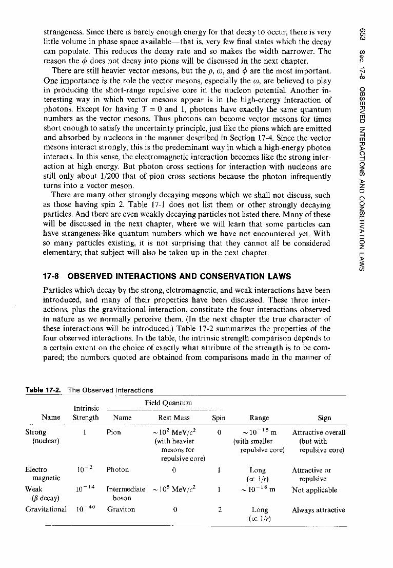
01 w strangeness. Since there is barely enough energy for that decay to occur, there is very little volume in phase space available—that is, very few final states which the decay can populate. This reduces the decay rate and so makes the width narrower. The reason the 4) does not decay into pions will be discussed in the next chapter.

There are still heavier vector mesons, but the p, w, and 4) are the most important. One importance is the role the vector mesons, especially the w, are believed to play

in producing the short-range repulsive core in the nucleon potential. Another in-teresting way in which vector mesons appear is in the high-energy interaction of photons. Except for having T = 0 and 1, photons have exactly the same quantum numbers as the vector mesons. Thus photons can become vector mesons for times short enough to satisfy the uncertainty principle, just like the pions which are emitted and absorbed by nucleons in the manner described in Section 17-4. Since the vector mesons interact strongly, this is the predominant way in which a high-energy photon interacts. In this sense, the electromagnetic interaction becomes like the strong inter-action at high energy. But photon cross sections for interaction with nucleons are still only about 1/200 that of pion cross sections because the photon infrequently turns into a vector meson.

There are many other strongly decaying mesons which we shall not discuss, such as those having spin 2. Table 17-1 does not list them or other strongly decaying particles. And there are even weakly decaying particles not listed there. Many of these will be discussed in the next chapter, where we will learn that some particles can have strangeness-like quantum numbers which we have not encountered yet. With so many particles existing, it is not surprising that they cannot all be considered elementary; that subject will also be taken up in the next chapter.

17-8 OBSERVED INTERACTIONS AND CONSERVATION LAWS

Particles which decay by the strong, eletromagnetic, and weak interactions have been introduced, and many of their properties have been discussed. These three inter-actions, plus the gravitational interaction, constitute the four interactions observed in nature as we normally perceive them. (In the next chapter the true character of these interactions will be introduced.) Table 17-2 summarizes the properties of the four observed interactions. In the table, the intrinsic strength comparison depends to a certain extent on the choice of exactly what attribute of the strength is to be com-pared; the numbers quoted are obtained from comparisons made in the manner of

Table 17-2. The Observed Interactions

Intrinsic Field Quantum

Name Strength Name Rest Mass Spin Range Sign

Strong 1 Pion —10 2 MeV/c 2 0 '-10 -15 m Attractive overall (nuclear) (with heavier

mesons for repulsive core)

(with smaller repulsive core)

(but with repulsive core)

Electro magnetic

0 -2 Photon 0 1 Long (cc 1/r)

Attractive or repulsive

Weak (/3 decay)

10 -14 Intermediate boson

—105 MeV/c2 1 —10 -18 m Not applicable

Gravitational 10 -40 Graviton 0 2 Long Always attractive (cc 1/r)

OB

SE

RV

ED

INT

ER

AC

TION

S A

ND

CO

NS

ER

VA

TIO

N LA

WS

INT

RO

DU

CT

ION

TO

EL

EM

EN

TA

RY

PA

RT

ICL

ES

Section 16-4. All of the entries in the table have been discussed previously, except for the characteristics of the quantum of the gravitational field.

The gravitational field quantum is called the graviton. Its rest mass must be zero since the gravitational interaction has the same long range as the electromagnetic interaction, whose quantum is the zero rest mass photon. The spin of the graviton is known to be 2. The reason is the absence of negative gravitational mass, which prevents the existence of the oscillating gravitational dipole that would be required to radiate a spin 1 graviton. The lowest possible multipolarity oscillating gravitational source is a quadrupole (a distribution of mass oscillating between a prolate and oblate ellipsoidal shape), and a quadrupole source emits a spin 2 quantum. This is essentially the same argument as the one we used in Section 16-5 to con-clude that a photon has spin 1 because there are no oscillating electromagnetic monopoles. While there is indirect astronomical evidence for gravitons, the laboratory searches have not yet yielded direct proof of their existence. These are extremely difficult experiments because the effects that can be studied on a laboratory scale are so small. However, the gravitational interaction is the only one of the four that is both long range and always of the same sign. Therefore its effects are cumulative so that, despite its intrinsic weakness, gravity is by far the most obvious of the interactions on the scale of the macroscopic world.

Table 17-3 lists the three interactions of the microscopic world, i.e., of quantum physics, and all of the quantities that are conserved in certain interactions. The entry yes, or no, means that a quantity is, or is not, conserved. We have discussed all of the entries in this table, except those referring to charge conjugation and time reversal, which will be discussed shortly. However, the basis for some of the other entries will be taken up first.

The conservation of energy, linear momentum, angular momentum, and parity all relate to symmetries of space and time. Each of these conservation laws implies an invariance principle, which results from a symmetry. For example, conservation of linear momentum comes from the invariance of the system to a spatial translation, and that invariance is a result of the homogeneity of space. That is, if one part of space is like another, then it does not matter where in space the system is located. If that is true, momentum will be conserved since there are no external forces. Similarly, angular momentum conservation occurs when there is invariance to the rotation of the system, which will be the case if space is isotropic. Energy is conserved if there is invariance to translation in time, which will occur if time is homogeneous.

Table 17-3. Applicability of the Conservation Laws to the Observed Interactions ("yes" Means Conserved; "no" Means Not Conserved)

Quantity Electro- Conserved Strong magnetic Weak

Energy yes yes yes Linear momentum yes yes yes Angular momentum yes yes yes Charge yes yes yes Electronic lepton number yes yes yes Muonic lepton number yes yes yes Tauonic lepton number yes yes yes Baryon number yes yes yes Isospin magnitude yes no no (A T = 1/2 for nonleptonic) Isospin z component yes yes no (A TZ = 1/2 for nonleptonic) Strangeness yes yes no (AS = 1) Parity yes yes no Charge conjugation yes yes no Time reversal (or CP) yes yes yes (But 10 -3 violation in K ° decay)

All three of these relations among conservation laws, invariance principles, and sym-metries can be proved classically or quantum mechanically. Parity conservation, which generally is a useful concept only for quantum mechanical systems, results from reflection invariance arising from a symmetry between left and right.

The familiar conservation of charge results from a different kind of invariance principle, called gauge invariance. While the student may be familiar with gauge in-variance from the study of electromagnetism, he probably will not have learned of its relation to charge conservation, to be explained next.

In its simplest application, gauge invariance means that only differences of electric potential can have physical significance, and that a unique value cannot be assigned to a single potential. Wigner has given a simple demonstration of the relationship between gauge invariance in this sense and the conservation of charge. He supposes that charge is not conserved and that a charge creating and destroying device exists at a potential V which creates a charge Q, requiring an amount of work W to do so. Next the charge and the device are transferred some distance to a place where the potential is V', with V' < V. The charge and the device gain an amount of energy Q(V — V') in this transfer. At the new position the device is used to destroy the charge, regaining the energy W expended in its creation. This is possible because regaining W is independent of the particular value of the potential as a consequence of gauge invariance. Now the chargeless device can be brought back to the initial position where the potential is V without doing any work against the electric field associated with the potential difference between the two positions. In this cycle there has been a net gain in energy of Q(V — V'). Thus if gauge invariance and the non-conservation of charge are assumed, energy conservation is violated.

The various lepton numbers and baryon numbers are chargelike quantum num-bers. However, there is no known gauge principle which assures their conservation and hence lepton and baryon number conservation may not be absolute conservation laws, but only extremely good approximations. This issue is taken up in the next chapter. Also in that chapter is a discussion of the reasons for the conservation of isospin and strangeness and the introduction of other strangeness-like conservation laws.

Concerning the new entries in Table 17-3, charge conjugation is the process of changing every particle of a system into its antiparticle. As an example, the charge conjugate of the ground state deuterium atom contains a nucleus with an antineutron and an antiproton, and an atomic positron. All available experimental evidence is consistent with the conclusion that the operation of both the strong and electromag-netic interactions is unaffected by, or invariant to, charge conjugation. For instance, such invariance is found experimentally in the strong interaction annihilation of a proton and an antiproton into the particle antiparticle pair K + K- , plus other par-ticles, and is also found in measurements of the electromagnetic decay of the pi °

meson. Therefore, we believe that the nucleus of the antideuterium atom (whose behavior is governed by the strong interaction) and also the positron (whose behavior is governed by the electromagnetic interaction) would act in the same way, because they are in the same quantum state at the same energy as the nucleus and the electron in the normal deuterium atom. So we may say, as indicated by the "yes" symbols in the table, that charge conjugation is conserved in the strong and electromagnetic interactions because the description of a system governed by either of these inter-actions is invariant to the operation. This is parallel to the terminology we use when we say by the "no" symbols in the table, and elsewhere, that parity is not conserved in the weak interaction because a description of a system whose behavior it governs is not invariant to the parity operation.

In fact, the experimental evidence for the "no" symbol in the table that indicates charge conjugation is not conserved in the weak interaction, i.e., that the weak

OB

SE

RV

ED

INT

ER

AC

TIO

NS

AN

D C

ON

SE

RV

AT

ION

LAW

S

> 0

^

• p2 = 0 71-

Case #2

positive z

• p2 < 0

INTR

OD

UC

TIO

N T

O E

LEM

EN

TA

RY

PA

RT

I CLE

S

interaction does distinguish between a system and its charge conjugate, is the same as

the experimental evidence for parity nonconservation in that interaction. This can be

understood quite simply from the pion decay of (17-19) or (17-20), which is shown

schematically in Figure 17-21 for a frame in which the pion is at rest. In that frame

the µ and y go off in opposite directions with equal magnitude of momentum p.

Because the 2t has zero spin, the spin —1/2 u and y must have their spins essentially parallel or antiparallel to their directions of motion so that the two spin angular

momenta add to zero. The parallel case (# 1) is shown above a mirror and the anti-parallel case (# 2) is shown below the mirror. Each is a mirror reflection of the other.

This is true because in such a reflection—or parity operation—the linear momenta

reverse direction but the angular momenta do not because they describe circulations

which do not reverse their sense. (Compare the situation here with the one illustrated

SZ = +1/2 p2 > 0

C-›) •

Case #1 Sz = 0 • pz = 0 IT

positive z

CD • S=—½ l ^

pz < 0

Mirror /

Figure 17-21 The decay it—> µ + y in the rest frame of the ir. The directions of the linear momentum of the it and of the y are indicated by arrows labeled by the signs of their z com-ponents, such as pz > O. The directions of their angular momenta are indicated by straight

arrows labeled with the values of the z components, such as Sz = +1/2, and also by curved arrows showing the senses of the corresponding circulations. Since reflection in a mirror whose plane is parallel to the plane of circulation does not change its sense, the reflection

does not change the directions of the angular momentum vectors. But reflection in a mirror

whose plane is perpendicular to the direction of motion reverses that direction. Therefore . the linear momentum vectors are reversed by the reflection. The two possible cases which conserve both linear and angular momentum in the decay are shown, and labeled #1 and #2. Each is the parity inversion (mirror reflection) of the other. For 7r µ + v u , only case #1 is seen in nature, while for 7r

+ -) µ+ + v, only case #2 is seen. These observations

show that neither parity nor charge conjugation are conserved in the decay.

in Figure 16-15, being sure to take into account the difference in orientation of the mirrors in the two figures.) Since parity is not conserved in this weak decay, # 1 or # 2 will be observed, but not both equally. If charge conjugation were conserved and parity not conserved, whichever of the decays # 1 or # 2 dominated, the same one would have to dominate if the system (say, 7c+ p+ + vii) were charge conjugated (to n - —> u- + I,L ). That is not observed. Instead, # 1 dominates for n - decay and # 2 for n+ decay, showing that both parity P and charge conjugation C are not con-served. Thus the entries for both of these should, in fact, be the "no" symbols shown in the weak interaction column of Table 17-3.

The combination of P and C violation can be expressed by saying that particles are left-handed. That is, the y has its momentum and angular momentum antiparallel, as would a left-handed screw, while the antiparticle v is like a right-handed screw with its momentum and angular momentum parallel. This handedness, or helicity (which was introduced in Section 16-4), is at or near a maximum for the y or v because these particles are traveling at or near the velocity of light since their mass is zero or close to it. Angular momentum conservation forces the y+ or ,u - to have helicity opposite to what it would like to have (i.e., the particle y is naturally left-handed and the antiparticle µ+ naturally right-handed), and this suppresses the rate of n decay by a factor of 10 5 . But n decay occurs at all only because the y has mass and is traveling at y < c. It is possible to have a reference frame traveling faster than a particle of finite rest mass. In such a frame the helicity is reversed since the spin is unchanged but the particle appears to be moving in the opposite direction. A zero rest mass particle travels at y = c, and it is not possible to have a more rapidly traveling reference frame. So the helicity cannot be reversed unless the rest mass is nonzero.

When P and C were found to be not conserved in the weak interaction, the hope was that the combined operation CP (that is, performing in sequence each of the two operations) would leave invariant the description of a system governed by this inter-action. For example, if such CP conservation were valid it would require that if decay # 1 in Figure 17-21 occurs for the n - then decay # 2 would occur for the n + . This is just what is observed. Indeed, experimental tests show that CP is conserved to at least

the 1% level in weak interactions. We shall see shortly that CP is closely related to time reversal.

Time reversal is the process of changing the time variables describing the evolution of a microscopic system into their negatives. In other words, it changes the direction of flow of time, like running a motion picture backwards. Application of time reversal to Figure 17-21 is not interesting because it leads to a description of the improbable situation in which a y and a y collide to form a n. It is worthwhile noting, however, that time reversal preserves helicity. To see this, take the y as an example. Time re-versal reverses the direction of the vector describing the linear motion; but it also reverses the sense of circulation so that the spin vector reverses as well, keeping the particle left-handed.

Time reversal invariance cannot be tested by measuring the rates for forward and backward weak interactions because one of the rates would be too small to measure. But that method has been used for the strong and electromagnetic interactions. An example is p + p < n+ + d, which can be observed in both directions as was discus-sed in Section 17-4. Another example of a time reversal experiment for the strong interaction is a comparison of the cross section for a reaction such as

12Mg24 + 2He4 -* 13Al27 + 1H1

and the cross section for its inverse 13 Al27 + 1H1

--^ 12Mg24 + 2He4

OB

SE

RV

ED

INT

ER

AC

TION

S A

ND

CO

NS

ER

VA

TIO

N L

AW

S

with the momentum vectors of the bombarding and target nuclei in the second reac- tion adjusted to be equal but opposite to ttlose of the product and residual nuclei of

INT

RO

DU

CT

ION

TO

ELE

ME

NT

AR

Y P

AR

TIC

LES

the first reaction. Time reversal T (not to be confused with isospin) is found by such experiments to be a good symmetry for strong and electromagnetic interactions. In somewhat more complicated experiments (involving trying to observe processes de-scribed by an odd number of momenta and angular momenta vectors which would change sign under the time-reversal operation), invariance to T is found in weak interactions to the 1% level.

Although testing time-reversal inva riance directly to a high degree of accuracy for the weak interaction is difficult, a sensitive indirect test is available by using the so-called CPT theorem. This is a very general theorem of relativistic quantum mechanics which shows that, for any system governed by any interaction conforming to the rela-tivistic requirement that cause must precede effect, the result of successively carrying out the charge conjugation operation C, the parity operation P, and the time-reversal operation T is to leave the essential description of the behavior of the system un-changed. As a consequence of the CPT theorem, the observed violation of P in the weak interaction requires that C and/or T be violated as well. Direct experiments show that C is violated, as was discussed above. If T is also violated then the CPT theorem demands that CP be violated. Hence if the CPT theorem is correct—and not only would its failure destroy the basic theoretical structure of much of physics, but also it has been tested extensively by experiment—then a test of CP is also a test of T.

As this is being written there is only one particle known whose properties provide sufficient sensitivity to test for small effects of the nonconservation of CP or T, and that is the K ° . In a rather amazing demonstration of quantum mechanics, the K °

that is produced in a strong interaction is not the same particle as the one which subsequently decays by the weak interaction. The particle produced by the strong interaction, which conserves strangeness, must be described by an eigenfunction of a strangeness operator whose eigenvalue is one or the other of the two possibilities for the K, namely + 1 or —1. That is, either the K ° with S = +1 or the K ° with S = —1

is the produced particle. But since strangeness is not conserved by the weak inter-action responsible for the decay of the K, the particle that decays is not required to be described by an eigenfunction of the strangeness operator. Now the neutral K

is observed to decay into n+ + i , a system described by an eigenfunction of the CP operator with eigenvalue + 1. This can be seen simply from Figure 17-22, where

• I • vrf x = 0 zr -

l^ • I •

a- x=0 ar+

• I • �+ x = 0 a-

Figure 17-22 The diagram on the top represents a m + and a 7E — of zero angular momentum from K ° decay. They are located on the x axis on each side of its origin and at equal distances from it. When the parity operation P is carried out by interchanging the signs of the

coordinates of the two pions, the diagram in the center is obtained.

When the charge conjugation operation C is carried out on the center diagram by interchanging the signs of the charges of the two

pions, the diagram on the bottom is obtained. Since it is identical

to the diagram on the top, the combined effect of the two operations is to make no change in the system.

the parity operation interchanges the 7r + and it and the charge conjugation opera-tion changes them back again. The result is to leave the i + 7c - system just as it was in the beginning; in other words, the eigenvalue of the operator CP for the eigenfunc-tion describing the decay has the value + 1. Now if CP is conserved by the weak interaction, then the neutral K which decays to 7r + + ,r - must also have eigenvalue + 1. However, neither the K ° nor the K ° are described by eigenfunctions of the CP operator because charge conjugation of the K ° gives the K ° , and vice versa—a change which cannot be undone by the subsequent parity operation. Since the same state is not obtained after the CP operation on a neutral K, the state cannot be an eigenfunction of CP.

How can we create eigenfunctions of CP in the neutral K system? First we note that the CPT theorem requires that particle and antiparticle have the same mass. Thus the K ° and K ° are degenerate in energy. But if these degenerate states suffer a small perturbation then we can consider them to be linear combinations of per-turbed states which do not have quite the same energy. (See Appendix J.) The ex-tremely small perturbation comes about through the process

K ° ±27r4 K ° (17-50)

which has a particularly low rate because it involves two successive weak interactions. The process gives the perturbed states, called K° and K2, slightly different masses. The K° and K° are then described by eigenfunctions of CP, constructed as follows

1 K° _ [K° + CP(K°)] _ (K° + K°) (17-51) 1

K2 = [K° — CP(K °)] _ (K° — K °) (17-52) where the symbols represent the eigenfunctions for the corresponding particles and 1/4 gives the correct normalization. By applying CP to (17-51), the student will see that this operator gives the same eigenfunction back again, so that the corresponding eigenvalue is + 1. In the same way he can see that (17-52) is an eigenfunction of CP with an eigenvalue of —1. (The careful student may note that these statements seem apparent when using just C, as did Gell-Mann and Pais when they first investigated this subject, but that P introduces a bothersome minus sign. However, the charge conjugation operation has an undetermined phase which can be taken to be —1, so the original Gell-Mann-Pais convention can be retained.) Thus to conserve CP it is necessary to have

K° î+ + 7r - but K° n + + it (17-53) The K° can decay into a 7C + and 7r - , but the K2 cannot.

Since the 7c° is its own antiparticle, under charge conjugation it goes into itself and has a C eigenvalue of + 1. Its P eigenvalue is —1. Hence a system of three nc ° 's has a CP eigenvalue of (+ 1) 3(-1) 3 = —1. Therefore

K2 -+ 7r ° + + n:° but K° + It° + rc° (17-54) All of the possible decays of the K2 have at least three particles in the final state. This means that the volume occupied in phase space is small, making the decay much slower than that for the K°. Thus the K° has a lifetime of about 10 -10 sec, while the K2 has a lifetime of about 5 x 10 -8 sec, which is why it was not observed in the early cosmic ray experiments. Note that if (17-51) and (17-52) are added or subtracted

the result is

SM

F' N

OI1

b'/1

1:13S

NO

0 G

NV

SN

OIlO

`d1:1

31N

I 03/

1a

3S

80

K° = ^ (K° + K2) (17-55)

0 co co

INT

RO

DU

CTI

ON

TO

ELE

ME

NT

AR

Y P

AR

TIC

LES

or

= (K° — K3) (17-56)

Thus, if a K ° or K° is produced, half of the decays will occur through the short-lifetime mode K° and half through the long-lifetime modè K.

A casual glance at (17-51), (17-52) and (17-55), (17-56) gives us an interesting, 'if somewhat oversimplified, view of the time evolution of the K°. Say a K ° is produced. It corresponds to an eigenfunction of the S operator, but not of the CP operator, being half K° and half K. However, the K° component decays quickly, leaving just KZ which corresponds to an eigenfunction of CP but not of S, consisting of half K° and half K ° . Now suppose the K2 goes through matter. Because the K° has S = — 1, just as do the hyperons, there are many reactions it can undergo, as we have already noted in connection with (17-35). Hence the K ° component can be absorbed out, leaving just the K° with S = + 1. The process is called regeneration. We see that either allowing the system to evolve in time, or to pass through matter, changes the nature of the particle. This means that, if the S eigenvalue is measured, information on CP is lost, and vice versa. The situation is analogous to determining the com-ponents of angular momentum in a Stern-Gerlach experiment.

The above description of the time evolution is not quite accurate because the small mass difference between the K? and K° causes the relative phase of the two corresponding wave functions to change with time, changing the K °K ° mixture. This actually produces oscillations in the amount of K° and K° present. By measuring the wavelength of these oscillations, the K?—K? mass difference Am can be found. Since Am arises from the process (17-50), we might expect by the uncertainty principle to have

AEAt = (Amc 2)(At 1 ) — h (17-57)

where At 1 is the K° lifetime, or Am — h/At 1 c 2 . Measurements give about half this value, or about 4 x 10 -6 eV/c2 . Since Am has been measured to better than 1%, and since the value of m is about 5 x 10 2 MeV/c2, the inaccuracy in the mass difference is smaller than the mass itself by 16 orders of magnitude!

The discussion of the K ° began with the question of CP conservation. Clearly (17-53) and (17-54) test its validity. In 1964 Christenson, Cronin, Fitch and Turley found, at such a distance from the K° production point that the K°'s had all decayed, about 0.1% of the K°'s decayed by the CP-violating 2n decay. Thus to this miniscule degree CP conservation and hence, by the CPT theorem, T invariance are violated. Other experiments on the K° system have shown directly that it is T, and not CPT, which is not conserved along with CP. That is, there is evidence that through the rare mode in the weak interaction decay of the long-lived component of the K °K ° system nature can distinguish at a microscopic level the direction of flow of time. This startling result would seem to be of great significance. In the next chapter we shall return to the issue while discussing gauge theories of particle interactions.

Example 17-6. Discuss each of the following reactions in terms of the conservation laws listed in Table 17-3 and the particle quantum numbers listed in Table 17-1.

(a)i - +K ► This reaction is impossible because it requires a strangeness change of 2. •

(b) K - +p S. +K+ + K° 110-This is the reaction in which the SF, which has S = —3, was first produced. It is strangeness conserving since S = +1 for the K + and K°, while S = —1 for the K - . Charge and baryon number are conserved. So are angular momentum and parity because the final state can have one unit of orbital angular momentum. (Recall that the parity associated with orbital angular momentum is given by (— 1) 1.) Since isopin and its z component are also conserved, we see

that the reaction can proceed via the strong interaction. If this were not the case, the cross section would be too small for it to be observable. •

(c)52 - ->E° + it

■Here charge and baryon number are conserved. Angular momentum and parity are also con-served by the final state containing one unit of orbital angular momentum. Since the values of T are 0 for the S2 - , 1/2 for the E °, and 1 for the it we see that there must be an isospin change of at least A T = 1/2. Also, T is 0 for the 0 , + 1/2 for the E°, and —1 for the n - , so the z component of isospin changes by A TZ = 1/2, which is equivalent to AS = 1. These quantum number changes do allow the decay to proceed by the weak interaction, but they prohibit it from proceeding more rapidly by the electromagnetic or strong interactions. 4

(d)m + +p—*p+p+n ■First we must determine the quantum numbers of the antineutron n. Applying the quoted rules to the table, we find: Q = 0, s = 1/2, B = —1, P = odd, T = 1/2, TZ = + 1/2, S = O. In-spection demonstrates that all quantum numbers are conserved by the reaction, so it can take place by the strong interaction. 4

(e) +e+ +ve ► If this goes at all, it must be by the weak interaction since v e does not participate in any of the others. Charge is conserved since Q = —1 for the p. The total baryon number equals —1 before and after, so it is conserved also. Electronic lepton number is conserved because it has the values —1 for the e + and + 1 for the ye . Angular momentum can be conserved. Parity is not defined for leptons, but parity is not a significant consideration for a weak interaction involving leptons. The same is true for isopin and strangeness. So the reaction can take place by the weak interaction. Note that it is just the charge conjugate of the /3 decay of the neutron.

• (f)A° --► n+y

► This reaction, if it can occur, obviously must be electromagnetic. Since TZ = 0 for the A° and y, while TZ = — 1/2 for the n, we see that it cannot occur because TZ is conserved in the elec-tromagnetic interaction. This conclusion agrees with experiment, and it is one of the reasons why TZ = 0 is assigned to the photon. The same conclusion could be reached by considering S; the student should do so. •

QUESTIONS

1. Why is 3 P 1 not a component of the ground state of the deuteron? What about '5 0? 2. What experiments can be performed to test for the existence of a stable system of two

protons? Of two neutrons? 3. In the center-of-mass frame of reference the differential cross section for neutron-proton

scattering is isotropic at low energies. Describe qualitatively the behavior of the differ-ential cross section in a frame of reference in which the target proton is initially stationary.

4. In considering the quantum mechanical behavior of a system of two identical particles, we talk of exchange of the labels of the particles. In considering neutron-proton scattering, we talk of exchange of the particles. What is the reason for this difference?

5. Why is the proton-proton scattering differential cross section necessarily symmetric about 90° in the center-of-mass frame of reference?

6. Explain why the scattering differential cross section is isotropic if only the 1 = 0 state participates in the interaction that produces the scattering.

7. A very large part of what we know about the forces acting in atoms is obtained from the study of the bound states of the simplest atom, hydrogen. Why is only a small part of what we know about the forces acting in nuclei obtained from the study of the bound states of the simplest nucleus, deuterium?

8. Why is the name isospin an appropriate one to use for the concept discussed in Section 17-3?

9. Can the exclusion principle be expressed in terms of isospin? See Figure 17-14. 10. Is there a physical picture of how the momentum of a zc meson transferred between the

fields of two nucleons leads to an attractive force between them? From the point of view

SN

OIlS

3f1

0

INT

RO

DU

CTI

ON

TO

EL

EM

EN

TA

RY

PA

RT

ICLE

S

of the position-momentum uncertainty principle, is it realistic to expect to be able to construct such a picture?

11. What species of it mesons are exchanged in proton-proton scattering? In neutron-neutron scattering?

12. What particle would remain if a proton emitted a it - meson? If a neutron emitted a 7r + meson? Why is it that the proton field cannot contain only a it - meson, and the neutron field cannot contain only a i+ meson?

13. Why is it believed that the repulsive core of the nucleon potential arises from the exchange of mesons heavier than the pion?

14. What examples have been considered in earlier chapters of the conservation of the num-ber of fermions, and the nonconservation of the number of bosons, in an isolated system?

15. Exactly what is meant by the statement that a pion has odd intrinsic parity?

16. Comparison of the decay rate of cosmic ray muons in flight with the decay rate of muons at rest provided the first experimental verification of relativistic time dilation. What would be a possible way to carry out such a comparison?

17. Cosmic ray muons have been used in an attempt to discover hidden burial chambers in Egyptian pyramids, in much the same way that x rays are used to discover internal imper-fections in a metal casting caused by gas bubbles. Why were muons used?

18. Are there any particles other than neutrinos and antineutrinos which have definite heli- T cities? Explain.

20. There are four distinctly different K mesons. Why do we not assign to them the isospin quantum number T = 3/2 so that they would constitute an isospin quartet?

21. Exactly what does the strangeness quantum number S specify? 22. Why is the copious production of A ° and K particles very difficult to reconcile with their

slow decay, without the concept of strangeness? How does strangeness provide a rec-onciliation?

23. Is there a conflict between the statement that isospin magnitude is not conserved in the electromagnetic interaction, and the statement that isospin z component is conserved in that interaction?

24. Consider viewing the fl-decay experiment illustrated in Figure 16-15 in a mirror located below the nucleus (the mirror being horizontal) instead of in a mirror located to one side of the nucleus (the mirror being vertical). Explain how the arguments in the text concerning the appearance of the mirror image of the charge conjugate would be modified, but in such a way as to lead to the same conclusion.

25. Give an example of a macroscopic system whose behavior is invariant to time reversal, and of a macroscopic system whose behavior is not invariant to this operation.

26. Why can we say that the 7r ° meson is its own antiparticle? Do all particles have anti-particles? What about the photon?

27. Does it seem reasonable to you to say that a meson or baryon resonance is an elementary particle? Just what is an elementary particle?

28. Suppose a virtual particle and a real particle that decays by the strong interaction have about the same lifetime. What is the difference between them? To what mass or energy does their lifetime relate (through the uncertainty principle) in each case?

â c 19. Why must all field quanta be bosons? U

PROBLEMS

1. Consult the discussion of the centrifugal potential in Section 15-8, and then: (a) Write the equation which determines the radial dependence R(r) of the deuteron eigenfunction, by evaluating (7-17) for l = O. (b) Show that it can also be written

h2 d2u(r) + V(r)u(r) = Eu(r)

2µ dr2

where u(r) = rR(r)

(c) Compare this with the time-independent Schroedinger equation for one-dimensional problems. (d) Give a physical interpretation of u*(r)u(r). (e) Evaluate, and give a physical interpretation of, the reduced mass u.

2. (a) In the equation obtained in Problem 1, take the nucleon potential V(r) to be a square well of radius r' and depth V0 , as in Figure 17-2. (b) Show by substitution that the general solution to the equation obtained is

u(r)=A sin k ir +B cos k i r

u(r) = Ce- k2r + Dek2 r

(c) Evaluate k 1 and k2 in terms of p, Vo , and the deutron binding energy AE. 3. (a) Apply to the general solution obtained in Problem 2 the conditions that R(r), and

therefore u(r), must be finite, continuous, and single valued, and have first derivatives with the same properties. (b) Show that the application of these conditions at r = 0, r = r', and r -> oo leads to the relation

V2µ(Vh- AE)

cot [J2 u(Vo^ - AE) r ,1 _ N/2^4E

4. Show, by substitition, that the relation obtained in Problem 3 has a solution with AE = 2.2 MeV, the observed deuteron binding energy, when the potential has a radius and depth of r' = 2.0 F and Vo = 36 MeV.

5. (a) Use the calculations in Problems 1 through 4 to evaluate the radial dependence of the eigenfunction for the ground state of the deuteron in a potential of radius 2.0 F and depth 36 MeV. (b) Sketch the potential V(r) and the function u(r) = rR(r). (c) Also sketch the radial probability density P(r).

6. A nucleon is incident on a nucleon which is initially stationary. Its kinetic energy, which is also the total kinetic energy of the system in that frame of reference, is K. Show that the total kinetic energy of the system, in a frame of reference in which the center of mass of the system is stationary, is K/2.

7. (a) Show that, for a nucleon potential of radius r' = 2 F, the maximum value of the orbital angular momentum quantum number is lmax = 1 unless the kinetic energy of each nu-cleon exceeds about 30 MeV in the center-of-mass frame of reference. (b) Also show that /max = 2 unless the kinetic energies exceed about 60 MeV.

8. (a) Calculate the value of /max for a 50 MeV proton incident on a nucleus of atomic weight A = 100. Take the radius r' of the optical model potential acting on the proton as the sum of the half-value charge distribution radius a = 1.07A"3 F and the range of nucleon forces 2.0 F. (b) Also evaluate 8 1/r', and compare with the angle between adjacent minima in the differential scattering cross section shown in Figure 16-26.

9. (a) Use the results of the electron scattering measurements, presented in Figure 15-6, to calculate the total number of nucleons per unit volume in the interior of a typical nucleus. (b) Then calculate the average center-to-center spacing of the nucleons. (c) Compare this with the radius of the repulsive core of the nucleon potential, and with the range of the nucleon force.

10. The position-momentum uncertainty principle produces an effect which tends to prevent the collapse of a nucleus that would occur if the nucleon potentials had no repulsive regions. (a) Show that this principle demands the kinetic energy of a typical nucleon confined to a nucleus of radius r' must be a least K, where

1 K cc +

Although K becomes more positive as r' decreases, the potential energy V of the typical nucleon becomes more negative if the nucleon potentials are purely attractive and the nucleus is sufficiently collapsed to make the separation between all pairs of nucleons

r < r' r > r'

sw31

8oa

d

INT

RO

DU

CTI

ON

TO

EL

EM

EN

TA

RY

PA

RT

ICL

ES

less than the range of the nucleon potential. Show that, in these circumstances

1 Vcc —r3

(c) Then show that the total energy of the typical nucleon, E = K + V, would become more negative as r' decreases further so that the nucleus would continue to collapse, despite the uncertainty princple, if the nucleon potentials had no repulsive regions.

11. Use information contained in Figure 16-14 and 16-36 to assign values of T and TZ to the isobaric analogue ground state levels of: (a) 1H3 and 2He3 ; (b) 3 Li 7 and 4Be7 .

12. (a) Estimate the maximum time that a it meson can exist in the field of an isolated nucleon before it is absorbed by that nucleon. (b) Estimate how many it mesons there can be at any instant in the field at distances from the nucleon about equal to the range of the nucleon force, 2 F. (c) Estimate how many there can be at distances about equal to the radius of the repulsive core, 0.5 F.

13. The it° lifetime has been determined by studying the decay from rest of the K + meson in the mode K + -* it° + 7E +. The average distance traveled by the i° in a block of photo-graphic emulsion before it decays in the easily observable mode it —> e + + e— + y is

measured, and from the calculated velocity of flight of the rc ° its lifetime is obtained. Given that the lifetime is 0.8 x 10 -16 sec, predict the average distance traveled by a 7r °

before it decays. 14. In the laboratory (LAB) frame of reference, particle 1 is at rest with total relativistic

energy E 1 , and particle 2 is moving to the right with total relativistic energy E2 and r momentum p2 . (a) Use the relativistic momentum-energy transformation equations U

i Px — (Px — vE/ C 2)

— v2/c2

py = pv PZ = PZ

1 E'=

(E— vPx) — v2/c2

to show that the frame in which the center of the relativistic masses of the system is at rest is moving to the right with velocity

v = c cp2

E1 +E2

relative to the laboratory frame, and show that the total momentum of the system is zero in this center-of-mass (CM) frame. (b) Now let the two particles have the same rest mass m° , and let the total relativistic energy of the system in the laboratory frame be ELAB. Evaluate ECM, the total relativistic energy of the system in the center-of-mass frame, and show that

ECM = 2m°C 2 FLAB

15. Use the relation quoted in Problem 14b to evaluate the kinetic energy in the laboratory frame of the bombarding proton at which the proton, antiproton pair production process, (17-16), becomes energetically possible.

16. (a) Estimate the cross section for a 1 MeV electronic antineutrino incident on a proton to produce the reaction

v e +p—>n+e+

(Hint: (i) Assume there is some probability of the reaction occurring when the distance between the v e and p is within the v e de Broglie wavelength ). Then estimate the time interval during which they can be that close. (ii) Estimate the probability P as the ratio of that time interval to the characteristic time —10 3 sec for the reaction. (It is the inverse of n + e + —> p + ie , which is an alternative to n —> p + e + ve; detailed balancing requires that all three have the same characteristic time which, we see, is just the neutron f-decay lifetime.) (iii) Take the cross section to be — P). 2 .) (b) Use the estimate to evaluate the

mean free path of a 1 MeV v e in lead, by justifying the assumption that the cross section for its interaction with a lead nucleus is —10 2 times larger than the cross section for its interaction with a proton.

17. (a) Why is the p ° meson not allowed to decay into two n ° mesons? (b) Assuming that the incident deuteron has sufficient energy, why is the reaction d + d --+ 2He4 + 7Z° not allowed? (c) Why is the decay of a ir + meson into an e + and a y not possible? (d) What prevents the reaction n —* p + e - + ve from taking place when the neutron is part of a deuteron?

18. For each of the following reactions state the fastest interaction through which the conservation laws allow it to proceed. If the reaction is forbidden by all interactions, state why. (a) p—*7r + +e+ +e (b)A° —> p + e (c)p --> e + ve + vµ (d)n+p-*E + +A° (e)p+pay+ y

(f) p +p —>n +E° +K° (g)K°

^ n+ + n — + n° + n°

SW3180ad

18 MORE ELEMENTARY

PARTICLES

18-1 INTRODUCTION

particles that are more elementary; the new strong interaction; unification of electromagnetic and weak interactions

18-2 EVIDENCE FOR PARTONS

partons, or pointlike constituents of hadrons; evidence from neutrino-nucleus scattering and electron-proton deep inelastic scattering

18-3 UNITARY SYMMETRY AND QUARKS

composite particles on the basis of isospin, or SU(2); including strangeness or hypercharge to make SU(3); quarks from SU(3); u, d, and s quark prop-erties and multiplets; basis of isospin and strangeness conservation

18-4 EXTENSIONS OF SU(3)—MORE QUARKS

a fourth quark flavor, c; e + e - colliding beam production of ce states; Zweig-forbidden decays of quark- antiquark states; charmonium spectrum; particles with charm; c, b, and t quark properties; the T states of bb; quark masses; evidence for new quarks from 6(e + + e- — hadrons)/ 6(e + +e —>µ+µ )

18-5 COLOR AND THE COLOR INTERACTION

necessity for the color quantum number; evidence for color; color charge as the source of the true strong interaction; gluons; interquark gluon po-tential; asymptotic freedom and color confinement; gluon flux tube and hadronic energy density; magnitude of the color force

18-6 INTRODUCTION TO GAUGE THEORIES

gauge theories for all the fundamental interactions; converting a global gauge symmetry into a local one in classical electromagnetism; electromag-netic gauge invariance in quantum mechanics; application to relativistic quantum mechanics; Yang-Mills gauge theory; Abelian and non-Abelian theories

18-7 QUANTUM CHROMODYNAMICS

SU(3) of color; changing global color symmetry to local color symmetry; properties of gluons; evidence for gluons; gluon couplings to give quark-antiquark and three-quark binding; gluon masslessness and confinement; running coupling constant ; and antiscreening

18-8 ELECTROWEAK THEORY

from Yang-Mills theory to electroweak theory; renormalization; spontane- ous symmetry breaking; Goldstone and Higgs mechanisms; weak isospin; gauge bosons; Higgs particle; role of the W ± and Z°; neutral currents;

667

667

673

678

683

688

691

699

666

SN

Ola

bd

biO

3 3

0N

3aIn

3

Cabibbo quark mixing; GIM mechanism; lepton-quark symmetry; masses and discovery of the W ± and Z °; relation between weak and electromag-netic interactions; apparent weakness of the weak interaction

18-9 GRAND UNIFICATION OF THE FUNDAMENTAL INTERACTIONS

706

unification of the coupling constants; SU(5) unification of strong, electro-magnetic, and weak interactions; experimental tests of unification (proton and double beta decays); neutrino mass searches; other unification schemes; cosmological consequences (dark mass, baryon-antibaryon ratio)

QUESTIONS

710

PROBLEMS

712

18-1 INTRODUCTION

In the previous chapter a large number of particles have been introduced, and the existence of many more has been mentioned. As ever increasing numbers of particles were discovered, it became more and more apparent that all of these could not be elementary. Once again by probing with finer resolution, which means higher energy, it was possible to discover particles which were more elementary. However, this time these constituent particles could not be separated and studied directly, so their dis-covery and the elucidation of their hidden properties makes an impressive detective story. This in turn has led to a completely new understanding of the strong, electro-magnetic, and weak interactions. The strong interaction is not at all what it has seemed to be, and the electromagnetic and weak interactions are closely related to each other. Further unification of all the fundamental interactions appears likely. The 1970's produced a true revolution in fundamental physics, and it is the purpose of this chapter to present in an introductory way the consequences of that revolution.

18-2 EVIDENCE FOR PARTONS

The proliferation of particles led to the general feeling that most, if not all, must be composites of other, more elementary particles. In addition, some theoretical models (of which the most important will be discussed in Section 18-3) suggested this com-posite nature. Additional impetus for this belief then came from experiments. In this section two of these experimental results will be discussed and their interpretation in terms of the parton model will be introduced. Parton is the name given to whatever are the constituents of hadrons such as the proton. Partons are pointlike (i.e., having no detected size), quasi-free constituents, only some of which will turn out to be the quarks discussed in the next section.

One demonstration that hadrons have pointlike constituents is provided by the total cross section, as a function of energy, for neutrino-nuclear scattering. This statement requires considerable explanation. But first the utilization of neutrinos should be explained because the neutrino seems an unlikely particle to use for this purpose. It has only the weak interaction, which means for example that neutrinos from beta decays in the sun have about one chance in a million of interacting with anything even if they pass through the earth along a diameter. Thus doing experi-ments with these particles requires large numbers of them and very massive detectors. To produce neutrino beams, protons from a high-energy particle accelerator strike a nuclear target, creating r and K mesons. These mesons are focused by magnetic fields

MO

RE

ELE

ME

NT

AR

Y P

AR

TIC

LES

Figure 18-1 Electronic neutrino detectors (of the CDHS and CHARM groups) at the CERN laboratory, Geneva, Switzerland. This illustrates the massiveness of detectors required to measure the scattering of these weakly interacting particles.

so as to create beams that go long distances, allowing decay, principally into muons and neutrinos (see (17-19), (17-20), and (17-40)). While the muons are also weakly interacting particles, they possess charge and hence undergo electromagnetic inter-actions, enabling them to lose energy by collisions with electrons in matter. By inter-posing sufficient shielding material (often iron or earth), the muons can be stopped. Those mesons which have not decayed interact strongly in this shielding material, and hence only neutrinos are left to enter the detector. Figure 18-1 shows a large electronic neutrino detector. Such a detector can identify each neutrino interaction and hence determine a total cross section. By changing the incident meson beam energy, the total neut rino cross section a as a function of neutrino energy E can be determined, and typical results are shown in Figure 18-2. It is seen that the cross section has the behavior a cc E. This proportionality is the result expected if the apparently complicated process of the neutrino interaction, which produces many hadrons as well as a muon, is basically just the elastic scattering of a neutrino by a single pointlike particle.

The promised explanation of this last statement will now be given. If the point-like neutrino and a pointlike constituent of the nucleon undergo an elastic scattering, the probability or cross section for this contact interaction would depend only on the strength of that interaction (given by /3, the weak interaction coupling constant; cf. Section 16-4) and by the volume in phase space available for the process. That is, /3 determines the rate for a transition to any particular final state, and the phase space volume determines the number of possible final states. Since the interaction occurs at a point, the coordinates are unique, and hence momentum space is the same as phase space. The phase space volume thus depends just on the momentum, p, of the two particles in the center of mass system. In momentum space, p is the length of a radius vector, and the volume available with a momentum between p and p + Ap is a spherical shell 4np2Ap. Thus a oc p2 . Now a relativistic calculation shows that p2 = mE/2, where E is the laboratory energy of the neut rino scattering elastically

SN

Ola

t/d a

Od 3

0N

34

IA3

130

120

110

100

90 0 a) U

C 80 N

E

4 70

b 60

40 60 80 100 120 140 160 180 200 0

0 20 Laboratory neutrino energy E (GeV)

Figure 18-2 Total neutrino cross section Q on nucleons as a function of neutrino labora-tory energy E from experiments at CERN (Switzerland), Fermilab (U.S.A.), and Serpukhov (U.S.S.R.). The linear dependence of c on E over two orders of magnitude in E is a demonstration of pointlike constituents (partons) inside the nucleon. The measurement errors are shown only for a few points at the higher energies, but these are typical percentage errors, so they would not be visible at lower energies.

from a pointlike target at rest of mass m. Therefore the experimental result that a cc E is to be expected for a contact interaction between a neutrino and a parton.

While evidence for the existence of partons accumulated from different neutrino ex-periments over a period of time, evidence for partons came from even the first experi-ment on deep-inelastic electron-nucleon scattering at the Stanford Linear Accelerator Center (SLAC) in 1968. The term deep -inelastic scattering needs to be explained. In Section 17-4 the charge distributions of the proton and neutron as determined by elastic electron-nucleon scattering experiments were shown. These displayed the exis-tence of the pion cloud and the nucleon core. To explore the latter in more detail re-quired higher electron energy to get a smaller de Broglie wavelength. However, the elastic cross section drops rapidly with energy, making the measurements much more difficult. Furthermore, elastic scattering implies that the nucleon recoils as a whole object, whereas exploring its structure indicates breaking it apart. Thus inelastic electron-nucleon scattering, in which other hadrons are produced from the nucleon, proved to be the way to find the parton structure of the nucleon. The adjective "deep" implies that the collision is highly inelastic.

We illustrate the difference between elastic and inelastic electron-proton scattering by the Feynman diagrams of Figure 18-3. These diagrams are actually prescriptions for making calculations of rates or cross sections. But they have become the language

O

^

^

MO

RE

EL

EM

EN

TA

RY

PA

RT

ICL

ES

Time

Figure 18-3 Feynman diagrams for (a) elastic and (b) inelastic electron-proton scattering. The space coordinate is the ordinate and time is the abscissa. The e and

p approach each other and exchange a virtual photon, after which the e goes off in one direction, and either (a) the p or (b)

some group of particles of net mass W go off in the other direction. In the inelastic case, the electron's energy changes in the

W interaction from E to E', with the virtual photon carrying off the difference, E — E'.

cu

o o U

Time

of particle physics, and hence we introduce them in this present simple application. As drawn here, time increases along the abscissa and space, represented by a single coordinate, is the ordinate. Thus the electron and proton are pictured as coming together in their center of mass system, and then interacting electromagnetically by the exchange of a virtual photon. After the interaction the electron goes off in one direction and, for elastic scattering, the proton in the opposite direction. For inelastic scattering, the proton breaks up, producing other particles which recoil oppositely to the electron. In the original experiments, only the final state electron was measured; hence the nature of the other particles was not important.

To provide a little more familiarity with Feynman diagrams, we shall interrupt the discussion of electron-proton scattering to give another example of using these diagrams.

Example 18-1. Construct a Feynman diagram for neutron-proton scattering resulting from

the exchange of a 7C meson. •Initially the neutron and proton approach each other, so lines are needed which start apart

and converge. It does not matter whether the neutron or the proton is at the top, nor does it

matter what kind of line is used. However, solid lines are most frequently used for baryons,

just as the wavy line shown in Figure 18-3 is almost always used for the photon. For the

exchanged pion a dashed line will be used to distinguish it more clearly from the baryons. Now we have a choice. The first possibility is that the proton emits a 7C + , turning into a

neutron, and the 7r+ is absorbed by the initial neutron, turning it into a proton, as shown in

Figure 18-4a. The second possibility is that the neutron emits a i turning into a proton, and the 7C — is absorbed by the initial proton, turning it into a neutron, as shown in Figure 18-4b. Note that the dashed lines for the pions have appropriately different slopes in the two

cases, indicating the two different origins and time progressions. However, these two diagrams

are completely equivalent. The reason is that these virtual pions exist for too short a time to

permit, even in principle, any measurement which could distinguish Figure 18-4a from 18-4b.

Since the it+ and 7E — are antiparticles of each other, this illustrates the principle that an anti-particle is equivalent to a particle going backward in time. (That is, the emission of an antipar-ticle is equivalent to the absorption of a particle.) Because the distinction between (a) and (b)

is meaningless, we shall frequently draw vertical lines for the extremely short-lived exchanged

virtual particle. (The infinite slope of a vertical line does not imply that the particle travels with infinite speed.) •

p n

n

P

(a) ^

^ ,t ^

Figure 18-4 Feynman diagrams for proton-neutron scattering through the exchange of a virtual n meson. In (a) the proton emits a 7C + meson, becoming a neutron, and the neutron absorbs the it+, becoming a proton. In (b) exactly the same process is described as the neutron emitting a 7E - to become a proton, and the proton absorbing the Tc - to become a neutron.

We now return to inelastic electron-proton scattering. A qualitative result of the inelastic electron-proton scattering is that there was an excess of electrons scattered at large angles, reminiscent of the Rutherford scattering of particles which indicated the existence of the nucleus, as explained in Sections 4-1 and 4-2. Thus the electrons appeared to be hitting small, hard objects. A more quantitative analogy can be drawn between the inelastic electron-proton scattering and the inelastic proton-nucleus scat-tering discussed in Section 16-7. As discussed there and shown in Figure 16-27, the energy spectrum of protons emitted at a forward angle shows an elastic peak at high energy, followed by inelastic peaks at lower energy, corresponding to low-lying levels of the residual nucleus, and at still lower proton energy there is a continuum. The same features are shown in Figure 18-5a for electron scattering from a nucleus at forward angles, which means small momentum transfers from the electron to the nucleus. In terms of a diagram like Figure 18-3, the interaction is one in which the virtual photon transfers a small relativistic momentum. If the momentum transfer becomes large, as shown in the larger angle case of Figure 18-5b, the scattered elec-tron spectrum becomes different. The elastic and inelastic peaks shrink, while the con-tinuum becomes more important, being dominated by a broad bump. This bump is due to elastic scattering of the electrons from individual nucleons in the nucleus. It is not a sharp peak because the nucleons are in rapid motion due to their confinement in the nucleus. From the uncertainty principle, AxAp x ti h, if the nucleon is confined to a small region Ax it will have a large spread in momentum, Ap x . Sometimes this momentum, called the Fermi momentum, is directed toward the incident electron, giv-ing a higher energy collision, and sometimes it is directed away from the electron,

giving a lower energy collision. The result is an appreciable broadening of the elastic

peak. For electron-proton scattering, we see in Figure 18-5c much the same features as

in the electron-nucleus case. The proton elastic peak is followed at lower electron

energy by inelastic peaks and then by a continuum. The inelastic peaks are due to

the production of the short-lived nucleon-like N and A states (or pion-nucleon reso-nances) which were discussed in Section 17-7. Their masses, W, can be read off a scale

antiparallel to that of the scattered electron energies. The most interesting part of the

spectrum is the continuum. It corresponds to elastic scattering from the charged par-tons, which we shall identify as quarks in the next section. In this case the "bump"

is too broad to be distinguished as such because the mass of the quark is about equal

SN

Ola

`dd

1:103

30N

3aU

13

MO

RE

ELE

ME

NT

AR

Y P

AR

TIC

LES

Elastic

Inelastic peaks from excited states

E'

E

(a)

E'

(b)

E

Elastic

(c) E'(GeV)

2.2 2.0 1.8 1.6 1.4 1.2 1.0

E W (GeV/c2 )

Figure 18 -5 Approximate representation of the spectrum of energies E' of a scattered electron of initial energy E for scattering at (a) a forward angle from a nucleus, (b) a larger angle from a nucleus, and (c) a relatively large angle from a proton. In case (c) inelastic peaks are seen at mass W of 1.24, 1.51, and 1.69 GeV/c 2 , and the quark elastic peak is smeared over the continuum by Fermi momentum.

to its Fermi momentum divided by c, resulting in a considerable spreading of the peak. In addition, the scattered electron energy E' is not the most appropriate kine-matic variable to use to see the effect. Unlike the elastic and inelastic peaks, this con-tinuum remains large as the momentum transfer is increased, which is characteristic of scattering from a pointlike object.

Thus using both neutrinos and electrons, which are pointlike probes, to scatter from nucleons, it became increasingly evident in the late 1960s that the nucleons were

S>1

1:1b1

10 a

Nd

A1:1

13W

WAS

AI:I

b 'lI

Nfl

not elementary particles but that they had a structure. The results of these and other experiments could be explained to a surprising degree of accuracy by the simple par-ton model proposed by Feynman in 1969. In this model the partons acted as almost free, pointlike constituents. The partons participating in the electron or neutrino scattering discussed above are those which interact electromagnetically or weakly. However, the lepton-nucleon scattering experiments also demonstrated that there are some partons which are inert to leptons. It was found that the partons which were responsible for the scattering of leptons made up only about half the energy-momentum available in the nucleon. The nature of these inert partons will be dis-cussed in Section 18-5. In that section also there will be an explanation of how the partons, which must have large binding energies and be relativistic, can act like al-most unbound, nonrelativistic particles, as required in the parton model.

18-3 UNITARY SYMMETRY AND QUARKS

The experimental evidence for partons was obtained in a climate in which there had been proposed numerous theoretical models for composite particles. The first attempt along these lines was by Fermi and Yang in 1949. Although their model was not cor-rect, it has in simplified form important features of a later successful model and hence will serve as a good introduction to that more complicated theory.

If it is suspected that particles are composites, it is natural to assume that of the known particles a few are elementary and the rest are made up of combinations of those few. Taking this point of view, Fermi and Yang noted that the pion—the only other hadronic particle then established—could be considered a composite of the nucleon and the antinucleon. Another way of saying this, in terms of isospin T and its z component T2 , is that a particle of isospin 1/2 (the proton p or neutron n) can be combined with an antiparticle of isospin 1/2 (the antiproton p or antineutron n) to form a particle (the pion n) of isospin 1. Recalling that p and n have T. = + 1/2 and p and n have T. = —1/2, we have the triplet combinations which are just like those for spin in (9-18):

TZ = + 1 from (+ 1/2,+ 1/2) is equivalent to ph, which makes n+

TZ = 0 from [(+ 1/2, — 1/2) + (-1/2,+ 1/2)]/J is equivalent to (pp + nn)/V2, which makes n°

T. = —1 from (-1/2, — 1/2) is equivalent to np, which makes It -

The n° is the symmetric combination of isospins (ignoring charge conjugation sign conventions which are irrelevant here), with 1/ \/-2- for correct normalization. The antisymmetric combination, (pp — nn)/-12-, would have T = O. This singlet could be associated with the n° meson, but that particle was not known in 1949. Note that if the nucleon and antinucleon have spins that are essentially antiparallel, the spin of the n is correctly 0 and its parity properly odd, since nucleon and antinucleon have opposite parities.

To prepare for the more interesting and complicated model to be discussed shortly, we shall put the above results into the language of group theory, without actually using any group theory, which the student is not expected to know. Isospin plays a central role in making the particle combinations. Just as angular momentum con-servation comes from rotational invariance in real space, so isospin conservation arises from isospin invariance in charge or isospin space. Now the rotational trans-formations in either real or isospin space form a group called the SU(2) group, which stands for the Special Unitary group in 2 dimensions. Under such a transformation a nucleus of A nucleons, of which Z are protons and A — Z are neutrons, would be changed into one with Z' protons and A — Z' neutrons, without any change in its properties so far as the strong (nuclear) interactions are concerned. This is what is

ti ^

MO

RE

EL

EM

EN

TA

RY

PA

RT

ICL

ES

meant by isospin invariance or rotational invariance in isospin space. The simplest

representation of the group SU(2) is that having T = 1/2 and containing p and n. This is called the 2 representation from the number of components, since 2T + 1 =

2(1/2) + 1 = 2. The other simple representation is called the 2 and contains p and n, and hence also has T = 1/2. The one result of group theory that we need is that

larger representations of that group can be made from these simpler ones. We have

just seen that the 2 and 2 representation can make a singlet and a triplet, or 2 Qx 2 =

1 Q+ 3. The circles around the symbols indicate that although the results are like sim-ple arithmetic, we are dealing with groups. The singlet and triplet are said to be

irreducible because they cannot be transformed into each other. Thus (p,n) and (p,n) make the singlet r7° and the triplet ir + n° , - . This is just a fancy way of saying that

two spins 1/2 (with 2 components each) can add to give spin 0 and spin 1 (with 1 and 3 components, respectively).

Thus SU(2) classifies many of the hadrons just using T. However, when strange particles were discovered, SU(2) was obviously no longer adequate to classify the

particles having strangeness. If it was to be useful at all, a group of greater dimen-sionality was needed, and in 1961 Gell-Mann and Ne'eman independently proposed

using the group SU(3). This permitted introducing another quantum number, which

could be strangeness. However, a related quantity which is called hypercharge Y and is just the sum of strangeness S and baryon number B (i.e., Y = S + B) is more convenient, since it treats baryons and mesons on an equal basis. Just as the 2 and

2 were the simplest representations of SU(2), so the 3 and the 3 are the simplest

representations of SU(3), and we shall have much more to say about these shortly.

For mesons the 3 and 3 can be combined to produce a singlet and an octet, or

3 Qx 3 = 1 Q+ 8. The octet of mesons having spin 0 and odd parity is of particular

interest, and it is shown in Figure 18-6, which plots the hypercharge Y against T... It will be noticed that the Tc ° and 17 ° both occupy the Y = TZ = 0 position, but we have already seen that one has T = 1 and the other T = 0. The singlet is the a7 ° ' (958) with T= 0.

Note that all the members of the multiplet have the same spin and parity. In the

limit of exact SU(3) symmetry they would also all have the same mass. Since the ir, K, and n masses are quite different, that symmetry is badly broken. This is our first

example of what is called a broken symmetry, but we shall encounter more later.

Regardless of the symmetry breaking, each such multiplet would have a different

central mass. Several such multiplets are now known. One example is the spin-one,

odd-parity vector mesons consisting of the p, w, and K* (1891). Baryons are formed in a different way, combining three 3 representations, or

3 0 3 Qx 3 = 1 O+ 8 O+ 8 O+ 10. The octets have exactly the same TZ and Y quantum numbers as for the meson octets, as Figure 18-7 shows in the case of the spin-1/2,

+ 1

Y o

K° K +

7r- 71 0

0 71+

K - K°

I I I Figure 18-6 The odd parity, spin 0 meson octet in — 1 — 1/2 0 +1/2 +1 a plot of hypercharge Y against the z component of

TZ isospin T..

S>1

1: It/f1

O 4

Md

Aa1

3WW

AS

AbI

H1I

Nf1

— I -

A°

-o

-1 -1/2 0 +1/2 +1 TZ

+1 n p

Y 0

Figure 18-7 The even parity, spin 1/2 baryon octet.

even-parity baryons. Again, the A ° with T = 0 and E° with T = 1 occupy the Y = TZ = 0 position. Since this octet also has the nucleons and E, it includes most of the baryons we have discussed so far, but other octets with different spins and parities are now known.

The 10 representation, or decuplet, is particularly interesting for learning more about the structure of the particles, as we shall see. It is shown plotted in Figure 18-8. In the decuplet only the S2 - decays by the weak interactions, while the rest of the multiplet consists of strongly decaying particles, of which the A(1232) has been specifically discussed in Section 17-7. All of the particles in the decuplet have spin 3/2 and even parity.

Even from this brief description we can see that SU(3) was useful in bringing some order out of the chaos of particles. However, this theory of unitary symmetry and, in particular, its specification of how SU(3) symmetry was broken, did much more in making successful pre-dictions. Most impressive was the prediction of the quantum numbers and mass of the f2 -before it was discovered in 1964. However, we no longer need to know about these details of the theory because it has been superseded by the hypothesis of quark constituents, and it is much easier to understand the successful result in terms of the quarks.

In 1964 Gell-Mann and Zweig independently realized that the 3 representation could be more than a mathematical construct and could describe more fundamental

+ 1 — A - (1232) 0 0 (1232) A + (1232) p+ (1232)

0 — E - (1385) 10(1385) i+ (1385)

Y

g- (1530) ,1,7+ (1530)

-2 st -

I I I I I I I -3/2 -1 -1/2 0 +1/2 +1 +3/2

T.,

Figure 18-8 The even parity, spin 3/2 baryon decuplet.

MO

RE

EL

EM

EN

TA

RY

PA

RT

ICLE

S

constituent particles. Gell-Mann called these particles quarks. Just as in the SU(2) case in which the 2 representation was a T. = + 1/2 particle (the p) and a T. = —1/2 particle (the n), so in the SU(3) case the 3 representation gave three fundamental particles. Unlike the Fermi-Yang model, these constituents could not be known par-ticles. For example, if three of them are needed to make a baryon, they must each have baryon number B = 1/3. The decuplet of Figure 18-8 will be used to determine other quark quantum numbers. Since the S2 - has strangeness S = — 3, it must be made up of three quarks each having S = —1. Thus one of the quarks, which shall be called the s quark, has S = —1 and T. = 0, since the S2 - has T = TZ = 0. To make other members of the decuplet, the other two quarks, called the u quark and the d quark, must have S = O. To make the A ++ , which has T. = 3/2, would require three quarks each with T. = + 1/2; call this one the u quark. To make the A - with T. = — 3/2 would require three quarks each with TZ = — 1/2; call this one the d quark. If the quarks are really the constituents that make up these particles, they must obey the Gell-Mann-Nishijima relation, (17-36), just as the particles do. Using this, the charges of the quarks can be determined. The charge in units of the electron charge is given by the following: For the up (isospin direction) or u quark

11

Q=TZ + 2(B+S)=2+2(3+01=+3 ( 18-1)

For the down or d quark jjjjj

Q=TZ +2(B+S)= —+ 2 (3+0 = — 3 (18 -2)

For the strange or s quark

Q=0+2(3-1) = — 3 (18-3)

We therefore get peculiar fractional charges. Experimental searches for quarks have sought this unique signature. Despite extensive attempts, the results have been gen-erally negative. When QCD is discussed in Section 18-7, reasons will be presented for believing that quarks will never be detected directly, and that they are perma-nently confined to the hadrons they make up.

To show that these charge assignments work, consider the S2 - which is sss (that is, it consists of three s quarks). Each s has charge —1/3, giving the correct total of —1. The A - is ddd, and again the —1/3 quarks add properly to —1. The A + + is uuu, and three charges of + 2/3 give the expected + 2.

Example 18-2. Show that the quark quantum numbers give the corresponding quantities for the E0(1385) particle. ► The E °(1385) has Q = 0, B = 1, S = —1 (hence Y = 0), T = 1, and TZ = 0. It is made up of one of each kind of quark, or uds. Taking the u, d, and s properties in order, we have

Q=+2/3-1/3-1/3=0 B = 1/3 + 1/3 + 1/3 = 1 S =0+0-1=-1 T = 1/2 + 1/2 + 0 = 1

TZ= +1/2 — 1/2+0=0 •

To give appropriate spin to all the particles it is necessary that each quark have spin 1/2. For instance, take the E °(1385), which has spin 3/2. In this case if the three quark spins are essentially parallel, they will give the proper value of 3/2. Because they cannot be determined relative to anything else, the s quark parity and the parity

of either the u or d quark must be defined as even. Since the A , which is ddd, and A++, which is uuu, are two charge states of the same particle, they must have the same parity. Thus ddd and uuu have the same parity, so the u and d parities mus t. be the same, or all three quarks have even parity. Because the spin of the E °(1385) or of the A can be made 3/2 from just quark spins, no relative quark angular momentum. is required. Thus there is no angular momentum factor (i.e., (-1) 1 ) in determining the E°(1385) or A parity. It will be just the product of the three even quark parities, in agreement with experiment.

While the s quark is an isospin singlet, since no other quark possesses strangeness, the u and d quarks form an isospin doublet. This implies that the u and d quarks are alike except for T. and Q. It would be more correct to turn this statement around. and say that the real basis of isospin is that there are two quarks which have, aside from electromagnetic effects, the same mass and interactions. Since isospin utilizes the well developed mathematics of spin, it is a very useful concept. But its content can always be reduced to this simple quark basis. Thus the proton and neutron have the same strong interaction because they are, respectively, uud and ddu, and substituting a d for a u quark makes no difference in the strong interaction. Understanding isospin and its conservation then means understanding why these two quarks exist which differ in just their electromagnetic properties, and so far there is no answer to that question.

This similarity in the masses of the u and d quarks is apparent from the small mass differences among isospin multiplets, such as between p and n. The difference between the u or d quark mass and that of the s quark is responsible for the success, men-tioned above, in predicting the mass of the S2 - . However, that was not known at the time, and the prediction was made on a different basis. In going from row to row in Figure 18-8, that is, from Y = + 1 to Y = — 2, each step means substituting an s quark for a u or d quark. Thus A has no s, /(1385) has one s, E(1530) has two s's, and Sr has three s's. Now strange particles are more massive than their ordinary particle counterparts, so the mass of the s quark must be greater than that of the u or d quark. Thus each step in Y means adding the mass difference between the s quark and a u or d quark. To avoid electromagnetic mass differences we can compare the differences between the masses of the A - , E - (1385), (1530), and S2 - . The first two give a mass difference of about 150 MeV/c 2, so in — m„ or d ^ 150 MeV/c2. We can then predict, correctly, that the Sr is more massive than the (1530) by about 150 MeV/c2 .

Detailed quark models have been constructed which predict the masses of essentially all the hadrons, based on just a few constants which have to be determined from measured masses. The constants include not only the quark masses, but also the details of the potential well in which the quarks are placed and the degree of such effects as spin-spin and spin-orbit inter-actions. The process is very like that of finding nuclear binding energies in the shell model. The success of such models adds credence to the quark picture of hadrons.

We close this section by discussing the quark content of mesons. In SU(3), mesons are combinations of 3 and 3. That is, they are combinations of a quark and an anti-quark. For example, the n+ is ud. This is true since the antiquark, being a fermion, has opposite charge to the quark, so that d has Q = + 1/3 and hence T = + 1/2. This quark assignment correctly gives Q = + 1 and T. = + 1 for the n+, since u has Q = + 2/3 and .T = + 1/2. The n - is the charge conjugate ûd, while the it° is a combination of uû and dd. Since the s will have S = + 1, opposite to that of the s, the K + meson is us, and the K ° is ds. The quark-antiquark pairs forming these pseudo-scalar mesons are in a 1 S0 state, whereas the same combinations in a 3S, state form the vector meson octet.

S>11

:1b'f1

0 a

Nb

Jl1

:1131

AIW

AS

AE

IVlIN

fl

MO

RE

EL

EM

EN

TA

RY

PA

RT

ICL

ES

^r

{

d

>

dl K°

u > \ ( > s

u > ) > s

p u - u ,g °

d _ d

(a)

A° t

u > u

d > d p

s / u

(b)

(c)

Figure 18 -9 Quark flow diagrams showing (a) strangeness conservation (production of an s§

pair of quarks) in the strong reaction i + p --► A° + K u and strangeness violation in the weak decays (b) A° — p+n and (c)K° a rc + + ir In the decays the weak interaction is repre-sented by a circle, but this will be treated more completely in Section 18-8.

Just as the meaning of isospin is simplified in the quark picture, so also is strange-ness. The conservation of strangeness in the strong interaction, such as n + p —

A° + K° , merely means that an ss pair must be created. This is a manifestation of the requirement that any fermion has to be created in a fermion-antifermion pair. The process is shown in Figure 18-9a, which is a Feynman diagram on the quark level. It represents the history of the quarks as a function of time, which increases to the right. Note that the u and û quarks annihilate and an ss pair is produced. Strangeness nonconservation in the weak interaction, such as A ° p + it - and K° --> rc + + zr- , is then the conversion of the s or the s to a nonstrange quark. This is shown in an oversimplified way in Figures 18-9b and c, where it is seen also that in each case a uû pair must be created. In Section 18-8 on the electroweak interaction this conversion of one type of quark to another, which must involve the W intermediate boson, will be treated more correctly.

18-4 EXTENSIONS OF SU(3) —MORE QUARKS

The unitary symmetry theory of SU(3) was successful in classifying particles then known and in predicting the existence of others found later. It was particularly useful in introducing the u, d, and s quarks. In a development in 1967 which will be discussed in Section 18-8 yet another type of quark was needed to explain some experimental results. It was not until 1974 that direct evidence for the new quark was found. The new quark has to possess a property like strangeness which was called "charm." In other words, there needed to be a new quantum number making this c quark different from the others. The u, d, s, and c quarks are then of different types, or `flavors," as these properties are usually designated.

The 1974 experiments actually detected a meson which was the combination cc and hence did not itself possess charm, since c has the charm quantum number ' = +1

and c has = —1. The ce is a vector (spin 1, parity odd, charge conjugation eigen-

SN

adnO

31:

101A

1-(E

)f1

S 3

O S

NO

ISN

31

X3

Figure 18-10 Electromagnetic decay of the cc state IN into a p + p - pair.

value negative) meson, just like the p, w, or çp, and just like those mesons it can decay electromagnetically (via a virtual photon) into a p + it - pair. This is shown in Figure 18-10 and was the means by which it, designated the J meson, was detected in an experiment at the Brookhaven National Laboratory. At about the same time an experiment at the Stanford Linear Accelerator Center (SLAC) also detected this par-ticle, there designated the i/i meson, by quite a different means.

At SLAC a colliding beam accelerator, called SPEAR, was used. In this device counter-rotating beams of e + and e - are guided in a ring by magnets, colliding at designated positions (two at SPEAR). Particle detectors in the interaction regions measure the products of the collision. These detectors have to be very large and complex to study the results of each collision, since the collisions are relatively few. The more usual type of accelerator, in which a beam hits a fixed target with an extremely large number of particles in it gives vastly more collisions. However the collisions are in the laboratory system, whereas they are in the center of mass system in a colliding beam accelerator. This makes a vast difference in the available energy. For example, an e +-e - collider with 10 GeV (=10,000 MeV) per beam gives a col-lision with 20 GeV in the center of mass. To get that same energy in the collision of an e + with an e - at rest would require a laboratory energy of about 4 x 10 5 GeV!

When the e + and e - collide they produce a virtual photon, which then can turn into other particles. Because the tfi/J is a vector meson, it has the same quantum numbers as the photon, so it is readily produced. It can decay electromagnetically, as in Figure 18-10, but since it is so massive (3097 MeV/c 2) it would be expected to decay with a very short lifetime via the strong interaction into hadrons. Thus it would be expected to have a very large mass width ( 10 2 MeV/c2) like the strongly decay-ing particles discussed in Section 17-7. Instead it has a strikingly narrow width, which is the reason it was discovered. The mass width, which can be deduced from measure-ments although it is smaller than the experimental resolution, is only 0.06 MeV/c 2 . Why does such a small width occur? The problem is that the cc state could decay readily into two mesons, one containing a c and the other a c but the masses of even the least massive mesons (called the D meson and the D meson) with such constituents are too large. That is, MD + MD > Mop so the decay cannot occur. Any other hadronic decay, such as into 37t's, is greatly inhibited or, as it is said, Zweig forbidden. The e + -e - production of the '/J and its subsequent Zweig forbidden decay into 7C + + ic - + n° is shown in_Figure 18-11. The forbiddenness comes from the difficulty in going from the cc annihilation to the unconnected uû (or dd—one is drawn in the figure but both occur) pair production. It was the narrowness of the /i/J peak that indicated a new quantum number was involved.

Figure 18 -11 Production of the cc state electromagnetically by e + - e - annihilation and its subsequent Zweig-forbidden strong decay into pions.

(a)

t/A3767)

DD 0 (3685)

n = 2

x(3507) x(3551)

x(3414)

0(3097)

'77(2976)

n = 1

MO

RE

ELE

ME

NT

AR

Y P

AR

TIC

LES

This same reason for the inhibition of a strong decay was actually encountered

before, in Section 17-7. There it was mentioned that the cp ° vector meson did not decay into pions. The reason is that the (p ° is an ss state, so it can decay readily only into two mesons, one of which carries the s and the other the s. In this case the mass of the two K mesons is slightly smaller than the mass of the (p ° so such a decay is allowed.

An excited state of cc, called >y', at 3685 MeV/c 2 was discovered in 1975 at SPEAR, and subsequently another state t/i" at 3767. Since the i/i" is massive enough to decay

into D + D, it has a large mass width. Subsequently other so-called charmonium states (that is, states of cc), shown in Figure 18-12(a), were discovered. The t/i states are (like

the other vector mesons) 3S 1 states of cc, whereas the x states shown are 3P and hence have opposite parity and charge conjugation quantum numbers. The II, state at 2976 is a pseudoscalar ( 1 S ( ) cc combination. If the quark model is correct, then the cc states are analogous to those of the e + e - in positronium (Sections 2-7 and 4-7)—both are

(b)

3s 1

n = 2 3

P P 3 0

^o

3S 1

So

n = 1

I I I I I

0 -+ 1-- 0++ 1++ 2++ JPC

Figure 18-12 Energy levels of (a) charmonium (cd) and (b) positronium (e + e - ). The rela-tive energy of the level is plotted against its quantum numbers, which are designated as JPC , where J is the spin, P is the sign of the parity, and C is the sign of the charge conju-gation quantum number. The angular momenta of the fermion-antifermion cd system is the same as that given in spectroscopic notation for the corresponding state in the e + e -system.

3P2

fermion-antifermion pointlike particles in a potential well. Indeed Figure 18-12b shows that the positronium levels are remarkably similar, despite a difference in the energy scale of a factor of 10 8 ! This is strong evidence for the quark model.

The charmonium (ce) states do not possess charm, and actual observation of a particle having that quantum number came later. Hints of the decay of such a particle were seen in a neutrino experiment at Fermilab, and one bubble chamber event at Brookhaven was interpreted as the A, particle. Charm was clearly seen at SPEAR in 1976 (the D° meson) and then in photoproduction at Fermilab (the A c baryon). A few more states have since been observed, but a large number are possible.

If thought is given to extending SU(3) to SU(4) to include charm, the possible number of particles is greatly increased. Consider Figures 18-6, 18-7, and 18-8 made three-dimensional, with charm as the third axis. Because the c quark mass is much larger than those of the u, d, or s quarks, SU(4) is a much more badly broken sym-metry than SU(3). Recall that the symmetry requires all the particles in a multiplet to have the same mass Thus it is better simply to consider the additional combina-tions that can be made with the added freedom of including one to three c quarks in making baryons and a c or a ë in making mesons. As examples, the D + is cd, the D° is eû, the A c is udc (i.e., like the A, but with c replacing s), and the F+ meson is cs. In making those combinations we note that the c quark must have Q = + 2/3, like the u quark. Since it has charm ' = + 1, the now extended Gell-Mann-Nishijima relation

Q=TZ +(B+S+')/2 (18-4) would (with B = 1/3 again and S = 0) properly give TZ = 0. The c quark must have TZ = 0, since as a singlet (the only quark with 9) it must have T = 0.

The much-amended equation which is presently (18-4) is still not complete, for there are at least two more flavors of quarks. Each of these two quarks possesses a separate quantum number, analogous to strangeness or charm. One quark is labeled b for bottom or "beauty" and the other is labeled t for top or "truth." Like strangeness, the W, <4, and „% quantum numbers are conserved in the strong and electromagnetic interactions and change by one unit in the weak interaction. This simply means that the number of quarks minus antiquarks for each of s, c, b, and t must remain constant in strong or electromagnetic interactions, while in the weak interaction there is a change of quark flavor with the preferred sequence being t —* b —p c —* s. Thus a favored decay is D° K - + n +, or cû -+ sû + ud, which has Ace = 1 and c —* s.

Because of the uniqueness of their M or . quantum numbers, the b and t quarks must each be T = 0, hence TZ = 0. As in the casë of other quarks, they each have baryon number B = 1/3. The b quark with i = —1 has Q = —1/3, and the t quark with .J = + 1 has Q = + 2/3. These assignments are compatible with

Q=TZ +(B+S+ + +<%)/2 (18-5) which, hopefully, is the final form of that relation, and which should now apply to all hadrons. The quark quantum numbers are summarized in Table 18-1.

The b quark is well established. In 1977 at Fermilab narrow resonances in the mass range of 9.5 to 10.5 GeV/c 2 were seen in the mass spectrum of muon pairs, similarly to the discovery of the narrow J at Brookhaven. It was deduced that two or three bb resonances were present. The lowest mass state was called the upsilon, or T, and the higher states the T' and T". One year later at the DORIS e + e_ collider in Hamburg the T and Y'' were clearly resolved, and later at the CESR collider (Cornell) the T" was observed distinctly, and a fourth state (T"') was also identified. These are all 3S 1 states of bb with different radial excitations, analogous to the principal quan-tum number of atomic physics. The four states are at 9.46, 10.02, 10.35, and 10.57 GeV/c 2, with energy spacings well predicted by the quark model. The first three states

EX

TEN

SIO

NS

OF

SU

(3)-MO

RE

QU

AR

KS

MO

RE

ELE

ME

NT

AR

Y P

AR

TIC

LES

Table 18-1 Quark Quantum Numbers, Utilizing

Q= TZ +(B+S+W+.4+.%)/2

Quantum Number d u Quark Flavor

s c b t

Charge, Q (in units of e) — 1/3 + 2/3 —1/3 + 2/3 —1/3 + 2/3 Isospin, T 1/2 1/2 0 0 0 0 Isospin z component, TZ —1/2 + 1/2 0 0 0 0 Baryon number, B 1/3 1/3 1/3 1/3 1/3 1/3 Strangeness, S 0 0 —1 0 0 0 Charm, ce 0 0 0 + 1 0 0 Bottom (beauty), a 0 0 0 0 -1 0 Top (truth), .9 0 0 0 0 0 + 1

are very narrow; e.g., the Y has the same width as the iJi , 0.06 MeV/c2 . The fourth is quite broad, indicating that its mass is above that necessary for decay into a BB pair of mesons, where the B + is bu and the B° is bd. By running the CESR acceler-ator at an energy corresponding to the peak of the Y' mass, the B meson has been identified, and it has a mass of 5.27 GeV/c 2 .

Thus quark masses get rapidly heavier in going from one flavor to the next. We can get a rough idea of the effective mass of the quarks inside a hadron from the hadronic masses. Thus the u and d quarks must have a mass close to one-third the nucleon mass, or about 0.3 GeV/c 2 . From the mass differences in the baryon decuplet we have seen that m s — mu or d = 0.15 GeV/c 2 . Hence the strange quark mass is about 0.5 GeV/c 2 . We can check this since the 0 °

meson (1.02 GeV/c2) is an ss state, so the s mass is about half of 1 GeV/c 2 . Similarly using the 0 masses, the c quark must be about 1.7 GeV/c 2. From the T mass the b quark must be about 5 GeV/c 2 . From this progression, the t quark can be expected to be quite heavy. Indeed, late in 1983 experiments indicated that it may be around 30 GeV/c 2 . One caveat must be intro-duced: What is meant by a quark mass depends on the application, since quarks are not ob-served in the free state.

Although at the time of writing the evidence for particles possessing the t quark is not con-clusive, there is strong reason to believe that this quark exists. The reason will be given in Section 18-8, but suffice it to say now that it has to do with a symmetry between quarks and leptons. Both classes of particles are, as far as it is known at present, pointlike and apparently elementary. The symmetry is that there should be equal numbers of quarks and leptons. There are 6 leptons (e, v e, µ, v µ , r, vt) and there then ought to be 6 quarks (u, d, s, c, b, t).

One way that has been used to search for the t quark is to look at the total cross section for e+ + e- —* hadrons, because this goes through an intermediate step in which the virtual photon from e +-e - annihilation produces a quark- antiquark pair. This is shown in Figure 8-13a. The quark and antiquark subsequently become hadrons, which are observed experimentally. This process can be compared with e + + e- µ+ + µ-, shown in Figure 18-13b. The relative rates for these two pro-cesses can be obtained by closer examination of the diagrams. The first part of both, e+-e - annihilation to produce a virtual photon, is the same and hence does not enter into the relative rates for the two processes. In an electromagnetic interaction the photon coupling is to the charge, which is e for the muon and Qe for the quark, where Q is 1/3 or 2/3. The diagram represents an amplitude, and the probability or cross section is the square of the amplitude. Note in passing that e2 , which enters into the probability for a process, is usually expressed as the dimensionless coupling constant, e2/4rc€°hc, which is also called the fine structure constant. Hence the ratio of the cross sections for the two similar processes at a given energy will be just the ratio of their coupling constants (or the squares of the charges), that is Q 2 . The photon

NO

IlO

`dI:1

31N

I a0

10

0 3H

1 a

Nb

' b

1010

0

(b)

(a)

Figure 18-13 Annihilation of e + with e - to produce a virtual photon. In (a), the photon produces a quark-antiquark pair, which sub-sequently forms hadrons. In (b) the photon produces a µ + f - pair. The cross section for the process depends on the coupling of the photon to the charge of the fermion

-antifermion pair, which is therefore shown at each vertex.

will couple to as many quarks as is allowed energetically. Thus at a given beam energy the ratio

R = u(e+ + e- —> hadrons) 2

6(e + + e- u + + ,u -)

_ Qa (18-6 )

is the sum of the squares of the quark charges for all quarks which can be produced. It follows that at the threshold energy for producing the t quark, R ought to increase by (2/3) 2 = 4/9. This is appreciable, since Q? for u, d, s, c, and b quarks is just 2(2/3) 2 + 3(1/3)2 = 11/9. We shall see in the next section how well the latter predic-tion is borne out.

18-5 COLOR AND THE COLOR INTERACTION

With six leptons and six quarks there are already an appreciable number of elemen-tary particles, but even this is not sufficient. Consider the difficulty encountered when the quark structure of three members of the 3/2 + baryon decuplet is examined closely. Recall that the A is made up of three d quarks, the A ++ of three u quarks, and the

- of three s quarks. To get spin 3/2, the spins of all the quarks must be essentially parallel since the spin of each is 1/2. To then have even parity, the quarks must all have zero relative orbital angular momentum. Therefore, all the quarks would be in the same quantum state. Since the quarks are fermions, for them all to be in the same state would violate the Pauli exclusion principle. Each of the quarks must there-fore have a different value of some new quantum number, and the quantum number must have at least three different values. Because this quantum number has never been observed, the A - , A + +, and û - must not possess it, even though their constit-uents do. Thus the quantum numbers assigned to the three quarks have to cancel to give zero.

These considerations suggest an analogy to color, since the three primary colors taken together are colorless. Then the observed A -, A + +, and 0 -, described as "color singlets," are "colorless," while each of their three constituent quarks possess a differ-ent "color." The three possibilities for the quantum number "color" will here be des-ignated as the subtractive primary colors red, yellow, and blue, since these three mix as pigments to give colorless black. Often red, green, and blue are used, since these additive primary colors when mixed as light give colorless white. Note that this color analogy works for mesons as well as baryons, since the color of a quark will just cancel the anticolor of the antiquark to which it is bound. Since the resulting particles must be colorless, there are just two combinations, quark-antiquark and three quarks, which achieve this, and hence only these combinations of quarks produce bound

Y

co (O

MO

RE

ELE

ME

NT

AR

Y P

AR

TI C

LES

states. Providing some understanding of the problem of binding and eliminating an apparent violation of the exclusion principle are both important gains. However, these gains are obtained at the cost of having 18 quarks (three colors of each of six flavors) and yet another quantum number.

Is there experimental evidence for color? Returning to the subject at the end of the previous section, we see in Figure 18-14 measurements of R as defined in (18-6). At energies high enough to be above resonances for vector meson production (> 10 GeV center of mass beam energy), the measurements of R from the PETRA collider at DESY in Hamburg have the constant value of 11/3. At this energy the u, d, s, c, and b quarks can contribute, and the square of the charges adds to 11/9. However, if there are three times that number of quarks because of the color degree of freedom, then the value of 11/3 is expected. The excellent agreement between this expectation and the experimental result gives direct evidence for color. Note also from the figure that up to a mass value of about 37 GeV/c 2 the tT state has not appeared. This could pro-duce a resonance, but also it would surely increase R by 3 (2/3) 2 = 4/3.

The existence of the quantum number which is conveniently called color has a sig-nificance well beyond satisfying the exclusion principle or providing a rationale for the way in which quark combinations bind. The color quantum number is to the true strong interaction as the electric charge is to the electromagnetic interaction. Just as the electromagnetic interaction is the exchange of photons emitted and absorbed by electric charge, so the real strong interaction is the exchange of gluons emitted and absorbed by color "charge." This color interaction is to be distinguished from the interaction between hadrons, sometimes referred to as the nuclear interaction. The latter has been called the strong interaction, but the true strong interaction is that due to color. That which we have been calling the strong interaction is to the color interaction much as the van der Waals interaction (Section 13-2) between molecules is to the electromagnetic interaction. In other words, the basic strong interaction is that which binds quarks together to form particles, the exchange of which gives rise to the apparent strong interaction. It is ironic that because its manifestations are so indirect, the very existence of this fundamental interaction was not even guessed until the 1970s.

Paw J/ il< _f ¢

6

8

R 4

,d,s

— 44f

0 +' i i I t 1 I 11 1 I I i I 1 I I r r i, I t I I i I 1 i i i I i i I 1 I

0 5 10 15 20 25 30 35 40 Center of mass energy (GeV)

Figure 18 -14 The ratio R of the cross sections for e + + e - -> hadrons to e + + e -> µ+ + p - is plotted versus the energy E the e + and e - provide in their center of mass collision. The positions of the sharp vector meson resonances (p, w, c-p, Ili, Ili', T, T', T") are shown. The data come from many storage ring experiments, with the points above 10 GeV from PETRA (Hamburg). In this upper energy region, if u, d, s, c, and b quarks, each with three colors, contribute, R should be 11/3.

NO

I1J

`da3

1NI 1

: 1O

1O

0 3E

11 aN

t/ 1:1

O1

O0

Because of its importance as one of the four fundamental interactions of nature, it is obviously necessary to discuss the color interaction further. Important features of the color interaction will be described in this section, but the theory of that inter-action will be taken up in Section 18-7 after necessary background information has been supplied in the next section. That theory is called quantum chromodynamics (QCD), combining the concept of color with guidance from the most successful theory in physics, quantum electrodynamics (QED).

Since the theory will come later, let us seek the features of the interaction empiri-cally, instead of deriving them from QCD. In Figure 18-12 the similarity between the energy levels of positronium and charmonium was seen. For this to be true it is necessary not only that the e + e - and cc both be pointlike fermion-antifermion pairs, but also that the potential which describes their interaction be of similar form. For positronium that Coulomb potential is proportional to the square of the electric charges and inversely proportional to the distance between them. Since there is a

factor of 108 difference in energy scale between charmonium and positronium, the strength factor (square of the charges) is obviously irrelevant to the similarity of the spectrum. However, the 1/r distance dependence is crucial. A potential with a 1/r dependence is obtained only if the exchanged particle is massless, which means that the gluon must be massless like the photon.

If instead of merely exploiting the similarity between positronium and charmonium energy levels, a detailed fitting of the charmonium levels is performed, the form of potential needed turns out to be

V = -k l

+ kZr (18-7)

The first term is the expected Coulomb-like form due to the exchange of massless gluons, which are emitted and absorbed by color charge. The constant k 1 can be fixed from one level separation, and then it not only works for the other levels, but for those of the T states as well. The unexpected second term is all-important in providing the distinguishing features of the color force. First, being proportional to r, this term is small at small distances, a feature which is called asymptotic freedom. Thus the tli and T energy levels are determined mainly by the first term. The color potential is weak at small distances because k 1 is very small. This short-distance weakness is the feature that makes the parton model work. When they are close to-gether, the quarks are in a rather weak potential, and hence they act as almost free, nonrelativistic particles. Another aspect of the parton model is now also explained: In Section 18-2 it was stated that the lepton-nucleon scattering experiments gave evidence for the existence of partons without weak or electromagnetic interactions. The gluons are those inert partons, since they possess color charge, but not weak or electric charge. Electrons and neutrinos cannot scatter from gluons.

Returning to the term in (18-7) proportional to distance and going to large r, we find that the potential gets very strong. This is the feature that confines quarks and gluons to the hadrons. The quarks and gluons cannot escape to be detected in the free state, and hence color is never observed directly. Implicit in this statement is the information which will be discussed in Section 18-7 that gluons possess color. This is an important distinction between photons and gluons, since photons do not carry electric charge, while gluons do carry color charge.

A qualitative picture can be given of the process by which quarks and gluons are confined and only colorless particles are detected. Consider trying to separate a quark from a proton. The gluon field binding that quark increases in energy as the quark moves away from the other two quarks. As that energy increases it becomes more likely that the gluon (which carries anticolor as well as color) will break up into a quark-antiquark pair. The new quark would reconstitute the proton, and the new antiquark would combine with the separating quark to

MO

RE

EL

EM

EN

TA

RY

PA

RT

I CLE

S

(a)

(b)

Figure 18-15 (a) Electric lines of force between a positive and negative charge. (b) Color lines of force between a quark and an antiquark. The color lines are pulled together because of the interaction among the gluons carrying the color force. (c) Crude model of a meson in which the color force lines are drawn together into a rotating tube of force. (c)

form a meson. In this way, colorless particles are produced until all the available energy is dissipated, and the quarks and gluons remain confined and unobservable.

The color potential providing confinement can become very strong indeed, as we shall see from a simple calculation in the next example. Because the gluon possesses color, there is a very strong interaction between gluons, giving a characteristic form to the color force field. This is best illustrated by contrasting it with the electric force field, such as that between two charges, which is shown in Figure 18-15a. Since the photon carries no charge, there is no interaction between electric lines of force. However, the lines of force between a quark and an antiquark, shown in Figure 18-15b, look quite different. The gluon-gluon interaction pulls these together. As the separation between the quark pair increases, the interaction energy increases, and the color lines get closer together. This is analogous to the quarks being tied together by rubber bands which stretch as the distance increases.

Example 18 -3. Determine k 2 in (18-7) from the energy in the color lines of force between a quark and an antiquark by determining the angular momentum of this meson. ■ Suppose the color lines of force have been pulled together until they form a tube, and the interaction energy is then so high that the masses of the quarks can be neglected in comparison

t 11 2

J

19

15

2

2

2 --^'1232

7 2

3

1385,

/ 1115—

2030 / 00

1765// /% 1830

0 • 195

? 2455/585 ?

?2250// ' 2350 ?

/ 2420

to it. If this system is now considered to be rotating, we have a crude model for a meson with

angular momentum. We can use this to deduce k 2 , which will be the energy per unit length of the force tube, and also the second constant in (18-7). For definiteness, assume the ends of

the force tube rotate at velocity c and that the tube has a half length of p, as shown in Figure 18-15c. The total mass M of the system is given by

P

k 2 dr

o ^1 — v2/c2

This is true since k 2 dr is the rest mass energy of an infinitesimal length dr so that its total relativistic energy is k 2 dr/.J1 — v 2/c 2 (see Appendix A). At a distance r from the center of the tube the velocity will be y = cr/p. Making this substitution in (18-8) gives

Mc 2 = 2k2 dr = xk

2p (18-9)

— r2/p2

Now the angular momentum of the infinitesimal mass at the distance r from the center where the velocity is y is vrk2 dr/c 2 ,J1 — v2/c 2 . Thus the total angular momentum of the tube in

units of h is

2 J=

h ,1 o

P

f vrk 2 dr 2k2 P

r2 dr irk2p 2 (Mc2 )

2 (18-10)

c2N11 — v 2/c2 h o

cp Ji — r2/p2 2hc 2nk 2hc Although this is a crude model, the result that J cc M2 is in agreement with experiment:.

If the mass squared of mesons of the same structure but differing in angular momentum is plotted against that quantity, a straight line is obtained with the slope dJ/d(Mc2)2 =

0.9 GeV -2 . A similar plot, Figure 18-16, for baryons is more spectacular because there are

Mc2 = 2 (18-8)

o

CO

LO

R A

ND

TH

E C

OLO

R IN

TE

RA

CT

ION

5 2

2

I I I I I 2 4 6 8 10

M2 (GeV/c2 ) 2

Figure 18-16 Baryon spins versus the square of their masses for three sequences: A has T = 3/2, S = 0, and spin J and sign of parity, P, expressed as JP = 3/2 + , 7/2 + , 11/2 + ; A has T = 0, S = —1, JP = 1/2 + , 3/2 - , 5/2 + , ; and E has T = 1, S = —1, JP = 3/2 + , 5/2 - , 7/2 + .... Particles for which the spin-parity is not well established at the time of writing have a question mark with their mass value in MeV/c2 .

13 2

9 2

MO

RE

ELE

ME

NT

AR

Y P

AR

TI C

LES

more known examples. Again, straight lines and the same slope are obtained. According to the model this slope has the value

d(Mc 2)2 — 0.9 GeV - 2 = (2irk2 hc) -1

Solving (18-11) for k2 gives k2 = [27(0.9 GeV -2)(0.2 GeV-F)] -1 = 1 GeV-F -1

(18-12)

where we have used the convenient value hic = 197 MeV-F. Is this result reasonable? Since the proton has a rest mass energy of about 1 Gev and a

radius of about 1 F, this is indeed a correct order of magnitude energy density for a hadron. Accepting this value, we then find that at a distance of a typical hadron radius of 1 F the confinement energy of the quark is about 1 GeV, which is a hundred times nuclear binding energies. Put another way, the force, which is constant with distance, is 10 15 GeV/m (-10 5

newtons), or about 10 tons on each pointlike quark! •

18-6 INTRODUCTION TO GAUGE THEORIES

In the previous section some of the features of quantum chromodynamics were dis-cussed. This theory has provided a remarkably successful explanation of hadronic interactions. It is an example of a gauge theory. Another gauge theory is quantum electrodynamics, which has given more precise predictions than any other theory. Yet another gauge theory is general relativity. We shall be discussing an additional gauge theory which combines the weak and electromagnetic interactions and also has been extremely successful. In short, all the fundamental interactions in nature are described by gauge theories. Hence it is important to have at least a qualitative understanding of the content and approach of such theories. Since gauge theories stem from the concept of gauge invariance in classical electromagnetism, this subject will be explained qualitatively. Then a description will be given of how the ideas are extended to the quantum domain. (A simplified quantitative treatment of classical and quantum mechanical gauge invariance is given in Appendix R.) The final subject of this section will be a short description of a pioneering attempt to construct a gauge theory of the strong interactions. This was unsuccessful but was important to the later successful work, and it illustrates some of the needed procedures. The following section will provide some more information on QCD, followed by a section on the electroweak gauge theory, and then finally a brief discussion of grand unified theories.

To start on familiar ground, we begin with classical electromagnetism. The fact that charge conservation is assured by gauge invariance has already been discussed in Section 17-8. In that demonstration only electric fields were dealt with. The inde-finiteness of the scalar potential V is what is known as a global gauge symmetry. Changing the value of V everywhere has no physical effect. A squirrel can walk as safely on a high voltage transmission line as on a grounded one; he must simply avoid a large difference of potential. This global symmetry assures global charge conservation: the total charge in the universe is a constant.

Can this global symmetry be converted into a local gauge symmetry, assuring local charge conservation? That is exactly what Maxwell did in 1868. While the de-tails are spelled out in Appendix R, a summary of this point and other aspects of gauge invariance in classical and quantum electromagnetism covered in that appen-dix will be presented here. Maxwell noticed that Ampere's Law in differential form was not consistent with the continuity equation connecting current flow and the rate of change of electric charge. To restore charge conservation in an arbitrarily small volume, he had to add a term involving the electric field to Ampere's Law, which otherwise deals with just the magnetic field. In other words, to convert global charge conservation to local charge conservation it was necessary to couple together the electric and magnetic fields.

dJ

SgI

EIO

3H1

3Of1

bJ 0

1 N

OI1

0f1

4OH

lNI

This result can be put in a different way. Recall that the indefiniteness of the scalar potential V is a global gauge symmetry and leads to global charge conservation (see Section 17-8). Since it was necessary to introduce another field to get local charge conservation, it is equivalently necessary to introduce another potential, the vector potential A, to produce the same result. Just as the electric field can be obtained from V, so the magnetic field can be obtained from A. Indeed, Maxwell's addition to Ampere's Law has its counterpart in changing the way the electric field is ob-tained from the potential, since now A is involved as well as V. The result is a local gauge symmetry: A and V are not unique for the given physical electric and magnetic fields. The corresponding local gauge invariance is that the equations determining the electric and magnetic fields, which are the only physical observables, are unchanged despite quite arbitrary, but correlated, changes in A and V. The correlation between A and V is important. Now V can be made different at any point (local symmetry), not just changed everywhere at once (global symmetry) because a compensating change can be made in A. To change a global symmetry into a local symmetry a new field had to be introduced, either A with V, or equivalently the magnetic field with the electric field.

Although we shall not go into it, relativity also follows this pattern. In brief, the global space-time coordinate transformations of special relativity are turned into local ones by the addition of a field, gravity. The result is the gauge theory of general relativity.

We turn now to electromagnetic gauge invariance in quantum mechanics Akin to the indeterminacy of the absolute value of the potential V is the fact that thé absolute phase of a wave function cannot be measured. As discussed in Section 5-4, a physical observable is the expectation value O of an operator O o, given by

Ô =

I*(x,t) O0 (x,t) dx

where x stands for x, y, and z. It is invariant under a global phase transformation P(x,t) 'P'(x,t) = eie 'P(x,t) (18-13)

This is a global phase transformation because 8 is any scalar, not dependent on x or t. To demand local phase invariance would require the transformation

'P(x,t) —*'P'(x,t) = e` O( .t)P(x,t) It is left to the student to put P'(x,t) into a free particle Schroedinger equation, and show that Y''(x,t) will not satisfy that equation because of the space and time derivatives.

How can local phase invariance be obtained? If the classical procedure is followed, this would be done by introducing a new field to provide compensating local changes. If that is done the appropriate Schroedinger equation will no longer be force free, and so will no longer describe a free particle. The invariance will be manifested in the inability to distinguish whether particle motion is due to the local phase change or the new field of force. The compensating field needed is just the electromagnetic field. In the phase transformation if 8 = Qx(x,t), where Q is the charge of the particle involved and x(x,t) is an arbitrary function, then

P(x,t) ''(x,t) = eiQxcx,tnp(x,t) (18-14) Since the electromagnetic field is now included, it is necessary when (18-14) occurs

to make the same correlated gauge transformation on the potentials A and V as in the classical case. If the gauge and phase transformations are made simultaneously, then the Schroedinger equation will be satisfied. That is, the Schroedinger equation will be invariant to these changes, and it is then said to be gauge invariant. However,

MO

RE

ELE

ME

NT

AR

Y P

AR

TI C

LES

as promised, this is not the free-particle Schroedinger equation, but rather one which includes the electromagnetic field. This equation is obtained in Appendix R, but suffice it to say here that turning the free-particle Schroedinger equation into one containing the electromagnetic field involves inserting QA in the spatial derivatives and QV in the time derivative. This is important to note because a very similar sub-stitution of derivatives works to insert the compensating fields in the other gauge theories we shall discuss. In fact, exactly the same substitution is needed in the relativistic wave equations, the Klein-Gordon equation (Section 17-4) and the Dirac equation (Section 5-2).

To summarize in simplified form the procedure for setting up a gauge theory: (1) a global gauge symmetry (invariance) must be found which can be expressed by a transformation; (2) this global symmetry is converted to a local symmetry by changing the transformation so that it depends on space and time coordinates and contains something equivalent to a charge; and (3) the local transformation is com-

a° pensated by adding new fields which can be put into the field-free wave equation by a suitable substitution of derivatives.

Since even the same substitution of derivatives works in relativistic wave equations, the relativistic quantum theory of electromagnetism follows along the same lines as the nonrelativistic case discussed above. This theory, quantum electrodynamics (QED), is interesting to understand qualitatively. The vector potential A becomes the wave function of the photon. The general idea is that a particle, say an electron, emits a photon and by that emission process the phase of its wave function changes. However, when that photon is reabsorbed by the same or a different electron, there is a compensating phase change. The photon emission and absorption correlates the phase changes, maintaining the overall symmetry because the electrons are indistinguishable. This process is directly equivalent in the nonrelativistic case to the simultaneous phase and gauge transformations.

Since QED works so well, it was natural that it should be used as a guide in trying to develop a theory of the strong interaction. The pioneering work of Yang and Mills in 1954 is instructive to review in a brief, qualitative way. They sought to make a local symmetry out of the global symmetry of isospin invariance as a means of ar-riving at a theory of the strong interaction. The global symmetry is that, in the absence of the electromagnetic interaction, changing all protons to neutrons and vice versa would leave the world unaltered. The global symmetry can be expressed as a phase transformation similar to (18-13). However, in this case the wave function must have two components, one for the protons and one for the neutrons. This is most conveniently expressed by putting each wave function in a column matrix

(Wp \kn

The transformation then acts on both wave function components and so correlates the change in the number of protons and the number of neutrons. To make this transformation on a two-component wave function requires a 2 x 2 matrix instead of the simple phase angle of (18-13).

This difference is important, making the electromagnetism case an Abelian gauge theory and the Yang-Mills theory a non-Abelian one. All subsequent gauge theories we discuss will be non-Abelian. An Abelian transformation is commutative: If two transformations are made in succession, the result is the same regardless of the order in which they are made. An example is a rotation in two dimensions; the angles add regardless of which comes first. Thus in the electromagnetic case successive phase shifts can be made without regard to order. Non-Abelian transformations are not commutative. An example is a sequence of three-dimensional rotations. An airplane flying horizontally which makes first a left turn and then dives downward will be

traveling quite a different final direction than if it made first the dive downward and then the left turn. The Yang-Mills theory is non-Abelian because two isospin rota-tions will usually lead to different final numbers of protons and neutrons, depending upon the order in which they were done. We shall see, especially in the case of QCD, that the non-Abelian nature of the theory has important physical consequences.

Returning to Yang-Mills, the next step after setting up the transformation which expresses the global symmetry is to turn it into one expressing a local symmetry. As before in going from (18-13) to (18-14), the global transformation is altered by (1) inserting a "charge" and (2) making the transformation depend on space and time. The "charge" in this case is a coupling constant, but that is the role charge plays in electromagnetism (i.e., a = e2/4irEOhc). Also as before, fields have to be introduced to compensate for the equivalent of a local phase change. Introducing the fields into the wave equation is done in a manner quite similar in form to the substitution of derivatives previously discussed, except that 2 x 2 matrices are involved. Just as 2 x 2 matrices are required for transforming the two-component wave functions, so also is it necessary in this case to introduce more than one compensating field. Recall from Section 18-3 that the symmetry group of isospin is SU(2) and that the simplest representations are 2 and 2. To compensate the phase changes in these simplest representations 2 ®x 2 = 1 Q+ 3 fields are needed. The singlet field is as in QED just A, which is the wave function of the photon. The triplet of fields are also massless like the photon. However, unlike the photon, these fields carry isospin, which means that they must have charges + 1, 0, and —1. This is the important distinction between an Abelian transformation and a non-Abelian transformation. In the Abelian case, as in QED, the result is a carrier of the field (photon) which does not possess the source of the field (charge). In the non-Abelian case, as in Yang-Mills, the carrier of the field also has the source of the field (isospin).

The non-Abelian nature of the Yang-Mills theory destroys it, because charged massless fields or particles would have been detected, so they do not exist. However, it is just this feature which makes the theory valuable, since QCD and the electroweak theory, which build on this base, are non-Abelian theories.

18-7 QUANTUM CHROMODYNAMICS

Recall that the Fermi-Yang composite model of hadrons (Section 18-3) based on SU(2) of isospin had to be replaced by the unitary symmetry (and later quark) model based on SU(3) of flavor. Similarly the Yang-Mills theory of thè strong interaction based again on SU(2) of isospin had to be replaced by QCD based on SU(3) of color. Now SU(3) of flavor, underlying which are the u, d, and s quarks, is an inexact or broken symmetry because the s quark is more massive than the u or d quarks. How-ever, SU(3) of color is an exact symmetry, because all three colors are equivalent.

The global symmetry of color is that if every red quark became a yellow quark, every yellow quark became a blue quark, and every blue quark became a red quark, all hadrons would still be colorless. The symmetry is such that a total change in color can occur without its being observable. Once again this symmetry can be ex-pressed as a transformation, but now three-component wave functions are needed, corresponding to the three colors. Therefore, 3 x 3 matrices are involved in the transformation itself.

To convert the global symmetry to a local one the same prescription is followed as for electromagnetism or Yang-Mills. The transformation is altered to include a coupling constant and to make it a function of space and time. This transformation by itself would change the color of one quark without simultaneously altering others and hence give a hadron color. Thus, as before, compensating fields—called gauge fields —must be added. Once more the fields are included in the wave equation by a

SOIIN

`dN

AaO

WO

1= 1H

O I■

f1lM

df10

MO

RE

ELE

ME

NT

AR

Y P

AR

TIC

LES

substitution of derivatives in the manner described above, but now 3 x 3 matrices are involved. Since, as was discussed in Section 18-3, the simplest representations of SU(3) are the 3 (corresponding to the three colors) and the 3 (corresponding to the three anticolors), we expect 3 Qx 3 = 1 O+ 8 gauge fields.

The octet of gauge fields are the gluons, which have already been discussed. Each gluon possesses a color (red = r, yellow = y, blue = b) and an anticolor (r, ÿ, b). There are nine combinations of color and anticolor, of which six are obvious: rÿ, rb, yr, yb,

br, bÿ. The remaining three are not the obvious rr, y9, and bb, but rather the mixtures which form orthogonal eigenfunctions (see Appendix J), one of which has no net color and is the singlet. The other two combinations still have color and are

(r? — yŸ)/-\/2

and (18-16) (rr + yy — 2bb)/J

This is like combining three spins of 1/2, and so is reminiscent of the familiar com-bining of two spins of 1/2 to form spin 0 and 1. Recall that in the latter case the symmetric combination of spin up and spin down has spin 1 but zero projection on the z axis, while the antisymmetric combination has both projection and total spin of zero. For three combinations (of color and anticolor), the symmetry is opposite to that for adding two spins of 1/2. In the color case the singlet is the symmetric combination, (r? + yy + bb)/ 0, which would then violate the exclusion principle for the quarks in the A - A ++ , and Q. Recall that color was introduced to prevent such a violation by making the total eigenfunction of these fermions antisymmetric, since the space, spin, and isospin parts are symmetric.

How does the octet of gluons provide local color symmetry? This is illustrated in Figure 18-17 for a baryon. The red quark becomes a blue quark by emitting a red-antiblue gluon. When a blue quark absorbs that gluon its blue color is canceled, and it becomes red. Since the quarks are indistinguishable, the baryon remains colorless, and there is no way to observe the transformation. Color can then be changed dif-ferently at any point of space-time, and the gluon field restores the symmetry. The three colors of quark necessitate having eight gluons to bring this about.

The gluons perform the necessary function of converting a global symmetry into a local one because they have color. That the carrier of the field possess the source of the field (color charge) is an attribute of a non-Abelian gauge theory, as was discussed in the Yang-Mills case. In Section 18-5 one of the physical consequences of gluons having color charge was stated. It was seen that the strong gluon-gluon interaction pulls the field lines together, unlike the electromagnetic case. This strong gluon-gluon force should produce binding, and meson-like glueballs probably exist. At the time of writing there are some candidates for glueballs, but it

(a) (b) (c)

Figure 18-17 Local color symmetry permits individual quarks to change color but leave the hadron colorless. In the illustration, the baryon is colorless because in (a) it has r, b,

and y quarks. If the r quark changes to b by emitting a r5 gluon, as in (b), the b quark will absorb that gluon, turning into an r quark and leaving the baryon colorless as in (c). Gluons are usually represented by a coil-like line, as shown here and in subsequent figures.

is experimentally difficult to distinguish these from quark-antiquark mesons, or worse, from possible mixtures of the two kinds of structure.

There is direct evidence for the existence of gluons. Mentioned in Sections 18-2 and 18-5• was the indirect evidence for inert partons from lepton-nucleon scattering which could be interpreted as due to gluons. The PETRA (Hamburg) e + e - colliding beam accelerator has yielded much more direct evidence for gluons. Recall Figure 18-13a, in which the e + and e - collide to produce a virtual photon, which then makes a quark- antiquark pair. The quark and antiquark start off back-to-back to conserve energy and momentum, since the e + and e - have equal energies in their head-on collision. The quark and antiquark each soon form other particles. At high incident energies the number of particles formed can be quite large and, because they are produced with relatively small momentum transverse to the beam direction, these particles can be close together. Thus the quark forms one jet of particles, and the antiquark forms another jet. This two jet structure is shown in Figure 18-18. It is interesting to note that the angular distribution of the axis of the two narrow jets with respect to the colliding beam direction is the same as for the axis of the ,u +

pair from e + + e - —> µ+ + µ- (see Figure 18-13b). Since the ,u has spin 1/2, this is direct evidence that the quark also has spin 1/2.

Figure 18-18 Example of a two-jet event in e + -e collisions in the TASSO detector at PETRA (Hamburg). This is a computer reproduction of the measured particle tracks projected onto a plane. The particle tracks are curved because they are in a mag-netic field. A small three-dimensional representation of the event is also shown.

SJI

WbN

Ad

0IN

0aH

J W

f11N

df1

0

MO

RE

ELE

ME

NT

AR

Y P

AR

TIC

LES

Figure 18-19 Gluon emission in e t -e - production of a quark-antiquark pair. At large center of mass energies this process gives three jets of hadrons.

Returning to the jet structure, as the energy of the beams is increased, one of the jets is increasingly often observed to be broad. This occurs because either the quark or antiquark radiates a gluon, from which another group of particles is formed. See Figure 18-19. As the beam energy is raised even more, this gluon-induced group of particles forms its own jet, and distinct three jet events are seen, as in Figure 18-20.

36152

Figure 18-20 Example of a three-jet event in e t -e - collisions at PETRA (Hamburg), as found in the TASSO detector.

SO

IW`d

NA

dO

INO

aHO

Wf1

1M

df1O

At even higher energies two gluons often are radiated, causing four jet events. The energy and angle distributions of the jets correspond closely to QCD calculations, quantitatively confirming the existence of gluons.

The gluons provide a simple quantitative explanation for the formation of quark-antiquark and three-quark hadrons but no other combinations. The qualitative ex-planation given in Section 18-5 is that only these combinations are colorless, but it is possible to go a step further and show why it is that the colorless combinations bind and other combinations do not. To do this it is first necessary to figure out the probabilities for various couplings between quarks due to gluons. In the electromag-netic cases associated with (18-6) we have seen that these probabilities depend on the charge involved. In the gluon case they will similarly depend on the color charge, which will be designated as x. The possible couplings are shown in Figure 18-21, where it will be noted that for an antiquark the color charge is denoted as — x, just as the sign of the electric charge reverses for an antiparticle. Starting with Figure 18-21a, a red quark couples to a blue quark by emitting a red-antiblue gluon (reversing the colors of the two quarks), and the resulting coupling probability is given by just the product of the color charges x 2. For a red and blue quark inter-acting without changing their color, as in Figure 18-21b, the coupling is provided by that color nonchanging gluon having both red and blue, which is the second combination in (18-16). At the upper vertex r —+ r, so the part of the gluon eigen-function which contributes involves rr, which is 1/N/6 of the whole eigenfunction. This coefficient multiplies the color charge x at the upper vertex, giving x// as the contribution to the coupling. At the lower vertex b —+ b and the bb part of the gluon eigenfunction has a coefficient of — 2/J. The lower vertex then contributes — 2x/J, giving a total color charge product of (x/N/6( — 2x/J) = —x 2/3. For a red quark coupling to a red quark, as in Figure 18-21c, both color nonchanging gluons can contribute. At the upper vertex the ri part of one contributes x/ Nii, and the rr part of the other contributes x/\. Since the lower vertex is just the same, there will again be x// from one and x/J from the other. Thus the color charge product is x212 from the exchange of one gluon and x 2/6 from the exchange of the other, for a total of x 2/2 + x2/6 = 2x2/3. Now the last three diagrams in Figure 18-21 involve the exchange of the same gluons as do the first three. So the color charge products are the same, but with opposite signs, since one vertex always involves antiquarks and hence has — x instead of x.

We shall now use these results to calculate three examples. The first two will show that colorless combinations of three quarks bind and that a quark-antiquark pair bind. The last example will be of one simple case, a quark-antiquark combination with color, which does not bind.

Example 18-4. Show that a baryon made of a colorless combination of three quarks does bind. • Since a baryon will have to have a totally antisymmetric color eigenfunction for its three quarks, it will be of the form

[(rb — br)y + (by — yb)r + (yr — ry)b]/J (18 - 17)

Its antisymmetry can be seen by interchanging any two color labels. This eigenfunction is to be used to determine the interaction between quarks, which occurs by gluon exchange. Any one interaction must be between the two quarks exchanging the gluon, with the third quark not participating, but all possible two-quark interactions must be considered. The mathemati-cal form expressing such an interaction involves the product of the initial state eigenfunction, the final state eigenfunction, and the interaction potential (it is a matrix element; see Appendix K). The part of the interaction potential relevant here is the gluon exchange color charge prod-uct, given in Figure 18-21. Equation (18-17) is the form of both the initial and final state eigenfunctions.

Diagram M

OR

E E

LE

ME

NT

AR

Y P

AR

TIC

LES

(b)

r r X

^

d (rr = +^)l,^

o) (rr + yy 2bb)lV-6- (fl -42/ 3

Color charge product

X2

- x2/3

r r

\,

d (rr - +^)l^

(c) d (rr + yy - 2b6,)1 -

2x2/3

- x2

r r X

I ^ I c=:2) (rr + yÿ - 2bb)l^

W o)

(e) A.2/ 3

r

Figure 18-21 Gluon coupling between quarks. All possible types of gluon exchange are represented by these six diagrams. That is, all other exchanges just involve a permutation

of color labels. The color eigenfunction is given for each exchanged gluon. The relative

probability for each type of exchange is given by the "color charge product," where x is the color charge.

SO

IWt/

NA

QO

WO

aHO

Wf1

lMdf

1O

Consider first the interaction of an r and a b quark, with y not participating. This interaction comes from the first parentheses in (18-17), i.e., (rb — br). Since (18-17) appears in both the initial and final state eigenfunction, the interaction strength (or matrix element) involves the square of (18-17). Hence the interaction of the r and b quark is described by (rb — br)2 . We expand, and then investigate the two squared terms, each of which represents the process rb —> rb. This process involves the gluon exchange of Figure 18-21b, which has a color charge product of —x 2/3. This value is multiplied by (1/ / ) 2 from the square of the normalization factor in (18-17). Recalling that there are two squared terms, we find that the total contribu-tion from rb —> rb is 2(1/6)(—x 2/3) = —x 2/9. The cross term in (rb — br) 2 , which contains a factor of —2, describes rb —> br, for which Figure 18-21a gives a color char e product of x2. When we include the square of the multiplicative normalization factor, 1/V6, the total contri-bution from rb —> br becomes —2(1/6)x 2 = —x 2/3. This gives a total for both possible rb interactions of —x 2/9 — x 2/3 = — 4x2/9. However, the other two color combinations, by and yr in the second and third parentheses, have exactly the same couplings as in the rb case, differing only in color labels. Thus the net contribution from all three sets of two-quark inter-actions is 3(-4x 2/9) = —4x 2/3. Just as —e 2 gives the strength of the coupling in the Coulomb potential between a positron and an electron, —e 2/4ire0r, so this result gives the strength of the Coulomb-like potential for quarks to be —4x 2/3r. The minus sign in both the positronium and the three-quark case shows that there is binding.

Example 18 -5. Show that the gluon couplings give binding also for a colorless quark and antiquark. • Since the quark-antiquark pair, if bound, form a meson (which is a boson), it will have a totally symmetric color part to its eigenfunction

(rr + yy + (18-18) The first term, rr — > rr, contributes (1/ ,J)2(-2x 2/3) _ — 21 2/9 from Figure 18-21f, but each of the other two terms in (18-18) are identical in form with different color labels. All three then give a total of 3(— 2x 2/9) = —2x 2/3. Also rr bb or yÿ, each giving (1/\/) 2(— x2) from Figure 18-21d, for a total of —2x 2/3. However, yy —* rr or bb and b6—> rr or yy, giving the same contributions as the rr. So the total is — 2x 2. The net coupling strength is — 2x2/3 — 2x 2 = — 8x2/3, giving a potential of — 8x 2/3r. Again, the minus sign indicates bind-ing. But other quark combinations give positive signs and nonbinding potentials. 1

Example 18 -6. Suppose a quark-antiquark pair possess color. Then it would have color-anticolor like a gluon. For definiteness, say it is rb. Find the form of the potential. • The gluon exchange between r and b cannot involve swapping colors since r —> b is not possible because a quark cannot become an antiquark. Thus only a non-color-changing gluon can be involved. Of the two available, only one has both r and b color; it is (rf + yÿ — 2bb)/J. Thus only Figure 18-21e is involved. For that diagram, the red part of the gluon couples at the upper vertex with color charge x/J. The antiblue part of the gluon couples at the lower vertex with color charge (— x)(— 2/ /) = 2x/ / . The color charge product is then (x/*)(2x/s) = x 2/3. This gives the positive, non-binding potential x 2/3r. 1

In addition to the question of the sign of the potential, there is its 1/r dependence to explain. Recall from Section 18-5 that the 1/r nature of the potential which is required to give cc and bb energy levels means the gluon must be massless. That is indeed the result QCD gives for the same reason the photon from QED and the gauge fields from Yang-Mills are massless. Gauge invariance requires them to be massless, and producing a mass would require adding something new to the theory. In the Yang-Mills case this masslessness was in fact the feature that made the theory surely in-correct. However, for gluons the situation is different in two respects. First, in QCD the only gauge fields which get added to the free-particle wave equation are the gluons. There is neither electromagnetic nor weak interactions. Since the gluons do not possess such interactions, this helps make them unobservable. Second, the gluons are confined inside hadrons because they carry color charge, just as the colored quarks are confined. Since gluons cannot be observed directly, their masslessness is no problem.

MO

RE

ELE

ME

NT

AR

Y P

AR

TIC

LES

Confinement and its accompanying feature at the other end of the distance scale,

asymptotic freedom, have been discussed in Section 18-5 on the basis of an empirical term proportional to distance in the quark binding potential. These two features are absolutely essential to the success of QCD, and hence the origin of the k 2r term re-quires explanation. Starting again with electrostatics, we consider a negative charge Q in a dielectric such as water. The polar water molecules near the charge line up with their positive end toward the charge, as shown in Figure 18-22a. This presence of

(a)

(b)

Quark

Antiquark

Gluons

(e)

Figure 18-22 (a) A polarizable dielectric screens a free charge. (b) Vacuum polarization resulting from virtual positron-electron pairs screens the charge around a real electron. (c) Because gluons carry color, they have an antiscreening e ffect, enhancing the color field between a quark and an antiquark. As shown in the figure, the antiblue quark "sees" more red due to the gluons. This effect increases with distance, since more and more gluons appear.

At: 1

O3H

1 N

b'3

MO

1d10

313

positive charge decreases the effectiveness of the negative charge Q, reducing the elec-tric field it produces. This could be described as saying that the effective magnitude of Q is reduced (say to Q'), provided the distance from Q at which the electric field is measured is larger than the size of a water molecule. For smaller distances the mag-nitude of the effective charge quickly increases from Q' to Q.

Going next to QED, we find that the same sort of effect will occur even with a charge in the vacuum by a process called vacuum polarization. This occurs because an electron is always emitting and absorbing virtual photons, and often these are energetic enough to create virtual positron-electron pairs. The e + e - pairs align them-selves with respect to the electron in the same manner as did the polar water mole-cules. Again the effective charge of the electron is reduced by this screening of the charge, as shown in Figure 18-22b. Because of the distribution of e +e - pairs with distance from the electron, the effective charge increases as distance to the electron decreases.

The same vacuum polarization phenomenon occurs for the quarks, reducing the quark's effective color charge x, or strong coupling constant as = x2/4irhc (like a = e2/47tE O hc). This causes as to increase as distance decreases. (Because its value de-pends on distance, as is sometimes called a running coupling constant.) However, the non-Abelian color field behaves differently from the Abelian electromagnetic field. Because the gluon carries color charge, unlike the photon with no electric charge, the gluons the quark emits and absorbs produce a dominating opposite effect, shown in Figure 18-22c. The farther apart the quarks get, the more the gluons (which attract each other) crowd together, as was described in terms of lines of force in Section 18-5. This antiscreening effect increases as the distance between quarks increases. Thus the effective color charge, the coupling constant, and the potential become larger with distance, producing quark and gluon confinement.

The fact that a s changes in this way, giving asymptotic freedom at small distances, was first worked out by Gross and Wilczek and independently by Politzer in 1973. The smallness of the potential at small distances enables the use of perturbation methods (see Appendices J, K, and L), and these QCD calculations agree very well with experiment. Calculations become difficult as the potential increases, and the details of confinement had not been worked out at the time this was written. How-ever, every indication at that time was that there is at last a successful theory of the strong interactions.

18-8 ELECTROWEAK THEORY

With successful gauge theories of the strong, electromagnetic, and gravitational in-teractions, it is natural to suppose that such a theory must exist for the weak inter-action as well. While such is the case, it is surprising that this theory is not just of the weak interaction, but it includes the electromagnetic interaction as well, giving a common origin to both. It is also rather unexpected that this electroweak theory would stem so directly from the Yang-Mills theory, which was an attempt to explain the strong interaction.

Recall from Section 18-6 that the Yang-Mills theory produced four gauge fields. One of these could be identified with the massless photon. But the others had three values of isospin, + 1, 0, and —1, and hence three values of charge, also + 1, 0, and —1, like the pion. Such massless charged particles would have been detected, and hence the theory could not correspond to reality. The only way the charged particles could exist and not have been detected is if they were so massive that no accelerator yet had enough energy to produce them. The desired result of giving the gauge fields mass is doubly difficult. First, it cannot be done arbitrarily; a mechanism must exist to pro-duce mass. Second, if a gauge boson did have mass, it would violate gauge invariance!

MO

RE

ELE

ME

NT

AR

Y P

AR

TIC

LES

Figure 18 -23 A virtual photon is emitted and reabsorbed by an electron in a time At. As the photon loop and hence At is made smaller, the energy associated with this process, AE h/At, becomes larger.

(Recall that gauge invariant electromagnetism has a massless photon.) Now gauge invariance is needed not just to have a gauge theory, but more importantly this gauge symmetry makes it possible to have a finite or renormalizable theory.

A brief diversion is necessary to explain renormalizability. In the discussion of vacuum polarization in the previous section, the effect of virtual particles on the effective charge of the electron was described. The emission and reabsorption of vir-tual photons also affects the mass of the electron. Consider the diagram in Figure 18-23, in which a virtual photon is emitted and reabsorbed by an electron. The time, At, taken by this process limits the energy, AE, associated with it by the uncertainty principle, AEAt — h. As the photon loop gets smaller, At gets smaller and AE gets larger. As the loop size approaches zero, AE —> oo and the effective energy or mass of the electron can seemingly become infinite. This makes no sense physically, but such infinities appear in the calculation. The problem was finally solved for mass and charge infinities in QED in 1948, especially through the efforts of Feynman, Schwinger, and Tomonaga, who shared the Nobel Prize in 1965. This process, called renormalization, is to find one negative infinity for each positive infinity so that these cancel, leaving a finite residue which is defined as the observed mass or charge. The bare mass or bare charge of the electron are never observed, since the electron is al-ways surrounded by a cloud of virtual particles. A highly symmetric theory is needed to get the canceling infinities, which is the importance of gauge symmetry in this connection. The previously available Fermi theory of the weak interaction was not renormalizable, but we shall return later to the problem of infinities in the weak interaction.

It appears as if a miracle is needed to get a weak interaction theory. Consider the conflicting requirements. First, gauge invariance is needed to get a renormalizable theory. Second, the gauge bosons have to be sufficiently massive so they would not have been detected long ago. Third, massive gauge bosons break gauge invariance. Indeed a rather miraculous solution did appear in the form of what is called sponta-neous symmetry breaking. This provided a mechanism for giving the gauge bosons mass as well as preserving gauge invariance.

In mentioning SU(3) and SU(4), we have stated that they are broken symmetries because all quarks do not have the same mass. Now we are discussing a process that causes a symmetry to be broken spontaneously. To understand spontaneous sym-metry breaking it is necessary to know about systems with hidden symmetries. A sim-ple example is a rod under axial pressure. Although the equations describing this situation are symmetric under rotations about the axis of the rod, as the pressure on the rod increases it will suddenly buckle in some definite but arbitrary direction. Another example is a perfect ferromagnet. The spins of the atoms have a rotational symmetry above the Curie temperature (see Section 14-4), but as the magnet is cooled below the Curie temperature the spins of the atoms in a domain suddenly line up in a definite but arbitrary direction. In both of these examples it cannot be predicted which of the infinite number of equivalent nonsymmetric final states will be chosen, but all of them have a lower energy than the symmetric ones. The original symmetry of the equations of motion is hidden in observations of the final states. In both cases of hidden symmetry there exists a critical value of some quantity (pressure or tem-perature in the cases just discussed) beyond which spontaneous symmetry breaking will occur. The spontaneous symmetry breaking holds out the hope that the gauge

invariance can still exist in the theory, but that the solutions in breaking the gauge symmetry will allow massive gauge bosons.

As a step along the way to the desired solution, in 1961 Goldstone investigated spontaneously broken global symmetry. Consider a potential of the form µYS*1 + 2(`Y*`Y) 2 where and 2 are constants. This is plotted for the case p2 > 0 in Figure 18-24a. It clearly is a symmetric potential, and the ground state at W = 0 is sym-metric under a global phase transformation 'I' -* 'Y' = ei °W. However, as the pa-rameter µ 2 is decreased, the critical value (like the pressure that breaks the rod, or the Curie temperature for the ferromagnet) is reached at µ 2 = O. For 122 < 0 (i.e., for it imaginary) the potential is still symmetric, as shown in Figure 18-24b. Now the phase transformation changes the relative amounts of the real and imaginary parts of W, which have become independent. There is now a ring of ground states, all non-symmetric. Note that just like the ferromagnet or the broken rod, the system will be in a definite but arbitrary ground state, and the energy of any of the nonsymmetric states is lower than the symmetric one. Although the argument cannot be presented here, it is important to know that when the symmetry is broken the field `Y breaks up into two scalar fields, one of which is massless (the so-called Goldstone boson) but the other of which acquires a mass.

The next step was taken by Higgs in 1964 when he investigated spontaneously broken local symmetry. He used a local phase transformation of the type discussed above for QED. It will be useful to note for later reference that the group of such transformations is the U(1) group, a unitary group in one dimension. The local phase transformation is compensated by a field which, like that of the photon, is a vector. Using the potential of Figure 18-24, Higgs again obtained from the spontaneous sym-metry breaking two scalar fields, one with mass and one without, in addition to the vector field. Then came the amazing result: by a suitable gauge transformation, the massless Goldstone boson disappeared, and the vector field acquired a mass. This has been described as the vector particle eating the Goldstone boson and getting heavy.

The form of the electroweak gauge theory was set up by Glashow in 1961, but he had no way then to make the gauge bosons massive. Independently in 1967 Weinberg and in 1968 Salam applied the Higgs mechanism to give mass to the gauge bosons

V(T* 111)

(a)

V(T )

Figure 18-24 The potential V = ,u I* 111 + Aert11 ) 2 for the cases (a) µ 2 > 0 and (b)

ft z < O. Re stands for "real part of" and 1m stands for "imaginary part of."

A>iO

3H

l >Id

3MO

1:11

03

13

MO

RE

EL

EM

EN

TA

RY

PA

RT

ICL

ES

and produced a consistent theory. In 1971 t'Hooft proved the theory was renormaliz-able, after which it was taken more seriously. Glashow, Salam, and Weinberg received the Nobel prize in 1979 for their work on this topic. A qualitative account of the structure of the theory will now be given.

The electroweak theory is based on the Yang-Mills theory already described. The latter theory was an attempt to make a local symmetry out of the global SU(2) sym-metry of isospin. Since isospin is a property of the strong interaction only, what can this have to do with the weak interaction? Formally the two-component wave func-tion for protons and neutrons, say (n), is like a similar two-component wave function for the electron and its neutrino, (ée) L . Here the subscript L denotes that only a left-handed helicity for particles is considered, as required by parity nonconservation in the weak interaction. To introduce the equivalent of isospin for the p and n, a weak isospin Tw is defined for the leptons, with y e having Tw= = + 1/2 and e - having Tw= = —1/2. This weak isospin has nothing to do with the usual isospin, but from the stand-point of a Yang-Mills type of gauge theory it then makes (Qe)L equivalent to (n). Of course, the other leptons can similarly be arranged in weak isospin doublets as and (2t)L, but only one of these need be dealt with, since the results for the others will be the same.

While the weak interaction produces left-handed particles, the e - with a right-handed helicity does exist and the theory cannot deal with one state and ignore the existence of the other. Since electromagnetism is not parity violating, it treats eL and eR on an equal footing. So to include eR , electromagnetism had to be built in. In the theory it is assumed that the neutrinos are massless, so there is then no vR possible (see Section 16-4). Thus a local phase symmetry with U(1) transformations as in QED was included, as well as a Yang-Mills-like local phase symmetry with SU(2) transformations. This is then often referred to as a U(1) x SU(2) theory. To compensate for these local changes, four gauge fields were needed; call them B (for the U(1) transformation), and W1 , W2 , and W3 (for the SU(2) transformation). The object to be identified with the massless photon is actually a combination of B and W3i call it A, where

A = B cos ew + W3 sin Ow The parameter O w, called the weak mixing angle, must be found from experiment. There is another linear combination of the B and W3 orthogonal to A called the Z° . It is

Z° = W3 COS Ow - B sin Ow Like B, the W3 is electrically neutral, but W1 and W2 carry electric charge. The states of definite charge are the combinations

W ± =W1 ±iW2 Just as the field A is to be identified with the photon which carries the elec-

tromagnetic force, so are the W and Z fields to be identified with the particles which carry the weak force. In relativistic quantum mechanics the terms field and particle become interchangeable.

The simplest way to give the particles W + , W- , and Z ° a mass via spontaneous symmetry breaking is to introduce four Higgs scalar fields, of which two are charged (+ and —) and two are neutral. The charged Higgs particles give the W ÷ and W masses, one of the neutral Higgs particles gives the Z ° a mass, and these three Higgs particles disappear with a suitable gauge transformation. The other neutral Higgs remains as a real particle. This remaining Higgs particle, the c °, plays an unusual role. Unlike any other known particle it has a nonzero vacuum expectation value. That is to say, normally the vacuum in its lowest energy state has no particle in it,

but such is not the case for the (1) ° . Instead, it costs energy to make the 0 ° dis-appear from the vacuum. Because of this feature, which makes the vacuum grainy at a scale on the order of 10 -18 m, the hidden symmetry is preserved. The weak isospin direction is defined with respect to the T ° field direction, but the latter direction is arbitrary.

To describe some of the consequences of the electroweak theory, we take up first the role of the weak gauge bosons. Recall in Section 18-2 that the neutrino-nucleon cross section was proportional to neutrino energy and that this was cited as evidence for the existence of partons. This is a useful result and causes no problems as far as measurements have gone, but it would be a disaster if such an energy dependence would continue. Not only would this weak interaction cross section soon become bigger than those for strong interactions, but it would continue to grow to infinite size, which hardly describes a nucleon. The infinity in the cross section arises because the weak interaction is assumed to occur at a point. Well before the development of the electroweak theory it was realized that a way to avoid such infinities was to have the weak interaction carried by a virtual particle, so as to spread out the inter-action spatially. Because the range of the weak interaction is so small, this inter-mediate boson had to be very massive indeed, in accordance with the uncertainty principle. In the electroweak theory the particles necessary for this purpose, the W +

and W- , are a consequence of the local gauge symmetry. These particles give the standard charge-changing weak interactions, such as beta decay, K decay or neu-trino scattering. Quark-level diagrams for these processes are given in Figure 18-25a, b, and c. The second of these diagrams is the more complete K decay process promised in Section 18-3. Quarks are involved here, as well as leptons, and it is an interesting consequence of the theory that the coupling of the W + to both quarks and leptons is the same. That is, quarks and leptons have equal strengths of weak interactions. This point will be explained more fully shortly.

While the W + and W- coming out of the theory fulfilled their expected role, the Z° was not anticipated. This gauge boson would mediate non-charge-changing weak interactions, and none had ever been observed. An example of such a so-called neutral current process is shown in Figure 18-25d. These were searched for and eventually found in a CERN (Geneva) bubble chamber experiment in 1973. This was obviously a triumph for the electroweak theory. However, neutral current processes also raised a severe problem for the theory. To understand this point it is necessary to know a little more about the coupling of the quarks to the intermediate bosons.

Comparing rates for various types of weak decay, Cabibbo in 1963 found that if the Fermi decay constant for a purely leptonic process like /2 - e - + ve + v is fi, then that for a non-strangeness changing process like ir - —> µ + vg is f3 cos 0,, and that for one in which AS = 1 like K µ + v is f3 sin O. Experimentally the Cabibbo angle 0, turns out to be about 0.23 rad. Thus the ratio of rates for AS = 0 to AS = 1 decays, aside from phase space factors, is tan g 0, ^ 0.06. Going to the quark level, this means that the s quark does not couple to the W + as strongly as, say, the u quark does. To be more specific, in the electroweak theory we have used two-component wave functions for the three lepton families, such as (ée) L , assigning weak isospin as (±iii). To determine their weak interactions, the quarks can be treated the same way. However, the doublet of particles is ( 1,0L, with u having weak isospin z component T,,, z = + 1/2 (and it also has isospin z component TZ = +1/2)

and de having T11, = = —1/2. Now d, is not the state d which has TZ = — 1/2, but rather it is the mixture d cos 0, + s sin O. This then gives the correct Cabibbo couplings already discussed for AS = 0 and AS = 1 decays.

This scheme works well with charged current weak interactions involving the W ± . However, the Z ° creates a problem. If the quark the Z ° interacts with is the u, there

Ab1O

3H

1 )

Ib'3

MO

1:11

0313

MO

RE

EL

EM

EN

TA

RY

PA

RT

ICLE

S

(a)

(b)

(c)

d (d)

Figure 18-25 Quark diagrams for weak interactions, with (a) neutron decay, (b) K --> rc + + m , and (c) vµ + n -+ 1u + p, all charged current processes, and (d) v IL + p -* vu + p, a neutral-current process. Double lines represent the exchanged bosons.

is no difficulty, but if it is the d„ this mixes d and s quarks. That makes possible s d (strangeness changing) neutral current processes, and these are known experi-mentally not to exist for ordinary weak interactions. A solution to this problem, now called the GIM mechanism, was proposed by Glashow, Iliopoulos, and Maiani in 1970 when they suggested that if a c quark existed there would be another quark doublet (sc)L, and that this would cancel s — d processes. This saving cancellation would occur because se = s cos 0, — d sin O is orthogonal to dc , and whenever one is present in a neutral current process the other can be also. When the c quark—the "charm" to ward off the evil strangeness-changing neutral current—was discovered in 1974, the electroweak theory and the GIM mechanism triumphed.

When it was later found that there is another quark doublet, the ( bc)L, the mixing among quarks became more complicated. It was expressed in terms of a 3 x 3 matrix by Kobayashi and Maskawa in 1972, but it is worked out similarly to the GIM

^ o cn

^ m ^

^

^

Ab1O

3H

1 N

`d3M

01:1

1031

3

(e)L^ ( l1 L^

(v,

t L

and

mechanism so that there is no flavor-changing neutral current process. It is important to note that this quark-mixing matrix has a phase which gives CP violation. At the time of writing it is widely believed, although not experimentally proved, that this is indeed the way in which CP violation occurs in K decay, and hence CP violation would not be seen in leptonic processes. The corresponding effect of time-reversal violation, which by the CPT theorem must accompany CP violation, would then result from this quark mixing.

The electroweak theory arranges the quarks and leptons in the following symmetric way, so far as their weak interactions are concerned:

((Jul' (a' (a These are all weak isospin doublets, and the right-handed helicity components are all weak

isospin singlets. As alluded to in Section 18-4, there is a reason to believe, aside from its esthetic

appeal, that even if more leptons or quarks are discovered, this type of symmetry will be

preserved. The reason is that a process called a triangle anomaly, illustrated by a diagram in Figure 18-26, can give devastating infinities unless the sum of all the charges of left-handed

fermions add to zero. Each quark doublet has charge + 2/3 and —1/3, adding to + 1/3, but

there are three colors of quark, so the total charge is + 1, just canceling the —1 of the

corresponding lepton doublet. Each paired quark and lepton doublet is called a generation, so for each generation the charges add to zero. So long as this symmetry holds within

each generation the triangle anomalies disappear. This ties together quark-lepton symmetry,

fractional quark charges, and color!

To the bigger successes of the electroweak theory, the discovery of neutral currents

and the c quark, can be added the discovery in 1983 of the W and also of the Z °. It is not just that these necessary particles have been found, but that they apparently

have about the right masses. The electroweak theory predicts the gauge boson masses

to be e2 ,./i 1/2

MW} -=

(8/^ sin g B ) sin OwGeV/c 2 = ML o cos O w (18-19)

Ow

That is, the masses of the W ± and the Z° are related, and both depend on just the

strengths of the electromagnetic (e) and the weak (fi) interactions and on their mixing (Ow). The angle OW , while an undetermined parameter in the theory, is measurable in

many different kinds of experiments. It is an important test of the theory that the

results for Ow agree well from these diverse determinations. Examples of experiments

are for charged currents, v e-e - scattering (involving only leptons) and v µ-nucleon scattering (leptons and quarks), and for neutral current processes the asymmetry

measurements due to Z °-y interference in e + + e- —* p+ + u - (leptons) and electron-deuteron scattering (leptons and quarks). The results of all of these give sin e

0.23. Inserting that value in (18-19) gives a mass of about 80 GeV/c 2 for the W, in agreement with experiments with 270 GeV proton-antiproton colliding beams at

CERN (Geneva). From the same experiments in 1983 there was also reported the

discovery of the Z° at about the expected mass of around 90 GeV/c 2 . At the time of writing, two accelerators (LEP at CERN and SLC at SLAC) are being built just to

Figure 18-26 An example of a triangle anomaly graph. While any one graph would give infinity, the

effects of graphs for each fermion within one gener-ation cancel, if the sum of all left-handed fermion charges also add to zero. The solid lines are the

fermions.

MO

RE

EL

EM

EN

TA

RY

PA

RT

ICLE

S

explore the large amount of physics that can be done with e +-e collisions at the Z° mass.

Much will undoubtedly be learned with the new accelerators, but already it is clear that the electroweak theory must be close to correct. The area about which there is the most uncertainty involves the Higgs particle t °. Unfortunately there is no prediction of its mass, but the (13 ,° is actively being sought.

Except for noting the existence of the gauge boson, A, in the theory and identifying this massless particle as the photon, little has been said about the electro part of the electroweak theory. All of QED comes out of the theory, but that is old stuff. What is new is that a surprising relation results between the electric charge e expressing the strength of the electromagnetic interaction, and the weak charge gw expressing the strength of the weak interaction. It is remarkable that this works, since everything is determined once Ow is known. The simple relation, already put in (18-19), is

e = 2 \h gw sin Ow (18-20) co This shows that the electromagnetic and weak interactions are of about the same c strength. What makes the weak interaction appear so weak are the large values of

the masses M w . and MZo, making the range of the interaction so short. The fact

is clearly shown when gw is related to the Fermi weak interaction coupling constant

f. The relation

__ V"gw ^ M2

can be obtained by combining (18-19) and (18-20). The electroweak theory combines and relates, particularly through (18-20), the electromagnetic and weak interactions.

18-9 GRAND UNIFICATION OF THE FUNDAMENTAL INTERACTIONS

Although the results of the electroweak theory include a close relationship between electromagnetism and the weak interaction, that is a result of spontaneous symmetry breaking. The underlying symmetry of the theory, if not broken, would make these two the same interaction. At some high enough energy this symmetry should apply. To get some idea of the unification energy, we can look at the behavior with energy of the electromagnetic and weak coupling constants or charges. Instead of using the electric charge e appropriate to the photon (or gauge boson A) which results from symmetry breaking, it is more appropriate to use the corresponding coupling g' for the gauge boson B of the U(1) transformations before symmetry breaking. But g' = e/cos 9w , so the two are almost alike, except that the weak mixing angle Ow

increases slowly with energy Similarly, instead of using gw appropriate to the W ± and Z ° after symmetry breaking, the coupling g for the W1 , W2 , and W3 of SU(2) before the symmetry breaking is to be used. Again the two are closely related: g = 2 \ gw .

However, this means g starts out at low energy larger than g', since from the relations given above g' = g tan O w . Now g decreases as the energy increases, while g' increases slowly as Ow increases with energy. Thus, g and g' approach each other as the energy

increases. Note that this increase in energy corresponds to a decrease in distance. High energy behavior means short-distance behavior, as can be seen either from the uncertainty principle, Ax h/Ap x , or the de Broglie wavelength,). = h/p = hc/E (see Section 3-1 and Appendix A).

Since the strong coupling constant a, also decreases as the distance decreases or

the energy increases (see Section 18-4), it is interesting to find out if the strong

interaction approaches the other two at high energy. Using x, (where we recall that aS = x 2/4ihc) to obtain a chargelike quantity as are g and g', we see the remarkable result in Figure 18-27. At an energy of about 2 x 10 14 GeV the three come together.

This energy corresponds to a distance which is best specified as )./2rc = hc/E =

(18-21)

SU(3) strong color field

Cou

plin

g co

nsta

nts

Log energy

Figure 18-27 The coupling constants of the strong (color) and electroweak (weak with

electromagnetism) interactions seem to extrapolate to a single value at about 2 x 10 14 GeV.

0.2 GeV-F/2 x 10 14 GeV — 10 -30 m. At this extremely high unification energy or very small distance there is a strong possibility that all three interactions become the same. For this reason much effort has gone into developing grand unified theories (called GUTs for brevity) in which SU(3) of the strong color interaction, SU(2) of the weak interaction, and U(1) of the electromagnetic interaction result from a further symmetry breaking of a unified interaction.

Many methods have been employed to incorporate the SU(3), SU(2), and U(1) symmetries into a more inclusive gauge symmetry. One such attempt used the larger group SU(5). This work of Georgi and Glashow (1974) is worth discussing briefly because it is the simplest to appear at the time of writing, although experimental evidence may rule it out. The procedure in obtaining this gauge theory is like that discussed before with the added complexity that there are 5-component wave func-tions and gauge transformations involving 5 x 5 matrices. Thus 5 Qx 5 = 1 O+ 24 gauge bosons are needed to compensate for the local phase transformations. As

usual, the singlet is not of interest, but of the 24, 8 are the gluons for the color

interaction, 4 others are the y, W ± , and Z ° and the remaining 12 are the so-called

X and Y bosons. The X and Y bosons are also called leptoquarks and have anti-particles X and Y. These four particles come in three colors, giving twelve particles

in all. To give an idea of the relationship among the leptons and quarks, a typical

5 representation of the group and schematic of the reactions among the particles is

shown: ve 1 e 1

5 = dr (18-22)

db )019.0 dyl^

Of the reactions carried by gauge bosons between the 5 particles, two are as before:

the ye combining with a W - to produce an e - , and a blue antidown quark emitting a blue-antiyellow gluon to become a yellow antidown quark. The new third reaction, carried by the X boson of charge —4/3, is between a quark d r of charge + 1/3 and a lepton e - of charge — 1; thus dr + X —* e - conserves charge. This last type of reaction would cause nucleons to decay, but the X and Y bosons have masses about equal to the unification energy, making this an extremely weak reaction.

The SU(5) theory has a number of highly desirable features, some of which are shared by other unification theories. For example, the total electric charge of any

GR

AN

D U

NIF

ICA

TIO

N O

F T

HE

FU

ND

AM

EN

TA

L IN

TE

RA

CT

I ON

S

MO

RE

EL

EM

EN

TA

RY

PA

RT

ICL

ES

multiplet, such as the 5 given in (18-22), must add to zero. This condition, like that

for eliminating triangle anomalies, works if the quarks have fractional charge and

also have color. This would give a reason for the proton to have the same magnitude

of charge as the electron. The leptoquark unification gives a reason for the weak

lepton and quark doublet patterns, such as (ee)L and (dc)L , and the fact that the difference in charge within each doublet is the same; i.e., Q(v e) — Q(e - ) = Q(u) — Q(dc). More quantitatively, the SU(5) theory predicts with remarkable accuracy the weak mixing angle Ow , the important undetermined parameter of the electroweak theory.

Unfortunately the theory has two serious difficulties. The first is called the hierarchy problem, resulting from the tremendous difference in the masses of the weak gauge bosons (10 2 GeV/c 2) and of the leptoquarks (10 15 GeV/c 2). To achieve that huge difference in masses requires an unbelievable fine-tuning of parameters, and there are added difficulties with the stability of these solutions under renormalization. The other problem is experimental: the predicted proton partial lifetime for the p e + + Tr° decay mode is 4.5 x 1029 ± 1 ^' years, while the limit from the experiment by the

University of California Irvine, University of Michigan, and Brookhaven National

Laboratory is > 10 32 years as this material is written.

The question of experimental tests of grand unification deserves a little more dis-cussion. For a long time it has been believed that lepton number and particularly

baryon number were absolutely conserved quantities, like charge. However, as was

discussed in Section 17-8, absolute conservation laws are connected with exact in-variance principles and symmetries. We have learned that charge conservation de-pends upon gauge invariance and the existence of an associated massless field. This

is a general result for charge-like conservation laws in gauge theories. There is no

gauge invariance with a massless field that can be associated with the conservation

of baryons or leptons. These are probably approximate conservation laws which

appear to be so exact because the unification energy, perhaps expressed as leptoquark

mass, is so large. Whatever the theory, if quarks and leptons are unified, baryons

and leptons will not be conserved. Shortly after the universe began expanding, at

a time when its thermal energy was comparable to the unification energy, these unifi-cation effects were large. Now these effects are extremely small because the thermal

energy or temperature of the universe is so low. Two of these effects will be cited

briefly as examples, the first being the already mentioned proton decay.

Man could not exist with the radiation from his own body if the lifetime of the

proton were not at least a million times longer than the age of the universe, which

is about 10 10 years. To detect a proton lifetime in the 10 30 years range requires a great deal more material than the human body, as well as a much more sensitive

detector. The experiment, which at the time of writing is giving the best limit of 10 32 years for the proton lifetime, uses about 8,000 tons of highly purified water viewed

by particle detectors and held in a plastic container lining the walls of a huge pit dug

in a very deep salt mine. It is necessary to go deep underground to eliminate the

effect of cosmic rays, particularly extremely high-energy muons. Cosmic ray neutrinos

cannot be absorbed out; they sometimes produce events difficult to separate from

proton decays and these may set a limit of about 10 33 years on the sensitivity of the experiments. Besides the great experimental difficulty in detecting proton decay

events in such a huge bulk of material, there is the problem of knowing for which

decay to design the instrumentation. While the initial experiments were made parti-cularly to detect p e + + 7c° as favored by SU(5), other theories suggest different

decays. Other, more finely grained detecting systems may do a better job on some of

these other decays. It may take some time to have definitive results, but the existence

of proton decay is crucial to grand unified theories.

Less crucial, because the effects could be unobservably small, but nevertheless

important, is the issue of the violation of lepton number conservation. Experiments

0 m

^ m C)

^

^

GR

AND

UN

IFI CA

TIO

N O

F T

HE

FU

ND

AM

EN

TA

L INT

ER

AC

TI O

NS

on this topic are even more theory dependent, but the most sensitive test is nuclear double beta decay. Even-even nuclei are bound much more tightly than their neigh-boring odd-odd nuclei because of the pairing energy explained in Section 15-9. For many of the even-even nuclei, while single beta decay is energetically impossible, double beta decay, via a two-step weak interaction, could give a transition to the next even-even nucleus. The expected process, involving the emission of 2e - + 2ve , is highly improbable but has possibly been observed in one laboratory experiment and also indirectly by looking for noble gas decay products in billion-year-old rocks. Having a much larger phase space volume is the decay in which only 2e - are emitted. This neutrinoless double beta decay would obviously not conserve lepton number. As shown in Figure 18-28, in the first decay an e - and a virtual V e are emitted. To get a second e - from the other beta decay requires that a virtual v e be absorbed. Thus, this decay demands the condition v e - v e , and if it is satisfied lepton number conservation is violated. A neutrino which is identical to its antineutrino is called a Majorana neutrino.

Because of parity violation in the weak decay, the neutrino emitted in the first decay will have a right-handed helicity. Because the e - , being a particle instead of an antiparticle, has to have left-handed helicity, angular momentum conservation requires the absorbed neutrino producing the second e - to be left-handed. There are two ways to provide the required helicity reversal of the neutrino. One way is if the weak interaction, through the existence of a very massive (» 100 GeV/c 2) right-handed W boson, can sometimes give particles (as opposed to antiparticles) a right-handed helicity. The other way is if the neutrino has a nonzero rest mass, since then its helicity is reversed simply by having a coordinate system which travels faster than the neutrino that no longer has y = c. (See the argument at the end of Section 16-4.) In principle, it is possible experimentally to separate these two helicity-reversing effects and provide a measure of v e or WR mass. So far such decays have not been observed, the experiments setting lifetime limits of greater than about 10 22

years. Expressed as a purely ve mass effect, this places a limit of < 10 eV/c 2 . The possible existence of a neutrino rest mass would most likely be a consequence

of the violation of lepton-number conservation. That is, all known mechanisms for giving a neutrino a mass require that it be a Majorana neutrino. Many experiments have been done to detect a neutrino mass. One Soviet experiment, examining closely the end-point energy spectrum of tritium beta decay, reported a nonzero mass and quoted a limit of > 20 eV/c 2. This result and the double beta decay limit are not necessarily incompatible, because of a possible mixing among the different types of neutrinos; but the Soviet result was contested on experimental grounds when this was written and similar experiments were being done as a check. Another class of experi-ments looks for neutrino oscillations, which require that at least one flavor of neu-trino have a mass and that flavor changing can occur among different kinds of neutrinos. The oscillations are, from a mathematical point of view, closely related to K °-K ° oscillations discussed in Section 17-8. In the neutrino case the measurements, of which there have been many, give a product of neutrino mass and degree of neutrino mixing. The mass limits set are quite small, unless neutrino mixing is at least as small as quark mixing. One of the motivations for looking for neutrino

P

Figure 18-28 Neutrinoless double beta decay requires that the virtual right-handed antineutrino emitted in the

first neutron decay becomes absorbed as a left-handed neutrino in order that the second neutron decay occur.

0 T

^

MO

RE

EL

EM

EN

TA

RY

PA

RT

ICL

ES

oscillations is provided by the observation of Davis and others, who find only about one-fourth as many solar neutrinos as are expected to reach the earth. If oscillations among the three kinds of neutrinos exist, then at the earth-sun distance only about one-third of the v e's would be detected.

The questions of baryon and lepton conservation and of neutrino mass apply generally in a qualitative way whatever the grand unification scheme, although quan-titative predictions differ. With so much uncertainty in the theoretical area, there is little point in devoting much space here to rival theories. Other groups, such as SO(10), have been used. Perhaps, as in the case of SU(3) of flavor which introduced quarks, one of these groups will lead to the next level of fundamental particles. Much work has already been done on this topic of preons, which are supposed to be the constituents of quarks and leptons. Another alternative is the supersymmetry theory, which was designed to avoid the hierarchy problem. In this theory every boson has a fermion partner, and vice versa. At the time of writing, the theory is very popular, but there is no experimental evidence for these squarks, sleptons, photinos, gluinos, etc. Another version of this theory, called supergravity, has the appealing feature that gravity does the symmetry breaking. This theory extends the hope that all four fundamental interactions may one day be unified in a single theory.

The manifestations of grand unification apply not only in particle physics, but also in cosmology. This is a large subject and so only a few topics will be touched upon briefly in the following paragraphs.

Neutrino mass may play a role in explaining the "dark mass" of the universe. From the

rotation rate of galaxies it is known that 80 to 90% of galactic masses are not observed. There

are so many neutrinos that if one type of neutrino had a mass between 4 and 80 eV/c 2 , even this miniscule value could provide most of the dark (i.e., unobserved) mass of the universe.

This would also provide a mechanism to produce galaxy formation, presently an unsolved

problem, and to give stability to galaxies. If the neutrino mass were sufficiently large it would

eventually stop the expansion of the universe and hence close it.

While neutrino mass is a by-product of grand unification, there are more direct mani-festations of this subject for cosmology. For example, the antibaryon-to-baryon ratio in the

universe has been difficult to understand. At an early stage of the universe's expansion this

ratio should have been unity. From observations of heavy cosmic ray nuclei and lack of

observation of the x-ray emission which would result from the annihilation of galactic matter

with intergalactic antimatter, it is known that this ratio is now <10 -4. Explanations for this large change have come from theories like SU(5) in which baryon nonconservation occurs

and which has a baryon-creating process that is CP violating, so that more baryons than

antibaryons are created.

More generally, since the very early universe was controlled by unified interactions, it is

to be expected that there are presently detectable results of that early era. About 10 -4° sec after the singularity that began the expansion of the universe (the big bang), its thermal

energy was at the grand unification level, and the breakdown of unifying gauge invariance

was just starting to appear.

The gauge theories have produced impressive increases in our understanding at both ends of

the distance scale, with applications to cosmology and to particles. Those simplifications and

unifications give hope that all of physics is being brought together into an understandable

whole.

QUESTIONS

1. What is really meant by an elementary particle? Consider such properties as mass, life-time, size, and reactions, especially decays into other particles and fusion to make other

particles. 2. How would the cross section for antineutrinos scattering from nucleons depend upon

laboratory energy? Why? From the reaction, how could you tell if a y or AT was incident?

3. The threshold laboratory kinetic energy for producing antiprotons by the reaction p+ p - p + p + p +pis 5630 MeV. If instead of a free proton target, protons bound in a nucleus are used, would you expect the threshold energy to be lower, higher, or the same, and why?

4. The elastic electron-proton cross section decreases rapidly with increasing electron energy, whereas the inelastic cross section does not. On the basis of the essential physical difference between those two processes, what is the reason for the disparity between the two energy dependencies?

5. The nucleon and antinucleon are each about 7 times more massive than the pion. How is it even conceivable that the 7E could be a combination of nucleon and antinucleon?

6. Why is isospin, like SU(3), a broken symmetry, and how is it broken? 7. What is the hypercharge of the u, d, and s quarks? 8. The 3 and 3 representation make a singlet and an octet. Would you expect the singlet

to have the same spin and parity as the octet? Why?

9. If a strong decay mass width for a particle is -10 2 MeV/c2 , what would you expect an electromagnetic decay width to be? How does this compare with the width of the /J?

10. Explain why the mass width of the cp ° is much smaller than that of the other vector mesons p and co which have an even lower mass.

11. The decay D + -p K - + it+ +n+ is allowed, but D + K + + n° and D + -> K + + n + + IL are strongly suppressed. Why is this?

12. Out of the spin 3/2, even parity decuplet only three members (A , A ++ , and S2 - ) have been selected to demonstrate a need for the color quantum number. Why have the others not been utilized?

13. In what ways are electromagnetic and color charges similar and different? 14. The fact that the photon is massless makes the electromagnetic interaction one of long

range. If the gluon is also massless, why is the strong color interaction also not of long range?

15. Suppose you have two dice, each of which you are going to rotate in some prescribed manner. Is the finite rotation of one die an Abelian or a non-Abelian operation? Is the choice of which die to rotate first an Abelian or a non-Abelian operation?

16. When a local phase transformation is constructed in the electromagnetic case, a charge is inserted and the phase angle is made to depend on space and time coordinates. In the Yang-Mills theory, what sort of chargelike quantity would be inserted? That is, what interaction would it relate to?

17. Local electromagnetic charge conservation depends upon gauge invariance and the exis-tence of an associated massless field, the photon. Do similar conditions apply in the color interaction and is there a similar absolutely conserved quantity?

18. Why is vacuum polarization necessarily a quantum effect only?

19. The cross section ratio R of (18-6) is based on the quark-parton model. This result is altered slightly in QCD because of the appearance of gluons. Considering what happens to hadronic jets as the energy increases, in what direction would you expect R to change due to QCD corrections and why?

20. In what way is the non-Abelian nature of QCD essential in converting the global sym-metry of color to a local symmetry? Why can the same result be achieved in Abelian QED?

21. What is the hidden symmetry in the electroweak theory? In answering this it may be useful to recall the Yang-Mills theory and the role of the Higgs boson.

22. Before the electroweak theory it was difficult to compare the weak coupling constant to the electromagnetic one because they have different dimensions. Explain these di-mensions and how the electroweak theory gives an appropriate strength to a dimension-less weak coupling constant.

23. What is the relationship, if any, between a Goldstone boson and a Higgs particle?

SN

OIl

S3

f10

MO

RE

ELE

ME

NT

AR

Y P

AR

TIC

LES

24. If neutrinoless double beta decay occurs, the neutrino is of the Majorana type, requiring

y = v. In neutrino-nucleon scattering, beams of "y" and of "v" are utilized, and they pro-duce different results. What physical characteristic makes an apparent "y" in a beam differ from a "v' and yet would allow these really to be Majorana neutrinos?

PROBLEMS

1. Prove the relation p2 = mE/2 quoted in the third paragraph of Section 18-2. (Hint: Use results obtained in the last problem of Appendix A.)

2. (a) The intensity of a beam of particles diminishes fractionally by dI/I = -dx/) in a dis-tance dx, if the mean free path for collision with n other particles per unit volume is

= 1/n6 for an interaction cross section a. Using these relations, estimate the probability that a solar neutrino will pass through the earth along a diameter without interacting. Take o- = 4 x 10 -44 m 2/nucleon, and the radius and mass of the earth to be 6.4 x 10 6 m and 6 x 1024 kg. (b) For a flux of neutrinos from the sun of 4 x 10 14 m -2-sec -1 , make a rough estimate of the number of neutrino-induced reactions in your body per day.

3. (a) Draw a Feynman diagram for the pion charge exchange reaction, n: + p -> n° + n. In this case the exchanged particle is a p meson. Explain what latitude you have in choosing the charge of the p. (b) Redraw the diagram of part (a) as a quark flow diagram (a Feynman diagram on the quark level).

4. The meson octet of Figure 18-6 is formed by quarks q iqi , where q i can be u, d, and s and qJ their antiparticles. Show that the baryon octet of Figure 18-7, which is made up of giqigk, can have the same TZ and Y quantum numbers as that of the meson octet. Proceed by finding which combinations of gigk have the same TZ and Y quantum numbers as qi .

5. (a) Using Table 18-1, determine the quark structure of the antiproton (p), E + baryon, and p - meson. (b) Since the n has spin 0 and the p has spin 1, what is the internal structure of the 2r and p? The angular momenta should be specified in spectroscopic nota-tion (e.g., 3 D 2 ).

6. In an e +-e - colliding beam accelerator, the ring radius is 350 m. Each beam has 15 milliamps of current, which can be considered as electrons or positrons (charge 1.6 x 10 -19 coulombs) traveling at velocity c. Determine first the number of circulating e + and e - . The luminosity L of the accelerator is defined so that there is a reaction rate of 6L per second for a process with cross section a. Now L depends on the particle den-sity transverse to the beam (i.e., particles per unit area) of each beam, the beam area, and the frequency of revolution. Find L if each beam has an area of 10 -6 m2 .

7. (a) Draw a quark-flow diagram for the strong decay 0(3767) D + + D. (b) Using the quark content as a guide, assign isospins (T and TZ) to the D +, D - , D°, and D°. In what way are these mesons similar to and different from the K mesons?

8. The D meson is a pseudoscalar and the D* meson is a vector with the same quark content. What would you expect to be the quark-antiquark states for the D and D*? Use spectro-scopic notation.

9. A charmed baryon, E c , with T = 1 has been discovered. From its name, what would you expect its quark content to be? Consider all three charge states.

10. Using (18-5) find the isospin of the B meson. How is this like the K meson? 11. Draw a quark-flow diagram for T -> E+ + 7r° + 7 and state how this decay relates to

the narrow mass width of the T. 12. Draw a quark- flow diagram for the decay T -> p+ + u . Recalling (18-6), determine the

ratio of the probability for p+ + u to that for T -> p+ +

13. Show that the condition for local phase invariance, P(x,t) -* tP'(x,t) = eie cx , t )LP(x,t) will not satisfy the free-particle Schroedinger equation; i.e., 'P'(x,t) is not a solution if `P(x,t) is. To save algebra, consider only one space variable x, although all three may be involved.

14. As an example of a possible particle possessing color, consider the color eigenfunction for a member of a "sextet" representation of color SU(3) made from a quark pair:

(QQ)6 = [rr + bb + yy + (rb + br) + ̂ (ry + yr) + (yb + by)]

From the quark couplings of Figure 18-21 find for this eigenfunction the (QQ) 6 potential. 15. Draw a quark-flow diagram for the weak decay i - -3 µ - +174 . Explicitly include the

appropriate intermediate vector boson. (b) By considering the production of it - and vu in the rest frame of the vector boson, show from the necessary parity nonconservation that the boson is indeed a vector type, that is, that it has spin one.

16. In neutrino-nucleon scattering, the actual interaction is mainly with u or d quarks. (a) Give Feynman diagrams for charged-current v µ and vµ scattering from u and d quarks, being sure to conserve all necessary quantum numbers. (b) Because gluons form virtual quark-antiquark pairs, scattering can occur with reduced probability from û and d quarks; give Feynman diagrams for v, and vµ scattering from û and d quarks. (c) For u and d quarks, give Feynman diagrams for neutral-current scattering with vµ incident. (d) For the processes in parts (a) and (c) and using proton or neutron (in a nucleus) targets, what would be the initial state nucleon and what would be the final state nucleon?

17. Show why observation of the process v + e - e + VI, provides proof of the existence

of neutral currents while v e + e - -> e - + ve does not. 18. Among the gluons are the combinations with color charges (rF - yÿ)/h and

(rr + yy - 2bb)l, These appear to treat the different colors unequally so that it would

matter which color had a specific label. Show that this is not true by taking the specific

case of Figure 18-21b; compute the coupling for the quark reaction r + y r + y and get the same coupling -x 2/3 as was the case for r + b -> r + b.

19. A neutral-current coupling to a u quark can be pictured as a u quark emitting or

absorbing a Z° and going on as a u quark with a different momentum. This is equivalent

to a u and û quark annihilating to form a Z °. Draw Feynman diagrams for both processes

and state why they are equivalent. From the u + û -> Z ° point of view, the amplitude for the process will involve the wave functions for uû. Similarly if d, and s, are involved, the amplitude will be proportional to the sum dcdc + scsc . Show that the strangeness-changing part of this amplitude vanishes because s cs, has been added to dcdc ; i.e., show that the GIM mechanism works.

sw318o

ad

Appendix A THE SPECIAL THEORY

OF RELATIVITY

The object of this appendix is to develop those results of Einstein's special theory of relativity that we shall need in our study of quantum physics. Of course it is likely that many students will have worked with relativity, in studying classical mechanics and/or electromagnetism, be-fore embarking on the study of quantum physics. For those students, this appendix can be useful as a review. For others, it should be useful as a concise treatment of the most impor-tant results of relativity.

THE GALILEAN TRANSFORMATION AND MECHANICS

In classical physics the state of a mechanical system at some instant can be described com-pletely by constructing a frame of reference and using it to specify the coordinates, and the time derivative of the coordinates, for the particles comprising the system at that instant. If we know the masses of the particles and the forces acting between them, Newton's equations of motion make it possible to calculate the state of the system at any future time in terms of its state at the initial time. Now, it is often desirable that during or after such a calculation we specify the state of the system in terms of a new frame of reference which is moving in translation (i.e., not rotating) relative to the first frame with constant velocity. Two questions arise: (1) How do we transform our description of the system from the old to the new frame? (2) What happens to the equations which govern the behavior of the system when we make the tr ansformation? These questions are the ones with which the special theory of relativity concerns itself. (In the general theory, which we shall not need in our study of quantum physics, transformations in-volving acceleration of one frame relative to the other are considered.)

Figure A-1 shows a particle of mass m whose motion under the influence of force F is speci-fied in terms of a primed and an unprimed frame of reference. The primed frame is moving rel-ative to the unprimed frame with constant velocity y in a direction which, by construction, is the positive direction of their collinear x' and x axes. By definition, the times t' and t mea-

y axis y' axis

x' axis

z axis z'

axis

Figure A-1 An x', y', z', t' frame of reference moving in translation with constant velocity y relative to an x, y, z, t frame. The x' and x axes are supposed to be collinear.

A-1

TH

E S

PE

CIA

L T

HE

OR

Y O

F R

EL

AT

IVIT

Y

C N

a

sured in the two frames are both zero at the instant when the y'z' plane coincides with the yz plane. With these two frames there are two sets of four numbers, (x',ÿ ,z',t') and (x,y,z,t), that can equally well be used to specify the coordinates of the particle at any instant of time. What are the relations between these sets of numbers? According to classical physics they are

x' =x — vt

= Y (A-1) z' = z

t' = t

These are known as the Galilean Transformation. The simple arguments of classical physics leading to them are:

1. If the zeros of the time scales used in different frames are defined to be the same at any time and location, then in classical physics both time scales will remain the same for all times and all locations, so t' = t.

2. Since by construction the x'ÿ and xy planes always coincide, we have z' = z; and similarly for y' = y.

3. Since in the time interval between zero and t' = t the y'z' plane moves in the positive direction a distance vt, the x' coordinate will be smaller than the x coordinate by that amount. Sox'=x— vt.

The Galilean transformation constitutes the answer that classical physics gives to the first question posed earlier.

The answer to the second question is given in classical mechanics by using the Galilean transformation to convert Newton's equations in the x, y, z, t frame

M d

2 z 2 t2 =

Fx m d t2 = F

,, m dt2 = FZ (A-2)

into whatever form these equations assume in the x', y', z', t' frame. Note that for (A-2) to be valid the x, y, z, t frame must be an inertial frame; i.e., one in which a body not under the influence of a force, and initially at rest, will remain at rest.

By differentiating each of the first three of (A-1) twice with respect to t, and then using the fourth to write t = t', it is trivial to show that

d 2x'_ d2x d 2y' _ d2y d2z' _ d2z

dt'2 dt2 dt'2 dt2 dt'2 dt2 In other words, the acceleration of the mass m measured in the primed frame is the same as it is when measured in the unprimed frame. Of course, the reason is that two frames related by a Galilean transformation are not accelerating with respect to each other, so the transfor-mation does not change the measured acceleration. Furthermore

Fx. = Fx Fy = F3, Fe = FZ because the component of the force F acting on m in the direction of the x' or x axis is the same as seen in either frame, and similarly for its other components. Evaluating the unprimed com-ponents of acceleration and force in (A-2) in terms of their primed counterparts, but doing noth-ing to the mass, since in classical physics mass is an intrinsic property of a particle whose value cannot depend on the frame of reference, we find the equations of motion in the primed frame

d2 2 m dt 2 = Fx , m dt 2 =F. m die

2' = FZ , (A-3)

Note that (A-3) have exactly the same mathematical form as (A-2). Thus part of the answer to the second question is that Newton's equations, which govern the behavior of the mechanical system, do not change when we make a Galilean transformation. The x, y, z, t frame was an inertial frame because 42x/dt 2 = d2y/dt 2 = d2z/dt 2 = 0 if F = O. From (A'3) we see that x', y', z', t' is also an inertial frame because d2x'/dt' 2 = d2ÿ /dt' 2 = d2z'/dt' 2 = 0 if F = O.

Since Newton's equations are identical in any two inertial frames, and since the behavior of a mechanical system is governed by these equations, it follows that the behavior of all mechani-cal systems will be identical in all inertial frames, although these frames move at constant veloc-ity with respect to each other. This prediction is verified by a wide variety of experimental evidence.

THE GALILEAN TRANSFORMATION AND ELECTROMAGNETISM

Next we inquire into the behavior of electromagnetic systems when we perform a Galilean transformation. Electromagnetic phenomena are treated in classical physics in terms of Max-well's equations, which govern their behavior just as Newton's equations govern the behavior of mechanical phenomena. We shall not actually carry through the Galilean transformation of Maxwell's equations, as we have for Newton's, since the calculation is complicated. Instead we shall state the results: Maxwell's equations do change their mathematical form under a Galilean transformation, in sharp contrast to the behavior of Newton's equations. We shall also discuss the physical significance of these results.

As the student probably knows, Maxwell's equations predict the existence of electromagnetic disturbances which propagate through space in the characteristic manner of wave motion. The nineteenth century physicists, who were very mechanistic in their outlook, felt quite sure that the propagation of waves predicted by Maxwell's equations requires the existence of a mechani-cal propagation medium. Just as sound waves propagate through a mechanical medium, air, so, according to their view, electromagnetic waves must propagate through a mechanical medium, which they called the ether. This propagation medium was required to have quite strange properties in order not to disagree with certain known facts. For instance, it would have to be massless since electromagnetic waves such as light can travel through vacuum; but it would have to have elastic properties to be able to transmit the vibrations inherent in the idea of wave motion. Nevertheless, physicists of that era felt the concept of the ether was more attractive than the alternative of electromagnetic waves propagating without the aid of a propagation medium.

It was assumed that the electromagnetic equations in the form presented by Maxwell were valid for the frame of reference at rest with respect to the ether, the so-called ether frame. A solution of these equations led to a prediction of the magnitude of the propagation velocity of electromagnetic waves in vacuum. The result was 2.998 x 10 8 m/sec = c, in agreement within experimental error with the value of the velocity of light that had been measured by Fizeau. However, in a frame of reference moving with constant velocity with respect to the ether, Maxwell's equations changed form when the Galilean transformation was used to eva-luate them in that moving frame. As might be expected, when these changed equations were used to obtain a prediction of the electromagnetic wave propagation velocity that would be measured in the frame moving with respect to the ether, the velocity was found to have a mag-nitude different from c.

The complicated calculation which predicted the velocity of light measured in a frame of reference moving with respect to the ether, performed by making a Galilean transformation of Maxwell's equations to the moving frame and then solving them in that frame, led to the simple prediction

Might wrt moving frame = Vlight wrt ether — moving frame wrt ether (A-4)

where wrt = with respect to, and Vlight wrt ether = C. The prediction agreed with two simple physical ideas:

1. Light propagates with a velocity of fixed magnitude c with respect to its propagation medium, the ether, just as sound waves propagate with a velocity of fixed magnitude with re-spect to their propagation medium, the air.

2. The velocity of light with respect to a frame moving with respect to the ether can be found from a normal vector addition of relative velocities.

It should be pointed out that the arguments justifying vector addition of velocities are really the same as those justifying the Galilean transformation. For instance, in a case when all motion is along the x' or x axis, (A-4) can be obtained immediately by a time differentiation of the first of (A-1), using also the fourth one, t' = t.

In summary, theoretical physics near the end of the nineteenth century was based on three fundamentals: Newton's equations, Maxwell's equations, and the Galilean transformation. Almost everything that could be derived from these fundamentals agreed well with the experi-ments that had been performed to that time. With regard to the questions we have been dis-cussing, they predicted that reference frames in uniform motion with respect to each other were completely equivalent as far as mechanical phenomena were concerned, but in regard to

TH

E G

ALILE

AN

TR

AN

SF

OR

MA

TIO

N A

ND

EL

EC

TRO

MA

GN

ETIS

M

TH

E S

PE

CIA

L T

HE

OR

Y O

F R

ELA

TIV

ITY

electromagnetic phenomena they were not equivalent; there was only one frame, the ether frame, in which the velocity of light had a magnitude with the numerical value c.

THE MICHELSON -MORLEY EXPERIMENT

In 1887 Michelson and Morley carried out an experiment which proved to be of extreme im-portance. The experiment was designed to investigate the motion of the earth with respect to the ether frame. Since the earth is moving about the sun, it would seem unrealistic to make the a priori assumption that the ether frame travels with the earth and, as we shall indicate later, experimental observations arguing against such an assumption were known at the time. It would be much more reasonable to assume that the ether frame was at rest with respect to the center of mass of the solar system, or the center of mass of the universe. In the first case the velocity of the earth with respect to the ether frame would have a magnitude of the order of 104 m/sec; in the second case the magnitude of the velocity would be somewhat greater. The basic idea of the experiment was to measure the velocity of light in two perpendicular direc-tions from a frame of reference fixed to the earth. A moment's consideration of the classical theory, as summarized by the vector addition (A-4), will show that the theory predicts the measured velocities should have different magnitudes for light traveling in different directions relative to the direction of motion of the observer through the ether.

Although the difference in the two measured light velocities was expected to be small, be-cause the velocity of the earth with respect to the ether is small compared to the velocity of light with respect to the ether, Michelson and Morley built a device incorporating an inter-ferometer that should have been more than sensitive enough to detect and measure the differ-ence. To their extreme surprise, they could not even detect a difference. They, and many other subsequent investigators, repeated the measurements with improved equipment, but an effect was never observed. Despite the predictions of the classical theory, the Michelson-Morley experiment showed that the velocity of light has the same magnitude, c, measured in perpendic-ular directions in a reference frame which is, presumably, moving through the ether frame.

These results captured the attention of most physicists, and a number of them tried to devise explanations that would be consistent with the Michelson-Morley results and yet retain as much as possible of the physical theories then in existence. Notable among them were the "ether drag hypothesis" and the "emission theory."

The ether drag hypothesis assumed that the ether frame was locally attached to all bodies of finite mass. It was attractive because it would explain the Michelson-Morley results and yet did not involve modification of the existing theories. But it could not be accepted for several reasons, the principal one having to do with an astronomical phenomenon called stellar aber-ration. It had been known since the 1700s that the apparent positions of stars move annually in circles of very small diameter. This is a purely kinematical effect due to the motion of the earth about the sun; in fact, it is the same as the effect causing a vertical shower of rain to ap-pear to a moving observer to be falling at an angle to the vertical. From this analogy it is easy to see that stellar aberration would not be present if light were to travel with velocity of fixed magnitude with respect to the ether frame, and if that frame were dragged along by the earth.

In the emission theory Maxwell's equations are modified in such a way that the velocity of light remains associated with the velocity of its source. This too would explain the Michelson-Morley results since their light source was fixed to the interferometer used to measure the light velocity difference, but it must be rejected because it conflicts with astronomical measurements concerning binary stars. Binary stars are pairs of stars which are rotating rapidly about their common center of mass. Consider such a pair at a time when one is moving toward the earth and the other is moving away. Then, if the emission theory is valid, relative to the earth the velocity of the light from one star would be larger than that of the light from the other star. This would cause the stars to appear to move in very unusual orbits. However, in 1913 De Sitter showed that observed motions of binary stars are accurately accounted for by Newtonian mechanics when the velocity of the light they emit is taken to have a magnitude independent of their motion.

All the experimental evidence (including evidence from a number of highly accurate con-temporary experiments) is consistent only with the conclusion that there is no special frame of reference, the ether frame, with the unique property that the velocity of light measured in

D in

that frame alone has a magnitude equal to c. Just as for inertial frames and mechanical phenom-ena, all frames in relative motion with constant velocity are equivalent in that the velocity of light measured in each frame has the same magnitude c. To succinctly put the experimental evidence:

The velocity of light in vacuum is independent of the motion of the observer and of the motion of the source.

A113N

t/ll

flUV

IS

EINSTEIN'S POSTULATE

Einstein, in 1905, was the first to realize that physicists should abandon the fruitless and mis-leading concept of the ether. In essence, he accepted the fact that light propagates through vacuum, and that vacuum really is empty! With no ether frame, the only frame of reference that can have any significance to an observer measuring the velocity of light is the frame fixed relative to himself. Then it is not surprising that an observer in all cases obtains the same numerical result, c, when he measures the magnitude of the velocity of light. Einstein stated as a postulate:

The laws of electromagnetic phenomena, as well as the laws of mechanics, are the same in all inertial frames of reference, despite the fact that these frames move with respect to each other. Consequently, all inertial frames are completely equivalent for all phenomena.

This postulate required that Einstein modify either Maxwell's equations or the Galilean transformation, since the two together imply the contrary of the postulate. Although in 1905 the emission theory could still be considered acceptable, he chose not to modify Maxwell's equations. He was then forced to modify the Galilean transformation. This was a bold move. The intuitive belief in the validity of the Galilean transformation was so strong that his con-temporaries had never seriously questioned it. Yet, as we shall see, the very different trans-formation that Einstein adopted in lieu of the Galilean one is based on realistic physical con-siderations, whereas the Galilean transformation is grossly unrealistic. Another indication of the boldness of Einstein is that our earlier considerations imply that any modification of the Galilean transformation would require some compensating modification of Newton's equations in order that the postulate continue to be satisfied for mechanics. We shall see soon what results this leads to, but first we must study the new transformation equations.

SIMULTANEITY

Consider the fourth of the Galilean transformation (A-1), which is t' = t

The equation says there is the same time scale at all places and for all times in any two frames of reference moving uniformly with respect to each other. This is equivalent to saying that there exists a universal time scale for all such frames. Is this true? To find out we must realisti-cally investigate the procedures used in time measurement.

Let us first concern ourselves with the problem of defining a time scale in a single frame. Now the basic process involved in any time measurement is a measurement of simultaneity. As Einstein wrote, "If I say `That train arrives here at 7 o'clock,' I mean something like this: `The pointing of the small hand of my watch to 7 and the arrival of the train are simultaneous events'." Of course there is no problem at all in determining the simultaneity of events which occur at essentially the same location, like the train and the nearby watch or clock used to time its arrival. But there is a problem in determining the simultaneity of events which occur at separated locations. In fact this is the key problem involved in setting up a time scale for a frame of reference. In order to have a time scale valid for a whole frame of reference we must have a number of clocks distributed throughout the frame so that there will everywhere be a nearby clock which can be used to measure time in its vicinity. These clocks must be syn-chronized; that is, we must be able to say of any two of these separated clocks A and B: "The little hand of clock A and the little hand of clock B pointed to 7 simultaneously."

A number of methods for determining simultaneity at separated locations are probably now suggesting themselves to the student. They surely all involve the transmission of signals be-tween the two locations. If we had at our disposal a method of transmitting signals with in-

TH

E S

PE

CIA

L T

HE

OR

Y O

F R

ELA

TIV

ITY

x

C a) a

x

Y

x2

Figure A-2 Illustrating Einstein's definition of simultaneity of separated events.

finite velocity there would be no more of a problem in determining the simultaneity of events

occurring at separated locations than there is of doing it for events occurring at the same location. This is where the Galilean transformation goes wrong by implicitly assuming the existence of such a method of synchronization. In fact, there is no such method. Since we have agreed to be realistic in developing a time scale, we must use real synchronization signals. Light (or other electromagnetic) signals are clearly the most appropriate because they have the same propagation velocity under all circumstances. This property enormously simplifies the process of determining simultaneity. Thus we are led to Einstein's definition of simultaneity of separated events:

An event occurring at time t 1 and location x 1 is simultaneous with an event occurring at time t2 and location x2 if light signals emitted at t 1 from x 1 and at t2 from x 2 arrive simultaneously at the geometrically measured midpoint between x 1 and x 2 .

This definition, illustrated in Figure A-2, makes the very reasonable statement that two

separated events are simultaneous to an observer located at their midpoint if he sees them

happening simultaneously. Note that in Einstein's theory simultaneity in time does not have

an absolute meaning, independent of location in space, as it does in the classical theory. The

definition intimately mixes the times t 1 , t2 and the space coordinates x 1 , x2 . A consequence of this is that two events which are simultaneous when observed from one

frame of reference are generally not simultaneous when observed from a second frame of ref-erence which is moving relative to the first. To see this, we consider a very simple "thought

experiment," adapted from one used by Einstein. Figure A-3 illustrates the following sequence

of events from the point of view of an observer 0 who is at rest relative to the ground. This observer has so placed two charges of dynamite C 1 and C2 that the distances OC 1 and OC2 are equal. He causes them to explode simultaneously in his frame of reference by simultaneously

sending out light signals to C 1 and C2 which actuate detonators. (He is invoking a reciprocal

of the definition quoted earlier.) Assume that he does this so that, in his frame, the explosions

occur when he is abreast of O', an observer stationed on a train moving by at a very high ve-locity v. The explosions leave marks C'1 and C'2 on the side of the train. After the experiment, O' can measure the distances O'C1 and 0'C'2 . He must, and will, find them equal because other-wise space would not be homogeneous. The explosions also produce flashes of light. Observer 0 will receive the flashes simultaneously, confirming that in his frame the explosions occurred

simultaneously. However O' will receive the flash which originated at C'2 before he receives the flash from C'1 simply because the train moved during the finite time required for the light

V-^

^

C2

0'

0

V -->-

C' TLE Cr-^Gt'

Cl 0 C2

Figure A-3 Two successive views of a train moving with constant velocity y, from the viewpoint of a ground based observer O. The small arrows indicate flashes of light.

to reach him. Since the explosions occurred at points equidistant from O', but the light signals were not received simultaneously, he must conclude that in his frame of reference the explosions were not simultaneous.

Such disagreements concerning simultaneity lead to interesting results. From the viewpoint of O, C 1 C2 = CiC'2 . But according to 0', C'2 passed C2 before C'1 passed C 1 since he re-ceived the signal from C'2 first. Therefore O' must conclude that C 1 C2 < CiC'. If this is not apparent, it can be demonstrated by constructing diagrams showing the sequence of events from the viewpoint of O'. The simultaneity disagreement will also cause the two observers to disagree concerning the rates of clocks fixed in their respective frames of reference. As we shall see, the nature of their disagreements about the measurement of dist ance and time intervals is such as to allow both O and O' to find the same value c for the velocity of the light pulses which came from C 1 or C2.

TIME DILATION AND LENGTH CONTRACTION

We consider here a second thought experiment designed to facilitate the quantitative evalu-ation of two relativistic effects that were noted qualitatively in the preceding thought experi-ment. An observer O', moving with velocity y relative to observer O, wishes to compare a time interval measured by his clock with a measurement of the same time interval made by clocks belonging to O. They have already established that, when at rest with respect to each other, all the clocks involved run at the same rate and are synchronized. Now it is apparent that, even when in relative motion, the reading of an O' clock can be compared with the reading of an O clock that happens to be momentarily coincident with the former without any complication. Thus measurements of a time interval made with clocks in the two frames can be compared by the procedure illustrated in Figure A-4. O' sends a light signal to a mirror, which reflects it back to him. Both O and 0' record the emission of the signal with clocks C 1 and C', which are coincident at that instant. They use the clocks C2 and C', which are coincident when the light signal is received back from the mirror, to record the time of its reception. The two events de-fining the beginning and end of the time interval to be compared are the emission and reception of the light signal.

The elapsed time between these two events measured by 0' is T' = 2At', where At' = l'/c with l' the distance to the mirror measured in his frame. The elapsed time measured by O is T = 2At. From the figure, and the Pythagorean theorem, it is apparent that

c2At2 = v2At2 + l2 where l is the distance to the mirror as measured by O. Solving for At, we have

Ate = l2 — l2 1

C 2 — v 2 c2 1 — v2/c2

or

At = c 1/1 — v2/c2

Mirror Mirror

1 1

TIM

E D

ILAT

ION

AN

D LE

NG

TH

CO

NT

RA

CT

ION

1'

O

Figure A-4 The comparison of a time interval measured by two observers. Left: The figure shows the situation at the instant of emission of a light signal (the small arrow), from the point of view of O'. Right: The figure shows the situation at the instant of its reception, from the point of view of O.

1 T=

TH

E S

PE

CIA

L T

HE

OR

Y O

F R

ELA

TIV

ITY

Now it is easy to show that observers in relative motion cannot disagree about the measure-ment of distances perpendicular to the direction of motion because disagreements about simultaneity concern finite synchronization signal propagation times for propagation in the direction parallel to the direction of relative motion. Thus we have 1 = l', and so

l' 1 At' At = =

c /l — v 2 /c 2 — v2/c2

Therefore we obtain

v 2 /c 2

We have found that a time interval between two events occurring at the same place in a cer-tain frame is measured to be longer by a factor of 1/V1 — v 2/c 2 in a frame moving relative to the first frame and, consequently, in which the two events occur at separated locations. The time interval measured in the frame in which the events occurred in the same place is called the proper time. The effect involved is called time dilation.

Next we consider the same thought experiment, but we imagine a measuring rod placed in the O frame with one end at clock C 1 and the other end at clock C2. Designate by L the length of the rod measured in the 0 frame, with respect to which it is at rest. We want to evaluate L' , the length of the rod measured from the O' frame.

In this frame the rod is moving in a direction parallel to its own length. Since the velocity of O' with respect to 0 is v, the velocity of O, and also of the rod, with respect to 0' must be precisely — v. Otherwise there would be an inherent asymmetry between the two frames that is not allowed by Einstein's postulate. T' is the time interval between the instant when O' sees the front end of the rod pass his clock C' and the instant when he sees the rear end pass the clock. This time interval is related to the length L' of the rod as measured in the O' frame, and to the magnitude v of its velocity measured in that frame, by the equation

L'=vT'

We may also establish an equation connecting the corresponding quantities as measured in the 0 frame. In this frame C', which is moving with velocity of magnitude v, travels the dis-tance L in time T. Thus

L = vT

From the last two equations we obtain T'

L' =L — T

But the time dilation argument shows that

T= v2 /c2

Therefore L' = — v 2/c2 L (A-6)

We have found that a rod is measured to be shorter by a factor \/1 — v 2 /c2 when the mea-surement is made in a frame in which it is moving parallel to its own length, compared to its length measured in a frame in which it is at rest. The length of the rod measured in the frame in which it is at rest is called its proper length. The effect is called the Lorentz contraction. Note that a comparison of (A-6) with the equation immediately above it shows the factor relating the primed to the uprimed time interval is the same as (and not the reciprocal of) the factor relating the primed to the uprimed distance interval.

It is not difficult to understand why the phenomenon of Lorentz contraction is unobserv-able in classical physics. Consider a railroad train which when stationary with respect to the ground has a measured length of 1 km. This is its proper length. If it is moving over the ground at velocity v = 100 km/hr = 27.8 m/sec and its length is measured from the ground, (A-6) predicts that the value obtained will be less than 1 km. But not by much. In fact, since v2/c 2 = (27.8/3.00 x 108 )2 = 8.59 x 10 -15 , the value of the Lorentz contraction factor is V1 — v2/c 2 = ,/l — 8.59 x 10 -15 1 — (1/2) x 8.59 x 10 -15 = 1 — 4.30 x 10 -15 . Thus

T' (A-5)

T

^o

NO

IlV

Wa

O3

SNt/

a1 Z

1N3

1:1O

1 3

H1

the length of the train is predicted to be contracted by about four parts in 10 15 . Such an effect would be completely unobservable because the lengths of objects dealt with in classical physics

cannot be measured with the necessary accuracy.

However, time intervals occurring in classical physics can be measured with very great accu-racy using atomic clocks. This makes it just possible to observe time dilation with classical

objects. An experiment performed in 1971 did so by sending atomic clocks on a trip around

the earth in commercial airliners, and comparing the readings of the traveling clocks with a

reference atomic clock at the U.S. Naval Observatory. After various corrections were made to

account for things having nothing to do with time dilation, the traveling clocks showed smaller readings, compared to the reference clock, which amounted to about 3 x 10 -7 sec for the entire round trip. This agreed, to the 0.2 x 10 - ' sec accuracy of the measurement, with the predictions of (A-5).

Both length contraction and time dilation are easy to observe for objects moving at veloc-ities whose magnitudes are an appreciable fraction of that of light. A particularly convincing

example is found in the behavior of particles called muons. These are known to be formed at

an elevation of around 10,000 m, near the top of the atmosphere, as a byproduct of collisions

of rapidly moving cosmic rays with the molecular constituents of the atmosphere. The muons

are projected toward the surface of the earth at velocities of about 0.999c. They are unstable

particles; on the average each lives for 2.2 x 10 -6 sec, as measured in a reference frame in

which the muons are stationary, before decaying into other particles. Now a particle moving

at essentially 3.0 x 10 8 m/sec for 2.2 x 10 -6 sec will travel only 660 m. Hence it might seem

that all muons would have decayed long before they are able to reach the ground, since they

must travel around 10,000 m to do so. But, in fact, observations show that nearly all the muons

formed at the top of the atmosphere reach ground level.

Time dilation explains the observations. A prediction as to whether or not a muon can

traverse the thickness of the atmosphere before it decays should not use 2.2 x 10 -6 sec for the time available. This value is the proper time the particles live, on the average, because it

is measured in a reference frame in which they are at rest. Instead, the corresponding dilated

time should be used since the observations are made in a reference frame in which the muons

are moving at a very high velocity. For v/c = 0.999, the time dilation factor has the value

1/.,/1 — v 2 /c 2 = 1/\/1 — 0.998 = 1/0.045 = 22. Hence the dilated lifetime has the value 22 x

2.2 x 10 -6 sec = 4.9 x 10 -5 sec. A particle moving at 3.0 x 10 8 m/sec for this time will travel

a distance of 14,000 m, more than enough to reach ground level before decaying.

An alternative explanation of the observations concerning muons involves Lorentz contrac-tion. It carries out the calculation in a reference frame in which the muons are stationary,

instead of in one in which the atmosphere is stationary. The muons live their proper lifetime

2.2 x 10 -6 sec in this reference frame. But in it the proper thickness of the atmosphere is

Lorentz-contracted by the factor ,/1 — v 2 /c2 = 0.045, and is only 0.045 x 10,000 m = 450 m thick. The time required for the atmosphere to move past the muons, as observed in the

reference frame in which they are stationary, is its contracted thickness divided by its velocity,

or 450 m/3.0 x 108 m/sec = 1.5 x 10 -6 sec. Since this is less than their proper lifetime, there

is no difficulty in understanding how it happens.

THE LORENTZ TRANSFORMATION

Now we shall obtain the equations that are used in relativity theory to transform space and

time variables from one frame to another moving with constant velocity relative to the first.

Our argument will be guided by what we have already learned, but in the final analysis it is an

independent derivation based on the experimental evidence that the velocity of light is inde-pendent of the motion of the observer and of the source.

We consider a third thought experiment involving two observers O' and O, with 0' moving relative to 0 at velocity of magnitude y in the positive direction of the x' and x axes. Their

x'y' and xy planes always coincide, as in Figure A-1, and the origins of their reference frames

coincide at the instant t' = t = 0. At that instant O' ignites a flash bulb at his origin which

produces a wavefront of light that expands away from the point of emission with velocity of

magnitude c in all directions. Therefore, according to O' at time t', the wave front will be a

TH

E S

PE

CIA

L T

HE

OR

Y O

F R

EL

AT

IVIT

Y

sphere, centered on his origin, of radius r' = ct'. The coordinates of any point on the wave front at that time will thus satisfy the equation of a sphere

z2 + ÿ 2 + z'2 = c2 t'2

(A-7)

But it will be equally true that according to 0 the light is expanding away from the point of emission, his origin, with velocity of magnitude c in all directions. Thus from the point of view of 0 the wave front at time t is also a sphere of radius r = ct centered on his own origin, and satisfying the equation

X2 + y2 + z 2 = c 2 t 2 (A-8) We shall find relations between the two sets of variables (x',y',z',t') and (x,y,z,t) which allow both (A-7) and (A-8) to be valid, i.e., which transform one equation into the other.

We are guided by our earlier considerations to assume the following form for the trans-formation equations

x' =y(x—vt)

Y^ = Y z' = z

t' =y(t+ S)

where y is a dimensionless quantity, presumably involving the relative velocity of the two

frames, v, and the velocity of light, c, and where S is a quantity, also presumably involving these

velocities, which must have the dimensions of time. Expressions for y and S will be determined soon, but we can say even now that we should have y -- ► 1 and S —* 0 if v/c -* 0. The reason is that for y = 1 and S = 0 (A-9) reduce to the Galilean transformation (A-1), which is as it should

be since the Galilean transformation would be essentially correct if the relative velocity v of the frames is extremely small compared to the velocity c of the signals used to synchronize the clocks in the frames. We inserted the additive term S in the fourth equation when v/c is not small because according to 0' the time of some event measured by 0 must be corrected for a synchronization error between the clock used by O at the event and the clock used by 0 at his origin, as discussed in our first thought experiment. Having accounted for synchronization, we

put the multiplicative factor y in the fourth equation to account for the discrepancy in time

intervals measured by 0' and O, as discussed in our second thought experiment. As was also

discussed there, the same factor y should appear in the first of (A-9) to account for the discrep-ancy in distance intervals measured by the two observers. Since y and z are distances mea-sured perpendicular to the direction of relative motion, we assumed that their values will not

be changed by the transformation. Now let us see whether the forms assumed in (A-9) can actually transform (A-7) into (A-8)

and, if so, what expressions for S and y are required to accomplish this. Using (A-9) to rewrite

each variable in (A-7) in terms of the unprimed variables, we have

y 2(x2 — 2vxt + v2 t2) + y2 + z2 = c2y2 (t 2 + 26t + 62)

As we must obtain from this (A-8), which does not contain a term with the combination of

variables xt, the second term in the parentheses on the left side must be canceled by something

on the right side. For the cancelation to be obtained for all values of the independent variable

t, it must be due only to the second term in the parentheses on the right. Thus we must have

—y 22vxt = c 2y 2 2St

or S = —vx/c 2 " (A-10)

Note that S has the dimensions of time, and that S —* 0 if v/c —* 0, as predicted earlier. A re-consideration of our first thought experiment will make it apparent why the synchronization

correction S is linearly proportional to both v and x. Gathering the factors of x2 and t2 in the remaining terms of the equation after evaluating 6 2, we obtain

x2y2(1 — v 2/c 2) + y2 + z2 = c2 t2y2(1 — v2/c2 )

Comparing this with the required form, (A-8), we see that we shall obtain it if

y 2(1 — v2/c2) = 1

(A-9)

or D _L

1 (A-11)

y ^1 — v2/c2

Note that y is dimensionless, and that y —> 1 if v/c —> 0, as also predicted earlier. Considering the results of our second thought experiment, it is not surprising that y involves the expression

— v2/c2 . Finally, we use (A-10) and (A-11) to evaluate y and S in (A-9), and successfully complete our derivation of the Lorentz transformation

1 = 2 2 (x—vt)

—v /c

Ÿ =Y z' = z

1 t' = (t — vx/c 2 )

/1 v2/c2

The space-time variables transformation of relativity is called the Lorentz transformation for

the historical reason that equations of the same mathematical form (but with a very different

physical significance because v represented a velocity with respect to the ether frame instead of

a velocity of any inertial frame with respect to any other inertial frame) had been proposed by

Lorentz in connection with a classical theory of electrons some years before the work of

Einstein. The Lorentz transformation reduces, as expected, to the Galilean transformation when the

relative velocity of the two frames, v, is small compared to the velocity of light, c. But signifi-cant differences between the predictions of the Galilean transformation and those of the rigor-ously correct Lorentz transformation are found when v is comparable to c. These had not been observed in classical physics because the appropriate experiments had not been per-formed. Many experimental results of quantum physics, some of which are discussed in this

book, show that the Lorentz tr ansformation is, in fact, the one that accurately describes

nature. Note that for v larger than c the Lorentz transformation equations are meaningless, in that real coordinates and times are transformed into imaginary ones. Thus c appears to play the role of a limiting velocity for all physical phenomena. We shall obtain a better under-standing of this as we go further into relativity theory.

THE RELATIVISTIC VELOCITY TRANSFORMATION

Consider the particle shown in Figure A-5, moving with velocity u as measured in a frame of

reference O. We would like to evaluate the velocity u' of the particle as measured in the frame

O', which is itself moving relative to O with velocity v. Measured in the 0 frame, the velocity vector of the particle has components

dx dy dz

ux = dt uy = dt uz =

dt

Y Y'

O Particle

(A-12)

NO

Il`d

Wa

OdS

Nd

al A

1I0

O1

3A

0I1

SIA

I1V

-131

:1 3

H1

v Figure A-5 A moving particle observed from

two frames of reference O and O', with the

latter moving relative to the former at velocity

v.

N

Q

The velocity vector, as measured in the O' frame, has components , dx' , dy' , dz'

lo — x dt'

zi = ' dt'

uZ = dt'

To establish the required relationships, we take the differentials of the Lorentz transformation,

(A-12), remembering that y is a constant. This gives'

dx' = 1 (dx — v dt) — v2/c2

dy' = dy

dz' = dz

dt' = 1 (dt — vdx /c 2 ). — v2 /c2

So we obtain

1 dx

^ 2 2 (dx—vdt) __ v

, dx ̂/i — v2/c2 dt ux — v ux =—= = _

dt 1 (

v dx) v dx 1

vux Q —

c2 1 c

2 dt — c2

x ,I1 — v2/v2 v â dy Q. —

â dÿ dy dt

uy _ —

dt' 1 2 (dt — v dxl

1 2 2(

1 — v2 dx 1— v Zx

^/1 — v /c2 c 2 ) ^1 — v /c ( c dt ) c

(A-13) \/1 — v 2/c2 uy

dz

_ dz' dz dt \ 1 — v 2/c2 uZ

uZ dt' 1 ( dx) vdx vu x /c 2 c 2 Cdt

— ) — v2

/ c2 (

1-- c2 dt

) c 2 1/1 — v2 ̀ 1 \

These equations constitute the relativistic velocity transformation.

Note that as v/c approaches zero (A-13) approach those which would be derived from the

Galilean transformation. Another interesting property is that it is impossible to choose

u and y such that u', the magnitude of the velocity measured in the new frame, is greater

than c. Consider the example illustrated in Figure A-6. As measured by O, particle 1 has velocity 0.8c in the positive x direction and particle 2 has velocity 0.9c in the negative x direc-tion. We evaluate the velocity of particle 1 as measured in a frame O' moving with particle 2 using the first of (A-13), with ux = u 1 = 0.8c and y = —0.9c. We obtain

, =

0.8c — (— 0.9c) = 1.70c u l

(-0.9c)(0.8c) 1.72 = 0.99c 1

The velocity transformation equations demonstrate another aspect of the fact that c acts as a limiting velocity for all physical phenomena.

y

—0.9c +0.8c n' 1 ^o o--^ 2 • o—^

2 1 1

x

y = — 0.9c E--

z z'

Figure A-6 Illustrating an example of the relativistic addition of velocities.

C2

D

w

SS

t/W 0

I1S

IAll

br13

1:1

E-- 02

RELATIVISTIC MASS

It has been emphasized that Einstein's modification of the transformation equations would necessitate some compensating modification in the equations of mechanics, so that these equations continue to satisfy the requirement of not changing form in a transformation from one inertial frame to another moving relative to the first. Now we shall begin to develop the new mechanics, which is called relativistic mechanics.

Clearly it is desirable to carry over into relativistic mechanics as much of classical mechanics as the circumstances allow. We shall see that it is possible to preserve Newton's equation of motion, in a form equivalent to the one originally given by Newton

F =dP dt

(A-14)

where p is the momentum of a particle acted on by force F. It is also possible to preserve the very closely related classical law of momentum conservation for the particles in an isolated system

C all particles P P

initial [all particles final (A-15)

It will even be possible to preserve the classical definition of the momentum of a particle

p =mv (A-16)

where in is its mass and v is its velocity. But to do all this it will be necessary to allow the mass of a particle to be a function of the magnitude of its velocity, i.e.

m = m(v) (A-17)

The form of this function is to be determined. However, we know a priori that we must have m(v) = mo if v/c « 1, where the constant mo is the classically measured mass of the particle. The reason is that when a characteristic velocity becomes very much smaller than the velocity of light the pertinent Lorentz transformation approaches a Galilean transformation and no modification of mechanics is necessary.

In order to evaluate the function m(v), we consider the following thought experiment. As measured in the x, y, z, t frame indicated in Figure A-7, observers 0 1 and 02 are moving in directions parallel to the x axis with equal magnitude but oppositely directed velocities. These observers have identical particles, say billiard balls B 1 and B2, each of mass mo as measured when they are at rest. While passing, each throws his ball so as to hit the other's ball with a velocity which, from his own point of view, is directed perpendicular to the x axis and is of magnitude u.

As observed in the x, y, z, t frame, B 1 and B2 will approach along parallel paths making angles e1, = 02 i with the x axis, and rebound on paths at angles e lf and 92f to that axis. Assuming conservation of momentum and that the collision is elastic, it is easy to show that 01 f = 192f and that the magnitude of the velocity of the balls is the same after the collision as

y

Figure A-7 A symmetrical collision between two balls of identical rest mass.

TH

E S

PE

CIA

L T

HE

OR

Y O

F R

EL

AT

IVIT

Y

V

Figure A-8 A symmetrical collision, as observed by O. Since u is supposed to be very much smaller than y, the angles made by the trajectories of B2 and the x axis are actually very much smaller than shown.

before. The actual value of 0 1 f and 02f depends on the impact parameter d, which we assume to be such that 0 1 f = 0 1 , shown in the figure.

Now consider the process from the point of view of 0 1 , as illustrated in Figure A-8. 0 1 throws B 1 along a line parallel to his y axis with velocity of magnitude u, which we shall take to be very small compared to c. It returns along the same line with velocity of the same magnitude but opposite sign. He sees B2 maintain a constant x com-ponent of velocity just equal to y the velocity of 0 2 relative to 0 1 , which we shall take to be comparable to c. The component of velocity of B2 along his y axis is observed by 0 1 to change sign during the collision but to maintain a constant magnitude. To evaluate this magnitude we realize that the y component of the velocity of B2, as measured by 0 2 , is u. Then we transform this to the 0 1 frame with the aid of the second of (A-13) and obtain u Ji — v2/c 2 for the magnitude of the y component of velocity of B2 as measured by 0 1 .

The y momenta of both B 1 and B2, as measured in the 0 1 frame, simply change sign during the collision. Consequently the total y momentum of the isolated system of two colliding balls changes sign. If the momentum conservation law (A-15) is to be valid, the total y momentum before the collision must equal the total y momentum after. This can be true only if the total y component of momentum of the system measured by 0 1 is zero before the collision because zero is the only quantity which can change sign without changing value. Evaluating y components of momentum as the masses times the y components of velocity from the definition of (A-16), and equating their sum to zero, we obtain an equation that is obviously self-contradictory if we insist that both masses have the value m o that they have when measured in frames in which they are at rest. The reason is that according to 0 1 the magnitude of the y component of velocity of B 1 is u, while the magnitude of the y component of velocity of B2 is UN/1 — v 2/c 2 .

However, if we allow the mass of a particle to be a function of the magnitude of its total velocity vector we can satisfy the momentum conservation law. Since u is very small compared to y, the magnitude of the velocity vector of B2 as measured by 0 1 is essentially y, as can be seen in Figure A-8. The magnitude of the velocity vector of B 1 according to 0 1 is just u. Thus 0 1 would write the requirement imposed by the momentum conservation law for y components as

m(u)u — m(v)u,\/1 — v2/c2 = 0

or

m(u) = m(v)J1 — v 2/c 2 Since u is very small compared to c, we may take m(u) = m o and obtain

1 m(v) = m0 (A-18)

•N/1 — v2/c2 A theory of relativistic mechanics consistent with momentum conservation demands that the mass m(v) of a particle measured when it is moving with velocity of magnitude y be larger than its mass m o measured when it is at rest by the factor 1/ N/1 — v 2/c2 . The mass m(v) is called the relativistic mass of the particle and m o is called the rest mass. A reconsideration of our arguments will show that the two observers in the thought experiment measure different values for the mass of the particle because of the difference in their measurements of its velocity component perpendicular to the direction of their relative motion, and that this arises because of the difference in their measurements of time intervals.

D 01

A9I

:I3N

3 J

IlS

InI1

b731

:1

1.8

1.7

1.6

1.5

g 1.4

1.3

1.2

1.1

10 0

m0 m —

^

I I

^1_v 2/c2

with c = 2.998 x 108 m/se^

.i•

^r M •

x. / ^t

— •^x ^Ix

I I I I 3 0.4 0.5 0.6 0.7 0.8 0.9

v /c

Figure A-9 An experimental verification of the dependence of mass on velocity.

For the quite high velocity y = 0.1c the relativistic m ass is only one-half of 1% greater

than the rest mass. But with increasing y the relativistic mass rapidly increases since m(v) oo

as y -* c if m o has any finite value. It is apparent that the velocity of a particle cannot exceed c. The first experimental confirmation of the predictions of relativity theory concerning the

dependence of mass on velocity was provided by Bucherer in 1909. He applied to electrons

of high velocity a variation of the technique used by Thomson to measure the charge to mass

ratio of slowly moving electrons (described in most elementary physics texts). Bucherer's results

are shown by the crosses in Figure A-9, some more extensive results obtained in recent years

are shown by dots, and the predictions of (A-18) are shown by the solid curve. Note that these

results prove not only that (A-18) has the correct functional form, but also that the velocity

c, which essentially enters the theory of relativity as the limiting velocity for the transmission

of information, actually is equal to the velocity of light, 2.998 x 10 8 m/sec.

RELATIVISTIC ENERGY

Consider a particle of rest mass m o initially stationary at x = x =. A force of magnitude F is then applied in the positive x direction and the particle moves under the influence of the force. It is interesting to calculate the total work done by the force when the particle moves to

x = x f . We shall label this work K. Taking the usual definition of work, we have

Xf

K = J

F dx xi

In order to evaluate the integral we must know the relativistic form of Newton's equation of motion. With a relativistically acceptable expression for momentum p = mv, where m is the relativistic mass, we can with confidence take over into relativity Newton's equation in the form of (A-14). For the one-dimensional situation of interest here, it reads

_ d(mv) _ dv dm F dt — m dt + v dt

Hence we have xf x

('

f \

K =J F

dx= J Cmdt+ v dt I dx

To obtain an easy evaluation of this integral, we go through the following sequence of

manipulations. First we write the relation (A-18) between m and y in the form

m2(1 — v 2/c 2) = mp This immediately yields

m2c2 — m 2 v2 = m20C

2

CO

Q

TH

E S

PE

CIA

L T

HE

OR

Y O

F R

ELA

TIV

ITY

dm = c2(m f — mi) i

Next we differentiate each term with respect to time, to obtain

C 2 d(m2) d(m2v2) = 0 dt dt

or

2c2m dm — 2m2v dt — 2v2m dm

= 0

or dv dm 2 dm 1 2 dm dt 2

dt dt _

dtdx

dm m—

at +v — ^ —c — c dx

We have used the fact that v = dx/dt so that 1/v = dt/dx. Now we can write X mf

K = J 2dm c dx = c 2

Xi

where mi and m f are the masses of the particle when it is at positions x i and x f , respectively. But m i = m0 since the particle starts from rest at x i and, according to (A-18), the mass of the

Q particle as it moves past x f with velocity v is m f = m0/\/1 — v 2/c2 . So we have X moc 2 c K = moc2 (A-19) a J1 — v2/c2

â Now the classical law of energy conservation implies that the total work done by the force

acting on the particle should equal its kinetic energy. Thus we would like to call K the kinetic energy of the particle. To check in the classical limit take v/c « 1, and expand the reciprocal

of the square root, to obtain

rr v 2) -112 ll rr 1 v 2

K m ° c2 L(1 — C2 — 1J ^ m oc2 I 1 + 2 c2 — 1 J

or moc 2 V2 m0v 2

K ^ — 2 c 2 2

This agrees with the classical expression for kinetic energy, and confirms our identification of

K in (A-19) as the relativistic kinetic energy. Continuing the interpretation of (A-19), we observe that K is a function of v which can be

written as the difference between a term depending on v and a constant term, as follows

K(v) = E(v) — E(0)

where E(v)in= moc2/ J1 — v 2/c2 = mc2 , with m the relativistic mass; and where E(0) is the

value of E(v) for v = 0, i.e., E(0) = m oc2. Since K is an energy, E(v) and E(0) must also be energies—E(v) being some energy associated with the particle when its velocity is v, and E(0)

some energy associated with the particle when its velocity is 0. To identify these energies, we

rewrite the equation as E(v) = K(v) + E(0)

The conclusion is inescapable. We must interpret E(v) as the total energy of the particle moving

with velocity v, since it is the sum of the kinetic energy K(v) of the particle and an intrinsic energy E(0) associated with the particle when it is at rest. The energy E(v) is called the total

relativistic energy, and E(0) is called the rest mass energy. We have established Einstein's well known relations between mass and energy: The rest

mass energy E(0) of a particle is c 2 times its rest mass m °

E(0) = moc2 (A-20)

and the total relativistic energy E of a particle is c2 times its relativistic mass m

E = mc2 (A-21)

Equation (A-19) tells us the relation between total relativistic energy E, relativistic kinetic energy K, and the rest mass energy m oc2

E = K + moc 2 (A-22)

It is often convenient to have an expression for the total relativistic energy that explicitly involves the momentum p. Such can be obtained by evaluating the quantity

m2c4 m 2 c4 = m 2 c4 1 = m2c4 v2/c 2

o — o 1 — v 2 /c2 ° 1 — v2/c2

2 2 2 =

Y12°C 71 = c2 m2 v2 = c2 p2

1 — v

2

/c 2

Thus

m 2 c4 = c2 p2 + mO 4 C

or

E2 = c2p2 + m02c4 (A-23) As an example of the relativistic theory of energy, we will calculate the relativistic kinetic

energy, total relativistic energy, rest mass energy, and relativistic momentum of a muon moving at velocity 0.999c, in terms of its known rest mass 1.9 x 10 -28 kg. The first thing to do is to calculate the rest mass energy. According to (A-20), it is m 0c 2 = 1.9 x 10 -28 kg x (3.0 x 10 8

m/sec)2 = 1.7 x 10 -11 joule. Now we can employ a result obtained in discussing time dilation for muons moving at 0.999c, namely 1/0 — v 2/c 2 = 22. Using (A-18) in (A-21), we find that the total relativistic energy is mc 2 = 22 m0c2 = 22 x 1.7 x 10 -11 joule = 3.8 x 10 -10 joule. The relativistic kinetic energy is then obtained from (A-19) to be K = mc 2 — m0c 2 = 3.8 x 10 -10

joule —0.17 x 10 -10 joule = 3.6 x 10 -10 joule. Finally, we use (A-16) to write the relativistic momentum as p = my = mc2(v/c)/c = 22m 0c 2(v/c)/c = 3.8 x 10 -10 joule x 0.999/3.0 x 10 8

m/sec = 1.3 x 10 -18 kg-m/sec. Another way would be to solve (A-21) for p in terms of mc 2 , m0c2 , and c. But the procedure we followed is easier in this case. A case in which (A-21) is truly useful is found in Section 2-4.

Although the choices made in the theory of relativistic mechanics seem reasonable, their ultimate justification is found in comparing the predictions of the theory with appropriate experiments. Several very successful comparisons are given in the text, but it is worthwhile here to point out that the existence of a rest mass energy m 0c 2 is not in conflict with classical physics. Since the experiments in that field all involve systems in which the total rest mass is essentially constant, the appropriate rest mass energies can he added to both sides of all classical energy balance equations without destroying their validity.

The theory is, however, of more than academic interest because there are important pro-cesses in nature in which the total rest mass of an isolated system changes significantly. For such processes the experiments of quantum physics show that the change in rest mass energy is exactly compensated for by a change in kinetic energy in such a way as to conserve the total relativistic energy of the system. This is, of course, what happens in a nuclear reactor. Consequently, in relativity we must replace the separate classical laws of conservation of mass and conservation of energy by a single comprehensive law of conservation of total relativistic energy:

As measured in a given inertial frame of reference, the total relativistic energy of an isolated system remains constant.

We close our concise development of relativity by stating that explicit calculations demon-strate that neither Newton's equation as expressed in (A-14), nor Maxwell's equations, change form under a Lorentz transformation from one frame of reference to another moving relative to the first. However, these calculations show that the force in the case of the mechanical equation, and the electric and magnetic fields in the case of the electromagnetic equations, change when Lorentz transformed from one frame to the other. Although we cannot go into these matters here, their study elsewhere is recommended to the student as adding very worth-while physical insight—particularly into the relationship between electric and magnetic fields.

PROBLEMS

1. At what speed will the Galilean and Lorentz expressions for x' (see (A-1) and (A-12)) differ by (a) 0.10%; (b) 1%; (c) 10%?

2. (a) Construct diagrams, similar to those in Figure A-3, showing the sequence of events from the point of view of the observer 0' stationed at the center of the train. Use them

sw3

18

oa

d

TH

E S

PE

CIA

L T

HE

OR

Y O

F R

ELA

TIV

ITY

to prove that C 1 C2 < C1C'2 . (b) Repeat the argument associated with Figure A-3, but letting 0' be the one who sends the light signals to detonate the two charges of dynamite, so that they explode simultaneously from his point of view. Present diagrams of the situation from his point of view and also from the point of view of O. Explain both the similarities and the differences for this case and for the case treated in the Appendix A.

3. The distance to the farthest star in our galaxy is of the order of 10 5 light years. Explain why it is possible, in principle, for a human being to travel to this star within his lifetime, and estimate the required velocity.

4. The length of a spaceship is measured to be exactly half its proper length. (a) What is the speed of the spaceship relative to the observer's frame? (b) What is the dilation of the spaceship's unit time?

5. Two spaceships, each of proper length 100 m, pass near each other heading in opposite directions. If an astronaut at the front of one ship measures a time interval of 2.50 x 10 -6 sec for the second ship to pass him, then (a) what is the relative velocity of the spaceships? (b) What time interval is measured on the first ship for the front of the second ship to pass from the front to the back of the first ship?

6. A passenger walks forward along the aisle of a train at a speed of 1.3 m/sec as the train moves along a straight track at a constant speed of 30.2 m/sec with respect to the ground.

v What is the passenger's speed relative to the ground? To the accuracy cited, do classical aa) and relativistic predictions differ? ° 7. One cosmic-ray particle approaches the earth along its axis with a velocity 0.80c toward

the North Pole, and another with a velocity 0.60c toward the South Pole. What is the relative speed of approach of one particle with respect to the other? (Hint: It is useful to consider the earth and one of the particles as the two inertial systems.)

8. In frame O, particle 1 is at rest and particle 2 is moving to the right with velocity u. Now consider a frame 0' which, relative to O, is moving to the right with velocity v. Find the value of v such that the two particles appear in 0' to be approaching each other with equal but opposite velocities.

9. What is the speed of an electron whose kinetic energy equals its rest energy? Does the result depend on the rest mass of the electron?

10. Compute the speed of (a) electrons and (b) protons that fall through an electrostatic potential difference of 10 million volts. (c) What is the ratio of relativistic mass to rest mass in each case?

11. (a) What potential difference will accelerate an electron to the speed of light according to classical physics? (b) With this potential difference, what speed will an electron acquire relativistically? (c) What would its relativistic mass be at this speed? (d) Its relativistic kinetic energy?

12. If m/m o = 40,000 for electrons emerging from the Stanford linear accelerator, what is their laboratory speed, in m/sec and in terms of c?

13. (a) Show that when v/c < 1/10, then K/m oc 2 < 1/200, and the classical expressions for kinetic energy and momentum may be used with an error of less than 1%. (b) Show that when v/c > 99/100, then K/m oc 2 > 6, and the relativistic relation p = E/c for a zero rest-mass particle may be used for a particle of rest mass m o with an error of less than 1%.

14. (a) Show that a particle that travels at the speed of light must have a rest mass of zero. (b) Show that for a particle of zero rest mass v = c, K = E, and p = E/c.

15. The "effective mass" of a photon (bundle of electromagnetic radiation of zero rest mass and energy hv) can be determined from the relation m = E/c2 . Compute the "effective mass" for photons of wavelengths (a) 5000 A (visible region), and (b) 1.0 A (x-ray region).

16. (a) How much energy is released in the explosion of a fission bomb containing 3.0 kg of fissionable material? Assume that 0.10% of the rest mass is converted to released energy. (b) What mass of TNT would have to explode to provide the same energy release? Assume that each mole of TNT liberates 820,000 calories upon exploding. The molecular mass of TNT is 0.227 kg. (c) For the same mass of explosive, how much more effective are

^

sw3

18oad

fission explosions than TNT explosions? That is, find the ratio, fission/TNT, of the

fraction of rest mass converted to released energy.

17. The nucleus 6C 12 consists of six protons and six neutrons held in close association by

strong nuclear forces. The atomic rest masses are

6012 :

1H1:

n:

12.000000u

1.007825u

1.008665u

in terms of the atomic mass unit u = 1.66 x 10 -27 kg. How much energy would be re-quired to separate a 6C 12 nucleus into its constituent protons and neutrons? This energy is called the binding energy of the 6C 12 nucleus. (The masses, except for the neutron, are really those of neutral atoms, but the extranuclear electrons have relatively negligible binding energy and are of equal number before and after the breakup of the nucleus.) As observed in an inertial reference frame O, a particle of rest mass m o moves at velocity u in the positive x direction. The components of its total relativistic momentum in that frame are px = m ou/\/1 — u2/c2 , py = 0, pZ = 0, and its total relativistic energy is E = moc 2/.1 — u 2/c2 . The inertial reference frame O' is moving relative to O in the positive x direction at velocity y, where y < u. In that frame the particle's components of relativ-istic momentum, and its total relativistic energy, are p' = moû /J1 — u' 2/c2 , p3, = 0, p'2 = 0, and E' = moc2R/1 — u' 2/c 2 , where u' is the velocity of the particle relative to 0'. Eval-uate u' from the relativistic velocity transformation. Then use it in the expressions for

pz, and E' to derive the following: 1

Px 2 2 (px —

vE/c 2) = 1—v /c

pv = py Pz = Pz

E' = 1 (E — vpx)

^1 — v2/c2

These equations are called the Lorentz transformation for momentum and energy. Com-pare them with the Lorentz transformation for space and time, (A-12), and_show_ .that the quantitites px, py, pz, E/c2 transform in ways that are identical to the ways the quantities x, y, z, t, respectively, transform. This fact forms the basis of a more advanced treatment

of special relativity employing the "four-vectors" with components (x, y, z, t) and (pr, py , pz, E/c 2).

Appendix B THE RADIATION FROM

AN ACCELERATED CHARGE

Here we give a largely qualitative view of the classical theory of emission of electromagnetic radiation from an accelerated charge, restricting ourselves to the c ase of a stationary charge in vacuum that is suddenly accelerated to a non-relativistic velocity y « c.

We know that a stationary charge has an associated static electric field E whose energy per unit volume is given by

p = EoE2 2 (B-1)

This energy is stored in the field and is not radiated away. If the charge moves with a uniform velocity, there is a magnetic field B associated with it as well as an electric field. The total energy stored in the nonstatic field of a uniformly moving charge is larger than for the static field of a stationary charge, the additional energy being supplied from the work done by the forces that initially produced the motion of the charge. The energy density in this case is given by

p = 1 E0E 2 + 1 B2 (B-2) 2 2µo

and the energy stored in the field moves along with the charge. That the energy is not radiated away, even in this case, follows from transforming to a reference frame in which the charge is stationary and applying the relativistic requirement that the behavior of the charge, including whether or not it radiates, cannot depend on the frame of reference from which it is viewed. Hence for a charge having constant velocity, the electric and magnetic fields are able to adjust themselves in such a way that no energy is radiated, even though these fields are not static.

For an accelerated charge, however, the nonstatic electric and magnetic fields cannot adjust themselves in such a way that none of the stored energy is radiated. We can understand this qualitatively by considering the behavior of the electric field. In Figure B-1 we describe this field by drawing some of the lines of force surrounding a charge which was at rest at the initial instant t, suffered a constant acceleration a to the right during the interval t to t', and then continued moving with a constant final velocity. The figure shows the lines of force at some later instant t", as viewed from the frame of reference moving at that velocity y. At small distances the lines of force are directed radially outward from the present position of the charge. At large distances they emanate from where the field would anticipate it to be if unaccelerated. The reason is that information concerning the position of the charge cannot be transmitted to distant locations with infinite velocity, but only with the velocity c. As a result, there are kinks in the lines of force found between a sphere centered on the anticipated position and of radius c(t" — t), which is the minimum distance at which the field can "know" the accelera-tion started, and a sphere centered on the actual position and of radius c(t" — t'), which is the minimum distance at which the field can know that the acceleration stopped. As t" increases, the region containing the kinks expands outward with velocity c. That is, each kink of adjust-ment propagates along its line of force in much the same way as a kink set up at one end of a long stretched rope propagates along the rope. The electric field in the region containing kinks has components which are both longitudinal and transverse to the direction of expan-sion. But, by constructing diagrams for several values of t", it is easy to see that the longitudinal

B-1

TH

E R

AD

IAT

ION

FR

OM

AN

AC

CE

LER

AT

ED

CH

AR

GE

N

m

Figure B-1 The lines of force surrounding an accelerated charge. Only some of the lines are shown.

component dies out very rapidly and can soon be ignored, whereas the transverse component dies out slowly. In fact, electromagnetic theory shows, by calculations based upon the same idea as in our qualitative discussion, that at large distances from the region of the acceleration (large t") the transverse electric field obeys the equation

E1 = qa 2 sin 0 (B-3) 4irEOC r

In this equation, which is valid only if v/c « 1, r = c(t" — t) is the magnitude of the vector r from the region at which the acceleration a took place to the point at which the transverse field is evaluated, and 6 is the angle between r and a. The dependence of E 1 on B and r can be seen from Figure B-1 and comparable diagrams for larger values of t", and it should be clear from our discussion that E 1 must be proportional to q and a. Similarly, there is a transverse magnetic field moving along with El, and at large distances from the region of acceleration its strength, if v/c « 1, is given by

B1 = Yoga sin B (B-4) 4ncr

These two transverse fields propagating outward with velocity c form the electromagnetic radiation emitted by the accelerated charge. The radiated field is polarized with E in the plane of a and r and with B at right angles to this plane. The energy density of the radiation is

1 2 1 Bl p =— €0E1 +

2 2 /j0 or, with c = 1//µ o€0 and B1 = E1/c

p = 2 e0El + 2 EoE1 = €0E1 (B-5)

The "Poynting vector," which gives the energy flow per unit area (i.e., the intensity of radiation) is directed along r and has a magnitude

S = pc = EocEi

Hence, from (B-3)

(B-6)

= d2x/dt 2 =

(B-8)

which can also be obtained from the relation defining the Poynting vector

S = 1

E x B Ito

Notice that no energy is emitted forward or backward along the direction of acceleration (0 = 0° or 180°) and that the energy emitted is a maximum at right angles to this direction (0 = 90° or 270°). The radiated energy is distributed symmetrically about the line of accel-erated motion and with respect to the forward and backward directions. We see also from (B-6) that the radiated intensity obeys the familiar inverse square law, S oc 1/r 2 . To get the rate R at which total energy is radiated in all directions per unit time, i.e., the power, we in-tegrate S over the area of a sphere of arbitrary radius r. That is

R = J S(9) dA = J S(0)2mrr 2 sin 9 dû

in which dA = 27rr 2 sin B dO is the differential ring-shaped element of area on the sphere in a range between 0 and 8 + dû. Carrying out the integration yields

R = 4ir€0 3 c3

(B-7) 1 2 g2a2

which is the rate of radiation of energy from the accelerated charge. The rate of radiation is seen to be proportional to the square of the acceleration.

It should be pointed out that energy must be supplied to maintain a constant linear acceleration of the charge, some of it simply to compensate for the energy radiated away. However, the radiation loss is usually negligible at nonrelativistic speeds. In the case of deceleration the radiated energy is supplied by the energy stored in the electromagnetic field of the charge whose velocity is decreasing. This is the bremsstrahlung radiation discussed in

Chapter 2. A frequent application of (B-7) is to a vibrating electric dipole. Let a charge q be vibrating

about the origin of the x axis with simple harmonic motion. Then the displacement of the charge as a function of time is x = A sin wt where A is the amplitude of the vibration and w = 2.7ry its angular frequency. The acceleration of the charge is given by a —w 2A sin wt = —w2 x. If we substitute this for a in (B-7) we obtain

2g2w4x 2

4it€ 03c 3 Because x varies with time, the power radiated also varies with time at the same frequency as the vibration of the dipole. The average value of x 2 = A 2 sin 2 cot over one period of vibration, however, is simply A 2/2, so that the average rate of radiation is given by

R= g2 w4A2

or, with w = 2iry 4rr€° 3c 3

47xE03c3 Now qx is the electric dipole moment of the vibrating dipole when the charge is at x. So qA

is the amplitude of the electric dipole moment. Writing qA = p, we have the useful expression

R = P (B-10) 4 3

V 4 p 2

3€0c3

PROBLEM

1. According to the classical electromagnetic theory of Appendix B, what power is radiated by a single electron in a gold atom during the roughly 10 -12 sec that it takes to collapse from an orbit of radius 1.0 x 10 -1° m to the surface of the nucleus, the nuclear radius being about 6.9 x 10 -15 m? Assume that all the lost electrostatic energy is radiated, the electron's kinetic energy remaining unchanged during the motion.

R=

1 6n4v4gzAz R= (B-9)

Appendix C THE BOLTZMANN

DISTRIBUTION

We present here a simple numerical argument that leads to an approximation of the Boltzmann distribution, and then an even simpler general argument that verifies the exact form of the dis-tribution. Consider a system containing a large number of physical entities of the same kind that are in thermal equilibrium at temperature T. To be in equilibrium they must be able to exchange energy with each other. In the exchanges the energies of the entities will fluctuate, and at any time some will have more than the average energy and some will have less. However, the classical theory of statistical mechanics demands that these energies g be distributed ac-cording to a definite probability distribution, whose form is specified by T. One reason is that the average value / of the energy of each entity is determined by the probability distribution, and I should have a definite value for a particular T.

To illustrate these ideas, consider a system consisting of entities, of the same kind, which can contain energy. An example would be a set of identical coil springs, each of which contains energy if its length is vibrating. Assume the system is isolated from the surrounding environ-ment so that the total energy content is const ant, and assume also that the entities can exchange energy with each other through some mechanism so that the constituents of the system can come into thermal equilibrium with each other. Purely for the purpose of simpli-fying the subsequent calculations, we shall, for the moment, also assume that the energy of any entity is restricted to one of the values g = 0, AC 2M, 3M, 4M, .... Later we shall let the interval M go to zero so that all the values of energy are permitted. For additional sim-plicity, we shall at first also consider that there are only four (an arbitrarily chosen small number) entities in the system and that the total energy of the system has the value 3M (which is also chosen arbitrarily to be a small one of the integral multiples of M that the total energy must, by the above assumption, necessarily be). Later we shall generalize to systems having a large number of entities and any total energy.

Because the four entities can exchange energy with one another, all possible divisions of the total energy 3Ag between the four entities can occur. In Figure C-1 we show all the possible divisions, the divisions being labelled by the letter i. For i = 1, three entities have g = 0 and the fourth entity has e = 3Ag, giving us the required total energy of 3M. Actually we can distinguish among four different ways of getting such a division, because any one of the four entities can be the one in the energy state e = 3M. We indicate this in the figure in the column marked "number of distinguishable duplicate divisions." A second possible type of division, labelled i = 2, is one in which two entities have g = 0, the third entity has e = Ag, and the fourth has g = 2Ae. There are twelve distinguishable duplicate divisions in this case, as we verify in the next paragraph. The third possible division, labelled i = 3, also has four distinguishable duplicate ways of letting one entity have e = 0 and the other three have e = Ag, giving the required total energy 3M.

In evaluating the number of duplicate divisions we count as distinguishable duplicates any rearrangement of entities between different energy states. However, any rearrangement of entities in the same energy state is not counted as a duplicate, because entities of the same kind having the same energy cannot be distinguished experimentally from one another. That is, the identical entities are treated as if they are distinguishable, except for rearrangements within the same energy state. The total number of rearrangements (permutations) of the four entities is 4! = 4 x 3 x 2 x 1. (The number of different ways of ordering four objects is 4! since there are four choices of which object is taken first, three choices of which of the remaining

C- 1

ek9

N

Û T

HE

BO

LTZ

MA

NN

DIS

TR

IBU

TIO

N

i =1

i =2 ✓✓ ✓ ✓

4 4/20

12 12/20

4 4/20 i = 3

^✓✓

✓✓✓

n'(& 40/20 24/20 12/20 4/20 0/20

Figure C-1 Illustrating a simple calculation leading to an approximation to the Boltzmann

distribution.

objects is taken next, two choices of which is taken next, and one choice only for the last

object. The total number of choices is 4 x 3 x 2 x 1 - 4!. For n objects the number of different

orderings is n! = n(n — 1)(n — 2) • • • 1.) But rearrangements within the same energy state do not

count. Hence, for example, in the case i = 2, the number of distinguishable duplicate divisions

is reduced from 4! to 4!/2! = 12 because there are 2! rearrangements within the state g = 0

that do not count as distinguishable. In cases i = 1, or i = 3, the number of such divisions is reduced from 4! to 4!/3! = 4 since there are 3! rearrangements within the state e = 0, or the state e = MM, that do not count as distinguishable.

We now make the final assumption: all possible divisions of the energy of the system occur

with the same probability. Then the probability that the divisions of a given type (or label) will

occur is proportional to the number of distinguishable duplicate divisions of that type. The

relative probability, Pi , is just equal to that number divided by the total number of such divisions. The relative probabilities are listed in the column marked Pi in Figure C-1.

Next let us calculate n'(e), the probable number of entities in the energy state e. Consider the energy state g = 0. For divisions of the type i = 1, there are three entities in this state,

and the relative probability Pi that these divisions occur is 4/20; for i = 2 there are two entities in this state, and Pi is 12/20; for i = 3 there is one entity, and Pi is 4/20. Thus n'(0), the probable number of entities in the state e = 0, is 3 x (4/20) + 2 x (12/20) + 1 x (4/20) = 40/20. The values of n(g) calculated in the same way for the other values of e are listed on the bottom of Figure_ C-1, marked n'(‘). (Note that the sum of these numbers is four, so that we find a

correct total of four entities in all the states.) The values of n'(tf) are also plotted as points in

Figure C-2. The solid curve in Figure C-2 is the decreasing exponential function

n(s) = Ae -gie0 (C-1)

where A and go are constants which have been adjusted to give the best fit of the curve to the

points representing the results of our calculation. The rapid drop in n'(g) with increasing e reflects the fact that, if one entity takes a larger share of the total energy of the system, the

remainder of the system must necessarily have a reduced energy, and so a considerably reduced

number of ways of dividing that energy between its constituents. That is, there are many fewer

divisions of the total energy of the system in situations where a relatively large part of the

energy is concentrated on one entity.

4 24e 30Z 444° ^ - •

Figure C-2 A comparison of the results of a simple calculation and the Boltzmann

distribution.

Imagine now that we successively make M smaller and smaller, increasing the number of

allowed states at the same time so as to keep the total energy at its previous value. The result

of such a process is that the calculated function WV) becomes defined for values of e which are closer and closer together. (That is, we get more points on our dist ribution.) In the limit as M -* 0, the energy 6' of an entity becomes a continuous variable, as classical physics

demands, and the distribution n'(,) becomes a continuous function. If, finally, we allow the

number of entities in the system to become large, this function is found to be identical with

the decreasing exponential n(s) of (C-1). (That is, as the points become closer and closer

together, they no longer scatter about the decreasing exponential but fall right on it.) To verify

this, by a straightforward extension of our calculation to the case of a very large number of

energy states and entities, involves some formidable bookkeeping in enumerating the

distinguishable divisions that have the required values of total energy and number of entities,

and then calculating the many relative probabilities. We shall verify the validity of the prob-ability distribution given in (C-1) by a more subtle, but much simpler, procedure.

Consider a system of many identical entities in thermal equilibrium with each other, en-closed in walls which isolate it from the surroundings. Equilibrium requires that the entities

be able to exchange energy. For instance, in interacting with the walls of the system, the

entities can exchange energy with the walls and so indirectly exchange energy with each other.

Thus the entities interact with each other in that if one gains energy, it does so at the expense

of the total energy content of the remainder of the system (all the other entities, plus the walls).

Except for this energy conservation constraint, the entities are independent of each other.

The presence of one entity in some particular energy state in no way inhibits or enhances the

chance that another identical entity will be in that state. Now consider two of these entities.

Let the probability of finding one of them in an energy state at energy g1 be given by p(gi). Then the probability of finding the other in a state at energy g2 will be given by the same probability distribution function, since the entities have identical properties, but evaluated at

the energy g2. The probability will be p(g2 ). Because of the independent behavior of the

entities, these two probabilities are independent of each other. As a consequence, the prob-ability that the energy of one entity will be e1 and that the energy of the other will be g2 is given by p(gi )p(g2 ). The reason is that independent probabilities are multiplicative. (If the probability of obtaining heads in one flip of a coin is 1/2, then the probability of obtaining

heads in each of two flips is (1/2) x (1/2) = 1/4, since the flips are independent.)

Next consider all divisions of the energy of the system in which the sum of the energies of

the two entities has the same fixed value Si + g2 as in the particular case just discussed, but

in which the two entities take different shares of that energy. Since the total energy of the

isolated system is constant, for all of these divisions the remainder of the system will also have

a fixed value of energy. So for all of them there are the same possible number of ways for the

remainder of the system to divide its energy between its constituents. As a consequence, the

probability of those divisions in which there is a certain sharing of the energy g 1 + e2 between the two entities can differ from the probability of other divisions, in which there is a different

sharing of that energy, only if these different sharings occur with different probabilities. If we

again assume that all possible divisions of the energy of the system occur with the same prob- ability we see that this cannot be, and we conclude that all divisions in which the same energy

NO

Ilf18

11ilS

Ia N

Nd

WZ

11O

9 31

-11

TH

E B

OLT

ZM

AN

N D

IST

RIB

UTI

ON

^1 + g2 is shared between the two entities in different ways occur with the same probability. In other words, the probability of all such divisions is a function only of 62'1 + g2 and so can be written as, say, q(g1 + f2). However, we concluded earlier that the probability for a partic-ular case can also be written as p(g1 )p(g2). Thus we find that p(A)p(g2) = q(g1 + g2).

The essential point here is that the probability distribution function p(g) has the property that the product of two of these functions, evaluated at two different values of the variables, g1 and g2 , is a function of the sum, g1 + g2, of these variables. But an exponential function, and only an exponential function, has this property. Recall that the product of two expo-nentials with different exponents is an exponential whose exponent is the sum of the two exponents. Specifically, if we take the probability p(g) of finding an entity in a state at energy g to be proportional to the probable number n(s) of entities in that state, as it certainly should be, and use (C-1) to evaluate n(s), we have the function

p(e) = Be -gig° (C-2)

where B is proportional to the A in (C-1). This function demonstrates the required prop-erty since

p(ei)p(ez) = Be-giIeoBe eZlgo = B2 e -(gi±g2)lgo = q(g1 + g2)

(There is no loss of generality in choosing e to be the base of the exponential function instead of some other number, such as 10. The reason is that an exponential function using any other base b can be transformed into an exponential with base e by the relation bx = ex In b Hence changing the base amounts to no more than changing the as-yet-not-evaluated constant go .)

Our argument does not actually prove that n(g) is a decreasing, instead of increasing, expo-nential, but an increasing exponential can be ruled out on physical grounds as its value goes to infinity for large values of g. Thus we have verified the general validity of (C-1).

Now we shall evaluate the constant go in (C-1)

n(s) = Ae-gle°

By treating a system containing two different kinds of entities in thermal equilibrium, it is not difficult to prove that the value of go does not depend on the type of entities comprising a system. Thus we shall use in our argument entities with the simplest properties. Since n(s) is the probable number of entities of the system in an energy state at e, the number of entities whose energies would be found in the interval from g to e + dg equals n(s) times the number of states in that interval. If that number is independent of the value of g (i.e., if the states are uniformly distributed in energy), then the number will be proportional to the size de of the interval. This is the case if the entities are simple harmonic oscillators, like the coil springs mentioned earlier. So the probable number of simple harmonic oscillators with an energy from g to e + dg, in an equilibrium system containing many of them, is proportional to n(g)dg. If the multiplicative constant A is given the proper value, this probability can be made equal to n(s) dg. Then the average energy of one of the oscillators is

CO

The integral in the numerator has an integrand which is the energy weighted by the number of

oscillators having that energy; the integral in the denominator is just the total number of

oscillators. If we evaluate n(g) from (C-1), we have ^

J Age -gIgOdtô

1 _ 0

J Ae - eIgOde

0

0 ^n

NO

Ilf1

81a1

SI0

NN

tlIN

Z11

O8

3H

1

(Note that we do not need to know the actual value of A.) By proceeding in a manner com-pletely analogous to what is done in Example 1-4, except that integrals are involved instead

of sums, we find e _ 4 (C-3)

But according to the classical law of equipartition of energy, as expressed in (1-16), for simple

harmonic oscillators in equilibrium at temperature T

g = kT (C-4)

where Boltzmann's constant k = 1.38 x 10 -23 joule/°K. Combining (C-3) and (C-4), we have

4 = kT (C-5)

This result is correct for entities of any type, even though we have obtained it for the particular

case of simple harmonic oscillators. Therefore we may write (C-1) as

n(s) = Ae -/k T (C-6)

This is the famous Boltzmann distribution. Since the value of A is not specified, (C-6) actually tells us about a proportionality: the probable number of entities of a system in equilibrium

at temperature T that will be in a state of energy 4 is proportional to e - gl kT Expressed in different terms: the probability that the state of energy f will be occupied by an entity is pro-portional to e -

The value chosen for the constant A is dictated by convenience. In Chapter 1 we apply the Boltzmann distribution to a system of simple harmonic oscillators. As discussed here, in such

a system n(g)dg is proportional to the probable number of oscillators with energy in the range

e to g + dg, since the states of a simple harmonic oscillator are uniformly distributed in

energy. Of course, n(g)de is also proportional to the probability PV) de of finding a partic-ular one of the oscillators with energy in this range. Thus we have

P(s)= Ce -g1"

providing the constant C is properly chosen. This is done by setting 09 00 CO

J P(ode = J Ce -674. de = C J e - ele° de = 1 (C-7) 0 0 0

That is, we define p(e)dg to be the probability of finding a particular simple harmonic oscillator with energy from e to g + dg, and so for consistency we must then demand that f ô p(e)dg have the value one because the integral is just the probability of finding it with any energy. By evaluating $ô e -elg° de in (C-7), and then solving for C, we find C = 1/kT. Then we have a special form of the Boltzmann distribution

e - 8/^° P(0) _ (C-8)

g/kT

kT

which is used in Chapter 1.

Appendix D FOURIER INTEGRAL

DESCRIPTION OF A WAVE GROUP

Section 3-4 presented a qualitative argument explaining how a single group of waves can be formed by combining an infinitely large number of component sinusoidal waves, each with infinitesimally different reciprocal wavelengths. Here the argument is made quantitative.

The work depicted in Figure 3-9 amounts to evaluating, at time t = 0 and for a particular set of A K and K, the summation

= E A K cos 2ir(Kx— Vt) (D-1)

The A K are the amplitudes of the component sinusoidal waves of reciprocal wavelengths K

which when added form the pattern at the bottom of the figure. The central group is the one of interest in representing the behavior of a freely moving particle. But auxiliary groups, such as the one shown partially on the right, are also formed by the addition because there are only a finite number of component sinusoidal waves. To prepare for adding an infinite number, we evaluate (D-1) for t = 0, obtaining

= E A K cos 27rKx (D-2) K

Then we make the transition by replacing the summation by an integration, as follows

`Y =J A(K) cos 27(Kx dK (D-3)

o

In this integral the reciprocal wavelength K is treated as the va riable and the coordinate x is treated as a constant. The quantity A(K) is the amplitude of the component sinusoidal wave whose reciprocal wavelength is K, and there are an infinite number of them with reciprocal wavelengths differing by the infinitesimal amounts dK. The right side of (D-3) is a form of what is called a Fourier integral.

A simple example of the Fourier integral is found in the case where the amplitude function A(K) has the form specified in Figure D-1. The amplitude has the value 1 for component sinu-soidal waves whose reciprocal wavelengths lie in the range K o — AK to Ko + AK, and the value 0 for those whose reciprocal wavelengths lie outside this range. In this case (D-3) reduces immediately to

This is equivalent to

i =

KO +AK

f K0 - AK

cos 27EKx dK (D-4)

27c(K0 + mK)x

cos 2 rKx d(2xKx)

2K(K0 - AK)x

D-1

1.0

0.5

—0.5

—1 .0

N 0

(D-5)

FO

UR

IER

IN

TE

GR

AL

DE

SC

RIP

TIO

N O

F A

WA

VE

GR

OU

P

1

0 Kp — AK Kp p + AK

K

Figure D -1 A flat-topped amplitude distribution.

which integrates to 1

^

2nx ^

sin 2Tr(K 0 + AK)x — sin 27c(K p — AK)x]

Now sin 2ir(K 0 + AK)x = (sin 221K0x)(cos 27rAK x) + (cos 27rKOx)(sin 2rrAK x)

and sin 2ir(KO — AK)x = (sin 2irK ox)(cos 27tAK x) — (cos 2nK ox)(sin 2rrAK x)

Therefore we have

1 ^ = — (COS 27rK0x)(Sin 21rAK x)

Tcx

or

= 2AK cos 2mic0x sin 2nAK x

2nAK x

= cos2TrKpx sin 2^r^x x

2AK 27rIK x for AK = 0.1Kp

sin 27rAK x versus AK

27rEK x

^ .

versus AK X,

w nimmININA!'^^nAW► ■^^nr^^^^^^^^ -

I "

Q

J

0

05

1.0

1.5

AK

Figure D -2 The wave group obtained from a Fourier integral of the amplitude distribution

in Figure D-1. Since the group is symmetrical about the origin, only the right half is plotted.

The continuous curve shows the detailed structure of the group, while the dashed curve

shows only the factor responsible for its gross structure.

o c;o

FO

UR

IER

INT

EG

RA

L DE

SC

RIP

TION

OF

A W

AV

E G

RO

UP

This result is illustrated in Figure D-2 by plotting `Y/2AK versus AK x for the typical case

AK = 0.1KO. Since Y' has symmetry about the point AK x = 0, only positive values of AK x need be used in the plot. The rapid oscillations arise from the cos 2lrK Ox factor. The slow variation of their amplitudes, which forms the group, is due to the factor sin 27rAK x/27rAK x. Because of the x in its denominator, this factor becomes negligible for large values of x. Hence there are no auxiliary groups formed at values of x larger than those shown in the figure; there is only the central group. This is in contrast to the case illustrated by Figure 3-9 where there are an infinite number of uniformly spaced auxiliary groups formed, in addition to the central group, because there are only a finite number of component sinusoidal waves.

Inspection of Figure D-2 shows that the amplitude of the group falls to half its maximum value when AK X = 0.30. Hence, if we define the length Ax of the group as its half width at half maximum amplitude, as in Section 3-4, this quantity has a value given by AKAx = 0.30, or

AxAK = 0.30 (D-6) But Figure D-1 makes it clear that the AK in this result represents the range of reciprocal wavelengths used to compose the group, measured in terms of half width at half maximum amplitude. Therefore 0.30 is the value of the length-reciprocal wavelength product AxAK for the single group formed by combining an infinite number of component sinusoidal waves, using the "flat-topped" amplitude distribution of Figure D-1.

This AxAK value is larger than the value 1/12 = 0.083 found in the work depicted in Figure 3-9. The reason is that there the component sinusoidal waves have a "tapered" distribution of amplitudes where here it is flat-topped. A smaller AxAK value can be obtained from the Fourier integral, while still producing only a single group, by properly adjusting the form of the function A(K) specifying the amplitudes of the component sinusoidal waves. As is stated in Section 3-4, the smallest value that can be obtained is 1/47r = 0.080. It is obtained by using a Gaussian distribution

A(K) = e- [(K- KO)/1.201 ]2

But some rather complicated mathematics must be employed to evaluate the integral for this case.

Then

or

Appendix E RUTHERFORD SCATTERING

TRAJECTORIES

Figure 4-4 shows the parameters for the scattering trajectory of a light particle of positive charge +ze by a heavy nucleus of positive charge +Ze. We saw in the text that the angular. momentum L = Mr2 dcp/dt is constant because the force on the particle is always acting in the radial direction. Let us apply Newton's law to the radial component of the motion, there-fore, to determine the particle's trajectory. From F = Ma we obtain

zZe d r dcp

47rE0r2 — M [

dt2 — r C dt ) J (E-1)

wherein the left-hand term is the Coulomb force and the right-hand terms are as follows: d2r/dt2 is the radial acceleration due to the change in the magnitude of r and —r(dcp/dt) 2 = —w 2r is the centripetal acceleration (which is also radially directed) due to the change in the direction of r. To get the trajectory we need to find r as a function of cp.

It simplifies the solution of (E-1) to write it, not in terms of the coordinates r, cp, but instead in terms of the coordinates u, cp, where

r = 1/u (E-2)

dr dr dcp dr du dcp dt dcp dt du dcp dt

dr 1 du Lu 2 L du

dt u 2 dcp M M dcp and

d2r d (dr)dcp L d 2u Lu 2

or

d2r L2u2 d2u dt2

M2 d29 Substituting this into (E-1), we have

L 2u2 d2u 1 ( Lu2 )2 — zZe 2u2

u M 47hE0M

or d2u zZe 2M _

l zZe2M

//E-3 ) 42

+ u = — 47r€ 0L2 471E0M2v2b2

since L = Mvb, where y is the initial speed of the particle and b is its impact parameter defined in Figure 4-4. If we let D = (zZe2/47te 0)/(Mv2 /2), as in (4-4), this simplifies to

d2u D

d92 + u = — 2b2 (E-4)

dt2 dcp dt dt M dcp2 M

M2 dcp 2

E-1

N

w R

UT

HE

RF

OR

D S

CA

TT

ER

ING

TR

AJE

CT

OR

IES

This is a second order ordinary differential equation for u as a function of go.

The general solution to (E-4) is u = A cos q + B sin 9 — D/2b 2 (E-5)

which contains the two arbitrary constants, A and B. We can prove that (E-5) is, in fact, the solution to (E-4) by evaluating

du d

= —A sin 9+B cos cp ^P

and d2u 492

= —A cos 9 — B sin 9

and substituting these into (E-4). This gives us

—A cos 9—B sin cp+A cos 9+B sin ce-2b2 —D/2b2

This identity proves the validity of the general solution. To get the particular solution we must evaluate the constants A and B. We require that (E-5)

conform to the initial conditions: cp - 0 as r —* co and dr/dt —> —y as r —> co. Thus

w u= 1 =O= A cos O+B sin O- 2b2

c or a^ Q D

A = 2b2

and dr L du _

dt M d9—v =— L (—A sin O+ B cos O)

or My My 1

B

_ _ L Mvb b

Therefore, the particular solution is

D 1 D u =

2b2 cos cp+ b s in 9 - 2b2

or

= -1 sin cp+ 2b2 (cos cp-1) (E-6)

This is the orbit equation, giving r as a function of cp. We see that the trajectory is hyperbolic, since (E-6) is the equation of a hyperbola in polar coordinates.

Appendix F COMPLEX QUANTITIES

The imaginary number i is a unit defined so that

i2 = 1 or i = —1

The name is appropriate because none of the real (i.e., ordinary) numbers have squares which are negative. A complex number z can be written in the general form

z=x+ iy (F-2) where both x and y are real numbers. The number x is called the real part of z, and the number y is called the imaginary part of z (even though y is real). Note that z reduces to a pure real num-ber if y = 0, while it reduces to a pure imaginary number if x = O.

Complex numbers obey the same laws of algebra that apply to real numbers, except for the property specified in the definition (F-1). Also, the definition of equality is extended so that two complex numbers are equal if, and only if, the real part of one equals the real part of the other, and the imaginary part of one equals the imaginary part of the other. That is

(F-1)

(F-3a)

(F-3b)

(F-4)

z1 = z2 implies

x1 = x2 Y1 = y2 and vice versa.

The complex conjugate of the number z = x + iy is written as z*, and is defined as z* =x — iy

From the definition it follows that z*z = (x — iy)(x + iy) = x 2 — i2y2 — ixy + ixy = x2 — i2y2

So z *z = x2 + y2 (F-5)

That is, the product of a complex number times its own complex conjugate always equals a real number.

Equation (F-5) is suggestive of the Pythagorean theorem. In fact, there is a very useful geo-metrical representation of complex numbers shown in Figure F-1. The location of a point P, relative to what are called the real and imaginary axes of the complex plane, is used in the man-ner defined in the figure to specify the real part x and the imaginary part y of the associated complex number. The location of the representative point P can also be specified by the polar coordinates r and 0, called the modulus and phase, which are defined in the figure. The two sets of coordinates are related by

x=r COS 8

y = r sin B

and

r2 = x2 + y 2

y

cos 9=—x sinB= —

r r From (F-2) and (F-6), we see that the general complex number can be expressed in polar co-ordinates as

z = r(cos B + i sin B) (F-8)

(F-6)

(F-7)

F-1

N

i

LL

CO

MP

LE

X Q

UA

NT

ITIE

S

Figure F -1 The geometrical representation of a complex number. The relations between the rec-tangular and polar coordinates of the represen-tative point P can be determined by inspecting the figure.

Real axis

Note also that z *z = r2 (F-9)

Important relations can be developed by considering rotations in the complex plane of the representative point P. In Figure F-2, z is a complex number that is represented by a point P lying on the real axis. If the representative point is rotated at constant r through an angle dB, the corresponding complex number becomes z + dz. It is apparent from the figure that

dz = iz dB

or

dz= idB

z

As this relation can be seen to be true independent of the initial location of the representative point, it can be integrated as follows

This yields

or

i® Zfinal = Zinitiale

If we take r = 1, then Z initial = 1 and, from (F-8), we also have Zfinal = cos O + i sin O. Thus we obtain an evaluation of the complex exponential

e`® = cos O + i sin O (F-10)

z +dz de

dz

z Real axis

Figure F-2 Illustrating a rotation, at constant distance from the origin, of a representative point.

Zfinal 0

J dz =iJ dB z

Zinitial o

In Zfinal = i0

Zinitial

Imag

inar

y a

x is

Rotation in the negative sense yields e - `® = cos (—O) + i sin (—Co)

which is

e i® = cos ®— i sin O (F-11) By adding and subtracting (F-10) and (F-11), it follows immediately that

cos Co = e`® + e-10 (F-12)

2 and

e i® — e - i® sin O =

2i (F-13)

Comparison of the definition of (F-4) with (F-10) and (F-11) shows that the complex conjugate of a complex exponential is obtained by reversing the sign of the i appearing in the exponent. That is

(e i®)* = e-i® (F-14) Applying (F-9) and (F-14) to a complex exponential, we find

r2 = z*z = (e i®) *ei® = e -i®ei® = eo = 1

Thus a complex exponential maintains a constant modulus r = 1, even if its phase is changing. But its real and imaginary parts, which are from (F-2) and (F-6) equal to cos O and sin O, are oscillatory functions of the phase O. If its phase is continually increasing from 0 to n/2 to x to 3n/2 to 2nc, and so on, a complex exponential changes in value from +1 to + i to —1 to —i to + 1, and repeats this cyclically. In this sense it is an oscillatory function of its phase.

In differentiating or integrating a complex quantity, the standard procedures of calculus are used with i treated as any other constant. An example of integration in found in the calcula-tion leading to (F-10). As another example, the first derivative of the complex exponential is

dei® = ie`® (F-15)

= ike ikx (F-16)

dO

Although the geometrical interpretation leads naturally to writing the phase of a complex exponential as an angle O, it can actually be any quantity which, like an angle, is dimension-less. In quantum mechanics, complex exponentials frequently used are

eikx eikx- cot) e- iEt/Ii

In the first of these, for example, the wave number k has the dimensions of (length) -1 , so k times the length x is dimensionless. All relations quoted for e`® have obvious extensions to eikx, and the others. For example, application of the rules of differentiation to eikx , with k con-stant, yields

dei"

dx

S31

111N

`df10

X31dW

O0

E

x = + a/2 u = +0.5

V(x) = Vo

Appendix G NUMERICAL SOLUTION

OF THE TIME-INDEPENDENT

SCHROEDINGER EQUATION FOR A

SQUARE WELL POTENTIAL

In quantum mechanics, as in other fields of science and engineering, many of the calculations that arise in current professional work are carried out on computers using numerical tech-niques. In some cases the potential energy function of interest is of such a form that its time-independent Schroedinger equation cannot be solved by even the most general analytical techniques (for reasons explained in Appendix I). In other cases analytical solutions can be obtained, but numerical solutions can be obtained more conveniently.

As a simple illustration of the numerical techniques, and of the "thought calculations" of Section 5-7, we shall obtain here a numerical solution of the time-independent Schroedinger equation for the potential energy function

V0 , a constant x < — a/2 or x > + a/2

V(x) = V0/2 x = +a/2 (G-1)

0 — a/2 < x < + a/2

This is called a square well potential, for reasons that are apparent from inspection of its form plotted in Figure G-1. (The figure implies that V(x) has no definite value at x = + a/2. In the

Figure G -1 A square well potential.

G-1

C7 N

UM

ER

ICA

L S

OLU

TIO

N F

OR

A S

QU

AR

E W

ELL

PO

TE

NT

IAL

x

C N

analytical work with a square well potential found elsewhere in this book, there is no need to define its value at these two points. But this is not true of numerical work, and so V(x) is defined to have the reasonable value V0/2 at x = ± a/2.) For this potential a numerical solution can be found quite easily on any computer. The time-independent Schroedinger equation for a square well potential can also be treated with fairly simple analytical techniques (see Appendix H), so we shall be able to compare the resulting exact solution with the results we obtain from our numerical solution.

Using the square well potential (G-1), we seek a numerical solution to the time-independent Schroedinger equation (5-45) for the eigenfunction >'(x). The equation is

d20(x) h2 [V(x) — E]0(x) (G-2)

Since numerical calculations can deal only with pure numbers, the first step is to switch to the dimensionless coordinate

x u = —

a

The relation between the second derivatives with respect to x and u is

d20(x) 1 d2 0(u) dx2 a2 du2

Thus we have

d2 0(u)u=

2 h2 [V(u) — EN(u)

Evaluating V(u) from (G-1) gives us

2ma2 Vo r E

h2 LV0 — 1] ti/(u) u < — 1/2 or u > + 1/2

d20(u) 2ma 2 Vo FE 11 h2 LV 2 ^ (u) u = ± 1/2

du2 0 2ma2 Vo E

— —1/2 < u < + 1/2 h2 Vo O(u)

We write this as d2 >/i = F du2

(G-4)

where

—/3(E — 1)0 u < —1/2 or u > +1/2 (G-5a) F = — /3(E — 1/2)0 u = ± 1/2 (G-5b)

—/30 —1/2 < u < + 1/2 (G-5c) with

f3 = h2

E = V (G-6)

0 The dimensionless parameter f3 = 2ma 2 Vo/h2 is a measure of the "strength" of the square well potential, and E = E/Vo is a dimensionless measure of the total energy of the system. The quantity F specifies the functional dependence of the second derivative on u and t/i.

From the arguments of Section 5-7, we know that the behavior of a solution i to the time-independent Schroedinger equation (G-2), with given values of the potential parameter f3 and the energy parameter E, should be completely determined for all values of u by the form of the equation and by the assumed initial values of 0 and d0/du. A procedure for doing this follows:

First calculate

(G-3)

2ma2 Vo E

_ di/i Au du 1,2 du ]o +

F 2

(G-7a)

Then calculate

Then set

Y' 1 = Ifro + d>y du

Au 1/2

(G-7b)

u 1 = u0 + Au (G-7c)

Next calculate

+ FAu [f ]u 3/2= [f ] 1/2

(G-8a)

Then calculate

^ 1 + [

11:4

ddû ] Au (G-8b)

Then set 3^2

u2 = u 1 + Au (G-8c)

Next calculate

[û ]5/2 [c/01

3/2 FAu (G-9a)

Then calculate

^r3 = I

2 + C/11/ du

Au 5/2

(G-9b)

Then set u3 = u2 + Au (G-9c)

Etc. In these equations Au is a small increment in the independent variable u. The quantity F,

being the second derivative with respect to u of the dependent variable ,Ii, is the derivative with respect to u of the first derivative d►Ii/du. Initial values of the independent variable, depen-dent variable, and the first derivative are written as uo , >Ji o , and [dpi/du]o . The first equation evaluates [d0/du] 1/2 , the derivative for u greater than its initial value by (1/2)Au. It does so

by adding to the initial value of the derivative the product FAu/2 of its rate of change with

respect to u and the change in u. Then in the second equation t/i i , the dependent variable for

u greater than the initial value by (1)Au, is found by adding to its initial value its rate of change

with respect to u, at the midpoint of the increment in u, times the change in u. Then the value of u is updated in the third equation. The second set of three equations is similar. But in the

first set the value of F is fixed by the initial values of the variables u and 0 on which it de-pends, whereas in the second set the value of F is fixed by the values of u and i/i obtained from the first set. The third set of equations, and all subsequent sets, are identical to the second set except that in each the F that is used is fixed at the value calculated from the latest values of u and i/i. For sufficiently small Au, these equations provide good approximations to the values of 0 and dpi/du.

Tables G-1 and G-2 list a computer program in BASIC which carries out the numerical procedure. Several comments should be made about this program:

1. It consists of a main program, listed in Table G-1, plus two related subroutines, listed. in Table G-2. The main program is a universal one, which can be used to solve any second-order ordinary differential equation. This is true because the numerical procedure it follows is universal; all such equations can be written in the form of (G-4) if u represents any independent variable, 0 represents any dependent variable, and F represents any function of the indepen-dent variable and/or the dependent variable and/or the first derivative. As an example, the

NU

ME

RIC

AL

SO

LU

TIO

N F

OR

A S

QU

AR

E W

EL

L P

OT

EN

TIA

L

NU

ME

RIC

AL

SO

LU

TIO

N F

OR

A S

QU

AR

E W

EL

L P

OT

EN

TIA

L

Table G -1 A Universal Program in BASIC for Solving Second-Order Ordinary Differential Equations

100 REM UNIVERSAL PROGRAM FOR SOLVING SECOND-ORDER DIFFERENTIAL EQUATIONS 110 REM REQUIRES SUBROUTINES TO INPUT PARAMETERS AND INTIAL CONDITIONS

AND TO CALCULATE THE SECOND DERIVATIVE 120 REM PROGRAM IS WRITTEN IN THE IBM PERSONAL COMPUTER DIALECT OF BASIC-

MINOR CHANGES MAY BE REQUIRED TO TRANSLATE IT TO ANOTHER DIALECT 130 DEF FNR(A)=INT(10"P*A+.5)/10"P: REM FUNCTION R ROUNDS ANY VARIABLE A TO

P DIGITS PAST THE DECIMAL PLACE 140 GOSUB 1000: REM INPUT PARAMETERS AND INITIAL CONDITIONS 150 CLS: REM CLEAR MONITOR SCREEN 160 PRINT "TO CONTINUE RUN AFTER A SET OF VALUES ARE DISPLAYED, PRESS C.

PRESS ANY OTHER KEY TO HALT": REM PUT INSTRUCTIONS ON SCREEN 170 PRINT: REM PUT BLANK LINE ON SCREEN 180 LET N=0: REM ZERO INDEX COUNTING SETS OF VALUES DISPLAYED 190 PRINT "INDEPENDENT VARIABLE","DEPENDENT VARIABLE": REM PUT TABLE HEADINGS

ON SCREEN 200 PRINT 210 GOSUB 2000: REM CALCULATE SECOND DERIVATIVE D2 220 LET D1=D1+D2*DEL/2: REM INCREMENT FIRST DERIVATIVE D1, FOR CHANGE DEL/2

IN INDEPENDENT VARIABLE, USING (G-7A) 230 PRINT FNR(I) ,, FNR(D0): REM DISPLAY ROUNDED VALUES OF INDEPENDENT VARIABLE I

AND DEPENDENT VARIABLE D0 240 LET N=N+1: REM INCREMENT INDEX N 250 LET D0=D0+D1*DEL: REM INCREMENT DEPENDENT VARIABLE USING (G-7B) OR

(G-8B), ETC. 260 LET I=I+DEL: REM INCREMENT INDEPENDENT VARIABLE 270 GOSUB 2000 280 LET D1=D1+D2*DEL: REM INCREMENT FIRST DERIVATIVE USING (G-8A) OR

(G-9A) , ETC. 290 IF N<10 THEN 230: REM IF <10 SETS OF VALUES DISPLAYED, CALCULATE ANOTHER 300 PRINT 310 LET N=O: REM REZERO INDEX N 320 LET A$=INKEY$: REM LABEL KEY PRESSED ON KEYBOARD AS A$ 330 IF A$="" THEN 320: REM IF NO KEY PRESSED TRY AGAIN 340 IF A$="C" THEN 230: REM IF C PRESSED CALCULATE 10 MORE SETS OF VALUES 350 END: REM TERMINATE PROGRAM AND RETURN TO COMMAND LEVEL

Table G -2 Subroutines Adapting the Universal Program to the Solution of the Time-Independent Schroedinger Equation for the Square Well Potential

1000 REM FINITE SQUARE WELL SCHROEDINGER EQUATION-INPUT PARAMETERS AND INITIAL CONDITIONS

1010 CLS 1020 PRINT "FINITE SQUARE WELL SCHROEDINGER EQUATION": REM PUT TITLE ON SCREEN 1030 PRINT 1040 PRINT "INITIAL PSI = ";: REM PUT QUERY ON SCREEN 1050 INPUT DO: REM ADD QUESTION MARK, AWAIT INPUT, ACCEPT IT AND LABEL AS D0 1060 PRINT "INITIAL DPSI/DU = "; 1070 INPUT D1 1080 PRINT "INITIAL U (USUALLY 0) _""; 1090 INPUT I 1100 PRINT "DELTA U (MUST DIVIDE EVENLY INTO .5) = "; 1110 INPUT DEL 1120 PRINT "BETA = "; 1130 INPUT B 1140 PRINT "EPSILON = "; 1150 INPUT E 1160 PRINT "NUMBER OF DIGITS PAST DECIMAL POINT TO BE SHOWN (USUALLY 3) = "; 1170 INPUT P 1180 RETURN: REM TERMINATE SUBROUTINE AND RETURN TO PROGRAM 2000 REM FINITE SQUARE WELL SCHROEDINGER EQUATION-CALCULATE THE SECOND

DERIVATIVE 2010 IF ABS(I)>.50001 THEN 2070: REM TEST IF OUTSIDE WELL 2020 IF ABS(ABS(I)-.5)<.00001 THEN 2050: REM TEST IF AT EDGE OF WELL 2030 LET D2=-B*E*D0: REM CALCULATE SECOND DERIVATIVE USING (G-5C) 2040 RETURN 2050 LET D2=-B*(E-.5)*D0: REM CALCULATE SECOND DERIVATIVE USING (G-5B) 2060 RETURN 2070 LET D2=-B*(E-1)*D0: REM CALCULATE SECOND DERIVATIVE USING (G-5A) 2080 RETURN

G) cn

NU

ME

RIC

AL

SO

LUT

ION

FO

R A

SQ

UA

RE

WE

LL PO

TE

NT

IAL

dt2

where

differential equation for a damped, sinusoidally driven, classical oscillator can be written as

d2x = F

F mx m dt + m

sin wt

with m the mass, C the force constant, f the frictional constant, a the amplitude of the driving force, and w its angular frequency. Hence (G-7), and the following equations, can be applied to solve this differential equation if u is replaced by t, Ili is replaced by x, and F is evaluated from the equation immediately above.

2. To make the universal character of the main program apparent, and to conform to the restrictions on variable names in BASIC, the symbols it uses internally to represent the in-dependent variable, dependent variable, first derivative, and second derivative are I, DO, D1, and D2, instead of those used externally, that is: u, tfr, dpi/du, and F.

3. The subroutines listed in Table G-2 cause the main program to solve the differential equation specified by (G-4) through (G-6). One of the subroutines inputs initial values of the variables and values of the parameters. The other calculates the second derivative. In doing this, they connect the symbols used internally and externally for the variables and do the same for the parameters, which are represented by B, E, and DEL internally and by 16, E, and Au externally. A different set of subroutines must be written if the main program is to be used for a different differential equation.

4. Both the main program and the subroutines are liberally documented with REMark statements. But they can be deleted, for the sake of rapid keyboard entry, if desired.

For the purpose of the illustrative calculations that we shall perform, any reasonable value of the parameter f3 specifying the strength of the square well potential can be used. So we take, rather arbitrarily

/3 = 64 (G-10)

We also must specify a numerical value of the energy parameter E to use in the calculations. Now we know, from the qualitative arguments of Section 5-7, that in the interior region of the square well the lowest energy eigenfunction will look something like half of a cosine wave fitted into the region. However, it will have a longer wavelength since it does extend for some dis-tance into the exterior regions. By evaluating the momentum p corresponding to a half wave-length 2/2 = a just fitting into the interior region, from de Broglie's relation p = h/A = h/2a, we can use the corresponding energy E = p 2/2m = h 2/8ma 2 = t2h2/2ma2 to help us estimate the actual value of E, and save effort in the numerical calculations. In terms of E, the esti-mated value of E is E = E/Vo = (n2h2/2ma2)/(32h2/ma2) = i1 2/64 = 0.1542. Since A is an under-estimate, E and E are overestimates. We therefore make an educated guess and try, in the initial calculations, the value E = 0.1000.

In consideration of what was learned in the qualitative arguments, it is apparent that the eigenfunction for the lowest allowed energy in the square well potential should be symmetrical about the point u = 0, relative to which the potential itself is symmetrical. This very much simplifies things because we need only carry out calculations in the range u >— 0, and because the symmetry immediately leads to the conclusion that di/i(u)/du = 0 at u = 0. We shall therefore start the calculations at u = 0. Since the choice of ifi(u) at u = 0 is immaterial because of the linearity of the differential equation, we shall take iii(u) = +1.000 at that point. Sufficient accuracy will be obtained by taking Au = 0.025.

The results of the calculations are shown by the dots labeled E = 0.1000 in Figure G-2. The calculations were terminated at u = 0.950 because >/i was rapidly going to — oo. This happened because the chosen value of E was too large. As a result, >/i bends too rapidly in the interior region, and consequently it goes through zero just a little way outside this region. Once it goes through zero, nothing can prevent it from going to — oo.

In an attempt to prevent the divergent behavior of >/i , a second set of calculations were per-formed. Because of the obvious sensitivity, the value of E was reduced by only 2%, to E = 0.0980. The results are shown in Figure G-2 by the crosses labeled with this value of E. These calcula-tions failed also, but in the opposite sense, because ,/i bent away from the axis in the exterior region and began to go to + oo.

.I . + e * t t t t

t

t

t

+.

1+

. -'

+ •

+•

+•

-I•.

*

t .*

+ + E = 0.0980

; t • t

+

+ +

+ e= 0.0981

• tt t^ + +i

+ + ++

• t ii^++++++*

• ..... + +++ •

• •

• .•• • '•.

• . • .

•

• • .

• •

• • e = 0.1000 • • e = 0.0982

0.1

0

—0.1

—0.2

co 1.0 Ci

NU

ME

RIC

AL

SO

LUT

ION

FO

R A

SQ

UA

RE

WE

LL P

OT

EN

TIA

L

0.9

0.8

0.7

0.6

0.5

0.4

0.3

0.2

0 0 1 0 2 0 3 0 4 0.5 0 6 0.7 0 8 0.9 1.0 1.1 1.2 1 3 1 4 1 5 1.6 1.7 1 8

^

u

edge

Figure G-2 Solutions to the time-independent Schroedinger equation for a square well

potential with four values of the energy parameter E.

The figure also shows results obtained in two more sets of calculations, using E = 0.0981 and E = 0.0982. None of them produced a solution to the differential equation which never

diverges to infinity But it is apparent that the divergence can be postponed more and more

by getting closer and closer to a certain value of E, and that that allowed value of the energy

parameter lies between 0.0981 and 0.0982. Additional calculations can be used to narrow the

limits, but it would be necessary to decrease the value of Au in order to reduce the numerical

inaccuracy of the calculation. A solution to the time-independent Schroedinger equation for

this potential using analytic methods (see Appendix H) yields E = 0.0980 for the lowest allowed value of the energy parameter. The agreement with our numerical calculations is very good,

^)

^

SW

d1

80

8d

but not perfect due to the numerical inaccuracy just mentioned. The analytic solution also shows that there are two additional bound allowed energies, corresponding to E = 0.383 and E = 0.808. Of course, any unbound energy, corresponding to E > 1, is allowed.

The procedure we have just used is sometimes called numerical integration. The second word is appropriate because we started with an equation containing d 2/i/dx2 and finally obtained i'/ itself; therefore, we have carried out a process which is the inverse of differentiation. If the

student has access to a computer, of even the smallest size, he will find that by performing

numerical integrations for bound and unbound states in various potentials he can rapidly develop a real intuitive feeling for many of the important features of quantum mechanics.

PROBLEMS

1. (a) Repeat the numerical integration of Appendix G for assumed values of E of higher energy, and find the first excited state of the potential treated there. (Hint: (i) For this state, iji = 0 at u = 0. (ii) Take diji/du = + 1 at that point, since linearity allows it to have any

value. (iii) The eigenfunction looks something like a full sine wave fitted into the region

of the well.) (b) Find the second excited state by numerical integration. 2. Find, via numerical integration, an acceptable solution to the square well potential equa-

tion for a value of the energy parameter E greater than one. Comment on the difference between the results obtained here and those obtained for the bound states.

3. (a) Use the numerical integration procedure, developed in Appendix G, to find the lowest allowed energy value E 1 , and the form of the corresponding eigenfunction ik 1 (x), for a particle of mass m moving in the potential

V(x) = 0 — a/2 < x < + a/2

As is proven in Chapter 6, since V(x) increases without limit when x is outside the region of length a, the particle is strictly prohibited from being found outside that region. There-fore tÿ 1 (x) goes to zero at x = ± a/2. Symmetry arguments show that for the lowest

eigenfunction dIi 1 (x)/dx is zero at x = 0. (Hint: The parameter fl cannot be defined in this problem, but the function F can still be defined directly in terms of E 1 .) (b) Compare the value of E 1 you obtain with the exact solution to this problem obtained analytically in Example 5-9.

4. Make the same calculation indicated in Problem 3, except for a potential containing a rectangular bump of height v ° and width a/2, centered at the bottom of the binding region. That is

no x < — a/2 or x > + a/2 V(x) = 0 — a/2 < x < —a/4 or + a/4 < x < + a/2

v ° — a/4 <x< +a/4

v 0 /2 x = ± a/2

Take v° to have the value 2^2

v0 8ma2

Problem 3 of Appendix H asks for an analytical solution to the time-independent Schro- edinger equation for this potential. (Hint: A guess concerning an appropriate initial choice of E 1 can be obtained from the qualitative considerations of Problem 25 of Chapter 5.)

5. Use the numerical integration procedure developed in Appendix G to find the first two eigenfunctions and eigenvalues of a simple harmonic oscillator potential. (Hint: Use (I-7) from Appendix I to write the time-independent Schroedinger equation in the form d2 ►///du e = —(E — u 2)0.) Compare the results you obtain with those obtained in Examples

5-3 and 6-7. 6. Use the numerical integration procedure developed in Appendix G to find the first three

eigenfunctions and eigenvalues for an anharmonic oscillator with potential energy of the

co x < — a/2 or x > + a/2

Û N

UM

ER

ICA

L S

OLU

TIO

N F

OR

A S

QU

AR

E W

EL

L P

OT

EN

TIA

L

form

V(x) = —2

2 + ^

x4

due Then express b in terms of D. Make calculations for the particular case S = 0.25. Compare the eigenvalues you obtain with the corresponding harmonic oscillator eigenvalues (that is,

with those that would be obtained for 8 = 0). There is no analytical solution to the anharmonic oscillator time-independent Schroedinger equation; it can only be solved

numerically.

Convert the time-independent Schroedinger equation to the dimensionless form

d2 ti=-(E — u2- (Su4 )4^

Appendix H ANALYTICAL SOLUTION

OF THE TIME-INDEPENDENT

SCHROEDINGER EQUATION FOR A

SQUARE WELL POTENTIAL

Here we develop the general solution of the time-independent Schroedinger equation for the bound states of a square well potential of finite depth, following the procedure that is dis-cussed in a qualitative way in Section 6-7. Then we apply the results to the particular case of a square well potential with the same parameters that were used in the numerical solution of Appendix G.

The description of the classical motion of a particle bound by a square well suggests that it would be most appropriate to look for solutions to the Schroedinger equation in the form of standing waves. Thus we take, as a general solution to the time-independent Schroedinger equation in the region — a/2 < x < + a/2 where V(x) = 0, the free particle standing wave eigen-function of (6-62), which we write here as

,G(x) = A sin kix + B cos kix —a/2 < x < +a/2 (H-1)

where ki = -\I2mE/h

In the regions x < — a/2 and x > + a/2 the time-independent Schroedinger equation has the general solutions displayed in (6-63) and (6-64). These are

0(x) = Cek ux + De - kux x < — a/2 (H-2)

and

where t/i(x) = FekIix + Ge - kiix x > +a/2 (H-3)

k 11 = f m(Vo — E)/hi with E < Vo To determine the arbitrary constants first impose the requirement that the eigenfunctions

remain finite for all x. Consider (H-2) in the limit x — oo. It is apparent that this requirement demands

D = 0 (H-4) Similarly, it is necessary to set

F=0

(H-5)

H-1

N

2 A

NA

LY

TIC

AL

SO

LU

TIO

N F

OR

A S

QU

AR

E W

ELL

PO

TE

NT

IAL

in order that (H-3) remain finite in the limit x -> + co. Next impose the requirement that the eigenfunctions and their first derivatives be continuous at x = - a/2 and x = + a/2. Four equa-tions are obtained. They are

- A sin (kw/2) + B cos (kia/2) = Ce - k"al2 (H-6)

Ak i cos (kIa/2) + Bk i sin (kia/2) = Ckiie -ki`a/2 (H-7)

A sin (kw/2) + B cos (k 1(1/2) = Ge kiia/2 (H-8)

Ak i cos (kia/2) - Bki sin (kIa/2) _ - Gkiie — kjIa/2 (H-9)

Subtracting (H-6) from (H-8) yields

2A sin (k ia/2) = (G - C)e - kiia/2 (H-10)

Adding (H-6) to (H-8) yields

2B cos (kia/2) = (G + C)e-kiia/2 (H-11) Subtracting (H-9) from (H-7) yields

2Bki sin (kia/2) = (G + C)kiie -k"11/2 (H-12)

Adding (H-9) to (H-7) yields

2Aki cos (k ia/2) = -(G - C)klie -k iia/2 (H-13)

Provided B 0 and (G + C) 0, we may divide (H-12) by (H-11) and obtain

kI tan (k ia/2) = k11 if B 0 and (G + C) 0 (H-14)

Provided A 0 0 and (G - C) 0, we may divide (H-13) by (H-10) and obtain

kI cot (kw/2) = - kii if A 0 0 and (G - C) 0 (H-15)

It is easy to see that both (H-14) and (H-15) cannot be satisfied simultaneously. If they could, the equation obtained by adding these two

kI tan (kia/2) + k1 cot (kw/2) = 0

would be valid. Multiply through by tan (kia/2). Then the equation becomes

ki tan 2 (k 1a/2) + ki = 0 or

tan 2 (k ia/2) = -1

But this cannot be valid as both k i and a/2 are real. Thus it is only possible either to satisfy (H-14) but not (H-15) or to satisfy (H-15) but not (H-14). The eigenfunctions of the square well potential form two classes. For the first class

k 1 tan (kia/2) = k11

A = 0 (H-16)

G-C= 0 Then (H-8) reads

and the eigenfunctions are

For the second class

Then (H-8) reads

B cos (k ia/2) =

G = B cos (kia/2)ekiia'2 = C

[B cos (kia/2)ekiia/2]ekiix

i/i(x) = [B] cos (kix) [B cos (kia/2)ekiia/ 2]e -kiix

kI cot (k ia/2) = -

G+C=0

x < - a/2

-a/2 < x < a/2 (H-17) x > a/2

(H-18)

A sin (kia/2) = Ge- k na/2

G = A sin (kia/2)ekiial2 = -C

and the eigenfunctions are [— A sin (kIa/2)ek" 2]ektix x < —a/2

0(x) = [A] sin (k I x) —a/2 < x < a/2 (H-19) [A sin ik x > a/2

Consider the first of (H - 16). Evaluating k1 and k11 , and multiplying through by a/2, the equation becomes

.mEa2/2h2 tan ( \/mEa2/2h 2 ) = Vm(Vo — E)a 2 /2h2 (H-20) For a given particle of mass m and a given potential well of depth Vo and width a, this is an equation in the single unknown E. Its solutions are the allowed values of the total energy of the particle—the eigenvalues for eigenfunctions of the first class. Solutions of this transcen-dental equation can be obtained only by numerical or graphical methods. We present a simple graphical method which will illustrate the important features of the equation. Let us make the change of variable

e - N/mEa 2/2h 2

so the equation becomes

If we plot the function p(e) = e tan g

and the function

q(f) = JmV0 a2 /2h 2 — g 2 the intersections specify values of f' which are solutions to (H-22).

Such a plot is shown in Figure H-1. The function p(s) has zeros at e = 0, it, 2rr, ... and has asymptotes at g = 77/2, 3n/2, 5rc/2, .... The function q(g) is a quarter-circle of radius

\/mV02/2h 2 . It is clear from the figure that the number of solutions which exist for (H-22) depends on the radius of the quarter-circle. Each solution gives an eigenvalue for E < V o corresponding to an eigenfunction of the first class. There exists one such eigenvalue if

NimVo a2/2h 2 < it; two if TE < \/mVo a2/2h 2 < 27t; three if 2rn < \/mV0 a2 /2h2 < 3n; etc. The case JmV0 a2 /2h2 = 4 is illustrated in the figure. Note that this corresponds to 2mV0a2/h2 =

64, the value used in the numerical integration of Appendix G. For this case accurate graphical (or numerical) work shows that there are two solutions: g 1.252 and e 3.595. From (H-21), the eigenvalues are

22 2 2

E = e2 ma2— e2 mVa 2Vo^^

1.^2^ Vo^ 0.0980Vo

0

7r 27r g—)-

Figure H-1 A graphical solution of the equation for eigenvalues of the first class of a

particular square well potential. Solution of

e tan e = JmVoa2/2h2 — g2

g tan e= VmVoa2/2h2 _ e2

(H-21)

(H-22)

AN

ALY

TI C

AL

SO

LU

TIO

N F

OR

A S

QU

AR

E W

EL

L P

OT

EN

TIA

L

or p(e) = g(e).

AN

AL

YT

ICA

L S

OL

UT

ION

FO

R A

SQ

UA

RE

WE

LL P

OT

EN

TIA

L

Figure H-2 A graphical solution of the equation for eigenvalues of the second class of a particular square well potential. Solution of

—S cot 6= v/mVo a 2 l2h 2 —S2

or r(S) = g( 6')•

and 2h 2 E ^2

mV a2 Vo ^ (3.595)2 V

o ^ 0.808 Vo o

The eigenvalues corresponding to eigenfunctions of the second class are found from the

solutions of an analogous equation obtained from (H-18), which is

—6' cot = JmVoa2/2h 2 — S2 (H-23)

Figure H-2 illustrates the solution of this equation. It is apparent that there will be no eigen-values for E < Vo corresponding to eigenfunctions of the second class if ✓mV0a 2 /2h 2 < n/2; there will be one if 7r/2 < */mVo a2 /2h 2 < 3ir/2; two if 3m/2 < ,/mVo a2 /2h 2 < 57r/2; etc. The figure illustrates the case \An Vo a 2 /2h 2 = 4. The single solution to (H-23) is ' 2.475, and the eigenvalue is

2h2 E ^ 2

mY a2 Vo ti

(2.475)2 Vo 0.383 Vo

o

We see that for a given potential well there are only a restricted number of allowed values of total energy E for E < Vo . These are the discrete eigenvalues for the bound states of the particle. On the other hand, we know that any value of E is allowed for E > Vo ; the eigen-values for the unbound states form a continuum. For a potential well which is very shallow or very narrow or both, only a single eigenvalue of the first class will be bound. With increasing values of .mVoa2/2h2 an eigenvalue of the second class will be bound. For even larger values of this parameter an additional eigenvalue of the first class will be bound. Next, an addi-tional eigenvalue of the second class will be bound, etc. As an example consider the case

T Continuum

Vo

(1st class) E3 = 0.808V0

(2nd class) E2 = 0.383V0

(1st class) E, = 0.0980V0

Figure H -3 The eigenvalues of a particular square well potential.

17.9 1

e

s. so â—Z

>/i l (x) = 1.26 1

cos 11.25 a/2)

17.9 e - 3.so â-2

a

x < — a/2

—a12 < x < a/2

x>_a/2

1 —18.6 e3. 16 Qiz

a

1J1 2(x) = 1.23 ^ sin (2.48 /2)

18.6 1 e

- 3'16 aiz

x < —a12

— a/2 < x < a/2 (H-25)

x > a/2

VmVoa2 /2h2 = 4. The potential and the discrete and continuum eigenvalues are illustrated to scale in Figure H-3. We have used the quantum numbers n = 1, 2, 3, 4, 5, ... to label the eigenvalues in order of increasing energy. For this potential only the first three eigenvalues are bound.

From the solutions g, of (H-22) and (H-23) for a given value of JmVoa2/2h2, the explicit forms of the eigenfunctions, (H-17) and (H-19), may be evaluated. The required relations are

kII 2 = VmVoa 2 12h2 — e2

The value of the constant A or B must be adjusted so that each eigenfunction satisfies the normalization condition. For the case .,/mV0 a2 /2h2 = 4, the three normalized eigenfunctions corresponding to the eigenvalues E 1 , E2, and E3 are

—5.80 e 1. ^ 4 â2

a

>/i 3 (x) = 1.13 ^ cos (3.60 a/2

—5.80 1 e -1 . 74 a!z Va

x < —a/2

—a/2 < x < a/2

x>_a/2

k1a2 = and (H-24)

1d

I1N

31

0d

113M

3a

bfl

OS

b' a

O3

NO

IIf1

i OS

1d

O11

A1

b'N

b'

Figure H -4 The eigenfunctions for the bound eigenstates of a particular square well

potential.

AN

AL

YT

ICA

L S

OL

UTI

ON

FO

R A

SQ

UA

RE

WE

LL

PO

TE

NT

IAL

The eigenfunctions, multiplied byj, are plotted in Figure H-4 as a function of x/(a/2).

PROBLEMS

1. Use a trial-and-error numerical procedure to find with three- decimal-place accuracy the solutions to the transcendental equations (H-20) and (H-23) for JmV0a 2/2i`î 2 = 4. Thereby verify the values quoted in Appendix H.

2. Use a graphical procedure to find with one-decimal-place accuracy all the solutions to the transcendental equations (H-20) and (H-23) for JmVoa 2/2hî 2 = 5. (Hint: Additions to Fig-ures H-1 and H-2 will yield results of sufficient accuracy.)

3. Obtain an analytical solution, as in Appendix H, to find the first eigenvalue of the potential

co x < —a/2 or x > +a/2

V(x) = 0 — a/2 < x < — a/4 or + a/4 < x < + a/2

vo —a/4 < x < + a/4

where ^2^2

vo 8ma2

Compare with the numerical integration of Problem 4 of Appendix G. (Hint: (i) Because

of the symmetry of V(x), the first eigenfunction i/i must be of even parity. This means there

can be no sine term in the form assumed by i/i in the region — a/4 < x < + a/4 surrounding

x = 0. (ii) Because of this symmetry, it is necessary only to match i/i and dpi/dx at x = + a/4, and to make i i = 0 at x = + a/2.)

or d20 2mE 27cmv 2 dx2+ [ î2 ( h ) x

1/1 =0

Appendix SERIES SOLUTION

OF THE TIME-INDEPENDENT

SCHROEDINGER EQUATION FOR A

SIMPLE HARMONIC OSCILLATOR POTENTIAL

In this appendix we shall use analytical techniques to solve the time independent Schroedinger equation for a particle of mass m bound in the simple harmonic oscillator potential

V(x) = 2x2 (I-1)

where C is the force constant of the corresponding linear restoring force. These techniques are worth studying not only because of the importance of the simple harmonic oscillator, but also because the solution of the time-independent Schroedinger equation for the even more impor-tant one electron atom involves techniques which are almost identical. Mathematically inclined students will, furthermore, find them to be quite interesting.

The time-independent Schroedinger equation for the potential is h2 d2 çl C 2 2m dx2 + 2 (I-2)

If we evaluate the force constant C in terms of the classical oscillation frequency

the equation becomes h2

d2^ + 2rc2mv 2x 20 = Et/i 2m dx2

Introducing the parameters

a = 2zzmv/hi and f = 2mE/h2 (I-4)

-1

SE

RIE

S S

OLU

TIO

N F

OR

A H

AR

MO

NIC

OS

CIL

LAT

OR

the equation assumes the more compact form

dx 2 + (fi a 2x2)0 = 0

It is convenient to express this in terms of the dimensionless variable

_ 2rrm C 1/z J 1/2 =

(Cm)1/4 x u ^ - x [ht2ir \m)

x h1 /2 =

We have dt/r - dudtfi = fi r di

dx dx du V a du

d2 1Ji du d di/i d2 ]f

dx 2 dx du (dx) - a

due

d22 + (R—au2)=0

dug + (-

13 - u2)0= 0 (I-7)

We must find solutions for which 1i(u) and its first derivative are single valued, continuous, and finite, for all u from - co to + co. The first two conditions will automatically be satisfied by the solutions we shall obtain. However, it will be necessary to take explicit consideration of the requirement that i/i(u) remain finite as lul -> co. For this purpose it is useful first to con-sider the form of 0(u) for very large values of ^ul.

Now for any finite value of the total energy E, the quantity f3/cc becomes negligible compared to u 2 for very large values of lul. Thus we may write, from (I-7)

d20 = u2,/ due

The general solution to this differential equation is = Ae-u212 + Beu

2/ 2 (I-9)

where A and B are arbitrary constants. We verify that this is a solution to (I-8) by calculating

dpi du

= A(- u)e - u 212 + Bueu212

and d2tk

A(-u) 2 e - u 212 - Ae - u212 + Bu2 eu212 + Beu212

du2

= A(u 2 - 1)e - u 2/ 2 + B(u2 + 1)eu 212

Since, for lid -> oo, this is essentially 2 d = Au 2e - u2/2 + Bu2eu212 due

or

d20 !

0 = u2 (Ae — u212 + Be u 212 ) = u2 4'

du2

it is obvious that it satisfies (I-8) identically.

Next we apply the condition that the eigenfunction must remain finite as lul -> co. It is

apparent from (I-9) that this requires us to set B = 0. Thus the form of the eigenfunctions for

very large lul must be

and

So the equation becomes

or

lul -> a) (I-8)

tli(u) = Ae-u212 1141' oo (I-10)

The form we have found in (I-10) suggests that we search for solutions to the full-fledged

T) S

ER

IES S

OLU

TIO

N F

OR

A H

AR

MO

NIC

OS

CILLA

TO

R

differential equation, (I-7), that can be written iji(u) = Ae -u212H(u) (I-11)

These solutions are to be valid for all u. So the H(u) must be functions which are slowly varying

compared to e - 142 / 2 as co, in order that (I-11) agree with (I-10). Elsewhere, the H(u) must have whatever forms are required to yield the correct forms for the Ji(u). To evaluate the H(u), we calculate

d>ji

—Aue-"212H + Ae-u2/2

dH

du du

and

/le -112 /2H + Au2 e - u 2l2H — Aue_u212 dH du

— Aue -u2i2 dH

+ Ae "2 d2H 2 ^

du du2

Ae - u 212 (— dH d2H^

H + u2 — 2u du + du

Then we substitute iJi and d21/î/du 2 into (I-7), to obtain 2

Ae-'212 C —H + u 2H — 2u

dH +

d Hl +

a A e U212H - Au2 e -142"2H = 0

Dividing by Ae '2/ 2, and cancelling the terms involving u2H, we have

d2H 2u dH +

f -1 H=0 (I-12) du2 du a

This differential equation determines the functions H(u). Let us recapitulate. We started with the time-independent Schroedinger equation, (I-7). For

reasons that will be explained, this equation cannot be directly solved. However, by writing

the solutions to the equation as products of the function Ae - 142 / 2 , which is the form of the solutions for 1141 —> oo, times the functions H(u), we transform the problem to one of solving

(I-12). This equation is solvable by means of the power series technique. In this, the most general technique available for the analytical solution of a differential equa-

tion, we begin by assuming that the solution can be written as a power series in the independent

variable. That is, we assume CO

H(u) = a1ul -ao +aiu+a2u2 + a3 u 3 +••• (I- 13) 1= 0

The coefficients ao , al , a2 , ... are then determined by substituting (I-13) into (I-12), and de- manding that the resulting equation be satisfied for any value of u. Calculating the derivatives

dH = E latu1- 1 - la i + 2a2u + 3a3 u2 + • •

du 1=1 and

d 2H co

du2 1E (1-1)la1u1 2 - 1. 2a2 +2.3a 3u+3.4a4u2 +•••

and substituting them into the differential equation, we obtain

1.2a2 +2.3a 3u+3.4a4u2 +4. 5a5 u3 + •• — 2- M i tt —2.2a 2u2 -2.3a 3 u3 —•••

+ (fi/a — 1)a0 + (Na — 1)a 1 u + (Na — 1)a2u2 + (fl/a — 1)a 3 u3 + • • = 0

Since this is to be true for all values of u, the coefficients of each power of u must vanish individually so that the validity of the equation will not depend on the value of u. Gathering

the coefficients together, and equating them to zero, we have

u° : 1 2a2 + (/3/a — 1)a0 = 0

u l : 2 3a3 + (f3/oc — 1 — 2 1)a1 = 0

u2 : 3 4a4 + (fl/a — 1 — 2.2)a 2 = 0

u3 : 4.5a5 + (f3/a — 1 — 2.3)a 3 = 0

d2

due

SE

RIE

S S

OLU

TIO

N F

OR

A H

AR

MO

NIC

OS

CIL

LA

TO

R

X ^ C a) az. a

For the lth power of u, the relation is u1 : (1 + 1)(l + 2)a1+ 2 + (/3/a - 1 - 21)al = 0

or

(13/a - 1 - 2 1 ) a1 + 2

(l + 1)(l + 2) a1

This is called the recursion relation. The relation allows us to calculate, successively, the coefficients a 2 , a4 , a6 , ... in terms of

ao , and the coefficients a 3 , a 5 , a7 , ... in terms of a l . The coefficients ao and a l are not specified by the recursion relation, but this is as it should be. Since the differential equation

for H(u) contains a second derivative, its general solution should contain two arbitrary con-stants. We see then that the general solution splits up into two independent series, which we

write as

H(u)=ao (l+a2 uz +a4 a2 u4 +a6 a4 a2 u6 +...1 ao a2 ao a4 a2 ao J

+ all u + a3u3 +asa3 u s + a^ asa3u 7 +...1 (I-15) a l a3 a1 a5 a3 al l

The ratios a1+2/a1 are given by the recursion relation. The first series is an even function of u, and the second series is an odd function of that variable.

The reason why (I-7) cannot be directly solved by application of the power series technique

is that it leads to a recursion relation involving more than two coefficients. The student can

show this immediately by applying the technique. If he then attempts to write an equation

analogous to (I-15), he will see that the technique fails because there can be only two arbitrary

constants in the solution of an equation containing a second derivative. We were able to cir-cumvent the difficulty by transforming the problem to one of solving (I-12). Essentially the

same trick is successful for the differential equations that arise from the time-independent

Schroedinger equation for the Coulomb potential, V(r) cc r - 1 , of a one-electron atom. There

are other potentials for which the trick does not work, and there is no analytical solution. Of

course, any potential can be treated by the numerical techniques of Appendix G.

For an arbitrary value of /3/a, both the even and the odd series of (I-15) will contain an

infinite number of terms. As we shall see, this will not lead to acceptable eigenfunctions. Consider either series, and evaluate the ratio of the coefficients of successive powers of u for large 1. This gives

a1+2 (/3/a— 1 — 21) 2l 2 a1 (1+l)(l+2) - 12 1

Let us compare it with the same ratio for the power series expansion of the function e" 2, which is

"2 2 u4 u6 u 1 u 1 +2

e = 1 + u + 2!

+ 3!

+ + (1/2)! + (1/2 + 1)!

For large 1, the ratio of the coefficients of successive powers of u is 1/(l/2 + 1)! (1/2)! (1/2)! 1 1 2

1/(l/2)! (//2 + 1)! (1/2 + 1)(//2)! 1/2 + 1 - 1/2 l The two ratios are the same. This means that the terms of high power in u in the series for e"2 can differ from the corresponding terms in the even series of H(u) by nothing more than a multiplicative constant K. They can only differ from the terms in the odd series of H(u) by u times another constant K'. But, for lul -> oc, the terms of low power in u are not important in determining the value of any of these series. Consequently, we conclude that

H(u) = aoKe" 2 + aiKtueu2 lul ' ao

According to (I-11), the solutions to the time-independent Schroedinger equation are

i/i(u) = Ae - "212H(u)

Thus, if the series of H(u) contain an infinite number of terms, the behavior of these solutions

for lul-> cois

Ae - "212H(u) = aoAKe" 2/2 + al AK'ue" 212

(I-14)

^

^

aO

ldT1

1JS

O O

INO

MIb

H V

1:1 O

3 N

OIlM

OS

S31 1

:13S

But this increases without limit as -> oo, which is not acceptable behavior for an eigen- function.

Acceptable eigenfunctions can be obtained, however, for certain values of Na. We set either the arbitrary constant ao , or the arbitrary constant al , equal to zero. Then we force the re-maining series of H(u) to terminate by setting

f3/a = 2n + 1 (I-16)

where n= 1,3,5,... if ao =0

n= 0,2,4,... if a l =

It is clear from (I-14) that such a choice of /3/a will cause the series to terminate at the nth term since we shall have, for 1 = n

(/3/a -1- 2n) (2n + 1 - 1 - 2n) an+2 = - (n + 1)(n + 2) an (n + 1)(n + 2)

a° = 0

The coefficients an+4 , an+6' an+s' • • • will also be zero since they are proportional to an+2. The resulting solutions Hn(u) are polynomials of order un, called Hermite polynomials. Each Hn(u) can be evaluated from (I-15) by calculating the coefficients from the recursion relation

with /3/a given by (I-16) for that value of n. The first few Hermite polynomials can be seen in

Table 6-1. They are the factors multiplying A ne - n 212 in the entries of the table. (In each case

the arbitrary constant ao or a 1 has been chosen so that the coefficient of each power of u can be written as a simple integer.)

For the polynomial solutions to the Hermite differential equation, (I-12), the corresponding

eigenfunctions

Y'n(u) = Ane n2"2Hn(u) (147) will always have the acceptable behavior of going to zero as 1141 -> oo. The reason is that, for

large (u^ , the exponential function e-u212 varies so much more rapidly than the polynomial

Hn(u) that it completely dominates the behavior of the eigenfunctions.

Evaluating a and /3 from (I-4), we obtain immediately from (I-16)

2mE h _ 2E _ 2E _ h2 2irmv 27 by by

2n + 1

or

E = Cn+Zf hv n= 0, 1, 2, 3, ... (I-18)

These are the eigenvalues of the simple harmonic oscillator potential, expressed in terms of its

classical oscillation frequency v.

PROBLEMS

1. Determine the forms of the first five simple harmonic oscillator eigenfunctions by eval-uating the coefficients of the polynomials from the recursion relation developed in Ap-pendix I.

2. Carry through, as far as possible, an attempt to make a direct series solution of (I-7) of Appendix I. Explain clearly why the attempt fails.

Appendix J TIME-INDEPENDENT

PERTURBATION THEORY

The technique Appendix I employed to solve the time-independent Schroedinger equation for

the simple harmonic oscillator potential will not, in general, be of use in the case of a potential

of arbitrary form V(x). What happens is that the recursion relation is found to involve more

than two coefficients, making it impossible to find analytical solutions to the differential equa-tion. In such cases the equation can always be solved by numerical integration in the manner

described in Appendix G. In addition, there are approximation techniques that are very useful

for treating certain potentials. The study of one of these techniques forms the subject of time-independent perturbation theory, to which this Appendix is devoted.

TIME-INDEPENDENT PERTURBATIONS

Consider a potential V'(x), for which it is either difficult or impossible to solve the time-independent Schroedinger equation analytically, but which can be decomposed as follows

V'(x) = V(x) + v(x) (J-1)

where V(x) is a potential for which the time-independent Schroedinger equation has been

solved, and where v(x) is a potential that is small compared to V(x). We shall develop expres-sions from which it will be easy to obtain good approximations to the eigenvalues and eigen-functions of the perturbed potential V'(x), in terms of the perturbation v(x) and the known eigenvalues and eigenfunctions of the unperturbed potential V(x). An example of (J-1) is illus-trated in Figure J-1. The potential V'(x) has been decomposed into a square well potential

V(x), plus a perturbation v(x) which is small compared to V(x). Let us write some particular perturbed eigenfunction tJi;,(x) as a linear combination of the

unperturbed eigenfunctions i/i i(x). That is, we write

Y' n(x) = E and i(x) (J-2)

The coefficients an, specify how much of each of the i/i i(x) is contained in Iin(x). The summation runs over all the values of the quantum number 1, including those in the continuum. The un-perturbed eigenfunctions are solutions to the time-independent Schroedinger equation for the

potential V, which is h2

i + VIP / = EA (J-3a) 2m dx 2

The perturbed eigenfunctions are solutions to the same equation for the potential V', which is

h2 d2Wn + V ' Y' n = En4'n 2m dx

Using (J-1) this can be written h2 d2 ,

2m dx2n + Vi^In + v4'n = EnY'n (J-3b)

J-1

TIM

E- I

ND

EP

EN

DE

NT

PE

RT

UR

BA

TIO

N T

HE

OR

Y

Continuum Continuum

4 4 3 3 2 2

1 1

= + V' (x) V (x) y (x)

Figure J-1 Illustrating the decomposition of a perturbed potential into an unperturbed

potential plus a perturbation.

Here El and En are, respectively, the unperturbed and perturbed eigenvalues. Now substitute

(J-2) into (J-3b), to obtain

E ant

pm dx2l + V111

11 + E a1vY', = an1En't 1

According to (J-3a) the bracket is equal toE 1 1Ji 1 .Thus we have

E ;1E1`V 1+ anlv'4' 1= E an1EnY' I I 1

or

/ 'J'

:1:73 E ;1(4— E1)Y' 1 = E an1v4' 1

N 1 I

â Multiplying through by the complex conjugate of a certain unperturbed eigenfunction Y'm, and integrating over all x, we have

L, a1(E — E1) J fi7Iijdx = E and J Y' mvtfrl dx (J-4)

op - co

The unperturbed eigenfunctions are, necessarily, orthogonal. That is, they have the ortho-gonality property described by the equation

1̂ m Pidx = 0

m l (J-5)

This is true for any two different eigenfunctions of any particular potential. See Problem 27 of Chapter 6, Example 9-la, and, particularly, Problem 10 of Chapter 9. We also assume the unperturbed eigenfunctions have been normalized. (This involves box normalization for the continuum eigenfunctions. In so doing, the continuum eigenvalues actually become discrete, although very closely spaced. This removes any difficulty of interpreting the summation E 1

for the continuum values of 1.) With this assumption, the integral on the left side of (J-4) will be equal to zero if 1 # m, and equal to one if l = m. Thus there will be only one non-vanishing term in the summation on the left side of the equation, and

CO

, anm(En — Em) = E ant I tPmvt1 dx

- o0

Let us define the symbol 00

vm! = J tfrm(x)v(x)01(x) dx (J-6) Then we can write

anm(En, — Em) = Ean lvm l (J-7)

—^ ^—

This equation is exact, but it is not very useful. In order to obtain one that is useful, we

shall employ the condition that the perturbation v(x) is small compared to the unperturbed

potential V(x), so that the perturbed potential V'(x) differs only slightly from V(x). For such a situation it is reasonable to assume that the perturbed eigenfunctions will differ only slightly from the unperturbed eigenfunctions. In terms of (J-2), this means that we assume

«1 l n ant 1 l

= n (J-8)

If we also require that v(x) be small compared to the eigenvalues of V(x), it is clear that the v,nt must then all be small compared to the unperturbed eigenvalues because, according to (J-6), these quantities are just certain averages of v(x). Now let us divide both sides of (J-7) by the unperturbed eigenvalue E n . We have

(En — Ern) vml

anm = law E.t Em

Every term in the summation, except the term l = n, is the product of two small quantities ant and vml/Em. We shall neglect such terms, keeping only the term for l = n. Then we have

(En — Em) vmn anm E _ ann m

or

Now take m = n. We obtain

SO

If we take m n, we obtain E

ann(E

anm(E ^ N n — Em) — annvmn

, n — En) ti annvnn

r n — En ti vnn

(J-9)

(J-10)

N anm nn Er — n m

Setting ann = 1 because of (J-8), this becomes

vmn

anm E —E En m

Using (J-10) to evaluate E;,, we find that

vmn vmn

(J-11)

(En — E.)(1 + vnn

— / En Em 1

vmn ( 1 + vnn 1 vmn ( 1 vnn

En — Em`\ En — Em) N En — Em En — Em

We have taken the first term in the binomial expansion of 1 plus the quantity vnn/(En — Em)• Next we shall drop the term involving the product of the two quantities vmn/(En — Em ) and vnn/(En — E m ). The validity of these two steps depends on the additional requirement that v(x) be small even compared to the difference between En and any other eigenvalue Em which enters into our calculations. We have finally

an. ^— vmn (J-12) En — Em

Equations (J-10) and (J-12) are the expressions which provide good approximations to the

eigenvalues and eigenfunctions of the perturbed potential V'(x). Consider (J-10), and evaluate

vnn from (J-6). This yields

r^

En — En ^— vnn = J 1.1/n (x)v(x)i/i n(x) dx (J-13a)

- o0

This gives an approximation to the nth perturbed eigenvalue in terms of the nth unperturbed

eigenvalue and a certain integral involving the corresponding unperturbed eigenfunction and

the perturbation v(x). The integral is the expectation value of v(x) for the nth unperturbed

vmn

nm En — Em +vnn

SN

O11V

8afl

la3d

1N

3o

N3d

34N

I-31

A1I1

eigenstate. To see this, consider (5-29), with V(x,t) = v(x) and'F(x,t) = ¶ n(x,t) = e - °E"trn tit n(x). That equation reads

^

�

TIM

E-I

ND

EP

EN

DE

NT

PE

RT

UR

BA

TIO

N T

HE

OR

Y 00

v(x) = J e`EntrnY'n(x)v(x)e-

aE„t/fii,l,n(x) dx

— co

or

v(x) = J i//n (x)v(x)t in(x) dx (J-13b)

— OD

Thus perturbation theory gives the very reasonable result that the shift in the energy of the nth eigenvalue, due to the presence of the perturbing potential v(x), is approximately equal to the value of v(x) averaged over the nth unperturbed eigenstate with a weighting factor equal to the probability density tin(x)On(x) for that eigenstate. Succinctly put, the energy shift in any state is approximately the expectation value for that state of the perturbing potential. Next consider (J-12), and evaluate the symbol v mn to obtain

Go 1

anmEn — Em

114,(x)v(x)tli n(x) dx m n (J-14) - co

This equation gives the approximate value of the coefficients anm which specify how much of each of the unperturbed eigenfunctions 1l/ m(x) is mixed in with the dominant unperturbed eigenfunction tfi n(x) to form the perturbed eigenfunction ifr (x). Then in the series (J-2), with

I replaced by m

W n(x) = E anml/ m(x) (J-15)

we may use (J-14) to evaluate all the coefficients except From From (J-8) we know ann 1. Its exact value can be determined by requiring that ilin(x) be normalized. Note that anm is pro-portional to 1/(E n — Em). Thus the perturbation v(x) will mix in with the unperturbed eigen-function O n(x) only a negligibly small amount of any unperturbed eigenfunction O m(x) whose eigenvalue E m is very different from the eigenvalue En . This has the important consequence

that a good approximation to the series (J-15) may be obtained by taking only the term for

m = n, plus a few terms for m not very different from n. The coefficient a nm is also propor-tional to the quantity

vmn = J V'm(x)v(x)Y'n(x) dx

w

This is a certain average of v(x), with a weighting factor i/im(x)t/i n(x) which depends on the eigenfunction for the mth unperturbed eigenstate as well as the eigenfunction for the nth un-perturbed eigenstate.

The quantities vmn , for m = n as well as m n, are called the matrix elements of the perturba-tion v taken between the state n and the state m. This terminology is used because in advanced

treatments of quantum mechanics it is convenient to consider a matrix in which each element

is one of the quantities v mn . Such a matrix

/Vll t'12 V13 Vi n

V21 V22 V23 • V2n •

V31 V32 V33 •

Vml vm2

CO

31d

WdX

3 N

V

L

V1

a/2 x-- Figure J-2 A V-bottom potential.

We consider this as the sum of an unperturbed potential

V(x) = 0 — a/2 < x< + a/2

x < —a/2 orx> + a/2 CXD

contains all possible information concerning the application of a perturbation v(x) to a system whose unperturbed eigenfunctions are >/i i (x), 4i 2(x), i/i 3 (x), tp4(x), ... .

AN EXAMPLE

Let us illustrate the use of (J-13a) and (J-14) by doing a simple perturbation calculation. We shall evaluate the first eigenvalue and eigenfunction for the potential indicated in Figure J-2 and specified by the equation

S /2 — a/2 < x < + a/2 (J-16)

V'(x) = x < —a/2 orx> + a/2

which is an infinite square well, plus a perturbation

v(x) = S I /2

According to (6-79), (6-80), and Example 5-10, the normalized unperturbed eigenfunctions can be written

'J' / ̂2/a cos (mltx/a) m = 1, m = 2,

m = 1, 2,

3,5, 4, 6,

3, 4,

4'mlx) J2/a sin (micx/a)

According to (6-81), the unperturbed eigenvalues are

Em = x2h2m2/2Ma2 where we use M for the mass of the particle. If S is small compared to the first eigenvalue

E1 = x2h2/2Ma2 the perturbation technique should be applicable.

To evaluate tli'1(x), take n = 1 in (J-14). This gives CO

aim = 1

0m(x)v(x)iffi(x) dx E 1 — E m

m 1

which is - o0

a/2

8M6 1 cos

m"x Ixl cos dx m = 3, 5, 7, 5,7, . . .

^ 2fz 2 (1 — m2) a \ a —a/2

atm _ a/2

8MS 1 i sin

x

mx ^xl cos

x dx m = 2, 4, 6, . , .

1r2^12 (1 — m2) a a ) —a/2

For m = 2, 4, 6, ... the integrand is an odd function of x. Since the integral is taken over a range

symmetrical about x = 0, the integral will vanish. Thus we have

a im =0 m=2,4,6,...

a13

a 15 =

a 17 =

a19 =

TIM

E- I

ND

EP

EN

DE

NT

PE

RTU

RB

AT

ION

TH

EO

RY

For m = 3, 5, 7, ... the integral is an even function of x; it gives

a/2 16 MS ( 1 2) (^ Cmnxl

Cox / aim = J cos

JJxcos —/Idx m = 3,5, 7,. .

1—m a a o

Let Z = nx/a; then this becomes rz/2

aim = g a 1

2 J cos (mZ) Z cos Z dZ n Ei (1 —m)

o

where we have introduced the convenient dimensionless ratio 6/E 1 = 2Ma28/n2 h 2. The in-tegral can be evaluated easily by writing cos (mZ) = (1/2)(e+imz + e -tmz ). The result is

8 8 1 (cos [(m + 1)n/2] — 1 cos [(m — 1)n/2] — 11 aim — 2 m2) l 2 +

1)2

)j m= 3,5,7,...

E1 (1 — 2(m + 1) 2(m — 1) The first few non-vanishing coefficients have the values

1 8 b

32 n2 E i 1 8 8

864 n2 E 1 1 8 ô

1728 Tc 2 E 1

1 8 (5 8000 7E 2 E1

It is not surprising that aim = 0 for m = 2, 4, 6, .... The perturbed potential V'(x) is sym-metrical about the origin, and so its first eigenstate must be of even parity. Consequently there

can be no odd parity unperturbed eigenfunctions mixed into the first perturbed eigenfunction,

and the odd parity unperturbed eigenfunctions are precisely those for m = 2, 4, 6, .... The per-turbed eigenfunction I/4(x) is obtained by substituting the aim in the series (J-15). Since the a im decrease rapidly with increasing m (owing partly to the 1/(E 1 — Em) term and partly to the vmi term), it is apparent that we can get a very good approximation to the series by taking

only the terms for m = 1 and m = 3. Thus

/4(x) ti aiitfri(x) + 32 8 Ei 03(x) (J-17)

Finally the coefficient al 1 must be adjusted so that Vi(x) is normalized, but we leave this as

an exercise for the student.

Figure J-3 illustrates (J-17). The relative amount of ' 3 (x) has been exaggerated for the sake of clarity. Fixing our attention on 1f/1(x) and 0 1 (x), we see that the second derivative of

the perturbed eigenfunction is relatively small near the ends of the region — a/2 to + a/2, and relatively large near the center, compared to the second derivative of the unperturbed

—a/2 0 a/2

x Figure J-3 Illustrating the composition of the first eigenfunction for a V-bottom potential.

eigenfunction. Consideration of the form of the time-independent Schroedinger equation for

the perturbed and unperturbed potentials will make it clear why this happens.

Next let us evaluate E1 — E 1 . Taking n = 1 in (J-13a), and inserting the appropriate un-perturbed eigenfunction, we have

a/2

El — E 1 = J Ixl cos2 axl

dx a^

— a/2

a

(

/

'

2

El —E 1 =â J xcos 2 ^^)dx

o R/2

E1 — E 1 =

8(5 Z cos2 ZdZ

o 8(5 (7r2 1) E1 —E1 = ^2

which is E'1 — E 1 = 0.297(5

Figure J-4 shows the perturbed eigenvalue E1 in terms of the dimensionless ratio (El —

E1 )/E 1 , plotted as a function of the dimensionless ratio (5/E 1 . Perturbation theory predicts the straight line of slope 0.297. The points are the correct answer. They were calculated from

the eigenvalues El obtained by an accurate (numerical integration) solution of the time-independent Schroedinger equation for the four potentials V'(x) corresponding to the values of (5/E 1 indicated. The shift in the energy of the first eigenvalue, as predicted by perturbation theory, is seen to be in error by about 10 percent for (5/E 1 ^ 0.9, which corresponds to (El E 1 )/E 1 ^ 0.25. For (E1 — E 1 )/E 1 ^ 0.05, the error is about 0.5 percent. Now it is apparent that the error in the perturbation theory we have developed is of the order of the square of a small quantity since, throughout the development, the squares of small quantities were always neglected. The numbers just quoted indicate that, in the present case, an approximate measure of the size of this small quantity is the ratio (E' 1 — E 1 )/E 1 . Note also that the eigenvalue E'1 calculated by perturbation theory is always too large. It can be shown that this is true for any form of the perturbation v(x), and it is easy to see why it happens. Perturbation theory uses the unperturbed eigenvalue tIi i (x) to evaluate E1 — E 1 = f°° ^ tlii(x)v(x)/i 1 (x)dx. Com-paring the plots of ifi 1 (x) and of 44(x), we see that this procedure gives too much weight to the

values of v(x) near the ends of the region. But near the ends of the region v(x) is largest, and

therefore the contribution of v(x) to the perturbed eigenvalue E'1 is overestimated.

A comparison of the exact form of the eigenfunction 411(x) of the potential V'(x) with the form (J-17) predicted by perturbation theory shows that the error in the coefficient a 13 is also of the order of the square of the quantity (E1 — E 1)/E 1 .

16 4

31d

WV

X3 N

V

0.1 0.2 0.3 0.4 0.5 0.6 0.7 0.8 0.9 1.0

E 1

Figure J-4 A comparison between the first eigenvalues for several V-bottom potentials

obtained from time-independent perturbation theory and from accurate solutions of the time-independent Schroedinger equation.

CO

^ T

IME

- IN

DE

PE

ND

EN

T P

ER

TU

RB

AT

ION

TH

EO

RY

If more accurate estimates of En and t//,,(x) are needed, it is possible to extend the perturba-

tion theory to obtain expressions in which the error is of the order of the cube, or even of a

higher power, of the appropriate small quantity. However, in practice (J-13a) and (J-14) are

normally adequate.

THE TREATMENT OF DEGENERACIES

Consider the case of two different unperturbed eigenfunctions, which we label Vi i (x) and 0 2(x), whose corresponding unperturbed eigenvalues E 1 and E2 happen to be exactly equal. These eigenfunctions are said to be degenerate. There are a number of important examples of this situation that actually arise in the study of atomic and nuclear physics. For instance, many of the eigenfunctions are degenerate for an electron bound in the 1/r Coulomb potential of a hydrogen atom. When eigenfunctions are degenerate, we shall often be interested in studying the effect of a small perturbation which changes the potential in such a way as to remove the degeneracy.

However, to apply perturbation theory in a case involving degenerate eigenfunctions, we must exercise care. This need is clearly indicated by (J-11), which makes the prediction a12 — 1 and a21 — 1 for the case E 1 = E2. (Equation (J-11) states a12 ^ v21/(E1 — E 2). Taking El = E2, and using (J-10), this becomes a12v2 1/(Ei — E1) = v21/v11 — 1, in general. Note that this result does not depend on the "additional requirement" that v(x) be small compared

to the difference between two unperturbed eigenvalues.) This really tells us only that the theory

we have developed breaks down in this case. But it also provides some clue to the nature of

the difficulty by showing that, when E 1 = E2, the assumption a 1 « 1 for n l of (J-8) is not consistent with the results obtained from that assumption in the cases n = 1, 2 and l = 1, 2. The difficulty is resolved when we realize that there is certainly no a priori basis for the assump-tion that a12 « 1 and a21 « 1, when tJr 1 (x) and (/i 2 (x) correspond to eigenvalues which are

exactly equal. Under such circumstances it might very well be that, in contrast to the assump-tion, a small perturbation could have a big effect and thoroughly mix up the two degenerate

eigenfunctions. To account for this situation we first investigate only the mixing, due to the presence of the

perturbation v(x), of the two degenerate unperturbed eigenfunctions tJr 1 (x) and 0 2 (x) with each other. In doing this we ignore the mixing with 0 1 (x) and tf/ 2 (x) of any of the non-degenerate unperturbed eigenfunctions 1/1 3(x), 04(x), t/r 5 (x), .... Now in many cases of physical interest the matrix elements have two symmetries. These are v11= v22 and y 12 = v21. In such cases the result of the investigation is that the perturbation mixes the tjr l(x) and 02(x) into the follow-ing two linear combinations

and

O °(x) =V2

C01(x) + 02(x)] (J-18a)

02)(x)

= r 01(x) — 02(x)] (J-18b)

These particular linear combinations have a very useful property: If the perturbation is

applied directly to either of them it will not cause one to mix with the other. This can be seen

by evaluating the integrals that appear in the coefficients which, according to (J-14), determine

the mixing. For instance ('

J 07*v0 (2) dx = J [1i + i]v [01 — t// 2] dx

2[J itei dx — JrV2 dx + J tIfivi I l dx — J 11441 a dx]

2[ = v11 — v12 +v21 — v22] = 0

Similarly,

c_ (ID

S3

13d

a3

N3J3

4 3

0 1

N3W

1d3

a1 3

H1

Node Node

Node

Figure J -5 Two independent degenerate vibrations of a circular drum head.

Node

So the perturbation does not mix iji? and iG° among themselves, and non-degenerate perturba-tion theory can be applied directly to these particular linear combinations to calculate the energy shifts, even though they are degenerate before the application of the perturbation.

But how can we find, in a general case, the particular linear combinations of degenerate eigenfunctions that have the very desirable property of not mixing among themselves when the perturbation is applied? There is a mathematical procedure—the one used to obtain (J-18a) and (J-18b)—but it is rather complicated. Fortunately, there are also physical arguments that can be used, instead of mathematical ones, to simplify the application of time-independent per-turbation theory to quantum mechanical systems that involve degeneracies.

Before considering a quantum mechanical system, it is informative to look at an example of a physical argument which can be used in a classical system. In one of the higher frequency modes of a circular drum head, the drum head vibrates with a nodal line lying along a dia-meter. This mode is degenerate because the same frequency is obtained for all orientations of the nodal line. But there is only a two-fold degeneracy because there are only two independent vibrations—the vibrations whose nodal lines are perpendicular. These independent degenerate vibrations are indicated in Figure J-5. All other vibrations at this frequency can be obtained by linear combinations of these two. In particular, other sets of two independent degenerate vibrations, with perpendicular nodal lines of different orientation, can be obtained by appro-priate linear combinations. In the absence of a perturbation, all these sets are equivalent.

Now imagine applying a perturbation by fixing a small weight to the drum head at some position other than its center, as indicated in Figure J-6. Because of the asymmetry introduced by the perturbation, the two previously independent vibrations are mixed together to form two new vibrations, as indicated in Figure J-7. Also the perturbation removes the degeneracy be-cause the weight lies along the nodal line for one vibration and therefore has no effect on the frequency of that vibration, while it does a ffect the frequency of the other vibration.

After gaining some experience with these problems, it is possible to tell from physical argu-ments what the form of the perturbed vibrations must be. This allows the set of independent degenerate unperturbed vibrations to be chosen as the particular set for which one nodal line runs through the weight. Then the application of the perturbation does not mix the vibrations because they have the same form both before and after its application, and the non-degenerate classical perturbation theory can be used in the calculation of the frequency shifts produced by the perturbation.

There are several implicit examples in the text of applying physical arguments to quantum mechanical systems to find the particular linear combinations of degenerate eigenfunctions that are not mixed by the application of a perturbation. The first is found in Section 8-6, where the energy shifts produced by the spin-orbit interaction in a hydrogen atom are evalu-ated. To clarify the point in question, we begin by observing that there is a redundancy of

Figure J -6 Applying a perturbation to a circular drum head.

O T

^

TIM

E- I

ND

EP

EN

DE

NT

PE

RT

UR

BA

TI O

N T

HE

OR

Y

Figure J-7 The results of applying a perturbation to a circular drum head.

quantum numbers in the one-electron atom if the spin-orbit interaction is neglected. That is, n, 1, ml , ms , j, and mj would all be "good" quantum numbers but, since there are only three spatial coordinates and one spin coordinate, only four quantum numbers are needed. In other words, if we ignore the spin-orbit interaction there are solutions to the time-independent Schroedinger equation for the hydrogen atom which can be written as i/ nim im s . But in these circumstances there are also solutions to the equation which can be written as ^i jm . The latter are certain linear combinations of the former. (It is not appropriate to use s as a label since it has only the single value 1/2.)

If we use the Cinlmtms to evaluate the spin-orbit energy shifts in perturbation theory there is

a difficulty. These unperturbed eigenfunctions are degenerate since the total energy of the state

specified by the quantum numbers n, 1, m l , ms depends only on the quantum number n. Instead, in Section 8-6 we use the set of degenerate unperturbed eigenfunctions /nljmJ. The reason is that since J and JZ , the quantities specified by j and mj, have definite values whether or not the spin-orbit interaction is present, it follows that the application of this perturbation

cannot change their values. (This is not true of LZ and SZ , the quantities specified by m 1 and ms). Consequently, the perturbation cannot produce a large mixing of the Ii n i , even though they are degenerate. So they must be the set of degenerate unperturbed eigenfunctions analo-gous to those in (J-18), to which nondegenerate perturbation theory can be applied directly

as is done in obtaining (8-35). Thus in Section 8-6 the quantum numbers used to specify the

state are precisely those that must be used to justify evaluating the spin-orbit energy by calcu-lating its expectation value according to nondegenerate perturbation theory. The forms Cairn,

of the eigenfunctions that must be used in (8-35) are not shown explicitly in that equation because the expectation value occurring in it is written in the compact notation (1/r) dV(r)/dr. But they are if the expectation value is written in an expanded notation analogous to (J-13b).

Note that the required forms are found by applying a physical argument, not a mathematical

argument. Explicit use is made in Section 17-8 of equations completely equivalent to (J-18).

PROBLEMS

1. Use time-independent perturbation theory to calculate the first eigenvalue E 1 and the first eigenfunction 0 1 (x) of the potential

oo

V(x) = 8

x

a/2 where 8 is small relative to E 1 . Compare with the results obtained in the example treated

in Appendix J. 2. Use time-independent perturbation theory to calculate the first eigenvalue E 1 for the

potential in Problem 3 of Appendix H. Compare your results with those obtained by the

analytical treatment in Problem 3 of Appendix H, and also those contained in Problem 4

of Appendix G, which applied to numerical integration of the potential.

3. Except for certain pathological cases, no degeneracies arise in problems involving one

particle moving in one dimension. In order to obtain a simple example of the application

of degenerate time-independent perturbation theory, consider one particle moving in the

two dimensional infinite square well potential co x < —a/2 or x > +a/2 or y < — a/2 or y > +a/2

x< —a/2orx> +a/2

—a/2 < x < + a/2

V(x,y) = 0 — a/2 < x < + a/2 and — a/2 < y < + a/2

^

^

SW

3-1

80ad

Use the techniques of Section 7-2 to set up the time-independent Schroedinger equation

for the potential. Separate this partial differential equation into two ordinary differential

equations by the usual method, making use of the fact that V(x,y) can be written as

V(x) + V(y). Since these equations, and the conditions on 4i at the edges of the well, have the same form as for a one dimensional infinite square we ll, their solutions can be written immediately. Note that there are degeneracies in almost all the eigenfunctions.

4. Consider the application of the perturbation 8 x>O and y>0

v(x,y) = 0 x<Oory<.0

to the particle in the two dimensional infinite square well of Problem 3. Investigate the effect of this perturbation on the first pair of eigenfunctions that are degenerate, as follows. Evaluate their four matrix elements with the perturbation. Use the results to justify the applicability of the linear combinations of these eigenfunctions quoted in (J-18a) and (J-18b). Then use these linear combinations to evaluate the energy shifts that the pertur-bation produces in the eigenvalues.

Appendix K TIME-DEPENDENT

PERTURBATION THEORY

Here we extend the theory of Appendix J to the case of perturbations which are functions of

both position and time. This is an important case for several reasons, one being that time-dependent perturbation theory provides the only nonnumerical method for solving the Schroe-dinger equation for a time-dependent potential V(x,t). (One exception is a time-dependent potential of the form V(x,t) = V1(x) + V2(t). For this form only, the Schroedinger equation can be separated in the manner of Section 5-5 by assuming a solution W(x,t) _ 11i(x)(p(t).)

Thus we consider a time-dependent potential V'(x,t) which can be decomposed as follows V'(x,t) = V(x) + v(x,t) (K-1)

where V(x) is a time-independent unperturbed potential and v(x,t) is a small time-dependent perturbation. The solutions to the Schroedinger equation for V(x) are the set of unperturbed wave functions

Pn(x,t) = e- iEnt, 1,n(x) (K-2)

where the En and ^in(x) are the unperturbed eigenvalues and eigenfunctions. Assume that a

solution to the Schroedinger equation for V'(x,t) can be written

'F'(x,t) = E an(t)W,(x,t) (K-3)

where the coefficients an(t) are functions of time. Different solutions will have different sets

of coefficients, but here we shall not use a second subscript to indicate this explicitly. Sub-stitute (K-3) into the equation

h2 a2q" aŸf' — 2M axe +V'W'— iii =O

at

which it is supposed to satisfy. This gives r 2 2

E, anL

— M a n+Vgin—t fi

O n]+ > anvP, — iŸ1 , dt '11 =O

n The bracket vanishes because the P n are solutions to the Schroedinger equation for the

potential V. Multiply the remaining terms by the complex conjugate of some particular un-perturbed wave function 111,n = e - `E"4/6 4/,n , and integrate over all x. Then, evaluating gi n, we have

V ane - i(En—Em)t/fi

n

f,„ 4' mv4'nltx = 12 E

da e- i(En - Em)t/ir

n dt CO L

Since the tji n are orthogonal as in (J-5), and normalized, this reduces to

dam(t) t) _ _ E

a (t)e - i(En—Em)tlmvmn (K-4) n

We have extended the definition of the matrix element v mn given in (J-6) to include time- dependent perturbations. And we have obtained, in (K-4), a set of coupled first order ordinary

differential equations, one for each m, which determine the an(t). The details of the solution

K-1

TIM

E- D

EP

EN

DE

NT

PE

RT

UR

BA

TIO

N T

HE

OR

Y

X

C a)

of these equations depend on the details of the particular problem at hand. We consider here a simple but illustrative case.

Assume a perturbation of the form

v(x,t) = v(x) t > 0 (K-5)

This is a perturbation v(x) which is "switched on" at t = O. For this case the set of unperturbed wave functions (K-2) are exact solutions for t < 0. Next assume that the wave function for the particle is known to be equal to a single one of these wave functions, say 'I' k(x,t), for t < 0. This amounts to assuming that the total energy of the particle is known to be precisely Ek for t < 0. This does not conflict with the uncertainty principle

AEAt >- h/2 (K-6)

because in the infinite time before t = 0 it would be possible to measure the energy of the particle with perfect precision. In terms of (K-3), this assumption provides the following set of initial conditions for the an(t) at t = 0.

an(0) = n k

(K-7)

(We assume that the an(t) do not change discontinuously at t = 0. This assumption will be justified by the results of the calculation.) We would like to find the perturbed wave function 'If'(x,t) for the particle at a time t > 0. To do this we shall evaluate the an(t) for t > 0.

Let us require that the perturbation v(x) be small enough, or that the time t be short enough, that

«1 n0k

an(t) ^., 1 n= k t > 0 (K-8)

Then we may neglect all terms in the right side of (K-4) except for n = k. This gives

dam(t) ," - f ak(t)e - t(E k - E„,)tl vmk (K-9)

To evaluate ak(t), set m = k. Then

d d t) -h ak(t)vkk

or

dak(t) _ t v dt ak(t) — h kk

Integrate both sides from 0 to t' > 0, remembering that the vmk are all independent of t for t > 0. This gives

[ln ak(t)JD

^ C - ^ vkktJ

which is

In Cak(til

^- - -

vkkt ' t' > 0

According to (K-7), ak(0) = 1. So we find ak(t) e- ivkkt/h t > 0 (K-10)

where we have dropped the primes to simplify the notation. Next evaluate the an(t), n k, by setting m = n in (K-9) and by making the additional ap-

proximation that ak(t) = 1. We have daâ t) e - ttE k - En)tl h n k via

or

dan` /t) - t

-i(Ek - En)tlh dt ti h nk n k

w

A1:1

O3H

1 N

OIl

b'8a(l

la3d

1N

34N

3d

30

-31/

1I1

Integrate from 0 to t' > 0 to obtain r r

[an(t)1o C vnk e - i(Ek - En)tlh

0 Ek — En To'

From (K-7), an(0) = 0, so

an(t) N vnk [e - i(Ek - En)tlh — 1] n k (K-11) _ Ek

— En where we have again dropped the primes. Evaluating `h'(x,t) from (K-3), (K-10), and (K-11) we find

e-i(Ek+vkk)tIhY'k(x) + E EUnk—E

[e -i(Ek-En)t/i'i —

ne- Mal

(K-12)

n#k k n

Note that the energy Ek + Vkk appearing in the exponential of the first term is exactly the

perturbed energy Ek = Ek +vkk, which would be predicted for a completely time-independent

perturbation equal to v(x).

It is of interest to consider the quantity a,'(t)an(t). This real function of t is the square of the magnitude of the coefficient an(t). Multiplying (K-11) into its complex conjugate, we find

sin' v kvnk (

En — Ek) t^

(K-13) L 2h an (t)an(t) ^

2

h En — Ek 2

^ 2h I This quantity oscillates in time between zero and 4v kv nk/(En — Ek) 2, with frequency y = (En — Ek)/h. We plot in Figure K-1 the factor sin e [(En — Ek)t/2h]/[(En — Ek)/2h] 2 as a func-tion of (En — Ek)/2h for fixed t. Now the wave function describing the particle initially contained

only the wave function Y'k(x,t) for its single quantum state with quantum number k. The per-turbation v(x,t) has the effect of mixing in contributions from other states over a whole range

of the quantum number n. However, we see that the most important contributions come from

those n which correspond to eigenvalues En lying within a range centered about Ek and of width AE, where

AE/2h nit

or AE 2i h/t (K-14)

Now the value of an(t)an(t) at any instant t is equal to the probability of finding the par-ticle in the quantum state n at that instant. (If this statement is not considered self-evident,

- 37r - - ^r t t

0 ^ 2ar 3^r

En - Ek 2X

Figure K-1 The plot of a function which arises in time-dependent perturbation theory.

TIM

E-D

EP

EN

DE

NT

PE

RT

UR

BA

TIO

N T

HE

OR

Y

it can be proven by using the second operator association of (5-32) to calculate the expectation value of the particle's total energy for the wave function of (K-3), and then interpreting the results in light of the fact that if the particle is in quantum state n a measurement of its total energy can yield only En .) Thus at any time t there is a certain probability of finding the par-ticle in final quantum state n which is different from the initial quantum state k, and with total energy En different from the initial total energy Ek. This appears to be a violation of the law of conservation of energy by an amount En — Ek, which may be large compared to the energy vkk supplied by the perturbation. However, in the time interval 0 to t the probability of finding the particle with energy En is important only when En — Ek is at most equal to about AE, where t and AE are related by (K-14). According to the uncertainty principle (K-6), any mea-surement of the total energy of the particle which is carried out in this time interval must be uncertain by an amount of the order of b/t, which is comparable to AE. This removes the difficulty and provides an example of the uncertainty principle.

Consider (K-13) for small values of t > O. The equation says that the probability of finding the particle in a particular quantum state n is proportional to the square of t. This statement is in contrast to the linear dependence on t that might be expected intuitively. However, phys-ical intuition is always based on our experience with systems in the classical limit In that limit the resolution of any experimental apparatus is so large compared to the separation of the eigenvalues, or even to the width of the range AE, that it is not possible to measure an(t)an(t) for a single value of n. All that can be measured classically is the total probability of finding that the particle has made a transition from the initial quantum state k to some other final quantum state n. We express this in terms of the transition probability Pk, which is defined as

n n# k

To evaluate it, we assume that there are a large number of closely spaced final quantum states

in the range AE; the number of final quantum states dNn per energy interval dEn is the density of final states p n = dNn/dEn . Then the summation over n can be approximated by an integral over dN n . That is

co

Pk

an (t)an(t) dNn = ^

a(t)an(t) dE " dEn n

— c0

Evaluating an(t)an(t) from (K-13), we

N 1

Pk —

^2 J -

have

°

r

° *

vnkUnkpn

00

— 00

t^ sin

[(En 2h dE

(En — E 2 kl

2h

2h The quantum number n now refers to a typical final quantum state in the neighborhood of the initial quantum state k. Let Z = (E„— Ek)t/2h; then

co

vnkvnk sin 2 Z Pk ^_ h2

pn2l^2t J Z2 dZ

— 00

which gives

X_ ^

O. ^

Q Pk = E an (t)an(t) (K-15)

Owing to the factor sin 2 [(En — E k)t/2h]/[(En — E k)/2fî] 2 , most of the contribution to the inte-gral comes from the range AE. If we assume that the matrix element v nk and the density of final states pn are both slowly varying functions of n in that range, we can write

sin2 [(En — Ek)

tJ2h Pk —

N v h2nk

Pn dE

CE k

n— \2 n

- cp

2n Pk ti

^ v kvnkPnt (K-16)

The transition probability is proportional to t, as expected. The transition rate Ric - dPk/dt is independent of t, since

27E R. ti ^ vrykvrykP n (K-17)

This important formula is often called Golden Rule No. 2. It is very widely used in advanced

work in quantum physics because it is of very general applicability. In any situation in which

transitions are made to an essentially continuous range of final states under the influence of

a constant perturbation, the transition rate can be evaluated from this formula. Note that we

have here a good example of the use of quantum mechanics in the evaluation of transition

rates. The ability to do this is one of its most important advantages over the old quantum

theory. An equation in the text that is closely related to Golden Rule No. 2 is (8-43), giving the

rate at which atoms make transitions from a higher energy quantum state to a lower energy

one. Although it is not identified in the text as such, the basic equation in the treatment of

beta decay of radioactive nuclei is actually Golden Rule No. 2. In this equation, (16-12), the

beta decay matrix element M plays the role of v„ k in (K-17). And the term (E — K e) 2pe, being proportional to the product of the number of quantum states per unit energy interval for the

antineutrino and for the electron, plays the role of p„. Appendix L is based entirely on Golden

Rule No. 2.

PROBLEM

1. At t < 0 an electron is known to be in the n = 1 quantum state of a one-dimensional infinite square well potential which extends from x = — a/2 to x = + a/2. At t = 0 a uni-form electric field is applied in the direction of increasing x. The electric field is left on

for a short time r and then removed. Use time-dependent perturbation theory to calculate

the probability that the electron will be in the n = 2, 3, or 4 quantum states for t > i, in terms of the strength of the electric field. Make plots of these probabilities as a function

of r. (Hint: Some of results of Problem 1 of Appendix J can be used.)

w318oad

Appendix L THE BORN

APPROXIMATION

In this appendix we develop a method, due to Born, for obtaining approximate quantum me-chanical predictions for the differential cross section da/dil and cross section a that describe the way a potential V(r) scatters a particle in three dimensions. It depends on material developed in Appendices J and K.

The first step is to give a quantum mechanical description of a particle in the beam that is incident upon the scattering potential. We do this by extending to three dimensions results that are familiar in one dimension. Equation (6-9) shows that a one-dimensional eigenfunction for a free particle of mass m traveling with velocity y in the positive direction along the x axis is

tfr(x) = Ae` k X (L-la) where

k = 2it/)l = 2icp/h = my/h (L-lb) and where A is a constant. The student may show by substitution that the traveling wave eigen-function (L-1a) is also a solution to the three-dimensional time-independent Schroedinger equa-tion for a free particle

where

h2 [

a2ja20 a2 Jax2 + ay2 + ôz2 = EIP (L-2a)

E = p2/2m = h 2 k2/2m (L-2b) In three dimensions, (L-1a) describes a particle which is definitely known to be moving parallel

to the x axis with velocity y, whose y and z coordinates are entirely unknown since tJi*(x)/i(x) is obviously independent of y and z, and whose x coordinate is also entirely unknown since

0*(x)(x) = A*e ikxAeikx = A*A (L-3)

Thus the particle is moving somewhere in a beam, parallel to the x axis, of infinite transverse

and longitudinal dimensions. Of course, this is not physically realistic since all beams are al-ways limited in their transverse dimensions by diaphragms of finite aperture and in their longi-tudinal dimensions by the finite length of the apparatus. On the other hand, the dimensions of real beams are extremely large compared to the characteristic atomic or nuclear dimensions. Therefore (L-la) provides an accurate description of the incident particle in the region of im-portance where the atomic or nuclear potential which produces the scattering has any appreci-able value.

The unrealistic aspects of (L-1a) are, however, the origin of certain problems concerning the normalization of the eigenfunction. In Section 6-2 we showed that these problems can always be handled and can usually be ignored. The present calculation provides an example of a case in which they cannot be ignored; we must use a three-dimensional extension of the technique of box normalization in a form called periodic boundary conditions. We set

A= L -3 / 2 (L-4) where L is the edge length of a very large cubical box surrounding the region of the scattering

potential, and we restrict the range of the space variables to lie within the box. Then the eigen-function is normalized because

►^*^ = A*A = A 2 = L-3 (L-5)

L-1

TH

E B

OR

N A

PP

RO

XIM

AT

ION

L >< L L

Figure L -1 The space dependence of the real part of an eigenfunction in box normalization

with periodic boundary conditions.

and

J = L JdT = L 3L3 = 1

where di is the volume element, and where the integration is now taken only over the volume of the box. We furthermore demand that the eigenfunction and its space derivative in the direction normal to the wall have the same values at corresponding points of the opposing walls of the box. The real (or imaginary) part of i/i will then typically have the behavior plotted in Figure L-1 as a function of one of the space variables, holding the other two constant. Using periodic boundary conditions, the eigenfunction will be completely periodic, with period L, in all three directions. Its behavior repeats indefinitely in adjacent boxes (just as a scene ob-served from within a cube with mirror walls repeats indefinitely), and we are justified in con-sidering what happens only within a single box—that is, in restricting the range of variables to the box.

In most cases of physical interest the scattering potential is a spherically symmetrical func-tion V(r). We assume this to be true, although it is not a necessary restriction. It is then obvious-ly convenient to describe the incident particle in terms of the spherical coordinates r, 8, 4) instead of the rectangular coordinates x, y, z. Define the origin to be at the center of the potential and the polar axis to be along the x axis. This means

x= r cos 8

and >Ji for a free particle of the incident beam can be written I, = L-3/2 eikx = L - 3/2 eikr cos B = L-3/2eik•r (L-6)

where k is a vector of magnitude k directed along the beam direction, which is the direction of the x axis, and where r is a vector from the origin to the point (r,B,çi). In this form the normal-ized eigenfunction for a free particle traveling in some other direction can be written

= L— 3/2eik' • r (L-7)

where k' is a vector in the direction in question of magnitude equal to the value of k' appro-priate to the mass and velocity of the particle. The validity of (L-7) can be verified by the same

arguments as were used for (L-6) Now consider a particle in the incident beam impinging upon the potential V(r). We want to

calculate the probability per unit time that the particle will be scattered in some direction. If

V(r) is not too strong, we can treat this as a perturbation problem: What is the rate at which

a constant (in time) perturbation V(r) induces transition from the initial quantum state associ-ated with the free particle eigenfunction (L-6) to a final quantum state associated with the free

particle eigenfunction (L-7)? Since the final quantum state is in an essentially continuous range

of final quantum states because the possible eigenvalues E' = h2ki2/2m are almost contin-uously distributed even with box normalization, the answer is given, approximately, by a three-dimensional extension of Golden Rule No. 2, developed in Appendix K. It is

2n Rk ^

h vk'kvk 'kl^k' (L-8a)

where Rk is the rate we wish to calculate, where we have used the vectors k and k', instead of quantum numbers, to label the initial and final states, and where v k • k is the matrix element of the potential taken between these states. That is

vk k = (L— 3 /2eik' r )

* V(r)L- 3 /2 e ik • rdZ = L— 3 I V(r)ei(k —k') rdz = L — 3 Vk'k (L-8b)

with r w

Vk'k = f V(r)e i(k - k') • r di

The quantity pie of (L-8a) is the number of possible quantum states per unit energy interval for the particle associated with the final eigenfunction. As we have employed box normalization with periodic boundary conditions (required because the eigenfunctions appearing in V k'k must be normalized), the density of final states p ie will have some finite value since the boundary conditions impose restrictions on the possible de Broglie wavelengths. As an example, consider k' parallel to one edge of the box. Then the real (or imaginary) part of tfi would typically have the appearance shown in Figure L-1, with the distance d equal to the de Broglie wavelength

= 2x/k'. The periodic boundary conditions can be satisfied for propagation parallel to one edge of the box only if L contains exactly an integral number of wavelengths of the traveling waves. Compare this with the case of free particle standing wave eigenfunctions in a box with impenetrable walls, which is treated in Section 6-8. In that case, the boundary conditions de-mand that the have nodes at the walls of the box. For the propagation direction parallel to one edge of the box, the condition can be satisfied if L contains either an integral number of wavelengths or a half-integral number of wavelengths. Consequently, in every wavelength or energy interval there are two times as many allowed wavelengths in the standing wave case as there are in the traveling wave case. However, for each possible wavelength there are two separate traveling waves, one propagating in one direction and another propagating in the opposite direction. The factors of 2 cancel out, not only for propagation in directions parallel to the edges of the box but also for propagation in all directions, and the number of possible quantum states per unit energy interval is therefore the same in both c ases.

Example 1-3 calculates the number of electromagnetic standing waves that fit into an impenetrable-walled box, for each interval of wave frequency. Section 11-10 shows that the re-sults of the calculation immediately yield (11-49), which specifies the number of standing wave eigenfunctions per unit energy interval that fit into such a box. Since the number of possible quantum states per unit energy interval is the same for the case of traveling wave eigenfunc-tions in box normalization with periodic boundary conditions, we may use (11-49) here. In our present notation, it is

m3/2L3E'1/2 dE' Pk' dE' =

where L 3 is the volume of the box and where

E' = h2k'2/2m Therefore

M3/2L3 hk'_ mL 3k' Pk' = 2

1/2n2 ^i 3 21/2m 1/2 27r 2 fi 2 (L-10)

This is not quite what we want because it is the density of all states associated with k', whereas we want pie , the density of states associated with k' when that vector lies within some certain range of directions. Now it is clear that for a spherically symmetrical potential V(r) the scat-tering angular distribution will not depend on the azimuthal angle 4. Consequently, it is ap-propriate to consider together all final states associated with vectors k' whose directions lie anywhere within the angular range B to B + dB. The density pk ' of these states is smaller than Pk , by a factor equal to the ratio of the solid angle an = 2x sin B dB contained within the range B to .0 + dB to the total solid angle 47r contained within the entire angle of B. (See Figure 4-8 for a definition of solid angle.) That is

dS2 Pk' = 4̂ Px'

so

Using this in (L-8a), we have

mL 3 k' Pk' —

87r3

h2 dS2

2n _ 6 k' dûRk ^

hk kVk k

87E3h2

21/2 ir2h3 (L-9)

NO

IldW

IXO

Fid

d`d

N1:I

O9

3H

1

TH

E B

OR

N A

PP

RO

XIM

AT

ION

Now let us calculate the probability per unit time that the particle in the initial quantum state associated with the vector k will cross a unit area normal to the direction of k. This is the incident probability flux I. Its value is proven in the caption of Figure L-2 to be the product of the probability ,li* /i of finding the particle in a unit volume and the velocity y of the particle. That is

I = v/i*fi (L-13) With (L-1b) and (L-5), this becomes

kh - s I = L m

(L-14)

Next, divide the transition rate Rk by the element of solid angle dit to obtain the rate of transi-tions per unit solid angle into the final states associated with the vector k'. Then we have the probability per unit time of scattering into a unit solid angle at the angle 0, which is S(0), the scattered probability flux. Thus

mL -3k' S(0) ^- 4^2iz3 Vk'kVk'k (L-15)

Section 4-3 defined a differential cross section in terms of an incident beam containing many particles and a target containing many scattering centers, and used an arbitrary time interval in the definition. Here we deal with a single particle incident on a single scattering potential, and also consider a unit time interval. We adapt the previous definition to the present need by writing

S(0) = dS2 (L-16)

Here I and S(0) are the incident and scattered probability fluxes, defined as above, and the differential scattering cross section dQ/di2 is defined to be the proportionality constant relating the two.

Solving (L-16) for du/di2, and using (L-14) and (L-15), we obtain daS(9) m mL -3k' _ dit I

khL - 3 4ir2b3 Vk kYk k

But k' = mv'/h = my/>h = k because the initial and final speeds of the particle are the same when

it scatters from the potential V(r) whose center remains fixed at the origin of coordinates.

Therefore da m 2 dit 27th

2 Vk'kVk'k (L-17a)

where

Vk'k = V(r)e i(k -k') ' r di (L-17b)

with the integration taken over a very large box surrounding the scattering potential. This is

the Born approximation for dQ/di2. Note that the size of the box has dropped out since L does not appear in (L-17a), and since contributions to the integral in (L-17b) will come only

from the small region in which V(r) has any appreciable value and therefore the value of the integral is independent of ifs limits. (We use this limit independence in writing (L-19).)

Figure L -2 Proof that I = WO. At time zero consider a rectangular parallelepiped with ends of area da and length y dt extending along the particle's direction of motion. If the particle

Area da is anywhere within its volume then by time dt it will cross the end toward which it is moving. The probability that this will happen is the probability per unit volume `l`*tY = t*ti of finding the particle in the parallelepiped mul-tiplied by its volume vdtda, or dtda. The probability per unit time per unit area is v>L"i/i. This is the quantity defined to be the probability flux /.

Length udt

or

f00

f

n

Vk'k =

J J V(r)e`Xr cos ° 2xr2 sin O dr dO

Figure L-3 Illustrating the relation between the vectors which enter in the Born approximation.

It is possible to carry out part of the integration of (L-17b) immediately. Define

X= k —k' (L-18) which is, physically, 1/h times the negative of the momentum transferred to the scattered

particle by the scattering potential. Also define a set of spherical coordinates r, 0, 0 with an origin at the center of the potential and polar axis along the direction of x. (They should

not be confused with the spherical coordinates r, 0, 0 whose polar axis lies along the direction of k.) Then

and

so

(k —k')•r=x•r=xrcos0

di = r2 sin 0 dr dO d0

^ n Z7c

Vk'k = J J J V(r)e`Xr cos ° r2 sin O dr d0 d0

0 0 0

(L-19)

31dW

`dX3 N

V

0 0

The Co integral can be evaluated by making the change of variable Z = ixr cos O. The result is co

which is

r

[et

Xr — e -

eXr

Vk'k = J V(r) J 27CY 2 dr

ixr 0

Tick = V(r) sin xr 47xY

2 dr

xr 0

(L-20a)

(L-20b)

Finally, let us express x in terms of the scattering angle O. Consider the vector diagram of Figure L-3, which illustrates the relation (L-18). From this figure it is apparent that

x = 2k sin (0/2) (L-21)

AN EXAMPLE

Consider a three-dimensional attractive square well potential

V(r) O V o r> R

(L-22)

whose radial dependence is illustrated in Figure L-4. Here

R

sin xr 2 Vk ,k = — Vo 47CY dr

0 Zr

and we obtain upon integration 3 [sin xR — xR cos xR]

Vick = —47rVoR (xR)3

TH

E B

OR

N A

PP

RO

XIM

AT

ION

0

Figure L-4 An attractive square well potential.

So

d6 m 2 2 6 [sin xR — zR cos xR] 2

dS2 ^ (2^h21 16^r2 V°R (xR)6

or

do- 4m2 2 6 {sin [2kR sin (0/2)] — 2kR sin (0/2) cos [2kR sin (0/2)] } 2

X dO — h4 V°R

[2kR sin (0/2)]6 (L-23)

c The form of this differential scattering cross section is indicated in Figure L-5. At 0 = 0, xR = 0

â but [sin xR — xR cos zR] 2/(zR)6 = 1/9. Consequently da/dS2 has a finite maximum at 0 = O.

â It drops with increasing angle, reaching its first zero when sin zR — xR cos xR = 0 has its first nonzero root. This is

zR = 4.49

or 2kR sin (0'/2) = 4.49

At high energies, kR » 1, 0' « 1, and the value of 0 at the first zero of da/dS2 is

4.49 B'

kR (L-24)

For this scattering potential, or for any other with a moderately "sharp" edge, da/dS2 has the characteristic behavior of an optical diffraction pattern: it has consecutive maxima and minima with the largest maximum in the forward direction. The angle 0' decreases with increasing k

(increasing energy of the particle or increasing frequency of the photon in the optical case), and the angular distribution becomes more strongly peaked forward. The separation in angle between adjacent minima has a value 0 which is given approximately by

4.49 4.49 A 4.49 2 BNB^N N— N—

kR 2ir R 6.28 R

or

0NA

R (L-25)

This result is used on several occasions in the text when discussing nuclear and particle physics.

The scattering cross section for the potential we have considered can be evaluated from its differential cross section by calculating

v = J ^̂ dS2 (L-26)

— Va

e '

Figure L-5 The differential scattering cross section for an attractive square well potential.

where the integral is taken over all solid angle. (This obvious equality follows from the defini-tions of the quantities involved.) We shall not actually carry out the integration because the important characteristics of the scattering cross section are easy to see qualitatively. That is, Q decreases with increasing k because the angular region in which d6/dll has an appreciable value becomes smaller.

In closing, we must discuss the range of applicability of the Born approximation. The con-dition of validity of the perturbation theory underlying the approximation is (K-8), which states that the amplitude of the wave function for the scattered particle is small compared to the amplitude of the wave function for the incident particle. It is also necessary that the free particle wave function for (L-6) be a reasonable representation of the incident wave function and that the free particle wave function for (L-7) be a reasonable representation of the scattered wave function, in the region of the scattering potential where Vk-k is evaluated. These condi-tions will usually be met if the energy E of the incident particle is large compared to the mag-nitude of the scattering potential, that is, if

E» IV(r)I

for all r (L-27)

because then the scattering potential is a small perturbation which can usually produce only a small effect. When the Born approximation is not applicable a method called partial wave analysis can be applied to evaluate the scattering produced by a potential. A development of this mathematically complicated method can be found in most quantum mechanics textbooks.

PROBLEMS

1. Use the Born approximation to evaluate the differential scattering cross section for an attractive Gaussian potential

V(r) = — Yoe (1111)2

Define the "width" of the forward maximum in terms of the angle at which it falls to 1/e of its peak value. Then compare it to the width of the forward maximum for the attractive square well potential, defined as O' in (L-24).

2. Use the Born approximation to calculate the differential scattering cross section for the screened Coulomb potential

V(r) = (ZZe 2/4rcEor)e - rid

This provides a useful approximation to the potential between a charged particle and a neutral atom if d is set equal to the radius of the atom. Then let d -> oo, and show that dQ/dII approaches the Rutherford scattering differential cross section (4-9) when V(r) ap-proaches the normal Coulomb potential.

SW

318

0ad

Appendix M THE LAPLACIAN AND

ANGULAR MOMENTUM OPERATORS IN

SPHERICAL POLAR COORDINATES

THE LAPLACIAN OPERATOR

The Laplacian operator V 2, which enters into the three-dimensional Schroedinger equation, is defined in rectangular coordinates as

a

Y

2 a2 a2 v2 = ax2 + a 2 + az2

(M-1)

We show here how to transform the operator into the form it assumes in spherical polar coordinates, which is

2

02 r ar

Crz drj +

r sin B acp 2 + r sin B 00 Csin B a9) (M-2)

The most straightforward way to carry out the transformation is \ to make repeated applica-tions of the "chain rule" of partial differentiation. This is a tedious procedure. But the first term of (M-2) can be obtained, without too much tedium, by considering a case in which the Laplacian operates on a function i/ = /i(r) of the radial coordinate alone. In this case, the de-rivatives in the last two terms of (M-2) yield zero, and we have

V2 1 a \r2 atk)

r2 ar ar

We shall obtain this expression from the expression

2 a2^ a2i a2^ V20 = ax2 + ay2

aZ2 which is the Laplacian in rectangular coordinates of (M-1), operating on si(r). To do this, we use the relation

r = (x2 + y2 + z2)112

connecting the rectangular and the spherical polar coordinates (see Figure 7-2).

We evaluate

M - 1

N

2 T

HE

LA

PL

AC

IAN

AN

D A

NG

UL

AR

MO

ME

NT

UM

OP

ER

AT

OR

S

and

a2 lk a x a>/i ax 1 a:ji a (i alp) ax2 ax ( r ar ) ax (r ar ) x ax r ar a2 tp 1 alk ar a 1 a ►y ax2 r ar +

x ax ar ^ r ar )

a2 0 1 ao x2 a1 al k) r' ar + r ar ( r ar )

Similarly, the y and z derivatives yield

a2 tp _ 1 alp y2 a (tatp ) r ar + r ar r Or ayz

and

a20 _ 130 z2 a az2 rar + r ar ( r ar

Adding these three expressions, we obtain

2 3

00 (x2 +

y2 + z2) a (1 a^ ) ° = ar + r Or r ar

or

2 3 ao a C1 ovi) °— r ar +r ar

—r

—Or

Now note that the expression we have obtained expands to

v 2 3 a+ (— 1

a2tp

i r ar r2 ar r ar t

a) or

v2 2 a, 020 r ar ar2

Also note that the first term of (M-2), that is

expands to

or

2 2 a, 4' a2 ° — rar + ar2

Comparison shows that the expression we have obtained is identical to the first term of (M-2).

The second and third terms can be obtained by taking tfi = CO, and then taking t = O(B).

THE ANGULAR MOMENTUM OPERATORS

In rectangular coordinates, the operators for the three components of orbital angular momen-tum are

Lxop = — ih\y a — za)

Y

_ C a a) LyoP = t^2 z

ax — x az

—

C

a al LZop = i^i x a — y ax Y

°2,/' _ 1 a (r2 a^) V20 r2 ar ar

2 , J ,

° 2 0 = r

(2r ^ + r2 07,2 )

(M-3)

When transformed to spherical polar coordinates, these operators asssume the forms

Lxop = ih (sin cp ae + cot 0 cos go ) W

Lyop = ih C—cos q) 0 + cot 0 sin 9 a /

(M-4) cP

LZop = —ih a9 We shall show that these are equivalent, taking L Zop as the simplest example. To do this, we must use the relations

x=r sin 0 cos q)

y = r sin 0 sin cp

z = r cos 0

connecting the rectangular and spherical polar coordinates (see Figure 7-2).

It is easiest if we start by applying the chain rule to aVi/acp, and obtain

alalp ax a>y ay a^ OZ —

7cp ax 7cp + ay acp + az 8cp

From (M-5), we have ax - = —r sin O sin cp= —y 89

ay - = r sin O cos cp= x

cP

aZ - =o

Thus alfr alif alp acp

—

y ax + x ay As an operator equation, this reads

a _ a a &p —y ax +x ay

which verifies the equivalence of the two forms of LZop quoted in (M-3) and (M-4). Similar calculations will do the same for L xop and Lyop •

In rectangular coordinates, the operator for the square of the magnitude of the orbital an-gular momentum is

L2 2 2 2 (M-b

) op = Lx op + Lyo p + L Zop

By squaring Lxop , Lyop , and LZop , and adding, it is found after some manipulation of the sinusoidal functions that

[sin

/ \2

Lôp = —fie 1 a (s in O a t+ z a 2 J

(M-7) 0 a0 \ a0/ sin 0 a9

Note the relation between (M-7) and the last two terms in (M-2). It forms the basis of an alter-native way of obtaining those terms, which can be found in mathematical reference books.

PROBLEM

1. By using the techniques of Appendix M, show that Lxop has the form stated in (7-37).

(M-5)

acp

w31

eoad

Appendix N SERIES SOLUTIONS OF

THE ANGULAR AND RADIAL EQUATIONS

FOR A ONE-ELECTRON ATOM

This appendix outlines the procedures used to obtain analytical solutions to (7-16) and (7-17), the differential equations that specify the angular and radial behavior of the one-electron atom eigenfunctions and also lead to the determination of the eigenvalues. These equations are

2 ^ N _ M m _

sin B dB si

Mn B

d9 + sine O l(l + 1)O

and

— —

r dr (r2

dR) + Z [E — V(r)]R = 1(1 + 1)

(N-2)

The central feature of the procedures is essentially the same as that employed in Appendix I to obtain a power series solution to the time-independent Schroedinger equation for a simple harmonic oscillator potential. The treatment given in that appendix was quite detailed, while the one given here is brief. Thus the student should read Appendix I carefully before beginning this material.

THE ANGULAR EQUATION

The first step in solving (N-1) is to write it in a more concise form by changing to the independent variable.

z = COS B (N-3) After expressing the derivatives in terms of the new variable, and using the relation cos t O +

sine O = 1, it is easy to show that the equation assumes the form

N 2

dz [(1 — z2)

dO] + [/(/ + 1) — 1 mi z2]O = 0 (N-4)

The solutions to this differential equation are called the associated Legendre functions, which we write as Ot„,,(z). But it is convenient to deal with the Legendre polynomials, written as P1(z), because they are more widely encountered and because they solve a simpler differential

equation. The relation between the two functions is

Olm t(Z) = (1 — Z2)Imtl/2 dlmt lmt!

dz tl

and the differential equation satisfied by the P1(z) is 2

(1 — z2) d Pi

2z dPi + 1(1 + 1)P1 = 0

dz dz

(N-1)

(N-5)

(N-6)

N-1

N

z S

ER

IES

SO

LUTI

ON

S FO

R A

ON

E-E

LEC

TR

ON

AT

OM

z x

a^ o. o.

To show that the relation between the two functions defined by (N-5) is consistent with the differential equations satisfied by each of them, (N-4) and (N-6), first differentiate the latter

miI times, to obtain 2 dlmil+ 2 dlmtl +l

(1 — z) dzlmtl+2 P

i — 2(lmil + 1 )z dz lm l l+l Pi

dint!' + [l(l + 1) — Imil(Imil + 1)] dzlmil Pi 0

Next substitute Oimt = (1 — z2)Im11/2I, into (N-4) to produce

2 (1 — z2)

dz2 — 2(1111/1 + 1)z

dz + [1(1 + 1) — I miI (I miI + 1)]F = 0

Comparison of (N-7) and (N-8) shows that F = (dlmtl/dzlmtl)P i so that Oimt = (1 — z2)Imtl/2 x (dlmtl/dz l in/ l )Pi , in accord with (N-5).

A power series solution to (N-6) begins by assuming that the P1 can be written as

Pi(z) _ akz k (N-9) k=o

Substituting into (N-6), and gathering coefficients of common powers of z, yields

E {k(k — 1)a kzk-2 — [k(k + 1) — l(l + 1)]akzk } = 0 k=o

After writing out explicitly a number of terms in this series, and again gathering coefficients of common powers of z, it is seen that the equation can be expressed as

E {(j + 2)(j + 1)aj+2 — [1(j + 1) — l(l + 1)]azj = j= o

In order that the equality be maintained for any value of z, it is necessary that the coefficient of each power of z must vanish. Thus the recursion relation

aj+2 = (j+ 2)(j+ 1 ) a./

j(j + 1) — 1(1 + 1) (N-10)

must be satisfied. Because this relation connects the values of the constants a whose indices differ by two, the series (N-9) breaks into two independent series; one involves even powers and

the other involves odd powers. The even series contains as a common factor the single arbitrary

constant ao . All the other constants in that series are determined in terms of a0 by the recursion relation. For the odd series the single arbitrary constant is al .

The recursion relation requires that aj+2 aj as j —> co. And consideration of (N-9) shows that this means both of the series will lead to the result Pi(z) —> oo at z = + 1 if they actually are infinite series. This, in turn, would lead to physically unacceptable behavior of the eigenfunctions constructed from the Pi(z). But it can be prevented as follows. One of the series is suppressed by setting its arbitrary constant equal to zero. Then the other series is pre-vented from being an infinite series by requiring that l be one of the integers

1=0, 1,2,3,... (N-11)

The recursion relation shows that this terminates the series at the lth term, so that the Legendre polynomials are of degree 1. It is straightforward to use the recursion relation to show that the first few have the forms

Po = 1, P1 = z, P2 = 1 — 3z 2, P3 = 3z — 5z 3 (N-12)

For each poylnomial the arbitrary constant a o or a l has been chosen so that the coefficients of all powers of z are simple integers. This means that the polynomials are not normalized.

The associated Legendre functions are obtained immediately from the Legendre polynomials by employing (N-5). The first few are

(N-7)

(N-8)

Ooo = 1

0 10 = z, O 1 +1 = (1 - z 2 ) 1/2

020 = 1 — 3z2, 02 ±1 = (1 — z2)1/2z, 02±2 = 1 — z2

O30 = 3z — 5z3, 03 +1 = (1 — z 2) 112 (1 — 5z2), e3+ 2 = (1 — Z 2)z, 03 ±3 = (1 — Z 2) 312

(N-13)

The arbitrary constants have, again, been adjusted to make these unnormalized polynomials look as simple as possible. Note that for a given value of 1 the combined properties of (N-5) and (N-12) require that m 1 be one of the integers

mj =-1,-1+1,...,0,...,1-1,1 (N-14)

This is just the condition of (7-27), which Example 7-1 shows to be equivalent to the condition of (7-20). By using (N-3) to convert from z back to cos 0, and using also the relation cost 0 + sin2 0 = 1, the O l,,, i can be written as polynomials involving sin 0 and cos 0. If the student does this, he will recognize that their general behavior is correctly described by (7-21). He will also recognize the specific behavior seen in the one-electron atom eigenfunctions of Table 7-2.

Z

w

NO

lb'f1

O3 1b

`IdH

a 3

H1

THE RADIAL EQUATION

Upon writing the potential energy as V(r) = - Zee /4n €0r, the radial equation, (N-2), assumes the form

In terms of the new independent

where

and also using

the equation becomes

1 d 21 E+

Ze2 r2 dR R=1(1

2

y

+1)R

.------

() i,A j ^z

R= 0

(N-15)

(N-16)

(N-17)

(N-18)

(N-19)

r2 dr ( dr ) h2 [ 47cE or

variable p = 2,6r

2µE 132 = h

µZe 2 Y 47cE0h2/3

1 d 2 dR 1 1(1 + 1) p2 dp (P dp +L- 4- p2 + P [

The power series procedure cannot be applied directly to (N-19) because it leads to a

recursion relation involving more than two of the constants appearing in the series. But it can

be applied indirectly by first considering the form of the solutions R(p) for very large values of p. For p -> co the second and third terms in the brackets can be ignored in comparison to

the first term and so (N-19) reduces to

1 d (

p2 dR = - pi dp dp l 4

It is easy to verify that R(p) = e Pl2 p -> co (N-21)

is a solution to (N-20) which remains finite. This suggests that we search for a solution to

(N-19) of the form R(p) = e - P/2F(P)

Substitution of (N-22) into (N-19) leads, after some manipulation, to

d2F+ (2 -1 1 dF + ry-1 1(l + 1 )1 F=0 dp2 p f dP LL p P2 J

This differential equation determines the functions F(p). A power series solution to (N-23) begins with the assumption

(X)

(N-22)

(N-23)

F(p) = pS akpk ao 0, s > 0 (N-24) k= 0

This form is used because it ensures that F will be finite at p = 0, even though there are several terms in (N-23) which become infinite there. Substituting into (N-23), and gathering coefficients

p -> co (N-20)

-r z S

ER

IES

SO

LUT

ION

S F

OR

A O

NE

-ELE

CT

RO

N A

TO

M

of common powers of p, produces CO

E {[(s + k)(s + k + 1) -1(1+ 1)]akps+k-2 —(s + k+ 1 —y)a kps +k-1 } = 0 k=0

After writing out explicitly a number of terms in this series, and again gathering coefficients of common powers of p, it is seen that the equation can be expressed as

[s(s + 1) — 1(1 + 1)]aops -2 +

{[(s + j + 1)(s + j + 2) — 1(1 + 1)]a+ 1

i=0 —(s + j + 1 —y)ai}ps+i1 = 0

In order that the equality be maintained for any value of p, it is necessary that two relations be satisfied. They are

s(s + 1) — 1(1 + 1) = 0 (N-25)

and _ s+j+1—y (N-26) a

'+1 (s+1+1)(s+j+2)— l(1 +1) a'

The first determines the possible values of s; it is called the indicial equation. The second is the recursion relation connecting the values of the constants a whose indices differ by one.

The indicial equation, (N-25), is quadratic in s. Its two roots are easy to find; they are s =1 and s = —(1 + 1). The latter must be rejected because it violates the physical condition s >_ 0 so that F(p), or any eigenfunction constructed from it, is finite at p = 0. Thus we set s =1 in (N-26) and write the recursion relation as

j+1+1—y

aj+ 1 _ (j + 1 +1)(j +1 +2) — l(1 +1) aJ

(N-27)

Inspection of the recursion relation shows that for j —* oo it requires aj+1 -' ai/j. This ratio of the successive constants in the series expansion of F(p) is the same as in the series expansion for es'. Thus R(p) = e °12 F(p) —* oo as p — co if the F(p) series actually is an infinite series. To

prevent such physically unacceptable behavior in the eigenfunctions containing R(p), the series is terminated by requiring that y be one of the integers

y = n (N-28) where

n=1+ 1, 1+ 2, 1+ 3,... (N-29) with

1= 0, 1, 2, 3, ... (N-30)

Consideration of (N-27) verifies that doing so causes the series to terminate at the [n — (1 + 1)]-th term. And inspection of (N-24) shows this makes the F(p) be polynomials of order n — 1.

The condition (N-29) is identical to (7-26), which expresses the possible values of the quantum number n for a given value of the quantum number 1. The one-electron atom energy quantization equation, (7-27), is obtained from (N-17), (N-18), and (N-28), as follows

p2h2 112Z2 e4h2

E =21/ (47cE0) 2h4n22µ

or µZ2e4

En (4^cEO) 22h2n2

= — n = 1, 2, 3, ... (N-31)

Schroedinger's very first substantial application of his new theory was to the one-electron

atom. When he obtained (N-31), which he knew to be in accurate agreement with experiment,

he knew the theory must be taken seriously. The functions expressed by (N-24) are written as Fn1 to indicate that their specific de-

pendences on p are determined by the values of n and 1. By using (N-27) and (N-28), it is

z en

sw318o

ad

straightforward to determine their forms. The first few are Flo = 1

F20 = 2 — p, F21 = P (N-32)

F30 = 6 — 6p + p2 , F31= 4p— p 2 , F32 = p2

For each of these unnormalized polynomials, the arbitrary constant has been adjusted to give it the simplest appearance. They are closely related to what are called the associated Laguerre polynomials. According to (N-22), the functions specifying the radial dependence of the one-electron atom eigenfunctions can be written as

R„1 = e nl2Fnt (N-33) If the student uses (N-16), (N-18), and (N-28) to express the R,a as functions of r, instead of p, he will then recognize the general behavior described by (7-24) as well as the specific behavior seen in Table 7-2.

PROBLEMS

1. Fill in all the details leading from (N-1) to (N-6), the differential equation satisfied by Legendre polynomials. Also make the comparison between (N-7) and (N-8).

2. Carry out in detail the power series solution to (N-6), the differential equation satisfied by Legendre polynomials, to the point of obtaining the recursion relation (N-10).

3. Use the Legendre polynomial recursion relation, (N-10), and the condition that l be an integer, to show that the first few polynomials have the forms quoted in (N-12). Then verify the forms quoted in (N-13) for the first few associated Legendre functions, and use them to show that (7-21) and the entries in Table 7-2 have the correct dependence on O.

4. Fill in all the details leading from (N-15) to (N-23), the differential equation for the function F(p) which determines in part the radial dependence of the one-electron atom eigenfunctions.

5. Carry out in detail the power series solution to (N-23), the differential equation for the function F(p) which determines in part the radial dependence of the one-electron atom eigenfunctions, to the point of obtaining the indicial equation (N-25) and the recursion relation (N-26).

6. Use the indicial equation, (N-25), and the recursion relation, (N-26), to verify that the first few functions Fr1 , which determine in part the radial dependence of the one-electron atom eigenfunctions, have the forms quoted in (N-32). Then use these forms to show that (7-24) and the entries in Table 7-2 have the correct dependence on r.

Appendix O THE THOMAS PRECESSION

The relativistic effect which introduces the factor of 1/2 in (8-25) for the spin-orbit orientational potential energy is called the Thomas precession. It is not difficult to understand if we keep the geometry sufficiently simple. For this purpose, let us assume that the electron moves about the nucleus in a circular Bohr orbit, as illustrated in Figure 0-1. The figure shows the situation as seen by an observer in the nuclear rest frame xy. The electron is momentarily at rest in the frame xiy i at the instant t 1 , and momentarily at rest in the frame x 2y2 at the slightly later instant t 2 . Both the axes of xy and of x 2y2 have been constructed parallel to the axes of x iy i , as seen by an observer in x iy i . Nevertheless, we shall show that the observer in xy sees the axes of x 2y2 rotated slightly relative to his own axes. He sees the axes of the x 3y3 frame rotated even more, etc. Thus he sees that the set of axes in which the electron is instantaneously at rest are precessing, relative to his own set of axes, as the electron goes around the nucleus—even though the observers instantaneously at rest relative to the electron contend that each set of axes x„+ 1Y„+ 1 is parallel to the preceding set x„y„. By using a sequence of reference frames x„y„ in which the electron is momentarily at rest, and which are each moving with constant velocity relative to the others and relative to the xy frame, we can apply special rela-tivity theory to the problem even though the electron is accelerating relative to the xy frame.

Figure 0-2 shows xy, x iy i , and x 2y2 from the point of view of the observer in x 1 y 1 . Since the electron is moving with velocity y relative to the nucleus, the axes xy are moving with velocity —y in the direction of the negative x 1 axis relative to x 1 Yi . As seen in x 1 y i , the electron is accelerating toward the nucleus with acceleration a in the direction of the positive y i axis. If the time interval (t 2 — t 1 ) is very small, the change in velocity of the electron in that interval is

dv = a(t2 — t 1 ) = a dt (0-1)

and this will be the velocity of x 2y2 as seen by x iy i . Now let us use the relativistic velocity transformation equations of Appendix A to evaluate the components of u a, the velocity of x2y2 as seen by xy. These give

= v 1 vxdvx 1 — v • 0

2 C2

2 dv y 1 —

uQy = c = dv

1 vxdvx

C 2

dvx — v x O+v

Figure 0-1 The frames of reference used in calculating x2 x3 the Thomas precession.

O-1

c2

v

2/

Y2 N i

O T

HE

TH

OM

AS

PR

EC

ES

SIO

N

x2

Figure 0-2 The frames of reference used in calculating the x Thomas precession, as seen in the x l y 1 frame.

Using the same transformation equations to evaluate the components of u b, the velocity of xy

as seen by x2y2 , we have

ubx =

v — v uby = v d v = — dv dvyv 1 y

c2

Next we calculate the angle between the vector u a and the x axis of the xy frame. It is

11 2 dv

c2 B — uQy — 11 1 a

uax

The angle between the vector u b and the x axis of the x 2y2 frame is

6b —

ub —y — dv

ubx

Figure 0-3 shows the x2y2 and xy frames from the point of view of xy. Because of the equiv-alence of inertial frames, u a and ub must be exactly opposite in direction. Since the angles

between the x axes and the relative velocity vectors are not the same, the x2y2 frame appears to be rotated relative to the xy frame. The angle of rotation is

Y1

y

du

xl

v

1 dv2

C2

d6= Bb — Ba =

V

dv

v2 1— i

C 2

dv2

C 2

As dv is a differential, we may neglect dv 2/c2 and obtain

dB = v̂ I1— v \

As the velocity of an electron in a one-electron atom is relatively small compared to the veloc- ity of light, v2/c 2 « L (This is also true for the electrons responsible for the optical spectra in other atoms.) Thus we may obtain an excellent approximation to dû by making a binomial

Y 2

X2

Figure 0-3 An exaggerated illustration of

the Thomas precession.

O

■3

18

oad

expansion of the square root, keeping only the first two terms. That is 13 2

dB . dv[1—(1--.— 2c 2

dv v 2 vdv vadt 2vc2 = 2c2 = 2c2

where we have evaluated dv from (O-1). The axes in which the electron is instantaneously at rest appear to precess, relative to the nucleus, with the so-called Thomas frequency

_ dB va wT

dt = 2c2 Inspection of the figures will verify that the sense of precession is given by the vector equation

1 _ œT 2c2 v

x a (O-2)

Relative to frames in which the electron is at rest, its spin magnetic dipole moment precesses in the magnetic field it experiences at the Larmor frequency w. But these frames are themselves precessing with frequency w T relative to the frame in which the nucleus is at rest. Consequently, the dipole moment is seen in the nuclear rest frame to precess with angular frequency

w'=w+wT (O-3) Using an equation analogous to (8-14), plus (8-24), and evaluating g and jib , we have

=- 2 v xE=-2mc2h vxE=—

mc 2 (O-4)h

To evaluate w T in similar terms, we may use Newton's law to express the acceleration of the electron as a function of the electric field: a = F/m = — eE/m. With this, (O-2) yields

_ e wT 2mc2

v x E (O-5)

Thus, the precessional frequency in the nuclear rest frame is

w ' =— e v xE+

e vxE= —

e vxE

mC 2 2mC2 2mc2

Comparing (O-4) and (O-6), we see that the effect of transforming the spin magnetic dipole precession frequency, from the frames in which the electron is at rest to the normal frame in which the nucleus is at rest, is to reduce its magnitude by exactly a factor of 1/2. The same is true of the orientational potential energy AE since the magnitude of that quantity is pro-portional to the magnitude of the precession frequency w. This can be seen from equations analogous to (8-13) and (8-14)

AE= —µs• B= h

S•B

and

= -T- B

Thus we have completed our verification of the factor of 1/2 in (8-25).

PROBLEM

1. The Thomas precession can also be described in terms of a time dilation between the refer-ence frame in which the nucleus is at rest and the reference frames in which the electron is instantaneously at rest, which leads to a disagreement between an observer at the nucleus and the observers at the electron concerning the time required for each to make a complete revolution about the other. Work out the details of this description, and compare with the results of Appendix O.

(O-6)

Appendix P THE EXCLUSION

PRINCIPLE IN LS COUPLING

If an atom contains two or more electrons that have common values of the quantum num-bers n and 1, because they are in the same subshell, the exclusion principle imposes restrictions on the possible values of the remaining quantum numbers. In the Hartree approximation, these are the mi and ms quantum numbers of each electron. In this case the exclusion princi-ple says simply that no two electrons can have the same set of all four quantum numbers. In LS coupling, the quantum numbers that are used, in addition to n and I for each electron, are 1', s', j', mi'. These quantum numbers specify the way the electrons interact in LS coupling. The restrictions imposed by the exclusion principle on the possible values of these quantum num-bers are more complicated, but they can be determined as follows.

Working first in the Hartree approximation, the possible values of m l and ms are used to determine the possible values of the quantum numbers m' 1 , ms , ml. From these the possible values of 1', s', j', in are then determined. Although in LS coupling the z components of L' and S', which are specified by ml and ms, are changed by the residual Coulomb and spin-orbit interactions, L', S', J', Jz are not changed. Therefore, the restrictions that are found in the Hartree approximation concerning the associated quantum numbers, 1', s', j', m also apply in LS coupling.

As an example, we determine the LS coupling quantum numbers which satisfy the exclusion principle for two electrons in the 2p subshell. Referring to Table P-1, we first list all the possible sets of values of m 1 and ms for the two electrons, which satisfy the exclusion principle. There are 15 different sets of m 1 and ms for the two electrons which satisfy the exclusion principle, and a number of others, such as m i l = + 1, ms , = + 1/2, m12 = + 1, ms2 = + 1/2,

Table P-1 Possible Quantum Numbers for an np 2 Configuration

Entry m11 ms, m12 mSZ mi MS mi.

1 +1 +1/2 +1 —1/2 +2 0 +2 2 +1 +1/2 0 +1/2 +1 +1 +2 3 +1 +1/2 0 T1/2 +1 0 +1 4 +1 +1/2 —1 +1/2 0 +1 +1 5 +1 +1/2 —1 —1/2 0 0 0 6 +1 —1/2 0 —1/2 +1 —1 0 7 +1 —1/2 —1 +1/2 0 0 0 8 +1 —1/2 —1 —1/2 0 —1 —1 9 0 +1/2 +1 —1/2 +1 0 + 1

10 0 + 1/2 0 —1/2 0 0 0 11 0 +1/2 —1 +1/2 —1 +1 0 12 0 +1/2 —1 —1/2 —1 0 —1 13 —1 +1/2 0 —1/2 —1 0 —1 14 -1 +1/2 —1 —1/2 —2 0 —2 15 —1 —1/2 0 —1/2 —1 —1 —2

P-1

N i ^

TH

E E

XC

LUS

ION

PR

INC

IPLE

IN

LS

CO

UP

LIN

G

Table P-2 Possible Quantum Numbers for an np 6 Configuration

Entry m1 1 ms1 m12 ms2 m13 ms3 ml4 ms4 m15 ms5 m16 ms6 ml ms m^

1 +1 + 1/2 + 1 - 1/2 0 + 1/2 0 -1/2 -1 +1/2 -1 - 1/2 0 0 0

which are ruled out because they violate it. For each set the corresponding values of the quantum numbers nib m, m^ are evaluated from the relations mi = m11 + m12 , ms = ms , + ms2 , mi = mt + ms, which represent z components of the angular momentum addition equa-tions, (10-6), (10-8), and (10-10).

The problem now is to identify the allowed quantum states, specified in Table P-1 in terms

of m4, ms, m', with the specification of these states in terms of l', s', j'. We begin by using (10-14), which represent other requirements of angular momentum conservation. Setting 1 1 = l2 = 1, we find that the possible combinations of l', s', j', expressed in spectroscopic notation,

are as follows: 1 S0 , iPl, 1D2, 35 1 , 3P0, 3P,, 3P2, 3D,, 3D2, 3D 3 . The 3D 3 states are im-

mediately ruled out because for these states there would be m values of + 3 and -3, but we see that there are none listed in Table P-1. Since there are no 3D 3 states, there can be no 3D 2 or 3D, states; all these states correspond to S' and L' vectors of the same magnitude in the same multiplet and they stand or fall together. Now, entry number 1 in the table says there must be states with s' >_ 0 and l' >- 2, since ms = -s', ... , s' and mi = -1', ... , l'. These requirements can be satisfied only by the states 1 D2 . There are five such states corresponding

to the five values mJ = -2, - 1, 0, 1, 2. Entry number 2 says that there must be states with

s' >- 1 and l' > 1. This requires the presence of the states 3P0 , 3P 1 , 3P2 . For 3P0 there is one state corresponding to mi = O. For 3P, there are three states corresponding to m = -1, 0, 1.

For 3P2 there are five corresponding to m = - 2, -1, 0, 1, 2. The number of states we have

identified so far is 5 + 1 + 3 + 5 = 14. Only a single state is left, and this must be a state

with mi = 0 because all the other m i values of the table have been used. It is clear then that this must be the single quantum state 1 S0 .

We have found that in the Hartree approximation the only possible quantum states for two electrons with the configuration 2p 2 are those associated with the symbols 1 S0,'D2, 3P0,1,29 This is equally true for an np 2 configuration with any n. Since these restrictions are expressed

in terms of the quantum numbers l', s', j', they are also valid in LS coupling. Note that these results agree with the states that are observed to be present in the 6C energy-level diagram of Figure 10-8.

As a second example, consider six electrons in the same p subshell, that is, consider the configuration np6 , with any n. Table P-2 lists the allowed quantum states for this case, in analogy to the listing for the np2 configuration, but in the present case the table has only one entry. The entry is obviously the single state 'S o . Of course, six electrons represents the maximum number that can occupy a p subshell. Thus we conclude that when this subshell is filled, its total spin angular momentum, total orbital angular momentum, and total angular momentum, are all zero. Furthermore, it is apparent that the same conclusion will be obtained for any completely filled subshell. The conclusion is confirmed by the analysis of the optical spectra of noble gas atoms. Also, if a completely filled subshell has no net spin or orbital angular momentum, there can be no net magnetic dipole moment. This is confirmed by Stern-Gerlach experiments on noble gas atoms.

Table P-3 lists the quantum states allowed by the exclusion principle for some configurations containing several electrons in the same subshell. Each symbol gives the l' and s' values of an allowed multiplet. The possible values of j' and mi' for the states of that multiplet can be determined in terms of l' and s' from (10-13) and (10-14). Entries are given for configurations

ranging from no electrons in the subshell up to the maximum number of electrons consistent

with the exclusion principle. For no electrons, l' = s' = j' = 0, which is described by the symbol 1S0 . For one electron in any subshell, s' = 1/2, and the allowed states are necessarily 2S1/2, or

2- 1/2,3/2, etc. The allowed states for other configurations are determined by the calculations in the examples above, or by similar calculations. The allowed states can also be obtained from more elegant calculations based on the mathematical theory of groups.

It is particularly interesting to note the symmetries in Table P-3 about the half-filled sub-shell configurations. The number of states is greatest for this configuration, and the states for a configuration in which a subshell is filled except for a certain number of electrons are

Table P-3 Possible Quantum Numbers for Configurations Containing Several Electrons in the Same Subshell

nso 1 S ns l 2S ns2 1 S

npo ls

np i np2 1 S, 1 D np3 np4 1s

, 1D

np5 np6 1S

2D, 2p, 2D, 2F, 2G, 2H 4p 4F

ls, 1 D, 1 G, ls, 1 D, 1 G, 1 F, 1 1 3P, 3F, 3P, 3D, 3F, 3 G, 3H 5D 2D, 2p, 2D, 2F, 2G, 2H, 2 ,5, 2D, 2F, 2G, 2I 4P, 4F, 4D, 4G 6S

iS, 1 D, 1 G, 1 S, 1D, 1 G, 1 F, 1j 3P, 3F, 3P, 3 D, 3F, 3 G, 3H 5D 2D, 2p, 2D, 2F, 2G, 2H 4p, 4F

1 S, 1 D, 1 G 3P, 3 F 2D

Is

exactly the same as the states for the configuration in which there are just that number of electrons in the subshell. This result can also be expressed by saying that the allowed states for electrons are the same as the allowed states for holes-a fact that has important consequences in solid state and nuclear physics, as well as atomic physics. The symmetries are a striking demonstration of the effect of the exclusion principle because, if it were not for this principle, the number of states would increase monotonically as the number of electrons in the subshell increased.

nd° ndl

nd2 nd3 nd4 nd 5 nd6 nd7 nd8 nd9

ndlo

ls

1 S , iD, 1G

2p 3p

2P, 2D 4s

3p 2p

2D

3p, 3F

JN

Ild

f1O

0 S

7 N

I 31d

ION

Iad

NO

ISf1

1OX

3 3

H1

Appendix Q CRYSTALLOGRAPHY

An ideal crystal consists of a large number of identical groups of atoms positioned to form a regular array in three dimensions. The group of atoms which is repeated is known as the basis of the crystal and may contain a single atom, several atoms, or as many as several thousand atoms, depending on the crystal. Each of the replicas, throughout the crystal, con-tains the same kinds of atoms at the same positions relative to each other and all the replicas have exactly the same orientation.

Placement of the basis replicas is described by giving a regular array of points, called a lattice, such that the disposition of atoms about any lattice point is the same as about any other lattice point. The idea, for a two dimensional crystal, is illustrated in Figure Q-1, which shows lattice points and a basis of two atoms, labeled with the symbols O and • . A par-ticular three dimensional lattice is defined by three vectors, a, b, and c, not in the same plane, such that the positions of the lattice points are given by n i a + n2b + n3c, where n 1 , n2 , and n3 are integers (positive, negative, or zero). The vectors a, b, and c are called the fundamental translation vectors for the lattice and linear combinations with integer coefficients are called lattice translation vectors. It is usually convenient, though not necessary, to position the lattice so that atoms are at lattice points. For a particular crystal, a can be chosen to be one of the shortest displacement vectors from some atom in one basis replica to the analagous atom in a neighboring replica, then b can be chosen as another such vector, not colinear with a, and finally c can be chosen as another, not coplanar with a and b. If the N atoms of the basis are labeled i = 1, 2, ... N and the origin is placed at one of the lattice points, then the atomic positions are given by vectors of the form n 1 a + n2b + n 3c + p.. The first three terms locate a lattice point while the last locates an atom relative to that point.

The periodicity of the atomic positions can also be described by means of a unit cell. This is a geometric figure, such as a cube or rectangular solid, constructed so that when a large number of them are placed with the same periodicity as the lattice points they fill the space with no overlap and without any space between. One way to construct a unit cell is shown in Figure Q-2. The cell is a parallelepiped. Two opposite sides are parallelograms with a and b as edges, two other opposite sides are parallelograms with b and c as edges, and the final two sides are parallelograms with a and c as edges.

There is one unit cell for each lattice point and the atoms in the unit cell may be taken as the basis. If atoms lie at the corners of the cell, they are linked by lattice translation

O O O • • •

• • . O O O O

• • • • • • •

O O O O • • • •

Figure Q-1 Part of a two dimensional crystal structure. Lattice points are marked by •,

atoms of one type by O, and atoms of another type by •. The arrows labeled a and b are fundamental lattice vectors; the displacement vectors joining lattice points all have the form n ia + n2b, where n 1 and n 2 are integers. The arrows labeled p1 and p2 are basis vectors which give the positions of the basis atoms relative to a lattice point.

Q-1

CR

YS

TA

LLO

GR

AP

HY

Q N

Figure Q-2 A parallelopiped unit cell with lattice points at the corners. The faces are parallelograms, with edges along fundamental lattice vectors.

vectors and only one of them can be included in the basis. If an atom lies on one of the faces, there must be an identical atom on the opposite face, with a lattice translation vector joining them, and only one of this pair can be included in the basis. Similarly, if an atom lies on a cell edge, there must be identical atoms on three other edges, separated by lattice translation vectors, and only one of these four can be included in the basis.

For any given crystal the lattice, basis, and unit cell are not unique. It is always possible, for example, to use a basis and unit cell which are twice as large as the originals. Then the lattice consists of half the points of the original lattice. If the basis is the smallest possible group of atoms which repeats throughout the crystal, then the associated lattice and unit cell are said to be primitive. Lattice vectors and unit cells for a primitive lattice are also not unique. A look at Figure Q-1 should convince the student that there are other choices for the vectors a and b such that vectors of the form n la + n2b give the positions of all lattice points.

Crystal lattices are categorized according to the symmetry they display and the symmetry, in turn, is evident in the shape of the conventional unit cell. There are 14 different lattice types, a typical lattice of each type being called a Bravais lattice. The 14 Bravais lattices are arranged in 7 lattice systems, as shown in Figure Q-3. Notation for the cell edges and angles are defined in the diagram of a general cell, shown at the top of the figure.

For the simple or p rimitive (P) cubic lattice, a cube is the primitive unit cell and there are lattice points only at the corners. A cube is not primitive for the body centered (I) or face centered (F) lattices. In addition to primitive lattice points at the cube corners, the first of these has a primitive lattice point at the cube center while the second has a primitive lattice point at the center of each face.

The tetragonal unit cell has two square and four rectangular faces. In addition to the primitive cell there is a body centered cell in the tetragonal system. If, instead of the cells shown, new cells are constructed using the square formed by base diagonals of four adjoining original cells, the primitive cell becomes base centered and the body centered cell becomes face centered. These are not new lattice types. The orthorhombic unit cell has six rectangular faces. In addition to the primitive cell there are base centered, body centered, and face centered cells in the system. Primitive lattice points are shown in the diagrams The base of a mono-clinic cell is an oblique parallelogram and the sides are rectangles, perpendicular to the base. A triclinic cell also has an oblique parallelogram for a base, but at least two sides and per-haps all four are not perpendicular to the base.

In the base plane of a hexagonal lattice, the points are at the vertices and center of a regular hexagon. The primitive unit cell has a base which is a parallelogram with equal edges, and interior angles of 60° and 120°, as shown in the diagram. The sides are rectangles,

P

Triclinic

a = b c

Cubic

a = b = c a =/3 = y= 7r/2

y

fJ

JlHdda0O11dls

llaO

P

F

Tetragonal

a = b ^ c a= /3= y =7r/2

P

Orthorhombic

a = b # c a= (3= y=7r/2

P

C

F

Monoclinic

a # b * c a = /3 = 7r /2 = y

P

P

Hexagonal

a = b # c a# /3# y# 7r/2 a= /3= 7r/2,y=27r/3

Figure Q -3 The 7 lattice systems and the 14 Bravais lattices.

P

Trigonal

a = b = c a=/3=y# 7r/2

perpendicular to the base. The edges of a trigonal cell are of equal length and the three edges which meet at a corner make equal angles with each other. They are symmetrically arranged around the body diagonal, shown as a dashed line in the diagram.

In general the crystalline structure of a particular material is determined by the interaction between the constituent particles and, at low temperature, the most stable configuration is the one for which the total energy is a minimum. In many cases the difference in energy for two

^

C^

CR

YS

TA

LLO

GR

AP

HY

Figure Q-4 The hexagonal close packed structure. Dots rep-resent atomic positions. The smaller primitive unit cell is also

shown.

or more structures is slight and the material may have a different structure at higher tem-peratures. A few simple structures are discussed as examples.

Most elemental metals crystallize in one of the close packed structures: the face centered

cubic (FCC) structure with a face centered cubic lattice and a primitive basis of one atom

or the hexagonal close packed (HCP) structure with a hexagonal lattice and a basis of two

atoms. The HCP structure is shown in Figure Q-4. The base of the unit cell can be divided

into two equilateral triangles, inverted with respect to each other. Then, if one of the basis

atoms of the HCP structure is placed at a lattice point, the other is at the midpoint of the

line which joins the center of one of the triangles to the center of the triangle directly above

it on the top face. The similar line through the center of the other triangle marks an open

channel through the crystal.

The close packed structures can be generated by arranging layers of spheres, packed together

as tightly as possible. In any layer the sphere centers form the base plane of a hexagonal

lattice, as shown in Figure Q-5. The next layer above is identical in structure but it is

shifted so that its spheres fit snugly into the wells formed by spheres below. There are two

sets of wells, marked by small crosses and by small dots on the diagram, and either set may

be used. These wells are at the centers of the triangles formed by the lines joining sphere

centers. Spheres of the third layer fit into the wells of the second layer and, in different

structures, may be either directly over spheres of the first layer or directly over wells of the

first layer. The layer pattern is then repeated and, in the first case, an HCP structure is

formed while, in the second case, an FCC structure is formed.

For the HCP structure the centers of first and third layer spheres form a hexagonal lattice.

Centers of second layer spheres are along the line joining wells of the first layer to wells of

the third layer directly above. For the FCC structure the layer shown in Figure Q-5 cuts

obliquely across the cube so that three neighboring spheres lie respectively at a cube corner

and two neighboring face centers, as shown in Figure Q-6. Successive layers form parallel

planes through primitive lattice points.

Figure Q-5 Close packing of spheres with centers on a plane. One set of wells between

spheres is marked by dots and the other by crosses. The base of the hexagonal primitive unit cell is also shown.

Figure Q -6 A close packed plane in the FCC structure. Only atoms in the plane are shown. Other close packed planes are

parallel to the one shown and pass through the other atomic positions. A two-dimensional hexagonal cell is also pictured.

^

in

AHd`daJO11`d1SJlHO

For both the HCP and FCC structures each atom is surrounded by twelve neighboring

atoms. If, for either structure, the atoms are replaced by spheres as described above, the

spheres would occupy 74% of the volume, the highest occupation (or packing) fraction of any

crystalline structure. At room temperature 16 of the chemical elements, including calcium, nickel, platinum, cop-

per, silver, gold, and aluminum, have FCC structures. Iron is FCC above 1401°C and below

906°C. The rare gases neon, argon, krypton, and xenon bond via van der Wa als forces and, when they crystallize at low temperatures, they also form FCC structures. Twenty-two of the

chemical elements form HCP structures at room temperature. These include magnesium,

titanium, cobalt, zinc, zirconium, cadmium, thallium, and many of the rare earth metals. For

most of these the model of close packed spheres closely predicts the ratio of cell height to

hexagonal edge. For some however, the hexagonal layers have greater separation than the

close packed model and the packing fraction is less than for ideal HCP. Zinc and cadmium

belong to this group. The body centered cubic structure (BCC), with a body centered cubic lattice and a primitive

basis of one atom, is slightly less tightly packed than the FCC and HCP structures. Every

atom has only eight nearest neighbors, each a distance (0/2)a away, but there are six other

neighbors a distance a away and, if the atoms were replaced by the largest spheres consistent

with the cube size, they would occupy 68% of the volume. At room temperature 14 chemical

elements, including lithium, sodium, potassium, rubidium, cesium, tungsten, and iron, are

BCC. Many intermetallic compounds, such as CuPd, CuZn (called f3 brass) AgMg, A1Ni, and

BeCu, as well as some ionic compounds, including many of the halides of cesium and thallium,

crystallize with a cesium chloride (CsCI) structure. This structure may be characterized by a

cubic cell with atoms of one type at the corners and an atom of the other type at the

cube center. The lattice is simple cubic and the primitive basis contains one atom of each

type, separated by half the cube diagonal or (-0/2)a. Each atom sits at the center of a cube

with eight atoms of the other type at the corners. If the two atoms of the basis were iden-tical this structure would be BCC.

Many covalently bonded materials have diamond or zinc blende structures. Both of these

have face centered cubic lattices and a primitive basis of two atoms. In the diamond struc-ture the two atoms are of the same type while in the zinc blende structure they are of

different types. Otherwise the two structures are the same. The two atoms of the basis are

displaced from each other along a line which is parallel to one of the body diagonals of the

cubic cell and their separation is one fourth the diagonal length or ( ^/4)a. Figure Q-7 shows a diagram of the structure. Each atom sits at the center of a regular tetrahedron with four

atoms at the vertices. In zinc blende the surrounding atoms are of a different type than the

central atom. The structures are loosely packed. A diamond structure composed of spheres

which touch along the body diagonal has only 34° ° of its volume occupied by spheres. The elemental semiconductors silicon and germanium have diamond structures. Each of

these atoms has four electrons in its outer shell and can form four covalent bonds with

neighboring atoms. The diamond structure results when these bonds are of equal length and

are symmetrically arranged. Carbon has a diamond structure only if formed at high tempera-ture and pressure. At room temperature, its stable form is graphite, with a complex hexagonal

structure. Many compound semiconductors with equal numbers of two types of atoms crys-tallize with a zinc blende structure. If one of the atoms has N electrons in its outer shell and

m U

C

RY

ST

ALL

OG

RA

PH

Y

1 0 2 0 Q Q O

.

1 \^ 3 4

Q QO 2

^

3 4

o ^

0 1 0 2

(a) (b)

Figure Q -7 (a) Perspective and (b) plan views of the zinc blende structure. Atoms of each type are arranged with a face centered cubic lattice and the two lattices are displaced from each other by one fourth the cube body diagonal. The diamond structure is the same except

that all atoms are of the same type. Elevations are in units of the cube edge a.

the other has 8 — N, then in the crystal each atom can form covalent bonds with four

neighbors of the other type. Some examples are GaAs, ZnSe, SiC, CdS, and ZnS, which is

zinc blende itself. Many ionic crystals have the structure of sodium chloride. This structure has a face centered

cubic lattice with a primitive basis of two atoms, separated by half the cube edge, as shown

in Figure Q-8. There are four atoms of each type per cube and each atom has six nearest

neighbors, all of the other type. Most of the alkali halides, and most of the sulphides, selenides,

and tellurides of the alkaline rare earths have NaC1 structures. So do many nitrides, phos-phides, and hydrides.

Crystals formed by most of the chemical elements on the right side of the periodic table

are less symmetric than the examples given above. For example, gallium and indium are

tetragonal, iodine, oxygen, and one form of sulfur are orthorhombic, and arsenic, antimony,

bismuth, mercury, and another form of sulfur are trigonal. For many of these the primitive

basis is large and the structure is quite complicated.

The structure of a crystal is most apparent in the external shape of the sample. Crystals

tend to cleave along planes with high densities of atoms and these planes form the outer

surfaces. In general the sample does not have the same shape as the unit cell since many of

these cleavage planes are not parallel to cell faces. Nevertheless, the angles between sample

faces are determined by the crystalline structure and measurement of these angles is often a

first step in identifying the structure. Physical properties depend on the crystal structure. The

electrical conductivity of a tetragonal or hexagonal crystal, for example, is different for an

electric field parallel to the rectangular cell faces than for an electric field parallel to the cell

base. Most methods for investigating the crystal structure involve the scattering of x rays from

crystal samples. Although it is the electrons which scatter x rays, the periodic arrangement

of the atoms leads to a formulation of the scattered amplitude in terms of reflections from

planes which pass through atomic positions. At each plane the angle of reflection is the

same as the angle of incidence and waves reflected by all planes interfere to produce the

scattered wave. In general, the scattered wave is diffuse and has a small amplitude. If, how-ever, the angle of incidence for any set of parallel planes satisfies the Bragg relation of (3-3)

Figure Q -8 The NaCI structure. Each type atom is arranged

in a face centered cubic lattice and the two lattices are dis-placed from each other by one half the cube edge.

p

AHdda0O11dlsJla

O

(a) (b) (c)

Figure Q-9 Some planes in simple cubic lattices. (a) The (100), (010), and (001) planes. (b) A (110) plane. (c) A (111) plane.

for n = 1, that is

= 2d sin 0 then waves from all planes in the set add constructively and a large amplitude reflected wave is obtained. Here ) is the x-ray wavelength, d is the distance between adjacent planes of the set, and 0 is the angle between the propagation direction of the incident or reflected wave and one of the planes. This is exactly as described in Section 3-1 for electron waves.

A set of parallel crystal planes is identified by means of three integers, called Miller indices and related to the intercepts of the planes on the crystal axes, along the fundamental trans-lation vectors a, b, and c. To find the indices of a plane, its intercept on a is measured in units of a, its intercept on b is measured in units of b, and its intercept on c is measured in units of c. The reciprocals of these numbers are multiplied by a common factor so that the result is three integers with no common integer divisor, except 1. These integers are the Miller indices. They are displayed by placing them in parentheses: (hkl). All planes in the set have the same indices. If an index is negative a bar is placed above its magnitude. If a plane is parallel to a crystal axis its intercept on that axis is taken to be at infinity and the corre-sponding index is 0.

The geometry for cubic crystals is particularly easy to deal with. For these materials (hkl) planes are perpendicular to vectors with components h, k, and 1, respectively, along three mutually perpendicular cube edges. Some planes are shown in Figure Q-9. The (100), (010), and (001) planes are perpendicular to a, b, and c respectively. They are parallel to cube faces. The (110), (101), (011), (110), (101), and (011) planes cut through diagonals on opposite cube faces. The (111), (111), (111), and (I1 1) planes are perpendicular to cube body diagonals.

For simple cubic lattices, adjacent planes with indices (hkl) are separated by the distance d, whose value is

a

\/h2 + k2 +12

For example, (100) planes are separated by a cube edge a, (110) planes are separated by a face diagonal or a/J, and (111) planes are separated by a body diagonal or a/.. For face centered and body centered cubic lattices there are planes between these planes and the separation is less.

In an x-ray diffraction experiment, Bragg reflection angles are measured for scattering from a large number of differently oriented planes, then the Bragg relation is used to compute interplanar separations. A lattice type is assumed and Miller indices are assigned to the various planes so that ratios of experimentally determined interplanar separations match the values predicted. If a match is obtained, cell dimensions can then be calculated.

d =

Appendix R GAUGE INVARIANCE IN

CLASSICAL AND QUANTUM

MECHANICAL ELECTROMAGNETISM

The discussion which follows is more quantitative than that in Section 18-6 because it is as-sumed that the student is familiar with Maxwell's equations in differential form and the vector potential, and has at least heard of Hamilton's equations of mechanics. We shall treat gauge invariance first from a classical standpoint and then add more quantitative material to the discussion in Section 18-6 of gauge invariance in quantum mechanics.

In 1868 Maxwell had available to him four equations of electromagnetism which were (in the simplest form, since units will be of no concern here)

V•E= p, V x E= —0B/0t, V•B=0, ando x B=j

where E is the electric field, B the magnetic field, p the charge per unit volume, and j the cur-rent per unit area. Maxwell noticed that taking the divergence of the last equation gave

V•(V x B)=V•j=0 since the divergence of a curl is zero. This result was in conflict with the continuity equation for electric charge

V .j= —ôp/ât

if the charge density p is not a constant in time, so he modified Ampere's law to be

V x B=j+ 0E/cat

This insured the local conservation of charge, since the continuity equation says that no net charge can be created or destroyed in an arbitrarily small volume. Global charge conservation does not help here, since creating a charge at point x 1 while destroying a similar charge at point x 2 will not satisfy the continuity equation if x 1 and x 2 are not both inside the volume considered.

To understand the deeper significance of Maxwell's addition to Ampere's law, it is easier to deal with the vector and scalar potentials A and V instead of the fields, so we use

B=V x A and E = —V V — aA/at

The origin of gauge invariance lies in the fact that A and V are not unique for given physical fields E and B. That is to say, gauge transformations on A and V leave E and B unaltered. The associated invariance of the Maxwell equations is called gauge invariance. As an example of a gauge transformation, let V —* V' = V — ex/at, where x is arbitrary. To leave E unchanged there must be the simultaneous transformation A —+ A' = A + Vx. That is, E —* —V V + V(ôx/ôt) — ôA/dt — 88(O x)/8t = E by changing the order of space and time derivatives. Note that this leaves B unchanged also, since the curl of a gradient is zero, so that B — V x A + V x Vx=VxA=B.

R-1

N

GA

UG

E I

NV

AR

IAN

CE

IN C

LAS

SIC

AL A

ND

QU

AN

TU

M M

EC

HA

NIC

AL

ELE

CT

RO

MA

GN

ET

ISM

The important point is that the global symmetry of the electric field (and global charge conservation) has been converted into a local symmetry with local charge conservation because of the addition of a new field, the magnetic field. In other words, V can now be made different at any point—not just changed everywhere at once—by introducing a compensating change in A. The result is still the symmetry that E and B, the only physical observables, remain un-changed.

It is interesting to note that the above process can be turned around. The local invariance requirement forces a relationship between V and A and hence between E and B fields. With the aid of Lorentz invariance, Maxwell's equations can be derived from this local symmetry requirement. This approximates the procedures to be used in obtaining gauge theories: A global symmetry is turned into a local symmetry by the addition of one or more new fields, and from the resulting relations the field equations are obtained.

As explained in Section 18-6, the related problem in quantum mechanics is turning a global phase invariance into a local one, and this requires the addition of the electromagnetic field to compensate the local phase change. If Q is the charge of the particle involved, the required local phase transformation, as given in (18-14), is

W(x t) --> kP'(x,t) = eiQx(x,t),I,( x,t )

There needs to be simultaneously a correlated change in the electromagnetic quantities, which will be just the previously discussed gauge transformations

A —* A' = A + V (x,t) and V -4 V' = V — ax(x,t)/at

Now the Schroedinger equation will be satisfied. However, as discussed in Section 18-6, this is not the free particle Schroedinger equation, but rather one which includes the electromagnetic field. It may be obtained by using the fact that classically the Lorentz force F on a particle of charge Q moving at velocity y, which is

F = QE + Qv x B can be obtained from Hamilton's equations of mechanics using the Hamiltonian H of the form

H = 2m (p — QA) 2 + QV

where p is the particle's momentum. The Hamiltonian is then converted to an operator equation by using the quantum mechan-

ical replacement p — ihV, which is a three-dimensional extension of (5-32). By allowing the operator equation to operate on the wavefunction P(x,y,z,t), we obtain

[2m (— ihV — QA) 2 + QV1f(x,Y,z,t) = iii a( at

,z,t)

°C This is the desired Schroedinger equation with the full spatial dependence displayed. Com- x paring this with the free-particle Schroedinger equation, we see that this equation results from

Q substituting V — V — iQA and a/at a/at + iQV/h

These same substitutions work in the Klein-Gordon equation (Section 17-4) and in the Dirac equation (Section 5-2). Thus this prescription for converting a global symmetry into a local one works relativistically as well.

Appendix S ANSWERS TO

SELECTED PROBLEMS

Answers to approximately one half of those problems that are not self-answering, and do not involve graphing.

Chapter 1 (4) 7.51 W. (5a) 4.09 x 10 9 kg (5b) 6.5 x 10 -14 (7) 5466 A (10b) 280°K (15a) 2.50 (15b) 2.14 (15c) 1.00 (21) 1.8152., 0.6142maX (22a) 1410°C (22b) 1.26 cm (24) 18,020°K

Chapter 2 (2a) 2.0 eV (2b) zero (2c) 2.0 V (2d) 2950 A (2e) 2.0 x 10 14 /cm2 -sec (4) 3820 A (8a) 3.1 keV (8b) 14.4 keV (10) 3.6 x 10 -17 W (12) 1.235 x 10 2Ô Hz, 2.427 x 10 -2 A, 2.731 x 10 -22 kg-m/sec (20) 300% (21) 44° (23) 2.64 x 10 -5 A (26a) 5.725 keV (26b) 0.870 A, 2.170 A (29a) 2.022 MeV (29b) 29.7% (30a) 5.46 x 10 -22 kg-m/sec (30b) 2.71 eV, yes (31) c/3

Chapter 3 (2) 4.34 x 10 -6 eV (4) neutron (6) 1.096 x 10 -6 A (14a) 1.287 A (14b) 11.6° (15) 1.596 A (17) 41.3° (18) 37.7 KV (27) 1.40 x 104 A3 (28a) 0.987 keV/c, yes (28b) 9.87 MeV/c, no (28c) 9.87 MeV/c, yes (30) 4.17 x 10 - 8 eV

Chapter 4 (3) Z 1 / 3 RH (6a) 4.29 x 10 -14 m (6b) 3.72 x 10 -14 m (7) 1.58 x 10 -14 m (9) 4000 A (10) 4240, 11.4 (13) 7 (14) Fgrav/Fcoul = 4.4 x 10 -40 , yes (18) 1.2 km/sec (19) 13.46 eV, 13.46 eV/c, 921.2 A, 4.30 m/sec (25a) 23.2 eV (25b) 36.8 eV (30) 4.90 A (31) 1.50 x 10 6 m/sec (34) 26.7 A (35) n = 5 (38a) 6, 4 (38b) smaller (38c) 2.68 A (39a) AA) = 3647n 2/(n 2 - 16), n = 5, 6, 7, . . . (39b) visible, infrared (39c) 3647 A (39d) 54.4 eV (40) 2.38 A

Chapter 5 (4) (C/mit 2 ) 1 " 2 (5) 0.84 (7a) 0.1955 (7b) 0.3333 (9b) 2n 2 h2 /ma2 = 4E0 (11) zero, 7.067 x 10 -2 a2 (12) zero, (h/a)2 (25) E, will increase (26) smaller (29a) 0.4 A (33a) c i ci E 1 + c2c2E 2

Chapter 6 (8a) 0.62 (8b) 1.07 x 10 -56 (8c) 2.1 x 10 -6 (9b) proton: 3.07 x 10 -5 , deuteron: 2.51 x 10 -7 (10b) 2 x 10 -3 VO (10c) 0.0073 (15a) [1 + (sin 2 k2 a)/4x(x - 1 )] -1 , x = E/VO (15b) (20a) 9 eV (20b) 1 eV (21a) 2.05 MeV (25a) (25c) 0.0777a 2 (25d) 88.826(h/a) 2 (29b) 1 0 36

(32b) 0.049 joule (32c) 1.5 x 10 32 (32d) 3.3 x 10 - (32e) 1.3 x 10 -33 m

n 2n 2 h 2 /2ma2 zero (25b) zero

(32a) 0.5 Hz 34 j oule

(l0a) 4.32 MeV

S- 1

AN

SW

ER

S T

O S

ELE

CT

ED

PR

OB

LEM

S

Chapter 7 (7a) 4a0 (7b) 5a0 (9a) 2E 2 (9b) 2E2 (11a) 4.147% (lib) 11.44% (12b) 54.7°, 125.3° (12c) 35.3°, 144.7° (13a) -0.85 eV (13b) 9.52 A (13c) 3.46h (13d) 2h (13e) zero (13f) zero (16a) hcot Be`'V21-1 (26a) mh (26b) m2h2 , rn2h2 , mh

Chapter 8 (3a) 6.51 x 10 -24 nt-m (3b) 1.89 x 10 -22 nt (3c) 1.48 x 10 -5 eV (5) 29 tesla/m (7) 0.019 eV (10a) 74.5° (10b) 74.5° (10c) 25.2° (19) An = ±1, +3, +5,... (21) 27

Chapter 9 (14a) 2.4 (15a) 0.48 A (15b) 1.6 A (25) 870 V (26a) 8.65 x 106 m -1 , 1.7 (27a) Co: 8.50 keV, Fe: 7.83 keV (27b) 8.50 keV (28) 2.44 x 10 -16 sec

Chapter 10 (la) 6700 A (lb) 0.152 A (8) 10.0° (17a) 12 (20c) 1.8 x 10 -3 A (20d) 2000 A (22a) 1.4 eV (22b) 104 tesla (22c) no

Chapter 11 (5a) 0.418 eV (5b) 4410°K (10b) vm = v\3N °/2ta, B = (hv/k)J3N °/Ica (20a) none (20b) 51.4 joule (21) 1.28 x 10 16 sec -1 (27) 3.1 eV (28) 10.3 eV (29a)

Chapter 12 (1) 4.64 eV (2) 18 A (5b) r = 4 (6) 120°K (l0a) 1 (10b) 1 (10c) 2 (lOd) 2 (10e) 2 (10f) 2 (lla) 1/72 (llb) 210/1 (15) 0.190 A (17) 2900 cm -1 , 40 cm -1 (20) D2: 0.375 eV, HD: 0.460 eV (22a) 2.49 x 10 14 Hz (22b) 3650 nt/m (25a) 2.91 (25b) 2.88 (26a) 8.7 x 10 -47 kg-m 2, 6.9 x 10 -47 kg-m 2 (26b) 0.1 eV (29) 3/2

Chapter 13 (4a) metallic (4b) covalent (semiconductor) (4c) ionic (4d) covalent (insulator) (4e) molecular (6) 101° V/m (9a) 0.47 mm/sec (9b) 1.2 x 10 5 m/sec (9c) 1.6 x 10 6 m/sec (11a) 65.4 m (lib) 4.4 x 104 A (13b) ,N5 (Vi) + /) (15a) 6.95 eV (19) 0.756 eV -1 (20) 5.5 x 10 -3 (24) 377°K (33) 1.834 x 10 -5 amp

Chapter 14 (1) 1.3 x 104 A (11a) 8.4 x 10 -5 amp/m (11b) 700 amp/m (12a) 0.549 (12b) 1.43 x 10 -23 joule/tesla (17a) 5.4 x 10 8 amp/m (17b) 1.73 x 10 6 amp/m (17c) 1200 joule (18b) 310

Chapter 15 (1) 3/2 (3a) 5.8 x 10 -37 MeV (3b) 0.72 MeV (5) 2.4 F (7) 3.02 cm (10a) 5.95 MeV (11) 23.0 MeV (14a) 23.8 MeV (14b) 0.48 MeV (16a) 2.764 MeV (16b) 3.44 F (18a) 7.275 MeV (18b) 14.44 MeV (23a) 5/2 (23b) even (23c) negative (23d) zero (25a) 1.09 (25b) 6.0526 F (25e) 6.31 F, 5.79 F

Chapter 16 (4) 1(1 - e -R")/R (7a) 4 x 10 9 yr (7b) 23 g (7c) 4 x 10 -7 g (9a) 13.1 g (9b) 3.61 g (lla) 4.0 x 104 m/sec, (ila) allowed, Gamow-Teller (11b) forbidden, 10 -6 supression (11c) allowed, Fermi or Gamow-Teller (lid) forbidden, 10 -3 supression (15a) 2.9 x . 10 -62 joule-m 3 (22b) a= -3.1 x 10 -35 m4/sec, b = 2.5 x 103 mm/sec, p3 = 8.0267 x 10 34 m -3 , P4 = g.0248 x 10 34 m 3 (24) 78° (26c) 1/2k1 (28) 0.67 bn/sr (29) 0.074 rad (32a) 0.154 MeV (32b) 154 eV (32c) 0.065 eV (32d) 99 (34a) 3.27 MeV (34b) 2.53 x 10 3 kg

Chapter 17 (5a) 0.16 sin (0.90r), r < 2; 0.24e -°.23., r > 2, r in F (8a) 10 (8b) 33° (12a) 5 x 10 -24 sec (12b) 1 (12c) 3 (13) 2.2 x 10 -8 m (15) 6m0c2 = 5360 MeV (16a) -10 -43 cm2 (16b) 10 18 cm

.itr2 h2 /32m1 2 (29b) 4 /3

(2a) 1.7 x 10 -6 (2b) —10 5 (5a) arid, uus, ûd (5b) = 1So , p = 3S 1 (6) 6 x 10 34 m -2-sec -1 (12) 4 (14) +2x2/3r

Chapter 18

Appendix A (5a) 3.965 x 107 m/sec (Sb) 2.522 x 10 - 6 sec (7) 0.946c

(8) (c2/v)(1 — ^/1 — v 2/c 2) (12) 2.991 x 108 m/sec, 0.9975c (16a) 2.696 x 10 14 joules (16b) 1.783 x 10 7 kg (16c) 5.94 x 10 6

AN

SWE

RS T

O S

ELE

CT

ED

PR

OB

LE

MS

INDEX

A and B coefficients, 394, 395 Abelian transformation, 690 Absorption, stimulated, 393 Absorption edge, 342 Absorption spectra, 98

and emission spec tra, 104 Absorptivity, 6 Acceptor impurity, 469 Acoustic radiation, 399 Actinide, 334 Action, 111 Adiabatic demagnetization, 506 Age:

of earth, 561 of universe, 608

Alkali, 336 spectra of, 349

Allowed band, 447 Allowed beta decay, 572 Alpha decay, 206, 555

energy of, 556 Alpha particle model, 552 Alpha particle scattering, 88 Alternation of intensities, 436 Angstrom unit, 5 Angular correlation experiment, 465 Angular frequency, 129 Angular momentum, see specific types Angular momentum operator, 255, M-1 Annihilation, 44, 464 Anomalous Zeeman effect, 364 Antiferromagnetism, 503 Antineutrino, 566

detection of, 575 Antiscreening, 699 Antisymmetric eigenfunction, 305 Associated Laguerre polynomial, N-5 Associated Legendre function, N-1 Asymmetry term, 527 Asymptotic freedom, 685, 698 Atomic eigenfunction, 323 Atomic mass unit, 520 Atomic number, 94, 342, 511 Atomic radius, 86, 327 Atomic spectra, 96 Atomic stability, 95 Attenuation coefficient, 50 Attenuation length, 50 Azimuthal quantum number, 115, 240

Balmer formula, 97 Balmer series, 97, 98 Band, conduction, 450

valence, 450 Band spectra, 430

Band theory, 445 Band width, 454 Barn unit, 517, 597 Barrier penetration, 201, 206, 558 Barrier potential, 199 Baryon, 640, 649 Baryon number, 640, 649, 651 BCS theory, 487 Beta decay, 562

coupling constant, 569, 574 energy, 564 interaction, 569, 572. See also Weak interaction matrix element, 568 rate, 570 spectrum, 567

Big bang theory, 20, 608, 710 Binding energy, 102, 524

per nucleon, 524, 530 Blackbody, 3 Blackbody radiation:

and Big bang theory, 20 and cavity radiation, 5 energy density of, 5 and photon gas, 34, 399 Planck spec tral formula for, 17 Planck theory of, 13, 398 Rayleigh-Jeans theory of, 7 spectral measurements, 3 and thermometry, 19

Bloch eigenfunctions, 457 B meson, 682 Bohr magneton, 269 Bohr microscope, 67 Bohr model, 100

and hydrogen energy levels, 286 Bohr quantization postulate, 98

and de Broglie postulate, 112 and Wilson- Sommerfeld rules, 114

Bohr radius, 100, 246 Boltzmann constant, 12, 740 Boltzmann dist ribution, 13, 104, 377, 384, C-1

and quantum systems, 391 Boltzmann factor, 391, 392 Bombarding particle, 521 Bond:

covalent, 418 ionic, 416 metallic, 444 molecular, 444

Born approximation, L-1 Born postulate, 64, 135 Bose condensation, 399, 402 Bose distribution, 382, 384

for photons, 398 Boson, 310, 378

1

N Box normalization, 182 Brackett series, 98 Bragg scattering condition, 58, 459 Bravais lattice, Q-2 Breeder reactor, 606 Breit- Wigner formula, 596 Bremsstrahlung, 42 Brillouin zone, 460 Broken symmetry, 674 Brueckner theory, 529

Cabibbo angle, 703 Carbon atom, energy levels of, 361 Carbon cycle, 610 Cascade hyperon, 649 Causality and quantum theory, 79, 139 Cavity radiation; see Blackbody radiation Centrifugal potential, 345, 536 Chain reaction, 602 Charge conjugation, 655 Charge density:

atomic, 323 nuclear, 516

Charge independence, 618, 621 Charm, 678

quantum number, 678 Charmonium, 680 Classical limit

for orbital angular momentum, 259 of quantum theory, 117, 184 for simple harmonic oscillator, 21, 136, 165 for step potential, 198

Classically excluded region, 213 Collective model, 545, 549 Color, 683 Color charge, 684, 699 Color force field, 686 Comparative lifetime, 571 Complementarity principle, 63 Complex conjugate, 135, F-1 Complex exponential, F-2 Complex number, F-1

and Schroedinger equation, 134 Compound nucleus, 591, 595 Compound nucleus resonance, 595 Compton effect, 34

theory of, 36 and uncertainty principle, 68

Compton scattering cross section, 49 Compton shift, 35, 37 Compton wavelength, 37 Conduction band, 450 Conduction electron, 32, 191, 215, 405 Conductivity, 450, 463 Conductors, 449 Configuration, 332 Conservation laws:

for nuclear reactions, 588 for observed interactions, 654

Contact potential, 27, 407 Continuity of eigenfunction and derivative,

214 Continuum energy states, 110

and Schroedinger theory, 163 Contraction, Lorentz, A-8

Control rod, 606 Cooper pair, 487, 546 Copenhagen interpretation, 79 Correlation angle, 465 Correspondence principle, 117 Cosmic rays, 42, 44 Coulomb potential, 234

screened, L-7 Coulomb scattering, 90, 591, E-1

cross section for, 95 Coulomb term, 527 Coupling constant, 682

beta, 569, 573 electromagnetic, 639 nuclear, 638

Covalent bond, 418 Covalent solid, 444 CP operation, 657 CPT theorem, 658 Critical field, 485 Critical temperature, 484 Cross section, 48

Compton scattering, 49 Coulomb scattering, 95 pair production, 49 photoelectric, 49 total photon, 49

Crystal lattice, 443 Crystallography, 448, Q-1 Curie law, 494 Curie temperature, 497

ferromagnetic, 497 Curve of stability, 563

Daughter nucleus, 556 Davisson-Germer experiment, 57 De Broglie postulate, 56

and Bohr quantization postulate, 112 and infmite square well, 218 and Schroedinger equation, 129 and uncertainty principle, 72

De Broglie wave, 56, 69 De Broglie wavelength, 56 Debye specific heat theory, 389 Debye temperature, 390 Decay energy:

alpha, 556 beta, 564

Decay law, 558 Decay rate, 558

alpha, 207 beta, 570 gamma, 579

Deep-inelastic scattering, 669 Degeneracy, 115, 239, 240, 327

of atomic eigenfunctions in applied field, 252

for Coulomb potential, 536 exchange, 305 perturbation theory of, J-8

155, Degeneracy effect for gases, 401 Delayed neutron emission, 606 Delta particle, 651 Density of states, in band, 455

and effective mass, 463

for free particle, 453 for photons, 398

Detailed balancing, 381, 639 Deuterium, 107 Deuteron, 619 Diamagnetism, 493 Differential cross section, 94, L-4 Differential equation, 127 Differential operator, 144 Diffraction:

general formula for, 57 of particles, 58, 76 and uncertainty principle, 67, 77

Dilation, time, A-8 Dirac theory:

and beta decay, 566 and hydrogen energy levels, 286 and pair production, 47 and Schroedinger theory, 132

Direct interaction, 591, 593 Directional bond, 422 Distance of closest approach, 91 Distribution function, 3. See also specific types D meson, 679 Domains, 500 Donor impurities, 468 Doping, 467 Doppler shift

and Mdssbauer effect, 586 relativistic, 46

Drift speed, 450 Dual nature of radiation, see Wave-particle

duality Dulong-Petit law, 388 Dynamical quantity, 143

Effective mass, in crystal lattice, 461 in nuclei, 533

Effective Z, 325 Eigenfunction, 154, 166, 242, 262

degenerate, J-8 required properties of, 155

Eigenvalue, 165, 239, 262 Eigenvalue equation, 259, 262 Einstein A and B coefficients, 394, 395 Einstein photon hypothesis, 30, 63 Einstein relativity postulate, A-5 Einstein specific heat theory, 388 Elastic scattering, 593, 668 Electric dipole radiation, B-3 Electric dipole transition, 289, 580 Electric quadrupole moment, 514, 546,

600 Electromagnetic interaction, 574, 653, 655 Electromagnetic spectrum, 33 Electron, 59 Electron affinity, 336 Electron capture, 564 Electron emission, 564 Electron gas, 404, 406 Electron molecular spectra, 429 Electronic neutrino, 642 Electronic specific heat, 406 Electron-positron annihilation, 464 Electron-positron pair, 43

Electron radius, 277 Electron spin resonance, 369 Electron volt unit, 29 Electroweak gauge theory, 699, 701 Elements:

abundances of, 510 origin of, 607 periodic table of, 330

Emission: spontaneous, 291, 393 stimulated, 291, 393

Emission spectrum, 98 Emissivity, 6 End point, 565 Energy band, 446 Energy gap, 489 Energy level diagram, 20

x-ray, 339 Energy quantization:

of one-electron atom, 101 Planck postulate of, 14 of radiation, 30 in Schroedinger theory, 157 and uncertainty principle, 68 by Wilson-Sommerfeld rules, 110

Enhancement factor, 380 Entropy, 410 Equilibrium decay, 559 Equipartition of energy, 12 Eta meson, 651 Ether frame, A-3 Even function, 140 Exchange:

of particle lables, 306 of phonons, 487 of pions, 634

Exchange degeneracy, 305 Exchange force, 316 Exchange interaction, 498 Exchange operator, 624 Excited state, 102 Exclusion principle, 308, 319

and atomic structure, 337 in LS coupling, 363, P-1 and nuclear structure, 531

Exhaustion region, 481 Expectation value, 141

general presc ription for, 146, 171

Exponential attenuation, 50 Exponential decay law, 558 Extrinsic conductivity, 467 Extrinsic region, 481

Fermi distribution, 383, 384 Fermi energy, 385

for metals, 406 for nucleus, 531 in semiconductors, 471

Fermi gas, 405 Fermi gas model, 531, 549 Fermi momentum, 465, 480, 671 Fermion, 310, 378, 382 Fermi selection rules, 571 Fermi temperature, 480

Fermi unit, 94, 511 Fermi velocity, 479

X Fermi-Yang model, 673 W Ferrimagnetism, 503 0 Ferromagnetism, 493, 497 — Feynman diagram, 669

Filled subshell, 252, 363 Fine structure, 114, 276

in hydrogen atom, 287 Landé interval rule for, 359

Fine structure constant, 116, 286, 639, 682 Finiteness of eigenfunction and derivative, 155 Fission, 525, 602 Fission fragment, 602 Flavors, 678 Flux, probability, 196 Flux quantization, 491 Fock calculation, 322 Forbidden band, 447 Forbidden beta decay, 572 Forward bias, 473 Fourier integral, D-1 Franck-Condon principle, 432 Franck-Hertz experiment, 107 Free electron gas, 404 Free electron model, 452 Free particle:

density of states for, 453 quantum mechanical behavior of, 178

Frustrated total internal reflection, 205 FT value, 571 Fundamental translation vectors, Q-1 Fusion, 525 Fusion reactor, 607

Galilean transformation, A-1 Gamma decay, 578

selection rules for, 580 transition rate, 5 79

Gamma ray, 32, 578 Gamow-Teller selection rules, 572 Gas degeneration, 401 Gauge fields, 691 Gauge invariance, 655, R-1 Gauge invariant, 689 Gauge theories, 688 Gauge transformation, R-1 Gaussian distribution, D-3 Gaussian potential, L-7 Geiger-Marsden experiment, 89 Gell-Mann-Nishijima relation, 646, 681 Generation, quark-lepton, 705 g factor, Landé, 368

orbital, 269 spin, 274

GIM mechanism, 704 Global gauge symmetry, 688 Glueballs, 692 Gluons, 684, 692

mass of, 697 Golden Rule No. 2, K-5 Goldstone boson, 701 Goudsmit-Uhlenbeck postulate, 276 Grand unification theories, 706

Gravitational interaction, 574, 654 Gravitational red shift, 588 Graviton, 654 Ground state, 102 Group velocity, 72 Group wave function, 182, 192 Group of waves, 70

Hadron, 649 Half-life, 559 Hall coefficient, 451, 479 Hall effect, 451 Halogen, 336 Hamiltonian, 262 Handedness, see Helicity Harmonic oscillator, see Simple harmonic

oscillator Hartree theory, 319 Heat capacity, 388 Heisenberg matrix mechanics, 261 Heisenberg principle, see Uncertainty principle Helicity, 577, 642, 657 Helium energy levels, 317 Hermite polynomials, I-5 Heteropolar bond, 418 Heusler alloy, 499 Hidden variables, 79 Hierarchy problem, 708 Higgs particles, 702 Hole, 451

in filled band, 464 and positron, 47 and x-ray spec tra, 338

Homopolar bond, 422 Hydrogen energy levels, 101, 286 Hydrogen molecular ion, 418 Hypercharge, 674 Hyperfine splitting, 288, 363, 512 Hyperon, 648 Hysterisis, 501

Identical particles, 302 Imaginary number, 131, F-1 Imaginary part, F-1 Impact parameter, 90 Independent particle motion:

in atoms, 320 in nuclei, 531

Indeterminacy principle, see Uncertainty principle

Indicial equation, N-4 Indistinguishability, 303

and quantum statistics, 377 Induced fission, 603 Inelastic scattering, 593 Inertial frame, A-2 Infmite square well potential, 214

ground state of, 147 Inhibition factor, 378 Insulator, 448 Interactions, comparison of properties, 574, 653 Interatomic force, 416 Intermediate boson, 643, 653 Internal conversion, 581

coefficient of, 582 Intensity, of radiation, 63 Interval rule, 359

in hyperfine splitting, 514 Intrinsic conductivity, 467 Intrinsic parity, 639 Inversion of NH3, 209 Ionic bond, 416 Ionization energy, 110, 335, 336 Irreducible, 674 Isobar, 601, 632 Isobaric analogue levels, 633 Isolated band, 448, 449 Isomer shi ft, 587 Isospin, 631 Isotope, 521 Isotope effect, 486 Isotopic abundance, 428, 437 Isotopic spin, see Isospin

Jastrow potential, 627 Jet, 693 JJ coupling:

atomic, 356 nuclear, 540

J meson, 679 Josephson effect, 491

Kirchoff law, 6 Klein-Gordon equation, 639 K meson, 644, 649

decay of, 658 Kronig Penney model, 457 Kurie plot, 569

Laguerre polynomials, associated, N-5 Lamb shift, 288 Lambda particle, 644 Lambda point, 402 Landé g-factor, 368 Landé interval rule, 359, 514 Lanthanide, 334 Laplacian operator, 235, 236, M-1 Larmor frequency, 270 Larmor precession, 270 Laser, 291, 392 Lattice translation vector, Q-1 Laue diffraction pattern, 61 Legendre functions, associated, N-1 Legendre polynomials, N-1 Lenz law, 493 Lepton, 641 Lepton number conservation, 642 Leptoquark, 707 Level densities, of band, 463 Lifetime, 292, 558 Linearity of Schroedinger equation, 132, 166 Line spectrum, 97

formation of, 102, 348 Line width, 76 Liquid drop model, 526, 549 Liquid helium, 402 Local gauge symmetry, 688 Lorentz contraction, A-8

Lorentz transformation, A-11 LS coupling, 356

exclusion principle in, P-1 selection rules for, 364

Lyman series, 98

Magic numbers, 530, 561 Magnetic dipole moment:

atomic, 365 nuclear, 512, 543 orbital, 267, 268 spin, 274

Magnetic field strength, 492 Magnetic induction, 492 Magnetic quantum number, 240 Magnetic resonance, nuclear, 392 Magnetic susceptibility, 493 Magnetization, 492 Majorana neutrino, 709 Many body effects:

in nuclei, 545 in solids, 484

Many particle states, 595 Maser, 393 Mass deficiency, 523 Mass formula, 528 Mass number, 511 Mass spectrometry, 519 Mass unit, 520 Mass width, 652 Matrix element

beta decay, 568 electric dipole, 290 electric quadrupole, 581 magnetic dipole, 581 nuclear, 569 perturbation, 771 and selection rules, 292

Matrix mechanics, 261 Matter waves, 56, 69 Maxwell distribution, 3, 14, 377 Mean free path, 450 Meissner effect, 484 Meson, 650. See also specific types Meson theory, 634 Metallic bond, 445 Metallic solid, 445 Metastable state, 295, 393 Michelson-Morley experiment, A-4 Miller indices, Q-7 Mirror nuclei, 552, 601 Mobility, 451 Models and theories, 509, 545 Moderator, 606 Molecular bond, 444 Molecular solid, 444 Momentum spectrum, 567 Moseley formula, 341 Miissbauer effect, 584 Multiple scattering, 89 Multiplet, 359 Multipolarity, 579 Muon, 641 Muonic atom, 106

(Ji

Z

m

Muonic neutrino, 641

Natural line width, 76 Negative resistance, 477 Net potential:

atomic, 320 nuclear, 531, 541

Neutral current process, 703 Neutrino, 566

electronic, 642 muonic, 641 production of, 667 tauonic, 642

Neutrino oscillations, 709 Neutron, 512 Neutron number, 526 Neutron-proton scattering, 622 Noble gas, 335 Normal Zeeman effect, 364 Normalization, 138, 149

in box, 182 n-type semiconductor, 468 Nuclear abundance, 526 Nuclear binding energy, 524 Nuclear charge density, 517 Nuclear electric quadrupole moment, 514, 546 Nuclear force, 511

coupling constant, 638 see also Nucleon force

Nuclear interaction, 574 parity conse rvation in, 595 see also Strong interaction

Nuclear magnetic dipole moment, 512, 543 Nuclear magnetic resonance, 392 Nuclear magneton, 512 Nuclear mass, 519 Nuclear mass density, 518 Nuclear mass formula, 528 Nuclear matrix element, 569 Nuclear pairing interaction, 541 Nuclear parity, 542 Nuclear potential scattering, 591 Nuclear radius, 518 Nuclear reaction, 588

energy balance in, 521 Nuclear reactor, 602 Nuclear spin, 434, 512, 542 Nuclear spin-orbit interaction, 537 Nuclear spin quantum number, 435 Nuclear symmetry character, 434, 512 Nucleon, 512 Nucleon force, 618. See also Nuclear force Nucleon potential, 619 Nucleon resonances, 651 Nucleus, discovery of, 90 Numerical integration, G-7 Numerical solution of Schroedinger equation, G-1

Observed interactions, 653 Odd function, 142 Old quantum theory, 2

critique of, 118, 295 Omega meson, 652 Omega particle, 648

One-electron atom: eigenfunctions, 243 eigenvalues, 239 Schroedinger equation, 235

Operator. angular momentum, 255, M-2 Laplacian, 235, M-1 linear momentum, 145

Operator equation, 145 Optical excitation, 348 Optically active electron, 349 Optical model, 592 Optical pumping, 396 Optical pyrometer, 3, 19 Optical spectra, 348 Orbital angular momentum, 254

and parity, 294 quantization of, 99 quantum mechanical conservation law for, 259 quantum numbers, 253 total, 355

Orbital g-factor, 269 Orbital magnetic dipole moment, 268 Orthogonality, 230, 307, 344, J-2 Ortho-molecule, 435

Pair annihilation, 43, 45 Pairing

in covalent bonds, 421 in nuclei, 541 in superconductivity, 487

Pairing energy, 542 Pairing term, 527 Pair production, 43

cross section for, 49 Dirac theory of, 47

Paramagnetism, 493 Para-molecule, 435 Parent nucleus, 556 Parity, 220, 294, 576

conservation in electromagnetic interaction, 576 conservation in nuclear interaction, 595 intrinsic, 639 nonconservation in beta decay, 576 nuclear, 542 operation, 294 and orbital angular momentum, 294 and selection rules, 295, 572, 580

Partial band, 499 Partial derivative, 127 Particle in a box, 215 Particle-wave duality, see Wave-particle duality Parton, 667 Paschen-Bach effect, 370 Paschen series, 98 Pauli principle, see Exclusion principle Penetration of classically excluded region, 189 Penetration distance, 190 Periodic table, 330, 331 Permanent magnetism, 501 Perturbation theory:

time dependent, K-1 time independent, J-1

Pfund series, 98

Phase integral, 111 Phase space, 111, 409 Phi meson, 652 Phipps-Taylor experiment, 273 Phonon, 399, 484

and superconductivity, 487 Phonon wing, 585 Phosphorescence, 295 Photoconductivity, 467 Photoelectric effect, 27

cross section for, 49 Einstein theory of, 29

Photoelectron, 28 Photon, 40, 650, 653

momentum of, 35 rest mass of, 35

Photon gas, 34, 398 Pi meson, see Pion Pickering series, 123 Pion, 634, 653 Pion field, 634 Pion resonances, 651 Planck blackbody spectrum, 17

theory of, 13, 398 Planck const ant, 16, 31 Planck energy quantization, 20, 410

and Schroedinger theory, 222 and Wilson-Sommerfeld rules, 111

Planck postulate, 20 Plasma, 609 p-n junction, 472 Polar molecule, 418 Population inversion, 396 Positron, 43, 464 Positron emission, 564 Positronium, 45, 106, 466 Pound-Rebka experiment, 588 Power series technique, I-3 Poynting vector, 63, B-2 Preons, 710 Primitive unit cell, Q-2 Principal quantum number, 115, 240, 535 Probability density, 135, 244

average, 252 directional, 249 radial, 244

Probability flux, 196 Product particle, 521 Prompt fission neutron, 605 Proper length, A-8

Proper time, A-8 Proton, 511

Proton-proton cycle, 609 Psi meson, 679 p-type semiconductor, 469

Quantization: of action, 111 of energy, see Energy quantization of magnetic flux, 491 of orbital angular momentum, 99, 254 space, 273 of spin angular momentum, 274

Quantum chromodynamics, 691

Quantum electrodynamics, 288, 291, 295, 635, 639, 685, 690

Quantum number, 20, 100, 238. See also specific types

Quantum Mate, 20,166 Quantum statistics, 377

Quark, 673, 676, 678 mass of, 682

Quark quantum number, 682 Q-value, 522, 589

Rad, unit, 616 Radial node quantum number, 534 Radial probability density, 244 Radiancy, 4 Radiation:

by accelerated charge, B-1 by atoms and Bohr model, 99 by atoms and Schroedinger theory, 167 intensity, 63

Radioactive series, 560 Radioactivity, 555 Radius:

atomic, 86, 327 Bohr, 100, 246 nuclear, 518

Raman effect, 432 Ramsauer effect, 202, 229, 592 Range of interaction:

beta, 574, 653 electromagnetic, 636, 653 gravitational, 574, 653 nuclear, 635, 653

Rare earth, 334 Rayleigh-Jeans blackbody theory, 6 Rayleigh-Jeans spectrum, 12 Rayleigh scattering, 38, 49, 55, 432 Reaction, nuclear, 588 Reactor.

fusion, 607 nuclear, 602

Real part, F-1 Reciprocal wavelength, 70 Reciprocity property, 197 Recombination current, 473 Rectifiers, 472 Recursion relation, I-4 Reduced mass, 105, 233 Reflection coefficient, 188, 196 Regeneration, 660 Reines-Cowan experiment, 575 Relativistic energy, A-15 Relativistic mass, 523, A-14 Relativity theory, A-1

and electron spin, 277 and hydrogen atom, 116, 286

Renormalization, 700 Repulsive core, 627, 629 Residual Coulomb interaction, 353 Residual nucleus, 521 Resistance, 450, 464

negative, 477 Resistivity, 450 Resonances, pion-nucleon, 651

Z v m

00 Resonant absorption, 584 Rest mass, A-14

X Rest mass energy, A-16 W Rho meson, 652 0 Z Rigid rotator, 264, 299, 423, 599

Rotational quantum number, 424 Rotational spectra:

molecular, 423 nuclear, 599 selection rules, 424

Ruby laser, 396 Russell-Saunders coupling, 356 Rutherford model, 90 Rutherford scattering, 90, E-1

cross-section for, 95, 591 Rydberg constant

for finite nuclear mass, 105 for hydrogen, 97 for infinite nuclear mass, 102

Saturation: in molecular binding, 422 of nuclear forces, 524, 618, 629

Scattering, nuclear, 88, 593 Scattering probability flux, L-4 Schmidt line, 543 Schottky specific heat, 413, 506 Schroedinger equation, 132

and de Broglie postulate, 129 and differential operators, 145 and Dirac theory, 132 and Newton law, 184 plausibility argument for, 128

Screened Coulomb potential, L-7 Selection rules:

for alkali atoms, 351 for beta decay, 572 and correspondence principle, 117 for gamma decay, 580 for LS coupling, 364 for matrix elements, 292 for one-electron atoms, 288 x-ray, 340

Self-conjugate, 641 Self-consistency, 320 Semiconductor, 450, 467 Semiempirical mass formula, 528 Separation constant, 152 Separation of va riables, 151

in one-electron atom Schroedinger equation, 235 Serber potential, 624 Series limit, 97 Series solution of Schroedinger equation, I-1 Shell, 246, 325 Shell model, 534, 549

excited states of, 599 predictions of, 540

Sigma particle, 648 Simple harmonic oscillator

classical limit of, 117, 136, 165 eigenfunctions of, 223 eigenvalues of, 222 energy levels in old quantum theory, 20 ground state probability density, 136

ground state wave function, 133 phase diagram, 111 potential for, 221 series solution of, I-1

Simultaneity, A-5 Single particle state, 592 Singlet state, 312 Single-valuedness:

of eigenfunction and derivative, 155 of one-electron atom eigenfunction, 237

Size resonance, 202, 592 Slater determinant, 309 Solar cell, 27 Solar constant, 23 Solid angle, 95 Sommerfeld model, 114

and hydrogen energy levels, 286 Space quantization, 273 Specific heat, 388

Debye, 390 Einstein, 388 Electronic, 406 Shottky, 413

Spectral line, 97, 102 Spectral radiancy, 3 Spectroscopic notation, 331, 339, 358 Spectroscopy, 97 Spherical polar coordinates, 235, M-1 Spin:

electron, 272, 274 nuclear, 434, 512, 542 total, 355

Spin dependence of nucleon potential, 621 Spin eigenfunction, 311 Spin g-factor, 274 Spin magnetic dipole moment, 274 Spin-orbit interaction, 278

in alkali atoms, 350, 372 general formula for, 285 in multielectron atoms, 353 in nuclear potential, 537 in nucleon potential, 629 and Thomas precession, O-1

Spin quantum number electron, 274 nuclear, 435, 512, 542 total, 358

Spin resonance, electron, 369 Spontaneous emission, 291, 393 Spontaneous fission, 560, 603 Spontaneous symmetry breaking, 700 Square well potential, 209

analytical solution of, H-1 numerical solution of, G-1

Standing waves, 8, 113 Stefan-Boltzmann constant, 4 Stefan law, 4

and Planck spectrum, 19 Stellar formation, 609 Step potential (E < V0), 184

(E > V0), 193 Steradian, 597 Ste rn-Gerlach experiment, 272 Stimulated absorption, 393

Stimulated emission, 291, 393 Stopping potential, 28 Strangeness, 643, 644 Strange particles, 643 Strong coupling constant, 699 Strong interaction, 641, 653, 655. See also

Nuclear interaction Subshell, 252, 329

properties when filled, 252, 363 Superconducting state, 484 Superconductor, 484

type II, 491 Superfluid, 402 Supergravity, 710 Superheavy elements, 561 Supernova, 611 Superposition principle, 64 Supersymmetry theory, 710 Surface term, 527 Susceptibility, 493

paramagnetic, 495 SU (2) theory, 673 SU (3) theory, 674, 678 Symmetric eigenfunction, 305 Symmetry character, 310

nuclear, 435, 512

Target nucleus, 521 Tau particle, 647 Tauonic neut rino, 642 Tauons, 642 Taylor experiment, 77 Thermal current, 473 Thermal equilibrium, 381, C-1 Thermal radiation, 2. See also Blackbody

radiation Thermionic emission, 407 Theta particle, 647 Thomas frequency, O-3 Thomas precession, O-1 Thomson experiment, 58 Thomson model, 86 Time, flow of, 660 Time dilation, A-8

Time-independent Schroedinger equation, 150 and classical wave equation, 203 and energy quantization, 156 plausibility argument for, 154

Time reversal, 657 Total angular momentum, 281, 355 Total internal reflection, 203 Total magnetic dipole moment, 365 Total orbital angular momentum, 355 Total radial probability density, 323 Total relativistic energy, A-16 Total spin angular momentum, 312, 355 Transistor, 474 Transition group, 336 Transition probability, K-4 Transition rates:

for alpha decay, 207 for beta decay, 570 for electric dipole radiation, 290 for gamma decay, 579

and selection rules, 288, 289 Transmission coefficient, 196 Triangle anomaly, 705 Triplet state, 312 Tri tium, 571 Tunnel diode, 209, 475 Tunneling, 199, 201, 558, 603 Type II superconductor, 491

Ultraviolet catastrophe, 13 Uncertainties, 150 Uncertainty principle, 65

consequences of, 77 and de Broglie postulate, 72 and infinite square well, 150. interpretation of, 66 and stability of atom, 248 and statistical nature of qu antum theory, 139 verification of, 586 and wave-particle duality, 191 and zero-point energy, 217

Unitary group, 701 Unitary symmetry, 673 Unit cell, 448, Q-1

primitive, Q-2 Universal 3 °K blackbody radiation, 20, 609

Vacuum polarization, 699 Valence, 336 Valence band, 450 Van Allen belts, 42 Van der Waals attraction, 444 Vector meson, 652 Vector model, 258, 283 Vector potential, 689 Vibrational quantum number, 426 Vibrational spectra, 427

molecular, 426 nuclear, 600

Vibration-rotation spectra, 426 Virial theorem, 263 Virtual particle, 634 Volume term, 527

W± particles, 702 Wave function, 64, 134, 166

interpretation of, 64, 134 and probability density, 135

Wave group, 70 Wave number, 129 Wave velocity, 72 Wave-particle duality, 62

and matter, 56 and radiation, 40

Weak interaction, 641, 647, 653. See also Beta decay

Weak isospin, 702 Weak mixing angle, 702 Width of energy levels, 583 Wien displacement law, 4, 5

and Planck spectrum, 19 Wilson-Sommerfeld quantization rules, 111 Work function, 30, 408 Wu experiment, 575

Xi particle, 648

Yukawa potential, 638 X-ray, 32, 40

Yukawa theory, 634 X-ray continuum spectrum, 41

X X-ray line spectrum, 337

Z° particle, 702 Q X-ray production, 40, Zeeman effect, 274, 364 Z 42, 337 Zero point energy, 217, 429

X-ray selection rules, 340 of electromagnetic field, 291

X-ray tube, 41 and stability of atom, 248

Zero potential, 178 Yang-Mills theory, 690

Zweig forbidden, 679

.. Date Due

SIUKA-S #P R777 Return this book on or before the last date stamped below

$

Useful Constants and Conversion Factors

Quoted to a useful number of significant figures.

Speed of light in vacuum Electron charge magnitude Planck's constant

Boltzmann's constant

Avogadro's number Coulomb's law constant

Electron rest mass Proton rest mass Neutron rest mass Atomic mass unit (C 12 - 12)

c = 2.998 x 10 8 m/sec e = 1.602 x 10 -19 coul h = 6.626 x 10 -34 joule-sec h = h/2n = 1.055 x 10 -34 joule-sec

= 0.6582 x 10 -15 eV-sec k =1.381 x 10 -23 joule/°K

= 8.617 x 10 -5 eV/ °K No = 6.023 x 1023/mole 1 /47cE 0 = 8.988 x 109 nt-m2/coul2

m e = 9.109 x 10 -31 kg mp = 1.672 x 10 -27 kg mn = 1.675 x 10 -27 kg u = 1.661 x 10 -27 kg=

0.5110 MeV/c 2 = 938.3 MeV/c2

= 939.6 MeV/c2 931.5 MeV/c2

Bohr magneton Nuclear magneton Bohr radius Bohr energy

Electron Compton wavelength Fine-structure constant kT at room temperature

µ b = eh/2m, = 9.27 x 10 -24 amp-m2 (or joule/tesla) = eh/2m p = 5.05 x 10 -27 amp-m 2 (or joule/tesla)

ao = 47rEO h2/mee2 = 5.29 x 10 -11 m = 0.529 A E1 = — mee4/(47cE0) 22h 2 = —2.17 x 10 -18

joule = —13.6 eV

Ac = h/mec = 2.43 x 10 -12 m = 0.0243 A a = e2 /47cE Ohc = 7.30 x 10 -3 ^ 1/137 k300°K = 0.0258 eV ^ 1/40 eV

1 eV = 1.602 x 10 -19 joule

1A =10 -10 m

1 joule = 6.242 x 10 18 eV 1F=10 -15 m 1 barn (bn) = 10 -28 m2