Efimov Physics in Fermionic

Lithium atoms

DISSERTATION

Presented in Partial Fulfillment of the Requirements for the DegreeDoctor of Philosophy in the Graduate School of The Ohio State

University

By

Daekyoung Kang, B.S.

Graduate Program in Physics

The Ohio State University

2011

Dissertation Committee:

Eric Braaten, Advisor

Richard Furnstahl

Mohit Randeria

Gregory Lafyatis

c© Copyright by

Daekyoung Kang

2011

Abstract

Efimov physics refers to universal phenomena that are characterized by discrete scal-

ing behavior in three-body systems consisting of particles that interact with a large

scattering length. The most well-known example is Efimov trimers, a sequence of

universal bound states that in the case of infinite scattering length have a geometric

spectrum with an accumulation point at the three-particle threshold. Efimov physics

is also manifested in scattering processes through log-periodic dependence on the col-

lision energy or on the scattering length. In experiments with trapped ultracold gases,

the most dramatic features associated with Efimov physics are resonant enhancements

of loss rates from an Efimov trimer near a scattering threshold. This thesis presents

studies of Efimov physics in the three lowest hyperfine states of fermionic 6Li atoms.

We calculate the spectrum of the Efimov trimers as a function of the magnetic field.

We calculate the three-body recombination rate at threshold, which exhibits loss res-

onances and interference minima associated with Efimov physics. We also calculate

the relaxation rate of diatomic molecules due to inelastic collision with an atom,

which also exhibit loss resonances and local minima. We compare our results with

experimental measurements using trapped ultracold gases of 6Li atoms.

ii

To Hee Joo, my love.

iii

Acknowledgments

From the bottom of my heart, I want to thank my advisor Eric Braaten for his infinite

support and patient guidance, without which my research would have been impossible.

His rigorous intuition and warmhearted spirit are virtues for a physicist that I should

strive to achieve throughout my lifetime. I also appreciate Mim Braaten’s generous

caring for Eric’s group and friends.

Jungil Lee provided me a chance to jump into research during undergraduate

school. He is not only an excellent physicist but also a thoughtful educator who keeps

his eyes on his students and tries to give them more opportunities. His advice and

concern make me feel warm inside. I especially thank him for his encouragement,

without which I would not have been able to start the PhD program in OSU.

Lucas Platter was more like a co-advisor to me than a collaborator. He taught

me not only the numerical techniques for solving the three-body problem but also

an attitude of looking out for future directions. I am deeply grateful for his caring,

especially during the period when he was a postdoc at OSU.

It was an honor to collaborate with Geoffrey Bodwin, from whom I learned a

scholar’s faithfulness. I was very glad to collaborate with Hans-Werner Hammer on

the thesis topic. I was always happy to talk to Pierre Artoisenet about anything. He

tried to answer even my stupid questions and he found the answer most of the time. I

would like to congratulate Christian Langmack on his wedding with Ghazal and wish

him good luck with both his new life and his research. I am also in debt to Chaehyun

iv

Yu, Jong-Wan Lee, and Hee Sok Chung for their collaboration and discussions. I

personally relied much on Heechang Na and I thank him for his time.

My last thanks go to my family. Without my wife Hee Joo Choi and her endless

love, my research could not have been completed. My parents always waited patiently

without any doubts and any demands. I especially thank my father-in-law Jaiyul

Choi for his attention to my study and for his constant encouragement. I dedicate

this thesis to my family.

v

Vita

December 14, 1979 . . . . . . . . . . . . . . . . . . . . . . . . . Born—Jinju, South Korea

February, 2005 . . . . . . . . . . . . . . . . . . . . . . . . . . . . . B.S., Korea University, Seoul, SouthKorea

vi

Publications

E. Braaten, D. Kang, and L. Platter, Universal relations for identical bosons fromthree-body physics, Phys. Rev. Lett. 106, 153005 (2011).

H. W. Hammer, D. Kang, and L. Platter, Efimov Physics in Atom-Dimer Scatteringof 6Li Atoms, Phys. Rev. A 82, 022715 (2010).

P. Artoisenet, E. Braaten, and D. Kang, Using Line Shapes to Discriminate betweenBinding Mechanisms for the X(3872), Phys. Rev. D 82, 014013 (2010).

E. Braaten, D. Kang, and L. Platter, Short-Time Operator Product Expansion forrf Spectroscopy of a Strongly-interacting Fermi Gas, Phys. Rev. Lett. 104, 223004(2010).

E. Braaten, H. W. Hammer, D. Kang, and L. Platter, Efimov Physics in 6Li Atoms,Phys. Rev. A 81, 013605 (2010).

E. Braaten, D. Kang, J. Lee, and C. Yu, Optimal spin quantization axes for quarko-nium with large transverse momentum, Phys. Rev. D 79, 054013 (2009).

E. Braaten, H. W. Hammer, D. Kang, and L. Platter, Three-body Recombinationof Fermionic Atoms with Large Scattering Lengths, Phys. Rev. Lett. 103, 073202(2009).

E. Braaten, D. Kang, J. Lee, and C. Yu, Optimal spin quantization axes for thepolarization of dileptons with large transverse momentum, Phys. Rev. D 79, 014025(2009).

E. Braaten, D. Kang, and L. Platter, Exact Relations for a Strongly-interactingFermi Gas near a Feshbach Resonance, Phys. Rev. A 78, 053606 (2008).

H. S. Chung, J. Lee, and D. Kang, Cornell Potential Parameters for S-wave HeavyQuarkonia, J. Korean Phys. Soc. 52, 1151 (2008).

E. Braaten, H. W. Hammer, D. Kang, and L. Platter, Three-Body Recombination ofIdentical Bosons with a Large Positive Scattering Length at Nonzero Temperature,Phys. Rev. A 78, 043605 (2008).

vii

G. T. Bodwin, H. S. Chung, D. Kang, J. Lee, and C. Yu, Improved determinationof color-singlet NRQCD matrix elements for S-wave charmonium, Phys. Rev. D 77,094017 (2008).

D. Kang, T. Kim, J. Lee, and C. Yu, Inclusive Charm Production in Υ(nS) Decay,Phys. Rev. D 76, 114018 (2007).

G. T. Bodwin, E. Braaten, D. Kang, and J. Lee, Inclusive Charm Production in χb

Decays, Phys. Rev. D 76, 054001 (2007).

E. Braaten, D. Kang, and L. Platter, Universality Constraints on Three-Body Re-combination for Cold Atoms: from 4He to 133Cs, Phys. Rev. A 75, 052714 (2007).

D. Kang and E. Won, Precise Numerical Solutions of Potential Problems UsingCrank-Nicholson Method, J. Comput. Phys. 227, 2970 (2008).

G. T. Bodwin, D. Kang, and J. Lee, Potential-model calculation of an order-v2

NRQCD matrix element, Phys. Rev. D 74, 014014 (2006).

G. T. Bodwin, D. Kang, and J. Lee, Reconciling the light-cone and NRQCD ap-proaches to calculating e+e− → J/ψ + ηc, Phys. Rev. D 74, 114028 (2006).

D. Kang, J.-W. Lee, and J. Lee, Color-evaporation-model prediction for σ(e+e− →J/ψ +X) at B factories, J. Korean Phys. Soc. 47, 777 (2005).

D. Kang, J.-W. Lee, J. Lee, T. Kim, and P. Ko, Inclusive production of 4 charmhadrons in e+e− annihilation at B factories, Phys. Rev. D 71, 071501 (2005).

D. Kang, J.-W. Lee, J. Lee, T. Kim, and P. Ko, Color-evaporation-model calculationof e+e− → J/ψ + cc+X at

√s = 10.6 GeV, Phys. Rev. D 71, 094019 (2005).

viii

Fields of Study

Major Field: Physics

Studies in:

Atomic physics: Efimov physics in ultracold atomsHigh energy physics: QCD phenomenology and heavy quarkonium

Advisor: Eric Braaten

ix

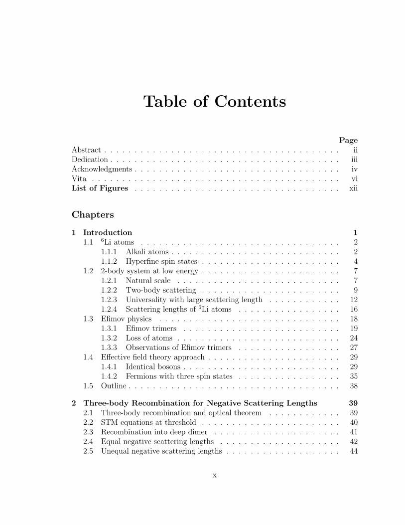
Table of Contents

Page

Abstract . . . . . . . . . . . . . . . . . . . . . . . . . . . . . . . . . . . . . . . iiDedication . . . . . . . . . . . . . . . . . . . . . . . . . . . . . . . . . . . . . . iiiAcknowledgments . . . . . . . . . . . . . . . . . . . . . . . . . . . . . . . . . . ivVita . . . . . . . . . . . . . . . . . . . . . . . . . . . . . . . . . . . . . . . . . viList of Figures . . . . . . . . . . . . . . . . . . . . . . . . . . . . . . . . . . xii

Chapters

1 Introduction 1

1.1 6Li atoms . . . . . . . . . . . . . . . . . . . . . . . . . . . . . . . . . 21.1.1 Alkali atoms . . . . . . . . . . . . . . . . . . . . . . . . . . . . 21.1.2 Hyperfine spin states . . . . . . . . . . . . . . . . . . . . . . . 4

1.2 2-body system at low energy . . . . . . . . . . . . . . . . . . . . . . . 71.2.1 Natural scale . . . . . . . . . . . . . . . . . . . . . . . . . . . 71.2.2 Two-body scattering . . . . . . . . . . . . . . . . . . . . . . . 91.2.3 Universality with large scattering length . . . . . . . . . . . . 121.2.4 Scattering lengths of 6Li atoms . . . . . . . . . . . . . . . . . 16

1.3 Efimov physics . . . . . . . . . . . . . . . . . . . . . . . . . . . . . . 181.3.1 Efimov trimers . . . . . . . . . . . . . . . . . . . . . . . . . . 191.3.2 Loss of atoms . . . . . . . . . . . . . . . . . . . . . . . . . . . 241.3.3 Observations of Efimov trimers . . . . . . . . . . . . . . . . . 27

1.4 Effective field theory approach . . . . . . . . . . . . . . . . . . . . . . 291.4.1 Identical bosons . . . . . . . . . . . . . . . . . . . . . . . . . . 291.4.2 Fermions with three spin states . . . . . . . . . . . . . . . . . 35

1.5 Outline . . . . . . . . . . . . . . . . . . . . . . . . . . . . . . . . . . . 38

2 Three-body Recombination for Negative Scattering Lengths 39

2.1 Three-body recombination and optical theorem . . . . . . . . . . . . 392.2 STM equations at threshold . . . . . . . . . . . . . . . . . . . . . . . 402.3 Recombination into deep dimer . . . . . . . . . . . . . . . . . . . . . 412.4 Equal negative scattering lengths . . . . . . . . . . . . . . . . . . . . 422.5 Unequal negative scattering lengths . . . . . . . . . . . . . . . . . . . 44

x

2.6 Postscript . . . . . . . . . . . . . . . . . . . . . . . . . . . . . . . . . 48

3 Efimov trimer spectrum and three-body recombination 50

3.1 Theoretical formalism . . . . . . . . . . . . . . . . . . . . . . . . . . . 513.1.1 Three-body recombination rates . . . . . . . . . . . . . . . . . 513.1.2 STM equations . . . . . . . . . . . . . . . . . . . . . . . . . . 533.1.3 Three equal scattering lengths . . . . . . . . . . . . . . . . . . 553.1.4 Homogeneous STM equations and Efimov trimers . . . . . . . 573.1.5 Dimer relaxation . . . . . . . . . . . . . . . . . . . . . . . . . 59

3.2 Low-field universal region . . . . . . . . . . . . . . . . . . . . . . . . 603.2.1 Three-body recombination revisited . . . . . . . . . . . . . . . 603.2.2 Efimov trimers . . . . . . . . . . . . . . . . . . . . . . . . . . 63

3.3 High-field universal region . . . . . . . . . . . . . . . . . . . . . . . . 663.3.1 Measurements of three-body recombination . . . . . . . . . . . 663.3.2 Efimov trimers . . . . . . . . . . . . . . . . . . . . . . . . . . 683.3.3 Predictions for three-body recombination . . . . . . . . . . . . 713.3.4 Atom-dimer resonance . . . . . . . . . . . . . . . . . . . . . . 733.3.5 Many-body physics . . . . . . . . . . . . . . . . . . . . . . . . 75

3.4 Summary and discussion . . . . . . . . . . . . . . . . . . . . . . . . . 793.5 Postscript . . . . . . . . . . . . . . . . . . . . . . . . . . . . . . . . . 81

4 Dimer relaxation 82

4.1 Dimer relaxation . . . . . . . . . . . . . . . . . . . . . . . . . . . . . 834.2 STM equations for non-zero energy . . . . . . . . . . . . . . . . . . . 854.3 Zero temperature results . . . . . . . . . . . . . . . . . . . . . . . . . 874.4 Finite temperature results . . . . . . . . . . . . . . . . . . . . . . . . 944.5 Summary and outlook . . . . . . . . . . . . . . . . . . . . . . . . . . 964.6 Postscript . . . . . . . . . . . . . . . . . . . . . . . . . . . . . . . . . 98

5 Outlook 99

xi

List of Figures

Figure Page

1.1 Hyperfine energy levels of 6Li atoms . . . . . . . . . . . . . . . . . . . 61.2 Illustration of Feshbach resonance . . . . . . . . . . . . . . . . . . . . 151.3 Scattering lengths of 6Li atoms in the low-field region . . . . . . . . . 181.4 Scattering lengths of 6Li atoms in the high-field region . . . . . . . . 191.5 Energy spectrum of Efimov trimers for identical bosons . . . . . . . . 211.6 Illustration of three-body recombination . . . . . . . . . . . . . . . . 251.7 Illustration of dimer relaxation . . . . . . . . . . . . . . . . . . . . . . 261.8 Diagrams for 2-atom amplitude . . . . . . . . . . . . . . . . . . . . . 311.9 Integral equation for atom-diatom amplitude . . . . . . . . . . . . . . 34

2.1 Coefficients C and D in the three-body recombination rate . . . . . . 432.2 Three-body recombination rate in the low-field region . . . . . . . . . 452.3 Three-body recombination rate in the high-field region . . . . . . . . 47

3.1 Three-body recombination rate in the low-field region . . . . . . . . . 613.2 Energy and width of the Efimov trimer in the low-field region . . . . 643.3 Three-body recombination rate in the high-field region . . . . . . . . 673.4 Energies of the Efimov trimers in the high-field region . . . . . . . . . 693.5 Widths of the Efimov trimers in the high-field region . . . . . . . . . 703.6 Three-body recombination rates in the high-field region . . . . . . . . 723.7 Dimer relaxation rate near the atom-dimer resonance . . . . . . . . . 75

4.1 Relaxation rate for the 23-dimer . . . . . . . . . . . . . . . . . . . . . 894.2 Relaxation rate for the 13-dimer . . . . . . . . . . . . . . . . . . . . . 914.3 Relaxation rate for the 12-dimer . . . . . . . . . . . . . . . . . . . . . 924.4 Relaxation rate for the 23-dimer at nonzero temperature . . . . . . . 95

xii

Chapter 1

Introduction

The year 2011 is the 100th anniversary of the discovery of superconductivity. A

century of study has enabled great achievements in understanding the mechanism

for this phenomenon and for the related phenomenon of superfluidity. However, our

understanding has not reached the level to achieve the ultimate goal: superconduc-

tivity at room temperature. Toward the advancement of this goal, ultracold atoms

can play a role as a laboratory to improve our understanding of this phenomenon

because the fundamental interactions in these systems are simple and experimentally

controllable. There have been extensive investigations of ultracold atoms consisting

of fermionic atoms with two spin states [1]. This system has a superfluid phase at low

temperature. As the interaction strength of the atoms is varied, the mechanism for

superfluidity exhibits a smooth crossover from the BCS mechanism (Cooper pairing of

atoms) to the BEC mechanism (Bose-Einstein condensation of diatomic molecules).

For fermionic atoms with three spin states, there is the possibility of new superfluid

phases and new mechanisms for superfluidity [2, 3, 4, 5, 6]. The first experiments

with such a system have been carried out using the three lowest hyperfine states of

6Li atoms [7, 8].

Fermionic atoms with three spin states also open up new possibilities in few-

body physics. If the pair scattering lengths are large, there are remarkable three-

1

body phenomena which do not occur in fermions with two spin states. If the three

scattering lengths are infinitely large, there is an infinite sequence of three-atom bound

states called Efimov trimers with a geometric spectrum and an accumulation point

at the three-atom threshold [9, 10]. The ratio of the binding energies of successive

Efimov trimers is approximately 1/515. This remarkable three-body phenomenon is

characterized by discrete scale invariance. Universal phenomena associated with the

discrete scale invariance are referred to as Efimov physics [11, 12]. In this thesis, we

present our studies of Efimov physics in the three lowest hyperfine states of 6Li atoms.

In Sec. 1.1, the basic properties of alkali atoms and their hyperfine states are

reviewed. In Sec. 1.2, the low energy physics in the two-body system and its universal

behavior are explained. In Sec. 1.3, Efimov physics and its observations are discussed.

In Sec. 1.4, our theoretical framework is described. We outline the following chapters

in Sec. 1.5.

1.1 6Li atoms

In this section, we review the basic properties of alkali atoms and their hyperfine

states.

1.1.1 Alkali atoms

The types of atoms that are most easily cooled to ultra-low temperatures are the

alkali atoms that lie below hydrogen in the periodic table. They are lithium (Li),

sodium (Na), potassium (K), rubidium (Rb), and cesium (Cs). In this section, we

review the basic properties of alkali atoms due to their constituents.

The constituents of an atom are protons, neutrons, and electrons. Their electric

charges in units of the proton charge are +1, 0, and −1, respectively. The proton

and neutron are much heavier than an electron; their masses are larger by a factor

2

of about 1840. The structure of an atom consists of a tiny massive core called the

atomic nucleus, surrounded by clouds of electrons that are arranged in shells. The

nucleus consists of protons and neutrons. The number of protons in the nucleus

determines the element of the atom. For example, lithium (Li) atoms have a nucleus

with 3 protons. In an electrically neutral atom, the number of electrons is equal to the

number of protons. The total number of protons and neutrons in the nucleus is called

the atomic mass number and it determines the isotope of the atom. The isotope is

commonly specified by giving the atomic mass number as a pre-superscript. The most

common isotopes of lithium are 6Li and 7Li. The nucleus of these isotopes contain

three and four neutrons, respectively. The electronic structure of an alkali atom such

as Li consists of closed shells of electrons plus a single electron in the outermost shell.

The mass m of a 6Li atom is approximately six times that of a proton. A convenient

conversion constant for 6Li atoms is

h

m= 1.0558× 10−4 cm2/s, (1.1)

where h is Planck’s constant.

All elementary particles can be classified into two categories: bosons and fermions.

Collections of identical particles have dramatically different behavior depending on

whether they are bosons or fermions. For identical bosons, the quantum state must

be symmetric under exchange of any two bosons. This implies that any number of

identical bosons can occupy the same quantum state. The ground state of a many-

body system of N noninteracting identical bosons is a Bose-Einstein condensate, in

which all N bosons occupy the lowest-energy quantum state. For identical fermions,

the quantum state must be antisymmetric under exchange of any two fermions. This

implies the Pauli exclusion principle, which states that two identical fermions cannot

occupy the same quantum state. The ground state of a many-body system of N

3

noninteracting identical fermions consists of a single fermion occupying each of the

N lowest-energy quantum states. Protons, neutrons, and electrons are all fermions.

Composite particles, such as atoms, can also be classified as either fermions or

bosons. A composite particle is a boson if its constituents include an even number

of fermions and it is a fermion if its constituents include an odd number of fermions.

Since a neutral atom contains an equal number of protons and electrons, it is a boson

if its nucleus includes an even number of neutrons and a fermion if its nucleus includes

an odd number of neutrons. For example, a 6Li atom is a fermion and a 7Li atom is

a boson. The majority of the experiments with ultracold fermionic atoms have been

carried out using 6Li atoms.

1.1.2 Hyperfine spin states

An alkali atom in its electronic ground state has multiple spin states. There are two

contributions to its spin: the electronic spin S with quantum number s = 12

and the

nuclear spin I with quantum number i. The 2(2i + 1) spin states can be labeled

|ms,mi〉, where ms and mi specify the eigenvalues of Sz and Iz. The Hamiltonian for

a single atom includes a hyperfine term that can be expressed in the form

Hhyperfine =2Ehf

(2i+ 1)h2I · S. (1.2)

This term splits the ground state of the atom into two hyperfine multiplets with

energies differing by Ehf . The eigenstates can be labeled by the eigenvalues of the

hyperfine spin F = I + S. The associated quantum numbers f and mf specify the

eigenvalues of F 2 and Fz. The eigenvalues of Hhyperfine are

Ef,mf=f(f + 1)− i(i+ 1)− 3

4

2i+ 1Ehf . (1.3)

4

The two hyperfine multiplets of an alkali atom consist of 2i+ 2 states with f = i+ 12

and 2i states with f = i − 12. For example, a 6Li atoms has nuclear spin quantum

number i = 1. The two hyperfine multiplets consist of four states with f = 32

and

two states with f = 12. The f = 3

2multiplet is higher energy by Ehf . The frequency

associated with the hyperfine splitting is Ehf/h ≈ 225 MHz.

In the presence of a magnetic field B = Bz, the Hamiltonian for a single atom

has a magnetic term. The magnetic moment µ of the atom is dominated by the

term proportional to the spin of the electron: µ = µS/( 12h). The magnetic moment

µ of an alkali atom such as Li is approximately that of the single electron in the

outermost shell: µ ≈ −2µB, where µB is the Bohr magneton. The magnetic term in

the Hamiltonian can be expressed in the form

Hmagnetic = −2µ

hS ·B. (1.4)

If B 6= 0, this term splits the two hyperfine multiplets of an alkali atom into 2(2i+1)

hyperfine states. In a weak magnetic field satisfying µB Ehf , each hyperfine mul-

tiplet is split into 2f + 1 equally-spaced Zeeman levels |f,mf 〉. In a strong magnetic

field satisfying µB Ehf , the states are split into a set of 2i+1 states with ms = +12

whose energies increase linearly with B and a set of 2i + 1 states with ms = −12

whose energies decrease linearly with B. Each of those states is the continuation

in B of a specific hyperfine state |f,mf 〉 at small B. It is convenient to label the

states by the hyperfine quantum number f and mf for general B, in spite of the

fact that those states are not eigenstates of F 2 if B 6= 0. We denote the eigenstates

of Hhyperfine + Hmagnetic by |f,mf ;B〉 and their eigenvalues by Ef,mf(B). The two

eigenstates with the maximal value of |mf | are independent of B:

∣

∣f = i+ 12,mf = ±(i+ 1

2);B

⟩

=∣

∣ms = ±12,mi = ±i

⟩

. (1.5)

5

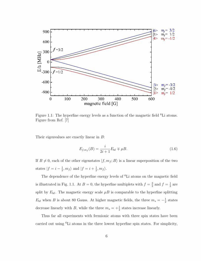
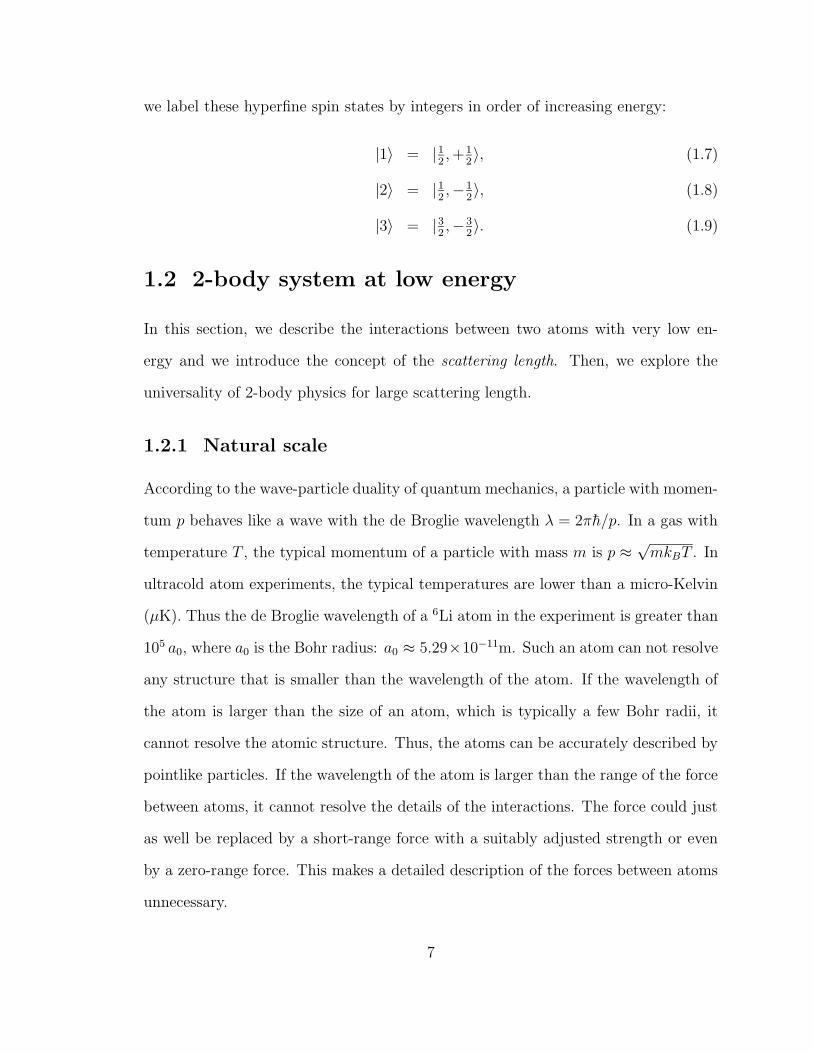
Figure 1.1: The hyperfine energy levels as a function of the magnetic field 6Li atoms.Figure from Ref. [7]

Their eigenvalues are exactly linear in B:

Ef,mf(B) =

i

2i+ 1Ehf ∓ µB. (1.6)

If B 6= 0, each of the other eigenstates |f,mf ;B〉 is a linear superposition of the two

states |f = i− 12,mf〉 and |f = i+ 1

2,mf 〉.

The dependence of the hyperfine energy levels of 6Li atoms on the magnetic field

is illustrated in Fig. 1.1. At B = 0, the hyperfine multiplets with f = 32

and f = 12

are

split by Ehf . The magnetic energy scale µB is comparable to the hyperfine splitting

Ehf when B is about 80 Gauss. At higher magnetic fields, the three ms = −12

states

decrease linearly with B, while the three ms = +12

states increase linearly.

Thus far all experiments with fermionic atoms with three spin states have been

carried out using 6Li atoms in the three lowest hyperfine spin states. For simplicity,

6

we label these hyperfine spin states by integers in order of increasing energy:

|1〉 = |12,+1

2〉, (1.7)

|2〉 = |12,−1

2〉, (1.8)

|3〉 = |32,−3

2〉. (1.9)

1.2 2-body system at low energy

In this section, we describe the interactions between two atoms with very low en-

ergy and we introduce the concept of the scattering length. Then, we explore the

universality of 2-body physics for large scattering length.

1.2.1 Natural scale

According to the wave-particle duality of quantum mechanics, a particle with momen-

tum p behaves like a wave with the de Broglie wavelength λ = 2πh/p. In a gas with

temperature T , the typical momentum of a particle with mass m is p ≈√mkBT . In

ultracold atom experiments, the typical temperatures are lower than a micro-Kelvin

(µK). Thus the de Broglie wavelength of a 6Li atom in the experiment is greater than

105 a0, where a0 is the Bohr radius: a0 ≈ 5.29×10−11m. Such an atom can not resolve

any structure that is smaller than the wavelength of the atom. If the wavelength of

the atom is larger than the size of an atom, which is typically a few Bohr radii, it

cannot resolve the atomic structure. Thus, the atoms can be accurately described by

pointlike particles. If the wavelength of the atom is larger than the range of the force

between atoms, it cannot resolve the details of the interactions. The force could just

as well be replaced by a short-range force with a suitably adjusted strength or even

by a zero-range force. This makes a detailed description of the forces between atoms

unnecessary.

7

The force between two atoms can be specified by a potential U(r) which gives

the potential energy as a function of the separation r of the atoms. The potential

between two neutral atoms is highly repulsive at short distances that are comparable

to the Bohr radius and it is attractive at longer distances. The repulsion between

the outermost electron shells of the two atoms can change the charge distributions

of the shells, making the atoms electrically polarized. This deformation causes an

attractive force between the polarized atoms. This attractive potential is called the

van der Waals potential:

UvdW (r) = −C6

r6, (1.10)

where C6 is a constant that is different for each element. The constant C6 defines a

length scale called the van der Waals length `vdW :

`vdW =4

√

mC6/h2. (1.11)

This is the distance at which the kinetic energy p2/m ∼ h2/m`2vdW of a pair of

atoms is comparable to their potential energy |UvdW (`vdW )| ∼ C6/`6vdW . For 6Li

atoms, `vdW ≈ 65 a0. The van der Waals length is the natural length scale for the

interaction between neutral atoms with sufficiently low energy. Atoms with de Brogile

wavelengths larger than `vdW are unable to resolve even the power-law tail of the

interatomic potential. Their interactions can therefore be described by a short-range

potential or even by a zero-range potential.

The constant C6 also determines the van der Waals energy scale given by

EvdW =h2

m`2vdW

. (1.12)

This is the typical size of the binding energy of the most weakly-bound diatomic

molecules. It also sets the temperature scale EvdW/kB below which we consider the

atoms to be ultracold. For 6Li atoms, this temperature is 6.8 mK. This is comparable

8

to the temperature Ehf/kB set by hyperfine splitting for 6Li atoms, which is about

11 mK. Since the typical wavelength of ultracold atoms is larger than `vdW , they

are unable to resolve details of the interaction potential. This makes it possible to

describe their interactions accurately by a few parameters.

1.2.2 Two-body scattering

In this section, we briefly review scattering of a 2-body system and define some of

the important scattering parameters at low energy.

Let us consider the scattering of a beam of atoms on a target. Part of the beam

is scattered by the target and the remainder of the beam passes through the target

unscattered. If a beam travels along the z axis, the wavefunction of the atom in

the absence of the target is a plane wave eikz, where k is the wavenumber of the

atom, which is determined by its energy: E = h2k2/(2m). The plane wave at a

large distance r from the target can be expressed as an infinite sum of incoming and

outgoing spherical waves [13]:

eikz −→ i

2k

∞∑

l=0

(2l + 1)il[

e−i(kr−lπ/2)

r− ei(kr−lπ/2)

r

]

Pl(cos θ), (r →∞)

(1.13)

where Pl(cos θ) is the Legendre polynomial. Assuming that the potential is rotation-

ally symmetric, the scattered waves are azimuthally symmetric. In the presence of

the target, the wavefunction ψ(r) of the atom at large distance r can still be de-

composed into incoming and outgoing spherical waves. Conservation of probability

requires that the outgoing spherical waves have the same amplitude as in the plane

wave but they can differ in phase:

ψ(r) −→ i

2k

∞∑

l=0

(2l+1)il[

e−i(kr−lπ/2)

r− e2iδl

ei(kr−lπ/2)

r

]

Pl(cos θ), (r →∞)

(1.14)

9

where δl is the phase shift due to the scattering, which depends on the wavenumber

k. The asymptotic wavefunction ψ(r) can be expressed as the sum of the incident

plane wave in Eq. (1.13) and an outgoing spherical wave:

ψ(r) −→ eikz + f(θ)eikr

r, (r →∞) (1.15)

where f(θ) is the scattering amplitude:

f(θ) =∞∑

l=0

2l + 1

k cot δl − ikPl(cos θ). (1.16)

A convenient observable associated with the scattering probability is the cross sec-

tion. The number of incident atoms per unit time and unit area is proportional

to their velocity times their probability density: (hk/m) × |eikz|2 = hk/m. Simi-

larly, the number of scattered atoms per unit time and unit area is proportional to

(hk/m)× |f(θ)eikr/r|2 = (hk/m)|f(θ)|2/r2. Taking the ratio of these two quantities

and integrating over the surface gives the cross section. The differential cross section

is therefore given by

dσ

dΩ= |f(θ)|2. (1.17)

The differential solid angle is dΩ = 2π sin θdθ. The cross section σ is obtained by

integrating over the scattering angle θ.

If the potential is short-ranged with no power-law tail, it is known that the

k2l+1 cot δl for small scattering energy E = h2k2/(2m) can be expanded in powers

of k2 [14]:

k2l+1 cot δl =∞∑

n=0

cl,nk2n. (1.18)

The coefficients cl,n are called effective range parameters. For the S-wave phase shift,

the leading terms in the effective range expansion are

k cot δ0 = −1

a+

1

2rek

2 + · · · , (1.19)

10

where a is the scattering length and re is the effective range. The natural magnitudes

for the effective range coefficients is determined by the length scale ` set by the range

of interaction. By dimensional analysis, cl,n can be expressed as `2n−2l−1 multiplied

by a dimensionless coefficient. In the absence of an enhancement mechanism, we

expect the dimensionless coefficient to be order 1. An example of an enhancement

mechanism is a bound state that is very close to the two-atom threshold. If the bound

state is in the S-wave (l = 0) channel, the scattering length a is large compared to

`. Upon inserting k cot δl from Eq. (1.18) into the scattering amplitude in Eq. (1.16),

one can see that that the S-wave (l = 0) term dominates the amplitude at low energy.

The higher partial waves (l > 0) are suppressed by (k`)2l.

The low energy expansions in Eqs. (1.18) and (1.19) express the information about

the potential that is relevant at low energy in terms of a few parameters, such as a

and re. The coefficients of higher powers of k in the effective range expansion are less

important, because they are suppressed by powers of the energy.

The potential between atoms is not short-ranged, because it has the power-law

tail at large r given by the van der Waals potential in Eq. (1.10). Consequently,

the low energy expansions in Eq. (1.18) break down [15]. Since the van der Waals

potential decreases as a high power of r, some of the terms in the expansion are the

same as for a short-range potential. For the S-wave phase shift, the two leading terms

in the effective range expansion still have the form in Eq. (1.19). The expansion of

k cot δ1 still starts at order k−2, so the P-wave term in the cross section is suppressed

by k2 at low energy. For all higher partial waves (l ≥ 2), the expansion of k cot δl

start at order k−4, so the corresponding terms in the cross section are suppressed by

k4. Therefore, the S-wave term still dominates at sufficiently low energy [15, 11]. At

extremely low energy, the only relevant interaction parameter is the scattering length

a.

11

1.2.3 Universality with large scattering length

As discussed in the previous section, in the generic case when the effective range

parameters have natural values set by the range `, low energy scattering can be

treated systematically by expanding in powers of the energy. In this subsection, we

discuss the case of an unnaturally large scattering length |a| ` and we introduce

the concept of universality.

We consider two particles with a large scattering length |a| ` and with energy

small compared to the scale h2/m`2 set by the range. For convenience, we will refer

to the particles as atoms. We will see that this system has nontrivial properties that

are completely determined by the scattering length. We will refer to these properties

as universal. This adjective is appropriate because different systems with a large

scattering length will have identical low-energy behavior up to one overall length

scale that is set by a. If we insert the expansion in Eq. (1.19) into the S-wave term

in the amplitude in Eq. (1.16), there are two terms that are not suppressed. These

terms define the universal scattering amplitude:

f(k) =1

−1/a− ik . (1.20)

By inserting Eq. (1.20) into Eq. (1.17) and integrating over the solid angle, we obtain

the total cross section:

σ(k) =4π

1/a2 + k2. (1.21)

Thus the cross section for low-energy scattering has a nontrivial form that is com-

pletely determined by the scattering length.

If the scattering length a is large and positive, there is a diatomic molecule with

universal properties. We will refer to this bound state as the shallow dimer. Quan-

tum mechanics implies that bound states are associated with poles in the scattering

12

amplitude f(k) for complex values of the momentum k. If f(k) has a pole on the

positive imaginary axis at k = iκ, then there is a bound state with binding energy

h2κ2/m. The scattering amplitude in Eq. (1.20), has a pole at k = i/a. If a > 0, this

pole is in the upper half-plane of the complex variable k, so there is a corresponding

bound state. The universal expression for the binding energy of the shallow dimer is

ED =h2

ma2(a > 0). (1.22)

The typical separation of its constituents is a. In addition to the shallow dimer,

there may also be diatomic molecules whose binding energies are of order h2/(m`2),

or larger. We will refer to them as deep dimers, because they are much more deeply

bound than the shallow dimer. A deep dimer has no universal properties. Its binding

energy is much larger than that of the shallow dimer. The typical separation of its

constituents is order ` or smaller, so it is much smaller than the shallow dimer.

The limit of large scattering length |a| ` is closely related to the zero-range

limit `→ 0. The zero-range limit can be achieved by taking the range of the interac-

tion potential to zero while simultaneously increasing its depth so that the scattering

length remains fixed. The limit is independent of the shape of the potential. In

the zero-range limit, the universal scattering amplitude in Eq. (1.20) becomes ex-

act up to arbitrarily high energies. The universal expression for the binding energy

in Eq. (1.22) also becomes exact. If there are any deep dimers, their binding ener-

gies become infinitely large. Since the universal results are the same in both limits,

we will sometimes use the phrases large scattering length, zero-range, and universal

interchangeably.

In the limit a → ∞, the universal cross section approaches 4π/k2, which is the

maximum value allowed by unitarity. The limit a → ±∞ is therefore called the

unitary limit. In this limit, there is no length scale associated with the interactions.

13

Thus the system has a symmetry under scaling the spacial coordinates by an arbitrary

positive factor λ and the time by a factor λ2. This symmetry is called scale invariance.

The scale invariance of the unitary limit manifests itself at finite scattering length

by simple scaling behavior under simultaneous scaling of a and kinematic variables.

For example, when a and the momentum variable k are scaled by the factors λ and

λ−1, the cross section in Eq. (1.21) is changed by a factor λ2: σ(λ−1k;λa) = λ2σ(k; a).

The binding energy in Eq. (1.22) also shows the scaling behavior. When a is scaled

by λ, ED is changed by a factor λ−2: ED(λa) = λ−2ED(a). This scaling behavior is

a general feature of the system with large scattering length. It follows from the fact

that the scattering length a is the only interaction parameter that sets a length scale

in the zero-range limit.

Universality is important, because it relates phenomena in various fields of physics.

There are examples of systems with large scattering lengths in nuclear physics and

high energy physics as well as in atomic physics. In nuclear physics, the best example

is the neutron, whose two spin states interact with a large negative scattering length.

In high energy physics, a good example is the charm mesons D∗0 and D0, which form

a very weakly bound state called the X(3872) and therefore must have a large positive

scattering length. A classic example in atomic physics is 4He atoms, whose scattering

length is about +200 a0, which is much larger than the van der Waals length scale

`vdW ≈ 10 a0. Another example in atomic physics is the three lowest hyperfine states

of 6Li atoms at a large magnetic field. Each pair of spin states interacts with a

scattering length −2160 a0, which is much larger than the van der Waals length scale

`vdW ≈ 65 a0.

Atomic physics is unique in that it is also possible to tune the scattering lengths of

atoms experimentally. This can be accomplished by adjusting the magnetic field near

a Feshbach resonance. A Feshbach resonance arises when a diatomic molecule is near

14

B

aa bg

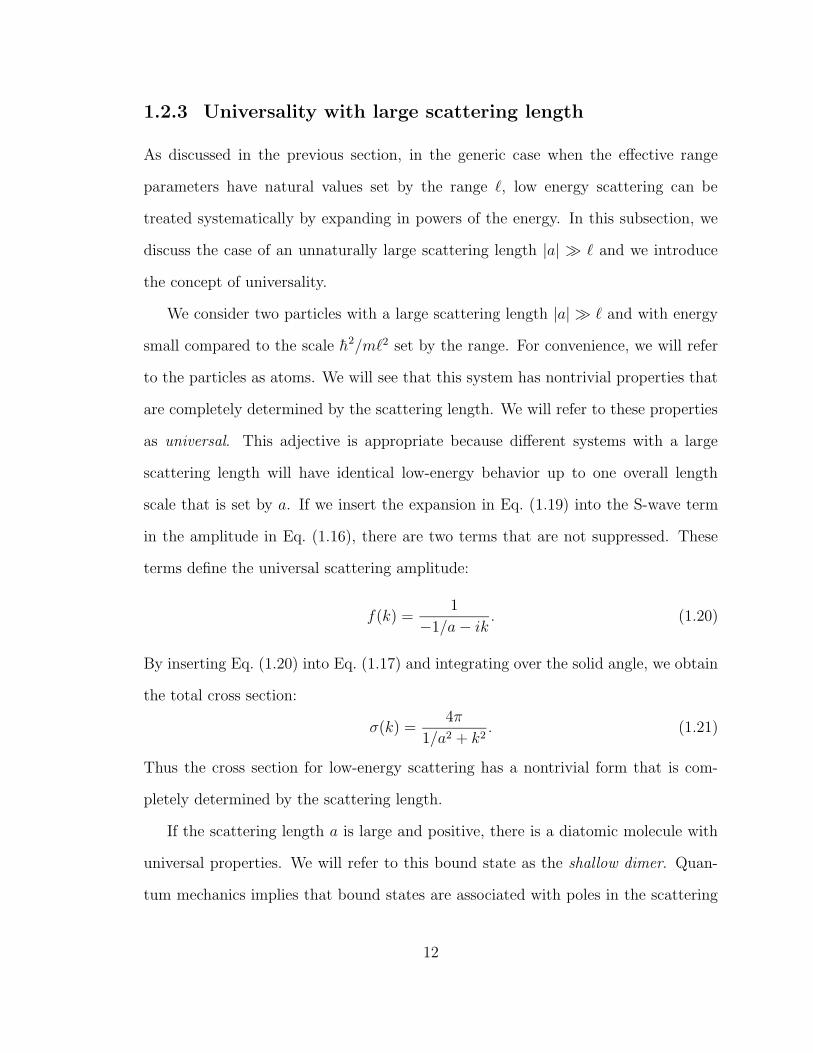
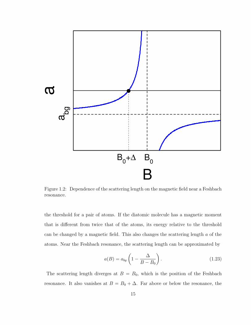
B0+∆ B0

Figure 1.2: Dependence of the scattering length on the magnetic field near a Feshbachresonance.

the threshold for a pair of atoms. If the diatomic molecule has a magnetic moment

that is different from twice that of the atoms, its energy relative to the threshold

can be changed by a magnetic field. This also changes the scattering length a of the

atoms. Near the Feshbach resonance, the scattering length can be approximated by

a(B) = abg

(

1− ∆

B − B0

)

. (1.23)

The scattering length diverges at B = B0, which is the position of the Feshbach

resonance. It also vanishes at B = B0 + ∆. Far above or below the resonance, the

15

scattering length approaches abg. The dependence of the scattering length on the

magnetic field is illustrated in Fig. 1.2 for the case ∆ < 0. By adjusting the magnetic

field, the scattering length can be tuned to any desired value. In particular, it can

be made infinitely large by tuning B to B0. For a detailed discussion of Feshbach

resonances, the readers is referred to a review article [16].

1.2.4 Scattering lengths of 6Li atoms

In this subsection, we introduce our conventions for the scattering lengths of a

fermionic atom with three spin states. We also show how the scattering lengths

for the three lowest hyperfine states of 6Li atoms depend on the magnetic field.

We label the three spin states of the atom by the integers 1, 2, and 3. We

denote the scattering length of the pair ij by either aij = aji or ak, where (ijk) is

a permutation of (123). The two-body physics for fermions with two distinct spin

states that have a large pair scattering length aij is very simple in the zero-range

limit. The scattering amplitude for the pair ij with relative wavenumber k is given

by

fij(k) =1

−1/aij − ik, (1.24)

which is Eq. (1.20) with a replaced by aij. For positive aij , there is a weakly-bound

diatomic molecule with constituents i and j that we will refer to as either the (ij)

dimer or the ij-dimer. Its binding energy is h2/(ma2ij). We refer to the (12), (23), and

(13) dimers collectively as shallow dimers. As mentioned in previous section, there

are also deep dimers whose binding energies are comparable to or larger than the van

der Waals energy scale and are insensitive to changes in the large scattering lengths.

In the case of 6Li atoms, the three spin states are the hyperfine states given

in Eqs. (1.7), (1.8), and (1.9). The pair scattering lengths a12, a23, and a13 have

Feshbach resonances near 834 G, 811 G, and 690 G, respectively [17]. Beyond these

16

Feshbach resonances, all three scattering lengths approach the triplet scattering length

−2140 a0, which is large and negative. The zero-range approximation should be

accurate if |a12|, |a23|, and |a13| are all much larger than `vdW ≈ 62.5 a0 and it should

be at least qualitatively useful if |aij | > 2`vdW. There are two regions of the magnetic

field in which all three scattering lengths are larger than 2`vdW ≈ 125 a0: a low-field

region 122 G < B < 485 G and a high-field region B > 608 G. These two universal

regions are separated by a non-universal region in which all three scattering lengths

go through zeros. Efimov physics in the universal regions will be characterized by

values of κ∗ and η∗ that may not be the same in the two regions. In general, these

parameters may be expected to vary slowly with the magnetic field, just like the

scattering length away from a Feshbach resonance. In a sufficiently narrow region of

magnetic field, they can be treated as constants. While their values could in principle

be calculated from microscopic atomic physics, in practice they have to be determined

by measurements of 3-body observables.

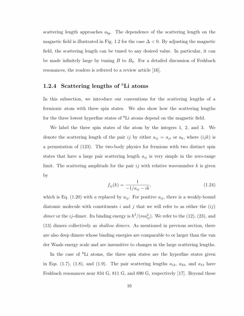
In Fig. 1.3, the three scattering lengths a12, a23, and a13 are shown as functions

of the magnetic field in the low-field region from 0 to 600 G [18]. Throughout most

of this region, the smallest scattering length is a12. It satisfies |a12| > 2 `vdW in the

interval 122 G < B < 485 G and achieves its largest value −290 a0 = −4.6 `vdW near

320 G. This interval therefore contains a universal region in which all three scatter-

ing lengths are negative and relatively large. The zero-range approximation should

be quantitatively useful in the middle of this interval, but it becomes increasingly

questionable as one approaches the edges.

In Fig. 1.4, the three scattering lengths a12, a23, and a13 are shown as functions

of the magnetic field [18] in the high-field region from 600 G to 1200 G. This region

includes the Feshbach resonances in a12, a23, and a13 near 834 G, 811 G, and 690 G,

respectively. Beyond these Feshbach resonances, all three scattering lengths approach

17

0 200 400 600B [G]

-1.0

-0.5

0.0

0.5

1.0

a [u

nits

of 1

03a 0]

122313

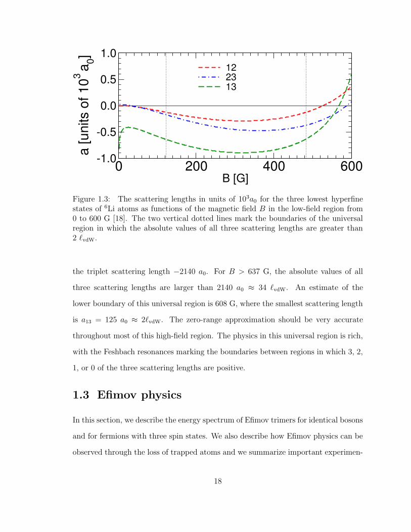
Figure 1.3: The scattering lengths in units of 103a0 for the three lowest hyperfinestates of 6Li atoms as functions of the magnetic field B in the low-field region from0 to 600 G [18]. The two vertical dotted lines mark the boundaries of the universalregion in which the absolute values of all three scattering lengths are greater than2 `vdW.

the triplet scattering length −2140 a0. For B > 637 G, the absolute values of all

three scattering lengths are larger than 2140 a0 ≈ 34 `vdW. An estimate of the

lower boundary of this universal region is 608 G, where the smallest scattering length

is a13 = 125 a0 ≈ 2`vdW. The zero-range approximation should be very accurate

throughout most of this high-field region. The physics in this universal region is rich,

with the Feshbach resonances marking the boundaries between regions in which 3, 2,

1, or 0 of the three scattering lengths are positive.

1.3 Efimov physics

In this section, we describe the energy spectrum of Efimov trimers for identical bosons

and for fermions with three spin states. We also describe how Efimov physics can be

observed through the loss of trapped atoms and we summarize important experimen-

18

600 800 1000 1200B [G]

-5

0

5

10

a [u

nits

of 1

03a 0]

122313

Figure 1.4: The scattering lengths in units of 103a0 for the three lowest hyperfinestates of 6Li atoms as functions of the magnetic field B in the high-field region from600 G to 1200 G [18]. The three vertical lines mark the positions of the Feshbachresonances.

tal observations as of July 2011.

1.3.1 Efimov trimers

Three particles with large scattering length also have universal properties, but they

are much more intricate than those for two particles. These universal properties were

discovered by Vitaly Efimov [9, 10] and developed in a series of subsequent papers.

The most dramatic consequence is the existence of a sequence of universal 3-body

bound states that are now called Efimov trimers. The spectrum of Efimov trimers is

particularly simple and remarkable in the unitary limit in which the scattering length

is taken to infinity. There are an infinite number of geometrically spaced low-energy

bound states with an accumulation point at zero energy. In the case of identical

bosons, the binding energies of two successive trimers differ by a multiplicative fac-

tor of λ20 ≈ 515, where λ0 = eπ/s0 ≈ 22.7. The constant s0 is the solution to a

19

transcendental equation:

s0 cosh(πs0/2) =8√3

sinh(πs0/6). (1.25)

The numerical value of s0 is approximately 1.00624. The spectrum of Efimov trimers

in the unitary limit can be expressed as

E(n)T = λ

2(n∗−n)0

h2κ2∗

m(a = ±∞) , (1.26)

where κ∗ is the binding wavenumber of the trimer labeled n∗ and n is an integer.

In the 2-body sector, the unitary limit is characterized by scale invariance. How-

ever scale invariance requires the binding energies of discrete bound states to be either

0 or∞. Thus the existence of Efimov trimers indicates that scale invariance is violated

in the 3-body sector. However, there is a remnant of that symmetry. The Efimov

spectrum in Eq. (1.26) is compatible with discrete scale invariance with the discrete

scaling factor λ0. We will refer to universal phenomena associated with discrete scale

invariance in the three-body sector as Efimov physics [11].

In the 2-body sector, the scattering length is the only length scale provided by

interactions in the zero-range limit. In the 3-body sector, the discrete spectrum of

Efimov states in the unitary limit requires a 3-body parameter that provides another

length scale in addition to the scattering length. If there were no such parameter,

the system would have continuous scale invariance in the unitary limit. One simple

choice for the 3-body parameter is the wavenumber κ∗ defined by the spectrum of

Efimov trimers in the unitary limit in Eq. (1.26). Discrete scale invariance requires

that any dependence of physical quantities on the parameter κ∗ much be log-period

with discrete scaling factor λ0. The universal properties in the 3-body sector for

identical bosons are determined by the scattering length a and the 3-body parameter

κ∗.

20

1/a

K

x 22.7

x 22.7

Figure 1.5: Binding energies of three successive Efimov trimers (red curves) for iden-tical bosons. Arrows indicate the discrete scaling invariance along the directions ofthe arrows. The variable K is defined in Eq. (1.27).

The binding energies of three successive Efimov trimers are illustrated in Fig. 1.5

using variables that are particularly well suited to exhibiting the discrete scale invari-

ance. The horizontal axis is the inverse scattering length a−1. The vertical axis is an

energy variable K that also has a dimension (length)−1:

K = sign(E)√

m|E|/h. (1.27)

According to the Efimov effect, there are infinitely many trimer states along the

vertical axis (a = ±∞) as one approaches the origin from below. Only three of those

infinitely many trimers are shown in the figure. The spectrum of Efimov trimers is

K = −λn∗−n0 κ∗, so the ratio of the positions of two adjacent trimers on the axis is

λ0 ≈ 22.7. In the figure, the straight line approaching the origin at a 45 angle

with respect to the horizontal axis represents the threshold for atom-dimer scattering

21

states, which is K = −1/a. For a > 0, the trimers disappear through the atom-

dimer threshold at values of the scattering length a = λn∗−n0 a∗ that differ by the

discrete scaling factor. There is a threshold resonance in atom-dimer scattering at

each of these scattering lengths because of the trimer state near the threshold. The

horizontal axis corresponds to the threshold for three-atom scattering states. For

a < 0, the trimer states cross the three-atom threshold at values of the scattering

length a = λn∗−n0 a′∗ that differ by the discrete scaling factor. There is a resonance in

three-atom scattering at each of those values of the scattering lengths because of the

Efimov trimer near the 3-atom threshold. The scattering lengths a∗ and a′∗ at which

the Efimov trimers cross the thresholds differ from 1/κ∗ by universal multiplicative

constants: a∗ = 0.071/κ∗ and a′∗ = −1.5/κ∗.

Efimov trimers are sharp states with the spectrum in Eq. (1.26) only if there are

no deep dimers in the 2-body spectrum. If there are deep dimers, Efimov trimer can

decay into an atom and a deep dimer and this gives the trimer a width. The inclusive

effects of all the deep dimers can be taken into account by analytically continuing

the Efimov parameter κ∗ to a complex value that is conveniently expressed in the

form κ∗ exp(iη∗/s0), where κ∗ and η∗ are positive real parameters [19]. Making the

substitution κ∗ → κ∗ exp(iη∗/s0) on the right side of Eq. (1.26), we find that binding

energies of the Efimov trimers acquire imaginary parts. The imaginary part can be

interpreted as half of the decay width Γ(n)T of the Efimov resonance. The binding

energies and widths of the Efimov trimers are

E(n)T = λ

2(n∗−n)0

h2κ2∗ cos(2η∗/s0)

m(a = ±∞) , (1.28)

Γ(n)T = λ

2(n∗−n)0

2h2κ2∗ sin(2η∗/s0)

m. (1.29)

Efimov trimers can also exist in fermionic system. The simplest fermionic system

is identical fermions. Because of the Pauli exclusion principle, S-wave interactions are

22

prohibited so their scattering length is zero. Thus, identical fermions with extremely

low energy are essentially noninteracting. In the case of fermionic atoms with two spin

states, the two spin states can interact through a large scattering length. However in

the 3-atom sector, the interaction is not strong enough to produce the Efimov effect.

The simplest case in which the Efimov effect arises is fermionic atoms with three

spin states. The low-energy interaction of each pair ij of spin states is given by a

scattering length aij . Thus there are three independent scattering lengths: a12, a23,

and a13. The Efimov effect arises only if all three scattering lengths are large. The

discrete scaling factor for fermions with 3 spin states has the same value λ0 ≈ 22.7

as for identical bosons. The universal properties are completely determined by the 3

scattering lengths a12, a23, and a13 and by the 3-body parameters κ∗ and η∗.

We take the zero of energy to be the scattering threshold for three atoms in the

three different spin states. If ajk is positive, the scattering threshold for an atom of

type i and a (jk) dimer is −h2/(ma2jk). We will refer to this scattering threshold as

the i + (jk) atom-dimer threshold. A trimer whose constituents are atoms of types

1, 2, and 3 must have energy below the 3-atom threshold and below the i + (jk)

atom-dimer threshold if ajk > 0. In general the spectrum of Efimov trimers depends

in a complicated way on the three scattering lengths. However if the three scattering

lengths are all equal, the spectrum reduces to that for identical bosons, which is

illustrated in Fig. 1.5. In the case, we can write a12 = a23 = a31 = a. In the unitary

limit a = ±∞, the trimer energies are given by Eq. (1.26) or by Eq. (1.29) if there are

deep dimers. The Efimov trimers disappear through the 3-atom threshold at negative

values of a given by a = λn−n∗

0 a′∗. They disappear through the atom-dimer threshold

at positive values of a given by a = λn−n∗

0 a∗.

The first experimental studies of fermionic atoms with three spin states have been

carried out using the three lowest hyperfine states of 6Li atoms [7, 8]. Efimov physics

23

in the system is complicated because the three pairwise scattering lengths a12, a23,

and a31 all change with the magnetic field as illustrated in Figs. 1.3 and 1.4.

One of the most important theoretical developments in few-body physics in re-

cent years was the discovery that the universality of particles with large scattering

lengths extends to the 4-body sector. In papers published in 2004 and 2007, Platter,

Hammer, and Meissner showed that there are two universal four-body bound states

associated with each Efimov trimer [20, 21]. They calculated the binding energies of

these universal tetramers in a limited range of 1/a. In 2009, von Stecher, D’Incao,

and Green mapped out the spectrum of the universal tetramers over the entire range

of 1/a [22]. In particular, they calculated the scattering lengths at which the univer-

sal tetramers appear at the 4-atom threshold and they pointed out that they could

be observed through 4-atom loss resonances. Universality in the 4-body sector and

beyond remains an important frontier of few-body physics.

1.3.2 Loss of atoms

The easiest way to observe Efimov trimers in ultracold atomic gases is through reso-

nant enhancement of loss rates. The atoms are trapped in a potential created by a

magnetic field or by laser beams. An atom can escape from the trapping potential if

it acquires a kinetic energy that is larger than the depth of the potential through an

inelastic scattering process. The escaping atoms can usually not be observed directly,

but they can be observed indirectly through the decrease in the number of trapped

atoms. By appropriate choice of hyperfine states, one can arrange that two-body

inelastic processes are forbidden by conservation of energy. At sufficiently low densi-

ties, the dominant loss mechanisms will then be through inelastic scattering processes

involving three atoms. There are two such loss mechanisms: three-body recombination

and dimer relaxation [23, 24, 25].

24

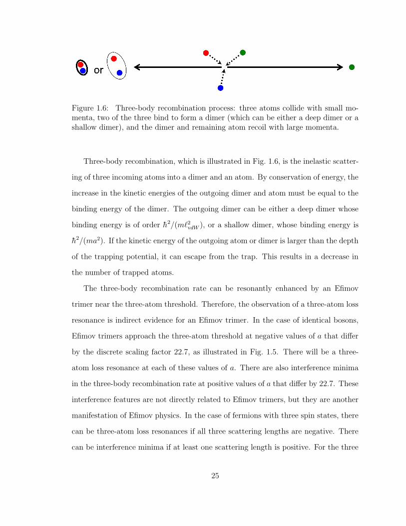
Figure 1.6: Three-body recombination process: three atoms collide with small mo-menta, two of the three bind to form a dimer (which can be either a deep dimer or ashallow dimer), and the dimer and remaining atom recoil with large momenta.

Three-body recombination, which is illustrated in Fig. 1.6, is the inelastic scatter-

ing of three incoming atoms into a dimer and an atom. By conservation of energy, the

increase in the kinetic energies of the outgoing dimer and atom must be equal to the

binding energy of the dimer. The outgoing dimer can be either a deep dimer whose

binding energy is of order h2/(m`2vdW ), or a shallow dimer, whose binding energy is

h2/(ma2). If the kinetic energy of the outgoing atom or dimer is larger than the depth

of the trapping potential, it can escape from the trap. This results in a decrease in

the number of trapped atoms.

The three-body recombination rate can be resonantly enhanced by an Efimov

trimer near the three-atom threshold. Therefore, the observation of a three-atom loss

resonance is indirect evidence for an Efimov trimer. In the case of identical bosons,

Efimov trimers approach the three-atom threshold at negative values of a that differ

by the discrete scaling factor 22.7, as illustrated in Fig. 1.5. There will be a three-

atom loss resonance at each of these values of a. There are also interference minima

in the three-body recombination rate at positive values of a that differ by 22.7. These

interference features are not directly related to Efimov trimers, but they are another

manifestation of Efimov physics. In the case of fermions with three spin states, there

can be three-atom loss resonances if all three scattering lengths are negative. There

can be interference minima if at least one scattering length is positive. For the three

25

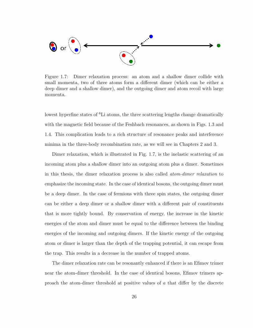
Figure 1.7: Dimer relaxation process: an atom and a shallow dimer collide withsmall momenta, two of three atoms form a different dimer (which can be either adeep dimer and a shallow dimer), and the outgoing dimer and atom recoil with largemomenta.

lowest hyperfine states of 6Li atoms, the three scattering lengths change dramatically

with the magnetic field because of the Feshbach resonances, as shown in Figs. 1.3 and

1.4. This complication leads to a rich structure of resonance peaks and interference

minima in the three-body recombination rate, as we will see in Chapters 2 and 3.

Dimer relaxation, which is illustrated in Fig. 1.7, is the inelastic scattering of an

incoming atom plus a shallow dimer into an outgoing atom plus a dimer. Sometimes

in this thesis, the dimer relaxation process is also called atom-dimer relaxation to

emphasize the incoming state. In the case of identical bosons, the outgoing dimer must

be a deep dimer. In the case of fermions with three spin states, the outgoing dimer

can be either a deep dimer or a shallow dimer with a different pair of constituents

that is more tightly bound. By conservation of energy, the increase in the kinetic

energies of the atom and dimer must be equal to the difference between the binding

energies of the incoming and outgoing dimers. If the kinetic energy of the outgoing

atom or dimer is larger than the depth of the trapping potential, it can escape from

the trap. This results in a decrease in the number of trapped atoms.

The dimer relaxation rate can be resonantly enhanced if there is an Efimov trimer

near the atom-dimer threshold. In the case of identical bosons, Efimov trimers ap-

proach the atom-dimer threshold at positive values of a that differ by the discrete

26

scaling factor 22.7, as illustrated in Fig. 1.5. There will be an atom-dimer loss reso-

nance at each of these values of a. In the case of fermions with three spin states, there

can be atom-dimer loss resonances if at least one of the three scattering lengths is

positive. If at least two of the three scattering lengths are positive, there can also be

interference minima in the dimer relaxation rates. The minima are a manifestation

of Efimov physics that has no analog in identical bosons [26]. For the three lowest

hyperfine states of 6Li atoms, the dramatic changes in the three scattering lengths

as a function of the magnetic field leads to a rich structure in the dimer relaxation

rates, as we will see in Chapter 4.

1.3.3 Observations of Efimov trimers

The first discovery of an Efimov trimer in atomic physics was made in August 2007

by a group at the University of Innsbruck led by Rudi Grimm [27]. They observed

a resonant enhancement in the three-body recombination rate in a gas of ultracold

bosonic 133Cs atoms with large negative scattering length. They also observed an

interference minimum in the recombination rate at a positive scattering length. In a

subsequent experiment with a mixture of 133Cs atoms and dimers, the Innsbruck group

observed an atom-dimer loss resonance [28]. Efimov trimers have also been observed

using other types of bosonic atoms. In January 2009, a group at the University of

Florence observed three-body recombination loss resonances in a mixture of 41K and

87Rb atoms [29]. They can be attributed to heteronuclear Efimov trimers that are

composed of both K and Rb atoms. In April 2009, the Florence group observed

the three-body recombination loss resonances associated with two successive Efimov

trimers in a gas of ultracold 39K atoms [30]. The ratio of the scattering lengths at

these resonances was consistent with the predicted discrete scaling factor of 22.7. In

June 2009, a group at Bar-Ilan University observed an Efimov loss resonance and an

27

interference minimum on opposite sides of a Feshbach resonance in gas of ultracold

7Li atoms [31]. In November 2009, a group at Rice University observed two Efimov

loss resonances and two interference minima on opposite sides of the same Feshbach

resonance [32].

The universal tetramers associated with Efimov trimer have been observed through

four-atom loss processes [20, 21, 22]. In March 2009, the Innsbruck group observed loss

features from two universal tetramers associated with an Efimov trimer in 133Cs atoms

[33]. In November 2009, the Rice group measured two sets of universal tetramers that

are associated with two successive Efimov trimers in 7Li atoms [32].

Efimov physics has also been observed in fermionic systems with three or more

spin states [9, 10]. There are three groups that have carried out experiments with

many-body systems consisting of 6Li atoms in the three lowest hyperfine states:

• a group at Pennsylvania State University led by Ken O’Hara, which we will

refer to as the Penn State group,

• a group at the University of Heidelberg led by Selim Jochim, which we will refer

to as the Heidelberg group,

• a group at University of Tokyo led by Masahito Ueda, which we will refer to as

the Tokyo group.

Several observations of Efimov features in 6Li atoms have been reported by these three

groups. The discovery of a three-body recombination loss resonance in the low-field

region was announced by the Heidelberg group in June 2008 [7] and by the Penn State

group in October 2008 [8]. The first theoretical analysis explaining these loss features

in terms of an Efimov trimer close to the three-atom threshold appeared in November

2008 [34]; it makes up Chapter 2 of this thesis. Another recombination loss resonance

in the high-field region was discovered by the Penn State group in August 2010 [35].

28

A more comprehensive analysis of Efimov physics in 6Li atoms was completed in

August 2009 [36]; it makes up Chapter 3 of this thesis. This work predicted two

resonances in atom-dimer relaxation due to an Efimov trimer near the atom-dimer

threshold. The resonances were identified in March 2010 by the Heidelberg group [37]

and by the Tokyo group [38]. A thorough analysis of Efimov physics in atom-dimer

relaxation was completed in June 2010 [39]; it makes up Chapter 4 of this thesis. The

most exciting recent experimental development in this field is the radio-frequency

association of atoms and dimers into Efimov trimers announced by the Heidelberg

group in June 2010 [40] and by the Tokyo group in October 2010 [41].

1.4 Effective field theory approach

Effective field theory (EFT) is a general method for describing the low-energy de-

grees of freedom of a system using the formalism of quantum field theory [42, 43].

The simplest EFT that can describe particles with a large scattering length is the

zero-range model, which describes point particles that interact only through contact

interactions. The EFT is particularly useful in exploring universality at large scat-

tering length, because all nonuniversal terms suppressed by `/a are set exactly to

zero. In this section, the EFT approach to the 2-atom and 3-atom problem using the

zero-range model will be discussed. In this section, we set h = m = 1 for simplicity.

1.4.1 Identical bosons

In this subsection, we discuss the EFT approach for identical bosons.

In the quantum field theory framework, an atom is annihilated by a quantum

field ψ(r, t) and is created by a quantum field ψ†(r, t) at space-time point r and t.

Symmetry under the exchange of identical bosons is implemented through equal-time

29

commutation relations:

[ψ(r, t), ψ(r′, t)] = 0, (1.30a)

[

ψ(r, t), ψ†(r′, t)]

= δ3(r − r′). (1.30b)

The Lagrangian density for a nonrelativistic free field is given by

Lfree = ψ†(

i∂

∂t+∇2

2

)

ψ. (1.31)

This is the kinetic term in the Lagrangian density for interacting atoms. It implies

that the Feynman propagator for an atom of energy E and momentum k is i/(E −

k2 + iε).

The interaction terms in the Lagrangian must respect the symmetries of the funda-

mental interactions. Power counting rules can be developed that indicate the relative

importance of all the possible interaction terms [44, 45]. The power-counting rules for

nonrelativistic particles with short-range interactions reveal that the most important

interaction is a contact interaction between the particles. We will not develop these

power-counting rules. Instead, we will simply argue that a contact interaction is a

natural choice to describe low-energy atoms because their long wavelengths prevent

them from resolving the structure of their interaction potential. The interaction terms

of the zero-range model are given by

Lint = −g2

4

(

ψ†ψ)2 − g3

36

(

ψ†ψ)3, (1.32)

where g2 and g3 are the coupling constants for the 2-atom and 3-atom contact inter-

actions, respectively. The factors 4 and 36 in the denominators are chosen to cancel

symmetry factors associated with permutations of identical bosons. The interaction

term in Eq. (1.32) implies that the Feynman rules for the two-atom and three-atom

vertices are −ig2 and −ig3, respectively.

30

= + + + · · ·

= +

Figure 1.8: Diagrams for 2-atom amplitude: (upper diagram) summation over allorder diagrams in g2. (lower diagram) Lippmann-Schwinger integral equation.

All effects of interactions in the two-atom sector can be encoded concisely in a

function of a single variable: the transition amplitude A(E) for the scattering of a

pair of atoms with total energy E in their center-of-momentum frame. For example,

the scattering amplitude f(E) in Eq. (1.20) is given by

A(E = k2) = 8πf(k). (1.33)

Fig. 1.8 shows two diagrammatic equations for the 2-atom transition amplitude. The

upper diagrammatic equation shows the perturbative expansion of the amplitude or-

der by order in the coupling constant g2. Because of the large scattering length,

these diagrams must be summed to all orders in g2. The lower diagrammatic equa-

tion in Fig. 1.8 is an alternative way to calculate the amplitude that exploits the

recursive nature of the perturbative expansion. The corresponding equation is called

Lippmann-Schwinger integral equation:

iA(E) = −ig2 + (−ig2)1

2

∫

d3k

(2π)3

i

E − k2 + iε

(

iA(E))

. (1.34)

The integral over the momentum k in Eq. (1.34) is ultraviolet divergent. It can be

calculated analytically by imposing a ultraviolet momentum cutoff |k| < Λ. The

31

Eq. (1.34) then reduces to an algebraic equation for A(E) whose solution is

A(E) = −[

1

g2

+Λ

4π2− 1

8π

√−E − iε

]−1

. (1.35)

This amplitude depends explicitly on the momentum cutoff Λ. It can be independent

of the cutoff only if the coupling constant g2 depends implicitly on Λ in such a way

that the cutoff dependences in Eq. (1.35) cancel out. The dependence on g2 and Λ

can be eliminated in favor of a physical quantity, such as the scattering length a. The

scattering amplitude f(k) defined by Eq. (1.33) is

f(k) =

[

8π

g2

+2Λ

π+ ik

]−1

. (1.36)

This has the same dependence on k as the universal scattering amplitude in Eq. (1.20)

if a is identified with the following function of g2 and Λ:

a =1

8π

[

1

g2

+Λ

4π2

]−1

. (1.37)

After using this equation to eliminate g2 from the transition amplitude in Eq. (1.35),

we find that it is independent of the ultraviolet cutoff:

A(E) = −8π

[

1

a−√−E − iε

]−1

. (1.38)

This procedure of removing the cutoff dependence by eliminating g2 in favor of a is

called renormalization. The parameter g2 is often referred to as a bare coupling con-

stant while a is the renormalized coupling constant. Since the transition amplitude

A(E) in Eq. (1.38) encodes all physical observables in the 2-body sector, the renor-

malization of g2 is sufficient to remove all dependence on the ultraviolet cutoff in the

2-atom sector. The fact that the renormalization of the 2-atom transition amplitude

is simple and analytic is very useful in the calculation of 3-atom amplitudes.

The transition amplitude for three atoms is much more complicated than that for

32

two atoms. The general amplitude in the center-of-momentum frame is a function

of 9 independent variables: three energies and two momentum vectors. However all

Efimov physics in the three-atom sector can be encoded in a much simpler function

AS(p, k;E) called the STM amplitude which is a function of only 3 variables: the total

energy E and two relative momenta. The STM amplitude satisfies an integral equa-

tion called the STM equation that was first derived by Skorniakov–Ter-Martirosian

[46].

The three-body problem for particles with large scattering length was not under-

stood within the EFT framework until 1999, when important progress was made by

by Bedaque, Hammer, and van Kolck [47, 48]. They introduced a diatom field d by

changing the interaction Lagrangian in Eq. (1.32) to

LBHvK =g2

4d†d− g2

4

(

d†ψ2 + ψ†2d)

− g3

36d†dψ†ψ. (1.39)

There is no kinetic term for d in the Lagrangian, so its equation of motion is

d− ψ2 − (g3/9g2) dψ†ψ = 0. (1.40)

The 3-atom contact interaction (ψ†ψ)3 in Eq. (1.32) has been replaced by an atom-

diatom contact interaction d†dψ†ψ and by an interaction that allows a transition

from a diatom to a pair of atoms and vice versa. The Lagrangian in Eq. (1.39) is

equivalent to that in Eq. (1.32). This can be seen in the 2-atom or 3-atom sector

simply by eliminating d using the equation of motion in Eq. (1.40). It is more difficult

to show that it is also equivalent in the N -atom sector with N ≥ 4.

The diatom field trick of Ref. [47] allows the general 3-atom transition amplitude

to be reduced to the much simpler transition amplitude for an atom and a diatom.

The atom-diatom transition amplitude satisfies an integral equation that is equivalent

to the STM equation. Fig. 1.9 shows a diagrammatic integral equation for the atom-

33

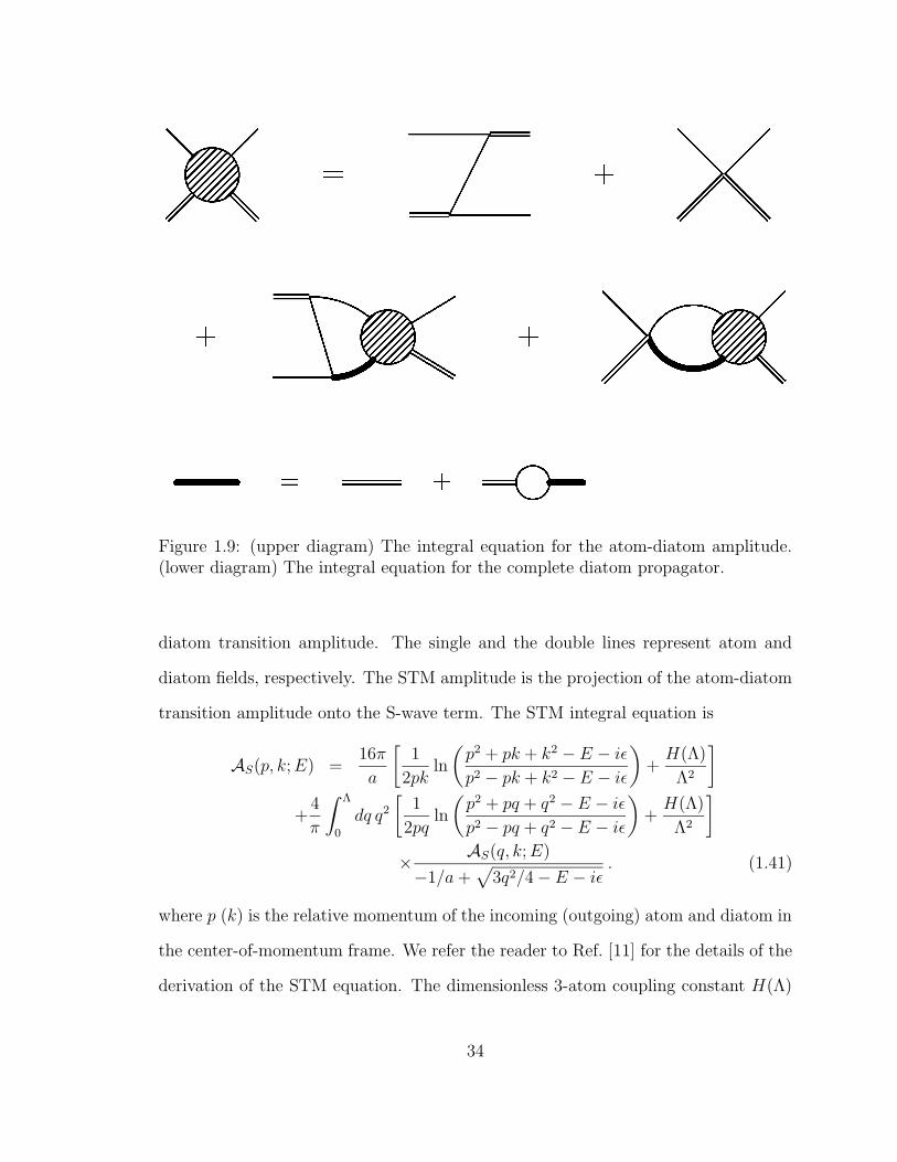
Figure 1.9: (upper diagram) The integral equation for the atom-diatom amplitude.(lower diagram) The integral equation for the complete diatom propagator.

diatom transition amplitude. The single and the double lines represent atom and

diatom fields, respectively. The STM amplitude is the projection of the atom-diatom

transition amplitude onto the S-wave term. The STM integral equation is

AS(p, k;E) =16π

a

[

1

2pkln

(

p2 + pk + k2 − E − iεp2 − pk + k2 − E − iε

)

+H(Λ)

Λ2

]

+4

π

∫ Λ

0

dq q2

[

1

2pqln

(

p2 + pq + q2 − E − iεp2 − pq + q2 − E − iε

)

+H(Λ)

Λ2

]

× AS(q, k;E)

−1/a+√

3q2/4− E − iε. (1.41)

where p (k) is the relative momentum of the incoming (outgoing) atom and diatom in

the center-of-momentum frame. We refer the reader to Ref. [11] for the details of the

derivation of the STM equation. The dimensionless 3-atom coupling constant H(Λ)

34

is defined by

g3 = −9g22

Λ2H(Λ), (1.42)

where H(Λ) is a dimensionless log-periodic function of Λ that can be approximated

by

H(Λ) ≈ h0cos[s0 ln(Λ/Λ∗) + arctan s0]

cos[s0 ln(Λ/Λ∗)− arctan s0]. (1.43)

This renormalization condition defines a renormalized three-body parameter Λ∗. The

analytic approximation derived in Ref. [47] was Eq. (1.43) with h0 = 1. In Ref. [49],

it was found that the analytic approximation is accurate only to about 10%. It

was found however that to a numerical accuracy of about 10−3, H is given by the

expression in Eq. (1.43) with the multiplicative numerical constant h0 = 0.879 [49].

For the practical solution of the STM equation in Eq. (1.41), it is convenient to fix

the numerical value of H(Λ) and then tune Λ to reproduce a three-body observable,

such as the binding energy of an Efimov trimer. Given the numerical value of H(Λ),

one can use Eq. (1.43) to determine Λ∗ although it is not necessary. The use of the

approximate expression in Eq. (1.43) with a generic cutoff Λ introduces an uncertainty

of about 10−3 associated with renormalization of the 3-atom contact interaction. This

uncertainty can be avoided by the very simple choice H = 0. In this case, there is no

atom-diatom contact interaction and it is the ultraviolet cutoff Λ that plays the role

of the 3-body parameter.

1.4.2 Fermions with three spin states

In this subsection, we discuss the EFT approach for fermions with three spin states.

Much of the formalism is similar to that for identical bosons except for symmetry

factors. We will focus our discussion on aspects associated with the difference in

symmetry factors.

We denote the fermionic quantum fields for the three spin states by ψi(r, t) and

35

ψ†i (r, t), where i = 1, 2, and 3. Antisymmetry under the exchange of identical

fermions is implemented through equal-time anticommutation relations:

ψi(r, t), ψj(r′, t) = δij, (1.44a)

ψi(r, t), ψ†j (r

′, t)

= δij δ3(r − r′). (1.44b)

The Lagrangian density has a kinetic term for each spin state:

Lfree =∑

i=1,2,3

ψ†i

(

i∂

∂t+∇2

2

)

ψi. (1.45)

The interactions between the atoms consist of two-atom contact interaction between

pairs of atoms in different spin states and a three-atom contact interaction between

three atoms in different spin states. The interaction terms in the Lagrangian density

are given by

Lint = −∑

i>j

gij ψ†iψ

†jψiψj − g123 ψ

†1ψ

†2ψ

†3ψ3ψ2ψ1. (1.46)

Note that there are no symmetry factors multiplying the coupling constants, unlike

in the interaction term for identical bosons in Eq. (1.32).

All effects of interactions in the two-atom sector can be encoded in three function

of a single variable: the transition amplitude Aij(E) = Aji(E) for a pair of atoms in

different spin states i and j. For example, the scattering amplitude fij(k) for that

pair of atoms is given by

Aij(E = k2) = 4πfij(k). (1.47)

Note that there is a factor of 2 difference from the corresponding equation for identical

bosons in Eq. (1.33). The diagrammatic equations for the transition amplitudeAij(E)

are similar to those in Fig. 1.8, with the two boson lines replaced by a line for atom

36

i and a line for atom j. The Lippmann-Schwinger integral equation is

iAij(E) = −igij + (−igij)

∫

d3k

(2π)3

i

E − k2 + iε

(

iAij(E))

. (1.48)

Note that there is no symmetry factor of 12

in front of the integral, unlike Eq. (1.48) for

identical bosons. The amplitude Aij differs from that for identical bosons Eq. (1.35)

in the symmetry factor:

Aij(E) = −[

1

gij

+Λ

2π2− 1

4π

√−E − iε

]−1

. (1.49)

The renormalization of the coupling constant gij is given by

aij =1

4π

[

1

gij+

Λ

2π2

]−1

, (1.50)

where aij is the scattering length for the pair of spin state i and j.

The diatom field trick of Bedaque, Hammer, and van Kolck can be generalized to

the field theory for fermion with three spin states. Three diatom fields d12, d23, and

d13 are introduced through the interaction Lagrangian

LBHvK =∑

i<j

gij

(

d†ijdij − d†ijψiψj − ψ†iψ

†jdij

)

−g123

3

(

d†12d12ψ†3ψ3 + d†23d23ψ

†1ψ1 + d†13d13ψ

†2ψ2

)

. (1.51)

All Efimov physics in the 3-atom sector can be encoded in a set of 9 STM amplitudes

Aii′(p, k;E). They are the transition amplitudes from atom i and diatom jk to atom

i′ and diatom j ′k′, where (i, j, k) and (i′, j′, k′) are permutations of (1, 2, 3). The

Lagrangian with diatom fields can be used to derive the STM equations for these

amplitudes, which are a set of 9 coupled integral equations. The explicit forms for

these equations are given in Chapter 2, 3, and 4, where they are used to calculate

various aspect of Efimov physics for the three lowest hyperfine states of 6Li atoms.

37

1.5 Outline

In the following three chapters, we present theoretical studies on Efimov physics in 6Li

atoms that were published in Refs. [34, 36, 39]. In Chapter 2, we calculate the 3-body

recombination rate for fermionic atoms with three spin states and large negative pair

scattering lengths. We provide semi-analytic expressions for the cases of 2 or 3 equal

scattering lengths. We obtain numerical results for the case of the three lowest hyper-

fine states of 6Li atoms and compare with experimental measurements of three-body

recombination rate in the low-field region. In Chapter 3, we calculate the universal

predictions for the spectrum of Efimov states and for the 3-body recombination rate

with any combination of signs for the three pair scattering lengths. Using the position

and width of an observed Efimov loss resonance as input, we calculate the binding

energies and widths of Efimov trimers and the three-body recombination rate for 6Li

atoms in the high-field region. We predict two atom-dimer loss resonances associ-

ated with Efimov trimers disappearing through the atom-dimer threshold. We also

predict an interference minimum in the three-body recombination rate at a magnetic

field where the 3-spin mixture may be sufficiently stable to allow experimental study

of the many-body system. In Chapter 4, we calculate the atom-dimer relaxation rate

for atoms and dimers composed of fermionic atoms with three spin states. We give

detailed prediction for Efimov features in 6Li atoms in the high-field region, including

the two atom-dimer loss resonance and two local minima in the dimer relaxation rate.

We conclude in Chapter 5 with an outlook on Efimov physics in 6Li atoms.

38

Chapter 2

Three-body Recombination for

Negative Scattering Lengths

In this chapter, we present calculations of the 3-body recombination rate at threshold

in the zero-range limit for fermionic atoms with three spin states and large negative

pair scattering lengths. We provide semi-analytic expressions for the cases of 2 or

3 equal scattering lengths and we obtain numerical results for the general case of 3

different scattering lengths. We apply our general results to the three lowest hyperfine

states of 6Li atoms and compare with the first 3-body recombination rate measure-

ments for these atoms. The analysis presented in this chapter was carried out in

collaboration with Eric Braaten, Hans-Werner Hammer, and Lucas Platter and was

published in Physical Review Letters [34] in August 2009.

2.1 Three-body recombination and optical theorem

We consider an atom of mass m with three distinguishable states that we label 1, 2,

and 3 and refer to as spin states. We denote the scattering length of the pair i and

j by either aij = aji or ak, where (ijk) is a permutation of (123). The rate equations

for the number densities ni of atoms in the three spin states are

d

dtni = −K3n1n2n3. (2.1)

39

By the optical theorem, the event rate constant K3 in the low-temperature limit can

be expressed as twice the imaginary part of the forward T-matrix element for 3-atom

elastic scattering in the limit where the momenta of the atoms all go to 0. Using

diagrammatic methods, the T-matrix element for elastic scattering can be expressed

as the sum of 9 amplitudes corresponding to the 3 possible pairs that are the first

to scatter and the 3 possible pairs that are the last to scatter. For small collision

energies, the leading contributions to those amplitudes come from the S-wave terms,

which we denote by Aij(p, p′), where p (p′) is the relative momentum between the

pair that scatters first (last) and the third atom labelled i (j). The rate constant K3

in Eq. (4.1) is

K3 =32π2

m

∑

i,j

aiajImAij(0, 0), (2.2)

where the sums are over i, j = 1, 2, 3.

2.2 STM equations at threshold

The amplitudes Aij(p, p′) can be calculated in the zero-range limit by solving 9 cou-

pled integral equations that are generalizations of the Skorniakov–Ter-Martirosian

(STM) equation [46]. To determine ImAij(0, 0), it is sufficient to solve the 9 coupled

STM equations for Aij(p, 0):

Aij(p, 0) =1− δijp2

+2

π

∑

k

(1− δkj)

×∫ Λ

0

dq Q(q/p)Dk(q)Aik(q, 0), (2.3)

where

Q(x) =x

2log

1 + x+ x2

1− x+ x2, (2.4)

Dk(q) = (−1/ak +√

3q/2)−1, (2.5)

40

and Λ is an ultraviolet cutoff. The solutions to Eqs. (2.3) are singular as p → 0.

The singular terms, which are proportional to 1/p2, 1/p, and ln p, appear only in

ReAij(p, 0) for real p and can be derived by iterating the integral equations [50].

Since ImAij(p, 0) must be extrapolated to p = 0, it is useful to transform Eqs. (2.3)

into coupled STM equations for amplitudes Aij(p, 0) obtained by subtracting the

singular terms from Aij(p, 0). For p Λ, the solutions depend log-periodically on

Λ with a discrete scaling factor eπ/s0 ≈ 22.7, where s0 = 1.00624. The dependence

on the arbitrary cutoff Λ can be eliminated in favor of a physical 3-body parameter,

such as the Efimov parameter κ∗ defined by the spectrum of Efimov states in the

limit where all 3 scattering lengths are infinitely large [11]:

En = −(

e2π/s0

)−n h2κ2∗

m(a12 = a23 = a31 = ±∞). (2.6)

If we restrict Λ to a range that corresponds to a multiplicative factor of 22.7, then Λ

differs from κ∗ only by a multiplicative numerical constant. Thus we can also simply

take Λ as the 3-body parameter.

2.3 Recombination into deep dimer

If aij > 0, there is a contribution to K3 from 3-body recombination into the shallow

dimer whose constituents have spins i and j and whose binding energy is h2/(ma2ij). If

a12, a23, and a31 are all negative, there are no shallow dimers. The solutions Aij(p, 0)

to the coupled STM equations in Eq. (2.3) are all real-valued in this case, so the rate

constant K3 in Eq. (2.2) is predicted to be 0.

If there are deeply-bound diatomic molecules (deep dimers) in any of the three 2-

body channels, there are also contributions to K3 from 3-body recombination into the

deep dimers. If all 3 scattering lengths are negative, these are the only contributions to

K3. The coupled STM equations in Eq. (2.3) do not take into account contributions

41

from deep dimers. The inclusive effect of all the deep dimers can be taken into

account by analytically continuing the Efimov parameter κ∗ to a complex value [19]:

κ∗ → κ∗ exp(iη∗/s0), where η∗ is a positive real parameter. Making this substitution

in Eq. (2.6), we find that the Efimov states acquire nonzero decay widths determined

by η∗. If we use the ultraviolet cutoff Λ as the 3-body parameter, the inclusive effects

of deep dimers can be taken into account by changing the upper limit of the integral

in Eq. (2.3) to Λ exp(iη∗/s0), so the path of integration extends into the complex

plane. Having made this change, the solutions Aij(p, 0) are complex-valued even if

a12, a23 and a31 are all negative. The rate constant K3 in Eq. (2) is a function of

the scattering lengths a12, a23, and a31 and the 3-body parameters Λ and η∗ and it

vanishes as η∗ → 0. It gives the inclusive rate for 3-body recombination into all deep

dimers.

2.4 Equal negative scattering lengths

We focus our attention on cases in which all scattering lengths are negative, so the

only recombination channels are into deep dimers. We first consider the case of 3

equal scattering lengths: a12 = a23 = a13 = a < 0. In this case Eq. (2.3) reduces –

after summing over i and j – to the STM equation for identical bosons. In Ref. [19],

Braaten and Hammer deduced an analytic expression for the 3-body recombination

rate constant for identical bosons with a large negative scattering length a:

K3 =16π2C sinh(2η∗)

sin2[s0 ln(D|a|κ∗)] + sinh2 η∗

ha4

m, (2.7)

where s0 = 1.00624, C, andD are numerical constants. This formula exhibits resonant

enhancement for a near the values (eπ/s0)n(Dκ∗)−1 for which there is an Efimov state

at the 3-body threshold. Fitting our numerical results for K3/a4 as functions of aΛ

and η∗, we determine the numerical constants to be C = 29.62(1) and D = 0.6642(2).

42

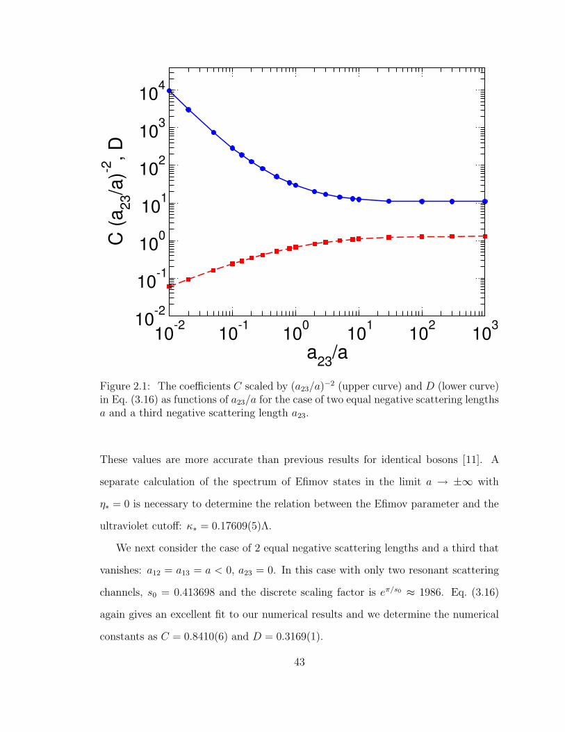
10-2 10-1 100 101 102 103

a23/a10-2

10-1

100

101

102

103

104

C (a

23/a

)-2, D

Figure 2.1: The coefficients C scaled by (a23/a)−2 (upper curve) and D (lower curve)

in Eq. (3.16) as functions of a23/a for the case of two equal negative scattering lengthsa and a third negative scattering length a23.

These values are more accurate than previous results for identical bosons [11]. A

separate calculation of the spectrum of Efimov states in the limit a → ±∞ with

η∗ = 0 is necessary to determine the relation between the Efimov parameter and the

ultraviolet cutoff: κ∗ = 0.17609(5)Λ.

We next consider the case of 2 equal negative scattering lengths and a third that

vanishes: a12 = a13 = a < 0, a23 = 0. In this case with only two resonant scattering

channels, s0 = 0.413698 and the discrete scaling factor is eπ/s0 ≈ 1986. Eq. (3.16)

again gives an excellent fit to our numerical results and we determine the numerical

constants as C = 0.8410(6) and D = 0.3169(1).

43

We now consider the case of 2 equal negative scattering lengths and a third that

is unequal: a12 = a13 = a < 0, a23 < 0. Eq. (3.16) with s0 = 1.00624 continues

to provide an excellent fit to our numerical results. The fitted values of C and D

are shown as functions of a23/a in Fig. 2.1. For |a23| |a|, the coefficients seem to

have the limiting behaviors C ≈ 10.88(2) (a23/a)2 and D ≈ 1.30(1). Their limiting

behaviors for |a23| |a| do not seem to be simple power laws. This is not surprising,

because the discrete scaling factor 22.7 changes to 1986 when a23 = 0.

2.5 Unequal negative scattering lengths

Finally we consider the general problem of 3 different negative scattering lengths, for

which we can obtain numerical results for given values of a12, a23, and a13. We apply

our method to 6Li atoms in the three lowest hyperfine states. The 3 pair scattering

lengths a12, a23, and a13 are shown as functions of the magnetic field in Fig. 1.3 and

1.4. There are two regions of the magnetic field in which all 3 scattering lengths are

negative and satisfy |aij | > 2`vdW: a low-field region 122 G < B < 485 G and a

high-field region B > 834 G. In the low-field region, the smallest scattering length

is a12 and it achieves its largest value −290 a0 = −4.6 `vdW near 320 G. The zero-

range approximation may be reasonable near this value of B. In the high-field region,

the smallest scattering length is a13. It increases from −3285 a0 at B = 834 G to

−2328 a0 ≈ −37 `vdW at 1200 G. Thus the zero-range approximation should be very

accurate in this region. We emphasize that the 3-body parameters κ∗ and η∗ need

not be the same in the two universal regions, since there are zeroes of the scattering

lengths between them.

The 3-body recombination rate K3 for 6Li atoms in the three lowest hyperfine

states has recently been measured by the Heidelberg group [7] and by the Penn State

group [8]. Their results are shown in Figs. 2.2 and 2.3. In Ref. [7], K3 was measured

44

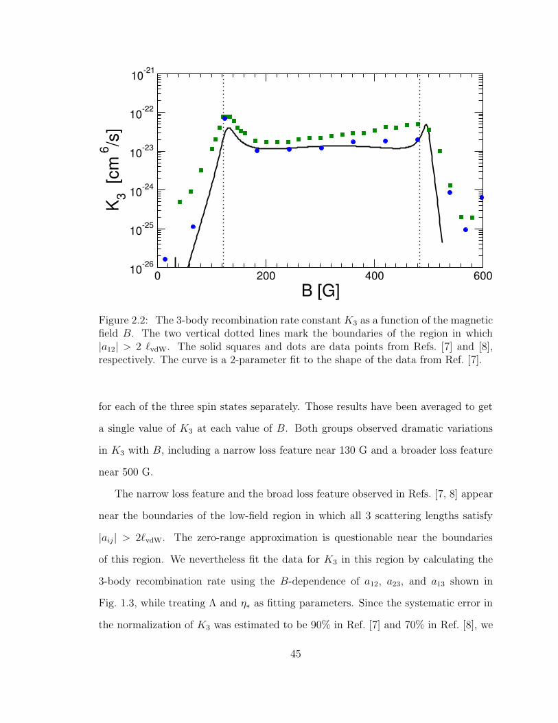
0 200 400 600B [G]

10-26

10-25

10-24

10-23

10-22

10-21

K 3 [cm

6/s

]

Figure 2.2: The 3-body recombination rate constant K3 as a function of the magneticfield B. The two vertical dotted lines mark the boundaries of the region in which|a12| > 2 `vdW. The solid squares and dots are data points from Refs. [7] and [8],respectively. The curve is a 2-parameter fit to the shape of the data from Ref. [7].

for each of the three spin states separately. Those results have been averaged to get

a single value of K3 at each value of B. Both groups observed dramatic variations

in K3 with B, including a narrow loss feature near 130 G and a broader loss feature

near 500 G.

The narrow loss feature and the broad loss feature observed in Refs. [7, 8] appear

near the boundaries of the low-field region in which all 3 scattering lengths satisfy

|aij | > 2`vdW. The zero-range approximation is questionable near the boundaries

of this region. We nevertheless fit the data for K3 in this region by calculating the

3-body recombination rate using the B-dependence of a12, a23, and a13 shown in

Fig. 1.3, while treating Λ and η∗ as fitting parameters. Since the systematic error in

the normalization of K3 was estimated to be 90% in Ref. [7] and 70% in Ref. [8], we

45

only fit the shape of the data and not its normalization. A 2-parameter fit to the data

from Ref. [7] in the region 122 G < B < 485 G gives Λ = 436 a−10 and η∗ = 0.11. The

fit to the shape of the narrow loss feature is excellent as shown in Fig. 2.2. Having

fit the position and width of the loss feature feature, the normalization of K3 is

determined. In the region of the narrow loss feature, the prediction for K3 lies below

the data of Ref. [7] by about a factor of 2, which is well within the systematic error

of 90%. The excellent fit to the shape of the narrow loss feature and the prediction of

the normalization of K3 consistent with the data suggests that this loss feature may

arise from an Efimov state near the threshold for atoms in spin states 1, 2, and 3. As

shown in Fig. 2.2, our fit predicts that K3 should be almost constant in the middle of

the low-field region and that there should be another narrow loss feature at its upper

end near 500 G. The data from both groups in Fig. 2.2 increases monotonically in the

middle of the low-field region and, instead of a narrow loss feature, there is a broad

loss feature near the upper end of this region. We are unable to get a good fit to the

slope of logK3 in the middle of the low-field region or to the shape of the broad loss

feature by adjusting Λ and η∗.

In Ref. [8], the 3-body recombination rate was also measured at higher values of

the magnetic field. They include three data points in the region B > 834 G, where all

3 scattering lengths are extremely large and negative. If the central values of the last

two data points are used to determine the 3-body parameters, we obtain Λ = 37.0 a−10

and η∗ = 2.9×10−4. As shown in Fig. 2.3, this fit predicts the resonant enhancement

of the 3-body recombination rate near 1160 G. If we allow for the systematic error

by increasing or decreasing both data points by 70%, the position of the resonance

does not change, but η∗ increases to 5×10−4 or decreases to 9×10−5, respectively. If

we take into account the statistical errors by increasing or decreasing the data points

by one standard deviation, the position of the resonance can be shifted downward to

46

600 800 1000 1200 1400B [G]

10-22

10-21

10-20

10-19

10-18

10-17

10-16

K 3 [cm

6/s

]

Figure 2.3: The 3-body recombination rate constant K3 as a function of the magneticfield B. The three vertical dashed lines mark the positions of the Feshbach resonances.The solid dots are data points from Ref. [8]. The curve is a 2-parameter fit to thelast two data points.

1109 G or upward to 1252 G. Thus it might be worthwhile to search for an Efimov

resonance in this region. If such a feature were observed, measurements of its position

and width would determine accurately the two 3-body parameters κ∗ and η∗. Our

equations could then be used to predict the total 3-body recombination rate in the

entire universal region B > 610 G, including the regions where 1, 2, or 3 of the

scattering lengths are positive. Note that the third-to-last data point in Fig. 2.3

shows no sign of the large increase in K3 near the Feshbach resonance at 834 G that

is predicted by our fit. However the measurement of K3 involves a model for the

heating of the system, and the failure of our fit at 835 G might be attributable to the

breakdown of that model near the Feshbach resonance.

In summary, we have calculated the recombination rate of three distinguishable

47

atoms with large negative pair scattering lengths in the zero-range limit. We have

provided simple semi-analytical expressions for the rate if 2 or 3 scattering lengths

are equal. Using our general result for 3 unequal scattering lengths, we showed that

the narrow 3-body loss feature for 6Li atoms with three spin states [7, 8] may be

attributed to an Efimov state near threshold. In next chapter, it will be clarified by

calculating the energy spectrum of the Efimov trimer.

2.6 Postscript

The analysis presented in this chapter was completed in November 2008. Shortly after

it appeared, similar analyses of the three-body recombination rate in the low-field

region were completed by a group at the University of Tokyo in November 2008 [51]

and a group at the University of Heidelberg in December 2008 [52]. The Heidelberg

group used a functional renormalization group method to calculate the three-body

recombination rate. The Tokyo group calculated the three-body recombination rate

by solving the free three-body Schrodinger equation with boundary conditions at

short distance. They also calculated the binding energy of the Efimov trimer. This

demonstrated explicitly that the narrow loss resonance near 120 G and the broad

loss resonance near 480 G are both due to the Efimov trimer crossing the three-

atom threshold. The different width of these two loss resonances was subsequently

explained by the experimental group at Heidelberg as being due to the changes with

the magnetic field of the binding energies of the deep dimers that are produced by

three-body recombination [53].

In the analysis presented above, we pointed out that there should also be an

Efimov loss resonance for 6Li atoms in the high-field region above 600 G. In August

2009, a narrow loss resonance was discovered near 900 G by the Penn State group [35]

and also by the Heidelberg group [54]. In Chapter 3, we use the measured position

48

and width of this feature to make universal predictions for the Efimov spectrum and

the three-body recombination rate for 6Li atoms in the high-field region.

49

Chapter 3

Efimov trimer spectrum and

three-body recombination

In this chapter, we calculate universal predictions for various aspects of Efimov physics

for the three lowest hyperfine spin states of 6Li atoms. In Section 3.1, we explain how

universal predictions for 3-body observables can be calculated efficiently by solving

coupled sets of integral equations. We apply these methods specifically to the 3-body

recombination rate and to the binding energies and widths of Efimov trimers. In

Section 3.2, we summarize previous experimental and theoretical work on 6Li atoms

in the universal region at low magnetic fields where all 3 scattering lengths are negative

and relatively large. In Section 3.3, we use the complex 3-body parameter determined

by the Penn State group to calculate universal predictions for the binding energies and

widths of Efimov trimers and for the three-body recombination rate in regions where

one or more of the scattering lengths are large and positive. We predict an atom-dimer

resonance at 672 ± 2 G where an Efimov trimer disappears through an atom-dimer

threshold. We predict an interference minimum in the 3-body recombination rate at

759± 1 G where the 3-spin mixture may be sufficiently stable to allow experimental

study of the many-body system. We also discuss the implications of our predictions

for the many-body physics of 6Li atoms. We summarize our results in Section 3.4.

The analysis presented in this chapter was carried out in collaboration with Eric

50

Braaten, Hans-Werner Hammer, and Lucas Platter and was published in Physical

Review A [36] in January 2010.

3.1 Theoretical formalism

3.1.1 Three-body recombination rates

Three-body recombination is a three-atom collision in which two of the atoms form a

dimer. In the case of three fermions in the same spin state, 3-body recombination is

strongly suppressed at low temperature, because each pair of atoms has only P-wave

interactions. In the case of two fermions of type i and a third atom of a different type

j, two of the pairs have S-wave interactions with scattering length aij . The rate for

3-body recombination in the zero-range limit still decreases to 0 as the energy E of

the atoms approaches the threshold, decreasing like E if aij > 0 [55] and like E3 if

aij < 0 [56]. In the case of three distinct spin states, all three pairs of atoms can have

S-wave interactions. There is no threshold suppression of three-body recombination

if at least two of the three scattering lengths are large. If aij is large and positive,

one of the recombination channels is into the (ij) dimer and a recoiling atom with

complimentary spin k. If there are deep dimers in any of the three 2-body channels,

they provide additional recombination channels. If all three scattering lengths are

negative, the only recombination channels are into deep dimers.

The rate equations for the number densities ni of atoms in the three spin states

are

d

dtni = −K3n1n2n3. (3.1)

The event rate constant K3 can be separated into the inclusive rate constant Kdeep3

for recombination into deep dimers and the exclusive rate constants K(ij)3 for recom-

51

bination into each of the three possible shallow dimers:

K3 = Kdeep3 +Kshallow

3 , (3.2)

Kshallow3 = K

(12)3 +K

(23)3 +K

(13)3 . (3.3)

The term K(ij)3 is nonzero only if aij > 0.

In the low-temperature limit, the rate constantK3 and the exclusive rate constants

K(ij)3 can be expressed in terms of T-matrix elements for processes in which the initial

state consists of three atoms in the spin states 1, 2, and 3 with momentum 0. By the

optical theorem, K3 is twice the imaginary part of the forward T-matrix element for

3-atom elastic scattering in the limit where the momenta of the atoms all go to 0:

K3 = 2 Im T (0,0,0;0,0,0). (3.4)

The T-matrix element is singular as all the momenta go to zero, but its imaginary

part is not. If aij > 0, the rate constant K(ij)3 for recombination into the (ij) dimer

is the square of the T-matrix element for three atoms with momentum 0 to scatter

into the dimer and a recoiling atom multiplied by the atom-dimer phase space:

K(ij)3 =

4m

3√

3πhak

|Tk(0,0,0; p,−p)|2∣

∣

∣

∣

|p|=2h/(√

3ak)

. (3.5)

The dimer and the recoiling atom with complementary spin k both have momentum

2h/(√

3ak). For convenience, we will switch to wavenumber variables in the remainder

of the paper.

The T-matrix elements in Eqs. (3.4) and (3.5) can be expressed in terms of am-

plitudes Aij(p, q;E) for the transition from an atom of type i and a complimentary

diatom pair into an atom of type j and a complimentary diatom pair, with the two

diatom pairs being the first to interact and the last to interact, respectively. The

projection onto S-waves reduces the amplitude to a function of three variables: the

52

relative wavenumber p of the incoming atom and diatom, the relative wavenumber q

of the outgoing atom and diatom, and the total energy E of either the incoming atom

and diatom or the outgoing atom and diatom. The rate constant K3 in Eq. (3.4) can

be expressed as

K3 =32π2h

m

∑

i,j

aiajImAij(0, 0; 0), (3.6)

where the sums are over i, j = 1, 2, 3. The exclusive rate constant in Eq. (3.5) for

3-body recombination into the (ij) dimer can be expressed as

K(ij)3 =

512π2h

3√

3ma2k

∣

∣

∣

∣

∣

∑

l

alAlk(0, 2/(√

3ak); 0)

∣

∣

∣

∣

∣

2

, (3.7)

where k is the complimentary spin to ij and the sum is over l = 1, 2, 3.

3.1.2 STM equations

The 9 amplitudes Aij(p, q;E) satisfy coupled integral equations in the variable q

that are generalizations of the Skorniakov–Ter-Martirosian (STM) equation [46]. To

determine the rate constants for 3-body recombination in Eqs. (3.6) and (3.7), it is

sufficient to set the relative wavenumber in the initial state to 0 and the total energy

to 0. The 9 coupled STM equations for Aij(0, p; 0) are [34]

Aij(0, p; 0) =1− δijp2

+2

π

∑

k

(1− δkj)

∫ Λ

0

dq Q(p, q; 0)Dk(3q2/4)Aik(0, q; 0),(3.8)

where

Q(p, q;E) =q

2plog

p2 + pq + q2 −mE/h2

p2 − pq + q2 −mE/h2 , (3.9)

Dk(p2) =

[

−1/ak +√

p2 − iε]−1

, (3.10)

and Λ is an ultraviolet cutoff that must be large compared to p, 1/|a1|, 1/|a2|, and

1/|a3|. Since the T-matrix elements in Eqs. (3.6) and (3.7) involve only the three

53

linear combinations∑

i aiAij(0, p; 0), the 9 coupled STM equations can be reduced to

3 coupled integral equations for these 3 linear combinations. If Λ is sufficiently large,

the solutions to the integral equations in Eqs. (3.8) depend only log-periodically on

Λ with a discrete scaling factor λ0 ≈ 22.7. The dependence on the arbitrary cutoff

Λ can be eliminated in favor of a physical 3-body parameter, such as the Efimov

parameter κ∗ defined by Eq. (1.26). If we restrict Λ to a range that corresponds to a

multiplicative factor of 22.7, then Λ differs from κ∗ only by a multiplicative numerical

constant. Thus, we can also simply use Λ as the 3-body parameter [57].

If Λ is real valued, the STM equations describe atoms that have no deep dimers.

The rate Kdeep3 for 3-body recombination into deep dimers, which can be obtained

by combining Eqs. (3.2), (3.3), (3.6), and (3.7), must therefore be zero. For atoms

that have deep dimers, the effects of the deep dimers can be described indirectly by

using a complex-valued 3-body parameter. If we use the ultraviolet cutoff Λ as the

3-body parameter, the inclusive effects of deep dimers can be taken into account by

analytically continuing the upper endpoint of the integral Λ in Eqs. (3.8) to a complex

value Λ exp(iη∗/s0). The path of integration in the variable q can be taken to run

along the real axis from 0 to Λ and then along the arc from Λ to Λ exp(iη∗/s0). This

path can be deformed to run along the straight line from 0 to Λ exp(iη∗/s0) provided

we add explicitly the contributions from any poles that are crossed as the contour is

deformed. These poles arise from the diatom propagator Dk(p2), which in the case

ak > 0 has a pole associated with the shallow dimer at p = 1/ak. For example, if

ak > 0, the integral in Eq. (3.8) with a complex ultraviolet cutoff Λeiη∗/s0 can be

written

(

∫ Λ

0

dq +

∫ Λeiη∗/s0

Λ

dq

)

Q(p, q; 0)Dk(3q2/4)Aik(0, q; 0)

= Q(p, qk; 0)4πi√

3Aik(0, qk; 0) +

∫ Λeiη∗/s0

0

dq Q(p, q; 0)Dk(3q2/4)Aik(0, q; 0),(3.11)

54

where qk = 2/(√

3ak). In the integral on the right side, the integration contour runs

along the straight line path from 0 to Λeiη∗/s0. With the ultraviolet cutoff replaced by

Λ exp(iη∗/s0), the rate Kdeep3 for 3-body recombination into deep dimers is nonzero.

The rate constant K3 in Eq. (3.6) requires the extrapolation of the solutions

Aij(0, p; 0) to the STM equations in Eqs. (3.8) to p = 0. These solutions are singular as

p→ 0. The singular terms, which are proportional to 1/p2, 1/p, and ln p, appear only

in ReAij(0, p; 0) for real p and can be derived by iterating the integral equations [50].

Since ImAij(0, p; 0) must be extrapolated to p = 0, it is useful to transform Eqs. (3.8)

into coupled STM equations for amplitudes Aij(0, p; 0) obtained by subtracting the

singular terms from Aij(0, p; 0):

Aij(0, p; 0) = Aij(0, p; 0) − 1− δijp2

+π

3p

∑

n

an(1− δin)(1− δnj)

− logp

Λ

√3

π

∑

n

a2n(1− δin)(1− δnj)

−2

3

∑

m,n

aman(1− δim)(1− δmn)(1− δnj)

.(3.12)

3.1.3 Three equal scattering lengths

We can obtain analytic results for the 3-body recombination rate in the case of three

equal scattering lengths: a12 = a23 = a13 = a. In this case, the 3-body recombination

rates in Eqs. (3.6) and (3.7) depend only on the combination∑

iAij(0, p; 0). One

can show that the solutions to the STM equation for∑

iAij(p, q;E) are the same

for j = 1, 2, 3 and are equal to the corresponding amplitude A(p, q;E) for identical

bosons with scattering length a:

∑

i

Aij(p, q;E) = A(p, q;E), j = 1, 2, 3. (3.13)

55

The STM equation analogous to Eq. (3.8) for identical bosons is1

A(0, p; 0) =2

p2+

4

π

∫ Λ

0

dq Q(p, q; 0)D(3q2/4)A(0, q; 0). (3.14)

If the low-temperature limit is taken with the number density for the identical bosons

much smaller than the critical density for Bose-Einstein condensation, the rate con-

stant for 3-body recombination of identical bosons into the shallow dimer is [11]

Kshallow3 =

512π2h√3m

∣

∣

∣A(0, 2/(

√3a); 0)

∣

∣

∣

2

. (3.15)

Upon making the substitution∑

l alAlk → aA in Eq. (3.7), we see that the re-

combination rate K(ij)3 for the three fermions into the (ij) dimer is exactly 1/3 of

the recombination rate for identical bosons in Eq. (3.15). Summing over the three

shallow dimers, we find that the expression for the recombination rate of the three

fermions into shallow dimers is identical to the expression for the recombination rate

of identical bosons into the single shallow dimer. Similarly, we find that the expres-

sion in Eq. (3.6) for the total recombination rate of the three fermions is identical to

that for the total recombination rate of identical bosons.

Braaten and Hammer deduced a semi-analytic expression for the rate constant

for 3-body recombination of identical bosons into deep dimers with a large negative

scattering length a [19]:

Kdeep3 =

16π2C sinh(2η∗)

sin2[s0 ln(a/a′∗)] + sinh2 η∗

ha4

m(a < 0), (3.16)

where s0 = 1.00624, a′∗ = −1/(Dκ∗), and C and D are numerical constants. The most

accurate values for the numerical constants are C = 29.62(1) and D = 0.6642(2)

[34, 58]. The relation between the Efimov parameter and the ultraviolet cutoff is

1The amplitude A(p, q; E) differs from the amplitude AS(p, q; E) in Ref. [11] by a multiplicativefactor of a/(8π).

56

κ∗ = 0.17609(5)Λ, modulo multiplication by an integer power of λ0 ≈ 22.7. The

expression for the recombination rate constant in Eq. (3.16) exhibits resonant en-

hancement for a near the values λn0a∗ for which there is an Efimov trimer at the

3-body threshold. The line shape in Eq. (3.16) for the 3-atom loss resonance as a

function of the scattering length played a key role in the discovery of an Efimov state

for 133Cs atoms in the lowest hyperfine state [27]. It applies equally well to three

fermions with equal negative pair scattering lengths.

Macek, Ovchinnikov, and Gasaneo [59] and Petrov [60] have deduced a completely

analytic expression for the 3-body recombination rate constant for identical bosons

with a large positive scattering length a in the case where there are no deep dimers.

Braaten and Hammer generalized their result to the case where there are deep dimers

by making the analytic continuation κ∗ → κ∗ exp(iη∗/s0) in the amplitude for this

process [12]. The resulting analytic expression for the recombination rate is [12]

Kshallow3 =

128π2(4π − 3√

3)(sin2[s0 ln(a/a∗0)] + sinh2 η∗)

sinh2(πs0 + η∗) + cos2[s0 ln(a/a∗0)]

ha4

m(a > 0) , (3.17)

where a∗0 ≈ 0.32κ−1∗ . This expression exhibits minima for a near the values λn

0a∗0

arising from destructive interference between two pathways for recombination. This

formula applies equally well to three fermions with equal positive pair scattering

lengths. It gives the recombination rate K shallow3 in Eq. (3.3), which is summed over

the 3 shallow dimers.

3.1.4 Homogeneous STM equations and Efimov trimers

The transition amplitudes Aij(p, q;E) have poles in the total energy E at the energies

E(n) of the Efimov trimers. Near the pole, the amplitudes factor:

Aij(p, q;E) −→ Bi(p)∗Bj(q)

E − E(n). (3.18)

57

The spectrum of Efimov trimers can be obtained by solving the three coupled homo-

geneous integral equations for Bj(q):

Bj(p) =2

π

∑

k

(1− δkj)

∫ Λ

0

dq Q(p, q;E)Dk(3q2/4−mE/h2)Bk(q), (3.19)

where the ultraviolet cutoff Λ must be much larger than p, |mE/h2|1/2, and all three

inverse scattering lengths 1/ai. The set of homogeneous STM equations in Eq. (3.19)

are nonlinear eigenvalue equations for E. If Λ is real valued, the eigenvalues are real

valued if the energy is below all the scattering thresholds. The Efimov trimers are

therefore sharp states with 0 widths. There is always a 3-atom scattering threshold

at E = 0. If aij > 0, the atom-dimer scattering threshold at E = −h2/(ma2ij) has

lower energy.

If there are deep dimers, the Efimov trimers can decay into a deep dimer and a

recoiling atom. Their widths can be calculated by analytically continuing the upper

endpoint of the integral Λ in Eqs. (3.19) to a complex value Λ exp(iη∗/s0). The

complex energy eigenvalue for the trimer can be expressed as

E(n) = −E(n)T − iΓ

(n)T /2. (3.20)

If Γ(n)T is small compared to the difference between E

(n)T and the nearest scattering

threshold, then E(n)T and Γ

(n)T can be interpreted as the binding energy and the width

of the trimer, respectively. If Γ(n)T is not small, they do not have such precise inter-

pretations.

If η∗ 1, the binding energies and widths of the Efimov trimers can be calculated

approximately by solving the STM equation with a real-valued cutoff Λ. The complex

energy E(n) in Eq. (3.20) is a function of the complex parameter Λ exp(iη∗/s0) that

must be real valued in the limit η∗ → 0. Expanding that function in powers of η∗, we

58

find that the leading approximations to the binding energy and the width are

E(n)T ≈ −E(n)

∣

∣

η∗=0, (3.21)

Γ(n)T ≈ −2η∗

s0

Λ∂

∂ΛE(n)

∣

∣

∣

∣

η∗=0

. (3.22)

The derivative with respect to Λ in Eq. (3.22) is calculated with the scattering lengths

aij held fixed. The leading corrections to Eqs. (3.21) and (3.22) are suppressed by a

factor of η2∗.

3.1.5 Dimer relaxation

If our system of fermionic atoms is a mixture of (jk) dimers and atoms of type i,

another 3-atom loss process is dimer relaxation: the inelastic scattering of the atom

and the (jk) dimer into an atom and a dimer with a larger binding energy. If i

coincides with j so there are only two distinct spin states, the dimer relaxation rate

decreases as a−3.33ik as the scattering length increases [61]. The atom-dimer mixture

is therefore remarkably stable when the scattering length is very large. This stability

was verified in the recent experiments with 6Li atoms [7, 8]. If i is distinct from

both j and k so there are three distinct spin states, there is no Pauli suppression

of the atom-dimer relaxation rate. The rate increases as the scattering lengths are

increased. On top of that, there can also be resonant enhancement associated with

Efimov physics.

To be definite, we consider a mixture of (23) dimers and atoms of type 1. We

denote the number densities of atoms and (23) dimers by n1 and n(23), respectively.

The loss rate from atom-dimer relaxation can be expressed in terms of a rate constant

β1(23):

d

dtn1 =

d

dtn(23) = −β1(23)n1n(23). (3.23)

Atom-dimer relaxation channels are also inelastic atom-dimer scattering channels. So

59

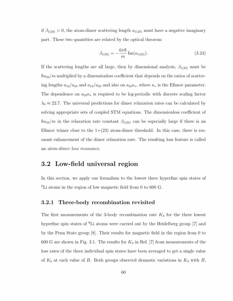
if β1(23) > 0, the atom-dimer scattering length a1(23) must have a negative imaginary

part. These two quantities are related by the optical theorem:

β1(23) = −6πh

mIm(a1(23)). (3.24)

If the scattering lengths are all large, then by dimensional analysis, β1(23) must be

ha23/m multiplied by a dimensionless coefficient that depends on the ratios of scatter-

ing lengths a12/a23 and a13/a23 and also on a23κ∗, where κ∗ is the Efimov parameter.

The dependence on a23κ∗ is required to be log-periodic with discrete scaling factor

λ0 ≈ 22.7. The universal predictions for dimer relaxation rates can be calculated by

solving appropriate sets of coupled STM equations. The dimensionless coefficient of

ha23/m in the relaxation rate constant β1(23) can be especially large if there is an

Efimov trimer close to the 1+(23) atom-dimer threshold. In this case, there is res-

onant enhancement of the dimer relaxation rate. The resulting loss feature is called

an atom-dimer loss resonance.

3.2 Low-field universal region

In this section, we apply our formalism to the lowest three hyperfine spin states of

6Li atoms in the region of low magnetic field from 0 to 600 G.

3.2.1 Three-body recombination revisited

The first measurements of the 3-body recombination rate K3 for the three lowest

hyperfine spin states of 6Li atoms were carried out by the Heidelberg group [7] and

by the Penn State group [8]. Their results for magnetic field in the region from 0 to

600 G are shown in Fig. 3.1. The results for K3 in Ref. [7] from measurements of the

loss rates of the three individual spin states have been averaged to get a single value

of K3 at each value of B. Both groups observed dramatic variations in K3 with B,

60

0 200 400 600B [G]

10-26

10-25

10-24

10-23

10-22

10-21

K 3 [cm

6/s

]

Figure 3.1: Three-body recombination rate constant K3 as a function of the magneticfield B from 0 to 600 G. The solid squares and dots are data points from Refs. [7]and [8], respectively. The curve is the absolutely normalized result for Kdeep

3 withκ∗ = 76.8 a−1

0 and η∗ = 0.11. The two vertical dotted lines mark the boundaries ofthe region in which the absolute values of all three scattering lengths are greater than2 `vdW.

including a narrow loss feature near 130 G and a broader loss feature near 500 G.

The narrow loss feature and the broad loss feature in the measurements of Refs. [7,

8] both appear near the boundaries of the region in which all three scattering lengths

satisfy |aij | > 2`vdW. The effects of the finite range of the interaction may be sig-

nificant near the boundaries of this region. In Ref. [34], we fit the data for K3 in

this region by calculating the 3-body recombination rate Kdeep3 in Eq. (3.6), using

the magnetic field dependence of the three scattering lengths shown in Fig. 1.3 and

treating Λ and η∗ as fitting parameters. Since the systematic error in the normal-

ization of K3 was estimated to be 90% in Ref. [7] and 70% in Ref. [8], we only fit

the shape of the data and not its normalization. A 3-parameter fit to the data from

Ref. [7] in the region 122 G < B < 485 G with an adjustable normalization factor

61

determines the 3-body parameters Λ = 436 a−10 and η∗ = 0.11. This value of the

cutoff is equivalent to κ∗ = 76.8 a−10 . These parameters κ∗ and η∗ determine the

normalization of Kdeep3 , so the theoretical curve in Fig. 3.1 is absolutely normalized.

The fit to the shape of the narrow loss feature is excellent. The normalization is also

correct to within the systematic error in the data. However the fit predicts that K3

should be almost constant in the middle of the low-field region and that there should

be another narrow loss feature at its upper end near 500 G. These predictions are not

consistent with the data in Fig. 3.1, which increases monotonically in the middle of

the low-field region and has a broad loss feature near the upper end of this region.

Similar results for the 3-body recombination rate of 6Li atoms were obtained

subsequently by two other groups [51, 52]. Naidon and Ueda used hyperspherical

methods to calculate the recombination rate [51]. For their 3-body parameters, they

used the real and imaginary parts of the logarithmic derivative of the hyperradial

wavefunction. Schmidt, Floerchinger, and Wetterich used functional renormalization

methods to calculate the recombination rate [52]. For their 3-body parameters, they

used the real and imaginary parts of the detuning energy of a triatomic molecule.

The results of both groups for K3 as a function of the magnetic field are similar to

our results in Fig. 3.1. One difference is that in Refs. [51, 52] the recombination rate

was calculated only up to an overall normalization constant that was determined by

fitting the data. In our calculation, the absolute normalization is determined by the

3-body parameters κ∗ and η∗.

In Ref. [53], the Heidelberg group provided an explanation for the loss feature

near 500 G being much broader than predicted in Refs. [34, 51, 52]. They pointed

out that there are deep dimers whose binding energies vary significantly over the

low-field region. These dimers are those responsible for the Feshbach resonances

690 G, 811 G, and 834 G. In the high-field region, they are shallow dimers, but they

62

become deep dimers in the low-field region. Their binding energies change over the

low-field universal region by as much as a factor of 6. The Heidelberg group assumed

that contributions to the 3-body parameter η∗ scale like the inverse of the binding

energy of the deep dimer. They used the coefficient in this scaling relation as a fitting

parameter along with the 3-body parameter equivalent to κ∗. They obtained an

excellent fit to K3 over the entire low-field region, including the narrow loss feature,

the broad loss feature, and the monotonic rise in between. Their assumption for the

scaling of η∗ with the binding energy of the deep dimer can be justified by an explicit

calculation in a two-channel model [62].

In Ref. [53], the Heidelberg group proposed a simple analytic approximation for

the 3-body recombination rate in regions where all 3 scattering lengths are negative.

Their approximation is the analytic result for equal scattering lengths in Eq. (3.16),

with a replaced by an effective scattering length am given by

am = −[

(a21a

22 + a2

2a23 + a2

3a21)/3

]1/4. (3.25)

Another possible choice for an effective scattering length is the geometric mean of the

three scattering lengths:

ag = −|a1a2a3|1/3. (3.26)

We can use our universal results to test the accuracy of that approximation. We find

that the analytic result in Eq. (3.16) with a replaced by the geometric mean ag in

Eq. (3.26) is a significantly more accurate approximation.

3.2.2 Efimov trimers

Naidon and Ueda [51] and Schmidt, Floerchinger, and Wetterich [52] calculated the

binding energy of the Efimov trimer that is responsible for the loss features in Fig. 3.1.

Its binding energy goes to 0 near both the observed narrow loss feature near 130 G

63

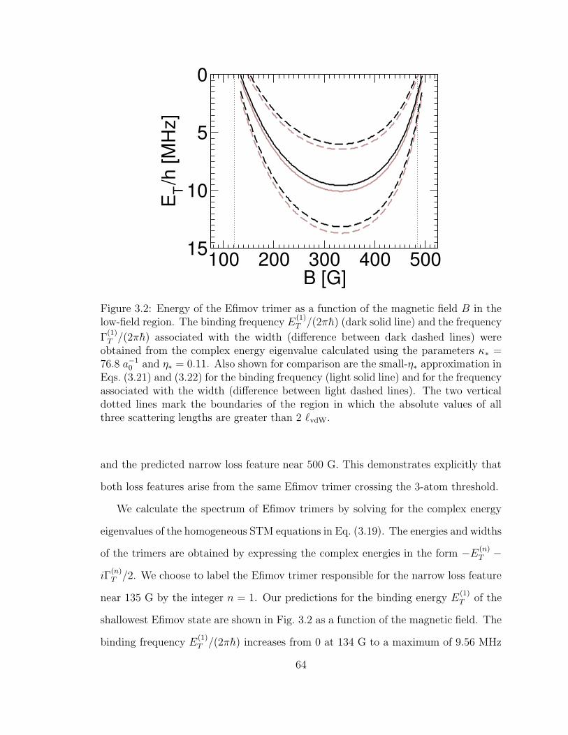
100 200 300 400 500B [G]

0

5

10

15

E T/h [M

Hz]

Figure 3.2: Energy of the Efimov trimer as a function of the magnetic field B in thelow-field region. The binding frequency E

(1)T /(2πh) (dark solid line) and the frequency

Γ(1)T /(2πh) associated with the width (difference between dark dashed lines) were

obtained from the complex energy eigenvalue calculated using the parameters κ∗ =76.8 a−1

0 and η∗ = 0.11. Also shown for comparison are the small-η∗ approximation inEqs. (3.21) and (3.22) for the binding frequency (light solid line) and for the frequencyassociated with the width (difference between light dashed lines). The two verticaldotted lines mark the boundaries of the region in which the absolute values of allthree scattering lengths are greater than 2 `vdW.

and the predicted narrow loss feature near 500 G. This demonstrates explicitly that

both loss features arise from the same Efimov trimer crossing the 3-atom threshold.

We calculate the spectrum of Efimov trimers by solving for the complex energy

eigenvalues of the homogeneous STM equations in Eq. (3.19). The energies and widths

of the trimers are obtained by expressing the complex energies in the form −E (n)T −

iΓ(n)T /2. We choose to label the Efimov trimer responsible for the narrow loss feature

near 135 G by the integer n = 1. Our predictions for the binding energy E(1)T of the

shallowest Efimov state are shown in Fig. 3.2 as a function of the magnetic field. The

binding frequency E(1)T /(2πh) increases from 0 at 134 G to a maximum of 9.56 MHz

64

at 334 G and then decreases to 0 at 494 G. Our maximum binding frequency agrees

well with the maximum frequencies of about 10 MHz and about 11 MHz obtained in

Refs. [51] and [52], respectively. The binding frequency E(0)T /(2πh) associated with the

next deeper Efimov trimer is predicted to change gradually from 12.1 GHz at 134 G

to 12.5 GHz at 334 G and then to 12.1 GHz at 494 G. Since this binding energy is

much larger than the van der Waals frequency νvdW = 154 MHz, this Efimov trimer

and all the deeper ones predicted by the STM equations are artifacts of the zero-

range approximation. Our value of κ∗ can be interpreted as the binding wavenumber

(mE(−2)T /h2)1/2 of the fictitious Efimov trimer labelled by n = −2. It corresponds to

the choice n∗ = −2 in Eq. (1.26).

We note that the finite range corrections to the binding energies of the deeper

trimers can be substantial if their energy becomes comparable to the van der Waals

energy even if all scattering lengths are large. The leading corrections to the binding

energy for the deep trimers are of order `vdW (mE(n)T /h2)1/2. For the trimer labeled

n = 1, these corrections are 25% for the largest value of the binding energy.

In Ref. [51], Naidon and Ueda also calculated the width of the Efimov trimer.

In Fig. 3.2, our results for the width Γ(1)T are illustrated by plotting the frequencies

associated with the energies E(1)T ± Γ

(1)T /2 as functions of the magnetic field. The

frequency Γ(1)T /(2πh) increases from 2.73 MHz at 134 G to a maximum of 7.14 MHz

at 332 G and then decreases to 2.56 MHz at 494 G. Our maximum width is more than

twice as large as the maximum width of about (3 MHz)×2πh obtained in Ref. [51].

Since our result for Γ(1)T is always comparable to or larger than E

(1)T , the interpretations

of E(1)T and Γ

(1)T as the binding energy and width of the trimer should be viewed with

caution.

Since η∗ = 0.11 is relatively small, we can also use the small-η∗ approximations to

the binding energy and the width given in Eqs. (3.22) and (3.21). These approxima-

65

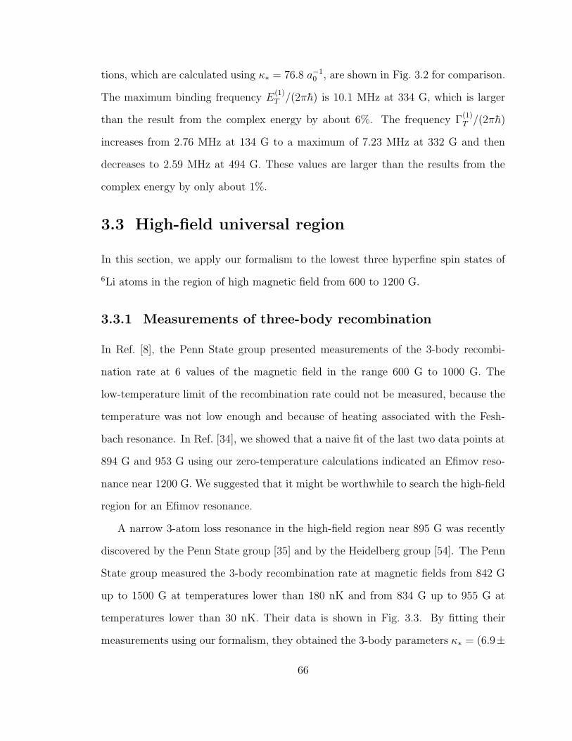
tions, which are calculated using κ∗ = 76.8 a−10 , are shown in Fig. 3.2 for comparison.

The maximum binding frequency E(1)T /(2πh) is 10.1 MHz at 334 G, which is larger

than the result from the complex energy by about 6%. The frequency Γ(1)T /(2πh)

increases from 2.76 MHz at 134 G to a maximum of 7.23 MHz at 332 G and then

decreases to 2.59 MHz at 494 G. These values are larger than the results from the

complex energy by only about 1%.

3.3 High-field universal region

In this section, we apply our formalism to the lowest three hyperfine spin states of

6Li atoms in the region of high magnetic field from 600 to 1200 G.

3.3.1 Measurements of three-body recombination

In Ref. [8], the Penn State group presented measurements of the 3-body recombi-

nation rate at 6 values of the magnetic field in the range 600 G to 1000 G. The

low-temperature limit of the recombination rate could not be measured, because the

temperature was not low enough and because of heating associated with the Fesh-

bach resonance. In Ref. [34], we showed that a naive fit of the last two data points at

894 G and 953 G using our zero-temperature calculations indicated an Efimov reso-

nance near 1200 G. We suggested that it might be worthwhile to search the high-field

region for an Efimov resonance.

A narrow 3-atom loss resonance in the high-field region near 895 G was recently

discovered by the Penn State group [35] and by the Heidelberg group [54]. The Penn

State group measured the 3-body recombination rate at magnetic fields from 842 G

up to 1500 G at temperatures lower than 180 nK and from 834 G up to 955 G at

temperatures lower than 30 nK. Their data is shown in Fig. 3.3. By fitting their

measurements using our formalism, they obtained the 3-body parameters κ∗ = (6.9±

66

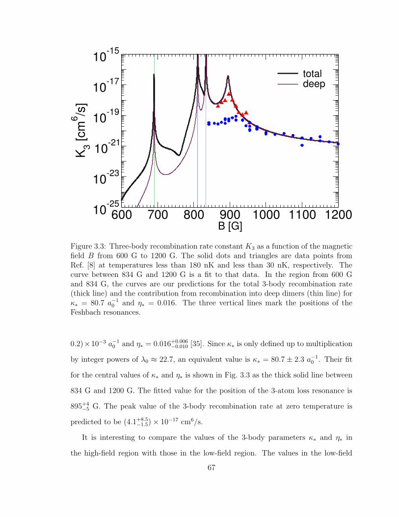
600 700 800 900 1000 1100 1200B [G]

10-25

10-23

10-21

10-19

10-17

10-15

K 3 [cm

6 /s]

totaldeep

Figure 3.3: Three-body recombination rate constant K3 as a function of the magneticfield B from 600 G to 1200 G. The solid dots and triangles are data points fromRef. [8] at temperatures less than 180 nK and less than 30 nK, respectively. Thecurve between 834 G and 1200 G is a fit to that data. In the region from 600 Gand 834 G, the curves are our predictions for the total 3-body recombination rate(thick line) and the contribution from recombination into deep dimers (thin line) forκ∗ = 80.7 a−1

0 and η∗ = 0.016. The three vertical lines mark the positions of theFeshbach resonances.

0.2)×10−3 a−10 and η∗ = 0.016+0.006

−0.010 [35]. Since κ∗ is only defined up to multiplication

by integer powers of λ0 ≈ 22.7, an equivalent value is κ∗ = 80.7± 2.3 a−10 . Their fit

for the central values of κ∗ and η∗ is shown in Fig. 3.3 as the thick solid line between

834 G and 1200 G. The fitted value for the position of the 3-atom loss resonance is

895+4−5 G. The peak value of the 3-body recombination rate at zero temperature is

predicted to be (4.1+8.5−1.5)× 10−17 cm6/s.

It is interesting to compare the values of the 3-body parameters κ∗ and η∗ in

the high-field region with those in the low-field region. The values in the low-field

67

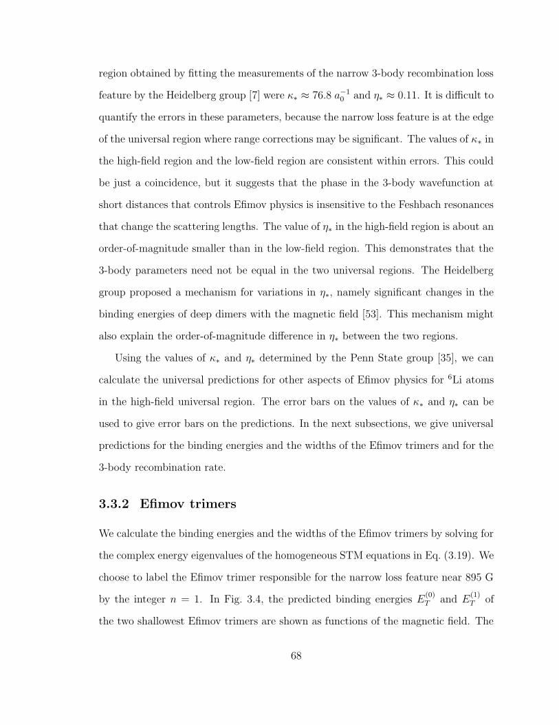
region obtained by fitting the measurements of the narrow 3-body recombination loss

feature by the Heidelberg group [7] were κ∗ ≈ 76.8 a−10 and η∗ ≈ 0.11. It is difficult to

quantify the errors in these parameters, because the narrow loss feature is at the edge

of the universal region where range corrections may be significant. The values of κ∗ in

the high-field region and the low-field region are consistent within errors. This could

be just a coincidence, but it suggests that the phase in the 3-body wavefunction at

short distances that controls Efimov physics is insensitive to the Feshbach resonances

that change the scattering lengths. The value of η∗ in the high-field region is about an

order-of-magnitude smaller than in the low-field region. This demonstrates that the

3-body parameters need not be equal in the two universal regions. The Heidelberg

group proposed a mechanism for variations in η∗, namely significant changes in the

binding energies of deep dimers with the magnetic field [53]. This mechanism might

also explain the order-of-magnitude difference in η∗ between the two regions.

Using the values of κ∗ and η∗ determined by the Penn State group [35], we can

calculate the universal predictions for other aspects of Efimov physics for 6Li atoms

in the high-field universal region. The error bars on the values of κ∗ and η∗ can be

used to give error bars on the predictions. In the next subsections, we give universal

predictions for the binding energies and the widths of the Efimov trimers and for the

3-body recombination rate.

3.3.2 Efimov trimers

We calculate the binding energies and the widths of the Efimov trimers by solving for

the complex energy eigenvalues of the homogeneous STM equations in Eq. (3.19). We

choose to label the Efimov trimer responsible for the narrow loss feature near 895 G

by the integer n = 1. In Fig. 3.4, the predicted binding energies E(0)T and E

(1)T of

the two shallowest Efimov trimers are shown as functions of the magnetic field. The

68

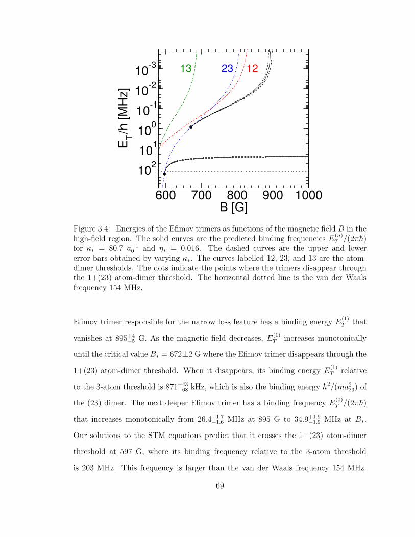
600 700 800 900 1000B [G]

10-3

10-2

10-1

100

101

102

E T/h

[MHz

]

13 23 12

Figure 3.4: Energies of the Efimov trimers as functions of the magnetic field B in thehigh-field region. The solid curves are the predicted binding frequencies E

(n)T /(2πh)

for κ∗ = 80.7 a−10 and η∗ = 0.016. The dashed curves are the upper and lower

error bars obtained by varying κ∗. The curves labelled 12, 23, and 13 are the atom-dimer thresholds. The dots indicate the points where the trimers disappear throughthe 1+(23) atom-dimer threshold. The horizontal dotted line is the van der Waalsfrequency 154 MHz.

Efimov trimer responsible for the narrow loss feature has a binding energy E(1)T that

vanishes at 895+4−5 G. As the magnetic field decreases, E

(1)T increases monotonically

until the critical value B∗ = 672±2 G where the Efimov trimer disappears through the

1+(23) atom-dimer threshold. When it disappears, its binding energy E(1)T relative

to the 3-atom threshold is 871+43−68 kHz, which is also the binding energy h2/(ma2

23) of

the (23) dimer. The next deeper Efimov trimer has a binding frequency E(0)T /(2πh)

that increases monotonically from 26.4+1.7−1.6 MHz at 895 G to 34.9+1.9

−1.9 MHz at B∗.

Our solutions to the STM equations predict that it crosses the 1+(23) atom-dimer

threshold at 597 G, where its binding frequency relative to the 3-atom threshold

is 203 MHz. This frequency is larger than the van der Waals frequency 154 MHz.

69

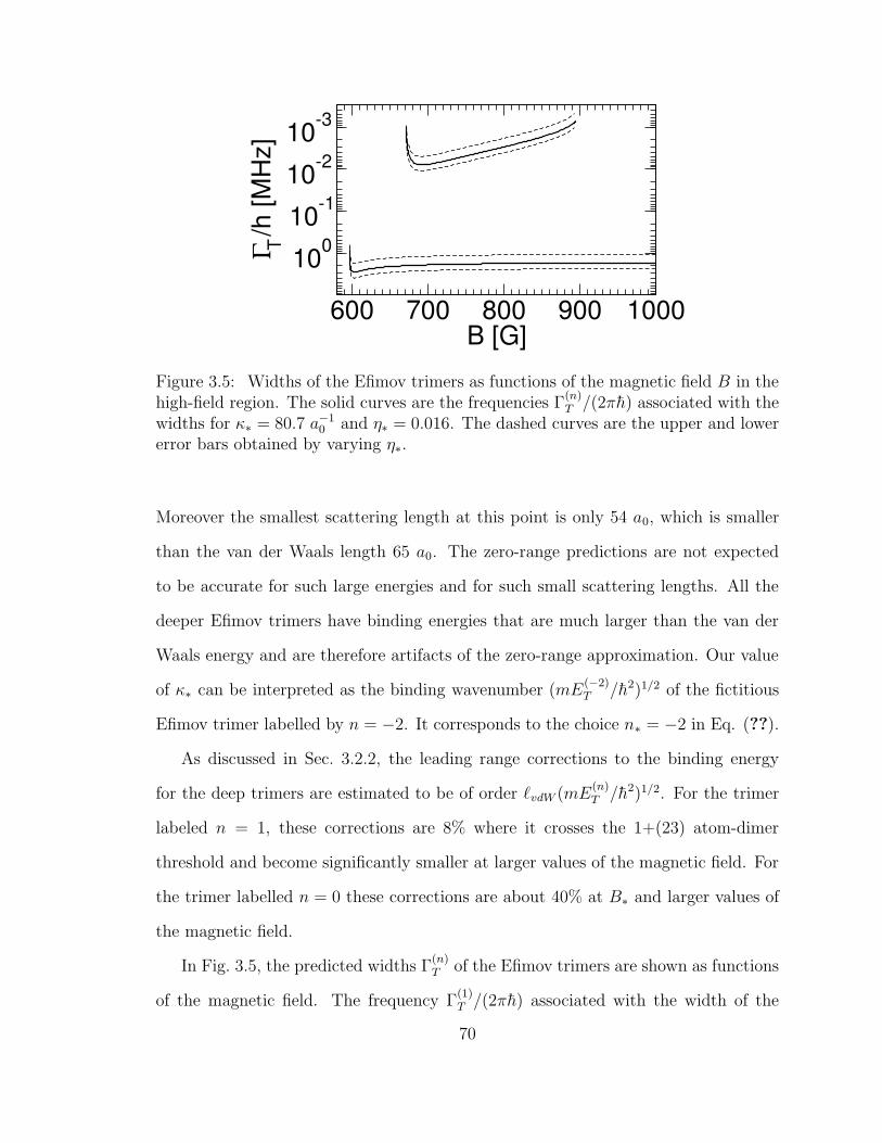
600 700 800 900 1000B [G]

10-3

10-2

10-1

100Γ T/h

[MHz

]

Figure 3.5: Widths of the Efimov trimers as functions of the magnetic field B in thehigh-field region. The solid curves are the frequencies Γ

(n)T /(2πh) associated with the

widths for κ∗ = 80.7 a−10 and η∗ = 0.016. The dashed curves are the upper and lower

error bars obtained by varying η∗.

Moreover the smallest scattering length at this point is only 54 a0, which is smaller

than the van der Waals length 65 a0. The zero-range predictions are not expected

to be accurate for such large energies and for such small scattering lengths. All the

deeper Efimov trimers have binding energies that are much larger than the van der

Waals energy and are therefore artifacts of the zero-range approximation. Our value

of κ∗ can be interpreted as the binding wavenumber (mE(−2)T /h2)1/2 of the fictitious

Efimov trimer labelled by n = −2. It corresponds to the choice n∗ = −2 in Eq. (??).

As discussed in Sec. 3.2.2, the leading range corrections to the binding energy

for the deep trimers are estimated to be of order `vdW (mE(n)T /h2)1/2. For the trimer

labeled n = 1, these corrections are 8% where it crosses the 1+(23) atom-dimer

threshold and become significantly smaller at larger values of the magnetic field. For

the trimer labelled n = 0 these corrections are about 40% at B∗ and larger values of

the magnetic field.

In Fig. 3.5, the predicted widths Γ(n)T of the Efimov trimers are shown as functions

of the magnetic field. The frequency Γ(1)T /(2πh) associated with the width of the

70

shallower trimer increases from 0.706 kHz at 895 G to a maximum of 7.98 kHz at

692 G and then decreases to 0.940 kHz at B∗. The frequency Γ(0)T /(2πh) associated

with the width of the deeper trimer increases from 1.74 MHz at 895 G to 2.00 MHz

at B∗.

3.3.3 Predictions for three-body recombination

Our predictions for the 3-body recombination rate in the region 600 G to 834 G,

where one or more of the scattering lengths are positive, are shown in Fig. 3.3. The

upper curve is the total recombination rate K3, while the lower one is the contri-

bution Kdeep3 from deep dimers. Besides the Efimov resonance at 895 G, the only

other peaks are at the Feshbach resonances at 690 G, 811 G, and 834 G. They arise

simply from the scaling of K3 as a4 up to logarithms, where a is some appropri-

ate mean of the scattering lengths a12, a23, and a13. The total recombination rate

K3 is predicted to have three local minima. There is a broad local minimum at

759± 1 G, where the minimum recombination rate is (2.5+0.5−0.5)× 10−22 cm6/s. There

is a narrow local minimum at 829 ± 1 G, where the minimum recombination rate

is (2.2+0.9−1.3) × 10−18 cm6/s. Finally there is a local minimum at 861 ± 2 G between

the last Feshbach resonance and the 3-atom Efimov resonance, where the minimum

recombination rate is (5.8+3.8−4.0)× 10−19 cm6/s.

In Fig. 3.6, we show the predictions for the 3-body recombination rate in the

region from 650 G to 850 G in more detail. In addition to K3 and Kdeep3 , we show the

contributions from recombination into the (12), (23), and (13) dimers. This figure

reveals that the local minima at 759 G and 829 G are associated with interference in

the recombination into shallow dimers. The narrow minimum at 829 G arises from the

combination of a rapidly increasing rate into deep dimers and a rapidly decreasing

rate into (12) dimers, which has its minimum at 830 G. The broad minimum at

71

650 700 750 800 850B [G]

10-25

10-23

10-21

10-19

10-17

10-15

K 3 [cm

6 /s]

totaldeep122313

Figure 3.6: Three-body recombination rate constant K3 as a function of the magneticfield B from 650 G to 850 G. The curves are our predictions for the total 3-bodyrecombination rate (thick solid line), the contribution from recombination into deepdimers (thin solid line), and the contributions from recombination into the (12) dimer(short-dashed line), the (23) dimer (dash-dotted line), and the (13) dimer (long-dashed line) for κ∗ = 80.7 a−1

0 and η∗ = 0.016.

759 G arises from minima in the rates into (12) and (23) dimers at 757 G and 765 G,

respectively. There are also minima in the rates into the (13) dimer at 672 G and

the (23) dimer at 600 G, but their effects are not visible in the total recombination

rate. We have verified that these minima in the recombination rates into individual

shallow dimers arise from interference effects by showing that they become zeroes as

η∗ is decreased to 0. Thus these minima are the result of destructive interference

between two recombination pathways. In the case of three equal positive scattering

lengths, a similar interference effect is evident in the analytic expression for the 3-body

72

recombination rate into shallow dimers in Eq. (3.17).

3.3.4 Atom-dimer resonance

An atom-dimer loss resonance can appear at a value of the scattering length for which

an Efimov trimer crosses the atom-dimer threshold. From the Efimov trimer spectrum

in Fig. 3.4, one can see that atom-dimer resonances are predicted at the two values of

the magnetic field where the Efimov trimers cross the 1+(23) atom-dimer threshold.

The atom-dimer resonance associated with the shallower of the two Efimov trimers

is predicted to occur at B∗ = 672 ± 2 G. The universal predictions for the dimer

relaxation rate near this resonance can be calculated by solving appropriate sets of

coupled STM equations. The atom-dimer resonance associated with the deeper of

the two Efimov trimers is predicted to occur at B ′∗ = 597 G. This resonance occurs

slightly outside the universal region, so universal predictions for the position of the

resonance and for the dimer relaxation rate are not expected to be accurate.

If we restrict our attention to magnetic fields very near the atom-dimer resonance

at B∗, we can get an approximation to the universal predictions for the dimer re-

laxation rate β1(23) without actually solving the STM equations. We take advantage

of the fact that the atom-dimer scattering length a1(23) diverges at B∗. The 3-atom

problem in this region therefore reduces to a universal 2-body problem for the atom

and the (12) dimer. The universal properties are determined by the large scattering

length a1(23). For example, in the region B > B∗ but very close to B∗, the binding

energy of the Efimov trimer is well approximated by the sum of the binding energy of

the (23) dimer and a universal term determined by the atom-dimer scattering length:

E(1)T ≈ −

(

h2

ma223

+3h2

4ma21(23)

)

. (3.27)

This should be a good approximation as long as the second term is much smaller

73

than the first term. In the region near B∗, the atom-dimer scattering length can

be approximated by an expression that has the same form as the analytic result for

identical bosons but with different numerical coefficients:

a1(23) ≈ (C1 cot[s0 ln(a23/a∗) + iη∗] + C2) a23, (3.28)

where a∗ = a23(B∗). The coefficients C1 and C2 can in principle depend on ratios of the

scattering lengths, but a13 is an order of magnitude larger so it essentially decouples

and a13 and a23 are both increasing with B so their ratio does not change rapidly

near B∗. Thus we can treat C1 and C2 as numerical constants. These constants can

be determined by using Eq. (3.27) to extract a1(23) from the results for the real part

of the trimer binding energy shown in Fig. 3.4 and then fitting those results to the

expression for the atom-dimer scattering length in Eq. (4.10). The resulting constants

are C1 = 0.67 and C2 = 0.65.

With the constant C1 in hand, we can obtain an approximation for the dimer

relaxation rate constant β1(23) for B near B∗ simply by inserting the approximation

for a1(23) in Eq. (4.10) into the optical theorem relation in Eq. (3.24). The resulting

expression is

β1(23) ≈9.44C1 sinh(2η∗)

sin2[s0 ln(a23/a∗)] + sinh2 η∗

ha23

m. (3.29)

If B∗ = 672 G, the value of a∗ is 835 a0. The only dependence on the magnetic

field is through the B-dependence of a23. This approximation for β1(23) is shown as

a function of B − B∗ in Fig. 3.7. The maximum value of β1(23) at the peak of the

resonance is 4× 10−7 cm3/s for η∗ = 0.016.

Since the atom-dimer resonance associated with the deeper of the two Efimov

trimers occurs slightly outside the universal region, universal predictions for the dimer

relaxation rate are not expected to be accurate. They might however be useful for

making order-of-magnitude estimates. If we apply the analysis described above to

74

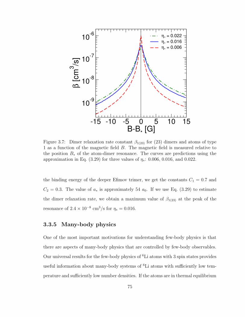
-15 -10 -5 0 5 10 15B-B* [G]

10-9

10-8

10-7

10-6

β [c

m3 /s

]

η* = 0.022η* = 0.016η* = 0.006

Figure 3.7: Dimer relaxation rate constant β1(23) for (23) dimers and atoms of type1 as a function of the magnetic field B. The magnetic field is measured relative tothe position B∗ of the atom-dimer resonance. The curves are predictions using theapproximation in Eq. (3.29) for three values of η∗: 0.006, 0.016, and 0.022.

the binding energy of the deeper Efimov trimer, we get the constants C1 = 0.7 and

C2 = 0.3. The value of a∗ is approximately 54 a0. If we use Eq. (3.29) to estimate

the dimer relaxation rate, we obtain a maximum value of β1(23) at the peak of the

resonance of 2.4× 10−8 cm3/s for η∗ = 0.016.

3.3.5 Many-body physics

One of the most important motivations for understanding few-body physics is that

there are aspects of many-body physics that are controlled by few-body observables.

Our universal results for the few-body physics of 6Li atoms with 3 spin states provides

useful information about many-body systems of 6Li atoms with sufficiently low tem-

perature and sufficiently low number densities. If the atoms are in thermal equilibrium

75

at temperature T , an important scale is the thermal length λT = (2πmkBT/h2)−1/2.

If the atoms of type i have number density ni, another important scale is the Fermi

wavenumber kFi = (3π2ni)1/3. In our calculation of the 3-body recombination rate,

we set the wavenumbers of the incoming atoms to 0. In order for our result to apply

quantitatively to all atoms in the system, it is necessary that λ−1T , kF1, kF2, and kF3

all be small compared to the wavenumber scale (1/a21 + 1/a2

2 + 1/a23)

1/2 set by the

interactions. Even if this condition is not well satisfied, our result can be used to

obtain order-of-magnitude estimates of the relevant time scales.

There are several relevant time scales that we can extract from our few-body

calculations. If the system contains Efimov trimers, an important time scale is the

lifetime h/Γ(n)T of the Efimov trimer, where Γ

(n)T is its width. The universal predic-

tions for the widths of the Efimov trimers are shown in Fig. 3.5. If the system can

be approximated by a gas of individual low-energy atoms, the time scale for disap-

pearance of a significant fraction of the atoms is set by the 3-body recombination

rate constant K3. From the rate equation in Eq. (4.1), we see that the time scale

for loss of a significant fraction of the atoms of type i is (K3njnk)−1, where j and

k are the two complimentary spin states. The universal predictions for the 3-body

recombination rate are shown in Figs. 3.3 and 3.6. Finally if the system contains

low-energy dimers and low-energy atoms in the complimentary spin state, the time

scale for disappearance of a significant fraction of the atoms or dimers is set by the

appropriate dimer relaxation rate constant. From the rate equation in Eq. (3.23), we

see that the time scales for loss of significant fractions of (23) dimers and of atoms of

type 1 are (β1(23)n1)−1 and (β1(23)n(23))

−1, respectively. The only universal informa-

tion we have about dimer relaxation rates is the approximation for β1(23) in Eq. (3.29),

which should be accurate for magnetic fields within about 10 G of B∗ ≈ 672 G. For

magnetic fields further from this critical value but still within the region where a23 is

76

positive, one may be able to use the extrapolation of this expression as an estimate

for the dimer relaxation rate.

If the system contains a Bose-Einstein condensate of low-energy dimers as well

as low-energy atoms in the complimentary spin state, another important few-body

observable is the atom-dimer scattering length for that particular atom and dimer.

The real part of the atom-dimer scattering length determines the mean-field en-

ergy of the atom in the dimer condensate. The mean-field energy of an atom of

type 1 in the (23) dimer condensate with sufficiently low number density n(23) is

(3πh2/m) Re(a1(23))n(23). The approximation for a1(23) in Eq. (4.10) should be accu-

rate for magnetic fields within about 10 G of B∗ ≈ 672 G.

We will illustrate the relevance of our universal result to many-body physics by

applying them to two specific values of the scattering length that are interesting from

a symmetry perspective. If the pair scattering lengths aij and aik are equal, atoms of

types j and k are related by an SU(2) symmetry. If all three scattering lengths are

equal, the three spin states are related by an SU(3) symmetry. There is an SU(2)

symmetry point at 731 G, where the scattering lengths are a12 = a23 ≈ +2500 a0 and

a13 ≈ −7100 a0. An SU(3) symmetry point can be approached by going to very high

magnetic fields, where all three scattering lengths approach the spin-triplet scattering

length −2140 a0 [17].

A quantum degenerate Fermi gas of 6Li atoms with approximately equal popu-

lations of the three lowest hyperfine spin states at 1500 G has been realized by the

Penn State group [35]. The scattering lengths are a12 ≈ −2460 a0, a23 ≈ −2360 a0,

and a13 ≈ −2240 a0, so there is an approximate SU(3) symmetry. One candidate

for a metastable ground state is a state that can be approximated by filled Fermi

spheres for all three spin states, with Cooper pairing that breaks the SU(3) symme-

try down to a U(1) subgroup. The lifetime for such a system is determined by the

77

3-body recombination rate K3, which is predicted to be about 8 × 10−22 cm6/s at

1500 G. Another candidate for a metastable ground state is a filled Fermi sphere of

Efimov trimers. The binding energy E(0)T of the Efimov trimer is predicted to be about

25 MHz×(2πh) at 1500 G. Its width Γ(0)T is predicted to be about 1.7 MHz×(2πh),

which corresponds to a lifetime h/Γ(0)T of about 9× 10−8 s.

We now consider a many-body system at 731 G, where there is an SU(2) symmetry

relating the atoms of types 1 and 3. For a state that can be approximated by filled

Fermi spheres for all three spin states, the lifetime is determined by the the 3-body

recombination rate K3, which is predicted to be about 7× 10−22 cm6/s at 731 G. A

better candidate for a metastable ground state is a state containing a Bose-Einstein

condensate of dimers, which breaks the SU(2) symmetry down to a U(1) subgroup,

and a filled Fermi sphere of the complimentary atoms. The lifetime of the state is

determined by the dimer relaxation rates β1(23) and β3(12), which are equal by the

SU(2) symmetry. We can estimate β1(23) by extrapolating the expression for the

dimer relaxation rate β1(23) in Eq. (3.29) to 731 G, which gives 3 × 10−10 cm3/s.

We can also estimate the mean-field energy of an atom of type 1 in a (23) dimer

condensate with number density n(23) by extrapolating the expression for the atom-

dimer scattering length a1(23) in Eq. (4.10) to 731 G. The resulting estimate is 2 ×

10−9 Hz cm3 × (2πh n(23)). The positive sign of the real part of a1(23) implies that

the atoms of type 1 are repelled by the (23) dimer condensate. A state in which

the dimer condensate and the atoms are spatially separated is therefore energetically

favored over a homogeneous state. A final candidate for a metastable ground state

is a filled Fermi sphere of Efimov trimers. The binding energy E(1)T of the shallower

Efimov trimer is predicted to be about 190 kHz×(2πh) at 731 G. Its width Γ(1)T is

predicted to be about 6 kHz×(2πh) at 731 G, which corresponds to a lifetime h/Γ(1)T

of about 3× 10−5 s.

78

3.4 Summary and discussion

Systems consisting of 6Li atoms with 3 spin states provide a rich playground for

the interplay between few-body physics and many-body physics. The experimental

study of many-body physics is only possible if the loss rates of atoms from few-

body processes are sufficiently low. Measurements of the position and width of a

single Efimov loss feature can be used to determine the 3-body parameters κ∗ and η∗.

Calculations in the zero-range limit can then be used to predict few-body reaction

rates in the entire universal region.

In the low-field region for 6Li atoms, the universal predictions were only qualita-

tively successful. A fit to the measurements of the 3-body recombination rate by the

Heidelberg group gives the 3-body parameters κ∗ ≈ 77 a−10 and η∗ ≈ 0.11. With these

parameters, the universal results for the 3-body recombination rate as a function of

the magnetic field give a good fit to the narrow loss feature near 130 G but do not

agree well with measurements in the upper half of the low-field region [34, 51, 52]. A

reasonable explanation was proposed by the Heidelberg group [53]: η∗ is particularly

sensitive to the binding energies of the shallowest of the deep dimers and there are 6Li

dimers whose binding energies change dramatically across the low-field region. As-

suming the scaling behavior η∗ ∼ E−1deep, they obtained a good fit to the recombination

rate in the low-field region.

In the high-field region for 6Li atoms, the scattering lengths are much larger so the

universal predictions should be much more accurate. A narrow 3-atom loss feature

near 895 G was discovered by the Penn State group [35] and by the Heidelberg group

[54]. By fitting their measurements of the 3-body recombination rate, the Penn

State group determined the 3-body parameters associated with Efimov physics to be

κ∗ = 80.7 ± 2.3 a−10 and η∗ = 0.016+0.006

−0.010. We used those parameters to calculate

the universal predictions for the binding energies and widths of the Efimov trimers

79

shown in Fig. 3.4 and 3.5. The Efimov trimer responsible for the narrow loss feature

is predicted to disappear through the 1+(23) atom-dimer threshold at 672 ± 2 G,

producing a spectacular atom-dimer loss resonance. There is also a deeper Efimov

trimer whose binding frequency and width in the universal region are approximately

30 MHz and 2 MHz×(2πh), respectively. This trimer is also predicted to disappear

through the 1+(23) atom-dimer threshold, but this happens outside the universal

region. We also used the 3-body parameters determined by the Penn State group

to calculate the universal predictions for the 3-body recombination rate, which are

shown in Figs. 3.3 and 3.6. Local minima in K3 are predicted at 759±1 G, 829±1 G,

and 861±1 G. Finally an approximate calculation of the dimer relaxation rate in the

region of the atom-dimer resonance is presented in Fig. 3.7. We look forward to the

experimental verification of these predictions.

In order to understand the behavior of atom-dimer mixtures at low temperatures,

it would be useful to have universal predictions for other 3-atom observables. They

include the atom-dimer scattering lengths, which are in general complex. The real

part of an atom-dimer scattering length determines the mean-field shifts of the atom in

the dimer condensate. Its imaginary part is proportional to the dimer relaxation rate.

For the shallow dimer with the largest binding energy, which is the (23) dimer for B <

730 G and the (12) dimer for 730 G < B < 834 G, the only relaxation channels are into

deep dimers. For shallow dimers with smaller binding energy, there are also relaxation

channels into other shallow dimers. It would be especially useful to have definitive

universal predictions for the relaxation rate constant β1(23) near the predicted atom-

dimer threshold at 672±2 G. It would improve upon the approximation illustrated in

Fig. 3.7 by taking into account the B-dependence of the ratios of scattering lengths.

There have not yet been any direct observations of Efimov trimers in ultracold

atoms. They have only been observed indirectly through the resonant enhancement

80

of 3-body recombination and through the resonant enhancement of atom-dimer re-

laxation provided by virtual Efimov trimers. The direct production of Efimov trimers

would be another milestone in the study of Efimov physics in ultracold atoms. Of

course, once they are produced, they would decay quickly. In the high-field universal

region for 6Li atoms, the deeper Efimov trimer is predicted to have a very short life-

time of about 10−7 s. The shallower Efimov trimer is predicted to have a lifetime of

10−4 s to 10−5 s. Our universal predictions for the binding energies of these Efimov

trimers should be useful in devising experimental strategies for producing them.

3.5 Postscript

The analysis presented in this chapter was completed in August 2009. The prediction

of two atom-dimer loss resonances in the high-field region was verified in experiments

by the Heidelberg group [37] and by the Tokyo group [38] in March 2010. The

measured position of the narrow resonance was 685±2 G, which is about 15 G above

the universal prediction of 672± 2 G. The position of the second wider resonance is

near 603 G. The scattering lengths at this magnetic field are not large enough for

universal predictions to be reliable. The Tokyo group also calculated the universal

predictions for the atom-dimer relaxation rate [38], with results consistent with the

analysis described above. To resolve the discrepancy between the measured position

of the narrow resonance and the universal prediction, the Tokyo group proposed a

model in which the three-body parameter varies with the magnetic field [38].

The Heidelberg group also reported two local minima in the atom-dimer relaxation

rate [37]. These loss features will be discussed in Chapter 4, in which we calculate

the dimer relaxation rate for fermions with three spin states.

81

Chapter 4

Dimer relaxation

In this chapter, we study Efimov physics in the atom-dimer relaxation rate for 6Li

atoms in the three lowest hyperfine states. We perform a complete zero-range cal-

culation at zero temperature and estimate the finite range corrections and the finite

temperature corrections. Our zero-range calculation predicts the two resonances and

the two minima that have been observed in experiment. Quantitatively, our zero

temperature results show deviations from the data. An approximate finite temper-

ature calculation near one of the resonances improves the description of the data

considerably and shows that finite temperature effects account for about 25% of the

discrepancy. In Sections 4.1 and 4.2, we explain our theoretical framework. The

numerical results at zero temperature are displayed and compared with the experi-

mental data in Sec. 4.3. In Sec. 4.4, we carry out an approximate finite temperature

calculation near the resonance at B = 685 G. We summarize our results and conclude

in Sec. 4.5. The analysis presented in this chapter was carried out in collaboration

with Hans-Werner Hammer and Lucas Platter and was published in Physical Review

A [39] in August 2010.

82

4.1 Dimer relaxation

In this section we discuss the losses of atoms and dimers through inelastic scattering

processes and present expressions for the relaxation rate constants.

Before proceeding with our discussion of atom-dimer scattering, we explain our

notation and terminology. We label an atom in one of the three hyperfine states

of the 6Li atoms with an index i where i = 1, 2 or 3. The S-wave scattering length

between atoms in states i and j is denoted either as aij or as ak where k 6= i 6= j. Two

atoms in the same state can not scatter in an S-wave because of the Pauli principle.

If the scattering length aij is positive and much larger than the van der Waals length

`vdW ≈ 65a0, the atoms i and j can form a dimer with binding energy h2/(ma2ij).

We call this dimer the (shallow) ij-dimer or simply a shallow dimer. Shallow dimers

have to be distinguished from deep dimers with binding energy of order h2/(m`2vdW)

or larger.

In a gas of atoms i and jk-dimers, the atoms and dimers can undergo inelastic

collisions into atoms and deeply bound dimers with a binding energy larger than that

of the jk-dimer. This inelastic process is called dimer relaxation. The difference in

the binding energies of the initial and final state dimers is released as kinetic energy

and the atom and dimer in the final state recoil from each other. If their kinetic

energies are larger than the trapping potential, they escape the trap. The loss rate

for the number density ni of atoms i and number density njk of jk-dimers is

d

dtni =

d

dtnjk = −βi ninjk, (4.1)

where the coefficient βi is the relaxation rate constant for the jk-dimer and atom i.

In the case of identical bosons, dimer relaxation is possible only if the final state

consists of an atom and a deep dimer. However, in the three-fermion system relaxation

can also occur into into shallow dimers. For example, in a scattering process of an

83

atom i and a jk-dimer, relaxation can proceed into the ij-dimer provided the binding

energy of the ij-dimer is larger than that of the jk-dimer. Therefore, the total rate

βi is the sum of all relaxation rates into atoms plus shallow dimers and atoms plus

deep dimers

βi =∑

j 6=i

βshi→j + βdeep

i , (4.2)

where the index i implies atom i plus jk-dimer in the initial state and the j implies

atom j plus ik-dimer in the final state. For brevity, we refer to βshi→j as the rate into

the shallow dimer or the rate into the (final) ik-dimer and to βdeepi as the rate into

the deep dimers.

The relaxation rate can be calculated from the T-matrix element for atom-dimer

scattering T ADij (k, p;E) where k and p are the relative wave numbers of the atom and

dimer in initial and final state, respectively, and E is the total energy. By using the

optical theorem, we can calculate the total rate for atom-dimer scattering which is the

sum of elastic and inelastic rates. However, in the low energy limit k → 0, the elastic

rate scales as k because T ADii (k, k;E) is constant and the two-body phase space gives

one power of k [11]. The elastic rate therefore vanishes at zero energy and the optical

theorem gives the total relaxation rate βi

βi =2h

mImT AD

ii (0, 0,−1/(ma2i )). (4.3)

The rate into the shallow dimer βshi→j is determined by the square of the T-matrix

element multiplied by the two-body phase space:

βshi→j =

2ph

3πm

∣

∣T ADij (0, p,−1/(ma2

i ))∣

∣

2θ(ai − aj), (4.4)

where the wave number p = (2/√

3)√

a−2j − a−2

i and the θ-function is inserted because

the relaxation is allowed only when the initial dimer binding energy is smaller than

the final one. The prefactor 2p/(3π) comes from the two-body phase space integral.

84

From Eq. (4.4), one can deduce that βshi→j vanishes as

√ai − aj near the crossing of

the ik- and jk-dimers where ai approaches aj .

The relaxation rate into deep dimers βdeepi could also be calculated by using the

T-matrix in a similar way to Eq. (4.4) if the theory described deep dimers explicitly.

Alternatively, the effects of deep dimers can be taken into account indirectly by

using an analytic continuation of the three-body parameter into the complex plane

as introduced in Ref. [63]. Then, the partial rate βdeepi can be obtained by using the

relation in Eq. (4.2).

D’Incao and Esry have calculated the scattering length dependence of ultracold

three-body collisions near overlapping Feshbach resonances for a variety of cases [26].

For the relaxation rate into the shallow dimer βshi→j, they find that it scales like a2

j/ai

times a log-periodic function of aj if ai aj while ak is non-resonant. The rate into

deep dimers βdeepi scales like a2

j/ai times a prefactor that is a constant for positive aj

and a log-periodic function of aj for negative aj.

4.2 STM equations for non-zero energy

The Skorniakov–Ter-Martirosian (STM) equation [46] is an integral equation that

describes three-atom scattering interacting through zero-range interactions. In this

section, we discuss the STM equation and relate the T-matrix element T ADij to the

amplitude Aij that is the solution to the STM equation.

We consider only the S-wave contribution and assume that higher partial wave

contributions are suppressed at low temperature. For the three-fermion system, the

STM equation forms 9 coupled equations for the amplitudes Aij(k, p;E) [34, 36]. For

85

non-zero energy, the equation is given by

Aij(k, p;E) = (1− δij)Q(k, p;E)

+2

π

∑

k

(1− δkj)

∫ Λ

0

dqq2Q(q, p;E)Dk(q;E)Aik(k, q;E), (4.5)

where Aij(k, p;E) is the amplitude for an atom i and a complementary pair of atoms

to scatter into an atom j and a complementary pair and Λ is an ultraviolet cutoff.

The function Q(k, p;E) and the 2-atom propagator Dk(q;E) are given by

Q(k, p;E) =1

2kpln

[

k2 + kp+ p2 −mE − iεk2 − kp+ p2 −mE − iε

]

, (4.6)

Dk(q;E) =1

−1/ak +√

34q2 −mE − iε

. (4.7)

The solutions of the STM equation (4.5) depend log-periodically on Λ with a

discrete scaling factor eπ/s0 ≈ 22.7, where s0 ≈ 1.00624. The dependence on the

arbitrary cutoff Λ can be eliminated in favor of a physical 3-body parameter such as

the binding wave number of an Efimov trimer in the unitary limit. For convenience,

we choose to work directly with the wave number cutoff Λ in our calculations. If

deep dimers are present, the trimer has a finite width that allows it to decay into

an atom and a deep dimer. The effects of deep dimers can be taken into account by

analytically continuing the cutoff Λ into the complex plane [63]

Λ→ Λeiη∗/s0 , (4.8)

where η∗ is a width parameter associated with the effects of the deep dimers. Λ and

η∗ are determined from experimental measurements of three-body recombination in

the 6Li system [35] and their numerical values are Λ = 456 a−10 and η∗ = 0.016 [36]

where a0 is the Bohr radius.

In order to obtain the T-matrix element, the amplitude Aij must be multiplied

86

with the dimer-wavefunction renormalization factors√

ZiZj, where Zi = 8π/ai,

T ADij (k, p;E) =

8π√aiaj

Aij(k, p;E). (4.9)

By solving the STM equation (4.5) and using the relation in Eq. (4.9), we can calculate

the relaxation rates in Eqs. (4.3) and (4.4).

4.3 Zero temperature results

In this section we present our numerical results for the dimer relaxation rate constants

βi at zero temperature and compare them with recent measurements in Refs. [37, 38].

We solve the STM equation in Eq. (4.5) numerically with 5 input parameters: the

three pair scattering lengths ai, i = 1, 2, 3, the cutoff Λ and the width parameter

η∗. We use the values Λ = 456 a−10 and η∗ = 0.016 that have been determined from

measurements of the three-body recombination rate in Ref. [35] and have been used

in Ref. [36] to predict the atom-dimer relaxation rate.

Fig. 1.4 shows the scattering lengths for the 3 lowest hyperfine state of 6Li as a

function of the magnetic field. The atom-dimer relaxation rate βi is non-zero in the

region of positive scattering length ai. The upper limit of the region is set by the

Feshbach resonances at 811 G, 690 G, and 834 G for a1, a2, and a3, respectively. If

the scattering length is much larger than the van der Waals length `vdW ≈ 65a0, the

universal theory is valid. We denote this region as the universal region. Corrections

due to the finite range of the interaction should be small in the universal region. In

practice, we apply the universal zero-range theory when all scattering lengths are at

least two times larger than `vdW corresponding to magnetic fields B > 608 G. The

expected error due to finite range corrections is `vdW/a and therefore smaller than

50% in this region.

In Ref. [36], two crossings of Efimov trimers with the atom-dimer threshold have

87

been predicted. Both are located at the 1(23)-threshold: at B∗ = 672 G and at

B′∗ ≈ 597 G. Here the index 1 denotes the atom and the index (23) the dimer. Since

the atom-dimer relaxation is resonant when the trimer appears near the threshold,

two resonances are expected in the rate β1 near B∗ and B′∗. The resonance at B∗ is

well in the universal region where all scattering lengths are much larger than `vdW

while B′∗ is slightly outside. Therefore, the resonance position B∗ should be accurately

determined with corrections of order `vdW/a23 ≈ 10% where the value of a23 at the

resonance was used. The position B ′∗ is outside the universal region and can receive

large non-universal corrections of order 100%. These error estimates are accurate up

to a prefactor of order one. The exact value of this prefactor can only be obtained

from an explicit calculation of the range corrections. Note also that these percentage

errors apply to the positions in terms of the scattering length. To obtain the errors

for the corresponding magnetic field they have to be converted using Fig. 1.4.

In Fig. 4.1, we show our numerical results for β1 and compare them with the

recent measurements of Refs. [37, 38]. We give the full relaxation rate as well the

individual contributions from shallow and deep dimers. In the magnetic field region

from 590 G to 730 G, only the relaxation into deep dimers contributes to β1 since the

energy of the 23-dimer is larger than the energy of the other shallow dimers. At a

magnetic field of 730 G, the 23-dimer crosses the 12-dimer and the relaxation channel

into 12-dimers opens up. As the crossing is approached from above, the rate vanishes

as√a1 − a3 in agreement with the analytical result from Sec. 4.1. Between 790 and

810 G, the condition a1 a3 with a2 non-resonant is satisfied approximately. The

rate into the shallow dimer in this region scales approximately as a23/a1 in agreement

with the prediction of D’Incao and Esry [26]. At 811 G, the 23-dimer disappears

through the three-atom threshold and the relaxation rate vanishes.

Our results show two resonances at B∗ = 672 G and B′∗ ≈ 597 G. There is also a

88

600 650 700 750 800B [G]

10-11

10-10

10-9

10-8

10-7

10-6

β 1 [cm

3 /s]

β1

β1->3sh

β1deep

Figure 4.1: The relaxation rate constant for the 23-dimer and atom 1 as a functionof the magnetic field B. The squares and circles are data points from Ref. [37] andRef. [38], respectively. The curves are our results for the total rate β1 (solid line),the partial rate into atom 3 and the 12-dimer βsh

1→3 (dashed line), and the rate intoan atom and a deep dimer βdeep

1 (dashed-dotted line). The light solid line gives thetotal rate β1 for the parameters obtained in Ref. [37] while the vertical line marks theboundary of the universal region.

dramatic change in the relaxation rate at 730 G because the relaxation channel into

12-dimers opens and the corresponding rate into the 12-dimer increases rapidly. Our

results describe the resonances in the experimental data qualitatively. The second

resonance has been measured at Bexp∗ = 685 G in Ref. [37, 38]. This value is 13 G

away from the theoretical prediction B∗ = 672 G. In terms of the scattering length,

this corresponds to a23(Bexp∗ )/a23(B∗) = 1076/835 ≈ 1.3, leading to a 30% shift in the

resonance position. This shift is a factor three larger than the naive error estimate

of 10%. Taking into account the unknown prefactor of order one in the estimate,

89

however, the two values are consistent. Except near the resonance, the experimental

data are generally above our results.

The Heidelberg group [37] analyzed their data near the resonance at B∗ using an

approximate analytic expression from [36] and extracted the resonance position and

the width parameter η∗. They found the value η∗ = 0.34 which is more than an order

of magnitude larger than the value 0.016 extracted from three-body recombination.

Moreover, the normalization of the relaxation rate was adjusted to describe the data.

The light solid curve in Fig. 4.1 gives our universal result for the parameters Λ =

329 a−10 (which reproduces the resonance position Bexp

∗ = 685 G) and η∗ = 0.34.

These parameters give a much better description of the data in Refs. [37, 38] but

are generally a factor 2-3 above the experimental data. However, one should keep

in mind that the experimental data are only a factor three lower than the unitarity

bound and finite temperature effects are likely important. We will come back to this

issue in the next section.

The reason for the considerably larger value of η∗ extracted in [37] compared to the

value from recombination data is not understood. However, we note that a similar

discrepancy between the values of η∗ from atom-dimer relaxation and three-body

recombination occurs in the bosonic system of 133Cs atoms [28, 64].

The Tokyo group [38] performed a numerical analysis for β1 based on the uni-

versal theory and on a two-channel model. Their results obtained with the universal

theory agree with our calculation. Within the two-channel model they derived energy-

dependent scattering lengths which introduce non-universal effects in the two-body

amplitudes. Because this model cannot resolve the discrepancy between the universal

results and the measurements they concluded that the three-body parameters Λ and

η∗ depend on the magnetic field.

In Fig. 4.2, we show the experimental data from Ref. [37] and our numerical

90

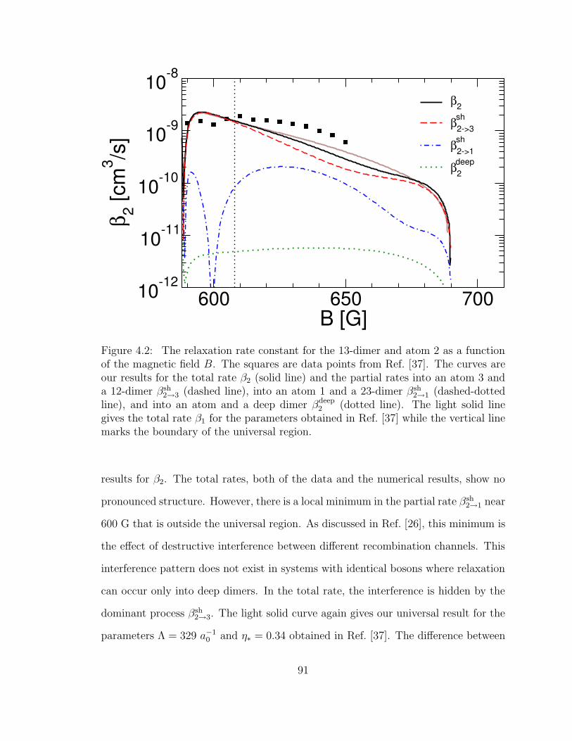
600 650 700B [G]

10-12

10-11

10-10

10-9

10-8

β 2 [cm

3 /s]

β2

β2->3sh

β2->1sh

β2deep

Figure 4.2: The relaxation rate constant for the 13-dimer and atom 2 as a functionof the magnetic field B. The squares are data points from Ref. [37]. The curves areour results for the total rate β2 (solid line) and the partial rates into an atom 3 anda 12-dimer βsh

2→3 (dashed line), into an atom 1 and a 23-dimer βsh2→1 (dashed-dotted

line), and into an atom and a deep dimer βdeep2 (dotted line). The light solid line

gives the total rate β1 for the parameters obtained in Ref. [37] while the vertical linemarks the boundary of the universal region.

results for β2. The total rates, both of the data and the numerical results, show no

pronounced structure. However, there is a local minimum in the partial rate βsh2→1 near

600 G that is outside the universal region. As discussed in Ref. [26], this minimum is

the effect of destructive interference between different recombination channels. This

interference pattern does not exist in systems with identical bosons where relaxation

can occur only into deep dimers. In the total rate, the interference is hidden by the

dominant process βsh2→3. The light solid curve again gives our universal result for the

parameters Λ = 329 a−10 and η∗ = 0.34 obtained in Ref. [37]. The difference between

91

600 650 700 750 800B [G]

10-12

10-11

10-10

10-9

10-8

10-7

β 3 [cm

3 /s]

β3

β3->1sh

β3deep

Figure 4.3: The relaxation rate constant for the 12-dimer and atom 3 as a function ofthe magnetic field B. The squares are data points from Ref. [37]. The curves are ourresults for the total rate β3 (solid line), the partial rate into atom 1 and a 23-dimerβsh

3→1 (dashed line), and the rate into an atom and a deep dimer βdeep3 (dashed-dotted

line). The light solid line gives the total rate β1 for the parameters obtained inRef. [37] while the vertical line marks the boundary of the universal region.

the two parameter sets is very small for β2, but the alternative set gives a slightly

better description of the data. Between 670 and 690 G, a2 is much larger than a1 and

a3 which are approximately equal. The scaling of the calculated rates into the shallow

dimers is consistent with the prediction of D’Incao and Esry [26]: βsh2→3 ∼ a2

3/a2 and

βsh1→3 ∼ a2

1/a2.

Fig. 4.3 shows our results and the recent measurement [37] for β3. Between 590 G

and 730 G, the energy of the 12-dimer is smaller than the energy of the 23-dimer

and the relaxation channel into 23-dimers is open. After the 23-dimer crosses the

12-dimer at 730 G this relaxation channel is closed and only relaxation into deep

92

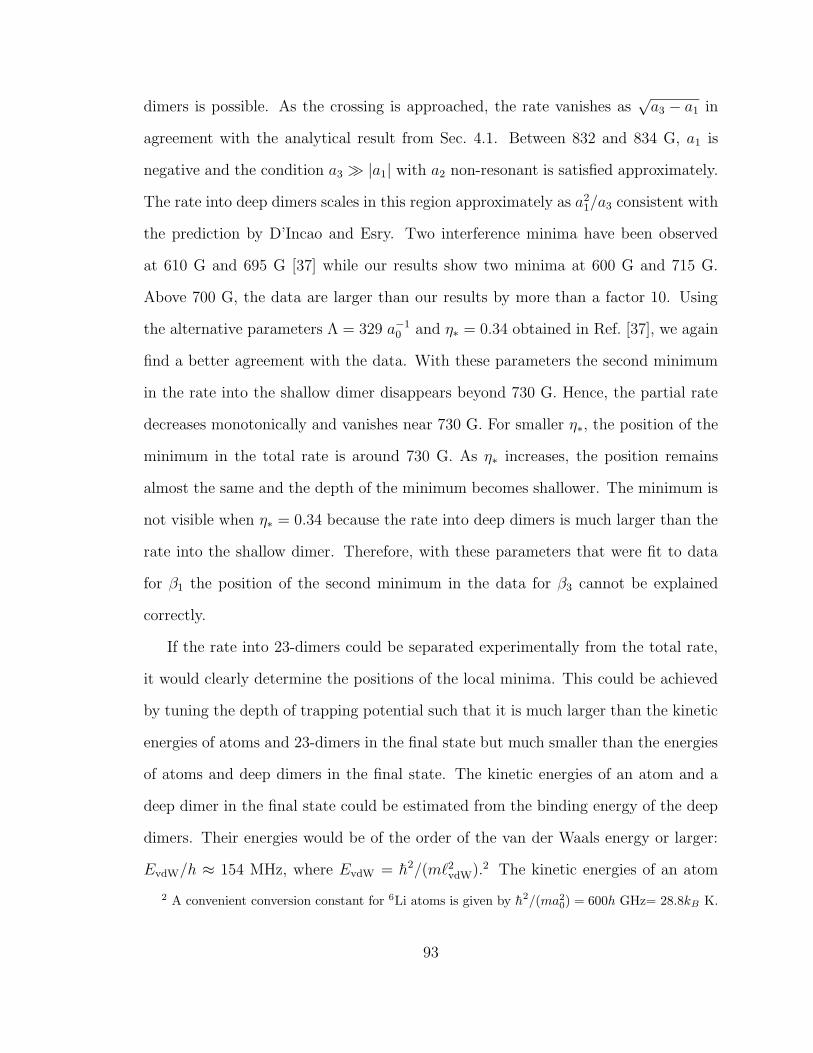
dimers is possible. As the crossing is approached, the rate vanishes as√a3 − a1 in

agreement with the analytical result from Sec. 4.1. Between 832 and 834 G, a1 is

negative and the condition a3 |a1| with a2 non-resonant is satisfied approximately.

The rate into deep dimers scales in this region approximately as a21/a3 consistent with

the prediction by D’Incao and Esry. Two interference minima have been observed

at 610 G and 695 G [37] while our results show two minima at 600 G and 715 G.

Above 700 G, the data are larger than our results by more than a factor 10. Using

the alternative parameters Λ = 329 a−10 and η∗ = 0.34 obtained in Ref. [37], we again

find a better agreement with the data. With these parameters the second minimum

in the rate into the shallow dimer disappears beyond 730 G. Hence, the partial rate

decreases monotonically and vanishes near 730 G. For smaller η∗, the position of the

minimum in the total rate is around 730 G. As η∗ increases, the position remains

almost the same and the depth of the minimum becomes shallower. The minimum is

not visible when η∗ = 0.34 because the rate into deep dimers is much larger than the

rate into the shallow dimer. Therefore, with these parameters that were fit to data

for β1 the position of the second minimum in the data for β3 cannot be explained

correctly.

If the rate into 23-dimers could be separated experimentally from the total rate,

it would clearly determine the positions of the local minima. This could be achieved

by tuning the depth of trapping potential such that it is much larger than the kinetic

energies of atoms and 23-dimers in the final state but much smaller than the energies

of atoms and deep dimers in the final state. The kinetic energies of an atom and a

deep dimer in the final state could be estimated from the binding energy of the deep

dimers. Their energies would be of the order of the van der Waals energy or larger:

EvdW/h ≈ 154 MHz, where EvdW = h2/(m`2vdW).2 The kinetic energies of an atom

2 A convenient conversion constant for 6Li atoms is given by h2/(ma2

0) = 600h GHz= 28.8kB K.

93

and a 23-dimer are given by the difference in binding energies between the 12-dimer

and the 23-dimer: h/(2πm)(a−223 − a−2

12 ) is about 1 MHz at 650 G and vanishes at

730 G. This way one may be able to measure the rate into deep dimers separately

and to extract the rate into the 23-dimer.

4.4 Finite temperature results

The results from the previous section suggest that finite temperature effects may play

an important role in understanding the atom-dimer relaxation data from Refs. [37, 38].

A full finite temperature calculation of the 6Li system is beyond the scope of this work.

Therefore, we perform an approximate calculation of the relaxation rate β1 near the

resonance at Bexp∗ = 685 G.

We start from the approximate expression for the scattering length between an

atom 1 and a 23-dimer near the resonance at B∗ that was extracted from a calculation

of the trimer binding energy in [36]:

a1(23) ≈ (C1 cot[s0 ln(a23/a∗) + iη∗] + C2) a23, (4.10)

where a∗ = a23(B∗) and the coefficients are C1 = 0.67 and C2 = 0.65. Using the

scattering length approximation for the S-wave atom-dimer scattering amplitude in

the 1(23)-channel,

f1(23)(k) =[

−1/a1(23) − ik]−1

, (4.11)

we can calculate the inelastic scattering cross section. At low temperatures, the

contributions from higher partial waves can be neglected. We subtract the elastic

cross section from the total cross section obtained via the optical theorem as in [65]

and find for the inelastic cross section:

σ(inelastic)1(23) (k) =

4π

k

−Im a1(23)

1− 2kIm a1(23) + k2|a1(23)|2. (4.12)

94

0.6 0.8 1 1.2 1.4a/a*

10-9

10-8

10-7

10-6

β 1 [cm

3 /s] η* = 0.016

η* = 0.34

Figure 4.4: The relaxation rate constant β1 for a 23-dimer and an atom 1 as a functionof a/a∗ near the resonance at Bexp

∗ = 685 G (a∗ = 1076 a0). Squares and circles aredata points from Ref. [37] and Ref. [38], respectively. The solid (dashed) curvescorrespond to η∗ = 0.016 (η∗ = 0.34). The upper curves give the zero temperatureresult, while the lower curves give the finite temperature result for T = 60 ± 15 nKwith the shaded area indicating the temperature uncertainty.

The total dimer-relaxation rate β1 can then be calculated by taking a Boltzmann

thermal average of the inelastic reaction rate vrel σ(inelastic)1(23) (k) where vrel = 3hk/(2m)

is the relative velocity of the atom and dimer in the initial state. This leads to the

expression

β1(T ) =3h

2m〈kσ(inelastic)

1(23) (k)〉 =3h

2m

3λ3T

4π2

√

3

2

∫ ∞

0

k2dk kσ(inelastic)1(23) (k) e

− 3h2k2

4mkBT , (4.13)

where λT =√

2πh2/(mkBT ) is the thermal de Brogile wavelength of the atoms.

Our results for the atom-dimer relaxation rate constant near the resonance at

95

Bexp∗ = 685 G are shown in Fig. 4.4. The results for the width parameters η∗ = 0.016

and η∗ = 0.34 are given by the solid and dashed curves, respectively. In each case the

upper curves give the zero temperature result while the lower curves give the finite

temperature result for T = 60±15 nK. Here, the shaded area indicates the uncertainty

from the temperature. The value of a∗ = 1076 a0 has been fixed to reproduce the

resonance position at Bexp∗ = 685 G. For η∗ = 0.016, the finite temperature effects

decrease the height of the peak by an order of magnitude but the predicted resonance

shape is still much narrower than the data. The finite temperature effects are much

less severe for η∗ = 0.34. They only lead to a reduction of β1 by about 25 % but clearly

improve the description of the data. We conclude that finite temperature effects can

not resolve the question of the different values for η∗ in the three-body recombination

and dimer-relaxation data. Moreover, while finite temperature effects are important,

a qualitative description of the data at T ≈ 60 nK can be already achieved with a

zero temperature calculation.

4.5 Summary and outlook

In this chapter, we have studied Efimov physics in atom-dimer relaxation of 6Li

atoms in the three lowest hyperfine states using the universal zero-range theory. Two

resonances were observed at magnetic fields 603 G and 685 G in the relaxation rate

β1 in recent experiments [37, 38]. These resonances are consequences of two Efimov

trimers close to the atom-dimer threshold. Their positions have been predicted by

Braaten et al. [36]. The measured position of the resonance at 685 G [37, 38], which

is well within the universal region, is larger than the prediction by about 30%. This is

consistent with an error of order 10% error due to effective range corrections. However,

the value η∗ = 0.016 extracted from the three-body recombination data is not able to

describe the atom-dimer relaxation data which require the larger value η∗ = 0.34 [37].

96

The reason for the larger value of η∗ in dimer relaxation compared to the value from

recombination data is not understood. However, we note that a similar discrepancy

between the values of η∗ from atom-dimer relaxation and three-body recombination

occurs in the bosonic systems of 133Cs atoms [28, 64].

Using the value η∗ = 0.34, our zero temperature calculation is able to describe

the data qualitatively. In the vicinity of this resonance, we have also performed an

approximate finite temperature calculation and find sizable temperature effects that

can suppress the relaxation rate by an order of magnitude if η∗ = 0.016. For the

larger value η∗ = 0.34, however, these effects lead to a moderate suppression of about

25%, such that zero temperature results are useful as a first approximation.

In Ref. [37], also two local minima at 610 G and 695 G are discovered in the rate

β3. Those minima can be associated with destructive interference between different

recombination channels [26]. Our numerical results show that the partial rate into

23-dimers is responsible for the minima but the positions of the minima are displaced

by -10 G and +20 G from the measurements. These displacements correspond to

a 30% shift in terms of the scattering length compared to our predictions. Since

the scattering length, a23, is about a factor two larger in this magnetic field region

than around the resonance in β1, one would expect smaller corrections here. The

observed shifts indicate that the destructive interference leading to the minima might

be dominated by wave numbers k larger than 1/a23 such that corrections of order

k`vdW are important. Moreover, finite temperature effects could fill the minima in an

asymmetric fashion. The total rate β2 shows no structure. However, the partial rate

into the 23-dimer shows a local minimum near 600 G. In the total rate this feature is

hidden by the dominant rate into the 12-dimer.

In order to better understand the discrepancy between the values of η∗ and the

resonance positions extracted from three-body recombination and atom-dimer relax-

97

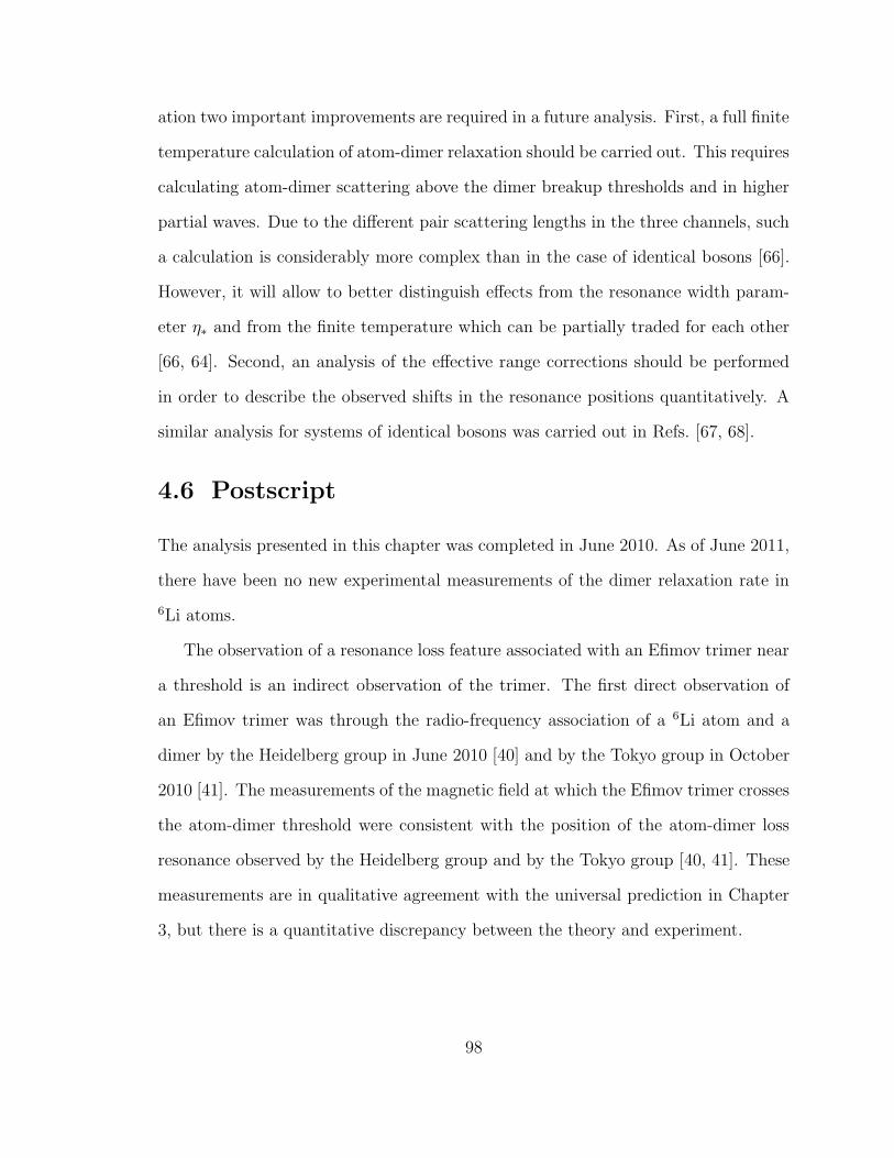
ation two important improvements are required in a future analysis. First, a full finite

temperature calculation of atom-dimer relaxation should be carried out. This requires

calculating atom-dimer scattering above the dimer breakup thresholds and in higher

partial waves. Due to the different pair scattering lengths in the three channels, such

a calculation is considerably more complex than in the case of identical bosons [66].

However, it will allow to better distinguish effects from the resonance width param-

eter η∗ and from the finite temperature which can be partially traded for each other

[66, 64]. Second, an analysis of the effective range corrections should be performed

in order to describe the observed shifts in the resonance positions quantitatively. A

similar analysis for systems of identical bosons was carried out in Refs. [67, 68].

4.6 Postscript

The analysis presented in this chapter was completed in June 2010. As of June 2011,

there have been no new experimental measurements of the dimer relaxation rate in

6Li atoms.

The observation of a resonance loss feature associated with an Efimov trimer near

a threshold is an indirect observation of the trimer. The first direct observation of

an Efimov trimer was through the radio-frequency association of a 6Li atom and a

dimer by the Heidelberg group in June 2010 [40] and by the Tokyo group in October

2010 [41]. The measurements of the magnetic field at which the Efimov trimer crosses

the atom-dimer threshold were consistent with the position of the atom-dimer loss

resonance observed by the Heidelberg group and by the Tokyo group [40, 41]. These

measurements are in qualitative agreement with the universal prediction in Chapter

3, but there is a quantitative discrepancy between the theory and experiment.

98

Chapter 5

Outlook

To conclude this thesis, we summarize unresolved questions raised in the studies of

the Efimov physics in 6Li atoms and we suggest what can be done to answer these

questions. We also discuss possible future directions.

In Chapter 2, we calculated the three-body recombination rate at zero tempera-

ture for fermions with three spin states and large negative scattering lengths. Our

calculation of the rate for 6Li atoms gave an excellent fit to the narrow loss resonance

near 130 G and predicted an equally narrow loss resonance near 500 G. The observed

loss resonance near 500 G is much broader [7, 8]. The Heidelberg group pointed out

that the three shallowest of the deep dimers in this region of magnetic field are the

diatomic molecules that are responsible for the Feshbach resonances in the high-field

region [53]. The binding energies of these dimers are zero at the Feshbach resonances

at 690 G, 811 G, and 830 G. Their binding energies increase as the magnetic field

decreases, changing by about a factor of 7 from 500 G to 130 G. The Heidelberg group

proposed a simple empirical relation between the three-body width parameter η∗ and

the binding energy Edeep of a deep dimer that dominates the width : η∗ ∝ 1/Edeep.

Rittenhouse deduced a more complicated functional form for η∗(Edeep) by calculating

the recombination rate using a simple model with two hyperspherical channels [69]. In

this thesis, we have implicitly assumed that the three-body parameters κ∗ and η∗ are

99

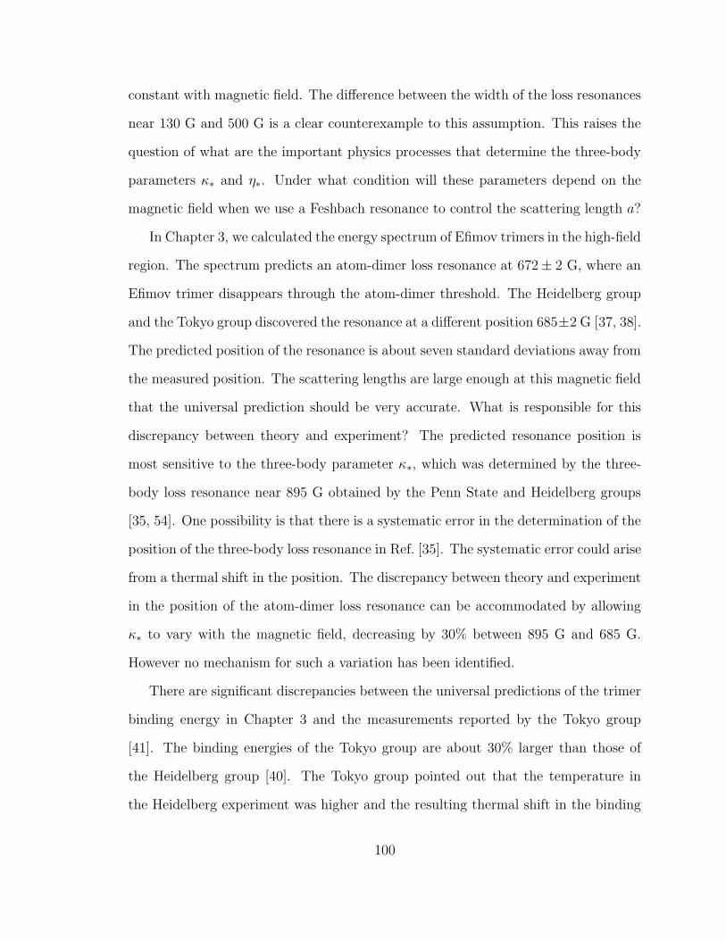
constant with magnetic field. The difference between the width of the loss resonances

near 130 G and 500 G is a clear counterexample to this assumption. This raises the

question of what are the important physics processes that determine the three-body

parameters κ∗ and η∗. Under what condition will these parameters depend on the

magnetic field when we use a Feshbach resonance to control the scattering length a?

In Chapter 3, we calculated the energy spectrum of Efimov trimers in the high-field

region. The spectrum predicts an atom-dimer loss resonance at 672± 2 G, where an

Efimov trimer disappears through the atom-dimer threshold. The Heidelberg group

and the Tokyo group discovered the resonance at a different position 685±2 G [37, 38].

The predicted position of the resonance is about seven standard deviations away from

the measured position. The scattering lengths are large enough at this magnetic field

that the universal prediction should be very accurate. What is responsible for this

discrepancy between theory and experiment? The predicted resonance position is

most sensitive to the three-body parameter κ∗, which was determined by the three-

body loss resonance near 895 G obtained by the Penn State and Heidelberg groups

[35, 54]. One possibility is that there is a systematic error in the determination of the

position of the three-body loss resonance in Ref. [35]. The systematic error could arise

from a thermal shift in the position. The discrepancy between theory and experiment

in the position of the atom-dimer loss resonance can be accommodated by allowing

κ∗ to vary with the magnetic field, decreasing by 30% between 895 G and 685 G.

However no mechanism for such a variation has been identified.

There are significant discrepancies between the universal predictions of the trimer

binding energy in Chapter 3 and the measurements reported by the Tokyo group

[41]. The binding energies of the Tokyo group are about 30% larger than those of

the Heidelberg group [40]. The Tokyo group pointed out that the temperature in

the Heidelberg experiment was higher and the resulting thermal shift in the binding

100

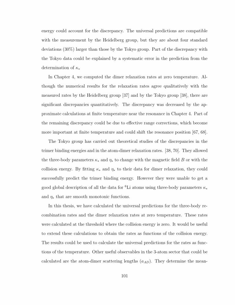
energy could account for the discrepancy. The universal predictions are compatible

with the measurement by the Heidelberg group, but they are about four standard

deviations (30%) larger than those by the Tokyo group. Part of the discrepancy with

the Tokyo data could be explained by a systematic error in the prediction from the

determination of κ∗

In Chapter 4, we computed the dimer relaxation rates at zero temperature. Al-

though the numerical results for the relaxation rates agree qualitatively with the

measured rates by the Heidelberg group [37] and by the Tokyo group [38], there are

significant discrepancies quantitatively. The discrepancy was decreased by the ap-

proximate calculations at finite temperature near the resonance in Chapter 4. Part of

the remaining discrepancy could be due to effective range corrections, which become

more important at finite temperature and could shift the resonance position [67, 68].

The Tokyo group has carried out theoretical studies of the discrepancies in the

trimer binding energies and in the atom-dimer relaxation rates. [38, 70]. They allowed

the three-body parameters κ∗ and η∗ to change with the magnetic field B or with the

collision energy. By fitting κ∗ and η∗ to their data for dimer relaxation, they could

successfully predict the trimer binding energy. However they were unable to get a

good global description of all the data for 6Li atoms using three-body parameters κ∗

and η∗ that are smooth monotonic functions.

In this thesis, we have calculated the universal predictions for the three-body re-

combination rates and the dimer relaxation rates at zero temperature. These rates

were calculated at the threshold where the collision energy is zero. It would be useful

to extend these calculations to obtain the rates as functions of the collision energy.

The results could be used to calculate the universal predictions for the rates as func-

tions of the temperature. Other useful observables in the 3-atom sector that could be

calculated are the atom-dimer scattering lengths (aAD). They determine the mean-

101

field energy shift of an atom in a Bose-Einstein condensate of shallow dimers. For suf-

ficiently low dimer density such that nDa3AD 1, the energy shift is 3π3h aADnD /m.

Finally, universality in the 4-atom sector for fermions with three spin states is com-

pletely unexplored territory. It would be particularly valuable to have predictions of

the binding energies of universal tetramers.

In 2005, Tan derived some universal relations that hold for any system that con-

sists of fermion with two spin states that interact with a large scattering length

[71, 72, 73]. They relate various observables to an extensive property of the system

called the contact. The contact is a measure of the probability for two atoms to be

close together. The universal relations can be derived using the analytic solution

to the two-body problem. They therefore reveal aspects of many-body physics that

are controlled by two-body physics. Tan’s universal relations were rederived by us-

ing quantum field theory methods, including the operator product expansion [74, 75].

Many other universal relations involving the contact have been derived subsequently

[76]. This technique clearly shows the connection of few-body physics to many-body

physics. Recently, analogous universal relations for identical bosons were derived [77].

In addition to the two-body contact these relations involve a three-body contact, which

is a measure of the probability for three atom to be close together [77]. In some of the

relations, the coefficient of the three-body contact is log-periodic function, which is a

signature of Efimov physics. It would be useful to derive the analogous universal re-

lations for fermions with three spin states. These relations would involve a two-body

contact for each of the three pairs of spin states and the three-body contact, which

is a measure of the probability for three atoms in the three different spin states to be

close together. These universal relations are a promising new probe to study Efimov

physics in 6Li atoms.

102

Bibliography

[1] M. Inguscio, W. Ketterle, and C. Salomon, ed., Ultracold Fermi Gases (IOSPress, Amsterdam, 2008).

[2] P. F. Bedaque and J. P. D’Incao, Superfluid phases of the three-species fermiongas, Annals Phys. 324, 1763 (2009).

[3] T. Paananen, J.-P. Martikainen, and P. Torma, Pairing in a three-componentFermi gas, Phys. Rev. A 73, 053606 (2006).

[4] L. He, M. Jin, and P. Zhuang, Superfluidity in a three-flavor Fermi gas withSU(3) symmetry, Phys. Rev. A 74, 033604 (2006).

[5] H. Zhai, Superfluidity in three-species mixtures of Fermi gases across Feshbachresonances, Phys. Rev. A 75, 031603 (2007).

[6] J.-P. Martikainen, J. J. Kinnunen, P. Torma, and C. J. Pethick, Induced Inter-actions and the Superfluid Transition Temperature in a Three-Component FermiGas, Phys. Rev. Lett. 103, 260403 (2009).

[7] T. B. Ottenstein, T. Lompe, M. Kohnen, A. N. Wenz, and S. Jochim, CollisionalStability of a Three-Component Degenerate Fermi Gas, Phys. Rev. Lett. 101,203202 (2009).

[8] J. Huckans, J. Williams, E. Hazlett, R. Stites, and K. O’Hara, Three-bodyrecombination in a three-state Fermi gas with widely tunable interactions, Phys.Rev. Lett. 102, 165302 (2009).

[9] V. Efimov, Energy levels arising form the resonant two-body forces in a three-body system, Phys. Lett. B33, 563 (1970).

[10] V. Efimov, Energy levels of three resonantly interacting particles, Nucl. Phys.A210, 157 (1973).

[11] E. Braaten and H.-W. Hammer, Universality in few-body systems with largescattering length, Phys. Rept. 428, 259 (2006).

103

[12] E. Braaten and H.-W. Hammer, Efimov Physics in Cold Atoms, Annals Phys.322, 120 (2007).

[13] S. Gasiorwicz, Quantum Physics (John Wiley & Sons, 2003).

[14] J. R. Tayler, Scattering Theory: The Quantum Theory on Nonrelativistic Colli-

sions (John Wiley & Sons, 1972).

[15] L. D. Landau and E. M. Lifshitz, Quantum Mechanics (Pergamon, New York,1980).

[16] C. Chin, R. Grimm, P. Julienne, and E. Tiesinga, Feshbach resonances in ultra-cold gases, Rev. Mod. Phys. 82, 1225 (2010).

[17] M. Bartenstein et al., Precise Determination of 6Li Cold Collision Parametersby Radio-Frequency Spectroscopy on Weakly Bound Molecules, Phys. Rev. Lett.94, 103201 (2005).

[18] P. Julienne, private communication.

[19] E. Braaten and H.-W. Hammer, Enhanced dimer deactivation in an atomic /molecular BEC, Phys. Rev. A 70, 042706 (2004).

[20] L. Platter, H.-W. Hammer, and U.-G. Meißner, Four-boson system with short-range interactions, Phys. Rev. A 70, 052101 (2004).

[21] H.-W. Hammer and L. Platter, Universal Properties of the Four-Body Systemwith Large Scattering Length, Eur. Phys. J. A32, 113 (2007).

[22] J. von Stecher, J. D’Incao, and C. Greene, Signatures of universal four-bodyphenomena and their relation to the Efimov effect, Nature Physics 5, 417 (2009).

[23] E. Nielsen and J. H. Macek, Low-Energy Recombination of Identical Bosons byThree-Body Collisions, Phys. Rev. Lett. 83, 1566 (1999).

[24] B. D. Esry, C. H. Greene, and J. P. Burke, Recombination of Three Atoms inthe Ultracold Limit, Phys. Rev. Lett. 83, 1751 (1999).

[25] P. F. Bedaque, E. Braaten, and H.-W. Hammer, Three-body Recombination inBose Gases with Large Scattering Length, Phys. Rev. Lett. 85, 908 (2000).

[26] J. P. D’Incao and B. D. Esry, Ultracold Three-Body Collisions near OverlappingFeshbach Resonances, Phys. Rev. Lett. 103, 083202 (2009).

[27] T. Kraemer et al., Evidence for Efimov quantum states in an ultracold gas ofcaesium atoms, Nature 440, 315 (2006).

[28] S. Knoop et al., Observation of an Efimov-like trimer resonance in ultracoldatom-dimer scattering, Nature Physics 5, 227 (2009).

104

[29] G. Barontini et al., Observation of Heteronuclear Atomic Efimov Resonances,Phys. Rev. Lett. 103, 043201 (2009).

[30] M. Zaccanti et al., Observation of an Efimov spectrum in an atomic system,Nature Physics 5, 586 (2009).

[31] N. Gross, Z. Shotan, S. Kokkelmans, and L. Khaykovich, Observation of Uni-versality in Ultracold 7Li Three-Body Recombination, Phys. Rev. Lett. 103,163202 (2009).

[32] S. E. Pollack, D. Dries, and R. G. Hulet, Universality in Three- and Four-BodyBound States of Ultracold Atoms, Science 326, 1683 (2009).

[33] F. Ferlaino et al., Evidence for Universal Four-Body States Tied to an EfimovTrimer, Phys. Rev. Lett. 102, 140401 (2009).

[34] E. Braaten, H.-W. Hammer, D. Kang, and L. Platter, Three-Body Recombi-nation of 6Li Atoms with Large Negative Scattering Lengths, Phys. Rev. Lett.103, 073202 (2009).

[35] J. R. Williams et al., Evidence for an Excited-State Efimov Trimer in a Three-Component Fermi Gas, Phys. Rev. Lett. 103, 130404 (2009).

[36] E. Braaten, H. W. Hammer, D. Kang, and L. Platter, Efimov physics in 6Liatoms, Phys. Rev. A 81, 013605 (2010).

[37] T. Lompe et al., Atom-Dimer Scattering in a Three-Component Fermi Gas,Phys. Rev. Lett. 105, 103201 (2010).

[38] S. Nakajima, M. Horikoshi, T. Mukaiyama, P. Naidon, and M. Ueda, Nonuni-versal Efimov Atom-Dimer Resonances in a Three-Component Mixture of 6Li,Phys. Rev. Lett. 105, 023201 (2010).

[39] H.-W. Hammer, D. Kang, and L. Platter, Efimov physics in atom-dimer scat-tering of 6Li atoms, Phys. Rev. A 82, 022715 (2010).

[40] T. Lompe et al., Radio-Frequency Association of Efimov Trimers, Science 330,940 (2010).

[41] S. Nakajima, M. Horikoshi, T. Mukaiyama, P. Naidon, and M. Ueda, Measure-ment of an Efimov Trimer Binding Energy in a Three-Component Mixture of6Li, Phys. Rev. Lett. 106, 143201 (2011).

[42] P. F. Bedaque and U. van Kolck, Effective field theory for few nucleon systems,Ann. Rev. Nucl. Part. Sci. 52, 339 (2002).

[43] L. Platter, Low-Energy Universality in Atomic and Nuclear Physics, Few BodySyst. 46, 139 (2009).

105

[44] E. Braaten, M. Kusunoki, and D. Zhang, Scattering Models for Ultracold Atoms,Annals Phys. 323, 1770 (2008).

[45] D. B. Kaplan, Five lectures on effective field theory, nucl-th/0510023.

[46] G. Skorniakov and K. Ter-Martirosian, Three Body Problem for Short RangeForces: 1. Scattering of Low Energy Neutrons by Deuterons, Sov. Phys. JETP4, 648 (1957).

[47] P. F. Bedaque, H. W. Hammer, and U. van Kolck, Renormalization of the three-body system with short-range interactions, Phys. Rev. Lett. 82, 463 (1999).

[48] P. F. Bedaque, H. W. Hammer, and U. van Kolck, The three-boson system withshort-range interactions, Nucl. Phys. A646, 444 (1999).

[49] E. Braaten, D. Kang, and L. Platter, Universal relations for identical bosonsfrom three-body physics, Phys. Rev. Lett. 106, 153005 (2011).

[50] E. Braaten, H.-W. Hammer, and T. Mehen, The Dilute Bose-Einstein condensatewith large scattering length, Phys. Rev. Lett. 88, 040401 (2002).

[51] P. Naidon and M. Ueda, Possible Efimov Trimer State in a Three-Hyperfine-Component Lithium-6 Mixture, Phys. Rev. Lett. 103, 073203 (2009).

[52] R. Schmidt, S. Floerchinger, and C. Wetterich, Three-body loss in lithium fromfunctional renormalization, Phys. Rev. A 79, 053633 (2009).

[53] A. N. Wenz et al., Universal trimer in a three-component Fermi gas, Phys. Rev.A 80, 040702 (2009).

[54] S. Jochim, private communication.

[55] D. S. Petrov, Three-body problem in Fermi gases with short-range interparticleinteraction, Phys. Rev. A 67, 010703 (2003).

[56] J. P. D’Incao and B. D. Esry, Scattering Length Scaling Laws for UltracoldThree-Body Collisions, Phys. Rev. Lett. 94, 213201 (2005).

[57] H.-W. Hammer and T. Mehen, A Renormalized equation for the three-bodysystem with short range interactions, Nucl. Phys. A690, 535 (2001).

[58] A. O. Gogolin, C. Mora, and R. Egger, Analytical Solution of the BosonicThree-Body Problem, Phys. Rev. Lett. 100, 140404 (2008).

[59] J. H. Macek, S. Ovchinnikov, and G. Gasaneo, Solution for boson-diboson elasticscattering at zero energy in the shape-independent model, Phys. Rev. A 72,032709 (2005).

106

[60] D. Petrov, Three-boson problem near a narrow Feshbach resonance, talk at theWorkshop on Strongly Interacting Quantum Gases (Ohio State University, April2005).

[61] D. Petrov, C. Salomon, and G. Shlyapnikov, Weakly Bound Dimers of FermionicAtoms, Phys. Rev. Lett. 93, 090404 (2004).

[62] E. Braaten and D. Kang, unpublished.

[63] E. Braaten, H.-W. Hammer, and M. Kusunoki, Universal equation for Efimovstates, Phys. Rev. A 67, 022505 (2003).

[64] K. Helfrich and H.-W. Hammer, Resonant Atom-Dimer Relaxation in UltracoldAtoms, Europhys. Lett. 86, 53003 (2009).

[65] E. Braaten and H.-W. Hammer, Resonant dimer relaxation in cold atoms witha large scattering length, Phys. Rev. A 75, 052710 (2007).

[66] E. Braaten, H.-W. Hammer, D. Kang, and L. Platter, Three-body recombinationof identical bosons with a large positive scattering length at nonzero temperature,Phys. Rev. A 78, 043605 (2008).

[67] H.-W. Hammer, T. A. Lahde, and L. Platter, Effective-range corrections tothree-body recombination for atoms with large scattering length, Phys. Rev. A75, 032715 (2007).

[68] C. Ji, D. R. Phillips, and L. Platter, Beyond universality in three-body recom-bination: An effective field theory treatment, Europhys. Lett. 92, 13003 (2010).

[69] S. T. Rittenhouse, Magnetic-field dependence and Efimov resonance broadeningin ultracold three-body recombination, Phys. Rev. A 81, 040701 (2010).

[70] P. Naidon and M. Ueda, The Efimov effect in lithium 6, Comptes RendusPhysique 12 (2011).

[71] S. Tan, Energetics of a strongly correlated Fermi gas, Annals Phys. 323, 2952(2008).

[72] S. Tan, Large momentum part of a strongly correlated Fermi gas, Annals Phys.323, 2971 (2008).

[73] S. Tan, Generalized virial theorem and pressure relation for a strongly correlatedFermi gas, Annals of Phys. 323, 2987 (2008).

[74] E. Braaten and L. Platter, Exact Relations for a Strongly Interacting Fermi Gasfrom the Operator Product Expansion, Phys. Rev. Lett. 100, 205301 (2008).

[75] E. Braaten, D. Kang, and L. Platter, Universal relations for a strongly interactingFermi gas near a Feshbach resonance, Phys. Rev. A 78, 053606 (2008).

107

[76] E. Braaten, Universal Relations for Fermions with Large Scattering Length,arXiv:1008.2922.

[77] E. Braaten, D. Kang, and L. Platter, Universal relations for identical bosonsfrom three-body physics, Phys. Rev. Lett. 106, 153005 (2011).

108