
Micromanipulation of neutral atoms with nanofabricated structures
Upload
khangminh22Category
view
2download
0
Prog. Quonr. Elecr,: 1997, Vol. 21, No. 1, pp. 1-79 @ 1997 Elsevier Science Ltd
SOO79-6727(96)00006-7 Printed in Great Britain. All rights reserved 0019-6727197 $32.00
LASER COOLING AND TRAPPING OF NEUTRAL ATOMS
C. S. ADAMS
Department of Physics, Durham University, Durham DHl 3LE, UK
E. RIIS
Department of Physics and Applied Physics, Strathclyde University, Glasgow G4 ONG, UK
Abstract: The ability to cool, manipulate, and trap atoms using laser light has allowed a new, rapidly expanding field to emerge. Current research focuses on improving existing cooling techniques, and the development of cold atoms as a source for applications ranging from atomic clocks to studies of quantum degeneracy. This review explains the basic mechanisms used in laser cooling and trapping, and illustrates the development of the field by describing a selection of key experiments. Copyright @ 1997 Elsevier Science Ltd. All rights reserved
CONTENTS
I Introduction 2 Historical background
2.1 Introduction 2.2 Slowing of atomic beams 2.3 Doppler cooling 2.4 Traps
2.4.1 Optical Dipole traps 2.4.2 Magnetic traps 2.4.3 Traps based on the scattering force
2.5 The magneto-optical trap 2.5. I Loading rates 2.5.2 Trap loss 2.5.3 Dark magneto-optical trap
3 Sub-Doppler cooling 3.1 Introduction 3.2 Breakdown of Doppler theory 3.3 Temperature
3.3.1 Definition 3.3.2 Measurement
3.4 Beyond Doppler cooling: the Sisyphus effect 3.5 Qualitative models 3.6 linllin polarisation gradient cooling 3.7 (r+ u- polarisation gradient cooling 3.8 Experimental verification 3.9 Sub-Doppler cooling in a magnetic field
2 6 6
9 I2 I2 I5 I6 17 I7 I8 20 20 20 20 21 21 22 23 24 27 28 28 29

2 C. S. ADAMS & E. RIIS
4 Sub-recoil cooling
4. I Introduction
4.2 Velocity selective coherent population trapping
4.2. I Theory
4.2.2 Experiment
4.3 kdmdn cooling
4.3.1 Experiments
5 Precision measurements with cold atoms
5. I Introduction
5.2 The atomic fountain 5.2.1 The first cold-atom fountain experiment
5.2.2 Second generation of fountains
5.3 Atomic clocks
5.3.1 Limiting factors
5.3.2 Prospects for optical clocks
5.4 Precision spectroscopy
5.5 Atom interferometers
5.5.1 Measurement of g
5.5.2 Measurement of h/m
6 Cold atomic beams
6.1 Introduction
6.2 Cooling of beams
6.3 Focusing of atomic beams
6.4 Atom lithography
7 Optical dipole traps and lattices 7.1 Introduction
7.2 Optical dipole traps
7.2. I Red-detuned traps
7 22 Blue-detuned traps
7.3 Optical lattices
7.3. I I-D optical lattices: spectroscopic techniques
7.3. I. I Heterodyne Huorescence spectroscopy
7.3. I .2 Probe absorption spectroscopy
7.3.2 2-D and 3-D optical lattices
7.3.3 Dark lattices
7.3.4 Adiabatic cooling
7.3.5 Bragg diffraction
7.4 Summary and outlook
8 Towards quantum degeneracy
8. I Introduction 8.2 Magnetic traps
X.2.1 Laser cooling in magnetic traps
8.22 Evaporative cooling
8.2.3 Bose condensation
8.3 Optical dipole traps
9 Conclusions
32
32
33 33
36
37
39
40
40
41
41
43
44
44
44
45
46
47
48
48
48
49
50
51
53
53
53
54
56
58
58
59
60
62
63
63
63
64
65
65
66
67
68
68
70
70
1. INTRODUCTION
The possibility of lasers manipulating, trapping, and extracting mechanical energy from neutral atoms has revolutionised large areas of atomic physics, and opened completely new research fields. It is now routine, in an ever increasing number of laboratories throughout the world, to prepare atomic samples cooled to a few /AC, and trapped with densities approaching one atom per urn’. With more elaborate techniques even lower temperatures and higher densities can be achieved. Such samples present an ideal starting point for further experimental work: the atoms can be confined in a relatively perturbation free environment, Doppler shifts are virtually non-existent, and extremely long interaction times are possible. These achievements

Laser cooling and trapping of neutral atoms 3
represent the culmination of around 25 years of technical and theoretical developments in one of the most rapidly expanding areas of atomic and laser physics.
Although the concept of light pressure was familiar at the turn of the century, its mechanical effect was considered insignificant. This was entirely due to the low brightness of available light sources. Things changed dramatically after the invention of narrow linewidth tunable lasers. In 1975 HHnsch and Schawlow(‘) realised that such light sources could exert a substantial force on atoms and potentially be used for cooling. * A few years later, the use of lasers for atom trapping was proposed by Ashkin. c3) Initially progress was slow, the important experimental milestones were reported almost a decade later: the first stopping of a thermal beam in 1982;(4) the first 3-D cooling in 1985;(5) and the first optical trapping in 1986.(@ Most of the early work on laser cooling and trapping was performed using Na, because it has an almost ideal level structure, it is easy to produce a thermal beam, and the cooling transition can be driven by a cw dye laser, operated with one of the most efficient and reliable dyes, Rhodamine 6G. As other tunable sources became available, such as laser diodes and Ti:sapphire lasers, research has shifted towards the heavier alkalis, Rb and Cs, which have a similar level structure but their resonance lines are in the near infrared. Now, more than 15 different elements, some with several isotopes, have been used in cooling and trapping experiments (see Appendix).
The probability for an atom absorbing light depends on its velocity through the Doppler shift. If the light is red-detuned a moving atom is most likely to absorb photons it is moving towards. The absorption-fluorescence cycle imparts momentum which tends to slow it down. If light is applied from each direction the atom experiences a .friction-like ,fbrce. Due to the central role of the Doppler shift this process is known as Doppler cooling (see Section 2). The final velocity distribution of the atoms is the result of a balance between dissipation, and diffusion due to the stochastic nature of the spontaneous emission process. For a typical atom the equilibrium temperature, known as the Doppler temperature, is of order low4 K. which is comparable to the best that can be achieved with other cooling techniques as illustrated in Fig. 1.
Fig. 1. Schematic diagram showing the temperature scales relevant to laser cooling. The main cooling mechanisms and their characteristic temperatures are indicated.
* Laser cooling of trapped ions was proposed by Wineland and Dehmelt at about the same time.(2’

4 C. S. ADAMS & E. RIIS
The basic idea behind laser cooling is the conservation of energy and momentum during the absorption and emission of radiation. Although this seems perfectly innocuous, attempts to gain a fuller understanding of the mechanisms at work met with a number of surprises. Perhaps the most pleasant surprise occurred when the measured temperatures were found to be below the Doppler limit. (7) This discovery stimulated further experiments, and a new theoretical understanding. It was realised that the multi-level character of real atoms and the spatial variation of the polarisation of the light field played an important role in the cooling process. (S-10) The new cooling mechanisms, which became known as sub-Doppler or polarisation gradient cooling, produced temperatures of order 10e5 K (see Section 3). Again there is a fundamental temperature limit: an atom cannot end up with less kinetic energy than that corresponding to one photon recoil. Typically the recoil limit corresponds to a temperature of between 10e7 and low6 K. However, there is a way around the recoil limit: allow atoms to scatter photons until, by chance, the final recoil happens to leave them with a velocity very close to zero. Such schemes, known as sub-recoil cooling, (11,12) have achieved 3-D temperatures below 10-6K(‘3,‘4) (see Section 4).
The primary goal of any cooling technique is to increase the phase space density nh&, where n is the density and h&i is the thermal de Broglie wavelength of the atoms. This requirement distinguishes cooling from velocity selection. High phase space density, i.e. many atoms with narrow spatial and velocity distributions, is an advantage for most experiments in atomic physics. In addition, the phase space density determines whether the atomic vapour behaves as a classical or a quantum gas. For nh& > 2.62, known as the quantum degenerate regime, the de Broglie waves of neighbouring bosonic atoms begin to overlap and interfere constructively, and one expects to observe interesting collective effects such as Bose-Einstein condensation and superfluidity.(r5)
Laser cooling alone can lead to a significant increase in the phase space density, but it works even better in conjunction with a trap. The first demonstration of simultaneous cooling and trapping in 1987 used a combination of light and magnetic fields.“@ This device, known as the magneto-optical trap, was extremely successful and now forms the basic building block of most experiments on cold atoms (see Sections 2.4 and 2.5). A typical magneto-optical trap contains up to lOi atoms, with a temperature of order 10-100 PK and a density of up to 10i2cm-‘. The phase space density is a factor of 1012 higher than for a typical atomic beam, but still a factor of million away from the quantum degenerate regime. In a magneto-optical trap, both the density and the temperature are limited by the presence of near-resonant light.
The pursuit of higher phase space density has concentrated on transferring cold atoms to more passive traps and introducing alternative cooling techniques (see Section 8). The most successful example is forced-evaporative cooling of atoms confined iu a purely magnetic trap. Evaporative cooling combined with adiabatic relaxation of the potential has produced temperatures of less than 10e9 K. More importantly, the technique of evaporative cooling in a magnetic trap led to the first observation of Bose-Einstein condensation in a dilute atomic vapour in 1995.(r7-r9) A weakly interacting Bose gas has been considered as a holy grail of modern atomic physics, and this breakthrough represents a powerful statement of the success of laser cooling and trapping.
The second area where laser cooling and trapping has produced an enormous impact is that of precision measurements (see Section 5). For any precision measurement, one would like a large number of atoms, in a perturbation-free environment for as long as possible. The perturbation-free requirement tends to rule out the use of trapped atoms and on the earth, free atoms fall due to gravity. Over 40 years ago, Zacharias proposed that the desired long interrogation times could be achieved by directing the atoms upwards to form an atomic fiuntain.t20) The problem was that the slower atoms, which would turn around first, were bombarded by faster atoms. Still, Zacharias’ idea was a good one, it just needed laser cooling

Laser cooling and trapping of neutral atoms
to make it work! An atomic fountain with arbitrary height (typically a fraction of a meter, and hence an interrogation time of a fraction of a second) can be produced by starting with a source of laser cooled atoms (e.g. from a magneto-optical trap) and using the radiation pressure force to launch them. The first atomic fountain was demonstrated by Kasevich et al. in 1989’*” and the technique has already become the standard for the next generation of atomic clock~.(****~) Atomic fountains are also ideally suited for other precision measurements such as the Doppler shift of a falling atom (atomic gravitometer),‘24) and an accurate determination of the recoil of an atom due to absorption of a single photon.(25)
Light forces may also be used to collimate, focus, and increase the monochromicity of an atomic source (see Section 6). Such bright atomic beams are ideal for atom optics.‘*@ Both atom interferometryC24*25) and atom lithography (27*28) have benefited greatly from advances in laser cooling and trapping. Similar advances have also opened doors to a number of newfields. One of these is the study of optical lattices: atoms trapped in a periodic array of potential wells created by interfering light beams (see Section 7). These lattices display long-range order and it is hoped that their properties will help to develop a deeper understanding of more complex periodic systems in solid-state physics. Another example is photo-associative spectroscopy,(29p30) where a probe laser is tuned to excite a bound state between two colliding atoms. The ex- cited molecule subsequently decays by spontaneous emission to form a groundstate long-range molecule (i.e. a molecule in a highly excited vibrational state). The photo-associative spectra provide information about the long-range pair potentials which can be used to calculate the scattering fength, a critical component in the theory of Bose-Einstein condensation. Laser cooling also provides a new angle on many existing fields in atomic physics. For example, cold atoms, free of residual Doppler or pressure broadening, form a unique sample for exper- iments in quantum optics,(“l) and are ideal for precision measurement of atomic transition frequenciesC3*) and lifetimes.““)
In this article, we attempt to review the development of laser cooling and trapping of neutral atoms. The field has always thrived on the close interplay between theory and experiment, and so experimental breakthroughs and the underlying theory are considered in parallel. The field can be roughly divided into efforts to develop and understand new laser cooling techniques, and experiments which take advantage of the unique properties of cold atoms. The article is arranged as follows. In Section 2 we describe the historical development of laser cooling and trapping, including experiments on slowing atomic beams, Doppler cooling, and the magneto-optical trap. Section 3 presents a qualitative discussion of sub-Doppler cooling mechanisms. In Section 4 two sub-recoil cooling techniques are considered: velocity selective coherent population trapping and Raman cooling. Precision measurement using cold atoms are discussed in Section 5. This includes techniques such as the atomic fountain and atom interferometry. In Section 6 the application of laser cooling to the preparation of well- collimated, intense atomic beams is reviewed. In Section 7 we consider optical trapping of atoms, in particular, optical dipole traps and optical lattices. Section 8 deals with the pursuit of high phase space density, and describes the techniques used to produce a Bose-Einstein condensate. Finally, in the Appendix key parameters are listed for a range of elements which have been used or proposed for experiments on laser cooling.
Both introductory and more specialised material on laser cooling and trapping can be found in the following references. The historical development of the field may be followed in a succession of general articles,(j4-“8) Special Issues(“9~40) and Summer School Proceedings.(4’-4” The semi-classical theory of light-atom interactions is considered in Refs 44,45. More detailed treatment of the theory of atomic motion in laser light may be found in Refs 46,47. The use of light forces for atom optics and atom interferometry are reviewed in Ref 26.
In parallel with work on neutral atoms, a significant amount of research has been carried out on laser cooling of trapped ions. Many of the ideas and techniques are very similar to

6 C. S. ADAMS & E. RIIS
those presented here, except that ions can be trapped for much longer, thanks to their stronger interaction with electric and magnetic fields. The penalty, however, is that only a few ions can be trapped simultaneously due to their mutual Coulomb repulsion. The topic of ion trapping is outside the scope of this review and the interested reader is referred e1sewhere.(48)
2. HISTORICAL BACKGROUND
2.1. Introduction
The idea that light can exert pressure has been around for a long time. For instance, in the 17th century, Kepler speculated that the repulsion of comet tails from the sun may be due to light pressure. It was later realised that other processes were more important, but the hypothesis did identify a significant astrophysical effect, and stimulated further work on understanding its origin. However, it was not until Maxwell formulated his electromagnetic theory of light in 1 873(49) that a proper theoretical basis for the concept was established. He showed that an electromagnetic field exerts a pressure equal to its energy per unit volume. For light from the sun, or from a thermal source, the radiation pressure is extremely small. Even so, the value predicted by Maxwell was verified experimentally by Lebedev,(50’ and Nichols and H~ll(‘~’ around the turn of the century.
An important step towards our present understanding of radiation pressure, and indeed the basis for the most intuitive model of the effect, came with the introduction of a quantum mechanical view of light. In 1917 Einstein showed that a quantum of light, or photon, with energy hv, carries a momentum, hvlc = h/h, where h is Planck’s constant, c, v, and h are the speed, frequency, and wavelength of the light respective1y.‘52’ The basic mechanism for radiation pressure is the conservation of momentum during the absorption and emission of light. The photon momentum, directed along the propagation direction of the light, is expressed in terms of the wave vector k (k = 27-r/h) as Ak, where A = h/2rr.
Striking evidence for the particle-like nature of radiation, as well as an excellent demonstra- tion of the effect of conservation of both momentum and energy in the interaction of radiation with matter, were obtained shortly after the theory was developed. The Compton effect, dis- covered in the early 1920~,(~~) IS a manifestation of these conservation laws in the scattering of X-rays by electrons. The wavelength of the scattered X-rays was observed to increase by an amount known as the Compton wavelength, h, = h/m,c = 2.4 pm, where m, is the mass of an electron. The corresponding energy is transferred to the recoiling electron. Although the recoil of an atom produced by scattering a single photon is substantially smaller, the ra- diation pressure on atoms can be much larger due to the resonant nuture of the process. For an allowed optical transition, the resonant scattering rate is typically lo7 photons per second corresponding to an atomic acceleration of order 105g.
If an atom of mass m absorbs a photon, the energy hv is almost entirely converted into internal energy, i.e. the atom ends up in an excited state. The momentum, however, causes the atom to recoil in the direction of the incoming light and change its velocity v by an amount Rk/m. The atom soon returns to the ground state by spontaneously emitting a photon. The conservation of momentum in this process causes the atom to recoil again. However, this time, the direction is opposite to that of the emitted photon. As spontaneous emission is a random process with a symmetric distribution given by the appropriate dipole radiation pattern, it does not contribute to the net change in momentum when averaged over many absorption/spontaneous emission cycles or a large sample of atoms. Figure 2 illustrates how an atom, on average, changes its velocity by an amount Rk/m each time it runs through this cycle.

Laser cooling and trapping of neutral atoms
The first experimental demonstration of this effect in an atomic system was reported by Frisch in 1933.(54) A well collimated thermal Na beam with a mean velocity of 900 ms-’ was resonantly excited from the side with a Na lamp. The recoil (for the yellow Na resonance line) corresponds to a velocity change of 3 ems-’ per scattered photon. Frisch observed this as a slight deflection away from the lamp. The results were consistent with an estimate that only one third of the atoms were excited. The low excitation rate was a fundamental limitation, which would persist until the development of narrow-band tunable lasers. The high spectral brightness of laser sources dramatically increases the rate of absorption-fluorescence cycles, resulting in a substantial force.
Ashkin showed(55* %) that under realistic experimental conditions, the radiation pressure force produced by a laser resonant with a strong optical transition, such as the resonance transition of an alkali atom, could be used for isotope separation, velocity analysis, and atom trapping. The radiation pressure force is given by,t5@
F=2_ fik At Tlf'
(1)
where T is the natural lifetime of the excited state, and f is the fraction of time an atom spends in the excited state. For the Na resonance transition, T = 16 ns, and the maximum acceleration corresponding to f = l/2 is 1.5~ lo6 ms-*. Following the development of cw dye lasers in the 1970s it became experimentally feasible to observe a significant deflection of an atomic beam in laser based versions of Frisch’s experiment.(57,58)
In this Chapter, the important concepts in laser cooling and trapping of atoms are intro- duced. The main sections describe techniques for slowing atomic beams, the basic theory of the cooling process and atom traps, one of which, the magneto-optical trap, has developed into a highly reliable workhorse for a large number of experiments in atomic physics.
2.2. Slowing of atomic beams
The first application of radiation pressure, produced by a near-resonant laser, was to slow an atomic beam. The average velocity of a Na atom escaping from an oven at 600 K is about 900 ms-’ . Stopping a Na atom at this velocity requires the scattering of about 30,000 counter-
Fig. 2. The cooling cycle: A two-level atom, initially in its ground state (top), absorbs a photon with momentum Rk. The atom is now in the excited state and has increased its velocity by Rk/m in the direction of the incoming beam. The internal atomic energy is released by spontaneous emission of a photon, in a direction described by a symmetric probability distribution, so the average velocity change associated with this process is zero.
The atom returns to the ground state and is ready to start the cycle over again.

8 C. S. ADAMS & E. RIIS
propagating photons. To be resonant with an atom moving at 900 ms-*, the light should be -1.5 GHz below the atomic resonance. However, as the atom slows down the Doppler shift changes and effectively tunes the laser out of resonance. For Na, scattering a mere 200 photons changes the Doppler shift by a natural linewidth (10 MHz).
An additional problem encountered in the early experiments on atomic beam slowing, was the possibility of optical pumping into another hyperfine ground state. Figure 3 shows the hyperfine structure of the levels connected by the resonance transition in Na, 32Si,2 - 32Ps,2. This structure is typical for all the alkalis, although the magnitudes of the hyperfine splittings vary widely. Not shown in Fig. 3 is that each of the hyperfine levels is split in 2F + 1 sublevels labelled by the quantum number mF (ImFI 5 F) leading to a substantial number of possible transitions between the 32Sij2 and 32Ps,2 states. To keep the cooling process going, it is important to choose a closed transition, i.e. a transition where spontaneous decay always returns the atom to the same initial level. In Na, the only closed transition is F = 2 to F’ = 3. However, occasional off-resonant excitation into F’ = 2 permits spontaneous decay to F = 1, which terminates the slowing process as the F = 1 state is too far from resonance to allow further excitation. One way to combat this problem is to use circularly polarised light tuned to the mF = 2 to rnk = 3 transition. (59) However, considering the number of photons required to stop a thermal atom, this technique relies heavily on the purity of the polarisation and is sensitive to stray magnetic fields. By applying a magnetic field of a few hundred Gauss along the beam, a further discriminant was added through the large Zeeman shift of the competing off-resonant transition.(4) An alternative, now widely adopted, is to introduce a small amount of light resonant with, for instance, the F = 1 to F’ = 2 transition, thus bringing the optically pumped atoms back into the main cooling cycle. (60) This light is generally referred to as the repumping light.
F’:
60 MHz
36 MHz
16 MHz
MHz
Fig. 3. The energy levels associated with laser cooling of *‘Na (not drawn to scale)
The problem of the changing Doppler shift, as the atoms slow down, can be addressed either by changing the laser frequency(59’ or the atomic transition frequency.c4’ In early slowing experiments,(59’ the atoms were excited by a dye laser whose frequency could be scanned rapidly to track the transition frequency. Later repumping light was added by operating the dye laser on two modes separated by the groundstate hyperfine splitting of - 1.7 GHz.(~]) A more precise version of this frequency chirping technique is obtained by using a fixed-frequency laser and producing the frequency shift with a broad-band electro-optic modulator.(60) The hyperfine repumping is added by another modulator operating near 1.7 GHz. Chirped slowing becomes

Laser cooling and trapping of neutral atoms 9
technically less difficult when diode lasers are used, as in the case of Cs.t6*) The frequency chirp can then be produced directly by modulating the diode laser current, Experiments have also been reported using broad-band radiation to maintain resonance as the atoms slow down.(6J)
Chirped slowing, inherently, gives a pulsed slowed beam, and many atoms ‘miss’ the chirp or travel too far before they stop. To catch all the atoms, it is better to compensate the changing Doppler shift with a spatial variation of the atomic resonance frequency. The first experiments employing this technique were carried out at NBS (now NIST) Gaithersburg.‘64”6) A schematic of the experimental set-up is shown in Fig. 4(a). As they travelled through a tapered solenoid, the atoms were slowed by a counter-propagating laser beam. The solenoid produced a varying magnetic field such that the Doppler shift was exactly compensated by a Zeeman shift of the transition frequency. The final velocity distribution was recorded by monitoring the fluorescence from a weak probe beam, which intercepted the atomic beam at an angle of 1 lo. An example of a slowed distribution is shown in Fig. 4(b). Detection becomes increasingly more difficult for lower terminal velocities due to the transverse expansion of the beam, but velocities down to about 40 ms-’ were observed with a width of about 10 ms-i.
More recent Zeeman slowers are very similar to the early design, except that, to facilitate the loading of a magneto-optical trap (see Section 2.4), the magnetic field is sometimes designed to pass through zero, such that the slowed atoms are in resonance with a red-detuned laser beam.((j7)
2.3. Doppler cooling
In the experiments described above, the light provides a unidirectional force. Although a substantial reduction in the velocity spread was observed, this was not, strictly speaking, cooling, merely a reduction of the mean velocity in one direction (the slowed distribution is observed before the light has a chance to turn the atoms around and accelerate them back towards the source). The possibility of using laser radiation to cool atoms, i.e. to obtain a narrow distribution around v = 0, was first proposed by HHnsch and Schawlow in 1975.“) The idea was to illuminate an atom from all directions with light tuned slightly below an atomic absorption line. This is illustrated for 1-D in Fig. 5(a). A moving atom sees the light it moves towards Doppler shifted closer to resonance, whereas the light it moves away from is shifted away from resonance. Thus, the atom predominantly scatters photons from the forward direction and is slowed down. As the Doppler effect plays a central role, the process is normally referred to as Doppler cooling.
Although the cooling process is quantum mechanical in nature, as represented by the discrete momentum steps, the atomic motion may be treated classically, if the atomic wavepacket is well-localised in position and momentum space. In this case, the time-averaged interaction can be separated into a mean cooling force, and a diffusive term which accounts for the stochastic nature of the spontaneous emission. (45) For 1-D Doppler cooling, the cooling force is generally obtained by treating the two beams independently. Each beam of intensity Z exerts a force displaying the power broadened Lorentzian lineshape of the absorption line as shown in Fig. 5(b). The total force is,
IlLat 4(A - kv)*/I-2 + (1 + 2Z/Z,,,) I
z/L+t 4(A + kv)*/P + (1 + 21/Z,,,) 1 ’
(2)
where Zsat is the saturation intensity, i.e. the intensity of resonant light at which the atom spends l/4 of the time in the excited state, I = I/T is the natural linewidth, and A = WL - IU~ is the detuning (negative for the laser tuned below resonance). The factors of two in the power

IO C. S. ADAMS & E. RIIS
broadening terms in the denominators are included as a simplified way of accounting for the interaction with both beams. As shown in Fig. 5(b), near v = 0, the force varies linearly with velocity,
where
F = --(xv, (3)
LX = -4AIZI 2A/T
Z,,, [4A2/r2 + (1 + 2Z/Z&12 ’ (4)
is referred to as the friction coeficient (a > 0 for red detuning). Equation (3) describes the motion of a particle in a viscous medium. The solution is an
exponential damping of the velocity towards v = 0. However, as for particles in a liquid, where an equilibrium is eventually reached due to Brownian motion, the stochastic nature of the absorption and spontaneous emission processes puts a lower limit on the width of the atomic
/ / I4 Collection optics
Varying field solenoid
k----- 1 IOcm ____t_ 40cm 4
- AV
V0 =1130 M/S
V=520 M/S
1
0 t Doppler shift “I
Fig. 4. Zeeman slowing of a thermal beam of Na atoms. (a) The experimental set-up, showing the atomic beam, the tapered solenoid, the cooling and detection beams. (b) An example of the atomic velocity distribution before (dashed curve), and after slowing. The cooling laser was in resonance with atoms at the high-field end of the solenoid. Both figures
are from Ref. 65.

Laser cooling and trapping of neutral atoms 11
velocity distribution. Indeed, the analysis of the 1-D Doppler cooling is very similar to that of Brownian motion. The velocity distribution is determined by a Fokker-Planck equation with a force term given by Eq. (3) and diffusion term characterised by a momentum d$fusion coeficient D, (VI. For laser cooled atoms, the velocity distribution is relatively narrow (kv I I’), so the force is accurately described by the linear term (Eq. (3)) and the diffusion coefficient is well represented by its value at v = 0. D, is determined by considering the increase in the mean-squared momentum, along the beam axis, of an ensemble of atoms, due to absorption and emission,
(p*(t)) = 2D,t = (ftk)*(l + Q + ZJRt, (5)
where R is the scattering rate at v - 0. There are three distinct contributions to the diffusion coefficient.‘45) The unity factor describes the statistics of the absorption process - even with- out spontaneous emission, the velocity distribution is broadened because not all the atoms absorb the same number of photons. The term proportional to the Mandel Q-parameter Q = [(An)* - (41 l(n) d escribes an anomalous diffusion reflecting the anti-bunching of the scat- tered photons. For intensities of interest, this term is small and may be neglected. The term proportional to 5 represents the recoil due to spontaneous emission. The value of Ij is de- termined by the angular distribution of spontaneous photons for a particular transition. For the emission of linearly polarised light 5 = 2/5, while for circular polarisation 5 = 3/ 10. For the hypothetical, truly 1-D configuration, where the photons are emitted along the beam axis, g= 1.
In analogy to the derivation of Eq. (3) the scattering rate is given by,
rz/zsat R = 4A2/12 + (1 + 21/Z,,,)’
By equating the cooling rate, due to friction, with the heating rate, due to momentum diffusion, one finds that the equilibrium temperature T is proportional to the ratio of diffusion and friction coefficients, i.e.
kBT = %’ = -vhr [” + rcl + 2z,zS,t~] a I- 2A
where kg is Boltzmann’s constant. For Z << Zsat the minimum temperature,
(7)
Fig. 5. One-dimensional Doppler cooling. (a) The frequency of the standing laser field WL is detuned by A from the atomic resonance, which has a linewidth T. (b) The two counterpropagating beams both exert a force with a Lorentzian velocity dependence. For an intensity equal to the saturation intensity, the maximum force corresponds to one photon recoil every four natural lifetimes. The thick curve shows the combined force from the two
beams, displaying viscous damping around v = 0.

12 C. S. ADAMS & E. RIIS
(8)
is obtained for A = -I/2. For the resonance transition in Na, hr/2ka Y 240 PK. Other values are given in the Appendix. A more complete theoretical treatment of 1-D cooling, including the scattering force, and the interaction between the induced electric dipole moment and the electric field (resulting in the dipole force, see Section 2.4.1) has been given by Gordon and Ashkin.(44)
The extension of Doppler cooling to three dimensions is obvious. By using six beams, forming three orthogonal standing waves, an atom will everywhere see a viscous damping force, F = -cm, opposing its motion. However, it was later realised that the generalisation to 3-D was less than trivial. For clarity and in order to stay in line with the historical development, a thorough discussion of this topic will be deferred until Chapter 3.
The first experimental demonstration of 3-D Doppler cooling was reported by Chu et af. in 1985.(5) A beam of Na atoms was produced by irradiating a pellet of Na metal with a short pulse of UV light and slowed using the chirped slowing technique. The slowed atoms were directed towards the intersection of three orthogonal standing waves, formed by six -7 mm diameter beams. The cooling laser was tuned slightly below the 2St12, F = 2 to 2Ps12, F’ = 3 transition. An electro-optic modulator provided repumping light nearly resonant with the 2Si12, F = 1 to 2P3j2, F’ = 2 transition. Despite the apparent inefficiency of the production and slowing of the atomic beam, the experiment was still able to confine around lo5 atoms, enough that the cloud was clearly visible by eye. Due to the viscous quality of the force, it was christened optical molasses (and the name stuck!). By turning the cooling light off for a variable time (a few msec), and detecting the loss of atoms from a given volume due to ballistic expansion, the temperature was estimated to be 240?ii” PK.
Although this first experiment would appear to be in fair agreement with the theoretical expectation, a number of mysteries soon appeared. As a result of work aimed at gaining a more quantitative understanding of the cooling process, it soon became apparent that 3-D optical molasses worked significantly better than had been anticipated. Some of this work and the subsequent theoretical understanding of the subtle nature of the cooling mechanism will be reviewed in Chapter 3.
2.4. Traps
Atom traps can be divided roughly into three groups, those based on: (i) an induced atomic dipole moment; (ii) magnetic fields; and (iii) a combination of radiation pressure and static fields. The idea of using radiation pressure to trap or manipulate atoms dates back to a proposal by Letokhov in 1968. c6*) A wealth of proposals for atom traps, based on radiation pressure or requiring laser cooled atoms as input, followed. . (1,69-72) It is worth noting that optical molasses is not a trap. While it does provide viscous damping, the atoms are free to diffuse around, they eventually reach the surface of the interaction region, and escape.
2.4.1. Optical Dipole traps The principle of an optical dipole trap has its origin in the work by Ashkin on trapping and
levitating microscopic transparent particles using light. (55,56) In a laser field E, a particle with polarisability o(r, has a dipole moment or,E and a potential energy -o(,E2. Thus, for (xp > 0 the particle is attracted towards high intensity. This force is referred to as the optical dipole force and the corresponding trap as an optical dipole trap. For an atom in its ground state, the polarisability is positive for laser frequencies up to the first resonance, so Ashkin proposed that atoms could be trapped by a strongly focused laser beam tuned below the atomic resonance (red detuned).(55,56) The trapping potential is illustrated in Fig. 6. For experimentally realisable

Laser cooling and trapping of neutral atoms 13
conditions, the trapping potential is rather shallow. It is equivalent to a temperature of only a few mK, so optical trapping became feasible only after the development of 3-D laser tooling.(5) In the first optical trapping experiment,‘@ a dye laser with a power of a few hundred mW was focused to a spot size of 10 pm near the centre of a cloud of Na atoms cooled by optical molasses. Radiative heating of the atoms by the trapping light was compensated by alternating the dipole and molasses beams. A small, elongated trap, containing a few hundred atoms, was formed when the light was tuned several hundred MHz below the atomic resonance. Although this work was the first to report 3-D trapping, the optical dipole force had previously been used to guide and focus atoms travelling along the axis of the laser beam.(73) Optical dipole traps will be considered in more detail in Section 7.2.
Fig. 6. The optical dipole trap. The potential energy of an atom is lowered in the presence of a strong light field tuned below resonance. The ee2 radius of the strongly focused laser beam is wg. The characteristic length of the trap along the beam axis is ZCJ = &J /A, which
is typically much larger than ~0.
It is useful to dwell briefly on the physical origin of the polarisability of an atom from a quantum mechanical point of view. (74) Consider for simplicity a two-level atom, as shown on the left-hand side of Fig. 7(a), with ground state ) g) and excited state I e) , coupled to a laser field with detuning A. The atom can be described by the Hamiltonian,
ffA=hwOie) (ei, (9)
where the eigenstate I e) has the energy Acoo relative to state 1 g) . The laser field, with frequency UQ_ = ~00 + A, is described by the Hamiltonian,
where ur and a are the creation and annihilation operators respectively. If we neglect the coupling between the atom and the field, the eigenstates of the combined system HA + HL
are characterised by the atomic state (g or e), and the number of photons, n, in the field. The energy levels form a ladder of manifolds, separated by ~UJL, each containing two states of the form ( g, n) and I e, IZ - 1) . If A = 0, the levels in each manifold are degenerate. The left-hand side of Fig. 7(b) shows two steps of the ladder for red detuning.
We now introduce the atom-field interaction, in the dipole approximation,
I& = -d . E(r), (11)
where d is the electric dipole moment operator of the atom, and E(v) the electric field operator at position r. The interaction couples states within the same manifold with a matrix element,

14 C. S. ADAMS & E. RIlS
(12)
where WR = dE/A is known as the Rabifrequency. The eigenfunctions for the coupled system, referred to as dressed states. are:
I I(n)) =cosOle,n- 1) -sin8 Ig,n)
12(n)) =sineIe,n- 1) +cos.O /g,n),
(13)
where tan28 = -o&/A. The atom-field interaction causes the original levels to repel (Fig. 7(b)). The dressed states are separated by an energy,
AR = trJA2 + co;. (14)
This light-induced shift of the atomic energy levels is known as the ac-Stark shift, and R is referred to as the generalised Rabifrequency. In the limit WR < 1 Al, the ground (excited) state is lowered (raised) by hcu2,/4 IAl, and we can identify the dressed states I 1 (n)) and 12(n)) with the ground and excited states, respectively, with only small admixtures of the other state. For blue detuning the shifts are in the opposite directions. The Rabi frequency is related to the laser intensity I by,
The change in the potential energy of an atom is given by,
(15)
(16)
for both positive (blue) and negative (red) detuning. Note that the linear dependence of the potential energy on laser intensity is the same as for microscopic particles. The light induced potential can be so shallow that the scattering of a single photon may lead to trap loss. For a
(W Il(n+l)>
$ le,n> +
i-t Ig,n+l> Y I 12(n+l)>
OL I 11(n)>
:_I_ le,n-l> 4
4 Igw 7 12(n)>
Fig. 7. (a) Two atomic levels 1 g) and 1 e) are coupled by a light field with frequency wt. The coupling strength is characterised by the Rabi frequency WR. If the laser is tuned below resonance, the ac-Stark shift causes the levels to repel. For ma K A the energy shift is Rwi/4 IAl. (b) In the dressed atom picture, the atom and the laser field are considered jointly. The energy of a ground state atom and n photons is almost degenerate with with that of an excited atom and n - I photons. The dressed energy levels form a ladder of manifolds separated by the photon energy RWL. The atom-field interaction splits the levels
within each manifold by RR = Rdw. The eigenstates for the coupled system (I 1 (PI)),
/ 2(n)), etc.) are linear combinations of the uncoupled states ( 1 g, H) , I e, n - I ) , etc.).
Laser cooling and trapping of neutral atoms 1s
stable trap, the potential (0~ Z/A) must be as deep as possible, while the scattering rate (0~ z/A~)
should be as low as possible. This can be achieved by using intense (large I), far-off resonant (large A), trapping beams. c7% This idea will be discussed in more detail in Section 7.2.2.
2.4.2. Magnetic traps The principle of a magnetic trap is the same as in the Stern-Gerlach effect,(76) i.e. the force on
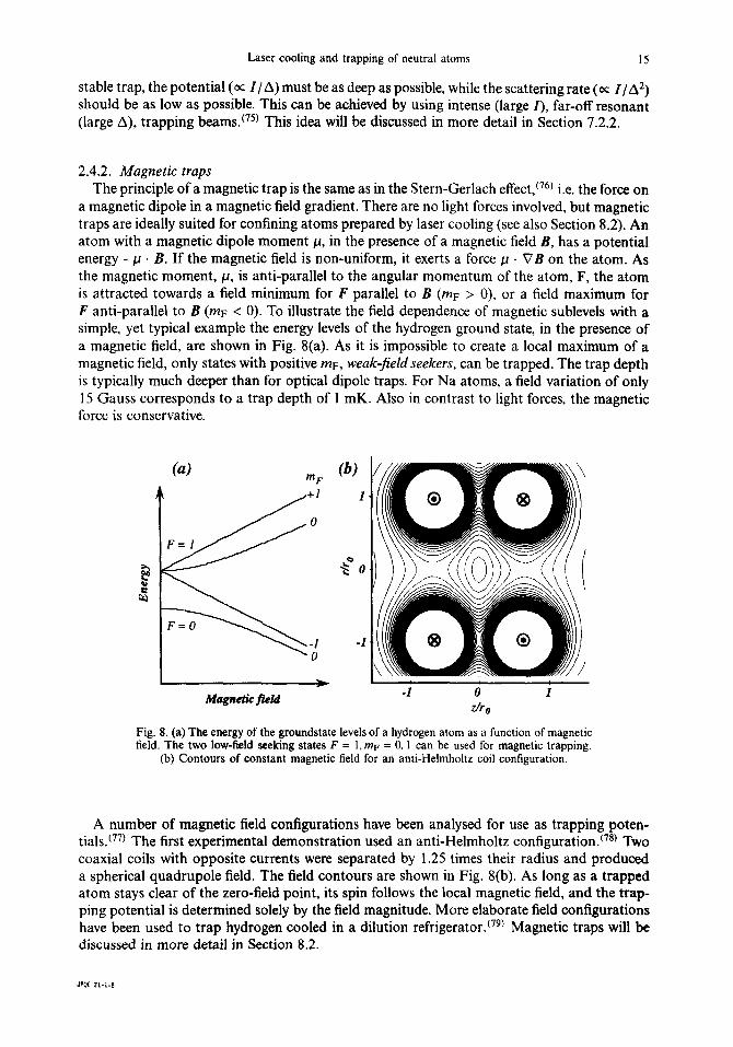
a magnetic dipole in a magnetic field gradient. There are no light forces involved, but magnetic traps are ideally suited for confining atoms prepared by laser cooling (see also Section 8.2). An atom with a magnetic dipole moment cc, in the presence of a magnetic field B, has a potential energy - u . B. If the magnetic field is non-uniform, it exerts a force P . VB on the atom. As the magnetic moment, ~1, is anti-parallel to the angular momentum of the atom, F, the atom is attracted towards a field minimum for F parallel to B (mF > 0), or a field maximum for F anti-parallel to B (mF < 0). To illustrate the field dependence of magnetic sublevels with a simple, yet typical example the energy levels of the hydrogen ground state, in the presence of a magnetic field, are shown in Fig. 8(a). As it is impossible to create a local maximum of a magnetic field, only states with positive mF, weak-field seekers, can be trapped. The trap depth is typically much deeper than for optical dipole traps. For Na atoms, a field variation of only 15 Gauss corresponds to a trap depth of 1 mK. Also in contrast to light forces, the magnetic force is conservative.
-I
* Magnetic jWi
-1 0 1
z/T0
Fig. 8. (a) The energy of the groundstate levels of a hydrogen atom as a function of magnetic field. The two low-field seeking states F = 1, MF = 0,l can be used for magnetic trapping.
(b) Contours of constant magnetic field for an anti-Helmholtz coil configuration.
A number of magnetic field configurations have been analysed for use as trapping poten- tials.(77’ The first experimental demonstration used an anti-Helmholtz configuration.(78) Two coaxial coils with opposite currents were separated by 1.25 times their radius and produced a spherical quadrupole field. The field contours are shown in Fig. 8(b). As long as a trapped atom stays clear of the zero-field point, its spin follows the local magnetic field, and the trap- ping potential is determined solely by the field magnitude. More elaborate field configurations have been used to trap hydrogen cooled in a dilution refrigerator.r7” Magnetic traps will be discussed in more detail in Section 8.2.

16 C. S. ADAMS & E. RIIS
2.4.3. Traps based on the scattering force The idea of constructing a trap based on the scattering force is very appealing. By taking
advantage of its dissipative nature, in a set-up which also provides confinement, one could conceive of a simple and robust trap. (69) However, Ashkin and Gordon proved that a trap based solely on absorption and spontaneous emission, from a static configuration of laser beams, is fundamentally unstable. c70) This is known as the optical Earnshaw theorem by analogy with the theorem in electrostatics, which states that it is impossible to trap a charged particle with static fields: for a charge free region the divergence of the electric field is zero, and therefore any point with a vanishing field gradient must a position of unstable equilibrium. The optical analogue is a region in space where there are no sources or sinks for photons (such as vacuum). If the scattering force is proportional to the photon flux (intensity), it will have zero divergence, corresponding to an unstable trap. However, the optical Earnshaw theorem only applies if the scattering force is proportional to the light intensity. If some external field alters this proportionality in a position dependent way, a stable trap can be formed.(80)
The most successful example of this concept is the magneto-optic trap (MOT).“@ The idea, as originally conceived by .I. Dalibard, was to use circularly polarised light for optical molasses and add a spherical quadrupole magnetic field such that an atom which moves away from the origin is Zeeman shifted into resonance with a beam which pushes it back. Fig. 9(a) shows how this works in 1-D (the z-axis), for an atom with a J = 0 to J’ = 1 transition. The magnetic field is of the form B(z) = bz, so the m = + 1 and m = - 1 sub-levels of the excited state experience Zeeman shifts which are linear in position. To provide cooling, the laser is tuned below resonance. The beams propagating in the fz directions have (T’-polarisations and drive Am = + 1 transitions respectively. An atom with a positive z-coordinate sees the o- beam closer to resonance, scatters more cr- than of photons, and is pushed back towards z = 0. Similarly an atom with z < 0, scatters more CT+ photons, and is also pushed towards z = 0. Thus, in addition to friction, the atom experiences a restoring force F = -KZ. The spring constant K can be determined in much the same way as the friction coefficient o( in the previous section, one finds,
(17)
where g, is the g-factor of the excited state, and j.& is the Bohr magnetron.
x
0 z
Fig. 9. The magneto-optical trap. (a) An atom with a J = 0 to J’ = 1 transition is placed in a linearly varying magnetic field B,(z) = bz. For an atom with a positive z-coordinate, the (T- beam, driving the Am = -1 transition, is Zeeman shifted into resonance and pushes the atom back towards z = 0. (b) The 3-D generalisation of (a) uses anti-Helmholtz coil
and three orthogonal &u- standing waves.

Laser cooling and trapping of neutral atoms 17
The generalisation to 3-D is illustrated in Fig. 9(b). The magnetic field is produced by an anti-Helmholtz coil, as for a magnetic trap (Section 2.4.2) except that fields required are much weaker. The first demonstration of the magneto-optical trap used field gradients of -5 Gauss/cm, and achieved a depth of -0.4 K, (‘@ which meant that atoms slower than a critical velocity, v, - 17 ms-‘, could be trapped. Around 10’ atoms were confined in a -0.5 mm diameter cloud. The trapped atoms had a temperature of less than 1 mK and a lifetime of around 2 minutes.
2.5. The magneto-optical trap
This first demonstration of a magneto-optical trap used the same set-up as in the optical molasses experiment,(s) I.e. the atoms were obtained from a slowed atomic beam. Later, it was shown that the magneto-optical trap can collect atoms directly from a room temperature vapour. (*I) There are enough atoms in the tail of the thermal Maxwell-Boltzmann distribution, slower than the capture velocity v,, to provide a substantial loading rate. The convenience of this set-up has helped the magneto-optical trap to become the basic building block in many experiments using cold atoms. However, the simplicity of the experimental apparatus is in stark contrast with the many subtleties in the theoretical description. Considerable effort has been devoted to understanding the mechanisms behind the magneto-optical trap, in particular, the factors which limit the number of trapped atoms and the density. Here, we shall only attempt to describe a few of the main features.
In the above discussion of laser cooling, we implicitly assumed that all atoms see the same amount of light, and that the scattered photon is lost and plays no further role. However, considering the high optical densities attainable, these are no longer safe assumptions. The cloud of trapped atoms scatters a significant fraction of the incident light, so on the one hand, the outer shell casts a shadow over the centre of the cloud, which tends to compress it, while on the other, the light which is scattered from the centre and subsequently reabsorbed tends to blow it apart. ‘82) At first sight these effects might appear to cancel, but the spectrum of the scattered light is slightly different from that of the laser. (“) This is most easily seen by considering the dressed atom picture of Fig. 7(b). While most of the fluorescence light has a frequency near the laser frequency WL, a small amount will appear at frequencies OL -+ R, corresponding to spontaneous decay from the dressed states I 1 (n + 1)) to 12(n)) and from I2(n + 1)) to I 1 (n)) . The problem, as far as the magneto-optical trap is concerned, is that the light at LUL + R is quite close to resonance and therefore provides a strong outward pressure (s’) placing an upper limit, n,, on the density. As the magneto-optical trap fills, the 7 atomic cloud initially resembles an ideal gas with a constant volume and a Gaussian density distribution.(s2,R4) When around lo4 atoms are trapped, the peak density n, is approached, and the cloud starts expanding and develops a flat density profile. As more atoms are trapped the optical thickness of the cloud increases until the point where a significant number of photons are scattered more than twice. This leads to a further increase in the outward radiation pressure and the density starts to decrease.(85,86)
2.5.1. Loading rates The steady-state number of atoms in a vapour cell magneto-optical trap is given by the
balance between loading and loss. The loading and loss rates are most easily observed by recording the number of atoms in the trap as a function of time just after it has been switched on. If the filling rate is Rf, and we assume that the loss coefficient y is independent of the number of trapped atoms N(t), we find,
dN(t) - = Rf - yN(t),
dt (18)

18 C. S. ADAMS & E. RIIS
which has the solution,
N(t) = T (1 - eeyr). (19)
Rf is the rate at which atoms with a velocity lower than the critical velocity Y, enter the trapping volume V,(*l)
(20)
where n, is the density of the background vapour, and u = ,I- is the most probable velocity of atoms in a vapour with temperature TV. Figure 10 shows an example of such a filling curve.
5
Time (set)
IO
Fig. 10. The filling of atoms into a magneto-optical trap is observed by detecting the fluorescence from the trap. The filling rate Rf is given by the initial slope and the loss
coefficient y is given by the inverse of the time-constant.
If we assume that the laser cooling transition is saturated, such that the atoms will decel- erate at a constant rate, the capture velocity will be proportional to the square root of the characteristic linear dimension d of the trap. This leads to a filling rate proportional to d4, and linear in the vapour pressure. Therefore to maximise the filling rate, the obvious choice is to use a high vapour pressure and large beams, provided that sufficient laser power is avail- able to bring the transition close to saturation. Using 55 mm diameter beams, Gibble and co-workersCs7) demonstrated a trap capable of collecting more than lOi atoms in a fraction of a second. While this approach does indeed work, there is a slight downside. Not surprisingly, the loss rate also increases at higher vapour pressure, as collisions with uncooled atoms be- come more frequent. At high pressure, this becomes the dominant loss mechanism, and since it has the same dependence on pressure as the filling rate, the steady state number of atoms is pressure independent. For more subtle reasons, the trap loss rate also increases with laser intensity and trap density.
2.5.2. Trap loss In the first paper on the magneto-optical trap, it was realised that two-body collisions could
severely limit the density and number of trapped atoms. (r6) The average density n, after the light was turned off, was observed to decay more steeply than a simple exponential. The decay could be described more accurately by an equation of the form,‘*@
dn dt-
- - yn - Bn2, (21)

Laser cooling and trapping of neutral atoms 19
where j3 is a parameter characterising the two-body loss. An example of such non-exponential decay from a Rb magneto-optical trap is shown in Fig. 1 l(a).
(4
1 O’O n- ‘E v
= log
(b) 16”
3 E v
Q , o-lz
0 50 100 150 200 0 5 10 15 20
t (set) I, (rrlW/crn2)
Fig. 1 I. (a) The non-exponential decay from a 87Rb magneto-optical trap. The solid curve is given by the solution of Eq. (21). (b) The intensity dependence of the two-body loss parameter, /3, for the two isotopes of rubidium. At low intensity, hyperfine-changing collisions become the dominant loss mechanism and the difference between the isotopes is due to the
difference in the ground state hyperfine structure. Both figures are from Ref. 9 I.
Theoretical work(89) and a careful experimental study of the trap 1ifetime(90) provided a physical picture of the processes involved. Two dominant loss mechanisms were identified:$ne- structure changing collisions and radiative redistribution. Both can be understood by considering the interaction potential between two colliding atoms. If both atoms are in the ground state (Si,z for alkali atoms), the long-range potential is dominated by the weak re6 van der Waals attraction with a typical range of about 1 nm. If one atom is in the excited state, there is a much stronger re3 resonant dipole-dipole interaction with a range of order 100 nm, and there are a number of possible molecular states with both attractive (e.g. Sl,z + P3,2) or repulsive (e.g. S1,2 + 9,~) interatomic potentials, as shown in Fig. 12.
Interatomic separation
Fig. 12. Two colliding groundstate atoms are attracted by the long range van der Walls potential. A groundstate atom colliding with an excited atom may experience either an
attractive or a repulsive potential.
Consider a collision where the Si,2 + P3,2 state is excited by the red detuned cooling laser (this process eventually becomes resonant as the atoms approach). The Si 12 + P3,2 potential is attractive and the atoms accelerate towards each other. In a fine-structure changing collision, the atoms transfer to the repulsive Si ,2 + PI ,2 potential and separate with an additional kinetic energy equal to the fine-structure splitting AErS. For Na AEfs/2kB - 12 K, which is more

20 C. S. ADAMS & E. RIIS
than enough to eject both atoms from the trap. Alternatively the excited molecular state may decay at a small interatomic separation, In this case, the atomic kinetic energy increases by the difference between the absorbed and emitted photons, (equivalent to a temperature change of up to 1 K).
Obviously this light induced two-body loss rate will depend on the laser intensity and detuning. The intensity dependence of the loss parameter /3 is demonstrated in Fig. 1 l(b). For high intensity, the dependence is close to linear, but fi rises sharply at low intensity. This is due to hyperfine changing collisions, which add to the loss rate only at low intensity where the trap depth becomes less than the hyperfine splitting. (9’) This interpretation is supported by the observed difference in the position of the minimum loss rate for the two isotopes of Rb, which have approximately a factor of two difference in their groundstate hyperfine splittings.
2.5.3. Dark magneto-optical trap By excluding the repumping light from the centre of a magneto-optical trap, atoms are
optically pumped into the lower hyperfine state and no longer couple to the cooling light. This leads to a dramatic reduction in the light-induced loss, allowing trap densities approaching 1 012 atoms crne3 to be achieved. cg6) This technique is known as a dark magneto-optical trap.(86) As optical pumping into the dark ground state relies on off-resonant excitation of the second highest hyperfine level in the excited state (2Pj,2, F’ = 2 for Na, as shown in Fig. 3) the pumping rate depends critically on the excited state hyperfine splitting. For the heavier alkalis (Rb and Cs) the splitting is 20 to 50 linewidths (as opposed to 6 for Na), and the successful operation of a dark magneto-optical trap requires an additional beam, close to resonance with the second highest hyperfine level, to efficiently depump atoms into the dark ground state.(92,9”)
3. SUB-DOPPLER COOLING
3.1. Introduction
Although the first demonstration of optical molasses appeared to be in fair agreement with the Doppler theory outlined in Chapter 2, it soon became apparent that the behaviour was not quite as expected. In fact the experiments worked much better than expected! A number of careful measurements yielded the crucial evidence that there was more to optical molasses than Doppler theory. The key to understanding the results was to drop the two simplifying assumptions of Doppler theory, the two-level nature of the atom (Na has more than a dozen levels playing an active role in the cooling process), and the assumption that the light field has a pure state of polarisation (at best only possible to realise in two dimensions). This Chapter reviews the experimental evidence for the breakdown of Doppler theory, outlines the new sub- Doppler theory, and gives examples of experiments which verify it. Finally we consider the implications of sub-Doppler cooling for the magneto-optical trap.
3.2. Breakdown of Doppler theory
Early quantitative measurements by the NIST group on the properties of optical molasses yielded a number of surprising results, at odds with the Doppler theory outlined in Chap- ter 2.(94995’ By treating atoms in optical molasses as particles in a viscous fluid, it is possible to derive an expression for the spatial diffusion constant, Dx, in terms of the momentum dif- fusion coefficient, D,, and the friction coefficient, a. In 1-D one findsc9@
D,=s. (22)

Laser cooling and trapping of neutral atoms 21
From this expression, one may estimate the lifetime of the optical molasses from the time it takes an atom to diffuse to the edge of the interaction region. Even after accounting for the 3-D geometry of the experiment, a striking difference between the theoretical result and the experimental data was observed.(94q95) For detunings of - -2T, the lifetime was measured to be about an order of magnitude longer than expected.
Doppler theory also predicts that the lifetime ofopticalmolasses should be extremely sensitive to slight imbalances in the intensities of counterpropagating beams: an imbalance of a few percent should lead to a drift velocity of several ems -I. With a characteristic size of the interaction region of 1 cm, the lifetime would be no more than a few tens of msec. However, experiments showed lifetimes on the order of 0.5 s and hardly any effect for intensity imbalances of up to 10’%.(g4,95) Furthermore, deliberate misalignment of the beams led to even longer confinement times:‘97) a configuration referred to as ‘super molasses’. However, the clearest evidence that something was terribly wrong was the measurement by Lett et ~1.‘~) of the optical molasses temperature. The result was 43+-20 mK, much lower than the expected value of 240 mK. Also, the detuning dependence of the measured temperature was completely different from that predicted by Doppler theory and expressed by Eq. (7).
3.3. Temperature
In light of its importance in the field of laser cooling, it is worth dwelling on how temperatures are defined and measured.
3.3.1. Dejnition The concept of temperature is used as a way of characterising the width of the atomic velocity
distribution. For many relevant situations, both Doppler and sub-Doppler cooling theories predict a Maxwellian velocity distribution, so assigning a temperature is quite appropriate. The familiar kinetic theory for a dilute gas in thermal equilibrium yields the following expression for the velocity distribution along the ith direction,
-“? p(vi) = kvoi exp F& . ( 1 (23)
where rsi is the r.m.s. velocity (half width of the distribution at 1 I&) in the ith direction. Often, there is no direct coupling between the degrees of freedom, and the three r.m.s. velocities may be different. An effective n-dimensional temperature can be defined by
(24)
Although effective 1-D and 2-D temperatures are often quoted in the literature, a more ap- propriate measure of the success of any optical cooling technique (for n < 3) is the width of the velocity distribution in units of the recoil velocity vreC = Rklm.
The definition of a recoil temperature T,, is somewhat arbitrary. Here we adopt the most common definition: Tree is the temperature at which the r.m.s. velocity is equal to the recoil velocity vreC = hklm in each dimension, which gives,
(25)
where erec = R2k2 /2m is the recoil energy.
22 C. S. ADAMS & E. RIIS
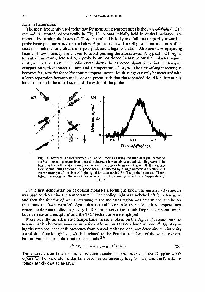
3.3.2. Measurement The most frequently used technique for measuring temperatures is the time-offlight (TOF)
method, illustrated schematically in Fig. 13. Atoms, initially held in optical molasses, are released by turning the lasers off. They expand ballistically and fall due to gravity towards a probe beam positioned several cm below. A probe beam with an elliptical cross section is often used to simultaneously obtain a large signal, and a high resolution. Also counterpropagating beams of low intensity are chosen to avoid pushing the atoms away. A typical TOF signal for rubidium atoms, detected by a probe beam positioned 74 mm below the molasses region, is shown in Fig. 13(b). The solid curve shows the expected signal for a initial Gaussian distribution with diameter 1.2 mm and a temperature of 14 PK. The time-of-flight technique becomes less sensitivefor colder atoms: temperatures in the I.IK range can only be measured with a large separation between molasses and probe, such that the expanded cloud is substantially larger than both the initial size, and the width of the probe.
Time-of-flight (s)
Fig. 13. Temperature measurements of optical molasses using the time-of-flight technique. (a) Six intersecting beams form optical molasses, a few cm above a weak standing wave probe beam with an elliptical cross-section. When the molasses beams are turned off, fluorescence from atoms falling through the probe beam is collected by a large numerical aperture lens. (b) An example of the time-of-flight signal for laser cooled Rb. The probe beam was 74 mm below the molasses. The smooth curve is a tit to the signal expected for a temperature of
I4 /JK.
In the first demonstration of optical molasses a technique known as release and recapture was used to determine the temperature. (5) The cooling light was switched off for a few msec and then the fraction of atoms remaining in the molasses region was determined: the hotter the atoms, the fewer were left. Again this method becomes less sensitive at low temperatures, where the dominant effect is gravity. In the first observation of sub-Doppler temperatures,(7) both ‘release and recapture’ and the TOF technique were employed.
More recently, an alternative temperature measure, based on the degree of second-order co- herence, which becomes more sensitive for colder atoms has been demonstrated.(98) By observ- ing the time sequence of fluorescence from optical molasses, one may determine the intensity correlation function gc2’(-r), which is related to the Fourier transform of the velocity distri- bution. For a thermal distribution, one finds,‘99’
gc2’(T) = 1 + exp(--kgTkZT2/m). (26)
The characteristic time for the correlation function is the inverse of the Doppler width k,/m. For cold atoms, this time becomes conveniently long (> 1 PS) and the function is comparatively easy to measure.

Laser cooling and trapping of neutral atoms 23
All the above methods have their individual advantages and disadvantages, in terms of ease of use, sensitivity, and model dependence. However, if high sensitivity is required, the best technique is to use stimulated Raman transitions to map out the velocity distribution.‘*‘) The idea is to drive a two-photon transition between two long-lived states (ground state hyperIme levels) in a way that is sensitive to the Doppler shift of the optical transition, but insensitive to laser frequency fluctuations. For a particular velocity this results in a linewidth, that, in principle, is only limited by the time of the measurement. Stimulated Raman transitions will be explained in more detail in Section 4.3.
3.4. Beyond Doppler cooling: the Sisyphus effect
As mentioned in the Introduction the key to understanding the sub-Doppler temperatures in optical molasses is to consider the multi-level character of real atoms, and the spatial variation of the polarisation found in most experimental set-ups. However before considering multi- level atoms and polarisation gradients, it is worth taking a qualitative look at the motion of a two-level atom in an intense standing wave lightfield. The dressed state model of this system provides an intuitive introduction to the mechanisms of sub-Doppler cooling.[roO)
Consider an atom in a strong (WR > A) standing wave laser field tuned above resonance (A > 0). The dressed atom picture, Fig. 14, looks similar to Fig. 7 (A < 0), except that the ground and excited state labels (g and e) are interchanged, and the dressed state energies vary sinusoidally with position. Just as important for the arguments to follow, the wavefunctions change from the uncoupled states (I e, n) and 1 g, it + 1) ) at the field nodes, to superpositions of I e, n) and ) g, n + 1) at the anti-nodes (cf. Eq. (14)).
The mechanical effect of the light can be understood by following the trajectory of an atom through the dressed state potentials and including the dissipative effect of spontaneous emission. Consider an atom that starts in the ground state near a field node (for instance with M + 2 photons in the field). If it moves slowly (kv < WR), it remains on the I 1 (n + 1)) potential curve until disturbed by spontaneous emission. As it moves away from the field node, the increase in internal energy results in a decrease in kinetic energy, i.e. the atom climbs the hill and slows down. In addition, the wavefunction acquires, more and more, the character of an excited state (1 e, n + 1) ), and the probability of spontaneous emission increases. The atom may decay either to an equivalent state one step down the ladder, i.e. I 1 (n)) , which from a mechanical point of view is insignificant, or to the state 12(n)) in which case it finds itself back at the bottom of a potential valley. From here, as it climbs the next hill, the excited state component and the probability of decay again increase towards a maximum at the field node. and the atom is most likely to fall from the top of a hill to a valley in the I l(n - 1)) potential. Thus, the atom spends more time climbing hills. The net result is that kinetic energy is converted into potential energy, which is subsequently carried away by the fluorescence, leaving the atom colder. This cooling mechanism is generally referred to as Sisyphus coofing. *
Contrary to Doppler cooling, the Sisyphus effect provides cooling with the laser tuned above resonance. The mechanism only works for atoms which move from a node to an anti-node or less (5 h/4) in a natural lifetime, therefore the force vs velocity curve consists of a broad Doppler contribution causing heating, and a narrow feature near v = 0 providing cooling. An alternative description views the cooling mechanism as the effect of resonant multi-photon processes involving absorption and stimulated emission from the strong counterpropagating beams.(lo2) The effect is also referred to as stimulated cooling or blue molasses and was first demonstrated as a technique to collimate an atomic beam.(‘O’)
* Scholars of the classical literature will recognise the similarity with the Greek myth of Sisyphus, who was condemned by the Gods to continually push a rock up a hill, only to find it slide back down again.

24 C. S. ADAMS & E. RIIS
3.5. Qualitative models
We now return to the discussion of sub-Doppler cooling. Two distinct mechanisms were identified to explain the lower than expected temperatures observed experimentally.@-‘O) They can be associated with the two types of polarisation gradients, which, in l-D, are represented by the field configurations linllin (counterpropagating beams with orthogonal linear polari- sations), and CT+(T- (counterpropagating beams with opposite circular polarizations). In the former, the polarisation varies between linear and circular over a distance h/2, as shown in Fig. 15(a). In the latter, the polarisation is linear everywhere but the direction rotates to form a helix, as shown in Fig. 15(b). This section presents qualitative models for the two sub-Doppler or polarisation gradient cooling mechanisms. A quantitative description is deferred until Sec- tions 3.6 and 3.7. A more technical overview of theoretical work on sub-Doppler cooling can be found in dedicated theoretical reviews.(46v47)
As mentioned earlier, the other important ingredient in understanding sub-Doppler cooling is the multi-level character of the atom. Figure 16(a) and (b) show the magnetic sub-levels of
Position -
Fig. 14. Sisyphus cooling of an atom in a standing wave light field. Spontaneous emission occurs preferentially where the dressed state contains most excited state character, i.e. at the anti-nodes of the field for dressed states labelled 1, and the nodes for those labelled 2. The solid curve represents the motion of a slow atom through the standing wave. The net effect of spontaneous emission is that the atom spends more time climbing hills, resulting in the conversion of kinetic energy to potential energy which is subsequently carried away
by blue-shifted fluorescence photons.

Laser cooling and trapping of neutral atoms 25
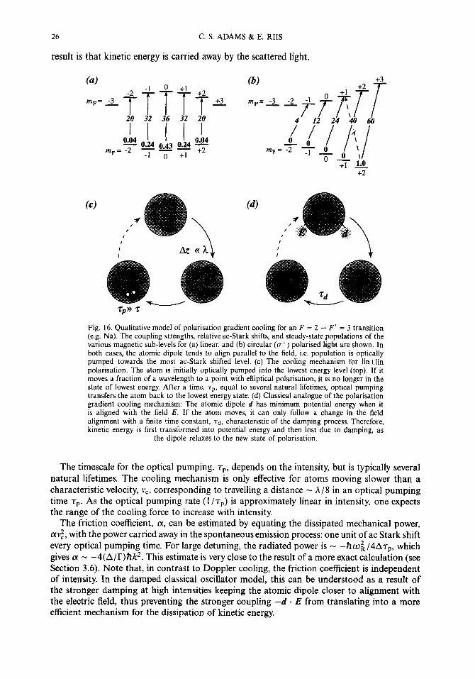
the 32S1,2(F = 2) to 3*&(F’ = 3) transition in Na subject to linear and circular polarised light respectively. Optical pumping tends to transfer population to the most ac-Stark shifted level (i.e. that with the strongest coupling). This is equivalent to an alignment of the atomic dipole with the field. Indeed, an F - F + 1 transition behaves very much like a classical damped oscillator, whose motion follows the driving field with a time delay characteristic of the relaxation process causing the damping. (lo3 This is the basis of a model referred to as orientational cooling.“O)
The polarisation gradient cooling mechanism for linilin polarisation is illustrated schemat- ically in Fig. 16(c) and (d). Figure 16(c) considers the process from a quantum mechanical point of view, showing the light shifts and population transfer as an atom moves through the light field and relaxes to the state of lowest potential energy. Fig. 16(d) depicts the anal- ogy with a classical damped dipole d driven by an electric field E. Consider an atom which begins at a position with linear polarisation (top). Optical pumping tends to populate the lowest energy level, i.e. the atomic dipole is aligned with the field. If the atom then moves a fraction of a wavelength in less than an optical pumping time, the polarisation becomes el- liptical but the state of the atom does not have time to adjust, i.e. population is transferred non-adiabatically to a superposition of levels, that on average are less strongly coupled to the light. The corresponding reduction in the ac-Stark shift means that the atom has increased its internal energy at the expense of kinetic energy. In the classical dipole picture, Fig. 16(d), the potential energy -da E increases because the dipole does not follow the change in the electric field instantaneously. Subsequently, the atom is optically pumped back into the lowest energy, i.e. the atomic dipole d is realigned parallel to the field E. The principle is very similar to the Sisyphus mechanism explained above: when the atom is pumped back into the lowest energy state, the emitted photons have slightly more energy than the absorbed photons, and the net
(b)
Fig. 15. The two field configurations considered in polarisation gradient cooling: (a) coun- terpropagating beams, linearly polarised in orthogonal directions (lin.r.lin). The polarisation varies from linear through circular, to the opposite linear, and back again, over a distance of h/2. (b) counterpropagating beams, circularly polarised in orthogonal directions (&a-). The electric field is linearly polarised everywhere, but the direction of polarisation rotates
around the beam axis with a pitch of h/2.
26 C. S. ADAMS & E. RIIS
result is that kinetic energy is carried away by the scattered light.
mp=
(4
Fig 16. Qualitative model of polarisation gradient cooling for an F = 2 - F’ = 3 transition (e.g. Na). The coupling strengths, relative ac-Stark shifts, and steady-state populations of the various magnetic sub-levels for (a) linear, and (b) circular (of) polarised light are shown. In both cases, the atomic dipole tends to align parallel to the field, i.e. population is optically pumped towards the most ac-Stark shifted level. (c) The cooling mechanism for linllin polarisation. The atom is initially optically pumped into the lowest energy level (top). If it moves a fraction of a wavelength to a point with elliptical polarisation, it is no longer in the state of lowest energy. After a time, TV, equal to several natural lifetimes, optical pumping transfers the atom back to the lowest energy state. (d) Classical analogue of the polarisation gradient cooling mechanism: The atomic dipole 1 has minimum potential energy when it is aligned with the field E. If the atom moves, it can only follow a change in the field alignment with a finite time constant, Td, characteristic of the damping process. Therefore, kinetic energy is first transformed into potential energy and then lost due to damping, as
the dipole relaxes to the new state of polarisation.
The timescale for the optical pumping, TV, depends on the intensity, but is typically several natural lifetimes. The cooling mechanism is only effective for atoms moving slower than a characteristic velocity, v,, corresponding to travelling a distance - h/8 in an optical pumping time T,,. As the optical pumping rate (1 /TV) is approximately linear in intensity, one expects the range of the cooling force to increase with intensity.
The friction coefficient, LX, can be estimated by equating the dissipated mechanical power, a$, with the power carried away in the spontaneous emission process: one unit of ac Stark shift every optical pumping time. For large detuning, the radiated power is - -/?u$/~AT,, which gives o( - -4(A/I)M?. This estimate is very close to the result of a more exact calculation (see Section 3.6). Note that, in contrast to Doppler cooling, the friction coefficient is independent of intensity. In the damped classical oscillator model, this can be understood as a result of the stronger damping at high intensities keeping the atomic dipole closer to alignment with the electric field, thus preventing the stronger coupling -d . E from translating into a more efficient mechanism for the dissipation of kinetic energy.

Laser cooling and trapping of neutral atoms 2-I
The mechanism involved in (T+(T- sub-Doppler cooling is somewhat different. As the field polarisation is linear everywhere and has constant amplitude, the Sisyphus mechanism is not active. The starting point is again an atom at rest in the optically pumped state shown in Fig. 16(a). When the atom starts to move, the symmetry between in the light-atom interaction is broken. An atom moving towards the u+ beam, sees the (T+ component closer to resonance and is optically pumped towards the positive mF levels. This is a run-away effect because the positive mF levels are more strongly coupled to cr+ light (for the mF = 2 level in Na, the cr+ coupling is 15 times stronger than for (T-, as shown in Fig. 16(b)). This motion induced
redistribution of the population enhances the difference between the photon scattering rates leading to a much stronger frictional force than would occur for a two-level atom (Doppler cooling). For atoms faster than a characteristic velocity, vC, (same order of magnitude as for linllin polarisation), the redistribution of the population washes out and the cooling force returns to the normal Doppler expression.
We shall now briefly summarise the results of a more quantitative analysis of the two sub- Doppler cooling mechanisms.(*)
3.6. lin.Un polarisation gradient cooling
The linllin system is analysed for a F = l/2 - F’ = 3/2 transition.(46) This is the simplest example, in terms of the number of sub-levels involved, which displays the essential features of the interaction. The polarisation gradient cooling force, averaged over a wavelength, may be written as,
F(v) = -CO
1 + (v/v# (27)
where the friction coefficient is given by,
and the critical velocity by,
o( = -3~k2n r’ (28)
Figure 17 shows the total cooling force (Doppler plus sub-Doppler) as a function of velocity for Z = Isat, Zsat/2, and ZJ4. The figure clearly illustrates some of the important differences between Doppler and sub-Doppler cooling. Doppler cooling (dashed lines in Fig. 17) has a friction coefficient that is proportional to intensity and a range which depends on the detuning. In contrast, sub-Doppler cooling has friction coefficient which depends on the detuning and a range which is proportional to the intensity. For typical parameters, e.g. for Na with Z = Isat, A = -T, the sub-Doppler friction coefficient is about an order of magnitude larger, and the range is more than an order of magnitude smaller. Furthermore, the critical velocity is - 4Rk,
or - 0.4 times the r.m.s. velocity of a Doppler cooled sample, therefore sub-Doppler cooling is very effective at taking over where Doppler cooling gives up.
To estimate the equilibrium sub-Doppler temperature, one determines the momentum diffu- sion coefficient Dr. For IAl B T one finds,
kaT=$ m-2 z
= JimI,,,’ (30)
It is apparent from Eq. (30) that the minimum kinetic energy is approximately equal to the a&Stark shift of the levels involved.

28 C. S. ADAMS & E. RIIS
3.7. CT+ CT- poiarisation gradient cooling
The analysis of the (T+(T- configuration uses an F = 1 to F’ = 2 transition and is somewhat more complicated than the linllin system. c4@ However, the results are qualitatively similar: the cooling force is characterised by a strong damping coefficient (Y, and a velocity range of order W; /k I A 1, beyond which the force gradually approaches the normal Doppler expression. The following expressions are found for the friction coefficient and the temperature,
,,_24& 1 17 T 4(A/r)2 + 1’
and,
keT
Rr2 z 29+_
254 1
= -- 2 1 A 1 Zsat 300 75 4(A/f)2 + 1 I
(31)
(32)
For large detuning, this result is quite similar to the one obtained for lin_/_lin polarisation. Similar results for both configurations were obtained by Ungar et aLC9) by numerically solving the optical Bloch equations for the relevant levels of Na.
Both Eq. (30) and (32) suggest that the temperature can be made arbitrarily low by reducing the intensity or increasing the detuning. This is clearly unphysical. The analysis breaks down when the atomic momentum becomes comparable to the atomic recoil associated with the absorption or emission of a single photon. At this point the atomic de Broghe wavelength is comparable to the laser wavelength rendering the semi-classical treatment described above invalid. A full quantum treatment of the 1-D linllin system predicts a minimum temperature corresponding to an r.m.s. momentum of - 6Ak.(‘“)
3.8. Experimenta! veriJication
Following the discovery of the sub-Doppler temperatures, a range of experiments were carried out on Na and Cs, to investigate the dependence of the molasses temperature on the laser parameters such as detuning and intensity. (10,95, *05,106) Experiments were also performed on polarisation configurations where neither sub-Doppler mechanism should be effective. For example, for a (~+cr+ light field, the atoms are optically pumped into the mF = F level forming a pure two-level system (cf. Fig. 16(b)), and the measured temperatures agreed with Doppler theory.(tO) Similar results were obtained for parallel linear polarisations, lin I( lin.(r”)
Fig. 17. The cooling force vs velocity for linllin polarisation. The three solid curves are for I = Isa,, I,,,/2, and &t/4. The dashed lines are the corresponding contributions from
Doppler cooling.

Laser cooling and trapping of neutral atoms 29
The lowest temperature of 2.5 pK, compared with the Doppler limit of 120 PK, was obtained for 3-D optical molasses in Cs. (to7) This corresponds to an r.m.s. momentum of - 3.5Ak in each direction. Further careful investigation of 3-D optical molasses was performed by Drewsen et u1.(to8) The starting point for these experiments was around lo8 atoms in a magneto- optical trap. The magnetic field was switched off, and the atoms allowed to reach equilibrium for the chosen intensity and detuning, before all light was extinguished. As the atoms were originally confined to a small volume, the effect of the initial size on the time-of-flight signal was negligible, allowing accurate temperature measurements. It was found that, for a sufficiently large detuning (IAl 2 ST) the temperature was proportional to &/A as expected (Eq. (30) and (32)). Figure 18 shows the experimental data for detunings in the range -2I to -1OI.
70
60
50
40
30
20
10
0 0 0.2 0.4 0.6 0.8 1
Fig. 18. The temperature of 3-D ufo- optical molasses as a function of the parameter (uJ~/ IAl)r. The detunings are: A = -2r (open squares), A = -3r (filled circles), A = -5r (filled squares), A = -6r (open triangles), A = -8r (open circles), A = - 1Or (filled
triangles). (Adapted from Ref. 108 courtesy of M. Drewsen.)
Despite the successful observation of sub-Doppler temperatures, and the close agreement with theory, the experiments described above only measured the friction and diffusion coeffi- cients, and not the velocity dependence of the cooling force. The first experimental evidence for the complex velocity dependence was the observation of a bimodal velocity distribution.(iO, io6) Later, the velocity dependence was measured directly for a beam of Ne atoms cooled trans- versely by a 1-D o+oT- light field. (io9) More accurate measurements were subsequently made on Rb atoms in a 3-D u+(T- molasses. (‘i”) The change in the atomic velocity after a brief in- teraction with optical molasses was observed as a function of initial velocity. Figure 19 shows the data for an interaction time of 10 ps. Although no analytical expression exists for the cool- ing force in this configuration, the data fit remarkably well to the velocity change expected for a 1-D lin_tlin field (Eq. (27)).
3.9. Sub-Doppler cooling in a magnetic field
The importance, in sub-Doppler cooling theory, of the a&Stark shifts of the individual magnetic sublevels, and the crucial role played by the optical pumping process, suggests that

30 C. S. ADAMS & E. RIIS
the mechanism might be quite sensitive to magnetic fields. This sensitivity has important implications for the magneto-optical trap (see Section 2.4.3). Early experiments indicated that the lowest molasses temperatures were obtained for background magnetic fields of order 10 mG or less.(*O’ This corresponds to a Zeeman shift of -10 kHz, i.e. significantly less than the natural linewidth of the transition, or even a typical ac-Stark shift, but comparable to the inverse of the optical pumping time TV.
The detrimental effect of a magnetic field on sub-Doppler cooling is caused by the com- petition between Larmor precession, and the alignment of the atomic dipole due to optical pumping. The equivalent energy level picture is complicated, because the eigenstates, coupled by both electric and magnetic fields, are linear combinations of the natural basis states for a given polarisation. One might think that sub-Doppler mechanisms would not be active in the relatively strong magnetic fields of a magneto-optical trap. However, as the atoms are trapped around the zero-fieldpoint, a small trap does produce temperatures below the Doppler firnit: with a typical field gradient of 5 Gem-‘, a 1OOpm diameter trap involves fields of less than 25 mG, consistent with the existence of sub-Doppler cooling. Indeed, for a sufficiently small trap, the temperature is found to be identical to that for cr+u- optical molasses.(‘08) Figure 20 shows that the temperature, for larger traps, increases roughly proportional to N”?, where the number of atoms N ranges from lo5 to 108.“08’
As if to remind us of the subtle nature of sub-Doppler cooling, a magnetic field of a few hundred mG perpendicular to the axis of a 1-D of& standing wave was observed to produce sub-Doppler cooling. (‘o,“3’ In the absence of a magnetic field, the (~‘6 system provides an experimental realisation of a two-level atom, because the atoms are optically pumped into the mF = F sub-level, and the results show good agreement with Doppler theory. However, when a magnetic field is introduced, the magnetic interaction dominates near the nodes of the light field, causing the atomic dipole to precess away from the beam axis. Thus, a moving atom passes non-adiabatically through the field nodes, leaving in states which have higher potential energy (due to a smaller ac-Stark shift). Near the anti-nodes, where the atomic transition is strongly driven, optical pumping tends to transfer the atoms back to the most ac-Stark shifted level (i.e. realign the dipole). The net effect is that the atom climbs steeper hills than it descends and energy is carried away by blue-shifted photons. The dissipative mechanism is very similar to Sisyphus cooling (Section 3.4). This cooling scheme is referred to as ‘magnetic orientational cooling’(‘O’ or ‘magnetically induced laser cooling’ (MILC).““’
Fig. 19. The velocity dependence of the cooling force in 3-D ufu- optical molasses. Laser cooled Rb atoms interact with the light for a period of 10 /.Is. The change in velocity is measured as a function of the initial velocity. The solid curve shows the expected velocity change for F(V) = -(WV/ ( I + v*/v$. The laser intensity was 0.75& and the detuning -7.5r.
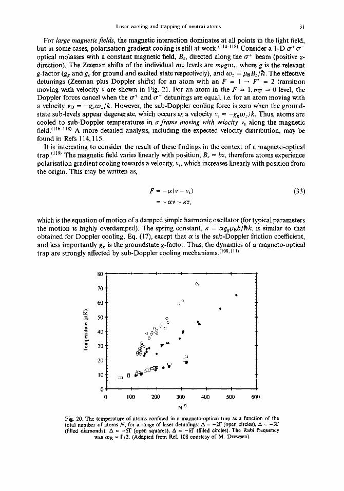
Laser cooling and trapping of neutral atoms 31
For large magneticfields, the magnetic interaction dominates at all points in the light field, but in some cases, polarisation gradient cooling is still at work.(‘14-‘18) Consider a 1-D (T+u- optical molasses with a constant magnetic field, B,, directed along the u+ beam (positive z- direction). The Zeeman shifts of the individual mr levels are mpgc& where g is the relevant g-factor (gR and g, for ground and excited state respectively), and (Us = p~B,/h. The effective detunings (Zeeman plus Doppler shifts) for an atom with an F = 1 - F’ = 2 transition moving with velocity v are shown in Fig. 21. For an atom in the F = 1, mr = 0 level, the Doppler forces cancel when the u+ and (T- detunings are equal, i.e. for an atom moving with a velocity Vn = -gew5/k. However, the sub-Doppler cooling force is zero when the ground- state sub-levels appear degenerate, which occurs at a velocity vS = -g,wz/k. Thus, atoms are cooled to sub-Doppler temperatures in a frame moving with velocity vs along the magnetic field (116-118) A more detailed analysis, including the expected velocity distribution, may be foundin Refs 114,115.
It is interesting to consider the result of these findings in the context of a magneto-optical trap. (‘r9) The magnetic field varies linearly with position, B, = bz, therefore atoms experience polarisation gradient cooling towards a velocity, v,, which increases linearly with position from the origin. This may be written as,
F = -NV - vs) (33) = -CD - KZ,
which is the equation of motion of a damped simple harmonic oscillator (for typical parameters the motion is highly overdamped). The spring constant, K = cxgRpgb/Rk, is similar to that obtained for Doppler cooling, Eq. (17), except that (x is the sub-Doppler friction coefficient, and less importantly g, is the groundstate g-factor. Thus, the dynamics of a magneto-optical trap are strongly affected by sub-Doppler cooling mechanisms.(‘08* ” ‘)
80 !
0
. i
.
04 c 0 100 200 300 400 500 600
N’”
Fig. 20. The temperature of atoms confined in a magneto-optical trap as a function of the total number of atoms N, for a range of laser detunings: A = -2T (open circles), A = -3r (filled diamonds), A = -5r (open squares), A = -6r (filled circles). The Rabi frequency
was wa = r/2. (Adapted from Ref. 108 courtesy of M. Drewsen).

32 C. S. ADAMS & E. RIIS
4. SUB-RECOIL COOLING
4.1. Introduction
In Chapter 3 we saw that, for multi-level atoms, the fundamental laser cooling limit is characterised by the recoil temperature Tree, where kBTrec = h2k2/m. The recoil limit may also be expressed as an r.m.s. velocity rrec = hk/m. A way around the recoil limit is to rely on the stochastic nature of spontaneous emission to kick atoms into a select region of velocity space, with dimension less than vrec, where subsequently they are left alone. This idea is sometimes referred to as velocity space optical pumping and the excitation free region around v = 0 is known as a dark state or dark region. Such a scheme requires extremely high velocity selectivity around v = 0, but should still address any atoms with v > vrec. This is the inverse of the usual excitation spectrum: a narrow linewidth transition excites only those atoms within a narrow velocity range, whereas for sub-recoil cooling the goal is to excite all atoms except those within a narrow velocity range.
The two most successful sub-recoil schemes achieve this goal in very different ways. In velocity selective coherent population trapping (VSCPT),“‘) atoms close to v = 0 are decoupled from the light due to destructive interference between two terms which contribute to the excitation rate. In stimulatedRaman cooIing,(12) a narrow linewidth transition is used to actively remove atoms from the wrong velocity classes (i.e. everywhere except around v = 0). The process of tuning through the velocity distribution means that Raman cooling is inherently a pulsed scheme (similar to the chirped slowing of an atomic beam discussed in Chapter 2).
Both sub-recoil schemes may be used to cool any number of dimensions. However, as they both rely on momentum diffusion, the cooling time scales rapidly with the dimensionality: in l-D, the random walk must find a plane in velocity space, in 2-D a line, and in 3-D a point. It follows that the cooling time is proportional to (Vdark/VO)n, where n = 1, 2, 3 is the number of dimensions, vg is the velocity width of the uncooled distribution, and V&rk is dimension of the dark velocity region or trapped state.
An intuitive model of the stochastic filling of the dark state is provided by Levy flight statis- tics.(‘20) In the Levy flight approach, one defines a dark region or trapping zone by I VI i V&k, and the dynamics of an atom are modelled as a sequence of trapping periods with durations
Fe = 2
Fg = 1
Fig. 21. Effective detunings, including Zeeman and Doppler shifts, for an F = 1 - F’ = 2 transition in o+(T- optical molasses, where A is the detuning, gs and g, are the ground
and excited state g-factors respectively.

Laser cooling and trapping of neutral atoms 33
~1, 72, . interspersed by escape tiItIeS T;, T;, . . . . The probability for escape is described by a velocity dependent excitation rate I’(v). For velocity selective coherent population trapping the smaller the velocity, the smaller T(v), and the longer the trapping periods become. This is illustrated in the simulation shown in Fig. 22(a). Once outside the dark region, one relies on diffusion to get back, which can take quite a long time. In contrast for Raman cooling, although the time steps involved in the cooling process are much longer (more than a few hundred natural lifetimes), the process of finding the region around v = 0 is more efficient leading to a very different time evolution (Fig. 22(b)).
60 I I I ’ b-4
40- I
g 20 -
& L
E
0y I ,l.,. I IL! .,
5 -20 - XZ t -40 -
$ -60 - E
I I I 1
2 20 ’ - @) -
0 20000 40000 60000 80000 100000
Time (r-l)
Fig 22. Monte Carlo simulation showing the time evolution of the atomic momentum for (a) velocity selective coherent population trapping, and (b) Raman cooling. (a) For velocity selective coherent population trapping, the closer the atom moves towards v = 0, the longer it remains there, however an atom which moves away from v = 0 must rely on a random walk to bring it back, which can take quite a long time. (b) Raman cooling is very effective at removing atoms with large momenta and pushing them closer to v = 0. However to achieve smaller and smaller velocities requires longer and longer time steps, during which
the atoms have an increasing chance to be kicked out of the dark state.
This chapter is divided into two sections. First, we give a brief outline of the central idea behind velocity selective coherent population trapping and discuss experimental implementa- tions of the technique. Second, we describe experiments using Raman cooling.
4.2. Velocity selective coherent population trapping
4.2.1. Theory An intuitive picture of VSCPT is obtained by considering atoms with a J = 1 - J’ = 1
transition in a (T+(T- light field. (‘2’,‘22) The (T’ laser beams propagate in the +z-directions and we choose the quantisation axis along z. The atomic states are labelled according to their internal and external degrees of freedom, i.e. ( i, p) where i and p denote the internal state and the momentum respectively. The level scheme is depicted in Fig. 23. The magnetic sub-levels can be divided into two families; { 1 e-, p - WC) , ( go, p) , 1 e,, p + MC) } which form a V- system,and{Ig-,p-Rk), (eo,p), Ig+,p+Rk)) h’hf w IC orm a A-system. The two families are coupled by spontaneous emission, however this is a one way process because there is no
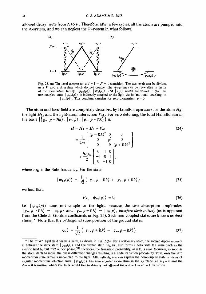
34 C. S. ADAMS & E. RIIS
allowed decay route from A to V. Therefore, after a few cycles, all the atoms are pumped into the A-system, and we can neglect the V-system in what follows.
Fig. 23. (a) The level scheme for a J = 1 - J’ = 1 transition. The sub-levels can be divided in a V and a A-system which do not couple. The A-system can be re-written in terms of the momentum family 1 a&)), 1 G%(P)), and 1 e,p) which are shown in (b). The non-coupled state 1 I,,) is indirectly coupled to the light via its ‘motional coupling’ to
1 o/,(p)). This coupling vanishes for zero momentum p = 0.
The atom and laser field are completely described by Hamilton operators for the atom HA, the light HL, and the light-atom interaction CAL. For zero detuning, the total Hamiltonian in the basis { 1 g-, p - Plk) , 1 eo, P> , 1 g+, p + hk) 1 is,
H=HA+HL+ VAL (34)
1 (p- RkY 0 0
=- 2m
0 p2 0 0 0 (p+ Rk12 I
+hWR -
2
[ -10 0 10 1 I
) 0 -10
where (UR is the Rabi frequency. For the state
1 G%&)) = + (1 g-, P - hk) + ) g,, p + hk) ) , (35)
we find that,
VAL 1 (I/n&) > = 0, (36)
i.e. 1 &(p)) does not couple to the light, because the two absorption amplitudes, Ig-9P-W - Ieo,p) and Ig+,p+W - Imp), interfere destructively (as is apparent from the Clebsch-Gordon coefficients in Fig. 23). Such non-coupled states are known as dark states. * Note that the orthogonal superposition of the ground states,
1%) = $h+.p+Rk) - jg-,p-Rk)), (37)
* The (T+u- light field forms a helix, as shown in Fig 15(b). For a stationary atom, the atomic dipole moment d, between the dark state 1 IJ+JP)) and the excited state 1 e0.p) , also forms a helix with the same pitch as the electric field E, but IT/~ out-of phase, (‘I) therefore, the transition probability, 0~ &E, is zero. However, as soon as the atom starts to move, the phase difference changes resulting in a finite transition probability. Thus, only the zero momentum state remains uncoupled to the light. Alternatively, one can explain the non-coupled state in terms of angular momentum selection rules: 1 q&)) h as zero angular momentum in the .VJJ plane, i.e. m, = 0 and the Am = 0 transition which the laser would like to drive is not allowed for a F = 1 - F’ = I transition.

Laser cooling and trapping of neutral atoms 35
is coupled to the light: in this case the two absorption amplitudes interfere constructively.
I I I
0.2
-10 -5 0 5
Momentum (photon recoils)
10
Fig. 24. Monte Carlo simulation showing the evolution of the momentum distribution during velocity selective coherent population trapping. The three curves correspond to interaction
times of 0 (thin line), 1007, and 400~ (thick line), where T is the excited state lifetime.
Now consider the new momentum family { 1 eo, p) , 1 q,(p)) , 1 q&(p)) } shown schemat- ically in Fig. 23(b). The light-atom interaction &_ couples 1 eo, p) and 1 c&(p)) , but not I a, p) and I (v&)), or I W,(P)> and I I&,~@)). The effect of the total Hamiltonian H on I (c~,,~(P)) is therefore described by the coupling through the external degrees of freedom given by the atomic Hamiltonian HA;
HA I 4’,,,(P)) = I (Clnc(P) >
% I (UC(P))
(38)
+
Thus, HA introduces a motionaf coupling, Rkplm, between I t&(p)) and I (u,,(p)) . For p = 0 the coupling disappears, hence the state I I,& (0)) is completely isolated, and any atom which happens to be optically pumped into this state will stay there forever. For p e 0, ( qnC(p)) can decay because it is indirectly coupled to the excited state I eo, p) via the motional coupling to I WC(p)). In the limit of weak coupling WR << I’ the decay rate can be shown to be,
4k2p2 rnc(p) = ---&-J-,
R
i.e. the dark state decays with a probability proportional to p2 near p = 0. For an atom with momentum p to remain trapped in the dark state for a time F ,ntr the excitation probability during this time must be small, i.e. mC(p)Tint < 1, which gives,
‘“pi UR m 2JKt’
(40)
Thus, coherent population trapping acts as a momentum filter, with an allowed momentum width which decreases as 1 / ,/7’Z, where rint is the interaction time. The effect is that atoms

36 C. S. ADAMS & E. RIIS
tend to accumulate in the p = 0 state. For long interaction times, the momentum distribu- tion tends towards two narrow peaks at p = +Ak (because I &(O)) is a superposition of ) g-, p + Ak) and ) g+, p - Ak)) with widths - mwRl2kfi. The evolution of the mo- mentum distribution is illustrated in Fig. 24.
4.2.2. Experiment The phenomena of coherent population trapping was first observed in a sodium cell us-
ing a bichromatic field in 1976. (‘*s) The first application of this effect to sub-recoil cooling, i.e. velocity selective coherent population trapping (VSCPT) was performed on a metastable helium atomic beam by Aspect et al. in 1988. (l’) The helium atoms crossed a (T+(T- light field resonant with the 2”St - 2’Pt transition (J = 1 - J’ = 1 as described above). The veloc- ity distribution was measured by detecting the far-field spatial distribution. The characteristic doubled-peaked structure was observed, with a peak width equivalent to an r.m.s. velocity of - 0.65 AkIm.
This observation of sub-recoil cooling was a remarkable achievement. The experiment was made considerably more difficult by the constraint of having to use a supersonic atomic beam (a source of laser cooled helium atoms was not developed until a few years later”24’), therefore, to achieve a significant interaction time, the light beam had to be very large. A 4 cm diameter beam produced an interaction time of - 40 PS, still relatively short compared to what is now routine with cold atom sources. The large interaction region posed additional problems. The magnetic field must be extremely uniform throughout the interaction region, as Zeeman shifts move the position of the dark state in velocity space. A magnetic field variation as low as 1 mGauss limits the minimum r.m.s. velocity to - 0.1 Ak/m. Also the relative phase of the (T+ and cr- components must remain constant throughout the interaction region. A relative phase, or frequency shift between the (T+ and (T- beams results in imperfect cancellation of the absorption amplitudes such that the v = 0 state is no longer completely decoupled. In the experiment, the CT’ beam pair were derived from a single laser using a waveplate and mirror. The constraint of constant relative phase demands the use of high quality optics.
These difficulties are diminished if the atomic beam is replaced by a source of cold atoms, e.g. atoms released from a magneto-optical trap. In this case, the size of the interaction region can be substantially reduced (so the problems of zeroing the field and maintaining the phase fronts become much less severe), while still increasing the interaction time. The same I-D velocity selective coherent population trapping experiment, performed in 1994 by releasing the atoms from a magneto-optical trap, increased the interaction time by an order of magnitude, and achieved a final r.m.s. momentum spread of - 0.2hk/m.(‘25)
Recently I-D sub-recoil cooling of rubidium using velocity selective coherent population trapping has also been demonstrated. (**@ Like metastable helium, the Dl line of 87Rb also contains an eligible (F = 1 - F’ = 1) transition. Improved velocity capture was attempted by simultaneous sub-Doppler cooling on the D2 line. Measurement of the final r.m.s. velocity spread of the cooled dimension was limited by the resolution of the detection system to - 0.6hk/m. An interesting design feature of this experiment was that atoms emerging from the interaction region saw the laser beam which drove the 1 g+, hk) - I eo, 0) transition turn-off first. This has the effect that the dark state evolves adiabatically into 1 g-, p + hk) and hence the cold atoms emerge in a single momentum state. Adiabaticity requires WR > I which is not the normal parameter regime for velocity selective coherent population trapping. However, even for reasonable values a significant population transfer (- 80%) can be expected.(‘26’
Sub-recoil cooling of helium using velocity selective coherent population trapping has re- cently been extended to two”*‘) and three dimensions.““) For a light field, formed by super- position of N laser beams with wavevectors ki (i = I, 2,. . . , N), the dark state is given by an identical superposition of de Broglie waves, i.e. the atoms are found in a superposition of N

Laser cooling and trapping of neutral atoms 37
wavepackets with momenta Akj. For 2-D cooling, two orthogonal counterpropagating beam pairs were used, and so four wavepackets were observed at momenta thk,, and dk,, as shown in Fig. 25. The r.m.s. velocity width of the peaks was - 0.25Aklm. In 3-D six wavepack- ets were observed as expected, and the final velocity width was - 0.21Rk/m.(i3) A larger frac- tion of the initial atomic distribution were transferred to the dark state when the light was blue detuned (A = +I’). This result confirms theoretical predictions that for A > 0, Sisyphus cooling should assist in populating the dark state (see references in(“)). However, even in this case less than lo”% of the atoms were cooled into the sub-recoil peak. Finally we add that by adiabatically lowering the intensity of all the beams except one, the entire population of the dark state can, in principle, be transferred to a single momentum state. This final state would be both spin polarised and has a momentum spread < Rk.
Fig. 25. (a) Experimental set-up for 2-D velocity selective coherent population trapping. The interaction region consists of two orthogonal u+(T- light fields. (b) The dark state is of a superposition of four momentum states, +Rk, and *My, leading to the atomic distribution
shown. Reprinted from Ref. 127.
4.3, Raman cooling
In Raman cooling, a two-photon transition between two hyperfine levels in the ground state (see Fig. 26(a)) is used to select a narrow velocity class and push it towards zero velocity. As both the initial and final levels are ground states, the transition linewidth is only limited by the interaction time, which means that extremely narrow velocity classes can be selected.(21)
For an atom with velocity V, the Raman resonance condition is,
Wt - Co2 = (k, - k2) . Y + &fs, (41)
where WI,*, ki,2 are the frequencies and wavevectors of the two laser beams. For co-propagating beams ki = IE2 and the Doppler shifts cancel (this is the Doppler-free configuration traditionally used in Raman spectroscopy). For counterpropagating beams kt = -k2, the Doppler shifts add and the transition remains Doppler sensitive. In this velocity sensitive configuration, the Raman beams can be tuned to address a particular velocity class, with a width determined by the duration of the Raman pulse.
The Raman cooling cycle is depicted schematically in Fig. 26. The Raman beams are detuned to the red of the two-photon resonance such that an atom initially in the lower hypertine level with velocity v (v - -4hk in Fig. 26(c)) is transferred to the upper level with a final velocity v + 2fik. The atom is returned back to the lower level by an optical pumping pulse resonant

38 C. S. ADAMS & E. RIIS
with the single photon transition (Fig. 26(b) and (d)). The optimum direction of the optical pumping pulse depends on the initial velocity of the atom. For I VJ > 2Rk, the optical pumping pulse propagates parallel to the direction of the Raman recoil, such that the net momentum transfer during one cooling cycle is 3hk, whereas for Iv/ < 2hk, the direction is reversed so that the net momentum transfer is only tik. By reversing the direction of the Raman and the optical pumping beams, atoms with the opposite velocity are slowed down. Thus, a sequence of Raman pulses with various detunings and directions can be used to push all the atoms towards v = 0.
Both the linewidth and the lineshape of the Raman transitions can be tailored to optimise the cooling process. A typical cooling sequence consists of short pulses to cool broad slices of fast atoms, followed by longer pulses to define a narrow dark region around v = 0. A well- defined dark region also requires control of the lineshape, which is determined by the temporal profile of the Raman pulse. A square pulse produces a sinc2-lineshape, which is undesirable because the higher harmonics may induce excitation out of the dark region. A good choice is a Blackman pulse which has an intensity profi1e,(12)
I(r)+ 21+25cos$ t-; +4cos$ t-; [ ( > ( )I , (42)
for 0 I t I T. In this case, the higher harmonics are cancelled by the higher frequency cosine such that there is very little power outside the central lobe of the frequency spectrum.
(a) 1 le> Cc)
--A-
-5 0 5 ftk
Fig. 26. (a) Schematic showing a velocity-selective stimulated Raman transition between two hyperfine levels in the ground state. The laser beams are both detuned by the same amount A from the single photon resonance. (b) A resonant optical pumping pulse, which is applied after the Raman transition to transfer the atom back to the initial state. (c) The effect of a red detuned, velocity-selective Raman pulse on the momentum distribution of an atomic ensemble prepared by polarisation gradient cooling. The selected velocity class is pushed 2Rk closer to p = 0. (d) The effect of optical pumping pulses on the velocity distribution. The absorbed photon results in a momentum transfer of R/c towards p = 0. The ensuing spontaneous decay leads to a smearing out of the momentum distribution of the cooled
atoms.
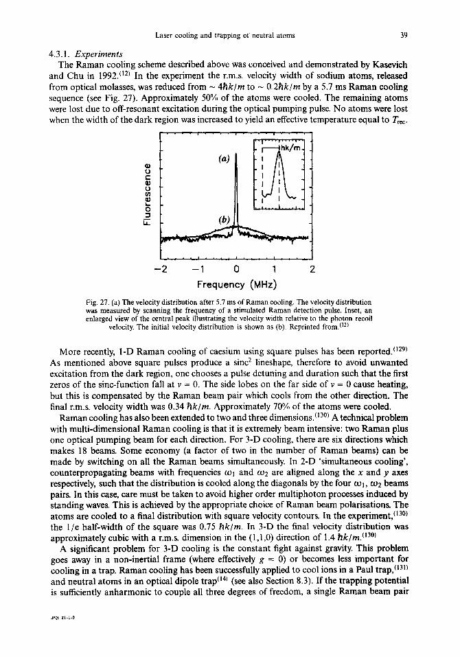
Laser cooling and trapping of neutral atoms 39
4.3.1. Experiments The Raman cooling scheme described above was conceived and demonstrated by Kasevich
and Chu in 1992.(i2) In the experiment the r.m.s. velocity width of sodium atoms, released from optical molasses, was reduced from - 4Rklm to - Q2Rklm by a 5.7 ms Raman cooling sequence (see Fig. 27). Approximately 50%) of the atoms were cooled. The remaining atoms were lost due to off-resonant excitation during the optical pumping pulse. No atoms were lost when the width of the dark region was increased to yield an effective temperature equal to Tree.
-2 -1 0 1 2
Frequency (MHz)
Fig. 27. (a) The velocity distribution after 5.7 ms of Raman cooling. The velocity distribution was measured by scanning the frequency of a stimulated Raman detection pulse. Inset, an enlarged view of the central peak illustrating the velocity width relative to the photon recoil
velocity. The initial velocity distribution is shown as (b). Reprinted from.(“)
More recently, 1-D Raman cooling of caesium using square pulses has been reported.(‘29’ As mentioned above square pulses produce a sinc2 lineshape, therefore to avoid unwanted excitation from the dark region, one chooses a pulse detuning and duration such that the first zeros of the sine-function fall at v = 0. The side lobes on the far side of v = 0 cause heating, but this is compensated by the Raman beam pair which cools from the other direction. The final r.m.s. velocity width was 0.34 Plklm. Approximately 70% of the atoms were cooled.
Raman cooling has also been extended to two and three dimensions.(*30) A technical problem with multi-dimensional Raman cooling is that it is extremely beam intensive: two Raman plus one optical pumping beam for each direction. For 3-D cooling, there are six directions which makes 18 beams. Some economy (a factor of two in the number of Raman beams) can be made by switching on all the Raman beams simultaneously. In 2-D ‘simultaneous cooling’, counterpropagating beams with frequencies wi and w2 are aligned along the x and y axes respectively, such that the distribution is cooled along the diagonals by the four wi , w2 beams pairs, In this case, care must be taken to avoid higher order multiphoton processes induced by standing waves. This is achieved by the appropriate choice of Raman beam polarisations. The atoms are cooled to a final distribution with square velocity contours. In the experiment,(i30) the l/e half-width of the square was 0.75 Rk/m. In 3-D the final velocity distribution was approximately cubic with a r.m.s. dimension in the (1 ,l ,O) direction of 1.4 hk/m.(‘30)
A significant problem for 3-D cooling is the constant fight against gravity. This problem goes away in a non-inertial frame (where effectively g = 0) or becomes less important for cooling in a trap. Raman cooling has been successfully applied to cool ions in a Paul trap,““‘) and neutral atoms in an optical dipole trap(r4) (see also Section 8.3). If the trapping potential is sufficiently anharmonic to couple all three degrees of freedom, a single Raman beam pair

40 C. S. ADAMS & E. RIIS
is sufficient to provide 3-D cooling. The velocity distribution of sodium atoms confined in an optical dipole trap before and after Raman cooling are shown in Fig. 28.(t4) After cooling, the r.m.s. velocity spread was 0.65 Aklm, corresponding to a temperature of 1.0 PK. This represents the first demonstration of sub-recoil temperatures in 3-D using Raman cooling.
Velocity @k/m)
Fig. 28. The velocity distribution of sodium atoms confined in a far-off resonant optical dipole trap before (dashed curve) and after Raman cooling. The final temperature was
1.0 FK, which is well below the recoil temperature for sodium. Reprinted from Ref. 14.
5. PRECISION MEASUREMENTS WITH COLD ATOMS
5.1. Introduction
The prospect of using slow atoms for precision measurements has been a significant moti- vating factor behind the development of laser cooling and trapping techniques. The potential for improving the atomic frequency standard is particularly appealing.(132) The fact that the current standard is based on caesium, one of the most ideal elements for optical manipulation, is a fortunate coincidence.
The field of precision measurement is closely related to the development of fundamental SI standards. The standard for time (or frequency) is particularly important, and will set the strongest demands in the future. Consequently, a great deal of work is going into improving the current standard, and exploring the possibilities for a successor. Our ability to make electronic measurements of frequency is far superior to measurements relative to artefacts (e.g. the old standard meter or kilogram) or measurements based on delicate set-ups (e.g. the ampere). For this reason, considerable effort is also devoted to realising new standards which may be related to a frequency measurement. The definition of the meter is the best known example of this process: by defining of the speed of light, the artefact was made redundant. Similarly, the electrical standards are now linked to a frequency measurement through the Josephson frequency-to-voltage ratio 2elh. Finally, a range of fundamental experiments can be recast in the shape of frequency measurements, and therefore depend not only on the existence of a proper standard, but are in themselves frequency measurements with the utmost requirements for precision.

Laser cooling and trapping of neutral atoms 41
As a source for precision measurements, a sample of laser cooled atoms has a number of advantages over room temperature vapours or thermal beams. The most obvious is the pos- sibility of achieving significantly longer interrogation times. Although the accuracy of a fre- quency measurement is often limited by other factors, the ultimate limit is set by gravity. For practical equipment dimensions, atoms cooled to sub-Doppler temperatures allow interroga- tion times of up to one second, which translates into a potential linewidth of -1 Hz. Other advantages of cold atoms include the virtual elimination of Doppler and collision-induced shifts, weak coupling to the interrogating fields, and the possibility of preparing state-selected and isotopically pure samples.
The limited number of elements which can be laser cooled (cf. Appendix) prevents the technique from being developed into a general spectroscopic tool. However, an increasing number of key experiments rely on the unique properties of laser cooled atoms. In this section, we introduce the techniques of precision spectroscopy using cold atoms, and discuss specific applications such as improved frequency standards and the measurement of fundamental constants.
5.2. The atomicfbuntain
The advantage of slow atoms for precision frequency measurements follows immediately from the uncertainty principle, however, the experimental implementation is less straightfor- ward. In the original proposal for an improved caesium frequency standard, Zacharias sug- gested aiming a thermal beam upwards and detecting only atoms in the slow tail of the dis- tribution, atoms with velocities of 6 m/s or less. (20) These atoms would turn around less then 2 m above the source and fall back down again under the influence ofgravity. This would not only yield interrogation times of order 1 s, but the geometry also lends itself to the application of Ramsey’s technique of separated oscillatory jields,(‘“3’ with the convenient simplification that only one field region is needed because the atoms pass through both on their way up and down. Unfortunately Zacharias’ fountain did not work because collisions with the faster atoms (the vast majority) effectively removed the slow tail.
Despite the failure of the original experiment, the idea survived and the problem of collisions was solved with the first demonstration of an atomic fountain based on laser cooled atoms in 1989.(z” The idea was to trap and cool a sample of sodium atoms and subsequently launch them with a velocity of 2-3 m/s. The experimental set-up is shown in Fig. 29.
In order to give the reader an appreciation of the large number of steps involved in a typical cold atom experiment, the following subsection gives a detailed description of this experiment, including the optical and electronic systems not shown in Fig. 29.
5.2.1. The first cold-atom fountain experiment The central component of the fountain experiment was a magneto-optical trap (see Sec-
tion 2.4.3). It was formed inside a large vacuum system (with background pressure -lo-r0 Torr) by two 10 cm diameter coils separated by 6 cm. The magneto-optical trap was filled from a thermal Na beam slowed using the chirped slowing technique described in Section 2.2. The laser beams used for slowing and cooling/trapping were all derived from a commercial single frequency Rhodamine 6G dye laser pumped by an Ar+ laser. The frequency of the dye laser was stabilised, with a variable offset, to one of the hyperfine components of the saturated absorption spectrum in a Na vapour cell.
The main laser beam was passed through an electro-optic modulator operating at a frequency of 17 12 MHz, with a sideband-to-carrier intensity ratio of 1: 10. The frequency was chosen such that when the carrier was tuned to cool on the 2Si,2, F = 2 to 2P3,2, F’ = 3 transition, the upper sideband would be resonant with the 2Sr,2, F = 1 to 2P3,2, F’ = 2 transition, producing

42 C. S. ADAMS & E. RIIS
efficient repumping of the lower hyperfine level. The laser beam was then split into light for the magneto-optical trap (molasses beams) and for slowing. The former was passed through a length of polarisation preserving optical fibre in order to provide spatial filtering and a stable alignment, while the latter was passed through a travelling-wave electro-optic modulator, whose frequency was swept from 1 GHz to 100 MHz in about 2 msec. All the beams could be extinguished completely using mechanical shutters. This was important in order to allow the atoms to travel in the atomic fountain without seeing any near resonant light.
The slowing light was converted to circular polarisation, overlapped with the atomic beam, and focused on the aperture of the oven. Atoms leaving the oven with a velocity of about 600 m/s would remain in resonance with the lower sideband and be brought to rest near the centre of the magneto-optical trap. The molasses light was formed into three orthogonal standing waves with 9 mm diameter (e -2 FWHM). One beam was horizontal, while the other two were in a perpendicular plane at +45” to the vertical. This geometry provided free access in the vertical direction. The required (T+(T- polarisations for the magneto-optical trap were obtained by passing the light through h/4 plates, both before and after the vacuum chamber.
Typical operating conditions for the magneto-optical trap were a detuning of -2I, an in- tensity of 2.51,,,, and a magnetic field gradient of 1 G/mm. Fluorescence from the atoms was monitored by a photo-multiplier tube and the temperature determined using the time-of-flight technique. In order to achieve the lowest possible temperature before the atoms were launched, the trapping field was switched off (in less then 1 msec) and the intensity reduced to 0.3 I,,,. The temperature was typically measured to be 50 ,oK corresponding to an r.m.s. velocity in each direction of 14 cm/s.
In the first demonstration of the atomic fountain, the atoms were launched on ballistic trajectories by applying a short pulse of light, resonant with the 2Si,~, F = 2 to 2P3/z, F’ = 2 transition, entering from below. This transition was chosen to allow efficient optical pumping into the F = 1 ground state by switching off the drive power to the electro-optic modulator
t-f in
Fig. 29. Schematic diagram showing the experimental set-up used to produce a cold-atom fountain. The main components are the magneto-optical trap, the rf waveguide, and the
detection region. From Ref. 21

Laser cooling and trapping of neutral atoms 43
providing the repumping light. For a 3.6 msec launch pulse, the atoms would scatter around 80 photons giving an initial velocity of 2.4 m/s and a fountain height of 30 cm.
The atoms in the fountain were detected using a resonant photo-ionisation scheme. A 1 msec pulse from the dye laser excited the atoms to the 22Ps,~ level from which they could be ionised by a 10 nsec, 25 mJ pulse from a frequency-tripled Nd:YAG laser at 355 nm. The ions created in this process were electrostatically focused onto a micro-channel-plate detector. The advantage of this detection scheme over optical detection is the high efficiency (around 10%) and a low background count level.
A typical timing sequence for the fountain experiment was as follows. The magneto-optical trap was filled to its steady-state capacity of 5~10~ atoms in 500 msec. The atomic beam and slowing beam were blocked by the mechanical shutters, the trapping magnetic field was switched off, and the intensity in the molasses beams reduced. After about 15 ms the minimum temperature was reached and the molasses beams were extinguished. Immediately thereafter the launch beam was applied as explained above. A variable delay allowed the photo-ionising pulses to be fired anywhere within the 500 msec free-flight time in the fountain.
The groundstate hyperhne transition at 1.772 GHz was excited by the application of two short r-r/2 rf pulses as the atoms were turning around inside a waveguide. Fig. 30 shows exam- ples of the Ramsey fringe patterns obtained in this experiment. The data shown in Fig. 30(b) represent a 1000 set integration time, and allows the line centre to be determined to 10 mHz. For an interrogation time (i.e. time between the two rf pulses) of AT = 255 ms, the expected linewidth, Av = 1/2AT = 2 Hz was observed.
100 130 160 190
Y (-1 771 626 000 Hz)
Fig. 30. (a) The observed rf signal in a cold-atom fountain experiment. The fringes were produced by Ramsey’s technique of separated oscillatory fields.(‘33) As the atoms passed upwards through the rf cavity, they were excited into a coherence superposition of the two groundstate hyperfine levels by a rr/2 pulse. This superposition is equivalent to a precessing dipole. When the atoms fell back through the cavity, the population was transferred to the upper (or lower) hyperfine level if the dipole was in (or out of) phase with the rf field. The phase difference was varied by changing the rf frequency. The rf-pulses had a duration of 32 ms, and were separated by 125 ms. (b) An expanded view of the central fringes obtained
with 3.2 ms pulses separated by 255 ms. after 1000 s of integration. From Ref. 21.
5.2.2. Second generation offountains While the first realisation of an atomic fountain did provide an impressive demonstration of
the potential of cold atoms as a tool in precision measurements, it also identified a number of factors which make this particular set-up less than ideal. One of these was the launch. A range

44 C. S. ADAMS & E. RIIS
of initial velocities would be expected due to the statistical variation in the number of photons scattered (N & fl, where N - SO), and also spontaneous emission causes significant heating in all dimensions. Both are highly undesirable as they result in loss of signal and increase the sensitivity to Doppler shifts and broadening. This can be largely avoided by using the moving
molasses launch technique.‘22,128) The frequencies of the molasses beams are changed such that there is an upward moving frame in which all six beams appear Doppler shifted to the same frequency, so that atoms experience sub-Doppler cooling in the moving frame. For the set-up shown in Fig. 29, this is achieved by increasing the frequency of the upward moving beams in the vertical plane by a few MHz and reducing the frequency of the downward moving beams by the same amount. Another obvious step to improve the atomic fountain was to use a heavier element such as caesium, where the sub-Doppler temperature corresponds to a velocity distribution about ten times narrower than for sodium. This leads to a more compact fountain, reducing the sensitivity to field inhomogeneities and Doppler broadening.
5.3. Atomic clocks
As described above, the first demonstration of the atomic fountain was used for a precision measurement of the Na groundstate hyperfine splitting. As this transition is equivalent to that used in the caesium clock, the experiment was a prototype for an atomic frequency standard based on laser cooled atoms. To turn the experimental set-up shown in Fig. 29 into an atomic clock, the rf waveguide should be replaced by a cavity. The counterpropagating rf fields in a cavity significantly reduce the sensitivity to the horizontal component of the atomic velocity. Subsequent work on Cs atomic fountains has demonstrated the accuracy of the system, and begun to explore the limitations of the technique. (22,23,‘34) The fountain has many advantages over traditional thermal beam clocks including reduction in the observed linewidth, and virtual elimination of the second-order Doppler shift, but just as important, many of the factors which limit the accuracy of beam clocks are significantly reduced. One example is the cavity phase shift error. This is the largest uncertainty in present Cs beam standards, and arises because the two Ramsey interactions take place in two separate cavities. Any phase difference between the cavities translates into a shift of the observed line. In a fountain clock, this problem does not arise because there is only one cavity! Also the much narrower linewidth in a fountain means that the bias magnetic field required to isolate the clock transition (mF = 0 to rn; = 0) can be reduced dramatically, resulting in a smaller quadratic Zeeman shift.
5.3.1. Limiting factors
Of the systematic frequency shifts known from traditional beam clocks, the bias magnetic field would appear to be the most severe in a fountain, limiting the estimated accuracy (Av/v) to around the lo-r6 level. This represents an improvement of 2-3 orders of magnitude com- pared to a beam clock. However, the use of cold atoms introduces new problems. As discussed in Section 2.5 the energy levels of colliding atoms shift, so if they shift differently for the two hyperfine levels of the clock transition, this will give rise to a density dependent frequency shift. Frequency shifts of several mHz have been measured for densities of order IO9 cm-3.(233 However, as the shift is linear, an extrapolation to zero density is feasible. With this correction an accuracy of lo-l6 should be possible.
5.3.2. Prospects for optical clocks The fact that laser cooling works so well for caesium, the element that was already chosen
for the definition of time, is a fortunate coincidence. However, in the light of advances in laser technology, and the development of techniques such as laser cooling, it is interesting to consider whether the current definition is still the best. An obvious guideline would be to
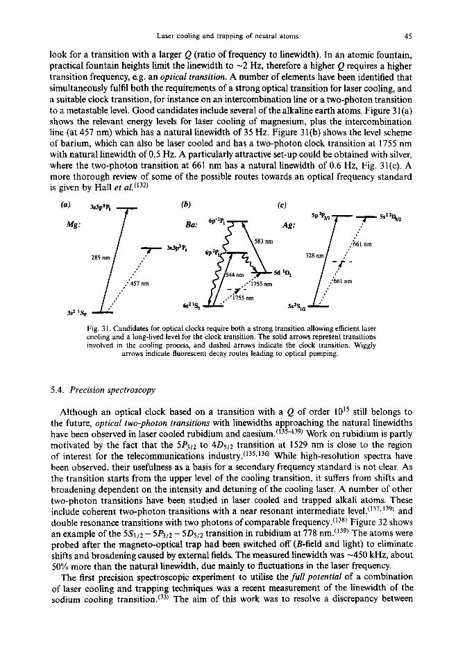
Laser cooling and trapping of neutral atoms 45
look for a transition with a larger Q (ratio of frequency to linewidth). In an atomic fountain, practical fountain heights limit the linewidth to -2 Hz, therefore a higher Q requires a higher transition frequency, e.g. an optical transition. A number of elements have been identified that simultaneously fulfil both the requirements of a strong optical transition for laser cooling, and a suitable clock transition, for instance on an intercombination line or a two-photon transition to a metastable level. Good candidates include several of the alkaline earth atoms. Figure 3 1 (a) shows the relevant energy levels for laser cooling of magnesium, plus the intercombination line (at 457 nm) which has a natural linewidth of 35 Hz. Figure 31(b) shows the level scheme of barium, which can also be laser cooled and has a two-photon clock transition at 1755 nm with natural linewidth of 0.5 Hz. A particularly attractive set-up could be obtained with silver, where the two-photon transition at 661 nm has a natural linewidth of 0.6 Hz, Fig. 31(c). A more thorough review of some of the possible routes towards an optical frequency standard is given by Hall et a1(‘32)
Mg:
Fig. 3 I. Candidates for optical clocks require both a strong transition allowing efficient laser cooling and a long-lived level for the clock transition. The solid arrows represent transitions involved in the cooling process, and dashed arrows indicate the clock transition. Wiggly
arrows indicate fluorescent decay routes leading to optical pumping.
5.4. Precision spectroscopy
Although an optical clock based on a transition with a Q of order 1015 still belongs to the future, optical two-photon transitions with linewidths approaching the natural linewidths have been observed in laser cooled rubidium and caesium.(135-139) Work on rubidium is partly motivated by the fact that the 5P 312 to 40512 transition at 1529 nm is close to the region of interest for the telecommunications industry. (135,130 While high-resolution spectra have been observed, their usefulness as a basis for a secondary frequency standard is not clear. As the transition starts from the upper level of the cooling transition, it suffers from shifts and broadening dependent on the intensity and detuning of the cooling laser. A number of other two-photon transitions have been studied in laser cooled and trapped alkali atoms. These include coherent two-photon transitions with a near resonant intermediate level,(137~‘3g) and double resonance transitions with two photons of comparable frequency.(138) Figure 32 shows an example of the 5Sr12 - 5Pj12 - 5Ds,2 transition in rubidium at 778 nm.(139) The atoms were probed after the magneto-optical trap had been switched off (B-field and light) to eliminate shifts and broadening caused by external fields. The measured linewidth was -450 kHz, about 50% more than the natural linewidth, due mainly to fluctuations in the laser frequency.
The first precision spectroscopic experiment to utilise the full potential of a combination of laser cooling and trapping techniques was a recent measurement of the linewidth of the sodium cooling transition. (33) The aim of this work was to resolve a discrepancy between

46 C. S. ADAMS & E. RIB
calculated and measured lifetimes of the 3P level. The traditional way of measuring lifetimes is to observe a fluorescent decay, which suffers from a number of systematic effects related to the exact experimental geometry. Laser cooling allows the lifetime to be determined from accurate measurements of the natural linewidth of the transition. This measurement resolved the discrepancy and is in agreement with a recent and more careful measurement of the fluorescence decay.(i40)
5.5. Atom interferometers
In general, a frequency (or time interval) can be measured with a much greater accuracy than any other physical quantity. It is therefore desirable to re-cast any precision measurement in the shape of a frequency measurement. To conclude this section we shall consider two examples. Both illustrate the use of atom interferometry for precision measurements.
The similarity between the wave nature of light and atoms enables many of the techniques of classical optics to be extended to atoms. One example is interferometry. Atom interferometers based on Young’s double slit(‘41’ and grating dzfiaction”42) were first demonstrated in 1991 (further details can be found in a recent review on Atom Optics (26)). In this Section, we consider an atom interferometer of the Mach-Zehnder type based on stimulated Raman transitions.(24) This interferometer is an extension of the Ramsey technique described above, Again, the sensitivity increases with interaction time, favouring the use of an atomic fountain geometry. Indeed, the experimental set-up of the first cold-atom interferometer was very similar to Fig. 29.
Atom interferometry based on stimulated Raman transitions is related to the technique of Raman cooling described in Section 4.3. As shown in Fig. 33(a), a two-photon Raman transition can be induced between the groundstate hype&e levels, I 1) and I2), using two lasers separated in frequency by the hyperfine splitting, and tuned well below the excited state 1 e) to avoid spontaneous emission. If an atom initially in state ) 1) is excited by a
0.8
+ 0.6
7 3 0.4
& i;j 0.2
-10 0 10 20 30 40 50 60 70
Laser frequency /MHz
Fig. 32. Two-photon spectroscopy of laser cooled rubidium atoms. The 5Sri2 -S&z - 5D5,2 transition at 778 nm is probed using a mode-locked Ti:sapphire laser. The top curve shows the experimental data with a Lorentzian fit, while the lower two curves indicate the positions of the lines calculated from published data. The observed signal is a coherent superposition of contributions from a large number of individual pulses. The signal size is comparable to a cw experiment, but the spectrum repeats at an interval equal to half the pulse repetition rate, and the observed linewidth approaches the natural linewidth, even though the laser
bandwidth is six orders of magnitude larger. From Ref. 139

Laser cooling and trapping of neutral atoms 47
n/2 Raman pulse, the output is a coherent superposition of I 1) and ( 2). If the laser beams are counterpropagating, the excited hyperfine component receives a momentum kick, - 2Ak. Thus, a 7r/2 pulse acts as a 50:50 beamsplitter, as shown in Fig. 33(b). For a r-r pulse, atoms are transferred from I 1) to I 2) or vice versa, and momentum is transferred, simulating a grazing incidence mirror (Fig. 33(c)). It follows that a Mach-Zehnder interferometer may be formed by a n/2 - r-r - rr/2 pulse sequence, as shown in Fig. 33(d). The output (i.e. state I 1) or I 2) ) depends on the relative phases of the interfering wavepackets and the 7-r/2 Raman pulses.
(a) +ld
7---A----- (4
0, @A
/
t . . . . . . \ . . . . . . . . . ...* 12)
%b II)
Fig. 33. Schematic diagram illustrating the principle of an atom interferometer based on stimulated Raman transitions. (a) A stimulated Raman transition is induced between two groundstate hyperfine levels I 1) and I 2) by two beams whose frequency difference wr - ~2 is exactly equal to the hyperfine splitting, W&. (b) If the Raman beams are counterpropagating and switched on to form a n/2 pulse, the initial state is excited into a coherent superposition of the two hyperfine levels. Due to the momentum exchanged the two components separate with a velocity - 2Rk/m, i.e. the pulse acts as a 5050 ‘beam splitter’. (c) If a rr pulse is excited, the internal states are interchanged and two photon momenta are exchanged, producing a reflection. (d) A Mach-Zehnder interferometer is formed by the pulse sequence,
n/2 - lr - n/2.
Figure 34 shows the number of atoms transferred to the upper hyperfine level as a function of the phase of the final rr/2 pulse. (24) The contrast of the interference fringes is degraded by a number of effects. First, due to the spread in atomic velocities not all atoms experience exact n/2 and rr pulses. Second, the phase is referenced to an ‘inertial’ frame. In the experiment, this was a vibration-isolated platform which supported the mirror controlling the Raman beam pair. Sub-wavelength movement of this platform induces a phase shift which tends to wash out the interference. The same is true for irregularities and instabilities in the Raman beam wavefronts.
5.5.1. Measurement of g By directing the Raman beams vertically, the Mach-Zehnder interferometer shown in
Fig. 33(d) can be used to measure the acceleration due to gravity, g. While travelling through the interferometer one wavepacket is, on average, at a higher gravitational potential than the other, which appears as a phase shift. A sensitivity of Ag/g = 3 x 10-s with -30 mins integration time has been demonstrated.(24’

48 C. S. ADAMS & E. RIIS
55.2. Measurement of A/m In the analysis of absorption and emission processes presented in Section 2.1, we were
primarily interested in the conservation of momentum. However, in addition to light forces, the photon recoil also produces a measurable spectroscopic effect. An atom (or molecule) initially at rest recoils with a velocity Aklm, so the equation for the conservation of energy will include a kinetic energy term corresponding to a shift of the absorption line. Similar arguments show that the resonance frequency for an atom stimulated back to the ground state depends on the direction of the stimulating beam relative to the recoiling atom, such that two resonances occur separated by Ao = 2Rk2/m. An accurate measurement of this recoil splitting will yield the ratio A/m, which is of fundamental interest, as the mass only appears in this ratio in quantum mechanics.
The recoil splitting was first observed in saturated absorption spectroscopy of methane excited by a 3.39 pm HeNe laser. (143) The recoil splitting was -2 kHz. The exquisite velocity sensitivity provided by stimulated Raman transitions has allowed a precision measurement of the recoil splitting to be carried out using the atom interferometer described above.(25) Additional absorptions and stimulated emissions were inserted in the interferometer to increase the recoil splitting to 60 photons worth of momentum. For caesium, R/m was measured with a precision of lo-’ with a 2 h integration time.(25)
6. COLD ATOMIC BEAMS
6.1. Introduction
In Sections l-5, we concentrated on the production and applications of atomic samples with a small velocity spread and zero mean velocity, or at most a vertical velocity of a few meters per second, typical for an atomic fountain (Section 5.2). However, for many experiments, an atomic beam with a small velocity spread but non-zero mean velocity is desired. Well collimated, bright atomic beams with arbitrary longitudinal velocity can be prepared using the techniques of laser cooling.
Central for the production of these beams is the ability to realise atomic lenses. For a lens based on conservative forces, a reduction in beam size is accompanied by an increase in the divergence. This is Liouville’s theorem. In contrast, the dissipative nature of the spontaneous
600 300 L
co
Zi \ 300 3
150
5
00
0 0 0 180 360 0 180 380
Phase (deg.)
Fig. 34. Interference fringes produced by an atom interferometer based on stimulated Raman transitions. The pulse interval was (a) 1 ms and (b) 40 ms. The scans were made by varying the phase of the second n/2 pulse. For the 40 ms pulse interval, the wavepackets were
separated by 2.4 mm at the centre of the interferometer. From Ref. 24.

Laser cooling and trapping of neutral atoms 49
force means that a lens based on this force can produce a significant increase in the atomic ‘brightness’. An example of a dissipative optical component, the atomicfunnel, will be described in Section 6.2.
There is particular interest in focusing atomic beams to small spot sizes. Such focused beams could be used for a variety of applications from atom lithography to probing surfaces (see Ref. 26). One attraction of atomic beams is the possibility of achieving a resolution far superior to that obtained with light. In practice, the minimum atomic spot size is only limited by the strength of the lens and the initial velocity spread of the atomic beam (see Section 6.3). As the initial velocity distribution is important, laser cooling plays a crucial role in preparing beams for focusing.
Finally, in Section 6.4 we discuss the application of laser cooling and focusing to atom lithography.
6.2. Cooling of beams
Transverse laser cooling is frequently used to increase the flux and reduce the transverse velocity spread of an atomic beam. (144) It is achieved by applying a section of 2-D optical molasses perpendicular to the atomic beam axis. If this cooling section is positioned close to the source, a significant increase in beam flux can be achieved. Unfortunately the length of the cooling section can easily become inconveniently large.
A more radical approach for creating a slow and cold atomic beam was taken with the de- velopment of the atomic funnel. (‘45) This is essentially a magneto-optical trap in two dimensions (transverse) and a moving molasses in the third. The principle of the funnel is illustrated in Fig. 35. A conventional magnetic quadrupole field is created by running a high current through four long wires positioned in a square, such that neighbouring wires have opposing currents. Atoms are collected from a vapour or a slowed beam, and pushed towards the symmetry axis by radiation pressure produced by four circularly polarised beams propagating perpendicular to the axis. Along the axis, a pair of beams with appropriate frequency offsets cool the atoms in a moving frame. The overall operation of the device is therefore to collect atoms with an initial velocity, less than a typical capture velocity of 20 m/s, bring them into line, cool them, and flush them out along the axis in a continuous process.
With a funnel loaded from a chirp-slowed atomic beam, an integrated flux of order lo9 Na atoms per second was demonstrated. (14% The beam diameter was 1.5 mm, the longitudinal velocity could be varied in the range l-5 m/s, and the temperature in the moving frame was -200 PK. * The brightness of the beam, defined as the integrated flux divided by the volume in velocity space (Av,Av,Av,), was 3000 times larger than for the original thermal beam.
A similar technique, using permanent magnets, was used to compress a Na beam.(r4@ Atoms, slowed by a chirped laser, entered a compression stage, consisting of permanent magnets producing a quadrupole field which increased linearly along the beam axis. The atoms were captured at low field (50 G/cm), allowing a larger capture range, and left, compressed, at the high field end (500 G/cm). No additional longitudinal cooling was attempted within the compressor. Longitudinal cooling using a moving molasses technique has been demonstrated on a beam of metastable Ar atoms. (14’) The final velocity spread was reduced to more than 800 times less than the mean velocity. No attempt was made to reduce the transverse velocity spread.
* For the set-up used in this experiment, the longitudinal and transverse laser frequencies were not corrected to give polarisation gradient cooling in the moving frame and so the final temperature was comparable to the Doppler limit.

50 C. S. ADAMS & E. RIIS
6.3. Focusing of atomic beams
Focusing of atomic beams is important for high resolution imaging of surfaces and lithog- raphy. Atomic waves may be focused by refraction from a parabolic potential or by diffraction, e.g. by a Fresnel zone plate. Of particular interest in any focusing experiment is the minimum achievable spot size. For light, Fourier optics suggests that the minimum spot size is of order h/2. This argument assumes that the beam is diffraction limited (AxoAps = h/2), and that the lens can turn the initial longitudinal momentum (h/h) into transverse momentum. Similar arguments suggest that the minimum spot size for an atomic beam should be &n/2, where hdn = h/mv is the de Broghe wavelength of the atomic beam. However, this expression relates to an unattainable experimental situation as both the above assumptions are inappropriate for atoms. First, atomic beams are, typically, far from diffraction limited: due to the trans- verse velocity spread, an atomic beam is equivalent to a superposition of a large number of transverse modes, i.e. AxoA~o > t7/2. Second, in contrast to light, the maximum momentum imparted by the lens is limited by the physical processes responsible for the focusing.
To estimate the spot size consider an ideal lens, which imparts a transverse momentum which increases linearly with distance x from the optical axis, Aprens = -<x, where 5 is a coefficient which represents the strength of the lens. By geometry, the focal length is,
(43)
where pz is the longitudinal atomic velocity. If the initial transverse momentum spread is Ape, the focused spot size is w - fApo/pz. Substituting for f,
w_apo 5 (44)
Fig. 35. The principle of the atomic funnel. The current carried by the four wires create a quadrupole magnetic field. Four circularly polarised laser beams with elliptical cross sections collect atoms with velocities below 20 m/s and compress them to the symmetry axis. The atoms are flushed out along the axis using a moving molasses. This is achieved by choosing the frequencies of the two axial beams Aw = kv higher and lower than that of the transverse
beams.

Laser cooling and trapping of neutral atoms 51
Hence the spot size only depends on the transverse velocity spread and the strength of the lens. The effect of longitudinal velocity spread (of similar magnitude to the transverse spread) is much less. It follows that for a small focus, extremely good collimation and high monochromic- ity are required. In this respect, laser cooling is essential for preparing atomic beams for deep focusing.
The first experiments on the focusing of atomic beams were based on static electric and magnetic fields. In 1951 Friedburg and Paul (‘48’ demonstrated focusing of an atomic beam using a hexapole magneticfield. The hexapole field produced a Zeeman shift with a quadratic spatial dependence leading to a focusing effect for atoms in the correct magnetic sub-level. The same principle, using electric fields was used by Gordon to focus excited ammonia molecules in the first maser.(‘4g) The main drawback of focusing using static fields is that the interaction is too weak to permit the realisation of compact lenses. After the invention of laser cooling, it was realised that near-resonant light is particularly well-suited for focusing atomic beams. The interaction is relatively strong, and lens-like potentials occur for a variety of light field configurations. The focusing and de-focusing of sodium atoms using light was first reported by Bjorkholm et al. in 1978. (73) This was the first experimental demonstration of the application of the optical dipole force for the manipulation of atomic beams. The minimum atomic spot size, 28 pm, was limited by diffusive aberration due to fluctuations in the dipole force. Diffusive aberrations are particularly severe for this configuration, because the atoms are confined to a region of high intensity. A partial solution is to use a blue-detuned co-propagating TEMsi mode 7 (iso) which has the advantage that the atoms are deflected towards low intensity.
Focusing can also be obtained using the scattering force from diverging laser beams.(i5’) For an atomic beam propagating perpendicular to two counterpropagating diverging beams, the atoms experience a radiation pressure which is proportional to their distance from the axis. For a long interaction time, the atoms are first focused and then cooled transversely in the optical molasses formed by the balanced intensities on axis. Again, a drawback of near- resonant light is the diffusive aberration caused by spontaneous emission, which, in this case limited the minimum spot size to - 100 ~m.t’51)
A transverse standing wave light field can also be used to focus an atomic beam. Atoms close to the anti-node of a red-detuned standing wave (or the node of a blue-detuned standing wave) experiences an approximately parabolic potential (the optical potentials for atoms in a standing wave light are shown in Fig. 14) i.e. the optical potential behaves as a converging lens. Focusing of a metastable helium beam using an anti-node of a large period standing wave was demonstrated by Sleator et a1.“s2) in 1992.
As in conventional optics, the smallest spot sizes are achieved by increasing the strength of the lens. For very short focal lengths, one moves into the thick lens regime. For a sufficiently wide standing wave light field, atoms are focused after one-quarter of an oscillation period in the optical potential. The principle is similar to the GRIN (graded-index) lens used in conventional optics. A standing wave light field may be thought of as an array of cylindrical GRIN lenses. If the atomic beam is wider than the individual potential wells it is focused into a series of parallel lines separated by half the optical wavelength. This idea is discussed in the next section.
6.4. Atom lithography
The development of techniques to manipulate atomic beams using laser light has made it possible to deposit sub-wavelength sized structures directly onto surfaces.(27,28, 153,154) This technique, referred to as atom lithography, has a number of advantages over more conven- tional techniques. First, the resolution can, in principle, be several orders of magnitude smaller than an optical wavelength, Second, the technique inherently lends itself to parallel process-

52 C. S. ADAMS & E. RIIS
ing, because a large number of identical structures can be deposited simultaneously. Recent experiments have demonstrated the simultaneous deposition of parallel lines’**) and a regular array of dots.(*5”)
Figure 36(a) shows a schematic diagram of the experimental set-up for a typical atom lithog- raphy experiment. The atomic beam is collimated by transverse cooling using two orthogonal standing waves detuned below resonance. The collimated atomic beam is then focused by a strong blue detuned standing wave as discussed above. The optical potentials of the standing wave are strong enough that the atoms are deflected towards the nodes and then guided tightly along them. The sample is placed close to the point of tightest confinement, i.e. at the centre of the standing wave.
Sample
Collimating beams
t Focusing
beam
Fig. 36. (a) Experimental set-up for atom lithography. A thermal atomic beam is collimated using transverse laser cooling. The atoms are then focused onto a sample using the dipole force exerted by a blue detuned standing wave. (b) An image of chromium lines focused by
a near-resonant light field. From Ref. 155.
In 1992 Timp et LZ~.(*~) used a standing wave light field to deposit a series of regularly spaced lines of sodium on a substrate. The expected periodicity of the exposed surface was confirmed by optical diffraction. In 1993 McClelland et al. (28) wrote a chromium line structure on a silicon substrate. Chromium is a good element for lithography because it has low surface mobility, and the structures are air stable. The structure was analysed using an atomic force microscope (AFM). The lines had a width of 65 nm, a spacing h/2 =212.8 nm, and a height of - 34 nm for a 20 min exposure time. In a later experiment, two orthogonal standing waves were used to deposit a regular array of dots. (i5s) The dots had a FWHM of 80 nm. A typical chromium line structure is shown in Fig. 36(b).
The diffraction limited spot size for the atomic lens formed by the standing light field used in the chromium experiment was about 9 nm, substantially smaller than the measured width.‘28) The actual width was larger mostly due to the transverse velocity spread of the beam as discussed above. The transverse cooling stage reduced the beam divergence to - 0.2 mrad, but this is still far short of a diffraction limited beam. After correcting for the atomic velocity distribution and the finite size of the AFM tip, the measured line width are in fair agreement with the calculated value.
A different approach to atom lithography uses a hybrid technique based on Self-Assembled Monolayers or SAMs. (‘54) A 30 nm thick gold layer on a silicon sample is coated with a 1.5 nm thick layer of dodecanethiolate molecules, which assemble in a monolayer on the surface. If a SAM molecule is hit by a metastable helium atom, it is destroyed by a UV photon emitted by the decaying metastable. This exposes the gold layer, which can then be etched using conventional techniques. The distribution of metastable helium atoms can be defined
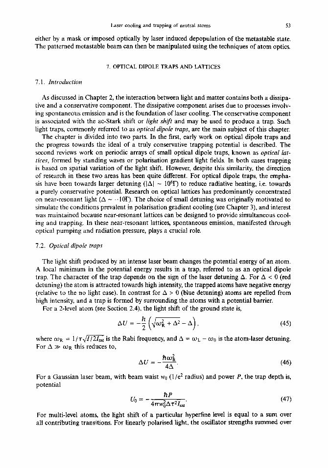
Laser cooling and trapping of neutral atoms 53
either by a mask or imposed optically by laser induced depopulation of the metastable state. The patterned metastable beam can then be manipulated using the techniques of atom optics.
7. OPTICAL DIPOLE TRAPS AND LATTICES
7.1. Introduction
As discussed in Chapter 2, the interaction between light and matter contains both a dissipa- tive and a conservative component. The dissipative component arises due to processes involv- ing spontaneous emission and is the foundation of laser cooling. The conservative component is associated with the ac-Stark shift or light shift and may be used to produce a trap. Such light traps, commonly referred to as optical dipole traps, are the main subject of this chapter.
The chapter is divided into two parts. In the first, early work on optical dipole traps and the progress towards the ideal of a truly conservative trapping potential is described. The second reviews work on periodic arrays of small optical dipole traps, known as optical lat- tices, formed by standing waves or polarisation gradient light fields. In both cases trapping is based on spatial variation of the light shift. However, despite this similarity, the direction of research in these two areas has been quite different. For optical dipole traps, the empha- sis have been towards larger detuning (IAl - 1061’) to reduce radiative heating, i.e. towards a purely conservative potential. Research on optical lattices has predominantly concentrated on near-resonant light (A - - lOI). The choice of small detuning was originally motivated to simulate the conditions prevalent in polarisation gradient cooling (see Chapter 3) and interest was maintained because near-resonant lattices can be designed to provide simultaneous cool- ing and trapping. In these near-resonant lattices, spontaneous emission, manifested through optical pumping and radiation pressure, plays a crucial role.
7.2. Optical dipole traps
The light shift produced by an intense laser beam changes the potential energy of an atom. A local minimum in the potential energy results in a trap, referred to as an optical dipole trap. The character of the trap depends on the sign of the laser detuning A. For A < 0 (red detuning) the atom is attracted towards high intensity, the trapped atoms have negative energy (relative to the no light case). In contrast for A > 0 (blue detuning) atoms are repelled from high intensity, and a trap is formed by surrounding the atoms with a potential barrier.
For a 2-level atom (see Section 2.4), the light shift of the ground state is,
AU=-;@&-&A), (45)
where WR = 1 /T,J~; is the Rabi frequency, and A = WL - wo is the atom-laser detuning. For A B WR this reduces to,
(46)
For a Gaussian laser beam, with beam waist wg (1 /e* radius) and power P, the trap depth is, potential
(47)
For multi-level atoms, the light shift of a particular hyperfine level is equal to a sum over all contributing transitions. For linearly polarised light, the oscillator strengths summed over

54 C. S. ADAMS & E. RIIS
the excited state hyperfine structure is the same for all the groundstate magnetic sub-levels. Therefore, if the detuning is larger than the excited state hypertme splitting, all the groundstate magnetic sub-levels move together. This degeneracy of the magnetic sub-levels in a linearly polarised far-off resonance optical dipole trap allows atoms in an arbitrary spin state to be trapped. Furthermore, if the detuning is larger than the fine-structure splitting, then, as far as the light is concerned, the atom looks like a 2-level system, and the trap depth is given by Eq. (47) with the saturation intensity equal to its 2-level value Z,,, = ~T~c/~TA~.‘~~’
A significant problem in optical dipole traps is the heating due to spontaneous scattering. For detunings larger than a few linewidths the spontaneous scattering rate is,
& Ys = -&$. (48)
For small detunings this radiative heating severely limits the lifetime of the trap. A solution to this problem is apparent by comparing equations (47) and (48). Whereas the trap depth is proportional to Z/A, the scattering rate is proportional to Z/AZ, so by increasing both the intensity and the detuning one can maintain the trap depth and reduce the radiative heating. In the limit of far detuning, one expects the light to create an almost conservative potential, such that in practice the lifetime of the trap is only limited by the background pressure. Figure 37 shows the lifetime of a far-off resonant trap for different pressures. As expected the lifetime varies linearly with the pressure, except at very low pressures (- IO-” Torr) where it tends to saturate at a few seconds due to other possible heating mechanisms (e.g. beam vibration).
I I I I
0 5 10 15 20
Time (s)
Fig. 37. Data showing the effect of background pressure (measured in Torr) on the lifetime of a far-off resonant optical dipole trap.(‘56)
7.2.1. Red-de&wed traps The simplest form of an optical dipole trap is a single focused Gaussian laser beam detuned
to the red of the atomic resonance. To establish the feasibility of optical trapping we estimate the potential depth for trapping sodium using a dye laser. For a 100 mW laser beam focused to a 10 ~_mr waist and detuned 5 nm from the sodium D-lines, the trap depth is equivalent to
Laser cooling and trapping of neutral atoms 55
a temperature of 0.5 mK. Optical trapping of atoms therefore had to wait until the invention of laser cooling!
The first experiment on an optical dipole trap was reported in 1986,(@ one year after the first 3-D laser cooling experiment. U) The trap was produced by focusing a 220 mW laser beam to a 10 pm waist at the centre of a sodium optical molasses. The trapping laser was detuned between 650 and 1300 GHz to the red of the D2 line. The trap was loaded by switching between optical molasses and trapping beams with a frequency between 100 kHz and 2 MHz. Evidence of an optical confinement was produced by video imaging of the trapping region. Stronger fluorescence indicated a higher density than in the surrounding molasses and time resolved measurements showed that the trapped atoms hung around for longer.
Due to the relatively small detuning, the scattering rate exceeded 10’ photons/s resulting in significant heating. When this was not compensated by cooling from the optical molasses beams, the trap lifetime was only a few milliseconds. @) An improved lifetime was observed with the first experimental demonstration of a far-off resonance optical dipole trap, reported by Miller et al. in 1993. (75) The trap was constructed from a focused laser beam (wg - 10 pm) detuned between 5 and 65 nm from the rubidium Dl line at 795 nm. The trapping beam, derived from a Ti:sapphire laser, was linearly polarised and had an average power of 0.6-0.9 W. Around 1000 atoms were trapped with a lifetime of up to 200 ms. The lifetime was limited by the relatively high rubidium vapour pressure (4 x lo-’ Torr). For the largest detunings, the photon scattering rate was of order 100 per second. The temperature of atoms in the trap was measured by velocity selective stimulated Raman transitions (see Sections 4.3). The measured temperature was found to scale roughly linearly with trap depth (kT - UO/ 10).
In addition the same group measured the rate of population transfer from the lower to the upper hyperfine levels in the ground state (F = 2 - 3 for gSRb). The population transfer is caused by spontaneous Raman transitions induced by the trapping laser. For detunings larger than the fine structure splitting, the Raman scattering amplitudes for the Dl and D2 lines interference destructively,(‘57) such that the Raman scattering rate (K 1 /A4) is much slower that the total spontaneous scattering rate (Raman plus Rayleigh scattering, cc l/AZ). This results in long spin relaxation times which makes optical dipole traps interesting for a variety of experiments in precision spectroscopy and cold collisions. The far-off resonance dipole trap has also proved a good system for studying photo-association. (‘%) The absorption of a photon from a probe laser during a collision between two atoms results in the formation of a long range molecule which is ejected from the trap. The photo-associative spectrum is built up by monitoring the trap loss as a function of the probe frequency.
A further step towards the ideal of a truly conservative trapping potential was made in a experiment on trapping sodium (atomic resonance 589 nm) using a krypton-ion laser (h =647 nm)(159) and later a Nd:YAG laser (h =I064 nm).(160) For the Nd:YAG trap the detuning is significant compared to the laser frequency, and therefore the rotating wave ap- proximation, which is commonly assumed in the theory of light-atom interactions,(t6’) is no longer accurate. An additional term in the expresion for the potential (the ‘counter-rotating term’) has the effect of increasing the trap depth.
Finally, we complete this section by mentioning that atoms have also been trapped by the magnetic dipole force produced by a microwavefield. (‘62) For a 83 W microwave source tuned near the groundstate hyperfine transition in caesium, the trap depth was - 0.3 mK. A few hundred atoms were trapped with a lifetime of - 1 s, probably limited by background gas pressure. More recently, a hybrid optical dipole/electrostatic trap was reported,(163) where transverse confinement was provided by vertical laser beam detuned by Ah - 1 nm from the caesium resonance, and a HV electrode produced a Stark shift to support the atoms against gravity.

56 C. S. ADAMS & E. RIIS
7.2.2. Blue-detuned traps In a blue-detuned trap atoms are repelled from regions of high intensity and therefore
very low photon scattering rates can be obtained. A simple blue-detuned dipole trap can be produced by crossing two doughnut mode laser beams. To minimise the trap loss rate care must be taken to avoid any interference effects which may lead to breaches in the light barrier. Much lower photon scattering rates can be achieved in a trap with independent control of the volume and wall thickness. The light-atom interaction time can be minimised by creating a hard-wallpotential (the same principle applies to light based atom mirrorP4)). For example a sodium atom with energy crec bouncing on an argon-ion laser beam (10 pm waist) experiences a photon scattering rate of - 10M4 s-‘.
The idea of bouncing cold atoms from a blue-detuned light field was first implemented using evanescent waves to produce a hard wall potential. (~5~) The addition of transverse confinement using a curved evanescent wave increased the number of bounces observed to more than 8(r6@ (see Fig. 38). However, a problem with this scheme is the glass surface required to produce the evanescent wave. In practice, the glass surface must be positioned a small distance (- 1 mm) below the source of cold atoms, and a very large light shift is required to reflect the atoms from this height. Consequently only moderate detunings can be used and the photon scattering rates are still high (of order 1 per bounce”@).
v) 10’ E 0
3 106 6 t
4 105
5 c
10’ 0 200 400 600
time in ms Fig. 38. The fluorescence produced by caesium atoms bouncing on a curved evanescent
wave. Reprinted from Ref. 166.
This problem is eliminated by using free propagating laser beams. A blue-detuned optical dipole trap for sodium atoms based on sheets of argon ion laser light was first reported in 1994.(r6’) Two sheets of light (- 10 x 300 pm), orientated at +45” to the vertical, were aligned at the centre of sodium magneto-optical trap. The potential at a height of 50 pm above the intersect is shown in Fig. 39. Weak confinement along the axis of the beams was produced by diffraction of the focused sheets. As the atoms spend most of their time in free fall, the perturbation by the light field is minimal (the spontaneous scattering rate is expected to be around 10V4 s-l), which makes this type of trap an ideal candidate for spectroscopy. This point was illustrated by spectroscopy of the groundstate hypetfine structure using Ramsey’s technique of separated oscillatory fields.(r6’)
A typical Ramsey fringe for a 4 s measurement time is shown in Fig. 40. The observed reduc- tion in the fringe visibility as a function of the measurement time is caused by the dephasing of atoms making different orbits in the trap. Dephasing due spontaneous emission is negligible due to the extremely low spontaneous scattering rate. The dephasing time, or coherence time was measured at 7 s. An equivalent measurement time would require a 7 km thermal beam, or a 60 m atomic fountain. However, the longer measurement time does not necessarily imply a higher sensitivity. Typically, a trap has orders of magnitude fewer atoms than a fountain or

Laser cooling and trapping of neutral atoms 5-l
X
Fig. 39. A cross section of the potential produced by two sheets of light orientated at +45” to the vertical. Longitudinal confinement of the atoms is provided by the diffraction of the Gaussian light sheets, The x and y axes are in microns. The intensity is arbitrary units,
Reprinted from Ref. 167.
a beam and consequently an inferior signal-to-noise ratio. In addition, the dephasing due to interactions with the walls of the trap limits their application to relative measurements (as for instance required for a measurement of permanent electric dipole moment, EDM) rather than absolute frequency measurements (as for instance required for atomic clocks).
-0.3 -0.2 -0.1 0.0 0.1 0.2 0.3
f - 1,771,626,130 Hz
Fig. 40. Ramsey fringes produced by microwave spectroscopy of sodium atoms confined in a blue-detuned far-off resonant optical dipole trap. The rf-pulses were separated by 4 s.
Reprinted from Ref. 167.
An improved blue detuned trap, based on the same principle, can be constructed by crossing two sets of V-shaped light distributions to form a 4-sided invertedpyramid.(‘4’ The light sheets were approximately 600 pm long by 10 pm thick which for sodium results in a trap depth mgh - 10erec, where h - 400 pm was the height of the trap. Due to the relatively large volume, over 500,000 atoms could be trapped. The trap lifetime was around 7 s.
Finally we note that a hybrid, magnetic/optical dipole trap has been used for the observation of Bose-Einstein condensation”9’ (see Chapter 8).
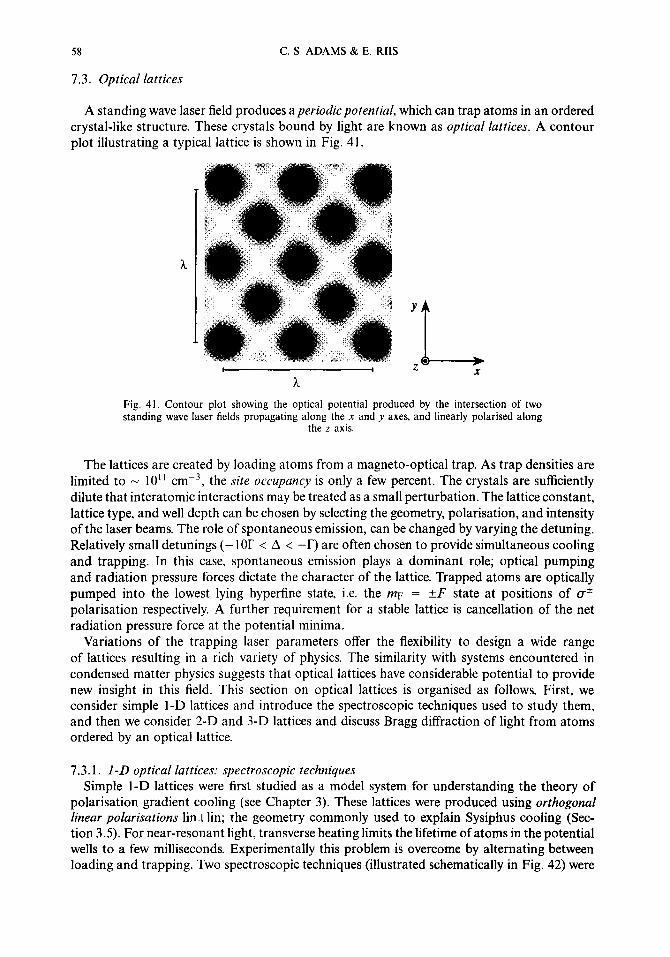
58 C. S. ADAMS & E. RIIS
1.3. Optical lattices
A standing wave laser field produces aperiodic potential, which can trap atoms in an ordered crystal-like structure. These crystals bound by light are known as optical lattices. A contour plot illustrating a typical lattice is shown in Fig. 41.
+ x I I
h
Fig. 41. Contour plot showing the optical potential produced by the intersection of two standing wave laser fields propagating along the x and y axes, and linearly polarised along
the z axis.
The lattices are created by loading atoms from a magneto-optical trap. As trap densities are limited to - 10” cmm3, the site occupancy is only a few percent. The crystals are sufficiently dilute that interatomic interactions may be treated as a small perturbation. The lattice constant, lattice type, and well depth can be chosen by selecting the geometry, polarisation, and intensity of the laser beams. The role of spontaneous emission, can be changed by varying the detuning. Relatively small detunings (- 1 OI’ < A < -lJ are often chosen to provide simultaneous cooling and trapping. In this case, spontaneous emission plays a dominant role; optical pumping and radiation pressure forces dictate the character of the lattice. Trapped atoms are optically pumped into the lowest lying hyperfine state, i.e. the mF = +F state at positions of (T’ polarisation respectively. A further requirement for a stable lattice is cancellation of the net radiation pressure force at the potential minima.
Variations of the trapping laser parameters offer the flexibility to design a wide range of lattices resulting in a rich variety of physics. The similarity with systems encountered in condensed matter physics suggests that optical lattices have considerable potential to provide new insight in this field. This section on optical lattices is organised as follows. First, we consider simple 1-D lattices and introduce the spectroscopic techniques used to study them, and then we consider 2-D and 3-D lattices and discuss Bragg diffraction of light from atoms ordered by an optical lattice.
7.3.1. 1-D optical lattices: spectroscopic techniques
Simple 1-D lattices were first studied as a model system for understanding the theory of polarisation gradient cooling (see Chapter 3). These lattices were produced using orthogonal linear polarisations linllin; the geometry commonly used to explain Sysiphus cooling (Sec- tion 3.5). For near-resonant light, transverse heating limits the lifetime of atoms in the potential wells to a few milliseconds. Experimentally this problem is overcome by alternating between loading and trapping. Two spectroscopic techniques (illustrated schematically in Fig. 42) were

Laser cooling and trapping of neutral atoms 59
introduced to probe atoms in the lattice: (a) heterodynejluorescence spectroscopy;(‘6@ and (b) probe absorption spectroscopy.(‘69)
60 (b)
Fig. 42. Experimental arrangements for (a) heterodyne fluorescence spectroscopy, and (b) probe absorption spectroscopy, of atoms confined by a 1 -D optical lattice.
7.3.1.1. Heterodynefluorescence spectroscopy Evidence for the localisation of atoms in the optical potentials present in 3-D optical molasses was first demonstrated using the technique of heterodyne fluorescence detection in 1990. (168) The idea, illustrated schematically in Fig. 42(a), is to spectrally analyse light scattered by atoms trapped in optical potential wells. For a stationary atom, the scattered light has exactly the same frequency as the laser, but when the atom moves, the scattered light acquires a Doppler shift: the atom behaves like a moving mirror. For typical atomic velocities in optical molasses, the Doppler width is a few hundred kHz, i.e. much narrower than the natural linewidth of the optical transition. Thus, the interesting part of the spectrum is a relatively narrow region on top of the central peak of the Mollow triplet.(83)
The spectrum is detected by interfering the scattered light with light derived from the trap- ping laser, shifted by tens of MHz using an acousto-optic modulator (AOM). This frequency shifted light is referred to as the local oscillator. The heterodyne beat frequency between the local oscillator and the scattered light contains all the information about the atomic veloc- ity distribution but is centred on the AOM frequency, and therefore is easily recorded using a standard rf spectrum analyser. As the fluorescence intensity falls off as 1/A2, heterodyne detection can only be used for situations with moderate detunings I A I < 1 Or.
The characteristic shape of the rf beat spectrum is shown in Fig. 43. The sidebands, which are observed at the trap oscillation frequency (uoSC, result from atoms which make a transition between vibrational levels of the optical potential. Despite the complex energy level structure of typical trapped atoms, the observed spectrum is characteristic of a harmonically bound 2-level atom.(170) This simplification occurs because optical pumping transfers most of the population to the mF = F level and light scattering occurs on the closed, mr = F to mr’ = F + 1 transition.
The spectrum can be explained semi-classically by considering the light scattered by an atom undergoing oscillatory motion. The spectrum contains sidebands at the oscillation frequency. The amplitude of the nth sideband is J,, (2rrao/ A), where a0 is the amplitude of the atomic mo- tion, and J,, is the nth order Bessel function. The experimentally observed spectrum (Fig. 43), with only very weak first order sidebands, indicates that the modulation index is very small, i.e. the atomic centre of mass motion is well-locafised on the scale of an optical wavelength. The ratio of sideband to carrier intensity is approximately k2a$ For a harmonic potential, a0 = JA72m(o, where wosc is the oscillation frequency, and therefore k2u$ = ~~~~~~~~~~~

60 C. S. ADAMS & E. RIIS
Fig. 43. The rf beat spectrum produced by heterodyne fluorescence spectroscopy of atoms confined in a 1-D optical lattice. The lower and upper sidebands correspond to transitions
up and down the vibrational ladder as indicated below.
where ~~~ is the recoil energy. This ratio is often referred to as the Lamb-Dicke factor. The condition kao < 1 or crec < Rwosc describes what is known as the Lamb-Dicke regime which is commonly encountered in ion trapping (see e.g. Ref. 189). The width of the sidebands is de- termined by the lifetime of the vibrational states, which depends on the excitation rate and the Lamb-Dicke factor because transfer between different vibrational levels is suppressed by this amount. The measured width consists of a sum over the contributions from each vibrational level, and is typically a few kHz for caesium.
The asymmetry between the intensity of the red and blue sidebands reflects the thermal distribution of atoms among the vibrational levels. (17’) Assuming a Boltzmann distribution the ratio of populations in the nth and (n + 1 )th levels is exp( -hwosc /ka T). Measurement of the asymmetry and the oscillation frequency is sufficient to determine the temperature of the trapped atoms.
The central peak in the rf spectrum is due to Rayleigh scattering, i.e. light scattering which leaves the atom in the same quantum state (in this case, the same vibrational level of the potential well). For a 1-D lattice the width of the Rayleigh peak is dominated by Doppler broadening due to the component of transverse motion along the measurement direction. The character of the Rayleigh resonance will be discussed in more detail in the next section.
7.3.1.2. Probe absorption spectroscopy The technique of probe absorption is illustrated in Fig. 42(b). A weak probe beam with variable frequency cop is directed as close as possible along axis of the lattice. The absorption or amplification of the probe as its frequency is scanned around the trap laser frequency WL is recorded by a photodiode. A typical probe absorption spectrum is shown in Fig. 44. The features of the spectrum can be explained in terms of the stimulated redistribution of photons between the probe and trapping lasers. The

Laser cooling and trapping of neutral atoms 61
Raman transitions, from the nth to n 7 1 vibrational levels are resonant when cop = wL rfr CO,,, . The probe beam can induce either absorption or stimulated emission and a net effect is only observed if there is a population difference between the initial and final states. For a Boltzmann energy distribution, the population of the lower state is always higher and one expects to see net stimulated emission or gain for CUP = WL - mOSC, and absorption or loss for LOP = wL + ~~~~~
Fig. 44. The spectrum produced by probe absorption spectroscopy of atoms confined in a I-D optical lattice. The broad dispersion profile can be explained in terms of the loss or gain of the probe due to the net balance of absorption and stimulated emission, as illustrated schematically below the spectrum: the two central arrows represent absorption and stimulated emission of the probe while the outer arrows represent the trapping light. The asymmetry occurs due to the Boltzmann population distribution of the vibrational levels. Processes beginning at a lower vibrational level dominate, as indicated by the thicker arrows. This leads to net stimulated emission for wp = WL - wosc, and absorption for wp = WL + wOsc. The much narrower central feature is associated with the transverse atomic
motion as explained in the text.
The central feature of the probe absorption spectrum, referred to as a recoil-induced reso- nance,(171) is associated with the transverse degrees of freedom. If the angle between the probe and the lattice axes is 0, then for small 8, an atom scattering a photon from the lattice to the probe or vice versa acquires a recoil - kf9 in direction approximately perpendicular to the lattice axis. For a 1-D lattice, the atom is unbound in this direction, and therefore the energy change associated with the recoil is,
(p + Rk@2 p2 Rkpe ---_- 2m 2m m ’
where p is the initial transverse momentum. This process is resonant when,
i.e. when the frequency difference is equal to the transverse component of the Doppler shift. As for the stimulated Raman transitions between vibrational levels, the gain or loss of the

62 C. S. ADAMS & E. RIIS
probe arises due to the population difference between the initial and final states, (in this case, the initial and final transverse velocity states). As the populations are described by a Maxwell-Boltzmann distribution, the population difference is proportional to the derivative of a Gaussian, which explains the characteristic shape of the resonance.
7.3.2. 2-D and 3-D optic& lattices In the first experimental demonstration, a 2-D optical lattice was formed by the intersection
of two standing waves, aligned along the x and y axes, and linearly polarised in the x - y plane.(‘72) The character of the interference pattern depends on the relative phase 4 of the standing waves. For 4 = 0” the polarisation is linear everywhere, but the direction rotates. For C#I = 90”, there is a regular 2-D array of alternating (T’ polarisations. The realisation of a stable lattice structure requires stabilisation of the relative phase. Experimentally this can be achieved by forming the lattice at the intersection between two arms in a Michelson interferometer and locking to the appropriate point in the interference signal. The 4 = 90” lattice is more stable, because the potential wells corresponds to positions of pure circular polarisation, which results in efficient optical pumping to the lowest hyperfine state. Atoms with mr = +F are trapped at positions of cr’ polarisation respectively, and the lattice is somewhat analogous to an antiferromagnetic medium.
If an n-dimensional optical lattice is constructed from just n + 1 beams, then a change in their relative phase produces a translation of the lattice but does not alter the structure. If the beams are derived from the same laser, then the phase fluctuations are mainly due to mirror vibrations, which have characteristic frequencies much less than woSc. In this case, the atoms can follow the lattice translations adiabatically, and no additional phase stabilisation is required. 2-D and 3-D lattices using three and four beams were first constructed by Grynberg et af.(“” The beam geometry commonly used to form a stable 3-D lattice is shown in Fig. 45. The two beams in the xy and yz planes form standing waves along the x and z axes respectively. Interference between the two pairs produces a lattice structure along y. For this lattice, the potential wells are anisotropic: the oscillation frequency parallel to the z-axis is a factor of two larger. The fluorescence spectrum is only sensitive to motion along the direction of observation, therefore both sets of sidebands are only observed along a non-Cartesian axis. In a recent experiment,(i74) the paramagnetic properties of this lattice were investigated by applying a dc magnetic field. The field shifts the magnetic sub-levels, resulting in a transfer of population towards the lowest lying state producing a net magnetisation of the lattice.
Fig. 45. Geometry used to form a 3-D optical lattice using 4 beams. The beam propagating from the left and the right form standing waves along the z and x axes respectively. The
two standing waves interfere to form a 3-D lattice.

Laser cooling and trapping of neutral atoms 63
For 2-D and 3-D lattices, the central Rayleigh feature is much narrower (a few hundred hertz(175)). This can be partly explained in terms of a narrower transverse velocity distribution, however given that there is no longer a continuum of states in the transverse dimensions, the recoil-induced resonance picture described above is no longer appropriate.
1.3.3. Dark lattices There is considerable interest in achieving higher densities and hence higher occupancy in
optical lattices. The present limits are imposed by the loading technique (typically from a magneto-optical trap) and the lattice itself. During loading and trapping, the atomic density is limited to - 10” cm-j by the presence of near-resonant light. An interesting idea for achieving higher densities is to trap atoms in a state which does not couple to the light, i.e. a dark state. In such a dark optical lattice, the usual light-induced density-limiting processes are turned off, allowing much higher densities to be achieved.
A 2-D dark lattice has been demonstrated using the F = 1 - F’ = 1 transition in the Dl line (5Si,2 - 5P,,$ of 87Rb. (‘76) The dark state has the same properties as discussed in the context of velocity selective coherent population trapping in Chapter 4. The lattice is formed by a linllin light field propagating along the z axis (see Fig. 15). The degeneracy of the magnetic sub-levels is lifted by applying a magnetic field B directed along the x axis. At positions where the polarisation is parallel to B, atoms are optically pumped into the dark state m, = 0. However, due to the finite size of the atomic distribution, the atoms are still exposed to small amount of the wrong polarisation which can drive an optical transition, hence the term grey lattice.
1.3.4. Adiabatic cooling The atoms in a optical lattices are highly localised (the size of the atomic distribution is
around one-tenth of the optical wavelength). By slowly reducing the spring constant of the optical potential wells, one may trade off spatial localisation for a lower temperature. This process, known as adiabatic cooling, is depicted schematically in Fig. 46. The spring constant can be reduced, either by lowering the intensity of the trapping light, or by expanding the lattice, e.g. by changing the angle between the laser beams. As the intensity is lowered the lowest energy bound state tends towards a unbound state with de Broglie wavelength equal to the periodicity of the lattice, and one expects a minimum temperature of order T,,,. This technique has been used to cool caesium atoms to 700 nK .(177) Lower temperatures can be achieved by expanding the lattice, (178) however this is more difficult to implement experimentally.
Fig. 46. Schematic illustration of cooling induced by relaxation of the confining potential. If the potential is relaxed slowly the atoms remain in the same quantum states and the mean
atomic energy is lowered.
7.3.5. Bragg difliaction The spectroscopic techniques discussed above do not reveal any information about long-
range order in optical lattices. This limitation has motivated research on developing Bragg dlfiaction as a diagnostic tool. Recently groups at both NIST(179’ and Munich”“’ have observed Bragg diffraction of light from atomic samples ordered by optical lattices. In the

64 C. S. ADAMS & E. RIB
NIST experiment, a weak probe beam was diffracted from a sample of Cs atoms prepared by a 4 beam 3-D lattice.(i79) To enhance the scattering efficiency, the frequency of the probe beam was chosen close to resonance with the 6Sr12 to 6Ps,2 transition. This transition was also used to create the lattice, which means that a probe beam incident along one of the lattice beam axes is diffracted to exit along the other three. To avoid four-wave mixing processes involving the trapping light, the Bragg probe beam was applied shortly after (- 100 ns) the main beams were turned off. For longer delays the diffraction efficiency decayed due to ballistic expansion of the scattering centres. The diffraction intensity is reduced by the Debye- Waller,factor,
/3 = exp [ -k&Ax2(t)], (51)
where Ax2(t) = Axi + vz,,,, t2 is the size of the atomic distribution. For low density the Bragg reflection coefficient is proportional to Bn2a2(~p) where o(wp) is the absorption cross section. Therefore, the Bragg intensity peaks on resonance and has an approximately Lorentzian frequency dependence with width - T. For higher densities (> 2 x 1O’O cmp3) the atomic cloud becomes optically thick and the Bragg efficiency peaks away from resonance (at A - G).c179) The combination of low filling factor and atomic delocalisation (small Debye-Waller factor) means that the light scattering is predominately diffuse. The maximum diffraction efficiency for Bragg scattering was - 0.3%.
In the Munich experiment,(‘*O) Bragg diffraction from a rubidium 3-D lattice, produced by three orthogonal standing waves, was observed. In contrast to the NIST experiment, different transitions were used to produce and probe the lattice. The probe beam was nearly resonant with the 5Si,2 to 6Pi12 transition at 422 nm, while the lattice was produced by light nearly resonant with 5Si ,2 to 5Pyi2 at 780 nm. The probe beam was aligned to reflect from the (2,l ,O) plane: the diffraction angle was - 57O and the lattice beams were left on during the Bragg measurement.
An interesting modification in this experiment was the addition of a weak probe beam at 780 nm. The probe beam was scanned through the atomic resonance resulting in a probe ab- sorption spectrum shown Fig. 47. When the probe frequency was (up = WL + LO,,~, population was transferred from lower to higher vibrational levels. This increases the size of the atomic distribution AXO, which decreases the Debye-Waller factor 0, and one expects a corresponding decrease in the Bragg intensity. Interestingly the dips in the Bragg signal were much narrower than the corresponding resonances in the probe absorption spectrum (see Fig. 47). The rea- son is that the Bragg signal is particularly sensitive to the lowest lying vibrational levels (the exponential dependence of the Debye-Waller factor on the size of the distribution means that most localised states are the main contributors to the diffraction intensity). This point is fur- ther illustrated by the absence of anharmonicity in the Bragg spectrum: the second resonance appears at exactly fcc,,c, whereas in the probe absorption spectrum the contribution from higher lying levels, which are separated by less than ~~~~ tends to smear out the position of the resonance.
7.4. Summary and outlook
In this Chapter we have reviewed research on the trapping of neutral atoms using the light shift induced by a laser. By using far-off resonant light the ideal of a purely conservative trapping potential can be approached. Such traps are well-suited for storing and manipulating cold atoms.
The outlook for optical lattices is particularly promising. In the immediate future interesting developments are likely to come from combining existing technologies. For example, a move towards far-off resonant lattices will introduce added flexibility by separating the functions

Laser cooling and trapping of neutral atoms 65
2 E 0.8
-352 -252 42 0 sz 2Q 352 probe frequent y detuning
Fig. 47. (a) The intensity of a Bragg diffracted beam as a function of the detuning of a weak probe. The absorption/gain spectrum of the probe is shown in (b). The probe beam excites transitions to higher vibrational levels which reduces the Bragg intensity through the Debye-Wailer factor. The narrow resonances in the Bragg spectrum and their coincidence with multiples of the oscillation frequency indicates the sensitivity of the Bragg signal the
lowest vibrational states. Reprinted from Ref. 180.
of cooling and trapping. A number of cooling schemes, e.g. Raman sideband cooling, can be conceived. Magnetic trapping combined with evaporative cooling is capable of producing atomic densities in excess of 1 Oi4 cm-- ‘(i9) which opens up the exciting prospect of far-off reso- nant optical lattices with close to loo”% occupancy. In this regime interactions between atoms become important and one would expect to observe long range cooperative ordering. Spec- troscopic techniques such as the recently demonstrated Bragg diffraction(‘79~*8@ will become a key diagnostic for investigating long range order in these systems.
8. TOWARDS QUANTUM DEGENERACY
8.1. Introduction
One of the most remarkable consequences of quantum mechanics is the behaviour of systems at low temperature or high density. The quantum behaviour sets in when the average particle separation becomes comparable to the thermal de Broglie wavelength, h& = ,/m, i.e. when the phase space density, n&, where n is the density, exceeds unity.(ls) In this regime, known as quantum degeneracy, the behaviour of bosons and fermions is dramatically different: bosons tends to congregate in the lowest energy state to form a Bose-Einstein condensate, whereas fermions remain stacked up to a level necessary to accommodate just one particle per state. Quantum degeneracy is a crucial ingredient in our understanding in a wide variety of phenomena encompassing many areas of modern physics: Bose-Einstein condensation (BEC) is linked to collective behaviour such as superfluidity and superconductivity.(‘8’) In high energy particle physics, the normal state of the vacuum is a condensate, and one asks whether it is possible to create a non-condensed phase. The character of degenerate Fermi gases plays a central role in areas ranging from the properties of semiconductors to the stability of white

66 C. S. ADAMS & E. RIB
dwarf stars. A common feature of the phenomena mentioned above is that the purely quantum effects are
masked by strong particle interactions. For example, liquid helium undergoes a phase transition to a superfluid state at a temperature close to the Bose-Einstein condensation temperature, however, the properties of the superfluid are very different from those of a weakly-interacting Bose fluid. For this reason, the search for a weakly-interacting degenerate system has been considered a holy grail of modern atomic physics. Such a weakly-interacting system could provide significant insight into more complex collective phenomena.
For the last few decades, one of the most promising candidates for the realisation of a weakly- interacting quantum degenerate system has been spin-polarised hydrogen. A recent review of work in this field may be found in Ref 182. Enormous progress in techniques to trap and cool hydrogen have been made. The invention offorced evaporative cooling(‘83) allowed phase space densities very close to degeneracy to be achieved.(184)
The advent of laser cooling and trapping promised a dramatic increase in the phase space density of atomic systems and presented a new approach for the realisation of a near-ideal degenerate system. The magneto-optical trap is capable of producing temperatures of - lOT,, and densities of lO”cm-’ corresponding to a phase space density of - IO-5. Large traps with many atoms (> 108) tend to have higher temperatures and lower density due to the breakdown of polarisation gradient cooling for atoms far from B = 0 (see Section 3.9). Also radiative repulsion and optical thickness constraints tend to limit the phase space density (see Section 2.5 and Ref. 86 for a more detailed discussion). The density limit can be circumvented by decreasing the exposure of atoms to the light. The dark magneto-optical trap (Section 2.5.3) was first applied to sodium, resulting in a density of 8 x lO”cm-’ with 1O’O atoms (the temperature was 1.2 mK).(86) However, the pursuit of even higher phase space density requires the extinction of all near-resonant light, and consequently both conventional laser cooling and the magneto-optical trap must be abandoned. Two alternative trapping technologies which have been explored are magnetic traps (see Section 8.2) andfar-offresonant optical dipole traps (see Section 8.3). At present the only alternative cooling techniques is evaporation (Section 8.2.2). The combination of magnetic trapping and evaporative cooling has been particularly successful at increasing the phase space density of samples prepared by laser cooling (Section 8.2.3).
8.2. Magnetic traps
The principle of the magnetic trap was discussed briefly in Chapter 2. The atoms are optically pumped into a spin up level. In this state, they are low field seeking and can be trapped by a magnetic field which increases in every direction from the origin. For magnetic coils of radius R, producing a magnetic field B, the trapping potential scales roughly as,
where p is the atomic magnetic moment, and r -zx R. Linear traps, n = 1, (e.g. a quadrupole field * ) produce the strongest confinement, but are inherently leaky because the field is zero at the origin. An atom passing around the origin sees the direction of the magnetic field rotate. The atomic spin follows adiabatically and the atom remains trapped. However, if the atom passes through the origin, the field inverts instantaneously, and the atomic spin cannot follow. In this case, the atom can find itself in an anti-trapped state and will be ejected. In practice, there is a small region around the zero field position where the atomic spin becomes
* Note that much larger field gradients are required for magnetic trapping (a field gradient of 15 Gauss cm-’ is required to cancel gravity for Rb) than are typically used in a magneto-optical trap.

Laser cooling and trapping of neutral atoms 61
disorientated leading to trap loss. This loss mechanism is known as a Mcajorana spinflip. The effect is disastrous for cooling because as the atoms are cooled they spend more time in the vicinity of zero field and become more likely to flip. Any attempt to achieve a high phase space density in a quadrupole trap needs to address this problem. Quadratic traps n = 2 produce weaker confinement, but may have a non-zero field at the origin (e.g. the cloverleuftrup(18S* 18~) or baseball tr~p~‘*~) d d an so o not suffer from spin-flip loss. When steps are taken to reduce the spin-flip loss inherent in the linear trap, the potential near the origin becomes parabolic and the advantage of tighter confinement is degraded.
Recently two techniques have been developed to reduce the spin flip loss in linear quadrupole traps. First, the time orbiting potential (or TOP) trap,“**) where an additional oscillatory magnetic field rotates the zero-field position. If the field rotates faster than the oscillation period of atoms in the trap, the efictive potential appears parabolic and the level crossing to the anti-trapped state is removed, as shown schematically in Fig. 48. In the first experimental demonstration, the time orbiting potential increased the lifetime of atoms from a few seconds to around 100 s. (ig8) The second technique used an opticalpfug, a blue-detuned laser beam which prevents atoms from entering the zero-field position.(‘9) The laser is far- detuned to prevent significant radiative heating of the atomic sample. Both techniques reduce the confinement.
(b)
m=O , ’ \
, k , \
, \ , \
I \ , \
I \
m=+l \I ln=- 1
In=- I
m=O
I \ 1’ m=+l
Fig. 48. Schematic diagram illustrating the principle of the time-orbiting potential. An oscillatory magnetic field is applied to rotate the zero-field position. If the rotation period is much faster than the oscillation period of trapped atoms, the effect is to average over the trapping potential, producing an effective potential with a parabolic dependence and no
zero-crossing. The result is that spin-flip loss rate is significantly reduced.
8.2.1. Laser cooling in magnetic traps If a magnetic trap is loaded from a magneto-optical trap, the atoms are already cooled to the
Doppler temperature or below. * However, a significant build-up of phase space density could still be achieved by subsequently applying sub-Doppler or sub-recoil cooling. Unfortunately
* In recent experiments, the magnetic trap is loaded directly from a dark magneto-optical trap to provide the maximum initial phase space density.“7*‘9’

68 C. S. ADAMS & E. RIIS
none of the cooling schemes described in Chapters 3 and 4 are readily applicable to cooling magnetically trapped atoms.
Cooling in a trap is typically very different to cooling in free space. The character of the cooling mechanism depends on the relative magnitude of the time to drive the cooling transition (- 1 /a&, where c1)R is the Rabi frequency) and the trap oscillation time (tosc = 1 /wosc). For
(OR +C wosc, the separation between the vibrational levels is much larger than the linewidth of the cooling transition, and a sideband cooling picture is appropriate. This regime is typical for ion traps: sideband cooling of trapped ions was first demonstrated by Diedrich et al. in 1989.(ig9) For WR z+ coosc, the atoms complete many cooling cycles before making one round-trip in the trap, which approximates to the free space cooling situation. Most neutral atom traps approach the free-space regime. Sub-Doppler cooling of rubidium in a magnetic trap based on a cyclic cooling scheme (lg6) has recently been demonstrated.(igO) A phase space build-up of 25 was achieved.
8.2.2. Evaporative cooling A particularly attractive feature of magnetic traps is the ability to eject atoms with a well
defined energy by driving an rf transition to the anti-trapped state. This idea was first sug- gested as a technique to initiate evaporative cooling of magnetically trapped hydrogen(i8”) and subsequently applied, with great success, to magnetically trapped alkali atoms. Evaporative cooling of trapped atoms has recently been reviewed by Ketterle et ~1.“~~) The principle is illustrated schematically in Fig. 49. In a collision between two atoms with roughly the same initial energies, the final energies have a range of possible values. If the hotter atom is allowed to escape, the net effect. after rethermalisation, is to leave the remaining sample colder.
Fig. 49. Schematic diagram illustrating the principle of evaporative cooling. Two atoms, with the same initial energies, collide and scatter into different vibrational states. If the hotter atom is allowed to escape, the net effect, after rethermalisation, is to leave the remaining
sample colder.
Collisions are the key component in evaporative cooling, without them, evaporation would amount to no more than velocity selection, and would not increase the phase space density. For the evaporative cooling process to be sustained, one requires greater than 100 elastic collisions per trap lifetime. Until recently, the difficulty was how to attain this threshold using laser cooling. Either one had to increase the density or the trap lifetime. As we have seen, the density is typically capped at < IO’* cm-s by the presence of near-resonant light (see Section 2.5) therefore, transferring the atoms to traps which do not rely on the light scattering has proved the most successful approach. For magnetic traps, extremely long lifetimes (a few minutes)(i8) are achievable by reducing the background pressure (to < lo-” Torr) and eliminating the possibility of spin-flip loss. The combination of such traps and evaporative cooling has allowed phase space densities above degeneracy to be achieved, as discussed below.
8.2.3. Bose condensation As outlined in the introduction, one of the primary motivations for pursuing high phase den-
sity is the potential observation of Bose-Einstein condensation in a weakly-interacting system. In 1995, the technique of rf evaporation of magnetically trapped atoms produced evidence of BEC in rubidium,(i7’ lithium,(i8) and sodium.(*g) In this section, we will briefly describe these

Laser cooling and trapping of neutral atoms 69
experiments and their interesting features. More details on the phenomena of Bose-Einstein condensation in dilute vapours may be found in the recent review by Burnett.(192)
In the Rb experiment, performed at JILA, (17) 4 x IO6 atoms were loaded into the magnetic trap with a density of 2x 1O’O cme3 and a temperature of 90 /X, corresponding to a phase space density approximately seven orders of magnitude away from BEC. After 70 s of evaporative cooling, with 2 x lo3 atoms remaining, a final density of 3 x 10¹³ cmP3 and a temperature of 170 nK were measured, which gives n& > 1. Three main signatures of Bose-Einstein condensation were observed: first, a discontinuous change in the density as the rf frequency was scanned towards the zero-field resonance; second, a bimodal velocity distribution, indicating the appearance of a significant population in the ground state; and third, an anisotropy in the velocity distribution of the groundstate component, reflecting the anisotropy of the trapping potential.
Fig. 50. Two dimensional probe absorption images showing the velocity distribution of sodium atoms released from a magnetic trap (6 ms time-of-flight). The sequence shows the emergence of a Bose-Einstein condensate. The three images show a cloud cooled to (a) just above the transition temperature, (b) just after the condensate appeared, and (c) well below the transition temperature where almost all the atoms are in the condensate. From Ref. 193.
In the lithium experiment, (‘8) 2 x 1 O8 7Li atoms were trapped using six cylindrical permanent magnets. For this geometry, the trapping potential increases quadratically. The trap minimum was offset by a bias field to prevent non-adiabatic spin-flips at the origin. The initial temperature and density were 200 PK and 7 x 1O’O cmm3 respectively, and the lifetime exceeded 10 minutes (indicating an extremely low background pressure). The atoms were further cooled by forced rf evaporation as described above. The sample was monitored using a weak probe beam. After a 5 minute evaporation period, the probe light acquired a diffraction halo, which was interpreted as diffraction from a condensate.
An interesting aspect of this experiment is that 7Li is known to have a negative scattering length, a < 0. This means that the atoms experience an attractive interaction, making the vapour unstable against collapse. However in a trap, the zero-point motion can be sufficient to stabilise the sample against collapse. The experimental indication for BEC of 7Li(‘8) suggest that, at least for a small number of atoms, it is possible to form a condensate with atoms with attractive interactions. This somewhat unexpected result has yet to be verified in other work.

70 C. S. ADAMS & E. RIIS
In the sodium experiment, performed at MIT, around lo9 sodium atoms were loaded into a magnetic quadrupole trap,(‘9) or more recently a ‘cloverleaf’ trap.(‘94) The initial density and temperature were IO’ ’ cm-j and 200 pK, respectively, corresponding to a phase space density - lo6 away from BEC. The Large number of atoms was achieved using an intense thermal atomic beam and carefully designed Zeeman slower. After 30 s of rf-induced evaporative cooling, there were 5 x IO6 atoms remaining with a density of lOI cm-s and a temperature of 1.5 ,uK.(*94) As in the Rb experiment, a number of signatures of a phase transition were observed: a bimodal velocity distribution; a discontinuity in the rate of change of the size of the atomic cloud; and anisotropic velocity distribution below the transition temperature. These features are illustrated by the 2-D velocity distributions shown in Fig. 50.
The final density, of order 1014 cme3, is significantly higher than achieved in previous experiments on laser cooling and trapping of alkali atoms. At such high densities, the repulsive interatomic interactions have a significant effect on the size and shape of the condensate. The condensate was observed to be six times larger than the dimension of the groundstate wavefunction, and its shape mirrors the form of the trapping potential, i.e. it has a parabolic density distribution rather than the Gaussian distribution expected for an ideal Bose gas.
8.3. Optical dipole traps
An alternative to the magnetic traps described above is the optical dipole trap (see Chapter 7). The advantages are better spatial and temporal control of the trapping potential, higher spring constants, and trapping more than one spin state. The disadvantages are that a light-induced potential cannot be completely passive: even for far-off resonant light some residual heating or loss is still expected. Also, although evaporative cooling has been observed in an optical dipole trap,(160) there is no efficient mechanism for ejecting hot atoms. An alternative approach is to apply an optical cooling technique, e.g. Raman cooling (see Chapter 4).
If the trapping laser detuning is much larger than the groundstate hypert?ne splitting A > Al,,, the relative shift between the hyperfine levels is L&/A times the light shift, i.e. the hyperfine states essentially move together, and stimulated Raman transitions (see Section 4.3) are resonant at every point in the trap. This means it is possible to apply Raman cooling to atoms confined in far-off optical dipole trap. The most successful Raman cooling results have been obtained using a blue-detuned inverted pyramid geometry.(‘4’ This trap was a few hundred microns across and completely dark except for the walls. This is very close to a free- space situation. However, the trap still coupled the translational degrees of freedom, such that cooling along one axis cools all three dimensions, After 180 ms of Raman cooling, the final temperature was 0.4 r,,,. As the cold atoms sink to the apex of the pyramid, the density increased during cooling by a factor of 20 to 4 x 10” cm-3. The phase space density increased by a factor of 320 without loss of atoms. The final phase-space density is the highest achieved by an all optical technique, but still two orders of magnitude below degeneracy.
9. CONCLUSIONS
In this article, we have attempted to provide an overview of laser cooling and trapping of neutral atoms. The historical development of the field was illustrated by a discussion of a number of the important breakthroughs: slowing of beams, optical molasses, the magneto- optical trap, sub-Doppler cooling, the atomic fountain, sub-recoil cooling, dipole traps, optical lattices, and some recent experiments on Bose-Einstein condensation. This list is by no means complete and certainly will not end here. The field continues to expand, more and more research groups are springing up, and the rate of progress continues to increase.
Laser cooling and trapping of neutral atoms 71
Cold atoms and their interactions will remain a system of interest. Theoretical and exper- imental work continually deepens our understanding of the cooling and trapping processes. At the same time samples of laser cooled and trapped atoms form the starting point for an increasing number of experiments. Exciting developments can be expected in the areas of precision measurement and the study of the properties and applications of coherent atomic samples. Optical atomic clocks and atom ‘lasers’ are obvious examples of future experimental milestones.
An ever increasing number of atoms and isotopes have been used for laser cooling experi- ments and the list is bound grow longer. This, combined with the developments in the ability to focus atoms to nanometer sized spots, opens up the possibility of depositing sub-wavelength scale patterns on surfaces or even building three-dimensional structures using laser manipu- lation of materials appropriate for a particular technological application. Attempts can also be expected to extend the techniques for cooling and manipulation to include molecules and solids.
The field of laser cooling and trapping of neutral atoms seems to be wider than ever. It has most certainly developed into a much more diverse and vigorous research area in atomic physics than anticipated by the pioneers of the field a mere couple of decades ago. The future is bright!
Acknowledgements- Part of the work presented in this paper was supported by the United Kingdom Engineering and Physical Sciences Research Council (EPSRC). Numerous helpful and stimulating discussions with friends and collaborators at Stanford University and Strathclyde University are also gratefully acknowledged. It is a particular pleasure to thank D. H. McIntyre, C. J. Foot, A. I. Ferguson, S. M. Barnett, and M. J. Snadden for critical reading of the manuscript and a number of valuable suggestions for clarifications and improvements, The help of M. J. Snadden in preparing a number of the figures as well as the manuscript itself is much appreciated. We would also like to thank colleagues for kindly providing us with figures and the permission to reproduce them.
REFERENCES
1. T. W. Hglnsch and A. L. Schawlow, Opt. Comm. 13, 68 (1975). 2. D. J. Wineland and H. G. Dehmelt, Buff. Am. Phys. Sot. 20, 637 (1975). 3. A. Ashkin, Phys. Rev. Lett. 40, 729 (1978). 4. W. D. Phillips and H. Metcalf, Phys. Rev. Lett. 48, 596 (1982). 5. S. Chu, L. Hollberg, J. E. Bjorkholm, A. Cable and A. Ashkin, Phys. Rev. Lett. 55, 48
(1985). 6. S. Chu, J. E. Bjorkholm, A. Ashkin and A. Cable, Phys. Rev. Lett. 57, 3 14 (1986). 7. F? D. Lett, R. N. Watts, C. 1. Westbrook, W. D. Phillips, P L. Gould and H. J. Metcalf,
Phys. Rev. Lett. 61, 169 (1988). 8. J. Dalibard and C. Cohen-Tannoudji, J Opt. Sot. Am. B6,2023 (1989). 9. P. J. Ungar, D. S. Weiss, E. Riis and S. Chu, J Opt. Sot. Am. B6, 2058 (1989).
10. D. S. Weiss, E. Riis, Y. Shevy, P J. Ungar and S. Chu, J Opt. Sot. Am. B6, 2072 (1989). II. A. Aspect, E. Arimondo, R. Kasier, N. Vansteenkiste and C. Cohen-Tannoudji, Phys. Rev.
Lett. 61, 826 (1988). 12. M. Kasevich and S. Chu, Phys. Rev. Lett. 69, 1741 (1992). 13. J. Lawall, S. Kulin, F. Bardou, B. Saubamea, N. Bigelow, M. Leduc and C. Cohen-
Tannoudji, Phys. Rev. Lett. 75, 4194 (1995). 14. H. J. Lee, C. S. Adams, M. Kasevich and S. Chu, Phys. Rev. Lett. 76, 2658 (1996). 15. K. Huang, Statistical Mechanics. Wiley, New York, 1990. 16. E. L. Raab, M. Prentiss, A. Cable, S. Chu and D. E. Pritchard, Phys. Rev. Lett. 59, 2631
(1987).

12 C. S. ADAMS & E. RIIS
17. M. H. Anderson, J. R. Ensher, M. R. Matthews, C. E. Wieman, and E. A. Cornell, Science 269, 198 (1995).
18. C. C. Bradley, C. A. Sackett, J. J. Tolett and R. G. Hulet, Phys. Rev. Lett. 75 1687 (1995). 19. K. B. Davis, M. 0. Mewes, M. R. Andrews, N. J. van Druten, D. S. Durfee, D. M. Kurn
and W. Ketterle, Phys. Rev. Lett. 75, 3969 (1995). 20. J. Zacharias, Phys. Rev. 94, 751 (1954). 21. M. Kasevich, E. Riis, S. Chu and R. DeVoe, Phys. Rev. Lett. 63, 612 (1989). 22. A. Clairon, C. Salomon, S. Guellati and W.D. Phillips, Europhys. Lett. 16, 165 (1991); A.
Clairon, P Laurent, G. Santanelli, S. Ghezah, S. N. Lea and M. Bahoura, IEEE Trans. Instr. Meas. 44, 128 (1995).
23. K. Gibble and S. Chu, Phys. Rev. Lett. 70, 1771 (1993). 24. M. Kasevich and S. Chu, Phys. Rev. Lett. 67, 181 (1991); and AppZ. Phys. B54,321 (1992). 25. D. S. Weiss, B. N. Young and S. Chu, Phys. Rev. Lett. 70, 2706 (1993). 26. C. S. Adams, M. Sigel and J. Mlynek, Phys. Rep. 240, 143 (1994). 27. G. Timp, R. E. Behringer, D. M. Tennant and J. E. Cunningham, Phys. Rev. Lett. 69,1636
(1992). 28. J. J. McClelland, R. E. Scholten, E. C. Palm and R. J. Celotta, Science 262, 877 (1993). 29. T. Walker and P Feng, Adv. At. Mol. Phys. 34, 125 (1994). 30. K. Burnett, P Julienne, P Lett and K.-A. Suominem, Phys. World 8, 42 (Oct. 1995). 31. A. Lambrecht, J. M. Courty, S. Reynaud and E. Giacobino, Appl. Phys. B60, 129 (1995);
and N. P Georgiades, E. S. Polzik, K. Edamatsu, H. J. Kimble, and A. S. Parkins, Phys. Rev. Lett. 75, 3426 (1995).
32. M. Zhu, C. W. Oates and J. L. Hall, Opt. Lett. 18, 1186 (1993). 33. C. W. Oates, K. R. Vogel and J. L. Hall, Phys. Rev. Lett. 76, 2866 (1996). 34. A. Ashkin, Science 210, 1081 (1980). 35. W. D. Phillips, P L. Gould and I? D. Lett, Science 239, 877 (1988). 36. C. Cohen-Tannoudji and W. D. Phillips, Phys. Today 43, 33 (Oct. 1990). 37. S. Chu, Science 253, 861 (1991). 38. C. J. Foot, Contemp. Phys. 32, 369 (1991). 39. I? Meystre and S. Stenholm, (eds.), Mechanical Eficts of Light, Special issue J: Opt. Sot.
Am. B2, (November 1985). 40. S. Chu and C. Wieman, (eds.), Laser Cooling and Trapping of Atoms and Zons, Special issue
J Opt. Sot. Am. B6, (November 1989). 41. J. Dalibard, J.-M. Raimond, and J. Zinn-Justin (eds.) Fundamental Systems in Quantum
Optics. North Holland, Amsterdam, 1992. 42. E. Arimondo, W. D. Phillips, E Strumia (eds.) Laser manipulation of atoms and ions, Vol.
CXVIII, Proc. Int. School of Physics “Enrico Fermi”, 1991. North Holland, Amsterdam, 1992.
43. T. W. Hansch, M. Inguscio (eds.), Frontiers in Laser Spectroscopy, vol. CXX, Proc. of the Int. School of Physics “Enrico Fermi”, 1992. North Holland, Amsterdam, 1993.
44. J. P. Gordon and A. Ashkin, Phys. Rev. A21, 1606 (1980). 45. S. Stenholm, Rev. Mod. Phys. 58, 699 (1986). 46. C. Cohen-Tannoudji, Phys. Rep. 219, 153 (1992). 47. H. Wallis, Phys. Rep. 255, 203 (1995). 48. W. M. Itano, J. C. Bergquist, J. J. Bollinger and D. J. Wineland, Physica Scripta T59, 106
(1995); R. Blatt, P Gill and R. C. Thompson, J Mod. Opt. 39, 193 (1992). subsequent articles in this special issue cover a wide range of current activity in the field; R. C. Thompson, Measurement Science and Technology 1,93 (1990).
49. J. C. Maxwell, A Treatise on Electricity and Magnetism, (1st Ed, Oxford 1873). 50. P. Lebedev, Ann. der Phys. 4, 29 (1901).

Laser cooling and trapping of neutral atoms 13
5 1. E. F. Nichols and G. F. Hull, Phys. Rev. 13, 307 (1901); 17, 26 (1903); 17, 90 (1903). 52. A. Einstein, Phys. Z. 18, 121 (1917). 53. J. A. Grey, J. Franklin Inst. 190, 633 (1920); A. H. Compton, Phys. Rev. 21, 715 (1923). 54. R. Frisch, Z. Phys. 86, 42 (1933). 55. A. Ashkin, Phys. Rev. Lett. 24, 156 (1970). 56. A. Ashkin, Phys. Rev. Lett. 25, 1321 (1970).
57. R. Scheider, H. Walther and L. WBste, Opt. Comm. 5, 337 (1972).
58. P. Jaquinot, S. Liberman, J.-L. Picque and J. Pinard, Opt. Comm. 8, 163 (1972).
59. V. I. Balykin, V. S. Letokhov and V. I. Mushin, JETP Lett. 29, 560 (1979).
60. W. Ertmer, R. Blatt, J. L. Hall and M. Zhu, Phys. Rev. Lett. 54, 996 (1985).
61. V. I. Balykin, V S. Letokhov and A. 1. Sidorov, Opt. Comm. 49, 248 (1984).
62. R. N. Watts and C. E. Wieman, Opt. Lett. 11,291 (1986); J Opt. Sot. Am. B3, 188 (1986). 63. M. Zhu, C. W. Oates and J. L. Hall, Phys. Rev. Lett. 67,46 (1991); I. C. M. Littler, H.-M.
Keller, U. Gaubatz and K. Bergmann, Z. Phys. D18, 307 (1991). 64. J. V. Prodan, W. D. Phillips and H. Metcalf, Phys. Rev. Lett. 49, 1149 (1982). 65. W. D. Phillips, J. V. Prodan and H. J. Metcalf, Progress in Quantum Electronics 8, 119
(1984). 66. J. V. Prodan, A. Migdall, W. D. Phillips, I. So, H. Metcalf and J. Dalibard, Phys. Rev. Lett.
54, 992 (1985).
67. M. Walhout, H. J. L. Megens, A. White and S. L. Rolston, Phys. Rev. A48, R879 (1993). 68. V. S. Letokhov, JETP Lett. 7, 272 (1968).
69. V. G. Minogin and J. Javanainen, Opt. Comm. 43, 119 (1982). 70. A. Ashkin and J. I? Gordon, Opt. Lett. 8, 511 (1983). 71. A. Ashkin, Opt. Lett. 9, 454 (1984).
72. See also Progress in Quantum Electronics 8 (1984), Proceedings of the Workshop on Spec- troscopic Applications of Slow Atomic Beams, W. D. Phillips (ed.).
73. J. E. Bjorkholm, R. R. Freeman, A. Ashkin and D. B. Pearson, Phys. Rev. Lett. 41, 1361
(1978). 74. C. Cohen-Tannoudji, J. DuPont-Roe and G. Grynberg, Atom-photon Interactions. Wiley,
New York 1992. 75. J. D. Miller, R. A. Cline and D. J. Heinzen, Phys. Rev. A47, R4567 (1993). 76. 0. Stern and W. Gerlach, Z. Phys. 8, 110 (1922); 9, 349 (1922). 77. T. Bergeman, G. Erez and H. J. Metcalf, Phys. Rev. A35, 1535 (1987). 78. A. L. Migdall, J. V. Prodan, W. D. Phillips, T. H. Bergeman and H. J. Metcalf, Phys. Rev.
Lett. 54, 2596 (1985). 79. H. F. Hess, G. P Kochanski, J. M. Doyle, N. Masuhara, D. Kleppner and T. J. Greytak,
Phys. Rev. Lett. 59, 672 (1987). 80. D. E. Pritchard, E. L. Raab, V. Bagnato, C. E. Wieman and R. N. Watts, Phys. Rev. Lett.
57, 310 (1986). 81. C. Monroe, W. Swann, H. Robinson and C. Wieman, Phys. Rev. Lett. 65, 1571 (1990). 82. T. Walker, D. Sesko and C. Wieman, Phys. Rev. Lett. 64,408 (1990).
83. B. R. Mollow, Phys. Rev. 188, 1969 (1969); Phys. Rev. A5, 2217 (1972). 84. D. W. Sesko, T. G. Walker and C. E. Wieman, J: Opt. Sot. Am. B8,946 (1991). 85. K. Lindquist, M. Stephens and C. Wieman, Phys. Rev. A46,4082 (1992). 86. W. Ketterle, K. B. Davis, M. A. Joffe, A. Martin and D. E. Pritchard, Phys. Rev. Lett. 70,
2253 (1993). 87. K. E. Gibble, S. Kasapi and S. Chu, Optics Lett. 17, 526 (1992). 88. M. Prentiss, A. Cable, J. E. Bjorkholm, S. Chu, E. L. Raab and D. E. Pritchard, Optics
Lett. 13, 452 (1988). 89. A. Gallagher and D. E. Pritchard, Phys. Rev. Lett. 63, 957 (1989).

74 C. S. ADAMS & E. RIIS
90. D. Sesko, T. Walker, C. Monroe, A. Gallagher and C. Wieman, Phys. Rev. Lett. 63, 961 (1989).
91. C. D. Wallace, T. P. Dinneen, K.-Y. N. Tan, T. T. Grove and P. L. Gould, Phys. Rev Lett. 69, 897 (1992).
92. M. H. Anderson, W. Petrich, J. R. Ensher and E. A. Cornell, Phys. Rev. A50, R3597 (1994). 93. C. G. Townsend, N. H. Edwards, K. P. Zetie, C. J. Cooper, J. Rink and C. J. Foot, Phys.
Rev A53, 1702 (1996). 94. P. L. Gould, I? D. Lett and W. D Phillips, p. 64 in Laser Spectroscopy VIII, ed. W. Persson
and S. Svanberg (Springer Verlag, Berlin, 1987). 95. P D. Lett, W.D. Phillips, S. L. Ralston, C. E. Tanner, R. N. Watts and C. I. Westbrook, L
Opt. Sot. Am. B6,2084 (1989). 96. F. Reif, Fundamentals of Statistical and Thermal Physics. McGraw-Hill, New York, 1965. 97. S. Chu, M. G. Prentiss, A. E. Cable and J. E. Bjorkholm, p. 58 in Laser Spectroscopy VIII,
ed. W. Persson and S. Svanberg. Springer Verlag, Berlin, 1987. 98. C. Jurczak, K. Sengstock, R. Kaiser, N. Vansteenkiste, C.I. Westbrook and A. Aspect,
Opt. Comm. 115,480 (1995). 99. R. Loudon, The Quantum Theory of Light, 2nd ed. Clarendon Press, Oxford, 1983. 100. J. Dalibard and C. Cohen-Tannoudji, J. Opt. Sot. Am. B2, 1707 (1985). 101. A. Aspect, J. Dalibard, A. Heidmann, C. Salomon and C. Cohen-Tannoudji, Phys. Rev
Lett. 57, 1688 (1986). 102. V. G. Minogin and V. S. Letokhov, Laser Light Pressure on Atoms. Gordon and Breach,
New York, 1986. 103. S. Chu in Laser Manipulation of Atoms and Zons, Vol. CXVIII of Proceedings of the
International School of Physics Enrico Fermi 1991, eds. E. Arimondo, W. D. Phillips, and F. Strumia. North-Holland, Amsterdam, 1992.
104. Y. Castin and J. Dalibard, Europhys. Lett. 14, 761 (1991). 105. J. Dalibard, C. Salomon, A. Aspect, E. Arimondo, R. Kaiser, N. Vansteenkiste and C.
Cohen-Tannoudji, p. 199 in Atomic Physics II, eds. S. Haroche, J.C. Gay G. Grynberg (World Scientific, Singapore, 1989).
106. Y. Shevy, D. S. Weiss, P. J. Ungar and S. Chu, Phys. Rev Lett. 62, 1118 (1989). 107. C. Salomon, J. Dalibard, W. D. Phillips, A. Clairon and S. Guellati, Europhys. Lett. 12,
683 (1990). 108. M. Drewsen, I? Laurent, A. Nadir, G. Santarelli, A. Clairon, Y. Castin, D. Grison and
C. Salomon, Appf. Phys. B59,283 (1994). 109. M. D. Hoogerland, H. F. P de Bie, H. C. W. Beijerinck, K. A. H. van Leuven, P. van der
Straten, E. J. D. Vrendenbregt and H. J. Metcalf, Phys. Rev Lett. 72, 3332 (1994). 110. A. G. Sinclair and E. Riis, Opt. Commun. 119, 527 (1995). 11 I. A. M. Steane and C. J. Foot, Europhys. Lett. 14, 231 (1991). 112. C. J. Cooper, G. Hillenbrand, J. Rink, C. G. Townsend, K. Zetie and C. J. Foot, Europhys.
Lett. 28, 397 (1994). 113. B. Sheehy, S. -Q. Shang, P van der Straten, S. Hatamian and H. Metcalf, Phys. Rev Lett.
64, 858 (1990). 114. M. Walhout, J. Dalibard, S. L. Rolston and W. D. Phillips, J Opt. Sot. Am. B9, 1997
(1992). 115. J. Werner, H. Wallis and W. Ertmer, Opt. Comm. 94, 525 (1992). I 16. S. -Q. Shang, B. Sheehy, P van der Straten and H. Metcalf, Phys. Rev Lett. 65,3 17 (1990);
S. -Q. Shang, B. Sheehy, H. Metcalf, P van der Straten and G. Nienhuis, Phys. Rev. Lett. 67, 1094 (1991).
117. C. Valentin, M.-C. Gagnt, J. Yu and P. Pillet, Europhys. Lett. 17, 133 (1992). I 18. E. Riis, Phys. Rev. A52, R920 (1995).

Laser cooling and trapping of neutral atoms 15
119. A. M. Steane, M. Chowdhury and C. J. Foot, J Opt. Sot. Am. B9, 2142 (1992). 120. F. Bardou, J. P Bouchaud, 0. Emile, A. Aspect and C. Cohen-Tannoudji, Phys. Rev. ~.a.
72, 203 (1994). 121. A. Aspect, E. Arimondo, R. Kasier, N. Vansteenkiste and C. Cohen-Tannoudji, J Opt.
Sot. Am. B6, 2112 (1989). 122. C. Cohen-Tannoudji, Atomic Motion in Laser Light, p.144 in Fundamental Systems in
Quantum Optics, J. Dalibard, J.-M. Raimond, and J. Zinn-Justin (eds.). North Holland, Amsterdam, 1992.
123. G. Alzetta, A. Gozzini, L. Moi and G. Orriols, Nuovo Cimento B 36, 5 (1976). 124. F. Bardou, 0. Emile, J. M. Courty, C. I. Westbrook and A. Aspect, Europhys. Lett. 20
681 (1992). 125. F. Bardou, B. Saubamea, J. Lawall, K. Shimizu, 0. Emile, C. Westbrook, A. Aspect and
C. Cohen-Tannoudji, C R. Acad. Sci. Paris 318, 877 (1994). 126. T. Esslinger, F. Sander, M. Weidemtiller, A. Hemmerich and T. W. Hansch, Phys. Rev.
Lett. 76, 2432 (1996). 127. J. Lawall, F. Bardou, B. Saubamea, K. Shimizu, M. Leduc, A. Aspect and C. Cohen-
Tannoudji, Phys. Rev Lett. 73, 1915 (1994). 128. M. Kasevich, D. S. Weiss, E. Riis, K. Moler, S. Kasapi and S. Chu, Phys. Rev, Lett. 66,
2297 (1991). 129. J. Reichel, F. Bardou, M. Ben Dahan, E. Peik, S. Rand, C. Salomon, and C. Cohen-
Tannoudji, Phys. Rev. Lett. 75,4575 (1995). 130. N. Davidson, H. J. Lee, M. Kasevich and S. Chu, Priys. Rev Lett. 72, 1741 (1994). 131. C. Monroe, D. M. Meekhof, B. E. King, S. R. Jefferts, W. M. Itano, D. J. Wineland and
P Gould, Phys. Rev Lett. 75, 4011 (1995). 132. J. L. Hall, M. Zhu and I? Buch, 1 Opt. Sot. Am. B6,2194 (1989). 133. N. F. Ramsey Molecular Beams. Oxford University Press, Oxford, 1956. 134. K. Gibble and S. Chu, Metrologia 29, 201 (1992). 135. R. W. Fox, S. L. Gilbert, L. Holberg, J. H. Marquardt and H. G. Robinson, Opt. Lett.
18, 1456 (1993). 136. A. G. Sinclair, B. D. MacDonald, E. Riis and G. Duxbury, Opt. Comm. 106,207 (1994). 137. N. P. Georgiades, E. S. Polzik and H. J. Kimble, Opt. Lett. 19, 1474 (1994). 138. T. T. Grove, V. Sanchezvillicana, B. C. Duncan, S. Maleki and P. L. Gould, Physica
Scripta 52, 271 (1995). 139. M. J. Snadden, A. S. Bell, E. Riis and A. I. Ferguson, Opt. Comm. 125, 70 (1996). 140. U. Volz, M. Majerus, H. Liebel, A. Schmitt and H. Schmoranzer, Phys. Rev. Lett. 76,
2862 (1996). 141. 0. Carnal and J. Mlynek, Phys. Rev. Lett. 66, 2689 (1991). 142. D. W. Keith, C. R. Ekstrom, Q. A. Turchette and D. E. Pritchard, Phys. Rev. Lett. 66,
2693 (1991). 143. J. L. Hall, C. J. Borde and K. Uehara, Phys. Rev. Lett. 37, 1339 (1976). 144. V. I. Balykin, V. S. Letokhov, V G. Minogin and A. I. Sidorov, Pis’ma Zh. Eksp. Tear.
Fiz. 40, 251 (1984). V I. Balykin and V. S. Letokhov, Opt. Comm. 64, 151 (1987). 145. E. Riis, D. S. Weiss, K. A. Moler and S. Chu, Phys. Rev. Lett. 64, 1658 (1990). 146. J. Nellessen, J. Werner and W. Ertmer, Opt. Comm. 78, 300 (1990). 147. A. Faulstich, A. Schnetz, M. Sigel, T. Sleator, 0. Carnal, V. Balykin, H. Takuma and J.
Mlynek, Europhys. Lett. 17, 393 (1992). 148. H. Friedburg and W. Paul, Naturwiss. 38, 159 (1951); Z. Physik 130, 493 (1951). 149. J. P. Gordon, Phys. Rev. 99, 1253 (1955). 150. V. I. Balykin and V S. Letokhov, Opt. Commun. 64, 151 (1987). 151. V. I. Balykin, V. S. Letokhov, Yu. B. Ovchinnikov and A. I. Sidorov, J Mod. Optics 35,
17 (1988).

76 C. S. ADAMS & E. RIIS
152. T. Sleator, T. Pfau, V. Balykin and J. Mlynek, Appl. Phys. B54, 375 (1992). 153. R. Gupta, J. J. McClelland, Z. J. Jabbour and R. J. Celotta, Appl. Phys. Lett. 67, 1378
(1995). 154. K. K. Berggren, A. Bard, J. L. Wilbur, J. D. Gillaspy, A. G. Helg, J. J. McClelland, S. L.
Rolston, W. D. Phillips, M. Prentiss G. M. and Whitesides, Science 269, 1255 (1995).
155. T. Pfau and J. Mlynek, (to be published). 156. H. J. Lee, C. S. Adams, M. Kasevich and S. Chu, (unpublished). 157. R. A. Cline, J. D. Miller, M. R. Matthews and D. J. Heinzen, Opt. Lett. 19, 207 (1994).
158. R. A. Cline, J. D. Miller and D. J. Heinzen, Phys. Rev. Lett. 73, 632 (1994). 159. H. J. Lee, C. S. Adams, N. Davidson, M. Weitz, B. Young, M. Kasevich and S. Chu, in
Atomic Physics 14, edited by C. E. Wieman D. Wineland (AIP, New York 1995). 160. C. S. Adams, H. J. Lee, N. Davidson, M. Kasevich and S. Chu, Phys. Rev. Lett. 74, 3577
(1995).
161. L. Allen and J. H. Eberly, Optical Resonance and Two-Level Atoms. Wiley Interscience, New York, 1975.
162. R. J. C. Spreeuw, C. Gerz, L. S. Goldner, W. D. Phillips, S. L. Rolston, C. 1. Westbrook, M. W. Reynolds and I. F. Silvera, Phys. Rev. Lett. 72, 3 162 (1994).
163. F? Lemonde, 0. Morice, E. Peik, J. Reichel, H. Perrin, W. Hansel, and C. Salomon, Europhys. Lett. 32, 555 (1995)
164. V. I. Balykin, V S. Letokhov, Yu. B. Ovchinnikov and A. I. Sidorov, JETP Lett. 45, 282
(1987). 165. M. A. Kasevich, D. S. Weiss and S. Chu, Opt. Left. 15, 607 (1990). 166. C. G. Aminoff, A. M. Steane, P Bouyer, P Desbiolles, J. Dalibard and C. Cohen-
Tannoudji, Phys. Rev. Lett. 71 3083 (1993).
167. N. Davidson, H. J. Lee, C. S. Adams, M. Kasevich and S. Chu, Phys. Rev. Lett. 74, 13 11 (1995).
168. C. I. Westbrook, R. N. Watts, C. E. Tanner, S. L. Rolston, W. D. Phillips, l? D. Lett and P L. Gould, Phys. Rev. Left. 65, 33 (1990).
169. P. Verkerk, B. Lounis, C. Salomon, C. Cohen-Tannoudji, J.-Y. Courtois, and G. Grynberg, Phys. Rev. Lett. 68, 3861 (1992).
170. I? S. Jessen, C. Gerz, P D. Lett, W. D. Phillips, S. L. Rolston, R. J. C. Spreeuw and C. I. Westbrook, Phys. Rev. Lett. 69, 49 (1992).
17 1. J.-Y Courtois, G. Grynberg, B. Lounis and P Verkerk, Phys. Rev. Lett. 72, 3017 (1994).
172. A. Hemmerich and T. W. Hansch, Phys. Rev. Lett. 70, 410 (1993). 173. G. Grynberg, B. Lounis, P Verkerk, J.-Y Courtois and C. Salomon, Phys. Rev. Lett. 70,
2249 (1993).
174. D. R. Meacher, S. Guibal, C. Mennerat, J.-Y. Courtois, K. I. Petsas, and G. Grynberg, Phys. Rev. Lett. 74, 1958 (1995).
175. A. Hemmerich, C. Zimmermann and T. W. Hansch, Europhys. Lett. 22, 89 (1993).
176. A. Hemmerich, M. Weidemtiller, T. Esslinger, C. Zimmermann, and T. W. Hansch, Phys.
Rev. Left. 75, 37 (1995). 177. A. Kastberg, W. D. Phillips, S. L. Rolston, R. J. C. Spreeuw and I? S. Jessen, Phys. Rev.
Left. 74, 1542 (1995). 178. B. l? Anderson, T. L. Gustavson and M. Kasevich, Phys. Rev. A53, R3727 (1996). 179. G. Birkl, M. Gatzke, I. H. Deutsch, S. L. Rolston, and W. D. Phillips, Phys. Rev. Lett.
75, 2823 (1995). 180. M. Weidemtiller, A. Hemmerich, A. Giirlitz, T. Esslinger and T. W. Hansch, Phys. Rev.
Lett. 75, 4583 (1995). 18 1. A. Griffin, D. W, Snoke S. Stringari (eds.) Bose-Einstein Condensation, (CUP, Cambridge,
1995).

Laser cooling and trapping of neutral atoms II
182. T. J. Greytak in Bose-Einstein condensation, A. Griffin, D. W. Snoke S. Stringari, (eds.), p. 131 (CUP, Cambridge, 1995).
183. H. F. Hess, Phys. Rev. B 34, 3476 (1986). 184. J. M. Doyle, J. C. Sandberg, I. A. Yu, C. L. Cesar, D. Kleppner and T. J. Greytak, whys.
Rev. Left. 67, 603 (1991). 185. Y. V. Gott, M. S. Ioffe and V. G. Telkovsky, in Nuclear Fusion, Suppl. 1962, pt. 3, pp.
1045-1049 (Int. Atomic Energy Ag., Vienna 1962); 186. D. E. Pritchard, Phys. Rev. Lett. 51, 1336 (1983). 187. T. Bergeman, G. Erez H. Metcalf, Phys. Rev.A35, 1535 (1987); C. R. Monroe, E. A.
Cornell, C. A. Sackett, C. J. Myatt and C. E. Wieman, Phys. Rev. Lett. 70,414 (1993). 188. W. Petrich, M. H. Anderson, J. R. Ensher and E. A. Cornell, Phys. Rev. Lett. 74, 3352
(1995). 189. F. Diedrich, J. C. Berquist, W. M. Itano and D. J. Wineland, Phys. Rev. Lett. 62, 403
(1989). 190. N. R. Newbury, C. J. Myatt, E. A. Cornell and C. E. Wieman, Phys. Rev. Lett. 74, 2196
(1994). 191. W. Ketterle and N. J. van Druten, Adv. AZ. Mol. Phys. 37, 181 (1996). 192. K. Burnett, Contemp. Phys. 1, 1 (1996). 193. W. Ketterle, M. R. Andrews, K. B. Davis, D. S. Durfee, D. M. Kurn, M.-O. Mewes and
N. J. van Druten, Physica Scripta (to be published). 194. M.-O. Mewes, M. R. Andrews, N. J. van Druten, D. M. Kurn, D. S. Durfee, and W.
Ketterle, Phys. Rev. Lett. 77,416 (1996). 195. I. D. Setija, H. G. C. Werij, 0. J. Luiten, M. W. Reynolds, T. W. Hijmans and J. T. M.
Walraven, Phys. Rev. Lett. 70, 2257 (1993). 196. Z. Lin, K. Shimizu, M. Zhan, F. Shimizu and H. Takuma, Jpn. J Appl. Phys. 30, L1324
(1991). 197. F. Shimizu, K. Shimizu and H. Takuma, Phys. Rev. A39, 2758 (1989). 198. W. Ertmer, in Laser Manipulation of Atoms and Zons, Vol. CXVIII of Proceedings of the
International School of Physics Enrico Fermi 1991, eds. E. Arimondo, W. D. Phillips F. Strumia (North-Holland, Amsterdam, 1992).
199. N. Beverini, F. Giammanco, E. Maccioni, F. Strumia, and G. Vissani, 1 Opt. Sot. Am. B6, 2188 (1989).
200. R. W. McGowan, D. M. Glitner and S.-A. Lee, Opt. Let?. 20, 2535 (1995). 201. H. Katori and F. Shimizu, Jpn. J Appf. Phys. 29, L2124 (1990). 202. R. S. Williamson III and T. Walker, 1 Opt. Sac. Am. B12, 1393 (1995). 203. T. Kurosu and F. Shimizu, Jpn. J Appl. Phys. 29, L2127 (1990). 204. R. G. Scholten, J. J. McClelland, E. C. Palm, A. Gavrin, and R. J. Celotta, J: tic. Sri.
Technof. B12, 1847 (1994). 205. J. Dirscherl and H. Walther, Poster at the 14th International Conference on Atomic
Physics, 1994. 206. B. Sheehy, S.-Q. Shang, R. Watts, S. Hatamian and H. Metcalf, J Opt. Sot. Am. B6,2165
(1989). 207. J. E. Simsarian, A. Ghosh, G. Gwinner, L. A. Orozco, G. D. Sprouse, and P. A. Voytas,
Phys. Rev. Left. 76, 3522 (1996).
APPENDIX
Although many experiments on laser cooling use alkali atoms (in particular sodium, rubid- ium, and caesium), the techniques are by no means limited to this group. This appendix lists

78 C. S. ADAMS & E. RIIS
a range of elements that have been used for laser cooling, trapping or manipulation, or have been proposed as candidates for precision measurements such as an optical frequency stan- dard. Several more elements are candidates for experiments on atom lithography or nanofab- rication, but for cooling and trapping they may pose insurmountable practical problems in terms of optical pumping into a vast number of metastable states.
The atomic source ranges from a simple thermal vapour or beam, to a gas jets, and even magnetically trapped cryogenic hydrogen or radioactive francium. Important laser cooling parameters are given for the most abundant isotope in each case. While the mass variation between isotopes is generally not significant, the different atomic level structure, caused by different nuclear spin, often is. For example, the detuning of the repumping laser, and the extent to which sub-Doppler cooling is effective, can be expected to differ. A case in point is magnesium, where for the most abundant isotope, 24Mg, both the total angular momentum J and nuclear spin Z are zero, so there is no hyperfine structure and no sub-Doppler cooling. In contrast the other stable isotope, 25Mg, has a nuclear spin of 5/2, allowing sub-Doppler cooling.
For atoms with cooling transitions in the ultra-violet region, a practical problem is to generate enough light through non-linear processes to saturate the transition. As the saturation intensity increases dramatically at shorter wavelengths this can be non-trivial.
121.6 1083 671.0 640.4 389.0
99.5 1.6 5.9 a.2 9.9
+ 1.4 +o.a + 1.7 NonC
lzhz
nA2 0.16 2.36 4.09 6.34 446 mW/cm2
2388 38.4 142 I97 23s la% CK
32a.5 92.2 a3.0 31.2 29.5 38.4 .rmnk
1295 4.1 6.1 2.3 2.4 9.8 CK
193
h)
z
4%
0.17
I24
i)
7knMlbam
la73
1.12
1%
j)
dEg#
610
0.23
7nmkd- 7xmwaIbmm vapmwceu I
I97
r;)
al0 a70 ml5
0.36 0.03 m
4 198
1) m)

Laser cooling and trapping of neutral atoms
2’ 40 39
St2 0 3n
100 99.6 93.3
zpm - 3203n 115 - 2pq 0. r) 42sl&P,
309.4
13.0
-309J
s7.4
312
47.8
7.4
‘hmlalbeam
12sa
0.40
200
0)
811.8
6.15
NaC
1.50
148
12.3
0.73
db&e
430
0.39
201
k)
766.0
6.2
+ 0.46
1.81
149
13.4
0.84
40 52
0 0
%.9 83.8
4&&P, 47S347P,
422.6 425.6
35.1 5.0
NOM 658.649 0)
61.9 8.49
as7 120
23.6 18.0
2.7 2.0
62.5 680 940
0.75 0.09 156
202 199,203 153.2n4
PI q) 0
84 85
0 sn 57.0 72.2
1,s - 2pp f).l) szs~~-szp,
811.5 780.2
4.6 5.9
NOM i3.0
1.13 1.63
110 142
5.9 6.0
0.35 0.37
ctu jeu dischqqe ?$zz?r
300 380
0.53 0.65
201 206
k). 8) 0
Sr As XE CJ Eta Yb F? uniu
88 107 132 133 138 174 210 unu
0 l/2 0 7n 0 0 6
82.6 52.8 27.0 100 71.9 31.8 Ulmlbk %
S’S6 _ S’Pl sxs,&P, 113 - 2fq 0.d 62S++Pm 6$.6’P, 6’S&P, 72Sln-72Pm
461.0 328.0 882.0 852.3 554.0 555.8 718.2 nm
31.8 20.7 6.0 s.0 11.5 0.18 8.0 MHZ
NOIt. -1.9
NOM +9.2
NanC NOM? +46.2 I
&
42.5 76.8 1.14 1.06 13.5 0.14 2.83 IllWh&
763 497 144 lm 420 4.3 192 w
9.8 11.4 3.4 3.5 5.2 4.1 2.6 mmlr
1.02 1.66 0.19 0.20 0.45 0.36 0.18 ILR
Th.?mlalbuml Thennalbrcun corjev LQcmufbranu’ lnelmolbelul lIennafbmm
NUClUW discharge mpmr cell reacdon
430 S70 300 290 451 360 Ida
0.09 0.22 0.70 0.76 0.35 27.8 - m
203 205,132 61 62 132 132 207
4) u) v) 0. w u) U) X)
Copyright © 2022 FDOKUMEN