Seediscussions,stats,andauthorprofilesforthispublicationat:https://www.researchgate.net/publication/235455078

RenormalisationFlowandUniversalityforUltracoldFermionicAtoms

ArticleinPhysicalReviewA·November2007

DOI:10.1103/PhysRevA.76.053627·Source:arXiv

CITATIONS

43

READS

14

4authors,including:

JanM.Pawlowski

UniversitätHeidelberg

142PUBLICATIONS3,925CITATIONS

SEEPROFILE

ChristofWetterich

UniversitätHeidelberg

316PUBLICATIONS14,598CITATIONS

SEEPROFILE

AllcontentfollowingthispagewasuploadedbyChristofWetterichon01December2016.

Theuserhasrequestedenhancementofthedownloadedfile.Allin-textreferencesunderlinedinbluearelinkedtopublicationsonResearchGate,lettingyouaccessandreadthemimmediately.

arX

iv:c

ond-

mat

/070

3366

v2 [

cond

-mat

.sup

r-co

n] 3

0 O

ct 2

007

Renormalisation Flow and Universality for Ultracold Fermionic Atoms

S. Diehla, H. Giesb, J. M. Pawlowskib, and C. WetterichbaInstitute for Quantum Optics and Quantum Information of the Austrian Academy of Sciences,

A-6020 Innsbruck, AustriabInstitut fur Theoretische Physik, Philosophenweg 16, D-69120 Heidelberg, Germany

A functional renormalisation group study for the BEC-BCS crossover for ultracold gases offermionic atoms is presented. We discuss the fixed point which is at the origin of universalityfor broad Feshbach resonances. All macroscopic quantities depend only on one relevant parameter,the concentration akF, besides their dependence on the temperature in units of the Fermi energy.In particular, we compute the universal ratio between molecular and atomic scattering length invacuum. We also present an estimate to which level of accuracy universality holds for gases of Liand K atoms.

PACS numbers: 03.75.Ss; 05.30.Fk

I. INTRODUCTION

The quantitatively precise understanding of thecrossover from a Bose-Einstein condensate (BEC) to BCSsuperfluidity [1] in gases of ultracold fermionic atoms[2, 3] is a theoretical challenge. If it can be met, the com-parison with future experimental precision results couldset a new milestone for the understanding of the tran-sition from known microscopic laws to macroscopic ob-servations at length scales several orders of magnitudelarger than the characteristic atomic or molecular lengthscales. Furthermore, these systems could become a ma-jor testing ground for theoretical methods dealing withthe fluctuation problem in complex many-body systemsin a context where no small couplings are available. Thetheoretical progress could go far beyond the understand-ing of critical exponents, amplitudes and the equation ofstate near a second-order phase transition. Then, a wholerange in temperature and coupling constants could be-come accessible to precise calculations and experimentaltests [4].

The qualitative features of the BEC-BCS crossoverthrough a Feshbach resonance can already be well re-produced by extensions of mean field theory which ac-count for the contribution to the density from di-atom ormolecule collective or bound states [5]. Furthermore, inthe limit of a narrow Feshbach resonance the crossoverproblem can be solved exactly [6], with the possibility of aperturbative expansion for a small Feshbach or Yukawacoupling. A systematic expansion beyond the case ofsmall Yukawa couplings has been performed as a 1/N -expansion [7]. The crossover regime is also accessibleto ǫ-expansion techniques [8]. At zero temperature [9]as well as at finite temperature [10], numerical resultsbased on various Monte-Carlo methods are available atthe crossover. A unified picture of the whole phase di-agram has arisen from functional field-theoretical tech-niques, in particular from self-consistent or t-matrix ap-proaches [11], Dyson-Schwinger equations [6, 12], 2PImethods [13], and the functional renormalisation group(RG) [14].

Recently, it has been advocated [6] that a large uni-

versality holds for broad Feshbach resonances: all purely“macroscopic” quantities can be expressed in terms ofonly two parameters, namely the concentration c = akF

and the temperature in units of the Fermi energy, T =T/ǫF. Here, kF and ǫF are defined by the density ofatoms, n = k3

F/(3π2), ǫF = k2

F/(2M) and a is the scat-tering length. Universality means that the thermody-namic quantities and the correlation functions can becomputed independently of the particular realizations ofmicroscopic physics, as for example the Feshbach reso-nances in 6Li or 40K. A special point in this large uni-versality region is the location of the resonance, c → ∞,where the scaling argument by Ho [15] applies.

We emphasise that the universal description in termsof two parameters holds even in situations where the un-derstanding of the microscopic physics may necessitateseveral other parameters. It is thus much more than thesimple observation that the appropriate model involvesonly two parameters. The fact that two effective param-eters are sufficient is related to the existence of a fixedpoint in the renormalisation group flow; for a given T ,this fixed point has only one relevant direction, namelythe concentration c. Then, the question of accuracy ofa two-parameter description is related to the rate howfast this fixed point is approached by the flow towardsthe infrared. It depends on the scales involved and thephysical questions under investigation. As in statisticalphysics, the deviations from universality can be related tothe scaling dimensions of operators evaluated at infraredfixed points. We will address these questions quantita-tively for Feshbach resonances in 6Li or 40K.

Even for broad Feshbach resonances not all quantitiesadmit a universal description. An example is given by thenumber density of microscopic molecules which dependson further parameters [5, 12, 16].

The quantitative study of this universality has firstbeen performed through the solution of Schwinger-Dysonequations, including the molecule fluctuations [6, 12, 17].Already in this work it has been argued that the key for aproper understanding of universality lies in the renormal-isation flow and its (partial) fixed points. A similar pointof view has been advocated by Nikolic and Sachdev [7].

2

A first functional renormalisation group study evaluat-ing the renormalisation flow for the whole phase diagramhas been put forward in [14]. In the present paper, weperform a systematic study of the universality aspectsof the renormalisation flow for various couplings therebyextending the results of [14] concerning universality. Werelate the universality for broad Feshbach resonances toa non-perturbative fixed point which is infrared stableexcept for one relevant parameter corresponding to theconcentration c.

Our approach is based on approximate solutions of ex-act functional renormalisation group equations [18], forreviews see [19, 20, 21], and for applications to non-relavtivistic fermions see [26]. These are derived by vary-ing an effective “infrared” cutoff associated to a momen-tum scale k (in units of kF). The solution to the fluc-tuation problem corresponds then to the limit k → 0.In this way, a continuous interpolation from the micro-scopic Hamiltonian or classical action to the macroscopicobservables described by the effective action is achieved.In this paper, we will use a very simple cutoff associatedto an additional negative chemical potential. This workswell on the BEC side of the crossover and in the vac-uum limit of vanishing density and temperature. Sincethe crucial characteristics of the fixed points relevant foruniversality can be found in the vacuum limit, this will besufficient for our purpose. The investigation of the wholephase diagram in [14] has been performed with a differentcutoff more amiable to this global task, see [21, 22].

The simple form of the cutoff allows for analytic solu-tions of the flow equations; these can be used for a di-rect check of the more general arguments, resulting fromthe investigation of fixed points and their stability. Asa concrete example, we compute the universal ratio ofthe molecular scattering length to the atomic scatteringlength in vacuum. This ratio is reduced as compared toits mean field value by the presence of fluctuations ofcollective bosonic degrees of freedom. We also presentquantitative estimates to what precision universality isrealized for ultracold gases of Li and K.

In Sect. II, we introduce the functional-integral formu-lation of our model for the Feshbach resonance. It con-tains explicit bosonic fields for di-atom states [23, 24, 25].In the limit of a divergent Feshbach or Yukawa coupling

hϕ, this model is equivalent to a purely fermionic formu-lation with a point-like interaction. In Sect. III, we brieflyrecapitulate the framework of the exact flow equation forthe effective average action, and specify our cutoff andtruncations. The initial values of the flow at the micro-scopic scale are given in Sect. IV, while explicit formulaefor the flow of couplings and the effective potential arecomputed in Sect. V and VI.

In Sect. VII, we specialise to T = 0 and solve the flowequations for various couplings explicitly within our trun-cation. Sect. VIII generalises these results and presentsa general discussion of the fixed points in the flow of therescaled dimensionless parameters h2

ϕ, m2ϕ and λψ , corre-

sponding to the Yukawa coupling, the energy difference

between open- and closed-channel states and an addi-tional point-like four-fermion vertex which accounts fora “background scattering length”. In particular, the fixedpoint describing broad Feshbach resonances has only onerelevant parameter c, whereas the fixed point characteris-tic for narrow Feshbach resonances has two relevant pa-rameters c and h2

ϕ. Sect. IX supplements a discussionof the density which is needed for a practical contact toexperiment, and Sect. X relates the initial values of theflow (the classical action) to observable quantities, suchas the molecular binding energy or the scattering lengthdepending on a magnetic field B.

In Sect. XI, we discuss the fixed-point behaviour foran additional parameter, namely the effective four-bosonvertex λϕ. This fixed point is responsible for the uni-versal ratio between the scattering length for moleculesand for atoms. We finally present a general discussionof universality for ultracold fermionic atoms in Sect. XII,and we estimate the deviations from the universal broad-resonance limit for Li and K in Sect. XIII. Sect. XIVcontains our conclusions.

II. FUNCTIONAL INTEGRAL

We start from the partition function in presence of

sources (∫

dx =∫

d3~xdτ )

ZB[jφ] =

∫

DψDφ exp

− S[ψ, φ] (1)

+

∫

dx[

j∗φ(x)φ(x) + jφ(x)φ∗(x)

]

,

with

S=

∫

dx[

ψ†(

∂τ − − σ)

ψ +(λψ + δλψ)

2(ψ†ψ)2

+φ∗(

∂τ −2

+ ν + δν − 2σ)

φ

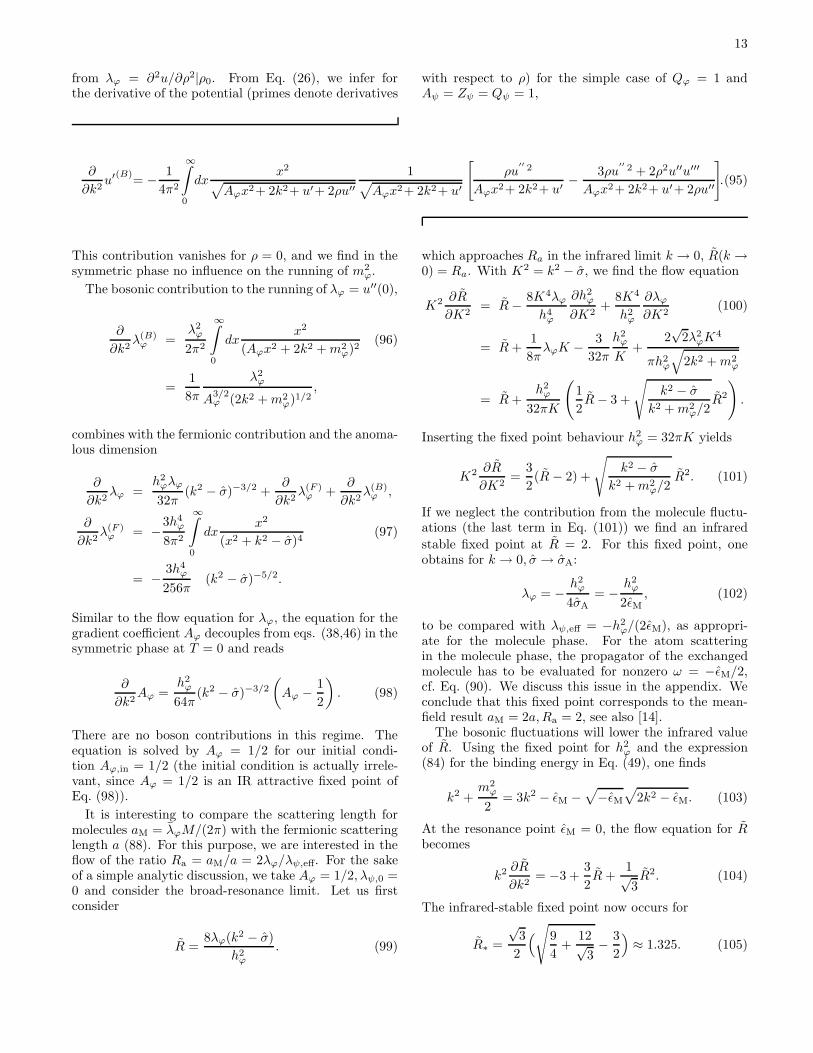
−(hϕ + δhϕ)(

φ∗ψ1ψ2 − φψ∗1ψ

∗2

)]

.

Here, we have rescaled the fields and couplings, to-

gether with the space and time coordinates ~x = k~x,

τ = (k2/2M)τ , withM being the mass of the atoms. Ourunits are ~ = c = kB = 1. We use the Matsubara formal-ism with Euclidean time τ on a torus with a circumfer-ence given by the inverse temperature T−1. The thermo-

dynamic variables are T = 2MT/k2 and σ = 2Mσ/k2,with σ denoting the effective chemical potential.

The model parameters are:

(1) the detuning of the magnetic field B − B0 (withµ = 2µB for 6Li and µ = 1.57µB for 40K)

ν =2M

k2µ(B −B0), (2)

3

(2) the Feshbach or Yukawa coupling hϕ which can beextracted from the properties of the quantum me-chanical two-atom system as the molecular bindingenergy or the scattering cross section,

(3) a point-like interaction for the fermionic atoms pa-

rameterised by λψ. The shifts δν, δλψ and δhφ arecounter terms that are removed by the ultravioletrenormalisation. Details of the rescaling and theformulation can be found in [12, 14].

The scale k (which sets the units) is arbitrary. (A typical

value is k = 1eV.) Under a rescaling of k → k/µ allquantities scale according to their canonical dimension,i.e.,

x = kx→ x/µ, τ = (k2/(2M))τ → τ /µ2,

T → µ2T , σ → µ2σ, ν → µ2ν, hφ → µ1/2hφ,

λψ → λψ/µ, ψ → µ3/2ψ, φ→ µ3/2φ. (3)

We observe that the canonical dimension of time is mi-nus two and therefore the nonrelativistic Lagrangian hasdimension five and not four, as for a relativistic quantumfield theory. The total atom density n defines the Fermimomentum kF,

n =k3F

3π2. (4)

If one associates k with kF all quantities are expressed inunits of the Fermi momentum [12].

From the partition function the effective action Γ ob-

tains by the usual Legendre transform, ϕ = 〈φ〉,

Γ[ϕ] = − lnZ[jφ[ϕ]] +

∫

dx(j∗φϕ+ jφϕ∗). (5)

The order parameter ϕ0 for superfluidity corresponds tothe minimum of Γ for jφ = 0 and obeys the field equation

δΓ

δϕ

∣

∣

∣

ϕ0

= 0. (6)

The effective action generates the 1PI Green’s functionssuch that the propagators and transition amplitudes canbe directly related to the functional derivatives of Γ. Theconstruction above is easily extended to an effective ac-tion that is also a functional of fermionic fields by intro-ducing the appropriate fermionic sources, see below.

III. EXACT FUNCTIONAL FLOW EQUATION

AND TRUNCATION

The variation of Γ with the change of an effective in-frared cutoff k is given by an exact renormalisation groupequation [18, 19, 20, 21]. For the present theory, this ap-proach has been implemented in [14] within a study ofthe phase diagram; see also [26]. For RG studies of thepurely bosonic system, see [27].

For the purpose of the present work, we extend thetruncation used in [14] as well as using a particular ver-sion of the flow equation where the cutoff acts like a shiftin the respective chemical potentials for ψ and ϕ, as alsodone in [28]. To that end, we introduce an infrared-regularised partition function Zk by adding a cutoff termto the action in Eq. (1),

S[ψ, φ] → S[ψ, φ] + ∆Sk[ψ, φ], (7)

where the cutoff term ∆Sk is chosen as

∆Sk[ψ, φ] =

∫

dx(R(F )k ψ†ψ +R

(B)k φ∗φ), (8)

with

R(F )k = Zψ(k)k2 , R

(B)k = 2Zϕ(k)k2,

∂R(F )k

∂k2= QψZψ ,

∂R(B)k

∂k2= 2QϕZϕ,

Qψ,ϕ = 1 − ηψ,ϕ/2 , ηψ,ϕ = −k ∂∂k

lnZψ,ϕ. (9)

The k-dependent wave function renormalisationZψ,ϕ willbe determined below, and we note that k is measured in

units of the fixed scale k. Introducing the effective aver-age action Γk in terms of a modified Legendre transform,

Γk[ψ, ϕ] = − lnZk[jψ , jφ] − ∆Sk[ψ, ϕ]

+

∫

dx(j∗φϕ+ jφϕ∗ + j†ψψ − ψ†jψ),(10)

the exact functional renormalisation group equation (flowequation) can straightforwardly be derived,

∂Γk∂k2

=

∫

dx(

ZψQψ〈ψ†ψ〉c + 2ZϕQϕ〈φ∗φ〉c)

= Tr

− ZψQψ(

Γ(2)k +Rk

)−1

ψ∗ψ

+2ZϕQϕ(

Γ(2)k +Rk

)−1

ϕ∗ϕ

. (11)

Here, we have expressed the propagators of the fermionicand the bosonic fields by the corresponding componentsof the inverse of the matrix of second functional deriva-tives of Γk. The trace Tr contains an integration overx or a corresponding momentum integration as well as a

trace over all internal indices. Both Γk and Γ(2)k are func-

tionals of arbitrary fields ϕ and ψ which are kept fixedfor the k derivative in Eq. (11).

The flow equation (11) is a nonlinear functional differ-ential equation and we can only hope to find approximatesolutions by suitable truncations of the most general form

4

of Γk. In this work, we exploit the ansatz

Γk =

∫

dx[

Zψψ†(

∂τ −Aψ − σ)

ψ

+Zϕϕ∗(

∂τ −Aϕ)

ϕ+ u(ϕ, σ)

−hϕ(

ϕ∗ψ1ψ2 − ϕψ∗1ψ

∗2

)

+λψ2

(ψ†ψ)2]

=

∫

dx[

ψ†(

∂τ −Aψ − σ)

ψ

+ϕ∗(

∂τ −Aϕ)

ϕ+ u(ϕ, σ)

−hϕ(

ϕ∗ψ1ψ2 − ϕψ∗1ψ

∗2

)

+λψ2

(ψ†ψ)2]

, (12)

In the second equation, we have used renormalised fields

ψ = Z1/2ψ ψ, ϕ = Z1/2

ϕ ϕ (13)

and renormalised couplings

hϕ = hϕZ−1ψ Z−1/2

ϕ , λψ = λψZ−2ψ . (14)

The ansatz (12) generalises that of [14] by the four-fermion interaction with coupling λψ . This term is par-ticularly important in the limit of broad Feshbach reso-nances as will be discussed later.

The global symmetry of U(1) phase rotations impliesthat the effective potential u can only depend on ρ =ϕ∗ϕ. If the ground state corresponds to a homogeneousϕ0 the pressure and density can be computed from theproperties of the effective potential

∂u

∂ϕ

∣

∣

∣

ϕ0

= 0 , u0(σ) = u(ϕ0, σ) ,

p = − k5

2Mu0 , n = −k3∂u0

∂σ. (15)

At this point, some comments concerning the wavefunction renormalisations are in order:

(i) Analytic continuation to “real time” and a Fouriertransform to (real) frequency space results in ∂τ →−ω. We define Zψ,ϕ by the coefficient of the term

linear in ω in the full inverse propagator Pψ,ϕ given

by the terms quadratic in ψ or ϕ in Γk. More pre-cisely, we choose in Fourier space

Zϕ = −∂Pϕ∂ω

∣

∣

∣

~q=0,ω=0. (16)

(ii) With this definition of Zψ and Zϕ, the renormalisedfields ψ, ϕ have a unit residuum for the pole in thepropagator for ~q → 0 if the “on shell value” of ωvanishes for ~q = 0.

(iii) We use the same Zψ,ϕ in the definition of the cutoff(9) as in Eq. (12).

(iv) The fields ψ and ϕ describe “microscopic” or “bare”atoms and molecules while the renormalised fieldϕ describes dressed molecules. The wave func-tion renormalisation Zϕ accounts for a descriptionof dressed molecules as a mixing of microscopicmolecules and di-atom states [5, 6, 14].

IV. INITIAL CONDITIONS

Inserting the truncation (12) into the flow equation(11), and taking appropriate functional derivatives, leadsto a coupled set of differential equations for the couplingsZψ, Aψ, Zϕ, Aϕ, hϕ, λψ as well as the effective potentialu(ϕ). The task is to follow the flow of these couplings asthe cutoff scale k is changed. The initial values for largek are taken as

Zϕ = Zψ = 1 , Aϕ =1

2, Aψ = 1,

u = m2ϕρ,

m2ϕ = ν + δν − 2σ. (17)

Here ν is related to the detuning of the magnetic field

ν =2M

k2µ(B −B0) (18)

and we have to fix δν (i.e., the renormalised counterpartof δν in Eq. (1)) such that the Feshbach resonance invacuum occurs for ν = 0. The initial values of λψ and hϕare chosen such that the molecular binding energy andscattering of two atoms in vacuum is correctly described.

A realistic model contains an effective ultraviolet cutoffΛ which is given roughly by the inverse of the range of

the van der Waals force. For k ≪ Λ/k we can take thelimit Λ → ∞ since all momentum integrals are ultravioletfinite. All ultraviolet “divergencies” are already absorbedin the computation of ΓΛ [12, 14]. For 6Li or 40K and

k = 1eV one has Λ/k of order 102 to 103.

V. RUNNING COUPLINGS AND ANOMALOUS

DIMENSIONS

The flow equations for the various couplings and thedensities derived from (11) have a simple interpretationas renormalisation group improved one-loop equations[18] with full propagators and dressed vertices, but areexact. The renormalisation constants Zϕ, Zψ are relatedto the dependence of the unrenormalised inverse propa-

gators (for ϕ and ψ) on the (Minkowski) frequency, i.e.,the coefficients of the terms linear in ω(= − ∂/∂τ) inΓ(2). The second derivative of Eq. (11) yields exact flowequations for the inverse propagator [18, 19, 20, 21] andtherefore for Zϕ, Zψ. We define

ηψ,ϕ = ηψ,ϕ/2k2 = −∂ lnZψ,ϕ/∂k

2 (19)

5

and obtain in our approximation

ηϕ = −h2ϕQψ

2

∂

∂k2I(F )ϕ + η(B)

ϕ . (20)

Here the fermion loop integral

I(F )ϕ =

1

8T 2

∫

d3q

(2π)3γγ−3

ϕ [tanh γϕ − γϕ cosh−2 γϕ] (21)

involves

γϕ =1

2T

√

(Aψ q2 + k2 − σ)2 + h2ϕρ,

γ =1

2T(Aψ q

2 + k2 − σ). (22)

In our truncation, the boson fluctuations contribute to

ηϕ only in the superfluid phase (η(B)ϕ (ρ = 0) = 0) [14].

Crucial quantities for the investigation of this problemare the running of the Yukawa coupling hϕ,

∂

∂k2h2ϕ = (ηϕ + 2ηψ)h2

ϕ + 2h2ϕλψQψJ

(F )ϕ , (23)

with

J (F )ϕ =

1

16T 2

∫

d3q

(2π)3γγ−5

ϕ [(3γ2 − γ2ϕ) tanh γϕ

+γϕ cosh−2 γϕ(

− 3γ2 + γ2ϕ

+2γϕ(γ2ϕ − γ2) tanh γϕ

)

], (24)

and the point-like four-fermion interaction

∂

∂k2λψ = 2ηψλψ + λ2

ψQψ(I(F )ϕ + Iλψ ), (25)

Iλψ = − 1

4T 2

∫

d3q

(2π)3γγ−1

ϕ tanh γϕ cosh−2 γϕ.

For both quantities, we neglect the contribution fromthe molecule fluctuations. This is a valid approximationfor the parameter ranges for which we give quantitativeresults. In other ranges, the molecule fluctuations givemore dominant contributions, see [14] and the discussion

below. For ρ = 0, we note J(F )ϕ = I

(F )ϕ .

VI. FLOW OF THE EFFECTIVE POTENTIAL

Keeping now ρ (and not ρ) fixed, the flow of the effec-tive potential obeys,

∂

∂k2u(ρ) = ζF (ρ) + ζB(ρ) + ηϕρu

′(ρ), (26)

with

ζF (ρ) = −Qψ∫

d3q

(2π)3

( γ

γϕtanh γϕ − 1

)

,

ζB(ρ) = Qϕ

∫

d3q

(2π)3

(α+ κ2

αϕcothαϕ − 1

)

. (27)

Here, we define

αϕ =1

2T

[

(Aϕq2 + 2k2 + u′)

(Aϕq2 + 2k2 + u′ + 2ρu′′)

]1/2

,

α =Aϕq

2 + 2k2 + u′

2T,

κ2 =ρu′′

2T, κ3 =

ρ2u′′′

2T, (28)

and the primes denote derivatives with respect to ρ. Thecontribution of the boson fluctuations is computed in abasis where the complex field ϕ is written in terms of tworeal fields with inverse bosonic propagator

Pϕ =

(

Aϕq2 + 2k2 + u′ + 2ρu′′ −2πnT

2πnT Aϕq2 + 2k2 + u′

)

.(29)

Then, Eq. (11) evaluated for constant ϕ becomes

ζB(ρ) = TQϕtr∑

n

∫

d3q

(2π)3

(

P−1ϕ − 1

1

Aϕq2 + 2k2

)

,(30)

in accordance with [29]. The subtraction of a ρ-independent part renders the momentum integral ultra-violet finite. For extensive numerical studies one wouldrather rely on cutoff choices as in [14] which do not re-quire any ultraviolet subtraction, and minimise the nu-merical costs. However, this is of no importance for thequantities computed in this paper – the dependence ofAϕon σ and T is negligible, and simplicity of the approachis the more important property.

In the symmetric phase (SYM), one has ρ0 = 0, u′(0) =m2ϕ, u

′′(0) = λϕ, whereas in the presence of sponta-neous symmetry breaking (SSB) we use ρ0 > 0, u′(ρ0) =0, u′′(ρ0) = λϕ. Eq. (26) yields in the symmetric phase

∂

∂k2m2ϕ = h2

ϕQψI(F )ϕ (ρ = 0) −QϕI

(B)ϕ (ρ = 0) + ηϕm

2ϕ.

(31)Here, we define the boson loop integral

I(B)ϕ =

λϕ

2T

∫

d3q

(2π)3(32)

×

[

(2α+ κ2)u′′ + αρu′′′

] α+ κ2

α2ϕ sinh2 αϕ

+[

κ2(κ2 − α) − ακ3

]

u′′cothαϕα3ϕ

,

such that

I(B)ϕ (ρ = 0) =

λϕ

T

∫

d3q

(2π)3sinh−2 α. (33)

The flow starts with a positive m2ϕ for large k and is

therefore in the symmetric regime. As k decreases, m2ϕ

6

decreases according to Eq. (31), with ηϕ being positive.At high temperature, m2

ϕ stays positive for all k and thesystem is in the symmetric phase and ungapped for allmomenta. At temperatures below a pseudo-critical tem-perature Tp, m

2ϕ hits zero at some critical kc. For k < kc,

the flow first continues in the broken-symmetry regimewith nonzero ρ0. Whereas fermionic fluctuations tendto increase ρ0, molecule fluctuations cause its depletion.For temperatures inbetween the critical temperature andthe pseudo-critical temperature, Tc < T < Tp, moleculefluctuations eventually win out over the fermionic fluc-tuations and ρ0 vanishes again at smaller k; here, thesystem is in the symmetric phase. Identifying the k de-pendence of the fermionic 2-point function with the mo-mentum dependence, the non-zero value of ρ0 for finitek can be associated with a pseudo-gap [30]. Below thecritical temperature Tc, ρ0 stays finite for k → 0, cor-responding to the superfluid phase with a truly gappedspectrum.

Molecule fluctuations are particularly important dur-ing those stages of the flow where ρ0 is non-zero, i.e.,for k < kc and below the pseudo-critical temperature Tp,

see [14]. In this work, we focus on the properties of theflow in the symmetric regime, where ρ0 = 0 for all val-ues of k under consideration. We still include moleculefluctuations for all quantities that are associated withthe effective potential u(ρ), in particular the moleculedensity and the molecule-molecule scattering length, seeSects. IX and XI below. But molecule fluctuations areneglected for the other running couplings which are dom-inated by fermion fluctuations in the parameter rangesconsidered here.

VII. SOLVING THE FLOW EQUATION FOR

ZERO TEMPERATURE

Let us first concentrate on T = 0 and k2 − σ > 0. Wedefine

K2 = k2 − σ (34)

and employ ∂/∂k2 = ∂/∂K2. Then the flow equation foru takes the explicit form

∂

∂K2u(ρ) = ηϕρu

′ − 1

2π2

∞∫

0

dxx2

Qψ

Aψx2 +K2

√

(Aψx2 +K2)2 + h2ϕρ

− 1

(35)

−Qϕ(

Aϕx2 + 2k2 + u′ + ρu′′

√

(Aϕx2 + 2k2 + u′)(Aϕx2 + 2k2 + u′ + 2ρu′′)− 1

)

.

For ρ = 0, T = 0, σ < 0, one also finds

I(F )ϕ =

1

16πA

−3/2ψ K−1 , Iλψ = 0, (36)

and, in our approximation, the contributions of the bosonloops to ηϕ, ∂h

2ϕ/∂k

2 and ∂λψ/∂k2 vanish for m2

ϕ > 0.

At T = 0 and σ < 0, we can use Zψ = Aψ = 1, Qψ = 1.This is an exact result [7] as long as all propagators inthe relevant diagrams have simple poles in the imaginaryq0 plane. With

ηϕ =h2ϕ

64πK−3, (37)

we find the coupled system of flow equations for the sym-metric phase

∂h2ϕ

∂K=

h4ϕ

32πK−2 +

h2ϕλψ

4π,

∂λψ∂K

=λ2ψ

8π. (38)

The solution of the last equation,

λ−1ψ = λ−1

ψ,in +1

8π(Kin −K)

= λ−1ψ,0 −

K

8π, (39)

renders λψ almost independent of K if K ≪ Kin +8π/λψ,in. Here, we assume implicitly that λψ,in is not toomuch negative such that λψ remains finite in the wholek range of interest. For positive λψ, the self-consistencyof the flow requires an upper bound λψ,0/(8π) < 1/Kin.

In contrast, for λψ = 0 the solution for h2ϕ,

h−2ϕ = h−2

ϕ,in +1

32π

(

K−1 −K−1in

)

, (40)

is dominated by small K.For λψ 6= 0, the flow of hϕ is modified, however, with-

out changing the characteristic behaviour for K → 0.Indeed, in the limit K → 0 the term ∼ λψ becomes sub-dominant for the evolution of h2

ϕ. The flow for the ratio

h2ϕ/K reaches a fixed point 32π. We can explicitely solve

the system (38) by consecutive integrations. One obtains

7

for h2ϕ = Zϕh

2ϕ

h2ϕ = h2

ϕ,in exp

− 1

4π

Kin∫

K

dxλψ(x)

= h2ϕ,in (1 − c0Kin)

2(1 − c0K)

−2

= h2ϕ,0

(

1 − c0K)−2

. (41)

This yields for the wave function renormalisation

Zϕ = 1 +1

32π

K−1

∫

K−1

in

d(x−1)h2ϕ(x−1)

= 1 +h2ϕ,0

32π

[

1

K

(

1 − c01/K − c0

)

(42)

+2c0 ln

(

1

K− c0

)

− (K → Kin)

]

,

with

c0 =λψ,08π

,1

K> c0. (43)

For K → 0, the ratio h2ϕ/h

2ϕ,in obviously reaches a con-

stant which depends on λψ,in,Kin, whereas Zϕ diverges

≈ h2ϕ,0/(32πK), as is consistent with the fixed-point be-

haviour h2ϕ ≈ 32π. Neglecting c0 (as always appropriate

for small enough K) and assuming a broad resonance

h2ϕ,0 ≫ 32π, we arrive at the simple relation

Zϕ ≈h2ϕ,0

32πK. (44)

In this limit, the factor Qϕ appearing in the flow equa-tions is given by

Qϕ = 1 − k2

2(k2 − σ)(45)

and approaches 1/2 for k2 ≫ −σ. We note that in this

range the bosonic cutoff function R(B)k = 2Zϕk

2 is effec-tively linear in k and not quadratic.

We finally investigate the flow equation for m2ϕ in the

symmetric phase. As we will see below, the boson loops(the last contribution in Eq. (35)) vanish in our trunca-tion. This yields

∂m2ϕ

∂K=h2ϕ

8π+h2ϕm

2ϕ

32πK−2, (46)

or

∂m2ϕ

∂K=

∂

∂K(Zϕm

2ϕ) =

h2ϕ

8π. (47)

The solution reads

m2ϕ =

2Mµ(B −B0)

k2− 2σ + δν (48)

−h2ϕ,in(1 − c0Kin)

2

8πc0

(

1

1 − c0Kin− 1

1 − c0K

)

.

The counterterm δν is determined from the conditionm2ϕ(B = B0, σ = 0, k = 0) = 0, such that (up to minor

corrections)

m2ϕ =

2Mµ(B −B0)

k2+h2ϕ,0

8π

K

1 − c0K− 2σ. (49)

In particular, for k = 0 and σ < 0 one has K =√−σ,

and Eq. (49) yields the expression for m2ϕ in the presence

of all fluctuations

m2ϕ =

2Mµ(B −B0)

k2+

h2ϕ,0

√−σ

8π − λψ,0√−σ

− 2σ. (50)

At this point, we have the explicit solution of the flowequation for T = 0. In the present simple truncation, weexpect that the description of the system is qualitativelycorrect. Higher quantitative precision will require a moreextended truncation; however, this is not the main em-phasis of the present work which rather concentrates onthe structural properties related to the fixed points.

VIII. FLOW EQUATIONS AND FIXED POINTS

The explicit solution of the preceding section is indeedvery useful for verifying and explicitly demonstrating thegeneral fixed-point properties. The following features ofthe flow equations hold in a much wider context of differ-ent microscopic actions and different cutoffs. The overallpattern of the flow is governed by the existence of fixedpoints. Some of these fixed points may correspond toparticularly simple situations, being less relevant for thephysics under discussion. By contrast, the stability orinstabilities of small deviations from the various fixedpoints are much more important, as they determine thetopology of the flow in the space of coupling constants, asdemonstrated in Fig. 1. If the system is in the vicinity ofany of the different fixed points the number of effectivecouplings needed for a description of the macrophysics(beyond T ) corresponds to the number of relevant direc-tions.

A particularity of our system concerns a certain redun-dancy in the description: a pointlike interaction can bedescribed either by the four-fermion coupling λψ or bya limiting behaviour of the scalar exchange. Indeed, for

h2ϕ,in → ∞ and fixed h2

ϕ,in/m2ϕ,in the molecule exchange

interaction becomes effectively point-like. Therefore, wemay define an effective point-like coupling

λψ,eff = λψ −h2ϕ

m2ϕ

= λψ −h2ϕ

m2ϕ

(51)

which describes the interaction in the zero-momentumlimit. Combining the flow equations (38), (46) for

λψ, h2ϕ, m

2ϕ, one obtains

∂λψ,eff∂K

=λ2ψ,eff

8π. (52)

8

This is the same flow equation as for λψ (38).Next, we may consider the renormalised couplings in

units of kk instead of k. This will reveal the relevant fixedpoints for the flow more clearly. We define, according tothe scaling dimensions of Eq. (3),

λψ = λψk , λψ,eff = λψ,effk,

hϕ =hϕ√k, m2

ϕ = m2ϕ/k

2,

t = ln k/kin, (53)

and obtain the dimensionless flow equations

∂tλψ = λψ +λ2ψy

8π, ∂tλψ,eff = λψ,eff +

λ2ψ,effy

8π,

∂th2ϕ = −h2

ϕ +h4ϕy

3

32π+h2ϕλψy

4π,

∂tm2ϕ = −2m2

ϕ +h2ϕy

8π+h2ϕm

2ϕy

3

32π, (54)

with

y =

(

k2

k2 − σ

)1/2

. (55)

Let us first consider σ = 0, or, more generally, k2 ≫−σ, such that y = 1. In this case, we observe two fixedpoints for λψ , either λψ = 0 or λψ = −8π. The corre-

sponding fixed points for h2ϕ 6= 0 are

(A) : λψ = 0 , h2ϕ = 32π , m2

ϕ = 4

(B) : λψ = −8π , h2ϕ = 96π , m2

ϕ = −12.(56)

(We will discuss later the fixed points with h2ϕ =

0 , m2ϕ = 0.) The fixed point (A) is infrared stable

for λψ and h2ϕ – both couplings run towards their fixed-

point values as k is lowered, as is visualised in Fig. 1. Incontrast, m2

ϕ is infrared unstable – the detuning B −B0

corresponds to a relevant perturbation of the fixed point.With h2

ϕ at the fixed-point value, m2ϕ deviates from its

fixed point with an anomalous dimension

m2ϕ = 4 + δm2

in

kin

k. (57)

Comparing this with the explicit solution (49) for λψ =

0, σ = 0, hϕ = hϕ,0, namely

m2ϕ =

h2ϕ

8π+

2Mµ(B −B0)

Zϕk2k2(58)

with Eq. (42),

Zϕ ≈h2ϕ,0

32πk, (59)

0 1 2 3

−1.2

−1

−0.8

−0.6

−0.4

−0.2

0

0.2

(A)(C)

(B)

(D)h2

ϕ

32π

λψ8π

FIG. 1: Location of fixed points (A)-(D) projected onto

the plane which is spanned by the couplings λψ/(8π) and

h2ϕ/(32π). The arrows characterise the flow of the couplings

towards the infrared.

we can identify

δm2ϕ =

64πMµ(B −B0)

k2h2ϕ,0kin

. (60)

We conclude that broad Feshbach resonances (largeenough Yukawa couplings) can be characterised by the

fixed point (A), with hϕ and λψ being irrelevant andm2ϕ ∼ B −B0 the relevant coupling.

For the second fixed point (B), λψ becomes a relevant

parameter. For h2ϕ, the fixed point (56) with h2

ϕ = 96π

remains infrared attractive, but the fixed point for m2ϕ

occurs for negative m2ϕ where our computation in the

symmetric phase is no longer valid.Finally, we turn to the fixed points with h2

ϕ = 0. In

this case, h2ϕ is always a relevant coupling and increases

as k is lowered. The fixed point

(C) : λψ = 0 , h2ϕ = 0 , m2

ϕ = 0 (61)

is infrared attractive for λψ. For this case of a narrowFeshbach resonance, the crossover problem can be solvedexactly [6], and perturbation theory around the exact so-

lution becomes valid for small h2ϕ, λψ. The coupling m2

ϕ

is a second relevant parameter around this fixed point.

As one increases h2ϕ,0, a crossover to the fixed point (A)

occurs [6]. The “narrow-resonance fixed point” (C) de-scribes the limit of a combined model with free fermionsand free bosons, sharing the same chemical potential.We emphasise that, for small hϕ, the equivalent purelyfermionic description typically has a nonlocal interaction.

For the fourth fixed point of our system,

(D) : λψ = −8π , h2ϕ = 0 , m2

ϕ = 0, (62)

all three parameters are relevant. This point corre-sponds again to strong attractive interactions between

9

the fermionic atoms. The flow away from this fixed pointfor non-vanishing h2

ϕ/m2ϕ can be characterised by the flow

of the ratio (y = 1)

∂t

(

h2ϕ

m2ϕ

)

=

(

1 +λψ4π

)

h2ϕ

m2ϕ

− 1

8π

(

h2ϕ

m2ϕ

)2

(63)

which does not have a fixed point for positive h2ϕ, m

2ϕ.

Formally, the flow runs for negative m2ϕ towards the fixed

point (B) with h2ϕ/m

2ϕ = −8π. Actually, it may be possi-

ble to consider λψ as a redundant parameter using partialbosonisation and rebosonisation during the flow [31], see

also [21]. Then, the fixed points with λψ = −8π mayagain be associated with broad Feshbach resonances. Weshow the four fixed points A, B, C, D and the infraredflow of the couplings h2

ϕ and λϕ in Fig. 1We should emphasise that the inclusion of the omitted

contributions from boson fluctuations to the flow of λψcould result in corrections (y = 1),

∂tλψ = λψ +λ2ψ

8π+

c132π

h4ϕ +

c232π

λψh2ϕ, (64)

such that the flow of λψ remains no longer independent of

h2ϕ. This will change the precise location of fixed points

(A) and (B). We expect that the qualitative characteris-tics of the fixed point (A) remain unchanged, whereas thefate of the fixed point (B) is less clear. We may consider

the flow of the ratio λψ/h2ϕ,

∂t

(

λψ

h2ϕ

)

= 2

(

λψ

h2ϕ

)

(65)

+h2ϕ

32π

c1 + (c2 − 1)λψ

h2ϕ

− 4

(

λψ

h2φ

)2

.

For any possible fixed point, one has

h2φ = 32π

(

1 − λψ4π

)

⇒h2φ

32π=

(

1 + 8λψ

h2φ

)−1

, (66)

and therefore obtains the fixed point condition for Q =λψ/h

2φ as

c1 + (c2 + 1)Q+ 12Q2 = 0. (67)

In general, this quadratic equation has two distinct solu-tions, where the larger value of Q is infrared stable andcorresponds to (A), while the smaller value of Q is un-stable and corresponds to (B).

We finally include the effect of a nonzero negativechemical potential σ. As soon as k2 becomes smallerthan σ, the parameter y (55) rapidly goes to zero. Then,only the first term in the flow equations (54) matters. In

this range of k, the couplings λφ, h2φ, m

2ϕ remain constant.

A negative σ acts as an additional infrared cutoff, such

15 12.5 10 7.5 5 2.5 0

200

400

600

800

1000

k2

h2ϕ

(b)

10000 8000 6000 4000 2000 00

500

1000

1500

2000

2500

k2

h2ϕ

(a)

FIG. 2: Sensitivity of the renormalised Yukawa coupling hϕ to

the two-body Yukawa coupling hϕ,0 at fixed λψ,0: (a) UV and

(b) IR flow of the Yukawa coupling. We use k = kF = 1eV,

abgk = λψ,0/(8π) = 0.38 as appropriate for 6Li and T = 0.5,c−1 = 1. The different curves correspond to the two-bodyvalue of the Yukawa coupling h2

ϕ,0 = 3.72·(103, 104, 105) (fromtop to bottom), where the last value corresponds to 6Li whilethe first one is comparable to that of 40K. Universality withrespect to the value of the two-body Yukawa coupling is verystrong even for a comparatively large (fixed) λψ.

that the flow is effectively stopped for k2 < −σ. This

yields a simple rough picture: the couplings λψ , h2ϕ, m

2ϕ

flow according to Eq. (54) for k2 > −σ until the flowstops when k2 < −σ.

The fixed points are relevant not only for T = 0. Wedemonstrate the influence of the fixed point (A) on the

flow of the Yukawa coupling for T = 0.5 and c = 1 inFigs. 2, 3. In Fig. 2, we observe that the renormalisedYukawa coupling hϕ at small k becomes almost indepen-

dent of its initial value h2ϕ,0 if the latter is large. Figure 3

demonstrates the influence of the background scatteringlength abg for a fixed value of a, again for T = 0.5 andc = 1.

10

15 12.5 10 7.5 5 2.5 0

200

400

600

800

1000

k2

h2ϕ

(b)

10000 8000 6000 4000 2000 00

2500

5000

7500

10000

12500

15000

k2

h2ϕ

(a)

FIG. 3: Sensitivity of the renormalised Yukawa coupling hϕto the two-body background scattering length λψ for fixed

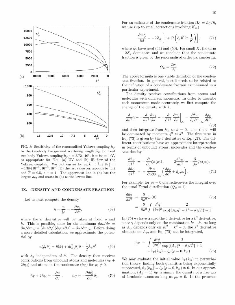
two-body Yukawa coupling hϕ,0 = 3.72 · 105, k = kF = 1eV,as appropriate for 6Li: (a) UV and (b) IR flow of the

Yukawa coupling. We plot curves for abgk = λψ/(8π) =−0.38·(10−3 , 10−2, 10−1, 1) (the last value corresponds to 6Li)

and T = 0.5, c−1 = 1. The uppermost line in (b) has thelargest abg and starts in (a) as the lowest line.

IX. DENSITY AND CONDENSATE FRACTION

Let us next compute the density

n =n

k3= −∂u0

∂σ, (68)

where the σ derivative will be taken at fixed ρ andk. This is possible, since for the minimum du0/dσ =∂u/∂σ|ρ0 + (∂u/∂ϕ)(∂ϕ0/∂σ) = ∂u/∂σ|ρ0 . Before doinga more detailed calculation, we approximate the poten-tial by

u(ρ, σ) = u(σ) + m2ϕ(σ)ρ+

1

2λϕρ

2 (69)

with λϕ independent of σ. The density then receivescontributions from unbound atoms and molecules (nF +2nM) and atoms in the condensate (nC) for ρ0 6= 0,

nF + 2nM = −∂u∂σ

, nC = −∂m2

ϕ

∂σρ0. (70)

For an estimate of the condensate fraction ΩC = nC/n,we use (up to small corrections involving Kin)

∂m2ϕ

∂σ= −2Zϕ

[

1 + O(

c0K ln1

K

)]

, (71)

where we have used (44) and (50). For small K, the term−2Zϕ dominates and we conclude that the condensatefraction is given by the renormalised order parameter ρ0,

ΩC =2ρ0

n. (72)

The above formula is one viable definition of the conden-sate fraction. In general, it still needs to be related tothe definition of a condensate fraction as measured in aparticular experiment.

The density receives contributions from atoms andmolecules with different momenta. In order to describeeach momentum mode accurately, we first compute thechange of the density with k,

d

dk2n = − d

dk2

∂u0

∂σ= − ∂

∂k2

∂u0

∂σ

∣

∣

∣

∣

ρ0

− ∂2u

∂ρ∂σ

∣

∣

∣

∣

ρ0

dρ0

dk2,

(73)and then integrate from kin to k = 0. The r.h.s. willbe dominated by momenta q2 ≈ k2. The first term inEq. (73) is given by the σ derivative of Eq. (27). The dif-ferent contributions have an approximate interpretationin terms of unbound atoms, molecules and the conden-sate density

dnF

dk2= − ∂

∂σζF (ρ0) , 2

dnM

dk2= − ∂

∂σζB(ρ0),

dnC

dk2= − ∂2u

∂ρ∂σ

∣

∣

∣

∣

ρ0

(

dρ0

dk2+ ηϕρ0

)

. (74)

For example, for ρ0 = 0 one rediscovers the integral overthe usual Fermi distribution (Qψ = 1)

dnF

dk2=

∂

∂k2ζF (0) (75)

=∂

∂k2

∫

d3q

(2π)22

exp(Aψ q2 + k2 − σ)/T + 1.

In (75) we have traded the σ derivative for a k2 derivative,since γ depends only on the combination k2− σ. As longas Aψ depends only on K2 = k2 − σ, the k2 derivativealso acts on Aψ, and Eq. (75) can be integrated,

nF =

∫

d3q

(2π)32

exp(Aψ q2 − σ)/T + 1

+nF(kin) − ζF (ρ = 0, kin). (76)

We may evaluate the initial value nF(kin) in perturba-tion theory, finding both quantities being exponentiallysuppressed, nF(kin) = ζF (ρ = 0, kin) ≈ 0. In our approx-imation, (Aψ = 1) nF is simply the density of a free gasof fermionic atoms as long as ρ0 = 0. In the presence

11

of a condensate (ρ0 6= 0), we typically find a flow whereρ0(k) = 0 for k > kc, such that the flow of nF(k) remainsunchanged in this range. On the other hand, the contri-bution from modes with q2 < k2

c will be suppressed bythe presence of a gap ∆ = hϕ

√ρ0 in the propagator. We

emphasise that the derivative ∂/∂k2 in Eq. (75) does notact on ρ0, since the σ derivative in Eq. (74) is taken atfixed ρ. Therefore the flow for nF has to be integratednumerically if ρ0 6= 0.

For the computation of the molecule density nM, weneed ∂ζB/∂σ. Let us concentrate on ρ0 = 0 and neglectthe σ dependence of Qϕ and Aϕ, such that

∂ζB∂σ

= 2Qϕ

∫

d3q

(2π)3∂

∂σ(

exp

(Aϕq2 + 2k2 +m2

ϕ)/T

− 1)−1

= Qϕ∂m2

ϕ

∂σ

∂

∂k2

∫

d3q

(2π)3(77)

×(

exp(Aϕq2 + 2k2 +m2ϕ)/T − 1

)−1

.

We next use Eq. (71)

dm2ϕ

dσ≈ −2 −m2

ϕ

∂

∂σlnZϕ. (78)

The second term can be approximated for small K by

m2ϕ

∂

∂σlnZϕ ≈

m2ϕ

2(k2 − σ). (79)

If we neglect this term and set Qϕ = 1 we find the intu-itive formula

nM =

∫

d3q

(2π)31

exp

(Aϕq2 +m2ϕ)/T

− 1. (80)

This is the expression for a free boson gas. What is cru-cial, however, is the appearance of the inverse propagatorfor the renormalised bosonic field ϕ instead of the micro-scopic or “bare” molecule field ϕ. The propagators forthe renormalised and bare fields are related by a rela-tive factor Zϕ, such that we find for the density of baremolecules

nM,bare = Z−1ϕ nM. (81)

As a consequence, one may have a substantial moleculefraction 2nM/n even if the density of bare molecules istiny. These features reproduce the results from a solu-tion of the Schwinger-Dyson equations [6] where a baremolecule density in accordance with the experimental re-sult of Partridge et al. [32] has been found. It is one ofthe important advantages of our functional renormalisa-tion group approach that it accounts for the distinctionbetween renormalised and bare molecules in a very directand straightforward manner [14]. Within a Hamiltonianformulation, this issue is related to the mixing between

open-channel and closed-channel atoms, and its correcttreatment is crucial for a quantitatively reliable descrip-tion of the crossover. We emphasise that the renor-malised molecule field plays an important role even onthe BCS side of the crossover. The composite bosons arecrucial effective degrees freedom, even though the micro-scopic theory can be very well approximated by a point-like interaction between fermionic atoms without any ref-erence to molecules. On the BCS side, the renormalisedfield ϕ describes Cooper pairs. Nevertheless, one neverneeds these physical interpretations explicitly, since thedensity only involves the σ dependence of the potentialat its minimum, which is a well-defined quantity.

We finally turn to the condensate density. If we canapproximate the σ dependence of (u−u) by a term −2σρ,as suggested by Eq. (78), we infer

dnC

dk2= 2

dρ0

dk2+ 2ηϕρ0 = 2Zϕ

d

dk2

ρ0

Zϕ. (82)

(This approximation needs to hold only in the range ofk where ρ0 differs from zero.) The dominant flow of nC

typically arises from a region where the k dependenceof Zϕ is already sub-leading, resulting in nC ≈ 2ρ0, asfound above. In practice, all these various approxima-tions of our analytical discussion need not to be made,since it is sufficient to follow the flow of n(k) numerically,starting from an initial value n(kin) ≈ 0 and extractingthe physical density for k = 0.

X. VACUUM AND TWO-ATOM SCATTERING

It is one of the advantages of our method that itcan access simultaneously the many-body physics of agas in thermal equilibrium and the two-body physics ofatom scattering and molecular binding. Indeed, the two-body physics describes excitations above the vacuum. Inturn, the vacuum and the properties of its excitationsobtain in our formalism simply by taking the limit ofvanishing density and temperature. (More precisely, the

limit should be taken such that the ratio T /n2/3 is largeenough that no condensate occurs.) The scattering crosssection between two atoms can then be directly inferredfrom the Yukawa coupling and the propagator of themolecule field in the vacuum.

For T = 0, the condition of zero density requires σ ≤ 0in order to ensure nF = 0, cf. Eq. (76). On the otherhand, we infer from Eq. (80) that m2

ϕ ≥ 0 is needed fornM = 0, whereas a vanishing condensate density requiresρ0 = 0. The vacuum is the state that is reached as densityand temperature approach zero from above. It thereforecorresponds to the boundary of the region where σ ≤0,m2

ϕ ≥ 0. There are two branches of vacuum states(for a more detailed discussion, see [17]). The first has anegative σ = σA < 0 andm2

ϕ = 0. In this case, the single-atom excitations have a gap −σA > 0 which corresponds

12

to half the binding energy of the stable molecules,

ǫM = k2σA/M , ǫM = 2σA. (83)

We identify this state with the “molecule phase” wherestable molecules exist in the vacuum. This phase is re-alized for B < B0, with ǫM or σA being a function of Bthat vanishes for B → B0. The other branch correspondsto σ = 0,m2

ϕ > 0. This “atom phase” of the vacuum is

realized for B > B0, with m2ϕ a function of B vanishing

for B → B0. In the atom phase the “binding energy”

ǫM = k2m2ϕ/(2M) is positive and the “molecules” corre-

spond to unstable resonances. We observe a continuousphase transition between the molecule and atom phase[6, 14] for m2

ϕ = 0, σ = 0, corresponding to the locationof the Feshbach resonance at B = B0. This fixes δν inthe initial value of m2

ϕ (18) by the requirement that for

ν = 0 the mass term m2ϕ(σ) vanishes precisely for σ = 0

if T = 0.The vacuum state can be used to fix the parameters of

our model by direct comparison to experimentally mea-sured binding energies and cross sections. Let us firstconsider the molecular binding energy ǫM(B) that canbe computed from Eq. (50) by requiring m2

ϕ = 0, i.e.,

ǫM(B) =σA(B)k2

M(84)

= µ(B −B0)

+kh2

ϕ,0

16π√M

√

|ǫM|(

1 − λψ,0√

M |ǫM|8πk

)−1

.

In the vicinity of the Feshbach resonance (small |ǫM|) thebinding energy depends quadratically on B

ǫM = − (16π)2Mµ2(B0 −B)2

k2h4ϕ,0

. (85)

Using

a0 =λψ,0

8πk, h2

ϕ,0 =kh2

ϕ,0

4M2,

a = −h2ϕ,0M

4π[

µ(B −B0) − ǫM

] + a0 (86)

Eq. (84) reads

√

M |ǫM| =1

a. (87)

The scattering length for the fermionic atoms is deter-mined by the total cross section in the zero-momentumlimit, σ = 4πa2, such that

a =M

4πλψ,eff =

λψ,eff

8πk. (88)

More details are described in the appendix. For the atomphase (ǫM > 0), one has [6]

λψ,eff = λψ,0 −h2ϕ,0

m2ϕ(σ = 0)

= λψ,0 + λψ,R. (89)

For the molecule phase, the effective interaction dependson the energy ω of the exchanged molecule

λψ,R(ω = 0, ~p = 0) = −h2ϕ(σA)

2Zϕ(σA)σA,

λψ,R(ω = −2σA, ~p = 0) = −h2ϕ(σA)

4Zϕ(σA)σA. (90)

We find for the atom phase

a = a0 −h2ϕ,0M

4πµ(B −B0)= a0 + ares, (91)

which agrees with a (86) for ǫM = 0. Eq. (87) thereforerelates the binding energy in the molecule phase to thescattering length in the atom phase.

The value of hϕ,0 can now be extracted from theresonant part, ares, whereas λψ,0 follows from the B-independent “background scattering length” a0 = abg

which has been measured as a(Li)bg = −1420aB , a

(K)bg =

174aB (aB the Bohr radius), or, expressed in units

~ = c = kB = 1 (aB = 2.6817 · 10−4eV−1), a(Li)bg =

−0.38eV−1 , a(K)bg = 4.67 · 10−2eV−1. For k = 1eV cor-

responding to a density n = 4.4 · 1012cm−3, we find thedimensionless expressions for 6Li and 40K:

h2(Li)ϕ,0 = 3.72 · 105 , h

2(K)ϕ,0 = 6.1 · 103, (92)

λ(Li)ψ,0 = −9.55 , λ

(K)ψ,0 = 1.17.

From these values, one can compute the initial valuesλψ,in, h

2ϕ,in. For 6Li, we use the values

kin = 103, h2(Li)ϕ,in = 2.56, λ

(Li)ψ,in = −2.51 · 10−2, (93)

whereas for 40K we take

kin =√

300, h2(K)ϕ,in = 1.67 · 105, λ

(K)ψ,in = 6.14. (94)

For 40K, we observe large values of h2ϕ,in and λψ,in. Sim-

ilar values for 6Li are observed in the corresponding K

range, e.g. h2ϕ,in(K

2 = 300) = 6490, λ(Li)ψ (K2 = 300) =

2024. The broad Feshbach resonances indeed describestrongly coupled systems. In our approximation, the so-lutions of the flow equations for h2

ϕ, λψ and Zϕ do not

depend on m2ϕ provided m2

ϕ remains positive during theflow.

XI. SCATTERING LENGTH FOR MOLECULES

So far, we have only discussed the contributions of themolecule fluctuations to ∂u/∂σ in order to extract themolecule density nM. In this section, we discuss theirinfluence on the effective potential for T = 0 more sys-tematically. In particular, we will extract the scatter-ing length for molecule-molecule scattering in vacuum

13

from λϕ = ∂2u/∂ρ2|ρ0. From Eq. (26), we infer forthe derivative of the potential (primes denote derivatives

with respect to ρ) for the simple case of Qϕ = 1 andAψ = Zψ = Qψ = 1,

∂

∂k2u′

(B)= − 1

4π2

∞∫

0

dxx2

√

Aϕx2+ 2k2+ u′+ 2ρu′′1

√

Aϕx2+ 2k2+ u′

[

ρu′′ 2

Aϕx2+ 2k2+ u′− 3ρu

′′ 2 + 2ρ2u′′u′′′

Aϕx2+ 2k2+ u′+ 2ρu′′

]

.(95)

This contribution vanishes for ρ = 0, and we find in thesymmetric phase no influence on the running of m2

ϕ.

The bosonic contribution to the running of λϕ = u′′(0),

∂

∂k2λ(B)ϕ =

λ2ϕ

2π2

∞∫

0

dxx2

(Aϕx2 + 2k2 +m2ϕ)2

(96)

=1

8π

λ2ϕ

A3/2ϕ (2k2 +m2

ϕ)1/2,

combines with the fermionic contribution and the anoma-lous dimension

∂

∂k2λϕ =

h2ϕλϕ

32π(k2 − σ)−3/2 +

∂

∂k2λ(F )ϕ +

∂

∂k2λ(B)ϕ ,

∂

∂k2λ(F )ϕ = −

3h4ϕ

8π2

∞∫

0

dxx2

(x2 + k2 − σ)4(97)

= −3h4

ϕ

256π(k2 − σ)−5/2.

Similar to the flow equation for λϕ, the equation for thegradient coefficient Aϕ decouples from eqs. (38,46) in thesymmetric phase at T = 0 and reads

∂

∂k2Aϕ =

h2ϕ

64π(k2 − σ)−3/2

(

Aϕ − 1

2

)

. (98)

There are no boson contributions in this regime. Theequation is solved by Aϕ = 1/2 for our initial condi-tion Aϕ,in = 1/2 (the initial condition is actually irrele-vant, since Aϕ = 1/2 is an IR attractive fixed point ofEq. (98)).

It is interesting to compare the scattering length formolecules aM = λϕM/(2π) with the fermionic scatteringlength a (88). For this purpose, we are interested in theflow of the ratio Ra = aM/a = 2λϕ/λψ,eff. For the sakeof a simple analytic discussion, we take Aϕ = 1/2, λψ,0 =0 and consider the broad-resonance limit. Let us firstconsider

R =8λϕ(k2 − σ)

h2ϕ

. (99)

which approaches Ra in the infrared limit k → 0, R(k →0) = Ra. With K2 = k2 − σ, we find the flow equation

K2 ∂R

∂K2= R− 8K4λϕ

h4ϕ

∂h2ϕ

∂K2+

8K4

h2ϕ

∂λϕ∂K2

(100)

= R+1

8πλϕK − 3

32π

h2ϕ

K+

2√

2λ2ϕK

4

πh2ϕ

√

2k2 +m2ϕ

= R+h2ϕ

32πK

(

1

2R− 3 +

√

k2 − σ

k2 +m2ϕ/2

R2

)

.

Inserting the fixed point behaviour h2ϕ = 32πK yields

K2 ∂R

∂K2=

3

2(R − 2) +

√

k2 − σ

k2 +m2ϕ/2

R2. (101)

If we neglect the contribution from the molecule fluctu-ations (the last term in Eq. (101)) we find an infrared

stable fixed point at R = 2. For this fixed point, oneobtains for k → 0, σ → σA:

λϕ = −h2ϕ

4σA= −

h2ϕ

2ǫM, (102)

to be compared with λψ,eff = −h2ϕ/(2ǫM), as appropri-

ate for the molecule phase. For the atom scatteringin the molecule phase, the propagator of the exchangedmolecule has to be evaluated for nonzero ω = −ǫM/2,cf. Eq. (90). We discuss this issue in the appendix. Weconclude that this fixed point corresponds to the mean-field result aM = 2a,Ra = 2, see also [14].

The bosonic fluctuations will lower the infrared valueof R. Using the fixed point for h2

ϕ and the expression(84) for the binding energy in Eq. (49), one finds

k2 +m2ϕ

2= 3k2 − ǫM −

√

−ǫM√

2k2 − ǫM. (103)

At the resonance point ǫM = 0, the flow equation for Rbecomes

k2 ∂R

∂k2= −3 +

3

2R +

1√3R2. (104)

The infrared-stable fixed point now occurs for

R∗ =

√3

2

(

√

9

4+

12√3− 3

2

)

≈ 1.325. (105)

14

Precisely on the Feshbach resonance (B = B0), theasymptotic behaviour obeys the scaling form

λϕ =h2ϕR∗

8k2=

4πR∗

k. (106)

For B < B0, the mass term m2ϕ is smaller as compared

to the critical value for B = B0. For a given K the

expression√

2k2 +m2ϕ =

√

2K2 + 2σ +m2ϕ is therefore

smaller and the term ∼ R2 in the flow Eq. is enhanced.As a consequence, λϕ turns out smaller than the criticalvalue (106).

It is instructive to study the flow in the range wherek2 ≪ −ǫM/2,K ≈

√

−ǫM/2 + k2/√−2ǫM and therefore

k2 +m2ϕ

2≈ 2k2. (107)

The flow equation for R reads

k2 ∂

∂k2R =

3

2(R − 2) +

√2k2 − ǫM

2kR2

k2

k2 − ǫM/2.

(108)For k → 0, the second term dominates,

∂R

∂k=

√2R2

√

k2 − ǫM/2, (109)

and the running stops for k → 0, resulting in

R−1(k = 0) ≈ R−1(ktr) +√

2Arsinh

(√2ktr√−ǫM

)

. (110)

Here, ktr is a typical value for the transition from thescaling behaviour (104) for k2 ≫ −ǫM/2 to the bosondominated running (109) for k2 ≪ −ǫM/2. We may give

a rough estimate using ktr =√

−ǫM/2 and R(ktr) = R∗,

R(0) =R∗

1 +√

2Arsinh(1)R∗

≈ 0.5. (111)

The value for a numerical solution turns out somewhathigher and we find for k → 0

R(k → 0) =aM

a= 0.81. (112)

This is mainly due to the presence of fermion fluctuationswhich enhance R.

Following the flow of λϕ in a simple truncation thuspredicts aM/a ≃ 0.81, in qualitative agreement withrather refined quantum mechanical computations [33],numerical simulations [9], and sophisticated diagram-matic approaches [34], aM/a ≃ 0.6. The resummationobtained from our flow equation is equivalent to the oneperformed in [35], yielding aM/a ≃ 0.78 ± 4. FunctionalRG flows in the present truncation with optimised cutoffs[21, 22] lead to aM/a ≃ 0.71 [14]. It should be possible

to further improve the quantitative accuracy by extend-ing the truncation, for example by including an interac-tion of the type ψ†ψϕ∗ϕ corresponding to atom-moleculescattering. Already at this stage, it is clear that the fi-nal value of Ra results from an interesting interplay be-tween the fermionic and bosonic fluctuations. In a modeldescribing only interacting bosonic particles (atoms ormolecules), the flow of λϕ can be taken from Eq. (96) form2ϕ = 0, Aϕ = 1

2

∂λϕ∂k

=1

2πλ2ϕ. (113)

(For an application to bosonic atoms, one should recallthat our normalisation of the particles corresponds toatom number 2 and mass 2M .) The bosonic fluctuationeffects have the tendency to drive λϕ towards zero, ac-cording to the solution of Eq. (113) for k → 0,

λϕ =λϕ,in

1 + λϕ,inkin/2π. (114)

This solution reflects the infrared-stable fixed point forλϕ = λϕk,

(λϕ)∗ = 0, (115)

resulting from

k∂

∂kλϕ = λϕ +

λ2ϕ

2π. (116)

On the other hand, the fermion fluctuations have theopposite tendency: they generate a non-vanishing λϕeven for an initial value λϕ,in = 0 and slow down thedecrease of λϕ as compared to Eq. (113) in the range ofsmall k. The resulting Ra results from a type of balancebetween the opposite driving forces. If the scaling be-haviour (104) is approximately reached during the flow,the final value of Ra is a universal ratio which does notdepend on the microscopic details. This is a direct conse-quence of the “loss of microscopic memory” for the fixedpoint (105).

XII. UNIVERSALITY

The essential ingredient for the universality of theBEC-BCS crossover for a broad Feshbach resonance isthe fixed point in the renormalisation flow for large h2

ϕ

(fixed point (A) in sect. IX). This fixed point is infraredstable for all couplings except one relevant parameter cor-responding to the detuning B−B0. For T = 0, this fixedpoint always dominates the flow at B = B0 as long as ef-fects from a nonzero density can be neglected. However,for any kF 6= 0 the flow will finally deviate from the scal-ing form due to the occurrence of a condensate ρ0 6= 0.Typically, this happens once k reaches the gap for single

fermionic atoms, k ≈ ∆ = hϕ√ρ0. (If we use k = kF the

15

relevant scale is k = 16Ωc/(3π).) For k ≪ ∆, the contri-bution from fermionic fluctuations to the flow gets sup-pressed. Also the contribution from the “radial mode”of the bosonic fluctuations will be suppressed due to amass-like term m2

ϕ ≈ 2λϕρ0. Only the Goldstone modecorresponding to the phase of ϕ will have un-suppressedfluctuations.

For nonzero density it is convenient to express all quan-tities in units of the Fermi momentum kF and the Fermienergy ǫF, i.e., to set k = kF. As compared to the scalingform at zero density the flow equations are now modi-fied by two effects. They concern the influence of ρ0 6= 0and the nonzero value for σ = σ∗ which corresponds toB = B0. (Typically, this value σ∗ is positive, as op-posed to σ∗ = 0 for the zero density case.) Nevertheless,all these modifications only concern the flow for smallk. If the flow for large k has already approached thefixed point close enough no memory is left from the mi-croscopic details. We can immediately conclude that allphysical quantities are universal for B = B0.

The same type of arguments applies for nonzero tem-perature. For T 6= 0, a new effective infrared cutoffis introduced for the fermionic fluctuations. Also thecontributions from the bosonic fluctuations get modified.Again, this only concerns the flow for k ≪ πT . The lossof microscopic memory due to the attraction of the flowfor large k towards the fixed point remains effective.

In a similar way, we can consider the flow for B 6= B0.Away from the exact location of the resonance, the ob-servable quantities will now depend on the relevant pa-rameter. The latter can be identified with the concen-tration c = akF [6]. Still, the deviation from the scalingflow only concerns small k, namely the range when thefirst term in Eq. (49) becomes important. This happensfor

k ≈ 16πMµ|B − B0|h2ϕ,0k

2F

=1

c. (117)

If the flow for large k has been attracted close enough tothe fixed point all physical quantities at nonzero densityare universal functions of two parameters, namely c andT = T/ǫF. These functions describe all broad resonances.

XIII. DEVIATIONS FROM UNIVERSALITY

The functional flow equations also allow for simplequantitative estimates for the deviations from universal-ity for a given atom gas. Typically, these correctionsare power suppressed ∼ (ΛIR/ΛUV)p. The microscopicscale ΛUV roughly denotes the inverse of the character-istic range of van der Waals forces and we may associateΛUV ≃ 1/(100aA) with aA the “radius” of the atoms.More precisely, ΛUV corresponds to the scale at which theattraction to the fixed point sets in. In some cases, thismay be substantially below the van der Waals scale, as forthe case of 40K, as we will argue below. The relevant in-frared scale ΛIR depends on the density, ΛIR = L(c, T )kF.

In view of the discussion in the preceding section, we ap-proximate L by the highest value of k where the deviationfrom the scaling form of the flow equations sets in, i.e.,

L = max|c−1|, πT ,√

|σ|, ∆. (118)

We note that σ and ∆ = hϕ√ρ0 depend on c and T .

The power p of the suppression factor reflects the“strength of attraction” of the fixed point. More pre-cisely, we may consider the flow of various dimensionlesscouplings αi. If we denote their values at the fixed pointby αi∗, the flow of small deviations δαi = αi − αi∗ isgoverned by the “stability matrix” Aij

k∂

∂kδαi = Aijδαj . (119)

The relevant parameter corresponds to the negativeeigenvalue of A. All other eigenvalues of A are positive,and p is given by the smallest positive eigenvalue of A.

Typical couplings αi are (λψ , h2ϕ, m

2ϕ, R). For these

couplings, the stability matrices reads for fixed point (A):

A =

1, 0, 0, 08, 1, 0, 00, 1

4π , −1, 00, e1, e2, e3

(120)

with e1 = (R∗ − 6 + 2R2∗)/(32π), e2 = −R2

∗/(6√

3), e3 =

3 + 4R∗/√

3. The eigenvalues are (1, 1 − 1, e3) and weconclude p = 1. This situation is not expected to changeif more couplings like Aϕ, Aψ or the ρ3 term in the po-tential are included.

We may use our findings for a rough estimate for therange in c−1 and T for which deviations from universalityare smaller than 1%. From our previous considerationsthis holds for

|c−1| .ΛUV

100kF,

√

T .ΛUV

300kF. (121)

As a condition for ΛUV, we require that all couplingsare in a wider sense in the “vicinity” of the fixed pointat the scale kUV = ΛUV/kF. Of course, one necessarycondition is ΛUV < Λ. Also, the flow equations must bemeaningful for k < kUV. While this poses no restrictionon Li where λψ,0 < 0, the case of K with positive λψ,0requires kUVc0 < 1 or kUV . 20. If we would try to

extrapolate the flow to even higher k the value of h2ϕ(k)

would diverge as can be seen from Eq. (41). As a furthercondition for the flow to be governed by the universalbehaviour of the fixed point we require Zϕ− 1 & 1. Thistells us that the notion of a di-atom state ϕ starts to beindependent of the detailed microscopic properties. ForLi and K, this happens for scales only somewhat belowkin.

A reasonable estimate at this stage may be k(Li)UV =

800, k(K)UV = 15. One percent agreement with the univer-

sal behaviour would then hold for

Li : |c−1| . 8 ,√

T . 3,

K : |c−1| . 0.15 ,√

T . 0.05,(122)

16

which corresponds to

Li : |akF| & 0.13 , T/TF . 9,K : |akF| & 6.7 , T/TF . 0.0025.

(123)

Already at this stage, we conclude that the universal be-haviour for K covers only a much smaller range in c andT as compared to Li. In particular, experiments with Liare indeed performed within the universal regime whichextends far off resonance and to temperatures well abovethe quantum degenerate regime T/TF ≈ 1, while forK it will be hard to reach the truly universal domain,since the lowest available temperatures range down toT/TF ≈ 0.04, and the magnetic field tuning is too low toresolve a regime where |akF| & 6.7.

At first sight, the limitation to a rather small value

k(K)UV = 15 for 40K may seem to be of a technical nature,

enforced by the breakdown of the flow for λψ for k > k(K)UV .

However, this technical shortcoming most likely revealsthe existence of some additional physical scale close to

k(K)UV , as, for example, associated to a further nearby res-

onance state not accounted for in our simple model. In-deed, if our model (without modifications and additional

effective degrees of freedom) would be valid for k ≫ k(K)UV ,

one could infer an effective upper bound for λψ from itsflow. Starting at some kin with an arbitrarily large pos-itive λψ,in, the value of λψ(k) would be renormalised to

a finite value, bounded by λψ(K = 0) < 8π/Kin (cf.Eq. (39)). This would lead to a contradiction with theobserved value unless Kin is sufficiently low. The ob-served value of λψ,0 therefore implies the existence of a

scale near k(K)UV where our simple description needs to be

extended. This issue is very similar to the “trivialitybound” in the standard model for the electroweak inter-actions in particle physics.

As further concern, one may ask if h2ϕ(kUV) is al-

ready close enough to the fixed point value 32π and ifλψ(kUV) is close enough to zero. This is an issue, sincewe know of the existence of a different fixed point fornarrow Feshbach resonances at h2

ϕ = λψ = 0. At thescale kUV, the flow should not be in the vicinity of this“narrow-resonance fixed point” anymore, but at leastin the crossover region towards the “broad-resonancefixed point”. If we evaluate the couplings at the scales

k(Li)UV = 800 , k

(K)UV = 15 we obtain for c−1 = 0

Li : h2ϕ(kUV) = 5.00 · 10−3, λψ(kUV) = −25.0,

m2ϕ(kUV) = 6.07 · 10−2;

K : h2ϕ(kUV) = 4.53 · 103, λψ(kUV) = 58.8,

m2ϕ(kUV) = 54.0. (124)

For K, the relevance of the broad-resonance fixed pointseems plausible, but the small value of h2

ϕ(kUV) for Limay shed doubts. However, one should keep in mindthat for a strong enough λψ,eff the distribution betweenλψ and −h2

ϕ/m2ϕ concerns mainly the dependence of the

scattering length on the magnetic fieldB and not so muchthe physics for a given a or c. Indeed, we could absorbλψ by partial bosonisation (Hubbard-Stratonovich trans-formation) in favour of a change of h2

ϕ and m2ϕ. Up to

terms ∼ q4, which are sub-leading for the low-momentumphysics, a model with given λψ , h

2ϕ,m

2ϕ is equivalent to a

model with λ′ψ = 0, but new values h′2ϕ and m′

ϕ2 related

to the original parameters by

h′2ϕ = h2

ϕ − 2λψm2ϕ +

λ2ψm

4ϕ

h2ϕ

m′2ϕ = m2

ϕ −λψm

4ϕ

h2ϕ

. (125)

The value of the new Yukawa coupling for Li, h′2ϕ (kUV) =

4.65·102, is much larger and seems acceptably close to thebroad resonance fixed point. Using partial bosonisationand the technique of rebosonisation during the flow [31],it may actually be possible to treat λψ as a redundantparameter, thus enlarging the “space of attraction” of thefixed point (A). In this context, we note that we shouldinclude the contribution of the bosonic fluctuations tothe running of λψ for our truncation. This will shift theprecise location of the fixed points. In a language withrebosonisation where λψ remains zero, these additional

contributions will be shifted into the flow of m2ϕ and h2

ϕ.Our estimate for the deviations from universality con-

cerns only the overall suppression factor. Detailed pro-portionality coefficients cO for the deviation of a givenobservable O from the universal strong-resonance limit,δO = cOΛIR/ΛUV, depend on the particular observ-able. The deviations from universality should thereforebe checked by explicit solutions of the flow equation forLi and K.

XIV. CONCLUSIONS

In this paper, we have performed a functional renor-malisation group study for ultracold gases of fermionicatoms. We have concentrated on four parameters: theYukawa coupling of the molecules to atoms hϕ, the off-set between molecular and open channel energy levelsm2ϕ which is related to the detuning, the background

atom-atom-interaction λψ and the molecule-molecule in-teraction λϕ. This system exhibits a fixed point for therescaled couplings which is infrared stable except for onerelevant parameter. This parameter can be associatedwith the inverse concentration c−1 = (akF)−1.

Whenever for a given system the trajectories of theflow in coupling-constant space approach this fixed pointclose enough, the macroscopic physics looses the mem-ory of the microphysical details except for one parame-ter, namely c−1. In consequence, for a certain range inc−1 around 0 and for a certain range in temperature Tall dimensionless macroscopic quantities can only dependon c and T . Here dimensionless quantities are typically

17

obtained by multiplication with appropriate powers of kF

or ǫF.The macroscopic quantities include all thermodynamic

variables and, more generally, all quantities that can beexpressed in terms of n-point functions for renormalisedfields at low momenta. In particular, the correlationfunctions for atoms and “molecules” as well as their in-teractions depend only on c and T , independently of theconcrete microscopic realization of a broad Feshbach res-onance. Here “molecules” refers to bosonic quasi parti-cles as collective di-atom states which may be quite differ-ent from the notion of microscopic or “bare” molecules.In a certain sense this situation has an analogue in theuniversal critical behaviour near a second order phasetransition. In contrast to this, however, the universaldescription includes now a temperature range betweenT = 0 and substantially above the critical temperature,and the universal quantities depend on an additional rele-vant parameter c−1. We may also compare to a quantumphase transition at T = 0 which is realized in function ofa parameter analogous to c−1. In our case, universalityis extended to nonzero temperature as well.

The “broad resonance fixed point” is not the only fixedpoint of the system. Another “narrow resonance fixedpoint” at h2

ϕ = 0, λϕ = 0 allows for an exact solutionof the crossover problem for narrow Feshbach resonances[6, 36] and a perturbative expansion around this solution.The narrow-resonance fixed point has two relevant pa-rameters c−1 and h2

ϕ. A typical flow away from this fixed

point at small enough c−1 and λψ describes a crossovertowards the broad resonance fixed point.

For a given physical system characterised by somemicroscopic Hamiltonian, it is important to determinehow close it is to the universal behaviour of the broad-resonance limit. We have performed here a first estimatefor the range in c−1 and T for which universality holdswithin one percent accuracy for the experimentally stud-ied Feshbach resonances in 6Li and 40K. It will be anexperimental challenge to verify of falsify these predic-tions of universality.

APPENDIX: SCATTERING LENGTH AND

CROSS SECTION

In this appendix, we collect useful formulae for thescattering of molecules in vacuum. In quantum field the-ory, the scattering cross section for identical nonrelativis-tic bosons is given by

σB =1

2

∫

dΩdσ

dΩ. (A.1)

The factor 1/2 is a convention, motivated by integra-tion over half the spatial angle in order to avoid doublecounting of the identical particles. The differential crosssection is related to the scattering amplitude by

dσ

dΩ=M2B|AB|216π2

, (A.2)

such that, in case of isotropic (e.g. s-wave) scattering

σB =M2B|AB|28π

. (A.3)

Next, we relate the above results to nonrelativistic quan-tum mechanics: The scattering length a is a quantitywhich is directly meaningful in nonrelativistic quantummechanics only. It measures the strength of the 1/r de-cay of the scattered wave function at low energies as a/r.Equivalently, a is defined by the l = 0 phase shift for thescattered wave function. This definition leads to the re-lation between scattering length and cross section (iden-tical bosons)

σB = 8πa2B. (A.4)

We can use Eqs. (A.3), (A.4) in order to relate the scat-tering amplitude to the scattering length or rather todefine this relation,

|AB| =8πaB

MB=

2λϕZ2ϕ

. (A.5)

The scattering amplitude is given by the effective four-boson vertex, as obtained by functional derivatives of theeffective action, Z2

ϕAB = Γ(4) = 2λϕ. In the limit of

a point-like interaction, λϕ is a constant. (Note thatthe notion of scattering amplitude is used to describedifferent quantities in quantum mechanics and QFT.)

For fermions, the definitions are similar,

σF =

∫

dΩdσ

dΩ. (A.6)

Now, the integration covers the full space angle, since thefermions can be distinguished by their spin. The differ-ential cross section is related to the scattering amplitudeby

dσ

dΩ=M2

F|AF|216π2

, (A.7)

such that for isotropic scattering

σF =M2

F|AF|24π

. (A.8)

For distinguishable fermions, one has in quantum me-chanics

σ = 4πa2F, (A.9)

such that the scattering amplitude and scattering lengthare related by

|AF| =4πaF

MF= λψ,eff(ω, ~q). (A.10)

The scattering amplitude AF is given by the tree levelgraph for the molecule exchange fermions plus a contri-bution from the fermionic 1PI vertex λψ . The energy-

18

and momentum-dependent resonant four-fermion vertexgenerated by the molecule exchange reads

λψ,eff(ω, ~q) − λψ,0 = −h2ϕ(σA)

Pϕ(ω, ~q)(A.11)

= −h2ϕ(σA)

−ω + ~q2

4M + m2ϕ +

(

∆Pϕ(ω, ~q) − ∆Pϕ(0,~0))

with

∆Pϕ(ω, ~q) =h2ϕ(σA)M3/2

4π

√

−ω − 2σA +~q2

4M.(A.12)

With ~q1, ~q2 the momenta of the scattered atoms, onefinds for the momentum and energy of the exchangedmolecule ~q = ~q1 + ~q2, ω = ~q21/(2M) + ~q22/(2M) − 2σA.Here, we take into account the binding energy – the en-ergy of an incoming atom is −σA+~q2i /(2M). We now con-sider the limit ~qi → 0 and work in the broad-resonancelimit h2

ϕ → ∞. The vacuum in the molecule phase is

characterised by m2ϕ = 0, and we end up with

λψ,eff − λψ,0 =4π

M3/2√−2σA

. (A.13)

One infers for the scattering length of atoms in themolecule phase

a =Mλψ,eff(−2σA,~0)

4π=

1√−2MσA

+ a0. (A.14)

The relation between our rescaled quantities and the

scattering amplitudes is given by

λϕ = 2MkFλϕ, λϕ =λ

Z2ϕ

, λψ,eff = 2MkFλψ,eff,

h2ϕ,0 =

4M2

kFh2ϕ, σA =

σA

ǫF, m2

ϕ =m2ϕ

ǫF. (A.15)

With MB = 2M , the ratio between molecular and atomicscattering length (aM = aB, aMkF = λϕ/(4π)) thereforereads

aM

a=

2λϕ/Z2ϕ

λψ,eff(ω, ~q)=

2λϕλψ,eff(−2σA, ~q)

. (A.16)

Using the definition of the renormalised Yukawa coupling

h2ϕ = h2

ϕ/Zϕ, we may express

λψ,eff(−2σA, 0) − λψ,0 =8π√−σA

= −h2ϕ

4σA= −

h2ϕ

2ǫM.

(A.17)In the last two expressions, we have used the leadingterms in Eqs. (41), (42) for K =

√−σA → 0.

ACKNOWLEDGMENTS

We thank S. Florchinger, H.C. Krahl, M. Scherer andP. Strack for useful discussions. H.G. acknowledges sup-port by the DFG under contract Gi 328/1-3 (Emmy-Noether program).

[1] A. J. Leggett, in: Modern Trends in the Theory

of Condensed Matter (Springer Verlag, Berlin, 1980),A. Pekalski and R Przystawa ed.; P. Nozieres andS. Schmitt-Rink, J. Low Temp. Phys. 59, 195 (1985);C. A. R. Sa de Melo, M. Randeria, and J. R. Engelbrecht,Phys. Rev. Lett. 71, 3202 (1993).

[2] H. T. C. Stoof, M. Houbiers, C. A. Sackett, and R. G.Hulet, Phys. Rev. Lett. 76, 10 (1996); R. Combescot,Phys. Rev. Lett. 83, 3766 (1999); H. Heiselberg, C. J.Pethick, H. Smith, and L. Viverit, Phys. Rev. Lett. 85,2418 (2000).

[3] Q. Chen, J. Stajic, S Tan, and K Levin, Phys. Rept. 412,1 (2005).

[4] C. A. Regal, M. Greiner, and D. S. Jin, Phys. Rev. Lett.92, 040403 (2004); M. Zwierlein, A. Stan, C. H. Schunck,S. M. F. Raupach, A. J. Kerman, and W. Ketterle, Phys.Rev. Lett. 92, 120403 (2004); C. Chin, M. Bartenstein,A. Altmeyer, S. Riedl, S. Jochim, J. Hecker Denschlag,and R. Grimm, Science 305, 1128 (2004);

[5] M. W. J. Romans and H. T. C. Stoof, Phys. Rev. A 74,053618 (2006).

[6] S. Diehl and C. Wetterich, Phys. Rev. A 73, 033615(2006).

[7] P. Nicolic and S. Sachdev, Phys. Rev. A 75, 033608

(2007)[8] Y. Nishida and D. T. Son, Phys. Rev. Lett. 97, 050403

(2006), Phys. Rev. A 75, 063617 (2007); Y. Nishida,Phys. Rev. A 75, 063618 (2007); J. W. Chen andE. Nakano, Phys. Rev. A 75 043620 (2007)

[9] G.E. Astrakharchik, J. Boronat, J. Casulleras, andS. Giorgini, Phys. Rev. Lett. 93, 200404 (2004).

[10] A. Bulgac, J. E. Drut and P. Magierski, Phys.Rev. Lett. 96, 090404 (2006) [arXiv:cond-mat/0505374];E. Burovski, N. Prokof’ev, B. Svistunov, M. Troyer,Phys. Rev. Lett. 96, 160402 (2006).

[11] R. Haussmann, Z. Phys. B 91, 291 (1993), Q. Chen,I. Kosztin, K. Levin, Phys. Rev. Lett. 85, 2801 (2000)R. Micnas, Acta Physica Polonica A100(s), 177-194(2001), P. Pieri and G. C Strinati, Phys. Rev. B 70,094508 (2004).

[12] S. Diehl and C. Wetterich, Nucl. Phys. B 770, 206 (2007).[13] R. Haussmann, W. Rantner, S. Cerrito, W. Zwerger,

Phys. Rev. A 75, 023610 (2007).[14] S. Diehl, H. Gies, J. M. Pawlowski, and C. Wetterich,

Phys. Rev. A 76, 021602(R) (2007).[15] T. L. Ho, Phys. Rev. Lett. 92, 090402 (2004).[16] Q. Chen and K. Levin, Phys. Rev. Lett. 95, 260406

(2005).

19

[17] S. Diehl (2007), cond-mat/0701157.[18] C. Wetterich, Phys. Lett. B 301, 90 (1993); Z. Phys. C

57, 451 (1993).[19] J. Berges, N. Tetradis, and C. Wetterich, Phys. Rept.

363, 223 (2000).[20] T. R. Morris, Prog. Theor. Phys. Suppl. 131 (1998) 395;

K. Aoki, Int. J. Mod. Phys. B 14 (2000) 1249; C. Bagnulsand C. Bervillier, Phys. Rept. 348 (2001) 91; J. Polonyi,Central Eur. J. Phys. 1 (2003) 1; M. Salmhofer andC. Honerkamp, Prog. Theor. Phys. 105 (2001) 1; B. De-lamotte, D. Mouhanna and M. Tissier, Phys. Rev. B69 (2004) 134413; B. J. Schaefer and J. Wambach,hep-ph/0611191.

[21] J. M. Pawlowski, Annals Phys. doi:10.1016/j.aop.2007.01.007 (2007).

[22] D. F. Litim, Phys. Lett. B 486 (2000) 92; Phys. Rev. D64 (2001) 105007.

[23] S. J. Kokkelmans, M. L. Chiofalo, R. Walser, and M. J.Holland, Phys. Rev. Lett 87, 120406 (2001); M. L. Chio-falo, S. J. Kokkelmans, J. N. Milstein, and M. J. Holland,Phys. Rev. A 66, 043604 (2002); M. L. Chiofalo, S. J.Kokkelmans, J. N. Milstein, and M. J. Holland, Phys.Rev. Lett. 88, 090402 (2002); J. Stajic, J. N. Milstein,Q. Chen, M. L. Chiofalo, M. Holland, K. Levin, Phys.Rev. A 69, 063610 (2004).

[24] A. Griffin and Y. Ohashi, Phys. Rev. Lett. 89, 130402(2002); A. Griffin and Y. Ohashi, Phys. Rev. A 67,033603 (2003); E. Timmermans, K. Furuya, P. W.Milonni, and A. Kerman, Phys. Lett. A 285, 228 (2001).

[25] R. A. Duine and H. T. C. Stoof, J. Opt. B: Quantum

Semiclass. Opt. 5, S212 (2003); Phys. Rep. 396, 115(2004); G. M. Falco and H. T. C. Stoof, Phys. Rev. Lett.92, 140402 (2004).

[26] M. C. Birse, B. Krippa, J. A. McGovern and N. R. Walet,Phys. Lett. B 605 (2005) 287; B. Krippa, arXiv:cond-mat/0704.3984

[27] N. Hasselmann, S. Ledowski and P. Kopietz,Phys. Rev. A 69, 061601(R), (2004); J.-P. Blaizot,R. Mendez-Galain and N. Wschebor, hep-th/0603163.

[28] J. Berges, D. Jungnickel, and C. Wetterich, Int. J. Mod.Phys. A 18, 3189 (2003).

[29] T. Gollisch and C. Wetterich, Phys. Rev. B 65, 134506(2002).

[30] T. Domanski and J. Ranninger, Phys. Rev. B 63, 134505(2001); Phys. Rev. Lett. 91, 255301 (2003).

[31] H. Gies and C. Wetterich, Phys. Rev. D 65, 065001(2001).

[32] G. B. Partridge, K. E. Strecker, R. I. Kamar, M. W. Jack,and R. G. Hulet, Phys. Rev. Lett. 95, 020404 (2005).

[33] D. S. Petrov, C. Salomon, and G. V. Shlyapnikov,Phys. Rev. Lett 93, 090404 (2004).

[34] I.V. Brodsky, A.V. Klaptsov, M.Yu. Kagan,R. Combescot, X. Leyronas, JETP Letters 82, 273(2005); J. Levinsen and V. Gurarie, Phys. Rev. A 73,053607 (2006).

[35] P. Pieri and G. C. Strinati, Phys. Rev. B 61, 15370(2000).

[36] V. Gurarie and L. Radzihovsky, Annals of Physics 322,2 (2007).