Z. Phys. B - Condensed Matter 86, 111-124 0992) Condensed

Zeitschrift M a t t e r for Physik B �9 Springer-Verlag 1992

Phase diagrams of the semi-infinite Z(q) models by real space renormalization-group method A. Benyoussef 1, L. Laanait 2, and M. Loulidil

i Laboratoire de Magnetisme, Facutt~ des Sciences, B.P 1014, Rabat, Morocco 2 Ecole Normale Superieure, B.P 5118, Rabat, Morocco, Laboratoire de Physique Th4orique, Facult6 des Sciences, Morocco

Received June 11, 1991

B.P 1014, Rabat,

We investigate the three-dimensional semi-infinite Z(q) models using an infinitesimal Migdal-Kadanoff method. A rich variety of phase diagrams is obtained. The mass- less spin-wave phase which appears in the infinite two- dimensional Z(q) models on the Clock line between the disordered and ferromagnetic phase for q>q~ is also present in the semi-infinite system on the surface when the bulk is disordered. We also observe that if the bulk is in the phase to which the symmetry is engendered by a subgroup Z(p), such that p<q, the surface of the system is in the same phase or in a less symmetrical phase to which the symmetry is engendered by a sub- group Z(m) of Z(p) such that p=am (re<p) with a an integer number satisfying 1 __< :~ < p. The case c~ = p corre- sponds to the least symmetrical phase. Since the infinite Z(q) models exhibit a rich variety of phase transitions and multicritical points, the semi-infinite models present new ordinary, extraordinary, surface and special phase transitions which do not occur in the semi-infinite Ising- like systems. As the Z(q) model transforms into the X - Y model when q ~ c~, we have deduced the phase diagram of the semi-infinite X - Y model. It is qualita- tively similar to the phase diagram of the semi-infinite Ising model.

1. Introduction

The two dimensional Z(q) spin models have been inten- sively studied. Several attempts have been made to con- struct the phase diagram of these models and to locate the value qc of q above which the spin-wave phase [lJ would appear. Elitzur et al. [2] attacked the problem using analogies with the known properties of the X - Y model I-1, 3], Griffiths-type inequalities and duality. Us- ing the Villain form of the Clock models they argued that the spin-wave phase should appear above q =4. In the Hamiltonian limit of the models, strong- and weak- coupling expansions [2J suggest that the massless phase starts around q = 5. Alcaraz et al. and Cardy [5] using the duality transformation showed that q~ = 5. The criti-

cal properties of a family of self-dual two dimensional Z(q) models are studied by Alcaraz [6]. By exploring finite-size scaling ideas and the conformal invariance of the critical infinite system he showed, for q = 5, that the massless-spin wave phase originates at a bifurcation point. The self dual Z(q) models are exactly solvable by using the star-triangle relations, at particular critical points [7]. Their critical behaviour is governed by a Z(q) invariant quantum field theory constructed by Zamolod- chikov and Fateev [8]. An exact solution of the ground states of these models is presented by Alcaraz and Santos [9J. The real-space renormalization-group investigation of the infinite two dimensional Z(q) model [10] indicates the existence of massless phases for q>qc=6, then we shall not present the phase diagram of the semi-infinite Z(5) model. Roomany et al. developed a finite-lattice ap- proach [11] to study the critical properties of the model in the Hamiltonian limit. Their calculation gives qc = 6. Recently Bonnier et al. [123 studied the critical proper- ties of the Z(q) models from an exact finite-lattice ap- proach. They showed qc=5 by an exact calculation of the mass-gap using the Callan Symanzik fi function [11].

Since the two-dimensional Z(q) spin models present a rich variety of phase diagrams, it is very interesting to study the effects of the surface in the semi-infinite Z (q) models. However, critical behaviour in semi-infinite systems has been the subject of numerous studies, and a detailed review article containing an extensive list of references has been published by Binder [13J. Most works have been devoted to systems which undergo sec- ond order phase transitions. The standard example is the semi-infinite simple cubic ferromagnetic Ising model described by the following Hamiltonian:

- f i H = + K s ~, aicr;+K B ~, a kr h ( i , j ) (k , l)

(1)

where K s is the reduced coupling constant between neighbouring spins located on the two-dimensional sur- face of the system and K B is the reduced coupling con- stant between remaining neighbouring spins. Various methods [14] have been used to study this model whose

112

properties are now well understood. It exhibits four dif- ferent types of phase transitions associated with the sur- face. The accepted terminology [15] is the following: if the ratio R = KB/K s is greater than a critical value R~, the system becomes ordered at the bulk ferromagnet- ic transition temperature. If R is less than R~, the system exhibits two successive transitions. The surface becomes ordered at a temperature higher than the bulk transition temperature, and, as the temperature is lowered in the presence of the ordered surface, the bulk becomes or- dered at the bulk transition temperature. These two phase transitions are the surface and the extraordinary transition, respectively. If R = R~ the system becomes or- dered at the bulk transition temperature but in this case the critical exponents differ from those of the ordinary transition. This is the special phase transition.

For the semi-infinite q-state Potts model [17] no explicit calculations have appeared in the literature for q>2. Naively we expect that the phase diagram is similar to the phase diagram of the Ising model. Since the nature of transition depends on q~(d), all transitions should be continuous for q < q~(d) and discontinuous for q > qr Here q~(d) is the critical value above which the model exhibits a first order transition. For q~(d)<q <q~(d-1), the surface transition should be continuous while the other three transitions should be discontin- uous. Lipowsky [18] was concerned with the case q > q~(d-1). He considered the extreme situation where q ~ oe. In this limit both mean field theory and Migdal- Kadanoff renormalization-group scheme predict a new low temperature phase where the bulk is ordered while the free surface is disordered.

The purpose of this paper is to investigate the three- dimensional semi-infinite Z(q) models, for certain values of q, which generalize the q-state Potts model, within the Migdal-Kadanoff renormalization-group (MKRG) scheme. Such systems exhibit a rich variety of phase tran- sitions and multicritical points so we shall determine only some phase diagrams as function of certain ratios

Ro (@= 1, 2, ..., [2]), [2] is the integer part of q) of bulk

and surface interactions. We obtain for q > q~ that the massless spin-wave phase occurs on the surface whenever the bulk is in the disordered phase. The paper is orga- nized as follows: In Sect. 2 we define the model and de- scribe the M K R G method. Section 3 contains our results for different values of q. In Sect. 4 we discuss our results.

2. Model and method

Model

The three-dimensional semi-infinite cubic Z(q) model is described by the following reduced Hamiltonian:

Q

Z Z K cosm ( ,-oj) < i , j > m = 1

Q

+ Z Z (2) < i , j > m = 1

where (i, j> denotes pairs of ncarest-neighbour spins on the surface and {k, l> denotes pairs of remaining neigh-

bouring spins. Here c~ = - - and Q = . The exponents q

S and B refer to the surface and to the bulk, respectively. The different phases of the infinite Z(q) model can be characterized by the order parameters defined by:

m~ = <e-(i~e~,)> = <cos (~ 6 ai)> (6 = 1, 2, ..., Q). (3)

The high-temperature phase is characterized by all m6 = 0 while the low-temperature phase is characterized by all m6 # 0. For even values of q there exists in addition a partially ordered-phase characterized by mo# 0 for some values of 6 [10].

For q = 2 and q = 3 the model corresponds to the Ising model and the three-state Potts model [17], respectively. The q = 4 case is the symmetric Ashkin-Teller model [19]. If the coupling Km vanishes for m > l we obtain the Clock or vector Potts model. For special values of K m the Z(q) model reduces to the standard Potts model defined as:

-fill= ~ K(q0~,~j-1) (4) <i, j )

Method

The M K R G method is explained in many papers, so we describe it briefly. Choose a scale factor b and consid- er a one-dimensional chain of spins coupled by nearest- neighbour interactions all equal to K,,. Perform the trace over all spins on the chain except those at the end. The end spins are then coupled by an effective interaction /s which is a function of {K,~}. Moving the bonds in the infinite d-dimensional cubic lattice along Migdal's scheme we obtain that the renormalized couplings K;, are related to the effective coupling/(,~ as follows:

K',. = b d-1/(,. ({Km}). (5)

In the case of a semi-infinite d-dimensional cubic Z(q) model described by the Hamiltonian (2) it is straightfor- ward to extend Migdal's approximate recursion relation (5) to get [20],

~ B B --m/("B' _ _ _ _ ~ d - 1 K m ({Kin}) ( 6 a )

- s s __m-vgs'-hd-2Km({Km})+�89 (6b)

For the Z(q) model we introduce the variables

cog = exp B K,,cos (me(5)- 1) 1

(7a)

(~ ) coS=exp ~ KS(cos(me'b) - 1 ) k in= 1

in order to write the recursion relations:

(7b)

co ,, o ) S " - - [rT~S~b d - 2 / r T ~ B . ~ (b - t ) b d - 2

(8 a)

(8 b)

with

Q - 1

1 + 2 ~ (t,~) b cos (m e 6) + 1"/(t~) b cos (Qc~ 6) x - - m = 1 (9)

1 + 2 ~ (t~) b + tl (t~) b m=l

where t,~ is given by:

Q - I

1+2 ~ co,~ cos(mc~d)+t/co~ cos(Qc~6)

t~- ~' =~ (10) Q-1

1+2 E co~+~co~ m = l

Here X denotes the bulk and the surface which are re- ferred to by B and S, respectively, and the parameter q = 2 for odd values of q and q = 1 for even values of q.

In the limit of an infinitesimal scale factor b = 1 + the recursion relations are given by:

B' B B B coa =coa +eG~ ({coa})

cG= + G ({coy, co }) ( l la)

( l lb)

where

acos'

As usual for semi-infinite systems, the renormalized bulk variables coy' given by (l la) depend only upon the initial bulk variables coy. Therefore, in order to determine the coordinates ({coy', cos'}) of each fixed point we shall first determine the {coy*} coordinates from (l la) and deter- mine the remaining {cos*} coordinates from (l lb) after having replaced coy by different values of coy*.

To denote the various fixed points in the 2Q-dimen- sional parameter space we shall use the symbols X and Y,, namely each fixed point will be denoted by a pair (X, Y) where X refers to the coordinates ({col*}) and Y to the coordinates ({cos*}) of the fixed point. This proce- dure therefore implies that the symbol X characterizes the Q-dimensional invariant subspace in which the fixed point (X, Y) is located. In this paper we are limited to the bulk ferromagnetic parameter space.

113

We remind that the M K R G method can not predict well the order of transition so we do not mention it for some fixed points.

3. Results

A. q = 4

The q =4 case is the symmetric Ashkin-Teller model [19]. It can be rewritten in terms of two coupled Ising models [21] with two-spin coupling L2 = �89 K1 and four- spin coupling L4 = K2. The infinite ferromagnetic model has seven fixed points which are given in Table 1. The corresponding phase diagram for d = 3 is shown in Fig. 1. It is qualitatively similar to the infinite two-dimensional model [16]. Indeed, besides Monte-Carlo and series data analysis [22] the mean field renormalization group [23] shows that the ferromagnetic Z(4) model ( K t > 0 and K2 >0) presents qualitatively the same phase diagram for d = 2 and d = 3.

The model has three different phases, the ferromag- netic phase characterized by ml =I = 0 and m2 + 0, the disor- dered phase characterized by mx= 0 and m2 4= 0 and the partially ordered phase (ferromagnetic phase with differ-

(o.1) (1,1

/ " ,21 | . / / / F2 ~2 / ~ , I l l i - ' . , t / , '

, / \ d // // I~

, I / I

/ / / 1 i /

/ i I /

, / 1 / / /

F / / / i / I

(0,0) %

Fig. I. Phase diagram for Z(4) model in d=3. The dashed line given by c02=(col) 2 bounds the ferromagnetic region of the model. The arrows indicate the stability of the fixed points

Table 1. Coordinates and classification of the fixed points of the infinite Z(4) model Fixed for d = 2 and d = 3 points

F P &

Iz I1 P4

Type (co T , co*) coordinates

d = 2 d=3

Domain in the (%, ooz) space

Ferromagnetic phase (0, 0) (0, 0) Surface F Paramagnetic phase (1, 0) (t, l) Surface P Ferromagnetic phase (0, 1) (0, t) Surface F2

with difference two Second order (0, 1 /2 -1) (0, 0.756) Critical line Second order (~2-- 1, 1) (0.756, 1) Critical line Second order d / 2 - 1 , ( ~ - 1) z) (0.756, 0.572) Critical line Second order (�89 �89 (0.659, 0.659) Tricritical point

114

ence two between neighbouring spins) characterized by m1=0 and m2#0 [10]. These phases are the regions of attraction of the three phases sinks F, D and F2.

In order to classify the different fixed points for the semi-infinite Z(4) model, we distinguish the following cases.

a) In the invariant subspace X = F there is only one fixed point: Y= F. This means that if the bulk is ferro- magnetic (F) the surface is also necessarily ferromagnetic.

b) In the invariant subspace X = F2 there are three fixed points: Y= F, F2 and I*. The first and second fixed point are trivial, they characterize the ferromagnetic phase and the ferromagnetic phase with difference two between neighbouring spins (F2) of the surface. This means that if the bulk is ferromagnetic, the surface can be ferromag- netic F or ferromagnetic F2. The last fixed point is non- trivial. It characterizes the three-dimensional second- order Ising-like hypersurface transition in the four-di- mensional (co~, co~, co s, cos) phase diagram between the phases F and Fz on the surface, the bulk being in the ferromagnetic F2 phase. This phase transition is similar to the surface transition in the three-dimensional semi- infinite Ising model.

c) In the invariant subspace X = I* there are three fixed points: Y = F, I* and I s. The first fixed point character- izes an extraordinary Ising-like phase transition between F and F2. The fixed point (I* (0, 0.756), I* (0, 0.948)) char- acterizes a simultaneous transition between the phases F and F2, on the surface and in the bulk. Such a phase transition is similar to the ordinary phase transition in the three-dimensional semi-infinite Ising model.

The fixed point (I*(0, 0.756), Is(O, 0.507)) character- izes a two-dimensional transition surface. On this critical surface the bulk and the surface of the system exhibit a transition between the phases F and F2. However, in this case the critical exponents are different from the previous case. Such a phase transition is similar to the special Ising-like phase transition.

d) In the invariant subspace X = I 2 there are five fixed points: Y=F, F2, 12, 1.5, I~2. The first and the second fixed point characterize a ferromagnetic F and ferromag- netic F2 phase on the surface while the bulk exhibits an Ising-like phase transition between disordered (P) and ferromagnetic F2 phase. The second transition is similar to the extraordinary phase transition in the three-dimen- sional semi-infinite Ising model. But the first is a new extraordinary transition. It does not occur in the semi- infinite Ising-like systems. The fixed point (I2, I*~) repre- sents a three-dimensional transition hypersurface. On this hypersurface the bulk and the surface of the system exhibit a transition between the phases P and F2. This transition is similar to the ordinary phase transition in the three-dimensional semi-infinite Ising model.

The fixed point (I 2, I*~(0, 2 ~ 1 ) ) characterizes a two-dimensional transition surface. It describes the inter- section between the two extraordinary hypersurface transitions characterized by the fixed points (I2, F) and (I2, F2). On this surface the bulk exhibits a transition between P and F 2 while the surface undergoes a transi-

Table 2. Classification and coordinates of the fixed points located in subspace X=I1 for q=4. Dim denotes the dimensionality of the domain in the (~o], cn~, oJ~) space

Y Type (~o]*, o3~*) Dim

F Extraordinary (0, 0) 3 I* Ordinary (0, 0.756) 3 I1 Ordinary (0.948, 0.958) 3 I~ Special (0, 0.730) 2 I *s Special (0.387, 0.825) 2 P Special (0.507, 0.257) 2 P~ Special tricritical (0.362, 0.588) 1

tion between F2 and F. This is a new type of special phase transition. The fixed point (I2 (0.756, 1), 13(0.507, 1)) characterizes a two-dimensional surface transition which describes the intersection between the extraordinary and the ordinary hypersurface transitions characterized by the fixed points (I2, F) and (I2, Ia). This is a special Ising-like phase transition.

e) In the invariant subspace X =I1 there are seven fixed points: Y= F, 11, I*, I], P2, 1.5, P~. Their classification and their coordinates (col*, co~*) are given in Table 2. The first one characterizes an extraordinary phase transi- tion similar to the one obtained in the semi-infinite Ising model. Namely the surface is ferromagnetic F while the bulk exhibits a transition between ferromagnetic F and disordered P phases. The second one describes an ordi- nary Ising-like phase transition. The bulk and the surface exhibit together a transition between disordered and fer- romagnetic F phases. The fixed point (11, I]) character- izes a special phase transition between the ordinary (I1, It) and the extraordinary (I1, F) phase transitions. The fixed point (I*, I2) characterizes a three-dimensional hypersurface transition where the bulk undergoes a tran- sition between P and F while the surface exhibits a tran- sition between F2 and F. This is a new type of ordinary phase transition.

The fixed point (I1, I *~) describes a two-dimensional critical surface, it characterizes the intersection between the new ordinary and the extraordinary hypersurface transitions which are described respectively by the fixed points (It, 12) and (It, F). The fixed point (It, 1.5) charac- terizes a new type of special phase transition. As the previous case (ll, I~) is a new special fixed point describ- ing the intersection between the two ordinary hypersur- face transitions characterized by the fixed points (I 1, 12) and (It, It). (I1, P4) is a multicritical special fixed point describing the intersection between the three special criti- cal surfaces mentioned above.

f ) In the invariant subspace X = P4 there are seven fixed points. Their classification and coordinates (col*, co~*) are indicated in Table 3.

For the bulk undergoing a multicritical phase transi- tion we have a multicritical extraordinary phase transi- tion (P4, F) and a multicritical ordinary phase transitions (P4, 12) and (P4, P4). The two multicritical special fixed points (P4, I *s) and (P4, II) describe the coexistence be- tween an extraordinary and an ordinary multicritical

i15

Table 3. Classification and coordinates of the fixed points located in subspace X= P4 for q =4. Dim denotes the dimensionality of the domain in the (~o~, co~, co], co~2,) space

F Extraordinary (0, 0) 2 I* Tricritical ordinary (0, 0.897) 2 11 Tricritical ordinary (0.932, 0.932) 2 I~ Multicritical special (0, 0.574) 1 I *~ Multicritical special (0.475, 0.575) 1 P Multicritical special (0.462, 0.908) 1 P~ Mutticritical special (0.428, 0.428) 0

surfaces, while the two ordinary multicritical surfaces meet on the line described by the multicriticat special fixed point (P4, I~). The intersection between these special multicritical surfaces is characterized by the four-state Potts multicritical special fixed point (P4, P]).

g) The determination of the fixed points located in the invariant subspace X = P is very simple. The bulk is in the disordered phase. The different values of the compo- nent Y,, reported in Table 1, correspond to the fixed points of the infinite two-dimensional system.

s tO 2

SF 2

BF 2

(I2,I2)

(1,1)

/ ' / /

(12.12) O // ~ / i/D///

/ /

/ SF / / BF /

/ /

(o.o) ~

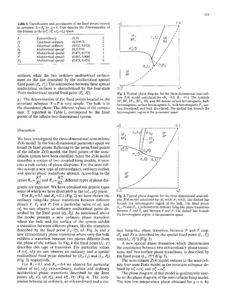
Fig. 2. Typical phase diagram for the three-dimensional semi-infi- nite Z(4) model calculated for (R1=0.5, R2=0.1 ). The symbols SF, BF, SF 2, BF2, SD, and BD denote surface ferromagnetic, bulk ferromagnetic, surface ferromagnetic F2, bulk ferromagnetic F2, sur- face disordered, and bulk disordered. The dashed line bounds the ferromagnetic region in the parameter space

Discussion

We have investigated the three-dimensional semi-infinite Z(4) model. In the four-dimensional parameter space we found 26 fixed points. Referring to the seven fixed points of the infinite Z(4) model, the fixed points of the semi- infinite system have been classified. Since the Z(4) model describes a system of two coupled Ising models, it pres- ents a rich variety of phase diagrams. For the semi-infi- nite system a new type of extraordinary, ordinary surface and special phase transitions appears. According to the

K~ K~ ratios R x =~-Kx and R 2 = K~' different types of phase dia-

grams are expected. We have obtained ten generic types some of which we have illustrated in the (c0], co~) plane.

For R~ =0.5 and R2=0.1 (Fig. 2) we have shown the ordinary Ising-like phase transitions between different phases F, F2 and P. For a particular value of col and e)~ we can observe an ordinary multicritical point de- scribed by the fixed point (P4, P4)- As mentioned above the model presents a new ordinary phase transition where the bulk and the surface of the system exhibit a transition between different phases, like the transition described by the fixed point (Ix, I*), (cf. Fig. 3), and a new extraordinary phase transition where only the bulk exhibits a transition between two phases different from the phase of the surface. In Fig. 4 the fixed point (I2, F) describes this type of transition. For particular values of (o~, co~) we can observe an ordinary and a special multicritical fixed point denoted by (P4, 12) and (Ix, P~) (Fig. 3), respectively.

For R~ =0.1 and R2=0.4 we observe for particular values of (~o~, co~) extraordinary, surface and ordinary multicritical phase transitions described by the fixed points (P4, F), (D, Pc), and (P4, I2") (Fig. 4). The coex- istence between an ordinary, an extraordinary and a sur-

(1.1} W

(I2 F2)7-f(pI2) SP ,'~ ' / / ' ' BP '

BF2 ] ~ SF 2 / / {/ -BP //

* * i i

(It,1;) (I~.I~)7 /

/ / / / /

SF ," BF . ,/" I" / t

(o.o) w~

Fi B. 3. Typical phase diagram for the three-dimensional semi-infi- nite Z(4) model calculated for (RI =0.8, R2 =0.3). The dashed line bounds the ferromagnetic region of the bulk. The fixed points (Ia, P) and (I1, I1) characterize ordinary Ising-like phase transitions between F and F 2 and between F and P. The dashed line bounds the ferromagnetic region in the parameter space

face Ising-like phase transition between P and F resp. (F 2 and F) is described by the special fixed point (11, I~) resp ((12, I2"~)) (Fig. 5).

A new special phase transition which characterizes the coexistence between two extraordinary phase transi- tions and two surface phase transitions, is described by the fixed point (12, I~ s) (Fig. 5).

The semi-infinite Z(4) model reduces to the semi-infi- nite four-state Ports model in the invariant subspace de- fined by co~ = o~ and ~o~ = co~.

The phase diagram of this model is qualitatively simi- lar to the phase diagram of the semi-infinite Ising model. The new low-temperature phase obtained for q--+ oo by

116

$ W 2

SF2 1 BF2 (I2.F/(P,I2)

I . (Pi'I~) / / \ IMF "

[-'z /SF ~-'~{P,I,' SF l(I; 'FI / BP./" BF ~ (P.,,F)

(1,1) (1.1) wz /i SP ,,

BP / / /

/ /

/ /

/ /

/ /

(0,0) (ivF) w~ Fig. 4. Typical phase diagram for the three-dimensional semi-infi- nite Z(4) model calculated for (R1 = 0.8, RE = 0.3). The fixed points (F2, I2), (O, I0, (D, lz) and (O, Iz) describe the surface transitions and the fixed points (I z F) and (!2, F2) characterize ordinary Ising- like phase transitions between F and F: and between F and D. The dashed line bounds the ferromagnetic region in the parameter space

BF 2 (Iz,Fz

(IZ.I:S)//

II:.Fl /

(P, 2) BP /,11

I?l/ . . . . / , ' ~(P,I I) ,,

/ /f~(12fi) ,,,/

BP {I1.F) ] /I (IvI~/"

(P4'F) / / / /

(o,o) w~ Fig. 5. Typical phase diagram for the three-dimensional semi-infi- nite Z(4) model calculated for (R1=0.5, R2=0.2 ). The symbols on the transition lines and multicritical points refer to the fixed points characterizing the transition. The dashed line bounds the ferromagnetic region in the parameter space

L ipowsky [18, 24] for which the bulk is o rdered while the free surface is not, does not a p p e a r for finite q within the M K R G method .

The mode l reduces also to the semi-infinite Is ing m o d - el in the invar ian t subspaces col = co~ = 0 and co~ = co~ = 1 and the usual phase d i ag ram is obta ined.

B . q = 6

The phase s t ructure of the two-d imens iona l Z(6) mode l was discussed in detail by different au thors [10, 25]. I t

can be r epa ramet r i zed in te rms of the (3, 2) mode l of D o m a n y and Riedel [25] by the identif ication

K 1 cos c~(A~)+K2 cos 2 e ( A a ) + K 3 cos 3c~(Aa)

21-/ where c ~ = ~ - , A a = a i - a j , A m = m i - m j , a i = 0 , 1, . . . , 5,

m j = 0 , 1, 2, S#= -t- 1.

Table 4. Coordinates and classification of the fixed points of infinite Z(6) model for d = 2 and d = 3

Fixed Type (col, toe, co~) coordinates Domain in the points (col, 0)2, oJ3) space

F Ferromagnetic phase (0, 0, 0) (0, 0, 0) Volume F P Paramagnetic phase (1, 1, 1) (1, 1, 1) Volume P F2 Ferromagnetic phase with difference two (0, 1, 0) (0, 1, 0) Volume Fz /73 Ferromagnetic phase with difference three (0, 0, l) (0, 0, 1) Volume F 3 S (0.585, 0.128, 0.025) (0.874, 0.654, 0 .559) Critical surface

Critical surface

I Second order (0, 0, ] / 2 - 1 (0, 0, 0.756) Critical surface I* Second order ( I f2-1, 1, I f 2 -1 ) (0.756, 1, 0.756) Critical surface

,07071 P3* Second order 1, 2 '

C (0.320, 0.320, 0.167) (0.660, 0.660, 0.467) Critical line C* (0.341, 0.216, 0.341) (0.657, 0.545, 0 .657) Critical line

Critical line

,0,990,990,9 , P6 ' 5 ' point

Therefore the model describes a coupled Ising and a three-state Potts model. From M K R G method one obtains 13 fixed points [10] (see Table 4). The model has four phase sinks: the ferromagnetic phase F, the ferromagnetic phase with difference two between neigh- bouring spins F 2, the ferromagnetic phase with difference three between neighbouring spins F3 and the paramag- netic phase P which are characterized by [10]: (m~ :I=0, m2+0, m3@0), (ml=0, m240, m3=0), (ml=t=0, m2=0, m3=0) and (m1=0, m2=0, m3=0). Within the M K R G method for the two-dimensional infinite Z(6) model the fixed point which defines the universality class of the vector Potts model is stable within the plane invariant under duality (DIP) [10]. Moreover, its region of stabili- ty appears to extend a short distance beyond the DIP. This behaviour is reflected by plotting all functions

Go = l&0; \ ~ ) on the Clock line. As seen observed by b = l

Rujan et al. the emergency of a well simulated massless spin-wave-like phase appears beyond the Clock fixed point S [101.

The structure of the phase diagram of the two and three-dimensional infinite Z(6) model are qualitatively similar except that the massless spin-wave phase does not occur for the three-dimensional infinite model. The phase diagram for d = 3 is shown in Fig. 6.

In order to classify the different fixed points for the semi-infinite model we distinguish the following cases.

a) In the invariant subspace X = F there is only one fixed point Y= F. The bulk and the surface of the system are together in the ferromagnetic phase.

b) In the invariant subspace X = F2 there are three fixed points: Y= F, F2, P3. The first two points describe two phase sinks. For the first, one the bulk is ferromagnetic Fa while the surface is ferromagnetic F. For the second one the bulk and the surface of the system are ferromag- netic F2. The surface transition between F and Fa is char- acterized by the fixed point P3.

w3 !(0.0.1) / / / ' ~ - . . . . . . . . . . . . . . . . . 7.1

/ / / ,LF3 . . . . // I[ L_.-------'~/ /~ // i l

// 1

/ ' -

/ ;q i/ ::t S " " - . (OLO)

I I / li Y /

, t

Fig. 6. Phase diagram for the three-dimensional infinite ferromag- netic Z(6) model

117

0.2

0.1

0

-0.1

/ /

/

1

.i+"

Fig. 7. G~ functions vs col on the line generated by the flow trajec- tory starting on the Clock line in the invariant subspace X=P for the semi-infinite Z(6) model. A clear tendency to a line of fixed points which is defined by all G~'s being zero is observed

c) In the invariant subspace X = F3 there are three fixed points: Y= F, F3, I. We have only surface transition be- tween F and F3 described by the fixed point I while the bulk is in the ferromagnetic F3 phase.

d) The determination of the fixed points located in the invariant subspace X = P is very simple. In this case, the bulk is in the paramagnetic phase. The coordinates of the components Y are those of the two-dimensional infinite system given in Table 6. However, we can locate the massless spin-wave phase while the bulk is in the disordered phase. To illustrate the Kosterlitz-Thouless like phase on the surface we have plotted all functions

G~ ~b ]b=l on the Clock line (see Fig. 7). We see the

emergence of a well-simulated massless spin-wave phase. In this invariant subspace we have only surface transi- tions, the bulk is in the disordered phase.

e) In the invariant subspace X = I there are three fixed points: Y = F, I, I s. The first fixed point characterizes an extraordinary Ising-like phase transition. The bulk ex- hibits a transition between F and F3 while the surface is in the ferromagnetic phase F. The second fixed point (1(0, 0, 0.756), 1(0, 0, 0.948)) characterizes an ordinary Is- ing-like phase transition between F and /73. The fixed point (I(0, 0, 0.756), Is(O, O, 0.507)) describes a four-di- mensional hypersurface transition. At a point of this hy- persurface the bulk and the surface of the system exhibit a special Ising-like phase transition between F and F3.

f ) In the invariant subspace X=P3 where the model reduces to the three-state Potts model there are three fixed points: Y= F, P3, P~.

The bulk and the surface of the system exhibit the usual extraordinary, ordinary and special Ising- like phase transitions between F and F2 described by (P3, f), (P3(0, 0.7, 0), P3(0, 0.9385, 0)) and (P3(0, 0.7, 0), P3S(0, 0.461, 0)), respectively.

g) In the invariant subspace X = I * there are 11 fixed points. Their coordinates and their classification are giv- en in Table 5. The fixed points (I*, F2), (I*, I*) and (I*, I *s) describe the extraordinary, ordinary and special

118

Table 5. Coordinates and classification of the fixed points located in subspace X=I* for q=6. Dim denotes the dimensionality of the domain in the (co~, B co2, co3, co], co~, co~) space

Y Type (col*, co~*) Dim

F Extraordinary (0, 0, 0) 4 Fa Extraordinary (0, 1, 0) 4 I* Ordinary (0.948, 1, 0.948) 4 / Ordinary (0, 0, 0.948) 4

P~ Special (0, ~ , 0) 3

I *~ Special (0.507, 1, 0.507) 2 P Special (0, 0, 0.507) 3

P3 *~ Special (0.347, ~ , 1, 0.948) 3

S s Special (0.587, 0.230, 0.112) 3 D~ Multicritical (0 ~ @ )

special .186, ,0.507 2

C s Multicritical (0.420, 0.295, 0.166) 2 special

Table 6. Coordinates and classification of the fixed points located in subspace X=D for q=6. Dim denotes the dimensionality of the domain in the (co~, co~, co~, co], co~, co~) space

Y Type (co]*, co~*, co~*) Dim

D Ordinary (0.890, 0.939, 0.948) 4 P3 Ordinary (0, 0.939, 0) 4 I Ordinary (0, 0, 0.948) 4 F Extraordinary (0, 0, 0) 4 S ~ Special (0.476, 0.939, 0.507) 3 P3 ~ Special (0, 0.461, 0) 3 P Special (0, 0, 0.507) 3 I *~ Special (0.476, 0.939, 0.507) 3 P3 "*~ Special (0.437, 0.461, 0.948) 3 D ~ Multicritical (0.234, 0.461, 0.507) 2

special

Table 7. Coordinates and classification of the fixed points located in subspace X=S for q=6. Dim denotes the dimensionality of the domain in the (co~, co2 B, e)~, co], co~, c0~) space

Y Type (col*, co~*, co~*) Dim

F Extraordin- ary (0, 0, 0) 5

S Ordinary (0.973, 0.920, 0.893) 5 P3 Ordinary (0, 0.919, 0) 5 S s Special (0.403, 0.920, 0.370) 4 P~ Special (0, 0.485, 0) 4 I *s Special (0.345, 0.278, 0.610) 3 C ~ Multicritical (0.335, 0.447, 0.189) 3

special

Ising-like phase transitions between Fa and P, respective- ly. The fixed point (I*, F) characterizes a new extraordin- ary phase transition. The bulk exhibits a transition be- tween P and F 2 while the surface is in the ferromagnetic phase F. Its coexistence with the extraordinary phase

transition described by the fixed point (I*, F2) is charac- terized by the special fixed point (I*, P3S). A new ordinary phase transition for which the bulk exhibits a transition between P and F2 while the surface exhibits a transition between F 3 and F is described by the fixed point (I*, I).

The special fixed points (I*, P), (I*, S ~) and (I *~, P3) describe the coexistence between the transitions charac- terized by the fixed points (1", 1) and (I*, F) (I*, I*) and (I*, F), and (1", I) and (I*, I*), respectively. The fixed points (1", D s) and (/*, C s) characterize critical lines de- scribing the coexistence between different special transi- tions. They are special multicritical fixed points.

h) In the invariant subspace X = D the behaviour of the surface is described by the multicritical fixed points. There are 10 fixed points. Their coordinates and their classification are given in Table 6. The fixed point (D, F) characterizes a multicritical extraordinary phase transi- tion. Namely that the bulk exhibits a multicritical phase transition between F, F2, F3 and P while the surface is in the ferromagnetic phase. The multicritical ordinary Ising-like phase transition is described by the fixed point (O, O). The fixed point (O, P3) resp ((D, I)) characterizes a new multicritical ordinary phase transition. Since the bulk exhibits a phase transition between F, F2, F3 and P the surface undergoes a phase transition only between F2 and F resp (F3 and F). The coexistence between the multicritical extraordinary and different multicritical or- dinary phase transitions is described by the multieritical special fixed points (D, Ss), (D, P3 s) and (D, I*~). The mul- ticritical special fixed points (D, I *~) and (D, P3 ~*) charac- terize the coexistence between the multicritical ordinary phase transitions ((O, D) and (D, P3)) and ((D, O) and (D, I)), respectively.

(D, D s) is the decoupling point of two independent ferromagnetic Z(2) and Z(3) models. It describes the coexistence between hypersurface transitions character- ized by the fixed points (D, P3~), (D, I) and (D, P).

i) In the invariant subspaee X = S there are 7 fixed points. Their coordinates and their classification are giv- en in Table 7. The coexistence between the new ordinary phase transition, (S, P3), and the extraordinary phase transition is described by the fixed point (S, P3~).

The two ordinary phase transitions meet on the hy- persurface described by the fixed point (S, I*~). The fixed point (S, C s) characterizes the coexistence between all special phase transitions.

j ) In the invariant subspace X = C there are 7 fixed points. Their coordinates and their classification are giv- en in Table 8. As the bulk exhibits a multicritical phase transition between F, Fa and P the system undergoes a multicritical extraordinary, an ordinary, and a special phase transition. At the ordinary multicritical surface transition described by the fixed point (C, C) both bulk and surface of the system exhibit the same phase transi- tions while for the new multicritical ordinary phase tran- sition described by the fixed point (C, P3) they are not the same. (C, C ~) corresponds to the multicritical special fixed point of the cubic model.

Table 8. Coordinates and classification of the fixed points located in subspace X = C for q=6. Dim denotes the dimensionality of the domain in the (co~, co~, co B * s 3, o9~, o)2, o)3) space

Y Type (col*, e)~*, o9~*) Dim

F Extraordinary (0, 0, 0) 4 C Ordinary (0.929, 0.929, 0.871) 4 P3 Ordinary (0, 0.922, 0) 4 P3 ~ Special (0, 0.482, 0) 3 I *~ Special (0.483, 0.924, 0.452) 3 S ~ Special (0.649, 0.330, 0.205) 3 C ~ Multicritical (0.415, 0.415, 0.225) 2

special

Table 9. Coordinates and classification of the fixed points located in subspace X= C* for q=6. Dim denotes the dimensionality of the domain in the B B B , s (coi, ~%, co3, col, 092, COg) space

Y Type (col*, co~*, co~*) Dim

F Extraordinary (0, 0, 0) 4 C* Ordinary (0.933, 0.903, 0.933) 4 P3 Ordinary (0, 0.842, 0) 4 I Ordinary (0, 0, 0.895, 0) 4 S ~ Special (0.436, 0.418, 0.908) 3 P3 ~ Special (0, 0.573, 0) 3 P Special (0, O, 0.577) 3 P*' Special (0.326, 0.488, 0.326) 2 C *~ Multicritical (0.435, 0.305, 0.435) 2

special

Table 10. Coordinates and classification of the fixed points located in subspace X=P* for q=6. Dim denotes the dimensionality of the domain in the (co~, B B 092, o3, col, o~, o)~) space

Y Type (co]*, co~*, co~*) Dim

F Extraordinary (0, 0, 0) 4 F3 Extraordinary (0, 0, 1) 4 P* Ordinary (0.939, 0.939, 1) 4 P3 Ordinary (0. 0.939, 0) 4 P3 ~ Special (0, 0.461, 0) 3 P Special (0, 0, 1~ - 1) 3 P*~ Special (0.461, 0.461, 1) 2 S ~ Special (0.587, 0.262, 0.191) 3 I *~ Special (0.389, 0.939, 0.414) 3 D ~ Multicritical (0.191, 0.461, 0.414) 2

special C *s Multicritical (0.475, 0.259, 0.275) 2

special

k) In the invariant subspace X = C * there are 9 fixed points. Their coordinates and their classification arc giv- en in Table 9. As the bulk exhibits a multicrit ical phase t ransi t ion between F, F 3 and P the system undergoes a multicrit ical ext raordinary , an ord inary and a special phase transit ion. The fixed points (C*, F) and (C*, C*) describe the multicri t ical ex t raord ina ry and the multi- critical o rd inary Ising-like phase transit ions while the fixed points (C*, I) and (C*, P3) describe a new multicriti- cal ord inary phase transit ion.

119

The multicritical special fixed points (C*, P), (C*, P3~), (C*, S s) describe the coexistence between the different multicritical o rd inary phase transi t ions and the extraor- dinary phase t ransi t ion which are character ized by the fixed points ((C*, I) and (C*, F)), ((C*,/'3) and (C*, F)) and ((C*, F) and (C*, C*)), respectively, while the new multicritical special fixed points (C*, I) and (C*, P3) de- scribe the coexistence between the multicrit ical ord inary phase transit ions which are character ized by the fixed points ((C*, C*) and (C*, P3)) and ((C*, C*) and (C*, I)). The coexistence between the multicrit ical special fixed points (C*, SS), (C*, P3) and (C*, P) is described by the multicritical cubic fixed point (C*, C'S).

l) In the invariant subspace X = P3* there are 11 fixed points. Their coordinates and their classification are giv- en in Table 10. The fixed points (P*,/;3) and (P3*, P*) describe an ex t raord inary and an ord inary Ising-like phase transi t ion between P and F3. While the bulk un- dergoes a second order phase transi t ion between P and F3 the surface can be in the ferromagnet ic phase F. This is a new ex t raord inary phase t ransi t ion described by the fixed point (P3, F). At the new ord inary critical surface described by the fixed point (P3, P3) the surface exhibits a phase transi t ion between F2 and F. The three-dimen- sional hypersurface transit ions which are character ized by the fixed points (P*, PaS), (P3*, P), (P3*, P* s),(P3*, S S) and (P3*, I 'S) describe the coexistence between different new ordinary and ex t raord inary phase transitions. These new special critical hypersurfaces meet on the two-dimension- al multicrit ical surfaces which are character ized by the multicritical fixed points (P3*, DS) and (P3*, C~).

m) In the invariant subspace X = P6 the bulk undergoes a multicrit ical phase transi t ion between F, P, F2 and F3. Howeve r the system exhibits multicrit ical ext raordinary , ord inary and special phase transitions. The coordinates and the classification of fixed points are given in Ta- ble 11. (P6, P~) is the six-state Pot ts multicrit ical fixed point which describes the coexistence between the mul- ticritical special fixed points.

Table 11. Coordinates and classification of the fixed points located in subspace X=P 6 for q=6. Dim denotes the dimensionality of the domain inthe (co~, co~, co3 B, co], co~, co~) space

Y Type (col* , o9~*, o9~*) Dim

F Multicritical (0, 0, 0) 3 extraordinary

P~ Multicritical ordinary (0.922, 0.922, 0.922) 3 I Multicritical ordinary (0, 0.835) 3 P3 Multicritical ordinary (0, 0.888, 0) 3 P Multicritical special (0, 0, 0.646) 2 I *s Multicritical special (0.439, 0.897, 0.439) 2 S s Multicritical special (0.585, 0.331, 0.253) 2 P3 *s Multicritical special (0.408, 0.408, 0.872) 2 P3 s Multicritical special (0, 0.522, 0) 2 C ~ Multicritical special (0.388, 0.388, 0.363) 1 Pj Multicritical special (0.383, 0.383, 0.383) 0

120

Discussion

Within the M K R G method the semi-infinite Z(6) model possess 92 fixed points in the six-dimensional parameter space. The semi-infinite Z(6) model as the Z(4) model presents a rich variety of more complicated phase dia- grams. The Z(6) system exhibits a new type of extraor- dinary, ordinary, surface and special phase transitions between F, F2, F3 and P, like the semi-infinite Z (4) model. As usual the surface of the system can not be more disor- dered than the bulk. Indeed if the bulk is in the ferromag- netic F phase or in the partially ordered phase (F2 or F3) the surface may be only in the same phase or in the ferromagnetic phase F if the bulk is in the partially ordered phase.

K~ K~ and According to the ratios RI=K-~I, R2=K~2 R3 = K~ several types of phase diagrams are expected.

For some values of R1, R2 and R 3 w e can locate in the (col, co~, co~) space all different types of phase transi- tions as for the semi-infinite Z (4) model.

The localization of the spin-wave phase on the surface in the semi-infinite Z(6) model within the M K R G meth-

od is very interesting since it can only be observed on the surface if the bulk is in the disordered phase.

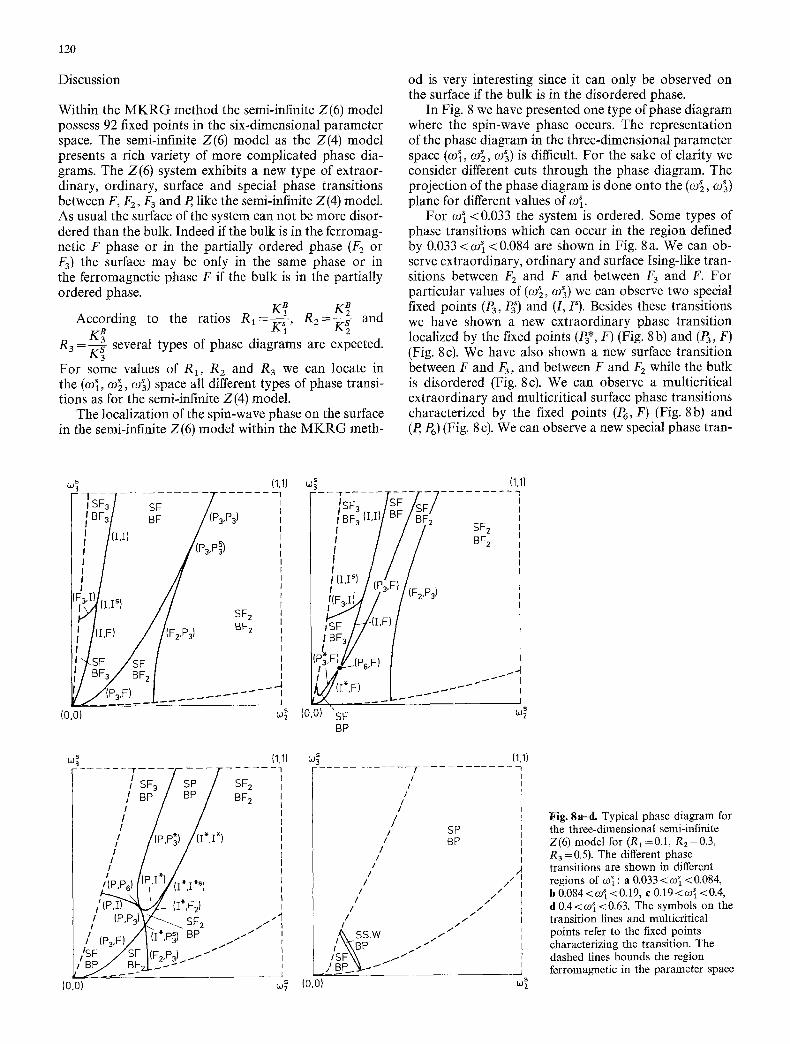
In Fig. 8 we have presented one type of phase diagram where the spin-wave phase occurs. The representation of the phase diagram in the three-dimensional parameter space (co], co~, co~) is difficult. For the sake of clarity we consider different cuts through the phase diagram. The projection of the phase diagram is done onto the (co~, co~) plane for different values of col.

For co] <0.033 the system is ordered. Some types of phase transitions which can occur in the region defined by 0.033 <co] <0.084 are shown in Fig. 8a. We can ob- serve extraordinary, ordinary and surface Ising-like tran- sitions between F2 and F and between /73 and F. For particular values of (co~, co~) we can observe two special fixed points (P3, P~) and (I, P). Besides these transitions we have shown a new extraordinary phase transition localized by the fixed points (P3*, F) (Fig. 8 b) and (P3, F) (Fig. 8 c). We have also shown a new surface transition between F and F3, and between F and F z while the bulk is disordered (Fig. 8c). We can observe a multicritical extraordinary and multicritical surface phase transitions characterized by the fixed points (P6, F) (Fig. 8b) and (P, P6) (Fig. 8 c). We can observe a new special phase tran-

oJ~ (1,1) co~ (1,1} ISF SF i F ] S F3 7 S F i ] F ' ~ I ZB F ~F 7 I

| I BF# BF /(P3,P3 ) I / ,BF~(UV' /BF~ -F I / I / ( I , I } / S II I b 2 I / i / / / / , / / (P3,P3) I,, i ] I I / j

I i l / , / ,< , i , , /oL, / I (F3I) , ~ / ../b';3'~-'/(f2m3) I

,, /7 / i ' ', !I (I'F) f(F2'P3) 'F3// [ "

II I '~, 7 ~(P6.F) / .~ It / BF3/ BF2 - - i ' ' . . - - - " I

' 7 L___. . . . . . , 10.0) w~ 10.0) SF w~

BP

LO~ (1,1) cd~

. . . . . . . 7 7 U T - W 7 / IP, * * *)

/'(pI/~) " _(I* F21 / (P,P3) # ~ SF2

/ (P3,F)/l I*,P~)BP .I'" /SF /SF l(F,.p~)j.J "'~ ~,

I _BE J -----: (o,o) w~

T /

/ /

/ /

/ !

/ SP / BP /

/ /

/ /

/ /

/ /

/~SS.W . . z , \ \BP .." /SFX\ ...1""

/ /

/ / /

/

(o.o)

(1.11 l I F I I

I I I I

,4 /

Fig. 8a-d. Typical phase diagram for the three-dimensional semi-infinite Z(6) model for (R1 =0.1, R2=0.3, R3 =0.5). The different phase transitions are shown in different regions of co~ : a 0.033 < co~ <0.084, b 0.084 < e)~ <0.19, c 0.19 <co] <0.4, d 0.4 < co~ < 0.63. The symbols on the transition lines and multicritical points refer to the fixed points characterizing the transition. The dashed lines bounds the region ferromagnetic in the parameter space

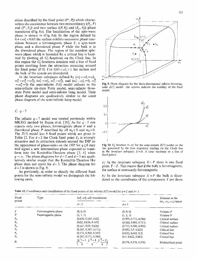
sition described by the fixed point (I*, P3 ~) which charac- terizes the coexistence between two extraordinary ((P3, F) and (1% F2)) and two surface ((P, P3) and (F2, P3)) phase transitions (Fig. 8c). The localization of the spin-wave phase is shown in (Fig. 8d). In the region defined by 0.4 < col < 0.63 the surface exhibits successive phase tran- sitions between a ferromagnetic phase F, a spin-wave phase and a disordered phase P while the bulk is in the disordered phase. The region of the massless spin- wave phase which is bounded by a critical line is local- ized by plotting all G~ functions on the Clock line. In this region the G~ functions simulate well a line of fixed points resulting from the attraction occurring around the fixed point (P, S). For 0.63 < ~0] < 1 the surface and the bulk of the system are disordered.

In the invariant subspaces defined by (o9~ = co~ = co~, (.o1B = (DB __ (DB~ B __ B z - 3,, (co] = co~, col-m3) , and (co~ = o~ = 0, co~ =co~=0) the semi-infinite Z(6) model reduces to the semi-infinite six-state Potts model, semi-infinite three- state Potts model and semi-infinite Ising model. Their phase diagrams are qualitatively similar to the usual phase diagram of the semi-infinite Ising model.

C.q=7

The infinite q =7 model was treated previously within M K R G method by Rujan et al. [-10]. As for q = 5 one expects only two phases, ferromagnetic phase F and a disordered phase P described by all too#0 and m~=0. The Z(7) model has 9 fixed points which are given in Table 12. For d = 2 the Clock fixed point Sa is strongly attractive and its attraction extends around the DIP so the appearence of phase-sinks on the DIP for q > 6 may well signal a new intermediate phase expected to trans- form into the Kosterlitz-Thouless phase I-3, 4] when q ~ oe. The phase diagrams for d = 2 and d = 3 are quali- tatively similar except that the Kosterlitz-Thouless like phase does not occur for d = 3. The phase diagram for d = 3 is shown in Fig. 9.

As previously, in order to classify the different fixed points for the semi-infinite model we distinguish the fol- lowing cases.

121

533

/ / f

r 1 6 2 . . . . . . . . . . . . ' ~ + ' / I I �9

/ ~ ' - " = " l ~

; I

f c000/ I\

{ / / / ~

2' Fig. 9. Phase diagram for the three-dimensional infinite ferromag- netic Z(7) model. The arrows indicate the stability of the fixed points

0.2

0A

0

-0.1

s [/g2 :1 :t k

~' g~

Fig. 10. G~ function vs o9] for the semi-infinite Z(7) model on the line generated by the flow trajectory starting on the Clock line in the invariant subspace X = D . A clear tendency to a line of fixed points

a) In the invariant subspace X=F there is one fixed point Y = F. This means that if the bulk is ferromagnetic, the surface is necessarily ferromagnetic.

b) In the invariant subspace X = P the bulk is disor- dered so the coordinates of the components Y are those

Table 12. Coordinates and classification of the fixed points of the infinite Z(7) model for d = 2 and d = 3

Fixed Type points

(o9", o9"2, co*~3j coordinates

d = 2 d = 3

Domain in the (o91, o92, co3) space

F Ferromagnetic phase (0, 0, 0) P Paramagnetic phase (1, 1, 1) S1 (0.636, 0.167, 0.02) $2 (0.02, 0.636, 0.167) S~ (0.167, 0.02, 0.636) F1 (0.305, 0.347, 0.171) F2 (0.171, 0.305, 0.347) F3 (0.347, 0.171, 0.305)

' 6 ' 6 ,)

(o, o, o) (1, 1, 1) (0.905, 0.713, 0.580) (0.580, 0.905, 0.713) (0.713, 0.580, 0.905) (0.682, 0.5, 0.622) (0.622, 0.682, 0.5) (0.5, 0.622, 0.682)

(0.576, 0.576, 0.576)

Volume F Volume P Critical surface Critical surface Critical surface Critical line Critical line Critical line

Multicritical point

122

of the two-dimensional infinite model given in Table 12. However, in this invariant subspace we can localize the massless-spin-wave phase around the fixed point Sa (Fig. 10) which is strongly attractive. Since the bulk is in the disordered phase we have only surface transitions.

c) In the invariant subspace X = $1 there are three fixed points Y=F, S~, S~. The first and the second one de- scribe an extraordinary and an ordinary lsing-like phase transition while the Clock fixed point (S1(0.98, 0.935, 0.9), S](0.2, 0.676, 0.32)) characterizes a special phase transition between F and P.

Table 13. Coordinates and classification of the fixed points located in subspace X = F~ for q = 7. Dim denotes the dimensionality of the domain in the (0)~, 0)~, c~ 0)1,~ 0)2,~ 0)~) space

Y Type (0)]*, 0)~*, 0)~*) Dim

F Extraordinary (0, 0, 0) 4 /71 Ordinary (0.937, 0.887, 0.924) 4 S~ Special (0.391, 0.208, 0.648) 3 S] Special (0.717, 0.385, 0.259) 3 F~ Multicritical (0.438, 0.246, 0.406) 2

special

The symmetry of the model under permutation 0-)1 ~ (-02 "--)' (03 ( K 1 ~ K2 ~ K3) l e a d s to t h e s a m e phase transitions in the invariant subspaces X = $2 and X = $3. They are described by the same fixed points with coordi- nates exchanged.

d) In the invariant subspace X=/~] the behaviour of the surface is described by multicritical fixed points. There are 5 fixed points. Their coordinates and their classification are given in Table 13. We have only a mul- ticritical ordinary and an extraordinary Ising-like phase transition. The multicritical special fixed point (F~, F#) describes the coexistence between the multicritical spe- cial fixed points (F1, S~) and (F1, S~).

The symmetry of the model leads to the same phase transitions in the invariant subspaces X = F2 and X =/73. They are described by the same fixed points. Their coor- dinates are given by permutations (01 --+ (02 -'9" 0)3"

e) In the invariant subspace X = Pv there are eight fixed points. Their coordinates and their classification are giv- en in Table 14. Since the bulk exhibits a multicritical phase transition the system undergoes a multicritical ex- traordinary an ordinary, and a special phase transition in this invariant subspace. (PT, P79 is the seven-state Potts multicritical fixed point.

Table 14. Coordinate and classification of the fixed points located in subspace X = P7 for q = 7. Dim denotes the dimensionality of the domain in the (co~, co~, co~, 0)~, 0)~, 0)~)

Y Type (0)]*, 0)~*, 0)~*) Dim

F Multieritical (0, 0, 0) 3 extraordinary

P7 Multicritical ordinary (0.919, 0.919, 0.919) 3 S~ Multicritical special (1.12, 0.123, 0.02) 2 S~ Multicritical special (0.02, 1.12, 0.123) 2 S~ Multicritical special (0.123, 0.02, 1.12) 2 F~ ~ Multicritical special (0.356, 0.381, 0.363) 1 F2 Multicritical special (0.363, 0.356, 0.381) 1 F3 ~ Multicritical special (0.381, 0.363, 0.356) 1 P7 ~ Multicritical special (0.366, 0.366, 0.366) 0

Discussion

The three-dimensional semi-infinite Z(7) model is inves- tigated using the M K R G method. We found 42 fixed points in the six-dimensional parameter space. It exhibits only extraordinary, ordinary, special and surface Ising- like phase transitions, r, _ K~ K~

According to the ratios * - 1 - ~ [ , R 2 - - - - KS and R 3 =

KS different types of phase diagrams are expected. In

Fig. 11 we have presented one type of them where differ- ent phase transitions occur. The representation of the phase diagram in the three parameter space ((0~, (0~, o~) is very difficult. So for clearness we consider different

w~ r

/ / j / / / // s // / / / / / (S1,F)// ' \ ' , /

SF ' / /(P.Sl) j"

SF BF

/

(S F) S~S.W / / , / / / ' / ~F :~'~t BP ..-'" 3P~JL-'"

SP BP

/ / /

/ /

(tl

/ / /

/ /

Z

Fig. l l a , b. Typical phase diagram for the three-dimensional semi- infinite Z(7) model for (R1 =0.172, R2=0.96, R3 =0.6). The different phase transitions are shown in different regions of 0)] : a 0.384 <0)] <0.6. We have shown the usual phase transitions namely the ordinary, extraordinary, surface and special, b 0.6<0)] < 1. Besides the transitions described above we can observe the Kosterlitz-Thouless like phase. The symbols on the transition lines and multicritical points refer to the fixed points characterizing the transition. The dashed lines bounds the ferromagnetic region in the parameters space

cuts of the phase diagram in the plane (co~, o)~) for differ- ent values of col.

For R 1 =0.172, R2=0.96 and R3=0.6 the Kosterlitz- Thouless like phase can be localized in the region 0.6 < e)~ < 1 (Fig. 1 lb). As a semi-infinite Z(6) model, the massless-spin-wave phase occurs on the surface only when the bulk is in the disordered phase. In the region 0.348 < co~ < 0.6 we have shown ordinary, extraordinary, surface and special Ising-like phase transitions between F and P (Fig. lla). For 0<o0~ <0.348 the system is ferro- magnetic.

In the invariant subspace (e)~=co2=co3,s s o)l~--co 2 ~ = c03 B) the model reduces to the semi-infinite seven-state Potts model. Their phase diagrams are qualitatively simi- lar to the semi-infinite Ising model.

4. General conclusion

The semi-infinite Z(q) model was investigated using the MKRG method. It has a rich variety of phase diagrams. Several fixed points are obtained so the phase diagrams are very difficult, they are noted in 2Q-dimensional space by the symbol (X, Y) where X and Y refer to bulk and surface of the system. The semi-infinite Z(q) model in- volves several models. It reduces to the semi-infinite Ising model for q = 2 and in some invariant subspaces for even values of q. It reduces also to the semi-infinite q-state Potts model in the invariant subspace (o~]=co~ . . . . = co~, COlB= co~ . . . . . co~?). The phase diagrams of these models are qualitatively similar to the semi-infinite Ising model which presents the usual ordinary, extraordinary, surface and special phase transitions. Nevertheless Li- powsky [18] pointed out that for the infinite value of q there exist a new low temperature phase for which the bulk is ordered while the free surface is not.

It is commonly observed that the surface of the semi- infinite system can not be more disordered than the bulk. For the Z(q) models using the MKRG method we have shown that if the bulk is in a partially ordered phase engendered by a subgroup Z(p) such that p<q, the sur- face is in the same phase or in a partially ordered phase to which the symmetry is engendered by a subgroup, Z(m), of Z(p) such that p=c~m (re<p) with e an integer number satisfying 1 __<c~<p. It can also be in the ferro- magnetic phase (F). If the bulk is in the ferromagnetic phase (F), the surface is necessarily ferromagnetic.

Kf According to the ratios Ra = K-~ (6 = 1, 2, ..., Q) sever-

als types of phase diagrams are expected. They have been represented in the Q-dimensional space (col, co~, ..., co~). New ordinary, extraordinary and special phase transi- tions which do not occur in the semi-infinite Ising-like system are localized for even values of q, namely that the bulk and the surface of the system exhibit a phase transition in different ways. For example, in the Z(4) model the surface exhibits a phase transition between F and F 2 while the bulk undergoes a second order phase transition between F and P. This is a new ordinary phase transition described by the fixed point (I1, I*).

123

Since the massless spin-wave phase is localized within the MKRG method for two-dimensional infinite Z(q) models for q > 6, we have found that the surface of the three dimensional semi-infinite model can be in a spin- wave like phase only when the bulk is disordered. This is quite natural. If we turn off the bulk interactions the surface becomes a two-dimensional system decoupled from the bulk. Therefore the surface of the semi-infinite model exhibits phase transitions successively between the disordered phase, the spin wave like phase and the ferro- magnetic phase only if the bulk is disordered. In addition there are surface transitions.

In the limit q ~ oe the Z(q) model reduces to the continum X - Y model. However, we can estimate the phase diagram of the semi-infinite X - Y model. Indeed, for the Z(q) model the spin-wave phase is localized on the surface only if the bulk is in the disordered phase. At the fixed point of the bulk which defines the universal- ity class of the Clock model the system exhibits an ordi- nary, an extraordinary and a special Ising-like phase transition between F and P. However, in the limit q ~ oo the spin-wave phase transforms into the Kosterlitz- Thouless (KT) phase on the surface only if the bulk is in the disordered phase. So we have a surface transition between KT and disordered phases if the bulk is disor- dered. At bulk criticality the semi-infinite X - Y model exhibits an ordinary Ising-like phase transition between F and P and a new extraordinary phase transition be- tween P and F in the bulk and between KT and F on the surface. The phase diagram of the three-dimensional semi-infinite X - Y model is qualitatively analogous to the phase diagram obtained by Larson [26] (Fig. 12).

We are grateful to Professor J. Zittartz for helpful discussions. This work has been done in the framework of the agreement of coopera- tion between the CNR (Morocco) and D F G (Germany) for which we wish to than both organizations.

t s E (1,1) O~m,-

I SKT

S ~ SF ' BF

SP

[

{0,0} t B

Fig. 12. Phase diagram for the three-dimensional semi-infinite X - Y model. The extraordinary, surface, ordinary and special fixed points are denoted by the symbols E, S, O, and SP. The shorthand notation ts = t h Ks, t~ = t h KB was used

124

References

1. Jos6, J., Kadanoff, L.P., Kirkpatrick, S., Nelson, D. : Phys. Rev. B16, 1217 (1977)

2. Elitzur, S., Pearson, S.B., Shigemitsu, S. : Phys. Rev. D 19, 3698 (1979)

3. Kosterlitz, J.M., Thouless, D.J.: J. Phys. C6, 1181 (1972) 4. Zittartz, J. : Private communication 5. Alcaraz, F.C., K6berle, R.: J. Phys. A13, L153 (1980);

Cardy, J i . : J. Phys. A13, 1507 (1980) 6. Alcaraz, F.C.: J. Phys. A25, 2511 (1987) 7. Fateev, V.A., Zamalodchikov, A.B.: Phys. Lett. A92, 37 (1982) 8. Fateev, V.A., Zamalodchikov, A.B.: Zh. Eksp. Teor. Fiz. 89,

380 [Sov. Phys. JETP 62, 215] (1985) 9. Alcaraz, F.C., Santos, A.L. : Nucl. Phys. B275 [FS17], 436 (1986)

10. Rujan, P., Williams, G.O., Frish, H.L., Forgacs, G.: Phys. Rev. B23, 1362 (1980)

11. Roomany, H.H., Wyld, H.W., Holloway, L.E.: Phys. Rev. D21, 1557 (1980); Roomany, H.H., Wyld, H.W.: Phys. Rev. B23, 1357 (1981)

12. Bonnier, B., Hontebeyrie, M., Meyers, C.: Phys. Rev. B39, 4079 0989)

13. Binder, K.: Critical behaviour at surfaces in phase transitions and critical phenomena. Vol. 8, pp. 1-144. Domb, C., Lebowitz, J. (eds.). New York: Academic Press 1983; Diehl, H.W.: Phase transition and critical phenomena. Vol. 10. Domb, C., Lebowitz, J. (eds.). New York: Academic Press 1986

14. Kaganov, M.I.: Omel'Yanchuk: Zh. Eksp. Teor. Fiz. 61, 1679 (1971); rEngl, trans. Soy. Phys. JETP 34, 895 (1972)]; Binder, K., Hohenberg, P.C.: Phys. Rev. B6, 3461 (1972); Svrakic, N.M., Wortis, M.: Phys. Rev. B15, 396 (1977); Diehl, H.W., Dietrich, S.: Z. Phys. B42, 65 (1981)

15. Lubensky, T.C., Rubin, M.H.: Phys. Rev. B12, 3885 (1975); Bray, A.J., Moore, M.A.: J. Phys. A10, 1927 (1977)

16. Baxter, R.J.: J. Phys. C6, L445 (1973); Aharony, A., Phytte, E.: Phys. Rev. B23, 362 (1981); Nienhuis, B., Riedel, E.K., Schick, M.: Phys. Rev. B23, 6055 (1981)

17. Potts, R.B.: Proc. Cambridge Philos. Soc. 48, 106 (1952); Wu, F.Y.: Rev. Mod. Phys. 54, 235 (1982} Lipowsky, R. : Z. Phys. B - Condensed Matter 45, 229 (1982) Ashkin, J., Teller, E.: Phys. Rev. 64, 178 (1943) Lipowsky, R., Wagner, H.: Z. Phys. B42, 355 (1981); Nagai, O., Toyonaga, M.: J. Phys. C14, L545-9 (1981); Benyoussef, A., Boccara, N., Saber, M.: J. Phys. C 18, 4275 (1985)

21. Fan, C.: Phys. Lett. A39, 136 (1972); Knops, H.J.F.: J. Phys. A8, 1508 (1975)

22. Ditzian, R.V., Banavar, J.R., Grest, G.S., Kadanoff, L.P.: Phys. Rev. B22, 2542 (1980)

23. Murilo, P., DeOlivera, C., SA Barreto, F.C.: J. Stat. Phys. 57, 53 (1989)

24. Lipowsky, R.: Z. Phys. B - Condensed Matter 51, 165 (1983) 25. Domany, E., Riedel, E.K.: Phys. Rev. B19, 5817 (1979) 26. Larsson, T.A.: J. Stat. Phys. 43, 671 (1985)

18. 19. 20.