
Motility of small nematodes in disordered wet granular media
Upload
khangminh22Category
view
1download
0
The Renormalization Groupfor Disordered Systems
Thesis codirected between Dipartimento di Fisica, Università La Sapienza,Rome, Italy and Laboratoire de Physique Théorique et Modèles Statistiques,Université Paris Sud, Orsay, France.
Scuola Dottorale in Scienze Astronomiche, Chimiche, Fisiche, Matematichee della Terra “Vito Volterra”.École Doctorale ED517 “Particules, Noyaux et Cosmos”.
Dottorato di Ricerca in Fisica – XXIII Ciclo
Candidate
Michele CastellanaID number 694948
Thesis Advisors
Professor Giorgio ParisiProfessor Marc Mézard
A thesis submitted in partial fulfillment of the requirementsfor the degree of Doctor of Philosophy in Physics
October 2010

Thesis defended on January 31, 2012in front of a Board of Examiners composed by:
Professor Federico Ricci-Tersenghi (chairman)Professor Alain BilloireProfessor Marc MézardProfessor Giorgio ParisiProfessor Emmanuel TrizacProfessor Francesco Zamponi
Michele Castellana. The Renormalization Groupfor Disordered Systems.Ph.D. thesis. Sapienza – University of Rome© 2011
version: April 30, 2012
email: [email protected]

a Laureen


Abstract
In this thesis we investigate the Renormalization Group (RG) approach in finite-dimensional glassy systems, whose critical features are still not well-established, orsimply unknown. We focus on spin and structural-glass models built on hierarchicallattices, which are the simplest non-mean-field systems where the RG frameworkemerges in a natural way. The resulting critical properties shed light on the criticalbehavior of spin and structural glasses beyond mean field, and suggest futuredirections for understanding the criticality of more realistic glassy systems.
v


Acknowledgments
Thanks to all those who supported me and stirred up my enthusiasm and mywillingness to work.
I am glad to thank my italian thesis advisor Giorgio Parisi, for sharing with mehis experience and scientific knowledge, and especially for teaching me a scientificframe of mind which is characteristic of a well-rounded scientist. I am glad to thankmy french thesis advisor Marc Mézard, for showing me how important scientificopen-mindedness is, and in particular for teaching me the extremely precious skill oftackling scientific problems by considering only their fundamental features first, andof separating them from details and technicalities which would avoid an overall view.
Thanks to my family for supporting me during this thesis and for pushing meto pursue my own aspirations, even though this implied that I would be far from home.
My heartfelt thanks to Laureen for having been constantly by my side with mild-ness and wisdom, and for having constantly pushed me to pursue my ideas, and tokeep the optimism about the future and the good things that it might bring.
Finally, I would like to thank two people who closely followed me in my personaland scientific development over these three years. Thanks to my friend Petr Šulc forthe good time we spent together, and in particular for our sharing of that dreamyway of doing Physics that is the only one that can keep passion and imaginationalive. Thanks to Elia Zarinelli, collaborator and friend, for sharing the experienceof going abroad, leaving the past behind, and looking at it with new eyes. Thanksto him also for the completely free and pleasing environment where our scientificcollaboration took place, and which should lie at the bottom of any scientific research.
vii


Contents
I Introduction 1
1 Historical outline 3
2 Hierarchical models 172.1 Hierarchical models for ferromagnetic systems . . . . . . . . . . . . . 172.2 Hierarchical models for spin and structural glasses . . . . . . . . . . 21
II The Hierarchical Random Energy Model 25
3 Perturbative computation of the free energy 31
4 Spatial correlations of the model 39
III The Hierarchical Edwards-Anderson Model 45
5 The RG in the replica approach 515.1 The RG method à la Wilson . . . . . . . . . . . . . . . . . . . . . . . 515.2 The RG method in the field-theory approach . . . . . . . . . . . . . 58
6 The RG approach in real space 656.1 The RG approach in real space for Dyson’s Hierarchical Model . . . 656.2 The RG approach in real space for the Hierarchical Edwards-Anderson
model . . . . . . . . . . . . . . . . . . . . . . . . . . . . . . . . . . . 706.2.1 Simplest approximation of the real-space method . . . . . . . 716.2.2 Improved approximations of the real-space method . . . . . . 81
IV Conclusions 87
A Properties of Dyson’s Hierarchical Model 91A.1 Derivation of Eq. (2.5) . . . . . . . . . . . . . . . . . . . . . . . . . . 91A.2 Structure of the fixed points of Eq. (2.7) . . . . . . . . . . . . . . . . 92A.3 Calculation of νF . . . . . . . . . . . . . . . . . . . . . . . . . . . . . 94
B Calculation of φ0 97
C Calculation of Υm,0 99
ix

D Derivation of the recurrence equations (5.9) 101
E Results of the two-loop RG calculation à la Wilson 105
F One-loop RG calculation in the field-theory approach 107
G Computation of the observables 6.7 in Dyson’s HierarchicalModel 111
H Solution of the real-space RG equations with thehigh-temperature expansion 113
I Numerical discretization of the matrix MRS in thek0 = 2-approximation 117
V Reprints of the papers 121
x

Part I
Introduction
1


Chapter 1
Historical outline
Paraphrasing P. W. Anderson [4], “the deepest and most interesting unsolved problemin solid state theory is probably the nature of glass and the glass transition”. Indeed,the complex and rich behavior of simplified models for real, physical glassy systemshas interested theoreticians for its challenging complexity and difficulty, and openednew avenues in a large number of other problems such as computational optimizationand neural networks.
When speaking of glassy systems, one can distinguish between two physicallydifferent classes of systems: spin glasses and structural glasses.
Spin glasses have been originally [59] introduced as models to study disordereduniaxial magnetic materials, like a dilute solution of, say, Mn in Cu, modeled byan array of spins on the Mn arranged at random in the matrix of Cu, interactingwith a potential which oscillates as a function of the separation of the spins. Typicalexamples of spin-glass systems are FeMnTiO3 [76, 71, 85, 14], (H3O)Fe3(SO4)2(OH)6[56], CdCr1.7In0.3S4 [81, 156], Eu0.5Ba0.5MnO3 [129] and several others.
Spin glasses exhibit a very rich phenomenology. Firstly, the very first magne-tization measurements of FeMnTiO3 in a magnetic field showed [76] the existenceof a cusp in the susceptibility as a function of the temperature. Occurring at afinite temperature Tsg, this experimental observation is customary interpreted asthe existence of a phase transition.Later on, further experimental works confirmed this picture [71], and revealed somevery rich and interesting features of the low-temperature phase: the chaos and mem-ory effect. Consider a sample of CdCr1.7In0.3S4 in a low-frequency magnetic field[81]. The system is cooled from above Tsg = 16.7K down to 5K, and is then heatedback with slow temperature variations. The curve for the out-of-phase susceptibilityχ′′ as a function of the temperature obtained upon reheating will be called thereference curve, and is depicted in Fig. 1.1.
One repeats the cooling experiment but stops it at T1 = 12K. Keeping thesystem at T1, one waits 7 hours. In this lapse of time χ′′ relaxes downwards, i. e. thesystem undergoes an aging process. When the cooling process is restarted, χ′′ mergesback with the reference curve just after a few Kelvins. This immediate merging backis the chaos phenomenon: aging at T1 does not affect the dynamics of the system
3

4 1. Historical outlineVOLUME 81, NUMBER 15 P HY S I CA L REV I EW LE T T ER S 12 OCTOBER 1998
0 5 10 15 20 250.00
0.01
0.02
CdCr1.7
In0.3
S4
0.04 Hz
aging at
T1=12 K
!"
(a.u
.)
Decreasing T
Increasing T
Reference
T (K)FIG. 1. Out-of-phase susceptibility x 00 of the CdCr1.7In0.3S4spin glass. The solid line is measured upon heating thesample at a constant rate of 0.1 K!min (reference curve). Opendiamonds: the measurement is done during cooling at this samerate, except that the cooling procedure has been stopped at 12 Kduring 7 h to allow for aging. Cooling then resumes down to5 K: x 00 is not influenced and goes back to the reference curve(chaos). Solid circles: after this cooling procedure, the data istaken while reheating at the previous constant rate, exhibitingmemory of the aging stage at 12 K.
Thus, aging at T1 ! 12 K has not influenced the result atlower temperatures (“chaos” effect).
The surprise is that when the sample is reheated at a
constant heating rate (i.e., no further stops on the way
up), we find that the trace of the previous stop (the dip
in x 00) is exactly recovered (see Fig. 1). The memory
of what happened at T1 ! 12 K has not been erased
by the further cooling stage, even though x 00 at lowertemperatures lies on the reference curve. The system can
actually retrieve information from several stops if they
are sufficiently separated in temperature. In Fig. 2, we
show a “double memory experiment,” in which two aging
evolutions, one at T1 ! 12 K and the other at T2 ! 9 K,are retrieved [13]. In the inset of Fig. 2, the result of a
similar experiment on a Cu:Mn sample is shown [11].
As discussed above, the cooling rate dependence of
the dynamics in spin glasses is largely governed by the
chaos effect. For example, it has been shown that there
is no difference in the aging behavior if the spin glass has
been directly quenched from above Tg or if it has been
subjected to a very long waiting pause immediately below
Tg [7]. However, the influence of the cooling rate was not
quantitatively characterized in systematic measurements,
and this point is of a particular interest for the comparison
between spin glasses and other glassy systems. We have
therefore performed the following experiment. We cool
the sample progressively and continuously (in fact, by
steps of 0.5 K) from above Tg to 12 K ! 0.72Tg, using
three very different cooling rates. The result is shown
in Fig. 3. The initial values of x 0 and x 00 are indeed
FIG. 2. Same as in Fig. 1 (CdCr1.7In0.3S4 insulating sample),but with two stops during cooling, which allow the spin glass toage 7 h at 12 K and then 40 h at 9 K. Both aging memories areretrieved independently when heating back (solid circles). Theinset shows a similar “double memory” experiment performedon the Cu:Mn metallic spin glass [11].
different: Slower cooling yields a smaller initial value of
the susceptibility, a value that is closer to “equilibrium.”
A small horizontal shift of the curves along the time scale
allows the superposition of the three of them; the curves
obtained after a slower cooling are somewhat “older.”
0 10000 20000
0.015
0.020
0.025fast
medium
slow
!"(
a.u)
t (s)
0 10000 20000
0.015
0.020
0.025
t (s)
!"(
a.u
) fast
slow
FIG. 3. x 00 relaxation at 12 K as a function of time: effect ofthe cooling rate on aging. The CdCr1.7In0.3S4 sample has beencooled from above Tg ! 17 to 12 K at very different speeds:2.6 K!min (solid circles), 0.08 K!min (crosses), 0.015 K!min(open diamonds). In the inset, another procedure is used whichshows that this cooling rate effect is due only to the lasttemperature interval: constant rate of 0.8 K!min (solid circles)or 0.08 K!min (open diamonds) from 17 to 14 K, but in bothcases rapid quench from 14 to 12 K.
3244
Figure 1.1. Out out phase susceptibility χ′′ of CdCr1.7In0.3S4 as a function of the temper-ature. The solid curve is the reference curve. The open diamonds-curve is obtained bycooling the system and stopping the cooling process at T1 = 7K for seven hours. Thesolid circles-curve is obtained upon re-heating the system after the above cooling process.Data is taken from [81].
at lower temperatures. From a microscopic viewpoint, the aging process brings thesystem at an equilibrium configuration at T1. When cooling is restarted, such anequilibrium configuration behaves as a completely random configuration at lowertemperatures, because the susceptibility curve immediately merges the referencecurve. The effective randomness of the final aging configuration reveals a chaoticnature of the free-energy landscape.
The memory effect is even more striking. When the system is reheated at a con-stant rate, the susceptibility curve retraces the curve of the previous stop at T1. Thisis quite puzzling, because even if the configuration after aging at T1 behaves as a ran-dom configuration at lower-temperatures, the memory of the aging at T1 is not erased.
Such a rich phenomenology challenged the theoreticians for decades. The theo-retical description of such models, even in the mean-field approximation, revealeda complex structure of the low-temperature phase that could be responsible forsuch a rich phenomenology. Still, such a complex structure has been shown tobe correct only in the mean-field approximation, and the physical features of thelow-temperature phase beyond mean field are still far from being understood.
Structural glasses, also known as glass-forming liquids or glass-formers, are liquidsthat have been cooled fast enough to avoid crystallization [16, 150]. When coolinga sample of o− Terphenyl [103], or Glycerol [112], the viscosity η or the relaxationtime τ can change of fifteen order of magnitude when decreasing the temperature of
5
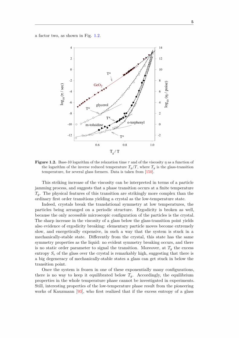
a factor two, as shown in Fig. 1.2.
Tg / T
0.6 0.8 1.0
log
10
(!
/ se
c)
-12
-10
-8
-6
-4
-2
0
2
4
log
10 ("
/ p
ois
e)
-2
0
2
4
6
8
10
12
14
T*
glycerol
GeO2
m-toluidine o-terphenyl
T*
T*
T*
Figure 1.2. Base-10 logarithm of the relaxation time τ and of the viscosity η as a function ofthe logarithm of the inverse reduced temperature Tg/T , where Tg is the glass-transitiontemperature, for several glass formers. Data is taken from [150].
This striking increase of the viscosity can be interpreted in terms of a particlejamming process, and suggests that a phase transition occurs at a finite temperatureTg. The physical features of this transition are strikingly more complex than theordinary first order transitions yielding a crystal as the low-temperature state.
Indeed, crystals break the translational symmetry at low temperatures, theparticles being arranged on a periodic structure. Ergodicity is broken as well,because the only accessible microscopic configuration of the particles is the crystal.The sharp increase in the viscosity of a glass below the glass-transition point yieldsalso evidence of ergodicity breaking: elementary particle moves become extremelyslow, and energetically expensive, in such a way that the system is stuck in amechanically-stable state. Differently from the crystal, this state has the samesymmetry properties as the liquid: no evident symmetry breaking occurs, and thereis no static order parameter to signal the transition. Moreover, at Tg the excessentropy Se of the glass over the crystal is remarkably high, suggesting that there isa big degeneracy of mechanically-stable states a glass can get stuck in below thetransition point.
Once the system is frozen in one of these exponentially many configurations,there is no way to keep it equilibrated below Tg. Accordingly, the equilibriumproperties in the whole temperature phase cannot be investigated in experiments.Still, interesting properties of the low-temperature phase result from the pioneeringworks of Kauzmann [93], who first realized that if the excess entropy of a glass
6 1. Historical outline
former [143] is extrapolated from above Tg down in the low-temperature phase, thereis a finite temperature TK , the Kauzmann temperature, where this vanishes. This israther startling because, if the geometry of the crystal is not too different from thatof the liquid, one expects the entropy of the liquid to be always larger than that ofthe crystal. There have been countless speculations on the solution of this paradox[93, 16, 150], and the existence of a Kauzmann temperature in a real glass-former isnowadays a still hotly-debated and untamed problem from both an experimentaland theoretical viewpoint.
Despite the triking difference between these two kinds of systems spin glassesand structural glasses have some deep common features. Indeed, according to awide part of the community, spin-glass models with quenched disorder are goodcandidates to mimic the dynamically-induced disorder of glass-forming liquids [16],even if some people are still critical about this issue [102]. There are several pointssupporting the latter statement. For instance, it has been shown that hard particlelattice models [18] describing the phenomenology of structural glasses, display thephenomenology of spin systems with quenched disorder like spin glasses. Accordingly,there seems to be an underlying universality between the dynamically-induced disor-der of glass-formers and the quenched disorder of spin glasses, in such a way thatthe theoretical description of spin glasses and that of structural glasses shared animportant interplay in the last decades. More precisely, in the early 80’s the solutionof mean-field versions of spin [136] and structural [53] glasses were developed, andnew interesting features of the low temperature phase were discovered. Since then,a huge amount of efforts has been done to develop a theoretical description of real,non-mean-field spin and structural glasses. A contribution in this direction throughthe implementation of the Renormalization Group (RG) method would hopefullyshed light on the critical behavior of such systems.
Before discussing how the RG framework could shed light on the physics of finite-dimensional spin and structural glasses, we give a short outline of the mean-fieldtheory of spin and structural glasses, and on the efforts that have been done toclarify their non-mean-field regime.
The Sherrington-Kirkpatrick model
The very first spin-glass model, the Edwards-Anderson (EA) model, was introducedin the middle 70’s [59] as a model describing disordered uniaxial magnetic materials.Later on, Sherrington and Kirkpatrick (SK) [144] introduced a mean-field version ofthe EA model, which is defined as a system of N spins Si = ±1 with Hamiltonian
H[~S] = −N∑
i>j=1JijSiSj , (1.1)
with Jij independent random variables distributed according to a Gaussian distribu-tion with zero mean and variance 1/N .
The model can be solved with the replica method [119]: given n replicas~S1, ~S2, . . . , ~Sn of the system’s spins, the order parameter is the n × n matrixQab ≡ 1/N
∑Ni=1 Sa,iSb,i representing the overlap between replica a and replica

7
b. The free energy is computed as an integral over the order parameter, and ther-modynamic quantities are calculated with the saddle-point approximation, which isexact in the thermodynamic limit. SK first proposed a solution for the saddle pointQ∗ab, which was later found to be inconsistent, since it yields a negative entropyat low temperatures. This solution is called the replica-symmetric (RS) solution,because the matrix Q∗ab has a uniform structure, and there is no way to discernbetween two distinct replicas. Some mathematically non-rigorous aspects of thereplica approach had been blamed [155] to explain the negative value of the entropyat low-temperatures. Amongst these issues, there is the continuation of the replicaindex n from integer to non-integer values, and the exchange of the n→ 0-limit withthe thermodynamic limit N →∞. Still, no alternative approach was found to avoidthese issues.
In the late 70’s Parisi started investigating more complicated saddle points. Inthe very first work [134], an approximate saddle point was found, yielding a stillnegative but small value of the entropy at low temperatures. The solution wascalled replica-symmetry-broken solution, because Q∗ab was no more uniform, butpresented a block structure. Notwithstanding the negative values of the entropy atlow temperatures, the solution was encouraging, since it showed a good agreementwith Monte Carlo (MC) simulations [95], whereas the replica-symmetric solutionshowed a clear disagreement with MC data. Later on, better approximation schemesfor the saddle point were considered [135], where the matrix Q∗ab was given by ahierarchical structure of blocks, blocks into blocks, and so on. The step of thishierarchy is called the replica-symmetry-breaking (RSB) step K. The final resultof such works was presented in the papers of 1979 and 1980 [133, 136], where thefull-RSB (K = ∞) solution was presented. According to this solution, the sad-dle point Q∗ab is uniquely determined in terms of a function q(x) in the interval0 ≤ x ≤ 1, being the order parameter of the system. Parisi’s solution resultedfrom a highly nontrivial ansatz for the saddle point Q∗ab, and there was no proofof its exactness. Still, the entropy of the system resulting from Parisi’s solution isalways non-negative, and vanishes only at zero temperature, and the quantitativeresults for thermodynamic quantities such as the internal energy showed a goodagreement [133] with the Thouless-Almeida-Palmer (TAP) solution [153] at lowtemperatures. These facts were rather encouraging, and gave a strong indicationthat Parisi’s approach gave a significant improvement over the original solution by SK.
Still, the physical interpretation of the order parameter stayed unclear until1983 [137], when it was shown that the function q(x) resulting from the bafflingmathematics of Parisi’s solution is related to the probability distribution P (q) ofthe overlap q between two real, physical copies of the system, through the relationx(q) =
∫ q−∞ dq
′P (q′). Accordingly, in the high temperature phase the order parame-ter q(x) has a trivial form, resulting in a P (q) = δ(q), while in the low-temperaturephase the nontrivial form of q(x) predicted by Parisi’s solution implies a nontrivialstructure of the function P (q). In particular, the smooth form of P (q) implies theexistence of many pure states.
Further investigations in 1984 [117] and 1985 [121] gave a clear insight into theway these pure states are organized: below the critical temperature the phase space is
8 1. Historical outline
fragmented into several ergodic components, and each component is also fragmentedinto sub-components, and so on. The free-energy landscape could be qualitativelyrepresented as an ensemble of valleys, valleys inside the valleys, and so on. Spinconfigurations can be imagined as the leaves of a hierarchical tree [119], and thedistance between two of them is measured in terms of number of levels k one hasto go up in the tree to find a common root to the two leaves. To each hierarchicallevel k of the tree one associates a value of the overlap qk, where the set of possiblevalues qk of the overlap is encoded into the function q(x) of Parisi’s solution.
Parisi’s solution was later rederived with an independent method in 1986 byMézard et al [118], who reobtained the full-RSB solution starting from simple physi-cal grounds, and presented it in a more compact form.
Finally, the proof of the exactness of Parisi’s solution came in 2006 by Talagrand[149], whose results are based on previous works by Guerra [69], and who showedwith a rigorous formulation that the full-RSB ansatz provides the exact solution ofthe problem.
This ensemble of works clarified the nature of the spin-glass phase in the mean-field case. According to its clear physical interpretation, the RSB mechanism ofParisi’s solution became a general framework to deal with systems with a largenumber of quasi-degenerate states. In particular, in 2002 the RSB mechanism wasapplied in the domain of constraint satisfaction problems [120, 122, 123, 19], showingthe existence of a new replica-symmetry broken phase in the satisfiable region whichwas unknown before then.
Despite the striking success in describing mean-field spin glasses, it is not clearwhether the RSB scheme is correct also beyond mean field. Amongst the otherscenarios describing the low-temperature phase of non-mean-field spin glasses, thedroplet picture has been developed in the middle 80’s by Bray, Moore, Fisher, Huseand McMilllan [111, 64, 61, 60, 62, 63, 27]. According to this framework, in thewhole low-temperature phase there is only one ergodic component and its spinreversed counterpart, as in a ferromagnet. Differently from a ferromagnet, in afinite-dimensional spin glass spins arrange in a random way determined by theinterplay between quenched disorder and temperature.
On the one hand, there have been several efforts to understand the strikingphenomenological features of three-dimensional systems in terms of the RSB [78],the droplet or alternative pictures [81]. Still, none of these was convincing enoughfor one of these pictures to be widely accepted by the scientific community as thecorrect framework to describe finite-dimensional systems.
On the other hand, there is no analytical framework describing non-mean-fieldspin glasses. Perturbative expansions around Parisi’s solution have been widelyinvestigated by De Dominicis and Kondor [52, 55], but proved to be difficult andnon-predictive. Similarly, several efforts have been done in the implementation innon-mean-field spin glasses of a perturbative field-theory approach based on thereplica method [72, 99, 39], but they turned out to be non-predictive, because nonper-
9
turbative effects are completely untamed. Amongst the possible underlying reasons,there is the fact that such field-theory approaches are all based on a φ3-theory, whoseupper critical dimension is dc = 6. Accordingly, a predictive description of physicalthree-dimensional systems would require an expansion in ε = dc − 3 = 3, whichcan be quantitatively predictive only if a huge number of terms of the ε-series wereknown [173]. Finally, high-temperature expansions for the free energy [141] turn outto be badly behaved in three dimensions [51], and non-predictive.
Since analytical approaches do not give a clear answer on such finite-dimensionalsystems, most of the knowledge comes from MC simulations, which started withthe first pioneering works from Ogielsky [131], and were then intensively carried onduring the 90’s and 00’s [15, 109, 110, 104, 108, 132, 100, 7, 87, 171, 89, 91, 82, 47, 83,48, 106, 73, 10, 49, 86, 3, 8]. None of these gave a definitive answer on the structureof the low-temperature phase, and on the correct physical picture describing it. Thisis because a sampling of the low-temperature phase of a strongly-frustrated systemlike a non-mean-field spin glass has an exponential complexity in the system size[9, 160]. Accordingly, all such numerical simulations are affected by small systemsizes, which prevent from discerning which is the correct framework describing thelow-temperature phase. An example of how finite-size effects played an importantrole in such analyses is the following. According to the RSB picture, a spin-glassphase transition occurs also in the presence of an external magnetic field [119], whilein the droplet picture no transition occurs in such a field [64]. MC studies [89, 92]of a one-dimensional spin glass with power-law interactions yielded evidence thatthere is no phase transition beyond mean field in a magnetic field. Later on, afurther MC analysis [105] claimed that the physical observables considered in such aprevious work were affected by strong finite-size effects, and yielded evidence of aphase transition in a magnetic field beyond mean field through a new method ofdata analysis. Interestingly, a recent analytical work [126] based on a replica analysissuggests that below the upper critical dimension the transition in the presence of anapplied magnetic field does disappear, in such a way that there is no RSB in thelow-temperature phase [124].
This exponential complexity in probing the structure of the low-temperaturephase has played the role of a perpetual hassle in such numerical investigations, andstrongly suggests that the final answer towards the understanding of the spin-glassphase in finite dimensions will not rely on numerical methods [75].
The Random Energy Model
The simplest mean-field model for a structural glass was introduced in 1980 byDerrida [53, 54], who named it the Random Energy Model (REM). In the originalpaper of 1980, the REM was introduced from a spin-glass model with quencheddisorder, the p-spin model. It was shown that in the limit p→∞ where correlationsbetween the energy levels are negligible, the p-spin model reduces to the REM: amodel of N spins Si = ±1, where the energy ε[~S] of each spin configuration ~S is arandom variable distributed according to a Gaussian distribution with zero mean andvariance 1/N . Accordingly, for every sample of the disorder {ε[~S]}~S , the partition
10 1. Historical outline
function of the REM is given by
Z =∑~S
e−βε[~S]. (1.2)
This model became interesting because, despite its striking simplicity, its solutionreveals the existence of a phase transition reproducing all the main physical featuresof the glass transition observed in laboratory phenomena. Indeed, there exists afinite value Tc of the temperature, such that in the high temperature phase thesystem is ergodic, and has an exponentially-large number of states available, whilein the low-temperature phase the system is stuck in a handful of low-lying energystates. The switchover between these two regimes is signaled by the fact that theentropy is positive for T > Tc, while it vanishes for T < Tc. Interestingly, thistransition does not fall in any of the universality classes of phase transitions forferromagnetic systems [173]. Indeed, on the one hand the transition is strictly secondorder, since there is no latent heat. On the other hand, the transition presents thetypical freezing features of first-order phase transitions of crystals [115].
Later on, people realized that the phenomenology of the REM is more general,and typical of some spin-glass models with quenched disorder, like the p-spin model.Indeed, the one-step RSB solution scheme of the SK model was found [50] to beexact for both of the p-spin model and the REM [115], and the resulting solutionsshow a critical behavior very similar to each other. Accordingly, the REM, the p-spinmodel and other models with quenched disorder are nowadays considered to belongto the same class, the 1-RSB class [16].
The solution of the p-spin spherical model reveals that the physics of such 1-RSBmean-field models is the following [16]. There exists a finite temperature Td suchthat for T > Td the system is ergodic, while for T < Td it is trapped in one amongstexponentially-many metastable states: These are the Thouless Almeida Palmer(TAP) [153] states. Since the energy barriers between metastable states are infinitein mean-field models, the system cannot escape from the metastable state it istrapped in. The nature of this transition is purely dynamical, and it shows up inthe divergence of dynamical quantities like the relaxation time τ , while there isno footprint of it in thermodynamic quantities. We will denote by f∗(T ) the freeenergy of each of these TAP states and by fp(T ) the free energy of the system inits paramagnetic state. Accordingly, the total free energy of the glass below Td isgiven by f∗(T ) − TΣ(T ). Since there is no mark of the dynamical transition inthermodynamic quantities, one has that the free energy of the glass below Td mustcoincide with fp(T )
fp(T ) = f∗(T )− TΣ(T ). (1.3)
Below Td, there exists a second finite temperature TK < Td, such that the complexityvanishes at and below TK : the number of TAP states is no more exponential, andthe system is trapped in a bunch of low-lying energy minima: the system undergoesa Kauzmann transition at TK . The nature of this transition is purely static, andshows up in the singularities of thermodynamic quantities such as the entropy.
11
An important physical question is whether this mean-field phenomenology persistsbeyond mean field. In 1989 Kirkpatrick, Thirumalai and Wolynes (KTW) [96]proposed a theoretical framework to handle finite-dimensional glass formers, which isknown as the Random First Order Transition Theory (RFOT). Their basic argumentwas inspired by the following analogy with ferromagnetic systems. Consider amean-field ferromagnet in an external magnetic field h > 0. The free energy has twominima, f+ and f−, with positive and negative magnetization respectively. Beingh > 0, one has f− > f+. Even though the +-state has a lower free energy, it cannotnucleate because the free-energy barriers are infinite in mean field. Differently, infinite dimensions d the free-energy barriers are finite, and the free-energy cost fornucleation of a droplet of positive spins with radius R reads
∆f = C1Rd−1 − (f− − f+)C2R
d, (1.4)
where the first addend is the surface energy cost due to the mismatch between thepositive orientation of the spins inside the droplet and the negative orientation ofthe spins outside the droplet, while the second addend represents the free-energygain due to nucleation of a droplet of positive spins, and is proportional to thevolume of the droplet. According to the above free-energy balance, there exists acritical value R∗ such that droplets with R < R∗ do not nucleate and shrink to zero,while droplets with R > R∗ grow indefinitely. Inspired by the physics emergingfrom mean-field models of the 1-RSB class, KTW applied a similar argument toglass-forming liquids. Before discussing KTW theory, is important to stress thatthe dynamical transition at Td occurring in the mean-field case disappears in finitedimensions. This is because the free-energy barriers between metastable states areno more infinite in the thermodynamic limit. Thus, the sharp mean-field dynamicaltransition is smeared out in finite dimensions, and it is plausible that Td is replacedby a crossover temperature T∗, separating a free flow regime for T > T∗ from anactivated dynamics regime for T < T∗ [16].
According to KTW, for T < T∗ the system is trapped in a TAP state withfree energy f∗. Following the analogy with the ferromagnetic case, the TAP stateis associated with the −-state, while the paramagnetic state with the +-state.Accordingly, by Eq. (1.3) one has f− − f+ = TΣ. Nucleation of a droplet of size Rof spins in the liquid state into a sea of spins in the TAP state has a free-energy cost
∆f = C1Rθ − TΣC2R
d,
where the exponent θ is the counterpart of d− 1 in the ferromagnetic case, Eq. (1.4).Since the presence of disorder is expected to smear out such a surface effects withrespect to the ferromagnetic case, one has θ < d− 1. Liquid droplets with radiussmaller than R∗ ≡
(C1θ
TΣC2d
) 1d−θ disappear, while droplets with radius larger that R∗
extend to infinity. Since there are many spatially localized TAP states, dropletscan’t extend to infinity as in the mean-field case. The system is rather said to be ina mosaic state, given by liquid droplets that are continually created and destroyed[16].
In analogy with the 1-RSB phenomenology, RFOT theory predicts that Σ van-ishes at a finite temperature TK < T∗. Below this temperature liquid droplets cannot

12 1. Historical outline
nucleate anymore, because R∗ =∞, and the system is said to be in a ideal glassystate, i. e. a collectively-frozen and mechanically-stable low-lying energy state. Sill,the crucial question of the existence of a Kauzmann transition in real glass-formers isan open issue. It cannot be amended experimentally, because real glasses are frozenin an amorphous configuration below Tg, and the entropy measured in laboratoryexperiments in this temperature range does not give an estimate of the number ofdegenerate metastable states. Accordingly, analytical progress in non-mean-fieldmodels of the 1-RSB class describing the equilibrium properties below Tg wouldyield a significant advance on this fundamental issue.
A clear way to explore critical properties of non-mean-field systems came fromthe RG theory developed by Wilson in his papers of 1971 [164, 165]. The RG theorystarted from a very simple physical feature observed experimentally in physicalsystems undergoing a phase transition [161]. Consider, for instance, a mixture ofwater and steam put under pressure at the boiling temperature. As the pressureapproaches a critical value, steam and water become indistinguishable. In particular,bubbles of steam and water of all length scales, from microscopic ones to macro-scopic ones, appear. This empirical observation implies that the system has nocharacteristic length scale at the critical point. In particular, as the critical pointis approached, any typical correlation length of the system must tend to infinity,in such a way that no finite characteristic length scale is left at the critical point.Accordingly, if we suppose to approach the critical point by a sequence of elementarysteps, the physically important length scales must grow at each step. This procedurewas implemented in the original work of Wilson, by integrating out all the lengthscales smaller than a given threshold. As a result, a new system with a larger typicallength scale is obtained, and by iterating this procedure many times one obtains asystem whose only characteristic length is infinite, and which is said to be critical.
The above RG scheme yields a huge simplification of the problem. Indeed, systemshaving a number of microscopic degrees of freedom which is typically exponentialin the number of particles are reduced to a handful of effective long-wavelengthdegrees of freedom. These are the only physically relevant degrees of freedom in theneighborhood of the critical point, and all the relevant physical information can beextracted from them.
In the first paper of 1971 Wilson’s made quantitative the above qualitativepicture for the Ising model. Following Kadanoff’s picture [84], short-wavelengths
13
degrees of freedom were integrated out by considering blocks of spins acting as a unit,in such a way that one could treat all the spins in a block as an effective spin. Giventhe values of the spins in the block, the value of this effective spin could be easilyfixed to be +1 if the majority of spins in the block are up, and −1 otherwise. Theresulting approximate RG equations were analyzed in the second paper of 1971 [165],where Wilson considered a simplified version of the Ising model and showed thatthis framework could make precise predictions on physical quantities like the criticalexponents, which were extracted in perturbation theory. There the author realizedthat if the dimensionality d of the system was larger than 4 the resulting physics inthe critical regime was the mean-field one, while for d < 4 non-mean-field effectsemerge. These RG equations for the three-dimensional Ising model were treatedperturbatively in the parameter ε ≡ 4− d, measuring the distance from the uppercritical dimension d = 4, in a series of papers in the 70’s [169, 166]. The validity ofthis perturbative framework was later confirmed by the reformulation of Wilson’sRG equations in the language of field theory. There, the mapping of the Ising modelinto a φ4-theory and the solution of the resulting Callan-Symanzik (CS) equations[28, 147, 173] for this theory made the RG method theoretically grounded, and theproof of the renormalizability of the φ4-theory [29] to all orders in perturbationtheory served as a further element on behalf of this whole theoretical framework.Finally, the picture was completed some years later by high-order implementationsof the ε-expansion for the critical exponents [157, 41, 40, 43, 42, 94, 68, 97, 98] whichwere in excellent agreement with experiments [173, 1] and MC simulations [140, 5].
Because of this ensemble of works, the RG served as a fundamental tool inunderstanding the critical properties of finite-dimensional systems. Hence, it isnatural to search for a suitable generalization of Wilson’s ideas to describe thecritical regime of non-mean-field spin or structural glasses. The drastic simpli-fication resulting from the reduction of exponentially many degrees of freedomto a few long-wavelength degrees of freedom would be a breakthrough to tacklethe exponential complexity limiting our understanding of the physics of such systems.
Still, a construction of a RG theory for spin or structural glasses is far moredifficult than the original one developed for ferromagnetic systems. Indeed, in theferromagnetic case it is natural to identify the order parameter, the magnetization,and then implement the RG transformation with Kadanoff’s majority rule. Con-versely, in non-mean-field spin or structural glasses, the order parameter describingthe phase transition is fundamentally unknown.
For non-mean-field spin glasses, the RSB and droplet picture make two radi-cally different predictions on the behavior of a tentative order parameter in thelow-temperature phase. In the RSB picture the order parameter is the probability dis-tribution of the overlap P (q), being P (q) = δ(q) in the high-temperature phase andP (q) a smooth function of q in the low-temperature phase [133]. Such a smooth func-tion reflects the hierarchical organization of many pure states in the low-temperaturephase. In the droplet picture [64] P (q) reduces to two delta functions centered on thevalue of a scalar order parameter, the Edwards-Anderson order parameter qEA [59].Such an order parameter is nonzero if the local magnetizations are nonzero, i. e. if thesystem is frozen in the unique low-lying ergodic component of the configuration space.

14 1. Historical outline
For structural glasses, after important developments in the understanding of thecritical regime came in 2000 [66], a significant progress in the identification of theorder parameter has been proposed in 2004 [25] and numerically observed in 2008[17] by Biroli et al., who suggested that the order parameter is the overlap betweentwo equilibrated spin-configurations with the same boundary conditions: the influ-ence of the boundary conditions propagates deeper and deeper into the bulk as thesystem is cooled, signaling the emergence of an amorphous order at low temperatures.
A justification of the difficulty in the definition of a suitable order parameterfor a spin or structural glass has roots in the frustrated nature of the spin-spininteractions. To illustrate this point, let us consider a spin system like the SK wherethe sign of the couplings Jij are both positive and negative, Eq. (1.1), and tryto mimic Wilson’s block-spin transformation [164] for the SK model. Given thevalues of the spins in a block, Kadanoff’s majority rule does not give any usefulinformation on which should the value of the effective spin. Indeed, choosing theeffective spin to be +1 if most of the spins in the block are up and −1 otherwisedoes not make sense: being the Jijs positive or negative with equal probability, themagnetization inside the block is simply zero on average, and does not give any usefulinformation on which value should be assigned to the effective spin. Again, frus-tration is the main stumbling block in the theoretical understanding of such systems.
In order to overcome this difficulty, we recall that Wilson’s approximate RGequations were found to be exact [161] on a particular non-mean-field model forferromagnetic interactions, where the RG recursion formulas have a strikingly simpleand natural form. This is Dyson’s Hierarchical Model (DHM), and was introducedby Dyson in 1969 [57]. There, the process of integrating out long-wavelength de-grees of freedom emerged naturally in an exact integral equation for the probabilitydistribution of the magnetization. This equation was the forerunner of Wilson’s RGequations.
The aim of this thesis is to consider a suitable generalization of DHM describ-ing non-mean-field spin or structural glasses, and construct a RG framework forthem. These models will be generally denoted by Hierarchical Models (HM), andwill be introduced in Section 2.2. The definition of HM is quite general, and bymaking some precise choices on the form of the interactions, one can build upa HM capturing the main physical features a non-mean-field spin or structuralglass. Thanks to their simplicity, HM allow for a simple and clear construction ofa RG framework. Our hope is that such a RG framework could shed light on the

15
criticality of the glass transition beyond mean field, and on the identification ofthe order parameter describing the emergence of an amorphous long-range order,if present. As a long-term future direction, the RG method on HM could also beuseful to understand the features of the low-temperature phase of such glassy systems.
The thesis is structured as follows. In Chapter 2 of Part I we discuss DHM, andintroduce HM for spin or structural glasses. In Part II we study a HM mimicking thephysics of a non-mean-field structural glass, the Hierarchical Random Energy Model(HREM), being a hierarchical version of the REM. In this Part we show how one canwork out a precise solution for thermodynamic quantities of the system, signalingthe existence of a Kauzmann phase transition at finite temperature. The HREMconstitutes the first non-mean-field model of a structural glass explicitly exhibitingsuch a freezing transition as predicted by RFOT. Interestingly, the solution suggestsalso the existence of a characteristic length growing as the critical point is approached,in analogy with the predictions of KTW. In Part III we study a HM mimicking thephysics of a non-mean-field spin glass, the Hierarchical Edwards-Anderson model(HEA), being a hierarchical version of the Edwards-Anderson model. The RGtransformation is first implemented with the standard replica field-theory approach,which turns out to be non-predictive because nonperturbative effects are completelyuntamed. Consequently, a new RG method in real space is developed. This methodavoids the cumbersome formalism of the replica approach, and shows the existenceof a phase transition, making precise predictions on the critical exponents. Thereal-space method is also interesting from a purely methodological viewpoint, becauseit yields the first suitable generalization of Kadanoff’s RG decimation rule for astrongly frustrated system. Finally, in Part IV we discuss the overall results of thiswork, by paying particular attention to its implications and future directions in thephysical understanding of realistic systems with short-range interactions.

Chapter 2
Hierarchical models
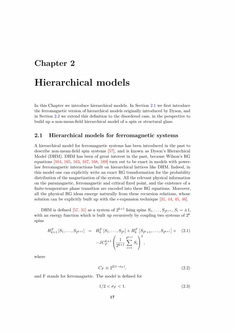
In this Chapter we introduce hierarchical models. In Section 2.1 we first introducethe ferromagnetic version of hierarchical models originally introduced by Dyson, andin Section 2.2 we extend this definition to the disordered case, in the perspective tobuild up a non-mean-field hierarchical model of a spin or structural glass.
2.1 Hierarchical models for ferromagnetic systems
A hierarchical model for ferromagnetic systems has been introduced in the past todescribe non-mean-field spin systems [57], and is known as Dyson’s HierarchicalModel (DHM). DHM has been of great interest in the past, because Wilson’s RGequations [164, 165, 163, 167, 168, 169] turn out to be exact in models with power-law ferromagnetic interactions built on hierarchical lattices like DHM. Indeed, inthis model one can explicitly write an exact RG transformation for the probabilitydistribution of the magnetization of the system. All the relevant physical informationon the paramagnetic, ferromagnetic and critical fixed point, and the existence of afinite-temperature phase transition are encoded into these RG equations. Moreover,all the physical RG ideas emerge naturally from these recursion relations, whosesolution can be explicitly built up with the ε-expansion technique [31, 44, 45, 46].
DHM is defined [57, 31] as a system of 2k+1 Ising spins S1, . . . , S2k+1 , Si = ±1,with an energy function which is built up recursively by coupling two systems of 2kspins
HFk+1 [S1, . . . , S2k+1 ] = HF
k [S1, . . . , S2k ] +HFk
[S2k+1, . . . , S2k+1
]+ (2.1)
−JCk+1F
12k+1
2k+1∑i=1
Si
2
,
where
CF ≡ 22(1−σF ), (2.2)
and F stands for ferromagnetic. The model is defined for
1/2 < σF < 1. (2.3)
17

18 2. Hierarchical models
The limits (2.3) can be derived by observing that for σF > 1 the interaction energygoes to 0 for large k, and no finite-temperature phase transition occurs, while forσF < 1/2 the interaction energy grows with k faster than 2k, i. e. faster than thesystem volume, in such a way that the model is thermodynamically unstable.
The key issue of DHM is that the recursive nature of the Hamiltonian functionencoded in Eq. (2.1) results naturally into an exact RG equation. This equationcan be easily derived by defining the probability distribution of the magnetizationm for a 2k-spin DHM, as
pk(m) ≡ C∑~S
e−βHFk [~S]δ
12k
2k∑i=1
Si −m
, (2.4)
where δ denotes the Dirac delta function, and C a constant enforcing the normalizationcondition
∫dmpk(m) = 1. Starting from Eq. (2.1), one can easily derive a recursion
equation relating pk to pk+1. This equation is derived in Section A.1 of Appendix A,and reads
pk+1(m) = eβJCk+1F m2
∫dµ pk(m+ µ)pk(m− µ), (2.5)
where any m-independent multiplicative constant has been omitted to simplify thenotation. Eq. (2.5) relies the probability distribution of a DHM with 2k spins withthat of a DHM with 2k+1 spins. Accordingly, Eq. (2.5) is nothing but the flow ofthe function pk(m) under reparametrization 2k → 2k+1 of the length scale of thesystem. Historically, Eq. (2.5) has been derived by Dyson [57], and then served asthe starting point for the construction of the RG theory for ferromagnetic systemslike the Ising model. Indeed, Wilson’s RG recursion formulas for the Ising model[164, 165, 163] are approximate, while they turn out to be exact when applied toDHM, because they reduce to Eq. (2.5). DHM has thus played a crucial role inthe construction of the RG theory for ferromagnetic systems, because in a sensethe work of Wilson on finite-dimensional systems has been pursued in the effortto generalize the exact recursion formula (2.5) to more realistic systems with nohierarchical structure, like the three-dimensional Ising model.
Equation (2.5) has also been an important element in the probabilistic formu-lation of RG theory, originally foreseen by Bleher, Sinai [20] and Baker [6], andlater developed by Jona-Lasinio and Cassandro [79, 31]. Indeed, Eq. (2.5) aims toestablish the probability distribution of the average of 2k spin variables {Si}i fork → ∞. In the case where the spins are independent and identically distributed(IID), the above analogy becomes transparent, because the answer to the abovequestion is yield by the central limit theorem. Following this connection betweenRG and probability theory, one can even prove the central limit theorem startingfrom the RG equations (2.5) [31].
Equation (2.5) has been of interest in the last decades also because it is simpleenough to be solved with high precision, and the resulting solution gives a clearinsight into the critical properties of the system, showing the existence of a phasetransition. The crucial observation is that Eq. (2.5) can be iterated k � 1 timesin 2k operations. Indeed, the magnetization m of a 2k-spin DHM can take 2k + 1

2.1 Hierarchical models for ferromagnetic systems 19
possible values {−1,−1 + 2/2k, · · · , 0, · · · , 1− 2/2k, 1}. According to Eq. (2.4), thefunction pk(m) is nonzero only if m is equal to one of these 2k + 1 values. It followsthat in order to compute pk+1(m), one has to perform a sum in the right-hand sideof Eq. (2.5), involving 2k + 1 terms. This implies that the time to calculate pk(m)for k � 1 is proportional to 2k. Thus, the use of the hierarchical structure encodedin Eq. (2.5) yields a significant improvement in the computation of pk(m) withrespect to a brute-force evaluation of the sum in the right-hand side of Eq. (2.4),which involves 22k terms.
Let us now discuss the solution of Eq. (2.5). For Eq. (2.5) to be nontrivial fork →∞, one needs to rescale the magnetization variable. Otherwise, the Ck+1
F -termin the right-hand side of Eq. (2.5) would diverge for k →∞. Setting
pk(m) ≡ pk(C−k/2F m), (2.6)
Eq. (2.5) becomes
pk+1(m) = eβJm2∫dµ pk
(m+ µ
C1/2F
)pk
(m− µC
1/2F
). (2.7)
The structure of the fixed points of Eq. (2.7) is discussed in Section A.2 ofAppendix A. In particular, it is shown that there exists a value βc F of β, suchthat if β < βc F Eq. (2.7) converges to a high-temperature fixed point, while ifβ > βc F Eq. (2.7) converges to a low-temperature fixed point. Both of these fixedpoints are stable, and can be qualitatively represented as basins of attraction inthe infinite-dimensional space where pk(m) flows [163]. These basins of attractionare separated by an unstable fixed point p∗(m), which is reached by iterating Eq.(2.7) with β = βc F . p∗(m) is called the critical fixed point, and is characterizedby the fact that the convergence of pk to p∗ for β = βc F implies the divergence ofthe characteristic length scale ξF of the system in the thermodynamic limit k →∞.Accordingly, in what follows βc F will denote the inverse critical temperature of DHM.In the neighborhood of the critical temperature the divergence of ξF is characterizedby a critical exponent νF , defined by
ξFT→Tc F≈ A
(T − Tc F )νF , (2.8)
where A is independent of the temperature. The critical exponent νF is an importantphysical quantity characterizing criticality, and is quantitatively predictable fromthe theory. In Section A.3 of Appendix A we show how νF can be computed startingfrom the RG equation (2.7). This derivation serves as an important example ofthe techniques that will be employed in generalizations of DHM involving quencheddisorder, that will be discussed in the following Sections.
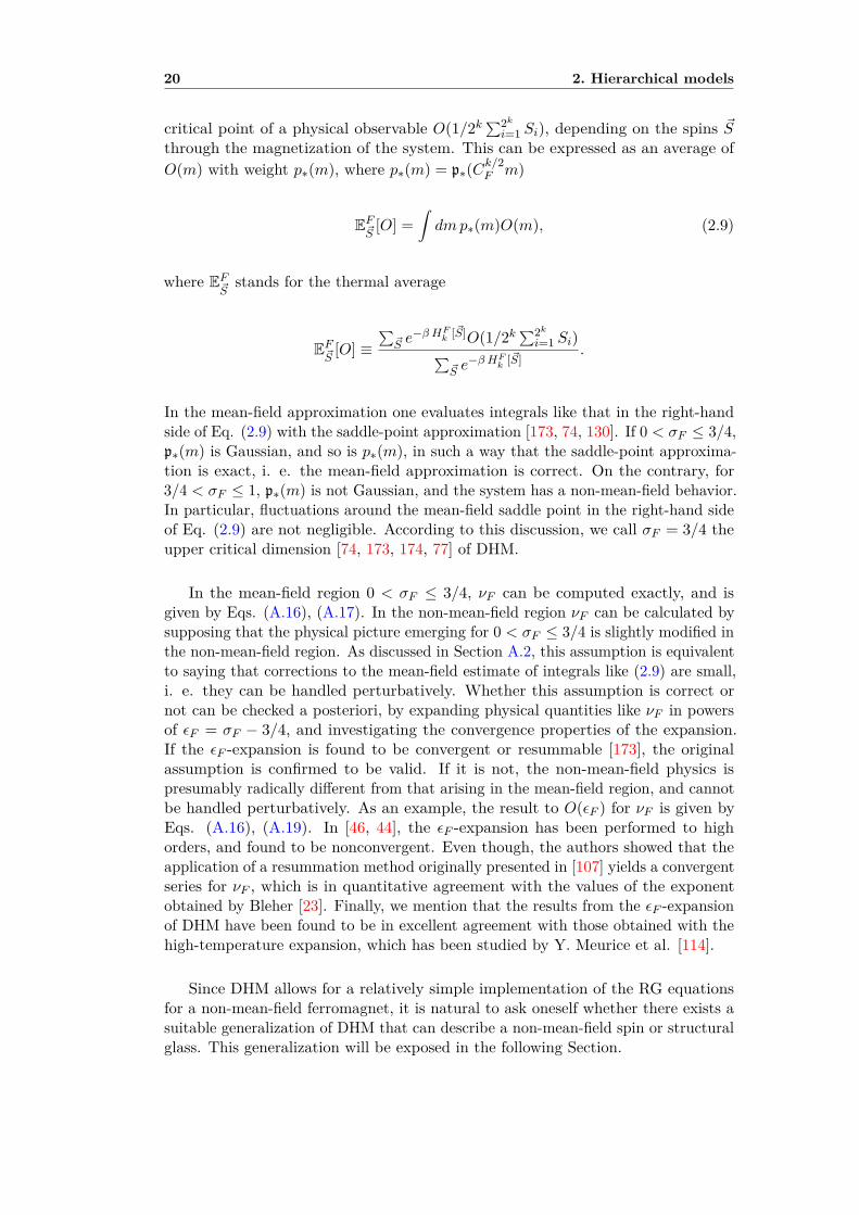
The calculation of νF relies on the fact that for 0 < σF ≤ 3/4 the critical fixedpoint p∗(m) is a Gaussian function of m, while for 3/4 < σF < 1 p∗(m) is notGaussian, as illustrated in Section A.2. We recall [44, 45, 31, 163, 173, 174] that aGaussian p∗(m) corresponds to a mean-field regime of the model. The expressionmean field is due to the following. Consider for instance the thermal average at the
20 2. Hierarchical models
critical point of a physical observable O(1/2k∑2ki=1 Si), depending on the spins ~S
through the magnetization of the system. This can be expressed as an average ofO(m) with weight p∗(m), where p∗(m) = p∗(Ck/2F m)
EF~S [O] =∫dmp∗(m)O(m), (2.9)
where EF~S stands for the thermal average
EF~S [O] ≡∑
~S e−β HF
k [~S]O(1/2k∑2ki=1 Si)∑
~S e−β HF
k[~S]
.
In the mean-field approximation one evaluates integrals like that in the right-handside of Eq. (2.9) with the saddle-point approximation [173, 74, 130]. If 0 < σF ≤ 3/4,p∗(m) is Gaussian, and so is p∗(m), in such a way that the saddle-point approxima-tion is exact, i. e. the mean-field approximation is correct. On the contrary, for3/4 < σF ≤ 1, p∗(m) is not Gaussian, and the system has a non-mean-field behavior.In particular, fluctuations around the mean-field saddle point in the right-hand sideof Eq. (2.9) are not negligible. According to this discussion, we call σF = 3/4 theupper critical dimension [74, 173, 174, 77] of DHM.
In the mean-field region 0 < σF ≤ 3/4, νF can be computed exactly, and isgiven by Eqs. (A.16), (A.17). In the non-mean-field region νF can be calculated bysupposing that the physical picture emerging for 0 < σF ≤ 3/4 is slightly modified inthe non-mean-field region. As discussed in Section A.2, this assumption is equivalentto saying that corrections to the mean-field estimate of integrals like (2.9) are small,i. e. they can be handled perturbatively. Whether this assumption is correct ornot can be checked a posteriori, by expanding physical quantities like νF in powersof εF = σF − 3/4, and investigating the convergence properties of the expansion.If the εF -expansion is found to be convergent or resummable [173], the originalassumption is confirmed to be valid. If it is not, the non-mean-field physics ispresumably radically different from that arising in the mean-field region, and cannotbe handled perturbatively. As an example, the result to O(εF ) for νF is given byEqs. (A.16), (A.19). In [46, 44], the εF -expansion has been performed to highorders, and found to be nonconvergent. Even though, the authors showed that theapplication of a resummation method originally presented in [107] yields a convergentseries for νF , which is in quantitative agreement with the values of the exponentobtained by Bleher [23]. Finally, we mention that the results from the εF -expansionof DHM have been found to be in excellent agreement with those obtained with thehigh-temperature expansion, which has been studied by Y. Meurice et al. [114].
Since DHM allows for a relatively simple implementation of the RG equationsfor a non-mean-field ferromagnet, it is natural to ask oneself whether there exists asuitable generalization of DHM that can describe a non-mean-field spin or structuralglass. This generalization will be exposed in the following Section.
2.2 Hierarchical models for spin and structural glasses 21
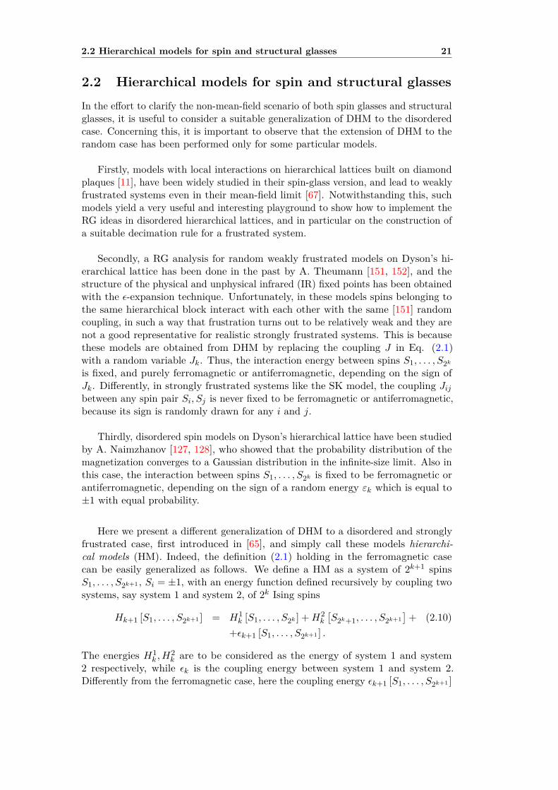
2.2 Hierarchical models for spin and structural glassesIn the effort to clarify the non-mean-field scenario of both spin glasses and structuralglasses, it is useful to consider a suitable generalization of DHM to the disorderedcase. Concerning this, it is important to observe that the extension of DHM to therandom case has been performed only for some particular models.
Firstly, models with local interactions on hierarchical lattices built on diamondplaques [11], have been widely studied in their spin-glass version, and lead to weaklyfrustrated systems even in their mean-field limit [67]. Notwithstanding this, suchmodels yield a very useful and interesting playground to show how to implement theRG ideas in disordered hierarchical lattices, and in particular on the construction ofa suitable decimation rule for a frustrated system.
Secondly, a RG analysis for random weakly frustrated models on Dyson’s hi-erarchical lattice has been done in the past by A. Theumann [151, 152], and thestructure of the physical and unphysical infrared (IR) fixed points has been obtainedwith the ε-expansion technique. Unfortunately, in these models spins belonging tothe same hierarchical block interact with each other with the same [151] randomcoupling, in such a way that frustration turns out to be relatively weak and they arenot a good representative for realistic strongly frustrated systems. This is becausethese models are obtained from DHM by replacing the coupling J in Eq. (2.1)with a random variable Jk. Thus, the interaction energy between spins S1, . . . , S2kis fixed, and purely ferromagnetic or antiferromagnetic, depending on the sign ofJk. Differently, in strongly frustrated systems like the SK model, the coupling Jijbetween any spin pair Si, Sj is never fixed to be ferromagnetic or antiferromagnetic,because its sign is randomly drawn for any i and j.
Thirdly, disordered spin models on Dyson’s hierarchical lattice have been studiedby A. Naimzhanov [127, 128], who showed that the probability distribution of themagnetization converges to a Gaussian distribution in the infinite-size limit. Also inthis case, the interaction between spins S1, . . . , S2k is fixed to be ferromagnetic orantiferromagnetic, depending on the sign of a random energy εk which is equal to±1 with equal probability.
Here we present a different generalization of DHM to a disordered and stronglyfrustrated case, first introduced in [65], and simply call these models hierarchi-cal models (HM). Indeed, the definition (2.1) holding in the ferromagnetic casecan be easily generalized as follows. We define a HM as a system of 2k+1 spinsS1, . . . , S2k+1 , Si = ±1, with an energy function defined recursively by coupling twosystems, say system 1 and system 2, of 2k Ising spins
Hk+1 [S1, . . . , S2k+1 ] = H1k [S1, . . . , S2k ] +H2
k
[S2k+1, . . . , S2k+1
]+ (2.10)
+εk+1 [S1, . . . , S2k+1 ] .
The energies H1k , H
2k are to be considered as the energy of system 1 and system
2 respectively, while εk is the coupling energy between system 1 and system 2.Differently from the ferromagnetic case, here the coupling energy εk+1 [S1, . . . , S2k+1 ]

22 2. Hierarchical models
of any spin configuration S1, · · · , S2k+1 is a random variable, which is chosen to havezero mean for convenience.
Since the interaction energy εk+1 couples 2k+1 spins, and since its order ofmagnitude is give by its variance, one must have
Eε[ε2k+1] < 2k+1, (2.11)
where Eε stands for the expectation value with respect to all the coupling energiesεk of the model. Eq. (2.11) states that the interaction energy between 2k+1 spins issub extensive with respect to the system volume 2k+1, and ensures [119, 130] thatHM are non-mean-field models. The mean-field limit will be constantly recoveredin the following chapters as the limit where Eε[ε2k+1] becomes of the same order ofmagnitude as the volume 2k+1.
As we will show in the following, the form (2.10) of the Hamiltonian correspondsto dividing the system in hierarchical embedded blocks of size 2k, so that the in-teraction between two spins depends on the distance of the blocks to which theybelong [65, 34, 35], as shown in Fig 2.1.
ǫ1
ǫ2
ǫ3
S1 S2 S3 S4 S5 S6 S7 S8
Figure 2.1. A 23-spin hierarchical model obtained by iterating Eq. (2.10) until k = 3.The arcs coupling pairs of spins represent the energies ε1 at the first hierarchical levelk = 1. Those coupling quartets of spins represent ε2 at the second hierarchical levelk = 2. Those coupling octets of spins represent the energies ε3 at the third hierarchicallevel k = 3.
The random energies εk of HM can be suitably chosen to mimic the interactionsof a strongly frustrated structural glass (Part II), or of a spin glass (Part III), in theperspective to give some insight into the non-mean-field behavior and criticality ofboth of these models. In this thesis such features will be investigated by means ofRG techniques. Indeed, as for DHM, the recursive nature of the definition (2.10)suggests that HM are particularly suitable for an explicit implementation of theRG transformation. As a matter of fact, the definition (2.10) is indeed a RG flowtransformation from the length scale 2k to the length scale 2k+1. As we will showexplicitly in Part III, one can analyze the fixed points of such an RG flow, in orderto establish if a phase transition occurs, and investigate the critical properties of thesystem.
It is important to observe that without the hierarchical structure this would beextremely difficult. This is mainly because of the intrinsic and deep difficulty in

2.2 Hierarchical models for spin and structural glasses 23
identifying the correct order parameter discussed in Section 1, and thus write anRG equation for a function (or functional) of it without making use of the replicamethod [55, 119] which, up to the present day, could not be used to make predictionsfor the non-mean-field systems under consideration in this thesis.
After introducing HM in their very general form, we now make a precise choicefor the random energies εk in order to build up a hierarchical model for a structuralglass, the Hierarchical Random Energy Model, and discuss its solution.


Part II
The Hierarchical RandomEnergy Model
25


27
As discussed in Section 1, the REM is a mean-field spin model mimicking thephenomenology of a supercooled liquid. Given the general definition of HM, it iseasy to make a particular choice for the random energies εk in (2.10), to build upa non-mean-field version of the REM, i. e. a HM being a candidate for describingthe phenomenology of a supercooled liquid beyond mean field. Indeed, we choosethe energies εk to be independent variables distributed according to a Gaussiandistribution with zero mean and variance proportional to C2k
Eε[ε2k] ∼ C2k, (2.12)
where we setC2 = 21−σ. (2.13)
For σ < 0 the thermodynamic limit k →∞ is ill-defined, because the interactionenergy Eε[ε2k] grows faster than the volume 2k. For σ > 1, Eε[ε2k] goes to 0 ask →∞, implying that there is no phase transition at finite temperature. Hence, theinteresting region that we will consider in the following is
0 < σ < 1, (2.14)
which is the equivalent of Eq. (2.3) for DHM. As we will discuss in the following,this HM reproduces the REM in the mean-field case σ = 0, and will thus be calledthe Hierarchical Random Energy Model (HREM) [33, 36]. According to the generalclassification of models with quenched disorder given in Section 1, the HREM has tobe considered as a model mimicking a structural glass.
Before discussing the solution of the HREM, it is important to focus our attentionon some important features of the model that make it interesting in the perspectiveof investigating the non-mean-field regime of a structural glass.
Firstly, the hierarchical structure of the HREM allows an almost explicit solutionwith two independent and relatively simple methods.The first method will be described very shortly here (a complete discussion canbe found in [33, 32]) and relies on the fact that the recursive nature of Eq. (2.10)implies a recursion relation for the function Nk(E), defined as the number of stateswith energy E at the k-the step of the recursion. By solving this recursion equationfor large k, one can compute the entropy of the system
s(E) ≡ 12k log [Nk(E)] , (2.15)
and thus investigate its equilibrium properties. The computation time needed toimplement this recursion at the k-th step is proportional to a power of 2k, andrepresents a neat improvement on the exact computation of the partition function,involving a time proportional to 22k . This recursive method is also significantlybetter than estimating thermodynamic quantities with MC simulations, because thelatter are affected by a severe increase of the thermalization time when approachingthe critical point, as discussed in Section 1.The second method investigates the thermodynamic properties of the HREM bya perturbative expansion in the parameter C, physically representing the coupling
28
ǫ(1)1 ǫ
(2)1 ǫ
(3)1 ǫ
(4)1
ǫ(2)2ǫ
(1)2
ǫ(1)3
S1 S2 S3 S4 S5 S6 S7 S8S1 S2 S3 S4 S5 S6 S7 S8
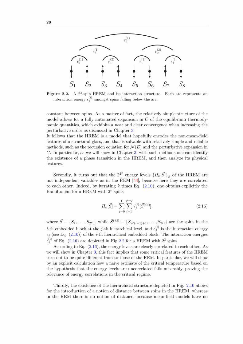
Figure 2.2. A 23-spin HREM and its interaction structure. Each arc represents aninteraction energy ε(i)j amongst spins falling below the arc.
constant between spins. As a matter of fact, the relatively simple structure of themodel allows for a fully automated expansion in C of the equilibrium thermody-namic quantities, which exhibits a neat and clear convergence when increasing theperturbative order as discussed in Chapter 3.It follows that the HREM is a model that hopefully encodes the non-mean-fieldfeatures of a structural glass, and that is solvable with relatively simple and reliablemethods, such as the recursion equation for N (E) and the perturbative expansion inC. In particular, as we will show in Chapter 3, with such methods one can identifythe existence of a phase transition in the HREM, and then analyze its physicalfeatures.
Secondly, it turns out that the 22k energy levels {Hk[~S]}~S of the HREM arenot independent variables as in the REM [53], because here they are correlatedto each other. Indeed, by iterating k times Eq. (2.10), one obtains explicitly theHamiltonian for a HREM with 2k spins
Hk[~S] =k∑j=0
2k−j∑i=1
ε(i)j [~S(j,i)], (2.16)
where ~S ≡ {S1, · · · , S2k}, while ~S(j,i) ≡ {S2j(i−1)+1, · · · , S2ji} are the spins in thei-th embedded block at the j-th hierarchical level, and ε(i)j is the interaction energyεj (see Eq. (2.10)) of the i-th hierarchical embedded block. The interaction energiesε(i)j of Eq. (2.16) are depicted in Fig 2.2 for a HREM with 23 spins.
According to Eq. (2.16), the energy levels are clearly correlated to each other. Aswe will show in Chapter 3, this fact implies that some critical features of the HREMturn out to be quite different from to those of the REM. In particular, we will showby an explicit calculation how a naive estimate of the critical temperature based onthe hypothesis that the energy levels are uncorrelated fails miserably, proving therelevance of energy correlations in the critical regime.
Thirdly, the existence of the hierarchical structure depicted in Fig. 2.10 allowsfor the introduction of a notion of distance between spins in the HREM, whereasin the REM there is no notion of distance, because mean-field models have no

29
spatial geometry [119]. As we will show in Chapter 4, such a length scale can beintroduced in the HREM by defining a suitable correlation function, and extractingthe characteristic length scale associated with its exponential decay at large distances.It is then interesting to ask oneself whether such a length diverges at the criticalpoint as in ferromagnetic systems [74, 101, 173, 174, 163, 162, 138]. This point willbe investigated in Chapter 4, by means of the perturbative expansion method.
We will now present the perturbative computation of the equilibrium propertiesof the HREM, and discuss the results on the critical behavior of the model [33].


Chapter 3
Perturbative computation ofthe free energy
Given a sample of the random energies {ε} ≡ {ε(i)j }j,i, the free energy of a HREMwith 2k spins is defined as [115, 119]
f [T, {ε}] ≡ − 1β2k log [Z [T, {ε}]] , (3.1)
whereZ [T, {ε}] ≡
∑~S
exp(−βHk[~S]
), (3.2)
β ≡ 1/T is the inverse temperature, and Hk[~S] is given by Eq. (2.16). To simplifythe notation, in the following we omit the volume label k in the free energy f andin the partition function Z unless necessary.
The free energy (3.1) of a typical sample {ε} can be computed by hypothesizingthat the self-averaging property holds. According to this property, holding in thethermodynamic limit of a broad class of disordered systems with quenched disorder[119, 37], the free energy computed on a fixed and typical sample of the disorder isequal to the average value of the free energy over the disorder. Here we hypothesizethat this property holds, so that in the thermodynamic limit k →∞ we computef [T, {ε}] on a typical sample {ε} as the average of Eq. (3.1) over the random energies
limk→∞
f [T, {ε}] = limk→∞
Eε [f [T, {ε}]] . (3.3)
The advantage of using the self-averaging property is that the right-hand sideof Eq. (3.3) is easier to compute than the left-hand side by using the replica trick[119, 115]
Eε [f [T, {ε}]] = − 1β2k lim
n→0
Eε [Z[T, {ε}]n]− 1n
. (3.4)
According to the general prescriptions of the replica trick [119, 136, 133, 37], theargument of the limit in Eq. (3.4) is here computed for integer n, and an analyticfunction of n is obtained. The left-hand side of (3.4) is then computed by continuingsuch a function to real n, and taking its n→ 0 limit.
31

32 3. Perturbative computation of the free energy
As observed in Section 1, the use of the replica trick in mean-field models can benon-rigorous, because of the assumption that one can exchange the thermodynamiclimit and the n → 0 limit [119, 115, 136, 37]. It is important to observe that thisissue does not occur in this case. Indeed, by using Eqs. (3.1), (3.3) and (3.4), onehas
limk→∞
f [T, {ε}] = limk→∞
limn→0
1− Eε [Z[T, {ε}]n]nβ2k . (3.5)
In order to compute Eq. (3.5) in mean-field models, one hypothesizes that one canfirst compute the right-hand side of Eq. (3.6) in the thermodynamic limit k →∞by using the saddle-point approximation, and then take n→ 0, by exchanging thelimits. Being the HREM a non-mean-field model, the saddle-point approximationis wrong even in the thermodynamic limit, so that the right-hand side of Eq. (3.5)cannot be computed by taking its saddle point, and we do not need to exchangethe limits. Hence, the subtleties resulting from the exchange of the limits do notoccur in this case. In other words, here the replica trick is simply a convenient wayto perform the computation of the quenched free energy, and a direct inspection ofEq. (3.5) in perturbation theory shows that one can do the computation withoutreplicas, and obtain the same result as that obtained with the replica trick to anyorder in C. We observe that this fact is true also in the mean-field theory of spinglasses, where the full-RSB solution [133] can be rederived [118] without making useof the replica method.
Let us now focus on the explicit computation of the right-hand side of Eq. (3.5)for integer n and on the n→ 0-limit. One has
Eε [Z[T, {ε}]n] =∑
{~Sa}a=1,··· ,n
exp
β2
4
k∑j=0
C2j2k−j∑i=1
n∑a,b=1
δ~S(j,i)a ,~S
(j,i)b
, (3.6)
where ~S1, · · · , ~Sn denote the spin configurations of the n replicas of the system[136, 137, 37, 130]. We then expand Eq. (3.6) in power of C2, and take then→ 0, k →∞-limits. It is important to observe that this C2-expansion is equivalentto a high-temperature expansion. Indeed, in Eq. (3.6) any power C2j of the couplingconstant is multiplied by a factor β2, so that the smallness of C2 is equivalent tothe smallness of the inverse temperature β.By Eq. (3.5), the expansion of Eq. (3.6) in powers of C2 results into an expansionfor f [T, {ε}], that can be written as
f [T, {ε}] =∞∑i=0
C2iφi(T ), (3.7)
where for simplicity we omit the k →∞-limit, and the dependence of f on {ε} hasdisappeared because of the self-averaging property (3.3). The coefficients φi(T ) canbe explicitly calculated for large i by means of a symbolic manipulation program [170],handling the tensorial operations on the replica indices [33, 32]. This computationis carried on for integer n and an analytic function of n is obtained, so that thelimit n→ 0 can be safely taken. In Appendix B we give an example of how thesecomputations are performed, by doing the explicit calculation of the coefficient φ0.

33
In the following, the expansion (3.7) will be worked out at a fixed order l, under theunderlying assumption that the resulting free energy
fl(T ) ≡l∑
i=0C2iφi(T ) (3.8)
approximates the exact free energy (3.7) as l is large
fl(T ) l→∞→ f∞(T ) = f [T, {ε}].
Before discussing the result of this computation for 0 < σ < 1, it is interestingto test perturbation theory in the region σ < 0 for the following reason. As statedin Section 2.2, for σ < 0 the thermodynamic limit of the model is ill-defined. Thisis because the interaction energy εk defined in Eq. (2.10) grows with k faster thanthe volume 2k according to Eq. (2.12). Notwithstanding this, having the HREM 2kspins, one can redefine the inverse temperature
β → 2kσ/2β, (3.9)
in such a way that the variance of εk defined in Eq. (2.12) becomes
Eε[ε2k]→ 2k. (3.10)
The thermodynamic limit is now well-defined, because the coupling energy scales asthe volume, and the model is a purely mean-field one. A direct numerical inspectionof the expansion (3.8) after such a redefinition of β for σ < 0 shows that as l isincreased the free energy of the HREM converges to that of a REM [53, 54] withcritical temperature
T σ<0c U ≡ 1
2√
log 2(1− 2σ). (3.11)
The label U in Eq. (3.14) stands for uncorrelated, because the value (3.14) of thecritical temperature can be easily worked out by hypothesizing that the energy levelsare uncorrelated as in the REM. Indeed, the fact that the free energy (3.8) convergesto that of the REM for σ < 0 tells us that in this region correlations are irrelevant,and the model reduces to a purely mean-field one with the same features as the REM.This is what we expected from the fact that the energy scales as the system vol-ume (Eq. (3.10)), and serves as an important test of the perturbative expansion (3.7).
We now focus on the region 0 < σ < 1. From a direct analysis of the data for thefree energy fl(T ), it turns out that there exists an l-dependent critical temperatureT lc , defined in such a way that the entropy at the l-th order in C2 vanishes at T = T lc
sl(T lc) ≡ −dfl(T )dT
∣∣∣∣T=T lc
= 0. (3.12)
As discussed in Section 1, in the REM the fact that the entropy vanishes at a giventemperature signals a Kauzmann phase transition. Hence, by definition T lc can be

34 3. Perturbative computation of the free energy
considered as the l-th order critical temperature of the system. Since perturbationtheory is approximate, and there is no guarantee that a perturbative expansionconverges at a critical point [74, 173, 174, 138], it is important to check the behaviorof T lc as l is increased. In Fig. 3.1, T lc as a function of l is depicted for σ = 0.1.Even for l ≤ 10, a clear convergence is observed, and the resulting ‘exact’ criticaltemperature T∞c is easily determined by fitting T lc vs. l with a function of the forma − b × cl, with c < 1, and setting T∞c = a. In this way, T∞c as a function of σ isdetermined in the region 0 ≤ σ ≤ 0.15, where T lc vs. l for l ≤ 10 exhibits a clearconvergence as a function of l, and the extrapolation for l→∞ is meaningful.
According to Eq. (3.12), the entropy of the HREMThe HREM has afinite temperaturephase transition à
la Kauzmann. s(T ) ≡ −df∞(T )dT
(3.13)
vanishes for T = T∞c . This allows a straightforward interpretation of the phasetransition occurring at T = T∞c , resembling to that occurring in the REM [53]: forT > T∞c the entropy is positive, and the system explores an exponentially large num-ber of states in the configuration space, while for T < T∞c the system is trapped in ahandful of low-lying energy states. We have thus shown that the HREM undergoesa phase transition à la Kauzmann at a finite temperature T∞c , whose features aresimilar to that of the phase transition of the REM and, more generally, of mean-fieldstructural glasses [16].
In the inset of Fig. 3.1, T∞c as a function of σ is depicted, and T∞c turns out tobe a decreasing function of σ. This fact is physically meaningful, because accordingto Eq. (2.13), the larger σ the smaller the coupling C between spins, and so thesmaller the temperature T∞c such that for T < T∞c all the spins are frozen in alow-lying energy state.As in the σ < 0-case, we can hypothesize that the energy levels act as uncorrelatedrandom variables, in such a way that the HREM behaves as a REM. In this case,the critical temperature can be computed exactly, and is given by
T σ>0c U ≡ 1
2√
log 2(1− 2−σ). (3.14)
Differently from the σ < 0-case, here the decorrelation hypothesis turns out to bewrong. Indeed, by looking at the inset of Fig 3.1, T∞c does not coincide with T σ>0
c U .This fact is a clear evidence that correlations between the energy levels play a crucialrole in the region σ > 0, and cannot be neglected.
In Fig 3.2 the free energy fl(T ) as a function of the temperature T for σ = 0.1and different values of l ≤ 10 is depicted. fl(T ) is found to converge to a finitevalue f∞(T ) for T > T∞c , while for T < T∞c the lower the temperature the worsethe convergence of the sequence fl(T ) vs. l. Hence, when descending into thelow-temperature phase from T > T∞c , a breakdown of perturbation theory occurs,signaling the possibility of a nonanalyticity of the free energy at the critical point,resembling to the nonanalytical behavior of physical quantities occurring in second-order phase transitions for ferromagnetic systems [74, 101, 173, 174, 138].

35
0
0.5
1
1.5
2
0 2 4 6 8 10
Tl c
l
0
0.5
1
1.5
2
0 2 4 6 8 10
Tl c
l
0
0.5
1
1.5
2
0 2 4 6 8 10
Tl c
l
0
2
4
6
8
0 0.05 0.1 0.15
T∞ c
σ
0
2
4
6
8
0 0.05 0.1 0.15
T∞ c
σ
T ∞c
a − b × clT l
c
T ∞c
T σ>0c U
Figure 3.1. Critical temperature T lc (black points), its fitting function a− b× cl (red solidcurve) and asymptotic value T∞c = 1.861± 0.021 (blue dashed line) as a function of lfor σ = 0.1. T∞c = a has been determined as a fit parameter. Inset: critical temperatureT∞c (red points) in the region 0 < σ < 0.15 where the first 10 orders of the perturbativeexpansion show a clear convergence, and critical temperature Tσ>0
c U (black curve), as afunction of σ. The error bars on T∞c are an estimate of the error resulting from the fiton the parameter a. T∞c is clearly non-consistent with Tσ>0
c U , showing that correlationsbetween energy levels are important. The σ → 0+-limit of T∞c does not coincide withthe σ → 0−-limit of Tσ<0
c U because of the abrupt change (3.9) in the normalization ofthe temperature when switching from σ > 0 to σ < 0.
According to the above discussion, the perturbative expansion (3.7) yields areliable method to estimate physical quantities in the high-temperature phaseT > T∞c . Notwithstanding this, no conclusions can be drawn on the behavior ofthe free energy in the low-temperature phase with this perturbative framework.In particular, this method gives no insight into the structure of the states of thesystem in the low-temperature phase. An interesting approach yielding a tentativesolution in the low-temperature phase can be worked out by hypothesizing that then replicas ~S1, · · · , ~Sn in Eq. (3.6) are grouped into n/x groups, where each groupis composed by x replicas [119, 115]. For any two replicas a, b in the same groupone has ~Sa = ~Sb. We can look at the small C2-expansion (3.7) in the particularcase where the replicas are grouped as described above. We call the free energyto the l-th order obtained with this ansatz fRSB
l (T, x). RSB stands for replica-symmetry-breaking, and has the same physical interpretation as the ordinary RSBmechanism described in Section 1 for structural glasses: as in the REM, a replica-symmetry-broken structure in the low-temperature phase implies that the systemis no more ergodic, because it is trapped in a handful of low-lying energy states[16, 119, 130, 53, 54, 136, 137, 115]. By performing the computation explicitly, it iseasy to find out that fRSB
l (T, x) = fl(T/x). According to the general prescriptionsof the replica approach [119, 115, 136, 133, 137], as we take the n → 0-limit theparameter x, originally defined as an integer number, has to be treated as a real

36 3. Perturbative computation of the free energy
-4
-3.5
-3
-2.5
-2
-1.5
-1
-0.5
1.5 2 2.5 3 3.5 4 4.5 5
f
T
-4
-3.5
-3
-2.5
-2
-1.5
-1
-0.5
1.5 2 2.5 3 3.5 4 4.5 5
f
T
-4
-3.5
-3
-2.5
-2
-1.5
-1
-0.5
1.5 2 2.5 3 3.5 4 4.5 5
f
T
-4
-3.5
-3
-2.5
-2
-1.5
-1
-0.5
1.5 2 2.5 3 3.5 4 4.5 5
f
T
-4
-3.5
-3
-2.5
-2
-1.5
-1
-0.5
1.5 2 2.5 3 3.5 4 4.5 5
f
T
-4
-3.5
-3
-2.5
-2
-1.5
-1
-0.5
1.5 2 2.5 3 3.5 4 4.5 5
f
T
-4
-3.5
-3
-2.5
-2
-1.5
-1
-0.5
1.5 2 2.5 3 3.5 4 4.5 5
f
T
T ∞c
fl(T − T ∞c + T l
c)
f3(T − T ∞c + T 3
c )
f6(T − T ∞c + T 6
c )
f10(T − T ∞c + T 10
c )
f∞(T )
Figure 3.2. Free energy f as a function of temperature T for σ = 0.1. We depictfl(T −T∞c +T lc) for l = 1, 2, · · · , 10 (gray points), f3(T −T∞c +T 3
c ) (green dashed curve),f6(T −T∞c +T 6
c ) (blue dashed curve), f10(T −T∞c +T 10c ) (black dashed curve), and the
extrapolated free energy f∞(T ) as a function of T (red points and solid curve). We alsodepict the critical temperature T∞c (violet dashed line). For any fixed T , f∞(T ) hasbeen obtained by fitting the sequence fl(T − T∞c + T lc) vs. l with a function of the forma− b× cl, with c < 1, and setting f∞(T ) = a. To compute f∞(T ), we used the sequencefl(T −T∞c +T lc) vs. l instead of fl(T ) vs. l because the former has the same limit as thelatter for l→∞, and exhibits a better convergence for the accessible values of l ≤ 10.The error bars on f∞(T ) are given by an estimate of the fit error on the parameter a.
number lying in the interval [0, 1]. Hence, the maximization of fRSBl (T, x) with
respect to x gives x = 1 for T ≥ T lc , and x = T/T lc for T < T lc . It follows thataccording to this this RSB ansatz the exact free energy reads
fRSB∞ (T ) =
{f∞(T∞c ) T < T∞cf∞(T ) T ≥ T∞c
. (3.15)
The form (3.15) of the RSB free energy is the same as that of the REM [119, 53, 54],and predicts that in the low-temperature phase the HREM has a one-step RSB,reflecting ergodicity breaking. On the one hand, this RSB ansatz predicts a freeenergy f∞(T ) which is exact for T ≥ T∞c , because it coincides with the free energycomputed with perturbation theory without making use of any ansatz. On the otherhand, there is no guarantee that fRSB is exact in the low-temperature phase. Inparticular, the n replicas could be grouped in a more complicated pattern than theRSB one described above, and this configuration could yield a free energy that islarger than fRSB for T < T∞c . Since in the replica method the exact free energy isnot the minimum, but the maximum of the free energy as a function of the orderparameter configurations [115, 119], such a more complicated pattern would yieldthe exact free energy of the system. The investigation of the existence of such anoptimal pattern is an extremely interesting question that could be subject of futurework, and give some insight into the low-temperature phase of the HREM, andmore generally into the low-temperature features of non-mean-field structural glasses.

37
Once the existence of a phase transition has been established, we ask ourselveswhat are its physical features. In particular, an interesting question is whether,as in second-order phase transitions [74, 163, 162, 173, 174], the system has nocharacteristic scale length at the critical point. Indeed, answering this questionfor the HREM is particularly interesting, because an analysis of the characteristiclength scales of the system in the critical region could give some insight into theconstruction of a RG theory for non-mean-field structural glasses.

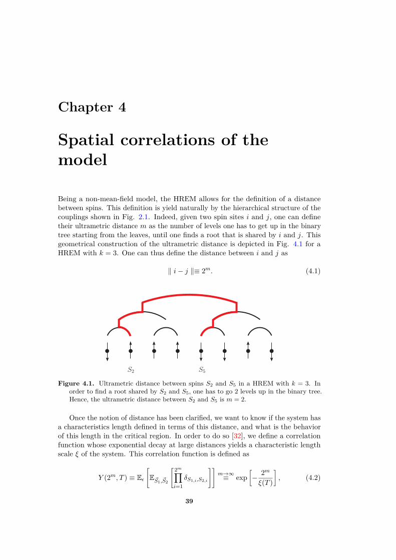
Chapter 4
Spatial correlations of themodel
Being a non-mean-field model, the HREM allows for the definition of a distancebetween spins. This definition is yield naturally by the hierarchical structure of thecouplings shown in Fig. 2.1. Indeed, given two spin sites i and j, one can definetheir ultrametric distance m as the number of levels one has to get up in the binarytree starting from the leaves, until one finds a root that is shared by i and j. Thisgeometrical construction of the ultrametric distance is depicted in Fig. 4.1 for aHREM with k = 3. One can thus define the distance between i and j as
‖ i− j ‖≡ 2m. (4.1)
S2 S5
Figure 4.1. Ultrametric distance between spins S2 and S5 in a HREM with k = 3. Inorder to find a root shared by S2 and S5, one has to go 2 levels up in the binary tree.Hence, the ultrametric distance between S2 and S5 is m = 2.
Once the notion of distance has been clarified, we want to know if the system hasa characteristics length defined in terms of this distance, and what is the behaviorof this length in the critical region. In order to do so [32], we define a correlationfunction whose exponential decay at large distances yields a characteristic lengthscale ξ of the system. This correlation function is defined as
Y (2m, T ) ≡ Eε
[E~S1,~S2
[2m∏i=1
δS1,i,S2,i
]]m→∞≡ exp
[− 2m
ξ(T )
], (4.2)
39
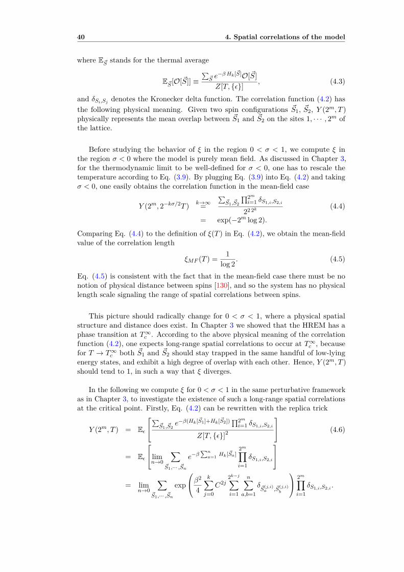
40 4. Spatial correlations of the model
where E~S stands for the thermal average
E~S [O[~S]] ≡∑
~S e−β Hk[~S]O[~S]Z[T, {ε}] , (4.3)
and δSi,Sj denotes the Kronecker delta function. The correlation function (4.2) hasthe following physical meaning. Given two spin configurations ~S1, ~S2, Y (2m, T )physically represents the mean overlap between ~S1 and ~S2 on the sites 1, · · · , 2m ofthe lattice.
Before studying the behavior of ξ in the region 0 < σ < 1, we compute ξ inthe region σ < 0 where the model is purely mean field. As discussed in Chapter 3,for the thermodynamic limit to be well-defined for σ < 0, one has to rescale thetemperature according to Eq. (3.9). By plugging Eq. (3.9) into Eq. (4.2) and takingσ < 0, one easily obtains the correlation function in the mean-field case
Y (2m, 2−kσ/2T ) k→∞=∑
~S1,~S2
∏2mi=1 δS1,i,S2,i
22 2k (4.4)
= exp(−2m log 2).
Comparing Eq. (4.4) to the definition of ξ(T ) in Eq. (4.2), we obtain the mean-fieldvalue of the correlation length
ξMF (T ) = 1log 2 . (4.5)
Eq. (4.5) is consistent with the fact that in the mean-field case there must be nonotion of physical distance between spins [130], and so the system has no physicallength scale signaling the range of spatial correlations between spins.
This picture should radically change for 0 < σ < 1, where a physical spatialstructure and distance does exist. In Chapter 3 we showed that the HREM has aphase transition at T∞c . According to the above physical meaning of the correlationfunction (4.2), one expects long-range spatial correlations to occur at T∞c , becausefor T → T∞c both ~S1 and ~S2 should stay trapped in the same handful of low-lyingenergy states, and exhibit a high degree of overlap with each other. Hence, Y (2m, T )should tend to 1, in such a way that ξ diverges.
In the following we compute ξ for 0 < σ < 1 in the same perturbative frameworkas in Chapter 3, to investigate the existence of such a long-range spatial correlationsat the critical point. Firstly, Eq. (4.2) can be rewritten with the replica trick
Y (2m, T ) = Eε
∑~S1,~S2e−β(Hk[~S1]+Hk[~S2])∏2m
i=1 δS1,i,S2,i
Z[T, {ε}]2
(4.6)
= Eε
limn→0
∑~S1,··· ,~Sn
e−β∑n
a=1 Hk[~Sa]2m∏i=1
δS1,i,S2,i
= lim
n→0
∑~S1,··· ,~Sn
exp
β2
4
k∑j=0
C2j2k−j∑i=1
n∑a,b=1
δ~S(j,i)a ,~S
(j,i)b
2m∏i=1
δS1,i,S2,i .

41
The last line of Eq. (4.6) is very similar to (3.6), used in Chapter 3 to compute thefree energy of the HREM. Hence, the very same techniques used to compute f inperturbation theory can be employed here to calculate the correlation function Y .In particular, one can expand the correlation function (4.6) in the coupling constantC2
Y (2m, T ) =∞∑i=0
C2iΥm,i(T ), (4.7)
and explicitly evaluate the coefficients Υm,i by a symbolic manipulation program[170] until the order i = 9. In Appendix C we present the steps of the computation ofΥm,0(T ), to give some insight into the main techniques employed in the calculationto high orders.
For any fixed m and T , the exact value of Y (2m, T ) has been computed byextrapolating the sequence
Yl(2m, T ) ≡l∑
i=0C2iΥm,i(T ) (4.8)
to l →∞, with the underlying assumption that for large l Eq. (4.8) converges tothe exact value of the correlation function
Yl(2m, T ) l→∞→ Y∞(2m, T ) = Y (2m, T ).
The sequence Yl(2m, T ) as a function of m for fixed σ, l and T is shown in Fig.4.2 for m = 3, T = 3.5. Even though Yl is nicely convergent even to relatively loworders for the values of m and T considered in Fig. 4.2, an explicit analysis ofYl(2m, T ) for different values of m shows that the larger m, the larger the numberof orders needed to see a nice convergence with respect to l. This fact can be easilyunderstood by recalling that the C2-expansion is equivalent to a high-temperatureexpansion (see Chapter 3). It is a general feature of high-temperature expansions[172, 30, 146, 51] that with a finite number of orders of the β-series, one cannotdescribe arbitrarily large length scales. Hence, with a finite number of orders (9 inour case) for Yl(2m, T ), one cannot describe the correlations Yl(2m, T ) for too largem.Another important fact is that, for any fixed m the convergence of Yl(2m, T ) getsworse as the temperature T is decreased, because more terms in the β-expansion,and so in the C2 expansion, are needed.Practically speaking, these limitations of the perturbative expansion made us takem ≤ 3 and T > T0, where T0 is a σ-dependent value of the temperature signaling abreakdown of perturbation theory. As we will discuss in the following, notwithstand-ing the very small values of m here available, it has been possible to compute thecorrelation length ξ(T ) defined in Eq. (4.2) in a wide interval of temperatures.
The correlation length ξ(T ) has been computed for every temperature T byfitting the data for Y∞(2m, T ) vs. m, according to the definition of ξ(T ) given inEq. (4.2).
Once ξ(T ) is known, we investigate its behavior at low temperatures. As statedabove, one cannot take too low values of T because of the non-convergence of the

42 4. Spatial correlations of the model
0.008
0.0082
0.0084
0.0086
0.0088
0.009
0.0092
2 3 4 5 6 7 8 9 10
Yl(
2m
,T)
l
0.008
0.0082
0.0084
0.0086
0.0088
0.009
0.0092
2 3 4 5 6 7 8 9 10
Yl(
2m
,T)
l
0.008
0.0082
0.0084
0.0086
0.0088
0.009
0.0092
2 3 4 5 6 7 8 9 10
Yl(
2m
,T)
l
Y∞(2m, T )
a − b × cl
Yl(2m, T )
Figure 4.2. Yl(2m, T ) (black points), its fitting function a− b× cl (blue dashed curve) asa function of l, and Y∞(2m, T ) = a (red solid line), determined as a fit parameter. Hereσ = 0.1,m = 3 and T = 3.5.
perturbative expansion. Notwithstanding this, it is still possible to approach enoughthe critical point T∞c and investigate the existence of long-range spatial correlations.In particular, we test the validity of the hypothesis of a diverging ξ(T ) for T → T∞c .In order to do so, we check whether the data for ξ(T ) is consistent with a power-lawdivergence at some temperature T ξc
ξ(T )T→T ξc≈ C
(T − T ξc )ν. (4.9)
The validity of the hypothesis (4.9) has been tested in the following way. We supposethat Eq. (4.9) holds, and determine the value of T ξc such that the data for ξ(T ) bestfits with Eq. (4.9). We fit the data for log [ξ(T )] vs. log(T − T ξc ) for different valuesof T ξc . The value T ξc such that log [ξ(T )] vs. log(T −T ξc ) best fits with a straight line,is such that the data for ξ(T ) is consistent with a power-law divergence at T ξc , accord-ing to (4.9). The top panel of Fig. 4.3 shows that for σ = 0.1 the optimal value ofT ξc is compatible with the critical temperature T∞c for σ = 0.1 obtained in Chapter 3.
The data for ξ(T ) is thus consistent with a diverging correlation length at theThe data for thecorrelation lengthof the HREM isconsistent with a
power-lawdivergence at the
Kauzmanntransition
temperature.
Kauzmann transition temperature T∞c . In the bottom panel of Fig. 4.3, ξ(T ) asa function of T for σ = 0.1 is depicted, together with its fitting function (4.9)with T ξc = T∞c . ξ(T ) increases as the temperature is decreased, and its shape iscompatible with a power-law divergence at the Kauzmann transition temperatureT∞c .
Since this work establishes the existence of a thermodynamic phase transitionand the possibility of a diverging correlation length in the HREM, it also shows the
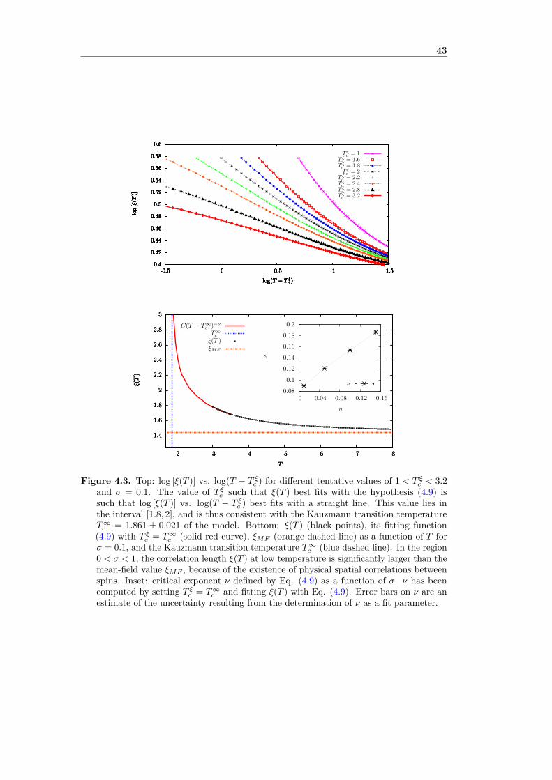
43
0.4
0.42
0.44
0.46
0.48
0.5
0.52
0.54
0.56
0.58
0.6
-0.5 0 0.5 1 1.5
log
[ξ(T
)]
log(T − T ξc )
0.4
0.42
0.44
0.46
0.48
0.5
0.52
0.54
0.56
0.58
0.6
-0.5 0 0.5 1 1.5
log
[ξ(T
)]
log(T − T ξc )
0.4
0.42
0.44
0.46
0.48
0.5
0.52
0.54
0.56
0.58
0.6
-0.5 0 0.5 1 1.5
log
[ξ(T
)]
log(T − T ξc )
0.4
0.42
0.44
0.46
0.48
0.5
0.52
0.54
0.56
0.58
0.6
-0.5 0 0.5 1 1.5
log
[ξ(T
)]
log(T − T ξc )
0.4
0.42
0.44
0.46
0.48
0.5
0.52
0.54
0.56
0.58
0.6
-0.5 0 0.5 1 1.5
log
[ξ(T
)]
log(T − T ξc )
0.4
0.42
0.44
0.46
0.48
0.5
0.52
0.54
0.56
0.58
0.6
-0.5 0 0.5 1 1.5
log
[ξ(T
)]
log(T − T ξc )
0.4
0.42
0.44
0.46
0.48
0.5
0.52
0.54
0.56
0.58
0.6
-0.5 0 0.5 1 1.5
log
[ξ(T
)]
log(T − T ξc )
0.4
0.42
0.44
0.46
0.48
0.5
0.52
0.54
0.56
0.58
0.6
-0.5 0 0.5 1 1.5
log
[ξ(T
)]
log(T − T ξc )
T ξc = 1
T ξc = 1.6
T ξc = 1.8T ξ
c = 2T ξ
c = 2.2T ξ
c = 2.4T ξ
c = 2.8T ξ
c = 3.2
1.4
1.6
1.8
2
2.2
2.4
2.6
2.8
3
2 3 4 5 6 7 8
ξ(T
)
T
1.4
1.6
1.8
2
2.2
2.4
2.6
2.8
3
2 3 4 5 6 7 8
ξ(T
)
T
1.4
1.6
1.8
2
2.2
2.4
2.6
2.8
3
2 3 4 5 6 7 8
ξ(T
)
T
1.4
1.6
1.8
2
2.2
2.4
2.6
2.8
3
2 3 4 5 6 7 8
ξ(T
)
T
0.08
0.1
0.12
0.14
0.16
0.18
0.2
0 0.04 0.08 0.12 0.16
ν
σ
C(T − T ∞c )−ν
T ∞c
ξ(T )ξMF
ν
Figure 4.3. Top: log [ξ(T )] vs. log(T − T ξc ) for different tentative values of 1 < T ξc < 3.2and σ = 0.1. The value of T ξc such that ξ(T ) best fits with the hypothesis (4.9) issuch that log [ξ(T )] vs. log(T − T ξc ) best fits with a straight line. This value lies inthe interval [1.8, 2], and is thus consistent with the Kauzmann transition temperatureT∞c = 1.861 ± 0.021 of the model. Bottom: ξ(T ) (black points), its fitting function(4.9) with T ξc = T∞c (solid red curve), ξMF (orange dashed line) as a function of T forσ = 0.1, and the Kauzmann transition temperature T∞c (blue dashed line). In the region0 < σ < 1, the correlation length ξ(T ) at low temperature is significantly larger than themean-field value ξMF , because of the existence of physical spatial correlations betweenspins. Inset: critical exponent ν defined by Eq. (4.9) as a function of σ. ν has beencomputed by setting T ξc = T∞c and fitting ξ(T ) with Eq. (4.9). Error bars on ν are anestimate of the uncertainty resulting from the determination of ν as a fit parameter.

44 4. Spatial correlations of the model
way forward to the study of finite-dimensional spin or structural-glass models.For instance, the REM has been found [154, 26] to have a dynamical phase transitionat finite temperature if a particular dynamics is chosen: it would be interestingto study these dynamical properties in the HREM, by introducing some suitabledynamics of the spins, and by investigating the existence of a dynamical phasetransition, and of a diverging dynamical correlation length.Another interesting future direction would be to generalize the techniques used inthe solution of the REM to more realistic non-mean-field spin or structural-glassmodels, like p-spin models [50] built on a hierarchical lattice. Indeed, even thoughthe HREM serves as a model representing a non-mean-field structural glass, itsstructure is still far from being realistic: strictly speaking, the spins ~S in the HREMare not physical degrees of freedom, but serve as mere labels for the energy variablesHk[~S] as in the REM [53, 115, 130]. Moreover, a criticism one could address to thesolution techniques developed in Chapters 3 and 4 is that these do not give anyinsight into the construction of a suitable RG protocol. In particular, a decimationrule on spins is still lacking.
In the following Part we introduce a HM of a spin glass, in the effort to addressthese two points: in such a HM spins are real physical degrees of freedom, in such away that a decimation rule on spins naturally emerges, and one can explicitly solvethe resulting RG equations.

Part III
The HierarchicalEdwards-Anderson Model
45


47
As discussed in Section 1, the SK model is a mean-field spin glass, whose criticalproperties have been clarified in Parisi’s solution [133, 136, 137, 119, 115, 130].Whether the physical features of this solution persist also in a non-mean-field versionof the SK, or the non-mean-field case is described by a radically different scheme[111, 64, 61, 60, 62, 63, 27, 125], is one of the most hotly debated topics in sta-tistical physics. Being this a very difficult question, it is interesting to considernon-mean-field versions of the SK that presumably capture all the non-mean-fieldphysics, and that are simple enough to be solved quite easily, by means of an explicitimplementation of the RG transformation.
Starting from the general definition (2.10) of Hierarchical models given in Section2.2, here we explicitly chose the random energies εk to build up a non-mean-fieldversion of the SK model having these features: the Hierarchical Edwards-Andersonmodel (HEA) [65, 34, 35, 36]. The HEA is defined by choosing the random energyεk in the following way [65]
εk+1[S1, . . . , S2k+1 ] ≡ −(C2
2
)k+1 2k+1∑i<j=1
J12,ijSiSj , (4.10)
where C is still defined by Eq. (2.13), and J12,ij are Gaussian random variables withzero mean and unit variance.
Starting from Eq. (4.10) and from the definition of the J12s, it is easy to showthat εk+1 has zero mean, and that its variance satisfies
Eε[ε2k]k→∞∼ 22k(1−σ). (4.11)
It follows that for σ < 1/2 the interaction energy (6.35) grows faster than the volume2k, and the thermodynamic limit k → ∞ is not defined. The purely mean-fieldcase, i. e. the case where the interaction energy scales with k as the volume 2k, isrecovered for σ = 1/2. Moreover, for σ > 1 the interaction energy (6.35) goes to 0as k →∞, in such a way that no phase transition can occur. Hence, in the followingwe will take
1/2 < σ < 1, (4.12)
which is the equivalent of Eq. (2.3) for DHM.
Physically speaking, the interaction energy (4.10) of the HEA introduces two-spin interactions, while the interaction energy of the HREM defined in Part II has2k+1-spin interactions. Another fundamental difference between the HEA and theHREM is that, according to the general classification of models with quencheddisorder given in Section 1, the HEA has to be considered as a model for a spinglass, while the HREM as a model mimicking the physics of a structural glass [16].Compared to the HREM, the HEA is a more realistic model, because according tothe definition (4.10), here the spins of the system are physical degrees of freedom,and not mere labels for the energy variables as in the REM and in the HREM. Aswe will see in the following, the HEA also allows for an explicit construction of asuitable decimation rule on spins, and so of a RG transformation.
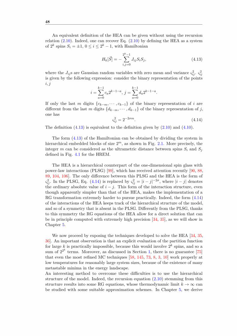
48
An equivalent definition of the HEA can be given without using the recursionrelation (2.10). Indeed, one can recover Eq. (2.10) by defining the HEA as a systemof 2k spins Si = ±1, 0 ≤ i ≤ 2k − 1, with Hamiltonian
Hk[~S] = −2k−1∑i,j=0
JijSiSj , (4.13)
where the Jijs are Gaussian random variables with zero mean and variance ς2ij . ς2
ij
is given by the following expression: consider the binary representation of the pointsi, j
i =k−1∑a=0
ca2k−1−a, j =k−1∑a=0
da2k−1−a.
If only the last m digits {ck−m, · · · , ck−1} of the binary representation of i aredifferent from the last m digits {dk−m, · · · , dk−1} of the binary representation of j,one has
ς2ij = 2−2σm. (4.14)
The definition (4.13) is equivalent to the definition given by (2.10) and (4.10).
The form (4.13) of the Hamiltonian can be obtained by dividing the system inhierarchical embedded blocks of size 2m, as shown in Fig. 2.1. More precisely, theinteger m can be considered as the ultrametric distance between spins Si and Sjdefined in Fig. 4.1 for the HREM.
The HEA is a hierarchical counterpart of the one-dimensional spin glass withpower-law interactions (PLSG) [99], which has received attention recently [90, 88,89, 104, 106]. The only difference between this PLSG and the HEA is the form ofς2ij . In the PLSG, Eq. (4.14) is replaced by ς2
ij = |i − j|−2σ, where |i − j| denotesthe ordinary absolute value of i − j. This form of the interaction structure, eventhough apparently simpler than that of the HEA, makes the implementation of aRG transformation extremely harder to pursue practically. Indeed, the form (4.14)of the interactions of the HEA keeps track of the hierarchical structure of the model,and so of a symmetry that is absent in the PLSG. Differently from the PLSG, thanksto this symmetry the RG equations of the HEA allow for a direct solution that canbe in principle computed with extremely high precision [34, 35], as we will show inChapter 5.
We now proceed by exposing the techniques developed to solve the HEA [34, 35,36]. An important observation is that an explicit evaluation of the partition functionfor large k is practically impossible, because this would involve 2k spins, and so asum of 22k terms. Moreover, as discussed in Section 1, there is no guarantee [75]that even the most refined MC techniques [58, 145, 73, 8, 3, 10] work properly atlow temperatures for reasonably large system sizes, because of the existence of manymetastable minima in the energy landscape.An interesting method to overcome these difficulties is to use the hierarchicalstructure of the model. Indeed, the recursion equation (2.10) stemming from thisstructure results into some RG equations, whose thermodynamic limit k →∞ canbe studied with some suitable approximation schemes. In Chapter 5, we derive

49
these RG equations with the replica approach, and analyze their fixed points withstandard field-theory techniques. We show that notwithstanding their simplicity, theperturbative solution of these RG equations results into a perturbative series whichis probably non-convergent. Hence, an alternative real-space approach which doesnot rely on the replica method is developed in Chapter 6. In this latter approach,the hierarchical structure of the model is again used to write some RG equationsthat can be solved numerically with high precision. The replica RG approach andthe real-space approach are then compared, by considering their predictions on thecritical exponents of the model.

Chapter 5
The RG in the replica approach
In this Chapter we derive and solve the RG equations for the HEA model with thereplica approach [34, 35]. These RG equations can be derived with two differentmethods. The first, exposed in Section 5.1, derives the RG equations by usingdirectly the hierarchical structure of the model. We will call this approach method àla Wilson, because it implements a coarse-graining RG step relating a 2k-spin HEAto a 2k+1-spin HEA, and this yields a RG equation similar to the RG equationsoriginally obtained by Dyson [57, 44, 45, 31] for DHM, and so analogous to Wilson’sRG equations [161, 164, 165, 163]. The second approach, exposed in Section 5.2,reformulates the problem in terms of a φ3-field theory [173], and the resulting RGequations are nothing but the Callan-Symanzig equations [173, 174] for such a fieldtheory. The two formulations are tested to be equivalent by an explicit computationof the critical exponents.
5.1 The RG method à la Wilson
Let us consider the partition function Z[T, {ε}] of a HEA with 2k spins, which isdefined by Eq. (3.2). According to the general features of the replica approach[119, 115, 130, 65], the physics of the model is encoded into the n→ 0 limit of then-times replicated partition function
Eε[Z[T, {ε}]n] = Eε
∑{~Sa}a=1,...,n
exp(−β
n∑a=1
Hk[~Sa]) , (5.1)
where Eε denotes the expectation value with respect to the random distribution ofthe energies εk, i. e. with respect to all the random couplings J12, ij of Eq. (4.10),and ~Sa is the spin configuration of the a-th replica of the system. One can thenconsider the n × n matrix Qab [119, 115, 130] physically representing the overlapbetween replicas a and b, which is defined as
Qab ≡12k
2k∑i=1
Sa,iSb,i ∀a 6= b,
Qaa ≡ 0 ∀a.
51

52 5. The RG in the replica approach
An interesting quantity which is derived from (5.1) is the probability distribution ofthe overlap over the quenched disorder {ε}
Pk[Q] ≡ Eε
∑{~Sa}a=1,...,n
exp(−β
n∑a=1
Hk[~Sa])
n∏a<b=1
δ
Qab − 12k
2k∑i=1
Sa,iSb,i
,(5.2)
where the volume dependence has been explicitly restored with the label k in Pk,and δ denotes the Dirac delta function. The quantity Pk[Q] is interesting becausewhen one iterates the recursion equation (2.10), and a 2k+1-spin HEA is built up,the resulting Pk+1 can be related to Pk by a simple recursion equation, which is
Pk+1[Q] = exp(β2C4(k+1)
4 Tr[Q2])∫
[dQ1dQ2]Pk[Q1]Pk[Q2]× (5.3)
×n∏
a<b=1δ
(Qab −
Q1,ab +Q2,ab2
),
where Tr denotes the trace over the replica indices a, b, . . ., and the integral over thematrix Q is denoted by
∫[dQ] ≡
∫ ∏na<b=1 dQab. Eq. (5.3) is equivalent to the recur-
sion equation (2.5) for DHM [57], and it yields the flow of the function Pk obtainedby coupling two systems with volume 2k to obtain a system with volume 2k+1. Itfollows that Eq. (5.3) can be considered as the flow of Pk under the reparametrization2k → 2× 2k of the length scale [164, 165, 163, 173, 174, 77, 138, 74]. According tothese considerations, Eq. (5.3) is a RG equation.
The very same techniques developed in Section 2.1 and in Appendix A to solveEq. (2.5) for DHM can be used to solve Eq. (5.3). Notwithstanding this, the solutionof Eq. (5.3) turns out to be much more cumbersome than that of Eq. (2.5), becausethe former is a flow equation for a function Pk[Q] of a matrix Qab, while the latteris a flow equation for a function pk(m) of a number m. In what follows we will showthe main steps of the solution of Eq. (5.3).
First of all, we seek for a solution of Eq. (5.3) for k →∞, in order to investigatethe critical properties of the HEA in the thermodynamic limit. To this end, let usrescale the variable Q in Eq. (5.3), by setting
Pk[Q] ≡ Pk[C−2kQ], (5.4)
in such a way that Eq. (5.3) becomes
Pk[Q] = exp(β2
4 Tr[Q2])∫
[dP ] Pk−1
[Q+ P
C2
]Pk−1
[Q− PC2
]. (5.5)
Similarly to Eq. (2.6), Eq. (5.4) is the correct rescaling for Eq. (5.3) to convergeto a nontrivial fixed point for k →∞, because according to Eqs. (2.13), (4.12) onehas C > 1, and the C4(k+1)-term in the right-hand side of Eq. (5.3) is an increasingfunction of k allowing for no nontrivial fixed point for k → ∞. It follows thatphysically speaking, this rescaling aims to look at the RG equations (5.3) on thescales that are relevant for large k, by means of a ‘zoom’ on the function Pk[Q],

5.1 The RG method à la Wilson 53
which is encoded in the definition (5.4). An analogous rescaling will be presented inthe real-space approach discussed in Chapter 6.
Eq. (5.5) can now be solved by making an ansatz for Pk[Q], following the samelines as in the solution of DHM illustrated in Appendix A. The simplest form onecan guess for Pk[Q] is the Gaussian
Pk[Q] = exp(−rkTr[Q2]
). (5.6)
This form corresponds to a mean-field solution [65]. By plugging Eq. (5.6) into Eq.(5.5), one finds an evolution equation relating rk to rk−1
rk = 2rk−1C4 − β2
4 . (5.7)
Even though the mean-field solution (5.6) is a fixed point of the RG equation(5.5), there is no guarantee that more complex and physically meaningful fixedpoints do not exist. By hypothesizing that Pk[Q] can be expanded in powers of Q,non-gaussian fixed points can be explicitly built up in a perturbative framework, byfollowing the same lines as in the Ising model [163] and in DHM [44, 45, 31]. Indeed,we can add non-Gaussian terms in Eq. (5.6), proportional to higher powers of Q,and consistent with the symmetry properties of the model. For instance, in principlethere would be several possible replica invariants proportional to Q3, but it is possibleto show that the only invariant that is consistent with the original symmetries ofthe Hamiltonian Hk is Tr[Q3]. It follows that the simplest non-mean-field ansatz forPk[Q] reads
Pk[Q] = exp[−(rkTr[Q2] + wk
3 Tr[Q3])]
. (5.8)
This non-Gaussian ansatz can be handled by supposing that the coefficient wk,representing the deviations from the Gaussian solution, is small for every k. It isimportant to point out that this is an hypothesis which is equivalent to assuming thatthe non-mean-field regime of this model can be described in terms of a perturbationof the mean-field regime [55]. As discussed in Section 1, there is no general agreementon the fact that the non-mean-field behavior of a spin glass can be described interms of a slight modification of the mean-field picture [111, 64, 61, 60, 62, 63, 27].Hence, one should keep in mind that this assumption is far from being trivial andsurely innocuous.As shown in Appendix D, if one plugs the ansatz (5.8) into the RG equation (5.5)and expands up to O(w3
k), one finds a recursion relation for the vector (rk, wk),which is expressed as a function of (rk−1, wk−1) rk = 2rk−1
C4 − β2
4 −n−2
4
(wk−1
2C2rk−1
)2+O(w4
k−1),
wk = 2wk−1C6 + n−2
2
(wk−1
2C2rk−1
)3+O(w4
k−1).(5.9)
Eqs. (5.9) are analogous to Wilson’s RG equations for the Ising model. Indeed,the mass rk and the coupling constant uk of the φ4-theory describing the Ising model

54 5. The RG in the replica approach
[173] satisfy a recursion equation very similar to Eq. (5.9) [169, 163].
In general Eqs. (5.9) do not have a finite fixed point rk = rk−1 ≡ r∗, wk =wk−1 = w∗ for every value of β. Concerning this, let us suppose that there exists afinite and nonzero inverse temperature βc such that Eqs. (5.9) have a finite fixedpoint. By definition, βc physically represents the inverse temperature such that thesystem is invariant under the RG step k → k + 1, i. e. under reparametrization ofthe length scale. Hence, at βc the system has no characteristic length scale, i. e. itis critical [161]. We call βc the inverse critical temperature of the HEA, because itseparates the high and low-temperature phases β < βc, β > βc where the system isnot invariant under reparametrization of lengths.
We now set β = βc and sketch qualitatively the flow of the coefficient wk towardsits fixed-point value w∗. Let us consider first the case 2/C6 < 1, i. e. ε < 0, with
ε ≡ σ − 2/3. (5.10)
In this case wk is decreased as k → k + 1, and tends to zero, in such a way thatPk[Q] tends to a Gaussian solution for large k.The situation is different when ε > 0. In order to better understand the case ε > 0,let us rewrite the recursion equation for wk as
wk − wk−1 =( 2C6 − 1
)wk−1 + n− 2
2
(wk−1
2C2rk−1
)3+O(w4
k−1), (5.11)
and suppose for simplicity that wk−1 is positive. Being 2/C6 > 1, the first addend inthe right-hand side of Eq. (5.11) is positive, while the second addend is negative in thephysical limit n→ 0. Hence, the first addend aims to increase wk, while the secondaims to decrease it. As we will show in the following, these two effects compensateeach other, in such a way that wk tends to a finite and nonzero fixed point for k →∞.
Following the very same lines as Wilson, we call P∗[Q],P∗[Q] the fixed-pointprobability distributions of the overlap, obtained by setting rk = r∗, wk = w∗ inPk[Q],Pk[Q] respectively. The equations for n = 0 yield
w2∗ =
0 ε ≤ 048 log 2
(β2/4
21/3−1
)3ε+O(ε3/2) ε > 0.
(5.12)
As anticipated above, for ε > 0, wk tends to a finite and nonzero value, which isfound to be proportional to ε in Eq. (5.12).
We recall [44, 45, 31, 163, 173, 174] that a Gaussian P∗[Q] corresponds toa mean-field regime of the model. Indeed, in the mean-field approximation oneevaluates with the saddle-point method the functional integral yielding the replicatedpartition function [119, 130, 115, 133, 136]
Eε[Z [T, {ε}]n] =∫
[dQ]P∗[Q], (5.13)
where Eq. (5.2) and Eq. (5.1) have been used. If σ ≤ 2/3, i. e. ε < 0, P∗[Q] isGaussian, and so is P∗[Q], in such a way that the saddle-point approximation is
5.1 The RG method à la Wilson 55
exact in the right-hand side of Eq. (5.13), i. e. the mean-field approximation iscorrect. On the contrary, for 2/3 < σ ≤ 1, P∗[Q] is not Gaussian, and the systemhas a non-mean-field behavior. In particular, fluctuations around the mean-fieldsaddle point in the right-hand side of Eq. (5.13) cannot be neglected. Hence, wecall σ = 2/3 the upper critical dimension [74, 173, 174, 77] of the HEA.In the computation of a given physical quantity O(σ) for σ > 2/3, fluctuations showup in the guise of some corrections proportional to ε to the mean-field value of thisquantity. It is important to emphasize that these ε-corrections are not merely anumerical improvement on the predictions for the observable, but somehow encodethe strength of the corrections to the mean-field physics. For instance, if O(σ) wasexpanded in powers of ε around σ = 2/3, and if this expansion could be resummedand made convergent, this would mean that the non-mean-field physics of the systemcould be considered as a ‘small correction’ to the mean-field physics. On the contrary,if such a non-mean-field physics were substantially different, the latter statementwould be incorrect, and this fact would dramatically show up in a divergent andnon-resummable ε-series for O(σ).
These observations can be directly illustrated by considering as observable Othe critical exponent ν, related to the divergence of the correlation length ξ
ξT→Tc∼ (T − Tc)−ν . (5.14)
ν can be computed [163] by linearizing the transformation (5.9) in the neighborhoodof r∗, w∗. Such a linearization is performed by considering the 2× 2-matrix
Mij ≡∂(rk+1, wk+1)∂(rk, wk)
∣∣∣∣rk=r∗,wk=w∗
.
It can be shown that ν is related to the largest eigenvalue Λ of M by the relation
ν = log 2log Λ . (5.15)
A straightforward calculation yields ν at order ε, for n = 0
ν ={
12σ−1 σ ≤ 2/33 + 36ε+O(ε2) σ > 2/3. (5.16)
A detailed analysis of the computation of Appendix E reveals that in this O(w3k)-
calculation resulting in the O(ε)-estimate of ν, one considers all the one-particleirreducible (1PI) [173, 158, 159] one-loop Feynman diagrams generated by the Q3-vertex in Eq. (5.8). These are diagrams I1,I7 in Fig. 5.1. Similarly, in thecomputation at order w5
k, resulting in the O(ε2)-estimate of ν, one considers two-loop1PI Feynman diagrams I2, · · · ,I6 and I8, · · · ,I10 in Fig. 5.1, and so on.
As can be seen by Eq. (5.16), the coefficient of ε in Eq. (5.16) is quite large, anit is plausible that the full ε-series of ν does not converge. According to the abovediscussion, the convergence or resummability of the series would give some deepinsight into how strongly the mean-field physical picture should be modified in thenon-mean-field region σ > 2/3. In particular, a non-resummable series would suggest

56 5. The RG in the replica approach
I1 I2
I4
I3
I5 I6
I7 I8 I9
I10
Figure 5.1. One and two-loop 1PI Feynman diagrams deriving from the Tr[Q3]-interactionterm, which contribute to the computation of the critical exponent ν in the method à laWilson presented in Section 5.1, and in the field-theory method presented in Section5.2. In the method à la Wilson, diagrams I1, · · · ,I6 with two external lines haveto be considered without crosses on the internal lines, and represent the diagramscontributing to the Tr[Q2]-term in Pk[Q]. In the same method, it can be shown thatdiagrams I7, · · · ,I10 with three external lines contribute to the Q3, Q4, Q5-terms inPk[Q]. In the field-theory method, diagrams I1, · · · ,I6 and I7, · · · ,I10 contribute tothe 1PI two-point and three-point correlation functions respectively, and crosses standfor Tr[Q2]-insertions [173]. This graphical identification of the same diagrams in the twomethods is an important test of their mutual consistency.
5.1 The RG method à la Wilson 57
that the non-mean-field physics cannot be described in terms of a perturbation ofthe mean-field one, and would have a strong impact on the general problem of spinglasses in finite dimensions. It is thus interesting to investigate the properties of theν-series by directly computing higher orders in ε, and checking the convergence orthe resummability of the series.
The computation of the ε-expansion at high orders can be performed with acomputer program. This is a particular feature of the HEA, because thanks to thehierarchical structure of the system, the RG equations (5.5) have a simple formcompared to the RG equations of the PLSG [99] or of the EA model [72]. Indeed, thelatter are nothing but the Callan-Symanzik equations [28, 147, 173] for a Q3-fieldtheory, and their solution in perturbation theory requires an explicit enumerationof all the Feynman diagrams deriving from the Q3-vertices, and the computationof their IR-divergent part. This enumeration is extremely hard to implement in acomputer program, and has never been automated even in the simplest case of theIsing model [70]. On the contrary, we believe that a symbolic manipulation programcould handle Eqs. (5.5) and automate the computation to higher orders in wk, withno need to evaluate the IR-divergent part of Feynman integrals, which is not neededin the present approach à la Wilson.In order to perform this automation, we have evaluated by hand the first few termsof the series, which has been computed to O(ε2) with the method à la Wilson, andwith a quite independent field-theory method exposed in Section 5.2. Both methodsgive the same two-loop result for ν, which will serve as a severe test for a futureautomation of the ε-expansion to high orders. This automation is very difficult froma purely technical viewpoint, and is beyond the scope of this thesis.
Here we sketch the main steps of the two-loop computation of ν, more detailsare given in [35]. We showed that if we plug the ansatz (5.8) into the right-handside of Eq. (5.5) and systematically neglect terms of order higher than w3
k, we get aPk+1[Q] which is still of the form (5.8), i. e. the RG equations are closed. This isnot true if we keep also terms of order higher than w3
k. Indeed, it is easy to showthat in this case terms of order Q4 arise in the right-hand side of Eq. (5.5), andthese terms are not present in the original ansatz. This fact implies that to O(w4
k),Pk[Q] must contain also Q4-terms, and that these terms must be proportional tow4k. By plugging the fourth-degree polynomial Pk[Q] in Eq. (5.5) and expanding
the right-hand side up to O(w5k), Q5-terms are generated. It follows that at O(w5
k),Pk[Q] must contain also Q5-terms, and that these terms must be proportional to w5
k.If this perturbative framework is consistent, by iterating such a procedure to higherorders we reconstruct the exact function Pk[Q]. In particular, at the j-th step ofthis procedure we generate nj monomials of order Qj , and call these monomials{I(j)l [Q]}l=1,...,nj . Hence, if this procedure is iterated until step number j = p, Pk[Q]
can be written in the compact form
Pk[Q] = exp
−c(2)
1, kI(2)1 [Q] +
p∑j=3
1j
nj∑l=1
c(j)l, kI
(j)l [Q]
, (5.17)
58 5. The RG in the replica approach
whereI(2)[Q] ≡ Tr[Q2], I(3)[Q] ≡ Tr[Q3],
n3 ≡ 1, c(2)1, k ≡ rk, c
(3)1, k ≡ wk.
In the present work such a procedure has been pushed up to order w5k, and Pk[Q]
has been computed as a fifth-degree polynomial in Q. In particular, one generatesn4 = 4 invariants I(4)[Q] of fourth degree and n5 = 4 invariants I(5)[Q] of fifth degreein Q. The explicit expression for all the monomials I(j)
l [Q] at this order is given inTable E.1 of Appendix E. The set of two RG equations (5.9) for the two-dimensionalvector (rk, wk) = (c(2)
1, k, c(3)1, k) obtained in the one-loop calculation here becomes a
set of ten equations for the vector c(2)1, k, c
(3)1, k, c
(4)1, k, · · · , c
(4)4, k, c
(5)1, k, · · · , c
(5)4, k, Eqs. (E.1)-
(E.10). By linearizing these equations at the critical fixed point one can computethe 10 × 10-matrix M , and extract Λ. By Eq. (5.15), one can then compute theexponent ν at two loops for ε > 0 and n = 0
ν = 3 + 36ε+[432− 27
(50 + 55 · 21/3 + 53 · 22/3) log 2
]ε2 +O(ε3). (5.18)
The coefficient of ε2 in Eq. (5.18) is about −5.1 × 10³: the first two ordersThe replicaε-expansion for
the criticalexponents of the
HEA ispresumably badly
behaved, andnon-predictive.
of the ε-expansion show that this is probably badly-behaved and out of control.In particular, it is impossible to make any prediction on ν with the first two or-ders of the series. Differently, the ε-expansion for the critical exponents of theIsing model (consider for instance the exponent γ in [173]) is nonconvergent, butit settles to a reasonable value as the order is increased from zero up to at leastthree, and then it deviates from such a value when higher orders are considered(see [157, 41, 40, 43, 42, 94, 68, 97, 98] for five-loop computations of the exponents).Though, in that case the expansion can be resummed and made finite, giving aresult for the exponents which is in excellent agreement with experiments [1] andMC simulations [140, 5].
As anticipated above, it is interesting to reproduce the two-loop result (5.18)with an independent method. Indeed, in the effort to build up a fully automatedε-expansion it is important to check that the prediction (5.18) is not only correct, butalso well-defined, i. e. it does not depend on the RG scheme used in the calculation.For instance, in this approach à la Wilson the IR limit of the theory is taken byrequiring invariance under the transformation k → k + 1, which doubles the systemvolume at each step. On the contrary, in Section 5.2 we perform the IR limit byconsidering a real parameter λ physically representing the typical energy scale of thesystem, and by sending it smoothly to zero. As we will show in the next Section,these two independent ways of taking the IR limit yield the same two-loop result forν.
5.2 The RG method in the field-theory approachThe replica formulation for the HEA allows for a quite general treatment of the IRbehavior of the system, based on the path-integral formulation. This formulation

5.2 The RG method in the field-theory approach 59
can be developed along the lines of the path-integral formulation of the Ising model[173, 174, 138, 159]. In the latter the partition and correlation functions are repre-sented in terms of a path integral over a field φ, weighted with a φ4-action. Settingε ≡ 4− d (for the Ising model we use a different font for ε, to avoid confusion withthe ε of the HEA defined in Eq. (5.10)), one finds that in the physically relevantcase ε > 0 this φ4-field theory presents IR divergences occurring when the temper-ature T approaches its critical value. These divergences are removed by means ofthe observation that one can construct an auxiliary field theory, the renormalizedone, which makes the same physical predictions as the original one and has no IRdivergences. Indeed, it has been shown that these divergences can be removed at anyorder in perturbation theory [29], and reabsorbed in the renormalization constants.Once the renormalized theory has been built up, one can extract the critical ex-ponents in perturbation theory from the ε-expansion of the renormalization constants.
Here we show how the result (5.18) for ν can be reproduced along these lines,more details can be found in [35], while an extensive treatment of the renormalizationgroup theory used here is given in [173].
First, this computation is better performed by taking a definition of the HEAwhich is slightly different from that of Eqs. (2.10), (4.10), and that has the samecritical exponent ν. First, let us relabel the spins S1, · · · , S2k as S0, · · · , S2k−1. Weredefine the interaction term in Eq. (4.10) as
εk+1[S0, . . . , S2k+1−1]→ −(C2
2
)k+1 2k−1∑i=0
2k+1−1∑j=2k
J12,ijSiSj . (5.19)
The redefinition (5.19) has the following physical meaning. In the original definition(4.10), one couples two systems, say system 1 and system 2, with 2k spins each, andobtains a 2k+1-spin system. The interaction energy between 1 and 2 is given bycouplings between spins belonging to 1 (given by the terms in the sum in Eq. (4.10)with 1 ≤ i, j ≤ 2k), couplings between spins belonging to 2 (given by the terms inthe sum in Eq. (4.10) with 2k + 1 ≤ i, j ≤ 2k+1), and couplings between 1 and 2(given by the terms in the sum in Eq. (4.10) with 1 ≤ i ≤ 2k, 2k + 1 ≤ j ≤ 2k+1).In the redefinition (5.19), only the latter couplings are kept, and neither couplingswithin system 1 nor 2 appear in the definition.
The equivalence between the two definitions can be shown as follows. If oneconsiders two spins Si, Sj and their interaction energy, it is easy to show [65] that inthe model defined by Eq. (5.19) the variance of such an interaction energy scales withthe ultrametric distance between Si and Sj in the same way as in the model definedby Eq. (4.10), and that the two variances differ only in a constant multiplicativefactor. It follows that the long-wavelength features of the two models are the same.According to general universality arguments, both of the models must have the samecritical exponents, because these depend only on the long-wavelength features of thesystem, like the way interactions between spins decay at large distances [163, 161].Notwithstanding this fact, non-universal quantities are generally different in the twomodels. For instance, it is well known that if one multiplies the interaction strengthbetween spins by a constant factor, one changes the microscopic energy scale of the

60 5. The RG in the replica approach
system. According to dimensional analysis [173], the critical temperature must beproportional to this energy scale, and is thus multiplied by the same factor. Hence,the critical temperature of the model defined by Eq. (4.10) is different from thatof the model defined by Eq. (5.19). This can be verified by considering how therecursion relation (5.5) is modified when one applies the redefinition (5.19). Indeed,if one starts from Eq. (5.19) and goes through the steps of the derivation of Eq. (5.5),one finds a recursion equation that differs from Eq. (5.5) by a factor multiplying β.The reason why the definition (5.19) is more suitable for this field-theory approachwill be clarified below.
The path-integral formulation of the HEA can now be introduced by observingthat one can write the replicated partition function (5.1) in terms of a functionalintegral over a local overlap field Qi, ab ≡ Sai Sbi , 0 ≤ i ≤ 2k − 1
Eε[Z[T, {ε}]n] =∫
DQ e−S[Q], (5.20)
where∫
DQ ≡∫ ∏2k−1
i=0∏na<b=1 dQi, ab stands for the functional integral over the
field Qi, ab. The action S[Q] can be worked out by supposing that there exists acritical temperature Tc such that the characteristic length of the system divergesas T approaches Tc. We stress that this hypothesis has been made also in the RGapproach à la Wilson, where we assumed the existence of a Tc such that the RGequations (5.9) have a nontrivial fixed point, i. e. a fixed point such that the systemhas no finite characteristic length.
By taking T ≈ Tc, one can select the IR-dominant terms in S[Q], and obtain
S[Q] = 12
2k−1∑i,j=0
∆′i,jTr[QiQj
]+ g
3!
2k−1∑i=0
Tr[Q3i ]. (5.21)
In Eq. (5.21) the propagator ∆′i,j depends on i, j through the difference I(i)− I(j),where for any 0 ≤ i ≤ 2k − 1 the function I(i) is defined in terms of the expressionin base 2 of i as
i =k−1∑j=0
aj2j , I(i) ≡k−1∑j=0
ak−1−j2j . (5.22)
According to the above definition of I(i), the quadratic term of Eq. (5.21) isnot invariant under spatial translations i → i + l. Accordingly [158, 173], theFourier transform of the propagator ∆′i,j does not depend only on the momentum passociated with the variable i− j, but it generally depend on both of the momentap, q associated with the variables i, j respectively. With this complicated form ofthe propagator, any explicit computation of the loop integrals, which is necessaryfor the computation of the critical exponents, is extremely difficult to perform. Thisproblem can be overcome with a simple relabeling of the sites of the lattice. Indeed,if one sets
I(i)→ i, ∀i = 0, . . . , 2k − 1,it is easy to show that Eq. (5.20) still holds, with an action S[Q] which now reads
S[Q]→ 12
2k−1∑i,j=0
∆i,jTr[QiQj
]+ g
3!
2k−1∑i=0
Tr[Q3i ], (5.23)

5.2 The RG method in the field-theory approach 61
where ∆i,j ≡ ∆′I−1(i),I−1(j). Since ∆′i,j depends on i, j through the differenceI(i)− I(j), ∆i,j depends on i, j through the difference i− j. It follows that S[Q]is now translationally invariant, and the ordinary Fourier transform techniques[148, 113] can be used. In particular, the Fourier transform ∆(p) of ∆i,j dependsonly on the dyadic norm |p|2 (see [139] for a precise definition of the dyadic norm)of the momentum p relative to the variable i− j, and can be written as
∆(p) = |p|2σ−12 +m, (5.24)
where the mass m is proportional to T − Tc, and has dimensions [m] = 2σ − 1.
The action defined by Eq. (5.23) yields a Tr[Q3]-field theory, which is known todescribe the spin-glass transition in both short-range [39] and long-range [38, 99]spin glasses. Notwithstanding this, an interesting and novel feature of the propagator(5.24) is that it depends on the momentum p through its dyadic norm |p|2. This factis rather interesting, because it implies a direct analogy with the original derivationof the RG equations for the Ising model in finite dimensions, in particular withthe Polyakov derivation [163, 142]. Indeed, the basic approximation scheme in thePolyakov derivation consists in introducing an ultrametric structure in momentumspace, such that the momentum space is divided into shells and the sum of twomomenta in a given shell cannot give a momentum of a higher momentum scalecell. This feature is analogous to a general property of the dyadic norm, suchthat if p1, p2 are two integers in 0, . . . , 2k − 1, their dyadic norms satisfy [139]|p1 + p2|2 ≤ max (|p1|2, |p2|2). This fact implies that if p1, p2 are inside a shell ofradius max (|p1|2, |p2|2), the momentum p1 +p2 is still in that shell. Thus, the dyadicstructure of Eq. (5.24) emerges naturally in more general contexts where thereis no hierarchical structure, such as finite-dimensional systems with short-rangeinteractions.
A perturbative expansion in g of the two and three-point 1PI correlation func-tions deriving from the action (5.23) reveals that if ε < 0 the field theory (5.23) iswell-defined and finite, while if ε > 0 IR divergences occur when m→ 0. Accordingto a simple dimensional argument, if ε < 0 the critical exponent ν is given by thefirst line of Eq. (5.16). On the contrary, if ε > 0 a more elaborated treatment isneeded to deal with IR divergences and compute ν.
For ε > 0, IR divergences can be eliminated by defining a renormalized fieldtheory having a renormalized mass and coupling constant mr, gr, which are definedin terms of the bare mass and coupling constant
m = mr + δm, (5.25)
g = m3ε
2σ−1r grZg, (5.26)
where δm is the mass shift due to renormalization, and Zg is the renormalizationconstant of the coupling g. According to general results on models with long-rangeinteractions, the field Qi, ab is not renormalized, i. e. its renormalization constantZQ is equal to one. On the contrary, one has to introduce a renormalization constantZQ2 enforcing the renormalization of the Tr[Q2
i ]-field. According to the minimal

62 5. The RG in the replica approach
subtraction scheme, the renormalization constants δm,Zg, ZQ2 are chosen in such away that they subtract the divergences occurring in the two and three-point 1PIcorrelation functions of the renormalized theory. In the IR limit mr → 0, thesedivergences appear in the shape of poles in ε. Since here δm,Zg, ZQ2 are expanded inpowers of the renormalized coupling gr, and since these IR divergences are subtractedorder by order in gr, the constants δm,Zg, ZQ2 are given by a series in gr whosecoefficients contain poles in ε. From a detailed analysis it turns out that these seriescontain only even powers of gr, that only Zg and ZQ2 are needed to compute ν, andthat a-loops Feynman diagrams contribute to order g2a
r in Zg, ZQ2 . In Appendix Fwe sketch the main steps of the one-loop computation of Zg, ZQ2 , which are given inEqs. (F.7), (F.8).
By following the very same techniques as those exposed in Appendix F, wecomputed Zg, ZQ2 at two loops. For n = 0 one has
Zg = 1 + g2r
48ε log 2 + g4r
[1
1536ε2(log 2)2 + 5 + 2 · 22/3
512ε log 2
]+O(g6
r ), (5.27)
ZQ2 = 1 + g2r
24ε log 2 + g4r
[1
576ε2(log 2)2 − 5(1 + 11 · 21/3 + 7 · 22/3)2304ε log 2
]+
+O(g6r ). (5.28)
One can also show that δm = O(g4r ).
Eqs. (5.27), (5.28) explicitly construct the renormalized theory, which is free ofIR divergences. In this theory, we can safely perform the IR limit, and in particularcompute physical quantities in this limit. In order to do this, we introduce a functiong(λ), physically representing the effective coupling constant of the model at theenergy scale λ. g(λ) can be computed from the Callan-Symanzik equations [28, 147],as the solution of the differential equation
β(g(λ)) = λdg(λ)dλ
, (5.29)
where the β-function is defined as
β(gr) ≡ µ∂gr∂µ
∣∣∣∣g,m
, (5.30)
and µ ≡ m1
2σ−1r . Eq. (5.29) states that β(gr) governs the flow of the effective coupling
g(λ) under changes in the energy scale λ of the system. β(gr) can be explicitlycomputed in terms of the renormalization constant Zg, Eq. (5.27)
β(gr) = −3εgr + g3r
8 log 2 + 35 + 2 · 22/3
128 log 2 g5r +O(g7
r ). (5.31)
The effective coupling g(λ) in the IR limit is obtained by letting the energy scaleλ go to zero, and is given by g∗r ≡ g(λ = 0). By definition, g∗r is a fixed point of theflow equation (5.29), and is obtained perturbatively in the shape of a series in ε, asthe solution of the fixed-point equation β(g∗r ) = 0. Moreover, one can show from
5.2 The RG method in the field-theory approach 63
Eq. (5.31) that the IR fixed point g∗r = 0 is stable only for ε < 0, while for ε > 0a nontrivial fixed point g∗r 6= 0 of order
√ε arises. The same fixed-point structure
arises in Wilson’s method, Eq. (5.12). Notwithstanding this, in Wilson’s method theIR limit is reached by doing a set of discrete steps k → k + 1 each of which doublesthe volume of the system, while in this approach this limit is reached by letting theenergy scale λ go to zero smoothly.
Once the effective coupling in the IR limit is known, the scaling relations yieldthe critical exponent ν in terms of g∗r and of the renormalization constant ZQ2
ν = 1η2(g∗r ) + 2σ − 1 , (5.32)
whereη2(gr) ≡ µ
∂ logZQ2
∂µ
∣∣∣∣g,m
. (5.33)
By plugging the two-loop result (5.28) for ZQ2 into Eqs. (5.33) and evaluating η(gr)for gr = g∗r , we can extract ν for n = 0 from Eq. (5.32). The result is exactly thesame as that of with Wilson’s method, Eq. (5.18).
The fact that the method à la Wilson and the field-theory method yield thesame two-loop prediction for ν shows that the IR limit of the HEA is well-defined,because it does not depend on the RG framework used to reach it: even though thetwo methods have a few underlying common features, they yield the same resultfor the universal quantities of the system, which are encoded into the coefficientsof the ε-expansion. We want to stress that these universal quantities stay thesame when changing the RG approach and redefining the microscopical details ofthe model, Eq. (5.19). Accordingly, this picture suggests that the ordinary RGideas for the Ising model work consistently also in this disordered case: the HEAhas a characteristic length diverging at the critical point, and the universal physi-cal features in the critical region are governed by long-wavelength degrees of freedom.
Notwithstanding the positiveness of this result, the ε-expansion is still non-predictive, because the first few terms of the series (5.18) have a nonconvergentbehavior. On the one hand, one could test empirically the reliability of the presentperturbative approach, and so the convergence properties of the perturbative series,by solving Eq. (5.5) numerically for integer n > 0 and by comparing the result tothe first three orders of the perturbative expansion. On the other hand, it wouldbe much more difficult to test whether the series could be made resummable bysome suitable techniques, by explicitly computing high orders of the expansion. Tothis end, our two-loop result constitutes a starting point and a severe test of thishigh-order computation. An eventual evidence of the resummability of the serieswould suggest that the non-mean-field behavior of this model can be considered as a

64 5. The RG in the replica approach
perturbation of the mean-field one. On the contrary, a failure of the resummationtechniques would imply that the non-mean-field behavior is radically different fromthe mean-field one.
Another weak spot of this replica RG approach is that the method does notidentify the correct spin-decimation rule in a non-mean-field strongly frustrated case,which, as discussed in Section 1, is one of the fundamental questions and difficultiesin the construction of a RG theory for finite-dimensional spin glasses.
Both of these weak spots of the replica RG approach made us seek for analternative methodology which, based on a transparent spin-decimation rule, couldovercome over the difficulties of the replica method, and make quantitative predictionsfor the critical exponents. This methodology will be illustrated in Chapter 6, anddoes not rely on the replica method, but on a real-space RG criterion.
Chapter 6
The RG approach in real space
As discussed in Section 1, a fundamental ingredient for constructing of a RG theoryis the introduction of a decimation rule. Through decimation, one practicallyimplements a coarse-graining process that changes the length scale with which onelooks at the physics of the system. For ferromagnetic systems, a suitable spindecimation rule has been originally introduced by Kadanoff [84], and relies on theconstruction of block spins. As discussed in Section 1, Kadanoff’s decimation ruledoes not work in a disordered system like the HEA, because the average over disorderof the magnetization inside a block of spins is trivially zero. In this Chapter wepropose a real-space decimation rule for the HEA which overcomes this problem,and which is not directly based on the block-spin construction. This method will befirst applied to DHM in Section 6.1, and then generalized to the HEA in Section 6.2.
6.1 The RG approach in real space for Dyson’s Hierar-chical Model
Let us consider a DHM, defined by Eqs. (2.1), (2.2). The real-space RG methodis built up by initially iterating exactly the recursion equation (2.1) for k = k0steps, assuming for simplicity that HF
0 [S] = 0. In this way, a DHM with 2k0 spinsS1, · · · , S2k0 and Hamiltonian HF
k0[S1, · · · , S2k0 ] is obtained exactly. Practically
speaking, this means that in the following we compute exactly the physical observ-ables of this 2k0-spin DHM. For instance, if k0 = 2 we have a 4-spin DHM whoseHamiltonian is
HF2 [S1, · · · , S4] = −
{CFJ
[(S1 + S2
2
)2+(S3 + S4
2
)2]
+
+C2FJ
(S1 + S2 + S3 + S4
4
)2}. (6.1)
We recall for future purpose that in the Hamiltonian (6.1), and similarly for arbitraryvalues of k0, when one goes one hierarchical level up, the couplings are multipliedby a factor CF . In particular, the first addend in braces in Eq. (6.1) physicallyrepresents the couplings at the first hierarchical level, while the second addendrepresents the couplings at the second hierarchical level.
65

66 6. The RG approach in real space
≈
S1S1 S2 S3 S4 S ′1 S ′
2
Figure 6.1. Approximation of the real-space approach for k0 = 2. In the implementationof the real-space approach to DHM exposed in Section 6.1, a 22-spin DHM with spinsS1, · · · , S4 and Hamiltonian (6.1) is approximated by a 2-spin DHM with spins S′1, S′2and Hamiltonian (6.2).In the implementation of the real-space approach to the HEA exposed in Section 6.2, a22-spin HEA with spins S1, · · · , S4 and Hamiltonian (6.11) is approximated by a 2-spinHEA with spins S′1, S′2 and Hamiltonian (6.12).
We now want to build up a 2k0+1-spin DHM starting from such a 2k0-spin DHM.As shown in Section 2.1, DHM is a special case where this procedure can be iteratedk times in 2k operations, by using the hierarchical structure of the system resultingin the recurrence equation (2.5). On the contrary, if the recurrence equations (2.5)did not hold, in order to build up a 2k-spin DHM one should compute exactly thepartition function, which involves 22k operations. To our knowledge, for the HEAmodel there is no known recursion equation analogous to (2.5). Indeed, the onlyrecursion equation that one can derive for the HEA is Eq. (5.3), which relies onthe replica approach. To derive a recurrence equation for a function or functionalof a suitably defined order parameter without relying on the replica approach isvery difficult. The origin of this difficulty is nothing but the problem of how toidentify of a suitable order parameter and a function of it, which should replace themagnetization m and its probability pk(m) in the recursion equation (2.5) of DHM.Since we have not been able to derive such a recurrence equation without relyingon the replica approach, the construction of a 2k-spin HEA model still requires acomputational effort of 22k . It is hence clear that an approximation scheme is neededto reach the thermodynamic limit k →∞ for the HEA. We now illustrate this ap-proximation scheme for DHM first, and then generalized it to the HEA in Section 6.2.
Once a 2k0-spin DHM has been built exactly, we consider 2k0−1-spin DHM,where J is replaced by another coupling J ′. More precisely, such a 2k0−1-spinDHM is defined by iterating k0 − 1 times Eq. (2.1) with J → J ′, and for thesake of clarity its spins will be denoted by S′1, · · · , S′2k0−1 , and its Hamiltonian byH ′Fk0−1[S′1, · · · , S′2k0−1 ]. For k0 = 2 the Hamiltonian of this DHM reads
H ′F1 [S′1, S′2] = −CFJ ′
(S′1 + S′2
2
)2. (6.2)
Given J , the coupling J ′ is chosen in such a way that the 2k0−1-spin DHM representsas well as possible the 2k0-spin DHM, as qualitatively depicted in Fig. 6.1. Theprecise meaning of this representation will be illustrated shortly.
6.1 The RG approach in real space for Dyson’s Hierarchical Model 67
According to the iterative construction of Eq. (2.1), a new DHM is thenconstructed by taking two copies of the 2k0−1-spin DHM. Say that the first copy hasspins S′1, · · · , S′2k0−1 and Hamiltonian H ′Fk0−1[S′1, · · · , S′2k0−1 ], while the second copyhas spins S′2k0−1+1, · · · , S
′2k0 and Hamiltonian H ′Fk0−1[S′2k0−1+1, · · · , S
′2k0 ]. We make
these two copies interact and form a 2k0-spin DHM with Hamiltonian
H ′Fk0−1[S′1, · · · , S′2k0−1 ] +H ′
Fk0−1[S′2k0−1+1, · · · , S
′2k0 ]− J ′Ck0
F
12k0
2k0∑i=1
S′i
2
. (6.3)
Since each of the DHMs that we make interact represents a 2k0-spin DHM,the model defined by Eq. (6.3) represents a 2k0+1-spin DHM. Once again, thisDHM is then approximated by a 2k0−1-spin DHM with coupling, say, J ′′, and twocopies of such a 2k0−1-spin DHM are then taken and coupled again, to obtaina system representing a 2k0+2-spin DHM. Such a recursive construction is iter-ated k times, and a system representing a 2k0+k-spin DHM is obtained. SettingJ0 ≡ J, J1 ≡ J ′, J2 ≡ J ′′, · · · , this procedure establishes a relation between Jk andJk+1. Since at each step k of this procedure we double the system size, this flowphysically represents the RG flow of the coupling Jk under reparametrization of theunit length 2k → 2k+1.
Let us now describe how a 2k0-spin system has been approximated by a 2k0−1-spin system. Consider a physical observable OFk0
(βJ) of the 2k0-spin DHM, whosespins are S1, · · · , S2k0 , and whose Hamiltonian is HF
k0[S1, · · · , S2k0 ]. Consider also
an observable OFk0−1(βJ ′) of the 2k0−1-spin DHM, whose spins are S′1, · · · , S′2k0−1 ,and whose Hamiltonian is H ′Fk0−1[S′1, · · · , S′2k0−1 ]. The normalized magnetizationson the left and right half of the 2k0-spin system are
mL ≡1
2k0−1∑2k0−1i=1 Si√
E~S[(
12k0−1
∑2k0−1i=1 Si
)2] ,
mR ≡1
2k0−1∑2k0i=2k0−1+1 Si√
E~S[(
12k0−1
∑2k0i=2k0−1+1 Si
)2] (6.4)
respectively, where E~S stands for the thermal average at fixed temperature T ,performed with the Boltzmann weight exp(−βHF
k0). Similarly, the normalized
magnetizations on the left and right half of the 2k0−1-spin system are
m′L ≡1
2k0−2∑2k0−2i=1 S′i√
E ~S′
[(1
2k0−2∑2k0−2i=1 S′i
)2] ,
m′R ≡1
2k0−2∑2k0−1
i=2k0−2+1 S′i√
E ~S′
[(1
2k0−2∑2k0−1
i=2k0−2+1 S′i
)2] (6.5)

68 6. The RG approach in real space
respectively, where E ~S′stands for the thermal average with the Boltzmann weight
exp(−βH ′Fk0−1).
According to Kadanoff’s block-spin rule, in order that the 2k0−1-spin DHM mightbe a good approximation of the 2k0-spin DHM, one should map the block of spinsin the left half of the 2k0-spin DHM into the block of spins in the left half of the2k0−1-spin DHM, and so for the right half. Accordingly, one should find a methodwhich quantitatively implements the qualitative equalities
mL = m′L, mR = m′R. (6.6)
To this end, we choose the following observables
OFk0(βJ) ≡ E~S [mLmR] ,OFk0−1(βJ ′) ≡ E~S′
[m′Lm
′R
]. (6.7)
According to Eqs. (6.6), Kadanoff’s block-spin rule described in Eq. (6.6) can bepractically implemented by imposing the constraint
OFk0(βJ) = OFk0−1(βJ ′). (6.8)
For any fixed J , Eq. (6.8) is the equation determining J ′ as a function of J , asthe value of the coupling of the 2k0−1-spin DHM such that this is the best-possibleapproximation of the 2k0-spin DHM. According to the above discussion, Eq. (6.8) isthe RG equation relating the coupling J at the scale 2k to the coupling J ′ at thescale 2k+1.
The RG Eq. (6.8) is not exact, because it relies on the fact that a 2k0-spinDHM is approximated by a 2k0−1-spin DHM. Even though, such an approximationbecomes asymptotically exact for large k0, as we will explicitly show in the following.Another important issue of this RG scheme is that there is a considerable amount offreedom in the choice of the observables OFk0
, OFk0−1, and that the RG equations (6.8)depend on this choice. This is the reason why in what follows the whole method willbe systematically tested a posteriori, by comparing its predictions to the predictionsobtained heretofore with other methods, if these exist. As we will show shortly, theencouraging outcome of this comparison makes us guess that if k0 is large enough,the results of this RG approach do not depend on the choice of the observables, ifthis is reasonable.
Quite large values of k0 can be achieved by using the hierarchical structure ofthe system. Indeed, thanks to this structure the thermal averages appearing in Eqs.(6.7), which would involve 22k0 terms in a brute-force computation, can be computedin 2k0 operations, as shown in Appendix G.
Back to the predictions of Eq. (6.8), one can show that for any k0 they reproducethe interval (2.3). Indeed, for σF > 1 Eq. (6.8) gives J ′ < J ∀J, β, in such a way thatthe coupling J goes to 0 when the RG transformation is iterated many times, and nophase transition occurs. On the contrary, for σF < 1/2 one has J ′ > J ∀J, β, in sucha way that the model is thermodynamically unstable. The fact that the interval

6.1 The RG approach in real space for Dyson’s Hierarchical Model 69
0
0.2
0.4
0.6
0.8
1
1.2
1.4
1.6
0 0.2 0.4 0.6 0.8 1 1.2
βJ
′
βJ
0
0.2
0.4
0.6
0.8
1
1.2
1.4
1.6
0 0.2 0.4 0.6 0.8 1 1.2
βJ
′
βJ
0
0.2
0.4
0.6
0.8
1
1.2
1.4
1.6
0 0.2 0.4 0.6 0.8 1 1.2
βJ
′
βJ
βJ
βJ ′
(Kc, Kc)
Figure 6.2. βJ ′ as a function of βJ for CF = 1.2, k0 = 8, and point (Kc,Kc) where thetwo curves intersect. According to the discussion in the text, β Q βRScF implies thatJ ′ Q J .
(2.3) is reproduced is a first test of the correctness of the real-space approach. For1/2 < σF < 1 there is a finite inverse temperature βRScF such that for β < βRScF one hasJ ′ < J , while for β > βRScF one has J ′ > J , where the label RS stands for real space.For β = βRScF , J ′ = J , i. e. the system is invariant under reparametrization of thelength scale 2k → 2k+1. Hence βRScF is the critical temperature of the model [161, 163].
The RG transformation (6.8) is illustrated in Fig 6.2, where βJ ′ is depicted as afunction of βJ for a given CF and k0-value. Interesting properties about universalityemerge from this plot. Indeed, the curve βJ ′ as a function of βJ intersects thestraight line βJ for a unique value of the coupling βJ ≡ Kc. Now let us iterate theRG transformation several times, starting with a given J = J0, then determiningJ ′ = J1, J
′′ = J2, and so on. At the first step of the iteration, J1 = J0 if and onlyif βJ0 = Kc. It follows that βRScF = Kc/J0. Similarly, at the next steps Kc/J0 isthe only value of the inverse temperature such that Jk = J0 ∀k. Since Kc is definedas the solution of the equations OFk0
(Kc) = OFk0−1(Kc), it does not depend on theinitial condition J0, and thus it is universal. As an analogy, Kc corresponds to thedimensionless nearest-neighbor critical coupling of the Ising model, which has beenextensively measured in three dimensions by means of Monte Carlo RenormalizationGroup (MCRG) calculations [5, 140]. On the other hand, dimensional quantitieslike βRScF = Kc/J0 are not universal. Indeed, βRScF = Kc/J0 depends on the couplingJ0 at the initial step of the iteration, i. e. at microscopic length scales. This is inagreement with the very general RG picture of ferromagnetic systems like the Isingmodel [163], where the critical temperature is not universal because it depends onthe microscopic properties of the lattice.
An important universal quantity is the critical exponent νF , defined in termsof the correlation length by Eq. (2.8). According to the general RG theory in the

70 6. The RG approach in real space
neighborhood of the critical fixed point Kc, νF is given by
νF = log 2log ΛF RS
, (6.9)
where ΛF RS is here defined as
ΛF RS ≡dβJ ′
dβJ
∣∣∣∣βJ=Kc
. (6.10)
Since in this case the RG transformation involves only one variable J , ΛF RS issimply the largest eigenvalue of the 1× 1 matrix linearizing the transformation inthe neighborhood of the critical fixed point. A more complex case where the RGtransformation involves an infinite number of variables will be discussed in Section6.2. In Fig. 6.3 we depict ΛF RS from Eq. (6.10) together with the values of ΛF
(Eq. (A.16)) presented in [46] resulting from the field-theory approach of Section2.1 and Appendix A, as a function of 1/2 < σF < 1. The field-theory methodmakes the exact prediction (A.17) for ΛF in the region 1/2 < σF < 3/4 where themean-field approximation is exact, while it estimates ΛF in the non-mean-field region3/4 < σF < 1 by means of a resummed εF = σF − 3/4-expansion. The first order ofthis expansion is given by Eq. (A.19).
As k0 is increased, ΛF RS computed with the real-space method approaches theThe real-space RGapproach makes aprediction for thecritical exponents
of Dyson’sHierarchical
Model which is ingood agreement
with that obtainedwith othermethods.
field-theory value ΛF , confirming the validity of the real-space RG approach. Noticethat according to Eqs. (A.17) and (A.19), the derivative with respect to σF of ΛF isdiscontinuous at σF = 3/4. On the contrary, ΛF RS is a smooth function of σF . Thisdiscrepancy is presumably due to the fact that k0 is not large enough, and shoulddisappear for larger k0, because the real-space approach is exact for k0 →∞.
Since the real-space approach for DHM reproduces the interval (2.3) and, forlarge k0, also the critical exponents obtained with other methods, it is natural togeneralize it to the HEA model. Accordingly, its predictions will be compared tothose obtained with the replica approach in the mean-field region 1/2 < σ ≤ 2/3where the latter is predictive, yielding a precise consistency test of the two approaches.On the contrary, in the non-mean-field region 2/3 < σ < 1 the replica approachis not predictive, and thus a quantitative comparison of the values of the criticalexponents would be meaningless. Even though, an interesting question is whetherthe real-space approach is predictive in this non-mean-field region. These points willbe addressed in the following Section.
6.2 The RG approach in real space for the HierarchicalEdwards-Anderson model
It turns out that the definition of the HEA which is suitable to implement thereal-space approach is the one where the interaction energies are redefined by Eq.(5.19). Accordingly, in what follows the HEA will be defined by Eqs. (2.10), (5.19),and we set for simplicity H0[S] = 0.

6.2 The RG approach in real space for the Hierarchical Edwards-Andersonmodel 71
1
1.05
1.1
1.15
1.2
1.25
1.3
1.35
1.4
1.45
0.5 0.55 0.6 0.65 0.7 0.75 0.8 0.85 0.9 0.95 1
21/ν
F
σF
ΛF RS , k0 = 5ΛF RS , k0 = 6ΛF RS , k0 = 7ΛF RS , k0 = 8ΛF RS , k0 = 9
ΛF RS , k0 = 10ΛF RS , k0 = 11ΛF RS , k0 = 12
ΛF , mean-field valueΛF , resummed ǫF -expansion
Upper critical dimension σF = 3/4
Figure 6.3. ΛF RS and ΛF as a function of σF for 1/2 < σF < 1. The black dashed linerepresents the upper critical dimension σF = 3/4 discussed in Section 2.1 and AppendixA. The points represent ΛF RS for 5 ≤ k0 ≤ 12. The orange dashed curve and the redsolid curve represent ΛF obtained with the field-theory method in the mean-field region1/2 < σF ≤ 3/4 and in the non-mean-field region 3/4 < σF < 1 respectively. The orangedashed curve represent the exact mean-field value of ΛF given by Eq. (A.17), and the redcontinuous curve represents ΛF computed with the resummed εF = σF − 3/4-expansion[46] (see Eq. (A.19) for the first order of the εF -expansion).
6.2.1 Simplest approximation of the real-space method
Let us now illustrate how to implement in the spin-glass case the real-space approachpresented in Section 6.1 for k0 = 2. The reader should follow our derivation in closeanalogy with the one exposed in Section 6.1 for DHM. A HEA model with 22 spinsS1, · · · , S4 is built up exactly by means of the recursion equation (2.10). SettingJij ≡ C2/2Jij , the Hamiltonian of this model is
H2[S1, · · · , S4] = −{
[J12S1S2 + J34S3S4] + C2
2 [J13S1S3 + J14S1S4 +
+J23S2S3 + J24S2S4]}. (6.11)
By definition, the couplings {Jij}ij are IID random variables, and the probabilitydistribution of each of them will be denoted by p(J ).
Thus, we consider a 2-spin HEA model, defined by iterating once Eq. (2.10).For the sake of clarity its spins will be denoted by S′1, S′2, and its Hamiltonian reads
H ′1[S′1, S′2] = −J ′12S′1S′2. (6.12)
For each realization of the couplings {Jij}ij , we choose J ′12 as a function of{Jij}ij in such a way that the 2-spin HEA model yields the best-possible approxi-mation of the 22-spin HEA. This procedure is analogous to that exposed in Section
72 6. The RG approach in real space
6.1 for DHM, and is qualitatively depicted in Fig. 6.1. By choosing J ′12 in this way,the distribution p(J ) induces a distribution of J ′12, that we will denote by p′(J ′12).The technical details on how p′(J ) is computed from p(J ) will be given shortly.
According to the iterative construction of Eq. (2.10), a new HEA is thenconstructed by taking two realizations of the 2-spin HEA. Each realization is givenby drawing the coupling J ′ according to its probability distribution p′(J ′). Say thatthe first realization has spins S′1, S′2 and Hamiltonian H ′1[S′1, S′2] = −J ′12S
′1S′2, while
the second realization has spins S′3, S′4 and Hamiltonian H ′1[S′3, S′4] = −J ′34S′3S′4.
We make these two copies interact and form a 22-spin HEA with Hamiltonian
H ′1[S′1, S′2] +H ′1[S′3, S′4]− C2
2 [J ′13S′1S′3 + J ′14S
′1S′4 + J ′23S
′2S′3 + J ′24S
′2S′4], (6.13)
where J ′13,J ′14,J ′23,J ′24 have been drawn independently from the distribution p′(J ′).Since each of the HEA models that we made interact represents a 22-spin HEA,the model defined by Eq. (6.13) represents a 23-spin HEA. At the next step of theiteration, this HEA model is again approximated by a 2-spin HEA with coupling,say, J ′′12, and the probability distribution p′′(J ′′12) of J ′′12 is computed from p′(J ′).Two realizations of such a 2-spin HEA are then taken and coupled again, to obtaina system representing a 24-spin HEA. This step is repeated k-times, and a systemrepresenting a 22+k-spin HEA is obtained.
Setting p0(J ) ≡ p(J ), p1(J ) ≡ p′(J ), p2(J ) ≡ p′′(J ), · · · , this procedure estab-lishes a relation between pk(J ) and pk+1(J ). Since at each step k of this procedurewe double the system size, this physically represents the RG flow of the probabil-ity distribution of the coupling pk(J ) under reparametrization of the unit length2k → 2k+1.
A 22-spin HEA has been approximated by a 2-spin HEA as follows. Consider aphysical observable O2({βJij}ij) of the 22-spin HEA, depending on the 6 couplings{Jij}ij and β through the dimensionless quantities {βJij}ij . Consider also an ob-servable O1(βJ ′12) of the 2-spin HEA, depending on the coupling J ′12 and β throughthe dimensionless quantity βJ ′12. We recall that in the real-space approach for DHMwith k0 = 2 we built up the observables (6.7) as products of the magnetizationsinside the left and right-half of the 22-spin DHM and of the 2-spin DHM. In a sensethat choice was natural, because we know that the magnetization is the correctorder parameter of DHM. When one tries to generalize that choice to the HEA,one has to face the fact that the order parameter for non-mean-field spin glassesis not known, and so the choice of the observables is more difficult and ambiguous.Inspired by the fact that the order parameter in the mean-field case is the overlap[133, 136, 137, 119, 130], here we will build up O2, O1 as thermal averages of productsof spin overlaps. We want to stress that to a certain extent this choice relies onthe underlying assumption that the overlap is still the good quantity describing thephysics of the system, and should be thus be verified a posteriori. In particular, thereis no guarantee that this choice is correct for values of σ lying in the non-mean-fieldregion 2/3 < σ < 1. A detailed analysis of the predictions of this real-space approachfor the critical exponents in this region will be exposed in the following.
6.2 The RG approach in real space for the Hierarchical Edwards-Andersonmodel 73
To build up O2 and O1, consider two real replicas ~S1, ~S2 of the spins of the22-spin model, and two real replicas ~S′
1, ~S′
2of the spins of the 2-spin model. The
normalized overlap between ~S1 and ~S2 on the left and on the right leaf of the 22-spinHEA are
QL =S1
1S21+S1
2S22
2√E~S1,~S2
[(S1
1S21+S1
2S22
2
)2] ,
QR =S1
3S23+S1
4S24
2√E~S1,~S2
[(S1
3S23+S1
4S24
2
)2] (6.14)
respectively, where E~S denotes the thermal average at fixed disorder {J }ij andtemperature, performed with the Hamiltonian (6.11). The normalized overlapbetween ~S′
1and ~S′
2on the left and on the right leaf of the 2-spin HEA are
Q′L = S′11 S′21 ,
Q′R = S′12 S′22 (6.15)
respectively. Following Kadanoff’s decimation rule, we want to map the 22-spinHEA into the 2-spin HEA by imposing that the spins S1, S2 correspond to the spinS′1, and that the spins S3, S4 correspond to the spin S′2. This mapping results in acorrespondence between the overlaps in Eq. (6.14) and those in Eq. (6.15), whichcan be qualitatively written as
QL = Q′L, QR = Q′R. (6.16)
Making the following choice for the observables
O2({βJij}) ≡ E~S1,~S2 [QLQR] , (6.17)O1(βJ ′12) ≡ E~S′1,~S′2
[Q′LQ
′R
],
Kadanoff’s decimation rule encoded in Eq. (6.16) can be practically implemented byenforcing the constraint
O2({βJij}) = O1(βJ ′12), (6.18)where E ~S′
denotes the thermal average at fixed disorder J ′12 and temperature,performed with the Hamiltonian (6.12). For any realization of the couplings {Jij}ij ,Eq. (6.18) determines J ′12 as a function of {Jij}ij in such a way that the 2-spinHEA yields the best-possible approximation of the 22-spin HEA. The mapping (6.18)results into a mapping between the probability distribution p(J ) of each of thecouplings {Jij}ij and p′(J ′12). Indeed, Eq. (6.18) can be easily rewritten as
O2({βJij}) = tanh2(βJ ′12).
and thus the mapping between p(J ) and p′(J ′) is
p′(J ′) =∫ [∏
i<j
p(Jij)dJij
]12
[δ
(J ′ − 1
βarctanh
(√O2({βJij})
))+
+δ(J ′ + 1
βarctanh
(√O2({βJij})
))]. (6.19)

74 6. The RG approach in real space
Eq. (6.19) is the RG flow relating the distribution of the disorder p(J ) at lengthscale 2k with the distribution of the disorder p′(J ′) at length scale 2k+1, and is thegeneralization of Eq. (6.8) holding for DHM. We recall that the RG equation (6.8)for DHM yields a flow for a number J , while Eq. (6.19) yields a flow for a functionp(J ), which can be seen as a set {p(J )}J of an infinite number of degrees of freedom,each of which is the value of p(J ) at a point J . Accordingly, the solution of Eq.(6.19) is slightly more complicated than that of Eq. (6.8), and it has been workedout with two independent techniques. The first one transforms Eq. (6.19) into arecursion equation relating the moments of p(J ) to the moments of p′(J ′), which isbuilt up perturbatively by means of a high-temperature expansion, and is presentedin Section 6.2.1.1. The second one is purely numerical, and solves Eq. (6.19) bymeans of the population dynamics algorithm, as illustrated in Section 6.2.1.2. Inthe following two Sections we thus illustrate these solution techniques for Eq. (6.19),and analyze the resulting fixed-points structure and show how the critical exponentscan be calculated in the k0 = 2-approximation. Then, we illustrate how the verysame techniques can be implemented in better approximations of the real-spaceapproach, i. e. k0 > 2, and analyze the predictions of the real-space approach forthe critical exponents as a function of k0.
6.2.1.1 Solution of the real-space RG equations with the high-temperatureexpansion
Since it is not easy to handle analytically the continuous set of degrees of freedom{p(J )}J in Eq. (6.19), it is better to transform the latter into an equation forthe moments of p(J ), p′(J ′). Since there is ±J -symmetry, p(J ), p′(J ′) are evenfunctions of J ,J ′ respectively. Hence, setting
ma ≡∫dJ p(J )J a,
m′a ≡∫dJ ′p′(J ′)(J ′)a,
one has m2a+1 = m′2a+1 = 0, and Eq. (6.19) can be transformed into an equationrelating {m2a}a to {m′2a}a. Indeed, let us call the 6 couplings J12,J13, . . . ,J34J1, · · · ,J6 respectively, and integrate both sides of Eq. (6.19) with respect to J ′
m′2a =∫ [ 6∏
α=1dJαp(Jα)
]1β2a
[arctanh 2a
(√O2({βJγ}γ)
)]≡ F2a[{m2b}b]. (6.20)
The function F2a depends in a complicated way on the even moments {m2b}b, andwe have not been able to compute it explicitly. Still, this dependence can be sys-tematically worked out by expanding in powers of β the square brackets in theright-hand side of Eq. (6.20). If we truncate the expansion at a given order β2m, theright-hand side of Eq. (6.20) becomes a linear combination of {m2b}b=1,...,m whichcan be computed explicitly. Hence, if we take Eq. (6.20) for a = 1, . . . ,m, we obtaina set of equations relating {m′2a}a=1,...,m to {m2b}b=1,...,m. This set of equations isnothing but the flow p(J )→ p′(J ′) represented with the discrete set of degrees offreedom {m2a}a=1,...,m → {m′2b}b=1,...,m.
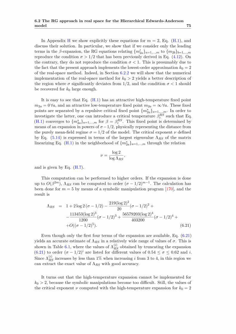
6.2 The RG approach in real space for the Hierarchical Edwards-Andersonmodel 75
In Appendix H we show explicitly these equations for m = 2, Eq. (H.1), anddiscuss their solution. In particular, we show that if we consider only the leadingterms in the β-expansion, the RG equations relating {m′2a}a=1,...,m to {m2b}b=1,...,mreproduce the condition σ > 1/2 that has been previously derived in Eq. (4.12). Onthe contrary, they do not reproduce the condition σ < 1. This is presumably due tothe fact that the present approach implements the lowest-order approximation k0 = 2of the real-space method. Indeed, in Section 6.2.2 we will show that the numericalimplementation of the real-space method for k0 > 2 yields a better description ofthe region where σ significantly deviates from 1/2, and the condition σ < 1 shouldbe recovered for k0 large enough.
It is easy to see that Eq. (H.1) has an attractive high-temperature fixed pointm2a = 0 ∀a, and an attractive low-temperature fixed point m2a =∞∀a. These fixedpoints are separated by a repulsive critical fixed point {m∗2a}a=1,...,m. In order toinvestigate the latter, one can introduce a critical temperature βRSc such that Eq.(H.1) converges to {m∗2a}a=1,...,m for β = βRSc . This fixed point is determined bymeans of an expansion in powers of σ−1/2, physically representing the distance fromthe purely mean-field regime σ = 1/2 of the model. The critical exponent ν definedby Eq. (5.14) is expressed in terms of the largest eigenvalue ΛRS of the matrixlinearizing Eq. (H.1) in the neighborhood of {m∗2a}a=1,...,m through the relation
ν = log 2log ΛRS
,
and is given by Eq. (H.7).
This computation can be performed to higher orders. If the expansion is doneup to O(β2m), ΛRS can be computed to order (σ − 1/2)m−1. The calculation hasbeen done for m = 5 by means of a symbolic manipulation program [170], and theresult is
ΛRS = 1 + 2 log 2 (σ − 1/2)− 219(log 2)2
20 (σ − 1/2)2 +
−113453(log 2)3
1200 (σ − 1/2)3 + 56579203(log 2)4
403200 (σ − 1/2)4 +
+O((σ − 1/2)5). (6.21)
Even though only the first four terms of the expansion are available, Eq. (6.21)yields an accurate estimate of ΛRS in a relatively wide range of values of σ. This isshown in Table 6.1, where the values of Λ(i)
RS obtained by truncating the expansion(6.21) to order (σ − 1/2)i are listed for different values of 0.54 ≤ σ ≤ 0.62 and i.Since Λ(i)
RS increases by less than 1% when increasing i from 3 to 4, in this region wecan extract the exact value of ΛRS with good accuracy.
It turns out that the high-temperature expansion cannot be implemented fork0 > 2, because the symbolic manipulations become too difficult. Still, the values ofthe critical exponent ν computed with the high-temperature expansion for k0 = 2
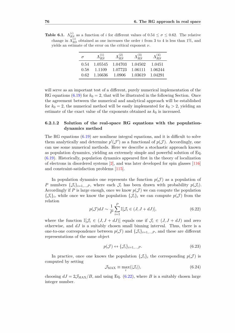
76 6. The RG approach in real space
Table 6.1. Λ(i)RS as a function of i for different values of 0.54 ≤ σ ≤ 0.62. The relative
change in Λ(i)RS obtained as one increases the order i from 3 to 4 is less than 1%, and
yields an estimate of the error on the critical exponent ν.
σ Λ(1)RS Λ(2)
RS Λ(3)RS Λ(4)
RS
0.54 1.05545 1.04703 1.04502 1.04510.58 1.1109 1.07723 1.06111 1.062440.62 1.16636 1.0906 1.03619 1.04291
will serve as an important test of a different, purely numerical implementation of theRG equations (6.19) for k0 = 2, that will be illustrated in the following Section. Oncethe agreement between the numerical and analytical approach will be establishedfor k0 = 2, the numerical method will be easily implemented for k0 > 2, yielding anestimate of the exact value of the exponents obtained as k0 is increased.
6.2.1.2 Solution of the real-space RG equations with the population-dynamics method
The RG equations (6.19) are nonlinear integral equations, and it is difficult to solvethem analytically and determine p′(J ′) as a functional of p(J ). Accordingly, onecan use some numerical methods. Here we describe a stochastic approach knownas population dynamics, yielding an extremely simple and powerful solution of Eq.(6.19). Historically, population dynamics appeared first in the theory of localizationof electrons in disordered systems [2], and was later developed for spin glasses [116]and constraint-satisfaction problems [115].
In population dynamics one represents the function p(J ) as a population ofP numbers {Ji}i=1,...,P , where each Ji has been drawn with probability p(Ji).Accordingly if P is large enough, once we know p(J ) we can compute the population{Ji}i, while once we know the population {Ji}i we can compute p(J ) from therelation
p(J )dJ ∼ 1P
P∑i=1
I[Ji ∈ (J, J + dJ)], (6.22)
where the function I[Ji ∈ (J, J + dJ)] equals one if Ji ∈ (J, J + dJ) and zerootherwise, and dJ is a suitably chosen small binning interval. Thus, there is aone-to-one correspondence between p(J ) and {Ji}i=1,...,P , and these are differentrepresentations of the same object
p(J )↔ {Ji}i=1,...,P . (6.23)
In practice, once one knows the population {Ji}i the corresponding p(J ) iscomputed by setting
JMAX ≡ maxi
(|Ji|), (6.24)
choosing dJ = 2JMAX/B, and using Eq. (6.22), where B is a suitably chosen largeinteger number.
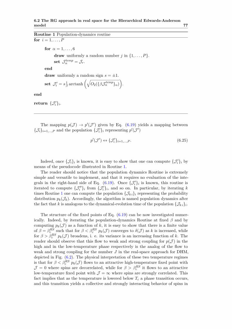
6.2 The RG approach in real space for the Hierarchical Edwards-Andersonmodel 77
Routine 1 Population-dynamics routinefor i = 1, . . . , P
for α = 1, . . . , 6draw uniformly a random number j in {1, . . . , P}.set J tempα = Jr.
enddraw uniformly a random sign s = ±1.
set J ′i = s 1β arctanh
(√O2({βJ tempα }α)
).
end
return {J ′i }i.
The mapping p(J ) → p′(J ′) given by Eq. (6.19) yields a mapping between{Ji}i=1,...,P and the population {J ′i }i representing p′(J ′)
p′(J ′)↔ {J ′i }i=1,...,P . (6.25)
Indeed, once {Ji}i is known, it is easy to show that one can compute {J ′i }i bymeans of the pseudocode illustrated in Routine 1.
The reader should notice that the population dynamics Routine is extremelysimple and versatile to implement, and that it requires no evaluation of the inte-grals in the right-hand side of Eq. (6.19). Once {J ′i }i is known, this routine isiterated to compute {J ′′i }i from {J ′i }i, and so on. In particular, by iterating ktimes Routine 1 one can compute the population {Jk i}i representing the probabilitydistribution pk(Jk). Accordingly, the algorithm is named population dynamics afterthe fact that k is analogous to the dynamical-evolution time of the population {Jk i}i.
The structure of the fixed points of Eq. (6.19) can be now investigated numer-ically. Indeed, by iterating the population-dynamics Routine at fixed β and bycomputing pk(J ) as a function of k, it is easy to show that there is a finite valueof β = βRSc such that for β < βRSc pk(J ) converges to δ(J ) as k is increased, whilefor β > βRSc pk(J ) broadens, i. e. its variance is an increasing function of k. Thereader should observe that this flow to weak and strong coupling for p(J ) in thehigh and in the low-temperature phase respectively is the analog of the flow toweak and strong coupling for the number J in the real-space approach for DHM,depicted in Fig. (6.2). The physical interpretation of these two temperature regimesis that for β < βRSc pk(J ) flows to an attractive high-temperature fixed point withJ = 0 where spins are decorrelated, while for β > βRSc it flows to an attractivelow-temperature fixed point with J =∞ where spins are strongly correlated. Thisfact implies that as the temperature is lowered below Tc a phase transition occurs,and this transition yields a collective and strongly interacting behavior of spins in

78 6. The RG approach in real space
the low-temperature phase. Even though this result has been derived in the k0 = 2-approximation, the implementations of the real-space method for k0 > 2 will confirmthis picture. The existence of a finite-temperature phase transition for a dilutedversion of the HEA model has been established heretofore with MC simulations bymeans of finite-size scaling techniques [65]. Since the critical properties of such adiluted version of the HEA should be the same [65] as those of the HEA definedhere, the real-space approach confirms the picture on the criticality of the systemgiven by MC simulations.
An important feature of the population-dynamics approach is that for σ < 1/2the thermodynamic limit is ill-defined, which has been discussed in Part III, Eq.(4.12). Indeed, the numerics show that for σ → 1/2 βRSc → 0, in such a way thatthe system is always in the low-temperature phase, i. e. the variance of pk(J ) isan increasing function of k, and the thermodynamic limit k →∞ is ill-defined. Onthe other hand, according to Eq. (4.12) one should have that βRSc →∞ as σ → 1,because for σ > 1 no finite-temperature phase transition occurs. Unfortunately, thiscondition is not reproduced by the real-space approach. As discussed in Section6.2.1.1, this is presumably due to the fact that k0 is small, i. e. that Eq. (6.19)implements only the lowest-order approximation of the real-space method (k0 = 2).This hypothesis is supported by the fact that the estimate of the critical exponentsthat we will give in what follows significantly improve as k0 is increased in the regionwhere σ differs significantly from 1/2, while they hardly change in the region σ ≈ 1/2,implying that the closer σ to 1, the larger the values of k0 needed. Accordingly, forσ → 1 a significantly better description would be obtained if larger values of k0 wereaccessible, and the σ < 1-limit would be recovered.
The numerical implementation of Routine 1 also shows that there is a repulsivecritical fixed point, that we will call p∗(J ), which is reached by iterating Routine 1with β = βRSc
p∗(J ) =∫ [ 6∏
α=1p∗(Jα)dJα
]12
[δ
(J − 1
βRScarctanh
(√O2({βRSc Jα}α)
))+
+δ(J + 1
βRScarctanh
(√O2({βRSc Jα}α)
))]. (6.26)
This critical fixed point is analogous to the critical value of the coupling Kc in thereal-space method for DHM, depicted in Fig. (6.2). In the numerical implementationboth βRSc and p∗(J ) are computed by iterating Routine 1 and by dynamicallyadjusting β at each step to its critical value, which is approximately determined asthe value of β such that
∫dJ ′p′(J ′)(J ′)2 =
∫dJ p(J )J 2. In order to do so, one
starts with two values of the temperature Tmin, TMAX such that
Tmin < TRSc < TMAX, (6.27)
and then iterates the bisection Routine 2.Each iteration k of Routine 2 is one step of the RG transformation performed at
temperature T = (Tmin + TMAX)/2, and if the second moment of p′(J ′) is smallerthan that of p(J ), T is in the high-temperature phase, and the interval [Tmin, TMAX]

6.2 The RG approach in real space for the Hierarchical Edwards-Andersonmodel 79
Routine 2 Bisection routinefor k = 1, . . . , kMAX
set T = (Tmin + TMAX)/2.set ς2 = 1
P
∑Pi=1 J 2
i .compute {J ′i }i from Routine 1 and set Ji = J ′i ∀i = 1, . . . , P .set ς ′2 = 1
P
∑Pi=1 J ′
2i .
if ς ′2 > ς2 set Tmin = Tmin + x(TMAX − Tmin).else set TMAX = TMAX − x(TMAX − Tmin).
end
return TRSc = T and {Ji}i ↔ p∗(J )
is reduced by 0 < x < 1 by lowering the upper limit TMAX, and vice versa if T isin the low-temperature phase. By iterating this procedure kMAX � 1 times, theRoutine returns an estimate of the critical temperature TRSc = T and of the criticalfixed point {Ji}i ↔ p∗(J ).Since population dynamics is a stochastic approach, this bisection Routine is notdeterministic, and might give slightly different results when one runs it several timesif the population size P is not large enough. In particular, such a stochastic charactercan introduce some instabilities when approaching the repulsive fixed point, andthese might let the bisection Routine flow towards the low or high-temperaturefixed point, far away from p∗(J ). Accordingly, the parameter x has been chosen byhand in order to minimize this instability, and the numerical implementation of thebisection Routine has shown that x ∼ 0.1 yields a good estimate of the critical fixedpoint.
The critical fixed point p∗(J ) obtained with this bisection method is depictedin Fig. 6.4 for a given σ-value, where we also represent p∗(J ) obtained with thek0 = 3, 4-approximations that will be described in what followins.
Once the fixed point p∗(J ) has been computed numerically, the critical exponentscan be determined by linearizing the transformation (6.19) in the neighborhoodof p∗(J ). Being the RG equations (6.19) a flow for a continuous set of degrees offreedom {p(J )}J , the matrix linearizing the RG transformation in the neighborhood

80 6. The RG approach in real space
0
0.5
1
1.5
2
2.5
-1.5 -1 -0.5 0 0.5 1 1.5
p∗(
J)
J
0
0.5
1
1.5
2
2.5
-1.5 -1 -0.5 0 0.5 1 1.5
p∗(
J)
J
0
0.5
1
1.5
2
2.5
-1.5 -1 -0.5 0 0.5 1 1.5
p∗(
J)
J
k0 = 3k0 = 2
k0 = 4
Figure 6.4. Fixed point p∗(J ) as a function of J for σ = 0.5146 and k0 = 2, 3, 4,obtained by iterating Routine 2 starting with p0(J ) = 1/
√2πe−J 2/2. For k0 = 2,
kMAX = 50, P = 2× 10⁶, x = 0.1 and B = 96. For k0 = 3, kMAX = 50, P = 106, x = 0.1and B = 96. For k0 = 4, kMAX = 20, P = 2 × 10⁴, x = 0.1 and B = 96. p∗(J ) hascompact support and a convergent behavior as k0 is increased. This convergence indicatesthat k0 is large enough in such a way that the real-space approach is asymptoticallyexact for this value of σ.
of p∗(J ) has continuous indices J ,J ′, and is defined as
MRSJ ,J ′ ≡
δp′(J )δp(J ′)
∣∣∣∣p=p∗, β=βRSc
=6∑
γ=1
∫ 6∏λ6=γ=1
p∗(Jλ)dJλ
××1
2
[δ
(J − 1
βRScarctanh
(√O2({βRSc Jλ}
γ,J ′λ )
))+
+δ(J + 1
βRScarctanh
(√O2({βRSc Jλ}
γ,J ′λ )
))], (6.28)
where {βRSc Jλ}γ,J ′λ ≡ {βRSc J1, . . . , β
RSc Jγ−1, β
RSc J ′, βRSc Jγ+1, . . . , β
RSc J6} and in
the second line of Eq. (6.28) Eq. (6.19) has been used.
In the rigorous treatment [45] of the εF -expansion for DHM, the linearization ofthe transformation pk(m)→ pk+1(m) in the neighborhood of p∗(m) is formulated interms of a linear functional acting on a suitably defined space of functions φ(m), andthe critical exponents are extracted from the eigenvalues of this functional. Theseeigenvalues are determined by the theory of linear functionals, in particular by thetheory of Hermite polynomials. Similarly, here the matrix MRS defines a linearfunctional L acting on a suitably defined space of functions φ(J ), and yielding a
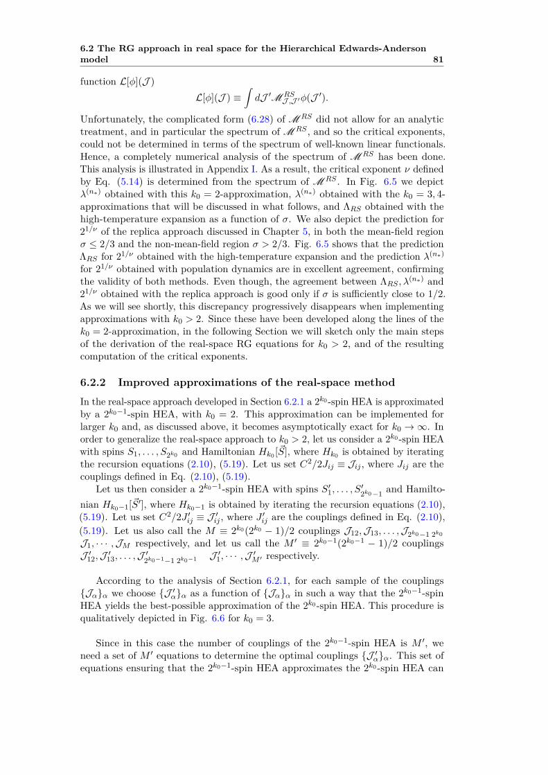
6.2 The RG approach in real space for the Hierarchical Edwards-Andersonmodel 81
function L[φ](J )L[φ](J ) ≡
∫dJ ′MRS
J ,J ′φ(J ′).
Unfortunately, the complicated form (6.28) of MRS did not allow for an analytictreatment, and in particular the spectrum of MRS , and so the critical exponents,could not be determined in terms of the spectrum of well-known linear functionals.Hence, a completely numerical analysis of the spectrum of MRS has been done.This analysis is illustrated in Appendix I. As a result, the critical exponent ν definedby Eq. (5.14) is determined from the spectrum of MRS . In Fig. 6.5 we depictλ(n∗) obtained with this k0 = 2-approximation, λ(n∗) obtained with the k0 = 3, 4-approximations that will be discussed in what follows, and ΛRS obtained with thehigh-temperature expansion as a function of σ. We also depict the prediction for21/ν of the replica approach discussed in Chapter 5, in both the mean-field regionσ ≤ 2/3 and the non-mean-field region σ > 2/3. Fig. 6.5 shows that the predictionΛRS for 21/ν obtained with the high-temperature expansion and the prediction λ(n∗)
for 21/ν obtained with population dynamics are in excellent agreement, confirmingthe validity of both methods. Even though, the agreement between ΛRS , λ(n∗) and21/ν obtained with the replica approach is good only if σ is sufficiently close to 1/2.As we will see shortly, this discrepancy progressively disappears when implementingapproximations with k0 > 2. Since these have been developed along the lines of thek0 = 2-approximation, in the following Section we will sketch only the main stepsof the derivation of the real-space RG equations for k0 > 2, and of the resultingcomputation of the critical exponents.
6.2.2 Improved approximations of the real-space method
In the real-space approach developed in Section 6.2.1 a 2k0-spin HEA is approximatedby a 2k0−1-spin HEA, with k0 = 2. This approximation can be implemented forlarger k0 and, as discussed above, it becomes asymptotically exact for k0 →∞. Inorder to generalize the real-space approach to k0 > 2, let us consider a 2k0-spin HEAwith spins S1, . . . , S2k0 and Hamiltonian Hk0 [~S], where Hk0 is obtained by iteratingthe recursion equations (2.10), (5.19). Let us set C2/2Jij ≡ Jij , where Jij are thecouplings defined in Eq. (2.10), (5.19).
Let us then consider a 2k0−1-spin HEA with spins S′1, . . . , S′2k0−1 and Hamilto-nian Hk0−1[~S′], where Hk0−1 is obtained by iterating the recursion equations (2.10),(5.19). Let us set C2/2J ′ij ≡ J ′ij , where J ′ij are the couplings defined in Eq. (2.10),(5.19). Let us also call the M ≡ 2k0(2k0 − 1)/2 couplings J12,J13, . . . ,J2k0−1 2k0
J1, · · · ,JM respectively, and let us call the M ′ ≡ 2k0−1(2k0−1 − 1)/2 couplingsJ ′12,J ′13, . . . ,J ′2k0−1−1 2k0−1 J ′1, · · · ,J ′M ′ respectively.
According to the analysis of Section 6.2.1, for each sample of the couplings{Jα}α we choose {J ′α}α as a function of {Jα}α in such a way that the 2k0−1-spinHEA yields the best-possible approximation of the 2k0-spin HEA. This procedure isqualitatively depicted in Fig. 6.6 for k0 = 3.
Since in this case the number of couplings of the 2k0−1-spin HEA is M ′, weneed a set of M ′ equations to determine the optimal couplings {J ′α}α. This set ofequations ensuring that the 2k0−1-spin HEA approximates the 2k0-spin HEA can
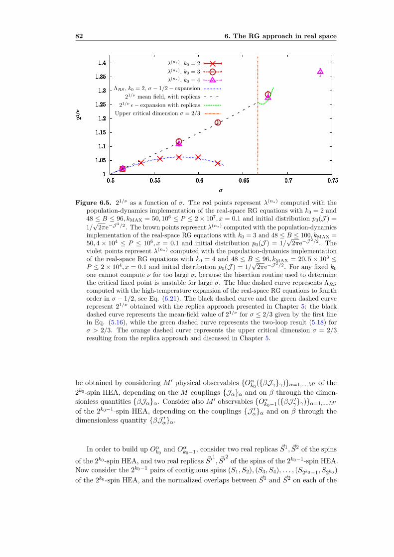
82 6. The RG approach in real space
1
1.05
1.1
1.15
1.2
1.25
1.3
1.35
1.4
0.5 0.55 0.6 0.65 0.7 0.75
21/ν
σ
1
1.05
1.1
1.15
1.2
1.25
1.3
1.35
1.4
0.5 0.55 0.6 0.65 0.7 0.75
21/ν
σ
1
1.05
1.1
1.15
1.2
1.25
1.3
1.35
1.4
0.5 0.55 0.6 0.65 0.7 0.75
21/ν
σ
1
1.05
1.1
1.15
1.2
1.25
1.3
1.35
1.4
0.5 0.55 0.6 0.65 0.7 0.75
21/ν
σ
1
1.05
1.1
1.15
1.2
1.25
1.3
1.35
1.4
0.5 0.55 0.6 0.65 0.7 0.75
21/ν
σ
1
1.05
1.1
1.15
1.2
1.25
1.3
1.35
1.4
0.5 0.55 0.6 0.65 0.7 0.75
21/ν
σ
1
1.05
1.1
1.15
1.2
1.25
1.3
1.35
1.4
0.5 0.55 0.6 0.65 0.7 0.75
21/ν
σ
λ(n∗), k0 = 2
λ(n∗), k0 = 3
λ(n∗), k0 = 4
21/ν mean field, with replicas
ΛRS , k0 = 2, σ − 1/2 − expansion
21/ν ǫ − expansion with replicas
Upper critical dimension σ = 2/3
Figure 6.5. 21/ν as a function of σ. The red points represent λ(n∗) computed with thepopulation-dynamics implementation of the real-space RG equations with k0 = 2 and48 ≤ B ≤ 96, kMAX = 50, 106 ≤ P ≤ 2× 10⁷, x = 0.1 and initial distribution p0(J ) =1/√
2πe−J 2/2. The brown points represent λ(n∗) computed with the population-dynamicsimplementation of the real-space RG equations with k0 = 3 and 48 ≤ B ≤ 100, kMAX =50, 4 × 10⁴ ≤ P ≤ 106, x = 0.1 and initial distribution p0(J ) = 1/
√2πe−J 2/2. The
violet points represent λ(n∗) computed with the population-dynamics implementationof the real-space RG equations with k0 = 4 and 48 ≤ B ≤ 96, kMAX = 20, 5 × 10³ ≤P ≤ 2× 10⁴, x = 0.1 and initial distribution p0(J ) = 1/
√2πe−J 2/2. For any fixed k0
one cannot compute ν for too large σ, because the bisection routine used to determinethe critical fixed point is unstable for large σ. The blue dashed curve represents ΛRScomputed with the high-temperature expansion of the real-space RG equations to fourthorder in σ − 1/2, see Eq. (6.21). The black dashed curve and the green dashed curverepresent 21/ν obtained with the replica approach presented in Chapter 5: the blackdashed curve represents the mean-field value of 21/ν for σ ≤ 2/3 given by the first linein Eq. (5.16), while the green dashed curve represents the two-loop result (5.18) forσ > 2/3. The orange dashed curve represents the upper critical dimension σ = 2/3resulting from the replica approach and discussed in Chapter 5.
be obtained by considering M ′ physical observables {Oαk0({βJγ}γ)}α=1,...,M ′ of the
2k0-spin HEA, depending on the M couplings {Jα}α and on β through the dimen-sionless quantities {βJα}α. Consider also M ′ observables {Oαk0−1({βJ ′γ}γ)}α=1,...,M ′
of the 2k0−1-spin HEA, depending on the couplings {J ′α}α and on β through thedimensionless quantity {βJ ′α}α.
In order to build up Oαk0and Oαk0−1, consider two real replicas ~S1, ~S2 of the spins
of the 2k0-spin HEA, and two real replicas ~S′1, ~S′
2of the spins of the 2k0−1-spin HEA.
Now consider the 2k0−1 pairs of contiguous spins (S1, S2), (S3, S4), . . . , (S2k0−1, S2k0 )of the 2k0-spin HEA, and the normalized overlaps between ~S1 and ~S2 on each of the

6.2 The RG approach in real space for the Hierarchical Edwards-Andersonmodel 83
≈
S4S1S1 S2 S3 S8S5 S6 S7 S ′4S ′
1 S ′2 S ′
3
Figure 6.6. Approximation of the real-space approach for k0 = 3. A 23-spin HEA withspins S1, · · · , S8 and Hamiltonian H8[~S] is approximated by a 22-spin HEA with spinsS′1, . . . , S
′4 and Hamiltonian H2[~S′].
leaves defined by these pairs
Qα =S1
2α−1S22α−1+S1
2αS22α
2√√√√E~S1,~S2
[(S1
2α−1S22α−1+S1
2αS22α
2
)2] ,
where α = 1, . . . , 2k0−1, and E~S1,~S2 denotes the expectation value with respectto ~S1, ~S2 with Boltzmann weight e−βHk0 . Now consider the normalized overlapsbetween ~S′1 and ~S′2 on each of the spins of the 2k0−1-spin HEA
Q′α = S′1α S′2α ,
where α = 1, . . . , 2k0−1.Kadanoff’s decimation rule is implemented by imposing the correspondence
between Qα and Q′α ∀α = 1, . . . , 2k0−1. This can be done by choosing the followingobservables
O1k0({βJγ}γ) = E~S1,~S2 [Q1Q2],
O2k0({βJγ}γ) = E~S1,~S2 [Q1Q3],
. . .
OM′
k0 ({βJγ}γ) = E~S1,~S2 [Q2k0−1−1Q2k0−1 ], (6.29)
O1k0−1({βJ ′γ}γ) = E~S′1,~S′2 [Q′1Q′2],
O2k0−1({βJ ′γ}γ) = E~S′1,~S′2 [Q′1Q′3],
. . .
OM′
k0−1({βJ ′γ}γ) = E~S′1,~S′2 [Q′2k0−1−1Q′2k0−1 ], (6.30)
where E~S′1,~S′2 denotes the expectation value with respect to ~S′1, ~S′2 with Boltzmannweight e−βHk0−1 . The 2k0-spin HEA can now be approximated by the 2k0−1-spinHEA by enforcing the constraints
Oαk0({βJγ}γ) = Oαk0−1({βJ ′γ}γ) ∀α = 1, . . . ,M ′. (6.31)

84 6. The RG approach in real space
In what follows we assume that Eq. (6.31) can be written as
J ′α = 1/βfα({βJγ}γ), (6.32)
where in Eq. (6.32) we have used the fact that the right-hand side of Eq. (6.31)depends on {J ′α}α through the dimensionless products {βJ ′α}α.
Now suppose that the couplings {Jα} are independent and that each of them isdistributed according to a given p(J ). According to Eq. (6.32), the couplings {J ′α}αare not independent, because the entangled structure of Eq. (6.32) introduces somecorrelation between them. Accordingly, the joint probability distribution of {J ′α}α is
p′C({J ′α}α) =∫ M ′∏
α=1p(Jα)dJα
M ′∏α=1
δ
(J ′α −
1βfα({βJγ}γ)
), (6.33)
where the label C stands for correlated. Hence, starting with a set of uncorrelatedcouplings {Jα}α, after one step of the RG transformation we generate some correla-tion between the couplings. This situation occurs in many cases where one performsan effective reduction of the degrees of freedom of a system under reparametrizationof the length scale. Indeed, it is a quite general fact that if one starts with a set ofdegrees of freedom at a given length scale L, additional degrees of freedom are gener-ated at the length scale 2L. A typical example is the RG flow for the Ising model indimensions d ≈ 4, where in the effective φ4-theory one generates additional φ6, φ8, · · · -terms after one RG step (see [164, 165, 163, 162, 168] for a general discussion in theapproach à la Wilson and [173] for a discussion in the field-theory approach for theIsing model). Notwithstanding this, it turns out that in the field-theory RG approach[173] these terms are finite, i. e. non singular in 1/(4− d), so they do not need to beabsorbed into the renormalization constants, and do not contribute to the criticalexponents. This fact is intrinsically related to the perturbative renormalizability ofthe φ4-theory [173], and implies that the RG equations can be written in closed form.
It is not easy to tell if the above correlation can be consistently neglected in thisreal-space approach, and the answer to this question could be intrinsically relatedto the renormalizability of the theory. In our approach we will not address thisdelicate point, and we will simply get rid of the above correlation between the J ′αs byassuming that they are independent, and that each of them is distributed accordingto a distribution p′(J ′) given by the average of M ′ marginalized distributions, eachof which is obtained by integrating p′C({J ′α}α) over M ′ − 1 couplings
p′(J ′) = 1M ′
M ′∑α=1
∫ M ′∏γ=1,γ 6=α
dJ ′γ
p′C(J ′1, . . . ,J ′α−1,J ′,J ′α+1, . . . ,J ′M ′). (6.34)
By plugging Eq. (6.33) into Eq. (6.34) we obtain the RG equation relating p(J )to p(J ′)
p′(J ′) = 1M ′
M ′∑α=1
∫ M ′∏γ=1
p(Jγ)dJγ
δ (J ′ − 1βfα({βJγ}γ)
). (6.35)

6.2 The RG approach in real space for the Hierarchical Edwards-Andersonmodel 85
A procedure along the lines of that presented in Section 6.2.1 can be applied toEq. (6.35): once a 2k0-spin HEA has been approximated by a 2k0−1-spin HEA, onetakes two realizations of the latter and couples them to obtain a system representinga 2k0+1-spin HEA, and iterates this procedure. In this way one obtains a sequencep(J ) ≡ p0(J ), p′(J ′) ≡ p1(J ′), p′′(J ′′) ≡ p2(J ′′), . . . physically representing the RGflow of the disorder distribution.
In the numerical implementation p(J ) and p′(J ′) are represented by two popu-lations, and the RG equations (6.35) are implemented in population dynamics bygeneralizing Routine 1. The numerical implementation of Eq. (6.35) shows that themain qualitative features of the k0 = 2-case stay the same here. In particular, thereis a finite value of β, that we will call βRSc , such that for β < βRSc pk(J ) converges tothe high-temperature fixed point δ(J ) as k is increased, while for β > βRSc the widthof pk(J ) is an increasing function of k, and pk(J ) converges to the low-temperaturefixed point. If one iterates Eq. (6.35) with β = βRSc , the iteration converges to afinite critical-fixed-point p∗(J ).
The critical fixed point p∗(J ) is obtained by implementing Routine 2, and isdepicted in Fig. 6.4 as a function of J for a given σ-value and k0 = 3, 4.
The matrix MRSJ ,J ′ linearizing the RG transformation in the neighborhood of
p∗(J ) is defined in the same way as in Eq. (6.28), and its eigenvalue λ(n∗) defined byEq. (I.14) yields the critical exponent ν defined by Eq. (5.14) according to Eq. (I.15).
λ(n∗) for k0 = 3, 4 is depicted in Fig 6.5 as a function of σ. Fig. 6.5 shows that The real-space RGmethod makesprecise predictionsfor the criticalexponents of theHierarchicalEdwards-Anderson model,which are inagreement withthose of thereplica method inthe classicalregion. In thenon-classicalregion thesepredictions cannotbe compared tothose of thereplica method.
even though for k0 = 2 λ(n∗) is significantly different from the mean-field valueobtained with the replica approach, as k0 is increased both λ(n∗) for k0 = 3 andλ(n∗) for k0 = 4 agree very well with the mean-field value obtained with the replicaapproach in the whole mean-field region 1/2 < σ ≤ 2/3. This is an important aposteriori test of the whole real-space RG framework presented here. The situationsubtler in the non-mean-field region σ > 2/3. In this region the ε-expansion basedon the replica approach is non-predictive, because the first few orders (5.18) of theseries have a nonconvergent behavior. Still, the data of the real-space approach canbe compared to that of MC simulations [65] performed on a diluted version of theHEA, where ν is an increasing function of σ in the non-mean-field region σ > 2/3,which disagrees with the results of the real-space approach, Fig. 6.5.
There might be several reasons for this disagreement [36]. A first issue might bethe smallness of k0 in the real-space approach: it is plausible that for larger k0 thederivative of λ(n∗) at σ = 2/3+ turns out to be negative, in agreement with the MCresults. Another issue might be that the exponent ν is not universal: the exponentν of the HEA model studied here might be different from that of the diluted versionof the HEA studied in MC simulations. Indeed, universality in non-mean-field spinglasses has never been established rigorously [75]. On the one hand, universalityviolation in finite-dimensional systems [12, 13] resulted from numerical studies doneheretofore, even though more recent analyses based on MC simulations [91] andhigh-temperature expansion [51] suggest that universality holds. A third importantissue might be that the couplings correlation has been neglected in the real-space
86 6. The RG approach in real space
approach for k0 > 2, see Eq. (6.34). Indeed, this couplings correlation might play avital role in the non-mean-field region 2/3 < σ < 1, and it might yield a radicallydifferent critical behavior of the system if one took it into account.
These issues could be investigated in some future directions of this real-spacemethod. For instance, it would be interesting to find a way to handle couplingscorrelation in the real-space approach. One could then investigate the relevance ofthis correlation in both the mean and the non-mean-field region, and compare theresulting values of the critical exponents to those obtained with MC simulations.Another interesting future direction would be to implement this approach in thepresence of an external magnetic field. Indeed, by analyzing the existence of acritical fixed point one could establish whether there is a phase transition in thenon-mean-field region, which has been a hotly debated issue in the last years [89, 105],and could give some insight into the correct picture describing the low-temperaturephase of the system [64]. Finally, it would be interesting to implement the presentapproach for more realistic spin-glass systems, like the three-dimensional EA model.Indeed, a simple analysis shows that this method can be easily generalized to modelswith short-range interactions built on a finite-dimensional hypercube.

Part IV
Conclusions
87

89
This thesis has investigated the implementation of renormalization-group (RG)techniques in finite-dimensional glassy systems, in order to shed light on the criticalbehavior of spin and structural glasses beyond mean field. In finite dimensionsthe existence of a phase transition in structural glasses is not well-established, andthe structure of the low-temperature phase for both spin and structural glasses isfundamentally unknown and controversial. Since Wilson’s RG equations emerge in anatural and simple way in ferromagnetic spin models with a hierarchical interactionstructure, in this work we considered two finite-dimensional models of spin andstructural glasses built on Dyson’s hierarchical lattice [57].
After giving a brief introduction on spin and structural glasses in Part I, in Part IIwe focused on a structural-glass model built on a hierarchical lattice, the HierarchicalRandom Energy Model (HREM) [33, 32]. In this study, we showed the first evidenceof a non-mean-field model of a supercooled liquid undergoing a Kauzmann phasetransition. On the one hand, the features of the phase transition are different fromthe mean-field case [53]. The free energy is found to be nonanalytical at the criticalpoint, and our study of the correlation length of the system in the critical regionshows that the data is consistent with the existence of a diverging correlation length.On the other hand, by investigating the properties of the low-temperature phase weshowed that the free energy has a one-step replica-symmetry-breaking (RSB) saddlepoint in the low-temperature phase, describing a fragmentation of the free-energylandscape into disconnected components.
A first future direction of this work would be to generalize it to more realisticmodels, like 1-RSB models with p-spin interactions and p ≥ 3, which have anentropy-crisis transition in the mean-field case: it would be interesting to build up anon-mean-field version of these models on a hierarchical lattice, and to implementa suitable generalization of the RG techniques used for the HREM to study theircritical behavior. A second future direction would be to study the dynamics of theHREM and of these hierarchical 1-RSB models. In particular, 1-RSB models have adynamical phase transition in the mean-field case mimicking the dynamical arrest inglass-formers at the glass-transition temperature predicted by the Mode CouplingTheory. If one could check whether this transition persists or is smeared out in suchhierarchical counterparts of mean-field 1-RSB models, one could test directly someof the building blocks of the Random First Order Transition Theory.
In Part III we presented the study of a spin-glass model built on a hierarchicallattice, the Hierarchical Edwards-Anderson Model (HEA). Differently from theHREM, in the HEA the spins are not mere labels for the energy variables, but theyare physical degrees of freedom. This fact allowed for an implementation of a RGdecimation protocol, which has been implemented with two different approaches.The first approach is based on the replica method [34, 35], while the second one doesnot rely on the replica formalism, but on a real-space picture [36].
90
In the replica RG approach the infrared (IR) limit of the theory has been takenwith two different methods, and both of them yield the same two-loop prediction forthe ε-expansion of the critical exponents. This shows that the IR limit of the theoryis well defined, and suggests the existence of a diverging correlation length in thesystem. Unfortunately, this approach makes predictions for the critical exponentsonly in the classical region, i. e. in the parameter region where the mean-fieldapproximation is exact. In the non-classical region the two-loop ε-expansion hasa nonconvergent behavior, in such a way that no conclusion can be drawn on theactual values of the critical exponents.
In the real-space RG approach a generalization of Kadanoff’s block-spin decima-tion is implemented in spin glasses, and the resulting RG equations are worked outby means of a series of approximation steps. These equations have been solved bymeans of the high-temperature expansion and of the population-dynamics method,yielding consistent results. Similarly to the replica RG method, the real-spaceapproach shows that a phase transition occurs in the HEA and that the correlationlength diverges at the critical point. At variance with the replica RG method, thismethod makes precise predictions for the critical exponents in both the classicalregion, where the critical exponents are in excellent agreement with those of thereplica method, and in the non-classical region. The real-space predictions in thisregion are in disagreement with Monte Carlo (MC) simulations done for a dilutedversion of the HEA. There might be several possible reasons for this disagreement:the discrepancy should disappear if better approximation steps were considered inthe real-space approach, or the critical exponents of the HEA model defined heremight be different from those of the diluted HEA, i. e. universality might be violated.
There are several future directions for the replica and for the real-space approach.As far as the replica approach is concerned, the two-loop calculation that we havedone here is a base of departure for an automated computation of the ε-expansionfor the critical exponents. Despite its highly technical nature, the calculation ofhigh orders of the ε-series would clarify whether the ε-expansion can be resummedand made convergent, and so whether the non-mean-field physics of the system canbe considered as a small perturbation of the mean-field one. As far as the real-space approach is concerned, it would be interesting to improve the approximationscheme to check whether the disagreement with MC simulations disappears. If thedisagreement does not disappear, one could test the universality of the exponents bychecking directly whether the critical indices stay the same when changing the detailsof the quenched-disorder probability distribution. Moreover, in order to shed lighton the structure of the low-temperature phase, it would be interesting to implementthe real-space method in the presence of an external magnetic field and to verify theexistence of a phase transition in the non-classical region, by searching for a criticalfixed point of the RG equations. Indeed, the existence of a phase transition in afield is one of the fundamental elements discriminating between the RSB and thedroplet picture for finite-dimensional spin glasses, and it would shed light on thefeatures of the low-temperature phase of these systems.
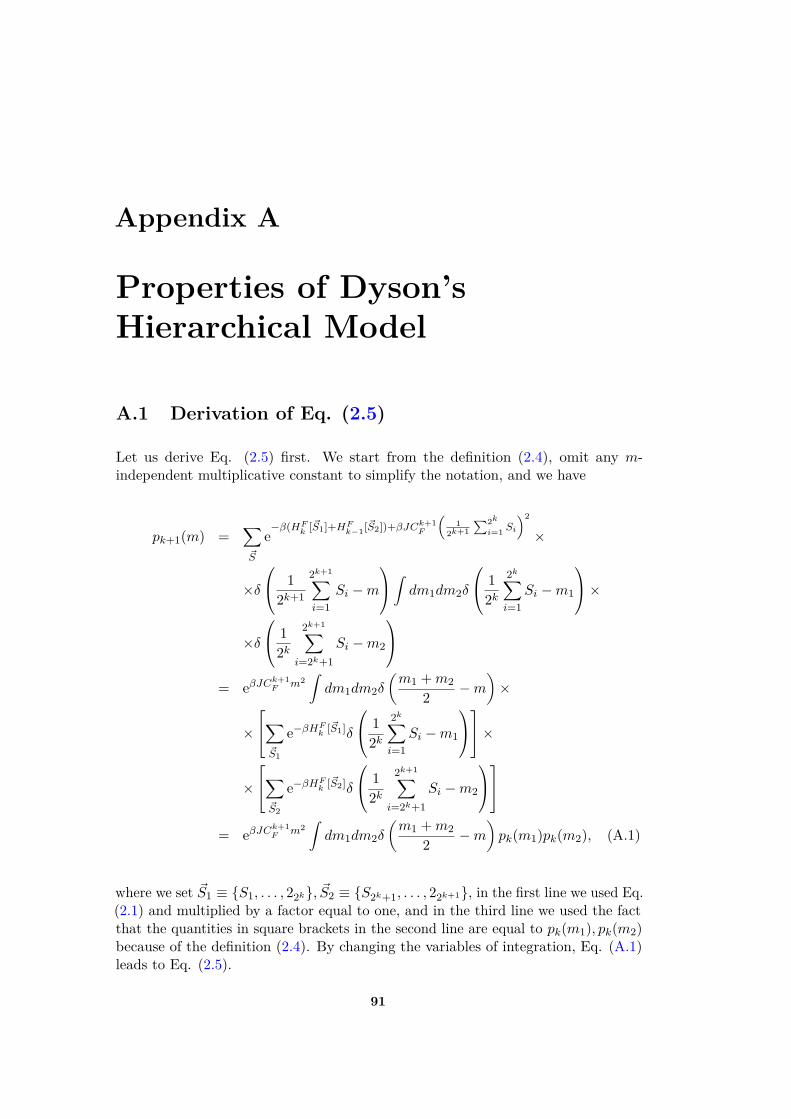
Appendix A
Properties of Dyson’sHierarchical Model
A.1 Derivation of Eq. (2.5)
Let us derive Eq. (2.5) first. We start from the definition (2.4), omit any m-independent multiplicative constant to simplify the notation, and we have
pk+1(m) =∑~S
e−β(HF
k [~S1]+HFk−1[~S2])+βJCk+1
F
(1
2k+1∑2k
i=1 Si
)2
×
×δ
12k+1
2k+1∑i=1
Si −m
∫ dm1dm2δ
12k
2k∑i=1
Si −m1
××δ
12k
2k+1∑i=2k+1
Si −m2
= eβJC
k+1F m2
∫dm1dm2δ
(m1 +m2
2 −m)×
×
∑~S1
e−βHFk [~S1]δ
12k
2k∑i=1
Si −m1
××
∑~S2
e−βHFk [~S2]δ
12k
2k+1∑i=2k+1
Si −m2
= eβJC
k+1F m2
∫dm1dm2δ
(m1 +m2
2 −m)pk(m1)pk(m2), (A.1)
where we set ~S1 ≡ {S1, . . . , 22k}, ~S2 ≡ {S2k+1, . . . , 22k+1}, in the first line we used Eq.(2.1) and multiplied by a factor equal to one, and in the third line we used the factthat the quantities in square brackets in the second line are equal to pk(m1), pk(m2)because of the definition (2.4). By changing the variables of integration, Eq. (A.1)leads to Eq. (2.5).
91

92 A. Properties of Dyson’s Hierarchical Model
A.2 Structure of the fixed points of Eq. (2.7)
Taking HF0 [S] = 0, the Hamiltonian HF
k [~S] has ±~S symmetry, and thus according toEqs. (2.4), (2.6), pk(m) is an even function of m. Hence, the simplest approximationis to assume that it is a Gaussian
pk(m) = e−rFk m2, (A.2)
by neglecting higher powers of m in the exponential. Non-Gaussian terms will belater added in the argument of the exponential of Eq. (A.2). For the integral ofpk(m) with respect to m to be finite, we have rFk > 0.
By plugging Eq. (A.2) into Eq. (2.7), we obtain a recursion equation for rFk
rFk+1 = 2rFkCF− βJ. (A.3)
Eq. (A.3) can be solved explicitly, and yields
rFk =( 2CF
)k (rF0 −
βJ2CF− 1
)+ βJ
2CF− 1
. (A.4)
It follows that if β = βc F , with
βc F ≡ rF0 /J(2/CF − 1), (A.5)
rFk has a finite limit r∗ = r0 for k →∞. This fixed point will be called the criticalfixed point. The critical fixed point is unstable, because any small deviation of βfrom βc F would let rFk flow away from rF∗ towards another fixed point, as one cansee from Eq. (A.4). If β < βc F or β > βc F , this attractive fixed point is calledthe high or low-temperature fixed point respectively. According to Eq. (A.5), thecritical temperature depends on the value rF0 at the initial step of the iteration,i. e. at microscopic length scales 2k ∼ 1. This fact is in agreement with the verygeneral picture occurring in ferromagnetic systems like the Ising model [163], wherethe critical temperature is not universal, because it depends on the microscopicproperties of the lattice, like the nearest-neighbor couplings between spins.
Another important feature of the solution of Eq. (A.3) is the following. Takeβ < βc F and k � 1. According to Eqs. (2.6), (A.2) and (A.4), one has
pk(m) = exp[−2k
(rF0 −
βJ2CF− 1
)m2]. (A.6)
Eq. (A.6) shows that for large k the variable m = 1/2k∑2ki=1 Si is distributed
according to a Gaussian distribution with variance proportional to 1/2k. This is theresult that one could have guessed with the central limit theorem, supposing thespins Si to be independent. Now take β = βc F . According to Eqs. (2.6), (A.2) andto the fact that rk = r∗ ∀k, for large k one has
pk(m) = e−r∗CkFm2. (A.7)

A.2 Structure of the fixed points of Eq. (2.7) 93
Eq. (A.7) shows that the distribution of m is still Gaussian, but its variance isproportional to 1/CkF , while supposing the spins to be independent by means of thecentral limit theorem, one would predict the variance to be proportional to 1/2k.The physical interpretation of these facts resulting from Eqs. (A.6), (A.7) is thefollowing. For β < βc F spins can be considered as independent, and so m has thek-dependence predicted by the central limit theorem. On the contrary, at the criticalpoint strong correlations are developed, resulting in a collective behavior of spinswhich cannot be considered as independent anymore, and yielding a magnetization mwith a k-dependence different from that predicted with the independence hypothesis.
Let us now seek for a more accurate approximation of pk, by adding a quarticterm in the exponential in the right-hand side of Eq. (A.2)
pk(m) = e−(rFk m2+wFk m
4), (A.8)
where for the integral of pk(m) with respect to m to be finite, one has wFk > 0.In the following we will suppose that the non-Gaussian term wFk is small for
every k, i. e. that an expansion in powers of wFk is meaningful. Practically speaking,this is equivalent to supposing that the above qualitative picture resulting from theGaussian ansatz (A.2) is slightly modified from the introduction of non-Gaussianterms in Eq. (A.8). The correctness of this assumption will be tested a posterioriby checking if the resulting perturbative series for physical quantities is convergent,or if it can be made convergent with some suitable resummation technique [173].Plugging Eq. (A.8) into Eq. (2.7) and developing in powers of wFk , one has
pk+1(m) = e−2rFk
CFm2+βJm2
{1− 1
8(rFk )2
[3 + 8m2rFk (3CF + 2m2rFk )
C2F
]wFk +
+ 1128C4
F (rFk )4 [105C4F + 720C3
F rFk m
2 + 1824C2F (rFk )2m4 +
+768CF (rFk )3m6 + 256(rFk )4m8](wFk )2 +O((wFk )3)}. (A.9)
The right-hand side of Eq. (A.9) does not have the same form as the ansatz(A.8). Notwithstanding this, one can rewrite the term in braces in the right-handside of Eq. (A.9) as an exponential up to order (wFk )2, and obtain
pk+1(m) = exp{−[
2rFkCF− βJ + 3
CF rFkwFk −
92CF (rFk )3 (wFk )2
]m2 +
−[
2C2F
wFk −9
C2F (rFk )2 (wFk )2
]m4 +O((wFk )3)
}. (A.10)
Comparing Eq. (A.10) to Eq. (A.8), one has rFk+1 = 2rFkCF− βJ + 3
CF rFk
wFk −9
2CF (rFk
)3 (wFk )2 +O((wFk )3),wFk+1 = 2
C2FwFk −
9C2F (rF
k)2 (wFk )2 +O((wFk )3).
(A.11)

94 A. Properties of Dyson’s Hierarchical Model
The second line of Eq. (A.11) can be rewritten as
wFk+1 − wFk =(
2C2F
− 1)wFk −
9C2F (rFk )2 (wFk )2 +O((wFk )3).
If follows that σF ≶ 3/4 implies 2/C2F ≶ 1, and so wFk+1 ≶ wFk . Hence, for σ ≤ 3/4
wFk → 0 for k → ∞, and any fixed point is Gaussian, while for σF > 3/4 a non-Gaussian fixed point arises for k →∞. Historically, the analysis of Gaussian fixedpoints of Eq. (2.6) was first done in [20, 22, 21], while non-Gaussian fixed points havebeen studied first in [24], and their analysis was later developed in [46, 45, 44, 80].According to the above assumption that an expansion in powers of wFk is meaningful,the structure of the fixed points of Eq. (2.7) discussed in the Gaussian case muststill hold. Let us set
εF ≡ σF −34 (A.12)
and show this explicitly in Fig. A.1, where a parametric plot of (rFk , wFk ) as afunction of k is depicted for three different temperatures T < Tc F , T > Tc F andT ≈ Tc F for a given εF and J-value, with εF > 0. The Figure shows the ex-istence of two attractive fixed points, the high-temperature fixed point and thelow-temperature fixed point, and of an unstable critical fixed point separatingthem, as illustrated in the Gaussian case. Given an initial condition, the parametersrFk , w
Fk converge to the critical fixed point only if β is equal to its critical value βc F .
Let us now focus on the critical fixed point. This is obtained by setting β = βc Fand by requiring that rFk+1 = rFk = rF∗ , w
Fk+1 = wFk = wF∗ in Eq. (A.11) rF∗ = 2rF∗
CF− βc FJ + 3
CF rF∗wF∗ − 9
2CF (rF∗ )3 (wF∗ )2 +O((wF∗ )3),wF∗ = 2
C2FwF∗ − 9
C2F (rF∗ )2 (wF∗ )2 +O((wF∗ )3).
(A.13)
If wF∗ is nonzero, one can divide the second equality of Eq. (A.13) by wF∗ , and get
1− 2C2F
= − 9C2F (rF∗ )2w
F∗ +O((wF∗ )2). (A.14)
Since wF∗ must be positive, we have 1−2/C2F < 0, i. e. εF > 0. As anticipated above,
a non-Gaussian critical fixed point wF∗ 6= 0 exists only if εF > 0, and according toEq. (A.14) it is proportional to εF . Accordingly, if εF ≤ 0 one has wF∗ = 0.
A.3 Calculation of νFThe critical exponent νF can be calculated [163] by linearizing Eq. (A.13) in theneighborhood of the critical fixed point rF∗ , wF∗ . Let us introduce the 2× 2 matrix
M Fij ≡
∂(rFk+1, wFk+1)
∂(rFk , wFk )
∣∣∣∣∣rFk
=rF∗ ,wFk =wF∗
. (A.15)
One can show [163], that the critical exponent νF is related to the largest eigenvalueΛF of M F
νF = log 2log ΛF
. (A.16)

A.3 Calculation of νF 95
0.0085
0.009
0.0095
0.01
0.5 1 2
wF k
rFk
(rF0 , wF
0 )
(rF∗ , wF
∗ )
0.0085
0.009
0.0095
0.01
0.5 1 2
wF k
rFk
(rF0 , wF
0 )
(rF∗ , wF
∗ )
T < Tc,F
T > Tc,F
T ≈ Tc,F
Figure A.1. Parametric plot of (rFk , wFk ) as a function of k with εF = 0.01, J = 1. The blackpoints represent (rFk , wFk ) for increasing k from top to bottom, with T < Tc F . The bluepoints represent (rFk , wFk ) for increasing k from left to right, with T > Tc F . The red pointsrepresent (rFk , wFk ) for increasing k from top to bottom: here T has been dynamicallyadjusted as follows at each step k. At the step k = 0 of the iteration we consider twoinitial values of the temperature TmF , TM F such that TmF < Tc F < TM F . Then, weiterate the following procedure. We choose T = (TmF +TM F )/2 and compute rFk+1, w
Fk+1
as a function of rFk , wFk with Eqs. (A.11). If rFk+1 > rFk , we are in the high-temperaturephase, and thus we lower the upper bound on T by setting TM F → (TmF + TM F )/2,otherwise we are in the low-temperature phase, and we raise the lower bound bysetting TmF → (TmF + TM F )/2. Then we set k → k + 1 and repeat. By iteratingthis procedure many times, we obtain an estimate of the critical temperature Tc F bysuccessive bisections of the interval [TmF , TM F ], and we also obtain an estimate of thecritical fixed point rF∗ , wF∗ , which is depicted in the Figure. This bisection procedure isanalog to the bisection Routine 2, illustrated in Section 6.2.1.2 for the RG approach inreal space.
If εF ≤ 0, one has rF∗ = βc FJ/(2/CF−1), wF∗ = 0. M F can be directly computedfrom Eq. (A.11), and one has
ΛF = 22σF−1. (A.17)
Even though Eq. (A.17) has been derived by using the approximate ansatz (A.8),one can show that any ansatz including m6,m8, · · · -terms in pk(m) would lead toEq. (A.17). Hence, Eq. (A.17) is exact.
If εF > 0, the critical fixed point rF∗ , wF∗ can be computed perturbatively as apower series in εF by observing from Eq. (A.14) that wF∗ = O(εF ), and by expandingthe left and the right-hand side of Eq. (A.13) in powers of εF . The result is
rF∗ = (1 +√
2)βc FJ −103 (4 + 3
√2)βc FJ log 2 · εF +O(ε2F ),
wF∗ = 89(3 + 2
√2)(βc FJ)2 log 2 · εF +O(ε2F ). (A.18)
96 A. Properties of Dyson’s Hierarchical Model
Using Eqs. (A.15), (A.11), (A.18), one has
ΛF =√
2(
1 + 23 log 2 · εF +O(ε2F )
). (A.19)
Differently from Eq. (A.17), Eq. (A.19) is not exact, because it is the first order ofa series in εF .
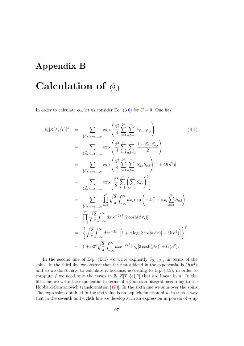
Appendix B
Calculation of φ0
In order to calculate φ0, let us consider Eq. (3.6) for C = 0. One has
Eε[Z[T, {ε}]n] =∑
{~Sa}a=1,...,n
exp
β2
4
2k∑i=1
n∑a,b=1
δSa,i,Sb,i
(B.1)
=∑
{~Sa}a=1,...,n
exp
β2
4
2k∑i=1
n∑a,b=1
1 + Sa,iSb,i2
=
∑{~Sa}a=1,...,n
exp
β2
8
2k∑i=1
n∑a,b=1
Sa,iSb,i
[1 +O(n2)]
=∑
{~Sa}a=1,...,n
exp
β2
8
2k∑i=1
(n∑a=1
Sa,i
)2
=∑
{~Sa}a=1,...,n
2k∏i=1
√2π
∫ ∞−∞
dxi exp(−2x2
i + βxi
n∑a=1
Sa,i
)
=2k∏i=1
√2π
∫ ∞−∞
dxie−2x2
i [2 cosh(βxi)]n
={√
2π
∫ ∞−∞
dxe−2x2 [1 + n log [2 cosh(βx)] +O(n2)]}2k
= 1 + n2k√
2π
∫ ∞−∞
dxe−2x2 log [2 cosh(βx)] +O(n2).
In the second line of Eq. (B.1) we write explicitly δSa,i,Sb,i in terms of thespins. In the third line we observe that the first addend in the exponential is O(n2),and so we don’t have to calculate it because, according to Eq. (3.5), in order tocompute f we need only the terms in Eε[Z[T, {ε}]n] that are linear in n. In thefifth line we write the exponential in terms of a Gaussian integral, according to theHubbard-Stratonovich transformation [173]. In the sixth line we sum over the spins.The expression obtained in the sixth line is an explicit function of n, in such a waythat in the seventh and eighth line we develop such an expression in powers of n up
97

98 B. Calculation of φ0
to linear terms.
Plugging Eq. (B.1) in Eq. (3.5) and using Eq. (3.7), one has
φ0(T ) = − 1β
√2π
∫ ∞−∞
dxe−2x2 log [2 cosh(βx)] .
This calculation has been automated with a symbolic manipulation program[170], and the coefficients φi(T ) have been computed for 0 ≤ i ≤ 10.

Appendix C
Calculation of Υm,0
From the last line of Eq. (4.6) with C = 0, one has
Υm,0(T ) = limn→0
∑{~Sa}a=1,...,n
exp
β2
4
2k∑i=1
n∑a,b=1
δSa,i,Sb,i
2m∏i=1
δS1,i,S2,i (C.1)
= limn→0
∑{~Sa}a=1,...,n
exp
β2
4
2k∑i=1
n∑a,b=1
1 + Sa,iSb,i2
2m∏i=1
δS1,i,S2,i
= limn→0
∑{~Sa}a=1,...,n
exp
β2
8
2k∑i=1
n∑a,b=1
Sa,iSb,i
2m∏i=1
δS1,i,S2,i [1 +O(n2)]
= limn→0
∑{~Sa}a=1,...,n
exp
β2
8
2k∑i=1
(n∑a=1
Sa,i
)2 2m∏i=1
δS1,i,S2,i
= limn→0
∑{~Sa}a=1,...,n
2k∏i=1
√2π
∫ ∞−∞
dxi exp(−2x2
i + βxi
n∑a=1
Sa,i
)××
2m∏i=1
δS1,i,S2,i
= limn→0
{ ∑{~SaI }
na=1
[2m∏i=1
√2π
∫ ∞−∞
dxi exp(−2x2
i + βxi
n∑a=1
Sa,i
)]×
2m∏i=1
δS1,i,S2,i
}×
×{ ∑{~SaO}
na=1
2k∏i=2m+1
√2π
∫ ∞−∞
dxi exp(−2x2
i + βxi
n∑a=1
Sa,i
)}
99
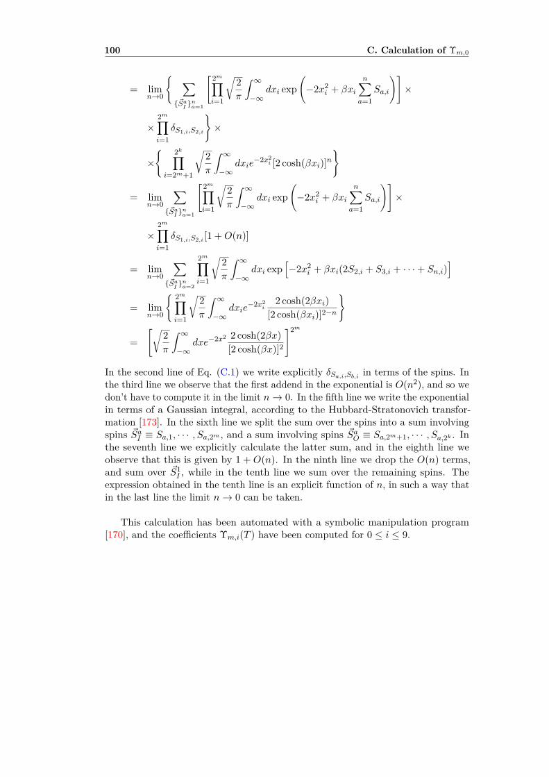
100 C. Calculation of Υm,0
= limn→0
{ ∑{~SaI }
na=1
[2m∏i=1
√2π
∫ ∞−∞
dxi exp(−2x2
i + βxi
n∑a=1
Sa,i
)]×
×2m∏i=1
δS1,i,S2,i
}×
×{ 2k∏i=2m+1
√2π
∫ ∞−∞
dxie−2x2
i [2 cosh(βxi)]n}
= limn→0
∑{~SaI }
na=1
[2m∏i=1
√2π
∫ ∞−∞
dxi exp(−2x2
i + βxi
n∑a=1
Sa,i
)]×
×2m∏i=1
δS1,i,S2,i [1 +O(n)]
= limn→0
∑{~SaI }
na=2
2m∏i=1
√2π
∫ ∞−∞
dxi exp[−2x2
i + βxi(2S2,i + S3,i + · · ·+ Sn,i)]
= limn→0
{ 2m∏i=1
√2π
∫ ∞−∞
dxie−2x2
i2 cosh(2βxi)
[2 cosh(βxi)]2−n
}
=[√
2π
∫ ∞−∞
dxe−2x2 2 cosh(2βx)[2 cosh(βx)]2
]2m
In the second line of Eq. (C.1) we write explicitly δSa,i,Sb,i in terms of the spins. Inthe third line we observe that the first addend in the exponential is O(n2), and so wedon’t have to compute it in the limit n→ 0. In the fifth line we write the exponentialin terms of a Gaussian integral, according to the Hubbard-Stratonovich transfor-mation [173]. In the sixth line we split the sum over the spins into a sum involvingspins ~SaI ≡ Sa,1, · · · , Sa,2m , and a sum involving spins ~SaO ≡ Sa,2m+1, · · · , Sa,2k . Inthe seventh line we explicitly calculate the latter sum, and in the eighth line weobserve that this is given by 1 + O(n). In the ninth line we drop the O(n) terms,and sum over ~S1
I , while in the tenth line we sum over the remaining spins. Theexpression obtained in the tenth line is an explicit function of n, in such a way thatin the last line the limit n→ 0 can be taken.
This calculation has been automated with a symbolic manipulation program[170], and the coefficients Υm,i(T ) have been computed for 0 ≤ i ≤ 9.
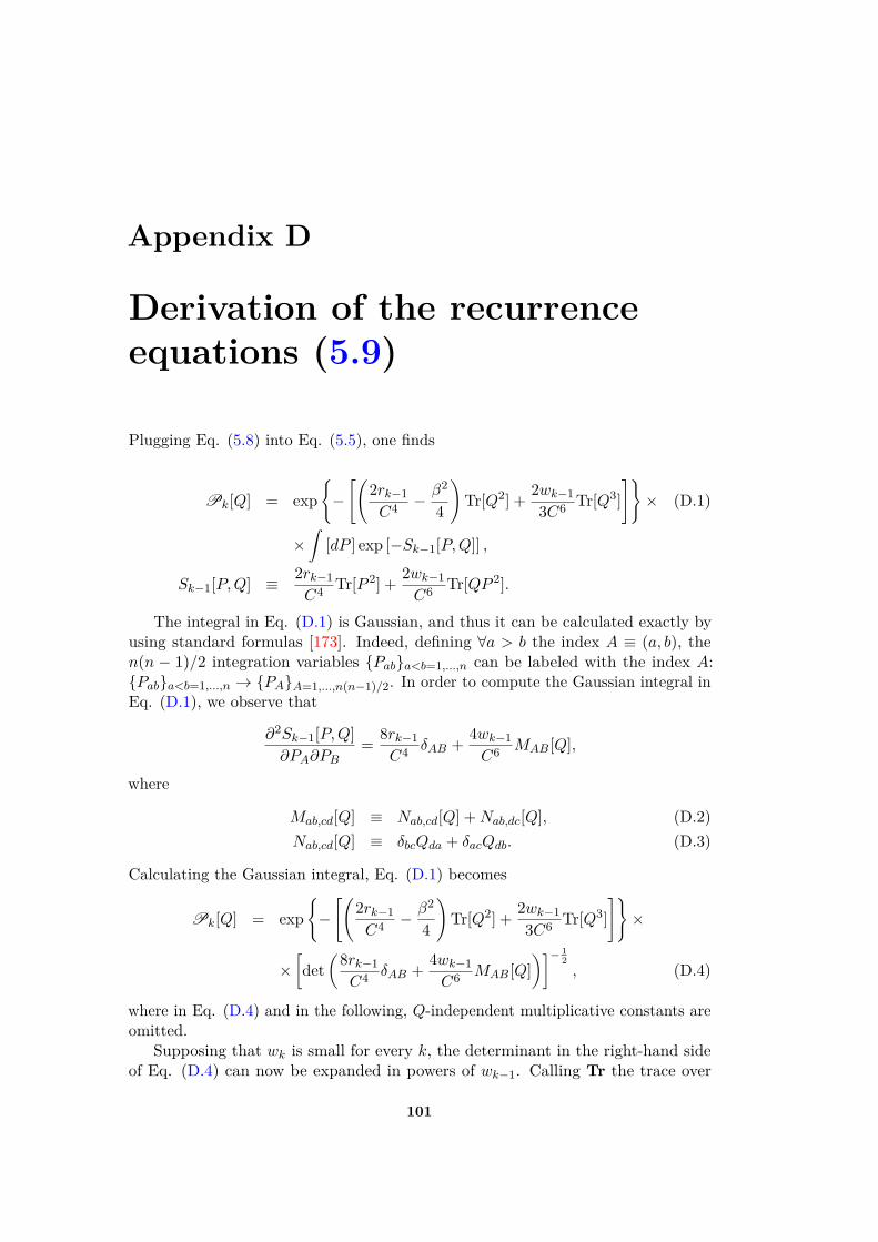
Appendix D
Derivation of the recurrenceequations (5.9)
Plugging Eq. (5.8) into Eq. (5.5), one finds
Pk[Q] = exp{−[(
2rk−1C4 − β2
4
)Tr[Q2] + 2wk−1
3C6 Tr[Q3]]}× (D.1)
×∫
[dP ] exp [−Sk−1[P,Q]] ,
Sk−1[P,Q] ≡ 2rk−1C4 Tr[P 2] + 2wk−1
C6 Tr[QP 2].
The integral in Eq. (D.1) is Gaussian, and thus it can be calculated exactly byusing standard formulas [173]. Indeed, defining ∀a > b the index A ≡ (a, b), then(n − 1)/2 integration variables {Pab}a<b=1,...,n can be labeled with the index A:{Pab}a<b=1,...,n → {PA}A=1,...,n(n−1)/2. In order to compute the Gaussian integral inEq. (D.1), we observe that
∂2Sk−1[P,Q]∂PA∂PB
= 8rk−1C4 δAB + 4wk−1
C6 MAB[Q],
where
Mab,cd[Q] ≡ Nab,cd[Q] +Nab,dc[Q], (D.2)Nab,cd[Q] ≡ δbcQda + δacQdb. (D.3)
Calculating the Gaussian integral, Eq. (D.1) becomes
Pk[Q] = exp{−[(
2rk−1C4 − β2
4
)Tr[Q2] + 2wk−1
3C6 Tr[Q3]]}×
×[det
(8rk−1C4 δAB + 4wk−1
C6 MAB[Q])]− 1
2, (D.4)
where in Eq. (D.4) and in the following, Q-independent multiplicative constants areomitted.
Supposing that wk is small for every k, the determinant in the right-hand sideof Eq. (D.4) can now be expanded in powers of wk−1. Calling Tr the trace over
101
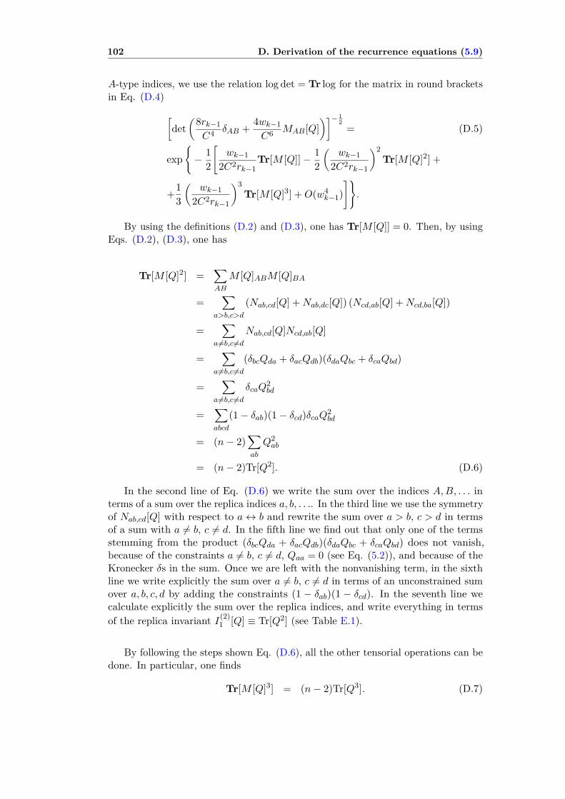
102 D. Derivation of the recurrence equations (5.9)
A-type indices, we use the relation log det = Tr log for the matrix in round bracketsin Eq. (D.4)
[det
(8rk−1C4 δAB + 4wk−1
C6 MAB[Q])]− 1
2= (D.5)
exp{− 1
2
[wk−1
2C2rk−1Tr[M [Q]]− 1
2
(wk−1
2C2rk−1
)2Tr[M [Q]2] +
+13
(wk−1
2C2rk−1
)3Tr[M [Q]3] +O(w4
k−1)]}.
By using the definitions (D.2) and (D.3), one has Tr[M [Q]] = 0. Then, by usingEqs. (D.2), (D.3), one has
Tr[M [Q]2] =∑AB
M [Q]ABM [Q]BA
=∑
a>b,c>d
(Nab,cd[Q] +Nab,dc[Q]) (Ncd,ab[Q] +Ncd,ba[Q])
=∑
a6=b,c 6=dNab,cd[Q]Ncd,ab[Q]
=∑
a6=b,c 6=d(δbcQda + δacQdb)(δdaQbc + δcaQbd)
=∑
a6=b,c 6=dδcaQ
2bd
=∑abcd
(1− δab)(1− δcd)δcaQ2bd
= (n− 2)∑ab
Q2ab
= (n− 2)Tr[Q2]. (D.6)
In the second line of Eq. (D.6) we write the sum over the indices A,B, . . . interms of a sum over the replica indices a, b, . . .. In the third line we use the symmetryof Nab,cd[Q] with respect to a↔ b and rewrite the sum over a > b, c > d in termsof a sum with a 6= b, c 6= d. In the fifth line we find out that only one of the termsstemming from the product (δbcQda + δacQdb)(δdaQbc + δcaQbd) does not vanish,because of the constraints a 6= b, c 6= d, Qaa = 0 (see Eq. (5.2)), and because of theKronecker δs in the sum. Once we are left with the nonvanishing term, in the sixthline we write explicitly the sum over a 6= b, c 6= d in terms of an unconstrained sumover a, b, c, d by adding the constraints (1 − δab)(1 − δcd). In the seventh line wecalculate explicitly the sum over the replica indices, and write everything in termsof the replica invariant I(2)
1 [Q] ≡ Tr[Q2] (see Table E.1).
By following the steps shown Eq. (D.6), all the other tensorial operations can bedone. In particular, one finds
Tr[M [Q]3] = (n− 2)Tr[Q3]. (D.7)

103
By plugging Eqs. (D.6), (D.7) into Eq. (D.5), and then substituting Eq. (D.5)into the recursion relation (D.4), one finds
Pk[Q] = exp{−[(
2rk−1C4 − β2
4 −n− 2
4
(wk−1
2C2rk−1
)2)Tr[Q2] + (D.8)
+13
(2wk−1C6 + n− 2
2
(wk−1
2C2rk−1
)3)Tr[Q3] +O(w4
k−1)]}.
Comparing Eq. (D.8) to the ansatz (5.8) for Pk, one finds the recursion relations(5.9) for the coefficients rk, wk.

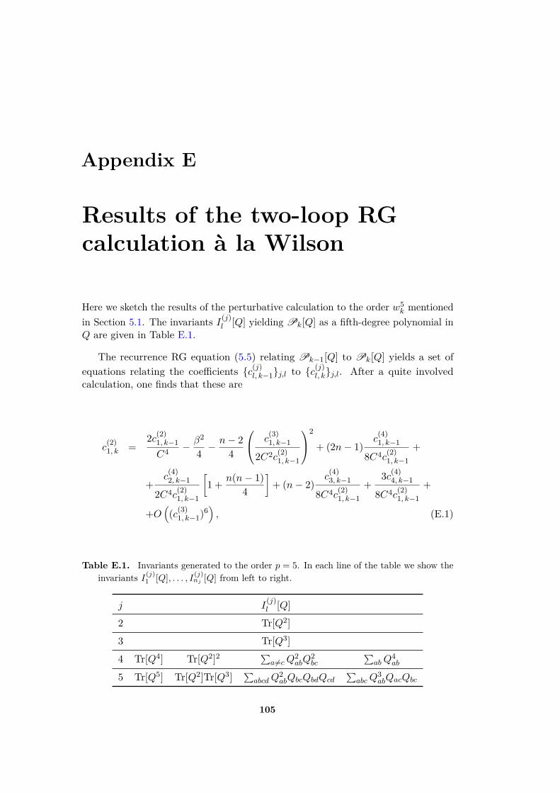
Appendix E
Results of the two-loop RGcalculation à la Wilson
Here we sketch the results of the perturbative calculation to the order w5k mentioned
in Section 5.1. The invariants I(j)l [Q] yielding Pk[Q] as a fifth-degree polynomial in
Q are given in Table E.1.
The recurrence RG equation (5.5) relating Pk−1[Q] to Pk[Q] yields a set ofequations relating the coefficients {c(j)
l, k−1}j,l to {c(j)l, k}j,l. After a quite involved
calculation, one finds that these are
c(2)1, k =
2c(2)1, k−1C4 − β2
4 −n− 2
4
c(3)1, k−1
2C2c(2)1, k−1
2
+ (2n− 1)c
(4)1, k−1
8C4c(2)1, k−1
+
+c
(4)2, k−1
2C4c(2)1, k−1
[1 + n(n− 1)
4
]+ (n− 2)
c(4)3, k−1
8C4c(2)1, k−1
+3c(4)
4, k−1
8C4c(2)1, k−1
+
+O((c(3)
1, k−1)6), (E.1)
Table E.1. Invariants generated to the order p = 5. In each line of the table we show theinvariants I(j)
1 [Q], . . . , I(j)nj [Q] from left to right.
j I(j)l [Q]
2 Tr[Q2]
3 Tr[Q3]
4 Tr[Q4] Tr[Q2]2∑a6=cQ
2abQ
2bc
∑abQ
4ab
5 Tr[Q5] Tr[Q2]Tr[Q3]∑abcdQ
2abQbcQbdQcd
∑abcQ
3abQacQbc
105

106 E. Results of the two-loop RG calculation à la Wilson
c(3)1, k =
2c(3)1, k−1C6 + n− 2
2
c(3)1, k−1
2C2c(2)1, k−1
3
+3nc(5)
1, k−1
4C6c(2)1, k−1
+
+(n+ 3)3c(5)
2, k−1
20C6c(2)1, k−1
+9c(5)
3, k−1
20C6c(2)1, k−1
+
+3c(5)
4, k−1
20C6c(2)1, k−1
[12 + n(n− 1)] +
−3c(3)
1, k−1
4C6c(2)1, k−1
(n− 1)c(4)1, k−1
2C4c(2)1, k−1
+2c(4)
2, k−1
C4c(2)1, k−1
+c
(4)3, k−1
2C4c(2)1, k−1
+
+O((c(3)
1, k−1)7), (E.2)
c(4)1, k =
2c(4)1, k−1C8 − n
2
c(3)1, k−1
2C2c(2)1, k−1
4
+O((c(3)
1, k−1)6), (E.3)
c(4)2, k =
2c(4)2, k−1C8 − 3
2
c(3)1, k−1
2C2c(2)1, k−1
4
+O((c(3)
1, k−1)6), (E.4)
c(4)3, k =
2c(4)3, k−1C8 + 8
c(3)1, k−1
2C2c(2)1, k−1
4
+O((c(3)
1, k−1)6), (E.5)
c(4)4, k =
2c(4)4, k−1C8 + 4
c(3)1, k−1
2C2c(2)1, k−1
4
+O((c(3)
1, k−1)6), (E.6)
c(5)1, k =
2c(5)1, k−1C10 + n+ 6
2
c(3)1, k−1
2C2c(2)1, k−1
5
+O((c(3)
1, k−1)7), (E.7)
c(5)2, k =
2c(5)2, k−1C10 − 40
c(3)1, k−1
2C2c(2)1, k−1
5
+O((c(3)
1, k−1)7), (E.8)
c(5)3, k =
2c(5)3, k−1C10 + 30
c(3)1, k−1
2C2c(2)1, k−1
5
+O((c(3)
1, k−1)7), (E.9)
c(5)4, k =
2c(5)4, k−1C10 + 5
c(3)1, k−1
2C2c(2)1, k−1
5
+O((c(3)
1, k−1)7). (E.10)

Appendix F
One-loop RG calculation in thefield-theory approach
In this Appendix we present the computation of the RG functions Zg, ZQ2 to order g2r .
In the bare theory, 1PI correlation functions are defined by the action (5.23), andthey can be obtained as the derivative of the bare 1PI generating functional Γ[Q]with respect to Qi, ab. Similarly, the renormalized 1PI correlation functions are thederivatives with respect to Q of the generating functional Γr[Q] of the renormalizedtheory, which depends on the renormalized parameters mr, gr. Accordingly, Γr[Q]can be expanded in powers of gr by means of the loop expansion
Γr[Q] = 12
2k−1∑i,j=0
∆ijTr[QiQj ] + m3εr gr3!
∑i
Tr[Q3i ](Zg + (F.1)
+n− 28 m
6ε2σ−1r I7g
2r
)+O(g5
r ).
The Feynman diagram I7 is depicted in Fig. 5.1, and is equal to
I7 = 12k
2k−1∑p=0
1(mr + δm+ |p|2σ−1
2
)3 . (F.2)
It is easy to show that I7 has a finite limit for k →∞. Indeed, the propagator(5.24) in the sum in the right-hand side of Eq. (F.2) depends on p through its dyadicnorm. Hence, the sum over p in the right-hand side of Eq. (F.2) can be easilytransformed into a sum over all the possible values of |p|2. In order to do so, werecall [139] that the number of integers 0 ≤ p ≤ 2k − 1 which satisfy |p|2 = 2−jis given by 2−j+k−1. This number is the volume of a shell in a space of integernumbers p, where the distance between two integers p1, p2 is given by the dyadicnorm |p1 − p2|2. Hence, Eq. (C.1) becomes
I7 =k−1∑j=0
2−j−1 1[mr + δm+ 2−j(2σ−1)]3 (F.3)
k→∞=∞∑j=0
2−j−1 1[mr + δm+ 2−j(2σ−1)]3 ,107
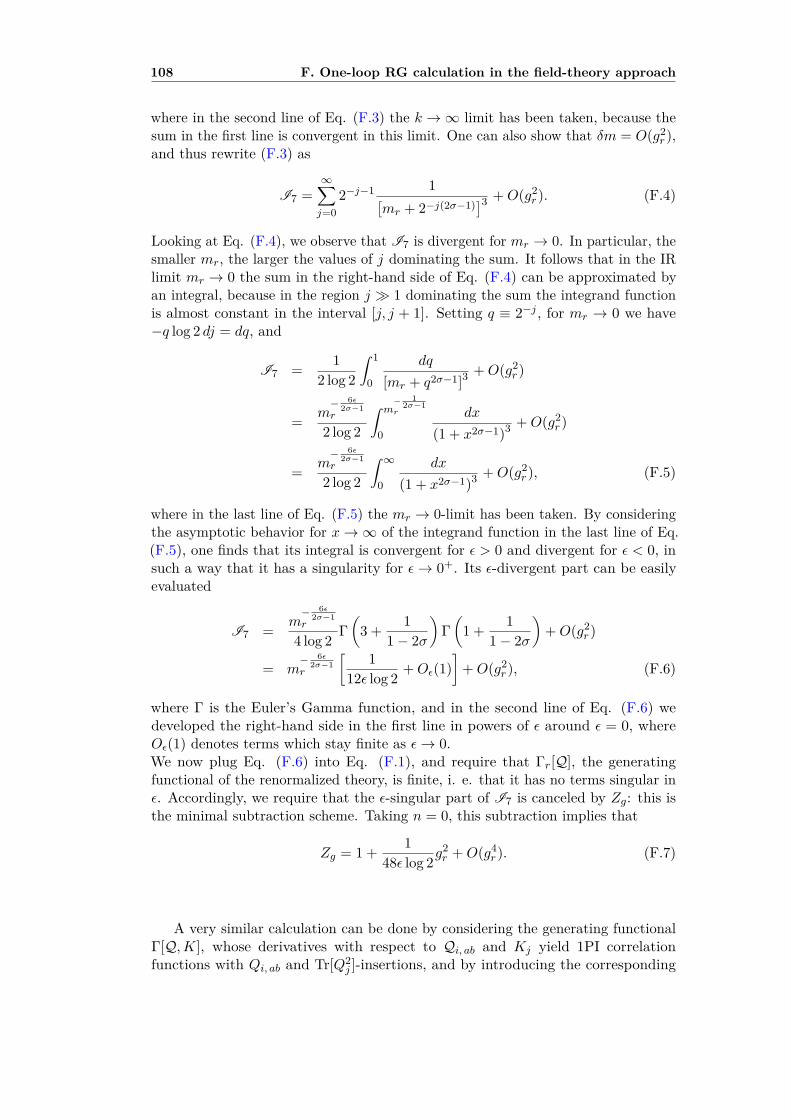
108 F. One-loop RG calculation in the field-theory approach
where in the second line of Eq. (F.3) the k →∞ limit has been taken, because thesum in the first line is convergent in this limit. One can also show that δm = O(g2
r ),and thus rewrite (F.3) as
I7 =∞∑j=0
2−j−1 1[mr + 2−j(2σ−1)]3 +O(g2
r ). (F.4)
Looking at Eq. (F.4), we observe that I7 is divergent for mr → 0. In particular, thesmaller mr, the larger the values of j dominating the sum. It follows that in the IRlimit mr → 0 the sum in the right-hand side of Eq. (F.4) can be approximated byan integral, because in the region j � 1 dominating the sum the integrand functionis almost constant in the interval [j, j + 1]. Setting q ≡ 2−j , for mr → 0 we have−q log 2 dj = dq, and
I7 = 12 log 2
∫ 1
0
dq
[mr + q2σ−1]3+O(g2
r )
= m− 6ε
2σ−1r
2 log 2
∫ m− 1
2σ−1r
0
dx
(1 + x2σ−1)3 +O(g2r )
= m− 6ε
2σ−1r
2 log 2
∫ ∞0
dx
(1 + x2σ−1)3 +O(g2r ), (F.5)
where in the last line of Eq. (F.5) the mr → 0-limit has been taken. By consideringthe asymptotic behavior for x→∞ of the integrand function in the last line of Eq.(F.5), one finds that its integral is convergent for ε > 0 and divergent for ε < 0, insuch a way that it has a singularity for ε→ 0+. Its ε-divergent part can be easilyevaluated
I7 = m− 6ε
2σ−1r
4 log 2 Γ(
3 + 11− 2σ
)Γ(
1 + 11− 2σ
)+O(g2
r )
= m− 6ε
2σ−1r
[ 112ε log 2 +Oε(1)
]+O(g2
r ), (F.6)
where Γ is the Euler’s Gamma function, and in the second line of Eq. (F.6) wedeveloped the right-hand side in the first line in powers of ε around ε = 0, whereOε(1) denotes terms which stay finite as ε→ 0.We now plug Eq. (F.6) into Eq. (F.1), and require that Γr[Q], the generatingfunctional of the renormalized theory, is finite, i. e. that it has no terms singular inε. Accordingly, we require that the ε-singular part of I7 is canceled by Zg: this isthe minimal subtraction scheme. Taking n = 0, this subtraction implies that
Zg = 1 + 148ε log 2g
2r +O(g4
r ). (F.7)
A very similar calculation can be done by considering the generating functionalΓ[Q,K], whose derivatives with respect to Qi, ab and Kj yield 1PI correlationfunctions with Qi, ab and Tr[Q2
j ]-insertions, and by introducing the corresponding
109
functional of the renormalized theory Γr[Q,K]. By requiring that Γr[Q,K] is finite,we obtain
ZQ2 = 1 + 124ε log 2g
2r +O(g4
r ). (F.8)
Eqs. (F.7), (F.8) are the one-loop renormalization constants Zg, ZQ2 .


Appendix G
Computation of the observables6.7 in Dyson’s HierarchicalModel
In order to compute the observables (6.7), it is convenient to introduce for anyk a discrete magnetization variable µ taking 2k + 1 possible values {−1,−1 +2/2k, · · · , 0, · · · , 1− 2/2k, 1}, and its probability distribution
πk(µ) ≡∑
~S e−βHF
k [~S]δ(
12k∑2ki=1 Si = µ
)Zk
, (G.1)
where
Zk ≡∑~S
e−βHFk [~S],
and δ denotes the Kronecker delta. Eq. (2.1) implies [57] that πk(µ) satisfies arecursion equation analogous to Eq. (2.5)
πk+1(µ) = eJβCk+1F µ2 ∑
µ1,µ2
πk(µ1)πk(µ2)δ(µ1 + µ2
2 = µ
), (G.2)
where a µ-independent multiplicative constant has been omitted in the right-handside of Eq. (G.2).
Given βJ , the recursion equation (G.2) can be iterated numerically k0 − 1 timesin 2k0 operations. Once πk0(µ) is known, the observable OFk0
(βJ) can be easilycomputed. Indeed, according to Eqs. (6.7), (6.4), we have
OFk0(βJ) =E~S[(
12k0−1
∑2k0−1i=1 Si
) (1
2k0−1∑2k0i=2k0−1+1 Si
)]E~S[(
12k0−1
∑2k0−1i=1 Si
)2] . (G.3)
111
112G. Computation of the observables 6.7 in Dyson’s Hierarchical
Model
The numerator of Eq. (G.3) is
E~S
12k0−1
2k0−1∑i=1
Si
12k0−1
2k0∑i=2k0−1+1
Si
=
= 1Zk0
∑~S
exp
−β (HFk0−1[~S1] +HF
k0−1[~S2])
+ βJCk0F
12k0
2k0∑i=1
Si
2×
×
12k0−1
2k0−1∑i=1
Si
12k0−1
2k0∑i=2k0−1+1
Si
××∑µ1,µ2
δ
12k0−1
2k0−1∑i=1
Si = µ1
δ 1
2k0−1
2k0∑i=2k0−1+1
Si = µ2
=
Z2k0−1Zk0
∑µ1,µ2
eβJCk0F
(µ1+µ2
2
)2
µ1µ2πk0−1(µ1)πk0−1(µ2), (G.4)
where S1 ≡ {S1, · · · , S2k0−1}, S2 ≡ {S2k0−1+1, · · · , S2k0}, and in the first line of Eq.(G.4) we used the recurrence relation (2.1), and we multiplied by a factor equal toone, while in the second line we used the definition (G.1). By following the samesteps as in Eq. (G.4), the denominator in Eq. (G.3) is
E~S
1
2k0−1
2k0−1∑i=1
Si
2 =
Z2k0−1Zk0
∑µ1,µ2
eβJCk0F
(µ1+µ2
2
)2
µ21πk0−1(µ1)πk0−1(µ2).
(G.5)By dividing Eq. (G.4) by Eq. (G.5), the multiplicative constants cancel out, and weare left with
OFk0(βJ) =∑µ1,µ2 e
βJCk0F
(µ1+µ2
2
)2
µ1µ2πk0−1(µ1)πk0−1(µ2)∑µ1,µ2 e
βJCk0F
(µ1+µ2
2
)2
µ21πk0−1(µ1)πk0−1(µ2)
. (G.6)
The right-hand side of Eq. (G.6) can be computed in 2k0 operations.
Appendix H
Solution of the real-space RGequations with thehigh-temperature expansion
In this Appendix we show how the RG equations (6.20) can be solved with a sys-tematic expansion in powers of β, by illustrating an explicit example where thisexpansion is performed up to order β4.
Expanding in powers of β the arctanh term in the right-hand side of Eq. (6.20)we have {
m′2 = C4
2 m2 + C4
2 β2(m2)2 + C8
8 β2(m2)2 − C8
24 β2m4,
m′4 = 3C8
16 (m2)2 + C8
16m4.(H.1)
An important feature of Eq. (H.1) is that it reproduces the fact that for σ < 1/2the thermodynamic limit is ill-defined, as we discussed in Part III, Eq. (4.12). Inorder to see this, let us look at the first line of Eq. (H.1). The first addend in theright-hand side is the O(β2)-term resulting from the β-expansion of the term in squarebrackets in the right-hand side of Eq. (6.20), while the other addends are O(β4)-terms. Keeping only the first term and using Eq. (2.13), we have m′2 = 21−2σm2. Accordingly, if σ < 1/2 we have m′2 > m2, i. e. the variance of the coupling Jincreases at each RG step, in such a way that in the thermodynamic limit k →∞the interaction energy diverges, and the model is ill-defined. On the other hand, Eq.(H.1) does not reproduce the condition σ < 1. This fact will emerge also in the nu-merical solution of the RG equations (6.19), and it will be discussed in Section 6.2.1.1.
Eq. (H.1) is formally analogous to Eq. (A.11) for DHM, and to Eq. (5.9),(E.1), (E.2) for the HEA. Accordingly, it is easy to see that Eq. (H.1) has a stablehigh-temperature fixed point m2 = m4 = 0, and a stable low-temperature fixedpoint m2 = m4 =∞. These fixed points are separated by an unstable critical fixedpoint m2 = m∗2,m4 = m∗4. By iterating k times Eq. (H.1) we generate the sequencem2 k,m4 k, and we depict the flow {m2 k,m4 k}k in Fig. H.1 for different values of thetemperature. Fig. H.1 shows that there is a value of the temperature TRSc such that
113

114H. Solution of the real-space RG equations with the
high-temperature expansion
for T = TRSc {m2 k,m4 k}k converges to m∗2,m∗4, while for T ≷ TRSc {m2 k,m4 k}kconverges to the high or low-temperature fixed point respectively.
0.0001
0.001
0.01
0.1
0 0.05 0.1 0.15 0.2 0.25 0.3
m4
k
m2 k
0.0001
0.001
0.01
0.1
0 0.05 0.1 0.15 0.2 0.25 0.3
m4
k
m2 k
T < T RSc
T > T RSc
T ≈ T RSc
Figure H.1. Parametric plot of (m2 k,m4 k) as a function of k with σ = 0.6. The blackpoints represent (m2 k,m4 k) for increasing k from left to right, with T < TRSc . The bluepoints represent (m2 k,m4 k) for increasing k from top to bottom, with T > TRSc . Thered points represent (m2 k,m4 k) for increasing k from top to bottom: here T has beendynamically adjusted to TRSc at each step k with the same procedure as that describedin the Caption of Fig A.1 for DHM.
We now use the same procedure as that illustrated in Section A.2 to calculatem∗2,m
∗4, by taking β = βRSc in such a way that Eq. (H.1) has a nontrivial fixed point
ma = m′a = m∗a{m∗2 = C4
2 m∗2 + C4
2 (βRSc )2(m∗2)2 + C8
8 (βRSc )2(m∗2)2 − C8
24 (βRSc )2m∗4,
m∗4 = 3C8
16 (m∗2)2 + C8
16m∗4.
(H.2)
The second line in Eq. (H.2) yields
m∗4 = 3C8(m∗2)2/[16(1− C8/16)], (H.3)
and by plugging Eq. (H.3) into the first line of Eq. (H.2) we obtain
m∗2 = C4
2 m∗2
{1 +
[1 + C4
4 + C12
26(−1 + C8/16)
](βRSc )2m∗2
}. (H.4)
Eq. (H.4) has a solution m∗2 = 0 which is ruled out, and a nonzero solutionm∗2 ∝ 1−C4/2. In the following we will compute this solution with an expansion inthe neighborhood of σ = 1/2. According to Eq. (2.13) one has 1−C4/2 = O(σ−1/2),thus we have m∗2 = O(σ − 1/2), and m∗4 = O((σ − 1/2)2). More precisely, from Eqs.(H.4), (H.3) we have
m∗2 = 3 log 22(βRSc )2 (σ − 1/2) +O((σ − 1/2)2),
m∗4 = 9(log 2)2
4(βRSc )4 (σ − 1/2)2 +O((σ − 1/2)3). (H.5)
115
Once the critical fixed point has been found, we can linearize the RG transfor-mation (H.1) in the neighborhood of m∗2,m∗4 to extract the critical exponents. Tothis end, we introduce the 2× 2 matrix
Mij ≡∂m′2i∂m2j
∣∣∣∣∣~m=~m∗
(H.6)
and its largest eigenvalue ΛRS . From Eqs. (H.6), (H.1), (H.5) one finds
ΛRS = 1 + 2 log 2 (σ − 1/2) +O((σ − 1/2)2). (H.7)
This high-temperature expansion can be implemented to higher orders in β.More precisely, it turns out that if the expansion of the term in square brackets in Eq.(6.20) is done up to order β2m, one obtains a set of m RG equations analogous toEq. (H.1), relating {m2a}a=1,...,m to {m′2a}a=1,...,m. The critical fixed point and thematrix M linearizing the RG transformation in its neighborhood are then extracted.The largest eigenvalue ΛRS of M can be computed as a power series in σ − 1/2 upto order (σ − 1/2)m−1. This computation has been done for m ≤ 5 by means of asymbolic manipulation program [170], and the result is given in Eq. (6.21).


Appendix I
Numerical discretization of thematrix MRS in thek0 = 2-approximation
In this Section we describe the numerical computation of the matrix MRS and ofits spectrum through a discretization of the continuous variable J .
Suppose that by iterating Routine 2 we computed the critical fixed point p∗(J )↔{Ji}i. As shown in Fig. 6.4, p∗(J ) has a compact support [−JMAX,JMAX], whereJMAX is defined by Eq. (6.24). This feature of the critical fixed point suggests arather natural way to compute MRS
J ,J ′ , based on a discretization of the continuousvariable J in the compact interval [−JMAX,JMAX]. Let us consider
J (i) ≡[1
2 + (i− 1)] 2JMAX
B− JMAX, ∀i = 1, . . . , B, (I.1)
and the B ×B matrixMij ≡MRS
J (i),J (j). (I.2)
The matrix M, and so MRS , can be easily computed numerically with a population-dynamics routine which is quite similar to Routine 1.
In Fig. I.1 we depict MRSJ ,J ′ as a function of J ,J ′, computed by means of
Eq. (I.2) for a given σ-value, and we show that by taking B large enough thediscretization method reconstructs a smooth function of J ,J ′.
The eigenvalues of M can be easily extracted numerically, and the eigenvaluesof MRS , which are related to the critical exponents, can be easily obtained fromthose of M as follows. The n-th eigenvalue λ(n) and the left and right eigenfunctionsφLn(J ), φRn (J ) of MRS are defined by∫
dJ ′MRSJ ,J ′φ
Rn (J ′) = λ(n)φRn (J ), (I.3)∫
dJ φLn(J )MRSJ ,J ′ = λ(n)φLn(J ′). (I.4)
117

118I. Numerical discretization of the matrix MRS in the
k0 = 2-approximation
-3-2
-10
12
3
-3-2
-10
12
3
0
1
2
3
4
5
M RSJ ,J ′
J
J ′
M RSJ ,J ′
00.511.522.533.544.5
Figure I.1. Matrix MRSJ ,J ′ as a function of J ,J ′ in the k0 = 2-approximation obtained with
the discretization method (I.2) with σ = 0.6215, P = 107, B = 96, kMAX = 50, x = 0.1.The matrix is not symmetric, and thus some eigenvalues are complex. Notwithstandingthis, the explicit numerical computation of the spectrum of MRS shows that theeigenvalue yielding the critical exponent ν is real.
The n-th eigenvalue λ(n)D and the left and right eigenvectors φLDn(i), φRDn(i) of M are
defined by
B∑j=1Mijφ
RDn(j) = λ
(n)D φRDn(i), (I.5)
B∑i=1
φRLn(i)Mij = λ(n)D φLDn(j). (I.6)
If we multiply Eqs. (I.5), (I.6) by dJ ≡ 2JMAX/B, take the large-B limit, transformthe sums in Eqs. (I.5), (I.6) into integrals and use the definition (I.2), by comparingEqs. (I.5), (I.6) to Eqs. (I.3), (I.4) we obtain the following identifications holding inthe B →∞-limit
λ(n)D × dJ = λ(n), (I.7)φRDn(i) = φRn (J (i)), (I.8)φLDn(i) = φLn(J (i)). (I.9)
In particular, from Eq. (I.7) we can extract the eigenvalues of MRS from those ofM.
In order to extract the critical exponents, one should observe that there is aneigenvalue, that we will call λ(1), which can be calculated analytically and whichdoes not contribute to ν even though it is part of the spectrum of MRS . Indeed,by multiplying Eq. (6.28) by p∗(J ′), integrating with respect to J ′ and using Eq.(6.26), we obtain ∫
dJ ′MRSJ ,J ′p∗(J ′) = 6p∗(J ), (I.10)
while by multiplying Eq. (6.28) by a constant A and integrating with respect to J

119
we have ∫dJAMRS
J ,J ′ = 6A. (I.11)
Comparing Eqs. (I.10), (I.11) to Eqs. (I.3), (I.4) we have
λ(1) = 6,φR1 (J ) = p∗(J ),φL1 (J ) = A. (I.12)
Following the very same procedure as Wilson’s [163], if we iterate the RG equations(6.19) k times for T ≈ TRSc and then iterate l times, the difference between pk+l andp∗ is given by
pk+l(J )− p∗(J ) =∫dJ ′[(MRS)l]J ,J ′ [pk(J ′)− p∗(J ′)]
=∫dJ ′
∑n
(λ(n))lφRn (J )φLn(J ′)[pk(J ′)− p∗(J ′)], (I.13)
where [(MRS)l]J ,J ′ is the J ,J ′-th component of the matrix (MRS)l, and in the sec-ond line of Eq. (I.13) the spectral representation of MRS has been used. Accordingto the third line of Eq. (I.12), the integral in the second line of Eq. (I.13) vanishesfor n = 1 because of the normalization condition
∫dJ ′pk(J ′) =
∫dJ ′p∗(J ′) = 1.
Hence, the eigenvalue λ(1) does not contribute either to the exponential divergenceof pk+l from p∗ nor to ν [163]. This fact is rather natural, because the eigenvalueλ(1) = 6 is an artefact of the k0 = 2-approximation, where a 22-spin HEA model withexactly six couplings {Jα}α is reduced to a 2-spin HEA. This fact will be elucidatedfurther in Section 6.2.2 when illustrating the k0 > 2-approximations. Indeed also fork0 > 2 there is an eigenvalue λ(1) = 2k0(2k0 − 1)/2 which depends explicitly on theapproximation degree k0, but which does not contribute to ν.
The eigenvalue of MRS determining ν is easily found by defining n∗ in such away that
|λ(n∗)| = maxn
(|λ(n)|) and∫dJ φLn∗(J )[pk(J )− p∗(J )] 6= 0, (I.14)
and by observing that [163] the critical exponent ν defined by Eq. (5.14) is given by
ν = log 2log λ(n∗)
. (I.15)


Part V
Reprints of the papers
121


Hierarchical Random Energy Model of a Spin Glass
Michele Castellana,1,2 Aurelien Decelle,1 Silvio Franz,1 Marc Mezard,1 and Giorgio Parisi2
1Laboratoire de Physique Theorique et Modeles Statistiques, CNRS - Universite Paris Sud, Batiment 100, 91405 Orsay Cedex, France2Dipartimento di Fisica, Universita di Roma ‘‘La Sapienza,’’ 00185 Rome, Italy
(Received 18 December 2009; revised manuscript received 1 March 2010; published 26 March 2010)
We introduce a random energy model on a hierarchical lattice where the interaction strength between
variables is a decreasing function of their mutual hierarchical distance, making it a non-mean-field model.
Through small coupling series expansion and a direct numerical solution of the model, we provide
evidence for a spin-glass condensation transition similar to the one occurring in the usual mean-field
random energy model. At variance with the mean field, the high temperature branch of the free-energy is
nonanalytic at the transition point.
DOI: 10.1103/PhysRevLett.104.127206 PACS numbers: 75.10.Nr, 05.10.�a, 05.50.+q
Clarifying the nature of glassy states is a fundamentalgoal of modern statistical physics. Both for spin glasses [1]and for structural glasses [2], the mean-field theory ofdisordered systems provides a suggestive picture of labo-ratory glassy phenomena as the reflection of an idealthermodynamic phase transition. Unfortunately, the devel-opment of a first principles theory of glassy systems goingbeyond mean field has resisted decades of intense research[3–5]. One of the main obstacles towards this goal lies inthe lack of reliable real space renormalization group (RG)schemes allowing us to reduce the effective number ofdegrees of freedom and identify the relevant fixed pointsdescribing glassy phases. In ferromagnetic systems, animportant role in the understanding of the real space RGtransformation has been played by spin systems withpower law interactions on hierarchical lattices [6,7]. Inthese models, the RG equations take the simple form ofnonlinear integral equations for an unknown function (asopposed to the functional of statistical field theory), thatcan be solved with high precision. In this perspective, it isnatural to generalize these models to spin glasses [8,9].
In this Letter, we introduce the simplest such spin-glassmodel, a random energy model (REM) [13,14]. As we shallsee, the hierarchical REM is such that the interactionenergy between subsystems scales subextensively in thesystem size. It thus qualifies as a non-mean-field model.We report in what follows the results of a small couplingexpansion and of an algorithmic solution of the RG equa-tions for the entropy that, exploring complementary re-gions of parameter space, provide the first analyticevidence in favor of an ideal glass transition in a non-mean-field model. Interestingly, this transition turns out tohave—as in the case of the standard REM—the characterof an entropy catastrophe analogous to the one hypothe-sized long ago for the structural glasses [15,16].
The hierarchical REM can be defined as a system ofN ¼ 2k Ising spins with an energy function defined recur-sively. The recursion is started at the level of a single spink ¼ 0, with the definition of H0½S� ¼ �0ðSÞ, where the
single spin energies are independent identically distributed(i.i.d.) random variables extracted from a distribution�0ð�Þ. At the level kþ 1, we consider then two indepen-dent systems of 2k spins S1 ¼ fS1ig, i ¼ 1; . . . ; 2k and S2 ¼fS2ig, i ¼ 1; . . . ; 2k with Hamiltonians H1k½S1� andH2k½S2�, respectively, and put them in interaction to forma composite system of 2kþ1 spins and Hamiltonian
Hkþ1½S1; S2� ¼ H1k½S1� þH2k½S2� þ �k½S1; S2�;where the �k are i.i.d. random variables extracted from adistribution �kþ1ð�Þ, chosen to have zero mean and vari-
ance h�k½S1; S2�2i � 2ðkþ1Þð1��Þ. The interaction term�k½S1; S2� is physically analogous to a surface interactionenergy between the two subsystems. For � 2 ð0; 1Þ, thismodel qualifies as a non-mean-field system, where theinteraction energy between different parts of the systemscales with volume to a power smaller than unity. On thecontrary, when � � 0, the interaction energy grows fasterthan the volume. A rescaling of the energy is then neces-sary to get a well-defined thermodynamic limit. The sys-tem behaves in this case as a mean-field model. Finally, for�> 1, the interaction energy decreases with distance andasymptotically the model behaves as a free system. In thefollowing, we focus on the most interesting region 0<�< 1.We have studied this model with two different methods.
The first one is a replica study of the quenched free energy,performed through a small coupling perturbative expan-sion. The second one is a numerical estimate of the micro-canonical entropy as a function of the energy. Bothmethods suggest that a REM-like finite-temperature phasetransition occurs for all � 2 ð0; 1Þ.Perturbative computation of the free energy.—In order to
make the calculations as simple as possible, we havechosen a Gaussian distribution for the energies �k. Wethen considered the perturbative expansion in g � 21��
of the free energy fðTÞ ¼ fðmÞðTÞ þOðgmþ1Þ. Notice thatthe expansion of f to the mth order takes into account just
PRL 104, 127206 (2010) P HY S I CA L R EV I EW LE T T E R Sweek ending
26 MARCH 2010
0031-9007=10=104(12)=127206(4) 127206-1 � 2010 The American Physical Society
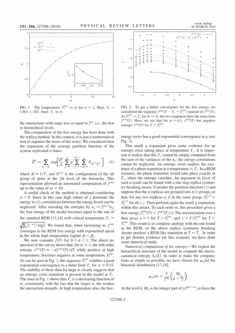
the interactions with range less or equal to 2m, i.e., the firstm hierarchical levels.
The computation of the free energy has been done withthe replica method. In this context, it is just a mathematicaltool to organize the terms of the series. We considered thenthe expansion of the average partition function of thesystem replicated n times
Zn ¼ X
S1���Snexp
��2
4
Xk
j¼0
gjX2k�j
i¼1
Xn
a;b¼1
�Sðj;iÞa Sðj;iÞ
b
�(1)
where � � 1=T, and Sðj;iÞ is the configuration of the ithgroup of spins at the jth level of the hierarchy. This
representation allowed an automated computation of fðmÞup to the value of m ¼ 10.
A useful check of the method is obtained considering�< 0. Since in this case high values of j dominate theenergy in (1), correlations between the energy levels can be
neglected. After rescaling the energies by �j ! 2k�=2�j,
the free energy of the model becomes equal to the one of
the standard REM [13,14] with critical temperature Tc ¼ffiffiffiffiffiffiffiffiffiffiffiffiffiffiffiffiffiffiffiffiffiffiffiffiffiffiffiffiffiPj2
��j= log2q
. We found that, when increasing m, fðmÞ
converges to the REM free energy with exponential speedin the whole high temperature regime �<�c.
We now consider fðTÞ for 0<�< 1. The direct in-spection of the curves shows that, form � 1, themth order
entropy sðmÞðTÞ � �dfðmÞðTÞ=dT while positive at high
temperature, becomes negative at some temperature TðmÞc .
As can be seen in Fig. 1, the sequence TðmÞc exhibits a good
exponential convergence to a finite limit Tc for � � 0:15.The stability of these data for large m clearly suggests thatan entropy crisis transition is present in the model at Tc.The inset in Fig. 1 shows that Tc is a decreasing function of�, consistently with the fact that the larger �, the weakerthe interaction strength. At high temperature also, the free-
energy series has a good exponential convergence in g (seeFig. 2).This small g expansion gives some evidence for an
entropy crisis taking place at temperature Tc. It is impor-tant to realize that this Tc cannot be simply computed fromthe sum of the variances of the �k: the energy correlationscannot be neglected. An entropy crisis implies the exis-tence of a phase transition at a temperature� Tc. In a REMscenario, the phase transition would take place exactly atTc, when the entropy vanishes. An argument in favor ofsuch a result can be found with a one-step replica symme-try breaking ansatz. Consider the partition function (1) andsuppose that the n replicas are grouped into n=x groups, so
that, for any two replicas a, b in the same group, Sðj;iÞa ¼Sðj;iÞb for all i, j. Then perform again the small g expansion,
within this ansatz. To each order m, this procedure gives a
free energy fðmÞx ðTÞ ¼ fðmÞðT=xÞ. The maximization over x
then gives x ¼ 1 for T > TðmÞc , and x ¼ T=TðmÞ
c for T <
TðmÞc . This result is in complete analogy with the one found
in the REM, so the above replica symmetry breakingAnsatz predicts a REM-like transition at T ¼ Tc. In orderto get distinct evidence for this scenario, we have donesome numerical study.Numerical computation of the entropy.—We exploit the
hierarchical structure of the model to compute the micro-canonical entropy SkðEÞ. In order to make the computa-tions as simple as possible, we have chosen for �kð�Þ thebinomial distribution [17,18],
�kð�Þ ¼ 1
2Mk
Mk
�þ Mk
2
� �:
At the level k,Mk is the integer part of �2kð1��Þ, to have the
FIG. 1. The temperatures TðmÞc vs m for � ¼ :1. Here, Tc ¼
1:861� :021. Inset: Tc vs �.
FIG. 2. To get a better convergence for the free energy, we
considered the sequence fðmÞðT � Tc þ TðmÞc Þ instead of fðmÞðTÞ.
As TðmÞc ! Tc form ! 1, the two sequences have the same limit
fð1ÞðTÞ. Here, we see that for � ¼ 0:1, fðmÞðTÞ has negative
entropy sðmÞðTÞ for T < TðmÞc .
PRL 104, 127206 (2010) P HY S I CA L R EV I EW LE T T E R Sweek ending
26 MARCH 2010
127206-2

same scaling of the variance as in the Gaussian model. Theconstant � is chosen so that for all the values of � studied,
bð�2kð1��ÞÞc=ð�2kð1��ÞÞ 1 for every k. Consider thedisorder-dependent density of states for a sample a:N a
kðEÞ ¼P
S�HkðSÞ;E. The recursion relation that defines
the model’s Hamiltonian implies that when two samples aand b at the level k are merged to define a sample at thelevel kþ 1, the resulting density of states N c
kþ1ðEÞ sat-isfies
N ckþ1ðEÞ ¼
X
Ea;Eb;�E¼EaþEbþ�
nkðEa; Eb; �Þ (2)
where nkðEa; Eb; �Þ ¼P
S1;S2�Ha
kðS1Þ;Ea
�Hb
kðS1Þ;Eb
��kðS1;SeÞ;� is the number of states in the composite
system that have Ha ¼ Ea, Hb ¼ Eb and interaction en-ergy equal to �. For given Ea and Eb, the joint distributionof the nkðEa; Eb; �Þ for the different values of � is multi-nomial with parameters q� ¼ hnkðEa; Eb; �Þi ¼N a
kðEaÞN bkðEbÞ�kð�Þ, while nk’s with different first or
second argument are independent.Our algorithmic approach starts from the exact iteration
of Eq. (2). Thanks to the use of a discrete interactionenergy, the iteration time grows with k proportionally to
2kð3��Þ. This allowed us to reach the level k ¼ 12. Theresults of the iteration shows that the values of the energycan be divided in bulk region of energy density around the
origin where the number of states N kðEÞ ¼ e2kSkðE=2kÞ is
exponential in the system size, and an edge region wherethe number of states is of order one (see Fig. 3).
In order to proceed further, we assume the existence andself-averaging property of the entropy density SðeÞ in thethermodynamic limit. We then coarse grain our descrip-tion. We discretize the energy density in the bulk region
and use an approximated iteration for the entropy, wherethe sum (2) is approximated by its maximum term. Weaccount for the edge region using the exact recursion forthe N0 ¼ 10 000 lowest energy levels. We can in this wayiterate many times and obtain a good estimate of thethermodynamic limit behavior.In Fig. 3, we present the average entropy density as a
function of the energy density e for various values of �. Inorder to identify the transition, it is more convenient toaverage the data obtained with a fixed energy differencefrom the fluctuating ground states. We can get in this waygood estimates of the value of the inverse critical tempera-ture of the model �c ¼ s0ðe0Þ. An interesting featureemerging from our analysis is that close to the ground stateenergy density e0, the entropy is not analytic and behavesas SðeÞ �cðe� e0Þ þ Cðe� e0Þa with a well fitted bythe value a ¼ 2� �. This behavior, when translated inthe canonical formalism, implies a singularity of the
free energy close to Tc, FðTÞ ¼ E0 þ const ðT �TcÞð2��Þ=ð1��Þ, corresponding to a specific heat exponent� ¼ � �
1�� .
Having found evidence for a thermodynamic phase tran-sition, we turn our attention to the distribution of low-lyingenergy states. The REM picture suggests that, close to theground state, the number of energy levels with givenenergy E are independent Poissonian variables with den-
sity hN 1ðEÞi ¼ e�cðE�E0Þ. A computation using extremevalue statistics shows that the probability Q‘ðkÞ that theground state and first ‘� 1 excited states are occupied by nlevels is given by
Q‘ðnÞ ¼ ½1� expð�‘�cÞ�n=ð‘�cnÞ: (3)
In Fig. 4, we show theQ‘ðnÞ obtained numerically togetherwith a fit with the form (3). This procedure confirms the
FIG. 3. The entropy sðeÞ vs e=ffiffiffiffi�
pfor � ¼ 0:9, 0.8, 0.7, 0.6
(with � ¼ 30, 10, 5, 5, respectively), from the outside to theinside. Inset: power law behavior of �� �c. The slopes areclose to 1� �, with � ¼ 0:6, 0.7, 0.8 from bottom to top.
FIG. 4. Numerical data (cross) and the fitting function Q3ðnÞfor the statistics of occupation of the ground state and the firsttwo occupied levels. Here, k ¼ 10, � ¼ 0:6 and � ¼ 5. Thedashed line is a fit with the form (3) with �c ¼ 1:20.
PRL 104, 127206 (2010) P HY S I CA L R EV I EW LE T T E R Sweek ending
26 MARCH 2010
127206-3

validity of a REM-like transition, and provides an alter-native way of estimating the critical temperature. As Fig. 5shows, the two estimates for different values of k tend tothe same limit from opposite directions.
Conclusions.—In this Letter, we have introduced a hier-archical, non-mean-field REM. We have analyzed itthrough small coupling series, through a 1RSB replicaansatz, and through an algorithmic approach. The twoapproaches point to the existence of a REM-like phasetransition at the temperature where the entropy vanishes.At variance with the mean-field result (which predicts adiscontinuity in the specific heat), one finds a nontrivialspecific heat exponent at Tc. It will be interesting to studythe replica structure of this hierarchical REM in order toexplore other possible replica solutions at low tempera-tures. Another important theme of future research is thestudy of spin-glass models with p-body interaction[13,19,20]: at the mean-field level, these models displayan entropy crisis transition similar to the one of the REM
whenever p � 3. It will be interesting to study them onhierarchical lattices.
[1] M. Mezard, G. Parisi, and M.A. Virasoro, Spin GlassTheory and Beyond (World Scientific, Singapore, 1987).
[2] T. Castellani and A. Cavagna, J. Stat. Mech. (2005)P05012.
[3] C. De Dominicis and I. Giardina, Random Fields and SpinGlasses: A Field Theory Approach (Springer, New York,2006).
[4] J. H. Chen and T. C. Lubensky, Phys. Rev. B 16, 2106(1977).
[5] G. Kotliar, P.W. Anderson, and D. L. Stein, Phys. Rev. B27, 602 (1983).
[6] F. J. Dyson, Commun. Math. Phys. 12, 91 (1969).[7] P. Collet and J. Eckmann, A Renormalization Group
Analysis of the Hierarchical Model in StatisticalMechanics (Springer-Verlag, Berlin, 1978).
[8] S. Franz, T. Jorg, and G. Parisi, J. Stat. Mech. (2009)P02002.
[9] These models should not be confused with models withlocal interactions on hierarchical lattices built on diamondplaquettes [10], which, starting from Ref. [11], have beenwidely studied in their spin-glass version and lead toweakly frustrated systems even in their mean-field limit[12].
[10] A. N. Berker and S. Ostlund, J. Phys. C 12, 4961 (1979).[11] S. R. McKay, A.N. Berker, and S. Kirkpatrick, Phys. Rev.
Lett. 48, 767 (1982).[12] E. Gardner, J. Phys. (Les Ulis, Fr.) 45, 1755 (1984).[13] B. Derrida, Phys. Rev. Lett. 45, 79 (1980).[14] D. J. Gross and M. Mezard, Nucl. Phys. B240, 431 (1984).[15] W. Kauzmann, Chem. Rev. 43, 219 (1948).[16] J. H. Gibbs and E.A. DiMarzio, J. Chem. Phys. 28, 373
(1958).[17] C. Moukarzel and N. Parga, Physica A (Amsterdam) 177,
24 (1991).[18] K. Ogure and Y. Kabashima, Prog. Theor. Phys. 111, 661
(2004).[19] E. Gardner, Nucl. Phys. B257, 747 (1985).[20] T. R. Kirkpatrick, D. Thirumalai, and P.G. Wolynes, Phys.
Rev. A 40, 1045 (1989).
FIG. 5. Finite volume estimation of the inverse critical tem-
perature,ffiffiffiffi�
p�ðkÞ
c vs k, for � ¼ 0:6 and � ¼ 5 determined by (3)
(circle) and by �c ¼ s0ðe0Þ (triangles). The latter have been fittedwith a function of the type �ðkÞ
c ¼ �c � BCk (solid line). Theasymptotic value �c is given by the dashed line.
PRL 104, 127206 (2010) P HY S I CA L R EV I EW LE T T E R Sweek ending
26 MARCH 2010
127206-4

J.Stat.M
ech.(2011)
P03023
ournal of Statistical Mechanics:J Theory and Experiment
Adversarial satisfiability problem
Michele Castellana1,2,3 and Lenka Zdeborova3,4
1 Dipartimento di Fisica, Universita di Roma ‘La Sapienza’, 00185 Rome, Italy2 LPTMS, CNRS and Universite Paris-Sud, UMR8626, Batiment 100, 91405Orsay, France3 Theoretical Division and Center for Nonlinear Studies, Los Alamos NationalLaboratory, NM 87545, USA4 Institue de Physique Theorique, IPhT, CEA Saclay, and URA 2306, CNRS,91191 Gif-sur-Yvette cedex, FranceE-mail: [email protected] and [email protected]
Received 4 November 2010Accepted 26 February 2011Published 28 March 2011
Online at stacks.iop.org/JSTAT/2011/P03023doi:10.1088/1742-5468/2011/03/P03023
Abstract. We study the adversarial satisfiability problem, where the adversarycan choose whether the variables are negated in clauses or not, in order tomake the resulting formula unsatisfiable. This problem belongs to a generalclass of adversarial optimization problems that often arise in practice and arealgorithmically much harder than the standard optimization problems. We usethe cavity method to compute large deviations of the entropy in the randomsatisfiability problem with respect to the configurations of negations. We concludethat in the thermodynamic limit the best strategy the adversary can adopt is tosimply balance the number of times every variable is negated and the number oftimes it is not negated. We also conduct a numerical study of the problem, andfind that there are very strong pre-asymptotic effects that may be due to the factthat for small sizes exponential and factorial growth is hardly distinguishable. Asa side result we compute the satisfiability threshold for balanced configurationsof negations, and also the random regular satisfiability, i.e. when all variablesbelong to the same number of clauses.
Keywords: message-passing algorithms, random graphs, networks
c©2011 IOP Publishing Ltd and SISSA 1742-5468/11/P03023+22$33.00
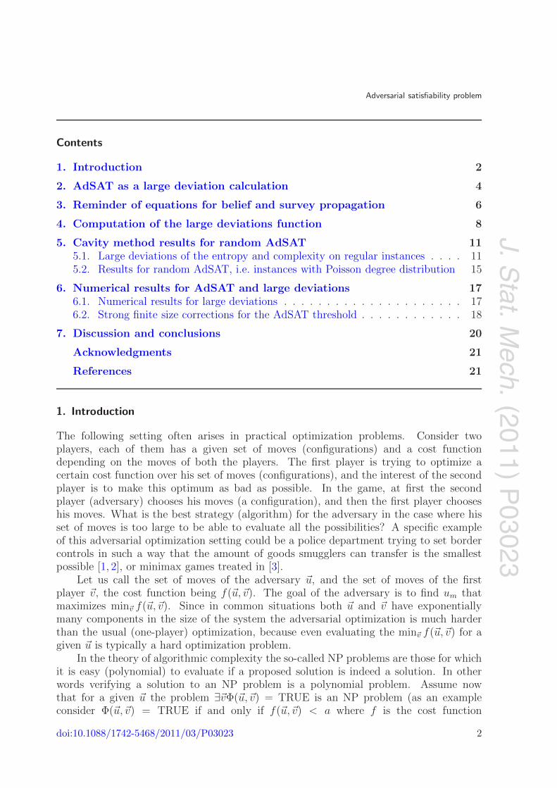
J.Stat.M
ech.(2011)
P03023
Adversarial satisfiability problem
Contents
1. Introduction 2
2. AdSAT as a large deviation calculation 4
3. Reminder of equations for belief and survey propagation 6
4. Computation of the large deviations function 8
5. Cavity method results for random AdSAT 115.1. Large deviations of the entropy and complexity on regular instances . . . . 115.2. Results for random AdSAT, i.e. instances with Poisson degree distribution 15
6. Numerical results for AdSAT and large deviations 176.1. Numerical results for large deviations . . . . . . . . . . . . . . . . . . . . . 176.2. Strong finite size corrections for the AdSAT threshold . . . . . . . . . . . . 18
7. Discussion and conclusions 20
Acknowledgments 21
References 21
1. Introduction
The following setting often arises in practical optimization problems. Consider twoplayers, each of them has a given set of moves (configurations) and a cost functiondepending on the moves of both the players. The first player is trying to optimize acertain cost function over his set of moves (configurations), and the interest of the secondplayer is to make this optimum as bad as possible. In the game, at first the secondplayer (adversary) chooses his moves (a configuration), and then the first player chooseshis moves. What is the best strategy (algorithm) for the adversary in the case where hisset of moves is too large to be able to evaluate all the possibilities? A specific exampleof this adversarial optimization setting could be a police department trying to set bordercontrols in such a way that the amount of goods smugglers can transfer is the smallestpossible [1, 2], or minimax games treated in [3].
Let us call the set of moves of the adversary �u, and the set of moves of the firstplayer �v, the cost function being f(�u,�v). The goal of the adversary is to find um thatmaximizes min�v f(�u,�v). Since in common situations both �u and �v have exponentiallymany components in the size of the system the adversarial optimization is much harderthan the usual (one-player) optimization, because even evaluating the min�v f(�u,�v) for agiven �u is typically a hard optimization problem.
In the theory of algorithmic complexity the so-called NP problems are those for whichit is easy (polynomial) to evaluate if a proposed solution is indeed a solution. In otherwords verifying a solution to an NP problem is a polynomial problem. Assume nowthat for a given �u the problem ∃�vΦ(�u,�v) = TRUE is an NP problem (as an exampleconsider Φ(�u,�v) = TRUE if and only if f(�u,�v) < a where f is the cost function
doi:10.1088/1742-5468/2011/03/P03023 2

J.Stat.M
ech.(2011)
P03023
Adversarial satisfiability problem
from above, and a is a constant). Then the associated adversarial decision problemis defined as ∃�u ∀�vΦ(�u,�v) = TRUE. Hence if the class of polynomial problems isconsidered easy, and the NP problems correspond to the first level of difficulty, thenthe adversarial problems correspond to the second level of difficulty. We could continuethis construction by adding even more levels of logical quantifiers; this would lead to theso-called polynomial hierarchy of complexity classes. For more details on these notions seefor instance [4, 5]. Without doubt, the theoretical understanding of hard optimization anddecision problems is crucial for many areas of science, and the same holds for adversarialproblems.
The most famous benchmark of an algorithmically hard problem is theK-satisfiability(K-SAT) of Boolean formulas. Call a clause a logical disjunction (operation ‘or’) of Kvariables or their negations. Given a set of N Boolean variables xi, and a set of M clauses,the satisfiability problem consists in deciding whether all clauses can be simultaneouslysatisfied or not. The K-SAT problem was the first problem shown to be NP-complete,that is as hard as any other NP problems [6]. It has a large number of applicationsin automated verification and design. The random K-SAT problem, where variables inclauses are chosen randomly and negated with probability 1/2, provides easy to generatehard formulas [7].
Random K-SAT thus became a common playground for new algorithms, andtheoretical ideas for understanding the origin of algorithmic hardness. The statisticalphysics approach related to the physics of diluted spin glasses contributed tremendouslyto the understanding of the properties of randomK-SAT formulas, see e.g. [8, 9]. Followingthis path in this paper we introduce a random adversarial satisfiability problem anddevelop a statistical mechanics framework to understand its properties. This frameworkcan be readily applied to other random adversarial optimization and decision problems.We study the large deviation functions for the original optimization problem with respectto the moves of the adversary. The main ideas of our approach to the study of largedeviations come from studies of spin glasses and the cavity method [10]–[13]. Our approachis also closely linked to the well established fact that the replicated free energy in Parisi’sreplica symmetry breaking (RSB) [14, 15] can be interpreted as Legendre transformationof the large deviation function. We will, however, derive our method independently ofthese notions, by using only the factor graph representation of the problem and the beliefpropagation (BP) algorithm.
One natural setting for the random adversarial satisfiability problem is to introducethe negation-variables Jia, where Jia = 1 if variable i is negated in clause a, and Jia = 0 ifnot. The set of moves of the adversary is then all the possible configurations of negations{Jia}, while the moves of the first player are all the possible configurations of the variables{xi}. The graph of interactions is chosen at random as before. The goal of the adversaryis to set the negations in such a way that the resulting formula is as frustrated as possible.In particular, we will be interested in the question: can the adversary make the formulaunsatisfiable or not? We will call this problem random AdSAT.
An independent interest in the random AdSAT comes from the study of the randomquantum satisfiability (quantum SAT) problem [16]–[18]. It was shown that if theadversary can make the random formula unsatisfiable, then also the random quantumSAT is unsatisfiable. A natural question is whether the quantum SAT is much morerestrictive than the AdSAT or not.
doi:10.1088/1742-5468/2011/03/P03023 3
J.Stat.M
ech.(2011)
P03023
Adversarial satisfiability problem
Note also that the quantified satisfiability (QSAT) problem is another SAT-basedproblem that belongs to the general adversarial setting as introduced above. In the QSATproblem one introduces two types of variables: the existential variables xi and the universalvariables yi. The QSAT then consists in deciding whether ∀ �y ∃�xG(�x, �y) = TRUE, whereG(�x, �y) is a satisfiability formula (with negation-variables fixed). Random ensemblesof QSAT were introduced and studied in [19]. QSAT is arguably more important forindustrial applications than the AdSAT that we study here. We chose the AdSAT definedas above because it is slightly simpler, and it provides information relevant to the originalrandom SAT problem. We plan to apply our approach to the random QSAT problem inthe near future.
In terms of methodology our study is also closely related to the work on optimizationunder uncertainty [20], where the goal is to find argmin�uE�t min�v f(�u,�v, t). In other wordsone needs to minimize an expectation of a result of an independent minimization, whichitself can be hard to compute. In [20] the authors studied the stochastic bipartite matchingproblem with a message passing technique very closely related to the one we use for theadversarial SAT problem here.
The present paper is structured as follows. In section 2 we set the adversarialsatisfiability problem, and describe our statistical physics approach to solve it. In section 3we recall the standard belief and survey propagation (SP) equations for the random K-satisfiability problem. In section 4 we derive the equations to compute the large deviationswith respect to the configurations of negations. In section 5 we first present and discussthe cavity result for random regular adversarial satisfiability, then we do the same forthe canonical (Poissonian) random adversarial satisfiability. As a side result we obtainthe satisfiability threshold for the (non-adversarial) random regular and random balancedSAT. In section 6 we compare our theoretical result to numerical simulations, performingan exhaustive search of all the solutions. Finally, in section 7 we conclude and discuss theperspectives of this work.
2. AdSAT as a large deviation calculation
The random K-SAT problem is defined as follows. Consider N Boolean variables{xi}i=1,...,N , xi = {0, 1}, and M = αN clauses ψa. Each clause depends on K randomvariables from the N available ones. If a variable i belongs to clause ψa, then we setJai = 1 if the variable is negated, and Jia = 0 if it is not. The K-SAT problem canbe represented via a so-called factor graph, a bipartite graph between variables (variablenodes) and clauses (function nodes), with edges between variable i and clause a if i belongsto clause a. The negation-variables can be seen as attributes of the edges. The randomK-SAT instance corresponds to the case where the Jias are drawn uniformly at random.Probably, the most well known property of the random K-SAT is the existence of a phasetransition at a value αc such that if α < αc then with high probability (probability goingto one as N → ∞) there exists a configuration {xi} that satisfies all the clauses, and forα > αc no such configuration exists with high probability. We define ∂i as the ensembleof function nodes connected to the variable node i, ∂a as the ensemble of variable nodesconnected to the function node a.
The adversarial satisfiability problem (AdSAT) is defined by drawing a random K-SAT instance as before without deciding the negation-variables {Jia} ≡ J . A solution to
doi:10.1088/1742-5468/2011/03/P03023 4

J.Stat.M
ech.(2011)
P03023
Adversarial satisfiability problem
the AdSAT problem is given by a set J such that the resulting instance is unsatisfiable.Just as in random K-SAT there is a threshold αa in the random AdSAT such that forα < αa no solution to the AdSAT formula exists with high probability. And for α > αa asolution exists with high probability. We observe that αa ≤ αc since above αc a randomconfiguration of negations makes the formula unsatisfiable, recall αc(K = 3) = 4.2667 [21].Also αa ≥ αp, where αp = 1/K is the percolation threshold below which the graph isbasically a collection of small trees and a few single loop components, which are bothsatisfiable for any configuration of negations. One of the goals of the present paper is toestimate the value of the AdSAT threshold αa.
In random K-SAT the satisfiability threshold can be found by counting the numberof configurations that have a certain energy E({xi}) (i.e. number of unsatisfied clauses).To compute the entropy one introduces a Legendre parameter β and computes the freeenergy f defined as
e−βNf(β) =∑
{xi}e−βE({xi}) = eN [s(e)−βe],
∂s(e)
∂e= β, (1)
where the number of configurations having energy E is eS(E), and the saddle-pointapproximation for N → ∞ has been used. If E = 0 belongs to the support of thefunction S(E) then the problem is in the satisfiable phase, if not than the problem isin the unsatisfiable phase. In the satisfiable phase we call s = S(0)/N the entropy ofsatisfying configurations. The cavity method and the replica symmetry breaking serveto compute f(β) in the thermodynamic limit N → ∞ [22, 8]. There are two crucialproperties that make this calculation possible. First, the energy can be written as a sumof local terms:
E({xi}) =∑
a
∏
i∈∂a
δxi,Jia. (2)
Second, the underlying factor graph is locally tree-like. These computations moreoverprovide much more information about the problem than the value of the satisfiabilitythreshold.
In the study of random AdSAT we will proceed analogously. We consider the numberof configurations of the negations that yield a given value of the entropy of solutions s
s(J ) =1
Nlog
⎡⎣∑
{xi}
M∏
a=1
(1 −
∏
i∈∂a
δxi,Jia
)⎤⎦. (3)
We define a large deviation function L(s) as the logarithm of this number divided by thesize of the system N . Again to compute L(s) it is advantageous to introduce its Legendretransform
Z(x) = eNΦ(x) =∑
JexNs(J ) = eN [L(s)+xs],
∂L(s)
∂s= −x, (4)
where the saddle-point approximation for N → ∞ has been used.We stress here that L(s) is the large deviation function with respect to the negation-
configurations; it is hence defined for a given geometry of the satisfiability formula.In what follows we assume, as is usual, that L(s) is self-averaging with respect to the
doi:10.1088/1742-5468/2011/03/P03023 5
J.Stat.M
ech.(2011)
P03023
Adversarial satisfiability problem
formula geometry, i.e. L(s) is almost surely the same function for two randomly chosenformulas. This assumption is a generalization of the self-averaging property of the freeenergy in the canonical K-SAT problem. Note also that when writing this expression weimplicitly assume that the number of negation-configurations that give a certain entropyis exponential in N . If it is smaller that exponential in N computation of Φ(x) will leadto L(s) = −∞. We will come back to this point in section 6.
Note two special cases: for x = 0 the partition function (4) is simply equal to thetotal number of negation-configurations Φ(0) = Kα log 2; for x = 1, the partition functionabove is related to the annealed partition function, Φ(1) = log 2 + α log(2K − 1).
The major difficulty in calculating Φ(x), for a general value of x, is that the entropys(J ) is not defined as a sum of local terms. On the other hand the geometry of theunderlying factor graph is still tree-like in the random AdSAT, hence for any configurationof negations J we can apply the cavity method (with replica symmetry breaking if needed)to compute the entropy s(J ). In the cavity method, as is reminiscent of the Betheapproximation, the entropy (or more generally Bethe free energy) can be written as asum of local terms. This fact enables us to calculate Φ(x).
The statistical physics treatment of the random K-SAT problem among others ledto a discovery that the replica symmetry breaking approach is needed [22, 8, 9] in orderto correctly compute the entropy close to the satisfiability threshold αc. In other words,in that region the space of solutions splits into well ergodically separated clusters. Wedefine the complexity function Σ as the logarithm of the total number of clusters pervariable. The value of the complexity can then be computed with the survey propagationequations [8]. At the satisfiability threshold the complexity goes to zero, whereas theentropy density of solutions is a positive number even at the threshold. With this in mindit will be useful to define also
eNΦSP(x) =∑
JexNΣ(J ) = eN [LSP(Σ)+xΣ],
∂LSP(Σ)
∂Σ= −x, (5)
where LSP(Σ) is the entropy density of negation-configurations that give a certaincomplexity function Σ, and the saddle-point approximation for N → ∞ has been used.
3. Reminder of equations for belief and survey propagation
With the notation introduced in section 2 we write the belief propagation equations andthe Bethe entropy as derived, e.g., in [23, 24]. These equations are asymptotically exacton locally tree-like graphs as long as all the correlation length scales are finite. If theyare not then splitting the phase space into clusters such that within each cluster thecorrelations decay again might be possible. SP then estimates the total number of suchclusters [8], and it does so asymptotically exactly at least close enough to the satisfiabilitythreshold [25, 9].
Denoting by {mia, mai} the BP (SP) messages, we write the BP (SP) fixed-pointequations as
mia = gia({mbi}b∈∂i\a, {Jbi}b∈∂i), (6)
mai = gai({mja}j∈∂a\i, {Jja}j∈∂a). (7)
doi:10.1088/1742-5468/2011/03/P03023 6

J.Stat.M
ech.(2011)
P03023
Adversarial satisfiability problem
In the BP case, the messages read [24] mia = {ν0ia, ν
1ia}, mai = {ν0
ai, ν1ai}, and
gria({νbi}b∈∂i\a) =
∏b∈∂i\a ν
rbi∏
b∈∂i\a ν0bi +
∏b∈∂i\a ν
1bi
,
grai({νja}j∈∂a\i, {Jja}j∈∂a) =
1 − δr,Jai
∏j∈∂a\i ν
Jja
ja
2 −∏j∈∂a\i νJja
ja
,
(8)
where r = 0, 1. In the SP case, mia = {QSia, Q
Uia, Q
∗ia}, mai = Qai, and
g∗ia({Jbi}b∈∂i, {Qbi}b∈∂i\a) = C
∏
b∈∂i\a
(1 − Qbi),
gSia({Jbi}b∈∂i, {Qbi}b∈∂i\a) = C
∏
b∈Uia
(1 − Qbi)
[1 −
∏
b∈Sia
(1 − Qbi)
],
gUia({Jbi}b∈∂i, {Qbi}b∈∂i\a) = C
∏
b∈Sia
(1 − Qbi)
[1 −
∏
b∈Uia
(1 − Qbi)
],
gai({Qja}j∈∂a\i) =∏
j∈∂a\i
QUja,
(9)
where C is a normalization constant enforcing the relation g∗ia + gS
ia + gUia = 1, and Sia, Uia
are defined as
if Jia = 0 Sia = ∂0i\a, Uia = ∂1i,
if Jia = 1 Sia = ∂1i\a, Uia = ∂0i,(10)
where ∂0/1i = {a ∈ ∂i such that Jia = 0/1}.
If {mia, mai} is a fixed point of equations (6)–(7), the Bethe entropy for BP and thecomplexity for SP are both written in a general form
s({Jia, mia, mai}) =M∑
a=1
Sa({mia, Jia}i∈∂a) +N∑
i=1
Si({mai, Jia}a∈∂i) −∑
(ia)
Sai(mia, mai),
(11)
where for BP
Sa({νia, Jia}i∈∂a) = log
(1 −
∏
i∈∂a
νJiaia
),
Si({νai, Jia}a∈∂i) = log
(∏
b∈∂i
ν0bi +
∏
b∈∂i
ν1bi
),
Sai(νia, νai) = log(ν0
iaν0ai + ν1
iaν1ai
),
(12)
doi:10.1088/1742-5468/2011/03/P03023 7

J.Stat.M
ech.(2011)
P03023
Adversarial satisfiability problem
while for SP
Sa({Qia, Jia}i∈∂a) = log
(1 −
∏
j∈∂a
QUja
),
Si({Qai, Jia}a∈∂i) = log
[∏
b∈∂0i
(1 − Qbi) +∏
b∈∂1i
(1 − Qbi) −∏
b∈∂i
(1 − Qbi)
],
Sai(Qia, Qai) = log(1 −QU
iaQai
).
(13)
Readers unfamiliar with the interpretation and derivation of the belief and the surveypropagation (8)–(10) are referred to [23, 26, 24]. However, for understanding of our methodin what follows the general form (6)–(7) and (11) is sufficient.
4. Computation of the large deviations function
The most important formula of section 3 is (11): in certain regimes it gives theasymptotically exact entropy or complexity in a form factorized in local terms. Theremaining complication is that now everything depends on the fixed point of the BP (SP)equations. We can, however, write
Z(x) =∑
J
∫ ∏
ia
dmiadmaieNxs({Jia,mia,mai})
∏
(ia)
δ(mia − gia({mbi}b∈∂i\a, {Jbi}b∈∂i))
×∏
(ia)
δ(mai − gai({mja}j∈∂a\i, {Jja}j∈∂a)). (14)
If we now introduce auxiliary variables ωia ≡ {Jia, mia, mai} the partition function definedby (4) can be re-written in the common local form
Z(x) =∑
{ωia}
⎧⎨⎩
[M∏
a=1
Ψa({ωia}i∈∂a)
][N∏
i=1
Ψi({ωia}a∈∂i)
][∏
(ia)
Ψai(ωia)
]⎫⎬⎭ , (15)
where
Ψa({ωia}i∈∂a) ≡ exSa({mia,Jia}i∈∂a)∏
i∈∂a
δ(mai − gai({mja}j∈∂a\i, {Jja}j∈∂a)),
Ψi({ωia}a∈∂i) ≡ exSi({mai,Jai}a∈∂i)∏
a∈∂i
δ(mia − gia({mbi}b∈∂i\a, {Jbi}b∈∂i)),
Ψai(ωia) ≡ e−xSai(mia,mai).
(16)
In equation (15) and in the following the sum over ωia stands for the sum over Jia andthe integral over mia, mai.
The probability measure in equation (15) is local and can hence be represented withan auxiliary factor graph that can be viewed as decorating the original K-SAT factorgraph. Figure 1 depicts this construction.
The partition function Z(x) can now be computed by implementing the general BPformalism to the auxiliary graph, just as is done in the derivation of the 1RSB equationsin [24] (note indeed the close formal resemblance of our approach and the 1RSB equations).
doi:10.1088/1742-5468/2011/03/P03023 8
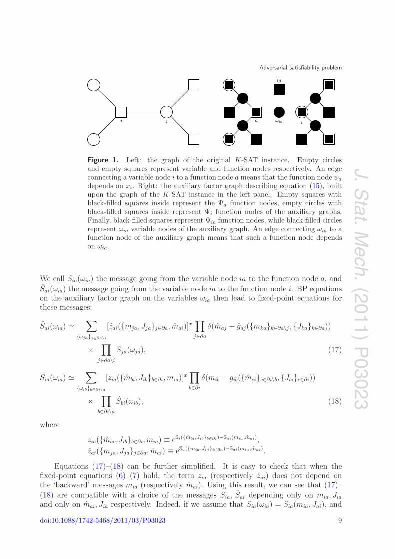
J.Stat.M
ech.(2011)
P03023
Adversarial satisfiability problem
Figure 1. Left: the graph of the original K-SAT instance. Empty circlesand empty squares represent variable and function nodes respectively. An edgeconnecting a variable node i to a function node a means that the function node ψa
depends on xi. Right: the auxiliary factor graph describing equation (15), builtupon the graph of the K-SAT instance in the left panel. Empty squares withblack-filled squares inside represent the Ψa function nodes, empty circles withblack-filled squares inside represent Ψi function nodes of the auxiliary graphs.Finally, black-filled squares represent Ψia function nodes, while black-filled circlesrepresent ωia variable nodes of the auxiliary graph. An edge connecting ωia to afunction node of the auxiliary graph means that such a function node dependson ωia.
We call Sia(ωia) the message going from the variable node ia to the function node a, and
Sai(ωia) the message going from the variable node ia to the function node i. BP equationson the auxiliary factor graph on the variables ωia then lead to fixed-point equations forthese messages:
Sai(ωia) ∑
{ωja}j∈∂a\i
[zai({mja, Jja}j∈∂a, mai)]x∏
j∈∂a
δ(maj − gaj({mka}k∈∂a\j , {Jka}k∈∂a))
×∏
j∈∂a\i
Sja(ωja), (17)
Sia(ωia) ∑
{ωib}b∈∂i\a
[zia({mbi, Jib}b∈∂i, mia)]x∏
b∈∂i
δ(mib − gib({mci}c∈∂i\b, {Jci}c∈∂i))
×∏
b∈∂i\a
Sbi(ωib), (18)
where
zia({mbi, Jib}b∈∂i, mia) ≡ eSi({mbi,Jib}b∈∂i)−Sai(mia,mai),
zai({mja, Jja}j∈∂a, mai) ≡ eSa({mia,Jia}i∈∂a)−Sai(mia,mai).
Equations (17)–(18) can be further simplified. It is easy to check that when thefixed-point equations (6)–(7) hold, the term zia (respectively zai) does not depend onthe ‘backward’ messages mia (respectively mai). Using this result, we can see that (17)–
(18) are compatible with a choice of the messages Sia, Sai depending only on mia, Jia
and only on mai, Jia respectively. Indeed, if we assume that Sia(ωia) = Sia(mia, Jai), and
doi:10.1088/1742-5468/2011/03/P03023 9

J.Stat.M
ech.(2011)
P03023
Adversarial satisfiability problem
Sai(ωia) = Sai(mai, Jai), then (17)–(18) become
Sia(mia, Jai) ∑
{Jbi}b∈∂i\a
∫ ∏
b∈∂i\a
dmbiSbi(mbi, Jbi) [zia({mbi, Jib}b∈∂i\a)]x
× δ(mia − gia({mbi}b∈∂i\a, {Jbi}b∈∂i)), (19)
Sai(mai, Jai) ∑
{Jaj}j∈∂a\i
∫ ∏
j∈∂a\i
dmjaSja(mja, Jja) [zai({mja, Jja}j∈∂a\i)]x
× δ(mai − gai({mja}j∈∂a\i, {Jja}j∈∂a)). (20)
The free energy Φ(x) can then be computed using the general expression for the Bethefree entropy [24]
NΦ(x) =M∑
a=1
Fa +N∑
i=1
Fi −∑
(ia)
Fia, (21)
where
Fa = log
[ ∑
{Jia}i∈∂a
∫ ∏
i∈∂a
dmiaSia(mia, Jia)exSa({mia,Jia}i∈∂a)
], (22)
Fi = log
[ ∑
{Jia}a∈∂i
∫ ∏
a∈∂i
dmaiSai(mai, Jia)exSi({mai}a∈∂i)
], (23)
Fia = log
[∑
Jia
∫dmia dmaiSia(mia, Jia)Sai(mai, Jia)e
xSia(mia,mai)
]. (24)
Equations (19)–(20) clearly show the formal analogy with the 1RSB cavityequations [24]. The difference between equations (19)–(20) and the latter is that in theAdSAT case the negations are considered as physical degrees of freedom of the partitionfunction Z(x), and the resulting cavity equations (19)–(20) consist in a weighted averageof the quantities [zia({mbi, Jib}b∈∂i\a)]
x, [zai({mja, Jja}j∈∂a\i)]x over {Jia, mia, mai}. On the
contrary, in the 1RSB case the only degrees of freedom are the BP messages {mia, mai} insuch a way that the resulting 1RSB cavity equations consist in an average over (mia, mai)at fixed Jias.
The biggest advantage of the formal resemblance of equations (19)–(20) to the1RSB cavity equations is that in order to solve (19)–(20) numerically we can use thevery same technique and all the related knowledge as in the case of 1RSB. We indeeduse the population dynamics [22], where the distributions Sia(mia, Jia), Sai(mai, Jia) arerepresented as populations of P messages. When the size of the population P is large, weexpect the populations to reproduce well the distributions Sia(mia, Jia), and Sai(mai, Jia).The cavity equations (19)–(20) can be written in terms of these populations. Starting froma given initial configuration, the iteration of the cavity equations yields the fixed-pointpopulations satisfying (19)–(20). Once this fixed point is achieved the free energy Φ(x)can be computed numerically by means of (21)–(24). This is repeated for different values
doi:10.1088/1742-5468/2011/03/P03023 10

J.Stat.M
ech.(2011)
P03023
Adversarial satisfiability problem
of x and finally the Legendre transform L(s) is evaluated. Everything is done in the verysame way as the 1RSB equations are usually solved, for more details see, e.g., [22, 27, 28].The only difference is in the treatment of the negation-variables. In our case one writesthe distributions Sia(mia, Jia), Sai(mai, Jia) as
Sia(mia, Jia) = 12Sia(mia|Jia), Sai(mai, Jia) = 1
2Sai(mai|Jia),
because Sia(Jia) =∫
dmiaSia(mia, Jia) = 1/2 = Sai(Jia), as can be seen byexplicitly integrating equations (19)–(20). We then introduce a pair of populations
{S1ia[s], S
1ai[s]}s=1,...,P and {S0
ia[s], S0ai[s]}s=1,...,P representing the probability distributions
Sia(mia|1), Sai(mai|1) and Sia(mia|0), Sai(mai|0) respectively. The population dynamics isthen implemented in terms of such populations, and the resulting fixed point investigatednumerically.
5. Cavity method results for random AdSAT
In this section we present the solution of the cavity equations (19)–(20), and itsimplications for the random AdSAT problem.
5.1. Large deviations of the entropy and complexity on regular instances
Before addressing the random AdSAT as defined in section 1 we will study it on randomregular instances. On L-regular instances every variable belongs to exactly L clauses. Arandom L-regular instance is chosen uniformly at random from all possible ones with agiven number of variables N and number of clauses M , provided that KM = LN . Notethat, as far as we know, this ensemble of random SAT instances was not treated in theliterature previously.
In the 3-SAT problem discussed in this paper the Bethe entropy is asymptoticallyexact only as long as the BP equations converge to a fixed point [9]; the non-convergenceis equivalent to the spin glass instability, or a continuous transition to a replica symmetrybreaking phase. On random regular graphs with random values of negations, BP stopsconverging at L = 12 (this is the reason why these and larger values are omitted fromtable 1), meaning that for L ≥ 12 there is a need for SP (or another form of replicasymmetry breaking solution). For L ≥ 15 BP iterations for random regular 3-SAT leadto contradictions (zero normalizations) meaning that in this region the large randominstances are almost surely unsatisfiable. Survey propagation on random regular 3-SAThas a trivial fixed point for L ≤ 12, and a non-trivial fixed point for L = 13 with thevalue of complexity Σ(L = 13) = 0.008. SP does not converge for L ≥ 14; if we ignorethe non-convergence, and compute the complexity from the current values of messages,we get on average Σ(L = 14) = −0.03. This means that L = 13 is the largest satisfiablecase.
The great advantage of random regular instances is that topologically the localneighborhood looks the same for every variable i. Moreover, we recall that in regimeswhere the BP equations are asymptotically exact the properties of variable i dependonly on the structure of the local neighborhood of i. Hence on regular graphsall the quantities in equations (19)–(20) are independent of the indices i, j, anda, b. This so-called factorization property simplifies crucially the numerical solution of
doi:10.1088/1742-5468/2011/03/P03023 11

J.Stat.M
ech.(2011)
P03023
Adversarial satisfiability problem
Table 1. The Bethe free entropy on regular instances with random negation-configurations (sran), with balanced negation-configurations (sB), and non-frustrated with Jia = 0 ∀(ia) (sU). The entropy for the non-frustrated caseand for the balanced case for even degree L ≤ 10 can be computed analyticallysince the BP fixed point is factorized in these cases. In the other cases we iteratethe BP equations on large random graphs and compute the entropy from thecorresponding BP fixed point. The star signals that BP did not converge andthe value of entropy was obtained by averaging over an interval of time. The ×means that BP converged to contradictions for these densities of constraints.
L sran sB sU
2 0.6039 0.5710 0.61963 0.5592 0.5324 0.59754 0.5134 0.4488 0.57965 0.4686 0.4120 0.56446 0.4220 0.3266 0.55137 0.3750 0.2902 0.53978 0.3302 0.2044 0.52939 0.2816 0.1677 0.5199
10 0.2319 0.082 * 0.511411 0.1813 0.042 * 0.503512 0.128 * × 0.496213 0.07 * × 0.489414 × × 0.4831
equations (19)–(20); the 2KM distributions {Sia(νia, Jia), Sai(νai, Jai)} reduce to only
two (J = 0 and 1) distributions S(ν, J), S(ν, J). Moreover, the thermodynamic limit istaken directly without increasing the computational effort. (To avoid confusion, we recallhere that for the canonical random K-SAT problem where negation-variables are chosenuniformly at random and fixed, the BP solution is not factorized. In the adversarialversion one sums over the negation-variables, hence the factorization.)
In figure 2 we show the large deviation function L(s) of the Bethe entropy s obtainedby the population dynamics over BP messages on regular graphs with K = 3 and variabledegree L = 4, i.e. by solving equations (19), (20) and (21)–(24). First of all, in the‘infinite temperature’ case, i.e. when the Legendre parameter x = 0, that is at themaximum of L(s), we recover the logarithm of the total number of negation-configurationsL(x = 0) = L log 2. The corresponding value of entropy s(x = 0) = sran is the Betheentropy for a random choice of negations (values summarized in table 1).
The inset of the figure shows that as the Legendre parameter x → ±∞ both L ands converge to well defined ending points (the same data in a logarithmic plot show thatthe convergence is exponential). Let us denote the lowest entropy ending point (left,x → −∞) (sL,LL), and the highest entropy ending point (right, x → ∞) (sR,LR).We observe systematically that the value of sR is equal to sU, where sU is the entropyof the uniform negation-configuration which is obtained by computing a fixed point ofequations (6)–(7) such that νai = ν ∀(ai), νia = ν ∀(ia) and Jia = 0 ∀(ia), and pluggingit into equation (11). The values of sU as a function of L are summarized in table 1. Anedge-independent fixed point of the BP equations is called factorized. We realize that sU
doi:10.1088/1742-5468/2011/03/P03023 12

J.Stat.M
ech.(2011)
P03023
Adversarial satisfiability problem
Figure 2. Left: the BP large deviation function L(s) versus the Bethe entropys computed by population dynamics on regular graphs with K = 3, L = 4,population size P = 104. The left ending point (fL,LL) corresponds to balancedconfigurations of negations, whereas the right ending point (fR,LR) to thepolarized configurations of negations (more details in the text). Right: the SPlarge deviation function LSP(Σ) versus the complexity Σ computed by populationdynamics on regular graphs with K = 3, L = 13, P = 104 (bottom), andK = 3, L = 12, P = 75 × 103 (top).
also corresponds to the value of the Bethe entropy when every variable is either alwaysnegated or never negated; we call such negation-configurations polarized. There are 2LN
polarized negation-configurations, and indeed the logarithm of the number of such choicescorresponds to the value of LR = log 2. Intuitively such configurations of negation arefrustrating the formula in the least possible way, and figure 2 shows that such intuition isasymptotically exact in this case.
Similarly, for the lowest entropy ending point, for even values of the degree L, werealize that LL = log
(L
L/2
)and sL corresponds to a value sB that is obtained from a
factorized BP fixed point when each variable is L/2 times negated and L/2 times non-negated; values are summarized in table 1. Such balanced configurations of negationslocally frustrate the variables in a maximal way (half of the clauses want the variableto be 1, the other half 0). And the computation presented in figure 2 suggests thatasymptotically there are no correlated negation-configurations that would frustrate theformula even more and decrease the value of the entropy further.
We investigate in more detail the result following from figure 2, i.e. that the mostfrustrated configurations of negations on the regular graphs with even degree are thebalanced negations; we denote the balanced negation-configurations {Jia}B = JB. There
are(
LL/2
)Nsuch negation-configurations. Does our result mean that all of them lead
to the same number of solutions N (JB)? We will see in section 6 that this is nottrue for finite N . The correct conclusion from the result presented in figure 2 is thatlimN→∞[log N (JB)]/N = sB = sL independently of the realization of JB. This can alsobe seen directly from the solution of the BP equations on the formulas with balancednegations. Indeed, for even L the fixed point of the BP equations is factorized and
doi:10.1088/1742-5468/2011/03/P03023 13

J.Stat.M
ech.(2011)
P03023
Adversarial satisfiability problem
independent of the realization of negations and also of the size of the graph. We triednumerically formulas of various sizes and many possible realizations of balanced negations,and for even degree L < 10 BP always converges to the factorized fixed point (at L = 10BP stops converging, as we will discuss later in the paper), giving always the same Betheentropy density sB. Further discussion about the true entropy fluctuations compared tothe constant Bethe entropy in this case will be presented in section 6.
For regular graphs with odd degree L we cannot achieve ideal balancing of everyvariable. Instead, we call a configuration of negations balanced if for every variable thereis either (L − 1)/2 or (L + 1)/2 negations. The total number of such configurations
is then 2N(
L(L−1)/2
)N. The BP fixed point on the balanced instances for odd L is not
factorized anymore. We can, however, solve the cavity equations (19)–(20) restricted toonly balanced values of negations and we obtain that within the error-bars of the numericalresolution of the equations (that are less than 1%) all the balanced configurations givethe same value of Bethe entropy also in the odd L case.
Our results for large deviations of the Bethe entropy lead to a conclusion that forthe regular instances and in the limit N → ∞ the most frustrated formulas are allthose with balanced configurations of negations. Let us hence conclude this section bysummarizing the properties of regular SAT instances with balanced negations. BP onbalanced instances converges for L ≤ 9, and leads to contradictions for L ≥ 13. Surveypropagation on balanced regular instances has a trivial fixed point for L ≤ 9, for L = 10a fixed point with complexity ΣB(L = 10) = 0.018, and for L ≥ 11 the complexity isnegative (e.g. ΣB(L = 11) = −0.001, ΣB(L = 12) = −0.075).
For completeness, we also computed the large deviations of the complexity function.That is, we solved equations (19)–(20) using SP as the basic message passing scheme.Figure 2 (right) shows some of the results for L = 12 and 13; we indeed see thatthere are configurations of negations that lead to negative complexity. Unfortunately,it is hard to extract any information from these curves for very negative values of x,because of the noise introduced by the finite population size effects. This also posesa problem for L = 10 and 11, where we know that a non-trivial fixed point of SPexists for the balanced configurations of negations. In the population dynamics weshould hence see a non-trivial solution for very negative values of x. Instead we wereonly able to obtain very noisy and inconclusive data from the population dynamicswith population sizes up to 7.5 × 10⁴. For L = 10 the SP equations have onlyone factorized fixed point for all the balanced configurations of negations; this againstrongly suggests that instances with balanced negations are the most frustrated ones,and hence that for L = 10 the adversary cannot make large formulas unsatisfiable. Forlower values of L ≤ 9 the population dynamics has always only a trivial fixed pointgiven by Sia(Qia, Jia) = δ(QS
ia)δ(QUia)δ(Q
∗ia − 1)/2, Sai(Qai, Jia) = δ(Qai)/2 yielding
Φ(x) = Kα log 2. SP is hence not very useful in this case to obtain new informationabout the random AdSAT problem.
In summary, for L ≥ 11 the adversary will succeed in making a large formulaunsatisfiable by simply balancing the negations (for L ≥ 14 a random choice of negationswould do). On the other hand, following our previous conclusion that the balancedformulas are the most frustrated ones, for L ≤ 10 the adversary will not be able to makelarge random regular SAT instances unsatisfiable by adjusting the values of negation-variables.
doi:10.1088/1742-5468/2011/03/P03023 14

J.Stat.M
ech.(2011)
P03023
Adversarial satisfiability problem
5.2. Results for random AdSAT, i.e. instances with Poisson degree distribution
In the most commonly considered ensemble of the random K-satisfiability problem,K variables appearing in each clause are chosen independently at random (avoidingrepetitions). For large system sizes this procedure generates Poissonian degree distributionwith mean Kα. In this case every node has a different local neighborhood and hencethe fixed point of equations (19)–(20) is not factorized, and the distribution Sia(mia, Jai),
Sai(mai, Jai) are different on every edge. We hence solve equations (19)–(20) by generatingan instance of the problem (graph) of size N , associating one population of size Pwith every directed edge, and iterate following equations (19)–(20). This is morecomputationally involved, and we are able to treat only modestly large N and P , typicallyseveral hundreds. The resulting large deviation function L(s) is depicted in figure 3 forseveral values of constraint density α.
For low values of the constraint density, e.g. α = 1 in figure 3, the location of theright (large entropy, least frustrated) ending point (sR,LR) corresponds, as in the case ofrandom regular instances, to the value of Bethe entropy that is obtained if no negationsare present in the instance (Jia = 0 for all ia), and LR = (1−e−Kα) log 2 (corresponding tothe number of negation-configurations where no variable is locally frustrated). For largervalues of the constraint density, e.g. α = 2 in figure 3, the results from population sizes aslarge as we were able to achieve are very noisy for large values of x ≈ 100. We observedthat the data are getting smoother as the population size is growing, however not enoughto be able to confirm from these data that (sR,LR) is the right ending point.
The part of the curve corresponding to a very large negative parameter x does notconverge to an ending point. Instead at some x0 the large deviation function L(s) ceasesto be concave, and an unphysical branch appears for x < x0. This unphysical branch isnot present on random regular instances with even degree; when the degree is odd thedata for large negative x are inconclusive in the sense that we might see a unphysicalbranch or only a numerical noise. We define the left ending point as the extreme of thephysical branch sL = s(x0), and LL = L(x0). We observe systematically that in the regionof interest (say for α ≥ 1) the values sL and LL are very close to the values correspondingto balanced instances (sB,LB). In balanced instances each variable is negated as manytimes as non-negated (for variables of odd degree the absolute value of the differencebetween the number of negations and non-negations is one). In the thermodynamic limitthe number of such balanced negation-configurations is
LB =
∞∑
i=0
log
(2ii
)e−kα (kα)2i
(2i)!+
∞∑
i=0
log
[2
(2i+ 1i
)]e−kα (kα)2i+1
(2i+ 1)!. (25)
We made a number of attempts to obtain a value of entropy considerably smallerthan the balanced entropy, s < sB. First, we removed the leaves from the formula andbalanced only the residual formula. This indeed leads to a lower value of the entropy, butfor α > 1 the difference was less than 1%. We tested the population dynamics limitedto the balanced negation-configurations, i.e. we solved equations (19)–(24) where the sumover the negation-variables in equations (20) and (23) was limited only to the balancednegation-configurations. The large deviation function L(s) obtained in this way did notdiffer more than by 1% from the value (sB,LB), see figure 3 (left). We also investigated theresults of population dynamics over the SP equations and we were not able to find cases
doi:10.1088/1742-5468/2011/03/P03023 15

J.Stat.M
ech.(2011)
P03023
Adversarial satisfiability problem
Figure 3. Left: the BP large deviation function L(s) versus the Bethe entropy scomputed by population dynamics on Poissonian graphs with random negation-configurations, for K = 3, various values of the constraint density α, and bothpositive and negative x. For α = 1–3 the part of the curve with x < 0 has beencomputed with N = P = 300. For α = 1 the part of the curve with x > 0 reachesthe right ending point, and has been computed with N = P = 500. For α = 2, 3the part of the curve with positive x has been computed with N = P = 300,and it does not reach the right ending point; even larger N and P are needed toremove the noise from the data for very large positive x. For x < 0, an unphysicalbranch (concave part of the curve) starts at x0 ≈ −42, x0 ≈ −44, x0 ≈ −40 forα = 1, 2, 3 respectively. The points indicate the values for balanced configurationsof negations (sB,LB), and for configurations of negations where all the variablesare non-negated (sR,LR). Right: zoom of the large deviation function L(s)versus s for α = 1 close to the low entropy ending point for N = P = 500.The data become noisy close to the low entropy ending point; larger graph andpopulation sizes lead to an improvement. We plotted the data down to thelowest value of entropy s; hence the unphysical branch is not plotted. The pointindicates the value (sB,LB) for balanced configurations of negations. The bluedata points show the large deviation function restricted to balanced configurationsof negations for N = 102, P = 103. Notice the narrow range of entropies splotted in the latter, and how little the lowest entropy we achieved differs fromthe balanced value.
where the complexity would decrease by more than 1% below the complexity value onthe balanced instances. We also tried simulated annealing on the negation-variables usingthe Bethe entropy as the cost function, with the same result. All this makes us concludethat with at least 1% of precision the satisfiability threshold for random adversarial SATequals the satisfiability threshold of the balanced random ensemble.
Let us hence summarize the results about BP and SP for the random satisfiabilityproblem with balanced configurations of negations. For K = 3 the BP ceases to convergefor α ≥ 2.96. SP starts to converge to a non-trivial fixed point for α > 3.20, and thecomplexity decreases to zero at
αB = 3.399 ± 0.001; (26)
this is hence the satisfiability threshold on the balanced random formulas. All our
doi:10.1088/1742-5468/2011/03/P03023 16

J.Stat.M
ech.(2011)
P03023
Adversarial satisfiability problem
Figure 4. Left: LN (s) versus s for regular random graphs with random negations,computed exactly for 15 ≤ N ≤ 60 withNs = 105 samples J , and binning intervalΔs = (smax−smin)/100 withK = 3, L = 8, where smax and smin are the maximumand minimum entropies of the Ns samples respectively. We also plot L(s) versuss computed with the population dynamics for both negative x (P = 5 × 10⁴)and positive x (P = 2 × 10⁴). Right: LN (s) versus s for regular random graphswith balanced negations, computed exactly for 39 ≤ N ≤ 87, Ns = 105, binninginterval Δs = (smax−smin)/100, and K = 3, L = 8. The curves do not superpose,so the large deviations decay faster than exponentially.
observations about the large deviation function suggest that the threshold for the randomadversarial satisfiability problem satisfies αa > 3.39.
6. Numerical results for AdSAT and large deviations
In this final section we compare theoretical predictions from the cavity method withnumerical results.
6.1. Numerical results for large deviations
First, we investigate numerically the number of configurations of negations yielding aformula with a certain entropy of solutions. For one given random graph geometryof size N , we generate independently at random I � 1 different configurations ofnegations, and for each of them we count the number of solutions using a publicly availableimplementation of the exact counting algorithm relsat [29]. We define the probabilityPN(s) over the negation-configurations that the value of the entropy density is between sand s+ Δs, where Δs is a binning interval that we will specify later.
Following the assumption of exponentially-small large deviations made inequation (4), we define
LN(s) =1
N
[logPN(s) − log max
sPN(s)
]. (27)
The numerical result for LN(s) is depicted in figure 4 (left) for L = 8, and compared tothe predictions of the large deviations of the Bethe entropy from section 5. The agreementbetween the numerical data point and the theoretical prediction is not good in the low
doi:10.1088/1742-5468/2011/03/P03023 17
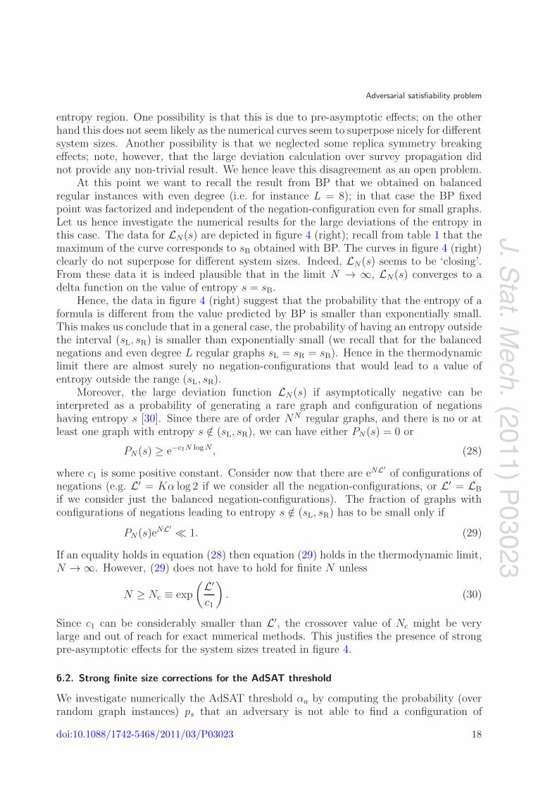
J.Stat.M
ech.(2011)
P03023
Adversarial satisfiability problem
entropy region. One possibility is that this is due to pre-asymptotic effects; on the otherhand this does not seem likely as the numerical curves seem to superpose nicely for differentsystem sizes. Another possibility is that we neglected some replica symmetry breakingeffects; note, however, that the large deviation calculation over survey propagation didnot provide any non-trivial result. We hence leave this disagreement as an open problem.
At this point we want to recall the result from BP that we obtained on balancedregular instances with even degree (i.e. for instance L = 8); in that case the BP fixedpoint was factorized and independent of the negation-configuration even for small graphs.Let us hence investigate the numerical results for the large deviations of the entropy inthis case. The data for LN(s) are depicted in figure 4 (right); recall from table 1 that themaximum of the curve corresponds to sB obtained with BP. The curves in figure 4 (right)clearly do not superpose for different system sizes. Indeed, LN(s) seems to be ‘closing’.From these data it is indeed plausible that in the limit N → ∞, LN(s) converges to adelta function on the value of entropy s = sB.
Hence, the data in figure 4 (right) suggest that the probability that the entropy of aformula is different from the value predicted by BP is smaller than exponentially small.This makes us conclude that in a general case, the probability of having an entropy outsidethe interval (sL, sR) is smaller than exponentially small (we recall that for the balancednegations and even degree L regular graphs sL = sR = sB). Hence in the thermodynamiclimit there are almost surely no negation-configurations that would lead to a value ofentropy outside the range (sL, sR).
Moreover, the large deviation function LN(s) if asymptotically negative can beinterpreted as a probability of generating a rare graph and configuration of negationshaving entropy s [30]. Since there are of order NN regular graphs, and there is no or atleast one graph with entropy s /∈ (sL, sR), we can have either PN(s) = 0 or
PN(s) ≥ e−c1N log N , (28)
where c1 is some positive constant. Consider now that there are eNL′of configurations of
negations (e.g. L′ = Kα log 2 if we consider all the negation-configurations, or L′ = LB
if we consider just the balanced negation-configurations). The fraction of graphs withconfigurations of negations leading to entropy s /∈ (sL, sR) has to be small only if
PN(s)eNL′ 1. (29)
If an equality holds in equation (28) then equation (29) holds in the thermodynamic limit,N → ∞. However, (29) does not have to hold for finite N unless
N ≥ Nc ≡ exp
(L′
c1
). (30)
Since c1 can be considerably smaller than L′, the crossover value of Nc might be verylarge and out of reach for exact numerical methods. This justifies the presence of strongpre-asymptotic effects for the system sizes treated in figure 4.
6.2. Strong finite size corrections for the AdSAT threshold
We investigate numerically the AdSAT threshold αa by computing the probability (overrandom graph instances) ps that an adversary is not able to find a configuration of
doi:10.1088/1742-5468/2011/03/P03023 18
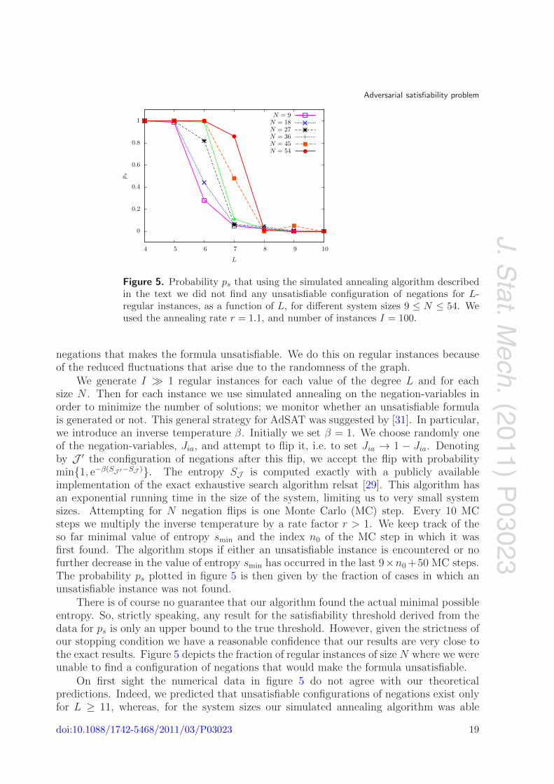
J.Stat.M
ech.(2011)
P03023
Adversarial satisfiability problem
Figure 5. Probability ps that using the simulated annealing algorithm describedin the text we did not find any unsatisfiable configuration of negations for L-regular instances, as a function of L, for different system sizes 9 ≤ N ≤ 54. Weused the annealing rate r = 1.1, and number of instances I = 100.
negations that makes the formula unsatisfiable. We do this on regular instances becauseof the reduced fluctuations that arise due to the randomness of the graph.
We generate I � 1 regular instances for each value of the degree L and for eachsize N . Then for each instance we use simulated annealing on the negation-variables inorder to minimize the number of solutions; we monitor whether an unsatisfiable formulais generated or not. This general strategy for AdSAT was suggested by [31]. In particular,we introduce an inverse temperature β. Initially we set β = 1. We choose randomly oneof the negation-variables, Jia, and attempt to flip it, i.e. to set Jia → 1 − Jia. Denotingby J ′ the configuration of negations after this flip, we accept the flip with probabilitymin{1, e−β(SJ ′−SJ )}. The entropy SJ is computed exactly with a publicly availableimplementation of the exact exhaustive search algorithm relsat [29]. This algorithm hasan exponential running time in the size of the system, limiting us to very small systemsizes. Attempting for N negation flips is one Monte Carlo (MC) step. Every 10 MCsteps we multiply the inverse temperature by a rate factor r > 1. We keep track of theso far minimal value of entropy smin and the index n0 of the MC step in which it wasfirst found. The algorithm stops if either an unsatisfiable instance is encountered or nofurther decrease in the value of entropy smin has occurred in the last 9×n0 +50 MC steps.The probability ps plotted in figure 5 is then given by the fraction of cases in which anunsatisfiable instance was not found.
There is of course no guarantee that our algorithm found the actual minimal possibleentropy. So, strictly speaking, any result for the satisfiability threshold derived from thedata for ps is only an upper bound to the true threshold. However, given the strictness ofour stopping condition we have a reasonable confidence that our results are very close tothe exact results. Figure 5 depicts the fraction of regular instances of size N where we wereunable to find a configuration of negations that would make the formula unsatisfiable.
On first sight the numerical data in figure 5 do not agree with our theoreticalpredictions. Indeed, we predicted that unsatisfiable configurations of negations exist onlyfor L ≥ 11, whereas, for the system sizes our simulated annealing algorithm was able
doi:10.1088/1742-5468/2011/03/P03023 19
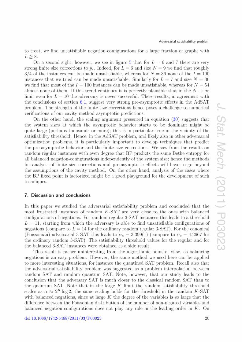
J.Stat.M
ech.(2011)
P03023
Adversarial satisfiability problem
to treat, we find unsatisfiable negation-configurations for a large fraction of graphs withL ≥ 8.
On a second sight, however, we see in figure 5 that for L = 6 and 7 there are verystrong finite size corrections to ps. Indeed, for L = 6 and size N = 9 we find that roughly3/4 of the instances can be made unsatisfiable, whereas for N = 36 none of the I = 100instances that we tried can be made unsatisfiable. Similarly for L = 7 and size N = 36we find that most of the I = 100 instances can be made unsatisfiable, whereas for N = 54almost none of them. If this trend continues it is perfectly plausible that in the N → ∞limit even for L = 10 the adversary is never successful. These results, in agreement withthe conclusions of section 6.1, suggest very strong pre-asymptotic effects in the AdSATproblem. The strength of the finite size corrections hence poses a challenge to numericalverifications of our cavity method asymptotic predictions.
On the other hand, the scaling argument presented in equation (30) suggests thatthe system sizes at which the asymptotic behavior starts to be dominant might bequite large (perhaps thousands or more); this is in particular true in the vicinity of thesatisfiability threshold. Hence, in the AdSAT problem, and likely also in other adversarialoptimization problems, it is particularly important to develop techniques that predictthe pre-asymptotic behavior and the finite size corrections. We saw from the results onrandom regular instances with even degree that BP predicts the same Bethe entropy forall balanced negation-configurations independently of the system size; hence the methodsfor analysis of finite size corrections and pre-asymptotic effects will have to go beyondthe assumptions of the cavity method. On the other hand, analysis of the cases wherethe BP fixed point is factorized might be a good playground for the development of suchtechniques.
7. Discussion and conclusions
In this paper we studied the adversarial satisfiability problem and concluded that themost frustrated instances of random K-SAT are very close to the ones with balancedconfigurations of negations. For random regular 3-SAT instances this leads to a thresholdL = 11, starting from which the adversary is able to find unsatisfiable configurations ofnegations (compare to L = 14 for the ordinary random regular 3-SAT). For the canonical(Poissonian) adversarial 3-SAT this leads to αa = 3.399(1) (compare to αc = 4.2667 forthe ordinary random 3-SAT). The satisfiability threshold values for the regular and forthe balanced 3-SAT instances were obtained as a side result.
This result is rather uninteresting from the algorithmic point of view, as balancingnegations is an easy problem. However, the same method we used here can be appliedto more interesting situations, for instance the quantified SAT problem. Recall also thatthe adversarial satisfiability problem was suggested as a problem interpolation betweenrandom SAT and random quantum SAT. Note, however, that our study leads to theconclusion that the adversary SAT is much closer to the classical random SAT than tothe quantum SAT. Note that in the large K limit the random satisfiability thresholdscales as α ≈ 2K log 2; the same scaling holds for the threshold in the random K-SATwith balanced negations, since at large K the degree of the variables is so large that thedifference between the Poissonian distribution of the number of non-negated variables andbalanced negation-configurations does not play any role in the leading order in K. On
doi:10.1088/1742-5468/2011/03/P03023 20

J.Stat.M
ech.(2011)P
03023
Adversarial satisfiability problem
the other hand, the satisfiability threshold of the quantum SAT was upper-bounded by2K log 2/2 [17, 18]; hence the quantum effect must be responsible for this drastic decreaseof the threshold value.
We obtained our results by studying the large deviations of the entropy in the ordinaryrandom K-SAT. In particular, an approach leading to equations very similar to the 1RSBequations leads to the calculation of the large deviations in the case where rare instancesare exponentially rare. Exponential large deviations are common in statistical physics. Insome cases, see, e.g., [32], [11]–[13], the large deviations are rarer than exponentially rare.In our study this arises for regular random K-SAT instances with balanced negations andeven degree. In cases where the large deviation function decays faster than exponentiallywith the system size extremely strong finite size corrections and pre-asymptotic effectscan be induced, as we argued in section 6, where we presented numerical studies of thelarge deviations and of the satisfiability threshold. Interestingly, methods based on thestandard cavity method are not straightforwardly applicable to study of the related finitesize corrections and pre-asymptotic behavior. It remains a theoretical challenge to find outhow to describe analytically and algorithmically these pre-asymptotic effects that mightbe crucial for solving some industrial instances of adversarial optimization problems.
Finally we did not address the possibility of replica symmetry breaking in the spaceof negations (due to its technical difficulty) and this should also be a subject of futureworks.
Acknowledgments
We thank Cris Moore for introducing us to the adversarial SAT problem,Antonello Scardicchio for very helpful discussions, and Guilhem Semerjian for very helpfuldiscussions and very useful comments about a preliminary version of the paper. We alsoacknowledge support from the DI computational center of University Paris-Sud.
References
[1] McMasters A W and Mustin T M, Optimal interdiction of a supply network , 1970 Nav. Res. Logist. Q.17 261
[2] Wood R K, Deterministic network interdiction, 1993 Math. Comput. Modelling 17 1[3] Varga P, Minimax games, spin glasses, and the polynomial-time hierarchy of complexity classes, 1998 Phys.
Rev. E 57 6487[4] Papadimitriou C H, 1994 Computational Complexity (Reading, MA: Addison-Wesley)[5] Moore C and Mertens S, 2011 The Nature of Computation (Oxford: Oxford University Press)[6] Cook S A, The complexity of theorem-proving procedures, 1971 Proc. 3rd STOC (New York, NY) ACM
pp 151–8[7] Mitchell D G, Selman B and Levesque H J, Hard and easy distributions for SAT problems, 1992 Proc. 10th
AAAI (Menlo Park, CA: AAAI Press) pp 459–65[8] Mezard M, Parisi G and Zecchina R, Analytic and algorithmic solution of random satisfiability problems,
2002 Science 297 812[9] Krzakala F, Montanari A, Ricci-Tersenghi F, Semerjian G and Zdeborova L, Gibbs states and the set of
solutions of random constraint satisfaction problems, 2007 Proc. Nat. Acad. Sci. 104 10318[10] Rivoire O, The cavity method for large deviations, 2005 J. Stat. Mech. P07004[11] Parisi G and Rizzo T, Large deviations in the free energy of mean-field spin glasses, 2008 Phys. Rev. Lett.
101 117205[12] Parisi G and Rizzo T, Phase diagram and large deviations in the free energy of mean-field spin glasses, 2009
Phys. Rev. B 79 134205[13] Parisi G and Rizzo T, Large deviations of the free energy in diluted mean-field spin-glass, 2010 J. Phys. A:
Math. Theor. 43 045001
doi:10.1088/1742-5468/2011/03/P03023 21

J.Stat.M
ech.(2011)
P03023
Adversarial satisfiability problem
[14] Parisi G, A sequence of approximated solutions to the SK model for spin-glasses, 1980 J. Phys. A: Math.Gen. 13 L115
[15] Dotsenko V, Franz S and Mezard M, Partial annealing and overfrustration in disordered systems, 1994J. Phys. A: Math. Gen. 27 2351
[16] Laumann C R, Moessner R, Scardicchio A and Sondhi S L, Phase transitions and random quantumsatisfiability , 2010 Quantum Inf. Comput. 10 1
[17] Bravyi S, Moore C and Russell A, Bounds on the quantum satisfibility threshold , 2009 arXiv:0907.1297v2[18] Laumann C R, Lauchli A M, Moessner R, Scardicchio A and Sondhi S L, Product, generic, and random
generic quantum satisfiability , 2010 Phys. Rev. A 81 062345[19] Chen H and Interian Y, A model for generating random quantified boolean formulas, 2005 IJCAI 2005:
Proc. 19th Int. Joint Conf. on Artificial Intelligence pp 66–71[20] Altarelli F, Braunstein A, Ramezanpour A and Zecchina R, Statistical physics of optimization under
uncertainty , 2010 arXiv:1003.6124v1, 2010[21] Mertens S, Mezard M and Zecchina R, Threshold values of random k-SAT from the cavity method , 2006
Random Struct. Algorithms 28 340[22] Mezard M and Parisi G, The Bethe lattice spin glass revisited , 2001 Eur. Phys. J. B 20 217[23] Yedidia J S, Freeman W T and Weiss Y, Understanding belief propagation and its generalizations, 2003
Exploring Artificial Intelligence in the New Millennium (San Francisco, CA: Morgan Kaufmann) pp 239–6[24] Mezard M and Montanari A, 2009 Physics, Information, Computation (Oxford: Oxford Press)[25] Montanari A, Parisi G and Ricci-Tersenghi F, Instability of one-step replica-symmetry-broken phase in
satisfiability problems, 2004 J. Phys. A: Math. Gen. 37 2073[26] Mezard M and Zecchina R, Random k-satisfiability problem: from an analytic solution to an efficient
algorithm, 2002 Phys. Rev. E 66 056126[27] Zdeborova L and Krzakala F, Phase transitions in the coloring of random graphs, 2007 Phys. Rev. E
76 031131[28] Montanari A, Ricci-Tersenghi F and Semerjian G, Clusters of solutions and replica symmetry breaking in
random k-satisfiability , 2008 J. Stat. Mech. P04004[29] Bayardo R J Jr and Pehousek J D, Counting models using connected components, 2000 Proc. 17th AAAI
(Menlo Park, CA: AAAI Press) pp 157–62[30] Rivoire O, Properties of atypical graphs from negative complexities, 2004 J. Stat. Phys. 117 453[31] Nagaj D and Scardicchio A, 2010 in preparation[32] Monthus C and Garel T, Matching between typical fluctuations and large deviations in disordered systems:
application to the statistics of the ground state energy in the sk spin-glass model , 2010 J. Stat. Mech.P02023
doi:10.1088/1742-5468/2011/03/P03023 22
Renormalization group computation of the critical exponents of hierarchical spin glasses
Michele Castellana1,2 and Giorgio Parisi11Dipartimento di Fisica, Università di Roma ‘La Sapienza’, 00185 Rome, Italy
2LPTMS–CNRS–Universite Paris-Sud, UMR 8626, Bât. 100, 91405 Orsay, France�Received 29 June 2010; revised manuscript received 16 September 2010; published 15 October 2010�
The large scale behavior of the simplest non-mean-field spin-glass system is analyzed, and the criticalexponent related to the divergence of the correlation length is computed at two loops within the �-expansiontechnique with two independent methods. The techniques presented show how the underlying ideas of therenormalization group apply also in this disordered model, in such a way that an �-expansion can be consis-tently set up. By pushing such calculation to high orders in �, a consistent non-mean-field theory for suchdisordered system could be established, giving a substantial contribution the development of a predictivetheory for real spin glasses.
DOI: 10.1103/PhysRevE.82.040105 PACS number�s�: 64.60.ae, 75.10.Nr, 05.10.Cc
The understanding of glassy systems and their criticalproperties is a subject of main interest in statistical physics.The mean-field theory of spin-glasses �1� and structuralglasses �2� provides a physically and mathematically richtheory. Nevertheless, real spin-glass systems have short-range interactions, and thus cannot be successfully describedby mean-field models �1�. This is the reason why the devel-opment of a predictive and consistent theory of glassy phe-nomena going beyond mean field is still one of the mosthotly debated, difficult and challenging problems in this do-main �3–5�, so that a theory describing real glassy systems isstill missing. This is because nonperturbative effects arepoorly understood and not under control, and the basic prop-erties of large scale behavior of these systems still far frombeing clarified.
In ferromagnetic systems, the physical properties of theparamagnetic-ferromagnetic transition emerge in a clear wayalready in the original approach of Wilson �7�, where one canwrite a simple renormalization group �RG� transformation. Itwas later realized that Wilson’s equations are exact in modelswith ferromagnetic power-law interactions on hierarchicallattices as the Dyson model �8,9�. This model contains all thephysical RG properties, and is simple enough to yield a so-lution of the RG equations within the �-expansion �10�.
The extension of this approach to random systems isavailable only in a few cases. An RG analysis for randommodels on the Dyson hierarchical lattice has been pursued inthe past �11,12�, and a systematic analysis of the physicaland unphysical infrared �IR� fixed points has been developedwithin the �-expansion technique. Unfortunately, in suchmodels spins belonging to the same hierarchical block inter-act each other with the same �11� random coupling J, in sucha way that frustration turns out to be relatively weak and theyare not a good representative of realistic strongly frustratedsystem. Moreover, there has recently been a new wave ofinterest for strongly frustrated random models on hierarchi-cal lattices �13–15�: for example, it has been shown �14� thata generalization of the Dyson model to its disordered version�the hierarchical random energy model �HREM�� has a ran-dom energy model-like phase transition.
In this letter we present a field theory analysis of thecritical behavior of a generalization of Dyson’s model
to the disordered case, known as the hierarchical Edwards-Anderson Model �HEA� �13�. The HEA is of particular in-terest, since it is a non-mean-field strongly frustrated modelwith long-range interaction. It follows that its RG analysispursued in this work makes a contribution to the develop-ment of a theory describing real glassy systems with short-range interaction. Indeed, the symmetry properties of theHEA make an RG analysis simple enough to be done withtwo independent methods, showing that its IR-limit is physi-cally well-defined, independently on the computation tech-nique that one uses. The same symmetry properties makethe RG equations simple enough to make a high-order�-expansion tractable by means of a symbolic manipulationprogram, resulting in a first predictive theory for the criticalexponents for a strongly frustrated non-mean-field systemmimicking a real spin-glass. It is possible that such a pertur-bative expansion turns out to be nonconvergent: if this hap-pens, it may help us to pin down the nonperturbative effects.Motivated by this purpose, we show with a two-loop calcu-lation that such �-expansion can be set up consistently, andthat the ordinary RG underlying ideas actually apply also inthis case, so that the IR limit of the theory is well-definedindependently on the regularization technique.
The Hamiltonian of the HEA is defined �13� as HJ�S�=−�i,kJi,kSiSk where the spin Sis take values �1 and Ji,k areGaussian random variables with zero mean and variance �i,k
2 .Everything depends on the form of �i,k
2 that will be chosen insuch way to make the model simple enough, and a goodcandidate mimicking a real glassy system. At large distancewe have that �i,k
2 =O��i−k�−2��, where � is a parameter tuningthe decay of the interaction strength with distance: we re-cover the mean-field regime for �=1 /2, while no transitionis present for ��1 �13�. We will thus be interested in thecase 1 /2���1, where the interaction strength mimics thenon-mean field forces of a real spin glass. The form of �i,k
2 isgiven by the following expression: if only the last m digits inthe binary representation of the points i and k are different,�i,k
2 =2−2�m. This form of the Hamiltonian corresponds in di-viding the system in hierarchical embedded blocks of size2m, such that the interaction between two spins depends onthe distance of the blocks to which they belong. The quantity�i,k
2 is not translational invariant, but it is invariant under a
PHYSICAL REVIEW E 82, 040105�R� �2010�
RAPID COMMUNICATIONS
1539-3755/2010/82�4�/040105�4� ©2010 The American Physical Society040105-1

huge symmetry group and this will be crucial in the study ofthe model.
We reproduce the IR behavior of the HEA by two differ-ent methods. The first method is analogous to the coarse-graining Wilson’s method for the Ising model: the IR limit isobtained by imposing invariance with respect to the compo-sition operation taking two systems of 2k spins and yieldinga system of 2k+1 spins, for which one can obtain closed for-mulas because of hierarchical structure of the Hamiltonian.The second method is more conventional: we perform theIR-limit of the theory by constructing an IR-safe renormal-ized theory and performing its IR limit by the Callan-Symanzik equation.
Wilson’s method. As mentioned before, the hierarchicalsymmetry structure of the model makes the implementationof a recursionlike RG equation simple enough to be solvedwithin an approximation scheme, yielding �13� a recurrencerelation for the probability distribution of the overlap �1,2�Qab ,a=1, ¯ ,n
Zk�Q� = e�2/4 Tr�Q2�� �dP�Zk−1�Q + P
C1/2 � Zk−1�Q − P
C1/2 ,
�1�
where C22�1−��, �1 /T is the inverse-temperature and��dP� stands for the functional integral over Pab. The recur-sion relation �1� can be solved by supposing Zk�Q� to be amean-field solution, i.e., a Gaussian function of Q. As it willbe explicitly shown in the following, the resulting fixed pointZ��Q� of Eq. �1� turns out �13� to be stable just for ��− 2
3 �0. For ��0 the stable fixed point is no more Gaussian,and we search for a solution to Eq. �1� as a small perturba-tion to the mean-field solution
Zk�Q� = exp�− �rk Tr�Q2� + wk/3 Tr�Q3�� . �2�
General RG arguments �7� suggest that the corrections to themean-field solution must be proportional to �.
A complete reconstruction of the function Zk�Q� for ��0 stems from the following systematic expansion proce-dure. In first approximation, we write Zk�Q� as in Eq. �2�,and take into account only the cubic term. By inserting Eq.�2� into Eq. �1�, and expanding in terms of wk−1 to up toO�wk−1
3 �, we find that Zk�Q� has the same functional form asin Eq. �2�, where the coefficients rk ,wk are given by somefunctions of rk−1 ,wk−1 that can be directly computed. It fol-lows that the recursion Eq. �1� yields a relation betweenrk ,wk and rk−1 ,wk−1. In particular, the recursion relation giv-ing wk as a function of rk−1 ,wk−1
wk =2wk−1
C3/2 +n − 2
16C3/2�wk−1
rk−1�3
+ O�wk−15 � ,
shows that for ��0 the fixed point is Gaussian, while for��0 a non-Gaussian fixed point arises. It is important pointout that the value of �=�−2 /3 is different by the ��=�−1 /2, arising in the generalization Dyson model to its disor-dered version that has been already pursued in the literature�11,12�. This is because in the latter the frustration is muchweaker than in the HEA, in such a way that the IR-behaviorof the theory turns out to be generally different.
Higher order corrections to the Gaussian solution can behandled systematically: inserting Eq. �2� into Eq. �1�, andexpanding to O�wk−1
4 �, we generate in Zk�Q� four monomials�I4
l �Q� l=1,. . .,4 of fourth degree in Q. In order to close therecursion relation �2�, it is then natural to set
Zk�Q� = exp�− rk�Tr�Q2� + wk/3 Tr�Q3� +1
4�l=1
4
�kl I4
l �Q�� ,
�3�
where �kl =O�wk
4�. By plugging Eq. �3� into Eq. �1�, weobtain a recursion equation relating rk ,wk , ��k
l l=1,¯,4 tork−1 ,wk−1 , ��k−1
l l=1,¯,4. This procedure can be pushed to ar-bitrary high order p in wk, yielding an p-degree polynomialfor
Zk�Q� = exp�− �j=2
p
�l=1
nj
cj,kl Ij
l�Q�� , �4�
where the number nj of monomials proliferates for increasingj. Following the method explained above, a recursion equa-tion relating �cj,k
l j,l to �cj,k−1l j,l can be obtained, and the criti-
cal fixed point �cj,�l j,l computed by solving perturbatively in
� the fixed-point equations. Following the standard RG, wesuppose that the system has a characteristic correlationlength , diverging at the critical point, where the system isinvariant under change in the scale length. By linearizing therecursion relation close to such fixed point, the critical expo-nent governing the power-law divergence of for T→Tccan be obtained in terms of the largest eigenvalue � of thematrix M linearizing such transformation next to the fixedpoint �7�: −1=log2 �.
We performed this systematic expansion to the order p=5, generating n4=4 invariants of fourth degree, and n5=4invariants of fifth degree in Q. Such computation yields tothe order �2. For n→0, we find
= 3 + 36� + �432 − 27�50 + 55 · 21/3 + 53 · 22/3�log 2��2
+ O��3� . �5�
The one-loop result for is the same as that of the power-lawinteraction spin-glass studied in �5� �where �3��−2 /3��.Notwithstanding this, the coefficients of the expansion inthese two models will be in general different at two or moreloops. As a matter of fact, the binary tree structure of theinteraction of the HEA emerges in the nontrivial log 2 ,21/3
factors in the coefficient of �2 in Eq. �5�, that can’t be therein the power-law case.
Before discussing the result in Eq. �5�, we point out thatWilson’s method explicitly implements the binary-tree struc-ture of the model when approaching the IR limit. Neverthe-less, if the IR limit is well-defined, physical observables like must not depend on the technique we use to compute themin such a limit. It is then important to reproduce Eq. �5� witha different approach.
Field-theoretical method. Here the �-expansion is per-formed by constructing a functional integral field theory andby removing its IR divergences within the minimal subtrac-tion scheme. The field theory is constructed by expressing
MICHELE CASTELLANA AND GIORGIO PARISI PHYSICAL REVIEW E 82, 040105�R� �2010�
RAPID COMMUNICATIONS
040105-2

the average of the replicated partition function as a func-tional integral over the local overlap field
Qiab SiaSi
b, EJ�Zn� =� �dQ�e−S�Q�. �6�
A short computation yields the IR-dominant terms in theeffective Hamiltonian for a system of 2k spins,
S�Q� =1
2 �i,j
0,2k−1
��i,j2 + �2�−1�ij�Tr�QiQj� +
g
3! �i=0
2k−1
Tr�Qi3� ,
�7�
where Tr denotes the trace over the replica indexes and�2�−1 T−Tc. The field theory defined by Eq. �7� reproducesthe Q3 interaction term of the well-know effective actionsdescribing the spin-glass transition in short-range �16� andlong-range �5,17� spin glasses. Notwithstanding this similar-ity, the novelty of the HEA is that a high-order �-expansioncan be quiet easily automatized by means of a symbolic ma-nipulation program solving the simple RG Eq. �1� to highorders in �. This is not true for such short and long-range�5,16,17� models, where the only approach to compute theexponents is the field-theoretical one. Indeed, nobody evermanaged to automatize at high orders a computation of thecritical exponents within the field-theoretical minimal sub-traction scheme, either for the simplest case of the Isingmodel.
To start our field-theoretical analysis, we observe that Eq.�7� presents an unusual quadratic term that is not invariantunder spatial translations and it is difficult to perform explicitcalculations. This difficulty can be overcome by a relabelingof the sites of the lattice i=0, ¯ ,2k−1, following the sameprocedure of �18,19�. After relabeling one obtains that �i,j
2
�i− j�2−2�, where �i�2 is the diadic norm of i, i.e., if 2m divides
i and i /2m is odd, �i�2=2−m. Even if this representation isquite unusual �if you are not an expert in p-adic numbers�, inthis way the variance of the couplings Ji,j is translationalinvariant, since it depends only on i− j �each realization ofthe system is not translational invariant�. In the replica for-malism we need to know only the variance of the couplings,not the actual couplings and therefore the effective Hamil-tonian in replica space is translational invariant and we canuse the standard Fourier transform �19,20� in order to com-pute loop integrals. The field theory defined by Eq. �7� canbe now analyzed within the loop expansion framework. Weexpand the 1PI correlation functions
�a1b1i1¯ambmim;j1¯jl�m,l�
2−l�Qi1a1b1¯ Qimambm
Tr�Qj12 � ¯ Tr�Qjl
2��1PI,
in terms of the renormalized coupling constant gr andtake the small renormalized mass limit �r→0. According
to general results �6� concerning long-range models,the field Q is not renormalized, and all we needare the Tr�Q2�-renormalization constant Z2, and theg-renormalization constant Zg. An explicit evaluation of theloop integrals related to the action �Eq. �7�� shows that the IRdivergences arising for ��0, �r→0 can be reabsorbed intoZg ,Z2 by means of the minimal subtraction scheme �6�. AnIR-safe renormalized theory can be constructed, and its IRfixed point gr
� is computed as the zero of the �-function�(g���)=�g����, yielding the effective coupling constantg��� of the theory at the energy scale �. is given in termsof gr
� ,Z2
�2�gr� �r� � log Z2
��r�
g,�,
1
= �2�gr
�� + 2� − 1. �8�
As predicted by dimensional considerations, the fixedpoint gr
�=0 is stable only for ��0, while for ��0 a non-Gaussian fixed point gr
� of order � arises. By plugging thetwo-loop result for gr
� and Z2 into Eq. �8� and taking n→0,we reproduce exactly the result �Eq. �5�� derived within Wil-son’s method.
Conclusions. In this paper we consider a strongly frus-trated non-mean-field spin-glass system, the HEA model, andperformed an RG analysis yielding results and future devel-opments for a predictive theory of the critical exponents forreal spin-glass systems. We set up two perturbative ap-proaches to compute the IR behavior of the HEA. The firstexplicitly exploits the hierarchical structure of the model,and implements a Wilson-like coarse-graining technique toreach the IR limit. The second relies on the construction ofan effective field theory reproducing the IR limit by means ofthe Callan-Symanzik equation. In both methods, we imple-mented the basic RG underlying ideas. Among these, theexistence of a characteristic length diverging at the criticalpoint, where the theory is invariant with respect to changesin its energy scale. The two approaches yield the same pre-diction for the critical exponent related to the divergence of, showing that the IR limit of the theory is well-defined andindependent on the actual method one uses to reproduce it.
Thanks to the hierarchical symmetry of the model, a high-order �-expansion for the HEA could be automatized bymeans of a symbolic manipulation program. If such seriescould be made convergent �6� by means of some resumma-tion technique, such high-order calculation would yield ananalytical control on the critical exponents, resulting in aprecise prediction for a non-mean-field spin-glass.
We are glad to thank S. Franz, M. Mézard and N. Sourlasfor interesting discussions and suggestions.
RENORMALIZATION GROUP COMPUTATION OF THE… PHYSICAL REVIEW E 82, 040105�R� �2010�
RAPID COMMUNICATIONS
040105-3

�1� M. Mézard, G. Parisi, and M. A. Virasoro, Spin Glass Theoryand Beyond �World Scientific, Singapore, 1987�.
�2� T. Castellani and A. Cavagna, J. Stat. Mech.: TheoryExp. �2005� P05012.
�3� C. De Dominicis and I. Giardina, Random Fields and SpinGlasses: A Field Theory Approach �Springer, New York,2006�.
�4� J. H. Chen and T. C. Lubensky, Phys. Rev. B 16, 2106 �1977�.�5� G. Kotliar, P. W. Anderson, and D. L. Stein, Phys. Rev. B 27,
602 �1983�.�6� J. Zinn-Justin, Quantum Field Theory and Critical Phenom-
ena, Vol. 113 of The International Series of Monographs onPhysics �Clarendon, Oxford, 2002�.
�7� K. G. Wilson and J. B. Kogut, Phys. Rep. 12, 75 �1974�.�8� F. J. Dyson, Commun. Math. Phys. 12, 91 �1969�.�9� P. Collet and J. Eckmann, A Renormalization Group Analysis
of the Hierarchical Model in Statistical Mechanics �Springer-
Verlag, Berlin, 1978�.�10� M. Cassandro and G. Jona-Lasinio, Adv. Phys. 27, 913 �1978�.�11� A. Theumann, Phys. Rev. B 21, 2984 �1980�.�12� A. Theumann, Phys. Rev. B 22, 5441 �1980�.�13� S. Franz, T. Jörg, and G. Parisi, J. Stat. Mech.: Theory
Exp. �2009� P02002.�14� M. Castellana, A. Decelle, S. Franz, M. Mézard, and G. Parisi,
Phys. Rev. Lett. 104, 127206 �2010�.�15� Y. V. Fyodorov, A. Ossipov, and A. Rodriguez, J. Stat. Mech.:
Theory Exp. �2009� L12001.�16� A. B. Harris, T. C. Lubensky, and J. H. Chen, Phys. Rev. Lett.
36, 415 �1976�.�17� M. C. Chang and J. Sak, Phys. Rev. B 29, 2652 �1984�.�18� G. Parisi and N. Sourlas, Eur. Phys. J. B 14, 535 �2000�.�19� Y. Meurice, J. Math. Phys. 36, 1812 �1995�.�20� M. Taibleson, Fourier Analysis on Local Fields �Princeton
University Press, Princeton, NJ, 1976�.
MICHELE CASTELLANA AND GIORGIO PARISI PHYSICAL REVIEW E 82, 040105�R� �2010�
RAPID COMMUNICATIONS
040105-4

PHYSICAL REVIEW E 83, 041134 (2011)
Renormalization-group computation of the critical exponents of hierarchical spin glasses:Large-scale behavior and divergence of the correlation length
Michele Castellana1,2 and Giorgio Parisi11Dipartimento di Fisica, Universita di Roma “La Sapienza,” I-00185 Rome, Italy
2Laboratoire de Physique Theorique et Modeles Statistiques (LPTMS), CNRS and Universite Paris-Sud,UMR8626, Batiment 100, F-91405 Orsay, France
(Received 5 November 2010; published 29 April 2011)
In a recent work [M. Castellana and G. Parisi, Phys. Rev. E 82, 040105(R) (2010)], the large-scale behaviorof the simplest non-mean-field spin-glass system has been analyzed, and the critical exponent related to thedivergence of the correlation length has been computed at two loops within the ε-expansion technique by twoindependent methods. By performing the explicit calculation of the critical exponents at two loops, one obtainsthat the two methods yield the same result. This shows that the underlying renormalization group ideas applyconsistently in this disordered model, in such a way that an ε-expansion can be set up. The question of theextension to high orders of this ε-expansion is particularly interesting from the physical point of view. Indeed,once high orders of the series in ε for the critical exponents are known, one could check the convergence propertiesof the series, and find out if the ordinary series resummation techniques, yielding very accurate predictions forthe Ising model, work also for this model. If this is the case, a consistent and predictive non-mean-field theory forsuch a disordered system could be established. In that regard, in this work we expose the underlying techniquesof such a two-loop computation. We show with an explicit example that such a computation could be quite easilyautomatized, i.e., performed by a computer program, in order to compute high orders of the ε-expansion, andso eventually make this theory physically predictive. Moreover, all the underlying renormalization group ideasimplemented in such a computation are widely discussed and exposed.
DOI: 10.1103/PhysRevE.83.041134 PACS number(s): 05.20.−y, 75.10.Nr, 64.60.ae
I. INTRODUCTION
Spin glasses, structural glasses, and the physical descriptionof their critical properties have interested statistical physicistsfor several decades. The mean-field theory of these models[1–4] provides a physically and mathematically rich picture oftheir physics and of their critical behavior. Notwithstandingthe great success of such mean-field theories, real spin-glass systems are non-mean-field systems, because they haveshort-range interactions. It follows that these systems cannotbe described by mean-field models. As a matter of fact,the generalization of the above mean-field theories to thenon-mean-field case is an extremely difficult task that has stillnot been achieved, so that the development of a predictive andconsistent theory of glassy phenomena for real systems is stillone of the most hotly debated and challenging problems in thisdomain [5–11].
There are several reasons why this task is so difficultto achieve. For example, the standard field-theoretical tech-niques [12,13], yielding the Ising model critical exponentswith striking agreement with experimental data, usually donot apply to locally interacting glassy systems. Indeed, aconsiderable difficulty in the setup of a loop expansion fora spin glass with local interactions is that the mean-fieldsaddle point has a very complicated structure [3], and couldeven be nonuniquely defined. It follows that the predictionsof a loop expansion performed around one selected saddlepoint could actually depend on the choice of the saddle pointitself [14], resulting into an intrinsic ambiguity in the physicalpredictions of such an expansion. Moreover, nonperturbativeeffects are poorly understood and not under control, and thebasic properties of the large-scale behavior of these systems
are still far from being clarified. From the physical point ofview, the fact that one cannot handle perturbatively correctionsto the mean-field solution could imply that the physics of realsystems is radically different from the mean-field one, so thata completely new description is needed.
The physical properties of the paramagnetic-ferromagnetictransition emerge in a clear way in ferromagnetic systems,as was already discussed in the original work of Wilson[13], where one can write a simple renormalization group(RG) transformation, describing a flow under length-scalereparametrizations. These RG equations turn out to be exactin models with power-law ferromagnetic interactions built onhierarchical lattices such as the Dyson model [15,16]. As amatter of fact, in these models one can explicitly write anexact RG transformation for the probability distribution ofthe magnetization of the system. All the relevant physicalinformation on the paramagnetic, ferromagnetic, and criticalfixed point, and the existence of a finite-temperature phasetransition are encoded into these RG equations. Moreover, allthe physical RG ideas emerge naturally from these recursionrelations, whose solution can be explicitly built up with theε-expansion technique [16–18]. The convergence propertiesof such an ε-expansion in the Dyson model have beeninvestigated in Ref. [17]. It turns out that the ε seriesis divergent, but can be made convergent with a suitableresummation technique.
The extension of this approach to random systems has beenperformed only for some particular models. On the one hand,a RG analysis for random models on the Dyson hierarchicallattice has been done in the past [19,20], and a systematicanalysis of the physical and unphysical infrared (IR) fixedpoints has been performed within the ε-expansion technique.
041134-11539-3755/2011/83(4)/041134(13) ©2011 American Physical Society

MICHELE CASTELLANA AND GIORGIO PARISI PHYSICAL REVIEW E 83, 041134 (2011)
Unfortunately, in such models spins belonging to the samehierarchical block interact with each other with the same [19]random coupling J , in such a way that frustration turns out tobe relatively weak, and they are not a good representative ofa realistic strongly frustrated system.
On the other hand, models with local interactions onhierarchical lattices built on diamond plaquettes [21] havebeen widely studied in their spin-glass version, and also lead toweakly frustrated systems even in their mean-field limit [22].Notwithstanding this, such models yield a very useful andinteresting playground to show how to implement the RGideas in disordered hierarchical lattices, and in particular onthe construction of a suitable decimation rule for a frustratedsystem, which is one of the basic topics in the constructionof a RG for spin glasses, and so in the identification of theexistence of a spin-glass phase in finite dimension.
In addition, recently there has been a new wave ofinterest for strongly frustrated random models on hierarchicallattices [23–25]: For example, it has been shown [24] that ageneralization of the Dyson model to its disordered version[the hierarchical random energy model (HREM)] has a randomenergy model-like phase transition, yielding interesting newcritical properties that do not appear in the mean-field case.
In a recent work [26], we performed a field theory analysisof the critical behavior of a generalization of Dyson’smodel to the disordered case, known as the hierarchicalEdwards-Anderson model (HEA) [23], that is physicallymore realistic than the HREM and presents a stronglyfrustrated non-mean-field interaction structure, being thusa good candidate to mimic the critical properties of a realspin glass. This analysis is based on the replica method,and in particular on the assumption that the physics of thesystem is encoded in the n → 0-limit [1,2]. Moreover, thesymmetry properties of the HEA make a RG analysis simpleenough to be performed with two independent methods, tocheck if the IR limit of the model is physically well definedindependently on the computation technique that one uses.Another element of novelty of the HEA is that its hierarchicalstructure makes the RG equations simple enough to make ahigh-order ε-expansion eventually tractable by means of asymbolic manipulation program, resulting in a quantitativetheory for the critical exponents beyond mean field for astrongly frustrated spin-glass system. It is possible that sucha perturbative expansion turns out to be nonconvergent: Ifthis happens, it may help us to pin down the nonperturbativeeffects. Motivated by this purpose, we have shown [26] witha two-loop calculation that such an ε-expansion can be setup consistently, and that the ordinary RG underlying ideasactually apply also in this case, so that the IR limit of the theoryis well defined independently on the regularization technique.
In the present work, we show how the underlying RG ideasemerge in the computation of Ref. [26], and in particular howsuch a calculation has been performed, so that the reader canfully understand and reproduce it. Moreover, we show by anexplicit example of such a computation how the ε-expansioncould be automatized, i.e., implemented by a computerprogram, in such a way that high orders of the expansioncould be computed to establish its summability properties.
The HEA is defined [23,26] as a system of 2k+1 spins,S0, . . . ,S2k+1−1,Si = ±1, with an energy function defined
recursively by coupling two systems of 2k Ising spins
HJk+1[S0, . . . ,S2k+1−1]
= HJ1k [S0, . . . ,S2k−1] + H
J2k [S2k , . . . ,S2k+1−1]
− 1
2(k+1)σ
0,2k+1−1∑i<j
J12,ij SiSj , (1)
where
HJ1 [S1,S2] = −J2−σ S1S2,
and all the couplings Jij are Gaussian random variables withzero mean and unit variance. Here σ is a parameter tuning thedecay of the interaction strength with distance.
As we will show in the following, the form (1) of theHamiltonian corresponds to dividing the system in hierarchicalembedded blocks of size 2k , so that the interaction betweentwo spins depends on the distance of the blocks to which theybelong [23,24].
The HEA is a hierarchical counterpart of the one-dimensional spin glass with power-law interactions [11],which has received attention recently [27–31].
It is crucial to observe [23] that the sum of the squares ofthe interaction terms that couple the two subsystems in Eq. (1)scales with k as 22k(1−σ ). Hence, for σ > 1/2 the interactionenergy scales sub-extensively in the system volume, yieldinga non-mean field behavior of the model, while for σ < 1/2 itgrows faster than the volume, and the thermodynamic limitis not defined. On the contrary, for σ > 1 the interactionenergy goes to 0 as k → ∞, so that no finite-temperaturephase transition can occur. Hence, the interesting region wewill study is σ ∈ (1/2,1).
An equivalent definition of the HEA can be given withoutusing the recursion relation (1). Indeed, one can recover Eq. (1)by defining the HEA as a system of 2k Ising spins with theHamiltonian,
Hk[S] = −2k−1∑i,j=0
JijSiSj , (2)
where Jij are Gaussian random variables with zero meanand variance σ 2
ij . The form of σ 2ij is given by the following
expression: If only the last m digits in the binary representationof the points i and j are different, σ 2
ij = 2−2σm. This form of theHamiltonian corresponds to dividing the system in hierarchicalembedded blocks of size 2m, such that the interaction betweentwo spins depends on the distance of the blocks to whichthey belong. It is important to observe that the quantity σ 2
ij
is not translational invariant, but it is invariant under a hugesymmetry group, and this will be crucial in the study of themodel. The two definitions (1) and (2) are equivalent.
We reproduce the IR behavior of the HEA and calculateits critical exponents by two different methods. Both methodsassume the existence of a growing correlation scale length ξ ,diverging for T → Tc as
ξ ∝ (T − Tc)−ν,
in such a way that for T → Tc the theory is invariant underreparametrizations of the length scale.
041134-2

RENORMALIZATION-GROUP COMPUTATION OF THE . . . PHYSICAL REVIEW E 83, 041134 (2011)
The first method is analogous to the coarse-grainingWilson’s method for the Ising model: The scale-free limitis obtained by imposing invariance with respect to thecomposition operation of Eq. (1), taking two systems of2k spins and yielding a system of 2k+1 spins. As forthe Dyson ferromagnetic model, thanks to the hierarchicalstructure of the Hamiltonian, one can obtain closed formulasfor physical quantities with respect to such a compositionoperation, analyze the critical and noncritical fixed points, andextract ν.
The second method is more conventional: The IR diver-gences appearing for k → ∞ and T → Tc are removed byconstructing a renormalized IR-safe theory. The fundamentalphysical information one extracts from such a renormalizedtheory is the same as that of the original theory defined byEq. (1). In particular, the correlation length and its power-lawbehavior close to the critical point must be the same, and sothe critical exponent ν.
The rest of this paper is divided into three main sections: InSec. II we go through the main steps of the computation withWilson’s method, show that the tensorial operations can beeasily implemented diagrammatically, and thus performed by acomputer program to compute high orders of the ε-expansion.Moreover, we give the two-loop result for ν. In Sec. III thesame result is reproduced with the field-theoretical method,and the analogies between the two methods are discussed.In particular, we discuss why Wilson’s method would bedefinitely better than the field-theoretical method for a high-order automatization of the ε-expansion. In Secs. II and III,we explicitly do all the steps of the calculation at one loop,giving to the reader all the information needed to reproduce the
two-loop result for ν. Finally, in Sec. IV the two-loop resultis discussed in the perspective of the setup of a high-orderε-expansion.
II. WILSON’S METHOD
As mentioned before, the hierarchical symmetry structureof the model makes the implementation of a recursive RGequation simple enough to be solved within an approximationscheme. As a matter of fact, let us define the probabilitydistribution of the overlap [1,2],
Qab, a,b = 1, . . . ,n(3)
Qab = Qba, Qaa = 0 ∀a,b = 1, . . . ,n
as
Zk[Q] ≡ EJ
⎡⎣∑
{Sai }i,a
exp
(−β
n∑a=1
HJk
[Sa
0 , . . . ,Sa2k−1
])
×n∏
a<b=1
δ
⎛⎝Qab − 1
2k
2k−1∑i=0
Sai Sb
i
⎞⎠⎤⎦ , (4)
where β ≡ 1/T is the inverse temperature and EJ theexpectation value with respect to all the couplings {J12,ij }ij .
It is easy to show that the recursion relation (1) for theHamiltonian results in a recursion relation for Zk[Q]. Denotingby Tr the trace over the replica indexes, by
∫[dQ] the
functional integral over {Qab}a<b, and setting
C ≡ 22(1−σ ), (5)
this recursion relation can be derived [23] as follows:
Zk[Q] = EJ
{ ∑{Sa
i }i,aexp
[− β
n∑a=1
(H
J1k−1
[Sa
0 , . . . ,Sa2k−1−1
]+ HJ2k−1
[Sa
2k−1 , . . . ,Sa2k−1
]
− 1
2kσ
0,2k−1∑i<j
J12,ij Sai Sa
j
)]n∏
a<b=1
δ
(Qab − 1
2k
2k−1∑i=0
Sai Sb
i
)}
×∫
[dQ1dQ2]n∏
a<b=1
⎡⎣δ
⎛⎝Q1,ab − 1
2k−1
2k−1−1∑i=0
Sai Sb
i
⎞⎠ δ
⎛⎝Q2,ab − 1
2k−1
2k−1∑i=2k−1
Sai Sb
i
⎞⎠⎤⎦
=∫
[dQ1dQ2]∑
{Sai }i,a
EJ1
⎡⎣exp
(− β
n∑a=1
HJ1k−1
[�Sa1
]) n∏a<b=1
δ
⎛⎝Q1,ab − 1
2k−1
2k−1−1∑i=0
Sai Sb
i
⎞⎠⎤⎦
×EJ2
⎡⎣exp
(− β
n∑a=1
HJ2k−1
[�Sa2
]) n∏a<b=1
δ
⎛⎝Q2,ab − 1
2k−1
2k−1∑i=2k−1
Sai Sb
i
⎞⎠⎤⎦
×EJ12
⎡⎣exp
⎛⎝ β
2kσ
n∑a=1
0,2k−1∑i<j
J12,ij Sai Sa
j
⎞⎠⎤⎦ n∏
a<b=1
δ
(Qab − Q1,ab + Q2,ab
2
)
=∫
[dQ1dQ2]∑
{Sai }i,a
EJ1
⎡⎣exp
(− β
n∑a=1
HJ1k−1
[�Sa1
]) n∏a<b=1
δ
⎛⎝Q1,ab − 1
2k−1
2k−1−1∑i=0
Sai Sb
i
⎞⎠⎤⎦
×EJ2
⎡⎣exp
(− β
n∑a=1
HJ2k−1
[�Sa2
]) n∏a<b=1
δ
⎛⎝Q2,ab − 1
2k−1
2k−1∑i=2k−1
Sai Sb
i
⎞⎠⎤⎦
041134-3

MICHELE CASTELLANA AND GIORGIO PARISI PHYSICAL REVIEW E 83, 041134 (2011)
× exp
⎡⎣ β2
422kσ
0,2k−1∑i,j
(n∑
a=1
Sai Sa
j
)2⎤⎦ n∏
a<b=1
δ
(Qab − Q1,ab + Q2,ab
2
)
=∫
[dQ1dQ2]∑
{Sai }i,a
EJ1
⎡⎣exp
(− β
n∑a=1
HJ1k−1
[�Sa1
]) n∏a<b=1
δ
⎛⎝Q1,ab − 1
2k−1
2k−1−1∑i=0
Sai Sb
i
⎞⎠⎤⎦
×EJ2
⎡⎣exp
(− β
n∑a=1
HJ2k−1
[�Sa2
]) n∏a<b=1
δ
⎛⎝Q2,ab − 1
2k−1
2k−1∑i=2k−1
Sai Sb
i
⎞⎠⎤⎦
× exp
⎡⎢⎣ β2
422k(σ−1)
n∑a,b=1
⎛⎝ 1
2k
0,2k−1∑i
Sai Sb
i
⎞⎠
2⎤⎥⎦ n∏
a<b=1
δ
(Qab − Q1,ab + Q2,ab
2
)
= exp
(β2Ck
4Tr[Q2]
)∫[dQ1dQ2]Zk−1[Q1]Zk−1[Q2]
n∏a<b=1
δ
(Qab − Q1,ab + Q2,ab
2
). (6)
The main steps of Eq. (6) can be summarized as follows. Weobserve first that in the composition operation of Eq. (1), asystem 1 of 2k−1 spins �S1 ≡ {S0, . . . ,S2k−1−1} with couplingsJ1,ij and a system 2 with 2k−1 spins �S2 ≡ {S2k−1 , . . . ,S2k−1} andcouplings J2,ij are put into interaction with couplings J12,ij ,and a system with 2k+1 spins is obtained. In the first line ofEq. (6) we used Eq. (1) and inserted the integrals over theQ1,Q2 that are both equal to 1. In the third line we performedthe integral over J12, which is found in the fourth line todepend only on the overlap Qab. In the fifth line we use thedefinition (4) of Zk−1[Q], and obtain the equation relatingZk−1[Q] to Zk[Q]. Here and in the rest of this paper, all theQ-independent constants multiplying Zk[Q] are omitted forsimplicity. Equation (6) is analogous to the recursion equationin Dyson’s model [15–18], relating the probability distributiongk(m) of the magnetization at the k-th hierarchical level togk−1(m). According to the general prescriptions of the replicaapproach, all the physics of the model is encoded in the n → 0limit of Zk[Q].
We define the rescaled overlap distributions as
Zk[Q] ≡ Zk[C−k/2Q],
and observe that the recursion relation (6) for Zk[Q] impliesa recursion relation for Zk[Q]:
Zk[Q] = exp
(β2
4Tr[Q2]
)∫[dP ]
×Zk−1
[Q + P
C1/2
]Zk−1
[Q − P
C1/2
]. (7)
To illustrate the technique used to solve (7) for Zk[Q],we present our method in a simple toy example, where thematricial field Qab is replaced by a one-component field φ, thefunctional Zk[Q] by a function k(φ), and Eq. (7) by
k(φ) = exp
(β2
4φ2
)∫dχk−1
[φ + χ
C1/2
]k−1
[φ − χ
C1/2
].
(8)
As for Dyson’s model, Eq. (8) can be solved by making anansatz for k(φ). The simplest ansatz for k(φ) is the Gaussianone:
k(φ) = exp[−(dkφ2 + ekφ)]. (9)
This form corresponds to a mean-field solution. By insertingEq. (9) into Eq. (8), one finds two recursion equations relatingdk,ek to dk−1,ek−1:
dk = 2dk−1
C− β2
4,
ek = 2ek−1
C1/2.
Non-Gaussian solutions can be explicitly constructed pertur-batively. Indeed, by setting
k(φ) = exp
[−(
dkφ2 + ekφ + uk
3φ3
)], (10)
and supposing that uk is small, one can plug Eq. (10) intoEq. (8) and get
k(φ) = exp
(−{[
2dk−1
C− β2
4− 1
4
(uk−1
C1/2dk−1
)2]
φ2
+(
2ek−1
C1/2+ uk−1
2C1/2dk−1
)φ
+ 1
3
[2uk−1
C3/2+1
2
(uk−1
C1/2dk−1
)3]φ3 + O
(u4
k−1
)}),
(11)
where φ-independent constants multiplying k(φ) are omittedfor simplicity here and hereinafter. Comparing Eq. (11) withEq. (10), one finds three recurrence equations relating dk,ek,uk
041134-4
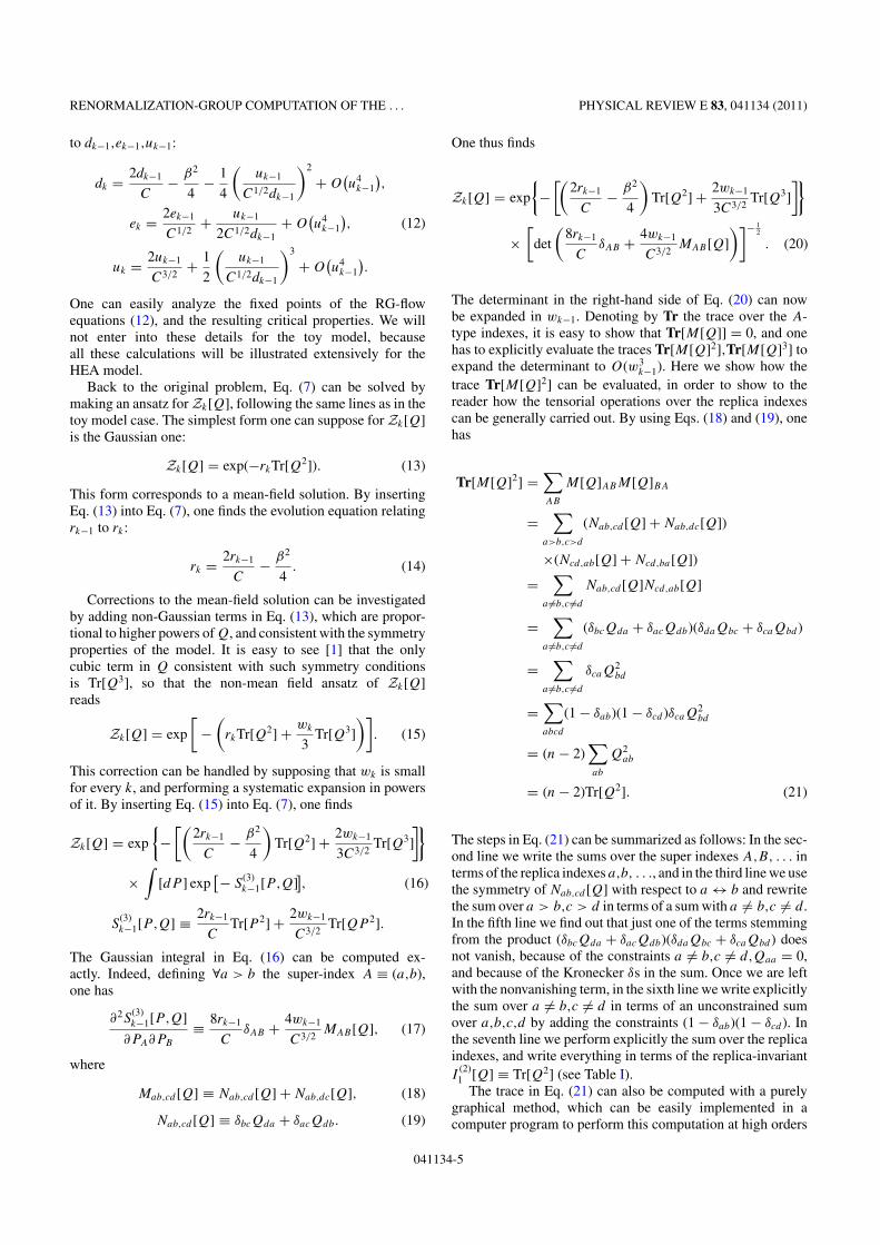
RENORMALIZATION-GROUP COMPUTATION OF THE . . . PHYSICAL REVIEW E 83, 041134 (2011)
to dk−1,ek−1,uk−1:
dk = 2dk−1
C− β2
4− 1
4
(uk−1
C1/2dk−1
)2
+ O(u4
k−1
),
ek = 2ek−1
C1/2+ uk−1
2C1/2dk−1+ O(u4
k−1
), (12)
uk = 2uk−1
C3/2+ 1
2
(uk−1
C1/2dk−1
)3
+ O(u4
k−1
).
One can easily analyze the fixed points of the RG-flowequations (12), and the resulting critical properties. We willnot enter into these details for the toy model, becauseall these calculations will be illustrated extensively for theHEA model.
Back to the original problem, Eq. (7) can be solved bymaking an ansatz for Zk[Q], following the same lines as in thetoy model case. The simplest form one can suppose for Zk[Q]is the Gaussian one:
Zk[Q] = exp(−rkTr[Q2]). (13)
This form corresponds to a mean-field solution. By insertingEq. (13) into Eq. (7), one finds the evolution equation relatingrk−1 to rk:
rk = 2rk−1
C− β2
4. (14)
Corrections to the mean-field solution can be investigatedby adding non-Gaussian terms in Eq. (13), which are propor-tional to higher powers of Q, and consistent with the symmetryproperties of the model. It is easy to see [1] that the onlycubic term in Q consistent with such symmetry conditionsis Tr[Q3], so that the non-mean field ansatz of Zk[Q]reads
Zk[Q] = exp
[−(
rkTr[Q2] + wk
3Tr[Q3]
)]. (15)
This correction can be handled by supposing that wk is smallfor every k, and performing a systematic expansion in powersof it. By inserting Eq. (15) into Eq. (7), one finds
Zk[Q] = exp
{−[(
2rk−1
C− β2
4
)Tr[Q2] + 2wk−1
3C3/2Tr[Q3]
]}
×∫
[dP ] exp[− S
(3)k−1[P,Q]
], (16)
S(3)k−1[P,Q] ≡ 2rk−1
CTr[P 2] + 2wk−1
C3/2Tr[QP 2].
The Gaussian integral in Eq. (16) can be computed ex-actly. Indeed, defining ∀a > b the super-index A ≡ (a,b),one has
∂2S(3)k−1[P,Q]
∂PA∂PB
≡ 8rk−1
CδAB + 4wk−1
C3/2MAB[Q], (17)
where
Mab,cd [Q] ≡ Nab,cd [Q] + Nab,dc[Q], (18)
Nab,cd [Q] ≡ δbcQda + δacQdb. (19)
One thus finds
Zk[Q] = exp
{−[(
2rk−1
C− β2
4
)Tr[Q2] + 2wk−1
3C3/2Tr[Q3]
]}
×[
det
(8rk−1
CδAB + 4wk−1
C3/2MAB[Q]
)]− 12
. (20)
The determinant in the right-hand side of Eq. (20) can nowbe expanded in wk−1. Denoting by Tr the trace over the A-type indexes, it is easy to show that Tr[M[Q]] = 0, and onehas to explicitly evaluate the traces Tr[M[Q]2],Tr[M[Q]3] toexpand the determinant to O(w3
k−1). Here we show how thetrace Tr[M[Q]2] can be evaluated, in order to show to thereader how the tensorial operations over the replica indexescan be generally carried out. By using Eqs. (18) and (19), onehas
Tr[M[Q]2] =∑AB
M[Q]ABM[Q]BA
=∑
a>b,c>d
(Nab,cd [Q] + Nab,dc[Q])
×(Ncd,ab[Q] + Ncd,ba[Q])
=∑
a =b,c =d
Nab,cd [Q]Ncd,ab[Q]
=∑
a =b,c =d
(δbcQda + δacQdb)(δdaQbc + δcaQbd )
=∑
a =b,c =d
δcaQ2bd
=∑abcd
(1 − δab)(1 − δcd )δcaQ2bd
= (n − 2)∑ab
Q2ab
= (n − 2)Tr[Q2]. (21)
The steps in Eq. (21) can be summarized as follows: In the sec-ond line we write the sums over the super indexes A,B, . . . interms of the replica indexes a,b, . . ., and in the third line we usethe symmetry of Nab,cd [Q] with respect to a ↔ b and rewritethe sum over a > b,c > d in terms of a sum with a = b,c = d.In the fifth line we find out that just one of the terms stemmingfrom the product (δbcQda + δacQdb)(δdaQbc + δcaQbd ) doesnot vanish, because of the constraints a = b,c = d,Qaa = 0,and because of the Kronecker δs in the sum. Once we are leftwith the nonvanishing term, in the sixth line we write explicitlythe sum over a = b,c = d in terms of an unconstrained sumover a,b,c,d by adding the constraints (1 − δab)(1 − δcd ). Inthe seventh line we perform explicitly the sum over the replicaindexes, and write everything in terms of the replica-invariantI
(2)1 [Q] ≡ Tr[Q2] (see Table I).
The trace in Eq. (21) can also be computed with a purelygraphical method, which can be easily implemented in acomputer program to perform this computation at high orders
041134-5
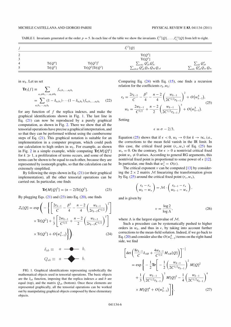
MICHELE CASTELLANA AND GIORGIO PARISI PHYSICAL REVIEW E 83, 041134 (2011)
TABLE I. Invariants generated at the order p = 5. In each line of the table we show the invariants I(j )1 [Q], . . . ,I (j )
nj[Q] from left to right.
j I(j )l [Q]
2 Tr[Q2]3 Tr[Q3]4 Tr[Q4] Tr[Q2]2
∑a =c Q2
abQ2bc
∑ab Q4
ab
5 Tr[Q5] Tr[Q2]Tr[Q3]∑
abcd Q2abQbcQbdQcd
∑abc Q3
abQacQbc
in wk . Let us set
Tr2[f ] ≡∑
a1 =b1,···,ak =bk
fa1b1,...,akbk
=∑
a1b1,···,akbk
(1 − δa1b1 ) · · · (1 − δakbk)fa1b1,...,akbk
(22)
for any function of f the replica indexes, and make thegraphical identifications shown in Fig. 1. The last line inEq. (21) can now be reproduced by a purely graphicalcomputation, as shown in Fig. 2. There we show that all thetensorial operations have precise a graphical interpretation, andso that they can be performed without using the cumbersomesteps of Eq. (21). This graphical notation is suitable for animplementation in a computer program, which could pushour calculation to high orders in wk . For example, as shownin Fig. 2 in a simple example, while computing Tr[M[Q]k]for k � 1, a proliferation of terms occurs, and some of theseterms can be shown to be equal to each other, because they arerepresented by isomorph graphs, so that the calculation can beextremely simplified.
By following the steps shown in Eq. (21) (or their graphicalimplementation), all the other tensorial operations can becarried out. In particular, one finds
Tr[M[Q]3] = (n − 2)Tr[Q3]. (23)
By plugging Eqs. (21) and (23) into Eq. (20), one finds
Zk[Q] = exp
(−{[
2rk−1
C− β2
4− n − 2
4
(wk−1
2rk−1C1/2
)2]
× Tr[Q2] + 1
3
[2wk−1
C3/2+ n − 2
2
(wk−1
2rk−1C1/2
)3]
× Tr[Q3] + O(w4
k−1
)}). (24)
δab ≡
Qab ≡ a b.
a b,
FIG. 1. Graphical identifications representing symbolically themathematical objects used in tensorial operations. The basic objectsare the δab function, imposing that the replica indexes a and b areequal (top), and the matrix Qab (bottom). Once these elements arerepresented graphically, all the tensorial operations can be workedout by manipulating graphical objects composed by these elementaryobjects.
Comparing Eq. (24) with Eq. (15), one finds a recursionrelation for the coefficients rk,wk:
rk = 2rk−1
C− β2
4− n − 2
4
(wk−1
2C1/2rk−1
)2
+ O(w4
k−1
),
(25)
wk = 2wk−1
C3/2+ n − 2
2
(wk−1
2C1/2rk−1
)3
+ O(w5
k−1
).
Setting
ε ≡ σ − 2/3,
Equation (25) shows that if ε < 0, wk → 0 for k → ∞, i.e.,the corrections to the mean field vanish in the IR limit. Inthis case, the critical fixed point (r∗,w∗) of Eq. (25) hasw∗ = 0. On the contrary, for ε > 0 a nontrivial critical fixedpoint w∗ = 0 arises. According to general RG arguments, thisnontrivial fixed point is proportional to some power of ε [12].In particular, one finds that w2
∗ = O(ε).The critical exponent ν can be computed [13] by consider-
ing the 2 × 2 matrix M linearizing the transformation givenby Eq. (25) around the critical fixed point (r∗,w∗),(
rk − r∗wk − w∗
)= M ·
(rk−1 − r∗
wk−1 − w∗
),
and is given by
ν = log 2
log �, (26)
where � is the largest eigenvalue of M.Such a procedure can be systematically pushed to higher
orders in wk , and thus in ε, by taking into account furthercorrections to the mean-field solution. Indeed, if we go back toEq. (20) and consider also the O(w4
k−1) terms on the right-handside, we find
[det
(8rk−1
CδAB + 4wk−1
C3/2MAB[Q]
)]− 12
= exp
{− 1
2Tr
[− 1
2
(wk−1
2C1/2rk−1
)2
M[Q]2
+ 1
3
(wk−1
2C1/2rk−1
)3
M[Q]3 − 1
4
(wk−1
2C1/2rk−1
)4
×M[Q]4 + O(w5
k−1
)]}. (27)
041134-6
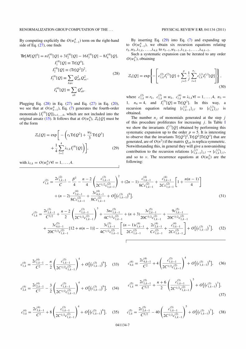
RENORMALIZATION-GROUP COMPUTATION OF THE . . . PHYSICAL REVIEW E 83, 041134 (2011)
By computing explicitly the O(w4k−1) term on the right-hand
side of Eq. (27), one finds
Tr[M[Q]4] = nI(4)1 [Q] + 3I
(4)2 [Q] − 16I
(4)3 [Q] − 8I
(4)4 [Q],
I(4)1 [Q] ≡ Tr[Q4],
I(4)2 [Q] ≡ (Tr[Q2])2,
(28)I
(4)3 [Q] ≡
∑b =c
Q2abQ
2ac,
I(4)4 [Q] ≡
∑ab
Q4ab.
Plugging Eq. (28) in Eq. (27) and Eq. (27) in Eq. (20),we see that at O(w4
k−1), Eq. (7) generates the fourth-order
monomials {I (4)l [Q]}l=1,...,4, which are not included into the
original ansatz (15). It follows that at O(w4k ), Zk[Q] must be
of the form
Zk[Q] = exp
[−(
rkTr[Q2] + wk
3Tr[Q3]
+ 1
4
4∑l=1
λl,kI(4)l [Q]
)], (29)
with λl,k = O(w4k ) ∀l = 1, . . . ,4.
By inserting Eq. (29) into Eq. (7) and expanding upto O(w4
k−1), we obtain six recursion equations relatingrk,wk,λ1,k, . . . ,λ4,k to rk−1,wk−1,λ1,k−1, . . . ,λ4,k−1.
Such a systematic expansion can be iterated to any orderO(wp
k ), obtaining
Zk[Q] = exp
⎧⎨⎩−⎡⎣c
(2)1,kI
(2)1 [Q] +
p∑j=3
1
j
nj∑l=1
c(j )l,k I
(j )l [Q]
⎤⎦⎫⎬⎭ ,
(30)
where c(2)1,k ≡ rk, c
(3)1,k ≡ wk, c
(4)l,k ≡ λl,k∀l = 1, . . . ,4, n3 =
1, n4 = 4, and I(3)1 [Q] ≡ Tr[Q3]. In this way, a
recursion equation relating {c(j )l,k−1}j,l to {c(j )
l,k }j,l isobtained.
The number nj of monomials generated at the step j
of this procedure proliferates for increasing j . In Table Iwe show the invariants I
(j )l [Q] obtained by performing this
systematic expansion up to the order p = 5. It is interestingto observe that the invariants Tr[Q2]2,Tr[Q2]Tr[Q3] that aregenerated, are of O(n2) if the matrix Qab is replica symmetric.Notwithstanding this, in general they will give a nonvanishingcontribution to the recursion relations {c(j )
l,k−1}j,l → {c(j )l,k }j,l ,
and so to ν. The recurrence equations at O(w5k ) are the
following:
c(2)1,k = 2c
(2)1,k−1
C− β2
4− n − 2
4
(c
(3)1,k−1
2C1/2c(2)1,k−1
)2
+ (2n − 1)c
(4)1,k−1
8Cc(2)1,k−1
+ c(4)2,k−1
2Cc(2)1,k−1
[1 + n(n − 1)
4
]
+ (n − 2)c
(4)3,k−1
8Cc(2)1,k−1
+ 3c(4)4,k−1
8Cc(2)1,k−1
+ O[(
c(3)1,k−1
)6], (31)
c(3)1,k = 2c
(3)1,k−1
C3/2+ n − 2
2
(c
(3)1,k−1
2C1/2c(2)1,k−1
)3
+ 3nc(5)1,k−1
4C3/2c(2)1,k−1
+ (n + 3)3c
(5)2,k−1
20C3/2c(2)1,k−1
+ 9c(5)3,k−1
20C3/2c(2)1,k−1
+ 3c(5)4,k−1
20C3/2c(2)1,k−1
[12 + n(n − 1)] − 3c(3)1,k−1
4C1/2c(2)1,k−1
[(n − 1)c(4)
1,k−1
2Cc(2)1,k−1
+ 2c(4)2,k−1
Cc(2)1,k−1
+ c(4)3,k−1
2Cc(2)1,k−1
]+ O[(
c(3)1,k−1
)7], (32)
c(4)1,k = 2c
(4)1,k−1
C2− n
2
(c
(3)1,k−1
2C1/2c(2)1,k−1
)4
+ O[(
c(3)1,k−1
)6], (33)
c(4)2,k = 2c
(4)2,k−1
C2− 3
2
(c
(3)1,k−1
2C1/2c(2)1,k−1
)4
+ O[(
c(3)1,k−1
)6], (34)
c(4)3,k = 2c
(4)3,k−1
C2+ 8
(c
(3)1,k−1
2C1/2c(2)1,k−1
)4
+ O[(
c(3)1,k−1
)6], (35)
c(4)4,k = 2c
(4)4,k−1
C2+ 4
(c
(3)1,k−1
2C1/2c(2)1,k−1
)4
+ O[(
c(3)1,k−1
)6], (36)
c(5)1,k = 2c
(5)1,k−1
C5/2+ n + 6
2
(c
(3)1,k−1
2C1/2c(2)1,k−1
)5
+ O[(
c(3)1,k−1
)7],
(37)
c(5)2,k = 2c
(5)2,k−1
C5/2− 40
(c
(3)1,k−1
2C1/2c(2)1,k−1
)5
+ O[(
c(3)1,k−1
)7], (38)
041134-7

MICHELE CASTELLANA AND GIORGIO PARISI PHYSICAL REVIEW E 83, 041134 (2011)
Tr[M [Q]2] = Tr2[N [Q]N [Q]]
= Tr2
[(+
)(+ +
)]
+= Tr2
[
= Tr2
[ ]
== − − +
== − 2×
== − 2×n×
= (n − 2)Tr[Q2]
Example of a graphical computation
+
]
+
FIG. 2. Graphical computation of Tr[M[Q]2] in Eq. (21). In thesecond line, the two addends of the matrix N [Q]ab,cd in Eq. (19) arerepresented graphically in terms of the graphical objects defined inFig. 1. In the third line, the legs of such addends are contracted witheach other, and four terms are generated. The second and the thirdterm can be easily recognized to be topologically identical, and soequal. According to the condition Qaa = 0 in Eq. (3), the first termin the third line vanishes. Indeed, in this term the lines coming outof the square vertex Qab are connected by a circuit, meaning that thematrix element Qab is computed with a = b, and thus vanishes. Thesecond and third terms in the third line also vanish because, accordingto Eq. (22), the dummy indexes in Tr2 must satisfy a1 = b1,a2 = b2,while the graphical structure of the second and third terms enforcesthe constraint a2 = b2,a1 = b1 respectively. Moreover, the two toplines in the third term are actually equivalent to just one line, becauseof the relation δ2
ab = δab. Hence, we are left with a single term in thefourth line. In the fifth line, we perform graphically the operation Tr2.Such an operation can be easily implemented graphically by lookingat the second line of Eq. (22). Let us expand the product of δs in thesecond line of Eq. (22), and recall from Fig. 1 that δab represents aline with a circular dot connecting a with b. Hence, given a graphicalobject O with external legs (indexes) (a1,b1), . . . ,(ak,bk), Tr2[O] isnothing but the sum of all the possible 2k contractions (performedwith a line with a circular dot) of these external legs, where eachcontracted term is multiplied by (−1)# of contractions of the term. In thiscase k = 2, so we generate 22 terms in the fifth line. In the sixthline, we take into account the fact that the second and third termsin the fifth line are topologically isomorph, and that the fourth termin the fifth line vanishes because of the condition Qaa = 0. In theseventh line the unconstrained sum over the replica indexes is finallyperformed. This can be done graphically in the following way: Whenwe have an external line connected to a round vertex, summing overthe replica index represented by that line means that one has to simplyremove the line (this is the graphical implementation of the relation∑
b δabgb = ga). We do this in the first term: We sum over the top-leftindex, and remove the line on the top. Then we sum over the top-rightindex by simply multiplying by n. The sum over the bottom-left andbottom-right indexes simply yields Tr[Q2]. We do the same for thesecond term: We sum over the top-right index and remove the topline, then sum over the top-left index and remove the top-left line.Then, the sum over the bottom-left and bottom-right indexes yieldsTr[Q2]. Hence, we get the same result as in Eq. (21).
c(5)3,k = 2c
(5)3,k−1
C5/2+ 30
(c
(3)1,k−1
2C1/2c(2)1,k−1
)5
+ O[(
c(3)1,k−1
)7], (39)
c(5)4,k = 2c
(5)4,k−1
C5/2+ 5
(c
(3)1,k−1
2C1/2c(2)1,k−1
)5
+ O[(
c(3)1,k−1
)7]. (40)
By looking at Eqs. (33)–(40) and using the definition (5),it is easy to see that the coefficients c
(4)l,k ,c
(5)l,k scale to zero as
k → ∞ if ε < 1/12. It is easy to find out that this is actuallytrue for all the coefficients c
(j )l,k with j > 3. Such a critical
value ε = 1/12 will be reproduced also in the field-theoreticalapproach in Sec. III.
The evolution Eqs. (31)–(40) depend smoothly on thereplica number n, so that the analytical continuation n → 0,can be done directly. By linearizing the transformation (31)–(40) around the critical fixed point {c(j )
l∗ }j,l and computing thematrix M, one can extract �, and so ν for n = 0 to the orderε2 by using Eq. (26). We find
ν = 3 + 36ε + [432 − 27(50 + 55 × 21/3
+ 53 × 22/3) log 2]ε2 + O(ε3). (41)
At order ε, our result for ν is the same as that of thepower-law interaction spin glass [11] [where ε ≡ 3(σ − 2/3)].Notwithstanding this, the coefficients of the expansion in thesetwo models will be in general different at two or more loops.As a matter of fact, the binary-tree interaction structure ofthe HEA emerges in the nontrivial log 2,21/3 factors in thecoefficient of ε2 in Eq. (41), which cannot be there in thepower-law case.
Before discussing the result in Eq. (41), we point outthat Wilson’s method explicitly implements the binary-treestructure of the model when approaching the IR limit. Asa matter of fact, the hierarchical structure of the modelis explicitly exploited to construct the steps of the RGtransformation. Nevertheless, if the IR limit is unique andwell defined, physical observables such as ν must not dependon the technique we use to compute them in such a limit.It is thus important to verify that Eq. (41) does not dependon the method we used to reproduce the IR behavior of thetheory. This has been done by reproducing Eq. (41) with aquite different field-theoretical approach.
III. FIELD-THEORETICAL METHOD
Here the IR limit is performed by constructing a functionalintegral field theory and by removing its IR divergences withinthe minimal subtraction scheme.
While in Wilson’s method the IR limit was performed bylooking at the scale-invariant fixed points for k → ∞ aftersolving the recursion relation (7), in this case we performbefore the large-k limit, remove the resulting IR singularitiesthrough re-normalization, and then perform the scale-invariant(IR) limit by means of the Callan-Symanzik equation.
041134-8

RENORMALIZATION-GROUP COMPUTATION OF THE . . . PHYSICAL REVIEW E 83, 041134 (2011)
This computation is better performed by slightly changingthe definition of the model. Indeed, the following redefinitionof the interaction term in Eq. (1),
0,2k+1−1∑i<j
J12,ij SiSj →2k−1∑i=0
2k+1−1∑j=2k
J12,ij SiSj (42)
is equivalent to the original definition (1) and makes the field-theory computations simpler. The equivalence of Eq. (42) withthe original definition (1) can be shown [23] by observing thatthe scaling of the spin coupling in the model defined by Eq. (42)differs from that in Eq. (1) for a constant multiplicative factor,and thus that the two options are equivalent, and must yieldthe same critical exponents. Notwithstanding this, the criticaltemperature of the model defined by Eq. (1) and that of themodel defined by Eq. (42) are different. This can be verified byconsidering how the recursion relation (6) is modified whenone applies the redefinition (42).
The only difference is the third factor in the second line ofEq. (6), which is now given by
EJ12
⎡⎣exp
⎛⎝ β
2kσ
n∑a=1
2k−1−1∑i=0
2k−1∑j=2k−1
J12,ij Sai Sa
j
⎞⎠⎤⎦
= exp
{β2Ck
4
[Tr[Q2] − 1
4
(Tr[Q2
1
]+ Tr[Q2
2
])]}.
It follows that the recursion relation (6) becomes
Zk[Q] = exp
(β2Ck
4Tr[Q2]
)∫[dQ1dQ2]
× exp
(−β2Ck
16Tr[Q2
1
])Zk−1[Q1]
× exp
(−β2Ck
16Tr[Q2
2
])Zk−1[Q2]
×n∏
a<b=1
δ
(Qab − Q1,ab + Q2,ab
2
). (43)
Setting
Xk[Q] ≡ exp
(−β2C
16Tr[Q2]
)Zk[C−k/2Q],
one can rewrite Eq. (43) as
Xk[Q] = exp
[β2
4
(1 − C
4
)Tr[Q2]
] ∫[dP ]
×Xk−1
(Q + P
C1/2
)Xk−1
(Q − P
C1/2
). (44)
By comparing Eq. (44) with Eq. (7), it is finally clear thatthe redefinition (42) results in an effective redefinition of theinverse temperature β.
The redefinition (42) also has a clear physical meaning.Indeed, the original definition (1) is such that, when twosubsystems of 2k spins are coupled to form a system with2k+1 spins, one introduces couplings J12,ij between the twosubsystems and between the spins within each subsystem,while in Eq. (42) only couplings between the two subsystemsare introduced.
By iterating the recursion relation (1), one has an explicitform for the Hamiltonian HJ
k [�S] of a system of 2k spins inthe large-k limit. Then, the average of the replicated partitionfunction is expressed as an integral over the local overlap fieldQiab ≡ Sa
i Sbi :
EJ [Zn] = EJ
⎡⎣∑
{Sai }i,a
exp
(−β
n∑a=1
HJk
[Sa
0 , . . . ,Sa2k−1
])⎤⎦=∫
[dQ] e−S[Q].
By using a dimensional analysis, it is easy to pick up the termsin S[Q] that are relevant in the IR limit. It is easy to check thatS[Q] is given by the sum of a quadratic term in Qiab, plus acubic term, plus higher-degree terms. The dimensions of thefield Qiab can be computed by imposing the adimensionalityof the quadratic term, and so the dimensions of the coefficient gof the cubic term and of those of the higher-degree terms. Onefinds that the dimensions of g in energy is [g] = 3ε. Thus, as inWilson’s method, the cubic term scales to zero in the IR limitfor ε < 0, while a nontrivial fixed point appears for ε > 0. Asin Wilson’s method, it is easy to see that for ε < 1/12 all thehigher-degree terms in S[Q] scale to zero in the IR limit. Thus,the IR-dominant part of the action reads
S[Q] = 1
2
2k−1∑i,j=0
�ij Tr[QiQj ] + g
3!
2k−1∑i=0
Tr[Q3
i
]. (45)
In the derivation of Eq. (45), the bare propagator �ij
originally depends on i,j through the difference I(i) − I(j ),where the function I(i) is defined as follows: Given i ∈[0,2k − 1] and its expression in base 2,
i =k−1∑j=0
aj 2j , I(i) ≡k−1∑j=0
ak−1−j 2j . (46)
Hence, the quadratic term of Eq. (45) is not invariant underspatial translations. This would make any explicit computationof the loop integrals, and so of the critical exponents, extremelydifficult to perform. This problem can be overcome by arelabeling of the sites of the lattice [33],
I(i) → i,∀i = 0, . . . ,2k − 1.
After relabeling one obtains that �ij depends on i,j justthrough the difference i − j , thus S[Q] is translationally in-variant, and the ordinary Fourier transform techniques [33,34]can be employed. In particular, the Fourier representation ofthe propagator is
�ij = 1
2k
2k−1∑p=0
exp
[−2πıp(i − j )
2k
] (|p|2σ−12 + m
), (47)
where |p|2 is the diadic norm of p [32], and the mass m ∝T − Tc has dimensions [m] = 2σ − 1.
An interesting feature of the action (45) is the fact thepropagator � in Eq. (47) depends on the momentum p throughits diadic norm |p|2. If we look at the original derivation of therecursion RG equation for the Ising model in finite dimension(in particular, to the Polyakov derivation [13]), we find that the
041134-9
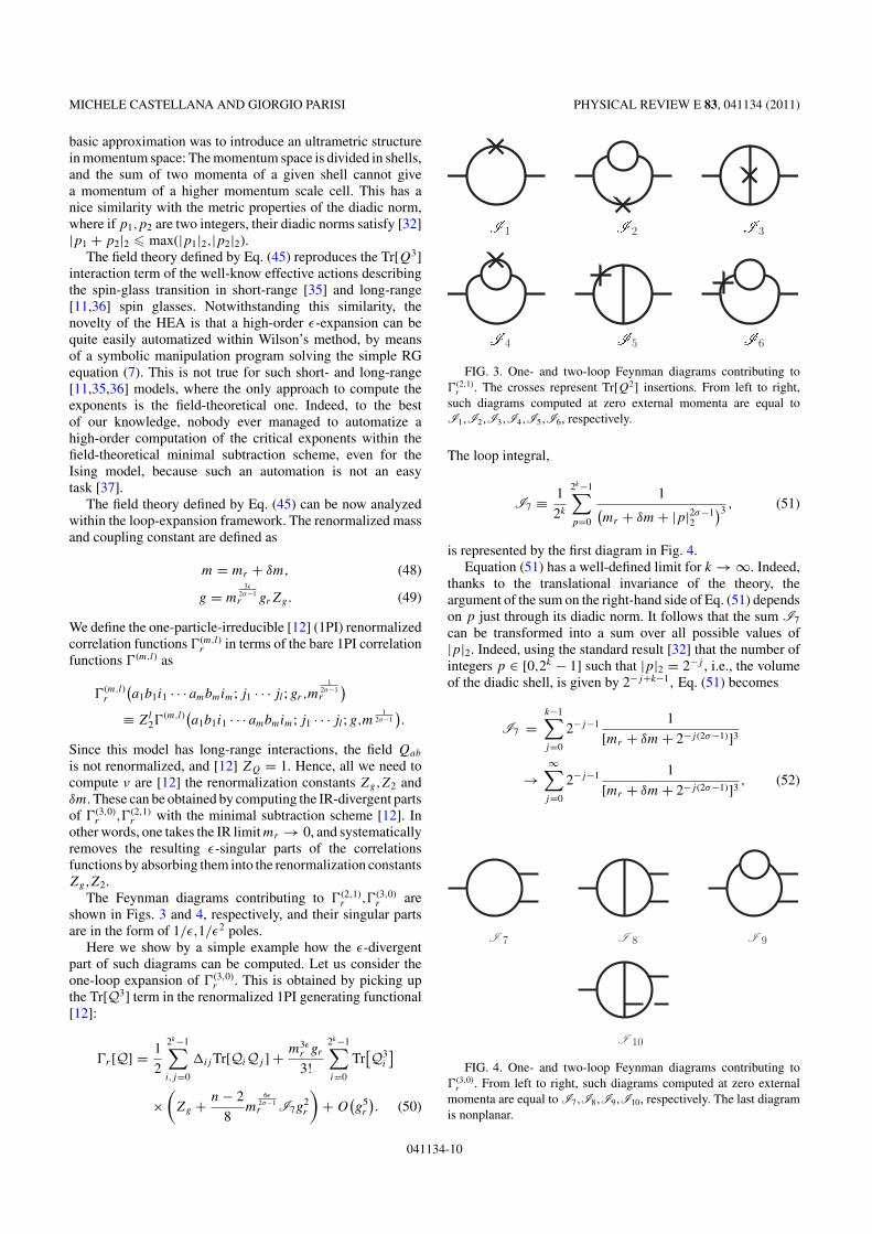
MICHELE CASTELLANA AND GIORGIO PARISI PHYSICAL REVIEW E 83, 041134 (2011)
basic approximation was to introduce an ultrametric structurein momentum space: The momentum space is divided in shells,and the sum of two momenta of a given shell cannot givea momentum of a higher momentum scale cell. This has anice similarity with the metric properties of the diadic norm,where if p1,p2 are two integers, their diadic norms satisfy [32]|p1 + p2|2 � max(|p1|2,|p2|2).
The field theory defined by Eq. (45) reproduces the Tr[Q3]interaction term of the well-know effective actions describingthe spin-glass transition in short-range [35] and long-range[11,36] spin glasses. Notwithstanding this similarity, thenovelty of the HEA is that a high-order ε-expansion can bequite easily automatized within Wilson’s method, by meansof a symbolic manipulation program solving the simple RGequation (7). This is not true for such short- and long-range[11,35,36] models, where the only approach to compute theexponents is the field-theoretical one. Indeed, to the bestof our knowledge, nobody ever managed to automatize ahigh-order computation of the critical exponents within thefield-theoretical minimal subtraction scheme, even for theIsing model, because such an automation is not an easytask [37].
The field theory defined by Eq. (45) can be now analyzedwithin the loop-expansion framework. The renormalized massand coupling constant are defined as
m = mr + δm, (48)
g = m3ε
2σ−1r grZg. (49)
We define the one-particle-irreducible [12] (1PI) renormalizedcorrelation functions �(m,l)
r in terms of the bare 1PI correlationfunctions �(m,l) as
�(m,l)r
(a1b1i1 · · · ambmim; j1 · · · jl ; gr,m
12σ−1r
)≡ Zl
2�(m,l)(a1b1i1 · · · ambmim; j1 · · · jl ; g,m
12σ−1).
Since this model has long-range interactions, the field Qab
is not renormalized, and [12] ZQ = 1. Hence, all we need tocompute ν are [12] the renormalization constants Zg,Z2 andδm. These can be obtained by computing the IR-divergent partsof �(3,0)
r ,�(2,1)r with the minimal subtraction scheme [12]. In
other words, one takes the IR limit mr → 0, and systematicallyremoves the resulting ε-singular parts of the correlationsfunctions by absorbing them into the renormalization constantsZg,Z2.
The Feynman diagrams contributing to �(2,1)r ,�(3,0)
r areshown in Figs. 3 and 4, respectively, and their singular partsare in the form of 1/ε,1/ε2 poles.
Here we show by a simple example how the ε-divergentpart of such diagrams can be computed. Let us consider theone-loop expansion of �(3,0)
r . This is obtained by picking upthe Tr[Q3] term in the renormalized 1PI generating functional[12]:
�r [Q] = 1
2
2k−1∑i,j=0
�ij Tr[QiQj ] + m3εr gr
3!
2k−1∑i=0
Tr[Q3
i
]
×(
Zg + n − 2
8m
6ε2σ−1r I7g
2r
)+ O(g5
r
). (50)
1 2 3
4 5 6
FIG. 3. One- and two-loop Feynman diagrams contributing to�(2,1)
r . The crosses represent Tr[Q2] insertions. From left to right,such diagrams computed at zero external momenta are equal toI1,I2,I3,I4,I5,I6, respectively.
The loop integral,
I7 ≡ 1
2k
2k−1∑p=0
1(mr + δm + |p|2σ−1
2
)3 , (51)
is represented by the first diagram in Fig. 4.Equation (51) has a well-defined limit for k → ∞. Indeed,
thanks to the translational invariance of the theory, theargument of the sum on the right-hand side of Eq. (51) dependson p just through its diadic norm. It follows that the sum I7
can be transformed into a sum over all possible values of|p|2. Indeed, using the standard result [32] that the number ofintegers p ∈ [0,2k − 1] such that |p|2 = 2−j , i.e., the volumeof the diadic shell, is given by 2−j+k−1, Eq. (51) becomes
I7 =k−1∑j=0
2−j−1 1
[mr + δm + 2−j (2σ−1)]3
→∞∑
j=0
2−j−1 1
[mr + δm + 2−j (2σ−1)]3, (52)
FIG. 4. One- and two-loop Feynman diagrams contributing to�(3,0)
r . From left to right, such diagrams computed at zero externalmomenta are equal to I7,I8,I9,I10, respectively. The last diagramis nonplanar.
041134-10

RENORMALIZATION-GROUP COMPUTATION OF THE . . . PHYSICAL REVIEW E 83, 041134 (2011)
where in the second line of Eq. (52) the k → ∞ limit has beentaken, because the sum in the first line is convergent. By usingthe fact that δm = O(g2
r ), we can rewrite Eq. (52) as
I7 =∞∑
j=0
2−j−1 1
[mr + 2−j (2σ−1)]3+ O(g2
r
). (53)
It is easy to see that I7 is IR divergent for mr → 0. Indeed, inthe limit mr → 0 the sum over j in Eq. (53) is dominated by theterms in the IR region 2−j = |p|2 → 0. The js correspondingto this region go to infinity as mr → 0, yielding a divergentsum in I7.
In the IR region, the sum on the right-hand side of Eq. (53)can be approximated by an integral, because the integrandfunction is almost constant in the interval [j,j + 1] for largej . Setting q ≡ 2−j , for mr → 0 we have −q log 2dj = dq,and
I7 = 1
2 log 2
∫ 1
0
dq
[mr + q2σ−1]3+ O(g2
r
)
= m− 6ε
2σ−1r
2 log 2
∫ m− 1
2σ−1r
0
dx
(1 + x2σ−1)3+ O(g2
r
)
→ m− 6ε
2σ−1r
2 log 2
∫ ∞
0
dx
(1 + x2σ−1)3+ O(g2
r
). (54)
The integral on the right-hand side of the last line inEq. (54) is convergent for ε > 0, and diverges as ε → 0.Its ε-divergent part can be easily evaluated,
I7 = m− 6ε
2σ−1r
4 log 2�
(3 + 1
1 − 2σ
)
�
(1 + 1
1 − 2σ
)+ O(g2
r
)= m
− 6ε2σ−1
r
[1
12ε log 2+ Oε(1)
]+ O(g2
r
), (55)
where � is the Euler-gamma function and Oε(1) denotes termsthat stay finite as ε → 0. As we will show in the following,these finite terms give a contribution to the renormalizationconstants at two loops. By plugging Eq. (55) into Eq. (50),one can compute the g2
r coefficient of Zg by imposing thatthe ε-singular part of I7 is canceled by Zg . For n = 0we have
Zg = 1 + 1
48ε log 2g2
r + O(g4
r
). (56)
By repeating the same computation for the generating func-tional �r [Q,K] of correlation functions with Tr[Q2] insertionsand imposing that the
∑2k−1i=0 KiQ2
i term is finite, i.e., that �(2,1)r
is finite, we obtain
Z2 = 1 + 1
24ε log 2g2
r + O(g4
r
).
Such a procedure has been pushed at two loops by an explicitcalculation. Even if the evaluation of the ε-divergent partof the two-loop diagrams is more involved, the techniquesand underlying ideas are exactly the same as those used tocompute the one-loop diagram I7. In Figs. 3 and 4 we showthe Feynman diagrams contributing to the finiteness conditionsof �(2,1)
r and of �(3,0)r , respectively. We denote by I7, . . . ,I6
the diagrams in Fig. 3 evaluated at zero external momenta, andby I7, . . . ,I10 those in Fig. 4 evaluated at zero momenta. Itis easy to show that the equalities
I7 = I7,
I2 = I6 = I9,
I3 = I10,
I4 = I5 = I8
hold, and so that all we need to compute the renormalizationconstants are I7,I2,I3,I4. I7 is given by Eq. (51), whilethe other loop integrals are
I2 = 1
22k
2k−1∑p=0
2k−1∑q=0
1(mr + δm + |p|2σ−1
2
)4(mr + δm + |q|2σ−1
2
)(mr + δm + |p − q|2σ−1
2
) ,
I3 = 1
22k
2k−1∑p=0
2k−1∑q=0
1(mr + δm + |p|2σ−1
2
)2(mr + δm + |q|2σ−1
2
)2(mr + δm + |p − q|2σ−1
2
)2 ,
I4 = 1
22k
2k−1∑p=0
2k−1∑q=0
1(mr + δm + |p|2σ−1
2
)3(mr + δm + |q|2σ−1
2
)2(mr + δm + |p − q|2σ−1
2
) .In the limit mr → 0, I2,I3,I4 are given by
I2 = m−12ε2σ−1r
[(2
22/3 − 1− 1
21/3 − 1− 1
)1
48ε log 2
]+ Oε(1) + O
(g2
r
),
I3 = m−12ε2σ−1r
(1
21/3 − 1
1
16ε log 2
)+ Oε(1) + O
(g2
r
),
041134-11
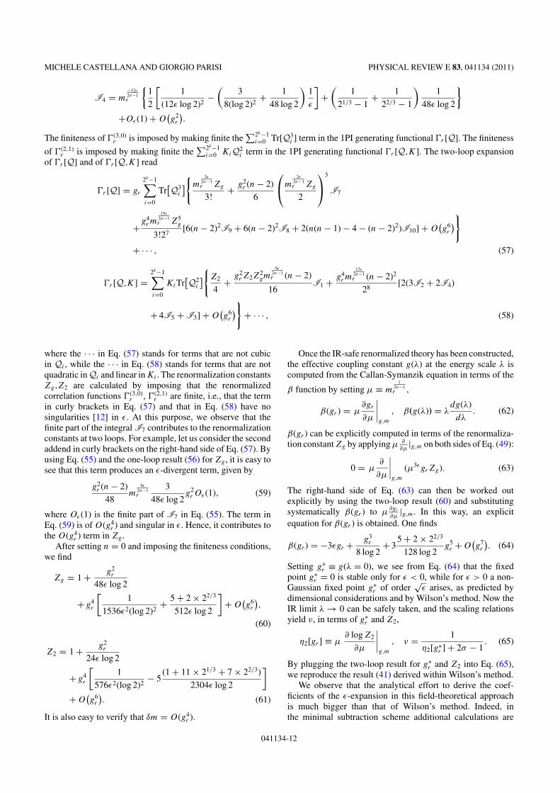
MICHELE CASTELLANA AND GIORGIO PARISI PHYSICAL REVIEW E 83, 041134 (2011)
I4 = m−12ε2σ−1r
{1
2
[1
(12ε log 2)2−(
3
8(log 2)2+ 1
48 log 2
)1
ε
]+(
1
21/3 − 1+ 1
22/3 − 1
)1
48ε log 2
}+Oε(1) + O
(g2
r
).
The finiteness of �(3,0)r is imposed by making finite the
∑2k−1i=0 Tr[Q3
i ] term in the 1PI generating functional �r [Q]. The finiteness
of �(2,1)r is imposed by making finite the
∑2k−1i=0 KiQ2
i term in the 1PI generating functional �r [Q,K]. The two-loop expansionof �r [Q] and of �r [Q,K] read
�r [Q] = gr
2k−1∑i=0
Tr[Q3
i
]{m3ε
2σ−1r Zg
3!+ g2
r (n − 2)
6
⎛⎝m
3ε2σ−1r Zg
2
⎞⎠
3
I7
+g4r m
15ε2σ−1r Z5
g
3!27[6(n − 2)2I9 + 6(n − 2)2I8 + 2(n(n − 1) − 4 − (n − 2)2)I10] + O
(g6
r
)}
+ · · · , (57)
�r [Q,K] =2k−1∑i=0
KiTr[Q2
i
]{Z2
4+ g2
r Z2Z2gm
6ε2σ−1r (n − 2)
16I1 + g4
r m12ε
2σ−1r (n − 2)2
28[2(3I2 + 2I4)
+ 4I5 + I3] + O(g6
r
)}+ · · · , (58)
where the · · · in Eq. (57) stands for terms that are not cubicin Qi , while the · · · in Eq. (58) stands for terms that are notquadratic in Qi and linear in Ki . The renormalization constantsZg,Z2 are calculated by imposing that the renormalizedcorrelation functions �(3,0)
r , �(2,1)r are finite, i.e., that the term
in curly brackets in Eq. (57) and that in Eq. (58) have nosingularities [12] in ε. At this purpose, we observe that thefinite part of the integral I7 contributes to the renormalizationconstants at two loops. For example, let us consider the secondaddend in curly brackets on the right-hand side of Eq. (57). Byusing Eq. (55) and the one-loop result (56) for Zg , it is easy tosee that this term produces an ε-divergent term, given by
g2r (n − 2)
48m
9ε2σ−1r
3
48ε log 2g2
r Oε(1), (59)
where Oε(1) is the finite part of I7 in Eq. (55). The term inEq. (59) is of O(g4
r ) and singular in ε. Hence, it contributes tothe O(g4
r ) term in Zg .After setting n = 0 and imposing the finiteness conditions,
we find
Zg = 1 + g2r
48ε log 2
+ g4r
[1
1536ε2(log 2)2+ 5 + 2 × 22/3
512ε log 2
]+ O(g6
r
),
(60)
Z2 = 1 + g2r
24ε log 2
+ g4r
[1
576ε2(log 2)2− 5
(1 + 11 × 21/3 + 7 × 22/3)
2304ε log 2
]+O(g6
r
). (61)
It is also easy to verify that δm = O(g4r ).
Once the IR-safe renormalized theory has been constructed,the effective coupling constant g(λ) at the energy scale λ iscomputed from the Callan-Symanzik equation in terms of the
β function by setting μ ≡ m1
2σ−1r ,
β(gr ) = μ∂gr
∂μ
∣∣∣∣g,m
, β(g(λ)) = λdg(λ)
dλ. (62)
β(gr ) can be explicitly computed in terms of the renormaliza-tion constant Zg by applying μ ∂
∂μ|g,m on both sides of Eq. (49):
0 = μ∂
∂μ
∣∣∣∣g,m
(μ3εgrZg). (63)
The right-hand side of Eq. (63) can then be worked outexplicitly by using the two-loop result (60) and substitutingsystematically β(gr ) to μ
∂gr
∂μ|g,m. In this way, an explicit
equation for β(gr ) is obtained. One finds
β(gr ) = −3εgr + g3r
8 log 2+ 3
5 + 2 × 22/3
128 log 2g5
r + O(g7
r
). (64)
Setting g∗r ≡ g(λ = 0), we see from Eq. (64) that the fixed
point g∗r = 0 is stable only for ε < 0, while for ε > 0 a non-
Gaussian fixed point g∗r of order
√ε arises, as predicted by
dimensional considerations and by Wilson’s method. Now theIR limit λ → 0 can be safely taken, and the scaling relationsyield ν, in terms of g∗
r and Z2,
η2[gr ] ≡ μ∂ log Z2
∂μ
∣∣∣∣g,m
, ν = 1
η2[g∗r ] + 2σ − 1
. (65)
By plugging the two-loop result for g∗r and Z2 into Eq. (65),
we reproduce the result (41) derived within Wilson’s method.We observe that the analytical effort to derive the coef-
ficients of the ε-expansion in this field-theoretical approachis much bigger than that of Wilson’s method. Indeed, inthe minimal subtraction scheme additional calculations are
041134-12
RENORMALIZATION-GROUP COMPUTATION OF THE . . . PHYSICAL REVIEW E 83, 041134 (2011)
needed to extract the coefficients of the ε poles of theFeynman diagrams in Figs. 3 and 4. It follows that for anautomatized implementation of the high-order ε-expansion,Wilson’s method turns out to be much better performingthat the field-theoretical method. Notwithstanding this, thetensorial operations needed to compute the Q-dependence ofthe diagrams in this field-theoretical approach turn out to beexactly the same as those needed in Sec. II, and no additionaleffort has been required to compute them.
IV. CONCLUSIONS
In a previous work [26], we set up two perturbativeapproaches to compute the IR behavior of a strongly frustratednon-mean-field spin-glass system, the HEA model. The twomethods are based on the replica approach, and in particularon the assumption that the physics of the system is encoded inthe limit where the number of replicas n tends to zero. Withinthe ε-expansion framework, the two approaches yield the sameprediction at two loops for the critical exponent ν related tothe divergence of the correlation length.
In this work the two-loop computation is shown in allits most relevant details, so that the reader can reproduceit. Moreover, we show the underlying renormalization groupideas implemented in the two computation methods. One ofthese is the existence of a characteristic length ξ diverging at
the IR critical fixed point, where the theory is invariant withrespect to reparametrization of the length scale.
In addition, we show with an explicit example that such acomputation of the critical exponents could be quite easilyautomatized, i.e., implemented in a computer program, inorder to compute high orders of the ε-expansion, and soeventually make this theory physically predictive. Indeed, wegive a graphical interpretation of the cumbersome tensorialoperations needed to compute ν and previously used inRef. [26]. Such a graphical method makes the calculationsmuch more straightforward and suitable for an implementationin a computer program to compute high orders of the ε
series. We observe that once this high-order series in ε willbe known, some resummation technique will be needed tomake the theory predictive, because the series probably hasa nonconvergent behavior. If the high-order series could bemade convergent by means of some appropriate resummationtechnique, this calculation would yield an analytical controlon the critical exponents, resulting in a precise prediction fora non-mean-field spin glass mimicking a real system.
ACKNOWLEDGMENT
We thank N. Sourlas, S. Franz, and M. Mezard forinteresting discussions and suggestions.
[1] M. Mezard, G. Parisi, and M. A. Virasoro, Spin Glass Theoryand Beyond (World Scientific, Singapore, 1987).
[2] T. Castellani and A. Cavagna, J. Stat. Mech. (2005) P05012.[3] G. Parisi, J. Phys. A 13, 1101 (1980).[4] B. Derrida, Phys. Rev. Lett. 45, 79 (1980).[5] W. L. McMillan, J. Phys. C 17, 3179 (1984).[6] A. J. Bray and M. A. Moore, Phys. Rev. Lett. 58, 57 (1987).[7] D. S. Fisher and D. A. Huse, Phys. Rev. B 38, 373 (1988).[8] T. R. Kirkpatrick, D. Thirumalai, and P. G. Wolynes, Phys. Rev.
A 40, 1045 (1989).[9] C. De Dominicis and I. Giardina, Random Fields and Spin
Glasses: A Field Theory Approach (Springer, Berlin, 2006).[10] J. H. Chen and T. C. Lubensky, Phys. Rev. B 16, 2106 (1977).[11] G. Kotliar, P. W. Anderson, and D. L. Stein, Phys. Rev. B 27,
602 (1983).[12] J. Zinn-Justin, Int. Ser. Monogr. Phys. 113, 1 (2002).[13] K. G. Wilson and J. B. Kogut, Phys. Rept. 12, 75 (1974).[14] I. Giardina (private communication).[15] F. J. Dyson, Commun. Math. Phys. 12, 91 (1969).[16] P. Collet and J. Eckmann, Lect. Notes Phys. 74 (1978).[17] P. Collet and J. Eckmann, Commun. Math. Phys. 55, 67
(1977).[18] M. Cassandro and G. Jona-Lasinio, Adv. Phys. 27, 6 (1978).[19] A. Theumann, Phys. Rev. B 21, 2984 (1980).[20] A. Theumann, Phys. Rev. B 22, 5441 (1980).[21] A. N. Berker and S. Ostlund, J. Phys. C12, 4961 (1979).
[22] E. Gardner, J. Phys. (Paris) 45, 1755 (1984).[23] S. Franz, T. Jorg, and G. Parisi, J. Stat. Mech. (2009) P02002.[24] M. Castellana, A. Decelle, S. Franz, M. Mezard, and G. Parisi,
Phys. Rev. Lett. 104, 127206 (2010).[25] Y. V. Fyodorov, A. Ossipov, and A. Rodriguez, J. Stat. Mech.
(2009) L12001.[26] M. Castellana and G. Parisi, Phys. Rev. E 82, 040105(R)
(2010).[27] H. G. Katzgraber and A. P. Young, Phys. Rev. B 67, 134410
(2003).[28] H. G. Katzgraber and A. P. Young, Phys. Rev. B 72, 184416
(2005).[29] H. G. Katzgraber, A. K. Hartmann, and A. P. Young, in
Condensed Matter Physics XXI, edited by D. P. Landau, S. P.Lewis, and H. B. Schuttler (Springer, Heidelberg, 2008).
[30] L. Leuzzi, J. Phys. A 32, 1417 (1999).[31] L. Leuzzi, G. Parisi, F. Ricci-Tersenghi, and J. J. Ruiz-Lorenzo,
Phys. Rev. Lett. 101, 107203 (2008).[32] G. Parisi and N. Sourlas, Eur. Phys. J. B 14, 3 (2000).[33] Y. Meurice, J. Math. Phys. 36, 1812 (1995).[34] M. Taibleson, Fourier Analysis on Local Fields (Princeton
University Press, Princeton, NJ, 1976).[35] A. B. Harris, T. C. Lubensky, and J. H. Chen, Phys. Rev. Lett.
36, 415 (1976).[36] M. C. Chang and J. Sak, Phys. Rev. B 29, 2652 (1984).[37] R. Guida and P. Ribeca, J. Stat. Mech. (2006) P02007.
041134-13
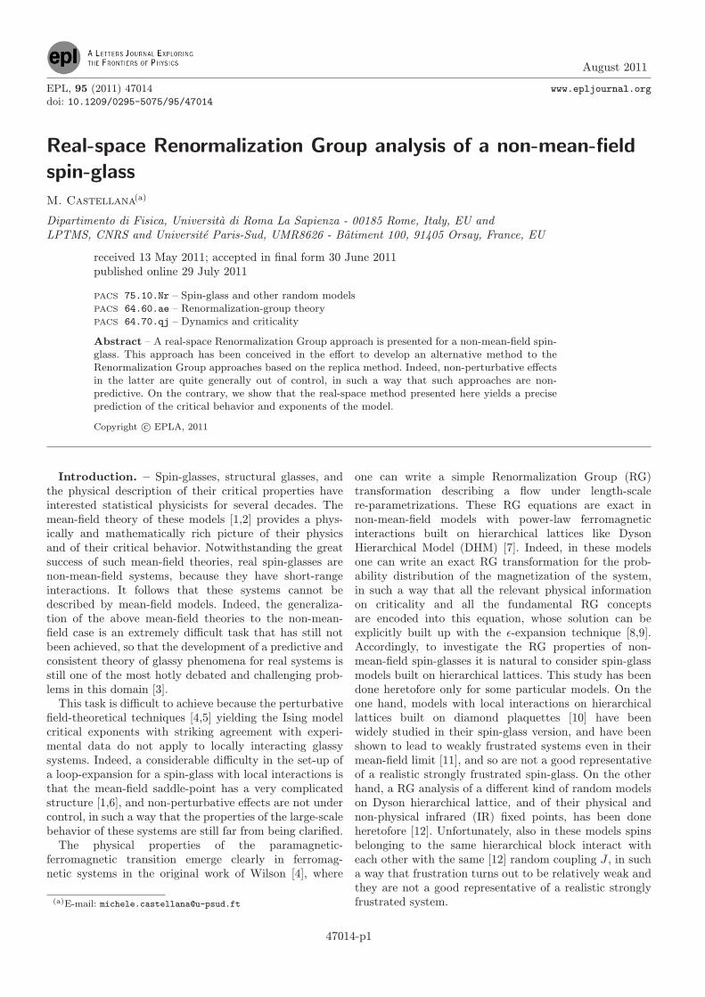
August 2011
EPL, 95 (2011) 47014 www.epljournal.orgdoi: 10.1209/0295-5075/95/47014
Real-space Renormalization Group analysis of a non-mean-fieldspin-glassM. Castellana(a)
Dipartimento di Fisica, Universita di Roma La Sapienza - 00185 Rome, Italy, EU andLPTMS, CNRS and Universite Paris-Sud, UMR8626 - Batiment 100, 91405 Orsay, France, EU
received 13 May 2011; accepted in final form 30 June 2011published online 29 July 2011
PACS 75.10.Nr – Spin-glass and other random modelsPACS 64.60.ae – Renormalization-group theoryPACS 64.70.qj – Dynamics and criticality
Abstract – A real-space Renormalization Group approach is presented for a non-mean-field spin-glass. This approach has been conceived in the e!ort to develop an alternative method to theRenormalization Group approaches based on the replica method. Indeed, non-perturbative e!ectsin the latter are quite generally out of control, in such a way that such approaches are non-predictive. On the contrary, we show that the real-space method presented here yields a preciseprediction of the critical behavior and exponents of the model.
Copyright c! EPLA, 2011
Introduction. – Spin-glasses, structural glasses, andthe physical description of their critical properties haveinterested statistical physicists for several decades. Themean-field theory of these models [1,2] provides a phys-ically and mathematically rich picture of their physicsand of their critical behavior. Notwithstanding the greatsuccess of such mean-field theories, real spin-glasses arenon-mean-field systems, because they have short-rangeinteractions. It follows that these systems cannot bedescribed by mean-field models. Indeed, the generaliza-tion of the above mean-field theories to the non-mean-field case is an extremely di!cult task that has still notbeen achieved, so that the development of a predictive andconsistent theory of glassy phenomena for real systems isstill one of the most hotly debated and challenging prob-lems in this domain [3].This task is di!cult to achieve because the perturbative
field-theoretical techniques [4,5] yielding the Ising modelcritical exponents with striking agreement with experi-mental data do not apply to locally interacting glassysystems. Indeed, a considerable di!culty in the set-up ofa loop-expansion for a spin-glass with local interactions isthat the mean-field saddle-point has a very complicatedstructure [1,6], and non-perturbative e"ects are not undercontrol, in such a way that the properties of the large-scalebehavior of these systems are still far from being clarified.The physical properties of the paramagnetic-
ferromagnetic transition emerge clearly in ferromag-netic systems in the original work of Wilson [4], where
(a)E-mail: [email protected]
one can write a simple Renormalization Group (RG)transformation describing a flow under length-scalere-parametrizations. These RG equations are exact innon-mean-field models with power-law ferromagneticinteractions built on hierarchical lattices like DysonHierarchical Model (DHM) [7]. Indeed, in these modelsone can write an exact RG transformation for the prob-ability distribution of the magnetization of the system,in such a way that all the relevant physical informationon criticality and all the fundamental RG conceptsare encoded into this equation, whose solution can beexplicitly built up with the !-expansion technique [8,9].Accordingly, to investigate the RG properties of non-mean-field spin-glasses it is natural to consider spin-glassmodels built on hierarchical lattices. This study has beendone heretofore only for some particular models. On theone hand, models with local interactions on hierarchicallattices built on diamond plaquettes [10] have beenwidely studied in their spin-glass version, and have beenshown to lead to weakly frustrated systems even in theirmean-field limit [11], and so are not a good representativeof a realistic strongly frustrated spin-glass. On the otherhand, a RG analysis of a di"erent kind of random modelson Dyson hierarchical lattice, and of their physical andnon-physical infrared (IR) fixed points, has been doneheretofore [12]. Unfortunately, also in these models spinsbelonging to the same hierarchical block interact witheach other with the same [12] random coupling J , in sucha way that frustration turns out to be relatively weak andthey are not a good representative of a realistic stronglyfrustrated system.
47014-p1

M. Castellana
The study of such non-mean-field strongly frustratedspin-glasses is di!cult also because it is hard to identifythe correct order parameter and write the resulting RGequations for a function or functional of it without relyingon the replica method, which is generally able to makepredictions for the critical exponents only in the mean-field case [6].In this letter we present a real-space RG method for a
non-mean-field strongly frustrated spin-glass on a hierar-chical lattice, the Hierarchical Edwards-Anderson model(HEA) [13], that does not rely on the replica method.Even if this method does not identify the order parame-ter of the system, it is interesting from the methodolog-ical point of view, because it yields a way to implementKadano"’s [14] block-spin decimation rule in a stronglyfrustrated system, and to write the resulting RG equa-tions. In this way, precise predictions on the critical expo-nents are obtained.The HEA is defined as a system of 2k+1 spinsS1, . . . , S2k+1 , Si =±1, with an energy function definedrecursively by coupling two systems, say system 1 andsystem 2, of 2k spins
Hk+1 [S1, . . . , S2k+1 ] =H1k [S1, . . . , S2k ]
+H2k [S2k+1, . . . , S2k+1 ]! 2!!(k+1)2k!
i=1
2k+1!
j=2k+1
JijSiSj ,
(1)
where Jij are random couplings distributed accordingto a Gaussian law with zero mean and unit variance,and H0[S] = 0. " is a parameter tuning the decay ofthe interaction strength between spins with distance. Itturns out that for "< 1/2 the thermodynamic limit isill-defined, because the interaction energy grows with kfaster than the volume 2k, while for "> 1 the interactionenergy goes to zero for large k, and no finite-temperaturephase transition occurs. Accordingly, in the following wewill take 1/2< "< 1. In this interval, the model is a non-mean-field one, and the mean-field limit is recovered for"" 1/2 [13].The critical properties of the HEA have been studied
heretofore within the replica formalism [15], showing thatthe system has a classical behavior in the region 1/2<"! 2/3, where the mean-field approximation is correct,while non-mean-field e"ects are important for 2/3< "< 1.This analysis makes a prediction for the critical exponentsonly in the classical region 1/2< "! 2/3, because in thenon-classical region 2/3< "< 1 the first few orders ofthe "! 2/3# !-expansion have a non-convergent behavior,and higher orders are not known.Before exposing the real-space approach for the HEA,
let us illustrate it in the case where the couplings Jij ineq. (1) are ferromagnetic, i.e. for the well-known DHM [7],in order to test the consistency of our method.
The real-space approach for Dyson HierarchicalModel. – DHM is defined [7] as a system of 2k+1 spins
S1, . . . , S2k+1 , Si =±1, with an energy function definedrecursively by coupling two systems, say system 1 andsystem 2, of 2k spins
HFk+1 [S1, . . . , S2k+1 ] =HFk [S1, . . . , S2k ]
+HFk [S2k+1, . . . , S2k+1 ]!J22(1!!F )(k+1)"
# 12k+1
2k+1!
i=1
Si
$
%2
,
(2)
where HF0 [S] = 0, the su!x F stands for “ferromagnetic”,and one can show that 1/2< "F < 1, with the sameargument as that used to derive the constraints on " forthe HEA.The real-space RG method is built up by iterating
exactly k0 times the recursion equation (2). In this way,a DHM with 2k0 spins S1, . . . , S2k0 and HamiltonianHFk0 [S1, . . . , S2k0 ] is obtained. We now want to build up
a 2k0+1-spin DHM starting from such a 2k0-spin DHM,which can be done as follows. We consider a 2k0!1-spinDHM, where J is replaced by another coupling J ". Such a2k0!1-spin DHM is defined by iterating k0! 1 times eq. (2)with J" J ", and its Hamiltonian is H !F
k0!1[S"1, · · ·, S"2k0"1 ].
Given J , the coupling J " is chosen in such a way thatthe 2k0!1-spin DHM represents as well as possible the2k0-spin DHM, as qualitatively depicted in fig. 1. Thisapproximation is practically implemented by consideringa physical observable OFk0(#J) of the 2
k0 -spin DHM, and
an observable OFk0!1(#J") of the 2k0!1-spin DHM, where #
is the inverse temperature. The normalized magnetizationon the left half of the 2k0 -spin DHM is
mL #&1
2k0!1
2k0"1!
i=1
Si
'(
E"S
)&1
2k0!1
2k0"1!
i=1
Si
'2*+! 12,
and an analog expression holds for the right-half magne-tization mR, where E"S stands for the thermal average atfixed #, performed with weight exp(!#HFk0). The normal-ized magnetization on the left half of the 2k0!1-spin DHMis
m"L #&1
2k0!2
2k0"2!
i=1
S"i
'(
E "S!
)&1
2k0!2
2k0"2!
i=1
S"i
'2*+! 12,
and an analog expression holds for the right-half magneti-zation m"R, where E "S! stands for the thermal average withweight exp(!#H "Fk0!1). Mimicking Kadano"’s block-spinrule, for the 2k0!1-spin DHM to be a good approximationof the 2k0-spin DHM, we map the block of the spins in theleft half of the 2k0-spin DHM into the block of the spins inthe left half of the 2k0!1-spin DHM, and do the same forthe right half. In order to do so, we choose the observablesto be OFk0(#J)#E"S [mLmR], O
Fk0!1(#J
")#E"S! [m"Lm"R],and impose the equation
OFk0(#J) =OFk0!1(#J
"). (3)
For any fixed J , eq. (3) determines J " as a function of J , asthe value of the coupling of the 2k0!1-spin DHM such that
47014-p2

Real-space Renormalization Group analysis of a non-mean-field spin-glass
!
S1S1 S2 S3 S4 S1 S2
Fig. 1: Approximation of the real-space approach for k0 = 2.In the implementation of the real-space approach for DHM,a 22-spin DHM is approximated by a 2-spin DHM. In theimplementation of the real-space approach for the HEA,a 22-spin HEA is approximated by a 2-spin HEA.
this yields the best possible approximation of the 2k0 -spinDHM.Let us take two copies of the 2k0!1-spin DHM. We
make these two copies interact according to eq. (2), andform a 2k0-spin DHM. Since each of the DHMs that wemake interact represents a 2k0-spin DHM, the 2k0 -spinDHM result of this composition e"ectively represents a2k0+1-spin DHM. Once again, this DHM is then approxi-mated as a 2k0!1-spin DHM with coupling, say, J "", and soon. Setting J0 # J, J1 # J ", J2 # J "", . . ., eq. (3) establishesa relation between Jk and Jk+1, physically representingthe RG flow of the coupling Jk under reparametrizationof the unit length 2k" 2k+1.The RG eq. (3) is not exact, because it relies on the
fact that a 2k0-spin DHM is approximated by a 2k0!1-spinDHM. Nevertheless, such an approximation must becomeasymptotically exact in the large k0-limit, where both 2k0
and 2k0!1 tend to infinity. Quite large values of k0 canbe reached by exploiting the hierarchical structure of thesystem [7], in such a way that the observables OFk0 , O
Fk0!1
can be calculated with a computational cost proportionalto 2k0 . It is possible to show that for any k0 the real-spacemethod reproduces the constraints 1/2< "F < 1. Indeed,for "F > 1 eq. (3) gives J " <J , $J,#, so that the couplingJk goes to 0 for large k, and no phase transition occurs.On the contrary, for "F < 1/2 one has J " >J , $J,#, andthe model is thermodynamically unstable.The critical exponent $F related to the divergence of
the correlation length [5] is easily obtained by linearisingthe transformation #J" #J " in the neighborhood of thecritical fixed point #J = #J " #Kc [4], 21/#F = d$J
!
d$J |$J=Kc .In fig. 2 we depict 21/#F computed with this method,together with 21/#F computed by Bleher [9,16] with anindependent approach, as a function of 1/2! "F ! 1.The latter calculation makes an exact prediction for21/#F in the region 1/2< "F ! 3/4 where the mean-fieldapproximation is exact, while it estimates 21/#F in thenon-mean-field region 3/4< "F ! 1 by means of a seriesof successive approximations. In the bottom inset of fig. 2we show how #F RS for finite k0 has been extrapolated tothe k0"%-limit: for every "F the sequence #F RS vs. k0is fitted with a function of the form a! b · %k0 , and a isthe resulting extrapolated value. The parameter % < 1 isan indicator of the speed of convergence with respect to
1
1.05
1.1
1.15
1.2
1.25
1.3
1.35
1.4
1.45
0.5 0.55 0.6 0.65 0.7 0.75 0.8 0.85 0.9 0.95 1
21/!
F
!F
0.65
0.7
0.75
0.8
0.85
0.9
0.6 0.7 0.8 0.9 1
"
!F
0.65
0.7
0.75
0.8
0.85
0.9
0.6 0.7 0.8 0.9 1
"
!F
1.26
1.28
1.3
1.32
1.34
4 5 6 7 8 9 10 11 12 13
!F
RS
k0
!F RS , k0 = 5!F RS , k0 = 6!F RS , k0 = 7!F RS , k0 = 8!F RS , k0 = 9
!F RS , k0 = 10!F RS , k0 = 11!F RS , k0 = 12
!F RS , extr.!F , mean-field value
!F , BleherUpper critical dimension !F = 3. 4
"
!F RS
!F RS , extr.a " b · "k0
Fig. 2: (Color online) 21/!F as a function of !F for 1/2!!F ! 1. The black dashed line represents the upper criticaldimension !F = 3/4 discussed in [8]. The points are given by21/!F computed with the real-space method for 5! k0 ! 12,and the gray points are 21/!F extrapolated to k0!" by fitting"F RS vs. k0 with a function of the form f(k0)# a$ b · "k0 . Theorange dashed curve and the green triangular points are 21/!F
obtained in [16]. Top inset: " vs. !F . Bottom inset: "F RS vs.k0 for !F = 0.92, its fitting function f(k0) and the extrapolatedvalue a.
k0: the larger % the slower the convergence. In the mainplot of fig. 2 the extrapolated value is depicted, and thisis in good agreement with the value given in [9,16]. Theregion where the disagreement between the two methods islargest is "F & 3/4, where 21/#F must be non-analytic [8].This non-analiticity cannot show up for finite k0. However,in the top inset of fig. 2 we show that the parameter %has a maximum at "F & 3/4. This fact shows that theconvergence slows down in the neighborhood of "F = 3/4,i.e. that the real-space method signals the appearance ofa non-analiticity of $F at "F = 3/4, which results from theswitchover from a mean-field to a non-mean-field regime.It is now natural to generalise this real-space approach
to the HEA model, to compare its predictions with thoseobtained with the replica method.
The real-space approach for the HierarchicalEdwards-Anderson model. – Let us now illustrate howto apply the real-space method to the HEA, by consideringfirst the simplest case k0 = 2. The reader should follow ourderivation in close analogy with that exposed above forDHM. A HEA with 22 spins S1, · · ·, S4 and HamiltonianH2[S1, . . . , S4] is built up exactly by means of the recursionequation (1). We set Jij # 2!!Jij , where by definition thecouplings {Jij}ij are independent identically distributedrandom variables, and the probability distribution of eachof them will be denoted by p(J ). Thus, we considera 2-spin HEA, whose Hamiltonian reads H "1[S"1, S
"2] =
!J "12S"1S"2. For each realization of the couplings {Jij}ij ,we choose J "12 as a function of {Jij}ij in such a way thatthe 2-spin HEA yields the best possible approximation ofthe 22-spin HEA, as qualitatively depicted in fig. 1.
47014-p3

M. Castellana
In order to do so, let us consider a physical observableO2({#Jij}ij) of the 22-spin HEA, depending on the 6couplings {Jij}ij and #, and an observable O1(#J "12)of the 2-spin HEA. Inspired by the fact that the orderparameter in the mean-field case is the overlap [1], herewe build up O2 and O1 as the thermal average of productsof spin overlaps. To build up O2 and O1, consider two realreplicas &S1, &S2 of the spins of the 22-spin model, and two
real replicas &S"1, &S"2of the spins of the 2-spin model. The
normalized overlap between &S1 and &S2 on the left leaf ofthe 22-spin HEA is
QL #S11S
21 +S
12S22
2
(
E"S1,"S2
)&S11S
21 +S
12S22
2
'2*+! 12,
and an analog expression holds for the right-leaf over-lap QR, where E"S stands for the thermal average atfixed disorder {Jij}ij and #. The normalized overlapbetween &S"
1and &S"
2on the left leaf of the 2-spin HEA
is Q"L = S!11 S
!21 , and an analog expression holds for the
right-leaf overlap Q"R. Following Kadano"’s decimationrule, we map the 22-spin HEA into the 2-spin HEA byimposing that the spins S1, S2 correspond to the spinS"1, and that the spins S3, S4 correspond to the spinS"2. This mapping results in a correspondence betweenQL and Q"L, and between QR and Q
"R. By choosing the
observables as O2({#Jij})#E"S1,"S2 [QLQR], O1(#J "12)#E"S!1,"S!2 [Q"LQ"R], Kadano"’s decimation rule can be prac-tically implemented by imposing the equality
O2({#Jij}) =O1(#J "12), (4)
where E "S! stands for the thermal average at fixed disorderJ "12 and #. For any realization of the couplings {Jij}ij ,eq. (4) determines J "12 as a function of {Jij}ij in such away that the 2-spin HEA yields the best possible approx-imation of the 22-spin HEA. Accordingly, the distributionp(J ) induces a distribution of J "12, that we will denoteby p"(J "12). The mapping between p(J ) and p"(J ") can beshown to be given by
p"(J ") =, -.
i<j
p(Jij)dJij/12
')
'
0J "! 1
#arctanh
01O2({#Jij})
22
+'
0J "+ 1
#arctanh
01O2({#Jij})
22*
. (5)
According to the iterative construction of eq. (1), anew HEA is then constructed by taking two realizationsof the 2-spin HEA. Each realization is given by throw-ing the coupling J " according to its probability distrib-ution p"(J "). We make these two copies interact to forma 22-spin HEA. Since each of the HEAs that we put intointeraction represents a 22-spin HEA, the 22-spin HEAresult of this composition e"ectively represents a 23-spin
HEA. At the next step of the iteration, this 22-spin HEAis again approximated as a 2-spin HEA with coupling, say,J ""12, and the probability distribution p""(J ""12) of J ""12 iscomputed from p"(J "), and so on. This step is repeatedk-times, and a system representing a 22+k-spin HEA isobtained.Setting p0(J )# p(J ), p1(J )# p"(J ), p2(J )#
p""(J ), . . ., eq. (5) establishes a relation between pk(J )and pk+1(J ), physically representing the RG flow ofthe probability distribution of the coupling pk(J ) underreparametrization of the unit length 2k" 2k+1.Equation (5) has been solved by means of the population
dynamics algorithm. In population dynamics, one repre-sents the function p(J ) as a population of P ( 1 numbers{Ji}i=1,...,P , where each Ji has been drawn with proba-bility p(Ji). The mapping p(J )" p"(J ") given by eq. (5)results into a mapping between {Ji}i and the population{J "i }i representing p"(J ").The structure of the fixed points of eq. (5) has been
thus investigated numerically, showing that there existsa finite value of # = #c such that for # < #c pk(J )shrinks to a '(J ) as k is increased, while for # > #cpk(J ) broadens, i.e. its variance is an ever-increasingfunction of k. The physical interpretation of these twotemperature regimes is that for # < #c pk(J ) flows tothe attractive high-temperature fixed point with J = 0where spins are decorrelated, while for # > #c it flows tothe attractive low-temperature fixed point with J =%where spins are strongly correlated. This fact impliesthat as the temperature is lowered below Tc = 1/#c aphase transition occurs, resulting in the appearance ofa collective and strongly interacting behavior of spinsin the low-temperature phase. The existence of such afinite-temperature phase transition for a diluted version ofHEA model has already been established heretofore in MCsimulations by means of finite-size scaling techniques [13].The population dynamics approach reproduces the fact
that for "< 1/2 the thermodynamic limit is ill-defined,as we discussed above. Indeed, the numerics show thatfor "" 1/2 #c" 0, in such a way that the variance ofpk(J ), and so that of H2, is an ever-increasing functionof k, and the thermodynamic limit k"% is ill-defined.Unfortunately, the second constraint "< 1 is not repro-duced. This is presumably due to the fact that eq. (5)implements only the lowest-order approximation of thereal-space method, k0 = 2, and that the method is exactonly for large k0. This hypothesis is supported by the esti-mate of the critical exponents that we will discuss in thefollowing, suggesting that the closer " to one, the largerthe values of k0 needed to have a good estimate of theexact result. Accordingly, for "" 1 a significantly betterdescription would be obtained if larger values of k0 wereaccessible, and the "< 1-limit would be recovered.The numerical implementation of eq. (5) also reveals the
existence of a repulsive critical fixed point with a finitewidth, that we will denote by p#(J ), and that is reachedby iterating eq. (5) with # = #c. The critical exponent
47014-p4
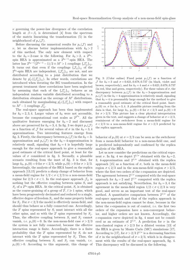
Real-space Renormalization Group analysis of a non-mean-field spin-glass
$ governing the power-law divergence of the correlationlength at # = #c is determined [4] from the spectrumof the matrix linearising the transformation (5) in theneighborhood of p#(J ).Before discussing the numerical results for p#(J ) and$, let us discuss better implementations with k0 > 2of this method. The only new element with respectto the k0 = 2-case is the following. For k0 > 2, a 2k0 -spin HEA is approximated as a 2k0!1-spin HEA. Thelatter has 2k0!1(2k0!1! 1)/2#M " > 1 couplings {J "ij}ij .It turns out that even if the couplings {Jij}ij of the2k0-spin HEA are independent, {J "ij}ij are not, and aredistributed according to a joint distribution that wedenote by p"C({J "ij}ij). In other words, correlations areintroduced when iterating the RG transformation. In thepresent treatment these correlations have been neglectedby assuming that each of the {J "ij}ij behaves as anindependent random variable distributed according to adistribution obtained as the average of M " distributions,each obtained by marginalising p"C({J "ij}ij) with respectto M "! 1 couplings J "ij .The real-space approach has been thus implemented
for k0 = 2, 3, 4. Larger values of k0 were not accessible,because the computational cost scales as 22
k0 . All thequalitative features emerging for k0 = 2 and discussedabove are preserved for k0 = 3, 4. In fig. 3 we depict p#(J )as a function of J for several values of " in the k0 = 3, 4approximations. Two interesting features emerge fromfig. 3. Firstly, the discrepancy between p#(J ) in the k0 = 3-approximation and p#(J ) in the k0 = 4-approximation isrelatively small, signaling that k0 = 4 is hopefully largeenough for the real-space approach to give a reasonablygood estimate of the critical fixed point, at least for thevalues of " considered in fig. 3. Secondly, a plausiblescenario resulting from the inset of fig. 3 is that, forlarge k0, p#(0) = 0 for "< 2/3, while p#(0)> 0 for "> 2/3.Interestingly, the analysis of the HEA based on the replicaapproach [13,15] predicts a sharp change of behavior froma mean-field regime for 1/2< "! 2/3 to a non-mean-fieldregime for 2/3< "< 1. In the real-space approach Jij isnothing but the e"ective coupling between spins Si andSj of a 2k0 -spin HEA. At the critical point, Si is obtainedas the coarse-graining of a group of 2l, l( 1 spins, whichhave been progressively decimated and reduced to a single,e"ective degree of freedom Si, and the same property holdsfor Sj . For "< 2/3 the model is e"ectively mean-field, andshould thus behave as a fully connected one. Accordingly,the 2l spins represented by Si must interact with all theother spins, and so with the 2l spins represented by Sj .Thus, the e"ective coupling between Si and Sj cannotvanish, i.e. p#(0) = 0. In the non-mean-field case "> 2/3the system is not fully connected, because the e"ectiveinteraction range is finite. Accordingly, there is a finiteprobability that the 2l spins represented by Si do notinteract with the 2l spins represented by Sj . Thus, thee"ective coupling between Si and Sj can vanish, i.e.p#(0)> 0. According to this argument, this change of
0
0.1
0.2
0.3
0.4
0.5
0.6
0.7
0.8
0.9
-2 -1.5 -1 -0.5 0 0.5 1 1.5 2
p!(
J)
J
0
0.02
0.04
0.06
0.5 0.6 0.7 0.8
p!(
0)
!
k0 = 3, ! = 0.621k0 = 3, ! = 0.678k0 = 3, ! = 0.737k0 = 4, ! = 0.621k0 = 4, ! = 0.678k0 = 4, ! = 0.737
k0 = 3k0 = 4
! = 2/3
Fig. 3: (Color online) Fixed point p!(J ) as a function ofJ for k0 = 3 and != 0.621, 0.678, 0.737 (in black, violet andbrown, respectively), and for k0 = 4 and != 0.621, 0.678, 0.737(in red, blue and green, respectively). For these values of !, thediscrepancy between p!(J ) in the k0 = 3-approximation andp!(J ) in the k0 = 4-approximation is relatively small, signalingthat k0 = 4 is presumably large enough for the method to givea reasonably good estimate of the critical fixed point. Inset:p!(0) vs. ! for k0 = 3, 4. A plausible picture resulting from thedata is that, for large k0, p!(0) = 0 for !< 2/3 and p!(0)> 0for !> 2/3. This picture has a clear physical interpretationgiven in the text, and suggests a change of behavior at != 2/3,reminiscent of the switchover from a mean-field regime for!< 2/3 to a non-mean-field regime for !> 2/3 predicted bythe replica approach.
behavior of p#(0) at "= 2/3 can be seen as the switchoverfrom a mean-field behavior to a non-mean-field one, andis predicted independently and confirmed by the replicaanalysis of the HEA.Let us now consider the predictions on the critical expo-
nent $. In fig. 4 we depict 21/# obtained with the k0=2,3, 4-approximation and 21/# obtained with the replicaapproach [15] as a function of ", both in the mean-fieldregion "! 2/3 and in the non-mean-field region "> 2/3,where the first two orders of the !-expansion are depicted.The agreement between 21/# computed with the real-spaceapproach for k0 = 2 and 21/# computed with the replicaapproach is not satisfying. Nevertheless, for k0 = 3, 4 theagreement in the mean-field region 1/2< "! 2/3 is verygood, and serves as an important test of the real-spacemethod. A quantitative comparison between 21/# of thereal-space approach and that of the replica approach inthe non-mean-field region cannot be done, because in thelatter the !-expansion is out of control, i.e. the first twoorders of the expansion have a non-convergent behav-ior, and higher orders are not known. Accordingly, the!-expansion curve depicted in fig. 4 must not be consid-ered as an estimate of 21/# . A prediction for $ in thenon-classical region "> 2/3 for a diluted version [13] ofthe HEA is given by Monte Carlo (MC) simulations [17].According to [17], for "> 2/3 21/# is a decreasing functionof " in the neighborhood of "= 2/3, which is in disagree-ment with the results of the real-space approach, fig. 4.This discrepancy will be discussed in the following.
47014-p5

M. Castellana
/!
1
1.05
1.1
1.15
1.2
1.25
1.3
1.35
1.4
5 0 5 0.5 .60. 0.65 0.7 0.75
21
!
21/! , k0 = 2
21/! , k0 = 3
21/! , k0 = 4
21/! , mean field, with replicas
21/! " expansion with replicas
Upper critical dimension ! = 2/3
Fig. 4: (Color online) 21/! as a function of !. The red,brown and blue points are 21/! computed with the real-spaceapproach for k0 = 2, 3, 4, respectively. The black dashed curveand the green dashed curve are 21/! obtained with the replicaapproach [15], and the orange dashed line is the relative uppercritical dimension != 2/3 [13]: the black dashed curve is themean-field value of 21/! for !! 2/3, while the green dashedcurve is the two-loops result obtained with the #-expansion.
Discussion and conclusions. – In this letter wedeveloped a real-space RG approach for a non-mean-field spin-glass, the Hierarchical Edwards-Anderson model(HEA). This approach is innovative with respect to theRG approaches to disordered, strongly frustrated systemsdeveloped heretofore that generally rely on the replicamethod [6]. Indeed, the present approach does not makeuse of the replica method, which is generally predictiveonly in the mean-field case, and cannot handle pertur-batively fluctuations around the mean-field saddle-point,because these turn out to be out of control [6]. Througha systematic approximation scheme, the present approachimplements Kadano"’s block-spin decimation rule [14] onspins. The implementation of such a decimation rule to adisordered, strongly frustrated system has not been devel-oped heretofore because of the intrinsic di!culties intro-duced by frustration, and allows for an e"ective reductionof the degrees of freedom of the system. Kadano"’s block-spin rule is practically implemented by approximating a2k0-spin HEA as a 2k0!1-spin HEA. Such an approxi-mation is practically performed by imposing that someobservables of the 2k0 -spin HEA are equal to some corre-sponding observables of the 2k0!1-spin HEA. For large k0,the method is asymptotically exact, and so are its predic-tions on the critical features of the system. The methodhas been tested in the simplest case of Dyson Hierarchi-cal Model [7], which is the ferromagnetic version of theHEA, and the resulting predictions for the critical expo-nents are in good agreement with the results obtainedheretofore [16].The method has been then applied to the HEA, and
identifies the existence of a phase transition in the system,yielding a prediction on the critical exponent $ relatedto the power-law divergence of the correlation length atthe critical point. Above the upper critical dimension
("< 2/3), the results for $ are in very good quantitativeagreement with those given by the replica method [15]even for small k0 = 3, 4. Below the upper critical dimen-sion ("> 2/3), the !-expansion for the critical exponentsperformed within the replica method is not predictive,because the first few orders have a non-convergent behav-ior, and higher orders are not known. Hence, a quantita-tive comparison between the real-space approach and thereplica approach is not possible. On the contrary, MonteCarlo (MC) simulations [17] for a diluted version of theHEA yield a prediction for the critical exponents in thisregion. These are in disagreement with those of the real-space approach. This discrepancy could be due both tothe smallness of k0 in the real-space approach, or to thenon-universality of the exponent $ when switching fromthe HEA defined here to its diluted version, or to thefact that correlations between the spin couplings havebeen neglected in the real-space approach. Accordingly,the quantitative estimate of $ below the upper criticaldimension is a still untamed issue, which could be suitablefor future investigations and developments of the presentreal-space method.
) ) )
I am glad to thank G. Parisi, M. Mezard and S.Franz for extremely useful discussions and suggestionson this work, and A. Decelle for collaborating on thereal-space method for Dyson Hierarchical Model. I alsoacknowledge support from the D. I. computational centerof Universite Paris Sud.
REFERENCES
[1] Parisi G., Phys. Rev. Lett., 43 (1979) 1754.[2] Derrida B., Phys. Rev. Lett., 45 (1980) 79.[3] Fisher D. S. andHuse D. A., Phys. Rev. Lett., 56 (1986)1601.
[4] Wilson K. and Kogut J., Phys. Rep., 12 (1974) 75.[5] Zinn-Justin J., Int. Ser. Monogr. Phys., 113 (2002) 1.[6] Dominicis C. D. and Giardina I., Random Fields andSpin-glasses: A Field-theory Approach (Springer) 2006.
[7] Dyson F., Commun. Math. Phys., 12 (1969) 91.[8] Collet P. and Eckmann J., Lect. Notes Phys., 74(1978).
[9] Collet P., Eckmann J. P. and Hirsbrunner B., Phys.Lett. B, 71 (1977) 385.
[10] Berker A. N. and Ostlund S., J. Phys. C: Solid StatePhys., 12 (1979) 4961.
[11] Gardner E., J. Phys., 45 (1984) 1755.[12] Theumann A., Phys. Rev. B, 21 (1980) 2984.[13] Franz S., Jorg T. and Parisi G., J. Stat. Mech.: Theory
Exp. (2009) P02002.[14] Kadanoff L. P., Physics, 2 (1966) 263.[15] Castellana M. and Parisi G., Phys. Rev. E, 82 (2010)
040105; 83 (2011) 041134.[16] Bleher P. M., Preprint, Institute of Applied Mathemat-
ics of the Academy of Sciences USSR (1975).[17] Franz S. and Decelle A., in preparation.
47014-p6

PHYSICAL REVIEW B 84, 144417 (2011)
Role of Tracy-Widom distribution in finite-size fluctuations of the critical temperature of theSherrington-Kirkpatrick spin glass
Michele Castellana1,2,* and Elia Zarinelli1,†1LPTMS, CNRS and Universite Paris-Sud, UMR8626, Bat. 100, F-91405 Orsay, France
2Dipartimento di Fisica, Universita di Roma ‘La Sapienza’, I-00185 Rome, Italy(Received 20 April 2011; published 10 October 2011)
We investigate the finite-size fluctuations due to quenched disorder of the critical temperature of theSherrington-Kirkpatrick spin glass. In order to accomplish this task, we perform a finite-size analysis of thespectrum of the susceptibility matrix obtained via the Plefka expansion. By exploiting results from randommatrix theory, we obtain that the fluctuations of the critical temperature are described by the Tracy-Widomdistribution with a nontrivial scaling exponent 2/3.
DOI: 10.1103/PhysRevB.84.144417 PACS number(s): 64.70.Q−, 75.10.Nr, 02.50.−r
I. INTRODUCTION
The characterization of phase transitions in terms of anonanalytic behavior of thermodynamic functions in theinfinite-size limit has served as a milestone1–5 in the physicalunderstanding of critical phenomena. In laboratory and numer-ical experiments, the system size is always finite so that thedivergences that would result from such a nonanalytic behaviorare suppressed, and are replaced by smooth maxima occurringin the observation of physical quantities as a function of thetemperature. In disordered systems, the pseudocritical tem-perature, defined as the temperature at which this maximumoccurs, is a fluctuating quantity depending on the realizationof the disorder. A question naturally arises: Can the fluctu-ations of the pseudocritical temperature be understood anddetermined with tools of probability theory? Several effortshave been made to study the fluctuations of the pseudocriticaltemperature for disordered finite-dimensional systems6–9 andtheir physical implications. For instance, recently Sarlat et al.10
showed that the theory of finite-size scaling, which is validfor pure systems, fails in fully-connected disordered modelsbecause of strong sample-to-sample fluctuations of the criticaltemperature.
The extreme value statistics of independent random vari-ables is a well-established problem with a long historydating from the original work of Gumbel,11 while less resultsare known in the case where the random variables arecorrelated. The eigenvalues of a Gaussian random matrixare an example of strongly-correlated random variables.12
Only recently, Tracy and Widom calculated13–16 exactly theprobability distribution of the typical fluctuations of thelargest eigenvalue of a Gaussian random matrix around itsinfinite-size value. This distribution, known as Tracy-Widomdistribution, appears in many different models of statisticalphysics, such as directed polymers17,18 or polynuclear growthmodels,19 showing profound links between such differentsystems. Conversely, to our knowledge no evident connectionsbetween the Tracy-Widom distribution and the physics of spinglasses have been found heretofore.20
The purpose of this work is to try to fill this gap. We considera mean-field spin glass model, the Sherrington-Kirkpatrick(SK) model,21 and propose a definition of finite-size criticaltemperature inspired by a previous analysis.8 We investigatethe finite-size fluctuations of this pseudocritical temperature
in the framework of extreme value statistics and show that theTracy-Widom distribution naturally arises in the descriptionof such fluctuations.
II. THE MODEL
The SK model21 is defined by the Hamiltonian
H [{Si},{xij }] = − J
N1/2
N∑i>j=1
xijSiSj +N∑
i=1
hiSi, (1)
where Si = ±1, the couplings {xij }i>j=1,...,N ≡ {x}, xji ≡xij∀i > j are distributed according to normal distribution withzero mean and unit variance
P (x) = 1√2π
e− x2
2 , (2)
and J is a parameter tuning the strength of the interactionenergy between spins.
The low-temperature features of the SK model have beenwidely investigated in the past and are encoded in Parisi’ssolution,22–27 showing that the SK has a finite-temperaturespin glass transition at Tc = J in the thermodynamic limitN → ∞. The critical value Tc can be physically thought of asthe value of the temperature where ergodicity breaking occursand the spin glass susceptibility diverges.25–27
While Parisi’s solution has been derived within the replicamethod framework, an alternative approach to study the SKmodel had been previously proposed by Thouless, Anderson,and Palmer (TAP).28 Within this approach, the system isdescribed in terms of a free energy at fixed local magnetization,and the physical features derived in terms of the resultingfree-energy landscape. Later on, Plefka29 showed that theTAP free energy can be obtained as the result of a systematicexpansion in powers of the parameter
α ≡ βJ
N1/2,
where β is the inverse temperature of the model. This α
expansion, known as Plefka expansion, has thus served asa method for deriving the TAP free energy for several classesof models, and has been extensively used in different contextsin physics, from classical disordered systems,30–32 to generalquantum systems.33–36 It is a general fact that, if the model is
144417-11098-0121/2011/84(14)/144417(9) ©2011 American Physical Society
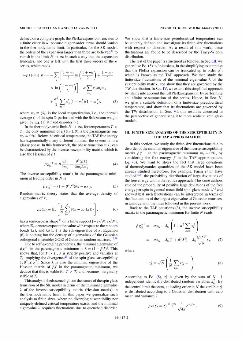
MICHELE CASTELLANA AND ELIA ZARINELLI PHYSICAL REVIEW B 84, 144417 (2011)
defined on a complete graph, the Plefka expansion truncates toa finite order in α, because higher-order terms should vanishin the thermodynamic limit. In particular, for the SK model,the orders of the expansion larger than three are believed37 tovanish in the limit N → ∞ in such a way that the expansiontruncates, and one is left with the first three orders of the α
series, which reads
−βf ({mi},β) = −∑
i
[1 + mi
2ln
(1 + mi
2
)+ 1 − mi
2
× ln
(1 − mi
2
)]+ α
∑i>j
xijmimj
+ α2
2
∑i>j
x2ij
(1 − m2
i
)(1 − m2
j
), (3)
where mi ≡ 〈Si〉 is the local magnetization, i.e., the thermalaverage 〈〉 of the spin Si performed with the Boltzmann weightgiven by Eq. (1) at fixed disorder {x}.
In the thermodynamic limit N → ∞, for temperatures T >
Tc, the only minimum of βf ({m},β) is the paramagnetic onemi = 0 ∀i. Below the critical temperature, the TAP free energyhas exponentially many different minima: the system is in aglassy phase. In this framework, the phase transition at Tc canbe characterized by the inverse susceptibility matrix, which isalso the Hessian of βf
βχ−1ij ≡ β
∂hi
∂mj
= ∂2(βf )
∂mi∂mj
. (4)
The inverse susceptibility matrix in the paramagnetic mini-mum at leading order in N is
βχ−1ij = (1 + β2J 2)δij − αxij . (5)
Random-matrix theory states that the average density ofeigenvalues of x,
ρN (λ) ≡ Ex
[1
N
N∑i=1
δ(λ − λi({x}))]
, (6)
has a semicircular shape38 on a finite support [−2√
N,2√
N ],whereEx denotes expectation value with respect to the randombonds {x}, and λi({x}) is the ith eigenvalue of x. Equation(6) is nothing but the density of eigenvalues of the Gaussianorthogonal ensemble (GOE) of Gaussian random matrices.12,39
Due to self-averaging properties, the minimal eigenvalue ofβχ−1 in the paramagnetic minimum is λ = (1 − βJ )2. Thisshows that, for T > Tc, λ is strictly positive and vanishes atTc, implying the divergence25 of the spin glass susceptibility1/β2Tr[χ2]. Since λ is also the minimal eigenvalue of theHessian matrix of βf in the paramagnetic minimum, wededuce that this is stable for T > Tc and becomes marginallystable at Tc.
This analysis sheds some light on the nature of the spin glasstransition of the SK model in terms of the minimal eigenvalueλ of the inverse susceptibility matrix (Hessian matrix) inthe thermodynamic limit. In this paper we generalize suchanalysis to finite sizes, where no diverging susceptibility noruniquely-defined critical temperature exists, and the minimaleigenvalue λ acquires fluctuations due to quenched disorder.
We show that a finite-size pseudocritical temperature canbe suitably defined and investigate its finite-size fluctuationswith respect to disorder. As a result of this work, thesefluctuations are found to be described by the Tracy-Widomdistribution.
The rest of the paper is structured as follows. In Sec. III, wegeneralize Eq. (5) to finite sizes, in the simplifying assumptionthat the Plefka expansion can be truncated up to order α2,which is known as the TAP approach. We then study thefinite-size fluctuations of the minimal eigenvalue λ of thesusceptibility matrix, and show that they are governed by theTW distribution. In Sec. IV, we extend this simplified approachby taking into account the full Plefka expansion, by performingan infinite re-summation of the series. Hence, in Sec. V,we give a suitable definition of a finite-size pseudocriticaltemperature, and show that its fluctuations are governed bythe TW distribution. In Sec. VI, this result is discussed inthe perspective of generalizing it to more realistic spin glassmodels.
III. FINITE-SIZE ANALYSIS OF THE SUSCEPTIBILITY INTHE TAP APPROXIMATION
In this section, we study the finite-size fluctuations due todisorder of the minimal eigenvalue of the inverse susceptibilitymatrix βχ−1 at the paramagnetic minimum mi = 0 ∀i, byconsidering the free energy f in the TAP approximation,Eq. (3). We want to stress the fact that large deviationsof thermodynamics quantities of the SK model have beenalready studied heretofore. For example, Parisi et al. havestudied40,41 the probability distribution of large deviations ofthe free energy within the replica approach. The same authorsstudied the probability of positive large deviations of the freeenergy per spin in general mean-field spin-glass models,42 andshowed that such fluctuations can be interpreted in terms ofthe fluctuations of the largest eigenvalue of Gaussian matrices,in analogy with the lines followed in the present work.
Back to the TAP equations (3), the inverse susceptibilitymatrix in the paramagnetic minimum for finite N reads
βχ−1ij = −αxij + δij
⎛⎝1 + α2
∑k =i
x2ki
⎞⎠
= −αxij + δij (1 + β2J 2) + δij
(βJ )2
√N
zi2, (7)
where
zi2 ≡
√N
⎛⎝ 1
N
∑k =i
x2ki − 1
⎞⎠ . (8)
According to Eq. (8), zi2 is given by the sum of N − 1
independent identically-distributed random variables x2ij . By
the central limit theorem, at leading order in N the variable zi2
is distributed according to a Gaussian distribution with zeromean and variance 2
pN
(zi
2 = z) N→∞→ 1√
4πe−z2/4, (9)
144417-2

ROLE OF TRACY-WIDOM DISTRIBUTION IN FINITE- . . . PHYSICAL REVIEW B 84, 144417 (2011)
where pN (zi2 = z) denotes the probability that zi
2 is equal to z
at finite size N .We set
βχ−1ij ≡ δij (1 + β2J 2) + αMij . (10)
According to Eq. (8), the diagonal elements of Mij arerandom variables correlated to out-of-diagonal elements. Thestatistical properties of the spectrum of a random matrix whoseentries are correlated to each other has been studied heretoforeonly in some cases. For instance, Staring et al.43 studiedthe average eigenvalue density for matrices with a constraintimplying that the row sum of matrix elements should vanish,and other correlated cases have been investigated both from aphysical44 and mathematical45 point of view.
In recent years, a huge amount of results has been obtainedon the distribution of the minimal eigenvalue of a N × N
random matrix drawn from Gaussian ensembles, such as GOE.In particular, Tracy and Widom13–16 deduced that for large N ,small fluctuations of the minimal eigenvalue λGOE of a GOEmatrix around its leading-order value −2
√N are given by
λGOE = −2√
N + 1
N1/6φGOE, (11)
where φGOE is a random variable distributed according tothe Tracy-Widom (TW) distribution for the GOE ensemblepGOE(φ). It follows that for βJ = 1 if zi
2 was independent on{x}, the matrix Mij would belong to the GOE ensemble, andthe minimal eigenvalue λ of βχ−1 would define a variable φ
according to
λ = 1
N2/3φ, (12)
and φ would be distributed according to the TW distributionpGOE(φ).
As shown in Appendix A, this is indeed the case for zi2,
which can be treated, at leading order in N , as a randomvariable independent on xij . The general idea is that zi
2 is givenby the sum of N − 1 terms all of the same order of magnitude,and only one amongst these N − 1 terms depends on xij . Itfollows that at leading order in N , zi
2 can be considered asindependent on xij . Since in Eq. (7) zi
2 is multiplied by asub-leading factor 1/
√N , in Eq. (7) we can consider zi
2 atleading order in N , and treat it as independent on xij .
To test this independence property, we set βJ = 1, generatenumerically S 1 samples of the N × N matrix βχ−1, andcompute the average density of eigenvalues of βχ−1, definedas in Eq. (6), together with the distribution of the minimaleigenvalue λ for several sizes N . The eigenvalue distributionρN (λ) as a function of λ is depicted in Fig. 1, and tends to theWigner semicircle as N is increased, showing that the minimaleigenvalue λ tends to 0 as N → ∞.
The finite-size fluctuations of λ around 0 are then investi-gated in Fig. 2. Defining φ in terms of λ by Eq. (12), in Fig. 2 wedepict the distribution pN (φ) of the variable φ for several sizesN , and show that for increasing N , pN (φ) approaches the TWdistribution pGOE(φ). Let us introduce the central moments
μN1 ≡ EN [φ],
μNi ≡ EN [(φ − EN [φ])i] ∀i > 1
0
0.05
0.1
0.15
0.2
0.25
0.3
0.35
0 1 2 3 4
ρ(λ
)
λ
ρSC(λ)ρ64(λ)
ρ128(λ)ρ256(λ)ρ512(λ)
ρ1024(λ)
FIG. 1. (Color online) Density of eigenvalues ρN (λ) of the matrixβχ−1 for N = 64,128,256,512,1024 (in red, blue, yellow, green, vio-let respectively), βJ = 1 and S = 16 × 103, and Wigner semicircularlaw ρSC(λ) = 1/(2π )
√4 − (2 − λ)2 (black) as a function of λ. ρN (λ)
approaches ρSC(λ) as N is increased.
of pN (φ), and the central moments
μGOE1 ≡ EGOE[φ],
μGOEi ≡ EGOE[(φ − EGOE[φ])i] ∀i > 1
of the TW distribution, where
EN [·] ≡∫
dφ pN (φ) · ,
EGOE[·] ≡∫
dφ pGOE(φ) · .
In the inset of Fig. 2 we depict μNi for several sizes N and
μGOEi as a function of i, showing that μN
i converges to μGOEi
as N is increased.In Fig. 3, this convergence is clarified by depicting �μN
i ≡(μN
i − μGOEi )/μGOE
i for several values of i > 1 as a functionof N . �μN
i is found to converge to 0 for large N . In the insetof Fig. 3, we depict �μN
1 as a function of N , showing thatthe convergence of the first central moment with N is muchslower than that of the other central moments. It is interestingto observe that a slowly-converging first moment has beenrecently found also in experimental46 and numerical47 dataof models of growing interfaces where the TW distributionappears.
The analytical argument proving the independence propertyof zi
2 has been thus confirmed by this numerical calculation.Hence, the main result of this section is that the finite-sizefluctuations of the minimal eigenvalue of the susceptibilitymatrix βχ−1 in the TAP approximation for βJ = 1 are ofthe order of N−2/3 and are distributed according to the TWlaw. These fluctuations have already been found to be ofthe order of N−2/3 in a previous work,48 and more recentlyreconsidered,49 following an independent derivation based onscaling arguments, even though the distribution has not beenworked out. Our approach sheds some light on the nature ofthe scaling N−2/3, which is nontrivial, since it comes from theN−1/6 scaling of the TW distribution, which is found to governthe fluctuations of λ. Moreover, the fact that we find the samescaling as that found in such previous works can be consideredas a consistency test of our calculation.
144417-3
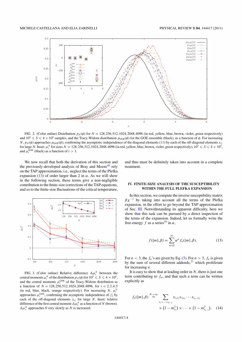
MICHELE CASTELLANA AND ELIA ZARINELLI PHYSICAL REVIEW B 84, 144417 (2011)
0
0.05
0.1
0.15
0.2
0.25
0.3
0.35
0.4
-4 -2 0 2 4 6
p(φ
)
φ
-200
-100
0
100
2 4 6 8
μi
i
pGOE(φ)p128(φ)p256(φ)p512(φ)
p1024(φ)p2048(φ)p4096(φ)
μ128i
μ256i
μ512i
μ1024i
μ2048i
μ4096i
μGOEi
FIG. 2. (Color online) Distribution pN (φ) for N = 128,256,512,1024,2048,4096 (in red, yellow, blue, brown, violet, green respectively)and 105 � S � 4 × 10⁵ samples, and the Tracy-Widom distribution pGOE(φ) for the GOE ensemble (black), as a function of φ. For increasingN , pN (φ) approaches pGOE(φ), confirming the asymptotic independence of the diagonal elements (11) by each of the off-diagonal elements xij
for large N . Inset: μNi for sizes N = 128,256,512,1024,2048,4096 (in red, yellow, blue, brown, violet, green respectively), 105 � S � 4 × 10⁵,
and μGOEi (black) as a function of i > 1.
We now recall that both the derivation of this section andthe previously-developed analysis of Bray and Moore48 relyon the TAP approximation, i.e., neglect the terms of the Plefkaexpansion (13) of order larger than 2 in α. As we will showin the following section, these terms give a non-negligiblecontribution to the finite-size corrections of the TAP equations,and so to the finite-size fluctuations of the critical temperature,
-0.1
0
0.1
0.2
0.3
0.4
128 256 512 1024 2048 4096
Δμ
N i
N
2.4
2.7
128 256 512 1024 2048 4096
Δμ
N 1
N
ΔμN2
ΔμN3
ΔμN4
ΔμN5
ΔμN1
FIG. 3. (Color online) Relative difference �μNi between the
central moments μNi of the distribution pN (φ) for 105 � S � 4 × 10⁵,
and the central moments μGOEi of the Tracy-Widom distribution as
a function of N = 128,256,512,1024,2048,4096, for i = 2,3,4,5(in red, blue, black, orange respectively). For increasing N , μN
i
approaches μGOEi , confirming the asymptotic independence of zi
2 byeach of the off-diagonal elements xij for large N . Inset: relativedifference of the first central moment �μN
1 as a function of N (brown).�μN
1 approaches 0 very slowly as N is increased.
and thus must be definitely taken into account in a completetreatment.
IV. FINITE-SIZE ANALYSIS OF THE SUSCEPTIBILITYWITHIN THE FULL PLEFKA EXPANSION
In this section, we compute the inverse susceptibility matrixβχ−1 by taking into account all the terms of the Plefkaexpansion, in the effort to go beyond the TAP approximationof Sec. III. Notwithstanding its apparent difficulty, here weshow that this task can be pursued by a direct inspection ofthe terms of the expansion. Indeed, let us formally write thefree-energy f as a series29 in α,
f ({m},β) =∞∑
n=0
αnfn({m},β). (13)
For n < 3, the fn’s are given by Eq. (3). For n > 3, fn is givenby the sum of several different addends,37 which proliferatefor increasing n.
It is easy to show that at leading order in N , there is just oneterm contributing to fn, and that such a term can be writtenexplicitly as
fn({m},β)N→∞≈
∑i1>···>in−1
xi1i2xi2i3 · · · xin−1i1
× (1 − m2
i1
) × · · · × (1 − m2
in−1
). (14)
144417-4

ROLE OF TRACY-WIDOM DISTRIBUTION IN FINITE- . . . PHYSICAL REVIEW B 84, 144417 (2011)
It follows that by plugging Eq. (14) into Eq. (13) andcomputing βχ−1 for mi = 0, one obtains a simple expressionfor the inverse susceptibility at the paramagnetic solution
βχ−1ij = −αxij + δij
(1 + α2
∑k =i
x2ki + 2
∞∑n=3
αn
×∑
i1>···>in−1
xii1xi1i2 · · · xin−1i
)
= −αxij + δij (1 + β2J 2) + δij
1√N
×[
(βJ )2zi2 + 2
∞∑n=3
(βJ )n√(n − 1)!
zin
]. (15)
where
zin ≡
√(n − 1)!
Nn−1
2
∑i1>···>in−1
xii1xi1i2 · · · xin−1i ,∀n > 2. (16)
According to Eq. (16), one has that at leading order in N ,
Ex
[zin
] = 0 ∀n > 2,(17)
Ex
[(zin
)2] = 1 ∀n > 2,
where in the second line of Eq. (17) the multiple sum definingzin has been evaluated at leading order in N .
We observe that the random variables zin and xjk in Eq. (15)
are not independent, since each zin depends on the bond
variables {x}. Following an argument similar to that given inSec. III for zi
2, we observe that, by Eq. (16) and at leading orderin N , zi
n is given by a sum of O(Nn−1) terms which are all of thesame order of magnitude. Each term is given by the product ofn − 1 bond variables xii1xi1i2 · · · xin−1i forming a loop passingby site i. For any fixed i, j, k, and n, only O(Nn−2) termsamongst the O(Nn−1) terms of zi
n are entangled with therandom bond variable xjk . It follows that at leading order inN , zi
n can be considered as independent by xjk . Since the sumin the second line of Eq. (15) has a 1/
√N factor multiplying
each of the zin’s, we can consider the zi
n at leading order inN . Hence, in Eq. (15) we can consider each of the zi
n’s asindependent on xjk .
In Appendix B we show that at leading order in N , thedistribution of zi
n is a Gaussian with zero mean and unitvariance for every i and n > 2, while in Appendix C weshow that at leading order in N the variables {zi
n}n,i aremutually independent. Both these predictions are confirmed bynumerical tests, illustrated in Appendix B and C respectively.
Hence, at leading order in N the term in square bracketsin Eq. (15) is nothing but the sum of independent Gaussianvariables, and is thus equal to a random variable σ × ζi , whereζi is Gaussian with zero mean and unit variance, and
σ 2 = 2(βJ )4 + 4∞∑
n=3
(βJ )2n
(n − 1)!
= 2(βJ )2{2(e(βJ )2 − 1) − (βJ )2}.
It follows that Eq. (15) becomes
βχ−1ij = −αxij + δij
(1 + β2J 2 + σ√
Nζi
)= −αx ′
ij + δij (1 + β2J 2), (18)
where
x ′ij ≡ xij − δij
σ
βJζi. (19)
Because of the additional diagonal term in Eq. (19), the matrixx ′
ij does not belong to the GOE ensemble. Notwithstanding thisfact, it has been shown by Soshnikov50 that the presence ofthe diagonal elements in Eq. (19) does not alter the universaldistribution of the maximal eigenvalue of x ′
ij , which is stilldistributed according to the TW law. Hence, denoting by λ theminimal eigenvalue of βχ−1, we have
λ = (1 − βJ )2 + βJ
N2/3φGOE, (20)
where φGOE is a random variable depending on the sample xij ,and distributed according to the TW law.
In this section, we have calculated the inverse susceptibilitymatrix βχ−1, by considering the full Plefka expansion. Inthis framework, additional diagonal terms are generated thatwere not present in the TAP approximation. These additionalterms can be handled via a resummation to all orders in thePlefka expansion. As a result, we obtain that the fluctuationsof the minimal eigenvalue λ of the susceptibility βχ−1 arestill governed by the TW law, as in the TAP case treated inSec. III.
V. FINITE SIZE FLUCTUATIONS OF THE CRITICALTEMPERATURE
We can now define a finite-size critical temperature, andinvestigate its finite-size fluctuations due to disorder. In theprevious sections, we have shown that for a large but finitesize N , the minimal eigenvalue of the inverse susceptibilitymatrix, i.e., the Hessian matrix of βf ({m},β) evaluated inthe paramagnetic minimum mi = 0, is a function of thetemperature and of a quantity φGOE, which depends onthe realization of the disorder {x}. Since the TW law, i.e., thedistribution of φGOE, has support for both positive and negativevalues of φGOE, the subleading term in Eq. (20) can be positiveor negative. Accordingly, for samples {x} such that φGOE < 0,there exists a value of βJ ≈ 1 such that λ(βJ ) = 0, in sucha way that the spin-glass susceptibility in the paramagneticminimum diverges. This fact is physically meaningless, sincethere cannot be divergences in physical quantities at finitesize. This apparent contradiction can be easily understood byobserving that if λ(βJ ) = 0, the true physical susceptibilityis no more the paramagnetic one, but must be evaluated inthe low-lying nonparamagnetic minima of the free energy,whose appearance is driven by the emergent instability ofthe paramagnetic minimum. According to this discussion, inthe following we will consider only samples {x} such thatφGOE > 0.
144417-5
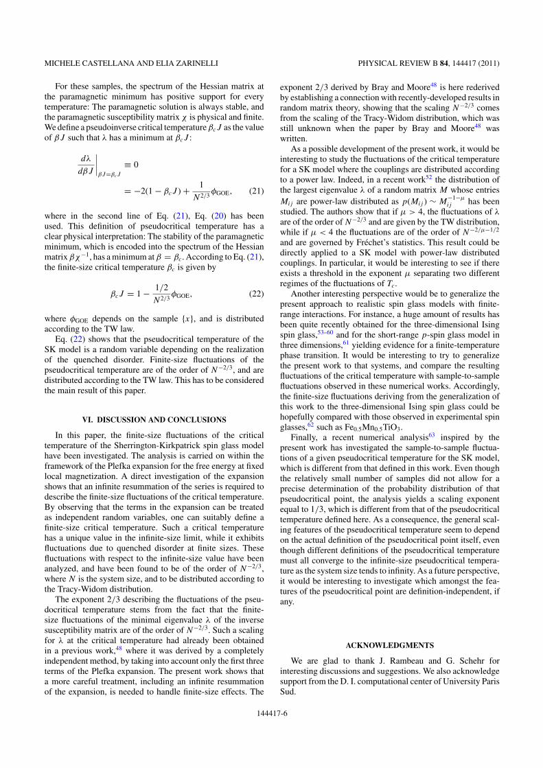
MICHELE CASTELLANA AND ELIA ZARINELLI PHYSICAL REVIEW B 84, 144417 (2011)
For these samples, the spectrum of the Hessian matrix atthe paramagnetic minimum has positive support for everytemperature: The paramagnetic solution is always stable, andthe paramagnetic susceptibility matrix χ is physical and finite.We define a pseudoinverse critical temperature βcJ as the valueof βJ such that λ has a minimum at βcJ :
dλ
dβJ
∣∣∣∣βJ=βcJ
≡ 0
= −2(1 − βcJ ) + 1
N2/3φGOE, (21)
where in the second line of Eq. (21), Eq. (20) has beenused. This definition of pseudocritical temperature has aclear physical interpretation: The stability of the paramagneticminimum, which is encoded into the spectrum of the Hessianmatrix βχ−1, has a minimum at β = βc. According to Eq. (21),the finite-size critical temperature βc is given by
βcJ = 1 − 1/2
N2/3φGOE, (22)
where φGOE depends on the sample {x}, and is distributedaccording to the TW law.
Eq. (22) shows that the pseudocritical temperature of theSK model is a random variable depending on the realizationof the quenched disorder. Finite-size fluctuations of thepseudocritical temperature are of the order of N−2/3, and aredistributed according to the TW law. This has to be consideredthe main result of this paper.
VI. DISCUSSION AND CONCLUSIONS
In this paper, the finite-size fluctuations of the criticaltemperature of the Sherrington-Kirkpatrick spin glass modelhave been investigated. The analysis is carried on within theframework of the Plefka expansion for the free energy at fixedlocal magnetization. A direct investigation of the expansionshows that an infinite resummation of the series is required todescribe the finite-size fluctuations of the critical temperature.By observing that the terms in the expansion can be treatedas independent random variables, one can suitably define afinite-size critical temperature. Such a critical temperaturehas a unique value in the infinite-size limit, while it exhibitsfluctuations due to quenched disorder at finite sizes. Thesefluctuations with respect to the infinite-size value have beenanalyzed, and have been found to be of the order of N−2/3,where N is the system size, and to be distributed according tothe Tracy-Widom distribution.
The exponent 2/3 describing the fluctuations of the pseu-docritical temperature stems from the fact that the finite-size fluctuations of the minimal eigenvalue λ of the inversesusceptibility matrix are of the order of N−2/3. Such a scalingfor λ at the critical temperature had already been obtainedin a previous work,48 where it was derived by a completelyindependent method, by taking into account only the first threeterms of the Plefka expansion. The present work shows thata more careful treatment, including an infinite resummationof the expansion, is needed to handle finite-size effects. The
exponent 2/3 derived by Bray and Moore48 is here rederivedby establishing a connection with recently-developed results inrandom matrix theory, showing that the scaling N−2/3 comesfrom the scaling of the Tracy-Widom distribution, which wasstill unknown when the paper by Bray and Moore48 waswritten.
As a possible development of the present work, it would beinteresting to study the fluctuations of the critical temperaturefor a SK model where the couplings are distributed accordingto a power law. Indeed, in a recent work52 the distribution ofthe largest eigenvalue λ of a random matrix M whose entriesMij are power-law distributed as p(Mij ) ∼ M
−1−μ
ij has beenstudied. The authors show that if μ > 4, the fluctuations of λ
are of the order of N−2/3 and are given by the TW distribution,while if μ < 4 the fluctuations are of the order of N−2/μ−1/2
and are governed by Frechet’s statistics. This result could bedirectly applied to a SK model with power-law distributedcouplings. In particular, it would be interesting to see if thereexists a threshold in the exponent μ separating two differentregimes of the fluctuations of Tc.
Another interesting perspective would be to generalize thepresent approach to realistic spin glass models with finite-range interactions. For instance, a huge amount of results hasbeen quite recently obtained for the three-dimensional Isingspin glass,53–60 and for the short-range p-spin glass model inthree dimensions,61 yielding evidence for a finite-temperaturephase transition. It would be interesting to try to generalizethe present work to that systems, and compare the resultingfluctuations of the critical temperature with sample-to-samplefluctuations observed in these numerical works. Accordingly,the finite-size fluctuations deriving from the generalization ofthis work to the three-dimensional Ising spin glass could behopefully compared with those observed in experimental spinglasses,62 such as Fe0.5Mn0.5TiO3.
Finally, a recent numerical analysis63 inspired by thepresent work has investigated the sample-to-sample fluctua-tions of a given pseudocritical temperature for the SK model,which is different from that defined in this work. Even thoughthe relatively small number of samples did not allow for aprecise determination of the probability distribution of thatpseudocritical point, the analysis yields a scaling exponentequal to 1/3, which is different from that of the pseudocriticaltemperature defined here. As a consequence, the general scal-ing features of the pseudocritical temperature seem to dependon the actual definition of the pseudocritical point itself, eventhough different definitions of the pseudocritical temperaturemust all converge to the infinite-size pseudocritical tempera-ture as the system size tends to infinity. As a future perspective,it would be interesting to investigate which amongst the fea-tures of the pseudocritical point are definition-independent, ifany.
ACKNOWLEDGMENTS
We are glad to thank J. Rambeau and G. Schehr forinteresting discussions and suggestions. We also acknowledgesupport from the D. I. computational center of University ParisSud.
144417-6

ROLE OF TRACY-WIDOM DISTRIBUTION IN FINITE- . . . PHYSICAL REVIEW B 84, 144417 (2011)
APPENDIX A: PROOF OF THE ASYMPTOTICINDEPENDENCE OF xi j AND zi
2
Here we show that at leading order in N , the variables xij
and zi2 are independent, i.e., that at leading order in N
pN
(xij = x,zi
2 = z) = pN (xij = x) × pN
(zi
2 = z). (A1)
Let us explicitly write the left-hand size of Eq. (A1) as
pN
(xij = x,zi
2 = z)
= E{xik}k =i
[δ(xij − x)δ
(zi
2 − z)]
,
= Exij
⎡⎣δ(xij − x)E{xik}k =i,k =j
×⎧⎨⎩ δ
⎡⎣√
N
⎛⎝ 1
N
∑k =i,k =j
x2ki − 1
⎞⎠ − z
ij
2
⎤⎦
⎫⎬⎭⎤⎦ , (A2)
where Exlm,xno,··· denotes the expectation value with respectto the probability distributions of the variables xlm,xno, . . ., δ
denotes the Dirac delta function, and
zij
2 ≡ z − x2ij√N
. (A3)
Proceeding systematically at leading order in N , the secondexpectation value in the second line of Eq. (A2) is nothingbut the probability that the variable
√N ( 1
N
∑k =i,k =j x2
ki − 1)
is equal to zij
2 . We observe that according to the central limittheorem, at leading order in N this probability is given by
E{xik}k =i,k =j
⎡⎣δ
⎛⎝√
N
⎛⎝ 1
N
∑k =i,k =j
x2ki − 1
⎞⎠ − z
ij
2
⎞⎠
⎤⎦
= 1√4π
e− (zij2 )2
4 . (A4)
By plugging Eq. (A4) into Eq. (A2) and using Eq. (A3), onehas
pN
(xij = x,zi
2 = z) = 1√
4π
∫dxijP (xij )δ(xij − x)
×e− (z−x2ij
/√
N)2
4
= P (x)1√4π
e− (z−x2/√
N)2
4 (A5)
= pN (xij = x) × pN
(zi
2 = z),
where in the first line we explicitly wrote the expectation valuewith respect to xij in terms of the probability distribution (2),while in the third line proceeded at leading order in N , andused Eq. (9).
APPENDIX B: COMPUTATION OF THE PROBABILITYDISTRIBUTION OF zi
n
Here we compute the probability distribution of zin at lead-
ing order in N . Let us define a super index L ≡ {i1, . . . ,in−1},where L stands for loop, since L represents a loop passing bythe site i. Let us also set XL ≡ xii1xi1i2 · · · xin−1i . By Eq. (16)
one has
zin =
√(n − 1)!
Nn−1
2
∑L
XL,∀n > 2. (B1)
We observe that the probability distribution of XL is the samefor every L. Hence, according to Eq. (B1), zi
n is given by thesum of equally distributed random variables. Now pick two ofthese variables, XL and XL′ . For some choices of L,L′, XL andXL′ are not independent, since they can depend on the samebond variables xij . If one picks one variable XL, the numberof variables appearing in the sum (B1) which are dependenton XL are those having at least one common edge with theedges of XL. The number of these variables, at leading orderin N , is O(Nn−2), since they are obtained by fixing one of then − 1 indexes i1, . . . ,in−1. The latter statement is equivalent tosaying that if one picks at random two variables XL and XL′ ,the probability that they are correlated is
O(Nn−2/Nn−1) = O(N−1). (B2)
Hence, at leading order in N , we can treat the ensemble of thevariables {XL}L as independent. According to the central limittheorem, at leading order in N , the variable
√(n − 1)!
Nn−1
2
zin = 1
Nn−1
(n−1)!
∑L
XL
is distributed according to a Gaussian distribution with meanEx[XL] = 0 and variance
Ex
[(√(n − 1)!
Nn−1
2
zin
)2]
= Ex
[X2
L
]Nn−1
(n−1)!
= 1Nn−1
(n−1)!
, (B3)
where in Eq. (B3) Eq. (2) has been used. It follows that atleading order in N , zi
n is distributed according to a Gaussiandistribution with zero mean and unit variance
pN
(zin = z
) N→∞→ 1√2π
e− z2
2 , (B4)
where pN (zin = z) is defined as the probability that zi
n is equalto z at size N .
Eq. (B4) has been tested numerically for the first few valuesof n: pN (zi
n = z) has been computed by generating S 1samples of {x}, and so of zi
n. For n = 3 and 4, the resultingprobability distribution pN (zi
n = z) converges to a Gaussiandistribution with zero mean and unit variance as N is increased,confirming the result (B4). This convergence is shown in Fig. 4,where pN (z1
4 = z) is depicted for different values of N togetherwith the right-hand side of Eq. (B4), as a function of z.
APPENDIX C: INDEPENDENCE OF THE zin’s AT LEADING
ORDER IN N
Let us consider two distinct variables zin and z
jm, and proceed
at leading order in N . Following the notation of Appendix B,we write Eq. (16) as
zin =
√(n − 1)!
Nn−1
2
∑L
XL, (C1)
zjm =
√(m − 1)!
Nm−1
2
∑L′
XL′ , (C2)
144417-7

MICHELE CASTELLANA AND ELIA ZARINELLI PHYSICAL REVIEW B 84, 144417 (2011)
0
0.05
0.1
0.15
0.2
0.25
0.3
0.35
0.4
-3 -2 -1 0 1 2 3
p(z
1 4=
z)
z
0
0.05
0.1
0.15
0.2
0.25
0.3
0.35
0.4
-3 -2 -1 0 1 2 3
p(z
1 4=
z)
z
0.12
0.16
-1.5 -1.4 -1.3 -1.2
p(z
1 4=
z)
0.12
0.16
-1.5 -1.4 -1.3 -1.2
p(z
1 4=
z)
z
p64(z14 = z)
p128(z14 = z)
p256(z14 = z)
p512(z14 = z)
p1024(z14 = z)
1/√
2πe−z /2
FIG. 4. (Color online) Probability distribution pN (z14 = z) for
S = 105 and different values of N = 64,128,256,512,1024 (in red,blue, yellow, green, violet respectively) together with a Gaussiandistribution 1/
√2πe−z2/2 with zero mean and unit variance (black),
as a function of z. As N is increased, pN (z14 = z) converges to
1/√
2πe−z2/2, as predicted by the analytical calculation, Eq. (B4).Inset: zoom of the above plot explicitly showing the convergence ofpN (z1
4 = z) to 1/√
2πe−z2/2 as N is increased.
where L,L′ represent a loop of length n,m passing by the sitei,j respectively. Some of the variables XL depend on some ofthe variables XL′ , because they can depend on the same bondvariables xij . Let us pick at random one variable XL appearingin zi
n, and count the number of variables XL′ in zjm that are
dependent on XL. At leading order in N , these are given bythe number of XL′ having at least one common bond with XL,and are O(Nm−2). Hence, if one picks at random two variablesXL,XL′ in Eqs. (C1), (C2) respectively, the probability thatXL,XL′ are dependent is
O(Nm−2/Nm−1) = O(N−1).
-3-2-10123
-3-2
-10
12
3
0
0.05
0.1
0.15
pN
(z1 3
=z,z
1 4=
z′ )
p∞(z13 = z) × p∞(z1
4 = z )p1024(z
13 = z, z1
4 = z )
z
z
pN
(z1 3
=z,z
1 4=
z)
0
0.05
0.1
0.15
0.2
FIG. 5. (Color online) p1024(z13 = z,z1
4 = z′) for S = 105 samples(red), and the N → ∞ limit of the right-hand side of Eq. (C3) (black),as a function of z,z′. For large N , pN (z1
3 = z,z14 = z′) equals pN (z1
3 =z) × pN (z1
4 = z′), as predicted by Eq. (C3). Hence, at leading orderin N , the variables z1
3 and z14 are independent.
It follows that zin and z
jm are independent at leading order
in N , i.e., for N → ∞pN
(zin = z,zj
m = z′) = pN
(zin = z
) × pN
(zjm = z′), (C3)
where pN (zin = z,z
jm = z′) denotes the joint probability that
zin equals z and z
jm equals z′, at fixed size N .
Eq. (C3) has been tested numerically for n = 3,m = 4:pN (z1
3 = z,z14 = z′) has been computed by generating S 1
samples of {x}, and so of z13,z
14. As a result, the left-hand
side of Eq. (C3) converges to the right-hand side as N isincreased, confirming the predictions of the above analyticalargument. This is shown in Fig. 5, where p1024(z1
3 = z,z14 =
z′) is depicted together with the N → ∞ limit of theright-hand side of Eq. (C3) [see Eq. (B4)], as a functionof z,z′.
*[email protected]†[email protected]. D. Lee and C. N. Yang, Phys. Rev. 87, 410 (1952).2C. Yang, Phys. Rev. 87, 404 (1952).3K. Huang, Statistical mechanics (Wiley, New York, 1987).4M. Biskup, C. Borgs, J. T. Chayes, L. J. Kleinwaks, andR. Kotecky , Phys. Rev. Lett. 84, 4794 (2000).
5D. Ruelle, Phys. Rev. Lett. 26, 303 (1971).6C. Monthus and T. Garel, J. Stat. Mech.: Theory Exp. 2005, P12011.7C. Monthus and T. Garel, Eur. Phys. J. B 48, 393 (2005).8F. Igloi, Y. C. Lin, H. Rieger, and C. Monthus, Phys. Rev. B 76,064421 (2007).
9C. Monthus and T. Garel, Phys. Rev. E 74, 011101(2006).
10T. Sarlat, A. Billoire, G. Biroli, and J. P. Bouchaud, J. Stat. Mech.:Theory Exp. 2009, P08014.
11E. J. Gumbel, Statistics of extremes (Columbia University Press,New York, 1958).
12M. L. Mehta, Random matrices (Academic Press, Amsterdam,2004).
13C. A. Tracy and H. Widom, Distribution Functions for LargestEigenvalues and Their Applications, in Proceedings of the
International Congress of Mathematicians, Vol. I, edited by LITatsien (Higher Education Press, Beijing, 2002), pp. 587–596.
14C. A. Tracy and H. Widom, Commun. Math. Phys. 177, 727(1996).
15C. A. Tracy and H. Widom, Commun. Math. Phys. 159, 151 (1994).16C. A. Tracy and H. Widom, Phys. Lett. B 305, 115 (1993).17K. Johansson, Commun. Math. Phys. 209, 437 (2000).18J. Baik and E. M. Rains, J. Stat. Phys. 100, 523 (2000).19M. Prahofer and H. Spohn, Phys. Rev. Lett. 84, 4882 (2000).20G. Biroli, J. P. Bouchaud, and M. Potters, J. Stat. Mech.: Theory
Exp. 2007, P07019.21D. Sherrington and S. Kirkpatrick, Phys. Rev. Lett. 35, 1792 (1975).22G. Parisi, J. Phys. A: Math. Gen. 13, 1101 (1980).23G. Parisi, Phys. Rev. Lett. 50, 1946 (1983).24M. Talagrand, Comptes Rendus Mathematique 337, 111 (2003).25M. Mezard, G. Parisi, and M. A. Virasoro, Spin Glass Theory and
Beyond (World Scientific, Singapore, 1987).26M. Mezard and A. Montanari, Information, Physics and Computa-
tion (Oxford University Press, Oxford, 2009).27H. Nishimori, Statistical Physics of Spin Glasses and Information
Processing: An Introduction (Oxford University Press, Oxford, UK,2001).
144417-8

ROLE OF TRACY-WIDOM DISTRIBUTION IN FINITE- . . . PHYSICAL REVIEW B 84, 144417 (2011)
28D. J. Thouless, P. W. Anderson, and R. G. Palmer, Philos. Mag. 35,593 (1977).
29T. Plefka, J. Phys. A: Math. Gen. 15, 1971 (1982).30A. Georges, M. Mezard, and J. S. Yedidia, Phys. Rev. Lett. 64, 2937
(1990).31J. S. Yedidia and A. Georges, J. Phys. A: Math. Gen. 23, 2165
(1990).32T. Yokota, Phys. Rev. B 51, 962 (1995).33T. Plefka, Phys. Rev. E 73, 016129 (2006).34H. Ishii and T. Yamamoto, J. Phys. C 18, 6225 (1985).35L. De Cesare, K. L. Walasek, and K. Walasek, Phys. Rev. B 45,
8127 (1992).36G. Biroli and L. F. Cugliandolo, Phys. Rev. B 64, 014206
(2001).37J. S. Yedidia, in Advanced Mean Field Methods: Theory and
Practice (MIT Press, Cambridge, MA, 2001), pp. 21–36.38E. P. Wigner, The Annals of Mathematics 62, 548 (1955).39Y. V. Fyodorov, in Recent Perspectives in Random Matrix Theory
and Number Theory, Vol. 322 (Cambridge Univ. Press, 2005), p.31.
40G. Parisi and T. Rizzo, Phys. Rev. Lett. 101, 117205 (2008).41G. Parisi and T. Rizzo, Phys. Rev. B 79, 134205 (2009).42G. Parisi and T. Rizzo, Phys. Rev. B 81, 094201 (2010).43J. Staring, B. Mehlig, Y. V. Fyodorov, and J. M. Luck, Phys. Rev.
E 67, 047101 (2003).44P. Shukla, Phys. Rev. E 71, 026226 (2005).45Z. Bai and W. Zhou, Statistica Sinica 18, 425 (2008).46K. A. Takeuchi and M. Sano, Phys. Rev. Lett. 104, 230601 (2010).47J. Rambeau and G. Schehr (unpublished).
48A. J. Bray and M. A. Moore, J. Phys. C 12, L441 (1979).49T. Aspelmeier, A. Billoire, E. Marinari, and M. A. Moore, J. Phys.
A: Math. Theor. 41, 324008 (2008).50A. Soshnikov, Commun. Math. Phys. 207, 697 (1999).51P. J. Forrester, S. N. Majumdar, and G. Schehr, Nucl. Phys. B 844,
500 (2011).52G. Biroli, J. P. Bouchaud, and M. Potters, Europhys. Lett. 78, 10001
(2007).53R. A. Banos, A. Cruz, L. A. Fernandez, J. M. Gil-Narvion,
A. Gordillo-Guerrero, M. Guidetti, A. Maiorano, F. Mantovani,E. Marinari, V. Martin-Mayor et al., J. Stat. Mech.: Theory Exp.2010, P06026.
54M. Hasenbusch, A. Pelissetto, and E. Vicari, Phys. Rev. B 78,214205 (2008).
55R. Alvarez Banos et al., Phys. Rev. Lett. 105, 177202 (2010).56F. Belletti, A. Cruz et al., J. Stat. Phys. 135, 1121 (2009).57P. Contucci, C. Giardina, C. Giberti, G. Parisi, and C. Vernia, Phys.
Rev. Lett. 99, 057206 (2007).58P. Contucci, C. Giardina, C. Giberti, G. Parisi, and C. Vernia, Phys.
Rev. Lett. 103, 017201 (2009).59F. Krzakala and O. C. Martin, Phys. Rev. Lett. 85, 3013 (2000).60E. Marinari, G. Parisi, and J. J. Ruiz-Lorenzo, Phys. Rev. B 58,
14852 (1998).61M. Campellone, B. Coluzzi, and G. Parisi, Phys. Rev. B 58, 12081
(1998).62K. Gunnarsson, P. Svedlindh, P. Nordblad, L. Lundgren, H. Aruga,
and A. Ito, Phys. Rev. B 43, 8199 (1991).63A. Billoire, L. A. Fernandez, A. Maiorano, E. Marinari, V. Martin-
Mayor, and D. Yllanes, e-print arXiv:1108.1336.
144417-9

Extreme Value Statistics Distributions in Spin Glasses
Michele Castellana,1,2,* Aurelien Decelle,1 and Elia Zarinelli1
1LPTMS, CNRS and Universite Paris-Sud, UMR8626, Bat. 100, 91405 Orsay, France2Dipartimento di Fisica, Universita di Roma ‘‘La Sapienza’’, 00185 Rome, Italy
(Received 6 August 2011; published 27 December 2011)
We study the probability distribution of the pseudocritical temperature in a mean-field and in a short-
range spin-glass model: the Sherrington-Kirkpatrick and the Edwards-Anderson (EA) model. In both
cases, we put in evidence the underlying connection between the fluctuations of the pseudocritical point
and the extreme value statistics of random variables. For the Sherrington-Kirkpatrick model, both with
Gaussian and binary couplings, the distribution of the pseudocritical temperature is found to be the Tracy-
Widom distribution. For the EA model, the distribution is found to be the Gumbel distribution. Being the
EA model representative of uniaxial magnetic materials with quenched disorder like Fe0:5Mn0:5TiO3 or
Eu0:5Ba0:5MnO3, its pseudocritical point distribution should be a priori experimentally accessible.
DOI: 10.1103/PhysRevLett.107.275701 PACS numbers: 64.70.Q�, 02.10.Yn, 02.50.�r
Disordered uniaxial magnetic materials having a glassybehavior like Fe0:5Mn0:5TiO3 [1] and Eu0:5Ba0:5MnO3 [2]have interested physicists for decades. Since the first pio-neering work of Edwards and Anderson (EA) [3], thesesystems have been studied by means of spin-glass modelswith quenched disorder, which were later considered intheir mean-field version by Sherrington and Kirkpatrick(SK) [4]. In the thermodynamic limit, Parisi’s solution forthe SK model [5] predicts a phase transition at a finitecritical temperature separating a high-temperature para-magnetic phase from a low-temperature glassy phase.Differently, for the EAmodel there is no analytical solutionand the existence of a finite-temperature phase transitionrelies entirely on numerical simulations [6].
Even though criticality in a physical system can emergeonly in the thermodynamic limit [7,8], in laboratory andnumerical experiments the system size is always finite:singularities of physical observables are smeared out andreplaced by smooth maxima. In order to characterize thecritical point of finite-size systems, a suitably defined pseu-docritical temperature must be introduced, e.g., the tem-perature at which such maxima occur. In finite-size systemswith quenched disorder, such a pseudocritical temperatureis a random variable depending on the realization of thedisorder. The characterization of the distribution of thepseudocritical point and of its scaling properties is still anopen problem which has drawn the attention of physicistssince the very first works of Harris [9–13]. Further studiesof such distributions in spin glasses have been performed ina recent work [14], where some of the authors showed aconnection between the fluctuations of the pseudocriticaltemperature of the SK model and the theory of extremevalue statistics (EVS) of correlated random variables.
The EVS of independent identically distributed (IID)random variables is a well-established problem: a funda-mental result [15] states that the limiting ProbabilityDistribution Function (PDF) of the maximum of IID
random variables belongs to three families of distributions:the Gumbel, Frechet, or Weibull distribution. Much less isknown about the EVS of correlated random variables. Anoteworthy case of an EVS distribution of correlated ran-dom variables that has been recently discovered is theTracy-Widom (TW) distribution [16], describing the fluc-tuations of the largest eigenvalue of a Gaussian randommatrix. The TW distribution has been found to describe thefluctuations of observables of a broad number of physicaland mathematical models, like the longest common se-quence in a random permutation [17], directed polymersin disordered media [18], and polynuclear growth models[19], which can be described by the Kardar-Parisi-Zhangequation [20,21]. Recently the TW distribution has beenfound to describe the conductance fluctuations in two- andthree- dimensional Anderson insulators [22,23] and hasbeen measured in growing interfaces of liquid-crystal tur-bulence [24,25] experiments.In this Letter we study the distribution of the pseudo-
critical temperature in the SK and in the EA model bymeans of numerical simulations. Our numerical findingsshow that the fluctuations of the pseudocirtical temperatureof the SK model both with Gaussian and binary couplingsare described by the TW distribution. This result suggeststhat the features of the fluctuations of the pseudocriticaltemperature are universal, i. e., stable with respect to thedistribution of the disorder. To our knowledge, this is thefirst time that the ubiquitous TW distribution is shown toplay a role in spin glasses. Moreover, our numerical analy-sis shows that the fluctuations of the pseudocritical point ofthe EA model are described by the Gumbel distribution.These two results shed light on the role played by EVS inspin glasses.To pose the problem, let us consider a system of N spins
Si ¼ �1 located at the vertices of a graph, interacting via
the Hamiltonian H½ ~S� ¼ �Pði;jÞJijSiSj, where the sum
runs over the interacting spin pairs (i, j). For the SK model
PRL 107, 275701 (2011) P HY S I CA L R EV I EW LE T T E R Sweek ending
30 DECEMBER 2011
0031-9007=11=107(27)=275701(5) 275701-1 � 2011 American Physical Society

with Gaussian couplings (GSK) and for the SK model withbinary couplings (BSK) the interacting spin pairs are all thedistinct pairs. The couplings Jij are IID Gaussian random
variables with zero mean and variance 1=N for the GSK
model [4], and are equal to�1=ffiffiffiffiN
pwith equal probability
for the BSK model [26]. For the EA model the interactingspin pairs are the nearest-neighbor pairs on a three-dimensional cubic lattice with periodic boundary condi-tions, and Jij are IID random variables equal to �1 with
equal probability [3]. For the BSK and EA model, thebinary structure of the couplings allowed for the use ofan efficient asynchronous multispin-coding simulationtechnique [6], yielding an extensive number of disordersamples and system sizes.
Let us now define the physical observables used to carryon the numerical analysis of the problem. Given two real
spin replicas ~S1, ~S2, their mutual overlap q � 1N
PNi¼1 S
1i S
2i
is a physical quantity characterizing the spin-glass transi-
tion in the thermodynamic limit [5,6]: hq2iJ ð�Þ ¼ 0 if
�< �c, hq2iJ ð�Þ> 0 if �>�c, where h� � �iJ denotesthe thermal average performed with the Boltzmann weight
defined by the Hamiltonian H½ ~S�, � � 1=T is the inversetemperature, and � � � stands for the average over quencheddisorder J � fJijgij. The finite-size inverse pseudocriticaltemperature �c J of a sample with a realization J of the
disorder can be defined as the value of � at which hq2iJ ð�Þsignificantly differs from zero, i. e., becomes critical. Thisqualitative definition is made quantitative by setting
hq2iJ ð�c J Þ ¼ hq2iJ ð�Nc Þ: (1)
Both for the GSK and BSK model, �Nc is chosen to be the
average critical temperature at size N, which is defined as
the temperature at which the Binder ratio B � 1=2ð3�hq4iJ =hq2iJ 2Þ of a system of sizeN equals the Binder ratio
of a system of size 2N. For the EA model we simply take�N
c to be equal to the infinite-size critical temperature�c ¼ 0:855 [27], because in this case the Binder ratioscross at a temperature which is very close to the infinite-size critical temperature �c. The definition (1) and �N
c arequalitatively depicted in Fig. 1. The distribution of �c J
can be characterized by its mean �c J , its variance �2� N �
�2c J � �c J
2, and by the PDF pNðxJ Þ of the natural scal-ing variable xJ � ð�c J � �c J Þ=�� N. We can expect
that, to leading order in N, ��N � N��, and that for large
N, pNðxJ Þ converges to a nontrivial limiting PDF p1ðxJ Þ.Sherrington-Kirkpatrick model.—Let us start discussing
the distribution of �c J for the GSK and BSK model.
Monte Carlo (MC) simulations have been performed withparallel tempering for system sizes N ¼ 32, 64, 128, 256(GSK) and N ¼ 16, 32, 64, 128, 256, 512, 1024, 2048,4096 (BSK), allowing for a numerical computation ofhq2iJ and so of �c J for several samples J . The data
shows that as the system size N is increased, �c J
approaches �c. Setting TcJ �1=�cJ , �2T N � T2
c J �Tc J
2 � N��, the power law fit of �T N shown in Fig. 2gives the value of the scaling exponent � ¼ 0:31� 0:07(GSK) and� ¼ 0:34� 0:05 (BSK). These values of� areboth consistent with the value � ¼ 1=3 one wouldexpect from scaling arguments by considering the variable
y � N1=3ðT � TcÞ [28].The PDF pN of the rescaled variable xJ is depicted in
Fig. 2. The curves pNðxJ Þ collapse quite satisfyingly in-
dicating that we are close to the asymptotic regime N!1.Even though one could naively expect the fluctuations ofthe pseudocritical point to be Gaussian, Fig. 2 shows thatthis is not the case.To understand this fact, let us recall the analysis pro-
posed in a recent work [14] by some of the authors. In orderto study the sample-to-sample fluctuations of the pseudo-critical temperature one uses the Thouless-Anderson-Palmer approach for the SK model. In the TAP approacha free energy function of the local magnetization is built upfor any sample J of the disorder, and its Hessian matrixHij calculated at the paramagnetic minimum is a random
matrix in the Gaussian orthogonal ensemble. In the ther-modynamic limit, the spectrum of Hij is described by the
Wigner semicircle, centered in 1þ �2 and with radius 2�.The critical temperature �c ¼ 1 of the SK model is iden-tified as the value of � such that the minimal eigenvalue ofHij vanishes. In [14] the fluctuations of the pseudocritical
temperature are investigated in terms of the fluctuations ofthe minimal eigenvalue of Hij. One introduces a definition
of pseudocritical temperature �c J , which is different fromthat considered in the present work. The finite-size fluctu-
ations of �c J are found to be described by the relation
FIG. 1. Square value of the overlap hq2iJ for a sample J(dashed curve) for the binary Sherrington-Kirkpatrick model
with N ¼ 128, its average hq2iJ over the samples J (solid
curve) as a function of the inverse-temperature �, and criticaltemperatures �N
c and �c J . The dashed vertical lines depict the
definition (1) of �c J . Inset: Binder parameter B as a function of
the temperature T for N ¼ 128, 256, and average pseudocriticaltemperature T128
c , with TNc � 1=�N
c .
PRL 107, 275701 (2011) P HY S I CA L R EV I EW LE T T E R Sweek ending
30 DECEMBER 2011
275701-2
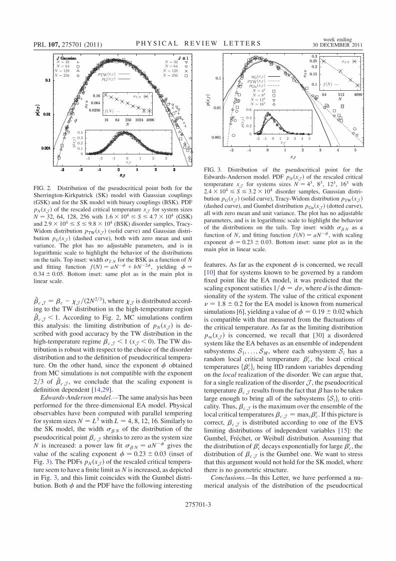
�c J ¼ �c � �J =ð2N2=3Þ, where �J is distributed accord-
ing to the TW distribution in the high-temperature region
�c J < 1. According to Fig. 2, MC simulations confirm
this analysis: the limiting distribution of pNðxJ Þ is de-
scribed with good accuracy by the TW distribution in thehigh-temperature regime �c J < 1 (xJ < 0). The TW dis-
tribution is robust with respect to the choice of the disorderdistribution and to the definition of pseudocritical tempera-ture. On the other hand, since the exponent � obtainedfrom MC simulations is not compatible with the exponent
2=3 of �c J , we conclude that the scaling exponent is
definition dependent [14,29].Edwards-Anderson model.—The same analysis has been
performed for the three-dimensional EA model. Physicalobservables have been computed with parallel temperingfor system sizesN ¼ L3 with L ¼ 4, 8, 12, 16. Similarly tothe SK model, the width ��N of the distribution of the
pseudocritical point �c J shrinks to zero as the system size
N is increased: a power law fit ��N ¼ aN�� gives the
value of the scaling exponent � ¼ 0:23� 0:03 (inset ofFig. 3). The PDFs pNðxJ Þ of the rescaled critical tempera-
ture seem to have a finite limit asN is increased, as depictedin Fig. 3, and this limit coincides with the Gumbel distri-bution. Both � and the PDF have the following interesting
features. As far as the exponent � is concerned, we recall[10] that for systems known to be governed by a randomfixed point like the EA model, it was predicted that thescaling exponent satisfies 1=� ¼ d�, where d is the dimen-sionality of the system. The value of the critical exponent� ¼ 1:8� 0:2 for the EA model is known from numericalsimulations [6], yielding a value of� ¼ 0:19� 0:02whichis compatible with that measured from the fluctuations ofthe critical temperature. As far as the limiting distributionp1ðxJ Þ is concerned, we recall that [30] a disordered
system like the EA behaves as an ensemble of independentsubsystems S1; . . . ;SM, where each subsystem Si has arandom local critical temperature �i
c, the local criticaltemperatures f�i
cgi being IID random variables dependingon the local realization of the disorder. We can argue that,for a single realization of the disorderJ , the pseudocriticaltemperature�c J results from the fact that� has to be taken
large enough to bring all of the subsystems fSigi to criti-cality. Thus,�c J is the maximum over the ensemble of the
local critical temperatures�c J ¼ maxi�ic. If this picture is
correct, �c J is distributed according to one of the EVS
limiting distributions of independent variables [15]: theGumbel, Frechet, or Weibull distribution. Assuming thatthe distribution of�i
c decays exponentially for large�ic, the
distribution of �c J is the Gumbel one. We want to stress
that this argument would not hold for the SK model, wherethere is no geometric structure.Conclusions.—In this Letter, we have performed a nu-
merical analysis of the distribution of the pseudocrtical
FIG. 2. Distribution of the pseudocritical point both for theSherrington-Kirkpatrick (SK) model with Gaussian couplings(GSK) and for the SK model with binary couplings (BSK). PDFpNðxJ Þ of the rescaled critical temperature xJ for system sizes
N ¼ 32, 64, 128, 256 with 1:6� 104 � S � 4:7� 104 (GSK)and 2:9� 104 � S � 9:8� 104 (BSK) disorder samples, Tracy-Widom distribution pTWðxJ Þ (solid curve) and Gaussian distri-
bution pGðxJ Þ (dashed curve), both with zero mean and unit
variance. The plot has no adjustable parameters, and is inlogarithmic scale to highlight the behavior of the distributionson the tails. Top inset: width �T N for the BSK as a function of Nand fitting function fðNÞ ¼ aN�� þ bN�2�, yielding � ¼0:34� 0:05. Bottom inset: same plot as in the main plot inlinear scale.
FIG. 3. Distribution of the pseudocritical point for theEdwards-Anderson model. PDF pNðxJ Þ of the rescaled critical
temperature xJ for systems sizes N ¼ 43, 83, 123, 163 with
2:4� 104 � S � 3:2� 104 disorder samples, Gaussian distri-bution pGðxJ Þ (solid curve), Tracy-Widom distribution pTWðxJ Þ(dashed curve), and Gumbel distribution pGuðxJ Þ (dotted curve),all with zero mean and unit variance. The plot has no adjustableparameters, and is in logarithmic scale to highlight the behaviorof the distributions on the tails. Top inset: width �� N as a
function of N, and fitting function fðNÞ ¼ aN��, with scalingexponent � ¼ 0:23� 0:03. Bottom inset: same plot as in themain plot in linear scale.
PRL 107, 275701 (2011) P HY S I CA L R EV I EW LE T T E R Sweek ending
30 DECEMBER 2011
275701-3

temperature in two mean-field spin glasses, theSherrington-Kirkpatrick model with Gaussian couplingsand with binary couplings, and in a short-range spin glass,the Edwards-Anderson model. The analysis for theSherrington-Kirkpatrick models shows that the distributionof the pseudocritical temperature in the high-temperaturephase is described with good accuracy by the Tracy-Widom distribution, as suggested by an analytical predic-tion previously published by some of the authors [14]. Toour knowledge, this is the first time that the Tracy-Widomdistribution is shown to play a role in spin glasses. The factthat both the Sherrington-Kirkpatrick model with Gaussiancouplings and the Sherrington-Kirkpatrick model withbinary couplings yield the Tracy-Widom distributionsuggests that the Tracy-Widom distribution is universalwith respect to the bonds’ distribution.
The analysis pursued for the three-dimensionalEdwards-Anderson model shows that the liming distribu-tion of the pseudocritical temperature is the Gumbel dis-tribution. An argument to understand this result has beenproposed. These two numerical analyses put in evidence aconnection between the critical regime of spin-glass mod-els and the extreme value statistics theory which has neverbeen proposed heretofore.
The present Letter opens several perspectives. As far asthe Sherrington-Kirkpatrick model is concerned, we recallthat the Tracy-Widom distribution describes typical fluc-tuations of the maximal eigenvalue of a Gaussian orthogo-nal ensemble random matrix, while the large deviationsregime of these fluctuations has been studied only recently[31]. It would be interesting to study numerically the largedeviations regime of the fluctuations of the critical tem-perature, where the distribution of the pseudocritical pointcould be described by the large deviations function derivedin [31]. It would be also interesting to consider the casewhere the couplings Jij are Gaussian with a positive bias J0[32]. Depending on the value of J0, the Sherrington-Kirkpatrick model has a phase transition from a paramag-netic to a spin-glass phase or from a ferromagnetic to amixed phase [32]: it would be interesting to investigate,both analytically and numerically, the fluctuations of thesepseudocritical points. Moreover, in order to bridge thegap between a mean-field and a short-range interactionsregime, it could be interesting to investigate the fluctua-tions of the pseudocritical temeperature in spin-glassmodels with tunable long-range interactions, like thoseintroduced in [33]. As far as the Edwards-Andersonmodel is concerned, it would be interesting to test experi-mentally the scenario found here in Fe0:5Mn0:5TiO3 [1] orEu0:5Ba0:5MnO3 [2] spin-glass materials. Indeed, ac-susceptibility measurements in these systems show [1]that the spin-glass critical temperature can be identifiedas the temperature where the susceptibility has a cusp.Accordingly, the pseudocritical point could be identifiedand measured, and one could test whether the resulting
rescaled pseudocritical point distribution converges to theGumbel distribution as the system size is increased.We are glad to thank G. Parisi, A. Rosso and P. Vivo
for interesting discussions and suggestions. We alsoacknowledge support from the D. I. computational centerof University Paris Sud and from the LPTMS cluster.
*[email protected][1] K. Gunnarsson et al., Phys. Rev. B 43, 8199 (1991).[2] S. Nair and A.K. Nigam, Phys. Rev. B 75, 214415
(2007).[3] S. F. Edwards and P.W. Anderson, J. Phys. F 5, 965
(1975).[4] D. Sherrington and S. Kirkpatrick, Phys. Rev. Lett. 35,
1792 (1975).[5] M. Mezard, G. Parisi, and M.A. Virasoro, Spin glass
theory and beyond (World Scientific, Singapore,1987).
[6] M. Palassini and S. Caracciolo, Phys. Rev. Lett. 82, 5128(1999).
[7] T.D. Lee and C.N. Yang, Phys. Rev. 87, 410(1952).
[8] C. Yang, Phys. Rev. 87, 404 (1952).[9] A. Harris, J. Phys. C 7, 1671 (1974).[10] A. Aharony and A. B. Harris, Phys. Rev. Lett. 77, 3700
(1996).[11] S. Wiseman and E. Domany, Phys. Rev. Lett. 81, 22
(1998).[12] K. Bernardet, F. Pazmandi, and G.G. Batrouni, Phys. Rev.
Lett. 84, 4477 (2000).[13] F. Igloi et al., Phys. Rev. B 76, 064421 (2007).[14] M. Castellana and E. Zarinelli, Phys. Rev. B 84, 144417
(2011).[15] J. Galambos, The asymptotic Theory of Extreme Order
Statistics (R. E. Krieger Publishing Co., Malabar, Florida,1987).
[16] C. A. Tracy and H. Widom, in Proc. InternationalCongress of Mathematicians (Beijing, 2002) (HigherEducation Press, Beijing, 2002), Vol. 1.
[17] J. Baik, P. Deift, and K. Johansson, J. Am. Math. Soc. 12,1119 (1999).
[18] K. Johansson, Commun. Math. Phys. 209, 437(2000).
[19] M. Prahofer and H. Spohn, Phys. Rev. Lett. 84, 4882(2000).
[20] M. Kardar, G. Parisi, and Y. C. Zhang, Phys. Rev. Lett. 56,889 (1986).
[21] P. Calabrese and P. Le Doussal, Phys. Rev. Lett. 106,250603 (2011).
[22] A.M. Somoza, M. Ortuno, and J. Prior, Phys. Rev. Lett.99, 116602 (2007).
[23] C. Monthus and T. Garel, Phys. Rev. B 79, 205120(2009).
[24] K. A. Takeuchi and M. Sano, Phys. Rev. Lett. 104, 230601(2010).
[25] K. A. Takeuchi et al., Sci. Rep. 1 (2011) 34.[26] B. Coluzzi et al., J. Phys. A 33, 3851 (2000).[27] T. Nakamura et al., J. Phys. A 36, 10895 (2003).
PRL 107, 275701 (2011) P HY S I CA L R EV I EW LE T T E R Sweek ending
30 DECEMBER 2011
275701-4

[28] G. Parisi et al., J. Phys. A 26, 247 (1993).[29] A. Billoire et al., J. Stat. Mech. (2011) P10019.[30] T. Vojta, J. Phys. A 39, R143 (2006).[31] D. S. Dean and S.N. Majumdar, Phys. Rev. Lett. 97,
160201 (2006).
[32] H. Nishimori, Statistical Physics of Spin Glasses andInformation Processing: An Introduction (OxfordUniversity Press, Oxford, UK, 2001).
[33] G. Kotliar, P.W. Anderson, and D. L. Stein, Phys. Rev. B27, 602 (1983).
PRL 107, 275701 (2011) P HY S I CA L R EV I EW LE T T E R Sweek ending
30 DECEMBER 2011
275701-5


Bibliography
[1] Phase transitions. In Proceedings of the Cargese Summer Institute (edited byM. Lévy, J. C. Le Guillou and J. Zinn-Justin), vol. B72. Plenum (1982).
[2] Abou-Chacra, R., Thouless, D. J., and Anderson, P. W. A selfcon-sistent theory of localization. Journal of Physics C: Solid State Physics, 6(1973), 1734.
[3] Alvarez Baños, R., et al. Static versus dynamic heterogeneities in thed = 3 Edwards-Anderson Ising spin glass. Physical Review Letters, 105 (2010),177202.
[4] Anderson, P. W. Through the glass lightly. Science, 267 (1995), 1615.
[5] Baillie, C. F., Gupta, R., Hawick, K. A., and Pawley, G. S. MonteCarlo renormalization-group study of the three-dimensional Ising model. Phys-ical Review B, 45 (1992), 10438.
[6] Baker Jr, G. Ising model with a scaling interaction. Physical Review B, 5(1972), 2622.
[7] Ballesteros, H. G., et al. Critical behavior of the three-dimensional Isingspin glass. Physical Review B, 62 (2000), 14237.
[8] Baños, R. A., et al. Nature of the spin-glass phase at experimental lengthscales. Journal of Statistical Mechanics: Theory and Experiment, (2010),P06026.
[9] Barahona, F. On the computational complexity of Ising spin glass models.Journal of Physics A: Mathematical and General, 15 (1982), 3241.
[10] Belletti, F., et al. An in-depth view of the microscopic dynamics of Isingspin glasses at fixed temperature. Journal of Statistical Physics, 135 (2009),1121.
[11] Berker, A. and Ostlund, S. Renormalization group calculations of finitesystems: order parameter and specific heat for epitaxial ordering. Journal ofPhysics C: Solid State Physics, 12 (1979), 4961.
[12] Bernardi, L. and Campbell, I. A. Violation of universality for Isingspin-glass transitions. Physical Review B, 52 (1995), 12501.
187
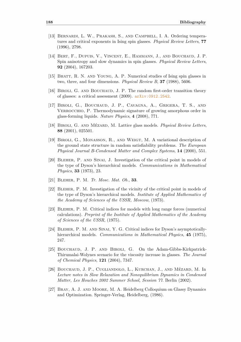
188 Bibliography
[13] Bernardi, L. W., Prakash, S., and Campbell, I. A. Ordering tempera-tures and critical exponents in Ising spin glasses. Physical Review Letters, 77(1996), 2798.
[14] Bert, F., Dupuis, V., Vincent, E., Hammann, J., and Bouchaud, J. P.Spin anisotropy and slow dynamics in spin glasses. Physical Review Letters,92 (2004), 167203.
[15] Bhatt, R. N. and Young, A. P. Numerical studies of Ising spin glasses intwo, three, and four dimensions. Physical Review B, 37 (1988), 5606.
[16] Biroli, G. and Bouchaud, J. P. The random first-order transition theoryof glasses: a critical assessment (2009). arXiv:0912.2542.
[17] Biroli, G., Bouchaud, J. P., Cavagna, A., Grigera, T. S., andVerrocchio, P. Thermodynamic signature of growing amorphous order inglass-forming liquids. Nature Physics, 4 (2008), 771.
[18] Biroli, G. and Mézard, M. Lattice glass models. Physical Review Letters,88 (2001), 025501.
[19] Biroli, G., Monasson, R., and Weigt, M. A variational description ofthe ground state structure in random satisfiability problems. The EuropeanPhysical Journal B-Condensed Matter and Complex Systems, 14 (2000), 551.
[20] Bleher, P. and Sinai, J. Investigation of the critical point in models ofthe type of Dyson’s hierarchical models. Communications in MathematicalPhysics, 33 (1973), 23.
[21] Bleher, P. M. Tr. Mosc. Mat. Ob., 33.
[22] Bleher, P. M. Investigation of the vicinity of the critical point in models ofthe type of Dyson’s hierarchical models. Institute of Applied Mathematics ofthe Academy of Sciences of the USSR, Moscow, (1973).
[23] Bleher, P. M. Critical indices for models with long range forces (numericalcalculations). Preprint of the Institute of Applied Mathematics of the Academyof Sciences of the USSR, (1975).
[24] Bleher, P. M. and Sinai, Y. G. Critical indices for Dyson’s asymptotically-hierarchical models. Communications in Mathematical Physics, 45 (1975),247.
[25] Bouchaud, J. P. and Biroli, G. On the Adam-Gibbs-Kirkpatrick-Thirumalai-Wolynes scenario for the viscosity increase in glasses. The Journalof Chemical Physics, 121 (2004), 7347.
[26] Bouchaud, J. P., Cugliandolo, L., Kurchan, J., and Mézard, M. InLecture notes in Slow Relaxation and Nonequilibrium Dynamics in CondensedMatter, Les Houches 2002 Summer School, Session 77. Berlin (2002).
[27] Bray, A. J. and Moore, M. A. Heidelberg Colloquium on Glassy Dynamicsand Optimization. Springer-Verlag, Heidelberg, (1986).
Bibliography 189
[28] Callan, C. Broken scale invariance in scalar field theory. Physical Review D,2 (1970), 1541.
[29] Callan, C. Methods in field theory. In Les Houches 1975 (edited by R. Balianand J. Zinn-Justin). North-Holland, Amsterdam (1976).
[30] Campostrini, M., Pelissetto, A., Rossi, P., and Vicari, E. Improvedhigh-temperature expansion and critical equation of state of three-dimensionalIsing-like systems. Physical Review E, 60 (1999), 3526.
[31] Cassandro, M. and Jona-Lasinio, G. Critical point behaviour and proba-bility theory. Advances in Physics, 27 (1978), 913.
[32] Castellana, M., Decelle, A., Franz, S., Mézard, M., and Parisi,G. Hierarchical random energy model of a spin-glass: critical behavior of thecorrelation length. To be published.
[33] Castellana, M., Decelle, A., Franz, S., Mézard, M., and Parisi, G.Hierarchical random energy model of a spin glass. Physical Review Letters,104 (2010), 127206.
[34] Castellana, M. and Parisi, G. Renormalization group computation of thecritical exponents of hierarchical spin glasses. Physical Review E, 82 (2010),040105.
[35] Castellana, M. and Parisi, G. Renormalization group computation ofthe critical exponents of hierarchical spin glasses: Large-scale behavior anddivergence of the correlation length. Physical Review E, 83 (2011), 041134.
[36] Castellana, M. Real-space renormalization group analysis of a non-mean-field spin-glass. Europhysics Letters, 95 (2011), 47014.
[37] Castellani, T. and Cavagna, A. Spin-glass theory for pedestrians. Journalof Statistical Mechanics: Theory and Experiment, (2005), P05012.
[38] Chang, M. and Sak, J. Spin-glass with long-range random exchangeinteraction. Physical Review B, 29 (1984), 2652.
[39] Chen, J. and Lubensky, T. Mean field and ε-expansion study of spinglasses. Physical Review B, 16 (1977), 2106.
[40] Chetyrkin, K., Kataev, A., and Tkachov, F. Errata. Physics Letters B,101 (1981), 457.
[41] Chetyrkin, K., Kataev, A., and Tkachov, F. Five-loop calculations inthe gφ4 model and the critical index η. Physics Letters B, 99 (1981), 147.
[42] Chetyrkin, K. G., Gorishny, S. G., Larin, S. A., and Tkachov, F. V.Five-loop renormalization group calculations in the gφ4 theory. Physics LettersB, 132 (1983), 351.
[43] Chetyrkin, K. G. and Tkachov, F. V. Integration by parts: The algorithmto calculate β-functions in 4 loops. Nuclear Physics B, 192 (1981), 159.
190 Bibliography
[44] Collet, P. and Eckmann, J. A renormalization group analysis of thehierarchical model in statistical mechanics. Lecture Notes in Physics, 74(1978).
[45] Collet, P. and Eckmann, J. P. The ε-expansion for the hierarchical model.Communications in Mathematical Physics, 55 (1977), 67.
[46] Collet, P., Eckmann, J. P., and Hirsbrunner, B. A numerical testof Borel summability in the ε-expansion of the hierarchical model. PhysicsLetters B, 71 (1977), 385.
[47] Contucci, P., Giardinà, C., Giberti, C., Parisi, G., and Vernia, C.Ultrametricity in the Edwards-Anderson model. Physical Review Letters, 99(2007), 057206.
[48] Contucci, P., Giardinà, C., Giberti, C., Parisi, G., and Vernia, C.Contucci et al. reply:. Physical Review Letters, 100 (2008), 159702.
[49] Contucci, P., Giardinà, C., Giberti, C., Parisi, G., and Vernia, C.Structure of correlations in three dimensional spin glasses. Physical ReviewLetters, 103 (2009), 017201.
[50] Crisanti, A. and Sommers, H. J. The spherical p-spin interaction spinglass model: the statics. Zeitschrift für Physik B Condensed Matter, 87 (1992),341.
[51] Daboul, D., Chang, I., and Aharony, A. Test of universality in the Isingspin glass using high temperature graph expansion. The European PhysicalJournal B-Condensed Matter and Complex Systems, 41 (2004), 231.
[52] de Dominicis, C. and Kondor, I. On spin glass fluctuations. Journal dePhysique Lettres, 45 (1984), 205.
[53] Derrida, B. Random-energy model: Limit of a family of disordered models.Physical Review Letters, 45 (1980), 79.
[54] Derrida, B. Random-energy model: An exactly solvable model of disorderedsystems. Physical Review B, 24 (1981), 2613.
[55] Dominicis, C. D. and Giardina, I. Random fields and spin-glasses: afield-theory approach. Springer (2006).
[56] Dupuis, V., Vincent, E., Alba, M., and Hammann, J. Aging, rejuvena-tion and memory effects in re-entrant ferromagnets. The European PhysicalJournal B-Condensed Matter and Complex Systems, 29 (2002), 19.
[57] Dyson, F. Existence of a phase transition in a one-dimensional Ising ferro-magnet. Communications in Mathematical Physics, 12 (1969), 91.
[58] Earl, D. J. and Deem, M. W. Parallel tempering: Theory, applications,and new perspectives. Physical Chemistry Chemical Physics, 7 (2005), 3910.
[59] Edwards, S. and Anderson, P. Theory of spin glasses. Journal of PhysicsF: Metal Physics, 5 (1975), 965.
Bibliography 191
[60] Fisher, D. and Huse, D. Absence of many states in realistic spin glasses.Journal of Physics A: Mathematical and General, 20 (1987), L1005.
[61] Fisher, D. and Huse, D. Pure states in spin glasses. Journal of Physics A:Mathematical and General, 20 (1987), L997.
[62] Fisher, D. and Huse, D. Equilibrium behavior of the spin-glass orderedphase. Physical Review B, 38 (1988), 386.
[63] Fisher, D. and Huse, D. Nonequilibrium dynamics of spin glasses. PhysicalReview B, 38 (1988), 373.
[64] Fisher, D. S. and Huse, D. A. Ordered phase of short-range Ising spin-glasses. Physical Review Letters, 56 (1986), 1601.
[65] Franz, S., Jörg, T., and Parisi, G. Overlap interfaces in hierarchicalspin-glass models. Journal of Statistical Mechanics: Theory and Experiment,(2009), P02002.
[66] Franz, S. and Parisi, G. On non-linear susceptibility in supercooled liquids.Journal of Physics: Condensed Matter, 12 (2000), 6335.
[67] Gardner, E. A spin glass model on a hierarchical lattice. Journal de Physique,45 (1984), 1755.
[68] Gorishny, S. G., Larin, S. A., and Tkachov, F. V. ε-expansion forcritical exponents: The O(ε5) approximation. Physics Letters A, 101 (1984),120 .
[69] Guerra, F. Broken replica symmetry bounds in the mean field spin glassmodel. Communications in Mathematical Physics, 233 (2003), 1.
[70] Guida, R. and Ribeca, P. Towards a fully automated computation ofRG functions for the three-dimensional O(N) vector model: parametrizingamplitudes. Journal of Statistical Mechanics: Theory and Experiment, (2006),P02007.
[71] Gunnarsson, K., Svedlindh, P., Nordblad, P., Lundgren, L., Aruga,H., and Ito, A. Static scaling in a short-range Ising spin glass. PhysicalReview B, 43 (1991), 8199.
[72] Harris, A. B., Lubensky, T. C., and Chen, J.-H. Critical properties ofspin-glasses. Physical Review Letters, 36 (1976), 415.
[73] Hasenbusch, M., Pelissetto, A., and Vicari, E. Critical behavior ofthree-dimensional Ising spin glass models. Physical Review B, 78 (2008),214205.
[74] Huang, K. Statistical mechanics. Wiley (1987).
[75] Huse, D. Private communication (2011).
192 Bibliography
[76] Ito, A., Aruga, H., Torikai, E., Kikuchi, M., Syono, Y., and Takei, H.Time-dependent phenomena in a short-range Ising spin-glass, Fe0.5Mn0.5TiO3.Physical Review Letters, 57 (1986), 483.
[77] Itzykson, C. and Drouffe, J. M. Statistical Field Theory (CambridgeMonographs on Mathematical Physics). Cambridge University Press (1991).
[78] Joh, Y. G., Orbach, R., and Hammann, J. Spin glass dynamics under achange in magnetic field. Physical Review Letters, 77 (1996), 4648.
[79] Jona-Lasinio, G. The renormalization group: A probabilistic view. Il NuovoCimento B (1971-1996), 26 (1975), 99.
[80] Jona-Lasinio, G. Renormalization group and probability theory. PhysicsReports, 352 (2001), 439.
[81] Jonason, K., Vincent, E., Hammann, J., Bouchaud, J. P., and Nord-blad, P. Memory and chaos effects in spin glasses. Physical Review Letters,81 (1998), 3243.
[82] Jörg, T., Katzgraber, H., and Krzakala, F. Behavior of Ising spinglasses in a magnetic field. Physical Review Letters, 100 (2008), 197202.
[83] Jörg, T. and Krzakala, F. Comment on “Ultrametricity in the Edwards-Anderson model”. Physical Review Letters, 100 (2008), 159701.
[84] Kadanoff, L. P. Scaling laws for Ising models near Tc. Physics (Long Island.City, N.Y.), 2 (1966), 263.
[85] Katori, H. A. and Ito, A. Experimental study of the de Almeida-Thoulessline by using typical Ising spin-glass FexMn1−xTiO3 with x = 0.41, 0.50, 0.55and 0.57. Journal of the Physical Society of Japan, 63 (1994), 3122.
[86] Katzgraber, H. and Hartmann, A. Ultrametricity and clustering of statesin spin glasses: A one-dimensional view. Physical Review Letters, 102 (2009),37207.
[87] Katzgraber, H., Palassini, M., and Young, A. Monte Carlo simulationsof spin glasses at low temperatures. Physical Review B, 63 (2001), 184422.
[88] Katzgraber, H. and Young, A. Monte Carlo studies of the one-dimensionalIsing spin glass with power-law interactions. Physical Review B, 67 (2003),134410.
[89] Katzgraber, H. and Young, A. Probing the Almeida-Thouless line awayfrom the mean-field model. Physical Review B, 72 (2005), 184416.
[90] Katzgraber, H. G., Hartmann, A. K., and Young, A. P. ComputerSimulation Studies in Condensed Matter Physics, vol. XXI. Springer Verlag,Heidelberg (2008).
[91] Katzgraber, H. G., Körner, M., and Young, A. P. Universality inthree-dimensional Ising spin glasses: A Monte Carlo study. Physical Review B,73 (2006), 224432.
Bibliography 193
[92] Katzgraber, H. G., Larson, D., and Young, A. P. Study of the deAlmeida-Thouless line using power-law diluted one-dimensional Ising spinglasses. Physical Review Letters, 102 (2009), 177205.
[93] Kauzmann, W. The nature of the glassy state and the behavior of liquids atlow temperatures. Chemical Reviews, 43 (1948), 219.
[94] Kazakov, D. The method of uniqueness, a new powerful technique formultiloop calculations. Physics Letters B, 133 (1983), 406.
[95] Kirkpatrick, S. and Sherrington, D. Infinite-ranged models of spin-glasses. Physical Review B, 17 (1978), 4384.
[96] Kirkpatrick, T. R., Thirumalai, D., and Wolynes, P. Scaling conceptsfor the dynamics of viscous liquids near an ideal glassy state. Physical ReviewA, 40 (1989), 1045.
[97] Kleinert, H., Neu, J., Schulte-Frohlinde, N., Chetyrkin, K. G., andLarin, S. A. Five-loop renormalization group functions of O(n)-symmetricφ4-theory and ε-expansions of critical exponents up to ε5. Physics Letters B,272 (1991), 39.
[98] Kleinert, H., Neu, J., Schulte-Frohlinde, V., Chetyrkin, K. G.,and Larin, S. A. Erratum (Five-loop renormalization group functions ofO(n)-symmetric φ4-theory and ε-expansions of critical exponents up to ε5:(Physics Letters B 272 (1991), 39 )). Physics Letters B, 319 (1993), 545.
[99] Kotliar, G., Anderson, P., and Stein, D. One-dimensional spin-glassmodel with long-range random interactions. Physical Review B, 27 (1983),602.
[100] Krzakala, F. and Martin, O. C. Spin and link overlaps in three-dimensional spin glasses. Physical Review Letters, 85 (2000), 3013.
[101] Landau, L. and Lifshitz, E. M. Statistical Physics: Course of TheoreticalPhysics, Vol. 5. Pergamon (1980).
[102] Langer, J. The mysterious glass transition. Physics Today, 60 (2007), 8.
[103] Laughlin, W. T. and Uhlmann, D. R. Viscous flow in simple organicliquids. The Journal of Physical Chemistry, 76 (1972), 2317.
[104] Leuzzi, L. Critical behaviour and ultrametricity of Ising spin-glass withlong-range interactions. Journal of Physics A: Mathematical and General, 32(1999), 1417.
[105] Leuzzi, L., Parisi, G., Ricci-Tersenghi, F., and Ruiz-Lorenzo, J.Ising spin-glass transition in a magnetic field outside the limit of validity ofmean-field theory. Physical Review Letters, 103 (2009), 267201.
[106] Leuzzi, L., Parisi, G., Ricci-Tersenghi, F., and Ruiz-Lorenzo, J. J.Dilute one-dimensional spin glasses with power law decaying interactions.Physical Review Letters, 101 (2008), 107203.

194 Bibliography
[107] Loeffel, J. J. Transformation of an asymptotic series in a convergent one.In Workshop on Padé approximants. Marseille (1975).
[108] Mari, P. O. and Campbell, I. A. Ising spin glasses: Corrections to finitesize scaling, freezing temperatures, and critical exponents. Physical Review E,59 (1999), 2653.
[109] Marinari, E., Parisi, G., and Ritort, F. On the 3d Ising spin glass.Journal of Physics A: Mathematical and General, 27 (1994), 2687.
[110] Marinari, E., Parisi, G., and Ruiz-Lorenzo, J. J. Phase structure ofthe three-dimensional Edwards-Anderson spin glass. Physical Review B, 58(1998), 14852.
[111] McMillan, W. L. Scaling theory of Ising spin glasses. Journal of Physics C:Solid State Physics (1968-1988), 17 (1984), 3179.
[112] Menon, N., O’Brien, K. P., Dixon, P. K., Wu, L., Nagel, S. R.,Williams, B. D., and Carini, J. P. Wide-frequency dielectric susceptibilitymeasurements in glycerol. Journal of Non-Crystalline Solids, 141 (1992), 61.
[113] Meurice, Y. The high-temperature expansion of the hierarchical Ising model:From Poincaré symmetry to an algebraic algorithm. Journal of MathematicalPhysics, 36 (1995), 1812.
[114] Meurice, Y., Niermann, S., and Ordaz, G. The oscillatory behavior of thehigh-temperature expansion of Dyson’s hierarchical model: A renormalizationgroup analysis. Journal of Statistical Physics, 87 (1997), 363.
[115] Mézard, M. and Montanari, A. Information, Physics and Computation.Oxford University Press (2009).
[116] Mézard, M. and Parisi, G. The Bethe lattice spin glass revisited. TheEuropean Physical Journal B-Condensed Matter and Complex Systems, 20(2001), 217.
[117] Mézard, M., Parisi, G., Sourlas, N., Toulouse, G., and Virasoro,M. Replica symmetry breaking and the nature of the spin glass phase. Journalde Physique, 45 (1984), 843.
[118] Mézard, M., Parisi, G., and Virasoro, M. A. SK model: The replicasolution without replicas. Europhysics Letters, 1 (1986), 77.
[119] Mézard, M., Parisi, G., and Virasoro, M. A. Spin glass theory andbeyond. World Scientific (1987).
[120] Mézard, M., Parisi, G., and Zecchina, R. Analytic and algorithmicsolution of random satisfiability problems. Science, 297 (2002), 812.
[121] Mézard, M. and Virasoro, M. The microstructure of ultrametricity.Journal de Physique, 46 (1985), 1293.

Bibliography 195
[122] Mézard, M. and Zecchina, R. Random K-satisfiability problem: Froman analytic solution to an efficient algorithm. Physical Review E, 66 (2002),056126.
[123] Monasson, R. and Zecchina, R. Statistical mechanics of the randomK-satisfiability model. Physical Review E, 56 (1997), 1357.
[124] Moore, M. A. Ordered phase of the one-dimensional Ising spin glass withlong-range interactions. Physical Review B, 82 (2010), 014417.
[125] Moore, M. A., Bokil, H., and Drossel, B. Evidence for the dropletpicture of spin glasses. Physical Review Letters, 81 (1998), 4252.
[126] Moore, M. A. and Bray, A. J. Disappearance of the de Almeida-Thoulessline in six dimensions. Physical Review B, 83 (2011), 224408.
[127] Naimzhanov, A. Hierarchical models of spin glasses. Theoretical and Mathe-matical Physics, 51 (1982), 416.
[128] Naimzhanov, A. Hierarchical model of spin glass. Theoretical and Mathe-matical Physics, 57 (1983), 1163.
[129] Nair, S. and Nigam, A. K. Critical exponents and the correlation lengthin the manganite spin glass Eu0.5Ba0.5MnO3. Physical Review B, 75 (2007),214415.
[130] Nishimori, H. Statistical physics of spin glasses and information processing:An introduction. Oxford University Press, Oxford, UK (2001).
[131] Ogielski, A. T. Dynamics of three-dimensional Ising spin glasses in thermalequilibrium. Physical Review B, 32 (1985), 7384.
[132] Palassini, M. and Caracciolo, S. Universal finite-size scaling functions inthe 3-d Ising spin glass. Physical Review Letters, 82 (1999), 5128.
[133] Parisi, G. Infinite number of order parameters for spin-glasses. PhysicalReview Letters, 43 (1979), 1754.
[134] Parisi, G. Toward a mean field theory for spin glasses. Physics Letters A, 73(1979), 203 .
[135] Parisi, G. A sequence of approximated solutions to the SK model for spinglasses. Journal of Physics A: Mathematical and General, 13 (1980), L115.
[136] Parisi, G. The order parameter for spin glasses: A function on the interval0− 1. Journal of Physics A: Mathematical and General, 13 (1980), 1101.
[137] Parisi, G. Order parameter for spin-glasses. Physical Review Letters, 50(1983), 1946.
[138] Parisi, G. Statistical Field Theory (Advanced Book Classics). Westview Press(1998).

196 Bibliography
[139] Parisi, G. and Sourlas, N. p-adic numbers and replica symmetry breaking.The European Physical Journal B-Condensed Matter and Complex Systems,14 (2000), 535.
[140] Pawley, G. S., Swendsen, R. H., Wallace, D. J., and Wilson, K. G.Monte Carlo renormalization-group calculations of critical behavior in thesimple-cubic Ising model. Physical Review B, 29 (1984), 4030.
[141] Plefka, T. Convergence condition of the TAP equation for the infinite-rangedIsing spin glass model. Journal of Physics A: Mathematical and General, 15(1982), 1971.
[142] Polyakov, A. M. Interaction of Goldstone particles in two dimensions.Applications to ferromagnets and massive Yang-Mills fields. Physics Letters B,59 (1975), 79 .
[143] Richert, R. and Angell, C. Dynamics of glass-forming liquids. V. On thelink between molecular dynamics and configurational entropy. The Journal ofChemical Physics, 108 (1998), 9016.
[144] Sherrington, D. and Kirkpatrick, S. Solvable model of a spin-glass.Physical Review Letters, 35 (1975), 1792.
[145] Swendsen, R. H. and Wang, J.-S. Replica Monte Carlo simulation ofspin-glasses. Physical Review Letters, 57 (1986), 2607.
[146] Sykes, M., Gaunt, D., Roberts, P., and Wyles, J. High temperatureseries for the susceptibility of the Ising model. II. Three dimensional lattices.Journal of Physics A: General Physics, 5 (1972), 640.
[147] Symanzik, K. Small distance behaviour in field theory and power counting.Communications in Mathematical Physics, 18 (1970), 227.
[148] Taibleson, M. Fourier analysis on local fields. Princeton University Press,Princeton, NJ (1976).
[149] Talagrand, M. The Parisi formula. Annals of Mathematics-Second Series,163 (2006), 221.
[150] Tarjus, G. and Kivelson, D. The viscous slowing down of supercooled liq-uids and the glass transition: phenomenology, concepts, and models. Jammingand rheology: constrained dynamics on microscopic and macroscopic scales,(2001), 20. arXiv:cond-mat/0003368v1.
[151] Theumann, A. Critical properties of the random hierarchical model. PhysicalReview B, 21 (1980), 2984.
[152] Theumann, A. Ferromagnetic and spin-glass behavior in the random hierar-chical model. Physical Review B, 22 (1980), 5441.
[153] Thouless, D. J., Anderson, P. W., and Palmer, R. G. Solution of‘Solvable model of a spin-glass’. Philosophical Magazine, 35 (1977), 593.

Bibliography 197
[154] van Duijvendijk, K., Schehr, G., and van Wijland, F. Slow relax-ation, dynamic transitions, and extreme value statistics in disordered systems.Physical Review E, 78 (2008), 011120.
[155] van Hemmen, J. L. and Palmer, R. G. The replica method and solvablespin glass model. Journal of Physics A: Mathematical and General, 12 (1979),563.
[156] Vincent, E., Dupuis, V., Alba, M., Hammann, J., and Bouchaud, J. P.Aging phenomena in spin-glass and ferromagnetic phases: Domain growth andwall dynamics. Europhysics Letters, 50 (2000), 674.
[157] Vladimirov, A. A., Kazakov, D. I., and Tarasov, O. V. Calculationof the critical indices by the methods of quantum field theory. ZhurnalEksperimental’noi i Teoreticheskoi Fiziki, 77 (1979), 1035.
[158] Weinberg, S. The quantum theory of fields, Volume I: Foundations. Cam-bridge University Press (2005).
[159] Weinberg, S. The quantum theory of fields, Volume II: Modern applications.Cambridge University Press (2005).
[160] Welsh, D. J. A. Complexity: Knots, colourings and counting. Volume 186of London Mathematical Society Lecture Notes Series. Cambridge UniversityPress (1993).
[161] Wilson, K. The renormalization group and critical phenomena, Nobel lecture,8 December 1982. Nobel Lectures, Physics, 1990 (1982).
[162] Wilson, K. The renormalization group and critical phenomena. Reviews ofModern Physics, 55 (1983), 583.
[163] Wilson, K. and Kogut, J. The renormalization group and the ε expansion.Physics Reports, 12 (1974), 75.
[164] Wilson, K. G. Renormalization group and critical phenomena. I. Renormal-ization group and the Kadanoff scaling picture. Physical Review B, 4 (1971),3174.
[165] Wilson, K. G. Renormalization group and critical phenomena. II. Phase-space cell analysis of critical behavior. Physical Review B, 4 (1971), 3184.
[166] Wilson, K. G. Feynman-graph expansion for critical exponents. PhysicalReview Letters, 28 (1972), 548.
[167] Wilson, K. G. Quantum field-theory models in less than 4 dimensions.Physical Review D, 7 (1973), 2911.
[168] Wilson, K. G. Critical phenomena in 3.99 dimensions. Physica, 73 (1974),119.
[169] Wilson, K. G. and Fisher, M. E. Critical exponents in 3.99 dimensions.Physical Review Letters, 28 (1972), 240.

198 Bibliography
[170] Wolfram, S. The Mathematica book, third edition. Cambridge UniversityPress (1996).
[171] Young, A. and Katzgraber, H. Absence of an Almeida-Thouless line inthree-dimensional spin glasses. Physical Review Letters, 93 (2004), 207203.
[172] Zinn-Justin, J. Analysis of Ising model critical exponents from high-temperature series expansion. Journal de Physique, 40 (1979), 969.
[173] Zinn-Justin, J. Quantum field theory and critical phenomena. InternationalSeries of Monographs on Physics, 113 (2002), 1.
[174] Zinn-Justin, J. Phase transitions and renormalization group. Oxford Univer-sity Press (2007).
Copyright © 2022 FDOKUMEN