Dynamic renormalization group analysis of propagation of elastic

waves in two-dimensional heterogeneous media

Reza Sepehrinia,1 Alireza Bahraminasab,1,2 Muhammad Sahimi,3,† and

M. Reza Rahimi Tabar1,4,5

1Department of Physics, Sharif University of Technology, Tehran 11365-9161, Iran

2Department of Physics, Lancaster University, Lancaster LA1 4YB, United Kingdom

3Mork Family Department of Chemical Engineering & Materials Science, University of

Southern California, Los Angeles, California 90089-1211, USA

4CNRS UMR 6529, Observatoire de la Cote d’Azur, BP 4229, 06304 Nice Cedex 4, France

5Carl Institute of Physics, von Ossietzky University, D-26111 Oldenburg, Germany

We study localization of elastic waves in two-dimensional heterogeneous solids with ran-

domly distributed Lame coefficients, as well as those with long-range correlations with a power-

law correlation function. The Matin-Siggia-Rose method is used, and the one-loop renormal-

ization group (RG) equations for the the coupling constants are derived in the limit of long

wavelengths. The various phases of the coupling constants space, which depend on the value

ρ, the exponent that characterizes the power-law correlation function, are determined and de-

scribed. Qualitatively different behaviors emerge for ρ < 1 and ρ > 1. The Gaussian fixed

point (FP) is stable (unstable) for ρ < 1 (ρ > 1). For ρ < 1 there is a region of the coupling

constants space in which the RG flows are toward the Gaussian FP, implying that the disorder

is irrelevant and the waves are delocalized. In the rest of the disorder space the elastic waves are

localized. We compare the results with those obtained previously for acoustic wave propagation

in the same type of heterogeneous media, and describe the similarities and differences between

the two phenomena.

PACS numbers(s): 62.30.+d, 47.56.+r, 05.10.Cc, 71.23.An

†Electronic address: moe@iran.usc.edu

1

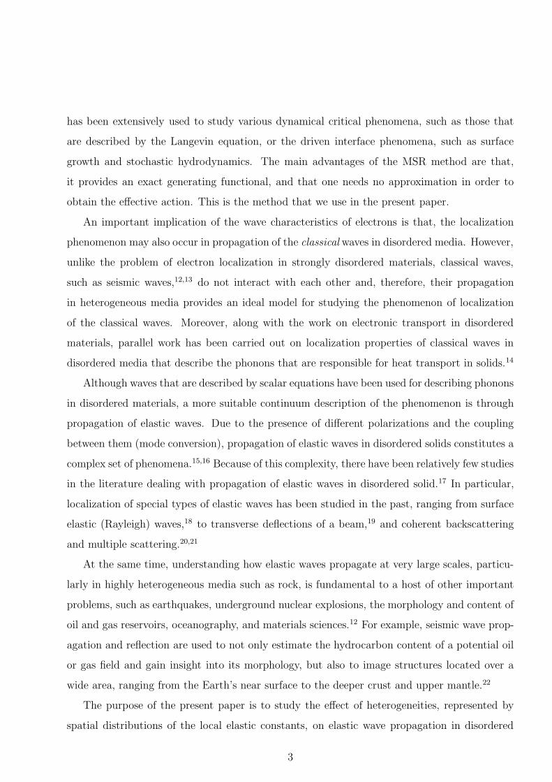
I. INTRODUCTION

Ever since the discovery of electron localization,1 much attention has been devoted to this

phenomenon, since it is not only of fundamental scientific interest, but also has much practical

importance. There is now extensive experimental evidence for the localization phenomenon in

disordered materials.2,3 On the theoretical side, the problem has been studied for decades by

several analytical methods, ranging from the scaling theory4 to the self-consistent perturba-

tion theory.5,6 In addition, numerical simulations using such techniques as the transfer-matrix

method and the statistics of energy levels have been used to verify the predictions of the ana-

lytical results.

The development of the one-parameter scaling theory4 of electron localization in terms of

the concepts of critical phenomena suggests that, the problem can be reformulated by using

an effective field theory which, when done, leads to the so-called σ model which is a nonlinear

model. Wegner7 proposed such a description of disordered conductors. Also noteworthy among

the theoretical developments is the work of Efetov et al.,8 who proposed the supersymmetric

approach, now used widely. The renormalization group (RG) approach, one of the most pow-

erful methods in statistical physics, has also been used to examine the critical properties of the

resulting effective field theory.9 The RG approach leads to a set of equations for the coupling

constants, such as the diffusivity and conductance of the disordered materials under study.

The main prediction of all of these approaches is that, for space dimensions d > 2, there is

a transition from the localized to extended states, so that the lower critical dimension of the

localization phenomenon is, dc = 2. However, despite convincing numerical evidence for the

validity of this prediction,10 the exponent ν that characterizes the power-law behavior of the

localization length ξ near the phase transition, ξ ∝ |W −Wc|−ν (where Wc is the critical value

of the disorder intensity W ), predicted by the RG method, is not in agreement with the nu-

merical results. A possible explanation for this discrepancy is that, some of the terms that are

neglected in the construction of the field theory may actually be relevant to the RG analysis.

Another approach to the field-theoretic description of the problem is based on the method

first developed by Martin, Siggia, and Rose (MSR),11 by which one constructs an effective action

(see below) based on the governing stochastic equation of motion for the phenomenon under

study. The MSR approach is well developed for critical phenomena far from equilibrium,11 and

2

has been extensively used to study various dynamical critical phenomena, such as those that

are described by the Langevin equation, or the driven interface phenomena, such as surface

growth and stochastic hydrodynamics. The main advantages of the MSR method are that,

it provides an exact generating functional, and that one needs no approximation in order to

obtain the effective action. This is the method that we use in the present paper.

An important implication of the wave characteristics of electrons is that, the localization

phenomenon may also occur in propagation of the classical waves in disordered media. However,

unlike the problem of electron localization in strongly disordered materials, classical waves,

such as seismic waves,12,13 do not interact with each other and, therefore, their propagation

in heterogeneous media provides an ideal model for studying the phenomenon of localization

of the classical waves. Moreover, along with the work on electronic transport in disordered

materials, parallel work has been carried out on localization properties of classical waves in

disordered media that describe the phonons that are responsible for heat transport in solids.14

Although waves that are described by scalar equations have been used for describing phonons

in disordered materials, a more suitable continuum description of the phenomenon is through

propagation of elastic waves. Due to the presence of different polarizations and the coupling

between them (mode conversion), propagation of elastic waves in disordered solids constitutes a

complex set of phenomena.15,16 Because of this complexity, there have been relatively few studies

in the literature dealing with propagation of elastic waves in disordered solid.17 In particular,

localization of special types of elastic waves has been studied in the past, ranging from surface

elastic (Rayleigh) waves,18 to transverse deflections of a beam,19 and coherent backscattering

and multiple scattering.20,21

At the same time, understanding how elastic waves propagate at very large scales, particu-

larly in highly heterogeneous media such as rock, is fundamental to a host of other important

problems, such as earthquakes, underground nuclear explosions, the morphology and content of

oil and gas reservoirs, oceanography, and materials sciences.12 For example, seismic wave prop-

agation and reflection are used to not only estimate the hydrocarbon content of a potential oil

or gas field and gain insight into its morphology, but also to image structures located over a

wide area, ranging from the Earth’s near surface to the deeper crust and upper mantle.22

The purpose of the present paper is to study the effect of heterogeneities, represented by

spatial distributions of the local elastic constants, on elastic wave propagation in disordered

3

media, such as rock, which represents a highly heterogeneous natural material. Recently, ex-

tensive experimental data for the spatial distributions of the local elastic moduli, the density,

and the wave velocities in several large-scale porous rock formations, both off- and onshore,

were analyzed.23 The analysis provided strong evidence for the existence of long-range corre-

lations in the spatial distributions of the measured quantities, characterized by a power-law

correlation function. The existence of such correlations in the data provided the impetus for

the present study and motivated an important question that we address in the present paper:

how do large-scale heterogeneities and long-range correlations affect elastic wave propagation

in disordered media? Another question that we address in the present paper is whether, in

the presence of the heterogeneities, the elastic waves can be delocalized. By localization we

mean a situation in which, over finite length scales (which can, however, be large), the waves’

amplitude decays and essentially vanishes.

Localization of elastic waves in rock would imply, for example, that seismic exploration

yields useful information only over distances r from the explosion’s site that are of the order of

the localization length ξ. Thus, if, for example, ξ is on the order of a few kilometers, but the

linear size of the area for which a seismic exploration is done is significantly larger than ξ, then,

seismic recordings can, at best, provide only partial information about the area. Localization

of elastic waves also implies that, if the stations that collect data for seismic waves that are

emanated from an earthquake in rock are farther from the earthquake’s hypocenter than ξ, no

useful information on the seismic activity prior to and during the earthquake can be gleaned

from the data24.

We use a field-theoretic formulation to study propagation of elastic waves in two-dimensional

(2D) disordered media in which the Lame coefficients are spatially distributed. Our approach

is based on the MSR method.11 We calculate the one-loop β functions (see below) for both spa-

tially random and power-law correlated distribution23 of the local elastic constants. Although

our work is primarily motivated by the analysis of experimental data for the spatial distribution

of elastic constants of rock at large scales,23 the results presented in this paper are general and

applicable to any solid material in which the local elastic constants follow the statistics of the

distributions that we consider. The present paper represents the continuation of our previous

work25,26 in which we studied acoustic wave propagation in the same type of heterogeneous

media. We will compare the results with those obtained previously for propagation of acoustic

4

waves.

The rest of this paper is organized as follows. In Sec. II the model is described and the

governing equations are presented. Section III describes the field-theoretic description of the

elastic wave equation, and the development of the MSR formulation for the propagation of the

waves in heterogeneous media. In Sec. IV the perturbative RG calculations, based on the MSR

action, are carried out and the results are analyzed. In Sec. V we compare the results with those

obtained previously25,26 for propagation of acoustic waves in the same type of heterogeneous

media that we consider in the present paper. The paper is summarized in Sec. VI.

II. THE MODEL AND GOVERNING EQUATIONS

To analyze propagation of elastic waves in a disordered medium, we begin with the equation

of motion of an elastic medium with the mean density m,

m∂2ui

∂t2= ∂jσij , (1)

where ui is the displacement in the ith direction, and σij the ijth component of the stress

tensor σ. As usual, σij is expressed in terms of the strain tensor,

σij(x) = 2µ(x)uij + λ(x)ukkδij . (2)

For small deformations, the strain tensor is given by,

uij =1

2(∂iuj + ∂jui) , (3)

where λ and µ are the Lame coefficients. For simplicity, we take the two Lame coefficients to

be equal, but the main results of the paper presented below will not change if they are unequal,

but follow the same type of statistical distributions. Hence, we write,

µ(x) = λ(x) = λ0 + η(x) , (4)

where λ0 = 〈λ(x)〉, with 〈·〉 representing a spatial averaging. We assume that η(x), the fluc-

tuating part of the Lame coefficients, is a Gaussian random process. Thus, in performing the

spatial average over the disorder we use a probability distribution of the form

P [η(x)] ∝ exp[

−∫

dxdx′η(x)D(x− x′)η(x′)]

, (5)

5

where D(x) is the inverse of the correlation function C(x). The disorder that we include

in the model consists of two parts. One is (random) δ−correlated, while the second part is

characterized by a power-law correlation function. Hence, the overall correlation function of

the spatial distribution of the disorder is given by

〈η(x)η(x′)〉 = 2C(x− x′) = 2D0δd(x− x′) + 2Dρ|x− x′|2ρ−d , (6)

in which D0 and Dρ are, respectively, the strengths of the disorder for the random and the

power-law correlated parts, C(x− x′) satisfies the following condition

∫

dx′′C(x− x′′)D(x′′ − x′) = δ(x− x′) , (7)

and d is the spatial dimension (d = 2 in this paper). Note that, in 2D, ρ = H + 1, with H

being the Hurst exponent.

A Gaussian distribution of the form (5) gives rise to quadratic couplings in the interac-

tion part of the action defined below. Moreover, the Gaussian distribution (5) may include a

tail of inadmissible negative values of the Lame coefficients. In principle, the unphysical tail

can be removed by introducing a modified probability distribution function which, however,

would produce couplings of higher order in the action. But, interactions of orders higher than

quadratic are irrelevant in the RG analysis and, therefore, can be ignored.

We now take the Fourier transform of Eq. (1) with respect to the time variable, which

yields the governing equation for a monochromatic wave with angular frequency ω,

∂jσij + ω2mui ≡ λ0Lijuj = 0 . (8)

Here, L is a 2× 2 differential matrix operator (see below).

III. FIELD-THEORETIC REPRESENTATION OF THE ELASTIC WAVE

EQUATION

Using the formalism developed by De Dominicis and Peliti27 (see also Hochberg et al.28),

one obtains a MSR generating functional that corresponds to the (Fourier-transformed) wave

equation (8)

P [uRi , uI

i ] =1

N∫

[Dη][D{uRi , uI

i }]δ(

L1juRj

)

δ(

L2juRj

)

δ(

L1juIj

)

δ(

L2juIj

)

× J

(

∂L∂uR

)

J

(

∂L∂uI

)

exp[

−∫

dxdx′η(x)D(x− x′)η(x′)]

. (9)

6

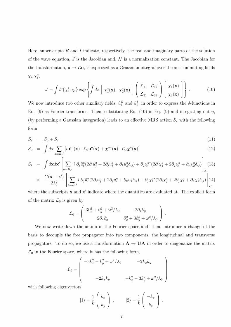
Here, superscripts R and I indicate, respectively, the real and imaginary parts of the solution

of the wave equation, J is the Jacobian and, N is a normalization constant. The Jacobian for

the transformation, u → Lu, is expressed as a Grassman integral over the anticommuting fields

χi, χ∗i ,

J =∫

D{χ∗i , χi} exp

∫

dx[

χ∗1(x) χ∗

2(x)

]

L11 L12

L21 L22

χ1(x)

χ2(x)

. (10)

We now introduce two other auxiliary fields, uRi and uI

i , in order to express the δ-functions in

Eq. (9) as Fourier transforms. Then, substituting Eq. (10) in Eq. (9) and integrating out η,

(by performing a Gaussian integration) leads to an effective MRS action Se with the following

form

Se = S0 + SI (11)

S0 =∫

dx∑

a=R,I

[i ua(x) · L0ua(x) + χ

a∗(x) · L0χa(x)] (12)

SI =∫

dxdx′

∑

a=R,I

i ∂juai (2∂iu

aj + 2∂ju

ai + ∂ku

akδij) + ∂jχ

a∗i (2∂iχ

aj + 2∂jχ

ai + ∂kχ

akδij)

x

(13)

× C(x− x′)

2λ20

∑

a=R,I

i ∂juai (2∂iu

aj + 2∂ju

ai + ∂ku

akδij) + ∂jχ

a∗i (2∂iχ

aj + 2∂jχ

ai + ∂kχ

akδij)

x′

,(14)

where the subscripts x and x′ indicate where the quantities are evaluated at. The explicit form

of the matrix L0 is given by

L0 =

3∂2x + ∂2

y + ω2/λ0 2∂x∂y

2∂x∂y ∂2x + 3∂2

y + ω2/λ0

.

We now write down the action in the Fourier space and, then, introduce a change of the

basis to decouple the free propagator into two components, the longitudinal and transverse

propagators. To do so, we use a transformation A → UA in order to diagonalize the matrix

L0 in the Fourier space, where it has the following form,

L0 =

−3k2x − k2

y + ω2/λ0 −2kxky

−2kxky −k2x − 3k2

y + ω2/λ0

with following eigenvectors

|1〉 =1

k

kx

ky

, |2〉 =1

k

−ky

kx

.

7

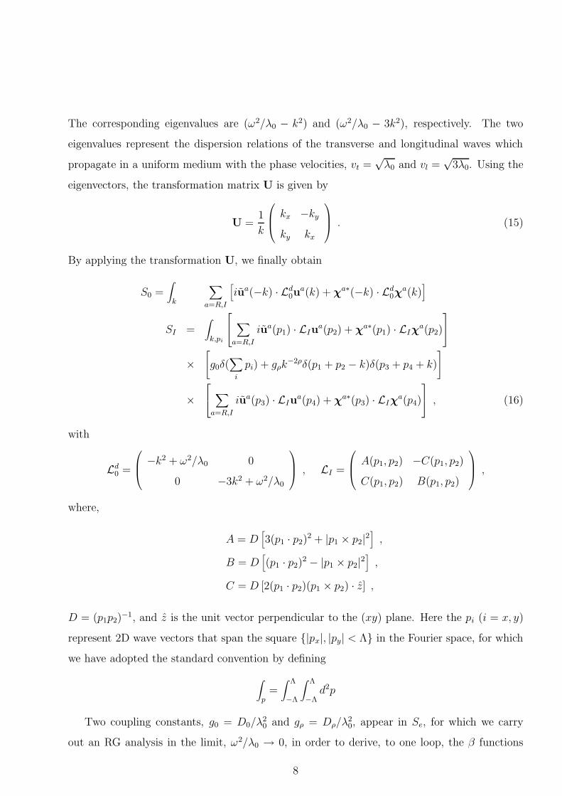
The corresponding eigenvalues are (ω2/λ0 − k2) and (ω2/λ0 − 3k2), respectively. The two

eigenvalues represent the dispersion relations of the transverse and longitudinal waves which

propagate in a uniform medium with the phase velocities, vt =√

λ0 and vl =√

3λ0. Using the

eigenvectors, the transformation matrix U is given by

U =1

k

kx −ky

ky kx

. (15)

By applying the transformation U, we finally obtain

S0 =∫

k

∑

a=R,I

[

iua(−k) · Ld0u

a(k) + χa∗(−k) · Ld

0χa(k)

]

SI =∫

k,pi

∑

a=R,I

iua(p1) · LIua(p2) + χ

a∗(p1) · LIχa(p2)

×[

g0δ(∑

i

pi) + gρk−2ρδ(p1 + p2 − k)δ(p3 + p4 + k)

]

×

∑

a=R,I

iua(p3) · LIua(p4) + χ

a∗(p3) · LIχa(p4)

, (16)

with

Ld0 =

−k2 + ω2/λ0 0

0 −3k2 + ω2/λ0

, LI =

A(p1, p2) −C(p1, p2)

C(p1, p2) B(p1, p2)

,

where,

A = D[

3(p1 · p2)2 + |p1 × p2|2

]

,

B = D[

(p1 · p2)2 − |p1 × p2|2

]

,

C = D [2(p1 · p2)(p1 × p2) · z] ,

D = (p1p2)−1, and z is the unit vector perpendicular to the (xy) plane. Here the pi (i = x, y)

represent 2D wave vectors that span the square {|px|, |py| < Λ} in the Fourier space, for which

we have adopted the standard convention by defining

∫

p=∫ Λ

−Λ

∫ Λ

−Λ

d2p

Two coupling constants, g0 = D0/λ20 and gρ = Dρ/λ

20, appear in Se, for which we carry

out an RG analysis in the limit, ω2/λ0 → 0, in order to derive, to one loop, the β functions

8

that describe their behavior in the coupling space. Note that for those terms of SI with

symmetric products of the fields under an exchange of momenta, the corresponding coefficients

will also retain the symmetric part. For example, the coefficient of g0uR1 (p1)u

R1 (p2)u

R1 (p3)u

R1 (p4)

is written as a sum of the symmetric and antisymmetric parts,

A(p1, p2)A(p3, p4) =1

2[A(p1, p2)A(p3, p4) + A(p1, p2)A(p3, p2)] ,

+1

2[A(p1, p2)A(p3, p4)− A(p1, p2)A(p3, p2)] , (17)

so that the antisymmetric part is cancelled by integrating over the momenta.

IV. RENORMALIZATION GROUP ANALYSIS

To study whether the elastic waves are localized or delocalized in the 2D heterogeneous

media of the type that we consider, we apply the RG method to the effective action, Eq. (16).

To do so, we follow the momentum shell RG29,30 and sum over the short wavelength degrees of

freedom. More specifically, we denote all the fields in the action (16) by Φ(k). To facilitate the

analysis, we change the domain of the integration from the square to a circle of radius Λ. Since

the small k modes are supposed to control the critical behavior of the system in the vicinity

of localization-delocalization transition, the change does not make any qualitative difference to

the results. Hereafter, we refer to the small k modes as the slow modes, and the rest as the

fast modes. We then define two sets of variables

Φ< = Φ(k) for 0 < k < Λ/l , slow modes ,

Φ> = Φ(k) for Λ/l ≤ k ≤ Λ , fast modes ,

where l > 1 is the rescaling parameter of the RG transformation. Then, the action is expressed

in terms of Φ< and Φ> as

S(Φ<, Φ>) = S0(Φ<) + S0(Φ>) + SI(Φ<, Φ>) .

S0 is a quadratic function of its arguments that can be separated into slow and fast terms,

but SI mixes the two modes. Then, the partition function Z is separated and written as follows

Z =∫

[DΦ<]∫

[DΦ>] exp[S0(Φ<)] exp[S0(Φ>)] exp[SI(Φ<, Φ>)] ≡∫

[DΦ<] exp[S ′0(Φ<)]

9

which defines the effective action S ′(Φ<) for the slow modes:

exp[S ′(Φ<)] = exp[S0(Φ<)]∫

[DΦ>] exp[S0(Φ>)] exp[SI(Φ<, Φ>)]

= exp[S0(Φ<)]∫

[DΦ>] exp[S0(Φ>)]

∫

[DΦ>] exp[S0(Φ>)] exp[SI(Φ<, Φ>)]∫

[DΦ>] exp[S0(Φ>)]

= Z0> exp[S0(Φ<)]〈exp[SI(Φ<, Φ>)]〉0> , (18)

where 〈·〉0> denotes an average with respect to the fast modes, and Z0> is the partition function

of S0(Φ>) which adds a constant to the action, independent of Φ<. The next step is to calculate

the average 〈exp[SI(Φ<, Φ>)]〉0>, which we treat perturbatively for weak disorder using the

relation

〈exp(V )〉 = exp[

〈V 〉+1

2!(〈V 2〉 − 〈V 〉2) + · · ·

]

. (19)

Therefore, according to Eqs. (18) and (19), we have, up to one-loop order

S ′(Φ<) = 〈SI〉+1

2!(〈S2

I 〉 − 〈SI〉2) . (20)

Each term in the series contains some monomials in the fast and slow modes. The former

must be averaged with respect to S0(Φ>). The first term in Eq. (20) yields tree-level terms,

as well as the corrections to the kinetic term of S0. We introduce a graphical representation of

the terms which is shown in the Fig. 1. The Feynman diagrams that contribute to the kinetic

term of the propagator uR1 uR

1 are shown in the Fig. 2. According to Fig. 2, apart from a naive

dimensional rescaling, one should rescale the fields by a factor F in the following way, in order

to keep the coefficient of the kinetic term to be the same as in the original action

Φ → 1√F

Φ , (21)

with

F = 1− 18π(Λ2g0 + Λ−2ρ+2gρ)δl +O(g20, g

2ρ, g0gρ) , (22)

where δl = l − 1.

We now derive the RG equations for the disorder strengths by renormalization of the cou-

pling of the vertex uR1 (p1)u

R1 (p2)u

R1 (p3)u

R1 (p4). The Feynman diagrams that contribute to the

renormalized coupling in one-loop order of the perturbation expansion, and the corresponding

10

symmetry factors, are shown in the Fig. 3. Note that the couplings are functions of the mo-

menta and, therefore, we consider the first term in the Taylor expansion and set the external

momenta to be parallel. The expressions for all the Feynman diagrams are listed in the Ap-

pendix. It can be seen by dimensional analysis that the canonical dimensions of the couplings

in units of length are

[g0] = 2 , (23)

[gρ] = 2− 2ρ. (24)

The following rules should be considered in expressing the Feynman diagrams of the vertex

function shown in Fig. 3:

(i) The diagrams that are made by different vertices have an extra factor of 2, due to the

quadratic term of the cumulant expansion.

(ii) All the diagrams have a factor 1/2! due to the cumulant expansion.

(iii) An extra (-1) factor should be included for the diagrams with Grassmanian loop.

Given the above rules, we obtain the following renormalized couplings

g′0 l2Λ′2 = F−2

(

g0Λ2 +

937

18πg2

0Λ4δl +

716

27πg2

ρΛ−4ρ+4δl +

3635

54πg0gρΛ

−2ρ+4δl)

, (25)

g′ρ l−2ρ+2Λ′−2ρ+2 = F−2

(

gρΛ−2ρ+2 + 36πg0gρΛ

−2ρ+4δl +1948

27g2

ρΛ−4ρ+4δl

)

, (26)

where Λ′ = Λ/l. Using Eq. (22) and writing the equations in differential forms, we obtain the

following expressions for the β functions that describe the couplings

β(g0) ≡∂g0

∂ ln l= −2g0 +

(

36 +937

18

)

g20 +

716

27g2

ρ +(

36 +3635

54

)

g0gρ , (27)

β(gρ) ≡∂gρ

∂ ln l= (2ρ− 2)gρ + 72g0gρ +

(

36 +1948

27

)

g2ρ , (28)

where g0 and gρ are dimensionless parameters defined by

g0 = πg0Λ2 , (29)

gρ = πgρΛ−2ρ+2 . (30)

The β functions that we have derived, Eqs. (27) and (28), describe how the two couplings

- g0 and gρ - behave, if we rescale all the lengths and consider the elastic medium at coarser

scales. If, for example, a small g0 diverges under the RG rescaling, its implication is that a

11

small g0 at small length scales behaves as very strong disorder at much larger scales. Therefore,

under such condition, every wave amplitude will be localized. If, on the other hand, for some

g0 < gc (where gc is a critical value of g0) g0 vanishes under the RG rescaling, it implies that,

in this regime, g0 does not contribute much to the behavior of the propagating waves at large

length scales. Therefore, one way of defining a localized state may be as follows: The waves

are localized if, under the RG rescaling, at least either g0 or gρ diverges.

We must also point out that, one may begin the RG rescaling and analysis with the assump-

tion that the couplings g0 and gρ are small. If, under the RG rescaling, we find stable fixed

points (FPs), it would imply that the assumption of the couplings being small about such FPs

is still valid. However, around an unstable FP the couplings can grow and, hence, the pertur-

bation expansion that we have developed would fail. For our main purpose, however, namely,

determining the localized/extended regimes and the transition between them, the most impor-

tant goal is to determine the condition(s) under which the FPs are unstable, around which the

couplings can diverge.

The FPs of the model are the roots of β functions. The RG equations, together with the

parameter ρ, have a complex phase space. Depending on ρ, there are four regimes:

(i) For ρ < (−17557527 + 128√

19977620601)/3888601 ' 0.14 there are two FPs: The

trivial Gaussian FP, {g∗0 = g∗ρ = 0}, which is stable, and a nontrivial FP, {g∗0 = 36/1585 '0.022, g∗ρ = 0} which has one positive eigenvalue (along the eigendirection of which is unstable)

and one negative one (along the eigendirection direction of which is stable); see Fig. 4a.

Physically, this implies that the diagram is divided into two parts. In one part the Gaussian

FP is relevant and the disorder does not have any effect, so that all the states are delocalized.

In the second part, the values of couplings increase under rescaling, so that the disorder (both

random and correlated) is relevant and, therefore, the elastic waves are localized. Thus, the line

(more precisely, the curve) that separates the two parts is where the localization-delocalization

transition takes place.

(ii) Four FPs exist if 0.14 < ρ < 289/1585 ' 0.18. The Gaussian FP is stable. The

other FPs are unstable in one eigendirection but stable in the other eigendirection, except,

{g∗0 = 0.022, g∗ρ = 0}, which has a negative eigenvalue and, hence is stable in all directions.

This is shown in Fig. 4b.

(iii) There are three FPs for 0.18 < ρ < 1. The Gaussian FP is again stable. The other two

12

FPs are unstable. Figure 4c presents this part of the RG flow diagram.

In both (ii) and (iii), as ρ increases, the system tries to move away from case (i) (the

delocalized-localized transition) to a purely localized state (see also below). Moreover, in (i) -

(iii) there is a point on the gρ axis which obviously is not a FP, but the RG flows change their

direction on gρ axis at that point. This means that one of the β functions is zero on this axis,

while the other one is not.

(iv) For ρ > 1 there are two FPs. As Fig. 4d indicates, the Gaussian FP is stable on the

g0 axis but unstable on the gρ axis, and the nontrivial FP, {g∗0 = 0.022, g∗ρ = 0}, is unstable in

all directions. The implication is that, while the power-law correlated disorder is relevant, no

new FP exists to one-loop order and, therefore, the long-wavelength behavior of the system is

determined by the long-range component of the disorder. This means that for ρ > 1 the elastic

waves are localized in 2D.

Let us note that the extension of the present RG analysis to 3D systems is difficult, but

doeable. The reason for the difficulty is twofold. (i) It is difficult to determine the transfor-

mation matrix U [see Eq. (15)] for a 3D system, in order to diagonalize the relevant matrices.

(iii) The number of contributing Feyman diagrams is very large.

V. COMPARISON WITH ACOUSTIC WAVE PROPAGATION

Since scalar equations have often been invoked for describing propagation of elastic waves,

it is of interest to compare the above results with those that we derived previously25,26 for the

scalar model of (acoustic) wave propagation in heterogeneous media with precisely the same

type of disorder as what we consider in the present paper. The governing equation for such

waves is given by

m∂2u

∂t2= ∇ · [λ(x)∇u(x)]. (31)

The analysis was carried out25,26 for a d−dimensional system, but we summarize its results for

2D media. The RG analysis indicated that, depending on ρ, there can be two distinct regimes

(unlike the four regimes described above):

(i) For 0 < ρ < 1 there are three sets of FPs. One set represents the Gaussian FP,

{g∗0 = g∗ρ = 0}, which is stable. The other two are {g∗0 = 1/4, g∗ρ = 0}, and

g∗0 = − 4

41

[

2 +5

8(ρ− 1)

]

− 4

41

√

[

2 +5

8(ρ− 1)

]2

+205

64(ρ− 1)2 ,

13

g∗ρ =3

4g∗0 +

1

8(1− ρ) , (32)

which is stable in one eigendirection but unstable in the other eigendirection. Therefore, for

0 < ρ < 1 the one-loop RG analysis indicated that a medium with uncorrelated disorder is

unstable against long-range correlated disorder towards a new FP in the space of the coupling

constants. Hence, there is a phase transition from delocalized to localized acoustic waves with

increasing the disorder intensity.

Thus, the physical implication of the RG results for acoustic wave propagation described by

Eq. (31) is as follows. In the interval, 0 < ρ < 1, there is a region in the space of the coupling

constants {g0, gρ} in which the RG flows take any initial point to the Gaussian FP. This implies

that, for 0 < ρ < 1, a disordered medium of the type considered in this paper and our previous

work25,26 looks like a pure (ordered or homogeneous) medium at large length scales, implying

that acoustic waves are extended or delocalized.

However, when g0 or gρ are large enough that the initial point is out of the basin of attraction

of the Gaussian FP, the RG flows move such points toward large values, hence implying that,

under the RG rescaling, the probability density function of the disorder becomes broader and

broader at increasingly larger length scales. Therefore, in this case, a propagating acoustic wave

samples a medium with very large spatial fluctuations in the elastic stiffness or moduli. We also

found that,25,26 even if one starts in a disordered medium with purely long-range correlations

(i.e., one with g0 = 0), the RG equations indicate that the growth of gρ will lead to increasing,

i.e., nonzero, g0, hence implying that uncorrelated disorder will be produced by the rescaling.

Since the local fluctuations in the bulk moduli play the role of scattering points, the implication

for acoustic waves is that the multiple scattering of a propagating wave from the uncorrelated

disorder will destroy the wave’s coherence, leading eventually to the localization of acoustic

waves.

(ii) For ρ > 1 there are two FPs: the Gaussian FP which is stable on the g0 axis but not

on the gρ axis, and a second FP, {g∗0 = 1/4, g∗ρ = 0}, which is unstable in all directions.

The implication for acoustic waves is that, although power-low correlated disorder is relevant,

no new FP exists to one-loop order and, therefore, the system’s long-wavelength behavior

is determined by the long-range component of the disorder. This implies that for ρ > 1 the

acoustic waves are localized (in fact, in this case they are localized for any d), which is similar to

14

the elastic waves studied in the present paper. In addition, in both cases the system undergoes

a disorder-induced transition when only the uncorrelated disorder is present.

Let us note that we argued in our previous papers25,26 that, in the case of acoustic waves,

although, similar to the elastic waves considered in the present paper, the RG calculations

were carried out to one-loop order, the analysis should still be valid for higher orders of the

perturbation as well. The argument was based on the fact that the signs of the higher-order

terms are all positive. That this is so is due to the following. We must keep in mind that

the contraction coefficients for auxiliary fields are always greater than those of auxiliary and

Grassmanian fields that supply the negative terms. Moreover, the numbers of diagrams of, e.g.,

a real auxiliary field and an imaginary auxiliary field are equal to number of diagrams of an

auxiliary and Grassmanian field. This implies immediately that the signs of higher-order terms

should also be positive. We, therefore, concluded that25,26 the one-loop results for the acoustic

waves should be valid to all orders. However, we now believe that this is only a necessary but

not sufficient conditions. In the case of elastic waves, though, we cannot even determine a

priori the signs of the higher-order terms.

Thus, comparison of propagation of elastic and acoustic waves in the type of heterogeneous

media that we consider in this paper indicates that, while the RG flow diagrams for the elastic

waves is more complex than those of the acoustic waves, the region of the coupling constants

space in which they are delocalized is narrower than that of the acoustic waves.

VI. SUMMARY

We developed a field-theoretic description of propagation and localization of elastic waves in

2D heterogeneous solids using a RG approach. Two types of heterogeneities, random disorder

and one with long-range correlations with a power-law correlation function, were considered.

We found that in presence of power-law correlated disorder with the exponent ρ > 1 (non-

decaying correlations) the RG flows are toward the strong coupling regime, and the waves are

localized. For ρ < 1, and depending on its value, there are other fixed points. One, which

is stable, is the Gaussian FP with a small domain of attraction. In this domain, long-range

correlated disorder, as well as the random disorder, are irrelevant and, therefore, the waves are

delocalized. In this regard, the delocalized states in the Gaussian domain are unlike electrons

in 2D systems, which remain localized for any disorder.

15

Whether the delocalized states predicted for the Gaussian domain persist, if we analyze the

RG flows beyond the one-loop approximation, remains to be seen. It may be that the domain

of attraction of the Gaussian FP shrinks (and might disappear completely), or exanpds, if we

consider the contributions of the higher order loops. However, analytical determination of the

contribution of even the second-order loops for this problem is extremely difficult.

As we mentioned in the Introduction, a challenging feature of the localization problem is

obtaining an analytical estimate of the localization length exponent. In this regard, the previous

analytical approaches are in contradiction with the numerical results. We hope that the method

developed in this paper can provide a precise way of describing the critical properties of the

localization-delocalization transition and its critical exponents in higher dimensions.

We are currently carrying out extensive numerical simulations in order to further check the

accuracy of the predictions of the dynamical RG method developed in this paper. The results

will be reported in the near future.

ACKNOWLEDGMENT

The work of R.S. was supported by the NIOC.

16

Appendix: Integrals for the Feynman Diagrams

In this Appendix we list all the expressions for the Feynman diagrams shown in Fig. 2.

a1 =∫

d2q

(q2 − ω2

λ0

)2× 1

4[A(p1, p2)A(−q, q) + A(q, p2)A(p1,−q)]

× [A(p3, p4)A(q,−q) + A(q, p4)A(p3,−q)] .

=1

4p1p2p3p4

∫

qdq∫

dθ[9 + (3 cos2 θ + sin2 θ)2]2 =1523π

16p1p2p3p4

∫

qdq .

a2 =∫

d2q

(q2 − ω2

λ0

)2× 4[A(p2, p1)A(q,−q)][A(p4, p3)A(q,−q)] .

= 324p1p2p3p4

∫

qdq∫

dθ = 648πp1p2p3p4

∫

qdq .

a3 = −∫ d2q

(3q2 − ω2

λ0

)(q2 − ω2

λ0

)× 1

2[A(−q, p1)C(p2, q)][A(p4, q)C(−q, p3)] .

=1

3p1p2p3p4

∫

qdq∫

dθ(3 cos2 θ + sin2 θ)2 sin2(2θ) =17π

12p1p2p3p4

∫

qdq .

a4 =∫

d2q

(3q2 − ω2

λ0

)2× 4[A(p2, p1)B(−q, q)− C(p2, q)C(−q, p1)]

× [A(p4, p3)B(−q, q) + C(p4, q)C(−q, p3)] .

=4

9p1p2p3p4

∫

qdq∫

dθ[3 + sin2(2θ)]2 = 11πp1p2p3p4

∫

qdq .

a5 =∫

d2q

(3q2 − ω2

λ0

)2× 4[A(p2, p1)B(−q, q)][A(p4, p3)B(q,−q)] .

= 4p1p2p3p4

∫

qdq∫

dθ = 8πp1p2p3p4

∫

qdq .

a6 =∫ d2q

(q2 − ω2

λ0

)2× 1

4[A(q, p1)A(−q, p3) + A(−q, p1)A(q, p3)]

× [A(p2,−q)A(p4, q) + A(p4,−q)A(p2, q)] .

= p1p2p3p4

∫

qdq∫

dθ(3 cos2 θ + sin2 θ)2 = 9πp1p2p3p4

∫

qdq .

a7 = −∫

d2q

(3q2 − ω2

λ0

)(q2 − ω2

λ0

)× 4[A(q, p1)C(−q, p3)][A(p2,−q)C(p4, q)] .

=4

3p1p2p3p4

∫

qdq∫

dθ =8π

3p1p2p3p4

∫

qdq .

a8 =∫ d2q

3(q2 − ω2

λ0

)(3q2 − ω2

λ0

)× 1

4[C(q, p1)C(−q, p3) + C(−q, p1)C(q, p3)]

× [C(p2,−q)C(p4, q) + C(p4,−q)C(p2, q)] .

=1

9p1p2p3p4

∫

qdq∫

dθ sin4(2θ) =π

12p1p2p3p4

∫

qdq .

a9 = a10 = −∫

d2q

(q2 − ω2

λ0

)2× 4[A(p2, p1)A(q,−q)][A(p4, p3)A(q,−q)] .

17

= −324p1p2p3p4

∫

qdq∫

dθ = −648πp1p2p3p4

∫

qdq .

a11 = a12 = −∫

d2q

(3q2 − ω2

λ0

)2× 4[A(p2, p1)B(q,−q)][A(p4, p3)B(q,−q)] .

= −4p1p2p3p4

∫

qdq∫

dθ = −8πp1p2p3p4

∫

qdq .

b1 =∫

d2q

(q2 − ω2

λ0

)2× 1

2[A(p2,−q)A(p1, q)][A(p4, p3)A(q,−q) + A(q, p3)A(p4,−q)] .

=1

2p1p2p3p4

∫

q−2ρ+1dq∫

dθ[9 + (3 cos2 θ + sin2 θ)2](3 cos2 θ + sin2 θ)2

=551π

8p1p2p3p4

∫

q−2ρ+1dq .

b2 = b3 =∫

d2q

(q2 − ω2

λ0

)2× 1

4[A(p2, q)A(p4,−q) + A(p4, q)A(p2,−q)]

× [A(p1, q)A(p3,−q) + A(p1,−q)A(p3, q)] .

= p1p2p3p4

∫

q−2ρ+1dq∫

dθ(3 cos2 θ + sin2 θ)2 = 9πp1p2p3p4

∫

q−2ρ+1dq .

b4 =∫

d2q

3(q2 − ω2

λ0

)(3q2 − ω2

λ0

)× 1

4[C(q, p1)C(−q, p3) + C(−q, p1)C(q, p3)]

× [C(p2,−q)C(p4, q) + C(p4,−q)C(p2, q)] .

=1

9p1p2p3p4

∫

q−2ρ+1dq∫

dθ sin4(2θ) =π

12p1p2p3p4

∫

q−2ρ+1dq .

b5 = −∫

d2q

3(q2 − ω2

λ0

)(q2 − ω2

λ0

)× [A(p4,−q)C(q, p3)][A(q, p1)C(p2,−q)] .

=2

3p1p2p3p4

∫

q−2ρ+1dq∫

dθ sin2(2θ)(3 cos2 θ + sin2 θ)2 =17π

6p1p2p3p4

∫

q−2ρ+1dq .

b6 = −∫

d2q

(3q2 − ω2

λ0

)(q2 − ω2

λ0

)× 2[A(q, p3)C(p4,−q)][A(p2,−q)C(q, p1)] .

=2

3p1p2p3p4

∫

q−2ρ+1dq∫

dθ sin2(2θ)(3 cos2 θ + sin2 θ)2 =17π

6p1p2p3p4

∫

q−2ρ+1dq .

b7 = −∫

d2q

(3q2 − ω2

λ0

)(q2 − ω2

λ0

)× 4[A(q, p1)C(−q, p3)][A(p2,−q)C(p4, q)] .

=4

3p1p2p3p4

∫

q−2ρ+1dq∫

dθ sin2(2θ)(3 cos2 θ + sin2 θ)2 =17π

3p1p2p3p4

∫

q−2ρ+1dq .

b8 =∫ d2q

(3q2 − ω2

λ0

)(3q2 − ω2

λ0

)× 4[A(p4, p3)B(q,−q)− C(q, p3)C(p4,−q)][C(p2,−q)C(q, p1)] .

=4

9p1p2p3p4

∫

q−2ρ+1dq∫

dθ[3 + sin2(2θ)] sin2(2θ) =15π

3p1p2p3p4

∫

q−2ρ+1dq .

c1 =∫

d2q

(q2 − ω2

λ0

)2× [A(q, p1)A(p2,−q)][A(p3,−q)A(q, p4)] .

= p1p2p3p4

∫

q−4ρ+1dq∫

dθ(3 cos2 θ + sin2 θ)4 =227π

4p1p2p3p4

∫

q−4ρ+1dq .

18

c2 =∫

d2q

(q2 − ω2

λ0

)2× [A(q, p1)A(−q, p3)][A(p2,−q)A(p4, q)] .

= p1p2p3p4

∫

q−4ρ+1dq∫

dθ(3 cos2 θ + sin2 θ)4 =227π

4p1p2p3p4

∫

q−4ρ+1dq .

c3 =∫ d2q

(3q2 − ω2

λ0

)2× 4[C(q, p1)C(p2,−q)][C(p4,−q)C(q, p3)] .

=4

9p1p2p3p4

∫

q−4ρ+1dq∫

dθ sin4(2θ) =π

3p1p2p3p4

∫

q−4ρ+1dq .

c4 =∫

d2q

(3q2 − ω2

λ0

)(q2 − ω2

λ0)× (−4)[A(q, p1)C(p2,−q)][A(p4,−q)C(q, p3)] .

= p1p2p3p4 ×4

3

∫

q−4ρ+1dq∫

dθ(3 cos2 θ + sin2 θ)2 sin2(2θ) =17π

3p1p2p3p4

∫

q−4ρ+1dq .

c5 =∫

d2q

(3q2 − ω2

λ0

)(q2 − ω2

λ0

)× (−4)[A(q, p1)C(−q, p3)][A(p2,−q)C(p4, q)] .

=4

3p1p2p3p4

∫

q−4ρ+1dq∫

dθ(3 cos2 θ + sin2 θ)2 sin2(2θ) =17π

3p1p2p3p4

∫

q−4ρ+1dq .

c6 =∫

d2q

(3q2 − ω2

λ0

)(3q2 − ω2

λ0

)× [C(q, p1)C(−q, p3)][C(p2,−q)C(p4, q)] .

=1

9p1p2p3p4

∫

q−4ρ+1dq∫

dθ sin4(2θ) =π

12p1p2p3p4

∫

q−4ρ+1dq .

d1 =∫ d2q

(q2 − ω2

λ0

)2× 1

2[A(p2, p1)A(−q, q) + A(−q, p1)A(p2, q)][A(p4, p3)A(q,−q)] .

=9

2p1p2p3p4

∫

qdq∫

dθ[9 + (3 cos2 θ + sin2 θ)2] =243π

2p1p2p3p4

∫

qdq .

d2 =∫

d2q

(q2 − ω2

λ0

)2× 4[A(p2, p1)A(−q, q)][A(p4, p3)A(q,−q)] .

= 324p1p2p3p4

∫

qdq∫

dθ = 324πp1p2p3p4

∫

qdq .

d3 = d4 = 0 .

d5 = d6 =∫ d2q

(3q2 − ω2

λ0

)2× 4[A(p2, p1)B(q,−q)][A(p3, p4)A(q,−q)] .

= 4p1p2p3p4

∫

qdq∫

dθ = 8πp1p2p3p4

∫

qdq .

d7 = d8 = −∫ d2q

(3q2 − ω2

λ0

)2× 4[A(p2, p1)B(q,−q)][A(p4, p3)A(−q, q)] .

= −324p1p2p3p4

∫

qdq∫

dθ = −648πp1p2p3p4

∫

qdq .

d9 = d10 = 0 .

e1 =∫

d2q

(q2 − ω2

λ0

)2× [A(q, p1)A(p2,−q)][A(p4, p3)A(q,−q)] .

= 9p1p2p3p4

∫

q−2ρ+1dq∫

dθ(3 cos2 θ + sin2 θ)2 = 81πp1p2p3p4

∫

q−2ρ+1dq .

19

e2 = e3 = 0 .

e4 =∫

d2q

(3q2 − ω2

λ0

)2× (−4)[C(q, p1)C(p2,−q)][A(p4, p3)B(q,−q)] .

=4

3p1p2p3p4

∫

q−2ρ+1dq∫

dθ sin2(2θ) =4π

3p1p2p3p4

∫

q−2ρ+1dq .

20

1P. W. Anderson, Phys. Rev. 109, 1492 (1958); N. F. Mott and W. D. Twose, Adv. Phys.

10, 107 (1961).

2S. He and J. D. Maynard, Phys. Rev. Lett. 57, 3171 (1986); J. D. Maynard, Rev. Mod.

Phys. 73, 401 (2001).

3D. S. Wiersma, P. Bartolini, A. Lagendijk, and R. Righini, Nature (London) 390, 671 (1997).

4E. Abrahams, P. W. Anderson, D. C. Licciardello, and T. V. Ramakrishnan, Phys. Rev.

Lett. 42, 673 (1979); P. W. Anderson, E. Abrahams, and T. V. Ramakrishnan, ibid. 43,

718 (1979).

5D. Vollhardt and P. Wolfle, Phys. Rev. B 22, 4666 (1980).

6T. R. Kirkpatrick, Phys. Rev. B 31, 5746 (1985); C. A. Condat and T. R. Kirkpatrick, ibid.

33, 3102 (1986); ibid. 36, 6782 (1987).

7F. J. Wegner, Z. Phys. B 25, 327 (1976); 35, 207 (1979); 36, 209 (1980); Nucl. Phys. B

180[FS2], 77 (1981).

8K. B. Efetov, A. I. Larkin, and D. E. Khmelnitskii, Sov. Phys. JETP 52, 568 (1980).

9S. Hikami, Phys. Rev. B 24, 2671 (1981).

10A. MacKinnon and B. Kramer, Z. Phys. B 53, 1 (1983); B. Kramer and A. MacKinnon,

Rep. Prog. Phys. 56, 1469 (1993).

11P. C. Martin, E. D. Siggia, and H. A. Rose, Phys. Rev. A 8, 423 (1973).

12N. Bleistein, J. K. Cohen, and J. W. Stockwell, Jr., Mathematics of Multidimensional Seis-

mic Imaging, Migration, and Inversion (Springer, New York, 2001); A. Ishimaru, Wave

Propagation and Scattering in Random Media (Oxford University Press, Oxford, 1997).

13For recent experimental observation of weak localization of seismic waves see, for example,

E. Larose, L. Margerin, B. A. van Tiggelen, and M. Campillo, Phys. Rev. Lett. 93,

048501 (2004).

14S. John, H. Sompolinsky, and M. J. Stephen, Phys. Rev. B 27, 5592 (1983).

21

15M. Sahimi, Heterogeneous Materials I (Springer, New York, 2003), chapters 6 and 9; P.

Sheng, Introduction to Wave Scattering, Localization, and Mesoscopic Phenomena (Aca-

demic, San Diego, 1995).

16For reviews see, for example, Refs. [15] and, T. Nakayama, K. Yakubo, and R. Orbach, Rev.

Mod. Phys. 66, 381 (1994).

17M. Belhadi, O. Rafil, R. Tigrine, A. Khater, A. Virlouvet, and K. Maschke, Eur. Phys. J. B

15, 435 (2004); J. J. Ludlam, S. N. Taraskin, and S. R. Elliot, Phys. Rev. B 67, 132203

(2003); J. J. Ludlam, T. O. Stadelmann, S. N. Taraskin, and S. R. Elliot, J. Non-Cryst.

Solids 293-295, 676 (2001); D. Garcıa-Pablos, M. Sigalas, F. R. Montero de Espinosa,

M. Torres, M. Kafesaki, and N. Garcia, Phys. Rev. Lett. 84, 4349 (2000).

18B. Garber, M. Cahay, and G. E. W. Bauer, Phys. Rev. B 62, 12831 (2000).

19F. M. Li, Y. S. Wang, C. Hu, and W. H. Huang, Waves in Random Media 14, 217 (2004).

20B. A. van Tiggelen, L. Margerin, and M. Campillo, J. Acous. Soc. Am. 110, 1291 (2001).

21L. Margerin, M. Campillo, and B. van Tiggelen, J. Geophys. Res. 105, 7873 (2000).

22See, for example, M. Bouchon, Pure Appl. Geophys. 160, 445 (2004); W. Sun and H. Yang,

Acta Mech. Solida Sinica 16, 283 (2004); T.-K. Hong and B. L. N. Kennet, Geophys. J.

International 154, 483 (2003); ibid. 150, 610 (2002); T. Bohlen, Comput. Geosci. 28,

887 (2002); H. A. Friis, T. A. Johansen, M. Haveraaen, H. Muthe-Kaas, and A. Drottning,

Appl. Num. Math. 39, 151 (2001).

23M. Sahimi and S. E. Tajer, Phys. Rev. E 71, 046301 (2005).

24M. R. Rahimi Tabar, M. Sahimi, F. Ghasemi, K. Kaviani, M. Allamehzadeh, J. Peinke, M.

Mokhtari, M. Vesaghi, M. D. Niry, A. Bahraminasab, S. Tabatabai, S. Fayyazbakhsh,

and M. Akbari, in Modelling Critical and Catastrophic Phenomena in Geoscience, edited

by P. Bhattacharyya and B. K. Chakrabarti (Springer, Berlin, 2006).

25F. Shahbazi, A. Bahraminasab, S. M. Vaez Allaei, M. Sahimi, and M. R. Rahimi Tabar,

Phys. Rev. Lett. 94, 165505 (2005).

22

26A. Bahraminasab, S. M. Vaez Allaei, F. Shahbazi, M. Sahimi, M. D. Niry, and M. R. Rahimi

Tabar, Phys. Rev. B 75, 064301 (2007).

27C. De Dominicis and L. Peliti, Phys. Rev. Lett. 38, 505 (1977); Phys. Rev. B 18, 353

(1978).

28D. Hochberg, C. Molina, J. Perez, and M. Visser, Phys. Rev. E 60, 6343 (1999).

29J. Cardy, Scaling and Renormalization in Statistical Physics (Cambridge University Press,

London, 1996).

30N. Goldenfeld, Lectures on Phase Transitions and the Renormalization Group

(Addison-Wesley, New York, 1992).

23

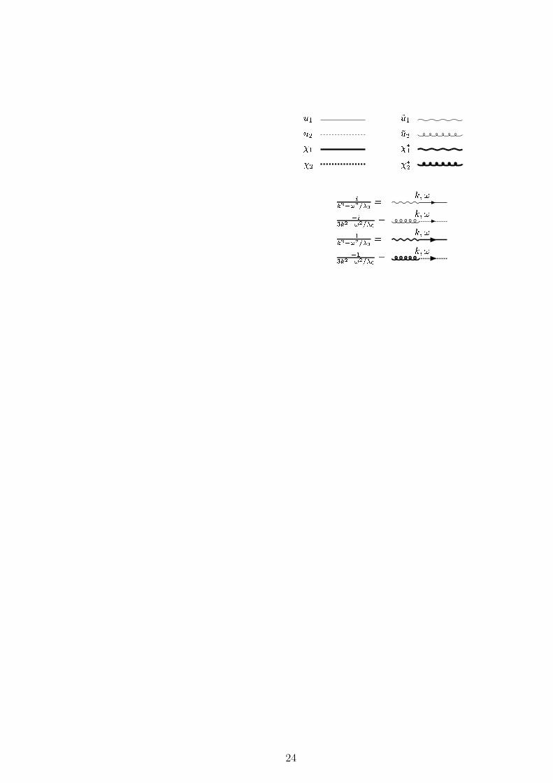
Figure 1: Graphical representation of the fields and the Feynman rules for the propagators.

24

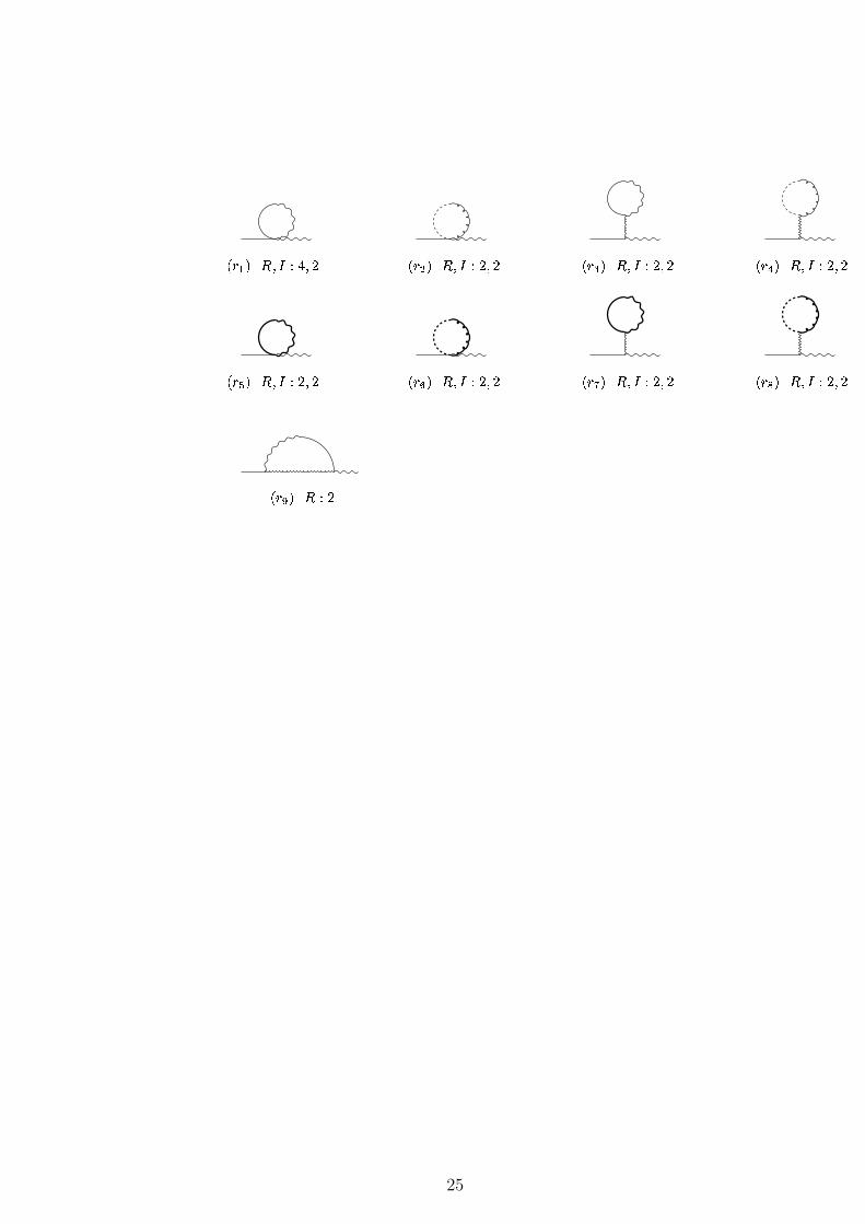
Figure 2: Feynman diagrams for renormalization of the kinetic term −iuR1 (−k)k2uR

1 (k) of

S0. They appear in the cumulant expansion to the lowest order. External legs are the slow

modes, while the internal fields are the fast modes, and the integration is done over the fast

modes. Those fields that cosist of loops can be real or imaginary, and are denoted by R and I,

respectively. The number of choices for the construction of each diagram is also shown. The

diagrams with long-range interactions (zigzag lines) are divergent, due to the zero momentum

carried by the zigzag lines, but such diagrams are canceled by the corresponding diagrams with

Grassmanian loops (thick lines). In fact, only r1 and r9 contribute.

25

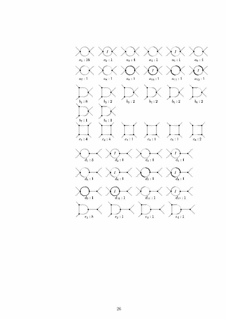
Figure 3: Feynman diagrams for the renormalization of uR1 (p1)u

R1 (p2)u

R1 (p3)u

R1 (p4) in the action.

The diagrams with loops of imaginary fields are indicated with I. The number of choices for

constructing each diagram is also given.

26

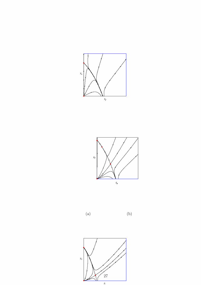
(a) (b)

(c) (d)

Figure 4: Renoemalization group flows for (a) ρ < 0.14; (b) 0.14 < ρ < 0.18; (c) 0.18 < ρ < 1,

and (d) ρ > 1.

27