Prog. Theor. Exp. Phys. 2012, 00000 (20 pages)DOI: 10.1093/ptep/0000000000

Fermionic Functional Renormalization GroupApproach to Superfluid Phase Transition

Yuya Tanizaki1,2,∗, Gergely Fejos2, and Tetsuo Hatsuda2,3

1Department of Physics, The University of Tokyo, Tokyo 113-0033, Japan2Theoretical Research Division, Nishina Center, RIKEN, Wako 351-0198, Japan3Kavli IPMU (WPI), The University of Tokyo, Chiba 277-8583, Japan∗E-mail: yuya.tanizaki@riken.jp

. . . . . . . . . . . . . . . . . . . . . . . . . . . . . . . . . . . . . . . . . . . . . . . . . . . . . . . . . . . . . . . . . . . . . . . . . . . . . . .A fermionic functional renormalization group (FRG) is applied to describe the super-fluid phase transition of the two-component fermionic system with attractive contactinteraction. The connection between the fermionic FRG approach and the conventionalBardeen-Cooper-Schrieffer (BCS) theory with Gorkov and Melik-Barkhudarov (GMB)correction are clarified in detail in the weak coupling region by using the renormalizationgroup flow of the fermionic four-point vertex with particle-particle and particle-hole scat-tering contributions. To go beyond the BCS+GMB theory, coupled FRG flow equationsof the fermion self-energy and the four-point vertex are studied under an Ansatz con-cerning their frequency/momentum dependence. We found that the fermion self-energyturns out to be substantial even in the weak couping region, and the frequency depen-dence of the four-point vertex is essential to obtain the correct asymptotic-ultravioletbehavior of the flow for the self-energy. The superfluid transition temperature and theassociated chemical potential are calculated in the region of negative scattering lengths.. . . . . . . . . . . . . . . . . . . . . . . . . . . . . . . . . . . . . . . . . . . . . . . . . . . . . . . . . . . . . . . . . . . . . . . . . . . . . . . . . . . . . . . . . . . . . .Subject Index A40, A63, B32, I22

1. Introduction

Superfluidity in many-fermion systems is one of the central problems in condensed mat-

ter, atomic, nuclear and particle physics. Examples include liquid superfluid 3He, electron

superconductivity, cold atoms, nucleon superfluidity, color superconductivity [1], and so on.

Among others, ultracold atomic gases play an important role in revealing the nature of

superfluidity from weak to strong couplings in a single physical system: inter atomic inter-

actions in dilute systems are rather simple and the strength of the interaction is tunable via

the Feshbach resonance technique [2]. The experimental discovery of the Bardeen-Cooper-

Schrieffer (BCS) to Bose-Einstein condensate (BEC) crossover in two-component fermionic

atoms [3–6] is a characteristic example of such a high level of control.

Two seemingly different kinds of superfluidity, BCS superfluid of weakly coupled fermions

and BEC of Bose gas, turned out to be the same phenomenon connected via a smooth

crossover for two-component fermionic systems. On the BCS side, weak attraction causes

pairing instability against the Fermi surface leading to the formation of Cooper pairs [7],

while on the BEC side, pairs of fermions form tightly-bound composite bosons and super-

fluidity occurs due to their condensation at low temperature. Furthermore, the crossover

between those two forms of superfluidity can be studied by combining the number equation

and the assumption of the ground state being a BCS pairing wave function [8–10].

c© The Author(s) 2012. Published by Oxford University Press on behalf of the Physical Society of Japan.

This is an Open Access article distributed under the terms of the Creative Commons Attribution License

(http://creativecommons.org/licenses/by-nc/3.0), which permits unrestricted use,

distribution, and reproduction in any medium, provided the original work is properly cited.

arX

iv:1

310.

5800

v3 [

cond

-mat

.qua

nt-g

as]

24

Apr

201

4

From a theoretical point of view, quantitative description of fermionic superfluidity in

the weak coupling limit requires not only the BCS theory but also its Gorkov and Melik-

Barkhudarov (GMB) correction [11, 12]. However, the BCS+GMB theory still ignores higher-

order many-body correlations which become important when the scattering length between

fermions (as) becomes large in the so-called unitary regime. This is the reason why various

non-perturbative techniques such as Monte Carlo simulations [13–17], ε-expansion [18], the

functional renormalization group (FRG) method with auxiliary bosonic field [19–23], and

the t-matrix approach [24–27] have been developed to attack the problems at and around

unitarity.

The purpose of this paper is to develop a fermionic FRG (f-FRG) method without

introducing the auxiliary bosonic field, not only to make a firm connection between the

non-perturbative FRG approach and the conventional BCS+GMB theory but also to go

beyond the BCS+GMB theory on a solid ground. First we will show how BCS+GMB the-

ory is obtained from the renormalization group (RG) flow of the fermionic four-point vertex

with particle-particle and particle-hole interactions, and then we explore the role of the RG

flow of the fermion self-energy to go beyond BCS+GMB theory. We note that such analyses

can be best achieved by fermionic FRG without introducing bosonic auxiliary fields. Com-

pared with the auxiliary field method, which contains ambiguities in how to introduce the

auxiliary field and usually requires a priori knowledge on the ground state property of the

system, fermionic FRG can provide systematic and unbiased study of interacting fermions

[28–31].

Throughout this paper, the main focus will be on the weak and intermediate coupling

regime, where as is negative. We will clarify the physical meaning of each approximation

of f-FRG, and give physical interpretations of our results, based on the analysis of the flow

equations in detail. Although our formalism itself is not limited to this regime, the case

of as > 0 is not accessible at the level of approximations in the present paper, as will be

discussed later. Nevertheless, we will extrapolate our results of the critical temperature and

associated chemical potential to the unitary regime to see their qualitative behavior.

The contents of this paper is as follows. In Sec. 2, we introduce fermionic FRG formalism

and explain how the critical temperature of the superfluid phase transition and the number

density of fermions is calculated. In Sec. 3, we construct approximate flow equations of

the effective coupling, which reproduce the results of the critical temperature of particle-

particle random phase approximation (i.e. BCS theory) and the GMB correction. In Sec. 4,

we concentrate on the flow equation of the self-energy correction, describing its problems

and their possible resolution. In Sec. 5, we solve the coupled flow equations numerically

and derive the self-energy correction, the critical temperature, and the associated chemical

potential. Sec.6 is devoted to summary and concluding remarks. The reader can find some

useful analytic formulas in the appendices.

2. Fermionic FRG Formalism

We consider non-relativistic two-component fermions ψ =

(ψ↑ψ↓

)with a contact interac-

tion:

S[ψ,ψ] =

∫ β

0dτ

∫d3x

[ψ

(∂τ −

∇2

2m− µ

)ψ + gψ↑ψ↓ψ↓ψ↑

], (1)

2/20

where β(= 1/T ), µ, m and g are the inverse temperature, the chemical potential, the mass

and the bare coupling constant, respectively. The action S can be written in momentum

space as

S[ψ,ψ] =

∫ (T )

pψ(p)G−1(p)ψ(p)

+ g

∫ (T )

pe−ip

00+

∫ (T )

q,q′ψ↑(p/2 + q)ψ↓(p/2− q)ψ↓(p/2− q′)ψ↑(p/2 + q′), (2)

where G−1(p) = ip0 + p2

2m − µ is the inverse propagator with p = (p0,p). Also, we adopt

an abbreviated notation,∫ (T )p ≡

∫ d3p(2π)3T

∑p0 . The factor exp(−ip00+) originates from

the normal ordering of fermionic operators in the interaction term. The classical action

(2) is symmetric under global U(1) phase rotation, SU(2) spin rotation, and space-time

translation.

Following the idea of the FRG method [32–34], we define a scale-dependent generating

functional Wk[η, η] by

exp(Wk[η, η]) =

∫DψDψ exp

[−(S[ψ,ψ] +

∫ (T )

pψ(p)Rk(p)ψ(p)

)+

∫ (T )

p

(η(p)ψ(p) + η(p)ψ(p)

)], (3)

where η and η are fermionic Grassmannian sources and Rk is an infrared (IR) regulator which

suppresses modes with momentum smaller than scale k. We require this function to satisfy

conditions Rk → 0 (+∞) as k → 0 (+∞). Then the scale-dependent one-particle-irreducible

(1PI) effective action Γk[ψ,ψ] is defined via Legendre transformation:

Γk[ψ,ψ] =

∫ (T )

p

(η(p)ψ(p) + η(p)ψ(p)

)−Wk[η, η]−

∫ (T )

pψ(p)Rk(p)ψ(p), (4)

where η, η in (4) are determined by inverting the relations δLWk/δη = ψ and δLWk/δη = ψ.

Here, we distinguish left and right derivatives via subscripts, δL and δR, respectively. Due to

the property of Rk, Γk→∞ reduces to the classical action S (up to a constant), while Γk=0

is the full 1PI quantum effective action Γ. Γk[ψ,ψ] obeys the flow equation [32–34]

∂kΓk[ψ,ψ] = −1

2Tr

[1

Γ(2)k [ψ,ψ] +Rk

∂kRk

], (5)

where the negative sign on the right-hand side can be interpreted as the result of a closed

fermionic loop, and Tr denotes the trace operation in both matrix and functional spaces

with

(Γ

(2)k [ψ,ψ] +Rk

)p,q

=

δLδRΓk[ψ,ψ]

δψ(p)δψ(q)

δLδRΓk[ψ,ψ]

δψ(p)δψ(q)δLδRΓk[ψ,ψ]

δψ(p)δψ(q)

δLδRΓk[ψ,ψ]

δψ(p)δψ(q)

+

(0 Rk(p)δp,q

−Rk(p)δp,q 0

).

(6)

Eq. (5) implies that the change of the 1PI effective action in terms of k is given by one-

loop Feynman diagrams with dressed Green functions, 1PI interaction vertices, and a single

3/20

insertion of a two-point vertex ∂kRk. Integrating (5) starting from a large enough but oth-

erwise arbitrary scale (denoted by ΛUV) down to k = 0, we can obtain Γ = Γk=0. Since we

can obtain the dressed fermion propagator and 1PI vertex functions, all information on

thermodynamics is available using fermionic FRG formalism.

To solve the flow equation (5), we consider the following vertex expansion of Γk:

Γk[ψ,ψ] =

∫ (T )

pψ(p)[G−1 − Σk](p)ψ(p)

+

∫ (T )

p,q,q′Γ

(4)k (p; q, q′)ψ↑(

p

2+ q)ψ↓(

p

2− q)ψ↓(

p

2− q′)ψ↑(

p

2+ q′) +O((ψψ)3),(7)

where Σk and Γ(4)k are the self-energy and the four-point vertex, respectively. In the following,

we truncate the expansion up to fourth order and study the flow equations of Σk and Γ(4)k

without the introduction of auxiliary bosonic fields. (We call such an approach a fermionic

FRG method or f-FRG method.) The critical temperature Tc of the superfluid transition

will always be obtained from the high temperature side, which means that we will work

in the normal phase. To study the superfluid phase below Tc, one needs to introduce an

explicit symmetry breaking term in the classical action. Otherwise, a second order phase

transition would occur in terms of k at a nonzero value (since the flow always crosses the

critical surface) leading to the divergence of the four-point function and the breakdown of

the flow equation [30, 35].

Let us now discuss the actual choice of the IR regulator Rk, which needs to suppress low-

energy excitations of the system properly. In the weak coupling regime, where fermions form

a Fermi sphere, Rk must suppress both particle and hole excitations around the Fermi level

defined through p2/2m = µ+ σ0: Here σ0 is a constant part of the self-energy Σ0 near the

Fermi sphere. A suitable regulator for this purpose is Litim’s optimized regulator [36] with

a self-energy term [22];∫ (T )

pψ(p)Rk(p)ψ(p) ≡

∫ (T )

pψ(p)

[ k2

2msgn(ξ(p))− ξ(p)

]θ( k2

2m− |ξ(p)|

)ψ(p), (8)

where ξ(p) ≡ p2

2m − µ− σ0 denotes the energy relative to the Fermi level. For a second-order

phase transition, the critical point T = Tc can be determined from the Thouless criterion [37]

by looking at the divergence of the fermion-fermion scattering matrix at the total momentum

p = 0. In our case, this reads [Γ

(4)k=0(p = 0)

]−1= 0 at T = Tc. (9)

Our primary goal is to calculate the ratios Tc/εF and µ/εF as a function of the dimension-

less constant 1/(kFas): Here as is the scattering length between fermions, kF ≡ (3π2n)1/3

with n being the fermion number density and εF ≡ k2F /2m = (3π2n)2/3/2m. Note that the

number density n is related to T and µ through the number equation:

n = 〈ψψ〉 = 2

∫ (T )

p

−1

G−1(p)− Σ0(p). (10)

3. BCS+GMB theory from fermionic FRG method

Taking the vertex expansion (7) of the scale dependent 1PI effective action Γk[ψ,ψ] up to

n = 2 and applying the flow equation (5), a closed set of equations for the self-energy and

4/20

∂kp = ∂k

p

l

∂k

p2+ q p

2− q

p2 + q′ p

2− q′

= ∂k

(p2 + q

p2 − q

p2 + l p

2 − l

p2 + q′ p

2 − q′

+∑± p

2 + q p2 − ql

l + q ± q′p2 ± q′p

2+q′ )

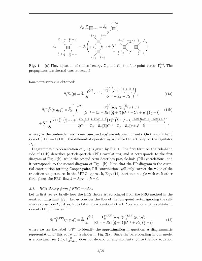
Fig. 1 (a) Flow equation of the self energy Σk and (b) the four-point vertex Γ(4)k . The

propagators are dressed ones at scale k.

four-point vertex is obtained:

∂kΣk(p) = ∂k

∫ (T )

le−il

00+Γ

(4)k

(p+ l; p−l2 , p−l2

)[G−1 − Σk +Rk](l)

, (11a)

−∂kΓ(4)k (p; q, q′) = ∂k

[∫ (T )

l

Γ(4)k (p; q, l)Γ

(4)k (p; l, q′)

[G−1 − Σk +Rk](p

2 + l)

[G−1 − Σk +Rk](p

2 − l) (11b)

+∑±

∫ (T )

l

Γ(4)k

(p2 + q + l; p/2+q−l

2 , p/2∓2q′−q−l2

)Γ

(4)k

(p2 ± q′ + l; −p/2+2q±q′+l

2 , −p/2∓q′+l

2

)2[G−1 − Σk +Rk](l)[G−1 − Σk +Rk](q ± q′ + l)

],

where p is the center-of-mass momentum, and q, q′ are relative momenta. On the right hand

side of (11a) and (11b), the differential operator ∂k is defined to act only on the regulator

Rk.

Diagrammatic representation of (11) is given by Fig. 1. The first term on the ride-hand

side of (11b) describes particle-particle (PP) correlations, and it corresponds to the first

diagram of Fig. 1(b), while the second term describes particle-hole (PH) correlations, and

it corresponds to the second diagram of Fig. 1(b). Note that the PP diagram is the essen-

tial contribution forming Cooper pairs, PH contributions will only correct the value of the

transition temperature. In the f-FRG approach, Eqs. (11) start to entangle with each other

throughout the FRG flow k = ΛUV → k = 0.

3.1. BCS theory from f-FRG method

Let us first review briefly how the BCS theory is reproduced from the FRG method in the

weak coupling limit [28]. Let us consider the flow of the four-point vertex ignoring the self-

energy correction Σk. Also, let us take into account only the PP correlation on the right-hand

side of (11b). Then we find

−∂kΓ(4,PP)k (p; q, q′) = ∂k

∫ (T )

l

Γ(4,PP)k (p; q, l)Γ

(4,PP)k (p; l, q′)

[G−1 +Rk](p

2 + l)

[G−1 +Rk](p

2 − l) , (12)

where we use the label “PP” to identify the approximation in question. A diagrammatic

representation of this equation is shown in Fig. 2(a). Since the bare coupling in our model

is a constant (see (1)), Γ(4)k=ΛUV

does not depend on any momenta. Since the flow equation

5/20

∂k

p2+ q p

2− q

p2 + q′ p

2− q′

= ∂k

p2 + q

p2 − q

p2 + l p

2 − l

p2 + q′ p

2 − q′

=

+

Fig. 2 (a) Flow equation for Γ(4)k (square vertex) restricted to the PP-channel without

self-energy corrections, and (b) standard PP-RPA with the bare coupling g denoted by the

point-vertex.

(12) does not have any explicit relative momentum dependence, it cannot be produced for

Γ(4,PP)k either. Therefore, at any k it is only a function of the center of mass momentum p,

and we can replace Γ(4,PP)k (p; q, l) by Γ

(4,PP)k (p). Eq. (12) can be rewritten as

∂k

(1

Γ(4,PP)k (p)

)= ∂k

∫ (T )

l

1

[G−1 +Rk](p2 + l)[G−1 +Rk](

p2 − l)

. (13)

Since in this approximation the entire k-dependence is due to the regulator, we have replaced

∂k on the right hand side by ∂k. This means that the flow equation can be integrated trivially

as

1

Γ(4,PP)k (p)

=1

Γ(4,PP)ΛUV

+

∫ (T )

|l|<ΛUV

1

[G−1 +Rk](p2 + l)[G−1 +Rk](

p2 − l)

− mΛUV

6π2. (14)

Taking k = 0 and defining 1g ≡ 1

Γ(4,PP)ΛUV

−mΛUV

6π2 , we end up with the standard BCS result above

Tc which corresponds to Fig. 2(b). Note that, the UV cutoff ΛUV in (14) can be removed by

the standard renormalization procedure Γ(4,PP)k=0 (0)|µ=0,T=0 = 4πas

m , which requires

(Γ(4,PP)ΛUV

)−1 =m

4πas−(∫ ΛUV

0

d3l

(2π3)

1

2l2/2m− mΛUV

6π2

)=

m

4πas− mΛUV

3π2. (15)

After renormalization, the Thouless criterion [Γ(4)k=0(p = 0)]−1

∣∣T=Tc

= 0 together with (14)

leads to the standard form

π

2|as|=

1

2

∫ ∞0

√2mεdε

[tanh ((ε− µ)/2Tc)

ε− µ − 1

ε

]. (16)

If we further take the weak coupling limit ((kFas)−1 → −∞) with µ = εF , (16) provides the

standard BCS result

TBCSc

εF≡ 8

πeγE−2e−π/2kF |as|. (17)

3.2. GMB correction from f-FRG method

Now we consider the particle-hole correlation (second term on the right hand side of Fig. 1)

in the flow equation of Γ(4)k . As reported in Ref. [20], this leads to the Gorkov and Melik-

Barkhudarov (GMB) correction [11]. The main aim of this subsection is to clarify the origin

of the GMB correction in detail and to analyze the approximations to be employed in a

6/20

precise way. Such an analysis is particularly useful for going beyond the BCS+GMB theory

in later sections.

In general, the four-point vertex function Γ(4)k (p; q, q′) depends not only on the center-

of-mass momentum p but also on relative momenta q and q′. If we restrict ourselves to

particle-particle correlations, the dependence on q and q′ disappears as we have shown in

the previous subsection. However, once we have particle-hole correlations, such a simplifi-

cation does not occur anymore. However, since we are interested in s-wave superfluidity,

instead of solving the full momentum dependence, we can consider the case |q| = |q′| = kFand take the s-wave projection averaged over the directions of q and q′: Γ

(4)k (p; q0, q′0) =∫ d2q

4πd2q′

4π Γ(4)k (p; q, q′)

∣∣∣|q|=|q′|=kF

. This is motivated by the fact that, for low energy single-

particle excitations are given by fermionic quasi-particles in the vicinity of the Fermi surface,

and q and q′ will be of the order of the Fermi momentum kF ≈√

2mµ with the loop momen-

tum l being also restricted to the region |l| ∼ kF due to the presence of the regulator Rk.

Finally, we define Γ(4)k (p) ≡ Γ

(4)k (p; 0, 0), so that Γ

(4)k (p = 0) can be regarded as the effective

coupling constant at scale k. The corresponding flow equation is given by

∂k

(1

Γ(4,PP+PH)k (0)

)= ∂k

∫ (T )

l

1

[G−1 +Rk](l)[G−1 +Rk](−l)

+∂k

∫{|q|=kF }

d2q

4π

d2q′

4π

∫ (T )

l

1

[G−1 +Rk](l)[G−1 +Rk](q − q′ + l), (18)

where we have used the label ”PP+PH” to identify the approximation taken here. Note that,

the angular integration of q and q′ still remain in the particle-hole contribution through the

regularized fermion propagator. Further discussions on the approximation adopted here are

given at the end of this subsection on the basis of the detailed flow pattern as a function of

k in the weak coupling regime.

Since both sides of (18) became total derivatives, it can be solved as

1

Γ(4,PP+PH)k (0)

=1

Γ(4,PP)k (0)

+

8mµ∫0

d|Q|28mµ

∫d3l

(2π)3

nF

((l+Q)2

2m − µ+Rk(l + Q))− nF

(l2

2m − µ+Rk(l))

((l+Q)2

2m − µ+Rk(l + Q))−(

l2

2m − µ+Rk(l)) , (19)

where Q ≡ q − q′ and nF is the Fermi-Dirac distribution function. The first term in the

right-hand side of (19) has already been evaluated in (14). Also, considering the fact that

the critical temperature Tc is much smaller than the Fermi energy εF in the weak coupling

regime, the second term in the right-hand side of (19) can be evaluated at T = 0 as

8mµ∫0

d|Q|28mµ

∫d3l

(2π)3

θ(

(l+Q)2

2m − µ)− θ

(l2

2m − µ)

((l+Q)2

2m − µ)−(

l2

2m − µ) = −1 + ln 4

3

mkF2π2

. (20)

Then we find that, at the end of the flow (k → 0), the particle-hole contribution simply shifts

the value of the inverse scattering length from as to aeffs :

1

aeffs

=1

as− 2kF

π

1 + ln 4

3. (21)

7/20

0

0.02

0.04

0.06

0.08

0.1

0 0.5 1 1.5 2 2.5

-∂k(

Γ k(4

) )-1/2

m

k/√ 2 mµ

PP flowPP+PH flow

Fig. 3 Derivative of 1/Γ(4)k (0) at Tc/µ = 0.06 (which corresponds to (|kFas|)−1 ∼ O(1))

with and without the PH loop included. The figure shows that only when k ∼ kF ≈√

2mµ,

particle-hole fluctuations change the behavior of the flow.

k2/2m� πTc πTc � k2/2m� k2F /2m k2/2m� k2

F /2m

PP O(kFk5/T 3

c ) O(kF /k) O(1)

PH O(k5/kFT2c ) O(k/kF ) O(k3

F /k3)

Table 1 Contributions from the particle-particle (PP) correlation and the particle-hole

(PH) correlation to ∂k(Γ(4)k (0))−1 in the right-hand side of Eq. (18). This behavior is

consistent with that of the prediction from Shanker’s RG analysis [28].

Therefore, taking into account the correction coming from PH correlations, the BCS critical

temperature in the weak coupling regime is corrected as

TGMBc

εF=

1

(4e)1/3· T

BCSc

εF. (22)

This is exactly the Gorkov and Melik-Barkhudarov result[11, 12], showing the reduction of

Tc due to the effect of order parameter fluctuations in agreement with previous FRG studies

as well [20].

8/20

Let us now discuss the structure of the flow equation (18) in more detail to gain a deeper

understanding of why exactly the GMB result was reproduced from f-FRG within the above

approximation. The parametric k-dependence of the first term (particle-particle correlation)

and the second term (particle-hole correlation) of the right-hand side of (18) are summarized

in Table 1 (the corresponding explicit formulas are given in B). We mention here that PH

contribution has opposite sign to the PP contribution. From Table 1, we observe that PH

contribution is much smaller than the PP contribution in the high-energy region (k � kF )

and the low-energy region (k � kF ). 1 Only for k ' kF do the PH and PP contributions

become comparable. Such a behavior can be seen explicitly in Fig. 3, where numerical solu-

tions of ∂k(Γ(4)k (0))−1 with and without the PH correlation are plotted. The figure shows

that the screening of the effective coupling from the PH correlation takes place only around

k ∼ kF . This implies that we can neglect the momentum dependence of Γ(4)k in the PH con-

tribution, at least for weak couplings, where we have the hierarchy 1/as � kF � Tc/kF . In

such a regime, 1/Γ(4)k is O(1/as) around k ∼ kF , therefore the momentum dependence of Γ

(4)k

in the PH contribution is negligible. Although such a justification is questionable beyond

the weak coupling limit, we will later adopt this approximation as a working hypothesis to

make a qualitative study towards the unitary regime.

For later purposes, we show here the structure of Γ(4,PP+PH)k as a function of the center-of-

mass momentum p for large values of the flow parameter k. In such an asymptotic regime,

PP correlation is the dominant contribution as discussed above. Therefore, (14) leads to

1

Γ(4,PP+PH)k (p)

k→∞−−−→ − 2m

6π2

[k − 3π

4as+

2m

k

(ip0 +

p2

4m− 3

2µ

)]. (23)

4. f-FRG with fermion self-energy

So far, we have not taken into account the effect of the self-energy correction Σk in the

flow equations. Since σk (the constant part of Σk near the Fermi sphere) gives a shift of

the chemical potential µ→ µk ≡ µ+ σk, its importance grows as the system approaches the

unitary regime. In the following, we focus only on the lowest Matsubara frequency part of

Σk and define σk as its real part: σk ≡ <Σk(±πT,0). We note that even with the present

(constant) self-energy, non-trivial resummation of the original perturbative series occurs via

the self-consistent nature of the coupled flow equations, and therefore it is a good starting

point for analysing the role of the self-energy going beyond BCS+GMB theory. In this section

we first will study the behavior of σk for asymptotically large k, and formulate coupled flow

equations of σk and Γ(4)k , an then proceed to perform a numerical solution of them.

4.1. Asymptotic behavior of the self-energy at large k

Within the momentum independent vertex discussed in the previous section, using (11a),

the constant part of the self-energy near the Fermi sphere (i.e. σk), satisfies

∂kσk = ∂k

∫ (T )

l

Γ(4)k (0)

G−1(l)− σk +Rk(l), (24)

1 The behavior of these terms in f-FRG method are qualitatively consistent with the Shankar’s RGanalysis of interacting fermions [28].

9/20

which can be rewritten using an effective Fermi level µk = µ+ σk as

∂kµk = −(2m)1/2kΓ(4)k (0)

3π2

[((µ0 + k2/2m)3/2 − (µ0)3/2

)n′F (ω+)

−(

(µ0)3/2 −<(µ0 − k2/2m)3/2)n′F (ω−)

], (25)

where ω± = ±k2/2m+ µ0 − µk, and nF is the Fermi-Dirac distribution function. By taking

k →∞ (note that kas can take any negative values) and using the asymptotic form of Γ(4)k (0)

given in (23), one finds

σk = e−k2/2mT

(k2/2m

1− 3π/4kas+O(1)

). (26)

This asymptotic behavior is, however, not correct as can be seen from the following argu-

ment. First of all, the present theory is asymptotically free in the sense that Γ(4)k (0) '

−(3π2)/(m(k − 3π/4as)) for large k as obtained from (23). Then, since perturbative analysis

is valid for large k, we can evaluate σk for large k as

σk ' <∫ (T )

l

Γ(4)k (p+ l)e−il

00+

i(p0 + l0) + l2

2m − µ+Rk(l), (27)

where p0 = ±πT . Taking into account the correct leading-order frequency dependence as

Γ(4)k (l) ' − (3π2k/2m2)

(il0 + k2/2m− 3πk/8mas)and carrying out the integral, one finds

σk = <∫ (T )

l

e−il00+

il0 + l2

2m − µ+Rk(l)

−3π2k/2m2

i(p0 + l0) + k2/2m− 3πk/8mas

'√

2m(µ+ σ0)3/2

2k(1− 3π/8kas), (28)

where we omitted the spatial-momentum dependence of Γk(p+ l) giving only subleading

contributions. Thus we observe that σk must decrease as 1/k, unlike (26). Another way to

see the problem of (26) is that the number density nk = 〈ψψ〉 for large k simply vanishes

contrary to the true behavior expected from the lowest-order perturbation at large k; nk →(2mµ0

)3/2/(3π2).

4.2. Coupled flow equations for self-energy and 4-point vertex

From the discussion of the previous subsection, we see that the momentum dependence of

Γ(4)k , especially its frequency dependence, is essential to determine σk in the f-FRG approach.

To study such a frequency dependence by avoiding the quite demanding numerical calcula-

tion of solving the coupled flow-equation of Σk and Γk with full momentum dependence, we

adopt a hybrid approach described below as a first step, in order to explore the effect of the

self-energy.

10/20

Let us start with the following coupled equations;

∂kσk = <∂k∫ (T )

l

Γ(4)k (±πT + l0, l)

G−1(l)− σk +Rk(l), (29)

∂kΓ(4)−1k (0) = ∂k

∫ (T )

l

1

[G−1(l)− σk +Rk(l)][G−1(−l)− σk +Rk(−l)]

+ ∂k

8mµ∫0

d|Q|28mµ

∫ (T )

l

1

[G−1 − σk +Rk](l)[G−1 − σk +Rk](Q+ l), (30)

with Q = (0,Q). In (29), the frequency of the fermion self-energy is restricted to the lowest

values ±πT . After performing the Matsubara sum, σk and σ0 appear as a combination σ0 −σk (= µ0 − µk). Since the approximate particle-hole symmetry would make this combination

small for k < kF where PH contribution is already not significant, we take σk = σ0 in the

actual calculation of the PH contribution.

To take into account the momentum dependence in a minimal, but sufficient way we make

the following expansion and keep first few terms:

Γ(4)−1k (p0 + l0, l) ≈ −Z−1

k

[i(l0 + p0) + S

(1)k · |l|+ S

(2)k · l2 + |µBk |

], (31)

where we have introduced the notations

Z−1k = i∂l0Γ

(4)−1k (0), |µBk | = −ZkΓ

(4)−1k (0),

S(1)k = −Zk∂|l|Γ(4)−1

k (0), S(2)k = −Zk∂|l|2Γ

(4)−1k (0). (32)

Now we adopt a hybrid approach in which Γ−1k (0) is calculated from the flow equation,

while its derivatives with respect to the frequency and momentum are estimated by the RPA

analysis in the particle-particle channel given in Appendix A. After applying the expansion

(31), the flow equation for the self-energy becomes

∂kσk = <∂k∫ (T )

l

1

G−1(l)− σk +Rk(l)

−Zki(l0 ± πT ) + S

(1)k |l|+ S2

kl2 + |µBk |

(33)

= −<∂k∫ ∞

0

dll2

2π2

(nB(ωBk (l)) + nF (ωk(l))

) Zkωk(l)− ωBk (l)∓ iπT , (34)

where ωk(l) = l2

2m − µk +Rk(l), and ωBk (l) = |µBk |+ S(1)k |l|+ S

(2)k l2, with nB being the Bose-

Einstein distribution function.

This formula shows the importance of the momentum dependence of Γ(4)k as well as its

correct boundary condition in the frequency space. Due to these, bosonic (Cooper pair)

contributions appeared in the flow equation of the self-energy. We note that a peculiar

linear term in ωBk (l) is only due to the presence of the regulator, and one can show that it

disappears at k = 0. After performing the ∂k differentiation, we obtain the following coupled

11/20

flow equations:

∂kµk = − k

2m

√2mµ0+k2∫√

2mµ0

dl

π2l2Zk<

[∂ωnF (ωk+)

ωk+ − ωBk (l)∓ iπT −nB(ωBk (l)) + nF (ωk+)

(ωk+ − ωBk (l)∓ iπT )2

]

+k

2m

√2mµ0∫

<√

2mµ0−k2

dl

π2l2Zk<

[∂ωnF (ωk−)

ωk− − ωBk (l)∓ iπT −nB(ωBk (l)) + nF (ωk−)

(ωk− − ωBk (l)∓ iπT )2

], (35a)

∂kΓ(4)−1k =

(2m)1/2k

3π2

(− 1

2ω2+

+nF (ω+)

ω2+

− n′F (ω+)

ω+

)((µ0 + k2/2m)3/2 − (µ0)3/2

)−(2m)1/2k

3π2

(− 1

2ω2−

+nF (ω−)

ω2−− n′F (ω−)

ω−

)((µ0)3/2 −<(µ0 − k2/2m)3/2

)

+∂k

8mµ∫0

d|Q|28mµ

∫d3l

(2π)3

nF

((l)2

2m +Rk(l)− µk)− nF

((l+Q)2

2m +Rk(l + Q)− µk)

(l)2/2m+Rk(l)− (l + Q)2/2m−Rk(l + Q), (35b)

where ωk± = ±k2/2m+ µ0 − µk. The effective Fermi level µk starts to flow from the chemical

potential at k =∞, µk=∞ = µ, and converges to µ0 = µ+ σ0. Because of the appearance of

bosonic (Cooper pair) contributions to the flow equation for µk = µ+ σk, (35a) indeed shows

the correct asymptotic behavior at large k consistent with the discussion in the previous

subsection:

∂kµk = −√

2mµ3/20

2(k − 3π/8as)2+O(1/k4) =⇒ σk =

√2m(µ+ σ0)3/2

2k(1− 3π/8kas)+O(1/k3). (36)

5. Numerical Results

Now we are ready to solve (35a) and (35b) together with the number equation, (10). In order

to get the transition temperature Tc, one may start from a large k at the UV cutoff scale,

and let the flow equations run towards k = 0. Then Tc is obtained through the Thouless

criterion, Γ(4)−1k=0 (0) = 0, while the chemical potential µ and the number density n are related

via the number equation (10). However, the actual numerical calculation is much more

efficient by starting from k = 0 with Γ(4)−1k=0 (0) = 0 and letting the flow towards large k.

Keeping the temperature on a certain value and choosing µ = 1, the flow of σk and Γ(4)−1k

are numerically obtained on a grid with a step size of ∆k = 10−4. Then we fit these quantities

by their known asymptotic behavior for large k to determine σk=∞ and Γ(4)k=∞. We choose

the highest scale to be kUV = 50.0 and fit the functions in the interval [49.0, 50.0]. After

subtracting the “divergent” −mk/3π2 piece in (23), Γ(4)−1k=∞ should be equal to m/4πas, from

which we obtain the function as = as(Tc). Since the self-energy always has to approach zero

at large k, a unique solution is obtained by adjusting σk=0 this way.

Even after taking into account the self-energy correction, we found numerically that the

flow of the four-point vertex Γ(4)k shows a qualitatively similar behavior to the PP+PH

flow shown in Fig. 3. Also, the scalings with respect to flow parameter k are the same as

those given in Table 1. Therefore, we can safely use the Thouless criterion (9) to determine

the critical temperature of the superfluid transition without singular behavior of the flow

12/20

-0.09

-0.08

-0.07

-0.06

-0.05

-0.04

-0.03

-0.02

-0.01

0

0 1 2 3 4 5

(Γk(4

) )-1/2

m√2

mµ

k/√ 2 mµ

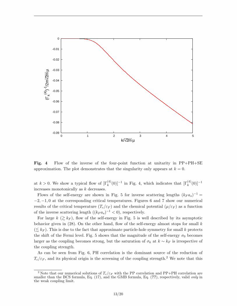
Fig. 4 Flow of the inverse of the four-point function at unitarity in PP+PH+SE

approximation. The plot demonstrates that the singularity only appears at k = 0.

at k > 0. We show a typical flow of [Γ(4)k (0)]−1 in Fig. 4, which indicates that [Γ

(4)k (0)]−1

increases monotonically as k decreases.

Flows of the self-energy are shown in Fig. 5 for inverse scattering lengths (kFas)−1 =

−2,−1, 0 at the corresponding critical temperatures. Figures 6 and 7 show our numerical

results of the critical temperature (Tc/εF ) and the chemical potential (µ/εF ) as a function

of the inverse scattering length ((kFas)−1 < 0), respectively.

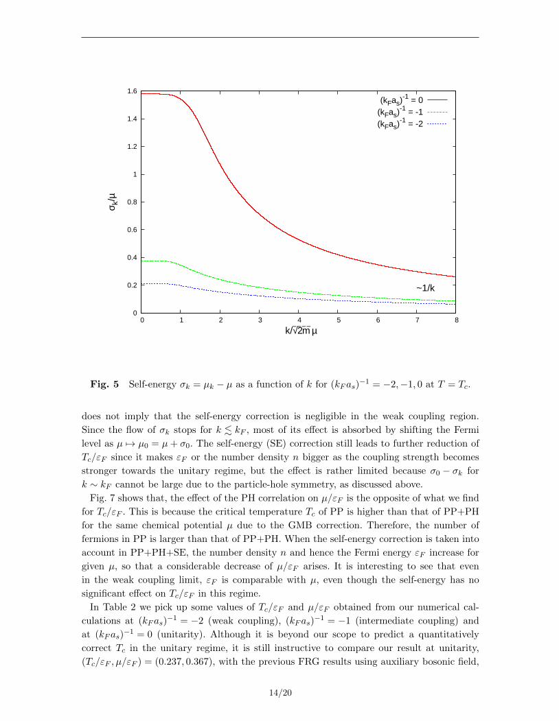
For large k (& kF ), flow of the self-energy in Fig. 5 is well described by its asymptotic

behavior given in (28). On the other hand, flow of the self-energy almost stops for small k

(. kF ). This is due to the fact that approximate particle-hole symmetry for small k protects

the shift of the Fermi level. Fig. 5 shows that the magnitude of the self-energy σ0 becomes

larger as the coupling becomes strong, but the saturation of σk at k ∼ kF is irrespective of

the coupling strength.

As can be seen from Fig. 6, PH correlation is the dominant source of the reduction of

Tc/εF , and its physical origin is the screening of the coupling strength.2 We note that this

2 Note that our numerical solutions of Tc/εF with the PP correlation and PP+PH correlation aresmaller than the BCS formula, Eq. (17), and the GMB formula, Eq. (??), respectively, valid only inthe weak coupling limit.

13/20

0

0.2

0.4

0.6

0.8

1

1.2

1.4

1.6

0 1 2 3 4 5 6 7 8

σ k/µ

k/√ 2 mµ

~1/k

(kFas)-1 = 0

(kFas)-1 = -1

(kFas)-1 = -2

Fig. 5 Self-energy σk = µk − µ as a function of k for (kFas)−1 = −2,−1, 0 at T = Tc.

does not imply that the self-energy correction is negligible in the weak coupling region.

Since the flow of σk stops for k . kF , most of its effect is absorbed by shifting the Fermi

level as µ 7→ µ0 = µ+ σ0. The self-energy (SE) correction still leads to further reduction of

Tc/εF since it makes εF or the number density n bigger as the coupling strength becomes

stronger towards the unitary regime, but the effect is rather limited because σ0 − σk for

k ∼ kF cannot be large due to the particle-hole symmetry, as discussed above.

Fig. 7 shows that, the effect of the PH correlation on µ/εF is the opposite of what we find

for Tc/εF . This is because the critical temperature Tc of PP is higher than that of PP+PH

for the same chemical potential µ due to the GMB correction. Therefore, the number of

fermions in PP is larger than that of PP+PH. When the self-energy correction is taken into

account in PP+PH+SE, the number density n and hence the Fermi energy εF increase for

given µ, so that a considerable decrease of µ/εF arises. It is interesting to see that even

in the weak coupling limit, εF is comparable with µ, even though the self-energy has no

significant effect on Tc/εF in this regime.

In Table 2 we pick up some values of Tc/εF and µ/εF obtained from our numerical cal-

culations at (kFas)−1 = −2 (weak coupling), (kFas)

−1 = −1 (intermediate coupling) and

at (kFas)−1 = 0 (unitarity). Although it is beyond our scope to predict a quantitatively

correct Tc in the unitary regime, it is still instructive to compare our result at unitarity,

(Tc/εF , µ/εF ) = (0.237, 0.367), with the previous FRG results using auxiliary bosonic field,

14/20

0

0.05

0.1

0.15

0.2

0.25

0.3

0.35

0.4

0.45

0.5

-1.4 -1.2 -1 -0.8 -0.6 -0.4 -0.2 0

Tc/

ε F

1/(kFas)

PP PP+PH

PP+PH+SE

Fig. 6 Tc/εF as a function of the dimensionless scattering strength, (kFas)−1, in

different levels of approximation: PP (particle-particle correlation only), PP+PH (particle-

particle and particle-hole correlation without self-energy), PP+PH+SE (particle-particle

and particle-hole correlation with self-energy).

Tc/εF µ/εF

(kFas)−1 −2 −1 0 −2 −1 0

PP 0.027 0.126 0.496 1 0.987 0.747

PP+PH 0.012 0.058 0.276 1 0.997 0.929

PP+PH+SE 0.012 0.053 0.237 0.828 0.713 0.367

Table 2 Numerical values of Tc/εF and µ/εF at (kFas)−1 = −2, −1, and 0 in different

levels of approximation. The meaning of PP, PP+PH and PP+PH+SE are the same as

those in Fig. 6.

(Tc/εF , µ/εF ) ' (0.264, 0.68) [20], ' (0.276, 0.63) [21], ' (0.248, 0.51) [22, 23], and with the

results of the t-matrix approach, Tc/εF ' 0.16 [26], and Tc/εF ' 0.217 [27, 38]. Note that

quantum Monte Carlo simulations[13–17] for Tc/εF vary in the range 0.15−0.3.

15/20

0.3

0.4

0.5

0.6

0.7

0.8

0.9

1

-2 -1.5 -1 -0.5 0

µ/ε F

1/(kFas)

PP+PH PP

PP+PH+SE

Fig. 7 µ(Tc)/εF as a function of the dimensionless scattering strength, (kFas)−1. The

meaning of each line is the same as in Fig.6.

6. Summary and Concluding Remarks

We developed a fermionic FRG (f-FRG) method with a modified Litim’s regulator to describe

the superfluid phase transition for two-component fermions with a contact interaction. By

making vertex expansion of the 1PI effective action Γk[ψ, ψ] up to the four-point vertex and

solving the RG flow equation, we determined the critical temperature Tc in the regime of

negative scattering lengths using the Thouless criterion [Γ(4)k=0(p = 0)]−1 = 0.

In order to clarify the relation between the FRG approach and the conventional many-body

theory such as the BCS theory + GMB correction, we have taken into account the particle-

particle correlation, the particle-hole correlation and the self-energy correction step by step

in the flow equations. In agreement with the literature, we saw that the flow equation with a

single PP correlation reduces to the BCS theory, and we have also found that equipped with

the PH correlation in the flow equation, a momentum-independent vertex approximation

precisely reproduces the GMB correction. The major part of the PH contribution originated

from the region k ∼ kF .

To go beyond the BCS+GMB theory in our framework, we considered the flow of the

constant part of the self-energy σk, together with the flow of the 4-point vertex Γ(4)k (p = 0).

We found that the self-energy decreases slowly as σk ∼ 1/(k − 3π/(8as)) for k →∞, while it

16/20

saturates as σk ∼ σ0 for k (. kF ) due to approximate particle-hole symmetry. We also carried

out a numerical calculation with a hybrid approach, in which Γ(4)k (p = 0) is determined from

the flow equation, while the p-dependent part of Γ(4)k (p) necessary to reproduce correct

asymptotic behavior of σk is evaluated using PP-RPA. Resultant value of Tc/εF does not

receive large correction from the self-energy except for the unitary regime (1/(kFas)→ 0).

On the other hand, µ/εF shows a large reduction by the self-energy correction due to the

increase of the Fermi energy given µ even for relatively weak-coupling region (kFas)−1 . −1.

Extrapolation to unitarity gives Tc/εF = 0.237 and µ/εF = 0.367.

We note that the approximations employed in the present paper, particularly the assump-

tion of constant self-energy, is valid only in the regime 1/(kFas) < 0. To enter into the BEC

side (1/(kFas) > 0), momentum-dependent self-energy is crucial in f-FRG method, since it

provides the information of composite bosons in the number equation. Therefore, solving the

flow equations with momentum-dependent self-energy is one of the important problems to

be studied in the future. More sophisticated treatments could also be employed, e.g. the use

of the two-particle-irreducible (2PI) formalism [39–41] combined with the f-FRG method is

expected to be an efficient way to describe the superfluid phase transition, with its power

of resumming an even wider class of Feynman diagrams. Another direction to study the

superfluid phase transition is to consider f-FRG with an IR regulator in the fermion vertex

[42], which enables to treat the nontrivial momentum dependence of the fermion self-energy.

These methods may open new ways for unbiased studies of the BCS-BEC crossover in the

future by extending the f-FRG approach given in the present paper.

Acknowledgements

Y. T. is supported by JSPS Research Fellowships for Young Scientists. G. F. is supported

by the Foreign Postdoctoral Research program of RIKEN. T. H. is partially supported by

RIKEN iTHES project. This work was partially supported by the Program for Leading

Graduate Schools, MEXT, Japan.

A. RPA results for the vertex function at finite k

In this appendix, we show the results of the four-point vertex function in particle-particle

RPA (PP-RPA). According to (14), the basic equation is given by

1

Γ(4,PP)k (p)

=1

g+

∫{|l|<ΛUV}

d3l

(2π)3

1−∑± nF ((p2 ± l)2 − µ+Rk(p2 ± l)

)ip0 +

∑±{

(p2 ± l)2 − µ+Rk(p2 ± l)

} , (A1)

where we take 2m = 1 for simplicity, and g is the bare coupling constant, as we indicated

after (14). We consider the expansion given in (31) with the parameterization denoted as

Γ(4,PP)k (p) = − Zk

ip0 + S(1)k |p|+ S

(2)k p2 + |µBk |

, (A2)

where parameters Zk, S(1)k , S

(2)k , and |µBk | are positive.

Let us first consider Zk, which may be regarded as the wave function renormalization

constant of Cooper pairs. According to (A2), we obtain,

Z−1k = −∂Γ

(4,PP)−1k

∂(ip0)(0) =

∫d3l

(2π)3

1− 2nF (l2 − µ+Rk(l))

[2(l2 − µ+Rk(l))]2. (A3)

17/20

Using the notation k2± = ±k2 + µ, we find that

Z−1k =

1

8π2

[1

2

(k+

k2+ − µ

+1õ

tanh−1

õ

k+

)+k3

+ −√µ3

3

1− 2nF (k2+ − µ)

(k2+ − µ)2

−1

2<(

k−k2− − µ

+1õ

tanh−1 k−√µ

)+

√µ3 −<k3

−3

1− 2nF (k2− − µ)

(k2− − µ)2

−2

(∫ <k−0

+

∫ ∞k+

)l2dl

nF (l2 − µ)

(l2 − µ)2

]. (A4)

According to the expression (A4), asymptotic behavior of Zk in the large k limit is given by

Z−1k =

1

6π2k+

(1 +

µ

k2+

)+O(1/k4). (A5)

In order to get the spatial momentum dependence of the four-point function, we must per-

form the integration (A1) with great care concerning the singularities associated with the

IR regulator. The coefficient of the |p|-linear term is given by

S(1)k =

µZk8π2

(tanh β

2k2

k2− β/2

cosh2 β2k

2

). (A6)

This term originates from the discontinuity of the regulator Rk(l) at |l| = õ, and it vanishes

at k = 0. As for the quadratic term in p, we find that

S(2)k =

Zk16π2

[1

2

(k+

k2+ − µ

+1õ

tanh−1

õ

k+

)+k3

+

3

1− 2nF (k2+ − µ)

(k2+ − µ)2

+2

3

k3+n′F (k2

+ − µ)

k2+ − µ

− 1

2

( <k−k2− − µ

+1õ

tanh−1 <k−√µ

)

+2

(∫ <k−0

+

∫ ∞k+

)l2dl

(−nF (l2 − µ)

(l2 − µ)2+n′F (l2 − µ) + 2

3 l2n′′F (l2 − µ)

l2 − µ

)

−<k3−

3

(2n′F (k2

− − µ)

k2− − µ

+1− 2nF (k2

− − µ)

(k2− − µ)2

)]. (A7)

The large-k behavior of this quantity reads as

S(2)k =

1

2+µ3/2

4k3+O(1/k5), (A8)

which implies that the effective mass of the two-particle resonance is nothing but twice of

the fermion mass, if k is sufficiently large.

Although we are not using the PP-RPA estimate of |µBk | in the text, we show it here for

the sake of completeness:

|µBk | = Zk

[1

8πas+

∫d3l

(2π)3

(1− 2nF (l2 − µ+Rk(l))

2(l2 − µ+Rk(l))− 1

2l2

)], (A9)

whose large-k asymptotic behavior is given by

µBk = k2 − µ− 3π

4as

√k2 + µ+O(1/k). (A10)

18/20

B. Asymptotic behavior of the PP and PH contributions

Here we list the analytic formulas for the asymptotic k behavior of the right-hand side of

(18). Considering the k-derivative of the inverse coupling, ∂k(1/Γ(4)k ), the first term in the

right-hand side of (18), the PP contribution, reads

∂k

∫ (T )

l

1

[G−1 +Rk](l)[G−1 +Rk](−l)

'

−(m

3π2+m

2π

k2F

k2

), (k2/2m� k2

F /2m,πT ),

−mπ2

kFk, (πT � k2/2m� k2

F /2km),

− kF96π2m2T 3

k5, (k2/2m� k2F /2m,πT ),

(B1)

with k2F = 2mµ. The second term in the right-hand side of (18), the PH contribution, reads

∂k

∫d2q

4π

d2q′

4π

∫ (T )

l

1

[G−1 +Rk](l)[G−1 +Rk](q − q′ + l)

'

8m

15π2

k3F

k3, (k2/2m� k2

F /2m,πT ),

3m

4π2

k

kF, (πT � k2/2m� k2

F /2m),

f(T/µ)

2π5mkFT 2k5, (k2/2m� k2

F /2m,πT ),

(B2)

where f(x) is given by

f(x) =

∞∑n=1

1

(2n− 1)3

[∫ 2

0dQ

(π − tan−1 (2n− 1)πx

1− (Q− 1)2− tan−1 (2n− 1)πx

(Q+ 1)2 − 1

)

+(2n− 1)πx

16ln

(1 +

(8

(2n− 1)πx

)2)]

. (B3)

References

[1] Leon N. Cooper, BCS: 50 Years, (World Scientific Publishing Company, 1 edition, 6 2010).[2] M. Randeria and E. Taylor (2013).[3] M. Greiner, C.A. Regal, and D.S. Jin, Nature, 426(6966), 537–540 (2003).[4] M. W. Zwierlein, C. A. Stan, C. H. Schunck, S. M. F. Raupach, S. Gupta, Z. Hadzibabic, and

W. Ketterle, Phys. Rev. Lett., 91, 250401 (Dec 2003).[5] C. A. Regal, M. Greiner, and D. S. Jin, Phys. Rev. Lett., 92, 040403 (Jan 2004).[6] M. W. Zwierlein, C. A. Stan, C. H. Schunck, S. M. F. Raupach, A. J. Kerman, and W. Ketterle, Phys.

Rev. Lett., 92, 120403 (Mar 2004).[7] J. Bardeen, L. N. Cooper, and J. R. Schrieffer, Phys. Rev., 108, 1175–1204 (Dec 1957).[8] D. M. Eagles, Phys. Rev., 186, 456–463 (Oct 1969).[9] A. Leggett, Diatomic molecules and cooper pairs, In Modern Trends in the Theory of Condensed

Matter, volume 115 of Lecture Notes in Physics, pages 13–27. Springer Berlin Heidelberg (1980).[10] P. Nozieres and S. Schmitt-Rink, Journal of Low Temperature Physics, 59(3), 195–211 (1985).[11] LP Gorkov and TK Melik-Barkhudarov, Sov. Phys. JETP, 13(5), 1018 (1961).[12] H. Heiselberg, C. J. Pethick, H. Smith, and L. Viverit, Phys. Rev. Lett., 85, 2418–2421 (Sep 2000).[13] Evgeni Burovski, Nikolay Prokof’ev, Boris Svistunov, and Matthias Troyer, Phys. Rev. Lett., 96, 160402

(Apr 2006).

19/20

[14] Evgeni Burovski, Evgeny Kozik, Nikolay Prokof’ev, Boris Svistunov, and Matthias Troyer, Phys. Rev.Lett., 101, 090402 (Aug 2008).

[15] Piotr Magierski, Gabriel Wlaz lowski, Aurel Bulgac, and J. E. Drut, Phys. Rev. Lett., 103, 210403 (Nov2009).

[16] Olga Goulko and Matthew Wingate, Phys. Rev. A, 82, 053621 (Nov 2010).[17] Vamsi K. Akkineni, D. M. Ceperley, and Nandini Trivedi, Phys. Rev. B, 76, 165116 (Oct 2007).[18] Yusuke Nishida, Phys. Rev. A, 75, 063618 (Jun 2007).[19] Michael C Birse, Boris Krippa, Judith A McGovern, and Niels R Walet, Physics Letters B, 605(3),

287–294 (2005).[20] S. Floerchinger, M. Scherer, S. Diehl, and C. Wetterich, Phys. Rev. B, 78, 174528 (Nov 2008).[21] S. Diehl, S. Floerchinger, H. Gies, J.M. Pawlowkski, and C. Wetterich, Annalen der Physik, 522(9),

615–656 (2010).[22] S. Floerchinger, M. M. Scherer, and C. Wetterich, Phys. Rev. A, 81, 063619 (Jun 2010).[23] M. M. Scherer, S. Floerchinger, and H. Gies (2010).[24] R. Haussmann, Zeitschrift fur Physik B Condensed Matter, 91(3), 291–308 (1993).[25] R. Haussmann, Phys. Rev. B, 49, 12975–12983 (May 1994).[26] R. Haussmann, W. Rantner, S. Cerrito, and W. Zwerger, Phys. Rev. A, 75, 023610 (Feb 2007).[27] Q. Chen, arXiv:1109.2307 (2011).[28] R. Shankar, Reviews of Modern Physics, 66(1), 129 (1994).[29] M. Salmhofer and C. Honerkamp, Prog.Theor.Phys., 105, 1–35 (2001).[30] Walter Metzner, Manfred Salmhofer, Carsten Honerkamp, Volker Meden, and Kurt Schonhammer, Rev.

Mod. Phys., 84, 299–352 (Mar 2012).[31] Andreas Eberlein and Walter Metzner, Phys. Rev. B, 87, 174523 (May 2013).[32] C. Wetterich, Physics Letters B, 301(1), 90–94 (1993).[33] Tim R. Morris, International Journal of Modern Physics A, 9(14), 2411–2450 (1994).[34] U. Ellwanger, Zeitschrift fur Physik C Particles and Fields, 62(3), 503–510 (1994).[35] Manfred Salmhofer, Carsten Honerkamp, Walter Metzner, and Oliver Lauscher, Progress of Theoretical

Physics, 112, 943–970 (2004).[36] D.F. Litim, Physics Letters B, 486(1-2), 92–99 (2000).[37] D.J. Thouless, Annals of Physics, 10(4), 553–588 (1960).[38] Qijin Chen, Phys. Rev. A, 86, 023610 (Aug 2012).[39] C. Wetterich, Phys. Rev. B, 75, 085102 (Feb 2007).[40] J. Polonyi and K. Sailer, Phys. Rev. D, 71, 025010 (Jan 2005).[41] N. Dupuis, The European Physical Journal B - Condensed Matter and Complex Systems, 48, 319–338

(2005).[42] Yuya Tanizaki, PTEP, 2014, 023A04 (2014).

20/20