arX

iv:a

stro

-ph/

9601

186v

1 3

0 Ja

n 19

96

TABLE 2

Parameters for Bisector Regressions

m1.16dyn m

1.35H v

3.73r2.68

ℓ .43(.90) .57(.82) .60(.82) .52(.85)r2.68 .44(.90) .38(.92) .73(.74) · · ·v3.73 .30(.95) .76(.71) · · · · · ·

m1.35H .52(.86) · · · · · · · · ·

NOTE.—Entries are in the format: scatter σreg

(correlation coefficient).

1

arX

iv:a

stro

-ph/

9601

186v

1 3

0 Ja

n 19

96

TABLE 3

Surface Density Regression Slopes

ΣL ΣH Σdyn

ℓ +0.343± .032 −0.021± .029 +0.117± .033r2.68 +0.107± .036 −0.054± .030 +0.015± .029v3.73 +0.267± .025 −0.016± .022 +0.264± .022

m1.35H +0.134± .027 +0.051± .031 +0.031± .030

m1.16dyn +0.220± .031 −0.035± .026 +0.177± .032

average 0.214 −0.015 0.120

1

arX

iv:a

stro

-ph/

9601

186v

1 3

0 Ja

n 19

96

TABLE 1

Sources of Maps through 1994

Source Telescope Source Telescope

Single beam maps: Single beam maps:

Bajaja, Huchtmeier & Klein (1994) Effelsberg Briggs (1982) AreciboBriggs et al. (1980) Arecibo Carignan (1985) ParkesCorbelli, Schneider & Salpeter (1989) Arecibo Giovanardi & Salpeter (1985) AreciboGiovanelli, Williams & Haynes (1991) Arecibo Haynes (1981) AreciboHaynes, Giovanelli & Roberts (1979) Arecibo Helou, Salpeter & Terzian (1982) AreciboHelou, Hoffman & Salpeter (1984) Arecibo Hewitt, Haynes & Giovanelli (1983) AreciboHoffman et al. (1989) Arecibo Huchtmeier (1979) EffelsbergHuchtmeier & Seiradakis (1985) Effelsberg Huchtmeier, Seiradakis & Materne (1980) EffelsbergHuchtmeier, Seiradakis & Materne (1981) Effelsberg Huchtmeier & Witzel (1979) EffelsbergKrumm & Burstein (1984) Arecibo Rots (1980) Green BankSchneider (1989) Arecibo Schneider et al. (1986) Arecibovan Zee, Haynes & Giovanelli (1995) Arecibo · · · · · ·Synthesis array maps: Synthesis array maps:

Begeman (1989) WSRT Bosma, van der Hulst & Athanassoula (1988) WSRTBottema (1989) WSRT Bottema, Shostak & van der Kruit (1986) WSRTBoulanger & Viallefond (1992) WSRT & DAO Braine, Combes & van Driel (1993) WSRTBrinks & Klein (1988) VLA B Broeils (1992) WSRTBroeils & van Woerden (1994) WSRT Carignan & Beaulieu (1989) VLA DCarignan, Beaulieu & Freeman (1990) VLA C Carignan et al. (1990) WSRTCarignan & Freeman (1988) VLA D Carignan & Puche (1990a,b) VLA CDCarignan, Sancisi & van Albada (1988) WSRT Carilli & van Gorkom (1992) VLA C&D, WSRTCasertano & van Gorkom (1991) VLA D Cayatte et al. (1990, 1994) VLA DChengalur, Salpeter & Terzian (1994) VLA C Comte, Lequeux & Viallefond (1985) VLA DCote, Carignan & Sancisi (1991) WSRT Deul & van der Hulst (1986) WSRTDickey, Hanson & Helou (1990) VLA D England (1989) VLA BC&CDEngland, Gottesman & Hunter (1990) VLA C Guhathakurta et al. (1988) VLA DHummel, Dettmar & Wielebinski (1986) VLA CD Hunter, van Woerden & Gallagher (1994) VLA C&DIrwin & Seaquist (1991) VLA BCD Irwin et al. (1987) VLA C&DIsrael & van Driel (1990) WSRT Jobin & Carignan (1990) VLA C&DKamphuis & Briggs (1992) VLA D Koribalski et al. (1993) VLA CDLake, Schommer & van Gorkom (1990) VLA C Lake & Skillman (1989) VLA CDLequeux & Viallefond (1980) WSRT Li & Seaquist (1994) VLA CLiszt (1992) VLA D Lo, Sargent & Young (1993) VLA C&DMartimbeau, Carignan & Roy (1994) WSRT Ondrechen & van der Hulst (1989a,b) VLA CPedlar et al. (1992) VLA C Peters et al. (1994) TESTPuche & Carignan (1991) VLA CD & D Puche, Carignan & Bosma (1990) VLA CDPuche, Carignan & van Gorkom ( 1991) VLA D Puche, Carignan & wainscoat (1991) VLA CDPuche et al. (1992) VLA BCD Rand (1994) WSRTRownd, Dickey & Helou (1994) VLA D Rupen (1991) VLA BCDSaikia et al. (1990) VLA BC Sandage & Fomalont (1993) VLA CDSargent, Sancisi & Lo (1983) WSRT Schneider & Corbelli (1993) VLA BCDShostak & Skillman (1989) WSRT Skillman & Bothun (1986) VLA DSkillman et al. (1987) VLA C Skillman et al. (1988) VLA DTacconi & Young (1986) VLA D Taylor, Brinks & Skillman (1993) VLA DTaylor et al. (1994) VLA C Tully et al. (1978) WSRTvan Albada et al. (1985) WSRT van Driel & Buta (1991) WSRTvan Driel & van Woerden (1994) WSRT van Moorsel (1988) VLA D

1

TABLE 1—Continued

Source Telescope Source Telescope

Viallefond (1990) VLA D Viallefond & Thuan (1983) WSRTWarmels (1988a,b,c) WSRT Wevers, van der Kruit & Allen (1986) WSRTWilding, Alexander & Green (1993) VLA C&D · · · · · ·

2

arX

iv:a

stro

-ph/

9601

186v

1 3

0 Ja

n 19

96

Correlation Statistics of Irregular and Spiral Galaxies Mapped in

H I

E.E. Salpeter

Center for Radiophysics and Space Research, Cornell University

and

G. Lyle Hoffman

Dept. of Physics, Lafayette College

ABSTRACT

Several measures of galaxy size and mass obtained from the neutral

hydrogen mapping of 70 dwarf irregular galaxies (Sm, Im and BCD, hereafter

generically called “dwarfs” irrespective of size or luminosity) presented in

the preceding paper are compared statistically to those for the set of all

available H I-mapped dwarfs and H I-mapped spirals distributed within the

same spatial volume to investigate variations in Tully-Fisher relations and in

surface densities as functions of galaxy size and luminosity or mass. Some

ambiguities due to the “non-commutativity” of the correlations among the

variables are addressed. From linear regressions of logarithms we find that

ℓ ∝ r2.68 ∝ v3.73 ∝ m1.35H ∝ m1.16

dyn where ℓ is blue luminosity, r is the geometric

mean of the radius to the outermost detectable H I and the optical radius, v

is the velocity profile half-width incorporating rotation and random motions,

mH is the mass of H I, and mdyn = v2r/G. All are normalized by the values

appropriate to a galaxy with blue luminosity of 109L⊙, typical of the region of

overlap between dwarf and spiral galaxies. The surface density ΣH of neutral

hydrogen (averaged within the “isophotal” radius r) is almost constant along the

sequence of size/mass/luminosity while surface density ΣL of blue luminosity

increases with galaxy size.

For quantities not involving H I we find no evidence for a “break” between

dwarfs and spirals, but we do find some curvature in log v vs. log r and in the

Tully-Fisher relation, log v vs. log ℓ. Two consequences are: (i) ℓ ∝ v3.7 is more

appropriate for the whole sequence than is ℓ ∝ v2.5 as found for large spirals

alone; (ii) the surface density Σdyn of total dynamic mass (∝ v2/r) is almost

constant along the lower portion of the luminosity sequence, but increases

appreciably with ℓ along the upper portion.

– 2 –

There is an indication for a difference in the correlations involving H I mass

or radius between dwarfs alone and spirals alone, in the sense that irregulars

have somewhat more H I mass or slightly larger H I radii than spirals at a given

blue luminosity, optical radius, or velocity profile width. It is not clear if this is

a true morphological effect or merely due to mH varying less strongly than ℓ.

Subject headings: Galaxies: Irregular — Galaxies: Kinematics and Dynamics —

Galaxies: Structure — Radio Lines: Galaxies

1. Introduction

In Paper I (Hoffman et al. 1996) we have presented H I mapping of a sample

of 70 dwarf irregular galaxies distributed throughout the Virgo Cluster and the Local

Supercluster. Here and throughout this paper, we use “dwarf” to mean morphological type

Sdm, Sm, Im or BCD irrespective of the intrinsic luminosity or size of the galaxy. Other

research groups have mapped dwarf galaxies in the meantime, and the available literature

on mapped spiral galaxies has also been growing steadily. In this paper we combine

our sample of mapped dwarfs with those mapped in H I by other authors using either

single beam instruments or synthesis arrays, and with a sample of mapped spiral galaxies

distributed within the same volume of space. The combined sample is of interest for several

questions: Roberts & Haynes (1994) present a thorough study of how physical parameters

vary along the morphological sequence. Are dwarf irregulars, statistically speaking, just the

low mass continuation of the spiral sequence, or a population with a distinct evolutionary

history (Hodge 1989 and references therein; Gallagher & Hunter 1984; Fanelli, O’Connell

& Thuan 1988; Tyson & Scalo 1988; Dufour & Hester 1990; Schombert et al. 1990;

Westerlund 1990; Drinkwater & Hardy 1991; Kruger & Fritze-von Alvensleben 1994; van

den Bergh 1994)? Does the evidently episodic star formation history (Izotov, Thuan &

Lipovetsky 1994; McGaugh 1994; Meurer, Mackie & Carignan 1994) of the dwarfs cause

the Tully-Fisher correlations of optical properties (luminosity or diameter) vs. rotation

velocity to deviate systematically from that for spirals (Hoffman, Helou & Salpeter 1988;

Schneider et al. 1990; Gavazzi 1993; Sprayberry et al. 1995; Zwaan et al. 1995)? Do

the unusual systems DDO 154, DDO 137 (Paper I) and H I 1225+01 (Giovanelli, Williams

& Haynes 1991) continue to appear as unique systems when compared to a larger sample?

Recently a sequence of Low Surface Brightness (LSB) galaxies ranging in size from

Malin I , comparable in size to the largest spirals but with much reduced star formation

(past and current) across the disk, down to LSB irregulars of very small size, has been

– 3 –

identified (Bothun et al. 1987, 1990; Impey & Bothun ; Sprayberry et al. 1993;

McGaugh, Schombert & Bothun 1995; McGaugh 1995). Another recent study (van Zee,

Haynes & Giovanelli 1995) observed galaxies with particularly low blue luminosity to H I

mass ratios, which favors LSB galaxies. Our Paper I selected dwarf galaxies by morphology,

but does not necessarily favor LSB. The combined sample of the present paper therefore

covers a very large range in each of five extensive variables (blue luminosity LB, radius R,

velocity profile half-width Vc, hydrogen mass MH , and indicative dynamic mass Mdyn) and

of surface brightness ΣL = LB/4πR2. The selection criteria for our sample are given in

detail in Sect. 2 (and selection biases are discussed in Sect. 3.1), but some salient features

(besides the broad range covered) are: H I mapping was required for all dwarfs and spirals.

In addition to dwarfs (Sdm, Sm, Im and BCD), only late-type spirals (Sb through Sd)

distributed within the same spatial volume were considered. The Virgo cluster was included

in the volume, but the omission of S0, Sa and Sab types and the insistence on a measured

H I radius (which selects against gas-stripped galaxies) means that the Virgo cluster core

does not dominate our sample.

We selected a large and representative sample, but did not insist on high precision

measurements. Especially for the dwarfs, intrinsic variations as well as measuring errors

are large, and some pairs of quantities are poorly correlated. We therefore pay special

attention to the ambiguities in the correlation statistics, following the discussion of Isobe et

al. (1990 — hereafter IFAB). Various measures of galaxy size and mass are available, and

we select a particular set of five for analysis and discuss correlations among them in Sect.

4. We address questions of ambiguity in Sect. 4.1 and questions of whether or not there are

breaks between the dwarf and spiral sequences or curvature on log-log plots in Sect. 4.2.

We shall see that some of the ambiguity arises from “non-commutativity” in correlation

statistics and from similar effects for products and ratios: If some definition for regression

lines gives b ∝ aβ, c ∝ aγ , (bc) ∝ ap, then p can sometimes differ appreciably from (β × γ).

Our data do not allow us to obtain local surface density profiles, but we have ΣL, ΣH

and Σdyn, the surface densities of blue luminosity, H I mass and indicative gravitational

mass averaged over the entire disks of the galaxies. The correlations among these three

“intensive” properties, and their variations with the extensive variables, are explored in

Sect. 5. The variation of the ratio ΣL/Σdyn = LB/Mdyn is particularly interesting and

particularly controversial. We compare our analysis with that from four previous surveys

(Gavazzi 1993; Roberts & Haynes 1994; Sprayberry et al. 1995; Zwaan et al. 1995) and

discuss implications in Sect. 6.

– 4 –

2. Sample Selection

The definition of the sample we mapped at Arecibo is given in Paper I. In brief, the

galaxies are chosen from three lots: 45 from the Virgo Cluster Catalog (Binggeli, Sandage &

Tammann 1985) and Leo (Ferguson & Sandage 1990); 14 from the field survey of Binggeli,

Tarenghi & Sandage (1990); and an additional 12 chosen to complete the sample of nearby

dwarfs within 6 Mpc of the Sun mapped at Arecibo. In combination, these subsamples

produce a rather heterogeneous lot.

Additional dwarfs mapped in H I were culled from the available literature (through

the end of 1994). All dwarfs mapped with sufficient resolution to determine H I extents

have been included, whether from single beam or synthesis array mapping. We adopted for

a sample of late-type spirals (types Sb through Sd) all those mapped similarly within 20

Mpc of the Local Group (Ho = 75 km/s/Mpc), excluding those thought to be members of

tidally interacting pairs or groups. Neither sample is complete in any sense (except that we

have not rejected any non-interacting mapped galaxy a priori). There is some bias toward

systems in the Virgo cluster and its environs since so much Arecibo mapping effort has been

expended in that area of the sky (Helou et al. 1981; Helou, Hoffman & Salpeter 1984;

Hoffman et al. 1989), but the majority of both samples (dwarfs and spirals) is distributed

throughout the Local Supercluster. In all, including our 70 galaxies, we find a total of

112 mapped dwarfs out to a distance of 20 Mpc from the Local Group with another 16 at

greater distances; the sample of mapped spirals numbers 119. We drew the data from the

original references (see Table 1) in each case.

In all cases, we have sought to obtain measures of galaxy properties equivalent to those

for our Arecibo mappings as defined in Paper I: blue luminosity LB, optical radius at the

25 mag arcsec−2 isophote R25, dynamical speed (rotation plus dispersion) Vc, galaxy-wide

H I mass MH , H I radius at 1/e of the central H I intensity RH,e and H I radius at the

outermost detected point (at a sensitivity of typically a few ×1019 atoms cm−2) RH,max.

Optical properties were taken from RC3 (de Vaucouleurs et al. 1991) or equivalent

photometry presented in the literature for each galaxy. For the dynamically-relevant

velocity we adopt V 2c ≡ Vrot

2 + 3σz2 where Vrot is the inferred maximum rotation speed

and σz is the line-of-sight velocity dispersion averaged roughly over an Arecibo beam; see

Paper I for discussion. In the case of Arecibo or other single beam maps, we determined

these quantities as in Paper I; for synthesis array maps we determined the quantities from

the rotation curves provided by the authors, or from galaxy-wide (or single-beam) H I

profiles in a manner similar to that employed in Paper I. Since inclination corrections to

the rotation speed become quite uncertain at small inclination angles, and self-extinction

corrections to the blue luminosity become uncertain for nearly face-on galaxies, we will

– 5 –

mainly restrict the sample to 45◦ ≤ i ≤ 85◦ for types Sb through Sm. Im and BCD galaxies

of all inclinations are retained in the sample since it is not clear how inclinations should be

measured for these galaxies in any case.

The diameter of the outermost recorded H I intensity contour is taken for DH,max. For

our Arecibo maps this point is assumed to be about half a beam-width in from the center of

the outermost observed beam as explained in Paper I, and we defined DH,max similarly for

other single-beam maps. In the case of synthesis array maps for which a contour map was

displayed, we simply measured the diameter of the lowest-level contour shown. We defined

DH,e, the diameter at 1/e of the central flux, by fitting a flat-topped exponential model

to the observed beam fluxes as detailed in Paper I for our Arecibo maps. For synthesis

array maps this quantity could be measured directly from the displayed contour maps by

identifying the contour at a level 1/e times the central contour level. Single-beam maps

by other authors gave us more difficulty in defining DH,e. In some cases, e.g., van Zee,

Haynes & Giovanelli (1995), a diameter defined in a different way turned out to be close to

our DH,e for several galaxies in common between us and those authors, and so we simply

adopted their definition as equivalent to ours. For the several galaxies in the sample for

which maps did not extend to the sensitivity limit we have determined DH,max from the

regression of DH,max vs. DH,e. In this paper we shall use DH,max rather than DH,e since

the former is more directly related to the total mass of the galaxy. Unfortunately not

all galaxies are measured to the same sensitivity limit; in particular, many of the early

synthesis array maps do not reach below a sensitivity of 1020 atoms cm−2. This introduces

considerable systematic error into the measurement of DH,max in the sense that a number

of the values are too low.

3. Selection Biases, Extensive Variables and Comparison of Samples

3.1. Selection bias and hydrogen radius

The selection criteria stated above introduce a selection bias in some (but not all)

properties. There is no bias against low optical surface brightness ΣL (if one discounts

objects with such extremely small ΣL that special detection techniques are required), and

our sample ranges over a factor of ∼ 103 in ΣL. There is considerable bias against unusually

small hydrogen mass MH for galaxies selected for hydrogen mapping. There is no direct

bias against galaxies with very small hydrogen radius RH , i.e., a galaxy is included (as

long as mapping was attempted) even if it has only an upper limit for RH . However, since

hydrogen surface density ΣH ∝ MH/RH2 tends to lie in a narrow range, the absence of very

small MH indirectly discriminates against very small RH . The MH bias has two effects:

– 6 –

(i) galaxies of any luminosity L, which are greatly gas-deficient due to ram-pressure or

tidal stripping, are likely to be missing, and (ii) the lower end of the normal distribution of

MH/L is depleted for small L but not for large L (for indirect estimates of this effect see

Sects. 4.2 and 5).

As discussed in the preceding section, we have attempted to obtain a value for the

“isophotal H I radius,” RH,max = 12DH,max for each galaxy in our own sample from Paper

I and in the larger sample from the literature in Sect. 2 of this paper. For a few galaxies

in the combined sample we have only an upper limit to RH,max and in those cases we have

taken the measurement to be half the formal upper limit. In some cases this will be an

overestimate of the true radius. On the other hand, for a few galaxies in the sample drawn

from the literature the adopted H I radius may be too small as discussed in Sect. 2. For

all statistical purposes we shall omit the four “special” galaxies of Paper I along with HI

1225+01 (Giovanelli & Haynes 1989) which has a uniquely large H I to optical radius ratio

as we shall document below. On the other hand, our omission of galaxies with particularly

large RH is offset by the indirect bias against small RH mentioned above, i.e., the tails on

both sides of the distribution in RH/Ropt are depressed somewhat.

The optical isophotal radius R25 is known quite reliably for all the galaxies in our two

samples, and Figure 1 displays RH,max vs. R25 for each galaxy in the full sample. (a) In the

Figure, galaxies from Paper I are shown with larger symbols than those from the literature.

The inclusion of spirals in the sample flattens the slope of the best-fit correlation slightly

(although it is still within the uncertainty of the slope for the sample of Paper I alone),

but there is no evident systematic difference between the radii presented in Paper I and

those obtained from the literature. (b) As discussed in Paper I, many of the galaxies in our

sample are drawn from the Virgo Cluster Catalog (Binggeli, Sandage & Tammann 1985)

and some of those are within the core of the cluster, < 5◦ from its center. Similarly, some

of the mapped spirals drawn from the literature are in the Virgo cluster core. While it is

well-documented that some cluster spirals (Haynes, Giovanelli & Chincarini 1984) and

irregulars (Hoffman, Helou & Salpeter 1988) are highly deficient in H I, such galaxies are

not favored by our selection criteria and any effect of stripping is lost in the overall scatter

of the points in Fig. 1. (c) Fitting the 116 spirals separately from the 109 dwarfs, we obtain

(using bisector regressions as discussed below) for spirals RH,max = (2.02± .24)R(0.980±.051)25

and for dwarfs RH,max = (2.72 ± .11)R(1.039±.091)25 . The powers are identical, within the

uncertainties, but the fact that the scale factor is larger for dwarfs than for large spirals (by

a factor of 1.4) is presumably due to two causes: (i) RH/Ropt is overestimated, because of

the selection bias, for small L (dwarfs) but not for large L (spirals), and (ii) galaxies with

an irregular morphology may have less efficient star formation and may have retained more

of their gas (see also Sect. 4.2). Linear regression on the logarithms of the radii (using the

– 7 –

bisector of the direct and inverse regressions; see Sect. 4 and Isobe et al. 1990) gives the

correlation for spirals and dwarfs together:

RH,max

R25= (2.34± .14)

(

R25

4.25 kpc

)−0.110±.031

(1)

where the normalization length, 4.25 kpc, is a typical value for R25 corresponding to

LB = 109L⊙.

3.2. Definitions of extensive variables

To convert angular radii and magnitudes to physical units, we have taken distances

given by a Virgocentric infall model with asymptotic Ho = 74 km s−1/Mpc and a Local

Group deviation from Hubble flow of 273 km s−1 toward Virgo, as in Paper I. A number

of the nearby dwarfs (especially those in the Local Group) have distance estimates from

primary or secondary distance indicators; in those cases we have adopted the distances used

in the sources of the H I mapping with a few exceptions noted in Table 3 of Paper I. The

relative tightness of the correlation and its small deviation from linearity suggest that the

hybrid surface densities (H I mass over optical radius squared, e.g.) used by various authors

differ by only a scaling factor from quantities derived from H I measurements alone (with a

few significant exceptions as indicated by the solid symbols in Fig. 1). In later sections we

prefer to use a single radius for correlations against other variables. RH,max is in principle

more appropriate since it gives the outermost point where we have velocity measurements,

but R25 is measured more reliably. As a compromise, we shall use the geometric mean

radius Rgm between RH,max and 2.34R25, so that Rgm is close to RH,max in most cases:

Rgm = (2.34R25)0.5R0.5

H,max. (2)

We shall find it convenient to normalize the various extensive quantities, namely

luminosity, radius, velocity and H I mass, by their values appropriate to a luminosity of

109L⊙. Thus we define

ℓ =LB

109L⊙, r =

Rgm

12.30kpc, v =

Vc

80.51 km s−1, mH =

MH

5.76× 108M⊙. (3)

For the indicative dynamical mass Mdyn = Vc2Rgm/G we then have

– 8 –

mdyn = v2r = Mdyn/1.212× 1010M⊙. (4)

Although mdyn is not an independent observable, but simply constructed from v and r, we

shall treat it separately so that we have five normalized extensive variables ℓ, r, v, mH and

mdyn. There are then 10 pairs of variables, and we display just 6 of the 10 in Figs. 2 and 3.

We will discuss the correlation statistics in detail in Sect. 4, but first we note how the

galaxies from Paper I compare to the larger sample. In each of the panels of Figs. 2 and 3,

the Paper I data are shown with a larger symbol than data extracted from the literature.

The powers in the correlations above are all slightly smaller than those given in Paper I for

our data alone, but always within the uncertainties (3σ rule) in the powers for the smaller

dataset. In most cases the flattening of the regression lines seems to be due mainly to the

inclusion of the larger spirals in the sample, but in the case of log v vs. log ℓ there is an

apparent displacement of the points from Paper I with respect to those from the literature,

in the sense that our sample has smaller rotation speed at a given luminosity. This is most

likely due to the selection by some authors (especially van Zee, Haynes & Giovanelli 1995)

of low surface brightness objects for mapping: In terms of surface brightness ΣL defined

below (Eqn. 9) their 11 galaxies (which survive our inclination cuts) have a mean of log ΣL

equal to (−0.81 ± .19), compared with (−0.22 ± .05) for the 58 surviving galaxies from

Paper I.

4. Correlation Statistics for Five Extensive Variables

4.1. The combined sample

In the previous section we defined four physically independent variables, ℓ, r, v, and

mH , which are “extensive” in the sense that they are related to overall size and mass.

One complication is that the measurement errors are not quite independent since ℓ and

mH are proportional to d2 and r is proportional to d, where d is the adopted distance

which is sometimes controversial. A second complication is related to mdyn, defined in Eqn.

(4), which is physically even more important as an extensive variable since total mass is

less likely to fluctuate with time than ℓ does because of starbursts. The mass mdyn can

be treated as an independent variable for correlation purposes, but the results may be

inconsistent with the fact that mdyn is also the product of v2 and r.

Consider first the choices we would have if mdyn were truly independent. Physically, we

have to consider all five extensive variables on an equal footing a priori, so in each of the

– 9 –

10 pairs of variables we should choose one of the forms of correlation analysis that treats

the variables symmetrically. Variations in each variable are large, so that statistical results

can depend strongly on whether the physical variables themselves or their logarithms are

used. Especially because of measuring errors, the logarithms of the variables are closer to

being normally distributed than the variables themselves. As in most previous analyses, we

shall carry out all linear regressions using log10 of the variables ℓ, r, v, mH , and mdyn, so

that raising a physical variable to a power p merely rescales the logarithm by a multiplying

factor p (see Fig. 4 and Sect. 4b, however). Since we are interested in the fundamental

relationship between the quantities rather than predictions for one quantity given a value

for another, we seek a regression that treats errors in the two variables symmetrically.

Isobe et al. (1990 — hereafter IFAB) have discussed in detail three different symmetric

definitions of linear regression, have shown that they usually give different values for the

slope β of a line y = α+ βx and have demonstrated that the “bisector method” (the chosen

regression being the bisector of the direct and inverse ordinary least-squares regressions)

is usually preferred. This (logarithmic) bisector regression for the other four extensive

variables vs. ℓ gives

r = (1.002± .033)ℓ0.382±.013, v = (1.001± .027)ℓ0.276±.014,

mH = (1.028± .075)ℓ0.759±.033, mdyn = (0.999± .064)ℓ0.859±.027.

}

(5)

If the five variables were truly independent, a convenient way to proceed would be

to keep the first power of one of the five physical variables and then to raise each of the

other four to a particular power so that the rms deviation of the log10 from its mean, σm,

is the same for all five. We choose to keep the first power of ℓ, for which σm = 0.984

in log10 with the mean corresponding to ℓ = 0.86 × 109L⊙ (That σm is close to unity

is purely a coincidence). The powers that give exactly σm = 0.984 for the other four

variables would be 2.639 for r, 3.683 for v, 1.322 for mH , and 1.165 for mdyn, and for those

choices we would have unit slope for all 10 linear regressions no matter which of the three

symmetric definitions we employ. This would be convenient, but leads to an appreciable

inconsistency in mdyn = v2r, which is an example of the “non-commutativity” discussed

in the Introduction: If r2.639 and v3.683 were exactly equal to ℓ, then v2 = ℓ0.543, r = ℓ0.379,

and (v2r)1.165 = ℓ1.074. We thus have a 7.4% discrepancy in slope with the direct correlation

between m1.165dyn and ℓ.

Because of this discrepancy we cannot derive unique correlations but choose to adopt

compromise powers which decrease the discrepancy slightly, although slopes are no longer

unity. We choose

– 10 –

ℓ, r2.68, v3.73, m1.35H , m1.16

dyn (6)

and use the bisector regression between all 10 pairs. The slopes all lie between 0.97 and

1.03, and the formal statistical errors of the slopes (as defined in IFAB) lie between 3% and

10%. Note that systematic errors in the slopes could well be much larger. The discrepancy

in slope for v2 × r vs. ℓ where v2 and r are taken from the first three entries in Eqn. (5)

against the direct mdyn vs. ℓ slope is 5.48%. The zero-points in the 10 regressions are

within ±0.01 (in log10) when the normalizations in Eqn. (3) are used, but systematic errors

are likely to be much larger (although hopefully much smaller than σm ≈ 0.98).

Although the slopes of the 10 regressions are all close to unity, the tightness of the

correlations varies appreciably. Two measures of this tightness are displayed in Table 2: The

numbers in brackets are the correlation coefficients (the geometric mean of the slopes of the

direct and inverse ordinary least-squares regressions) while the numbers without brackets

give the rms deviation σreg of either variable from the regression line. The various σreg are

to be compared with σm ≈ 0.98. The tight correlation between mdyn and v is mainly due to

their interdependence (mdyn = v2r). On the other hand, the surprisingly tight correlation

between mH and r2.68 is only partly due to the fact that errors in distance d almost cancel

(mH ∝ d2, compared with d2.68 for r2.68); the physical correlation must also be quite tight.

The poorest correlation is seen between m1.35H and v3.73, but here we cannot tell which of two

possible causes for the poor correlation is dominant: (1) Distance errors matter, since one

variable is independent of d whereas m1.35H ∝ d2.70 (and similarly, inclination errors affect v

but not mH), and (2) the physical correlation between mH and v might itself be poor.

4.2. Possible nonlinearities or breaks between dwarfs and spirals

The scatter in most variables is larger for the dwarf galaxies than for the regular

spirals, partly due to genuinely larger fluctuations and partly due to warping and other

asymmetry in the disks giving larger errors in inclination and hence in v. Linear regressions

carried out separately for the dwarf irregulars (Hubble types Sdm and later) and for the

regular late-type spirals (Sb to Sd) have larger statistical errors (especially for the dwarfs)

than for the combined sample. We have nevertheless carried out these separate regressions

for the 10 pairs of (log10 of) the 5 variables in Eqn. (6), to look for any possible differences

in slope and/or zero-point between dwarfs and spirals. Some of the results are displayed in

the dashed lines in Figs. 1 and 2. Although there is some overlap in luminosity between

types Sd and Sdm, results would have been very similar if we had separated ℓ < 1 from

ℓ > 1 rather than by morphological type.

– 11 –

For the correlations involving H I, there seems to be a parallel displacement between

the dwarfs and spirals, with the dwarfs being more H I-rich: For the hydrogen radius

vs. optical radius relation in Fig. 1, in the vicinity of R25 ∼ 3 kpc, the dashed lines

give log10RH,max larger for the dwarfs by (0.158 ± .074) than for the spirals. Similarly in

Fig. 2a where 1.35 log10mH is plotted vs. log10 ℓ, the dwarfs lie higher than the spirals

by a zero-point difference of (0.71 ± .19), corresponding to a factor 3.4 in H I mass. The

difference in log10 RH,max corresponds to a factor 2.1 in (RH,max/R25)2. The slopes of the

pair of dashed lines are almost equal to each other (1.30 ± .09 for spirals, 1.22 ± .13 for

dwarfs) but, because of the displacement, are both larger than for the combined single line

(1± .03). The difference by a factor of 3.4 between dwarfs and spirals (or between faint and

bright galaxies) is statistically significant only in a formal sense, and it is smaller than the

variance in either group. Furthermore, this difference is reduced (although only slightly) if

one corrects for the selection bias, discussed above, which has caused some galaxies below

the regression line on the left hand side of Fig. 2a to be omitted. A downward correction

factor of the convenient form (ℓ/100)c (with positive c) should probably be applied to mH

from our figures, but two arguments show that c is small: (i) Stavely-Smith et al. (1992)

have carried out a dwarf-spiral comparison for mH vs. ℓ (without mapping) which had no

selection bias on mH , and their power law for mH as a function of ℓ is very similar to that

in our Fig. 2a with no c-correction; and (ii) the selection bias affects only the low end of

the distribution in mH/ℓ, but not the upper envelope of the scatter diagram in Fig. 2a.

The slope of this upper envelope is not very different from our solid line, and we feel that c

in the multiplicative correction factor (ℓ/100)c for mH could not be much larger than about

+0.07. Our main physical conclusions are then that (a) there is no strong, sudden break

between dwarfs and spirals, but (b) the ratio mH/ℓ decreases with increasing luminosity ℓ,

perhaps as steeply as ℓ−0.27 but probably more like ℓ−0.20.

Another correlation of interest is the Tully-Fisher (TF) relation, 3.73 log v vs. log ℓ,

shown in Fig. 3a, where we again fit bisector regressions for spirals and dwarfs separately.

A break in the zero-point would be expected if there were a physical distinction between

dwarfs and spirals, such as massive neutrinos contributing to the dark halos of spirals but

not to dwarfs. A mere change in slope would be expected if the TF relation is continuous

but has curvature, as has been reported before. For spirals we obtain a slope of (1.31± .14),

about 3σ steeper than that for dwarfs, (0.88± .10). The zero-points are almost the same,

(−0.21± .14) for spirals and (−0.10 ± .11) for dwarfs, suggesting continuity plus curvature

(a continuous change in slope). Although the errors in slope are large for our dwarfs and

spirals separately, the significance of the change in slope is strengthened by comparing our

combined sample (for which the error is much smaller, but dwarfs and irregular galaxies

are still emphasized) with previous work: Writing ℓ ∝ vs, our total sample gives a slope

– 12 –

s = (3.73 ± .19), while Pierce & Tully (1988) find s = (2.74 ± .10) for regular (bright)

spirals alone. For practical application of the TF relation, some authors use the direct

regression for regular spirals alone, which gives an even smaller value of s ∼ 2.5. However,

for a physical understanding of the Hubble sequence, our use of symmetric regression and

inclusion of dwarfs is more appropriate, and our averaged slope of s = 3.73 is closer to the

original TF suggestion of s = 4.

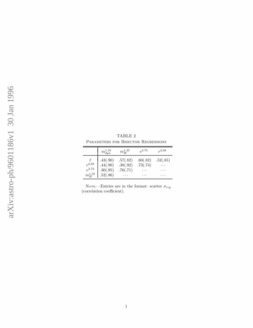
The regression of log v vs. log r in Fig. 3b also shows some curvature, so that the

luminosity-radius relation in Fig. 2c has almost constant slope throughout, ℓ ∝ r2.6 or r2.7

(the small displacement is probably not significant). For the three log-log relations shown

in Fig. 3, the curvature can be represented by a two-component fitting formula, but the

slopes and ratios of coefficients are very uncertain. The dashed curves in Fig. 3 show the

following particularly simple choices:

v5 ≈ 0.4ℓ+ 0.2ℓ2, (7)

v2 ≈ 0.5r + 0.4r2.5, (8)

mdyn ≈ 0.4ℓ0.6 + 0.4ℓ1.2. (9)

The use of logarithms in linear regressions is convenient and almost necessary if

variables have a log-normal distribution. However, the implied “logarithmic averaging” may

not be the physically meaningful procedure. In Newtonian mechanics the Virial Theorem

requires that velocity-related averages over an orbit be carried out for v2 rather than for

any other power or for a logarithm. We illustrate this with the logarithmic v vs. ℓ relation

in Fig. 3a for the dwarfs, where the dashed curve approximates v(4.22±.48) = (0.76 ± .21)ℓ

at the dwarf end. In Fig. 4 we have replotted the same data for dwarfs on linear scales for

v2 and ℓ1/2 and show the bisector regression line v2 = (−0.039 ± .048) + (1.02 ± .12)ℓ1/2.

In principle, averaging v2 over a log-normal distribution centered on the zero-point of

the 3.73 log v - log ℓ regression could give 〈v2〉 significantly larger than the square of v

corresponding to the zero-point itself, but in fact with the variance 0.652 in 3.73 log v we

get 〈v2〉 = 1.22, almost the same as the value 0.98 from the regression of v2 vs. ℓ1/2.

– 13 –

5. Three Surface Densities

Three surface densities are of physical interest, namely ΣL = LB/4πR2gm (related to

the average surface brightness in the blue), ΣH = MH/4πR2gm, and Σdyn = Mdyn/4πR

2gm.

These are related to the extensive variables in Eqn. (6) by

ΣL

1.23 L⊙pc−2=

ℓ

r2,

ΣH

0.709 M⊙pc−2=

mH

r2,

Σdyn

14.9 M⊙pc−2=

v2

r. (10)

We should emphasize that the radius r, which we use in Eqn. (10) and in the rest of

this paper, is mostly an “isophotal” or “isosurface-density” radius. If we could use some

“scale-length” radius rsl instead (unfortunately unavailable where the mapping is coarsely

resolved), the variation in ΣL and ΣH would be greater, since low / high central surface

brightness leads to a smaller / larger ratio of r/rsl (although only by a logarithmic factor

for an exponential disk). Central values of surface brightness and surface density would

presumably also have larger variations.

If the correlation coefficients of the pairs of extensive variables were unity (i.e., straight

lines on log-log plots and σreg = 0), and if the mdyn inconsistency discussed in Sect. 4

were absent, Eqn. (6) would give uniquely the dependence of the surface densities on

the extensive variables. In reality, the correlations are not very tight, and there is some

ambiguity and some curvature. To illustrate the uncertainties, consider first only the first

four entries in Eqn. (6) and pretend that they represent exact equalities. This would give

ΣL ∝ r0.68 ∝ ℓ0.25 ∝ v0.95 ∝ m0.34H ,

ΣH ∝ r−0.015 ∝ ℓ−0.006 ∝ v−0.021 ∝ m−0.007H ,

Σdyn ∝ r0.44 ∝ ℓ0.16 ∝ v0.61 ∝ m0.22H .

(11)

Instead, we can obtain the “direct logarithmic regression” for each of the three surface

densities separately against each of the five extensive variables in Eqn. (6). The five

alternative regression slopes (and their average) are shown in Table 3 for each of the three

surface densities, together with the formal statistical error. The alternative slopes can differ

by more than the formal errors, which illustrates a systematic artifact for poorly correlated

quantities: A ratio like ΣL ∝ ℓ/r2 has a larger slope in its regression against ℓ and a smaller

slope against r2.68 than in Eqn. (11), whereas the regression against a “neutral” extensive

variable (such as v3.73 or ℓr2) is probably more reliable.

To summarize our data so far on the variation of the surface densities along the mass

sequence: The blue surface brightness definitely increases steadily (without curvature) along

– 14 –

the sequence, approximately as ΣL ∝ (ℓr2)ǫ, with ǫ ∼ (0.13 to 0.16).. For our combined

sampled, ΣH varies very little along the sequence, but we saw in Sect. 4.2 that a small

correction in the form of a multiplying factor ∼ (ℓ/100)0.07 should probably be applied

to mH and hence to ΣH) because of the bias against faint galaxies with small mH . That

there is a correction to ΣH , but that it is small, can also be seen indirectly from the scatter

diagram in Fig. 5a of ΣH vs. ΣL for our sample: The selection bias applies only to the lower

portion of the diagram, not to the upper envelope which has only a small positive slope.

Some of the positive correlation must be an artifact due to measuring errors in r, which

enters both ΣH and ΣL to the same power. Thus, even the corrected ΣH should increase

little along the sequence. The variations in the scatter diagram of logΣL vs. log Σdyn

(Fig. 5c) combine systematic variations along the sequence with individual variations

“perpendicular to the sequence.” If one attempts to describe the “parallel” variation (along

the sequence) as ΣL ∝ (Σdyn)p‖ , then Eqn. (10) and Table 3 give p‖ ∼ 1.6 or 1.8. However,

the inclusion of curvature in Eqn. (8) gives

Σdyn ∝ (1 + 0.8r1.5) (12)

for the variation along the sequence, i.e., Σdyn hardly varies at the low end of the sequence

(whereas ΣL does), and p‖ is not a very meaningful parameter.

To investigate the variation of ΣL against Σdyn “perpendicular to the sequence,” we

eliminate the variations along the sequence by using slightly altered definitions: We choose

Σ′L =

ΣL

(ℓr2)0.16=

ℓ0.84

r2.32, Σ′

dyn =2Σdyn

1 + 0.8r1.5=

2v2

r + 0.8r2.5(13)

so that Σ′L and Σ′

dyn have little systematic variation along the sequence. The scatter

diagram is shown in Fig. 5d and the bisector regression line gives

Σ′L ∝ (Σ′

dyn)p⊥, p⊥ = 1.118± .085 (14)

Note that a similar slope would be obtained if there were little true correlation between Σ′L

and Σ′dyn but large measuring errors in r. The true value of p⊥ is therefore more uncertain

than indicated by the formal error in Eqn. (14).

6. Conclusion

– 15 –

6.1. Summary.

We have analyzed the statistical relations of five extensive (size-related) observables

for a large set of galaxies, with a broad range of absolute luminosity and surface brightness.

Only galaxies with H I mapping were included, early-type spirals (S0, Sa, Sab) and

ellipticals were excluded along with spirals thought to be members of tidally interacting

pairs or groups. Faint dwarf irregular galaxies are more prominent in our sample than they

would be in a magnitude-limited catalog. These five observables are ℓ (a normalized blue

luminosity LB), r (a normalized “geometric mean” radius Rgm, formed from an isophotal or

isosurface-density H I radius close to that of the outermost detectable H I and the optical

radius R25), v (a normalized velocity profile width Vc which incorporates both rotation

and random motion), mH (the normalized total mass MH of neutral atomic hydrogen),

and mdyn (the normalized indicative total dynamic mass out to radius Rgm, defined as

Mdyn = V 2c Rgm/G). These quantities are normalized by 109L⊙, 12.30 kpc, 80.51 km s−1,

5.76 × 108M⊙, and 1.212 × 1010M⊙, values typical of the region in which dwarf irregular

and spiral galaxies overlap.

For our complete sample we analyzed all Hubble types Sb through Im, which gives

a particularly large dynamic range of the five extensive observables, which peak around

Sbc (Roberts & Haynes 1994). Of the 225 galaxies in the complete sample, four were

anomolously H I-rich, and these were omitted in all statistical analyses. Because of a

selection bias for H I-mapping, extremely H I-poor galaxies are missing from the sample.

As most previous authors have done, we correlated logarithms of the variables rather than

the variables themselves. Since the five variables are on an equal footing physically a

priori, we followed Isobe et al. (1990, IFAB) in using the “bisector” prescription for a

symmetric form of a linear regression line for each of the 10 pairs of 5 variables. Because of

the large scatter in the data, correlations suffer some ambiguity from “non-commutativity,”

especially for the product mdyn = v2r. Nevertheless, we find that the regression slopes

for all 10 regressions between the log10 of ℓ, r2.68, v3.73, m1.35H , and m1.16

dyn lie between 0.97

and 1.03, with statistical errors ∼< 10%. Because of the non-commutativity for ratios, we

again have some ambiguities as to the variation along the size/mass/luminosity sequence

for the surface densities ΣL = ℓ/r2 for blue luminosity, ΣH = mH/r2 for neutral hydrogen

mass, and Σdyn = v2/r for indicative dynamic mass. The extent of the ambiguity and one

definition of an average slope for each pair are given in Table 3. We have also attempted to

characterize two kinds of variations of ΣL with Σdyn by first writing ΣL ∝ (Σdyn)p‖ for the

average changes along the mass sequence. These two surface densities were then corrected

for the average systematic variation along the sequence to obtain new variables Σ′L and

Σ′dyn. Then we fitted a regression line of the form Σ′

L ∝ (Σ′dyn)

p⊥ to the corrected variables

to represent the variation “perpendicular to the mean sequence.” The regressions gave

– 16 –

p‖ ∼ 1.6 or 1.8 and p⊥ ∼ 1.15, but these present values are unrealistic for reasons given

below.

We have looked for curvature in the logarithmic regressions of the various extensive

variables against each other, and we also investigated whether or not there are any

“breaks” in the correlations for “dwarfs,” defined as Sdm through Im (including BCD),

irrespective of size or luminosity, vs. those for “spirals,” types Sb through Sd. For the

variables not involving H I, we find no significant breaks between Hubble types, but the

large range of extensive variables enabled us to find curvature in some of the regressions:

For the Tully-Fisher relation ℓ ∝ vs, the bright spirals (which are preferred for practical

application) give s ≈ 2.5 or 2.7, our total sample gives s ≈ 3.7, and the fainter galaxies

give s slightly larger than 4, the power originally suggested by Tully and Fisher (1977).

There is little curvature in the relation ℓ ∝ r2.7, so that the surface brightness in the blue,

ΣL = ℓ/r2, increases steadily along the mass sequence (ΣL in the red or infrared increases

even more rapidly). There is curvature in the log v-log r relation, so that the surface

density of dynamic mass is almost constant at the low end of the mass/radius sequence

and increases appreciably along the upper end of the sequence. This variation, roughly

Σdyn = v2/r ∝ (1 + r0.8), coupled with the steady progression of ΣL, shows that a relation

of the form ΣL ∝ (Σdyn)p‖ is not very meaningful. The concept of the “perpendicular

parameter” p⊥ in Σ′L ∝ (Σ′

dyn)p⊥ is meaningful, but out present value for it (∼ 1.15) may

be quite uncertain because of a coincidence involving powers of the galactic radius r, which

may have large measuring errors at the moment: The definitions of Σ′L and Σ′

dyn are such

that particularly large errors, in the absence of strong real correlation, could mimic our

results.

Only for correlations involving H I content are there tentative indications of “breaks”

between dwarfs and spirals in the sense that the RH -Ropt relation lies higher by a factor

of ∼ 1.3, and the mH -ℓ relation by a factor of ∼ 3, for dwarfs than for spirals. These

“displacements” near ℓ ∼ 1 are smaller than the variances and it is not clear if the

effect is real. The surface density of H I mass, ΣH , in our sample varies little along the

luminosity/mass/radius sequence, and the individual variations from ΣH ∼ 0.7 M⊙ pc−2

are fairly small. Particularly small values of mH/ℓ and of ΣH tend to be absent (especially

for dwarfs) because of a selection bias, and we have estimated that mH/ℓ and ΣH should

be corrected downwards from our results by a multiplying factor of order (LB/1011L⊙)0.07.

– 17 –

6.2. Comparison with previous analyses.

Four recent papers have carried out related correlation studies with slightly different

emphases: (i) Roberts & Haynes (1994) mainly investigated variations with Hubble type

rather than with luminosity. (ii) Gavazzi (1993) concentrated on variation with luminosity,

as we do, but he included S0, Sa and Sab galaxies and did not have much data on very

faint dwarfs or low surface brightness (LSB) galaxies. On the other hand, (iii) Sprayberry

et al. (1995) and (iv) Zwaan et al. (1995) present extensive data on LSB galaxies and

compare with galaxies (of similar dynamic mass Mdyn) with normal surface brightness ΣL.

While there is agreement on most trends, there is considerable controversy regarding the

trends of ΣL (in the blue) and Σdyn along the size / mass / luminosity / Hubble sequences

and also on their correlations relative to each other “perpendicular to the sequence” (i.e.,

variations for fixed mdyn or ℓ). We show first that the apparent discrepancies are partly due

to uncertainties brought about by some near cancellations for variations along the sequence:

Assume that ℓ = vα and r = vβ along the whole mean mass sequence. With Σdyn = v2/r

and ΣL = ℓ/r2, we have

Σdyn = v(2−β); ΣL = v(α−2β); p‖ =α− 2β

2− β. (15)

Our derived approximate values are α ∼ 3.8 and β ∼ 1.4, so that α − 2β is appreciably

smaller than α and 2 − β smaller than 2. This leads to a large uncertainty in p‖ even for

constant α and β. Furthermore, we saw that α and β vary along the sequence (with 2− β

essentially vanishing on the low end), so that p‖ is not well defined.

Consider next the “variations perpendicular to the sequence,” i.e., changes in Σdyn at

fixed mdyn = v2r, so that v4 ∝ r−2 ∝ Σdyn. Assume that ΣL ∝ (Σdyn)p⊥ for variation at

constant mdyn with some value for the constant p⊥, so that

ℓ ∝ (Σdyn)p⊥−1, ℓ/vα = (Σdyn)

(p⊥−1)−α/4. (16)

For the special case of p⊥ = 1, the luminosity / mass ratio would then not depend on Σdyn

variations. For the special case of p⊥ = 1 + α/4 on the other hand, variations in Σdyn away

from the mean value along the sequence would not affect the Tully-Fisher v-ℓ relation at all.

Both Zwaan et al. (1995) and Sprayberry et al. (1995) compared the Tully-Fisher

(TF) relation between v and ℓ for normal galaxies with that for LSB galaxies, which gives

some information on Eqn. (15). However, there is some spread in the observations and the

two papers emphasize different aspects: The former notes that the difference in the two

– 18 –

TF relations is small, so that p⊥ should be close to (1 + α/4), which is about 1.9 (in the

blue and using our bisector slopes). On the other hand, the latter paper notes that there

is some difference in the TF relations — in the sense that “Malin I-like” objects with very

large r and small v, small Σdyn, have anomalously small ℓ/vα. These few galaxies at least

indicate that p⊥ < 1.9 (If p⊥ were as small as 1, then ℓ/mdyn would depend little on Σdyn,

but ℓ/vα would have a strong dependence.). Qualitatively, our own result of p⊥ ∼ 1.12 is

intermediate between 1 and 1.9, as it should be, but the combined data of Zwaan et al.

(1995) and Sprayberry et al. (1995) suggest a slightly larger value for p⊥ than ours. We

saw that the large present-day errors in radius make the value of p⊥ uncertain.

There is only an illusion of a discrepancy regarding the ratio ℓ/mdyn, which Gavazzi

(1993) has decreasing along the mass sequence whereas our averaged linear regression has

ℓ/mdyn ∝ m0.16dyn . Our Eqn. (9) indicates “regression curvature” in the sense that ℓ/mdyn

increases along the sequence for small ℓ and then decreases slightly for large ℓ [Fig. 2d in

Roberts & Haynes (1994) also indicates a peak in ℓ/mdyn at an intermediate Hubble type].

6.3. Discussion.

An important negative result of our compilation is the absence of any sudden break

between dwarf irregulars and regular spirals for variables not involving H I. In an overall

dynamic sense, small dwarfs are thus a continuation of the spiral Hubble sequence. Only

the fact that the RH -Ropt and mH-ℓ relations seem to lie higher for dwarf irregulars than

for spirals might indicate that gas depletion by star formation is reduced by morphological

irregularities. However, even this fact may only be a manifestation of the tendency

(discussed below) that hydrogen content decreases more slowly with decreasing mass than

luminosity does.

Of the three surface densities discussed above, only the blue surface brightness ΣL

increases steadily and appreciably along the mass/radius/luminosity/Hubble sequence. A

fourth density Σ∗ for total stellar mass is not measured explicitly for most of our sample,

but should be correlated best with ΣL in the visible to near infrared. We do not have ΣL

at those wavelengths either, but L, and hence ΣL, is known to increase more rapidly along

the sequence at longer wavelength than in the blue. Our uncorrected data has neutral

hydrogen mass surface density ΣH almost constant along the sequence; the correction

for selection bias would presumably have ΣH increase along the sequence, but only very

slowly, and ΣH/Σ∗ definitely decreases along the sequence from dwarfs to giants. As a

consequence, the total disk mass density (ΣH +Σ∗) increases slowly (and is gas dominated)

along the lowest portion of the sequence and increases rapidly along the middle and upper

– 19 –

portions of the sequence. The density Σdyn of total dynamic mass (mostly dark matter)

is almost constant along the lower sequence and increases along the upper portion, so

that the ratio (ΣH + Σ∗)/Σdyn probably increases quite slowly along the sequence. The

small variation of ΣH , compared with the large variation of Σ∗, fits in with the suggestion

by Kennicutt (1989) that star formation proceeds rapidly when the gas surface density

exceeds a threshold value: Rapid star formation on the upper sequence (where the initial

gas density ΣH +Σ∗ is large) depleted the gas rapidly, but the rapid depletion did not occur

on the lower sequence so that the present-day ΣH is almost constant along the sequence.

The small variation of ΣH in our Figs. 5a and b stems in part from our radius definition

and from a selection effect: As mentioned in Sect. 4, the use of isophotal radii r (instead

of scale-length radii rsl) decreases variations in both ΣL and ΣH , compared with central

values (de Blok, van der Hulst & Zwaan 1995, private communication). Galaxies with very

small ΣH are likely to have had low total mH and therefore not to have been chosen as

candidates for mapping in H I, so the lowest portion of Figs 5a and 5b may be absent from

our sample. However, this is not the case for upward fluctuations, and it is significant that

only a few out of the 225 galaxies have an unusually large H I content for their position

on the mass/luminosity sequence. This also meshes with the notion that an initially high

gas surface density usually produces rapid star formation and eventually depresses ΣH to

“typical values.”

We also have some qualitative information on the variation along the mass sequence

of two different volume densities: (i) The volume density nH of H (and other gas) in the

midplane of the galactic disk depends on ΣH ×Σdyn and inversely on the velocity dispersion

∆V⊥ normal to the plane. Although Vc is smaller for dwarfs than for large spirals, ∆V⊥ varies

little, as does ΣH . Since Σdyn decreases slowly with decreasing size/mass/luminosity, nH

also decreases slowly. (ii) For studying tidal effects on a galaxy, another quantity with the

dimensions of a volume density is important, namely ntid = Mdyn

(

3/4πR3gm

)

∝ Σdyn/Rgm.

Using Eqn. (6), we see that this quantity is actually slightly larger for dwarfs than for

spirals, varying roughly as ntid ∝ ℓ−0.26. Tidal effects should therefore be less pronounced

on dwarfs than on spirals. (iii) Although dwarfs are more “robust” from the point of view

of (ii), galactic winds, “blow-outs,” etc., depend on escape velocity [∝ (ΣdynRgm)1/2], and

dwarfs are less robust from this point of view.

Since the extensive variables peak around Sbc, it would be of interest to explore

the differences in correlations of the extensive variables and surface densities for three

morphological groupings: Sdm through Im (including BCD), Sbc through Sd, and S0

through Sb. There are at present too few detailed H I mappings of early-type spirals to

allow this comparison between the three groupings, but mapping is proceeding at a great

– 20 –

rate. It would also be useful to make more detailed comparisons between galaxies with

and without H I mapping to obtain p⊥ more reliably. For discussions of the empirical ℓ-v

Tully-Fisher relation one wants to know if p⊥ is always close to (1 + α/4); if so, that would

be a partial explanation for the narrow width of the relation.

We acknowledge fruitful discussions and correspondence with G. Bothun, J. Charlton,

E. Corbelli, E. de Blok, J. Dickey, G. Gavazzi, G. Helou, S. McGaugh, M. Roberts, E.

Skillman, D. Sprayberry, T. van der Hulst and M. Zwaan. This work was supported in part

by US National Science Foundation grants AST-9015181 and AST-9316213 at Lafayette

College and by AST-9119475 at Cornell.

REFERENCES

Bajaja, E., Huchtmeier, W.K., & Klein, U. 1984, A&A, 285, 385

Begeman, K.G. 1989, A&A, 223, 47

Binggeli, B., Sandage, A., & Tammann, G.A. 1985, AJ, 90, 1681 (BST)

Bosma, A., van der Hulst, J.M., & Athanassoula, E. 1988, A&A, 198, 100

Bothun, G.D., Impey, C.D., Malin, D.F., & Mould, J.R. 1987, AJ, 94, 23

Bothun, G.D., Schombert, J.M., Impey, C.D., & Schneider, S.E. 1990, ApJ, 360, 427

Bottema, R. 1989, A&A, 225, 358

Bottema, R., Shostak, G.S., & van der Kruit, P.C. 1986, A&A, 167, 34

Boulanger, F., & Viallefond, F. 1992, A&A, 266, 37

Braine, J., Combes, F., & van Driel, W. 1993, A&A, 280, 451

Briggs, F.H. 1982, ApJ, 259, 544

Briggs, F.H., Wolfe, A.M., Krumm, N., & Salpeter, E.E. 1980, ApJ, 238, 510

Brinks, E., & Klein, U. 1988, MNRAS, 231, 63P

Broeils, A.H. 1992, A&A, 256, 19

Broeils, A.H., & van Woerden, H. 1994, A&AS, 107, 129

Carignan, C. 1985, ApJ, 299, 59

Carignan, C., & Beaulieu, S. 1989, ApJ, 347, 760

Carignan, C., Beaulieu, S., & Freeman, K.C. 1990, AJ, 99, 178

– 21 –

Carignan, C., Charbonneau, P., Boulanger, F., & Viallefond, F. 1990, A&A, 234, 43

Carignan, C., & Freeman, K.C. 1988, ApJ, 332, L33

Carignan, C., & Puche, D. 1990a, AJ, 100, 394

Carignan, C., & Puche, D. 1990b, AJ, 100, 641

Carignan, C., Sancisi, R., & van Albada, T.S. 1988, AJ, 95, 37

Carilli, C.L., & van Gorkom, J.H. 1992, ApJ, 399, 373

Casertano, S., & van Gorkom, J.H. 1991, AJ, 101, 1231

Cayatte, V., Kotanyi, C., Balkowski, C., & van Gorkom, J.H. 1994, AJ, 107, 1003

Cayatte, V., van Gorkom, J.H., Balkowski, C., & Kotanyi, C. 1990, AJ, 100, 604

Chengalur, J.N., Salpeter, E.E., & Terzian, Y. 1994, AJ, 107, 1984

Comte, G., Lequeux, J., & Viallefond, F. 1985, in Star-Forming Dwarf Galaxies and Related

Objects, ed. D. Kunth, T.X. Thuan & J. Tran Thanh Van (Gif-sur-Yvette: Editions

Frontieres), 273

Corbelli, E., Schneider, S.E., & Salpeter, E.E. 1989, AJ, 97, 390

Cote, S., Carignan, C., & Sancisi, R. 1991, AJ, 102, 904

de Blok, E., van der Hulst, T., & Zwaan, M. 1995, private communication

Deul, E.R., & van der Hulst, J.M. 1986, A&AS, 67, 509

de Vaucouleurs, G., de Vaucouleurs, A., Corwin, H.G., Buta, R.J., Paturel, G., & Fouque,

P. 1991, Third Reference Catalog of Bright Galaxies, (New York: Springer-Verlag)

(RC3)

Dickey, J.M., Hanson, M.M., & Helou, G. 1990, ApJ, 352, 522

Drinkwater, M., & Hardy, E. 1991, AJ, 101, 94

Dufour, R.J., & Hester, J.J. 1990, ApJ, 350, 149

England, M.N. 1989, ApJ, 337, 191

England, M.N., Gottesman, S.T., & Hunter, J.H. 1990, ApJ, 348, 456

Fanelli, M.N., O’Connell, R.W., & Thuan, T.X. 1988, ApJ, 334, 665

Gallagher, J.S., & Hunter, D.A. 1984, ARA&A, 22, 37

Gavazzi, G. 1993, ApJ, 419, 469

Giovanardi, C., & Salpeter, E.E. 1985, ApJS, 58, 623

Giovanelli, R., & Haynes, M.P. 1983, AJ, 88, 881

– 22 –

Giovanelli, R., & Haynes, M.P. 1989, ApJ, 346, L5

Giovanelli, R., Williams, J.P., & Haynes, M.P. 1991, AJ, 101, 1242

Guhathakurta, P., van Gorkom, J.H., Kotanyi, C.G., & Balkowski, C. 1988, AJ, 96, 851

Haynes, M.P. 1981, AJ, 86, 1126

Haynes, M.P., Giovanelli, R., & Roberts, M.S. 1979, ApJ, 229, 83

Helou, G., Giovanardi, C., Salpeter, E.E., & Krumm, N. 1981, ApJS, 46, 267

Helou, G., Hoffman, G.L., & Salpeter, E.E. 1984, ApJS, 55, 433 (HHS84)

Helou, G., Salpeter, E.E., & Terzian, Y. 1982, AJ, 87, 1443

Hewitt, J.N., Haynes, M.P. & Giovanelli, R. 1983, AJ, 88, 272

Hodge, P. 1989, ARA&A, 27, 139

Hoffman, G.L., Helou, G., & Salpeter, E.E. 1988, ApJ, 324, 75 (HHS88)

Hoffman, G.L., Lewis, B.M., Helou, G., Salpeter, E.E., & Williams, H.L. 1989b, ApJS, 69,

65

Hoffman, G.L., Salpeter, E.E., Farhat, B., Roos, T., Williams, H. & Helou, G. 1996, ApJS,

in press (Paper I)

Huchtmeier, W.K. 1979, A&A, 75, 170

Huchtmeier, W.K., & Seiradakis, J.H. 1985, A&A, 143, 216

Huchtmeier, W.K., Seiradakis, J.H., & Materne, J. 1980, A&A, 91, 341

Huchtmeier, W.K., Seiradakis, J.H., & Materne, J. 1981, A&A, 102, 134

Huchtmeier, W.K., & Witzel, A. 1979, A&A, 74, 138

Hummel, E., Dettmar, R.-J., & Wielebinski, R. 1986, A&A, 166, 97

Hunter, D.A., van Woerden, H., & Gallagher, J.S. 1994, ApJS, 91, 79

Impey, C.D., & Bothun, G.D. 1989, ApJ, 341, 89

Irwin, J.A., & Seaquist, E.R. 1991, ApJ, 371, 111

Irwin, J.A., Seaquist, E.R., Taylor, A.R., & Duric, N. 1987, ApJ, 313, L91

Isobe, T., Feigelson, E.D., Akritas, M.G., & Babu, G.J. 1990, ApJ, 364, 104

Israel, F.P., & van Driel, W. 1990, A&A, 236, 323

Izotov, Y.I., Thuan, T.X., & Lipovetsky, V.A. 1994, ApJ, 435, 647

Jobin, M., & Carignan, C. 1990, AJ, 100, 648

Kamphuis, J., & Briggs, F. 1992, A&A, 253, 335

– 23 –

Kennicutt, R.C. 1989, ApJ, 344, 685

Koribalski, B., Dahlem, M., Mebold, U., & Brinks, E. 1993, A&A, 268, 14

Kruger, H., & Fritze-von Alvensleben, U. 1994, A&A, 284, 793

Krumm, N., & Burstein, D. 1984, AJ, 89, 1319

Lake, G., Schommer, R.A., & van Gorkom, J.H. 1990, AJ, 99, 547

Lake, G., & Skillman, E.D. 1989, AJ, 98, 1274

Larson, R.B., & Tinsley, B.M. 1978, ApJ, 219, 46

Lequeux, J., & Viallefond, F. 1980, A&A, 91, 269

Li, J.G., & Seaquist, E.R. 1994, AJ, 107, 1953

Liszt, H.S. 1992, AJ, 104, 563

Lo, K.Y., Sargent, W.L.W., & Young, K. 1993, AJ, 106, 507

Martimbeau, N., Carignan, C., & Roy, J.-R. 1994, AJ, 107, 543

McGaugh, S.S. 1994, ApJ, 426, 135

McGaugh, S.S. 1995, in New Light on Galaxy Evolution, ed. R. Bender & J. Davies

(Dordrecht: Kluwyer), in press

McGaugh, S.S., Schombert, J.M., & Bothun, G.D. 1995, AJ, 109, 2019

McMahon, R.G., Irwin, M.J., Giovanelli, R., Haynes, M.P., Wolfe, A.M., & Hazard, C.

1990, ApJ, 359, 302

Meurer, G.R., Mackie, G., & Carignan, C. 1994, AJ, 107, 2021

Ohta, K., Tomita, A., Saito, M., Sasaki, M., & Nakai, N. 1993, PASJ, 45, L21

Ondrechen, M.P., & van der Hulst, J.M. 1989a, ApJ, 342, 29

Ondrechen, M.P., & van der Hulst, J.M. 1989b, ApJ, 342, 39

Pedlar, A., Howley, P., Axon, D.J., & Unger, S.W. 1992, MNRAS, 259, 369

Peters, W.L., Freeman, K.C., Forster, J.R., Manchester, R.N., & Ables, J.G. 1994, MNRAS,

269, 1025

Pierce, M.J., & Tully, R.B. 1988, ApJ, 330, 579

Puche, D., & Carignan, C. 1991, ApJ, 378, 487

Puche, D., Carignan, C., & Bosma, A. 1990, AJ, 100, 1468

Puche, D., Carignan, C., & van Gorkom, J.H. 1991, AJ, 101, 456

Puche, D., Carignan, C., & Wainscoat, R.J. 1991, AJ, 101, 447

– 24 –

Puche, D., Westpfahl, D., Brinks, E., & Roy, J.-R. 1992, AJ, 103, 1841

Rand, R.J. 1994, A&A, 285, 833

Roberts, M.S., & Haynes, M.P. 1994, ARA&A, 32, 115

Rots, A.H. 1980, A&AS, 41, 189

Rownd, B.K., Dickey, J.M., & Helou, G. 1994, AJ, 108, 1638

Rupen, M.P. 1991, AJ, 102, 48

Sage, L.J. 1993, A&A, 272, 123

Saikia, D.J., Unger, S.W., Pedlar, A., Yates, G.J., Axon, D.J., Wolstencroft, R.D., &

Taylor, K. 1990, MNRAS, 245, 397

Sandage, A., & Fomalont, E. 1993, ApJ, 407, 14

Sargent, W.L.W., Sancisi, R., & Lo, K.Y. 1983, ApJ, 265, 711

Schneider, S.E. 1989, ApJ, 343, 94

Schneider, S.E., & Corbelli, E. 1993, ApJ, 414, 500

Schneider, S.E., Helou, G., Salpeter, E.E., & Terzian, Y. 1986, AJ, 92, 742

Schneider, S.E., Thuan, T.X., Magri, C., & Wadiak, J.E. 1990, ApJS, 72, 245

Schombert, J.M., Bothun, G.D., Impey, C.D., & Mundy, L.G. 1990, AJ, 100, 1523

Shostak, G.S., & Skillman, E.D. 1989, A&A, 214, 33

Skillman, E.D., & Bothun, G.D. 1986, A&A, 165, 45

Skillman, E.D., Bothun, G.D., Murray, M.A., & Warmels, R.H. 1987, A&A, 185, 61

Skillman, E.D., Terlevich, R., Teuben, P.J., & van Woerden, H. 1988, A&A, 198, 33

Sprayberry, D., Bernstein, G.M., Impey, C.D., & Bothun, G.D. 1995, ApJ, 438, 72

Sprayberry, D., Impey, C.D., Irwin, M.J., McMahon, R.G., & Bothun, G.D. 1993, ApJ,

417, 114

Stavely-Smith, L., Davies, R.D., & Kinman, T.D. 1992, MNRAS, 258, 334

Tacconi, L.J., & Young, J.S. 1986, ApJ, 308, 600

Taylor, C.L., Brinks, E., Skillman, E.D. 1993, AJ, 105, 128

Taylor, C.L., Brinks, E., Pogge, R.W., & Skillman, E.D. 1994, AJ, 107, 971

Tully, R.B., Bottinelli, L., Fisher, J.R., Gouguenheim, L., Sancisi, R., & van Woerden, H.

1978, A&A, 63, 37

Tully, R.B., & Fisher, J.R. 1977, A&A, 54, 661

– 25 –

Tyson, N.D., & Scalo, J.M. 1988, ApJ, 329, 618

van Albada, T.S., Bahcall, J.N., Begeman, K., & Sancisi, R. 1985, ApJ, 295, 305

van den Bergh, S. 1994, ApJ, 428, 617

van der Hulst, J.M., Skillman, E.D., Smith, T.R., Bothun, G.D., McGaugh, S.S., & de

Blok, W.J.G. 1993, AJ, 106, 548

van Driel, W., & Buta, R.J. 1991, A&A, 245, 7

van Driel, W., & van Woerden, H. 1994, A&A, 286, 395

van Moorsel, G.A. 1988, A&A, 202, 59

van Zee, L., Haynes, M.P., & Giovanelli, R. 1995, AJ, 109, 990

Viallefond, F. 1990, private communication

Viallefond, F., & Thuan, T.X. 1983, ApJ, 269, 444

Warmels, R.H. 1988a, A&AS, 72, 19

Warmels, R.H. 1988b, A&AS, 72, 57

Warmels, R.H. 1988c, A&AS, 72, 427

Westerlund, B.E. 1990, Astronomy & Astrophysics Review, 2, 29

Wevers, B.M.H.R., van der Kruit, P.C., & Allen, R.J. 1986, A&AS, 66, 505

Wilding, T., Alexander, P., & Green, D.A. 1993, MNRAS, 263, 1075

Zwaan, M.A., van der Hulst, J.M., de Blok, W.J.G., & McGaugh, S.S. 1995, MNRAS, 273,

L35

This preprint was prepared with the AAS LATEX macros v4.0.

– 26 –

Fig. 1.— Plot of radius RH,max to the outermost measured neutral hydrogen vs. optical

radius R25 at the 25 mag arcsec−2 isophote. Irregular galaxies from Paper I are shown as large

exes with BCDs as large open squares and upper limits shown at one-half the formal limit

as open triangles. Mapped irregulars from the literature are shown as small exes or squares,

similarly. Members of interacting binary systems are shown as asterisks and excluded from

all correlations. Mapped spiral galaxies from the literature are shown as small dots. Open

circles mark irregular galaxies with high luminosity (> 1010 L⊙). Five special cases are

indicated with filled symbols and are omitted from all correlations: DDO 154 by a circle,

DDO 137 by a triangle, the NGC 4532 / DDO 137 complex by a hexagon, VCC 2062 by

a diamond, and HI 1225+01 by a small square. The solid line is the bisector of the two

ordinary least-squares regression lines (y vs. x and x vs. y). The two dashed lines are

bisector regression lines for the spirals and dwarfs separately.

Fig. 2.— Logarithmic scatter plots and regressions of pairs of extensive variables, each

normalized to the value corresponding to a blue luminosity of 109 L⊙ as described in the text.

The powers (multiplicative factors in the logarithms) are explained in Sect. 4a. Symbols

are chosen as for Fig. 1. The solid line in each case is the bisector regression line, while

dashed lines are for dwarfs alone or spirals alone. (a) Neutral hydrogen mass mH vs. blue

luminosity ℓ. (b) mH vs. indicative dynamical mass mdyn. (c) Geometric mean radius r vs.

ℓ.

Fig. 3.— Logarithmic scatter plots and regressions of pairs of extensive variables, each

normalized to the value corresponding to a blue luminosity of 109 L⊙ as described in the text.

The powers (multiplicative factors in the logarithms) are explained in Sect. 4a. Symbols

are chosen as for Fig. 1. The dashed curve in each panel is an a smooth curve which

approximately matches the regressions for dwarfs alone at one end and for spirals alone at

the other. (a) Velocity profile half-width v vs. blue luminosity ℓ. (b) v vs. geometric mean

radius r. (c) Indicative dynamical mass mdyn = v2r vs. ℓ.

Fig. 4.— Scatter plot and regression of normalized velocity profile half-width squared vs.

square-root of normalized blue luminosity for dwarfs alone on linear, rather than logarithmic,

axes. The solid line is the bisector regression for the displayed points.

Fig. 5.— Logarithmic scatter plots of neutral hydrogen surface density, ΣH = mH/r2,

vs. (a) optical surface brightness, ΣL = ℓ/r2 and (b) dynamical mass surface density,

Σdyn = v2/r, and of (c) optical surface brightness, ΣL = ℓ/r2 vs. dynamical mass surface

density, Σdyn = v2/r and (d) reduced optical surface brightness, Σ′L, vs. reduced dynamical

mass surface density, Σ′dyn, as discussed in the text (Sect. 5). Symbols are defined as in Fig.

1.