Rational Cuspidal Curves - arXiv
139
Rational Cuspidal Curves by Torgunn Karoline Moe Thesis for the degree of Master in Mathematics (Master of Science) Department of Mathematics Faculty of Mathematics and Natural Sciences University of Oslo May 2008 arXiv:1511.02691v1 [math.AG] 9 Nov 2015
-
Upload
khangminh22 -
Category
Documents
-
view
0 -
download
0
Transcript of Rational Cuspidal Curves - arXiv

Rational Cuspidal Curvesby
Torgunn Karoline Moe
Thesis for the degree of
Master in Mathematics
(Master of Science)
Department of MathematicsFaculty of Mathematics and Natural Sciences
University of Oslo
May 2008
arX
iv:1
511.
0269
1v1
[m
ath.
AG
] 9
Nov
201
5


Rational Cuspidal Curves
by
Torgunn Karoline Moe
Supervised by
Professor Ragni Piene
Department of MathematicsFaculty of Mathematics and Natural Sciences
University of Oslo
May 2008


Contents
1 Introduction 1
2 Theoretical background 52.1 Rational cuspidal curves . . . . . . . . . . . . . . . . . . . . . 52.2 Invariants and conditions . . . . . . . . . . . . . . . . . . . . 72.3 Derived curves . . . . . . . . . . . . . . . . . . . . . . . . . . 152.4 Other useful results . . . . . . . . . . . . . . . . . . . . . . . . 182.5 Getting an overview . . . . . . . . . . . . . . . . . . . . . . . 19
3 Rational cuspidal cubics and quartics 213.1 Rational cuspidal cubics . . . . . . . . . . . . . . . . . . . . . 213.2 Rational cuspidal quartics . . . . . . . . . . . . . . . . . . . . 22
4 Projections 274.1 The projection map . . . . . . . . . . . . . . . . . . . . . . . 274.2 The rational normal curve . . . . . . . . . . . . . . . . . . . . 284.3 Cuspidal projections from Cn . . . . . . . . . . . . . . . . . . 304.4 Cuspidal projections from C3 . . . . . . . . . . . . . . . . . . 334.5 Cuspidal projections from C4 . . . . . . . . . . . . . . . . . . 35
5 Cremona transformations 415.1 Quadratic Cremona transformations . . . . . . . . . . . . . . 415.2 Explicit Cremona transformations . . . . . . . . . . . . . . . . 435.3 Implicit Cremona transformations . . . . . . . . . . . . . . . . 44
5.3.1 The degree of the strict transform . . . . . . . . . . . 445.3.2 Three proper base points . . . . . . . . . . . . . . . . 445.3.3 Elementary transformations . . . . . . . . . . . . . . . 445.3.4 Two proper base points . . . . . . . . . . . . . . . . . 455.3.5 One proper base point . . . . . . . . . . . . . . . . . . 46
5.4 Constructing curves . . . . . . . . . . . . . . . . . . . . . . . 475.5 A note on inflection points . . . . . . . . . . . . . . . . . . . . 595.6 The Coolidge–Nagata problem . . . . . . . . . . . . . . . . . 62
v

CONTENTS
6 Rational cuspidal quintics 636.1 The cuspidal configurations . . . . . . . . . . . . . . . . . . . 63
6.1.1 General restrictions . . . . . . . . . . . . . . . . . . . . 636.1.2 One cusp . . . . . . . . . . . . . . . . . . . . . . . . . 646.1.3 Two cusps . . . . . . . . . . . . . . . . . . . . . . . . . 656.1.4 Three or more cusps . . . . . . . . . . . . . . . . . . . 70
6.2 Possible cuspidal configurations . . . . . . . . . . . . . . . . . 786.3 Rational cuspidal quintics . . . . . . . . . . . . . . . . . . . . 79
7 More cuspidal curves 957.1 Binomial cuspidal curves . . . . . . . . . . . . . . . . . . . . . 957.2 Orevkov curves . . . . . . . . . . . . . . . . . . . . . . . . . . 977.3 Other uni- and bicuspidal curves . . . . . . . . . . . . . . . . 1007.4 Tricuspidal curves . . . . . . . . . . . . . . . . . . . . . . . . 101
7.4.1 Curves with µ = d− 2 . . . . . . . . . . . . . . . . . . 1017.4.2 Curves with µ = d− 3 . . . . . . . . . . . . . . . . . . 1027.4.3 Curves with µ = d− 4 . . . . . . . . . . . . . . . . . . 1037.4.4 Overview . . . . . . . . . . . . . . . . . . . . . . . . . 104
7.5 Rational cuspidal sextics . . . . . . . . . . . . . . . . . . . . . 104
8 On the number of cusps 1078.1 A conjecture . . . . . . . . . . . . . . . . . . . . . . . . . . . . 1078.2 An upper bound . . . . . . . . . . . . . . . . . . . . . . . . . 1078.3 Particularly interesting curves . . . . . . . . . . . . . . . . . . 108
8.3.1 All about C4 . . . . . . . . . . . . . . . . . . . . . . . 1088.3.2 All about C� . . . . . . . . . . . . . . . . . . . . . . . 110
8.4 Projections and possibilities . . . . . . . . . . . . . . . . . . . 111
9 Miscellaneous related results 1139.1 Cusps with real coordinates . . . . . . . . . . . . . . . . . . . 1139.2 Intersecting a curve and its Hessian curve . . . . . . . . . . . 1149.3 Reducible toric polar Cremona transformations . . . . . . . . 117
A Calculations and code 125A.1 General calculations . . . . . . . . . . . . . . . . . . . . . . . 125A.2 Projections . . . . . . . . . . . . . . . . . . . . . . . . . . . . 127
A.2.1 Code for analysis of projections . . . . . . . . . . . . . 127
vi

Chapter 1
Introduction
A classical problem in algebraic geometry is the question of how many andwhat kind of singularities a plane curve of a given degree can have. Thisproblem is interesting in itself. Additionally, the problem is interesting be-cause it appears in other contexts, for example in the classification of opensurfaces.
A curve in the projective plane is called rational if it is birational to aprojective line. Furthermore, if all its singularities are cusps, we call thecurve cuspidal. In this thesis we will investigate the above problem forrational cuspidal curves.
How many and what kind of cusps can a rational cuspidal curve have?
This problem has been boldly attacked with a variety of methods by a num-ber of mathematicians. Some fundamental properties of rational cuspidalcurves can be deduced from well known results in algebraic geometry. Addi-tionally, very powerful results have been discovered recently. Rational cuspi-dal curves of low degree have been classified by Namba in [25] and Fenske in[7]. Series of rational cuspidal curves have been discovered and constructedby Fenske in [7] and [8], Orevkov in [26], Tono in [30], and Flenner andZaidenberg in [11] and [12]. New properties of rational cuspidal curves havebeen found by Flenner and Zaidenberg in [11], Matsuoka and Sakai in [21],Orevkov in [26], Fernandez de Bobadilla et al. in [9], and Tono in [31].
Although a lot of technical tools have been developed, a definite answerto the above question has not been found. However, a vague contour of apartial, mysterious and intriguing answer has appeared.
Conjecture 1.0.1. A rational cuspidal curve can not have more than fourcusps.
1

CHAPTER 1. INTRODUCTION
In this thesis we present some of the results given in the mentioned worksand give an overview of most known rational cuspidal curves. One very im-portant tool in the mentioned works is Cremona transformations. We willtherefore give a thorough definition of Cremona transformations and usethem to construct some rational cuspidal curves of low degree. Moreover, arational cuspidal curve in the plane can be viewed as a resulting curve of aprojection of a curve in a higher-dimensional projective space. This repre-sents a new and interesting way to approach such curves. In this thesis wewill therefore also investigate the rational cuspidal curves from this point ofview.
In Chapter 2 we set notation and give an overview of the theoretical toolsused in this thesis in the analyzation of rational cuspidal curves.
In Chapter 3 we use some of the theoretical background to argue forthe existence of the rational cuspidal cubic and quartic curves. We brieflyintroduce these curves by giving some essential properties of each curve.
In Chapter 4 we give a general description of how rational cuspidal curvescan be constructed from the rational normal curve in a projective space. Wewill also analyze the cubic and quartic curves and the particular projectionsby which they can be constructed.
In Chapter 5 we give a thorough definition of Cremona transformations.We use these transformations to construct and also investigate the construc-tion of rational cuspidal cubic and quartic curves. In this process we en-counter some issues concerning inflection points, which will be briefly dis-cussed. Last in this chapter we present a conjecture linked to both rationalcuspidal curves and Cremona transformations.
In Chapter 6 we construct all rational cuspidal quintic curves with Cre-mona transformations and prove that they are the only rational cuspidalcurves of this degree.
In Chapter 7 we present a few series of rational cuspidal curves, some ofwhich are just recently discovered.
In Chapter 8 we address the question of how many cusps a rationalcuspidal curve can have, and we present the most recent discoveries on theproblem. Two particular curves draw our attention, and these curves willbe investigated in great detail. We additionally view the question from theperspective of projections.
In Chapter 9 we present miscellaneous results which are closely relatedto rational cuspidal curves. First, we discuss whether all cusps on a cuspi-dal curve can have real coordinates. Second, we propose and investigate aconjecture concerning the intersection multiplicity of a curve and its Hessiancurve. Third, we present an example of a reducible toric polar Cremonatransformation.
2

The work in this thesis has led to neither a confirmation nor a contradic-tion of Conjecture 1.0.1. The thesis presents an overview of rational cuspialcurves of low degree and explains how they can be constructed by Cremonatransformations. Nothing new concerning cusps of a curve has been discov-ered in this work, but questions concerning the construction of inflectionpoints have arisen. We have additionally shown that viewing rational cus-pidal curves from the perspective of projection might introduce some newpossibilities, but there are great obstacles blocking the way of new results,which we have not been able to step over.
A possibly interesting subject for further investigations is how Cremonatransformations can restrict the number of cusps of a rational cuspidal curve.Although there is no apparent way of attacking this problem generally, itseems to be strongly dependent of properties of rational cuspidal curves oflow degree and the Coolidge–Nagata problem.
All explicit information concerning the rational cuspidal curves presented inthis thesis have been found using the computer programs Maple [33] andSingular [15]. For examples of code and calculations, see Appendix A.
The figures in this thesis are made in Maple or drawn in GIMP [14]. Notethat the illustrations only represent the real images of the curves and thatthere sometimes are properties of the curves which we can not see.
3

CHAPTER 1. INTRODUCTION
4

Chapter 2
Theoretical background
Quite a lot of definitions, notations and results concerning algebraic curvesare needed in order to explain what a rational cuspidal curve actually is.Not surprisingly, explaining known and finding new properties of such curvesdemand even more of the above. This chapter is devoted to the mentionedtasks and presents most of the theoretical background material upon whichthis thesis is based.
2.1 Rational cuspidal curves
Let P2 be the projective plane over C, and let (x : y : z) denote the coordi-nates of a point in P2. Furthermore, let C[x, y, z] be the ring of polynomialsin x, y and z over C. Let F (x, y, z) ∈ C[x, y, z] be a homogeneous irreduciblepolynomial, and let V(F ) denote the zero set of F . Then C = V(F ) ⊂ P2
is called a plane algebraic curve. By convention, when F is a polynomial ofdegree d, we say that C has degree d. Furthermore, if F = F1 · . . . · Fν is areducible polynomial and all Fi are distinct, then the zero set of F defines aunion of curves V(F ) = V(F1) ∪ . . . ∪ V(Fν). If F is a reducible polynomialand some of the factors Fi are multiple, i.e., F = Fw1
1 · . . . · Fwνν , then wedefine V(F ) to be the zero set of the reduced polynomial F = F1 · . . . · Fν .
A curve C is rational if it is birationally equivalent to P1 and henceadmits a parametrization.
A point p = (p0 : p1 : p2) of C is a called a singularity or, equivalently, asingular point if the partial derivatives Fx, Fy and Fz satisfy
Fx(p) = Fy(p) = Fz(p) = 0. (2.1)
Otherwise, we call p a smooth point. The set of singularities of a curve C isusually referred to as SingC, and this is a finite set of points [10, Cor. 3.6.,pp.45–46].
5

CHAPTER 2. THEORETICAL BACKGROUND
Given C, to each point p ∈ P2 we assign an integer value mp, called themultiplicity of p on C. If p /∈ C, we define mp = 0. If p ∈ C, we move p to(0 : 0 : 1) using a linear change of coordinates. We write
F (x, y, 1) = f(x, y)
= f(m)(x, y) + f(m+1)(x, y) + . . .+ f(d)(x, y),
where each f(i)(x, y) denotes a homogeneous polynomial in x and y of degreei. We define mp = m. For a point p of an irreducible algebraic curve C,0 < mp < d, since F (x, y, 1) = f(d)(x, y) contradictorily implies that F isreducible. Additionally, it follows from the definition (2.1) that p is a singu-larity if and only ifmp > 1 and that p is a smooth point if and only ifmp = 1.
The tangent to a curve C at a point p = (p0 : p1 : p2) is denoted by TpC, orsimply Tp if there is no ambiguity. If p is a smooth point, then there existsa unique tangent Tp to C at p, given by [10, Prop. 3.6., pp.45–46]
Tp = p0Fx + p1Fy + p2Fz.
If p is a singularity, this definition fails. Relocating p to (0 : 0 : 1), we havethat
f(m)(x, y) =m∏i=1
Li(x, y),
where Li(x, y) are linear polynomials, not necessarily distinct. For the re-duced polynomial
f(m)(x, y) =k∏i=1
Li(x, y),
where the k, 1 ≤ k ≤ m, polynomials Li(x, y) are distinct, let Ti = V(Li(x, y)).Then V(f(m)(x, y)) is a union of k lines Ti through p,
V(f(m)(x, y)) =k⋃i=1
Ti.
The k lines Ti are called the tangents to C at p [10, pp.41–42]. In the par-ticular case that k = 1 and C only has one branch through p, p is called acusp.
If the set of singular points of C only consists of cusps, we call the curvecuspidal.
Definition 2.1.1 (Rational cuspidal curve). A rational cuspidal curve isa plane algebraic curve which is birational to P1 and is such that all itssingularities are cusps.
Note that since all curves in this thesis are rational, we often refer to thesecurves as merely cuspidal curves.
6

2.2. INVARIANTS AND CONDITIONS
2.2 Invariants and conditions
Now that we have defined a rational cuspidal curve, we add new, and furtherinvestigate the previously defined, properties of particular points on a curve.
Linear change of coordinates
A linear change of coordinates in P2, given by a map τ , will in the followingbe represented by an invertible 3× 3 matrix T ∈ PGL3(C).
τ : P2 −→ P2∈ ∈
(x : y : z) 7−→ (x : y : z) · T −1.
Observe that we may easily trace points under the transformation. Therows in T , representing points in P2, are moved to the respective coordinatepoints. The first row is moved to the point (1 : 0 : 0), the second row to(0 : 1 : 0) and the third row to (0 : 0 : 1).
Two curves C and D are called projectively equivalent if there exists a linearchange of coordinates such that C is mapped onto D.
Monoidal transformations
Let Y be a nonsingular surface and p a point of Y . A monoidal transforma-tions is the operation of blowing-up Y at p [17, p.386]. We denote this byσ : Y −→ Y . The transformation σ induces an isomorphism of Y \ σ−1(p)onto Y \ p. The inverse image of p is a curve E, which is isomorphic to P1
and is called the exceptional line.If C is a curve in Y , we define the strict transform C of C as the closure
in Y of σ−1(C ∩ (Y \ p)).We will refer to a monoidal transformation as a blowing-up of a point, and
the inverse operation will be referred to as a blowing-down of an exceptionalline.
Multiplicity sequence
Let (C, p) denote an irreducible analytic plane curve germ (C, p) ⊂ (C2, 0).Furthermore, let
C2 = Yσ1←− Y1
σ2←− . . . σn←− Yn∪ ∪ ∪
(C, p) = C ←− C1 ←− . . .←− Cn,
be a sequence of blowing-ups over p, where C = C0, and Ci+1 is the stricttransform of Ci. Let the sequence of blowing-ups be such that it resolves the
7

CHAPTER 2. THEORETICAL BACKGROUND
singularity p on C. Moreover, let the sequence be such that it additionallyensures that the reduced total inverse image D = σ−1
n ◦ . . . ◦ σ−11 (C) is a
simple normal crossing divisor, but σ−1n−1 ◦ . . . ◦ σ
−11 (C) is not. Then this se-
quence of blowing-ups is called the minimal embedded resolution of the cusp.
Figure 2.1: Minimal embedded resolution of a cusp with multiplicity se-quence (2).
For every i denote by pi the point corresponding to p ∈ C on the curve Ci.The points pi are infinitely near points of p on C, and they are referred to asthe strict transforms of p on C. Furthermore, let mp.i denote the multiplicityof the point pi ∈ Ci. Then we define the multiplicity sequence of p as
mp = (mp.0,mp.1, . . . ,mp.n).
The index p will be omitted whenever the reference point is clear from thecontext, and we write mp.i = mi. Note that m0 = mp, which by the previousconvention often is written merely m.
There are many important results concerning the multiplicity sequenceof a point. First of all, the multiplicity sequence of a cusp p has the propertythat [11, p.440]
m0 ≥ m1 ≥ . . . ≥ mn = 1.
We also have the following important result [11, Prop. 1.2., p.440].
Proposition 2.2.1 (On multiplicity sequences). Let m be the multiplicitysequence of a cusp p.
– For each i = 1, . . . , n there exists k ≥ 0 such that
mi−1 = mi + . . .+mi+k,
wheremi = mi+1 = . . . = mi+k−1.
– The number of ending 1’s in the multiplicity sequence equals the small-est mi > 1.
8

2.2. INVARIANTS AND CONDITIONS
In order to simplify notation, we introduce two conventions. First, wheneverthere are ki subsequent identical terms mi in the sequence, we compress thenotation by writing mp = (m,m1, . . . , (mi)ki , . . . , 1). We usually also omitthe ending 1’s in the sequence. For example, if a cusp has multiplicity se-quence (4, 2, 2, 2, 1, 1), we write merely (4, 23).
We define the delta invariant δp of any point p of C by
δp =∑ mq(mq − 1)
2,
where the sum is taken over all infinitely near points q lying over p, includingp [17, Ex. 3.9.3., p.393].
For a cusp p with multiplicity sequence mp we have [11, p.440],
δp =n∑i=0
mi(mi − 1)
2.
Let C be a rational cuspidal curve with cusps p, q, r, . . . . Then the curvecan be described by the multiplicity sequences of the cusps. We write[(mp), (mq), (mr), . . .] and call this the cuspidal configuration of the curve.
We define the genus g of a curve [10, Thm. 9.9, p.180],
g =(d− 1)(d− 2)
2−
∑p∈SingC
δp.
Furthermore, a rational curve has genus g = 0. From the above definitionwe derive a formula which is valid for rational cuspidal curves.
Theorem 2.2.2 (Genus formula for a rational cuspidal curve). Let d be thedegree of a rational cuspidal curve C with singularities pj , j = 1, ..., s, andlet mj.i be the multiplicity of pj after i blowing-ups. Let nj be the number ofblowing-ups required to resolve the singularity pj. Let δj be the delta invariantof pj. Then
(d− 1)(d− 2)
2=
s∑j=1
δj =
s∑j=1
nj∑i=0
mj.i(mj.i − 1)
2.
The multiplicity sequence is often used to describe a cusp. Sometimes, how-ever, it is convenient to use a different notation. In this thesis we will in-consistently refer to a cusp by either the multiplicity sequence, the Arnoldclassification or simply a common name. Customary notations for some ofthe more frequently encountered cusps are given in Table 2.1.
9

CHAPTER 2. THEORETICAL BACKGROUND
Common name Multiplicity sequence Arnold type
Simple cusp of multiplicity 2 (2) A2
Double cusp (22) A4
Ramphoid cusp ((k − 1)th type) (2k) A2k
Simple cusp of multiplicity 3 (3) E6
Fibonacci cusp (kth type) (ϕk, ϕk−1, . . . , 1, 1)1
1. ϕk is the kth Fibonacci number, see Chapter 7.
Table 2.1: What will you call a beautiful cusp?
The multiplicity and the multiplicity sequence serve as two very importantinvariants of a cusp. If two cusps have the same multiplicity sequence, thenthey are called topologically equivalent. This classification is, most of thetime, sufficient to give a good description of a cuspidal curve. We sometimesdo, however, need a finer classification of singularities. The intersectionmultiplicity of a cusp with its tangent appears to be an essential invariant inthis context.
Intersection multiplicity
Let C = V(F ) and D = V(G) be algebraic curves which do not have anycommon components. If a point p is such that p ∈ C and p ∈ D, we saythat C and D intersect at p. The point p is called an intersection point. Foran intersection point p = (0 : 0 : 1), the intersection multiplicity (C ·D)p isdefined as
(C ·D)p = dimCC[x, y](x,y)/(f, g),
where f = F (x, y, 1) and g = G(x, y, 1) [13, pp.75–76].
The intersection multiplicity can be calculated directly by
(C ·D)p =∑
mCpim
Dpi ,
where pi ∈ Ci ∩Di are infinitely near points of p, and mCpi and m
Dpi denote
the multiplicities of the points pi with respect to the curves Ci and Di re-spectively.
When working implicitly with curves, we are not able to calculate (C ·D)pdirectly. We can, however, estimate (C ·D)p.
First of all, we have Bezout’s theorem [10, Thm 2.7., p.31]. It provides apowerful global result on the intersection of two curves and hence an upperbound for an intersection multiplicity of two curves at an intersection point.
10

2.2. INVARIANTS AND CONDITIONS
Theorem 2.2.3 (Bézout’s theorem). For plane algebraic curves C and Dof degree degC and degD which do not have any common component, wehave ∑
p∈C∩D(C ·D)p = degC · degD.
In particular, for the intersection between a curve C of degree d and a lineL, we have ∑
p∈C∩L(C ∩ L)p = d.
By Bézout’s theorem, the set of intersection points of two curves C andD with no common component is finite. Let pj , j = 1, . . . , s, denote theintersection points of C and D. Then we write
C ·D = (C ·D)p1 · p1 + . . .+ (C ·D)ps · ps.
Second, if L is a line and p ∈ C ∩ L, then [10, Prop. 3.4, p.41]
mp ≤ (C · L)p.
Furthermore, for the tangent line Tp, the inequality is strict,
mp < (C · Tp)p. (2.2)
Hence, we have the inequality ∑p∈C∩L
mp ≤ d.
Note that the inequality is strict if and only if L is tangent to C at one ormore of the intersection points.
Moreover, if C is smooth at p, then (C · Tp)p ≥ 2. If (C · Tp)p = 2, wecall Tp a simple tangent. If (C · Tp)p ≥ 3, we call Tp an inflectional tangent.In the latter case we call the smooth point p an inflection point. Note thatwe refine the definition of inflection points by calling p an inflection point oftype t = (C · Tp)p − 2.
Third, we have a lemma linking multiplicity sequences and intersection mul-tiplicities [11, Lemma 1.4., p.442]. For this lemma we change the notationand define the multiplicity sequence to be infinite, setting mν = 1 for allν ≥ n. Note that in this notation a smooth point has multiplicity sequence(1, 1, . . .).
Lemma 2.2.4. Let (C, p) be an irreducible germ of a curve, and let p havemultiplicity sequence mp. Then there exists a germ of a smooth curve (Γ, p)through p with (Γ · C)p = k if and only if k satisfies the condition
k = m0 +m1 + . . .+ma for some a > 0 with m0 = m1 = . . . = ma−1.
11

CHAPTER 2. THEORETICAL BACKGROUND
All the above results can be used to estimate (C · Tp)p for a cusp. We willfrequently use the letter r for this invariant, i.e., rp = (C · Tp)p. Bézout’stheorem (2.2.3) provides an upper bound for (C · Tp)p, while Lemma 2.2.4combined with inequality (2.2) provides a lower bound.
m0 +m1 ≤ (C · Tp)p ≤ d. (2.3)
Lemma 2.2.4 additionally provides information about the possible valuesbetween the upper and lower bound.
(C · Tp)p =
a∑i=0
mi
= a ·m0 +ma for some a ≥ 1.
Puiseux parametrization
In order to investigate a point on a curve in more detail, we will occa-sionally parametrize the curve locally. Since smooth points and cusps areunibranched, each point on a cuspidal curve can be given a local parametriza-tion by power series, a Puiseux parametrization. Let (C, p) be the germ of acuspidal curve C at the point p = (0 : 0 : 1), and let V(y) be the tangent toC at p. With m = mp ≥ 1 and r = (C · Tp)p > m, the germ (C, p) can beparametrized by [10, Cor. 7.7, p.135]
x = tm,
y = crtr + . . . ,
z = 1,
(2.4)
where . . . denotes higher powers of t, the coefficients of ti in the power seriesexpansion of y are ci ∈ C, and cr 6= 0.
Observe that, in this form, the Puiseux parametrization reveals both themultiplicity of p and the intersection multiplicity of the curve and the tangentat the point. So far, the Puiseux parametrization seems like a straightforwardmatter. There are, however, some subtleties involved.
Example 2.2.5. Cusps of type A2k can topologically be represented by thenormal form [20, Table 2.2., p.219]
y2 + x2k+1.
The normal form implies the parametrization
(t2 : t2k+1 : 1).
We frequently need to describe the A2k-cusps in more detail. For example,if the curve has degree d = 4, then the tangent intersects the curve at the
12

2.2. INVARIANTS AND CONDITIONS
A2k-cusp with multiplicity 4 for k > 1. The cusp can then be parametrizedby
(t2 : c4t4 + (even powers of t) + c2k+1t
2k+1 + . . . : 1), c4, c2k+1 6= 0.
Type Puiseux parametrizationA2 (t2 : c3t
3 + c4t4 + . . . : 1)
A4 (t2 : c4t4 + c5t
5 + . . . : 1)
A6 (t2 : c4t4 + c6t
6 + c7t7 + . . . : 1)
Table 2.2: Puiseux parametrization for cusps of type A2k, k = 1, 2, 3, on acurve of degree d = 4.
If the curve has degree d = 5, the picture gets even more complicated. Forexample, if p is an A4-cusp of a quintic curve, then the tangent may intersectthe curve with multiplicity 4 or 5. The value of r must be determined byother methods.
The example reveals that the multiplicity sequence does not determine thefull complexity of the Puiseux parametrization. We are, however, able toto calculate the multiplicity sequence from the Puiseux parametrization [3,Thm. 12., p.516][21, p.234].
Given (C, p) and a Puiseux parametrization on the form (2.4), let thecharacteristic terms of the Puiseux parametrization be the terms cβ`t
β` ofthe power series expansion of y defined by
– m > gcd(m,β1) > . . . > gcd(m,β1, . . . , βg) = 1,
– cβ` 6= 0 for ` = 1, . . . , g,
– if β1, . . . , β`−1 have been defined and if gcd(m,β1, . . . , β`−1) > 1, thenβ` is the smallest β such that cβ` 6= 0 and gcd(m,β1, . . . , β`−1) >gcd(m,β1, . . . , β`−1, β`).
Let (D, q) be a germ given by the Puiseux parametrization of (C, p) in sucha way that the power series expansion of y only consists of characteristicterms,
x = tm
y = cβ1tβ1 + cβ2t
β2 + . . .+ cβg tβg
z = 1.
Although Example 2.2.5 reveals that there potentially are many differencesbetween (C, p) and (D, q), the point p of the germ (C, p) has the same mul-tiplicity sequence as the point q of the germ (D, q). Furthermore, we cancalculate the multiplicity sequence.
13

CHAPTER 2. THEORETICAL BACKGROUND
Theorem 2.2.6. Let q be a point of an irreducible germ (D, q) where thePuiseux parametrization only consists of characteristic terms. Then the mul-tiplicity sequence of q is determined by a chain of Euclidian algorithms. Letγ` = β` − β`−1, and β0 = 0. For each `, let
γ` = a`,1m`,1 +m`,2 (0 < m`,2 < m`,1)m`,1 = a`,2m`,2 +m`,3 (0 < m`,3 < m`,2)
. . . . . .m`,q`−1 = a`,q`m`,q` ,
where m1,1 = m, m`+1,1 = m`,q` , and mg,qg = 1. The multiplicity sequenceof the point q on D is given by
mq = (
a1,1︷ ︸︸ ︷m1,1, . . . ,m1,1, . . . ,
a`,k︷ ︸︸ ︷m`,k, . . . ,m`,k, . . . ,
ag,qg︷ ︸︸ ︷1, . . . , 1).
Properties of the blowing-up process
The blowing-up process has certain elementary properties that will be in-valuable in the later study of curves.
First of all, we have the self-intersection of the exceptional line E on Y . Wewill use, but not define, self-intersection here, see Hartshorne [17, pp.360–361] for a formal definition. For any monoidal transformation we have thatthe self-intersection of E on Y is E2 = −1 [17, p.386].
Second, we have the following important lemma from Flenner and Zaiden-berg [11, Lemma 1.3., pp.440–441].
Lemma 2.2.7. Let mp be the multiplicity sequence of a point p on a curveC as defined prior to Lemma 2.2.4. Let σi be a sequence of blowing-ups andlet Yi be the corresponding surfaces. Denote by E(k)
i the strict transform ofthe exceptional divisor Ei of σi at the surface Yi+k. Then
(Ei · Ci)pi = mi−1,
(E(k)i · Ci+k)pi+k = max{0,mi−1 −mi − . . .−mi+k−1}, k > 0,
(E(1)i · Ci+1)pi+1 = mi−1 −mi.
Third, note that we may calculate intersection multiplicities of strict trans-forms of curves. Since
(C ·D)p =∑
mCpim
Dpi ,
for points pi ∈ Ci ∩Di, we see that for a fixed k ≥ 0,
(Ck ·Dk)pk =∑i≥k
mCpim
Dpi
= (C ·D)p −∑i<k
mCpim
Dpi .
14

2.3. DERIVED CURVES
We will frequently use the fact that
(C1 ·D1)p1 = (C ·D)p −mCpm
Dp .
2.3 Derived curves
There are a number of associated curves which are useful in the analysis ofa curve C.
The polar curves
The polar PpC of a curve C with respect to a point p = (p0 : p1 : p2) ∈ P2 isdefined as
PpC = V(p0Fx + p1Fy + p2Fz).
This curve has degree d− 1.The points in the intersection PpC ∩ C are the points pj , j = 1, . . . , s,
for which the tangents Tpj to C at pj go through p, and additionally thesingularities of C [10, Thm. 4.3., p.64].
The dual curve
The dual space P2∗ consists of all lines in P2. Since smooth points of a curveC = V(f) have a unique tangent, we define the rational map ζ,
ζ : C \ SingC ⊂ P2 −→ Im(ζ) ⊂ P2∗
∈ ∈
p = (p0 : p1 : p2) 7−→ (Fx(p) : Fy(p) : Fz(p))
We define the dual curve C∗ as the closure of Im(ζ),
C∗ = Cl(Im(ζ)).
Furthermore, C and C∗ has the same genus [10, p.179].
We may describe the dual germ (C∗, p∗) of a germ (C, p). Let (C, p) be givenby its Puiseux parametrization,
(C, p) = (tm : crtr + cαt
α + . . . : 1), ci 6= 0, α > r > m.
Then (C∗, p∗) can be found by calculating the minors of the matrix [10,pp.73–94], [
x(t) y(t) 1
x′(t) y′(t) 0
].
(C∗, p∗) = (a∗tr−m + . . . : 1 : c∗rtr + c∗αt
α + . . .).
15

CHAPTER 2. THEORETICAL BACKGROUND
We have that
a∗ = −crrm, c∗r = cr
( rm− 1), c∗α = cα
( αm− 1).
Since ci 6= 0 and α > r > m, the constants a∗, c∗r , c∗α 6= 0. As a consequenceof the calculation, the power series c∗rtr + c∗αt
α + . . . contains precisely thesame powers of t as the power series crtr + cαt
α + . . ..Using properties of the Puiseux parametrization, we may determine im-
portant invariants, like the multiplicity sequence, of the dual point p∗ on C∗.In particular, observe that we can find the multiplicity m∗ of the dual pointp∗ on C∗,
m∗ = r −m.
Additionally, a classical PlÃ14cker formula gives the degree d∗ of the dual
curve C∗ [7, p.316].
Theorem 2.3.1. Let C be a curve of genus g and degree d having j singular-ities pj with multiplicities mpj = mj. Let bj denote the number of branchesof the curve at pj. Then the degree d∗ of the dual curve is given by
d∗ = 2d+ 2g − 2−∑
pj∈SingC
(mj − bj).
Corollary 2.3.2. For rational cuspidal curves we have
d∗ = 2d− 2−∑
pj∈SingC
(mj − 1).
The Hessian curve
Let H be the matrix given by
H =
Fxx Fxy Fxz
Fyx Fyy Fyz
Fzx Fzy Fzz
,where Fij denote the double derivatives of F with respect to i and j fori, j ∈ {x, y, z}.
Define a polynomial HF ,HF = detH.
Then the Hessian curve, HC of degree 3(d− 2), is given by
HC = V(HF ).
16

2.3. DERIVED CURVES
By Bézout’s theorem,
∑p∈C∩HC
(C ·HC)p = 3d(d− 2). (2.5)
Moreover, HC and C intersect at the singular points and the inflection pointsof C [10, p.67].
We have an interesting formula relating several invariants regarding the cus-pidal configuration of a curve C to the total intersection number between Cand its Hessian curve HC . The below formula is given for rational cuspidalcurves, but a similar result is valid for more general curves [3, Thm. 2.,pp.586–597].
Theorem 2.3.3 (Inflection point formula). Let C be a rational cuspidalcurve. Let s be the number of inflection points on C, counted such thatan inflection point of type t accounts for t inflection points. Let pj be thecusps of C with multiplicity sequences mj, delta invariants δj and tangentintersection multiplicities rj at pj. Let m∗j denote the multiplicities of thedual points p∗j on the dual curve C∗. Then the number of inflection points,counted properly, is given by
s = 3d(d− 2)− 6∑
pj∈SingC
δj −∑
pj∈SingC
(2mj +m∗j − 3)
= 3d(d− 2)− 6∑
pj∈SingC
δj −∑
pj∈SingC
(mj + rj − 3).
Using a few identities, we can rewrite this formula. For an inflection pointq, we have that mq = 1, which means that δq = 0. Additionally, the type tis a function of mq and m∗q ,
t = (C · Tq)q − 2
= mq +m∗q − 2
= 2mq +m∗q − 3.
Moreover, if qi are the inflection points of C, then s =∑ti.
We substitute for s and use identity (2.5) in the inflection point formula.Then we obtain the following corollary.
17

CHAPTER 2. THEORETICAL BACKGROUND
Corollary 2.3.4. Let C be a rational cuspidal curve. Let pj denote the set ofboth inflection points and cusps on C. Let mj be their respective multiplicitysequences, let rj = (C · Tpj )pj , and let δj be the delta invariant of the points.Let m∗j denote the multiplicities of the dual points p∗j on the dual curve C∗.Then ∑
pj∈C∩HC
(C ·HC)pj =∑
pj∈C∩HC
(6δj + 2mj +m∗j − 3)
=∑
pj∈C∩HC
(6δj +mj + rj − 3).
2.4 Other useful results
Euler’s identity
There is a fundamental dependency between a homogeneous polynomial Fand its partial derivatives [10, p.45].
Theorem 2.4.1 (Euler’s identity). If F ∈ C[x, y, z] is homogeneous of degreed, then
xFx + yFy + zFz = d · F.
The ramification condition
We have another condition on the multiplicities of points on a rational cus-pidal curve C, which is based on the Riemann–Hurwitz formula [11, Lemma3.1., p.446].
Lemma 2.4.2 (From Riemann–Hurwitz). Let C ⊂ P2 be a rational cuspidalcurve of degree d with a cusp p ∈ C of multiplicity mp with multiplicitysequence mp = (mp,mp.1, ...,mp.n). Then the rational projection map πp :C −→ P1 from p has at most 2(d−mp−1) ramification points. Furthermore,if p1, ..., ps are the other cusps of C and mpj = mj, then
s∑j=1
(mj − 1) + (mp.1 − 1) ≤ 2(d−mp − 1).
On the maximal multiplicity
Let C be a rational cuspidal curve with cusps pj , j = 1, . . . , s. Let mpj
denote the multiplicities of the cusps. Let µ denote the largest multiplicityof any cusp on the curve,
µ = maxpj{mpj}.
For every rational cuspidal curve there has to be at least one cusp with amultiplicity that is quite large [21, Thm., p.233].
18
2.5. GETTING AN OVERVIEW
Theorem 2.4.3 (Matsuoka–Sakai). Let C be a rational cuspidal plane curveof degree d. Let µ denote the maximum of the multiplicities of the cusps.Then
d < 3µ.
For µ ≥ 9 we have a better estimate [26, Thm. A., p.657].
Theorem 2.4.4 (Orevkov). Let C be a rational cuspidal plane curve ofdegree d. Let α = 3+
√5
2 . Then
d < α(µ+ 1) + 1√5.
2.5 Getting an overview
The theoretical background in this chapter provides powerful tools for thestudy of rational cuspidal curves. In the next chapters we will explore andapply this theory to cuspidal curves of low degree. Before we go on with thisanalysis, we will give an overview of the invariants directly involved in thestudy and description of a particular rational cuspidal curve.
Starting out with either a parametrization or a homogeneous definingpolynomial, we may investigate a rational cuspidal curve in depth. The firstthing we are interested in is finding the number cusps of the curve. Nextwe want to study each cusp in detail. We first find its multiplicity and itsmultiplicity sequence, which gives us the cuspidal configuration of the curve.We then find the tangent of each cusp and the intersection multiplicity ofthe tangent and the curve at the point. This enables us to distinguish cuspswith identical multiplicity sequences.
The above gives us the necessary overview of the cusps of a cuspidalcurve. There is, however, more to a rational cuspidal curve than its cusps.For example, two curves with identical cuspidal configurations are not nec-essarily projectively equivalent. They may have different number and typesof inflection points. In some of the descriptions of rational cuspidal curvesin this thesis, we will therefore include a discussion of the inflection pointsof the curve.
Since we have a restriction on the total intersection multiplicity, and be-cause we discuss the local intersection multiplicity of a curve and its Hessiancurve in Section 9.2, we also provide the intersection multiplicity of the Hes-sian curve and the curve at cusps and inflection points when we present thecurves.
19

CHAPTER 2. THEORETICAL BACKGROUND
20

Chapter 3
Rational cuspidal cubics andquartics
In this chapter we will use the results of Chapter 2 to obtain a list of pos-sible rational cuspidal cubics and quartics. Furthermore, in order to get anoverview of the curves, we briefly describe all cuspidal curves of mentioneddegrees up to projective equivalence.
3.1 Rational cuspidal cubics
Let C be a rational cuspidal cubic. Substituting d = 3 in Theorem 2.2.2gives
(3− 1)(3− 2)
2= 1 =
∑p∈SingC
np∑i=0
mi(mi − 1)
2.
We see from this formula that C can only have one cusp. In particular, thecusp must have multiplicity sequence m = (2). Hence, we have only onepossible cuspidal configuration for a cubic curve, [(2)].
The cuspidal cubic – [(2)]
The cuspidal cubic can be given by the parametrization
(s3 : st2 : t3).
An illustration of the cuspidal cubic and a brief summary of its propertiesare given in Table 3.1.
Using Singular and the code given in Appendix A, we find that the definingpolynomial of this curve is F = y3−xz2. The partial derivatives of F vanishat p = (1 : 0 : 0), hence this point is the cusp. C has tangent Tp = V(z) atp, and Tp intersects C at p with multiplicity (C · Tp)p = 3.
21

CHAPTER 3. RATIONAL CUSPIDAL CUBICS AND QUARTICS
(s3 : st2 : t3)
# Cusps = 1Cusp pj (C · Tpj )pj (C ·HC)pj
(2) 3 8
# Inflection points = 1Inflection point qj (C · Tqj )qj (C ·HC)qj
q1 3 1
Table 3.1: Cuspidal cubic – [(2)]
The Hessian curve HC is given by HF = 24yz2. Since (0 : 0 : 1) is asmooth point and
HC ∩ C = {(1 : 0 : 0), (0 : 0 : 1)},
C has an inflection point at q = (0 : 0 : 1). Indeed, we have the tangentat q given by Tq = V(x), and this line intersects C at q with multiplicity(C · Tq)q = 3.
The parametrization of C can be studied locally. Setting s = 1, we findthe germ of the curve at the cusp p,
(C, p) = (1 : t2 : t3).
Similarly, setting t = 1, we find the germ of the curve at the inflection pointq,
(C, q) = (s3 : s : 1).
3.2 Rational cuspidal quartics
Let C be a rational cuspidal quartic. Since d = 4 > mp ≥ 2, any cusp on Cmust have multiplicity m = 3 or m = 2. Additionally, substituting d = 4 inTheorem 2.2.2 gives
(4− 1)(4− 2)
2= 3 =
∑p∈SingC
np∑i=0
mi(mi − 1)
2. (3.1)
Assume that C has a cusp with m = 3. By (3.1), C can not have any othercusps. Moreover, the cusp must have multiplicity sequence (3).
Assume that C has a cusp with m = 2. By (3.1), C can not have more than
22

3.2. RATIONAL CUSPIDAL QUARTICS
three cusps. If there are three cusps on C, each cusp must have multiplicitysequence (2). If there are two cusps on C, then one cusp must have multi-plicity sequence (22), while the other cusp must have multiplicity sequence(2). If there is just one cusp on C and m = 2, then this cusp must havemultiplicity sequence (23).
For each of the possible cuspidal configurations there exists at least onequartic curve, up to projective equivalence. The classification of rationalcuspidal quartic curves up to projective equivalence is given by Namba in[25, pp.135,146]. The cuspidal quartic curves with maximal multiplicitym = 2 are unique up to projective equivalence. For the curve with a cuspwith multiplicity m = 3, however, there are two possibilities. An overviewof all existing rational cuspidal quartic curves up to projective equivalenceis given in Table 3.2.
# Cusps Curve Cuspidal configuration # Curves3 C1 (2), (2), (2) 12 C2 (22), (2) 1
1 C3 (23) 1C4 (3) 2 – AB
Table 3.2: Rational cuspidal quartic curves.
C1 – Tricuspidal quartic – [(2), (2), (2)]
(s3t− 12s
4 : s2t2 : t4 − 2st3)
# Cusps = 3Cusp pj (C · Tpj )pj (C ·HC)pj
(2) 3 8(2) 3 8(2) 3 8
# Inflection points = 0
23

CHAPTER 3. RATIONAL CUSPIDAL CUBICS AND QUARTICS
C2 – Bicuspidal quartic – [(22), (2)]
(s4 + s3t : s2t2 : t4)
# Cusps = 2Cusp pj (C · Tpj )pj (C ·HC)pj
(22) 4 15(2) 3 8
# Inflection points = 1Inflection point qj (C · Tqj )qj (C ·HC)qj
q1 3 1
C3 – Unicuspidal ramphoid quartic – [(23)]
(s4 + st3 : s2t2 : t4)
# Cusps = 1Cusp pj (C · Tpj )pj (C ·HC)pj
(23) 4 21
# Inflection points = 3Inflection point qj (C · Tqj )qj (C ·HC)qj
q1 3 1q2 3 1q3 3 1
24

3.2. RATIONAL CUSPIDAL QUARTICS
C4A – Ovoid quartic A – [(3)]
(s4 : st3 : t4)
# Cusps = 1Cusp pj (C · Tpj )pj (C ·HC)pj
(3) 4 22
# Inflection points = 1Inflection point qj (C · Tqj )qj (C ·HC)qj
q1 4 2
C4B – Ovoid quartic B – [(3)]
(s3t− s4 : st3 : t4)
# Cusps = 1Cusp pj (C · Tpj )pj (C ·HC)pj
(3) 4 22
# Inflection points = 2Inflection point qj (C · Tqj )qj (C ·HC)qj
q1 3 1q2 3 1
25

CHAPTER 3. RATIONAL CUSPIDAL CUBICS AND QUARTICS
26

Chapter 4
Projections
Projection is a method by which it is possible to construct curves in gen-eral and, particularly, cuspidal curves [23] [25] [19] [27]. In this thesis wewill not use projections to construct cuspidal curves. Rather, we will useknown properties of a particular cuspidal curve and the projection map to aposteriori analyze how this curve was constructed.
In this chapter we will first give an outline of the method of projection ingeneral. Then we will define the necessary tools to analyze a curve. Last, wewill take a closer look at the construction of the cuspidal cubics and quartics.
4.1 The projection map
Let (x0 : x1 : . . . : xn) denote the coordinates of a point in the n-dimensionalprojective space Pn. Let X be a projective variety of dimension r− 1 in Pn.Furthermore, let V ⊂ Pn be a linear subspace of dimension n − r − 1. V iscalled the projection center, and it can be given by the zero set
V = V(H0, . . . ,Hr),
where Hi ∈ C[x0, . . . , xn], i = 0, . . . , r, are linearly independent linear poly-nomials,
Hi =n∑k=0
aikxk.
Let AV be the (r + 1)× (n+ 1) coefficient matrix of the linear polynomialsHi,
AV =
a00 . . . a0n
.... . .
...
ar0 . . . arn
.
27

CHAPTER 4. PROJECTIONS
With a variety X and a projection center V in Pn we define the projectionmap ρV ,
ρV : X −→ Pr
∈ ∈
(p0 : . . . : pn) 7−→ (H0 : . . . : Hr)
=
(∑a0kpk : . . . :
∑arkpk).
In the language of matrices, this is nothing more than the matrix product
ρV :
p0
...
pn
7−→a00 . . . a0n
.... . .
...
ar0 . . . arn
·p0
...
pn
.Since Hi are linearly independent, we have that the kernel KV of the mapρV , KV = ker(AV ), is a linear subspace of AV . KV can be given by n − rlinearly independent basis vectors,
~bi =[bi0 . . . bin
], i = 1, . . . , n− r.
Furthermore, KV will frequently be given by a (n−r)×(n+1) matrix wherethe rows are given by the basis vectors,
KV =
b10 . . . b1n
.... . .
...
b(n−r)0 . . . b(n−r)n
.Moreover, the rows of the matrix KV span the projection center V , andwe will therefore often describe V by KV . Note that we have the relationsKV = ker(AV ) and, conversely, AV = ker(KV ).
4.2 The rational normal curve
All rational cuspidal curves in P2 are the resulting curves of different pro-jections from a particular curve in Pn. In this section we define the rationalnormal curve Cn and some associated varieties of this curve.
The rational normal curve
Let γ be the map
γ : P1 −→ Pn
∈ ∈
(s : t) 7−→ (sn : sn−1t : . . . : stn−1 : tn).
28

4.2. THE RATIONAL NORMAL CURVE
The rational normal curve Cn is a 1-dimensional variety in Pn, given byIm(γ(s, t)). It can be described in vector notation by
~γ =[sn sn−1t . . . stn−1 tn
].
Additionally, the rational normal curve is given by the common zero set of
xixj − xi−1xj+1, 1 ≤ i ≤ j ≤ n− 1.
The tangent and the tangent developable
For every point γ(s, t) of Cn we define the tangent T (s, t),
T (s, t) = a00γ(s, t) + a10∂
∂s(γ(s, t)) + a11
∂
∂t(γ(s, t)), aij ∈ C.
By Euler’s identity, the three terms above are linearly dependent. Hence,the tangent can be rewritten in matrix form as the row space of the matrixTM ,
TM =
[~γs
~γt
]
=
[nsn−1 (n− 1)sn−2t . . . tn−1 0
0 sn−1 . . . (n− 1)stn−2 ntn−1
].
We define the tangent developable Tn of Cn as the union of all the tangentsT (s, t). It is a 2-dimensional surface in Pn which, by the homogeneity ofthe rational normal curve, has similar properties for all values (s : t). Weobserve that Cn ⊂ Tn. The tangent developable Tn is smooth outside Cn,but the rational normal curve constitutes a cuspidal edge on Tn.
The tangent developable in Pn can be given by defining polynomials inC[x0, x1, . . . , xn] by elimination of s and t, see Appendix A.
Example 4.2.1. For degree d = 4, the tangent developable T4 is given by[1] = 3x2
2 − 4x1x3 + x0x4,
[2] = 2x1x2x3 − 3x0x23 − 3x2
1x4 + 4x0x2x4,
[3] = 8x21x
23 − 9x0x2x
23 − 9x2
1x2x4 + 14x0x1x3x4 − 4x20x
24.
Osculating k-planes
For every point γ(s, t) of the rational normal curve Cn we define the oscu-lating k-plane Ok(s, t),
Ok(s, t) = a00γ + a10∂γ
∂s+ a11
∂γ
∂t+ . . .
+ ak0∂kγ
∂sk+ ak1
∂kγ
∂s(k−1)∂t+ . . .+ ak(k−1)
∂kγ
∂s∂t(k−1)+ akk
∂kγ
∂tk,
where aij ∈ C, i = 0, . . . , k, j = 0, . . . , i. Note that T (s, t) = O1(s, t).
29

CHAPTER 4. PROJECTIONS
The terms of Ok(s, t) are linearly dependent, hence the k-dimensional os-culating k-plane can be rewritten in matrix form as the row space of the(k + 1)× (n+ 1) matrix OkM ,
OkM =
~γsk
~γsk−1t
...
~γstk−1
~γtk
.
Observe that we have obvious relations between the rational normal curve,the tangents and the osculating k-planes. For every value of (s : t), hencefor every point γ(s, t) ⊂ Pn, we have the chain
γ(s, t) ⊂ T (s, t) ⊂ O2(s, t) ⊂ O3(s, t) ⊂ . . . ⊂ On−1(s, t) ⊂ On(s, t) = Pn.
Secant variety
The secant variety Sn of the rational normal curve can be given as the idealgenerated by all 2×2 minors of the matrix Sα for any α such that n−α, α ≥ 2[16, Prop. 9.7., p.103],
Sα =
x0 x1 x2 . . . xn−α
x1 x2 x3 . . . xn−α+1
...
xα xα+1 xα+2 . . . xn
.
The secant variety is a subspace of Pn with the property
Cn ⊂ Tn ⊂ Sn.
4.3 Cuspidal projections from Cn
With a few exceptions there are so far not known sufficient conditions whichcan be imposed on the projection center V , such that the resulting curve C ′
of a projection from Cn is rational of degree n and cuspidal, with cusps ofa particular type. However, we do have some necessary conditions on theprojection center so that the resulting curve is cuspidal.
Let ρV be the projection map mapping Cn ⊂ Pn to a curve C ′ ⊂ P2. Count-ing dimensions, the projection center V of ρV must be a n − 3-dimensional
30

4.3. CUSPIDAL PROJECTIONS FROM CN
linear subspace of Pn. Furthermore, V can be given by the intersection ofthe zero sets of three linearly independent linear polynomials,
V = V(H0, H1, H2),
AV =
a00 . . . a0n
a10 . . . a1n
a20 . . . a2n
.The projection center V can also be given by a (n− 2)× (n+ 1) matrix KV ,where the rows consist of the (n − 2) linearly independent basis vectors ~bifor the kernel of AV .
In the language of matrices, the projection map ρV can be given by
ρV : Pn −→ P2
∪ ∪Cn −→ C ′
∈ ∈
sn
sn−1t
...
stn−1
tn
7−→
a00 . . . a0n
a10 . . . a1n
a20 . . . a2n
·
sn
sn−1t
...
stn−1
tn
.
If the resulting curve C ′ of a projection map ρV of Cn is rational and cuspidalof degree n, we say that ρV is a cuspidal projection. If V fulfills the followingcriteria, then ρV is a cuspidal projection [19, pp.89–90] [27, pp.95–97].
– V can not intersect Cn. If it did, C ′ would not be of degree n. Usingthe matrices above, we find that this is equivalent to the criterion
rankCnV = n− 1,
where CnV is the (n− 1)× (n+ 1) matrix
CnV =
sn sn−1t . . . stn−1 tn
KV
.31

CHAPTER 4. PROJECTIONS
– V must intersect the tangent developable Tn. If V intersects Tn atT (s0, t0), then the image of the point γ(s0, t0) will be a cusp on C ′.This is easily seen by looking at the Puiseux parametrization of a cusp,which is on the form
(tm : crtr + . . . : 1), r > m > 1.
Getting j cusps on a curve requires that V intersects the tangent de-velopable Tn in j points. This is equivalent to
rankTnV = n− 1
for j values (s : t), where TnV is the n× (n+ 1) matrix
TnV =
nsn−1 (n− 1)sn−2t . . . tn−1 0
0 sn−1 . . . (n− 1)stn−2 ntn−1
KV
.– V can not intersect the secant variety Sn of Cn outside Tn. If V did
intersect Sn \ Tn, C ′ would not be purely cuspidal. How to imposethis restriction is unknown. However, given V and using the matrixrepresentation of Sn on page 30, it can be checked that V does notintersect Sn \ Tn.
Remark 4.3.1. Observe that since T (s0, t0) ⊂ Ok(s0, t0) for all k > 1, anyprojection center V which intersects T (s0, t0) will intersect Ok(s0, t0) as well.
If V fulfills the above criteria, then we get a rational cuspidal curve withj cusps from the projection map ρV of Cn. However, we do not know howdifferent choices of V give different kinds of cusps on C ′. Although it is pos-sible to give qualified suggestions for V in order to get cusps with relativelysimple multiplicity sequences on C ′, finding general patterns for more com-plex cases seems difficult. To illustrate this problem, we will briefly explorethe subject for the quartic curves later in this chapter.
Although not directly involved in the discussion of the number of or typesof cusps on a curve, inflection points represent important properties of acurve. We have criteria on V so that an inflection point is produced by theprojection map.
If V intersects O2(s0, t0), but it intersects neither the curve Cn nor thetangent T (s0, t0), then the image of the point γ(s0, t0) will be an inflectionpoint on C ′. This follows from the Puiseux parametrization of an inflectionpoint, which generally is on the form
(t : crtr + . . . : 1), r ≥ 3.
32

4.4. CUSPIDAL PROJECTIONS FROM C3
Furthermore, getting j inflection points on a curve requires that, for j values(s : t),
detO2nV = 0 and V ∩ T (s, t) = ∅,
where O2nV is the (n+ 1)× (n+ 1) matrix
O2nV =
~γs2
~γst
~γt2
KV
.
Imposing the above restrictions and finding the appropriate projection cen-ters so that we may construct curves by projection is quite hard. For maxi-mally inflected curves of degree d = 4, this was done by Mork in [23, pp.45–62]. But generally there are many restrictions and many unknown parame-ters which have to be determined. Therefore, even with the help of computerprograms, it is difficult to find suitable projection centers.
Since we, by for example [25, pp.135,146,179–182] and [7, pp.327–328],explicitly know some cuspidal curves, we will use the parametrization of thecurves and essentially read off the associated projection centers V insteadof determining it based on the restrictions. For some curves the projec-tion centers will be investigated closely for the purpose of finding out moreabout the geometry of cuspidal projections. This will involve intersectingthe projection center with different osculating k-planes.
4.4 Cuspidal projections from C3
A projection of the rational normal curve C3 in P3 to a curve C ′ in P2 musthave as projection center a 0-dimensional linear variety, a point P ,
KP =[b0 b1 b2 b3
].
Because T3 is smooth outside C3, there is no point on the surface T3 \ C3
where two or more tangents intersect. Hence, we can maximally have onecusp on the curve C ′.
The cuspidal cubic curve can be represented by the parametrization
(s3 : st2 : t3).
We read off the parametrization that P is given by
P = V(x0, x2, x3),
33

CHAPTER 4. PROJECTIONS
AP =
1 0 0 0
0 0 1 0
0 0 0 1
, KP =[0 1 0 0
].
With this information on the projection center we observe, with the help ofSingular, that
– P ∩ C3 = ∅.For all (s : t) we have
rank
[s3 s2t st2 t3
0 1 0 0
]= 2.
ring r=0, (s,t),dp;matrix C[2][4]=s3,s2t,st2,t3,0,1,0,0;ideal I=(minor(C,2));solve(std(I));
[1]:[1]:
0[2]:
0
– P ∩ T3 = {p1}.For (s : t) = {(1 : 0)}, we have
rank
3s2 2st t2 0
0 s2 2st 3t2
0 1 0 0
= 2.
matrix T[3][4]=3s2,2st,t2,0,0,s2,2st,3t2,0,1,0,0;ideal I=(minor(T,3));ideal Is=I,s-1;ideal It=I,t-1;solve(std(Is));
[1]:[1]:
1[2]:
0
solve(std(It));
? ideal not zero-dimensional
This corresponds to precisely one cusp on the curve.
34

4.5. CUSPIDAL PROJECTIONS FROM C4
– P ∩O2(s, t) = {p1, p2}.For (s : t) = {(1 : 0), (0 : 1)}, we have
det
3s t 0 00 2s 2t 00 0 s 3t0 1 0 0
= 0.
matrix O_2[4][4]=3s,t,0,0,0,2s,2t,0,0,0,s,3t,0,1,0,0;ideal I=(det(O_2));ideal Is=I,s-1;ideal It=I,t-1;solve(std(Is));
[1]:[1]:
1[2]:
0
solve(std(It));
[1]:[1]:
0[2]:
1
Only one of these values, (s : t) = (0 : 1), additionally fulfill therestriction P ∩ T (s, t) = ∅. Hence, we have one inflection point on thecurve.
We conclude that the cuspidal cubic has one cusp and one inflection point.
4.5 Cuspidal projections from C4
The projection center of a projection of the rational normal curve C4 in P3
to a curve C ′ in P2 must be a 1-dimensional linear variety, a line L, given by
KL =
[b10 b11 b12 b13 b14
b20 b21 b22 b23 b24
].
In order to give a cuspidal projection, the following conditions must al-ways be fulfilled by L.
– L ∩ C4 = ∅.
rank
s4 s3t s2t2 st3 t4
b10 b11 b12 b13 b14
b20 b21 b22 b23 b24
= 3 for all (s : t).
35

CHAPTER 4. PROJECTIONS
– L ∩ T4 = {pj}.
rank
4s3 3s2t 2st2 t3 0
0 s3 2s2t 3st2 4t3
b10 b11 b12 b13 b14
b20 b21 b22 b23 b24
= 3 for j values of (s : t).
In [29, pp.55,65] it is explained that after a projection of C4 to a curveC ′ ⊂ P3 from a point in P4, there exist points in P3 where tangents of C ′
meet. The maximal number of tangents that intersect in a point in P3,regardless of the projection center of the initial projection, is three. Thistranslates to the fact that any line L ⊂ P4 can intersect the tangent devel-opable T4 in maximally three points in P4. Hence, the maximal number ofcusps of a rational quartic curve is three, which we have already seen is true.
We have have j inflection points on the curve if, for j pairs (s : t),
L ∩ T (s, t) = ∅ and L ∩O2(s, t) = {pj}.
The last requirement is equivalent to
det
6s2 3st t2 0 0
0 3s2 4st 3t2 0
0 0 s2 3st 6t2
b10 b11 b12 b13 b14
b20 b21 b22 b23 b24
= 0.
We may investigate the position of L in further detail. We know that L ⊂O2(s, t) if
rank
6s2 3st t2 0 0
0 3s2 4st 3t2 0
0 0 s2 3st 6t2
b10 b11 b12 b13 b14
b20 b21 b22 b23 b24
= 3.
36

4.5. CUSPIDAL PROJECTIONS FROM C4
Additionally, we know that L ⊂ O3(s, t) if
rank
4s t 0 0 0
0 3s 2t 0 0
0 0 2s 3t 0
0 0 0 s 4t
b10 b11 b12 b13 b14
b20 b21 b22 b23 b24
= 4.
The importance of this will become apparent when we next discuss the pro-jection centers of the rational cuspidal quartic curves. See Appendix A forthe code used in Singular to produce these results.
Tricuspidal quartic – [(2), (2), (2)]
The cuspidal quartic curve with three A2 cusps is given by the parametriza-tion
(s3t− 12s
4 : s2t2 : t4 − 2st3).
This parametrization corresponds to the projection center L, described by
L = V(x1 − 12x0, x2, x4 − 2x3),
AL =
−1
2 1 0 0 0
0 0 1 0 0
0 0 0 −2 1
, KL =
[2 1 0 0 0
0 0 0 1 2
].
With this information on the projection center we observe that
– L ∩ C4 = ∅.
– L ∩ T4 = {p1, p2, p3} for (s : t) = {(1 : 0), (1 : 1), (0 : 1)}.
– L ∩O2(s, t) = {p1, p2, p3} for (s : t) = {(1 : 0), (1 : 1), (0 : 1)}.
– L * O2(s, t) for any (s : t).
– L * O3(s, t) for any (s : t).
The results imply well known properties of this curve. It has three cusps andno inflection points. We furthermore observe that we get an A2-cusp whenL intersects T4, but is not contained in any other osculating k-plane. Thisis consistent with the standard Puiseux parametrization of an A2-cusp, i.e.,(t2 : t3 + . . . : 1), and the results of Mork in [23, p.47].
37

CHAPTER 4. PROJECTIONS
Bicuspidal quartic – [(22), (2)]
The cuspidal quartic curve with two cusps, one A4-cusp and one A2-cusp,and one inflection point of type 1 is given by the parametrization
(s4 + s3t : s2t2 : t4).
This parametrization corresponds to the projection center L, described by
L = V(x0 + x1, x2, x4),
AL =
1 1 0 0 0
0 0 1 0 0
0 0 0 0 1
, KL =
[0 0 0 1 0
−1 1 0 0 0
].
With this information on the projection center we observe that
– L ∩ C4 = ∅.
– L ∩ T4 = {p1, p2} for (s : t) = {(1 : 0), (0 : 1)}.
– L ∩O2(s, t) = {p1, p2, p3} for (s : t) = {(1 : 0), (0 : 1), (1 : −83)}.
– L * O2(s, t) for any (s : t).
– L ⊂ O3(s, t) for (s : t) = {(1 : 0)}.
The first three observations are consistent with the fact that we have twocusps and one inflection point on this quartic. Interestingly, the last obser-vation reveals that the two cusps are different. We see that L ⊂ O3(s, t) for(s : t) = (1 : 0). Although the below analysis of the cuspidal quartic withone ramphoid cusp of type A6 reveals that this is not a sufficient condition, itapparently accounts for the A4-type of the cusp corresponding to this valueof (s : t). This is consistent with the parametrization of the A4-cusp givenin Table 2.2 on page 13 and the results of Mork in [23, p.50].
Unicuspidal ramphoid quartic – [(23)]
The cuspidal quartic curve with one ramphoid cusp, an A6-cusp, and threeinflection points of type 1 is given by the parametrization
(s4 + st3 : s2t2 : t4).
This parametrization corresponds to the projection center L, described by
L = V(x0 + x3, x2, x4),
AL =
1 0 0 1 0
0 0 1 0 0
0 0 0 0 1
, KL =
[0 1 0 0 0
−1 0 0 1 0
].
With this information on the projection center we observe that
38

4.5. CUSPIDAL PROJECTIONS FROM C4
– L ∩ C4 = ∅.
– L ∩ T4 = {p1} for (s : t) = {(1 : 0)}.
– L ∩O2(s, t) = {p1, p2, p3, p4} for
(s : t) = {(1 : 0), (1 : −2), (1 : 1− i√
3), (1 : 1 + i√
3)}.
– L * O2(s, t).
– L ⊂ O3(s, t) for (s : t) = {(1 : 0)}.
The first three observations confirm that we have one cusp and three inflec-tion points on the quartic curve. Furthermore, we observe that L ⊂ O3(s, t)for (s : t) = (1 : 0), which seems to be the reason why the cusp is of type A6.This is consistent with the parametrization of the A6-cusp given in Table 2.2on page 13, where there is no term with t3.
Remark 4.5.1. Note that the above discussion reveals that we do not havesufficient criteria for the formation of A4- and A6-cusps on curves of degreed = 4 under projection. We need further restrictions, and several attemptshave been made to find these. David and Wall prove in [5, Lemma 4.2.,p.558] and [32, p.363] that the production of an A6-cusp is a special case ofthe production of an A4-cusp. Translating these results to the language ofmatrices has so far not been successful.
Ovoid quartic A– [(3)]
The cuspidal quartic curve with one ovoid cusp, an E6-cusp, and one inflec-tion point of type 2 is given by the parametrization
(s4 : st3 : t4).
This parametrization corresponds to the projection center L, described by
L = V(x0, x3, x4),
AL =
1 0 0 0 0
0 0 0 1 0
0 0 0 0 1
, KL =
[0 1 0 0 0
0 0 1 0 0
].
With this information on the projection center we observe that
– L ∩ C4 = ∅.
– L ∩ T4 = {p1} for (s : t) = {(1 : 0)}.
39

CHAPTER 4. PROJECTIONS
– L ∩O2(s, t) = {p1, p2} for (s : t) = {(1 : 0), (0 : 1)}.
– L ⊂ O2(s, t) for (s : t) = {(1 : 0)}.
– L ⊂ O3(s, t) for (s : t) = {(1 : 0), (0 : 1)}.
We observe that L intersects T4 for the value (s : t) = (1 : 0), and thatthe image of this point will be a cusp. We also note that L additionally iscontained in O2(s, t) for (s : t) = (1 : 0), which accounts for the multiplicitym = 3 of the cusp. This is consistent with the Puiseux parametrization ofthe cusp, (t3 : t4 : 1), and Mork in [23, p.50].
Additionally, L intersects O2(s, t) for (s : t) = (0 : 1), hence the image ofthis point is an inflection point. We also note that L is contained in O3(s, t)for (s : t) = (0 : 1), which ensures that the inflection point is of type 2.
Ovoid quartic B – [(3)]
The cuspidal quartic curve with one ovoid cusp, an E6-cusp, and two inflec-tion points of type 1 is given by the parametrization
(s3t− s4 : st3 : t4).
This parametrization corresponds to the projection center L, described by
L = V(x1 − x0, x3, x4),
AL =
−1 1 0 0 0
0 0 0 1 0
0 0 0 0 1
, KL =
[1 1 0 0 0
0 0 1 0 0
].
With this information on the projection center we observe that
– L ∩ C4 = ∅.
– L ∩ T4 = {p1} for (s : t) = {(1 : 0)}.
– L ∩O2(s, t) = {p1, p2, p3} for (s : t) = {(1 : 0), (1 : 2), (0 : 1)}.
– L ⊂ O2(s, t) for (s : t) = {(1 : 0)}.
– L ⊂ O3(s, t) for (s : t) = {(1 : 0)}.
As above, the first two and the fourth observation accounts for the cusp andits multiplicity m = 3. The third observation is consistent with the fact thatwe have two inflection points on this curve, and these are of type 1 by thelast observation.
40

Chapter 5
Cremona transformations
The concept of Cremona transformations provides a powerful tool that makesconstruction of curves in general, and cuspidal curves in particular, quitesimple. Constructing cuspidal curves with Cremona transformations can beapproached in two radically different, although entwined, ways. We mayregard Cremona transformations algebraically and apply an explicitly giventransformation to a polynomial, or we may use geometrical properties ofCremona transformations and implicitly prove the existence of curves. Inthis chapter we will first define and describe Cremona transformations, withparticular focus on quadratic Cremona transformations. Then we will useboth given approaches to construct and prove the existence of the cuspidalcubics and quartics.
5.1 Quadratic Cremona transformations
Let ψ be a birational transformation,
ψ : P2 99K P2
∈ ∈
(x : y : z) 7−→ (Gx(x, y, z) : Gy(x, y, z) : Gz(x, y, z)),
where Gx, Gy and Gz are linearly independent homogeneous polynomials ofthe same degree d with no common factor. Then ψ is called a plane Cremonatransformation of order d. In particular, if ψ is a birational transformationof order 2, then ψ is called a quadratic Cremona transformation.
The birational transformations are precisely the maps for which the setV(Gx)∩ V(Gy)∩ V(Gz) consists of exactly d2 − 1 points, counted with mul-tiplicity [22]. These points are called the base points of ψ. This immediatelyimplies that any linear change of coordinates is a Cremona transformation.A quadratic Cremona transformation must have 3 base points, counted withmultiplicity.
41

CHAPTER 5. CREMONA TRANSFORMATIONS
By Hartshorne [17, Theorem 5.5, p.412] it is possible to factor a birationaltransformation into a finite sequence of monoidal transformations and theirinverses. More specifically, a quadratic Cremona transformation acts onP2 by blowing up the three base points and blowing down three associatedlines. This process will transform any curve C = V(F ) ⊂ P2, and we will gothrough the process in detail in the next sections.
Before we discuss how Cremona transformations can transform curves,we observe that by allowing the base points to be not only proper pointsin P2, but also infinitely near points of any other base point, we get threeapparently different kinds of quadratic Cremona transformations [1, Section2.8., pp.63–66].
Three proper base points – ψ3
ψ3 is a Cremona transformation which has three proper base points, p, q andr, in P2. We will write ψ3(p, q, r) for this transformation. Note that since wehave three base points, orienting curves in P2 such that explicit applicationsof this kind of Cremona transformations have the desired effect, is easilydone.
Two proper base points – ψ2
ψ2 is a Cremona transformation which has two proper base points, p and q,in P2, and one infinitely near base point, q. The latter point is here definedto be the infinitely near point of q lying in the intersection of the exceptionalline E of q and the strict transform of a specified line L ⊂ P2 through q. Wewrite ψ2(p, q, L) for this transformation. Note that although the point q isnot in P2, we are still able to orient a curve such that this kind of Cremonatransformation gives the sought after effect. This is because q together withany point r ∈ L \ q ⊂ P2 determine L.
One proper base point – ψ1
ψ1 is a Cremona transformation which has one proper base point, p, in P2.The last two base points, called p and ˆp, are infinitely near points of p. Thepoint p is an infinitely near point of p in the intersection of the exceptionalline E of p and the strict transform of a line L through p. The point ˆp isan infinitely near point of both p and p, lying somewhere on the exceptionalline Ep of the blowing-up of p. We write ψ1(p, L,−) for this transformation.Note that there is no apparent representative for ˆp in P2, hence it may bedifficult to appropriately orient curves to get the desired effect from explicitapplications of Cremona transformations of this kind.
These quadratic Cremona transformations are not that different after all. Allof them can be written as a product of linear transformations and quadraticCremona transformations with three proper base points. The transforma-tion with two proper base points is a product of two, and the transformationwith one proper base point is a product of four quadratic Cremona transfor-mations with three proper base points [1, pp.246–247].
42

5.2. EXPLICIT CREMONA TRANSFORMATIONS
5.2 Explicit Cremona transformations
Cremona transformations can be applied to P2, thereby transforming a curveC = V(F ) [13, pp. 170–178]. For each kind of quadratic Cremona transfor-mation, we choose an explicit representation of ψ such that ψ ◦ ψ is theidentity on P2 outside the base points. We may apply ψ to the curve C bymaking the substitutions x = Gx, y = Gy and z = Gz in the defining polyno-mial F . The polynomial FQ(x, y, z) = F (Gx, Gy, Gz) may be reducible, andCQ = V(FQ) is called the total transform of C. Carefully removing linearfactors of FQ, we get a polynomial F ′(x, y, z), which is the defining polyno-mial of the strict transform C ′ of C. Note that the removal of linear factorsin FQ is depending on the particular Cremona transformation. Moreover, ifC is irreducible, so is C ′. We also have that (C ′)′ = C.
The three different types of quadratic Cremona transformations presentedin Section 5.1 can be given explicitly by standard maps. By combiningthese maps with linear changes of coordinates, we can produce all quadraticCremona transformations.
Three proper base points – ψ3
After a linear change of coordinates which moves p to (1 : 0 : 0), q to(0 : 1 : 0), and r to (0 : 0 : 1), ψ3(p, q, r) can be written on standard form.This map is commonly referred to as the standard Cremona transformation.
ψ3 : (x : y : z) 7−→ (yz : xz : xy).
ψ3 applied to F gives FQ, the defining polynomial of the total transform,CQ. To get F ′, the defining polynomial of the strict transform C ′, removethe factors x, y and z with multiplicity mp, mq and mr respectively [13,p.173].
Two proper base points – ψ2
After a linear change of coordinates which moves p to (1 : 0 : 0), q to(0 : 1 : 0), and lets L be the line V(x), ψ2(p, q, L) can be written on standardform.
ψ2 : (x : y : z) 7−→ (z2 : xy : zx).
ψ2 applied to F gives FQ. To get F ′, remove the factors x with multiplicitymp and z with multiplicity mq + mq. Note that mq = 0 if and only if L isnot the tangent line to C at q. If L = Tq, then mq = mq.1.
One proper base point – ψ1
Although we are not able to control the orientation of this kind of Cremonatransformation completely, the following explicit map is appropriate in laterexamples. The base point of this transformation is (1 : 0 : 0).
ψ1 : (x : y : z) 7−→ (y2 − xz : yz : z2).
43

CHAPTER 5. CREMONA TRANSFORMATIONS
ψ1 applied to F gives the defining polynomial FQ of the total transform CQ.To get F ′, remove the factor z with multiplicity mp +mp +m ˆp. These mul-tiplicities are hard to find explicitly. It is easier to use the implicit approachto get the complete picture.
5.3 Implicit Cremona transformations
Explicitly applying Cremona transformations is useful for obtaining definingpolynomials of strict transforms of curves. It hides, however, much of theongoing action in the process of transforming a curve. By describing the Cre-mona transformation implicitly, much information about the strict transformof a curve, and in particular its singularities, can be deduced directly, i.e.,without using the defining polynomial and without needing to worry aboutexplicit orientation in P2. In this section we will first describe how we canfind the degree of the strict transform of a curve. Then we will investigateeach kind of Cremona transformations and describe them implicitly in orderto clarify notation. Examples will be given in the next section.
5.3.1 The degree of the strict transform
Observe that we may estimate the degree d′ of the strict transform C ′ ofthe curve C of degree d without explicitly calculating the strict transform.FQ has degree 2 · d, and to get F ′ we remove linear factors with a knownmultiplicity. Abusing notation, we let p, q and r denote the three base pointsof ψj , regardless of the nature of the point. Let mp denote the multiplicityof the point p with respect to the curve Ci, where i = 0 if p is a proper basepoint, i = 1 if p is in the exceptional line of any proper base point, and i = 2if p is in the exceptional line of any non-proper base point. The degree d′ ofC ′ is given by
d′ = 2 · d−mp −mq −mr.
5.3.2 Three proper base points
A quadratic Cremona transformation of type ψ3(p, q, r) can be regarded asnothing more than a simultaneous blowing-up of three points and a blowing-down of the strict transforms of the three lines connecting them. By theproperties of monoidal transformations, it is possible to deduce intersectionmultiplicities and multiplicity sequences of points on the strict transform C ′
of a curve C under this type of Cremona transformation.
5.3.3 Elementary transformations
Before we discuss the quadratic Cremona transformations with two, respec-tively one, proper base point, we introduce the concept of elementary trans-
44

5.3. IMPLICIT CREMONA TRANSFORMATIONS
formations on ruled surfaces.In this thesis we adopt the notation of Fenske in [8] and define a ruled
surface as a surface X isomorphic to a Hirzebruch surface
Σn = P(OP1 ⊕OP1(n)), for some n > 0.
X has a horizontal section E and vertical fibers F . The fibers F have self-intersection F 2 = 0, and the horizontal section has self-intersection E2 = −n.Observe that for n = 1 this is equivalent to the surface obtained via ablowing-up of a point p in P2 . The horizontal section E, with E2 = −1,is the exceptional line from the blowing-up, and the fibers F are the stricttransforms of the lines through p.
An elementary transformation of a fiber F at a point q ∈ F on a ruledsurface X is a composition of the blowing-up of X at the point q and theblowing-down of the strict transform of the fiber F . To shorten notation, wesay that we have an elementary transformation in q.
The blowing-up of X at q produces a surface which we denote X. Onthis surface we have the strict transforms E and F of E and F respectively.Additionally we have the new exceptional line of the blowing-up of q, denotedEq.
Blowing down F , we obtain a new ruled surface X ′, where the fiberF is replaced by the strict transform of the exceptional line Eq from theblowing-up of q. Hopefully making notation simpler, we call this fiber F ′.Furthermore, the strict transform of the horizontal section E is referred toas E′. Note that E′ has the property that if q ∈ E, then E′2 = E2 − 1. Ifq /∈ E, then E′2 = E2 + 1.
By the properties of the blowing-up process on page 14, we are able tocalculate intersection multiplicities between the strict transform of a curveand the fibers of the ruled surface throughout an elementary transformation.We are additionally able to predict changes in the multiplicity sequence of acusp caused by the elementary transformation.
5.3.4 Two proper base points
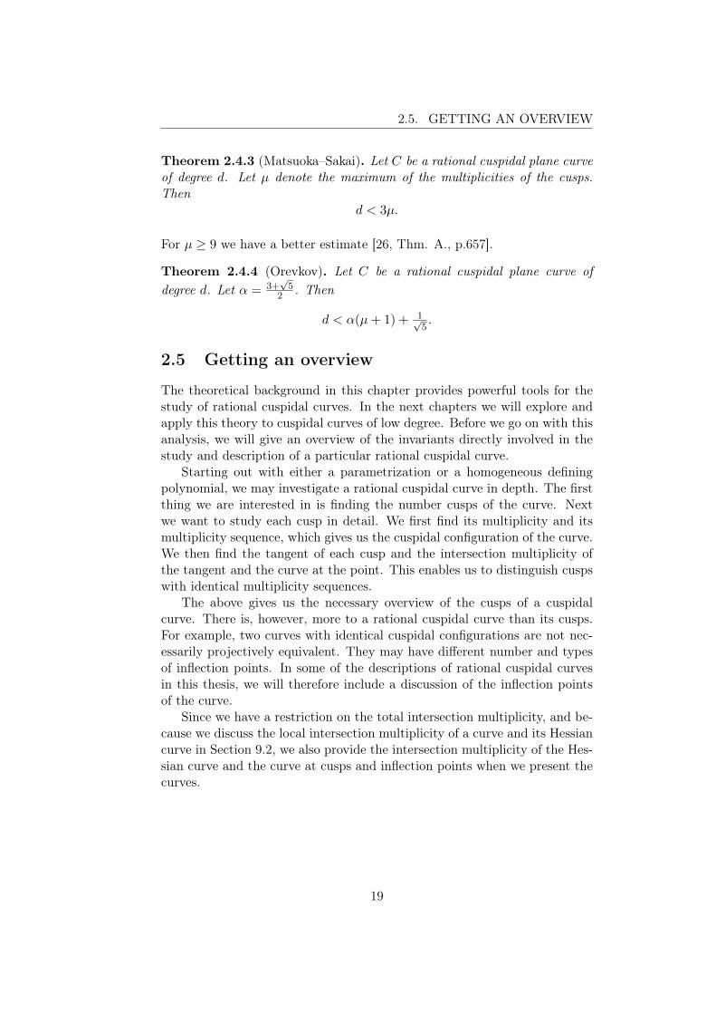
Let p and q be points in P2. Let Lpq be the line between the two points, andlet L be another line through q. Then the quadratic Cremona transforma-tion of type ψ2(p, q, L) can be decomposed into three main steps.
Blowing up at qThe first step is blowing up the point q ∈ P2, hence producing a ruled surfaceX1 with an exceptional line E1. We have E2
1 = −1.
Elementary transformations in p1 and qThe second step is performing two elementary transformations of two fibersat two points on X1. The two fibers are the strict transform of the line Lpq,
45

CHAPTER 5. CREMONA TRANSFORMATIONS
Lpq1 , and the strict transform of the line L, L1. The two points are the stricttransform of p, p1 ∈ Lpq1 , and the point q, which is uniquely determined bythe fact that q ∈ E1 ∩ L1.
After performing the elementary transformations, we obtain another ruledsurface, X2. The horizontal section E2 of this surface is the strict transformof E1 under the elementary transformations. On X2 we have fibers L2 andLpq2 , the strict transforms of the exceptional lines Eq and Ep1 under the ele-mentary transformation.
Blowing down E2
By properties of elementary transformations, E2 satisfies E22 = −1. Hence,
the third step of the Cremona transformation is blowing down E2, whichleads us back to P2 .
Since the Cremona transformation is a composition of blowing-ups andblowing-downs, we are able to follow the intersection multiplicities and themultiplicity sequences of points of a curve and transformations of the curve inevery step of the Cremona transformation. In particular, we can determinethe invariants for the strict transform of the curve.
5.3.5 One proper base point
Let p be a point and let L be a line through p in P2. A quadratic Cremonatransformation of type ψ1(p, L,−) can then be decomposed into four mainsteps.
Blowing up at pThe first step is blowing up the point p ∈ P2. This results in a ruled surfaceX1 with horizontal section E1, where E2
1 = −1. On X1 we additionally havethe fiber L1, the strict transform of the line L, and the point p, which isgiven by p = E1 ∩ L1.
Elementary transformation in pThe second step is performing an elementary transformation of the fiber L1
at the point p on X1. This results in a new ruled surface X2, with horizon-tal section E2 and the fiber L2. E2 denotes the transform of the horizontalsection E1, and L2 denotes the transform of the exceptional line Ep of theelementary transformation. Note that E2
2 = −2.
Elementary transformation in ˆpThe third step is performing an elementary transformation of the fiber L2
at a point ˆp, where ˆp /∈ E2. This results in a new ruled surface X3, in whichwe have the transform of E2, E3, where E2
3 = −1. Analogous to the above,we denote by L3 the transform of the exceptional line E ˆp.
46

5.4. CONSTRUCTING CURVES
Blowing down E3
Since E23 = −1, blowing down the horizontal section E3 ⊂ X3 is the last
step in the Cremona transformation, taking us back to P2 .
As above, we are able to follow the intersection multiplicities and the mul-tiplicity sequences of points of a curve and transformations of the curve inevery step of the Cremona transformation.
5.4 Constructing curves
In this section we will make use of the quadratic Cremona transformationsdescribed above and construct the cuspidal cubic and quartic curves.
The pictures of the implicit Cremona transformations of curves displayedin this thesis are merely illustrations of the action described in the text, andthey do not give a complete overview of the curves and surfaces.
Some of the points and lines are marked with notation in the illustrations.Points which are going to be blown up are marked with name and a blackdot. Lines which are going to be blown down are marked with two blackdots. The curves C stand out in the images, hence, they are not marked.Furthermore, vertical fibers in the ruled surfaces will be marked by name onlywhen they are exceptional lines of blowing-ups. The other vertical fibers arepossible to identify from the context. Moreover, in order to avoid problemswith the notation, we will write T p for the tangent line to C at p.
Cuspidal cubic – [(2)]
We construct the cuspidal cubic with the help of a quadratic Cremona trans-formation with two proper base points.
Let C be an irreducible conic. Two arbitrarypoints p and r on C have unique tangents T p
and T r, which only intersect C at p and r,respectively.
T p · C = 2 · p,T r · C = 2 · r.
Let q denote the intersection point T p ∩ T r,and note that q /∈ C.
Applying the transformation ψ2(p, q, T r) to C, we get the desired cubic.
47

CHAPTER 5. CREMONA TRANSFORMATIONS
Blowing up at q
Blowing up at q, we get the ruled surfaceX1 with horizontal section E1 and the trans-formed curve C1. No points or intersectionmultiplicities have been affected by this pro-cess. Note that since q /∈ C, E1 ∩ C1 = ∅.
The points q = E1 ∩T r1 and p1 = C1 ∩T p1 aremarked in the figure.
Elementary transformations in q and p1
Blowing up at q and p1 gives on X1 two ex-ceptional lines Eq and Ep1 . We have the in-tersections
T r1 · C1 = 2 · r1,
T r1 ∩ E1 = ∅,T p1 · C1 = ((T p1 · C1)p1 −mp1) · p1
= 1 · p1,
Ep1 · C1 = 1 · p1.
Blowing down T r1 and T p1 gives the surfaceX2. On this surface we have T r2 , the stricttransform of Eq, and T
p2 , the strict transform
of Ep1 .
Because of the above intersection concerningr1, r2 is a cusp with multiplicity sequence (2).Note that r2 /∈ E2.
The smooth point p1 is transformed into thesmooth point p2. Furthermore, T p2 is actually the tangent to C2 at p2,and p2 ∈ E2.
(T p2 · C2)p2 = ((T p1 · C1)p1 + (Ep1 · C1)p1)
= 2,
(E2 · C2)p2 = (T p1 · C1)p1
= 1.
48

5.4. CONSTRUCTING CURVES
Blowing down E2
Blowing down E2 gives a curve C ′ with onecusp r′ with multiplicity sequence (2). Addi-tionally, the above intersection multiplicitiesensure that the point p′ is an inflection point.
T p′ · C ′ = ((T p2 · C2)p2 + (E2 · C2)p2) · p′
= 3 · p′.
To see that C ′ really is a cubic, observe that
d′ = 2 · d−mq −mq −mp1
= 2 · 2− 1
= 3.
We may do this explicitly by using the Cremona transformation ψ2 to trans-form the conic C,
C = V(y2 − xz).
We get the desired cubic curve C ′ with an A2-cusp,
C ′ = V(xy2 − z3).
C1 – Tricuspidal quartic – [(2), (2), (2)]
Performing a quadratic Cremona transformation with three proper basepoints on an appropriately oriented irreducible conic produces the tricus-pidal quartic curve.
Let C be an irreducible conic. Choose threepoints s, t and u on C, and let T s, T t and T u
be the respective tangent lines to C at thethree points,
T s · C = 2 · s,T t · C = 2 · t,T u · C = 2 · u.
By Bézout’s theorem, the tangent lines inter-sect in three different points, p, q and r, which can not be on C.
49
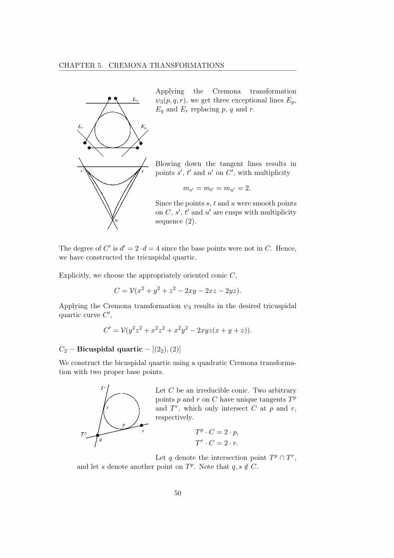
CHAPTER 5. CREMONA TRANSFORMATIONS
Applying the Cremona transformationψ3(p, q, r), we get three exceptional lines Ep,Eq and Er replacing p, q and r.
Blowing down the tangent lines results inpoints s′, t′ and u′ on C ′, with multiplicity
ms′ = mt′ = mu′ = 2.
Since the points s, t and u were smooth pointson C, s′, t′ and u′ are cusps with multiplicitysequence (2).
The degree of C ′ is d′ = 2 ·d = 4 since the base points were not in C. Hence,we have constructed the tricuspidal quartic.
Explicitly, we choose the appropriately oriented conic C,
C = V(x2 + y2 + z2 − 2xy − 2xz − 2yz).
Applying the Cremona transformation ψ3 results in the desired tricuspidalquartic curve C ′,
C ′ = V(y2z2 + x2z2 + x2y2 − 2xyz(x+ y + z)).
C2 – Bicuspidal quartic – [(22), (2)]
We construct the bicuspidal quartic using a quadratic Cremona transforma-tion with two proper base points.
Let C be an irreducible conic. Two arbitrarypoints p and r on C have unique tangents T p
and T r, which only intersect C at p and r,respectively.
T p · C = 2 · p,T r · C = 2 · r.
Let q denote the intersection point T p ∩ T r,and let s denote another point on T p. Note that q, s /∈ C.
50

5.4. CONSTRUCTING CURVES
Applying the transformation ψ2(s, q, T r) to C, we get the desired quartic C ′.
Blowing up at q
Blowing up at q, we get the ruled surface X1
with horizontal section E1, fibers Tp1 and T r1 ,
and the transformed curve C1. No points orintersection multiplicities have been affectedby this process. Since q /∈ C, we have E1 ∩C1 = ∅.
The points q = E1 ∩ T r1 and s1 ∈ T p1 aremarked in the figure.
Elementary transformations in q and s1
Blowing up at q and s1 gives on X1 two ex-ceptional lines Eq and Es1 . We have the in-tersections
T r1 · C1 = 2 · r1,
T r1 ∩ E1 = ∅,T p1 · C1 = 2 · p1,
T p1 ∩ E1 6= ∅.
Blowing down T r1 and T p1 gives the surfaceX2.On this surface we have fibers T r2 , the stricttransform of Eq, and T
p2 , the strict transform
of Es1 .
Because of the intersections above, r2 andp2 are cusps, both with multiplicity sequence(2). Additionally, r2 /∈ E2, but p2 ∈ E2.
We have the intersections
T p2 · C2 = 2 · p2,
E2 · C2 = 2 · p2.
51

CHAPTER 5. CREMONA TRANSFORMATIONS
Blowing down E2
Blowing down E2 gives a curve C ′ with twocusps r′ and p′. The cusp r′ is unaltered bythe last blowing-down, and it has multiplicitysequence (2). Because of the intersection
E2 · C2 = 2 · p2,
the cusp p′ has multiplicity sequence (22).
To see that C ′ is a quartic, note that
d′ = 2 · d−mq −mq −ms1
= 2 · 2= 4.
We may get this curve explicitly by using the Cremona transformation ψ2
to transform the conic C,
C = V(y2 − 2xy + x2 − xz).
We get the desired quartic curve C ′ with an A2- and A4-cusp,
C ′ = V(z4 − xz3 − 2xyz2 + x2y2).
C3 – Unicuspidal ramphoid quartic – [(23)]
We construct the unicuspidal ramphoid quartic using a quadratic Cremonatransformation with one proper base point.
Let C be an irreducible conic. Choose twoarbitrary points q and r on C, and let T q andT r be the respective tangent lines to C atthese points,
T q · C = 2 · q,T r · C = 2 · r.
Let p denote the intersection point T q ∩ T r,and note that p /∈ C.
Applying the transformation ψ1(p, T r,−) to C, we get the desired quartic.
52

5.4. CONSTRUCTING CURVES
Blowing up at p
Blowing up at p, we get the ruled surface X1
with horizontal section E1, fibers T r1 and T q1 ,and the transformed curve C1. No points orintersection multiplicities have been affectedby this process. Note that since p /∈ C, wehave E1 ∩ C1 = ∅.
The point p = E1∩T r1 is marked in the figure.
Elementary transformation in p
Blowing up at p, we get on X1 an exceptionalline Ep. We have the intersections
T r1 · C1 = 2 · r1,
T r1 ∩ E1 = ∅.
Blowing down T r1 gives the surface X2. Onthis surface we have horizontal section E2 andthe fiber T r2 , the strict transform of Ep. OnT r2 we have marked the point ˆp.
Because of the intersection above, r2 is a cuspwith multiplicity sequence (2). Note that r2 /∈E2 and that E2
2 = −2.
Elementary transformation in ˆp
Blowing up at ˆp we get on X2 an exceptionalline E ˆp. We have the intersections
T r2 · C2 = 2 · r2,
T r2 ∩ E2 6= ∅.
53

CHAPTER 5. CREMONA TRANSFORMATIONS
Blowing down T r2 gives the surface X3. Onthis surface we have the fiber T r3 , the stricttransform of E ˆp. The horizontal section E3
has self-intersection E23 = −1.
Because of the intersection above concerningr2, r3 is a cusp with multiplicity sequence(22). Since T r2 ∩ E2 6= ∅, r3 ∈ E3. Further-more, we have the intersection
E3 · C3 = 2 · r3.
Blowing down E3
Blowing down E3 gives a curve C ′ with onecusp r′. Because of the above intersectionconcerning r3, the cusp r′ has multiplicity se-quence (23).
To see that C ′ is a quartic, note that
d′ = 2 · d−mp −mp −m ˆp
= 2 · 2= 4.
We may construct the curve explicitly by using the Cremona transformationψ1 to transform the conic C,
C = V(yz + x2).
We get the desired cuspidal quartic curve C ′ with an A6-cusp,
C ′ = V(y4 − 2xy2z + yz3 + x2z2).
54

5.4. CONSTRUCTING CURVES
C4A– Ovoid quartic A – [(3)]
We construct the ovoid quartic with one inflection point of type 2 using aquadratic Cremona transformation with two proper base points.
Let C be the cuspidal cubic with a cusp p,mp = (2), and an inflection point r of type 1.The points p and r have tangents T p and T r,which only intersect C at p and r respectively.
T p · C = 3 · p,T r · C = 3 · r.
Let q denote the intersection point T p ∩ T r,and note that q /∈ C.
Applying the transformation ψ2(p, q, T r) to C, we get the desired quartic.
Blowing up at q
Blowing up at q we get on X1 a horizontalsection E1, fibers T
p1 and T r1 , and the trans-
formed curve C1. No points or intersectionmultiplicities have been affected by this pro-cess. Since q /∈ C, we have E1 ∩ C1 = ∅.The points q = E1 ∩ T r1 and p1 ∈ T p1 aremarked in the figure.
Elementary transformations in q and p1
Blowing up at q and the cusp p1 gives on X1
two exceptional lines Eq and Ep1 . We nowhave two smooth points, r1 and p1, and theintersections
T r1 · C1 = 3 · r1,
T r1 ∩ E1 = ∅,T p1 · C1 = ((T p1 · C1)p1 −mp1) · p1
= (3− 2) · p1
= 1 · p1,
T p1 ∩ E1 6= ∅,Ep1 · C1 = mp1 · p1
= 2 · p1.
55

CHAPTER 5. CREMONA TRANSFORMATIONS
Blowing down T r1 and T p1 gives the surfaceX2. On this surface we have T r2 , the stricttransform of Eq, and T
p2 , the strict transform
of Ep1 .
Since E1 ∩ T p1 6= ∅, p2 ∈ E2. Moreover, sinceT r1 ∩ E1 = ∅, r2 /∈ E2. While p2 is a smoothpoint, r2 is a cusp with multiplicity sequence(3). The latter is a consequence of
T r1 · C1 = 3 · r1.
We also have the important intersections
T p2 · C2 = ((T p1 · C1)p1 + (Ep1 · C1)p1) · p2
= (1 + 2) · p2
= 3 · p2,
E2 · C2 = (T p1 · C1)p1 · p2
= 1 · p2.
Blowing down E2
Blowing down E2 gives a curve C ′ with onecusp r′. The cusp is unaltered by the lastblowing-down, and it has multiplicitysequence (3). Because of the above intersec-tions concerning p2, C has an inflection pointp′ of type 2.
To see that C ′ is a quartic, note that
d′ = 2 · d−mq −mq −mp1
= 2 · 3− 2
= 4.
We may construct the curve explicitly by using the Cremona transformationψ2 to transform the cubic C,
C = V(xz2 − y3).
We get the desired quartic curve C ′ with one E6-cusp and one inflectionpoint of type 2,
C ′ = V(z4 − xy3).
56

5.4. CONSTRUCTING CURVES
C4B – Ovoid quartic B – [(3)]
We construct the ovoid quartic with two inflection points using a quadraticCremona transformation with two proper base points. By direct calcula-tion and investigation of the curve and its orientation with respect to theCremona transformation, we know that this construction is valid. Thereare, however, some unanswered questions concerning the number of inflec-tion points constructed with Cremona transformations. This issue will bediscussed in Section 5.5.
Let C be the cuspidal cubic with a cusp p,mp = (2), and an inflection point r. Choosea smooth point s, s 6= r. The tangents T p
and T s intersect C,
T p · C = 3 · p,T s · C = 2 · s+ 1 · t,
where t is a smooth point.
Additionally, we denote by L = Lps the line through the cusp p andthe point s. Intersecting L with C gives
L · C = 2 · p+ 1 · s.
Finally, let q denote the intersection point T p ∩ T s.
Applying the transformation ψ2(q, p, L) to C, we get the desired quartic.Note that the inflection point r will not be affected by this process.
Blowing up at p
Blowing up at the cusp p, we get X1 withhorizontal section E1, fibers L1 and T p1 , andthe transformed curve C1. The points p =E1∩L1 and q are marked in the figure. Sincewe blew up at p with multiplicity sequence(2), p1 is smooth. Additionally,
E1 · C1 = 2 · p1,
T p1 · C1 = ((T p · C)p −mp) · p1
= (3− 2) · p1
= 1 · p1,
L1 · C1 = 1 · s1.
57

CHAPTER 5. CREMONA TRANSFORMATIONS
Elementary transformations in p and q
Blowing up at p and q gives on X1 two excep-tional lines Ep and Eq, which do not changeany points or intersections.
Blowing down L1 and T p1 gives the surfaceX2. On this surface we have the fibers L2,the strict transform of Ep, and T
p2 , the strict
transform of Eq.
We get the intersection multiplicity
E2 · C2 = ((E1 · C1)p1 + (T p1 · C1)p1) · p2
= (2 + 1) · p2
= 3 · p2.
Additionally, note that we have affected the point s2 with this ele-mentary transformation. On X1, assuming s1 has a tangent T andthen blowing down L1, we calculate the intersection multiplicity of thetangent T s2 to C2 at s2 and C2,
(T s2 · C2)s2 = ((T · C1)s1 + (L1 · C1)s1)
= (2 + 1)
= 3.
Hence, s2 is an inflection point of C2.
Blowing down E2
Blowing down E2 gives a curve C ′ with onecusp p′ and two inflection points r′ and s′.Because of the intersection E2 · C2 = 3 · p2,the cusp p′ has multiplicity sequence (3).
To see that C ′ is a quartic, observe that
d′ = 2 · d−mp −mp −mq
= 2 · 3− 2
= 4.
58

5.5. A NOTE ON INFLECTION POINTS
We may construct this curve explicitly by using the Cremona transformationψ2 to transform the cubic C,
C = V(yz2 − x2z + x3).
We get the desired quartic curve C ′ with one E6-cusp and two inflectionpoints of type 1,
C ′ = V(x3y − z3x+ z4).
5.5 A note on inflection points
We observe that if two curves have the same cuspidal configuration, buta different number of inflection points, then they can not be projectivelyequivalent. We are therefore interested in the configuration of inflectionpoints of a curve, in addition to the cuspidal configuration. In this section wegive examples on how the configuration of inflection points can be determinedby other properties of the curve. Furthermore, we give examples on howinflection points behave unpredictably under Cremona transformations.
Configuration of inflection points
The ovoid quartic curves are examples of curves which are not projectivelyequivalent, even though they have the same cuspidal configuration. Themost prominent difference between the two curves is the configuration ofinflection points.
Fortunately, when C is a curve of degree d with a given cuspidal con-figuration, we can often determine which of the possible configurations ofinflection points actually exist.
Example 5.5.1. Consider a cuspidal quartic curve C with cusps p and qwith multiplicity sequences mp = (22) and mq = (2). Since C is a quartic,the intersection multiplicity of the curve and the tangents at the cusps mustbe rp = 4 and rq = 3. A quartic curve with this cuspidal configuration must,by Theorem 2.3.3, have precisely one inflection point of type 1.
s = 3 · 4 · (4− 2)− 6 · (2 + 1)− (2 + 4− 3)− (2 + 3− 3)
= 1.
Example 5.5.2. Consider a quartic curve with one cusp p with multiplicitysequence (23). Since C is a quartic, the intersection multiplicity of the curveand the tangent at the cusp is rp = 4. We want to determine the configura-tion of inflection points of this curve.
The curve must have three inflection points, counted properly.
s = 3 · 4 · (4− 2)− 6 · 3− (2 + 4− 3)
= 3.
59

CHAPTER 5. CREMONA TRANSFORMATIONS
We show that the only existing curve with this cuspidal configuration hasthree inflection points of type 1. We will do this by excluding all other config-urations of inflection points and checking that the mentioned configurationdoes not violate any restrictions.
The dual curve C∗ has degree
d∗ = 2 · d− 2− (mp − 1)
= 2 · 4− 2− 1
= 5.
The curve C can at the cusp p be given by the Puiseux parametrization
(C, p) = (t2 : c4t4 + c7t
7 + . . . : 1).
The dual curve C∗ can at the dual point p∗ be given by the Puiseuxparametrization
(C∗, p∗) = (a∗t2 + . . . : 1 : c∗4t4 + c∗7t
7 . . .).
Hence, p∗ is a cusp, m∗p = (23), and r∗p = 4.
Assume that C only has one inflection point q of type 3. Then the curvemust locally around q be parametrized by
(C, q) = (t : c5t5 + . . . : 1).
In this parametrization of the quartic we have that rq = 5, but that is aviolation of Bézout’s theorem since rq = 5 > 4 = d. Hence, C can not haveone inflection point of type 3.
Assume that C has two inflection points q and r of type 1 and 2, respectively.Then we have
(C, q) = (t : c3t3 + . . . : 1),
(C, r) = (t : c4t4 + . . . : 1).
Moreover,
(C∗, q∗) = (a∗t2 + . . . : 1 : c∗3t3 + . . .),
(C∗, r∗) = (a∗t3 + . . . : 1 : c∗4t4 + . . .),
implying that q∗ and r∗ are cusps with multiplicity sequences (2) and (3).Then the dual curve C∗ has three singularities, and
∑j=p∗,q∗,r∗ δj = 7. This
contradicts the genus formula (2.2.2). Hence, C can not have two inflectionpoints.
60

5.5. A NOTE ON INFLECTION POINTS
Assume that C has three inflection points q, r and u of type 1. Then the dualquintic curve C∗ has four cusps p∗, q∗, r∗ and u∗ with multiplicity sequences(23), (2), (2) and (2), respectively. Indeed, C∗ does not contradict the genusformula, ∑
j=p∗,q∗,r∗,u∗
δj = 6 =(5− 1)(5− 2)
2.
Additionally, we do not get any contradiction when we calculate the numberof inflection points on C∗.
s∗ = 3 · 5 · (5− 2)− 6 · 6− (2 + 4− 3)− 3 · (2 + 3− 3)
= 0.
We shall later see that C∗ is a remarkable curve.
Inflection points and Cremona transformations
Constructing inflection points with Cremona transformations is a bit moresubtle than constructing cusps. The constructions of the cuspidal quarticsgive examples of this subtlety.
Example 5.5.3. To construct the ovoid quartic with one inflection point onpage 55, we use a cuspidal cubic with one inflection point of type 1. In thetransformation we transform the inflection point of the cubic into the cuspof the quartic. Furthermore, the cusp of the cubic is transformed into theinflection point of type 2 of the quartic. Moreover, the construction of theinflection point is directly visible in the action of the Cremona transforma-tion.
Example 5.5.4. To construct the ovoid quartic with two inflection pointson page 57, we also use a cuspidal cubic with one inflection point of type1. The cusp of the cubic is transformed into the cusp of the quartic. Theinflection point on the cubic is unaffected by the Cremona transformation.The construction of the second inflection point, however, is not directly vis-ible in the pictures of the Cremona transformation. We carefully argued forthe construction of this inflection point based on elementary properties ofmonoidal transformations.
Example 5.5.5. To construct the bicuspidal quartic on page 50, we trans-form a conic. We make the intriguing observation that there is no apparentreason why the Cremona transformation of the conic should give this curvean inflection point. We have, however, seen that the curve must have aninflection point earlier in this section.
61

CHAPTER 5. CREMONA TRANSFORMATIONS
The three examples clearly show the unpredictable behavior of the inflectionpoints in the construction of curves by Cremona transformations. This is ofcourse of little relevance when it comes to the construction of a particularcuspidal configuration of a curve of given degree. However, it is essentialto note this unpredictable affair in the construction of all, up to projectiveequivalence, rational cuspidal curves of a given degree.
5.6 The Coolidge–Nagata problem
If a rational curve can be transformed into a line by successive Cremonatransformations, then we call the curve rectifiable. The following problemwas introduced by Coolidge in [4, pp.396–399], but because of [24] it alsohas the name of Nagata.
The Coolidge–Nagata problem. Which rational curves can birationallybe transformed into a line? In particular, which rational cuspidal curves havethis property?
Coolidge noted that most rational curves of low degree are rectifiable. Thereexist, however, rational curves which are not rectifiable. An example of sucha curve is the sextic with ten singularities, each having two distinct tangents.
There are actually no known rational cuspidal curves which are not rec-tifiable. In particular, all rational cuspidal curves we will encounter in thisthesis are rectifiable by construction. This claim can easily be verified forthe curves we have encountered this far. All these curves are somehow con-structed from an irreducible conic. Hence, applying the inverse transforma-tion to any of the cuspidal curves will produce the conic. Moreover, anyirreducible conic can be transformed into a line by applying a quadratic Cre-mona transformation with three base points, just choose the base points onthe conic.
The complement of a rational cuspidal curve in P2 is an open surface.For an open surface P2 \C, where C is a rational cuspidal curve, there existsassumptions with which it is possible to prove that C is rectifiable. For adetailed discussion of these results, see [9, pp.418–419].
Matsuoka and Sakai observed that if a curve is transformable to a line byCremona transformations, then the Matsuoka–Sakai inequality on page 19is a consequence of one of Coolidge’s results. Since they were able to inde-pendently prove that the inequality is valid for all rational cuspidal curves,they proposed the following conjecture [21, p.234].
Conjecture 5.6.1. Every rational cuspidal curve can be transformed into aline by a Cremona transformation.
62

Chapter 6
Rational cuspidal quintics
In this chapter we will describe the rational cuspidal quintic curves. Usingthe method provided by Flenner and Zaidenberg in [12] and methods de-scribed in Chapter 2, we will obtain a list of possible cuspidal configurationsfor a rational quintic. We will construct and describe examples of all thesecurves.
6.1 The cuspidal configurations
We want to find all possible cuspidal configurations for rational cuspidalquintics. The idea is the same as for lower degrees, only now getting theresults requires more theoretical background.
Flenner and Zaidenberg find in [12, pp.104–105] all possible cuspidalconfigurations for quintics with three or more cusps. Unfortunately, thereare some incomplete explanations and one minor error in their work. Inthe following we will generalize the ideas of Flenner and Zaidenberg’s proof.We will obtain a list of cuspidal configurations for all cuspidal quintics byusing general restrictions and Flenner and Zaidenberg’s ideas to exclude thenonexistent ones. Included in this work are Flenner and Zaidenberg’s results,with complementary additions and appropriate corrections.
6.1.1 General restrictions
Assume that we have a rational cuspidal curve of degree d = 5 with a finitenumber of cusps p, q, r, . . . . Let the cusp p have multiplicity sequencemp = (mp,m1, ...,mnp) and delta invariant δp. Define the same invariantsfor the other cusps. By Theorem 2.2.2 the cusps of C satisfy
(5− 1)(5− 2)
2= 6 =
∑p∈SingC
np∑i=0
mi(mi − 1)
2.
63

CHAPTER 6. RATIONAL CUSPIDAL QUINTICS
We sort the cusps by their multiplicity such thatmp ≥ mq ≥ mr ≥ . . .. Thenthe largest multiplicity of the cusps on the curve is µ = mp. By Bézout’stheorem we immediately get
µ ≤ 4.
If there are two or more cusps on the curve, then we can improve this re-striction. Let L be a line which intersects the rational cuspidal curve C intwo of its cusps. Then the sum of the intersection multiplicities of L and Cin these two points is less than or equal to the degree of the curve. For anypair of cusps, in particular the largest cusps p and q,
(C · L)p + (C · L)q ≤ 5.
Since the minimal intersection multiplicity between a line and any cusp isequal to the minimal multiplicity of any cusp, i.e., 2, mp can not be greaterthan 3. Hence, for curves with two or more cusps, we have the restriction
µ ≤ 3.
Further restrictions on the multiplicities can be found using the results inChapter 2, and we will refer to these in the following.
6.1.2 One cusp
Assuming we only have one cusp p, the above restrictions leave us with fourcuspidal configurations, of which two can be excluded.
Maximal multiplicity 4
Let µ = 4. Then δ = 6. Hence, (4) is the only possible multiplicity sequence.Curves with this multiplicity sequence exist.
Maximal multiplicity 3
Let µ = 3. By elementary properties of the multiplicity sequence, m1 ≤ 3.Furthermore, the only multiplicity sequences satisfying the genus formulaare (32) and (3, 23). Neither of these multiplicity sequences are possible ona rational cuspidal quintic curve. The sequence (32) violates m0 + m1 ≤ 5from (2.3) on page 12. The sequence (3, 23) does not satisfy the property ofthe multiplicity sequence given in Proposition 2.2.1 on page 8.
Maximal multiplicity 2
Let µ = 2. Then the only possible multiplicity sequence is (26). Curves withthis multiplicity sequence exist.
64

6.1. THE CUSPIDAL CONFIGURATIONS
Conclusion
We have two possible cuspidal configurations for unicuspidal quintics.
Curve Cuspidal configurationC1 (4)
C2 (26)
6.1.3 Two cusps
Assuming we have two cusps p and q, the above restrictions leave us withsix cuspidal configurations, of which three can be excluded.
Maximal multiplicity 3
Let µ = mp = 3. Then mq = 2, and we have three cuspidal configurationssatisfying the genus formula,
[(3, 22), (2)] [(3, 2), (22)] [(3), (23)].
The configuration [(3, 22), (2)] violates properties of the multiplicity sequencegiven in Proposition 2.2.1. The two remaining configurations actually exist.
Maximal multiplicity 2
Let µ = mp = 2. Then mq = 2, and we have three cuspidal configurationssatisfying the genus formula,
[(25), (2)] [(24), (22)] [(23), (23)].
The first and last configurations can be excluded by a similar argumentinvolving Cremona transformations.
Curve – [(25), (2)]
Assume that there exists a rational cuspidalquintic C with two cusps p and q with mul-tiplicity sequences mp = (25) and mq = (2).Let T denote the tangent line of p and let Lbe the line between the two cusps.
Since C is a quintic and p has multiplicitysequence (25), Lemma 2.2.4 implies that
(C · T )p = 4.
By Bézout’s theorem, T must intersect C transversally in a smoothpoint t,
C · T = 4 · p+ 1 · t.
65

CHAPTER 6. RATIONAL CUSPIDAL QUINTICS
Applying the Cremona transformation ψ(p, T,−) to C gives a quartic curve.We shall obtain a contradiction by observing that this particular quarticcurve does not exist. This implies that the quintic curve C can not existeither.
Note that the Cremona transformation does not affect the A2-cusp q,and we will therefore keep this point out of the discussion.
Blowing up at p
Blowing up at p, we get the ruled surface X1,where the transform p1 of p is a cusp withmultiplicity sequence (24). We also have theintersections
C1 · E1 = mp · p1
= 2 · p1,
C1 · T1 = ((C · T )p −mp) · p1 + 1 · t1= 2 · p1 + 1 · t1.
Elementary transformation in p1
Blowing up at p1 gives the cusp p1 with mul-tiplicity sequence (23) on the surface X1. Theexceptional line Ep1 separates E1 and T1. Weget the intersections
E1 ∩ C1 = ∅,Ep1 · C1 = mp1 · p1
= 2 · p1,
T1 · C1 = 1 · t1,T1 ∩ E1 = ∅.
Blowing down T1 gives the surface X2. Thetransform T2 of Ep1 intersects C2 in the A6-cusp p2 and the smooth point t2. In partic-ular, t2 /∈ E2 because of the last intersectionabove. We have the intersection
T2 · C2 = 2 · p2 + 1 · t2.
66

6.1. THE CUSPIDAL CONFIGURATIONS
Elementary transformation in p2
Blowing up at p2 gives the cusp p2 with multi-plicity sequence (22) on the surface X2. Notethat the exceptional line Ep2 does not sepa-rate E2 and T2, but we have the intersections
Ep2 · C2 = 2 · p2,
T2 · C2 = 1 · t2.
Blowing down T2 gives the surface X3 withthe A4-cusp p3, and the intersections
E3 · C3 = 1 · t3,T3 · C3 = 1 · t3 + 2 · p3.
Note that both E3 and T3 intersect C3
transversally at t3.
Blowing down E3
Since neither of the cusps p3 and q3 lie on E3,blowing down E3 gives a curve C ′ with oneA4-cusp p′ and one A2-cusp q′. Since both E3
and T3 intersect C3 transversally in the pointt3, this point is transformed into a smoothpoint t′ ∈ C ′, with the property that the tan-gent line at t′ will be the transform T ′ of T3.This is a result of the intersection multiplicity
(T ′ · C ′)t′ = (T3 · C3)t3 + (E3 · C3)t3
= 2.
Note that by the intersection T3 ·C3 above, T ′ must intersect C ′ at theA4-cusp p′. We have
T ′ · C ′ = 2 · t′ + 2 · p′.
Observe that C ′ is a quartic since
d′ = 2 · d−mp −mp1 −mp2
= 2 · 5− 2− 2− 2
= 4.
67

CHAPTER 6. RATIONAL CUSPIDAL QUINTICS
Up to projective equivalence, there is only one quartic curve D with cuspidalconfiguration [(22), (2)]. Let D be the zero set of F = z4−xz3−2xyz2+x2y2.D has an A4-cusp at p = (0 : 1 : 0). The polar of C at p is given by
PpC = V(−2xz2 + 2x2y).
Calculations in Maple reveal that the polar of D at p does not intersect Dat any smooth point. This implies that there is no point t ∈ D such thatthe tangent TtD intersects D at p. Hence, neither C ′ nor the quintic curvewith multiplicity sequence [(25), (2)] exist.
Curve – [(23), (23)]
Assume that there exists a rational cuspidalquintic C with two cusps p and q with mul-tiplicity sequences mp = (23) and mq = (23).Let T = T p be the tangent line of p and letL = Lpq be the line between the two cusps.Let s and t be smooth points of C. Then wehave
C · T = 4 · p+ 1 · t,C · L = 2 · p+ 2 · q + 1 · s.
We proceed with the Cremona transformation ψ2(q, p, T ). This will lead toa contradiction.
Blowing up at p
Blowing up at the cusp p with multiplicitysequence (23) gives a ruled surface X1 withexceptional line E1. The transform p1 of p isa cusp with multiplicity sequence (22). Wehave
(C1 · T1)p1 = (C · T )p −mp
= 4− 2
= 2,
E1 · C1 = mp · p1
= 2 · p1.
Additionally, with q1 still an A6-cusp, we have the intersections
C1 · T1 = 2 · p1 + 1 · t1,C1 · L1 = 2 · q1 + 1 · s1.
68

6.1. THE CUSPIDAL CONFIGURATIONS
Elementary transformations in p1 and q1
Blowing up at p1 and q1, we get on the surfaceX1 the exceptional lines Ep1 and Eq1 . We getone A2-cusp p1 and one A4-cusp q1. Addi-tionally, Ep1 separates T1 and E1, while Eq1does not separate L1 and E1. We have theintersections
E1 ∩ C1 = ∅,T1 ∩ E1 = ∅,L1 ∩ E1 6= ∅,Ep1 · C1 = 2 · p1,
T1 · C1 = 1 · t1,Eq1 · C1 = 2 · q1,
L1 · C1 = 1 · s1.
Blowing down the lines T1 and L1, we get thesurface X2 with horizontal section E2, whereE2
2 = −1. We let T2 denote the transform ofEp1 , and L2 the transform of Eq1 on X2. Thecurve C2 has two cusps p2 and q2, of type A2
and A4 respectively. We have
T2 · C2 = 2 · p2 + 1 · t2,L2 · C2 = 2 · q2 + 1 · s2,
E2 · C2 = 1 · s2.
Blowing down E2
The curve C ′ has two cusps, p′ of type A2 andq′ of type A4. Since both E2 and L2 intersectC2 transversally in the point s2, this point istransformed into a smooth point s′ ∈ C ′ withthe property that the tangent line at s′ willbe the transform L′ of L2. This is a result ofthe intersection multiplicity
(L′ · C ′)s′ = (L2 · C2)s2 + (E2 · C2)s2
= 2.
69

CHAPTER 6. RATIONAL CUSPIDAL QUINTICS
Note that by the intersection L2 ·C2 above, L′ must also intersect C ′ at theA4-cusp q′. We have
L′ · C ′ = 2 · s′ + 2 · q′.
We observe that C ′ is a quartic curve,
d′ = 2 · d−mp −mp1 −mq1
= 2 · 5− 2− 2− 2
= 4.
As in the previous case, the quartic curve with this cuspidal configurationdoes not have a point like s′. Hence, the quintic curve C does not exist.
Conclusion
We have three possible cuspidal configurations for bicuspidal quintics.
Curve Cuspidal configurationC3 (3, 2), (22)
C4 (3), (23)
C5 (24), (22)
6.1.4 Three or more cusps
Assuming we have three or more cusps p, q, r, . . ., the general restrictionsleave us with seven cuspidal configurations, of which four can be excluded.
Maximal multiplicity 3
Assuming that µ = 3 and letting p be the cusp where µ = mp = 3, Lemma2.4.2 on page 18 gives a maximum of two ramification points in the projectionof C from p. Thus, C can have up to three cusps. By the assumption thatC has at least three cusps, C must have exactly three cusps. By Bézout’stheorem, the only possible configuration of cusps for such a curve is
[(3), (2a), (2b)], a, b ∈ N.
Theorem 2.2.2 gives the necessary restriction on a and b. In this situation, theformula can be reduced to 6 = 3 + a+ b. Therefore, assuming a ≥ b > 0, wemust have a = 2 and b = 1. Hence, the only possible cuspidal configurationis
[(3), (22), (2)].
This curve will be constructed by Cremona transformations at the end ofthis chapter.
70

6.1. THE CUSPIDAL CONFIGURATIONS
Maximal multiplicity 2
If µ = 2, then all the cusps must have multiplicity m = 2. Let p, q, r . . .denote the cusps of C with multiplicity sequences (2p), (2q), (2r) . . . respec-tively, p, q, r . . . ∈ N. Although this notation is ambiguous, the nature of theobjects we refer to by p, q, r . . . should be clear from the context.
In this situation, Theorem 2.2.2 leads to the sum p+ q+ r+ . . . = 6. Byreordering the cusps, we may assume that p ≥ q ≥ r ≥ . . .. Projecting Cfrom the cusp p gives, by Lemma 2.4.2, four ramification points. Hence, Chas at most five cusps, and we have the following cuspidal configurations.
1) C has 3 cusps, p = (22), q = (22), r = (22).
2) C has 3 cusps, p = (24), q = (2), r = (2).
3) C has 3 cusps, p = (23), q = (22), r = (2).
4) C has 4 cusps, p = (23), q = (2), r = (2), s = (2).
5) C has 4 cusps, p = (22), q = (22), r = (2), s = (2).
6) C has 5 cusps, p = (22), q = (2), r = (2), s = (2), t = (2).
Only cases 1) and 4) exist. These curves will later be constructed and de-scribed. We will now exclude curves 2), 3), 5) and 6) from the list of possiblecuspidal configurations.
Curve 6) – [(22), (2), (2), (2), (2)]
The curve with 5 cusps is easily excluded from the above list because itcontradicts Lemma 2.4.2.∑
j=q,r,s,t
(mj − 1) + (mp.1 − 1) ≤ 2(d−mp − 1)
is contradicted by
5 = 4 · (2− 1) + (2− 1) � 2 · (5− 2− 1) = 4.
Curve 5) – [(22), (22), (2), (2)]
An argument involving the dual curve contradicts the existence of this curve.Theorem 2.3.1 implies that the dual curve of C has degree
d∗ = 2d− 2−∑
j=p,q,r,s
(mj − 1)
= 2 · 5− 2− 4
= 4.
71

CHAPTER 6. RATIONAL CUSPIDAL QUINTICS
Remark 6.1.1. Flenner and Zaidenberg claim that the dual curve has degreed∗ = 3.
The degree of the dual curve does not give a contradiction in itself. Acontradiction additionally requires a local calculation of the correspondingconfiguration of singularities on the dual curve.
We first analyze the simple cusps r and s. By Lemma 2.2.4, (C ·Tr)r = 3.We then have a Puiseux parametrization for the germ (C, r),
(C, r) = (t2 : c3t3 + . . . : 1).
The dual germ (C∗, r∗) consequently has Puiseux parametrization
(C∗, r∗) = (a∗t+ . . . : 1 : c∗3t3 + . . .).
Hence, r∗ is an inflection point of type 1 on C∗. The same is true for s∗.The fate of the A4-cusps p and q, with multiplicity sequences (22), can
be determined in the same way. Since C is a quintic, the upper and lowerbound on (C · Tp)p are given by identity (2.3) on page 12,
4 ≤ (C · Tp)p ≤ 5.
Thus, we have two possibilities for the intersection multiplicity and thePuiseux parametrization.
– If (C · Tp)p = 5, then the cusp p has local Puiseux parametrization
(C, p) = (t2 : c5t5 + . . . : 1).
The dual point on the dual germ has Puiseux parametrization
(C∗, p∗) = (a∗t3 + . . . : 1 : c∗5t5 + . . .).
This implies that p∗ is a cusp with multiplicity sequence (3, 2).
– If (C · Tp)p = 4, then the cusp p has local Puiseux parametrization
(C, p) = (t2 : c4t4 + c5t
5 + . . . : 1).
The dual point on the dual germ has Puiseux parametrization
(C∗, p∗) = (a∗t2 + . . . : 1 : c∗4t4 + c∗5t
5 + . . .).
This implies that p∗ is a cusp of the same kind as p. They are bothA4-cusps with multiplicity sequence (22).
Hence, the two cusps p∗ and q∗ on the dual curve C∗, corresponding to pand q on C, may be the following pairs.
72

6.1. THE CUSPIDAL CONFIGURATIONS
i) Both p∗ and q∗ have multiplicity sequence (22).
ii) Both p∗ and q∗ have multiplicity sequence (3, 2).
iii) One cusp, p∗, has multiplicity sequence (22), and the other cusp, q∗,has multiplicity sequence (3, 2).
Case i) implies that the curve C∗ has genus g ≤ −1, so it is not irreducible.Hence, C is not a rational cuspidal quintic curve.
To exclude case ii), observe that the line L∗ = L∗p∗q∗ between the two cuspsp∗ and q∗ intersects the curve with multiplicity at least
∑j=p∗,q∗
(C∗ · L∗)j ≥ m∗p +m∗q = 6.
But 6 > d∗ = 4, which contradicts Bézout’s theorem. Hence, C∗ and C cannot exist. A nearly identical argument rules out case iii).
We may conclude that no rational cuspidal quintic curve with cuspidal con-figuration [(22), (22), (2), (2)] can exist.
Curve 3) – [(23), (22), (2)]
Assume that the curve C with three cusps, p,q and r, exists. The cusps have multiplicitysequences (23), (22) and (2) respectively. LetT = Tp denote the tangent line at the cusp p,and let L = Lpq denote the line between thecusps p and q. By Lemma 2.2.4, we have theintersections
C · T = 4 · p+ 1 · t,C · L = 2 · p+ 2 · q + 1 · s.
We proceed with the Cremona transformation ψ2(q, p, T ). This will give acontradiction. The A2-cusp r will not be altered by this process, and it willtherefore only be mentioned at the end of the discussion.
73

CHAPTER 6. RATIONAL CUSPIDAL QUINTICS
Blowing up at p
Blowing up at the cusp p with multiplicity se-quence (23) gives a ruled surface X1 with theexceptional line E1. The transform p1 of p isa cusp with multiplicity sequence (22). Wehave the intersection multiplicity and inter-section
(C1 · T1)p1 = (C · T )p −mp
= 4− 2
= 2,
E1 · C1 = mp · p1
= 2 · p1.
Furthermore, we also have the intersection
C1 · T1 = 2 · p1 + 1 · t1.
For the A4-cusp q the situation is unaltered for the transform of thepoint, q1, but the blowing up process gives the intersection
C1 · L1 = 2 · q1 + 1 · s1.
Elementary transformations in p1 and q1
Blowing up at p1 and q1, we get on the sur-face X1 the exceptional lines Ep1 and Eq1 .We get two A2-cusps p1 and q1. Addition-ally, Ep1 separates T1 and E1, while Eq1 doesnot separate L1 and E1. Besides, we have theintersections
E1 ∩ C1 = ∅,Ep1 · C1 = 2 · p1,
T1 · C1 = 1 · t1,Eq1 · C1 = 2 · q1,
L1 · C1 = 1 · s1.
74

6.1. THE CUSPIDAL CONFIGURATIONS
Blowing down the lines T1 and L1, we get asurface X2 with horizontal section E2. Welet T2 denote the transform of Ep1 , and L2
the transform of Eq1 on X2. C2 has threeA2-cusps, p2, q2 and r2. We have
T2 · C2 = 2 · p2 + 1 · t2,L2 · C2 = 2 · q2 + 1 · s2,
E2 · C2 = 1 · s2.
Blowing down E2
Since neither of the A2-cusps p2, q2 or r2 lie on E2, blowing down E2 does notalter these. Hence, the curve C ′ has three A2-cusps p′, q′ and r′. However,since both E2 and L2 intersect C2 transversally in the point s2, this point istransformed into a point s′ ∈ C ′, with the property that the tangent line ats′ will be the transform L′ of L2. This happens because
(L′ · C ′)s′ = (L2 · C2)s2 + (E2 · C2)s2
= 2.
By the above intersection L2 · C2 = 2 · q2 + 1 · s2, we have
L′ · C ′ = 2 · s′ + 2 · q′.
Before we go on with the exclusion, we observe that C ′ is a quartic curve,
d′ = 2 · d−mp −mp1 −mq1
= 2 · 5− 2− 2− 2
= 4.
Up to projective equivalence, there exists only one rational cuspidal quarticwith three cusps, the tricuspidal quartic. By investigating the defining poly-nomial of this explicitly given curve directly, it can easily be proved that asmooth point like s′ does not exist.
Let F = x2y2 +y2z2 +x2z2−2xyz(x+y+ z) be the defining polynomialof the tricuspidal quartic D with cusps p, q and r. By symmetry, these cuspsmust have similar properties. Hence, it is enough to investigate one of them.Let q be the cusp in (1 : 0 : 0). The polar of D at q is given by
PqD = V(2xy2 + 2xz2 − 4xyz − 2y2z − 2yz2).
A calculation in Maple reveals that the only intersection points of the curvesPqD and D are the cusps. A point s with tangent Ts that intersects D inany of the cusps, does therefore not exist on this curve. Hence, neither thecurve C ′ nor the quintic curve C with cuspidal configuration [(23), (22), (2)]exist.
75

CHAPTER 6. RATIONAL CUSPIDAL QUINTICS
Curve 2) – [(24), (2), (2)]
Assume that C is a quintic with three cusps,p, q and r, with multiplicity sequences (24),(2) and (2) respectively. Let T = Tp denotethe tangent line at the A8-cusp p. Since Cis a quintic and because of Lemma 2.2.4, wehave
C · T = 4 · p+ 1 · t,
for a smooth point t ∈ C.
The application of the Cremona transformation ψ(p, T,−) will give a quarticcurve similar to the one described above, and will therefore rule out thisquintic curve.
The Cremona transformation will not affect the two A2-cusps q and r,and they will therefore only be mentioned at the end of the discussion.
Blowing up at p
Blowing up at p, we get the ruled surfaceX1, where the transform p1 of p is a cuspwith multiplicity sequence (23). By elemen-tary properties of the blowing up process, wehave the intersections
C1 · E1 = mp · p1
= 2 · p1,
C1 · T1 = 2 · p1 + 1 · t1.
Elementary transformation in p1
Blowing up at p1 gives the cusp p1 with mul-tiplicity sequence (22) on the surface X1. Theexceptional line Ep1 separates E1 and T1. Ad-ditionally, we get the intersections
Ep1 · C1 = mp1 · p1
= 2 · p1,
T1 · C1 = 1 · t1.
76

6.1. THE CUSPIDAL CONFIGURATIONS
Blowing down T1 gives the surface X2. Thetransform T2 of Ep1 intersects C2 in the A4-cusp p2 and a smooth point t2. In particular,since E1 and T1 were separated by Ep1 , t2 /∈E2. We have the intersection
T2 · C2 = 2 · p2 + 1 · t2.
Elementary transformation in p2
Blowing up at p2 gives the A2-cusp p2 withmultiplicity sequence (2) on the surface X2.Note that the exceptional line Ep2 does notseparateE2 and T2. We have the intersections
Ep2 · C2 = 2 · p2,
T2 · C2 = 1 · t2.
Blowing down T2 gives the surface X3 withthe A2-cusp p3 and the intersections
T3 · C3 = 2 · p3 + 1 · t3,E3 · C3 = 1 · t3.
Blowing down E3
Since neither of the cusps p3, q3 or r3 lie on E3, blowing down E3 gives acurve C ′ with three A2-cusps p′, q′ and r′. However, because both E3 andT3 intersect C3 transversally at t3, the curve C ′ also has a point t′ such thatthe tangent T ′t′ intersects C
′ at the cusp p′.
Observe that C ′ is a quartic since
d′ = 2 · d−mp −mp1 −mp2
= 2 · 5− 2− 2− 2
= 4.
Apart from some notation, the exact same argument is used in the exclusionof this curve as for the exclusion of curve number 3). Hence, curve number2) can also be excluded from the list of possible rational cuspidal quintics.
77
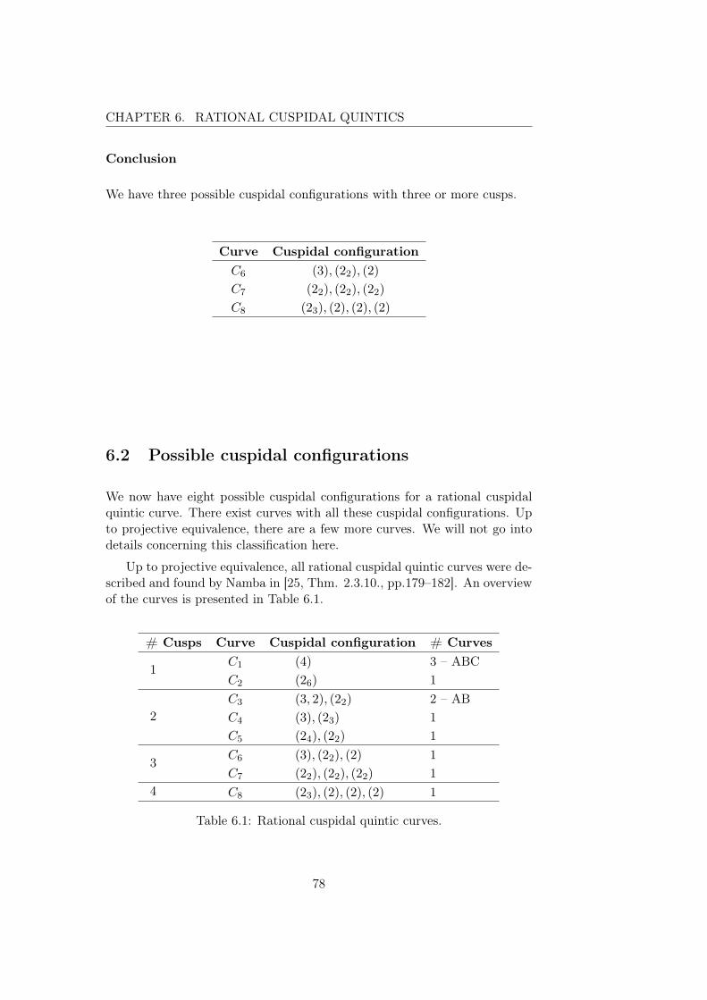
CHAPTER 6. RATIONAL CUSPIDAL QUINTICS
Conclusion
We have three possible cuspidal configurations with three or more cusps.
Curve Cuspidal configurationC6 (3), (22), (2)
C7 (22), (22), (22)
C8 (23), (2), (2), (2)
6.2 Possible cuspidal configurations
We now have eight possible cuspidal configurations for a rational cuspidalquintic curve. There exist curves with all these cuspidal configurations. Upto projective equivalence, there are a few more curves. We will not go intodetails concerning this classification here.
Up to projective equivalence, all rational cuspidal quintic curves were de-scribed and found by Namba in [25, Thm. 2.3.10., pp.179–182]. An overviewof the curves is presented in Table 6.1.
# Cusps Curve Cuspidal configuration # Curves
1 C1 (4) 3 – ABCC2 (26) 1
2C3 (3, 2), (22) 2 – ABC4 (3), (23) 1C5 (24), (22) 1
3 C6 (3), (22), (2) 1C7 (22), (22), (22) 1
4 C8 (23), (2), (2), (2) 1
Table 6.1: Rational cuspidal quintic curves.
78
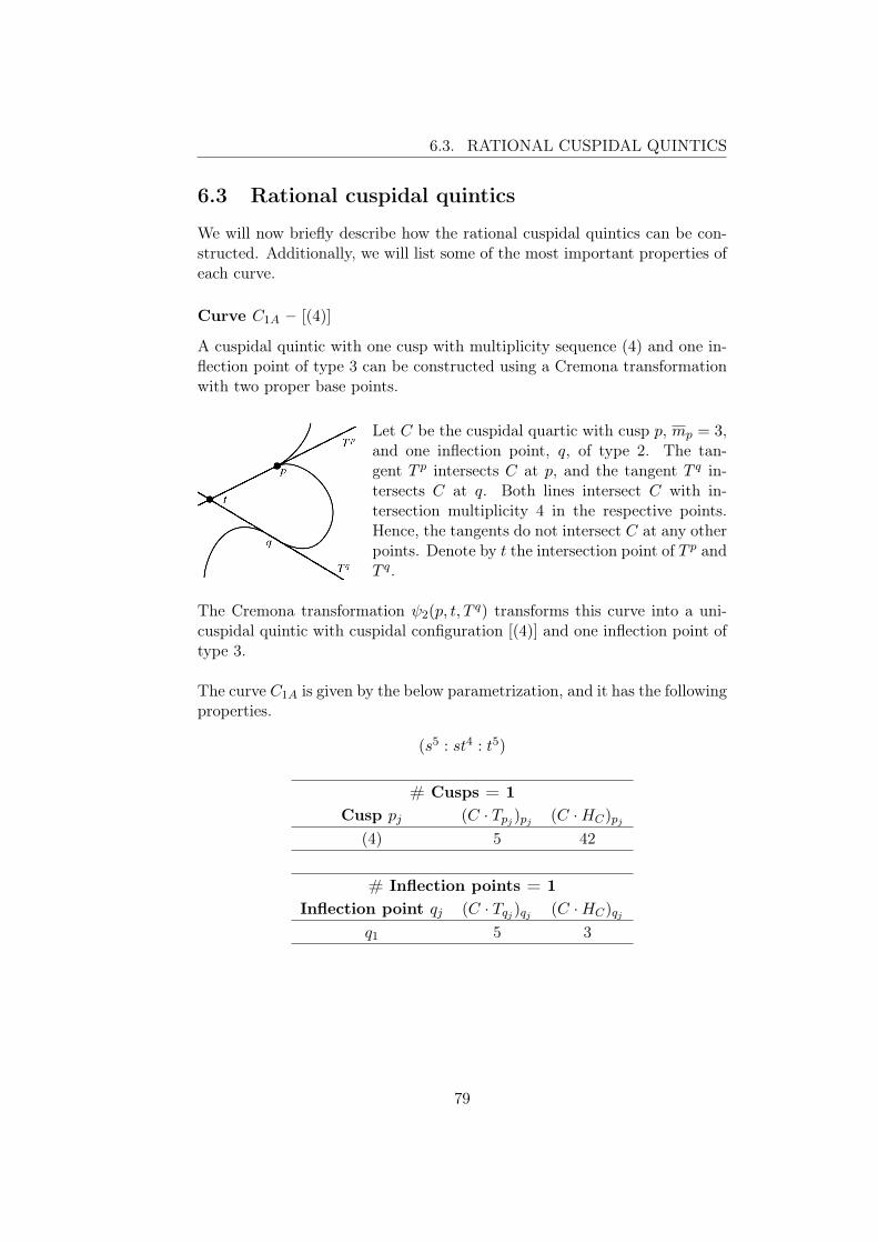
6.3. RATIONAL CUSPIDAL QUINTICS
6.3 Rational cuspidal quintics
We will now briefly describe how the rational cuspidal quintics can be con-structed. Additionally, we will list some of the most important properties ofeach curve.
Curve C1A – [(4)]
A cuspidal quintic with one cusp with multiplicity sequence (4) and one in-flection point of type 3 can be constructed using a Cremona transformationwith two proper base points.
Let C be the cuspidal quartic with cusp p, mp = 3,and one inflection point, q, of type 2. The tan-gent T p intersects C at p, and the tangent T q in-tersects C at q. Both lines intersect C with in-tersection multiplicity 4 in the respective points.Hence, the tangents do not intersect C at any otherpoints. Denote by t the intersection point of T p andT q.
The Cremona transformation ψ2(p, t, T q) transforms this curve into a uni-cuspidal quintic with cuspidal configuration [(4)] and one inflection point oftype 3.
The curve C1A is given by the below parametrization, and it has the followingproperties.
(s5 : st4 : t5)
# Cusps = 1Cusp pj (C · Tpj )pj (C ·HC)pj
(4) 5 42
# Inflection points = 1Inflection point qj (C · Tqj )qj (C ·HC)qj
q1 5 3
79

CHAPTER 6. RATIONAL CUSPIDAL QUINTICS
Curve C1B – [(4)]
A cuspidal quintic with one cusp with multiplicity sequence (4) and twoinflection points of type 1 and 2 respectively, can be constructed using aCremona transformation with two proper base points.
Let C be the cuspidal quartic with a cusp p, mp =3, and two inflection points, q and r, of type 1. LetT p be the tangent to C at p. Choose a point t onT p. Let L = Lpq denote the line between p and theinflection point q. By Bézout’s theorem, L and Cdo not intersect in any other points. We have theintersections
T p · C = 4 · p,L · C = 3 · p+ 1 · q.
The Cremona transformation ψ2(t, p, L) transforms this curve into a unicus-pidal quintic with cuspidal configuration [(4)] and two inflection points oftype 1 and 2.
The curve C1B is given by the below parametrization, and it has the followingproperties.
(s5 − s4t : st4 : t5)
# Cusps = 1Cusp pj (C · Tpj )pj (C ·HC)pj
(4) 5 42
# Inflection points = 2Inflection point qj (C · Tqj )qj (C ·HC)qj
q1 4 2q2 3 1
80

6.3. RATIONAL CUSPIDAL QUINTICS
Curve C1C – [(4)]
A cuspidal quintic with one cusp with multiplicity sequence (4) and threeinflection points of type 1, can be constructed using a Cremona transforma-tion with two base points.
Let C be the cuspidal quartic with a cusp p,mp = 3and two inflection points q and r of type 1. Let T p
denote the tangent line at p. Choose a point t onT p. Furthermore, choose a point s ∈ C differentfrom the above mentioned points. Let L = Lps
denote the line between the cusp p and the point s.We have the intersections
T p · C = 4 · p,L · C = 3 · p+ 1 · s.
The Cremona transformation ψ2(t, p, L) transforms this quartic curve intoa unicuspidal quintic with cuspidal configuration [(4)] and three inflectionpoints of type 1.
The curve C1C is given by the below parametrization, and it has the followingproperties.
(s5 + as4t− (1 + a)s2t2 : st4 : t5), a ∈ C, a 6= −1.
# Cusps = 1Cusp pj (C · Tpj )pj (C ·HC)pj
(4) 5 42
# Inflection points = 1Inflection point qj (C · Tqj )qj (C ·HC)qj
q1 3 1q2 3 1q3 3 1
81

CHAPTER 6. RATIONAL CUSPIDAL QUINTICS
Curve C2 – [(26)]
The rational cuspidal quintic with cuspidal configuration [(26)] can be con-structed by transforming the unicuspidal ramphoid quartic using a Cremonatransformation with one base point.
Since the action of a Cremona transformation with one base point is hardto analyze in P2, we will construct this curve explicitly with a transformationthat is known to work. Let C be given by
C = V((yx− z2)2 − x3z).
Then the Cremona transformation ψ1 transforms this curve into
C2 = V(xy4 − 2x2y2z + x3z2 − 2y3z2 + 2xyz3 + z5).
The implicit construction can be explained ade-quately. Let C be the quartic with one cusp p withmultiplicity sequence (23). The polar of C at thecusp p intersects C in a smooth point s. Denote byT s the tangent line at s, which intersects C in twopoints,
C · T = 2 · p+ 2 · s.
The appropriate Cremona transformation in thissituation consists of blowing up s, performing elementary transformations inthe two successive infinitely near points s1 and s2 on the strict transformsof C, and then blowing down the horizontal section.
The curve C2 is given by the below parametrization, and it has the followingproperties.
(s4t : s2t3 − s5 : t5 − 2s3t2)
# Cusps = 1Cusp pj (C · Tpj )pj (C ·HC)pj
(26) 4 39
# Inflection points = 6Inflection point qj (C · Tqj )qj (C ·HC)qjqj , j = 1, . . . , 6 3 1
82

6.3. RATIONAL CUSPIDAL QUINTICS
Curve C3A – [(3, 2), (22)]
A cuspidal quintic with cuspidal configuration [(3, 2), (22)] and no inflectionpoints can be constructed using a Cremona transformation with two basepoints.
Let C be the cuspidal cubic with a cusp p, mp =(2), and one inflection point, q, of type 1. Let T q bethe tangent line at q. Let L = Lpq be the line be-tween p and q, which by Bézout’s theorem does notintersect C in any other point. Choose an arbitrarypoint r ∈ T q. We have the intersections
T q · C = 3 · q,L · C = 2 · p+ 1 · q.
The Cremona transformation ψ2(r, q, L) transforms this cubic into the bi-cuspidal quintic with cuspidal configuration [(3, 2), (22)].
The curve C3A is given by the below parametrization, and it has the followingproperties.
(s5 : s3t2 : t5)
# Cusps = 2Cusp pj (C · Tpj )pj (C ·HC)pj
(3, 2) 5 29(22) 5 16
# Inflection points = 0
83

CHAPTER 6. RATIONAL CUSPIDAL QUINTICS
Curve C3B – [(3, 2), (22)]
A cuspidal quintic with cuspidal configuration [(3, 2), (22)] and one inflectionpoint of type 1 can be constructed using a Cremona transformation with twobase points.
Let C be the cuspidal cubic with a cusp p, mp =(2), and one inflection point, q, of type 1. Choosean arbitrary smooth point r ∈ C, r 6= q and let T r
denote the tangent line at this point. By Bézout’stheorem,
T r · C = 2 · r + 1 · s,
for another smooth point s. Make sure s 6= q. Fur-thermore, denote by T p the tangent line at the cusp
p. The tangents T r and T p intersect at a point t /∈ C.
The Cremona transformation ψ2(s, t, T p) transforms this cubic into the bi-cuspidal quintic with cuspidal configuration [(3, 2), (22)] and one inflectionpoint of type 1.
The curve C3B is given by the below parametrization, and it has the followingproperties.
(s5 : s3t2 : st4 + t5)
# Cusps = 2Cusp pj (C · Tpj )pj (C ·HC)pj
(3, 2) 5 29(22) 5 15
# Inflection points = 1Inflection point qj (C · Tqj )qj (C ·HC)qj
q1 3 1
84

6.3. RATIONAL CUSPIDAL QUINTICS
Curve C4 – [(3), (23)]
A cuspidal quintic with cuspidal configuration [(3), (23)] and two inflectionpoints of type 1 can be constructed by a Cremona transformation with twobase points.
Let C be the cuspidal cubic with a cusp p, mp =(2), and one inflection point, q, of type 1. Choosean arbitrary smooth point r ∈ C, r 6= q and let L =Lpr denote the line through p and r. Furthermore,denote by T q the tangent line at the inflection pointq. The lines T q and L intersect at a point s /∈ C.We have the intersections
L · C = 2 · p+ 1 · r,T q · C = 3 · q.
The Cremona transformation ψ2(r, s, T q) transforms the cubic into the bicus-pidal quintic with cuspidal configuration [(3), (23)] and two inflection pointsof type 1.
The curve C4 is given by the below parametrization, and it has the followingproperties.
(s4t− 12s
5 : s3t2 : 12st
4 + t5)
# Cusps = 2Cusp pj (C · Tpj )pj (C ·HC)pj
(3) 4 22(23) 4 21
# Inflection points = 2Inflection point qj (C · Tqj )qj (C ·HC)qj
q1 3 1q2 3 1
85

CHAPTER 6. RATIONAL CUSPIDAL QUINTICS
Curve C5 – [(24), (22)]
A cuspidal quintic with cuspidal configuration [(24), (22)] and three inflec-tion points of type 1 can be constructed by a Cremona transformation withtwo base points.
Let C be the bicuspidal quartic with two cusps,p and q, with mp = (22) and mq = (2), and oneinflection point, r, of type 1. The polar of C at thecusp q intersects C in a smooth point s. Denote byT s the tangent line at s, which has the property
T s · C = 2 · q + 2 · s.
Let L = Lps be the line through the cusp p and thesmooth point s. Since T p · C = 4 · p, we have that L 6= T p. By Bézout’stheorem, L must intersect C in yet another smooth point t. We have theintersection
L · C = 2 · p+ 1 · s+ 1 · t.
The Cremona transformation ψ2(t, s, T s) transforms the quartic into the bi-cuspidal quintic with cuspidal configuration [(24), (22)] and three inflectionpoints of type 1.
The curve C5 is given by the below parametrization, and it has the followingproperties.
(s4t− s5 : s2t3 − 532s
5 : − 47128s
5 + 1116s
3t2 + st4 + t5)
# Cusps = 2Cusp pj (C · Tpj )pj (C ·HC)pj
(24) 4 27(22) 4 15
# Inflection points = 3Inflection point qj (C · Tqj )qj (C ·HC)qj
qj , j = 1, 2, 3 3 1
86

6.3. RATIONAL CUSPIDAL QUINTICS
Curve C6 – [(3), (22), (2)]
A cuspidal quintic with cuspidal configuration [(3), (22), (2)] and no inflec-tion points can be constructed using a Cremona transformation with twoproper base points.
Let C be the cuspidal cubic with a cusp p,where mp = (2), and one inflection point, q,of type 1. Denote by T q the tangent line at q.Choose an arbitrary smooth point r ∈ C, r 6=q. Then the tangent line at r, T r, intersectsT q in a point s /∈ C. Furthermore, T r inter-sects C in another smooth point t. We havethe intersection
T r · C = 2 · r + 1 · t.
The Cremona transformation ψ2(t, s, T q) transforms the cubic into the tri-cuspidal quintic with cuspidal configuration [(3), (22), (2)].
Blowing up at s
Blowing up at s, we get the ruled surfaceX1 with horizontal section E1 and the trans-formed curve C1. We have the intersections
E1 ∩ C1 = ∅,T q1 · C1 = 3 · q1,
T r1 · C1 = 2 · r1 + 1 · t1.
Elementary transformations in t1 and s
Blowing up at t1 and s gives two exceptionallines Et1 and Es. We have the intersections
E1 ∩ C1 = ∅,Es ∩ C1 = ∅,T q1 · C1 = 3 · q1,
Et1 · C1 = 1 · t1,T r1 · C1 = 2 · r1.
87

CHAPTER 6. RATIONAL CUSPIDAL QUINTICS
Blowing down T q1 and T r1 gives the surfaceX2. On this surface we have T q2 , the stricttransform of Es, and T r2 , the strict transformof Et1 .
Because of the intersection multiplicitiesabove, q2 is a cusp with mq2 = (3), and r2
is a cusp with mr2 = (2). Note that r2 ∈ E2.We have the important intersection
E2 · C2 = 2 · r2.
Blowing down E2
Blowing down E2 gives a curve C ′ with three cusps p′, q′ and r′, wheremp′ = (2), mq′ = (3) and mr′ = (22).
To see that C ′ is a quintic, note that
d′ = 2 · d−ms −ms −mt1
= 2 · 4− 1− 1− 1
= 5.
The curve C6 is given by the below parametrization, and it has the followingproperties.
(s4t− 12s
5 : s3t2 : −32st
4 + t5)
# Cusps = 3Cusp pj (C · Tpj )pj (C ·HC)pj
(3) 4 22(22) 4 15(2) 3 8
# Inflection points = 0
88

6.3. RATIONAL CUSPIDAL QUINTICS
Curve C7 – [(22), (22), (22)]
A cuspidal quintic with cuspidal configuration [(22), (22), (22)] and no inflec-tion points can be constructed using a Cremona transformation with twobase points.
Let C be the bicuspidal quartic with two cuspsp and q, with mp = (22) and mq = (2), andone inflection point, r, of type 1. The polarof C at the point q intersects C in a smoothpoint s. Denote by T s the tangent line at s,which has the property T s · C = 2 · q + 2 · s.The polar of C at the point s intersects C ina smooth point t, t 6= r. Denote by T t the
tangent line at t, which by Bézout’s theorem intersects C in a smoothpoint u. We have the intersection
T t · C = 2 · t+ 1 · s+ 1 · u.
The Cremona transformation ψ2(u, s, T s) transforms the bicuspidal quarticinto the tricuspidal quintic with cuspidal configuration [(22), (22), (22)].
Blowing up at s
Blowing up at s, we get the ruled surfaceX1 with horizontal section E1 and the trans-formed curve C1. We have the intersections
E1 · C1 = 1 · s1,
T t1 · C1 = 1 · u1 + 2 · t1,T s1 · C1 = 1 · s1 + 2 · q1.
Elementary transformations in u1 and s1
Blowing up at u1 and s1 gives on X1 two ex-ceptional lines Eu1 and Es1 . We then havethe intersections
E1 ∩ C1 = ∅,Eu1 · C1 = 1 · u1,
T t1 · C1 = 2 · t1,Es1 · C1 = 1 · s1,
T s1 · C1 = 2 · q1.
89

CHAPTER 6. RATIONAL CUSPIDAL QUINTICS
Blowing down T t1 and T s1 gives the surfaceX2. On this surface we have T t2, the stricttransform of Eu1 , and T s2 , the strict transformof Es1 .
Because of the intersection multiplicitiesabove, q2 is a cusp with mq2 = (22), and t2 isa cusp with mt2 = (2). Note that t2 ∈ E2.
We have the important intersection
E2 · C2 = 2 · t2.
Blowing down E2
Blowing down E2 gives a curve C ′ with three cusps p′, q′ and t′. All thesecusps have multiplicity sequence (22).
To see that C ′ is a quintic, note that
d′ = 2 · d−ms −ms1 −mu1
= 2 · 4− 1− 1− 1
= 5.
The curve C7 is given by the below parametrization, and it has the followingproperties.
(s4t− s5 : s2t3 − 532s
5 : −125128s
5 − 2516s
3t2 − 5st4 + t5)
# Cusps = 3Cusp pj (C · Tpj )pj (C ·HC)pj
(22) 4 15(22) 4 15(22) 4 15
# Inflection points = 0
90

6.3. RATIONAL CUSPIDAL QUINTICS
Curve C8 - [(23), (2), (2), (2)]
The rational cuspidal quintic with four cusps is the dual curve of the uni-cuspidal ramphoid quartic curve C. C has a cusp p of type A6 and threeinflection points of type 1. The explicit calculation can be done in the fol-lowing way.
We find the defining polynomial of the unicuspidal ramphoid quartic by usingthe parametrization given in chapter 3 and eliminating s and t with Singular.
ring R=0, (x,y,z,a,b,c,d,e,s,t), dp;ideal A6=x-(a-d),y-(c),z-(e);ideal ST=a-s4,b-s3t,c-s2t2,d-st3,e-t4;ideal A6ST=A6,ST;short=0;eliminate(std(A6ST),abcdest);_[1]=y^4-2*x*y^2*z+x^2*z^2-y*z^3
We find the defining polynomial of the dual curve C8 in Singular.
ring r=0,(x,y,z,s,t,u),dp;poly f=y^4-2*x*y^2*z+x^2*z^2-y*z^3;ideal I=f,s-diff(f,x),t-diff(f,y),u-diff(f,z);short=0;eliminate(std(I),xyz);_[1]=27*s^5+4*s^2*t^3-144*s^3*t*u-16*t^4*u+128*s*t^2*u^2-256*s^2*u^3
The above output is a polynomial in s, t, u defining the rational cuspidalquintic with four cusps. This can be verified by the following code in Maple.
with(algcurves):f := 27*s^5+4*s^2*t^3-144*s^3*t*u-16*t^4*u+128*s*t^2*u^2-256*s^2*u^3;u := 1;singularities(f, s, t);
[[x, y, z],mp, δp,#Branches],
[[−16
3, 8, 1], 2, 1, 1],
[[RootOf(9 _Z 2 − 48 _Z + 256
),−8 +
3
2RootOf
(9 _Z 2 − 48 _Z + 256
), 1], 2, 1, 1],
[[0, 0, 1], 2, 3, 1].
Although the above construction is by far the most elegant one, it is alsopossible to get C8 by using a Cremona transformation to transform theunicuspidal ramphoid quartic. The easiest way of showing this is to applythe standard Cremona transformation with three proper base points to C8
rotated such that the three simple cusps are placed in (1 : 0 : 0), (0 : 1 : 0)and (0 : 0 : 1). This gives a rational quartic with one single A6-cusp andthree inflection points. The inverse transformation gives the quintic. Weshow the latter transformation implicitly.
91

CHAPTER 6. RATIONAL CUSPIDAL QUINTICS
Let C be the unicuspidal ramphoid quartic.Then rotate this curve such that we have thespecific arrangement shown on the left. Wehave three lines T p, T q and T r which are tan-gent lines to C at three points p, q and r.The three lines additionally intersect in threepoints s, t and u ∈ C.
Using the Cremona transformation ψ3(s, t, u),we get three exceptional lines Es, Et and Eu,replacing s, t and u. Furthermore, the trans-forms of T p, T q and T r intersect the trans-form of C with multiplicity 2 in the trans-forms of the points p, q and r.
Blowing down the transforms of the tangentlines results in points p′, q′ and r′ on C ′, whichby elementary properties of the blowing-downprocess have multiplicity
mp′ = mq′ = mr′ = 2.
Since the points originally were smooth pointson C, p′, q′ and r′ are cusps with multiplicity sequence (2). Notice thatthe cusp of C is unaffected by the Cremona transformation.
The degree of C ′ is
d′ =2 · d−ms −mt −mq
=2 · 4− 1− 1− 1
=5.
Thus, we have constructed C8, a rational cuspidal quintic with cuspidal con-figuration [(23), (2), (2), (2)].
92

6.3. RATIONAL CUSPIDAL QUINTICS
The curve C8 is given by the below parametrization, and it has the followingproperties.
(s4t : s2t3 − s5 : t5 + 2s3t2)
# Cusps = 4Cusp pj (C · Tpj )pj (C ·HC)pj
(23) 4 21(2) 3 8(2) 3 8(2) 3 8
# Inflection points = 0
93

CHAPTER 6. RATIONAL CUSPIDAL QUINTICS
94

Chapter 7
More cuspidal curves
The rational cuspidal cubics, quartics and quintics presented in this thesis,have been known for a while because of Namba’s classification of curvesin [25]. For some time there were only a few known examples of rationalcuspidal curves of degree d ≥ 6. In recent years this has changed. In thischapter we will present more cuspidal curves.
7.1 Binomial cuspidal curves
Amongst the most simple cuspidal curves are curves which are given as thezero set of a binomial, a homogeneous polynomial with two terms,
F(mn) = zn−mym − xn, n > m ≥ 1, gcd(m,n) = 1.
These curves are cuspidal and are called binomial curves. They are unicusp-idal if m = 1 or symmetrically n−m = 1, and they are bicuspidal if m ≥ 2.In the first case, the curves have one cusp and one inflection point of typen − 2, which can be verified by direct calculation. In the latter case, thecurves have one cusp in p = (0 : 0 : 1) with multiplicity mp = m, one cuspin q = (0 : 1 : 0) with multiplicity mq = n − m, and no inflection points.The two cusps have different multiplicity sequences, but are quite similar inthe sense that they can be investigated by identical methods and arguments.Note that since m and n are relatively prime, so are n − m and n. Theobservation that a general bicuspidal binomial curve does not have inflectionpoints can be verified by a direct calculation of the Hessian curve and theintersection multiplicity of the Hessian curve and the curve at the cusps. Wewill come back to this in Section 9.2.
A binomial curve can be parametrized by
(sn−mtm : tn : sn).
95

CHAPTER 7. MORE CUSPIDAL CURVES
The projection center V , by which it can be projected from the rationalnormal curve in Pn, is given by
V = V(x0, xm, xn),
AV =
1 0 . . . 0 . . . 0
0 0 . . . 1 . . . 0
0 0 . . . 0 . . . 1
.
We want to investigate a cusp on a binomial curve. Because of the symmetryof the unicuspidal binomial curves we may always assume that the binomialcurve C has a cusp in p = (0 : 0 : 1). C can then be represented around pby the affine curve given by f ,
f = ym − xn.
The cusp has multiplicity m, and the multiplicity sequence can be calculatedby the algorithm given in Theorem 2.2.6 on page 14. The cusp has tangentV(y), which intersects the curve with multiplicity (Tp · C)p = n. Hence, thecurve can locally around the cusp be parametrized by
(C, p) = (tm : tn : 1).
Fibonacci curves
We define the Fibonacci numbers ϕk recursively. For k ∈ N we define
ϕ0 = 0,
ϕ1 = 1,
ϕk+1 = ϕk + ϕk−1.
With ϕk as above we define a subseries of binomial cuspidal curves calledthe Fibonacci curves [2]. The kth Fibonacci curve is defined as
Ck = V(yϕk − xϕk−1zϕk−2), for all k ≥ 2.
This curve has degree ϕk. For k = 2 we have a line. For k = 3 we havean irreducible conic. For k = 4 the curve is a cuspidal cubic with a simplecusp in (0 : 0 : 1). For all k ≥ 5 the curve Ck has two cusps. The two cuspsare located in (1 : 0 : 0) and (0 : 0 : 1). They have multiplicity sequences(ϕk−2, {ϕi}k−2
i=1 ) and ({ϕi}k−1i=1 ) respectively. The curves are bicuspidal since
any two successive Fibonacci numbers are relatively prime integers. If theydid have a common factor 6= 1, so would their sum and their difference,which is the next and the previous number in the series. This indicates thatall Fibonacci numbers have a common factor 6= 1, but that is certainly nottrue.
These curves will be revisited in Section 9.3.
96
7.2. OREVKOV CURVES
Semi-binomial curves
Carefully adding a few terms to the defining polynomial of the binomialcurves produces series of curves strongly related to the binomial curves.Adding terms can be done such that it simply corresponds to a linear changeof coordinates. These curves provide nothing new. However, it is possible toadd terms in such a way that the resulting curves have precisely the samecuspidal configuration as the original binomial curve, but such that they arenot projectively equivalent. This can happen because the introduction ofnew terms in the defining polynomial sometimes leads to inflection points.Because they are strongly related to the binomial curves, we choose to callthese curves semi-binomial curves.
We have presented several examples of this phenomenon in this thesis.For example, the ovoid cuspidal quartic with one inflection point is binomial,
C4A = V(z4 − xy3).
The ovoid cuspidal quartic with two inflection point is semi-binomial,
C4B = V(x3y − z3x+ z4).
7.2 Orevkov curves
In [26], Orevkov gave a proof of the existence of certain unicuspidal rationalcurves, which from here on will be referred to as Orevkov curves. The proofexplains a way of constructing series of such curves explicitly by applying aproduct of Cremona transformations to simple, nonsingular algebraic curvesof low degree. In the following we will describe the series of Orevkov curvesand their construction.
Let ϕk denote the kth Fibonacci number. An algebraic curve Ck of degreedk = ϕk+2 with a single cusp of multiplicity mk = ϕk is called an Orevkovcurve. Moreover, an algebraic curve C?k of degree d?k = 2ϕk+2 with a singlecusp of multiplicity m?
k = 2ϕk is also called an Orevkov curve.Let N be a rational cubic curve with a singularity with two distinct
tangents. The singularity is commonly referred to as a node, and the curveitself is called a nodal cubic. Furthermore, let C−3 and C−1 be the tangentsto the branches of N at the singular point, and let C0 be the inflectionaltangent. Each of the three lines intersects N in only one point. Additionally,let C?0 be a conic which intersects N in one smooth point. Then a Cremonatransformation ψ which is biregular on P2 \N will transform the mentionednonsingular curves into unicuspidal Orevkov curves.
97

CHAPTER 7. MORE CUSPIDAL CURVES
N , C−3 and C−1 N and C0 N and C?0
Figure 7.1: Initial curves in the series of Orevkov curves, z = 1.
Note that in Figure 7.1, N and C0 intersect in the point (1 : 1 : 0), which isnot in the chosen affine covering.
We define recursively,
Ck = ψ(Ck−4), k ≥ 3, k 6= 2 (mod 4),
C?k = ψ(C?k−4), k > 0, k ≡ 0 (mod 4).
Theorem 7.2.1. [26, p.658] The following series of Orevkov curves exist.
Orevkov I – Ck for any k > 1, k ≡ 1 (mod 4),
Orevkov II – Ck for any k > 0, k ≡ 3 (mod 4),
Orevkov III – Ck for any k > 0, k ≡ 0 (mod 4),
Orevkov IV – C?k for any k > 0, k ≡ 0 (mod 4).
ChooseN = V(xyz − x3 − y3).
Then the Orevkov curves can explicitly be constructed by the Cremona trans-formation
ψ = σ5 ◦ σ4 ◦ σ3 ◦ σ2 ◦ σ1.
σ1 σ2 σ3 σ4 σ5
x1 = x2 x2 = x1z1 x3 = y2z2 x4 = x3z3 + y23 x5 = x4y4
y1 = xy y2 = y1z1 − x21 y3 = x2z2 y4 = y3z3 y5 = y24z1 = xz − y2 z2 = z21 z3 = x2y2 z4 = z23 z5 = y4z4 + x24
Note that the five above Cremona transformations are not their own inverses;they are compositions of linear changes of coordinates and the quadraticCremona transformations given in Chapter 5. Therefore, in applying the
98

7.2. OREVKOV CURVES
above transformations to defining polynomials, we must perform the neces-sary substitutions with the inverse transformations. The fact that the trans-formations are not on standard form complicates finding the strict transform.Although this causes problems in the direct calculations given below, we willnot discuss this problem here.
σ−11 σ−12 σ−13 σ−14 σ−15
x = x21 x1 = x2z2 x2 = y3z3 x3 = x4z4 − y24 x4 = x5y5
y = x1y1 y1 = y2z2 + x22 y2 = x3z3 y3 = y4z4 y4 = y25z = x1z1 + y21 z1 = z22 z2 = x3y3 z3 = z24 z4 = y5z5 − x25
Orevkov I. Choose the tangent of one branch of the nodal cubic at thenode. It can be given by C−3 = V(F−3), where F−3 = x. Applying ψ tothis curve results in the curve C1 = V(F1), where F1 = yz − x2. This curveis nonsingular, hence not an Orevkov curve. Another application of ψ givesthe Orevkov curve C5, a rational cuspidal curve of degree d5 = ϕ7 = 13,with a single cusp of multiplicity m5 = ϕ5 = 5. Successive applications of ψproduce the series of Orevkov I curves.
Orevkov II. To produce the second series of Orevkov curves, choose thetangent to the other branch of the nodal cubic at the node. It can be given byC−1 = V(F−1), where F−1 = y. Applying ψ to this curve gives the Orevkovcurve C3, a rational cuspidal curve of degree d3 = ϕ5 = 5, with a single cuspof multiplicity m3 = ϕ3 = 2. Successive applications of ψ produce the seriesof Orevkov II curves.
Orevkov III. Produce the third series of Orevkov curves by choosing aninflectional tangent of the nodal cubic N . We let the curve C0 = V(F0),where F0 = 3x+3y+z, be this inflectional tangent. Applying ψ to this curvegives the Orevkov curve C4, a rational cuspidal curve of degree d4 = ϕ6 = 8,with a single cusp of multiplicity m4 = ϕ4 = 3. Successive applications of ψproduce the series of Orevkov III curves.
The cusp of an Orevkov curve Ck of any of these three series has multiplicitysequence
mk = (ϕk, Sk, Sk−4, . . . , Sν),
where ν = 3, 4, 5 is determined by k = 4j + ν, j ∈ N0, and Si denotes thesubsequence
Si = ((ϕi)5, ϕi − ϕi−4).
Orevkov IV. To get the fourth series of Orevkov curves, choose a conicC?0 = V(F ?0 ), where F ?0 = 21x2−22xy+21y2−6xz−6yz+z2. This particularconic intersects the nodal cubic in exactly one smooth point. Applying ψ tothis curve gives the Orevkov curve C?4 , a rational cuspidal curve of degreed?4 = 2ϕ6 = 16, with a single cusp of multiplicity m?
4 = 2ϕ4 = 6. Successiveapplications of ψ produce the series of Orevkov IV curves.
99

CHAPTER 7. MORE CUSPIDAL CURVES
The cusp of an Orevkov curve C?k has almost the same multiplicity sequenceas the cusp of the curve Ck. The only difference is that every multiplicity ismultiplied by 2.
Remark 7.2.2. Note that the birationality of the Cremona transformations al-lows the application of the inverse transformation ψ−1 to all Orevkov curves.This immediately implies that all Orevkov curves of type I, II and III can betransformed into lines by a sequence of Cremona transformations. This isalso the case for Orevkov curves of type IV. These curves can be transformedinto an irreducible conic, and any such curve can in turn be transformed intoa line. Hence, all Orevkov curves are rectifiable.
7.3 Other uni- and bicuspidal curves
The search for more cuspidal curves led Fenske in [7] to the discovery ofessentially eight different series of rational uni- and bicuspidal curves. Thecurves were found using suitable Cremona transformations to transform thefollowing binomial and semi-binomial cuspidal curves of degree d,
V(xyd−1 − zd) and V(xyd−1 − zd − yzd−1).
An overview is given in Table 7.1. Note that since the curves Ci are stricttransforms of the above curves, the degree of Ci is given as a function of d.
Curve degCa,d Cuspidal configurationC1 da+ d (da, da+b, d− 1), (da−b)
C1a da+ d (da, d2a, d− 1)
C2 da+ d (da, da+b), (da−b, d− 1)
C2a da+ d (da, d2a), (d− 1)
C3 da+ d+ 1 (da+ 1, da), (da+1)
C4 da+ d+ 1 (da, da+1), ((d+ 1)a)
C5 da+ d+ 1 (da, da), ((d+ 1)a, d)
C6 da+ d+ 2 (da+ 1, da), ((d+ a)a+1)
C7 da+ 2d− 1 (da+ d− 1, da, d− 1), (da+1, d− 1)
C8 a+ 2 (a), (2a)
d ≥ 2 and 0 ≤ b < a integers.
Table 7.1: Fenske’s uni- and bicuspidal curves [7, Thm. 1.1., p.310].
100

7.4. TRICUSPIDAL CURVES
7.4 Tricuspidal curves
Curves with three or more cusps are quite rare. We have three series oftricuspidal curves, which were found by Flenner, Zaidenberg and Fenske in[11] [12] [8]. The series of curves can be produced from simple cuspidal curvesof low degree using successive quadratic Cremona transformations.
7.4.1 Curves with µ = d− 2
In [11], Flenner and Zaidenberg constructed a series of tricuspidal curveswhere the maximal multiplicity of any cusp of the curves was µ = d − 2.They found that for any degree d ≥ 4, a ≥ b ≥ 1, with a+ b = d− 2, there isa unique, up to projective equivalence, rational cuspidal curve C = Cd,a ⊂ P2
of degree d with three cusps. The curve Cd,a has cuspidal configuration
[(d− 2), (2a), (2b)].
The restrictions on a and b imply that for every d there are exactly⌊d−2
2
⌋tricuspidal curves of this kind. Furthermore, Flenner and Zaidenberg provedthat any rational cuspidal curve with one cusp with multiplicity d− 2 has atmost three cusps. Additionally, they proved that if there are three cusps onthe curve, then it has the given cuspidal configuration.
The parametrization
In [11], the tricuspidal curves with µ = d− 2 were painstakingly constructedby parametrization methods. They started out with a general parametriza-tion. Then they imposed restrictions on the parametrization in order to getthe desired type of cusps. They found that the curve is parametrized by
((s− t)d−2s2 : (s− t)d−2t2 : s2t2 · q(s, t))
where the polynomial q(1, t), and thus the homogeneous polynomial q(s, t),can be found by feeding Maple the below code.
c[k] := (product(2*a-2*i+1, i = 1 .. k))/2^k;f(t) := expand(1+ sum((c[k])/(k!)(t^(2)-1)^(k),k=1..(d-3)));q[d,a](t) := sort((factor(f(t)+t^((2 a-1))))/((1+t)^((d-2))));
The parametrization enables us to find and investigate the projection centerfor every such curve. Further investigating these projection centers could beinteresting, but goes beyond the scope of this thesis.
101

CHAPTER 7. MORE CUSPIDAL CURVES
Construction by Cremona transformations
In [12], Flenner and Zaidenberg presented an elegant way of constructing thetricuspidal curves using Cremona transformations.
Let C be a curve with cusps q, p and r, with multiplicity sequencesmq = (d − 2), mp = (2a) and mr = (2b). Then let Lpq denote the linethrough p and q, Lqr the line through q and r, and T q the tangent line at q.
By Bézout’s theorem and Lemma 2.2.4, the tangent line T q intersects Cwith multiplicity d−1 at q. Hence, T q intersects C transversally in a smoothpoint s. Applying the Cremona transformation ψ2(s, q, Lpq) to C results in acurve C ′ of degree d+1 with three cusps with multiplicity sequences (d−1),(2a+1) and (2b).
We may also perform the Cremona transformation ψ2(p, q, Lqr) to C,this time getting a tricuspidal curve of degree d and multiplicity sequences(d− 2), (2a+1) and (2b−1).
With these transformations, Flenner and Zaidenberg proved that all tri-cuspidal curves of degree d with µ = d − 2 can be constructed from thetricuspidal quartic curve. This implies that all these curves are rectifiable.
7.4.2 Curves with µ = d− 3
The work on the tricuspidal curves with maximal multiplicity µ = d − 2was soon followed by a parallel result for tricuspidal curves with a cusp withµ = d − 3. In [12], Flenner and Zaidenberg proved that for a tricuspidalcurve of degree d = 2a+ 3 with a cusp with maximal multiplicity µ = d− 3,the only possible cuspidal configuration is
[(2a, 2a), (3a), (2)].
Furthermore, they proved that for each a ≥ 1 there exists such a rationalcuspidal curve. The existence was proved performing a sequence of Cremonatransformations to the rational cuspidal cubic and constructing the curvesinductively. The construction proves that the curves are rectifiable. It wasalso proved that the curves are unique up to projective equivalence.
Remark 7.4.1. Observe that when a = 1, then d = 5. Then the curvehas the same cuspidal configuration as curves in this series, but the maximalmultiplicity of the cusps is µ = 3 = 5−2. Hence, this curve does by definitionnot belong to this series. Rather, it is an example of a curve from the seriesof curves with µ = d− 2.
102

7.4. TRICUSPIDAL CURVES
7.4.3 Curves with µ = d− 4
The last series of tricuspidal curves was presented by Fenske in [8]. In this ar-ticle, Fenske found that for every d = 3a+4, a ≥ 1, there exists a tricuspidalcurve with cuspidal configuration
[(3a, 3a), (4a, 22), (2)].
The existence was proved by induction and performing a sequence of Cre-mona transformation to the bicuspidal quartic with one inflection point.Fenske also found that these curves are unique up to projective equivalenceand that they are rectifiable.
Fenske was not able to generally prove that if a curve of degree d has threecusps and µ = d − 4, then the curve has this cuspidal configuration. How-ever, he was able to prove this result under the condition that χ(ΘV 〈D〉) ≤ 0,where χ(ΘV 〈D〉) is the Euler characteristic and D is the divisor with simplenormal crossings of the minimal embedded resolution of the singularities ofC.
By [11, Cor. 2.5., p.446], we can compute the Euler characteristic χ(ΘV 〈D〉)of a rational cuspidal curve using the degree and the multiplicity sequencesof the cusps of the curve.
χ(ΘV 〈D〉) = −3(d− 3) +∑
p∈SingC
Mp,
where Mp = ηp + ωp − 1,
ηp =
np∑i=0
(mp.i − 1) and ωp =
np∑i=1
(⌈mp.i−1
mp.i
⌉− 1
).
There are, so far, no known rational cuspidal curves with χ(ΘV 〈D〉) >0. Moreover, χ(ΘV 〈D〉) ≤ 0 is a consequence of a conjecture given byFernï¿1
2ndez de Bobadilla et al. in [9, Conj. 4.1., pp.420–424].
Conjecture 7.4.2. Let C be a rational cuspidal curve with Mp and d asabove. Furthermore, let dim StabPGL(3)(C) denote the dimension of thegroup of transformations in PGL3(C) which do not move C. Then∑
p∈SingC
Mp ≤ 3d− 9 + dim StabPGL(3)(C).
Remark 7.4.3. Observe that when a = 1, then d = 7. Then the curve hasthe same cuspidal configuration as the curves in this series, but the maximalmultiplicity of the cusps is µ = 4 = 7−3. Hence, this curve does by definitionnot belong to this series. Rather, it is an example of a curve from the seriesof curves with µ = d− 3.
103

CHAPTER 7. MORE CUSPIDAL CURVES
7.4.4 Overview
We have three series of rational tricuspidal curves. For curves with degreed ≥ 6, assuming χ(ΘV 〈D〉) ≤ 0, these are actually the only tricuspidalcurves with these cuspidal configurations, up to projective equivalence.
Series d mp mq mr Valid forI d (d− 2) (2a) (2d−2−a) d ≥ 4 d− 3 ≥ a ≥ 1
II 2a+ 3 (d− 3, 2a) (3a) (2) d ≥ 5 a ≥ 1
III 3a+ 4 (d− 4, 3a) (4a, 22) (2) d ≥ 7 a ≥ 1
Table 7.2: Tricuspidal curves.
These results allow us to count the number N of tricuspidal curves for eachdegree d ≥ 4, up to projective equivalence. For degrees d = 4 and d = 5,we have seen that N = 1 and N = 2. For degree d = 6 we see in Table7.2 that we know N = 2 tricuspidal curves, and for d = 7 we know N = 3tricuspidal curves. For any degree d ≥ 8, d ≡ k (mod 6) the number N ofknown tricuspidal curves is given in Table 7.3. To simplify notation we writeN0 =
⌊d−2
2
⌋, so that N0 is the number of curves in series I for each d.
k # Tricuspidal curves N Series represented0, 2 N0 I1 N0 + 2 I, II, III
3, 5 N0 + 1 I, II4 N0 + 1 I, III
Table 7.3: The number of known tricuspidal curves for d ≥ 8, d ≡ k (mod 6).
7.5 Rational cuspidal sextics
The search for rational cuspidal curves of a given degree is made slightlyeasier with all the above results. With the results it was possible for Fenskein [7, Cor. 1.5., p.312] to present a list of all existing cuspidal configurationsof rational cuspidal sextics. He also gave explicit parametrizations of allrational cuspidal sextic curves with one and two cusps, up to projectiveequivalence [7, pp.327–328]. For the rational cuspidal sextic curves withthree cusps, the explicit parametrizations of the curves are given by Flennerand Zaidenberg in [11, Thm. 3.5., p.448].
104

7.5. RATIONAL CUSPIDAL SEXTICS
# Cusps Curve Cuspidal configuration # Curves
1C1 (5) 4 – ABCDC2 (4, 24) 2 – ABC3 (33, 2) 3 – ABC
2
C4 (33), (2) 2 – ABC5 (32, 2), (3) 1C6 (32), (3, 2) 1C7 (4, 23), (2) 1C8 (4, 22), (22) 1C9 (4), (24) 1
3 C10 (4), (23), (2) 1C11 (4), (22), (22) 1
Table 7.4: Rational cuspidal sextic curves [7, Cor. 1.5., p.312].
105

CHAPTER 7. MORE CUSPIDAL CURVES
106

Chapter 8
On the number of cusps
All the examples of rational cuspidal curves presented in this thesis are in-teresting in themselves. Some are, however, more intriguing than the othersin the search for an upper bound on the number of cusps on a rational cus-pidal curve. The particularly interesting curves are the curves with three ormore cusps. Indeed, we so far only know one rational cuspidal curve withfour cusps, the quintic with cuspidal configuration [(23), (2), (2), (2)]. Fur-thermore, we only know one tricuspidal curve not contained in table 7.2, thequintic with cuspidal configuration [(22), (22), (22)].
8.1 A conjecture
The above observation was made by Piontkowski, and in 2007 he proposedthe following conjecture after investigating almost all cuspidal curves of de-gree ≤ 20 [28, Conj. 1.4., p.252].
Conjecture 8.1.1 (On the number of cusps of rational cuspidal curves). Arational cuspidal plane curve of degree d ≥ 6 has at most three cusps. Thecurves of degree d ≥ 6 with precisely three cusps occur in the three series inTable 7.2 on page 104.
8.2 An upper bound
The general research on rational cuspidal curves has not only circled aroundconstructing curves and series of curves. The most recent progress was madein 2005, when Tono lowered the upper bound for the number of cusps on acuspidal plane curve of genus g. Thus, he also found a new upper boundfor the number of cusps on a rational cuspidal plane curve [31, Thm. 1.1.,p.216].
Theorem 8.2.1 (An upper bound). A cuspidal plane curve of genus g hasno more than 21g+17
2 cusps.
107

CHAPTER 8. ON THE NUMBER OF CUSPS
Corollary 8.2.2 (An upper bound for rational curves). A rational cuspidalplane curve has no more than 8 cusps.
8.3 Particularly interesting curves
Noting Tono’s theorem and keeping Piontkowski’s conjecture in mind, weare naturally led to the investigation of the two particular quintic curves inTable 8.1.
Curve # Cusps Cuspidal configuration Degree dC4 3 [(22), (22), (22)] d = 5
C� 4 [(23), (2), (2), (2)] d = 5
Table 8.1: Particularly interesting cuspidal curves.
8.3.1 All about C4
The quintic curve with cuspidal configuration [(22), (22), (22)] is special sinceit is the only tricuspidal curve which is not found in any of the three series oftricuspidal curves in Table 7.2. Apart from that, however, it is hard to findways in which this curve stands out. In Chapter 6 we saw that this curvecan be constructed by a Cremona transformation of the bicuspidal quartic,and there was nothing worth noting in this construction. Next we will seethat projection and dualization do not reveal any secrets of this curve either.
Projection
The parametrization given in [25, Thm. 2.3.10., pp. 179–182] gives us theprojection center V .
V = V(−x0 + x1,− 532x0 + x3,−125
128x0 − 2516x2 − 5x4 + x5),
AV =
−1 1 0 0 0 0
− 532 0 0 1 0 0
−125128 0 −25
16 0 −5 1
, KV =
0 0 1 0 0 25
16
325
325 0 1 0 25
4
0 0 0 0 1 5
.With this information on the projection center we observe that the curveC4 has three cusps pi with (Tpi · C)pi = 4.
– V ∩ C5 = ∅.
– V ∩ T5 = {p1, p2, p3} for
(s : t) = {(0 : 1), (−10+6√
55 : 1), (−10−6
√5
5 : 1)}.
108

8.3. PARTICULARLY INTERESTING CURVES
– V ∩O2(s, t) = {p1, p2, p3} for
(s : t) = {(0 : 1), (−10+6√
55 : 1), (−10−6
√5
5 : 1)}.
– V * O2(s, t) for any (s : t).
– V ⊂ O3(s, t) = {p1, p2, p3} for
(s : t) = {(0 : 1), (−10+6√
55 : 1), (−10−6
√5
5 : 1)}.
– V * O4(s, t) for any (s : t).
The dual curve
Using the parametrization, we find, with the help of Singular, that the curveC4 can be given by the following defining polynomial.
ring R=0, (x,y,z,a,b,c,d,e,f,s,t), dp;ideal C=x-(b-a),y-(d-5/32*a),z-(-125/128*a-25/16*c-5e+f);ideal ST=a-s5,b-s4t,c-s3t2,d-s2t3,e-st4,f-t5;ideal CS=C,ST;short=0;eliminate(std(CS),abcdefst);_[1]=709375*x^5+4800000*x^4*y+54560000*x^3*y^2-199424000*x^2*y^3+265420800*x*y^4-8126464*y^5-3360000*x^4*z-17664000*x^3*y*z+18022400*x^2*y^2*z+49807360*x*y^3*z-1048576*y^4*z+4915200*x^3*z^2-3932160*x^2*y*z^2+2097152*x*y^2*z^2-1048576*x^2*z^3
Calculating the dual curve with Singular gives C∗4.
ring R=0,(x,y,z,s,t,u),dp;poly f=709375*x^5+4800000*x^4*y+54560000*x^3*y^2-199424000*x^2*y^3+265420800*x*y^4-8126464*y^5-3360000*x^4*z-17664000*x^3*y*z+18022400*x^2*y^2*z+49807360*x*y^3*z-1048576*y^4*z+4915200*x^3*z^2-3932160*x^2*y*z^2+2097152*x*y^2*z^2-1048576*x^2*z^3;ideal I=f,s-diff(f,x),t-diff(f,y),u-diff(f,z);short=0;eliminate(std(I),xyz);_[1]=65536*s*t^4+12288*t^5-524288*s^2*t^2*u-163840*s*t^3*u+83200*t^4*u+1048576*s^3*u^2+19333120*s^2*t*u^2+972800*s*t^2*u^2-256000*t^3*u^2-101888000*s^2*u^3+2560000*s*t*u^3-2900000*t^2*u^3-152400000*s*u^4-17250000*t*u^4-66796875*u^5
With Maple we find that C∗4 has exactly the same cuspidal configuration asC4.
with(algcurves);f := 65536*s*t^4+12288*t^5-524288*s^2*t^2*u-163840*s*t^3*u+83200*t^4*u+1048576*s^3*u^2+19333120*s^2*t*u^2+972800*s*t^2*u^2-256000*t^3*u^2-101888000*s^2*u^3+2560000*s*t*u^3-2900000*t^2*u^3-152400000*s*u^4-17250000*t*u^4-66796875*u^5u := 1singularities(f, s, t);
[[1, 0, 0], 2, 2, 1],
[[RootOf(65536_Z
2+ 416000_Z + 90625
),−
32
15RootOf
(65536_Z
2+ 416000_Z + 90625
)−
125
24, 1], 2, 2, 1].
109

CHAPTER 8. ON THE NUMBER OF CUSPS
8.3.2 All about C�
The curve C� is truly unique since it is the only known rational cuspidalcurve with more than three cusps. We have already seen that this curveis the dual curve of the unicuspidal ramphoid quartic, and that it can beconstructed from this curve by a Cremona transformation with three properbase points. Unfortunately, there are no surprising properties to be foundwhen analyzing the curve from the perspective of projection.
Projection
The parametrization given in [25, Thm. 2.3.10., pp. 179–182] gives us theprojection center V .
V = V(x1,−x0 + x3, 2x2 + x5),
AV =
0 1 0 0 0 0
−1 0 0 1 0 0
0 0 2 0 0 1
, KV =
0 0 0 0 1 0
1 0 0 1 0 0
0 0 1 0 0 −2
.With this information on the projection center we observe that the curveC� has four cusps p1, p2, p3 and p4. For the three cusps p2, p3 and p4,with multiplicity sequences (2), (Tpi · C)pi = 3. For the ramphoid cusp p1,(Tp1 · C)p1 = 4.
– V ∩ C5 = ∅.
– V ∩ T5 = {p1, p2, p3, p4} for
(s : t) = {(0 : 1), (−4−13 : 1), (4−
13 e
πi3 : 1), (4−
13 e
5πi3 : 1)}.
– V ∩O2(s, t) = {p1, p2, p3, p4} for
(s : t) = {(0 : 1), (−4−13 : 1), (4−
13 e
πi3 : 1), (4−
13 e
5πi3 : 1)}.
– V * O2(s, t) for any (s : t).
– V ⊂ O3(s, t) = {p1} for (s : t) = {(0 : 1)}.
– V * O4(s, t) for any (s : t).
110

8.4. PROJECTIONS AND POSSIBILITIES
The dual curve
Using the parametrization, we find, with the help of Singular, that C� canbe given by the following defining polynomial.
ring R=0, (x,y,z,a,b,c,d,e,f,s,t), dp;ideal C=x-(b),y-(d-a),z-(f+2c);ideal ST=a-s5,b-s4t,c-s3t2,d-s2t3,e-st4,f-t5;ideal CS=C,ST;short=0;eliminate(std(CS),abcdefst);_[1]=27*x^5-2*x^2*y^3+18*x^3*y*z-y^4*z+2*x*y^2*z^2-x^2*z^3
Calculating the dual curve with Singular gives C∗�.
ring R=0,(x,y,z,s,t,u),dp;poly f=27*x^5-2*x^2*y^3+18*x^3*y*z-y^4*z+2*x*y^2*z^2-x^2*z^3;ideal I=f,s-diff(f,x),t-diff(f,y),u-diff(f,z);short=0;eliminate(std(I),xyz);t^4-8*s*t^2*u+16*s^2*u^2+128*t*u^3
With Maple we find that C∗� is the unicuspidal ramphoid quartic with threeinflection points.
with(algcurves);f := t^4-8*s*t^2*u+16*s^2*u^2+128*t*u^3singularities(f, s, t);
[[1, 0, 0], 2, 3, 1]
8.4 Projections and possibilities
In the search for an upper bound on the number of cusps of a rationalcuspidal curve in P2, we are led to investigate the problem from Pn withthe language of projections. If we could find a way to estimate the maximalnumber of intersections of a n − 3-dimensional projection center V of acuspidal projection and the tangent developable Tn of the rational normalcurve, then we would have an upper bound on the number of cusps of arational curve of degree d = n.
We give the projection center V as the intersection of the zero set of threelinearly independent linear polynomials, three hyperplanes. The hyperplanesare often represented by the coefficient matrix AV .
V = V(
n∑k=0
a0kxk,
n∑k=0
a1kxk,
n∑k=0
a2kxk),
AV =
a00 a01 a02 . . . a0n
a10 a11 a12 . . . a1n
a20 a21 a22 . . . a2n
.111

CHAPTER 8. ON THE NUMBER OF CUSPS
Since we for any n can find the tangent developable Tn on polynomial form byelimination, it should be possible to intersect it with the three hyperplanes ofV . In theory this sounds promising. Unfortunately, the number of variablesand constants soon gets out of hand. And additionally, a general result ishard to extract, since we have to deal with each degree separately.
Although it does not solve the above problems, we are able to slightlyimprove this result. We know that the tangent developable Tn of the rationalnormal curve Cn has similar properties for all values (s : t) by the homo-geneity of Cn. Therefore, we may freely fix one of the intersection points ofthe projection center and Tn. Let this point be (0 : 1 : 0 : . . . : 0). Then theprojection center V1 of this projection can be represented by the coefficientmatrix AV1 ,
AV1 =
a00 0 a02 . . . a0n
a10 0 a12 . . . a1n
a20 0 a22 . . . a2n
.Keeping Piontkowski’s conjecture in mind, we propose the following conjec-ture concerning the number of intersection points of a projection center andthe tangent developable.
Conjecture 8.4.1. Let V be a projection center of a cuspidal projection fromPn to P2 such that V intersects neither the rational normal curve Cn nor thesecant variety Sn outside the tangent developable Tn. Then V intersects thetangent developable Tn in maximally three points for all n ≥ 4, n 6= 5. Forn = 5, the maximal number of intersection points is four.
Notice that we, assuming Piontkowski’s conjecture and recalling the infor-mation given in Table 7.3 on page 104, additionally know how many differentkinds of intersections are possible for each n.
112

Chapter 9
Miscellaneous related results
9.1 Cusps with real coordinates
An interesting question concerning rational cuspidal curves is whether or notall the cusps of a cuspidal curve can have real coordinates.
For all cuspidal curves with three cusps or less it is elementary that we,by a linear change of coordinates, can assign real coordinates to all the cusps.
For C�, the only known curve with more than three cusps, an answer tothe above question is much harder to find. Although C� in Chapter 8 waspresented with two cusps with real and two cusps with complex coordinates,we can not a priori exclude the possibility that there might exist a linearchange of coordinates that will give us a curve where all four cusps have realcoordinates. However, we can prove a partial result.
We call a curve C = V(F ) real if F [x, y, z] ∈ R[x, y, z]. The real image of C,denoted by C(R), is defined as C(R) = V(F ) ∩ P2
R.We will prove that if C� is a real curve, then all the cusps can not have
real coordinates. Let C� be a real curve.
For real algebraic curves the Klein–Schuh theorem holds [23, Thm. 3.2.2.,p.23].
Theorem 9.1.1 (Klein–Schuh). Let C be a real algebraic curve of degree dwith real singularities pj ∈ C(R), j = 1, . . . , sp. Let mj denote the multiplic-ity of pj and let bj be the number of real branches of C at pj. Let C∗ be thedual curve of C with degree d∗ and real singularities qi, i = 1, . . . , sq. Let mi
denote the multiplicity of qi, and let bi denote the number of real branches ofC∗ at qi. For every real algebraic curve C ⊂ P2 with dual curve C∗ ⊂ P2∗
we have
d−∑
pj∈SingC(R)
(mj − bj) = d∗ −∑
qi∈SingC∗(R)
(mi − bi).
113

CHAPTER 9. MISCELLANEOUS RELATED RESULTS
We know that C� is a quintic with cuspidal configuration [(23), (2), (2), (2)].We also know that C∗� is a quartic with cuspidal configuration [(23)]. Assumethat all cusps on the curve C� has real coordinates. Since C� is a real curve,the cusp on C∗� has real coordinates. Then C� contradicts the Klein–Schuhtheorem,
5− (2− 1)− 3 · (2− 1) 6= 4− (2− 1),
2 6= 4.
Hence, all cusps on C� can not be real.
9.2 Intersecting a curve and its Hessian curve
Calculating the intersection points and intersection multiplicities of a curveC and its Hessian curve HC is a classical problem. Nevertheless, if we wishto calculate the intersection multiplicity of a curve and its Hessian curve ata point, we are often overwhelmed by the complexity of the expressions weneed to deal with.
We can simplify the calculations by using an affine form of the Hessian curvewhen we search for intersection multiplicities at the point (0 : 0 : 1). LetC be given by a defining polynomial F (x, y, z). Setting z = 1, we haveF (x, y, 1) = f(x, y). We can then derive the following matrix from theexpression of the Hessian matrix on page 16 using Euler’s identity [10, p.66].
H =
df fx fy
(d− 1)fx fxx fyx
(d− 1)fy fxy fyy
.
This radically simplifies the defining polynomial for the affine part of HC .
Hf = df(fxxfyy − f2xy)− (d− 1)f2
xfyy
+ 2(d− 1)fxfyfxy − (d− 1)f2y fxx.
Following Fulton [13, pp.74–75] we can now calculate (C ·HC)(0:0:1) directly.We introduce the notation (C ·HC)(0:0:1) = I(f,Hf ). For p = (0 : 0 : 1) wecan, using properties given by Fulton, simplify I(f,Hf ) to
I(f, 2fxfyfxy − f2xfyy − f2
y fxx).
This is rarely enough simplification to find the intersection multiplicity.
114

9.2. INTERSECTING A CURVE AND ITS HESSIAN CURVE
To further simplify the calculation of (C ·HC)p, observe that Corollary 2.3.4on page 18 hints to the following conjecture proposed by Ragni Piene, con-cerning the intersection multiplicity of C and HC at a cusp or an inflectionpoint p.
Conjecture 9.2.1 (Intersection multiplicity). The intersection multiplicity(C ·HC)p of a rational cuspidal curve C and its Hessian curve HC in a cuspor an inflection point p is given by
(C ·HC)p = 6δp + 2(mp − 1) +m∗p − 1
= 6δp +mp + rp − 3,
where mp and m∗p denotes the multiplicity of p and the dual point p∗, δpdenotes the delta invariant of p, and rp denotes the intersection multiplicity(Tp · C)p.
Although all our examples imply that the conjecture holds, we have not beenable to give a local proof. For specific curves and cusps, however, the resultcan be verified.
Theorem 9.2.2 (Intersection multiplicity for binomial curves). Let p be acusp on a binomial cuspidal curve C given by a defining polynomial F ,
F = zn−mym − xn, gcd(m,n) = 1.
Then Conjecture 9.2.1 holds.
Proof. The proof consists of calculating the expressions on each side of theequation in the conjecture, and subsequently observe that they coincide. Theintersection multiplicity on the left hand side of the equation will be calcu-lated by the method presented by Fischer in [10, p.156]. The right hand sidewill be calculated directly.
Let C be a binomial cuspidal curve. The proof of Theorem 9.2.2 is identi-cal for any cusp on this curve. We let p be a cusp on C with coordinates(0 : 0 : 1). Then the affine part of C around p can be given by f = ym− xn,and we calculate the expressions in the conjecture.
Left – (C ·HC)pThe polynomial f has partial derivatives and double derivatives
fx = −nxn−1,
fy = mym−1,
fxx = −n(n− 1)xn−2,
fxy = 0,
fyy = m(m− 1)ym−2.
115

CHAPTER 9. MISCELLANEOUS RELATED RESULTS
This leads to the following polynomial defining the Hessian curve,
Hf = nffxxfyy − nff2xy − (n− 1)f2
xfyy
+ 2(n− 1)fxfyfxy − (n− 1)f2y fxx,
Hf (x, y) =−m(m− 1)n2(n− 1)xn−2y2m−2
+m(m− 1)n2(n− 1)x2n−2ym−2
−m(m− 1)n2(n− 1)x2n−2ym−2
+m2n(n− 1)2xn−2y2m−2.
The curve has a Puiseux parametrization around p given by
(C, p) = (tm : tn : 1).
Substituting, we get
Hf (t) =−m(m− 1)n2(n− 1)tm(n−2)+n(2m−2)
+m(m− 1)n2(n− 1)tm(2n−2)+n(m−2)
−m(m− 1)n2(n− 1)tm(2n−2)+n(m−2)
+m2n(n− 1)2tm(n−2)+n(2m−2).
All terms in this polynomial in t has degree 3mn− 2m− 2n. Hence, this isthe value of the intersection multiplicity,
(C ·HC)p = 3mn− 2m− 2n.
Right – 6δp + 2(mp − 1) + m∗p − 1By Fischer [10, pp.207,214], we have that, for this particular point and curve,
δp =(n− 1)(m− 1)
2.
We know that mp = m. We may also find m∗p by using the Puiseuxparametrization of p and finding the Puiseux parametrization of the dualpoint p∗,
(C∗, p∗) = (tn−m : 1 : tn).
We find that m∗p = n−m.The calculation is henceforth straightforward,
6δp + 2(mp − 1) +m∗p − 1 = 3(n− 1)(m− 1) + 2(m− 1) + (n−m)− 1
= 3mn− 3m− 3n+ 3 + 2m− 2 + n−m− 1
= 3mn− 2m− 2n,
which is exactly what we wanted.
�
116

9.3. REDUCIBLE TORIC POLAR CREMONA TRANSFORMATIONS
9.3 Reducible toric polar Cremona transformations
Cremona transformations are phenomena which have been carefully studiedand thoroughly described [18] [4] [1] [6]. There are, however, still unan-swered questions concerning birational maps. A discussion with ProfessorKristian Ranestad concerning Fibonacci curves resulted in an example of aCremona transformation of a particular kind.
Let Fx, Fy and Fz denote the partial derivatives of a homogeneous polyno-mial F (x, y, z) ∈ C[x, y, z]. Then a Cremona transformation φ which can bewritten on the form
φ : (x : y : z) 7−→ (xFx : yFy : zFz)
is called a toric polar Cremona transformation. The polynomial F is called atoric polar Cremona polynomial. Note that F can be irreducible or reducible.The zero set C = V(F ) of the polynomial F is called a toric polar Cremonacurve.
In this section we will give an example of a series of reducible toric polarCremona curves, where each irreducible component actually is a cuspidalcurve. Additionally, we will give a constructive proof of this claim.
The kth Fibonacci curve was defined as Ck = V(yϕk − xϕk−1zϕk−2) for allk ≥ 2 on page 96. Additionally, define C1 = V(y − z). Ck is then a curve ofdegree ϕk for all k ≥ 1.
Proposition 9.3.1 (The Fibonacci example). The curve Ck ∪ Ck−1 withdefining polynomial
F (k + 1) = (yϕk − xϕk−1zϕk−2)(yϕk−1 − xϕk−2zϕk−3)
= yϕk+1 + xϕkzϕk−1 − xϕk−2yϕkzϕk−3 − xϕk−1yϕk−1zϕk−2 .
is a reducible toric polar Cremona curve for every k ≥ 3.
To simplify notation we will henceforth write F = F (k + 1). With F asabove, the proposition has the consequence that the map
φ : (x : y : z) 7−→ (xFx : yFy : zFz)
is a Cremona transformation for k ≥ 3,
xFx = ϕkxϕkzϕk−1 − ϕk−2x
ϕk−2yϕkzϕk−3 − ϕk−1xϕk−1yϕk−1zϕk−2 ,
yFy = ϕk+1yϕk+1 − ϕkxϕk−2yϕkzϕk−3 − ϕk−1x
ϕk−1yϕk−1zϕk−2 ,
zFz = ϕk−1xϕkzϕk−1 − ϕk−3x
ϕk−2yϕkzϕk−3 − ϕk−2xϕk−1yϕk−1zϕk−2 .
117

CHAPTER 9. MISCELLANEOUS RELATED RESULTS
Proof. The proposition will be proved by construction. First we constructthree polynomials G100, G010 and G001 which define a Cremona transfor-mation. They will define a Cremona transformation since they will be con-structed by a sequence of linear changes of coordinates and standard Cre-mona transformations. Furthermore, we will show that there exists a linearchange of coordinates which sends xFx, yFy and zFz to the three polynomi-als. Then xFx, yFy and zFz also define a Cremona transformation, and Fis a toric polar Cremona polynomial.
Let Labc = ax+by+cz be linear polynomials in C[x, y, z]. Polynomials Ga′b′c′of degree ϕk+1 may be constructed from these polynomials using successivelinear changes of coordinates and standard Cremona transformations.
To the polynomials ax+ by + cz, first apply a standard Cremona trans-formation. After removing linear factors, apply a linear transformation τ tothe resulting polynomials. The transformation τ is given by the matrix T ,
T =
−1 1 0−1 1 −10 1 −1
.Repeat this process another k − 4 times. A total of k − 3 repetitions arerequired in order to eventually achieve the appropriate degree.
To the resulting polynomials apply another standard Cremona trans-formation. Follow this transformation by removing linear factors and thenapply a linear transformation τ1 to the polynomials. Let τ1 be given by thematrix T1,
T1 =
1 −1 11 −1 00 1 0
.Last, apply another standard Cremona transformation and remove linear
factors in the resulting polynomials. Then apply a linear transformation τ0.Let τ0 be given by the matrix T0,
T0 =
1 0 0−1 1 10 0 −1
.
After applying the sequence of Cremona transformations, we get polynomi-als Gabc(k + 1) of degree ϕk+1. Gabc can be given explicitly, and it has anearly identical form for all k ≥ 3. The only difference occurring is that thecoefficients c and a switch places.
118

9.3. REDUCIBLE TORIC POLAR CREMONA TRANSFORMATIONS
For k + 1 odd we have
Gabc = −cyϕk+1 +axϕkzϕk−1 +(b−a)xϕk−2yϕkzϕk−3 +(c−b)xϕk−1yϕk−1zϕk−2 .
For k + 1 even we have
Gabc = −ayϕk+1 +cxϕkzϕk−1 +(b−c)xϕk−2yϕkzϕk−3 +(a−b)xϕk−1yϕk−1zϕk−2 .
In either case we get polynomials of degree ϕk+1 on the form Ga′b′c′ ,
Ga′b′c′ = a′yϕk+1 + c′xϕkzϕk−1 + (b′ − c′)xϕk−2yϕkzϕk−3 − (a′ + b′)xϕk−1yϕk−1zϕk−2
= a′(yϕk+1 − xϕk−1yϕk−1zϕk−2)
+ b′(xϕk−2yϕkzϕk−3 − xϕk−1yϕk−1zϕk−2)
+ c′(xϕkzϕk−1 − xϕk−2yϕkzϕk−3).
By construction, the three polynomials G100, G010 and G001 define a Cre-mona transformation.
Observe that the polynomials F , xFx, yFy and zFz have the same form asGa′b′c′ .
F = G101,
xFx = G0(ϕk−1)(ϕk),
yFy = G(ϕk+1)(−ϕk)0,
zFz = G0(ϕk−2)(ϕk−1).
The Fibonacci numbers have the property that for any k ≥ 2, ϕ2k−1 −
ϕkϕk−2 = (−1)k [26, p.667]. Using this property, an inspection of the coef-ficient matrix C of the three polynomials xFx, yFy and zFz reveals that thedeterminant is nonzero. Hence, the polynomials are linearly independent.
det(C) = det
0 ϕk−1 ϕkϕk+1 −ϕk 0
0 ϕk−2 ϕk−1
= −ϕk+1(ϕ2
k−1 − ϕk−2ϕk)
= (−1)k+1ϕk+1
6= 0 for all k.
Furthermore, the matrix C defines a linear transformation τp which sendsxFx, yFy and zFz to G100, G010 and G001. Then τ−1
p composed with thesequence of Cremona transformations described earlier in this section is aCremona transformation. Hence, F is a toric polar Cremona polynomial.
�
119

CHAPTER 9. MISCELLANEOUS RELATED RESULTS
Remark 9.3.2. Looking at the defining polynomials of the two curves Ck andCk−1, we see that they intersect in three points (1 : 1 : 1), (1 : 0 : 0) and(0 : 0 : 1). Hence, the union of curves Ck ∪Ck−1 has three singularities withthese coordinates. Using Maple we find that there is a nodal singularity in(1 : 1 : 1). Furthermore, we have more complex singularities in (1 : 0 : 0) and(0 : 0 : 1). These two singularities are multiple points with two branches,but they have the same multiplicity and delta invariant as the correspondingcusps of the curve Ck+1.
Remark 9.3.3. The Cremona transformation used in the construction ofGa′b′c′ of degree ϕk+1 was originally found in order to transform the ordinaryFibonacci curves Ck to lines. In particular, the inverse of the transformationused in the proof will transform any Ck+1 to the line given by the definingpolynomial L111. Hence, it is possible to show that all Fibonacci curvesare rectifiable. In the process of finding this suitable transformation, onlyone choice was made. The smooth point (1 : 1 : 1) of Ck+1 was moved to(0 : 1 : 0), which is a base point of the first standard Cremona transformation.
Remark 9.3.4. The examples of reducible toric polar Cremona polynomialsgiven by F = G101 corresponds to the line given by x − z. Performingthe described Cremona transformation ψ on this single line breaks downimmediately because one only considers the strict transform. By regardingthe total transform instead, we get the following remarkable result whenapplying ψ.
V(ψ(x− z)) = Ck ∪ Ck−1
k−3⋃i=0
(Ck−2−i)2i .
Note that the union of the two curves of highest degree is precisely the re-ducible toric polar Cremona curve.
Remark 9.3.5. The above results suggest further remarkable relations be-tween the Fibonacci numbers. These results can also be proved by induction.
1. We have the relation
2k−1 = ϕk + ϕk−1 +
k−3∑i=0
2iϕk−2−i. (9.1)
Proof. This result comes from comparing the degree of the total transformin Remark 9.3.4 with the predicted degree after k − 1 quadratic Cremonatransformations. For k = 2 this obviously holds,
21 = 1 + 1 = ϕ2 + ϕ1.
120

9.3. REDUCIBLE TORIC POLAR CREMONA TRANSFORMATIONS
The same is true for k = 3,
22 = 2 + 1 + 1 = ϕ3 + ϕ2 + ϕ1.
Now assume that (9.1) holds for k − 1. We then have
2k−2 = ϕk−1 + ϕk−2 +k−4∑i=0
2iϕk−3−i.
Multiplying with 2 on either side of the equation gives
2k−1 = 2(ϕk−1 + ϕk−2) + 2
k−4∑i=0
2iϕk−3−i
= ϕk + ϕk−1 + ϕk−2 +
k−4∑i=0
2i+1ϕk−3−i
= ϕk + ϕk−1 +k−3∑i=0
2iϕk−2−i.
�
2. We have the relation
ϕkϕk−1 =k−1∑i=1
ϕ2i . (9.2)
Proof. By Bézout’s theorem and Remark 9.3.2 above, we are led to searchfor a connection between Fibonacci numbers on the form
ϕkϕk−1 =3∑i=1
(Ck · Ck−1)pi ,
where (Ck · Ck−1)pi denotes the intersection multiplicity of Ck and Ck−1 inthe three respective intersection points pi.
Since the intersection point (1 : 1 : 1) is a node, we can conclude that
(Ck · Ck−1)(1:1:1) = 1.
The other two intersection multiplicities can be found by direct calculation.
(Ck · Ck−1)(0:0:1) = I(yϕk − xϕk−1 , yϕk−1 − xϕk−2)
= I(yϕk − xϕk−1 − yϕk−2(yϕk−1 − xϕk−2), yϕk−1 − xϕk−2)
= I(xϕk−2 , yϕk−1 − xϕk−2) + I(yϕk−1 − xϕk−2 , yϕk−2 − xϕk−3)
= . . .
= ϕk−1ϕk−2 + ϕk−2ϕk−3 + ...+ ϕ2ϕ1
=
k−1∑i=2
ϕiϕi−1.
121

CHAPTER 9. MISCELLANEOUS RELATED RESULTS
(Ck · Ck−1)(1:0:0) = I(yϕk − zϕk−2 , yϕk−1 − zϕk−3)
= I(yϕk − zϕk−2 − yϕk−2(yϕk−1 − zϕk−3), yϕk−1 − zϕk−3)
= I(zϕk−3 , yϕk−1 − zϕk−3) + I(yϕk−1 − zϕk−3 , yϕk−2 − xϕk−4)
= . . .
= ϕk−1ϕk−3 + ϕk−2ϕk−4 + ...+ ϕ3ϕ1
=
k−1∑i=2
ϕiϕi−2.
We get the equality
ϕkϕk−1 = 1 +
k−1∑i=2
ϕi(ϕi−1 + ϕi−2)
= 1 +
k−1∑i=2
ϕ2i
=k−1∑i=1
ϕ2i .
This equality is easily proved by induction. It obviously holds for k = 2,
ϕ2ϕ1 = ϕ21
1 = 1.
Assume that (9.2) holds for k − 1,
ϕk−1ϕk−2 =
k−2∑i=1
ϕ2i .
Then adding ϕ2k−1 to each side of the equation gives
ϕ2k−1 + ϕk−1ϕk−2 = ϕ2
k−1 +
k−2∑i=1
ϕ2i
ϕkϕk−1 =
k−1∑i=1
ϕ2i .
�
122

9.3. REDUCIBLE TORIC POLAR CREMONA TRANSFORMATIONS
Remark 9.3.6. The toric polar Cremona curves are not strongly linked tocuspidal curves. According to Ranestad, however, there is at least one cusp-idal curve which is also a toric polar Cremona curve. The tricuspidal quarticcurve given by C = V(F ) is a toric polar Cremona curve,
F = x2y2 + x2z2 + y2z2 − 2xyz(x+ y + z).
We have the Cremona transformation
ψ : (x : y : z) 7−→ (xFx : yFy : zFz).
123

CHAPTER 9. MISCELLANEOUS RELATED RESULTS
124

Appendix A
Calculations and code
Using the programs Maple [33] and Singular [15], a lot of properties of acurve can be found. In this appendix we will show some useful codes.
Note that Maple and Singular require that we load packages before we exe-cute the commands.
– Packages in Maple.
with(algcurves):with(LinearAlgebra):with(VectorCalculus):
– Packages in Singular.
LIB "all.lib";
A.1 General calculations
Multiplicity sequence
The multiplicity sequence of a cusp p in (0 : 0 : 1) can be found with Singular.
ring r=0,(x,y),dp;poly f=f(x,y);displayMultsequence(f);
Intersection multiplicity
Calculating the intersection multiplicity of two curves C = V(F ) and D =V(G) at a point p can be done directly as described in chapter 2. We can alsouse the parametrization method described by Fischer in [10, pp.147–169] orthe polynomial tangent comparison algorithm given in Fulton [13, pp.74–75].Anyhow, the calculations quickly turn messy. The following code in Singulargives the intersection multiplicity of two curves in (0 : 0 : 1).
125

APPENDIX A. CALCULATIONS AND CODE
ring r=0, (x,y), ls;poly f=f(x,y);poly g=g(x,y);ideal I=f,g;vdim(std(I));
Defining polynomial
Given a parametrization of a curve C = V(F ) on the form
(x(s, t) : y(s, t) : z(s, t)),
we find the defining polynomial F of C by eliminating s and t. This caneasily be done by feeding Singular
ring R=0, (x,y,z,s,t), dp;ideal C’=x-x(s,t),y-y(s,t),z-z(s,t);eliminate(std(C’),st);
Example A.1.1. The cuspidal cubic is given by the parametrization
(s3 : st2 : t3).
The defining polynomial can be found by
ring R=0, (x,y,z,s,t), dp;ideal C’=x-(s3),y-(st2),z-(t3);eliminate(std(C’),st);_[1]=y3-xz2
Dual curve
To find the dual curve of a curve C given by a polynomial F (x, y, z), useSingular and the code
ring R=0,(x,y,z,s,t,u),dp;poly F=F(x,y,z);ideal I=F,s-diff(F,x),t-diff(F,y),u-diff(F,z);short=0;eliminate(std(I),xyz);
Hessian curve
To find the Hessian curve of a curve C given by a polynomial F (x, y, z), useMaple and the code
F := F(x,y,z);H := Hessian(F, [x, y, z]);HC := Determinant(H);
126

A.2. PROJECTIONS
Singularities of a curve
To find the singularities of a curve C given by a polynomial F (x, y, z), useMaple and the code
F := F(x,y,z);singularities(F,x,y);
For every singularity p of C, the output is on the form
[[x, y, z],mp, δp,#Branches].
Intersection points of curves
Intersection points of curves C = V(F (x, y, z)) and D = V(G(x, y, z)) canbe found using Maple and the code
F := F(x,y,z);G := G(x,y,z);singularities(F*G,x,y);
The output will give the coordinates of the intersections.
A.2 Projections
The tangent developable
Defining polynomials for the tangent developable can be found in every de-gree with the help of Singular.
Example A.2.1. For degree d = 4 the tangent developable T4 can be foundby feeding Singular
ring r=0, (x0,x1,x2,x3,x4,a,b,t,s), dp;ideal T=(x0-4as3,x1-(3as2t+bs3), x2-(2ast2+2bs2t), x3-(at3+3bst2), x4-4bt3);ideal TD=eliminate(std(T), abst);std(TD);_[1]=3*x2^2-4*x1*x3+x0*x4_[2]=2*x1*x2*x3-3*x0*x3^2-3*x1^2*x4+4*x0*x2*x4_[3]=8*x1^2*x3^2-9*x0*x2*x3^2-9*x1^2*x2*x4+14*x0*x1*x3*x4-4*x0^2*x4^2
A.2.1 Code for analysis of projections
The analysis of projection centers presented in Section 4.5, was done withMaple and Singular. The calculations are equivalent for all curves, justsubstitute for the line L.
127

APPENDIX A. CALCULATIONS AND CODE
Bicuspidal quartic – [(22), (2)]
The cuspidal quartic curve with two cusps, one A4-cusp and one A2-cusp,and one inflection point of type 1 is given by the parametrization
(s4 + s3t : s2t2 : t4).
The projection center L can be presented as the intersection of three linearhyperplanes simply by reading off the parametrization,
L = V(x0 + x1, x2, x4),
AL =
1 1 0 0 0
0 0 1 0 0
0 0 0 0 1
.The basis vectors of the kernel of the projection, which are the componentsof KL, can be found using Maple,
with(linalg):A := Matrix([[1, 1, 0, 0, 0], [0, 0, 1, 0, 0], [0, 0, 0, 0, 1]]);K := kernel(A);{[0 0 0 1 0], [-1 1 0 0 0]}
Below we present the code used in Singular to verify each claim in the anal-ysis.
Initial code in Singular is
LIB "all.lib";ring r=0,(s,t),dp;
– L ∩ C4 = ∅.
matrix C[3][5]=s4,s3t,s2t2,st3,t4,-1,1,0,0,0,0,0,0,1,0;ideal I=(minor(C,3));solve(std(I));[1]:
[1]:0
[2]:0
– L ∩ T4 = {p1, p2} for (s : t) = {(1 : 0), (0 : 1)}.
matrix T[4][5]=4s3,3s2t,2st2,t3,0,0,s3,2s2t,3st2,4t3,-1,1,0,0,0,0,0,0,1,0;ideal I=minor(T,4);ideal Is=I,s-1;ideal It=I,t-1;solve(std(Is));[1]:
[1]:
128

A.2. PROJECTIONS
1[2]:
0solve(std(It));[1]:
[1]:0
[2]:1
– L ∩ O2(s, t) = {p1, p2, p3} for (s : t) = {(1 : 0), (0 : 1), (1 : −83)}.
Observe that (1 : −83) = (−3
8 : 1) in P1.
matrix O_2[5][5]=6s2,3st,t2,0,0,0,3s2,4st,3t2,0,0,0,s2,3st,6t2,-1,1,0,0,0,0,0,0,1,0;ideal I=det(O_2);ideal Is=I,s-1;ideal It=I,t-1;solve(std(Is));[1]:
[1]:1
[2]:-2.66666667
[2]:[1]:
1[2]:
0solve(std(It));[1]:
[1]:-0.375
[2]:1
[2]:[1]:
0[2]:
1
– L * O2(s, t).
matrix O_2[5][5]=6s2,3st,t2,0,0,0,3s2,4st,3t2,0,0,0,s2,3st,6t2,-1,1,0,0,0,0,0,0,1,0;ideal I=minor(O_2,4);ideal Is=I,s-1;ideal It=I,t-1;solve(std(Is));? ideal not zero-dimensional
solve(std(It));? ideal not zero-dimensional
– L ⊂ O3(s, t) for (s : t) = {(1 : 0)}.
matrix O_3[6][5]=0,3s,2t,0,0,0,0,2s,3t,0,4s,t,0,0,0,0,0,0,s,4t,-1,1,0,0,0,0,0,0,1,0;ideal I=minor(O_3,5);ideal Is=I,s-1;ideal It=I,t-1;
129

APPENDIX A. CALCULATIONS AND CODE
solve(std(Is));[1]:
[1]:1
[2]:0
solve(std(It));? ideal not zero-dimensional
130

Bibliography
[1] M. Alberich-Carramiñana. Geometry of the Plane Cremona Maps, vol-ume 1769 of Lecture Notes in Mathematics. Springer-Verlag, Berlin,2002.
[2] R. Breivik. Om ekvisingularitet av algebraiske kurver på en flate (orig-inal title). Thesis for the degree of cand.scient., University of Oslo,Department of Mathematics, 2001.
[3] E. Brieskorn and H. Knörrer. Plane algebraic curves. Birkhäuser Verlag,Basel, 1986. Translated from the German by John Stillwell.
[4] J. L. Coolidge. A treatise on algebraic plane curves. Dover PublicationsInc., New York, 1959.
[5] J. M. S. David. Projection-generic curves. J. London Math. Soc. (2),27(3):552–562, 1983.
[6] I. V. Dolgachev. Polar Cremona transformations. Michigan Math. J.,48:191–202, 2000. Dedicated to William Fulton on the occasion of his60th birthday.
[7] T. Fenske. Rational 1- and 2-cuspidal plane curves. Beiträge AlgebraGeom., 40(2):309–329, 1999.
[8] T. Fenske. Rational cuspidal plane curves of type (d, d − 4) withχ(ΘV 〈D〉) ≤ 0. Manuscripta Math., 98(4):511–527, 1999.
[9] J. Fernández de Bobadilla, I. Luengo, A. Melle-Hernández, andA. Némethi. On rational cuspidal plane curves, open surfaces and localsingularities. In Singularity theory, pages 411–442. World Sci. Publ.,Hackensack, NJ, 2007.
[10] G. Fischer. Plane algebraic curves, volume 15 of Student MathematicalLibrary. American Mathematical Society, Providence, RI, 2001. Trans-lated from the 1994 German original by Leslie Kay.
[11] H. Flenner and M. Zaidenberg. On a class of rational cuspidal planecurves. Manuscripta Math., 89(4):439–459, 1996.
131

BIBLIOGRAPHY
[12] H. Flenner and M. Zaidenberg. Rational cuspidal plane curves of type(d, d− 3). Math. Nachr., 210:93–110, 2000.
[13] W. Fulton. Algebraic curves. Advanced Book Classics. Addison-WesleyPublishing Company Advanced Book Program, Redwood City, CA,1989. An introduction to algebraic geometry, Notes written with thecollaboration of Richard Weiss, Reprint of 1969 original.
[14] GIMP Development Team. GIMP, GNU Image Manipulation Program,http://www.gimp.org/, c©1995–2007.
[15] G.-M. Greuel and G. Pfister. A Singular introduction to commuta-tive algebra. Springer-Verlag, Berlin, 2002. With contributions by OlafBachmann, Christoph Lossen and Hans Schönemann, With 1 CD-ROM(Windows, Macintosh, and UNIX).
[16] J. Harris. Algebraic geometry, volume 133 of Graduate Texts in Mathe-matics. Springer-Verlag, New York, 1992. A first course.
[17] R. Hartshorne. Algebraic geometry. Springer-Verlag, New York, 1977.Graduate Texts in Mathematics, No. 52.
[18] H. Hudson. Cremona Transformations in Plane and Space. CambridgeUniversity Press, London, 1927.
[19] T. Johnsen. Plane projections of a smooth space curve. In Parameterspaces (Warsaw, 1994), volume 36 of Banach Center Publ., pages 89–110. Polish Acad. Sci., Warsaw, 1996.
[20] S. Kleiman and R. Piene. Enumerating singular curves on surfaces.In Algebraic geometry: Hirzebruch 70 (Warsaw, 1998), volume 241 ofContemp. Math., pages 209–238. Amer. Math. Soc., Providence, RI,1999.
[21] T. Matsuoka and F. Sakai. The degree of rational cuspidal curves. Math.Ann., 285(2):233–247, 1989.
[22] T. K. Moe. Plane Cremona-transformasjoner (original title). Projectwork, MAT 2000, University of Oslo, Department of Mathematics,Spring 2007.
[23] H. Mork. Plane reelle kurver (original title). Thesis for the degree ofcand.scient., University of Oslo, Department of Mathematics, 2004.
[24] M. Nagata. On rational surfaces. I. Irreducible curves of arithmeticgenus 0 or 1. Mem. Coll. Sci. Univ. Kyoto Ser. A Math., 32:351–370,1960.
132

BIBLIOGRAPHY
[25] M. Namba. Geometry of projective algebraic curves, volume 88 of Mono-graphs and Textbooks in Pure and Applied Mathematics. Marcel DekkerInc., New York, 1984.
[26] S. Y. Orevkov. On rational cuspidal curves. I. Sharp estimate for degreevia multiplicities. Math. Ann., 324(4):657–673, 2002.
[27] R. Piene. Cuspidal projections of space curves. Math. Ann., 256(1):95–119, 1981.
[28] J. Piontkowski. On the number of cusps of rational cuspidal planecurves. Experiment. Math., 16(2):251–255, 2007.
[29] H. Telling. The Rational Quartic Curve in Space of Three and FourDimensions - Being an Introduction to Rational Curves. CambridgeUniversity Press, London, Fetter Lane, E.C.4, 1936.
[30] K. Tono. Defining equations of certain rational cuspidal curves. I.Manuscripta Math., 103(1):47–62, 2000.
[31] K. Tono. On the number of the cusps of cuspidal plane curves. Math.Nachr., 278(1-2):216–221, 2005.
[32] C. T. C. Wall. Projection genericity of space curves. J Topology,1(2):362–390, 2008.
[33] Waterloo Maple Incorporated. Maple, A General Purpose ComputerAlgebra System, http://www.maplesoft.com, c©1981–2007.
133