On Shape of Plane Elastic Curves

International Journal of Computer Vision

c© 2006 Springer Science + Business Media, LLC. Manufactured in the United States.

DOI: 10.1007/s11263-006-9968-0

On Shape of Plane Elastic Curves

WASHINGTON MIODepartment of Mathematics, Florida State University, Tallahassee, FL 32306-4510

ANUJ SRIVASTAVADepartment of Statistics, Florida State University, Tallahassee, FL 32306-4330

SHANTANU JOSHIDepartment of Electrical and Computer Engineering, Florida State University, Tallahassee, FL 32310-6046

Received September 19, 2005; Revised June 15, 2006; Accepted July 31, 2006

First online version published in September, 2006

Abstract. We study shapes of planar arcs and closed contours modeled on elastic curves obtained by bending,stretching or compressing line segments non-uniformly along their extensions. Shapes are represented as elementsof a quotient space of curves obtained by identifying those that differ by shape-preserving transformations. Theelastic properties of the curves are encoded in Riemannian metrics on these spaces. Geodesics in shape spaces areused to quantify shape divergence and to develop morphing techniques. The shape spaces and metrics constructedare novel and offer an environment for the study of shape statistics. Elasticity leads to shape correspondences anddeformations that are more natural and intuitive than those obtained in several existing models. Applications of shapegeodesics to the definition and calculation of mean shapes and to the development of shape clustering techniquesare also investigated.

Keywords: planar shapes, shape geodesics, mean shape, shape analysis, clustering shapes

1. Introduction

Shapes and textures associated with a distribution ofpixel values are two key elements in understanding theway an image is perceived. Many generative models at-tempt to capture the beautifully intricate, yet very nat-ural, interaction between these somewhat independentcomponents of images. Thus, the development of inde-pendent models of shapes and textures and the fusion ofthese to model images are natural problems in computervision. This paper introduces a novel representation ofplane shapes as curves obtained by stretching, com-pressing and bending elastic straight-line segments.

Using basic techniques from differential geometry,shape metrics and morphing techniques are developedto model energy-efficient deformations of shapes tak-ing elasticity into account. As discussed in more detailbelow, the proposed shape model leads to shape cor-respondences and deformations that are more naturaland intuitive than those obtained with many existingmodels making it better suited for many problems incomputer vision.

The quantitative study of shapes dates back to thework of D’Arcy Thompson in the first half of the 20thcentury (Thompson, 1992). Research in the area hasgained new impetus in recent years due to a large inflow

Mio, Srivastava and Joshi

of new ideas from areas such as computer vision andmedical imaging. Applications of algorithmic shapeanalysis include detection and recognition of objectsin images and videos, algorithmic analysis of MRIscans, automated interpretation of imaged scenes, andmorphometric studies of insects and fish. The seminalworks of Bookstein (1986) and Kendall (1984) rep-resent influential contributions to the modern theoryof shapes with the introduction of methods and tech-niques derived from differential geometry. In theirwork, shapes are represented by collections of orderedlandmark points; identifying sets of landmarks thatdiffer by shape-preserving transformations, a quotientshape space is obtained whose geometry reflects prop-erties of shapes. For example, geodesic distance is usedto quantify shape divergence and as a basic tool forstatistical shape analysis. Despite difficulties encoun-tered in the selection of landmarks and the dependenceof the resulting analysis of shapes on choices made,this approach has been used successfully in numer-ous applications. Of particular historical relevance isthe fact that Kendall’s shape manifolds have providedan environment for the development of a statisticaltheory of shapes via mean shapes and tangent-spaceprobability models (Le and Kendall, 1993; Drydenand Mardia, 1998). The techniques extend to the anal-ysis of data in more general Riemannian manifoldsand have been used in various different contexts. An-other approach, known as active shape model, usesprincipal component analysis on landmark representa-tions to model shape variations in observed samples.Despite its simplicity and ease of use, the fact thatit does not account for nonlinearity limits its scope(Cootes et al., 1995).

Grenander takes a different view and representsshapes using deformable templates (Grenander, 1993)with shape deformations modeled on the action ofgroups of diffeomorphisms. This approach has beenwidely explored (see e.g. Beg et al. (2005)), but typicalcomputational costs tend to be somewhat high as com-pared to those associated with shapes represented ascurves. This may represent a significant practical bar-rier in problems involving large collections of shapes.

In many applications, it is desirable that shape met-rics and deformations respect certain shape correspon-dences. For example, in medical imaging, a correspon-dence between contours is often established to preservesome landmark points. Shape matching algorithms toproduce correspondences that seek to optimally alignelements such as velocity fields or curvature functions

of contours have been investigated in Cohen et al.(1992), Geiger et al. (1995), Tagare et al. (2002), andSebastian et al. (2003). Such correspondences oftenrequire that curves be stretched or compressed non-uniformly along their extensions. Work toward a the-ory of shapes using elastic models has been carried outin Younes (1999, 1998), where some shape descrip-tors and metrics were derived. However, interpolationand statistical modeling problems were only partiallyaddressed.

Although particular applications sometimes invokeonly specific aspects of shape analysis, modern visionproblems require a unifying framework for the statis-tical study of shapes and the development of computa-tional strategies. This demand has spawned numerousstudies of shapes in recent years. As pointed out ear-lier, the shape theory of Bookstein and Kendall meetsmany of the requirements, but the use of landmarks isa drawback. Additionally, while the simplicity of theshape representation is very attractive from a compu-tational standpoint, it often leads to unsatisfactory in-terpolations, as illustrated below. Klassen et al. (2004)proposed an approach where shapes of curves are rep-resented via angle (or curvature) functions associatedwith their arc-length parameterizations. The statisticalapproach to shapes of Dryden and Mardia (1998) andLe and Kendall (1993) was extended to this settingin Klassen et al. (2004). However, as deformations ofcurves respect the arc-length parameter, stretch elas-ticity is not incorporated to the model and resultingshape correspondences are sometimes far from opti-mal. Other recent studies of planar shapes include workby Mumford and Sharon based on conformal mappings(Sharon and Mumford, 2004), as well as several modelsinvolving representations of shapes as curves with var-ious different metrics (Michor and Mumford, in press,; Mennucci and Yezzi, 2004).

In this paper, we develop an algorithmic approach toshapes of planar contours modeled on elastic curves.Shape spaces will be constructed with geometric struc-tures that will allow us to use geodesics to quan-tify shape divergence and model shape deformations.One of the goals is to retain some of the computa-tional advantages associated with models such as thearclength-preserving, bending-only model of Klassenet al. (2004), while introducing elasticity to obtain im-proved, more natural shape correspondences. Althoughbearing some philosophical similarities to Klassenet al. (2004)—in the sense that shape spaces are con-structed from spaces of parametric curves—elasticity


requires a completely different model and raises a se-ries of new delicate issues to be dealt with both atthe theoretical and computational levels. We presentthe heuristics of an infinite-dimensional model ofelastic shapes and focus the discussion on finite-dimensional approximations that lead to a computa-tional model.

A regular, parametric planar curve α : I → R2,where I = [0, 1], will be represented by a pair (φ, θ )of functions that encode the velocity field α′(t), 0 �t � 1, of the curve, as follows. The log-speed φ(t) =log ‖α′(t)‖ captures the rate at which the interval Iis stretched or compressed at t to form α, and θ (t)measures the angle the velocity vector α′(t) makeswith a horizontal axis, thus quantifying bending. Weconsider the infinite-dimensional manifold formed byall pairs (φ, θ ) representing shapes and form a quo-tient shape space by identifying those that differ byshape-preserving transformations and by reparameter-izations. This space will be equipped with a metricthat captures the elastic properties of the curves. In thismanner, we obtain an environment for the developmentof a statistical theory of elastic shapes. A fundamentalingredient is an algorithm to compute shape geodesics,which can be used to quantify shape divergence andto solve shape interpolation and extrapolation prob-lems. With these elements in place, methods of Leand Kendall (1993), Dryden and Mardia (1998), andSrivastava et al. (2005) can be adapted to the studyof shape statistics in the present context. Computa-tional techniques for estimating shape geodesics willbe developed using differential geometric techniquesand dynamic programming.

A few words about the organization of the paper. InSection 2, we introduce the shape representation to beadopted in the paper and examine the effect of shape-preserving transformations and curve reparameteriza-tions on the representation. The notion of pre-shapeis introduced in Section 3. A pre-shape represents aclass of curves that differ by shape-preserving trans-formations of the plane. Manifolds of pre-shapes ofarcs and closed curves are constructed and equippedwith a Riemannian metric that encodes the elasticityof the curves. An algorithm to calculate geodesics inpre-shape manifolds is developed in Section 4 and sev-eral examples are given. Dynamic programming shapematching is discussed in Section 5 and geodesics thatpreserve shape correspondences are used to quantifyshape divergence and interpolate shapes. Shape spacesobtained as quotient spaces of pre-shape manifolds by

identifying pre-shapes that differ by parameterizationsare introduced in Section 6, as well as shape metricsand geodesic morphing techniques. Applications ofgeodesics in pre-shape space to the definition and cal-culation of mean shapes, and to the development ofshape clustering techniques are presented in Sections 7and 8, respectively. This is followed by a few conclud-ing remarks in Section 9.

2. Shape Representation

We begin with the construction of a Riemannian man-ifold of plane curves, which ultimately will allow usto model and analyze shapes of planar curves algo-rithmically. To guide the discussion, we first presenta heuristic treatment of an infinite-dimensional modelfor smooth planar curves since a rigorous mathemati-cal description would take us too far afield. Then, wediscretize the model to obtain the algorithmic represen-tation of shapes that will be adopted.

2.1. Continuous Model

Let I denote the unit interval [0, 1] and α : I → R2

a smooth, regular parametric curve in the sense thatα′(t) �= 0, ∀t ∈ I . One may think of the mapping α

as a prescription for stretching (or compressing) andbending the interval I at varying rates to produce thecurve. To quantify these two rather independent no-tions of elastic deformation, write the velocity vectoras

α′(t) = eφ(t)e jθ (t), (1)

where φ : I → R and θ : I → R are smooth, andj = √−1. Here, we are using the standard identifi-cation of R2 with the complex plane C. The functionφ can be interpreted as the speed of α expressed inlogarithmic scale, and θ as a smooth measurement ofthe angle the velocity vector makes with a horizon-tal axis. Alternately, φ(t) may be viewed as a quanti-fier of the rate at which the interval I was stretchedor compressed at t to form the curve α, and θ (t) asdescribing how the interval I was bent at t to pro-duce the curve α. Note that φ(t) > 0 indicates localstretching near t , and φ(t) < 0 local compression. Thearc-length element of α is ds = eφ(t) dt . Curves pa-rameterized by arc length,i.e., traversed with constant


speed 1, are those with φ ≡ 0. We shall represent α viathe pair (φ, θ ) and denote by H the space of all suchpairs. Note that the angle function associated with α isonly defined up to the addition of integer multiples of2π .

2.1.1. Shape-Preserving Transformations. Para-metric plane curves that differ by the action of the groupof transformations generated by (orientation preserv-ing) rigid motions and homotethies of the plane areto be viewed as representing the same shape. Thus,we inspect the effect of these transformations on therepresentation (φ, θ ). Since the functions φ and θ en-code properties of the velocity field of the curve α,the pair (φ, θ ) is clearly invariant under translations ofthe curve. The effect of a rotation is to add a constantto θ keeping φ unchanged, and scaling the curve by afactor k > 0 changes φ to φ + log k leaving θ unal-tered. Depending on the application, one may wish toinclude orientation-reversing transformations such asreflections, as well.

2.1.2. Reparametrization. We now examine the ac-tion of reparameterizations on (φ, θ ). Reparameteriza-tions of α that preserve the orientation of the curveand the property that it is regular are those obtainedby composing α with an orientation-preserving diffeo-morphism γ : I → I of the unit interval; the actionof γ on α is to produce the curve β(t) = α(γ (t)).Since

β ′(t) = α′(γ (t)) γ ′(t) = eφ(γ (t))e jθ (γ (t)) γ ′(t)

= eφ(γ (t))+log γ ′(t)e jθ (γ (t)), (2)

the curve β is represented by (φ ◦ γ + log γ ′, θ ◦ γ ),where ◦ denotes composition of maps; note that γ ′(t) >

0 because γ is a diffeomorphism. Hence, reparameteri-zations define an action of the group DI of orientation-preserving diffeomorphisms of the interval I on H

by

(φ, θ ) · γ = (φ ◦ γ + log γ ′, θ ◦ γ ). (3)

2.1.3. Riemannian Structure. In order to comparecurves quantitatively, we assume that they are made ofan elastic material and adopt a metric that measures

how difficult it is to reshape a curve into another tak-ing elasticity into account. Infinitesimally, this can bedone using a Riemmanian structure on H. Recall thata Riemannian metric on a manifold M consists of in-ner products 〈 , 〉x on the tangent spaces Tx M , x ∈ M ,which vary smoothly along the manifold. Such struc-ture allows us to define basic geometric quantities suchas length of curves, not only infinitesimally, but also atlarger scales via integration.

Since the tangent space to H at any point is thespace H itself, for each (φ, θ ), we wish to define aninner product 〈 , 〉(φ,θ ) on H. We adopt the simplestRiemannian structure that will make the diffeomor-phism group DI act as transformations that respect theRiemannian structure on H, much like the way trans-lations and rotations act on standard Euclidean spaces.Given (φ, θ ) ∈ H, let hi and fi , i = 1, 2, represent in-finitesimal (first-order) deformations of φ and θ , resp.,so that (h1, f1) and (h2, f2) are tangent vectors to H at(φ, θ ). For a, b > 0, define

〈(h1, f1), (h2, f2)〉(φ,θ )

= a∫ 1

0

h1(t)h2(t) eφ(t) dt + b∫ 1

0

f1(t) f2(t) eφ(t) dt.

(4)

This is a weighted sum of the standard L2 inner prod-ucts of the h and f components with respect to thearc-length element ds = eφ(t) dt . A simple change-of-variables argument shows that reparameterizationsindeed preserve the inner product. We sometimes omitthe subscript (φ, θ ) from the notation.

The elastic properties of the curves are built-in tothe model via the parameters a and b, which can beinterpreted as tension and rigidity coefficients, respec-tively. Large values of the ratio χ = a/b indicate thatthe material offers higher resistance to stretching andcompression than to bending; the opposite holds for χ

small.To our knowledge, the only previously studied Rie-

mannian metric on shape manifolds that account forboth stretch and bending elasticity is due to Younes(1998). In the special case a = 1 and b = 1, the metricwe adopt is similar to the one used by Younes. How-ever, in his model, the penalty term on stretch elastic-ity is somewhat asymmetric; for example, stretchinga curve near a point by a factor 2 is not penalized inthe same way as compressing it by a factor 1/2. Inour model, symmetry is achieved using a logarithmicscale.


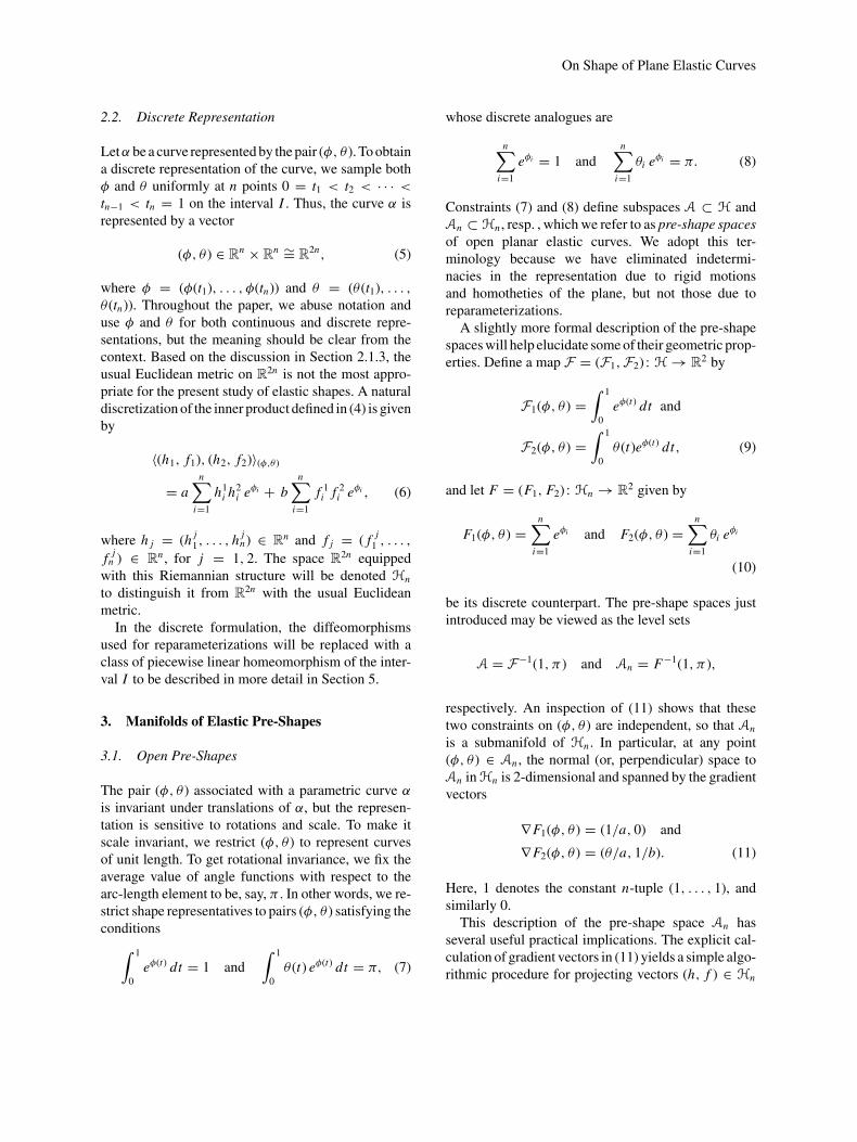
2.2. Discrete Representation

Letα be a curve represented by the pair (φ, θ ). To obtaina discrete representation of the curve, we sample bothφ and θ uniformly at n points 0 = t1 < t2 < · · · <

tn−1 < tn = 1 on the interval I . Thus, the curve α isrepresented by a vector

(φ, θ ) ∈ Rn × Rn ∼= R2n, (5)

where φ = (φ(t1), . . . , φ(tn)) and θ = (θ (t1), . . . ,θ (tn)). Throughout the paper, we abuse notation anduse φ and θ for both continuous and discrete repre-sentations, but the meaning should be clear from thecontext. Based on the discussion in Section 2.1.3, theusual Euclidean metric on R2n is not the most appro-priate for the present study of elastic shapes. A naturaldiscretization of the inner product defined in (4) is givenby

〈(h1, f1), (h2, f2)〉(φ,θ )

= an∑

i=1

h1i h2

i eφi + bn∑

i=1

f 1i f 2

i eφi , (6)

where h j = (h j1, . . . , h j

n) ∈ Rn and f j = ( f j1 , . . . ,

f jn ) ∈ Rn , for j = 1, 2. The space R2n equipped

with this Riemannian structure will be denoted Hn

to distinguish it from R2n with the usual Euclideanmetric.

In the discrete formulation, the diffeomorphismsused for reparameterizations will be replaced with aclass of piecewise linear homeomorphism of the inter-val I to be described in more detail in Section 5.

3. Manifolds of Elastic Pre-Shapes

3.1. Open Pre-Shapes

The pair (φ, θ ) associated with a parametric curve α

is invariant under translations of α, but the represen-tation is sensitive to rotations and scale. To make itscale invariant, we restrict (φ, θ ) to represent curvesof unit length. To get rotational invariance, we fix theaverage value of angle functions with respect to thearc-length element to be, say, π . In other words, we re-strict shape representatives to pairs (φ, θ ) satisfying theconditions∫ 1

0

eφ(t) dt = 1 and

∫ 1

0

θ (t) eφ(t) dt = π, (7)

whose discrete analogues are

n∑i=1

eφi = 1 andn∑

i=1

θi eφi = π. (8)

Constraints (7) and (8) define subspaces A ⊂ H andAn ⊂ Hn , resp. , which we refer to as pre-shape spacesof open planar elastic curves. We adopt this ter-minology because we have eliminated indetermi-nacies in the representation due to rigid motionsand homotheties of the plane, but not those due toreparameterizations.

A slightly more formal description of the pre-shapespaces will help elucidate some of their geometric prop-erties. Define a map F = (F1,F2) : H → R2 by

F1(φ, θ ) =∫ 1

0

eφ(t) dt and

F2(φ, θ ) =∫ 1

0

θ (t)eφ(t) dt, (9)

and let F = (F1, F2) : Hn → R2 given by

F1(φ, θ ) =n∑

i=1

eφi and F2(φ, θ ) =n∑

i=1

θi eφi

(10)

be its discrete counterpart. The pre-shape spaces justintroduced may be viewed as the level sets

A = F−1(1, π ) and An = F−1(1, π ),

respectively. An inspection of (11) shows that thesetwo constraints on (φ, θ ) are independent, so that An

is a submanifold of Hn . In particular, at any point(φ, θ ) ∈ An , the normal (or, perpendicular) space toAn in Hn is 2-dimensional and spanned by the gradientvectors

∇F1(φ, θ ) = (1/a, 0) and

∇F2(φ, θ ) = (θ/a, 1/b). (11)

Here, 1 denotes the constant n-tuple (1, . . . , 1), andsimilarly 0.

This description of the pre-shape space An hasseveral useful practical implications. The explicit cal-culation of gradient vectors in (11) yields a simple algo-rithmic procedure for projecting vectors (h, f ) ∈ Hn


orthogonally onto the tangent space T(φ,θ )An by sub-tracting normal components. This will be needed, e.g.,in numerical calculations of geodesics in An .

Algorithm 3.1.1. Orthogonal Projection of (h, f ) ∈Hn onto T(φ,θ )An .

(i) Apply Gram-Schmidt to {∇F1(φ, θ ), ∇F2(φ, θ )},with respect to the inner product 〈 , 〉(φ,θ ), to ob-tain an orthonormal basis {e1(φ, θ ), e2(φ, θ )} ofT(φ,θ )An .

(ii) The orthogonal projection of (h, f ) is givenby

(φ,θ )(h, f )

= (h, f ) −2∑

i=1

〈(h, f ), ei (φ, θ )〉(φ,θ )ei (φ, θ ).

Our calculations of geodesics in pre-shape manifoldswill also require a mechanism to project points in Hn

onto An . This is because, during numerical integrationsof the differential equation that governs geodesics inAn , points on An typically evolve to points slightlyoff the pre-shape manifold. The projection will thenplace them back on An . For (φ, θ ) ∈ Hn , the residualvector

r (φ, θ ) = (1, π ) − F(φ, θ ) (12)

quantifies how far off (φ, θ ) is from An and it is zero ifand only if (φ, θ ) ∈ An . To project (φ, θ ) onto An , weuse Newton’s method to search for a (nearby) zero ofr , initializing the search with (φ, θ ), as explained next.

The interesting infinitesimal variations of F occuralong directions perpendicular to its level sets. Thus,given (φ, θ ), we calculate the differential dF restrictedto the normal space N (φ, θ ) at (φ, θ ). The Jacobian ofthe mapping F restricted to N (φ, θ ) can be expressedin the basis {∇Fi (φ, θ ), 1 ≤ i ≤ 2} of N (φ, θ ) andthe standard basis of R2 as the 2 × 2 symmetric matrixJ (φ, θ ) whose (i, j) entry is

Ji j (φ, θ ) = ⟨∇Fi (φ, θ ), ∇Fj (φ, θ )⟩(φ,θ )

. (13)

Let ε > 0 be a small number.

Algorithm 3.1.2. Projection of (φ, θ ) ∈ Hn onto An .

1. Compute F(φ, θ ) and the residual vector accordingto Eq. (12).

2. If ‖r (φ, θ )‖ < ε, stop. Else, continue.3. Use (11) to calculate ∇Fi (φ, θ ), 1 ≤ i ≤ 2, and the

Jacobian matrix J (φ, θ ) whose entries are given by(13).

4. Solve the linear equation J (φ, θ )xT = r T (φ, θ ),where x = (x1, x2) and T denotes transposition.

5. Update (φ, θ ) = (φ, θ ) + ∑2j=1 x j∇Fj (φ, θ ). Re-

turn to Step 1.

3.2. Closed Pre-Shapes

We now consider a similar manifold Cn of closedpre-shapes where, in addition to (7), curves satisfy aclosure condition. A curve α is closed if and only if∫ 1

0α′(s) ds = 0. If α is represented by the pair (φ, θ ),

the closure condition can be expressed as∫ 1

0eφ(t) e jθ (t) dt = 0, or equivalently,

∫ 1

0

cos θ (t) eφ(t) dt = 0 and

∫ 1

0

sin θ (t) eφ(t) dt = 0.

This leads us to consider the mapping G : H → R4

defined by

G1(φ, θ ) =∫ 1

0

eφ(t) dt ;

G2(φ, θ ) =∫ 1

0

θ (t) eφ(t) dt ; (14)

G3(φ, θ ) =∫ 1

0

cos θ (t) eφ(t) dt ;

G4(φ, θ ) =∫ 1

0

sin θ (t) eφ(t) dt.

As before, G1(φ, θ ) = 1 and G2(φ, θ ) = π ensure thatcurves have length 1 and angle functions have averageπ with respect to the arc-length parameter, respectively.G3(φ, θ ) = G4(φ, θ ) = 0 guarantee that the closurecondition is satisfied. The finite-dimensional analogueof G is a mapping G : Hn → R4 obtained by discretiz-ing (14). The pre-shape spaces of closed plane curvesare defined as

C = G−1(1, π, 0, 0) and Cn = G−1(1, π, 0, 0).


The space Cn is a submanifold of Hn whose nor-mal space is 4-dimensional at any point. We com-pute the derivative of G explicitly. The derivatives ofG1 and G2 were computed in (11). In the continuousformulation,

d G3(h, f ) =∫ 1

0

h(t) cos θ (t) eφ(t) dt

−∫ 1

0

f (t) sin θ (t) eφ(t) dt

=⟨(h, f ),

(cos θ

a, − sin θ

b

)⟩(φ,θ )

;

(15)

d G4(h, f ) =∫ 1

0

h(t) sin θ (t) eφ(t) dt

+∫ 1

0

f (t) cos θ (t) eφ(t) dt

=⟨(h, f ),

(sin θ

a,

cos θ )

b

)⟩(φ,θ )

.

The corresponding calculation for G yields:

∇G1(φ, θ ) = (1/a, 0); ∇G2(φ, θ ) = (θ/a, 1/b);

∇G3(φ, θ ) = (cos θ/a, − sin θ/b); (16)

∇G4(φ, θ ) = (sin θ/a, cos θ/b).

As in the previous case, two projection algorithmscan be derived from this calculation. The extension ofAlgorithm 3.1.1. to closed shapes is straightforward,the only difference being that Gram-Schmidt is appliedto a set of four vectors instead of two. We only presentthe details of the calculation of the Jacobian matrix ofG needed for the projection of Hn onto Cn . Other thanthat, Algorithm 3.1.2. can be reproduced almost wordby word.

The normal space N (φ, θ ) to the level set of G at(φ, θ ) is spanned by the vectors ∇Gi (φ, θ ), 1 ≤ i ≤ 4.The Jacobian of the mapping G restricted to N (φ, θ )can be expressed in this basis of N (φ, θ ) and the stan-dard basis of R4 as the 4×4 symmetric matrix J whose(i, j)-entry is

Ji j (φ, θ ) = 〈∇Gi (φ, θ ), ∇G j (φ, θ )〉. (17)

For implementation purposes, we write J more

explicitly. Let

A(φ, θ ) =n∑

i=1

θi cos θi eφi ;

B(φ, θ ) =n∑

i=1

θi sin θi eφi ;

C(φ, θ ) =n∑

i=1

cos2(θi ) eφi ;

D(φ, θ ) =n∑

i=1

sin(2θi ) eφi ;

E(φ, θ ) =n∑

i=1

θ2i eφi .

Then,

J =

⎡⎢⎢⎢⎢⎢⎢⎢⎣

G1/a G2/a G3/a G4/a

G2/a G1/b + E/a A/a − G4/b B/a + G3/b

G3/a A/a − G4/b G1/b + C

(1

a− 1

b

)D

(1

2a− 1

2b

)G4/a B/a + G3/b D

(1

2a− 1

2b

)G1/a + C

(1

b− 1

a

)

⎤⎥⎥⎥⎥⎥⎥⎥⎦.

(18)

4. Geodesics in Pre-Shape Spaces

Let p0 = (φ0, θ0) and p1 = (φ1, θ1) represent pre-shapes in An or Cn . The geodesic distance, d(p0, p1),between p0 and p1 is defined as

d(p0, p1) = infγ

�(γ ), (19)

where γ ranges over all piecewise smooth paths inAn or Cn from p0 to p1, and �(γ ) is the length of γ

defined as

�(γ ) =∫

I‖γ ′(t)‖γ (t) dt =

∫I(〈γ ′(t), γ ′(t)〉γ (t))

1/2dt.

It is well known that, locally, the geodesic distanceis realized by a geodesic. For finite-dimensional,complete Riemannian manifolds, the Hopf-RinowTheorem asserts that the same holds in general (seee.g. do Carmo (1994)). In the remainder of the paper,we will work under the assumption that distances inAn and Cn are realized by geodesics. Thus, our nextgoal is to develop an algorithm to calculate geodesicsin pre-shape spaces with prescribed initial and terminalpoints. Our general strategy is similar to that adoptedin Klassen et al. (2004), however, the arguments aremuch more elaborate and the details differ significantly


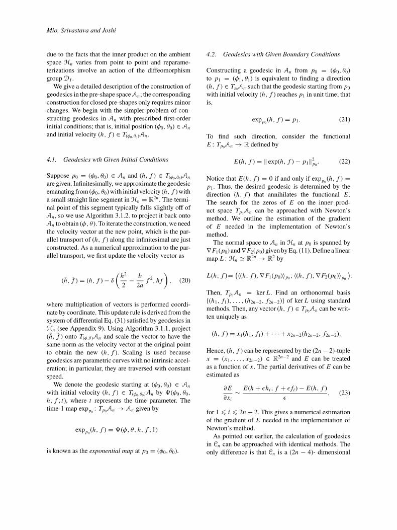
due to the facts that the inner product on the ambientspace Hn varies from point to point and reparame-terizations involve an action of the diffeomorphismgroup DI .

We give a detailed description of the construction ofgeodesics in the pre-shape space An; the correspondingconstruction for closed pre-shapes only requires minorchanges. We begin with the simpler problem of con-structing geodesics in An with prescribed first-orderinitial conditions; that is, initial position (φ0, θ0) ∈ An

and initial velocity (h, f ) ∈ T(φ0,θ0)An .

4.1. Geodesics wth Given Initial Conditions

Suppose p0 = (φ0, θ0) ∈ An and (h, f ) ∈ T(φ0,θ0)An

are given. Infinitesimally, we approximate the geodesicemanating from (φ0, θ0) with initial velocity (h, f ) witha small straight line segment in Hn = R2n . The termi-nal point of this segment typically falls slightly off ofAn , so we use Algorithm 3.1.2. to project it back ontoAn to obtain (φ, θ ). To iterate the construction, we needthe velocity vector at the new point, which is the par-allel transport of (h, f ) along the infinitesimal arc justconstructed. As a numerical approximation to the par-allel transport, we first update the velocity vector as

(h, f ) = (h, f ) − δ

(h2

2− b

2af 2, h f

), (20)

where multiplication of vectors is performed coordi-nate by coordinate. This update rule is derived from thesystem of differential Eq. (31) satisfied by geodesics inHn (see Appendix 9). Using Algorithm 3.1.1, project(h, f ) onto T(φ,θ )An and scale the vector to have thesame norm as the velocity vector at the original pointto obtain the new (h, f ). Scaling is used becausegeodesics are parametric curves with no intrinsic accel-eration; in particular, they are traversed with constantspeed.

We denote the geodesic starting at (φ0, θ0) ∈ An

with initial velocity (h, f ) ∈ T(φ0,θ0)An by (φ0, θ0,

h, f ; t), where t represents the time parameter. Thetime-1 map expp0

: Tp0An → An given by

expp0(h, f ) = (φ, θ, h, f ; 1)

is known as the exponential map at p0 = (φ0, θ0).

4.2. Geodesics with Given Boundary Conditions

Constructing a geodesic in An from p0 = (φ0, θ0)to p1 = (φ1, θ1) is equivalent to finding a direction(h, f ) ∈ Ts0

An such that the geodesic starting from p0

with initial velocity (h, f ) reaches p1 in unit time; thatis,

expp0(h, f ) = p1. (21)

To find such direction, consider the functionalE : Tp0

An → R defined by

E(h, f ) = ‖ exp(h, f ) − p1‖2p0

. (22)

Notice that E(h, f ) = 0 if and only if expp0(h, f ) =

p1. Thus, the desired geodesic is determined by thedirection (h, f ) that annihilates the functional E .The search for the zeros of E on the inner prod-uct space Tp0

An can be approached with Newton’smethod. We outline the estimation of the gradientof E needed in the implementation of Newton’smethod.

The normal space to An in Hn at p0 is spanned by∇F1(p0) and ∇F2(p0) given by Eq. (11). Define a linearmap L : Hn � R2n → R2 by

L(h, f )= (〈(h, f ), ∇F1(p0)〉p0, 〈(h, f ), ∇F2(p0)〉p0

).

Then, Tp0An = ker L . Find an orthonormal basis

{(h1, f1), . . . , (h2n−2, f2n−2)} of ker L using standardmethods. Then, any vector (h, f ) ∈ Tp0

An can be writ-ten uniquely as

(h, f ) = x1(h1, f1) + · · · + x2n−2(h2n−2, f2n−2).

Hence, (h, f ) can be represented by the (2n − 2)-tuplex = (x1, . . . , x2n−2) ∈ R2n−2 and E can be treatedas a function of x . The partial derivatives of E can beestimated as

∂ E

∂xi∼ E(h + εhi , f + ε fi ) − E(h, f )

ε, (23)

for 1 � i � 2n − 2. This gives a numerical estimationof the gradient of E needed in the implementation ofNewton’s method.

As pointed out earlier, the calculation of geodesicsin Cn can be approached with identical methods. Theonly difference is that Cn is a (2n − 4)- dimensional


1

2

3

45

678

9

1

2

3

45

678

9

1

2

3

45

678

9

1

2

3

45

678

9

1

2

3

45

678

9

1

2

3

45

678

9

1

2

3

45

67

8

9

1

2

345

67

8

9 1

2

345

67

8

91

2

34

5

67

8

91

2

34

5

67

8

91

2

3

4

5

67

8

91

2

3

4

5

67

8

91

2

3

4

5

67

8

9

Figure 1. Examples of geodesics in the pre-shape space An .

12

3

456

7

8

91

2

3

456

78

91

2

3

456

78

91

2

3

456

78

91

2

3

456

78

91

2

3

456

78

91

2

3

4

56

7 8

9

Figure 2. A geodesic in the pre-shape space of closed curves.

submanifold of Hn . An explicit basis for the normalspace at any point has been computed in (16).

4.3. Preliminary Illustrations

Figure 1 shows examples of geodesics in the pre-shapespace An computed with the methods described above.A similar illustration in the pre-shape space Cn ofclosed curves is shown in Fig. 2. For each curve, the la-bels represent points associated with 9 uniformly sam-pled points over the “time” interval I . In each row, theinitial and terminal frames display given pre-shapes tobe interpolated. The labels illustrate correspondencesobtained during geodesic morphing. The elasticity pa-rameters a = 0.1 and b = 1 were used in our ex-periments and the curves were sampled at n = 100points. A low tension coefficient was used to allowplenty of stretch elasticity. In this model, shape cor-respondences obtained during geodesic deformationslook natural and intuitively correct. For example, thefinger tips tend to be preserved, as well as some othergeometric features shared by the curves. Comparisonswith shape geodesics in other models are provided be-low.

Although we provide no theoretical assurance thatthe geodesics minimize length, extensive experimen-tation indicates that, for a vast collection of curves,the geodesics obtained are intuitively correct. However,further investigations along these lines are needed.

5. Matching and Interpolating Shapes

As pointed out in the Introduction, in many appli-cations, a correspondence matching points betweenshapes to be compared is given. For example, in medi-cal imaging, a correspondence between shapes is oftenestablished to preserve some landmark points. In suchcases, it is desirable that shape metrics and morph-ing techniques be compatible with the given matching.The same applies to situations where shape correspon-dences are established using matching techniques thatseek to optimally align elements such as velocity fieldsor curvature functions of contours, as in Cohen et al.(1992), Geiger et al. (1995), Tagare et al. (2002), andSebastian et al. (2003). The goals of this section are:

(i) to explain how geodesics in pre-shape spaces canbe used to quantify divergence and interpolateshapes in the presence of a preferred matching;

(ii) to investigate a variant of the dynamic program-ming shape matching strategy of Tagare et al.(2002), and Sebastian et al. (2003) using an en-ergy functional that is more compatible with theelastic curve model adopted in this paper.

5.1. Interpolations and Metric

We present the details of the case of general planecurves without the closure condition, but closed curvescan be treated in a similar manner. Let α0, α1 : I → R2


be parametric curves. The time parameter t inducesa correspondence between the curves, namely, α0(t)is matched with α1(t), for every t . Conversely, forsmooth plane curves with no self-intersections, any dif-feomorphic correspondence between them arises in thisfashion. Moreover, if β0 and β1 are parameterizationsof the same curves inducing the same correspondenceas α0 and α1, then the parameterizations differ by adiffeomorphism γ : I → I ; that is,

βi (t) = αi (γ (t)),

for i = 0, 1. This motivates the following approach.Think of a correspondence ρ between two curves C0

and C1 as given by a choice of parameterizations α0

and α1, and let (φ0, θ0), (φ1, θ1) ∈ An be the associatedpre-shapes obtained after applying the normalizationsdiscussed in Section 3. For a given choice of elasticityconstants a, b > 0, define the distance between thecurves, under the correspondence ρ, to be

dρ(C0, C1) = da,b ((φ0, θ0), (φ1, θ1)) , (24)

where da,b is the geodesic distance in pre-shape space.The length-minimizing geodesic between the pre-shapes gives a natural interpolation that is compatiblewith the given correspondence. Notice that the distancedρ(C0, C1) is well-defined because any other choice ofpre-shapes associated with the given correspondencecan be obtained by the action of a diffeomorphism γ

on (φ0, θ0), (φ1, θ1) (see Eq. (3)) and the diffeomor-phism group DI acts on An by distance-preservingtransformations, as explained in Section 2.1.3. A sim-ilar fact applies to geodesics. Let (φ(t, s), θ (t, s) be ageodesic in An between (φ0, θ0) and (φ1, θ1), where tand s denote the curve and deformation parameters, re-spectively. Then, the corresponding geodesic between(φ0, θ0) · γ and (φ1, θ1) · γ is obtained by the action ofγ ; that is, it is given by

(t, s) �→ (φ(γ (t), s) + log γ ′(t), θ (γ (t), s)).

As a consequence, in computations of distances andgeodesics with respect to given curve correspondences,we can choose any parameterization for one of thecurves and adjust the other to be compatible with thedesired matching. In particular, we can assume thatone of the curves is parameterized by arc length; i.e.,φ0 ≡ 0.

5.2. Shape Matching with Dynamic Programming

Consider curves represented by the pre-shapes(φ0, θ0), (φ1, θ1). As explained in the previous section,to establish a correspondence between the curves, onemay fix a parametrization of the first and consider allreparametrizations of the other. Thus, we assume thatnormalized pre-shapes initially have unit speed param-eterizations; that is, φ0 = φ1 ≡ 0. Given elasticityconstants a, b > 0 and a diffeomorphism γ : I →I , our matching criterion will seek to minimize thefunctional

E(γ ) = ‖(0, θ0) − (0, θ1) · γ ‖2(0,θ0)

=∫

I[a(log γ ′(t))2 + b (θ0(t)−θ1 ◦ γ (t))2] dt,

(25)

which quantifies the compatibility of (0, θ0) and thereparameterized pre-shape (0, θ1) · γ from the view-point of (φ0, θ0). More symmetric forms of the energycan be considered as in Tagare (1999). As before, eachpre-shape is sampled uniformly at n points on the in-terval I ; in our experiments, we use n = 100. Con-sider the uniform n × n grid on the square I × I withgrid points labeled (i, j), 0 � i, j � n − 1. As indi-cated in Fig. 3(a), diffeomorphisms of the interval Iwill be approximated by piecewise linear (PL) home-omorphisms whose graphs are PL paths on the squareI × I from (0, 0) to (n − 1, n − 1), with each node agrid point. Note that all segments in such paths havepositive slope. The matching problem is now reducedto finding the allowable path that minimizes (a discreteform of) the energy E(γ ). Dynamic programming, DP,is well suited for this problem since the cost associated

(0,0)

(i,j)

(i,0)(0,0)

(0,j)

)b()a(

Figure 3. (a) A piecewise linear path on the square I × I approx-

imating the graph of a diffeomorphism; (b) Restricting the possible

slopes of the path at a node (i, j).


with a path is additive over its segments. Thus, it isnatural to introduce a localized form of the energy Eover a segment. For k < i and l < j , let L(k, l; i, j)denote the line segment joining nodes (k, l) and (i, j)and let

E (k, l; i, j)

=∫

Iki

[a(log γ ′kli j (t))

2 + b(θ0(t) − θ1 ◦ γkli j (t))2] dt,

(26)

where Iki ⊆ I is the subinterval determined by the po-ints indexed by k and i , and γkli j is the lin-ear diffeomorphism from Iki to Il j whose graph isL(k, l; i, j).

To minimize the energy, in principle, one should con-sider all possible ways of reaching a node (i, j) throughsegments of the form L(k, l; i, j), k < i and l < j . Forcomputational efficiency, in practice, we restrict the in-dexes (k, l) to a subset Ni j . A possible choice of Ni j

is illustrated in Fig. 3(b). Define the minimum energyH (i, j) needed to reach the node (i, j), iteratively, asfollows:

(i) H (0, 0) = 0 ;(ii) H (i, j) = E(k, l; i, j) + H (k, l),

(a) (b) (c)

0 20 40 60 80 100 120 140 160

0

1

2

3

4

5

6

7

8θ

1θ

2θ

2(γ)

Figure 4. (a) Optimal correspondence between two shapes; (b) an intensity plot of the energy H and the graph of the matching diffeomorphism

γ ; (c) a plot of the angle functions θ0, θ1 and θ1 ◦ γ .

Figure 5. Optimal correspondences between closed curves.

where

(k, l) = argmin(k,l)∈Ni j

(E(k, l; i, j) + H (k, l)).

The energy H (i, j) is computed sequentially, startingfrom (0, 0) and increasing i, j until all allowable ver-tices are visited. For nodes that cannot be reached,we preassign H (i, j) = ∞. This is the case, e.g.,for all (i, 0) and (0, j), 1 � i, j � n − 1. OnceH (n − 1, n − 1) has been computed, we backtrackto find a path of minimum energy that represents aPL homeomorphism of the interval I . Further de-tails on the calculation of E(k.l; i, j) are presented inAppendix B.

Figure 4(a) illustrates this shape matching strategyapplied to pre-shapes initially parameterized by arclength; i.e., φ0 = φ1 ≡ 0. We adopted a low valuefor the tension parameter a in order to allow plentyof stretch elasticity. As stretching is essentially notpenalized, the matching diffeomorphism γ will attemptto align the angle functions θ0 and θ1 ◦ γ as much aspossible to minimize E . Figure 4(b) is an intensity plotof the energy H and the overlaid path represents theoptimal diffeomorphism γ estimated using dynamicprogramming. Figure 4(c) illustrates the improvedalignment of angle functions after the action of γ

on θ1.


The implementation for closed contours is similar,except that we also need to consider all possible choicesof initial points. Computational strategies to managethis extra degree of freedom are discussed in Sebastianet al. (2003). Examples of correspondences for closedshapes are shown in Fig. 5.

5.3. Geodesics

We conclude this section with several examples ofgeodesics between closed shapes that respect optimalalignments obtained via the dynamic programming ap-proach of Section 5.2. To illustrate the improvementover geodesics in the more rigid, bending-only shapemodel of Klassen et al. (2004) and the landmark modelof Kendall (1984), we offer a few comparisons of thesethree types of geodesics in Fig. 6.

Figure 7 shows an application of elastic shapegeodesics to echocardiography. The first and last panelsshow the end diastolic (ED) and end systolic (ES)frames, taken from the apical four-chamber view, dur-ing systole (the contracting part of the cardiac cycle).Overlaid on these frames are expert tracings of the

Figure 6. Geodesics in the fully elastic, bending-only and Kendall models. In each group, the first row shows a geodesic between elastic shapes

with low tension coefficient, aligned with dynamic programming techniques. For comparison purposes, the second and third rows in each group

display geodesics in the bending-only and Procrustes models, respectively.

epicardial (as solid lines) and endocardial (as dashedlines) contours of the left ventricle. Among otherthings, cardiologists are interested in the temporal evo-lution of these contours. Geodesics in the pre-shapespace of elastic curves with DP alignment were scaledand positioned appropriately to estimate the contoursfor intermediate frames. Images were acquired a rateof 30 frames per second; some of the frames are dis-played in the figure. Modeling shapes on elastic curvesthat can be stretched, compressed and bent in differentways along the extension of the curve has a series ofadvantages. For example, one can observe that the apexof both endocardial and epicardial contours as well assharp corners and edges are well aligned during theevolution.

6. Spaces of Elastic Shapes

Shape metrics and interpolations based on geodesicsin pre-shape spaces and DP alignment, as discussedin Section 5, are very attractive from a computationalstandpoint. Extensive experimentation also indicatesthat matchings and interpolations so obtained tend to


Figure 7. Interpolation using an elastic shape geodesic of the expert-drawn epicardial and endocardial contours of the left ventricle at end

diastole and end systole to estimate their evolution during systole.

be intuitively correct; further evidence of this fact willbe provided below. Thus, in practice, this is the modelwe propose to adopt. The framework that we have de-veloped also allow us to define spaces of shapes asquotient spaces of pre-shape spaces under the action ofreparameterizations and compute distances and inter-polations without assuming any preferred shape corre-spondences; as a matter of fact, finding an optimal cor-respondence becomes an intrinsic part of the problemof defining geodesic distance in shape space. However,the additional computational costs are significant. Ourexperiments indicate that geodesics with DP alignmentoffer accurate approximations to actual geodesics inshape space. For completeness, we briefly outline theconstruction of shape spaces, metrics, and morphingtechniques.

6.1. Shape of Planar Arcs

The shape of a planar arc admits multiple representativepre-shapes, as defined in Section 3.1, due to all possiblereparameterizations of a curve. Thus, we define theshape space S of planar arcs as the quotient space ofA by the action of DI , that is, S = A/DI . Define a(pseudo) metric on S by

d(s1, s2) = min(φ1,θ1),(φ2,θ2)

d((φ1, θ1), (φ2, θ2)),

where the minimum is taken over all pre-shapes (φ1, θ1)and (φ2, θ2) representing s1 and s2, respectively. Let

(0, θ∗i ) be the representative of si , i = 1, 2, parameter-

ized by arc length. Then, any pre-shape representing si

can be written as (0, θ∗i ) · γ , with γ ∈ DI . Moreover,

since DI acts on A by isometries, we can fix the repre-sentative of s1 to be (0, θ∗

1 ) and take the minimum onlyover (φ2, θ2). Thus, the distance in S can be expressedas

d(s1, s2) = infγ∈DI

d((0, θ∗1 ), (0, θ∗

2 ) · γ ).

The cost function (22) used in the construction ofgeodesics in pre-shape spaces is now modified to

E(h, f ; γ ) = ∥∥ exp(0,θ∗0 )(h, f ) − (0, θ∗

1 ) · γ∥∥2

(0,θ∗0 ).

(27)

to include the action of γ . A path realizing the geodesicdistance has the property that it is orthogonal to the or-bit of the diffeomorphism group at any point. Thus, inthe construction of geodesics, the search for the appro-priate direction (h, f ) to shoot a geodesic from (0, θ∗

0 )is restricted to those tangent to An and perpendicularto the orbit of DI at (0, θ∗

0 ) in Hn . The minimizationof E is carried out iteratively alternating between thevariables (h, f ) and γ . The optimization over γ is donewith dynamic programming as in Section 5.2. Gradientmethods are utilized for the optimization over (h, f ).


Sample Shapes Elastic Bending Only

Figure 8. Mean shapes calculated using the elastic model and the bending-only model.

Figure 9. A database of 50 shapes of hands at different poses.

6.2. Closed Shapes

Geodesic distance and morphing techniques for closedshapes can be treated in an almost identical manner,with the extra closure condition enforced.

7. Mean Shapes

Observations of the shape of an object or shapes asso-ciated with a family of similar objects typically exhibitsignificant variations. For example, contours of objects


in images are subject to variations due to pose, perspec-tive, noise, and partial occlusions. Hence, an importantgoal in the algorithmic study of shapes is to developtools for a statistical treatment of shapes. Tangent-spacerepresentation is becoming a standard approach to theanalysis of data on Riemannian manifolds (Dryden andMardia, 1998). The idea is to define and calculate thesample mean and lift the data to the tangent space atthe mean via the inverse exponential map. The datapoints are now represented as points on a vector spaceequipped with an inner product where standard toolsof data analysis can be applied. For example, estima-tion of covariance in the tangent-space representationhas been studied in many different contexts (see e.g.(Dryden and Mardia, 1998; Srivastava et al., 2005;Vailliant et al., 2004)). Thus, in this paper, we focuson the most basic notion needed, that of mean elasticshape. We adopt the notion of Frechet mean shape that

Figure 10. Ten clusters obtained with a variant of the k-MeansAlgorithm applied to the shapes shown in Fig. 9 using the geodesic

distance with DP alignment as metric.

has been previously used in the landmark and bending-only models (Dryden and Mardia, 1998; Klassen et al.,2004). These are special cases of a more general notionof mean on a Riemannian manifold studied by Karcher(1977). We present a formulation for closed shapes, butshapes of elastic arcs can be treated similarly.

Let s1, . . . , sk be a collection of closed shapes. Fora choice of elasticity constants a, b > 0, define thescatter of the collection with respect to a shape s to be

V (s) = 1

2

k∑i=1

d2a,b(s, si ), (28)

where da,b denotes geodesic distance. A Frechet meanof the collection is defined as a shape that is a (local)minimum of V . In practice, we approximate da,b(s, si )by the geodesic distance in pre-shape space after a DPalignment, as discussed in Section 5. To search for aFrechet mean of the collection, we adopt a gradient-type strategy. For data on a Riemannian manifold, the(negative) gradient of the scatter functional V is knownto be given by

−∇V (s) =k∑

i=1

vi , (29)

Figure 11. Eight clusters obtained using a hierarchical clustering

algorithm using the elastic geodesic distance with DP alignment as

metric.


where vi is the initial velocity vector of the geodesicthat runs from s to si in unit time (Karcher, 1977);that is, exps(vi ) = si . Motivated by this observation,initialize the search with s as one of the shapes in thegiven collection and choose pre-shapes p = (φ, θ ) andpi = (φi , θi ) representing s and si , 1 � i � k, witheach pi aligned with p via dynamic programming. Findthe geodesics in the pre-shape manifold Cn from p to pi

and calculate their initial velocities vi = (hi , fi ). Then,infinitesimally displace p in Cn along a geodesic fromp in the direction v = ∑k

i=1 vi (see Section 4.1). Theupdated shape s is the shape associated with the newpre-shape p. The process is iterated until the norm of v

falls below a set threshold thus yielding an estimationof a mean shape.

Figure 8 shows several examples of mean shapescomputed with the algorithmic procedure just de-scribed. For comparison purposes, we also display themean shape in the more rigid bending-only model ofKlassen et al. (2004). The examples illustrate well thefact that the finer shape correspondences built-in to theelastic model leads to more natural mean shapes. Onthe first three rows, unlike the bending-only means,the elastic means preserve the main features shared bythe shapes. Similarly, on the fourth row, more of the

Figure 12. Eight clusters obtained using a hierarchical clustering algorithm with the bending-only geodesic distance.

common sharp features of the sample shapes are re-tained by the elastic mean.

8. Clustering

Alongside statistical modeling of shapes, clusteringtechniques are of basic importance in applications in-volving large collections of shapes. In Srivastava et al.(2005), a variant of the classical k-Means Algorithmwas developed and implemented for clustering shapesusing the bending-only model. The MCMC techniquesadopted in that paper for the construction of clustersapply to other shape metrics since the shape model isonly used to compute the pairwise distances betweenthe sample shapes. Thus, here, we just offer illustrationsof results obtained by replacing the shape metric withthe elastic geodesic distance with DP alignment. Figure9 shows a collection of 50 shapes of hands at variousdifferent poses. Clusters obtained with the k-MeansAlgorithm with k = 10 are displayed in Fig. 10. Theresults of another clustering experiment with the elas-tic geodesic distance with DP alignment are shownin Fig. 11. Here, the 50 smaple shapes were groupedinto 8 clustersusing a hierarchical clustering algorithm.


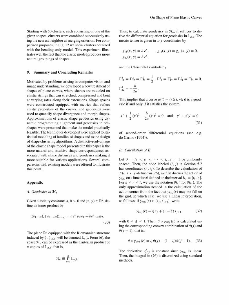
Starting with 50 clusters, each consisting of one of thegiven shapes, clusters were combined successively us-ing the nearest neighbor as merging criterion. For com-parison purposes, in Fig. 12 we show clusters obtainedwith the bending-only model. This experiment illus-trates well the fact that the elastic model produces morenatural groupings of shapes.

9. Summary and Concluding Remarks

Motivated by problems arising in computer vision andimage understanding, we developed a new treatment ofshapes of plane curves, where shapes are modeled onelastic strings that can stretched, compressed and bentat varying rates along their extensions. Shape spaceswere constructed equipped with metrics that reflectelastic properties of the curves, and geodesics wereused to quantify shape divergence and morph shapes.Approximations of elastic shape geodesics using dy-namic programming alignment and geodesics in pre-shapes were presented that make the model practicallyfeasible. The techniques developed were applied to sta-tistical modeling of families of shapes and to the designof shape clustering algorithms. A distinctive advantageof the elastic shape model presented in this paper is themore natural and intuitive shape correspondences as-sociated with shape distances and geodesics making itmore suitable for various applications. Several com-parisons with existing models were offered to illustratethis point.

Appendix

A. Geodesics in Hn

Given elasticity constants a, b > 0 and (x, y) ∈ R2, de-fine an inner product by

〈(v1, v2), (w1, w2)〉(x,y) = aex v1w1 + bex v2w2.

(30)

The plane R2 equipped with the Riemannian structureinduced by 〈 , 〉(x,y) will be denoted La,b. From (6), thespace Hn can be expressed as the Cartesian product ofn copies of La,b; that is,

Hn∼= n

i=1

La,b.

Thus, to calculate geodesics in Hn , it suffices to de-rive the differential equation for geodesics in La,b. Themetric tensor is given in x-y coordinates by

g11(x, y) = a ex , g12(x, y) = g21(x, y) = 0,

g22(x, y) = b ex ,

and the Christoffel symbols by

�111 = �2

12 = �221 = 1

2, �2

11 = �112 = �1

21 = �222 = 0,

�122 = − b

2a.

This implies that a curve α(t) = (x(t), y(t)) is a geod-esic if and only if it satisfies the system

x ′′ + 1

2(x ′)2 − b

2a(y′)2 = 0 and y′′ + x ′y′ = 0

(31)

of second-order differential equations (see e.g.do Carmo (1994)).

B. Calculation of E

Let 0 = t0 < t1 < · · · < tn−1 = 1 be uniformlyspaced. Then, the node labeled (i, j) in Section 5.2has coordinates (ti , t j ). To describe the calculation ofE(k, l; i, j) defined in (26), we first discuss the action ofγkli j on a function θ defined on the interval Iki = [tk, ti ].For k ≤ r ≤ i , we use the notation θ (r ) for θ (tr ). Theonly approximation needed in the calculation of theaction comes from the fact that γkli j (r ) may not fall onthe grid, in which case, we use a linear interpolation,as follows: if γkli j (r ) ∈ [s j , s j+1], write

γkli j (r ) = ξ s j + (1 − ξ ) s j+1, (32)

with 0 ≤ ξ ≤ 1. Then, θ ◦ γkli j (r ) is calculated us-ing the corresponding convex combination of θ ( j) andθ ( j + 1); that is,

θ ◦ γkli j (r ) = ξ θ ( j) + (1 − ξ ) θ ( j + 1). (33)

The derivative γ ′kli j is constant since γkli j is linear.

Then, the integral in (26) is discretized using standardmethods.


Acknowledgments

This work was supported in part by National ScienceFoundation grants CCF-0514743 and DMS-0101429,and Army Research Office grant W911NF-04-01-0268. The echocardiographic images used in the pa-per are courtesy of David Wilson at the University ofFlorida.

References

Beg, M.F., Miller, M.I., Trouve, A., and Younes, L. 2005. Computing

large deformation metric mappings via geodesic flows of diffeo-

morphisms. International Journal of Computer Vision, 61:139–

157.

Bookstein, F.L. 1986. Size and shape spaces for landmark data in

two dimensions. Statistical Science, 1:181–242.

Cohen, I., Ayache, N., and Sulger, P. 1992. Tracking points on de-

formable objects using curvature information. In Lecture Notes inComputer Science, vol. 588.

Cootes, T.F., Taylor, C.J., Cooper, D.H., and Graham, J. 1995. Active

shape models: Their training and applications. Computer Visionand Image Understanding, 61:38–59.

do Carmo, Manfredo, 1994. Riemannian Geometry. Birkhauser.

Dryden, I.L. and Mardia, K.V. 1998. Statistical Shape Analysis. John

Wiley & Son.

Geiger, D., Gupta, A., Costa, L.A., and Vlontzos, J. 1995. Dynamic

programming for detecting, tracking and matching elastic con-

tours. IEEE Trans. on Pattern Analysis and Machine Intelligence,

17(3):294–302.

Grenander, U. 1993. General Pattern Theory. Oxford University

Press.

Karcher, H. 1977. Riemann center of mass and mollifier smoothing.

Comm. Pure Appl. Math., 30:509–541.

Kendall, D.G. 1984. Shape manifolds, Procrustean metrics and com-

plex projective spaces. Bulletin of London Mathematical Society,

16:81–121.

Klassen, E., Srivastava, A., Mio, W., and Joshi, S. 2004. Analysis

of planar shapes using geodesic paths on shape manifolds. IEEETrans. on Pattern Analysis and Machine Intelligence, 26:372–383.

Le, H.L. and Kendall, D.G. 1993. The Riemannian structure of eu-

clidean shape spaces: a novel environment for statistics. Annals ofStatistics, 21(3):1225–1271.

Mennucci, A. and Yezzi, A. 2004. Metrics in the space of curves.

Technical report.

Michor, P. and Mumford, D. Riemannian geometries on spaces of

plane curves. J. Eur. Math. Soc. in press.

Sebastian, T.B., Klein, P.N., and Kimia, B.B. 2003. On aligning

curves. IEEE Transactions on Pattern Analysis and Machine In-telligence, 25(1):116–125.

Sharon, E. and Mumford, D. 2004. 2D-Shape analysis using confor-

mal mappings. In Proceedings of IEEE Conference on ComputerVision, pp. 350–357.

Srivastava, A., Joshi, S., Mio, W., and Liu, X. 2005. Statistical shape

analysis: Clustering, learning and testing. IEEE Trans. on PatternAnalysis and Machine Intelligence, 27:590–602.

Tagare, H.D. 1999. Shape-based non-rigid correspondence with ap-

plications to heart motion analysis. IEEE Trans. on Medical Imag-ing, 8(7):570–579.

Tagare, H.D., O’Shea, D., and Groisser, D. 2002. Non-rigid shape

comparison of plane curves in images. Journal of MathematicalImaging and Vision, 16:57–68.

Thompson, D.W. 1992. On Growth and Form: The Complete RevisedEdition. Dover.

Vailliant, M., Miller, M.I., and Younes, L. 2004. Statistics on dif-

feomorphisms via tangent space representations. NeuroImage,

23:161–169.

Younes, L. 1998. Computable elastic distance between shapes. SIAMJournal of Applied Mathematics, 58:565–586.

Younes, L. 1999. Optimal matching between shapes via elastic de-

formations. Journal of Image and Vision Computing, 17(5/6):381–

389.

On Shape of Plane Elastic Curves

Documents

Transcript of On Shape of Plane Elastic Curves