Determination of Stresses from the Stress Trajectory Pattern in a Plane Elastic Domain

http://mms.sagepub.com

Mathematics and Mechanics of Solids

DOI: 10.1177/1081286506067093 2007; 12; 75 originally published online May 19, 2006; Mathematics and Mechanics of Solids

Shamil A. Mukhamediev and Alexander N. Galybin Domain

Determination of Stresses from the Stress Trajectory Pattern in a Plane Elastic

http://mms.sagepub.com/cgi/content/abstract/12/1/75 The online version of this article can be found at:

Published by:

http://www.sagepublications.com

can be found at:Mathematics and Mechanics of Solids Additional services and information for

http://mms.sagepub.com/cgi/alerts Email Alerts:

http://mms.sagepub.com/subscriptions Subscriptions:

http://www.sagepub.com/journalsReprints.navReprints:

http://www.sagepub.co.uk/journalsPermissions.navPermissions:

at Univ of Western Austrlia on September 10, 2008 http://mms.sagepub.comDownloaded from

http://mms.sagepub.com/cgi/alerts

http://mms.sagepub.com/subscriptions

http://www.sagepub.com/journalsReprints.nav

http://www.sagepub.co.uk/journalsPermissions.nav


Determination of Stresses from the Stress Trajectory Pattern in aPlane Elastic Domain

SHAMIL A. MUKHAMEDIEVInstitute of Physics of the Earth, Russian Academy of Sciences, 10 Bol. Gruzinskaya str.,Moscow, 123995, Russia

ALEXANDER N. GALYBIN1

Wessex Institute of Technology, Ashurst Lodge, Ashurst, Southampton, SO40 7AA, UK

(Received 10 February 2004� accepted 25 January 2005)

Abstract: Identification of stresses acting in a plane (homogeneous and isotropic) elastic domain is performedbased on the analysis of principal stress trajectories. This problem, originated in photoelasticity, is now ofgreat importance in geodynamics. Given stress trajectories, in photoelasticity stresses are found by solvinga certain boundary value problem. We propose the solution of the problem without appealing to boundaryconditions, which is advantageous to geodynamics where boundary stresses are poorly constrained. Theanalysis of the given stress trajectory pattern is equivalently reduced to the investigation of the argument,�, of the complex-valued bi-holomorphic function, D, which represents the stress deviator of the 2D stresstensor. Necessary and sufficient conditions for the stress trajectory pattern to be admissible in elasticityare established. A procedure to obtain a particular solution, D1, is presented. The general solution for Dderived from D1 depends on four (if � is a harmonic function) or one (otherwise) arbitrary real constants.The procedure is illustrated by model examples for West European and Australian platforms.

Key Words: elastic material, stresses, trajectories of principal stress, photoelasticity, geodynamics

1. INTRODUCTION

Determination of stresses in a plane transparent model based on the concept of trajectoriesof principal stress (TPS) is a problem that emerged in photoelasticity in the early twentiethcentury. Frocht [1] defines TPS as “curves tangents to which represent the directions of oneof the principal stresses at the points of tangency”. TPS can be extracted by a graphicalmethod from black-and-white fringe patterns observed when light is transmitted through themodel (for details see [1–3]). The dark curves in the pattern represent isoclinics (loci ofpoints along which the principal stresses have parallel directions) and isochromatics. Theproduct (model thickness) � (principal stresses difference) is constant along the latter.Therefore the data available from a photoelastic test allow for immediate integration of theequations of equilibrium, especially if the Lamé–Maxwell form is used (e.g., [1–3]):

Mathematics and Mechanics of Solids, 12: 75–106, 2007

��2007 SAGE Publications

at Univ of Western Austrlia on Septemhttp://mms.sagepub.comDownloaded from

DOI: 10.1177/1081286506067093

ber 10, 2008


76 S H. A. MUK HAMEDIEV and A. N. GALYBIN

�T1

�s1� T1 � T2

r2� 0�

�T2

�s2� T1 � T2

r1� 0� (1)

Equations (1) represent a complete system of partial differential equations for the deter-mination of two unknown quantities (principal stresses T1 and T2) since the radii of curvatureof the stress trajectories (r1 and r2) are known (s1 and s2 are the arc lengths along mutuallyperpendicular TPS of the T1- and T2-families). Given that in photoelasticity the differenceT1 � T2 is also known, any equation in (1) can be used for separation of principal stresses(as in the classical Filon method [1]). If both equations are used, then the experimental pro-cedure can be simplified [2]. In any case, the magnitudes of boundary stresses have to beinvoked when calculating the stress field by the integration of (1).

Integration of system (1) does not require the knowledge of any constitutive law forthe material tested (provided that the field of stress trajectories is known). This would ob-viously produce the same result regardless of the material if similar boundary conditionshave been used. Therefore the results obtained in photoelasticity should, in principle, beverified whether they satisfy the complete system of elastic equations for isotropic homoge-neous material, i.e. if Laplace’s equation is also satisfied with a given accuracy (body forcesneglected)

��T1 � T2� � 0� (2)

It should be noted that differential equations of the second order are used in photoelastic-ity in order to check and improve the separation of principal stresses performed by step-by-step numerical integration of equations of equilibrium. The set of the second order equationsrecommended in [3] includes several equations combining Equation (2) and four equationsobtained by differentiation of equations of equilibrium with respect to two independent vari-ables. The complete result is assumed to be checked by several ways, in particular [3], basedon the properties of isopachics (lines along which T1 + T2 = const). However, one cannotuse these approaches if the difference T1 – T2 is unknown, therefore the direct transfer ofphotoelastic methods of stress separation to other applications of the TPS concept is limited.

In geodynamics, for example, the determination of stresses from known orientations ofprincipal stresses is of great significance (e.g., [4]). Data on in situ stress orientations havebeen summarized and incorporated in the World Stress Map database [5]. Observations indi-cate that two of three principal stresses in the upper Earth’s crust are usually sub-horizontal(e.g., [6]). Thus, plane elastic boundary value problems are frequently employed in modelingof regional stress states in stable blocks of the lithosphere (e.g., [7–9]).

In contrast to the photoelastic method that provides a pattern of continuous TPS, theorientations of stresses in the Earth’s crust are known at spatially discrete points. When theseare dense enough then TPS can be obtained by interpolation (e.g., [10, 11]). For instance,well-investigated regions within West European and North American platforms (e.g., [6, 12])can be approximated by homogeneous TPS ([9, 13]). Other regions may have more complexpatterns of TPS, as in Australia [9]. Considering these regions as elastic, one faces theproblem of solving Equations (1) and (2) if TPS are given. However, this problem differsfrom that in photoelasticity because the difference T1 – T2 and boundary stresses are a prioriunknown. Moreover, the compiled TPS can be unrealisable in elasticity, which is because



DE TE RMINATI ON OF S TR ESSES 77

the system of equations (1) and (2) is overdetermined (provided that TPS field is known).Thus, the method capable of (a) to verify if the TPS are admissible in elasticity and, if yes,(b) to determine stresses on the base of Equations (1) and (2) without appealing to boundarystresses would be of great importance in geodynamics.

The paper is devoted to the development of such a method. After introducing mathe-matical preliminaries (Section 2) and formulating the problem (Section 3) we investigate thequestion regarding the admissible stress trajectories and particular stress fields (Section 4).The general solution of the problem is given in Section 5. Some applications of the method tosimple (but practically interesting) TPS fields are considered in Section 6. Section 7 containssome examples from geodynamics. The paper is supplemented by three appendices.

2. PRELIMINARIES

2.1. Basic Formulae in Complex Variables

A symmetrical in-plane stress tensor T can be described by two stress functions P and Drelated to the stress components Txx , T yy , Txy in Cartesian coordinates x, y as follows (e.g.,Muskhelishvili [14]):

P � 1

2

�Txx � Tyy

�� D � 1

2�Tyy � Txx�� iTxy� (3)

These functions represent isotropic and deviatoric parts of the stress tensor, respectively.The function P is a real-valued function while D is a complex-valued function that can bewritten in the complex-exponential form

D � �D� ei�� (4)

where �D� and � � arg�D� stand for modulus and argument of the complex-valued functionrespectively.

The following relationships linking the stress functions (3) with the principal stresses T1

and T2 are valid:

P � 1

2�T1 � T2� � �D� � 1

2�T2 � T1� � (5)

The modulus of D coincides with the maximum shear stress

�D� � �max (6)

while its argument can be associated with the principal direction, , as follows:

� � �2� (7)

The angle is reckoned counterclockwise from the positive direction of the x-axis to theaxis of minor principal stress.




Instead of the Cartesian coordinates it is convenient to introduce two independent con-jugated complex variables in the form (e.g., [15])

z � x � iy� �z � x � iy� (8)

Hereafter all the functions describing the stress field (i.e., P, D, �max, �, T1, T2, ) areconsidered as the functions of these two variables.

By using complex variables (8) one can present two scalar equations of equilibrium inthe form of a single complex equation

�P �z� �z��z

� �D �z� �z�� z � 0� (9)

Here body forces have been omitted� otherwise, a force vector should be added in the right-hand side of (9).

In elasticity Equation (9) can be rewritten in terms of the stress function D�z� �z� only.For this purpose, one differentiates (9) with respect to the conjugated variable and takes intoaccount that

�2 P

�z� �z � 0�

�� 4

�2

�z� �z is the Laplace operator

�� (10)

hence

�2 D �z� �z�� z2

� 0� (11)

Equation (11) represents a complete system of partial differential equations of plane elasticityin terms of the stress function D�z� �z�.

As it follows from real valuedness of the function P�z� �z� and equations of equilibrium(9), Im �2 D

� �z2 � 0 regardless of constitutive behavior of the material, therefore the equality

Re �2 D� �z2 � 0 is specific for elastic materials (hereafter the symbols Re and Im denote, respec-

tively, the real and imaginary parts of a complex-valued function).Integration of (11) with respect to �z followed by the integration of (9) with respect to

z, in view of real-valuedness of P�z� �z�, immediately leads to the Kolosov–Muskhelishviliformulae [16]:

P �z� �z� � �z��z�� D �z� �z� � �z ��z��z�� (12)

Equations (12) represent the general solution of a plane elastic problem in terms of twoholomorphic functions (z) and �(z). The second equation in (12) suggests that D �z� �z�can be referred to as a bi-holomorphic function in the sense that it satisfies equation (11).2

If D�z� �z� is known, then P�z� �z� can be found by calculating the real part of the primitiveof the potential � �z�. When a well-posed problem is considered, functions �z� and ��z�are to be determined from two independent scalar boundary conditions posed on the entireboundary of a domain.




A real-valued bi-holomorphic function Dreal �z� �z� �Im Dreal �z� �z� � 0� is permanentlyused further on. A general form for it can be written as

Dreal �z� �z� � c2 �zz � c1z � c1z � c0� �Im c0 � Im c2 � 0�� (13)

(see Appendix A for derivation). Function Dreal �z� �z� is expressed through four real arbitraryconstants c0, c11 = Re c1, c12 = Im c1, and c2.

It is evident that any holomorphic function, A(z), can be considered as a special case ofbi-holomorphic function and that any bi-holomorphic function can be viewed as the productof holomorphic and bi-holomorphic functions. Multiplication of A(z) by the real-valued bi-holomorphic function Dreal �z� �z� produces a new bi-holomorphic function which argumentis identical to arg A(z) regardless of the constants c0, c1, and c2 in (13) provided that Dreal

is positive. It is shown in Section 5.1 that such a product is the most general form of therepresentation of bi-holomorphic functions having precisely the same argument as A(z).

2.2. 2D Trajectory Patterns

In view of (7) the TPS in Cartesian coordinates can be specified by the following differentialequations:

�dy

dx

�1

� � tan1

2��

�dy

dx

�2

� cot1

2�� (14)

There are two main situations to be considered in regard to the TPS pattern:

(i) T1-family and T2-family can be distinguished with respect to the magnitudes of principalstresses. Therefore it is exactly known if a particular trajectory is formed by major or byminor principal stress. In this situation it is assumed that

T1 � T2� (15)

(ii) These families cannot be distinguished with respect to the principal stresses.

In photoelasticity the TPS families can be distinguished with the aid of special expedi-ents (e.g., [2]). As far as TPS in the Earth’ crust are concerned, the families can be distin-guished if the principal orientations have become known from local stress measurements.The case (ii) can be realized if, for instance, palaeostresses in the Earth’s crust have beenreconstructed from the data on rock jointing (see details in [17]).

2.3. Singular Points in Trajectory Field

Regular TPS patterns can contain so-called isolated singular points of the first type at whichthe curvature of TPS becomes infinite and the angle of the TPS inclination is not defined.Such points may be located within domain as well as on its boundary. They are actuallyobserved in photoelasticity where they are known as isotropic points, [1–3]. These singularpoints correspond to zeros of the deviatoric function D�z� �z� (i.e., to points where T1 � T2)




and they should be distinguished from singular points of the second type in which stressand/or strain magnitudes have singularities (e.g., concentrated forces). For simplicity, thelatter are omitted from consideration. Otherwise it is impossible to distinguish a priori iden-tical TPS in the vicinity of singular points, e.g., if D � �z or D � z�1.

The asymptotic behavior of TPS near a first order zero of the function D�z� �z� at theorigin can be investigated by analyzing the linear function, D0 �z� �z�, of two variables

D0 �z� �z� � a �z � bz� (16)

provided that �z� 0 and a and b are complex constants. Note that function (16) can beconsidered as a deviatoric part of the stress tensor in plane elasticity since it is a special caseof bi-analitical function. Karakin and Mukhamediev [18] showed that three types of TPSpatterns can be realized in the vicinity of the singular point provided that �a� is not closeto �b�. They are topologically non-equivalent and stable with respect to perturbations of thevalues a, b. The coefficients a and b in representation (16) affect the type of the pattern andits properties. When �a� �b�, all TPS are convex in the direction outward the singularity,but when �a� � �b� they are concave in that direction. The pure hydrostatic stress state,T1 � T2, is realized in the vicinity of the singular point when �a� � �b�.

If an internal singular point coinciding with the first order zero is counterclockwise de-scribed then the principal orientations gain the increment of � that is positive for convexTPS and negative for concave TPS. Bearing this in mind one can introduce a quantity, 2K,that shows the increment of principal orientations (in portions of �) after the complete tra-verse of the closed contour � in positive (counterclockwise) direction. This quantity can berelated to the index of the stress function D over � and calculated as

2 K � Ind� D � � 1

�

��

d � 1

2�

��

d� � 1

2� i

��

d ln D� (17)

In particular, for the function D0 �z� �z� defined in (16) 2K = 1 if �a� � �b� and 2K = –1 if�a� �b�. It should be noted that this definition of the index agrees with the definition ofthe index for holomorphic functions (e.g., [16]). In the latter case 2K (if positive) is equal tothe number of zeros of the holomorphic function inside the domain bounded by � providedthat zeros of n-order are counted n times. This theorem is no longer valid for bi-analiticalfunctions due to the presence of zeros of various types. Note that (17) is valid for the casewhen the TPS singular points are not located on the contour �.

3. FORMULATION OF THE PROBLEM

Let a TPS field be given in a finite closed (generally, multiply-connected) domain �. It isassumed that the TPS are smooth enough (at least three times differentiable) everywhere in� with the possible exception of isolated singular points. One important matter has to bepointed out in regard to the concept of TPS in elasticity, namely whether the �-field can begiven arbitrary. To address this question one can consider an example of a plane elastic unitcircle inside which the �-field is given as




� � �0 � �z �z � 1�2 � ��0 � const� � (18)

Let � (� : �z� � 1) be the boundary of the domain, then it is easy to see that

� : � � �0��

�n� 0�

��

�n� n

�

�z� �n �

� �z�� (19)

where n = –i exp(i�) is the outward unit normal to the contour � (� is the polar angle).Galybin and Mukhamediev [19] showed that the homogeneous field of straight TPS withone of the family inclined at an angle 0 � ��0�2 presents the unique solution of theboundary value problem (19) and the principal stresses are expressed as follows:

T1 � P � Dreal� T2 � P � Dreal�

P � 2 Re

�e�i20

�1

2c2z2 � c1z

�� c (20)

Here Dreal is defined by formula (13) and c is an extra arbitrary real constant caused byintegration. If the case (i) is considered, then the choice of arbitrary constants in (13) issubjected to the additional condition Dreal 0. Thus, the TPS field expressed by (18) is notadmissible for the plane elasticity.

This example clearly demonstrates that not every TPS field can be realized in elasticity.Indeed, such a field uniquely defines the function ��z� �z� and therefore three scalar equationsimposed on two unknown real functions P �z� �z� and �max �z� �z� cannot be solved unless aspecial compatibility condition is introduced on the functions P �z� �z�, �max �z� �z�, and ��z� �z�.

In order to represent a field of elastic TPS the function � �z� �z� should allow for thefollowing equivalent representations:

ei� � �z � �z�� z��z � �z�� z�� or � �z� �z� � 1

2iln�z � �z�� z�z � �z�� z� (21)

where � �z� and � �z� are holomorphic functions. If � is represented in this form, the fieldof TPS can be realized in elasticity because � �z� �z� is the argument of the bi-holomorphicstress function D �z� �z�� and vice versa if � �z� �z� is the argument of any function D�z� �z�which can be considered as a deviatoric stress function in plane elasticity, then this functionis bi-holomorphic function and its argument can be written down in the form given by (21).This observation shows that the mechanical problem of deviatoric stresses reconstructionfrom given TPS can be reduced to the mathematical problem of the bi-holomorphic functiondetermination by its argument.

Thus, the problem is formulated as follows. Given the TPS field in a domain �,

(a) verify if it is admissible (i.e., it can be realized in elasticity) and allows for the determina-tion of at least one bounded stress tensor field�

(b) in the case of admissibility, determine all the possible bounded elastic stress fields pos-sessing the given TPS field.




In other words, it is required to determine a general form of the bi-holomorphic functionD �z� �z�, which satisfies (11) and argument of which is related to the TPS via (7), and thereal-valued harmonic function P �z� �z� related to D �z� �z� via the equations of equilibrium(9).

Some types of TPS patterns can be rejected at first sight. Indeed, for the given TPSpattern one can calculate index 2K (introduced by formula (17)) for any simply-connectedsubdomain of �. As shown by Galybin and Mukhamediev [19], for negative index 2K � �1the functions � �z� and� �z� cannot be holomorphic inside the domain enclosed by contourused for calculation of 2K, thus, no bounded solutions exist in this domain. By evaluating2K for contours encompassing every isolated singular point one can check if 2K � �1. Incase 2K � �1 the corresponding singular point surely is a singular point of the second typefor elasticity (with unbounded stresses in its vicinity). Alternatively, it is possible to evaluateindex 2K for the whole investigated simply-connected domain �. In Section 6 the othermethods of the given TPS field examination with the object to verify its admissibility arepresented. These methods are based on investigation of the TPS behavior in the domain �itself rather then in the vicinity of singular points� they use the equivalent statement of theproblem in terms of arg D �z� �z�.

Some remarks should be presented with regard to the formulation of the problem interms of argument �. In the presence of singular points in the TPS pattern the argument �cannot be represented as a continuous single-valued function of the coordinates. This impor-tant property immediately follows if one considers a closed contour surrounding an isolatedsingular point. In order to select a single-valued branch of � �z� �z� in � one should connectsingular points by cuts with another singular points and/or with the boundary of�. However,this precaution is unnecessary if periodical functions are introduced, e.g. exp(i�). Differenti-ation also removes the jump of � across a cut because the limiting values of derivatives fromboth sides of the cut are coincident. This property makes sense of the differentiation of � in� used below (derivatives of � in singular point should be understood as limiting values ofderivatives at this point).

The following steps are accomplished when solving the problem. First, the prescribedTPS field is checked to see whether it is admissible for elasticity. If positive, at least oneparticular solution of the problem is found. Then the general solution of the problem isconstructed by knowing particular solution.

4. REPRESENTATION OF A BI-HOLOMORPHIC FUNCTION VIA ITSARGUMENT: PARTICULAR SOLUTIONS

Let bi-holomorphic function D �z� �z� � �z ��z� � ��z� possessing argument � �z� �z� beknown inside the circle, �, of radius R with the center at the origin that is not a singularpoint of the TPS field (i.e., D �z� �z��z�0 �� 0) and, thus,

�� 0�� 0� (22)

It is also assumed that there are no zeros of D�z� �z� in � (i.e., Ind� D = 0, � �). Let uspresent D�z� �z� through its argument given by (21).




For the case

�� 0�� 0 (23)

the function D�z� �z� in� can be written as

D �z� �z� � �zzX �z��z�� (24)

where X �z� and� �z� are known holomorphic functions. Then the sought representation forD is

D �z� �z� � V �r�� z�� z �z � r2�� 1

2r�

dV �r�� z�

dr�� (25)

where r� is arbitrary parameter (0 � r� � R)� holomorphic function V �r�� z� parametricallydepending on r� is expressed as

V �r�� z� � �� 0��

1� r2�2� cos� � r4��2 exp �iS �r�� (26)

where

� � �X �0�� 0�� arg

X �0�

� �0�� (27)

and S �r��

S �r�� 1

2� i

��

2� ��

� � zd� � 1

2� i

��

� ��

�d� � 1

2�

2��0

� �r�� r� exp �i�� z

r� exp �i�� zd� (28)

is the Schwarz operator [16] for the interior domain �� (�� : �z� � r�) with respect to theargument defined on contour � � (� � : �z� � r�)� � �� is written as a function of the point� � � �, �(r, �) is the same argument expressed as a function of polar coordinates r, � (forderivation of (25) see Appendix B).

In view of Equations (26) and (27), the function D �z� �z� in (25) is expressed by itsargument � �z� �z� and the constants X �0� and� �0�. Parameter r� in (25) is the radius of anycircle which lies entirely in the domain of D’s definition and which does not contain zeros ofthe function D �z� �z�.

Now let us consider the case

�� 0�� 0� (29)

It is assumed again that the function D �z� �z� � �z ��z��z� is given in� (�: �z� � R �const) where it has no zeros. As shown in Appendix B, D �z� �z� can be expressed throughits argument � in the form



84 SH. A. MUK HAMEDIEV and A. N. GALYBIN

D �z� �z� � z � b �r��z

V �r�� z�� r 2� � �zz

2r�zd

dr��z � b �r�� V �r�� z�� (30)

where again r� is arbitrary parameter (0� r��R)� holomorphic function V �r�� z� is given byrelationship

V �r�� z� �� 0�b �r��

��

1� z � �b �r�� b �r��

�exp �iS �r�� (31)

the Schwarz operator S �r�� is defined by (28), and b �r�� is a unique root of the equation

b �r��r2�

� �� b �r�� b �r��

(32)

lying inside the contour � � (� � : �z� � r�), i.e., �b �r�� r�. Since � � �0�� and �� 0�� areboth non-zeros, �b �r�� tends to zero as r2

� when r� 0.Equation (30) should not depend on the parameter r� provided that it represents the

radius of any circle within the considered domain, �, and D �z� �z� has no zeros. However,in contrast to the case (23), the function D �z� �z� is not expressed through its argument andthree real-valued constants (�� 0��, w, and �) alone, but requires the determination of b �r��.

Representations of a bi-holomorphic function through its argument obtained in this sec-tion can be generalized to cover the case of the nth order singular point of the TPS fieldlocated at z � 0.

The results presented here by formulae (25)–(28), (30)–(32) are used for the identificationof trajectory patterns occurred in elasticity and for the determination of particular solution ofthe problem.

Firstly it should be noted that if � �z� �z� is a harmonic function it represents the argumentof a holomorphic function, say A �z�, and, hence, the TPS field is admissible one for the planeelasticity. To obtain function A �z�, which can be considered as a particular solution of theproblem, one has to determine a real-valued harmonic function � adjacent to �. This can bedone by using the Cauchy–Riemann equations and results in the following representation:

A �z� � Ce��x�y��i��x�y� (33)

where C is an arbitrary real factor (C 0 if case (i) is under consideration).In the case of non-harmonic argument satisfying the above necessary conditions one

can intend to check whether the function � �z� �z� is expressible in any of the forms (21). Thefunction � �z� �z� is admissible for elasticity if it can be transformed to such a form by elemen-tary operations. A more systematic and algorithmic method for checking the admissibilityof a given �-field for elasticity is based on the representations of bi-holomorphic functionthrough its argument obtained above in this section. In this case, one performs the followingsteps:

� for any circle entirely located within investigated domain� substitute the function � �z� �z�in formulas (26), (31) and calculate the holomorphic function V �r�� z��




� substitute the obtained function V �r�� z� into expressions (25), (30) for bi-holomorphicfunction D�

� check whether this function depends on r� or not.

If dependence on r� is pronounced, then the given function � �z� �z� cannot represent TPSin an elastic circle, otherwise the �-field is admissible for elasticity and obtained functionD �z� �z� represents the possible solution of the problem in the circle. The procedure is re-peated for a system of circles covering the domain �.

It should be noted that either of the above-described techniques, which are illustrated inSection 6.4, provide only a particular solution D1 �z� �z� � �z �1 �z� � �1 �z� of the problem(see next section for details).

Alternatively, non-admissibility of the TPS in elasticity can be established by consecu-tively verifying differential equations presented in Appendix C (see formulae (C.4), (C.11),(C.14), (C.16)). Depending on properties of function � �z� �z� one of these equations mustbe satisfied if � �z� �z� is admissible. If none of these equations is satisfied then the given�-field cannot be created in the elastic domain under consideration. Since the differentiationhas been involved in the algorithm above, the differential equations presented in Appendix Care not completely equivalent to the starting equation (A3.1), thus their fulfillment cannot beconsidered as the sufficient condition for the function � �z� �z� to be admissible for elasticity.

5. GENERAL SOLUTION

Let �-field for an elastic stress state be known in domain �. It is also assumed that a par-ticular solution for the bi-holomorphic function D1 �z� �z� � �z �1 �z��1 �z� correspondingto this field has been found in one way or another. Then one arrives to the problem of thedetermination of a general solution corresponding to the given �-field. It is obvious that themultiplication of D1 by a real positive constant (in case (i) considered in Section 2.2) or justby a real constant (in case (ii)) disturbs neither equilibrium nor the field of TPS. Thereforethe problem of the determination of stresses by the known TPS has no unique solution.

However, the question arises if other (more general) transformations exist that lead toanother bi-holomorphic function D �z� �z� � �z � �z� � � �z� that has the same argument asD1 but their moduli are different, i.e. � = argD = argD1 and �D� �� D1�. In other words thefollowing equation should be satisfied everywhere in �:

D �z� �z� � M �z� �z� D1 �z� �z� � �Im M �z� �z� � 0� M �z� �z� 0 for case �i�� (34)

Two essentially different cases (as will be evident from results) are separately consideredbelow.

5.1. Harmonic Argument �� z� �z� � 0 in��

In this case the particular solution can be presented as D1 �z� �z� � A �z� where A(z) is aholomorphic function which argument is known, arg A �z� � � �z� �z�. Since real-valued




function M �z� �z� appearing in (34) should satisfy condition �2 M� �z2 � 0, then this function is a

real-valued bi-holomorphic function Dreal �z� �z� defined in (13). Thus, the general form ofstress deviator is written as

D �z� �z� � Dreal �z� �z� A �z� � �c2 �zz � c1z � c1z � c0� A �z� � �Im c0 � Im c2 � 0�� (35)

By differentiating (35) with respect to �z one readily obtains that � �z� � �c2z � �c1� A �z�which (with regard to (12)1) leads to the following expression for mean stress P:

P �z� �z� � 2 Re��c2z � �c1� A �z� dz � c� �Im c � 0�� (36)

The general solution (35), (36) depends on five arbitrary real constants: four constantsc0, Re c1, Im c1, c2, choice of which should provide positiveness of function Dreal �z� �z� incase (i), and additional real constant c arising from integration of � �z�. Note that solution(35), (36) remains valid when instead of A(z) the function �a2z �z � a1z � a1z � a0� A �z�(Im a0 = Im a2 = 0� a0, a1, a2 are given coefficients) is chosen to represent particular solutionD1. The solution (35), (36) includes special cases when �1 �z� � 0 or �1 �z� � 0 in �.Despite both particular and general solutions possessing (by construction) the same singularpoints in the TPS field, the zeros of �1 �z� and � �z�, on the one hand, and�1 �z� and� �z�,on the other hand, do not necessarily coincide.

5.2. Non-harmonic Argument �� z� �z� �� 0 in��

It is obvious that in the case considered neither �1 �z� nor �1 �z� are identically zeros in �.Let �

� : �z � e� ��z � �e� � R2� (37)

be a circumference described about a point z � e � � at which �1 �z� �� 0, and let thecircle � : �z � e� � R belong to the investigated domain � (� �). By expressing �z viaz according to (37) it is seen that on the circumference � the function M �z� �z� introduced in(34) is the boundary value of the function B �z� defined as follows:

B �z� ��

R2 � �e �z � e�� z�� z � e�� z��

R2 � �e �z � e�� 1 �z�� z � e��1 �z�

� (38)

B �z� is holomorphic function in�: due to inequality �1 �e� �� 0, the radius R can be chosenso as the denominator in the right-hand side of (38) does not vanish anywhere within thecircle�. Since Im B �z� � 0 on � , the function B �z� in � is an arbitrary real constant, sayc3. Therefore, it follows from (38) that the following relation is valid in�:

� �z� ��

R2

z � e� �e��

c3�1 �z�� z�

�� c3�1 �z� � (39)




Substitution (39) in (34) followed by simple transformations results in

M �z� �z�� c3

R2 � �z � e� ��z � �e� �E �z�

D1 �z� �z� ��

E �z� � c3�1 �z�� z�

z � e

�� (40)

The left-hand side in (40) is a real-valued and, therefore, its argument is equal to 0 or � . Atthe same time, argument of the right-hand side under the stipulation that E�z� �� 0 is notconstant because E�z� possesses harmonic argument whereas argument � of the functionD1 is non-harmonic by hypothesis. Therefore, the equality (40) can be satisfied only whenE�z� � 0, that results in fulfillment of the equality � �z� � c3

�1 �z� within the circle �.

In accordance with the uniqueness theorem, the latter equality is valid everywhere in theinvestigated domain �. Then (39) leads to the equality � �z� � c3�1 �z� which is satisfiedin � as well. Hence, at the given non-harmonic argument �, the ratio M � D�D1 is anarbitrary constant, c3 (c3 0 in case (i)), in � and the general solution of the problem takesthe form

D �z� �z� � c3

��z �1�z��1�z�� P �z� �z� � c3

�1�z��1�z�

�� c

�Im c3 � 0� Re c3 0� Im c � 0� � (41)

In contrast to solution (35), (36) the general solution (41) for non-harmonic argumentdepends on two arbitrary real constants, c and c3, the latter being positive in case (i).

6. SPECIAL CASES

Several simple examples are considered in this section in order to illustrate the approachdeveloped above. In first three examples TPS coincide with coordinate curves of one oranother coordinate systems frequently used in the mechanics of deformable solids. Theinclination of the principal stresses is harmonic in these cases, thus, they are covered bythe case investigated in Section 5.1. To obtain solutions one can make use of formulae (35),(36) by putting

�1 �z� � 0� A �z� � �1 �z� � (42)

Solutions will be formally written for the whole plane, which means that function �1 �z� isallowed to possess poles.

Section 6.4 illustrates the proposed method for arbitrary axially symmetric argument.

6.1. Homogeneous Field of Straight Trajectories

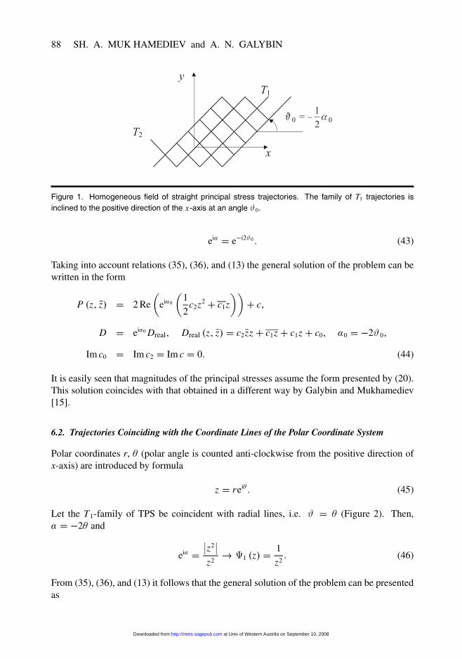
Let a TPS pattern inside a domain be represented by two families of straight orthogonal lineswith T1-family inclined at an angle 0 to the x-axis (Figure 1). Then, � � �20 and




Figure 1. Homogeneous field of straight principal stress trajectories. The family of T1 trajectories isinclined to the positive direction of the x-axis at an angle 0.

ei� � e�i20 � (43)

Taking into account relations (35), (36), and (13) the general solution of the problem can bewritten in the form

P �z� �z� � 2 Re

�ei�0

�1

2c2z2 � c1z

�� c�

D � ei�0 Dreal� Dreal �z� �z� � c2 �zz � c1z � c1z � c0� �0 � �20�

Im c0 � Im c2 � Im c � 0� (44)

It is easily seen that magnitudes of the principal stresses assume the form presented by (20).This solution coincides with that obtained in a different way by Galybin and Mukhamediev[15].

6.2. Trajectories Coinciding with the Coordinate Lines of the Polar Coordinate System

Polar coordinates r, � (polar angle is counted anti-clockwise from the positive direction ofx-axis) are introduced by formula

z � rei� � (45)

Let the T1-family of TPS be coincident with radial lines, i.e. � � (Figure 2). Then,� � �2� and

ei� ��z2��

z2 �1 �z� � 1

z2� (46)

From (35), (36), and (13) it follows that the general solution of the problem can be presentedas




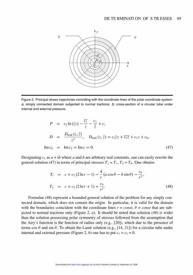
Figure 2. Principal stress trajectories coinciding with the coordinate lines of the polar coordinate system:a, simply connected domain subjected to normal tractions� b, cross-section of a circular tube underinternal and external pressure.

P � c2 ln ��zz�� c1

z� c1

�z � c�

D � Dreal �z� �z�z2

� Dreal �z� �z� � c2 �zz � c1z � c1z � c0�

Im c0 � Im c2 � Im c � 0� (47)

Designating c1 as a + ib where a and b are arbitrary real constants, one can easily rewrite thegeneral solution (47) in terms of principal stresses T1 = Tr , T2 = T� . One obtains

Tr � c � c2 �2 ln r � 1�� 4

r�a cos � � b sin �� c0

r2�

T � c � c2 �2 ln r � 1�� c0

r2� (48)

Formulae (48) represent a bounded general solution of the problem for any simply con-nected domain, which does not contain the origin. In particular, it is valid for the domainwith the boundaries coincident with the coordinate lines r = const, � = const that are sub-jected to normal tractions only (Figure 2, a). It should be noted that solution (48) is widerthan the solution possessing polar symmetry of stresses followed from the assumption thatthe Airy’s function is the function of radius only (e.g., [20]), which due to the presence ofterms cos � and sin � . To obtain the Lamè solution (e.g., [14, 21]) for a circular tube underinternal and external pressure (Figure 2, b) one has to put c1 = c2 = 0.




Figure 3. Principal stress trajectories coinciding with the coordinate lines of the parabolic cylindricalcoordinate system: a, simply connected domain subjected to normal tractions� b, simply connecteddomain subjected to normal tractions and containing the singular point z � 0.

6.3. Trajectories Coinciding with the Coordinate Lines of the Parabolic Cylindrical CoordinateSystem

Let parabolic cylindrical coordinates � , � be introduced by formulae

x � 1

2

�� 2 � �2

�� y � �� (49)

Two families of orthogonal coordinate lines are formed by curves

y2 � 2�2

�x � 1

2�2

�� y2 � �2� 2

�x � 1

2� 2

�� (50)

The pattern of these curves shown in Figure 3 differs from that presented in [21] by rotationthrough 90� around the origin. Note that by introducing the complex variable � � � � i�relations (49) are equivalent to conformal mapping

z � 1

2� 2� (51)

For the � = const trajectory family one has

dy

dx� tan � � tan

1

2� � �

�� tan �arg � � � tan

�1

2�

�(52)

which leads to




� � �� ei� � �z�z �1 �z� � 1

z� (53)

The general solution takes the form

P � c22 Re z � c1 ln z � c1ln z � c�

D � Dreal �z� �z� 1

z� Dreal � c2 �zz � c1z � c1z � c0�

Im c0 � Im c2 � Im c � 0� (54)

By taking into account relation (51) the solution can be rewritten as

P � c2 Re � 2 � c12 ln � � c12ln � � c� �c1 � c1� ln1

2�

D � �� 2

� 2 � �� c2

1

4

� �� 2 � c11

2� 2 � c1

1

2� 2 � c0�

Im c0 � Im c2 � Im c � 0� (55)

Expressions for principal stresses T1 and T2 in terms of the variables � , � can be found from(55) with the use of (5).

Formulae (54) or (55) express the general solution for any simply connected domainwhich does not contain the origin (Figure 3, a). A bounded solution for a domain with z � 0inside (Figure 3, b) can be deduced from (54) or (55) by putting c1 = c0 = 0. The function Din the latter solution coincides with the function (16) provided that a = c2, b = 0 in (16).

6.4. Axially Symmetric Argument

In this section the technique described in section 4 is illustrated on the basis of admissibil-ity investigation for one class of TPS. Namely, the example below examines the argumentindependent of the polar angle � , i.e.

� � ��r�� (56)

First the case of harmonic argument is considered in which the only possible form for �is the following:

� �r� � c1 ln r � c2� �Im c1 � Im c2 � 0� (57)

where c1 and c2 are real constants. A real-valued harmonic function � adjacent to � has theform

� � � �� c1� � c3� �Im c3 � 0� (58)




where c3 is an additional real constant. From (33) one obtains the particular solution of theproblem corresponding to (56)

D �z� �z� � A �z� � �C �ei ln z�c1�� C � Cec3�ic2

� (59)

Formula (59) represents a particular solution by means of a holomorphic function defined inany domain which does not contain the origin.

Let now � be an arbitrary (real) function depending on radius r. Consider admissiblefunctions � by reducing (56) to the form (21)2. Sufficient conditions can easily be found ina restricted class of functions D, which module also depends on r only. In this case one canpresent � as

� �r� � 1

2iln

F �r�

F �r�(60)

where F(r) is a complex-valued function expressed as

F �r� � �z � �z�� z� � re�i� ��rei�

�� rei�� (61)

Since F(r) is independent of � one finds

�F �r�

�� 0 re�i� ��

�rei�

�� rei��

� re�i2� ��rei�

� �z � � �z�� z �� z�� z� � �z�

from which it follows that

� �z� � c1z� � �z� � c2� (62)

Here c1 and c2 are arbitrary constants. Thus the only possible form of D depending on r is

D �z� �z� � D �r� � �zzc1 � c2 � r2c1 � c2� (63)

Let us also apply the technique utilizing the representations of a bi-holomorphic functionthrough its argument. First, case (22), (23) is considered. If argument � is given by (56),then one has from (28) that

S �r�� r�� (64)

and, therefore, function V �r�� z� from (19), (3.9) is represented as follows:

V �r�� z� � ��r2� X �0�� 0�� ei��r�� (65)

Relationship (65) is a complex-exponential form of holomorphic function, thus




� �r�� arg�r 2� X �0�� 0�� V �r�� z� � r2

� X �0�� 0� � (66)

By substituting V �r�� z� from (66) into (25) one obtains

D �z� �z� � �zz X �0�� 0� � (67)

It is evident from (67) that in the case (22), (23) the deviatoric stress function D is expressedin the form (63) if its argument only depends on r.

Investigation of the case (22), (29) for � given by (56) is as follows. By using (64) thefunction V �r�� z� from (31) can be written as a holomorphic function linearly dependingon z

V �r�� z� � �� 0�� r2� � zb �r��b �r�� r 2�

exp �i� �r�� (68)

Substitution of (68) into (A2.22) leads to the following expression for the elastic potential � �z�:

� �z� � � � �0��2r�

d

dr�

� z2

r2�ei��r��arg b�r��

� z

� �b �r��r 2�

� 1

�b �r��

ei��r�� ei��r��arg b�r��

(69)

Potential � �z� is independent of r� when each summand in brackets in (69) representsitself as linear function of r2

� . It is evident that this requirement cannot be fulfilled whateverfunctions � �r�� and b �r�� are given. Hence, neither of functions given by (56) represents theargument of the deviatoric function D provided that ��0� �� 0 and ��0� �� 0.

It may be concluded that the only admissible form of � �r� for the TPS pattern withoutany singular points is as follows:

� �r� � arg�r2 X �0�� 0�� (70)

and the bi-holomorphic function D is expressed in the form (63) where c1 � X �0�, c2 ��0�. If c1 and c2 are real constants, then this D is a particular case of real bi-holomorphicfunction Dreal. This result once more shows that the �-field given by (18) is not admissiblefor elasticity.

7. GEODYNAMIC EXAMPLES

In geodynamics, orientations of the principal stresses are obtained from both instrumentalmeasurements and the analysis of natural stress indicators [4]. These data are of differentquality ranging from A (high) to E (low), [5, 6]. The conventional approach to the theoreticaldetermination of the stress fields in stable blocks of the lithosphere (that can be considered




as elastic ones) is based on the solution of classical boundary value problems of elasticity inwhich the knowledge of boundary stresses is required, e.g., [7, 8, 22]. The calculated stressfield is considered to be appropriate if it fits the experimental data on stress orientationsinside a region. Therefore, the stress orientations are used as constraints imposed on thesought solution. The main shortcoming of this approach is that it cannot provide the criteriafor selecting the true solution. Even if a solution of the problem satisfies all the constraintseverywhere in the region, the calculated fields of stress magnitudes are still sensitive to theboundary stresses. The latter are usually derived from theoretical assessments of the plate-driving forces which can differ up to one order in magnitude. Significant differences in stressfields calculated for the same region (cf., e.g., [7, 22]) is mainly the result of postulatingdifferent plate-driving forces.

In these circumstances, the development of alternative approaches is of vital importance.One way to determine regional stress fields is to use the above procedure based on the knownTPS patterns. In order to illustrate geodynamic applications of the proposed approach, thestress fields of Europe and Australia are analysed and simple analytical solutions are pre-sented in this section. Despite their simplicity, these solutions might be considered as plau-sible alternatives to the previous studies based on numerical calculations. The arbitrary con-stants entering into solutions for the stress magnitudes can be determined by employing localin-situ stress measurements and, thus, the unique 2D stress tensor field can be singled out.

Throughout this section we will use the designations SH,max = –T1, SH,min = –T2 (T1 � T2).Symbols SH,max and SH,min which are customary in geodynamics stand for maximum andminimum compressive horizontal stress, correspondingly.

7.1. West European platform

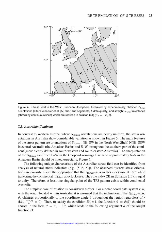
A large amount of experimental data on in situ stresses has been gathered over nearly ahalf-century of studying the stress state of the lithosphere of Western Europe (e.g., [6, 12]).Observations show that the present-day SH,max orientations in Western Europe are distrib-uted almost uniformly over large areas in Western Europe and virtually independently ofdepth (see Figure 4 for the quality A data). They are not affected by short-wavelength vari-ations in the thickness of the lithosphere, its structural features and topography, even thoughthey are locally disturbed by major geologic structures such as the Alps [5, 12]. The homo-geneity of the stress orientation is especially pronounced for the so-called western Europeanstress province north of the Alps and Pyrenees, with the SH,max axis consistently striking� N145�E26� [8, 12].

The main idea is that, for the first-order stress field in Western Europe, the trajectoriescan be approximated by straight lines with the SH,max family inclined at the angle of about –60�, see Figure 4 where the x1-axis is assumed to be eastward-directed. Then (for the elasticlithosphere) one can use (44), in which 0 � ��3.

Equation (44) shows why spatially non-homogeneous seismic regime is observed in thelithosphere of the West-European platform possessing homogeneous stress orientation. Non-homogeneity of stress magnitudes is explained by the presence of the real bi-holomorphicfunction Dreal in (44).




Figure 4. Stress field in the West European lithosphere illustrated by experimentally obtained SH,max

orientations (after Reinecker et al. [5]� short line segments, A data quality) and straight SH,max trajectories(shown by continuous lines) which are realized in solution (44) (0 � ��3).

7.2. Australian Continent

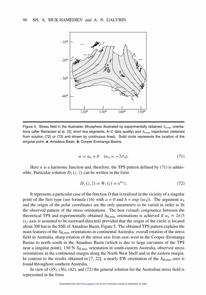
In contrast to Western Europe, where SH,max orientations are nearly uniform, the stress ori-entations in Australia show considerable variation as shown in Figure 5. The main featuresof the stress pattern are orientations of SH,max: NE–SW in the North West Shelf, NNE–SSWin central Australia (the Amadeus Basin) and E–W throughout the southern part of the conti-nent (more clearly defined in south-western and south-eastern Australia). The sharp rotationof the SH,max axis from E–W in the Cooper–Eromanga Basins to approximately N–S in theAmadeus Basin should be noted especially, Figure 5.

The following unique characteristic of the Australian stress field can be identified fromanalysis of natural stress indicators (e.g., [5, 6, 23]). The observed discrete stress orienta-tions are consistent with the supposition that the SH,max-axis rotates clockwise at 180� whiletraversing the continental margin anticlockwise. Thus the index 2K in Equation (17) is equalto unity. Therefore, at least one singular point of the TPS pattern exists within continentalAustralia.

The simplest case of rotation is considered further. For a polar coordinate system r, � ,with the origin located within Australia, it is assumed that the inclination of the SH,max-axis, , changes proportionally to the coordinate angle � throughout the region regardless of r(i.e., ��r��

�r � 0). Then, to satisfy the condition 2K = 1, the function � (�) should bechosen in the form � 0 � 1

2� , which leads to the following argument � of the soughtfunction D:




Figure 5. Stress field in the Australian lithosphere illustrated by experimentally obtained SH,max orienta-tions (after Reinecker et al. [5]� short line segments, A–C data quality) and SH,max trajectories (obtainedfrom solution (72) or (73) and shown by continuous lines). Solid circle represents the location of thesingular point� a, Amadeus Basin, b, Cooper Eromanga Basins.

� � �0 � � ��0 � �20�� (71)

Here � is a harmonic function and, therefore, the TPS pattern defined by (71) is admis-sible. Particular solution D1 �z� �z� can be written in the form

D1 �z� �z� � �1 �z� � ei�0 z� (72)

It represents a particular case of the function D that is realized in the vicinity of a singularpoint of the first type (see formula (16) with a = 0 and b = exp (i�0)). The argument �0

and the origin of the polar coordinates are the only parameters to be varied in order to fitthe observed pattern of the stress orientations. The best (visual) congruence between thetheoretical TPS and experimentally obtained SH,max orientations is achieved if �0 � 2� /3(x1-axis is assumed to be eastward-directed) provided that the origin of the circle is locatedabout 300 km to the SSE of Amadeus Basin, Figure 5. The obtained TPS pattern explains themain features of the SH,max orientations in continental Australia: overall rotation of the stressfield in Australia, sharp rotation of the stress axis from east–west in the Cooper–EromangaBasins to north–south in the Amadeus Basin (which is due to large curvature of the TPSnear a singular point), 130�N SH,max orientation in south-eastern Australia, observed stressorientations in the continental margin along the North West Shelf and in the eastern margin.In contrast to the results obtained in [7, 22], a nearly EW orientation of the SH,max-axis isfound throughout southern Australia.

In view of (35), (36), (42), and (72) the general solution for the Australian stress field isrepresented in the form




P �z� �z� � 2 Re

�ei�0

�1

3c2z3 � 1

2c1z2

�� c�

D � ei�0 zDreal� Dreal �z� �z� � c2 �zz � c1z � c1z � c0� �0 � 2

3��

Im c0 � Im c2 � Im c � 0� (73)

Here the choice of four arbitrary real constants c0, Re c1, Im c1, c2 should provideDreal 0.

The result given by (73) for the Australian platform has been obtained in [24, 9] bysolving a non-classical boundary value problem of elasticity in which SH,max orientationsand TPS curvatures are specified on the boundary of the region. Direct numerical modelingof the Australian stress field using discrete orientations of SH,max as input data [25] showsthat the singular point is shifted not much to south-east as compared with that shown inFigure 5. Nevertheless, the numerical solution preserves the main features of the stress fieldpresented by Equation (73).

8. CONCLUSIONS

The paper presents a novel approach for the reconstruction of stress fields if the pattern oftrajectories of principal stress (TPS) is specified in a plane homogeneous isotropic elasticdomain. This approach is based on the determination of the bi-holomorphic function (stressdeviator, D) from the known (differentiable almost everywhere) field of its argument (�-field). It is shown that not every TPS pattern can exist in plane elasticity since Laplace’sequation imposes constraints on the stress tensor satisfying the equations of equilibrium.

It is proposed to determine stress magnitudes in a different way than in conventionalmethods of the separation of principal stresses in photoelasticity. First, a given TPS fieldis examined for admissibility and, if admissible, a proper bi-holomorphic function, D1, isdetermined by using, in particular, the representation through its argument obtained in thepaper. Then the general solution (function D) is obtained from D1 by multiplying the lattereither by an arbitrary real constant (if arg(D1) is not a harmonic function) or by the real-valued bi-holomorphic function, Dreal, which depends on four real arbitrary constants (ifarg(D1) is a harmonic function). The real-valued multipliers should be positive definite iftwo different families of TPS are distinguishable with respect to the magnitude of principalstress. Once the deviatoric part of stress tensor (function D) is found, the mean stress (real-valued function P) can simply be obtained by integrating the already found elastic potential � �z�, which adds an extra arbitrary real constant to the general solution for the soughtstress state. Therefore the complete stress tensor found by this method depends on five ortwo arbitrary real constants. This conclusion remains valid for multiply connected domainsas well.

Thus, it is shown that determination of stresses from the stress trajectory pattern in aplane elastic domain is not a boundary value problem (in contrast to the common opinionexisting in photoelastic community). This important result is advantageous to geodynamicswhere (contrary to photoelasticity) boundary stresses are poorly constrained.




Although the paper deals with continuous TPS it is believed that the proposed approachcan be useful in many applications where principal directions are known at discrete points, inparticular, in geophysical problems that aimed at the determination of tectonic stress in stableblocks of the lithosphere. Geophysical applications are especially remarkable because elasticfields of tectonic stresses can uniquely be found in those regions where TPS fields are knownand local in situ stress measurements have been performed� the latter have to be used for thedetermination of arbitrary constants. In photoelasticity, the proposed approach can be usedinstead of the procedure of numerical (or graphical) integration of the equilibrium equationswith initial conditions. Moreover, it is applicable for solving the conjugated problem inwhich the field of maximum shear stresses is given. The solution of this problem entirelysimplifies the interpretation of photoelastic experiments because the stress state of the modelcan directly be obtained from the pattern of isohromatics.

APPENDIX A. GENERAL FORM OF A REAL-VALUED BI-HOLOMORPHICFUNCTION

The general form for function Dreal �z� �z�(Im Dreal �z� �z� � 0) is found from the condition

Im��z ��z��z�� 0� (A.1)

that yields

i��z ��z�� z ��z�

� � 2 Im��z�� (A.2)

The right-hand side of (A.2) is the imaginary part of an holomorphic function, i.e. a harmonicfunction. Thus, the left side of (A.2) vanishes after applying the Laplace operator� whence itfollows that

��z�� z� � 0 or Im ��z� � 0� (A.3)

Since holomorphic function ��z� is a real-valued function, it is a real constant, c2. Afterintegration of ��z� one obtains

��z� � c2z � �c1� �Im c2 � 0� c1 � c11 � ic12 � const� � (A.4)

By substituting (A.4) into (A.2) one finds the following expression for the second holo-morphic function:

��z� � c1z � c0� �c0 � const , Im c0 � 0� � (A.5)

Combining (A.5) and (A.4) immediately yields the expression (13) (see Section 2.1) for thereal valued bi-holomorphic function Dreal �z� �z�.




APPENDIX B. DERIVATION OF A BI-HOLOMORPHIC FUNCTION REPRESEN-TATIONS

Let � � be a circumference �z� � r� � R dividing the circular domain� introduced in section4 into inner,�� : �z� � r�, and outer,�� : r� � �z� � R, domains.

First, the case (23) is considered. According to (24) the following auxiliary holomorphicfunction, V �r�� z�, can be introduced in�

V �r�� z� � r2� X �z�� z� � (B.1)

This function coincides with D �z� �z� on the contour � � and its index is equal to zero afterthe complete traverse of � �, Ind� � V �r�� z� � 0, � � � �. Therefore V �r�� z� has no zerosin �. Since V �r�� z� and D �z� �z� are equal on the contour � �, the argument of V �r�� z� isequal to the argument of D �z� �z�

arg V �r�� arg D �z� �z��z�� r�� (B.2)

Here � �r�� is the known function � �z� �z� written in the polar coordinate system r, �for r � r�. Condition (B.2) is sufficient to express V �r�� z� in �� through its argument,� ��, given on � �. The problem can be reduced to the well-known problem (e.g., [16]) ofdetermining a holomorphic function ln V �r�� z� in �� by its imaginary part � �� given onthe contour � �. The solution of this problem has the form

V �r�� z� � Cr� exp �iS �r�� (B.3)

where Cr� is an arbitrary positive constant and S �r�� is the Schwarz operator for ��

with regard to function � �� defined by formula (28). In order to determine Cr� one shouldrecognize that V �r�� z� coincides with D �z� �z� on � �. By substituting � �z� �z� from (21) in(28) and by taking into account the following formulae:

��

ln�r2� X �� z

d� � ln�r2� X �z�� z��

��

ln�r2� X �� z

d� � ln�r2� X �0�� 0��

��

ln�r2� X ��

ln�r2� X �� d�

�� ln

�r2� X �0�� 0��

ln�r2� X �0�� 0�� (B.4)

where z � ��, it can be shown that

Cr� ��r2� X �0�� 0�� (B.5)




Thus, the auxiliary holomorphic function V �r�� z� defined by (B.1) can be uniquely pre-sented in the domain �� in the form (26), (27). It should be noted that arg V �r�� z�, gener-ally speaking, is not equal to � �z� �z� inside��.

The set of functions V �r�� z� calculated for each r�, 0 � r� � R, can be consideredas a single holomorphic function which is parametrically dependent on r� and defined in��(r�), the domain possessing circular boundary with varying radius r�. With the provisothat V �r�� z� is evaluated for two distinct arbitrary parameters, say r� and r��, belonging tothe half-interval (0, R], and by taking into account (B.1) it is possible to obtain potentialsX �z� and � �z� in the form

X �z� � V �r�� z�� V �r�� z�

r 2� � r2�� z� � r2

�V �r�� z�� r2��V �r�� z�

r2� � r2�� (B.6)

Here X �z� and � �z� are holomorphic functions in �z� � r� if r� � r�� or in �z� � r�� ifr� r��. Owing to arbitrariness of parameters r� and r��, (B.6) can be rewritten as

X �z� � 1

2r�

dV �r�� z�

dr�� z� � V �r�� z�� r�

2

dV �r�� z�

dr�(B.7)

which gives the required representation (24).A method similar to the above is used in order to express the function D �z� �z� through

its argument in the case (29). For this purpose one introduces the function �V �r�� z� �r2� z�1 � �z�� z� that coincides with D �z� �z� on the contour � � and has a pole at the origin.

If the pole is removed by multiplication �V �r�� z� by z this would not produce an appropriate

function because the modulus��z �V �r�� z�

�� vanishes at a point z � b �r�� determining by (32)

and lying inside the circle �z� � r�, which is due to the fact that the index of z �V �r�� z� isunity rather than zero.

Hence, the following holomorphic function can be introduced:

V �r�� z� � r 2�

� �z�� z� �z�

z � b �r��(B.8)

It has no zeros in �z� � r� and its boundary value is related to the boundary value of D �z� �z�as follows:

V �r��

� � b �r��D�� (B.9)

As a consequence,

arg V �r�� arg

��

� � b �r��

�� (B.10)

Similarly to the case (23) the function V �r�� z� can be found in the domain �� from(B.10) with the result




V �r�� z� � Cr� exp

�iS

�r�� arg

�

� � b �r��

��(B.11)

where Cr� is an arbitrary positive constant and S �r�� is the Schwarz operator for ��

defined in (28). By using the linearity of the Schwarz operator the above expression can bebrought to the form

V �r�� z� � Cr� exp

�iS

�r�� arg

�

� � b �r��

��exp �iS �r�� (B.12)

In order to satisfy (B.9) the parameter Cr� should be chosen as

Cr� � �V �r�� 0�� r2�� 0��b �r�� (B.13)

The second multiplier in (B.12) can be calculated explicitly. For this purpose the argu-ment of

�� b �r��1

�is represented on the contour � � in the following form:

2i arg�

� � b �r�� ln

�� b �r��

�� b �r�� ln

��

r2�� b �r��

�� b �r��

r2��

� ln�

� � b �r�� ln

�1� �b �r��

r 2�

�� (B.14)

This helps to evaluate the integral

I �r�� z� � 1

2� i

��

2i arg�

� � b �r��d�

� � z(B.15)

which enters into the expression for the Schwarz operator (see formula (28)). With the useof (B.14) this integral is represented as

I �r�� z� � J �r�� z�� K �r�� z� (B.16)

where

J �r�� z� � 1

2� i

��

ln�

� � b �r��d�

� � z�

K �r�� z� � 1

2� i

��

ln

�1� �b �r��

r 2�

�d�

� � z� (B.17)

By using the Cauchy formula, it is easy to obtain that




K �r�� z� � ln

�1� zb �r��

r2�

�� (B.18)

Integral J �r�� z� can be calculated by evaluating it along contour consisting of circum-ference � �, banks of a cut connecting a point on � � with points z � b �r�� and z � 0, andtwo small circumferences described around these points. Calculations result in

J �r�� z� � 0� (B.19)

With regard to (B.18) and (B.19) one obtains

exp

�iS

�r�� arg

�

� � b �r��

�� 1� zb �r��

r2�(B.20)

that combined with (B.12), (B.13) leads to the following form of holomorphic functionV �r�� z�:

V �r�� z� � �� 0�� r2� � zb �r��b �r�� r2�

exp �iS �r�� (B.21)

or in view of (32) to the form given by (31).Note that V �r�� z� in (25) cannot be obtained from (30) by formal passage to the limit

� � �0�� 0. Thus, the separate consideration of cases (23) and (29) given above is war-ranted.

As in the case (23), the function V �r�� z� can be treated as a single holomorphic functionparametrically dependent on r� and defined in the domain��(r�) possessing circular bound-ary with varying radius r�. Let V �r�� z� be evaluated for two distinct arbitrary parameters r�and r�� (r� r��) belonging to the half-interval (0, R]. Then Equation (B.8) results in

� �z� � �z � b �r�� V �r�� z�� z � b �r�� V �r�� z�

r2� � r2��

� �z� � r2� �z � b �r�� V �r�� z�� r2

�� z � b �r�� V �r�� z�

z�r2� � r2��

� � (B.22)

Because parameters r� and r�� are chosen arbitrary, then functions ��z� and ��z� canbe presented in the following form:

� �z� � 1

2r�

d

dr��z � b �r�� V �r�� z��

� �z� � z � b �r��z

V �r�� z�� r�2z

d

dr��z � b �r�� V �r�� z�� (B.23)

and, thus, the representation for D �z� �z� in the vicinity of z � 0 takes the form (30).




APPENDIX C. DIFFERENTIAL EQUATION FOR TPS TO BE ADMISSIBLE INPLANE ELASTICITY

The following algorithm can be proposed in order to check that a given TPS field is notan elastic one. Although the algorithm below is very simple, it requires some additionalrestrictions imposed on the function � �z� �z� due to differentiation of certain order used fur-ther. With these restrictions it can be considered as the necessary condition for the function� �z� �z� to present the TPS pattern in elasticity.

The following equality is valid everywhere in the domain:

D �z� �z� � e2i��z��z�D �z� �z�� (C.1)

By differentiating (C.1) twice with respect to the conjugated variable and taking into account(11) one obtains

�2e2i��z��z�

� �z2D �z� �z�� 2

�e2i��z��z�

� �z�D �z� �z�� z � e2i��z��z� �

2 D �z� �z�� z2

� 0� (C.2)

Since �2 D�z��z�� z2 is a conjugated bi-holomorphic function, its second derivative with respect to z

has to vanish. Therefore one has

�2

�z2

�e�2i��z��z�

�2e2i��z��z�

� �z2D �z� �z�� 2

�e2i��z��z�

� �z�D �z� �z�� z

� � 0� (C.3)

After conjugation of (C.3) followed by the substitution of the second formula in (12) into(C.3) the following expression is found:

A1 �z� �z� � �z�� A2 �z� �z�� z�� A3 �z� �z� �� z�� A4 �z� �z�� z� � 0� (C.4)

Here complex-valued functions Ak (k = 1, 2, 3, 4) are

A1 �z� �z� � �2

� �z2�zB1 �z� �z� � A2 �z� �z� � �2

� �z2B1 �z� �z� �

A3 �z� �z� � �2

� �z2�zB2 �z� �z� � A4 �z� �z� � �2

� �z2B2 �z� �z� (C.5)

where complex-valued functions B1 and B2 are expressed via argument through the givenfunction � �z� �z� as shown below

B1 �z� �z� � e2i��z��z� �2e�2i��z��z�

�z2� �2i

�2� �z� �z��z2

� 4

�� z� �z��z

�2

B2 �z� �z� � 2e2i��z��z� �e�2i��z��z�

�z� �4i

�� z� �z��z

� (C.6)




It is evident from (C.5) and (C.6) that Equation (C.4) is identically satisfied if � �z� �z� isharmonic, because all Ak � 0.

Firstly the case A4 � 0 is considered assuming that � is not harmonic. Then �� z� �z�is a holomorphic function of variable z and due to its real-valuedness it is a real constant, C

4�

� �z�

�z� �z� �z� � C�

��

�z� 1

4C �z � f �z� (C.7)

where f �z� is arbitrary holomorphic function. Substitution of (C.6) into (C.5) and accountfor (C.7) results in

A1 �z� �z� � �3

2C2 �z � 4C f �z� � A2 �z� �z� � �1

2C2� A3 �z� �z� � �2iC� (C.8)

Therefore (C.4) assumes the following form:

�3

2C2 �z � 4C f �z�

� � �z�� 1

2C2� �z�� 2iC �� z� � 0� (C.9)

Differentiation of (A3.9) with respect to conjugated variable leads to

C2 � �z� � 0 (C.10)

which means that C � 0 and/or � �z� � 0. In both cases � �z� �z� is harmonic. Thereforethe case A4 � 0 is similar to the case of harmonic argument in which Equation (C.4) isnecessarily satisfied.

The following steps are performed further on.Equation (4.4) is divided by A4 and then the differentiation with respect to the conjugated

variable is applied. This excludes the function � �(z) and leads to the following equation:

C1 �z� �z� � �z�� C2 �z� �z�� z�� C3 �z� �z� �� z� � 0� (C.11)

Here the complex-valued coefficients Ck �k � 1� 2� 3� are

C1 �z� �z� � �

� �zA1 �z� �z�A4 �z� �z� � C2 �z� �z� � �

� �zA2 �z� �z�A4 �z� �z� � C3 �z� �z� � �

� �zA3 �z� �z�A4 �z� �z� � (C.12)

If any of Ck is identically zero then one can find that (e.g., for the case C3 � 0)

C1 �z� �z� � �z� � �C2 �z� �z�� z� (C.13)

which immediately gives the following condition that should be imposed on C1 and C2 tosatisfy (C.11):

�

� �z lnC1 �z� �z�C2 �z� �z� � 0� (C.14)




If none of Ck is identically zero, then an equation similar to (C.13) can be obtained from(C.11) by dividing it by C3 followed by the differentiation with respect to the conjugatedvariable to exclude one of the holomorphic functions left, e.g., ��(z). This produces thefollowing result:

� �z��

� �zC1 �z� �z�C3 �z� �z� � �� z�

�

� �zC2 �z� �z�C3 �z� �z� � (C.15)

It follows from (C.15) that

�

� �z

ln�

� �zC1 �z� �z�C3 �z� �z� � ln

�

� �zC2 �z� �z�C3 �z� �z�

�� 0� (C.16)

Acknowledgments. This work was supported by the Australian Research Council (IREX) and by the Russian Founda-tion for Basic Research. The fundamental program No 5 sponsored by the Section of the Earth’s Sciences of RussianAcademy of Sciences and the MNRF project “Australian Computational Earth System Simulator” are also acknowl-edged.

NOTES

1. Corresponding author2. This definition is different from the other one accepted by some authors (namely the definition of poly-

analytic functions of nth order in [16] as�n

K�0 �z �z�k �k �z� where functions �k �z� are holomorphic).

REFERENCES

[1] Frocht, M. M. Photoelasticity, Vol. 1. Wiley, New York, 1941.

[2] Alexandrov, A. Y and Akhmetzyanov, M. H. Polarization—Optical Methods of the Mechanics of DeformableBodies, Nauka, Moscow, 1973 (in Russian).

[3] Kuske, A. and Robertson, G. Photoelastic Stress Analysis, Wiley, London, 1974.

[4] Amadei, B. and Stephanson, O. Rock Stress and its Measurement. Chapman and Hall, London, 1997.

[5] Reinecker J., Heidbach, O., and Mueller, B. The 2003 release of the World Stress Map (available online at www.world-stress-map.org).

[6] Zoback, M. L., Zoback, M. D., Adams J., Assumpção, M., Bell, S., Bergman, E. A., Blümling, P., Brereton, N. R.,Denham, D., Ding, J., Fuchs, K., Gay, N., Gregersen, S., Gupta, H. K., Gvishiani, A., Jacob, K., Klein, R., Knoll, P.,Magee, M., Mercier, J. L., Müller, B. C., Paquin, C., Rajendran, K., Stephansson, O., Suarez, G., Suter, M., Udias,A., Xu, Z. H., and Zhizhin, M. Global patterns of tectonic stress. Nature, 341, 291–298 (1989).

[7] Cloetingh, S. and Wortel, R. Stress in the Indo-Australian plate. Tectonophysics, 132 46–67 (1986).

[8] Gölke, M. and Coblenz, D. Origins of the European regional stress field. Tectonophysics, 266, 11–24 (1996).

[9] Mukhamediev, Sh. A. and Galybin, A. N. A direct approach to the determination of regional stress fields: A casestudy of the West European, North American, and Australian platforms. Izvestiya, Physics of the Solid Earth, 37,636–652 (2001).

[10] Hansen, K. M. and Mount, V. S. Smoothing and extrapolation of crustal stress orientation measurements. Journalof Geophysical Research, 95 (B), 1155–1165 (1990).

[11] Lee, J.-C. and Angelier, J. Paleostress trajectory maps based on the results of local determinations: the “Lissage”program. Computers and Geosciences, 20, 161–191 (1994).

[12] Müller, B., Zoback, M. L., Fuchs, K., Mastin, L., Gregersen, S., Pavoni, N., Stefansson, O. and Ljunggren, C.Regional patterns of tectonic stress in Europe. Journal of Geophysical Research, 97 (B), 11783–11803 (1992).

[13] Mukhamediev, Sh. A. Non-classical boundary value problems of the continuum mechanics for geodynamics. Dok-lady Earth Sciences, 373, 918–922 (2000).




[14] Muskhelishvili, N. I. Some Basic Problems of the Mathematical Theory of Elasticity, Noordhoff, Groningen-Holland, 1953.

[15] Vekua, I. N. Generalized Analytic Functions. Pergamon/Addisom Wesley, Reading, MA, 1962.

[16] Gakhov, F. D. Boundary Value Problems. Dover, New York, 1990.

[17] Belousov, T. P. and Mukhamediev, Sh. A. Reconstruction of paleostresses from rock fracturing. Izvestiya, EarthPhysics, 26, 115–127 (1990).

[18] Karakin, A. V. and Mukhamediev, Sh. A. Singularities in nonuniform field of trajectories of the principal tectonicstresses. Izvestiya, Physics of the Solid Earth, 29, 956–965 (1994).

[19] Galybin, A. N. and Mukhamediev, Sh. A. Plane elastic boundary value problem posed on orientation of principalstresses. Journal of Mechanics and Physics of Solids, 47, 2381–2409 (1999).

[20] Timoshenko, S. P. and Goodier, J. N. Theory of Elasticity, Third edition, McGraw-Hill, New York, 1970.

[21] Korn, G. A. and Korn, T. M. Mathematical Handbook for Scientists and Engineers: Def initions, Theorems, andFormulas. McGraw-Hill, New-York, 1968.

[22] Coblentz, D. D., Sandiford, M., Richardson, R. M., Zhou, S. and Hillis, R. The origins of the intraplate stress fieldin continental Australia. Earth and Planetary Sciences Letters, 133, 299–309 (1995).

[23] Denham, D., Alexander, L.G., and Worotnicki, G. Stress in the Australian crust: evidence from earthquakes andin-situ stress measurements. Bureau of Minerals and Resources, Journal of Australian Geology and Geophysics,4, 289–295 (1979).

[24] Mukhamediev, Sh. A., Galybin, A. N., and Brady, B. H. G. À direct approach to regional stress field determinationbased on the stress orientations. Research Report NG:1439. The University of Western Australia, GeomechanicsGroup. May 1999 (unpublished).

[25] Galybin, A. N. and Mukhamediev, Sh. A. Determination of elastic stresses from discrete data on stress orientations.International Journal of Solids and Structures, 41, 5125–5142 (2004).



Determination of Stresses from the Stress Trajectory Pattern in a Plane Elastic Domain

Documents

Transcript of Determination of Stresses from the Stress Trajectory Pattern in a Plane Elastic Domain