Coupled fixed point theorems in cone metric spaces with a c-distance and applications
Upload
independentCategory
view
0download
0
arX
iv:0
805.
1184
v2 [
mat
h.G
N]
20
Oct
200
8
THE PLANE FIXED POINT PROBLEM
ROBBERT FOKKINK, JOHN C. MAYER, LEX G. OVERSTEEGEN,AND E. D. TYMCHATYN
Dedicated to Harold Bell
Abstract. In this paper we present proofs of basic results, in-cluding those developed so far by H. Bell, for the plane fixed pointproblem. Some of these results had been announced much earlierby Bell but without accessible proofs. We define the concept ofthe variation of a map on a simple closed curve and relate it tothe index of the map on that curve: Index = Variation + 1. Wedevelop a prime end theory through hyperbolic chords in maximalround balls contained in the complement of a non-separating planecontinuum X . We define the concept of an outchannel for a fixedpoint free map which carries the boundary of X minimally intoitself and prove that such a map has a unique outchannel, andthat outchannel must have variation = −1. We also extend Bell’slinchpin theorem for a foliation of a simply connected domain, byclosed convex subsets, to arbitrary domains in the sphere.
We introduce the notion of an oriented map of the plane. Weshow that the perfect oriented maps of the plane coincide with con-fluent (that is composition of monotone and open) perfect maps ofthe plane. We obtain a fixed point theorem for positively oriented,perfect maps of the plane. This generalizes results announced byBell in 1982 (see also [1]). It follows that if X is invariant underan oriented map f , then f has a point of period at most two in X .
Contents
1. Introduction 22. Tools 42.1. Index 42.2. Stability of Index 52.3. Variation 6
Date: November 23, 2013.1991 Mathematics Subject Classification. Primary: 54F20; Secondary: 30C35.Key words and phrases. Plane fixed point problem, crosscuts, variation, index,
outchannel, dense channel, prime end, positively oriented map.The third named author was supported in part by grant NSF-DMS-0405774 and
the last named author by NSERC 0GP0005616.1

2 FOKKINK, MAYER, OVERSTEEGEN, AND TYMCHATYN
2.4. Index and variation for finite partitions 72.5. Locating arcs of negative variation 112.6. Crosscuts and bumping arcs 142.7. Index and Variation for Caratheodory Loops 162.8. Prime Ends 173. Kulkarni-Pinkall Partitions 184. Hyperbolic foliation of simply connected domains 235. KP chords and prime ends 255.1. Auxiliary Continua 286. Outchannels 306.1. Invariant Channel in X 337. Uniqueness of the Outchannel 368. Oriented maps 409. Induced maps of prime ends 4410. Fixed points for positively oriented maps 47References 48Index 50
1. Introduction
We denote the plane by C, the Riemann sphere by C∞ = C ∪ {∞},the real line by R and the unit circle by S1 = R/Z. Let X be a planecontinuum. Since C is locally connected and X is closed, complemen-tary domains of X are open. By T (X) we denote the topological hullof X consisting of X union all of its bounded complementary domains.Thus, U∞ = C∞ \T (X) is a simply-connected open domain containing∞. The following is a long-standing question in topology.
Fixed Point Question: “Does a continuous function taking a non-separating plane continuum into itself always have a fixed point?”
It is easy to see that a map of a plane continuum to itself can beextended to a perfect map of the plane. We study the slightly moregeneral question, “Is there a plane continuum Z and a perfect con-tinuous function f : C → C taking Z into T (Z) with no fixed pointsin T (Z)?” A Zorn’s Lemma argument shows that if one assumes theanswer is “yes,” then there is a subcontinuum X ⊂ Z minimal withrespect to these properties. It will follow from Theorem 6.5 that forsuch a minimal continuum, f(X) = X = ∂T (X) (though it may not bethe case that f(T (X)) ⊂ T (X)). Here ∂T (X) denotes the boundary ofT (X). We recover Bell’s result [2] (see also Sieklucki [23], and Iliadis[14]) that the boundary of X is indecomposable (with a dense channel,explained later).

FIXED POINTS IN PLANAR CONTINUA 3
In this paper we use tools first developed by Bell to elucidate theaction of a fixed point free map (should one exist). We are indebted toBell for sharing his insights with us. Many of the results of this paperwere first obtained by him. Unfortunately, many of the proofs werenot accessible. We believe that they deserve to be developed in orderto be useful to the mathematical community. The results of this paperare also crucial to several recent results regarding the extension of iso-topies of plane continua [20], the existence of fixed points for branchedcovering maps of the plane [7], fixed points in non-invariant plane con-tinua [5], the existence of locally connected models for all connectedJulia sets of complex polynomials [6] and an estimate on the numberof attracting and neutral periodic orbits of complex polynomials [8].
We have stated many of these results using existing notions such asprime ends. We introduce Bell’s notion of variation and prove his the-orem that index equals variation +1; Theorem 2.13. We also extendedBell’s linchpin Theorem 4.5 for simply connected domains to arbitrarydomains in the sphere and given a proof using an elegant argumentdue to Kulkarni and Pinkall [15]. Our version of this theorem (The-orem 3.5) is essential for the results later in the paper. Theorem 7.1(Unique Outchannel) is a new result due to Bell. Complete proofs ofTheorems 2.13, 2.14, 4.5 and 7.1 appear in print for the first time.
The classical fixed point question asks whether each map of a non-separating plane continuum into itself must have a fixed point. Cartwrightand Littlewood [10] showed that the answer is yes if the map can beextended to an orientation-preserving homeomorphism of the plane. Itwas 25 years before Bell [4] extended this to the class of all homeomor-phisms of the plane. Bell announced in 1984 (see also Akis [1]) thatthe Cartwright-Littlewood Theorem can be extended to the class of allholomorphic maps of the plane. These maps behave like orientation-preserving homeomorphisms in the sense that they preserve local ori-entation. Compositions of open, perfect and of monotone, perfect sur-jections of the plane are confluent and naturally decompose into twoclasses, one of which preserves and the other of which reverses localorientation. We show that any confluent map of the plane is itself acomposition of a monotone and a light-open map of the plane. We alsoshow that an oriented map of the plane induces a map to the circle ofprime ends of an acyclic continuum from the circle of prime ends of acomponent of its pre-image. Finally we will show that each invariantnon-separating plane continuum, under a positively-oriented map of theplane, must contain a fixed point. It follows that any confluent mapof the plane has a point of period at most two in any non-separatinginvariant sub-continuum.

4 FOKKINK, MAYER, OVERSTEEGEN, AND TYMCHATYN
For the convenience of the reader we have included an index at theend of the paper.
2. Tools
Let p : R → S1 denote the covering map p(x) = e2πix. Let g : S1 →S1 be a map. By the degree of the map g, denoted by degree(g), wemean the number g(1)− g(0), where g : R → R is a lift of the map g tothe universal covering space R of S1 (i.e., p◦ g = g◦p). It is well-knownthat degree(g) is independent of the choice of the lift.
2.1. Index. Let g : S1 → C be a map and f : g(S1) → C a fixed pointfree map. Define the map v : S1 → S1 by
v(t) =f(g(t)) − g(t)
|f(g(t)) − g(t)| .
Then the map v : S1 → S1 lifts to a map v : R → R. Define theindex of f with respect to g, denoted ind(f, g) by
ind(f, g) = v(1) − v(0) = degree(v).
Note that ind(f, g) measures the net number of revolutions of the vec-torf(g(t)) − g(t) as t travels through the unit circle one revolution inthe positive direction.
Remark 2.1. (a) If g : S1 → C is a constant map with g(S1) = c andf(c) 6= c, then ind(f, g) = 0.(b)If f is a constant map and f(C) = w with w 6∈ g(S1), then ind(f, g) =win(g, S1, w), the winding number of g about w. In particular, iff : S1 → T (S1) \ S1 is a constant map, then ind(f, id|S1) = 1, whereid|S1 is the identity map on S1.
Suppose S ⊂ C is a simple closed curve and A ⊂ S is a subarc ofS with endpoints a and b. Then we write A = [a, b] if A is the arcobtained by traveling in the counter-clockwise direction from the pointa to the point b along S. In this case we denote by < the linear order onthe arc A such that a < b. We will call the order < the counterclockwiseorder on A. Note that [a, b] 6= [b, a].
More generally, for any arc A = [a, b] ⊂ S1, with a < b in thecounterclockwise order, define the fractional index [9] of f on the sub-path g|[a,b] by
ind(f, g|[a,b]) = v(b) − v(a).
While, necessarily, the index of f with respect to g is an integer, thefractional index of f on g|[a,b] need not be. We shall have occasion touse fractional index in the proof of Theorem 2.13.

FIXED POINTS IN PLANAR CONTINUA 5
Proposition 2.2. Let g : S1 → C be a map with g(S1) = S, andsuppose f : S → C has no fixed points on S. Let a 6= b ∈ S1 with[a, b] denoting the counterclockwise subarc on S1 from a to b (so S1 =[a, b] ∪ [b, a]). Then ind(f, g) = ind(f, g|[a,b]) + ind(f, g|[b,a]).
2.2. Stability of Index. The following standard theorems and obser-vations about the stability of index under a fixed point free homotopyare consequences of the fact that index is continuous and integer-valued.
Theorem 2.3. Let ht : S1 → C be a homotopy. If f : ∪t∈[0,1]ht(S1) →
C is fixed point free, then ind(f, h0) = ind(f, h1).
An embedding g : S1 → S ⊂ C is orientation preserving if g isisotopic to the identity map id|S1. It follows from Theorem 2.3 thatif g1, g2 : S1 → S are orientation preserving homeomorphisms andf : S → C is a fixed point free map, then ind(f, g1) = ind(f, g2).Hence we can denote ind(f, g1) by ind(f, S) and if [a, b] is a positivelyoriented subarc of S1 we denote ind(f, g1|[a,b]) by ind(f, g1([a, b])), bysome abuse of notation when the extension of g1 over S1 is understood.
Theorem 2.4. Suppose g : S1 → C is a map with g(S1) = S, andf1, f2 : S → C are homotopic maps such that each level of the homotopyis fixed point free on S. Then ind(f1, g) = ind(f2, g).
In particular, if S is a simple closed curve and f1, f2 : S → C aremaps such that there is a homotopy ht : S → C from f1 to f2 with ht
fixed point free on S for each t ∈ [0, 1], then ind(f1, S) = ind(f2, S).
Corollary 2.5. Suppose g : S1 → C is an orientation preserving em-bedding with g(S1) = S, and f : S → T (S) is a fixed point free map.Then ind(f, g) = ind(f, S) = 1.
Proof. Since f(S) ⊂ T (S) which is a disk with boundary S and fhas no fixed point on S, there is a fixed point free homotopy of f |Sto a constant map c : S → C taking S to a point in T (S) \ S. ByTheorem 2.4, ind(f, g) = ind(c, g). Since g is orientation preserving itfollows from Remark 2.1 (b) that ind(c, g) = 1. �
Theorem 2.6. Suppose g : S1 → C is a map with g(S1) = S, andf : T (S) → C is a map such that ind(f, g) 6= 0, then f has a fixedpoint in T (S).
Proof. Notice that T (S) is a locally connected, non-separating, planecontinuum and, hence, contractible. Suppose f has no fixed point inT (S). Choose point q ∈ T (S). Let c : S1 → C be the constant mapc(S1) = {q}. Let H be a homotopy from g to c with image in T (S).Since H misses the fixed point set of f , Theorem 2.3 and Remark 2.1(a) imply ind(f, g) = ind(f, c) = 0. �

6 FOKKINK, MAYER, OVERSTEEGEN, AND TYMCHATYN
2.3. Variation. In this subsection we introduce the notion of variationof a map on an arc and relate it to winding number.
Definition 2.7 (Junctions). The standard junction JO is the unionof the three rays J i
O = {z ∈ C | z = reiπ/2, r ∈ [0,∞)}, J+O = {z ∈
C | z = r, r ∈ [0,∞)}, J−O = {z ∈ C | z = reiπ, r ∈ [0,∞)}, having
the origin O in common. A junction Jv is the image of JO under anyorientation-preserving homeomorphism h : C → C where v = h(O).We will often suppress h and refer to h(J i
O) as J iv, and similarly for the
remaining rays in Jv. Moreover, we require that for each neighborhoodW of v, d(J+
v \W,J iv \W ) > 0.
Definition 2.8 (Variation on an arc). Let S ⊂ C be a simple closedcurve, f : S → C a map and A = [a, b] a subarc of S such thatf(a), f(b) ∈ T (S) and f(A) ∩ A = ∅. We define the variation of f onA with respect to S, denoted var(f, A, S), by the following algorithm:
(1) Let v ∈ A and let Jv be a junction with Jv ∩ S = {v}.(2) Counting crossings: Consider the set M = f−1(Jv)∩[a, b]. Each
time a point of f−1(J+v )∩ [a, b] is immediately followed in M , in
the counterclockwise order < on [a, b] ⊂ S, by a point of f−1(J iv)
count +1 and each time a point of f−1(J iv)∩[a, b] is immediately
followed in M by a point of f−1(J+v ) count −1. Count no other
crossings.(3) The sum of the crossings found above is the variation var(f, A, S).
Note that f−1(J+v )∩ [a, b] and f−1(J i
v)∩ [a, b] are disjoint closed setsin [a, b]. Hence, in (2) in the above definition, we count only a finitenumber of crossings and var(f, A, S) is an integer. Of course, if f(A)does not meet both J+
v and J iv, then var(f, A, S) = 0.
If α : S → C is any map such that α|A = f |A and α(S\(a, b))∩Jv = ∅,then var(f, A, S) = win(α, S, v). In particular, this condition is satis-fied if α(S \ (a, b)) ⊂ T (S) \ {v}. The invariance of winding numberunder suitable homotopies implies that the variation var(f, A, S) alsoremains invariant under such homotopies. That is, even though thespecific crossings in (2) in the algorithm may change, the sum remainsinvariant. We will state the required results about variation belowwithout proof. Proofs can also be obtained directly by using the factthat var(f, A, S) is integer-valued and continuous under suitable ho-motopies.
Proposition 2.9 (Junction Straightening). Let S ⊂ C be a simpleclosed curve, f : S → C a map and A = [a, b] a subarc of S such thatf(a), f(b) ∈ T (S) and f(A) ∩ A = ∅. Any two junctions Jv and Ju

FIXED POINTS IN PLANAR CONTINUA 7
with u, v ∈ A and Jw ∩ S = {w} for w ∈ {u, v} give the same valuefor var(f, A, S). Hence var(f, A, S) is independent of the particularjunction used in Definition 2.8.
The computation of var(f, A, S) depends only upon the crossings ofthe junction Jv coming from a proper compact subarc of the open arc(a, b). Consequently, var(f, A, S) remains invariant under homotopiesht of f |[a,b] in the complement of {v} such that ht(a), ht(b) 6∈ Jv for allt. Moreover, the computation is stable under an isotopy ht of the planethat moves the entire junction Jv (even off A), provided in the isotopyht(v) 6∈ f(A) and f(a), f(b) 6∈ ht(Jv) for all t.
In case A is an open arc (a, b) ⊂ S such that var(f, A, S) is defined,it will be convenient to denote var(f, A, S) by var(f, A, S)
The following Lemma follows immediately from the definition.
Lemma 2.10. Let S ⊂ C be a simple closed curve. Suppose thata < c < b are three points in S such that {f(a), f(b), f(c)} ⊂ T (S)and f([a, b]) ∩ [a, b] = ∅. Then var(f, [a, b], S) = var(f, [a, c], S) +var(f, [c, b], S).
Definition 2.11 (Variation on a finite union of arcs). Let S ⊂ C be asimple closed curve and A = [a, b] a subcontinuum of S with partitiona finite set F = {a = a0 < a1 < · · · < an = b}. For each i letAi = [ai, ai+1]. Suppose that f satisfies f(ai) ∈ T (S) and f(Ai)∩Ai = ∅for each i. We define the variation of f on A with respect to S, denotedvar(f, A, S), by
var(f, A, S) =
n−1∑
i=0
var(f, [ai, ai+1], S).
In particular, we include the possibility that an = a0 in which caseA = S.
By considering a common refinement of two partitions F1 and F2
of an arc A ⊂ S such that f(F1) ∪ f(F2) ⊂ T (S) and satisfying theconditions in Definition 2.11, it follows from Lemma 2.10 that we getthe same value for var(f, A, S) whether we use the partition F1 or thepartition F2. Hence, var(f, A, S) is well-defined. If A = S we denotevar(f, S, S) simply by var(f, S).
2.4. Index and variation for finite partitions. What links Theo-rem 2.6 with variation is Theorem 2.13 below, first announced by Bellin the mid 1980’s (see also Akis [1]). Our proof is a modification ofBell’s unpublished proof. We first need a variant of Proposition 2.9.

8 FOKKINK, MAYER, OVERSTEEGEN, AND TYMCHATYN
Let r : C → T (S1) be radial retraction: r(z) = z|z|
when |z| ≥ 1 and
r|T (S1) = id|T (S1).
Lemma 2.12 (Curve Straightening). Suppose f : S1 → C is a mapwith no fixed points on S1. If [a, b] ⊂ S1 is a proper subarc withf([a, b]) ∩ [a, b] = ∅, f((a, b)) ⊂ C \ T (S1) and f({a, b}) ⊂ S1, then
there exists a map f : S1 → C such that f |S1\(a,b) = f |S1\(a,b), f |[a,b] :
[a, b] → (C \ T (S1)) ∪ {f(a), f(b)} and f |[a,b] is homotopic to f |[a,b] in{a, b}∪C\T (S) relative to {a, b}, so that r|f([a,b]) is locally one-to-one.
Moreover, var(f, [a, b], S1) = var(f , [a, b], S1).
Note that if var(f, [a, b], S1) = 0, then r carries f([a, b]) one-to-one onto the arc (or point) in S1 \ (a, b) from f(a) to f(b). If the
var(f, [a, b], S1) = m > 0, then r ◦ f wraps the arc [a, b] counterclock-
wise about S1 so that f([a, b]) meets each ray in Jv m times. A similarstatement holds for negative variation. Note also that it is possiblefor index to be defined yet variation not to be defined on a simpleclosed curve S. For example, consider the map z → 2z with S theunit circle since there is no partition of S satisfying the conditions inDefinition 2.8.
Theorem 2.13 (Index = Variation + 1, Bell). Suppose g : S1 → C isan orientation preserving embedding onto a simple closed curve S andf : S → C is a fixed point free map. If F = {a0 < a1 < · · · < an} isa partition of S and Ai = [ai, ai+1] for i = 0, 1, . . . , n with an+1 = a0
such that f(F ) ⊂ T (S) and f(Ai) ∩ Ai = ∅ for each i, then
ind(f, S) = ind(f, g) =
n∑
i=0
var(f, Ai, S) + 1 = var(f, S) + 1.
Proof. By an appropriate conjugation of f and g, we may assume with-out loss of generality that S = S1 and g = id. Let F and Ai = [ai, ai+1]be as in the hypothesis. Consider the collection of arcs
K = {K ⊂ S | K is the closure of a component of S ∩ f−1(f(S) \ T (S))}.For each K ∈ K, there is an i such that K ⊂ Ai. Since f(Ai)∩Ai = ∅,it follows from the remark after Definition 2.8 that var(f, Ai, S) =∑
K⊂Ai,K∈K var(f,K, S). By the remark following Proposition 2.9, we
can compute var(f,K, S) using one fixed junction for Ai. It is nowclear that there are at most finitely many K ∈ K with var(f,K, S) 6= 0.Moreover, the images of the endpoints of each K lie on S.
Let m be the cardinality of the set Kf = {K ∈ K | var(f,K, S) 6= 0}.By the above remarks, m <∞ and Kf is independent of the partitionF . We prove the theorem by induction on m.

FIXED POINTS IN PLANAR CONTINUA 9
Suppose for a given f we have m = 0. Observe that from the def-inition of variation and the fact that the computation of variation isindependent of the choice of an appropriate partition, it follows that,
var(f, S) =∑
K∈K
var(f,K, S) = 0.
We claim that there is a map f1 : S → C with f1(S) ⊂ T (S) and ahomotopy H from f |S to f1 such that each level Ht of the homotopy isfixed point free and ind(f1, id|S) = 1.
To see the claim, first apply the Curve Straightening Lemma 2.12 toeach K ∈ K (if there are infinitely many, they form a null sequence) to
obtain a fixed point free homotopy of f |S to a map f : S → C such thatr|f(K) is locally one-to-one on each K ∈ K, where r is radial retraction
of C to T (S), and var(f , K, S) = 0 for each K ∈ K. Let K be in Kwith endpoints x, y. Since f(K)∩K = ∅ and var(f , K, S) = 0, r|f(K) is
one-to-one, and r ◦ f(K)∩K = 0. Define f1|K = r ◦ f |K . Then f1|K isfixed point free homotopic to f |K (with endpoints of K fixed). Hence,if K ∈ K has endpoints x and y, then f1 maps K to the subarc of Swith endpoints f(x) and f(y) such that K ∩ f1(K) = ∅. Since K is anull family, we can do this for each K ∈ K and set f1|S1\∪K = f |S1\∪K sothat we obtain the desired f1 : S → C as the end map of a fixed pointfree homotopy from f to f1. Since f1 carries S into T (S), Corollary 2.5implies ind(f1, id|S) = 1.
Since the homotopy f ≃ f1 is fixed point free, it follows from The-orem 2.4 that ind(f, id|S) = 1. Hence, the theorem holds if m = 0 forany f and any appropriate partition F .
By way of contradiction suppose the collection F of all maps f onS1 which satisfy the hypotheses of the theorem, but not the conclusionis non-empty. By the above 0 < |Kf | < ∞ for each. Let f ∈ F be acounterexample for which m = |Kf | is minimal. By modifying f , wewill show there exists f1 ∈ F with |Kf1
| < m, a contradiction.Choose K ∈ K such that var(f,K, S) 6= 0. Then K = [x, y] ⊂
Ai = [ai, ai+1] for some i. By the Curve Straightening Lemma 2.12and Theorem 2.4, we may suppose r|f(K) is locally one-to-one on K.Define a new map f1 : S → C by setting f1|S\K = f |S\K and setting
f1|K equal to the linear map taking [x, y] to the subarc f(x) to f(y) onS missing [x, y]. Figure 1 (left) shows an example of a (straightened)f restricted to K and the corresponding f1 restricted to K for a casewhere var(f,K, S) = 1, while Figure 1 (right) shows a case wherevar(f,K, S) = −2.

10 FOKKINK, MAYER, OVERSTEEGEN, AND TYMCHATYN
Figure 1. Replacing f : S → C by f1 : S → C withone less subarc of nonzero variation.
Since on S \K, f and f1 are the same map, we have
var(f, S \K,S) = var(f1, S \K,S).
Likewise for the fractional index,
ind(f, S \K) = ind(f1, S \K).
By definition (refer to the observation we made in the case m = 0),
var(f, S) = var(f, S \K,S) + var(f,K, S)
var(f1, S) = var(f1, S \K,S) + var(f1, K, S)
and by Proposition 2.2,
ind(f, S) = ind(f, S \K) + ind(f,K)
ind(f1, S) = ind(f1, S \K) + ind(f1, K).
Consequently,
var(f, S) − var(f1, S) = var(f,K, S) − var(f1, K, S)
andind(f, S) − ind(f1, S) = ind(f,K) − ind(f1, K).
We will now show that the changes in index and variation, goingfrom f to f1 are the same (i.e., we will show that var(f,K, S) −var(f1, K, S) = ind(f,K)−ind(f1, K)). We suppose first that ind(f,K) =n+ α for some nonnegative n ∈ N and 0 ≤ α < 1. That is, the vectorf(z) − z turns through n full revolutions counterclockwise and α partof a revolution counterclockwise as z goes from x to y counterclockwise

FIXED POINTS IN PLANAR CONTINUA 11
along S. (See Figure 1 (left) for a case n = 0 and α about 0.8.) Thenas z goes from x to y counterclockwise along S, f1(z) goes along Sfrom f(x) to f(y) in the clockwise direction, so f1(z)−z turns through−(1 − α) = α − 1 part of a revolution. Hence, ind(f1, K) = α − 1. Itis easy to see that var(f,K, S) = n + 1 and var(f1, K, S) = 0. Conse-quently,
var(f,K, S) − var(f1, K, S) = n + 1 − 0 = n + 1
and
ind(f,K) − ind(f1, K) = n + α− (α− 1) = n+ 1.
In Figure 1 on the left we assumed that f(x) < x < y < f(y). Thecases where f(y) < x < y < f(x) and f(x) = f(y) are treated similarly.In this case f1 still wraps around in the positive direction, but thecomputations are slightly different: var(f,K) = 1, ind(f,K) = 1 + α,var(f1, K) = 0 and ind(f1, K) = α.
Thus when n ≥ 0, in going from f to f1, the change in variation andthe change in index are the same. However, in obtaining f1 we haveremoved one K ∈ Kf , reducing the minimal m = |Kf | for f by one,producing a counterexample f1 with |Kf1
| = m− 1, a contradiction.The cases where ind(f,K) = n + α for negative n and 0 < α < 1
are handled similarly, and illustrated for n = −2 and α about 0.4 inFigure 1 (right).
�
2.5. Locating arcs of negative variation. The principal tool inproving Theorem 7.1 (unique outchannel) is the following theorem firstobtained by Bell (unpublished). It provides a method for locating arcsof negative variation on a curve of index zero.
Theorem 2.14 (Lollipop Lemma, Bell). Let S ⊂ C be a simple closedcurve and f : T (S) → C a fixed point free map. Suppose F = {a0 <· · · < an < an+1 < · · · < am} is a partition of S, am+1 = a0 andAi = [ai, ai+1] such that f(F ) ⊂ T (S) and f(Ai) ∩ Ai = ∅ for i =0, . . . , m. Suppose I is an arc in T (S) meeting S only at its endpointsa0 and an+1. Let Ja0
be a junction in (C\T (S))∪{a0} and suppose thatf(I)∩(I∪Ja0
) = ∅. Let R = T ([a0, an+1]∪I) and L = T ([an+1, am+1]∪I). Then one of the following holds:
(1) If f(an+1) ∈ R, then∑
i≤n
var(f, Ai, S) + 1 = ind(f, I ∪ [a0, an+1]).

12 FOKKINK, MAYER, OVERSTEEGEN, AND TYMCHATYN
(2) If f(an+1) ∈ L, then∑
i>n
var(f, Ai, S) + 1 = ind(f, I ∪ [an+1, am+1]).
(Note that in (1) in effect we compute var(f, ∂R) but technically, wehave not defined var(f, Ai, ∂R) since the endpoints of Ai do not haveto map inside R but they do map into T (S). Similarly in Case (2).)
Proof. Without loss of generality, suppose f(an+1) ∈ L. Let C =[an+1, am+1]∪I (so T (C) = L). We want to construct a map f ′ : C → C,fixed point free homotopic to f |C, that does not change variation onany arc Ai in C and has the properties listed below.
(1) f ′(ai) ∈ L for all n + 1 ≤ i ≤ m + 1. Hence var(f ′, Ai, C) isdefined for each i > n.
(2) var(f ′, Ai, C) = var(f, Ai, S) for all n + 1 ≤ i ≤ m.(3) var(f ′, I, C) = var(f, I, S) = 0.(4) ind(f ′, C) = ind(f, C).
Having such a map, it then follows from Theorem 2.13, that
ind(f ′, C) =
m∑
i=n+1
var(f ′, Ai, C) + var(f ′, I, C) + 1.
By Theorem 2.4 ind(f ′, C) = ind(f, C). By (2) and (3),∑
i>n var(f ′, Ai, C)+var(f ′, I, C) =
∑i>n var(f, Ai, S) and the Theorem would follow.
It remains to define the map f ′ : C → C with the above properties.For each i such that n + 1 ≤ i ≤ m + 1, chose an arc Ii joining f(ai)to L as follows:
(a) If f(ai) ∈ L, let Ii be the degenerate arc {f(ai)}.(b) If f(ai) ∈ R and n + 1 < i < m + 1, let Ii be an arc in
R \ {a0, an+1} joining f(ai) to I.(c) If f(a0) ∈ R, let I0 be an arc joining f(a0) to L such that
I0 ∩ (L ∪ Ja0) ⊂ An+1 \ {an+1}.
Let xn+1 = yn+1 = an+1, y0 = ym+1 ∈ I \{a0, an+1} and x0 = xm+1 ∈Am \{am, am+1}. For n+1 < i < m+1, let xi ∈ Ai−1 and yi ∈ Ai suchthat yi−1 < xi < ai < yi < xi+1. For n+1 < i < m+1 let f ′(ai) be theendpoint of Ii in L, f ′(xi) = f ′(yi) = f(ai) and extend f ′ continuouslyfrom [xi, ai]∪[ai, yi] onto Ii and define f ′ from [yi, xi+1] ⊂ Ai onto f(Ai)by f ′|[yi,xi+1] = f ◦ hi, where hi : [yi, xi+1] → Ai is a homeomorphismsuch that hi(yi) = ai and hi(xi+1) = ai+1. Similarly, define f ′ on[y0, an+1] ⊂ I to f(I) by f |[y0,an+1] = f ◦ h0, where h0 : [y0, an+1] → I isan onto homeomorphism such that h(an+1) = an+1 and extend f ′ from

FIXED POINTS IN PLANAR CONTINUA 13
Figure 2. Bell’s Lollipop.
[xm+1, a0] ⊂ Am and [ao, y0] ⊂ I onto I0 such that f ′(xm+1) = f ′(y0) =f(a0) and f ′(a0) is the endpoint of I0 in L.
Note that f ′(Ai)∩Ai = ∅ for i = n+1, . . . , m and f ′(I)∩[I∪Ja0] = ∅.
To compute the variation of f ′ on each of Am and I we can use thejunction Ja0
Hence var(f ′, I, C) = 0 and, by the definition of f ′ on Am,var(f ′, Am, C) = var(f, Am, S). For i = n + 1, . . . , m − 1 we can usethe same junction Jvi
to compute var(f ′, Ai, C) as we did to computevar(f, Ai, S). Since Ii ∪ Ii+1 ⊂ T (S) \ Ai we have that f ′([ai, yi]) ∪f ′([xi+1, ai+1]) ⊂ Ii ∪ Ii+1 misses that junction and, hence, make nocontribution to variation var(f ′, Ai, C). Since f ′−1(Jvi
) ∩ [yi, xi+1] is

14 FOKKINK, MAYER, OVERSTEEGEN, AND TYMCHATYN
isomorphic to f−1(Jvi) ∩ Ai, var(f ′, Ai, C) = var(f, Ai, S) for i = n +
1, . . . , m.To see that f ′ is fixed point free homotopic to f |C , note that we can
pull the image of Ai back along the arcs Ii and Ii+1 in R without fixinga point of Ai at any level of the homotopy. Since f ′ and f |C are fixedpoint free homotopic and f has no fixed points in T (S), it follows fromTheorems 2.4 and 2.6, that ind(f ′, C) = ind(f, C) = 0. �
Note that if f is fixed point free on T (S), then ind(f, S) = 0 and thenext Corollary follows.
Corollary 2.15. Assume the hypotheses of Theorem 2.14. Suppose,in addition, f is fixed point free on T (S). Then if f(an+1) ∈ R thereexists i ≤ n such that var(f, Ai, S) < 0. If f(an+1) ∈ L there existsi > n such that var(f, Ai, S) < 0.
2.6. Crosscuts and bumping arcs. For the remainder of Section 2,our Standing Hypotheses are that f : C → C takes continuum X intoT (X) with no fixed points in T (X), and X is minimal with respect tothese properties.
Definition 2.16 (Bumping Simple Closed Curve). A simple closedcurve S in C which has the property that S ∩X is nondegenerate andT (X) ⊂ T (S) is said to be a bumping simple closed curve for X. Asubarc A of a bumping simple closed curve, whose endpoints lie in X,is said to be a bumping (sub)arc for X. Moreover, if S ′ is any bumpingsimple closed curve for X which contains A, then S ′ is said to completeA.
A crosscut of U∞ = C∞ \ T (X) is an open arc Q lying in U∞ suchthatQ is an arc with endpoints a 6= b ∈ T (X). In this case we will oftenwriteQ = (a, b). (As seems to be traditional, we use “crosscut of T (X)”interchangeably with “crosscut of U∞.”) If S is a bumping simple closedcurve so that X ∩ S is nondegenerate, then each component of S \Xis a crosscut of T (X). A similar statement holds for a bumping arc A.Given a non-separating continuum T (X), let A ⊂ C be a crosscut ofU∞ = C∞ \ T (X). Given a crosscut A of U∞ denote by Sh(A), theshadow of A, the bounded component of C \ [T (X) ∪A].
Since f has no fixed points in T (X) and X is compact, we canchoose a bumping simple closed curve S in a small neighborhood ofT (X) such that all crosscuts in S \X are small, have positive distanceto their image and so that f has no fixed points in T (S). Thus, weobtain the following corollary to Theorem 2.6.

FIXED POINTS IN PLANAR CONTINUA 15
Corollary 2.17. There is a bumping simple closed curve S for X suchthat f |T (S) is fixed point free; hence, by 2.6, ind(f, S) = 0. Moreover,any bumping simple closed curve S ′ for X such that S ′ ⊂ T (S) hasind(f, S ′) = 0. Furthermore, any crosscut Q of T (X) for which f hasno fixed points in T (X∪Q) can be completed to a bumping simple closedcurve S for X for which ind(f, S) = 0.
Proposition 2.18. Suppose A is a bumping subarc forX. If var(f, A, S)is defined for some bumping simple closed curve S completing A, thenfor any bumping simple closed curve S ′ completing A, var(f, A, S) =var(f, A, S ′).
Proof. Since var(f, A, S) is defined, A = ∪ni=1Ai, where each Ai is a
bumping arc with Ai ∩ f(Ai) = ∅ and |Ai ∩ Aj | ≤ 1 if i 6= j. By theremark following Definition 2.11, it suffices to assume that A∩ f(A) =∅. Let S and S ′ be two bumping simple closed curves completing Afor which variation is defined. Let Ja and Ja′ be junctions wherebyvar(f, A.S) and var(f, A, S ′) are respectively computed. Suppose firstthat both junctions lie (except for {a, a′}) in C \ (T (S) ∪ T (S ′)). Bythe Junction Straightening Proposition 2.9, either junction can be usedto compute either variation on A, so the result follows. Otherwise, atleast one junction is not in C \ (T (S) ∪ T (S ′)). But both junctionsare in C \ T (X ∪ A). Hence, we can find another bumping simpleclosed curve S ′′ such that S ′′ completes A, and both junctions lie in(C \ T (S ′′)) ∪ {a, a′}. Then by the Propositions 2.9 and the definitionof variation, var(f, A, S) = var(f, A, S ′′) = var(f, A, S ′). �
It follows from Proposition 2.18 that variation on a crosscut Q, withQ ∩ f(Q) = ∅, of T (X) is independent of the bumping simple closedcurve S for T (X) of which Q is a subarc and is such that var(f, S) isdefined. Hence, given a bumping arc A ofX, we can denote var(f, A, S)simply by var(f, A) when X is understood.
The following proposition follows from Corollary 2.17, Proposition 2.18and Theorem 2.13.
Proposition 2.19. Suppose Q is a crosscut of T (X) such that f isfixed point free on T (X ∪Q) and f(Q)∩Q = ∅. Suppose Q is replacedby a bumping subarc A with the same endpoints such that Q ∪ T (X)separates A \X from ∞ and each component Qi of A \X is a crosscutsuch that f(Qi) ∩Qi = ∅. Then
var(f,Q,X) =∑
i
var(f,Qi, X) = var(f, A,X).

16 FOKKINK, MAYER, OVERSTEEGEN, AND TYMCHATYN
2.7. Index and Variation for Caratheodory Loops. We extendthe definitions of index and variation to Caratheodory loops.
Definition 2.20 (Caratheodory Loop). Let g : S1 → C such that
g is continuous and has a continuous extension ψ : C∞ \ T (S1) →C∞ \ T (g(S1)) such that ψ|C\T (S1) is an orientation preserving homeo-morphism from C \ T (S1) onto C \ T (g(S1)). We call g (and loosely,S = g(S1)), a Caratheodory loop.
In particular, if g : S1 → g(S1) = S is a continuous extension ofa Riemann map ψ : ∆∞ → C∞ \ T (g(S1)), then g is a Caratheodoryloop, where ∆∞ = {z ∈ C∞ | |z| > 1} is the “unit disk” about ∞.
Let g : S1 → C be a Caratheodory loop and let f : g(S1) → C
be a fixed point free map. In order to define variation of f on g(S1),we do the partitioning in S1 and transport it to the Caratheodory loopS = g(S1). An allowable partition of S1 is a set {a0 < a1 < · · · < an} inS1 ordered counterclockwise, where a0 = an and Ai denotes the coun-terclockwise interval [ai, ai+1], such that for each i, f(g(ai)) ∈ T (g(S1))and f(g(Ai)) ∩ g(Ai) = ∅. Variation var(f, Ai, g(S
1)) = var(f, Ai) oneach path g(Ai) is then defined exactly as in Definition 2.8, except thatthe junction (see Definition 2.7) is chosen so that the vertex v ∈ g(Ai)and Jv ∩ T (g(S1)) ⊂ {v}, and the crossings of the junction Jv byf(g(Ai)) are counted (see Definition 2.8). Variation on the whole loop,or an allowable subarc thereof, is defined just as in Definition 2.11, byadding the variations on the partition elements. At this point in thedevelopment, variation is defined only relative to the given allowablepartition F of S1 and the parameterization g of S: var(f, F, g(S1)).
Index on a Caratheodory loop S is defined exactly as in Section 2.1with S = g(S1) providing the parameterization of S. Likewise, the def-inition of fractional index and Proposition 2.2 apply to Caratheodoryloops.
Theorems 2.3, 2.4, Corollary 2.5, and Theorem 2.6 (if f is also definedon T (S)) apply to Caratheodory loops. It follows that index on aCaratheodory loop S is independent of the choice of parameterizationg. The Caratheodory loop S is approximated, under small homotopies,by simple closed curves Si. Allowable partitions of S can be made tocorrespond to allowable partitions of Si under small homotopies. Sincevariation and index are invariant under suitable homotopies (see thecomments after Proposition 2.9) we have the following theorem.
Theorem 2.21. Suppose S = g(S1) is a parameterized Caratheodoryloop in C and f : S → C is a fixed point free map. Suppose variation off on S1 = A0 ∪ · · · ∪An with respect to g is defined for some partition

FIXED POINTS IN PLANAR CONTINUA 17
A0 ∪ · · · ∪ An of S1. Then
ind(f, g) =
n∑
i=0
var(f, Ai, g(S1)) + 1.
2.8. Prime Ends. Prime ends provide a way of studying the ap-proaches to the boundary of a simply-connected plane domain withnon-degenerate boundary. See [11] or [18] for an analytic summary ofthe topic and [25] for a more topological approach. We will be inter-ested in the prime ends of U∞ = C∞ \ T (X). Recall that ∆∞ = {z ∈C∞ | |z| > 1} is the “unit disk about ∞.” The Riemann MappingTheorem guarantees the existence of a conformal map φ : ∆∞ → U∞
taking ∞ → ∞, unique up to the argument of the derivative at ∞. Fixsuch a map φ. We identify S1 = ∂∆∞ with R/Z and identify pointse2πit in ∂∆∞ by their argument t (mod 1). Crosscut and shadow weredefined in Section 2.6.
Definition 2.22 (Prime End). A chain of crosscuts is a sequence{Qi}∞i=1 of crosscuts of U∞ such that for i 6= j, Qi∩Qj = ∅, diam(Qi) →0, and for all j > i, Qi separates Qj from ∞ in U∞. Hence, for allj > i, Qj ⊂ Sh(Qi). Two chains of crosscuts are said to be equivalentiff it is possible to form a sequence of crosscuts by selecting alternatelya crosscut from each chain so that the resulting sequence of crosscutsis again a chain. A prime end E is an equivalence class of chains ofcrosscuts.
If {Qi} and {Q′i} are equivalent chains of crosscuts of U∞, it can be
shown that {φ−1(Qi)} and {φ−1(Q′i)} are equivalent chains of crosscuts
of ∆∞ each of which converges to the same unique point e2πit ∈ S1 =∂∆∞, t ∈ [0, 1), independent of the representative chain. Hence, wedenote by Et the prime end of U∞ defined by {Qi}.Definition 2.23 (Impression and Principal Continuum). Let Et be aprime end of U∞ with defining chain of crosscuts {Qi}. The set
Im(Et) =∞⋂
i=1
Sh(Qi)
is a subcontinuum of ∂U∞ called the impression of Et. The set
Pr(Et) = {z ∈ ∂U∞ | for some chain {Q′i} defining Et, Q
′i → z}
is a continuum called the principal continuum of Et.
For a prime end Et, Pr(Et) ⊂ Im(Et), possibly properly. We will beinterested in the existence of prime ends Et for which Pr(Et) = Im(Et) =∂U∞.

18 FOKKINK, MAYER, OVERSTEEGEN, AND TYMCHATYN
Definition 2.24 (External Rays). Let t ∈ [0, 1) and define
Rt = {z ∈ C | z = φ(re2πit), 1 < r <∞}.We call Rt the external ray (with argument t). If x ∈ Rt then the(X, x)-end of Rt is the bounded component Kx of Rt \ {x}.
The external rays Rt foliate U∞.
Definition 2.25 (Essential crossing). An external ray Rt is said tocross a crosscut Q essentially if and only if there exists x ∈ Rt suchthat the (T (X), x)-end of Rt is contained in the bounded complementarydomain of T (X) ∪ Q. In this case we will also say that Q crosses Rt
essentially.
The results listed below are known.
Proposition 2.26 ([11]). Let Et be a prime end of U∞. Then Pr(Et) =Rt \ Rt. Moreover, for each 1 < r < ∞ there is a crosscut Qr of U∞
with {φ(re2πit)} = Rt ∩Qr and diam(Qr) → 0 as r → 1 and such thatRt crosses Qr essentially.
Definition 2.27 (Landing Points and Accessible Points). If Pr(Et) ={x}, then we say Rt lands on x ∈ T (X) and x is the landing point ofRt. A point x ∈ ∂T (X) is said to be accessible (from U∞) iff there isan arc in U∞ ∪ {x} with x as one of its endpoints.
Proposition 2.28. A point x ∈ ∂T (X) is accessible iff x is the landingpoint of some external ray Rt.
Definition 2.29 (Channels). A prime end Et of U∞ for which Pr(Et) isnondegenerate is said to be a channel in ∂U∞ (or in T (X)). If moreoverPr(Et) = ∂U∞ = ∂T (X), we say Et is a dense channel. A crosscut Qof U∞ is said to cross the channel Et iff Rt crosses Q essentially.
When X is locally connected, there are no channels, as the followingclassical theorem proves. In this case, every prime end has degenerateprincipal set and degenerate impression.
Theorem 2.30 (Caratheodory). X is locally connected iff the Riemannmap φ : ∆∞ → U∞ = C∞ \T (X) taking ∞ → ∞ extends continuouslyto S1 = ∂∆∞.
3. Kulkarni-Pinkall Partitions
Throughout this section let K be a compact subset of the planewhose complement U = C \ K is connected. In the interest of com-pleteness we define the Kulkarni-Pinkall partition of U and prove the

FIXED POINTS IN PLANAR CONTINUA 19
basic properties of this partition that are essential for our work in Sec-tion 4. Kularni-Pinkall [15] worked in closed n-manifolds. We willfollow their approach and adapt it to our situation in the plane.
We think of K as a closed subset of the Riemann sphere C∞, withthe spherical metric and set U∞ = C∞ \ K = U ∪ {∞}. Let B∞ bethe family of closed, round balls B in C∞ such that Int(B) ⊂ U∞ and|∂B∩K| ≥ 2. Then B∞ is in one-to-one correspondence with the familyB of closed subsets B of C which are the closure of a complementarycomponent of a straight line or a round circle in C such that Int(B) ⊂U and |∂B ∩K| ≥ 2.
Proposition 3.1. If B1 and B2 are two closed round balls in C suchthat B1 ∩ B2 6= ∅ but does not contain a diameter of either B1 or B2,then B1 ∩ B2 is contained in a ball of diameter strictly less than thediameters of both B1 and B2.
Proof. Let ∂B1 ∩ ∂B2 = {s1, s2}. Then the closed ball with center(s1 + s2)/2 and radius |s1 − s2|/2 contains B1 ∩B2. �
If B is the closed ball of minimum diameter that contains K, thenwe say that B is the smallest ball containing K. It is unique by Propo-sition 3.1. It exists, since any sequence of balls of decreasing diametersthat contain K has a convergent subsequence.
We denote the Euclidean convex hull of K by convE(K) . It is theintersection of all closed half-planes (a closed half-plane is the closureof a component of the complement of a straight line) which contain K.Hence p ∈ convE(K) if p cannot be separated from K by a straightline.
Given a closed ball B ∈ B∞, Int(B) is conformally equivalent tothe unit disk in C. Hence its interior can be naturally equipped withthe hyperbolic metric. Geodesics g in this metric are intersections ofInt(B) with round circles C ⊂ C
∞ which perpendicularly cross theboundary ∂B. For every hyperbolic geodesic g, B \ g has exactly twocomponents. We call the closure of such components hyperbolic half-planes of B. Given B ∈ B∞, the hyperbolic convex hull of K in B isthe intersection of all (closed) hyperbolic half-planes of B which containK ∩B and we denote it by convH(B ∩K).
Lemma 3.2. Suppose that B ∈ B is the smallest ball containing K ⊂C and let c ∈ B be its center. Then c ∈ convH(K ∩ ∂B).
Proof. By contradiction. Suppose that there exists a circle that sepa-rates the center c from K ∩ ∂B and crosses ∂B perpendicularly. Thenthere exists a line ℓ through c such that a half-plane bounded by ℓ

20 FOKKINK, MAYER, OVERSTEEGEN, AND TYMCHATYN
B2
B1
hyperbolic convex hulls
Figure 3. Maximal balls have disjoint hulls.
contains K ∩ ∂B in its interior. Let B′ = B + v be a translation of Bby a vector v that is orthogonal to ℓ and directed into this halfplane. Ifv is sufficiently small, then B′ contains K in its interior. Hence, it canbe shrunk to a strictly smaller ball that also contains K, contradictingthat B has smallest diameter. �
Lemma 3.3. Suppose that B1, B2 ∈ B∞ with B1 6= B2. Then
convH(B1 ∩ ∂U) ∩ convH(B2 ∩ ∂U) ⊂ ∂U.
In particular, convH(B1 ∩ ∂U) ∩ convH(B2 ∩ ∂U) contains at most twopoints.
Proof. A picture easily explains this, see Figure 3. Note that ∂U ∩[B1 ∪B2] ⊂ ∂(B1 ∪B1). Therefore B1 ∩ ∂U and B2 ∩ ∂U share at mosttwo points. The open hyperbolic chords between these points in therespective balls are disjoint. �
It follows that any point in U∞ can be contained in at most onehyperbolic convex hull. In the next lemma we see that each pointof U∞ is indeed contained in convH(B ∩ K) for some B ∈ B∞. So{U∞ ∩ convH(B ∩K) | B ∈ B∞} is a partition of U∞.
Since hyperbolic convex hulls are preserved by Mobius transforma-tions, they are more easy to manipulate than the Euclidean convex hullsused by Bell (which are preserved only by Mobius transformations thatfix ∞). This is illustrated by the proof of the following lemma.
Lemma 3.4 (Kulkarni-Pinkall inversion lemma). For any p ∈ C∞ \Kthere exists B ∈ B∞ such that p ∈ convH(B ∩K).

FIXED POINTS IN PLANAR CONTINUA 21
Proof. We prove first that there exists B∗ ∈ B∞ such that no line orcircle which crosses ∂B∗ perpendicularly separates K ∩ ∂B∗ from ∞.
Let B′ be the smallest round ball which contains K and let B =C \B′. Then B∗ = B ∪ {∞} ∈ B∞. If L is a circle which crosses∂B∗ = ∂B′ perpendicularly and separates K ∩ ∂B′ from ∞, then italso separates K∩∂B′ from the center c′ of B′, contrary to Lemma 3.2.[To see this note that if a hyperbolic geodesic g of B∗ separates K∩B∗
from ∞, then g is contained in a round circle C and C ∩ B′ separatesc′ from B′ ∩K, a contradiction.] Hence, ∞ ∈ convH(B∗ ∩K).
Now let p ∈ C∞\K. Let M : C∞ → C∞ be a Mobius transformationsuch that M(p) = ∞. By the above argument there exists a ball B∗ ∈B∞ such that ∞ ∈ convH(B∗ ∩M(K)). Then B = M−1(B∗) ∈ B∞
and, since M preserves perpendicular circles, p ∈ convH(B ∩ K) asdesired. �
From Lemmas 3.3 and 3.4, we obtain the following Theorem whichis a special case of a Theorem of Kulkarni and Pinkall [15].
Theorem 3.5. Suppose that K ⊂ C is a nondegenerate compact setsuch that its complement U∞ in the Riemann sphere is non-empty andconnected. Then U∞ is partitioned by the family
KPP = {U∞ ∩ convH(B ∩K) : B ∈ B∞} .
Theorem 3.5 is the linchpin of the theory of geometric crosscuts. Ananalogue of it was known to Harold Bell and used by him implicitlysince the early 1970’s. Bell considered non-separating plane continuaK and he used the equivalent notion of Euclidean convex hull of thesets B ∩ ∂U for all maximal balls B ∈ B (see the comment followingTheorem 4.5).
We will denote the partition {U∞ ∩ convH(B ∩K) : B ∈ B∞} of U∞
by KPP . Let B ∈ B∞. If B∩∂U∞ consists of two points a and b, thenits (hyperbolic) hull is an open circular segment g with endpoints a andb and perpendicular to ∂B. We will call the crosscut g a KP crosscutor simply a KP chord . If B ∩ ∂U contains three or more points, thenwe say that the hull convH(B ∩ ∂U) is a gap. A gap has nonemptyinterior. Its boundary in Int(B) is a union of open circular segments(with endpoints in K), which we also call KP crosscuts or KP chords.We denote by KP the collection of all open chords obtained as aboveusing all B ∈ B∞.
The following example may serve to illustrate Theorem 3.5.Example. Let K be the unit square {x+ yi : − 1 ≤ x, y ≤ 1}. There

22 FOKKINK, MAYER, OVERSTEEGEN, AND TYMCHATYN
are five obvious members of B. These are the sets
Imz ≥ 1, Imz ≤ −1, Rez ≥ 1, Rez ≤ −1, |z| ≥√
2,
four of which are half-planes. These are the only members of B whosehyperbolic convex hulls have non-empty interiors. However, for thisexample the family B defined in the introduction of Section 3 is infinite.The hyperbolic hull of the half-plane Imz ≥ 1 is the semi-disk {z | |z−i| ≤ 1, Imz > 1}. The hyperbolic hulls of the other three half-planesgiven above are also semi-disks. The hyperbolic hull of |z| ≥
√2 is
the unbounded region whose boundary consists of the four semi-circleslying (except for their endpoints) outside K and contained in the circlesof radius
√2 and having centers at −2, 2,−2i and 2i, respectively.
These hulls do not cover U as there are spaces between the hulls of thehalf-planes and the hull of |z| ≥
√2.
If C is a circle that circumscribes K and contains exactly two ofits vertices, such as 1 ± i, then the exterior ball B bounded by C ismaximal. Now convH(B ∩ K) is a single chord and the union of allsuch chords foliates the remaining spaces in C \K.
Lemma 3.6. If gi is a sequence of KP chords with endpoints ai andbi, and lim ai = a 6= b = lim bi, then gi is convergent and limgi = C,where g = C \ {a, b} ∈ KP is also a KP chord.
Proof. For each i let Bi ∈ B∞ such that gi ⊂ convH(Bi ∩K). Then Bi
converges to some B ∈ B∞ and gi converges to a closed circular arcC in B with endpoints a and b, and C is perpendicular to ∂B. Henceg = C \ {a, b} ⊂ convH(B ∩K). So g ∈ KP . �
By Lemma 3.6, the family KP of chords has continuity propertiessimilar to a foliation.
Lemma 3.7. For a, b ∈ K∩∂U∞, define C(a, b) as the union of all KPchords with endpoints a and b. Then if C(a, b) 6= ∅, C(a, b) is either asingle chord, or C(a, b)∪{a, b} is a closed disk whose boundary consistsof two KP chords contained in C(a, b) together with {a, b}.Proof. Suppose g and h are two distinct KP chords between a andb. Then S = g ∪ h ∪ {a, b} is a simple closed curve. Choose a pointz in the complementary domain V of S contained in U∞. Since thehyperbolic hulls partition U∞, there exists B ∈ B∞ such that z ∈convH(B ∩K) and convH(B ∩K) can only intersect S ∩K in {a, b}.So convH(B ∩ K) ∩ K = {a, b} and it follows that V is contained inC(a, b).
The rest of the Lemma follows from 3.6. �

FIXED POINTS IN PLANAR CONTINUA 23
4. Hyperbolic foliation of simply connected domains
In this section we will apply the results from Section 3 to the casethat K is a non-separating plane continuum (or, equivalently, thatU∞ = C∞ \ K is simply connected). The results in this section areessential to [20] but are not used in this paper. The reader who is onlyinterested in the fixed point question can skip this section.
Let D be the open unit disk in the plane. In this section we letφ : D → C∞\K = U∞ be a Riemann map onto U∞. We endow D withthe hyperbolic metric, which is carried to U∞ by the Riemann map.We use φ and the Kulkarni-Pinkall hulls to induce a closed collection Γof chords in D that is a hyperbolic geodesic lamination in D (see [24]).
Let g ∈ KP be a chord with endpoints a and b. Then a and bare accessible points in K and φ−1(g) is an arc in D with endpointsz, w ∈ ∂D. Let G be the hyperbolic geodesic in D joining z and w.Let Γ be the collection of all G such that g ∈ KP . We will provethat Γ inherits the properties of the family KP as described in Theo-rem 3.5 and Lemma 3.6 (see Lemma 4.3, Theorem 4.5 and the remarkfollowing 4.5).
Since members of KP do not intersect (though their closures arearcs which may have common endpoints) the same is true for distinctmembers of Γ. We will refer to the members of Γ (and their imagesunder φ) as hyperbolic chords or hyperbolic geodesics . Given g ∈ KPwe denote the corresponding element of Γ by G and its image φ(G) inU∞ by g. Note that Γ is a lamination of D in the sense of Thurston[24].By a gap of Γ (or of φ(Γ)), we mean the closure of a component ofD \ ⋃
Γ in D (or its image under φ in U∞, respectively).
Lemma 4.1 (Jørgensen [21, p.91]). Let B be a closed round ball suchthat its interior is in U∞. Let γ ⊂ D be a hyperbolic geodesic. Thenφ(γ) ∩ B is connected. In particular, if Rt is an external ray in U∞
and B ∈ B∞, then Rt ∩ B is connected.
If a, b ∈ ∂U∞, recall that C(a, b) is the union of all KP chords withendpoints a and b. From the viewpoint of prime ends, all chords inC(a, b) are the same. That is why all the chords in C(a, b) are replacedby a single hyperbolic chord g ∈ φ(Γ). The following lemma follows.
Lemma 4.2. Suppose g ∈ KP and g ⊂ convH(B ∩ ∂U∞) joins thepoints a, b ∈ ∂U∞ for some B ∈ B∞. We may assume that the Rie-mann map φ : D → U∞ is extended over all points x ∈ S1 so thatφ(x) is an accessible point of U∞. Let φ−1(a) = a, φ−1(b) = b and
φ−1(B) = B, and let G be the hyperbolic geodesic joining the points a
and b in D. Then g = φ(G) ⊂ B.

24 FOKKINK, MAYER, OVERSTEEGEN, AND TYMCHATYN
Proof. Suppose, by way of contradiction, that x ∈ G \ B. Let C be the
component of D\φ−1(g) which does not contain x. Choose ai → a and
bi → b in S1 ∩C and let Hi be the hyperbolic geodesic in D joining thepoints ai and bi. Then limHi = G and Hi ∩ B is not connected. Thiscontradiction with Lemma 4.1 completes the proof. �
Lemma 4.3. Suppose that {Gi} is a sequence of hyperbolic chords inΓ and suppose that xi ∈ Gi such that {xi} converges to x ∈ D. Thenthere is a unique hyperbolic chord G ∈ Γ that contains x. Furthermore,lim Gi = G.
Proof. We may suppose that the sequence {Gi} converges to a hyper-bolic chord G which contains x. Let gi ∈ KP so that φ−1(gi) is an openarc which joins the endpoints of Gi. By Lemma 3.6, limgi = g ∈ KP .It follows that G is the hyperbolic chord joining the endpoints of φ−1(g).Hence G ∈ Γ. �
So we have used the family of KP chords in U∞ to stratify D tothe family Γ of hyperbolic chords. By Lemma 4.2 for each KP chordg ⊂ convH(B ∩ ∂U∞) its associated hyperbolic chord g = φ(G) ⊂ B.Hence, there is a deformation of U∞ that maps
⋃KP onto⋃φ(Γ),
which suggests that components of U∞ \ ⋃φ(Γ) naturally correspond
to the interiors of the gaps of the Kulkarni-Pinkall partition. That thisis indeed the case is the substance of the next lemma.
Lemma 4.4. There is a 1 − 1 correspondence between complemen-tary domains Z ⊂ D \ ⋃
Γ and the interiors of Kulkarni-Pinkall gapsconvH(B∩K). Moreover, for each gap Z of Γ there exists a unique B ∈B∞ such that Z corresponds to the interior of the KP gap convH(B ∩K)∩U∞ in that ∂Z∩D =
⋃{G ∈ Γ | g ∈ KP and g ⊂ ∂convH(B∩K)}and φ(Z) ⊂ B.
Proof. Let g and h be two distinct KP chords in the boundary of thegap convH(B ∩ K) for some B ∈ B∞. Let {a, b} and {c, d} be theendpoints of φ−1(g) and φ−1(h), respectively. Then G has endpoints{a, b} and H has endpoints {c, d}. There exist disjoint irreducible arcsA and C in ∂D between the sets {a, b} and {c, d}. Since g and h arecontained in the same gap, no hyperbolic leaf of Γ has one endpoint inA and the other endpoint in C. Hence there exists a gap Z of Γ whoseboundary includes the hyperbolic chords G and H. It now follows easilythat for any g′ ∈ KP which is contained in the boundary of the samegap convH(B∩K), G′ is contained in the boundary of Z. Hence the KPgap convH(B∩K) corresponds to the gap Z of Γ. Conversely, if Z is agap of Γ in D then a similar argument, together with Lemmas 3.6 and

FIXED POINTS IN PLANAR CONTINUA 25
3.7, implies that Z corresponds to a unique gap convH(B∩K) for someB ∈ B∞. The rest of the Lemma now follows from Lemma 4.2. �
So if U∞ = C∞ \K is endowed with the hyperbolic metric inducedby φ, then there exists a family of geodesic chords that share thesame endpoints as elements of KP . The complementary domains ofU∞ \ ⋃{g | g ∈ KP} corresponds to the Kulkarni-Pinkall gaps. Wesummarize the results:
Theorem 4.5. Suppose that K ⊂ C is a non-separating continuumand let U∞ be its complementary domain in the Riemann sphere. Thereexists a family φ(Γ) of hyperbolic chords in the hyperbolic metric on U∞
such that for each g ∈ φ(Γ) there exists B ∈ B∞ and g ⊂ convH(B ∩∂U∞) so that g and g have the same endpoints and g ⊂ B. Eachdomain Z of U∞\φ(Γ) naturally corresponds to a Kulkarni-Pinkall gapconvH(B∩∂U∞) The bounding hyperbolic chords of Z in U∞ correspondto the KP chords (i.e., chords in KP) of convH(B ∩ ∂U∞).
In order to obtain Bell’s Euclidean foliation [3] we could have mod-ified the KP family as follows. Suppose that B ∈ B. Instead of re-placing a KP chord g ∈ convH(B ∩K) by a geodesic in the hyperbolicmetric on U∞, we could have replaced it by a straight line segment; i.e,the geodesic in the Euclidean metric. Then we would have obtained afamily of open straight line segments. In so doing we would have re-placed the gaps convH(B∩∂U∞) by convE (B∩∂U∞), which is the wayin which Bell originally foliated convE(K)\K. We hope that the aboveargument provides a more transparent proof of Bell’s result. Note thatboth in the hyperbolic and Euclidean case the elements of the foliationare not necessarily disjoint (hence we use the word “foliate” rather then“partition”). However, in both cases every point of U∞ is contained ineither a unique chord or in the interior of a unique gap.
5. KP chords and prime ends
We will follow the notation from Section 3 in the case thatK = T (X)where X is a plane continuum. Here we assume, as in the introductionto this paper, that f : C → C takes continuum X into T (X) with nofixed points in T (X), andX is minimal with respect to these properties.We apply the Kulkarni-Pinkall partition to U∞ = C∞ \ T (X). Recallthat KPP = {convH(B ∩K) ∩ U∞ | B ∈ B∞} is the Kulkarni Pinkallpartition of U∞ as given by Theorem 3.5.
Let B∞ ∈ B∞ be the maximal ball such that ∞ ∈ convH(B∞ ∩K).As before we use balls on the sphere. In particular, straight lines inthe plane correspond to circles on the sphere containing the point at

26 FOKKINK, MAYER, OVERSTEEGEN, AND TYMCHATYN
infinity. The subfamily of KPP whose elements are of diameter ≤ δ inthe spherical metric is denoted by KPPδ. The subfamily of chords inKP of diameter ≤ δ is denoted by KPδ.
By Lemma 3.6 we know that the families KP and KPP have nicecontinuity properties. However, KP and KPP are not closed in thehyperspace of compact subsets of C∞: a sequence of chords or hullsmay converge to a point in the boundary of U∞ (in which case it mustbe a null sequence).
Proposition 5.1 (Closedness). Let {gi} be a convergent sequence ofdistinct elements in KPδ, then either gi converges to a chord g in KPδ
or gi converges to a point of X. In the first case, for large i and δsufficiently small, var(f, g, T (X)) = var(f, gi, T (X)).
Proof. By Lemma 3.6, we know that the first conclusion holds if g =limgi contains a point of U∞. Hence we only need to consider the casewhen limgi = g ⊂ ∂U∞ ⊂ T (X). If the diameter of gi converged tozero, then g is a point as desired. Assume that this is not the case andlet Bi be the maximal ball that contains gi. Under our assumption,the diameters of {Bi} do not decay to zero. Then limBi = B ∈ B∞
and it follows limgi is a piece of a round circle which crosses ∂B per-pendicularly. Hence limgi ∩ Int(B) 6= ∅, contradicting the fact thatg ⊂ ∂U∞ ⊂ T (X). Note that for δ sufficiently small, g ∩ f(g) = ∅.Hence, var(f, g, T (X)) and var(f, gi, T (X)) are defined for all i suffi-ciently large. Then last statement in the Lemma follows from stabilityof variation (see Section 2.3). �
Corollary 5.2. For each ε > 0, there exist δ > 0 such that for allg ∈ KP with g ⊂ B(T (X), δ), diam(g) < ε.
Proof. Suppose not, then there exist ε > 0 and a sequence gi in KPsuch that lim gi ⊂ X and diam(gi) ≥ ε a contradiction to Proposi-tion 5.1. �
The proof of the following well-known proposition is omitted.
Proposition 5.3. For each ε > 0 there exists δ > 0 such that for eachopen arc A with distinct endpoints a, b such that A ∩ T (X) = {a, b}and diam(A) < δ, T (T (X) ∪ A) ⊂ B(T (X), ε).
Proposition 5.4. Let ε, δ be as in Proposition 5.3 above with δ < ε/2and let B ∈ B∞. Let A be a crosscut of T (X) such that diam(A) < δ.If x ∈ T (A ∪ T (X)) ∩ convH(B ∩ T (X)) \ T (X) and d(x,A) ≥ ε, thenthe radius of B is less than ε. Hence, diam(convH(B ∩ T (X))) < 2ε.

FIXED POINTS IN PLANAR CONTINUA 27
Proof. Let z be the center of B. If d(z, T (X)) < ε then diam(B) < 2εand we are done. Hence, we may assume that d(z, T (X)) ≥ ε. Wewill show that this leads to a contradiction. By Proposition 5.3 andour choice of δ, z ∈ C∞ \ T (A ∪X). The straight line segment ℓ fromx to z must cross T (X) ∪ A at some point w. Since the segment ℓis in the interior of the maximal ball B, it is disjoint from T (X), sow ∈ A. Hence d(x, w) ≥ ε and, since x ∈ B, B(w, ǫ) ⊂ B. This is acontradiction since A ⊂ B(w, δ) and δ < ǫ/2 so A would be contained inthe interior of B which is impossible since A is a crosscut of T (X). �
Proposition 5.5. Let C be a crosscut of T (X) and let A and B bedisjoint closed sets in T (X) such that C ∩ A 6= ∅ 6= C ∩ B. For eachx ∈ C, let Fx ∈ KPP so that x ∈ Fx. If each Fx intersects A∪B, thenthere exists an F∞ ∈ KPP such that F∞ intersects A, B and C.
Proof. Let a ∈ A, b ∈ B be the endpoints of C. Let Ca, Cb ⊂ C be theset of points x ∈ C such that Fx intersects A or B, respectively. ThenCa and Cb are closed subsets by Proposition 5.1. Note that d(A,B) > 0.If Ca = ∅, choose xi ∈ C converging to a ∈ A∩C. Then Fxi
∩B∞ 6= ∅and limFxi
= F∞ ⊂ convH(B∞ ∩K) ∈ KPP , limBi = B∞ and whereB∞, Bi ∈ B∞ such that Fxi
⊂ convH(Bi ∩T (X)) by Lemma 3.6. ThenF∞ ∩ B 6= ∅ and a ∈ A ∩ C ∩ F∞. Suppose now Ca 6= ∅ 6= Cb. ThenCa and Cb are closed and, since C is connected, Ca ∩ Cb 6= ∅. Lety ∈ Ca ∩ Cb. Then Fy ∩A 6= ∅ 6= Fy ∩ B and y ∈ Fy ∩ C. �
Proposition 5.5 allows us to replace small crosscuts which essentiallycross a prime end Et with non-trivial principal continuum by smallnearby KP chords which also essentially cross Et. For if C is a smallcrosscut of T (X) with endpoints a and b which crosses the externalray Rt essentially, let A and B be the closures of the sets in T (X)accessible from a and b, respectively by small arcs missing Rt. If theF∞ of proposition 5.5 is a gap convH(B ∩ T (X)), then a KP chord inits boundary crosses Rt essentially.
Fix a Riemann map ϕ : ∆∞ → U∞ = C∞ \ T (X) with ϕ(∞) = ∞.Recall that an external ray Rt is the image of the radial line segmentwith argument 2πti under the map ϕ.
Proposition 5.6. Suppose the external ray Rt lands on x ∈ T (X),and {gi}∞i=1 is a sequence of crosscuts of T (X) converging to x suchthat there exists a null sequence of arcs Ai ⊂ C \ T (X) joining gi toRt. Then for sufficiently large i, var(f, gi, T (X)) = 0.
Proof. Since f is fixed point free on T (X) and f(x) ∈ T (X), we maychoose a connected neighborhood W of x such that f(W )∩ (W ∪Rt) =

28 FOKKINK, MAYER, OVERSTEEGEN, AND TYMCHATYN
∅. For sufficiently large i, Ai ∪ gi ⊂ W . Then for each such i thereexists a junction Ji starting from a point in gi, staying in W close toAi until it reaches Rt, then following Rt to ∞. By our choice of W ,var(f, gi, T (X)) = 0. �
Proposition 5.7. Suppose that for an external ray Rt we have Rt ∩Int(convE(T (X))) 6= ∅. Then there exists x ∈ Rt such that the (T (X), x)-end of Rt is contained in convE(T (X)). In particular there exists achord g ∈ KP such that Rt crosses g essentially.
Proof. External rays in U∞ correspond to geodesic half-lines startingat infinity in the hyperbolic metric on C∞ \ T (X). Half-planes areconformally equivalent to disks. Therefore, Jørgensen’s lemma applies:the intersection of Rt with a halfplane is connected, so it is a half-line. Since the Euclidean convex hull of T (X) is the intersection of allhalf-planes containing T (X), Rt ∩ convE (T (X)) is connected. �
Lemma 5.8. Let Et be a channel (that is, a prime end such that Pr(Et)is non-degenerate) in T (X). Then for each x ∈ Pr(Et), for every δ > 0,there is a chain {gi}∞i=1 of chords defining Et selected from KPδ withgi → x ∈ ∂T (X).
Proof. Let x ∈ Pr(Et) and let {Ci} be a defining chain of crosscutsfor Pr(Et) with {x} = limCi. By Proposition 5.5, in particular bythe remark following the proof of that proposition, there is a sequence{gi} of KP chords such that d(gi, Ci) → 0 and Pr(Et) crosses each gi
essentially. By Proposition 5.4, the sequence gi converges to {x}. �
Lemma 5.9. Suppose an external ray Rt lands on a ∈ T (X) with{a} = Pr(Et) 6= Im(Et). Suppose {xi}∞i=1 is a collection of points in U∞
with xi → x ∈ Im(Et) \ {a} and φ−1(xi) → t. Then there is a sequenceof KP chords {gi}∞i=1 such that gi separates xi from ∞, gi → a andφ−1(gi) → t (for sufficiently large i).
Proof. The existence of the chords gi again follows from the remarkfollowing Proposition 5.5. It is easy to see that limϕ−1(gi) → t. �
5.1. Auxiliary Continua. We use KP chords to form Caratheodoryloops around the continuum T (X).
Definition 5.10. Fix δ > 0. Define the following collections of chords:
KP+δ = {g ∈ KPδ | var(f, g, T (X)) ≥ 0}
KP−δ = {g ∈ KPδ | var(f, g, T (X)) ≤ 0}

FIXED POINTS IN PLANAR CONTINUA 29
To each collection of chords above, there corresponds an auxiliary con-tinuum defined as follows:
T (X)δ = T (X ∪ (∪KPδ))
T (X)+δ = T (X ∪ (∪KP+
δ ))
T (X)−δ = T (X ∪ (∪KP−δ ))
Proposition 5.11. Let Z ∈ {T (X)δ, T (X)+δ , T (X)−δ }, and correspond-
ingly W ∈ {KPδ,KP+δ ,KP−
δ }. Then the following hold:
(1) Z is a nonseparating plane continuum.(2) ∂Z ⊂ T (X) ∪ (∪W).(3) Every accessible point y in ∂Z is either a point of T (X) or a
point interior to a chord g ∈ W.(4) If y ∈ ∂Z∩g with g ∈ W, then y is accessible, g ⊂ ∂Z and ∂Z is
locally connected at each point of g. Hence, if ϕ : ∆∞ → C∞\Zis the Riemann map and Rt is an external ray landing at y, thenϕ extends continuously to an open interval in S1 containing t.
Proof. By Proposition 5.1, T (X)∪(∪W) is compact. Moreover, T (X)∪(∪W) is connected since each crosscut A ∈ W has endpoints in T (X).Hence, the topological hull T (T (X) ∪ (∪W)) is a nonseparating planecontinuum, establishing (1).
Since Z is the topological hull of T (X)∪ (∪W), no boundary pointscan be in complementary domains of T (X) ∪ (∪W). Hence, ∂Z ⊂T (X) ∪ (∪W), establishing (2). Conclusion (3) follows immediately.
Suppose y ∈ ∂Z ∩ g with g ∈ W. Then Sh(g) ⊂ Z and there existsyi ∈ C \ Z such that lim yi = y. We may assume that all the points yi
are on the “same side” of the arc g (i.e., yi ∈ C\Sh(g)). This side of g iseither (1) a limit of KP chords gj , or (2) there exists a gap convH(B∩X)on this side with g in its boundary. In case (1), g ⊂ Sh(gj) and, sinceyi ∈ C \ Z for all i, gj 6∈ W. Hence each gj ⊂ C \ Z for all j. Itfollows that every point of g is accessible, g ⊂ ∂Z and ∂Z is locallyconnected at each point of g. In case (2) there exists a chord g′ 6= g inthe boundary of convH(B ∩X) which separates g from infinity. Theng′ 6∈ W and the interior of convH(B ∩ X) ⊂ C \ Z. Hence the sameconclusion follows.
The last part of (4) follows from the proof of Caratheodory’s theorem(see [21]).
�
Proposition 5.12. T (X)δ is locally connected; hence, ∂T (X)δ is aCaratheodory loop.

30 FOKKINK, MAYER, OVERSTEEGEN, AND TYMCHATYN
Proof. Suppose that T (X)δ is not locally connected. Then T (X)δ hasa non-trivial impression and there exist 0 < ε < δ/2 and a chain Ai
of crosscuts of T (X)δ such that diam(Sh(Ai)) > ε for all i. We mayassume that limAi = y ∈ T (X)δ.
By Proposition 5.11 (4) we may assume y ∈ X. Choose zi ∈ Sh(Ai)such that d(zi, y) > ε. We can enlarge the crosscut Ai of T (X)δ to acrosscut Ci of T (X) as follows. Suppose that Ai joins the points a+
i anda−i in T (X)δ. If a+
i ∈ T (X), put y+i = a+
i . Otherwise a+i is contained
in a chord g+i ∈ KPδ, with endpoints in T (X), which is contained in
T (X)δ. Since limAi = y, we can select one of these endpoints andcall it y+
i such that d(y+i , a
+i ) → 0. Define g−
i and y−i similarly. Theng+
i ∪Ai ∪ g−i contains a crosscut Ci of T (X) joining the points y+
i andy−i such that limCi = y. We claim that zi ∈ Sh(Ci). To see this notethat, since zi ∈ Sh(Ai), there exists a halfray Ri ⊂ C \ T (X)δ joiningzi to infinity such that |Ri∩Ai| is an odd number and each intersectionis transverse. Since Ri ∩ Ci = Ri ∩ Ai it follows that zi ∈ Sh(Ci).Let convH(Bi∩X) be the unique hull of the Kulkarni-Pinkall partitionKPP which contains zi. Since diam(Ci) → 0 and d(zi, y) > ε, itfollows from Proposition 5.4 that diam(convH(Bi∩X)) < 2ε < δ. Thiscontradicts the fact that zi ∈ C \ T (X)δ and completes the proof.
�
6. Outchannels
Suppose that f : C → C is a perfect map, X is a continuum, fhas no fixed point in T (X) and X which is minimal with respect tof(X) ⊂ T (X). Fix η > 0 such that for each KP chord g ⊂ T (X)η,g ∩ f(g) = ∅ and f is fixed point free on T (X)η. In this case we willsay that η defines variation near X and that the triple (f,X, η) satisfythe standing hypothesis. In this section we will show that X has atleast one negative outchannel, which is defined as follows. Note thatfor each KP chord g in T (X)η, var(f, g, T (X)) = var(f, g) is defined.
Definition 6.1 (Outchannel). Suppose that (X, f, η) satisfy the stand-ing hypothesis. An outchannel of the nonseparating plane continuumT (X) is a prime end Et of U∞ = C∞ \ T (X) such that for some chain{gi} of crosscuts defining Et, var(f, gi, T (X)) 6= 0 for every i. We callan outchannel Et of T (X) a geometric outchannel iff for sufficientlysmall δ, every chord in KPδ, which crosses Et essentially, has nonzerovariation. We call a geometric outchannel negative (respectively, pos-
itive) (starting at g ∈ KP) iff every KP chord h ⊂ T (X)η ∩ Sh(g) ,which crosses Et essentially, has negative (respectively, positive) varia-tion.

FIXED POINTS IN PLANAR CONTINUA 31
Lemma 6.2. Suppose that (f,X, η) satisfy the standing hypothesis andδ ≤ η. Let Z ∈ {T (X)+
δ , T (X)−δ }. Fix a Riemann map ϕ : ∆∞ →C
∞ \Z such that ϕ(∞) = ∞. Suppose Rt lands at x ∈ ∂Z. Then thereis an open interval M ⊂ ∂∆∞ containing t such that ϕ can be extendedcontinuously over M .
Proof. Suppose that Z = T (X)−δ and Rt lands on x ∈ ∂Z. By propo-sition 5.11 we may assume that x ∈ X. Note first that the family ofchords in KP−
δ form a closed subset of the hyperspace of C \ X, byProposition 5.1. By symmetry, it suffices to show that we can extendψ over an interval [t′, t] ⊂ S1 for t′ < t.
Let φ : ∆∞ → C \ T (X) be the Riemann map for T (X). Thenthere exists s ∈ S1 so that the external ray Rs of C \ T (X) lands at x.Suppose first that there exists a chord g ∈ KP−
δ such that G = ϕ−1(g)has endpoints s′ and s with s′ < s. Since KP−
δ is closed, there existsa minimal s” ≤ s′ < s such that there exists a chord h ∈ KP−
δ sothat H = ϕ−1(h) has endpoints s” and s. Then h ⊂ ∂Z and φ can beextended over an interval [t′, t] for some t′ < t, by Proposition 5.11 (4).
Suppose next that no such chord g exists. Choose a junction Jx forT (X)−δ and a neighborhood W of x such that f(W ) ∩ [W ∪ Jx] = ∅.We will first show that there exists ν ≤ δ such that x ∈ ∂T (X)ν . Wemay assume that ν is so small that any chord of KPν with endpoint xis contained in W . For suppose that this is not the case. Then thereexists a sequence gi ∈ KP of chords such that x ∈ Sh(gi+1) ⊂ Sh(gi),limgi = x and var(f, gi) > 0 for all i. This contradicts Proposition 5.6.Hence x ∈ ∂T (X)ν for some ν > 0.
By Proposition 5.12, the boundary of T (X)ν is a simple closed curveS which must contain x. If there exists a chord h ∈ KPν with endpointx such that H has endpoints s′ and s with s′ < s then, since h ⊂W , f(h) ∩ Jx = ∅, var(f,h) = 0 and h ∈ KP−
δ , a contradiction.Hence, chords h close to x in S so that H has endpoints less than s arecontained in W and, var(f,h) = 0 by Proposition 5.6. Hence a smallinterval [x′, x] ⊂ S, in the counterclockwise order on S is contained inT (X)−ν . It now follows easily that a similar arc exists in the boundaryof T (X)−δ and the desired result follows. �
By a narrow strip we mean the image of an embedding h : {(x, y) ∈C | x ≥ 0 and − 1 ≤ y ≤ 1} → C such that limx→∞ diam(h({x} ×[−1, 1])) = 0.
Lemma 6.3. Suppose that (f,X, η) satisfy the standing hypothesis. Ifthere is a chord g of T (X) of negative (respectively, positive) variation,

32 FOKKINK, MAYER, OVERSTEEGEN, AND TYMCHATYN
Rt
g H1
H2
Figure 4. The strip S from Lemma 6.3
such that there is no fixed point in T (T (X)∪g), then there is a negative(respectively, positive) geometric outchannel Et of T (X) starting at g.
Moreover, if Et is a positive (negative) geometric outchannel startingat the KP chord g, and S =
⋃{convH(B∩T (X)) | convH(B∩T (X)) ⊂T (X)η∩Sh(g) and a chord in convH(B∩T (X)) crosses Rt essentially}.Then S is an infinite narrow strip in the plane whose remainder is con-tained in T (X) and which is bordered by a KP chord and two halflinesH1 and H2 (see figure 4).
Proof. Without loss of generality, assume var(f, g, T (X)) = var(f, g) <0. If g ⊂ T (X)η, put g′ = g. Otherwise consider the boundary ofT (X)η which is locally connected by Proposition 5.12 and, hence, aCaratheodory loop. Then a continuous extension g : S1 → ∂T (X)η ofthe Riemann map φ : ∆∞ → C∞\T (X)η exists. Whence the boundary
of T (X)η contains a sub-path A = g([a, b]), which is contained in Sh(g),whose endpoints coincide with the endpoints of g. Note that for eachcomponent C of A \ X, var(f, C) is defined. Then it follows fromProposition 2.19, applied to a Caratheodory path, that there exists a
FIXED POINTS IN PLANAR CONTINUA 33
component C = g′ such that var(f, g′) < 0. Note that g′ is a KP chordcontained in the boundary of T (X)η.
To see that a geometric outchannel, starting with g exists, note thatfor any chord g′′ ⊂ T (X)δ with var(f, g′′, X) < 0, if g′′ = limgi, thenthere exists i such that for any chord h which separates gi and g′′
in U∞, var(f,h, X) < 0 (see Proposition 5.6). Also by the argumentabove, if in addition g′′ ⊂ convH(B ∩ T (X)), where convH(B ∩ T (X))is a gap, such that g′′ separates convH(B ∩ T (X)) \ g′′ from infinityin U∞, then there exists h 6= g′′ in convH(B ∩ T (X)) such that g′′
separates h from infinity in U∞ and var(f,h, X) < 0. The remainingconclusions of the Lemma follow from these two facts. �
6.1. Invariant Channel in X. We are now in a position to proveBell’s principal result on any possible counter-example to the fixedpoint property, under our standing hypothesis.
Lemma 6.4. Suppose Et is a geometric outchannel of T (X) under f .Then the principal continuum Pr(Et) of Et is invariant under f . SoPr(Et) = X.
Proof. Let x ∈ Pr(Et). Then for some chain {gi}∞i=1 of crosscuts defin-ing Et selected from KPδ, we may suppose gi → x ∈ ∂T (X) (byLemma 5.8) and var(f, gi, X) 6= 0 for each i. The external ray Rt
meets all gi and there is, for each i, a junction from gi which “par-allels” Rt. Since var(f, gi, X) 6= 0, each f(gi) intersects Rt. Sincediam(f(gi)) → 0, we have f(gi) → f(x) and f(x) ∈ Pr(Et). We con-clude that Pr(Et) is invariant. �
Theorem 6.5 (Dense channel, Bell). Suppose that (X, f, η) satisfyour standing hypothesis. Then T (X) contains a negative geometricoutchannel; hence, ∂U∞ = ∂T (X) = X = f(X) is an indecomposablecontinuum.
Proof. By Lemma 5.12 ∂T (X)η is a Caratheodory loop. Since f isfixed point free on T (X)η, ind(f, ∂T (X)η) = 0. Consequently, byTheorem 2.13 for Caratheodory loops, var(f, ∂T (X)η) = −1. By thesummability of variation on ∂T (X)η, it follows that on some chordg ⊂ ∂T (X)η, var(f, g, T (X)) < 0. By Lemma 6.3, there is a negativegeometric outchannel Et starting at g.
Since Pr(Et) is invariant under f by Lemma 6.4, it follows that Pr(Et)is an invariant subcontinuum of ∂U∞ ⊂ ∂T (X) ⊂ X. So by theminimality condition in our Standing Hypothesis, Pr(Et) is dense in∂U∞. Hence, ∂U∞ = ∂T (X) = X and Pr(Et) is dense in X. Itthen follows from a theorem of Rutt [22] that X is an indecomposablecontinuum. �

34 FOKKINK, MAYER, OVERSTEEGEN, AND TYMCHATYN
Theorem 6.6. Suppose that (X, f, η) satisfy our standing Hypothesisand δ ≤ η. Then the boundary of T (X)δ is a simple closed curve. Theset of accessible points in the boundary of each of T (X)+
δ and T (X)−δis an at most countable union of continuous one-to-one images of R.
Proof. By Theorem 6.5, X is indecomposable, so it has no cut points.By Proposition 5.12, ∂T (X)δ is a Caratheodory loop. Since X hasno cut points, neither does T (X)δ. A Caratheodory loop without cutpoints is a simple closed curve.
Let Z ∈ {T (X)+δ , T (X)−δ } with δ ≤ η. Fix a Riemann map φ :
∆∞ → C∞ \ Z such that φ(∞) = ∞. Corresponding to the choice ofZ, let W ∈ {KP+
δ ,KP−δ }. Apply Lemma 6.2 and find the maximal
collection J of disjoint open subarcs of ∂∆∞ over which φ can beextended continuously. The collection J is countable. Since X hasno cutpoints the extension is one-to-one over ∪J . Since angles thatcorrespond to accessible points are dense in ∂∆∞, so is ∪J . If Z =T (X)+
δ , then it is possible that ∪J is all of ∂∆∞ except one point, butit cannot be all of ∂∆∞ since there is at least one negative geometricoutchannel by Theorem 6.5. �
Theorem 6.6 still leaves open the possibility that Z ∈ {T (X)+δ , T (X)−δ }
has a very complicated boundary. The set C = ∂∆∞ \ ∪J is compactand zero-dimensional. Note that φ is discontinuous at points in C. Wemay call C the set of outchannels of Z. In principle, there could bean uncountable set of outchannels, each dense in X. The one-to-onecontinuous images of half lines in R lying in ∂Z are the “sides” of theoutchannels. If two elements J1 and J2 of the collection J happen toshare a common endpoint t, then the prime end Et is an outchannel inZ, dense in X, with images of half lines φ(J1) and φ(J2) as its sides. Itseems possible that an endpoint t of J ∈ J might have a sequence of el-ements Ji from J converging to it. Then the outchannel Et would haveonly one (continuous) “side.” Such exotic possibilities are eliminatedin the next section.
In the lemma below we summarize several of the results in this sectionand show that an arc component K of the set of accessible points ofthe boundary of T (X)−δ is efficient in connecting close points in K.
Proposition 6.7. Suppose that (X, f, η) satisfy our standing Hypoth-esis, that the boundary of T (X)−δ is not a simple closed curve, δ ≤ ηand that K is an arc component of the boundary of T (X)−δ so that Kcontains an accessible point. Let ϕ : ∆∞ → C
∞\T (X)−δ be a conformalmap such that ϕ(∞) = ∞. Then:

FIXED POINTS IN PLANAR CONTINUA 35
(1) ϕ extends continuously and injectively to a map ϕ : ∆∞ → U∞,
where ∆∞\∆∞ is a dense and open subset of S1 which containsK in its image. Let ϕ−1(K) = (t′, t) ⊂ S1 with t′ < t in thecounterclockwise order on S1. Hence ϕ induces an order < onK. If x < y ∈ K, we denote by < x, y > the subarc of K fromx to y and by < x,∞ >= ∪y>x < x, y >.
(2) Et and Et′ are positive geometric outchannels of T (X).(3) Let Rt be the external ray of T (X)−δ with argument t. There
exists s ∈ Rt, B ∈ B∞ and g ∈ KP such that s ∈ g ⊂convH(B ∩ X) and s is the last point of Rt in convH(B ∩ X)(from ∞), g crosses Rt essentially and for each B′ ∈ B withconvH(B′ ∩X) \X ⊂ Sh(g), diam(B′) < δ.
(4) There exists x ∈ K such that if B′ ∈ B∞ with Int(B′) ⊂ Sh(g),then convH(B′ ∩X)∩ < x,∞ > is a compact ordered subset ofK so that if C is a component of < x,∞ > \ convH(B′ ∩ X)with two endpoints in convH(B′ ∩X), C ∈ KP−
δ .(5) Let B∞
t ⊂ B∞ be the collection of all B ∈ B∞ such that Rt
crosses a chord in the boundary of convH(B ∩ X) essentiallyand Int(B) ⊂ Sh(g). Then S =
⋃B∈B∞
tconvH(B ∩ X) is a
narrow strip in the plane, bordered by two halflines H1 and H2,which compactifies on X and one of H1 or H2 contains the set< x′,∞ > for some x′ ∈ K.In particular, if max(x, x′) < p < q and diam(< p, q >) > 2δ,then there exists a chord g ∈ KP such that one endpoint of g
is in < p, q > and g crosses Rt essentially.
The same conclusion holds for T (X)+δ since its boundary cannot be a
simple closed curve.
Proof. By Proposition 5.11 and Theorem 6.6, and its proof, ϕ extendscontinuously and injectively to a map ϕ : ∆∞ → U∞ and (1) holds.
By Lemma 6.2, the external ray Rt does not land. Hence there exista chain gi of KPδ chords which define the prime end Et. If for any ivar(f, gi) ≤ 0, then gi ⊂ T (X)−δ a contradiction with the definition oft. Hence var(f, gi) > 0 for all i sufficiently small and Et is a positivegeometric outchannel by the proof of Lemma 6.3. Hence (2) holds.
Since Rt does not land, we can choose s′ ∈ Rt and B ∈ B∞ such thats′ ∈ convH(B ∩X), a chord g′ ⊂ convH(B ∩X) crosses Rt essentiallyand if B′ ∈ B∞ such that convH(B′ ∩ X) ⊂ Sh(g′) then diam(B′) <δ/2. Let s ∈ g ⊂ convH(B∩X) be the last point on Rt∩convH(B∩X),starting from ∞. Then (3) holds.
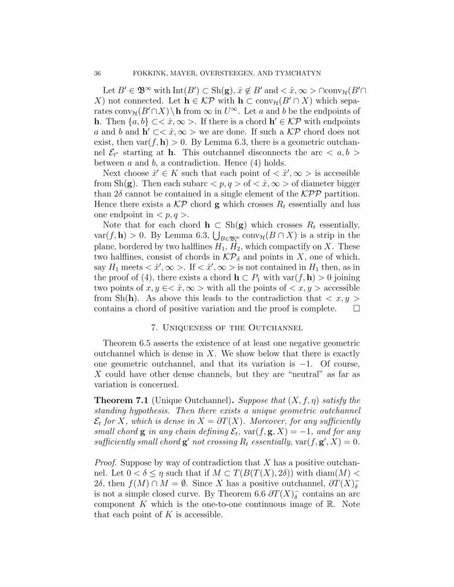
36 FOKKINK, MAYER, OVERSTEEGEN, AND TYMCHATYN
LetB′ ∈ B∞ with Int(B′) ⊂ Sh(g), x 6∈ B′ and< x,∞ > ∩convH(B′∩X) not connected. Let h ∈ KP with h ⊂ convH(B′ ∩X) which sepa-rates convH(B′∩X)\h from ∞ in U∞. Let a and b be the endpoints ofh. Then {a, b} ⊂< x,∞ >. If there is a chord h′ ∈ KP with endpointsa and b and h′ ⊂< x,∞ > we are done. If such a KP chord does notexist, then var(f,h) > 0. By Lemma 6.3, there is a geometric outchan-nel Et” starting at h. This outchannel disconnects the arc < a, b >between a and b, a contradiction. Hence (4) holds.
Next choose x′ ∈ K such that each point of < x′,∞ > is accessiblefrom Sh(g). Then each subarc < p, q > of < x,∞ > of diameter biggerthan 2δ cannot be contained in a single element of the KPP partition.Hence there exists a KP chord g which crosses Rt essentially and hasone endpoint in < p, q >.
Note that for each chord h ⊂ Sh(g) which crosses Rt essentially,var(f,h) > 0. By Lemma 6.3,
⋃B∈B∞
tconvH(B ∩X) is a strip in the
plane, bordered by two halflines H1, H2, which compactify onX. Thesetwo halflines, consist of chords in KPδ and points in X, one of which,say H1 meets < x′,∞ >. If < x′,∞ > is not contained in H1 then, as inthe proof of (4), there exists a chord h ⊂ P1 with var(f,h) > 0 joiningtwo points of x, y ∈< x,∞ > with all the points of < x, y > accessiblefrom Sh(h). As above this leads to the contradiction that < x, y >contains a chord of positive variation and the proof is complete. �
7. Uniqueness of the Outchannel
Theorem 6.5 asserts the existence of at least one negative geometricoutchannel which is dense in X. We show below that there is exactlyone geometric outchannel, and that its variation is −1. Of course,X could have other dense channels, but they are “neutral” as far asvariation is concerned.
Theorem 7.1 (Unique Outchannel). Suppose that (X, f, η) satisfy thestanding hypothesis. Then there exists a unique geometric outchannelEt for X, which is dense in X = ∂T (X). Moreover, for any sufficientlysmall chord g in any chain defining Et, var(f, g, X) = −1, and for anysufficiently small chord g′ not crossing Rt essentially, var(f, g′, X) = 0.
Proof. Suppose by way of contradiction that X has a positive outchan-nel. Let 0 < δ ≤ η such that if M ⊂ T (B(T (X), 2δ)) with diam(M) <2δ, then f(M) ∩M = ∅. Since X has a positive outchannel, ∂T (X)−δis not a simple closed curve. By Theorem 6.6 ∂T (X)−δ contains an arccomponent K which is the one-to-one continuous image of R. Notethat each point of K is accessible.

FIXED POINTS IN PLANAR CONTINUA 37
W
Ig
y
z
a
b c
d
p
q
Jz
+
J zi
J z
J z-
a0
Ja0
Ja0
+
Ja0
iJa0
-
L
L
R
Figure 5. Uniqueness of the negative outchannel.
Let ϕ : ∆∞ → V∞ = C \ T (X)−δ a conformal map. By Proposi-
tion 6.7, ϕ extends continuously and injectively to a map ϕ : ∆∞ →V∞, where ∆∞ \ ∆∞ is a dense and open subset of S1 which containsK in its image. Then ϕ−1(K) = (t′, t) ⊂ S1 is an open arc with t′ < tin the counterclockwise order on S1 (it could be that (t′, t) = S1 \ {t}and t = t′). By abuse of notation, let < denote the order in K inducedby ϕ and for x < y in K, denote the arc in K with endpoints x and yby 〈x, y〉. For x ∈ K, let 〈x,∞〉 = ∪y>x〈x, y〉

38 FOKKINK, MAYER, OVERSTEEGEN, AND TYMCHATYN
Let Et be the prime-end corresponding to t. By Proposition 6.7,Pr(Et) is a positive geometric outchannel and, hence, by Lemma 6.4,Pr(Et) = X. Let Rt = ϕ(reit), r > 1, be the external conformal raycorresponding to the prime-end Et of T (X)−δ . Since Rt \ Rt = X andthe small chords gx which define Pr(Et) have at least one endpoint inK, cross Rt essentially at x and have diameter going to zero as x ap-proaches X along Rt (by Proposition 5.4 and Lemma 5.8). Hence, X =Rt \ Rt =< x,∞ > \ < x,∞ >.
By Proposition 6.7, there is s ∈ Rt such that if B ∈ B∞ such thatconvH(B∩X)∩ [(X, s)-end of Rt] 6= ∅, then diam(B) < δ/2. Let B∞
t ={B ∈ B∞ | convH(B ∩X) contains a chord g such that g crosses the(X, s)-end of Rt essentially}.
By Proposition 6.7 there exists x ∈ K ∩ X such that for each arcA ⊂< x,∞ > with diameter > 2δ, there is a KP chord g whichcontains a point of A as an endpoint and crosses Rt essentially.
Let a0 ∈ K ∩X so that a0 > x and Ja0is a junction of T (X)−δ . Let
W be an open disk, with simple closed curve boundary, about a0 suchthat diam(W ) < δ/4 and f(W ) ∩ [W ∪ Ja0
] = ∅. Let a < a0 < b inK ∩ ∂W such that < a, b > is the component of K ∩W which containsa0. We may suppose that < b,∞ > ∩W is contained in one componentof W\ < a, b > since one side of K is accessible from C \ T (X)−δ anda0 ∈ X. If a ∈ X, let p = a. If not, then there exists a KP chordh such that a ∈ h. Then h ⊂ K by Proposition 5.11. Let p be theendpoint of h such that p < a.
Since X ⊂ < x,∞ > there are components of < b,∞ > ∩W whichare arbitrarily close to a0. Choose b < c < d in K so that the < c, d >is the closure of a component of W∩ < b,∞ > such that:
(1) a and d lie in the same component of ∂W \ {b, c}.(2) There exists z ∈< c, d > ∩X∩W and an arc I ⊂ {ao, z}∪[W\ <
p, d >] joining a0 to z.(3) There is a KP chord g ⊂ W with z and y as endpoints which
crosses Rt essentially. Hence, var(f, g) > 0.(4) diam(f(g)) < d(J+
a0\W,J i
a0\W ).
Conditions (1) and (2) follow because Ja0is a connected and closed
set from a0 to ∞ in {a0}∪[C\T (X)−δ ] and the ray < b,∞ > approachesboth a0 and p. Conditions (3) and (4) follow from Proposition 6.7. Ifd ∈ X, put q = d. Otherwise, let q ∈< d,∞ > such that there is a KPchord h ⊂ K containing d with endpoint q and such that d < q
By a simple extension of Corollary 2.17, there exists a bumping arcA′ of T (X) from p to q such that variation is defined on each component

FIXED POINTS IN PLANAR CONTINUA 39
of A′\X, S ′ = A′∪ < p, q > is a simple closed curve with T (X) ⊂ T (S ′)and f is fixed point free on T (S ′). Since g∩X = {z, y}, we may assumethat A′∩g = {y}. Let C be the arc in ∂W from a to d disjoint from b.The arc A′ may enter W and intersect I several times. However, in thiscase A′ must enter W through C. Since we want to apply the Lollipoplemma, we will modify the arc A′ to a new arc A which is disjoint fromI.
Let A be the set of points in A′∪C accessible from ∞ in C\ [S ′∪C].Then A is a bumping arc from p to q, A ∩ I = ∅, var(f, A) is defined,S = A∪ < p, q > is a simple closed curve with T (X) ⊂ T (S) and f isfixed point free on T (S). Note that y ∈ A. Then the Lollipop lemmaapplies to S with R = T (< a0, z > ∪I) and R = T (I∪ < z, q > ∪A∪ <p, a0 >).
Claim: f(z) ∈ R. Hence by Corollary 2.15, < a0, z > contains achord g1 with var(f, g1) < 0.
Proof of Claim. Note that the positive direction along g is from z toy. Since z, y ∈ X, {f(z), f(y)} ⊂ X ⊂ T (S) = T (R) ∪ T (L). Choosea junction Jy such that Ja0
\W ⊂ Jy and Jy runs close to Rt on itsway to g. Since g crosses Rt essentially, var(f, g) > 0. Since variationis invariant under suitable homotopies, we may assume that for each∗ ∈ {+, i,−}, J∗
y \W consists of exactly two components one of whichis contained in Ja0
. Let C∗y be the component of J∗
y \W which is disjoint
from J∗a0
. Then Ciy separates R∪C+
y from L∪C−y in C\W (see figure 5).
Since f(g) ∩ Ja0= ∅, if f(z) 6∈ T (R), var(f, g) ≤ 0, a contradiction.
Hence f(z) ∈ T (R) (and, in fact, f(y) ∈ T (L)) as desired.Since f(z) ∈ R, < a0, z > contains a chord g with var(f, g) < 0.
Repeating the same argument, replacing a0 by y and J0 by Jy we obtaina second chord g2 contained in < y,∞ > such that var(f, g2 >) < 0.
We will now show that the existence of two distinct chords g1 andg2 in K with variation < 0 on each leads to a contradiction. Recallthat a0 ∈ < b,∞ >. Hence we can find y′ ∈< b,∞ > with y′ ∈ Xsuch that g1 ∪ g2 ⊂ < a0, y
′ > and there exists a small arc I ′ ⊂ W ′
such that I ′∩ < a0, y′ >= {a0, y
′}. Since f(I ′)∩Ja0= ∅, var(f, I ′) = 0.
We may also assume that f is fixed point free on T (S ′), where S ′ =I ′∪ < a0, y
′ >. Since < a0, y′ > contains both g1, g2 and no chords of
positive variation, var(f,< a0, y′ >) ≤ −2 and var(f, S ′) ≤ −2. Then
ind(f, S ′) = var(f, S ′) + 1 ≤ −1 a contradiction with Theorem 2.6.Hence X has no positive geometric outchannel.
By Theorems 6.5 and 2.13, X has exactly one negative outchanneland its variation is −1.
�

40 FOKKINK, MAYER, OVERSTEEGEN, AND TYMCHATYN
Note that the following Theorem follows from Lemma 6.7 and The-orem 7.1.
Theorem 7.2. Suppose that X is a minimal counter example to theplane fixed point problem. Then there exists δ > 0 such that the contin-uum Y = T (X)+
δ is a non-separating continuum, f is fixed point freeon Y and all accessible points of Y are contained in one arc componentK of the boundary of Y . In other words, Y is homeomorphic to a diskwith exactly one channel removed which corresponds to the unique geo-metric outchannel of variation −1 of X. This channel compactifies onX. The sides of this channel are halflines consisting entirely of chordsof zero variation and points in X. There exist arbitrarily small home-omorphisms of the tails of these halflines to the tails of Rt which is theexternal ray corresponding to this channel.
8. Oriented maps
A perfect map is a closed continuous function each of whose pointinverses is compact. We will assume in the remaining sections thatall maps of the plane are perfect. Let X and Y be spaces. A mapf : X → Y is monotone provided for each continuumK ⊂ Y , f−1(K) isconnected. A map f : X → Y is confluent provided for each continuumK ⊂ Y and each component C of f−1(K), f(C) = K and f is lightprovided for each point y ∈ Y , f−1(y) is totally disconnected.
It is well know that each homeomorphism of the plane is eitherorientation-preserving or orientation-reversing. In this section we willestablish an appropriate extension of this result for confluent perfectmappings of the plane (Theorem 8.7) by showing that such maps ei-ther preserve or reverse local orientation. As a consequence it followsthat all perfect and confluent maps of the plane satisfy the MaximumModulus Theorem. We will call such maps positively- or negatively-oriented maps, respectively. For perfect mappings of the plane, Lelekand Read have shown that confluent is equivalent to the compositionof open and monotone maps [17]. Holomorphic maps are prototypes ofpositively-oriented maps but positively-oriented maps, unlike holomor-phic maps, do not have to be light. A non-separating plane continuumis said to be acyclic.
Definition 8.1 (Degree of fp). Let f : U → C be a map from a simplyconnected domain U ⊂ C into the plane. Let S ⊂ C be a positivelyoriented simple closed curve in U , and p ∈ U \ f−1(f(S)) a point.

FIXED POINTS IN PLANAR CONTINUA 41
Define fp : S → S1 by
fp(x) =f(x) − f(p)
|f(x) − f(p)| .
Then fp has a well-defined degree, denoted degree(fp). Note that degree(fp)is the winding number win(f, S, f(p)) of f |S about f(p).
Definition 8.2. A map f : U → C from a simply connected domainU is positively-oriented (respectively, negatively-oriented) provided foreach simple closed curve S in U and each point p ∈ T (S) \ f−1(f(S)),degree(fp) > 0 (degree(fp) < 0, respectively).
Definition 8.3. A perfect surjection f : C → C is oriented providedfor each simple closed curve S and each x ∈ T (S), f(x) ∈ T (f(S)).
Clearly every positively oriented and each negatively oriented mapis oriented. It will follow that all oriented maps satisfy the MaximumModulus Theorem 8.7.
It is well-known that both open maps and monotone maps (and hencecompositions of such maps) of continua are confluent. It will follow(Lemma 8.6) from a result of Lelek and Read [17] that each perfect,oriented surjection of the plane is the composition of a monotone mapand a light open map. The following Lemmas are in preparation forthe proof of Theorem 8.7.
Lemma 8.4. Suppose f : C → C is a perfect surjection. Then f isconfluent if and only if f is oriented.
Proof. Suppose that f is oriented. Let A be an arc in C and let C bea component of f−1(A). Suppose that f(C) 6= A. Let a ∈ A \ f(C).Since f(C) does not separate a from infinity, we can choose a simpleclosed curve S with C ⊂ T (S), S ∩ f−1(A) = ∅ and f(S) so close tof(C) that f(S) does not separate a from ∞. Then a 6∈ T (f(S)). Sincef is oriented, f(C) ⊂ T (f(S)). Hence there exists a y ∈ A ∩ f(S).This contradicts the fact that A ∩ f(S) = ∅. Thus f(C) = A.
Now suppose that K is an arbitrary continuum in C and let L bea component of f−1(K). Let x ∈ L and let Ai be a sequence of arcsin C such that limAi = K and f(x) ∈ Ai for each i. Let Mi bethe component of f−1(Ai) containing the point x. By the previousparagraph f(Mi) = Ai. Since f is perfect, M = lim supMi ⊂ L is acontinuum and f(M) = K. Hence f is confluent.
Suppose next that f : C → C is not oriented. Then there existsa simple closed curve S in C and p ∈ T (S) \ f−1(f(S)) such thatf(p) 6∈ T (f(S)). Let L be a half-line with endpoint f(p) running to

42 FOKKINK, MAYER, OVERSTEEGEN, AND TYMCHATYN
infinity in C \ f(S). Let L∗ be an arc in L with endpoint f(p) anddiameter greater than the diameter of the continuum f(T (S)). LetK be the component of f−1(L∗) which contains p. Then K ⊂ T (S),since p ∈ T (S) and L ∩ f(S) = ∅. Hence, f(K) 6= L∗, and so f is notconfluent. �
Lemma 8.5. Let f : C → C be a light, open, perfect surjection. Thenthere exists an integer k and a finite subset B ⊂ C such that f is a localhomeomorphism at each point of C\B, and for each point y ∈ C\f(B),|f−1(y)| = k.
Proof. Let C∞ be the one point compactification of C. Since f is
perfect, we can extend f to a map of C∞ onto C∞ so that f−1(∞) = ∞.By abuse of notation we also denote the extended map by f . Then f isa light open mapping of the compact 2-manifold C∞. The result nowfollows from a theorem of Whyburn [26, X.6.3]. �
The following is a special case, for oriented perfect maps, of themonotone-light factorization theorem.
Lemma 8.6. Suppose that f : C → C is an oriented, perfect map. Itfollows that f = g◦h, where h : C → C is a monotone perfect surjectionwith acyclic fibers and g : C → C is a light, open perfect surjection.
Proof. By the monotone-light factorization theorem [19, Theorem 13.3],f = g ◦ h, where h : C → X is monotone, g : X → C is light, and X isthe quotient space obtained from C by identifying each component off−1(y) to a point for each y ∈ C. Let y ∈ C and let C be a componentof f−1(y). If C were to separate C, then f(C) = y would be a pointwhile f(T (C)) would be a non-degenerate continuum. Choose an arcA ⊂ C \ {y} which meets both f(T (C)) and its complement and letx ∈ T (C) \ C such that f(x) ∈ A. If K is the component of f−1(A)which contains x, then K ⊂ T (C). Hence f(K) cannot map onto Acontradicting the fact that f is confluent. Thus, for each y ∈ C, eachcomponent of f−1(y) is acyclic.
By Moore’s Plane Decomposition Theorem [12], X is homeomorphicto C. Since f is confluent, it is easy to see that g is confluent. By atheorem of Lelek and Read [17] g is open since it is confluent and light(also see [19, Theorem 13.26]). Since h and g factor the perfect map fthrough a Hausdorff space C, both h and g are perfect [13, 3.7.5]. �
Theorem 8.7 (Maximum Modulus Theorem). Suppose that f : C → C
is a perfect surjection. Then the following are equivalent:
(1) f is either positively or negatively oriented.(2) f is oriented.

FIXED POINTS IN PLANAR CONTINUA 43
(3) f is confluent.
Moreover, if f is oriented, then for any non-separating continuum X,∂(f(X)) ⊂ f(∂(X)).
Proof. It is clear that (1) implies (2). By Lemma 8.4 every orientedmap is confluent. Hence suppose that f : C → C is a perfect confluentmap. By Lemma 8.6, f = g◦h, where h : C → C is a monotone perfectsurjection with acyclic fibers and g : C → C is a light, open perfectsurjection. By Stoilow’s Theorem [27] there exists a homeomorphismj : C → C such that g ◦ j is an analytic surjection. Then f = g ◦ h =(g ◦ j) ◦ (j−1 ◦ h). Since k = j−1 ◦ h is a monotone surjection of C
with acyclic fibers, it is a near homeomorphism [12, Theorem 25.1].That is, there exists a sequence ki of homeomorphisms of C such thatlim ki = k. We may assume that all of the ki have the same orientation.
Let fi = (g ◦ j) ◦ ki, S a simple closed curve in the domain of fand p ∈ T (S) \ f−1(f(S)). Note that lim f−1
i (fi(S)) ⊂ f−1(f(S)).Hence p ∈ T (S) \ f−1
i (fi(S)) for i sufficiently large. Moreover, since fi
converges to f , fi|S is homotopic to f |S in the complement of f(p) fori large. Thus for large i, degree((fi)p) = degree(fp), where
(fi)p(x) =fi(x) − fi(p)
|fi(x) − fi(p)|and fp(x) =
f(x) − f(p)
|f(x) − f(p)| .
Since g◦j is an analytic map, it is positively oriented and degree((fi)p) =degree(fp) > 0 if ki is orientation preserving and degree((fi)p) =degree(fp) < 0 if ki is orientation reversing. Thus, f is positively-oriented if each ki is orientation-preserving and f is negatively-orientedif each ki is orientation-reversing.
Suppose that X is a non-separating continuum and f is oriented.Let y ∈ ∂(f(X)). Choose yi ∈ ∂(f(X) and rays Ri, joining yi to ∞such that Ri ∩ f(X) = {yi} and lim yi = y. Choose xi ∈ X such thatf(xi) = yi. Since f is confluent, there exists closed and connected setsCi, joining xi to ∞ such that Ci ∩ X ⊂ f−1(yi). Hence there existx′i ∈ f−1(yi) ∩ ∂(X). We may assume that limx′i = x∞ ∈ ∂(X) andf(x∞) = y as desired. �
We shall need the following three results in the next section.
Lemma 8.8. Let X be a plane continuum and f : C → C a perfect,surjective map such that f−1(T (X)) = T (X) and f |C\f−1(T (X)) is con-fluent. Then for each y ∈ C \ T (X), each component of f−1(y) isacyclic.
Proof. Suppose there exists y ∈ C \ T (X) such that some componentC of f−1(y) is not acyclic. Then there exists z ∈ T (C)\f−1(y)∪T (X).

44 FOKKINK, MAYER, OVERSTEEGEN, AND TYMCHATYN
By unicoherence of C, T (X)∪{y} does not separate f(z) from infinityin C. Let L be a ray in C \ [T (X) ∪ {y}] from f(z) to infinity. ThenL = ∪Li, where each Li ⊂ L is an arc with endpoint f(z). For each ithe component Mi of f−1(Li) containing z maps onto Li. Then M =∪Mi is a connected closed subset in C \ f−1(y) from z to infinity. Thisis a contradiction since z is contained in a bounded complementarycomponent of f−1(y). �
Theorem 8.9. Let X a plane continuum and f : C → C a perfect,surjective map such that f−1(T (X)) = T (X) and f |C\f−1(T (X)) is con-fluent. If A and B are crosscuts of T (X) such that B ∪X separates Afrom ∞ in C, then f(B) ∪ T (X) separates f(A) \ f(B) from ∞.
Proof. Suppose not. Then there exists a half-line L joining f(A) toinfinity in C \ (f(B) ∪ T (X)). As in the proof of Lemma 8.8, thereexists a closed and connected set M ⊂ C\(B∪X) joining A to infinity,a contradiction. �
Proposition 8.10. Under the conditions of Theorem 8.9, if L is a rayirreducible from T (X) to infinity, then each component of f−1(L) isclosed in C \X and is a connected set from X to infinity.
9. Induced maps of prime ends
Suppose that f : C → C is an oriented perfect surjection andf−1(Y ) = X, where X and Y are acyclic continua. We will showthat in this case the map f induces a confluent map F of the circleof prime ends of X to the circle of prime ends of Y . This result wasannounced by Mayer in the early 1980’s but never appeared in print.It was also used (for homeomorphisms) by Cartwright and Littlewoodin [10]. There are easy counterexamples that show if f is not confluentthen it may not induce a continuous function between the circles ofprime ends.
Theorem 9.1. Let X and Y be non-degenerate acyclic plane continuaand f : C → C a perfect map such that:
(1) Y has no cut point,(2) f−1(Y ) = X and(3) f |C\X is confluent.
Let ϕ : ∆∞ → C∞ \X and ψ : ∆∞ → C
∞ \ Y be conformal mappings.
Define f : ∆∞ → ∆∞ by f = ψ−1 ◦ f ◦ ϕ.Then f extends to a map f : ∆∞ → ∆∞. Moreover, f−1(S1) = S1
and F = f |S1 is a confluent map.

FIXED POINTS IN PLANAR CONTINUA 45
Proof. Note that f takes accessible points of X to accessible points ofY . For if P is a path in [C \X] ∪ {p} with endpoint p ∈ X, then by(2), f(P ) is a path in [C \ Y ] ∪ {f(p)} with endpoint f(p) ∈ Y .
Let A be a crosscut of X such that the diameter of f(A) is lessthan half of the diameter of Y and let U be the bounded componentof C \ (X ∪ A). Let the endpoints of A be x, y ∈ X and suppose thatf(x) = f(y). If x and y lie in the same component of f−1(f(x)) theneach crosscut B ⊂ U of X is mapped to a generalized return cut of Ybased at f(x) (i.e., the endpoints of B map to f(x)) by (1). Note thatin this case by (1), ∂f(U) ⊂ f(A) ∪ {f(x)}.
Now suppose that f(x) = f(y) and x and y lie in distinct componentsof f−1(f(x)). Then by unicoherence of C, ∂U ⊂ A∪X is a connected setand ∂U 6⊂ A∪ f−1(f(x)). Now ∂U \ (A∪ f−1(f(x))) = ∂U \ f−1(f(A))is an open non-empty set in ∂U by(2). Thus there is a crosscut B ⊂U \ f−1(f(A)) of X with B \ B ⊂ ∂U \ f−1(f(A)). Now f(B) iscontained in a bounded component of C \ (Y ∪ f(A)) = C \ (Y ∪ f(A))by Theorem 8.9. Since Y ∩ f(A) = {f(x)} is connected and Y doesnot separate C, it follows by unicoherence that f(B) lies in a boundedcomponent of C \ f(A). Since Y \ {f(x)} meets f(B) and misses f(A)and Y \{f(x)} is connected, Y \{f(x)} lies in a bounded complementarycomponent of f(A). This is impossible as the diameter of f(A) issmaller than the diameter of Y . It follows that there exists a δ > 0such that if the diameter of A is less than δ and f(x) = f(y), then xand y must lie in the same component of f−1(f(x)).
In order to define the extension f of f over the boundary S1 of ∆∞,let Ci be a chain of crosscuts of ∆∞ which converge to a point p ∈ S1
such that Ai = ϕ(Ci) is a null chain of crosscuts or return cuts of Xwith endpoints ai and bi which converge to a point x ∈ X. There arethree cases to consider:
Case 1. f identifies the endpoints of Ai for some Ai with diameterless than δ. In this case the chain of crosscuts is mapped by f to achain of generalized return cuts based at f(ai) = f(bi). Hence f(ai)is an accessible point of Y which corresponds (under ψ−1) to a uniquepoint q ∈ S1 (since Y has no cutpoints). Define f(p) = q.
Case 2. Case 1 does not apply and there exists an infinite subse-quence Aij of crosscuts such that f(Aij ) ∩ f(Aik) = ∅ for j 6= k. Inthis case f(Aij) is a chain of generalized crosscuts which converges toa point f(x) ∈ Y . This chain corresponds to a unique point q ∈ S1
since Y has no cut points. Define f(p) = q.Case 3. Cases 1 and 2 do not apply. Without loss of generality
suppose there exists an i such that for j > i f(Ai) ∩ f(Aj) contains

46 FOKKINK, MAYER, OVERSTEEGEN, AND TYMCHATYN
f(ai). In this case f(Aj) is a chain of generalized crosscuts based atthe accessible point f(ai) which corresponds to a unique point q on S1
as above. Define f(p) = q.
It remains to be shown that f is a continuous extension of f and Fis confluent. For continuity it suffices to show continuity at S1. Letp ∈ S1 and let C be a small crosscut of ∆∞ whose endpoints are onopposite sides of p in S1 such that A = ϕ(C) has diameter less thanδ [18] and such that the endpoints of A are two accessible points ofX. Since f is uniformly continuous near X, the diameter of f(A) issmall and since ψ−1 is uniformly continuous with respect to connectedsets in the complement of Y ([25]), the diameter of B = ψ−1 ◦ f ◦ ϕ issmall. Also B is either a generalized crosscut or generalized return cut.Since f preserves separation of crosscuts, it follows that the image ofthe domain U bounded by C which does not contain ∞ is small. Thisimplies continuity of f at p.
To see that F is confluent let K ⊂ S1 be a subcontinuum and let Hbe a component of f−1(K). Choose a chain of crosscuts Ci such thatϕ(Ci) = Ai is a crosscut of X meeting X in two accessible points ai andbi, Ci ∩ f−1(K) = ∅ and limCi = H . It follows from the preservation
of crosscuts (see Theorem 8.9) that f(Ci) separates K from ∞. Hence
f(Ci) must meet S1 on both sides of K and lim f(Ci) = K. HenceF (H) = lim f(Ci) = K as required. �
Corollary 9.2. Suppose that f : C → C is a perfect, oriented map ofthe plane, X ⊂ C is a subcontinuum without cut points and f(X) = X.
Let X be the component of f−1(f(X)) containing X. Let ϕ : ∆∞ →C
∞ \ T (X) and ψ : ∆∞ → C∞ \ T (X) be conformal mappings. Define
f : ∆∞ \ ϕ−1(f−1(X)) → ∆∞ by f = ψ−1 ◦ f ◦ ϕ. Put S1 = ∂∆∞.
Then f extends over S1 to a map f : ∆∞ → ∆∞. Moreoverf−1(S1) = S1 and F = f |S1 is a confluent map.
Proof. By Lemma 8.6 f = g ◦m where m is a monotone perfect andonto mapping of the plane with acyclic point inverses, and g is an openand perfect surjection of the plane to itself. By Lemma 8.5, f−1(X)has finitely many components. It follows that there exist a simply con-nected open set V , containing T (X), such that if U is the component of
f−1(V ) containing X, then U contains no other components of f−1(X).It is easy to see that f(U) = V and that U is simply connected. HenceU and V are homeomorphic to C. Then f |U : U → V is a confluentmap. The result now follows from Theorem 9.1 applied to f restrictedto U . �

FIXED POINTS IN PLANAR CONTINUA 47
10. Fixed points for positively oriented maps
In this section we will consider a positively oriented map of the plane.As we shall see below, a straight forward application of the tools devel-oped above will give us the desired fixed point result. We will assume,by way of contradiction, that f : C → C is a positively oriented map,X is a plane continuum such that f(X) ⊂ T (X) and T (X) containsno fixed points of f .
Lemma 10.1. Let f : C → C be a map and X ⊂ C a continuumsuch that f(X) ⊂ T (X). Suppose C = (a, b) is a crosscut of thecontinuum T (X). Let v ∈ (a, b) be a point and Jv be a junction suchthat Jv∩(X∪C) = {v}. Then there exists an arc I such that S = I∪Cis a simple closed curve, T (X) ⊂ T (S) and f(I) ∩ Jv = ∅.Proof. Since f(X) ⊂ T (X) and Jv ∩X = 0, it is clear that there existsan arc I with endpoints a and b sufficiently close to T (X) such thatI ∪ C is a simple closed curve, T (X) ⊂ T (I ∪ C) and f(I) ∩ Jv = ∅.This completes the proof. �
Corollary 10.2. Suppose X ⊂ C is a continuum, f : C → C a posi-tively oriented map such that f(X) ⊂ T (X). Then for each crosscut Cof T (X) such that f(C) ∩ C = ∅, var(f, C) ≥ 0
Proof. Suppose that C = (a, b) is a crosscut of T (X) such that f(C)∩C = ∅ and var(f, C) 6= 0. Choose a junction Jv such that Jv ∩ (X ∪C) = {v} and v ∈ C \ X. By Lemma 10.1, there exists an arc Isuch that S = I ∪ C is a simple closed curve and f(I) ∩ Jv = ∅.Moreover, by choosing I sufficiently close to X, we may assume thatv ∈ C \ f(S). Hence var(f, C) = Win(f, S, v) ≥ 0 by the remarkfollowing Definition 2.8. �
Theorem 10.3. Suppose f : C → C is a positively oriented map andX is a continuum such that f(X) ⊂ T (X). Then there exists a pointx0 ∈ T (X) such that f(x0) = x0.
Proof. Suppose we are given a continuum X and f : C → C a positivelyoriented map such that f(X) ⊂ T (X). Assume that f |T (X) is fixedpoint free. Choose a simple closed curve S such that X ⊂ T (S) andpoints a0 < a1 < . . . < an in S ∩X such that for each i Ci = (ai, ai+1)is a sufficiently small crosscut of X, f(Ci) ∩ Ci = ∅ and f |T (S) is fixedpoint free. By Corollary 10.2, var(f, Ci) ≥ 0 for each i. Hence byTheorem 2.13, ind(f, S) =
∑var(f, Ci) + 1 ≥ 1. This contradiction
with Theorem 2.6 completes the proof. �

48 FOKKINK, MAYER, OVERSTEEGEN, AND TYMCHATYN
Corollary 10.4. Suppose f : C → C is a perfect, oriented map andX is a continuum such that f(X) ⊂ T (X). Then there exists a pointx0 ∈ T (X) of period at most 2.
Proof. By Theorem 8.7, f is either positively or negatively oriented. Ineither case, the second iterate f 2 is positively oriented and must havea fixed point in T (X) by Theorem 10.3. �
References
[1] V. Akis. On the plane fixed point problem. Topology Proc., 24:15–31, 1999.[2] H. Bell. On fixed point properties of plane continua. Trans. A. M. S., 128:539–
548, 1967.[3] H. Bell. A correction to my paper “Some topological extensions of plane ge-
ometry”, Rev. Colombiana 9 (1975), pp. 125–153. Rev. Colombiana, 10:93,1976.
[4] H. Bell. A fixed point theorem for plane homeomorphisms. Fund. Math.,100:119–128, 1978. See also: Bull. A. M. S. 82(1976), 778-780.
[5] A. Blokh and L. Oversteegen. Fixed points in non-invariant plane continua.Preprint.
[6] A. Blokh, C. Curry and L. Oversteegen. Locally connected models for Juliasets. Preprint.
[7] A. M. Blokh and L. G. Oversteegen. A fixed point theorem for branched cov-ering maps of the plane. Preprint.
[8] A. M. Blokh, G. Levin, L. G. Oversteegen and D. Schleicher. On the Fatou-Douady-Hubbard-Shishikura inequlity. In preparation.
[9] Morton Brown. Fixed point for orientation preserving homeomorphisms of theplane which interchange two points. Pacific J. of Math., 143:37–41, 1990.
[10] M. L. Cartwright and J. E. Littlewood. Some fixed point theorems. Annals of
Math., 54:1–37, 1951.[11] E. F. Collingwood and A. J. Lohwater. Theory of Cluster sets, volume 56 of
Cambridge Tracts in Math. and Math. Physics. Cambridge University Press,Cambridge, 1966.
[12] Robert J. Daverman. Decompositions of manifolds. Academic Press, Inc., 1986.[13] R. Engelking. General Topology. Heldermann Verlag, 1989.[14] S. D. Iliadis. Location of continua on a plane and fixed points. Vestnik
Moskovskogo Univ. Matematika, 25(4):66–70, 1970. Series I.[15] Ravi S. Kulkarni and Ulrich Pinkall. A canonical metric for Mobius structures
and its applications. Math. Z., 216(1):89–129, 1994.[16] Andrew Lelek. On confluent mappings. Colloq. Math., 15:232–233, 1966.[17] Andrew Lelek and David Read. Compositions of confluent mappings and some
other classes of functions. Colloq. Math., 29:101–112, 1974.[18] J. Milnor. Dynamics in One Complex Variable. Vieweg, Wiesbaden, second
edition, 2000.[19] S. B. Nadler, Jr. Continuum theory. Marcel Dekker Inc., New York, 1992.[20] Lex G. Oversteegen and E.D. Tymchatyn. Extending isotopies of planar con-
tinua. Preprint, 2007.[21] Ch. Pommerenke. Boundary behaviour of conformal maps, volume 299 of
Grundlehren der Math. Wissenschaften. Springer-Verlag, New York, 1992.

FIXED POINTS IN PLANAR CONTINUA 49
[22] N. E. Rutt. Prime ends and indecomposability. Bull. A. M. S., 41:265–273,1935.
[23] K. Sieklucki. On a class of plane acyclic continua with the fixed point property.Fund. Math., 63:257–278, 1968.
[24] W. P. Thurston. On the geometry and dynamics of iterated rational maps.Preprint, 1985.
[25] H. D. Ursell and L. C. Young. Remarks on the theory of prime ends. Mem. of
the Amer. Math. Soc., page 29p, 1951.[26] G. T. Whyburn. Analytic Topology, volume 28. AMS Coll. Publications, Prov-
idence, RI, 1942.[27] G. T. Whyburn. Topological Analysis. Princeton Math. Series. Princeton Univ.
Press, Princeton, NJ, 1964.

Index
accessible point, 14acyclic, 32allowable partition, 13
B, 15B∞, 15bumping
arc, 11simple closed curve, 11
C(a, b), 18Caratheodory Loop, 12chain of crosscuts, 13
equivalent, 13channel, 14
dense, 14, 26completing a bumping arc, 11C, 2C∞, 2convE(K), 15convH(B ∩ K), 15convex hull
Euclidean, 15hyperbolic, 15
counterclockwise orderon an arc in a simple closed curve,
3crosscut, 11
shadow, 12
D, 18defines variation near X , 24degree, 3degree(g), 3degree(fp), 32∂ boundary operator, 2∆∞, 13
embeddingorientation preserving, 4
Et, 13external ray, 14
end of, 14essential crossing, 14landing point, 14
fixed pointfor positively oriented maps, 37
(f, X, η), 24
G, 18g, 18g, 15Γ, 18gap, 17geodesic
hyperbolic, 18
hullhyperbolic, 17
hyperbolicgeodesic, 15halfplane, 15
hyperbolic chord, 18
id identity map, 3Im(Et), 14impression, 14index, 3
fractional, 4I=V+1 for Caratheodory Loops,
13Index=Variation+1 Theorem, 6
ind(f, A), 4ind(f, g), 3ind(f, g[a,b]), 4ind(f, S), 4
junction, 5Jørgensen Lemma, 18
KP , 17KPδ, 20KP chord, 17KP±
δ , 22KPP , 17KPPδ, 20Kulkarni-Pinkall
Lemma, 16Partition, 17
landing point, 14Lollipop Lemma, 9
mapconfluent, 31
50

FIXED POINTS IN PLANAR CONTINUA 51
light, 31monotone, 31negatively oriented, 32on circle of prime ends, 34oriented, 32perfect, 31positively oriented, 32
maximal ball, 15Maximum Modulus Theorem, 33
narrow strip, 27
orderon subarc of simple closed curve, 3
orientation preservingembedding, 4
outchannel, 24geometric, 24uniqueness, 28
point of period twofor oriented maps, 37
Pr(Et), 14prime end, 13
channel, 14impression, 14principal continuum, 14
principal continuum, 14
R, 2Rt, 14
shadow, 12Sh(A), 12smallest ball, 15standing hypothesis, 24
topological hull, 2T (X), 2T (X)δ, 22
U∞, 2
var(f, A), 12variation
for crosscuts, 11of a simple closed curve, 6on an arc, 5on finite union of arcs, 6
var(f, A, S), 5var(f, S), 6
win(g, S1, w), 3

52 FOKKINK, MAYER, OVERSTEEGEN, AND TYMCHATYN
Delft University, Faculty of Information and Systems, P.O. Box
5031, 2600 GA Delft, Netherlands
E-mail address, Robbert Fokkink: [email protected]
(John C. Mayer and Lex G. Oversteegen) Department of Mathematics,
University of Alabama at Birmingham, Birmingham, AL 35294-1170
E-mail address, John C. Mayer: [email protected]
E-mail address, Lex G. Oversteegen: [email protected]
(E. D. Tymchatyn) Department of Mathematics and Statistics, Uni-
versity of Saskatchewan, Saskatoon, Saskatchewan, Canada S7N 0W0
E-mail address, E. D. Tymchatyn: [email protected]
Copyright © 2022 FDOKUMEN