Prepared by:

Hunaiz Ali (hunaiz.ali@tum.de) Date: 17-01-2014

Technical University Of Munich Earth Oriented Space Science and Technology (ESPACE-2013/14)

Keplerian Orbits in Space-fixed, Earth-fixed and Topocentric systems

EXERCISE NO. 01

ORBITAL MECHANICS (Semester 01)

1

Abstract and Report Structure

The report gives a practical understanding of basic Orbital Mechanics. In this report, a step by step approach

is used to convert from one coordinate system to other and how to derive the position and velocity of a

satellite in orbit. The software used for computation and plotting is Matlab. The report is designed under the

supervision of Prof. Dr. Urs. Hugentobler (Technical University of Munich, Germany).

The step by step approach follows as:

Problem 01, 02 and 03 explain how to compute polar elements (radius and velocity) and anomalies of

satellite from given Keplerian elements. Later the orbits and their anomalies of satellites are plotted and

explained.

Problem 04 and 05 will show, how to transforms Keplerian elements to position and velocity in an

inertial (space-fixed) system and then you can find the trajectories in 3D and 2D (projection to x-y, x-z and y-

z planes) as well as a time series of the magnitude of velocity.

Problem 06, 07 and 08 is about how to transforms position and velocity in a space fixed system (that was

computed in previous problem) into position and velocity in an Earth-fixed system and an explanation of

trajectories in earth fixed system with the helps there interactive plots.

Problem 09, 10 and 11 explain how to visualize a satellite from a particular position on earth given

the coordinates of the station. Later it will also explain the visibility of satellite at that station.

The report also gives functions for transforming from one system to other, weaved in Matlab.

2

Contents

Given Data: ............................................................................................................................................................ 3

Problem 01: ........................................................................................................................................................... 4

Problem 02: ........................................................................................................................................................... 6

Problem 03: ........................................................................................................................................................... 7

Problem 04: ........................................................................................................................................................... 8

Problem 05: ........................................................................................................................................................... 9

Problem 06: ......................................................................................................................................................... 10

Problem 07: ......................................................................................................................................................... 11

Problem 08: ......................................................................................................................................................... 12

Problem 09: ......................................................................................................................................................... 13

Problem 10: ......................................................................................................................................................... 14

Problem 11: ......................................................................................................................................................... 14

Kep2orb ........................................................................................................................................................... 15

kep2cart .......................................................................................................................................................... 15

cart2efix........................................................................................................................................................... 16

efix2topo ......................................................................................................................................................... 16

3

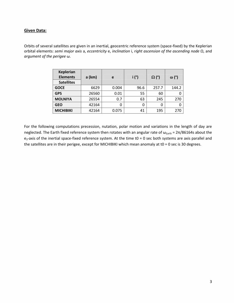
Given Data: Orbits of several satellites are given in an inertial, geocentric reference system (space-fixed) by the Keplerian orbital elements: semi major axis a, eccentricity e, inclination i, right ascension of the ascending node Ω, and argument of the perigee ω.

Keplerian Elements a (km) e i (°) (°) (°) Satellites

GOCE 6629 0.004 96.6 257.7 144.2

GPS 26560 0.01 55 60 0

MOLNIYA 26554 0.7 63 245 270

GEO 42164 0 0 0 0

MICHIBIKI 42164 0.075 41 195 270

For the following computations precession, nutation, polar motion and variations in the length of day are

neglected. The Earth fixed reference system then rotates with an angular rate of ωEarth = 2π/86164s about the

e3-axis of the inertial space-fixed reference system. At the time t0 = 0 sec both systems are axis parallel and

the satellites are in their perigee, except for MICHIBIKI which mean anomaly at t0 = 0 sec is 30 degrees.

4

Problem 01: Create a MATLAB-function kep2orb.m that computes polar coordinates r (radius) and ν (true anomaly) based on input orbital elements. Formulate your program in a way that the time t can be used as input parameter. Explanation: function [r,v,E,M] = kep2orb(a,e,u,t,z)

Where;

r=radius (to be calculated) v=true anomaly E=eccentric anomaly M=mean anomaly

a=semi major axis e=eccentricity u=gravitational constant t=time period z=a loop of required number of satellites

The designed function is capable of calculating geocentric radius (r) and true anomaly (v) when it is provided with u,t,z and required orbital elements (a,e). We will use the following Kepler’s equation to compute the radius from the given orbital elements. Radius or geocentric radius (r) is the distance of satellite from geocenter. For radius calculations: ----------------------------------------------------------------------------- (01) Where;

r=radius (to be calculated) a=semi major axis (given) e=eccentricity E=eccentric anomaly

Now in equation # 1, eccentric anomaly ‘E’ needs to be calculated. For that we will iterate the following set of equations:

------------------------------------------------------------------------------ (02)

Where M is the mean anomaly and can be calculate using: with

can be calculated using Kepler’s 3rd law, i.e.:

Where , is the geocentric gravitational constant.

-------------------------------------------------------- (03)

-------------------------------------------------------- (04)

Initially we will take and calculate . If the value of is greater than 10-6 we will add Ei and Ei to get the new value of . While writing the code of kep2orb, we will run a recursive loop to continuously calculate and check the value of using equations 02, 03 and 04. As the value of will become less than

5

or equal to 10-6, the loop will be terminated and the last value of Ei will be our final E to be used in equation 01. We will use the same value of E in the following equation 05 to calculate true anomaly of the satellite.

Or

------------------------------------------------------------------------ (05)

Limitations: The programme is designed for elliptical orbits only i.e. for those satellites or spatial objects in space fixed system whose orbital eccentricity is less than 1.

6

-5 -4 -3 -2 -1 0 1 2 3 4 5

x 107

-5

-4

-3

-2

-1

0

1

2

3

4

5x 10

7Q2: Satellite Orbits in Space Fixed System

X(m)

Y(m

)

GOCE

GPS

MOL

GEO

MIC

Problem 02: Plot the orbit for the 5 satellites in the orbital plane for one orbital revolution. Explanation: It can be seen from the given data of five satellites that eccentricity e of all satellites is less than zero, i.e. they have the elliptical orbit. So we can use kep2orb function to calculate the radius and true anomaly of GOCE, GPS, MOLNIYA, GEO and MICHIBIKI satellites.

First we have to calculate the time period which can be calculated using:

T=

----------------------------------------------------------------------------- (06)

Where; = GM=398.6005x1012 m3/s2 the Geocentric gravitational constant.

Now we will give semi major axis (a), eccentricity (e), geocentric gravitational constant (u), time period (t) and a loop value (z) to kep2orb function and will get the radius (r) and true anomaly (v). True anomaly (v) locates the satellite in the orbital plane and is the angular displacement measured from periapsis to the position vector along the direction of motion. According to that at any time t, the satellite will have x and y projection on the equator plane as we have shown in figure. So we will calculate the x=r x cos(v) and y= r x sin(v) projection and plot x against y for the period t=1 to t= T. We will run a loop that will calculate and plot the orbits of each required satellite. The results are following:

The resultant figure explains that the all satellites have elliptical orbits which we can confirm with the given eccentricity value. The projection of each satellite on earth’s equatorial plane can be seen.

7

Problem 03: Plot the mean anomaly M, the eccentric anomaly E, and the true anomaly ν as well as the difference ν – M for one orbital revolution for the GPS satellite and the Molniya satellite.

Explanation: The graph below shows the figurative comparison of Mean Anomaly (M), Eccentric Anomaly (E) and True Anomaly (v) of GPS and MOLNIYA Satellite. The third plot represents the difference of true anomaly and mean anomaly.

From the first two plots we can see that at periapsis (0 rad) and apoapsis ( rad) all three anomalies become equal. Also we can find the geocentric radius at periapsis and apoapsis from the figure. We can see it by zooming the figure, as shown in below figure.

0 0.5 1 1.5 2 2.5 3 3.5 4 4.5

x 104

-2

0

2Q2: v-M

rad

2.246 2.248 2.25 2.252 2.254 2.256 2.258 2.26 2.262

x 104

3.27

3.28

3.29

3.3

GPS

rad

M

E

v

0 0.5 1 1.5 2 2.5 3 3.5 4 4.5

x 104

0

5

10MOLNIYA

rad

M

E

v

8

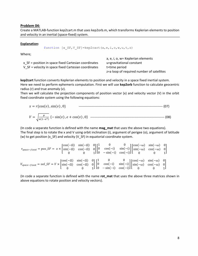
Problem 04: Create a MATLAB-function kep2cart.m that uses kep2orb.m, which transforms Keplerian elements to position and velocity in an inertial (space-fixed) system.

Explanation: function [x_SF,V_SF]=kep2cart(a,e,i,o,w,u,t,z)

Where;

x_SF = position in space fixed Cartesian coordinates V_SF = velocity in space fixed Cartesian coordinates

a, e, i, o, w= Keplerian elements u=gravitational constant t=time period z=a loop of required number of satellites

kep2cart function converts Keplerian elements to position and velocity in a space fixed inertial system. Here we need to perform ephemeris computation. First we will use kep2orb function to calculate geocentric radius (r) and true anomaly (v). Then we will calculate the projection components of position vector (x) and velocity vector (V) in the orbit fixed coordinate system using the following equations:

----------------------------------------------------------------------------- (07)

-------------------------------------------------------------------- (08)

(In code a separate function is defined with the name mag_mat that uses the above two equations). The final step is to rotate the x and V using orbit inclination (i), argument of perigee (o), argument of latitude (w) to get position (x_SF) and velocity (V_SF) in equatorial coordinate system.

(In code a separate function is defined with the name rot_mat that uses the above three matrices shown in above equations to rotate position and velocity vectors).

9

0 1 2 3 4 5 6 7 8 9

x 104

1000

2000

3000

4000

5000

6000

7000

8000

9000

10000

t(s)

V(m

/s)

Velocity of Satellites

GOCE

GPS

MOL

GEO

MIC

Problem 05: Compute position and velocity vectors of the 5 satellites for a period of one day. Assume true anomaly ν=0 for the beginning of the day. Visualize your results. Plot the trajectory in 3D and 2D (projection to x-y, x-z and y-z planes) as well as a time series of the magnitude of velocity.

Explanation: First we need to define time period which is according to given value is 1 day=86400 s. Also we need to convert o, i and w into radians. Then we will use kep2cart to get position and velocity vectors. The orbits can be easily plotted using these values. The results are shown below.

The figure is self explanatory and explains the trajectory of orbits in different 2-D coordinates. The 3D view helps to visualise the behaviour and purposes of each satellite’s elliptical orbit in space.

The velocity plot shows that except MOLNIYA satellite all four satellites’ orbit have earth at their centre. We can see that at t=0 the velocity is maximum because is at periapsis, as the time increases the MOLNIYA satellite is going far from the earth and so its velocity is decreasing. The earth is at one of the foci of MOLNIYA’s elliptical orbit. That we can also confirmed from the trajectory plot. The other orbits have very less variation in velocities. GEO is in a geostationary orbit whose property is that the satellite in such an orbit has an orbital period equal to the sidereal day. GPS and MICHIBIKI are acting approximately in the same way with a little variation in velocity. GOCE is a low orbit satellite. So have very high velocity.

-4-2

02

4

x 107

-4-2

02

4

x 107

-2

0

2

4

x 107

X(m)

Trajectories for satellites in 3D

Y(m)

Z(m

)

-5 0 5

x 107

-5

0

5x 10

7Trajectory in projection X-Y

X(m)Y

(m)

-5 0 5

x 107

-4

-2

0

2

4

6x 10

7 Trajectory in projection Y-Z

Y(m)

Z(m

)

-5 0 5

x 107

-4

-2

0

2

4

6x 10

7Q5

X(m)

Z(m

)

GOCE

GPS

MOL

GEO

MIC

10

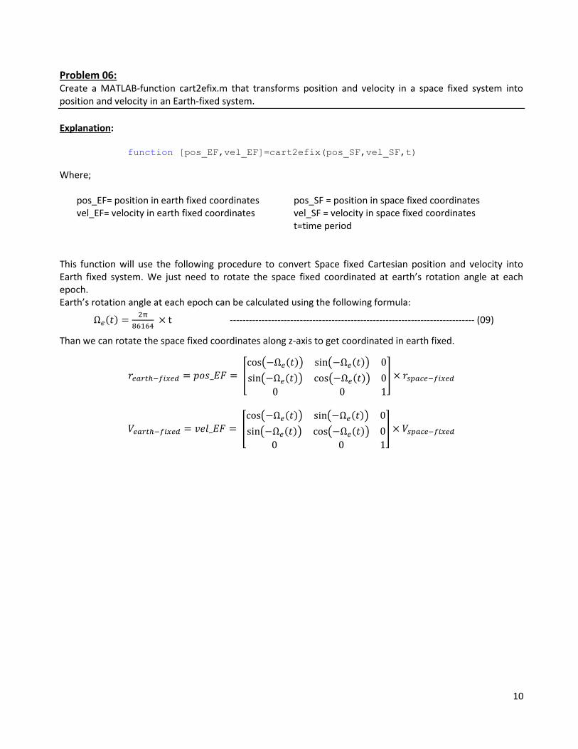
Problem 06: Create a MATLAB-function cart2efix.m that transforms position and velocity in a space fixed system into position and velocity in an Earth-fixed system.

Explanation: function [pos_EF,vel_EF]=cart2efix(pos_SF,vel_SF,t)

Where; pos_EF= position in earth fixed coordinates vel_EF= velocity in earth fixed coordinates

pos_SF = position in space fixed coordinates vel_SF = velocity in space fixed coordinates t=time period

This function will use the following procedure to convert Space fixed Cartesian position and velocity into Earth fixed system. We just need to rotate the space fixed coordinated at earth’s rotation angle at each epoch. Earth’s rotation angle at each epoch can be calculated using the following formula:

----------------------------------------------------------------------------- (09)

Than we can rotate the space fixed coordinates along z-axis to get coordinated in earth fixed.

11

Problem 07: Plot the trajectory of the satellites in 3D for the first two orbital revolutions.

Explanation: For the desired results we will use step by step process. First calculate position and velocity of satellite in Space fixed Cartesian from given Keplerian elements using kep2cart function. Then the space fixed velocity and position will need to be converted to earth fixed coordinated using cart2efix function. In result, we will have x, y and z projection of satellite’s position and velocity in earth fixed system and can be plotted in 3D.

-20

2

4

x 107

-2

0

2

x 107

-2

-1

0

1

2

3

4

x 107

x(m)

Q7: Satellite Orbits in Earth Fixed System

y(m)

z(m

)

GOCE

GPS

MOL

GEO

MIC

12

Problem 08: Calculate and draw the satellite ground-tracks on the Earth surface.

Explanation: At this point we have position and velocity in earth fixed system. To draw ground tracks we need longitude and latitude. We will use the following equations to calculate longitude and latitude.

------------------------------------------------------- (10)

------------------------------------------------------- (11)

-180 -150 -120 -90 -60 -30 0 30 60 90 120 150 180-90

-60

-30

0

30

60

90

deg

deg

Q8: satellite ground-tracks on the Earth surface

GOCE

GPS

MOL

GEO

MIC

13

Problem 09: Create a MATLAB-function efix2topo.m that transforms position and velocity in an Earth-fixed system into position and velocity in a Topocentric system centered at the station Wettzell which position vector in an Earth-fixed system is given by: rW = (4075.53022, 931.78130, 4801.61819)T km.

Explanation:

function [azim,elev,pos_topo] = efix2topo(pos_EF,vel_EF)

Where;

azim= azimuth elev= elevation pos_topo= position in Topocentric coordinates

pos_EF= position in earth fixed coordinates vel_EF= velocity in earth fixed coordinates

We are provided with the earth fixed position vector (rW=pos_wetz) of Wetzell station and we computed the

earth fixed position vector (pos_EF) of satellite using given Keplerian elements. First we will calculate the

longitude and latitude of Wetzell using the equations (10 & 11) and the given position vector. Now we can

calculate the Topocentric position vector by subtracting the position vector of Wetzell from position vector of

satellite in earth fixed system.

The next step is the transformation of the Topocentric vector from right handed system to left handed system by multiplying it with the following matrix.

Rotate the transformed Topocentric vector along the y-axis at latitude angle and z-axis at longitude angle to get the position in Topocentric coordinates. As a result we will have x, y and z coordinates in a vector form. In a Topocentric system we need azimuth and elevation angle to locate an object. So we need to calculate the azimuth and elevation angles using the following equations:

------------------------------------------------------- (12)

------------------------------------------------------- (13)

14

Problem 10: Plot the trajectory of the satellites as observed by Wettzell using the MATLAB-function skyplot.m.

Explanation: By using the efix2topo function we can plot the trajectories of the satellites, seen at Wetzell, as shown in following figure.

Problem 11: Calculate visibility (time intervals) for the satellites at the station Wettzell and visualize them graphically.

Explanation: This shows one of the most useful information. We can visualise the visibility of satellites at any location with knowing the position of the location. Here we were given with Wetzell position vector. By calculating the elevation we can say if elevation is greater than zero the satellite is visible. We can see for one day observation that the GEO satellite has highest visibility because it is a geostationary satellite. On the other hand GOCE is least visible because it is very closer to earth and cannot be seen at low elevation angles. The other satellites have varying visibility depending on the elevation.

15

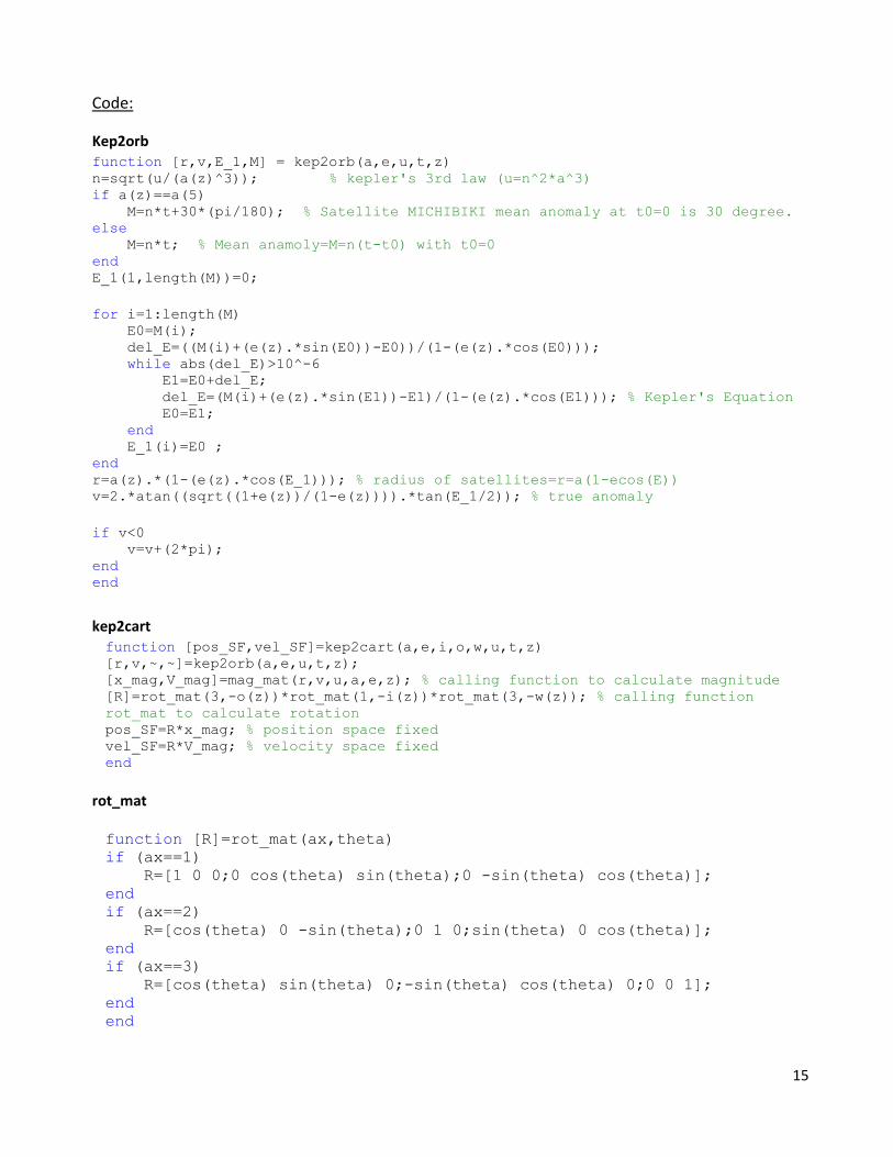
Code:

Kep2orb function [r,v,E_1,M] = kep2orb(a,e,u,t,z) n=sqrt(u/(a(z)^3)); % kepler's 3rd law (u=n^2*a^3) if a(z)==a(5) M=n*t+30*(pi/180); % Satellite MICHIBIKI mean anomaly at t0=0 is 30 degree. else M=n*t; % Mean anamoly=M=n(t-t0) with t0=0 end E_1(1,length(M))=0;

for i=1:length(M) E0=M(i); del_E=((M(i)+(e(z).*sin(E0))-E0))/(1-(e(z).*cos(E0))); while abs(del_E)>10^-6 E1=E0+del_E; del_E=(M(i)+(e(z).*sin(E1))-E1)/(1-(e(z).*cos(E1))); % Kepler's Equation E0=E1; end E_1(i)=E0 ; end r=a(z).*(1-(e(z).*cos(E_1))); % radius of satellites=r=a(1-ecos(E)) v=2.*atan((sqrt((1+e(z))/(1-e(z)))).*tan(E_1/2)); % true anomaly

if v<0 v=v+(2*pi); end end

kep2cart function [pos_SF,vel_SF]=kep2cart(a,e,i,o,w,u,t,z) [r,v,~,~]=kep2orb(a,e,u,t,z); [x_mag,V_mag]=mag_mat(r,v,u,a,e,z); % calling function to calculate magnitude [R]=rot_mat(3,-o(z))*rot_mat(1,-i(z))*rot_mat(3,-w(z)); % calling function

rot_mat to calculate rotation pos_SF=R*x_mag; % position space fixed vel_SF=R*V_mag; % velocity space fixed end

rot_mat function [R]=rot_mat(ax,theta)

if (ax==1)

R=[1 0 0;0 cos(theta) sin(theta);0 -sin(theta) cos(theta)];

end

if (ax==2)

R=[cos(theta) 0 -sin(theta);0 1 0;sin(theta) 0 cos(theta)];

end

if (ax==3)

R=[cos(theta) sin(theta) 0;-sin(theta) cos(theta) 0;0 0 1];

end

end

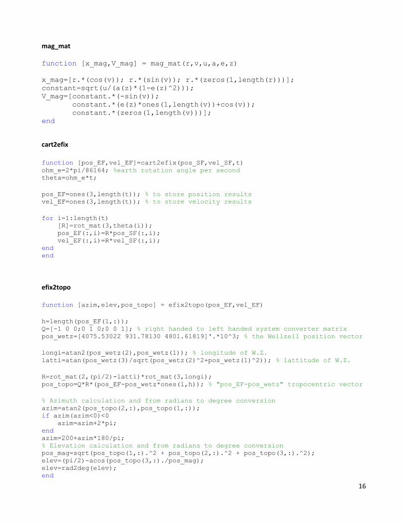
16

mag_mat function [x_mag,V_mag] = mag_mat(r,v,u,a,e,z)

x_mag=[r.*(cos(v)); r.*(sin(v)); r.*(zeros(1,length(r)))];

constant=sqrt(u/(a(z)*(1-e(z)^2)));

V_mag=[constant.*(-sin(v));

constant.*(e(z)*ones(1,length(v))+cos(v));

constant.*(zeros(1,length(v)))];

end

cart2efix

function [pos_EF,vel_EF]=cart2efix(pos_SF,vel_SF,t) ohm_e=2*pi/86164; %earth rotation angle per second theta=ohm_e*t;

pos_EF=ones(3,length(t)); % to store position results vel_EF=ones(3,length(t)); % to store velocity results

for i=1:length(t) [R]=rot_mat(3,theta(i)); pos_EF(:,i)=R*pos_SF(:,i); vel_EF(:,i)=R*vel_SF(:,i); end end

efix2topo

function [azim,elev,pos_topo] = efix2topo(pos_EF,vel_EF)

h=length(pos_EF(1,:)); Q=[-1 0 0;0 1 0;0 0 1]; % right handed to left handed system converter matrix pos_wetz=[4075.53022 931.78130 4801.61819]'.*10^3; % the Wellzell position vector

longi=atan2(pos_wetz(2),pos_wetz(1)); % longitude of W.Z. latti=atan(pos_wetz(3)/sqrt(pos_wetz(2)^2+pos_wetz(1)^2)); % lattitude of W.Z.

R=rot_mat(2,(pi/2)-latti)*rot_mat(3,longi); pos_topo=Q*R*(pos_EF-pos_wetz*ones(1,h)); % "pos_EF-pos_wetz" tropocentric vector

% Azimuth calculation and from radians to degree conversion azim=atan2(pos_topo(2,:),pos_topo(1,:)); if azim(azim<0)<0 azim=azim+2*pi; end azim=200+azim*180/pi; % Elevation calculation and from radians to degree conversion pos_mag=sqrt(pos_topo(1,:).^2 + pos_topo(2,:).^2 + pos_topo(3,:).^2); elev=(pi/2)-acos(pos_topo(3,:)./pos_mag); elev=rad2deg(elev); end