Comput. & Graphics Vol. 17, No.2, pp. 175-184, 1993Print.ed in Great Britain.

0097-8493/93 $6.00 + .00© 1993 Pergamon Press Ltd.

Chaos and Graphics

JULIA SETS AND QUASI-STABLE ORBITSTHE COMPLEX PLANE

Abstract-Theare explored. Ke.Lat1011~;hiJjS

PAUL K. SHERARDAstronomy, Ohio University, ''Athens,

~ z~ + c

1. .1.'1 , "....., .....,.'.1."

Various graphical aspectsset) have been reported ex1:enSlV1elvvelopment[1-4]. The techniqueshave involved escape time algorithms thatshow, quitebeautifully, the complexity in boundary regions of theM-set. Each pixel in such displays is a representationofthe outcome ofaspecific orbit in the complex plane,and has a unique Julia set associated with it. The dy­namics of such orbits, which are presented. in this tu­torial, can reveal details of its Julia set and also theattractors that are contained within it.

2. ITERATED MAPS

The generatiol1of M~set ima.ges isdetet111ined bythe orbits % (initial z =0), ofthe iteration:

zn+l = z~ + c.

If the progress ofthe iteration is plotted in the complexplane .(for a·particular value of c) it forms a two-di­mensional iteratedmap.>lngeneral, the paths ofsuchmaps either diverge, and head to infinity, or remainbounded to a point or set of points [5]. All values ofc whose orbits are bounded are members the M-setand have associated Julia sets that are connected [2 ] .A connected Julia set forms the boundary between thebasins of attraction of thecstable orbits and the attrac­tion to infinity [6] .

Orbits that are bounded generally fall into two cat-egories: either they are superstable or asymptotically­stable. In the superstable case the orbit is exactly pe­riodic. In the latter case the orbit approaches, asymp­totically, single (or multiple)· point attractors as theiteration proceeds. It has been shown that some peri­odic orbits can form fractal shapes, or strange attractors,in the complex plane within their associated Juliaset[7] .

The escape time, or dwell, of unstable orbits is theprecise number of iterations for which the magnitudeof Z becomes greater than 2. The final trajectory, whichheads off to infinity, can be considered an orbit's pathto infinity. For certain c values, the orbit is stronglyattracted to infinity and has a direct path to infinity;the antithesis of asymptotically stable orbits that col­lapse directly to attractive points in the complex plane.

Other unstable orbits escape to infinity after rela-

(JU.ifJ..\'l-.\'!.,fJ.fJJ'f' orbits tendto be equally attracted to within the complexplane and to infinity. As a the iteratedmap ofsuch an orbit fills in a region betweenthe attraction to infinity and the central attractor (s) .Since the associated Julia set is the boundary betweenthe central attractors and infinity, as stated, thisboundary region of the iterated map is also the Juliaset. For unstable orbits, the associated Julia set is, infact, a Cantor set [2] and is therefore .not closed. TheCantor sets ofquasi-stable orbits look very much likethe closed Julia sets, but what the iterated maps showis that these sets have narrow breaks through whichthe orbit's path eventually escapes.

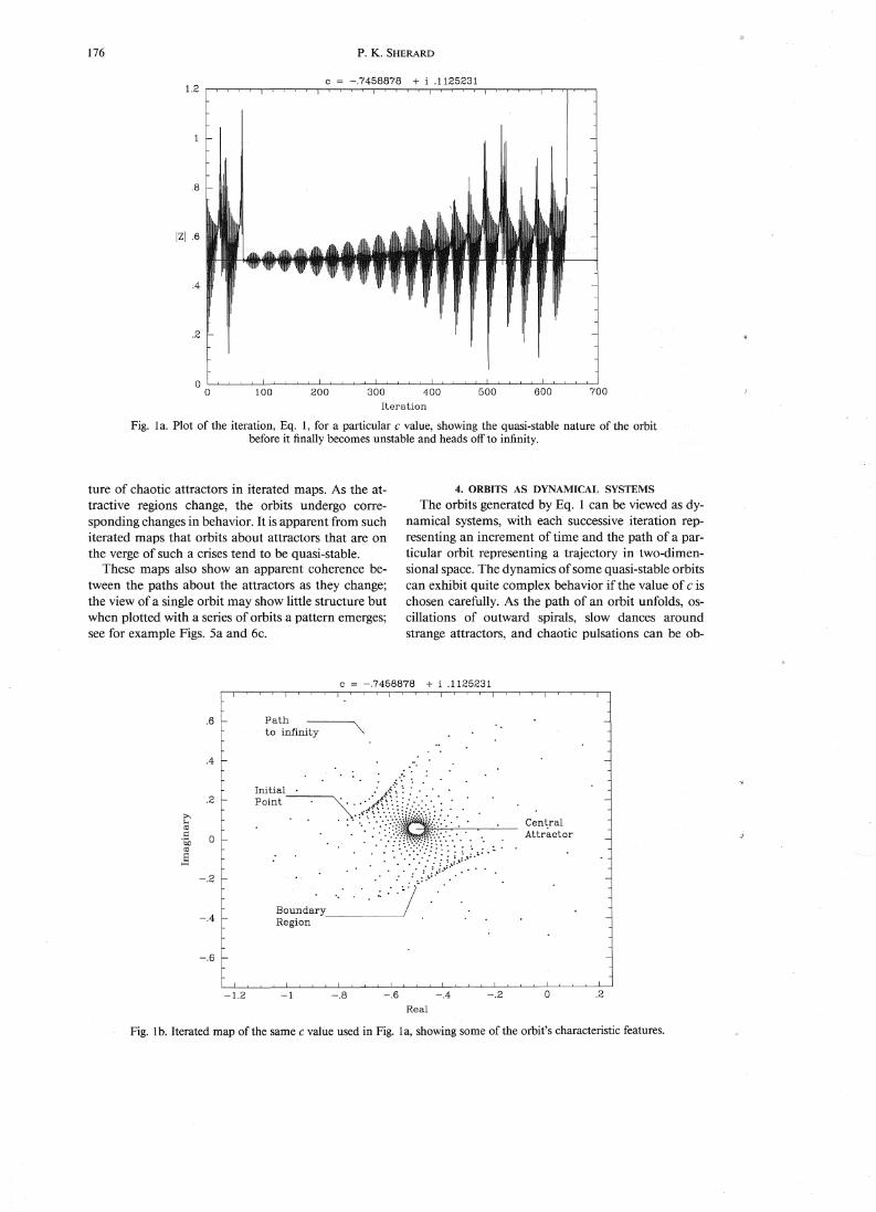
An example ofa quasi-stable orbit of 0 is shown inFig. 1 for a particular value of c. In Fig. 1a the mag­nitude of z vs. iteration number is plotted. It can beseen from the plot that the orbit has some semblanceof periodicity but eventually escapes after 650 .itera­tions. Figure 1b shows the iterated map of this orbitin the complex plane and points out the main featuresassociated with ..such quasi-stable orbits. The centralattractor is the location in the complex plane that theorbit tends to gravitate towards. Since the orbit is quasi­stable it is equally attracted to infinity and the orbittends to skirt a boundary region during its iterated life­time before escaping. In Fig. 1c the associated Julia setis superimposed on the iterated map. The Julia setsfor these particular displays, unless otherwise stated,were computed by the inverse iteration method [4] andplotted on the same scale as the iterated maps. It canbe seen that the Julia set opens up along broken cuspsor folds. These cusps act as escape routes from thecentral attractor to the attraction at infinity as observedby the orbit's path to infinity.

3. STEPWISE ITERATED MAPS

Another effective way ofdisplaying iterated maps isto vary the real part, or the imaginary part, ofthe valueofc in small steps, and plot the first 100, or so, iterationsfor each successive orbit, all on the same stepwise it­erated map. By overlaying orbits in this manner theprogression of the attractive regions in the complexplane can be seen directly; as the value for c is movedabout the M-set the location of the orbit's attractor( s)change correspondingly. Sudden changes of attractorsin this manner is analogous to a phenomena knownas crises[ 8], which is a description of the transient na-

175

176 P. K. SHERARD

c = -.7458878 + i .1125231

.8

IZI .6

.4

.2

100 200 300 400 500 600 700

Iteration

Fig. la. Plot of the iteration, Eq. 1, for a particular c value, showing the quasi-stable nature of the orbitbefore it finally becomes unstable and heads off to infinity.

ture of chaotic attractorsin iterated maps. As the at­tractive regions change,·· the . orbits ... undergo corre­sponding changes in behavior. It is apparent from suchiterated maps that orbits about attractors that are onthe verge of such a crises tend to be·quasi-stable.

These maps also show an apparent coherence be­tween the paths about the attractors as they change;the view of a single orbit may show little structure butwhen· plotted with a series oforbits a pattern emerges;see for example Figs. Sa and 6c.

4. ORBITS AS DYNAMICAL SYSTEMS

The orbits.generated by Eq. lean be viewed asdy­namical systems, with each successive iteration rep­resenting an increment of time and the path of a par­ticular orbit representing a trajectory in two-dimen­sional space. The dynamics ofsome quasi-stable orbitscan exhibit quite complex behavior if the value of c ischosen carefully. As the path of an orbit unfolds, .. os­cillations of outward spirals, . slow .dances. aroundstrange attractors, and chaotic pulsations can be. ob-

c = -.7458878 + i .1125231

Pathto infinity

.6

.4

.2

~l-;ro~

0'Soro

.§

-.2

-.4

-.6

...

~n;;~~l ~.. ;~:~~?)\~.b.~.:~.::.:.Ji.f.~.~ ..r:.·.~.:....:.. ..: ~ ::.:." .

BoUndary ·:_:_·:--.J·/jjJ.·;··;··:····

Region

CentralAttr~ctor

-1.2 -1 -.8 -.6

Real

-.4 -.2 o .2

Fig. lb. Iterated map of the same c value used in Fig. la, showing some of the orbit's characteristic features.

Julia sets and quasi-stable orbits

Fig. lc. Overlay of the associated Julia set with the iterated map of Fig. lb. Note how the escape route ofthe orbit occurs through the broken cusps in the Julia set.

177

served. The orbits take on almost life-like behavior attimes. There are also display tricks that can be used toenhance the images. For instance, by changing the color(or shade) of the points plotted every 1,000 iterations,or so, surprisingly coherent patterns can be broughtout. This also allows one to follow dense patterns moreeasily. This is how the grey-shade patterns were gen­erated in some of the figures. Also, clearing the screen

during an orbit or slowing down the iteration processcan reveal other interesting aspects of the iterated map.

5. GRAPHICS AND OBSERVATIONS

A sampling of such iterated maps is now discussed.Refer to Fig. 7 as to where in the M-set the c valuesfor a particular figure is located.

Figure 2a is a particularly interesting orbit that begins

c =-1.251 + iCenter= 8.8688 + i 8.8888

.818877295Side= 8.3888

,.~. I'·' I '

• ':!"o "

":}~,,,.•..~:~,,: ',': . ' 'vJ~' .~.,

: : , ':::'~:-': ~',:

.......

....·:·uI j 1-. In:' .

~:, ". .-, '1'."~:'"

\;~ ..

Fig. 2a. Magnified view of quasi-stable 0 orbit.

178 P.. K.· SHERARD

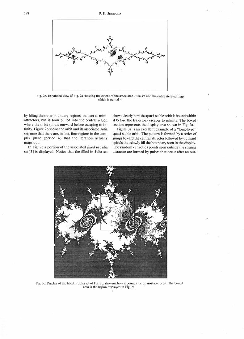
Fig. 2b. Expanded view of Fig. 2a showing the extent of the associated Julia set and the entire iterated mapwhich is period 4.

by filling the outer boundary regions, that act as mini­attractors, but is soon pulled into the central regionwhere the orbit spirals outward before escaping to in­finity. Figure 2b shows the orbit and its associated Juliaset; note that there are, in fact, four regions in the com­plex plane (period 4) that the iteration actuallymaps out.

In Fig. 2c a portion of the associated filled in Juliaset [3] is displayed. Notice that the filled in Julia set

shows clearly how the quasi-stable orbit is bound withinit before the trajectory escapes to infinity. The boxedsection· represents the display area shown in Fig. 2a.

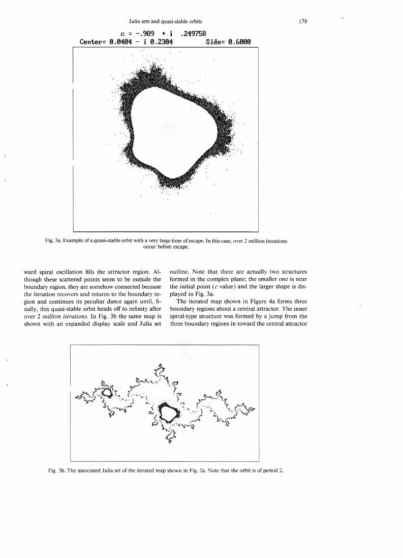
Figure 3a is an excellent example of a "long-lived"quasi-stable orbit. The pattern is formed by a series ofjumps toward the central attractor followed by outwardspirals that slowly fill the boundary seen in the display.The random (chaotic) pointsseelToutside the strangeattractor are formed by pulses that occur after an out-

Fig. 2c. Display of the filled in Julia set of Fig. 2b, showing how it bounds the quasi-stable orbit. The boxedarea is the region displayed in Fig. 2a.,

Julia sets and quasi-stable orbits 179

c =-.989 + iCenter= 8>..8484 - i 8.2384

.249158Side= 8.6888

Fig. 3a. Example of a quasi-stable orbit with a very large time ofescape. In this case, over 2 million iterationsoccur before escape.

ward spiral oscillation fills the attractor region. Al­though these scattered points seem to be outside theboundary region, they are somehow connected becausethe iteration recovers and returns to the boundary re­gion and continues its peculiar dance again until, fi­nally, this quasi-stable orbit heads off to infinity afterover 2 million iterations. In Fig. 3b the same map isshown with an expanded display scale and Julia set

outline. Note that there are actually two structuresformed in the complex plane; the smaller one is nearthe initial point (c value) and the larger shape is dis­played in Fig. 3a.

The iterated map shown in Figure 4a forms threeboundary regions about a central attractor. The innerspiral-type structure Was formed by a jump from thethree boundary regions in toward the central attractor

Fig. 3b. The associated Julia set of the iterated map shown in Fig. 2a. Note that the orbit is of period 2.

180 P.K. SHERARD

c = ~ .• 1145881 + iCenter::: -.2488 + i 8.3888

8>.658885Side:: 1~8888

Fig. 4a. Iterated map showing an orbit influenced equally by three outer regions of attraction and a centralattractor.

Fig. 4b. Display of the iterated map of Fig. 4a and its associated Julia set.

Julia sets and quasi-stable orbits 181

and then the orbit spiraled outward toward the attrac­tion at infinity. It can be seen from Fig. 4b how theorbit skirts the Julia set region before heading off toinfinity through the open cusps that pierce inward to­ward the central attractor.

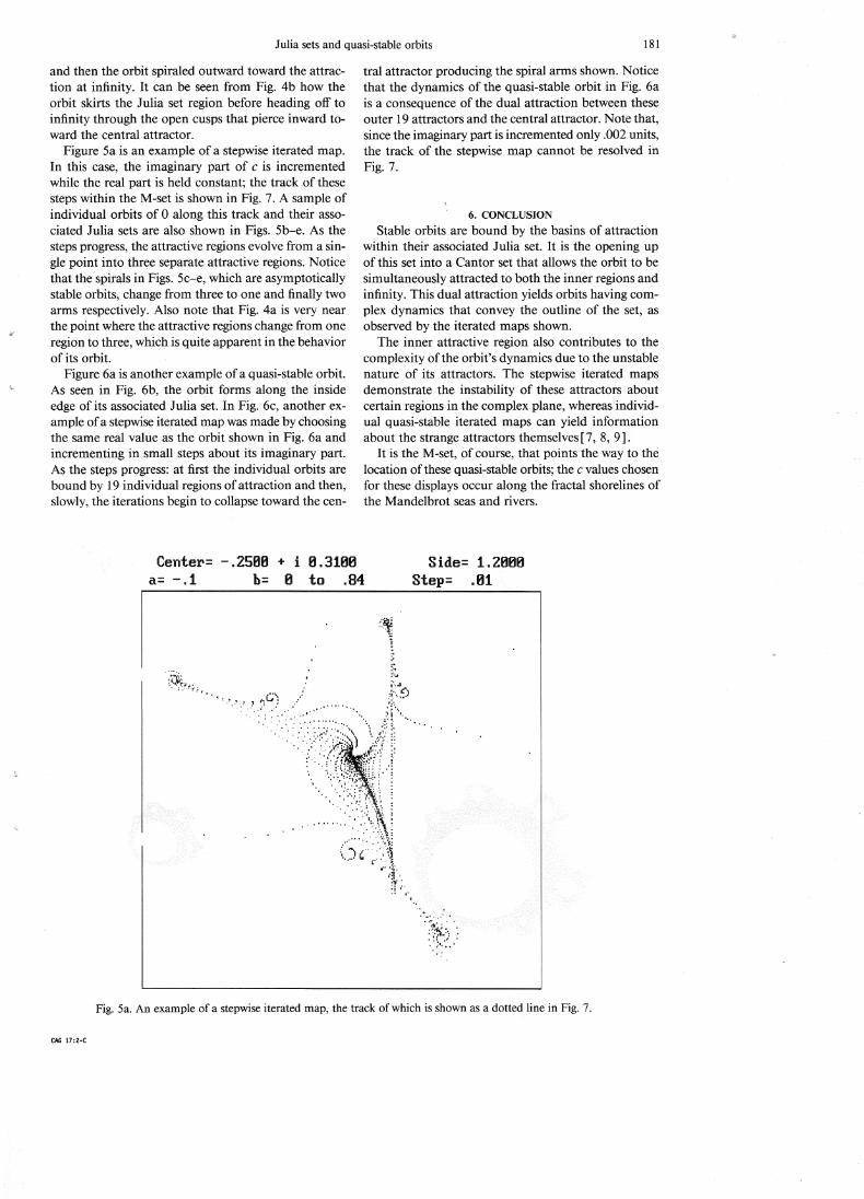
Figure 5a is an example of a stepwise iterated map.In this case, the imaginary part of c is incrementedwhile the real part is held constant; the track of thesesteps within the M-set is shown in Fig. 7. A sample ofindividual orbits of 0 along this track and their asso­ciated Julia sets are also shown in Figs. 5b-e. As thesteps progress, the attractive regions evolve from a sin­gle point into three separate attractive regions. Noticethat the spirals in Figs. 5c-e, which are asymptoticallystable orbits, change from three to one and finally twoarms respectively. Also note that Fig. 4a is very nearthe point where the attractive regions change from oneregion to three, which is quite apparent in the behaviorof its orbit.

Figure 6a is another example ofa quasi-stable orbit.As seen in Fig. 6b, the orbit forms along the insideedge of its associated Julia set. In Fig. 6c, another ex­ample ofa stepwise iterated map was made bychoosingthe same real value as the orbit shown in Fig. 6a andincrementing in small steps about its imaginary part.As the steps progress: at first the individual orbits arebound by 19 individual regions ofattraction and then,slowly, the iterations begin to collapse toward the cen-

tral attractor producing the spiral arms shown. Noticethat the dynamics of the quasi-stable orbit in Fig. 6ais a consequence of the dual·attraction between theseouter 19 attractors and the central attractor. Note that,since the imaginary part is incremented only .002 units,the track of the stepwise map cannot be resolved inFig. 7.

6. CONCLUSION

Stable orbits are bound by the basins of attractionwithin their associated Julia set. It is the opening upof this set into a Cantor set that allows the orbit to besimultaneously attracted to both the inner regions andinfinity. This dual attraction yields orbits having com­plex dynamics that convey the outline of the set, asobserved by the iterated maps shown.

The inner attractive region also contributes to· thecomplexity of the orbit's dynamics due to the unstablenature of its attractors. The stepwise iterated mapsdemonstrate the instability of these attractors aboutcertain regions-in the complex. plane, whereas individ­ual quasi-stable iterated maps can yield informationabout the strange attractors themselves [7, 8, 9].

It is the M-set, of Course, that points the way to thelocation of these quasi-stable orbits; the c values chosenfor these displays occur along the fractal shorelines ofthe Mandelbrot seas and rivers.

Cente:r= -.25B8a= - b=

+ i 8.31888 to .84

.~., .~ ~" ..

!

~~

Side= 1.2888step= .81

Fig. 5a. An example of a stepwise iterated map, the track of which is shown as a dotted line in Fig. 7.

CAG 17:2-C

182 P.K. SHERARD

(b)

(d)

(c)

(e)

Fig. 5b, c, d, e. A sequence of individual orbits (and their associated Julia sets) along the track ofthe stepwisemap shown in Fig. 5a.

c = .2156 + i EL 888183Center= 8.3888 + i 8.3888 Side= 1.8e8e

Fig. 6a. Another example of aqpasi-stableorbit influencedby multiple regions of attraction about a central attractor. Fig. 6b. Iterated map of Fig. 6aand its associated Julia set.

Julia sets and quasi-stable orbits of 0 183

a= .275£1 b= .BBS to .13113.3131313·· .. + ··i ·13 .3131313

Step= .131313131Side::···l.BBBB

Fig. 6c. Stepwise iterated map about the c value chosen forthe 0 orbit shown in Fig. 6a.

~ .::.,.~ ·;rt·

Fig. 7. Display of the Mandelbrot set in the complex plane (Real = -2.0 to 0.5 and Imaginary = -1.25 to1.25), showing the location of the c values chosen for various iterated maps shown in the corresponding

figure numbers. The vertical dotted line is the track of the orbits displayed in Fig. 5.

184 P.K. SHERARD

Acknowledgements-I'd like to>tliank Don Ashbaugh, oftheUniversity ofArizona Physicspepartmel1t, for his importantinput and discussions concerning this subject matter.

REFERENCES1. B. B. Mandelbrot, The Fractal Geometry of Nature,

W. H. Freeman, San Francisco ( 1983).2. B. B. Mandelbrot, On the quadratic mapping of z -+ Z2

- u: The fractal structure of its M set, and scaling. Physica7D, 224-239 ( 1983).

3. H.-a. Peitgen and P. H. Richter, The Beauty ofFractals,Springer Verlag, New York (1986) •.

4. H.-a. Peitgen and D. Saupe (Eds.), The Science ofFractalImages, Springer Verlag, Berlin (1988).

5. A. K. Dewdney, A Tour of the MandelbrdtiSet Aboardthe Mandelbus. Sci. Am. 88--9.1i(F'eIJr~ary1989).

6. A. K. Dewdney, Beauty and profundity: The Mandelbrofset and a flock of its cousins called Julia. Sci. Am. 118-­122 (November 1987).

7.N.••·S. Manton and.iM.Nauenberg, Universal scaling be­havior foriterated. maps in the complex plane. Commun.Math. Phys. 89, 555-570 ( 1983).

8. C. Grebogi, E. Ott, and J. A. York, Crisis, sudden changesin chaotic attractors, and transient chaos. Physica 7D,181-200 (1983).

9. D. Auerbach, P. Cvitanovic, J.-P. Eckmann, G. Guna­ratne, and I. Procaccia, Exploring chaotic motion throughperiodic orbits. Phys. Rev. Lett. 58, 2387-2389 (1987).

APPENDIX AAll maps were computed with programs written with the

mathcoprocessor version of Microsoft Quick Basic ver. 3.0.Double precision variables were used with all calculations.Different computer languages and compilers may, of course,produce slightly varied results due to more, or less, compu­tational precision.

APPENDIX BInput and display para.meters foriterated maps shown in figures.

Display Window

Center x y time ofFig. Real Imaginary x y side side escape

la -0.7458878 0.1125231 650Ib -0.7458878 0.1125231 -0.5 0.0 1.5 1.5 650Ie -0.7458878 0.1125231 0.0 0.3 3.2 2.0 6502a -1.251 .010877295 0.06 0.08 0.3 0.3 70,1232b -1.251 .010877295 0.0 0.0 3.5 3.5 70,1232c -1.251 .010877295 0.0 0.0 1.0 1.0 70,1233a -0.989 0.249758 0.0404 0.2304 0.6 0.6 2,211,6973b -0.989 0.249758 0 0 3.4 3.4 2,211,6974a -0.1145001 0.650005 -0.24 0.38 1.0 1.0 7,5874b -0.1145001 0.650005 0.0 0.0 2.8 2.8 7,5875a -0.1 0.0 to 0.84 -0.25 0.31 1.2 1.2 *150

(Step = .01)5b -0.1 0.41 0.0 0.0 2.7 2.75c -0.1 0.64 0.0 0.0 2.7 2.75d -0.1 0.66 0.0 0.0 2.7 2.75e -0.1 0.83 0.0 0.0 2.7 2.76a 0.2756 0.008783 0.3 0.3 1.0 1.0 327,6486b 0.2756 0.008783 0.0 0.0 2.5 2.5 327,6486c 0.008 to 0.01 0.3 0.3 1.0 1.0 *300

(Step = .00001)

* Maximum number displayed per step.