JID:YJMAA AID:18460 /FLA Doctopic: Applied Mathematics [m3L; v 1.132; Prn:29/04/2014; 11:18] P.1 (1-20)J. Math. Anal. Appl. ••• (••••) •••–•••

Contents lists available at ScienceDirect

Journal of Mathematical Analysis and Applications

www.elsevier.com/locate/jmaa

Orbits in a stochastic Goodwin–Lotka–Volterra model

A. Nguyen Huu a,∗, B. Costa-Lima b

a IMPA, Estrada Dona Castorina 110, Rio de Janeiro, 22460-320, Brazilb Department of Mathematics and Statistics, McMaster University, Hamilton, ON L8S 4L8, Canada

a r t i c l e i n f o a b s t r a c t

Article history:Received 13 August 2013Available online xxxxSubmitted by X. Zhang

Keywords:Lotka–Volterra modelGoodwin modelBrownian motionRandom perturbationBusiness cyclesStochastic Lyapunov techniques

This paper examines the cycling behavior of a deterministic and a stochastic versionof the economic interpretation of the Lotka–Volterra model, the Goodwin model. Weprovide a characterization of orbits in the deterministic highly non-linear model. Wethen study a stochastic version, with Brownian noise introduced via a heterogeneousproductivity factor. Existence conditions for a solution to the system are provided.We prove that the system produces cycles around a unique equilibrium point infinite time for general volatility levels, using stochastic Lyapunov techniques forrecurrent domains. Numerical insights are provided.

© 2014 Elsevier Inc. All rights reserved.

1. Introduction

The Lotka–Volterra equation is at the heart of population dynamics, but also possesses a famous economicinterpretation. Introduced by Richard Goodwin [9] in 1967, the model in its modern form [5] reduces to theplanar oscillator on a subset D of R+:

{dxt = xt

(Φ(yt) − α

)dt,

dyt = yt(κ(xt) − γ

)dt,

(1)

where xt denotes the wage share of the working population and yt the employment rate, α and γ areconstant, and the following assumption is made on κ and Φ.

Assumption 1. Consider system (1).

(i) Φ ∈ C2([0, 1)), Φ′(y) > 0, Φ′′(y) ≥ 0 for all y ∈ [0, 1), Φ(0) < α and limy→1− Φ(y) = +∞.(ii) κ ∈ C2(R+), −∞ < κ′(x) < 0 for all x ∈ R+, κ(0) > γ and limx→+∞ κ(x) = −∞.

* Corresponding author.E-mail address: adrien.nguyenhuu@gmail.com (A. Nguyen Huu).

http://dx.doi.org/10.1016/j.jmaa.2014.04.0350022-247X/© 2014 Elsevier Inc. All rights reserved.

JID:YJMAA AID:18460 /FLA Doctopic: Applied Mathematics [m3L; v 1.132; Prn:29/04/2014; 11:18] P.2 (1-20)2 A. Nguyen Huu, B. Costa-Lima / J. Math. Anal. Appl. ••• (••••) •••–•••

Lemma 1 below asserts that Assumption 1 is sufficient to have (xt, yt) ∈ D := R∗+ × (0, 1) for any

t ≥ 0 if (x0, y0) ∈ D. This property preserves the above interpretation for x and y: the employmentrate cannot exceed one for obvious reasons, but the wage share can, depending on the chosen economicassumptions, see [10]. This distinctive feature of the economic version (1) on its biological counterpartfollows from a construction based on assumptions describing a closed capitalist economy. It can be done inthree steps:

(I) Assume a Leontief production function Yt = min(Kt/ν; atytNt) with full utilization of capital, i.e.,Kt/ν = atytNt. Here, Yt is the yearly output, Kt the invested capital, ν > 0 a capital-to-output ratio,at := a0 exp(αt) is the average productivity of workers and Nt := N0 exp(βt) is the size of the laborclass.

(II) The capital depreciates and receives investment, i.e., dKt/dt = (κ(xt) − δ)Kt, where δ > 0 isthe depreciation rate and κ the investment function. Goodwin [9] originally invokes Say’s law, i.e.,κ : x ∈ R+ �→ (1 − x)/ν.

(III) Assume a reserve army effect for wage negotiation of the form dwt = Φ(yt)wtdt where wt := atxt

represents the real wage of the total working population, and Φ is the Phillips curve.

Defining γ := α + β + δ allows to retrieve (1) for (xt, yt) := (wt/at,Kt/(νatNt)). The class-strugglemodel (1) has been extensively studied because it allows to generate endogenous real business cycles af-fecting the production level Yt, e.g. [7,8,10,14,26,27]. On this matter, Goodwin himself conceded that themodel is “starkly schematized and hence quite unrealistic” [9]. It hardly connects with irregular observedtrajectories, see [12,21].

The objective of this paper is thus to study the following perturbed version of (1) by a standard Brownianmotion (Wt)t≥0 on a stochastic basis (Ω,F ,P):

{dxt = xt

((Φ(yt) − α + σ2(yt)

)dt + σ(yt)dWt

),

dyt = yt((κ(xt) − γ + σ2(yt)

)dt + σ(yt)dWt

),

(2)

where σ is a positive function of y bounded by σ0 > 0, and the filtration Ft is generated by paths of W .The form of σ is discussed in Remark 2 afterwards. A stronger condition, Assumption 3, is assumed later onthe behavior of σ to ensure that solutions of (2) remain in D. The example of Section 5 will also illustratehow such condition can hold. We modify the economic development (I), (II) and (III) by introducing theperturbation on one assumption, namely we assume that for t ≥ 0,

dat := atdαt = at(αdt− σ(yt)dWt

), a0 ≥ 0, (3)

instead of dat = atαdt. Using Itô formula with (3) in the previous reasoning retrieves (2). Productivityis one of the few exogenous parameters of the model, and one of those that were significantly invoked asinfluential over business cycles, e.g. [6,11]. Without arguing for the pertinence of that particular assumption,we simply suggest here that a standard continuous perturbation in this crucial parameter seems a goodstarting point.

To our knowledge, this is the first attempt to consider random noise in Goodwin interpretation of thefamous prey–predator model. To stay in the spirit of the economic application, the present paper studies thecyclical behavior of the deterministic system (1) and the stochastic version (2). Namely, our contribution isas follows, developed in the present order:

JID:YJMAA AID:18460 /FLA Doctopic: Applied Mathematics [m3L; v 1.132; Prn:29/04/2014; 11:18] P.3 (1-20)A. Nguyen Huu, B. Costa-Lima / J. Math. Anal. Appl. ••• (••••) •••–••• 3

• In Section 2, we fully characterize solutions of (1) and the period of their orbits. This generalizes standardresults on Lotka–Volterra systems to bounded domains of existence.

• In Section 3, we provide existence conditions for regular solutions of (2). We use the entropy of (1) toestimate the deviation induced by (3). We provide a definition of stochastic orbits for (2). The proofthat solutions of (2) draw stochastic orbits in finite time around a unique point is given in Sec-tion 4.

Our contribution has to be put in contrast with numerous studies of random perturbations of the Lotka–Volterra system. Apart from the obviously different origin of perturbations in the model, attention wasmainly given to systems like (2) for its asymptotic behavior (e.g., [16,20,23]), regularity, persistence andextinction of species (e.g., [3,19,23,24]), and the addition of regimes, jumps or delay (e.g., [2,18,28]). Here,we attempt to provide a relevant description of trajectories (xt, yt) and indirectly Yt, namely a cyclicalbehavior. This is done using stochastic Lyapunov techniques for recurrent domains as described in [15,25].By conveniently dividing the domain D, we obtain that almost every trajectory “cycles” around a point infinite time. The L1-boundedness is out of reach with our method, but numerical simulations are presented inSection 5, not only to provide expectation of cycles, but also allow to conjecture a limit cycle phenomenonfor the expectation of (xt, yt). It is somewhat unclear how Assumption 1 and late Assumption 3 on Φ, κand σ, are relevant in these results. We show below that they are sufficient to obtain existence of regularsolutions to (2). This actually emphasizes the role played by the entropy of the deterministic system in thewell-posedness of the stochastic system and as a natural measure for perturbation.

2. Deterministic orbits

According to Assumption 1, there exists only one non-hyperbolic equilibrium point to (1) in D given by(x, y) := (κ−1(γ), Φ−1(α)). On the boundary of D, there exists also an additional equilibrium (0, 0) whichis eluded along the paper.

Definition 1. Let V1, V2 and V be three functions defined by V : (x, y) ∈ R∗+ × (0, 1) �→ V1(x) + V2(y)

and

V1 : x ∈ R∗+ �→

x∫x

κ(x) − κ(s)s

ds, V2 : y ∈ (0, 1) �→y∫

y

Φ(s) − Φ(y)s

ds.

Lemma 1. Let (x0, y0) ∈ D. Let Assumption 1 hold. Then a solution (xt, yt) to (1) starting at (x0, y0) att = 0 describes closed orbits given by the set of points {(x, y) ∈ D : V (x, y) = V (x0, y0)}, and (xt, yt) ∈ D

for all t ≥ 0.

Proof. It is well-known [10] that V is a Lyapunov function and a constant of motion for system (1):V1 and V2 take non-negative values with V1(x) = V2(y) = 0, and dV/dt(x, y) = 0. Additionally, underAssumption 1(i)–(ii),

limx↑+∞

V1(x) = limx↓0+

V1(x) = limy↑1−

V2(y) = limy↓0+

V2(y) = +∞, (4)

so that for any (x0, y0) ∈ D, V (x0, y0) < +∞ and the solution stays in D. �The value of V characterizing an orbit, it is in bijection with its period. The following general-

izes [13].

JID:YJMAA AID:18460 /FLA Doctopic: Applied Mathematics [m3L; v 1.132; Prn:29/04/2014; 11:18] P.4 (1-20)4 A. Nguyen Huu, B. Costa-Lima / J. Math. Anal. Appl. ••• (••••) •••–•••

Theorem 1. Let (xt, yt)t≥0 be a solution to (1) satisfying Assumption 1, with (x0, x0) ∈ D\{(x, y)}. LetV0 := V (x0, y0), and x < x be the two solutions to equation V1(x) = V0. Define three functions F1, F2, G by

F1 : u ∈ R �→ V2(Φ−1(u+ + α

)), F2 : u ∈ R �→ V2

(Φ−1(−u− + α

)), G : z ∈ R �→ V0 − V1

(ez).

Then (xT , yT ) = (x0, y0) for T defined by

T (V0) :=log(x)∫

log(x)

1F−1

1 (G(z))− 1

F−12 (G(z))

dz. (5)

Proof. Let (x0, y0) ∈ D\{(x, y)}, V0 = V (x0, y0) > 0 and (xt, yt) be a solution to (1) starting at (x0, y0).According to Lemma 1, V1(xt) = V0 implies V2(yt) = 0. Then {x ∈ R+ : xt = x for some t ≥ 0} = [x, x] =: I.Homogeneity of (1) allows to set (x0, y0) = (x, y) without loss of generality. Let T1 := inf{t ≥ 0 : xt = x}.For t ∈ [0, T1], (xt, yt) ∈ [x, x] × [y, y], with y such that V2(y) = V0. Let zt := log(xt) for t ≥ 0. Then (1)rewrites dz = (Φ(y) − α)dt, y = Φ−1(dz/dt + α) and we get

d2z

dt2= Φ′(y)dy

dt= Φ′

(Φ−1

(dz

dt+ α

))Φ−1

(dz

dt+ α

)[κ(ez)− γ

].

Let u := Φ(y) − α and define Ψ := Φ′ ◦ Φ−1 × Φ−1, to rewrite again

{dz/dt = u,

du/dt = Ψ(u + α)[κ(ez)− γ

].

(6)

Since zt ∈ [z, z] := [log(x), log(x)] and ut ∈ [0, Φ(y)−α] for t ∈ [0, T1], separation of variables in (6) providestwo quantities F and G:

F (u) :=u∫

0

s

Ψ(s + α)ds =z∫

z

[κ(es)− γ

]ds =: G(z). (7)

The function F verifies F (0) = G(z) = 0, is increasing on [0, Φ(y)− α] and decreasing on [Φ(y)− α, 0] withy < y so that V2(y) = 0. Coming back to y = Φ−1(u + α) we get

F (u) =u∫

0

s

Φ′(Φ−1(s + α))Φ−1(s + α)ds =Φ−1(u+α)∫

y

Φ(s) − Φ(y)s

ds = V2(Φ−1(u + α)

),

implying that F (u) ∈ [0, V (x, y)] for u ∈ [Φ(y) + α,Φ(y) + α]. We can write F = F1 + F2 where F1 and F2

are the two restrictions of F on R+ and R− respectively. Notice that if t ∈ [0, T1], then ut := Φ(yt) + α ∈[0, Φ(y+α)]. Thus, F1(ut) is a strictly increasing function of t taking its values in [0, V (x, y)]. Getting backto x = ez for G, we have for z ≥ z

G(z) :=x∧ez∫

κ(s) − γ

sds +

ez∫z

κ(s) − γ

sds = V0 − V1

(ez).

x x∧e

JID:YJMAA AID:18460 /FLA Doctopic: Applied Mathematics [m3L; v 1.132; Prn:29/04/2014; 11:18] P.5 (1-20)A. Nguyen Huu, B. Costa-Lima / J. Math. Anal. Appl. ••• (••••) •••–••• 5

Since sign(κ(x)−γ) = sign(x−x) we have maxz∈[z,z] G(z) = G(log(x)) = V1(x) = V (x, y), while minimumsare given by G(z) = G(z) = 0. This sums up with G([z, z]) ⊂ [0, V0], so we can write on this intervalF−1

1 (G(z)) = u = dz/dt which finally gives

T1 =z∫

z

dz

F−11 (G(z))

.

We apply the same method for the other half orbit, taking (x0, y0) = (x, y) and T2 := inf{t ≥ 0 : xt = x},to reach the other half of expression (5), i.e., T (V0) = T1 + T2. �Remark 1. A first order approximation of (1) at (x, y) provides a linear homogeneous system, which solutionis trivially given by a linear combination of sines and cosines of (−xΦ′(y)yκ′(x)t). It follows that

limV0→0

T (V0) = 2π√−xΦ′(y)yκ′(x)

> 0.

3. Stochastic Goodwin model

We study a specific case of (2) where the deterministic part cancels at a unique point in D defined by(x, y) := (κ−1(γ − σ2(y)), y) where y comes from the following.

Assumption 2. There is a unique y ∈ (0, 1) such that Φ(y) − α + σ2(y) = 0.

For a stochastic differential equation to have a unique global solution for any given initial value, functionsΦ and κ are generally required to satisfy linear growth and local Lipschitz conditions, see [15]. We canhowever consider the following theorem of Khasminskii [15], which is a reformulation of Theorem 3.4,Theorem 3.5 and Corollary 3.1 of [15] to our context.

Theorem 2. Consider the following stochastic differential equation for z taking values in R2+:

dzt = μ(zt)dt + σ(zt)dWt. (8)

Let (Dn)n≥1 be an increasing sequence of open sets, and (Kn)n≥1 a sequence of constants, verifying:

(a) Dn ⊂ D for all n ≥ 1.(b)

⋃n Dn = D.

(c) For any n ≥ 1, functions μ and σ are Lipschitz on Dn and verify |μ(z)| + |σ(z)| ≤ Kn(1 + |z|) for anyz ∈ Dn.

Let ϕ ∈ C1,2,2(R+ ×D) and (K, k) ∈ R2+ be such that, denoting Lz the generator associated with (8),

(d) Lzϕ(t, zt) ≤ Kϕ(t, zt) + k on the set R+ ×D.(e) limn infD\Dn

ϕ(t, z) = +∞ for any t ≥ 0.

Then for any z ∈ D, there exists a regular adapted solution to (8), unique up to null sets, with the Markovproperty and verifying zt ∈ D for all t ≥ 0 almost surely.

To satisfy conditions (a) to (e), we study (2) under the additional sufficient growth conditions.

JID:YJMAA AID:18460 /FLA Doctopic: Applied Mathematics [m3L; v 1.132; Prn:29/04/2014; 11:18] P.6 (1-20)6 A. Nguyen Huu, B. Costa-Lima / J. Math. Anal. Appl. ••• (••••) •••–•••

Assumption 3. There exist two positive constants K, k such that

(i) σ2(y)Φ′(y) ≤ KV2(y) + k for all y ∈ (0, 1),(ii) −xκ′(x) − κ(x) ≤ KV1(x) + k for all x ∈ R

∗+.

Remark 2. Assumption 3(i) involves both Φ and σ to ensure that yt ∈ (0, 1) for all t ≥ 0 almost surely.Assumption 3(ii) holds for polynomial growth of κ, suiting the classical conditions of existence on R+ for xt.The dependence of σ could be generalized to x in full generality, implying a stronger condition than (ii).We refrain from doing this easy extension, emphasizing the unavoidable dependence in y.

For ϕ ∈ C1,2,2(R+ ×D), we recall the diffusion operator associated with (2) by

Lϕ(t, x, y) :=[∂ϕ

∂t+ ∂ϕ

∂xx(Φ(y) − α + σ2(y)

)+ ∂ϕ

∂yy(κ(x) − γ + σ2(y)

)

+ σ2(y)2

(∂2ϕ

∂x2 x2 + ∂2ϕ

∂y2 y2 + 2 ∂2ϕ

∂x∂yxy

)](t, x, y). (9)

Theorem 3. Let (x0, y0) ∈ D. Let Assumptions 1, 2 and 3 hold. Then there exists a solution (xt, yt)t≥0 to (2)staying in D almost surely.

Proof. Let us show that conditions (a) to (e) of Theorem 2 are fulfilled. Consider the sequence ofsets (Dn)n≥1 defined by Dn = (1/(n + 1), n) × (1/(n + 1), 1 − 1/(n + 1)). For any n ≥ 1, Dn is openand Dn ⊂ Dn+1. (a) and (b) are satisfied with the limit D = R

∗+ × (0, 1). According to Assumption 1, one

can always find Kn big enough such that max{|Φ(y)−α|; |κ(x)−γ|} ≤ Kn for any (x, y) ∈ Dn, and ensuresthe local Lipschitz condition (c).

Now consider V of Definition 1 which is C1,2,2 on D. Applying (9),

LV (x, y) =[κ(x) − κ(x)

](Φ(y) − α + σ2(y)

)+

[Φ(y) − Φ(y)

](κ(x) − γ + σ2(y)

)+

([κ(x) − κ(x) − xκ′(x)

]+

[Φ(y) − Φ(y) + yΦ′(y)

])σ2(y)/2.

Since α = Φ(y) and γ = κ(x),

LV (x, y) =([κ(x) − κ(x) − xκ′(x)

]+

[Φ(y) − Φ(y) + yΦ′(y)

])σ2(y)/2. (10)

Assumption 3 implies LV (x, y) ≤ max(σ20/2; 2K)V (x, y) + 2k for two positive constants K, k, checking

condition (d). From Definition 1,

infx∈[0,+∞)

V (x, y) = V2(y) + infx∈[0,+∞)

V1(x) = V2(y)

which implies that infD\DnV (x, y) ≥ inf{V2(y) : max{y, 1 − y} ≤ 1/n}, the latter going to infinity with n,

recall (4). Similarly, infy∈(0,1) V (x, y) goes to infinity as x goes to 0 or +∞. Condition (e) is then satisfied,which allows to apply Theorem 2. �Remark 3. Notice that y < y and thus x > x. Following Assumption 1, (10) at (x, y) provides LV (x, y) > 0.It is straightforward that (2) has no equilibrium point in D, nor on its boundary {0}× (0, 1)∪R

∗+×{0, 1}. If

the point (0, 0) cancels (2), we highlight that LV (0, 0) < 0 and by continuity, it holds on a small region [0, ε)2.Recalling (4) implies that (xt, yt) will diverge from (0, 0) almost surely if (x0, y0) ∈ D.

JID:YJMAA AID:18460 /FLA Doctopic: Applied Mathematics [m3L; v 1.132; Prn:29/04/2014; 11:18] P.7 (1-20)A. Nguyen Huu, B. Costa-Lima / J. Math. Anal. Appl. ••• (••••) •••–••• 7

A solution to (2) can be pictured as a trajectory continuously jumping from an orbit of (1) to another.Along this idea, V provides an estimate on trajectories, and can be related via Theorem 1 to the period T .

Theorem 4. Let (x0, y0) ∈ D, V0 := V (x0, y0), and (xt, yt)t≥0 be a regular solution to (2). We first introducea constant 0 ≤ ρ ≤ V0, the set D(V0, ρ) := {(x, y) ∈ D : |V (x, y) − V0| ≤ ρ} ⊂ D and the stopping timeτρ := inf{t > 0 : (xt, yt) /∈ D(V0, ρ)}. We then introduce two finite constants

R(V0, ρ) := maxD(V0,ρ)

{σ2(y)

(κ(x) − κ(x) − xκ′(x) + yΦ′(y) + Φ(y) − Φ(y)

)}and

I(V0, ρ) := maxD(V0,ρ)

{σ2(y)

(κ(x) − κ(x) + Φ(y) − Φ(y)

)2}.

Then for all μ > 0

P[τρ > Θ(ρ, μ)

]≥

(1 − I(V0, ρ)

μ2

)for Θ(ρ, μ) :=

2(μ2 + μ√μ2 + 2ρR(V0, ρ) + ρR(V0, ρ))

(R(V0, ρ)σ)2 . (11)

Proof. Fix μ > 0. Now we define the Fτρ-measurable set Aμ = {ω ∈ Ω : sup0<t≤τρ |Mt(ω)| ≤ μ} where(Mt)t≥0 is a martingale defined by Mt = 0 for t = 0 and for t > 0 by

Mt = 1√t

t∫0

σ(ys)(κ(x) − κ(xs) + Φ(ys) − Φ(y)

)dW (s).

The process M is not right-continuous at t = 0 but still verifies E[M2t ] ≤ I(V0, ρ) for all 0 < t ≤ τρ.

The property holds by replacing Mt by its càdlàg representation. Doob’s martingale inequality can then beapplied: P[Aμ] ≥ 1 − I(V0, ρ)/μ2. At last, using Itô’s formula, we have from (10):

∣∣V (xt, yt) − V0∣∣ ≤ 1

2

t∫0

σ2(ys)∣∣κ(x) − κ(xs) − xsκ

′(xs) + ysΦ′(ys) + Φ(ys) − Φ(y)

∣∣ds

+

∣∣∣∣∣t∫

0

σ(ys)(κ(x) − κ(xs) + Φ(ys) − Φ(y)

)dWs

∣∣∣∣∣so that on {(t, ω) ∈ R+ × Ω : (t, ω) ∈ Aμ × [0, τρ(ω)]} |V (xt, yt) − V0| ≤ 1

2R(V0, ρ)t + μ√t =: S(t) almost

surely. Also, |e(t, ω)| ≤ ρ on that set. Put in another way, τρ > S−1(ρ) =: Θ(ρ) on Aμ. According to Bayesrule,

P[τρ > Θ(ρ)

]≥ P

[τρ > Θ(ρ)

∣∣ Aμ

]P[Aμ] ≥ P[Aμ] ≥

(1 − I(V0, ρ)

μ2

). �

We now introduce the main result of the paper. We provide the following tailor-made definition for thecycling behavior of (2).

Definition 2. Let (x∗, y∗) ∈ E ⊆ R2 and (x0, y0) ∈ E\{(x∗, y∗)}. Let (xt, yt) be a stochastic process starting

at (x0, y0) staying in E almost surely. We then introduce (ρt)t≥0 the angle between [xt − x∗, yt − y∗]� and[x0 − x∗, y0 − y∗]�. Let S := inf{t > 0 : |ρt| ≥ 2π or (xt, yt) = (x∗, y∗)} be a stopping time (a stochasticperiod). Then, the process (xt, yt) is said to orbit stochastically around (x∗, y∗) in E if S < +∞ almostsurely.

JID:YJMAA AID:18460 /FLA Doctopic: Applied Mathematics [m3L; v 1.132; Prn:29/04/2014; 11:18] P.8 (1-20)8 A. Nguyen Huu, B. Costa-Lima / J. Math. Anal. Appl. ••• (••••) •••–•••

Fig. 1. Covering of D := R∗+ × (0, 1) by (Ri)i=1...8. Since f(0) < 1 and limy↑1 Φ(y) = +∞, the graph illustrates the general case.

Theorem 5. Let (x0, y0) ∈ D\{(x, y)} and (xt, yt) be a solution to (2) starting at (x0, y0). Then (xt, yt)orbits stochastically around (x, y) in D.

More precisely the system (2) produces clockwise orbits inside D. The angle ρt is only defined if (xt, yt) =(x, y). This can be ensured by either proving that (xt, yt) = (x, y) for all t ≥ 0 almost surely, or by defining S

as in Definition 2. See also Remark 4. The proof of Theorem 5 is removed to Section 4.

4. Proof of Theorem 5

4.1. Preliminary definitions and results

Recall that the probability space is given by (Ω,F ,P) with the filtration generated only by W is completedwith null sets. Our proof, although unwieldy, allows us to describe precisely the possible trajectories ofsolutions of (2), it consists in defining subregions (Ri)i of the domain D, see Definition 4 below illustratedby Fig. 1, and prove that the process exits from them in finite time by the appropriate frontier. According toTheorem 3 any regular solution of (2) is a Markov process. We then repeatedly change the initial conditionof the system, as equivalent of a time translation and use Definition 5 hereafter. We obtain recurrenceproperties via Theorem 3.9 in [15]. Since it is repeatedly used hereafter, we provide here a version suited toour context.

Theorem 6. Let (xt, yt)t≥0 be a regular solution of (2) in D, starting at (x0, y0) ∈ U , for some U ⊂ D.Let ϕ(t, x, y) ∈ C1,2,2(R+ × U) verifying ϕ(t, x, y) ≥ 0 for all (t, x, y) ∈ U and Lϕ(s, x, y) ≤ −ϕ(s) whereϕ(s) ≥ 0 and limt

∫ t

0 ϕ(s)ds = +∞. Then (xt, yt) leaves the region U in finite time almost surely.

Definition 3. Let f be defined by f : x ∈ R+ �→ f(x) := Φ−1(α − γ + κ(x)) as a concave decreasingfunction. For a solution (xt, yt) to (2), we define θt := yt/xt the finite variation process verifying dθt =θt(κ(x) − γ + α− Φ(y))dt = θt(Φ(f(x)) − Φ(y))dt. Additionally, let θ := y/x.

JID:YJMAA AID:18460 /FLA Doctopic: Applied Mathematics [m3L; v 1.132; Prn:29/04/2014; 11:18] P.9 (1-20)A. Nguyen Huu, B. Costa-Lima / J. Math. Anal. Appl. ••• (••••) •••–••• 9

Definition 4. We define eight sets (Ri)i=1,...,8 such that⋂8

i=1 Ri = (y, x) and⋃8

i=1 Ri = D, by

⎧⎪⎪⎪⎪⎪⎪⎪⎪⎪⎪⎪⎪⎪⎪⎪⎪⎨⎪⎪⎪⎪⎪⎪⎪⎪⎪⎪⎪⎪⎪⎪⎪⎪⎩

R1 :={(x, y) ∈ D : y ≥ y and θt ≤ θ

},

R2 :={(x, y) ∈ D : f(x) ≤ y ≤ y

},

R3 :={(x, y) ∈ D : y ≤ f(x) and x ≥ x

},

R4 :={(x, y) ∈ D : x ≤ x and θ ≤ θ

},

R5 :={(x, y) ∈ D : y ≤ y and θt ≥ θ

},

R6 :={(x, y) ∈ D : y ≤ y ≤ f(x)

},

R7 :={(x, y) ∈ D : y ≥ f(x) and xt ≤ x

},

R8 :={(x, y) ∈ D : y ≥ f(x) and xt ≤ x

}.

Definition 5. Let (xt, yt) be a solution to (2) starting at (x0, y0) = (x, y) ∈ D. For any i ∈ {1, . . . , 8}, wedefine the stopping times τi(x, y) := inf{t ≥ 0 : (xt, yt) ∈ Ri}.

Remark 4. It seems rather clear that the point (x, y) is not reached in finite time with a positive probability.In the following, the fact that LV (x, y) > ε for some small ε > 0 in a neighborhood of (x, y) implies that(x, y) is not a limit to almost every path of a solution to (2), recall Remark 3.

To ease the reading of the proof of Theorem 5 which follows from the following Propositions 1 to 10, wedivide it in four quadrants around (x, y). We first prove that the process cycles, even in infinite time, forsome particular starting points.

Proposition 1. If (x0, y0) ∈ R1, then P[τ8(x0, y0) ≤ τ7(x0, y0)] = 0. If (x0, y0) ∈ R5, then P[τ4(x0, y0) ≤τ3(x0, y0)] = 0.

Proof. This is a direct consequence of the absence of Brownian motion in θ. Take (x0, y0) ∈ R1. Then on[0, τ3(x0, y0)], the process θ is non-increasing almost surely, meaning that R8 cannot be reached withoutfirst crossing region R7. The other side is identical. �Remark 5. Proposition 1 holds even if τi = +∞, for any i involved. It also implies that if (x0, y0) ∈ R1∪R5,then τi(x0, y0) ≤ τj(x0, y0) almost surely for j ∈ {mod(i + 1, 8)}.

4.2. Eastern quadrant

We ought to prove that for (x0, y0) ∈ R1, the process reaches R3 in finite time almost surely.

Proposition 2. If (x0, y0) ∈ R1 then P[τ2(x0, y0) < +∞] = 1.

Proof. Let ϕ : y ∈ [0, 1] �→ √y. Then ϕ(y) ≥ ϕ(y) > 0 for any y such that (x, y) ∈ R1. Moreover,

Lϕ(y) = ϕ(y)2

(κ(x) − γ + 3

4σ2(y)

)≤ −σ2(y)ϕ(y)

8 ≤ −σ2(y)h(y)8 < 0.

Theorem 6 stipulates that (xt, yt) leaves R1 in finite time almost surely which is only possible via R2according to Proposition 1. Reaching the boundary is prevented by Theorem 3. �Proposition 3. If (x0, y0) ∈ R2 ∪R3 then P[τ1(x0, y0) ∧ τ4(x0, y0) < +∞] = 1.

JID:YJMAA AID:18460 /FLA Doctopic: Applied Mathematics [m3L; v 1.132; Prn:29/04/2014; 11:18] P.10 (1-20)10 A. Nguyen Huu, B. Costa-Lima / J. Math. Anal. Appl. ••• (••••) •••–•••

Proof. We follow the proof of Proposition 2 with ϕ : x ∈ R+ �→ √x. �

Proposition 4. If (x0, y0) ∈ R1 ∪R2 then P[τ3(x0, y0) < +∞] = 1.

Proof. Step 1. Let (υn)n≥0 be a sequence of stopping times defined by υ0 = 0 and

υn := inf{t ≥ υn−1 : yt = y or (xt, yt) ∈ R3

}, n ≥ 1.

By construction if (xυn, yυn

) ∈ R3 for some n ≥ 1, then υk = υn for all k > n. Following Propositions 1, 2and 3, υn < +∞ for all n ≥ 1 almost surely, and {τ3(x, y) = +∞} ⊂

⋂n≥1{yυn

= y}. We prove in step 2that this implies

limt→∞

θt(ω) = 0, for P-a.e. ω ∈{τ3(x, y) = +∞

}. (12)

Providing that (12) holds we immediately get P[τ3(x0, y0) = +∞] ≤ P[limn xυn= +∞] = 0.

Step 2. If ω ∈ {τ3(x, y) = +∞}, then for all n ≥ 1, yυn= y and according to Proposition 3, (xt, yt) does

not converge to the set R2 ∩ R3. Since θt is a positive decreasing process for (xt, yt) ∈ R1 ∪ R2, Doob’smartingale convergence theorem implies that θt converges path-wise in L∞([0, θ)). Assume now that θt doesnot converge to 0 with t on E ⊂ {τ3(x0, y0) = +∞}. Then for any ε > 0, and for almost every ω ∈ E

limt

t∫0

1{κ(xs(ω))−γ+α−Φ(ys(ω))<−ε}ds = Cε(ω) < +∞. (13)

If the integral (13) explodes to +∞ for some ε > 0 on some non-null subset F ⊂ E, then for almost everyω ∈ F ,

L log θt(ω) =(κ(xt(ω)

)− γ + α− Φ

(yt(ω)

))< −ε1{κ(xt(ω))−γ+α−Φ(yt(ω))<−ε}

and limt↑∞ log θt(ω) = −∞ for almost every ω ∈ F , implying that θt converges to 0 on F , a contradictionwith F ⊂ E, so that (13) holds on E. We then consider the random time tε,n, being the first time such that

tε,n∫0

1{κ(xs)−γ+α−Φ(ys)<−ε}ds ≥ Cε −1n, (14)

and kn the smallest index such that υkn≥ tε,n. Note that tε,n is not an F-stopping time and kn is not

F-adapted since they depend on Cε which is F∞-measurable. (14) implies that there exists a random timesn ∈ (υkn

, υkn+1/n) such that −ε < κ(xsn)− γ +α−Φ(ysn) < 0, otherwise we would have a contradiction

of (13) on a subset of E:

υkn+1/n∫0

1{κ(xs)−γ+α−Φ(ys)<−ε}ds ≥ Cε.

This implies that limn(sn − υkn)(ω) = 0 for almost every ω ∈ E, and (yt)t≥0 being a continuous process

limn

ysn(ω) = y, for P-a.e. ω ∈ D ⊂{τ3(x0, y0) = +∞

}.

This is impossible for ε > 0 small enough since θt is strictly decreasing and thus E is a null set. (12) holds. �

JID:YJMAA AID:18460 /FLA Doctopic: Applied Mathematics [m3L; v 1.132; Prn:29/04/2014; 11:18] P.11 (1-20)A. Nguyen Huu, B. Costa-Lima / J. Math. Anal. Appl. ••• (••••) •••–••• 11

4.3. Southern quadrant

We show that starting from R2 ∩R3, (xt, yt) reaches R5 in finite time almost surely.

Proposition 5. If (x0, y0) ∈ R2 ∩R3 then P[τ4(x0, y0) < +∞] = 1.

Proof. Step 1. We consider ϕt := ϕ(xt, yt) with ϕ : (x, y) ∈ D\{(x, y)} �→ (yt − y)/(xt − x), and aimto prove that the process Ft := F (ϕ(xt, yt)) with F : ϕ ∈ (−π/2, π/2) �→ tan(tan−1(ϕ) + tan−1(c)) is asupermartingale on R1 ∪R2 ∪R3, for c ∈ (0, θ−1). Notice that it is bounded in R1 ∪R2 ∪R3. Applying Itôto ϕ first gives

dϕt = dytxt − x

− yt − y

(xt − x)2 dxt + σ2(yt)(xt − x)2

[yt − y

xt − xx2t − xtyt

]dt.

Then, noticing that Ft = (ϕt + c)(1 − ϕtc), we obtain

dFt = 1 + c2

(1 − ϕtc)2

(dϕt + c

1 − ϕtcd〈ϕ〉t

).

It is clear that −(y − y)(Φ(y) − α + σ2(y)) ≤ 0 for all y ∈ [0, 1). Now notice that for (x, y) ∈ R1, we have(x− x)(κ(x) − γ + σ2(y)) < 0 so that

(x− x)4

σ2(y)(1 − ϕc)2

1 + c2LF ≤ (y − y)(x− x)x2 − xy(x− x)2 + 1

y/x− ϕ(yx− yx)2

= (x− x)[x2(y − y) − xy(x− x) + x(yx− yx)

]= (x− x)2xx

[y

x− y

x

]< 0.

Now on R2 ∪R3, x < x implies that (κ(x) − γ) < 0, so that

(x− x)4

σ2(y)(1 − ϕc)2

1 + c2LF ≤ (y − y)(x− x)x2 − yx(x− x)2 + 1

y/x− ϕ(yx− yx)2

= (x− x)[x2(y − y) − yx(x− x) + x(yx− yx)

]= (x− x)2x(y − y) < 0.

Denoting τ1,4 := τ1(x0, y0) ∧ τ4(x0, y0), we conclude that Ft∧τ1,4 is a supermartingale for t ≥ 0. Usingoptional sampling theorem, assisted by Proposition 3, τ1,4 < +∞ almost surely and

F0 ≥ E[Fτ1,4 ] = 1cP[τ4(x, y) < τ1(x, y)

]+ cP

[τ1(x0, y0) < τ4(x0, y0)

].

Since M := max{F (ϕ(x, y)) : (x, y) ∈ R2 ∩R3} < c then

P[τ4(x0, y0) < τ1(x0, y0)

]≥ c(c−M)

c2 + 1 > 0, ∀(x0, y0) ∈ R2 ∩R3.

Step 2. According to Proposition 3, τ1,4 < +∞ almost surely for any (x0, y0) ∈ R2 ∩ R3, and accordingto Proposition 4, τ3(x0, y0) < +∞ P-a.s. for all (x0, y0) ∈ R1. Taking (x0, y0) ∈ R2 ∩ R3, we define thesequence (τn1,4, τn3 )n≥0 with τ0

3 = 0 and

JID:YJMAA AID:18460 /FLA Doctopic: Applied Mathematics [m3L; v 1.132; Prn:29/04/2014; 11:18] P.12 (1-20)12 A. Nguyen Huu, B. Costa-Lima / J. Math. Anal. Appl. ••• (••••) •••–•••

{τn1,4 := inf

{t ≥ τn3 : (xt, yt) ∈ R1 ∪R4

},

τn+13 := inf

{t ≥ τn1,4 : (xt, yt) ∈ (R2 ∩R3) ∪R4

},

for all n ≥ 1.

We then have {τ4(x0, y0) = +∞} ⊂⋂

n≥1{xτn1,4 > x} for any (x0, y0) ∈ R2 ∩ R3. The sequence

({xτn1,4 > x})n≥1 is decreasing in the sense of inclusion, so that

P[τ4(x, y) = +∞

]= lim

nP[xτn

1,4 > x]. (15)

Using Baye’s rule,

P[xτn1,4 > x] ≤

n∏k=1

P[xτk1,4

> x | xτk−11,4

> x] ≤n∏

k=1

P[xτk1,4

> x | xτk3> x].

Using step 1 of the present proof and the Markov property of (xt, yt),

P[xτn1,4 > x] ≤

n∏k=1

P[τ1(xτk

3, yτk

3) < τ4(xτk

3, yτk

3)]≤

n∏k=1

(1 − c(c−M)

c2 + 1

).

Plugging this inequality into (15) concludes the proof. �Remark 6. Notice that by choosing c properly in the above proof, it is possible to be arbitrarily close to R5in finite time. The device is used later in Proposition 9.

Proposition 6. If (x0, y0) ∈ R3 ∩R4 then P[τ5(x0, y0) < +∞] = 1.

Proof. Step 1. We claim that τ2,5 := τ2(x0, y0) ∧ τ5(x0, y0) < +∞ almost surely. Consider the functionϕ : (x, y) ∈ D �→ √

xt∧υ0 . The process ϕt := ϕ(xt, yt) is a positive supermartingale on R2 ∪R3 ∪R4:

Lϕ(x, y) = ϕ(x, y)2

(Φ(y) − α + σ2(y)

2

)≤ −σ2(y)ϕ(x, y)

4 . (16)

According to Doob’s martingale convergence theorem, ϕt converges point-wise with t. Let ε > 0 and defineRε :=

⋃4i=2 Ri ∩ {x ≥ ε}. Then ϕt ≥ √

ε on Rε, and similarly to Proposition 3, we use Theorem 6 toassert that (xt, yt) leaves Rε in finite time almost surely. This being true for any ε > 0, limt ϕt(ω) = 0for almost every ω ∈ {τ2,5(ω) = +∞}. In R5, this is only possible if limt yt(ω) = 0 also, implying thatlimt(xt(ω), yt(ω)) = (0, 0) on this set. This being improbable, τ2,5 < +∞ almost surely.

Step 2. By denoting τ04 = 0, we then define the sequence (τn2,5, τn4 )n≥0 by

{τn4 := inf

{t ≥ τn−1

2,5 : xt = x or (xt, yt) ∈ R5},

τn2,5 := inf{t ≥ τn4 : (xt, yt) ∈ R2 ∪R5

},

for all n ≥ 1.

If (xτ02,5

, yτ02,5

) ∈ R2, then, according to Proposition 5, the process reaches back R4 in finite time. Usingstep 1, we have that P[τn4 < +∞] = P[τn2,5 < +∞] = 1. By construction and Proposition 5, for n ≥ 1

{(xτn

2,5 , yτn2,5) ∈ R2

}⊂ {xτn

4 = x} ={(xτn−1

2,5, yτn−1

2,5) ∈ R2

}= {xτn−1

2,5> x}. (17)

Therefore, {τ5(x0, y0) = +∞} =⋂

n≥0{(xτn2,5 , yτn

2,5) ∈ R2} and the sequence of sets ({(xτn2,5 , yτn

2,5) ∈ R2})n≥0is decreasing in the sense of inclusion. Altogether we get

P[τ5(x0, y0) = +∞

]= limP[xτn > x]. (18)

n 2,5

JID:YJMAA AID:18460 /FLA Doctopic: Applied Mathematics [m3L; v 1.132; Prn:29/04/2014; 11:18] P.13 (1-20)A. Nguyen Huu, B. Costa-Lima / J. Math. Anal. Appl. ••• (••••) •••–••• 13

Now using Bayes formula and (17), we finally obtain for every n ≥ 1

P[xτn2,5 > x] ≤

n∏k=1

P[xτk2,5

> x | xτk−12,5

> x] =n∏

k=1

P[xτk2,5

> x | xτk4

= x]. (19)

Putting (18) and (19) together, P[τ5(x0, y0) = +∞] > 0 implies that

limn

P[xτn2,5 > x | xτn

4 = x] = 1. (20)

Step 3. Let ϕ : (t, x) ∈ R2+ �→ √

x exp(18σ

2(y)t). According to (16) the process ϕt := ϕ(t, xt) is asupermartingale on [τn4 , τn2,5]. Fixing t > 0 and applying optional sampling theorem, we obtain

E[ϕ(t ∧ τn2,5, xt∧τn

2,5

)− ϕ

(t ∧ τn4 , xt∧τn

4

) ∣∣ xt∧τn4 = x

]≤ 0.

Since max(τn4 , τn2,5) < +∞ almost surely, we apply Fatou’s lemma and obtain

E[exp

(18σ

2(y)[τn2,5 − τn4

])√xτn

2,5(1{xτn2,5

<x} + 1{xτn2,5

>x})∣∣∣ xτn

4 = x

]≤

√x. (21)

Since √xτn

2,51{xτn2,5

<x} ≥ 0 and √xτn

2,51{xτn2,5

>x} ≥√x1{xτn

2,5>x} for all n ≥ 1, (21) implies

E[exp

(18σ

2(y)[τn2,5 − τn4

])1{xτn

2,5>x}

∣∣∣ xτn4 = x

]≤ 1,

leading to

E[(

exp(

18σ

2(y)[τn2,5 − τn4

])− 1

)1{x(τn

2,5)>x}

∣∣∣ xτn4 = x

]≤ 1 − P[xτn

2,5 > x | xτn4 = x]. (22)

If xτn4 = x then yτn

4 < y and by continuity {τn2,5 > τn4 } ⊃ {xτn4 = x}, implying

exp(

18σ

2(y)[τn2,5(ω) − τn4 (ω)

])> 1, for P-a.e. ω ∈ {xτn

4 = x}. (23)

Let’s assume that P[τ5(x0, y0) = +∞] > 0, so that (20) holds. According to (22), we get

0 ≤ E[(

exp(

18σ

2(y)[τn2,5 − τn4

])− 1

)1{xτn

2,5>x}

∣∣∣ xτn4 = x

]→ 0 as n → ∞.

Markov inequality then leads to the following convergence for any ε > 0:

limn

P[(

exp(

18σ

2(y)[τn2,5 − τn4

])− 1

)1{xτn

2,5>x} > ε

∣∣∣ xτn4 = x

]= 0.

Now Bayes rules with (23) provides

P[(

exp(

18σ

2(y)[τn2,5 − τn4

])− 1

)> ε

∣∣∣ xτn2,5 > x, xτn

4 = x

]P[xτn

2,5 > x | xτn4 = x]

= P[(τn2,5 − τn4

)> 8 ln(1 + ε)/σ2(y)

∣∣ xτn > x, xτn = x]P[xτn > x | xτn = x]

2,5 4 2,5 4

JID:YJMAA AID:18460 /FLA Doctopic: Applied Mathematics [m3L; v 1.132; Prn:29/04/2014; 11:18] P.14 (1-20)14 A. Nguyen Huu, B. Costa-Lima / J. Math. Anal. Appl. ••• (••••) •••–•••

which leads for any ε > 0 to P[(τn2,5 − τn4 ) > ε | xτn2,5 > x, xτn

4 = x] → 0 as n → ∞. From step 2,{τ5(x0, y0) = +∞} =

⋂n≥0({xτn

4 = x} ∩ {xτn2,5 > x}). Therefore on this set, the continuous map-

ping theorem asserts that (x, y) at consecutive stopping times converge in probability. By continuity, thisimplies limn yτn

4 (ω) = y and limn xτn2,5(ω) = x for P-a.e. ω ∈ {τ5(x0, y0) = +∞}. By the Markov prop-

erty of (xt, yt), limt→∞(xt, yt)(ω) = (x, y) for almost every ω ∈ {τ5(x0, y0) = +∞}. We conclude thatP[τ5(x0, y0) = +∞] = 0. �4.4. Western quadrant

Proposition 7. If (x0, y0) ∈ R5 ∪R6 then P[τ7(x0, y0) < +∞] = 1.

Proof. Step 1. Consider Rε := R5 ∪ R6 ∩ {x ≤ x − ε} for arbitrarily fixed ε > 0. Assume that(x0, y0) ∈ Rε. Denoting ϕt := ϕ(xt, yt) ≥ 0 with ϕ : (x, y) ∈ D �→ 1/y and recalling Definition 3,Lϕ(x, y) = −ϕ(x, y)(κ(x) − γ) < −(κ(x − ε) − γ)/f(0) < 0 for every (x, y) ∈ Rε. Theorem 6 then statesthat (xt, yt) exits Rε in finite time almost surely. Since that θ is non-decreasing on this set, and recallingTheorem 2, it is only possible via R7 and P[τ7(x0, y0) < +∞] = 1. This holds for any ε > 0.

Step 2. Assume now that (x0, y0) ∈ (R5 ∪ R6)\Rε. According to step 1, {τ7(x0, y0) = +∞} ⊂ {xt ≥ x,

∀t ≥ 0} and thus {τ7(x0, y0) = +∞} ⊂ {θt ≤ f(x)/x, ∀t ≥ 0}. Because θt is non-decreasing and accordingto Doob’s martingale convergence theorem, θt converges to θ0 ∈ L∞([θ, f(ω)/ω]) on {τ7(x0, y0) = +∞}.This implies that (xt, yt) converges with t to R6 ∩ R7 on {τ7(x0, y0) = +∞}. Since σ(y) > σ(f(0)), thisconvergence is improbable. �4.5. Northern quadrant

Finally we prove that if (x0, y0) ∈ R7, then the process reaches R1 in finite time almost surely. One cannotice that proofs are very similar to those of Sections 4.2 and 4.3.

Proposition 8. If (x0, y0) ∈ R6 ∪R7 then P[τ5 ∧ τ8(x0, y0) < +∞] = 1.

Proof. Define the sequence of regions {Bn}n∈N through Bn = R6 ∪R7 ∩ {y < 1− k/n} ∩ {x > k/n} wherek > 0 is sufficiently small to have (x0, y0) ∈ B1. Applying Itô to ϕ : (x, y) ∈ D �→

√x− xt we find that for

all (x, y) ∈ Bn

Lϕ(x, y) = − 12ϕ(x, y)

[x[Φ(y) − α + σ2(y)

]+ 1

4x2

x− xσ2(y)

]≤ − x2σ2(y)

8(x− x)3/2≤ − k2σ2(1 − k/n)

8√n(nx− k)3/2

< 0

while Lϕ(x, y) ≤ 0 in R6 ∪ R7. Doob’s supermartingale convergence theorem implies the existence of thepoint-wise limit ϕ∞ := limt ϕ(xt∧τ5,8 , yt∧τ5,8) almost surely, where we use the notation τ5,8 := τ5(x0, y0) ∧τ8(x0, y0). In addition, Theorem 6 guarantees that every set Bn is exited in finite time almost surely.Consequently if ω ∈ {τ5,8 = +∞}, we have that either limt xt(ω) = 0 or limt yt(ω) = 1, a contradiction ineither way. �Proposition 9. If (x0, y0) ∈ R6 ∩R7 then P[τ8(x0, y0) < +∞] = 1.

Proof. The proof is identical to the one of Proposition 5, with small modifications. Here ϕt := ϕ(xt, yt) withϕ : (x, y) ∈ D\{(x, y)} �→ (y− y)/(x− x) and F : (x, y) ∈ D\{(x, y)} �→ tan(tan−1(ϕ(x, y))+tan−1(c)). Theprocess Ft := F (xt, yt) is a supermartingale on R5∪R6∪R7 if we chose c ∈ (0, (θ+M/m)−1) where (m,M)are two positive constants given by m := min[x,x]×[y,y] xxσ

2(y) and M := max[x,x]×[y,y] y(x− x)[κ(x)− γ]−x(y − y)[Φ(y) − α]. The justification is the following. The domain Sc := D\{θ ≤ ϕ(x, y) ≤ 1/c} contains

JID:YJMAA AID:18460 /FLA Doctopic: Applied Mathematics [m3L; v 1.132; Prn:29/04/2014; 11:18] P.15 (1-20)A. Nguyen Huu, B. Costa-Lima / J. Math. Anal. Appl. ••• (••••) •••–••• 15

the area of interest R5 ∪ R6 ∪ R7. Using Proposition 5, we can prove that Ft is a supermartingale onSc\[x, x] × [y, y]. On [x, x] × [y, y],

(x− x)2 (1 −Rtc)2

1 + c2LFt ≤ y(x− x)

[κ(x) − γ

]− x(y − y)

[Φ(y) − α

]+ σ2(y)

[y(x− x) − x(y − y) + x

(y − x(1/c− x + x)

)]≤ y(x− x)

[κ(x) − γ

]− x(y − y)

[Φ(y) − α

]− xxσ2(y)(1/c− θ)

≤ M −m(1/c− θ) ≤ 0.

We then reproduce step 2 of the proof of Proposition 5, using Propositions 7 and 8 instead of Propositions 2and 3. �Proposition 10. If (x0, y0) ∈ R7 ∩R8 then P[τ1(x0, y0) < +∞] = 1.

Proof. We follow Proposition 6 with the minor following modifications.Step 1. We consider τ1,6 := τ1(x0, y0) ∧ τ6(x0, y0) the exit time of R7 ∪ R8. The process ϕt := ϕ(xt, yt)

with ϕ : (x, y) ∈ D �→ x−2t verifies

Lht = −2ht

(Φ(yt) − α + 3

2σ2(yt)

)< −εht < −εh(θ) < 0

for some ε > 0. Indeed Φ(y) − α + σ2(y) ≥ 0 and is null only if y = y, whereas σ2(y) = 0 only if y = 1.Applying Theorem 6 to R7 ∪R8, τ1,6 < +∞ almost surely.

Step 2. If (xτ1,6 , yτ1,6) ∈ R6, then the process reaches R8 in finite time almost surely according toProposition 9. We define the sequence (τn1,6, τn8 )n≥0 with τ0

8 := 0 and

{τn1,6 := inf

{t ≥ τn8 : (xt, yt) ∈ R6 ∪R1

},

τn+18 := inf

{t > τn1,6 : (xt, yt) ∈ (R7 ∩R8) ∪R1

},

for all n ≥ 0.

Proceeding as in step 2 Proposition 6, we obtain that P[τ1(x0, y0) = +∞] > 0 implies that

limn

P[xτn1,6 < x | xτn

8 = x] = 1. (24)

Step 3. Define m := inf{2(Φ(y) − α) + 3σ2(y) : y ∈ [y, 1)}, which is strictly positive according to step 1.Consider the new process ϕt := ϕ(xt, yt) with ϕ : (x, y) ∈ D �→ exp(−mt)x2

t . It is a positive submartingaleon [0, τ0

1,6], and similarly to step 3 of Proposition 6, we can obtain

x2 ≤ E[x2τn1,6

e−m(τn1,6−τn

8 ) ∣∣ xτn8 = x

]≤ x2E

[e−m(τn

1,6−τn8 )1{xτn

1,6<x}

∣∣ xτn8 = x

]+ θ−2E

[e−m(τn

1,6−τn8 )1{xτn

1,6≥x}

∣∣ xτn8 = x

].

Assuming (24), we have

0 ≤ E[(

1 − e−m(τn1,6−τn

8 ))1{xτn1,6

<x}∣∣ xτn

8 = x]≤ (1/λ− 1)

(1 − P[xτn

1,6 < x | xτn8 = x]

)n−→ 0.

We then proceed exactly as in step 3 of Proposition 6 to finish the proof. �

JID:YJMAA AID:18460 /FLA Doctopic: Applied Mathematics [m3L; v 1.132; Prn:29/04/2014; 11:18] P.16 (1-20)16 A. Nguyen Huu, B. Costa-Lima / J. Math. Anal. Appl. ••• (••••) •••–•••

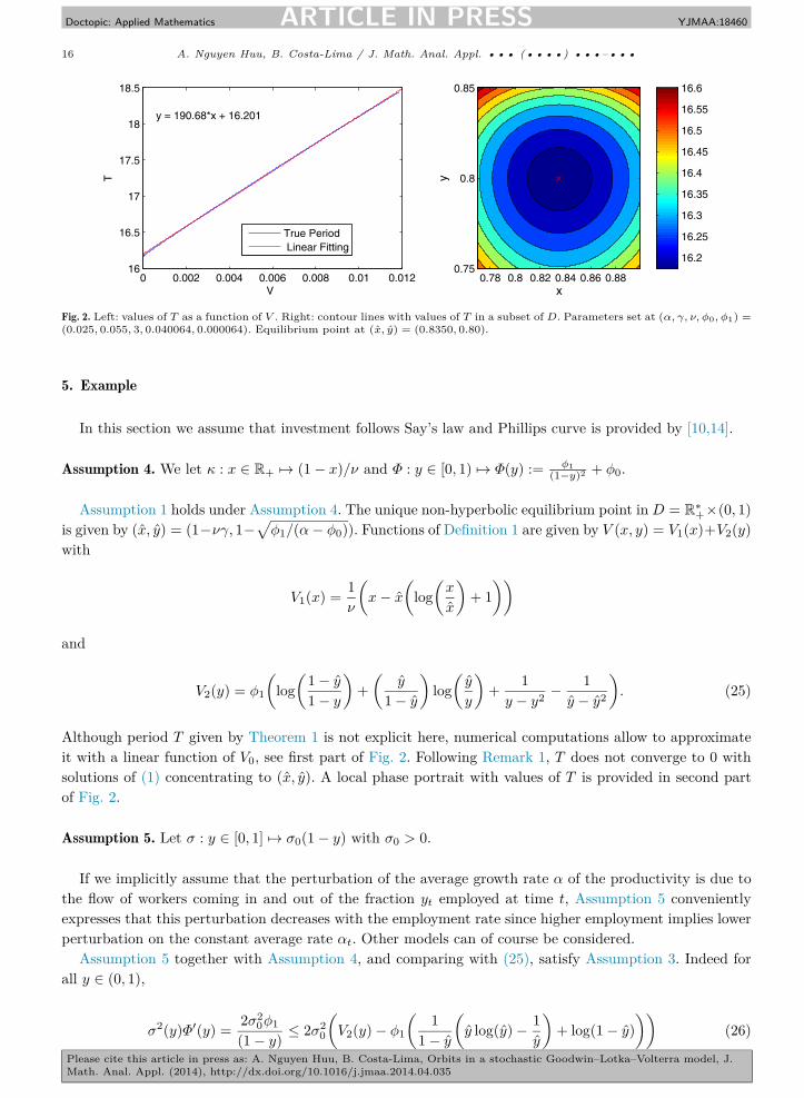
Fig. 2. Left: values of T as a function of V . Right: contour lines with values of T in a subset of D. Parameters set at (α, γ, ν, φ0, φ1) =(0.025, 0.055, 3, 0.040064, 0.000064). Equilibrium point at (x, y) = (0.8350, 0.80).

5. Example

In this section we assume that investment follows Say’s law and Phillips curve is provided by [10,14].

Assumption 4. We let κ : x ∈ R+ �→ (1 − x)/ν and Φ : y ∈ [0, 1) �→ Φ(y) := φ1(1−y)2 + φ0.

Assumption 1 holds under Assumption 4. The unique non-hyperbolic equilibrium point in D = R∗+×(0, 1)

is given by (x, y) = (1−νγ, 1−√φ1/(α− φ0)). Functions of Definition 1 are given by V (x, y) = V1(x)+V2(y)

with

V1(x) = 1ν

(x− x

(log

(x

x

)+ 1

))

and

V2(y) = φ1

(log

(1 − y

1 − y

)+

(y

1 − y

)log

(y

y

)+ 1

y − y2 − 1y − y2

). (25)

Although period T given by Theorem 1 is not explicit here, numerical computations allow to approximateit with a linear function of V0, see first part of Fig. 2. Following Remark 1, T does not converge to 0 withsolutions of (1) concentrating to (x, y). A local phase portrait with values of T is provided in second partof Fig. 2.

Assumption 5. Let σ : y ∈ [0, 1] �→ σ0(1 − y) with σ0 > 0.

If we implicitly assume that the perturbation of the average growth rate α of the productivity is due tothe flow of workers coming in and out of the fraction yt employed at time t, Assumption 5 convenientlyexpresses that this perturbation decreases with the employment rate since higher employment implies lowerperturbation on the constant average rate αt. Other models can of course be considered.

Assumption 5 together with Assumption 4, and comparing with (25), satisfy Assumption 3. Indeed forall y ∈ (0, 1),

σ2(y)Φ′(y) = 2σ20φ1 ≤ 2σ2

0

(V2(y) − φ1

(1

(y log(y) − 1

)+ log(1 − y)

))(26)

(1 − y) 1 − y y

JID:YJMAA AID:18460 /FLA Doctopic: Applied Mathematics [m3L; v 1.132; Prn:29/04/2014; 11:18] P.17 (1-20)A. Nguyen Huu, B. Costa-Lima / J. Math. Anal. Appl. ••• (••••) •••–••• 17

and along with the sub-linearity of the log function,

−κ(x) − xκ′(x) = 2x− 1ν

≤ 21 − x

(V1(x) + x− x log(x)

). (27)

In line with Assumptions 1 and 3 the vertical asymptote at y = 1 implies that σ2(y)Φ(y) ≤ K0V2(y) + k0for some K0, k0 ∈ R

2+. Under Assumption 3 and following (26) and (27), K0 = 0 and k0 = σ2

0(φ1 + φ0).Assumption 5 also implies that (1−y)2 is the root of a quadratic polynomial σ2

0(1−y)4−(α+φ0)(1−y)2+φ1 = 0. The latter shall have a unique root in (0, 1) to satisfy Assumption 2. The following example ofcondition is sufficient.

Assumption 6. We assume φ1 ≤ (α + φ0)/2 and σ0 ≤ max{(α + φ0)/(2√φ1 ), (α + φ0 − φ1)}.

We are now able to claim the existence of K, k ∈ R2+ such that |R(V0, ρ)| ≤ K(V0 + ρ) + k, where R is

defined in Proposition 4. A direct application provides

R(V0, ρ) := maxD(V0,ρ)

{σ2

0(1 − y)2(

2x− x

ν+ 2φ1y

(1 − y)3 + φ1

(1 − y)2 − φ1

(1 − y)2

)}.

Using (27), this estimate becomes |R(V0, ρ)| ≤ K(V0 +ρ)+k where K := (2σ20)/(1− x) and k is an explicitly

calculable constant. Following the same procedure with (26), I(V0, ρ) ≤ K(V0 + ρ)2 + k′ with the same K

and k′ = k. Now choosing μ = (ρ− (K(V0 +ρ)+k)θ/2)/√θ for some θ ≥ 0, so that Θ(ρ) = θ, Proposition 4

provides

P[τρ > θ] ≥(

1 − (K(V0 + ρ)2 + k′)θ(12 (K(V0 + ρ) + k)θ − ρ)2

).

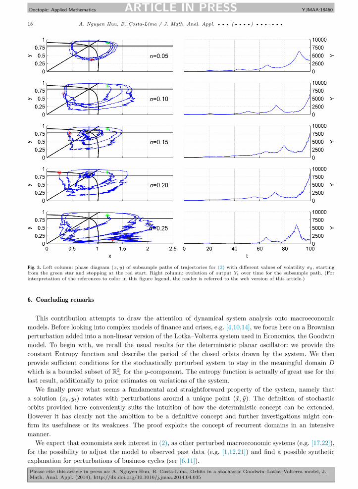
Theorem 5 is a straightly observable phenomenon with simulations, see Fig. 3. Under the assumptionsof this section, the system has been simulated using XPPAUT with a fourth order Runge–Kutta schemefor the deterministic part, and an Euler scheme for the Brownian part. Fig. 3 illustrates the effect of thevolatility level σ0 on trajectories of the system, as for the economic quantity Yt := atytNt.

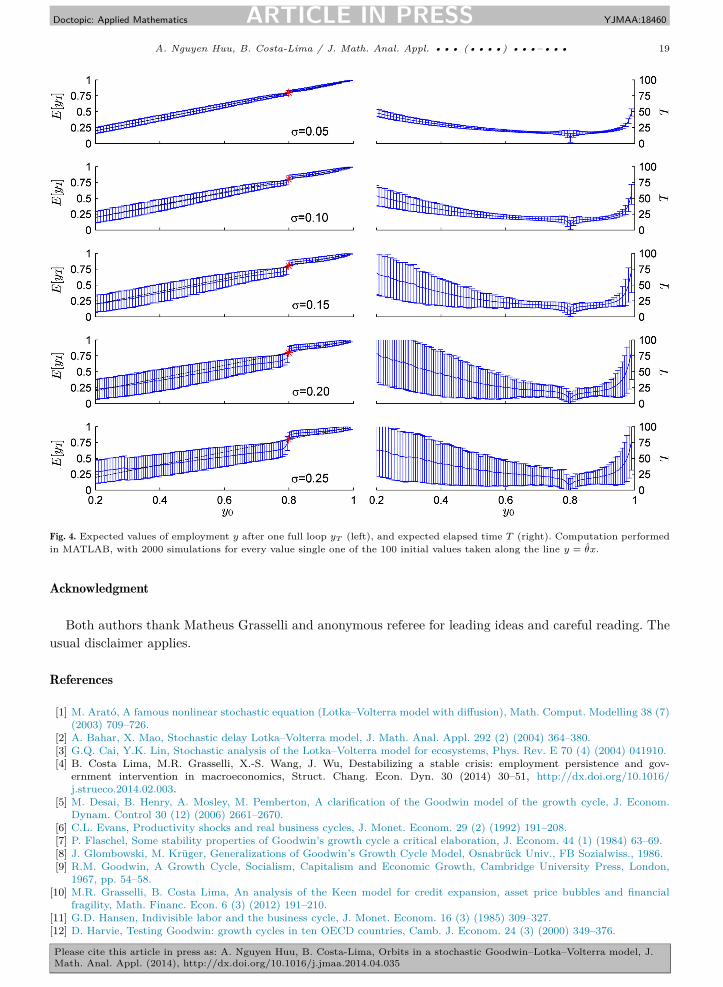
Apart from specific subregions of D as R1 or R5 where Corollary 3.2 in [15] can provide an estimatefor the expectation of the exit time, a bound for the expected period E[S] seems out of reach. Numericalsimulations have nevertheless always provide reasonable finite periods of stochastic orbits of (2). We thusexpect that E[S] is finite for a wide range of values of (x0, y0) ∈ D. Let us start with (x0, y0) ∈ R1 ∩R8 andreformulate S of Definition 2 as the time the process crosses the line y = θx for the second time. This isequivalent to take (x0, y0) ∈ R4 ∩R5. Resorting to numerical methods, we have simulated the system 2000times for 100 different starting points in R1 ∩ R8 and recorded the position at the time when this line iscrossed the second time, that is the positions after a full loop. Fig. 4 contains such examination for an arrayof values of σ0. The expected time E[S] to complete a full-loop is also illustrated. As observed, there seemsto be a stable attractive fixed point to y0 �→ E[yS ] for sufficiently large values of σ0. If the starting point ispicked too close to (x, y), the expected crossing value after one loop is further away from it. On the otherhand, if the one starts extremely far away from (x, y), say with y0 < 0.25, then the expected value after onloop is higher. This implies that after many loops, the expectation converges, and so does E[S] with thenumber of loops around (x, y). Assuming that E[S] < +∞ for enough initial points, Theorem 6 can be usedwith V at points (0, 0) and (x, y) to prove the following conjecture.

Conjecture 1. Consider the function S : y ∈ (0, y) �→ E[yS ] ∈ (0, y) such that (xt, yt) is a solution to (2)with (x0, y0) = (y/θ, y), and S is the finite stopping time defined by Theorem 5. Then S has at least onefixed point in (0, y).

JID:YJMAA AID:18460 /FLA Doctopic: Applied Mathematics [m3L; v 1.132; Prn:29/04/2014; 11:18] P.18 (1-20)18 A. Nguyen Huu, B. Costa-Lima / J. Math. Anal. Appl. ••• (••••) •••–•••

Fig. 3. Left column: phase diagram (x, y) of subsample paths of trajectories for (2) with different values of volatility σ0, startingfrom the green star and stopping at the red start. Right column: evolution of output Yt over time for the subsample path. (Forinterpretation of the references to color in this figure legend, the reader is referred to the web version of this article.)

6. Concluding remarks

This contribution attempts to draw the attention of dynamical system analysis onto macroeconomicmodels. Before looking into complex models of finance and crises, e.g. [4,10,14], we focus here on a Brownianperturbation added into a non-linear version of the Lotka–Volterra system used in Economics, the Goodwinmodel. To begin with, we recall the usual results for the deterministic planar oscillator: we provide theconstant Entropy function and describe the period of the closed orbits drawn by the system. We thenprovide sufficient conditions for the stochastically perturbed system to stay in the meaningful domain D

which is a bounded subset of R2+ for the y-component. The entropy function is actually of great use for the

last result, additionally to prior estimates on variations of the system.We finally prove what seems a fundamental and straightforward property of the system, namely that

a solution (xt, yt) rotates with perturbations around a unique point (x, y). The definition of stochasticorbits provided here conveniently suits the intuition of how the deterministic concept can be extended.However it has clearly not the ambition to be a definitive concept and further investigations might con-firm its usefulness or its weakness. The proof exploits the concept of recurrent domains in an intensivemanner.

We expect that economists seek interest in (2), as other perturbed macroeconomic systems (e.g. [17,22]),for the possibility to adjust the model to observed past data (e.g. [1,12,21]) and find a possible syntheticexplanation for perturbations of business cycles (see [6,11]).

JID:YJMAA AID:18460 /FLA Doctopic: Applied Mathematics [m3L; v 1.132; Prn:29/04/2014; 11:18] P.19 (1-20)A. Nguyen Huu, B. Costa-Lima / J. Math. Anal. Appl. ••• (••••) •••–••• 19

Fig. 4. Expected values of employment y after one full loop yT (left), and expected elapsed time T (right). Computation performedin MATLAB, with 2000 simulations for every value single one of the 100 initial values taken along the line y = θx.

Acknowledgment

Both authors thank Matheus Grasselli and anonymous referee for leading ideas and careful reading. Theusual disclaimer applies.

References

[1] M. Arató, A famous nonlinear stochastic equation (Lotka–Volterra model with diffusion), Math. Comput. Modelling 38 (7)(2003) 709–726.

[2] A. Bahar, X. Mao, Stochastic delay Lotka–Volterra model, J. Math. Anal. Appl. 292 (2) (2004) 364–380.[3] G.Q. Cai, Y.K. Lin, Stochastic analysis of the Lotka–Volterra model for ecosystems, Phys. Rev. E 70 (4) (2004) 041910.[4] B. Costa Lima, M.R. Grasselli, X.-S. Wang, J. Wu, Destabilizing a stable crisis: employment persistence and gov-

ernment intervention in macroeconomics, Struct. Chang. Econ. Dyn. 30 (2014) 30–51, http://dx.doi.org/10.1016/j.strueco.2014.02.003.

[5] M. Desai, B. Henry, A. Mosley, M. Pemberton, A clarification of the Goodwin model of the growth cycle, J. Econom.Dynam. Control 30 (12) (2006) 2661–2670.

[6] C.L. Evans, Productivity shocks and real business cycles, J. Monet. Econom. 29 (2) (1992) 191–208.[7] P. Flaschel, Some stability properties of Goodwin’s growth cycle a critical elaboration, J. Econom. 44 (1) (1984) 63–69.[8] J. Glombowski, M. Krüger, Generalizations of Goodwin’s Growth Cycle Model, Osnabrück Univ., FB Sozialwiss., 1986.[9] R.M. Goodwin, A Growth Cycle, Socialism, Capitalism and Economic Growth, Cambridge University Press, London,

1967, pp. 54–58.[10] M.R. Grasselli, B. Costa Lima, An analysis of the Keen model for credit expansion, asset price bubbles and financial

fragility, Math. Financ. Econ. 6 (3) (2012) 191–210.[11] G.D. Hansen, Indivisible labor and the business cycle, J. Monet. Econom. 16 (3) (1985) 309–327.[12] D. Harvie, Testing Goodwin: growth cycles in ten OECD countries, Camb. J. Econom. 24 (3) (2000) 349–376.

JID:YJMAA AID:18460 /FLA Doctopic: Applied Mathematics [m3L; v 1.132; Prn:29/04/2014; 11:18] P.20 (1-20)20 A. Nguyen Huu, B. Costa-Lima / J. Math. Anal. Appl. ••• (••••) •••–•••

[13] S.B. Hsu, A remark on the period of the periodic solution in the Lotka–Volterra system, J. Math. Anal. Appl. 95 (2)(1983) 428–436.

[14] S. Keen, Finance and economic breakdown: modeling Minsky’s financial instability hypothesis, J. Post Keynes. Econom.17 (4) (1995) 607–635.

[15] R.Z. Khasminskii, Stochastic Stability of Differential Equations, second ed., Springer-Verlag, Berlin, Heidelberg, 2012.[16] R.Z. Khasminskii, F.C. Klebaner, Long term behavior of solutions of the Lotka–Volterra system under small random

perturbations, Ann. Appl. Probab. 11 (3) (2001) 952–963.[17] E. Kiernan, D.B. Madan, Stochastic stability in macro models, Economica (1989) 97–108.[18] M. Liu, K. Wang, Stochastic Lotka–Volterra systems with Lévy noise, J. Math. Anal. Appl. 410 (2) (2014) 750–763.[19] X. Mao, G. Marion, E. Renshaw, Environmental Brownian noise suppresses explosions in population dynamics, Stochastic

Process. Appl. 97 (2002) 95–110.[20] X. Mao, S. Sabanis, E. Renshaw, Asymptotic behaviour of the stochastic Lotka–Volterra model, J. Math. Anal. Appl.

287 (1) (2003) 141–156.[21] S. Mohun, R. Veneziani, Goodwin cycles and the US economy, 1948–2004, 2006.[22] M. Neamtu, G. Mircea, M. Pirtea, D. Opris, The study of some stochastic macroeconomic models, in: Proceedings of the

11th WSEAS International Conference on Applied Computer and Applied Computational Science, 2012, pp. 172–177.[23] D. Nguyen Huu, S. Vu Hai, Dynamics of a stochastic Lotka–Volterra model perturbed by white noise, J. Math. Anal.

Appl. 324 (1) (2006) 82–97.[24] T. Reichenbach, M. Mobilia, E. Frey, Coexistence versus extinction in the stochastic cyclic Lotka–Volterra model, Phys.

Rev. E 74 (5) (2006) 051907.[25] U.H. Thygesen, A survey of Lyapunov techniques for stochastic differential equations, IMM, Department of Mathematical

Modeling, Technical University of Denmark, 1997, working paper, available at http://www.imm.dtu.dk.[26] K. Velupillai, Some stability properties of Goodwin’s growth cycle, J. Econom. 39 (3) (1979) 245–257.[27] R. Veneziani, S. Mohun, Structural stability and Goodwin’s growth cycle, Struct. Chang. Econ. Dyn. 17 (4) (2006) 437–451.[28] C. Zhu, G. Yin, On hybrid competitive Lotka–Volterra ecosystems, Nonlinear Anal. 71 (12) (2009) 1370–1379.