Determine dynamical behaviors by the Lyapunov function in competitiveLotka-Volterra systems

Ying Tang,1, 2, ∗ Ruoshi Yuan,3 and Yian Ma3

1ZhiYuan college, Shanghai Jiao Tong University, China2Shanghai Center for Systems Biomedicine, Shanghai Jiao Tong University, China

3Department of Computer Science and Engineering, Shanghai Jiao Tong University, China(Dated: October 30, 2012)

Global dynamical behaviors of the competitive Lotka-Volterra system even in 3-dimension are notfully understood. The Lyapunov function can provide us such knowledge once it is constructed. Inthis paper, we construct explicitly the Lyapunov function in three examples of the competitive Lotka-Volterra system for the whole state space: (1) the general 2-dimensional case; (2) a 3-dimensionalmodel; (3) the model of May-Leonard. The dynamics of these examples include bistable caseand cyclical behavior. The first two examples are the generalized gradient system defined in theAppendixes, while the model of May-Leonard is not. Our method is helpful to understand the limitcycle problems in general 3-dimensional case.

PACS numbers: 02.30.Hq, 87.23.Kg, 05.45.-a

I. INTRODUCTION

Lotka-Volterra system is one of the most fundamentalmodels describing the interaction of n species in mathe-matical ecology [1], physics and economics [2]. It is givenby the following ordinary differential equations:

Definition 1 (Lotka-Volterra system).

xi = xi

bi − n∑j=1

aijxj

, i = 1, . . . , n, (1)

where each xi(i = 1, · · · , n) represents the population ofone species and bi, aij(i = 1, · · · , n; j = 1, · · · , n) areconstants depending on the environment. The state spaceof the system (1) is represented by the non-negative vec-tors Rn+ = {(x1, · · · , xn) ∈ Rn|xi ≥ 0, i = 1, · · · , n}.When bi > 0, aij > 0(i = 1, · · · , n), it is the competitiveLotka-Volterra system.

Due to the nonlinear attributes of the competitiveLotka-Volterra system, its dynamics can be complexwhen n ≥ 3, such as cyclical behavior [3] and chaoticbehavior [4]. M. Hirsch has proved any trajectory of a n-dimensional competitive Lotka-Volterra system will con-verge to an invariant surface Σ, homeomorphic to (n−1)-

dimensional unit simplex ∆ = xi : xi ≥ 0,∑n−1i=1 xi = 1.

In 3-dimensional case, following M. Hirsch’s generalresult, M. L. Zeeman identified 33 stable equivalenceclasses, of which only classes 26 − 31 can have limit cy-cles. Then in [5], D. Xiao and W. Li proved the numberof limit cycles is finite without a heteroclinic polycycle.In [6], J. Hofbauer and J. So conjectured the number oflimit cycles is at most two. Nevertheless, three limit cy-cles were constructed numerically in [7, 8] and four in[9, 10]. M. L. Zeeman also tried to deduce global dy-namics by the edges of the carrying simplex [11, 12]. Till

now, however, the question of how many limit cycles canappears in M. L. Zeeman’s six classes 26 − 31 remainsopen.

To analyze global dynamics, M. Planck studied theLotka-Volterra system by hamiltonian theory, however,in limited parameter region [13]. The split Lyapunovfunction has been used [14], but it is not monotone alongall the trajectories in the state space, hence constructedlocally. Besides, the classical Lyapunov function has alsobeen constructed for n-dimensional case in the parameterregion with one global stable equilibrium [15, 16]. Asthere is no general way of constructing the Lyapunovfunction [17], this theory has not been explored more tostudy the competitive Lotka-Volterra system.

In this paper, based on the framework of general dy-namics recently proposed in [18, 19], we construct theLyapunov function in three examples of the compet-itive Lotka-Volterra system. This Lyapunov functionis monotone along trajectories in the state space, thuscan demonstrate global dynamics. The first example isthe general 2-dimensional case [15]. The second is a 3-dimensional system given by [15] and the constructionmethod is the same with the first’s as both are the gen-eralized gradient system defined in the Appendixes. Thethird example is the classical May-Leonard 3-dimensionalsystem [3]. As it is not the generalized gradient system,we provide there a different construction method.

This paper is organized as follows. In Sec. II, weuniformly construct the Lyapunov function for the 2-dimensional model, and analyze its dynamics in the statespace. In Sec. III, we study the 3-dimensional competi-tive Lotka-Volterra system given by [15]. In Sec. IV, westudy the model of May-Leonard. In Sec. V, we summa-rize our work. In the Appendixes, we introduce brieflyour construction framework, discuss the generalized gra-dient system, and then give detailed calculation on otherdynamical parts in our framework of the three examples.

arX

iv:1

210.

7662

v1 [

q-bi

o.PE

] 2

9 O

ct 2

012

2

II. THE GENERAL 2-DIMENSIONALCOMPETITIVE LOTKA-VOLTERRA SYSTEM

Example 1. The general 2-dimensional competitiveLotka-Volterra system is given by:{

x1 = x1(b1 − x1 − αx2)x2 = x2(b2 − βx1 − x2)

, (2)

where b1, b2, α, β are non-negative constants [15].By setting x1 = x2 = 0, four non-negative equi-libriums are derived: (1) a positive one E++ =(b1 − αb2, b2 − βb1) /(1 − αβ) existing when α < b1/b2,β < b2/b1 or α > b1/b2, β > b2/b1; (2) E+0 = (b1, 0);(3) E0+ = (0, b2); (4) E00 = (0, 0). Here the subscript +denotes the population of the species is positive and thesubscript 0 means the species dies out.

A. Construction of the Lyapunov function

Now we introduce our method to construct the Lya-punov function of the system. This method is based onthe framework in [18, 19]. The idea is as follows. Assumethere is a Lyapunov function φ and its partial derivativeis given by(

∂φ∂x1∂φ∂x2

).= −

(A11(x1, x2) A12(x1, x2)A21(x1, x2) A22(x1, x2)

)(x1x2

),

where A11(x1, x2), A12(x1, x2), A21(x1, x2), A22(x1, x2)are undetermined coefficients. Our aim is to chooseproper coefficients so that: (1)∇ × ∇φ = 0; (2)φ ≤ 0,i.e., Lie derivative of φ decreasing along trajectories.

We discover that A11(x1, x2) = β/x1, A12(x1, x2) = 0,A21(x1, x2) = 0, A22(x1, x2) = α/x2 is a proper setting.Thus we get {

∂φ∂x1

= −β(b1 − x1 − αx2)∂φ∂x2

= −α(b2 − βx1 − x2). (3)

With direct calculation, ∇×∇φ = 0 and

φ =∂φ

∂x1x1 +

∂φ

∂x2x2

= −βx1(b1 − x1 − αx2)2 − αx2(b2 − βx1 − x2)2 ≤ 0 ,

as x1 and x2 are all non-negative population species andβ and α are all non-negative constants. φ(x) = 0 hap-pens only at x ∈ ∪s∈R2

+ω(s), where ω(s) denotes the

ω-limit set [20]. Thus, we can get a Lyapunov functionby integrating the Eq. (3):

φ =β

2x21 +

α

2x22 − βb1x1 − αb2x2 + αβx1x2 . (4)

Here we mention that the choice on the coefficientsA11(x1, x2), A12(x1, x2), A21(x1, x2), A22(x1, x2) is notunique. Our choice is straightforward and meets the re-quirements.

B. Analysis on dynamics in the state space

In this subsection, we give a classified discussion ondynamics in each parameter region by the Hessian matrix

of the Lyapunov function at E++. As ∂2φ∂x2

1= β, ∂2φ

∂x22

=

α, ∂2φ∂x1∂x2

= ∂2φ∂x2∂x1

= αβ, we find the determinant ofHessian matrix:

∆.=∂2φ

∂x21

∂2φ

∂x22−(

∂2φ

∂x1∂x2

)2

= αβ(1− αβ) . (5)

Thus, the type of dynamics can be classified into fourcases:

(1) Stable coexistence case: α < b1/b2, β < b2/b1.

∆ > 0 and ∂2φ∂x2

1> 0 indicate E++ is a globally stable

equilibrium with the minimum energy value.

(2) Bistable case: α > b1/b2, β > b2/b1.

∆ < 0 indicates E++ is a saddle point. As the system(2) is bounded in the first quadrant, it has two stableequilibriums E+0 and E0+ on the boundary.

(3) One survival case: α < b1/b2, β > b2/b1 or α > b1/b2,β < b2/b1.

It has one globally stable equilibrium on an axis ofcoordinate, E+0 appears when α < b1/b2, β > b2/b1or E0+ appears when α > b1/b2, β < b2/b1. We justshow the case where the species x1 survives in Fig. 1,i.e., when α < b1/b2, β > b2/b1. The case where thespecies x2 survives can be shown similarly.

(4) Degenerate case: α = b1/b2, β = b2/b1.

The Lyapunov function has the minimum value alongthe line:√b1b2 −

√b2/b1x1 −

√b1/b2x2 = 0 as in this case

φ =1

2

(√b1b2 −

√b2/b1x1 −

√b1/b2x2

)2− b1b2 . (6)

Each trajectory will converge to one of the points onthe line, depending on the initial value.

Four remarks are made here:

• Our result on dynamics of the system is consistentwith the stability analysis near equilibriums in [15].Additionally, our Lyapunov function is constructeduniformly for the whole parameter space and thuscan provide dynamics for any perturbation on theparameters. Therefore, the criterion on the classi-fication on the type of dynamics due to parameterschanging can be based on the Lyapunov function:(1) when E++ exists, the Hessian matrix of theLyapunov function at E++ can show its type ofstability and we have the previous two cases; (2)when E++ does not exist, we have the case (3); (3)the remaining one is the case (4).

3

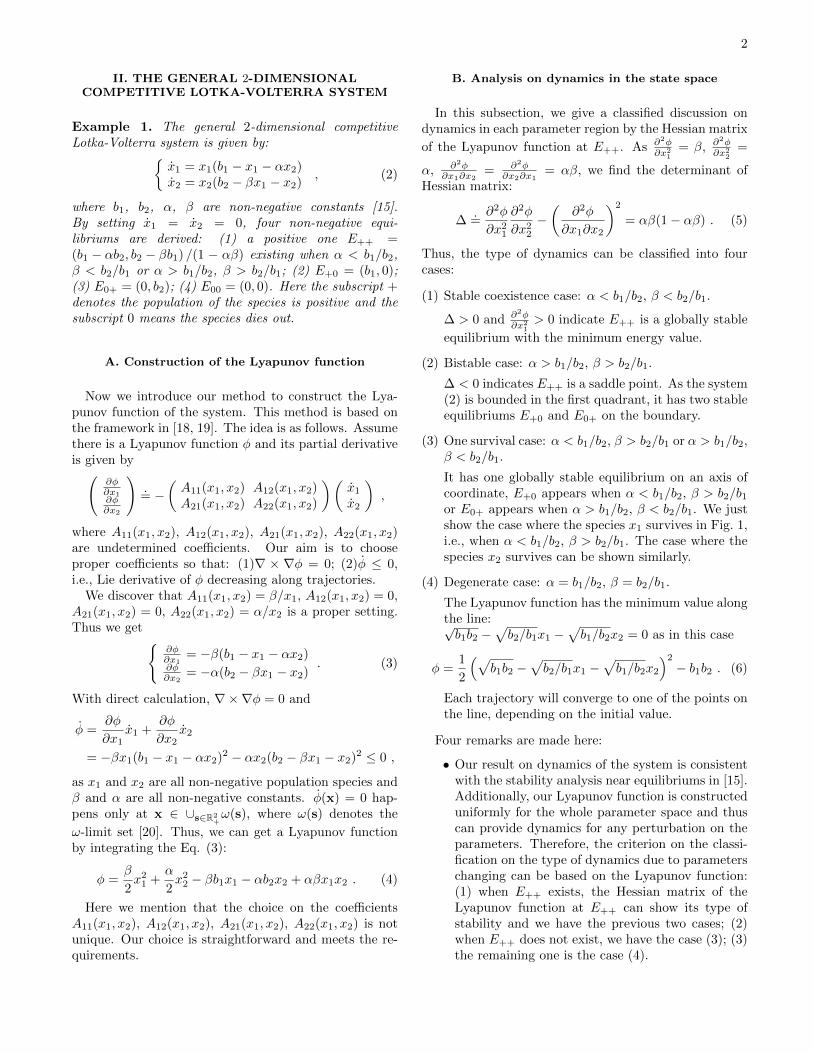
FIG. 1. The energy landscape of example (1) for the variouscases: (1) α = β = 1

2, b1 = b2 = 1: stable coexistence case;

(2) α = β = 2, b1 = b2 = 1: bistable case; (3) α = 12, β = 2,

b1 = b2 = 1: one survival case; (4) α = β = b1 = b2 = 1:degenerate case.

• Visualization with the energy landscape of the Lya-punov function (Fig. 1) provides a clear observationon dynamics in each case above: Fig. 1’s case (1)to case (4) relate to these cases (1) to (4) discussedabove respectively. Saddle-node bifurcation can beobserved from this energy landscape. The bifurca-tion happens from the case (1) to the case (2) andthe degenerate case (4) has the minimum energyvalue on a line.

• We show here the dynamics of the system can di-rectly be determined by the Lyapunov functionalone. In [21], M. L. Zeeman used the Lyapunovfunction to prove that the stable nullcline classescoincide with the stable topological classes in thissystem.

• In the Appendixes, we will define the general-ized gradient system, as a natural generalizationto typical gradient system. We thus find this 2-dimensional system meet the definition. Further-more, the construction method can be applied tothe generalized gradient system in n-dimension,and we will show a 3-dimensional example in nextsection.

III. A 3-DIMENSIONAL MODEL

Following the definition of the generalized gradient sys-tem in the Appendixes, we find that a 3-dimensional com-

petitive Lotka-Volterra system given by [15] is anotherone and thus we construct the Lyapunov function by thesame method as the last section’s.

Example 2. x1 = x1 (1− x1 − αx2)x2 = x2 (1− βx1 − x2 − βx3)x3 = x3 (1− αx2 − x3)

, (7)

where α, β are non-negative coefficients. By setting x1 =x2 = x3 = 0, non-negative equilibriums are derived: (1)a positive one E+++ = (1− α, 1− 2β, 1− α) /(1− 2αβ)existing when (1 − α)/(1 − 2αβ) > 0 and (1 − 2β)/(1 −2αβ) > 0; (2) E+0+ = (1, 0, 1); (3) E0+0 = (0, 1, 0); (4)E000 = (0, 0, 0).

A. Construction of the Lyapunov function

With the similar method used in the general 2-dimensional competitive Lotka-Volterra system, wechoose the corresponding undetermined matrix to be β/x1 0 0

0 α/x2 00 0 β/x3

,

then ∂φ∂x1

= −β (1− x1 − αx2)∂φ∂x2

= −α (1− βx1 − x2 − βx3)∂φ∂x3

= −β (1− αx2 − x3)

. (8)

Since ∇×∇φ = 0 and the Lie derivative of φ is

φ =− βx1 (1− x1 − αx2)2 − αx2 (1− βx1 − x2 − βx3)

2

− βx3 (1− αx2 − x3)2 ≤ 0 ,

as x1, x2 and x3 are all non-negative population speciesand β and α are all non-negative constants. φ(x) = 0happens only at x ∈ ∪s∈R3

+ω(s). We can construct a

Lyapunov function by integrating the Eq. (8).

φ =β

2(x21+x23)+

α

2x22+αβ(x1x2+x2x3)−β(x1+x3)−αx2 .

(9)

B. Analysis on dynamics in the state space

With the Lyapunov function constructed globally onR3

+, first the classified stability analysis near equilibriumsby [15] can be unified now. Second, when α = 1 andβ = 1/2,

φ =1

4

[(x1 + x2 − 1)2 + (x2 + x3 − 1)2 − 2

](10)

4

indicates the degenerate case of the system has the mini-mum energy on the intersection of the surfaces x1 +x2−1 = 0 and x2+x3−1 = 0. Third, as it is a generalized gra-dient system without a trajectory contouring along theenergy landscape of the Lyapunov function, the system(7) does not have a limit cycle [19].

IV. THE MODEL OF MAY-LEONARD

In [3], R. May and W. Leonard studied a 3-dimensionalcompetitive Lotka-Volterra system.

Example 3. x1 = x1 (1− x1 − αx2 − βx3)x2 = x2 (1− βx1 − x2 − αx3)x3 = x3 (1− αx1 − βx2 − x3)

, (11)

where α, β are non-negative coefficients. The possi-ble equilibriums contain: (1)(0, 0, 0); (2) three single-population survive (1, 0, 0), (0, 1, 0), (0, 0, 1); (3) three

two-population solutions of the form (1−α,1−β,0)1−αβ ; (4) and

three-population survive (1,1,1)1+α+β .

A. Construction of the Lyapunov function

We find that this model is not the generalized gradientsystem, and thus the construction method in Sec. II cannot be applied here. So we will give another method toconstruct the Lyapunov function in this section.

For convenience, let us introduce some new variables:γ = α+ β − 2, P = x1x2x3 and O = x1 + x2 + x3. Then

P = x1x2x3 + x1x2x3 + x1x2x3

= P [3− (1 + α+ β)O]

= P [3− (3 + γ)O]

= P [3(1−O)− γO] ,

and

O = x1 + x2 + x3

= O −[x21 + x22 + x23 + (α+ β)(x1x2 + x2x3 + x3x1)

]= O(1−O)− γ(x1x2 + x2x3 + x3x1),

where the P and O denotes the Lie derivative of P and Orespectively. Next, we construct the Lyapunov functionin two different parameter regions: (1)γ = 0; (2)γ 6= 0.

1. When γ = 0:

Noting that P = 3P (1 − O) and O = O(1 − O),thus

− PP

+ 3O = −3(1−O)2 ≤ 0. (12)

So if we can a function whose Lie derivative is−P /P + 3O, then it is a Lyapunov function. Thiscan be done by simply integrate −P /P + 3O andwe get a Lyapunov function

φ = 3O − lnP (13)

= 3(x1 + x2 + x3)− ln(x1x2x3). (14)

φ = 0 only when O− 1 = 0, i.e., all the trajectoriesconverge to the plane O = 1.

2. When γ 6= 0:

Noting that O = O(1−O)−γ(x1x2 +x2x3 +x3x1)and P = P [3(1−O)− γO], thus

γ[PO − 3OP

]= γ

[3PO(1−O)− γPO2 − 3PO(1−O)

+ 3γP (x1x2 + x2x3 + x3x1)]

= −γ2P[O2 − 3(x1x2 + x2x3 + x3x1)

]= −γ2P

[x21 + x22 + x23 − (x1x2 + x2x3 + x3x1)

]= −γ

2P

2

[(x1 − x2)2 + (x2 − x3)2 + (x3 − x2)2

]≤ 0.

So we need to find a function whose Lie derivativeis γ

[PO − 3OP

]. We notice that we can not in-

tegrate it directly, however, we find out that thefunction

φ = γP

O3(15)

has the Lie derivative

φ = γPO − 3OP

O4≤ 0. (16)

As a result, we get a Lyapunov function. φ = 0 canhappen at a point on the line x1 = x2 = x3 or inthe set (x1, x2, x3)|P = 0.

B. Analysis on dynamics in the state space

With the Lyapunov function constructed in the lastsubsection, we discuss dynamics in classified parameterspace of the system here.

1. γ = 0:

As φ = 0 only on the plane O = 1, all the tra-jectories will converge to this plane. Besides, onthis plane, the value of the Lyapunov functionφ = 3 + lnP will be a constant. Thus for eachtrajectory on the plane, the value of P will be a

5

constant. This means that the limit set for any ini-tial point will be the intersection of the plane O = 1and the hyperboloid that P equals to a constant,which is a cycle on the plane.

2. γ < 0:

As φ = γ PO3 is non-positive now, the minimum

value of φ will not be zero if its initial value isnot. Thus, in order to minimize the value of theLyapunov function, all the trajectory will convergeto one point on the line x1 = x2 = x3. So this casehas a global stable equilibrium.

3. γ > 0:

As φ = γ PO3 is non-negative now, the minimum

value of φ will be zero. That is, all the trajectorywill converge to the set (x1, x2, x3)|P = 0. In theneighborhood of P = 0, the terms of order x1x2,etc., in O asymptotically make a negligible contri-bution [3]. Thus O = O(1 − O) leads to O → 1 inthe end. Finally, the limit set in this case is the set(x1, x2, x3)|P = 0, O = 1.

Three remarks are made here:

• Our result is consistent with that in [3]. Further-more, we give a full description on dynamics for thewhole state space with the Lyapunov function. Theenergy landscape of the Lyapunov function on theplane x1 + x2 + x3 (Fig. 2) gives a direct observa-tion on dynamics: (1)when γ = 0, Fig. 2’s case(1) shows the system has hamiltonian structure;(2)when γ > 0, Fig. 2’s case (2) shows the systemhas a global stable equilibrium; (3)when γ < 0,Fig. 2’s case (3) shows the limit set of the systemis (x1, x2, x3)|P = 0, O = 1.

• A similar analytic form of the Lyapunov functionhave been constructed when γ > 0 in [22, 23]. Com-pared with theirs, our construction is for the wholeparameter space. Besides, we here provide a ex-plicit method to find this Lyapunov function.

• In [24], C. W. Chi study the asymmetric May-Leonard system. Our construction method heremay be able to be generalized to their system.

V. CONCLUSION

We have demonstrated that the Lyapunov functioncan be constructed in general 2-dimensional and two3-dimensional competitive Lotka-Volterra systems. Foreach example, we have shown dynamics in the whole statespace with the Lyapunov function. The 2-dimensionalcase includes the bistable case and the model of May-Leonard has cycles as its limit set. Besides, in the

Appendixes, we have defined the generalized gradientsystem and discussed its coherence and generality withthe classical gradient system. Furthermore, we noticethat the construction method used in the model of May-Leonard may be able to be generalized to the asymmetricMay-Leonard system in [24]. Thus the Lyapunov func-tion can be helpful to solve the limit cycle problems ingeneral 3-dimensional case.

ACKNOWLEDGMENT

The authors would like to express their sincere grati-tude for the helpful discussions with Ping Ao, Bo Yuan,Xinan Wang, Song Xu, Siyun Yang, Tianqi Chen andJianghong Shi. This work was supported in part bythe National 973 Projects No. 2010CB529200 and by theNatural Science Foundation of China No. NFSC61073087and No. NFSC91029738.

APPENDIXES

In the Appendixes, we first give the definition of theLyapunov function and the construction framework inthe Appendix I. Then we introduce the generalized gra-dient system in the Appendix II. Finally in the AppendixIII, we give detailed calculation on all the dynamicalparts in our framework of the third example.

APPENDIX I. THE LYAPUNOV FUNCTION

Definition 2. A smooth dynamical system is given by

x = f(x) , (17)

where x = (x1, · · · , xn) with x1, · · · , xn the n Cartesiancoordinates of the state space, x = dx/dt and f : Rn 7→Rn.

The conventional Lyapunov function for a given system(17) is defined as:

Definition 3 (Conventional Lyapunov Function). [20]Let L : O → R be a C1 function, where O is an open

set in Rn. L is a conventional Lyapunov function of thesystem (17) on O if

• for a specified equilibrium x∗ in O, L(x∗) = 0 andL(x) > 0 when x 6= x∗;

• L(x) = dLdt |x 6 0 for all x ∈ O.

La Salle has extended the conventional Lyapunov func-tion to include stable region by abandoning the positivedefinite requirement, but his generalization is too roughto lose stability information inside the stable region.

6

FIG. 2. The energy landscape of example (3) on the plane O = 1: (1) γ = 0; (2) γ = −0.1 < 0; (3) γ = 0.1 > 0.

Definition 4 (La Salle’s Lyapunov Function). [25]Let L : O → R be a C1 function, where O is an open

set in Rn. L is a La Salle’s Lyapunov function of thesystem (17) on O if L(x) = dL

dt |x 6 0 for all x ∈ O.

Following the Lyapunov function used in [18, 19], herewe give a more precise definition on the Lyapunov func-tion.

Definition 5 (Lyapunov Function). Let φ : Rn 7→ R be aC1 function. φ is a Lyapunov function of the system (17)if φ(x) = dφ

dt |x 6 0 for all x ∈ Rn and φ(x) = 0 only whenx belongs to the union of the ω-limit sets ∪s∈Rnω(s).

In the following, we will briefly introduce our construc-tion framework. It is recently discovered during the studyon the stability problem of a genetic switch [18, 26] andhas been found wildly useful in biology [27]. The keyresult of the framework is a transformation from the ndimensional system (17) to the vector differential equa-tion (for simplicity, we only discuss the deterministic casein this paper, with noise strength being zero, general re-sults with randomness can be found in [18]):

[S(x) + T (x)] x = −∇φ(x) . (18)

Here φ is a scalar function, the Lyapunov function. Sis a semi-positive definite and symmetric matrix. T is aantisymmetric matrix.

Symmetrically, if (S + T ) is nonsingular, the Eq. (18)can be rewritten as a reverse form

x = − [D(x) +Q(x)]∇φ(x) , (19)

whereD is a semi-positive definite and symmetric matrix,Q is a antisymmetric matrix.

From a physical point of view, S can be explained asa frictional force indicating dissipation of the potentialenergy, T as a Lorentz force and φ as a potential of thesystem influenced by the two forces. Symbol D denotes

the diffusion matrix indicating the random driving force,therefore for deterministic systems, D is free to choose.

We make four remarks here:

• As φ = xτ∇φ = −xτ [S + T ]x = −xτSx ≤ 0,where τ denotes transpose, φ in the Eq. (18) canbe a Lyapunov function.

• In this decomposition of the dynamical system, Scan be considered as gradient part and T as rota-tional part. When S = 0, it is a conserved sys-tem with first integral. If T is a scalar matrix atthe same time, it is a Hamiltonian system wherethe trajectory would be a contour along the energylandscape of the Lyapunov function. When T = 0,it is a generalized gradient system defined in thenext section. Thus both S and T can provide dy-namical information for a given system.

• If the explicit form of the Lyapunov function isnot obtained yet for a given system, such as thethird example, we can solve the Eq. (19) by choos-ing a suitable form of D (or S) to make φ satisfy∇×∇φ = 0 and φ ≤ 0. Here ∇× is a matrix gen-eralization of the “curl operator in 3 dimension”:(∇× x)ij

.= ∂ixj − ∂j xi. We have constructed the

Lyapunov function by this method in the first twoexamples.

• If one already has a Lyapunov function for a givensystem, we can obtain other dynamical parts [19]:

S = −∇φ · ff · f

I , (20)

T = −∇φ× f

f · f. (21)

The corresponding explicit expression of the diffu-sion matrix D and the antisymmetric matrix Q can

7

be provided as well:

D = −

[f · f∇φ · f

I +(∇φ× f)

2

(∇φ · f) (∇φ · ∇φ)

], (22)

Q =∇φ× f

∇φ · ∇φ. (23)

APPENDIX II. GENERALIZED GRADIENTSYSTEM

A. Definition

Definition 6 (Generalized Gradient System). A gener-alized gradient system on Rn is a dynamical system ofthe form

x = −D(x)∇φ(x) , (24)

where φ : Rn 7→ R is a continuous differentiable scalarfunction and D(x) is a semi-positive definite and sym-metric matrix.

By definition, when D is the product of a nonzero con-stant and the identity matrix, it degenerates to the clas-sical gradient system in [20]. The potential gradient ofthe system (24) is anisotropic, different from that of thegradient system. Such anisotropic system has been ob-served in real systems, like the Fourier’s equation in [28].T = 0 is equivalent to Q = 0 as

T (x) =1

2

[(D(x) +Q(x))−1 − (D(x)−Q(x))−1

].

B. Matrices S, T , D and Q of the first two examples

For the given system (2) in Sec. II, it is not a gradientsystem as the curl of the vector field ∇×x = αx1−βx2 6=0. But we can calculate the matrices using the resultsobtained in Sec. II. A:

S =

(β/x1 0

0 α/x2

), T = 0,

D =

(x1/β 0

0 x2/α

), Q = 0.

D being semi-positive definite and symmetric and T = 0indicate that the system (2) is a generalized gradient sys-tem with zero rotational part, and trajectory will not con-tour along the energy landscape of the Lyapunov func-tion. Besides, S is singular only on the coordinate axis inthis system. It means the dissipation is infinite and thusthe trajectory will stay on the axis once reaching it andapproach the equilibrium E+0 = (b1, 0) or E0+ = (0, b2).

As for the system (26) in Sec. III, the matrices are

S =

β/x1 0 00 α/x2 00 0 β/x3

, T = 0,

D =

x1/β 0 00 x2/α 00 0 x3/β

, Q = 0.

C. Linear Cases

A linear autonomous dynamical system is given by thefollowing ordinary differential equations:

x = Fx , (25)

where x = (x1, · · · , xn) with x1, · · · , xn the n Cartesiancoordinates of the state space, x = dx/dt and F is a con-stant matrix. To ensure the independence of all the statevariables, we require the determinant of the F matrix tobe finite: det(F ) 6= 0.

To illustrate the coherence and generality of the gen-eralized gradient system in the linear cases, we firstmention that a linear system (25) is a gradient systemx = −∇φ if and only if its F matrix is symmetric:

• A gradient system x = −∇φ has ∂φ/∂xi =−Σnj=1Fijxj , then ∇×∇φ = 0 leads to the F ma-trix being symmetric;

• If a linear system (25) has a symmetric F matrix,then by setting ∂φ/∂xi = −Σnj=1Fijxj , the solutionof φ exists, and we can rewrite (25) as x = −∇φ.

But a linear system (25) can be a generalized gradientsystem when the F matrix is asymmetric. Such systemshave nonzero curl, that is ∇×x 6= 0. We give an exampleof 2 dimensional linear generalized gradient system in thefollowing.

Example 4. This example is given by [20]:(x1x2

)=

(0 31 −2

)(x1x2

). (26)

We set a Lyapunov function to be φ = x22−x1x2 as itsLie derivative

φ = −3x22 − (x1 − 2x2)2 ≤ 0 .

Then the system (26) can be rewritten as(x1x2

)= −

(3 00 1

)( ∂φ∂x1∂φ∂x2

). (27)

Therefore, the original system (26) is a generalized gra-dient system by definition, but not a gradient system asits F matrix is asymmetric.

8

III. MATRICES S AND T FOR THE MODEL OFMAY-LEONARD

In this section, we calculate S and T by the Eq. (20)for the model of May-Leonard system. In Sec. V, wehave obtained the Lyapunov function:

1. When γ = 0:

φ = 3O − lnP

= 3(x1 + x2 + x3)− ln(x1x2x3).

2. When γ 6= 0:

φ = γP

O3

= γx1x2x3

(x1 + x2 + x3)3.

Thus we do calculation separately for this two cases inthe following.

1. When γ = 0:

As ∂φ∂x1

= 3x1−1x1

∂φ∂x2

= 3x2−1x2

∂φ∂x3

= 3x3−1x3

, (28)

S = −∇φ · ff · f

I

=3[1− (x1 + x2 + x3)]2

x21 + x22 + x23I . (29)

Notice on the plane x1 + x2 + x3 = 1, S is zeromatrix, thus on the plane the system is conservedwhen γ = 0.

As for T :

T = −∇φ× f

f · f

= −

(3xi−1xi

xj − 3xj−1xj

xi

)3×3

x21 + x22 + x23. (30)

Since T is antisymmetric, we just need to calculatethe elements T12, T13 and T23 of the above 3 × 3matrix. As we have proved all the trajectory willconverge to the plane x1+x2+x3 = 1, we calculatethe elements on the plane below. We first calculateT12.

T12 =3x1 − 1

x1x2 −

3x2 − 1

x2x1

=3x1 − 1

x1(1− βx1 − x2 − αx3)x2

− 3x2 − 1

x2(1− x1 − αx2 − βx3)x1 . (31)

We notice that 1−α = −(1−β) = β−α2 in the case

of γ = 0. Thus we have

T12 =β − α

2

[x2x1

[(x1 − x2) + (x1 − x3)](x3 − x1)

+x1x2

[(x2 − x1) + (x2 − x3)](x3 − x2)]. (32)

We calculate T13 and T23 similarly.

T13 =3x1 − 1

x1x3 −

3x3 − 1

x3x1

=3x1 − 1

x1(1− αx1 − βx2 − x3)x3

− 3x3 − 1

x3(1− x1 − αx2 − βx3)x1

=β − α

2

[x3x1

[(x1 − x2) + (x1 − x3)](x1 − x2)

+x1x3

[(x3 − x1) + (x3 − x2)](x2 − x3)]. (33)

T23 =3x2 − 1

x2x3 −

3x3 − 1

x3x2

=3x2 − 1

x2(1− αx1 − βx2 − x3)x3

− 3x3 − 1

x3(1− βx1 − x2 − αx3)x2

=β − α

2

[x3x2

[(x2 − x1) + (x2 − x3)](x1 − x2)

+x2x3

[(x3 − x1) + (x3 − x2)](x3 − x1)]. (34)

Thus we calculate out each element of matrix T onthe plane x1 + x2 + x3 = 1.

2. When γ 6= 0:

As∂φ∂x1

= γ PO4 [x2x3(x1 + x2 + x3)− 3x1x2x3]

∂φ∂x2

= γ PO4 [x1x3(x1 + x2 + x3)− 3x1x2x3]

∂φ∂x3

= γ PO4 [x1x2(x1 + x2 + x3)− 3x1x2x3]

, (35)

S = −∇φ · ff · f

I

=

γ2P2O4

[(x1 − x2)2 + (x2 − x3)2 + (x3 − x2)2

]x21 + x22 + x23

I .

(36)

Since on the plane x1 + x2 + x3 = 1, Sis not zero matrix except on the limit set(x1, x2, x3)|P = 0, O = 1. Thus on the plane thesystem is dissipative when γ 6= 0.

9

As for T :

T = −∇φ× f

f · f

= −γ P

2

O4

(O−3xi

xixj − O−3xj

xjxi

)3×3

x21 + x22 + x23. (37)

Again, as all the trajectory will converge to theplane O = x1 + x2 + x3 = 1, we just calculate theelements of above 3× 3 matrix on the plane:

Tij =1− 3xixi

xj −1− 3xjxj

xi. (38)

Here we use Tij to denote the matrix elements sothat they can be distinguished with the matrix ele-ments Tij in the case of γ = 0. Since 1−α = β−α−γ

2

and 1 − β = −β−α+γ2 in the case of γ 6= 0, we get

T12, T13 and T23 with similar calculation:

T12 =x1x2

[(x2 − x1) + (x2 − x3)][(1− α)x2 + (1− β)x3]

− x2x1

[(x1 − x2) + (x1 − x3)][(1− α)x3 + (1− β)x1] .

(39)

We calculate T13 and T23 similarly.

T13 =x1x3

[(x3 − x1) + (x3 − x2)][(1− α)x2 + (1− β)x3]

− x3x1

[(x1 − x2) + (x1 − x3)][(1− α)x1 + (1− β)x2] .

(40)

T23 =x2x3

[(x3 − x1) + (x3 − x2)][(1− α)x3 + (1− β)x1]

− x3x2

[(x2 − x1) + (x2 − x3)][(1− α)x1 + (1− β)x2] .

(41)

Thus we calculate out each element of matrix T onthe plane x1 + x2 + x3 = 1.

∗ Corresponding author. Email: james23@sjtu.edu.cn[1] R. M. May, Stability and complexity in model ecosystems,

Vol. 6 (Princeton University Press, Princeton, 2001).[2] J. Hofbauer and K. Sigmund, Evolutionary games and

population dynamics (Cambridge University Press, Cam-bridge (UK), 1998).

[3] R. M. May and W. J. Leonard, SIAM J. Appl. Math. 29,243 (1975).

[4] R. Wang and D. Xiao, Nonlinear Dyn. 59, 411 (2010).[5] D. Xiao and W. Li, J. Differ. Equ. 164, 1 (2000).[6] J. Hofbauer and J. So, Appl. Math. Lett. 7, 59 (1994).[7] Z. Lu and Y. Luo, Comput. Math. Appl. 46, 231 (2003).

[8] M. Gyllenberg, P. Yan, and Y. Wang, Appl. Math. Lett.19, 1 (2006).

[9] M. Gyllenberg and P. Yan, Comput. Math. Appl. 58, 649(2009).

[10] Q. Wang, W. Huang, and B. Li, Appl. Math. Comput.217, 8856 (2011).

[11] E. C. Zeeman, Nonlinearity 15, 1993 (2002).[12] E. C. Zeeman and M. L. Zeeman, Nonlinearity 15, 2019

(2002).[13] M. Plank, J. Math. Phys. 36, 3520 (1995).[14] E. C. Zeeman and M. L. Zeeman, Trans. Am. Math. Soc.

355, 713 (2003).[15] Y. Takeuchi, Global dynamical properties of Lotka-

Volterra systems (World Scientific Publishing Company,Singapore, 1996).

[16] B. S. Goh, Am. Nat. 111, 135 (1977).[17] S. H. Strogatz, Nonlinear dynamics and chaos: with ap-

plications to physics, biology, chemistry, and engineering(Perseus Books, Reading, 2000) p. 201.

[18] P. Ao, J. Phys. A: Math. Gen. 37, L25 (2004).[19] R.-S. Yuan, Y.-A. Ma, B. Yuan, and P. Ao, “Construc-

tive proof of global Lyapunov function as potential func-tion,” (2010), arXiv 1012.2721.

[20] M. W. Hirsch and S. Smale, Differential equations, dy-namical systems, and linear algebra (Academic Press,San Diego, 1974).

[21] M. Zeeman, Dynam. Stabil. Syst. 8, 189 (1993).[22] R. Robinson, An introduction to dynamical systems: con-

tinuous and discrete, Vol. 652 (Pearson Prentice Hall Up-per Saddle River, NJ, 2004).

[23] J. Hofbauer, Nonlinear Analy. Theory Methods Applic.5, 1003 (1981).

[24] C. Chi, L. Wu, and S. Hsu, SIAM J. Appl. Math. 58,211 (1998).

[25] J. P. La Salle, The stability of dynamical systems, 25 (So-ciety for Industrial and Applied Mathematics, Philadel-phia, 1976).

[26] X. Zhu, L. Yin, L. Hood, and P. Ao, Funct Integr Genom4, 188 (2004).

[27] P. Ao, J. Genet. Genomics 36, 63 (2009).[28] N. de Koker, Phys. Rev. Lett. 103, 125902 (2009).