1

Control-sharing and merging

control Lyapunov functions

Sergio Grammatico, Franco Blanchini, Andrea Caiti

Abstract

Given two control Lyapunov functions (CLFs), a “merging” is a new CLF whose gradient is a

positive combination of the gradients of the two parents CLFs. The merging function is an important

trade-off since this new function may, for instance, approximate one of the two parents functions close to

the origin while being close to the other far away. For nonlinear control-affine systems, some equivalence

properties are shown between the control-sharing property, i.e. the existence of a single control law which

makes simultaneously negative the Lyapunov derivatives of the two given CLFs, and the existence of

merging CLFs. It is shown that, even for linear time-invariant systems, the control-sharing property

does not always hold, with the remarkable exception of planar systems. The class of linear differential

inclusions is also discussed and similar equivalence results are presented. For this class of systems,

linear matrix inequalities conditions are provided to guarantee the control-sharing property. Finally, a

constructive procedure, based on the recently-considered “control Lyapunov R-functions”, is defined to

merge two smooth positively homogeneous CLFs.

Index Terms

Composite control Lyapunov functions; stabilizability of linear differential inclusions.

I. INTRODUCTION

Control design must quite often compromise among performance, robustness and constraints,

and Lyapunov theory offers suitable tools in this regard. The essential goals of the constrained

S. Grammatico and A. Caiti are with the Department of Information Engineering, University of Pisa, 56122 Pisa, Italy. E-mail

addresses: grammatico.sergio@gmail.com; a.caiti@dsea.unipi.it.

F. Blanchini is with the Department of Mathematics and Informatics, University of Udine, 33100 Udine, Italy. E-mail address:

blanchini@uniud.it.

October 9, 2012 DRAFT

2

robust performance control design are assuring stability, fulfilling constraints and facing uncer-

tainties. Lyapunov-based techniques for constrained robust control trace back to the 70s [1].

The solutions originally proposed where based on quadratic Lyapunov functions [2] and linear

(possibly saturated) controllers. However it became immediately clear that quadratic functions

are quite conservative in terms of both domain of attraction (DoA) [3], [4] and robustness margin

[5]. Solutions based on non-quadratic Lyapunov functions have been suggested for constrained

control, initially based on the polyhedral ones [3], [4] or smoothed-polyhedral functions [6]. An

intensive research activity has then been devoted in discovering suitable classes of Lyapunov

functions, including the composite Lyapunov functions [7], truncated quadratic functions [8],

[9], [10] and polynomial homogeneous functions [11], [12]. Surveys can be found in [13], [14].

There is a fundamental issue in the Lyapunov-based approach for control in which constraints,

robustness and optimality are of concern: it turns out that a single Lyapunov function is typically

suitable for one of these goals, but often ineffective for the others. For instance the size of the

“safe set”, namely the domain of initial conditions for which the constraints are not violated,

can be quite large if we consider a particular Lyapunov function. On the contrary, a different

Lyapunov function based on some “optimal” cost function and assuring local “optimality”, may

provide a significantly smaller domain. The established solution to this problem is the control

switching strategy. Two controllers are designed, each associated with one of these functions,

whose domains of attractions are typically (not necessarily) nested. The control system switches

from the “external” to the locally optimal gain as long as the state reaches the “smaller” region

of attraction. Obviously, several control gains can be considered with several controlled-invariant

regions [15], [16].

The drawback of the scheme is the discontinuity which can be “dangerous”, since the system

state and the control could be subject to jumps which can be even be persistent in the presence

of noise. Therefore it is of interest to find ways to “merge” the two Lyapunov functions in order

to have a “smooth” transient from the level set of the “external” one to the “internal” one. We

refer to a procedure of this kind as merging.

Recently, Andrieu and Prieur [17] proved that it is possible to merge two Control Lyapunov

Functions (CLFs), in a setting actually related to the problem of uniting local and global

controllers [18], [19]. Their technique works under the assumption that there exists a suitable

domain in which the two control Lyapunov function share a common control [17, Proposition

October 9, 2012 DRAFT

3

2.2]. More recently, Clarke [20] showed how to solve the problem of merging two semiconcave

(continuous, locally Lipschitz but not everywhere-differentiable) CLFs, deriving a semiconcave

function based on the min operator.

In this work we investigate the control-sharing property, namely the existence of a single con-

trol law which makes simultaneously negative the Lyapunov derivatives of two given Lyapunov

functions. We show some equivalence properties about the control sharing and the possibility of

adopting a merging procedure.

The control-sharing property is not necessarily satisfied even for and linear systems, with

the remarkable exception of the planar case (i.e. with two-dimensional state space). Therefore,

we provide efficient computational tests to check the control-sharing property for some special

classes of functions including polyhedral, quadratic, piecewise quadratic and truncated ellipsoids.

Finally we provide as merging example the technique based on the “R-functions” theory, first

presented in [21], [22], and we show how local optimality can be compromised with a large

DoA, under constraints, adopting a single smooth function.

The essential results of the paper are summarized next.

• For planar linear time-invariant systems two convex CLFs always share a control. A third-

order counterexample shows that this is not true in general.

• Given two CLFs V1, V2, a merging function V is defined as any positive definite function

whose gradient has the form ∇V (x) = γ1(x)∇V1(x) + γ2(x)∇V2(x), where γ1, γ2 : Rn →

R≥0 are continuous functions. For the class of control-affine nonlinear systems, it is shown

that any merging function V (i.e. for any possible γ1 and γ2) is also a CLF if and only if

V1 and V2 share a stabilizing control.

• For the class of linear systems, the above statements are also equivalent to the existence of

a “regular” type merging, namely, the case in which ∇V is “close” to ∇V1 far from the

state-space origin and ∇V is “close” to ∇V2 in a neighborhood of the origin.

• Several conditions are provided to check the control-sharing property. These are based

on Linear Programming (LP) in the case of piecewise-linear functions and Linear Matrix

Inequalities (LMIs) in the case of piecewise-quadratic and truncated-ellipsoidal functions.

• The “R-composition” merging technique presented in [23] is considered to solve the problem

of preserving the large DoA under constraints of one Lyapunov function and assuring local

optimality guaranteed by the other at the same time.

October 9, 2012 DRAFT

4

A. Notation

In denotes the n × n identity matrix. 1s := (1, 1, ..., 1)> ∈ Rs. The notation co(·) denotes

the convex hull [24]. intS denotes the interior of a set S and ∂S denotes its boundary. For any

positive (semi)definite function V : Rn → R≥0, LV denotes its 1-level set, i.e. LV := {x ∈ Rn |

V (x) ≤ 1}. Hence, for σ ∈ R≥0, L(V/σ) := {x ∈ Rn | V (x) ≤ σ}. A square matrix W ∈ Rs×s

is an M-matrix if Wi,j ≥ 0 ∀i 6= j.

B. Technical background

Let us consider nonlinear control-affine systems

x = f(x) + g(x)u, (1)

where x ∈ Rn, u ∈ Rm, and f : Rn → Rn, with f(0) = 0, g : Rn → Rn×m are locally-bounded

functions. We also consider the following notion of control Lyapunov function.

Definition 1 (CLF). A positive definite, radially unbounded, smooth away from zero, function

V : Rn → R≥0 is a control Lyapunov function for (1) if there exists a locally-bounded control

law u : Rn → Rm such that for all x ∈ Rn we have

∇V (x)(f(x) + g(x)u(x)) < 0. (2)

The following definition is fundamental in the sequel.

Definition 2 (Control-Sharing Property). Two control Lyapunov functions V1 and V2 for (1) have

the control-sharing property if there exists a locally-bounded control law u : Rn → Rm such

that for all x ∈ Rn we have the following inequalities simultaneously satisfied.

∇V1(x)(f(x) + g(x)u(x)) < 0 (3a)

∇V2(x)(f(x) + g(x)u(x)) < 0 (3b)

V1 and V2 have the control-sharing property under constraints x ∈ X ⊆ Rn, u ∈ U ⊆ Rm if (3)

holds for all x ∈ X with a constrained control law u : X→ U.

For the class of control-affine differential inclusions

x ∈ F (x) +G(x)u, (4)

October 9, 2012 DRAFT

5

where F : Rn ⇒ Rn and G : Rn ⇒ Rn×m are compact-valued mappings, the previous definitions

hold unchanged provided that conditions (2) and (3) holds with x = ϕ + Γu, for all (ϕ,Γ) ∈

(F (x), G(x)).

II. CONTROL-SHARING PROPERTY FOR LINEAR SYSTEMS

Let us also consider linear time-invariant (LTI) systems

x = Ax+Bu, (5)

where x ∈ Rn, u ∈ Rm, A ∈ Rn×n and B ∈ Rn×m.

For second-order systems, we have the following result on the control-sharing property.

Theorem 1. Two convex CLFs for (5) do necessarily have the control-sharing property if n ≤ 2.

Proof: We have to show that given κ1, κ2 : R2 → Rm such that for all x ∈ R2 we have

∇Vi(x)(Ax + Bκi(x)) < 0, for i = 1, 2, then for all x ∈ R2 there exists u ∈ Rm such that

the two inequalities ∇V1(x)(Ax + Bu) < 0 and ∇V2(x)(Ax + Bu) < 0 can be simultaneously

satisfied.

Without any restriction, we assume m = 1, so that B ∈ R2×1, otherwise the proof would be

trivial. Assume by contradiction that V1 and V2 do not share a common control, i.e. there exists

a point z 6= 0 such that the two inequalities (3a)-(3b) are not simultaneously satisfied.

If z and B are aligned, namely z = λB for some λ 6= 0, we can take u = −c/λ, for some

c > 0, so that we get

∇V1(z)(Az +Bu) = ∇V1(z)Az − c∇V1(z)z < 0 (6)

∇V2(z)(Az +Bu) = ∇V2(z)Az − c∇V2(z)z < 0. (7)

Since V1 and V2 are convex and positive definite, we have ∇V1(z)z > 0 and ∇V2(z)z > 0,

therefore for c large enough we have (6)-(7) simultaneously satisfied.

Let z and B be not aligned and hence consider the state transformation x := [B|z]−1x, so

that B := [B|z]−1B = (1, 0)> and z := [B|z]−1z = (0, 1)> as in Figure 1. We make this

transformation for ease of understanding, so that in the sequel we consider z = (0, 1)> and

B = (1, 0)>.

October 9, 2012 DRAFT

6

z

QP B

v yAz

Fig. 1. For linear systems of dimension n = 2, two control Lyapunov functions necessarily share a common controller.

Then consider the equation z = (Az +Bu) = −ωz in the unknown u and ω, or equivalently

[B|z] ( uω ) = −Az, which has unique solution as [B|z] = I2. Multiplying both sides by z> we

get z>Az + z>Bu = z>Az = −ωz>z, hence ω has opposite sign to z>Az.

Therefore if ω > 0 then we have z = Az + Bu = −ωz so that we simultaneously get

∇V1(z)(Az +Bu) = −ω∇V1(z)z < 0 and ∇V2(z)(Az +Bu) = −ω∇V2(z)z < 0.

Let ω < 0. Then the vector Az must be directed upwards, see Figure 1, so that z>Az ≥ 0.

Notice that ∇Vi(z)B 6= 0, for i = 1, 2. In fact, let, by contradiction, ∇V1(z)B = 0. Then

∇V1(z) is aligned to z and points upwards, i.e. ∇V1(z) = cz for some c > 0. But then

∇V1(z)(Az + Bu1) = cz>Az ≥ 0 ∀u1 ∈ R, contradicting the assumption that V1 is a CLF.

Similarly, also ∇V2(z)B = 0 would contradict the fact that V2 is a CLF.

If ∇V1(x)B and ∇V2(x)B have the same sign, then (3a) and (3b) can be simultaneously

satisfied for negative u with |u| large enough.

Let ∇V1(x)B and ∇V2(x)B have opposite sign. Consider the compact sets S1 = {x ∈ R2 |

V1(x) ≤ V1(z)} and S2 = {x ∈ R2 | V2(x) ≤ V2(z)}. The tangent lines to S1 and S2 in z (which

is on the boundary of both sets, see lines P −z and Q−z in Figure 1) respectively have positive

and negative slope, as an immediate consequence that ∇V1(z)B and ∇V2(z)B have opposite

signs.

October 9, 2012 DRAFT

7

Now let v and y be the “highest” points respectively inside S1 and S2, namely the so-

lutions of the following convex optimization problems: v := arg max{z>x | x ∈ S1} and

y := arg max{z>x | x ∈ S2}. Note that v and y are necessarily in the second and in the

first quadrant respectively, since the tangent lines in z have opposite slopes. In view of the

optimality conditions, we must have that the two gradients are vertical, then aligned with z:

∇V1(v) = c1z>, ∇V2(y) = c2z

>, for some c1, c2 > 0. Therefore they are orthogonal to B:

∇V1(v)B = ∇V2(y)B = 0.

On the other hand, we assumed that V1 and V2 are CLFs, i.e. in v and y, where the control

is “ineffective”, we have

∇V1(v)(Av +Bκ1(v)) = ∇V1(v)Av = c1z>Av < 0

∇V2(y)(Ay +Bκ2(y)) = ∇V2(y)Ay = c2z>Ay < 0,

so z>Av < 0 and z>Ay < 0.

We finally get a contradiction because z is in the cone generated by v and y, therefore

z = αv + βy for some α, β > 0, and z>Az = αz>Av + βz>Ay < 0, contradicting the fact that

z>Az ≥ 0.

However, even for second-order systems, the previous result is not “robust”. Consider the

class of Linear Differential Inclusions (LDIs)

x ∈ co {Aix+Biu | i ∈ [1, N ]} , (8)

for some N > 0, Ai ∈ Rn×n and Bi ∈ Rn×m for all i ∈ [1, N ]. The result of Theorem 1 does

not hold for this class of systems according to the following result.

Proposition 2. Two CLFs for (8) do not necessarily have the control-sharing property.

In general, for n > 2, the control-sharing property does not hold even for LTI systems.

Proposition 3. Two CLFs for (5) do not necessarily have the control-sharing property if n > 2.

III. GRADIENT-TYPE MERGING CONTROL LYAPUNOV FUNCTIONS

We start by considering as an example the simple double integrator system x = [ 0 10 0 ]x+[ 0

1 ]u

with constraints ‖x‖∞ ≤ 1, ‖u‖∞ ≤ 1.

October 9, 2012 DRAFT

8

x1

x2

−1 −0.8 −0.6 −0.4 −0.2 0 0.2 0.4 0.6 0.8 1

−1

−0.5

0

0.5

1

x1

x2

−1 −0.8 −0.6 −0.4 −0.2 0 0.2 0.4 0.6 0.8 1

−1

−0.5

0

0.5

1

Fig. 2. Level sets of the CLF V1 (top) and of a merging function (bottom) between V1 and V2.

A typical problem is to choose between a CLF V1(x) assuring a “large” domain of attraction,

see Figure 2 (top), or a function which is “locally optimal” in some sense, such as V2(x) = x>Px.

The main idea is compromising the two given functions by a non-homogeneous one which

looks like V2(x) close to 0 and like V1(x) far from 0 as in Fig. 2 (bottom). A CLF with such

characteristics is an example of what we call (regular) gradient-type merging CLF.

A. Merging homogeneous CLFs

In the sequel, we will mainly be concerned with positively homogeneous CLFs.

Standing Assumption 1. Functions V1, V2 : Rn → R≥0 are two positively homogeneous CLFs

of order 2, respectively in LV1 and LV2 .

Assuming homogeneous CLFs is a limitation. Choosing a degree 2 is without loss of generality

because, if V (x) ≤ −ηV (x), then ˙(V p)(x) ≤ −ηpV p(x) for any p > 0.

Definition 3 (Gradient-type merging CLF). Let V : Rn → R≥0 be positive definite and smooth

October 9, 2012 DRAFT

9

away from zero. V is a gradient-type merging candidate if there exist two continuous functions

γ1, γ2 : Rn → R≥0 such that (γ1(x), γ2(x)) 6= (0, 0) and

∇V (x) = γ1(x)∇V1(x) + γ2(x)∇V2(x). (9)

V is a gradient-type merging CLF if, in addition, it is a CLF.

Remark 1. All the possible merging functions form a class much wider of those considered specif-

ically later (based on “R-compositions”). For instance, the “smoothed max” V = (V p1 + V p

2 )1/p,

for even integer p, or V = γ1(V1, V2)V1 + γ2(V1, V2)V2 are possible merging candidates.

For nonlinear systems (1), we show that any gradient-type merging candidate is a CLF if and

only if there exists a common stabilizing controller between the CLFs V1 and V2.

Theorem 4. The following statements are equivalent for (1).

1) Any gradient-type merging of V1 and V2 is a CLF.

2) V1 and V2 have the control-sharing property.

The property that any gradient-type merging of two CLFs is a CLF is quite strong. In practice

we will be interested in the case in which the gradient-type merging candidate V has the same

domain of V1, namely LV = LV1; V has its gradient ∇V (x) aligned with ∇V1(x) whenever

x ∈ ∂LV , while (“almost”) aligned with ∇V2(x) whenever x is “close” to the origin.

Definition 4 (Regular gradient-type merging CLF). A gradient-type merging candidate V is

regular with tolerance ε ≥ 0 if LV = LV1 and the associated functions γ1, γ2 satisfy the following

conditions.

{γ1(x) = 1 and γ2(x) = 0} ⇐⇒ x ∈ ∂LV1 ;

0 ≤ γ1(0) ≤ ε and 1− ε ≤ γ2(0) ≤ 1.

A gradient-type merging candidate V is regular if it is regular with tolerance ε = 0. V is a

regular gradient-type merging CLF if, in addition, it is a CLF.

Definition 5. A control law u : Rn → Rm is regular if it is continuous and for any x ∈ Rn we

have

limλ→0+

u(λx)

λ= ux, with ‖ux‖ <∞.

October 9, 2012 DRAFT

10

For instance, for linear controllers u(x) = Kx, we just have ux = Kx. Definition 5 basically

is a “small control property”, which means that u(x) goes to 0 at least linearly as x→ 0.

For linear systems (5), we have the following result for the regular gradient-type merging.

Theorem 5. The following statements are equivalent for (5).

1) There exists a regular gradient-type merging CLF associated with a regular control.

2) Any gradient-type merging is a CLF associated with a regular control.

3) V1 and V2 share a regular control.

We can relate our “merging” CLFs to the literature on “blending” CLFs [20] and “uniting”

CLFs [17], [19] as follows. In [20, Theorem 9.1], it is shown that from the knowledge of two

CLFs V1, V2, it is possible to build up a “blending” CLF of the form V (x) = min{V1(x), cV2(x)+

d}, for appropriate c, d ≥ 0, so that V necessarily admits a stabilizing controller κ : Rn → Rm

of the form κ(x) ∈ {κ1(x), κ2(x)}. We show that even for linear systems (5), the result does

not necessarily hold for gradient-type merging CLFs, namely because of the differentiability

property of gradient-type merging candidates.

Proposition 6. Assume κ1, κ2 : Rn → Rm are control laws respectively associated with V1

and V2. Then, even for linear systems (5), a regular gradient-type merging CLF V does not

necessarily admit a control law of the kind κ(x) ∈ {κ1(x), κ2(x)}.

Remark 2. For nonlinear control-affine systems, [19, Section 2.2] shows that there exists a

topological obstruction in uniting a local and a global controller by means of a static time-

invariant continuous control law. It follows from the proof of Proposition 6, see Appendix B-C,

that such a obstruction is also valid for the class of linear systems whenever we look for a

controller of the kind used in the proof of [20, Theorem 9.1].

B. Gradient-type merging for differential inclusions

We now consider nonlinear differential inclusions (4) and we provide the following results.

Theorem 7. If V1 and V2 have the control-sharing property for (4), then any gradient-type

merging is a CLF.

October 9, 2012 DRAFT

11

Theorem 8. Assume that, in (4), the mapping G is single-valued. Then the following statements

are equivalent for (4).

1) Any gradient-type merging is a CLF.

2) V1 and V2 have the control-sharing property.

The result of Theorem 8 does also apply to LDIs (8) having Bi = B for all i ∈ [1, N ].

IV. CONDITIONS FOR THE EXISTENCE OF A COMMON CONTROLLER

In this section we consider the class of LDIs (8) and we propose several matrix inequality

conditions for the existence of a common controller between the CLFs V1 and V2. For ease

of presentation, the matrix conditions presented next do not include the control constraints;

however, it is worth mentioning that they can be considered without conceptual difficulties. We

address the following classes of homogeneous functions: (symmetric) polyhedral, quadratic, max

of quadratics and truncated ellipsoid.

Remark 3. Note that some of the mentioned functions are non-smooth. However, we can apply

the smoothing procedure in [25]. For instance, if ‖Fx‖2∞ is a polyhedral CLF (PCLF) with a

certain control law κ for an LDI (8), the same control law κ assures that ‖Fx‖22p is a Lyapunov

function if p > 0 is taken large enough [25]. Therefore if the CLF V1(x) = ‖Fx‖2∞ shares a

control with the CLF V2, then also ‖Fx‖22p does for p sufficiently large.

Let Vp : Rn → R≥0 be a positive definite polyhedral function and let X = [x1 | x2 | ... | xs] ∈

Rn×s be the matrix whose columns are the vertices of LVp , i.e.

Vp(x) := min

{s∑j=1

αj |s∑j=1

αjxj = x

}. (10)

Then Vp is a PCLF for (8) if and only if there exist η > 0,M-matrices W1,W2, ...,WN ∈ Rs×s

and U ∈ Rm×s such that for all i ∈ [1, N ] we have

AiX +BiU = XWi

1>sWi ≤ −η1

>s .

(11)

The following result is technical, and it will be exploited later. It states that given a PCLF

Vp represented by a matrix X , we can always add a “redundant vertex”, either in the interior

intLVp or on the boundary ∂LVp , achieving a feasibility condition similar to (11).

October 9, 2012 DRAFT

12

����

����

����

����

����

����

����

����

Fig. 3. In the construction of Theorem 10 we add redundant vertices to LV1 and LV2 : the black points are “true vertices”,

while the white points are “fictitious vertices”.

Lemma 9. Assume (11) is feasible. Given α1, α2, ..., αs ≥ 0 such that∑s

j=1 αj = 1, consider

x =∑s

j=1 αjxj and let X := [X | x] ∈ Rn×(s+1). Then there existM-matrices W1, W2, ..., WN ∈

R(s+1)×(s+1) such that for all i ∈ [1, N ] we have

AiX +BiU = XWi

1>s+1Wi ≤ −η1

>s+1

(12)

where U := [U | u] with U = [u1 | u2 | ... | us] and u =∑s

j=1 αjuj .

Let us consider the case of two PCLFs. In view of Lemma 9, according to the construction

of Figure 3, for any vertex x1k of LV1 we add a “fictitious” redundant vertex x1

k on the boundary

of LV2 aligned with x1k and vice-versa, so augmenting both the describing matrices X1 and X2.

We have the following result.

Theorem 10. Assume that V1 and V2 are two PCLFs of the form (10), with X1 = [x11|...|x1

s1]

and X2 = [x21|...|x2

s2], respectively. For each column of X1, namely each vertex x1

k, take point

x1k := cx1

k ∈ ∂LV2 , for some c > 0 (see Fig. 3). Analogously, take x2k := cx2

k ∈ ∂LV1 , for some

c > 0. Define X1 := [X1|x21|...|x2

s2] ∈ Rn×(s1+s2) and X2 := [x1

1|...|x1s1|X2] ∈ Rn×(s1+s2).

Then V1 and V2 have the control-sharing property if and only if there exist η > 0,M-matrices

W 11 , ..., W

1N ∈ R(s1+s2)×(s1+s2), W 2

1 , ..., W2N ∈ R(s1+s2)×(s1+s2), and U ∈ Rm×(s1+s2) such that for

October 9, 2012 DRAFT

13

all i ∈ [1, N ] we haveAiX

1 +BiU = X1W 1i

1>W 1i ≤ −η1

> (13a)

AiX2 +BiU = X2W 2

i

1>W 2i ≤ −η1

> (13b)

simultaneously satisfied.

We now consider the control-sharing between polyhedral and quadratic CLF (QCLF) for (8).

Theorem 11. Assume that V1 = Vp as in (10) and V2(x) = x>Px respectively are PCLF and

QCLF for (8). Let r be the number of facets of LV1 and let Vk be the set of the vertices belonging

to the kth facet, whose cardinality is sk ∈ [1, s]. For all k ∈ [1, r] and i ∈ [1, N ], define the

matrices Sk,i(η, U) ∈ Rsk×sk componentwise as

[Sk,i(η, U)]h,j := x>hP ((Ai + ηIn)xj +Biuj) + x>j P ((Ai + ηIn)xh +Biuh) , (14)

where xh, xj ∈ Vk. Then V1 and V2 have the control-sharing property if there exist η > 0,

M-matrices W1,W2, ...,WN ∈ Rs×s and U = [u1|...|us] ∈ Rm×s such that (11) holds and the

matrices −Sk,i(η, U) are copositive1 for all k ∈ [1, r] and i ∈ [1, N ].

The condition proposed in Theorem 11 requires the solution of a copositive programming

problem. This problem is convex, but still hard to solve. A sufficient condition which can be

checked via LP is that the matrices Sk,i(η, U) have non-positive elements.

Corollary 12. Under the assumptions of Theorem 11, V1 and V2 have the control-sharing

property if there exist η > 0, M-matrices W1,W2, ...,WN ∈ Rs×s and U ∈ Rm×s such that

(11) holds and the elements (14) of Sk,i(η, U) are non-positive for all k ∈ [1, r] and i ∈ [1, N ].

Then, we consider positive definite 0-symmetric functions Vs : Rn → R≥0 defined as

Vs(x) := max{x>Qkx | k ∈ [1, s]

}(15)

for some Q1, Q2, ..., Qs < 0, hence covering the case of symmetric polyhedral functions, trun-

cated ellipsoids and max of quadratics.

1M is copositive if x>Mx ≥ 0 for all nonnegative vectors x.

October 9, 2012 DRAFT

14

Theorem 13. Assume that V1 = Vs (15) and V2(x) = x>Px respectively are CLF and QCLF

for (8). Then V1 and V2 have the control-sharing property if there exist η > 0, λi,j,k ≥ 0,

Kk ∈ Rm×n, for i = 1, 2, ..., N , and j, k = 1, 2, ..., s, such that

(Ai +BiKk)>Qk +Qk(Ai +BiKk) 4 −2ηQk +

s∑i=1

λi,j,k (Qj −Qk) (16a)

(Ai +BiKk)>P + P (Ai +BiKk) 4 −2ηP +

s∑i=1

λi,j,k (Qj −Qk) (16b)

for all i ∈ [1, N ], k ∈ [1, s].

Remark 4. Theorem 13 is more general than [23, Theorem 2], because condition (16) relies on

a piecewise-linear common controller, rather than a linear common controller as in [23, matrix

conditions (11)].

V. THE R-COMPOSITION AS A GRADIENT-TYPE MERGING

In this section, we investigate the “R-composition” between two homogeneous CLFs proposed

in [23], [26], which is shown to be a regular gradient-type merging CLF in the sequel. The

composition consists of the following steps.

1) Define2 R1, R2 : Rn → R as Ri(x) = 1− Vi(x), i = 1, 2.

2) For fixed φ > 0, define R∧ : Rn → R as3

R∧(x) := ρ(φ)(φR1(x) +R2(x)−

√φ2R1(x)2 +R2(x)2

), (17)

where ρ(φ) :=(φ+ 1−

√φ2 + 1

)−1

is the normalization factor [23, Section 2].

3) Define the “R-composition” V∧ : Rn → R≥0 as

V∧(x) := 1−R∧(x). (18)

It turns out that [23, Proof of Theorem 1]

∇V∧(x) = ρ(φ) [φc1(φ, x)∇V1(x) + c2(φ, x)∇V2(x)] , (19)

2The level set 1 is taken without loss of generality. With this choice we have Ri(x) ≥ 0⇔ x ∈ LVi .3For ease of reading, the dependence of R∧ from φ is not made explicit in the notation.

October 9, 2012 DRAFT

15

where c1, c2 : R>0 × Rn → R≥0 are defined as

c1(φ, x) := 1 +−φR1(x)√

φ2R1(x)2 +R2(x)2, c2(φ, x) := 1 +

−R2(x)√φ2R1(x)2 +R2(x)2

. (20)

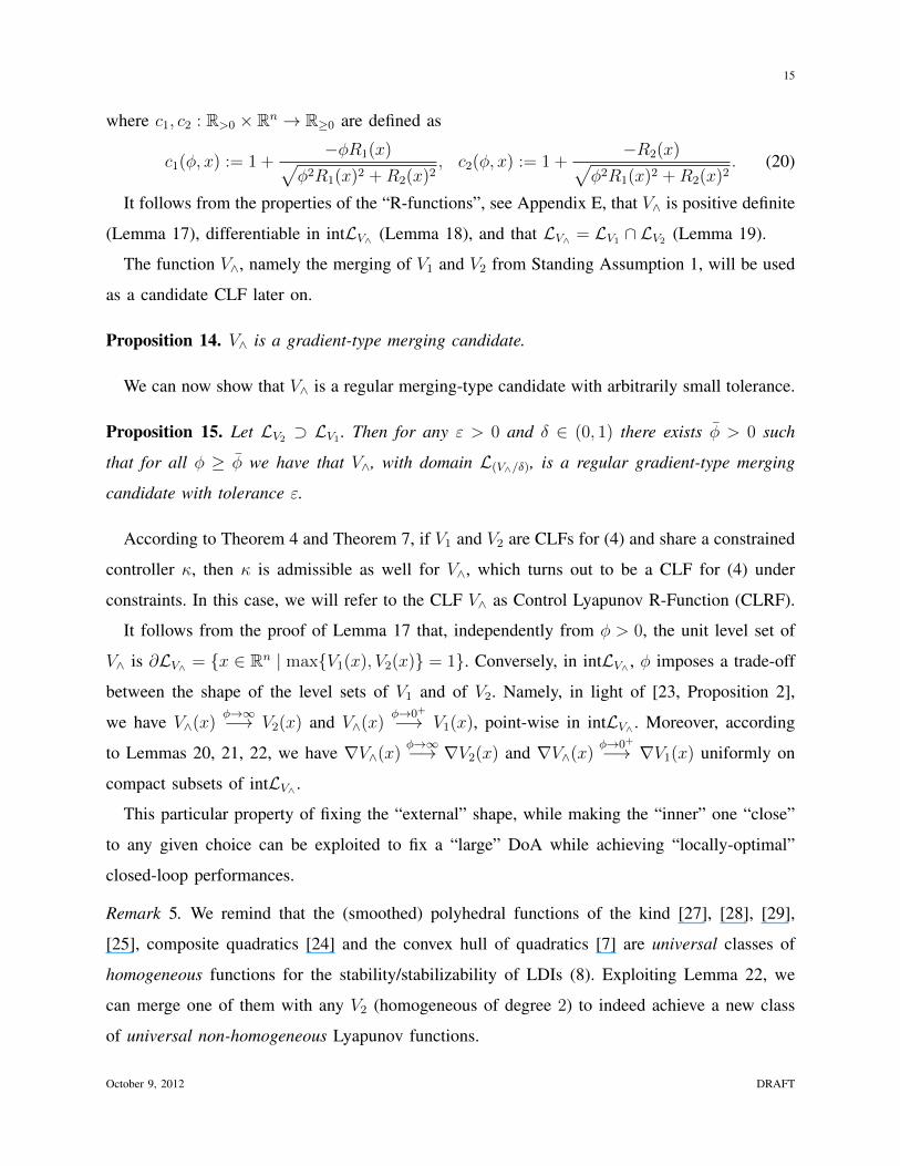
It follows from the properties of the “R-functions”, see Appendix E, that V∧ is positive definite

(Lemma 17), differentiable in intLV∧ (Lemma 18), and that LV∧ = LV1 ∩ LV2 (Lemma 19).

The function V∧, namely the merging of V1 and V2 from Standing Assumption 1, will be used

as a candidate CLF later on.

Proposition 14. V∧ is a gradient-type merging candidate.

We can now show that V∧ is a regular merging-type candidate with arbitrarily small tolerance.

Proposition 15. Let LV2 ⊃ LV1 . Then for any ε > 0 and δ ∈ (0, 1) there exists φ > 0 such

that for all φ ≥ φ we have that V∧, with domain L(V∧/δ), is a regular gradient-type merging

candidate with tolerance ε.

According to Theorem 4 and Theorem 7, if V1 and V2 are CLFs for (4) and share a constrained

controller κ, then κ is admissible as well for V∧, which turns out to be a CLF for (4) under

constraints. In this case, we will refer to the CLF V∧ as Control Lyapunov R-Function (CLRF).

It follows from the proof of Lemma 17 that, independently from φ > 0, the unit level set of

V∧ is ∂LV∧ = {x ∈ Rn | max{V1(x), V2(x)} = 1}. Conversely, in intLV∧ , φ imposes a trade-off

between the shape of the level sets of V1 and of V2. Namely, in light of [23, Proposition 2],

we have V∧(x)φ→∞−→ V2(x) and V∧(x)

φ→0+−→ V1(x), point-wise in intLV∧ . Moreover, according

to Lemmas 20, 21, 22, we have ∇V∧(x)φ→∞−→ ∇V2(x) and ∇V∧(x)

φ→0+−→ ∇V1(x) uniformly on

compact subsets of intLV∧ .

This particular property of fixing the “external” shape, while making the “inner” one “close”

to any given choice can be exploited to fix a “large” DoA while achieving “locally-optimal”

closed-loop performances.

Remark 5. We remind that the (smoothed) polyhedral functions of the kind [27], [28], [29],

[25], composite quadratics [24] and the convex hull of quadratics [7] are universal classes of

homogeneous functions for the stability/stabilizability of LDIs (8). Exploiting Lemma 22, we

can merge one of them with any V2 (homogeneous of degree 2) to indeed achieve a new class

of universal non-homogeneous Lyapunov functions.

October 9, 2012 DRAFT

16

A. Controller design under constraints

We now investigate the existence of a continuous locally-optimal control under constraints

x ∈ LV1 and u ∈ U ⊆ Rm which is closed (possibly compact) and convex. For simplicity, we

consider (8) with Bi = B for all i ∈ [1, N ]. Since the CLF V∧ is differentiable, in principle, the

existence of a stabilizing control law κ continuous with the exception of the origin, or including

x = 0 if V∧ satisfies the small control property4, could be proved by using the arguments in [31,

Chapters 2–4].

To have LV∧ = LV1 , we preliminary scale V2 so that LV2 ⊃ LV1 . In light of Theorem 7, we

formulate the control-sharing assumption, which can be checked using the results in Section IV.

Assumption 1. Functions V1 and V2 have the control-sharing property under constraints x ∈ LV1 ,

u ∈ U. Associated with V2 there is an “optimal” continuous control law κ2 : Rn → Rm such

that κ2(x) ∈ U for all x in a neighborhood of the origin.

It follows from the proof of Theorem 7 that, under Assumption 1, V∧ is a CLRF for (7)

under constraints. Namely, since for all x ∈ Rn we have min{V1(x), V2(x)} ≤ V∧(x) ≤

max{V1(x), V2(x)} [23, Proposition 1, Section 4.2], there exists η > 0 such that the following

convex-valued mapping of admissible (constrained) controls is non-empty for all x ∈ LV∧ .

U(x) :=

{u ∈ U | max

i∈[1,N ]∇V∧(x) (Aix+Bu) + ηx>x ≤ 0

}. (21)

We indeed propose the control law

κ(x) := arg min {‖υ − κ2(x)‖ | υ ∈ U(x)} . (22)

Theorem 16. Suppose Assumption 1 holds. Then the control law κ (22) associated with V∧ (18)

is continuous, satisfies the constraints in LV1 , and is locally optimal.

Remark 6. In the case of constrained “linear-quadratic” (LQ) stabilization, the approximate

Hamilton–Jacobi–Bellman control κ(x) := arg minυ∈U(x)

{∇V∧(x)(Ax+Bυ) + x>Qx+ υ>Rυ

}has been proposed in [23, Section 5]. An advantage of κ (22) over κ is that, according to

Theorem 16, local optimality is here guaranteed.

4A CLF V satisfies the small control property if, for u := κ(x), we have that for all v ∈ R>0 there exists ε ∈ R>0 so that,

whenever ‖x‖ < ε we have ‖u‖ < v [30].

October 9, 2012 DRAFT

17

B. Illustrative example

We address the constrained stabilization of a simplified inverted pendulum, whose dynamics

is given by the nonlinear differential equation Iθ(t) = mgl sin(θ(t)) + τ(t). The goal is the

stabilization of (θ, θ) to the origin, under the constraints |θ| ≤ π4, |θ| ≤ π

4and |τ | ≤ 2. With

notation x1 = θ, x2 = θ = x1, u = τ and w(x) :={

sin(x1)x1| |x1| ≤ π

4

}, the following constrained

uncertain linear model can be derived.

x ∈

0 1

aw(x) 0

x+

0

b

u, (23)

where a = (mgl/I), b = (1/I); w(x) ' [0.89, 1], w(0) = 1; |x1| ≤ π/4, |x2| ≤ π/4, |u| ≤ 2.

The numerical parameters used in the simulation are I = 0.05, m = 0.5, g = 9.81, l = 0.3.

We adopt the infinite-horizon quadratic performance cost J(x, u) :=∫∞

0(‖x(t)‖2

Q+‖u(t)‖2R)dt,

with weight matrices Q = I2, R = 10. Let us indeed define the locally-optimal (i.e. for w ≡ 1)

cost function V2(x) = x>Px, where P is the unique solution of the Algebraic Riccati Equation.

It can be shown that function V1(x) = ‖Fx‖2∞, with F =

[0 1.53 4/π

4/π 0.51 0

]>, is a PCLF for the

constrained LDI (23) and therefore also for the constrained nonlinear system. Then we define the

smoothed PCLF V1(x) = ‖Fx‖240 [25] and we indeed focus on the DoA LV1 . Let us also define

V2 scaling V2, so that LV2 ⊃ LV1 . Since the LMI condition (13) is satisfied under constraints,

V1 and V2 share a constrained controller in LV1 , therefore any gradient-type merging is a CLF.

We indeed construct a CLRF V∧ with φ = 20.

Now, V1 has a “large” DoA but it induces a “poor” performance when used with gradient-based

controllers of the kind (22) (Figure 4 in fact shows that the constraint u ∈ U(x) (21) with V1 in

place of V∧ may be “too restrictive”). On the other hand, V2 is locally optimal, but both gradient-

based controllers, for instance (22) with V2 in place of V∧, and the standard LQ regulator yield

constraint violations, even in the case w ≡ 1. We notice that V∧, see Figure 5, with controller

(22), inherits the benefits of V1 (“large” DoA under constraints) and V2 (local optimality). For

the linearized system (i.e. for w ≡ 1), our extensive Monte Carlo numerical experiments show

that the closed-loop performance is “quite close” to the constrained “global optimal” (obtained

via a receding “long”-horizon controller, under a “fine” system discretization).

October 9, 2012 DRAFT

18

−1 −0.8 −0.6 −0.4 −0.2 0 0.2 0.4 0.6 0.8 1−1

−0.8

−0.6

−0.4

−0.2

0

0.2

0.4

0.6

0.8

1

x1

x2

Fig. 4. A controlled state trajectory starting from x0 = (0.6, 0.1)> and converging to the origin. The state is actually “forced”

to always “enter” the level sets of the smoothed PCLF V1.

−1 −0.8 −0.6 −0.4 −0.2 0 0.2 0.4 0.6 0.8 1−1

−0.8

−0.6

−0.4

−0.2

0

0.2

0.4

0.6

0.8

1

x1

x2

Fig. 5. A controlled state trajectory starting from x0 = (0.6, 0.1)> and converging to the origin “in accordance” to the level

sets of the CLRF V∧.

VI. CONCLUSION

The problem of merging two Lyapunov functions is considered important for several applica-

tions, mainly because when concerning constraints, robustness and optimality, a single Lyapunov

function is typically suitable for one of these goals, but ineffective for the others.

Previous results show how to combine Lyapunov functions if these share a common control

October 9, 2012 DRAFT

19

in a suitable region of the state space. For the class of nonlinear control-affine systems, both

differential equations and inclusions, we have shown the equivalence between the control-sharing

property and the existence of merging control Lyapunov functions.

In order to guarantee the existence of a common control law, linear programs and linear matrix

inequalities conditions have been presented for the class of linear differential inclusions.

As an example of merging procedure, a constructive technique based on the R-composition

has been given. Further numerical experiments on practical case studies have to be presented.

From our experience, our approach is quite close to the constrained global optimality, but no

“close form” bounds have been given.

APPENDIX A

PROOFS OF SECTION II

A. Proof of Proposition 2

Proof: We show a numerical example for n = 2, m = 1, N = 2, in which two QCLFs

V1(x) = x>P1x and V2(x) = x>P2x do not share a common controller.

Consider (8) with A1 =[ −1.408 −0.476

0.819 −1.694

], A2 =

[ −0.357 1.196−1.428 1.721

], B1 = B2 = B = [ −1.981

0.600 ].

The eigenvalues of A1, A2 respectively are {−1.55± i0.61} and {0.68± i0.79}.

Let us consider P1 =[

3.478 −3.988−3.988 7.825

], P2 =

[4.610 −18.53−18.53 96.40

].

With the linear controllers κ1(x) = K1x and κ2(x) = K2x, being K1 = (0.4815, −0.6934) and

K2 = (8.310, −42.17), we have (Aj +BKi)>Pi + Pi(Aj +BKi) 4 −εiIn, ∀i, j ∈ {1, 2}, with

ε1, ε2 ≥ 10−3. Therefore x>P1x and x>P2x are CLFs for (8).

Then, we show that for the state x = (−1.813, −0.404)>, there cannot exists a common

control u ∈ R, i.e. the following system of equations is not admissible.∇V1(x)(A1x+Bu) < 0

∇V1(x)(A2x+Bu) < 0

∇V2(x)(A1x+Bu) < 0

∇V2(x)(A2x+Bu) < 0

(24)

In fact, we have 12∇V1(x)A2x = x>P1A2x = 6.94, 1

2∇V1(x)B = x>P1B = 11.74, therefore

u < −0.59 < 0; however 12∇V2(x)A1x = x>P2A1x = 1.89 and 1

2∇V2(x)B = x>P2B = −1.48,

therefore u > 1.28 > 0.

October 9, 2012 DRAFT

20

B. Proof of Proposition 3

Proof: We show a numerical example for n = 3, in which two QCLFs V1(x) = x>P1x and

V2(x) = x>P2x do not share a common controller.

Consider (5) with A =[ −1.990 −1.135 −1.063

1.745 0.536 −0.429−0.794 −1.243 −1.813

], B =

[ −1.925−0.342

0.257

].

Note that the eigenvalues of A are {0.276,−1.772± i0.114}.

Let us consider P1 =[

35.3372 27.5098 −39.092227.5098 21.4164 −30.4326−39.0922 −30.4326 43.2484

], P2 =

[0.00031 0.04321 −0.014650.04321 80.5695 −39.5654−0.01465 −39.5654 19.6646

].

With the linear controllers κ1(x) = K1x and κ2(x) = K2x, being K1 = (0.5037, 0.5799, −0.2013)

and K2 = (4.5451, 4.5697, −0.0669), we have (A + BKi)>Pi + Pi(A + BKi) 4 −εiIn, for

i = 1, 2, with ε1, ε2 ≥ 10−4. Therefore x>P1x and x>P2x are CLFs.

Then, we show that for the state x = (−0.329, −1.094, −1.537)>, there cannot exists a

common control u ∈ R, i.e. the following system of equations is not admissible. ∇V1(x)(Ax+Bu) < 0

∇V2(x)(Ax+Bu) < 0(25)

In fact, 12∇V1(x)Ax = x>P1Ax = −31.89, 1

2∇V2(x)Ax = x>P2Ax = 71.07, 1

2∇V1(x)B =

x>P1B = −45.46, 12∇V2(x)B = x>P2B = 12.76 therefore we get −31.91− 45.46u < 0 ⇔ u > −0.70

71.07 + 12.76u < 0 ⇔ u < −5.57

that clearly is not feasible.

Remark 7. The sets of equations (24) and (25) are not influenced by any scaling of the matrices

Pi, meaning that the set of admissible solutions remains the same for Pi 7→ δiPi, δi > 0, i = 1, 2.

Such a scaling would influence ε1, ε2 in (Aj+BKi)>Pi+Pi(Aj+BKi) 4 −εiIn in the following

sense. For any ε1, ε2 > 0, there exist δ1, δ2 > 0 such that (Aj +BKi)>δiPi + δiPi(Aj +BKi) 4

−εiIn for i = 1, 2. That is to say that we cannot run into numerical problems caused by “too

small” ε1, ε2.

APPENDIX B

PROOFS OF SECTION III

A. Proof of Theorem 4

Proof: V is a CLF if and only if for any x ∈ Rn there exists u ∈ Rm such that∇V (x)(f(x)+

g(x)u) < 0. Assume that V is a CLF and let x be fixed. By definition, for any γ1, γ2 ≥ 0 with

October 9, 2012 DRAFT

21

(γ1, γ2) 6= (0, 0), there exists u ∈ Rm such that (γ1∇V1(x) + γ2∇V2(x))(f(x) + g(x)u) < 0, or

equivalently for any (α1, α2) ∈ A := {(a, b) ∈ (R≥0)2 | a + b = 1} there exists u ∈ Rm such

that

(α1∇V1(x) + α2∇V2(x)) (f(x) + g(x)u) < 0.

Therefore we have

max(α1,α2)∈A

infu∈Rm

(α1∇V1(x) + α2∇V2(x)) (f(x) + g(x)u) < 0. (26)

Since A is compact and Rm is closed, and the function in (26) is linear in both (α1, α2) and

u, we can exchange “max” and “min” [32, Corollary 37.3.2] to get the following equivalent

condition.

max(α1,α2)∈A

infu∈Rm

(α1∇V1(x) + α2∇V2(x))(f(x) + g(x)u) =

infu∈Rm

max(α1,α2)∈A

(α1∇V1(x) + α2∇V2(x))(f(x) + g(x)u) =

infu∈Rm

max(α1,α2)∈A

{α1∇V1(x)(f(x) + g(x)u) + α2∇V2(x)(f(x) + g(x)u)} < 0 ⇐⇒

infu∈Rm

max {∇V1(x)(f(x) + g(x)u), ∇V2(x)(f(x) + g(x)u)} < 0. (27)

The last inequality is equivalent to the existence of a common controller. The result follows as

all the considered inequalities are equivalent.

B. Proof of Theorem 5

Proof: In view of Theorem 4, we need only to prove that if there exists a regular gradient-

type merging CLF, then the two functions have the control-sharing property.

Therefore, by assumption we have (γ1(x)∇V1(x)+γ2(x)∇V2(x))(Ax+Bu(x)) < 0 for some

locally bounded u(x).

Given a unit vector v ∈ Rn, ‖v‖ = 1, consider the ray R := {λv ∈ Rn | λ > 0}. Since the

functions are homogeneous, their gradients along R are aligned, namely for all x = λv we have

∇V1(x) = λp∇V1(v) and ∇V2(x) = λq∇V2(v) for some p, q > 0. Therefore we have

(γ1(λv)λp∇V1(v) + γ2(λv)λq∇V2(v))(λAv +Bu(λv)) < 0,

October 9, 2012 DRAFT

22

or equivalently (divide by γ1(λv)λp + γ2(λv)λq > 0 and by λ > 0) to get γ1(λv)λp

γ1(λv)λp + γ2(λv)λq︸ ︷︷ ︸=:α1(λ)

∇V1(v) +γ2(λv)λq

γ1(λv)λp + γ2(λv)λq︸ ︷︷ ︸=:α2(λ)

∇V2(v)

(Av +Bω) < 0,

where we define

ω :=u(λv)

λ.

Denote by λ the value of λ such that λv ∈ ∂LV , i.e. V (λv) = 1. For all λ ∈ [0, λ], we have

(α1(λ), α2(λ)) ∈ A := {(α, β) ∈ (R≥0)2 | α + β = 1}. Moreover as λ goes from 0 to λ, both

α1(λ) and α2(λ) = 1−α1(λ) assume all values from 0 to 1. This means that for all (α1, α2) ∈ A

there exists ω ∈ Rm such that (α1∇V1(v) + α2∇V2(v)) (Av +Bω) < 0, i.e.

max(α1,α2)∈A

infω∈Rm

(α1∇V1(v) + α2∇V2(v)) (Av +Bω) < 0.

To complete the proof we just need to apply the same min-max argument of the proof of

Theorem 4.

C. Proof of Proposition 6

Proof: We prove the claim by means of an example with n = m = 2. Consider the

linear system x = u, along with the linear controllers κ1(x) = K1x =[ −ε 1/a−a −ε

]and κ2(x) =

K2 = K>1 =[ −ε −a

1/a −ε], for some a, ε > 0. The functions V1(x) = 1

2

(ax2

1 + 1ax2

2

), V2(x) =

12

(1ax2

1 + ax22

), are two QCLFs, respectively with controllers κ1 and κ2. In fact, since ∇V1(x) =(

ax1,1ax2

), ∇V2(x) =

(1ax1, ax2

), we have ∇Vi(x)(Ax+Bu) = −εVi(x), for i = 1, 2.

Take any gradient-type merging candidate ∇V (x) = (γ1(x)∇V1(x) + γ2(x)∇V2(x)) and

{γ1(x) = 1, γ2(x) = 0} “far” from the state-space origin and, vice-versa, {γ1(x) = 0, γ2(x) = 1}

“close” to the origin. Therefore V is such that ∇V (x) = ∇V1(x) “far” from the origin and

∇V (x) = ∇V2(x) “close” to the origin. The controller κ(x) = −εx assures that V a CLF, as

∇V (x)(Ax+ Bu) = −ε∇V (x)x = −ε(∇V1(x) +∇V2(x))x = −ε(a+ 1a) (x2

1 + x22) is negative

definite ∀ε, a > 0.

Note that for a � 1 the vector ∇V1 is almost “horizontal”, while the vector ∇V2 is almost

“vertical”. Consider the ray (bisector) R = {x = (ξ, ξ), ξ ≥ 0}. Since ∇V is continuous, there

exists a point R on the bisector in which ∇V is aligned to the bisector itself, i.e. there exist

October 9, 2012 DRAFT

23

λ, ξ ≥ 0 such that ∇V (ξ) = λ · (ξ, ξ). In such a point, with both κ1(ξ) and κ2(ξ), we have

∇V (ξ)(Aξ +Bκi(ξ)) = λ(−2ε+

(1a− a))ξ2 that is strictly positive for ε� 1, a� 1.

D. Proof of Theorem 7

Proof: By assumption, for all x ∈ Rn there exists u ∈ Rm such that the inequalities

max(ϕ,Γ)∈(F (x),G(x))

∇V1(x) (ϕ+ Γu) < 0 ⇐⇒ max(ϕ,Γ)∈(F (x),G(x))

γ1∇V1(x) (ϕ+ Γu) < 0 (28a)

max(ϕ,Γ)∈(F (x),G(x))

∇V2(x) (ϕ+ Γu) < 0 ⇐⇒ max(ϕ,Γ)∈(F (x),G(x))

γ2∇V2(x) (ϕ+ Γu) < 0 (28b)

holds simultaneously for any γ1, γ2 ≥ 0, therefore also the following sum is negative:

max(ϕ,Γ)∈(F (x),G(x))

{γ1∇V1(x) (ϕ+ Γu)} + max(ϕ,Γ)∈(F (x),G(x))

{γ2∇V2(x) (ϕ+ Γu)} < 0,

which immediately implies

max(ϕ,Γ)∈(F (x),G(x))

(γ1∇V1(x) + γ2∇V2(x)) (ϕ+ Γu) < 0.

Having the left-hand side strictly less than zero is equivalent to claim that the gradient-type

merging is a CLF. The proof is complete if we notice that γ1 and γ2 have been chosen arbitrarily.

E. Proof of Theorem 8

Proof: The implication (2)⇒ (1) follows from Theorem 7. To prove the claim (1)⇒ (2)

we write G(x) = g(x) to mean that G is single-valued. Fix arbitrary γ1, γ2 > 0 and define

f(x) := arg maxϕ∈F (x)

(γ1∇V1(x) + γ2∇V2(x))ϕ.

Now, by assumption we have that maxϕ∈F (x) (γ1∇V1(x) + γ2∇V2(x)) (ϕ+ g(x)u) < 0, namely

maxϕ∈F (x)

{(γ1∇V1(x) + γ2∇V2(x))ϕ} + (γ1∇V1(x) + γ2∇V2(x)) g(x)u < 0.

According to the definition of f , the first term can be written as (γ1∇V1(x) + γ2∇V2(x)) f(x).

Finally, we can just follow the proof of Theorem 4 for the nonlinear system x = f(x) + g(x)u.

October 9, 2012 DRAFT

24

APPENDIX C

PROOFS OF SECTION IV

A. Proof of Lemma 9

Proof: For each i ∈ [1, N ] we explicitly construct Wi from Wi. Therefore, for ease of

notation, let us consider the case of N = 1. The general case easily follows as each Wi here

constructed will depend exclusively on Wi.

Let us denote W = [w1|w2|...|ws+1], where wi ∈ Rs+1. Moreover we use the notation wi(p) to

denote the pth component of a column vector wi and wi([p, q]) to denote its pth, (p+1)th, ..., (q−

1)th, qth components.

Then we have A[x1|...|xs|x] +B[u1|...|us|u] = [X|x][w1|...|ws|ws+1]. The first s equations are

Axi +Bui = [X|x]wi, i ∈ [1, s],

therefore we can take wi([1, s]) := wi([1, s]) and wi(s+1) := 0. Note that this definition respects

the fact that W has to be an M-matrix. The last equation is Ax = Bu = [X|x]ws+1, i.e.

A

(s∑i=1

αixi

)+B

(s∑i=1

αiui

)= Xws+1([1, s]) +

(s∑i=1

αixi

)ws+1(s+ 1).

Now the left-hand side can be written as

A

(s∑i=1

αixi

)+B

(s∑i=1

αixi

)=

s∑i=1

αi (Axi +Bui)︸ ︷︷ ︸=Xwi

= Xs∑i=1

αiwi (29)

while the right-hand side can be written as

Xws+1([1, s]) +

(s∑i=1

αixi

)ws+1(s+ 1) = X [ws+1([1, s]) + ws+1(s+ 1)α] (30)

where α := (α1, α1, ..., αs)>.

Therefore, from (29) and (30), it is sufficient to show that, for any given α ∈ (R≥0)s, there

exists ws+1 such thats∑i=1

αiwi = ws+1([1, s]) + ws+1(s+ 1)α. (31)

For ease of notation, we rename the free variables as ξ := ws+1([1, s]) ∈ (R≥0)s and

ζ := ws+1(s+ 1) ∈ R. Then, we define

W :=

w1(1) · · · ws(1)

... . . . ...

ws(1) · · · ws(s)

. (32)

October 9, 2012 DRAFT

25

Note that, as W is an M-matrix by assumption, we have wi(j) ≥ 0 ⇔ j 6= i. Therefore,

according to (31) and (32), we have to find ξ and ζ such that Wα = ξ + ζα, or equivalently:(W − ζIs

)α = ξ. (33)

Now defining ζ := −(maxi∈[1,s] |wi(i)|

), we get that the matrix

(Wr − ζI

)has all non-

negative entries, therefore(W − ζI

)α becomes a vector of all non-negative components. This

means that (33) can be satisfied by choosing ξ := (W − ζI)α ∈ (R≥0)s.

Summarizing, we found an admissible M-matrix W ∈ R(s+1)×(s+1) of the kind

W :=

W ξ

0>s ζ

. (34)

To conclude the proof, we have to show that 1>s+1W ≤ −η1

>s+1, i.e. that all the columns wi are

such that∑s+1

j=1 wi(j) ≤ −η. This is immediately true for the first s columns, as 1>sW ≤ −η1

>s

by assumption. In fact, see (34), we have wi(j) = wi(j) if 1 ≤ j ≤ s, 0 otherwise.

Finally, for the last column ws+1, from (33) we have that(s∑i=1

ξi

)+ ζ = α1

(s∑i=1

w1(i)

)︸ ︷︷ ︸

≤−η

+ . . .+ αs

(s∑i=1

ws(i)

)︸ ︷︷ ︸

≤−η

≤ −η

(s∑i=1

αi

)= −η.

B. Proof of Theorem 10

Proof: For each vertex xjk of LVj , say j = 1, (13a) is equivalent to the contraction of V1

in x1k, namely to having V1(x1

k) < 0. Then (13b) is equivalent to the contraction of V2 in x1k.

Since V2 is homogeneous and the condition holds for all i ∈ [1, N ], this is equivalent to the

contraction of V2 in x1k itself.

The common controller follows from U and therefore it is piecewise-linear. The proof im-

mediately follows since the choice of j ∈ {1, 2} and k ∈ [1, sj] have been made arbitrarily.

October 9, 2012 DRAFT

26

C. Proof of Theorem 11

Proof: The assumption that V1 is a PCLF is equivalent to the existence of a piecewise-linear

controller that follows from the control vectors u1, u2, ..., us (respectively associated with the

vertices x1, x2, ..., xs), namely the columns of U , which shows up in (11). According to Lemma

9, if {x1, x2, ..., xr} are the vertices of a given facet of the polyhedron LV1 , together with control

vectors {u1, u2, ..., ur}, then the control vector u(α) :=∑r

h=1 αhuh, for α = (α1, α2, ..., αr) ∈

A := {a ∈ (R≥0)r |∑r

h=1 ah = 1}, is an admissible control for V1 in the state point x(α) :=∑rh=1 αhxh.

Therefore it is sufficient to prove that for each facet of the polyhedron LV1 , the control u(α),

parameterized by α ∈ A, is admissible also for V2, i.e. there exists η > 0 such that

x(α)>P [(Ai + ηIn)x(α) +Biu(α)] ≤ 0 ∀i ∈ [1, N ].

Then we can write(r∑

h=1

αhxh

)>P

[(Ai + ηIn)

(r∑

h=1

αhxh

)+Bi

(r∑

h=1

αhuh

)]≤ 0 ∀i ∈ [1, N ] ⇐⇒

r∑h,j=1

αhαj(x>hP [(Ai + ηIn)xj +Biuj] + x>j P [(Ai + ηIn)xh +Biuh]

)︸ ︷︷ ︸=:[S·,i(η,U)]h,j

≤ 0 ∀i ∈ [1, N ].

We get that the left-hand side of the last inequality, namely α>S·,i(η, U)α, has to be non-positive

for α ∈ (R≥0)r. Therefore the matrices −Sk,i(η, U), where the subscript k indicates the kth facet,

have to be copositive. This is equivalent to the assumption made.

D. Proof of Theorem 13

Proof: For all k ∈ [1, s], define the sectors Sk := {x ∈ Rn | x>Pkx ≥ maxj x>Pjx}, so

that we have

x ∈ Sk =⇒ x>Pkx ≥ x>Pjx ∀j ∈ [1, s] =⇒ x>

(s∑j=1

λi,j,k(Pj − Pk)

)x ≤ 0 (35)

for any λi,j,k ≥ 0, where i ∈ [1, N ], j, k ∈ [1, s].

The matrix inequality condition (16a) is necessary and sufficient for V1 to be a CLF for (8)

[24], with piecewise-linear controller κ(x) := K(x)x, where K(x) := {Kk if x ∈ Sk}. Then we

show that (16b) is sufficient for κ to be a valid controller also for V2.

October 9, 2012 DRAFT

27

Consider x ∈ Sk and multiply (16b) by x> on the left and by x on the right, so that

2∇V2(x)(Ai +BiKk)x = x>[(Ai +BiKk)

>P + P (Ai +BiKk)]x ≤

− 2η x>Px︸ ︷︷ ︸=V2(x)

+ x>

(s∑j=1

λi,j,k(Pj − Pk)

)x ∀i ∈ [1, N ].

Therefore, in view of (35), we finally get to ∇V2(x)(Ai +BiKk)x ≤ −ηV2(x) ∀i ∈ [1, N ].

The proof follows since the choice of sector Sk 3 x has been made arbitrarily.

APPENDIX D

PROOFS OF SECTION V

A. Proof of Proposition 14

Proof: The proof follows from Lemma 18 as

∇V∧(x) = ρ(φ) (φc1(φ, x)∇V1(x) + c2(φ, x)∇V2(x)), where the functions c1, c2 : R>0 × Rn →

R≥0 defined in (20) are continuous.

B. Proof of Proposition 15

Proof: As V2 has been scaled so that LV2 ⊃ LV1 , we have LV∧ = LV1 from Lemma 19.

Let us use the notation γ1(x) := ρ(φ)φc1(φ, x) and γ2(x) := ρ(φ)c2(φ, x), so that ∇V∧(x) =

γ1(x)∇V1(x) + γ2(x)∇V2(x), where γ1 and γ2 also depend on the parameter φ.

According to the proof of Lemma 20, we have the following fact. For any ε > 0 and δ > 0

there exists φ1 > 0 such that for all φ ≥ φ1 we have maxx∈L(V∧/δ) γ1(x) ≤ ε. Analogously,

for any ε > 0 and δ > 0 there exists φ2 > 0 such that for all φ ≥ φ2 we have 1 − ε ≤

maxx∈L(V∧/δ) γ1(x) ≤ 1. The proof is complete if we take φ := max{φ1, φ2}, so that for all

φ ≥ φ and x ∈ L(V∧/δ) we have γ1(x) ∈ [0, ε] and γ2(x) ∈ [1− ε, 1].

C. Proof of Theorem 16

Proof: According to Theorem 7, V∧ is a CLF in LV∧ . Moreover, it follows from [23, Proposi-

tion 1] that V∧ grows quadratically, i.e. min{V1(x), V2(x)} ≤ V∧(x) ≤ max{V1(x), V2(x)} ∀x ∈

Rn. Therefore for some η > 0, we have that for all x ∈ LV∧ there exists u ∈ Rm such that

maxi∈[1,N ]∇V∧(x)(Aix+Bu) ≤ −ηx>x. Analogously, for some η > 0, which we do not relabel,

October 9, 2012 DRAFT

28

we also have that for all x ∈ LV1 there exists u ∈ Rm such that maxi∈[1,N ]∇V (x)(Aix+Bu) ≤

−ηx>x.

Let κ be the piecewise-linear controller shared by V1 and V2. It follows from the proof

of Theorem 7 that V∧ is a Lyapunov function for the closed-loop differential inclusion x ∈

co {Aix+Bκ(x) | i ∈ [1, N ]}, therefore V∧, and hence also V , satisfies the small control prop-

erty. The optimization problem (22) follows from the minimal selection control

m(x) := arg min

{‖υ‖ | max

i∈[1,N ]∇V∧(x)Aix+∇V∧(x)B(υ + κ2(x)) ≤ −ηx>x

},

that is known to be continuous [31, Section 4.2]. Hence the optimal solution of (22) can be

written as κ(x) := m(x) + κ2(x), which is the sum of two continuous functions.

In the following, we prove that κ2 is an admissible control for V∧ in a neighborhood of the

origin. This will also imply that V∧ satisfies the small control property.

According to Lemma 20, we have the following property. For any ε > 0 and σ ∈ (0, 1) there ex-

ists φ > 0 such that φ ≥ φ implies that ∇V∧(x) = ∇V2(x)+v(x)>, with maxx∈L(V∧/σ) ‖v(x)‖ ≤

ε. Therefore

maxi∈[1,N ]

∇V∧(x)(Aix+Bκ2(x)) = maxi∈[1,N ]

∇V2(x)(Aix+Bκ2(x)) + v(x)>(Aix+Bκ2(x)) ≤

maxi∈[1,N ]

∇V2(x)(Aix+Bκ2(x)) + maxi∈[1,N ]

v(x)>(Aix+Bκ2(x)). (36)

We notice that there exists η, σ2 > 0 such that maxi∈[1,N ]∇V∧(x)(Aix + Bκ2(x)) ≤ −2ηx>x

for all x in the compact set L(V2/σ2). Therefore we choose σ so that {x ∈ Rn | V∧(x) ≤ σ} ⊆

{x ∈ Rn | V2(x) ≤ σ2}, namely as σ := max{c ∈ [0, 1] | L(V∧/c) ⊆ L(V2/σ2)}.

We can now choose ε ≥ ‖v(x)‖ such that

maxx∈L(V∧/σ)

{maxi∈[1,N ]

v(x)>(Aix+Bκ2(x))− ηx>x}≤ 0. (37)

Therefore, using (37) in (36), we get that κ2 is an admissible control for V∧ in a neighborhood of

the origin, i.e. maxi∈[1,N ]∇V∧(x)(Aix+Bκ2(x)) ≤ −ηx>x. This means that for all x ∈ L(V∧/σ),

the constraint υ ∈ U(x) in (22) is not active and therefore κ(x) = κ2(x) is locally optimal.

Moreover, we also get that the controller κ is continuous also at the origin.

APPENDIX E

TECHNICAL PROPERTIES OF THE R-COMPOSITION

Lemma 17. V∧ is positive definite.

October 9, 2012 DRAFT

29

Proof: At the origin we have V1(0) = V2(0) = 0⇐⇒ R1(0) = R2(0) = 1. Therefore, from

(17), R∧(0) = 1 and hence V∧(0) = 1 − R∧(0) = 0. Conversely, V∧(x) = 0 ⇔ R∧(x) = 1.

From [23, Proposition 1], we have 1 = R∧(x) ≤ max{R1(x), R2(x)}. Since R1(x) ≤ 1 and

R2(x) ≤ 1 by construction, we have that R1(x) = 1 or R2(x) = 1 (or both). Say R1(x) = 1.

Therefore R1(x) = 1⇔ V1(x) = 0⇔ x = 0.

Lemma 18. Assume that V1 and V2 are differentiable respectively in LV1 and LV2 . Then V∧ is

differentiable in intLV∧ .

Proof: The proof immediately follows from (19) since φ > 0 is fixed and functions ci(φ, x),

i = 1, 2, are continuous whenever R1(x) and R2(x) are not simultaneously 0, i.e. in intLV∧ .

For ease of notation, in the following proofs, let us denote V1(x), V2(x), R1(x), R2(x), c1(φ, x),

c2(φ, x) without the explicit dependence on their arguments.

Lemma 19. LV∧ = LV1 ∩ LV2 .

Proof: According to [23, Lemma 1], we have R∧ > 0 ⇐⇒ {R1 > 0 and R2 > 0};

moreover, from (17), R∧ = 0 ⇐⇒ {R1 = 0 or R2 = 0}. Now by construction Vi = 1 − Ri,

i ∈ {1, 2}, and V∧ = 1 − R∧, therefore V∧ < 1 ⇐⇒ {V1 < 1 and V2 < 1}, and V∧ = 1 ⇐⇒

{V1 = 1 or V2 = 1}, i.e. LV∧ = LV1 ∩ LV2 .

Lemma 20. ∇V∧ converges to ∇V2 uniformly on compact subsets of intLV∧ , as φ→∞. Namely,

for any δ ∈ (0, 1) we have limφ→∞ maxx∈L(V∧/δ) ‖∇V∧(x)−∇V2(x)‖ = 0.

Proof: First we have

limφ→∞

ρ(φ) = limφ→∞

1

φ+ 1−√φ2 + 1

= limφ→∞

φ+ 1 +√φ2 + 1

2φ= 1. (38)

Then

limφ→∞

φc1 = limφ→∞

φ

(1 +

−φR1√φ2R2

1 +R22

)=

limφ→∞

R22

φR21 +R2

2/φ+R1

√φ2R2

1 +R22

≤ limφ→∞

1

2φR21

≤ limφ→∞

1

2φ(1− δ)2= 0. (39)

The last inequality holds uniformly as R1(x) ≥ 1 − δ > 0 whenever x ∈ L(V∧/δ) = {y ∈ Rn |

October 9, 2012 DRAFT

30

V∧(y) ≤ δ}. Then we can also write

limφ→∞

c2 = limφ→∞

(1 +

−R2√φ2R2

1 +R22

)=

limφ→∞

√φ2R2

1 +R22 −R2√

φ2R21 +R2

2

= limφ→∞

R21

R21 +R2

2/φ+ (R2/φ)√R2

1 +R22/φ

2= 1. (40)

Therefore, combining (38), (39) and (40), we get limφ→∞

∇V∧(x) = limφ→∞

ρ(φ)(φc1(φ, x)∇V1(x) +

c2(φ, x)∇V2(x)) = ∇V2(x) uniformly on compact subsets of the kind L(V∧/δ).

Lemma 21. ∇V∧ converges to ∇V1 uniformly on compact subsets of intLV∧ , as φ→ 0+. Namely,

for any δ ∈ (0, 1) we have limφ→0+ maxx∈L(V∧/δ) ‖∇V∧(x)−∇V1(x)‖ = 0.

Proof: Since ∇V∧ = ρ(φ) [φc1∇V1 + c2∇V2], we have to prove that for any δ ∈ (0, 1) we

have limφ→0+ ρ(φ)φc1(x) = 1 and limφ→0+ ρ(φ)c2(φ, x) = 0 for all x ∈ L(V∧/δ).

Similarly to (38) and (39) we have that

limφ→0+

ρ(φ)φc1 = limφ→0+

φ

φ+ 1−√φ2 + 1

(1 +

−φR1√φ2R2

1 +R22

)=

limφ→0+

φ+ 1−√φ2 + 1

2φ· φR2

2

φ2R21 +R2

2 + φR1

√φ2R2

1 +R22

= 1. (41)

The last equality holds uniformly as R1(x) ≥ 1 − δ > 0 and R2(x) ≥ 1 − δ > 0 (both the

numerator and the denominator are indeed strictly positive) whenever x ∈ L(V∧/δ) = {y ∈ Rn |

V∧(y) ≤ δ}. Then we can also write

limφ→0+

ρ(φ)c2 = limφ→0+

1

φ+ 1−√φ2 + 1

(1 +

−R2√φ2R2

1 +R22

)=

limφ→0+

φ+ 1 +√φ2 + 1

2φ·√φ2R2

1 +R22 −R2√

φ2R21 +R2

2

=

limφ→0+

φ+ 1 +√φ2 + 1

2· φR2

1(√φ2R2

1 +R22 +R2

)√φ2R2

1 +R22

= 0. (42)

Since R1(x), R2(x) ≥ 1 − δ > 0, the denominator is strictly positive and hence the last

equality holds uniformly. Therefore, from (41) and (42) we get limφ→0+

ρ(φ)(φc1(φ, x)∇V1(x) +

c2(φ, x)∇V2(x)) = ∇V1(x) uniformly on compact subsets of the kind L(V∧/δ).

October 9, 2012 DRAFT

31

Lemma 22. Assume LV2 ⊃ LV1 . Then ∇V∧ converges to ∇V1 uniformly on LV1 as φ→ 0+, i.e.

limφ→0+

maxx∈LV∧

‖∇V∧(x)−∇V1(x)‖ = 0. (43)

Proof: We first notice that, as LV2 ⊃ LV1 , we have LV∧ = LV1 in view of Lemma 19.

Then we can use the same proof of Lemma 21 if we notice that R2(x) is strictly positive in

LV∧ because LV2 ⊃ LV1 = LV∧ . In fact, R2(x) > 0 implies that both the numerator and the

denominator of (41), and also the denominator of (42), are strictly positive for all x ∈ LV∧ .

REFERENCES

[1] F. Schweppe, Uncertain dynamic systems. Englewood Cliff, N.J.: Prentice Hall, 1973.

[2] P. Gutman and P. Hagander, “A new design of constrained controllers for linear systems,” IEEE Trans. on Automatic

Control, vol. 30, no. 1, pp. 22–33, 1985.

[3] P. Gutman and M. Cwikel, “Admissible sets and feedback control for discrete-time linear dynamical systems with bounded

controls and states,” IEEE Trans. on Automatic Control, vol. 31, no. 4, pp. 373–376, 1986.

[4] S. Keerthi and E. Gilbert, “Computation of minimum-time feedback control laws for discrete-time systems with state-control

constraints,” IEEE Trans. on Automatic Control, vol. 32, no. 5, pp. 432–435, 1987.

[5] F. Blanchini and A. Megretski, “Robust state feedback control of LTV systems: nonlinear is better than linear,” IEEE

Trans. on Automatic Control, vol. 44, no. 4, pp. 802–807, 1999.

[6] F. Blanchini and S. Miani, “Constrained stabilization via smooth Lyapunov functions,” Systems & Control Letters, vol. 35,

pp. 155–163, 1998.

[7] T. Hu and Z. Lin, “Composite quadratic Lyapunov functions for constrained control systems,” IEEE Trans. on Automatic

Control, vol. 48, no. 3, pp. 440–450, 2003.

[8] B. O’Dell and E. Misawa, “Semi-ellipsoidal controlled invariant sets for constrained linear systems,” Journal of Dynamic

Systems, Measurement and Control, vol. 124, pp. 98–103, 2002.

[9] T. Thibodeau, W. Tong, and T. Hu, “Set invariance and performance analysis of linear systems via truncated ellipsoids,”

Automatica, vol. 45, pp. 2046–2051, 2009.

[10] A. Balestrino, E. Crisostomi, S. Grammatico, and A. Caiti, “Stabilization of constrained linear systems via smoothed

truncated ellipsoids,” Proc. of the IFAC World Congress, Milan (Italy), 2011.

[11] G. Chesi, A. Garulli, A. Tesi, and A. Vicino, “Homogeneous Lyapunov functions for systems with structured uncertainties,”

Automatica, vol. 39, no. 6, pp. 1027–1035, 2003.

[12] ——, Homogeneous polynomial forms for robustness analysis of uncertain systems. Springer, 2009.

[13] T. Hu and Z. Lin, Control of systems with actuator saturation. Boston, MA: Birkhauser, 2001.

[14] F. Blanchini and S. Miani, Set-theoretic methods in control, 1st ed. Birkhauser, 2007.

[15] G. Wredenhagen and P. Belanger, “Piecewise-linear LQ control for systems with input constraint,” Automatica, vol. 30,

no. 3, pp. 403–416, 1994.

[16] A. Benzaouia and A. Baddou, “Piecewise linear constrained control for continuous-time systems,” IEEE Trans. on Automatic

Control, vol. 44, no. 7, pp. 1477–1481, 1999.

October 9, 2012 DRAFT

32

[17] V. Andrieu and C. Prieur, “Uniting two Lyapunov functions for affine systems,” IEEE Trans. on Automatic Control, vol. 55,

no. 8, pp. 1923–1927, 2010.

[18] C. Prieur and Praly, “Uniting local and global controllers,” Proc. of the IEEE Conf. on Decision and Control, Phoenix

(Arizona, USA), pp. 1214–1219, 1999.

[19] C. Prieur, “Uniting local and global controllers with robustness to vanishing noise,” Mathematics of Control, Signals and

Systems, vol. 14, pp. 143–172, 2001.

[20] F. Clarke, “Lyapunov functions and discontinuous stabilizing feedback,” Annual reviews in control, vol. 35, pp. 13–33,

2011.

[21] A. Balestrino, A. Caiti, E. Crisostomi, and S. Grammatico, “Stabilizability of linear differential inclusions via R-functions,”

Proc. of the IFAC Symposium on Nonlinear Control Systems, Bologna (Italy), 2010.

[22] A. Balestrino, E. Crisostomi, and A. Caiti, “Logical composition of Lyapunov functions,” International Journal of Control,

vol. 84, no. 3, pp. 563–573, 2011.

[23] A. Balestrino, A. Caiti, and S. Grammatico, “A new class of Lyapunov functions for the constrained stabilization of linear

systems,” Automatica, vol. 48, no. 11, pp. 2951–2955, 2012.

[24] T. Hu and F. Blanchini, “Non-conservative matrix inequality conditions for stability/stabilizability of linear differential

inclusions,” Automatica, vol. 46, pp. 190–196, 2010.

[25] F. Blanchini and S. Miani, “A new class of universal Lyapunov functions for the control of uncertain linear systems,”

IEEE Trans. on Automatic Control, vol. 44, no. 3, pp. 641–647, 1999.

[26] A. Balestrino, A. Caiti, and S. Grammatico, “Multivariable constrained process control via Lyapunov R-functions,” Journal

of Process Control, vol. 22, no. 9, pp. 1762–1772, 2012.

[27] R. Brayton and C. Tong, “Constructive stability and asymptotic stability of dynamical systems,” IEEE Trans. on Circuits

and Systems, vol. 27, no. 11, pp. 1121–1130, 1980.

[28] A. Molchanov and E. Pyatnitskii, “Lyapunov functions specifying necessary and sufficient conditions of absolute stability

of nonlinear nonstationary control systems. Parts I, II, III.” Automatica and Remote Control, vol. 47, no. 3,4,5, pp. 344–354,

443–451, 620–630.

[29] F. Blanchini, “Nonquadratic Lyapunov functions for robust control,” Automatica, vol. 31, no. 3, pp. 451–461, 1995.

[30] E. Sontag, Mathematical Control Theory. Springer, 1998.

[31] R. Freeman and P. Kokotovic, Robust nonlinear control design. Boston: Birkhauser, 1996.

[32] R. Rockafellar, Convex Analysis. Princeton, New Yersey: Princeton University Press, 1970.

October 9, 2012 DRAFT