Weighted fusion graphs: merging properties and

watersheds

Jean Cousty, Michel Couprie, Laurent Najman, Gilles Bertrand

To cite this version:

Jean Cousty, Michel Couprie, Laurent Najman, Gilles Bertrand. Weighted fusion graphs:merging properties and watersheds. Discrete Applied Mathematics, Elsevier, 2008, 156 (15),pp.3011-3027. <hal-00622473>

HAL Id: hal-00622473

https://hal-upec-upem.archives-ouvertes.fr/hal-00622473

Submitted on 12 Sep 2011

HAL is a multi-disciplinary open accessarchive for the deposit and dissemination of sci-entific research documents, whether they are pub-lished or not. The documents may come fromteaching and research institutions in France orabroad, or from public or private research centers.

L’archive ouverte pluridisciplinaire HAL, estdestinee au depot et a la diffusion de documentsscientifiques de niveau recherche, publies ou non,emanant des etablissements d’enseignement et derecherche francais ou etrangers, des laboratoirespublics ou prives.

Weighted fusion graphs: merging properties

and watersheds

Jean Cousty, Michel Couprie, Laurent Najman andGilles Bertrand

Universite Paris-Est, LABINFO-IGM, UMR CNRS 8049, A2SI-ESIEE, France

Abstract

This paper deals with mathematical properties of watersheds in weighted graphslinked to region merging methods, as used in image analysis.

In a graph, a cleft (or a binary watershed) is a set of vertices that cannot bereduced, by point removal, without changing the number of regions (connectedcomponents) of its complement. To obtain a watershed adapted to morphologicalregion merging, it has been shown that one has to use the topological thinningsintroduced by M. Couprie and G. Bertrand. Unfortunately, topological thinningsdo not always produce thin clefts.

Therefore, we introduce a new transformation on vertex weighted graphs, calledC-watershed, that always produces a cleft. We present the class of perfect fusiongraphs, for which any two neighboring regions can be merged, while preserving allother regions, by removing from the cleft the points adjacent to both. An importanttheorem of this paper states that, on these graphs, the C-watersheds are topolog-ical thinnings and the corresponding divides are thin clefts. We propose a linear-time immersion-like algorithm to compute C-watersheds on perfect fusion graphs,whereas, in general, a linear-time topological thinning algorithm does not exist. Fur-thermore, we prove that this algorithm is monotone in the sense that the verticesare processed in increasing order of weight. Finally, we derive some characteriza-tions of perfect fusion graphs based on thinness properties of both C-watershedsand topological watersheds.

Key words: Graph theory, regions merging, watershed, fusion graphs, imagesegmentation, image processing

Email addresses: j.cousty@esiee.fr (Jean Cousty), m.couprie@esiee.fr(Michel Couprie), l.najman@esiee.fr (Laurent Najman), g.bertrand@esiee.fr(Gilles Bertrand).

Research Report IGM 2007-09, 2nd version 11 January 2008

Introduction

Image segmentation is the task of delineating objects of interest that appearin an image. In many cases, the result of such a process, also called a seg-mentation, can be viewed as a set of connected regions lying in a backgroundwhich constitutes the separation between regions. In order to define regions,an image is often considered as a graph whose vertex set is made of the pix-els and whose edge set is given by an adjacency relation between them. Forinstance, with the well-known 8-adjacency relation [1] each vertex is adjacentto its 8 closest neighbors. Then, the regions are simply the connected compo-nents of the set of foreground pixels. A popular approach to image analysis,called region merging [2,3], consists of progressively merging pairs of regions,starting from an initial segmentation that contains too many regions.

Given a grayscale image, or more generally a vertex-weighted graph (i.e., agraph and a map that assigns a scalar value to each vertex), how is it pos-sible to obtain an initial segmentation for a region merging procedure? Thewatershed transform [4–8] is a powerful tool for solving this problem. Letus consider a 2D grayscale image as a topographical relief, where the darkpixels correspond to basins and valleys, whereas bright pixels correspond tohills and crests. Suppose that we are interested in segmenting “dark” regions.Intuitively, the watersheds of an image are constituted by the crests which sep-arate the basins corresponding to regional minima. This notion is illustratedin Fig. 1, where the white points in Fig. 1c constitute a watershed of the imagein Fig. 1a equipped with the 8-adjacency relation. Due to noise and texture,real-world images often have a huge number of regional minima, hence the“mosaic” aspect of Fig. 1c. Nevertheless, it has been shown in numerous ap-plications that this segmentation is an interesting starting point for a regionmerging process (see, e.g., [9–11]) 1 .

In order to identify the next pair of neighboring regions to be merged, manymethods are based on the values of the points that belong to the initial sep-aration between regions. In particular, in mathematical morphology, severalmethods [13–15] are implicitly based on the assumption that the initial sepa-ration satisfies a fundamental constraint: the values of the points in the sepa-ration must convey a notion of contrast, called connection value, between theminima of the original image. The connection value between two minima Aand B is the minimal value k such that there exists a path from A to B themaximal value of which is k. From a topographical point of view, this value

1 Note that, in the framework of mathematical morphology, there exists another ap-proach, called watershed from markers [7], to reduce the so-called over-segmentationproblem. In many cases, this approach may be seen as a region merging procedure(see [12]).

2

can be intuitively interpreted as the minimal altitude that a global floodingof the relief must reach in order to merge the basins that flood A and B.

BA

Rpq

xwz

S

T

U

(a) (b) (c) (d)

Fig. 1. (a): Original image (cross-section of a brain, after applying a gradient op-erator); (b): a topological watershed of (a) with the 8-adjacency; (c): the divide X(white points) of the topological watershed shown in b; (d): a zoom on a part of c.The point x is interior for X and w and z are adjacent to a unique connectedcomponent of X.

In the topological approach to the watershed [8,16–18], we consider a trans-formation that iteratively lowers the value of a map F while preserving sometopological properties, namely the number of connected components of eachlower threshold of F . This transform and its result are called W-thinning ; atopological watershed being a W-thinning that is minimal for the relation ≤on maps. This notion is illustrated in Fig. 1 where the map H (Fig. 1b) is atopological watershed of F (Fig. 1a) equipped with the 8-adjacency relation.The divide of a map is the set of points that do not belong to any regionalminimum (see the divide of H in Fig. 1c). It has been proved in [16,18] thatthe values of the points in the divide of a W-thinning convey the connectionvalue between the minima of the original map. More remarkably, any set ofpoints that verifies this property can be obtained by a W-thinning. Therefore,the divide of a W-thinning is a good choice for the initial segmentation inmany region merging methods.

The divide of a W-thinning, and, in particular, of a topological watershedis not necessarily thin. Firstly, we observe that the divide of a topologicalwatershed can contain some points adjacent to a unique connected componentof its complement (see points w and z in Fig. 1d, which depicts a zoom on apart of Fig. 1c). Secondly, it may also contain some inner points, i.e., pointsthat are not adjacent to any point outside the divide (see point x in Fig. 1d).For implementing region merging schemes, these two kinds of thickness areproblems. For instance, in Fig. 1d, regions A and B could hardly be consideredas “candidate” to be merged since there is no point in the divide which isadjacent to both.

3

To solve the first problem, we want any divide to be a cleft , that is a setof vertices that does not contain any point adjacent to a unique connectedcomponent of its complement. In the case of an image, this notion correspondsto the intuitive idea of a frontier that separates connected regions. However, ingeneral, a cleft is not necessarily thin. It can indeed contain some inner pointsand thus the second problem remains. In [19,20], we provide a framework tostudy the properties of thinness of clefts in any kind of graph, and characterizethe class of graphs in which any cleft is thin. This class is strongly linked toa merging property. If we want to merge a pair of neighboring regions, whathappens if each point adjacent to these two regions is also adjacent to a thirdone, which is not wanted in the merging? Fig. 1d illustrates such a situation,where R and S are neighbor and where p is adjacent to regions R,S, T andq to R,S, U . A major contribution of [20] is the definition and the study offour classes of graphs, with respect to the possibility of “getting stuck” in amerging process. In particular, we say that a graph is a perfect fusion graph ifany two neighboring regions can be merged, while preserving all other regions,by removing from the divide all the points adjacent to both.

Let us now turn back to W-thinnings in vertex weighted graphs. Are the di-vides of topological watersheds always thin clefts on perfect fusion graphs? Inthis paper, we show that this is indeed true (Th. 18). This constitutes one ofour main results. In addition, the paper also contains the following originalcontributions:- we introduce a notion of thinness for maps and characterize, thanks to amerging property, the class of graphs in which any topological watershed isthin (Th. 9);- we introduce a transformation, called C-watershed, that necessarily producesa map whose divide is a cleft. We give a local characterization (Th. 17) of theclass of graphs in which any C-watershed is a W-thinning and deduce Th. 18from this characterization;- we introduce a linear-time immersion-like monotone algorithm to computeC-watersheds on perfect fusion graphs, whereas, in general, a linear-time W-thinning algorithm does not exist;- finally, we derive some characterizations of perfect fusion graphs based onthinness properties of both C-watersheds and topological watersheds (Prop. 21).

This paper extends a preliminary version published in a conference [21]. It in-cludes the proofs of the properties presented in [21] and two original theorems(Th. 9 and Th. 17).

4

1 Clefts and fusion graphs

1.1 Basic notions and notations

In this paper E stands for a finite nonempty set. We denote by |E| the numberof elements of E and by 2E the set composed of all the subsets of E. LetX ⊆ E,we write X the complementary set of X in E, i.e., X = E \X.

We define a graph as a pair (E,Γ) where E is a finite set and Γ is a binaryrelation on E (i.e., Γ ⊆ E×E), which is reflexive (for all x in E, (x, x) ∈ Γ) andsymmetric (for all x, y in E, (y, x) ∈ Γ whenever (x, y) ∈ Γ). Each element of E(resp. Γ) is called a vertex or a point (resp. an edge). We will also denote by Γthe map from E to 2E such that, for all x ∈ E, Γ(x) = {y ∈ E | (x, y) ∈ Γ}.If y ∈ Γ(x), we say that y is adjacent to x. We denote by Γ? the binary relationon E defined by Γ? = Γ \ {(x, x) | x ∈ E}. Let X ⊆ E, we define Γ(X) =∪x∈XΓ(x), and Γ?(X) = Γ(X) \ X. If y ∈ Γ(X), we say that y is adjacentto X. If X,Y ⊆ E and Γ(X) ∩ Y 6= ∅, we say that Y is adjacent to X.

Let G = (E,Γ) be a graph and let X ⊆ E, we define the subgraph of G inducedby X as the graph GX = (X,Γ ∩ [X ×X]). In this case, we also say that GX

is a subgraph of G. Let G′ = (E ′,Γ′) be a graph, we say that G and G′ areisomorphic if there exists a bijection f from E to E ′ such that, for all x, y ∈ E,y belongs to Γ(x) if and only if f(y) belongs to Γ′(f(x)).

Let (E,Γ) be a graph and let X ⊆ E. A path (of length `) in X is a se-quence π = 〈x0, ..., x`〉 such that xi ∈ X, i ∈ [0, l], and xi ∈ Γ(xi−1), i ∈ [1, `].We also say that π is a path from x0 to x` in X and that x0 and x` are linkedfor X. We say that X is connected if any x and y in X are linked for X.

Important Remark. From now, (E,Γ) denotes a graph, and we furthermoreassume for simplicity that E is connected.Notice that, nevertheless, the subsequent definitions and properties may beeasily extended to non-connected graphs.

Let X ⊆ E and Y ⊆ X. We say that Y is a (connected) component of X,or simply a component of X, if Y is connected and if Y is maximal for thisproperty, i.e., if Z = Y whenever Y ⊆ Z ⊆ X and Z connected. We denoteby C(X) the set of all connected components of X.

5

1.2 Clefts

In a graph, a cleft is a set of vertices which cannot be reduced without changingthe number of connected component of its complementary set. In image anal-ysis, this notion corresponds to the intuitive idea of a frontier that separatesconnected regions. Therefore, many segmentation algorithms are expected tocompute a cleft. We give in this section some formal definitions of these con-cepts (see [8,16,20]).

Definition 1 (cleft [16]) Let X ⊆ E and let x ∈ X. We say that x isuniconnected for X if x is adjacent to exactly one component of X.The set X is a cleft if there is no uniconnected point for X.

In Fig. 2a, y is uniconnected for the set constituted by the black vertices,whereas x is not. Observe that the set Y of black points in Fig. 2b is a cleftsince it contains no uniconnected point for Y . On the contrary, the bold setsin Figs. 2a and c are not clefts.

yx a c

bd

e

(a) (b) (c)

Fig. 2. (a): A graph (E,Γ) and a subset X (black points) of E; (b): the set Y ofblack points is a cleft; (c): the set obtained after merging two components of Ythrough the set {a, c}.

Definition 2 (thin set, Def. 3 in [20]) Let X ⊆ E and let x ∈ X. We saythat x is an inner point for X if x is not adjacent to X. The interior of X isthe set of all inner points for X, denoted by int(X). If int(X) = ∅, we saythat X is thin.

For example, the point x in Fig. 2a is an inner point for the set of black vertices.In Fig. 3a, the set of black vertices is thin whereas the set made of black andgray points is not thin: its interior, depicted in gray, is not empty. However,observe that this set is a cleft since it does not contain any uniconnected point.

Important Remark. In previous papers [16,20,21] by the same authors thenotion of cleft was called (binary) watershed. For the sake of clarity, we chose,in this paper, to keep the term of watershed only for the notion of topologicalwatershed. Note also that, in previous references [8,16,18,17,20,21], unicon-

6

nected points were called W-simple points .

1.3 Fusion Graphs

The theoretical framework set up in [19,20] enables to study the properties ofregion merging methods in graphs, as used in image analysis. In particular,one of the most striking outcomes of [20] links region merging properties anda thinness property of clefts. In this section, we recall some major definitionsand results of [20] that are useful in the sequel of this paper.

In the following definition the prefix “F-” stands for fusion.Let X ⊆ E. Let x ∈ X, we say that x is F-simple (for X), if x is adjacent toexactly two components of X. Let S ⊆ X. We say that S is F-simple (for X)if S is adjacent to exactly two components A,B ∈ C(X) such that A ∪B ∪ Sis connected.

Let us look at Fig. 2b. The set made of the black vertices separates its com-plementary set into four components. The points a and c are F-simple for theblack vertices whereas b and d are not. The sets {a, c, e} and {c, e} are F-simple and the sets {b, d} and {a, c, b} are not. Let X be a set that separatesits complementary X into k components. If we remove from X an F-simple set,then we obtain a set that separates its complementary into k− 1 components.For instance, if we remove from the black vertices in Fig. 2b the F-simpleset {a, c} or {c, e}, then we obtain a new set that separates its complemen-tary into three components (see Fig. 2c). This operation may be seen as anelementary merging in the sense that only two components are merged.

Let X ⊆ E and let A and B be two elements of C(X) with A 6= B. We saythat A and B can be merged (for X) through S if S is F-simple and A and Bare precisely the two components of X adjacent to S. We say that A can bemerged (for X) if there exists B ∈ C(X) and S ⊆ X such that A and B canbe merged through S.

Definition 3 (fusion graph, Def. 26 in [20]) We say that (E,Γ) is a fu-sion graph if for any subset of vertices X ⊆ E such that |C(X)| ≥ 2, anycomponent of X can be merged.

Notice that all graphs are not fusion graphs. For instance, the graph depictedin Fig. 3a is not a fusion graph: none of the components of the complementaryset of the black vertices can be merged. On the other hand, it can be verifiedthat the graph depicted in Fig. 3b is an example of a fusion graph.

Let A and B be two subsets of E. We set Γ?(A,B) = Γ?(A) ∩ Γ?(B) andif Γ?(A,B) 6= ∅, we say that A and B are neighbors.

7

x y

(a) (b) (c)

Fig. 3. (a): A graph induced by the 4-adjacency relation; a cleft X (black vertices)for which none of the components of X can be merged; a cleft Y (gray and blackvertices) which is not thin, its interior is depicted in gray. (b): A graph induced bythe 8-adjacency relation; a cleft X (black vertices); in gray two components of X, Aand B, which are neighbor and cannot be merged through Γ?(A,B) = {x, y}; (c):A graph induced by one of the two perfect fusion grids over Z2 and a cleft (blackvertices).

Definition 4 (perfect fusion graph, Def. 28 in [20]) We say that (E,Γ)is a perfect fusion graph if, for any X ⊆ E, any neighbors A and B in C(X)can be merged through Γ?(A,B).

In other words, the perfect fusion graphs are the graphs in which merging twoneighboring regions can always be performed by removing from the frontier setall the points which are adjacent to both regions. This class of graphs permits,in particular, to rigorously define hierarchical schemes based on region mergingand to implement them in a straightforward manner. It has been shown [20]that any perfect fusion graph is a fusion graph and that the converse is nottrue.

In image analysis, there are two fundamental adjacency relations definedover Z2. The 4-adjacency, denoted by Γ4, is defined by: ∀x, y ∈ Z2, (x, y) ∈ Γ4

iff |x1−y1|+|x1−y2| ≤ 1, where x = (x1, x2) and y = (y1, y2). The 8-adjacency,denoted by Γ8 is defined by: ∀x, y ∈ Z2, (x, y) ∈ Γ8 iff max{|x1−y1|, |x1−y2|} ≤1. Examples of graphs induced by the 4- and 8-adjacency are shown in respec-tively Figs. 3a and b.

The graphs induced by the 4-adjacency are not in general fusion graphs (see,for instance, the counter-example of Fig. 3a). On the contrary, the graphsinduced by the 8-adjacency are fusion graphs (see Prop. 48 in [20]). Neverthe-less, in general, they are not perfect fusion graphs. Consider for instance thegraph induced by the 8-adjacency depicted in Fig. 3b and the set Y made ofthe black vertices. The two components of Y , depicted in gray, are neighborssince the points x and y are adjacent to both but they cannot be merged. In[20] the authors introduce a family of adjacency relations on Zn, which canbe used in image processing, that induce perfect fusion graphs. For instance,

8

pqr

s

pqr

s t

(a) (b)

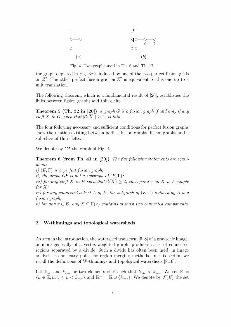
Fig. 4. Two graphs used in Th. 6 and Th. 17.

the graph depicted in Fig. 3c is induced by one of the two perfect fusion gridson Z2. The other perfect fusion grid on Z2 is equivalent to this one up to aunit translation.

The following theorem, which is a fundamental result of [20], establishes thelinks between fusion graphs and thin clefts.

Theorem 5 (Th. 32 in [20]) A graph G is a fusion graph if and only if anycleft X in G, such that |C(X)| ≥ 2, is thin.

The four following necessary and sufficient conditions for perfect fusion graphsshow the relation existing between perfect fusion graphs, fusion graphs and asub-class of thin clefts.

We denote by GN the graph of Fig. 4a.

Theorem 6 (from Th. 41 in [20]) The five following statements are equiv-alent:i) (E,Γ) is a perfect fusion graph;ii) the graph GN is not a subgraph of (E,Γ);iii) for any cleft X in E such that C(X) ≥ 2, each point x in X is F-simplefor X;iv) for any connected subset A of E, the subgraph of (E,Γ) induced by A is afusion graph;v) for any x ∈ E, any X ⊆ Γ(x) contains at most two connected components.

2 W-thinnings and topological watersheds

As seen in the introduction, the watershed transform [5–8] of a grayscale image,or more generally of a vertex-weighted graph, produces a set of connectedregions separated by a divide. Such a divide has often been used, in imageanalysis, as an entry point for region merging methods. In this section werecall the definitions of W-thinnings and topological watersheds [8,16].

Let kmin and kmax be two elements of Z such that kmin < kmax. We set K ={k ∈ Z; kmin ≤ k < kmax} and K+ = K ∪ {kmax}. We denote by F(E) the set

9

composed of all maps from E to K.

Let F ∈ F(E). If x ∈ E, F (x) is called the altitude of x. Let k ∈ K+. Wedenote by F [k] the set {x ∈ E;F (x) ≥ k} and by F [k] its complementaryset; F [k] is called an upper section of F and F [k], a lower section of F . Aconnected component of F [k] which does not contain a connected componentof F [k− 1] is a (regional) minimum of F . We denote by M(F ) ⊆ E the unionof all minima of F . We say that M(F ) is the divide of F . A subset X of E isflat for F if any two points x, y in X are such that F (x) = F (y). If X is flatfor F , the altitude of X is the altitude of any point of X.

By the mean of upper sections, the definitions of uniconnected points andclefts can be extended to the case of maps [8,16–18].

Let F ∈ F(E). The lowering of F at x, denoted by [F \x], is the map in F(E)such that:- [F \ x](x) = F (x)− 1; and- [F \ x](y) = F (y) for any y ∈ E \ {x}.

Definition 7 (watershed, Def. 10 in [16]) Let F ∈ F(E). Let x ∈ E andk = F (x). We say that x is W-destructible for F if x is uniconnected for F [k].If there is no W-destructible point for F we say that F is a (topological) wa-tershed.Let H ∈ F(E). We say that H is a W-thinning of F if:i) H = F ; or if:ii) there exists a W-thinning I ∈ F(E) of F such that H is the lowering of Iat a W-destructible point for I.If H is both a W-thinning of F and a watershed, we say that H is a (topolog-ical) watershed of F .

In other words, a point x such that F (x) = k is W-destructible for F if x isadjacent to exactly one component of F [k] = {y ∈ E | F (y) < k}. A map His a W-thinning of F , if there exists a (possibly empty) sequence of maps〈F0, . . . , F`〉 such that F0 = F , F` = H and, for any i ∈ [1, `], Fi is the loweringof Fi−1 at a W-destructible point for Fi−1. Furthermore, H is a topologicalwatershed of F , if H is a W-thinning of F which has no W-destructible point.

In Fig. 5a and b, assume that the images are equipped with the 8-adjacencyrelation. In both Fig. 5a and b, it may be seen that there are three minimawhich are the components with levels 0,1 and 2. In Fig. 5a, the point labeled ris W-destructible. In Fig. 5b, no point is W-destructible. The map depictedin Fig. 5b is a topological watershed of the map in Fig. 5a.

The divide of a topological watershed constitutes an interesting image segmen-tation [16,18] which possesses important properties not guaranteed by mostwatershed algorithms [5,6]. In particular, it preserves the connection value be-

10

5 4 4 3 2 2 2

6 9 9 9 2 2 2

6 9 1 9 9 9 2

8 9 9 8 8 9 2

8 9 0 9 9 9 4

7 9 9 9 4 4 4

6 5 5 5 4 4 4

r2 2 2 2 2 2 2

2 9 9 9 2 2 2

2 9 1 9 9 9 2

2 9 8 8 8 9 2

2 9 0 9 9 9 2

2 9 9 9 2 2 2

2 2 2 2 2 2 2

s t

(a) (b)

Fig. 5. The depicted images are equipped with the 8-adjacency relation. (a): A mapF ; (b): a topological watershed of F .

5

7 13

42

7 15

723

74

(a) (b)

Fig. 6. (a): A graph G. The values constitute a map F that weights the edges of G.(b): A graph G′ that is the line graph of G. The map F weights the vertices of G′.

tween the minima of the original map; intuitively, the connection value (see[16,18,22,23]) between two minima can be thought of as the minimal altitudeat which one need to climb in order to reach one minimum from the other. Ithas been shown (Th. 7 in [16]) that a topological watershed can be equiva-lently defined as a transformation which extends the lower sections (and hencethe minima) of the original map as much as possible while preserving the con-nection value between all pairs of minima. As said in the introduction, thiscontrast preservation property is a fundamental property on which rely manypopular region merging methods based on watersheds [13,15,14].

In image analysis applications, we sometimes deal with graphs whose edges,rather than vertices, are weighted by a cost map [12,24–27]. To finish thissection, we recall the definition of line graphs (see, e.g., [28]). This class ofgraphs allows us to highlight that the approaches of watershed and regionmerging based on edge-weighted graphs are particular cases of the approachesbased on vertex-weighted graphs developed in this paper.

The line graph of (E,Γ) is the graph (E ′,Γ′) such that E ′ = Γ? and (u, v)belongs to Γ′ whenever u ∈ Γ?, v ∈ Γ?, u 6= v and u, v share a common vertexof E.We say that the graph (E ′,Γ′) is a line graph if there exists a graph (E,Γ)such that (E ′,Γ′) is isomorphic to the line graph of (E,Γ).

11

For instance, the graph depicted in Fig. 6b is the line graph of the one depictedin Fig. 3a. It has been proved [20] that any line graph is a perfect fusiongraph and that the converse is not true. Thus, all definitions, properties andalgorithm for watershed on perfect fusion graphs developed in Secs. 4 and 3also hold for watershed approaches based on edge-weighted graphs. A moredetailed presentation of watersheds in edge-weighted graphs can be found in[26,27].

3 Thinness of topological watersheds

The divides produced by watershed algorithms [5–7], and in particular bytopological watershed algorithms [17], are not always clefts and can sometimesbe thick, even on fusion graphs. Consider, for instance, the digital image Fdepicted in Fig. 5b and assume that it is equipped with the graph inducedby the 8-adjacency. Although the map F is a topological watershed and theconsidered graph is a fusion graph (see Prop. 48 in [20]), the point labeled sis inner for M(F ). As said in the introduction, such thickness is a problem fordefining and implementing region merging schemes. In Sec. 1.3, we presenteda result of [20] which characterizes, thanks to a merging property, the class ofgraphs in which any cleft is thin (Th. 5). In this section, we provide a similarresult for the case of topological watersheds.

To this end, we introduce a notion of thinness for maps which extends the onefor sets by the mean of upper sections.

Definition 8 (thin map) Let F ∈ F(E), let x ∈ E and k = F (x). We saythat x is an inner point for F if x is inner for F [k]. The interior of F , denotedby int(F ), is the set of points in M(F ) that are inner for F . We say that Fis thin if int(F ) = ∅.

In other words, a point is inner for a map if all its neighbors have an altitudegreater than or equal to its own altitude. Thus, a map is thin if any point inits divide has at least one neighbor of strictly lower altitude. It may be seenthat the topological watershed depicted in Fig. 8b is thin whereas the one inFig. 5b is not.

From the very definition of a topological watershed and thanks to Th. 5, itmay be seen that any graph in which all topological watersheds are thin isnecessarily a fusion graph. Indeed, if we consider a graph (E,Γ) which is nota fusion graph, then, by Th. 5 there exists a cleft X ⊆ E (with |C(X)| ≥ 2),which is not thin (in the sense of Def. 2). From this set, we can construct themap F ∈ F(E) such that F (x) = 1 for any x ∈ X and F (x) = 0 otherwise.Clearly, by definitions of a cleft and of a watershed, F is not thin (in the sense

12

of Def. 8). Thus, if all topological watersheds are thin in (E,Γ), then (E,Γ)must be a fusion graph. The map in Fig. 5b shows that, contrarily to the caseof clefts (Th. 5), the converse is, in general, not true. However, as establishedby the following characterization theorem, deep links exist between these twoclasses of graphs.

Theorem 9 Any topological watershed in (E,Γ) is thin if and only if for anycleft X ⊆ E, for any A ∈ C(X), the subgraph of (E,Γ) induced by A is afusion graph.

The proof of Th. 9 can be found in annex.

We remark that the above condition, that characterizes the graphs in whichany topological watershed is thin, is a weakening of condition iv of Th. 6 whichcharacterizes the perfect fusion graphs. Thus, any topological watershed on aperfect fusion graph is thin. On the other hand, there exists some graphs whichare not perfect fusion graphs and in which any topological watershed is thin(see for instance Fig. 7).

In image analysis, a cleft (Sec. 1.2) can be seen as a frontier between connectedregions and the divide of a topological watershed constitutes an interestingsegmentation (Sec. 2). Therefore, a desirable property is that the divide of atopological watershed is a cleft. Unfortunately, such a property does not holdeven in the case of a graph in which any topological watershed is thin. Con-sider, for instance, the graph (E,Γ) and the topological watershed F depictedin Fig. 7a. It may be verified, thanks to Th. 9, that in (E,Γ) any topologicalwatershed is thin; this is, in particular, the case of F . However, it may bechecked that the points which are bold circled are uniconnected for the divideof F . Hence M(F ) is not a cleft. Observe also that the black vertex is inner (inthe sense of Def. 2) for M(F ) and thus that M(F ) is not thin. Thus, the no-tion of thinness defined in this section does not lead to topological watershedsadapted for region merging schemes. In the next sections, we study watershedsin perfect fusion graphs and show that this kind of problems cannot happen.

2

2

2

2

1 1 11

0

0

0

0

0

0

2

Fig. 7. A graph in which any topological watershed is thin. The values define a mapthat is a topological watershed. The black point is inner for the divide in the senseof Def. 2. The circled points are uniconnected for the divide.

13

0 0

0 0

00000

3

3

3

9

9

99 92 2

2 0 0

0 0

00000

9

9

99 92 2

0

0

0

0

(a) (b)

0 0

0 0

00000

2 2

0

0

0

0

2

2

2 2 2

0 0

0 0

00000

2 2

2 00

0 0

222

2

(c) (d)

Fig. 8. Example of maps on perfect fusion graphs, the minima are in white; (a): thebold circled vertex is M-cliff; (b): a C-watershed of (a); (c): a topological watershedof both (a) and (b); (d): a topological watershed of (a).

4 C-watersheds in perfect fusion graphs

In this section, we introduce a new grayscale transformation, called C-watershed,that always produces a map whose divide is a cleft. An important result(Th. 13) is that, on a perfect fusion graph, any C-watershed of a map is aW-thinning of this map whose divide is a thin cleft. Furthermore, we proposeand prove the correctness of a linear time algorithm to compute C-watershedson perfect fusion graphs.

Definition 10 (M-cliff point) Let F ∈ F(E) and let x ∈ E. We say that xis a cliff point (for F) if x is uniconnected for M(F ). We say that x is M-cliff(for F ) if x is a cliff point of minimal altitude (i.e., F (x) = min{F (y) | y ∈ Eis a cliff point for F}).

In other words, a cliff point for a map F ∈ F(E) is a point in M(F ) which isadjacent to a single minimum of F . A point x is M-cliff for F if no other pointof M(F ) adjacent to a single minimum has an altitude strictly lower than thealtitude of x.

In Fig. 8a, the points at altitude 3 are cliff points and the bold circled pointis the only M-cliff point. In Figs. 8b,c and d, it can be seen that there is noM-cliff point and no cliff point.

14

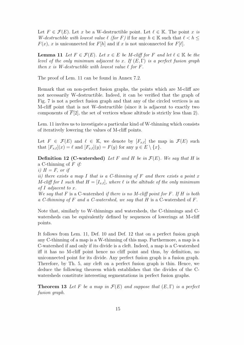
Let F ∈ F(E). Let x be a W-destructible point. Let ` ∈ K. The point x isW-destructible with lowest value ` (for F ) if for any h ∈ K such that ` < h ≤F (x), x is uniconnected for F [h] and if x is not uniconnected for F [`].

Lemma 11 Let F ∈ F(E). Let x ∈ E be M-cliff for F and let ` ∈ K be thelevel of the only minimum adjacent to x. If (E,Γ) is a perfect fusion graphthen x is W-destructible with lowest value ` for F .

The proof of Lem. 11 can be found in Annex 7.2.

Remark that on non-perfect fusion graphs, the points which are M-cliff arenot necessarily W-destructible. Indeed, it can be verified that the graph ofFig. 7 is not a perfect fusion graph and that any of the circled vertices is anM-cliff point that is not W-destructible (since it is adjacent to exactly twocomponents of F [2], the set of vertices whose altitude is strictly less than 2).

Lem. 11 invites us to investigate a particular kind of W-thinning which consistsof iteratively lowering the values of M-cliff points.

Let F ∈ F(E) and ` ∈ K, we denote by [Fx,`] the map in F(E) suchthat [Fx,`](x) = ` and [Fx,`](y) = F (y) for any y ∈ E \ {x}.

Definition 12 (C-watershed) Let F and H be in F(E). We say that H isa C-thinning of F if:i) H = F, or ifii) there exists a map I that is a C-thinning of F and there exists a point xM-cliff for I such that H = [Ix,`], where ` is the altitude of the only minimumof I adjacent to x.We say that F is a C-watershed if there is no M-cliff point for F . If H is botha C-thinning of F and a C-watershed, we say that H is a C-watershed of F .

Note that, similarly to W-thinnings and watersheds, the C-thinnings and C-watersheds can be equivalently defined by sequences of lowerings at M-cliffpoints.

It follows from Lem. 11, Def. 10 and Def. 12 that on a perfect fusion graphany C-thinning of a map is a W-thinning of this map. Furthermore, a map is aC-watershed if and only if its divide is a cleft. Indeed, a map is a C-watershediff it has no M-cliff point hence no cliff point and thus, by definition, nouniconnected point for its divide. Any perfect fusion graph is a fusion graph.Therefore, by Th. 5, any cleft on a perfect fusion graph is thin. Hence, wededuce the following theorem which establishes that the divides of the C-watersheds constitute interesting segmentations in perfect fusion graphs.

Theorem 13 Let F be a map in F(E) and suppose that (E,Γ) is a perfectfusion graph.

15

Let H be a C-watershed of F . Then, H is a W-thinning of F . Furthermore,the divide of H is a thin cleft.

To illustrate the previous theorem, let us look at Fig. 8. The map H depictedin (b) is a C-watershed of the map F depicted in (a). It can be verified that His a W-thinning of F and that the divide of H is a thin cleft. In general,a C-watershed is not a topological watershed. For instance, the map H is aC-watershed, but the points at altitude 9 are W-destructible. Nevertheless, asimplied by the following property, the divide of any C-watershed of F is equalto the divide of a topological watershed of F .

A W-thinning of F ∈ F(E) is a lowering (i.e., a map H such that for anyx ∈ E, H(x) ≤ F (x)) of F which preserves the number of components of alllower sections of F . In particular, it preserves the number of minima of F . Bythe preceding theorem, the divide of any C-watershed is a cleft. Hence, theminima of a C-watershed cannot be further “extended” while preserving allof them. As a consequence, we deduce the following property.

Property 14 Let F ∈ F(E) be a C-watershed. The divide of any W-thinningof F is equal to the divide of F .

The algorithms to compute (the divide of) a topological watershed [17] are notlinear and require the computation of an auxiliary data structure called com-ponent tree [29]. It is possible to reach a better complexity for the computationof a C-watershed on a perfect fusion graph.

In a C-thinning sequence, the points which are in a minimum at a given stepnever become M-cliff further in the sequence. This observation leads us to thedefinition of Algorithm 1, a very simple algorithm for C-watersheds.

At each iteration of the main loop (line 6) of Algorithm 1, it may be seen thatany point adjacent to a unique minimum of F is in the set L. Thus, it maybe easily deduced that at each iteration of the main loop, F is a C-thinning(hence, by Lem. 11, a W-thinning) of the input map.At the end of Algorithm 1, the set L is empty. Thus there is no point adjacentto a unique minimum of F , in other words, there is no point M-cliff or clifffor F . As a consequence of the preceding remarks, at the end of Algorithm 1,the map F is a C-watershed of the input map.

In Algorithm 1, the operations performed on the set L are the insertion of anelement and the extraction of an element with minimal altitude. Thus, L maybe managed as a priority queue. In [30], an efficient priority queue algorithmhas been proposed. It supports the operation of insertion, extraction of aminimal element or deletion in worst case time O(log logm) where m is thenumbers of elements in L. In fact, for computing a C-watershed, we can use afaster data structure. To reach this goal, we first need to establish the following

16

Algorithm 1: C-watershed

Data: a perfect fusion graph (E,Γ), a map F ∈ F(E)Result: FL := ∅; K := ∅;1

Attribute distinct labels to all minima of F and label the points of M(F )2

with the corresponding labels;foreach x ∈ E do3

if x ∈M(F ) then K := K ∪ {x};4

else if x is adjacent to M(F ) then L := L ∪ {x}; K := K ∪ {x};5

while L 6= ∅ do6

x := an element of L with minimal altitude for F ;7

L := L \ {x};8

if x is adjacent to exactly one minimum of F then9

Set F [x] to the altitude of the only minimum of F adjacent to x;10

Label x with the corresponding label;11

foreach y ∈ Γ?(x) ∩K do L := L ∪ {y}; K := K ∪ {y};12

fundamental theorem. It states that in a C-thinning sequence the points arelowered down by increasing order of altitude (for the original map F ).

Theorem 15 (monotony) Let F ∈ F(E) and suppose that (E,Γ) is a per-fect fusion graph. Let H be a C-thinning of F . Any point M-cliff for H has analtitude greater than or equal to the altitude of any point M-cliff for F .

A proof of Prop. 15 is given in Annex 7.3.

From Th. 15, we deduce that in Algorithm 1, when the map F is loweredat a point x with altitude k, any point inserted further in the set L hasa level greater than or equal to k. Thus, the set L may be managed by amonotone priority queue, that is, a priority queue whose minimum value isnon-decreasing over time (see [31] for an application of such a queue). M.Thorup [30] proved that if we can sort n keys in time n.s(n), then, and onlythen, there is a monotone queue with capacity n, supporting the insert andextract-min operations in s(n) amortized time.

In Algorithm 1, the set K is used to avoid multiple insertions of a same pointin the set L and can be managed as a Boolean array. Thus, the main loop(line 6) is executed at most |E| times. Furthermore, the minima of a map canbe extracted in linear time thanks to well known algorithms (see [32]). Wededuce Prop. 16 from these observations.

Property 16 If the elements of E can be sorted according to F in linear timewith respect to |E|, then Algorithm 1 terminates in linear time with respectto (|E|+ |Γ|).

17

Since Algorithm 1 possesses the monotone property discussed above, it canbe classified in the group of immersion algorithms (see [5–7] for examples).On non-perfect fusion graphs, Prop. 15 is in general not true. Consider, forinstance, the map F in Fig. 5b. The point labeled t, with altitude 9, is M-clifffor F , but is not W-destructible. Let H = [Ft,2], H is a C-thinning of F .We can remark that the point labeled s is the only M-cliff point for H andits altitude is strictly less than 9. Thus, on non-perfect fusion graphs a C-thinning sequence is in general not monotone. Moreover, it has been shown in[18] that in the case of a non-perfect fusion graph, some immersion algorithmsare not monotone and a monotone W-thinning algorithm does not, in general,produce a divide that satisfies Prop. 14.

In this section, we have introduced the C-watershed transformation and haveshown interesting properties on perfect fusion graphs. We may wonder whetherit is possible to extend (some of) these properties to other kinds of graphs. Inother words: what is the largest class of graphs such that Lem. 11 holds?

Let us denote by Gλ the graph depicted in Fig. 4b.

Theorem 17 The three following statements are equivalent:i) for any F ∈ F(E), any point M-cliff for F is W-destructible;ii) for any F ∈ F(E), any C-watershed of F is a W-thinning of F ;iii) the graph Gλ is not a subgraph of (E,Γ).

The proof of Th. 17 can be found in Annex 7.2.

5 Topological watersheds on perfect fusion graphs

As seen in the previous section, on a perfect fusion graph, a C-watershed isalways a W-thinning whose divide is a thin cleft. In this section, we extend thisresult to divides of topological watersheds. Then, we define a particular type oftopological watersheds that derive from the C-watersheds. We show that thisfamily of topological watershed satisfies an interesting additional property.Finally, we derive some new characterizations of perfect fusion graphs basedon both thinness properties of C-watersheds and topological watersheds.

If a map F is a topological watershed, then there is no point in E which isW-destructible for F . Since any point M-cliff for F is W-destructible for F ,we deduce the following property.

Theorem 18 Let F ∈ F(E) and assume that (E,Γ) is a perfect fusion graph.If F is a topological watershed, then F is a C-watershed. Furthermore, thedivide of any topological watershed is a thin cleft.

18

As shown in the previous section a C-watershed is not necessarily a topologicalwatershed. Thus, the converse of Th. 18 is, in general, not true.

Nevertheless, as stated by the next property, the C-watershed can be usedto design an interesting strategy for computing a topological watershed in aperfect fusion graph.

Definition 19 (C-topological watershed) Let F ∈ F(E) and assume that(E,Γ) is a perfect fusion graph. We say that H is a C-topological watershedof F , if there exists a C-watershed I of F such that H is a topological watershedof I.

In the case of a perfect fusion graph, it is proved by Th. 13 that a C-topologicalwatershed of a map is necessarily a topological watershed of this map. Onthe contrary, as we will see a little later, all topological watersheds are notC-topological watersheds. Among all topological watersheds of a map, the C-topological watersheds satisfy an additional property (Prop. 20). Informallyspeaking, it states that the divides of C-topological watersheds are locatedon the “highest crests” that separate the minima of the original map. Thefollowing property is a direct consequence of the monotony theorem (Th. 15)on C-watersheds.

Let F ∈ F(E). We say that a path π = 〈x0, . . . , x`〉 in E is descending for Fif for any k ∈ [1, `], we have F (xk) ≤ F (xk−1).

Property 20 Let F and H be two maps in F(E) and assume that (E,Γ) isa perfect fusion graph. If H is a C-topological watershed of F , then for anypoint x in M(H), there exist two minima of F which can be reached from xby a descending path for F .

The map H, depicted on Fig. 8c, is a C-topological watershed of the map F(Fig. 8a). It can be checked that from any point in M(H), two distinct minimaof F can be reached by a descending path for F . On the contrary, the previousproperty is not verified by all topological watersheds. For instance, let usanalyze the map I of Fig. 8d that is a topological watershed. We denote byx the vertex circled in Fig. 8a. Note that x ∈M(I). The only minimum of Fwhich can be reached from x by a descending path is the one at the top left ofthe figure. Thus, the topological watershed I of F , which is not a C-topologicalwatershed of F , does not verify Prop. 20.

From the preceding results, we derive some grayscale characterizations of per-fect fusion graphs based on thinness properties of both C-watersheds andtopological watersheds. Their proof can be found in Annex 7.4.

Let H ∈ F(E), x ∈ E and let k = H(x). If x is F-simple for H[k], i.e., x isadjacent to exactly two components of H[k], we say that x is F-simple for H.

19

Property 21 The four following statements are equivalent:i) (E,Γ) is a perfect fusion graph;ii) for any C-watershed F ∈ F(E), any point in M(F ) is F-simple for M(F );iii) for any topological watershed F ∈ F(E), any point in M(F ) is F-simplefor M(F );iv) for any topological watershed F ∈ F(E), any point in M(F ) is F-simplefor F .

6 Perspectives: perfect fusion grids and hierarchical schemes

With the counter-examples depicted in this paper, we have seen that thereexist topological watersheds whose divides are not thin clefts in 2D on thegraphs induced by the 4- and 8-adjacency relation. In 3D, similar counter-examples (see [20]) can be found for the graphs induced by the 6- and 26-adjacency relations that are the extensions of the 4- and 8-adjacency to Z3.On the contrary, we have shown that, on perfect fusion graphs, the divideof any topological watershed is a thin cleft. On these graphs, region mergingschemes are easy to rigorously define and straightforward to implement. Thus,the framework of perfect fusion graphs is adapted for region merging methodsbased on topological watersheds.

In [20], we introduced the family of perfect fusion grids over Zn, for any n ∈ N.Any element of this family is indeed a perfect fusion graph. We proved thatany of these grids is “between” the direct adjacency graph (which generalizesthe 4-adjacency to Zn) and the indirect adjacency graph (which generalizes the8-adjacency to Zn). These n-dimensional grids are all equivalent (up to a unittranslation) and, in a forthcoming paper, we intend to prove that they are theonly graphs that possess these two properties [33]. However, we must noticethat watersheds obtained from the same digital image using these differentgrids, may indeed be different. An example of (a restriction of) a 2-dimensionalperfect fusion grid is presented in Fig. 8.

Perfect fusion grids thus constitute an interesting alternative to classical gridsfor watershed-based region merging methods. An example of such a procedurecould be described, starting from the divide of a C-watershed, by the iterationof the following three steps: i) select the most significant region A accordingto a given criterion (e.g., , the dynamics described in [34,22]); ii) select a re-gion B such that A and B are neighbors and the minimal value of the pointsin Γ?(A,B) is minimal; and iii) merge A and B through Γ?(A,B). An illustra-tion of such a scheme using the dynamics is shown in Fig. 9. Future work willinclude revisiting hierarchical segmentation methods [13,15] on perfect fusiongrids and comparing these new schemes with previously published algorithms.

20

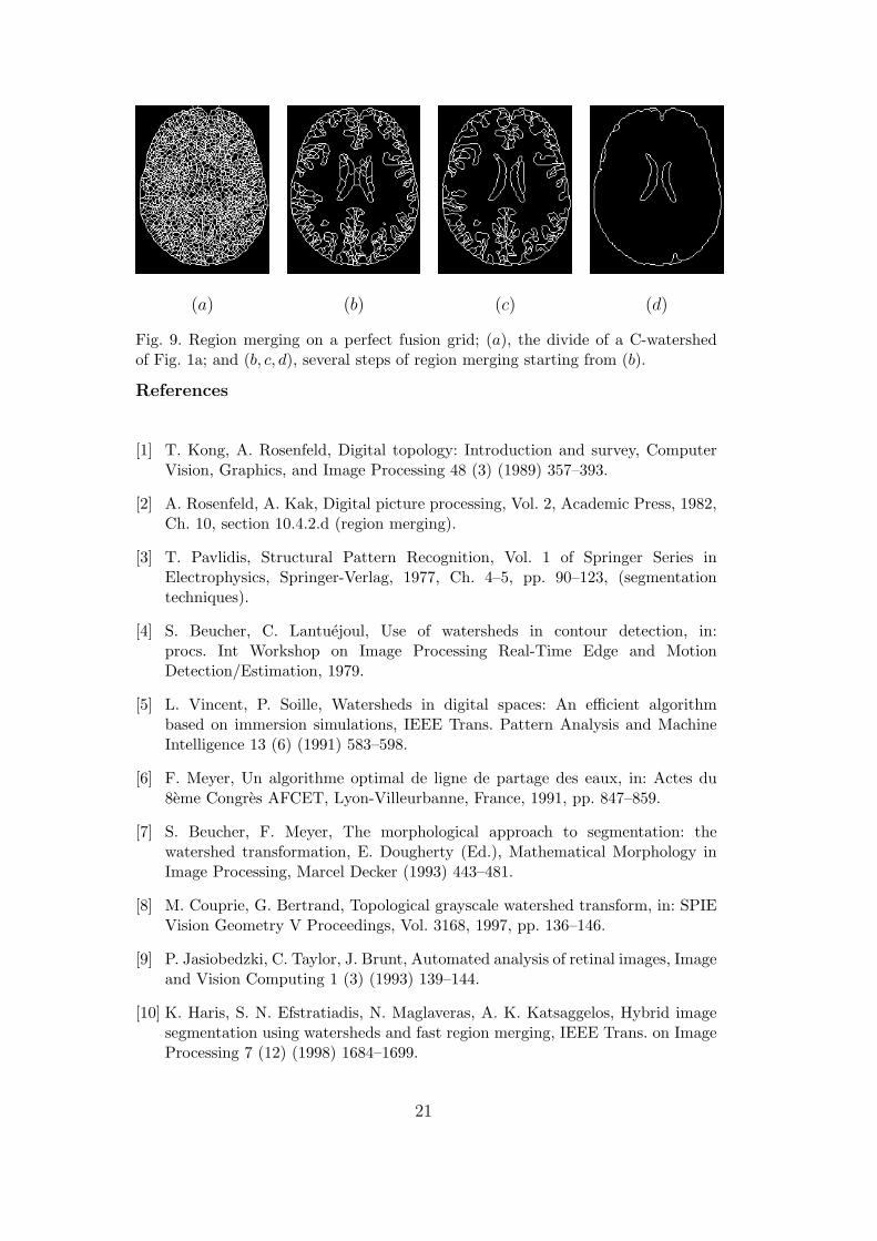
(a) (b) (c) (d)

Fig. 9. Region merging on a perfect fusion grid; (a), the divide of a C-watershedof Fig. 1a; and (b, c, d), several steps of region merging starting from (b).

References

[1] T. Kong, A. Rosenfeld, Digital topology: Introduction and survey, ComputerVision, Graphics, and Image Processing 48 (3) (1989) 357–393.

[2] A. Rosenfeld, A. Kak, Digital picture processing, Vol. 2, Academic Press, 1982,Ch. 10, section 10.4.2.d (region merging).

[3] T. Pavlidis, Structural Pattern Recognition, Vol. 1 of Springer Series inElectrophysics, Springer-Verlag, 1977, Ch. 4–5, pp. 90–123, (segmentationtechniques).

[4] S. Beucher, C. Lantuejoul, Use of watersheds in contour detection, in:procs. Int Workshop on Image Processing Real-Time Edge and MotionDetection/Estimation, 1979.

[5] L. Vincent, P. Soille, Watersheds in digital spaces: An efficient algorithmbased on immersion simulations, IEEE Trans. Pattern Analysis and MachineIntelligence 13 (6) (1991) 583–598.

[6] F. Meyer, Un algorithme optimal de ligne de partage des eaux, in: Actes du8eme Congres AFCET, Lyon-Villeurbanne, France, 1991, pp. 847–859.

[7] S. Beucher, F. Meyer, The morphological approach to segmentation: thewatershed transformation, E. Dougherty (Ed.), Mathematical Morphology inImage Processing, Marcel Decker (1993) 443–481.

[8] M. Couprie, G. Bertrand, Topological grayscale watershed transform, in: SPIEVision Geometry V Proceedings, Vol. 3168, 1997, pp. 136–146.

[9] P. Jasiobedzki, C. Taylor, J. Brunt, Automated analysis of retinal images, Imageand Vision Computing 1 (3) (1993) 139–144.

[10] K. Haris, S. N. Efstratiadis, N. Maglaveras, A. K. Katsaggelos, Hybrid imagesegmentation using watersheds and fast region merging, IEEE Trans. on ImageProcessing 7 (12) (1998) 1684–1699.

21

[11] A. Bleau, L. Leon, Watershed-based segmentation and region merging,Computer Vision and Image Understanding 77 (3) (2000) 317–370.

[12] F. Meyer, Minimum spanning forests for morphological segmentation, in: Procs.of the second international conference on Mathematical Morphology and itsApplications to Image Processing, 1994, pp. 77–84.

[13] S. Beucher, Watershed, hierarchical segmentation and waterfall algorithm, in:Mathematical Morphology and its Applications to Image Processing, 1994, pp.69–76.

[14] F. Meyer, The dynamics of minima and contours, in: P. Maragos, R. W. Schafer,M. A. Butt (Eds.), Mathematical Morphology and its Application to Image andSignal Processing, Kluwer Academic Publishers, Boston, 1996, pp. 329–336.

[15] L. Najman, M. Schmitt, Geodesic saliency of watershed contours andhierarchical segmentation, IEEE Trans. Pattern Analysis and MachineIntelligence 18 (12) (1996) 1163–1173.

[16] G. Bertrand, On topological watersheds, Journal of Mathematical Imaging andVision 22 (2-3) (2005) 217–230.

[17] M. Couprie, L. Najman, G. Bertrand, Quasi-linear algorithms for thetopological watershed, Journal of Mathematical Imaging and Vision 22 (2-3)(2005) 231–249.

[18] L. Najman, M. Couprie, G. Bertrand, Watersheds, mosaics and the emergenceparadigm, Discrete Applied Mathematics 147 (2-3) (2005) 301–324.

[19] J. Cousty, G. Bertrand, M. Couprie, L. Najman, Fusion graphs, region mergingand watersheds, in: Discrete Geometry for Computer Imagery, procs. of DGCI,Vol. 4245 of Lecture Notes in Computer Science, Springer, 2006, pp. 343–354.

[20] J. Cousty, G. Bertrand, M. Couprie, L. Najman, Fusion graphs:merging properties and watersheds, Journal of Mathematical Imaging andVision Accepted. Also in technical report IGM2005-04, http://igm.univ-mlv.fr/LabInfo/rapportsInternes/2005/04.v2.pdf.

[21] J. Cousty, M. Couprie, L. Najman, G. Bertrand, Grayscale watersheds onperfect fusion graphs, in: Combinatorial Image Analysis, procs. of IWCIA, Vol.4040 of Lecture Notes in Computer Science, Springer, 2006, pp. 60–73.

[22] G. Bertrand, On the dynamics, Image and Vision Computing 25 (4) (2007)447–454.

[23] A. Rosenfeld, The fuzzy geometry of image subsets, Pattern Recognition Letters2 (1984) 311–317.

[24] J. K. Udupa, S. Samarsekara, Fuzzy connectedness and object definition:Theory, algorithms, and applications in image segmentation, Graphical Modelsand Image Processing 58 (1996) 246–261.

22

[25] A. X. Falcao, J. Stolfi, R. de Alencar Lotufo, The image foresting transform:Theory, algorithm and applications, IEEE Trans. Pattern Analysis and MachineIntelligence 26 (2004) 19–29.

[26] J. Cousty, G. Bertrand, L. Najman, M. Couprie, Watershed cuts, in:Mathematical Morphology and its Applications to Signal and Image Processing,Procs. of ISMM, 2007, pp. 301–312.

[27] J. Cousty, G. Bertrand, L. Najman,M. Couprie, Watersheds, minimum spanning forests, and the drop of waterprinciple, Submitted. Also in technical report IGM2007-01, http://igm.univ-mlv.fr/LabInfo/rapportsInternes/2007/01.pdf.

[28] C. Berge, Graphes et hypergraphes, Dunod, 1970.

[29] L. Najman, M. Couprie, Building the component tree in quasi-linear time, IEEETrans. on Image Processing 15 (11) (2006) 3531–3539.

[30] M. Thorup, On RAM priority queues, SIAM Journal on Computing 30 (1)(2000) 86–109.

[31] R. Ahuja, K. Mehlhom, J. Orlin, R. Tarjan, Faster algorithms for the shortestpath problem, SIAM Journal on Computing 37 (2) (1990) 213–223.

[32] P. Soille, Morphological Image Analysis, Springer-Verlag, 1999.

[33] J. Cousty, G. Bertrand, Uniqueness of the perfect fusion grid on Zd Inpreparation.

[34] M. Grimaud, New measure of contrast: dynamics, in: P. Gader, E. Dougherty,J. Serra (Eds.), Image algebra and morphological image processing III, Vol.SPIE-1769, 1992, pp. 292–305.

7 Annex

7.1 Proof of Th. 9

Let us recall a characterization of topological watersheds (Th. 22) that willhelp us to prove Th. 9.

Let X and Y be two subsets of E. We say that Y is a W-thinning of X if:i) Y = X; or ifii) there exists a set Z that is a W-thinning of X and there exists a unicon-nected point x for Z such that Y = X \ {x}.Let C ⊆ X and assume that Y is a W-thinning of X. We say that Y is a cleftof X constrained by C if Z = Y whenever Z is a W-thinning of Y and C ⊆ Z.

23

In other words, Y is a cleft of X constrained by C if Y is a W-thinning of Xwhich contains C and if any point in Y \ C is not uniconnected for Y .

Theorem 22 (Th. 2 in [16]) Let F be in F(E). The map F is a topologicalwatershed if and only if, for each k ∈ K, F [k] is a cleft constrained by F [k+1].

We are now ready to prove Th. 9.

Proof of Th. 9i): Suppose that there exists a cleft X ⊆ E, and that there exists A ∈ C(X)such that (A,ΓA) is not a fusion graph. Then, by Th. 5, there exists a cleft Y ⊆A on (A,ΓA), such that |C(Y )| ≤ 2, that is not thin. Let us define the mapF ∈ F(E) as follows: for any x ∈ E, if x ∈ X, F (x) = 2, if x ∈ Y , F (x) = 1and if x ∈ (E \ (X ∪ Y )), F (x) = 0. It can be seen that F is a topologicalwatershed which is not thin.ii): Suppose that F is a topological watershed which is not thin. There existsx ∈ int(F ) with maximal altitude. Let k be the altitude of x. NecessarilyF [k+1]∩ int(F ) = ∅. Let A ∈ C(F [k + 1]) such that x ∈ A. Let Y = A∩F [k].Since A ∩ F [k + 1] = ∅ (as A ∈ C(F [k + 1])), by Th. 22, there is no pointuniconnected for F [k] in Y . Then any point y ∈ Y which is adjacent to F [k]is adjacent to at least two connected components of F [k]. Furthermore it canbe seen that these connected components are all included in A. Thus Y is acleft on (A,ΓA).Remark that x ∈ Y . From the very definition of int(F ) and since x ∈ int(F ),we have: x ∈ int(F [k]) and x ∈ int(Y ). Hence Y is a cleft on (A,ΓA) which isnot thin and by Th. 5 (A,ΓA) is not a fusion graph.We are now going to prove that there exists a cleft X ⊆ E on (E,Γ) such thatA ∈ C(X). More precisely, we are going to show that X = Γ?(A) is a cleft(and obviously A ∈ C(X)).If X = ∅ the proof is done. Otherwise, let z ∈ X and let k ′ = F (z). SinceA ∈ C(F [k + 1]) we know that k′ > k. Since k′ > k and since x is thehighest point of int(F ), we know that z cannot be inner for F . Hence, sinceF is a watershed, we deduce that z is adjacent to at least two connectedcomponents of F [k′]. One of these components, say A′, must contain A. Let Bbe any other one of these components. It must contain a point y adjacent to zsuch that y /∈ Γ(A′) (otherwise we would have B = A′). Since A ⊆ A′, wehave y /∈ Γ(A). Thus, z is adjacent to at least two components of X, whichare namely A and the component of X which contains y. Hence, z is not auniconnected for X and therefore, by the very definition of a cleft, we deducethat X = Γ?(A) is a cleft on (E,Γ) such that A ∈ C(X), hence Th. 9. 2

24

7.2 Proof of Lem. 11 and Th. 17

Observe that Lem. 11 is a corollary of Th. 17 (as shown below, after the proofof Th. 17). Thus we start by the proof of Th. 17.

Remark 23 Let F be a map in F(E). From the very definition of W-destructiblepoints and topological watersheds, it may be seen that if H is a W-thinningof F , then, for any k ∈ K+, we have |C(F [k])| = |C(H[k])|.

Proof of Th. 17i⇒ ii: Follows straightforwardly the definition of a C-watershed.iii ⇒ ii: Suppose that there exists five points p, q, r, s and t in E such thatthe subgraph G′ of (E,Γ) induced by {p, q, r, s, t} is isomorphic to Gλ. Let usconsider F ∈ F(E) such that: (a), F (p) = F (r) = F (t) = 0; (b), F (q) = 1;(c), F (s) = 2; and (d) for any x ∈ E \ {p, q, r, s, t}, F (x) = 4. Note that thefollowing arguments hold if either [E\{p, q, r, s, t}] 6= ∅ or [E\{p, q, r, s, t}] = ∅.It may be easily seen that F [2] is made of exactly two components. Observethat the point s is the only M-cliff point for F and that it is adjacent to {t}a minimum of F at altitude 0. Thus, for any C-watershed H of F (H 6= F ),we have H(s) = 0. It may be seen that |C(H[2])| = 1 whereas |C(F [2])| = 2.Thus we establish ii by the converse of Rem. 23.i⇒ iii: Suppose that there exists a map F ∈ F(E) such that there is a pointx1 ∈ E that is M-cliff for F and not W-destructible for F . Let h = F (x1). Letx0 ∈ Γ(x1) be any point in M ⊆M(F ) the only minimum of F adjacent to x1.It may be seen that x0 ∈ F [h]. Thus, since x1 is not W-destructible, x1 mustbe adjacent to X a connected component of F [h] which contains neither {x0}nor any point of M . Let Y = M(F )∩X. As a consequence of the definition of aminimum, Y is not empty. Let Π be the set of all paths 〈x0, x1, x2, . . . xk〉 suchthat x2, . . . xk are in X and xk is adjacent to Y . Let π = 〈x0, x1, x2, . . . x`〉 be ashortest path among the paths in Π (i.e., the length of any path in Π is greaterthan or equal to the length ` of π). Since x1 is adjacent to a unique minimumMof F and since M does not intersect X, x1 cannot be adjacent to Y . Hence,` > 1 and, by construction, it follows that x` ∈ X. Thus, F (x`) < h becauseX ⊆ F [h]. Suppose that x` is adjacent to a single minimum of F , then x`would be a cliff point, the altitude of which is less than the altitude of x1, acontradiction since x1 is M-cliff for F . Thus, there exist two points in Γ(x`),say y and z, which are in two distinct minima of F . To establish (iii), we arenow going to prove that the subgraph of (E,Γ) induced by {y, z, x`, x`−1, x`−2}is isomorphic to Gλ. Since y and z are in two distinct minima of F , y /∈ Γ(z).Furthermore, by construction, x`−1 ∈ Γ(x`−2), x` ∈ Γ(x`−1) and y and zboth belong to Γ(x`). It is thus sufficient to prove that y /∈ Γ(x`−1), y /∈Γ(x`−2) (and also z /∈ Γ(x`−1), z /∈ Γ(x`−2)) and that x` /∈ Γ(x`−2). If ` = 2,then x`−2 = x0 and x`−1 = x1. In this case, if x` ∈ Γ(x`−2), then x0 must

25

belong to X since x` ∈ X and F (x0) < h. This is by construction impossible.If ` > 2 and x` ∈ Γ(x`−2), then π is not a shortest among the paths in Πsince 〈x0, . . . , x`−2, x`〉 would also belong to Π. Therefore, in all cases, x`−2 /∈Γ(x`). If y ∈ Γ(x`−1), it may be seen that π′ = 〈x0, . . . x`−1〉 would belongto Π, which is impossible since the length of π ′ is less that the one of π. Inthe same manner, we can see that y /∈ Γ(x`−2), z /∈ Γ(x`−1), and z /∈ Γ(x`).Thus iii. 2

Proof of Lem. 11 Since (E,Γ) is a perfect fusion graph, from statement iiof Th. 6, GN is not a subgraph of (E,Γ). Remark that GN is a subgraph ofGλ. Thus Gλ is not a subgraph of (E,Γ). Let x ∈ E be any M-cliff point forF . From Th. 17, x is W-destructible for F .

Let ` be the level of the only minimum of F adjacent to x. When x has beenlowered down to F (x)−1 and while it has not been lowered down to `, x is theonly point M-cliff for F i (where F i = [F i−1 \ x], F 0 = F ). When x has beenlowered down to ` it is not W-destructible any more, hence ` is the lowestvalue of x. 2

7.3 Proof of Th. 15

Lemma 24 Assume that (E,Γ) is a perfect fusion graph. Let X ⊆ E be anonempty connected set and let Y be a nonempty subset of X. If int(X \Y ) 6=∅, then there exists y ∈ X \ Y adjacent to a single connected component of Y .

Proof Let us consider (X,ΓX) the subgraph of (E,Γ) induced by X. It is aconnected graph. By Th. 6iv, (X,ΓX) is a fusion graph. If |C(Y )| < 2, theresult follows from the connectedness of X. Otherwise, since int(X \ Y ) 6= ∅,we deduce from Th. 5 that X \ Y is not a cleft on (X,ΓX), hence there existsy ∈ [X \ Y ] which is uniconnected for [X \ Y ]. Therefore, by definition of auniconnected point, y is adjacent to a single connected component of (X \ Y )on (X,ΓX), hence y is adjacent to exactly one connected component of Y . 2

Proof of Th. 15 Let x be any point M-cliff for F . Let H0 = [Fx,`], where` is the altitude of the only minimum of F adjacent to x. Let y be any pointM-cliff for H0. It may be seen that y is adjacent to zero or one minimumof F . If y is adjacent to one minimum of F , y is a cliff point for F , andthen F (y) ≥ F (x) since x is M-cliff for F . Suppose now that y is not adjacentto any minimum of F (i.e., y ∈ int(M(F ))). Let k = F (y). Let X be thecomponent of F [k + 1] that contains y. From the definition of a minimum,it may be seen that the family M of all minima of F included in X is not

26

empty. Let Y = ∪{M ∈ M}. Since y ∈ int(M(F )), it can be seen that yis inner for [X \ Y ]. As a consequence, by Lem. 24, there exists z ∈ [X \ Y ]adjacent to a unique component of Y , that is z is a cliff point for F . As x isan M-cliff point for F , F (x) ≤ F (z). Since z ∈ F [k + 1], F (z) ≤ F (y). Wethus get F (x) ≤ F (y). By induction, Th. 15 is established. 2

7.4 Proof of Prop. 21

Proof of Prop. 21i ⇒ ii: The fact that (E,Γ) is a perfect fusion graph implies (from Th. 6iii)that any cleft X ⊆ E is such that any x ∈ X is F-simple for X. By definition,a map F ∈ F(E) is a C-watershed if and only if M(F ) is a cleft, hence ii.ii⇒ iii: By Th. 18, any topological watershed is a C-watershed hence iii.(i⇒ iii) and (i⇒ iv): Suppose that (E,Γ) is not a perfect fusion graph. Then,by Th. 6.iii, there exists a cleft Y ⊆ E such that there exists y ∈ Y which is notF-simple for Y . We define F ∈ F(E) such that for any x in Y , F (x) = 1 and forany x ∈ Y , F (x) = 0. Remark that Y = F [1] = M(F ), and that F [1] = M(F ).Thus, since Y is a cleft, there is no uniconnected point for M(F ) and thereis no W-destructible point for F . Thus, F is both a topological watershedand a C-watershed. Since y is not F-simple for Y , according to the precedingremarks, we deduce that y is neither F-simple for F nor F-simple for M(F ).Hence iii and iv both hold.i ⇒ iv: Let F ∈ F(E) be any topological watershed. Let x ∈ M(F ) and letk = F (x). Since (i ⇒ ii ⇒ iii), x is adjacent to exactly two minima of F .Hence, x is adjacent to at least one component of F [k]. Since F is a topologicalwatershed, x is not uniconnected for F [k]. Therefore, x is adjacent to at leasttwo components of F [k]. Since (E,Γ) is a perfect fusion graph, by Th. 6.v, xis adjacent to at most two components of F [k], hence x is F-simple for F . 2

27