NeuroImage 15, 329–344 (2002)doi:10.1006/nimg.2001.0975, available online at http://www.idealibrary.com on

Automated Sulcal Segmentation Using Watershedson the Cortical Surface1

Maryam E. Rettmann,* Xiao Han,† Chenyang Xu,† and Jerry L. Prince*,†*Department of Biomedical Engineering and †Department of Electrical and Computer Engineering,

Johns Hopkins University, Baltimore, Maryland 21218

Received March 20, 2001

The human cortical surface is a highly complex,folded structure. Sulci, the spaces between the folds,define location on the cortex and provide a parcella-tion into anatomically distinct areas. A topic that hasrecently received increased attention is the segmenta-tion of these sulci from magnetic resonance images,with most work focusing on extracting either the sul-cal spaces between the folds or curve representationsof sulci. Unlike these methods, we propose a techniquethat extracts actual regions of the cortical surface thatsurround sulci, which we call “sulcal regions.” Themethod is based on a watershed algorithm applied to ageodesic depth measure on the cortical surface. Awell-known problem with the watershed algorithm isa tendency toward oversegmentation, meaning that asingle region is segmented as several pieces. To ad-dress this problem, we propose a postprocessing algo-rithm that merges appropriate segments from the wa-tershed algorithm. The sulcal regions are thenmanually labeled by simply selecting the appropriateregions with a mouse click and a preliminary study ofsulcal depth is reported. Finally, a scheme is pre-sented for computing a complete parcellation of thecortical surface. © 2002 Elsevier Science

INTRODUCTION

Quantitative anatomic studies of the human cortexare challenging due to its highly complex, convolutedfolding pattern. The various folds, called gyri, and thespaces between the folds, called sulci, define locationon the cortex and provide a parcellation of the cortexinto anatomically distinct areas. With the advance-ment of magnetic resonance (MR) imaging techniques,high-resolution, high-contrast three-dimensional im-ages of the brain can now be routinely acquired in vivo.As a result, methods for modeling the cortical surface

1 This work was partially supported by the NSF ERC/CISST9731748 and by the NIH/NINDS R01NS37747 and a Whitaker Foun-dation graduate fellowship.

329

from these images have emerged, providing a meansfor furthering the understanding of morphometric vari-ability in human populations. A topic that has recentlyreceived increased attention is the study of sulci, inparticular, their segmentation from MR images (Man-gin et al., 1995; Thompson et al., 1996; Le Goualher etal., 1997; Vaillant and Davatzikos, 1997; Khaneja etal., 1998; Lohmann and von Cramon, 1998, 2000; Loh-mann, 1998; Royackkers et al., 1999; Zeng et al., 1999;Zhou et al., 1999; Renault et al., 2000; Tao et al., 2001).Sulci segmented from the cortex can be used in a va-riety of applications such as deformable atlas registra-tion algorithms and localizing activation sites in func-tional imaging. In addition, the geometric analysis ofsulci will lead to a better understanding of normalversus diseased cortical geometry and the morpholog-ical changes that occur with disease.

Previous work in the segmentation of sulci has fo-cused on fitting a surface (Thompson et al., 1996; Vail-lant and Davatzikos, 1997; Le Goualher et al., 1997;Zeng et al., 1999; Zhou et al., 1999), finding a set ofpoints (Mangin et al., 1995), or extracting the volumet-ric regions (Lohmann and von Cramon, 1998, 2000)within the sulcal spaces. Other work has focused onextracting curve representations of the sulci (Khanejaet al., 1998; Lohmann, 1998; Royackkers et al., 1999;Renault et al., 2000; Tao et al., 2001). Unlike thesemethods, we propose a technique that segments theactual cortical regions surrounding sulci. The advan-tage of segmenting actual cortical regions is that itallows for a direct geometric study of the cortical sur-face and provides a means for mapping functional ac-tivation sites. For ease of terminology, we refer to oursegmented regions as “sulcal regions,” which define theburied regions of cortex surrounding the sulcal spaces.Another advantage of the proposed method is that itsegments sulcal regions on the medial surface as wellas the lateral and inferior surfaces. In addition, thissegmentation method is completely automated and canbe used as a visualization tool for manual labeling ofindividual sulcal regions.

1053-8119/02 $35.00© 2002 Elsevier Science

All rights reserved.

330 RETTMANN ET AL.

In this paper, we describe our methodology for auto-matically segmenting sulcal regions using a watershedalgorithm applied to a geodesic depth measure on thecortical surface. A well-known problem with the water-shed algorithm is a tendency toward oversegmenta-tion, meaning that a single region is segmented asseveral pieces. To address this problem, we propose apostprocessing algorithm that merges appropriate seg-ments from the watershed algorithm. The idea of sulcalsegmentation using watersheds was first introduced byLohmann and von Cramon (1998) and extended inLohmann and von Cramon (2000). Although ourmethod is similar in basic concept to that described byLohmann, there are several important distinctions.First, our method operates on a cortical surface meshextracted from MR images rather than operating di-rectly on the image data. Second, our segmentationmethod produces pieces of the cortical surface, which isdefined on the continuum, rather than discrete vol-umes of gray matter and sulcal spaces. The relation-ship between the two results is that our surface seg-ments should pass through the volumes extracted byLohmann. In fact, these sulcal volumes were used toextract segments of a cortical surface by Kruggel andvon Cramon (2000). It may be advantageous to workdirectly on the cortical surface mesh, however, as thesulcal segmentation can be generated using the geom-etry of the continuous surface representation. Finally,our method segments sulci on the lateral, medial, andinferior surfaces of the brain while the work by Loh-mann and von Cramon (1998, 2000) focuses on sulcifrom the lateral surface only. We note that preliminaryresults of this work have been described in conferencepapers (Rettmann et al., 1999, 2000).

METHODS

Surface Estimation

In this paper, we use surfaces reconstructed fromMR images using the technique described in Xu et al.(1999) with several improvements (Xu et al., 2000; Hanet al., 2001a,b); however, our method is applicable toany reconstructed cortical surface model (cf. Davatzi-kos and Bryan, 1996; Drury et al., 1996; Sandor andLeahy, 1997; Xu et al., 1998; Dale et al., 1999; Mac-Donald et al., 2000). The method in Xu et al. (1999)combines fuzzy segmentation, isosurfaces, and deform-able surface models to reconstruct the layer of cortexlying in the geometric center, which is approximatelycytoarchitectonic layer 4. The reconstruction method iscomposed of three major steps. First, a three-classfuzzy segmentation of the MR data is computed corre-sponding to gray matter, white matter, and cerebrospi-nal fluid. Second, an initialization for the deformablesurface model is created by generating a topologically

correct isosurface (Han et al., 2001a) from the white

matter membership function obtained from the seg-mentation. The result of the isosurface algorithm is amesh that is a discrete representation of the continu-ous isosurface. Finally, a deformable surface model isused to refine the initial surface to the central layer ofthe gray matter, including all of the deep convolutedfolds within sulci on the lateral, medial, and inferiorsurfaces. The resulting surface is represented by atriangular mesh consisting of approximately 300,000vertices, as shown in Fig. 1a.

We have occasion to define several functions on thevertices of our cortical surfaces, and it is difficult tovisualize these functions due to the deep sulcal foldingof the cortex. To allow visualization of buried corticalregions, we generate a spherical representation foreach hemisphere of the reconstructed cortical surfaceusing the procedure described in Tosun and Prince(2001). This representation has a one-to-one mappingwith the original reconstructed surface and is convexfor ready visualization. An example of a spherical mapexhibiting the mean curvature of the cortical surface inFig. 1a is shown in Fig. 1b.

We note that as a final step in surface estimation, thehemispheres are automatically labeled. In a prepro-cessing step for the surface reconstruction, the volu-metric data are aligned along the anterior commissure(AC) and posterior commissure line and the location ofthe AC is determined. A cut plane that approximatelyseparates the hemispheres can then be estimated us-ing the location of the AC and a vector normal to thesagittal plane. A path around the corpus collosum trav-eling close to the cut plane is then determined usingthe connectivity of the triangle mesh. This defines aconnected boundary dividing the hemispheres, and thevertices are readily labeled as either left or right.

Sulcal Segmentation

The goal of this segmentation work is to extract theburied cortical regions surrounding each of the sulcalspaces. We define these regions as sulcal regions andrefer to the regions of cortex that are not buried in the

FIG. 1. (a) A reconstructed cortical surface and (b) a sphericalmap with its mean curvature displayed.

folds as “gyral regions.” These structures are depicted

331AUTOMATED SULCAL SEGMENTATION

in Fig. 2. A classification of points on the surface aseither gyral or sulcal is not, however, sufficient to ob-tain a distinct region corresponding to each sulcus assulci are frequently separated by a ridge buried withinthe cortical folds. This is illustrated in Fig. 3a with asimplified representation of two sulcal regions in threedimensions. This entire buried region is classified assulcal, but our aim is to obtain distinct regions corre-sponding to each of the two folds as illustrated in Fig.3b, in which one of the sulcal regions is outlined in lightgray and the other in dark gray. This diagram demon-strates that the ideal segmentation is identical to theresult that would be obtained by applying the water-shed algorithm on the buried regions of cortex.

Traditionally, the watershed transform has beenused in image processing for segmenting images intovarious catchment basins or for extracting watershedlines. While a complete description of the watershedtransform can be found in Meyer and Beucher (1990)and Vincent and Soille (1991), the key ideas are illus-trated in Fig. 4. As depicted on the left, the watershedtransform can be viewed as puncturing holes in thelocal minima of a function followed by an immersioninto a pool of water. Each region filling with water isassociated with a minima and will form a catchmentbasin. When the water from two regions begins tomerge, a dam is constructed to prevent water from oneregion spilling into the other. These dams are termedwatershed lines. When the immersion is complete, eachof the regions associated with a minima forms a sepa-rate catchment basin. From the above illustrations, itis intuitively clear that the catchment basins formed

FIG. 2. A simplified illustration of a cross section of the corticalsurface.

FIG. 3. A simplified illustration of (a) two sulcal regions and (b)

their ideal segmentation.

from the watershed algorithm would provide an appro-priate segmentation of sulcal regions. The main chal-lenge lies in defining a suitable function describing the“height” of the cortex, from which the watershed can becomputed.

Sulcal depth is often discussed in the literature andtextbooks on cortical anatomy (Ono et al., 1990). Ittypically represents a measure of the Euclidean dis-tance from the sulcal fundus to the outer cortical sur-face. In this paper, we develop a method to calculatethe depth from the outer cortical surface to each sur-face point lying within sulci. We use the geodesic dis-tance—a measure of distance on the surface—ratherthan three-dimensional Euclidean distance as a mea-sure of depth in order to avoid certain segmentationproblems. For example, certain parts of the insularcortex can be much shallower in Euclidean depth thanother parts, despite the fact that one is forced to cross“deeper” regions in order to move along the cortex itselfto get to the outer surface. Given the geodesic depthover the whole cortical surface, the height function of apoint on the surface is simply the maximum corticaldepth minus its own depth. The watershed segmenta-tion can then be computed.

Our approach for generating a sulcal segmentationfrom a cortical surface consists of four parts: sulcalclassification, geodesic depth calculation, watershedimplementation, and catchment basin merging. Thesteps are illustrated using one cortical surface; moreexamples are given under Results.

Sulcal Classification

Our first goal is to classify the cortical surface intosulcal and gyral regions. We accomplish this by firstdefining and finding an outer cortical surface. Intu-itively, the outer cortical surface is that part of thecortex that one could see, if the cerebral cortex wereisolated and separated into hemispheres. Now imaginea “shrink-wrap” process in which a flexible balloonsurrounding a hemisphere has air withdrawn from itsinterior until it conforms to the outer cortical surface.Those parts of the cortical surface in contact with theballoon are then defined as gyral regions, while the

FIG. 4. An illustration of the watershed algorithm.

remaining parts are sulcal regions. We implement this

332 RETTMANN ET AL.

classification procedure using a deformable surfacemodel, which we now describe.

A deformable surface is a parameterized surfacex(u) 5 [x(u), y(u), z(u)]T, u 5 (u1, u2) [ [0, 1] 3 [0, 1],that moves through the spatial domain of a three-dimensional image until the steady-state solution ofthe dynamic equation

­

­t~x~u, t!! 5 Fint~x~u, t!! 1 Fext~x~u, t!! (1)

is found. The internal forces control the tension on thesurface and are given by Fint 5 w1¹u

2x, where w1 is aweight and ¹u

2 5 ­2/(­u1)2 1 ­2/(­u2)2 is the Laplacianoperator defined in the parameter space. The externalforces, which drive the deformable surface toward thecortical surface, are derived from an edge map of thecortical surface as follows.

For each point on the cortical surface, its nearestvoxel is determined and assigned a value of 1, yieldinga binary image I, as shown in Fig. 5a. The hole intro-duced at the corpus callosum is filled by adding pointsnear the surface used to define the hemisphere cut. Theexternal forces are then computed as Fext 5 2w2¹d(m),where d(m) is the distance from voxel m to its nearestedge in I, w2 is a weight, and ¹ is the spatial gradientoperator. This type of external distance force has beendescribed previously in Cohen and Cohen (1993) andhas the advantage of a large capture range permittingthe initial surface to be far from the desired boundary.In addition, this force does not pull the deformablesurface into concave regions of the image (Xu andPrince, 1998).

A numerical solution to Eq. (1) can be found bydiscretizing the equation and solving the discrete sys-tem iteratively (cf. Kass et al., 1987). Parameter valuesrequired for the deformable surface algorithm weredetermined empirically from one data set as w1 5 0.75and w2 5 0.35 and held fixed for subsequent data sets.

FIG. 5. Cross-sectional view of (a) the edge map generated fromregions, (c) the barrier region, and (d) the shrink-wrap surface supe

The weight on the internal forces is set high relative to

the weight on the external forces to keep the deform-able surface rigid, thus reducing its ability to enter intothe cortical folds. The use of high internal forces, how-ever, can sometimes cause the deformable surface tobreak through the gyri as shown in Fig. 5b. To avoidthis, the iterative implementation of the deformablesurface is modified to incorporate a barrier region.

A barrier region is an image region into which thedeformable surface cannot move. A barrier region thatprevents the deformable surface from shrinking intothe gyri is created by applying a unidirectional inwardmorphological dilation to the edge map as shown inFig. 5c. This dilation is necessary to avoid holes in thebarrier region and is applied only in the inward direc-tion so that the final shrink-wrap surface is directlyadjacent to the cortical surface. The dilation is accom-plished by iteratively moving each point on the surfacealong its inward normal direction and the nearest vox-els in the barrier image are assigned a value of 1. Thealgorithm governing the motion of the deformable sur-face is then modified such that points on the surfaceare not allowed to enter regions of the image marked aspart of the barrier region. Before a point is moved, theintended location is checked and if it lies in a barrierregion the point is not moved. A second attempt ismade to move the point in the same direction but halfthe distance. If this new location is still in the barrierregion, the point remains at its current position. Thisessentially decreases the step size for this point at thecurrent iteration, resulting in a more accurate finalsolution without compromising the speed of conver-gence for the algorithm. The resulting barrier regionpermits high tension within the deformable surfacewhile preventing it from shrinking into the corticalsurface. We note that the possibility exists that holes inthe barrier force could still occur around inward pro-trusions with high curvature. However, the combina-tion of barrier forces in outer cortical regions and hightension forces prevents the shrink-wrap surface from

cortical surface, (b) the deformable surface breaking through gyralposed on the true cortical surface.

therim

coming into contact with these regions. Figure 5d is a

333AUTOMATED SULCAL SEGMENTATION

coronal cross section showing a contour of the finalshrink-wrap surface in gray and the reconstructed cor-tical surface in white.

Sulcal and gyral regions are readily defined giventhe two shrink-wrap surfaces (corresponding to the leftand right hemispheres). For each vertex on the corticalsurface, the minimum Euclidean distance to its corre-sponding shrink-wrap surface is computed. A vertex isdefined to be in a sulcal region if this distance isgreater than d, otherwise it is in a gyral region. Figure6a shows the Euclidean distance on a spherical map ofthe cortical surface from Fig. 1a, in which white rep-resents small distances and black represents large dis-tances. Figure 6b shows the resultant classification inwhich sulcal regions are colored gray and gyral regionswhite. We empirically chose d 5 2 mm in our work,because this distance is deep enough to eliminate mostincidental nonsulcal “dents” in cortical surfaces, butnot so deep that important true sulci are omitted. Atfirst glance, one may think that using the convex hullof the cortical surface as opposed to the shrink-wrapwould be a simpler approach with the same result.However, as can be seen in Fig. 5d, the entire cortical

FIG. 7. Upwind construction of the fast marching method.

FIG. 6. Spherical maps showing (a) a Euclidean distance func-tion and (b) a sulcal classification.

region from the medial temporal lobe to the inferiormedial surface would be classified as sulcal if the con-vex hull were used.

Geodesic Depth Calculation

In this section, we develop a “height” function for usein watershed segmentation of sulcal regions. It is nec-essary to perform this further segmentation for tworeasons. First, it is highly desirable that distinct sulciare separated, which does not occur reliably using thesimple classification performed in the previous section.Second, the watershed segmentation can actually dis-tinguish parts of the same sulcus separated by sulcalinterruptions. These features could be useful in sulcallabeling or in the detailed characterization of sulcalshape.

To define height, we need to first define a suitabledepth measure, then the basic height function we useis maximum depth minus depth. Use of the Euclideandepth (which we already calculated) is problematic,however, because of segmentation problems and anunusually strong tendency toward oversegmentation.The geodesic depth is a much better basis for detailedsegmentation because it is the natural measure on thesurface itself. We now describe a fast method for com-puting the geodesic depth.

All gyral regions have zero geodesic depth by defini-tion. The geodesic depth from the gyral regions to allvertices in sulcal regions can be calculated by solvingthe following Eikonal equation for T (Kimmel andSethian, 1998),

u¹T~x!u 5 1 in V,(2)

T~x! 5 0 in G,

where V is the set of vertices and triangles in sulcal

FIG. 8. Geodesic depth on spherical map.

regions—a continuous domain—and G is the set of ver-

334 RETTMANN ET AL.

tices and triangles in gyral regions. The desired func-tion T(x) is the time that it takes to travel from G to x;because unit speed propagation is assumed, T is equiv-alent to geodesic distance. This equation can be solvedusing the fast marching (FM) method originally devel-oped by Sethian (1996) and extended to triangulateddomains in Kimmel and Sethian (1998). For complete-ness, we present a brief summary of the algorithm andclarify some implementation details.

The FM method is based on the use of an upwind,entropy-satisfying scheme to approximate the gradientoperator of the Eikonal equation. The upwind struc-ture states that the information propagates fromsmaller to larger values of T (Sethian, 1996). Based onthis, the FM method builds the solution outward(downwind) from the boundary data (gyral regions, inour case) and updates points in the order of informa-tion propagation. A diagram of the information flow ofthe FM method along with some associated terminol-ogy is shown in Fig. 7.

It is useful to give a summary of the FM methodbefore presenting the details (see also Kimmel andSethian, 1998). First, we assign T 5 0 to all points(vertices on the triangle mesh) within gyral regionsand tag them as Accepted. All neighbors of the Ac-cepted points that are not already Accepted aretagged as NarrowBand, and all other points aretagged as FarAway. The value of T is computed for

FIG. 9. Illustration of the three possible relationships between t(labeled @) at level i.

FIG. 10. Illustration of the geodesic influence zone.

each Narrowband point using the T values of Ac-cepted points only. The equation for this computationis given in the Appendix. The value of T for eachFaraway point is set to `. This completes the algo-rithm initialization. The following loop is then re-peated until all points are Accepted.

Algorithm (Fast Marching)

1. Find the point in the Narrowband with thesmallest T value and denote it by Trial.

2. Relabel the Trial point as Accepted and removeit from Narrowband. If all points are Accepted thenquit.

3. Tag all neighbors of Trial that are not Acceptedas Narrowband.

4. Calculate all T values of Narrowband pointsthat are neighbors of Trial using only Accepted Tvalues.

5. Return to step 1.

For computational efficiency, the Narrowbandpoints are maintained on a heap data structure, whichallows fast sorting to find the point with the minimumvalue of T.

It is clear that the FM method can be thought of as a“wavefront” propagation algorithm (see also Fig. 7).This is the correct intuition to use in understandinghow the T values in the Narrowband region are com-puted from those in the Accepted region, as described

plateaus (labeled 3) at level i 1 1 relative to the catchment basins

FIG. 11. Result of the watershed algorithm.

he

335AUTOMATED SULCAL SEGMENTATION

in the Appendix. We have designed an efficient algo-rithm, detailed in the Appendix, for one aspect of thiscomputation.

Watershed Algorithm

The fast marching method yields the times T atwhich a unit speed wave originating from the boundaryof the gyral regions reaches the vertices in sulcal re-gions. We then define the geodesic depth for each ver-tex a on the cortical surface

g~a! 5 HT~a! if a [ 60 otherwise (3)

where 6 is defined to be the set of all vertices in sulcalregions. The geodesic depth function is shown on thespherical map in Fig. 8 in which blue indicates smallvalues and red and gray indicate large values. Themaximum geodesic depth is given by

gmax 5 maxa[6

g~a!.

The height function over which we wish to compute thewatershed is then given by

f~a! 5 gmax 2 g~a!, a [ 6. (4)

The goal of the watershed algorithm is to label eachvertex in the sulcal regions according to its “catchmentbasin.” We use the watershed by immersion algorithmwhich begins with the smallest height, identifies min-ima as they arise, and properly associates vertices withminima during the “immersion” until all vertices arelabeled. All vertices associated with a minima form acatchment basin. By strict definition, the region asso-ciated with a minima is termed a catchment basin onlyafter the immersion is complete; however, for simplic-ity, we will use this term in reference to both the finaland the forming catchment basin in the following dis-cussion. A fast immersion algorithm for computing wa-tersheds on images and graphs was described in Vin-cent (1989) and Vincent and Soille (1991). Thecomputation of watersheds on meshes is similar to its

computation on graphs; vertices of the mesh are anal-ogous to nodes of the graph. There are a few importantdifferences, however, due to the difference in the defi-nitions of distance between two vertices on a mesh anddistance between two nodes on a graph. We nowpresent a general approach to the computation of thewatershed segmentation on triangle meshes.

Step 1

Let 6 be the set of N vertices over which the water-shed segmentation is to be computed, and let f (ai), i 51, . . . , N represent the height function to be used inthe computation. The algorithm begins by sorting theheights into a list of values, a1, . . . , aK, ordered fromsmallest to largest. We note that K can be less than Nbecause height values are not unique in general. Infact, a connected component comprising vertices withexactly the same heights is called a plateau. The nextstep is to compute all plateaus in 6 whose vertices areat the smallest height; i.e., f (a) 5 a1. These plateausform the initial catchment basins. To enable recursiveprocessing, we set the level counter i 5 1.

Step 2

We now compute the plateaus satisfying f (a) 5 ai11.Figure 9 illustrates the three possible relationshipsbetween the plateaus at level i 1 1, labeled as 3,relative to the catchment basins at level i labeled as @(cf. Vincent and Soille, 1991). In Fig. 9a, 3 is a newminima because it does not touch any previously iden-tified catchment basin; it therefore forms a new catch-ment basin. In Fig. 9b, 3 touches just one existingcatchment basin; it is therefore added to this catch-ment basin. In Fig. 9c, 3 touches more than one exist-ing catchment basin. In this case, the plateau must beproperly divided between those catchment basins us-

FIG. 13. Result of merging algorithm followed by size filter.

ing the geodesic influence zone, as we now describe.

FIG. 12. Illustration of merging criterion.

336 RETTMANN ET AL.

A new plateau at level i 1 1 that touches more thanone existing catchment basin is divided using the con-cept of a geodesic influence zone (cf. Vincent and Soille,1991), adapted here to triangle meshes. Referring toFig. 10, let 3 be a new plateau and let @1, @2, . . . , @M

be the existing catchment basins touching 3. Letting= 5 3 ø ~øj51

M @j!, the geodesic influence zone of @ j

in = is the set of vertices in = that are closer to @ j

than any other @ k, k Þ j. When the watershedalgorithm is computed on graphs, the distance be-tween a node in = and the closest node in @ j iscomputed on the edges of the graph. On the trianglemesh, however, the distance between vertices mustbe the geodesic distance.

The FM method can be used to determine the geode-sic influence zone on a triangle mesh. In this case, theFM method is run M times, once for each of the “touch-ing” catchment basins. For the kth run, G is taken to bethe set of vertices and triangles of catchment basin @k;V is taken to be the remaining vertices and triangles of=. The marching time T is then computed using theFM method until all vertices in = are labeled. When all

FIG. 14. Final sulcal segmentation displayed on (a) la

M runs are done, each vertex a [ = has M marching

times T1(a), . . . , TM(a) associated with it. Finally, ver-tex a [ = is assigned to catchment basin @j, where

j 5 arg min Tk~a!, k 5 1, . . . , M.

If there are equidistant, closest catchment basins, thenwe label a as a watershed vertex.

Step 3

In Step 2, all vertices (except watershed vertices) inplateaus computed at level i 1 1 were assigned eitherto new or to existing catchment basins. If i 5 K, assignany remaining watershed vertex to its adjacent catch-ment basin with the smallest numerical label, thenquit. Otherwise increment i, reassign the height of allwatershed vertices as ai11, and go to Step 2. The heightreassignment on watershed vertices results in theirconsideration for assignment to a catchment basin atthe next level.

In the application of sulcal segmentation, the algo-rithm is actually terminated at level K 2 1 because

al, (b) medial, and (c) top views of the cortical surface.

ter

level K will contain all gyral regions. A typical result of

337AUTOMATED SULCAL SEGMENTATION

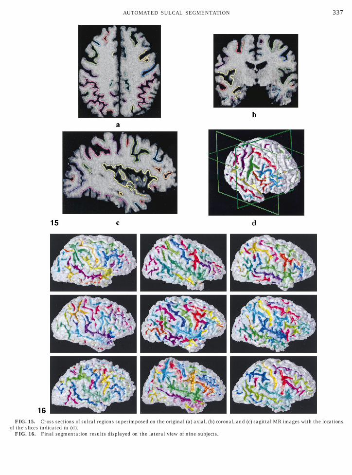
FIG. 15. Cross sections of sulcal regions superimposed on the original (a) axial, (b) coronal, and (c) sagittal MR images with the locationsof the slices indicated in (d).

FIG. 16. Final segmentation results displayed on the lateral view of nine subjects.

338 RETTMANN ET AL.

the watershed algorithm applied to the height functionis shown in Fig. 11 in which catchment basins arerepresented by different shades of gray. It is clear thatthe sulcal regions have been oversegmented, meaningthat several catchment basins represent a single sulcalregion. It is highly desirable to merge these basins inan “intelligent” way in order to arrive at sulci that aremore nearly segmented in whole rather than in parts.

Merging of Catchment Basins

Oversegmentation occurs in the watershed algo-rithm because small ridges in the sulcal regions resultin the formation of separate catchment basins. Over-segmentation is typically addressed in one of two ways(Meyer and Beucher, 1990; Vincent and Soille, 1991).The first approach is prospective; it uses markersplaced within the desired final catchment basins beforethe watershed is calculated. The height function ismodified to produce minima only at the markers, sup-pressing the other minima. The difficulty with thisapproach—which makes it impractical in our applica-tion—is in the prospective placement of appropriatemarkers on the highly variable cortical geometries.The second approach is retrospective; it attempts tomerge catchment basins after the watershed has beencomputed. It requires an appropriate merging criterionand can produce a result that is either oversegmentedor undersegmented if not done correctly. We pursuethe second approach with a heuristic, but effective,merging criterion, which we now describe.

Our merging criterion is based on the height of theridge separating two catchment basins. We define thisheight as the minimum height on the boundary be-tween two catchment basins. As graphically depictedin Fig. 12, this height can be used to compute the depthof the two catchment basins relative to the ridge sep-arating them. If the relative depth of both catchmentbasins is less than D—which we assign to be 1 cm in theresults herein—then the two catchment basins aremerged. We note that our merging criterion is similarin concept to that proposed in Lohmann and vonCramon (2000), but ours is implemented on the surfacemesh and has an explicit ordering criterion.

Two features of the algorithm are important in pre-venting the erroneous merging of catchment basins.First, the deeper catchment basins—i.e., those formedearlier in the watershed algorithm—should be mergedfirst. Accordingly, we create a sorted list of catchmentbasins and proceed from deepest to most shallow. Sec-ond, the merged catchment basin inherits the maxi-mum depth of the original catchment basins. For thealgorithm, it is convenient to create and maintain anadjacency graph of the catchment basins (Vincent andSoille, 1991). Each of the catchment basins is a node on

the graph and an edge indicates that two catchment

basins are adjacent to one another. 1(@) is the set ofcatchment basins adjacent to @.

The merging algorithm follows:

/*generate a list of all catchment basins (CBs) in theorder they were formed during the watershed algo-rithm */

CBlist 4 list of CBs from deepest to most shallowdefine fmin(!) 5 minai [!{ f (ai)} where ! is a set of

verticesnumMerges 4 0while end of list has not been reached

@ 4 next CB on list$4 CB in set 1(@) with smallest numerical label% 4 set of vertices on border between @ and $if ( fmin(%) 2 fmin(@) , D) AND ( fmin(%) 2 fmin($) , D)

merge $ to @remove $ from CBlist@ inherits 1($) except duplicatesnumMerges 4 numMerges 1 1

end ifend whileif (numMerges 5 0)

quitelse

numMerges 4 0repeat while loop starting at beginning of list

The final step of the segmentation is a size filter thatremoves small catchment basins. If a small catchmentbasin has no adjacent catchment basins it is simplyremoved, otherwise it is added to its adjacent catch-ment basin with the largest area. We empirically chosethe size threshold to be 3 cm2, which is held fixed for alldata sets. The result of the merging algorithm followedby the size filter is shown in Fig. 13 with several sulcalregions labeled according to their corresponding sul-cus. The central sulcus is segmented as a single catch-ment basin; however, some sulcal regions, such as thesuperior temporal, are still segmented as several catch-ment basins. These represent interrupted and pseudo-interrupted sulci (Ono et al., 1990). These types of sulciare broken into more than one piece by a gyral ridgeand are thus segmented in multiple pieces according toour definition of sulcal regions.

RESULTS

The final segmentation results are shown in Fig. 14with the sulcal regions superimposed on the corre-sponding semitranslucent cortical reconstruction atseveral views. These images illustrate that an appro-priate segmentation of the sulcal regions is obtainedwith the proposed methodology. On the lateral surface,the sulcal region corresponding to the central sulcus iscolored purple and the Sylvian fissure region is colored

yellow. Also seen on the lateral surface is the inferior

339AUTOMATED SULCAL SEGMENTATION

temporal region (colored cyan and purple), an exampleof an interrupted sulcus, and the superior temporalregion (colored red and green), an example of a pseudo-interrupted sulcus. Sulci on the medial surface, such asthe parieto-occipital (red), calcarine (blue), and cingu-late (cyan and orange) are also segmented with thismethodology. In Fig. 15, cross sections of the sulcalsegments are shown superimposed on the original MRimages illustrating that the segmented regions closelyfollow the actual data. The segmentation has beenapplied to 15 subjects from the Baltimore LongitudinalStudy of Aging (Shock et al., 1984; Resnick et al., 2000)ranging in age from 59 to 80. Sulcal segmentationsfrom 9 of these subjects are displayed on their corre-sponding cortical surfaces in Fig. 16, illustrating thatthe results are consistent and robust across the variousdata sets. In Fig. 16, each colored region represents anautomatically segmented region, but the color for aparticular sulcus is chosen randomly and is not thesame for each brain.

Geodesic Depth Analysis

In this section, we describe a pilot study of the geo-desic depth of several sulcal regions. The geodesicdepth, illustrated in Fig. 17, is defined as the distanceof the shortest path along the cortical surface from the

TABLE 1

Geodesic Depth in Millimeters (N 5 15)

Sulcus Mean SD Max Min

Ce (L) 20.5 2.27 24.5 16.1Ce (R) 20.1 1.20 22.0 18.1Syl (L) 40.8 2.71 45.0 36.7Syl (R) 39.3 2.89 46.2 35.7ST (L) 19.1 1.57 22.1 16.4ST (R) 21.2 2.64 25.6 16.0

Note. Ce, central sulcus; Syl, Sylvian fissure; ST, superior tempo-ral sulcus; L, left; R, right.

TAB

Results of Geodesic De

Sulcus

Subject 1

Scan 1 Scan 2 % differ

Ce (L) 18.02 17.57 22.Ce (R) 18.81 18.95 0.Syl (L) 38.65 39.33 1.Syl (R) 41.59 40.56 22.ST (L) 16.47 16.06 22.ST (R) 20.39 19.99 22.

Note. Ce, central sulcus; Syl, Sylvian fissure; ST, superior tempora

in millimeters.

deepest part of the sulcal region to the outer, visiblecortex.

Previous work on cortical depth measurements hasfocused on either the distance through the open spaceof the sulcal fold (Manceaux-Demiau et al., 1998; LeGoualher et al., 1999; Lohmann et al., 1999; Royack-kers et al., 1999) or tracing on two-dimensional slices ofthe images (Amunts et al., 1996). We have choseninstead to measure the distance along the cortical sur-face, because it provides a direct measurement of anintrinsic cortical property.

As previously described, we have computed the geo-desic distance from each sulcal point to the outer, gyralsurface, which was defined as g(a) in Eq. (3). Thisdepth function is plotted on a three-dimensional ren-dering of the buried cortical surface surrounding thecentral sulcus in Fig. 18, in which red indicates a largedepth and blue indicates a small depth. The geodesicdepth of a sulcal region is defined as the maximum ofthese distances.

The segmented sulcal regions corresponding to theright and left central sulci, superior temporal sulci, andSylvian fissures were manually labeled on each of the15 cortical surfaces. An interface was developed toallow a user to select the appropriate region corre-sponding to a given sulcus by simply clicking on theregion with a mouse. The display consists of both thespherical map and the cortical surface, as we found iteasiest to visually identify sulci on the cortex and sub-sequently select the region on the spherical map. If a

2

h Repeatability Study

Subject 2

e Scan 1 Scan 2 % difference

19.95 19.90 20.319.69 20.16 2.440.28 41.74 3.641.12 41.77 1.618.67 19.10 2.320.75 21.25 2.4

lcus; L, left; R, right. Values reported for scan 1 and scan 2 are given

FIG. 17. Illustration of geodesic depth.

LE

pt

enc

578550

l su

340 RETTMANN ET AL.

sulcal region was segmented as several catchment ba-sins, all basins were identified and grouped together inthe analysis. It is expected that this will occur quitefrequently as sulci are often interrupted. For example,in an analysis of 25 brains, the superior temporal sul-cus was interrupted 64% of the time on the right and72% of the time on the left (Ono et al., 1990). In ourlabeling step, we grouped basins 56% of the time forthe superior temporal sulcus, 30% of the time for theSylvian fissure, and 13% of the time for the centralsulcus. In addition, distinct sulcal regions were occa-sionally not separated by a large enough ridge andwere thus erroneously merged. In this case, we simplydecreased the threshold in the merging algorithm toobtain a correct segmentation. This occurred 12 timeswhen labeling the 90 sulci indicated above. These in-cluded connections of the superior temporal sulcuswith the inferior temporal sulcus or the Sylvian fissureand connections between the central and postcentralsulci. All of these types of connections were also ob-served in Ono et al. (1990). The mean, maximum, andminimum depths for each of the sulcal regions arereported in Table 1. In general, our depth values tendto be larger than other published results (Ono et al.,1990; Le Goualher et al., 1999; Royackkers et al., 1999).This is not surprising, however, considering that our

FIG. 18. Geodesic depth displayed on the region of cortex sur-rounding the central sulcus.

FIG. 19. Results of robustness test. (a) Depths computed when b

is held constant.

measure is along the surface as opposed to through thesulcal space.

Validation

In this section we describe experiments performed tovalidate our geodesic depth measurements. The firstexperiment was a repeatability study performed on twosubjects. In this experiment, two scans were acquiredfor each of the subjects within a 30-min interval duringwhich the subjects were repositioned in the scanner.For each data set acquired, we used the proposed meth-odology to obtain the sulcal depths for the three se-lected sulci on each hemisphere, with the results re-ported in Table 2. The measurements are highlyrepeatable for the two scans with a percentage differ-ence of less than 4% for all regions.

In the second experiment, we tested the robustnessof the proposed methodology. The goal of this experi-ment was to determine how the depth measurementchanges when the parameters of the sulcal segmenta-tion are varied. There are two parameters in the seg-mentation procedure that may affect the depth mea-surements. The first parameter is the shrink-wrapparameter, which we take to be the ratio of w1/w2. Thesecond parameter is the distance, d, from the cortex tothe shrink-wrap surface used to distinguish sulcal andgyral regions. A range of parameters was obtained forthe deformable surface by holding w2 fixed at 0.35 andvarying w1 from 0.5 to 1.0. The range used for d wasfrom 0.5 to 4.0 mm.

In Fig. 19a, the geodesic depth is plotted as a func-tion of d and w1. The figure shows that as d increases,the geodesic depth decreases. This is an expected resultsince the boundary of the sulcal region is moving far-ther into the buried region of the cortex as d increases.The depth measurement remains quite stable with re-spect to w1 with just a slight increase in the depth asthe shrink-wrap parameter increases. This occurs be-cause as the tension of the surface increases (by in-

parameters are varied. (b) d 5 2 mm is held constant. (c) w1 5 0.75

oth

341AUTOMATED SULCAL SEGMENTATION

creasing w1), the shrink-wrap becomes tighter and theboundaries of the sulcal regions are moved slightly outof the buried cortex.

For the results reported in the previous section, weused d 5 2 mm, w1 5 0.75, and w2 5 0.35. Figures 19band 19c show one-dimensional slices from the two-dimensional plot for d 5 2 mm and w1 5 0.75, respec-tively. In Fig. 19b, we see that for d 5 2 mm held fixed,the shrink-wrap parameter is particularly stable, withthe same depth computed for a range of parametersaround the normal value of w1. In Fig. 19c, we see thatfor w1 5 0.75, the depth varies linearly with d. Thus,changing d results in a predictable change in the mea-sured depth.

Parcellation

Our algorithm can be used to obtain a completeparcellation of the cortical surface by allowing the wa-

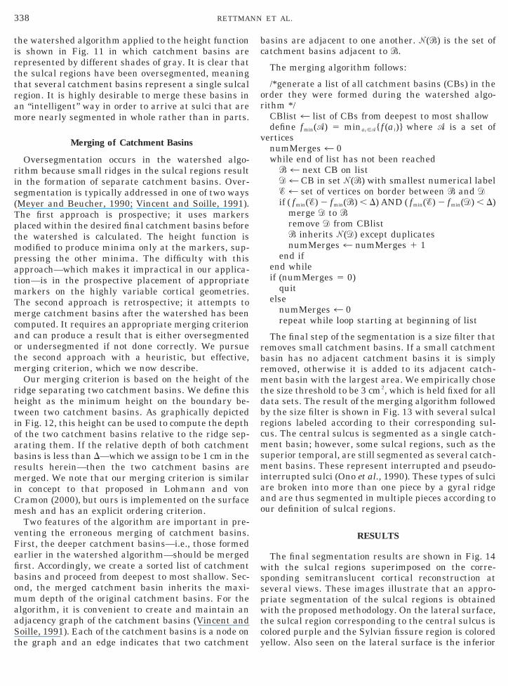
FIG. 20. Parcellation result displayed on (a)

FIG. 21. (a) Geometry of a triangle in which the value of T(C) issought from knowledge of T(A) and T(B). (b) An illustration of alinear approximation of T on the triangle (adapted from Kimmel andSethian (1998)).

tershed to stop at the largest height value rather thanone level below that height. For demonstration pur-poses, we have computed a cortical parcellation usingthe merged catchment basins as an initialization to thewatershed algorithm. At this point there is only oneremaining height level to be processed—the level cor-responding to gyral vertices. In the watershed, thisreduces to computing the geodesic influence zones ofthe catchment basins or, in this case, the current sulcalregions. The cortical parcellation result is shown inFig. 20 on both the lateral and the top views of thecortical surface. Other parcellation schemes (Jouandetet al., 1989; Rademacher et al., 1992; Caviness et al.,1996; Tzourio et al., 1997; Crespo-Facorro et al., 1999;Kim et al., 2000; Lohmann and von Cramon, 2000)have also used sulci as landmarks for dividing corticalregions. Our method differs from many of the previousmethods in that our parcellation units are regions ofcortex associated with each of the sulcal folds as op-posed to parcellating the cortex into its various gyri.

eral and (b) top views of the cortical surface.

FIG. 22. (a) Obtuse triangle ABC on the surface. (b) The sametriangle unfolded onto the plane (adapted from Kimmel and Sethian

lat

(1998)).

342 RETTMANN ET AL.

Also, several of the previously proposed parcellationschemes are much more detailed than the method pre-sented here. While our work is not meant to replacethese schemes, it does have the advantage that it iscompletely automatic; i.e., it requires no labor-inten-sive manual tracing. It could, therefore, serve as anautomatically generated starting point for more de-tailed parcellation methods.

CONCLUSIONS

In this work we have presented a method for auto-matically segmenting sulcal regions from a corticalsurface using a watershed algorithm. Geodesic depthswere computed for select sulcal regions and validationexperiments indicate that these measures are bothrepeatable and robust. Finally, we presented prelimi-nary results for a method to automatically parcellatethe entire cortical surface within this framework. Infuture work, we intend to use this methodology in alongitudinal study of regional cortical changes thatoccur during aging.

APPENDIX

Consider the triangle shown in Fig. 21, for which it isassumed that A and B are Accepted points and C is aNarrowband point. A wavefront is assumed to havepassed through A and B at the times TA and TB, re-spectively. For now, assume that ACB forms an acutetriangle, and (without loss of generality) assume thatTA # TB. It is also assumed that T is a linear functionon each triangle. Then from the geometry in Fig. 21,the gradient of T can be shown to be (t 2 u)/h, wheret 5 T(C) 2 T(A) and u 5 T(B) 2 T(A) are the differ-ences between the times of wavefront arrival at C andB from that at A. It can be shown that t must satisfy

~a 2 1 b 2 2 2ab cos u!t2 1 2bu~a cos u 2 b!t

1 b2~u 2 2 a 2sin 2u! 5 0,(5)

where u 5 /BCA.This quadratic equation has two real roots, and we

need to pick one as a candidate solution. The solutionmust satisfy two conditions. First, we must have thatt . u; otherwise the upwind condition is not met.Second, C should be updated from A and B only if thewave originated from a direction between A andB—i.e., the wave came from “within” the triangle.From the geometry, this means that t must satisfy

a cos u , h 5b~t 2 u!

,a

.

t cos u

It can be proved that only the larger root of Eq. (5) cansatisfy both conditions (Kimmel and Sethian, 1998). Ift is the larger root and it satisfies both conditions thenT(C) 5 min{T(C), t 1 T(A)}. The minimum is necessaryin case point C had been updated from another direc-tion already. If the largest root does not satisfy bothconditions then T(C) 5 min{T(C), T(A) 1 b, T(B) 1 a}.This equation allows for a previous update and for thewave propagating exactly along either of the edges ofthe triangle, whichever arrives first.

Two special cases require attention. First, if only oneof the points, say A, had been Accepted, then TC 5min{T(C), T(A) 1 b}, which accepts a faster time froma previous update triangle or allows the wave to prop-agate along the triangle’s edge. Second, if neither A norB is an Accepted point, then the triangle is ignored.

If all angles in the triangular mesh are acute—i.e.,the mesh comprises a nonobtuse triangulation—thenthe FM method can be implemented as describedabove. If some angles are obtuse, however, then a spe-cial extension is required (Kimmel and Sethian, 1998).In particular, if the angle /ACB is obtuse, then it isnecessary to allow for the possibility that T(C) is lessthan both T(A) and T(B) because the wave could arriveat C through the “long” edge AB sooner than it arrivedat either A or B. Kimmel and Sethian (1998) buildnumerical support for obtuse vertices by creating “vir-tual” acute triangles artificially through an unfoldingprocess. We now describe this approach, including afast unfolding algorithm that we have developed.

Consider the triangle ABC with obtuse angle /ACBshown in Fig. 22. In Fig. 22a, this triangle is depictedas it might look on the actual surface, while in Fig. 22bit is laid flat on the plane, as is a sequence of succes-sively adjacent triangles. The goal of unfolding is tofind a point D such that, when all triangles are appro-priately unfolded, both angles /ACD and /BCD areacute. The shaded region shown in both Figs. 22a and22b represents the region from which D can be selectedso that both angles will be acute.

The need to unfold occurs fairly frequently on a typ-ical triangular mesh surface. We have designed thefollowing computationally efficient unfolding algo-rithm that avoids explicit rotation of any vertex or theevaluation of any trigonometric function or its inverse.Instead, this algorithm makes use of the cosine theo-rem from plane trigonometry and the theorems fortrigonometric functions of sums. In the following recur-sive algorithm, XY denotes the length of the line seg-ment XY.

Algorithm (Unfolding)

1. Initialization: Let vertex X 5 A, vertex Y 5 B,vertex U 5 C. Compute XA, XB, XC, YA, YB, YC, and

XY from the vertex coordinates. Then compute three

343AUTOMATED SULCAL SEGMENTATION

cosines, cos XYA, cos XYB, and cos XYC using thecosine theorem. For example,

cos XYC 5

XY2

1 YC2

2 XC2

2 3 Î XY2

3 YC2

.

Compute the corresponding sines usingsin u 5 =1 2 cos2u.

2. Unfolding: Find the triangle DXY that shares theedge XY with the current triangle XYU. Compute DXand DY from the vertex coordinates, compute cos XYDusing the cosine theorem, and compute sin XYDfrom its cosine. Next, compute the lengths of the vir-tual edges DA, DB, and DC. For example,

DA2

5 DY2

1 YA2

2 2 3 Î DY2

3 YA2

3 ~cos XYA

3 cos XYD 2 sin XYA 3 sin XYD!.These lengths are equal to the distances between thecorresponding vertices on the unfolded plane.

3. Decide: The following computations determinewhether D is inside the acute section. If DA

2.

DC2

1 AC2, then set U 5 Y and Y 5 D, update

the lengths YA, YB, YC, and XY, then go to Step4. If DB

2. DC

21 BC

2, then set U 5 X and

X 5 D, update the lengths XA, XB, XC, and XY, thengo to Step 4. Otherwise, stop unfolding and computeT(C) in the two acute triangles DCA and DCB.

4. Update: Calculate the cosines and sines of Step 1using the updated lengths from Step 3, then go to Step 2.

One difficulty with unfolding is that, due to a partic-ular geometric arrangement of triangles on the mesh,it may not be possible to find a point D inside an acutesection in a reasonably small number of unfoldingsteps. In these cases, it is possible to pursue an alter-nate virtual edge-flipping scheme (see Barth andSethian, 1998), but we have implemented a more prag-matic approach. If D is not found in 10 unfolding steps,we simply set T(C) 5 min(T(C), T(A) 1 AC, T(B) 1BC). This threshold has been reached several timesduring our experiments, but we do not believe that ourpractical solution significantly affects the accuracy ofthe final solution.

ACKNOWLEDGMENTS

The authors thank Drs. Susan Resnick and Dzung Pham for manyvaluable discussions during the development of this work and forproviding the MR data. The authors also thank Drs. Michael Krautand Sinan Batman for sharing their expertise regarding this work.

REFERENCES

Amunts, K., Schlaug, G., Schleicher, A., Steinmetz, H., Dabringhaus,A., Roland, P. E., and Zilles, K. 1996. Asymmetry in the human

motor cortex and handedness. NeuroImage 4: 216–222.

Barth, T. J., and Sethian, J. A. 1998. Numerical schemes for theHamilton–Jacobi and level set equations on triangulated domains.J. Comput. Phys. 145: 1–40.

Caviness, V. S., Jr., Meyer, J., Makris, N., and Kennedy, D. N. 1996.MRI-based topographic parcellation of human neocortex: An ana-tomically specified method with estimate of reliability. J. Cognit.Neurosci. 8: 566–587.

Cohen, L. D., and Cohen, I. 1993. Finite-element methods for activecontour models and balloons for 2-D and 3-D images. IEEE Trans.on Pattern Anal. Machine Intelligence 15: 1131–1147.

Crespo-Facorro, B., Kim, J., Andreasen, N. C., O’Leary, D. S., Wiser,A. K., Bailey, J. M., Harris, G., and Magnotta, V. A. 1999. Humanfrontal cortex: An MRI-based parcellation method. NeuroImage10: 500–519.

Dale, A. M., Fischl, B., and Sereno, M. I. 1999. Cortical surface-basedanalysis. I. Segmentation and surface reconstruction. NeuroImage9: 179–194.

Davatzikos, C., and Bryan, R. N. 1996. Using a deformable surfacemodel to obtain a shape representation of the cortex. IEEE Trans.Med. Imaging 15: 785–795.

Drury, H. A., Van Essen, D. C., Anderson, C. H., Lee, C. W., Coogan,T. A., and Lewis, J. W. 1996. Computerized mappings of thecerebral cortex: A multiresolution flattening method and a surface-based coordinate system. J. Cognit. Neurosci. 8: 1–28.

Han, X., Xu, C., Braga-Neto, U., and Prince, J. L. 2001a. Graph-based topology correction for brain cortex segmentation. In Pro-ceedings of the XVIIth International Conference on InformationProcessing in Medical Imaging (IPMI’01), pp. 385–391.

Han, X., Xu, C., Rettmann, M. E., and Prince, J. L. 2001b. Automaticsegmentation editing for cortical surface reconstruction. In Pro-ceedings SPIE Med. Imaging, pp. 194–203.

Jouandet, M. L., Tramo, M. J., Herron, D. M., Hermann, A., Loftus,W. C., Bazell, J., and Gazzaniga, M. S. 1989. Brainprints: Com-puter-generated two-dimensional maps of the human cerebral cor-tex in vivo. J. Cognit. Neurosci. 1: 88–117.

Kass, M., Witkin, A., and Terzopoulos, D. 1987. Snakes: Activecontour models. Int. J. Comput. Vision 1: 321–331.

Khaneja, N., Miller, M. I., and Grenander, U. 1998. Dynamic pro-gramming generation of curves on brain surfaces. IEEE Trans.Pattern Anal. Machine Intelligence 20: 1260–1265.

Kim, J., Crespo-Facorro, B., Andreasen, N. C., O’Leary, D. S., Zhang,B., Harris, G., and Magnotta, V. A. 2000. An MRI-based parcella-tion method for the temporal lobe. NeuroImage 11: 271–288.

Kimmel, R., and Sethian, J. A. 1998. Computing geodesic paths onmanifolds. Proc. Natl. Acad. Sci. USA 95: 8431–8435.

Kruggel, F., and von Cramon, D. Y. 2000. Measuring the corticalthickness. In Proceedings of IEEE Workshop on MathematicalMethods in Biomedical Image Analysis, pp. 154–161.

Le Goualher, G., Barillot, C., and Bizais, Y. 1997. Modeling corticalsulci with active ribbons. IJPRAI 11: 1295–1315.

Le Goualher, G., Procyk, E., Collins, D. L., Venugopal, R., Barillot,C., and Evans, A. C. 1999. Automated extraction and variabilityanalysis of sulcal neuroanatomy. IEEE Trans. Med. Imaging 18:206–217.

Lohmann, G. 1998. Extracting line representations of sulcal andgyral patterns in MR images of the human brain. IEEE Trans.Med. Imaging 17: 1040–1048.

Lohmann, G., and von Cramon, D. Y. 1998. Sulcal basins and sulcalstrings as new concepts for describing the human cortical topography.In IEEE Workshop on Biomedical Image Analysis, pp. 24–33.

Lohmann, G., and von Cramon, D. Y. 2000. Automatic labelling ofthe human cortical surface using sulcal basins. Med. Image Anal.

4: 179–188.

344 RETTMANN ET AL.

Lohmann, G., von Cramon, D. Y., and Steinmetz, H. 1999. Sulcalvariability of twins. Cereb. Cortex 9: 754–763.

MacDonald, D., Kabani, N., Avis, D., and Evans, A. C. 2000. Auto-mated 3-D extraction of inner and outer surfaces of cerebral cortexfrom MRI. NeuroImage 12: 340–356.

Manceaux-Demiau, A., Bryan, R. N., and Davatzikos, C. 1998. Aprobabilistic ribbon model for shape analysis of the cerebral sulci:Application to the central sulcus. J. Comput. Assisted Tomogr. 22:962–971.

Mangin, J. F., Frouin, V., Bloch, I., Regis, J., and Lopez-Krahe, J.1995. From 3D magnetic resonance images to structural represen-tations of the cortex topography using topology preserving defor-mations. Math. Imaging Vision 5: 297–318.

Meyer, F., and Beucher, S. 1990. Morphological segmentation. J.Visual Commun. Image Representat. 1: 21–46.

Ono, M., Kubick, S., and Abernathey, C. D. 1990. Atlas of the Cere-bral Sulci. Thieme, New York.

Rademacher, J., Galaburda, A. M., Kennedy, D. N., Filipek, P. A.,and Caviness, V. S., Jr. 1992. Human cerebral cortex: Localization,parcellation, and morphometry with magnetic resonance imaging.J. Cognit. Neurosci. 4: 352–374.

Renault, C., Desvignes, M., and Revenu, M. 2000. 3D curves trackingand its application to cortical sulci detection. In IEEE Interna-tional Conference on Image Processing.

Resnick, S. M., Goldszal, A. F., Davatzikos, C., Golski, S., Kraut,M. A., Metter, E. J., Bryan, R. N., and Zonderman, A. B. 2000.One-year age changes in MRI brain volumes in older adults. Cereb.Cortex 10: 464–472.

Rettmann, M. E., Han, X., and Prince, J. L. 2000. Watersheds on thecortical surface for automated sulcal segmentation. In Proceedingsof IEEE Workshop on Mathematical Methods in Biomedical ImageAnalysis, pp. 20–27.

Rettmann, M. E., Xu, C., Pham, D. L., and Prince, J. L. 1999.Automated segmentation of sulcal regions. In Proceedings of Med-ical Image Computing and Computer-Assisted Intervention (MIC-CAI), pp. 158–167. Springer-Verlag, Berlin.

Royackkers, N., Desvignes, M., Fawal, H., and Revenu, M. 1999.Detection and statistical analysis of human cortical sulci. Neuro-Image 10: 625–641.

Sandor, S., and Leahy, R. 1997. Surface-based labeling of cortical anat-omy using a deformable atlas. IEEE Trans. Med. Imaging 16: 41–54.

Sethian, J. A. 1996. A fast marching level set method for monoton-ically advancing fronts. Proc. Natl. Acad. Sci. USA 93: 1591–1595.

Shock, N. W., Greulich, R. C., Andres, R., Arenberg, D., Costa, P. T.,

Jr., Lakatta, E., and Tobin, J. D. 1984. Normal Human Aging: The

Baltimore Longitudinal Study of Aging. U.S. Govt. Printing Office,Washington, DC.

Tao, X., Han, X., Rettmann, M. E., Prince, J. L., and Davatzikos, C.2001. Statistical study on cortical sulci of human brains. In Pro-ceedings of the XVIIth International Conference on InformationProcessing in Medical Imaging (IPMI’01), pp. 475–487.

Thompson, P. M., Schwartz, C., and Toga, A. W. 1996. High-resolu-tion random mesh algorithms for creating a probabilistic 3D sur-face atlas of the human brain. NeuroImage 3: 19–34.

Tosun, D., and Prince, J. L. 2001. A hemispherical map for thehuman brain cortex. In Proceedings of SPIE Medical Imaging, pp.290–300.

Tzourio, N., Petit, L., Mellet, E., Orssaud, C., Crivello, F., Benali, K.,Salamon, G., and Mazoyer, B. 1997. Use of anatomical parcellationto catalog and study structure–function relationships in the hu-man brain. Hum. Brain Mapping 5: 228–232.

Vaillant, M., and Davatzikos, C. 1997. Finding parametric represen-tations of the cortical sulci using an active contour model. Med.Image Anal. 1: 295–315.

Vincent, L. 1989. Mathematical morphology for graphs applied toimage description and segmentation. In Proceedings ElectronicImaging West, pp. 313–318, Pasedena, CA.

Vincent, L., and Soille, P. 1991. Watersheds in digital spaces: Anefficient algorithm based on emersion simulations. IEEE Trans.Pattern Anal. Mach. Intell. 13: 583–598.

Xu, C., Han, X., and Prince, J. L. 2000. Improving cortical surfacereconstruction accuracy using an anatomically consistent graymatter representation. In Proceedings of 6th International Confer-ence on Functional Mapping of the Human Brain, p. S581.

Xu, C., Pham, D. L., Rettmann, M. E., Yu, D. N., and Prince, J. L.1999. Reconstruction of the human cerebral cortex from mag-netic resonance images. IEEE Trans. Med. Imaging 18: 467–480.

Xu, C., Pham, D. L., Prince, J. L., Etemad, M. E., and Yu, D. N. 1998.Reconstruction of the central layer of the human cerebral cortexfrom MR images. In Proceedings of Medical Image Computing andComputer-Assisted Intervention (MICCAI), pp. 481–488. Springer-Verlag, Berlin.

Xu, C., and Prince, J. L. 1998. Snakes, shapes, and gradient vectorflow. IEEE Trans. Image Proc. 7: 359–369.

Zeng, X., Staib, L. H., Schultz, R. T., Tagare, H., Win, L., andDuncan, J. S. 1999. A new approach to 3D sulcal ribbon findingfrom MR images. In Proceedings of Medical Image Computing andComputer-Assisted Intervention (MICCAI), pp. 148–157. Springer-Verlag, Berlin.

Zhou, Y., Thompson, P. M., and Toga, A. W. 1999. Extracting and

representing the cortical sulci. Comp. Graph. Appl. 19: 49–55.