Journal of Computational and Applied Mathematics 228 (2009) 538–547

Contents lists available at ScienceDirect

Journal of Computational and AppliedMathematics

journal homepage: www.elsevier.com/locate/cam

An adaptive method for Volterra–Fredholm integral equations on thehalf lineA. Cardone a,∗, E. Messina b, A. Vecchio c

a Dipartimento di Matematica e Informatica, Università degli Studi di Salerno, Via Ponte don Melillo, I-84084 Fisciano (SA), Italyb Dipartimento di Matematica e Applicazioni, Università degli Studi di Napoli, “Federico II”, Via Cintia, I-80126 Napoli, Italyc Istituto per le Applicazioni del Calcolo “M.Picone”, Sezione di Napoli - IAC-CNR, via P. Castellino 111, I-80131 Napoli, Italy

a r t i c l e i n f o

Article history:Received 28 September 2006Received in revised form 6 June 2007

MSC:65R2065D3265Y05

Keywords:Volterra–Fredholm integral equationsHalf lineDirect QuadratureConvergenceParallelism

a b s t r a c t

In this paper we develop a direct quadrature method for solving Volterra–Fredholmintegral equations on an unbounded spatial domain. These problems, when related to someimportant physical and biological phenomena, are characterized by kernels that presentvariable peaks along space. The method we propose is adaptive in the sense that thenumber of spatial nodes of the quadrature formula varies with the position of the peaks.The convergence of the method is studied and its performances are illustrated by means ofa few significative examples. The parallel algorithm which implements the method and itsperformances are described.

© 2008 Elsevier B.V. All rights reserved.

1. Introduction

Volterra–Fredholm Integral Equations (VFIEs) of the type

u(t, x) = f (t, x)+∫ t

0

∫+∞

0k(t − s, x, ξ)g(u(s, ξ))dξds,

(t, x) ∈ I × [0,+∞[,

(1.1)

where I := [0, T], appear in many physical and biological applications.The literature on the numerical methods for VFIEs (see for example [3–5,9,11]) is mainly devoted to the solution of

VFIEs on bounded spatial domains. However, many problems originating from real life applications give rise to equations ofthe form (1.1), where the spatial domain is unbounded. For instance, in [1,2,14] some models of population dynamics areproposed, describing the growth of a population in space and time, where the spatial domain (for example a continent) islarge enough to be considered unbounded. Another example comes from the modelling of the coding mechanism, in thetransmission of nervous signals among neurons [8]. In this case the space variable represents the membrane potential andthe spatial domain is the half line.

For these reasons, we devote our investigations here to the construction and analysis of methods for the numericalsolution of (1.1), and we focus our attention on some kernels, which are typical in the real applications mentioned above. Inparticular, we have observed that:

∗ Corresponding author.E-mail address: ancardone@unisa.it (A. Cardone).

0377-0427/$ – see front matter © 2008 Elsevier B.V. All rights reserved.doi:10.1016/j.cam.2008.03.036

A. Cardone et al. / Journal of Computational and Applied Mathematics 228 (2009) 538–547 539

(1) their value becomes negligible when ξ x, and it is zero when t = s;(2) as functions of ξ they present peaks whose position, depending on x, t, s, cannot be predicted.

These two main peculiarities on the kernels structure motivated all the strategies adopted in the following section. Fromproperty 2, it follows that the peaks have a variable position and then it is difficult to approximate them. What is more, anytruncation of the infinite integral at a finite position would lead to disregard the contributions of all the peaks after that. Froma numerical point of view, a poor approximation of (1.1) in correspondence of these peaks would affect the accuracy of thewhole process. Gaussian quadrature formulas [10,15], which represent the most natural tool to numerically approximatean integral on unbounded domains, turn out to be unsuccessful, because they well approximate the peaks of the kernelonly when they are fixed. Hence, our main goal is to suitably discretize the problem in order not to neglect any importantinformation and significative contribution.

The method we propose here is specially tuned to the form of k; it is based on a trapezoidal Direct Quadrature (DQ)formula along space and time and, by exploiting the characteristics of the kernels, it adapts the spatial discretization in sucha way just to “cover” the peaks of k.

In this paper we limit ourselves to the analysis of the convergence properties of this double discretization and, althougha stability investigation is due, we postpone it to a further development of our research.

The paper is organized as follows. In Section 2 the difficulties arising in the numerical treatment of VFIEs on unboundedspatial domain when the kernel has “moving peaks” are explained in detail. The same section contains the description ofthe method and introduces the “pocket steps”, a parameter strictly connected to the truncation strategy adopted on thequadrature formula along space. Section 3 is devoted to the study of convergence of the method and to the derivation ofan a priori lower bound for the minimal number of pocket steps, required for an optimal convergence. In Section 4 theperformances of the method are shown by means of some significative examples, moreover we develop a parallel algorithmwhich implements the method and describe its performances. We conclude in Section 5 with some remarks about the workwe have done and about its future developments.

2. The method

As already mentioned in the previous section, in this paper we focus our attention on the numerical solution of VFIEs(1.1) and we assume that the kernel k has the following characteristics:

(a) k(t − s, x, ξ) has a peak for ξ ≈ x;(b) k(t − s, x, ξ) = 0 if t = s.

What is more, since most of the problems arising in the applications are linear [1,2,8,14], we assume that g(u) = u in (1.1).Hence, we consider the following VFIE:

u(t, x) = f (t, x)+∫ t

0

∫+∞

0k(t − s, x, ξ)u(s, ξ)dξds, t ∈ I, x ∈ R+. (2.1)

Here and in the following we suppose that the real-valued functions k and f satisfy the conditions:

HP i. f is nonnegative and monotonic nondecreasing with respect to t;HP ii. k(·, ·, ·) is defined and nonnegative on R+ × R+ × R+; for every x ≥ 0 and every T > 0, k(·, x, ·) ∈ L1([0, T] × R+).

HP iii. Let η(t, x) :=∫ t

0∫+∞

0 k(s, x, ξ)dξds, and let T > 0 be arbitrary, then the family of functions on [0, T] η(·, x)|x ≥ 0 isuniformly bounded and equicontinuous.

HP vi. For every T > 0 and every ε > 0 there exists δ = δ(ε, T) > 0 such that if x1, x2 ≥ 0 and |x1 − x2| ≤ δ, then∫ t0∫+∞

0 |k(s, x1, ξ)− k(s, x2, ξ)|dξds < ε.

These conditions guarantee the existence and uniqueness of the solution for (2.1), as stated in the following reformulatedversion of the Theorem 3.3 of [7]:

Theorem 1. Assume that HP i–vi hold, then (2.1) has a unique continuous bounded solution u : [0, T] × [0,+∞[→ R.

In order to describe the numerical method, we introduce a uniform mesh Iτ on I, Iτ := tn | n = 0, . . . ,N, tn = tn−1 + τ.The discretization of the Volterra part of (2.1) by a DQ method, leads to:

un(x) = f (tn, x)+ τn∑

j=0ωnj

∫+∞

0k(tn − tj, x, ξ)uj(ξ)dξ, n = 0, . . . ,N, (2.2)

where un(·) approximates the solution of (2.1) at tn and ωnj are the quadrature weights of the DQ formula. Note that, sincek satisfies (b), then k(tn − tj, x, ξ) = 0 when j = n, hence Eq. (2.2) becomes a recursive relation on the unknowns un(·),n = 0, . . . ,N, by means of integrals on [0,+∞[. This relation makes (2.2) very attractive from a computational point of viewand will turn out to be quite useful for the adaptiveness of the method proposed here. Now, our aim is to approximate un(·)by using a suitable discretization of the integrals of (2.2), which allows a reliable simulation of the phenomena and takesthe structural characteristics of the problem into account.

540 A. Cardone et al. / Journal of Computational and Applied Mathematics 228 (2009) 538–547

Let 0 = x0 < x1 < · · · be any mesh on the half line. Property (b) and the collocation of (2.2) on this mesh leads to:

un(xm) = f (tn, xm)+ τn−1∑j=0ωnj

∫+∞

0k(tn − tj, xm, ξ)uj(ξ)dξ, m = 0, 1, . . . , n = 0, . . . ,N, (2.3)

where, in view of property (a), k(tn − tj, xm, ξ) presents a peak for ξ close to xm. A quadrature formula with nodes thickenedaround xm, which seems to be a natural choice for the discretization of the integral∫

+∞

0k(tn − tj, xm, ξ)uj(ξ)dξ, (2.4)

would lead to a distribution of nodes that is dense in correspondence of each peak, as we would like, but is different for eachm. Hence, this procedure would need for an additional interpolation in order to compute the approximations in the nodesof the quadrature formula, thus increasing the computational cost of the overall method and maybe affecting the accuracy.

Therefore, in our opinion, it is more “convenient” to choose a quadrature formula on equidistant nodes which coincidewith the uniform mesh:

0 = x0 < · · · < xm < · · · , xm = xm−1 + h, (2.5)

and to decrease the stepsize h in order to improve the approximation, rather than trying to catch each peak by integratingon non-equidistant nodes. The resulting approximation scheme is:

unm = f (tn, xm)+ hτn−1∑j=0ωnj

+∞∑i=0

wik(tn − tj, xm, xi)uji, m = 0, 1, . . . , n = 0, . . . ,N, (2.6)

where unm ≈ un(xm), with un(·) given in (2.2), and wi are the weights of the quadrature formula for (2.4).Of course, in real-life problems, we are interested in observing the behavior of the solution of (2.1) for x ∈ [0, S], S < +∞

(see for example [10]), therefore, for n = 0, . . . ,N, we want to compute unm, with m running from 0 to a finite M, such thatxM ≤ S.

In other words, we have to solve (2.6) for m = 0, . . . ,M. Observe that, even if only a finite number of approximations unm

is required, the summation on i at the righthand side of (2.6), keeps on involving uji, i = 0, . . . ,+∞, j = 0, . . . , n− 1, and soa truncation of this infinite summation, which well approximate (2.4), is required.

Recall that each function k(tn − tj, xm, ξ) appearing in (2.4) has a peak around xm (see property (a)) and decreases afterthat. Hence the contribution of the ith addendum in the infinite summation in (2.6) is almost zero when i m. Therefore,

m+ν(h)∑i=0

wik(tn − tj, xm, xi) ≈+∞∑i=0

wik(tn − tj, xm, xi),

where the truncation point xm+ν(h), with ν(h) = νn,j,m(h) ∈ N, is chosen in such a way to “cover” the peak around xm. Takinginto account this idea, the formulation of the method becomes:

unm = f (tn, xm)+ hτn−1∑j=0ωnj

m+ν(h)∑i=0

wik(tn − tj, xm, xi)uji, m = 0, . . . ,M, n = 0, . . . ,N. (2.7)

The method is “adaptive” in the sense that the truncation point xm+ν(h) depends on the current point xm. The choice of ν(h)is crucial both for the computational complexity of the overall solving process and for the convergence of the method, as itwill be shown in the next section.

Clearly, unm cannot be expected to converge to u(tn, xm) as h→ 0 and τ→ 0, unless the relationship (m+ν(h))h→+∞ ash→ 0 holds between the stepsize h and the cut-off index m+ν(h). However, the precise nature of the functional relationshipν = ν(h) or h = h(ν) required to ensure that unm converges to u(tn, xm) is not obvious. The question is, among other things,dealt with in the next section.

Observe that for each fixed n, (2.7) represents a set of M + 1 decoupled explicit equations for computing un0, . . . , unM .Namely, in order to compute unm, we need uji, j = 0, . . . , n−1, i = 0, . . . ,m+ν(h), where m+ν(h) might exceed M. Therefore,for each j = 0, . . . , n − 1, we compute the numerical approximations uji, for some i > M, which although approximate thetrue solution u(tj, xi) outside the spatial range of interest [0, S], are necessary for future computations. These additional stepsare called “pocket steps”, because here the solution is computed and saved for being used in the future.

To be more precise, let us illustrate the algorithm in the case ν(h) = ν, ∀n, j,m.For n = 0, by evaluating the forcing function f , we get the solution [u00, . . . , u0M] = [f (t0, x0), . . . , f (t0, xM)] within the

interval of interest [0, S], and we perform the additional pocket steps in [(t0, xM+1), . . . , (t0, xM+Nν)].For n = 1, we compute the values of the solution [u10, . . . , u1M] within [0, S], by using [u00, . . . , u0M] and

[u0M+1, . . . , u0M+ν] in the formula (2.7); in addition, we perform (N − 1)ν pocket steps and compute the solution in[(t1, xM+1), . . . , (t1, xM+(N−1)ν)], exploiting the calculations performed at n = 0. The computation continues in an analogueway for n = 2, . . . ,N.

The scheme is shown in Fig. 1. From this figure it is clear that the number of pocket steps is about N2

2 ν and so thecomputational cost of pocket steps depends not only on ν, but also on the total number of time steps N.

A. Cardone et al. / Journal of Computational and Applied Mathematics 228 (2009) 538–547 541

Fig. 1. Computation scheme.

In this paper we use the trapezoidal formula, both for the time and for the spatial discretization. This choice, togetherwith the use of the pocket steps, leads to the final formulation of the method:

unm = f (tn, xm)+ hτn−1∑j=0ωnj

m+ν(h)∑i=0

wik(tn − tj, xm, xi)uji, m = 0, . . . ,M + (N − n)ν(h), n = 0, . . . ,N. (2.8)

with:

ωnj =

12

j = 0, n,

1 otherwise,and wi =

12

i = 0,

1 otherwise.(2.9)

The use of the trapezoidal formula is motivated by the fact that, in the applications mentioned in Section 1, two or threecorrect digits are sufficient for the scope of the simulation and the use of a cheap underlying quadrature method in (2.8) isof primary importance in order to obtain the numerical solution in a reasonable runtime.

From (2.8) it immediately follows that m runs from 0 to M+(N−n)ν(h) and that the length of the summation on i increaseswith m. This is the price to be payed in order to approximate the infinite integral without disregarding the contribution ofthe peak around xm.

3. Convergence

In this section we analyze the global error of convergence E(t, x) of the method (2.8)–(2.9) at the mesh points (tn, xm) |n = 0, . . . ,N, m = 0, . . . ,M:

E(tn, xm) = u(tn, xm)− unm = u(tn, xm)− un(xm)+ un(xm)− unm,

where un(xm) is defined by (2.3)–(2.9), and unm is the numerical solution of (2.1) given by (2.8)–(2.9). Thus, if we set:

en(xm) = u(tn, xm)− un(xm) and Enm = un(xm)− unm, (3.1)

then en(xm) represents the Volterra contribution to the error, while Enm comes from the spatial discretization of (2.3).In order to prove the boundedness of E(t, x), we first assume the following conditions on the functions involved in (2.1)

and (2.3):

HP1 k(0, x, ξ) = 0, ∀x, ξ ∈ R+;HP2 (i) f is bounded;

(ii) there exists K > 0 such that∫+∞

0|k(t − s, x, ξ)|dξ ≤ K < +∞, ∀t, s ∈ I, ∀x ∈ R+;

HP3 (i) k(t − s, x, ·)uj(·) ∈ C3(R+),(ii) there exists C > 0 such that limξ→+∞

∣∣∣ ∂∂ξ

[k(t − s, x, ξ)uj(ξ)

]∣∣∣ ≤ C,

(iii) there exists C′ > 0 such that∫+∞

0

∣∣∣ ∂3

∂ξ3

[k(t − s, x, ξ)uj(ξ)

]∣∣∣ dξ ≤ C′, j = 0, . . . ,N, ∀t, s ∈ I, ∀x ∈ R+, where uj(·) isthe jth solution of (2.2);

HP4 k(t − s, x, ξ) is decreasing with respect to ξ, for large values of ξ, ∀t, s ∈ I, x ∈ R+;HP5 (i) k(·, x, ξ), u(·, ξ) ∈ C2(I), ∀x, ξ ∈ R+;

(ii)∣∣∣∫ +∞0

∂2

∂s2[k(t − s, x, ξ)u(s, ξ)]dξ

∣∣∣ ≤ C′′, with C′′ > 0, ∀t, s ∈ I, ∀x ∈ R+;HP6

∫+∞

x+ν(h)h |k(t − s, x, ξ)|dξ = O(h2), as h→ 0 and ν(h)h→+∞, ∀t, s ∈ I, ∀x ∈ R+.

542 A. Cardone et al. / Journal of Computational and Applied Mathematics 228 (2009) 538–547

Let Ωh := x0, x1, . . . , xM be the truncated part of the mesh (2.5) on [0, S], with xm = xm−1 + h and xM = S.

Theorem 2. Let the conditions of Theorem 1 be satisfied and assume that HP1–6 hold. Moreover let N,M ∈ N and τN = T,hM = S. If h→ 0, τ→ 0, and ν(h) ∈ N is chosen such that ν(h)h→+∞, then

max|E(t, x)|, (t, x) ∈ Iτ × Ωh = O(h2)+ O(τ2). (3.2)

Proof. First of all we investigate on the spatial part Enm of the error, defined in (3.1). Set:

Anm = τn−1∑j=0ωnj

[∫+∞

0k(tn − tj, xm, ξ)uj(ξ)dξ− h

m+ν(h)∑i=0

wik(tn − tj, xm, xi)uj(xi)

], (3.3)

Bnm = τn−1∑j=0ωnj

[h

m+ν(h)∑i=0

wik(tn − tj, xm, xi)(uj(xi)− uji

)], (3.4)

then

Enm = Anm + Bnm, n = 0, . . . ,N,m = 0, . . . ,M + (N − n)ν(h). (3.5)

From (3.3) it is clear that:

Anm = τn−1∑j=0ωnj

[∫+∞

0k(tn − tj, xm, ξ)uj(ξ)dξ− h

+∞∑i=0

wik(tn − tj, xm, xi)uj(xi)

]

+τhn−1∑j=0ωnj

+∞∑i=m+ν(h)+1

wik(tn − tj, xm, xi)uj(xi)

= A(1)nm + A(2)

nm ,

where A(1)nm represents a weighted sum of the trapezoidal quadrature errors on the half line. Then, by assuming HP3 and using

the results in [6, p.167] and in [12, p. 246], it follows:

|A(1)nm | ≤ C1h

2τn−1∑j=0ωnj ≤ C1tnh

2, C1 > 0, (3.6)

where C1 is a positive constant independent of h.In order to find a bound for A(2)

nm , observe that from (2.2), since u0(x) = f (t0, x), wi ≤ 1, ∀i, and because of HP2, there existsU > 0 such that |uj(x)| ≤ U, ∀j = 0, . . . ,N. Hence:

|A(2)nm | ≤ hτU

n−1∑j=0ωnj

+∞∑i=m+ν(h)+1

|k(tn − tj, xm, xi)|. (3.7)

What is more, hypothesis HP4 (see [6, p. 167], formula (3.4.4)) and HP6, with ν(h)h large enough, imply that:

h+∞∑

i=m+ν(h)+1|k(tn − tj, xm, xi)| ≤

∫+∞

mh+ν(h)h|k(tn − tj, xm, ξ)|dξ ≤ C2h

2, (3.8)

j = 0, . . . , n, n = 0, . . . ,N,m = 0, . . . ,M + (N − n)ν(h), for a constant C2 > 0 not depending on h. Then, by substituting in(3.7):

|A(2)nm | ≤ UC2h

2τn−1∑j=0ωnj ≤ UC2h

2tn,

and so:

|Anm| ≤ |A(1)nm | + |A

(2)nm | ≤ C3tnh

2, (3.9)

for n = 0, . . . ,N and m = 0, . . . ,M + (N − n)ν(h), with C3 = C1 + UC2. From (3.5) and (3.9) we deduce that:

|Enm| ≤ C3tnh2+ τ

n−1∑j=0ωnjh

m+ν(h)∑i=0

wi|k(tn − tj, xm, xi)||Eji| (3.10)

when n = 0, . . . ,N and m = 0, . . .M + (N − n)ν(h), provided that ν(h)h is large enough. Since at the initial time t0 thesolution of (2.1) is known:

|E0m| = 0 =: p0h2, m = 0, . . . ,M + Nν(h),

A. Cardone et al. / Journal of Computational and Applied Mathematics 228 (2009) 538–547 543

hence, by (3.10),

|E1m| ≤ C3t1h2=: p1h

2, m = 0, . . . ,M + (N − 1)ν(h),

and

|E2m| ≤ C3t2h2+ τω21h

m+ν(h)∑i=0

wi|k(tn − tj, xm, xi)|p1h2

≤

(C3t2 + τhp1

m+ν(h)∑i=0|k(t2 − t1, xm, xi)|

)h2,

for m = 0, . . . ,M + (N − 2)ν(h).Since HP3 and HP4 hold, the kernel is bounded and there exists a positive constant K, independent of h, such that [6, p.

167]:

hm+ν(h)∑

i=0|k(t2 − t1, xm, xi)| ≤ h|k(t2 − t1, xm, x0)| +

∫+∞

0|k(t2 − t1, xm, ξ)|dξ

≤ (hK + K).

Therefore, for sufficiently small h > 0, there exists K > 0 independent of h, such that:

hm+ν(h)∑

i=0|k(t2 − t1, xm, xi)| ≤ K.

This leads to:

|E2m| ≤ C3t2h2+ τKp1h

2=: p2h

2, m = 0, . . . ,M + (N − 2)ν(h).

For each n > 2, the same procedure, applied to (3.10), leads to |Eji| ≤ pjh2, j = 0, . . . ,N, i = 0, . . . ,M + (N − j)ν(h), and so:

|Enm| ≤

(C3tn + τK

n−1∑j=0

pj

)h2=: pnh

2, (3.11)

n = 0, . . . ,N,m = 0, . . . ,M + (N − n)ν(h).From (3.11):

pn ≤ C3T + τKn−1∑j=0

pj,

and then, by Gronwall’s lemma [13, p. 101], pn ≤ C3T exp(Ktn). Hence,

|Enm| ≤ C3T exp(Ktn)h2, (3.12)

n = 0, . . . ,N,m = 0, . . . ,M + (N − n)ν(h).For the Volterra part of the error en(x) (see (3.1)), by exploiting HP5 and the error formula for the trapezoidal rule, there

exists s ∈ [0, t] such that:

en(xm) =

∫+∞

0−τ2

12tn

[∂2

∂s2 [k(tn, s, xm, ξ)u(s, ξ)]]s=s

dξ+ τn−1∑j=0ωnj

∫+∞

0k(tn, tj, xm, ξ)ej(ξ)dξ,

with n = 0, . . . ,N,m = 0, . . . ,M + (N − n)ν(h), and so:

|en(xm)| ≤ C′′tnτ2+ τ

n−1∑j=0ωnj

∫+∞

0|k(tn, tj, xm, ξ)||ej(ξ)|dξ. (3.13)

By writing down (3.13) for n = 0, 1, . . ., in sequence, we have:

|e0(xm)| = 0 =: q0τ2, m = 0, . . . ,M + Nν(h),

|e1(xm)| ≤ C′′t1τ2=: q1τ

2, m = 0, . . . ,M + (N − 1)ν(h),

|e2(xm)| ≤ (C′′t2 + τKq1)τ2=: q2τ

2, m = 0, . . . ,M + (N − 2)ν(h),

in general:

|en(xm)| ≤

(C′′tn + τK

n−1∑j=0

qj

)τ2=: qnτ

2,

544 A. Cardone et al. / Journal of Computational and Applied Mathematics 228 (2009) 538–547

n = 0, . . . ,N,m = 0, . . . , (N − n)ν(h), and by Gronwall’s lemma [13, p. 101]:

|en(xm)| ≤ C′′Tτ2 exp(Ktn). (3.14)

Inequalities (3.12) and (3.14) yield the result stated in the theorem.

Remark 1. We note that HP6 does not produce restrictions on the problem. As a matter of fact, limν(h)h→+∞

∫+∞

x+ν(h)h |k(t −s, x, ξ)|dξ = 0, ∀t, s ∈ I, ∀x ∈ R+, therefore, in order to get an order 2 convergence, it is always possible to choose ν(h)h largeenough to have (3.8). In this sense, HP6 is only a prescription on the relationship ν = ν(h).

Remark 2. Notice that HP3 involves the numerical solution (u0(·), . . . , uN(·)), but the role of (u0(·), . . . , uN(·)) is only formal,because we have:

u0(x) = f (t0, x),

u1(x) = f (t1, x)+ τω10

∫+∞

0k(t1 − t0, x, ξ)u0(ξ)dξ, (3.15)

u2(x) = f (t2, x)+ τω20

∫+∞

0k(t2 − t0, x, ξ)u0(ξ)dξ+ τω21

∫+∞

0k(t2 − t1, x, ξ)u1(ξ)dξ, (3.16)

. . . .

By substituting the expression of u0(·) in (3.15), the expression of u1(·) in (3.16), and so on, it follows that each uj(·) dependsonly on k and f . Hence, the hypothesis HP3 is immediately implied by sufficiently regular k and f .

As in many cases arising in real problems (see for example [1,8]), the kernel is of exponential type and/or can be bounded,at infinity, by functions of type const·(ξ−x)−p, with p > 1, we are interested in finding, for this type of kernels, lower boundsfor ν(h) in (2.8), which are sufficient to ensure convergence of order 2. The following Corollary establishes these bounds.

Corollary 3. Assume that HP6 is replaced by one of the following:

HP6′ there exist B′ > 0 and p > 1 such that ∀x ∈ R+, ∀t, s ∈ I, |k(t − s, x, ξ)| ≤ B′

(ξ−x)p, when ξ > x+ ν(h)h, and

ν(h) ≥ C(p)h1+p1−p , (3.17)

with C(p) = (p− 1)1

1−p ;HP6′′ there exists B′′ > 0 such that ∀x ∈ R+, ∀t, s ∈ I, |k(t − s, x, ξ)| ≤ B′′ exp(−(ξ− x)2), when ξ > x+ ν(h)h, and

erf(ν(h)h) ≥ 1−2√π

h2; (3.18)

then the result stated in Theorem 2 still holds.

Proof. The proof is immediate, once one observes that each of the hypotheses HP6′ and HP6′′ yields HP6.Under the hypothesis HP6′, we have:∫

+∞

x+ν(h)h|k(t, s, x, ξ)|dξ ≤

∫+∞

x+ν(h)h

B′

(ξ− x)pdξ =

[−

1p− 1

B′

(ξ− x)p−1

]+∞x+ν(h)h

=1

p− 1B′

(ν(h)h)p−1 ≤ B′ · h2.

On the other side, if HP6′′ holds,∫+∞

x+ν(h)h|k(t, s, x, ξ)|dξ ≤

∫+∞

x+ν(h)hB′′ exp(−(ξ− x)2)dξ

= B′′√π

2(1− erf(ν(h)h)) ≤ B′′ · h2.

Note that each of (3.17) and (3.18) implies that ν(h)h→+∞ as h→ 0, which is a necessary condition for the convergence.We underline that while in the first case the value for the minimal ν(h) is explicitly computed, in the last case we cannot

obtain ν(h) in a closed form. However, it is possible to get an estimate for this lower bound as a function of h, which willturn out to be quite reliable in our practical experiments.

A. Cardone et al. / Journal of Computational and Applied Mathematics 228 (2009) 538–547 545

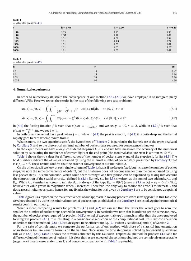
Table 1cd values for problem (4.1)

ν h = 0.40 h = 0.20 h = 0.10

10 1.35 1.83 1.3616 1.32 2.18 1.6850 1.31 2.09 2.54

125 1.31 2.05 2.77500 1.31 2.05 2.67

1000 1.31 2.05 2.672000 1.31 2.05 2.67

Table 2cd values for problem (4.2)

h ν cd

0.2 5 2.470.1 14 3.140.05 34 3.660.025 96 4.26

4. Numerical experiments

In order to numerically illustrate the convergence of our method (2.8)–(2.9) we have employed it to integrate manydifferent VFIEs. Here we report the results in the case of the following two test problems:

u(t, x) = f (t, x)+∫ t

0

∫+∞

0

1γ(x− ξ)2 + 1

(t − s)u(s, ξ)dξds, t ∈ [0, 2], x ∈ R+ (4.1)

u(t, x) = f (t, x)+∫ t

0

∫+∞

0exp(−(x− ξ)2)(t − s)u(s, ξ)dξds, t ∈ [0, 1], x ∈ R+. (4.2)

In (4.1) the forcing function f is such that u(t, x) = 1(1+x)(1+t) and we set γ = 10, S = 2, while in (4.2) f is such that

u(t, x) = exp(−x)1+t and we set S = 1.

In both cases the kernel has a peak when ξ = x; while in (4.1) the peak is smooth, in (4.2) it is quite deep and the kernelrapidly goes to zero when ξmoves from x.

What is more, the two equations satisfy the hypotheses of Theorem 2. In particular the kernels are of the types analyzedby Corollary 3, and so the theoretical minimal number of pocket steps required for convergence is known.

In the experiments we have always considered stepsizes h = τ and we have measured the accuracy of the numericalsolution by calculating the number cd of correct digits at the end point (the maximal absolute error is written as 10−cd).

Table 1 shows the cd values for different values of the number of pocket steps ν and of the stepsize h, for Eq. (4.1). Thebold numbers indicate the cd values obtained by using the minimal number of pocket steps prescribed by Corollary 3, thatis ν(h) = h−3. These results confirm that the order of convergence of our method is 2.

On the other side, if we look at each single column of Table 1, that is if we keep h fixed, but increase the number of pocketsteps, we note the same convergence of order 2, but the final error does not become smaller than the one obtained by usingless pocket steps. This phenomenon, which could seem “strange” at a first glance, can be explained by taking into accountthe composition of the spatial error Enm, defined in (3.1). Namely Enm in (3.5) is written as the sum of two addenda, Anm andBnm. While Anm vanishes as ν goes to infinity, Bnm is always of the type Bnm = O(h2) (since in (3.4) uj(xi) − uji = O(h2), ∀j, i),however its value grows in magnitude when ν increases. Therefore, the only way to reduce the error is to increase ν anddecrease h simultaneously, and hence, for any fixed h, the values for ν(h) given by Corollary 3 are to be considered as optimalvalues.

Table 2 gives us a report on the real effectiveness of our approach in solving problems with moving peaks. In this Table thecd values obtained by using the minimal number of pocket steps established in the Corollary 3 are listed. Again the numericalresults confirm our theory.

What is more, comparing results for problems (4.1) and (4.2) we can see that, the faster the kernel goes to zero, thesmaller the number of pocket steps needed for convergence is. In particular we note that in order to get the same accuracy,the number of pocket steps required for problem (4.2), (kernel of exponential type), is much smaller than the ones employedto integrate problem (4.1), thus resulting in a considerable reduction of the computational cost. This last considerationunderlines that the method (2.8)–(2.9) is designed to be efficient for Eq. (2.1) when k satisfies (a) and (b) of Section 2.

For the sake of completeness we compare the performances of our method with those of a classical implementationof an M-nodes Gauss–Laguerre formula on the half line. Once again the time stepping is solved by trapezoidal quadraturerule as in (2.8)–(2.9). Table 3 shows the cd values obtained by this Gaussian–Trapezoidal method for problem (4.1) and fordifferent values of the number of nodesM. It is clear that, as we expected, the solutions obtained are completely unacceptable(negative cd means error grater than 1) and hence no comparison with Table 1 is possible.

546 A. Cardone et al. / Journal of Computational and Applied Mathematics 228 (2009) 538–547

Table 3cd values for problem (4.1) by gaussian quadrature

M τ = 0.40 τ = 0.20 τ = 0.10

25 −0.68 −0.84 −0.8850 −0.72 −0.94 −0.8875 −0.75 −1.02 −1.10

100 −0.77 −1.08 −1.18125 −0.80 −1.13 −1.18150 −0.82 −1.18 −1.30175 −0.83 −1.22 −1.35

Table 4Efficiency values for problem (4.2)

P M = N = 20 M = N = 30 M = N = 40

2 0.99 0.99 0.994 0.91 0.92 0.958 0.46 0.86 0.87

16 0.61 0.80 0.8532 0.34 0.70 0.83

Besides confirm the convergence results, our numerical experiments show that, as we could expect, the doublediscretization with uniform meshes may cause a high computational cost. As a matter of fact the main part of thecomputational complexity is N2( 1

4M2+

124N

2ν2(h)+ 12MNν(h)) floating point operations, which is particularly high when the

time and space meshes are fine and when the kernel slowly goes to zero, since in this case the value of ν(h) is large. On theother hand the explicitness of the method suggests us to try to reduce the time requested by using parallel computation.

Therefore, we have developed a parallel algorithm for MIMD distributed memory architectures. We have parallelizedthe method (2.8)–(2.9) by assigning each processor s, at each time step tn, the computation of unmm∈Is , where Is is a suitablesubset of 0, 1, . . . ,M + (N − n)ν(h).

In order to uniformly distribute the workload among the processors we had to take into account two aspects. On the onehand, the number of approximations of the solution needed changes at each time step (see scheme shown in Fig. 1). On theother hand the number of operations required to compute each single approximation unm grows with m, since the length ofthe summation in (2.8) is m+ ν(h).

Therefore, we reorganize the workload by updating at each time step tn the set Is (so Is = I(n)s ). To be more specific,for any fixed n, we cyclically distribute the computation of un,m,m = 0, 1, . . . ,M + (N − n)ν(h) among processors: forexample, processor 0 computes un,0, un,P, un,2P, . . ., processor 1 computes un1, unP+1, un2P+1, . . ., where P is the total numberof processors. Thus, at each time step, the computational charge is almost the same for all the processors.

We have implemented our parallel algorithm on a 64 bit Computing Cluster of 20 dual nodes (40 processors), eachprocessor is an Opteron 248 2.2 GHz. Table 4 lists the values of Efficiency measured by integrating the problem (4.2), as thenumber of time and space mesh points and the number of processors increase. The Efficiency parameter EP on P processorsis defined as EP = (T1/TP)/P, where Ti is the execution time on i processors. Of course, the ideal value of Efficiency is 1. FromTable 4 it is clear that, as we expected, the values of EP improve as the dimension of the problem grows, and decrease withrespect to the number of processors involved, because of the communication at each tn. Finally we note that the values ofEfficiency are quite satisfactory already for coarse meshes.

5. Concluding remarks and future work

We have proposed the method (2.8)–(2.9) for the numerical solution of VFIEs (2.1) where the kernel k, when considered asa function of ξ, has moving peaks, in the sense that their position varies with x. Our approach consists of a double discretizationbased on the trapezoidal quadrature formula. The method is adaptive in the sense that we truncate the infinite sum of thetrapezoidal rule along space just to cover the peak. We have proved the convergence of the method and we have found apriori lower bounds for the truncation point, in some cases of practical interest. Numerical results confirm the reliability ofour method and of the bounds of the truncation points.

By exploiting the intrinsic parallelism of the method, we have implemented it in a parallel code for MIMD distributedmemory architectures. The tests carried out on an Opteron cluster show the expected reduction of the computation time.

One of the future developments of this paper is the study of the stability of the method (2.8)–(2.9). The theoryof the stability for VFIEs is still completely undeveloped. It could be approached by individuating a suitable equation(Volterra–Fredholm test equation), whose solution is known or can be easily studied, and by specifying the conditionsunder which the numerical solution inherits the characteristics of the analytical one. The study of the stability of (2.8)–(2.9) is certainly due considering the low order of the method. In the tests related to this paper we do not require a verysmall stepsize (two or three correct digits are often enough) and we never observed instability phenomena.

A. Cardone et al. / Journal of Computational and Applied Mathematics 228 (2009) 538–547 547

References

[1] F. van den Bosch, J.A. Metz, O. Diekmann, The velocity of spatial population expansion, J. Math. Biol. 28 (5) (1990) 529–565.[2] F. van den Bosch, J.A.J. Metz, J.C. Zadoks, Pandemics of focal plant disease, a model, Phytophatology 89 (1999) 495–505.[3] H. Brunner, Collocation methods for one-dimensional Fredholm and Volterra integral equations, in: A. Iserles, M.J.D. Powell (Eds.), The State of the Art

in Numerical Analysis, Clarendon Press, Oxford, 1987, pp. 563–600.[4] H. Brunner, E. Messina, Time-stepping methods for Volterra–Fredholm integral equations, Rend. Mat. Appl. (7) 23 (2) (2003) 329–342.[5] A. Cardone, E. Messina, E. Russo, A fast iterative method for discretized Volterra–Fredholm integral equations, J. Comput. Appl. Math. 189 (1–2) (2006)

568–579.[6] P.J. Davis, P. Rabinowitz, Methods of Numerical Integration, Academic Press, New York, London, 1975.[7] O. Diekmann, Thresholds and travelling waves for the geographical spread of infection, J. Math. Biol. 6 (2) (1978) 109–130.[8] M.T. Giraudo, L. Sacerdote, First entrance time distribution multimodality in a model neuron, Quad. Dip. Mat. Univ. Torino 18 (2002).[9] G. Han, Asymptotic error expansion for the Nyström method for a nonlinear Volterra–Fredholm integral equations, J. Comput. Appl. Math. 59 (1995)

49–59.[10] Z. Jackiewicz, M. Rahman, B.D. Welfert, Numerical solution of a Fredholm integro-differential equation modelling neuronal networks, Appl. Numer.

Math. 56 (3–4) (2006) 423–432.[11] J.P. Kauthen, Continuous time collocation methods for Volterra–Fredholm integral equations, Numer. Math. 56 (1989) 409–424.[12] A.R. Krommer, C.W. Ueberhuber, Computational Integration, SIAM, Philadelphia, PA, 1998.[13] P. Linz, Analytical and numerical methods for Volterra equations, in: SIAM Studies in Applied Mathematics, vol. 7, SIAM, Philadelphia, PA, 1985.[14] J.A.J. Metz, D. Mollison, F. van den Bosch, The dynamic of invasion waves, in: U. Dieckmann, R. Law, J.A.J. Metz (Eds.), The Geometry of Ecological

Interactions: Simplifying Spatial Complexity, Cambridge University Press, Cambridge, 2005, pp. 482–512.[15] I.H. Sloan, Quadrature methods for integral equations of second kind over infinite intervals, Math. Comp. 36 (154) (1981) 511–523.