Numerical methods for

Fredholm integral equations on the square

Donatella Occorsio, Maria Grazia Russo

Department of Mathematics and Computer Science, University of Basilicata,v.le dell’Ateneo Lucano 10, 85100 Potenza, Italy

donatella.occorsio@unibas.it,mariagrazia.russo@unibas.it

Abstract

In this paper we shall investigate the numerical solution of two-dimensionalFredholm integral equations by Nystrom and collocation methods based onthe zeros of Jacobi orthogonal polynomials. The convergence, stability andwell conditioning of the method are proved in suitable weighted spaces offunctions. Some numerical examples illustrate the efficiency of the methods.

Keywords:Fredholm integral equations, projection methods, Nystrom method2000 MSC: 65R20, 45E05

1. Introduction

This paper deals with the numerical approximation of the solution ofFredholm integral equations of the second kind, defined on the square S =[−1, 1]2,

f(x, y)− µ∫S

k(x, y, s, t)f(s, t)w(s, t) ds dt = g(x, y), (x, y) ∈ S, (1.1)

where w(x, y) := vα1,β1(x)vα2,β2(y) = (1 − x)α1(1 + x)β1(1 − y)α2(1 + y)β2 ,α1, β1, α2, β2 > −1, µ ∈ R. k and g are given functions defined on [−1, 1]4 and[−1, 1]2 respectively, which are sufficiently smooth on the open sets but canhave (algebraic) singularities on the boundaries. f is the unknown function.

This topic is of interest, since many problems in different areas, like com-puter graphics, engineering, mathematical physics etc., can be modeled by

Preprint submitted to Applied Mathematics and Computation June 25, 2013

bivariate Fredholm equations of the second kind (see for instance the render-ing equation in [9, 8]). Some of the existing numerical procedures make useof collocation or Nystrom methods based on piecewise approximating poly-nomials [2, 10] or Montecarlo methods [8], or discrete Galerkin methods [7].In this paper, following a well known approach in the one dimensional case(see for instance [3] and the reference therein), we propose a global approxi-mation of the solution by means of a Nystrom method based on a cubaturerule obtained as the tensor product of two univariate Gaussian rules and apolynomial collocation method, both based on Jacobi zeros. The reasons whythis approach is not trivial is that there are very few results in the literatureabout the polynomial approximation in two variables.

Moreover the additional difficulty of considering functions which can havesingularities on the boundaries can be treated only by introducing weightedapproximation schemes and weighted spaces of functions (see [5] for the onedimensional case).

Therefore some preliminary results about the best polynomial approx-imation, the Lagrange interpolation based on Jacobi zeros and the tensorproduct of Gaussian rules are given in weighted spaces of functions.

As it is well-known, in both the proposed methods we have to solve asystem of linear equations. Here, under suitable conditions, we prove thatthe system is uniquely solvable and well-conditioned. Moreover we prove thatboth methods are stable and convergent, giving error estimates in suitableSobolev spaces, equipped with the weighted uniform norm.

Finally, as an application, we take under consideration the case of integralequations, defined on different domains, reducible by suitable transformationsto equation of the type (1.1). In this sense the hypothesis of the squareddomain is not a restriction. However, as we will see, the price to be payed isthat the smoothness of the involved functions can be lost by the change ofvariables (see example 4).

The outline of this paper is as follows. Section 2 contains the notationand announced auxiliary results about the bivariate Lagrange interpolationand the cubature rule. The main results are given in the Section 3. Section4 contains the computational details about the construction of the approx-imating solutions and some numerical tests that show the performance ofour procedures and confirm the theoretical results. Section 5 contains theproofs of the main results. Finally the Appendix is devoted to the estimateof the bivariate best polynomial approximation error in weighted Lp norm,1 < p ≤ ∞, in terms of the best polynomial approximation w.r.t. the single

2

variables.

2. Notations and preliminary results

In this section we define the spaces of functions in which we will studythe equations under consideration. Moreover we will give some basic tools ofthe polynomial approximation theory in two variables.

Since we are considering the case of functions which can have singularitieson the boundaries of the square S, we introduce a weighted space of functionsas follows: the weight u(x, y) = vγ1,δ1(x)vγ2,δ2(y), γ1, δ1, γ2, δ2 ≥ 0, fixed, wedefine the space Cu,

Cu =

f ∈ C((−1, 1)2) :

−1 ≤ y ≤ 1, limx→±1 f(x, y)u(x, y) = 0−1 ≤ x ≤ 1, limy→±1, f(x, y)u(x, y) = 0

where the limit conditions hold uniformly w.r.t. the free variable. Wheneverone or more of the parameters γ1, δ1, γ2, δ2 is greater than 0, the functionsin Cu can be singular on one or more sides of the square S. In the caseγ1 = δ1 = γ2 = δ2 = 0 the definition reduces to the case of continuousfunctions and we set Cu = C(S).

Cu can be equipped with the weighted uniform norm on the square

‖f‖Cu = ‖fu‖∞ = sup(x,y)∈S

|f(x, y)u(x, y)|.

Now set ϕ1(x) =√

1− x2, ϕ2(y) =√

1− y2 and denote by fx and fy thefunction f(x, y) as a function of the only variable y or x respectively. Forsmoother functions, i.e. for functions having some derivatives which can bediscontinuous on the boundaries of S, we introduce the following Sobolev–type space

Wr(u) =f ∈ Cu : Mr(f, u) := sup

∥∥f (r)y ϕr1u

∥∥∞ ,∥∥f (r)

x ϕr2u∥∥∞

<∞

,

(2.2)where the superscript (r) denotes the rth derivative of the one-dimensionalfunction fy or fx. We equip Wr(u) with the norm

‖f‖Wr(u) = ‖fu‖∞ +Mr(f, u).

3

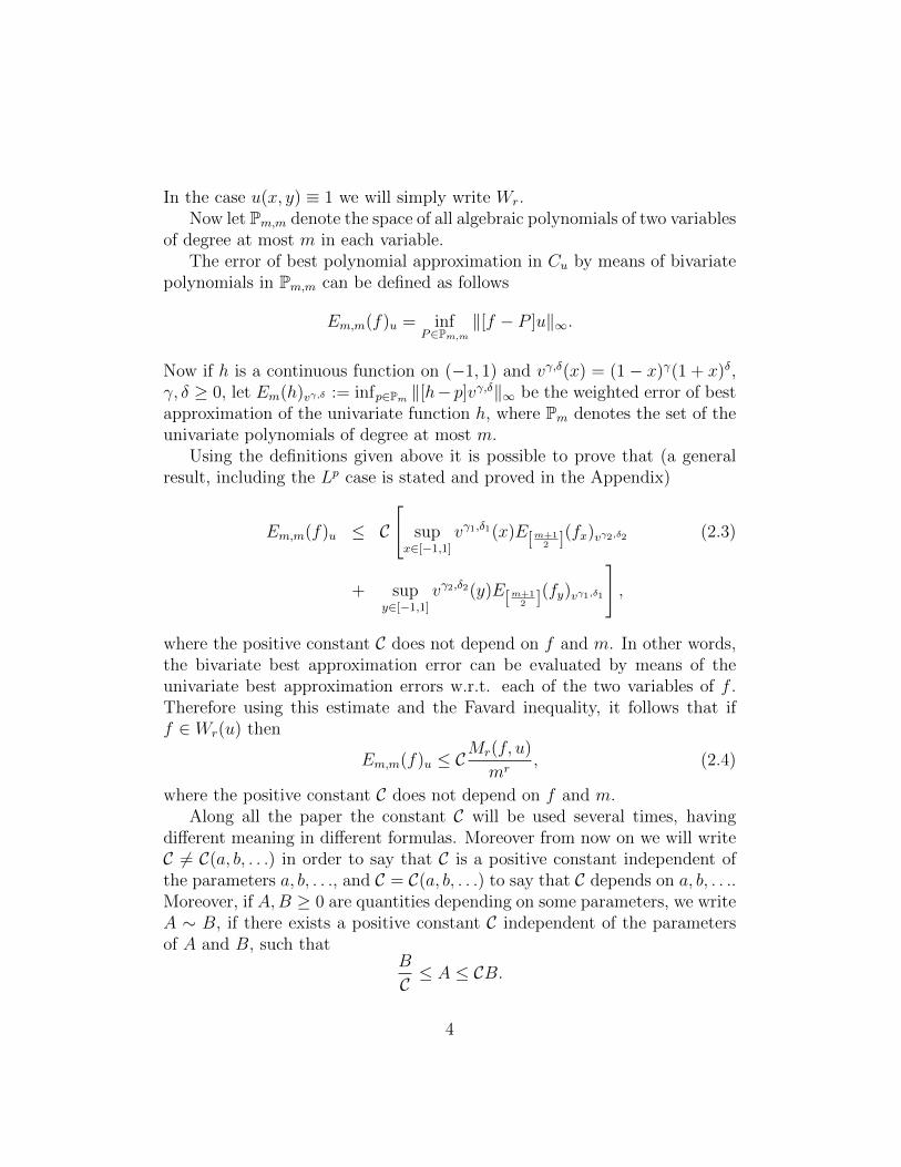
In the case u(x, y) ≡ 1 we will simply write Wr.Now let Pm,m denote the space of all algebraic polynomials of two variables

of degree at most m in each variable.The error of best polynomial approximation in Cu by means of bivariate

polynomials in Pm,m can be defined as follows

Em,m(f)u = infP∈Pm,m

‖[f − P ]u‖∞.

Now if h is a continuous function on (−1, 1) and vγ,δ(x) = (1− x)γ(1 + x)δ,γ, δ ≥ 0, let Em(h)vγ,δ := infp∈Pm ‖[h− p]vγ,δ‖∞ be the weighted error of bestapproximation of the univariate function h, where Pm denotes the set of theunivariate polynomials of degree at most m.

Using the definitions given above it is possible to prove that (a generalresult, including the Lp case is stated and proved in the Appendix)

Em,m(f)u ≤ C

[sup

x∈[−1,1]

vγ1,δ1(x)E[m+12 ](fx)vγ2,δ2 (2.3)

+ supy∈[−1,1]

vγ2,δ2(y)E[m+12 ](fy)vγ1,δ1

],

where the positive constant C does not depend on f and m. In other words,the bivariate best approximation error can be evaluated by means of theunivariate best approximation errors w.r.t. each of the two variables of f .Therefore using this estimate and the Favard inequality, it follows that iff ∈ Wr(u) then

Em,m(f)u ≤ CMr(f, u)

mr, (2.4)

where the positive constant C does not depend on f and m.Along all the paper the constant C will be used several times, having

different meaning in different formulas. Moreover from now on we will writeC 6= C(a, b, . . .) in order to say that C is a positive constant independent ofthe parameters a, b, . . ., and C = C(a, b, . . .) to say that C depends on a, b, . . ..Moreover, if A,B ≥ 0 are quantities depending on some parameters, we writeA ∼ B, if there exists a positive constant C independent of the parametersof A and B, such that

B

C≤ A ≤ CB.

4

2.1. The bivariate Lagrange interpolation

Denote by vα,β(z) = (1 − z)α(1 + z)β, α, β > −1, the Jacobi weight on[−1, 1] and let pm(vα,β)m be the sequence of the orthonormal polynomialsw.r.t. vα,β and with positive leading coefficients, i.e. pm(vα,β, z) = γmz

m+. . .,

γm > 0. Denoting by z(α,β)i , i = 1, . . . ,m, the zeros of pm(vα,β), we consider

the Lagrange polynomial interpolating the continuous univariate function Gat the knots z(α,β)

i mi=1, i.e.

Lα,βm (G, z) =m∑i=1

`α,βi (z)G(z(α,β)i ), (2.5)

where `α,βi (z) =pm(vα,β, z)

p′m(vα,β, z(α,β)i )(z − z(α,β)

i )denotes the i-th fundamental La-

grange polynomial.Now let vα1,β1(x), vα2,β2(y) be two different Jacobi weights, with α1, β1,

α2, β2 > −1 and denote by xi := z(α1,β1)i , yi := z

(α2,β2)i , i = 1, . . . ,m, the

zeros of pm(vα1,β1) and pm(vα2,β2), respectively.Using (2.5) it is possible to define, for any continuous function f on S,

the bivariate interpolating polynomial on the pairs (xi, yj), i, j = 1, . . . ,m,

Lm(f, x, y) =m∑i=1

m∑j=1

`α1,β1i (x)`α2,β2

j (y)f(xi, yj). (2.6)

The polynomial Lm(f) is of degree m− 1 in each variable and by its defini-tion it follows that Lm(Pm−1,m−1) ≡ Pm−1,m−1. Moreover we can state thefollowing result.

Proposition 2.1. Let u(x, y) = vγ1,δ1(x)vγ2,δ2(y), with γ1, δ1, γ2, δ2 ≥ 0 andα1, β1, α2, β2 > −1, be such that

max

0,α1

2+

1

4

≤ γ1 ≤

α1

2+

5

4, max

0,β1

2+

1

4

≤ δ1 ≤

β1

2+

5

4,

(2.7)

max

0,α2

2+

1

4

≤ γ2 ≤

α2

2+

5

4, max

0,β2

2+

1

4

≤ δ2 ≤

β2

2+

5

4.

5

Then for any f ∈ Cu it follows

‖[f − Lm(f)]u‖∞ ≤ C(1 + log2m)Em−1,m−1(f)u, (2.8)

and also

‖[f − Lm(f)]u‖∞ ≤ C log2m

[sup

x∈[−1,1]

vγ1,δ1(x)Em−1(fx)vγ2,δ2

+ supy∈[−1,1]

vγ2,δ2(y)Em−1(fy)vγ1,δ1

](2.9)

where in both cases C 6= C(f,m).

We remark that the choice of γ1, δ1 and γ2, δ2 as in (2.7), produces the bestorder for the Lebesgue constants of the interpolation process Lmm, asshown in [4].

2.2. The Gaussian cubature formula

Let us introduce a cubature formula on the square obtained by a tensorproduct of two Gaussian quadrature rules. Recall that the Gaussian quadra-ture rule on [−1, 1] w.r.t. the Jacobi weight vα,β(z), is defined as

∫ 1

−1

G(z)vα,β(z) dz =

∫ 1

−1

Lα,βm (G, z)vα,β(z) dz + em(G)

=m∑i=1

λ(α,β)i G(z

(α,β)i ) + em(G) (2.10)

where λ(α,β)i , i = 1, . . . ,m, denote the Christoffel numbers and em(G) = 0 for

any algebraic polynomial of degree less then or equal to 2m− 1.By means of the polynomial Lm(f) introduced in the previous section, we

can define the Gaussian cubature formula w.r.t. the weight w(x, y) =vα1,β1(x)vα2,β2(y) as follows∫

S

f(x, y)w(x, y) dx dy =

∫S

Lm(f, x, y)w(x, y) dx dy + Em(f)

=m∑i=1

m∑j=1

λ(α1,β1)i λ

(α2,β2)j f(xi, yj) + Em(f). (2.11)

6

By the quadrature formula (2.10) it immediately follows that Em(P2m−1,2m−1) =0. It is possible to deduce the convergence of this formula for the continuousfunctions using the standard procedure. For functions having singularitieson the sides of S the following proposition holds true.

Proposition 2.2. Let f ∈ Cu, with u(x, y) = vγ1,δ1(x)vγ2,δ2(y), and γ1, δ1,γ2, δ2 ≥ 0, and let w(x, y) be defined as above. If

0 ≤ γ1 < α1 + 1, 0 ≤ δ1 < β1 + 1,

(2.12)

0 ≤ γ2 < α2 + 1, 0 ≤ δ2 < β2 + 1,

then it results

|Em(f)| ≤ CE2m−1,2m−1(f)u

∫S

vα1−γ1,β1−δ1(x)vα2−γ2,β2−δ2(y) dx dy, (2.13)

where C is a positive constant independent of m and f .

3. Main results

In this section we describe some numerical methods in order to approx-imate the solution of equation (1.1) and we prove that these methods areconvergent, stable and well conditioned.

First, if we denote

Kf(x, y) = µ

∫S

k(x, y, s, t)f(s, t)w(s, t) ds dt

then (1.1) can be rewritten in operatorial form as

(I −K)f = g, (3.1)

where I is the identity operator on Cu. Here and in the sequel we will denotek(s,t) (respectively k(x,y)) for meaning that the function of four variables k isconsidered as a function of only (x, y) (respectively (s, t)).

Under suitable assumptions on the function k(s,t) it is possible to provethe following

7

Proposition 3.1. Assume that (2.12) holds true and that for some r ∈ N

sup(s,t)∈S

‖k(s,t)‖Wr(u) < +∞. (3.2)

Then the operator K : Cu → Cu is compact and Kf ∈ Wr(u) for any f ∈ Cu.

The previous Proposition assures that the Fredholm Alternative holds truefor (3.1) in Cu.

3.1. The Nystrom method

The first numerical approach we propose is a weighted Nystrom method.Starting with the Gaussian formula (2.11) we can define the following discreteoperator

Kmf(x, y) = µm∑i=1

m∑j=1

λ(α1,β1)i λ

(α2,β2)j k(x, y, xi, yj)f(xi, yj), (3.3)

where we recall that xi = z(α1,β1)i , yi = z

(α2,β2)i and z

(αc,βc)i , c = 1, 2, i =

1, 2, . . . ,m,, are the zeros of the m-th orthonormal polynomial w.r.t. theweight vαc,βc(x), while λ

(αc,βc)i are the corresponding Christoffel numbers.

Then we consider the operator equation

(I −Km)fm = g, (3.4)

where fm is unknown. Since we are considering equation (3.1) in the weightedspace Cu we do the same with (3.4). Therefore we multiply both sides of equa-tion (3.4) by the weight u and then we collocate it on the pairs (xh, y`), h, ` =1, . . . ,m. In this way we have that the quantities aij = f(xi, yj)u(xi, yj),i, j = 1, . . . ,m, are the unknowns of the linear system

ah` − µu(xh, y`)m∑i=1

m∑j=1

λ(α1,β1)i λ

(α2,β2)j

u(xi, yj)k(xh, y`, xi, yj)aij

= (gu)(xh, y`) h, ` = 1, . . . ,m. (3.5)

The matrix solution (a∗ij)i,j=1...,m of this system (if it exists) allows us toconstruct the weighted Nystrom interpolant in two variables

fm(x, y)u(x, y) = µu(x, y)m∑i=1

m∑j=1

λ(α1,β1)i λ

(α2,β2)j

u(xi, yj)k(x, y, xi, yj)a

∗ij

+ (gu)(x, y). (3.6)

8

which will approximate the unknown fu. Now denote by Am the coefficientmatrix of system (3.5), which is a m ×m block matrix the entries of whichare m×m matrices, and by cond(Am) its condition number in infinity norm.We can state the following theorem about the convergence and stability ofthe proposed Nystrom method.

Theorem 3.1. Let γ1, δ1, γ2, δ2 be as in (2.12). Assume that k satisfies(3.2) and that KerI −K = 0 in Cu. Denote by f ∗ the unique solutionof (3.1) in Cu for a given g ∈ Cu. If in addition, for some r ∈ N

g ∈ Wr(u) (3.7)

andsup

(x,y)∈Su(x, y)‖k(x,y)‖Wr < +∞, (3.8)

then, for m sufficiently large, system (3.5) is uniquely solvable and well con-ditioned too, since

cond(Am) ≤ C, C 6= C(m). (3.9)

Moreover there results

‖[f ∗ − fm]u‖∞ ≤ C‖f ∗‖Wr(u)

(2m)r, (3.10)

where C 6= C(m, f ∗) .

We remark that if we had considered a “classical” Nystrom method, i.e.without considering the multiplication for the weight u, the procedure isunstable and the obtained coefficient matrix is usually ill–conditioned.

3.2. The collocation method

In this section we propose a collocation method which is an alternative tothe Nystrom method whenever a polynomial approximation of the solutionof the equation is required. The proposed method is obtained by projectingequation (3.1) by means of the Lagrange operator (2.6) on the space Pm,mand searching for a polynomial solution Fm ∈ Pm,m. More precisely we getthe following finite dimensional equation

(I −Hm)Fm = Lm(g) (3.11)

9

whereHmf(x, y) := Lm (K∗f, x, y)

and

K∗f(x, y) := µ

∫S

Lm(k(x,y), s, t)f(s, t)w(s, t) ds dt.

Searching the unknown Fm in the form

Fm(x, y) =m∑i=1

m∑j=1

aij`α1,β1i (x)`α2,β2

j (y)

u(xi, yj),

multiplying equation (3.11) by the weight u and collocating on the pairs(xh, y`), h, ` = 1, 2, . . . ,m, we have that the unknown coefficients ah` ofFm have to satisfy a linear system that is exactly the same obtained in theNystrom method, i.e. system (3.5). Therefore this system is well conditionedaccording to (3.9) in Theorem 3.1. About the convergence and the stabilityof the method we get the following result.

Theorem 3.2. Let γc, δc, αc, βc, c = 1, 2, be satisfying (2.7) and (2.12).Assume that, for some r ∈ N, k satisfies (3.2) and (3.8) and that KerI −K = 0 in Cu. Denote by f ∗ the unique solution of (3.1) in Cu for a giveng ∈ Wr(u). Then, for m sufficiently large, the method (3.11) is stable andconvergent in Cu and it results

‖[f ∗ − Fm]u‖∞ ≤ C log2m‖f ∗‖Wr(u)

mr(3.12)

where C 6= C(m, f ∗) .

We remark that the only difference in estimates (3.12) and (3.10) is thefactor 2r log2m. Nevertheless from the computational point of view thisfactor does not produce significant effects w.r.t. the speed of convergence.

4. Computational details and numerical tests

4.1. The matrix Am

The m-blocks matrix Am takes the following expression

Am =

A(1,1) A(1,2) . . . A(1,m)

A(2,1) A(2,2) . . . A(2,m)

. . . . . . . . . . . .A(m,1) A(m,2) . . . A(m,m)

10

with the blocks defined as

A(h,`) = δh,`I− µDhK(h,`)m U`, h, ` = 1, 2 . . . ,m,

whereDh = diag (u(xh, y1), u(xh, y2), . . . , u(xh, ym)) ,

U` = diag

(λα1,β1` λα2,β2

1

u(x`, y1),λα1,β1` λα2,β2

2

u(x`, y2), . . . ,

λα1,β1` λα2,β2

m

u(x`, ym)

),

I denotes the identity matrix of order m and the m×m matrix K(h,`)m is

defined as

K(h,`)m (i, j) = k(xh, y`, xi, yj), i, j = 1, 2, . . . ,m.

5. Computational details and numerical tests

5.1. The matrix Am

The m-blocks matrix Am takes the following expression

Am =

A(1,1) A(1,2) . . . A(1,m)

A(2,1) A(2,2) . . . A(2,m)

. . . . . . . . . . . .A(m,1) A(m,2) . . . A(m,m)

with the blocks defined as

A(h,`) = δh,`I− µDhK(h,`)m U`, h, ` = 1, 2 . . . ,m,

whereDh = diag (u(xh, y1), u(xh, y2), . . . , u(xh, ym)) ,

U` = diag

(λα1,β1` λα2,β2

1

u(x`, y1),λα1,β1` λα2,β2

2

u(x`, y2), . . . ,

λα1,β1` λα2,β2

m

u(x`, ym)

),

I denotes the identity matrix of order m and the m×m matrix K(h,`)m is

defined as

K(h,`)m (i, j) = k(xh, y`, xi, yj), i, j = 1, 2, . . . ,m.

11

5.2. Numerical tests

Now we show the performance of our method by some numerical exam-ples. In any test we approximate the weighted solution fu by the weightedNystrom interpolant fmu given in (3.6). The m2−square linear system re-quired in order to construct fmu was solved by the Gaussian elimination, sothe major computational effort is of the order of m6

3. In the tables for each

m we give the maximum relative error attained in the computation of fmuat the grid of equally spaced points [−0.9 : 0.1 : 0.9] × [−0.9 : 0.1 : 0.9].All the computations were performed in 16−digits precision. Usually condi-tions (2.12) leads to a range for the choice of the parameters of the weightu. Usually the most convenient thing in to choose the upper bounds of thisrange.

The first two example we consider are two cases founded in the literature.In these cases the weight u ≡ 1 and the solution f is known and very smooth.In the examples 3 and 4 we do not know the exact solution and we consideredas exact those values of fmu performed with m = 60.

Example 1This example is obtained by a linear transformation of the equationproposed in [10, Example 1]:

f(x, y)− 4

∫S

e−4(1+x)(1+s)−4(1+y)(1+t)f(s, t) ds dt

= 1− e−8(2+x+y)(e8(1+x) − 1)(e8(1+y) − 1)

4(1 + x)(1 + y)

Here the exact solution is f(x, y) = 1 and the kernel and the parametersare

µ = 1, k(x, y, s, t) = e−4(1+x)(1+s)−4(1+y)(1+t),

α1 = β1 = 0, α2 = β2 = 0.

According to (2.12) the exponents of the weight u can be chosen as

δ1 = δ2 = 1, γ1, γ2 ∈[

1

4,5

4

].

According to the theoretical results we expect a very fast convergence.The numerical results are as follows:

12

m Relative Error4 0.28× 10−1

8 0.16× 10−5

10 0.25× 10−8

12 0.18× 10−11

16 0.28× 10−13

We remark that, for the same test, the best error obtained in [10] is0.2× 10−9.

Example 2This example can be found in [1, Example 2]. Setting T = [0,

√π]2,

the equation is

F (ξ, η)− 1

5

∫T

cos(ξσ) cos(ητ)F (σ, τ) dσ dτ = 1− sin(√πξ) sin(

√πη)

5ξη,

the exact solution of which is F (ξ, η) = 1. By the changes of variables

ξ =

√π

2(x+ 1), η =

√π

2(y + 1), σ =

√π

2(s+ 1), τ =

√π

2(t+ 1),

the equation can be rewritten as

f(x, y)− µ∫S

k(x, y, s, t)f(s, t) ds dt = g(x, y) (5.13)

where

f(x, y) = F

(√π

2(x+ 1),

√π

2(y + 1)

), µ =

π

20,

k(x, y, s, t) = cos(π

4(x+ 1)(s+ 1)

)cos(π

4(y + 1)(t+ 1)

),

g(x, y) = 1− 4sin(π2(x+ 1)

)sin(π2(y + 1)

)5π(1 + x)(1 + y)

,

α1 = β1 = 0, α2 = β2 = 0.

According to (2.12) the exponents of the weight u can be chosen as

δ1 = δ2 = 1, γ1, γ2 ∈[

1

4,5

4

]Also in this case we expect a very fast convergence. The numericalresults are the following

13

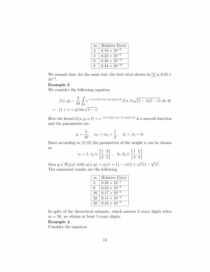
m Relative Error2 0.19× 10−2

4 0.22× 10−6

6 0.46× 10−11

8 0.44× 10−15

We remark that, for the same test, the best error shown in [1] is 0.23×10−9.

Example 3We consider the following equation

f(x, y)− 3

10

∫S

e−(1+x)(1+s)−(1+y)(1+t)f(s, t)√

(1− s)(1− t) ds dt

= (1 + x+ y) sin√

1− x.

Here the kernel k(x, y, s, t) = e−(1+x)(1+s)−(1+y)(1+t) is a smooth functionand the parameters are

µ =3

10, α1 = α2 =

1

2, β1 = β2 = 0.

Since according to (2.12) the parameters of the weight u can be chosenas

γ1 = 1, γ2 ∈[

1

2,3

2

], δ1, δ2 ∈

[1

4,5

4

]then g ∈ W2(u) with u(x, y) = u(x) = (1− x)(1 + x)

32 (1− y2)

54 .

The numerical results are the following

m Relative Error4 0.28× 10−1

8 0.23× 10−2

16 0.17× 10−3

32 0.11× 10−4

50 0.10× 10−5

In spite of the theoretical estimate, which assures 3 exact digits whenm = 50, we obtain at least 5 exact digits.

Example 4Consider the equation

14

1

10

∫S

(∣∣∣∣sin(1

2− x)∣∣∣∣3.2 s+ |cos(1 + y)|3.2 t

)f(s, t)

√1− t21− s

ds dt

= f(x, y)− e(1+x)(1+y).

Here the known function g(x, y) = e(1+x)(1+y) is a smooth function, thekernel k(x, y, s, t) = | sin

(12− x)|3.2s+ |cos(1 + y)|3.2 t and the param-

eters are

µ =1

10, α1 = −1

2, β1 = 0, α2 = β2 =

1

2,

while the exponents of u, according to (2.12), can be chosen as

γ1 ∈ [0, 1] , δ1 ∈[

1

4,5

4

], γ2, δ2 ∈

[1

2,3

2

].

Therefore, with u(x, y) = (1 − x)(1 + x)54 (1 + y)

32 (1 − y)

32 , we get

k(s,t) ∈ W3(u), uniformly w.r.t. s and t.The numerical results are as follows:

m Relative Error4 0.28× 10−4

8 0.47× 10−6

16 0.16× 10−7

32 0.31× 10−8

50 0.34× 10−9

We remark that with m = 50 we obtain 9 exact digits, while the theo-retical estimate assures us only 5 correct digits.

5.3. Application to different domains

Now we want to apply our results to other kinds of domains. Let it be

Ω = 0 ≤ x ≤ 1, xν+1 ≤ y ≤ xν, 0 ≤ ν ≤ 1.

In the next we refer to integral equations of the type

f(x, y)− µ∫

Ω

k(x, y, s, t)(sν − t)θsa(1− s)bf(s, t) ds dt = g(x, y) (5.14)

15

where a, b > −1, θ ≥ 0. In other words we are considering the case of akernel of the form k(x, y, s, t)(sν − t)θ. In this case, by the transformations

φ(ξ) =ξ + 1

2ψ(ξ, η) =

η + 1

2

(ξ + 1

2

)ν+

1− η2

(ξ + 1

2

)ν+1

(5.15)

equation (5.14) becomes

f(ξ, η)− µ

2d

∫Sk (ξ, η, σ, τ) f(σ, τ)vα1,β1(σ)vα2,β2(τ)dσdτ = g(ξ, η),

wherek(ξ, η, σ, τ) = k(φ(ξ), ψ(ξ, η), φ(σ), ψ(σ, τ)),

g(ξ, η) = g (φ(ξ), ψ(ξ, η)) , f(ξ, η) = f (φ(ξ), ψ(ξ, η))

vα1,β1(σ) = (1− σ)b+θ+1(1 + σ)a+ν+νθ, vα2,β2(τ) = (1− τ)θ

d = a+ b+ θ(ν + 2) + 3 + ν.

Now, by applying the previously introduced Nystrom method in the squareS, we obtain the weighted Nystrom interpolant

fm(ξ, η)vγ,δ(ξ, η) =µ

2dvγ,δ(ξ, η)

m∑i=1

m∑j=1

λiλjvγ,δ(xi, xj)

k(ξ, η, xi, xj)a∗ij

+ (gvγ,δ)(ξ, η)

which, according to the results of the previous sections, converges to thesolution fvγ,δ of the transformed equation. Inverting the transformations φand ψ it is possible to have an approximation of the weighted solution ofthe original equation. Unfortunately the known functions of the transformedequation are usually less smooth then the corresponding known functions ofthe original equations.

We show a numerical test in the case ν = 1/2.

Example 5Let

Ω = 0 ≤ x ≤ 1, x32 ≤ y ≤ x

12

be the domain of integration (see Figure 1). Consider the equation

f(x, y) −∫

Ω

(x2s2 + y2t2)s(1− s)f(s, t) ds dt (5.16)

= sin(y + x)− cx2 − dy2

16

c = 0.011065325673750182, d = 0.012669657886973633

with the exact solution f(x, y) = sin(x+ y).The kernel and the parameters are

µ = 1, k(x, y, s, t) = x2s2 + y2t2, ν =1

2,

a = 1, b = 1, θ = 0, d = 5.5, α1 = 2, β1 =3

2, α2 = β2 = 0.

According to (2.12) the exponent of the weight u can be chosen as

γ1 =5

4, δ1 = 2, γ2, δ2 ∈

[1

4,5

4

].

m Relative Error2 0.26× 10−3

4 0.11× 10−6

8 0.11× 10−8

10 0.29× 10−9

30 0.32× 10−10

In this case the exact solution f(x, y) = sin(x + y) of equation (5.16) inview of the transformations, becomes the solution of the new equation inthe class W4(u), with u(x, y) = u(x) = (1 − x)

54 (1 + x)2. This justifies the

slowness of the convergence. However, with m = 30 we obtain 9 exact digits,while the theoretical estimate assures us only 5 digits.

5.4. The case of non smooth known functions

The previous examples show as our method is much more effective whenthe known functions are smooth. In a forthcoming paper we will go deeperinto the cases of equations with non smooth known functions. Here we wantonly to give some ideas on how to proceed for improving the numerical per-formance in these cases.

When the known functions have singular low degree derivatives on theboundaries of S, as for instance in Example 3, a possible approach is firstto regularize the equation, by means of suitable transformations, and thento solve it numerically (see for instance the technique proposed in the one-dimensional case in [6]).

17

Figure 1: The domain Ω with ν = 1/2.

18

On the other hand, the singularities in the derivatives, can appear alsoin some isolated direction of the square. Sometimes this situation can behandled in a simple way.

Take for instance the following example:

f(x, y)−∫S

f(s, t)(xs+ yt)2√

1− t2 ds dt = |x| sin(x+ y)

where the known function g ∈ Cu, u(x, y) = (1 − x2)32 , but g /∈ W1(u).

Setting

f1(x, y) := f(x, y), (x, y) ∈ [−1, 0]× [−1, 1] := S1

f2(x, y) := f(x, y), (x, y) ∈ [0, 1]× [−1, 1] =: S2

the equation is equivalent to the following system of integral equations

∫S1

f1(s, t)(xs+ yt)2√

1− t2 ds dt+

∫S2

f2(s, t)(xs+ yt)2√

1− t2 ds dt

= f1(x, y) + x sin(x+ y),∫S1

f1(s, t)(xs+ yt)2√

1− t2 ds dt+

∫S2

f2(s, t)(xs+ yt)2√

1− t2 ds dt

= f2(x, y)− x sin(x+ y).

By linear transformations sending S1 and S2 in S, we get

1

2

∫S

f1

(s− 1

2, t

)((x− 1)(s− 1)

4+ yt

)2√1− t2 ds dt

+1

2

∫S

f2

(s+ 1

2, t

)((x− 1)(s+ 1)

4+ yt

)2√1− t2 ds dt

= f1

(x− 1

2, y

)+x− 1

2sin

(x− 1

2+ y

),

1

2

∫S

f1

(s− 1

2, t

)((x+ 1)(s− 1)

4+ yt

)2√1− t2 ds dt

+1

2

∫S

f2

(s+ 1

2, t

)((x+ 1)(s+ 1)

4+ yt

)2√1− t2 ds dt

= f2

(x+ 1

2, y

)− x+ 1

2sin

(x+ 1

2+ y

).

19

Setting F1(x, y) = f1

(x−1

2, y)

and F2(x, y) = f2

(x+1

2, y)

we have a linearsystem of two Fredholm integral equations in the unknowns F1 and F2 whichwill belong to Wr(u), for any r > 0 and with u(x, y) = (1− x2)

32 . Therefore

the proposed numerical method, applied to both the equations, will convergevery fast.

6. Proofs

Proof of Proposition 2.1. Let Pm−1,m−1 ∈ Pm−1,m−1. Then

‖[f − Lm(f)]u‖∞ ≤ ‖[f − Pm−1,m−1]u‖∞ + ‖Lm(f − Pm−1,m−1)u‖∞.

Since by the definition

‖Lm(f − Pm−1,m−1)u‖∞

≤ ‖[f − Pm−1,m−1]u‖∞ sup(x,y)∈S

m∑i=1

m∑j=1

u(x, y)

u(xi, yj)|`α1,β1i (x)`α2,β2

j (y)|

and it is known [11] that under the assumptions (2.7) it results

supx∈[−1,1]

vγ1,δ1(x)m∑i=1

|`α1,β1i (x)|vγ1,δ1(xi)

∼ logm,

and

supy∈[−1,1]

vγ2,δ2(y)m∑j=1

|`α2,β2j (y)|vγ2,δ2(yj)

∼ logm,

then (2.8) follows.Now we remark that, by the definition,

Lm(f, x, y) = Lα1,β1m (Lα2,β2

m (fx, y), x) ≡ Lα2,β2m (Lα1,β1

m (fy, x), y). (6.17)

We recall that [11] under the assumptions (2.7), for any univariate functionsh in the weighted continuous space w.r.t. the weight vγi,δi , it results

‖Lαi,βim (h)vγi,δi‖∞ ≤ C logm‖hvγi,δi‖∞, C 6= C(h,m) (6.18)

or equivalently

‖[h− Lαi,βim (h)]vγi,δi‖∞ ≤ C logmEm(h)vγi,δi . (6.19)

20

Therefore

‖[f − Lm(f)]u‖∞ ≤‖[f − Lα2,β2

m (f)]u‖∞ + ‖[Lα2,β2m (f)− Lα2,β2

m (Lα1,β1m (f))]u‖∞

= ‖[fx − Lα2,β2m (fx)]u‖∞ + ‖[Lα2,β2

m (fy − Lα1,β1m (fy))]u‖∞.

Consequently (2.9) follows by using (6.18)-(6.19).

Proof of Proposition 2.2. Let P2m−1,2m−1 ∈ P2m−1,2m−1 be arbitrarilychosen. Since the Gaussian cubature formula is exact for P2m−1,2m−1 we get,by the definition,

|Em(f)| = |Em(f − P2m−1,2m−1)|

≤∫S

|f(x, y)− P2m−1,2m−1(x, y)|w(x, y) dx dy

+m∑i=1

m∑j=1

λ(α1,β1)i λ

(α2,β2)j |f(xi, yj)− P2m−1,2m−1(xi, yj)|

≤ ‖[f − P2m−1,2m−1]u‖∞[∫

S

w(x, y)

u(x, y)dx dy

+m∑i=1

m∑j=1

λ(α1,β1)i λ

(α2,β2)j

u(xi, yj)

].

Note that the double sum at the right–hand side can be bounded withC∫Sw(x,y)u(x,y)

dx dy, where C 6= C(m), and since we are assuming (2.12), theproposition follows taking the infimum on P2m−1,2m−1.

Proof of Proposition 3.1. Following [15] it is sufficient to show that

limm

sup‖fu‖∞≤1

Em,m(Kf)u = 0.

Let Qm(x, y, s, t) be a polynomial of degree m in each variable and, forany f ∈ Cu, define the bivariate polynomial

KQmf(x, y) =

∫S

Qm(x, y, s, t)f(s, t)w(s, t) ds dt.

21

Then ∣∣Kf(x, y)−KQmf(x, y)∣∣u(x, y) =

=

∣∣∣∣∫S

[k(x, y, s, t)−Qm(x, y, s, t)] f(s, t)w(s, t) ds dt

∣∣∣∣u(x, y)

≤ ‖fu‖∞∫S

∣∣k(s,t)(x, y)−Qm(x, y, s, t)∣∣u(x, y)

w(s, t)

u(s, t)ds dt.

Therefore

Em,m(Kf)u ≤ ‖[Kf −KQmf ]u‖∞

≤ sup(x,y)∈S

u(x, y) sup(s,t)∈S

∣∣k(s,t)(x, y)−Qm(x, y, s, t)∣∣ ‖fu‖∞ ∫

S

w(s, t)

u(s, t)ds dt.

From (2.12) and since Qm can be arbitrarily chosen, we can conclude that

Em,m(Kf)u ≤ C‖fu‖∞ sup(s,t)∈S

Em,m(k(s,t))u

and hence the proposition follows by (3.2).

From now on, when the context is clear, we will omit the subscript in theoperator norms, i.e. we will simply denote ‖ · ‖ instead of ‖ · ‖Cu→Cu .

Proof of Theorem 3.1. First we prove that the Nystrom method is con-vergent and stable in Cu. This can be done by showing that,

1. limm‖[Kf −Kmf ]u‖∞ = 0 for any f ∈ Cu;

2. supm

limn

sup‖fu‖∞≤1

En,n(Kmf)u = 0.

By Step 1., by virtue of the principle of uniform boundedness, we candeduce immediately that,

supm‖Km‖ < +∞.

On the other hand Step 2. is equivalent to the collectively compactness ofKmm and hence it follows that ‖(K − Km)Km‖ → 0. Therefore (see for

22

instance [2]), under these assumptions and for m sufficiently large, I −Km

is invertible in Cu and is uniformly bounded since there results

‖(I −Km)−1‖ ≤ 1 + ‖(I −K)−1‖ ‖Km‖1− ‖(I −K)−1‖‖(K −Km)Km‖

(6.20)

and in addition

‖[f ∗ − fm]u‖∞ ∼ ‖[Kf −Kmf ]u‖∞, (6.21)

where the constants in ∼ are independent of m and f ∗.Thus start with proving Step.1. We note that

‖[Kf −Kmf ]u‖∞ = sup(x,y)∈S

|Em(k(x,y)f)|u(x, y).

Therefore by (2.13) it follows

‖[Kf −Kmf ]u‖∞ ≤ C sup(x,y)∈S

u(x, y)E2m−1,2m−1(k(x,y)f)u

≤ C sup(x,y)∈S

u(x, y)E2m−1,2m−1(k(x,y))‖fu‖∞

+ C sup(x,y)∈S

u(x, y)‖k(x,y)‖∞E2m−1,2m−1(f)u (6.22)

and hence Step 1 follows by (3.8). Moreover we remark that (3.10) followsby (6.21)-(6.22) and the assumptions on the kernel and on the right–handside.

In order to prove Step 2. it is necessary to estimate En,n(Kmf)u, for alln. Let Qn(x, y, s, t) be a polynomial of degree n in each variable and, for anyf ∈ Cu, define the bivariate polynomial

KQnf(x, y) = µm∑i=1

m∑j=1

λ(α1,β1)i λ

(α2,β2)j

u(xi, yj)Qn(x, y, xi, yj)f(xi, yj)u(xi, yj).

Then ∣∣Kmf(x, y)−KQnf(x, y)∣∣u(x, y) =

= u(x, y)

∣∣∣∣∣µm∑i=1

m∑j=1

λ(α1,β1)i λ

(α2,β2)j

u(xi, yj)[k(x, y, xi, yj)

− Qn(x, y, xi, yj)] f(xi, yj)u(xi, yj)|

≤ ‖fu‖∞u(x, y)|µ|m∑i=1

m∑j=1

λ(α1,β1)i λ

(α2,β2)j

u(xi, yj)|k(x, y, xi, yj)−Qn(x, y, xi, yj)| .

23

Therefore

En,n(Kmf)u ≤ ‖[Kmf −KQnf ]u‖∞≤ sup

(x,y)∈Su(x, y) sup

(s,t)∈S

∣∣k(s,t)(x, y)−Qn(x, y, s, t)∣∣

‖fu‖∞m∑i=1

m∑j=1

λ(α1,β1)i λ

(α2,β2)j

u(xi, yj)

Note that the double sum is dominated by C∫Sw(x,y)u(x,y)

dx dy, with C 6=C(m), and therefore, from (2.12) and since Qn can be arbitrarily chosen, wecan conclude that

En,n(Kmf)u ≤ C‖fu‖∞ sup(s,t)∈S

En,n(k(s,t))u

with the constant C independent of m,n, f . Hence Step 2 follows by (3.2).Finally we prove (3.9).Let Z be a matrix of order m, Z = zi,j, i, j = 1, 2, . . . ,m, and z be the

vector obtained by reordering the matrix Z row-by-row, i.e.z(i−1)n+j := zi,j, i = 1, 2, . . . ,m, j = 1, 2, . . . ,m.Consider now a function z ∈ Cu chosen s.t. z(xi, yj)u(xi, yj) = zi,j and

‖zu‖∞ = 1. Then

‖Am‖∞ = supz∈Rm2 ,‖z‖∞=1

‖Amz‖∞

= max1≤h≤m

max1≤`≤m

∣∣∣∣∣zh,` − µu(xh, y`)m∑i=1

m∑j=1

λ(α1,β1)i λ

(α2,β2)j

u(xi, yj)k(xh, y`, xi, yj)zi,j

∣∣∣∣∣≤ sup

(x,y)∈S

∣∣∣∣∣z(x, y)u(x, y)− µu(x, y)m∑i=1

m∑j=1

λ(α1,β1)i λ

(α2,β2)j

u(xi, yj)k(x, y, xi, yj)zi,j

∣∣∣∣∣By (3.3)

‖Am‖∞ ≤ ‖(I −Km)zu‖∞ ≤ ‖(I −Km)‖. (6.23)

Now we have to estimate the norm of the inverse of the matrix Am.Consider an arbitrary vector γ ∈ Rm2

obtained by reordering row-by-row amatrix Γ = γi,j, i = 1, 2, . . . ,m, j = 1, 2, . . . ,m and with ‖γ‖∞ = 1 and

24

let z such that z = Am−1γ, z also obtained taking row by row a matrix

Z = zi,j, i = 1, 2, . . . ,m, j = 1, 2, . . . ,m. Let f, g ∈ Cu, s.t.

f = (I −Km)g, g(xi, yj)u(xi, yj) = γi,j, ‖gu‖∞ = 1.

Because of the uniqueness of the solution of the linear system (3.5), it isf(xi, yj)u(xi, yj) = zi,j. Therefore for any γ

‖A−1m γ‖∞ = ‖z‖∞ ≤ ‖fu‖∞= ‖(I −Km)−1gu‖∞ ≤ ‖(I −Km)−1‖,

and thus‖A−1m ‖∞ ≤ ‖(I −Km)−1‖. (6.24)

By (6.23),(6.24),

cond(Am) ≤ ‖I −Km‖‖(I −Km)−1‖

and then the proof is complete.

Proof of Theorem 3.2. The crucial point is to prove that

limm‖K −Hm‖ = 0.

Indeed by standard arguments (see for instance [2]) it follows that

‖(I −Hm)−1‖ ≤ ‖(I −K)−1‖1− ‖(I −K)−1‖ ‖K −Hm‖

and also

‖[f ∗ − Fm]u‖∞ ≤ C (‖[g − Lm(g)]u‖∞ + ‖gu‖∞‖K −Hm‖) .

Let f ∈ Cu. We get

‖[Kf −Hmf ]u‖∞ ≤ ‖[Kf −K∗f ]u‖∞ + ‖[K∗f −Hmf ]u‖∞ =: A+B.

About A, we remark that under the assumptions (2.7) and (2.12), for any hcontinuous on [−1, 1], it results [14]

‖Lαi,βim (h)vαi−γi,βi−δi‖1 ≤ C‖h‖∞, C 6= C(h,m). (6.25)

25

Recalling once again that

Lm(f, x, y) = Lα1,β1m (Lα2,β2

m (fx, y), x) ≡ Lα2,β2m (Lα1,β1

m (fy, x), y)

and using (6.25) twice, we get, for any F ∈ C(S),∥∥∥Lm(F )w

u

∥∥∥1≤ C‖F‖∞. (6.26)

Hence, with this estimate, it immediately follows that

A ≤ C‖fu‖∞ sup(x,y)∈S

Em−1,m−1(k(x,y)) ≤Cmr‖fu‖∞, C 6= C(m, f),

having also used assumption (3.8).On the other hand by (2.8) it results

B ≤ C log2mEm−1,m−1(K∗f)u.

Thus we have to estimate Em−1,m−1(K∗f)u.Following the same idea in Proposition 3.1 define the polynomial

KQm−1f(x, y) =

∫S

Qm−1(x, y, s, t)f(s, t)w(s, t) ds dt.

Therefore, again by (6.26), it follows∣∣K∗f(x, y)−KQm−1f(x, y)∣∣u(x, y) =

= µ

∣∣∣∣∫S

Lm(k(x,y) −Qm−1(x, y, ·, ·), s, t)f(s, t)w(s, t) ds dt

∣∣∣∣u(x, y)

≤ u(x, y)µ

∫S

∣∣Lm(k(x,y) −Qm−1(x, y, ·, ·), s, t)f(s, t)u(s, t)∣∣ w(s, t)

u(s, t)ds dt

≤ C‖fu‖∞u(x, y)‖k(x,y) −Qm−1(x, y, ·, ·)‖∞.

Since Qm−1 can be arbitrarily chosen we can finally deduce that

Em−1,m−1(K∗f)u ≤ C‖fu‖∞ sup(x,y)∈S

u(x, y)Em−1,m−1(k(x,y))

and then by assumption (3.8) in conclusion we get

B ≤ C log2m

mr‖fu‖∞

and the Theorem follows.

26

7. Appendix

In order to state a result about the bivariate polynomial best approxi-mation, we introduce some notation. The weight u(x, y) = vγ1,δ1(x)vγ2,δ2(y),γ1, δ1, γ2, δ2 > −1, fixed, denote by Lpu, 1 < p <∞, the weighted space of Lp

functions in two variables, i.e. the collection of the functions f(x, y) defined

on S = [−1, 1]×[−1, 1] and such that ‖fu‖p =(∫

S|f(x, y)u(x, y)|p dx dy

) 1p <

∞. Consequently define by Em,m(f)u,p = infP∈Pm,m ‖[f − P ]u‖p the error ofbest polynomial approximation in Lpu. Moreover if h is a function defined on[−1, 1] and vγ,δ(x) = (1 − x)γ(1 + x)δ, γ, δ > −1, considering the usual Lp

weighted space equipped with the norm ‖hvγ,δ‖p =(∫ 1

−1|h(t)vγ,δ(t)|p dt

) 1p,

let Em(h)vγ,δ,p := infp∈Pm ‖[h− p]vγ,δ‖p be the weighted error of best approx-imation of the univariate function h in Lp norm, where Pm denotes the setof the univariate polynomials of degree m.

We get the following result

Theorem 7.1. Let f ∈ Lpu, 1 < p <∞, with u(x, y) = vγ1,δ1(x)vγ2,δ2(y) andγ1, δ1, γ2, δ2 > −1

p. Then

Em,m(f)u,p ≤ C

[(∫ 1

−1

|vγ1,δ1(x)Em(fx)vγ2,δ2 ,p|p dx) 1

p

(7.27)

+

(∫ 1

−1

|vγ2,δ2(y)Em(fy)vγ1,δ1 ,p|p dy) 1

p

]

where C is a positive constant independent of f and m. On the other hand ifγ1, δ1, γ2, δ2 ≥ 0, and f ∈ Cu, then

Em,m(f)u ≤ C

[sup

x∈[−1,1]

vγ1,δ1(x)E[m+12 ](fx)vγ2,δ2 (7.28)

+ supy∈[−1,1]

vγ2,δ2(y)E[m+12 ](fy)vγ1,δ1

],

where we used the notation introduced in Section 2 for the weighted contin-uous functions and also in this case the positive constant C does not dependon f and m.

27

Proof of Theorem 7.1.Let w(x, y) = w1(x)w2(y), where wi, i = 1, 2, are suitable Jacobi weights

satisfying the following conditions:

vγ1,δ1√w1ϕ

∈ Lp, w1

vγ1,δ1∈ Lq, 1

vγ1,δ1

√w1

ϕ∈ Lq,

q =p

p− 1(7.29)

vγ2,δ2√w2ϕ

∈ Lp, w2

vγ2,δ2∈ Lq, 1

vγ2,δ2

√w2

ϕ∈ Lq.

Consider now the sequences of orthonormal polynomials, with positive lead-ing coefficients, pm(wi)m, and, for any univariate function h in the Lp

weighted space w.r.t. the weight vγi,δi , the corresponding Fourier operators

Sm(wi, h, t) =∑m

i=0 ai(h)pi(wi, t), where ai =

∫ 1

−1

h(τ)pi(wi, τ)wi(τ) dτ .

It is well known (see for instance [12] and the reference therein) that assump-tions (7.29) are necessary and sufficient in order to get

‖Sm(wi, h)vγi,δi‖p ≤ C‖hvγi,δi‖p, C 6= C(m,h), i = 1, 2

and consequently

‖[h− Sm(wi, h)]vγi,δi‖p ≤ CEm(h)vγi,δi ,p, i = 1, 2. (7.30)

Now define the two dimensional Fourier operator as

Sm,m(w, f, x, y) = Sm(w2, Sm(w1, fy, x), y) ≡ Sm(w1, Sm(w2, fx, y), x)

where we recall that fx, fy denote the function f as a univariate function ofthe variable y and x respectively. By definition Sm,m(w, f) ∈ Pm,m. HenceEm,m(f)u,p ≤ ‖[f − Sm,m(w, f)]u‖p. Evaluate ‖[f − Sm,m(w, f)]u‖p. We get

‖[f − Sm,m(w, f)]u‖p ≤‖[f − Sm(w2, f)]u‖p + ‖[Sm(w2, f)− Sm(w2, Sm(w1, fy))]u‖p

= ‖[fx − Sm(w2, fx)]u‖p + ‖[Sm(w2, fy − Sm(w1, fy))]u‖p.

Therefore if the weights w1 and w2 satisfy (7.29) we immediately get (7.27)by applying (7.30).

28

Consider now the uniform case. Hence assume γ1, δ1, γ2, δ2 ≥ 0. Let wi(t),i = 1, 2, be suitable Jacobi weights. Define the De la Vallee Poussin operators

Vm(wi, h, t) =1

m

2m−1∑i=m

Si(wi, h, t), where the Fourier operators are defined as

above. Hence Vm(wi, h) ∈ P2m−1. Now set wi(t) = (1− t)αi(1 + t)βi , i = 1, 2.If h is an univariate function in the weighted continuous space w.r.t. theweight vγi,δi , it is known that [13], if for some ν ∈ [0, 1/2], the parametersγ1, δ1, αi, βi, i = 1, 2 satisfy the following inequalities

αi2

+1

4− ν ≤ γi < min

αi2

+5

4− ν, αi + 1

(7.31)

βi2

+1

4− ν ≤ δi < min

βi2

+5

4− ν, βi + 1

then

‖Vm(wi, h)vγi,δi‖∞ ≤ C‖hvγi,δi‖∞, C 6= C(h,m), i = 1, 2

or equivalently

‖[h− Vm(wi, h)]vγi,δi‖∞ ≤ CEm(h)vγi,δi C 6= C(h,m), i = 1, 2. (7.32)

Now define the two dimensional De la Vallee Poussin operator as

Vm,m(w, f, x, y) = Vm(w2, Vm(w1, fy, x), y) ≡ Vm(w1, Vm(w2, fx, y), x)

By definition Vm,m(w, f) ∈ P2m−1,2m−1. For the sake of simplicity assumethat m is odd (otherwise Em,m(f)u ≤ Em−1,m−1(f)u, with m− 1 odd). Then

Em,m(f)u ≤∥∥∥[f − Vm+1

2,m+1

2(w, f)

]u∥∥∥∞

.

Evaluate∥∥∥[f − Vm+1

2,m+1

2(w, f)

]u∥∥∥∞

. Exactly as before we get

∥∥∥[f − Vm+12,m+1

2(w, f)

]u∥∥∥∞≤∥∥∥[f − Vm+1

2(w2, f)]

]u∥∥∥∞

+∥∥∥[Vm+1

2(w2, f)− Vm+1

2(w2, Vm+1

2(w1, fy))

]u∥∥∥∞

=∥∥∥[fx − Vm+1

2(w2, fx)

]u∥∥∥∞

+∥∥∥[Vm+1

2(w2, fy − Vm+1

2(w1, fy))

]u∥∥∥∞.

Therefore if the parameters αi, βi, i = 1, 2, are chosen such that conditions(7.31) are satisfied, we immediately get (7.28) by applying (7.32).

29

Acknowledgments. The authors are grateful to Professor Giuseppe Mas-troianni for his helpful suggestions and remarks. They also thank the refereesfor the accurate reading of the paper.

References

[1] Alipanah A., Esmaeili S., Numerical solution of the two-dimensionalFredholm integral equations using Gaussian radial basis function, J.Comput. Appl. Math. in press, doi:10.1016/j.cam.2009.11.053

[2] Atkinson K.E., The Numerical Solution of Integral Equations of the sec-ond kind, Cambridge Monographs on Applied and Computational Math-ematics, Cambridge University Press 1997

[3] De Bonis M. C., Mastroianni G., Projection Methods and condition num-bers in uniform norm for Fredholm and Cauchy singular integral equa-tions, SIAM Journal on Numerical Analysis 44 no.4 (2006), 1351-1374

[4] Della Vecchia B., Mastroianni G., Vertesi P., Exact order of the Lebesgueconstants for bivariate Lagrange interpolation at certain node-systems,Studia Scient. Math. Hung. 46, no.1 (2009), 97–102

[5] Ditzian Z., Totik V., Moduli of smoothness, SCMG Springer-Verlag, NewYork Berlin Heidelberg London Paris Tokyo, 1987

[6] Fermo L., Russo M. G., Numerical methods for Fredholm integral equa-tions with singular right–hand sides, Adv. Comput. Math. 33, n. 3,305–330. doi: 10.1007/s10444-009-9137-4

[7] Han G., Wang R., Richardson extrapolation of iterated discrete Galerkinsolution for two-dimensional Fredholm integral equations, J. Comput.Appl. Math. 139, n. 1, (2002), 49–63

[8] Keller A., Instant Radiosity, Proceedings of the 24th annual conferenceon Computer graphics and interactive techniques (SIGGRAPH ’97).ACM Press,Addison-Wesley Publishing Co., New York, NY, USA, 49-56(1997). doi:10.1145/258734.258769

30

[9] Kajiya J. T., The rendering equation, SIGGRAPH Comput.Graph. 20, 4, ACM, New York, NY, USA, 143-150 (1986).doi=10.1145/15886.15902

[10] Liang F., Lin F.R., A fast numerical solution method for two dimen-sional Fredholm integral equations of the second kind based on piecewisepolynomial interpolation, Appl. Math. Comput. 216, n.10, (2010), 3073–3088 doi: 10.1016/j.amc.2010.04.027

[11] Mastroianni G., Russo M. G., Lagrange Interpolation in some weighteduniform spaces, Facta Univ. Ser. Math. Inform. 12 (1997), 185–201

[12] Mastroianni G., Russo M. G., Fourier sums in weighted spaces of func-tions. A survey., Jaen J. Approx. 1(2) (2009), 257–290

[13] Mastroianni G., Themistoclakis W., De la Valle Poussin means andJackson’s theorem, Acta Sci. Math. (Szeged) 74, no. 1-2, (2008), 147-170

[14] Nevai P., Mean convergence of Lagrange interpolation III, Trans. Amer.Math. Soc., 282 , no.2, (1984), 669–698

[15] Timan A.F., Theory of approximation of functions of a real variable,Pergamonn Press, Oxford, England, 1963

[16] Xie W.J., Lin F.R., A fast numerical solution method for two dimen-sional Fredholm integral equations of the second kind, Appl. Numer.Math. 59 (2008), 1709–1719.

31