Singular General Relativity - arXiv
128
University Politehnica of Bucharest Faculty of Applied Sciences Singular General Relativity Ph.D. Thesis Ovidiu Cristinel Stoica Supervisor Prof. dr. CONSTANTIN UDRIS ¸TE Corresponding Member of the Accademia Peloritana dei Pericolanti, Messina Full Member of the Academy of Romanian Scientists Bucharest 2013 arXiv:1301.2231v4 [gr-qc] 24 Jan 2014
-
Upload
khangminh22 -
Category
Documents
-
view
1 -
download
0
Transcript of Singular General Relativity - arXiv
University Politehnica of BucharestFaculty of Applied Sciences
Singular General RelativityPh.D. Thesis
Ovidiu Cristinel Stoica
Supervisor
Prof. dr. CONSTANTIN UDRISTECorresponding Member of the Accademia Peloritana dei Pericolanti, Messina
Full Member of the Academy of Romanian Scientists
Bucharest 2013
arX
iv:1
301.
2231
v4 [
gr-q
c] 2
4 Ja
n 20
14

Declaration of Authorship
I, Ovidiu Cristinel Stoica, declare that this Thesis titled, ‘Singular General Relativity’
and the work presented in it are my own. I confirm that:
Where I have consulted the published work of others, this is always clearly at-
tributed.
Where I have quoted from the work of others, the source is always given. With
the exception of such quotations, this Thesis is entirely my own work.
I have acknowledged all main sources of help.
Signed:
Date:
i
Abstract
This work presents the foundations of Singular Semi-Riemannian Geometry and Singular
General Relativity, based on the author’s research. An extension of differential geometry
and of Einstein’s equation to singularities is reported. Singularities of the form studied
here allow a smooth extension of the Einstein field equations, including matter. This
applies to the Big-Bang singularity of the FLRW solution. It applies to stationary black
holes, in appropriate coordinates (since the standard coordinates are singular at singu-
larity, hiding the smoothness of the metric). In these coordinates, charged black holes
have the electromagnetic potential regular everywhere. Implications on Penrose’s Weyl
curvature hypothesis are presented. In addition, these singularities exhibit a (geo)metric
dimensional reduction, which might act as a regulator for the quantum fields, includ-
ing for quantum gravity, in the UV regime. This opens the perspective of perturbative
renormalizability of quantum gravity without modifying General Relativity.

Acknowledgements
I thank my PhD advisor, Prof. dr. Constantin Udriste from the University Politehnica
of Bucharest, who accepted and supervised me, with a theme with enough obstacles and
subtleties. I thank my former Professors Gabriel Pripoae and Olivian Simionescu-Panait
from the University of Bucharest, for comments and important suggestions. I offer my
profound gratitude to the late Professor Kostake Teleman [135], for mentoring me during
my Master at the University of Bucharest. I wish to thank Professor Vasile Brınzanescu,
my former PhD advisor during the preparation years of my PhD degree program at the
Institute of Mathematics of the Romanian Academy, for preparing high standard exams
containing topics suited for my purposes, and for giving me the needed freedom, when
my research evolved in a different direction. I thank Professor M. Visinescu from the
National Institute for Physics and Nuclear Engineering Magurele, Bucharest, Romania,
for his unconditioned help and suggestions.
I thank Professor David Ritz Finkelstein from Georgia Tech Institute of Technology,
whose work was such an inspiration in finding the coordinates which remove the infinities
in the black hole solutions, and for his warm encouragements and moral support.
I thank Professors P. Fiziev and D. V. Shirkov for helpful discussions and advice received
during my stay at the Bogoliubov Laboratory of Theoretical Physics, JINR, Dubna.
I thank Professor A. Ashtekar from Penn State University, for an inspiring conversation
about some of the ideas from this Thesis, and possible relations with Loop Quantum
Gravity, during private conversations in Turin.
I thank the anonymous referees for the valuable comments and suggestions to improve
the clarity and the quality of the published papers on which this Thesis is based.
This work was partially supported by the Romanian Government grant PN II Idei 1187.
iii
Contents
Title page i
Declaration of Authorship i
Abstract ii
Acknowledgements iii
Contents iv
1 Introduction 1
1.1 Historical background . . . . . . . . . . . . . . . . . . . . . . . . . . . . . 1
1.2 Motivation for this research . . . . . . . . . . . . . . . . . . . . . . . . . . 3
1.3 Presentation per chapter . . . . . . . . . . . . . . . . . . . . . . . . . . . . 4
2 Singular semi-Riemannian manifolds 6
2.1 Introduction . . . . . . . . . . . . . . . . . . . . . . . . . . . . . . . . . . . 6
2.1.1 Motivation and related advances . . . . . . . . . . . . . . . . . . . 6
2.1.2 Presentation of this chapter . . . . . . . . . . . . . . . . . . . . . . 7
2.2 Singular semi-Riemannian manifolds . . . . . . . . . . . . . . . . . . . . . 8
2.2.1 Definition of singular semi-Riemannian manifolds . . . . . . . . . . 8
2.2.2 The radical of a singular semi-Riemannian manifold . . . . . . . . 9
2.3 The radical-annihilator . . . . . . . . . . . . . . . . . . . . . . . . . . . . . 9
2.3.1 The radical-annihilator vector space . . . . . . . . . . . . . . . . . 9
2.3.2 The radical-annihilator vector bundle . . . . . . . . . . . . . . . . 11
2.3.3 Radical and radical-annihilator tensors . . . . . . . . . . . . . . . . 12
2.4 Covariant contraction of tensor fields . . . . . . . . . . . . . . . . . . . . . 12
2.4.1 Covariant contraction on inner product spaces . . . . . . . . . . . 13
2.4.2 Covariant contraction on singular semi-Riemannian manifolds . . . 13
2.5 The Koszul object . . . . . . . . . . . . . . . . . . . . . . . . . . . . . . . 15
2.5.1 Basic properties of the Koszul object . . . . . . . . . . . . . . . . . 15
2.6 The covariant derivative . . . . . . . . . . . . . . . . . . . . . . . . . . . . 17
2.6.1 The lower covariant derivative of vector fields . . . . . . . . . . . . 17
2.6.2 Radical-stationary singular semi-Riemannian manifolds . . . . . . 19
2.6.3 The covariant derivative of differential forms . . . . . . . . . . . . 19
2.6.4 Semi-regular semi-Riemannian manifolds . . . . . . . . . . . . . . 22
iv
Contents v
2.7 Curvature of semi-regular semi-Riemannian manifolds . . . . . . . . . . . 22
2.7.1 Riemann curvature of semi-regular semi-Riemannian manifolds . . 22
2.7.2 The symmetries of the Riemann curvature tensor . . . . . . . . . . 23
2.7.3 Ricci curvature tensor and scalar curvature . . . . . . . . . . . . . 25
2.8 Relation with Kupeli’s curvature function . . . . . . . . . . . . . . . . . . 26
2.8.1 Riemann curvature in terms of the Koszul object . . . . . . . . . . 26
2.8.2 Relation with Kupeli’s curvature function . . . . . . . . . . . . . . 27
2.9 Examples of semi-regular semi-Riemannian manifolds . . . . . . . . . . . . 28
2.9.1 Diagonal metric . . . . . . . . . . . . . . . . . . . . . . . . . . . . . 28
2.9.2 Isotropic singularities . . . . . . . . . . . . . . . . . . . . . . . . . 29
2.10 Cartan’s structural equations for degenerate metric . . . . . . . . . . . . . 30
2.10.1 The first structural equation . . . . . . . . . . . . . . . . . . . . . 30
2.10.1.1 The decomposition of the Koszul object . . . . . . . . . . 30
2.10.1.2 The connection forms . . . . . . . . . . . . . . . . . . . . 31
2.10.1.3 The first structural equation . . . . . . . . . . . . . . . . 31
2.10.2 The second structural equation . . . . . . . . . . . . . . . . . . . . 33
2.10.2.1 The curvature forms . . . . . . . . . . . . . . . . . . . . . 33
2.10.2.2 The second structural equation . . . . . . . . . . . . . . . 33
2.11 Degenerate warped products . . . . . . . . . . . . . . . . . . . . . . . . . . 33
2.11.1 Introduction . . . . . . . . . . . . . . . . . . . . . . . . . . . . . . 34
2.11.2 General properties . . . . . . . . . . . . . . . . . . . . . . . . . . . 34
2.11.3 Warped products of semi-regular manifolds . . . . . . . . . . . . . 36
2.11.4 Riemann curvature of semi-regular warped products . . . . . . . . 37
3 Einstein equation at singularities 40
3.1 Einstein equation at semi-regular singularities . . . . . . . . . . . . . . . . 40
3.1.1 Einstein’s equation on semi-regular spacetimes . . . . . . . . . . . 40
3.2 Einstein equation at quasi-regular singularities . . . . . . . . . . . . . . . 42
3.2.1 Expanded Einstein equation and quasi-regular spacetimes . . . . . 42
3.2.2 Quasi-regular spacetimes . . . . . . . . . . . . . . . . . . . . . . . 43
3.2.3 Examples of quasi-regular spacetimes . . . . . . . . . . . . . . . . 44
3.2.3.1 Isotropic singularities . . . . . . . . . . . . . . . . . . . . 44
3.2.3.2 Quasi-regular warped products . . . . . . . . . . . . . . . 45
4 The Big-Bang singularity 46
4.1 Introduction . . . . . . . . . . . . . . . . . . . . . . . . . . . . . . . . . . . 46
4.2 The Friedmann-Lemaıtre-Robertson-Walker spacetime . . . . . . . . . . . 47
4.2.1 The Friedman equations . . . . . . . . . . . . . . . . . . . . . . . . 48
4.2.2 Distance separation vs. topological separation . . . . . . . . . . . . 49
4.3 Densitized Einstein equation on the FLRW spacetime . . . . . . . . . . . 49
4.3.1 What happens when the density becomes infinite? . . . . . . . . . 50
4.3.2 The Big Bang singularity resolution . . . . . . . . . . . . . . . . . 51
4.4 The Weyl curvature hypothesis . . . . . . . . . . . . . . . . . . . . . . . . 52
4.4.1 Introduction . . . . . . . . . . . . . . . . . . . . . . . . . . . . . . 52
4.4.2 The Weyl tensor vanishes at quasi-regular singularities . . . . . . . 53
4.4.3 Example: a general cosmological model . . . . . . . . . . . . . . . 54
4.4.4 Conclusion . . . . . . . . . . . . . . . . . . . . . . . . . . . . . . . 57

Contents vi
5 Black hole singularity resolution 58
5.1 Introduction . . . . . . . . . . . . . . . . . . . . . . . . . . . . . . . . . . . 58
5.1.1 The singularity theorems . . . . . . . . . . . . . . . . . . . . . . . 58
5.1.2 The black hole information paradox . . . . . . . . . . . . . . . . . 59
5.1.3 The meaning of singularities . . . . . . . . . . . . . . . . . . . . . . 59
5.2 Schwarzschild singularity is semi-regularizable . . . . . . . . . . . . . . . . 60
5.2.1 Introduction . . . . . . . . . . . . . . . . . . . . . . . . . . . . . . 60
5.2.2 Analytic extension of the Schwarzschild spacetime . . . . . . . . . 61
5.2.3 Semi-regular extension of the Schwarzschild spacetime . . . . . . . 62
5.3 Analytic Reissner-Nordstrom singularity . . . . . . . . . . . . . . . . . . . 64
5.3.1 Introduction . . . . . . . . . . . . . . . . . . . . . . . . . . . . . . 64
5.3.2 Extending the Reissner-Nordstrom spacetime at the singularity . . 64
5.3.3 Null geodesics in the proposed solution . . . . . . . . . . . . . . . . 66
5.3.4 The electromagnetic field . . . . . . . . . . . . . . . . . . . . . . . 67
5.4 Kerr-Newman solutions with analytic singularity . . . . . . . . . . . . . . 69
5.4.1 Introduction . . . . . . . . . . . . . . . . . . . . . . . . . . . . . . 69
5.4.2 Extending the Kerr-Newman spacetime at the singularity . . . . . 70
5.4.3 Electromagnetic field in Kerr-Newman . . . . . . . . . . . . . . . . 72
6 Global hyperbolicity and black hole singularities 73
6.1 Canceling the singularities of the field equations . . . . . . . . . . . . . . . 73
6.1.1 The topology of singularities . . . . . . . . . . . . . . . . . . . . . 74
6.2 Globally hyperbolic spacetimes . . . . . . . . . . . . . . . . . . . . . . . . 74
6.3 Globally hyperbolic Schwarzschild spacetime . . . . . . . . . . . . . . . . 75
6.3.1 Penrose-Carter diagram for the semi-regular solution . . . . . . . . 75
6.3.2 Globally hyperbolic Schwarzschild spacetime . . . . . . . . . . . . 76
6.4 Globally hyperbolic Reissner-Nordstrom spacetime . . . . . . . . . . . . . 78
6.4.1 The Penrose-Carter diagrams for our solution . . . . . . . . . . . . 78
6.4.2 Globally hyperbolic Reissner-Nordstrom spacetime . . . . . . . . . 80
6.5 Globally hyperbolic Kerr-Newman spacetime . . . . . . . . . . . . . . . . 83
6.5.1 Removing the closed timelike curves . . . . . . . . . . . . . . . . . 83
6.5.2 The Penrose-Carter diagrams for our solution . . . . . . . . . . . . 84
6.6 Non-stationary black holes . . . . . . . . . . . . . . . . . . . . . . . . . . . 85
6.7 Conclusions . . . . . . . . . . . . . . . . . . . . . . . . . . . . . . . . . . . 88
7 Quantum gravity from metric dimensional reduction at singularities 90
7.1 Introduction . . . . . . . . . . . . . . . . . . . . . . . . . . . . . . . . . . . 90
7.2 Suggestions of dimensional reduction coming from other approaches . . . 92
7.2.1 Dimensional reduction in Quantum Field Theory . . . . . . . . . . 92
7.2.1.1 Several hints of dimensional reduction from QFT . . . . . 92
7.2.1.2 Fractal universe and measure dimensional reduction . . . 92
7.2.1.3 Topological dimensional reduction . . . . . . . . . . . . . 93
7.2.2 Dimensional reduction in Quantum Gravity . . . . . . . . . . . . . 94
7.2.2.1 Asymptotic safety for the renormalization group . . . . . 95
7.2.2.2 Horava-Lifschitz gravity . . . . . . . . . . . . . . . . . . . 95
7.3 Dimensional reduction at singularities . . . . . . . . . . . . . . . . . . . . 96
7.3.1 The dimension of the metric tensor . . . . . . . . . . . . . . . . . . 96

Contents vii
7.3.2 Metric dimension vs. topological dimension . . . . . . . . . . . . . 97
7.3.3 Metric dimensional reduction and the Weyl tensor . . . . . . . . . 97
7.3.4 Lorentz invariance and metric dimensional reduction . . . . . . . . 98
7.3.5 Particles lose two dimensions . . . . . . . . . . . . . . . . . . . . . 98
7.3.6 Particles and spacetime anisotropy . . . . . . . . . . . . . . . . . . 99
7.3.7 The measure in the action integral . . . . . . . . . . . . . . . . . . 99
7.3.8 How can dimension vary with scale? . . . . . . . . . . . . . . . . . 100
7.4 Conclusions . . . . . . . . . . . . . . . . . . . . . . . . . . . . . . . . . . . 101
Bibliography 104
My Papers 119
Chapter 1
Introduction
1.1 Historical background
We are interested in the properties of a class of smooth differentiable manifolds which
have on the tangent bundle a smooth symmetric bilinear form (also named metric),
which is allowed to change its signature.
The first such manifolds which were studied have non-degenerate metric – starting with
the Euclidean plane and space, and continuing with the non-Euclidean geometries intro-
duced by Lobachevsky, Gauss, and Bolyai. After Gauss extended the study of the Eu-
clidean plane to curved surfaces, Bernhard Riemann generalized it to curved spaces with
arbitrary number of dimensions [159]. Riemann hoped to give a geometric description
of the physical space, in the idea that matter is in fact the effect of the curvature. The
previously discovered geometries – the Euclidean and non-Euclidean ones, and Gauss’s
geometry of surfaces – are all particular cases of Riemannian geometry. A Riemannian
manifold is a differentiable manifold endowed with a symmetric, non-degenerate and
positive definite bilinear form on its tangent bundle.
The necessity of studying spaces having a symmetric, non-degenerate bilinear form which
is not positive definite appeared with the Theory of Relativity [68]. A differentiable man-
ifold having on its tangent bundle a symmetric, non-degenerate bilinear form which is
not necessarily positive or negative definite is named semi-Riemannian manifold (some-
times pseudo-Riemannian manifold, and in older textbooks even is called Riemannian
manifold). Semi-Riemannian geometry constitutes the mathematical foundation of Gen-
eral Relativity. It was thoroughly studied, and the constructions made starting from the
non-degenerate metric, such as the Levi-Civita connection, the covariant derivative, the
Riemann, Ricci and scalar curvatures are very similar to the Riemannian case, when the
metric is positive definite. On the other hand, other properties, especially the global
ones, are very different in the indefinite case. Very good references for semi-Riemannian
geometry are the textbooks [22, 94, 140].
1

Introduction 2
If we allow the metric to be degenerate, many difficulties occur. For this reason, advances
were made slower than for the non-degenerate case, and only in particular situations.
The study of manifolds endowed with degenerate metric is pioneered by Moisil [131],
Strubecker [193–196], Vranceanu [223] 1.
One situation when the metric can be degenerate occurs in the study of submanifolds of
semi-Riemannian manifolds. In the Riemannian case, the submanifolds are Riemannian
too. But in general the image of a smooth mapping from a differentiable manifold to
a Riemannian or semi-Riemannian manifold may be singular, in particular may have
degenerate metric. In the case of varieties the problem of finding a resolution of its
singularities was proved to have positive answer by Hironaka [103, 104]. In the semi-
Riemannian case, the metric induced on a submanifold can be degenerate, even though
the larger manifold has non-degenerate metric. The properties of such submanifolds,
studied in many articles, e.g. in [153], [119, 121], [23, 66], were extended by Kupeli
to manifolds endowed with degenerate metric of constant signature [120, 122]. The
situation is much more difficult when the signature changes.
There are some situations in General Relativity when the metric becomes degenerate
or changes its signature. There are cosmological models of the Universe in which the
initial singularity of the Big Bang is replaced, by making the metric of the early Uni-
verse Riemannian. Such models, constructed in connection to the Hartle-Hawking no-
boundary approach to Quantum Cosmology, assume that the metric was Riemannian,
and it changed, becoming Lorentzian, so that time emerged from a space dimension.
Such a change of signature is considered to take place when traversing a hypersurface,
on which the metric becomes degenerate [168],[72, 73],[97–99], [59], [60–64, 101], [113–
118].
Another situation where the metric can become degenerate was proposed by Einstein
and Rosen, as a model of charged particles. They were the first to model charged
particles as wormholes, also named Einstein-Rosen bridges [69], and inspired Wheeler’s
charge without charge program [128, 229].
The Einstein’s equation, as well as its Hamiltonian formulation due to Arnowitt, Deser
and Misner [10], may lead to cases when the metric is degenerate. As the Penrose and
Hawking singularity theorems show, the conditions leading to singularities are very gen-
eral, applying to the matter distribution in our Universe [89–91, 94, 95, 144]. Therefore,
it is important to know how we can deal with such singularities. Many attempts were
done to solve this issue.
For example it was suggested that Ashtekar’s method of “new variables” [12, 13, 164]
can be used to pass beyond the singularities, because the variable Eai – a densitized
frame of vector fields – defines the metric, which can be degenerate. Unfortunately, it
1Gheorghe Vranceanu also introduced in 1926 the non-holonomic geometry, nowadays known assub-Riemannian geometry [134, 204, 221, 222]. Although at a point, there is a duality between thesub-Riemannian and the singular semi-Riemannian metrics, locally and especially globally there are toomany differences to allow an import of the rich amount of results already obtained in sub-Riemanniangeometry.
Introduction 3
turned out that in this case the connection variable Aia may become singular cf.e.g.[230].
In fact, this is the general case, because the connection variable Aia contains as a term
the Levi-Civita connection, which is singular in most cases when g becomes degenerate.
Quantum effects are suspected to play an important role in avoiding the singularities.
Loop Quantum Cosmology, by quantizing spacetime, provided a mean to avoid the Big-
Bang singularity and replace it with a Big-Bounce, due to the fact that the curvature
is bounded, because there is a minimum distance [15, 33, 167, 219]. A very interesting
model which is nonsingular at the end of the evolution and does not allow the anisotropic
universe to turn into an isotropic one is studied in [165, 166]. Another possibility to
avoid singularities is given in [151], within the Einstein-Cartan-Sciama-Kibble theory
[50, 51, 100], and also in f(R) modifications of General Relativity. Singularity removal
may arise arise in more classical contexts. For example, certain symmetries eliminates
the so-called NUT singularity, in certain conditions [56–58, 127].
A more classical proposal to avoid the consequences of singularities was initiated by R.
Penrose, with the cosmic censorship hypothesis [145–148]. According to the weak cos-
mic censorship hypothesis, all singularities (except the Big-Bang singularity) are hidden
behind an event horizon, hence are not naked. The strong cosmic censorship hypothesis
conjectures that the maximal extension of spacetime as a regular Lorentzian manifold
is globally hyperbolic.
The literature in the approaches to singularities is too vast, and it would be unjust to
claim to review it properly in a research work which is not a dedicated review. A great
review on the problem of singularities in General Relativity is given in [206], and a more
up-to-date one in [83].
1.2 Motivation for this research
In this Thesis is developed the mathematical formalism for a large class of manifolds
having on the tangent structure symmetric bilinear forms, which are allowed to become
degenerate. Then these results are applied to the singularities in General Realtivity.
This special type of singular semi-Riemannian manifold has regular properties in what
concerns
1. the Riemann curvature Rabcd (and not Rabcd, which in general diverges at singu-
larities),
2. the covariant derivative of an important class of differential forms,
3. and other geometric objects and differential operators which in general cannot be
defined properly because they require the inverse of the metric.

Introduction 4
These properties of regularity are not valid for any type of degenerate metric. This
justifies the name of semi-regular semi-Riemannian manifolds given here to these special
singular semi-Riemannian manifolds. Semi-regular metrics can also be used to give a
densitized version to the Einstein equation, and to approach the problem of singularities
in General Relativity.
The signature of the metric of a semi-regular semi-Riemannian manifold can change, but
when it doesn’t change, we obtain the “stationary singular semi-Riemannian manifolds”
with constant signature, researched by Kupeli [120, 122]. These in turn contain as par-
ticular case the semi-Riemannian manifolds, which contain the Riemannian manifolds.
In General Relativity, Einstein’s equation encodes the relation between the stress-energy
tensor of matter, and the Ricci curvature. In 1965 Roger Penrose [144], and later he and
S. Hawking [89–91, 94, 95], proved a set of singularity theorems. These theorems state
that, under reasonable conditions, the spacetime turns out to be geodesic incomplete –
i.e. it has singularities. They show that the conditions of occurrence of singularities
are quite common. Christodoulou [53] showed that these conditions are in fact more
common, and then Klainerman and Rodnianski [111] proved that they are even more
common.
Consequently, some researchers proclaimed that General Relativity predicts its own
breakdown, by predicting the singularities [13, 14, 16, 93, 95, 96]. Hawking’s discovery
of the black hole evaporation, leading to his information loss paradox [92, 93], made the
things even worse. The singularities seem to destroy information, in particular violating
the unitary evolution of quantum systems. The reason is that the field equations cannot
be continued through singularities.
Therefore, it would be important to better understand the singularities.
There are two main situations in which singularities appear in General Relativity and
Cosmology: at the Big-Bang, and in the black holes. We will see that the mathematical
apparatus developed in this Thesis finds applications in both these situations.
As the previous section shows, much work is done on singular metrics. But to the
author’s knowledge, the systematic approach presented here and the results are novel,
as well as the applications to General Relativity, and have no overlap with the research
that is previously done by other researchers.
1.3 Presentation per chapter
Chapter 2 introduces the geometry of metrics which can be degenerate, and are allowed
to change signature. It studies the main properties of such manifolds, and is based
almost entirely on the author’s research. It contains an invariant definition of metric
contraction between covariant indices, which works also when the metric is degenerate.
With the help of the metric, it is shown that in some cases one can construct covariant
Introduction 5
derivatives, and even define a Riemann curvature tensor. If the metric is non-degenerate,
all these geometric objects become the ones known from semi-Riemannian geometry.
Section 2.10 contains the derivation of a generalization of Cartan’s structural equations
for degenerate metric. Section 2.11 generalizes the notion of warped product to the case
when the metric can become degenerate. It provides a simple way to construct examples
of singular semi-Riemannian manifolds. The degenerate warped product turns out to
be relevant in some of the singularities which will be analyzed in the Thesis.
The following chapters, also based on author’s own research, applies the mathematics
developed in the first part to the singularities encountered in General Relativity. Chapter
3 introduces two equations equivalent to Einstein’s equation at the points where the
metric is non-degenerate, but which remain smooth at singularities. The first equation
remains smooth at the so-called semi-regular singularities. The second of the equations
applies to the more restricted case of quasi-regular singularities, which will turn out to
be important in the following chapters.
Chapter 4 shows, with the apparatus developed so far, that the Friedmann-Lemaıtre-
Robertson-Walker spacetime is semi-regular, but also quasi-regular. It also studies some
important properties of the FLRW singularity. The non-singular version of Einstein’s
equation is written explicitly, and shown to be smooth at singularity. Then, in section
§4.4, a more general solution, which is not homogeneous or isotropic, is presented. It is
shown that it contains as particular cases the isotropic singularities and the Friedmann-
Lemaıtre-Robertson-Walker singularities, and, being quasi-regular, satisfies the Weyl
curvature hypothesis of Penrose.
The black hole singularities are studied in chapter 5. It is shown that the Schwarzschild
singularity is semi-regularizable, by using a method inspired by that of Eddington and
Finkelstein [67, 74], used to prove that the metric is regular on the event horizon. This
method is also applied to make the Reissner-Nordstrom and the Kerr-Newman singular-
ities analytic. Then, it is shown that this approach allows the construction of globally
hyperbolic spacetimes with singularities (Chapter 6). This shows that it doesn’t follow
with necessity that black holes destroy information, leading by this to Hawking’s infor-
mation loss paradox and violations of unitary evolution. This suggests that a possible
resolution of Hawking’s paradox can be obtained without modifying General Relativity.
Chapter 7 explores the possibility that the dimensional reduction at singularities im-
proves the renormalization in Quantum Field Theory, and makes Quantum Gravity
preturbatively renormalizable.
Chapter 2
Singular semi-Riemannian
manifolds
The text in this chapter is based on author’s original results, communicated in the papers
[180], [182], and [181].
2.1 Introduction
2.1.1 Motivation and related advances
On a semi-Riemannian manifold (including the Riemannian case), one can use the metric
to define geometric objects like the Levi-Civita connection and the Riemann curvature.
One essential ingredient is the metric covariant contraction [154, 215]. In singular semi-
Riemannian geometry, the metric is not necessarily non-degenerate, and these standard
constructions no longer work, being based on the inverse of the metric, and on operations
defined with its help, like the metric contraction between covariant indices.
In this chapter, we define in an invariant way the canonical metric contraction between
covariant indices, which works even for degenerate metrics (although in this case is
well defined only on a special type of tensor fields, but this suffices for our purposes).
Then, we use this contraction to define in a canonical manner the covariant derivative
for radical-annihilator indices of covariant tensor fields, on a class of singular semi-
Riemannian manifolds. This newly defined covariant derivative helps us construct the
Riemann curvature, which is smooth on a class of singular semi-Riemannian manifolds,
named semi-regular. We also define the Ricci and scalar curvatures, which are smooth
for degenerate metric, so long as the signature is constant.
6

Singular semi-Riemannian manifolds 7
2.1.2 Presentation of this chapter
Section §2.2 recalls known generalities about singular semi-Riemannian manifolds, such
as the space of degenerate tangent vectors at a point.
Section §2.3 continues with the properties of the radical-annihilator space, consisting in
the covectors annihilating the degenerate vectors at a point. These spaces of covectors
are used to define tensor fields. On the space of radical-annihilator covectors we can
define a symmetric bilinear form which generalizes the inverse of the metric. This metric
will be used to perform metric contractions between covariant indices, for the tensor
fields constructed with the help of the radical-annihilator space, in section §2.4.
The standard way to define the Levi-Civita connection is by raising an index in the
Koszul formula. But this method works only for non-degenerate metrics, since it relies
on raising indices. We will be able to obtain differential operators like the covariant
derivative for a class of tensor fields, by using the right-hand side of the Koszul formula
(named here the Koszul object). The properties of the Koszul object are studied in
section §2.5. They are similar to those of the Levi-Civita connection, and are used to
construct a kind of covariant derivative for vector fields in section §2.6, and a covariant
derivative for differential forms in §2.6.3.
An important class of singular semi-Riemannian manifolds is that on which the lower
covariant derivative of any vector field, which is a 1-form, admits smooth covariant
derivatives. We define them in section §2.7, and call them semi-regular manifolds.
The Koszul object and of the covariant derivatives for differential forms introduced in
section §2.6 are used to construct, in §2.7, the Riemann curvature tensor, which has the
same symmetry properties as in the non-degenerate case. We show that on a semi-regular
semi-Riemannian manifold, the Riemann curvature tensor is smooth. Since it is radical-
annihilator in all of its indices, we can construct from it the Ricci and scalar curvatures.
Section §2.8, proves a useful formula of the Riemann curvature tensor, directly in terms
of the Koszul object. We compare the Riemann curvature we obtained, with the one
obtained by Kupeli by different methods in [120].
We give in section §2.9 two examples of semi-regular semi-Riemannian metrics: diagonal
metrics, and degenerate conformal transformations of non-degenerate metrics.
In section §2.10, we derive structural equations similar to those of Cartan, but for
degenerate metrics.
Section §2.11 contains the generalization of the warped product to singular semi-Rie-
mannian manifolds, where the warping function can be allowed to vanish at some points,
and the manifolds whose product is taken may be singular semi-Riemannian. It is shown
that the degenerate warped product of semi-Riemannian manifolds is semi-Riemannian,
under very general conditions imposed to the warping function. Degenerate warped
products will have important applications, both in the case of big-bang, and the black
hole singularities.
Singular semi-Riemannian manifolds 8
2.2 Singular semi-Riemannian manifolds
2.2.1 Definition of singular semi-Riemannian manifolds
Definition 2.1. (see e.g. [120], [142], p. 265 for comparison) Let M be a differentiable
manifold, and g ∈ T 02M a symmetric bilinear form on M . Then the pair (M, g) is called
singular semi-Riemannian manifold. The bilinear form g is called the metric tensor, or
the metric, or the fundamental tensor.
For any point p ∈M , the tangent space TpM has a frame in which the metric is
gp = diag(0, . . . , 0,−1, . . . ,−1, 1, . . . , 1),
where 0 appears r times, −1 appears s times, and 1 appears t times. The triple (r, s, t) is
called the signature of g at p. The relations dimM = r+s+t, and rank g = s+t = n−r,hold. If the signature of g is fixed, then (M, g) is said to have constant signature,
otherwise is said to be with variable signature. If g is non-degenerate, then the manifold
(M, g) is semi-Riemannian, and if g is positive definite, it is Riemannian.
Remark 2.2. The name “singular semi-Riemannian manifold” may suggest that such a
manifold is semi-Riemannian. In fact it is more general, containing the non-degenerate
case as a subcase. This may be a misnomer, but we adhere to it, because it is generally
used in the literature [122, 131, 223]. Moreover, for the geometric objects we introduce,
which are similar and generalize objects from the non-degenerate case, we will prefer to
import the standard terminology from semi-Riemannian geometry (see e.g. [140]).
The results obtained in the following don’t necessarily require the metric to be degen-
erate. Hence, they also apply to semi-Riemannian manifolds, including Riemannian.
Moreover, while in standard materials like [120, 122] was preferred to maintain the sig-
nature constant (because the most acute singular behavior takes place at the points
where the signature changes) we will not assume constant signature.
Example 2.1. Let r, s, t ∈ N, n = r + s+ t. The space
Rr,s,t := (Rn, 〈, 〉), (2.1)
with the metric g given, for any two vector fields X, Y on Rn at a point p on the
manifold, in the natural chart, by
〈Xp, Yp〉 = −s∑
i=r+1
XiY i +
n∑j=r+s+1
XjY j , (2.2)
is called the singular semi-Euclidean space Rr,s,t (see e.g. [142], p. 262). If r = 0 we
obtain the semi-Euclidean space Rns := R0,s,t (see e.g. [140], p. 58). If r = s = 0, then
t = n and we obtain as particular case the Euclidean space Rn, endowed with the natural
scalar product.
Singular semi-Riemannian manifolds 9
2.2.2 The radical of a singular semi-Riemannian manifold
Definition 2.3. (cf.e.g.[23], p. 1, [122], p. 3, and [140], p. 53) Let V be a finite
dimensional vector space, endowed with a symmetric bilinear form g which may be
degenerate. The space V := V ⊥ = X ∈ V |∀Y ∈ V, g(X,Y ) = 0 is named the radical
of V . The symmetric bilinear form g is non-degenerate if and only if V = 0.
Definition 2.4. (see e.g. [120], p. 261, [142], p. 263) Let (M, g) be a singular semi-
Riemannian manifold. The subset of the tangent bundle defined by T M = ∪p∈M (TpM)
is called the radical of TM . It is a vector bundle if and only if the signature of g
is constant on the entire M , and in this case, T M is a distribution. We denote by
X(M) ⊆ X(M) the set of vector fields W ∈ X(M) for which Wp ∈ (TpM).
Example 2.2. In the case of the the singular semi-Euclidean manifold Rr,s,t from the
Example 2.1, the radical T Rr,s,t is:
T Rr,s,t =⋃
p∈Rr,s,t
span((p, ∂ap)|∂ap ∈ TpRr,s,t, a ≤ r), (2.3)
and
X(Rr,s,t) = X ∈ X(Rr,s,t)|X =
r∑a=1
Xa∂a. (2.4)
2.3 The radical-annihilator
Let (V, g) be a vector space endowed with a bilinear form (also named inner product).
If g is non-degenerate, it defines an isomorphism [ : V → V ∗ (see e.g. [86], p. 15;
[82], p. 72). If g is degenerate, [ is a linear morphism, but not an isomorphism. This
prevents the definition of a dual for g on V ∗ in the usual sense. But we can still define
canonically a symmetric bilinear form g• ∈ [(V )∗ [(V )∗, which extends immediately
to singular semi-Riemannian manifolds, and can be used to contract covariant indices
and construct the needed geometric objects.
2.3.1 The radical-annihilator vector space
Definition 2.5. Let [ : V → V ∗, which associates to any u ∈ V a linear form [(u) :
V → R, defined by [(u)v := 〈u, v〉. Then, [ is a vector space morphism, called the index
lowering morphism. We will also use the notation u[ for [(u), and sometimes u•.
Remark 2.6. It is easy to see that V = ker [, so [ is an isomorphism if and only if g is
non-degenerate.
Definition 2.7. The vector space V • := im [ ⊆ V ∗ of 1-forms ω which can be expressed,
for some u ∈ V , as ω = u[, is called the radical-annihilator space (it is the annihilator of
the radical space V ). The forms ω ∈ V • are called radical-annihilator forms, and act
on V by ω(v) = 〈u, v〉.

Singular semi-Riemannian manifolds 10
It is easy to see that dimV •+ dimV = n. If g is non-degenerate, V • = V ∗. If u′ ∈ V is
another vector so that u′[ = ω, then u′−u ∈ V . Such 1-forms ω ∈ V • satisfy ω|V = 0.
Definition 2.8. The symmetric bilinear form g on V defines on V • a canonical non-
degenerate symmetric bilinear form g•, by g•(ω, τ) := 〈u, v〉, where u[ = ω and v = τ [.
We alternatively use the notation 〈〈ω, τ〉〉• = g•(ω, τ). This notation is consistent with
the notation u[ = u• ∈ V •.
Proposition 2.9. The inner product g• is well-defined, in the sense that it doesn’t
depend on the vectors u, v which represent the 1-forms ω, τ . It is non-degenerate, and
has the signature (0, s, t), where (r, s, t) is the signature of g.
Proof. Let u′, v′ ∈ V be other vectors so that u′[ = ω and v′[ = τ . Then, since u′−u ∈ V and v′ − v ∈ V , 〈u′, v′〉 = 〈u, v〉+ 〈u′ − u, v〉+ 〈u, v′ − v〉+ 〈u′ − u, v′ − v〉 = 〈u, v〉.
Let (ea)na=1 be a basis in which g is diagonal, the first r diagonal elements being 0. For
a ∈ 1, . . . , r, e[a = 0. For a ∈ 1, . . . , s + t, ωa := e[r+a are the generators of V •,
and 〈〈ωa, ωb〉〉• = 〈er+a, er+b〉. Hence, (ωa)s+ta=1 are linear independent, and g• has the
signature (0, s, t).
In Figure 2.1 we can see the various spaces associated with (V, g), and the inner products
induced by g on them.
(V,g) V*
uu+w
w (V,g)
(V,g)V=V/V
u
Figure 2.1: Let (V, g) be an inner product space. The morphism [ : V → V ∗ is definedby u 7→ u• := [(u) = u[ = g(u, ). The set of isotropic vectors in V forms the radicalV := ker [ = V ⊥. The image of [ is V • := im [ ≤ V ∗. The inner product g defines aninner product on V •, by g•(u
[1, u
[1) := g(u1, u2). The inner product g• is the inverse of
g iff det g 6= 0. The quotient space V • := V/V is made of the equivalence classes ofthe form u+ V . On V •, g defines an inner product g•(u1 + V , u2 + V ) := g(u1, u2).
The relations between the radical, the radical annihilator and the factor spaces can be
collected in the diagram:

Singular semi-Riemannian manifolds 11
0 V (V, g) (V •, g•) 0
0 V V ∗ (V •, g•) 0
i π•
π
[V
i•
[ ]
where V • = V •∗ =V
V and V = V
∗ = V ∗
V • .
Let (ea)na=1 be a basis of V in which g = diag(α1, α2, . . . , αn), αa ∈ R for all 1 ≤ a ≤ n.
Then
gab = 〈ea, eb〉 = αaδab, (2.5)
ea•(eb) := 〈ea, eb〉 = αaδab,
and, if (e∗a)na=1 is the dual basis of (ea)na=1,
ea• = αae
∗a. (2.6)
It is easy to see that
g•ab =
1
αaδab, (2.7)
for all a so that αa 6= 0.
2.3.2 The radical-annihilator vector bundle
It is straightforward to extend the notions from previous section to the cotangent bundle.
We define
T •M =⋃p∈M
(TpM)•, (2.8)
and we call
A•(M) := ω ∈ A1(M)|ωp ∈ (TpM)• for any p ∈M (2.9)
the space of radical-annihilator 1-forms.
Example 2.3. The radical-annihilator T •Rr,s,t of the space Rr,s,t from Example 2.1 is
T •Rr,s,t =⋃
p∈Rr,s,t
span(dxa ∈ T ∗pRr,s,t|a > r). (2.10)
The space of radical-annihilator 1-forms is
A•(Rr,s,t) = ω ∈ A1(Rr,s,t)|ωi = 0, i ≤ r, (2.11)
and they have the general form
ω =
n∑a=r+1
ωadxa. (2.12)
Singular semi-Riemannian manifolds 12
2.3.3 Radical and radical-annihilator tensors
The radical and radical-annihilator spaces determine special subspaces of tensors on
TpM , on which we can define the metric contraction in covariant indices.
Definition 2.10. Let T be a tensor of type (r, s). If T ∈ T k−10 M ⊗M T M ⊗M T r−ks M ,
we call it radical in the k-th contravariant slot. If T ∈ T rl−1M ⊗M T •M ⊗M T 0s−lM , we
call it radical-annihilator in the l-th covariant slot.
Proposition 2.11. Let T ∈ T rsM be a tensor. Then, T is radical in the k-th con-
travariant slot if and only if its contraction with any radical-annihilator linear 1-form
ω ∈ A1(M), Cks+1(T ⊗ ω) = 0.
Proof. Suppose k = r (the case k < r reduces to k = r, by using the permutation
automorphisms of the tensor space T rsTpM). The tensor T can be written as T =∑α Sα⊗vα, with Sα ∈ T r−1
s TpM and vα ∈ TpM . The contraction Cks+1(T ⊗ω) becomes∑α Sαω(vα). Since T is radical in the r-th contravariant slot, ω(vα) = 0, for all α and
any ω ∈ TpM•. Therefore∑
α Sαω(vα) = 0.
Reciprocally, if∑
α Sαω(vα) = 0, it follows that for any α, Sαω(vα) = 0, for any ω ∈TpM
•. Then, vα ∈ V .
Proposition 2.12. Let T ∈ T rsM be a tensor. Then, T is radical-annihilator in the
l-th covariant slot if and only if its l-th contraction with any radical vector field X,
Cr+1l (T ⊗X) = 0.
Proof. The proof is similar to that of Proposition 2.11.
Example 2.4. The inner product g ∈ T 02M is radical-annihilator in both of its slots.
Proposition 2.13. Let T ∈ T rsM be a tensor, radical in it’s k-th contravariant slot,
and radical-annihilator in it’s l-th covariant slot. Then, the contraction Ckl (T ) = 0.
Proof. The result follows from Proposition 2.11.
2.4 Covariant contraction of tensor fields
Contractions between one covariant and one contravariant indices don’t require a metric,
and the inner product g can contract between two contravariant indices, obtaining the
contravariant contraction operator Ckl (cf. e.g. [140], p. 83). But how we define the
metric contraction between two covariant indices, in the absence of an inverse of the
metric? We will see that g• can do this, although only for vectors or tensors which are
radical-annihilator in covariant slots. Luckily, these tensors are the relevant ones for our
purpose.

Singular semi-Riemannian manifolds 13
2.4.1 Covariant contraction on inner product spaces
Definition 2.14. Let T ∈ V • ⊗ V •, be a (2, 0)−tensor which is radical-annihilator in
both its slots. Then, C12T := g•abTab is the metric covariant contraction. This definition
is independent on the basis, because g• ∈ V •∗ ⊗ V •∗. Let r ≥ 0 and s ≥ 2, and let
T ∈ T rsV be a tensor which satisfies
T ∈ V ⊗r ⊗ V ∗⊗k−1 ⊗ V • ⊗ V ∗⊗l−k−1 ⊗ V • ⊗ V ∗⊗s−l, (2.13)
1 ≤ k < l ≤ s. We define the operator
Ckl : V ⊗r ⊗ V ∗⊗k−1 ⊗ V • ⊗ V ∗⊗l−k−1 ⊗ V • ⊗ V ∗⊗s−l → V ⊗r ⊗ V ∗⊗s−2,
by Ckl := Cs−1 s Pk,s−1;l,s, where Pk,s−1;l,s : T ∈ T rsV → T ∈ T rsV is the permutation
isomorphisms which moves the k-th and l-th slots in the last two positions, and Cs−1 s
is the operator
Cs−1 s := 1T rs−2V
⊗ C1,2 : T rs−2V ⊗ V • ⊗ V • → T rs−2V,
where 1T rs−2V
: T rs−2V → T rs−2V is the identity. Then, the operator Ckl is named the
metric covariant contraction between the covariant slots k and l. In a radical basis, the
contraction has the form
(CklT )a1...arb1...bk...bl...bs
:= g•bkblT a1...ar b1...bk...bl...bs . (2.14)
We denote the contraction CklT of T also by
T (ω1, . . . , ωr, v1, . . . , •, . . . , •, . . . , vs).
2.4.2 Covariant contraction on singular semi-Riemannian manifolds
We can now extend the metric covariant contraction in radical-annihilator slots to sin-
gular semi-Riemannian manifolds.
Definition 2.15. Let T ∈ T rsM , s ≥ 2, be a tensor field on M , which is radical-
annihilator in the k-th and l-th covariant slots, 1 ≤ k < l ≤ s. The operator
Ckl : T rk−1M ⊗M A•(M)⊗M T 0l−k−1M ⊗M A•(M)⊗M T 0
s−lM → T rs−2M
(CklT )(p) = Ckl(T (p))
is called the metric covariant contraction operator. We denote it also by
T (ω1, . . . , ωr, X1, . . . , •, . . . , •, . . . , Xs).

Singular semi-Riemannian manifolds 14
Lemma 2.16. Let T be a tensor field T ∈ T rsM , radical-annihilator in the k-th covariant
slot, 1 ≤ k ≤ s, where r ≥ 0 and s ≥ 1. Then
T (ω1, . . . , ωr, X1, . . . , •, . . . , Xs)〈Xk, •〉= T (ω1, . . . , ωr, X1, . . . , Xk, . . . , Xs).
(2.15)
Proof. Let’s work at a point p ∈ M , and consider first the case Tp ∈ T 01TpM , in fact,
Tp = ωp ∈ T •pM . Then, equation (2.15) becomes
ωp(•)〈Xp, •〉 = ωp(Xp). (2.16)
But ωp = Y [p for some vector Yp ∈ TpM , and ωp(•)〈Xp, •〉 = 〈〈ωp, X[
p〉〉• = ω(Xp).
The general case results from the linearity of the tensor product.
Corollary 2.17. 〈X, •〉〈Y, •〉 = 〈X,Y 〉.
Proof. It is obtained by applying Lemma 2.16 to g ∈ A•(M)M A•(M).
Theorem 2.18. Let (M, g) be a singular semi-Riemannian manifold with constant sig-
nature. Let T ∈ T rsM , be a tensor field as in Lemma 2.16. Then
T (ω1, . . . , ωr, X1, . . . , •, . . . , •, . . . , Xs)
=∑n
a=n−rank g+1
1
〈Ea, Ea〉T (ω1, . . . , ωr, X1, . . . , Ea, . . . , Ea, . . . , Xs),
(2.17)
for any X1, . . . , Xs ∈ X(M), ω1, . . . , ωr ∈ A1(M), where (Ea)na=1 is a local orthogonal
basis on M , so that E1, . . . , En−rank g ∈ X(M).
Proof. Since g• is diagonal and g•aa =
1
gaa=
1
〈Ea, Ea〉(Proposition 2.7),
g•abT (ω1, . . . , ωr, X1, . . . , Ea, . . . , Eb, . . . , Xs)
=∑n
a=n−rank g+1
1
〈Ea, Ea〉T (ω1, . . . , ωr, X1, . . . , Ea, . . . , Ea, . . . , Xs).
The metric covariant contraction of a smooth tensor is smooth, except for the points
where the signature changes, where the inverse of the metric becomes divergent, as seen
in equation (2.7).
Example 2.5. Let p ∈ M . Then, 〈•, •〉p = rank gp. This is also an example of metric
covariant contraction which is discontinuous when the signature changes.
Example 2.6. Let X ∈ X(M) and ω ∈ A•(M). Then, C12(ω ⊗M X[) = 〈〈ω,X[〉〉• =
ω(X) is smooth, even if the signature is not constant.
Singular semi-Riemannian manifolds 15
2.5 The Koszul object
Definition 2.19 (The Koszul object, see e.g. [120], p. 263). The object defined as
K : X(M)3 → R,
K(X,Y, Z) :=1
2X〈Y, Z〉+ Y 〈Z,X〉 − Z〈X,Y 〉−〈X, [Y, Z]〉+ 〈Y, [Z,X]〉+ 〈Z, [X,Y ]〉.
(2.18)
is called the Koszul object.
For non-degenerate metric, the Koszul object is nothing but the right hand side of the
Koszul formula
〈∇XY,Z〉 = K(X,Y, Z), (2.19)
which is used to construct the Levi-Civita connection, by raising the 1-form K(X,Y, )
(see e.g. [140], p. 61)
∇XY = K(X,Y, )]. (2.20)
This is not possible for degenerate metric. An alternative was proposed by Kupeli ([120],
p. 261–262). He defined the so-called Koszul derivatives, by raising the index with the
help of a distribution complementary to T M , provided that (M, g) is a singular semi-
Riemannian manifold with metric of constant signature, which satisfies the condition
of radical-stationarity (Definition 2.27). His Koszul derivative is therefore not unique,
depending on the choice of the complementary distribution, and is not a connection.
By contrast, our method doesn’t rely on arbitrary constructions, and works even if the
metric changes its signature. We will only rely on the Koszul object.
2.5.1 Basic properties of the Koszul object
We prove here explicitly some properties of the Koszul object which will be useful in the
following, and which correspond to known properties of the Levi-Civita connection of a
non-degenerate metric (cf. e.g. [140], p. 61), but are valid even on singular manifolds,
where the Levi-Civita connection can’t be defined.
Theorem 2.20. Let (M, g) be a singular semi-Riemannian manifold. Then, its Koszul
object has, for any X,Y, Z ∈ X(M) and f ∈ F (M), the properties:
1. It is additive and R-linear in all of its arguments.
2. It is F (M)-linear in the first argument:
K(fX, Y, Z) = fK(X,Y, Z).
3. Satisfies the Leibniz rule:
K(X, fY, Z) = fK(X,Y, Z) +X(f)〈Y,Z〉.

Singular semi-Riemannian manifolds 16
4. It is F (M)-linear in the third argument:
K(X,Y, fZ) = fK(X,Y, Z).
5. It is metric:
K(X,Y, Z) +K(X,Z, Y ) = X〈Y,Z〉.
6. It is symmetric or torsionless:
K(X,Y, Z)−K(Y,X,Z) = 〈[X,Y ], Z〉.
7. Relation with the Lie derivative of g:
K(X,Y, Z) +K(Z, Y,X) = (LY g)(Z,X),
where (LY g)(Z,X) := Y 〈Z,X〉 − 〈[Y,Z], X〉 − 〈Z, [Y,X]〉 is the Lie derivative of
g with respect to a vector field Y ∈ X(M).
8. K(X,Y, Z) +K(Y,Z,X) = Y 〈Z,X〉+ 〈[X,Y ], Z〉.
Proof. (1) It is a direct consequence of Definition 2.19, the fact that g is tensor, and the
linearity of the action of vector fields on scalars, and of the Lie brackets.
The other properties can also be proved by using the properties of g, of the action of
vector fields on scalars, of the Lie brackets, and of the Lie derivative, so we will give just
one example.
(2) 2K(fX, Y, Z) = fX〈Y, Z〉+ Y 〈Z, fX〉 − Z〈fX, Y 〉−〈fX, [Y,Z]〉+ 〈Y, [Z, fX]〉+ 〈Z, [fX, Y ]〉
= fX〈Y, Z〉+ Y (f〈Z,X〉)− Z(f〈X,Y 〉)−f〈X, [Y,Z]〉+ 〈Y, f [Z,X] + Z(f)X〉+〈Z, f [X,Y ]− Y (f)X〉
= fX〈Y,Z〉+ fY 〈Z,X〉+Y (f)〈Z,X〉 − fZ〈X,Y 〉−Z(f)〈X,Y 〉 − f〈X, [Y,Z]〉+ f〈Y, [Z,X]〉+Z(f)〈Y,X〉+ f〈Z, [X,Y ]〉 − Y (f)〈Z,X〉
= fX〈Y,Z〉+ fY 〈Z,X〉 − fZ〈X,Y 〉−f〈X, [Y,Z]〉+ f〈Y, [Z,X]〉+ f〈Z, [X,Y ]〉
= 2fK(X,Y, Z)
Remark 2.21. Let (Ea)na=1 ⊂ X(U) a local frame of vector fields on an open set U ⊆M .
Let gab = 〈Ea, Eb〉, and let C cab so that [Ea, Eb] = C c
abEc. Then,
Kabc := K(Ea, Eb, Ec)
=1
2Ea(gbc) + Eb(gca)− Ec(gab)− gasC s
bc + gbsCsca + gcsC
sab.
(2.21)
Singular semi-Riemannian manifolds 17
In the basis (Ea)na=1, the equations (5 – 8) in Theorem 2.20 become:
(5′) Kabc +Kacb = Ea(gbc).
(7′) Kabc +Kcba = (LEbg)ca.
(6′) Kabc −Kbac = gscC sab.
(8′) Kabc +Kbca = Eb(gca) + gscC sab.
If Ea = ∂a :=∂
∂xafor all a ∈ 1, . . . , n, then [∂a, ∂b] = 0, and the coefficients of the
Koszul object become Christoffel’s symbols of the first kind,
Kabc = K(∂a, ∂b, ∂c) =1
2(∂agbc + ∂bgca − ∂cgab). (2.22)
Corollary 2.22. Let X,Y ∈ X(M) be two vector fields. The map KXY : X(M)→ R
KXY (Z) := K(X,Y, Z) (2.23)
for any vector field Z ∈ X(M), is a differential 1-form.
Proof. Follows directly from Theorem 2.20, properties (1) and (4).
Corollary 2.23. Let X,Y ∈ X(M), and W ∈ X(M). Then
K(X,Y,W ) = K(Y,X,W ) = −K(X,W, Y ) = −K(Y,W,X). (2.24)
Proof. The first identity follows from Theorem 2.20, property (6), and the other two
from property (5).
2.6 The covariant derivative
In this section we will show that, even when the metric is degenerate, it is possible to
define in a canonical way the covariant derivative for differential forms which are radical
annihilator. We can use the Koszul object for a sort of covariant derivative, named here
lower covariant derivative, of vector fields, which associates to vector fields not vector
fields, but 1-forms. This means it doesn’t have the properties of a connection [112, 203],
but for our purpose will do the same job.
2.6.1 The lower covariant derivative of vector fields
Definition 2.24. Let X,Y ∈ X(M). The 1-form ∇[XY ∈ A1(M), defined by
(∇[XY )(Z) := K(X,Y, Z) (2.25)
Singular semi-Riemannian manifolds 18
for any Z ∈ X(M), is called the lower covariant derivative of the vector field Y in the
direction of the vector field X. The operator
∇[ : X(M)× X(M)→ A1(M), (2.26)
which associates to each X,Y ∈ X(M) the differential 1-form ∇[XY , is called the lower
covariant derivative operator.
Remark 2.25. The lower covariant derivative is well defined even if the metric is degen-
erate. When applying the lower covariant derivative to a vector field we don’t obtain
another vector field, but a differential 1-form, so it is not exactly a covariant derivative.
If the metric is non-degenerate, one obtains the covariant derivative by ∇XY = (∇[XY )].
In [113], p. 464–465 were used similar objects which map vector fields to 1-forms.
Theorem 2.26. Let (M, g) be a a singular semi-Riemannian manifold. The lower
covariant derivative operator ∇[ has the properties:
1. It is additive and R-linear in both of its arguments.
2. It is F (M)-linear in the first argument:
∇[fXY = f∇[XY.
3. Satisfies the Leibniz rule:
∇[XfY = f∇[XY +X(f)Y [,
or, explicitly,
(∇[XfY )(Z) = f(∇[XY )(Z) +X(f)〈Y,Z〉.
4. It is metric:
(∇[XY )(Z) + (∇[XZ)(Y ) = X〈Y,Z〉.
5. It is symmetric or torsionless:
∇[XY −∇[YX = [X,Y ][,
or, explicitly,
(∇[XY )(Z)− (∇[YX)(Z) = 〈[X,Y ], Z〉.
6. Relation with the Lie derivative of g:
(∇[XY )(Z) + (∇[ZY )(X) = (LY g)(Z,X).
7. (∇[XY )(Z) + (∇[Y Z)(X) = Y 〈Z,X〉+ 〈[X,Y ], Z〉,
for any X,Y, Z ∈ X(M) and f ∈ F (M).
Proof. Follows directly from Theorem 2.20.
Singular semi-Riemannian manifolds 19
2.6.2 Radical-stationary singular semi-Riemannian manifolds
Definition 2.27 (cf. [122] Definition 3.1.3). A singular semi-Riemannian manifold
(M, g) is radical-stationary if it satisfies the condition
K(X,Y, ) ∈ A•(M), (2.27)
for any X,Y ∈ X(M). Equivalently, K(X,Y,Wp) = 0 for any X,Y ∈ X(M) and
Wp ∈ X(Mp), p ∈M .
Remark 2.28. Kupeli introduced and studied the radical-stationary singular semi-Rie-
mannian manifolds of constant signature in [120], p. 259–260. In [122] Definition 3.1.3,
he called them “stationary singular semi-Riemannian manifolds”. We will call them
here “radical-stationary semi-Riemannian manifolds”, to avoid confusions with the more
spread usage of the term “stationary” for manifolds admitting a Killing vector field, and
particularly for spacetimes invariant at time translation. Kupeli needed them to ensure
the existence of what he called “Koszul derivative”, which is not needed in our invariant
approach.
Corollary 2.29. Let (M, g) be radical-stationary, and X,Y ∈ X(M) and W ∈ X(M).
Then,
K(X,Y,W ) = K(Y,X,W ) = −K(X,W, Y ) = −K(Y,W,X) = 0. (2.28)
Proof. It is a direct application of Corollary 2.23.
Remark 2.30. The manifold (M, g) is radical-stationary iff, for any X,Y ∈ X(M),
∇[XY ∈ A•(M). (2.29)
2.6.3 The covariant derivative of differential forms
When g is non-degenerate, the covariant derivative of a differential 1-form ω is
(∇Xω) (Y ) = X (ω(Y ))− ω (∇XY ) . (2.30)
To generalize this definition to the case of degenerate metrics, we have to replace
ω (∇XY ) with an expression which is well-defined even if the metric is degenerate, i.e.
ω (∇XY ) = K(X,Y, •)ω(•). (2.31)
This is defined on radical-stationary semi-Riemannian manifolds, if the 1-form ω is
radical-annihilator. This leads naturally to the definition:
Definition 2.31. Let (M, g) be a radical-stationary semi-Riemannian manifold. The
operator
(∇Xω) (Y ) := X (ω(Y ))− 〈〈∇[XY, ω〉〉•, (2.32)

Singular semi-Riemannian manifolds 20
is called the covariant derivative of a radical-annihilator 1-form ω ∈ A•(M) in the
direction of a vector field X ∈ X(M).
Proposition 2.32. If ∇Xω is smooth, then ∇Xω ∈ A•(M).
Proof. Follows from Definition 2.31: (∇Xω) (W ) = X (ω(W ))− 〈〈∇[XW,ω〉〉• = 0.
Notation 2.33. If (M, g) is a radical-stationary semi-Riemannian manifold, then
A •1(M) = ω ∈ A•(M)|(∀X ∈ X(M)) ∇Xω ∈ A•(M), (2.33)
A •k(M) :=k∧M
A •1(M), (2.34)
denote the vector spaces of differential forms having smooth covariant derivatives.
Theorem 2.34. Let (M, g) be a radical-stationary semi-Riemannian manifold. Then,
the covariant derivative operator ∇ of differential 1-forms has the following properties:
1. It is additive and R-linear in both of its arguments.
2. It is F (M)-linear in the first argument:
∇fXω = f∇Xω.
3. It satisfies the Leibniz rule:
∇Xfω = f∇Xω +X(f)ω.
4. It commutes with the lowering operator:
∇XY [ = ∇[XY ,
for any X,Y ∈ X(M), ω ∈ A•(M) and f ∈ F (M).
Proof. Property (1) follows directly from Theorem 2.26 and Definition 2.31.
(2) (∇fXω)(Y ) = fX (ω(Y ))− 〈〈∇[fXY, ω〉〉• = f(∇Xω)(Y ). (2.35)
(3) (∇Xfω)(Y ) = X (fω(Y ))− 〈〈∇[XY, fω〉〉•= X(f)ω(Y ) + fX (ω(Y ))− f〈〈∇[XY, ω〉〉•= f(∇Xω)(Y ) +X(f)ω(Y ).
(2.36)
(4) (∇XY [)(Z) = X(Y [(Z)
)− 〈〈∇[XZ, Y [〉〉•
= X〈Y,Z〉 − (∇[XZ)(Y )
= (∇[XY )(Z).
(2.37)

Singular semi-Riemannian manifolds 21
Now we define the covariant derivative for tensors which are covariant and radical anni-
hilator in all their slots (including differential forms). The obtained formulae generalize
the corresponding ones from the non-degenerate case, see e.g. [82], p. 70).
Definition 2.35. Let (M, g) be a radical-stationary semi-Riemannian manifold. The
operator ∇ : X(M)×⊗sMA •1(M)→ ⊗sMA•1(M),
∇X(ω1 ⊗ . . .⊗ ωs) := ∇X(ω1)⊗ . . .⊗ ωs + . . .+ ω1 ⊗ . . .⊗∇X(ωs) (2.38)
is called the covariant derivative of tensors of type (0, s). In particular, for a differential
k-form, ∇ : X(M)×A •k(M)→ A•k(M),
∇X(ω1 ∧ . . . ∧ ωs) := ∇X(ω1) ∧ . . . ∧ ωs + . . .+ ω1 ∧ . . . ∧∇X(ωs). (2.39)
Theorem 2.36. Let (M, g) be a radical-stationary semi-Riemannian manifold. Then,
(∇XT ) (Y1, . . . , Yk) = X (T (Y1, . . . , Yk))
−∑k
i=1K(X,Yi, •)T (Y1, , . . . , •, . . . , Yk).(2.40)
Proof. We will prove it for the case T = ω1⊗M . . .⊗M ωk, and extend by linearity. The
proof follows by applying the Definitions 2.35 and 2.31,
(∇XT )(Y1, . . . , Yk) = (∇Xω1)(Y1) · . . . · ωk(Yk) + . . .
+ω1(Y1) · . . . · (∇Xωk)(Yk)= (X(ω1(Y1))− 〈〈∇[XY1, ω1〉〉•) · . . . · ωk(Yk) + . . .
+ω1(Y1) · . . . · (X(ωk(Yk))− 〈〈∇[XYk, ωk〉〉•)= X(ω1(Y1)) · . . . · ωk(Yk) + . . .
+ω1(Y1) · . . . ·X(ωk(Yk))
−〈〈∇[XY1, ω1〉〉• · . . . · ωk(Yk)−ω1(Y1) · . . . · 〈〈∇[XYk, ωk〉〉•
= X (T (Y1, . . . , Yk))
−k∑i=1
K(X,Yi, •)T (Y1, , . . . , •, . . . , Yk).
(2.41)
Corollary 2.37. Let (M, g) be a radical-stationary semi-Riemannian manifold. Then,
the metric g is parallel:
∇Xg = 0. (2.42)
Proof. We apply Theorems 2.36 and 2.20, property (5):
(∇Xg)(Y, Z) = X〈Y,Z〉 − K(X,Y, •)g(•, Z)−K(X,Z, •)g(Y, •) = 0. (2.43)

Singular semi-Riemannian manifolds 22
2.6.4 Semi-regular semi-Riemannian manifolds
Definition 2.38. Let (M, g) be a singular semi-Riemannian manifold. If
∇[XY ∈ A •1(M) (2.44)
for any X,Y ∈ X(M), (M, g) is called semi-regular semi-Riemannian manifold.
Remark 2.39. Since A •1(M) ⊆ A•(M), any semi-regular semi-Riemannian manifold is
radical-stationary (cf. Definition 2.27).
Remark 2.40. From Definition 2.33, (M, g) is semi-regular iff for any X,Y, Z ∈ X(M),
∇X∇[Y Z ∈ A•(M). (2.45)
Proposition 2.41. A radical-stationary semi-Riemannian manifold (M, g) is semi-reg-
ular if and only if for any X,Y, Z, T ∈ X(M),
K(X,Y, •)K(Z, T, •) ∈ F (M). (2.46)
Proof. From Definition 2.31 follows that
(∇X∇[Y Z)(T ) = X((∇[Y Z)(T )
)− 〈〈∇[XT,∇[Y Z〉〉•
= X((∇[Y Z)(T )
)−K(X,T, •)K(Y,Z, •).
(2.47)
2.7 Curvature of semi-regular semi-Riemannian manifolds
If the metric is non-degenerate, the curvature is constructed from the Levi-Civita con-
nection (cf. e.g. [140], p. 59). But there is no Levi-Civita connection if g is degenerate.
In this section we will propose another way to define the Riemann curvature tensor,
which works and is invariant even if the metric is degenerate.
Further, in §2.7.3, we will obtain the Ricci curvature tensor and the scalar curvature, by
using the metric contraction of the Riemann curvature tensor in two covariant indices,
introduced in section §2.4. For a degenerate metric, this covariant contraction requires
the Riemann curvature tensor to be radical-annihilator in all its slots. Luckily, this
condition holds.
2.7.1 Riemann curvature of semi-regular semi-Riemannian manifolds
Definition 2.42. Let (M, g) be a radical-stationary semi-Riemannian manifold. The
operator
R[XY Z := ∇X∇[Y Z −∇Y∇[XZ −∇[[X,Y ]Z, (2.48)

Singular semi-Riemannian manifolds 23
for any vector fields X,Y, Z ∈ X(M), is called the lower Riemann curvature operator.
Theorem 2.43. Let (M, g) be a semi-regular semi-Riemannian manifold. The object
R(X,Y, Z, T ) := (R[XY Z)(T ), (2.49)
for any vector fields X,Y, Z, T ∈ X(M), is a smooth tensor field R ∈ T 04M .
Proof. The Riemann curvature R is additive and R-linear in all its arguments, due to
Theorem 2.26, property (1), and Theorem 2.34, property (1).
To show now that R is F (M)-linear in all its arguments, we check by using the properties
of the lower covariant derivative for vector fields (Theorem 2.26 properties (2)-(4)), and
those of the covariant derivative for differential 1-forms (Theorem 2.34, properties (2)-
(4)). It follows that for any function f ∈ F (M), R(fX, Y, Z, T ) = R(X, fY, Z, T ) =
R(X,Y, fZ, T ) = R(X,Y, Z, fT ) = fR(X,Y, Z, T ). For example,
R(fX, Y, Z, T ) = (∇fX∇[Y Z)(T )− (∇Y∇[fXZ)(T )− (∇[[fX,Y ]Z)(T )
= f(∇X∇[Y Z)(T )− (∇Y (f∇[XZ))(T )
−(∇[f [X,Y ]−Y (f)XZ)(T )
= f(∇X∇[Y Z)(T )− f(∇Y∇[XZ)(T )
−Y (f)(∇[XZ)(T )− f(∇[[X,Y ]Z)(T )
+Y (f)(∇[XZ)(T )
= fR(X,Y, Z, T ).
The smoothness of R follows from that of ∇[XZ, ∇[Y Z, and ∇[[X,Y ]Z.
Definition 2.44. The object from equation (2.49) is called the Riemann curvature
tensor. It generalizes the Riemann curvature tensor R(X,Y, Z, T ) := 〈RXY Z, T 〉 known
from semi-Riemannian geometry (cf. e.g. [140], p. 75).
Notation 2.45. We denote by R[ the map R[ : X(M)2 → T 02M ,
R[XY := ∇X∇[Y −∇Y∇[X −∇[[X,Y ], (2.50)
where, for any Z, T ∈ X(M),
R[XY (Z, T ) := (R[XY Z)(T ). (2.51)
2.7.2 The symmetries of the Riemann curvature tensor
The well-known symmetry properties of the Riemann curvature tensor of a non-degen-
erate metric (cf. e.g. [140], p. 75) can be extended to semi-regular metrics.
Proposition 2.46. Let (M, g) be a semi-regular semi-Riemannian manifold. Then, for
any X,Y, Z, T ∈ X(M), the Riemann curvature has the following symmetry properties

Singular semi-Riemannian manifolds 24
1. R[XY = −R[Y X
2. R[XY (Z, T ) = −R[XY (T,Z)
3. R[Y ZX +R[ZXY +R[XY Z = 0
4. R[XY (Z, T ) = R[ZT (X,Y )
Proof.
(1) R[XY Z = ∇X∇[Y Z −∇Y∇[XZ −∇[[X,Y ]Z
= −R[Y XZ
(2) It is enough to prove that, for any V ∈ X(M),
R[XY (V, V ) = 0. (2.52)
Definition 2.31 and Theorem 2.26, property (4) implies that
(∇X∇[Y V )(V ) =1
2XY 〈V, V 〉 − 〈〈∇[XV,∇[Y V 〉〉•. (2.53)
Also Theorem 2.26, property (4), saids
(∇[[X,Y ]V )(V ) =1
2[X,Y ]〈V, V 〉
Hence,
R[XY (V, V ) =1
2X(
(∇[Y V )(V ))− 〈〈∇[XV,∇[Y V 〉〉•
−1
2Y(
(∇[XV )(V ))
+ 〈〈∇[Y V,∇[XV 〉〉•−1
2 [X,Y ]〈V, V 〉 = 0
(3) We define the cyclic sum for any F : X(M)3 → A1(M) by
∑ F (X,Y, Z) := F (X,Y, Z) + F (Y,Z,X) + F (Z,X, Y ). (2.54)
Since it doesn’t change at cyclic permutations of X,Y, Z, from the properties of the
lower covariant derivative and from Jacobi’s identity,∑R[XY Z =
∑∇X∇[Y Z −
∑∇Y∇[XZ −
∑∇[[X,Y ]Z
=∑
∇X∇[Y Z −∑
∇X∇[ZY −∑
∇[[X,Y ]Z
=∑
∇X(∇[Y Z −∇[ZY
)−∑
∇[[X,Y ]Z
=∑
∇X [Y, Z][ −∑
∇[[X,Y ]Z
=∑
∇[X [Y, Z]−∑
∇[[Y,Z]X
=∑
[X, [Y,Z]][ = 0.

Singular semi-Riemannian manifolds 25
(4) By applying (3) four times (just like in the proof of the properties of the curvature
for non-degenerate metric),
R[XY (Z, T ) + R[Y Z(X,T ) + R[ZX(Y, T ) = 0
R[Y Z(T,X) + R[ZT (Y,X) + R[TY (Z,X) = 0
R[ZT (X,Y ) + R[TX(Z, Y ) + R[XZ(T, Y ) = 0
R[TX(Y, Z) + R[XY (T,Z) + R[Y T (X,Z) = 0.
We sum, then divide by 2, and get:
R[XY (Z, T ) = R[ZT (X,Y ).
Corollary 2.47 (see [120], p. 270). Let (M, g) be a radical-stationary manifold. Then,
for any X,Y, Z ∈ X(M) and W ∈ X(M),
R(W,X, Y, Z) = R(X,W, Y, Z) = R(X,Y,W,Z) = R(X,Y, Z,W ) = 0. (2.55)
Proof. Since, for any X,Y, Z ∈ X(M), ∇X∇[Y Z ∈ A•(M) (Remark 2.40), and ∇[XY ∈A•(M) (Remark 2.30), we get R(X,Y, Z,W ) = 0. The other identities follow from the
symmetry properties (1) and (4) from Theorem 2.46.
2.7.3 Ricci curvature tensor and scalar curvature
Definition 2.48. Let (M, g) be a radical-stationary semi-Riemannian manifold. Then,
Ric(X,Y ) := R(X, •, Y, •), (2.56)
for any X,Y ∈ X(M), is called the Ricci curvature tensor. If the metric has constant
signature, the Ricci tensor is smooth.
Proposition 2.49. The Ricci curvature tensor on a radical-stationary semi-Riemannian
manifold with constant signature is symmetric:
Ric(X,Y ) = Ric(Y,X) (2.57)
for any X,Y ∈ X(M).
Proof. From Proposition 2.46, for anyX,Y, Z, T ∈ X(M), R(X,Y, Z, T ) = R(Z, T,X, Y ).
Hence, Ric(X,Y ) = Ric(Y,X) (like in the non-degenerate case (cf. e.g. [140], p.
87)).
Definition 2.50. Let (M, g) be a radical-stationary semi-Riemannian manifold. Then,
s := Ric(•, •) (2.58)

Singular semi-Riemannian manifolds 26
is called the scalar curvature. It is smooth if the metric has constant signature.
2.8 Relation with Kupeli’s curvature function
Subsection §2.8.1 contains a useful formula for the Riemann curvature, in terms of the
Koszul object.
Subsection §2.8.2 contains a comparison of our Riemann curvature, and Kupeli’s curva-
ture function associated to the (non-unique) Koszul derivative ∇ [120]. We show that
his curvature coincides to our Riemann curvature tensor, introduced in an invariant way
in §2.7.
2.8.1 Riemann curvature in terms of the Koszul object
Proposition 2.51. Let (M, g) be a semi-regular semi-Riemannian manifold. For any
vector fields X,Y, Z, T ∈ X(M),
R(X,Y, Z, T ) = X((∇[Y Z)(T )
)− Y
((∇[XZ)(T )
)− (∇[[X,Y ]Z)(T )
+〈〈∇[XZ,∇[Y T 〉〉• − 〈〈∇[Y Z,∇[XT 〉〉•.(2.59)
Equivalently,
R(X,Y, Z, T ) = XK(Y,Z, T )− YK(X,Z, T )−K([X,Y ], Z, T )
+K(X,Z, •)K(Y, T, •)−K(Y, Z, •)K(X,T, •).(2.60)
Proof. From Definition 2.31 we obtain
(∇X∇[Y Z)(T ) = X(
(∇[Y Z)(T ))− 〈〈∇[XT,∇[Y Z〉〉•, (2.61)
hence, for any vector fields X,Y, Z, T ∈ X(M)
R(X,Y, Z, T ) = (∇X∇[Y Z)(T )− (∇Y∇[XZ)(T )− (∇[[X,Y ]Z)(T )
= X((∇[Y Z)(T )
)− Y
((∇[XZ)(T )
)− (∇[[X,Y ]Z)(T )
+〈〈∇[XZ,∇[Y T 〉〉• − 〈〈∇[Y Z,∇[XT 〉〉•.(2.62)
The formula (2.60) follows from Definition 2.24.
Remark 2.52. In a coordinate basis, the components of Riemann’s curvature tensor are
Rabcd = ∂aKbcd − ∂bKacd + g•st(KacsKbdt −KbcsKadt). (2.63)
Singular semi-Riemannian manifolds 27
Proof.
R(∂a, ∂b, ∂c, ∂d) = ∂aK(∂b, ∂c, ∂d)− ∂bK(∂a, ∂c, ∂d)−K([∂a, ∂b], ∂c, ∂d)
+K(∂a, ∂c, •)K(∂b, ∂d, •)−K(∂b, ∂c, •)K(∂a, ∂d, •)
= ∂aKbcd − ∂bKacd + g•st(KacsKbdt −KbcsKadt)
(2.64)
2.8.2 Relation with Kupeli’s curvature function
Demir Kupeli showed that for a radical-stationary semi-Riemannian manifold with con-
stant signature (M, g), there is always a Koszul derivative ∇[120]. From its curvature
function R∇ one can construct a tensor field 〈R∇( , ) , 〉. We will see that, for a radical-
stationary semi-Riemannian manifold, 〈R∇( , ) , 〉 coincides to the Riemann curvature
tensor from Definition 2.44.
Definition 2.53 (Koszul derivative, cf. Kupeli [120], p. 261). Let (M, g) be a radical-
stationary semi-Riemannian manifold with constant signature. A Koszul derivative on
(M, g) is an operator ∇ : X(M)× X(M)→ X(M) which satisfies
〈∇XY, Z〉 = K(X,Y, Z). (2.65)
Remark 2.54 (cf. Kupeli [120], p. 262). The Koszul derivative corresponds, for the non-
degenerate case, to the Levi-Civita connection. If g is degenerate, the Koszul derivative
is not unique.
Definition 2.55 (Curvature function, cf. Kupeli [120], p. 266). Let ∇ be a Koszul
derivative on a radical-stationary semi-Riemannian manifold (M, g) with constant sig-
nature. Then, the map R∇ : X(M)× X(M)× X(M)→ X(M), defined by
R∇(X,Y )Z := ∇X∇Y Z −∇Y∇XZ −∇[X,Y ]Z (2.66)
is called the curvature function of ∇.
Remark 2.56. In [120], p. 266-268, it is shown that 〈R∇( , ) , 〉 ∈ T 04M and it has the
same symmetry properties as the Riemann curvature tensor of a Levi-Civita connection.
Theorem 2.57. Let (M, g) be a radical-stationary semi-Riemannian manifold with con-
stant signature, and ∇ a Koszul derivative on M . The Riemann curvature tensor is
related to the curvature function, for any X,Y, Z, T ∈ X(M), by
〈R∇(X,Y )Z, T 〉 = R(X,Y, Z, T ). (2.67)

Singular semi-Riemannian manifolds 28
Proof. We apply Theorem 2.20, Definition 2.55, Lemma 2.16, and the Koszul formula
for the Riemann curvature tensor (2.60), and we obtain
〈R∇(X,Y )Z, T 〉 = 〈∇X∇Y Z, T 〉 − 〈∇Y∇XZ, T 〉 − 〈∇[X,Y ]Z, T 〉= X〈∇Y Z, T 〉 − 〈∇Y Z,∇XT 〉−Y 〈∇XZ, T 〉+ 〈∇XZ,∇Y T 〉 − 〈∇[X,Y ]Z, T 〉
= XK(Y, Z, T )−K(Y,Z, •)K(X,T, •)
−YK(X,Z, T ) +K(X,Z, •)K(Y, T, •)
−K([X,Y ], Z, T )
= R(X,Y, Z, T ).
2.9 Examples of semi-regular semi-Riemannian manifolds
2.9.1 Diagonal metric
Let (M, g) be a singular semi-Riemannian manifold. We assume that, around each
point p ∈ M , there is a local coordinate system in which the metric is diagonal, g =
diag(g11, . . . , gnn). From equation (2.22), 2Kabc = ∂agbc + ∂bgca − ∂cgab. Because g
is diagonal, remain only the possibilities Kbaa = Kaba = −Kaab = 12∂bgaa, for a 6= b,
and Kaaa = 12∂agaa. The condition that the manifold (M, g) is radical-stationary is
equivalent to the condition that, if gaa(q) = 0, ∂bgaa(q) = ∂agbb(q) = 0, for any q ∈M .
By Proposition 2.41, (M, g) is a semi-regular manifold if and only if
∑s∈1,...,n
gss 6=0
∂agss∂bgssgss
,∑
s∈1,...,ngss 6=0
∂sgaa∂sgbbgss
,∑
s∈1,...,ngss 6=0
∂agss∂sgbbgss
(2.68)
are smooth. It is easy to check that this can be ensured for example if√|gaa| and the
functions u, v : M → R defined as
u(p) :=
∂bgaa√|gaa|
gaa 6= 0
0 gaa = 0
and v(p) :=
∂agbb√|gaa|
gaa 6= 0
0 gaa = 0
(2.69)
are smooth for all a, b ∈ 1, . . . , n.
If the metric has the form g =∑
a εaα2adx
a ⊗ dxa, where εa ∈ −1, 1, then g is
semi-regular if there is a function fabc ∈ F (M) with supp(fabc) ⊆ supp(αc) for any
c ∈ a, b ⊂ 1, . . . , n, and
∂aα2b = fabcαc. (2.70)
If c = b, from ∂aα2b = 2αb∂aαb follows that the function is fabb = 2∂aαb. This has
to satisfy, in addition, the condition ∂aαb = 0 whenever αb = 0. The condition
Singular semi-Riemannian manifolds 29
supp(fabc) ⊆ supp(αc) is required because in order to be semi-regular, (M, g) has to
be radical-stationary.
2.9.2 Isotropic singularities
Definition 2.58. Let (M, g) be a singular semi-Riemannian manifold. If there is a non-
degenerate semi-Riemannian metric g on M and a smooth function Ω ∈ F (M), Ω ≥ 0,
so that g(X,Y ) = Ω2g(X,Y ) for any X,Y ∈ X(M), (M, g) is said to be conformally
non-degenerate, and is alternatively denoted by (M, g,Ω).
Proposition 2.59. [Generalizing a proposition (cf. e.g. [94], p. 42) to the degenerate
case] Let (M, g,Ω) be a conformally non-degenerate singular semi-Riemannian manifold
with the Koszul object of g = Ω2g denoted by K, and that of g by K. Then,
K(X,Y, Z) = Ω2K(X,Y, Z) + Ω [g(Y, Z)X + g(X,Z)Y − g(X,Y )Z] (Ω) (2.71)
Proof. Follows from the Koszul formula,
K(X,Y, Z) =1
2Ω2X(g(Y,Z)) + g(Y, Z)X(Ω2) + Ω2Y (g(X,Z))
+g(X,Z)Y (Ω2)− Ω2Z(g(X,Y ))− g(X,Y )Z(Ω2)
−Ω2g(X, [Y,Z]) + Ω2g(Y, [Z,X]) + Ω2g(Z, [X,Y ])
= Ω2K(X,Y, Z) +1
2g(Y,Z)X(Ω2)
+g(X,Z)Y (Ω2)− g(X,Y )Z(Ω2)= Ω2K(X,Y, Z) + Ω
[g(Y,Z)X
+g(X,Z)Y − g(X,Y )Z](Ω)
Theorem 2.60. Let (M, g,Ω) be a conformally non-degenerate singular semi-Riemann-
ian manifold. Then, (M, g = Ω2g) is a semi-regular semi-Riemannian manifold.
Proof. At any point, the metric g is either non-degenerate, or 0. Hence, (M, g) is radical-
stationary.
Let (Ea)na=1 be a local frame of vector fields orthonormal with respect to the non-
degenerate metric g, on an open U ⊆M . Then, g is diagonal in (Ea)na=1.
From proposition 2.59, the Koszul object is of the form K(X,Y, Z) = Ωh(X,Y, Z), where
h(X,Y, Z) = ΩK(X,Y, Z) + [g(Y, Z)X + g(X,Z)Y − g(X,Y )Z] (Ω) (2.72)
is a smooth function of X,Y, Z. If Ω = 0, then h(X,Y, Z) = 0, because ΩK(X,Y, Z) = 0,
and the other term is a sum of partial derivatives of Ω, which vanish when Ω = 0, being
a minimum.

Singular semi-Riemannian manifolds 30
From Theorem 2.18, for any X,Y, Z, T ∈ U , on regions of constant signature,
K(X,Y, •)K(Z, T, •) =∑n
a=r
K(X,Y,Ea)K(Z, T,Ea)
g(Ea, Ea)
=∑n
a=r
Ω2h(X,Y,Ea)h(Z, T,Ea)
Ω2g(Ea, Ea)
=∑n
a=1
h(X,Y,Ea)h(Z, T,Ea)
g(Ea, Ea),
(2.73)
where r = n − rank g + 1. If Ω = 0, then h(X,Y, Z) = 0, that’s why the last member
is independent on r. Hence, K(X,Y, •)K(Z, T, •) ∈ F (M), and Proposition 2.41 saids
that (M, g) is semi-regular.
2.10 Cartan’s structural equations for degenerate metric
In semi-Riemannian geometry (with non-degenerate metric), there is an important re-
lation between a connection and its curvature, in terms of the moving frames, captured
in a compact way in Cartan’s structural equations. Cartan’s first structural equation
expresses, by the means of the connection, the rotation of a moving coframe, due to the
displacement in one direction.
But if the fundamental tensor becomes degenerate, we have to avoid the metric connec-
tion and its curvature operator, and the local orthonormal frames and coframes, which
no longer exist.
In this section we show that we can construct in a canonical way geometric objects
similar to Cartan’s connection and curvature forms, based only on the metric. We
obtain structure equations similar to those of Cartan, which are identical to them if the
metric is non-degenerate. Along the way to this goal, we will obtain a compact version
of the Koszul formula.
In §2.10.1, the connection forms are introduced, and from them is derived the first
structural equation for radical-stationary manifolds. In §2.10.2, the curvature forms are
defined, and the second structural equation for radical-stationary manifolds is obtained.
2.10.1 The first structural equation
2.10.1.1 The decomposition of the Koszul object
Lemma 2.61. Let (M, g) be a singular semi-Riemannian manifold. The Koszul object
(2.18) can be decomposed as
2K(X,Y, Z) = (dY [)(X,Z) + (LY g)(X,Z). (2.74)

Singular semi-Riemannian manifolds 31
Proof. Follows immediately from the Lie derivative of g, and from the exterior derivative
of Y [,
(dY [)(X,Z) = X(Y [(Z)
)− Z
(Y [(X)
)− Y [([X,Z])
= X〈Y,Z〉 − Z〈X,Y 〉+ 〈Y, [Z,X]〉.
Corollary 2.62. The following property of the Koszul object (2.18) holds
(dY [)(X,Z) = K(X,Y, Z)−K(Z, Y,X). (2.75)
Proof. Follows immediately from Lemma 2.61 and Theorem 2.20.
2.10.1.2 The connection forms
Let (M, g) be a semi-Riemannian manifold. If (Ea)na=1 is a local orthonormal frame on
M with respect to g, its dual (ωb)nb=1, where ωb(Ea) = δba, is orthonormal. The 1-forms
ωab, 1 ≤ a, b ≤ n, where
ωab(X) := ωb(∇XEa) (2.76)
are named the connection forms (cf.e.g.[141]) 1.
For a degenerate metric g, the Levi-Civita connection ∇X with respect to g, and hence
∇XEa, don’t exist. Moreover, a frame (Ea)na=1 cannot be orthonormal (with respect to
g), but it can be orthogonal. But even so, the dual frame (ωb)nb=1 cannot be orthogonal,
because the metric g•(ω, τ) is defined only for T •M , and not for the full T ∗M . We will
see here a way to define connection 1-forms for the degenerate case.
Definition 2.63. Let (M, g) be a singular manifold, and X,Y ∈ X(M). The 1-form
ωXY (Z) := K(Z,X, Y ) (2.77)
is named the connection form associated to the metric g and the vector fields X,Y . We
also define ωab by
ωab(Z) := ωEaEb(Z). (2.78)
Remark 2.64. It is easy to see that ωXY is 1-form, because K is linear, and F (M)-linear
in the first argument.
2.10.1.3 The first structural equation
Let (M, g) be a radical-stationary manifold.
1Here the indices a, b don’t represent the components, they label the connection 1-forms ωab.
Singular semi-Riemannian manifolds 32
Lemma 2.65. The following equation holds
dX[ = ωX• ∧ •[, (2.79)
where ωX• ∧ •[ is the metric contraction of ωXY ∧ Z[ in Y,Z. Equation (2.79) is called
the first structural equation determined by the metric g.
Proof. From the formula (2.18) and the Lemma 2.61,
(dX[)(Y,Z) = K(Y,X,Z)−K(Z,X, Y ). (2.80)
By substituting (2.76),
(dX[)(Y, Z) = ωXZ(Y )− ωXY (Z). (2.81)
The properties of the metric contraction, and the property of (M, g) of being radical-
stationary, allow us to write
ωY Z(X) = ωY •(X)〈•, Z〉 = ωY •(X)(•[(Z)
)=
(ωY • ⊗ •[
)(X,Z).
(2.82)
Hence, equation (2.81) writes
(dX[)(Y,Z) =(ωX• ⊗ •[
)(Y,Z)−
(ωX• ⊗ •[
)(Z, Y )
=(ωX• ∧ •[
)(Y, Z).
(2.83)
Corollary 2.66. Let (M, g) be a semi-Riemannian manifold, (Ea)na=1 an orthonormal
frame, and (ωa)na=1 its dual. Then
dωa = −ωsa ∧ ωs. (2.84)
Proof. From Theorem 2.20:(5), follows that
ωEaEb(X) + ωEbEa(X) = X〈Ea, Eb〉 = X(δab) = 0, (2.85)
and hence
ωEaEb= −ωEbEa . (2.86)
From equation (2.79),
dE[a = ωEaEs ∧ ωs. (2.87)
Equation (2.84) follows from ωEaEs = −ωEsEa and ωa = E[a.
Remark 2.67. At points where the metric changes its signature, continuity is not ensured,
unless the manifold (M, g) is semi-regular.
Singular semi-Riemannian manifolds 33
2.10.2 The second structural equation
2.10.2.1 The curvature forms
Definition 2.68. Let (M, g) be a radical-stationary manifold, and X,Y ∈ X(M) two
vector fields. Then, the 2-form
ΩXY (Z, T ) := R(X,Y, Z, T ), (2.88)
where Z, T ∈ X(M), is called the Riemann curvature form associated to the metric g
and the vector fields X,Y . If (Ea)na=1 is a frame field, we make the notation
Ωab(Z, T ) := ΩEaEb(Z, T ). (2.89)
2.10.2.2 The second structural equation
Lemma 2.69. Let (M, g) be a radical-stationary manifold, and X,Y ∈ X(M) two vec-
tor fields. Then, the following equation (which we call the second structural equation
determined by the metric g) holds
ΩXY = dωXY + ωX• ∧ ωY • . (2.90)
Proof. The exterior derivative of ωXY is
dωXY (Z, T ) = Z (ωXY (T ))− T (ωXY (Z))− ωXY ([T,Z])
= ZK(T,X, Y )− TK(Z,X, Y )−K([T,Z], X, Y ).(2.91)
Also,
(ωX• ∧ ωY •) (Z, T ) = ωX•(Z)ωY •(T )− ωX•(T )ωY •(Z)
= K(Z,X, •)K(T, Y, •)−K(T,X, •)K(Z, Y, •).(2.92)
Equation (2.90) follows by plugging the identities (2.91) and (2.92) in (2.60).
2.11 Degenerate warped products
A large and important class of semi-regular singularities is given by degenerate warped
products of manifolds, with fundamental tensor allowed to be degenerate. We show
that a degenerate warped product of semi-regular manifolds is a semi-regular manifold,
provided that the warping function satisfies a certain condition. We express the main
geometric objects on the warped product in terms of those of the factor manifolds.
We provide examples of semi-regular manifolds, obtained as as warped products. The
techniques developed here will be applied to singularities in General Relativity, in the
remaining part of the Thesis.
Singular semi-Riemannian manifolds 34
2.11.1 Introduction
The warped product is used to construct new examples of semi-Riemannian manifolds
from known ones [21, 27, 140, 152]. In General Relativity, it is used in the study of black
holes and cosmological models. When the warping function becomes 0, the metric of
the product manifold becomes degenerate, singularities appear, and semi-Riemannian
geometry can’t be applied. Luckily, we will see that the tools developed here can be
applied at those singularities.
The degenerate warped products of singular manifolds are defined in §2.11.2. We derive
simple properties of the Koszul object of the warped product in terms of the Koszul
object of the factors. In §2.11.3 we prove that the warped products of radical-stationary
manifolds are also radical-stationary, if the warping function satisfies a certain condition.
Then, we show a similar result for semi-regular manifolds. We express, in §2.11.4, the
curvature of semi-regular warped products in terms of the factor manifolds.
Before starting, let’s recall some notions about the product manifold B × F of two
differentiable manifolds, B and F (cf. e.g. [140], p. 24–25).
Let p = (p1, p2) ∈M1 ×M2. At p, the tangent space decomposes as
T(p1,p2)(M1 ×M2) ∼= T(p1,p2)(M1)⊕ T(p1,p2)(M2), (2.93)
where T(p1,p2)(M1) := T(p1,p2)(M1 × p2) and T(p1,p2)(M2) := T(p1,p2)(p1 ×M2).
Let πi : M1 ×M2 → Mi, for i ∈ 1, 2, be the canonical projections. The following
definitions apply to each i ∈ 1, 2. Let fi ∈ F (Mi). The scalar field fi := fi πi ∈X(M1 ×M2) is called the lift of the scalar field fi. Let Xi ∈ X(Mi) be a vector field.
Then, the unique vector field Xi on M1×M2 satisfying dπi(Xi) = Xi is called the lift of
the vector field. Let L(M,Mi) denote the set of all vector fields X ∈ X(M1×M2) which
are lifts of vector fields Xi ∈ X(Mi).
2.11.2 General properties
Definition 2.70 (generalizing [140], p. 204). Let (B, gB) and (F, gF ) be two singular
manifolds, and f ∈ F (B) a smooth function. The manifold
B ×f F :=(B × F, π∗B(gB) + (f πB)π∗F (gF )
), (2.94)
where πB : B × F → B and πF : B × F → F are the canonical projections, is called the
warped product of B and F with warping function f . We call B the base and F the fiber
of the warped product B ×f F .
For all vector fields XB, YB ∈ X(B) and XF , YF ∈ X(F ), we will use the notations
〈XB, YB〉B := gB(XB, YB) and 〈XF , YF 〉F := gF (XF , YF ). For any point p ∈ B×F and
Singular semi-Riemannian manifolds 35
for any pair of tangent vectors x, y ∈ Tp(B × F ), the metric is
〈x, y〉 = 〈dπB(x), dπB(y)〉B + f2(p)〈dπF (x), dπF (y)〉F , (2.95)
or
ds2B×F = ds2
B + f2ds2F . (2.96)
Remark 2.71. The Definition 2.70 generalizes the usual warped product definition, given
for the case when both gB and gF are non-degenerate and f > 0 (see [27], [21] and [140]),
to the case of singular semi-Riemannian manifolds. We import some terms from [140],
p. 204–205. If pB ∈ B, the semi-Riemannian manifold π−1B (pB) = pB × F is named
the fiber through pB. If pF ∈ F , the semi-Riemannian manifold π−1F (pF ) = B × pF
is called the leave through pF . πB|B×pF is an isometry onto B, and, if f(pB) 6= 0,
πF |pB×F is a homothety onto F . For any (pB, pF ) ∈ B × F , B × pF and pB × F are
orthogonal at (pB, pF ). For simplicity, we will use sometimes the same notation for
the vector and its lift, if they can be distinguished from the context. For example,
〈V,W 〉F := 〈πF (V ), πF (W )〉F for V,W ∈ L(B × F, F ).
Some of the properties of the Levi-Civita connection for the warped product of (non-
degenerate) semi-Riemannian manifolds (cf. e.g. [140], p. 206) can be rewritten in
terms of the Koszul object, being thus extended to the degenerate case. We need this,
because the Levi-Civita connection is not defined for degenerate metric.
Proposition 2.72. Let B ×f F be a warped product, let X,Y, Z ∈ L(B × F,B), and
U, V,W ∈ L(B × F, F ). The Koszul object K on B ×f F can be expressed, in terms of
the lifts KB,KF of the Koszul objects on B, respectively F , by the following formulae
1. K(X,Y, Z) = KB(X,Y, Z).
2. K(X,Y,W ) = K(X,W, Y ) = K(W,X, Y ) = 0.
3. K(X,V,W ) = K(V,X,W ) = −K(V,W,X) = f〈V,W 〉FX(f).
4. K(U, V,W ) = f2KF (U, V,W ).
Proof. For X,Y, Z ∈ L(B × F,B) and U, V,W ∈ L(B × F, F ), it is easy to check that
〈X,V 〉 = 0, [X,V ] = 0, V 〈X,Y 〉 = 0, and X〈V,W 〉 = 2f〈V,W 〉FX(f) (similar to [140]).
The properties (1) and (4) follow immediately from the properties of the lifts of vector
fields, Definition 2.19, and equation (2.95).
(2) From 〈Y,W 〉 = 〈W,X〉 = 〈W, [X,Y ]〉 = 0, [Y,W ] = [W,X] = 0, and W 〈X,Y 〉 = 0,
follows that K(X,Y,W ) = 0.
Since K(X,W, Y ) = X〈W,Y 〉 − K(X,Y,W ), follows that K(X,W, Y ) = 0.
Because K(W,X, Y ) = K(X,W, Y )− 〈[X,W ], Y 〉, we have K(W,X, Y ) = 0.
Singular semi-Riemannian manifolds 36
(3) Property (2) implies thatK(X,V,W ) =1
2X〈V,W 〉 = f〈V,W 〉FX(f). FromK(V,X,W ) =
K(X,V,W )− 〈[X,V ],W 〉 and [X,V ] = 0, follows that K(V,X,W ) = f〈V,W 〉FX(f).
It is simple to see that K(V,W,X) = V 〈W,X〉 − K(V,X,W ), but since 〈W,X〉 = 0, it
follows that K(V,W,X) = −f〈V,W 〉FX(f).
In the following, we study some properties of the degenerate warped products, while
allowing the warping function f to vanish or change sign, and (B, gB) and (F, gF ) to be
singular and with variable signature.
2.11.3 Warped products of semi-regular manifolds
Theorem 2.73. Let (B, gB) and (F, gF ) be radical-stationary manifolds, and f ∈ F (B)
so that df ∈ A•(B). Then, the degenerate warped product B×f F is a radical-stationary
manifold.
Proof. We need to prove that K(X,Y,W ) = 0, for any X,Y ∈ X(B ×f F ) and W ∈X(B×fF ). It is enough to do this for the lifts of vector fields XB, YB,WB ∈ L(B×F,B),
XF , YF ,WF ∈ L(B × F, F ), where WB,WF ∈ X(B ×f F ).
Proposition 2.72 implies
• K(XB, YB,WB) = KB(XB, YB,WB) = 0,
• K(XB, YB,WF ) = K(XB, YF ,WB) = K(XF , YB,WB) = 0,
• K(XB, YF ,WF ) = K(YF , XB,WF ) = f〈YF ,WF 〉FXB(f) = 0, since 〈YF ,WF 〉F = 0,
• K(XF , YF ,WB) = −f〈XF , YF 〉FWB(f) = 0, from WB(f) = 0,
• K(XF , YF ,WF ) = f2KF (XF , YF ,WF ) = 0.
Theorem 2.74. Let (B, gB) and (F, gF ) be two semi-regular manifolds, and let f ∈F (B) be a smooth function so that df ∈ A •1(B). Then, the warped product B ×f F is
a semi-regular manifold.
Proof. By Theorem 2.73, all contractions of the form K(X,Y, •)K(Z, T, •) are well de-
fined. Proposition 2.41 implies that it is enough to show that they are smooth. It is
enough to prove it for lifts of vector fieldsXB, YB, ZB, TB ∈ L(B×F,B), XF , YF , ZF , TF ∈L(B × F, F ). Let •B and •F denote the symbol for the contraction on B, respectively
Singular semi-Riemannian manifolds 37
F . Then, Proposition 2.72 implies:
K(XB, YB, •)K(ZB, TB, •) = K(XB, YB, •B)K(ZB, TB, •B)
+K(XB, YB, •F )K(ZB, TB, •F )
= KB(XB, YB, •B)KB(ZB, TB, •B) ∈ F (B ×f F ),
K(XB, YB, •)K(ZF , TB, •) = K(XB, YB, •)K(ZB, TF , •)
= K(XB, YB, •B)K(ZB, TF , •B)
+K(XB, YB, •F )K(ZB, TF , •F ) = 0.
The other cases are obtained similarly.
Corollary 2.75. Let (B, gB) be a non-degenerate manifold, and f ∈ F (B). If (F, gF ) is
a radical-stationary (semi-regular) manifold, then B ×f F is a radical-stationary (semi-
regular) manifold. In particular, if (B, gB) and (F, gF ) are non-degenerate, and f ∈F (B), then B ×f F is semi-regular.
Proof. If (B, gB) is non-degenerate, any function f ∈ F (B) satisfies df ∈ A•(B) and
df ∈ A •1(B). Theorems 2.73 and 2.74 imply the desired result.
The warped product of (non-degenerate) semi-Riemannian manifolds stays non-degen-
erate for f > 0. If f → 0, the known formulate show that the connection ∇ ([140], p.
206–207), the Riemann curvature R∇ ([140], p. 209–210), the Ricci tensor Ric and the
scalar curvature s ([140], p. 211) diverge in general.
2.11.4 Riemann curvature of semi-regular warped products
Let (B, gB) and (F, gF ) be two semi-regular manifolds, f ∈ F (B) a smooth function so
that df ∈ A •1(B), and B ×f F the warped product of B and F . In this section we
will find the relation between the Riemann curvature of the warped product in terms of
that on the factors. To work in the degenerate case, the resulting formulae have to be in
terms of the curvature tensor Rabcd. They became, in the non-degenerate case, similar
to those in (cf. [140], p. 210–211) for the curvature operator Rabcd..
Definition 2.76. Let (M, g) be a semi-regular manifold, and f ∈ F (B), so that df ∈A •1(M). The smooth tensor field Hf ∈ T 0
2M defined by Hf (X,Y ) := (∇Xdf) (Y ), for
any X,Y ∈ X(M), is called the Hessian of f .
Theorem 2.77. Let (B, gB) and (F, gF ) be two semi-regular manifolds, f ∈ F (B) a
smooth function so that df ∈ A •1(B). Let RB, RF be the lifts of the curvature tensors
of B and F . Let X,Y, Z, T ∈ L(B × F,B), U, V,W,Q ∈ L(B × F, F ), and let Hf be the
Hessian of f . Then:
1. R(X,Y, Z, T ) = RB(X,Y, Z, T ),
2. R(X,Y, Z,Q) = 0, R(X,Y,W,Q) = 0, R(U, V, Z,Q) = 0,

Singular semi-Riemannian manifolds 38
3. R(X,V,W, T ) = −fHf (X,T )〈V,W 〉F
4. R(U, V,W,Q) =RF (U, V,W,Q)
+ f2〈〈df, df〉〉•B(〈U,W 〉F 〈V,Q〉F − 〈V,W 〉F 〈U,Q〉F
),
the other cases following from the symmetries of the curvature tensor.
Proof. We will use the formula (2.60) for the curvature. Let • denote the covariant
metric contraction on B ×f F , and B• ,
F• , the contractions on B, respectively F . From
Proposition 2.72, (2),
R(X,Y, Z, T ) = XK(Y,Z, T )− YK(X,Z, T )−K([X,Y ], Z, T )
+K(X,Z,B• )K(Y, T,B• )−K(Y,Z,B• )K(X,T,B• )
= RB(X,Y, Z, T ).
Similarly, R(X,Y, Z,Q) = 0 and R(X,Y,W,Q) = 0. From Proposition 2.72, (3) and (4),
equation (2.18), and since the contraction on F cancels the coefficient f2 of K(U, V,W )F ,
we obtain
R(U, V, Z,Q) = U (f〈V,Q〉FZ(f))− V (f〈U,Q〉FZ(f))
−f〈[U, V ], Q〉FZ(f)
+K(U,Z,B• )K(V,Q,B• )−K(V,Z,B• )K(U,Q,B• )
+K(U,Z, F• )K(V,Q, F• )−K(V,Z, F• )K(U,Q, F• )
= fZ(f) (U〈V,Q〉F − V 〈U,Q〉F − 〈[U, V ], Q〉F )
+K(U,Z, F• )K(V,Q, F• )F −K(V,Z, F• )K(U,Q, F• )F
= fZ(f) (U〈V,Q〉F − V 〈U,Q〉F − 〈[U, V ], Q〉F )
+f〈U, F• 〉FZ(f)K(V,Q, F• )F − f〈V, F• 〉FZ(f)K(U,Q, F• )F
= fZ(f)(U〈V,Q〉F − V 〈U,Q〉F − 〈[U, V ], Q〉F )
+K(V,Q,U)F −K(U,Q, V ))F = 0.
From Definition 2.76 and Proposition 2.72,
R(X,V,W, T ) = −X (fT (f)〈V,W 〉F )
+f〈V,W 〉Fdf(•)K(X,T,B• )B +X(f)〈W, F• 〉FT (f)〈V, F• 〉F= −X(f)T (f)〈V,W 〉F − fX(T (f))〈V,W 〉F
+f〈V,W 〉FK(X,T,B• )Bdf(B• ) +X(f)T (f)〈W,V 〉F= f〈V,W 〉F
[K(X,T,B• )Bdf(B• )−X〈T, grad f〉B
]= −fHf (X,T )〈V,W 〉F ,
R(U, V,W,Q) = RF (U, V,W,Q)
+K(U,W,B• )K(V,Q,B• )−K(V,W,B• )K(U,Q,B• )
= RF (U, V,W,Q) + f2〈U,W 〉Fdf(B• )〈V,Q〉Fdf(B• )
−f2〈V,W 〉Fdf(B• )〈U,Q〉Fdf(B• )
= RF (U, V,W,Q)
+f2〈〈df,df〉〉•B(〈U,W 〉F 〈V,Q〉F − 〈V,W 〉F 〈U,Q〉F
).
Singular semi-Riemannian manifolds 39
Remark 2.78. The Riemann tensor Rabcd is divergent when the warping function f → 0,
even in the non-degenerate case ([140], p. 209–210). But, since the warped product
manifold B ×f F is semi-regular, the curvature tensor Rabcd is smooth, and Theorem
2.77 confirms this.

Chapter 3
Einstein equation at singularities
This chapter relies on author’s original results, communicated in the papers [180] and
[192]. We apply the results from chapter 2 to construct two versions of Einstein’s
equation, which are equivalent to Einstein’s if the metric is non-degenerate, but remain
valid even in cases when the metric becomes degenerate.
The first version is constructed in §3.1, on semi-regular spacetimes, where the Einstein
tensor’s density of weight 2 remains smooth even in the presence of semi-regular singu-
larities. We can thus write a densitized version of Einstein’s equation, which is smooth,
and which is equivalent to the standard Einstein equation if the metric is non-degenerate.
Section §3.2 contains another version, which applies to a special class of semi-regular
spacetimes, which are called quasi-regular, and whose Riemann curvature tensor admits
smooth Ricci decomposition. This class of singularities will turn out to be important in
problems involving the Weyl curvature tensor, in section 4.4 and chapter 7.
The quasi-regular singularities include, isotropic singularities, and a class of warped
product singularities, the Schwarzschild singularity (see section §5.2), the Friedmann-
Lemaıtre-Robertson-Walker Big Bang singularity (see section §3.2.3.2). This equation is
constructed in terms of the Ricci part of the Riemann curvature (as the Kulkarni-Nomizu
product between Einstein’s equation and the metric tensor).
3.1 Einstein equation at semi-regular singularities
3.1.1 Einstein’s equation on semi-regular spacetimes
The Einstein tensor of a semi-regular semi-Riemannian manifold is defined as
G := Ric− 1
2sg, (3.1)
40

Einstein equation at singularities 41
in terms of the Ricci tensor and the scalar curvature, which can be defined even if the
metric is degenerate metric, as long as its signature is constant (see §2.7.3). Unfor-
tunately, at the points where signature changes, they may become infinite. Since the
singularities from General Relativity are like this, we need to find something else.
Definition 3.1. Let (M, g) be a semi-regular manifold of dimension 4, having the sig-
nature (0, 3, 1) at the points where it is non-degenerate. Then, (M, g) is called semi-
regular spacetime.
Theorem 3.2. Let (M, g) be a semi-regular spacetime. Then, it has smooth Einstein
density tensor of weight 2, G det g.
Proof. Let p ∈M be a point where the metric g is non-degenerate. The Hodge dual of
Rabcd with respect to the first and the second pairs of indices (cf. e.g. [149], p. 234) is
(∗R∗)abcd = εabstεcd
pqRstpq, (3.2)
where εabcd are the components of the volume form associated to the metric.
The Einstein tensor (3.1) can be written using the Hodge ∗ operator as
Gab = gst(∗R∗)asbt. (3.3)
Since, in coordinates, the volume form is, in terms of the Levi-Civita symbol,
εabcd = εabcd√−det g, (3.4)
we can rewrite the Einstein tensor as
Gab =gklε
akstεblpqRstpqdet g
. (3.5)
If det g → 0, the Einstein tensor becomes divergent. But the tensor density of weight 2
Gab det g = gklεakstεblpqRstpq, (3.6)
remains smooth, because it is constructed only from the Riemann curvature tensor,
which is smooth (see Theorem 2.43), and from the Levi-Civita symbol, which is constant
in the particular coordinate system. Even if Gab diverges, det g → 0 as needed to make
the tensor density Gab det g smooth. The tensor density Gab det g, obtained by lowering
its indices, is also smooth.
Remark 3.3. The densitized curvature scalar is smooth, since
s det g = −gabGab det g, (3.7)
and the densitized Ricci tensor is also smooth, because
Rab det g = gasgbtGst det g +
1
2sgab det g. (3.8)

Einstein equation at singularities 42
Definition 3.4. In General Relativity on a semi-regular spacetime, let T be the stress-
energy tensor. The equation
Gdet g + Λg det g = κT det g, (3.9)
or, in coordinates or local frames,
Gab det g + Λgab det g = κTab det g, (3.10)
where κ :=8πGc4
, G and c being Newton’s constant and the speed of light, is called the
densitized Einstein equation.
3.2 Einstein equation at quasi-regular singularities
In section §3.2.1 we introduce the expanded Einstein equation, by taking the Kulkarni-
Nomizu product between Einstein’s equation and the metric tensor. The expanded
Einstein equation holds on a special type of semi-regular spacetimes, named quasi-
regular. Given that we already have the densitized version of Einstein’s equation, which
holds on the full class of semi-regular spacetimes, why would we need a new set of
equations generalizing those of Einstein? The reason is that some applications require a
smooth Weyl curvature tensor, which is ensured in quasi-regular spacetimes (see section
§4.4, and chapter 7).
The quasi-regular singularities, on which the extended Einstein equations hold, in-
clude isotropic singularities (section §3.2.3.1), and a class of warped product singu-
larities, which includes the FLRW Big Bang singularity (section §3.2.3.2). Also, the
Schwarzschild singularity is quasi-regular (section §5.2).
3.2.1 Expanded Einstein equation and quasi-regular spacetimes
The expanded Einstein equation is
(G g)abcd + Λ(g g)abcd = κ(T g)abcd (3.11)
where the operation
(h k)abcd := hackbd − hadkbc + hbdkac − hbckad (3.12)
is the Kulkarni-Nomizu product of two symmetric bilinear forms h and k.
If g is non-degenerate, it can be removed from equation (3.11), which is therefore equiv-
alent to the Einstein equation. If det g → 0, it’s inverse becomes singular, and in general
the Einstein tensor Gab, blows up (because the Ricci and scalar curvatures blow up).

Einstein equation at singularities 43
But the metric term from the Kulkarni-Nomizu product G g tends to 0, and in some
cases this is enough to cancel the blow up of the Einstein tensor.
Let (M, g) be semi-Riemannian manifold of dimension n. The Riemann curvature tensor
can be decomposed algebraically (see e.g. [26, 82, 136, 176]) as
Rabcd = Sabcd + Eabcd + Cabcd, (3.13)
where
Sabcd =1
2n(n− 1)R(g g)abcd (3.14)
is the scalar part of the Riemann curvature, and
Eabcd =1
n− 2(S g)abcd (3.15)
is the semi-traceless part of the Riemann curvature. Here
Sab := Rab −1
nRgab (3.16)
is the traceless part of the Ricci curvature.
The traceless part of the Riemann curvature is called the Weyl curvature tensor,
Cabcd = Rabcd − Sabcd − Eabcd. (3.17)
Equations (3.1) and (3.16) allow us to write the Einstein tensor in terms of the traceless
part of the Ricci tensor and the scalar curvature:
Gab = Sab −1
4Rgab. (3.18)
From this equation, we can define an expanded Einstein tensor :
Gabcd := (G g)abcd
= (S g)abcd −1
4R(g g)abcd
= 2Eabcd − 6Sabcd,
(3.19)
and rewrite the expanded Einstein equation in terms of it
2Eabcd − 6Sabcd + Λ(g g)abcd = κ(T g)abcd. (3.20)
3.2.2 Quasi-regular spacetimes
A semi-regular manifold has a smooth Riemann curvature tensor Rabcd. In addition, we
want to impose the condition that the tensors Eabcd and Sabcd are smooth, so that the
expanded Einstein equation (3.20) makes sense and is smooth.

Einstein equation at singularities 44
Definition 3.5. Let (M, gab) be a semi-regular manifold. If the tensors Sabcd and Eabcd
are smooth, we say that the manifold (M, g) is quasi-regular, and that gab is a quasi-
regular metric.
3.2.3 Examples of quasi-regular spacetimes
The quasi-regular spacetimes include the ones with with non-degenerate metric, but are
more general than them. In the following we will see that this class is very large, and
contains some relevant kinds of singularities encountered in General Relativity.
3.2.3.1 Isotropic singularities
Isotropic singularities can be obtained by conformal rescalings of non-degenerate met-
rics, when the scaling function vanishes [8, 9, 54, 207–212].
Theorem 3.6. Let (M, gab) be a semi-Riemannian manifold, and let Ω : M → R be a
smooth function. Then, the manifold (M, gab := Ω2gab) is quasi-regular.
Proof. From Theorem 2.60, (M, gab) is semi-regular.
At points p ∈M where Ω 6= 0, the Ricci and scalar curvatures are ([94], p. 42.):
Rab = Ω−2Rab + 2Ω−1(Ω−1);bsgas − 1
2Ω−4(Ω2);stg
stδab (3.21)
R = Ω−2R− 6Ω−3Ω;stgst (3.22)
where the semicolon is the covariant derivative associated to g. From equation (3.21),
Rab = Ω2gasRsb = Rab + 2Ω(Ω−1);ab −
1
2Ω−2(Ω2);stg
stgab, (3.23)
which may tend to infinity as Ω → 0. Let’s show that the Kulkarni-Nomizu product
Ric g is smooth. The term g contributes with a factor Ω2, and
Ω2Rab = Ω2Rab + 2Ω3(Ω−1);ab −1
2(Ω2);stg
stgab, (3.24)
is smooth, as follows from
Ω3(Ω−1);ab = Ω3((Ω−1);a
);b
= Ω3(−Ω−2Ω;a
);b
= Ω3(2Ω−3Ω;bΩ;a − Ω−2Ω;ab
)= 2Ω;aΩ;b − ΩΩ;ab
(3.25)
Hence, the tensor Ric g is smooth. The smoothness of Rg g follows by noticing that
g g introduces a factor Ω4, while in the expression (3.22) of R, the power of Ω is ≥ −3.
Therefore, Eabcd and Sabcd are smooth, and the spacetime (M, gab) is quasi-regular.
Einstein equation at singularities 45
3.2.3.2 Quasi-regular warped products
We recall from Corollary 2.75 that the degenerate warped product of two semi-Riemann-
ian manifolds is a semi-regular manifold. Now we show that, under some assumptions
which correspond to the FLRW spacetime, it is also quasi-regular.
Theorem 3.7 (Quasi-regular warped product). Let (B, gB) and (F, gF ) be two semi-
regular manifolds, with dimB = 1 and dimF = 3, and let f ∈ F (B). Then, the
degenerate warped product (B ×f F, g = gB + f2gF ) is quasi-regular.
Proof. From Corollary 2.75, B ×f F is semi-regular.
From [140], p. 211, we know that, for horizontal vector fields X,Y ∈ L(B × F,B) and
vertical vector fields V,W ∈ L(B × F, F ),
1. Ric(X,Y ) = RicB(X,Y ) +dimF
fHf (X,Y )
2. Ric(X,V ) = 0
3. Ric(V,W ) = RicF (V,W ) + (f∆f + (dimF − 1)gB(grad f, grad f)) gF (V,W )
where Hf is the Hessian, ∆f is the Laplacian, and grad f the gradient. It is clear that
Ric(X,V ) and Ric(V,W ) are smooth, and we want to prove that Ric(X,Y ) is smooth
too. Since dimB = 1, the only terms in Ric g containing Ric(X,Y ) have the form
Ric(X,Y )g(V,W ) = f2Ric(X,Y )gF (V,W ).
Hence, Ric g is smooth.
The tensor Sabcd is smooth too, because the scalar curvature is
R = RB +RFf2
+ 2 dimF∆f
f+ dimF (dimF − 1)
gB(grad f, grad f)
f2. (3.26)
Hence, B ×f F is quasi-regular.
From Theorem 3.7 follows that the FLRW spacetime with smooth scale factor (the
warping function) is quasi-regular. In fact, from Theorem 3.7 this follows directly and
more generally:
Corollary 3.8. The FLRW spacetime, with smooth a : I → R, is quasi-regular.
Proof. This is a direct consequence of Theorem 3.7.
Chapter 4
The Big-Bang singularity
This chapter is based on author’s original results from the papers [190], [185], and [191].
4.1 Introduction
The cosmological principle states that our expanding universe, can be considered at very
large scale homogeneous and isotropic. This explains the success of the solution proposed
by A. Friedmann [78–80], which is an exact solution to Einstein’s equation, describing a
homogeneous, isotropic universe. It is known under the name of Friedmann-Lemaıtre-
Robertson-Walker (FLRW) spacetime, after the name of Georges Lemaıtre [124], H. P.
Robertson [161–163] and A. G. Walker [225], who rediscovered and made important
contributions to this solution.
From the FLRW model follows that the universe should be, at any time, either in
expansion, or in contraction. Hubble’s observations showed that the universe is currently
expanding, and more recent observations showed that the expansion is accelerated [150].
Modern cosmology saids that, long time ago, there was a huge concentration of matter
which exploded, thus the name Big Bang. It was suspected that General Relativity
implies that the density of matter at the beginning of the universe was infinite, and
Einstein’s equation was singular. This was shown to be true, under general hypotheses,
by Hawking’s singularity theorem [89–91, 94, 95] (who applied Penrose’s method for the
black hole singularities [144] backwards in time, to the past singularity of the Big Bang).
According to the standard cosmological model, the universe started with the Big Bang,
possibly singular, and expanded. It begins with a very short period of exponentially
accelerated expansion, called inflation (Fig. 4.1).
The extreme conditions which present at the Big Bang are very far from the range of
our experiments, and even of our theoretical models. Therefore, we don’t know very well
what happened then. Maybe the singularity was avoided, by some quantum effect which
circumvented the energy condition from the hypothesis of the singularity theorem. Such
46
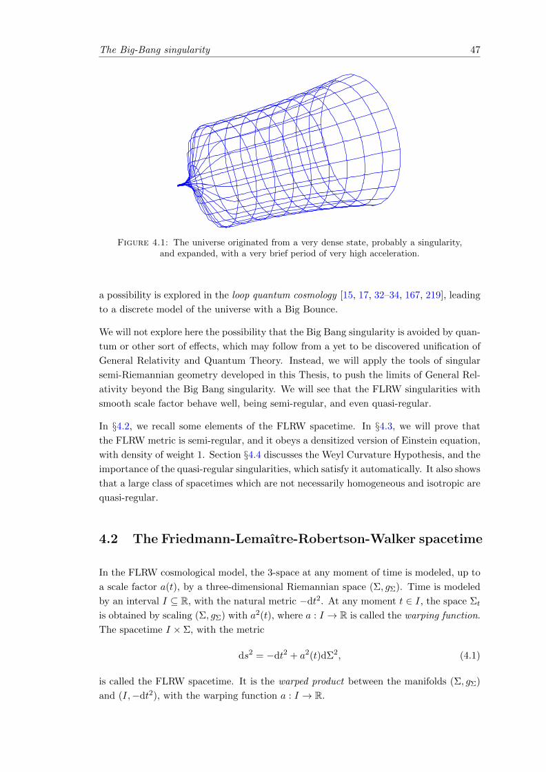
The Big-Bang singularity 47
Figure 4.1: The universe originated from a very dense state, probably a singularity,and expanded, with a very brief period of very high acceleration.
a possibility is explored in the loop quantum cosmology [15, 17, 32–34, 167, 219], leading
to a discrete model of the universe with a Big Bounce.
We will not explore here the possibility that the Big Bang singularity is avoided by quan-
tum or other sort of effects, which may follow from a yet to be discovered unification of
General Relativity and Quantum Theory. Instead, we will apply the tools of singular
semi-Riemannian geometry developed in this Thesis, to push the limits of General Rel-
ativity beyond the Big Bang singularity. We will see that the FLRW singularities with
smooth scale factor behave well, being semi-regular, and even quasi-regular.
In §4.2, we recall some elements of the FLRW spacetime. In §4.3, we will prove that
the FLRW metric is semi-regular, and it obeys a densitized version of Einstein equation,
with density of weight 1. Section §4.4 discusses the Weyl Curvature Hypothesis, and the
importance of the quasi-regular singularities, which satisfy it automatically. It also shows
that a large class of spacetimes which are not necessarily homogeneous and isotropic are
quasi-regular.
4.2 The Friedmann-Lemaıtre-Robertson-Walker spacetime
In the FLRW cosmological model, the 3-space at any moment of time is modeled, up to
a scale factor a(t), by a three-dimensional Riemannian space (Σ, gΣ). Time is modeled
by an interval I ⊆ R, with the natural metric −dt2. At any moment t ∈ I, the space Σt
is obtained by scaling (Σ, gΣ) with a2(t), where a : I → R is called the warping function.
The spacetime I × Σ, with the metric
ds2 = −dt2 + a2(t)dΣ2, (4.1)
is called the FLRW spacetime. It is the warped product between the manifolds (Σ, gΣ)
and (I,−dt2), with the warping function a : I → R.
The Big-Bang singularity 48
For the typical space Σ one can use any Riemannian manifold one may need, but in
most cases, because of the cosmological principle, one considers solutions which satisfy
the homogeneity and isotropy conditions. Hence, in most cases, Σ is taken to be, at
least at large scale, one of the homogeneous spaces S3, R3, and H3, having, in spherical
coordinates (r, θ, φ), the metric
dΣ2 =dr2
1− kr2+ r2
(dθ2 + sin2 θdφ2
), (4.2)
where k = 1 for the 3-sphere S3, k = 0 for the Euclidean space R3, and k = −1 for the
hyperbolic space H3.
4.2.1 The Friedman equations
After we choose the 3-space Σ, the only unknown part of the FLRW metric remains
the function a(t). This can be determined by making assumptions about matter. For
simplicity, it is in general considered that the universe is filled with a fluid with mass
density ρ(t) and pressure density p(t). These quantities depend on t only, because we
assume homogeneity and isotropy. The stress-energy tensor is
T ab = (ρ+ p)uaub + pgab, (4.3)
where ua is the timelike vector field ∂t, normalized.
The energy density component of the Einstein equation leads to the Friedmann equation
ρ =3
κ
a2 + k
a2. (4.4)
Here, κ :=8πGc4
[175]. We will use in the following units in which G = 1 and c = 1. The
trace of the Einstein equation gives the acceleration equation
ρ+ 3p = −6
κ
a
a. (4.5)
From these equations we get the fluid equation (the conservation of mass-energy):
ρ = −3a
a(ρ+ p) . (4.6)
Knowing the function a, determines uniquely ρ, from (4.4), and then p, from (4.5).
Recent observations on supernovae reveal that the expansion is accelerated, hence there
is a positive cosmological constant Λ [150, 160]. The equations (4.4), (4.5), and (4.6)
assume Λ = 0, but the generality is not lost, because the version of the equations having

The Big-Bang singularity 49
Λ 6= 0 are equivalent to the above ones, by the substitutionρ → ρ+ κ−1Λ
p → p− κ−1Λ. (4.7)
To simplify calculations, we will ignore Λ in the following, without any loss of generality.
4.2.2 Distance separation vs. topological separation
We can understand the singularities in the FLRW model, by making distinction between
topology and geometry. A manifold M is a topological space. If, in addition, there is a
metric tensor g on M , we obtain a geometry. The metric g defines a distance, and the
distance between two points p 6= q ∈M is zero only if the metric is Riemannian. If the
metric is semi-Riemannian, it is possible that the distance between two distinct points
p and q is zero, provided that they are separated by a lightlike interval. If the metric
g is allowed to be degenerate, then there are more possibilities to have zero distance
between distinct points. For example, consider a surface in R3, defined locally as the
image of a map f : U → R3, where U ∈ R2 is an open subset of R2. If the function f is
not injective, the resulting surface has self-intersections. Sometimes the surface can be
defined implicitly, as the set of solutions of an equation. In this case too it may have
self-intersections. The typical example is the cone
x2 − y2 − z2 = 0. (4.8)
It has a singularity at x = 0. To resolve it, we make the transformationx = u
y = uv
z = uw
(4.9)
which maps the cylinder v2 + w2 = 1 to the cone (4.8). This procedure was studied
starting with Isaac Newton [133], and is very used in mathematics, especially in algebraic
geometry.
The natural metric on the space (x, y, z) induces, by pull-back through the map (4.9), a
metric on the the cylinder v2 + w2 = 1. The induced metric is degenerate on the circle
u = 0 of the cylinder – the distance between any two distinct points of the circle u = 0
is zero.
4.3 Densitized Einstein equation on the FLRW spacetime
We show that the Friedmann equations and the Einstein equation can be written in an
equivalent form, which in addition avoids the infinities in a natural way, being thus valid
at the singularity a(t) = 0.

The Big-Bang singularity 50
Figure 4.2: The old method of resolution of singularities “unties” the cone into acylinder, removing the singularity.
4.3.1 What happens when the density becomes infinite?
When a→ 0, from (4.4) follows that ρ→∞, because a finite quantity of matter occupies
a volume equal to 0. From (4.5), the pressure density p may become infinite. So, is there
a way to avoid the infinities? The answer is yes, provided that we realize that not ρ and
p are the physical quantities, but the densities ρ√−g and p
√−g, which remain smooth.
In the Friedmann equations, ρ and p are scalar fields representing densities. But if
we change the coordinates, ρ and p change, so they are not in fact scalars, but the
components of another type of object. The adequate, invariant quantities representing
densities involve the volume form
dvol :=√−gdt ∧ dx ∧ dy ∧ dz, (4.10)
where√−g :=
√−det gab.
The correct densities are not the scalars ρ and p, but the differential 4-forms ρdvol and
pdvol. Their components in a coordinate system are ρ√−g and respectively p
√−g. They
become identical to ρ and p only if det g = −1, e.g. in an orthonormal frame, like the
comoving coordinate system of the FLRW model. But an orthonormal frame doesn’t
make sense when a→ 0, because det g → 0.
The determinant of the metric (4.1), in the FLRW coordinates, is
det g = −a6 det 3gΣ, (4.11)
where det3 gΣ is determinant of the metric of the 3-dimensional typical space Σ, and is
constant. Hence, the metric’s determinant in the comoving coordinates is
√−g = a3√gΣ. (4.12)
The Big-Bang singularity 51
Since√−g → 0 when a→ 0, we will see that
√−g cancels the singularities introduced
by ρ and p in ρdvol, respectively pdvol.
The conservation of energy takes the form
− a3ρ = 3a2aρ+3
c2a2ap, (4.13)
and is valid even when the volume a3 → 0.
4.3.2 The Big Bang singularity resolution
Let’s make the following substitution:ρ = ρ
√−g = ρa3√gΣ
p = p√−g = pa3√gΣ
(4.14)
Theorem 4.1. Let a : I → R be a smooth function. Then, the densities ρ, p, and the
densitized stress-energy tensor Tab√−g are smooth (and hence nonsingular), including
when a(t) = 0.
Proof. From the Friedmann equation (4.4), which becomes now
ρ =3
κa(a2 + k
)√gΣ, (4.15)
if a is smooth, ρ is smooth too. Similarly, p is smooth too, from the acceleration equation
(4.5)
ρ+ 3p = −6
κa2a√gΣ. (4.16)
Since ρ and p are smooth functions, the densitized stress-energy tensor
Tab√−g = (ρ+ p)uaub + pgab, (4.17)
is smooth too.
Due to Theorem 4.1, the smooth densitized version of the Einstein equation
Gab√−g + Λgab
√−g = κTab
√−g, (4.18)
makes sense and is smooth.
The Lagrangian density for General Relativity, proposed by Hilbert and Einstein, is
1
2κ
(R√−g − 2Λ
√−g)
+ L√−g, (4.19)
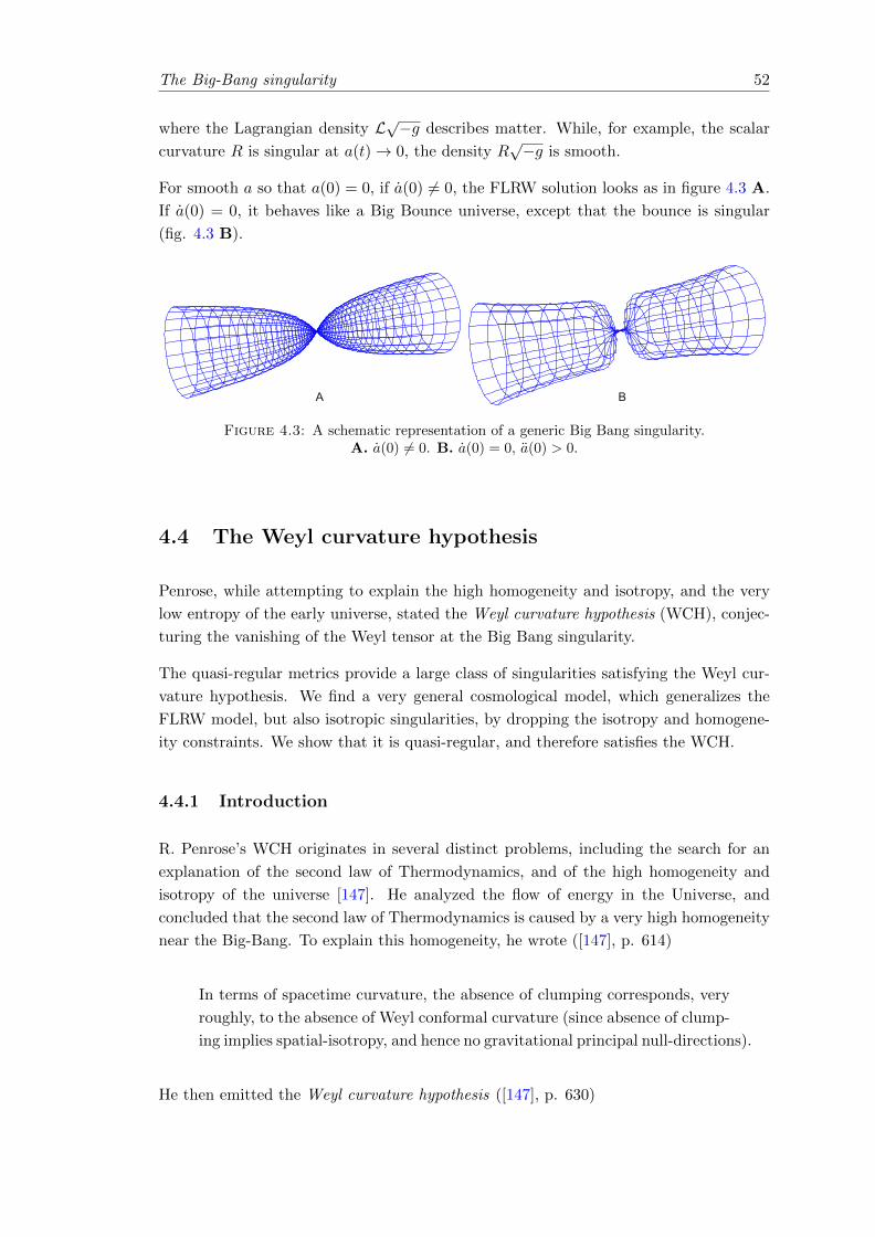
The Big-Bang singularity 52
where the Lagrangian density L√−g describes matter. While, for example, the scalar
curvature R is singular at a(t)→ 0, the density R√−g is smooth.
For smooth a so that a(0) = 0, if a(0) 6= 0, the FLRW solution looks as in figure 4.3 A.
If a(0) = 0, it behaves like a Big Bounce universe, except that the bounce is singular
(fig. 4.3 B).
A B
Figure 4.3: A schematic representation of a generic Big Bang singularity.A. a(0) 6= 0. B. a(0) = 0, a(0) > 0.
4.4 The Weyl curvature hypothesis
Penrose, while attempting to explain the high homogeneity and isotropy, and the very
low entropy of the early universe, stated the Weyl curvature hypothesis (WCH), conjec-
turing the vanishing of the Weyl tensor at the Big Bang singularity.
The quasi-regular metrics provide a large class of singularities satisfying the Weyl cur-
vature hypothesis. We find a very general cosmological model, which generalizes the
FLRW model, but also isotropic singularities, by dropping the isotropy and homogene-
ity constraints. We show that it is quasi-regular, and therefore satisfies the WCH.
4.4.1 Introduction
R. Penrose’s WCH originates in several distinct problems, including the search for an
explanation of the second law of Thermodynamics, and of the high homogeneity and
isotropy of the universe [147]. He analyzed the flow of energy in the Universe, and
concluded that the second law of Thermodynamics is caused by a very high homogeneity
near the Big-Bang. To explain this homogeneity, he wrote ([147], p. 614)
In terms of spacetime curvature, the absence of clumping corresponds, very
roughly, to the absence of Weyl conformal curvature (since absence of clump-
ing implies spatial-isotropy, and hence no gravitational principal null-directions).
He then emitted the Weyl curvature hypothesis ([147], p. 630)

The Big-Bang singularity 53
this restriction on the early geometry should be something like: the Weyl
curvature Cabcd vanishes at any initial singularity
There is also a motivation from the WCH, coming from Quantum Gravity. It is ex-
pected that, near the Big-Bang, the quantum effects of gravity become relevant, but
gravity is perturbatively nonrenormalizable at two loops [87, 202]. If the Weyl tensor
vanishes, local degrees of freedom, hence gravitons, vanish too, removing some problems
of Quantum Gravity, at least at the Big-Bang [47].
The Weyl tensor Cabcd is, from gravitational viewpoint, responsible for the tidal forces.
It is the traceless part of the Riemann curvature tensor Rabcd. The tensor Cabcd is
invariant at a conformal rescaling gab 7→ Ω2gab. It vanishes on an open set U ⊂ M ,
where dimM ≥ 4, if and only if the metric is conformally flat on U .
Isotropic singularities, studied by Tod [207–212], Claudel & Newman [54], Anguige &
Tod [8, 9], are obtained from non-degenerate metrics g on M , by a conformal rescaling
gab = Ω2gab, when Ω→ 0. They have finite Weyl curvature tensor Cabcd = Cabc
d, and
Cabcd = gsdCabcs = Ω2gsdCabc
s → 0. (4.20)
Another simple example of vanishing Weyl tensor comes from the FLRW cosmological
model. In fact, the Weyl tensor of the FLRW metric vanishes identically, and is not
relevant for WCH.
Both these types of singularities are particular cases of the quasi-regular singularities
(§3.2.3). Moreover, any quasi-regular singularity in spacetime satisfies WCH, as we will
show. From (3.17) we know that the Weyl curvature Cabcd is smooth. At semi-regular
singularities (therefore at quasi-regular too), the metric behaves as if it loses one or
more dimensions, and the Weyl curvature lives, from algebraic viewpoint, in a space of
dimension lower than 4, therefore it vanishes, because of its algebraic symmetries.
In §4.4.3 we propose a very general cosmological model which, unlike the FLRW model,
does not assume that the space slices have constant metric up to the overall scaling factor
a2(t). We will keep the overall scaling factor a2(t), but we will allow the space part of
the metric to change freely in time. We allow this generality because the Universe is not
perfectly isotropic and homogeneous. Due to the general conditions we assume, we will
not be concerned at this point with the particular matter content of this universe.
4.4.2 The Weyl tensor vanishes at quasi-regular singularities
Theorem 4.2. Let (M, g) be a quasi-regular manifold of dimension 4. Then, the Weyl
curvature tensor Cabcd vanishes at singularities.
Proof. The smoothness of Cabcd follows from the smoothness of Rabcd, Eabcd, Sabcd, and
from equation (3.17).
The Big-Bang singularity 54
From Corollary 2.47, the Riemann curvature tensor Rabcd of a semi-regular semi-Rie-
mannian manifold satisfies at any p ∈M
(Rabcd)p ∈ ⊗4T •pM. (4.21)
If at a point p the metric g is degenerate, then dim (T •pM) < 4. But in dimension ≤ 3,
any tensor having the symmetries of the Weyl tensor vanishes (see e.g. [26]), hence, at
any point p where g is degenerate,
(Cabcd)p = 0. (4.22)
4.4.3 Example: a general cosmological model
The universe is not homogeneous and isotropic at all scales, as it is assumed in the
FLRW model. Thus, we are motivated to study a spacetime (M, g) which is allowed to
be inhomogeneous and anisotropic.
We consider that the spacetime is a manifold of the form M = I ×Σ, where I ⊆ R is an
interval, and Σ is a three-dimensional manifold. Let τ : M → I, defined by τ(t, x) = t,
be a global time coordinate. Let’s consider that on each slice Σt = τ−1(t) there is a
Riemannian (hence non-degenerate) metric hij(t, x) (where 1 ≤ i, j ≤ 3), which depends
smoothly on (t, x) ∈ I × Σ. Let’s consider on I a smooth function N : I → R, and the
metric N2(t)dt2, which is allowed to be degenerate.
We represent the metric h(t) as an arc element by dσ2t , and assume that the metric g
on the total manifold M is
gij(t, x) := −N2(t)dt2 + a2(t)hij(t, x), (4.23)
where a : I → R is a smooth function. The function a(t) is allowed to vanish, the
Big-Bang singularity is obtained for a(t) = 0.
As an arc element, the metric is
ds2 = −N2(t)dt2 + a2(t)dσ2t . (4.24)
The FLRW model is obtained if N(t) = 1, and hij(t) is time independent, and of
constant curvature. But we will work in full generality, allowing dσ2t to vary freely in
time, to obtain therefore a much more general solution. When a(t) = 0, our Big-Bang
singularity is much more general than the FLRW one, because the geometry of space
slices (Σt, h(t)) may be inhomogeneous and variable in time.
If N(t) 6= 0 for any t ∈ I, then I can be reparameterized to obtain a constant metric,
so that we can consider N(t) = 1. Hence, the relevant differences introduced by using
The Big-Bang singularity 55
a non-constant N become important only when N(t) vanishes, together with a(t). For
reasons which will become apparent, we require that
f(t) :=a(t)
N(t)(4.25)
is not singular. For example, if f(t) = 1, then N(t) = a(t), and the resulting singularities
are just isotropic singularities.
We are here interested in the most general case.
Theorem 4.3. Let (M, g) be a spacetime, where M = I ×Σ, and the metric is given by
(4.24). Then, (M, g) is quasi-regular.
Proof. We will prove first that the metric is semi-regular, by showing that the terms
in the Riemann curvature tensor (2.63) are smooth. Then, we will show that the Ricci
decomposition
Rabcd = Eabcd + Sabcd + Cabcd. (4.26)
is smooth.
The metric g is
g(t, x) =
(−N2(t) 0
0 a2(t)hij(t, x)
), (4.27)
and its reciprocal is
g−1(t, x) =
(−N−2(t) 0
0 a−2(t)hij(t, x)
). (4.28)
The partial derivatives of the metric are
g00,0 = −2NN,
g00,k = 0,
gij,0 = a(2ahij + ahij),
gij,k = a2∂khij .
(4.29)
The second order partial derivatives of the metric are
g00,00 = −2(N2 +NN
),
g00,k0 = g00,0k = g00,kl = 0,
gij,00 = 2a2hij + 2aahij + 4aahij + a2hij ,
gij,k0 = a(
2a∂khij + a∂khij
),
gij,kl = a2∂k∂lhij .
(4.30)
To check that g is semi-regular, it is enough to check the smoothness of the terms of the
form gab,•gcd,• . From the equations (4.29),

The Big-Bang singularity 56
g00,•g00,• = −N−2g00,0g00,0 + a−2hcdg00,cg00,d
= −4N2,(4.31)
g00,•gij,• = −N−2g00,0gij,0 + a−2hcdg00,cgij,d
= 2Na
N
(2ahij + ahij
),
(4.32)
and
gij,•gkl,• = −N−2gij,0gkl,0 + a−2hcdgij,cgkl,d
= − a2
N2(2ahij + ahij)(2ahkl + ahkl) + a2hcd∂chij∂dhkl.
(4.33)
But for a smooth function f(t, x)
a(t, x) = f(t, x)N(t), (4.34)
therefore, the terms calculated above are smooth, as we can see:
g00,•g00,• = −4N2
g00,•gij,• = 2Nf(
2ahij + ahij
)gij,•gkl,• = f2
(−(2ahij + ahij)(2ahkl + ahkl).+N2hcd∂chij∂dhkl
) (4.35)
Hence, the metric g is semi-regular.
To prove that Ric g and Rg g are smooth, we have to contract the terms from (4.30)
and (4.35), and see what happens when taking Kulkarni-Nomizu products with g. The
tensor Ric g is a sum of products between gab,cd or gab,•gcd,• , and gef , and ggh. The
tensor Rg g is a sum of products between gab,cd or gab,•gcd,• , gefggh, and g g, which is
of the form N4(t)f2(t)qabcd. We resume these products in the tables 4.1 and 4.2, where
we can see that they are smooth. To write these tables, we used the following facts:
• only some particular combinations of indices are allowed when contracting, and in
the Kulkarni-Nomizu products,
• g g is of the form N4f2qabcd, with qabcd smooth,
• gab = N2gab, where gab is smooth; gab = N−2f−2gab, with gab smooth
• gij = a2hij = f2N2hij ; gij = a−2hij = f−2N−2hij .
By inspecting the tables, we see that all terms contained in Rabcd, Eabcd, and Sabcd are
smooth. Hence, the metric (4.24) is quasi-regular.
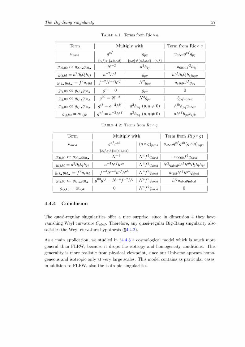
The Big-Bang singularity 57
Table 4.1: Terms from Ric g.
Term Multiply with Term from Ric g
uabcd gef gpq uabcdgefgpq
e,f⊂a,b,c,d p,q6=a,b,c,d−e,f
g00,00 or g00,•g00,• −N−2 a2hij −u0000f2hij
gij,kl = a2∂k∂lhij a−2hef gpq hef∂k∂lhijgpq
gij,•gkl,• = f2uijkl f−2N−2hef N2gpq uijklhef gpq
gij,00 or gij,•g00,• gi0 = 0 gpq 0
gij,00 or gij,•g00,• g00 = N−2 N2gpq gpquabcd
gij,00 or gij,•g00,• gij = a−2hij a2hpq (p, q 6= 0) hikhpquabcd
gij,k0 = avijk gef = a−2hef a2hpq (p, q 6= 0) ahefhpqvijk
Table 4.2: Terms from Rg g.
Term Multiply with Term from R(g g)
uabcd gefggh (g g)pqrs uabcdgefggh(g g)pqrs
e,f,g,h=a,b,c,d
g00,00 or g00,•g00,• −N−4 N4f2qabcd −u0000f2qabcd
gij,kl = a2∂k∂lhij a−4hefhgh N4f2qabcd N2qabcdhefhgh∂k∂lhij
gij,•gkl,• = f2uijkl f−4N−4hefhgh N4f2qabcd uijklhefhghqabcd
gij,00 or gij,•g00,• g00gij = N−4f−2hij N4f2qabcd hijuabcdqabcd
gij,k0 = avijk 0 N4f2qabcd 0
4.4.4 Conclusion
The quasi-regular singularities offer a nice surprise, since in dimension 4 they have
vanishing Weyl curvature Cabcd. Therefore, any quasi-regular Big-Bang singularity also
satisfies the Weyl curvature hypothesis (§4.4.2).
As a main application, we studied in §4.4.3 a cosmological model which is much more
general than FLRW, because it drops the isotropy and homogeneity conditions. This
generality is more realistic from physical viewpoint, since our Universe appears homo-
geneous and isotropic only at very large scales. This model contains as particular cases,
in addition to FLRW, also the isotropic singularities.
Chapter 5
Black hole singularity resolution
In this chapter are presented the original results published by the author in the papers
[183], [184], [189], and [187].
At least in classical General Relativity, black hole singularities are usually considered to
break the time evolution.
For each of the standard black hole solutions, we find coordinates which make the metric
smooth. This is somehow similar to the method used by Eddington [67] and Finkelstein
[74], to show that the event horizon singularity is due to the coordinates. In our case, the
singularities remain, but the metric becomes degenerate and analytic, without singular
components.
We show that the Schwarzschild singularity can be made analytic, and in fact semi-
regular, by such a coordinate transformation, in section §5.2. Sections §5.3 and §5.4
present coordinates in which the Reissner-Nordstrom, respectively the Kerr-Newman
singularities are made analytic. The latter involve the presence of an electromagnetic
field, and we show that this field and its potential are analytic in our coordinates, thus
being non-singular, as they appear in the standard, but singular coordinates.
In section §6 we show that these solutions can be utilized to construct spacetimes with
more general black hole singularities, which are created and then vanish by Hawking
evaporation.
The results are applied to non-stationary black holes, including evaporating ones.
5.1 Introduction
5.1.1 The singularity theorems
Despite the successes of General Relativity, one of its own consequences seems to question
it: the occurrence of singularities in the black holes. It is often said that General
58
Black hole singularity resolution 59
Relativity predicts, because of these singularities, it’s own breakdown [13, 14, 16, 93,
95, 96]. Such singularities follow from the singularity theorems of Penrose and Hawking
[89–91, 94, 95, 144]. The conditions leading to singularities were found to be common
(Christodoulou [53]), and then even more common (Klainerman and Rodnianski [111]).
Initially, there was some confusion regarding the singularities. In 1916, when Schwarzschild
proposed [169, 170] his solution to Einstein’s equation, representing a black hole, it was
believed that the event horizon is singular. Only after 1924, when Eddington proposed
another coordinate system which removed the singularity at the event horizon [67], and
1958, with the work of D. Finkelstein [74], it was understood that the event horizon’s
singularity was only apparent, being due to the choice of the coordinate system. But
the singularity at the center of the black hole remained independent of the particular
coordinates, and the singularity theorems showed that any black hole would have such
a singularity. In [183, 184, 189] we have shown that, although the genuine singulari-
ties cannot be removed, they can at least be made manageable – there are coordinate
changes which make the metric degenerate, but smooth.
5.1.2 The black hole information paradox
Black holes have interesting properties similar to the entropy and temperature in ther-
modynamics, which were studied in [20, 24, 214, 216–218].
Soon (in its proper time) after an object passes through the event horizon, it reaches
the singularity of the black hole. All the information contained in it seems to vanish in
the singularity.
On the other hand, the equations governing the physical laws are in general reversible,
guaranteeing that no information can be lost. But according to Hawking [92, 93] the
black hole may emit radiation and evaporate. If the black hole evaporates completely, it
seems to leave behind no trace of the information it swallowed. Moreover, it seems to be
possible for an originally pure state to end up being mixed, because the density matrix
of the particles in the black hole’s exterior is obtained by tracing over the particles lost
in the black hole with which they were entangled. This means that the unitarity appears
to be violated, and the problem becomes even more acute.
5.1.3 The meaning of singularities
The singularities in General Relativity are places where the evolution equations cannot
work, because the involved fields become infinite. If the Cauchy surface on which the
fields are defined is affected by singularities, then the equations cannot be developed in
time.

Black hole singularity resolution 60
From geometric viewpoint, these singularities are points where the metric becomes sin-
gular, and the geodesics become incomplete. Since we don’t know to extend the fields
to such points, normally we remove them from the spacetime.
Actually, we can rewrite the fields involved, and the equations defining them, so that
the fields remain finite at any point [69, 180, 183, 184, 189]. At the points where the
metric is non-singular, the equations remain equivalent to Einstein’s equation.
With this modification, the spacetime can be extended to the singular points.
Once we have the fields and the topology repaired, we have to check that we can choose
a maximal globally hyperbolic spacetime (or equivalently, admitting a Cauchy foliation)
so that the evolution equations can be defined.
Consequently, a natural interpretation of the singularities emerges, which makes them
harmless for the physical law, in particular for the information conservation.
We will illustrate this approach on the black hole solutions known from the literature.
5.2 Schwarzschild singularity is semi-regularizable
We show that the Schwarzschild metric can be made analytic at the singularity, by a
proper coordinate transformation. The singularity remains, but it is made degenerate
and smooth, and the infinities are removed. We find a family of analytic extensions,
and one of them is semi-regular. A degenerate singularity doesn’t break the topology.
We prove that the metric is semi-regular, hence the densitized version of Einstein’s
equation can be used, avoiding thus the infinities. Moreover, we show that the singularity
is quasi-regular. In the new coordinates, the Schwarzschild solution extends beyond
the singularity, suggesting the possibility that the information is not destroyed by the
singularity, and can be restored after the evaporation.
5.2.1 Introduction
The Schwarzschild metric, expressed in the Schwarzschild coordinates, is
ds2 = −(
1− 2m
r
)dt2 +
(1− 2m
r
)−1
dr2 + r2dσ2, (5.1)
where m the mass of the body, and the units were chosen so that c = 1 and G = 1, and
dσ2 = dθ2 + sin2 θdφ2 (5.2)
is the metric of the unit sphere S2 (see e.g. [94], p. 149).
From (5.1) follows that this spacetime is a warped product between a two-dimensional
semi-Riemannian space and the sphere S2 with the metric (5.2). This allows us to
Black hole singularity resolution 61
change the coordinates r and t independently on the other coordinates, and to ignore in
calculations the term r2dσ2, which we reintroduce at the end.
As r → 2m, gtt = −(
1− 2m
r
)−1
→ ∞. This is a coordinate singularity, and not a
genuine one, as shown by the Eddington-Finkelstein coordinates ([67, 74], [94], p. 150).
On the other hand, r → 0 is a genuine singularity, because RabcdRabcd →∞. This seems
to suggest that the Schwarzschild metric cannot be made smooth at r = 0. We will see
that, in fact, there are coordinate systems in which the components of the metric are
are analytic, hence finite, even r = 0. The singularity remains, because the metric is
degenerate. We find analytic and semi-regular extension of the Schwarzschild spacetime.
5.2.2 Analytic extension of the Schwarzschild spacetime
Theorem 5.1. Let’s consider the Schwarzschild spacetime, with the metric (5.1). There
is a singular semi-Riemannian spacetime, which extends it analytically beyond the sin-
gularity r = 0.
Proof. It suffices to find new coordinates in the region r < 2m, which is a neighborhood
of the singularity. On the region r < 2m, the coordinate t is spacelike, and r is timelike.
We use the transformation
r = τ2
t = ξτT, (5.3)
where T ∈ N, to be conveniently determined. Then, we have
∂r
∂τ= 2τ,
∂r
∂ξ= 0,
∂t
∂τ= TξτT−1,
∂t
∂ξ= τT. (5.4)
Recall that the metric coefficients in the Schwarzschild coordinates are
gtt =2m− rr
, grr =r
r − 2m, gtr = grt = 0. (5.5)
Let’s calculate the metric coefficients in the new coordinates. We will do explicitly one
such calculation:
gττ =
(∂r
∂τ
)2 r
r − 2m+
(∂t
∂τ
)2 2m− rr
= 4τ2 τ2
τ2 − 2m+ T2ξ2τ2T−2 2m− τ2
τ2
Hence
gττ = − 4τ4
2m− τ2+ T2ξ2(2m− τ2)τ2T−4 (5.6)
Similarly,
gτξ = Tξ(2m− τ2)τ2T−3, (5.7)
Black hole singularity resolution 62
gξξ = (2m− τ2)τ2T−2. (5.8)
The determinant is
det g = −4τ2T+2. (5.9)
The four-metric is
ds2 = − 4τ4
2m− τ2dτ2 + (2m− τ2)τ2T−4 (Tξdτ + τdξ)2 + τ4dσ2, (5.10)
and it is easy to see that it is analytic for T ≥ 2.
5.2.3 Semi-regular extension of the Schwarzschild spacetime
While proving Theorem 5.1, we found an infinite family of coordinates which make the
metric analytic. We prove now that among these solutions there is a semi-regular one.
Theorem 5.2. The Schwarzschild metric admits an analytic extension in which the
singularity at r = 0 is semi-regular.
Proof. We start with the coordinate transformation (5.3). To show that the metric is
semi-regular, cf. Proposition 2.41, it is enough to find T ∈ N so that there is a coordinate
system in which the products of the form
gstΓabsΓcdt (5.11)
are all smooth [180], where Γabc are Christoffel’s symbols of the first kind. In a coordinate
system in which the metric is smooth, as in §5.2.2 , Christoffel’s symbols of the first kind
are also smooth. But the inverse metric gst is not smooth for r = 0. We will show that
the products from the expression (5.11) are smooth.
We use the solution from Theorem 5.1, and try to find a value for T, so that the metric
is semi-regular.
The components of the inverse of the metric are given by gττ = gξξ/det g, gξξ = gττ/det g,
and gτξ = gξτ = −gτξ/det g. From (5.6–5.8), follows that
gττ = −1
4(2m− τ2)τ−4, (5.12)
gτξ =1
4Tξ(2m− τ2)τ−5, (5.13)
gξξ =τ−2T+2
2m− τ2− 1
4T2ξ2(2m− τ2)τ−6. (5.14)
Christoffel’s symbols of the first kind are given by
Γabc =1
2(∂agbc + ∂bgca − ∂cgab) , (5.15)
Black hole singularity resolution 63
so we have to calculate the partial derivatives of the coefficients of the metric.
From (5.4) and (5.6–5.8) we have:
∂τgττ = ∂τ
(− 4τ4
2m− τ2+ ξ2T2(2m− τ2)τ2T−4
)= −4
4τ3(2m− τ2) + 2τ5
(2m− τ2)2+ 2T2(2T− 4)mξ2τ2T−5
−T2(2T− 2)ξ2τ2T−3,
hence
∂τgττ = 8τ5 − 4mτ3
(2m− τ2)2+ 2T2(2T− 4)mξ2τ2T−5 − T2(2T− 2)ξ2τ2T−3. (5.16)
Similarly,
∂τgτξ = 2T(2T− 3)mξτ2T−4 − T(2T− 1)ξτ2T−2, (5.17)
∂τgξξ = 2m(2T− 2)τ2T−3 − 2Tτ2T−1, (5.18)
∂ξgττ = 2T2ξ(2m− τ2)τ2T−4, (5.19)
∂ξgτξ = T(2m− τ2)τ2T−3, (5.20)
and
∂ξgξξ = 0. (5.21)
To ensure that the expression (5.11) is smooth, we try to find a value of T for which it
doesn’t contain negative powers of τ . The least power of τ in equations (5.16–5.21) is
min(3, 2T−5), as we can see by inspection. The least power of τ in equations (5.12–5.14)
is min(−6,−2T + 2). Since min(−6,−2T + 2) = −3 −max(3, 2T − 5), the conjunction
of the two conditions is
− 1− 2T + 3 min(3, 2T− 5) ≥ 0 (5.22)
with the unique solution
T = 4. (5.23)
which ensures the smoothness of (5.11), and by this, the semi-regularity of the metric
in two dimensions (τ, ξ). The coordinate transformation becomesr = τ2
t = ξτT, (5.24)
When going back to four dimensions, we have to take the semi-regular warped product
between the two-dimensional extension (τ, ξ) and the sphere S2, with warping function
τ2, which is semi-regular, cf. Theorem 2.74.
Black hole singularity resolution 64
The metric in the proof is
ds2 = − 4τ4
2m− τ2dτ2 + (2m− τ2)τ4 (4ξdτ + τdξ)2 + τ4dσ2, (5.25)
which is a semi-regular analytic extension of the Schwarzschild metric.
It is easy to see that it is also quasi-regular.
Corollary 5.3. The Schwarzschild spacetime is quasi-regular (in any atlas compatible
with the coordinates (5.24)).
Proof. We know from [183] that the Schwarzschild spacetime is semi-regular. It is also
Ricci flat, hence Sabcd and Eabcd are smooth too, and the metric is quasi-regular.
5.3 Analytic Reissner-Nordstrom singularity
In this section, we derive an analytic extension of the Reissner-Nordstrom solution be-
yond the singularity, by using new coordinates. The metric’s components are made finite
and analytic, but degenerate at r = 0.
5.3.1 Introduction
The Reissner-Nordstrom is a solution to the Einstein-Maxwell equations, describing a
static, spherically symmetric, electrically charged, non-rotating black hole [139, 156].
The metric is
ds2 = −(
1− 2m
r+q2
r2
)dt2 +
(1− 2m
r+q2
r2
)−1
dr2 + r2dσ2, (5.26)
where q is the electric charge of the body, m the mass of the body, dσ2 is that from
equation (5.2), and the units were chosen so that c = 1 and G = 1 (cf. [94], p. 156).
The number of the event horizons of a Reissner-Nordstrom black hole equals the number
of real zeros of r2 − 2mr + q2. These are apparent singularities, that can be removed
for example by Eddington-Finkelstein coordinates [67, 74]. But in all cases, there is an
irremovable singularity at r = 0, which at least we will make degenerate.
5.3.2 Extending the Reissner-Nordstrom spacetime at the singularity
The main result of this section is contained in the following theorem.
Theorem 5.4. Let’s consider the Reissner-Nordstrom spacetime, with the metric (5.26).
There is a larger spacetime, which extends it analytically beyond the singularity r = 0.
Black hole singularity resolution 65
Proof. The metric (5.26) is a warped product between a two-dimensional semi-Riemann-
ian space of coordinates (t, r), and the sphere S2, parameterized by φ and θ. As in the
Schwarzschild case, we will use coordinate transformations which affect only the coor-
dinates r and t, in the neighborhood r ∈ [0,M) of the singularity, where M =∞ if the
black hole is naked, and M is the smallest real zero of r2− 2mr+ q2 otherwise. We take
the coordinates ρ and τ given by t = τρT
r = ρS(5.27)
and search for S,T ∈ N which make the metric analytic. This choice is motivated by
the need to smoothen the divergent components of the metric. Then,
∂t
∂τ= ρT,
∂t
∂ρ= TτρT−1,
∂r
∂τ= 0,
∂r
∂ρ= SρS−1. (5.28)
The following notation is standard
∆ := r2 − 2mr + q2 (hence ∆ = ρ2S − 2mρS + q2). (5.29)
We see that ∆ > 0 for ρ ∈ [0,M). The metric components from (5.26) become
gtt = − ∆
ρ2S , grr =ρ2S
∆, gtr = grt = 0. (5.30)
We calculate the metric components in the new coordinates.
gττ =
(∂r
∂τ
)2 ρ2S
∆−(∂t
∂τ
)2 ∆
ρ2S
= 0− ρ2T ∆
ρ2S .
Hence
gττ = −∆ρ2T−2S. (5.31)
gρτ =∂r
∂ρ
∂r
∂τ
ρ2S
∆− ∂t
∂ρ
∂t
∂τ
∆
ρ2S
= 0− Tτρ2T−1 ∆
ρ2S .
Then
gρτ = −T∆τρ2T−2S−1, (5.32)
and
gρρ = S2 ρ4S−2
∆− T2∆τ2ρ2T−2S−2. (5.33)
From the term S2 ρ4S−2
∆in equation (5.33), to have smooth gρρ, S has to be an integer
so that S ≥ 1. This condition also makes this term analytic at ρ = 0.

Black hole singularity resolution 66
To avoid negative powers of ρ, the other term in equation (5.33), and those from (5.31)
and (5.32), require that 2T− 2S− 2 ≥ 0. Hence, to remove the infinity of the metric at
r = 0 by a coordinate transformation like (5.27), S and T has to be integers, andS ≥ 1
T ≥ S + 1(5.34)
These conditions ensure that all metric’s components are analytic at the singularity.
Now we take the warped product between the space (τ, ρ), and the sphere S2, with
warping function ρS, to return to four dimensions. This degenerate warped product
results in a 4D manifold whose metric is analytic and degenerate at ρ = 0.
Corollary 5.5. In the coordinates from theorem 5.4, the Reissner-Nordstrom metric is
ds2 = −∆ρ2T−2S−2 (ρdτ + Tτdρ)2 +S2
∆ρ4S−2dρ2 + ρ2Sdσ2. (5.35)
Proof. From (5.28) follows
dt =∂t
∂τdτ +
∂t
∂ρdρ = ρTdτ + TτρT−1dρ = ρT−1(ρdτ + Tτdρ) (5.36)
and
dr =∂r
∂τdτ +
∂r
∂ρdρ = SρS−1dρ. (5.37)
We substitute them in the Reissner-Nordstrom equation (5.26), and obtain
ds2 = − ∆
ρ2Sdt2 +ρ2S
∆dr2 + r2dσ2
= −∆ρ2T−2S−2(ρdτ + Tτdρ)2 +S2
∆ρ4S−2dρ2 + ρ2Sdσ2.
5.3.3 Null geodesics in the proposed solution
Let’s discuss the geometric meaning of the extension proposed here, from the viewpoint
of the lightcones and the null geodesics. In the coordinates (τ, ρ), the metric is analytic
near the singularity ρ = 0 and has the form
g = −∆ρ2T−2S−2
ρ2 Tτρ
Tτρ T2τ2 − S2
∆2ρ6S−2T
(5.38)

Black hole singularity resolution 67
Let’s find the null directions at each point, i.e. the tangent vectors u 6= 0 satisfying
g(u, u) = 0. If we consider u = (sinα, cosα), we have to find α. We obtain the equation
ρ2 sin2 α+ 2Tτρ sinα cosα+
(T2τ2 − S2
∆2ρ6S−2T
)cos2 α = 0, (5.39)
which is quadratic in tanα
ρ2 tan2 α+ 2Tτρ tanα+
(T2τ2 − S2
∆2ρ6S−2T
)= 0, (5.40)
and has to the solutions
tanα± = −Tτρ± S
∆ρ3S−T−1. (5.41)
Hence, the incoming and outgoing null geodesics satisfy the differential equation
dτ
dρ= −Tτ
ρ± S
∆ρ3S−T−1. (5.42)
For the coordinate ρ to remain spacelike, it has to satisfy gρρ > 0. From equation (5.38),
this requires thatS2
∆2ρ6S−2T > T2τ2. (5.43)
To ensure (5.43) in a neighborhood of (0, 0), it is required that
T ≥ 3S. (5.44)
The null geodesics are integral curves of the null vectors (5.41). In coordinates (τ, ρ),
the null geodesics are oblique everywhere, except at ρ = 0, where they become tangent
to the axis ρ = 0. The degeneracy of the metric stretch the lightcones as approaching
ρ = 0, where they become degenerate (figure 5.1). At ρ = 0, the incoming and outgoing
null geodesics become tangent (figure 5.2).
5.3.4 The electromagnetic field
In the standard Reissner-Nordstrom solution, in coordinates (t, r, φ, θ), the potential of
the electromagnetic field is singular at r = 0, being
A = −qr
dt. (5.45)
On the other hand, in our solution both the electromagnetic potential, and the electro-
magnetic field, have better behavior.
Corollary 5.6. In the coordinates (τ, ρ, φ, θ), given by the coordinate change (5.27),
under the condition (5.34), the electromagnetic potential is
A = −qρT−S−1 (ρdτ + Tτdρ) , (5.46)
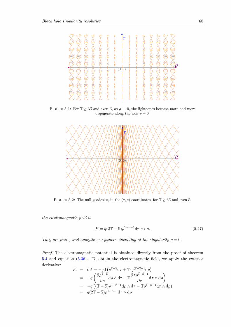
Black hole singularity resolution 68
(0, 0)
Figure 5.1: For T ≥ 3S and even S, as ρ→ 0, the lightcones become more and moredegenerate along the axis ρ = 0.
(0, 0)
Figure 5.2: The null geodesics, in the (τ, ρ) coordinates, for T ≥ 3S and even S.
the electromagnetic field is
F = q(2T− S)ρT−S−1dτ ∧ dρ. (5.47)
They are finite, and analytic everywhere, including at the singularity ρ = 0.
Proof. The electromagnetic potential is obtained directly from the proof of theorem
5.4 and equation (5.36). To obtain the electromagnetic field, we apply the exterior
derivative:F = dA = −qd
(ρT−Sdτ + TτρT−S−1dρ
)= −q
(∂ρT−S
∂ρdρ ∧ dτ + T
∂τρT−S−1
∂τdτ ∧ dρ
)= −q
((T− S)ρT−S−1dρ ∧ dτ + TρT−S−1dτ ∧ dρ
)= q(2T− S)ρT−S−1dτ ∧ dρ
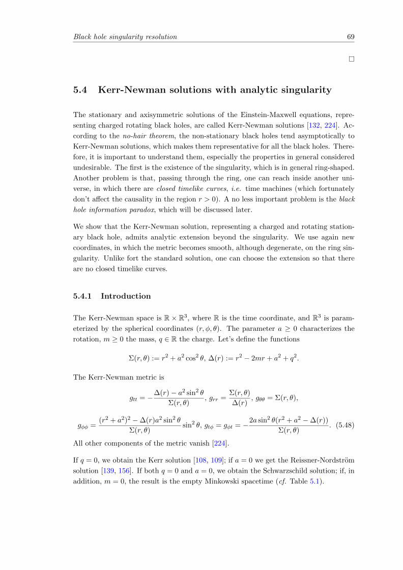
Black hole singularity resolution 69
5.4 Kerr-Newman solutions with analytic singularity
The stationary and axisymmetric solutions of the Einstein-Maxwell equations, repre-
senting charged rotating black holes, are called Kerr-Newman solutions [132, 224]. Ac-
cording to the no-hair theorem, the non-stationary black holes tend asymptotically to
Kerr-Newman solutions, which makes them representative for all the black holes. There-
fore, it is important to understand them, especially the properties in general considered
undesirable. The first is the existence of the singularity, which is in general ring-shaped.
Another problem is that, passing through the ring, one can reach inside another uni-
verse, in which there are closed timelike curves, i.e. time machines (which fortunately
don’t affect the causality in the region r > 0). A no less important problem is the black
hole information paradox, which will be discussed later.
We show that the Kerr-Newman solution, representing a charged and rotating station-
ary black hole, admits analytic extension beyond the singularity. We use again new
coordinates, in which the metric becomes smooth, although degenerate, on the ring sin-
gularity. Unlike fort the standard solution, one can choose the extension so that there
are no closed timelike curves.
5.4.1 Introduction
The Kerr-Newman space is R × R3, where R is the time coordinate, and R3 is param-
eterized by the spherical coordinates (r, φ, θ). The parameter a ≥ 0 characterizes the
rotation, m ≥ 0 the mass, q ∈ R the charge. Let’s define the functions
Σ(r, θ) := r2 + a2 cos2 θ, ∆(r) := r2 − 2mr + a2 + q2.
The Kerr-Newman metric is
gtt = −∆(r)− a2 sin2 θ
Σ(r, θ), grr =
Σ(r, θ)
∆(r), gθθ = Σ(r, θ),
gφφ =(r2 + a2)2 −∆(r)a2 sin2 θ
Σ(r, θ)sin2 θ, gtφ = gφt = −2a sin2 θ(r2 + a2 −∆(r))
Σ(r, θ). (5.48)
All other components of the metric vanish [224].
If q = 0, we obtain the Kerr solution [108, 109]; if a = 0 we get the Reissner-Nordstrom
solution [139, 156]. If both q = 0 and a = 0, we obtain the Schwarzschild solution; if, in
addition, m = 0, the result is the empty Minkowski spacetime (cf. Table 5.1).
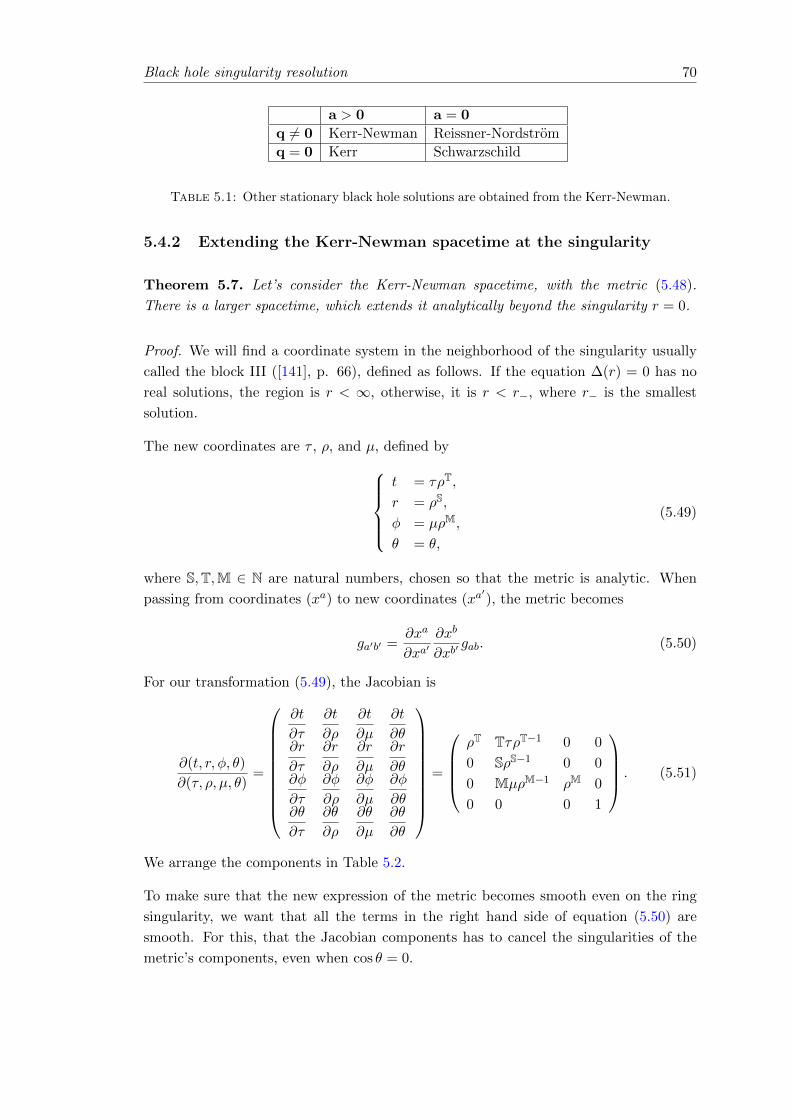
Black hole singularity resolution 70
a > 0 a = 0
q 6= 0 Kerr-Newman Reissner-Nordstrom
q = 0 Kerr Schwarzschild
Table 5.1: Other stationary black hole solutions are obtained from the Kerr-Newman.
5.4.2 Extending the Kerr-Newman spacetime at the singularity
Theorem 5.7. Let’s consider the Kerr-Newman spacetime, with the metric (5.48).
There is a larger spacetime, which extends it analytically beyond the singularity r = 0.
Proof. We will find a coordinate system in the neighborhood of the singularity usually
called the block III ([141], p. 66), defined as follows. If the equation ∆(r) = 0 has no
real solutions, the region is r < ∞, otherwise, it is r < r−, where r− is the smallest
solution.
The new coordinates are τ , ρ, and µ, defined byt = τρT,
r = ρS,
φ = µρM,
θ = θ,
(5.49)
where S,T,M ∈ N are natural numbers, chosen so that the metric is analytic. When
passing from coordinates (xa) to new coordinates (xa′), the metric becomes
ga′b′ =∂xa
∂xa′∂xb
∂xb′gab. (5.50)
For our transformation (5.49), the Jacobian is
∂(t, r, φ, θ)
∂(τ, ρ, µ, θ)=
∂t
∂τ
∂t
∂ρ
∂t
∂µ
∂t
∂θ∂r
∂τ
∂r
∂ρ
∂r
∂µ
∂r
∂θ∂φ
∂τ
∂φ
∂ρ
∂φ
∂µ
∂φ
∂θ∂θ
∂τ
∂θ
∂ρ
∂θ
∂µ
∂θ
∂θ
=
ρT TτρT−1 0 0
0 SρS−1 0 0
0 MµρM−1 ρM 0
0 0 0 1
. (5.51)
We arrange the components in Table 5.2.
To make sure that the new expression of the metric becomes smooth even on the ring
singularity, we want that all the terms in the right hand side of equation (5.50) are
smooth. For this, that the Jacobian components has to cancel the singularities of the
metric’s components, even when cos θ = 0.
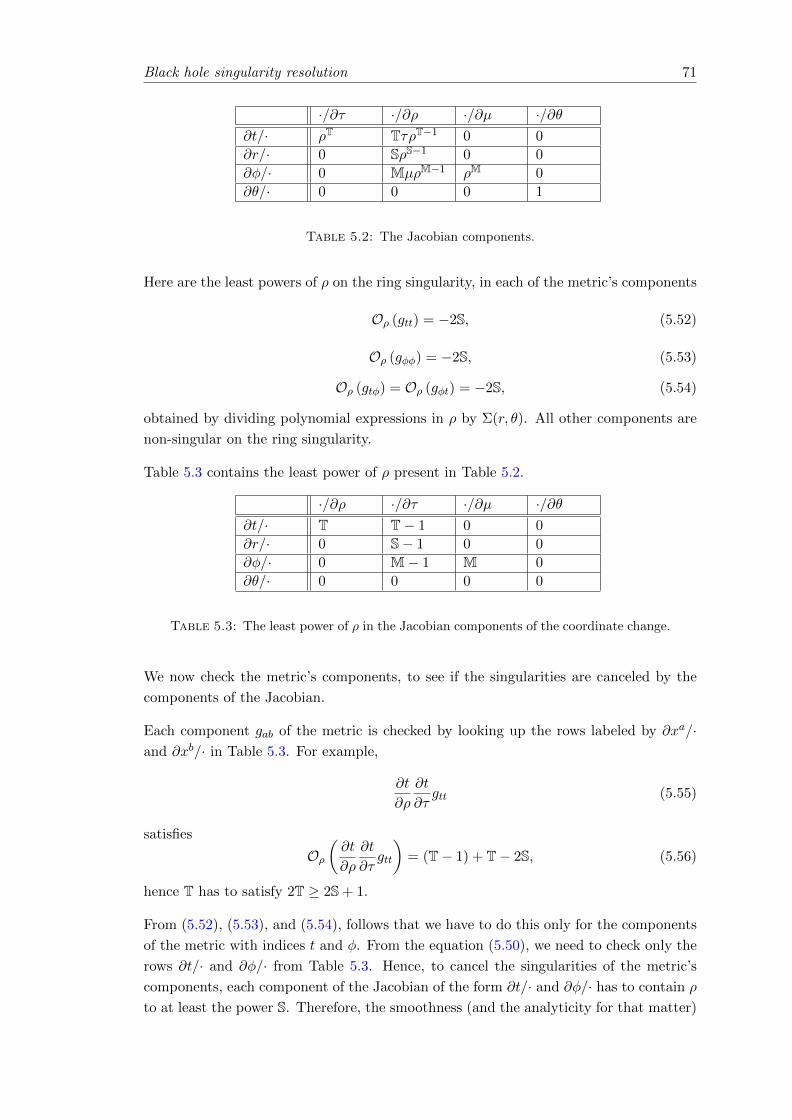
Black hole singularity resolution 71
·/∂τ ·/∂ρ ·/∂µ ·/∂θ∂t/· ρT TτρT−1 0 0
∂r/· 0 SρS−1 0 0
∂φ/· 0 MµρM−1 ρM 0
∂θ/· 0 0 0 1
Table 5.2: The Jacobian components.
Here are the least powers of ρ on the ring singularity, in each of the metric’s components
Oρ (gtt) = −2S, (5.52)
Oρ (gφφ) = −2S, (5.53)
Oρ (gtφ) = Oρ (gφt) = −2S, (5.54)
obtained by dividing polynomial expressions in ρ by Σ(r, θ). All other components are
non-singular on the ring singularity.
Table 5.3 contains the least power of ρ present in Table 5.2.
·/∂ρ ·/∂τ ·/∂µ ·/∂θ∂t/· T T− 1 0 0
∂r/· 0 S− 1 0 0
∂φ/· 0 M− 1 M 0
∂θ/· 0 0 0 0
Table 5.3: The least power of ρ in the Jacobian components of the coordinate change.
We now check the metric’s components, to see if the singularities are canceled by the
components of the Jacobian.
Each component gab of the metric is checked by looking up the rows labeled by ∂xa/·and ∂xb/· in Table 5.3. For example,
∂t
∂ρ
∂t
∂τgtt (5.55)
satisfies
Oρ(∂t
∂ρ
∂t
∂τgtt
)= (T− 1) + T− 2S, (5.56)
hence T has to satisfy 2T ≥ 2S + 1.
From (5.52), (5.53), and (5.54), follows that we have to do this only for the components
of the metric with indices t and φ. From the equation (5.50), we need to check only the
rows ∂t/· and ∂φ/· from Table 5.3. Hence, to cancel the singularities of the metric’s
components, each component of the Jacobian of the form ∂t/· and ∂φ/· has to contain ρ
to at least the power S. Therefore, the smoothness (and the analyticity for that matter)

Black hole singularity resolution 72
of the metric on the ring singularity, in the new coordinates, is ensured by the conditionsS ≥ 1
T ≥ S + 1
M ≥ S + 1,
(5.57)
where S,T,M ∈ N. Hence, in the new coordinates, all of the metric’s components are
analytic at the singularity.
5.4.3 Electromagnetic field in Kerr-Newman
Another feature of our extension is that the electromagnetic potential and electromag-
netic field become smooth.
In standard coordinates, the electromagnetic potential of the Kerr-Newman solution is
the 1-form
A = − qr
Σ(r, θ)(dt− a sin2 θdφ). (5.58)
In our coordinates, it is
A = − qρS
Σ(r, θ)(ρTdτ + TτρT−1dρ− a sin2 θρMdµ), (5.59)
because from the Table 5.2 it follows that
dt = ρTdτ + TτρT−1dρ (5.60)
dr = SρS−1dρ (5.61)
and
dφ = MµρM−1dρ+ ρMdµ. (5.62)
In our coordinates, there is no singularity of the electromagnetic potential A at ρ = 0
and cos θ = 0, because T > S and M > S, from the conditions (5.34). Because the
electromagnetic field F = dA, it is smooth too.
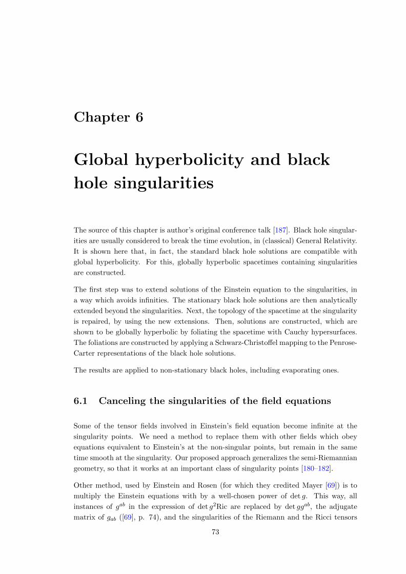
Chapter 6
Global hyperbolicity and black
hole singularities
The source of this chapter is author’s original conference talk [187]. Black hole singular-
ities are usually considered to break the time evolution, in (classical) General Relativity.
It is shown here that, in fact, the standard black hole solutions are compatible with
global hyperbolicity. For this, globally hyperbolic spacetimes containing singularities
are constructed.
The first step was to extend solutions of the Einstein equation to the singularities, in
a way which avoids infinities. The stationary black hole solutions are then analytically
extended beyond the singularities. Next, the topology of the spacetime at the singularity
is repaired, by using the new extensions. Then, solutions are constructed, which are
shown to be globally hyperbolic by foliating the spacetime with Cauchy hypersurfaces.
The foliations are constructed by applying a Schwarz-Christoffel mapping to the Penrose-
Carter representations of the black hole solutions.
The results are applied to non-stationary black holes, including evaporating ones.
6.1 Canceling the singularities of the field equations
Some of the tensor fields involved in Einstein’s field equation become infinite at the
singularity points. We need a method to replace them with other fields which obey
equations equivalent to Einstein’s at the non-singular points, but remain in the same
time smooth at the singularity. Our proposed approach generalizes the semi-Riemannian
geometry, so that it works at an important class of singularity points [180–182].
Other method, used by Einstein and Rosen (for which they credited Mayer [69]) is to
multiply the Einstein equations with by a well-chosen power of det g. This way, all
instances of gab in the expression of det g2Ric are replaced by det ggab, the adjugate
matrix of gab ([69], p. 74), and the singularities of the Riemann and the Ricci tensors
73

Global hyperbolicity and black hole singularities 74
can be canceled out for certain cases. The resulting equations still make sense as partial
differential equations in the components of the metric tensor. Of course, the geometric
objects of Semi-Riemannian Geometry have geometric meanings so long as the metric
tensor is non-singular. But once we allow it to become singular, the geometric objects
like covariant derivative and curvature become undefined. The quantities which replace
them if we multiply the equations with det g or other factors cannot give them this
meaning. Maybe a new kind of geometry is required to restore the ideas of covariant
derivative and curvature for singular metrics.
We preferred to have a generalization of Semi-Riemannian Geometry, which allows us to
define geometric objects like covariant derivative, Riemann curvature and Ricci tensor
even when the metric becomes degenerate.
In the following, we will explore the arena on which are defined the fields – the spacetime
– to make sure that the singularities don’t alter the topology in a way which breaks down
the evolution equations.
6.1.1 The topology of singularities
In the following we shall see that the main black hole solutions of Einstein’s equations
can be interpreted so that the time evolution is not jeopardized. To do this, we
1. Remove the singularities from the field equations.
2. Make sure that the solution is globally hyperbolic.
In this section, we shall see that these conditions can be ensured for the typical black
hole solutions of Einstein’s equation.
6.2 Globally hyperbolic spacetimes
A global solution to the Einstein equation is well-behaved when the initial data at a given
moment of time determine the solution for the entire future and past. This condition is
ensured by the global hyperbolicity, which is expressed by the requirements that
1. for any two points p and q, the intersection between the causal future of p, and
the causal past of q, J+(p) ∩ J−(q), is a compact subset of the spacetime;
2. there are no closed timelike curves ([94], p. 206).
The property of global hyperbolicity is equivalent to the existence of a Cauchy hyper-
surface – a spacelike hypersurface S that, for any point p in the future (past) of S,
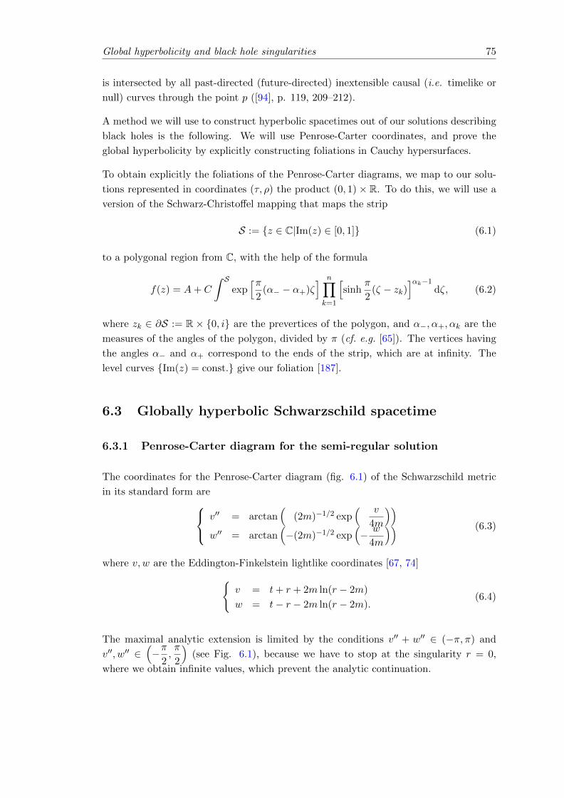
Global hyperbolicity and black hole singularities 75
is intersected by all past-directed (future-directed) inextensible causal (i.e. timelike or
null) curves through the point p ([94], p. 119, 209–212).
A method we will use to construct hyperbolic spacetimes out of our solutions describing
black holes is the following. We will use Penrose-Carter coordinates, and prove the
global hyperbolicity by explicitly constructing foliations in Cauchy hypersurfaces.
To obtain explicitly the foliations of the Penrose-Carter diagrams, we map to our solu-
tions represented in coordinates (τ, ρ) the product (0, 1)× R. To do this, we will use a
version of the Schwarz-Christoffel mapping that maps the strip
S := z ∈ C|Im(z) ∈ [0, 1] (6.1)
to a polygonal region from C, with the help of the formula
f(z) = A+ C
∫ Sexp
[π2
(α− − α+)ζ] n∏k=1
[sinh
π
2(ζ − zk)
]αk−1dζ, (6.2)
where zk ∈ ∂S := R × 0, i are the prevertices of the polygon, and α−, α+, αk are the
measures of the angles of the polygon, divided by π (cf. e.g. [65]). The vertices having
the angles α− and α+ correspond to the ends of the strip, which are at infinity. The
level curves Im(z) = const. give our foliation [187].
6.3 Globally hyperbolic Schwarzschild spacetime
6.3.1 Penrose-Carter diagram for the semi-regular solution
The coordinates for the Penrose-Carter diagram (fig. 6.1) of the Schwarzschild metric
in its standard form are v′′ = arctan(
(2m)−1/2 exp( v
4m
))w′′ = arctan
(−(2m)−1/2 exp
(− w
4m
)) (6.3)
where v, w are the Eddington-Finkelstein lightlike coordinates [67, 74]v = t+ r + 2m ln(r − 2m)
w = t− r − 2m ln(r − 2m).(6.4)
The maximal analytic extension is limited by the conditions v′′ + w′′ ∈ (−π, π) and
v′′, w′′ ∈(−π
2,π
2
)(see Fig. 6.1), because we have to stop at the singularity r = 0,
where we obtain infinite values, which prevent the analytic continuation.
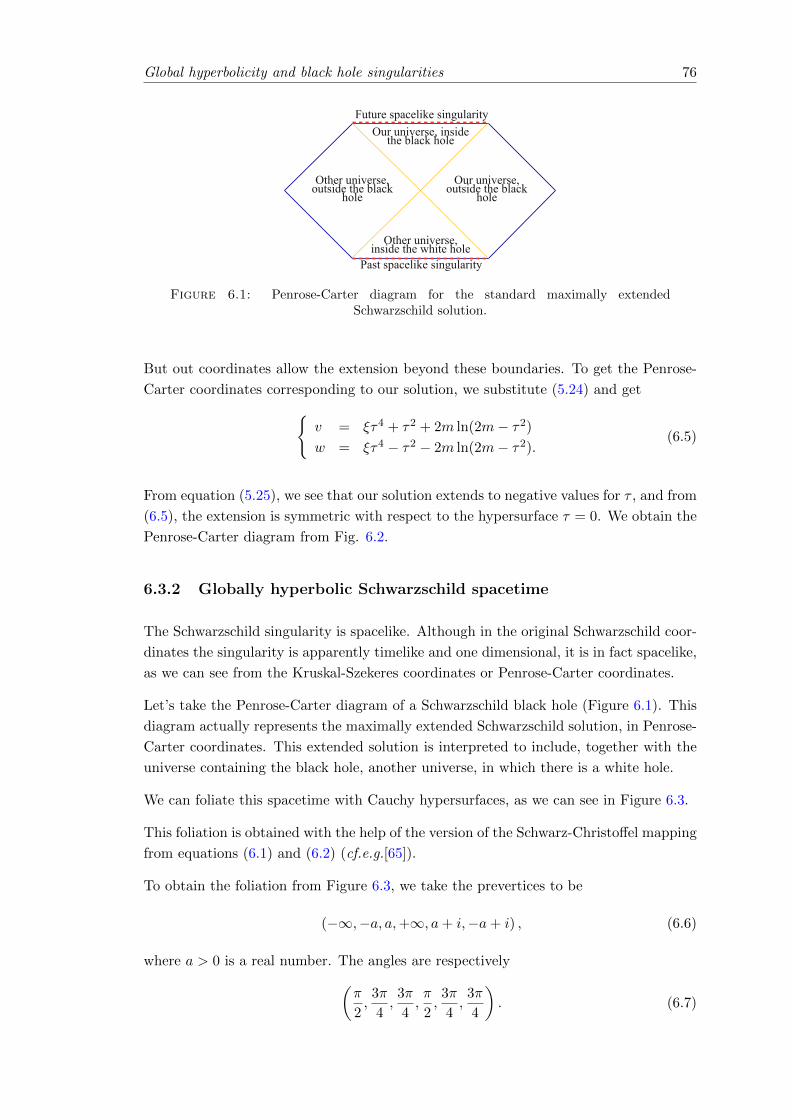
Global hyperbolicity and black hole singularities 76
Figure 6.1: Penrose-Carter diagram for the standard maximally extendedSchwarzschild solution.
But out coordinates allow the extension beyond these boundaries. To get the Penrose-
Carter coordinates corresponding to our solution, we substitute (5.24) and getv = ξτ4 + τ2 + 2m ln(2m− τ2)
w = ξτ4 − τ2 − 2m ln(2m− τ2).(6.5)
From equation (5.25), we see that our solution extends to negative values for τ , and from
(6.5), the extension is symmetric with respect to the hypersurface τ = 0. We obtain the
Penrose-Carter diagram from Fig. 6.2.
6.3.2 Globally hyperbolic Schwarzschild spacetime
The Schwarzschild singularity is spacelike. Although in the original Schwarzschild coor-
dinates the singularity is apparently timelike and one dimensional, it is in fact spacelike,
as we can see from the Kruskal-Szekeres coordinates or Penrose-Carter coordinates.
Let’s take the Penrose-Carter diagram of a Schwarzschild black hole (Figure 6.1). This
diagram actually represents the maximally extended Schwarzschild solution, in Penrose-
Carter coordinates. This extended solution is interpreted to include, together with the
universe containing the black hole, another universe, in which there is a white hole.
We can foliate this spacetime with Cauchy hypersurfaces, as we can see in Figure 6.3.
This foliation is obtained with the help of the version of the Schwarz-Christoffel mapping
from equations (6.1) and (6.2) (cf.e.g.[65]).
To obtain the foliation from Figure 6.3, we take the prevertices to be
(−∞,−a, a,+∞, a+ i,−a+ i) , (6.6)
where a > 0 is a real number. The angles are respectively(π
2,3π
4,3π
4,π
2,3π
4,3π
4
). (6.7)

Global hyperbolicity and black hole singularities 77
Figure 6.2: Penrose-Carter diagram for the semi-regular maximally extendedSchwarzschild solution.
Figure 6.3: Space-like foliation of the maximally extended Schwarzschild solution.
This foliation contains the past white hole, which one may consider unphysical. We can
make a similar foliation, but without the white hole (fig. 6.4), if we use the prevertices
(−∞,−a, 0, a,+∞, b+ i,−b+ i) , (6.8)
where 0 < b < a are positive real numbers. The angles are respectively(π
2,π
2,3π
2,π
2,π
2,3π
4,3π
4
). (6.9)

Global hyperbolicity and black hole singularities 78
Figure 6.4: Space-like foliation of the Schwarzschild solution, without white hole.
6.4 Globally hyperbolic Reissner-Nordstrom spacetime
6.4.1 The Penrose-Carter diagrams for our solution
The Penrose-Carter diagrams for the standard Reissner-Nordstrom spacetimes are pre-
sented in figure 6.5 ([94], p. 157-161).
C.B.
A.
Our universe,outside the black
hole
Inside the black hole
Other universe,outside the black
hole
Timelikesingularity
Other universe,outside the black
hole
Other universe,outside the black
hole
Cauchyhorizon
Our universe,outside the black
hole
Timelikesingularity
Other universe,outside the black
hole
Cauchyhorizon
Figure 6.5: Reissner-Nordstrom black holes. A. Naked solutions (q2 > m2). B.Extremal solution (q2 = m2). C. Solutions with q2 < m2.
To obtain the Penrose-Carter coordinates for our solution from section §5.3, we add our
coordinate transformation before the steps leading to the Penrose-Carter coordinates.
For odd S, there is a region ρ < 0, and the Penrose-Carter diagrams are the same as the
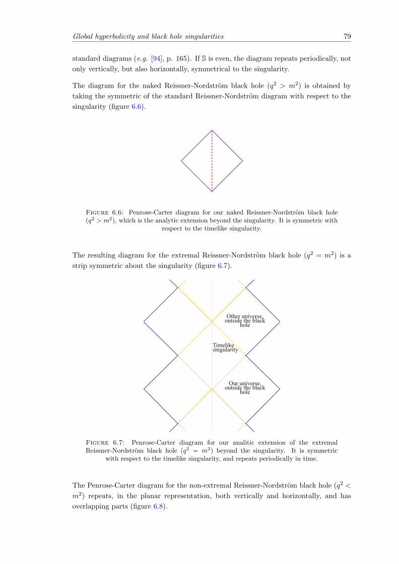
Global hyperbolicity and black hole singularities 79
standard diagrams (e.g. [94], p. 165). If S is even, the diagram repeats periodically, not
only vertically, but also horizontally, symmetrical to the singularity.
The diagram for the naked Reissner-Nordstrom black hole (q2 > m2) is obtained by
taking the symmetric of the standard Reissner-Nordstrom diagram with respect to the
singularity (figure 6.6).
Figure 6.6: Penrose-Carter diagram for our naked Reissner-Nordstrom black hole(q2 > m2), which is the analytic extension beyond the singularity. It is symmetric with
respect to the timelike singularity.
The resulting diagram for the extremal Reissner-Nordstrom black hole (q2 = m2) is a
strip symmetric about the singularity (figure 6.7).
Our universe,outside the black
hole
Timelikesingularity
Other universe,outside the black
hole
Figure 6.7: Penrose-Carter diagram for our analitic extension of the extremalReissner-Nordstrom black hole (q2 = m2) beyond the singularity. It is symmetric
with respect to the timelike singularity, and repeats periodically in time.
The Penrose-Carter diagram for the non-extremal Reissner-Nordstrom black hole (q2 <
m2) repeats, in the planar representation, both vertically and horizontally, and has
overlapping parts (figure 6.8).
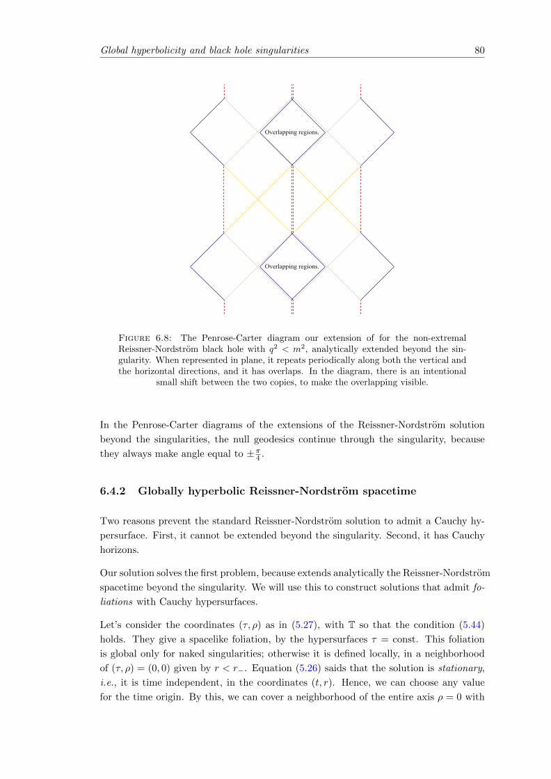
Global hyperbolicity and black hole singularities 80
Figure 6.8: The Penrose-Carter diagram our extension of for the non-extremalReissner-Nordstrom black hole with q2 < m2, analytically extended beyond the sin-gularity. When represented in plane, it repeats periodically along both the vertical andthe horizontal directions, and it has overlaps. In the diagram, there is an intentional
small shift between the two copies, to make the overlapping visible.
In the Penrose-Carter diagrams of the extensions of the Reissner-Nordstrom solution
beyond the singularities, the null geodesics continue through the singularity, because
they always make angle equal to ±π4 .
6.4.2 Globally hyperbolic Reissner-Nordstrom spacetime
Two reasons prevent the standard Reissner-Nordstrom solution to admit a Cauchy hy-
persurface. First, it cannot be extended beyond the singularity. Second, it has Cauchy
horizons.
Our solution solves the first problem, because extends analytically the Reissner-Nordstrom
spacetime beyond the singularity. We will use this to construct solutions that admit fo-
liations with Cauchy hypersurfaces.
Let’s consider the coordinates (τ, ρ) as in (5.27), with T so that the condition (5.44)
holds. They give a spacelike foliation, by the hypersurfaces τ = const. This foliation
is global only for naked singularities; otherwise it is defined locally, in a neighborhood
of (τ, ρ) = (0, 0) given by r < r−. Equation (5.26) saids that the solution is stationary,
i.e., it is time independent, in the coordinates (t, r). Hence, we can choose any value
for the time origin. By this, we can cover a neighborhood of the entire axis ρ = 0 with

Global hyperbolicity and black hole singularities 81
coordinate patches like (τ, ρ). To obtain global foliations, we use the Penrose-Carter
diagrams of section §6.4.1, figures 6.6, 6.7 and 6.8. Recall that in the Penrose-Carter
diagram, the null directions are represented as straight lines inclined at an angle of ±π4 .
It is easy to see that the naked Reissner-Nordstrom solution (figure 6.6) has a global
foliation, because the Penrose-Carter diagram is the same as for the Minkowski spacetime
(fig. 6.9). Hence, we use the same foliation as that for the Minkowski spacetime will.
To foliate it, we use the Schwarz-Christoffel mapping (6.2). By taking as prevertices
(−∞, 0,+∞, i) , (6.10)
and as angles (π2,π
2,π
2,π
2
), (6.11)
we obtain the foliation represented in fig. 6.9.
Timelike singularityCauchy hypersurface
pq
Figure 6.9: Spacelike foliation with Cauchy hypersurfaces, for the naked Reissner-Nordstrom solution extended beyond singularity.
The solutions whose singularity is not naked have Cauchy horizons (hypersurfaces which
are boundaries for the Cauchy development of the data on a spacelike hypersurface), and
don’t admit globally hyperbolic maximal extension. To obtain a globally hyperbolic
solution, we have to remove the regions beyond the Cauchy horizons, obtaining in a
natural way a subset of the Penrose-Carter diagram, symmetric about the singularity
r = 0, which admits foliation (Figures 6.10 and 6.11).
We take as prevertices for the Schwarz-Christoffel mapping (6.2) the set
(−∞,−a, 0, a,+∞, i) , (6.12)

Global hyperbolicity and black hole singularities 82
Timelike singularity
Internal horizonEvent horizon
Cauchy hypersurface
p
Figure 6.10: Foliation with Cauchy hypersurfaces, for the non-extremal Reissner-Nordstrom solution.
Timelike singularity
Event horizon
Cauchy hypersurface
p
Figure 6.11: Foliation with Cauchy hypersurfaces, for the extremal Reissner-Nordstrom solution.
where 0 < a is real. The corresponding angles are(π
2,π
2,3π
2,π
2,π
2,π
2
). (6.13)
By choosing a properly, we obtain the foliations represented in diagrams 6.10 and 6.11,
for the non-extremal, respectively the extremal solutions. Given that α− = α+ and
the edges are inclined at most at π4 , and alternate in such a way that the level curves
with Im(z) ∈ (0, 1) always make an angle strictly between −π4 and π
4 , our foliations are
spacelike everywhere.
Each of the figures 6.9, 6.10, and 6.11, contained a highlighted spacelike hypersurface.
This hypersurface is intersected by all past (future) directed inextensible causal curves
through a point p from its future (past), therefore it is Cauchy.
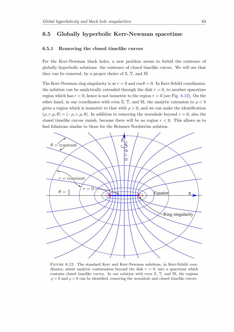
Global hyperbolicity and black hole singularities 83
6.5 Globally hyperbolic Kerr-Newman spacetime
6.5.1 Removing the closed timelike curves
For the Kerr-Newman black holes, a new problem seems to forbid the existence of
globally hyperbolic solutions: the existence of closed timelike curves. We will see that
they can be removed, by a proper choice of S, T, and M.
The Kerr-Newman ring singularity is at r = 0 and cos θ = 0. In Kerr-Schild coordinates,
the solution can be analytically extended through the disk r = 0, to another spacetime
region which has r < 0, hence is not isometric to the region r > 0 (see Fig. 6.12). On the
other hand, in our coordinates with even S, T, and M, the analytic extension to ρ < 0
gives a region which is isometric to that with ρ > 0, and we can make the identification
(ρ, τ, µ, θ) = (−ρ, τ, µ, θ). In addition to removing the wormhole beyond r = 0, also the
closed timelike curves vanish, because there will be no region r < 0. This allows us to
find foliations similar to those for the Reissner-Nordstrom solution.
Figure 6.12: The standard Kerr and Kerr-Newman solutions, in Kerr-Schild coor-dinates, admit analytic continuation beyond the disk r = 0, into a spacetime whichcontains closed timelike curves. In our solution with even S, T, and M, the regionsρ < 0 and ρ > 0 can be identified, removing the wormhole and closed timelike curves.
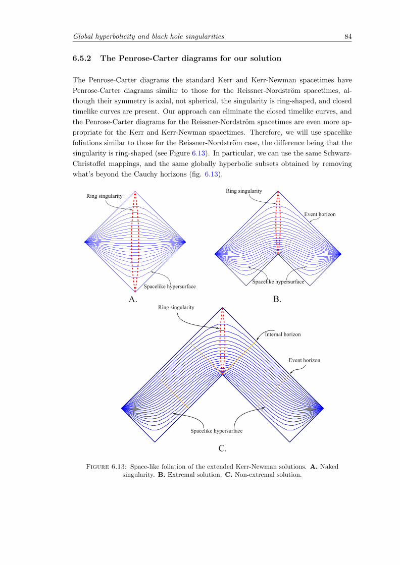
Global hyperbolicity and black hole singularities 84
6.5.2 The Penrose-Carter diagrams for our solution
The Penrose-Carter diagrams the standard Kerr and Kerr-Newman spacetimes have
Penrose-Carter diagrams similar to those for the Reissner-Nordstrom spacetimes, al-
though their symmetry is axial, not spherical, the singularity is ring-shaped, and closed
timelike curves are present. Our approach can eliminate the closed timelike curves, and
the Penrose-Carter diagrams for the Reissner-Nordstrom spacetimes are even more ap-
propriate for the Kerr and Kerr-Newman spacetimes. Therefore, we will use spacelike
foliations similar to those for the Reissner-Nordstrom case, the difference being that the
singularity is ring-shaped (see Figure 6.13). In particular, we can use the same Schwarz-
Christoffel mappings, and the same globally hyperbolic subsets obtained by removing
what’s beyond the Cauchy horizons (fig. 6.13).
Figure 6.13: Space-like foliation of the extended Kerr-Newman solutions. A. Nakedsingularity. B. Extremal solution. C. Non-extremal solution.
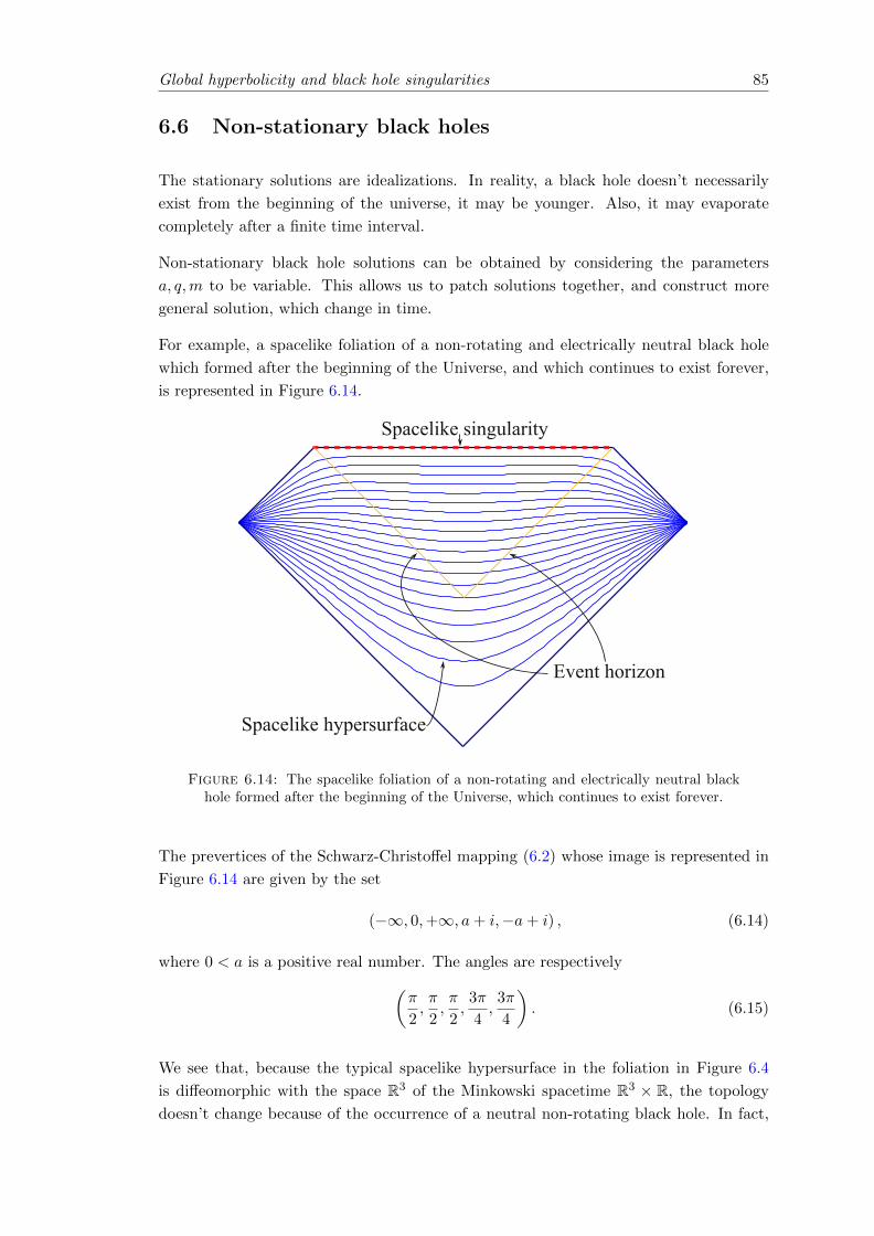
Global hyperbolicity and black hole singularities 85
6.6 Non-stationary black holes
The stationary solutions are idealizations. In reality, a black hole doesn’t necessarily
exist from the beginning of the universe, it may be younger. Also, it may evaporate
completely after a finite time interval.
Non-stationary black hole solutions can be obtained by considering the parameters
a, q,m to be variable. This allows us to patch solutions together, and construct more
general solution, which change in time.
For example, a spacelike foliation of a non-rotating and electrically neutral black hole
which formed after the beginning of the Universe, and which continues to exist forever,
is represented in Figure 6.14.
Figure 6.14: The spacelike foliation of a non-rotating and electrically neutral blackhole formed after the beginning of the Universe, which continues to exist forever.
The prevertices of the Schwarz-Christoffel mapping (6.2) whose image is represented in
Figure 6.14 are given by the set
(−∞, 0,+∞, a+ i,−a+ i) , (6.14)
where 0 < a is a positive real number. The angles are respectively(π
2,π
2,π
2,3π
4,3π
4
). (6.15)
We see that, because the typical spacelike hypersurface in the foliation in Figure 6.4
is diffeomorphic with the space R3 of the Minkowski spacetime R3 × R, the topology
doesn’t change because of the occurrence of a neutral non-rotating black hole. In fact,
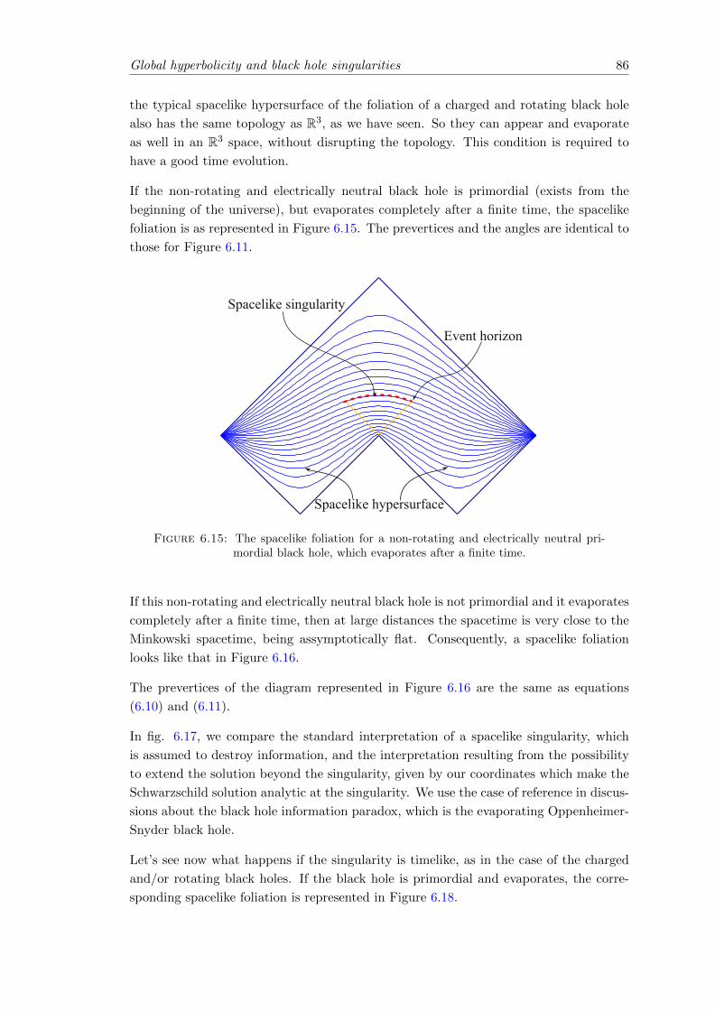
Global hyperbolicity and black hole singularities 86
the typical spacelike hypersurface of the foliation of a charged and rotating black hole
also has the same topology as R3, as we have seen. So they can appear and evaporate
as well in an R3 space, without disrupting the topology. This condition is required to
have a good time evolution.
If the non-rotating and electrically neutral black hole is primordial (exists from the
beginning of the universe), but evaporates completely after a finite time, the spacelike
foliation is as represented in Figure 6.15. The prevertices and the angles are identical to
those for Figure 6.11.
Figure 6.15: The spacelike foliation for a non-rotating and electrically neutral pri-mordial black hole, which evaporates after a finite time.
If this non-rotating and electrically neutral black hole is not primordial and it evaporates
completely after a finite time, then at large distances the spacetime is very close to the
Minkowski spacetime, being assymptotically flat. Consequently, a spacelike foliation
looks like that in Figure 6.16.
The prevertices of the diagram represented in Figure 6.16 are the same as equations
(6.10) and (6.11).
In fig. 6.17, we compare the standard interpretation of a spacelike singularity, which
is assumed to destroy information, and the interpretation resulting from the possibility
to extend the solution beyond the singularity, given by our coordinates which make the
Schwarzschild solution analytic at the singularity. We use the case of reference in discus-
sions about the black hole information paradox, which is the evaporating Oppenheimer-
Snyder black hole.
Let’s see now what happens if the singularity is timelike, as in the case of the charged
and/or rotating black holes. If the black hole is primordial and evaporates, the corre-
sponding spacelike foliation is represented in Figure 6.18.

Global hyperbolicity and black hole singularities 87
Figure 6.16: The spacelike foliation for a non-rotating and electrically neutral blackhole formed after the beginning of the Universe, and which evaporates after a finite
time.
Figure 6.17: The Penrose-Carter diagram for an evaporating Oppenheimer-Snyderblack hole. A. The standard view is that the singularity destroys the information. B.
Our approach suggests that the singularity doesn’t destroy the information.
The prevertices and the angles are the same as those for the Figure 6.11.
The spacelike foliation of a spacetime containing a black hole which is not primordial
and does not evaporate is represented in Figure 6.19. The prevertices and the angles
are again those from equations (6.10) and (6.11).
The same prevertices and angles are used to construct the spacelike foliation for a non-
primordial evaporating black hole, represented in Figure 6.20.

Global hyperbolicity and black hole singularities 88
Figure 6.18: Primordial evaporating black hole with timelike singularity.
Figure 6.19: Non-primordial non-evaporating black hole with timelike singularity.
If the black hole rotates, the singularity is ring-shaped (as in Fig. 6.13), but the diagrams
are similar.
6.7 Conclusions
This chapter shows how one can extend smoothly the black hole solutions at the singu-
larities, then find an appropriate foliation of the spacetime into spacelike hypersurfaces,
and an appropriate extension of the spacetime at singularities, so that the topology
of the spacelike hypersurfaces of the foliations is preserved. In our typical examples,
the time evolution in the presence of singularities is restored. The examples given here
showed this explicitly for the neutral and charged, rotating or non-rotating, primordial
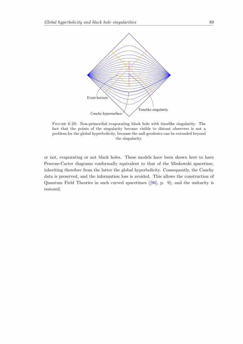
Global hyperbolicity and black hole singularities 89
Timelike singularityCauchy hypersurface
Event horizon
Figure 6.20: Non-primordial evaporating black hole with timelike singularity. Thefact that the points of the singularity become visible to distant observers is not aproblem for the global hyperbolicity, because the null geodesics can be extended beyond
the singularity.
or not, evaporating or not black holes. These models have been shown here to have
Penrose-Carter diagrams conformally equivalent to that of the Minkowski spacetime,
inheriting therefore from the latter the global hyperbolicity. Consequently, the Cauchy
data is preserved, and the information loss is avoided. This allows the construction of
Quantum Field Theories in such curved spacetimes ([96], p. 9), and the unitarity is
restored.
Chapter 7
Quantum gravity from metric
dimensional reduction at
singularities
This chapter is based on author’s original research, from article [186], and author’s talk
given in May 2012 at JINR, Dubna [188].
Old and recent theoretical investigations suggest that the quantization of gravity would
be possible, if a dimensional reduction takes place at high energy scales. This would also
solve other problems of Quantum Field Theory. But what is missing is a mechanism
which would cause the dimensional reduction.
The mathematical approach to singularities in General Relativity presented in this The-
sis leads to the conclusion that at singularities, the metric tensor becomes degenerate.
Geometry, and some of the fields, become independent of the directions in which the
metric is degenerate. Effectively, this is as if one or more spacetime dimensions vanish
at singularities. Consequently, it appears that singularities leads in a natural way to the
spontaneous dimensional reduction needed by Quantum Gravity.
7.1 Introduction
The most successful theories in fundamental theoretical physics are General Relativity
(GR) and Quantum Field Theory (QFT). They offer accurate and complementary de-
scriptions of the physical reality, and their predictions were confirmed with very high
precision.
But they are not without problems, especially with infinities. In GR, infinities are present
in the form of singularities. In QFT, infinities appear in the perturbative expansion. In
this Thesis we tried to offer a solution to the infinities in GR. The infinities in QFT
90
Quantum gravity from metric dimensional reduction at singularities 91
are considered much less problematic now, due to renormalization techniques, which are
shown to apply to the entire Standard Model of particle physics [198, 199, 201], and the
renormalization group [30, 31, 84, 171, 172, 197].
But it seems that, when one tries to combine GR and QFT, infinities reappear, and
renormalization can’t remove them. GR without matter fields is perturbatively non-
renormalizable at two loops [87, 202]. It required number of higher derivative countert-
erms with their coupling constants is infinite. The main cause of the problem is the
dimension of the Newton constant, which is [GN ] = 2−D = −2 in mass units.
Many theoretical1 investigations were made in understanding ultraviolet (UV) limit in
QFT, the small scale. Particularly in various approaches to Quantum Gravity (QG),
the evidence accumulated so far suggests, or even requires, that in the UV limit there is
a dimensional reduction to two dimensions. What is under debate is the meaning, the
nature, the explicit cause of this spontaneous dimensional reduction.
In this chapter we suggest that our approach to singularities predicts in a very concrete
way the dimensional reduction.
The usual position regarding the apparent incompatibility between QFT and GR, man-
ifested as the non-renormalizability of GR, is that General Relativity is to be blamed,
and has to be modified. It is hoped that one of the many known approaches to QG will
cure not only the non-renormalizability, but also the problem of singularities, if we are
willing to give up up one or more fundamental principles of GR.
We will take here an opposite position, namely that solving the problem of singularities
in GR, has as effect the dimensional reduction in the UV limit, which would make GR
renormalizable.
According to ’t Hooft [200],
Quantum Gravity is usually thought of as a theory, under construction, where
the postulates of quantum mechanics are to be reconciled with those of gen-
eral relativity, without allowing for any compromise in either of the two.
In this chapter, we will try to go as far as we can in reconciliating QFT and GR, without
making compromises.
In section §7.2, we will review some of the hints suggesting that if the spacetime be-
comes 2-dimensional at small scales, the quantization of gravity will become possible. In
section §7.3, we will explain how singularities studied in this Thesis cause dimensional
reduction. Then we will show some connections between dimensional reduction caused
by singularities, and other types of dimensional reduction, proposed so far in some of
the approaches to QG.
1Experimental data is not available for such small distances.

Quantum gravity from metric dimensional reduction at singularities 92
7.2 Suggestions of dimensional reduction coming from other
approaches
The original method of regularization through dimensional reduction appeared as a
method of regularization in QFT. It is rather formal, apparently with no implications
to the actual physical dimensions. It was suggested by the observations that the loop
integrations depend continuously on the number of dimensions. The poles can be avoided
by replacing the dimension 4 by 4− ε. At the end we just make ε→ 0 [35, 198, 201].
On the other hand, Quantum Gravity works fine in two dimensions. This justifies
the consideration of the possibility that, at small scales, the number of dimensions is
somehow reduced, while maintaining four dimensions at large scales. We review in the
following some of the indications suggesting the dimensional reduction.
7.2.1 Dimensional reduction in Quantum Field Theory
7.2.1.1 Several hints of dimensional reduction from QFT
Several different situations in QFT suggest that the two-dimensionality plays an impor-
tant role. Since the discovery of the first exactly solvable QFT model [205], the two-
dimensional QFT proved to be very productive, leading in a direct and non-perturbative
way to interesting results, which suggested hypotheses for four-dimensions (see [1] and
[81] and references therein).
In the Standard Model, one problem is that, to avoid the destabilization of the elec-
troweak symmetry breaking scale, the mass of the Higgs boson needs to be fine-tuned,
to an accuracy of 10−32 [7]. By fixing the cutoff at the electroweak scale, the SM works
well, and it is believed that this indicates new physics beyond this scale. In [7] is explored
the possibility of keeping unmodified the structure of the SM, and reduce the dimension.
One main idea is that the dimensional reduction to d = 2 space dimensions makes the
Higgs terms linearly divergent, and to d = 1 makes them logarithmically divergent. This
would make unnecessary the fine-tuning of the Higgs mass.
7.2.1.2 Fractal universe and measure dimensional reduction
G. Calcagni developed the fractal universe program, with the purpose to keep from the
Horava-Lifschitz gravity the nice feature that, in the UV regime, it leads to a two-
dimensional phase, but without giving up Lorentz invariance. He kept the isotropic
scaling, and compensates it, by replacing the standard measure used in the action with
another measure, (initially a Lebesgue-Stieltjes measure) which reduces the Hausdorff
dimension at the UV fixed point to two. The action becomes fractional, and the resulting
theory is non-unitary, being dissipative. But the energy is still conserved.
Quantum gravity from metric dimensional reduction at singularities 93
The used action was
S =
∫M
d%(x)L(φ, ∂µφ), (7.1)
with the measure
d%(x) = v dxD (7.2)
He used a weight of the form v :=∏D−1µ=0 f(µ)(x).
The original argument in [43] was that this measure leads to perturbative renormaliz-
ability. By similar ideas, Calcagni obtained a modified action for General Relativity,
and from this, a modified version of the Einstein equation.
He refined the theory introduced in [36, 37, 40], and put on more rigorous mathematical
basis, in the subsequent papers [11, 38, 39, 41–43, 45]. The mathematically foundation
of the fractal universe theory is a Lebesgue-Stieltjes measure or a fractional measure
[39], fractional calculus, and fractional action principles [70, 71, 213].
Later, in [46], it was shown that modified measure is not enough to ensure it, and in fact
the original power-counting argument from [43] fails. Yet, in [46] is argued that “[t]he
interest in fractional theories is not jeopardized”, and in [44] that multi-scale theories
are still of interest, not only for QG, but also for cosmology (accelerated expansion,
cosmological constant, alternative to inflation, early universe, big bounce, etc.).
Maybe the modified measure approach is insufficient to obtain perturbative renormaliz-
ability, but the dimensional flow at singularities is richer and provides some additional
features.
We will show in section §7.3.7 that our theory of singularities leads precisely to a measure
of the form (7.2).
7.2.1.3 Topological dimensional reduction
An interesting approach, proposed by D. V. Shirkov, was initially aimed to replace the
Higgs boson, which was expected to be found at 140 ± 25 GeV, with the Ginzburg-
Landau-Higgs solution of a constant classical Higgs field at ∼ 250 GeV. But in the
absence of a Higgs quantum field, the weak force would be non-renormalizable. Shirkov
realized that the regularization can be obtained by working in a spacetime with variable
topology, so that the number of dimensions varies from D = 4 in the IR limit, to
D = 1 + d < 4 in the UV limit, and the coupling constant is assumed to run between
these limits.
Shirkov proposed a gϕ4 QFT model described by a self-interacting Lagrangian L = T−V[173], where
V (m, g;ϕ) =m2
2ϕ2 +
4πd/2M4+d
9gdϕ
4, g > 0 (7.3)

Quantum gravity from metric dimensional reduction at singularities 94
The toy model he used was a manifold obtained by joining two cylinders SR,L and Sr,l,
of lengths L, l and radii R > r, with a transition region Scoll of variable radius. One
interesting problem taking place on this manifold, was to solve some QFT equations,
and then take the limit r → 0.
In momentum space, the volume element d4k was replaced by
dMk =d4k
1 + k2
M2
, (7.4)
yielding a one-loop Feynman integral, whose IR asymptote is the function
lnq2
m2i
, (7.5)
and the UV asymptote, the function
ln4M2
m2i
+M2
q2ln
q2
M2. (7.6)
This reversed the running of the coupling constant in the small distance region, to a
minimum value g2(∞) < g2(M2dr), where Mdr is the reduction scale.
Another feature of this approach is the possibility that the coupling constants of the
Standard Model converge in the UV limit toward the same minimum value, without
requiring by this a GUT scheme like SU(5) [18, 85].
The exploration of the idea of topological dimensional reduction was continued by P.
Fiziev and D. V. Shirkov in [75–77, 174], and applied to Klein-Gordon equation.
In section §7.3.2, we establish strong connections between our approach, and the topo-
logical dimensional reduction approach of Shirkov and Fiziev.
7.2.2 Dimensional reduction in Quantum Gravity
A review of the indications that various approaches to QG suggest a dimensional reduc-
tion at small scales, is done by Carlip [48, 49].
The causal dynamical triangulations approach approximates spacetime by flat four-
simplicial manifolds, as in quantum Regge calculus [155]. Additional constraints on
the lengths of the edges of the simplices are imposed [2–6]. To enforce causality, it is
required that the time-slicing at discrete times is fixed, and that the time-like edges
are in the same direction. The spectral dimension – the effective dimension of the diffu-
sion process, related to the dispersion relation of the corresponding differential operator,
turns out to be four at large distances, but two at short distances [5]. Spectral dimension
is calculated in other approaches to QG, and agrees [25, 48, 106, 123, 129, 130, 137].
There is a connection between the spectral dimension and the spacetime dimension, but
they are not equivalent [41, 77, 178, 179].
Quantum gravity from metric dimensional reduction at singularities 95
It has been noted [47] that, because in dimension < 3 the Weyl curvature vanishes, the
vacuum Einstein equation has only solutions of constant curvature (flat, if the cosmo-
logical constant is 0). Hence, local degrees of freedom are absent, that is, gravitational
waves in the classical case, and gravitons in QG, are absent. As we have seen in section
§4.4, quasi-regular singularities have vanishing Weyl curvature (see §7.3.3).
7.2.2.1 Asymptotic safety for the renormalization group
Even though GR appears to be non-renormalizable, the renormalization group analysis
may provide useful indications. The idea of asymptotic safety, proposed by S. Weinberg
[227], is that, although there is an infinite number of coupling constants, they become
“unified”, under the renormalization group flow, when approaching an ultraviolet fixed
point. That is, they converge to a finite-dimensional ultraviolet critical surface. To make
the 3 + 1-dimensional gravity asymptotically safe, one can supplement the Einstein-
Hilbert Lagrangian density L = − 1
16πGR√−det g with higher-order curvature terms.
For example, by replacing it with L = f(R)√−det g. Weinberg observed that “there is
an asymptotically safe theory of pure gravity in 2+ε dimensions, with a one-dimensional
critical surface”, and “[a]symptotic safety is also preserved when we add matter fields”,
if we add certain compensatory fields [227].
The evidence for asymptotic safety [55, 88, 126, 138, 157, 158], involves especially two
dimensions [107, 125]. The spectral dimension near the fixed point also is dS = 2
[123]. Other indications are that the existence of a non-Gaussian fixed point for the
dimensionless coupling constant gN = GNµd−2 requires two-dimensionality [138].
7.2.2.2 Horava-Lifschitz gravity
Horava-Lifschitz gravity, inspired by the quantum critical phenomena in condensed mat-
ter systems, was proposed in 2009 by Horava [105]. The idea is to assume that space
and time behave differently at scaling:x 7→ bx,
t 7→ bzt.(7.7)
To describe an UV fixed point, it is required that z = D − 1 = 3, and sometimes
that z = 4. The anisotropy (7.7) is required to be a symmetry of the solution, but
not necessarily of the action itself. In the UV limit, the theory describes interacting
non-relativistic gravitons. In 1 + 3 dimensions, it is power-counting renormalizable.
Lorentz symmetry is broken in the UV limit, but it is conjectured that it is restored at
large distances, and z → 1. The theory leads to field equations which are of high order
in space, to cancel the divergences of the loop integrals, and of second-order in time, to
avoid ghosts. The spectral dimension is 4 at low energies, and 2 at high energies [106].
Quantum gravity from metric dimensional reduction at singularities 96
The volume element has the dimension
[dtddx] = −d− z, (7.8)
which is incremented by each time derivative by
[∂t] = z, (7.9)
hence, κ is dimensionless when z = d, since its scaling dimension is
[κ] =z − d
2. (7.10)
Some objections have been raised, most of them objections coming from the difficulty to
prove that GR is recovered in the IR limit [28, 29, 52, 102, 110, 143, 177, 220, 226, 228].
In section §7.3.6 we will show how our singularities suggest a mechanism for the anisotropy
(7.7).
7.3 Dimensional reduction at singularities
While dimensional reduction seems to be needed for Quantum Gravity, little is known
about what causes it. But the singularities studied in this Thesis may provide an
explanation, because they act like sources for the dimensional reduction.
7.3.1 The dimension of the metric tensor
At points p ∈M where the metric tensor gab is degenerate, the distance vanishes along
the degenerate directions, which belong to the space ker([) := T⊥p (M) ≤ TpM (fig. 2.1).
These directions can be factored out by taking the quotient
Tp•M :=TpM
T⊥p (M), (7.11)
which has the dimension equal to the rank of the metric at p:
dimTp•M = rank gp. (7.12)
Because the metric g is degenerate, it can be reduced to a metric tensor on the space
Tp•M , and its inverse is a metric tensor on Tp•M , both spaces having dimension rank gp.
Quantum gravity from metric dimensional reduction at singularities 97
7.3.2 Metric dimension vs. topological dimension
Let (M, g) be a singular semi-Riemannian manifold. Even if the rank of the metric is,
at the points where the metric becomes degenerate, lower than dimM , the topological
dimension of the manifold remains dimM . Mathematically, there are three layers in
Differential Geometry: the topological structure, the differential structure, and the geo-
metric structure. The dimension of the vector space used in the charts of the atlas is
the topological dimension of M . The metric dimension, or the geometric dimension is
the rank of the metric, and can be at most equal to the topological dimension.
Kupeli showed that, if (M, g) is a radical-stationary semi-Riemannian manifold of con-
stant signature (k, l,m), it is locally isomorphic to a direct product manifold P ×0 N
between a (non-degenerate) semi-Riemannian manifold P of signature (l,m), and a k-
dimensional manifold N , whose metric can be considered equal to 0 [120]. Therefore,
from the viewpoint of geometry, at any point p ∈ M the degenerate directions can be
ignored, and we can identify the D-dimensional manifold M at p, with the rank gp-
dimensional manifold P . The information contained in the metric g of the manifold M
can be obtained by pull-back, from that of a metric on a manifold (P, h) with smaller
topological dimension.
In addition to the metric, in GR there are present other fields. To admit smooth met-
ric contractions between covariant indices, and to admit smooth covariant derivatives
(Chapter 2), the fields have to behave as if they don’t “see” the degenerate directions.
This connects our results with the topological dimensional reduction of D.V. Shirkov
and P. Fiziev (see section §7.2.1.3). Our approach confirm their observation [77]:
dimensional reduction of the physical space in general relativity (GR) can
be regarded as an unrealized and as yet untapped consequence of Einstein’s
equations (EEqs) themselves which takes place around singular points of
their solutions.
7.3.3 Metric dimensional reduction and the Weyl tensor
According to Theorem 4.2, in dimension 4, the Weyl curvature vanishes at quasi-regular
singularities, because at the points where the metric is degenerate, dimTp•M ≤ 3.
Because the Ricci decomposition is smooth, the Weyl curvature tensor Cabcd is smooth,
and remains small around the singularity, where it vanishes.
Examples of quasi-regular singularities include the Schwarzschild black hole (section
§5.2), which can represent a classical neutral spinless particle. It is not yet clear whether
the singularities of stationary charged and rotating black holes are quasi-regular, but
we know they are analytic. Such black holes undergo geometric dimensional reduction
at singularities. For the charged ones, the electromagnetic potential and its field are
analytic, and finite at r = 0 (see sections §5.3 and §5.4).
Quantum gravity from metric dimensional reduction at singularities 98
At singularities, because the Weyl curvature tensor vanishes, when quantizing, gravitons
are absent, making gravity renormalizable [47].
7.3.4 Lorentz invariance and metric dimensional reduction
At the points where the metric is degenerate, Lorentz invariance is affected. The metric
is, at those points, not invariant to a group of transformations isomorphic to Lorentz,
group. The role of the Lorentz group is taken by a larger group – the Barbilian group
[19]. If we factorize (at a point as in (7.11), or on a region of constant signature, if the
metric is radical-stationary) we reduce the Barbilian group to a subgroup, which is an
orthogonal subgroup of the Lorentz group.
Hence, in our approach, Lorentz invariance is maintained at all points where the metric
is non-degenerate, and the theory is equivalent with Einstein’s. At the points where the
metric is degenerate, no theory can maintain Lorentz invariance. The best we can do at
singularities is to maintain the invariance with respect to the subgroup of the Lorentz
group, obtained after the metric dimensional reduction.
Other approaches to Quantum Gravity, like Loop Quantum Gravity and Horava-Lifschitz
gravity, gave up Lorentz invariance even at the points where the metric is non-degenerate,
and hope that it emerges at large scales.
7.3.5 Particles lose two dimensions
From the viewpoint of GR, charged particles are charged black holes. As viewed in
Chapter 5, the metric of a charged black hole of type Reissner-Nordstrom or Kerr-
Newman can be made analytic. The electromagnetic potential and its field are also
analytic, and finite at r = 0. This can be easily extended to Yang-Mills fields.
Equation (5.35) shows that, in our coordinates, at ρ = 0 (which is equivalent to r = 0),
the metric loses two dimensions, dρ and dτ . The spherical metric seems to be canceled
by the factor ρ2S but this is only apparent, being due to the warped product – similar to
the spherical coordinates for R3, when we know that multiplying with r2 doesn’t make
the metric degenerate at r = 0.
Metric dimensional reduction is present also in the Schwarzschild and Kerr-Newman
models. So, we see that dimensional reduction takes place for particles which are charged
or neutral, spinning or not. The dimensional reduction, and the finiteness of the gauge
potential and fields at the singularity. Future developments of our research program
should check how these features affect the perturbative expansions and the renormal-
ization group analysis, including for the gravitational field, taking into account the new
results.

Quantum gravity from metric dimensional reduction at singularities 99
7.3.6 Particles and spacetime anisotropy
For the metric (5.35) to admit a foliation in spacelike hypersurfaces, the condition T ≥ 3Sis required in (5.27) [184]. This allows the space and time to be distinguished at ρ = 0,
with the price of an anisotropy between space and time. The anisotropy is manifest
when going back to the old Reissner-Nordstrom coordinates (t, r) – a rescaling which
is isotropic in the coordinates (τ, ρ), is anisotropic in the coordinates (t, r). If our
coordinates (τ, ρ) are the correct ones, diffeomorphism invariance should be considered
valid in these coordinates, and not in the singular coordinates (t, r).
P. Horava showed that an anisotropy like (7.7) leads to the correct dimension for the
Newton constant (see §7.2.2.2 and [105]). Could the anisotropy we obtained at the
Reissner-Nordstrom singularity, be related to the one proposed by Horava? They are
different in nature: our anisotropy follows from our coordinates, and GR, while Horava
modified GR. We don’t need to impose the recovery of standard GR at low energies,
since our approach is already equivalent to GR everywhere outside the singularities.
7.3.7 The measure in the action integral
As approaching the degenerate singularities, the volume form
dvol :=√−det gdx0 ∧ . . . ∧ dxD−1 =
√−det gdxD (7.13)
tends to 0. In the case of black hole singularities, this is due to the fact that in our
coordinates the metric is analytic. The volume form appears in the action principle
S =
∫M
dvol(x)L (7.14)
If, in some coordinates (xµ), the metric is diagonal, then
dvol(x) =D−1∏µ=0
√|gµµ(x)|dxD. (7.15)
We see that we obtain a measure of the type proposed by G. Calcagni [36, 37]. To see
this, we take in the Lebesgue measure from section §7.2.1.2, equation (7.1), the weights
f(µ)(x) =√|gµµ(x)|. (7.16)
Hence, much of the analysis developed in [36, 37] for QFT follows from the fact that the
metric becomes degenerate. The measure becomes
d%(x) =√−det gdxD, (7.17)
the standard measure from General Relativity, which we now allow to vanish.

Quantum gravity from metric dimensional reduction at singularities 100
Calcagni justifies the change of the measure by considering the spacetime to be fractal,
i.e. having Hausdorff dimension which changes with the scale. The Lebesgue-Stieltjes
measure he postulates is independent of GR, and he applies it both to flat spacetime
QFT, and to QG [36, 37, 40]. He applies his action (7.1) to Special Relativistic QFT.
On the other hand, the identification we proposed in (7.16) ises in place of the weights
fµ, the square root of the components of a diagonal metric, which we allowed to become
zero. This suggests that, at small scales, QFT is improved by GR, by dimensional
reduction.
Calcagni applies to GR the same recipe he used for Special Relativistic QFT, but multi-
plies the weights with√−det g [36]. His approach leads therefore to a modified Einstein
equation, and modified GR.
On the other hand, our approach keeps the standard GR everywhere where the metric is
not degenerate. The measure is similar to Calcagni’s measure which tames the infinities
of QFT, but it is just given by the volume form of a metric which becomes degenerate.
7.3.8 How can dimension vary with scale?
We have seen that the singularities with smooth but degenerate metric exhibit dimen-
sional reduction, and showed how it connects with dimensional reduction from other
approaches. It seems that our approach confirmed the intuition of some of these ver-
sions of dimensional reduction. What is more important, degenerate metric follows
naturally from GR, makes both big-bang and black hole singularities behave well, and
it was not invented ad-hoc to provide the needed dimensional reduction.
Our geometric dimensional reduction manifests as we approach a singularity. But what
is needed in QFT and QG, is that the dimensional reduction depends on the scale.
We will give only a qualitative justification, leaving the quantitative proof for future
research.
We will assume that it is enough to sum over the trivial topology, and there’s no need to
include non-trivial topologies. Because the topology of the black holes solutions which
can be used to describe particles can be taken the same as for the Minkowski spacetime
[183, 184, 187, 189], probably it will be enough to work with the same topology, and not
sum over all possible ones2.
If particles are to be represented by black hole singularities with degenerate metric,
then, if the number of particles are present in a given volume grows, the integral of
the volume form in a local coordinate system of a region containing them decreases
(fig. 7.1). That is, the average volume element decreases, as required for example in
Calcagni’s approach. The Feynman diagrams of higher order involve a larger number
of particles in the same volume. This leads to smaller volume element, hence to lower
contribution in the integrals.
2Also in Horava-Lifschitz gravity and CDT is not summed over other topologies.

Quantum gravity from metric dimensional reduction at singularities 101
1x|de
tg|
01
x|detg|
01
x|detg|
01
x|detg|
01
x|detg|
0Figure 7.1: Artistic representation of the principle that the metric’s average volumeelement decreases as the number of singularities (i.e. particles) in the region increases.
Singularities are represented as red dots, and |det g| is represented by blue curves.
While this argument refers to local coordinates, it is invariant, in the sense that the
constraint det g = 0 at singularities is the same in all coordinates obtained by a non-
singular transformation. Hence, the diffeomorphism invariance (general covariance) is
maintained in our argument.
Similar considerations can start with the fact that Cabcd = 0 for quasi-regular singu-
larities, and therefore, in average, as the number of particles in the Feynman diagrams
increase, the Weyl curvature becomes smaller, and the local degrees of freedom like
gravitons vanish with the energy.
Hence, our main conjecture, which we name the hypothesis of average dimensional re-
duction, is that the needed dimensional reduction which appears at smaller scales, is due
to the dimensional reduction at the singularities representing the particles.
7.4 Conclusions
We reviewed several results indicating that some problems concerning field quantization,
including of gravity, would be resolved if one sort or another of dimensional reduction
takes place at small scales. We showed that the theory of singularities developed in this
Thesis leads to a (geo)metric dimensional reduction, manifested in many ways similarly
to dimensional reduction from other approaches, ours having the bonus that General
Quantum gravity from metric dimensional reduction at singularities 102
Relativity is not modified. Therefore, our approach to the problem of singularities
opens new possibilities to be explored in Quantum Gravity.

Quantum gravity from metric dimensional reduction at singularities 103
Figure 7.2: Several examples of singularities, how they fit in our scheme, and howthey are resolved.
Bibliography
[1] E. Abdalla, M. C. B. Abdalla, and K. D. Rothe. Non-perturbative methods in 2
dimensional quantum field theory. World Scientific Pub Co Inc, 1991.
[2] J. Ambjørn, J. Jurkiewicz, and R. Loll. Nonperturbative Lorentzian path integral
for gravity. Phys. Rev. Lett., 85(5):924–927, 2000.
[3] J. Ambjørn, J. Jurkiewicz, and R. Loll. Emergence of a 4D world from causal
quantum gravity. Phys. Rev. Lett., 93(13):131301, 2004.
[4] J. Ambjørn, J. Jurkiewicz, and R. Loll. Reconstructing the universe. Phys. Rev.
D, 72(6):064014, 2005.
[5] J. Ambjørn, J. Jurkiewicz, and R. Loll. Spectral dimension of the universe. Phys.
Rev. Lett., 95(17):171301, 2005.
[6] J. Ambjørn, J. Jurkiewicz, and R. Loll. Quantum gravity, or the art of build-
ing spacetime. In D. Oriti, editor, Approaches to Quantum Gravity: Toward a
New Understanding of Space, Time and Matter, pages 341–359. Cambridge Uni-
versity Press, 2009. ISBN 9780521860451. URL http://arxiv.org/abs/hep-th/
0604212. arXiv:hep-th/0604212.
[7] L. Anchordoqui, D. C. Dai, M. Fairbairn, G. Landsberg, and D. Stojkovic. Van-
ishing dimensions and planar events at the LHC. Mod. Phys. Lett. A, 27(04),
2012.
[8] K. Anguige and K. P. Tod. Isotropic cosmological singularities: I. Polytropic
perfect fluid spacetimes. Ann. of Phys., 276(2):257–293, 1999.
[9] K. Anguige and K. P. Tod. Isotropic cosmological singularities: II. The Einstein-
Vlasov system. Ann. of Phys., 276(2):294–320, 1999.
[10] R. Arnowitt, S. Deser, and C. W. Misner. The Dynamics of General Relativity.
In Gravitation: An Introduction to Current Research, pages 227–264. Wiley, New
York, 1962.
[11] M. Arzano, G. Calcagni, D. Oriti, and M. Scalisi. Fractional and noncommutative
spacetimes. Phys. Rev. D, 84(12):125002, 2011. URL http://arxiv.org/abs/
1107.5308. arXiv:hep-th/1107.5308.
104
Bibliography 105
[12] A. Ashtekar. New Hamiltonian formulation of general relativity. Phys. Rev. D, 36
(6):1587–1602, 1987. ISSN 1550-2368.
[13] A. Ashtekar. Non-perturbative canonical gravity, Lecture notes in collaboration
with R. S. Tate. World Scientific, Singapore, 1991.
[14] A. Ashtekar. Singularity Resolution in Loop Quantum Cosmology: A Brief
Overview. J. Phys. Conf. Ser., 189:012003, 2009. doi: 10.1088/1742-6596/189/1/
012003. arXiv:gr-qc/0812.4703.
[15] A. Ashtekar and P. Singh. Loop quantum cosmology: a status report. Class.
Quant. Grav., 28(21):213001–213122, 2011. arXiv:gr-qc/1108.0893.
[16] A. Ashtekar and E. Wilson-Ewing. Loop quantum cosmology of Bianchi I mod-
els. Phys. Rev., D79:083535, 2009. doi: 10.1103/PhysRevD.79.083535. arXiv:gr-
qc/0903.3397.
[17] A. Ashtekar, M. Bojowald, and J. Lewandowski. Mathematical Structure of Loop
Quantum Cosmology. Advances in Theoretical and Mathematical Physics, 7(2):
233–268, 2003.
[18] Baez, J. And Huerta, J. The Algebra of Grand Unified Theories. American
Mathematical Society, 47(3):483–552, 2010.
[19] D. Barbilian. Galileische Gruppen und quadratische Algebren. Bull. Math. Soc.
Roumaine Sci., page XLI, 1939.
[20] J. M. Bardeen, B. Carter, and S. W. Hawking. The four laws of black hole me-
chanics. Comm. Math. Phys., 31(2):161–170, 1973.
[21] J. K. Beem, P. E. Ehrlich, and T. G. Powell. Warped Product Manifolds in
Relativity. In Th. M. Rassias, G. M. Rassias (Eds.), Selected Studies, North-
Holland, Amsterdam, pages 41–56, 1982.
[22] J. K. Beem, P. E. Ehrlich, and K. L. Easley. Global Lorentzian Geometry. CRC,
1996. ISBN 0824793242.
[23] A. Bejancu and K. L. Duggal. Lightlike Submanifolds of Semi-Riemannian Mani-
folds. Acta Appl. Math., 38(2):197–215, 1995. ISSN 0167-8019.
[24] J. D. Bekenstein. Black holes and entropy. Phys. Rev. D, 7(8):2333, 1973.
[25] D. Benedetti. Fractal properties of quantum spacetime. Phys. Rev. Lett., 102(11):
111303, 2009.
[26] A. L. Besse. Einstein Manifolds, Ergebnisse der Mathematik und ihrer Grenzgebi-
ete (3) [Results in Mathematics and Related Areas (3)], vol. 10. Berlin, New York:
Springer-Verlag, 1987.
[27] R. L. Bishop and B. O’Neil. Manifolds of Negative Curvature. Trans. Amer. Math.
Soc., 145:1–49, 1969.

Bibliography 106
[28] D. Blas, O. Pujolas, and S. Sibiryakov. On the extra mode and inconsistency of
horava gravity. Journal of High Energy Physics, 2009:029, 2009.
[29] D. Blas, O. Pujolas, and S. Sibiryakov. Comment on “strong coupling in extended
horava–lifshitz gravity” [phys. lett. b 685 (2010) 197]. Physics Letters B, 688(4):
350–355, 2010.
[30] N. N. Bogoliubov and D. V. Shirkov. Charge renormalization group in quantum
field theory. Il Nuovo Cimento, 3(5):845–863, 1956.
[31] N. N. Bogoliubov and D. V. Shirkov. Introduction to the theory of quantized fields.
John Wiley & Sons, 1980.
[32] M. Bojowald. Absence of a Singularity in Loop Quantum Cosmology. Phys. Rev.
Lett., 86(23):5227–5230, 2001.
[33] M. Bojowald. Absence of a Singularity in Loop Quantum Cosmology. Phys. Rev.
Lett., 86(23):5227–5230, 2001. arXiv:gr-qc/0102069.
[34] M. Bojowald. Loop Quantum Cosmology. Living Rev. Rel, 8(11):2006, 2005.
[35] C. G. Bollini and J. J. Giambiagi. Dimensional renorinalization: The number of
dimensions as a regularizing parameter. Il Nuovo Cimento B (1971-1996), 12(1):
20–26, 1972.
[36] G. Calcagni. Quantum field theory, gravity and cosmology in a fractal universe.
Journal of High Energy Physics, 2010(3):1–38, 2010. URL http://arxiv.org/
abs/1001.0571. arXiv:hep-th/1001.0571.
[37] G. Calcagni. Fractal universe and quantum gravity. Phys. Rev. Lett., 104(25):
251301, 2010. URL http://arxiv.org/abs/0912.3142. arXiv:hep-th/0912.3142.
[38] G. Calcagni. Discrete to continuum transition in multifractal spacetimes. Phys.
Rev. D, 84(6):061501, 2011. URL http://arxiv.org/abs/1106.0295. arXiv:hep-
th/1106.0295.
[39] G. Calcagni. Geometry of fractional spaces. arXiv:hep-th/1106.5787, 2011.
[40] G. Calcagni. Gravity on a multifractal. Physics Letters B, 2011. URL http:
//arxiv.org/abs/1012.1244. arXiv:hep-th/1012.1244.
[41] G. Calcagni. Diffusion in multi-fractional spacetimes. arXiv:hep-th/1205.5046,
2012.
[42] G. Calcagni. Diffusion in quantum gravity. arXiv:hep-th/1204.2550, 2012.
[43] G. Calcagni. Geometry and field theory in multi-fractional spacetime. Journal
of High Energy Physics, 2012(1):1–77, 2012. URL http://arxiv.org/abs/1107.
5041. arXiv:hep-th/1107.5041.
[44] G. Calcagni. Multi-scale gravity and cosmology. arXiv:hep-th/1307.6382, 2013.

Bibliography 107
[45] G. Calcagni and G. Nardelli. Momentum transforms and laplacians in fractional
spaces. arXiv:hep-th/1202.5383, 2012.
[46] G. Calcagni and G. Nardelli. Quantum field theory with varying couplings.
arXiv:hep-th/1306.0629, 2013.
[47] S. Carlip. Lectures in (2+ 1)-dimensional gravity. J. Korean Phys. Soc, 28:S447–
S467, 1995. arXiv:gr-qc/9503024.
[48] S. Carlip. The Small Scale Structure of Spacetime. arXiv:gr-qc/1009.1136, 2010.
[49] S. Carlip, J. Kowalski-Glikman, R. Durka, and M. Szczachor. Spontaneous dimen-
sional reduction in short-distance quantum gravity? In AIP Conference Proceed-
ings, volume 31, page 72, 2009.
[50] E. Cartan. Sur une generalisation de la notion de courbure de riemann et les
espaces a torsion. C. R. Acad. Sci. (Paris), 174:593–595, 1922.
[51] E. Cartan. Sur les varietes a connexion affine et la theorie de la relativite generalisee
(deuxieme partie). Ann. Ecole Norm. Sup, 42:17–88, 1925.
[52] C. Charmousis, G. Niz, A. Padilla, and P. M. Saffin. Strong coupling in horava
gravity. Journal of High Energy Physics, 2009:070, 2009.
[53] D. Christodoulou. The Formation of Black Holes in General Relativity, volume 4.
European Mathematical Society, 2009.
[54] C. M. Claudel and K. P. Newman. The Cauchy problem for quasi–linear hyperbolic
evolution problems with a singularity in the time. P. Roy. Soc. A-Math. Phy., 454
(1972):1073, 1998.
[55] A. Codello, R. Percacci, and C. Rahmede. Investigating the ultraviolet proper-
ties of gravity with a Wilsonian renormalization group equation. Ann. of Phys.,
324(2):414–469, 2009. URL http://arxiv.org/abs/0805.2909. arXiv:hep-
th/0805.2909.
[56] I. I. Cotaescu and M. Visinescu. Dynamical algebra and Dirac quantum modes in
the Taub–NUT background. Class. Quant. Grav., 18(17):3383, 2001.
[57] I. I. Cotaescu and M. Visinescu. The Dirac field in Taub–NUT background. In-
ternational Journal of Modern Physics A., 16(10):1743–1758, 2001.
[58] I. I. Cotaescu, S. Moroianu, and M. Visinescu. Gravitational and axial anomalies
for generalized Euclidean Taub–NUT metrics. J. Phys. A: Math. Gen., 38:7005–
7019, 2005.
[59] T. Dereli and R. W. Tucker. Signature Dynamics in General Relativity. Classical
Quantum Gravity, 10:365, 1993.
[60] T. Dray. Einstein’s Equations in the Presence of Signature Change. Journal of
Mathematical Physics, 37:5627–5636, 1996. arXiv:gr-qc/9610064.
Bibliography 108
[61] T. Dray, C. A. Manogue, and R. W. Tucker. Particle production from signature
change. Gen. Relativity Gravitation, 23(8):967–971, 1991. ISSN 0001-7701.
[62] T. Dray, C. A. Manogue, and R. W. Tucker. Scalar Field Equation in the Presence
of Signature Change. Phys. Rev. D, 48(6):2587–2590, 1993. ISSN 1550-2368.
[63] T. Dray, C. A. Manogue, and R. W. Tucker. Boundary Conditions for the Scalar
Field in the Presence of Signature Change. Classical Quantum Gravity, 12:2767,
1995.
[64] T. Dray, G. F. R. Ellis, and C. Hellaby. Note on Signature Change and Colombeau
Theory. Gen. Relativity Gravitation, 33(6):1041–1046, 2001. ISSN 0001-7701.
[65] T. A. Driscoll and L. N. Trefethen. Schwarz-Christoffel Mapping, volume 8. Cam-
bridge Univ. Pr., 2002.
[66] K. L. Duggal and A. Bejancu. Lightlike Submanifolds of Semi-Riemannian Man-
ifolds and Applications, volume 364. Kluwer Academic, 1996.
[67] A. S. Eddington. A Comparison of Whitehead’s and Einstein’s Formulae. Nature,
113:192, 1924.
[68] A. Einstein. Relativity: The special and the general theory. Space, 80(3):262,
1920.
[69] A. Einstein and N. Rosen. The Particle Problem in the General Theory of Rela-
tivity. Phys. Rev., 48(1):73, 1935.
[70] R. El-Nabulsi. A fractional action-like variational approach of some classical, quan-
tum and geometrical dynamics. International Journal of Applied Mathematics, 17
(3):299, 2005.
[71] R. El-Nabulsi and D. Torres. Fractional actionlike variational problems. Journal
of Mathematical Physics, 49(5):053521–053521, 2008.
[72] G. F. R. Ellis. Covariant Change of Signature in Classical Relativity. Gen. Rela-
tivity Gravitation, 24(10):1047–1068, 1992. ISSN 0001-7701.
[73] G. F. R. Ellis, A. Sumeruk, D. Coule, and C. Hellaby. Change of Signature in
Classical Relativity. Classical Quantum Gravity, 9:1535, 1992.
[74] D. Finkelstein. Past-future asymmetry of the gravitational field of a point particle.
Phys. Rev., 110(4):965, 1958.
[75] P. P. Fiziev. Riemannian (1+d)-Dim Space-Time Manifolds with Nonstandard
Topology which Admit Dimensional Reduction to Any Lower Dimension and
Transformation of the Klein-Gordon Equation to the 1-Dim Schrodinger Like
Equation. arXiv:math-ph/1012.3520, 2010.
Bibliography 109
[76] P. P. Fiziev and D. V. Shirkov. Solutions of the Klein-Gordon equation on man-
ifolds with variable geometry including dimensional reduction. Theoretical and
Mathematical Physics, 167(2):680–691, 2011. arXiv:hep-th/1009.5309.
[77] P. P. Fiziev and D. V. Shirkov. The (2+1)-dim Axial Universes – Solutions to
the Einstein Equations, Dimensional Reduction Points, and Klein–Fock–Gordon
Waves. J. Phys. A, 45(055205):1–15, 2012. URL http://arxiv.org/abs/1104.
0903. arXiv:gr-qc/arXiv:1104.0903.
[78] A. Friedman. Uber die Krummung des Raumes. Zeitschrift fur Physik A Hadrons
and Nuclei, 10(1):377–386, 1922.
[79] A. Friedman. Uber die Moglichkeit einer Welt mit konstanter negativer Krummung
des Raumes. Zeitschrift fur Physik A Hadrons and Nuclei, 21(1):326–332, 1924.
[80] A. Friedman. On the Curvature of Space. General Relativity and Gravitation, 31
(12):1991–2000, 1999.
[81] Y. Frishman and J. Sonnenschein. Non-perturbative Field Theory: From Two-
dimensional Conformal Field Theory to QCD in Four Dimensions. Cambridge
Monographs on Mathematical Physics. Cambridge University Press, 2010. ISBN
9780521662659.
[82] S. Gallot, D. Hullin, and J. Lafontaine. Riemannian Geometry. Springer-Verlag,
Berlin, New York, 3rd edition, 2004.
[83] A. Garcıa-Parrado and J. M. M. Senovilla. Causal structures and causal bound-
aries. Class. Quant. Grav., 22(9):R1–R84, 2005. arXiv:gr-qc/0501069.
[84] M. Gell-Mann and F. E. Low. Quantum electrodynamics at small distances. Phys.
Rev., 95(5):1300, 1954.
[85] H. Georgi. Lie algebras in particle physics: From isospin to unified theories. Ben-
jamin/Cummings Pub. Co., Advanced Book Program (Reading, Mass.), 1982.
[86] G. W. Gibbons. Part III: Applications of Differential Geometry to Physics. Cam-
bridge CB3 0WA, UK, 2006.
[87] M. H. Goroff and A. Sagnotti. The ultraviolet behavior of Einstein gravity. Nuclear
Physics B, 266(3-4):709–736, 1986.
[88] H. W. Hamber and R. M. Williams. Nonlocal effective gravitational field equations
and the running of newton’s constant G. Phys. Rev. D, 72(4):044026, 2005. URL
http://arxiv.org/abs/hep-th/0507017. arXiv:hep-th/0507017.
[89] S. W. Hawking. The occurrence of singularities in cosmology. P. Roy. Soc. A-Math.
Phy., 294(1439):511–521, 1966.
[90] S. W. Hawking. The occurrence of singularities in cosmology. II. P. Roy. Soc.
A-Math. Phy., 295(1443):490–493, 1966.
Bibliography 110
[91] S. W. Hawking. The occurrence of singularities in cosmology. III. Causality and
singularities. P. Roy. Soc. A-Math. Phy., 300(1461):187–201, 1967.
[92] S. W. Hawking. Particle Creation by Black Holes. Comm. Math. Phys., 43(3):
199–220, 1975.
[93] S. W. Hawking. Breakdown of Predictability in Gravitational Collapse. Phys. Rev.
D, 14(10):2460, 1976.
[94] S. W. Hawking and G. F. R. Ellis. The Large Scale Structure of Space Time.
Cambridge University Press, 1995.
[95] S. W. Hawking and R. W. Penrose. The Singularities of Gravitational Collapse
and Cosmology. Proc. Roy. Soc. London Ser. A, 314(1519):529–548, 1970.
[96] S. W. Hawking and R. W. Penrose. The Nature of Space and Time. Princeton
University Press, Princeton and Oxford, 1996.
[97] S. A. Hayward. Signature Change in General Relativity. Classical Quantum Grav-
ity, 9:1851, 1992.
[98] S. A. Hayward. Junction Conditions for Signature Change. arXiv:gr-qc/9303034,
1993.
[99] S. A. Hayward. Comment on ”Failure of Standard Conservation Laws at a Classical
Change of Signature”. Phys. Rev. D, 52(12):7331–7332, 1995. ISSN 1550-2368.
[100] F. W. Hehl, P. von der Heyde, G. D. Kerlick, and J. M. Nester. General relativity
with spin and torsion: Foundations and prospects. Reviews of Modern Physics, 48
(3):393–416, 1976.
[101] C. Hellaby and T. Dray. Failure of Standard Conservation Laws at a Classical
Change of Signature. Phys. Rev. D, 49(10):5096–5104, 1994. ISSN 1550-2368.
[102] M. Henneaux, A. Kleinschmidt, and G. L. Gomez. A dynamical inconsistency of
horava gravity. Phys. Rev. D, 81(6):064002, 2010.
[103] H. Hironaka. Resolution of Singularities of an Algebraic Variety Over a Field of
Characteristic Zero: I. The Annals of Mathematics, 79(1):109–203, 1964.
[104] H. Hironaka. Resolution of Singularities of an Algebraic Variety Over a Field of
Characteristic Zero: II. The Annals of Mathematics, 79(2):205–326, 1964.
[105] P. Horava. Quantum Gravity at a Lifshitz Point. Phys. Rev. D, 79(8):084008,
2009. URL http://arxiv.org/abs/0901.3775. arXiv:hep-th/0901.3775.
[106] P. Horava. Spectral dimension of the universe in quantum gravity at a lifshitz
point. Phys. Rev. Lett., 102(16):161301, 2009.
[107] H. Kawai, Y. Kitazawa, and M. Ninorniya. Renormalizability of quantum gravity
near two dimensions. Nuclear Physics B, 467(1):313–331, 1996. URL http://
arxiv.org/abs/hep-th/9511217. arXiv:hep-th/9511217.
Bibliography 111
[108] R. P. Kerr. Gravitational Field of a Spinning Mass as an Example of Algebraically
Special Metrics. Phys. Rev. Lett., 11(5):237–238, 1963.
[109] R. P. Kerr and A. Schild. A New Class of Vacuum Solutions of the Einstein Field
Equations. Atti del Congregno Sulla Relativita Generale: Galileo Centenario, 1965.
[110] I. Kimpton and A. Padilla. Lessons from the decoupling limit of horava gravity.
Journal of High Energy Physics, 2010(7):1–26, 2010.
[111] S. Klainerman and I. Rodnianski. On the Formation of Trapped Surfaces. arXiv:gr-
qc/0912.5097, 2009.
[112] S. Kobayashi and K. Nomizu. Foundations of Differential Geometry I. Number 15
in Interscience Tracts in Pure and Applied Mathematics. John Wiley & Sons, New
York, London, Sydney, 1963.
[113] M. Kossowski. Fold Singularities in Pseudo Riemannian Geodesic Tubes. Proc.
Amer. Math. Soc., pages 463–469, 1985. ISSN 0002-9939.
[114] M. Kossowski. Pseudo-Riemannian Metric Singularities and the Extendability of
Parallel Transport. Proc. Amer. Math. Soc., 99(1):147–154, 1987. ISSN 0002-9939.
[115] M. Kossowski and M. Kriele. Signature Type Change and Absolute Time in
General Relativity. Classical Quantum Gravity, 10:1157, 1993.
[116] M. Kossowski and M. Kriele. Smooth and Discontinuous Signature Type Change
in General Relativity. Classical Quantum Gravity, 10:2363, 1993.
[117] M. Kossowski and M. Kriele. The Einstein Equation for Signature Type Changing
Spacetimes. Proceedings: Mathematical and Physical Sciences, 446(1926):115–126,
1994. ISSN 0962-8444.
[118] M. Kossowski and M. Kriele. Transverse, Type Changing, Pseudo Riemannian
Metrics and the Extendability of Geodesics. Proceedings: Mathematical and Phys-
ical Sciences, pages 297–306, 1994. ISSN 0962-8444.
[119] D. Kupeli. On null submanifolds in spacetimes. Geom. Dedicata, 23(1):33–51,
1987.
[120] D. Kupeli. Degenerate manifolds. Geom. Dedicata, 23(3):259–290, 1987.
[121] D. Kupeli. Degenerate submanifolds in semi-Riemannian geometry. Geom. Dedi-
cata, 24(3):337–361, 1987.
[122] D. Kupeli. Singular Semi-Riemannian Geometry. Kluwer Academic Publishers
Group, 1996.
[123] O. Lauscher and M. Reuter. Fractal spacetime structure in asymptotically safe
gravity. Journal of High Energy Physics, 10:050, 2005.
Bibliography 112
[124] G. Lemaıtre. Un univers homogene de masse constante et de rayon croissant
rendant compte de la vitesse radiale des nebuleuses extra-galactiques. Annales de
la Societe Scietifique de Bruxelles, 47:49–59, 1927.
[125] D. Litim. On fixed points of quantum gravity. In A Century of relativity physics:
ERE 2005, XXVIII Spanish Relativity Meeting, Oviedo, Asturias, Spain, 6-10
September 2005, volume 841, pages 322–329. Amer Inst of Physics, 2006.
[126] D. F. Litim. Fixed points of quantum gravity. Phys. Rev. Lett., 92(20):201301,
2004.
[127] C. W. Misner. The flatter regions of Newman, Unti, and Tamburino’s generalized
Schwarzschild space. Journal of Mathematical Physics, 4:924, 1963.
[128] C. W. Misner and J. A. Wheeler. Classical Physics as Geometry: Gravitation,
Electromagnetism, Unquantized Charge, and Mass as Properties of Curved Empty
Space. Ann. of Phys., 2:525–603, 1957.
[129] L. Modesto. Fractal structure of loop quantum gravity. Class.Quant.Grav, 26:
242002, 2009.
[130] L. Modesto and P. Nicolini. Spectral dimension of a quantum universe. Phys. Rev.
D, 81(10):104040, 2010.
[131] G. C. Moisil. Sur les geodesiques des espaces de Riemann singuliers. Bull. Math.
Soc. Roumaine Sci., 42:33–52, 1940.
[132] E. T. Newman, E. Couch, K. Chinnapared, A. Exton, A. Prakash, and R. Torrence.
Metric of a Rotating, Charged Mass. Journal of mathematical physics, 6:918–919,
1965.
[133] I. Newton. Letter to Oldenburg (24 October 1676), 1960.
[134] L. Nicolescu and G. Pripoae. The work of Gh. Vranceanu on nonholonomic spaces.
An. Univ. Buc., Matem., LIV:21–28, 2005.
[135] L. Nicolescu, G. Pripoae, I. Hirica, and G. R. Kostake Teleman – a great Romanian
geometer. An. Univ. Buc., Matem., LVIII:3–16, 2009.
[136] L. Nicolescu, G. Pripoae, and V. Damian. On some families of linear connections.
Balkan Journal of Geometry and Its Applications, 16(1):98–110, 2011.
[137] P. Nicolini and E. Spallucci. Un-spectral dimension and quantum spacetime
phases. Physics Letters B, 695(1):290–293, 2011.
[138] M. Niedermaier. The asymptotic safety scenario in quantum gravity: An intro-
duction. Class. Quant. Grav., 24:R171, 2007.
[139] G. Nordstrom. On the Energy of the Gravitation field in Einstein’s Theory. Konin-
klijke Nederlandse Akademie van Weteschappen Proceedings Series B Physical Sci-
ences, 20:1238–1245, 1918.

Bibliography 113
[140] B. O’Neill. Semi-Riemannian Geometry with Applications to Relativity. Number
103 in Pure Appl. Math. Academic Press, New York-London, 1983.
[141] B. O’Neill. The Geometry of Kerr Black Holes. Wellesley: A. K. Peters Ltd., 1995.
[142] A. Pambira. Harmonic Morphisms Between Degenerate Semi-Riemannian
Manifolds. Contributions to Algebra and Geometry, 46(1):261–281, 2005.
arXiv:math/0303275.
[143] A. Papazoglou and T. P. Sotiriou. Strong coupling in extended horava-lifshitz
gravity. Physics Letters B, 685(2-3):197–200, 2010.
[144] R. Penrose. Gravitational Collapse and Space-Time Singularities. Phys. Rev. Lett.,
14(3):57–59, 1965.
[145] R. Penrose. Gravitational Collapse: the Role of General Relativity. Revista del
Nuovo Cimento; Numero speciale 1, pages 252–276, 1969.
[146] R. Penrose. Gravitational collapse. In C. Dewitt-Morette, editor, Gravitational
Radiation and Gravitational Collapse, volume 64 of IAU Symposium, pages 82–91,
1974.
[147] R. Penrose. Singularities and time-asymmetry. In General relativity: an Einstein
centenary survey, volume 1, pages 581–638, 1979.
[148] R. Penrose. The Question of Cosmic Censorship. In (ed. R. M. Wald) Black
Holes and Relativistic Stars, pages 233–248. University of Chicago Press, Chicago,
Illinois, 1998.
[149] R. Penrose and W. Rindler. Spinors and Space-Time: Volume 1, Two-Spinor Cal-
culus and Relativistic Fields (Cambridge Monographs on Mathematical Physics).
Cambridge University Press, 1987. ISBN 0521337070.
[150] S. Perlmutter, G. Aldering, G. Goldhaber, R. Knop, P. Nugent, P. G. Castro,
S. Deustua, S. Fabbro, A. Goobar, D. E. Groom, et al. Measurements of Ω and Λ
from 42 High-Redshift Supernovae. The Astrophysical Journal, 517:565, 1999.
[151] N. Pop lawski. Nonsingular, big-bounce cosmology from spinor-torsion coupling.
Phys. Rev. D, 85(10):107502, 2012.
[152] G. Pripoae. Semi-Riemannian geometry and theory of relativity. University Lec-
tures, 2005.
[153] R. R. Varietati izotrope si pseudoizotrope incluse ıntr-o varietate relativista. Edi-
tura Academiei Republicii Socialiste Romania, Bucuresti, 1972.
[154] L. Raigorodski, P. Stavrinos, and V. Balan. Introduction to the physical principles
of differential geometry. Athens: University of Athens, 1999.
[155] T. Regge. Nuovo cimento 19 558 collins pa and williams rm 1974. Phys. Rev. D,
10:3537, 1961.
Bibliography 114
[156] H. Reissner. Uber die Eigengravitation des elektrischen Feldes nach der Einstein-
schen Theorie. Annalen der Physik, 355(9):106–120, 1916.
[157] M. Reuter and F. Saueressig. Renormalization group flow of quantum gravity in
the Einstein-Hilbert truncation. Phys. Rev. D, 65:065016, 2002.
[158] M. Reuter and F. Saueressig. Functional renormalization group equations, asymp-
totic safety, and quantum Einstein gravity. arXiv:hep-th/0708.1317, 2007. URL
http://arxiv.org/abs/0708.1317.
[159] B. Riemann. On the hypotheses which lie at the bases of geometry. Nature, 8
(183):14–17, 1873.
[160] A. G. Riess, A. V. Filippenko, P. Challis, A. Clocchiatti, A. Diercks, P. M. Gar-
navich, R. L. Gilliland, C. J. Hogan, S. Jha, R. P. Kirshner, et al. Observational
Evidence from Supernovae for an Accelerating Universe and a Cosmological Con-
stant. The Astronomical Journal, 116:1009, 1998.
[161] H. P. Robertson. Kinematics and World-Structure. The Astrophysical Journal,
82:284, 1935.
[162] H. P. Robertson. Kinematics and World-Structure II. The Astrophysical Journal,
83:187, 1936.
[163] H. P. Robertson. Kinematics and World-Structure III. The Astrophysical Journal,
83:257, 1936.
[164] J. D. Romano. Geometrodynamics vs. Connection Dynamics. Gen.Rel.Grav., 25
(8):759–854, 1993. arXiv:gr-qc/9303032.
[165] B. Saha and M. Visinescu. Bel–Robinson tensor and dominant energy property in
the Bianchi type I universe. Mod. Phys. Lett. A, 21(11):847–861, 2006.
[166] B. Saha and M. Visinescu. Bianchi type-I model with cosmic string in the pres-
ence of a magnetic field: spinor description. International Journal of Theoretical
Physics, 49(7):1411–1421, 2010.
[167] B. Saha and M. Visinescu. Bianchi type-I string cosmological model in the pres-
ence of a magnetic field: classical versus loop quantum cosmology approaches.
Astrophysics and Space Science, 339(2):371–377, 2012.
[168] A. D. Sakharov. Cosmological Transitions with a Change in Metric Signature.
Sov. Phys. JETP, 60:214, 1984.
[169] K. Schwarzschild. Uber das Gravitationsfeld eines Massenpunktes nach der Ein-
steinschen Theorie. Sitzungsber. Preuss. Akad. D. Wiss., pages 189–196, 1916.
arXiv:physics/9905030.
[170] K. Schwarzschild. Uber das Gravitationsfeld eines Kugel aus inkompressibler
Flussigkeit nach der Einsteinschen Theorie. Sitzungsber. Preuss. Akad. D. Wiss.,
pages 424–434, 1916. arXiv:physics/9912033.

Bibliography 115
[171] D. V. Shirkov. The Bogoliubov Renormalization Group. arXiv:hep-th/9602024,
1996. URL http://arxiv.org/abs/hep-th/9602024. arXiv:hep-th/9602024.
[172] D. V. Shirkov. The Bogoluibov Renormalization Group in Theoretical and Math-
ematical Physics . arXiv:hep-th/9903073, 1999. URL http://arxiv.org/abs/
hep-th/9903073.
[173] D. V. Shirkov. Coupling running through the looking-glass of dimensional reduc-
tion. Phys. Part. Nucl. Lett., 7(6):379–383, 2010. arXiv:hep-th/1004.1510.
[174] D. V. Shirkov. Dream-land with Classic Higgs field, Dimensional Reduction and
all that. In Proceedings of the Steklov Institute of Mathematics, volume 272, pages
216–222, 2011.
[175] O. Simionescu. General relativity. University Lectures, 2005.
[176] I. M. Singer and J. A. Thorpe. The curvature of 4-dimensional Einstein spaces. In
Global Analysis (Papers in Honor of K. Kodaira), pages 355–365. Princeton Univ.
Press, Princeton, and Univ. Tokyo Press, Tokyo, 1969.
[177] T. P. Sotiriou. Horava-lifshitz gravity: a status report. In Journal of Physics:
Conference Series, volume 283, page 012034. IOP Publishing, 2011.
[178] T. P. Sotiriou, M. Visser, and S. Weinfurtner. From dispersion relations to spectral
dimension–and back again. Phys. Rev. D, 84(10):104018, 2011.
[179] T. P. Sotiriou, M. Visser, and S. Weinfurtner. Spectral dimension as a probe of
the ultraviolet continuum regime of causal dynamical triangulations. Phys. Rev.
Lett., 107(13):131303, 2011.
[180] O. C. Stoica. On singular semi-Riemannian manifolds. To appear in Int. J. Geom.
Methods Mod. Phys., May 2011. arXiv:math.DG/1105.0201.
[181] O. C. Stoica. Warped products of singular semi-Riemannian manifolds. Arxiv
preprint math.DG/1105.3404, May 2011. arXiv:math.DG/1105.3404.
[182] O. C. Stoica. Cartan’s structural equations for degenerate metric. Arxiv preprint
math.DG/1111.0646, November 2011. arXiv:math.DG/1111.0646.
[183] O. C. Stoica. Schwarzschild singularity is semi-regularizable. Eur. Phys. J. Plus,
127(83):1–8, 2012. URL http://dx.doi.org/10.1140/epjp/i2012-12083-1.
arXiv:gr-qc/1111.4837.
[184] O. C. Stoica. Analytic Reissner-Nordstrom singularity. Phys. Scr., 85(5):055004,
2012. URL http://stacks.iop.org/1402-4896/85/i=5/a=055004. arXiv:gr-
qc/1111.4332.
[185] O. C. Stoica. Beyond the Friedmann-Lemaıtre-Robertson-Walker Big Bang singu-
larity. Commun. Theor. Phys., 58(4):613–616, March 2012. arXiv:gr-qc/1203.1819.
Bibliography 116
[186] O. C. Stoica. Quantum gravity from metric dimensional reduction at singularities.
Arxiv preprint gr-qc/1205.2586, May 2012. arXiv:gr-qc/1205.2586.
[187] O. C. Stoica. Spacetimes with Singularities. An. St. Univ. Ovidius Constanta, 20
(2):213–238, July 2012. arXiv:gr-qc/1108.5099.
[188] O. C. Stoica. An exploration of the singularities in general relativity. Seminar
held at JINR, Dubna, May 2012. arXiv:gr-qc/1207.5303.
[189] O. C. Stoica. Kerr-Newman solutions with analytic singularity and no closed time-
like curves. To appear in U.P.B. Sci. Bull., Series A, 2013. arXiv:gr-qc/1111.7082.
[190] O. C. Stoica. Big Bang singularity in the Friedmann-Lemaıtre-Robertson-Walker
spacetime. The International Conference of Differential Geometry and Dynamical
Systems, October 2013. arXiv:gr-qc/1112.4508.
[191] O. C. Stoica. On the Weyl curvature hypothesis. Ann. of Phys., 338:186–194,
November 2013. arXiv:gr-qc/1203.3382.
[192] O. C. Stoica. Einstein equation at singularities. Central European Journal of
Physics, pages 1–9, 2014. ISSN 1895-1082. doi: 10.2478/s11534-014-0427-1. URL
http://dx.doi.org/10.2478/s11534-014-0427-1. arXiv:gr-qc/1203.2140.
[193] K. Strubecker. Differentialgeometrie des isotropen Raumes. I. Theorie der
Raumkurven. Sitzungsber. Akad. Wiss. Wien, Math.-Naturw. Kl., Abt. IIa, 150:
1–53, 1941.
[194] K. Strubecker. Differentialgeometrie des isotropen Raumes. II. Die Flachen kon-
stanter Relativkrummung K = rt − s2. Math. Z., 47(1):743–777, 1942. ISSN
0025-5874.
[195] K. Strubecker. Differentialgeometrie des isotropen Raumes. III. Flachentheorie.
Math. Z., 48(1):369–427, 1942. ISSN 0025-5874.
[196] K. Strubecker. Differentialgeometrie des isotropen Raumes. IV. Theorie der
flachentreuen Abbildungen der Ebene. Math. Z., 50(1):1–92, 1944. ISSN 0025-
5874.
[197] E. C. G. Stueckelberg and A. Petermann. Normalization of the constants in the
theory of quanta. Helvetica Physica Acta (Switzerland), 26, 1953.
[198] G. ’t Hooft. Dimensional regularization and the renormalization group. Nuclear
Physics B, 61:455–468, 1973.
[199] G. ’t Hooft. The glorious days of physics-renormalization of gauge theories.
arXiv:hep-th/9812203, 1998.
[200] G. ’t Hooft. The fundamental nature of space and time. In D. Oriti, editor,
Approaches to Quantum Gravity: Toward a New Understanding of Space, Time
and Matter, pages 13–36. Cambridge University Press, 2009. ISBN 9780521860451.

Bibliography 117
URL http://www.staff.science.uu.nl/~hooft101/gthpub/QuantumGrav_06.
pdf. Online version.
[201] G. ’t Hooft and M. Veltman. Regularization and renormalization of gauge fields.
Nuclear Physics B, 44(1):189–213, 1972.
[202] G. ’t Hooft and M. Veltman. One loop divergencies in the theory of gravitation.
Annales de l’Institut Henri Poincare: Section A, Physique theorique, 20(1):69–94,
1974.
[203] K. Teleman. A classification theorem for connections. Balkan Journal of Geometry
and Its Applications, 5(1):157–162, 2000.
[204] K. Teleman. The work of Gh. Vranceanu on nonholonomic spaces. An. Univ.
Buc., Matem., LIV:13–20, 2005.
[205] W. E. Thirring. A soluble relativistic field theory. Ann. of Phys., 3(1):91–112,
1958.
[206] F. J. Tipler, C. J. S. Clarke, and G. F. R. Ellis. Singularities and horizons. In
General Relativity and Gravitation II, volume 1, page 97, 1980.
[207] K. P. Tod. Quasi-local Mass and Cosmological Singularities. Class. Quant. Grav.,
4:1457, 1987.
[208] K. P. Tod. Isotropic Singularities and the γ = 2 Equation of State. Class. Quant.
Grav., 7:L13–L16, 1990.
[209] K. P. Tod. Isotropic Singularities and the Polytropic Equation of State. Class.
Quant. Grav., 8:L77, 1991.
[210] K. P. Tod. Isotropic Singularities. Rend. Sem. Mat. Univ. Politec. Torino, 50:
69–93, 1992.
[211] K. P. Tod. Isotropic Cosmological Singularities. The Conformal Structure of
Space-Time, pages 123–134, 2002.
[212] K. P. Tod. Isotropic Cosmological Singularities: Other Matter Models. Class.
Quant. Grav., 20:521, 2003.
[213] C. Udriste and D. Opris. Euler-Lagrange-Hamilton dynamics with fractional ac-
tion. WSEAS Transactions on Mathematics, 7(1):19–30, 2008.
[214] C. Udriste. Optimal control on nonholonomic black holes. Journal of Computa-
tional Methods in Science and Engineering, 13(1):271–278, 2013.
[215] C. Udriste and V. Balan. Linear algebra and analysis, volume 4 of applied sciences.
monographs, 2005.
[216] C. Udriste and V. Ciancio. Controllability of nonholonomic black holes systems.
International Journal of Geometric Methods in Modern Physics, 10(02), 2013.
Bibliography 118
[217] C. Udriste and I. Tevy. Equilibrium states after interaction of nonholonomic black
hole systems. In Proceedings of the 2013 International Conference on Systems,
Control, Signal Processing and Informatics (SCSI-13), July 16-19, 2013, Rhodes
(Rodos) Island, Greece, 2013.
[218] C. Udriste, V. Ciancio, and F. Farsaci. Black holes nonholonomic thermodynam-
ics. In Proceedings of the 12th WSEAS international conference on Mathematical
methods, computational techniques and intelligent systems, pages 162–171. World
Scientific and Engineering Academy and Society (WSEAS), 2010.
[219] M. Visinescu. Bianchi type-I string cosmological model in the presence of a mag-
netic field: classical and quantum loop approach. Romanian Reports in Physics,
61(3):427–435, 2009.
[220] M. Visser. Status of Horava gravity: A personal perspective. In Journal of Physics:
Conference Series, volume 314, page 012002. IOP Publishing, 2011.
[221] G. Vranceanu. Sur les espaces non holonomes. C.R. Acad. Sci. Paris, 183:852–854,
1926.
[222] G. Vranceanu. Sur une theorie unitaire non holonome des champs physiques. J.
Phys. Radium, 7(12):514–526, 1936.
[223] G. Vranceanu. Sur les invariants des espaces de Riemann singuliers. Disqu. Math.
Phys. Bucuresti, 2:253–281, 1942.
[224] R. M. Wald. General Relativity. University Of Chicago Press, June 1984. ISBN
0226870332.
[225] A. G. Walker. On Milne’s Theory of World-Structure. Proceedings of the London
Mathematical Society, 2(1):90, 1937.
[226] A. Wang and Q. Wu. Stability of spin-0 graviton and strong coupling in horava-
lifshitz theory of gravity. Phys. Rev. D, 83(4):044025, 2011.
[227] S. Weinberg. Ultraviolet divergences in quantum theories of gravitation. In General
relativity: an Einstein centenary survey, volume 1, pages 790–831, 1979.
[228] S. Weinfurtner, T. P. Sotiriou, and M. Visser. Projectable Horava–lifshitz gravity
in a nutshell. In Journal of Physics: Conference Series, volume 222, page 012054.
IOP Publishing, 2010.
[229] J. A. Wheeler. Geometrodynamics, volume 1 of Topics of Modern Physics. Aca-
demic Press, New York, 1962.
[230] G. Yoneda, H. Shinkai, and A. Nakamichi. Trick for Passing Degenerate Points in
the Ashtekar Formulation. Phys. Rev. D, 56(4):2086–2093, 1997. ISSN 1550-2368.
My Papers 119
My Papers
[1] O. C. Stoica. On the Weyl curvature hypothesis. Ann. of Phys., 338:186–194,
November 2013. arXiv:gr-qc/1203.3382.
[2] O. C. Stoica. Schwarzschild singularity is semi-regularizable. Eur. Phys. J. Plus,
127(83):1–8, 2012. arXiv:gr-qc/1111.4837.
[3] O. C. Stoica. Analytic Reissner-Nordstrom singularity. Phys. Scr., 85(5):055004,
2012. arXiv:gr-qc/1111.4332.
[4] O. C. Stoica. Kerr-Newman solutions with analytic singularity and no closed time-
like curves. To appear in U.P.B. Sci. Bull., Series A, 2013. arXiv:gr-qc/1111.7082.
[5] O. C. Stoica. Spacetimes with Singularities. An. St. Univ. Ovidius Constanta,
20(2):213–238, July 2012. arXiv:gr-qc/1108.5099.
[6] O. C. Stoica. Beyond the Friedmann-Lemaıtre-Robertson-Walker Big Bang singu-
larity. Commun. Theor. Phys., 58(4):613–616, March 2012. arXiv:gr-qc/1203.1819.
[7] O. C. Stoica. Einstein equation at singularities. Central European Journal of
Physics, pages 1–9, 2014. arXiv:gr-qc/1203.2140.
[8] O. C. Stoica. An exploration of the singularities in general relativity. Seminar held
at JINR, Dubna, May 2012. arXiv:gr-qc/1207.5303.
[9] O. C. Stoica. Tensor operations on degenerate inner product spaces. Arxiv preprint
gr-qc/1112.5864, December 2011. arXiv:gr-qc/1112.5864.
[10] O. C. Stoica. On singular semi-Riemannian manifolds. To appear in Int. J. Geom.
Methods Mod. Phys., May 2011. arXiv:math.DG/1105.0201.
[11] O. C. Stoica. Warped products of singular semi-Riemannian manifolds. Arxiv
preprint math.DG/1105.3404, May 2011. arXiv:math.DG/1105.3404.
[12] O. C. Stoica. Cartan’s structural equations for degenerate metric. Arxiv preprint
math.DG/1111.0646, November 2011. arXiv:math.DG/1111.0646.
[13] O. C. Stoica. Big Bang singularity in the Friedmann-Lemaıtre-Robertson-Walker
spacetime. The International Conference of Differential Geometry and Dynamical
Systems, October 2013. arXiv:gr-qc/1112.4508.
[14] O. C. Stoica. Quantum gravity from metric dimensional reduction at singularities.
Arxiv preprint gr-qc/1205.2586, May 2012. arXiv:gr-qc/1205.2586.
[15] C. Stoica. Flowing with a Frozen River. Foundational Questions Institute, “The
Nature of Time” essay contest, 2008. http://fqxi.org/community/forum/topic/322.
[16] O. C. Stoica. Modern Physics, Determinism, and Free-Will. Noema, Romanian
Committee for the History and Philosophy of Science and Technologies of the Roma-
nian Academy, XI:431–456, 2012. http://www.noema.crifst.ro/doc/2012 5 01.pdf.
My Papers 120
[17] O. C. Stoica. Quantum measurement and initial conditions, in preparation. Preprint
arXiv:quant-ph/1212.2601, December 2012.
[18] C. Stoica. Global and local aspects of causality in quantum mechanics. In TM 2012
– The Time Machine Factory [unspeakable, speakable] on Time Travel in Turin,
volume 58, page 01017. EPJ Web of Conferences, September 2013. Open Access.
[19] C. Stoica. Singular General Relativity. Ph.D. Thesis, January 2013.
arXiv:math.DG/1301.2231.
[20] C. Stoica. The Tao of It and Bit. Foundational Questions Insti-
tute, “It from Bit or Bit from It?” essay contest, fourth prize, 2013.
http://fqxi.org/community/forum/topic/1627.
[21] C. Stoica. The Geometry of Black Hole singularities. To appear in Advances in
High Energy Physics, 2014, May 2014.