Hierarchical Singular Value Decomposition of Tensors

Max-Plan k-Institutfur Mathematik

in den Naturwissenschaften

Leipzig

Hierarchical Singular Value Decomposition of

Tensors

(revised version: March 2010)

by

Lars Grasedyck

Preprint no.: 27 2009

HIERARCHICAL SINGULAR VALUE DECOMPOSITION OF

TENSORS

LARS GRASEDYCK†

Abstract. We define the hierarchical singular value decomposition (SVD) for tensors of orderd ≥ 2. This hierarchical SVD has properties like the matrix SVD (and collapses to the SVD ind = 2), and we prove these. In particular, one can find low rank (almost) best approximationsin a hierarchical format (H-Tucker) which requires only O((d − 1)k3 + dnk) parameters, where d

is the order of the tensor, n the size of the modes and k the (hierarchical) rank. The H-Tuckerformat is a specialization of the Tucker format and it contains as a special case all (canonical) rankk tensors. Based on this new concept of a hierarchical SVD we present algorithms for hierarchicaltensor calculations allowing for a rigorous error analysis. The complexity of the truncation (findinglower rank approximations to hierarchical rank k tensors) is in O((d−1)k4 +dnk2) and the attainableaccuracy is just 2–3 digits less than machine precision.

Key words. Tensor, Tucker, hierarchical Tucker, high-dimensional, low rank, SVD

AMS subject classifications. 15A69, 90C06, 65K10

1. Introduction. Several problems of practical interest in physical, chemical,biological or mathematical applications naturally lead to high-dimensional (multi-variate) approximation problems and thus are essentially not tractable in a naive waywhen the dimension d grows beyond d = 10. Examples are partial differential equa-tions with many stochastic parameters, computational chemistry computations, themultiparticle electronic Schrodinger equation etc. This is due to the fact that thecomputational complexity or error bounds must depend exponentially on the dimen-sion parameter d, which is coined by Bellman the curse of dimensionality. In orderto make the setting more concrete we consider a multivariate function

f : [0, 1]d → R

discretized by tensor basis functions

φ(i1,...,id)(x1, . . . , xd) :=

d∏

µ=1

φiµ(xµ), φiµ

: [0, 1] → R, 1 ≤ iµ ≤ nµ, 1 ≤ µ ≤ d :

f(x1, . . . , xd) =

n1∑

i1=1

· · ·nd∑

id=1

ci1,...,idφ(i1,...,id)(x1, . . . , xd).

The one-dimensional basis functions φiµ(xµ) could for example be higher order La-

grange polynomials, characteristic functions, higher order wavelets or any other setof basis functions for an nµ-dimensional subspace of R

[0,1].

The total number N of basis functions scales exponentially in d as N =∏d

µ=1 nµ.One strategy to overcome this curse (in complexity) is to assume some sort of smooth-ness of the function or object to be approximated so that one can choose a subspaceV of

V = span{φ(i1,...,id) | (i1, . . . , id) ∈ {1, . . . , n1} × · · · × {1, . . . , nd}}.

†Max Planck Institute for Mathematics in the Sciences, Inselstr. 22-26, D-04103 Leipzig, Ger-many. Phone: ++49(0)3419959827, ++49(0)3419959752. FAX: ++49(0)3419959999. Email:[email protected]

1

2 L. GRASEDYCK

This leads to the sparse grids method [19, 8] which chooses (adaptively [9] or non-adaptively) combinations of basis functions. An alternative way to approximate themultivariate function f is to separate the variables, i.e. to seek for an approximationof the form

f(x1, . . . , xd) ≈ f(x1, . . . , xd) =

k∑

i=1

d∏

µ=1

fµ,i(xµ)

where each of the univariate functions fµ,i(x) : [0, 1] → R is discretized by the fullone-dimensional set of basis functions φjµ

(x), jµ = 1, . . . , nµ. If the separation rank kis small compared to N , then this is an efficient data-sparse representation. However,whereas sparse grids define a linear space, the set of functions representable withseparation rank k is not a linear space. In particular it is not closed with respectto addition (the rank increases) and thus a necessary basic operation is to truncaterepresentations from larger to smaller rank:

For given f ∈ V find f ∈ V of rank k s.t. ‖f − f‖ ≈ infv∈V,rank(v)=k

‖f − v‖.

This approximation problem suffers from the following difficulties:1. A minimizer f does not necessarily exist (problem is ill-posed), cf. [5]. The

corresponding minimizing sequence consists of factors with increasing norm(and leads to severe cancellation effects). This can easily be overcome byLagrange multipliers or penalty terms involving the norm of the factors.

2. There are no known algorithms allowing for an a priori estimate of the trunca-tion error, see e.g. [12] for an overview on tensor algorithms. This is a severebottleneck, because even for model problems one cannot be sure to find ap-proximations of almost optimal rank — despite the fact that one might beable to prove that such a low rank approximation exists.

3. The approximation problem is rather difficult to solve if one wants to obtainan accuracy suitable for standard numerical applications, see e.g. [2, 7, 15]for the state of the art of efficient algorithms.

Thus, for some cases it is known how to construct a low separation rank approximationwith high accuracy and stable representation but in order to use this low rank formatas a basic format in numerical algorithms one needs a reliable truncation procedurethat can be used universally without tuning parameters.

A new kind of separation scheme was introduced by Hackbusch and Kuhn [10]and is coined hierarchical low rank tensor format. This new format allows the repre-sentation of order d tensors with (d− 1)k3 + k

∑dµ=1 nµ data, where k is the involved

— implicitly defined — representation rank. A similar format has been presented byother groups: the tree Tucker and tensor train format [14, 13] as well as the sequentialunfolding SVD [16]. To our best knowledge the first successful approach to a hierar-chical format has been developed by Beck & Jackle & Worth & Meyer [1] and Wang& Thoss[18] (these references were kindly pointed out to us by Christian Lubich andMichael Griebel). We refer to Section 5 for a more detailed comparison.

In this article we will define the hierarchical rank of a tensor by singular valuedecompositions (SVD). The hierarchical format is then characterized by a nestednessof subspaces that stem from the SVDs. We present a corresponding hierarchical SVDwhich has a similar property as the higher order SVD (HOSVD) by De Lathauwer etal. [4], namely that the best approximation up to a factor of

√2d− 3 is obtained via

cutting off the hierarchical singular values. We then derive a truncation procedure

Hierarchical SVD of Tensors 3

for (1.) dense or unstructured tensors as well as (2.) those already given in hierar-chical format. In both cases almost linear (optimal) complexity with respect to thenumber of input data is achieved, in the latter case the truncation is of complexityO((d − 1)k4 + k2

∑dµ=1 nµ). Finally, we present numerical examples that underline

the attainable accuracy which is close to machine precision (roughly 10−13 in dou-ble precision arithmetic) and apply the truncation for hierarchical tensors of orderd = 1, 000, 000.

2. Tucker Format. Notation 2.1 (Index set). Let d ∈ N and n1, . . . , nd ∈ N.We consider tensors as vectors over product index sets. For this purpose we introducethe d-fold product index set

I := I1 × · · · × Id, Iµ := {1, . . . , nµ}, (µ ∈ {1, . . . , d}).

The order of the index sets can be important, but since it will always be clearwhich index belongs to which index set we will treat them without specifying theorder. If the ordering becomes important it will be mentioned.

Definition 2.2 (Mode, matricization, fibre). Let A ∈ RI. The dimension

directions µ = 1, . . . , d are called the modes. Let µ ∈ {1, . . . , d}. We define the indexset

I(µ) := I1 × · · · × Iµ−1 × Iµ+1 × · · · × Id

and the corresponding µ-mode matricization by

Mµ : RI → R

Iµ×I(µ)

, (Mµ(A))iµ,(i1,...,iµ−1,iµ+1,...,id) := A(i1,...,id).

We use the short notation

A(µ) := Mµ(A)

and call this the µ-mode matricization of A. The columns of A(µ) define the µ-modefibres of A.

The µ-mode matricization A(µ) is in one-to-one correspondence with the tensor A.The vector 2-norm ‖A‖2 corresponds to the matrix Frobenius norm: ‖A(µ)‖F = ‖A‖2.

Definition 2.3 (Multilinear multiplication ◦). Let A ∈ RI, µ ∈ {1, . . . , d} and

Uµ ∈ RJµ×Iµ . Then the µ-mode multiplication Uµ ◦µA is defined by the matricization

(Uµ ◦µ A)(µ) := UµA(µ) ∈ R

Jµ×I(µ)

,

with entries

(Uµ ◦µ A)(i1,...,iµ−1,j,iµ+1,...,id) :=

nµ∑

iµ=1

(Uµ)j,iµA(i1,...,id).

The multilinear multiplication with matrices Uν ∈ RJν×Iν , ν = 1, . . . , d, is defined by

(U1, . . . , Ud) ◦A := U1 ◦1 · · ·Ud ◦d A ∈ RJ1×···×Jd .

The order of the mode multiplications is irrelevant for the multilinear multiplica-tion.

4 L. GRASEDYCK

Definition 2.4 (Tucker rank, Tucker format, mode frames). The Tucker rank ofa tensor A ∈ R

I is the tuple (k1, . . . , kd) with (element-wise) minimal entries kµ ∈ N0

such that there exist (column-wise) orthonormal matrices Uµ ∈ Rnµ×kµ and a so-called

core tensor C ∈ Rk1×···×kd with

A = (U1, . . . , Ud) ◦ C. (2.1)

The representation of the form (2.1) is called the orthogonal Tucker format, or in shortwe say A = (U1, . . . , Ud)◦C is an orthogonal Tucker tensor. We call a representation

of the form (2.1) with arbitrary Uµ ∈ Rnµ×kµ the Tucker format. The set of tensors

of Tucker rank at most (k1, . . . , kd) is denoted by Tucker(k1, . . . , kd). The matricesUµ are called mode frames for the Tucker tensor representation.

For fixed orthonormal mode frames Uµ ∈ Rnµ×kµ the unique core tensor C mini-

mizing ‖A− (U1, . . . , Ud) ◦ C‖ is

C = (UT1 , . . . , U

Td ) ◦A.

The following definition is due to De Lathauwer et al. [4].Definition 2.5 (Tucker truncation). Let A ∈ R

I . Let

A(µ) = UµΣµVTµ , Uµ ∈ R

nµ×nµ ,

be a singular value decomposition with diagonal matrix Σµ = diag(σµ,1, . . . , σµ,nµ).

Then the truncation of A to Tucker rank (k1, . . . , kd) is defined by

T(k1,...,kd)(A) := (U1UT1 , . . . , UdU

Td ) ◦A = (U1, . . . , Ud) ◦

((UT

1 , . . . , UTd ) ◦A

),

where Uµ is the matrix of the first kµ columns of Uµ.

The truncation T(k1,...,kd)(A) yields an orthogonal Tucker tensor (Uµ is orthogo-

nal). The exact representation A = (U1, . . . , Ud) ◦ C is called the higher order SVD(HOSVD). Since the core tensor is uniquely defined by the orthonormal mode framesUµ, the approximation of a tensor A in Tucker(k1, . . . , kd) is a minimization problemon a (product) Grassmann manifold. A best approximation Abest always exists. Thegeometry of the Grassmann manifold can be exploited to develop efficient Newtonand quasi-Newton methods for a local optimization [6, 17]. As an initial guess onecan use the Tucker truncation which allows for an explicit a priori error bound givennext.

Lemma 2.6 (Tucker approximation). Let A ∈ RI. We denote the best approx-

imation of A in Tucker(k1, . . . , kd) by Abest. The error of the truncation is boundedby

‖A− T(k1,...,kd)(A)‖ ≤

√√√√d∑

µ=1

nµ∑

i=kµ+1

σ2µ,i ≤

√d‖A−Abest‖,

where the σµ,i are the µ-mode singular values from Definition 2.5.Proof. Property 10 in [4].The error bound stated in Lemma 2.6 is an a priori upper bound for the truncation

error in terms of the best approximation error. The truncation is in general not a bestapproximation (but it may serve as an initial guess for a subsequent optimization).In the following section we will provide an elegant proof for this Lemma.


0 3210321Level:

{1,...,5}

{3,4,5}{4,5}

{4}

{5}

{3}

{1,2}

{2}

{1}

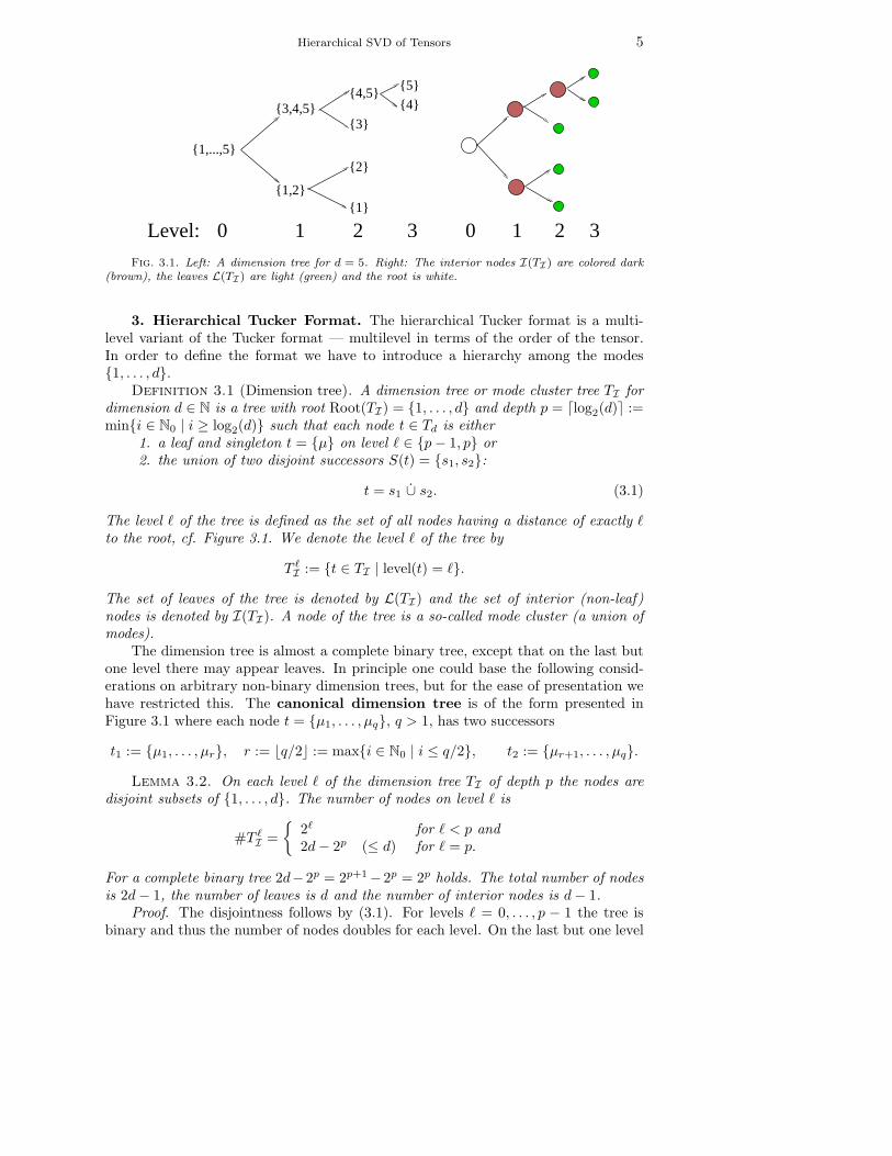
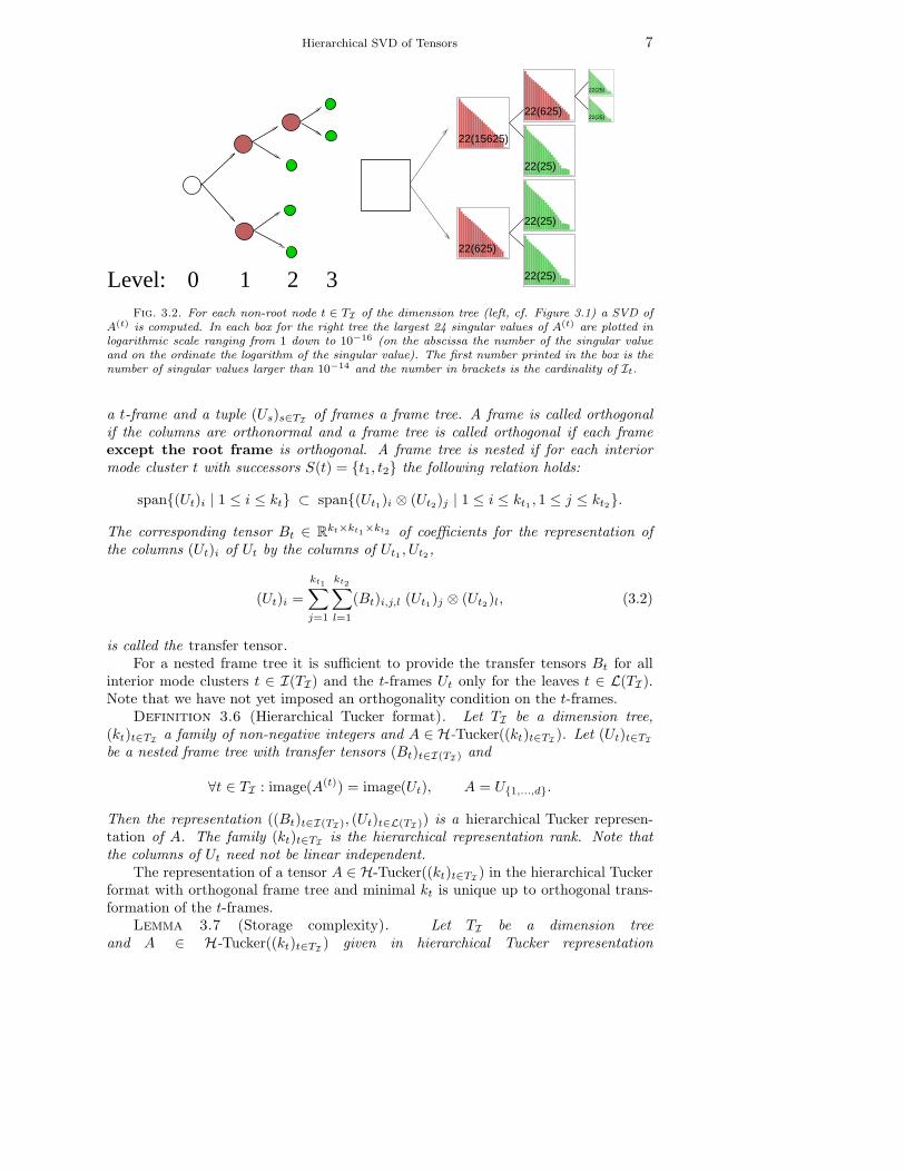
Fig. 3.1. Left: A dimension tree for d = 5. Right: The interior nodes I(TI) are colored dark(brown), the leaves L(TI) are light (green) and the root is white.

3. Hierarchical Tucker Format. The hierarchical Tucker format is a multi-level variant of the Tucker format — multilevel in terms of the order of the tensor.In order to define the format we have to introduce a hierarchy among the modes{1, . . . , d}.

Definition 3.1 (Dimension tree). A dimension tree or mode cluster tree TI fordimension d ∈ N is a tree with root Root(TI) = {1, . . . , d} and depth p = ⌈log2(d)⌉ :=min{i ∈ N0 | i ≥ log2(d)} such that each node t ∈ Td is either

1. a leaf and singleton t = {µ} on level ℓ ∈ {p− 1, p} or2. the union of two disjoint successors S(t) = {s1, s2}:

t = s1 ∪ s2. (3.1)

The level ℓ of the tree is defined as the set of all nodes having a distance of exactly ℓto the root, cf. Figure 3.1. We denote the level ℓ of the tree by

T ℓI := {t ∈ TI | level(t) = ℓ}.

The set of leaves of the tree is denoted by L(TI) and the set of interior (non-leaf)nodes is denoted by I(TI). A node of the tree is a so-called mode cluster (a union ofmodes).

The dimension tree is almost a complete binary tree, except that on the last butone level there may appear leaves. In principle one could base the following consid-erations on arbitrary non-binary dimension trees, but for the ease of presentation wehave restricted this. The canonical dimension tree is of the form presented inFigure 3.1 where each node t = {µ1, . . . , µq}, q > 1, has two successors

t1 := {µ1, . . . , µr}, r := ⌊q/2⌋ := max{i ∈ N0 | i ≤ q/2}, t2 := {µr+1, . . . , µq}.

Lemma 3.2. On each level ℓ of the dimension tree TI of depth p the nodes aredisjoint subsets of {1, . . . , d}. The number of nodes on level ℓ is

#T ℓI =

{2ℓ for ℓ < p and2d− 2p (≤ d) for ℓ = p.

For a complete binary tree 2d−2p = 2p+1−2p = 2p holds. The total number of nodesis 2d− 1, the number of leaves is d and the number of interior nodes is d− 1.

Proof. The disjointness follows by (3.1). For levels ℓ = 0, . . . , p − 1 the tree isbinary and thus the number of nodes doubles for each level. On the last but one level

6 L. GRASEDYCK

there are 2p−1 (disjoint) nodes, these can be either singletons (s) or two-element sets(t), thus #s + #t = 2p−1. The total number of modes is d, thus #s + 2#t = d.Together we have #t = d − 2p−1, i.e. 2#t = 2d − 2p nodes (singletons) on level p.The total number of nodes is

p−1∑

ℓ=0

2ℓ + 2d− 2p = 2p − 1 + 2d− 2p = 2d− 1.

Definition 3.3 (Matricization). For a mode cluster t in a dimension tree TI wedefine the complementary cluster t′ := {1, . . . , d} \ t,

It := ×µ∈t

Iµ, It′ := ×µ∈t′

Iµ,

and the corresponding t-matricization

Mt : RI → R

It×It′ , (Mt(A))(iµ)µ∈t,(iµ)µ∈t′:= A(i1,...,id),

where the special case is M∅(A) := M{1,...,d}(A) := A. We use the short notation

A(t) := Mt(A).We provide a simple example: let the tensor A be of the form

A = a⊗ b⊗ q ⊗ r ∈ RI1×I2×I3×I4 ,

where ⊗ denotes the usual outer product or tensor product

(x1 ⊗ · · · ⊗ xd)(i1,··· ,id) = (x1)i1 · · · · · (xd)id=

d∏

µ=1

(xµ)iµ.

Then the matricizations with respect to {1, 2} and {2, 3} are

A({1,2}) = (a⊗ b)(q ⊗ r)T ∈ R(I1×I2)×(I3×I4),

A({2,3}) = (b ⊗ q)(a⊗ r)T ∈ R(I2×I3)×(I1×I4).

Definition 3.4 (Hierarchical rank). Let TI be a dimension tree. The hierarchi-cal rank (kt)t∈TI

of a tensor A ∈ RI is defined by

∀t ∈ TI : kt := rank(A(t)).

The set of all tensors of hierarchical rank (node-wise) at most (kt)t∈TIis denoted by

H-Tucker((kt)t∈TI) := {A ∈ R

I | ∀t ∈ TI : rank(A(t)) ≤ kt}.

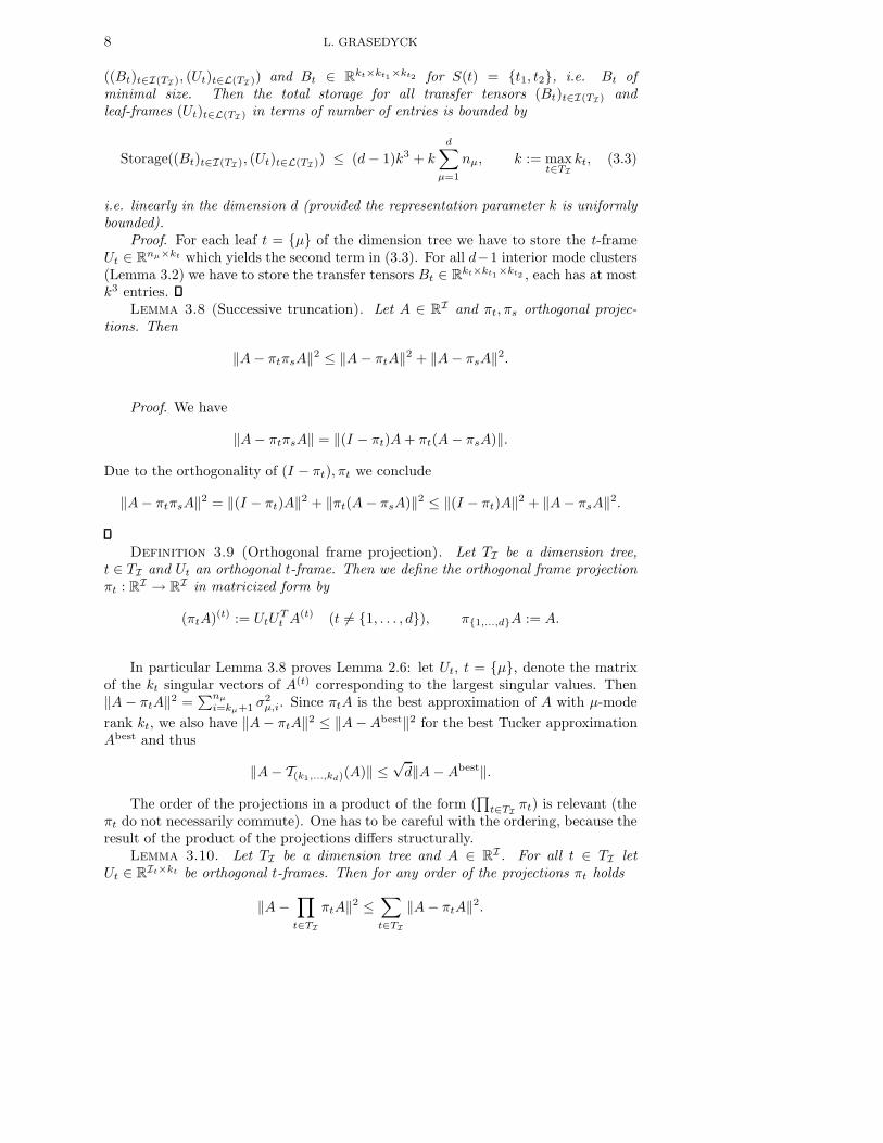
According to the definition of the hierarchical rank one can define the hierarchi-cal SVD by the node-wise SVDs of the matrices A(t), cf. Figure 3.2. However, itis not obvious why and how this should lead to an efficient representation and cor-respondingly efficient algorithms. Instead, we will introduce a nested representationand reveal the connection to the node-wise SVDs afterwards.

Definition 3.5 (Frame tree, t-frame, transfer tensor). Let t ∈ TI be a modecluster and (kt)t∈TI

a family of non-negative integers. We call a matrix Ut ∈ RIt×kt


3210Level:

22(625)

22(25)

22(25)

22(15625)

22(25)

22(625)22(25)

22(25)

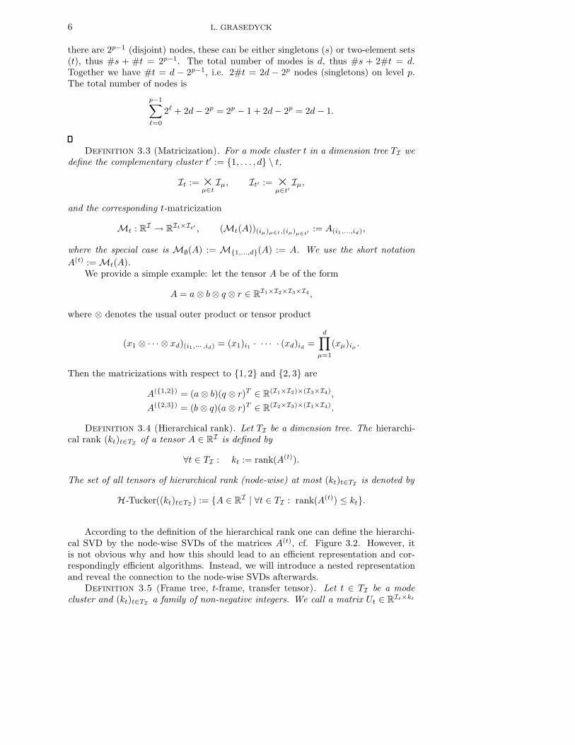
Fig. 3.2. For each non-root node t ∈ TI of the dimension tree (left, cf. Figure 3.1) a SVD ofA(t) is computed. In each box for the right tree the largest 24 singular values of A(t) are plotted inlogarithmic scale ranging from 1 down to 10−16 (on the abscissa the number of the singular valueand on the ordinate the logarithm of the singular value). The first number printed in the box is thenumber of singular values larger than 10−14 and the number in brackets is the cardinality of It.

a t-frame and a tuple (Us)s∈TIof frames a frame tree. A frame is called orthogonal

if the columns are orthonormal and a frame tree is called orthogonal if each frameexcept the root frame is orthogonal. A frame tree is nested if for each interiormode cluster t with successors S(t) = {t1, t2} the following relation holds:

span{(Ut)i | 1 ≤ i ≤ kt} ⊂ span{(Ut1)i ⊗ (Ut2)j | 1 ≤ i ≤ kt1 , 1 ≤ j ≤ kt2}.

The corresponding tensor Bt ∈ Rkt×kt1×kt2 of coefficients for the representation of

the columns (Ut)i of Ut by the columns of Ut1 , Ut2 ,

(Ut)i =

kt1∑

j=1

kt2∑

l=1

(Bt)i,j,l (Ut1)j ⊗ (Ut2)l, (3.2)

is called the transfer tensor.For a nested frame tree it is sufficient to provide the transfer tensors Bt for all

interior mode clusters t ∈ I(TI) and the t-frames Ut only for the leaves t ∈ L(TI).Note that we have not yet imposed an orthogonality condition on the t-frames.

Definition 3.6 (Hierarchical Tucker format). Let TI be a dimension tree,(kt)t∈TI

a family of non-negative integers and A ∈ H-Tucker((kt)t∈TI). Let (Ut)t∈TI

be a nested frame tree with transfer tensors (Bt)t∈I(TI) and

∀t ∈ TI : image(A(t)) = image(Ut), A = U{1,...,d}.

Then the representation ((Bt)t∈I(TI), (Ut)t∈L(TI)) is a hierarchical Tucker represen-tation of A. The family (kt)t∈TI

is the hierarchical representation rank. Note thatthe columns of Ut need not be linear independent.

The representation of a tensor A ∈ H-Tucker((kt)t∈TI) in the hierarchical Tucker

format with orthogonal frame tree and minimal kt is unique up to orthogonal trans-formation of the t-frames.

Lemma 3.7 (Storage complexity). Let TI be a dimension treeand A ∈ H-Tucker((kt)t∈TI

) given in hierarchical Tucker representation

8 L. GRASEDYCK

((Bt)t∈I(TI), (Ut)t∈L(TI)) and Bt ∈ Rkt×kt1×kt2 for S(t) = {t1, t2}, i.e. Bt of

minimal size. Then the total storage for all transfer tensors (Bt)t∈I(TI) andleaf-frames (Ut)t∈L(TI) in terms of number of entries is bounded by

Storage((Bt)t∈I(TI), (Ut)t∈L(TI)) ≤ (d− 1)k3 + k

d∑

µ=1

nµ, k := maxt∈TI

kt, (3.3)

i.e. linearly in the dimension d (provided the representation parameter k is uniformlybounded).

Proof. For each leaf t = {µ} of the dimension tree we have to store the t-frameUt ∈ R

nµ×kt which yields the second term in (3.3). For all d−1 interior mode clusters(Lemma 3.2) we have to store the transfer tensors Bt ∈ R

kt×kt1×kt2 , each has at mostk3 entries.

Lemma 3.8 (Successive truncation). Let A ∈ RI and πt, πs orthogonal projec-

tions. Then

‖A− πtπsA‖2 ≤ ‖A− πtA‖2 + ‖A− πsA‖2.

Proof. We have

‖A− πtπsA‖ = ‖(I − πt)A+ πt(A− πsA)‖.

Due to the orthogonality of (I − πt), πt we conclude

‖A− πtπsA‖2 = ‖(I − πt)A‖2 + ‖πt(A− πsA)‖2 ≤ ‖(I − πt)A‖2 + ‖A− πsA‖2.

Definition 3.9 (Orthogonal frame projection). Let TI be a dimension tree,t ∈ TI and Ut an orthogonal t-frame. Then we define the orthogonal frame projectionπt : R

I → RI in matricized form by

(πtA)(t) := UtUTt A

(t) (t 6= {1, . . . , d}), π{1,...,d}A := A.

In particular Lemma 3.8 proves Lemma 2.6: let Ut, t = {µ}, denote the matrixof the kt singular vectors of A(t) corresponding to the largest singular values. Then‖A− πtA‖2 =

∑nµ

i=kµ+1 σ2µ,i. Since πtA is the best approximation of A with µ-mode

rank kt, we also have ‖A− πtA‖2 ≤ ‖A−Abest‖2 for the best Tucker approximationAbest and thus

‖A− T(k1,...,kd)(A)‖ ≤√d‖A−Abest‖.

The order of the projections in a product of the form (∏

t∈TIπt) is relevant (the

πt do not necessarily commute). One has to be careful with the ordering, because theresult of the product of the projections differs structurally.

Lemma 3.10. Let TI be a dimension tree and A ∈ RI. For all t ∈ TI let

Ut ∈ RIt×kt be orthogonal t-frames. Then for any order of the projections πt holds

‖A−∏

t∈TI

πtA‖2 ≤∑

t∈TI

‖A− πtA‖2.


Proof. Apply Lemma 3.8 successively for all nodes of the dimension tree.Theorem 3.11 (Hierarchical truncation error). Let TI be a dimension tree and

A ∈ RI. Let Abest denote the best approximation of A in H-Tucker((kt)t∈I) and let πt

be the orthogonal frame projection for the t-frame Ut that consists of the left singularvectors of A(t) corresponding to the kt largest singular values σt,i of A(t). Then forany order of the projections πt, t ∈ TI, holds

‖A−∏

t∈TI

πtA‖ ≤√∑

t∈TI

∑

i>kt

σ2t,i ≤

√2d− 2‖A−Abest‖.

Proof. For any of the projections holds ‖A − πtA‖2 =∑

i>ktσ2

t,i ≤ ‖A− Abest‖and for the root ‖A− π{1,...,d}A‖ = 0 (w.l.o.g. k{1,...,d} = 1). Applying Lemma 3.10and Lemma 3.2 yields

‖A−∏

t∈TI

πtA‖2 ≤∑

t∈TI

∑

i>kt

σ2t,i ≤ (2d− 2)‖A−Abest‖2.

Remark 3.12. The estimate given in the previous theorem is not optimal andit can be improved as follows: for the root t of the dimension tree and its successorst1, t2 one can combine both projections πt1 .πt2 into a single projection via the SVD.This combined projection (with the pairs of the singular vectors) then has the sameerror as any of the two projections πt1 or πt2 . Thereby, the error of the truncationcan be estimated by

‖A−∏

t∈TI

πtA‖ ≤√

2d− 3‖A−Abest‖.

In dimension d = 2 this coincides with the SVD estimate and in d = 3 this coincideswith the original one-level Tucker estimate by De Lathauwer et al.

Definition 3.13 (Kronecker product). The Kronecker product A ⊗K B of twomatrices A ∈ R

I×J , B ∈ RK×L is defined by

(A⊗K B)(i,k),(j,ℓ) := Ai,jBk,ℓ, A⊗K B ∈ R(I×K)×(J×L).

Example 3.14 (Increasing the rank by projection). We consider the tensorA ∈ R

3×3×3 in matricized form

A({1,2}) :=[u1 ⊗ q1 u2 ⊗ q2 u1 ⊗ q2

], A

({1,2})(i,j),ℓ =

(u1 ⊗ q1)i,j if ℓ = 1(u2 ⊗ q2)i,j if ℓ = 2(u1 ⊗ q2)i,j if ℓ = 3

with vectors

u1 =

100

, u2 =

010

, q1 =

1/

√2

0

1/√

2

, q2 =

010

.

The mode cluster t = {1, 2} has the two successors t1 = {1}, t2 = {2} and we considerthe orthogonal mode frames

Ut :=[u1 ⊗ q1 u2 ⊗ q2 q1 ⊗ q2

], Ut1 :=

[u1 u2

], Ut2 :=

[q1 q2

].

10 L. GRASEDYCK

Clearly, πt1 will project to t1-rank rank((πt1A)(1)) = 2. We will now show that therank is at least 3 if we apply all three projectors. The matrix Q for the projectionπt1πt2 is given by the Kronecker product

Q = Ut1UTt1 ⊗K Ut2U

Tt2 = (u1u

T1 + u2u

T2 ) ⊗K (q1q

T1 + q2q

T2 ).

We thus obtain

QUt =[u1 ⊗ q1 u2 ⊗ q2

1√2u1 ⊗ q2

].

The combined projection reads

(πtπt1πt2A)({1,2}) = UtUTt QA

({1,2}) = Ut(QUt)TA({1,2})

= Ut

[u1 ⊗ q1 u2 ⊗ q2

1√2u1 ⊗ q2

]TA({1,2})

= Ut

1 0 00 1 00 0 1√

2

=[u1 ⊗ q1 u2 ⊗ q2

1√2q1 ⊗ q2

].

The matricization with respect to t1 = {1} is of rank three,

(πtπt1πt2A)(1) =[u1q

T1 u2q

T2 q1(

1√2q2)

T],

because u1, u2, q1 are linearly independent. We conclude: the first projection πt1πt2

maps A into Tucker(2, 2, 3), but after the coarser projection πt the 1-mode rank isthree and thus πtπt1πt2A 6∈ Tucker(2, 2, 3). This is because πt mixes the t1-frame andthe t2-frame.

Lemma 3.15 (Structure of the hierarchical truncation). Let TI be a dimen-sion tree of depth p, A ∈ R

I and (kt)t∈I a family of non-negative integers. Let(Ut)t∈TI

, Ut ∈ RIt×kt , be an orthogonal frame tree (not necessarily nested). Then the

tensor

AH :=∏

t∈T p

I

πt · · ·∏

t∈T 1I

πtA

belongs to H-Tucker((kt)t∈I).Proof. We define the tensors

AH,ℓ :=∏

t∈T ℓI

πt · · ·∏

t∈T 1I

πtA.

We prove rank(A(t)H,ℓ) ≤ kt for all t ∈ TI with level(t) ≤ ℓ by induction over the level

ℓ = 1, . . . , p. Level ℓ = 1 is the Tucker truncation and thus the statement is true forℓ = 1. Now let ℓ > 1 and assume that

∀t ∈ TI , level(t) ≤ ℓ− 1 : rank(A(t)H,ℓ−1) ≤ kt.

By construction

AH,ℓ =∏

t∈T ℓI

πtAH,ℓ−1.


This is the Tucker truncation on level ℓ applied to AH,ℓ−1 and thus for all t ∈ T ℓI on

level ℓ the rank bound is fulfilled. It remains to show that for all levels 0, . . . , ℓ−1 therank bound is (still) fulfilled, i.e., that the rank is not increased by the projections on

level ℓ. Now let t ∈ T jI , j < ℓ. Let s ∈ T ℓ

I . We will show that the rank of A(t)H,ℓ−1 is

not increased by the projection πs. Due to the tree structure s is either a subset of tor they are disjoint.Case s ⊂ t: Let s := t \ s. Then the projection πs is of the matricized form

(πsA)(t) =(UsU

Ts ⊗K I

)A(t)

with I being the Is × Is identity. The rank is not increased by the multiplication.Case s∩t = ∅: Let s := {1, . . . , d}\(t∪s). Then the projection πs is of the matricizedform

(πsA)(t) = A(t)(UsU

Ts ⊗K I

)

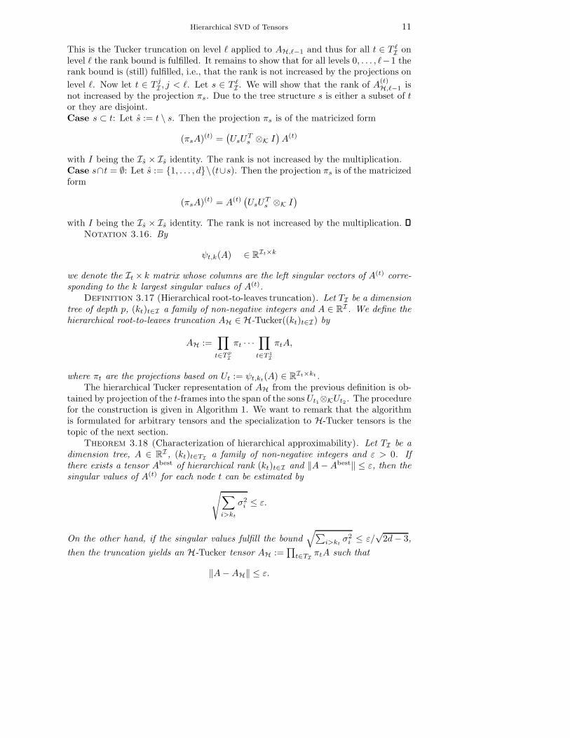
with I being the Is × Is identity. The rank is not increased by the multiplication.Notation 3.16. By

ψt,k(A) ∈ RIt×k

we denote the It × k matrix whose columns are the left singular vectors of A(t) corre-sponding to the k largest singular values of A(t).

Definition 3.17 (Hierarchical root-to-leaves truncation). Let TI be a dimensiontree of depth p, (kt)t∈I a family of non-negative integers and A ∈ R

I . We define thehierarchical root-to-leaves truncation AH ∈ H-Tucker((kt)t∈I) by

AH :=∏

t∈T p

I

πt · · ·∏

t∈T 1I

πtA,

where πt are the projections based on Ut := ψt,kt(A) ∈ R

It×kt .The hierarchical Tucker representation of AH from the previous definition is ob-

tained by projection of the t-frames into the span of the sons Ut1⊗KUt2 . The procedurefor the construction is given in Algorithm 1. We want to remark that the algorithmis formulated for arbitrary tensors and the specialization to H-Tucker tensors is thetopic of the next section.

Theorem 3.18 (Characterization of hierarchical approximability). Let TI be adimension tree, A ∈ R

I , (kt)t∈TIa family of non-negative integers and ε > 0. If

there exists a tensor Abest of hierarchical rank (kt)t∈I and ‖A−Abest‖ ≤ ε, then thesingular values of A(t) for each node t can be estimated by

√∑

i>kt

σ2i ≤ ε.

On the other hand, if the singular values fulfill the bound√∑

i>ktσ2

i ≤ ε/√

2d− 3,

then the truncation yields an H-Tucker tensor AH :=∏

t∈TIπtA such that

‖A−AH‖ ≤ ε.

12 L. GRASEDYCK

Proof. The second part is proven by Theorem 3.11. The first part follows from thefact that (Abest)(t) is a rank kt approximation of A(t) with ‖A(t) − (Abest)(t)‖F ≤ ε.

In Algorithm 1 we provide a method for the truncation of an arbitrary tensor tohierarchical rank (kt)t∈TI

, of course one can as well prescribe node-wise tolerances εt

for the truncation of singular values: according to Theorem 3.18 one can prescribenode-wise tolerance ε/

√2d− 2 in order to obtain a guaranteed error bound of ‖A−

AH‖ ≤ ε. The complexity of Algorithm 1 is estimated in Lemma 3.19.

Algorithm 1 Root-to-leaves truncation of arbitrary tensors to H-Tucker format

Require: Input tensor A ∈ RI , dimension tree TI (depth p > 0), target representa-

tion rank (kt)t∈TI.

for each singleton t ∈ L(TI) do

Compute an SVD of A(t) and store the dominant kt left singular vectors in thecolumns of the t-frame Ut.

end for

for ℓ = p− 1, . . . , 0 do

for each mode cluster t ∈ I(TI) on level ℓ do

Compute an SVD of A(t) and store the dominant kt left singular vectors in thecolumns of the t-frame Ut.Let Ut1 and Ut2 denote the frames for the successors of t on level ℓ+1. Computethe entries of the transfer tensor:

(Bt)i,j,ν := 〈(Ut)i, (Ut1)j ⊗ (Ut2)ν〉

end for

end for

Compute the entries of the root (with sons t1, t2) transfer tensor:

(B{1,...,d})1,j,ν := 〈(A, (Ut1)j ⊗ (Ut2)ν〉

return H-Tucker representation ((Ut)t∈L(TI), (Bt)t∈I(TI)) for AH ∈H-Tucker((kt)t∈TI

)).

Lemma 3.19 (Complexity of Algorithm 1). The complexity of Algorithm 1 for a

tensor A ∈ RI and dimension tree TI of depth p > 0 is in O

((∏dµ=1 nµ

)3/2)

.

Proof. We have to compute singular value decompositions for all A(t), and thosedecompositions have a complexity of O(min(#It,#It′)

2 max(#It,#It′)), where t′ isthe complementary mode cluster t′ := {1, . . .} \ t. Without loss of generality we canassume nµ ≥ 2 for all modes µ. Then the complexity of the SVD for the root is zero,that for the two successors t, t′ of the root is

CSV D(min(#It,#It′)2 max(#It,#It′)) ≤ CSV D

(d∏

µ=1

nµ

)3/2

,

where CSV D is a universal constant for the SVD. For each further level there are atmost two times more nodes, but the cardinality of It, It′ is reduced by at least a factorof two (nµ ≥ 2) so that the complexity for the SVDs is quartered. Therefore the total


complexity is bounded by

p∑

ℓ=0

2−ℓCSV D

(d∏

µ=1

nµ

)3/2

≤ 2CSV D

(d∏

µ=1

nµ

)3/2

.

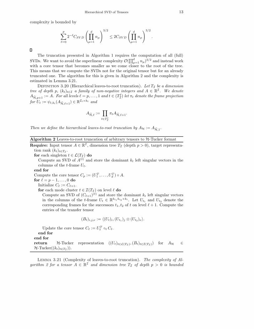
The truncation presented in Algorithm 1 requires the computation of all (full)

SVDs. We want to avoid the superlinear complexity O(∏d

µ=1 nµ)3/2 and instead workwith a core tensor that becomes smaller as we come closer to the root of the tree.This means that we compute the SVDs not for the original tensor but for an alreadytruncated one. The algorithm for this is given in Algorithm 2 and the complexity isestimated in Lemma 3.21.

Definition 3.20 (Hierarchical leaves-to-root truncation). Let TI be a dimensiontree of depth p, (kt)t∈I a family of non-negative integers and A ∈ R

I . We denoteA eH,p+1 := A. For all levels ℓ = p, . . . , 1 and t ∈ (T ℓ

I) let πt denote the frame projection

for Ut := ψt,kt(A eH,ℓ+1) ∈ R

It×kt and

A eH,ℓ :=∏

t∈T ℓI

πtA eH,ℓ+1.

Then we define the hierarchical leaves-to-root truncation by AH := A eH,1.

Algorithm 2 Leaves-to-root truncation of arbitrary tensors to H-Tucker format

Require: Input tensor A ∈ RI , dimension tree TI (depth p > 0), target representa-

tion rank (kt)t∈TI.

for each singleton t ∈ L(TI) do

Compute an SVD of A(t) and store the dominant kt left singular vectors in thecolumns of the t-frame Ut.

end for

Compute the core tensor Cp := (UT1 , . . . , U

Td ) ◦A.

for ℓ = p− 1, . . . , 0 do

Initialize Cℓ := Cℓ+1.for each mode cluster t ∈ I(TI) on level ℓ do

Compute an SVD of (Cℓ+1)(t) and store the dominant kt left singular vectors

in the columns of the t-frame Ut ∈ Rkt1kt2×kt . Let Ut1 and Ut2 denote the

corresponding frames for the successors t1, t2 of t on level ℓ+ 1. Compute theentries of the transfer tensor

(Bt)i,j,ν := 〈(Ut)i, (Ut1)j ⊗ (Ut2)ν〉.

Update the core tensor Cℓ := UTt ◦t Cℓ.

end for

end for

return H-Tucker representation ((Ut)t∈L(TI), (Bt)t∈I(TI)) for AH ∈H-Tucker((kt)t∈TI

)).

Lemma 3.21 (Complexity of leaves-to-root truncation). The complexity of Al-gorithm 2 for a tensor A ∈ R

I and dimension tree TI of depth p > 0 is bounded

14 L. GRASEDYCK

by

O(

d∑

µ=1

nµ

d∏

ν=1

nν + dk2d∏

ν=1

nν

), k := max

t∈TI

kt.

Proof. For all leaves t = {µ} we have to compute the singular value decomposi-tions of A(µ) which is of complexity (CSV D being again the generic constant for theSVD)

d∑

µ=1

CSV D n2µ

∏

ν 6=µ

nν = CSV D

d∑

µ=1

nµ

d∏

ν=1

nν .

For all other levels ℓ = 0, . . . , p − 1 we have to compute SVDs of matrices of size atmost kt1kt2 ×

∏ν 6∈t nν . The complexity for this is at most

CSV Dk2t1k

2t2

∏

ν 6∈t

nν ≤ CSV Dkt1kt2

d∏

ν=1

nν ≤ CSV Dk2

d∏

ν=1

nν .

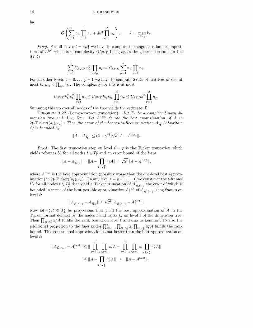
Summing this up over all nodes of the tree yields the estimate.Theorem 3.22 (Leaves-to-root truncation). Let TI be a complete binary di-

mension tree and A ∈ RI. Let Abest denote the best approximation of A in

H-Tucker((kt)t∈I). Then the error of the Leaves-to-Root truncation A eH (Algorithm2) is bounded by

‖A−A eH‖ ≤ (2 +√

2)√d‖A−Abest‖.

Proof. The first truncation step on level ℓ = p is the Tucker truncation whichyields t-frames Ut for all nodes t ∈ T ℓ

I and an error bound of the form

‖A−A eH,p‖ = ‖A−∏

t∈T pI

πtA‖ ≤√

2p‖A−Abest‖,

where Abest is the best approximation (possibly worse than the one-level best approx-imation) in H-Tucker((kt)t∈I). On any level ℓ = p−1, . . . , 0 we construct the t-framesUt for all nodes t ∈ T ℓ

I that yield a Tucker truncation of A eH,ℓ+1 the error of which is

bounded in terms of the best possible approximation Abestℓ of A eH,ℓ+1 using frames on

level ℓ:

‖A eH,ℓ+1 −A eH,ℓ‖ ≤√

2ℓ‖A eH,ℓ+1 −Abestℓ ‖.

Now let π∗t , t ∈ T ℓ

I be projections that yield the best approximation of A in theTucker format defined by the nodes t and ranks kt on level ℓ of the dimension tree.Then

∏t∈T ℓ

I

π∗tA fulfills the rank bound on level ℓ and due to Lemma 3.15 also the

additional projection to the finer nodes∏p

i=ℓ+1

∏t∈T i

I

πt

∏t∈T ℓ

I

π∗tA fulfills the rank

bound. This constructed approximation is not better than the best approximation onlevel ℓ:

‖A eH,ℓ+1 −Abestℓ ‖ ≤ ‖

p∏

i=ℓ+1

∏

t∈T iI

πtA−p∏

i=ℓ+1

∏

t∈T iI

πt

∏

t∈T ℓI

π∗tA‖

≤ ‖A−∏

t∈T ℓI

π∗tA‖ ≤ ‖A−Abest‖.


Thus we can estimate

‖A−A eH‖ ≤ ‖A−A eH,p‖ +

p−1∑

ℓ=1

‖A eH,ℓ+1 −A eH,ℓ‖

≤ (√

2p +

p−1∑

ℓ=1

√2ℓ)‖A−Abest‖ ≤ (2 +

√2)√d‖A−Abest‖.

4. Truncation of Hierarchical Tucker Tensors. In this Section we want toderive an efficient realization of the truncation procedures from the previous sectionfor the special case that the input tensor is already given in a data-sparse format,namely the hierarchical Tucker format.

Definition 4.1 (Brother of a mode cluster). Let TI be a dimension tree andt ∈ TI a non-root mode cluster with father f . Then we define the unique mode clustert ∈ TI such that f = t ∪ t as the brother of t.

Lemma 4.2. Let TI be a dimension tree and t ∈ I(TI) an interior node with twosuccessors t = t1∪t2. Further, let

A(t) =

k∑

ν=1

uνvTν

be a matricization of A. Let

uν =

k1∑

j=1

k2∑

l=1

cν,j,lxj ⊗ yl, xj ∈ RIt1 , yl ∈ R

It2 , ν = 1, . . . , k

be a representation of the uν . Then the matricization of A with respect to t1 is givenby

A(t1) =

k1∑

j=1

xj

(k∑

ν=1

k2∑

l=1

cν,j,lyl ⊗ vν

)T

.

Proof. For the first matricization holds

A(i1,...,id) = A(t)(iµ)µ∈t,(iµ)µ∈t′

=

k∑

ν=1

k1∑

j=1

k2∑

l=1

cν,j,l(xj)(iµ)µ∈t1(yl)(iµ)µ∈t2

(vν)(iµ)µ∈t′

=

k1∑

j=1

(xj)(iµ)µ∈t1

(k∑

ν=1

k2∑

l=1

cν,j,l(yl)(iµ)µ∈t2(vν)(iµ)µ∈t′

)

=

k1∑

j=1

(xj)(iµ)µ∈t1

(k∑

ν=1

k2∑

l=1

cν,j,lyl ⊗ vν

)

(iµ)µ∈t′1

.

Lemma 4.3 (Matricization of tensors in hierarchical Tucker format). Let TIbe a dimension tree, A ∈ H-Tucker((kt)t∈I) with nested orthogonal frame tree

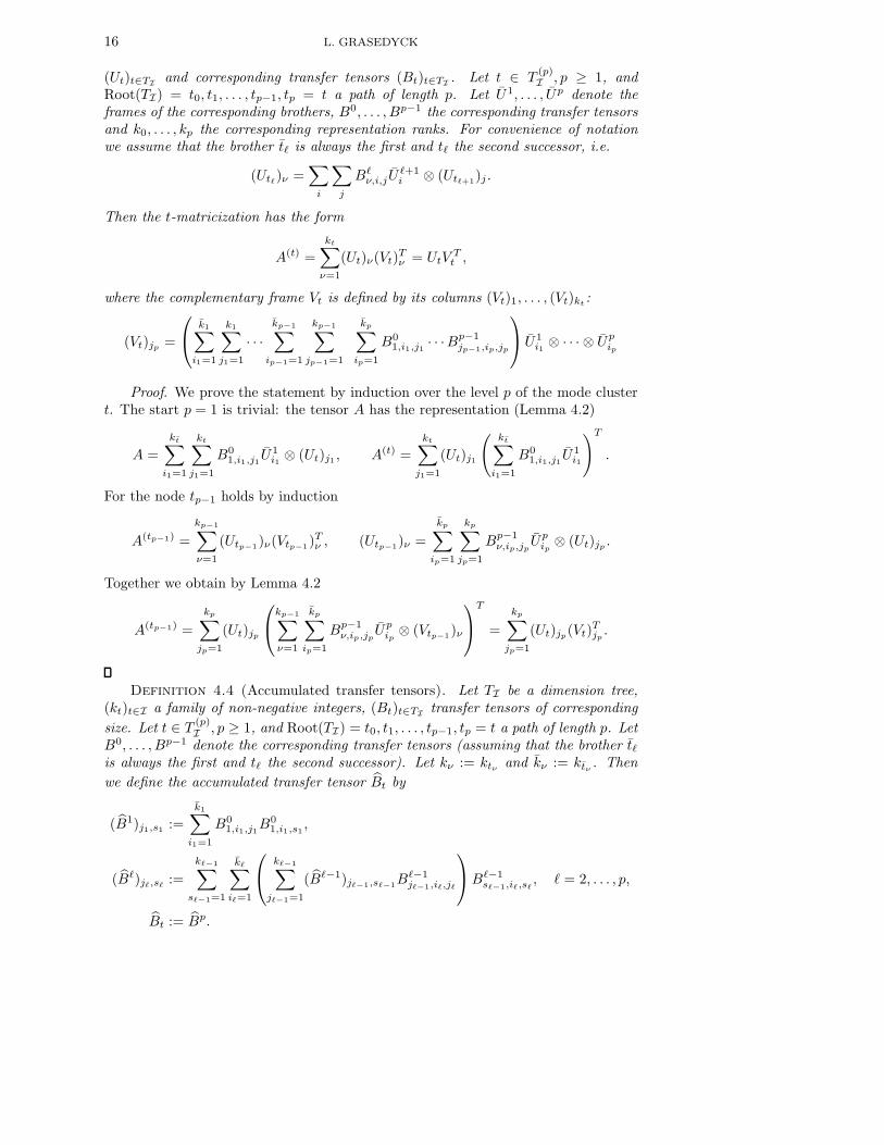
16 L. GRASEDYCK

(Ut)t∈TIand corresponding transfer tensors (Bt)t∈TI

. Let t ∈ T(p)I , p ≥ 1, and

Root(TI) = t0, t1, . . . , tp−1, tp = t a path of length p. Let U1, . . . , Up denote theframes of the corresponding brothers, B0, . . . , Bp−1 the corresponding transfer tensorsand k0, . . . , kp the corresponding representation ranks. For convenience of notationwe assume that the brother tℓ is always the first and tℓ the second successor, i.e.

(Utℓ)ν =

∑

i

∑

j

Bℓν,i,jU

ℓ+1i ⊗ (Utℓ+1

)j .

Then the t-matricization has the form

A(t) =

kt∑

ν=1

(Ut)ν(Vt)Tν = UtV

Tt ,

where the complementary frame Vt is defined by its columns (Vt)1, . . . , (Vt)kt:

(Vt)jp=

k1∑

i1=1

k1∑

j1=1

· · ·kp−1∑

ip−1=1

kp−1∑

jp−1=1

kp∑

ip=1

B01,i1,j1 · · ·B

p−1jp−1,ip,jp

U1i1 ⊗ · · · ⊗ Up

ip

Proof. We prove the statement by induction over the level p of the mode clustert. The start p = 1 is trivial: the tensor A has the representation (Lemma 4.2)

A =

kt∑

i1=1

kt∑

j1=1

B01,i1,j1 U

1i1 ⊗ (Ut)j1 , A(t) =

kt∑

j1=1

(Ut)j1

(kt∑

i1=1

B01,i1,j1 U

1i1

)T

.

For the node tp−1 holds by induction

A(tp−1) =

kp−1∑

ν=1

(Utp−1)ν(Vtp−1)Tν , (Utp−1)ν =

kp∑

ip=1

kp∑

jp=1

Bp−1ν,ip,jp

Upip⊗ (Ut)jp

.

Together we obtain by Lemma 4.2

A(tp−1) =

kp∑

jp=1

(Ut)jp

kp−1∑

ν=1

kp∑

ip=1

Bp−1ν,ip,jp

Upip⊗ (Vtp−1)ν

T

=

kp∑

jp=1

(Ut)jp(Vt)

Tjp.

Definition 4.4 (Accumulated transfer tensors). Let TI be a dimension tree,(kt)t∈I a family of non-negative integers, (Bt)t∈TI

transfer tensors of corresponding

size. Let t ∈ T(p)I , p ≥ 1, and Root(TI) = t0, t1, . . . , tp−1, tp = t a path of length p. Let

B0, . . . , Bp−1 denote the corresponding transfer tensors (assuming that the brother tℓis always the first and tℓ the second successor). Let kν := ktν

and kν := ktν. Then

we define the accumulated transfer tensor Bt by

(B1)j1,s1 :=

k1∑

i1=1

B01,i1,j1B

01,i1,s1

,

(Bℓ)jℓ,sℓ:=

kℓ−1∑

sℓ−1=1

kℓ∑

iℓ=1

kℓ−1∑

jℓ−1=1

(Bℓ−1)jℓ−1,sℓ−1Bℓ−1

jℓ−1,iℓ,jℓ

Bℓ−1sℓ−1,iℓ,sℓ

, ℓ = 2, . . . , p,

Bt := Bp.


Remark 4.5. The first accumulated tensors Bt1 , Bt2 for the two sons of the roott can be computed in O(kt1k

2t2 + k2

t1kt2). For each further node the second formula inDefinition 4.4 has to be applied and it involves inside the bracket a matrix multiplica-tion of complexity O(k2

t kt1kt2) for each son and the outer multiplication of complexityO(ktkt1k

2t2 + ktk

2t1kt2). For all nodes of the tree this sums up to

O

∑

t∈I(TI)

ktkt1k2t2 + ktk

2t1kt2

= O(dmax

t∈TI

k4t

).

Lemma 4.6 (Gram matrices of complementary frames). Let TI be a dimensiontree, A ∈ H-Tucker((kt)t∈I) with nested orthogonal frame tree (Ut)t∈TI

and corre-sponding transfer tensors (Bt)t∈TI

. For each t ∈ TI let Vt be the complementary

frame from Lemma 4.3. Then Bt is the Gram matrix for Vt:

V Tt Vt = Bt, 〈(Vt)ν , (Vt)µ〉 = (Bt)ν,µ.

Proof. We use the definitions and notations from Lemma 4.3. According toLemma 4.3 and due to the orthogonality of each of the tℓ-frames U ℓ we obtain

〈(Vt)ν , (Vt)µ〉 =

k1∑

i1=1

k1∑

j1=1

k1∑

s1=1

· · ·kp−1∑

ip−1=1

kp−1∑

jp−1=1

kp−1∑

sp−1=1

kp∑

ip=1

B01,i1,j1 · · ·B

p−2jp−2,ip−1,jp−1

Bp−1jp−1,ip,νB

01,i1,s1

· · ·Bp−2sp−2,ip−1,sp−1

Bp−1sp−1,ip,µ

=

k1∑

i1=1

k1∑

j1=1

k1∑

s1=1

k2∑

i2=1

· · ·kp−1∑

jp−1=1

kp−1∑

sp−1=1

kp∑

ip=1

B01,i1,j1B

01,i1,s1

· · ·Bp−2jp−2,ip−1,jp−1

Bp−2sp−2,ip−1,sp−1

Bp−1jp−1,ip,νB

p−1sp−1,ip,µ

= (Bt)ν,µ.

According to the previous Lemma we can easily compute the left singular vectorsof V T

t which are the eigenvectors of the kt × kt matrix Bt. The matrix Qt of singularvectors is the transformation matrix such that UtQt is the matrix of the left singularvectors of A(t) the singular values of which are the square roots of the eigenvaluesof Bt. Thus, one can truncate either to fixed rank or one can determine the rankadaptively in order to guarantee a truncation accuracy of ε.

The nested mode frames were required to be orthogonal. If this is not yet thecase, one has to orthogonalize the frame tree. The procedure for this is explainednext and the complexity is estimated afterwards.

Lemma 4.7 (Frame transformation). Let t ∈ TI be a mode cluster with t-frameUt, transfer tensor Bt and two sons t1, t2 with frames Ut1 , Ut2 , such that the columnsfulfill

(Ut)i =

k1∑

j=1

k2∑

l=1

(Bt)i,j,l(Ut1)j ⊗ (Ut2)l, i = 1, . . . , k.

18 L. GRASEDYCK

Let X ∈ Rk×k, Y ∈ R

k1×k1 , Z ∈ Rk2×k2 and Y, Z invertible. Then we can rewrite the

transformed frames as

(UtX)i =

k′

1∑

j=1

k′

2∑

l=1

(B′t)i,j,l(Ut1Y )j ⊗ (Ut2Z)l, B′

t := (XT , Y −1, Z−1) ◦Bt.

Proof. The formula follows from elementary matrix multiplications.

Algorithm 3 Orthogonalization of hierarchical Tucker tensors

Require: Input tensor AH ∈ H-Tucker((kt)t∈TI) represented by

((Ut)t∈L(TI), (Bt)t∈I(TI)).for each singleton t ∈ L(TI) do

Compute a QR-decomposition of the t-frame Ut and define

Ut := Q, Bf :=

{(I, I, R) ◦Bf if t is the second successor,(I, R, I) ◦Bf if t is the first successor

for the father f of t.end for

for each mode cluster t ∈ I(TI) \ {root(TI)} do

Compute a QR-decomposition of (Bt)({1,2}),

(Bt)({1,2}) = (Qt)

({1,2})R,

and set

Bt := Qt, Bf :=

{(I, I, R) ◦Bf if t is the second successor,(I, R, I) ◦Bf if t is the first successor

of the father f of t.end for

return nested orthogonal frames (Ut)t∈L(TI) and transfer tensors (Bt)t∈I(TI).

Lemma 4.8 (Complexity for the orthogonalization of nested frame trees). Thecomplexity of Algorithm 3 for a tensor AH ∈ H-Tucker((kt)t∈TI

) with nested frames(Ut)t∈L(TI) and transfer tensors (Bt)t∈I(TI) is bounded by

O

d∑

µ=1

nµk2µ +

∑

t∈I(TI),Sons(t)={t1,t2}k2

t kt1kt2 + ktk2t1kt2 + ktkt1k

2t2

.

Proof. For each interior node we have to compute QR decompositions whichare of complexity O(k2

t kt1kt2) and perform two mode multiplications X ◦µ Bf , µ =2, 3, which is of complexity O(ktk

2t1kt2 + ktkt1k

2t2). For the leaves t = {µ} a QR-

factorization is of complexity O(nµk2µ). The sum over all nodes of the tree yields the

desired bound.

Lemma 4.9 (Complexity for the H-Tucker truncation). The complexity forthe truncation of an H-Tucker((kt)t∈TI

)-Tensor A (not necessarily with orthogonal


frames) to lower rank is

O(dmaxt∈TI

k4t +

d∑

µ=1

nµk2µ).

Definition 4.10 (CANDECOMP, PARAFAC, Elementary Tensor Sum). LetA ∈ R

I. The minimal number k ≥ 0 such that

A =k∑

i=1

Ai, Ai = ai,1 ⊗ · · · ⊗ ai,d, ai,µ ∈ RIµ, (4.1)

is the tensor rank or canonical rank of A. The rank one tensors Ai are called elemen-tary tensors. A sum of the form (4.1) with arbitrary k ≥ 0 is called an elementarytensor sum with representation rank k. In the literature the alternative names CAN-DECOMP [3] or PARAFAC [11] or CP are commonly used.

Remark 4.11 (Conversion of elementary tensor sums to H-Tucker format). LetA ∈ R

I be a tensor represented by an elementary tensor sum

A =k∑

i=1

d⊗

µ=1

ai,µ, ai,µ ∈ RIµ .

Then A can immediately be represented in the hierarchical Tucker format by the t-frames

∀t = {µ} ∈ L(TI) : (Ut)i := ai,µ, i = 1, . . . , k, kµ := k,

and the transfer tensors

∀t ∈ I(TI) \ Root(TI) : (Bt)i,j,l :=

{1 if i = j = l0 otherwise,

, Bt ∈ Rk×k×k, kt := k.

The root transfer tensor is

(B{1,...,d})1,j,l :=

{1 if j = l0 otherwise,

, B{1,...,d} ∈ R1×k×k, k{1,...,d} := 1.

The frames are not yet orthogonal, so a subsequent orthogonalization and truncationis advisable to find a reduced representation. If we store the transfer tensors in sparseformat, then the amount of storage is k(d− 1) + k

∑dµ=1 nµ, i.e. almost the same as

for a tensor represented as an elementary tensor sum.The opposite conversion from H-Tucker to elementary tensor sums with (almost)

minimal representation rank k is highly non-trivial.

5. Comparison with other Formats. As mentioned in the introduction thehierarchical Tucker format is identical or similar to several other tensor formats.

5.1. Sequential Unfolding SVD, PARATREE. The sequential unfoldingSVD or PARATREE from [16] is defined quite similarly as the H-Tucker format. Thefirst separation is via the SVD of the familiar form

A =

r∑

i1=1

U1,i1 ⊗ U2,i1

20 L. GRASEDYCK

Each of the Uν,i1 (ν = 1, 2) on level 1 is then again split via the SVD into

Uν,i1 =

r∑

i2=1

Uν,i1,1,i2 ⊗ Uν,i1,2,i2 ,

i.e., for each i1 a different set of vectors Uν,i1,1,i2 , Uν,i1,2,i2 is used. Each of the vectorsis then split on level ℓ = 2, . . . separately. On level ℓ the frames are indexed by

Uν1,i1,...,νℓ,iℓ.

Thus, the complexity is no longer linear in the dimension d but scales exponentiallyin the depth of the tree.

5.2. Hierarchical MCTDH and Φ-System. The hierarchical or multilayerformat from [1, 18] is exactly of the H-Tucker form. This format is used in the Multi-Configuration Time-Dependent Hartree method (MCTDH) and to the best of ourknowledge this is the first occurrence of a hierarchical tensor format.

The Φ-system representation from [10] is identical to the H-Tucker-representation.In fact, it has been the starting point for our work and for writing this article.

The here presented analysis and hierarchical SVD, as well as the (almost best)truncation with a priori error estimate is thus a framework to perform arithmetics inthe hierarchical MCTDH formulation and for Φ-system representations.

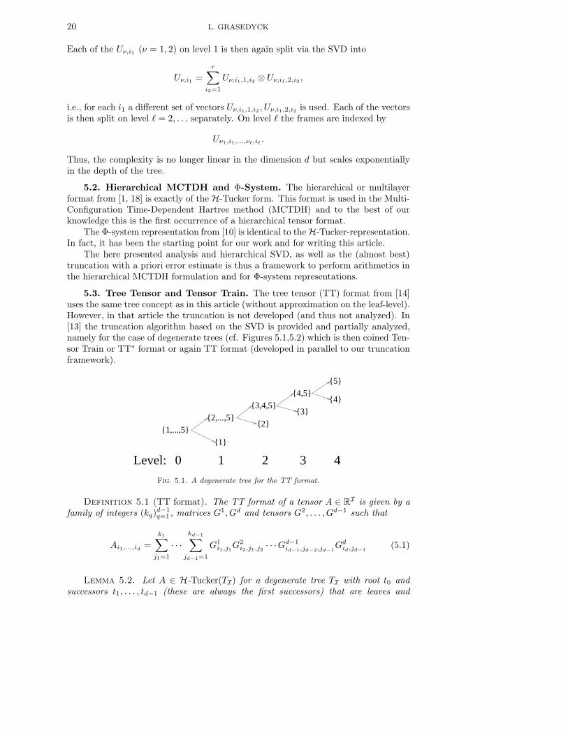
5.3. Tree Tensor and Tensor Train. The tree tensor (TT) format from [14]uses the same tree concept as in this article (without approximation on the leaf-level).However, in that article the truncation is not developed (and thus not analyzed). In[13] the truncation algorithm based on the SVD is provided and partially analyzed,namely for the case of degenerate trees (cf. Figures 5.1,5.2) which is then coined Ten-sor Train or TT∗ format or again TT format (developed in parallel to our truncationframework).

{1,...,5}

{2,...,5}

{1}

{3,4,5}

{2}

{4,5}

{3}

{5}

{4}

43210Level:

Fig. 5.1. A degenerate tree for the TT format.

Definition 5.1 (TT format). The TT format of a tensor A ∈ RI is given by a

family of integers (kq)d−1q=1 , matrices G1, Gd and tensors G2, . . . , Gd−1 such that

Ai1,...,id=

k1∑

j1=1

· · ·kd−1∑

jd−1=1

G1i1,j1G

2i2,j1,j2 · · ·Gd−1

id−1,jd−2,jd−1Gd

id,jd−1(5.1)

Lemma 5.2. Let A ∈ H-Tucker(TI) for a degenerate tree TI with root t0 andsuccessors t1, . . . , td−1 (these are always the first successors) that are leaves and


t0

t1

t1 t2

t2

td−1

td−1

0Level:

...

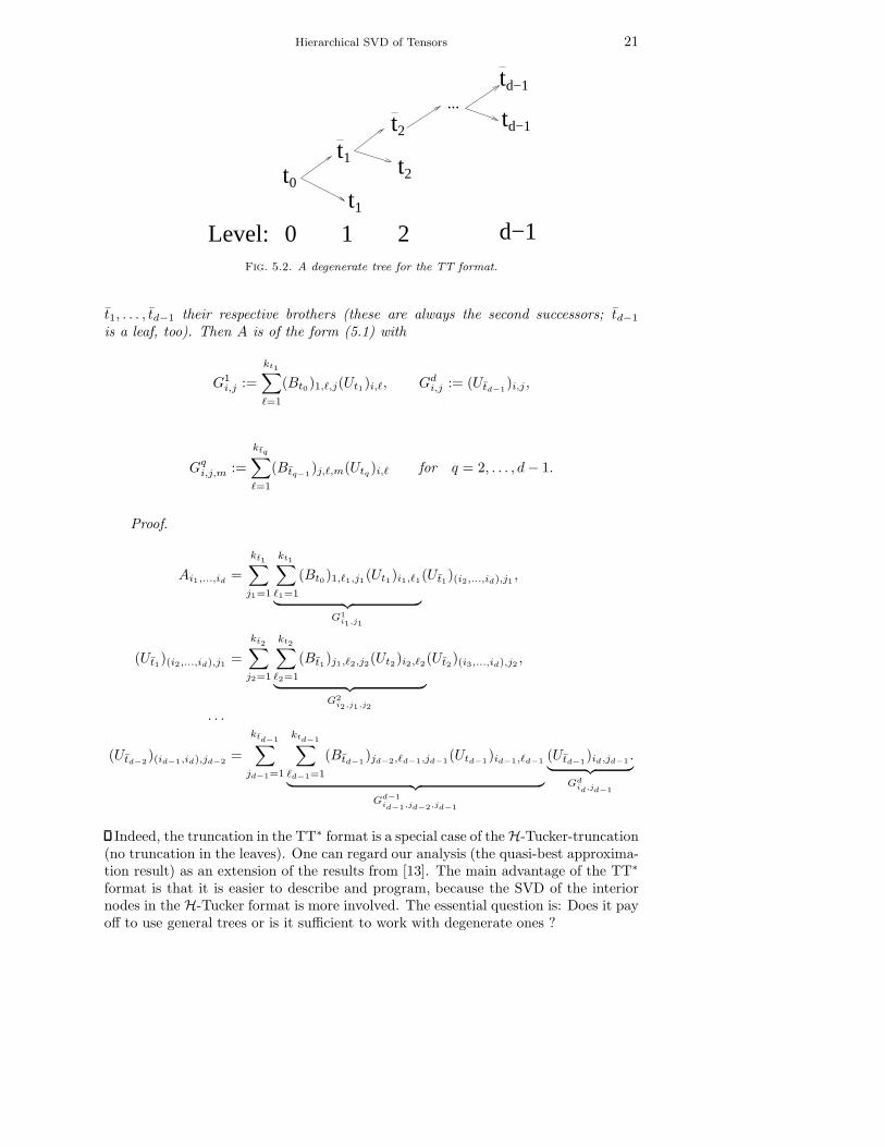
1 2 d−1Fig. 5.2. A degenerate tree for the TT format.

t1, . . . , td−1 their respective brothers (these are always the second successors; td−1

is a leaf, too). Then A is of the form (5.1) with

G1i,j :=

kt1∑

ℓ=1

(Bt0)1,ℓ,j(Ut1)i,ℓ, Gdi,j := (Utd−1

)i,j ,

Gqi,j,m :=

ktq∑

ℓ=1

(Btq−1)j,ℓ,m(Utq

)i,ℓ for q = 2, . . . , d− 1.

Proof.

Ai1,...,id=

kt1∑

j1=1

kt1∑

ℓ1=1

(Bt0)1,ℓ1,j1(Ut1)i1,ℓ1

︸︷︷︸G1

i1,j1

(Ut1)(i2,...,id),j1 ,

(Ut1)(i2,...,id),j1 =

kt2∑

j2=1

kt2∑

ℓ2=1

(Bt1)j1,ℓ2,j2(Ut2)i2,ℓ2

︸︷︷︸G2

i2,j1,j2

(Ut2)(i3,...,id),j2 ,

· · ·

(Utd−2)(id−1,id),jd−2

=

ktd−1∑

jd−1=1

ktd−1∑

ℓd−1=1

(Btd−1)jd−2,ℓd−1,jd−1

(Utd−1)id−1,ℓd−1

︸︷︷︸Gd−1

id−1,jd−2,jd−1

(Utd−1)id,jd−1

.︸︷︷︸

Gdid,jd−1

Indeed, the truncation in the TT∗ format is a special case of the H-Tucker-truncation(no truncation in the leaves). One can regard our analysis (the quasi-best approxima-tion result) as an extension of the results from [13]. The main advantage of the TT∗

format is that it is easier to describe and program, because the SVD of the interiornodes in the H-Tucker format is more involved. The essential question is: Does it payoff to use general trees or is it sufficient to work with degenerate ones ?

22 L. GRASEDYCK

5.3.1. Parallelization. The tree structure for (almost) balanced trees, i.e.,those having a depth proportional to log(d), is perfectly suited for parallelization.On each level all operations can be performed in parallel for all nodes on that level.Up to the logarithm for the depth of the tree one can obtain a perfect speedup. Usingd processors one obtains a scaling of log(d) for the overall truncation complexity. Thiswill be treated in more detail in a followup article.

The same kind of parallelization is not possible for the TT∗ format because thedepth of the degenerate tree is proportional to d and the truncation is inherentlysequential going from the root to the leaves.

5.3.2. Complexity. Let TI be an arbitrary dimension tree and A ∈ RI . We

denote by

kq := rank(A({1,...,q}))

the rank of the matricizations appearing in the TT∗ format, i.e. the representationrank for a degenerate tree. Then the H-Tucker-rank kt = rank(A(t)) for a nodet = {p, . . . , ℓ} can be bounded by

kt ≤ kp−1kℓ,

i.e. the largest necessary representation rank for the exact representation of A inH-Tucker((kt)t∈TI

) is bounded by the product of two TT∗-ranks: By assumptionthere exists U, V with kp−1, kq columns such that

A({1,...,p−1}) = UUTA({1,...,p−1}), A({1,...,q}) = V V TA({1,...,q}).

Then

A(t) = A(t)(UUT ⊗K V VT )

and the matrix on the right is of rank at most

rank(UUT ⊗K V VT ) ≤ rank(UUT )rank(V V T ) ≤ kp−1kq.

The opposite is not true: Let kt = rank(A(t)) for all t ∈ TI be uniformly boundedby k. Then the TT∗-rank kq can only be bounded by

kq . klog2(d)/2

for a balanced tree TI and

kq . kd/2

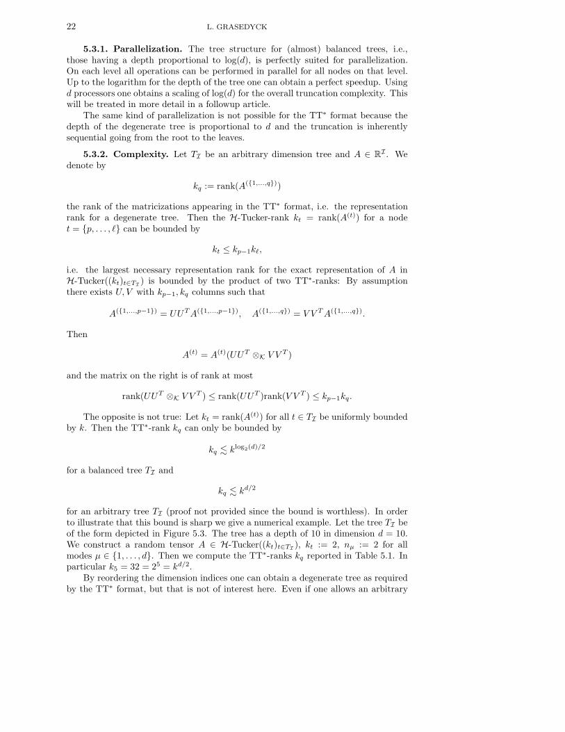
for an arbitrary tree TI (proof not provided since the bound is worthless). In orderto illustrate that this bound is sharp we give a numerical example. Let the tree TI beof the form depicted in Figure 5.3. The tree has a depth of 10 in dimension d = 10.We construct a random tensor A ∈ H-Tucker((kt)t∈TI

), kt := 2, nµ := 2 for allmodes µ ∈ {1, . . . , d}. Then we compute the TT∗-ranks kq reported in Table 5.1. Inparticular k5 = 32 = 25 = kd/2.

By reordering the dimension indices one can obtain a degenerate tree as requiredby the TT∗ format, but that is not of interest here. Even if one allows an arbitrary


{1,...,10}

{2,...,10}

{1}

{2,...,9}

{10}

{3,...,9}

{3,...,8}

{4,...,8}

{4,...,7}

{5,...,7}

{5,6}

{2} {3} {4} {5}

{6}

{9} {8} {7}

9876543210Level:

Fig. 5.3. A special dimension tree TI of depth 10.

q = 1 2 3 4 5 6 7 8 9kq = 2 4 8 16 32 16 8 4 2

Table 5.1TT∗-ranks for the special dimension tree TI from Figure 5.3.

reordering of the dimension indices for the TT∗ format, then a complete binary treeTI will still provide an example where maxq kq = klog2(d)/2.

For any tensor that allows an approximation by an elementary tensor sum withrepresentation rank k, both hierarchical formats have their ranks bounded by kt ≤k, kq ≤ k.

In practice it is of course a critical point to construct the dimension tree adaptivelysuch that the ranks stay small, and this will be presented in a followup article.

6. Numerical Examples. The numerical examples in this section are focusedon three questions:

1. How close to the measurements are the theoretical estimates of the trunca-tion error, i.e. the ratio between node-wise errors and the total error ? Inparticular we are interested in the question whether or not the factor

√d

appears.2. What is the maximal attainable truncation accuracy, i.e. how close can we

get to the machine precision ?3. What are problem sizes that can realistically be tackled by the H-Tucker

format in terms of the dimension d and the maximal rank k ?All computations are performed on an intel CPU with peak frequency 1.83 GHz andavailable main memory 1 GB.

6.1. Truncation from dense to H-Tucker format. Our first numerical ex-ample is in d = 5 with mode size nµ = 25. The tensor A is a dense tensor withentries

A(i1,...,id) :=

(d∑

µ=1

i2µ

)−1/2

which corresponds to the discretization of the function 1/‖x‖ on [1, 25]5. The time forthe conversion (Algorithm 1) of the dense tensor to H-Tucker format AH, the amountof storage needed for the frames Ut and transfer tensors Bt and the obtained relativeapproximation accuracy ‖A − AH‖ are presented in Table 6.1. The node-wise SVDis shown in Figure 3.2. From the truncation we lose roughly 2–3 digits of precisioncompared to the maximal attainable machine precision EPS ≈ 10−16. It seems that

24 L. GRASEDYCK

ε ‖A−AH‖/‖A‖ Storage (KB) times (Sec)1×10

−2 6.0×10−3 3.6 105.8

1×10−4 1.2×10

−4 11.2 104.11×10

−6 1.1×10−6 29.3 103.5

1×10−8 7.8×10

−9 58.1 104.81×10

−10 1.7×10−10 92.7 108.0

1×10−12 7.2×10

−13 153.2 104.81×10

−14 3.2×10−13 298.0 104.0

1×10−16 2.7×10

−14 615.1 106.9Table 6.1

Converting a dense tensor to H-Tucker format.

the node-wise rank is uniformly bounded (there is almost no variation between theranks kt) by k ∼ log(1/ε).

6.2. Truncation of elementary tensor sums in H-Tucker format. The sec-ond example is in higher dimension d with mode size nµ = 1000. The entries of thetensor AH are approximations of

A(i1,...,id) :=

(d∑

µ=1

i2µ

)−1/2

, iµ = 1, . . . , 1000,

by exponential sums,

AE :=

35∑

j=1

ωj

d⊗

µ=1

aj,µ, (aj,µ)iµ= exp(−i2µαj/d)

such that each entry is accurate up to εE = 10−10,

|A(i1,...,id) − (AE)(i1,...,id)| ≤ 7.315×10−10.

The weights ωj and exponents αj were obtained from W. Hackbusch and are availablevia the web page (k = 35, R = 1000000)

http://www.mis.mpg.de/scicomp/EXP_SUM

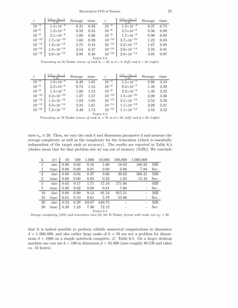
The tensor AE (represented as an elementary tensor sum) is then converted toH-Tucker format (error zero), which we denote by AH. The hierarchical rank iskt = 35 for every mode cluster t ∈ TI . From this input tensor we compute trunca-tions AH,ε to lower hierarchical rank by prescribing the (relative) truncation accuracyε. In Tables 6.2 and 6.3 we report the accuracy ‖AH − AH,ε‖/‖AH‖, the storage re-quirements for AH,ε in MB as well as the time in seconds used for the truncation. Weobserve that the accuracy is

‖AH −AH,ε‖/‖AH‖ ≈ 3ε

independent of the dimension d. The maximal attainable accuracy seems to be roughlyεmin ≈ 10−13.

6.3. Truncation of H-Tucker tensors. The third test is not any more con-cerned with the approximation accuracy, but purely with the computational com-plexity. Here, we setup an H-Tucker tensor with node-wise ranks kt ≡ k and mode


ε‖AH−AH,ε‖

‖A‖ Storage time

10−4 1.4×10−4 0.31 0.33

10−6 1.3×10−6 0.59 0.34

10−8 2.1×10−8 1.00 0.36

10−10 1.7×10−10 1.60 0.39

10−12 1.3×10−12 2.75 0.44

10−14 1.8×10−14 3.54 0.47

10−16 2.0×10−15 3.88 0.48

ε‖AH−AH,ε‖


10−4 1.3×10−4 0.37 0.73

10−6 2.5×10−6 0.50 0.80

10−8 1.7×10−8 0.90 0.88

10−10 3.7×10−10 1.22 0.83

10−12 2.2×10−12 1.87 0.80

10−14 3.9×10−14 2.76 0.91

10−16 2.6×10−14 4.05 0.97

Table 6.2Truncating an H-Tucker tensor of rank kt = 35 in d = 8 (left) and d = 16 (right).

ε‖AH−AH,ε‖


10−4 1.9×10−4 0.49 1.65

10−6 2.2×10−6 0.74 1.54

10−8 1.4×10−8 1.00 1.55

10−10 2.4×10−10 1.27 1.57

10−12 1.3×10−12 1.83 1.65

10−14 3.3×10−14 2.24 1.61

10−16 7.3×10−15 3.49 1.74

ε‖AH−AH,ε‖


10−4 5.5×10−5 0.98 3.19

10−6 9.2×10−7 1.48 3.39

10−8 3.2×10−8 1.49 3.23

10−10 1.5×10−10 2.00 3.36

10−12 3.1×10−12 2.52 3.50

10−14 1.1×10−13 3.09 3.31

10−16 1.1×10−13 4.53 3.52

Table 6.3Truncating an H-Tucker tensor of rank kt = 35 in d = 32 (left) and d = 64 (right).

sizes nµ ≡ 20. Then, we vary the rank k and dimension parameter d and measure thestorage complexity as well as the complexity for the truncation (which is essentiallyindependent of the target rank or accuracy). The results are reported in Table 6.4(dashes mean that for that problem size we ran out of memory (1GB)). We conclude

k d= 10 100 1,000 10,000 100,000 1,000,0001 size 0.00 0.02 0.16 1.60 16.02 160.22 MB1 time 0.00 0.00 0.01 0.08 0.86 7.88 Sec.2 size 0.00 0.04 0.37 3.66 36.62 366.21 MB2 time 0.00 0.00 0.03 0.22 1.63 15.43 Sec.5 size 0.02 0.17 1.71 17.16 171.66 - MB5 time 0.00 0.02 0.08 0.81 7.60 - Sec.10 size 0.08 0.90 9.14 91.54 915.51 - MB10 time 0.01 0.10 0.61 5.79 55.86 - Sec.20 size 0.52 6.29 63.97 640.75 - - MB20 time 0.20 1.23 7.36 72.12 - - Sec.

Table 6.4Storage complexity (MB) and truncation time for the H-Tucker format with mode size nµ = 20.

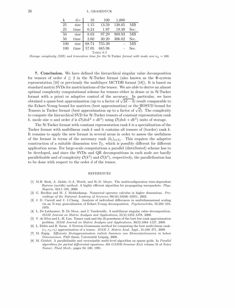
that it is indeed possible to perform reliable numerical computations in dimensiond = 1, 000, 000, and also rather large ranks of k = 50 are not a problem for dimen-sions d = 1000 on a simple notebook computer, cf. Table 6.5. On a larger desktopmachine one can use k = 100 in dimension d = 10, 000 (uses roughly 80 GB and takesca. 10 hours).

26 L. GRASEDYCK

k d= 10 100 1,00025 size 1.15 13.59 138.05 MB25 time 0.24 1.97 19.39 Sec.50 size 8.03 97.29 989.93 MB50 time 2.60 30.20 306.02 Sec.100 size 68.74 755.39 - MB100 time 57.05 685.98 - Sec.

Table 6.5Storage complexity (MB) and truncation time for the H-Tucker format with mode size nµ = 100.

7. Conclusion. We have defined the hierarchical singular value decompositionfor tensors of order d ≥ 2 in the H-Tucker format (also known as the Φ-systemrepresentation [10] or previously the multilayer MCTDH format [18]). It is based onstandard matrix SVDs for matricizations of the tensor. We are able to derive an almostoptimal complexity computational scheme for tensors either in dense or in H-Tuckerformat with a priori or adaptive control of the accuracy. In particular, we haveobtained a quasi-best approximation (up to a factor of

√2d− 3) result comparable to

the Eckart-Young bound for matrices (best approximation) or the HOSVD bound forTensors in Tucker format (best approximation up to a factor of

√d). The complexity

to compute the hierarchical SVD for H-Tucker tensors of constant representation rankk, mode size n and order d is O(dnk2 + dk4) using O(dnk + dk3) units of storage.

The H-Tucker format with constant representation rank k is a specialization of theTucker format with multilinear rank k and it contains all tensors of (border) rank k.It remains to apply the new format in several areas in order to assess the usefulnessof the format in terms of the necessary rank (kt)t∈TI

. This requires the adaptiveconstruction of a suitable dimension tree TI , which is possibly different for differentapplication areas. For large-scale computations a parallel (distributed) scheme has tobe developed, and since the SVDs and QR decompositions in each node are hardlyparallelizable and of complexity O(k3) and O(k4), respectively, the parallelization hasto be done with respect to the order d of the tensor.

REFERENCES

[1] M.H. Beck, A. Jackle, G.A. Worth, and H.-D. Meyer. The multiconfiguration time-dependentHartree (mctdh) method: A highly efficient algorithm for propagating wavepackets. Phys.Reports, 324:1–105, 2000.

[2] G. Beylkin and M. J. Mohlenkamp. Numerical operator calculus in higher dimensions. Pro-ceedings of the National Academy of Sciences, 99(16):10246–10251, 2002.

[3] J. D. Carroll and J. J.Chang. Analysis of individual differences in multidimensional scalingvia an N-way generalization of Eckart-Young decomposition. Psychometrika, 35:283–319,1970.

[4] L. De Lathauwer, B. De Moor, and J. Vandewalle. A multilinear singular value decomposition.SIAM Journal on Matrix Analysis and Applications, 21(4):1253–1278, 2000.

[5] V. de Silva and L.-H. Lim. Tensor rank and the ill-posedness of the best low-rank approximationproblem. SIAM Journal on Matrix Analysis and Applications, 30(3):1084–1127, 2008.

[6] L. Elden and B. Savas. A Newton-Grassmann method for computing the best multi-linear rank-(r1, r2, r3) approximation of a tensor. SIAM J. Matrix Anal. Appl., 31:248–271, 2009.

[7] M. Espig. Effiziente Bestapproximation mittels Summen von Elementartensoren in hohenDimensionen. PhD thesis, Universitat Leipzig, 2008.

[8] M. Griebel. A parallelizable and vectorizable multi-level algorithm on sparse grids. In Parallelalgorithms for partial differential equations, 6th GAMM-Seminar Kiel, volume 31 of NotesNumer. Fluid Mech., pages 94–100, 1991.


[9] M. Griebel. Adaptive sparse grid multilevel methods for elliptic pdes based on finite differences.Computing, 61:151–179, 1998.

[10] W. Hackbusch and S. Kuhn. A new scheme for the tensor representation. J. Fourier Anal.Appl., 15:706–722, 2009.

[11] R. A. Harshman. Foundations of the parafac procedure. UCLA Working Papers in Phonetics,16:1–84, 1970.

[12] T. G. Kolda and B. W. Bader. Tensor decompositions and applications. SIAM Review,51(3):455–500, 2009.

[13] I.V. Oseledets. Compact matrix form of the d-dimensional tensor decomposition. Preprint09-01, Institute of Numerical Mathematics RAS, Moscow, Russia, 2009.

[14] I.V. Oseledets and E.E. Tyrtyshnikov. Breaking the curse of dimensionality, or how to use svdin many dimensions. Preprint 09-03, HKBU, Kowloon Tong, Hong Kong, 2009.

[15] M. Rajih, P. Comon, and R. Harshman. Enhanced line search: a novel method to acceleratePARAFAC. SIAM Journal on Matrix Analysis and Applications, 30(3):1148–1171, 2008.

[16] J. Salmi, A. Richter, and V. Koivunen. Sequential unfolding SVD for tensors with applicationsin array signal processing. IEEE Trans. on Signal Processing, 2009. accepted.

[17] B. Savas and L.-H. Lim. Best multilinear rank approximation of tensors with quasi-Newtonmethods on Grassmannians. Technical Report LITH-MAT-R-2008-01-SE, Department ofMathematics, Linkopings Universitet, 2008.

[18] H. Wang and M. Thoss. Multilayer formulation of the multiconfiguration time-dependenthartree theory. J. Chem. Phys., 119:1289–1299, 2003.

[19] C. Zenger. Sparse grids, parallel algorithms for partial differential equations. In Parallelalgorithms for partial differential equations, 6th GAMM-Seminar Kiel, volume 31 of NotesNumer. Fluid Mech., pages 241–251, 1991.

Hierarchical Singular Value Decomposition of Tensors

Documents

Transcript of Hierarchical Singular Value Decomposition of Tensors