arX

iv:m

ath-

ph/0

1120

24v1

13

Dec

200

1

Singular Lagrangians in supermechanics

Jose F. Carinena

Departamento de Fısica Teorica, Universidad de Zaragoza, 50009 Zaragoza, Spain.

Hector Figueroa

Escuela de Matematica, Universidad de Costa Rica, San Jose, Costa Rica.

Abstract

The time evolution operator K is introduced in the graded context and its main properties

are discussed. In particular, the operator K is used to analize the projectability of constraint

functions arising in the Lagrangian formalism for singular Lagrangians.

Keywords: time evolution operator, supervector fields along a morphism, Hamiltonian andLagrangian constraints.1991 MSC numbers: Primary: 58A50, 58C50. Secondary: 70H33PACS numbers: 03.20+i, 02.90+p, 11.30.pb.

1. Introduction

The relevance of systems defined by singular Lagrangians for fundamental physicaltheories (generally covariant, Yang Mills and string theories) is nowadays fully understood.They are the only possibility for the occurrence of gauge freedom. Constraints, gaugeinvariance, gauge fixing, etc, are now concepts of common use in these theories. All ofthem are better understood when using an appropriate geometric framework, and the useof modern tools of Differential Geometry has very much clarified the different aspects ofthe theory of singular systems started by Bergmann [2] and Dirac [13].

The connection between the Lagrangian and Hamiltonian formalisms of regular sys-tems, given by the Legendre transformation, needs a more careful study and makes use offiner tools in the case of singular Lagrangians. In this case, constraint functions determin-ing the submanifold in which the dynamical equation has a consistent solution will appear.Moreover, in the Lagrange approach there will be more constraints functions determiningthe submanifold in which the dynamics admits a solution that is the restriction of a sec-ond order differential equation vector field. It has been shown that the relation among theconstraint functions arising in the Lagrangian formalism and those of the Hamiltonian onecan be established by means of a differential operator K, first introduced by Kamimura[19] and later used by Batlle et al [1], and whose geometric interpretation was given in[16] and [8]. For a recent review of these objects see [17]. The theory of sections alongmaps is the key point for establishing the operator K. In fact, vector fields along a map, orrelative vector fields along a map according to [24], simplify and clarify most constructionsin classical mechanics [3, 9,10] and they have recently been used in classical field theories[14].

On the other hand, the necessity of incorporating anticommuting variables for describ-ing dynamical systems with fermionic degrees of freedom has lead to the development of

1

the so-called supermechanics [18]. Moreover, it has been shown to be quite useful not onlyin physics but also in mathematics, particularly in the study of the geometry associatedto a Lie algebroid, mainly due to the Vaintrob Theorem [28].

Our aim in this paper is to discuss the generalization in the graded context of theoperator K, also called relative Hamiltonian vector field in [24], which allows us to relatein this way constraint functions arising in Hamilton formalism for singular systems withthose of the Lagrange approach. Our intention here is not to do a complete descriptionof the theory of constraints in supermechanics, but rather to introduce some elements toconvince the reader that this theory may be developed along parallel lines to the theoryof constraints in classical mechanics. The main difficulty in this enterprise lies in that theinformation of a graded manifold is encoded in the sheaf of superfunctions, instead of theunderlying manifold. Indeed, in the transition to the supermechanics setting the use of theconcepts of sections along a map is even more necessary because of the inconvenience ofworking with points in graded geometry. Thus one is forced to take an algebraic approach,which replaces all the intrinsic constructions that are based on points of the manifold inthe classical case. The interesting point is that this is accomplished by using vector fieldsand forms along a morphism of supermanifolds in the same way they where used in [9,10]in the classical setting. See [4-7] for details.

The paper is organized as follows: Section 2 is devoted to set our notation and, forthe reader convenience, we describe the material from the theory of graded manifolds thatwill be used in later Sections. In particular, we recall the concepts of vector fields andgraded forms along a morphism, and particular examples are given.

In Section 3 we introduce, in the graded context, the time evolution operator K as-sociated to a super-Lagrangian function L, and we discuss its main properties, in orderto study the Lagrangian constraints associated to a singular Lagrangian and the connec-tion with their Hamiltonian counterpart. Finally, Section 4 analyzes the projectability ofLagrangian constraint functions using the operator K.

2. Basic notation and background.

Naturally, the arena to develop Lagrangian or Hamiltonian supermechanics will be asuitable generalization, to the graded context, of the tangent and cotangent manifold of theconfiguration space. Surprisingly enough, even this requires some attention. The point isthat the superobjects that have the right geometrical structure: the tangent or cotangentsuperbundles, introduced by Sanchez–Valenzuela in [25], are too big, as their dimensionsare (2m + n, 2n + m), if the dimension of the starting graded manifold M = (M,A) (theconfiguration superspace) is (m, n). This can be fixed by considering the subsupermanifoldsof dimension (2m, 2n), introduced by Ibort and Marın in [18], which, nonetheless, do nothave all the geometrical richness that one is used to; for instance, supervector fields, thatis, derivations of A, can be considered as section of the tangent superbundle STM, butnot of the tangent supermanifold TM. Thus, it is advisable to define and study the mainproperties of the relevant objects in STM, but to perform the computations and theinterpretations after the restriction to TM [5].

For the reader convenience and to fix the notation, we shall describe the main objectsthat give the geometry of the tangent and cotangent bundles in the graded context, and

2

refer the reader to [5] for details. Through out we shall be working with supermanifoldsin the sense of Kostant [20] and Leıtes [21].

A supervector bundle is a quadruplet (E,AE), Π, (M,AM), VS such that V is a real(r, s)–dimensional supervector space, Π: (E,AE) → (M,AM) is a submersion of gradedmanifolds, and every q ∈ M lies in a coordinate neighbourhood U ⊆ M for which anisomorphism ΨU exists making the following diagram commutative:

(2.1)

(π−1(U),AE

(π−1(U)

)) ΨU−−−−−→(U ,AM(U)

)×VS

Π

y

yP1

(U ,AM (U)

) (U ,AM(U)

).

Here VS := S(V ⊕ ΠV ) where Π is the change of parity functor [21,22], hence (ΠV ) =(ΠV )0 ⊕ (ΠV )1, where (ΠV )i = Vi+1 for i = 0, 1, and S(V ) is the affine supermanifold

(2.2) S(V ) :=(V0, C

∞(V0) ⊗∧

(V ∗1 )

).

Equivalence classes of supervector bundles so defined are in a one–to–one correspondencewith equivalence classes of locally free sheaves of AM–modules over M of rank (r, s). Thetangent and cotangent superbundles are the superbundles corresponding to the sheavesX(A) := DerA and Ω1(A) := X(A)∗ respectively.

The main reason for considering the tangent superbundle (STM, STA), T , (M,A),and supervector bundles in general [25], is that their geometrical sections are in a one–to–one correspondence with the sections of the corresponding locally free sheaf of gradedA–modules; in our case, with the sections of the sheaf DerA, in other words, with thesupervector fields over M. Unfortunately, the use of the parity functor Π introduces someunwanted supercoordinates; the elimination of these coordinates lead to the tangent andcotangent supermanifolds [5].

Supervector fields, or graded forms, along a morphism are our main tool to describesupermechanics, in fact all the relevant objects can be defined as such [4–7]. This is sobecause of their algebraic nature and because the information of a graded manifold isconcentrated in the algebraic part, that is in the sheaf of superalgebras.

If Φ = (φ, φ∗): (N,B) → (M,A) is a morphism of graded manifolds, a homogeneoussupervector field along Φ is a morphism of sheaves over M , X :A → Φ∗B such that for eachopen subset U of M

(2.3) X(fg) = X(f) φ∗U(g) + (−1)|X| |f |φ∗

U (f) X(g) ,

whenever f ∈ A(U) is homogeneous of degree |f |. The sheaf of supervector fields along Φwill be denoted by X(Φ). If X is a supervector field on (M,A), an example of an elementin X(Φ) is given by

(2.4) X := φ∗ X .

3

Similarly if Y ∈ X(B), then

(2.5) Tφ(Y ) := Y φ∗,

also belongs to X(Φ). We say that Y is projectable with respect to Φ if there exists X ∈ X(A)such that Tφ(Y ) = X . Sometimes, we also say that X and Y are Φ-related.

X(Φ) is a locally free sheaf of Φ∗B–modules over M of rank (m, n) = dimM; a localbasis of X(Φ)(U) is given by

(2.6) ∂qi := ∂qi , ∂θα := ∂θα ,

if (qi, θα) (1 ≤ i ≤ m, 1 ≤ α ≤ n), are local supercoordinates on U ⊂ M [4].The sheaf of graded 1–forms along Φ is the sheaf of φ∗B–modules Ω1(Φ) := X(Φ)∗ =

Hom(X(Φ), φ∗B). If ω is a graded 1–form on M, ω defined by

(2.7) ω(X) := φ∗ ω(X) , ∀X ∈ X(AM) ,

belongs to Ω1(Φ). Moreover, a local basis is given by the elements dqi := dqi and dθα :=

dθα. On the other hand, if ω is a graded 1–form along Φ, then φ♯ω given by

(2.8) φ♯ω(Y ) := ω(Tφ(Y )

), ∀Y ∈ X(B) ,

is a graded 1–form on N . As a matter of fact, it is possible to classify the graded 1–formson N that come from graded 1–forms along Φ, when Φ is a submersion. The result is thatΩ1(Φ) is isomorphic to the φ∗B–modulo of Φ–semibasic 1–forms on N [4]. Naturally, wecan extend (2.7) and (2.8) to arbitrary graded forms.

Let E = (E,AE), Π, (M,AM), VS be a superbundle. A local section of E along

Φ, over an open subset U of M , is a morphism, Σ = (σ, σ∗):(φ−1(U),B

(φ−1(U)

))→

(π−1(U),AE

(π−1(U)

)), satisfying the condition ΦU = ΠU ΣU , where the subscript U

means the restriction of the morphism to the corresponding open graded submanifold. Theset of such sections is denoted by ΓΦ(Π|U ). When (E,AE) is the tangent or the cotangentsuperbundle these sections are in a one–to–one correspondence with supervector fields andgraded 1–forms along Φ, respectively [5].

In the case when the morphism Φ coincides with the projection Π of the supervectorbundle, the identity morphism on E gives a canonical section. In the tangent superbundleSTM, T ,M the supervector field along T = (τ, τ∗) that corresponds to the canonicalsection is called the total time derivative operator and is denoted by T. Whereas the Π–semibasic graded 1–form on ST ∗M associated to the graded 1–form along Π, correspondingto the canonical section of the cotangent superbundle ST ∗M, Π = (π, π∗),M, is calledthe canonical Liouville 1–form on ST ∗M and will be denoted by Θ0. The restrictions of T

and Θ0 to the tangent and cotangent supermanifolds, that will be denoted in the say way,can be written, in the natural supercoordinates of these supermanifolds [5] associated tothe supercoordinates qi, θα of M on U ⊂ M , as

(2.9) T =m∑

i=1

vi∂qi +n∑

α=1

ζα∂θα , and Θ0 =

m∑

i=1

pi dqi +n∑

α=1

ηα dθα.

4

The reason to consider these restrictions is that although Θ0 is formally equal to thecanonical 1–form of the cotangent bundle in non–graded geometry, it turns out that thegraded 2–form −dΘ0 is always degenerate, whereas the restriction of Θ0 to the cotangentsupermanifold T ∗M gives a non–degenerate graded 2–form ω0 := −dΘ0.

Using the abbreviation TA(U) for TA(τ−1(U)

), we associate to each superfunction

f ∈ A(U) the superfunction fV ∈ TA(U) defined by

(2.10) fV :=

m∑

i=1

∂F

∂qivi +

n∑

α=1

∂F

∂θαζα,

where F := τ∗(f) ∈ TA(U). It turns out that a supervector field Y on TM is determinedby its action on the superfunctions fV . Thus, if X is a supervector field on M, or asupervector field along T , its vertical lift is the supervector field XV on TM defined by

(2.11) XV (fV ) = τ∗(X(f)

), ∀f ∈ A .

In local supercoordinates, if X =∑m

i=1 X i∂qi +∑n

α=1 χα∂θα , then

(2.12) XV =

m∑

i=1

X i∂vi +

n∑

α=1

χα∂ζα .

We are now in a position to introduce the superobjects corresponding to the objects thatdetermine the geometry of the tangent manifold [12]: the vertical superendomorphism isthe graded tensor field of type (1, 1) S: X(TA) → X(TA) defined by

(2.13) S(Y ) :=(Tτ(Y )

)V.

On the other hand, the Liouville supervector field ∆ is the vertical lift of the total timederivative:

(2.14) ∆ := TV .

If Y =∑m

i=1 Y i∂qi +∑m

i=1 Yi∂vi +

∑nα=1 Υα∂θα +

∑nα=1 Ξα∂ζα then,

(2.15) S(Y ) =

m∑

i=1

Y i∂vi +

n∑

α=1

Υα∂ζα .

In analogy with ordinary Lagrangian mechanics, the graded Cartan 1 and 2–forms associ-ated to a given Lagrangian superfunction L in TA are defined by

(2.16) ΘL := dL S and ωL := −dΘL.

Since ΘL is a T –semibasic graded 1–form, and T is a submersion, it has associated a uniquegraded 1–form ΘL along T . In analogy with non–graded geometry, see [10], the restrictionto TM of the section FL: STM → ST ∗M along T that corresponds to the graded 1–formΘL is called the super–Legendre transformation. If L is even, locally, FL = (fl, f l∗) isdetermined by the morphism of superalgebras fl∗: T ∗A(U) → TA(U) described by therelations:

qi 7→ qi , θα 7→ θα ,(2.17)

pi 7→∂L

∂vi, ηα 7→ −

∂L

∂ζα.

For more details on the super–Legendre transformation see [5].

5

3. The time evolution operator.

In Lagrangian supermechanics the dynamics of a system (TM, ωL, L), associated to aregular Lagrangian L ∈ TM, is given by a vector field Γ ∈ X(TM) satisfying the dynamical

equation

(3.1) iΓωL = d EL .

This uniquely defined vector field Γ satisfies, automatically, the second order condition[18], which can be stated in several equivalent ways. A very convenient one, suitable togeneralization to higher orders [4,7], is

(3.2) Γ τ∗ = T .

To abbreviate, we say that Γ is a SODE vector field (Second Order Differential Equation).When the super-Lagrangian L is singular both the existence and uniqueness of Γ are injeopardy, and it is necessary to consider a submanifold of TM where (3.1) holds. Moreover,even on this submanifold (3.2) may fail, so both conditions have to be considered separately.Motivated by these issues we consider the following definition:

Definition 3.1. The time evolution operator K: T ∗A → TA, associated to a La-grangian super-function, L ∈ TM, is the unique supervector field along the super-Legendretransformation FL satisfying the dynamical condition

(3.3) iKω0 = d EL ,

and the second order condition

(3.4) K π∗ = T .

Since T is even, (3.4) implies that K is also even, hence iK : Ω(T ∗A) → Ω(TA) is theunique FL∗–derivation of bidegree (−1, 0) [4] defined by

(3.5) iKf = 0 and iKdf = K(f) .

In particular, one has

(3.6) iK(ω ∧ µ) = iKω ∧ FL∗µ + (−1)|ω|FL∗ω ∧ iKµ ,

when ω is homogeneous. Conditions (3.3) and (3.4) are the same conditions as those usedin [16] to define, in the non graded context, the time evolution operator, written in thealgebraic language of operators to avoid the use of points of the underlying manifold.

6

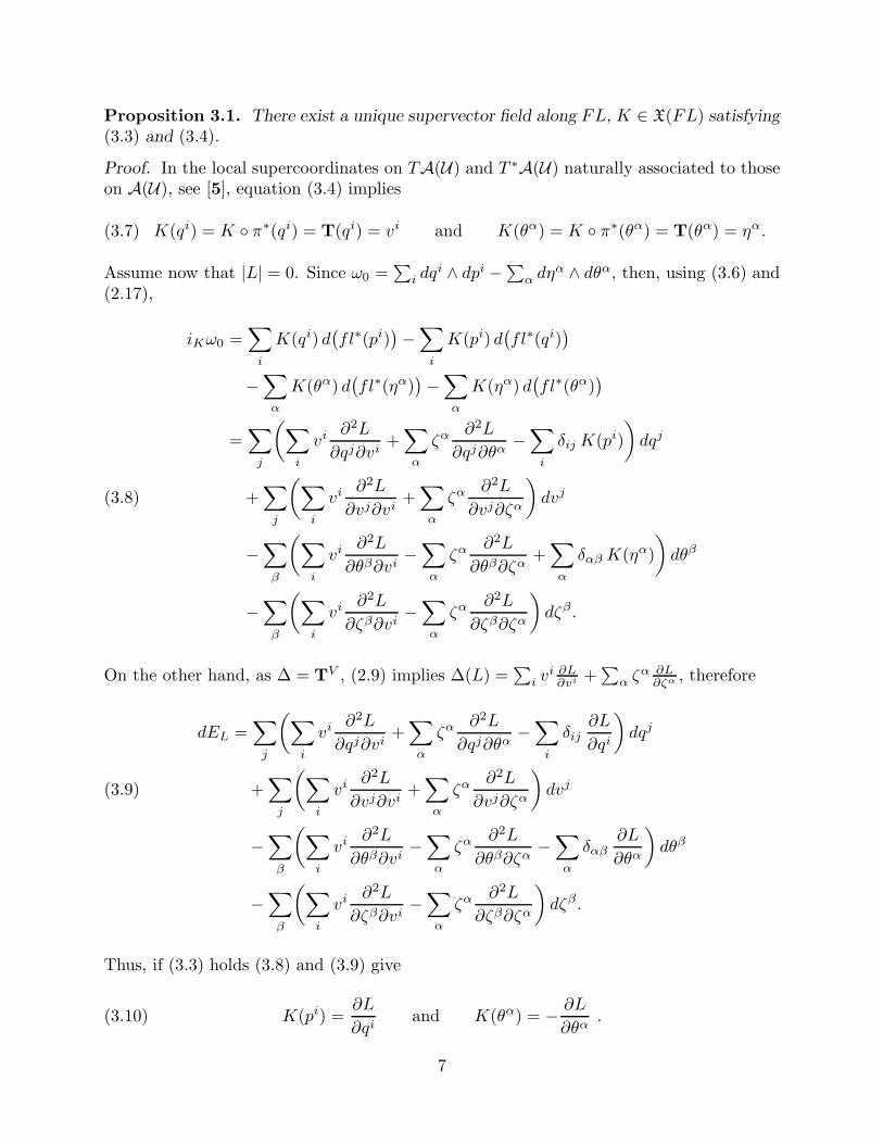
Proposition 3.1. There exist a unique supervector field along FL, K ∈ X(FL) satisfying

(3.3) and (3.4).

Proof. In the local supercoordinates on TA(U) and T ∗A(U) naturally associated to thoseon A(U), see [5], equation (3.4) implies

(3.7) K(qi) = K π∗(qi) = T(qi) = vi and K(θα) = K π∗(θα) = T(θα) = ηα.

Assume now that |L| = 0. Since ω0 =∑

i dqi ∧ dpi −∑

α dηα ∧ dθα, then, using (3.6) and(2.17),

iKω0 =∑

i

K(qi) d(fl∗(pi)

)−

∑

i

K(pi) d(fl∗(qi)

)

−∑

α

K(θα) d(fl∗(ηα)

)−

∑

α

K(ηα) d(fl∗(θα)

)

=∑

j

(∑

i

vi ∂2L

∂qj∂vi+

∑

α

ζα ∂2L

∂qj∂θα−

∑

i

δij K(pi)

)dqj

+∑

j

(∑

i

vi ∂2L

∂vj∂vi+

∑

α

ζα ∂2L

∂vj∂ζα

)dvj(3.8)

−∑

β

(∑

i

vi ∂2L

∂θβ∂vi−

∑

α

ζα ∂2L

∂θβ∂ζα+

∑

α

δαβ K(ηα)

)dθβ

−∑

β

(∑

i

vi ∂2L

∂ζβ∂vi−

∑

α

ζα ∂2L

∂ζβ∂ζα

)dζβ.

On the other hand, as ∆ = TV , (2.9) implies ∆(L) =∑

i vi ∂L∂vi +

∑α ζα ∂L

∂ζα , therefore

dEL =∑

j

(∑

i

vi ∂2L

∂qj∂vi+

∑

α

ζα ∂2L

∂qj∂θα−

∑

i

δij

∂L

∂qi

)dqj

+∑

j

(∑

i

vi ∂2L

∂vj∂vi+

∑

α

ζα ∂2L

∂vj∂ζα

)dvj(3.9)

−∑

β

(∑

i

vi ∂2L

∂θβ∂vi−

∑

α

ζα ∂2L

∂θβ∂ζα−

∑

α

δαβ

∂L

∂θα

)dθβ

−∑

β

(∑

i

vi ∂2L

∂ζβ∂vi−

∑

α

ζα ∂2L

∂ζβ∂ζα

)dζβ.

Thus, if (3.3) holds (3.8) and (3.9) give

(3.10) K(pi) =∂L

∂qiand K(θα) = −

∂L

∂θα.

7

This together with (3.7) imply the uniqueness of K. Moreover, it is easy to verify that(3.7) and (3.10) do define a supervector field along FL, which proves the proposition whenL is even; the odd case is proved in the same way but (3.10) are different.

In the non graded case the time evolution operator was defined in [8] using the gen-eralized Hamiltonian system defined on the mixed space TM ⊕ T ∗M [26,27] as follows:given a Lagrangian function L ∈ TM we consider on TM ⊕ T ∗M the 2-form Ω := pr∗2 ω0

and the function D := 〈pr1 | pr2〉 − pr∗1 L, where pri denotes the projection of TM ⊕ T ∗Monto the i–th factor. If W denotes the graph of the Legendre transformation

(3.11) W = (v, p) ∈ TM ⊕ T ∗M : p = FL(v) ,

then the map FL: TM → W given by FL(v) =(v, FL(v)

)is a diffeomorphism whose

inverse is pr1 |W [26,27]. To simplify the notation we shall also denote the restriction of

pri to W by pri. The time evolution operator K: C∞(T ∗M) → C∞(TM) is defined by

(3.12) K := FL∗ Z pr∗2

where Z is any vector field on W satisfying

(3.13) iZ Ω = dD.

Now, to prove that both definitions agree, we first notice that

(3.14) FL∗D(v) = D

(v, FL(v)

)= 〈v |FL(v)〉−FL

∗pr∗1 L(v) = ∆L(v)−L(v) = EL(v) ,

and

(3.15) FL∗Ω = FL

∗ pr∗2 ω0 = (pr2 FL)∗ω0 = FL∗ω0 = ωL .

Proposition 3.2. If X is a vector field on TM such that pr∗1 X = Z pr∗1, then iXωL =dEL and X τ∗ = T.

Proof. Since X FL∗

= FL∗ Z, equations (3.14) and (3.15) yield

(3.16) iXωL = iX FL∗Ω = FL

∗ iZΩ = FL

∗(dD) = dEL.

To prove the second assertion, for each α ∈ Ω1(M) let Yα ∈ X(T ∗M) be the unique vectorfield such that

(3.17) iYαω0 = π∗α ,

and let Zα ∈ X(W ) be such that Zα pr∗1 = 0 and Zα pr∗2 = pr∗2 Yα, then

(3.18) iZαΩ = iZα

pr∗2 ω0 = pr∗2 iYαω0 = pr∗2 π

∗α = (τ pr1)∗α ,

8

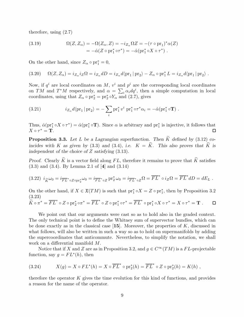
therefore, using (2.7)

Ω(Z, Zα) = −Ω(Zα, Z) = −iZαΩZ = −(τ pr1)

∗α(Z)(3.19)

= −α(Z pr∗1 τ∗) = −α(pr∗1 X τ∗) .

On the other hand, since Zα pr∗1 = 0,

(3.20) Ω(Z, Zα) = iZαiZΩ = iZα

dD = iZαd〈pr1 | pr2〉 − Zα pr∗1 L = iZα

d〈pr1 | pr2〉 .

Now, if qi are local coordinates on M , vi and pi are the corresponding local coordinateson TM and T ∗M respectively, and α =

∑i αidqi, then a simple computation in local

coordinates, using that Zα pr∗2 = pr∗2 Yα and (2.7), gives

(3.21) iZαd〈pr1 | pr2〉 = −

∑

i

pr∗1 vi pr∗1 τ∗αi = −α(pr∗1 T) .

Thus, α(pr∗1 X τ∗) = α(pr∗1 T). Since α is arbitrary and pr∗1 is injective, it follows thatX τ∗ = T.

Proposition 3.3. Let L be a Lagrangian superfunction. Then K defined by (3.12) co-

incides with K as given by (3.3) and (3.4), i.e. K = K. This also proves that K is

independent of the choice of Z satisfying (3.13).

Proof. Clearly K is a vector field along FL, therefore it remains to prove that K satisfies(3.3) and (3.4). By Lemma 2.1 of [4] and (3.14)

(3.22) iK

ω0 = iFL

∗

Zpr∗2

ω0 = iFL

∗

Zpr∗2 ω0 = i

FL∗

ZΩ = FL

∗ iZΩ = FL

∗dD = dEL .

On the other hand, if X ∈ X(TM) is such that pr∗1 X = Z pr∗1, then by Proposition 3.2(3.23)

K π∗ = FL∗Z pr∗2 π

∗ = FL∗Z pr∗1 τ

∗ = FL∗ pr∗1 X τ∗ = X τ∗ = T .

We point out that our arguments were cast so as to hold also in the graded context.The only technical point is to define the Whitney sum of supervector bundles, which canbe done exactly as in the classical case [15]. Moreover, the properties of K, discussed inwhat follows, will also be written in such a way so as to hold on supermanifolds by addingthe supercoordinates that anticommute. Nevertheless, to simplify the notation, we shallwork on a differential manifold M .

Notice that if X and Z are as in Proposition 3.2, and g ∈ C∞(TM) is a FL-projectablefunction, say g = FL∗(h), then

(3.24) X(g) = X FL∗(h) = X FL∗ pr∗2(h) = FL

∗ Z pr∗2(h) = K(h) ,

therefore the operator K gives the time evolution for this kind of functions, and providesa reason for the name of the operator.

9

The main property of K is that its action on Hamiltonian constraints generates theLagrangian constraints [1,8]. Before we see how this goes, we shall introduce anotheroperator that is also used to compare Hamiltonian and Lagrangian constraints [11], butagain we define it using an algebraic approach that can be generalized to the gradedcontext. Since a vector field on TM is determined by its action on the maps fV definedin (2.10), we associate to each U ∈ X(FL) the vector field on TM defined by

(3.25) RLU(fV ) := U π∗(f) ∀f ∈ C∞(M).

Now, if Y ∈ X(T ∗M), then FL∗Y ∈ X(FL), so we can define an operator RL: X(T ∗M) →X(TM) by

(3.26) RL(Y ) := RL(FL∗ Y ) .

When Y =∑m

i=1(Yi∂qi + Yi∂pi), then RL(Y ) =

∑mi=1 Y i∂vi . In particular, if h ∈

C∞(T ∗M), and Yh is the vector field such that

(3.27) iYhω0 = dh ,

then

(3.28) RL(Yh) =m∑

i=1

FL∗( ∂h

∂pi

) ∂

∂vi.

Moreover, if X ∈ X(TM) is a vector field such that X τ∗ = FL∗ Y π∗, then by (2.13)

(3.29) RL(Y )(fV ) = X τ∗(f) = (TτX)V (fV ) = S(X)(fV ) ,

so RL(Y ) = S(X).

Lemma 3.4. For each h ∈ C∞(T ∗M) there are vector fields Xh on TM such that S(Xh) =RL(Yh), where Yh is the vector field defined by (3.27).

Proof. First we choose Zh ∈ X(W ) such that Zh pr∗2 = pr∗2 Yh, then we take Xh suchthat Zh pr∗1 = pr∗1 Xh. Now,

pr∗1 Xh τ∗ = Zh pr∗1 τ∗ = Zh pr∗2 π

∗(3.30)

= pr∗2 Yh π∗ = pr∗1 FL∗ Yh π∗.

Since pr∗1 is injective Xh τ∗ = FL∗ Yh π∗, so by the comment before the statementS(Xh) = RL(Yh).

Note that Xh is by no means unique, but clearly the difference of two such vectorfields is τ -vertical.

10

Proposition 3.5. For each h ∈ C∞(T ∗M)

(3.31) K(h) = iXh[iΓωL − dEL] + iΓd(FL∗h) ,

where Xh is any vector field such that S(Xh) = RL(Yh), and Γ ∈ X(TM) is an arbitrary

SODE vector field.

Proof. Given Xh and Γ, we choose vector fields Uh and V in X(W ) such that Uh pr∗1 =pr∗1 Xh, and V pr∗1 = pr∗1 Γ. If Zh is as in the proof of the previous lemma, then,

(3.32) iZhΩ = iZh

pr∗2 ω0 = pr∗2 iYhω0 = pr∗2(dh) ,

so

K(h) = FL∗ Z pr∗2(h) = FL

∗ iZ iZh

Ω = −FL∗ iZh

iZΩ

= −FL∗ iZh−Uh

iZ−V Ω − FL∗ iZh

iV Ω(3.33)

+ FL∗ iUh

iV Ω − FL∗ iUh

iZΩ .

By the proof of Lemma 3.4, Zh − Uh is p-vertical, where p: W → M is the canonicalprojection. But Z−V is also p-vertical since Z(qi) = vi = V (qi), hence iZh−Uh

iZ−V Ω = 0.On the other hand, by (3.14) and (3.15),

FL∗ iUh

iZΩ = iXh FL

∗ iZΩ = iXh

FL∗(dD) = iXh

dEL ,(3.34)

FL∗ iUh

iV Ω = iXh FL

∗ iV Ω = iXh

iΓFL∗Ω = iXh

iΓωL .

Finally, using (3.32),

FL∗ iZh

iV Ω = −FL∗ iV iZh

Ω = −iΓ FL∗ iZh

Ω(3.35)

= −iΓ FL∗(d pr∗2 h) = −iΓd(pr2 FL)∗h = −iΓd(FL∗h) .

Plugging (3.34) and (3.35) into (3.33) we obtain (3.31).When h is a Hamiltonian constraint, so FL∗h = 0, (3.31) reduces to

(3.36) K(h) = iXh[iΓωL − dEL] ,

and the right hand side is a Lagrangian constraint [11,23]; actually, it is the constraintassociated to h through the operator RL. Thus, the operator K reproduces the Lagrangianconstraints, while the operator RL provides the non arbitrary part of the vector fieldsassociated to a given constraint.

11

4. Projectability of constraints

In order to analyze the projectability of these constraints we consider the followinglemmata.

Lemma 4.1. The energy function EL is FL-projectable.

Proof. We have to proof that EL is annihilated by all the elements of kerFL∗ = X ∈X(TM): X FL∗ = 0 . Since τ∗ = FL∗ π∗, it is clear that vector fields in ker FL∗ areτ -vertical. In particular, iXθL = 0 when X ∈ kerFL∗, as θL = dLS. On the other hand,if Γ is a SODE vector field, and X ∈ ker FL∗, then [X, Γ](qi) = XΓ(qi) = X(vi), so

(4.1) S([X, Γ]) = X .

Thus, if X ∈ kerFL∗,(4.2)X(EL) = LX(iΓθL − L) = i[X,Γ]θL − iΓLXθL −X(L) = dL S([X, Γ])−X(L) = 0 .

Consider the set M = X ∈ X(TM): S(X) ∈ VkerωL , where VkerωL denotes theset of those vector fields in ker ωL that are τ -vertical, that is Vker ωL := X

v(TM)∩kerωL.

Lemma 4.2. M coincides with the orthogonal complement of the set of vertical vector

fields with respect to ωL, M =(X

v(TM))⊥

.

Proof. Since

(4.3) ωL(X, S(U)) = −ωL(S(X), U)

for arbitrary X and U in X(TM) [12, Section 13.8] (or see [18] for a proof in the gradedcontext), then

(X

v(TM))⊥

= X ∈ X(TM): ωL(X, V ) = 0 for all V ∈ Xv(TM)

= X ∈ X(TM): ωL(X, S(U)) = 0 for all U ∈ X(TM) (4.4)

= X ∈ X(TM): ωL(S(X), U) = 0 for all U ∈ X(TM) = M .

Lemma 4.3. The kernel of the Cartan 2–form associated to a Lagrangian superfunction

is M⊥, i.e. ker ωL = M

⊥.

Proof. Obviously kerωL ⊆ M⊥. On the other hand, notice that ωL(V1, V2) = 0 if V1

and V2 are τ -vertical. This means that Xv(TM) ⊂

(X

v(TM))⊥

= M, therefore M⊥ ⊆(

Xv(TM)

)⊥= M.

Now, ∂qi ∈ M since S(∂qi) = ∂vi ∈ Xv(TM) ⊂ M, therefore if X ∈ M

⊥

(4.5) ωL(X, ∂qi) = 0 .

Furthermore, since M⊥ ⊆ M, then S(X) ∈ VkerωL, so using (4.3)

(4.6) 0 = ωL(S(X), ∂qi) = ωL(X, S(∂qi)) = ωL(X, ∂vi),

and i being arbitrary, it follows that X ∈ ker ωL.The importance of the set M lies in the following proposition.

12

Proposition 4.4. If h is a Hamiltonian constraint and Xh the corresponding vector field

constructed in Lemma 3.4, then Xh ∈ M.

Proof. By (4.3) and (2.7)

ωL(S(Xh), X) = −ωL(Xh, S(X)) = −ω0(Xh FL∗, S(X) FL∗)(4.7)

= −ω0(FL∗ Yh, S(X) FL∗) .

But for an arbitrary Y ∈ X(T ∗M),

(4.8) ω0(FL∗ Yh, Y ) = FL∗(ω0(Yh, Y )

)= FL∗

(df(Y )

)= df(Y ) ;

therefore ωL(S(Xh), X) = df(S(X) FL∗). On the other hand, using local coordinates,

it is easy to check that dh(X FL∗) = X FL∗(h) for all X ∈ X(TM). Thus, if h is aHamiltonian constraint FL∗h = 0, and

(4.9) ωL(S(Xh), X) = df(S(X) FL∗) = S(X) FL∗(h) = 0,

so S(Xh) ∈ kerωL.

Theorem 4.5. Let h ∈ C∞(T ∗M) be a Hamiltonian constraint. The associated La-

grangian constraint Ch := K(h) = iXh[iΓωL − dEL] is FL-projectable if, and only if, the

vector field Xh constructed in Lemma 3.4 belongs to kerωL.

Proof. Since EL is FL-projectable there exist H ∈ C∞(T ∗M) such that FL∗H = EL.Thus if Xh ∈ kerωL

Ch = iXhdEL = Xh FL∗(H) = Xh FL

∗ pr∗2(H)(4.10)

= FL∗ Zh pr∗2(H) = FL

∗ pr∗2 Yh(H) = FL∗

(Yh(H)

).

(Here we are using the notation as in the proof of Lemma 3.4).Conversely, assume that Ch is a FL-projectable function and that U ∈ ker FL∗, then

U(iXhdEL) = U FL∗ Yh(H) = 0, so

(4.11) 0 = U(Ch) = U(iXhiΓωL) = −LU (iXh

iΓωL) = −iΓLU iXhωL − i[U,Γ]iXh

ωL .

Now, since U ∈ ker FL∗, then U is FL-related to 0, therefore LU FL∗ = 0, so

(4.12) LU iXhωL = LU iXh

FL∗ω0 = LU FL∗ iYhω0 = 0 .

We conclude that

(4.13) i[U,Γ]iXhωL = 0 for all U ∈ ker FL∗ .

On the other hand, since S(X) is τ -vertical, (4.1) gives S(X) = S([S(X), Γ]), thereforeV := X − [S(X), Γ] is also τ -vertical. Now, for X ∈ X(TM) we can write

(4.14) iX iXhωL = i[S(X),Γ]iXh

ωL + iV iXhωL .

Moreover, when X ∈ M, S(X) ∈ ker FL∗ = VkerωL [11, Prop. 3], then by (4.13) thefirst term of (4.14) vanishes, while the second one vanishes by Lemma 4.2 and Proposition4.4, hence Xh ∈ M

⊥ = ker ωL.Thus, the Lagrangian dynamical constraints are exactly those that are FL-projectable,

while the non-projectable ones are associated to the SODE conditions. Moreover, thispartition of the Lagrangian constraints in two groups can also be explained in terms of theclassification of the Hamiltonian constraints:

13

Theorem 4.6. Let h ∈ C∞(T ∗M) be a Hamiltonian constraint, h is first class if, and

only if, Ch is FL-projectable.

Proof. If h is first class Yh is tangent to Im FL, in other words FL∗ Yh = 0. Then

(4.15) ωL(Xh, X) = ω0(Xh FL∗, X FL∗) = ω0(FL∗ Yh, X FL∗) = 0.

Thus, Xh ∈ ker ωL, so, by Theorem 4.5, Ch is FL-projectable.On the other hand, if h is second class there exists another constraint k such that

0 6= FL∗h, k = FL∗ω0(Yh, Yk) = ω0(FL∗ Yh, FL∗ Yk)(4.16)

= ω0(Xh FL∗, Xk FL∗) = ωL(Xh, Xk).

Hence Xh /∈ ker ωL, and again the previous theorem implies that Ch is not FL-projectable.

To finish, we point out that our algebraic approach allow us to generalize all the resultsto the graded context, without changing a single word in our arguments.

Acknowledgements

JFC acknowledges partial financial support from Spanish DGI under project BFM-2000-1066-C03-01. HF thanks the Vicerrectorıa de Investigacion de la Universidad deCosta Rica for support.

References

[1] C. Batlle, J. Gomis, J.M. Pons and N. Roman-Roy, Equivalence between the lagrangian

and hamiltonian formalism for constrained systems, J. Math. Phys. 27 (1986) 2953–2962.

[2] P.G. Bergmann and I. Goldberg, Transformations in phase space and Dirac brackets,Phys. Rev. 98 (1955) 531–38.

[3] J.F. Carinena and J. Fernandez–Nunez, Geometric theory of time–dependent singular

Lagrangians, Fortschr. Phys. 41 (1993) 517–552.

[4] J.F. Carinena and H. Figueroa, A geometrical version of Noether’s theorem in super-

mechanics, Rep. Math. Phys. 34 (1994) 277–303.

[5] J. F. Carinena and H. Figueroa, Hamiltonian versus Lagrangian formulation of super-

mechanics, J. Phys. A: Math. Gen. 30 (1997) 2705–2724.

[6] J. F. Carinena and H. Figueroa, Geometric formulation of higher order Lagrangian

systems in supermechanics, Acta Appl. Math. 51 (1998) 25–58.

[7] J. F. Carinena and H. Figueroa, Recursion operators and constants of motion in su-

permechanics, J. Diff. Geom. and Appl. 10 (1999) 191–202.

[8] J.F. Carinena and C. Lopez, The Time–Evolution Operator for Singular Lagrangians,Lett. Math. Phys. 14 (1987) 203–210.

14

[9] J.F. Carinena, C. Lopez and E. Martınez, A new approach to the converse of Noether’s

theorem, J. Phys. A: Math. Gen. 22 (1989) 4777–4786.

[10] J.F. Carinena, C. Lopez and E. Martınez, Sections along a map applied to Higher

Order Lagrangian Mechanics. Noether’s theorem, Acta Appl. Math. 25 (1991) 127–151.

[11] J.F. Carinena, C. Lopez and N. Roman–Roy, Geometric study of the connection be-

tween the Lagrangian and Hamiltonian constraints, J. Geom. Phys. 4 (1987) 315–334.

[12] M. Crampin and F.A.E. Pirani, Applicable Differential geometry, London Mathemat-ical Society Lecture Notes Series 59, Cambridge University Press, Cambridge, UK,1988.

[13] P.A.M. Dirac, Generalized Hamiltonian dynamics, Can. J. Math. 2 (1950) 129–148.

[14] A. Echeverrıa-Enrıquez, J. Marın-Solano, M.C. Munoz-Lecanda, and N. Roman-Roy,Sections along maps in field theories. The covariant field operators, e-print math-ph/0103019.

[15] H. Figueroa, Variedades graduadas y sus aplicaciones en supermecanica, Ph. D. disser-tation, Universidad de Zaragoza, July 1996, published in Publicaciones del SeminarioMatematico Garcıa de Galdeano, serie II, seccion 2, 55, (1997).

[16] X. Gracia and J. M. Pons, On an Evolution Operator connecting Lagrangian and

Hamiltonian Formalisms, Lett. Math. Phys. 17 (1989) 175–180.

[17] X. Gracia and J. M. Pons, Singular Lagrangians: some geometric structures along the

Legendre map, J. Phys. A: Math. Gen. 34 (2001) 3047–70.

[18] L.A. Ibort and J. Marın-Solano, Geometrical foundations of Lagrangian supermechan-

ics and supersymmetry, Rep. Math. Phys., 32 (1993) 385–409.

[19] K. Kamimura, Singular Lagrangian and Hamiltonian systems, generalized canonical

formalism, Nuovo Cim. 68 B (1982) 33–54.

[20] B. Kostant, Graded manifolds, graded Lie theory and prequantization, in Differential

Geometrical Methods in Mathematical Physics, Lecture Notes in Mathematics 570,Springer, Berlin, 1977.

[21] D. A. Leıtes, Introduction to the theory of supermanifolds, Russian Math. Surveys 35

(1980) 1–64.

[22] Yu.I. Manin, Gauge Field theory and Complex Geometry, Nauka. Moscow, (1984).English transl., Springer–Verlag, New York, (1988).

[23] M.C. Munoz and N. Roman–Roy, Lagrangian theory for presymplectic systems, Ann.Inst. H. Poincare 47 (1992) 27–45.

[24] F. Pugliese and A.M. Vinogradov, On the geometry of singular Lagrangians, J. Geom.Phys. 35 (2000) 35–55.

[25] O.A. Sanchez–Valenzuela, Differential–Geometric approach to supervector bundles,Comunicaciones Tecnicas IIMASS–UNAM, (Serie Naranja) 457, Mexico, (1986).

[26] R. Skinner, First order equations for classical mechanics, J. Math. Phys. 24 (1983)2581–2588.

15

[27] R. Skinner and R. Rusk, Generalized Hamiltonian dynamics I. Formulation on T ∗Q⊕TQ, J. Math. Phys. 24 (1983) 2589–2594.

[28] A. Vaintrob, Lie algebroids and homological vector fields, Russ. Math. Surv. 52 (1997)428–429.

16