Singular trajectories in multi-input time-optimal

problems: Application to controlled mechanical

systems

M. ChybaDept. of Mathematics

379 Applied Sciences BuildingUniversity of Santa Cruz

CA 95064

N.E. Leonard∗

Dept. of Mechanical and Aerospace Eng.D-234 Engineering Quad.

Princeton UniversityPrinceton, NJ 08544

E.D. Sontag†

Dept. of MathematicsHill Center

Rutgers UniversityPiscataway, NJ 08854-8019

November 7, 2002

Abstract

This paper addresses the time-optimal control problem for a class ofcontrol systems which includes controlled mechanical systems with possi-ble dissipation terms. The Lie algebras associated with such mechanicalsystems enjoy certain special properties. These properties are exploredand are used in conjunction with the Pontryagin maximum principle todetermine the structure of singular extremals and, in particular, time-optimal trajectories. The theory is illustrated with an application to atime-optimal problem for a class of underwater vehicles.

∗Research partially supported by the Office of Naval Research under grant N00014-98-1-0649 and by the National Science Foundation under grant BES-9502477.

†Supported in part by US Air Force Grant F49620-01-1-0063

1

1 Introduction

In studying and designing controllers for physical processes, optimality of tra-jectories with respect to a given criterion is often a central concern. One mightdesire, for instance, to minimize the amount of fuel used by an airplane, or theenergy spent by a given robotic system in order to reach a desired configuration.Similarly, one may wish to minimize flight time or operating time, since lengthycontrol efforts may be costly. In this paper, we focus on the time-optimal prob-lem for a class of systems that includes controlled mechanical systems, such asrigid manipulators or underwater vehicles, for which we generally have morethan one control. Controlled mechanical systems are of interest because of theirpractical significance in many applications and because of the special structureassociated with the vector fields that define their dynamics. It is this structurethat we make use of in this paper to better understand optimality of trajectories.

We consider both fully actuated and underactuated control systems. A firststudy on fully actuated conservative controlled mechanical systems was carriedout in [10, 11]. As in that work, we base our study on the Pontryagin maximumprinciple, which gives necessary conditions for trajectories of control systems tobe optimal with respect to a criterion such as energy or time. The idea is thatone may associate, to any given controlled mechanical system, a set of vectorfields describing the control system. Then, from the special form of the Liealgebra generated by these vector fields, one may extract from the maximumprinciple information on the structure of optimal trajectories. More precisely,according to the maximum principle, a time-optimal trajectory can be lifted tothe cotangent bundle of its phase space as a trajectory of a constrained Hamil-tonian system. This trajectory, combined with the corresponding control, iscalled an extremal. When the pointwise constraints in the maximum principleare nontrivial, one has nonsingular trajectories. These lead to boundary-valuedcontrols, determined by the signs of the associated switching functions. How-ever, it is well-known that an optimal trajectory may well be singular; that is,switching functions may vanish identically along the trajectory. The charac-terization of such trajectories, which is the question addressed in this paper, isin general a highly nontrivial problem. See for instance [1], [8] and [14] for asystematic use of Lie-algebraic techniques to restrict the trajectories candidatesto time optimality.

Our main theorem gives conditions for the existence of singular extremalsand the existence of trajectories with an infinite number of switchings. Forinstance, we can deduce from that theorem, for controlled mechanical systemswith external forces, the nonexistence of totally singular extremals in the fullyactuated situation (this result was already proved in [11]). We also give resultson the possibility of concatenations of singular trajectories. In the case of un-derwater vehicles, we use these results to show that certain trajectories are notoptimal.

While we focus here on mechanical systems (with the possibility of dissipativeforcing), we note that our main result can be applied to other types of systemsincluding nonholonomic robots.

2

In this paper, we perform computations using coordinates. However, it isof interest to translate our conditions into a coordinate-free formulation and tofurther study the geometry of our results. A geometrical approach to studyingoptimal problems associated with mechanical systems has been initiated in [6].

This paper is organized as follows. In Section 2 we state the problem andfocus on the special class of affine control systems represented by controlledmechanical systems with external forces. In Section 3, we first recall the neces-sary conditions from the maximum principle for a trajectory of an affine controlsystem to be time-optimal and introduce the switching functions which are thekey tool to characterize the time-optimal trajectories. Then, we state and provethe main result with a specific application to the case of controlled mechanicalsystems. Section 4 is dedicated to the study of an application to illustrate theuse of our main theorem. We treat the time-optimal problem for underwatervehicles and describe the singular trajectories.

2 Statement of the problem

In mechanics and robotics, most systems are described by an affine controlsystem on a smooth n-dimensional manifold M (for Lagrangian systems withconfiguration space Q, phase space is M = TQ). An affine control system onM takes the form

x(t) = f(x(t)) +m∑

i=1

gi(x(t))ui(t), x(t) ∈M (1)

where u : [0, T ] → U ⊂ IRm is a measurable bounded function called the control,f is a smooth vector field on M, and the smooth vector fields gi are assumedto be linearly independent. They are called the control vector fields. The vectorfield f is called the drift and represents the dynamics of the system. For a givencontrol u(.) defined on a time interval [0, T ] and an initial condition x(0) = x0, asolution x(.) of (1) is an absolutely continuous function defined on a sub-intervalof [0, T ].

In this paper we will make the following assumption on the control-value set:

Assumption 1. The domain of control is given by

U = u ∈ IRm; αi ≤ ui ≤ βi, i = 1, · · · ,m, αi < 0 < βi. (2)

Such constraints on the inputs are very natural as the control usually representsquantities such as acceleration, temperature, etc., that cannot take arbitrarilybig values. In the sequel an admissible control will refer to a measurable boundedfunction u(.) defined on some interval [0, T ] such that u(t) ∈ U for almost everyt.

We are interested in physical processes that can be governed; hence, it isnatural to ask for the best control with respect to a given performance crite-rion. In this paper we focus on the time-optimal problem. The initial state and

3

the target state of the system will be assumed to be points in the phase spaceM. To summarize, we shall consider the following problem: given xi, xf ∈ Mas initial and final states, find an admissible control u(.) such that the corre-sponding trajectory steers the system (1) from xi to xf in the shortest time.

A key tool in our study will be the Lie algebra generated by the vector fieldsdescribing the system.

Definition 1 Let X,Y be two smooth vector fields in M. Their Lie bracketdenoted by [X,Y ] is given by [X,Y ] = XY −Y X. The set of vector fields in Mendowed with the Lie bracket operation is a Lie algebra denoted by V∞(M).In the sequel Lf

G will denote the smallest sub-algebra of V∞(M) that containsf, g1, · · · , gm.

2.1 Controlled mechanical systems

Controlled mechanical systems arise as follows. One starts with the specificationof a Lagrangian of the form “kinetic minus potential energy”. The kinetic energyis given by a Riemannian metric on the configuration manifold Q. If we denoteby q = (q1, · · · , qr) the local coordinates of the configuration manifold (r is thenumber of degrees of freedom of the system), the Lagrangian defined on thephase space, L : TQ → IR, has the following expression in the local coordinates(q, q) on TQ:

L(q, q) =12qtM(q)q − V (q) ,

where M(q) is a symmetric positive definite r × r matrix and V (q) is a scalarfunction, the potential energy. We assume M and V are smooth with respect toq. The unforced equations of motion are given by the Euler-Lagrange equationsand can be written in the form

M(q)q + C(q, q)q +∂V

∂q

t

= 0

where

C(q, q)q =∂

∂q(M(q)q) q − ∂

∂q

(12qtM(q)q

). (3)

The term C(q, q)q, which is quadratic in q, accounts for centrifugal and Cori-olis forces. We also consider dissipation terms as well as other forces such asaerodynamic forces from fixed surfaces; we refer to these additional forces asexternal forces and collect them into an r-dimensional vector D(q, q). To modelthe action of external controls, we introduce a smooth r × m matrix Q(q) ofrank m, and write the equations of motion in local coordinates in the formQ(q)u = M(q)q +N(q, q), where

N(q, q) = C(q, q)q +∂V

∂q

t

(q)−D(q, q)

4

is a smooth r-dimensional vector and u(.) an admissible control. (Assumingthat Q depends only on configuration variables, and not velocities, means thatwe cannot include in the scope of our study some systems of interest, such asthose involving control inputs corresponding to controlled surfaces on a movingbody.) We will call the control system conservative (when u = 0) if D ≡ 0; thisimplies that the energy E = 1

2 qtMq + V is conserved. The above discussion

leads to the following definition.

Definition 2 A controlled mechanical system is a system with equationsof motion given in local coordinates by

Q(q(t))u(t) = M(q(t))q(t) +N(q(t), q(t)), q(t) ∈ Q (4)

where M(q) is a symmetric positive definite r × r matrix, N(q, q) is an r-dimensional vector and Q(q) is an r × m matrix of rank m. The functionu : [0, T ] → U is an admissible control as defined previously. All objects are as-sumed to be smooth. External forces (other than control forces) are included inthe vector N . We say that (4) represents a controlled mechanical system withquadratic external forces if N(q, q) is quadratic as a function of q. Thesystem is called conservative if N(q, q) = C(q, q)q+ ∂V

∂q

t(q) for C(q, q)q given

by (3) and for some smooth V . When m = r (same number of input forces asnumber degrees of freedom), the system is fully actuated. It is underactuated ifm < r.

From now on, we will assume that the configuration manifold Q is the Eu-clidean space IRr. As most of our results are local in nature, in applications theywill apply to trajectories staying in a fixed chart. In the sequel, we introduce asmooth n×m−matrix G whose columns are the vector fields gi. Hence G is ofrank m and the system (1) can be rewritten as:

x(t) = f(x(t)) +G(x(t))u(t), x(t) ∈ IRn. (5)

A controlled mechanical system can be written as a control system of theform (5). When working with applications, see for instance Section 4, it issometimes convenient to consider the following change of variables on the phasespace from configuration variables and velocities x = (q, q)t:

• x1 = ψ(q) ∈ IRr, where q 7→ ψ(q) is a smooth diffeomorphism;

• x2 = P (q)q ∈ IRr, where P (q) is a smooth n× n invertible matrix.

Given such ψ and P , the equations of motion (4) lead us to an affine controlsystem (1) where x = (x1, x2) and n = 2r. More precisely, the drift is given by

f(x) =(

F (x1)x2

f(x1, x2)

)2r×1

(6)

F (x1) =dψ

dqP−1, f(x1, x2) = PP−1x2 − PM−1N(ψ−1(x1), P−1x2)

5

and the control vector fields by

G(x) =(

0G(x1)

)2r×m

, G(x1) = PM−1Q (7)

the argument of the matrices being ψ−1(x1). Note that F is an invertible matrixof rank r. If the mechanical system is conservative or with quadratic externalforces, f is of order 2 as a function of x2. We denote by (gi(x1))i=1,···m thecolumns of the r × m matrix G and note that gi = (0, gi)t. Note that thevectors gi are linearly independent, because the matrix Q was assumed to be ofrank m, so for the fully actuated situation G is an invertible r × r matrix.

2.1.1 Lie algebra associated to controlled mechanical systems

We already discussed the fact that one may naturally associate a Lie algebra ofvector fields Lf

G to any controlled system. We now turn to a discussion of severalspecial properties of Lf

G which hold whenever the control system in question isderived from a controlled mechanical system. The first essential property in ourstudy is the commutativity condition satisfied by the vector fields gi. DefineI = 1, · · · ,m.

Lemma 1 A controlled mechanical system satisfies the following commutativitycondition:

[gi, gj ] ≡ 0, i, j = 1, · · · ,m. (8)

Moreover, the vector fields gi, [f, gi]i∈I are pointwise linearly independent. Ifthe system is fully actuated, the set of vector fields gi, [f, gi]i∈I generates, asa module over smooth functions, the set of all smooth vector fields on the phasespace IR2r.

Proof. The columns of G(x) are functions of the first r state variables only, andtheir first r components are zero. As a consequence, the relation [gi, gj ] = 0 isverified for all i, j ∈ I. Moreover, computing the Lie brackets of the drift andthe control vector fields we have:

[f, gi] =(−F (x1)gi(x1)hi(x1, x2)

)where hi is given by:

hi(x1, x2) =∂gi

∂x1(x1)F (x1)x2 −

∂f

∂x2(x1, x2)gi(x1) . (9)

Since G is a matrix of rank m and F is invertible, the family of vector fieldsgi, [f, gi]i∈I is linearly independent at every x.

Next, we make some preliminary remarks regarding the structure of Liealgebras generated by vector fields which have a polynomial structure in some

6

of the variables; later we apply these remarks to controlled mechanical systemsfor which the external forces are polynomial as a function of q.

By convention, we say that the polynomial “0” has degree −1. Assume weare given two vector fields X,Y on IRn with the following properties: if wedenote x = (x1, x2) ∈ IRn1 × IRn2 , with n1 + n2 = n, then:

• As a function of x2, the first n1 coordinates of X are polynomials of degreeat most a, and the last n2 of degree at most b.

• As a function of x2, the first n1 coordinates of Y are polynomials of degreeat most c, and the last n2 of degree at most d.

Then, as a function of x2, the first n1 coordinates of the Lie bracket [X,Y ] arepolynomial of degree at most max(a+ c, a+ d− 1, b+ c− 1) and the last n2 ofdegree at most max(b+c, a+d, b+d−1) with the convention that if a (resp. b, cor d) is negative then any term in these expressions containing a (resp. b, c or d)is -1, corresponding to the polynomial 0. In the sequel, V a,b

n1will denote the set

of vector fields in IRn whose first n1 coordinates are polynomial in x2 of degreeat most a and the last n2 coordinates (n2 = n − n1) are polynomial in x2 ofdegree at most b.

Of course, by adding more polynomial structure on the vector fields, we canobtain more conditions on the structure of the Lie brackets, but for our purposesthe situation considered here is sufficient.

We now apply the above observation about degrees to controlled mechanicalsystems. In this case, we have n = 2r and n1 = n2 = r.

Lemma 2 Assume that the external forces acting on a controlled mechanicalsystem are polynomial, which means N(q, q) is a polynomial as a function of q.Then f ∈ V 1,b

r for some b ≥ 2 (in particular, b = 2 if the system is conservative),and as gi ∈ V −1,0

r , we have:

adsfgi ∈ V (s−1)b−s+1,sb−s

r , [gj , adsfgi] ∈ V (s−1)b−s,sb−s−1

r (10)

for i, j = 1 · · · ,m. If the system is conservative or the external forces are ofdegree at most 2 as functions of x2, then

f ∈ V 1,2r , ads

fgi ∈ V s−1,sr ,∀s ≥ 0, [gj , [f, gi]] ∈ V −1,0

r (11)

for i, j = 1 · · · ,m.

Corollary 1 If a controlled mechanical system is fully actuated: m = r, the Liebrackets of the form [gj , [f, gi]] belong to the module over the smooth functionson IR2r generated by the vector fields gi.

3 Time-optimality

We are interested in time-optimal trajectories for affine control systems:

x(t) = f(x(t)) +G(x(t))u(t) (12)

7

where x(t) ∈ M = IRn (local study). Our study is based on the maximumprinciple, which provides necessary conditions for a trajectory to be optimal.For a general statement of the maximum principle, see [7] and [13] for instance.In the next section, we state the necessary conditions for our specific problem.

3.1 Maximum principle

Let xi, xf ∈ IRn be fixed, and suppose given an admissible time-optimal controlu : [0, T ] → U such that the corresponding time-optimal trajectory x(.) solutionof (12) is defined on [0, T ] and steers the system from xi to xf .

Using the maximum principle, we conclude that there exists an absolutelycontinuous vector λ : [0, T ] → IRn, λ(t) 6= 0 for all t, such that the followingconditions hold almost everywhere:

xj(t) =∂H

∂λj(λ(t), x(t), u(t)), λj(t) = − ∂H

∂xj(λ(t), x(t), u(t)) (13)

for j = 1, · · · , n, where H(λ, x, u) = λtf(x)+∑m

i=1 λtgi(x)ui is the Hamiltonian

function, and the maximum condition holds:

H(λ(t), x(t), u(t)) = maxv∈U

H(λ(t), x(t), v). (14)

Moreover, the maximum of the Hamiltonian is constant along the solutions of(13) and must satisfy H(λ(t), x(t), u(t)) = λ0, λ0 ≥ 0.

Definition 3 A triple (x, λ, u) which satisfies the maximum principle, in thesense just stated, is called an extremal. Its projection on the state space x(·) issaid to be a geodesic, and the vector function λ(·) an adjoint vector. Whenthe constant λ0 is zero, the extremal is said to be abnormal.

The maximum principle does not imply existence of optimal controls; forexistence theorems the reader should refer to [4] for instance.

Definition 4 The switching functions φi(.), i = 1, · · · ,m, along an extremal(x, λ, u) : [0, T ] → IRn × IRn\0 × U are defined by:

φi : [0, T ] → IR, φi(t) = λt(t)gi(x(t)). (15)

They are absolutely continuous functions.

Clearly these functions play a crucial role in the study of time-optimal trajec-tories. Indeed, for systems of the form (12) and under Assumption 1 of Section2 on the domain of control, the maximum condition (14) is equivalent to almosteverywhere:

ui(t) = αi if φi(t) < 0 and ui(t) = βi if φi(t) > 0, (16)

for i = 1, · · · ,m. Hence, the zeroes of the switching functions have to be carefullyanalyzed.

8

Definition 5 If there exists a nontrivial interval [t1, t2] ⊂ [0, T ] such that φi(t)is identically zero, the corresponding extremal is called ui-singular on [t1, t2].The component ui of the control is then called singular on [t1, t2]. An extremalis called totally singular on [t1, t2] if it is ui-singular on [t1, t2] for each i.The maximum principle implies that if φi(t) 6= 0 for almost all t ∈ [0, T ] thecomponent ui of the control is bang-bang, which means that it takes its valuesin αi, βi for almost every t ∈ [0, T ]. Assume that the component ui of thecontrol is bang-bang; then ts ∈ [0, T ] is called a switching time for ui if, foreach interval of the form ]ts − ε, ts + ε[∩[t1, t2], ε > 0, there is no constant csuch that ui(t) = c for almost all t ∈ [t1, t2]. An extremal is called ui-regular ifui is bang-bang with at most a finite number of switchings. An extremal is saidto be regular if it is ui-regular for all i.

Derivatives of the switching functions The study of the zeroes of theswitching functions is a key part of our analysis. Let us start by computing thefirst derivative: φi(t). It is an easy verification that if X is a smooth vector fieldin IRn and (x, λ, u) an extremal, then the derivative of the absolutely continuousfunction t 7→ λt(t)X(x(t)) with respect to t is given by

λt(t)[f,X](x(t)) +m∑

j=1

λt(t)[gj , X](x(t))uj(t) .

Hence, since φi(t) = λt(t)gi(x(t)), we have, almost everywhere in t:

φi(t) = λt(t)[f, gi](x(t)) +m∑

j=1

λt(t)[gj , gi](x(t))uj(t). (17)

Due to the fact that for generic affine control systems the Lie brackets [gi, gj ]do not commute, i.e. [gi, gj ] 6= 0, the appearance of the control in the expres-sion for φi(.) means that this is in general merely a measurable function, andone cannot compute further derivatives. However, when considering controlledmechanical systems, Lemmas 1 and 2 give some additional structure on the Liealgebra Lf

G. In particular, as controls disappear from (17), the derivatives ofthe switching functions are themselves absolutely continuous, and one can takefurther derivatives.

Lemma 3 Assume that the control system is derived from a controlled mechan-ical system. Then, if we write λ = (λ1, λ2) ∈ IRr × IRr, the switching functionsdepend only on x1 and λ2: φi(t) = λt

2(t)gi(x1(t)), i = 1, · · · , r where the vectorfields gi denote the columns of G. The switching functions are continuously dif-ferentiable, their second derivatives exist and are measurable bounded functions.We have

φi(t) = λt(t)[f, gi](x(t)) (18)= −λt

1(t)F (x1(t))gi(x1(t)) + λt2(t)hi(x1(t), x2(t))

9

φi(t) = λt(t)ad2fgi(x(t)) +

m∑j=1

λt(t)[gj , [f, gi]](x(t))uj(t) (19)

where the functions hi are given by (9). In particular, if the system is conser-vative or the external forces are of degree at most 2 as a function of x2, then φi

is linear as a function of x2 and we have

λt(t)[gj , [f, gi]](x(t)) = λt2(t) [gj , [f, gi]](x1(t))

with [gj , [f, gi]] an r × 1 vector and [gj , [f, gi]](x) =(

0[gj , [f, gi]](x1)

).

If the system is fully actuated, the second derivative can be written as

φi(t) = λt(t)ad2fgi(x(t)) +

r∑j=1

( r∑k=1

αkij(x(t))φk(t)

)uj(t) (20)

where the αkij are smooth functions defined by the relations

[gj , [f, gi]](x) =r∑

k=1

αkij(x)gk(x1) .

When the external forces are of degree at most 2 as functions of x2, the coeffi-cients αk

ij depend only on x1.

Proof. For a controlled mechanical system with external forces, G is given by

(7): G(x) =(

0G(x1)

)where G is a r × m matrix depending on the r first

variables x1 only. It follows that if λ = (λ1, λ2) ∈ IRr × IRr denotes the adjointvector, we have λt(t)gi(x(t)) = λt

2(t)gi(x1(t)). From Lemma 1, the Lie bracketsof the vector fields gi vanish, and then (17) becomes φi(t) = λt(t)[f, gi](x(t))and is an absolutely continuous function. Computing its derivative we obtain(19) which is a measurable bounded function. Moreover, if N(q, q) is of degreeat most 2 as a function of q, from Lemma 2 we have [gj , [f, gi]] ∈ V −1,0

r for alli, j = 1, · · · ,m. If the system is fully actuated, then there exist smooth functionsαk

ij such that [gj , [f, gi]](x) =∑r

i=1 αkij(x1)gk(x1), see Lemma 1. The rest of

the proof follows easily.A complete study of the time-optimal problem includes a complete charac-

terization of the singular trajectories, an understanding of what concatenationsof regular and singular extremals are possible, determination of a bound on thenumber of switching times (if one exists), proof of optimality of a sub-family ofextremals (an optimal control between two given states is not necessarily uniquefor nonlinear systems), discussion of the regularity of an optimal synthesis, andso forth. Each of these questions is highly nontrivial.

For processes described by linear control systems and under controllabilityand normality conditions, see [4] or [9] for instance, existence and uniquenesstheorems for time-optimal controllers are well-known and classical. In fact, in

10

that case the conditions of the maximum principle are necessary and sufficient,and all time-optimal trajectories are regular. This leads to an optimal synthesiswhere the optimal control is given as a function of the state x ∈ IRn. Whenthe system is nonlinear, as is the case for most controlled mechanical systems,the time-optimal problem becomes much harder. In this paper, we are mainlyconcerned with the existence and characterization of singular extremals. Indeed,it is well known that an optimal control may well contain singular pieces. Toanalyze this question, we make use of geometric (Lie-theoretic) techniques. Thepower of such tools in the analysis of nonlinear time-optimal problems has beenalready illustrated by many authors; a good example and source of references isthe paper [14] dealing with a car-like example with a polyhedral control-valueset.

In the next section, we state the main result of this paper and its applicationto mechanical systems.

3.2 Theorem

Our main theorem deals with the existence of singular extremals and accumu-lation points of zeroes for the switching functions. It gives sufficient conditionson the Lie brackets involving the vector fields describing our affine control sys-tem under which we can draw conclusions. The application of this theorem toinvestigate time-optimality or lack thereof for system trajectories is illustratedin Section 4 for the underwater vehicle example.

In this section, I denotes the set of the control indices: I = 1, · · · ,m.

Theorem 1 Let K1,K2 ⊆ I be such that K1 ∩K2 = ∅.Assume that (x, λ, u) is an extremal defined on [0, T ]. If along the extremal

there exists a finite sequence of nonempty sets Js ⊆ J ′s−1 ⊆ Js−1 · · · ⊆ J ′1 ⊆J1 ⊆ J0 = K1 ∪K2 such that for every l ≥ 1 we have

1. ∀j ∈ Jl,

[gk, adl−1f gj ] ∈ Spanadw

f gv; w = 0, · · · , l − 1, v ∈ Jw

∀k ∈ I;

2. ∀j ∈ J ′l ,

[gk, adl−1f gj ] ∈ Spanadw

f gv; w = 0, · · · , l − 1, v ∈ Jw

∀k ∈ I where Jw = Jw\Jw ∩K2;

3.Spanadw

f gv; w = 0, · · · , s, v ∈ Jw = IRn

then eithera) there exists i ∈ K1 such that the extremal is not ui-singular;orb) there is no common accumulation point of zeroes of φi, i ∈ K2.

11

If the subset K2 is empty then condition 2 is equivalent to condition 1 and wehave J ′w = Jw.

As we will see in Section 3.2.1 the following proposition gives informationon the regularity of the nonsingular controls.

Proposition 1 Let K1,K2 ⊆ I, K1 ∩K2 = ∅. Assume (x, λ, u) is an extremaldefined on [0, T ] with the following properties:

1. It is ui-singular for all i ∈ K1.

2. There is a common accumulation point of zeroes for all φi, i ∈ K2 withcorresponding time t0.

If conditions 1,2 of Theorem 1 are satisfied for a finite sequence of nonemptysets Ji, J

′i (as defined in Theorem 1) and K ⊆ I\K1,K2 is such that

Spangu, adwf gv;w = 1, · · · , s, u ∈ K1 ∪K2 ∪K, v ∈ Jw = IRn (21)

at t = t0, then the switching functions φk, k ∈ K have no common zero at t0.If K2 is empty, then the switching functions φk, k ∈ K have no common zeroalong the whole extremal.

Detailed proofs of Theorem 1 and Proposition 1 are given in Section 3.3.First, we study the consequences on Theorem 1 and Proposition 1 for the specialstructure of the Lie algebra Lf

G associated to controlled mechanical systems.

3.2.1 Application of Theorem 1 and Proposition 1 to controlled me-chanical systems

Lemma 4 For a controlled mechanical system, conditions 1 and 2 of Theorem1 are automatically satisfied for l = 1 (regardless of the sets K1,K2). For l = 2condition 1 (resp. condition 2) is equivalent to

[gk, [f, gj ]] ∈ Spangv; v ∈ J0 (resp. J0). (22)

Moreover,Spanadw

f gv; w = 0, 1, v ∈ Jw has dimension d, (23)

where d is the cardinality of J0 ∪ J1.

Proof. Condition 1 (resp. 2) for l = 1 is [gk, gj ] ∈ Spangv; v ∈ J0 (resp. v ∈J0). It is automatically satisfied by the commutativity condition: [gk, gj ] = 0,see Lemma 1. Relation (22) derives from the fact that the first r-coordinates ofthe vector fields gi and [gk, [f, gj ]] are zero (see Lemma 1) and that the r-firstcoordinates of the vector fields [f, gi] are linearly independent (see Lemma 1).Indeed, in any linear combination of the vector fields [gk, [f, gj ]] in terms of thevector fields g` and [f, gi], the coefficients of the latter must all vanish. FromLemma 1 we also know that the set consisting of all the vector fields gi, [f, gj ]is linearly independent, so we conclude that the subset in (23) also is.

12

Proposition 2 Assume given a fully actuated controlled mechanical system.Then,

1. Along an extremal we cannot have the same accumulation point of zeroesfor all switching functions φi, i ∈ I.

2. Let k be a fixed element of I. Suppose along the extremal there existst0 ∈]0, T [ corresponding to a common accumulation of zeroes for all φi,i 6= k. If φk(t0) = 0, then φk(t0) 6= 0 and if

Spangi, [f, gj ], ad2fgj ; i, j ∈ I, j 6= k = IR2r (24)

at t = t0, the switching function φk cannot vanish at t = t0.

Proof. The first part of the proposition is proved by applying Theorem 1 toK1 = ∅, K2 = I. Indeed in that case, by taking the sequence J0 = J1 = Iconditions 1,2 and 3 are satisfied (see Lemma 4). As K1 is empty we deducethat there is no accumulation point of zeroes for all switching functions φi,i ∈ K2 = I. Assume now that k is a fixed element of I and (x, λ, u) an extremalwith a common accumulation point of zeroes at t = t0 for all φi, i 6= k. Sincethe functions φi are continuously differentiable, this implies that

φi(t0) = λt(t0)gi(x(t0)) = 0, φi(t0) = λt(t0)[f, gi](x(t0)) = 0 (25)

for all i ∈ I, i 6= k. If φk and its first derivative vanish at t = t0, equations (25)are also satisfied for i = k. The vector fields gi, [f, gi] are linearly independent;hence this yields a contradiction with the nonvanishing condition for the adjointvector in the maximum principle.

If, instead, (24) is verified, then we can apply Proposition 1 with K1 =∅,K2 = I\k and K = k, the sequence of finite sets being given by J0 =J1 = J ′1 = J2 = I\k. We use the fact from Lemma 1 that the Lie bracketsof the form [gk, [f, gj ]] are obtained as combination over C∞(R2r) of the vectorfields gi.

An immediate consequence is the nonexistence of totally singular extremalfor a fully actuated controlled mechanical system. This result was alreadyproved for conservative controlled mechanical systems in [11].

Proposition 3 A fully actuated controlled mechanical system (m = r) doesnot have totally singular extremals. More precisely, if k is a fixed element ofI = 1, · · · , r and (x, λ, u) is ui-singular for all i 6= k, the extremal is uk-regular. Moreover, if one of these two following conditions is satisfied, then thecomponent uk of the control is constant:

(i) Spangi, [f, gj ], ad2fgj ; i, j ∈ I, j 6= k = IR2r along the extremal.

(ii) The extremal is abnormal, and along this extremal we have

Spanf, gi, [f, gj ]; i, j ∈ I, j 6= k = IR2r.

13

Computation of the singular controls: along a time interval such that φk doesnot vanish, the r − 1-singular components of the control are computed from thefollowing set of equations:

λtad2fgi(x) + αk

ik(x)φkuk

φk= −

∑j 6=k

αkij(x)uj , i ∈ I\k (26)

where the coefficients αkij are computed using formula (20) and under the hy-

pothesis that det(αkij(x)) 6= 0, j 6= k.

Proof. The proposition is a corollary of Proposition 2. It can also be proveddirectly by using Theorem 1 with K1 = I\k, K2 = k and Proposition 1 withK1 = I\k, K2 = ∅ and K = k. To prove that uk is constant if condition(ii) is satisfied we proceed as follows. Along an extremal that is ui-singular forall i 6= k, the Hamiltonian function becomes

H(λ(t), x(t), u(t)) = λt(t)f(x(t)) + φk(t)uk(t).

If the extremal is abnormal, the maximum of the Hamiltonian is identically 0.Thus, if there exists t0 such that φk(t0) = 0 we have λt(t0)f(x(t0)) = 0 (indeeduk is essentially bounded which means φk(t)uk(t) → 0 as t → t0 except atmost along a set of measure zero and λtf(x) is continuous). This and condition(ii) implies λ(t0) = 0 which is a contradiction. For a fully actuated controlledmechanical system, the second derivative is given by (20). Using the fact thatφi ≡ 0 for i 6= k, we obtain formula (26).

We have already noted, see Lemma 1, that for a fully actuated controlledmechanical system, the set of vector fields gi, [f, gi]i∈I generates the set of allsmooth vector fields on the phase space IR2r. Hence, conditions 1-3 of Theorem1 can be expressed in term of Lie brackets of length ≤ 2. This is illustrated in[3] on the underwater vehicle example. We also use in that paper Theorem 1to study extremals with fewer than r− 1 components of the control singular atthe same time.

In case the system is underactuated (m < r), sufficient conditions for thenonexistence of totally singular extremals are given by Theorem 1 in the follow-ing simplified form.

Proposition 4 Let k be a fixed element of I = 1, · · · ,m. Assume the ex-tremal (x, λ, u) is ui-singular for all i 6= k on the interval [0, T ]. If there existsa finite sequence of nonempty sets Js ⊆ · · · ⊆ J3 ⊆ J2 ⊆ I and J1 = J0 = Isuch that along the extremal

[gk, [f, gj ]] ∈ Spangv; v ∈ J0, ∀j ∈ J2, k ∈ I

[gk, adl−1f gj ] ∈ Spanadw

f gv; w = 0, · · · , l − 1, v ∈ Jw, ∀k ∈ I, l = 3, · · · , s

Spanadwf gv; w = 0, · · · , s, v ∈ Jw = IR2n,

then the extremal cannot be totally singular.

To obtain information on the nonsingular component of the control we referto Proposition 1. Proposition 4 will be illustrated on an underwater vehicleexample in Section 4.

14

3.3 Proofs of Theorem and Proposition 1

Let us first prove the following technical lemma.

Lemma 5 Let h : [0, T ] → IR be an absolutely continuous function. Assumethat its first derivative (defined almost everywhere) is of the form

h(t) = α(t) + β(t),

where α : [0, T ] → IR is a continuous function and β(.) is essentially bounded.Then, if h(.) has an accumulation point of zeroes at t = t0 ∈]0, T [ such thatβ(t) → 0 as t→ t0 (except along a set of zero measure), we have α(t0) = 0.

Proof. An absolutely continuous function h(.) is differentiable at almost allpoints of its definition interval. Assume h(t) = α(t) + β(t) with α, β as statedin the lemma, then h : [0, T ] → IR is a measurable bounded function. Supposeh(.) has an accumulation point of zeroes at t = t0 and β(t) → 0 as t tends tot0. Assume α(t0) = c > 0. Then there exists ε > 0 such that c

2 < α(t) + β(t)almost everywhere on the interval ]t0 − ε, t0 + ε[. This is equivalent to sayingthat there exists a set F ⊂ [0, T ] of measure zero such that if t ∈]t0−ε, t0 +ε[\Fthen h(t) ≥ c

2 . For t > t0, h(t) = h(t0) +∫ t

t0h(τ)dτ and h(t0) = 0. So, we have

h(t) ≥ c2 (t − t0) > 0 (if t < t0, we have h(t) < 0). Hence h(.) is a strictly

increasing function in a neighborhood of t0 which contradicts the fact that t0 isan accumulation point of zeroes. If we assume c < 0, then we obtain the samecontradiction with h(.) a strictly decreasing function.

Let us now prove Theorem 1.

3.3.1 Proof of Theorem 1

By assumption, there exists K1,K2 ⊆ I and a sequence of nonempty sets Ji, J′i

as stated in the theorem such that conditions 1-2 and 3 are satisfied. Assume theextremal (x, λ, u) is ui-singular for all i ∈ K1 and has a common accumulationpoint of zeroes for all φi, i ∈ K2. We will prove that it leads to a contradictionwith the necessary conditions of the maximum principle. In the rest of theproof, we will denote by t0 ∈]0, T [ any fixed time corresponding to a commonaccumulation point of zeroes for φi, i ∈ K2. If K2 is empty, t0 just denotes anarbitrary time (in particular in that case formula (31) is true for all t)

Assume that the extremal is defined on the time interval [0, T ].CLAIM: If j ∈ Jl, the corresponding switching function φj is of class Cl−1 ,

the l-th derivative exists, it is measurable bounded, and we have the followingrelations:

• Case l = 0:

φj(t) = λt(t)gj(x(t)) = 0, ∀t ∈ [0, T ], j ∈ K1, (27)φj(t0) = λt(t0)gj(x(t0)) = 0, j ∈ K2. (28)

15

• Case l ≥ 1:For c = 0, · · · , l − 1:

φ(c)j (t) = λt(t)adc

fgj(x(t)) = 0, ∀t ∈ [0, T ], j ∈ Jc ∩K1, (29)

φ(c)j (t0) = λt(t0)adc

fgj(x(t0)) = 0, j ∈ Jc ∩K2, (30)

andλt(t0)adl

fgj(x(t0)) = 0, ∀j ∈ Jl. (31)

Moreover, the derivatives may be expressed as follows:

φ(s)j (t) = λt(t)ads

fgj(x(t)), ∀t ∈ [0, T ], j ∈ J ′c, (32)

φ(l)j (t) = λt(t)adl

fgj(x(t)) +m∑

k=1

λt(t)[gk, adl−1f gj ]uk(t), j ∈ J ′l−1, (33)

for almost every t.

Proof of CLAIM.First assume l = 0. In this case, we have J0 = K1 ∪ K2. If the extremal isui-singular for all i ∈ K1, the corresponding switching functions are identicallyzero on [0, T ]: φi ≡ 0. In terms of vector fields, the following equations must besatisfied for all i ∈ K1:

φi(t) = λt(t)gi(x(t)) = 0,∀t ∈ [0, T ]. (34)

This is exactly (27). Moreover, relation (34) evaluated at t = t0 is satisfied forall i ∈ K2 which is equivalent to (28).

Assume now l = 1. Notice that in this case equations (29) and (30) areexactly (27) and (28), which we just proved. The switching functions beingidentically zero for all i ∈ K1, we have in particular that their first derivatives,which are measurable bounded functions, vanish almost everywhere:

φi(t) = λt(t)[f, gi](x(t)) +m∑

k=1

λt(t)[gk, gi](x(t))uk(t) = 0 (35)

for a.e. t ∈ [0, T ], ∀i ∈ K1. From condition 1 of the theorem, if j ∈ J1 we have

[gk, gj ] ∈ Spangv; v ∈ J0, ∀k ∈ I.

Hence, a consequence of (27) and (28) is that λt(t0)[gk, gj ](x(t0)) = 0 for allj ∈ J1, k ∈ I. Equation (35) implies then that λt(t0)[f, gj ](x(t0)) = 0 for allj ∈ J1 ∩K1. Indeed, as the components of the control are essentially boundedfunctions the terms λt(t)[gk, gj ](x(t))uk(t) tend to 0 as t tends to t0 except atmost along a set of measure zero. Now, since φj ≡ 0 and λt(t)[f, gj ](x(t)) iscontinuous, the latter function must vanish t0. This gives equation (31) forj ∈ J1 ∩K1. To prove that this equation is also true for j ∈ J1 ∩K2 we proceedas follows. Formula (17) for the first derivative of the switching functions holds

16

for any i ∈ I, not only under singularity assumptions. Hence if j ∈ J1 ∩ K2,we have an accumulation point of zeroes at t0 and φj(t) is given by (17) whereλt(t0)[gk, gj ](x(t0)) = 0 for all k ∈ I. The situation is covered by Lemma 5 withh(t) = φj(t), α(t) = λt(t)[f, gj ](x(t)) and β(t) = λt(t)[gk, gj ](x(t)). Hence wecan conclude that α(t0) = 0 for all j ∈ J1 ∩K2.

Let us next deal with the case l = 2; the generalization to arbitrary l willthen be clear. By definition J2 ⊂ J ′1. Let us then first describe condition 2 forl = 1. If j ∈ J ′1 and as J0\J0 ∩K2 = K1 we have

[gk, gj ] ∈ Spangv; v ∈ K1.

Hence equation (27) implies that λt(t)[gk, gj ](x(t)) is identically zero along theextremal, for all j ∈ J ′1, k ∈ I. This means that for j ∈ J ′1, the first derivative ofφj is absolutely continuous and is given by φj(t) = λt(t)[f, gj ](x(t)), ∀t ∈ [0, T ].We then can compute the second derivative for these switching functions andobtain

φj(t) = λt(t)ad2fgj(x(t)) +

m∑k=1

λt(t)[gk, [f, gj ]](x(t))uk(t), j ∈ J ′1. (36)

This is a measurable bounded function. Now, if j ∈ J2 we have also fromcondition 1 that

[gk, [f, gj ]] ∈ Spangv0,[f, gv1 ]; v0 ∈ J0, v1 ∈ J1.

Hence, from equations (29)-(31) for c = 0, l = 1, we obtain the relationλt(t0)[gk, [f, gj ]](x(t0)) = 0 for all j ∈ J2, k ∈ I. Using this last relation, (36),and Lemma 5, in a similar way to what was done in the case l = 1, we completethe proof of the claim for l = 2.

Finally, we sketch the general case. Let 3 ≤ l ≤ s where s is as stated inthe theorem and assume the claim is satisfied for any 0 ≤ c ≤ l. Then underthe assumptions of the theorem we will prove that the claim is true for l. Asthe claim is true for 0 ≤ c ≤ l, the switching functions φj , j ∈ Jl−1 are of classC(l−2), and their l−1-th derivatives exist and are measurable bounded functionsgiven by (33). From condition 1, if j ∈ Jl we have

[gk, adl−1f gj ] ∈ Spanadw

f gv; w = 0 · · · , l − 1, v ∈ Jw.

Using equations (29)-(30) for 0 ≤ c ≤ l − 1, we obtain the following relation:λt(t0)[gk, ad

l−1f gj ](x(t0)) = 0, for all j ∈ Jl, k ∈ I. We complete the proof the

same way as done for the cases l = 1 and l = 2, appealing to Lemma 5.Having proved the claim, we are almost done with the proof of Theorem 1.

Indeed condition 3 and relations (31) satisfied for l = 0, · · · , s imply a contra-diction with the fact that the adjoint vector cannot vanish along an extremal.Hence, either there exists i ∈ K1 such that the extremal is not ui-singular, orthere is no common accumulation point of zeroes of φi, i ∈ K2.

17

3.3.2 Proof of Proposition 1

Following the proof of Theorem 1 we have for l ≥ 0:

λt(t0)adlfgj(x(t0)) = 0 ∀j ∈ Jl. (37)

Moreover, if we have at t = t0 a common zero for the switching functions φk,k ∈ K the following relation is true:

λt(t0)gk(x(t0)) = 0 ∀k ∈ K. (38)

Equations (37)-(38) and the condition given by formula (21) imply λ(t0) = 0.This contradicts the maximum principle. In the case where K2 = ∅, equation(37) is satisfied for all t. This completes the proof.

3.4 Concatenation of singular extremals

In order to understand optimal strategies, it is essential to determine which con-catenations of pieces of extremals are allowed. This problem is in general verydifficult. The following is a result on the concatenation of singular extremalsalong an optimal trajectory.

Proposition 5 Let S1, S2 be nonempty subsets of I. For a = 1, 2, we assume(xa, λa, ua) is a ui-singular extremal for all i ∈ Sa and defined on a time interval[0, Ta]. Assume x1(T1) = x2(0). If for a = 1, 2, along (xa, λa, ua) there exists asequence of nonempty sets Ja

s ⊆ Jas−1 ⊆ · · · ⊆ Ja

1 ⊆ Ja0 = Sa such that for every

l ≥ 1 we have

1. ∀j ∈ Jal ,

[gk, adl−1f gj ] ∈ Spanadw

f gv; w = 0, · · · , l − 1, v ∈ Jcw

∀k ∈ I.

2.Spanadw

f gv(0); w = 0, · · · , s, v ∈ J1w ∪ J2

w = IRn.

Then, the concatenation (x, λ, u) obtained by

(x(t), λ(t), u(t)) =

(x1(t), λ1(t), u1(t)) t ∈ [0, T1](x2(T1 − t), λ2(T1 − t), u2(T1 − t)) t ∈ [T1, T1 + T2]

is not an extremal.

Proof. First note that if (x2(t), λ2(t), u2(t)) is an extremal defined on [0, T2] sois (x2(T1−t), λ2(T1−t), u2(T1−t)) defined on [T1, T1+T2]. Hence, let us assume(x2, λ2, u2) is defined on [T1, T1 + T2]. As the adjoint vector is defined moduloa multiplicative factor, we can assume λ2(T1) to be any arbitrary value, and,in particular, we can assume λ2(T1) = λ1(T1). If the concatenation (x, λ, u)is an extremal then λ : [0, T1 + T2] → IRn\0 is an absolutely continuous

18

function satisfying equations (13). Under condition 1, using a similar proof asfor Theorem 1 (with K2 = ∅) we can show that for j ∈ Ja

l :

λt(t)adcfgj(x(t)) = 0, c = 0, · · · , l (39)

for every t ∈ [0, T1] if a = 1 and every t ∈ [T1, T1 +T2] if a = 2. Hence, equation(39) and Condition 2 imply λ(T1) = 0 which contradicts the maximum principle.

Applying this result to underwater vehicles, we will prove that some specifictrajectories in the fully actuated situation are not optimal. Before doing so, wefirst give a result for fully actuated controlled mechanical systems.

Proposition 6 Consider a fully actuated controlled mechanical system. Then,an optimal trajectory cannot be the concatenation of a ui-singular extremal forall i ∈ S1 ⊂ I and of a ui-singular extremal for all i ∈ S2 ⊂ I if S1 ∪ S2 = I.

Proof. This is a direct consequence of Proposition 5 (take the sequences Ja0 =

Ja1 = Sa).

4 Application to underwater vehicles

Our application concerns the motion planning problem for underwater vehicles.For such vehicles, it is not only worthwhile to minimize the energy spent to carryout a desired motion, but one is often also concerned with the continuous powerconsumption of all devices on board, such as sensors and computers. Becauseof this last quantity (“hotel load”), the amount of time used to travel betweentwo desired configurations becomes a minimization criteria for our performancerequirements. This section contains those results obtained from Theorem 1when applied to such systems. Details of the computations, proofs, and moreinformation about time-optimal trajectories, can all be found in [3, 2]. In [2],we also include a brief discussion on energy minimization, and its relation withsome recent discoveries on marime mammal diving.

The dynamics of underwater vehicles can be described with the equationsof motion as follows, see [5] for more details. The position and orientation ofthe underwater vehicle are identified with the group of rigid-body motions inIR3: SE(3) = (R, b); R ∈ SO(3), b ∈ IR3. If we define Ω = (Ω1,Ω2,Ω3) andv = (v1, v2, v3) to be the angular and translational velocities of the vehicle inbody coordinates (see Figure 1), then the kinematic equations are

R = RΩ, Ω =

0 −Ω3 Ω2

Ω3 0 −Ω1

−Ω2 Ω1 0

(40)

b = Rv. (41)

We begin by assuming the vehicle is submerged in an infinitely large volumeof incompressible, irrotational and inviscid fluid at rest at infinity. Let us denote

19

Figure 1: Underwater vehicle

Figure 2: Planar version

by Π and P the angular and linear components of the impulse (roughly equiv-alent to momentum) of the body-fluid system with respect to the body-frame.The Kirchhoff equations of motion for a rigid body in such an ideal fluid aregiven by

Π = Π× Ω + P × v + τ, P = P × Ω + F (42)

where τ and F are external torque and force vectors. τ and F can be used toinclude gravity, buoyancy and control forces as well as viscous forces such as liftand drag. Notice that Π and P can be computed from the total kinetic energyT of the body fluid system: T = 1

2 (ΩtJΩ+2ΩtDv+vtMv), where M and J arerespectively the body-fluid mass and inertia matrices. In [5], the Hamiltonianstructure of the dynamics of the underwater vehicle is described.

We consider a neutrally buoyant, uniformly distributed, ellipsoidal vehiclemoving in the vertical inertial plane and we neglect viscous effects. We denoteby (x, z) the absolute position of the vehicle where x is the horizontal positionand z the vertical position. θ describes its orientation in this plane so thatq = (x, z, θ), see Figure 2. Given our assumptions, M and J are diagonal andD = 0 so that for our vehicle restricted to the plane T = 1

2 (IΩ2 +m1v21 +m3v

23)

where I is the body-fluid moment of inertia in the plane and m1,m3 are body-fluid mass terms in the body horizontal and vertical directions, respectively. Weassume that m1 6= m3, i.e., the planar vehicle is not a circle. We choose thestate vector to be w = (x, z, θ, v1, v3,Ω). Here Ω is the scalar angular rate inthe plane. The equations of motion of this mechanical system are

x = cos θv1 + sin θv3z = cos θv3 − sin θv1θ = Ω (43)

v1 = −v3Ωm3

m1

v3 = v1Ωm1

m3

Ω = v1v3m3 −m1

I.

Let us consider the fully actuated case: the control vector is u = (u1, u2, u3)where u1 is a force in the body 1-axis, u2 is a force in the body 3-axis and u3 isa pure torque in the plane. Accordingly, with the drift vector field f given by

20

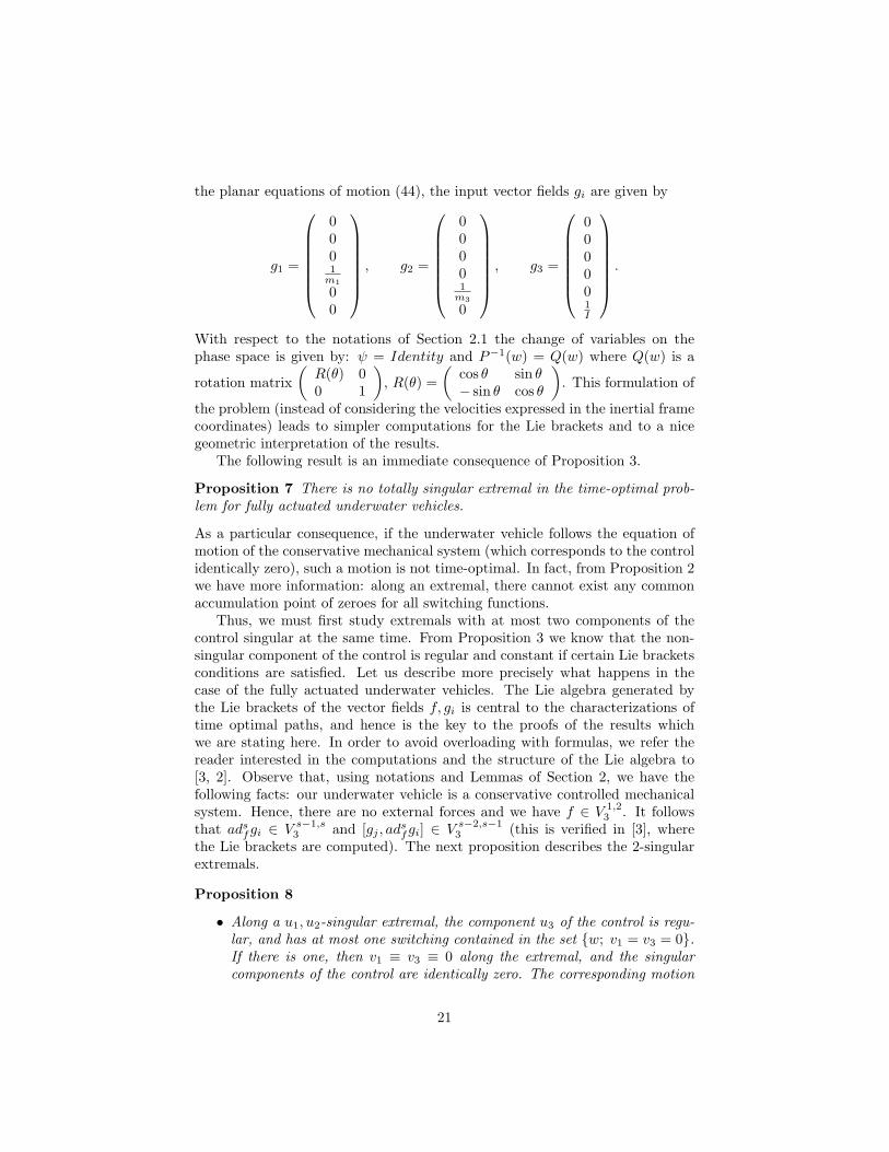
the planar equations of motion (44), the input vector fields gi are given by

g1 =

0001

m1

00

, g2 =

00001

m3

0

, g3 =

000001I

.

With respect to the notations of Section 2.1 the change of variables on thephase space is given by: ψ = Identity and P−1(w) = Q(w) where Q(w) is a

rotation matrix(R(θ) 00 1

), R(θ) =

(cos θ sin θ− sin θ cos θ

). This formulation of

the problem (instead of considering the velocities expressed in the inertial framecoordinates) leads to simpler computations for the Lie brackets and to a nicegeometric interpretation of the results.

The following result is an immediate consequence of Proposition 3.

Proposition 7 There is no totally singular extremal in the time-optimal prob-lem for fully actuated underwater vehicles.

As a particular consequence, if the underwater vehicle follows the equation ofmotion of the conservative mechanical system (which corresponds to the controlidentically zero), such a motion is not time-optimal. In fact, from Proposition 2we have more information: along an extremal, there cannot exist any commonaccumulation point of zeroes for all switching functions.

Thus, we must first study extremals with at most two components of thecontrol singular at the same time. From Proposition 3 we know that the non-singular component of the control is regular and constant if certain Lie bracketsconditions are satisfied. Let us describe more precisely what happens in thecase of the fully actuated underwater vehicles. The Lie algebra generated bythe Lie brackets of the vector fields f, gi is central to the characterizations oftime optimal paths, and hence is the key to the proofs of the results whichwe are stating here. In order to avoid overloading with formulas, we refer thereader interested in the computations and the structure of the Lie algebra to[3, 2]. Observe that, using notations and Lemmas of Section 2, we have thefollowing facts: our underwater vehicle is a conservative controlled mechanicalsystem. Hence, there are no external forces and we have f ∈ V 1,2

3 . It followsthat ads

fgi ∈ V s−1,s3 and [gj , ad

sfgi] ∈ V s−2,s−1

3 (this is verified in [3], wherethe Lie brackets are computed). The next proposition describes the 2-singularextremals.

Proposition 8

• Along a u1, u2-singular extremal, the component u3 of the control is regu-lar, and has at most one switching contained in the set w; v1 = v3 = 0.If there is one, then v1 ≡ v3 ≡ 0 along the extremal, and the singularcomponents of the control are identically zero. The corresponding motion

21

Figure 3: Initial and final position

for the underwater vehicle is a pure rotation with angular velocity varyinglinearly.

• Let i ∈ 1, 2 and k be such that k = 1 if i = 1, and k = 3 if i = 2.Along a ui, u3-singular extremal, there is at most one switching for thenonsingular component of the control and this switching is contained in theset w; vk = Ω = 0. Moreover, if there is one switching, then Ω ≡ 0 andvk ≡ 0, and both singular components of the control are identically zero.The corresponding motions for the underwater vehicle are translations inthe direction of the vertical (if i = 1) and horizontal (if i = 2) axis ofthe body frame coordinates, and the velocity of these translations dependslinearly on t.

• Along an abnormal extremal with 2 singular components of the control,there is a switching at the time ts only if the underwater vehicle is at restat t = ts: v1(ts) = v3(ts) = Ω(ts) = 0.

In [3] we describe an algorithm to compute the singular components of thecontrol when there is no switching and illustrate our results with simulations.The previous proposition shows that along a 2-singular extremal there is atmost one switching for the nonsingular component of the control. This is animportant result, indeed the existence of a uniform bound is not a consequenceof the maximum principle. This is a well-known question in optimal control: in[12] for instance, the author provides an example of optimal trajectories withan infinite number of switchings. A crucial question is the following: is there auniform bound on the number of switchings for all optimal trajectories? Thisis a highly nontrivial question, and we will try to give at least partial answersin forthcoming articles.

Conversely to Proposition 8, the following proposition states that the threebasic motions: pure rotation and translations in the direction of an axis of thebody coordinate frame, are 2-singular extremals.

Proposition 9 If along a trajectory we have v1 ≡ 0 and v3 ≡ 0, then thetrajectory is a u1, u2-singular extremal with at most one switching. The corre-sponding motion is a pure rotation and the singular components of the controlare identically zero: u1 ≡ u2 ≡ 0. If along a trajectory we have Ω ≡ 0 andv1 ≡ 0 (resp. v3 ≡ 0), then the trajectory is a u1, u3-singular extremal (resp.u2, u3) with at most one switching for u2 (resp. u1). The corresponding motionis a translation in the direction of the vertical (resp. horizontal) axis of the bodyframe coordinates.

Let us use Proposition 6 to discuss the optimality of some specific trajecto-ries. Consider the initial and final positions illustrated in Figure 3. Assume theunderwater vehicle to be at rest at these positions. On Figures 4 and 5 we rep-

22

Figure 4: Vertical + horizontal translation

Figure 5: Horizontal + vertical translation

resent two different ways to connect these positions; these are concatenationsof vertical and horizontal translations (the orientation is fixed along the mo-tion). Using the result given in Proposition 6 on the concatenation of singularextremals in the fully actuated situation, we can prove that these trajectoriesare not optimal.

More generally, we have the following result. Let wi and wf be arbitraryinitial and final positions such that the velocities are all zero. We can reachthese two positions by a motion formed by pure rotation and pure translationsin the direction of a body-frame axis. This is illustrated by Figures 6 and 7.We know that these trajectories are not optimal. The nonoptimality of such

trajectories is guaranteed by the fact that pure translational and rotationalmotions are necessarily 2-singular extremals, and by Proposition 6, which doesnot allow concatenations of 2-singular extremals in our case.

In order to obtain more information on the stucture of the time-optimaltrajectories, we also need to study extremals with only one component of thecontrol being singular, as well as trajectories with all components of the controlbang-bang. This will be done in a forthcoming article using results presentedin the previous sections. For instance, Proposition 2 gives information aboutextremals with one component singular only.

Proposition 10 Let i, j, k ∈ 1, 2, 3 such that i 6= j 6= k. If the extremal isui-singular, then φj and φk cannot have the same accumulation point of zeroes.If there exists t0 such that φj(t0) = φk(t0) = 0, we have φj(t0) 6= 0 or φk(t0) 6= 0.

As we already mentioned in this paper, our main result does not applyexclusively to the fully actuated situation. In a forthcoming article, we will studyunderactuated situations. These situations will be motivated by a buoyancydriven underwater vehicle; see [2] for a first approach.

References

[1] B. Bonnard and I. Kupka. Theorie des singularites de l’applicationentree/sortie et optimalite des trajectoires singuli’eres dans le problemedu temps minimal. Forum Math, pages 111–159, 1993.

Figure 6: Initial and final configurations

23

Figure 7: Path 1

[2] M. Chyba, N.E. Leonard, and E.D. Sontag. Time-optimal control for under-water vehicles. Lagrangian and Hamiltonian Methods for Nonlinear Control(N.E. Leonard, R. Ortega, eds), pages 117–122, 2000.

[3] M. Chyba, N.E. Leonard, and E.D. Sontag. Optimality for underwatervehicles. Proc. IEEE Conf. on Decision and Control, pages 4204–4209,2001.

[4] E.B. Lee and L. Markus. Foundations of optimal control theory. Wiley,1967.

[5] N.E. Leonard. Stability of a bottom-heavy underwater vehicle. Automatica,33:331–346, 1997.

[6] A.D. Lewis. The geometry of the maximum principle for affine connectioncontrol systems. Preprint, 2000.

[7] L.S. Pontryagin, B. Boltyanski, R. Gamkrelidze, and E. Michtchenko. Themathematical theory of optimal processes. Interscience, New-York, 1962.

[8] H. Schaettler. The local structure of time-optimal trajectories in dimen-sion 3 under generic conditions. SIAM J on Control and Optimization,26(4):899–918, 1988.

[9] E.D. Sontag. Remarks on the time-optimal control of a class of Hamiltoniansystems. IEEE Conf. on Decision and Control, pages 317–221, 1989.

[10] E.D. Sontag. Mathematical control theory: Deterministic finite dimensionalsystems. second edition. Springer-Verlag, New-York, 1998.

[11] E.D. Sontag and H.J. Sussmann. Time-optimal control of manipulators.Proc. IEEE Int. Conf. on Robotics and Automation, pages 1692–1697, 1986.

[12] H.J. Sussmann. The Markov-Dubins problem with angular accelerationcontrol. IEEE Conf. on Decision and Control, pages 2639–2643, 1997.

[13] H.J. Sussmann. The maximum principle of optimal control theory. Mathe-matical Control Theory, J. Baillieul, J.C. Willems (Eds), Springer-Verlag,pages 140–198, 1998.

[14] H.J. Sussmann and G.Q. Tang. Shortest paths for the Reeds-Shepp car: aworked out example of the use of geometric techniques in nonlinear optimalcontrol. To appear: Siam J. Control.

24