SINGULAR QUASILINEAR AND HESSIANEQUATIONS AND INEQUALITIES

Nguyen Cong PhucDepartment of Mathematics, Louisiana State University,

Baton Rouge, LA 70803, USAE-mail: pcnguyen@math.lsu.edu

and

Igor E. Verbitsky1

Department of Mathematics, University of Missouri,Columbia, MO 65211, USA

E-mail: igor@math.missouri.edu

1Supported in part by NSF grant DMS-05563091

2 PHUC AND VERBITSKY – SINGULAR NONLINEAR EQUATIONS

Abstract. We solve the existence problem in the renormalized, orviscosity sense, and obtain global pointwise estimates of solutions forquasilinear and Hessian equations with measure coefficients and data,including the following model problems:

−∆pu = σ uq + µ, Fk[−u] = σ uq + µ, u ≥ 0,

on Rn, or on a bounded domain Ω ⊂ Rn. Here ∆p is the p-Laplaciandefined by ∆pu = div (∇u|∇u|p−2), and Fk[u] is the k-Hessian, i.e., thesum of the k × k principal minors of the Hessian matrix D2u (k =1, 2, . . . , n); σ and µ are general nonnegative measurable functions (ormeasures) on Ω.

Keywords: Quasilinear equations, fully nonlinear equations, powersource terms, p-Laplacian, k-Hessian, Wolff’s potential, weighted norminequalities.

PHUC AND VERBITSKY – SINGULAR NONLINEAR EQUATIONS 3

1. Introduction

Let σ, ω be arbitrary nonnegative locally integrable functions, ormore generally, nonnegative locally finite measures on a domain Ω inRn. By Lq

σ, loc(Ω), q > 0, we denote the space of measurable functionsf such that |f |q is locally integrable with respect to σ in Ω.

In this paper we consider the following quasilinear and Hessian equa-tions with nonlinear source terms and measure coefficients and data:

−∆pu = σuq + ω, u ≥ 0, u is p-superharmonic in Ω, (1.1)

andFk[−u] = σuq + ω, u ≥ 0, −u is k-convex in Ω, (1.2)

where u ∈ Lqσ, loc(Ω), q > 0, 1 < p < ∞, and k = 1, . . . , n. Here ∆p is

the p-Laplacian defined by

∆pu = div(|∇u|p−2∇u),

and Fk[u] denotes the k-Hessian

Fk[u] =∑

1≤i1<···<ik≤n

λi1 · · ·λik ,

where λ1, . . . , λn are the eigenvalues of the Hessian matrix D2u. Inother words, Fk[u] is the sum of the k × k principal minors of D2u,which coincides with the Laplacian F1[u] = ∆2u = ∆u if k = 1, andthe Monge-Ampere operator Fn[u] = Det(D2u) if k = n.

The k-Hessian operator was first studied by Caffarelli, Nirenberg,and Spruck in [11], and also simultaneously by Ivochkina in [19]. Thefundamental properties of the p-Laplacian and the k-Hessian, alongwith the corresponding notions of p-superharmonicity and k-convexity,are discussed in [11], [18], [19], [31], [32].

In the semilinear case, i.e., when p = 2 in (1.1) or k = 1 in (1.2),such equations with nonlinear sources are well studied, especially forspecific coefficients and data σ, ω (see, e.g., [2], [3], [4]). For arbitrarypositive σ, ω (possibly singular measures), necessary and sufficient con-ditions for the existence of weak solutions, along with sharp pointwiseestimates of solutions, were given in [10], [23]. In [KV], more generallinear elliptic operators, as well as some nonlocal operators in place ofthe Laplacian were considered. We refer to [36] for a recent survey ofthese and other related results.

Quasilinear equations (1.1) in the special case σ ≡ 1 have beenstudied extensively over the past 20 years (see [5]–[7], [8], [9], [30], [36]).For the k-Hessian equation (1.2), when ω ≡ 0, the existence of nonzerobounded solutions was studied in [14]. Recently, in [25] we obtainednecessary and sufficient conditions for the solvability of (1.1) in this

4 PHUC AND VERBITSKY – SINGULAR NONLINEAR EQUATIONS

case, without any a priori assumption on the inhomogeneous term ω ≥0, along with a complete characterization of removable singularities forthe corresponding homogeneous equation. We also obtained analogousresults for Hessian equations (1.2).

A crucial role in [25] is played by estimates of solutions in terms ofWolff’s potentials:

Wα, sµ(x) =

∫ ∞

0

(µ(Bt(x))

tn−αs

) 1s−1 dt

t, x ∈ Rn, (1.3)

where µ ≥ 0 is a locally finite measure on Rn, α > 0 and s > 1.Here we set α = 1, s = p for the p-Laplacian, and α = 2k

k+1, s =

k + 1 for the k-Hessian. These potentials were originally introducedby Hedberg and Wolff as a tool for solving certain hard problems ofnonlinear potential theory and Sobolev spaces (see [1], Sections 4.9and 9.13). Their importance for quasilinear and Hessian equations wasdiscovered subsequently by Kilpelainen and Maly [21], and Labutin[22].

In particular, it was shown in [25] that if the equation of Lane–Emdentype,

−∆pu = uq + ω, u ≥ 0, u is p-superharmonic in Rn, (1.4)

has a solution, then W1, pω(x) < +∞ a.e., and there exists a constantC = C(n, p, q) > 0 such that

W1, p[(W1, pω)qdx](x) ≤ C W1, pω(x) dx-a.e., (1.5)

where dx stands for Lebesgue measure on Rn.Conversely, there exists a constant C0 = C0(n, p, q) > 0 such that if

W1, pω(x) < +∞ a.e., and if (1.5) holds for some C ≤ C0, then theequation (1.4) admits a solution u such that

c1W1, pω(x) ≤ u(x) ≤ c2W1, pω(x), (1.6)

where c1, c2 are positive constants depending only on n, p, q. Analogousresults are obtained in [25] for the corresponding Dirichlet problem ona bounded domain Ω ⊂ Rn, as well as for Hessian equations. Further-more, several equivalent characterizations of (1.5), along with simplersufficient and necessary coefficients are given there.

However, for variable coefficients σ in the source term, the globalexistence problem for (1.1), (1.2) and control of the corresponding so-lutions are much harder due to a nonlinear interplay between σ, theinhomogeneous term ω, and the operator on the left-hand side. Sucha phenomenon, observed previously in the semilinear case in [10], [23],

PHUC AND VERBITSKY – SINGULAR NONLINEAR EQUATIONS 5

becomes substantially more complicated for quasilinear and fully non-linear operators. Some partial results towards the solution of this prob-lem were obtained in [26].

In the present paper, we develop new techniques to establish criteriafor the solvability of (1.1) and (1.2) with a pair of general weights σand ω. Our results are new even in the special case of power weightsσ(x) = |x|γ, γ > −n (see [26], and the literature cited there).

As we will demonstrate below, an analogue of (1.5), namely thepointwise condition

Wα, s[(Wα, sω)qdσ](x) ≤ C Wα, sω(x) dσ-a.e., (1.7)

with α = 1, s = p (or α = 2kk+1

, s = k + 1), is still necessary andsufficient, with a gap only in the best constants, for the solvability of(1.1), or (1.2), respectively.

An important part of our approach, which distinguishes it from thatof [25], is concerned with nonlinear two-weight trace inequalities of thetype: ∫

Rn

[Wα, s(gdω)(y)]q dσ(y) ≤ C

∫Rn

gq

s−1 dω, (1.8)

where g ∈ Lq

s−1ω (Rn), g ≥ 0, and its “testing” counterpart:∫

B

[Wα, sωB(y)]q dσ(y) ≤ C ω(B), (1.9)

where B are balls in Rn, and dωB = χB dω. The preceding inequalityis deduced from (1.8) by letting g = χB.

It turns out that (1.8) is intimately connected with equations (1.1)and (1.2). We will show that (1.8), and hence (1.9), with α = 1, s = p(or α = 2k

k+1, s = k + 1), is necessary for the existence of a solution to

(1.1), or (1.2), respectively.Actually, it follows from our earlier work [25] that, for σ ≡ 1, (1.8) or

(1.9), with the appropriate α and s, is also sufficient for the solvabilityof (1.1) and (1.2).

In the case where σ is a general nonnegative measure, we will showbelow that (1.8), or (1.9), together with the additional pointwise con-dition∫ r

0

(σ(Bt(x))

tn−αs

) 1s−1 dt

t·[ ∫ ∞

r

(ω(Bt(x))

tn−αs

) 1s−1 dt

t

] qs−1

−1

≤ C, (1.10)

where C does not depend on x ∈ Rn and r > 0, with α = 1, s = p(or α = 2k

k+1, s = k + 1), is sufficient for the solvability of (1.1), or

(1.2), respectively. Remarkably, (1.10) with the appropriate α, s is alsonecessary for the solvability of (1.1) and (1.2), as was shown in [26].

6 PHUC AND VERBITSKY – SINGULAR NONLINEAR EQUATIONS

This gives a complete solution to the existence problem, with a gaponly in the best constants in the sufficiency and necessity parts. Suchcharacterizations of solvability were obtained earlier [23] for semilinearequations where p = 2 or k = 1.

Analogous results for equations of the type (1.1), (1.2) on boundeddomains Ω in Rn with Dirichlet boundary conditions are obtained inTheorems 3.11 and 4.9 below as well. In this case, we use a truncatedversion of Wolff’s potentials defined for α > 0, s > 1, and a nonnegativemeasure µ on Ω by

Wrα, sµ(x) =

∫ r

0

(µ(Bt(x))

tn−αs

) 1s−1 dt

t,

where x ∈ Ω and 0 < r < 2 diam(Ω).In the present paper, we use extensively dyadic models, and various

global and local Wolff’s potential estimates obtained in [12], [13], [21],[22], [25], [26], along with fundamental weak continuity theorems forquasilinear and Hessian equations [32]–[34]. This makes it possible togive a unified treatment for both quasilinear equations and equationsof Monge-Ampere type with general coefficients and data.

Our main results are summarized in the following theorems. In Theo-rems 1.1, we assume that A : Rn×Rn → Rn is a vector-valued mappingthat satisfies A(x, ξ) · ξ ≈ |ξ|p where 1 < p < n, i.e.,

A(x, ξ) · ξ ≥ α|ξ|p, |A(x, ξ)| ≤ β|ξ|p−1

for some α, β > 0. The precise structural conditions imposed on Aalong with the notion of A-superharmonic functions are introduced inthe next section. This includes the standard case A(x, ξ) = |ξ|p−2ξwhich corresponds to the usual p-Laplacian ∆p, and the correspondingnotion of p-superharmonic functions.

Theorem 1.1. Let ω and σ be nonnegative locally finite measures onRn and let q > p− 1 > 0. If the equation

−divA(x,∇u) = σuq + ω (1.11)

has a solution u ∈ Lqσ, loc(Rn), u ≥ 0, then there exists a constant

C = C(n, p, q, α, β) > 0 such that statements (i), (ii) and (iii) beloware valid.

(i) The inequality∫Rn

[W1, p(gdω)(y)]q dσ(y) ≤ C

∫Rn

gq

p−1 dω (1.12)

PHUC AND VERBITSKY – SINGULAR NONLINEAR EQUATIONS 7

holds for all g ∈ Lq

p−1ω (Rn), g ≥ 0, and∫ r

0

(σ(Bt(x))

tn−p

) 1p−1 dt

t·[ ∫ ∞

r

(ω(Bt(x))

tn−p

) 1p−1

] qp−1

−1dt

t≤ C (1.13)

holds for all x ∈ Rn and r > 0.(ii) The inequality∫

B

[W1, pωB(y)]q dσ(y) ≤ C ω(B) (1.14)

holds for all balls B ⊂ Rn, and (1.13) holds for all x ∈ Rn andr > 0.

(iii) For each x ∈ Rn,

W1, p[(W1, pω)qdσ](x) ≤ C W1, pω(x). (1.15)

Conversely, there exists a constant C0 = C0(n, p, q, α, β) > 0 suchthat if anyone of statements (i), (ii), (iii) holds with C ≤ C0 thenequation (1.11) has a solution u ∈ Lq

σ, loc(Rn), u ≥ 0, such that

M1W1, pω(x) ≤ u(x) ≤ M2W1, pω(x).

Theorem 1.2. Let ω and σ be nonnegative locally finite measures onRn, and let 1 ≤ k < n

2, q > k. If the equation

Fk[−u] = σuq + ω (1.16)

has a solution u ∈ Lqσ, loc(Rn), u ≥ 0, then there exists a constant

C = C(n, k, q) > 0 such that statements (i), (ii) and (iii) below arevalid.

(i) The inequality∫Rn

[W 2kk+1

, k+1(gdω)(y)]q dσ(y) ≤ C

∫Rn

gqk dω

holds for all g ∈ Lqkω (Rn), g ≥ 0, and∫ r

0

(σ(Bt(x))

tn−2k

) 1k dt

t·[ ∫ ∞

r

(ω(Bt(x))

tn−2k

) 1k] q

k−1dt

t≤ C (1.17)

holds for all x ∈ Rn and r > 0.(ii) The inequality∫

B

[W 2kk+1

, k+1ωB(y)]q dσ(y) ≤ C ω(B)

holds for all balls B ⊂ Rn, and (1.17) holds for all x ∈ Rn andr > 0.

8 PHUC AND VERBITSKY – SINGULAR NONLINEAR EQUATIONS

(iii) For each x ∈ Rn,

W 2kk+1

, k+1[(W 2kk+1

, k+1ω)qdσ](x) ≤ C W 2kk+1

, k+1ω(x).

Conversely, there exists a constant C0 = C0(n, k, q) > 0 such that ifanyone of statements (i), (ii), (iii) holds with C ≤ C0, then equation(1.16) has a solution u ∈ Lq

σ, loc(Rn), u ≥ 0 such that

M1W 2kk+1

, k+1ω(x) ≤ u(x) ≤ M2W 2kk+1

, k+1ω(x).

2. A-superharmonic functions

In this section, we recall for later use some facts on A-superharmonicfunctions, most of which can be found in [18], [20], [21], and [34]. LetΩ be an open set in Rn, and let p > 1. (We will be mostly interested inthe case Ω = Rn and 1 < p < n.) Let us assume that A : Rn × Rn →Rn is a vector-valued mapping which satisfies the following structuralproperties:

the mapping x → A(x, ξ) is measurable for all ξ ∈ Rn, (2.1)

the mapping ξ → A(x, ξ) is continuous for a.e. x ∈ Rn, (2.2)

and there are constants 0 < α ≤ β < ∞ such that for a.e. x in Rn,and for all ξ in Rn,

A(x, ξ) · ξ ≥ α|ξ|p, |A(x, ξ)| ≤ β|ξ|p−1, (2.3)

[A(x, ξ1)−A(x, ξ2)] · (ξ1 − ξ2) > 0, if ξ1 6= ξ2, (2.4)

A(x, λξ) = λ|λ|p−2A(x, ξ), if λ ∈ R \ 0. (2.5)

For u ∈ W 1, ploc (Ω), we define the divergence of A(x,∇u) in the sense

of distributions, i.e., if ϕ ∈ C∞0 (Ω), then

divA(x,∇u)(ϕ) = −∫

Ω

A(x,∇u) · ∇ϕ dx.

It is well known that every solution u ∈ W 1, ploc (Ω) to the equation

−divA(x,∇u) = 0 (2.6)

has a continuous representative. Such continuous solutions are said tobe A-harmonic in Ω. If u ∈ W 1, p

loc (Ω) and∫Ω

A(x,∇u) · ∇ϕ dx ≥ 0,

for all nonnegative ϕ ∈ C∞0 (Ω), i.e., −divA(x,∇u) ≥ 0 in the distri-

butional sense, then u is called a supersolution to (2.6) in Ω.A lower semicontinuous function u : Ω → (−∞,∞] is called A-

superharmonic if u is not identically infinite in each component of Ω,

PHUC AND VERBITSKY – SINGULAR NONLINEAR EQUATIONS 9

and if for all open sets D such that D ⊂ Ω, and all functions h ∈ C(D),A-harmonic in D, it follows that h ≤ u on ∂D implies h ≤ u in D.

We recall here the fundamental connection between supersolutionsof (2.6) and A-superharmonic functions [18].

Proposition 2.1 ([18]). (i) If u ∈ W 1, ploc (Ω) is such that

−divA(x,∇u) ≥ 0,

then there is an A-superharmonic function v such that u = v a.e.Moreover,

v(x) = ess lim infy→x

v(y), x ∈ Ω. (2.7)

(ii) If v is A-superharmonic, then (2.7) holds. Moreover, if v ∈W 1, p

loc (Ω), then

−divA(x,∇v) ≥ 0.

(iii) If v is A-superharmonic and locally bounded, then v ∈ W 1, ploc (Ω),

and

−divA(x,∇v) ≥ 0.

A consequence of the above proposition is that if u and v are twoA-superharmonic functions on Ω for which u ≤ v a.e. on Ω then u ≤ veverywhere on Ω.

Note that anA-superharmonic function u does not necessarily belongto W 1, p

loc (Ω), but its truncation minu, k does, for every integer k, byProposition 2.1(iii). Using this we set

Du = limk→∞

∇ [ minu, k],

defined a.e. If either u ∈ L∞(Ω) or u ∈ W 1, 1loc (Ω), then Du coincides

with the regular distributional gradient of u. In general we have thefollowing gradient estimates [20] (see also [18], [34]).

Proposition 2.2 ([20]). Suppose u is A-superharmonic in Ω and 1 ≤q < n

n−1. Then both |Du|p−1 and A(·, Du) belong to Lq

loc(Ω). Moreover,

if p > 2− 1n, then Du is the distributional gradient of u.

We can now extend the definition of the divergence of A(x,∇u) tothose u which are merely A-superharmonic in Ω. For such u we set

−divA(x,∇u)(ϕ) =

∫Ω

A(x, Du) · ∇ϕ dx,

10 PHUC AND VERBITSKY – SINGULAR NONLINEAR EQUATIONS

for all ϕ ∈ C∞0 (Ω). Note that by Proposition 2.2 and the dominated

convergence theorem,

−divA(x,∇u)(ϕ) = limk→∞

∫Ω

A(x,∇minu, k) · ∇ϕ dx ≥ 0

whenever ϕ ∈ C∞0 (Ω) and ϕ ≥ 0.

Since −divA(x,∇u) is a nonnegative distribution in Ω for an A-superharmonic u, it follows that there is a positive (not necessarilyfinite) Radon measure denoted by µ[u] such that

−divA(x,∇u) = µ[u] in Ω.

Conversely, given a nonnegative finite measure µ in a bounded domainΩ, there is an A-superharmonic function u (not necessarily unique)such that −divA(x,∇u) = µ in Ω and minu, k ∈ W 1,p

0 (Ω) for allintegers k; see [20].

The following weak continuity result in [34] will be used later to provethe existence of A-superharmonic solutions to quasilinear equations.

Theorem 2.3 ([34]). Suppose that un is a sequence of nonnega-tive A-superharmonic functions in Ω that converges a.e. to an A-superharmonic function u. Then the sequence of measures µ[un]converges to µ[u] weakly, i.e.,

limn→∞

∫Ω

ϕ dµ[un] =

∫Ω

ϕ dµ[u]

for all ϕ ∈ C∞0 (Ω).

In [20] and [21] the following two-sided pointwise potential estimateforA-superharmonic functions was established, which serves as a majortool in our study of quasilinear equations of Lane–Emden type.

Theorem 2.4 ([21]). Let u be an A-superharmonic function in Rn withinfRn u = 0. If µ = −divA(x,∇u), then

1

KW1, pµ(x) ≤ u(x) ≤ K W1, pµ(x)

for all x ∈ Rn, where K is a positive constant depending only on n, pand the structural constants α and β.

3. Quasilinear equations

In this section, we study the solvability problem for the quasilinearequation

−divA(x,∇u) = σuq + ω (3.1)

PHUC AND VERBITSKY – SINGULAR NONLINEAR EQUATIONS 11

in a bounded domain Ω ⊂ Rn or in the entire space Rn, where A(x, ξ) ·ξ ≈ |ξ|p is given as in Sec. 2. Here we assume p > 1, q > p−1, and ω isa nonnegative locally finite measure on Rn. The solvability of (3.1) inRn is understood in the “potential-theoretic” sense, i.e., u ∈ Lq

loc(Rn),u ≥ 0, is a solution to (3.1) if u is A-superharmonic, and

−divA(x,∇u)(ϕ) =

∫uqϕ dσ +

∫ϕ dω

for all test functions ϕ ∈ C∞0 (Rn). Here as discussed in Section 2,

−divA(x,∇u)(ϕ) =

∫limk→∞

A(x,∇minu, k) · ∇ϕ dx

for each ϕ ∈ C∞0 (Rn). On the other hand, to deal with (3.1) in bounded

domains we will use the notion of renormalized solutions.We first prove a necessary condition for the solvability of (3.1) in Rn

in terms of a certain nonlinear weighted norm inequality.

Theorem 3.1. Let u ∈ Lqσ, loc(Rn) be a nonnegative A-superharmonic

function for which

−divA(x,∇u) = σuq + ω

in Rn, where 1 < p < n and q > p− 1. Then∫Rn

[W1, p(gdω)]qdσ ≤ C

∫Rn

gq

p−1 dω (3.2)

for all g ∈ Lq

p−1ω (Rn), g ≥ 0, and for a constant C depending only on

n, p, q, and the structural constants α, β.

Proof. Let µ = σuq + ω. From the lower Wolff potential estimate,Theorem 2.4, there is a constant C = C(n, p, α, β) > 0 such that

u(x) ≥ C W1, pµ(x)

for all x ∈ Rn. From this we obtain

(W1, pµ)qdσ ≤ C dµ, (3.3)

where C = C(n, p, q, α, β). Moreover, it is also easily checked that allconstants C appearing in the rest of the proof depend only on n, p, q,and α, β, but not on the measures σ and ω. Inequality (3.3) now gives∫

Rn

(W1, pµ)q(Mµg)q

p−1 dσ ≤ C

∫Rn

(Mµg)q

p−1 dµ,

which holds for all g ∈ Lq

p−1µ . Here Mµ denotes the centered Hardy-

Littlewood maximal function defined for a locally µ-integrable function

12 PHUC AND VERBITSKY – SINGULAR NONLINEAR EQUATIONS

f by

Mµf(x) = supr>0

∫Br(x)

|f | dµ

µ(Br(x)).

Since Mµ is bounded on Lsµ(Rn), s > 1, (see, e.g., [16]), from (3.4) we

obtain ∫Rn

(W1, pµ)q(Mµg)q

p−1 dσ ≤ C

∫Rn

gq

p−1 dµ

for all g ∈ Lq

p−1µ (Rn), g ≥ 0. From this inequality and the estimate

[W1, pµ(x)]q[Mµg(x)]q

p−1 ≥ C [W1, p(gdµ)(x)]q

we deduce ∫Rn

[W1, p(gdµ)(x)]qdσ(x) ≤ C

∫Rn

gq

p−1 dµ. (3.4)

We now continue the proof of Theorem 3.1 with the cases 1 < p ≤ 2and p > 2 being treated separately.

The case 1 < p ≤ 2 : We first rewrite (3.4) in the form∫Rn

[ ∑j∈Z

(∫B(x, 2−j)

gdµ

(2−j)n−p

) 1p−1

]p−1 qp−1

dσ(x) ≤ C

∫Rn

gq

p−1 dµ.

Since 1 < p ≤ 2, by duality of spaces with mixed norms, Lq

p−1σ (`

1p−1 ) =[

Lq

q−p+1σ (`

12−p )

]∗, this is equivalent to∫

Rn

∑j∈Z

∫B(x, 2−j)

gdµ

(2−j)n−pφj(x)dσ(x) ≤ C||g||

Lq

p−1µ

||~φ||L

qq−p+1σ (`

12−p )

for all ~φ = φjj∈Z ∈ Lq

q−p+1σ (`

12−p ). Using Fubini’s theorem, the above

inequality can be rewritten as∫Rn

∫Rn

[ ∑j∈Z

χB(x, 2−j)(y)

(2−j)n−pφj(x)dσ(x)

]g(y)dµ(y) (3.5)

≤ C||g||L

qp−1µ

||~φ||L

qq−p+1σ (`

12−p )

.

Again by duality (3.5) is equivalent to∫Rn

[ ∫Rn

∑j∈Z

χB(x, 2−j)(y)

(2−j)n−pφj(x)dσ(x)

] qq−p+1

dµ(y) (3.6)

≤ C||~φ||q

q−p+1

Lq

q−p+1σ (`

12−p )

.

PHUC AND VERBITSKY – SINGULAR NONLINEAR EQUATIONS 13

Since ω ≤ µ, inequality (3.6), and hence inequality (3.4), holds also forω in place of µ, i.e.,∫

Rn

[W1, p(gω)(x)]qdσ(x) ≤ C

∫Rn

gq

p−1 dω

for all g ∈ Lq

p−1ω (Rn), g ≥ 0, which gives (3.2).

The case p > 2 : Since Q ⊂ B√n`(Q)(x) for every cube Q that

contains x, we see that∑Q∈D

( ∫Q

gdµ

`(Q)n−p

) 1p−1

χQ(x) ≤ CW1, p(gdµ)(x).

Thus from (3.4) we obtain∫Rn

[ ∑Q∈D

( ∫Q

gdµ

`(Q)n−p

) 1p−1

χQ(x)]q

dσ(x) (3.7)

≤ C

∫Rn

gq

p−1 dµ.

We next choose a number s such that s > max1, 1p−1

, 1q−p+1

and

replace g by gs(p−1) in (3.7) to get∫Rn

[ ∑Q∈D

(∫Q

gs(p−1)dµ

`(Q)n−p

) ss(p−1)

χQ(x)]q

dσ(x) ≤ C

∫Rn

gqsdµ.

Since s(p− 1) > 1, from this and Holder’s inequality we obtain∫Rn

[ ∑Q∈D

(cQ

∫Q

gdµ

µ(Q)

)s

χQ(x) 1

s]qs

dσ(x) (3.8)

≤ C

∫Rn

gqsdµ,

where we set cQ = [`(Q)p−nµ(Q)]1

s(p−1) . By duality (3.8) is equivalentto ∫

Rn

∑Q∈D

cQ

∫Q

gdµ

µ(Q)χQ(x)φQ(x)dσ(x) (3.9)

≤ C||g||Lqsµ||~φ||

L(qs)′σ (`s′ )

for all ~φ = φQQ∈D ∈ L(qs)′σ (`s′). Here and in what follows for r > 1

we denote by r′ its conjugate, i.e., r′ = rr−1

. Observe that inequality

14 PHUC AND VERBITSKY – SINGULAR NONLINEAR EQUATIONS

(3.9) can be rewritten in the form∫Rn

∑Q∈D

cQ

∫Q

φQdσ

µ(Q)χQ(y)g(y)dµ(y) ≤ C||g||Lqs

µ||~φ||

L(qs)′σ (`s′ )

,

which again by duality is equivalent to∫Rn

[ ∑Q∈D

cQ

∫Q

φQdσ

µ(Q)χQ(y)

](qs)′

dµ(y) ≤ C||~φ||(qs)′

L(qs)′σ (`s′ )

. (3.10)

Applying Proposition 2.2 in [13] we see that this inequality is equivalentto ∑

Q∈D

λQ

( 1

µ(Q)

∑Q′⊂Q

λQ′

)(qs)′−1

≤ C||~φ||(qs)′

L(qs)′σ (`s′ )

, (3.11)

where λQ = cQ

∫Q

φQdσ = [`(Q)p−nµ(Q)]1

s(p−1)∫

QφQdσ. Note that

1s(p−1)

− (qs)′ + 1 > 0 by the choice of s. Thus (3.11), and hence

(3.8), holds also for ω in place of µ, i.e.,∫Rn

[ ∑Q∈D

sQ

(∫Q

gdω

ω(Q)

)s

χQ(x)]q

dσ(x) (3.12)

≤ C

∫Rn

gqsdω,

which holds for all g ∈ Lqsω (Rn), g ≥ 0. We set sQ = [`(Q)p−nω(Q)]

1p−1 .

Let Mdµ denote the dyadic Hardy-Littlewood maximal function de-

fined for each locally µ-integrable function f by

Mdµf(x) = sup

Q3x

∫Q|f |dµ

µ(Q),

where the supremum is taken over all dyadic cubes that contain x. By

replacing g with [Mdω(gs(p−1))]

1s(p−1) in (3.12) we obtain∫

Rn

[ ∑Q∈D

sQ

(∫Q

gs(p−1)dω

ω(Q)

) 1p−1

χQ(x)]q

dσ(x) (3.13)

≤ C

∫Rn

[Mdω(gs(p−1))]

qp−1 dω.

Since q > p− 1, the boundedness of Mdω on Ls

ω, s > 1 (see, e.g., [27]),and (3.13) then yield∫

Rn

[ ∑Q∈D

sQ

(∫Q

gs(p−1)dω

ω(Q)

) 1p−1

χQ(x)]q

dσ(x) ≤ C

∫Rn

gqsdω.

PHUC AND VERBITSKY – SINGULAR NONLINEAR EQUATIONS 15

Thus replacing g with g1

s(p−1) in the above inequality we get∫Rn

[ ∑Q∈D

( ∫Q

gdω

`(Q)n−p

) 1p−1

χQ(x)]q

dσ(x) (3.14)

≤ C

∫Rn

gq

p−1 dω,

which holds for all g ∈ Lq

p−1ω (Rn), g ≥ 0. Note that a shifted version of

(3.14), namely,∫Rn

[ ∑Q∈D

( ∫Qt

gdω

`(Qt)n−p

) 1p−1

χQt(x)]q

dσ(x) (3.15)

≤ C

∫Rn

gq

p−1 dω,

holds for the same constant C > 0 independent of t ∈ Rn as well.Here Qt = Q + t for each t ∈ Rn. We next introduce the truncatedversion WR

1, p, R > 0, of Wolff’s potentials defined for each nonnegativemeasure ν by

WR1, pν(x) =

∫ R

0

(ν(Bt(x))

tn−p

) 1p−1 dt

t. (3.16)

It was established in [12], page 399, that

WR1, p(gdω)(x) ≤ C

Rn

∫|t|≤cR

∑Q∈D

( ∫Qt

gdω

`(Qt)n−p

) 1p−1

χQt(x)dt,

which holds for constants C, c > 0 depending only on n. From thisestimate, Holder’s inequality and the fact that q > p− 1 > 1 we get

[WR1, p(gdω)(x)]q ≤ C

Rn

∫|t|≤cR

[ ∑Q∈D

( ∫Qt

gdω

`(Qt)n−p

) 1p−1

χQt(x)]q

dt.

Thus in view of (3.15), applying Fubini’s Theorem and letting R →∞,we obtain (3.2).

In the next theorem we establish a pointwise inequality which willturn out to be necessary and sufficient for the solvability of (3.1) in Rn.

Theorem 3.2. Let σ and ω be nonnegative locally finite measures onRn for which ∫

B

[W1, pωB(y)]qdσ(y) ≤ Mω(B) (3.17)

16 PHUC AND VERBITSKY – SINGULAR NONLINEAR EQUATIONS

for all balls B ⊂ Rn, and∫ r

0

(σ(Bt(x))

tn−p

) 1p−1 dt

t·[ ∫ ∞

r

(ω(Bt(x))

tn−p

) 1p−1 dt

t

] qp−1

−1

≤ M (3.18)

for x ∈ Rn and 0 < r < ∞. Then

W1, p[(W1, pω)qdσ](x) ≤ C W1, pω(x)

for a constant C > 0 depending only on p, q and M .

Proof. Let dν = (W1, pω)qdσ and let x be as in the theorem. We haveto show that for a constant C = C(p, q, M),

W1, pν(x) =

∫ ∞

0

(ν(Br(x))

rn−p

) 1p−1 dr

r≤ C W1, pω(x).

For r > 0 we write ω = ω1 + ω2 where dω1 = χB2r(x)dω and dω2 =(1− χB2r(x))dω. From (3.17) we have

ν(Br(x)) =

∫Br(x)

[W1, pω(y)]qdσ(y) (3.19)

≤ C

∫Br(x)

[W1, pω1(y)]q + [W1, pω2(y)]q

dσ

≤ C ω(B2r(x)) + C

∫Br(x)

[W1, pω2(y)]qdσ,

where C = C(p, q, M). On the other hand, for y ∈ Br(x),

W1, pω2(y) =

∫ ∞

r

(ω2(Bt(y))

tn−p

) 1p−1 dt

t

≤∫ ∞

r

(ω(B2t(x))

tn−p

) 1p−1 dt

t,

since Bt(y) ⊂ B2t(x) for y ∈ Br(x) and t ≥ r. Thus,∫Br(x)

[W1, pω2(y)]qdσ ≤[ ∫ ∞

r

(ω(B2t(x))

tn−p

) 1p−1 dt

t

]q

σ(Br(x)).

From this inequality and (3.19) we get

W1, pν(x) ≤ C

∫ ∞

0

(ω(B2r(x))

rn−p

) 1p−1 dr

r+ C I(x), (3.20)

where

I(x) =

∫ ∞

0

[ ∫ ∞

r

(ω(B2t(x))

tn−p

) 1p−1 dt

t

] qp−1

(σ(Br(x))

rn−p

) 1p−1 dr

r.

PHUC AND VERBITSKY – SINGULAR NONLINEAR EQUATIONS 17

Using integration by parts we can write

I(x) =q

p− 1

∫ ∞

0

[ ∫ ∞

r

(ω(B2t(x))

tn−p

) 1p−1 dt

t

] qp−1

−1

×

×(ω(B2r(x))

rn−p

) 1p−1

[ ∫ r

0

(σ(Bt(x))

tn−p

) 1p−1 dt

t

]dr

r,

which by (3.18) gives

I(x) ≤ M

∫ ∞

0

(ω(B2r(x))

rn−p

) 1p−1 dr

r.

Thus in view of (3.20) we obtain for a constant C = C(p, q, M),

W1, pν(x) ≤ C

∫ ∞

0

(ω(B2r(x))

rn−p

) 1p−1 dr

r≤ C W1, pω(x),

which completes the proof of the theorem.

As we will employ the notion of renormalized solutions below, wenow recall two of its equivalent definitions established in [15]. In whatfollows, for a measure µ of bounded total variation on a bounded openset Ω we will denote by µ0 its continuous part (with respect to thecapacity cap1, p(·, Ω)), and by µs its singular part, which concentrateson a set of zero capacity. Here the capacity cap1, p(·, Ω) is defined by

cap1, p(K, Ω) = inf∫

Ω

|∇ϕ|pdx : ϕ ∈ C∞0 (Ω), u ≥ 1 on K

for each compact set K ⊂ Ω. Thus we can write

µ = µ0 + µ+s − µ−s ,

where µ+s and µ−s are positive and negative parts of µs respectively.

Definition 3.3. Let µ be a measure of bounded total variation on Ω.Then u is said to be a renormalized solution of

−divA(x,∇u) = µ in Ω,u = 0 on ∂Ω,

(3.21)

if the following conditions hold:(a) The function u is measurable and finite almost everywhere, andTk(u) belongs to W 1, p

0 (Ω) for every k > 0, where for k > 0 and s ∈ R,Tk(s) = max−k, mins, k .(b) The gradient Du of u satisfies |Du|p−1 ∈ Lq(Ω) for all q < n

n−1,

where Du is defined by

Duχ|u|<k = ∇Tk(u) a.e. on Ω, for all k > 0.

18 PHUC AND VERBITSKY – SINGULAR NONLINEAR EQUATIONS

(c) If w belongs to W 1, p0 (Ω)∩L∞(Ω) and if there exist k > 0, w+∞ and

w−∞ in W 1, r(Ω) ∩ L∞(Ω), with r > N , such thatw = w+∞ a.e. on the set u > k,w = w−∞ a.e. on the set u < −k

then∫Ω

A(x, Du) · ∇wdx =

∫Ω

wdµ0 +

∫Ω

w+∞dµ+s −

∫Ω

w−∞dµ−s .

Definition 3.4. Let µ be a measure of bounded total variation on Ω.Then u is a renormalized solution of (3.21) if u satisfies (a) and (b) inDefinition 3.3, and if the following conditions hold:(c) For every k > 0 there exist two nonnegative measures λ+

k andλ−k which are continuous with respect to the capacity cap1, p(·, Ω) andconcentrate on the sets u = k and u = −k, respectively, such thatλ+

k → µ+s and λ−k → µ−s in the narrow topology of measures, i.e.,∫

Ω

φdλ+k →

∫Ω

φdµ+s and

∫Ω

φdλ−k →∫

Ω

φdµ−s ,

for every bounded continuous function φ on Ω.(d) For every k > 0,∫

|u|<kA(x, Du) · ∇ϕdx =

∫|u|<k

ϕdµ0 +

∫Ω

ϕdλ+k −

∫Ω

ϕdλ−k

for every ϕ in W1, p0 (Ω) ∩ L∞(Ω).

Remark 3.5. As was shown in [25], if u is a renormalized solutionto (3.21) with measure data µ ≥ 0, then u has an A-superharmonicrepresentation. Thus when dealing with pointwise values of u we willimplicitly identify it with such an A-superharmonic representative.

One of the advantages of renormalized solutions is the followingglobal pointwise estimate proved in [25].

Theorem 3.6 ([25]). Suppose that u is a renormalized solution to theequation

−divA(x,∇u) = ν in Ω,u = 0 on ∂Ω,

where ν is a nonnegative finite measure on Ω. Then there exists aconstant K = K(n, p, α, β) such that

u(x) ≤ K W2diam(Ω)1, p ν(x)

for every x in Ω. Here for R > 0, WR1, pν is a truncated Wolff’s poten-

tial defined by (3.16).

PHUC AND VERBITSKY – SINGULAR NONLINEAR EQUATIONS 19

The following lemma was also proved in [25].

Lemma 3.7 ([25]). Let µ, ν be nonnegative finite measures on Ω.Suppose that u is a renormalized solution of

−divA(x,∇u) = µ in Ω,u = 0 on ∂Ω.

Then there exists v ≥ u such that−divA(x,∇v) = µ + ν in Ω,

v = 0 on ∂Ω

in the renormalized sense.

We next use Lemma 3.7 to obtain an existence result for quasilinearequations in bounded domains.

Theorem 3.8. Let ω and σ be nonnegative finite measures on Ω suchthat for q > p− 1 > 0,

W2R1, p[(W

2R1, pω)qdσ] ≤ C W2R

1, pω σ-a.e., (3.22)

where R = diam(Ω) and

C ≤( q − p + 1

qK max1, 2p′−2

)q(p′−1) p− 1

q − p + 1, (3.23)

where K is the constant in Theorem 3.6. Then there is a renormalizedsolution u ∈ Lq

σ(Ω) to the Dirichlet problem−divA(x, ∇u) = σuq + ω in Ω,

u = 0 on ∂Ω(3.24)

such thatu(x) ≤ M W2R

1, pω(x)

for all x in Ω, where the constant M depends only n, p, q, and thestructural constants α, β.

Proof. Using Lemma 3.7 we can construct a nondecreasing sequence offunctions ujj≥0 for which

−divA(x, ∇u0) = ω in Ω,u0 = 0 on ∂Ω,

and −∆puj = σuq

j−1 + ω in Ω,uj = 0 on ∂Ω

in the renormalized sense for each j ≥ 1. By Theorem 3.6 we have

u0 ≤ K W2R1, pω, um ≤ K W2R

1, p(uqm−1 + ω).

20 PHUC AND VERBITSKY – SINGULAR NONLINEAR EQUATIONS

Thus using (3.22), (3.23) and arguing by induction as in the proof ofTheorem 5.3 in [25] we obtain a constant M > 0 such that

uj ≤ M W2R1, pω

for all j ≥ 0. Therefore, the sequence ujj≥0 converges pointwiseincreasingly to a nonnegative function u for which

u ≤ M W2R1, pω.

Thus from the stability result in [15] we see that u is a renormalizedsolution of (3.24), which proves the theorem.

To obtain an existence result similar to that of Theorem 3.8 forequations in the entire space Rn we will need the following technicallemma.

Lemma 3.9. Let µ and ν be nonnegative locally finite measures on Rn

such that µ ≤ ν and W1, pν < ∞ a.e. Suppose that u is a nonnegativeA-superharmonic function for which

−divA(x,∇u) = µ in Rn,

and u is a pointwise a.e. limit of a subsequence of the sequence ukk≥1,where uk are renormalized solutions of

−divA(x,∇uk) = µBkin Bk+1,

uk = 0 on ∂Bk+1.(3.25)

Then there exists an A-superharmonic function v for which v ≥ u and−divA(x,∇v) = ν in Rn,

infRn v = 0.(3.26)

Moreover, v is also a pointwise a.e. limit of a subsequence of the se-quence vkk≥1, where vk are renormalized solutions of

−divA(x,∇vk) = νBkin Bk+1,

vk = 0 on ∂Bk+1.(3.27)

Proof. By Lemma 3.7, we choose a sequence of functions vk satisfyingequation (3.27) such that vk ≥ uk for each k ∈ N. Then by Theorem3.6 we have

vk ≤ K W1, pν. (3.28)

Thus there is a subsequence of vk that converges a.e. to an A-superharmonic function v ≥ u (see [20]). By Theorem 2.3 we have

−divA(x,∇v) = ν in Rn.

On the other hand, from (3.28) we have

v ≤ K W1, pν a.e.,

PHUC AND VERBITSKY – SINGULAR NONLINEAR EQUATIONS 21

which by Theorem 2.4 gives

v ≤ C(v − infRn

v).

Hence infRn v = 0. This completes the proof of the lemma.

Theorem 3.10. Let ω and σ be nonnegative locally finite measures onRn such that W1, pω < ∞ a.e., and for some q > p− 1 > 0,

W1, p[(W1, pω)qdσ] ≤ C W1, pω σ-a.e. (3.29)

with

C ≤( q − p + 1

qK max1, 2p′−2

)q(p′−1) p− 1

q − p + 1, (3.30)

where K is the constant in Theorem 2.4. Then there is a functionu ∈ Lq

σ, loc(Rn), A-superharmonic in Rn, such that−divA(x,∇u) = σuq + ω,

infRn u = 0,(3.31)

and

c1W1, pω ≤ u ≤ c2W1, pω (3.32)

for constants c1, c2 > 0 depending only on n, p, q, and the structuralconstants α, β.

Proof. Using Lemma 3.9 we can construct inductively a sequence ofnonnegative A-superharmonic functions uj such that uj ≤ uj+1,where

−divA(x,∇u0) = ω,infRn u0 = 0,

and −divA(x,∇uj) = σ(uj−1)

q + ω,infRn uj = 0

for each j ≥ 1. Note that uj ∈ Lqσ, loc(Rn) by Theorem 2.4 and condition

(3.29). Also from Theorem 2.4, conditions (3.29), (3.30) and arguingby induction we have

uj ≤K max1, 2p′−2q

q − p + 1W1, pω.

Thus by weak continuity (Theorem 2.3) uj ↑ u for an A-superharmonicfunction u ≥ 0 that satisfies equation (3.31) and estimate (3.32).

We are now in a position to prove Theorems 1.1 stated in Sec. 1.

22 PHUC AND VERBITSKY – SINGULAR NONLINEAR EQUATIONS

Proof of Theorem 1.1. Suppose first that u ∈ Lqσ, loc(Rn), u ≥ 0,

is a solution of (1.11). By Theorem 3.1 we obtain inequality (1.12)

which holds for all g ∈ Lq

p−1ω (Rn), g ≥ 0, and with a constant C =

C(n, p, q, α, β). Consequently, letting g = χB in (1.12) we deduce in-equality (1.14) also with C = C(n, p, q, α, β). On the other hand, byTheorem 2.4 in [26] we have inequality (1.13). Thus statements (i) and(ii) have been verified. Note that statement (iii) follows from statement(ii) and Theorem 3.2. Therefore, from Theorem 3.10 we obtain thelast statement of the theorem. Note that the constant C in Theorem3.10 can be chosen independently of the measures σ, ω and so is theconsntant C0 in Theorem 1.1

We next present similar results for quasilinear equations (1.11) on abounded domain Ω ⊂ Rn with the Dirichlet boundary condition.

Theorem 3.11. Let p > 1, q > p−1, and R = diam(Ω). Suppose thatω and σ are nonnegative finite measures on Ω such that supp(ω) b Ωand in the case 1 < p ≤ n we assume σ ∈ Ls(Ω \K) for some s > n

p

and a compact set K b Ω. If the equation−divA(x, ∇u) = σuq + ω in Ω,

u = 0 on ∂Ω(3.33)

has a nonnegative solution u ∈ Lqσ(Ω), then there exists a constant

C = C(n, p, q, α, β, u, σ, ω) > 0 such that statements (i), (ii) and (iii)below are valid.

(i) The inequality∫Rn

[W2R1, p(gdω)(y)]q dσ(y) ≤ C

∫Rn

gq

p−1 dω (3.34)

holds for all g ∈ Lq

p−1ω (Ω), g ≥ 0, and∫ r

0

(σ(Bt(x))

tn−p

) 1p−1 dt

t·[ ∫ 2R

r

(ω(Bt(x))

tn−p

) 1p−1 dt

t

] qp−1

−1

≤ C (3.35)

holds for all x ∈ Ω and 0 < r < 2R.(ii) The inequality∫

B

[W2R1, pωB(y)]q dσ(y) ≤ C ω(B) (3.36)

holds for all balls B ⊂ Rn, and (3.35) holds for all x ∈ Ω and0 < r < 2R.

(iii) For all x ∈ Ω,

W2R1, p[(W

2R1, pω)qdσ](x) ≤ C W2R

1, pω(x). (3.37)

PHUC AND VERBITSKY – SINGULAR NONLINEAR EQUATIONS 23

Conversely, there exists a constant C0 = C0(n, p, q, α, β) > 0 suchthat if anyone of statements (i), (ii), (iii) holds with C ≤ C0, thenequation (3.33) has a nonnegative renormalized solution u ∈ Lq

σ(Ω),for any nonnegative finite measures σ, ω on Ω. Moreover, u satisfiesthe following pointwise estimate:

u(x) ≤ M W2R1, pω(x).

Here we implicitly extend σ and ω to the whole space Rn in such a waythat σ(Rn \ Ω) = ω(Rn \ Ω) = 0.

Proof. We first adapt the proof of Theorem 3.1 to derive inequality(3.34). Suppose that u ∈ Lq

σ(Ω), u ≥ 0, is a solution of (3.33), whereω is compactly supported in Ω. Let r0 = dist(supp(ω), ∂Ω) and Ω′ =x ∈ Ω : dist(x, supp(ω)) < r0

2. In what follows we will need the

following obvious inequality

C1

∑j≥0

[µ(B(x, r22−j))

( r22−j)n−p

] 1p−1 ≤ Wr

1, pµ(x) ≤ C2

∑j≥0

[µ(B(x, r2−j))

(r2−j)n−p

] 1p−1

.

From the lower Wolff potential estimate (see [20], [21]) we have

u(x) ≥ C Wδ(x)3

1, p µ(x), x ∈ Ω,

where µ = σuq +ω and δ(x) = dist(x, ∂Ω). As in the proof of Theorem3.1, from this we obtain the following analogue of (3.4):∫

Rn

[ ∑j≥0

(∫B(x,

δ(x)6

2−j)gdµ

( δ(x)6

2−j)n−p

) 1p−1

]q

dσ(x) ≤ C

∫Rn

gq

p−1 dµ,

which holds for all g ≥ 0, g ∈ Lq

p−1µ (Rn). This implies that for all g ≥ 0,

g ∈ Lq

p−1µ (Rn) and supp(g) ⊂ Ω′ we have∫Rn

[ ∑j≥0

(∫B(x,

r048

2−j)gdµ

( r0

482−j)n−p

) 1p−1

]q

dσ(x) ≤ C

∫Rn

gq

p−1 dµ. (3.38)

Thus in the case 1 < p ≤ 2 arguing as before we see that this isequivalent to an analogue of (3.6):∫

Ω′

[ ∫Rn

∑j≥0

χB(x,r048

2−j)(y)

( r0

482−j)n−p

φj(x)dσ(x)] q

q−p+1dµ(y)

≤ C||~φ||q

q−p+1

Lq

q−p+1σ (`

12−p )

,

24 PHUC AND VERBITSKY – SINGULAR NONLINEAR EQUATIONS

which gives∫Rn

[Wr0481, p(gdω)(x)]qdσ(x) ≤ C

∫Rn

gq

p−1 dω, 1 < p ≤ 2, (3.39)

for all g ≥ 0, g ∈ Lq

p−1ω , since ω ≤ µ and supp(ω) ⊂ Ω′.

We now consider the case p > 2. As before, from (3.38) we get∫Rn

[ ∑Q∈D, `(Q)≤ r0

48√

n

( ∫Q

gdµ

`(Q)n−p

) 1p−1

χQ(x)]q

dσ(x)

≤ C

∫Rn

gq

p−1 dµ

for all g ≥ 0, g ∈ Lq

p−1µ and supp(g) ⊂ Ω′. Thus, with the same notation

as in (3.10), we obtain the following localized version of (3.10)∫Ω′

[ ∑Q∈D, `(Q)≤ r0

48√

n

cQ

∫Q

φQdσ

µ(Q)χQ(y)

](qs)′

dµ(y) ≤ C||~φ||(qs)′

L(qs)′σ (`s′ )

.

Let Qi, i = 1, . . . , N(r0), be dyadic cubes that intersect supp(ω) andthat r0

96√

n< `(Qi) ≤ r0

48√

n. Since Qi ⊂ Ω′, from the above inequality

we get

N(r0)∑i

∫Qi

[ ∑Q⊂Qi

cQ

∫Q

φQdσ

µ(Q)χQ(y)

](qs)′

dµ(y) ≤ C||~φ||(qs)′

L(qs)′σ (`s′ )

.

As before, by applying Proposition 2.2 in [13] we see that this inequalityis equivalent to the following analogue of (3.11)

N(r0)∑i=1

∑Q⊂Qi

λQ

( 1

µ(Q)

∑Q′⊂Q

λQ′

)(qs)′−1

≤ C||~φ||(qs)′

L(qs)′σ (`s′ )

,

where λQ and s are as in (3.11). Since ω ≤ µ and supp(ω) ⊂ ∪N(r0)i=1 Qi,

arguing as before we obtain an inequality similar to (3.12):∫Rn

[ ∑Q∈D, `(Q)≤ r0

48√

n

sQ

(∫Q

gdω

ω(Q)

)s

χQ(x)]q

dσ(x) (3.40)

≤ C

∫Rn

gqsdω,

for every nonnegative g in Lqsω (Rn) and sQ = [`(Q)p−nω(Q)]

1p−1 . Now

using (3.40) and adapting the argument after (3.12) in the proof of

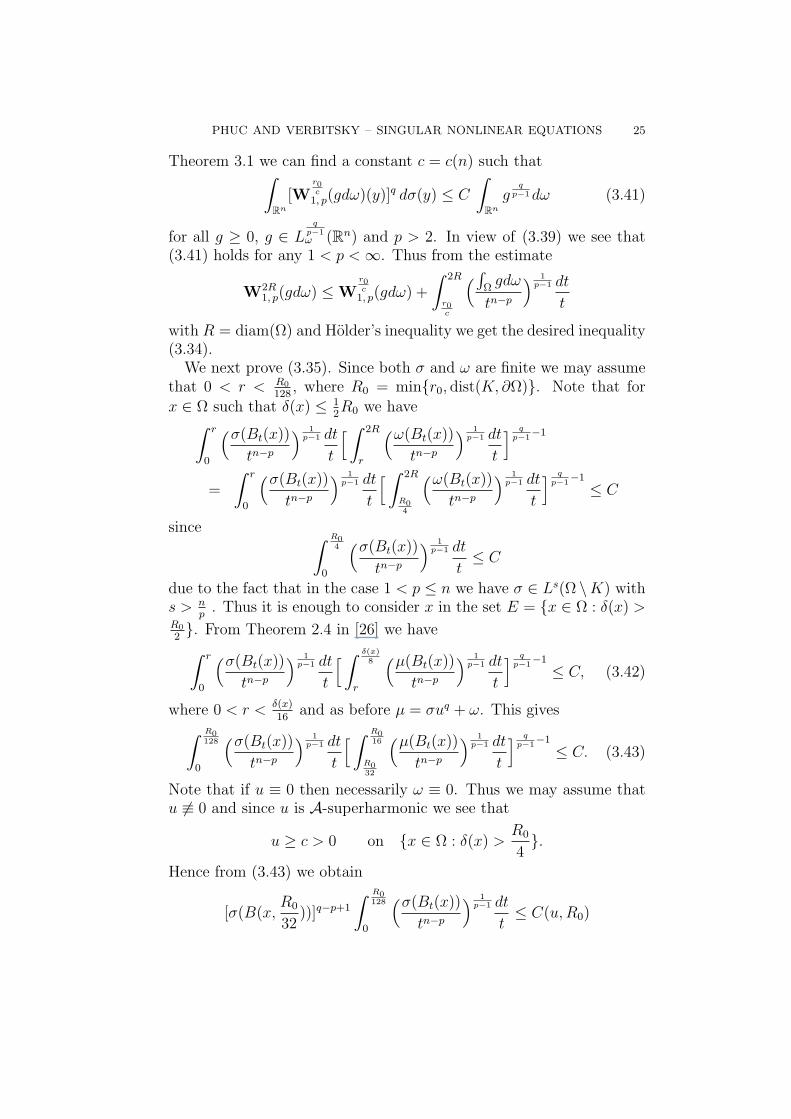
PHUC AND VERBITSKY – SINGULAR NONLINEAR EQUATIONS 25

Theorem 3.1 we can find a constant c = c(n) such that∫Rn

[Wr0c

1, p(gdω)(y)]q dσ(y) ≤ C

∫Rn

gq

p−1 dω (3.41)

for all g ≥ 0, g ∈ Lq

p−1ω (Rn) and p > 2. In view of (3.39) we see that

(3.41) holds for any 1 < p < ∞. Thus from the estimate

W2R1, p(gdω) ≤ W

r0c

1, p(gdω) +

∫ 2R

r0c

(∫Ω

gdω

tn−p

) 1p−1 dt

t

with R = diam(Ω) and Holder’s inequality we get the desired inequality(3.34).

We next prove (3.35). Since both σ and ω are finite we may assumethat 0 < r < R0

128, where R0 = minr0, dist(K, ∂Ω). Note that for

x ∈ Ω such that δ(x) ≤ 12R0 we have∫ r

0

(σ(Bt(x))

tn−p

) 1p−1 dt

t

[ ∫ 2R

r

(ω(Bt(x))

tn−p

) 1p−1 dt

t

] qp−1

−1

=

∫ r

0

(σ(Bt(x))

tn−p

) 1p−1 dt

t

[ ∫ 2R

R04

(ω(Bt(x))

tn−p

) 1p−1 dt

t

] qp−1

−1

≤ C

since ∫ R04

0

(σ(Bt(x))

tn−p

) 1p−1 dt

t≤ C

due to the fact that in the case 1 < p ≤ n we have σ ∈ Ls(Ω \K) withs > n

p. Thus it is enough to consider x in the set E = x ∈ Ω : δ(x) >

R0

2. From Theorem 2.4 in [26] we have∫ r

0

(σ(Bt(x))

tn−p

) 1p−1 dt

t

[ ∫ δ(x)8

r

(µ(Bt(x))

tn−p

) 1p−1 dt

t

] qp−1

−1

≤ C, (3.42)

where 0 < r < δ(x)16

and as before µ = σuq + ω. This gives∫ R0128

0

(σ(Bt(x))

tn−p

) 1p−1 dt

t

[ ∫ R016

R032

(µ(Bt(x))

tn−p

) 1p−1 dt

t

] qp−1

−1

≤ C. (3.43)

Note that if u ≡ 0 then necessarily ω ≡ 0. Thus we may assume thatu 6≡ 0 and since u is A-superharmonic we see that

u ≥ c > 0 on x ∈ Ω : δ(x) >R0

4.

Hence from (3.43) we obtain

[σ(B(x,R0

32))]q−p+1

∫ R0128

0

(σ(Bt(x))

tn−p

) 1p−1 dt

t≤ C(u, R0)

26 PHUC AND VERBITSKY – SINGULAR NONLINEAR EQUATIONS

We next cover the set E by a finite number of open balls B R0128

(xi)Ni=1.

For x ∈ B R0128

(xi) we have

B R0128

(x) ⊂ BR064

(xi) ⊂ BR032

(x).

Thus if x ∈ E ∩B R0128

(xi) with σ(BR064

(xi)) = 0 then∫ R0128

0

(σ(Bt(x))

tn−p

) 1p−1 dt

t= 0,

and if x ∈ E ∩B R0128

(xi) with σ(BR064

(xi)) > 0 we have∫ R0128

0

(σ(Bt(x))

tn−p

) 1p−1 dt

t≤ m−q+p−1C(u, R0),

wherem = minσ(BR0

64(xi)) : σ(BR0

64(xi)) > 0 > 0.

Therefore, for any x ∈ E we obtain∫ R0128

0

(σ(Bt(x))

tn−p

) 1p−1 dt

t≤ C(u, R0, σ).

It is then easy to see from this inequality and (3.42) that∫ r

0

(σ(Bt(x))

tn−p

) 1p−1 dt

t·[ ∫ 2R

r

(ω(Bt(x))

tn−p

) 1p−1 dt

t

] qp−1

−1

≤ C(u, R0, R, σ, ω)

for all 0 < r < R0

128and x ∈ E. This completes the proof of (3.35)

and hence that of statement (i). Note that statement (ii) follows fromstatement (i) as inequality (3.36) is a trivial consequence of (3.35).Moreover, by modifying the proof of Theorem 3.2 we see that (ii) im-plies (iii).

Finally, for finite measures σ and ω on Ω we observe that in theimplication (i) ⇒ (ii) ⇒ (iii) if the constants C in (i) depend only onn, p, q, and α, β then so do the constants C in (ii) and (iii). Thus fromTheorem 3.8 we obtain the last statement of the theorem.

4. Hessian equations

In this section, we study a fully nonlinear counterpart of the theorypresented in the previous sections. Here the notion of k-subharmonic(k-convex) functions associated with the fully nonlinear k-Hessian op-erator Fk, k = 1, . . . , n, introduced by Trudinger and Wang in [31]–[33]will play a role similar to that of A-superharmonic functions in thequasilinear theory.

PHUC AND VERBITSKY – SINGULAR NONLINEAR EQUATIONS 27

Let Ω be an open set in Rn, n ≥ 2. For k = 1, . . . , n and u ∈ C2(Ω),the k-Hessian operator Fk is defined by

Fk[u] = Sk(λ(D2u)),

where λ(D2u) = (λ1, . . . , λn) denotes the eigenvalues of the Hessianmatrix of second partial derivatives D2u, and Sk is the kth symmetricfunction on Rn given by

Sk(λ) =∑

1≤i1<···<ik≤n

λi1 · · ·λik .

Thus F1[u] = ∆u and Fn[u] = det D2u. Alternatively, we may alsowrite

Fk[u] = [D2u]k,

where for an n × n matrix A, [A]k is the k-trace of A, i.e., the sumof its k × k principal minors. Several equivalent definitions of k-subharmonicity were given in [32], one of which involves the languageof viscosity solutions: An upper-semicontinuous function u : Ω →[−∞,∞) is said to be k-subharmonic in Ω, 1 ≤ k ≤ n, if Fk[q] ≥ 0for any quadratic polynomial q such that u− q has a local finite max-imum in Ω. Equivalently, an upper-semicontinuous function u : Ω →[−∞,∞) is k-subharmonic in Ω if, for every open set Ω′ b Ω and forevery function v ∈ C2

loc(Ω′) ∩ C0(Ω′) satisfying Fk[v] ≥ 0 in Ω′, the

following implication holds:

u ≤ v on ∂Ω′ =⇒ u ≤ v in Ω′,

(see [32], Lemma 2.1). It turns out that a function u ∈ C2loc(Ω) is

k-subharmonic if and only if

Fj[u] ≥ 0 in Ω for all j = 1, . . . , k.

We denote by Φk(Ω) the class of all k-subharmonic functions in Ω whichare not identically equal to −∞ in each component of Ω. It was provenin [32] that Φn(Ω) ⊂ Φn−1(Ω) · · · ⊂ Φ1(Ω) where Φ1(Ω) coincides withthe set of all proper classical subharmonic functions in Ω, and Φn(Ω)is the set of functions convex on each component of Ω.

The following weak continuity result [32] is fundamental to potentialtheory associated with k-Hessian operators.

Theorem 4.1 ([32]). For each u ∈ Φk(Ω), there exists a nonnegativeBorel measure µk[u] in Ω such that(i) µk[u] = Fk[u] for u ∈ C2(Ω), and(ii) if um is a sequence in Φk(Ω) converging in L1

loc(Ω) to a functionu ∈ Φk(Ω), then the sequence of the corresponding measures µk[um]converges weakly to µk[u].

28 PHUC AND VERBITSKY – SINGULAR NONLINEAR EQUATIONS

The measure µk[u] in the above theorem is called the k-Hessian mea-sure associated with u. Due to (i) in Theorem 4.1 we sometimes writeFk[u] in place of µk[u] even in the case where u ∈ Φk(Ω) does notbelong to C2(Ω). The k-Hessian measure was used by Labutin [22]to derive local pointwise estimates for functions in Φk(Ω) in terms ofWolff potentials, from which we deduced in [25] the following globalversions.

Theorem 4.2. Let ω be a nonnegative finite measure on Ω such thatω = ω′ + f where ω′ is a nonnegative measure compactly supported inΩ, and f ≥ 0, f ∈ Ls(Ω) with s > n

2kif 1 ≤ k ≤ n

2, and s = 1 if

n2

< k ≤ n. Suppose that −u is a nonpositive k-subharmonic functionin Ω such that u is continuous near ∂Ω and solves the equation

Fk[−u] = ω in Ω,u = 0 on ∂Ω.

Then there is a constant K = K(n, k) > 0 such that

u(x) ≤ K W2diam(Ω)2k

k+1, k+1

ω(x)

for every x in Ω.

Theorem 4.3. Let u ≥ 0 be such that −u ∈ Φk(Rn), where 1 ≤ k < n2.

If µ = µk[−u] and infRn u = 0 then for all x ∈ Rn,

1

KW 2k

k+1, k+1µ(x) ≤ u(x) ≤ K W 2k

k+1, k+1µ(x)

for a constant K > 0 depending only on n and k.

We now recall an existence result for Hessian equations with measuredata established in [31], [32] for bounded uniformly (k − 1)-convexdomains Ω in Rn, i.e., ∂Ω ∈ C2 and Hj(∂Ω) > 0, j = 1, ..., k−1, whereHj(∂Ω) denotes the j-mean curvature of the boundary ∂Ω.

Lemma 4.4 ([31], [32]). Let Ω be a bounded uniformly (k − 1)-convexdomain in Rn. Suppose that µ = µ′ + f where µ′ is a nonnegativemeasure compactly supported in Ω, and f ≥ 0, f ∈ Ls(Ω) with s > n

2kif 1 ≤ k ≤ n

2, and s = 1 if n

2< k ≤ n. Then there exists u ≥ 0

such that −u ∈ Φk(Ω) and u is continuous near ∂Ω which satisfies theequation

µk[−u] = µ in Ω,u = 0 on ∂Ω.

(4.1)

The uniqueness of solutions to (4.1) remains an open problem forgeneral measure data µ. However, if µ is continuous with respect to

PHUC AND VERBITSKY – SINGULAR NONLINEAR EQUATIONS 29

the capacity capk(·, Ω), i.e., µ(E) = 0 whenever capk(E, Ω) = 0 wherecapk(·, Ω) is defined by

capk(K, Ω) = sup

µk[u](K) : u ∈ Φk(Ω) and − 1 < u < 0

for each compact set K ⊂ Ω, then the uniqueness follows from thefollowing comparison principle which was established in [33].

Theorem 4.5 ([33]). Suppose u, v ∈ Φk(Ω) are such that the measuresµk[u] and µk[v] are continuous with respect to capk(·, Ω), and u ≤ vcontinuously on ∂Ω. If µk[u] ≥ µk[v], then u ≤ v on Ω.

From Theorem 4.5 and the weak continuity result (Theorem 4.1) onegets the following analogue of Lemma 3.7, which was also proved earlierin [25].

Lemma 4.6 ([25]). Let Ω, µ and u be as in Lemma 4.4. Suppose thatν is a measure similar to µ, i.e., ν = ν ′ + g where ν ′ is a nonnegativemeasure compactly supported in Ω, and g ≥ 0, g ∈ Ls(Ω) with s > n

2kif 1 ≤ k ≤ n

2, and s = 1 if n

2< k ≤ n. Then there exists a function v

such that −v ∈ Φk(Ω), v ≥ u andµk[−v] = µ + ν in Ω,

v = 0 on ∂Ω.

The following technical lemma will be needed in the proof of Theorem4.8 below to construct a solution to Hessian equations. It is the Hessiancounterpart of Lemma 3.9.

Lemma 4.7. Let µ, ν be nonnegative locally finite measures on Rn forwhich µ ≤ ν and W 2k

k+1, k+1ν < ∞ a.e. Suppose that u is a nonnegative

function for which −u ∈ Φk(Rn), µk[−u] = µ, and u is a pointwise a.e.limit of a subsequence of the sequence um, where −um ∈ Φk(Bm+1)and

µk[−um] = µBm in Bm+1,um = 0 on ∂Bm+1.

Then there exists a function v for which −v ∈ Φk(Rn), v ≥ u andµk[−v] = ν,infRn v = 0.

(4.2)

Moreover, v is also a pointwise a.e. limit of a subsequence of the se-quence vm, where −vm ∈ Φk(Bm+1) and

µk[−vm] = νBm in Bm+1,vm = 0 on ∂Bm+1.

(4.3)

30 PHUC AND VERBITSKY – SINGULAR NONLINEAR EQUATIONS

Proof. By Lemma 4.6 we choose a sequence of functions vm satisfyingequation (4.3) such that vm ≥ um. Note that

vm ≤ K W 2kk+1

, k+1ν on Bm+1, (4.4)

by Theorem 4.2. Thus we can find a subsequence vmk that converges

a.e. to a function v such that −v ∈ Φk(Rn) and v ≥ u. From (4.4) wehave

v ≤ K W 2kk+1

, k+1ν a.e.,

which by Theorem 4.3 gives

v ≤ C(v − infRn

v).

Thus infRn v = 0. Finally, from (4.4) and weak continuity we see thatu satisfies equation (4.2).

We next obtain an existence result for fully nonlinear equations onRn which is an analogue of Theorem 3.10 in the quasilinear case.

Theorem 4.8. Let ω, σ be nonnegative locally finite measure on Rn forwhich W 2k

k+1, k+1ω < ∞ a.e. Let 1 ≤ k < n

2, and q > k. Suppose that

W 2kk+1

, k+1[(W 2kk+1

, k+1ω)qdσ] ≤ C W 2kk+1

, k+1ω σ-a.e. (4.5)

with

C ≤(q − k

qK

)q/k k

q − k, (4.6)

where K is the constant in Theorem 4.3. Then there exists u ≥ 0,u ∈ Lq

σ, loc(Rn), such that −u ∈ Φk(Rn) andFk[−u] = uqσ + ω,infx∈Rn u(x) = 0.

(4.7)

Moreover, u satisfies the two-sided estimate

c1W 2kk+1

, k+1ω(x) ≤ u(x) ≤ c2 W 2kk+1

, k+1ω(x) (4.8)

for all x in Rn, where the constants c1, c2 depend only on n, k, q.

Proof. Using Lemma 4.7 we can construct inductively a sequence ofnonnegative functions uj for which −uj ∈ Φk(Rn) and uj ≤ uj+1,where

Fk[−u0] = ω,infRn u0 = 0,

and Fk[−uj] = (uj−1)

qσ + ω,infRn uj = 0

PHUC AND VERBITSKY – SINGULAR NONLINEAR EQUATIONS 31

for each j ≥ 1. Note that uj ∈ Lqσ, loc(Rn) by Theorem 4.3 and condition

(4.5). Also from Theorem 4.3, conditions (4.5), (4.6) and arguing byinduction we have

uj ≤Kq

q − kW 2k

k+1, k+1ω.

Thus by weak continuity uj ↑ u for a function u ≥ 0 that satisfiesequation (4.7) and estimate (4.8).

We can now say a few words on the proof of Theorems 1.2 stated inSec. 1.

Proof of Theorem 1.2. The proof of this theorem is completely anal-ogous to that of Theorem 1.1. One only needs to use Theorem 4.8 inplace of Theorem 3.10 and argue as in Section 3 with W 2k

k+1, k+1 in place

of W1, p.

Finally, we consider the nonlinear Dirichlet problem on a boundeddomain Ω ⊂ Rn. In this case, one only needs to use the truncated Wolffpotential W2R

2kk+1

, k+1and adapt the arguments employed in the proof of

Theorem 3.11 to obtain the following theorem.

Theorem 4.9. Let 1 ≤ k ≤ n, q > k, and R = diam(Ω). Suppose thatω and σ are nonnegative finite measures on Ω such that supp(ω) b Ωand in the case 1 ≤ k ≤ n

2we assume σ ∈ Ls(Ω \K) for some s > n

2kand a compact set K b Ω. If the equation

Fk[−u] = σuq + ω in Ω,u = 0 on ∂Ω

(4.9)

has a nonnegative solution u ∈ Lqσ(Ω), then there exists a constant

C > 0 such that statements (i), (ii) and (iii) below are valid.

(i) The inequality∫Rn

[W2R2k

k+1, k+1

(gdω)(y)]q dσ(y) ≤ C

∫Rn

gqk dω

holds for all g ∈ Lqkω (Ω), g ≥ 0, and∫ r

0

(σ(Bt(x))

tn−2k

) 1k dt

t·[ ∫ 2R

r

(ω(Bt(x))

tn−2k

) 1k] q

k−1dt

t≤ C (4.10)

holds for all x ∈ Ω and 0 < r < 2R.(ii) The inequality∫

B

[W2R2k

k+1, k+1

ωB(y)]q dσ(y) ≤ C ω(B)

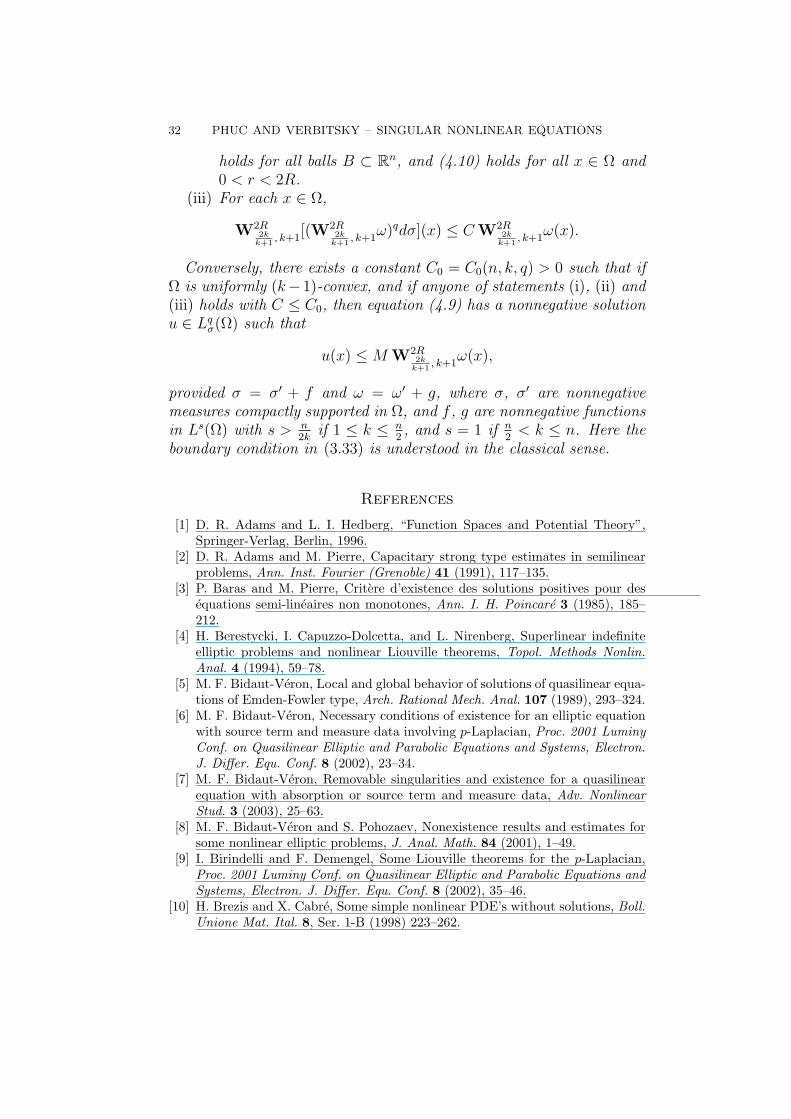
32 PHUC AND VERBITSKY – SINGULAR NONLINEAR EQUATIONS

holds for all balls B ⊂ Rn, and (4.10) holds for all x ∈ Ω and0 < r < 2R.

(iii) For each x ∈ Ω,

W2R2k

k+1, k+1

[(W2R2k

k+1, k+1

ω)qdσ](x) ≤ C W2R2k

k+1, k+1

ω(x).

Conversely, there exists a constant C0 = C0(n, k, q) > 0 such that ifΩ is uniformly (k−1)-convex, and if anyone of statements (i), (ii) and(iii) holds with C ≤ C0, then equation (4.9) has a nonnegative solutionu ∈ Lq

σ(Ω) such that

u(x) ≤ M W2R2k

k+1, k+1

ω(x),

provided σ = σ′ + f and ω = ω′ + g, where σ, σ′ are nonnegativemeasures compactly supported in Ω, and f , g are nonnegative functionsin Ls(Ω) with s > n

2kif 1 ≤ k ≤ n

2, and s = 1 if n

2< k ≤ n. Here the

boundary condition in (3.33) is understood in the classical sense.

References

[1] D. R. Adams and L. I. Hedberg, “Function Spaces and Potential Theory”,Springer-Verlag, Berlin, 1996.

[2] D. R. Adams and M. Pierre, Capacitary strong type estimates in semilinearproblems, Ann. Inst. Fourier (Grenoble) 41 (1991), 117–135.

[3] P. Baras and M. Pierre, Critere d’existence des solutions positives pour desequations semi-lineaires non monotones, Ann. I. H. Poincare 3 (1985), 185–212.

[4] H. Berestycki, I. Capuzzo-Dolcetta, and L. Nirenberg, Superlinear indefiniteelliptic problems and nonlinear Liouville theorems, Topol. Methods Nonlin.Anal. 4 (1994), 59–78.

[5] M. F. Bidaut-Veron, Local and global behavior of solutions of quasilinear equa-tions of Emden-Fowler type, Arch. Rational Mech. Anal. 107 (1989), 293–324.

[6] M. F. Bidaut-Veron, Necessary conditions of existence for an elliptic equationwith source term and measure data involving p-Laplacian, Proc. 2001 LuminyConf. on Quasilinear Elliptic and Parabolic Equations and Systems, Electron.J. Differ. Equ. Conf. 8 (2002), 23–34.

[7] M. F. Bidaut-Veron, Removable singularities and existence for a quasilinearequation with absorption or source term and measure data, Adv. NonlinearStud. 3 (2003), 25–63.

[8] M. F. Bidaut-Veron and S. Pohozaev, Nonexistence results and estimates forsome nonlinear elliptic problems, J. Anal. Math. 84 (2001), 1–49.

[9] I. Birindelli and F. Demengel, Some Liouville theorems for the p-Laplacian,Proc. 2001 Luminy Conf. on Quasilinear Elliptic and Parabolic Equations andSystems, Electron. J. Differ. Equ. Conf. 8 (2002), 35–46.

[10] H. Brezis and X. Cabre, Some simple nonlinear PDE’s without solutions, Boll.Unione Mat. Ital. 8, Ser. 1-B (1998) 223–262.

PHUC AND VERBITSKY – SINGULAR NONLINEAR EQUATIONS 33

[11] L. Caffarelli, L. Nirenberg, and J. Spruck, The Dirichlet problem for nonlinearsecond-order elliptic equations. III. Functions of the eigenvalues of the Hessian,Acta Math. 155 (1985), 261–301.

[12] C. Cascante, J. M. Ortega, and I. E. Verbitsky, Trace inequalities of Sobolevtype in the upper triangle case, Proc. London Math. Soc. 3 (2000), 391–414.

[13] C. Cascante, J. M. Ortega, and I. E. Verbitsky, Nonlinear potentials and twoweight trace inequalities for general dyadic and radial kernels, Indiana Univ.Math. J. 53 (2004), 845–882.

[14] K.-S. Chou and X.-J. Wang, Variational theory for Hessian equations, Comm.Pure Appl. Math. 54 (2001), 1029–1064.

[15] G. Dal Maso, F. Murat, A. Orsina, and A. Prignet, Renormalized solutions ofelliptic equations with general measure data, Ann. Scuol. Norm. Pisa (4) 28(1999), 741–808.

[16] R. Fefferman, Strong differentiation with respect to measures, Amer. J. Math.103 (1981), 33–40.

[17] N. Grenon, Existence results for semilinear elliptic equations with small mea-sure data, Ann. Inst. H. Poincare Anal. Non Lineaire 19 (2002), 1–11.

[18] J. Heinonen, T. Kilpelainen, and O. Martio, “Nonlinear Potential Theory ofDegenerate Elliptic Equations”, Oxford Univ. Press, Oxford, 1993.

[19] N. M. Ivochkina, Solution of the Dirichlet problem for some equations of theMonge-Ampere type, (Russian) Mat. Sb. 128 (1985), 403–415.

[20] T. Kilpelainen and J. Maly, Degenerate elliptic equations with measure dataand nonlinear potentials, Ann. Scuola Norm. Sup. Pisa, Cl. Sci. 19 (1992),591–613.

[21] T. Kilpelainen and J. Maly, The Wiener test and potential estimates for quasi-linear elliptic equations, Acta Math. 172 (1994), 137–161.

[22] D. A. Labutin, Potential estimates for a class of fully nonlinear elliptic equa-tions, Duke Math. J. 111 (2002), 1–49.

[23] N. J. Kalton and I. E. Verbitsky, Nonlinear equations and weighted norminequalities, Trans. Amer. Math. Soc. 351 (1999), 3441–3497.

[24] P. Mikkonen, On the Wolff potential and quasilinear elliptic equations involvingmeasures, Ann. Acad. Sci. Fenn., Ser AI, Math. Dissert. 104 1996, 1–71.

[25] N. C. Phuc and I. E. Verbitsky, Quasilinear and Hessian equations of Lane–Emden type, Ann. Math. 168 2008, 859–914.

[26] N. C. Phuc and I. E. Verbitsky, Local integral estimates and removable sin-gularities for quasilinear and Hessian equations with nonlinear source terms,Comm. Part. Diff. Equ. 31 (2006), 1779–1791.

[27] E. T. Sawyer, A characterization of a two-weight norm inequality for maximaloperator, Studia Math. 75 (1982), 1–11.

[28] J. Serrin, Local behavior of solutions of quasi-linear equations, Acta. Math.111 (1964), 247–302.

[29] J. Serrin, Isolated singularities of solutions of quasi-linear equations, Acta.Math. 113 (1965), 219–240.

[30] J. Serrin and H. Zou, Cauchy–Liouville and universal boundedness theoremsfor quasilinear elliptic equations and inequalities, Acta. Math. 189 (2002), 79–142.

[31] N. S. Trudinger and X. J. Wang, Hessian measures I, Topol. Meth. Nonlin.Anal. 10 (1997), 225–239.

34 PHUC AND VERBITSKY – SINGULAR NONLINEAR EQUATIONS

[32] N. S. Trudinger and X. J. Wang, Hessian measures II, Ann. Math. 150 (1999),579–604.

[33] N. S. Trudinger and X. J. Wang, Hessian measures III, J. Funct. Anal. 193(2002), 1–23.

[34] N. S. Trudinger and X. J. Wang, On the weak continuity of elliptic operatorsand applications to potential theory, Amer. J. Math. 124 (2002), 369–410.

[35] I. E. Verbitsky, Superlinear equations, potential theory and weighted norm in-equalities, Nonlinear Analysis, Function Spaces and Applications. Proc. SpringSchool 5, Prague, May 31-June 6, 1998, 1–47.

[36] L. Veron, Elliptic equations involving measures, Stationary Partial DifferentialEquations, Vol. I. Handbook of Partial Differential Equations, North-Holland,Amsterdam, 2004, 593–712.